Riemann-Hilbert Analysis for Laguerre Polynomials with ...

Computational Methods and Function TheoryVolume 1 (2001), No. 1, 205–233

Riemann-Hilbert Analysis for Laguerre Polynomials with

Large Negative Parameter

Arno B. J. Kuijlaars and Kenneth T.-R. McLaughlin

Abstract. In this paper we study the asymptotic behavior of Laguerre poly-

nomials L(αn)n (nz) as n → ∞, where αn is a sequence of negative parameters

such that −αn/n tends to a limit A > 1 as n→∞. These polynomials satisfya non-hermitian orthogonality on certain contours in the complex plane. Thisfact allows the formulation of a Riemann-Hilbert problem whose solution isgiven in terms of these Laguerre polynomials. The asymptotic analysis ofthe Riemann-Hilbert problem is carried out by the steepest descent methodof Deift and Zhou, in the same spirit as done by Deift et al. for the case oforthogonal polynomials on the real line. A main feature of the present paperis the choice of the correct contour.

Keywords. Riemann-Hilbert problems, generalized Laguerre polynomials,strong asymptotics, steepest descent method.

2000 MSC. 30E15, 33C45.

1. Introduction

1.1. Generalized Laguerre polynomials. The classical Laguerre polynomi-

als L(α)n are orthogonal on the interval [0,∞) with respect to the weight xαe−x,

that is

(1.1)

∫ ∞

0

L(α)n (x)L(α)

m (x)xαe−x dt = 0, if n 6= m.

The integral in (1.1) converges only if α > −1. The Laguerre polynomials aregiven by the explicit formula

(1.2) L(α)n (x) =

n∑

k=0

(

n+ α

n− k

)

(−x)kk!

Received August 27, 2001.The first author has been supported in part by FWO research project G.0176.02, by INTASproject 00-272, and by a research grant of the Fund for Scientific Research–Flanders.The second author has been supported in part by NSF grant # DMS-9970328.

ISSN 1617-9447/$ 2.50 c© 2001 Heldermann Verlag

206 A. B. J. Kuijlaars and K. T.-R. McLaughlin CMFT

and by the Rodrigues formula

(1.3) L(α)n (x) =

1

n!x−αex

(

d

dx

)n[

xα+ne−x]

,

see e.g. [30]. Both (1.2) and (1.3) make sense for arbitrary α (even complex) andthey define the generalized non-classical Laguerre polynomials. The recurrencerelation

(1.4) −xL(α)n (x) = (n+ 1)L

(α)n+1(x)− (2n+ α + 1)L(α)

n (x) + (n+ α)L(α)n−1(x),

with L(α)0 ≡ 1, L

(α)−1 ≡ 0, and the second order differential equation

(1.5) xy′′(x) + (α+ 1− x)y′(x) + ny(x) = 0, y(x) = L(α)n (x),

continue to hold for arbitrary α. We consider in this paper only real and nega-tive α, although extensions to complex α are possible.

1.2. Relations to other polynomials. Laguerre polynomials with negativeparameters appear in the literature in a number of forms. First we note thespecial cases α = −n and α = −n− 1, where we have

(1.6) L(−n)n (z) =

(−1)nn!

zn,

and

(1.7) L(−n−1)n (z) = (−1)n

n∑

k=0

zk

k!,

respectively. Thus for α = −n − 1, the generalized Laguerre polynomial agrees(up to a sign if n is odd) with the partial sum of the exponential series. Moregenerally, we have that for α = −n − m with n,m ∈ N, the generalized La-guerre polynomials appear as the numerator and denominator polynomials inthe rational Pade approximant for the exponential function. To be precise, if

(1.8) pn,m(x) = (−1)n(

n+m

n

)−1

L(−n−m−1)n (x)

and

(1.9) qn,m(x) = (−1)m(

n+m

m

)−1

L(−n−m−1)m (x)

then pn,m(0) = qn,m(0) = 1, and

(1.10) pn,m(x)− qn,m(x)ex = O

(

xn+m+1)

as x→ 0,

see e.g. [23], [25].

1 (2001), No. 1 Riemann-Hilbert Analysis for Laguerre Polynomials 207

Laguerre polynomials with negative parameters are also related to the so-calledgeneralized Bessel polynomials

(1.11) yn(z; a) =n∑

k=0

(

n

k

)

(n+ a− 1)k

(z

2

)k

,

since

(1.12) yn(z; a) = (−1)nn!(z

2

)n

L(−2n−a+1)n

(

2

z

)

.

The usual Bessel polynomials correspond to a = 2 in (1.11). See Grosswald [17]for a comprehensive account of these polynomials.

1.3. Earlier work on asymptotics. For α > −1, the Laguerre polynomialssatisfy the orthogonality (1.1) on the positive real axis, and therefore they haveonly positive real zeros. This property is lost for α < −1. Indeed, the generalizedLaguerre polynomials may have many non-real zeros. In Figure 1 we have plotted

the zeros of L(−40A)40 (40z) for a number of values of A > 0. Similar plots are shown

in the paper [20].

−0.2 0 0.2 0.4 0.6 0.8 1 1.2 1.4 1.6 1.8−1

−0.8

−0.6

−0.4

−0.2

0

0.2

0.4

0.6

0.8

1

−1 −0.5 0 0.5 1 1.5 2−1.5

−1

−0.5

0

0.5

1

1.5

−2 −1.5 −1 −0.5 0 0.5 1 1.5 2−3

−2

−1

0

1

2

3

Figure 1. Zeros of generalized Laguerre polynomials L(−An)n (nx)

for n = 40 and A = 0.81 (left), A = 1.01 (middle), and A = 2(right).

In Figure 1 we see that the zeros cluster along certain curves in the complexplane. Martınez et al. [20] identified these curves as trajectories of a quadraticdifferential, depending on a parameter A. For A > 1, the curve is a simple arc,which as A decreases to 1 closes itself to form for A = 1 the well-known Szegocurve [29], [24]. For 0 < A < 1, the curve consists of a closed loop together withan interval on the positive real axis.

A number of rigorous results on the asymptotic behavior of the zeros of general-

ized Laguerre polynomials L(αn)n (nx) such that

(1.13) limn→∞

αnn

= −A

are known from the literature. The first result is due to Szego [29] who studiedthe partial sum of the exponential series, that is αn = −n − 1 see (1.7). Szego


showed that the normalized zeros tend to the curve which now bears his name.Olver [21] considered the zeros of Hankel functions, which includes the Besselpolynomials as a special case. In terms of the generalized Laguerre polynomials,this is the case αn = −2n − 1. Saff and Varga [26] studied the zeros and polesof Pade approximants to the exponential function, see (1.8)–(1.9). Their main

result says that for integers αn < −n such that (1.13) holds, all zeros of L(αn)n (nx)

tend to a well-defined curve as n → ∞. The curve depends on A ≥ 1 only, andcoincides with the curve described in [20]. Saff and Varga also obtained the weaklimit of the zero counting measures. The proofs in [26] can be extended withoutany difficulty to non-integer αn < −n.Stated in terms of generalized Bessel polynomials (1.11)–(1.12) asymptotic re-sults on zeros are due to De Bruin et al. [4], Carpenter [5], and Wong andZhang [31]. These papers deal with the limit (1.13) with A = 2. The lat-ter paper also presents uniform asymptotic expansions of the generalized Besselpolynomials. In very recent work, Dunster [14] establishes uniform asymptoticexpansions in the complex plane for the case of general A, with the exception ofA = 0 and A = 1. The results on zeros in [14] are restricted to the case A > 1.

1.4. Asymptotics from Riemann-Hilbert problems. Most papers citedabove use some form of the steepest descent technique for integrals, see espe-cially [26] and [31]. Martınez et al. [20] use an orthogonality relation in thecomplex plane satisfied by generalized Laguerre polynomials. The approach ofDunster [14] starts from the differential equation (1.5) and is based on techniquesdeveloped by Olver [22].

In this paper we derive asymptotics of generalized Laguerre polynomials usingthe nonlinear steepest descent / stationary phase method for Riemann-Hilbertproblems introduced by Deift and Zhou in [12], and further developed in [13]and [11]. In later developments, the method was applied successfully to problemsin random matrix theory [8], [9], and in orthogonal polynomials [3], [9], [10], [19],and combinatorics [2]. For review of some of these developments, and a peda-gogic introduction to some of the material of random matrix theory, orthogonalpolynomials, and Riemann-Hilbert problems, see [6].

The Riemann-Hilbert approach to the asymptotics of generalized Laguerre poly-nomials starts from the observation that these polynomials satisfy orthogonalityrelations in the complex plane. The orthogonality is on a contour Σ going aroundthe positive real axis, but otherwise being quite arbitrary. The orthogonalityproperty allows the formulation of a Riemann-Hilbert problem, due to Fokas, Its,

and Kitaev [15], whose solution is given in terms of L(α)n . The Riemann-Hilbert

problem is analyzed in the large n limit with the steepest descent method asdone in [9] and [10] for orthogonal polynomials on the real line.

A novel feature for the problem at hand is that the arbitrary contour Σ hasto be chosen in a correct way in order to arrive at a Riemann-Hilbert problem


which is amenable to subsequent asymptotic analysis. The correct contour wasdescribed in [20]. It is a curve with the S-property of Stahl [27] and Goncharand Rakhmanov [16]. The structure of the curve depends on the value of Aas already explained before. In this paper we analyze the case of an open con-tour, that is, the case A > 1. In subsequent work we consider the case of aclosed loop plus an interval (0 < A < 1) and the case of a single closed con-tour (A = 1). We note that the steepest descent / stationary phase method forRiemann-Hilbert problems was augmented to handle cases in which the contourselection involves determining a set of nontrivial curves in the plane in [18], byKamvissis, McLaughlin, and Miller, in the context of the semi-classical limit ofthe focusing nonlinear Schrodinger equation.

We emphasize that the main interest in the present paper lies in the method weuse and not in the results obtained for the Laguerre polynomials. In particular,we do not improve upon the asymptotic expansions of Dunster [14]. The steepestdescent method for Riemann-Hilbert problems is a very powerful new method,and its use in the study of classical special functions is new. In future work weconsider generalized Laguerre polynomials for the cases 0 < A < 1 and A = 1,and the Riemann-Hilbert approach will lead to new results for these cases.

2. Complex orthogonality and the formulation of the

Riemann-Hilbert problem

2.1. Orthogonality. For α < −1, the generalized Laguerre polynomial L(α)n is

not orthogonal on the positive real axis, but instead satisfies a non-hermitianorthogonality in the complex plane.

Let F be the collection of all simple Jordan curves Σ in C \ [0,∞) that aresymmetric with respect to the real axis, and such that there is M > 0 such thatfor all x ≥ M , there is y(x) > 0, such that the intersection of Σ with Re z = xconsists of the two points x ± iy(x), and limx→∞ y(x) = L exists and is finite(possibly 0). Any curve Σ ∈ F divides the complex plane into two domains, Ω+

and Ω−, where Ω− contains the positive real axis. We choose the orientation of Σsuch that Ω+ is on the +-side (i.e., on the left) while traversing Σ and Ω− is onthe −-side. So Σ is oriented clockwise as in Figure 2.

In what follows we define xα with a branch cut along the positive real axis. Thusxα = |x|αeiα arg x with arg x ∈ [0, 2π).

Lemma 2.1. Let Σ ∈ F , n ∈ N, and α ∈ R. Then

(2.1)

∫

Σ

L(α)n (x)xkxαe−x dx = 0, for k = 0, 1, . . . , n− 1.

If in addition α + n+ 1 6∈ N, then

(2.2)

∫

Σ

L(α)n (x)xkxαe−x dx 6= 0, for k = n.


−3 −2 −1 0 1 2 3−3

−2

−1

0

1

2

3

Ω−

Ω+

Σ

Σ

0

Figure 2. Example of contour Σ

Proof. The orthogonality (2.1) follows from the Rodrigues formula (1.3) by re-peated integration by parts. In the same way, we also get

∫

Σ

L(α)n (x)xnxαe−x dx =

1

n!

∫

Σ

(

d

dx

)n(

xα+ne−x)

xndx

= (−1)n∫

Σ

xα+ne−x dx

For α + n > −1, we deform Σ to the positive real axis to obtain

(2.3)

∫

Σ

L(α)n (x)xnxαe−x dx = (−1)n

(

1− e2πiα)

∫ ∞

0

xα+ne−x dx

= (−1)n+12ieπiα sin(πα)Γ(α+ n+ 1),

where Γ denotes the Gamma function. By analytic continuation the integral in(2.2) is equal to (2.3) for every α, and (2.2) follows.

The formula (2.1) expresses orthogonality with respect to the complex measurexαe−xdx on Σ.

2.2. Riemann-Hilbert problem. Let α ∈ R. We consider the monic polyno-mials

(2.4) Pn(z) =(−1)nn!nn

L(α)n (nz), n = 0, 1, . . . .

Introducing a change of variables x = nz in (2.1) and (2.2), we see that

(2.5)

∫

Σ

Pn(z)zkzαe−nz dz

= 0, for k = 0, 1, . . . , n− 1,

6= 0, for k = n,


for every contour Σ ∈ F , provided that α + n+ 1 6∈ N.

The polynomial Pn is characterized through a Riemann-Hilbert problem due toFokas, Its, and Kitaev [15].

Riemann-Hilbert problem for Y : Let Σ be a contour from the class F , thatdivides the complex plane into two parts Ω+ and Ω−, as above. The problem isto determine a 2 × 2 matrix valued function Y : C \ Σ → C2×2 such that thefollowing hold.

(a) Y (z) is analytic for z ∈ C \ Σ,(b) Y (z) possesses continuous boundary values for z ∈ Σ, denoted by Y+(z)

and Y−(z), where Y+(z) and Y−(z) denote the limiting values of Y (z ′) as z′

approaches z ∈ Σ from Ω+ and Ω−, respectively, and

(2.6) Y+(z) = Y−(z)

(

1 zαe−nz

0 1

)

, for z ∈ Σ,

(c) Y (z) has the following behavior as z →∞:

(2.7) Y (z) =

(

I +O

(

1

z

))(

zn 00 z−n

)

as z →∞, z ∈ C \ Σ.

Proposition 2.2. Let α ∈ R with α + n 6∈ N. Then the unique solution of theRiemann-Hilbert problem for Y is given by

(2.8) Y (z) =

Pn(z)1

2πi

∫

Σ

Pn(ζ)ζαe−nζ

ζ − zdζ

Qn−1(z)1

2πi

∫

Σ

Qn−1(ζ)ζαe−nζ

ζ − zdζ

where Pn(z) is the monic generalized Laguerre polynomial (2.4) and

(2.9) Qn−1(z) =(−1)n+1nn+απe−πiα

sin(πα)Γ(α+ n)L(α)n−1(nz).

Proof. The proof is as in [6, Section 3.2]. Here we will only give the proof forthe second row, since that is where the condition on α plays a role.

From (2.6) it follows that Y21 is an entire function, which by (2.7) satisfiesY21(z) = O(zn−1) as z → ∞. Therefore Y21(z) = Qn−1(z) for some polyno-mial Qn−1 of degree at most n − 1. The (2,2) entry of the condition (2.6) is(Y22)+(z) = (Y22)−(z)+Qn−1(z)z

αe−nz, which by the Sokhotskii-Plemelj formulayields

(2.10) Y22(z) =1

2πi

∫

Σ

Qn−1(ζ)ζαe−nζ

ζ − zdζ.


From the (2,2) entry of (2.7) it follows that Y22(z) = z−n +O(z−n−1) as z →∞.Because of (2.10) this gives the conditions

(2.11)

∫

Σ

Qn−1(ζ)ζαe−nζζk dζ = 0 for k = 0, . . . , n− 2,

and

(2.12)

∫

Σ

Qn−1(ζ)ζαe−nζζn−1 dζ = −2πi.

The orthogonality conditions (2.11) are satisfied if Qn−1(z) = dnL(α)n−1(nz), and

the constant dn must be chosen so that (2.12) holds as well. Because of Lemma 2.1this can be done if α + n 6∈ N, and the result is given by (2.9).

3. Selection of the right contour

3.1. The right contour Σ. In Section 3–6, we assume n ∈ N and α < −n arefixed. We write A = −α/n, so that A > 1. [Later, when we let n→∞, α and A,as well as other notions introduced in these sections, will depend on n.]

A major step in the analysis of the Riemann-Hilbert problem for Y is the selectionof the right contour. In order that the subsequent analysis works, the contourcannot be arbitrary but has to be chosen in a precise way. The contour dependson A. We define

(3.1) β = 2− A+ 2i√A− 1

Martinez et al. [20] showed that the values of z for which

1

2πi

∫ z

β

(s− β)1/2(s− β)1/2

sds is real,

where the branch of the square roots is chosen so that they are analytic andsingle valued on the path of integration from β to z, form a system of curvesas shown in Figure 3 for a number of values of A. In geometric function theorythese curves are known as trajectories of the quadratic differential

(s− β)(s− β)

s2d2s,

see [28]. We see four smooth (in fact analytic) curves. Two curves are connect-ing β with β, one of them crosses the negative real axis, and the other one crossesthe positive real axis.

Definition 3.1. We define Γ as the trajectory of the quadratic differential

(s− β)(s− β)

s2d2s

from β to β which crosses the negative real axis. Γ is oriented from β to β.


−1 −0.5 0 0.5 1 1.5 2−1.5

−1

−0.5

0

0.5

1

1.5

−2 −1.5 −1 −0.5 0 0.5 1 1.5 2−3

−2

−1

0

1

2

3

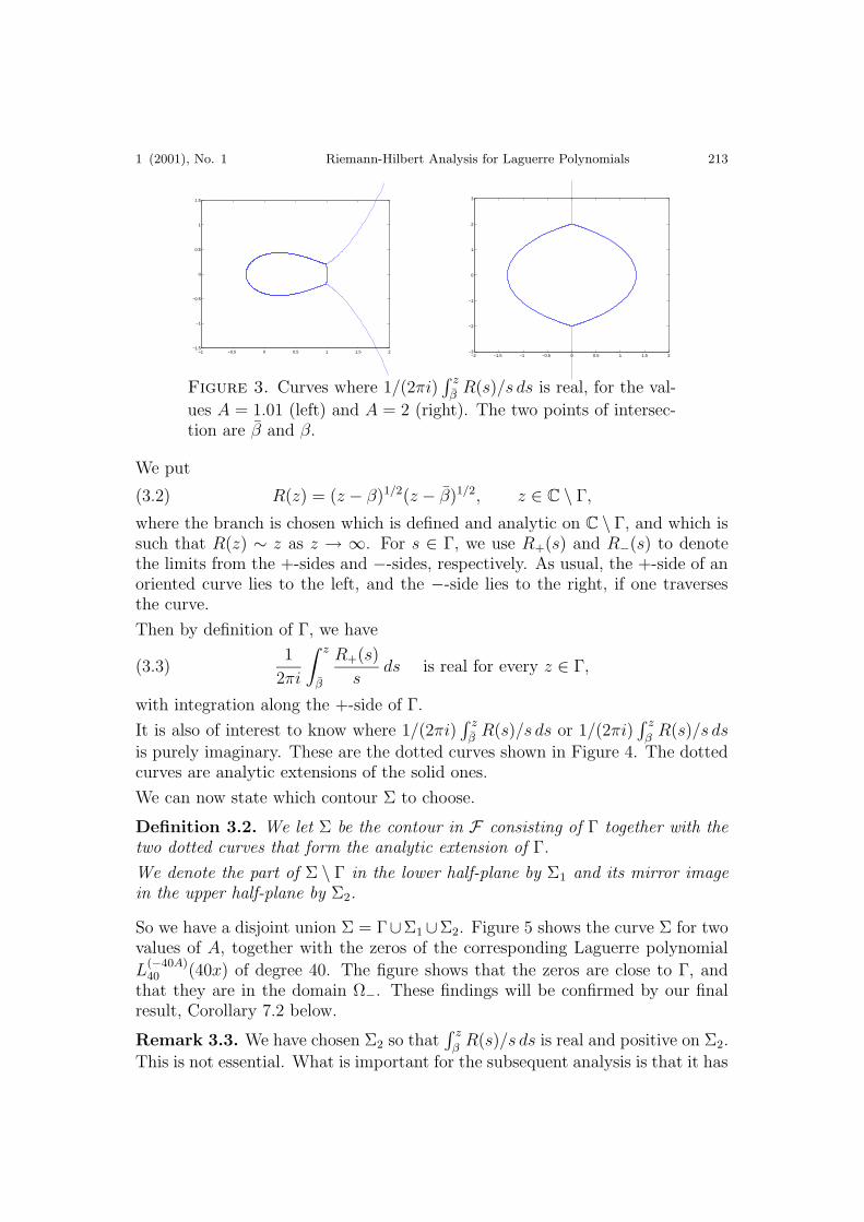
Figure 3. Curves where 1/(2πi)∫ z

βR(s)/s ds is real, for the val-

ues A = 1.01 (left) and A = 2 (right). The two points of intersec-tion are β and β.

We put

(3.2) R(z) = (z − β)1/2(z − β)1/2, z ∈ C \ Γ,where the branch is chosen which is defined and analytic on C \ Γ, and which issuch that R(z) ∼ z as z → ∞. For s ∈ Γ, we use R+(s) and R−(s) to denotethe limits from the +-sides and −-sides, respectively. As usual, the +-side of anoriented curve lies to the left, and the −-side lies to the right, if one traversesthe curve.

Then by definition of Γ, we have

(3.3)1

2πi

∫ z

β

R+(s)

sds is real for every z ∈ Γ,

with integration along the +-side of Γ.

It is also of interest to know where 1/(2πi)∫ z

βR(s)/s ds or 1/(2πi)

∫ z

βR(s)/s ds

is purely imaginary. These are the dotted curves shown in Figure 4. The dottedcurves are analytic extensions of the solid ones.

We can now state which contour Σ to choose.

Definition 3.2. We let Σ be the contour in F consisting of Γ together with thetwo dotted curves that form the analytic extension of Γ.

We denote the part of Σ \ Γ in the lower half-plane by Σ1 and its mirror imagein the upper half-plane by Σ2.

So we have a disjoint union Σ = Γ∪Σ1∪Σ2. Figure 5 shows the curve Σ for twovalues of A, together with the zeros of the corresponding Laguerre polynomial

L(−40A)40 (40x) of degree 40. The figure shows that the zeros are close to Γ, and

that they are in the domain Ω−. These findings will be confirmed by our finalresult, Corollary 7.2 below.

Remark 3.3. We have chosen Σ2 so that∫ z

βR(s)/s ds is real and positive on Σ2.

This is not essential. What is important for the subsequent analysis is that it has


−1 −0.5 0 0.5 1 1.5 2−1.5

−1

−0.5

0

0.5

1

1.5

−2 −1.5 −1 −0.5 0 0.5 1 1.5 2−3

−2

−1

0

1

2

3

Figure 4. Curves where 1/(2πi)∫ z

βR(s)/s ds is real (solid lines)

and curves where 1/(2πi)∫ z

βR(s)d/s ds or 1/(2πi)

∫ z

βR(s)/s ds is

purely imaginary (dotted lines), for the values A = 1.01 (left) andA = 2 (right).

−1 −0.5 0 0.5 1 1.5 2−1.5

−1

−0.5

0

0.5

1

1.5

β

β−Γ

Σ2

Σ1

−2 −1.5 −1 −0.5 0 0.5 1 1.5 2−3

−2

−1

0

1

2

3

β

β−

Γ

Σ2

Σ1

Figure 5. The curves Σ = Γ ∪ Σ1 ∪ Σ2, and the zeros of

L(−40A)40 (40x), for the values A = 1.01 (left) and A = 2 (right).

positive real part on Σ2. This means that we have the freedom to deform Σ2, aslong as we take care that the real part of

∫ z

βR(s)/s ds is positve on Σ2. However,

it will be convenient to do this deformation only away from β, so that in aneighborhood of β, we have Σ2 exactly as we defined it.

Similar remarks apply to∫ z

βR(s)/s ds and Σ1.

3.2. A probability measure on Γ. The following proposition gives one of thecrucial properties of Γ.

Proposition 3.4. The (complex) measure

1

2πi

R+(s)

sds

is a probability measure on Γ.

Proof. We show first that

(3.4)1

2πi

∫

Γ

R+(s)

sds = 1.


Let I =∫

ΓR+(s)/s ds. Since R−(s) = −R+(s) for s ∈ Γ, we have

2I =

∫

Γ

(

R+(s)

s− R−(s)

s

)

ds =

∮

γ

R(s)

sds,

where γ is a closed contour encircling the curve Γ once in the clockwise directionand not encircling z = 0.

After contour deformation, we pick up residues at z = 0 and at z =∞, namely

(3.5) 2I = 2πiResz=0R(z)

z− 2πiResz=∞

R(z)

z.

The residue at z = 0 is

(3.6) Resz=0R(z)

z= R(0) = |β| =

√

(2− A)2 + 4(A− 1) = A

and the residue at z = ∞ is the coefficient of z−1 in the Laurent expansionof R(z)/z

R(z)

z= (1− β/z)1/2(1− β/z)1/2

=

(

1− β

2z+O(z−2)

)(

1− β

2z+O(z−2)

)

= 1− β + β

2z+O(z−2).

Thus

(3.7) Resz=∞R(z)

z= −β + β

2= −Re β = −(2− A).

Hence by (3.5)–(3.7) we have 2I = 2πi(A+(2−A)) = 4πi, so that (3.4) follows.

Having (3.4) we can now prove the proposition. Let t 7→ z(t) for t ∈ [0, t0], bethe arc length parametrization of Γ starting at β. Thus z(0) = β and z(t0) = β.Then we have for z = z(t) with t ∈ (0, t0),

(3.8)1

2πi

∫ z

β

R+(s)

sds =

1

2πi

∫ t

0

R+(z(τ))

z(τ)z′(τ) dτ,

and this is real for every t by construction of Γ. It has the value 0 for t = 0 andthe value 1 for t = t0 (due to (3.4)). The derivative of (3.8) with respect to t is

1

2πi

R+(z(t))

z(t)z′(t)

which is not zero for t ∈ (0, t0). Thus (3.8) can only increase from 0 to 1 as tincreases from 0 to t0. Hence

1

2πi

R+(s)

sds

is a positive measure on Γ. It is a probability measure because of (3.4).


3.3. Auxiliary functions. With the measure

dµ(s) =1

2πi

R+(s)

sds

on Γ we define the so-called g-function as follows.

Definition 3.5. The g-function is the complex logarithmic potential of µ, thatis,

(3.9) g(z) =

∫

Γ

log(z − s) dµ(s), z ∈ C \ (Γ ∪ Σ1),

where for each s we view log(z−s) as an analytic function of the variable z, withbranch cut emanating from z = s. The cut is taken along Γ ∪ Σ1.

We need two more functions.

Definition 3.6. The φ-function is defined as

(3.10) φ(z) =1

2

∫ z

β

R(s)

sds, z ∈ C \ (Γ ∪ Σ1 ∪ [0,∞)),

where the path of integration from β to z lies entirely in C \ (Γ ∪ Σ1 ∪ [0,∞)),except for the initial point β.

The φ-function is defined as

(3.11) φ(z) =1

2

∫ z

β

R(s)

sds, z ∈ C \ (Γ ∪ Σ2 ∪ [0,∞)),

where the path of integration from β to z lies entirely in C \ (Γ ∪ Σ2 ∪ [0,∞)),except for the initial point β.

It is immediate from (3.3) that φ+(z) is purely imaginary for z ∈ Γ. By Proposi-tion 3.4 its imaginary part increases from 0 to π as z traverses the curve Γ from βto β. In particular we have φ+(β) = πi. Similarly φ−(β) = −πi. Thus we have

(3.12) φ(z) =

φ(z) + πi for z ∈ Ω+,

φ(z)− πi for z ∈ Ω−.

Proposition 3.7. There is a constant ` such that

(3.13) g(z) =1

2(A log z + z + `)− φ(z), z ∈ C \ (Γ ∪ Σ1 ∪ [0,∞)),

where log z is defined with a branch cut along [0,∞).

Proof. We note that

g′(z) =1

2πi

∫

Γ

1

z − s

R+(s)

sds =

1

2

1

2πi

∮

γ

1

z − s

R(s)

sds


where γ is a closed contour in C \ Γ, that encircles Γ once in the clockwisedirection, but does not encircle z and 0. Then exactly as in the proof of Propo-sition 3.4, we deform the contour, and now pick up residues at z, 0 and ∞. Wefind for z ∈ C \ Γ,

g′(z) =1

2

[

Ress=z

(

1

z − s

R(s)

s

)

+Ress=0

(

1

z − s

R(s)

s

)

−Ress=∞

(

1

z − s

R(s)

s

)]

(3.14)

=1

2

[

−R(z)z

+R(0)

z+ 1

]

=1

2

[

−R(z)z

+A

z+ 1

]

.

Let z ∈ C \ (Γ ∪ Σ1 ∪ [0,∞)). Integrating (3.14) from β to z along a curve inC \ (Γ ∪ Σ1 ∪ [0,∞), we find

(3.15) g(z) = g(β) +1

2(A log z + z)− 1

2(A log β + β)− φ(z).

Thus (3.13) holds with ` = 2g(β)− (A log β + β).

3.4. Jump properties of g. From Proposition 3.7 we obtain the followingjump relations for g across the contour Σ. These jumps are crucial for thesubsequent analysis.

Proposition 3.8. (a) We have

(3.16) g+(z)− g−(z) = 2πi for z ∈ Σ1,

and

(3.17) g+(z)− g−(z) = −φ+(z) + φ−(z) = −2φ+(z) = 2φ−(z) for z ∈ Γ.

(b) We have, with the same constant ` as in Proposition 3.7,

g+(z) + g−(z) = A log z + z + ` for z ∈ Γ,(3.18)

g+(z) + g−(z) = A log z + z + `− 2φ(z) for z ∈ Σ1,(3.19)

g+(z) + g−(z) = A log z + z + `− 2φ(z) for z ∈ Σ2.(3.20)

Proof. In (3.13) we let z approach Σ, from the +- and −-sides, respectively, toobtain

(3.21) g±(z) =1

2(A log z + z) +

1

2`− φ±(z), for z ∈ Σ.

Since φ changes sign across Γ, (3.17) and (3.18) immediately follow from (3.21).For z ∈ Σ1, we have by (3.12) and (3.21)

g+(z)− g−(z) = −φ+(z) + φ−(z) = −(φ+(z)− πi) + (φ−(z) + πi)

= 2πi− φ+(z) + φ−(z),


which is (3.16) as φ is analytic across Σ1. In addition, we have

g+(z) + g−(z) = A log z + z + `− φ+(z)− φ−(z)

= A log z + z + `− φ+(z)− φ−(z) for z ∈ Σ1.

which yields (3.19). Similarly, (3.20) follows.

4. First two transformations: Y 7→ U 7→ T

4.1. First transformation Y 7→ U . With the g-function and the constant `from Proposition 3.7, we perform the first transformation of the Riemann-Hilbertproblem.

Definition 4.1. We define for z ∈ C \ Σ,

(4.1) U(z) = e−n(`/2)σ3Y (z)e−ng(z)σ3en(`/2)σ3 .

Here, and in what follows, σ3 denotes the Pauli matrix

σ3 =

(

1 00 −1

)

,

so that for example

e−ng(z)σ3 =

(

e−ng(z) 00 eng(z)

)

.

From the Riemann-Hilbert problem for Y it follows by a straightforward calcu-lation that U is the unique solution of the following Riemann-Hilbert problem.

Riemann-Hilbert problem for U : The problem is to determine a 2×2 matrixvalued function U : C \ Σ→ C2×2 such that

(a) U(z) is analytic for z ∈ C \ Σ,(b) U(z) possesses continuous boundary values for z ∈ Σ, denoted by U+(z)

and U−(z), and

(4.2) U+(z) = U−(z)

(

e−n(g+(z)−g−(z)) z−Ane−nzen(g+(z)+g−(z)−`)

0 en(g+(z)−g−(z))

)

for z ∈ Σ,(c) U(z) behaves like the identity at infinity:

(4.3) U(z) = I +O

(

1

z

)

as z →∞, z ∈ C \ Σ.


The jump relation (4.2) for U has a different form on the three parts Γ, Σ1 and Σ2.On Γ we have that g+−g− = −2φ+ = 2φ− by (3.17), and g++g− = A log z+z+`by (3.18) so that

(4.4) U+(z) = U−(z)

(

e2nφ+(z) 10 e2nφ−(z)

)

for z ∈ Γ.

On Σ1 we use (3.16) and (3.19) to obtain

(4.5) U+(z) = U−(z)

(

1 e−2nφ(z)

0 1

)

for z ∈ Σ1,

and similarly it follows that

(4.6) U+(z) = U−(z)

(

1 e−2nφ(z)

0 1

)

for z ∈ Σ2.

The transformation Y 7→ U has the effect of normalizing the Riemann-Hilbertproblem at infinity. In addition, by the construction of Σ, we have that φ isreal and positive on Σ2, and φ is real and positive on Σ1. So the jump matricesfor U in (4.5) and (4.6) are close to the identity if n is large. Since φ has purelyimaginary boundary values on both sides of Γ, the jump matrix for U on Γin (4.4) has oscillatory diagonal entries.

4.2. Second transformation U 7→ T . The jump matrix for U on Γ, see (4.4),factors as

(4.7)

(

e2nφ+(z) 10 e2nφ−(z)

)

=

(

1 0e2nφ−(z) 1

)(

0 1−1 0

)(

1 0e2nφ+(z) 1

)

.

Observe that the first matrix in the right-hand side of (4.7) can be analyticallycontinued to the −-side of the contour Γ, and in doing so, the (1,2) entry becomesexponentially decaying in n. Similarly, the third matrix in the right-hand sideof (4.7) can be analytically continued to the +-side of the contour Γ, and in doingso, the (1,2) entry also becomes exponentially decaying in n. We are thus ledto introduce the following “contour augmentation” step, as part of the steepestdescent / stationary phase method for Riemann-Hilbert problems developed byDeift and Zhou. The oriented contour ΣT consists of Σ plus two simple curves Σ3

and Σ4 from β to β, contained in Ω+ and Ω−, respectively, as shown in Figure 6.We choose Σ3 and Σ4 such that Reφ(z) < 0 on Σ3 and Σ4.

It is possible to choose such curves. Indeed, φ is positive on Σ2, and its real partvanishes on Γ and on the other solid lines shown in Figure 4. So Reφ > 0 in thefull region on the right. In the two other regions, bounded by the solid lines, wethen have that Reφ < 0. Note that Reφ does not change sign across Γ.

Note that by (3.12) we also have Re φ(z) < 0 on Σ3 and Σ4.

Then C \ ΣT has four connected components, denoted by Ω1, Ω2, Ω3, and Ω4 asindicated in Figure 6.


−0.5 0 0.5 1 1.5 2−0.8

−0.6

−0.4

−0.2

0

0.2

0.4

0.6

0.8

β

β−

Γ

Σ2

Σ1

Σ3

Σ4

Ω4

Ω1

Ω1

Ω2

Ω3

Figure 6. Contour ΣT = Γ ∪ ⋃j Σj and the domains Ωj,j = 1, . . . , 4, for the Riemann-Hilbert problem for T , for the valueA = 1.01.

Definition 4.2. We define T : C \ ΣT → C2×2 by

T (z) = U(z) for z ∈ Ω1 ∪ Ω4,(4.8)

T (z) = U(z)

(

1 0−e2nφ(z) 1

)

for z ∈ Ω2,(4.9)

T (z) = U(z)

(

1 0e2nφ(z) 1

)

for z ∈ Ω3,(4.10)

Then from the Riemann-Hilbert problem for U and the factorization (4.7) weobtain that T is the unique solution of the following Riemann-Hilbert problem.

Riemann-Hilbert problem for T : The problem is to determine a 2×2 matrixvalued function T : C \ ΣT → C2×2 such that the following hold:

(a) T (z) is analytic for z ∈ C \ ΣT ,(b) T (z) possesses continuous boundary values for z ∈ ΣT , denoted by T+(z)

and T−(z), and

T+(z) = T−(z)

(

0 1−1 0

)

for z ∈ Γ,(4.11)

T+(z) = T−(z)

(

1 0e2nφ(z) 1

)

for z ∈ Σ3 ∪ Σ4,(4.12)

T+(z) = T−(z)

(

1 e−2nφ(z)

0 1

)

for z ∈ Σ1,(4.13)

T+(z) = T−(z)

(

1 e−2nφ(z)

0 1

)

for z ∈ Σ2,(4.14)


(c) T (z) behaves like the identity at infinity:

(4.15) T (z) = I +O

(

1

z

)

as z →∞, z ∈ C \ ΣT .

5. Construction of the parametrix for T

5.1. Parametrix away from β and β. As remarked following (4.7), the jumpmatrices appearing in (4.12) for z ∈ Σ3∪Σ4 are exponentially close to the identitymatrix away from β and β. Similarly, the jump matrices appearing in (4.13)and (4.14) are also exponentially close to the identity matrix away from β and β.This hints that these portions of the contour on which the Riemann-Hilbertproblem for T is posed should be somehow negligible. Thus we expect that theleading order asymptotics is determined by the solution N of the following modelRiemann-Hilbert problem:

Riemann-Hilbert problem for N : The problem is to determine a functionN : C \ Γ→ C2×2 such that the following hold.

(a) N(z) is analytic for z ∈ C \ Γ,(b) N(z) possesses continuous boundary values for z ∈ Γ \ β, β, denoted by

N+(z) and N−(z), and

(5.1) N+(z) = N−(z)

(

0 1−1 0

)

for z ∈ Γ \ β, β,

(c) N(z) = I +O(

1z

)

for z →∞.

This Riemann-Hilbert problem for N is solved explicitly by, see [10, p.1520] or[6, p.200],

(5.2) N(z) =

a(z) + a(z)−1

2

a(z)− a(z)−1

2ia(z)− a(z)−1

−2ia(z) + a(z)−1

2

,

where

(5.3) a(z) =(z − β)1/4

(z − β)1/4.

The branches of the roots in (5.3) are chosen such that a(z) is analytic on C \ Γand lim

z→∞a(z) = 1.

Remark 5.1. The solution (5.2) is not the only solution to the Riemann-Hilbertproblem for N . It is the unique solution that satisfies, in addition to (a), (b),and (c), the condition


(d) Near the endpoints β and β, we have

N(z) = O(|z − β|−1/4) as z → β,

N(z) = O(|z − β|−1/4) as z → β,

with the O-term being taken entry-wise.

Remark 5.2. For explicit calculations, it is useful to have an alternative expres-sion for N . For z = x real, it is clear from (5.3) that a(x) has modulus one. Ifarg(a(x)) = θ(x), then (5.2) shows

N(x) =

(

cos θ(x) sin θ(x)

− sin θ(x) cos θ(x)

)

.

Since tan(2θ(x)) = −2√A− 1/(x− 2 + A), we then find

(5.4)

N(z) =

cos

(

1

2arctan

(

2√A− 1

z − 2 + A

))

− sin

(

1

2arctan

(

2√A− 1

z − 2 + A

))

sin

(

1

2arctan

(

2√A− 1

z − 2 + A

))

cos

(

1

2arctan

(

2√A− 1

z − 2 + A

))

first for z = x real, but then also for arbitrary z ∈ C \ Γ by analytic continua-tion. We have to take the appropriate branch of the multivalued arctan functionin (5.4). Using trigonometric identities, one may then check that (5.4) reducesto

(5.5) N(z) =

(

1 +R′(z)

2

)1/2

−(

1−R′(z)

2

)1/2

(

1−R′(z)

2

)1/2 (

1 +R′(z)

2

)1/2

for z ∈ C \ Γ,

where as usual we have R(z) = (z − β)1/2(z − β)1/2. We can also verify directlythat (5.5) solves the Riemann-Hilbert problem for N .

5.2. Parametrix near β. The next step is a local analysis around the points βand β. We need to construct a local parametrix P in a neighborhood Uδ = z ∈C | |z − β| < δ of β such that

• P satisfies the jumps for T exactly in Uδ,• P matches N on the boundary of Uδ up to order 1/n.

See Figure 7 for the contours ΣT ∩ Uδ.More precisely, we have


0.75 0.8 0.85 0.9 0.95 1 1.05 1.1 1.15 1.20

0.05

0.1

0.15

0.2

0.25

0.3

0.35

0.4

βUδ

Σ2

Σ3

Σ4

Γ

Figure 7. Neighborhood Uδ of β and the parts of the contoursΓ, Σ2, Σ3, and Σ4 that are within Uδ. The value of A is 1.01.

Riemann-Hilbert problem for P : The problem is to determine, for a givenδ > 0 sufficiently small, a 2× 2 matrix valued function P : U δ \ΣT → C2×2 suchthat

(a) P (z) is analytic for z ∈ Uδ \ ΣT , and continuous on U δ \ ΣT ,(b) P (z) possesses continuous boundary values for z ∈ ΣT ∩ Uδ, denoted by

P+(z) and P−(z), and

P+(z) = P−(z)

(

0 1−1 0

)

for z ∈ Γ ∩ Uδ,(5.6)

P+(z) = P−(z)

(

1 0e2nφ(z) 1

)

for z ∈ (Σ3 ∪ Σ4) ∩ Uδ,(5.7)

P+(z) = P−(z)

(

1 e−2nφ(z)

0 1

)

for z ∈ Σ2 ∩ Uδ,(5.8)

(c) There exists a constant C > 0 such that for every z ∈ ∂Uδ \ ΣT ,

(5.9) ‖P (z)N−1(z)− I‖ ≤ C

n,

where ‖ · ‖ is any matrix norm.

The construction of P follows along the same lines as given by Deift et al. [10].From its definition (3.10) it is easy to see that the φ-function has a convergent


expansion

(5.10) φ(z) = (z − β)3/2∞∑

k=0

ck(z − β)k, c0 6= 0,

in a neighborhood of β. The factor (z− β)3/2 is defined with a cut along Γ∪Σ1.Then

(5.11) f(z) =

[

3

2φ(z)

]2/3

is defined and analytic in a neighborhood of β. We choose the 2/3-root with acut along Γ and such that f(z) > 0 for z ∈ Σ2. Recall φ > 0 on Σ2.

Then f(β) = 0 and f ′(β) 6= 0. Therefore we can and do choose δ so small thatζ = f(z) is a one-to-one mapping from Uδ onto a convex neighborhood f(Uδ) ofζ = 0. Under the mapping ζ = f(z), we then have that Σ2 ∩ Uδ corresponds to(0,∞) ∩ f(Uδ) and that Γ ∩ Uδ corresponds to (−∞, 0] ∩ f(Uδ).

Now we specify how to choose ΣT near β. For an arbitrary, but fixed σ ∈ (π/3, π),we choose Σ3 and Σ4 such that f maps Σ3 ∩ Uδ and Σ4 ∩ Uδ onto ζ ∈ f(Uδ) |arg ζ = σ and ζ ∈ f(Uδ) | arg ζ = −σ, respectively.Proposition 5.3. The Riemann-Hilbert problem for P is solved by

(5.12) P (z) = E(z)Ψσ(n2/3f(z))enφ(z)σ3

where

(5.13) E(z) =√πeπi/6

(

1 −1−i −i

)(

n1/6f(z)1/4

a(z)

)σ3

and Ψσ is an explicit matrix valued function built out of the Airy function Aiand its derivative Ai′ as follows(5.14)

Ψσ(ζ) =

(

Ai(ζ) Ai(ω2ζ)

Ai′(ζ) ω2Ai′(ω2ζ)

)

e−πiσ3/6 for arg ζ ∈ (0, σ),

(

Ai(ζ) Ai(ω2ζ)

Ai′(ζ) ω2Ai′(ω2ζ)

)

e−πiσ3/6

(

1 0

−1 1

)

for arg ζ ∈ (σ, π),

(

Ai(ζ) −ω2Ai(ωζ)

Ai′(ζ) −Ai′(ωζ)

)

e−πiσ3/6

(

1 0

1 1

)

for arg ζ ∈ (−π,−σ),

(

Ai(ζ) −ω2Ai(ωζ)

Ai′(ζ) −Ai′(ωζ)

)

e−πiσ3/6 for arg ζ ∈ (−σ, 0),

with ω = e2πi/3.


Proof. The proof is similar to [10, p.1523–1525].

Remark 5.4. An analysis of the proof in [10] shows that the constant C in (5.9)can be taken uniformly for σ in a compact subset Kσ of (π/3, π), for A in a com-pact subset KA of (1,∞), and for δ uniformly in some interval (δ0, δ1) dependingon Kσ and KA.

A similar remark applies to the parametrix P to be constructed below.

5.3. Parametrix near β. A similar construction yields a parametrix P in aneighborhood Uδ = z | |z− β| < δ that satisfies the following Riemann-Hilbertproblem.

Riemann-Hilbert problem for P : The problem is to determine, for a given

δ > 0 sufficiently small, a 2× 2 matrix valued function P : U δ \ΣT → C2×2 suchthat

(a) P (z) is analytic for z ∈ Uδ \ ΣT , and continuous on U δ \ ΣT ,(b) P (z) possesses continuous boundary values for z ∈ ΣT ∩ Uδ, denoted by

P+(z) and P−(z), and

P+(z) = P−(z)

(

0 1−1 0

)

for z ∈ Γ ∩ Uδ,(5.15)

P+(z) = P−(z)

(

1 0

e2nφ(z) 1

)

for z ∈ (Σ3 ∪ Σ4) ∩ Uδ,(5.16)

P+(z) = P−(z)

(

1 e−2nφ(z)

0 1

)

for z ∈ Σ1 ∩ Uδ.(5.17)

Recall that the φ-function is defined in (3.11).(c) There exists a constant C > 0 such that for every z ∈ ∂Uδ \ ΣT ,

(5.18) ‖P (z)N−1(z)− I‖ ≤ C

n.

There is a one-to-one analytic mapping ζ = f(z) such that

(5.19)2

3(−f(z))3/2 = φ(z).

Then f maps Uδ onto a convex neighborhood of ζ = 0.

Proposition 5.5. The Riemann-Hilbert problem for P is solved by

(5.20) P (z) = E(z)Ψσ(n2/3f(z))enφ(z)σ3

with

(5.21) E(z) =√πeπi/6

(

1 1i −i

)

(

n1/6(−f(z))1/4a(z))σ3

,


and

(5.22) Ψσ(ζ) =

(

1 00 −1

)

Ψσ(−ζ)(

1 00 −1

)

Proof. This follows as in [10, p.1527].

Remark 5.6. As in [10] there is a full asymptotic expansion of PN−1 and PN−1

in inverse powers of n. This expansion leads to uniform asymptotic expansionsfor the generalized Laguerre polynomials. In the present paper we will com-pute asymptotics for the polynomials to first order, but we will not carry outthe further computations to determine the coefficients of a complete asymptoticexpansion.

6. Final transformation T 7→ S

Using N , P , and P , we define for every n ∈ N,

S(z) = T (z)N(z)−1 for z ∈ C \ (ΣT ∪ U δ ∪ U δ),(6.1)

S(z) = T (z)P (z)−1 for z ∈ Uδ \ ΣT ,(6.2)

S(z) = T (z)P (z)−1 for z ∈ Uδ \ ΣT .(6.3)

Then S is defined and analytic on C\(

ΣT ∪ ∂Uδ ∪ ∂Uδ)

. However it follows from

the construction that S has no jumps on Γ and on ΣT ∩ (Uδ ∪ Uδ). Therefore Shas an analytic continuation to C \ ΣS (also denoted by S), where ΣS is thecontour indicated in Figure 8 for A = 1.01.

−0.5 0 0.5 1 1.5 2

−1

−0.8

−0.6

−0.4

−0.2

0

0.2

0.4

0.6

0.8

1

Uδ

Uδ∼

Σ2S

Σ1S

Σ3S

Σ4S

Ω3S

Ω1S

Ω1S

Ω2S

Figure 8. Contour ΣS = ∂Uδ ∪∂Uδ ∪⋃

j ΣSj and the domains Uδ,

Uδ, and ΩSj , j = 1, 2, 3, for the Riemann-Hilbert problem for S, for

the value A = 1.01.


Formally, the contours ΣSj are given by ΣS

j = Σj \ (U δ ∪ U δ) for j = 1, 2, 3, 4, and

the domains ΩSj are given by ΩS

1 = Ω1 \ (U δ∪ U δ), ΩS2 = (Ω2∪Γ∪Ω3)\ (U δ∪ U δ),

and ΩS3 = Ω4 \ (U δ ∪ U δ).

Then S satisfies the following Riemann-Hilbert problem.

Riemann-Hilbert problem for S: The problem is to determine a functionS : C \ ΣS → C2×2 such that the following hold.

(a) S(z) is analytic for z ∈ C \ ΣS,(b) S(z) possesses continuous boundary values for z ∈ ΣS, denoted by S+(z)

and S−(z), and

S+(z) = S−(z)P (z)N(z)−1 for z ∈ ∂Uδ,(6.4)

S+(z) = S−(z)P (z)N(z)−1 for z ∈ ∂Uδ,(6.5)

S+(z) = S−(z)N(z)

(

1 0e2nφ(z) 1

)

N(z)−1 for z ∈ ΣS3 ∪ ΣS

4 ,(6.6)

S+(z) = S−(z)N(z)

(

1 e−2nφ(z)

0 1

)

N(z)−1 for z ∈ ΣS1 ,(6.7)

S+(z) = S−(z)N(z)

(

1 e−2nφ(z)

0 1

)

N(z)−1 for z ∈ ΣS2 ,(6.8)

(c) S(z) = I +O(1/z) for z →∞.

The jump matrices for S are close to the identity matrix if n is large. Indeed,by (5.9) and (5.18) we have

‖P (z)N−1(z)− I‖ ≤ C

nfor z ∈ ∂Uδ,

‖P (z)N−1(z)− I‖ ≤ C

nfor z ∈ ∂Uδ,

with a constant C that is independent of z. The constant can also be chosenindependently of the value of A for A in a compact subset of (1,∞), see Re-mark 5.4.

The jump matrices in (6.6)–(6.8) are exponentially close to the identity matrix.

7. Asymptotics for polynomials L(αn)n (nz)

7.1. Asymptotics for S. In Sections 3–6 the values of n and α were assumedto be fixed. In order to study the asymptotics, we now let α = αn depend on nand we write An = −αn/n. We assume that An > 1 for every n, and

(7.1) limn→∞

−αnn

= limn→∞

An = A > 1.


Because of the n-dependence of An, all of the notions and results introducedin Sections 3–6 are n-dependent. For example, we have that the curves Γ, Σ,ΣT , and ΣS are all varying with n, and so we denote them by Γn, Σn, Σ

Tn , and

ΣSn. Likewise, we have that the functions R, g, φ, and φ, as well as all matrix-

valued functions are n-dependent, and we also use a subscript n to denote theirdependence on n. If now we use Γ, Σ, R, g, etc., without subscript n, then thisrefers to the limiting case. Due to (7.1) we have that the curves Γn tend to thelimiting curve Γ, etc.

At the end of the previous section, we observed that the jump matrix for Sn isI +O(1/n) uniformly on ΣS

n as n→∞. In addition, the jump matrix convergesto the identity matrix as z → ∞ along the unbounded components of ΣS

n suffi-ciently fast, so that the jump matrix is also close to I in the L2-sense. Since thecontours ΣS

n are only slightly varying with n, we may follow arguments as thosegiven in [2] and [6], to conclude that

(7.2) Sn(z) = I +O

(

1

n

)

as n→∞

uniformly for z ∈ C \ ΣSn. Briefly, the Riemann-Hilbert problem for Sn is

equivalent to a system of singular integral equations. This system is of theform γ(ζ) − F (γ)(ζ) = g(ζ), where γ is a matrix valued function defined onthe contour ΣS

n, and where the singular integral operator F (γ)(ζ) has operatornorm O(1/n). The system of singular integral equations can therefore be solvedby Neumann series in powers of 1/n, and this leads to a series expansion for thesolution of the Riemann-Hilbert problem.

Using more precise information on the jump matrix for Sn as indicated in Re-mark 5.6, and with additional assumptions on the limit (7.1), one is able toobtain a full asymptotic expansion for Sn(z) in powers of 1/n. This in returnwould give a full asymptotic expansion for the generalized Laguerre polynomials.

7.2. Strong asymptotics for generalized Laguerre polynomials. Unrav-eling the steps Yn 7→ Un 7→ Tn 7→ Sn and using (7.2), we obtain strong asymp-totics for Yn in all regions of the complex plane. In particular we are interestedin the (1,1) entry of Yn, since this is the monic generalized Laguerre polynomial.

Theorem 7.1. Suppose for each n ∈ N, we have a parameter αn < −n such that(7.1) holds where An = −αn/n. Then we have the following asymptotic results

for the generalized Laguerre polynomials L(αn)n (nz) as n→∞.

(a) Asymptotics away from Γ:Uniformly for z in compact subsets of C \ Γ, we have as n→∞,

(7.3) L(αn)n (nz) =

(−n)nn!

engn(z)(

1 +R′n(z)

2

)1/2(

1 +O

(

1

n

))

.


(b) Asymptotics on +-side of Γn, away from endpoints:Uniformly for z on the +-side of Γn away from β and β, we have as n→∞,

L(αn)n (nz) =

(−n)nn!

engn(z)(

1 +R′n(z)

2

)1/2

×[

1−(

1−R′n(z)

1 +R′n(z)

)1/2

e2nφn(z) +O

(

1

n

)

]

.(7.4)

(c) Asymptotics on −-side of Γn, away from endpoints:Uniformly for z on the −-side of Γn away from β and β, we have as n→∞,

L(αn)n (nz) =

(−n)nn!

engn(z)(

1 +R′n(z)

2

)1/2

×[

1 +

(

1−R′n(z)

1 +R′n(z)

)1/2

e2nφn(z) +O

(

1

n

)

]

.(7.5)

(d) Asymptotics near β:Uniformly for z in a (small) neighborhood of β, we have as n→∞,

L(αn)n (nz) =

(−n)nn!

exp(n

2(An log z + z + `)

)√π

×[

(

z − βnz − βn

)1/4(

n2/3fn(z))1/4

Ai(n2/3fn(z))

(

1 +O

(

1

n

))

−(

z − βnz − βn

)1/4(

n2/3fn(z))−1/4

Ai′(n2/3fn(z))

(

1 +O

(

1

n

))

]

.(7.6)

Proof. (a) Let K be a compact subset of C \ Γ. Then, for n large enough, sayn ≥ n0, we have K ⊂ C \ Γn. Let n ≥ n0. While choosing the contours (Σ3)nand (Σ4)n in Section 4, we then take care that (Ω2)n and (Ω3)n do not meetthe compact K, see Figure 6. We also choose δ so that the disks of radius δaround βn and βn are disjoint from K. Then K ⊂ (ΩS

1 )n ∪ (ΩS3 )n, see Figure 8.

For z ∈ K, we then have by (4.1), (4.8), and (6.1)

Yn(z) = en(`n/2)σ3Un(z)engn(z)σ3e−n(`n/2)σ3

= en(`n/2)σ3Tn(z)engn(z)σ3e−n(`n/2)σ3(7.7)

= en(`n/2)σ3Sn(z)Nn(z)engn(z)σ3e−n(`n/2)σ3 .

Using (2.8), (5.5), and (7.2), and the fact that |(Nn)11(z)| is bounded away fromzero on K, we obtain (7.3) from (7.7).


(b) For z ∈ (Ω2)n \ ((Uδ)n ∪ (Uδ)n), we have by (4.1) and (4.9)

(7.8) (Yn)11(z) = (Un)11(z)engn(z) =

[

(Tn)11(z) + (Tn)12(z)e2nφn(z)

]

engn(z)

Since Tn = SnNn by (6.1), Sn = I +O(1/n), and the entries of Nn are uniformlybounded away from zero in the region under consideration, we then get

(7.9) (Yn)11(z) =[

(Nn)11(z) + (Nn)12(z)e2nφn(z) +O(1/n)

]

engn(z),

uniformly for z ∈ (Ω2)n \ ((Uδ)n ∪ (Uδ)n). This proves (7.4).

(c) This is proved similarly as part (b). The only difference is that for z ∈(Ω3)n \ ((Uδ)n ∪ (Uδ)n) we use (4.10) instead of (4.9). This leads to

(Yn)11(z) =[

(Tn)11(z)− (Tn)12(z)e2nφn(z)

]

engn(z)

instead of (7.8). The rest of the proof is the same.

(d) The proof is as in [10, p.1539]. Let Uε be an ε-neighborhood of β with ε < δ.Then Uε ⊂ (Uδ)n for all large enough n, say n ≥ n1. Let z ∈ Uε and n ≥ n1. Forz ∈ (Ω1)n, we find by (4.1), (4.8), and (6.2) that

(7.10)(Yn)11(z) = (Un)11(z)e

ngn(z) = (Tn)11(z)engn(z)

= [(Sn)11(z)(Pn)11(z) + (Sn)12(z)(Pn)21(z)] engn(z).

By Proposition 5.3 we have

Pn(z) = En(z)Ψσ(ζ)enφn(z)σ3

where ζ = n2/3fn(z). For z ∈ (Ω1)n, we have that ζ belongs to the sector0 < arg ζ < σ, so that the first formula for Ψσ(ζ) in (5.14) applies. It followsthat

(7.11)

(

(Pn)11(z)

(Pn)12(z)

)

= En(z)

(

Ai(ζ)

Ai′(ζ)

)

e−πi6 enφn(z).

Using the definition (5.13) of En(z), we obtain from (7.11)(

(Pn)11(z)

(Pn)12(z)

)

=√π

(

1 −1−i −i

)

(

ζ1/4

an(z)

)

(

Ai(ζ)

Ai′(ζ)

)

enφn(z).

Then

(Sn)11(z)(Pn)11(z) + (Sn)12(z)(Pn)21(z)

=√π(

1 +O( 1n) −1 +O( 1

n))

ζ1/4

an(z)Ai(ζ)

an(z)

ζ1/4Ai′(ζ)

enφn(z).(7.12)

Combining (7.10) and (7.12) with ζ = n2/3fn(z), we obtain an expression for(Yn)11(z), which leads to (7.6) in view of (2.4) and (3.13).


Next, for z in the other regions (Ωj)n, j = 2, 3, 4, similar calculations lead to thesame expression for (Y11)n(z). Hence (7.6) holds uniformly for z ∈ Uε.

This completes the proof of Theorem 7.1.

Remark 7.2. Since αn is real, we have L(αn)n (nz) = L

(αn)n (nz), and so (7.6) also

describes the asymptotic behavior near β.

7.3. Asymptotics for zeros. From Theorem 7.1 we deduce the following re-

sults concerning the zeros of the generalized Laguerre polynomials L(αn)n (nz).

Corollary 7.3. Suppose we are in the same situation as in Theorem 7.1.

(a) (All zeros tend to Γ)For every neighborhood Ω of Γ, there is n0 such that for every n ≥ n0, all

zeros of L(αn)n (nz) are in Ω.

(b) (Zeros are on the −-side)For every δ > 0, there is n0 such that for every n ≥ n0, there are no zeros

of L(αn)n (nz) in the region (Ω2)n \ ((Uδ) ∪ (Uδ)).

Proof. (a) This is immediate from the asymptotic formula (7.3) since 1+R′n(z)does not vanish.

(b) Suppose z is a zero of L(αn)n (nz) lying in (Ω2)n \ ((Uδ)∪ (Uδ)), that is, on the

+-side of Γn. Then we have by (7.4)

(7.13)

(

1−R′n(z)

1 +R′n(z)

)1/2

e2nφn(z) = 1 +O

(

1

n

)

.

We know that Reφn(z) ≤ 0. In order to obtain a contradiction it is thus enoughto enough to prove that

(7.14) |1−R′n(z)| < |1 +R′n(z)|.Equality holds in (7.14) if and only if R′n(z) is purely imaginary, so that (R′n)

2(z)is real and negative. From the definition (3.2) of Rn, we get

(R′n)2(z) =

(z − βn+βn2

)2

(z − βn)(z − βn)=

(z − Re βn)2

(z − Re βn)2 + (Im βn)2.

This is real and negative if and only if z belongs to the vertical segment connect-ing βn and βn. Consequently, this is the set where |1−R′n(z)| = |1+R′n(z)|. Thevertical segment and Γ form a closed contour, and it may be checked that (7.14)holds for z outside of this contour, which includes the region (Ω2)n\((Uδ)∪(Uδ)).So we have a contradiction, and it follows that there are no zeros in (Ω2)n \((Uδ) ∪ (Uδ)) for n large enough.


Remark 7.4. From the uniform asymptotics (7.6) in a neighborhood of β it is

possible to derive asymptotics for the extreme zeros of L(αn)n (nz). For example,

it follows that for fixed k ∈ N and n ≥ k, there is a zero zk,n of L(αn)n (nz) such

that

(7.15) zk,n = βn −ιk

f ′n(βn)n2/3

+O

(

1

n

)

,

where −ιk is the kth largest (negative) zero of the Airy function Ai(x).

References

1. M. Abramowitz and I. A. Stegun, Handbook of Mathematical Functions, Dover Publica-tions, New York, 1966.

2. J. Baik, P. Deift, and K. Johansson, On the distribution of the length of the longestincreasing subsequence of random permutations, J. Amer. Math. Soc. 12 (1999), 1119–1178.

3. P. Bleher and A. Its, Semiclassical asymptotics of orthogonal polynomials, Riemann-Hilbertproblem, and universality in the matrix model, Ann. Math. 150 (1999), 185–266.

4. M. de Bruin, E. B. Saff, and R. S. Varga, On the zeros of generalized Bessel polynomials,I and II, Indag. Math. 43 (1981), 1–25.

5. A. J. Carpenter, Asymptotics for the zeros of the generalized Bessel polynomials, Numer.

Math. 62 (1992), 465–482.6. P. Deift, Orthogonal polynomials and random matrices: a Riemann-Hilbert approach,

Courant Lecture Notes 3, Courant Institute 1999.7. P. Deift, Integrable systems and combinatorial theory, Notices Amer. Math. Soc. 47 (2000),

631–640.8. P. Deift, A. Its, and X. Zhou, A Riemann-Hilbert approach to asymptotic problems arising

in the theory of random matrix models, and also in the theory of integrable statisticalmechanics, Ann. Math. 146 (1997), 149–235.

9. P. Deift, T. Kriecherbauer, K. T.-R. McLaughlin, S. Venakides, and X. Zhou, Uniformasymptotics for polynomials orthogonal with respect to varying exponential weights andapplications to universality questions in random matrix theory, Comm. Pure Appl. Math.

52 (1999), 1335–1425.10. P. Deift, T. Kriecherbauer, K. T.-R. McLaughlin, S. Venakides, and X. Zhou, Strong

asymptotics of orthogonal polynomials with respect to exponential weights, Comm. Pure

Appl. Math. 52 (1999), 1491–1552.11. P. Deift, S. Venakides, and X. Zhou, New results in small dispersion KdV by an extension

of the steepest descent method for Riemann-Hilbert problems. Internat. Math. Res. Notices

1997 6 (1997), 286–299.12. P. Deift and X. Zhou, A steepest descent method for oscillatory Riemann-Hilbert problems,

asymptotics for the mKDV equation, Ann. Math. 137 (1993), 295–368.13. P. Deift and X. Zhou, Asymptotics for the Painleve II equation, Comm. Pure Appl. Math.

48 (1995), 277–337.14. T. M. Dunster, Uniform asymptotic expansions for the reverse generalized Bessel polyno-

mials, and related functions, SIAM J. Math. Anal. 32 (2001), 987–1013.15. A. S. Fokas, A. R. Its, and A. V. Kitaev, The isomonodromy approach to matrix models

in 2D quantum gravity, Commun. Math. Phys. 147 (1992), 395–430.


16. A. A. Gonchar and E. A. Rakhmanov, Equilibrium distributions and the rate of rationalapproximation of analytic functions, Mat. Sbornik 134 (1987), 306–352; English transla-tion in Math. USSR-Sbornik 62 (1989), 305–348.

17. E. Grosswald, Bessel Polynomials, Lecture Notes Math. 698, Springer, New York, 1978.18. S. Kamvissis, K. T.-R. McLaughlin, and P. Miller, Semiclassical soliton ensembles for the

focusing nonlinear Schrodinger equation, manuscript.19. T. Kriecherbauer and K. T.-R. McLaughlin, Strong asymptotics of polynomials orthogonal

with respect to Freud weights. Internat. Math. Res. Notices 1999 6 (1999), 299–333.20. A. Martınez-Finkelshtein, P. Martınez-Gonzalez, and R. Orive, On asymptotic zero distri-

bution of Laguerre and generalized Bessel polynomials with varying parameters, J. Com-

put. Appl. Math. 127 (2001), 255-266.21. F. W. J. Olver, The asymptotic expansion of Bessel functions of large order, Philos. Trans.

Roy. Soc. London Ser. A 247 (1954), 328–368.22. F. W. J. Olver, Asymptotics and Special Functions, Academic Press, New York, 1974;

Reprinted by AK Peters, Wellesley, 1997.23. O. Perron, Die Lehre von den Kettenbruchen, 3rd ed., Teubner, Stuttgart, 1957.24. I. E. Pritsker and R. S. Varga, The Szego curve, zero distribution and weighted approxi-

mation, Trans. Amer. Math. Soc. 349 (1997), 4085–4105.25. E. B. Saff and R. S. Varga, On the zeros and poles of Pade approximants to ez, Numer.

Math. 25 (1975), 1–14.26. E. B. Saff and R. S. Varga, On the zeros and poles of Pade approximants to ez. III, Numer.

Math. 30 (1978), 241–266.27. H. Stahl, Orthogonal polynomials with complex valued weight function, I and II, Constr.

Approx. 2 (1986), 225–240, 241–251.28. K. Strebel, Quadratic Differentials, Springer-Verlag, Berlin, 1984.29. G. Szego, Uber eine Eigenschaft der Exponentialreihe, Sitzungsber. Berl. Math. Ges. 23

(1924), 50–64.30. G. Szego, Orthogonal Polynomials, AMS Colloquium Publications 23, Amer. Math. Soc.,

Providence RI, 1939.31. R. Wong and J.-M. Zhang, Asymptotic expansions of the generalized Bessel polynomials,

J. Comput. Appl. Math. 85 (1997), 87–112.

Arno B. J. Kuijlaars E-mail: [email protected]: Department of Mathematics, Katholieke Universiteit Leuven, Celestijnenlaan 200 B,

3001 Leuven, Belgium

Kenneth T.-R. McLaughlin E-mail: [email protected], [email protected]

Address: Department of Mathematics, University of North Carolina at Chapel Hill, Chapel

Hill, NC 27599, USA

Address: Department of Mathematics, University of Arizona, Tucson, AZ 85721, USA

Riemann-Hilbert Analysis for Laguerre Polynomials with ...

Documents

Transcript of Riemann-Hilbert Analysis for Laguerre Polynomials with ...