Using Hilbert curve in image storing and retrieving - CiteSeerX

Information Systems 27 (2002) 523–536

Using Hilbert curve in image storing and retrieving

Zhexuan Songa,*, Nick Roussopoulosb

aDepartment of Computer Science, University of Maryland, College Park, MD 20705, USAbDepartment of Computer Science and Institute For Advanced Computer Studies, University of Maryland, College Park,

MD 20705, USA

Abstract

In this paper, we propose a method to accelerate the speed of subset query on uncompressed images. First, we change

the method to store images: the pixels of images are stored on the disk in the Hilbert order instead of row-wise order

that is used in traditional methods. After studying the properties of the Hilbert curve, we give a new algorithm which

greatly reduces the number of data segments in subset query range. Although, we have to retrieve more data than

necessary, because the speed of sequential readings is much faster than the speed of random access readings, it takes

about 10% less elapsed time in our algorithm than in the traditional algorithms to execute the subset queries. In some

systems, the saving is as much as 90%. r 2002 Published by Elsevier Science Ltd.

Keywords: Row-wise order; Hilbert order; Subset query

1. Introduction

Handling images in a database is one ofthe basic requirements for current databasemanagement systems (DBMSs). The need forhandling image related query arises in manyapplications: scientific databases (e.g. the satellitepictures in ESIP project [1]), computer vision[2], etc.Many works [3–7] have been done to find the

images from database that contain the similarpattern as the intended target. After the images arefound and ranges that include the pattern aremarked, the next step is to efficiently retrieve allthe pixels in the range. This problem is sometimescalled ‘‘subset query problem’’. The formal defini-tion is: given a pixel set I (image) and a range R

(subset), retrieve all the pixels pAI such that p isin R:Basically, in a database, the images are stored

either in compressed format or in original format.While compressed format (such as JPEG and GIF)is used, the required space for storing images islowered. When subset queries are executed on thecompressed images, normally, the images areretrieved from disk and decompressed in mainmemory first before the pixels in queried subsetsare extracted. The cost of the decompression istrivial when the size of the images is small.However, as image size becomes large, (forexample, in NASA ESIP project, each imagecontains 7 bands and the size of each band isabout 60Mbytes) it is inefficient and sometimesimpracticable to do the decompression for eachquery due to the excessive computing resource usefor image decompression. In these cases, the onlychoice remained is to store images in original*Corresponding author.

0306-4379/02/$ - see front matter r 2002 Published by Elsevier Science Ltd.

PII: S 0 3 0 6 - 4 3 7 9 ( 0 2 ) 0 0 0 1 9 - 4

format. In this format, we can skip the informa-tion that is not related to the query and onlyretrieve the useful data. After the pipeline techni-que is adopted, the system requirement is mini-mized.In original format, the pixels are stored directly

on the disk. Traditionally, pixels are stored in row-wise order, i.e. starting at the top-left corner, fromleft to right, from up to down, the pixels are storedcontinuously. One or several bytes, which wecalled ‘‘pixel size’’, are used to represent theinformation of each pixel. Most of time, thebyte(s) only contains color information.We propose a new model to treat images—

‘‘pixel string model’’. According to their order onthe disk, the pixels form a string. In this modeleach image actually is a pixel string on the disk,and a subset query range cuts the pixel string intomany pieces. The query procedure is to find thestart position of each string piece and retrieve thepieces from the disk.Our algorithm is motivated by the following

observation. In most cases, the speed of sequentialreadings is much faster than the speed of randomaccess readings. In some of our other experiments,we found that the sequential readings was as fastas 15Mbytes per second while the random accessreading was o1Mbytes per second. If there is analgorithm that decreases the number of pixel stringpieces for any query ranges, more sequentialreadings will be generated and the retrievalefficiency will be improved.In this paper, to simplify the problem, two

assumptions are made. Firstly, we only considerthe rectangle query ranges. This assumption is alsomade in many research works on spatial databaserange query. For any irregular query range, it isalways possible to find the MBR (minimumbounding rectangle) for that range, and after onemore step to filter the useless pixels, the correctanswer will be returned. The second assumption isthat the images are stored continuously. Thisassumption guarantees that one string piece in ourmodel is physically clustered.Our main contributions in this paper include:

* We propose the pixel string model that mapshigh-dimensional pixels into one-dimensional

points based on their physical order. This modelmakes it possible to accept different orders tostore image pixels.

* In our paper, the Hilbert order instead of row-wise order is used to store images. Using thesame amount of storage space, in the Hilbertorder, the pixels are grouped locally. Therefore,for any given query range, the pixels within therange are more likely to form some long pixelstring pieces.

* We design a new algorithm that generates moresequential readings while retrieving subset fromthe disk. As shown in our experiment, the totalnumber of pixel string pieces in the query rangeis at least 50% less. The average execution timeof our algorithm is about 10% less than that ofthe traditional method. In some systems, thesaving is as much as 90%.

The organization of the paper is as following. InSection 2, a brief introduction of the Hilbert curveand some of its properties are discussed. In Section3, further researches on the Hilbert curve aregiven. Our algorithms are proposed in Section 4.The experimental results are studied in Section 5.In Section 6, we present some future research plansand in Section 7, the conclusions are presented.

2. Hilbert curve

Hilbert curve is a continuous curve that passesthrough each point in space exactly once. Itenables one to continuously map an image ontoa line and is an excellent 2-d-image-to-line map-ping. The position of each pixel on the mappedline is called the Hilbert order of that pixel.The following symbols are used in this paper. Hi

is a Hilbert curve whose order is i: R is a queryrange and c is its parameter. p is a pixel. The lengthof a string piece or a line segment is defined as thenumber of pixels on it. Also, we assume that thepixels on the query border are a part of the queryresult.Given an image, the Hilbert order of the pixels

can be obtained by doing the following transac-tions. Firstly, relative coordination values are

Z. Song, N. Roussopoulos / Information Systems 27 (2002) 523–536524

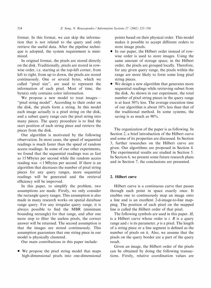
generated for the pixels. The pixel on the lower leftcorner has the value (0, 0). The pixel on its righthas the value (1, 0) and the one above it has thevalue (0, 1), and so on. The upper-right pixel of theimage whose size is m � n has the value (m; n).Next, a Hilbert curve is generated. Hilbert curve isa self-similar curve that is created recursively. Thebasic curve H1 has 2� 2 vertices. The Hilbertcurve Hi can be derived directly from Hi�1 byreplacing each vertex of Hi�1 with a basic curve,which may be rotated or rejected. Fig. 1 shows theshape of H1; H2 and H3: The black dots arethe vertices of the curves and the arrows mark thedirection.The Hilbert curve must be big enough to cover

all the pixels of the image by its vertices. Bydefinition, it is easy to see that a Hilbert curve withorder i has 2i � 2i vertices. Therefore, for an imagewith m � n pixels, we must at least build a Hilbertcurve with order k in order to cover all the pixelswhere k ¼ log2 ðmaxfm; ngÞ:After the Hilbert curve is generated, all the

pixels are on the vertices of the curve. Then, alongthe curve, the Hilbert order of each pixel can beuniquely decided. More details about Hilbertcurve can be found in [8–10].By the definition and the recursive generation of

the curve, Hilbert curve has many interestingproperties. We list two below which will be usedin our algorithm later.

Proposition 1. Suppose Hi, Hj are two Hilbert

curves with order i and j where i > j. The path of Hi

follows the path of Hj :

For example, H2 passes the four pixels in thelower-left quarter first, then the upper-left quarter,

the upper-right quarter and finally the lower-rightquarter. This order is exactly along the path of H1:

Proposition 2. Suppose pixel p of an image has the

relative coordination value (i; j), the previous

and the next pixels on the Hilbert curve must

be two of the following four pixels:

(i � 1; jÞ; ði þ 1; jÞ; ði; j � 1Þ and (i; j þ 1).

This is obvious because the Hilbert curve hasonly horizontal and vertical line segments.We store the pixels of an image in the Hilbert

order because in this order, pixels are groupedtogether. For any subset queries, the pixels insidethe query range are more likely to form some longstring pieces instead of equi-length pieces in row-wise order. We hope that the total number ofpieces within the query ranges may becomesmaller.However after several experiments, we find that

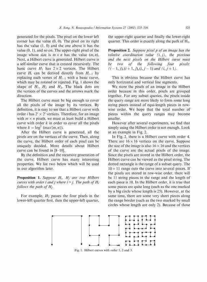
simply using the Hilbert order is not enough. Lookat an example in Fig. 2.In Fig. 2, there is a Hilbert curve with order 4.

There are 16� 16 vertices on the curve. Supposethe size of the image is also 16� 16 and the verticesof the curve are the actual pixels of the image.Since the pixels are stored in the Hilbert order, theHilbert curve can be viewed as the pixel string. Thedotted rectangle is the range of a subset query. The10� 11 range cuts the curve into several pieces. Ifthe pixels are stored in row-wise order, there willbe 11 string pieces in the range and the length ofeach piece is 10. In the Hilbert order, it is true thatsome pieces are quite long (such as the one markedby a big circle whose length is 25). However, at thesame time, there are some very short pieces alongthe range border (such as the two marked by smallcircles whose length are only 2). Because of those

Fig. 1. Hilbert curves with order 1, 2 and 3.

Z. Song, N. Roussopoulos / Information Systems 27 (2002) 523–536 525

short pieces, the total number of string pieceswithin the query range is 13. Comparing with thatof row-wise order, the number does not change toomuch.In order to improve the retrieval efficiency, we

must figure out a way to eliminate those shortpieces. In the next section, we will do moreresearch on the Hilbert curve and try to find asolution.

3. Cross point

Fig. 3 is a Hilbert curve with order 4. Weassume that the vertices of the curve are the pixelsof an image. There are 16 columns in this image,which are marked by the numbers above the curve.l is the left border of a query range. Currently l isat column 5. In order to observe the pixels on l

clearly, we slightly move the line left. There are 12pixels on the line. The pixels can be classified intothree categories according the position of theprevious and the next pixels on the curve.

1. From the nearest pixel left of l; the curvetraverses the pixel and goes up (or down) orright (such as pixel 1 in the figure).

2. From the nearest pixel right of l or on l; thecurve traverses the pixel and goes up (or down)or right (such as pixel 2 in the figure).

3. From the nearest pixel on l or right of l; thecurve traverses the pixel and goes left (such aspixel 3 in the figure).

In the second case, the previous and the nextpixels on the curve are both in the query range.For the rest two cases, either the previous pixel orthe next one is outside the query range. We callpixels of category 1 and 3 ‘‘cross points’’ on theborder.Randomly place a line on the Hilbert curve, we

find that the number of cross points among thepixels on the line satisfies the following theorem.

Theorem 3. Each pixel on the border of a subset

query range has 50% possibility to become a cross

point.

Proof. Suppose p is a pixel on line l which is theleft border of a query range. By definition, p is across point if and only if the previous or the nextpixel on the curve is on its left side. It means thatthere exists a horizontal line segment on the

Fig. 2. Range query on the Hilbert curve.

0 1 2 3 4 5 6 7 8 9 10 11 12 13 14 15

l

1

2

3

Fig. 3. Three kinds of pixels.


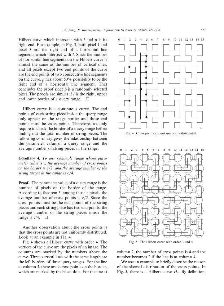
Hilbert curve which intersects with l and p is itsright end. For example, in Fig. 3, both pixel 1 andpixel 3 are the right end of a horizontal linesegments which intersect with l: Since the numberof horizontal line segments on the Hilbert curve isalmost the same as the number of vertical ones,and all pixels except two end points of the curveare the end points of two consecutive line segmentson the curve, p has about 50% possibility to be theright end of a horizontal line segment. Thatconcludes the proof since p is a randomly selectedpixel. The proofs are similar if l is the right, upperand lower border of a query range. &

Hilbert curve is a continuous curve. The endpoints of each string piece inside the query rangeonly appear on the range border and those endpoints must be cross points. Therefore, we onlyrequire to check the border of a query range beforefinding out the total number of string pieces. Thefollowing corollary gives the relationship betweenthe parameter value of a query range and theaverage number of string pieces in the range.

Corollary 4. To any rectangle range whose para-

meter value is c, the average number of cross points

on the border is c=2, and the average number of the

string pieces in the range is c=4:

Proof. The parameter value of a query range is thenumber of pixels on the border of the range.According to theorem 3, among those c pixels, theaverage number of cross points is c=2: Since thecross points must be the end points of the stringpieces and each string piece has two end points, theaverage number of the string pieces inside therange is c/4. &

Another observation about the cross points isthat the cross points are not uniformly distributed.Look at an example in Fig. 4.Fig. 4 shows a Hilbert curve with order 4. The

vertices of the curve are the pixels of an image. Thecolumns are marked by the numbers above thecurve. Three vertical lines with the same length arethe left borders of three query ranges. For the lineat column 5, there are 9 cross points on the border,which are marked by the black dots. For the line at

column 2, the number of cross points is 4 and thenumber becomes 2 if the line is at column 4.We use an example to briefly describe the reason

of the skewed distribution of the cross points. InFig. 5, there is a Hilbert curve H4: By definition,

0 1 2 3 4 5 6 7 8 9 10 11 12 13 14 15

Fig. 4. Cross points are not uniformly distributed.

0 0 1 2 1 2 3 3 4 4 5 6 5 6 7 8 7 8 9 9 10 10 11 11 12 12 13 13 14 14 1515

Fig. 5. The Hilbert curve with order 3 and 4.


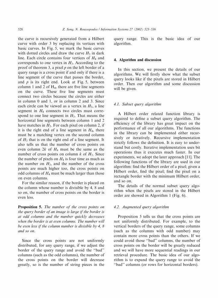
the curve is recursively generated from a Hilbertcurve with order 3 by replacing its vertices withbasic curves. In Fig. 5, we mark the basic curveswith dotted circles and draw the curve H3 in darkline. Each circle contains four vertices of H4 andcorresponds to one vertex in H3: According to theproof of theorem 3, a pixel p on the left border of aquery range is a cross point if and only if there is aline segment of the curve that passes the border,and p is its right end. Look at Fig. 5, betweencolumn 1 and 2 of H4, there are five line segmentson the curve. These five line segments mustconnect two circles because the circles are eitherin column 0 and 1, or in column 2 and 3. Sinceeach circle can be viewed as a vertex in H3; a linesegment in H4 connects two circles must corre-spond to one line segment in H3: That means thehorizontal line segments between column 1 and 2have matches in H3: For each pixel on column 2, ifit is the right end of a line segment in H4; theremust be a matching vertex on the second columnof H3 that is on the right end of a line segment. Italso tells us that the number of cross points oneven column 2k of H4 must be the same as thenumber of cross points on column k of H3: Sincethe number of pixels on H4 is four time as much asthe number on H3; and the number of the crosspoints are much higher too, the cross points onodd columns of H4 must be much larger than thoseon even columns.For the similar reason, if the border is placed on

the column whose number is divisible by 4, 8 andso on, the number of cross points on the border iseven less.

Proposition 5. The number of the cross points on

the query border of an image is large if the border is

at odd columns and the number quickly decreases

when the border is at even columns. The number will

be even less if the column number is divisible by 4, 8

and so on.

Since the cross points are not uniformlydistributed, for any query range, if we adjust theborder of the query range and avoid the ‘‘bad’’columns (such as the odd columns), the number ofthe cross points on the border will decreasegreatly, so is the number of string pieces in the

query range. This is the basic idea of ouralgorithm.

4. Algorithm and discussion

In this section, we present the details of ouralgorithms. We will firstly show what the subsetquery looks like if the pixels are stored in Hilbertorder. Then our algorithm and some discussionwill be given.

4.1. Subset query algorithm

A Hilbert order related function library isrequired to define a subset query algorithm. Theefficiency of the library has great impact on theperformance of all our algorithms. The functionsin the library can be implemented either recur-sively or iteratively. Recursive implementationstrictly follows the definition. It is easy to under-stand but costly. Iterative implementation uses bitoperations thus it executes much faster. In ourexperiments, we adopt the later approach [11]. Thefollowing functions of the library are used in ouralgorithm: find the Hilbert order of a pixel; given aHilbert order, find the pixel; find the pixel on arectangle border with the minimum Hilbert order,and so on.The details of the normal subset query algo-

rithm when the pixels are stored in the Hilbertorder are showed in Algorithm 1 (Fig. 6).

4.2. Augmented query algorithm

Proposition 5 tells us that the cross points arenot uniformly distributed. For example, to thevertical borders of the query range, some columns(such as the columns with odd number) maycontain more cross points than the others. If wecould avoid those ‘‘bad’’ columns, the number ofcross points on the border will be greatly reducedand we will have more sequential readings in ourretrieval procedure. The basic idea of our algo-rithm is to expand the query range to avoid the‘‘bad’’ columns (or rows for horizontal borders).


In our algorithm, we introduce a new parametern: This parameter is used to indicate whichcolumns (or rows) we should expand the bordersto. For example, when n ¼ 3; we should expandthe borders to the columns (or rows) whosenumbers are divisible by 23=8. It is worth notingthat the normal subset query algorithm in Fig. 6 isa special case of this algorithm if we set n ¼ 0: Thedetails are listed in Algorithm 2. (Fig. 7).

4.3. Discussion

In our algorithm, we expand the query range tomake the readings more sequentialized. The extracost we pay is that we have to retrieve more pixelsfrom the disk than necessary after the rangeexpansion. In our experiments, we find thatincreasing n has both positive and negativeinfluence on the performance. As n increases by1, on one hand, the number of pixel string piecesdrops about 50%. On the other hand, the number

of extraneous pixels contained in the augmentedquery range can be up to three times more. In thissubsection, we want to find out the relationshipbetween the performance of our algorithm and n;and the parameters that have impacts on theselection of n:In a system, suppose t1 is the average time of

one search on the disk, t2 is the average time ofreading one byte. There is a range query withparameter value c: When n ¼ 0; according toCorollary 4, averagely there are c=4 pixel stringpieces in the range and no useless pixels in thequery range. When n ¼ 1; the experiments showthat there are about c=8 pieces in the range.Therefore, the saving is ðc=8Þt1: At the same time,we have about c=2 useless pixels in our augmentedrange. The extra cost is ðc=2Þst2; where s is the pixelsize. So the benefit of changing n from 0 to 1 isB1 ¼ ðc=8Þt1 � ðc=2Þst2: When n changes from k �1 to k; the corresponding benefit is:

Bk ¼c

2kþ2

� �t1 �

c

2

� �3k�1st2

It is obvious that Bk is a monotonous decreasingsequence of k: Define n to be the greatest integerthat makes Bn > 0: That is

n ¼ max kjkolog3t1

2st2

� ��

At this point, the system has the best performance.The selection of n varies in different systems. Itdepends on at least two factors: t1=t2 and s:

Fig. 6. Subset query algorithm when the points are stored in the Hilbert order.

Fig. 7. Fast subset query algorithm.


The speed of the random access readings is slowbecause during the reading procedure, much timeis spent in disk searching. The value of t1=2 is thenumber of disk searches that can be executedduring the time of one byte reading. This rationumber sometimes can be used to indicate thesequential reading capability of a system. If t1 isbig and/or t2 is small, it means the system is morecapable of sequential readings. In that system, n

will be large. This conclusion is very intuitive.Another parameter that affects the selection of

n is the pixel size s: For each useless pixel weinclude in the augmented query range, we have toretrieve extra s bytes from the disk. If s is large, thebenefit we gained from the sequential readingsdoes not allow us to expand the query range toomuch. It means n will be a small number.It is worth noting that the selection of n does

not depend on the size or the location of the queryrange. This is a little different from our originalexpectation. This is a quite good attribute. Itshows that in any system, once n is found, it willremain the same for all queries. Therefore, theselection of n is a one-time work.

5. Experimental results

To access the merit of our algorithm, weimplemented our algorithm and performed someexperimental evaluations on both synthetic andreal data sets.

5.1. Experimental settings and methods selection

In our experiments, the methods we choseninclude: traditional method which stores the pixelsin row-wise order, normal subset query methodwhich stores the pixels in the Hilbert order butdoes not expand the query size, and augmentedquery method with different n: The abbreviationsof algorithms used in this section are shown inTable 1.All algorithms are implemented in C++. The

experiments using synthetic data sets wereperformed on a Sun Ultra 1 workstation runningon Solaris 2.7. The workstation has 128Mbytes ofmain memory and 4Gbytes of disk. The page size

is 4096 bytes. The experiments using real data setswere performed on one node of IBM SP2 machine.The real data sets are stored in a HPSS system [12].HPSS is very efficient for large file retrieving. Inour experiments, the 8-way ftp can be as fast as45M/s. The page size in HPSSis 1Mbytes and thememory buffer size we used for each query is2Mbytes.

5.2. Data sets and query sets

The synthetic data sets are used to study theimpact of different parameters on the performanceof our algorithm and the selection of n . In orderto find out the exact I/O performance of thealgorithms, all the buffer techniques (from bothC++ functions and the operating system) shouldbe avoided. We did two things: we only used lowlevel I/O function calls in C++ (such as read,write) instead of fstream classes to avoid theacceleration caused by the buffer techniques inthe standard function library. At the same time, weconstructed a large synthetic data set that consistsof several hundred images of the same size. Foreach subset query, an image is randomly chosenfrom the set. In this way, the operating systemwon’t have enough space to buffer the previousquery results.The real data sets are from the database of

NASA ESIP project. The project is to provideservices for checking and downloading satelliteimages online. The user group is earth scientists.The database size is several Tera bytes. Each imagein the database is one satellite picture whichcontains seven bands. The size of each band is58.8Mbytes and the pixel size is 1 byte per pixel.The query set includes many query ranges with

different parameter value. The queries are gener-ated as following. Given a length c; the width ofthe range is c=4 with a 10% margin. For example,

Table 1

Algorithms abbreviations

RW Traditional algorithm using row-wise order

NQ Normal subset query algorithm

AQ-n Augmented algorithm that expands the border to

columns (or rows) whose numbers are divisible by 2n


if the total length of the parameter is 400.The width of the range is randomly picked from[90, 110], and the height is (200-width). Thelocations of the query ranges are randomlygenerated. All of the results listed in our experi-ments are the average result of more than 1000 testcases.

5.3. Special readings

When we monitored the performance of ouralgorithms, we found that some readings spendmuch more time than the average value (about1000 times higher). We called them ‘‘specialreadings’’. The reason is that when our experi-ments are executed, during these readings, theoperating system switches the CPU control toother tasks. After our experiment regains thecontrol, much time has elapsed. Those ‘‘specialreadings’’ make it difficult to get the accurateresult. In order to solve the problem, we define athreshold and record the time of each reading. Ifthe time of one specific reading is more than ourthreshold, we replace that result with the averagevalue. The threshold is very high (normally 500–1000 times higher than the average time) and thenumber of ‘‘special readings’’ in one case isnormally less than 0.3% of total number ofreadings.

5.4. Experimental results using synthetic data sets

We use the synthetic data sets to study theparameters that affect the performance of algo-rithms: the parameter value of subset queries andthe pixel size.In the first experiment, we measure the number

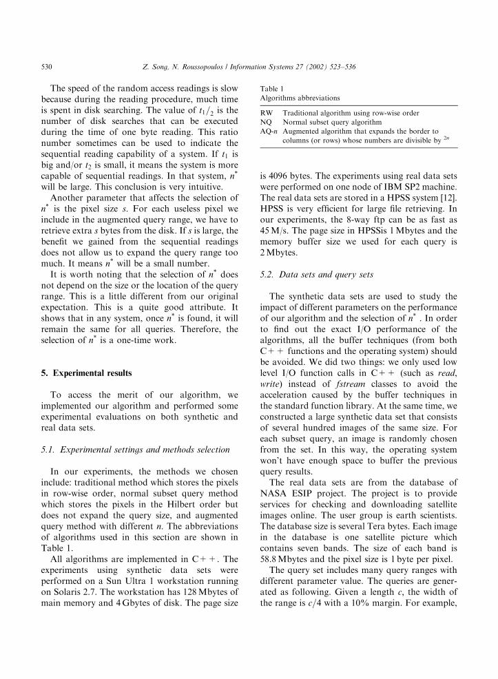
of pixel string pieces in the query range withvarious query range parameter value. The size ofthe images we used is 1024� 1024 pixels. Wegenerate a Hilbert curve with order 10 to cover allthe pixels. The experimental results are listed inFig. 8. In Fig. 8, the value of y-axis is the numberof pieces in the query range and x-axis lists sixalgorithms. The numbers in the legend aredifferent parameter value of query ranges used inthe experiment.

The following facts are showed in Fig. 8.

1. In RW, the number of pieces in the query rangeis the same as the value of the height of thequery range. Therefore, the average number ofthe pixel string pieces is one quarter of theparameter value.

2. Simply using the Hilbert order does not reducethe number of the string pieces. In ourexperiment, the value of NQ is almost the sameas or slightly higher than the value of RW in alltest cases, i.e. one quarter of the parameterslength. This result fits our corollary well.

3. As we augment the query range, the piecenumber drops quickly. As n increases by 1, thevalues are almost cut by half. The improve-ments are very obvious when n is small. Forlarge n; the absolute decreases are trivial.

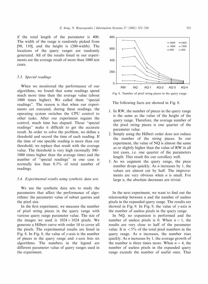
In the next experiment, we want to find out therelationship between n and the number of uselesspixels in the expanded query range. The results areshowed in Fig. 9. In Fig. 9, the value of y-axis isthe number of useless pixels in the query range.In NQ, no expansion is performed and the

number of useless pixels is 0. When n ¼ 1; theresults are very close to half of the parametervalue. It is o5% of the total pixel numbers in thequery range. As n increases, the number risesquickly. As n increases by 1, the average growth ofthe number is three times more. When n ¼ 4; thenumber of useless pixels in the expanded queryrange exceeds the number of useful ones. That

0

200

400

600

800

RW NQ AQ-1 AQ-2 AQ-3 AQ-4

3000 2400

1800 1200

600 200

Fig. 8. Number of pixel string pieces in the query range.


means in AQ-4, the actual number of pixels weretrieved from the disk is twice as many as thenumber of pixels in the query range.Next, we want to study the impact of the

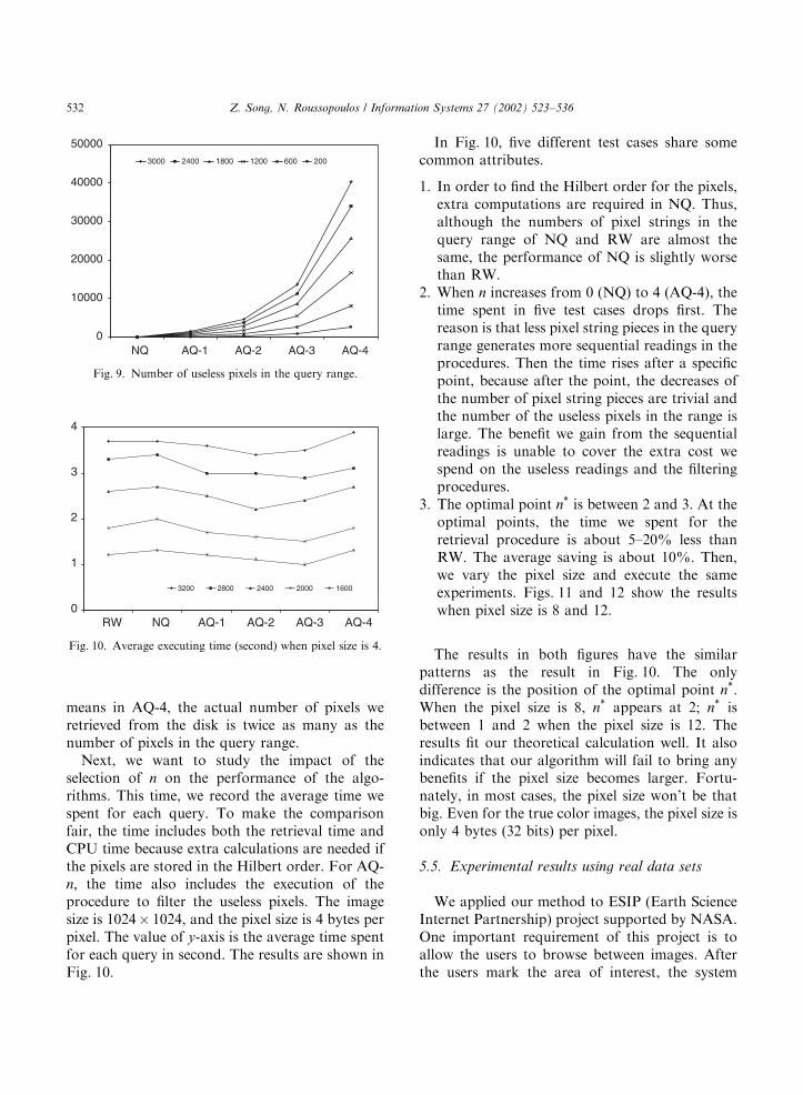
selection of n on the performance of the algo-rithms. This time, we record the average time wespent for each query. To make the comparisonfair, the time includes both the retrieval time andCPU time because extra calculations are needed ifthe pixels are stored in the Hilbert order. For AQ-n; the time also includes the execution of theprocedure to filter the useless pixels. The imagesize is 1024� 1024, and the pixel size is 4 bytes perpixel. The value of y-axis is the average time spentfor each query in second. The results are shown inFig. 10.

In Fig. 10, five different test cases share somecommon attributes.

1. In order to find the Hilbert order for the pixels,extra computations are required in NQ. Thus,although the numbers of pixel strings in thequery range of NQ and RW are almost thesame, the performance of NQ is slightly worsethan RW.

2. When n increases from 0 (NQ) to 4 (AQ-4), thetime spent in five test cases drops first. Thereason is that less pixel string pieces in the queryrange generates more sequential readings in theprocedures. Then the time rises after a specificpoint, because after the point, the decreases ofthe number of pixel string pieces are trivial andthe number of the useless pixels in the range islarge. The benefit we gain from the sequentialreadings is unable to cover the extra cost wespend on the useless readings and the filteringprocedures.

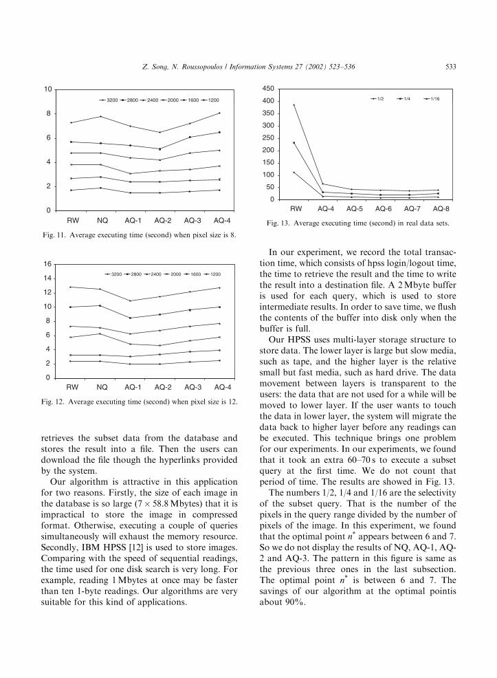
3. The optimal point n is between 2 and 3. At theoptimal points, the time we spent for theretrieval procedure is about 5–20% less thanRW. The average saving is about 10%. Then,we vary the pixel size and execute the sameexperiments. Figs. 11 and 12 show the resultswhen pixel size is 8 and 12.

The results in both figures have the similarpatterns as the result in Fig. 10. The onlydifference is the position of the optimal point n:When the pixel size is 8, n appears at 2; n isbetween 1 and 2 when the pixel size is 12. Theresults fit our theoretical calculation well. It alsoindicates that our algorithm will fail to bring anybenefits if the pixel size becomes larger. Fortu-nately, in most cases, the pixel size won’t be thatbig. Even for the true color images, the pixel size isonly 4 bytes (32 bits) per pixel.

5.5. Experimental results using real data sets

We applied our method to ESIP (Earth ScienceInternet Partnership) project supported by NASA.One important requirement of this project is toallow the users to browse between images. Afterthe users mark the area of interest, the system

0

10000

20000

30000

40000

50000

NQ AQ-1 AQ-2 AQ-3 AQ-4

3000 2400 1800 1200 600 200

Fig. 9. Number of useless pixels in the query range.

0

1

2

3

4


3200 2800 2400 2000 1600

Fig. 10. Average executing time (second) when pixel size is 4.


retrieves the subset data from the database andstores the result into a file. Then the users candownload the file though the hyperlinks providedby the system.Our algorithm is attractive in this application

for two reasons. Firstly, the size of each image inthe database is so large (7� 58.8Mbytes) that it isimpractical to store the image in compressedformat. Otherwise, executing a couple of queriessimultaneously will exhaust the memory resource.Secondly, IBM HPSS [12] is used to store images.Comparing with the speed of sequential readings,the time used for one disk search is very long. Forexample, reading 1Mbytes at once may be fasterthan ten 1-byte readings. Our algorithms are verysuitable for this kind of applications.

In our experiment, we record the total transac-tion time, which consists of hpss login/logout time,the time to retrieve the result and the time to writethe result into a destination file. A 2Mbyte bufferis used for each query, which is used to storeintermediate results. In order to save time, we flushthe contents of the buffer into disk only when thebuffer is full.Our HPSS uses multi-layer storage structure to

store data. The lower layer is large but slow media,such as tape, and the higher layer is the relativesmall but fast media, such as hard drive. The datamovement between layers is transparent to theusers: the data that are not used for a while will bemoved to lower layer. If the user wants to touchthe data in lower layer, the system will migrate thedata back to higher layer before any readings canbe executed. This technique brings one problemfor our experiments. In our experiments, we foundthat it took an extra 60–70 s to execute a subsetquery at the first time. We do not count thatperiod of time. The results are showed in Fig. 13.The numbers 1/2, 1/4 and 1/16 are the selectivity

of the subset query. That is the number of thepixels in the query range divided by the number ofpixels of the image. In this experiment, we foundthat the optimal point n appears between 6 and 7.So we do not display the results of NQ, AQ-1, AQ-2 and AQ-3. The pattern in this figure is same asthe previous three ones in the last subsection.The optimal point n is between 6 and 7. Thesavings of our algorithm at the optimal pointisabout 90%.

0

2

4

6

8

10


3200 2800 2400 2000 1600 1200


0

2

4

6

8

10

12

14

16


3200 2800 2400 2000 1600 1200


0

50

100

150

200

250

300

350

400

450

RW AQ-4 AQ-5 AQ-6 AQ-7 AQ-8

1/2 1/4 1/16

Fig. 13. Average executing time (second) in real data sets.


6. Future research

We plan to further our research in the followingthree areas.

6.1. Working in parallel environment

The Hilbert curves are generated recursively andthe curves with different order share similarstructures. This attribute of the curve is veryuseful in parallel environment.Suppose we want to store the pixels of an image

into multiple disks. In order to maximize theefficiency, the workload of the disks should bebalanced. The Hilbert curve is ideally designed forthis purpose. For example, we have four proces-sors available and each processor has its own diskspace. Along the Hilbert curve, we store the pixelsinto the four disks. Those pixels whose Hilbertorder is 4k goes to disk 0, 4k+1 goes to disk 1, andso on. The pixels on each disk form a Hilbert curvetoo, but with one order higher. The four curveshave identical structure. For the subset queries, weonly have to check the start positions and thelength of the string pieces on one disk. For the restthree disks, the result is the same. The number ofreadings from each disk is the same too.We ran some experiments on four nodes of an

IBM SP2 machine using MPI (Message PassingInterface) [13] library. One master node did thepreprocessing work and broadcast the cross pointset to the other three slave nodes. Then all fournodes retrieved the data from their own disk andthe slave nodes sent the result back to the masterone. The master node put the result together andreturned it to the user. Our result showed that withfour disks available, the total query time is veryclose to 1/4 of the time when we only use oneprocessor and one disk.

6.2. High-dimensional data

Currently, we only query two-dimensionalimages. In some applications, high-dimensionaldata are used. For example, in ESIP project, thedatabase contains many satellite images of Cali-fornia, USA at different time. The location and thesize of the images are identical. A usually

encountered query is that given a time periodand a subarea, retrieve the pixels in the subarea ofall images within the time period that contain thelocation. Currently, we store the images sepa-rately. The image metadata are saved in anotherdatabase. For this query, we check the metadatafirst and find all the images whose creation time iswithin the given time period. Then go back tomain database, launch the subset query on all theimages.We are thinking about using another approach.

Those images can be viewed as 3-d data after weintroduce time as another dimension. Then all thepixels of those images are stored in one big file,and the high-dimensional Hilbert curve may beused to store the pixels. Finally, the subset queriescan be handled with the similar augmented queryalgorithm. The problem left is that the thirddimension (time) is much thinner than the othertwo dimensions. When we use the high-dimen-sional Hilbert curve, on this dimension, a lot ofvertices are wasted.

6.3. Organizing multi-level previews in one file

In some online applications, the size of theactual images is very large. It is inefficient to putthe large image online directly. Therefore, pre-viewed images are generated for users to browseand search the images they want. After the usersmake the selection, the actual images are trans-ferred to them or links are provided for down-loading.Normally, users want to zoom in or zoom out

an interested preview image during browsing. Inorder to have quick response, multi-layer previewsare created. The basic idea is to generate severalpreviews with different sizes for one image. Thepreviews are stored in meta-database for quickretrieval. This design is sometimes called ‘‘imagepyramid’’. The zoom in operation is handled byreturning lower-level previews in the server. Forexample, in Microsoft TerraServer application[14], 7 layers are generated for each image. In thisstructure, extra entries are maintained in meta-database, and the change of the original imagemay cause some integrity problems.


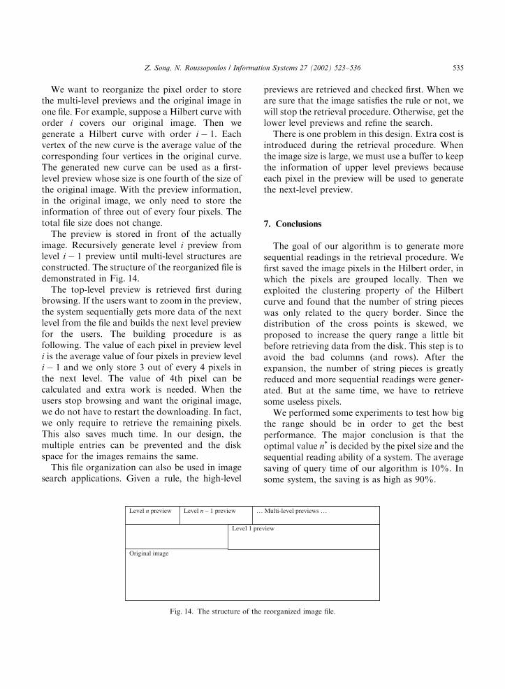
We want to reorganize the pixel order to storethe multi-level previews and the original image inone file. For example, suppose a Hilbert curve withorder i covers our original image. Then wegenerate a Hilbert curve with order i � 1: Eachvertex of the new curve is the average value of thecorresponding four vertices in the original curve.The generated new curve can be used as a first-level preview whose size is one fourth of the size ofthe original image. With the preview information,in the original image, we only need to store theinformation of three out of every four pixels. Thetotal file size does not change.The preview is stored in front of the actually

image. Recursively generate level i preview fromlevel i � 1 preview until multi-level structures areconstructed. The structure of the reorganized file isdemonstrated in Fig. 14.The top-level preview is retrieved first during

browsing. If the users want to zoom in the preview,the system sequentially gets more data of the nextlevel from the file and builds the next level previewfor the users. The building procedure is asfollowing. The value of each pixel in preview leveli is the average value of four pixels in preview leveli � 1 and we only store 3 out of every 4 pixels inthe next level. The value of 4th pixel can becalculated and extra work is needed. When theusers stop browsing and want the original image,we do not have to restart the downloading. In fact,we only require to retrieve the remaining pixels.This also saves much time. In our design, themultiple entries can be prevented and the diskspace for the images remains the same.This file organization can also be used in image

search applications. Given a rule, the high-level

previews are retrieved and checked first. When weare sure that the image satisfies the rule or not, wewill stop the retrieval procedure. Otherwise, get thelower level previews and refine the search.There is one problem in this design. Extra cost is

introduced during the retrieval procedure. Whenthe image size is large, we must use a buffer to keepthe information of upper level previews becauseeach pixel in the preview will be used to generatethe next-level preview.

7. Conclusions

The goal of our algorithm is to generate moresequential readings in the retrieval procedure. Wefirst saved the image pixels in the Hilbert order, inwhich the pixels are grouped locally. Then weexploited the clustering property of the Hilbertcurve and found that the number of string pieceswas only related to the query border. Since thedistribution of the cross points is skewed, weproposed to increase the query range a little bitbefore retrieving data from the disk. This step is toavoid the bad columns (and rows). After theexpansion, the number of string pieces is greatlyreduced and more sequential readings were gener-ated. But at the same time, we have to retrievesome useless pixels.We performed some experiments to test how big

the range should be in order to get the bestperformance. The major conclusion is that theoptimal value n is decided by the pixel size and thesequential reading ability of a system. The averagesaving of query time of our algorithm is 10%. Insome system, the saving is as high as 90%.

Original image

Level 1 preview

Level n preview Level n – 1 preview … Multi-level previews …

Fig. 14. The structure of the reorganized image file.


Acknowledgements

Thanks to Doug Moore who provides a fastHilbert curve function library online [11].

References

[1] http://www.umiacs.umd.edu/research/esip/(2000).

[2] D. Ballard, C. Brown, Computer Vision, Prentice-Hall,

Englewood Cliff, NJ, 1982.

[3] K. Hirata, T. Kato, Query by visual example—content

based image retrieval, in: Proceedings of the Advances in

Database Technology, Vienna, Austria, 1992.

[4] T. Gevers, A. Smuelders, An approach to image retrieval

for image database, in: Proceedings of the Database and

Expert Systems Application, Prague, Czechoslovakia, 1993.

[5] J. Liang, C. Chang, Similarly retrieval on pictorial

databases based upon module operation, in: Proceedings

of the Database Systems for Advanced Application,

Taejon, South Korea, 1993.

[6] C. Faloutsos, R. Barber, M. Flickner, J. Hafner, W.

Niblack, D. Perkovic, W. Equitz, Efficient and effective

querying by image content, J. Intell. Inform. Systems:

Interacting Artif. Intell. Database Technol. 3 (1994) 231–

262.

[7] S. Berchtold, C. Bohm, B. Braunmuller, D. Kein, H.P.

Kriegal, Fast parallel similarity search in multimedia

database, in: Proceedings of the ACM SIGMOD, Tucson,

Arizona, USA, 1997.

[8] T. Bially, Space-filling curves: their generation and their

application to bandwidth reduction, IEEE Trans. Inform.

Theory 15 (6) (1969) 658–664.

[9] J. Griffiths, An algorithm for displaying a class of

space-filling curves, Software-Pract. Exper. (1986)

403–411.

[10] I. Kamel, C. Faloutsos. An improved r-tree using fractals.

In: Proceedings of the VLDB Conference, Santiago, Chile,

1994, pp. 500–509.

[11] http://www.caam.rice.edu/dougm/twiddle/hilbert/(1999).

[12] http://www4.clearlake.ibm.com/hpss/index.jsp(2000).

[13] W. Gropp, E. Lush, A. Skjellum, Using MPI: portable

parallel programming with the message-passing interface,

The MIT Press, Cambridge, MA, 1994.

[14] T. Barclay, J. Gray, D. Slutz, Microsoft terraserver: a

spatial data warehouse, in: Proceedings of the ACM

SIGMOD, Dallas, Texas, USA, 2000.


http://www.umiacs.umd.edu/research/esip/

http://www.caam.rice.edu/dougm/twiddle/hilbert/

http://www4.clearlake.ibm.com/hpss/index.jsp

Using Hilbert curve in image storing and retrieving - CiteSeerX

Documents

Transcript of Using Hilbert curve in image storing and retrieving - CiteSeerX