lndexing and retrieving point and region objects

Azzarn Ibrahim1 and Farshad Fotouhi2

1 Metlife -MetSource Consulting, 200 Galleria Officenter, Suite 400Southfield, Michigan 48034

2 Wayne State University, Department of Computer ScienceDetroit, Michigan 48202

ABSTRACT

R-tree and its variants are examples of spatial data structures for paged-secondary memory. Toprocess a query, these structures require multiple path traversals. In this paper, we present a new imageaccess method, SB + -tree which requires a single path traversal to process a query. Also, SB + -tree willallow commercial databases an access method for spatial objects without a major change, since mostcommercial databases already support B + -tree as an access method for text data. The SB + -tree can be usedfor zero and non-zero size data objects. Non-zero size objects are approximated by their minimum boundingrectangles (MBRs). The number of SB + -trees generated is dependent upon the number of dimensions of theapproximation of the object. The structure supports efficient spatial operations such as Regions-Overlap,Distance and Direction. In this paper, we experimentally and analytically demonstrate the superiority of

SB+ -tree over R-tree.

1. INTRODUCTION

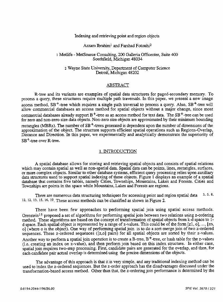
A spatial database allows for storing and retrieving spatial objects and consists of spatial relationswhich may contain spatial as well as non-spatial data. Spatial data can be points, lines, rectangles, surfaces,or more complex objects. Similar to other database systems, efficient query processing relies upon auxiliarydata structures used to support spatial indexing of these objects. Figure 1 displays an example of a spatialdatabase that contains five tables, namely Cities, Townships, Mountains, Lakes and Forests. Cities andTownships are points in the space while Mountains, Lakes and Forests are regions.

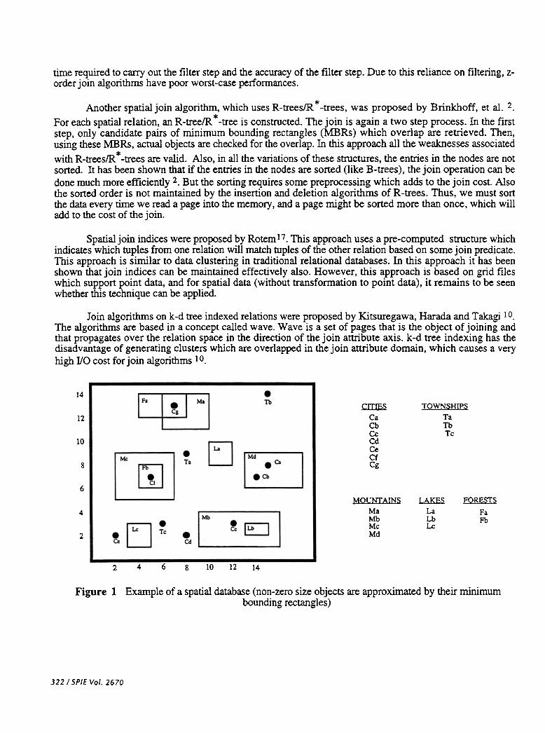
3.5, 8,There are numerous data structuring techniques for accessing point and region spatial data12, 12, 13, 15. 16, 19. These access methods can be classified as shown in Figure 2.

There have been few approaches to performing spatial join using spatial access methods.Orenstein 15 proposed a set of algorithms for performing spatial join between two relations using z-orderingmethod. These algorithms are based on the concept of transformation of spatial objects from k -d space to 1-d space. Each spatial object is represented by a range of z-values. This could be of the form [z1, 0], ..., [zn,0] (where 0 is the object). One way of performing spatial join is to do a sort-merge join of two z-orderedsequences. These z-ordered sequences ([z,o] pairs) for all spatial objects are sorted by their z-values.Another way to perform a spatial join operation is to create a B-tree, B + -tree, or hash table for the z-values(i.e. creating an index on z-value), and then perform join based on this index structure. In either case,spatial join requires two-step processing. First, candidate pairs are generated for the overlap, and then, foreach candidate pair actual overlap is detennined using the precise dimensions of the objects.

The advantage of this approach is that it is very simple, and any traditional indexing method can beused to index the z-ordered sequences. But the z-order approach has the disadvantages discussed under thetransformation-based access method. Other than that, the z-ordering join performance is determined by the

SPIE Vol. 2670/3210-8194-2044-1/96/$6.00

time required to carry out the filter step and the accuracy of the filter step. Due to this reliance on filtering, z-order join algorithms have poor worst-case perfonnances.

Another spatial join algorithm, which uses R-trees/R *-trees, was proposed by Brinkhoff, et al. 2.For each spatial relation, an R-tree/R *-tree is constructed. The join is again a two step process. In the firststep, only candidate pairs of minimum bounding rectangles (MBRs) which overlap are retrieved. Then,using these MBRs, actual objects are checked for the overlap. In this approach all the weaknesses associatedwith R-trees/R *-trees are valid. Also, in all the variations of these structures, the entries in the nodes are notsorted. It has been shown that if the entries in the nodes are sorted (like B-trees), the join operation can bedone much more efficiently 2. But the sorting requires some preprocessing which adds to the join cost. Alsothe sorted order is not maintained by the insertion and deletion algorithms of R-trees. Thus, we must sortthe data every time we read a page into the memory, and a page might be sorted more than once, which willadd to the cost of the join.

Spatial join indices were proposed by Rotem 17. This approach uses a pre-computed structure whichindicates which tuples from one relation will match wples of the other relation based on some join predicate.This approach is similar to data clustering in traditional relational databases. In this approach it has beenshown that join indices can be maintained effectively also. However, this approach is based on grid fileswhich support point data, and for spatial data (without transfonnation to point data), it remains to be seenwhether this technique can be applied.

Join algorithms on k-d tree indexed relations were proposed by Kitsuregawa, Harada and Takagi 10.The algorithms are based in a concept called wave. Wave is a set of pages that is the object of joining andthat propagates over the relation space in the direction of the join attribute axis. k-d tree indexing has thedisadvantage of generating clusters which are overlapped in the join attribute domain, which causes a veryhigh I/O cost for join algorithms 10.

.

Tb14

~CaCbCcCdCeCfCg

TOWNSHIPSTaTbTc

12

10

rJ.

Ta8

6MOUNTAINS

MaMbMcMd

L.AKf.S.LaLbLc

FORESTS

FaFb

4

~LJ~

.

Cd2

6 10 122 4 8 14

Example of a spatial database (non-zero size objects are approximated by their minimumbounding rectangles)

Figure 1

322/ SPIE Vol. 2670

I Approximationusing (;, "'\ App~m2bOn

, Using Grid

~

~I Tr2mfonn,I MBRs to Points

I

Column-"';'. scan Row-wise scan

ZoOrderiD&Gray-aldiD& orHilbtrt-ord.rinc

Column-";" ~Row-..;.. ~Z-orderingGray_ng orffilbcrt-ordering

R T...RioT...R+-T...

Region-Quadtroo "'

ill

KD-T...Grid FileKDB- T...Point Qaad ~

Column-";" JCaD~.,.;,. ~ZoOrderia&Cray-<odiDC orHilbert_DC

Si~..

B-TraB+oTrftHaohiag

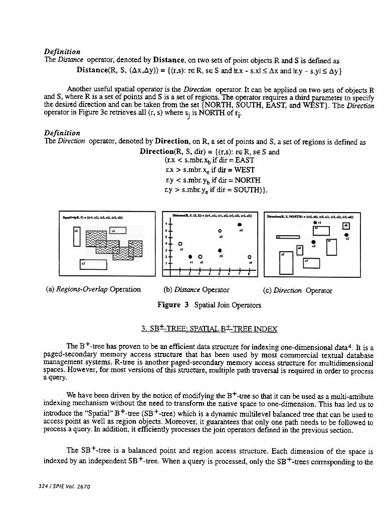
Figure 2 Classification of Spatial Access Methods

2. SPATIAL OPERATORS

Let r.mbr denote the minimum bounding rectangle of object r, r.mbr.xb/r.mbr.xe be thebeginning/ending margin of the MBR encompassing r in the X-axis direction, and r.mbr.Yb/r.mbr.Ye be thebeginning/ending margin of the MBR r's MBR in the Y-axis direction. If r is a point object, r.x and r. Yrespectively denote the x and Y coordinate of r in the space.

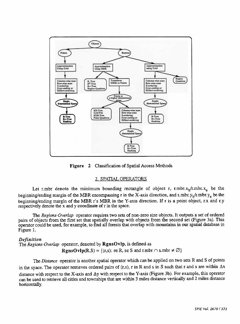
The Regions-Overlap operator requires two sets of non-zero size objects. It outputs a set of orderedpairs of objects from the first set that spatially overlap with objects from the second set (Figure 3a). Thisoperator could be used, for example, to find all forests that overlap with mountains in our spatial database inFigure 1.

DefinitionThe Regions-Overlap operator. denoted by RgnsOvlp, is defined as

RgnsOvlp(R,S) = {(r,s): re R, se S and r.rnbr n s.rnbr :t: 0}

The Distance operator is another spatial operator which can be applied on two sets R and S of pointsin the space. The operator retrieves ordered pairs of (r,s), r in Rand s in S such that r and s are within Ll.x

distance with respect to the X-axis and Ll.y with respect to the Y-axis (Figure 3b). For example, this operatorcan be used to retrieve all cities and townships that are within 3 miles distance vertically and 2 miles distance

horizontally.

SPIt Vol. 2670/323

DefinitionThe Distance operator, denoted by Distance, on two sets of point objects R and S is defined as

Distance(R, S, (ilx,ily» = {(r,s): re R, se S and Ir.x -s.xl ~ I1.x and Ir.y -s.yl ~ l1.y}

Another useful spatial operator is the Direction operator. It can be applied on two sets of objects Rand S, where R is a set of points and S is a set of regions. The operator requires a third parameter to specifythe desired direction and can be taken from the set {NORTH, SOUTH, EAST, and WEST}. The Directionoperator in Figure 3c retrieves all (r, s) where Sj is NORTH of ri.

DefinitionThe Direction operator, denoted by Direction, on R, a set of points and S, a set of regions is defined as

Direction(R, S, dir) = {(r,s): re R, se S and(r.x < s.mbr. xb if dir = EASTr.x > s.mbr. xe if dir = WESTr.y < s.mbr. Yb if dir = NORTHr.y> s.mbr.Ye if dir = SOUTH)}.

a.-'>"Pa. s) -j(rl. al), (02, aI), (J'2, 03)1

~

E~

(a) Regions-Overlap Operation (b) Distance Operator (c) Direction Operator

Figure 3 Spatial Join Operators

~Z- TREE: SPATIAL Bz- TREE INDEX

The B + -tree has proven to be an efficient data structure for indexing one-dimensional data 4. It is a

paged-secondary memory access structure that has been used by most commercial textual databasemanagement systems. R-tree is another paged-secondary memory access structure for multidimensionalspaces. However, for most versions of this structure, multiple path traversal is required in order to processa query.

We have been driven by the notion of modifying the B+ -tree so that it can be used as a multi-attributeindexing mechanism without the need to transform the native space to one-dimension. This has led us tointroduce the "Spatial" B + -tree (SB + -tree) which is a dynamic multilevel balanced tree that can be used to

access point as well as region objects. Moreover, it guarantees that only one path needs to be followed toprocess a query. In addition, it efficiently processes the join operators defined in the previous section.

The SB + -tree is a balanced point and region access structure. Each dimension of the space is

indexed by an independent SB + -tree. When a query is processed, only the SB + -trees corresponding to the

324/ SPIE Vol. 2670

dimensions referenced by the query are searched and the output is produced in terms of the outcome of theindividual searches. The following two definitions explain the terms: Indexing Point and Indexing Set.

DefinitionThe point ip is an indexing point of space S with respect to dimension p if there exists some object 0

in S such that the line p=ip represents the lower or upper bounding line of 0 with respect to pinS.

DefinitionThe indexing set of dimension p in a particular space; denoted by IP P is the set of all indexing points

of p in that space.

The previous definitions imply that the indexing set of a dimension is the set of points where :MERsbegin or end with respect to the dimension. For example, the :MER corresponding to mountain Mb in figure1.1 is (9..16, 1..4) where 9 and 16 are the minimum and maximum x values respectively; 1 and 4 are theminimum and maximum y values respectively. Therefore, 9 and 16 E IPx; 1 and 4 E IPy. City Ca is

located at (15,8) in the space. As a result, 15 E IPx and 8 E IPy. Considering all objects in the space, theindexing set of the X-axis, IPx is {2, 3, 4,5,6,7,8,9, 10,12,13,14,15,16, 18}, and that of the Y-axis

IPy is {I, 2, 3, 4, 5, 6, 7, 8,9, 10, 11, 12, 13, 14).

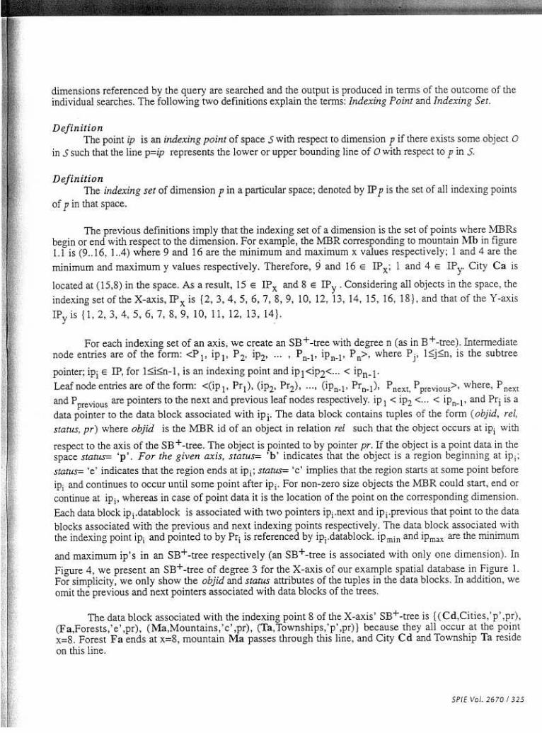
For each indexing set of an axis, we create an SB + -tree with degree n (as in B + -tree). Intermediatenode entries are of the form: <PI' iPI' P2' iP2' ..., P n-l' iPn-I' P n>' where Pj' l~j~, is the subtree

pointer; iPi E IP, for l~~n-l, is an indexing point and iPl<iP2<... < iPn-l.Leaf node entries are of the form: «ipI' Prl)' (ip2' Pr2)' ..., (iPn-I' Prn-l)' P next, P previous>' where, P nextand P previous are pointers to the next and previous leaf nodes respectively. ip I < iP2 <... < iPn-l' and Pri is adata pointer to the data block associated with iPi. The data block contains tuples of the form (objid, reI,status, pr) where objid is the MBR id of an object in relation reI such that the object occurs at iPi withrespect to the axis of the SB + -tree. The object is pointed to by pointer pro If the object is a point data in thespace status: 'p'. For the given axis, status: 'b' indicates that the object is a region beginning at iPi;status= 'e' indicates that the region ends at iPi; status: 'c' implies that the region starts at some point beforeiPi and continues to occur until some point after iPi. For non-zero size objects the MBR could start, end orcontinue at iPi' whereas in case of point data it is the location of the point on the corresponding dimension.Each data block ipi.datablock is associated with two pointers ipi.next and ipi.previous that point to the datablocks associated with the previous and next indexing points respectively. The data block associated withthe indexing point iPi and pointed to by Pri is referenced by ipi.datablock. iPmin and iPmax are the minimum

and maximum ip's in an SB+ -tree respectively (an SB+ -tree is associated with only one dimension). InFigure 4, we present an SB+ -tree of degree 3 for the X-axis of our example spatial database in ~i.gure 1.For simplicity, we only show the objid and status attributes of the tuples in the data blocks. In addItIon, weomit the previous and next pointers associated with data blocks of the trees.

The data block associated with the indexing point 8 of the X-axis' SB+ -tree is {(Cd,Cities,'p',pr),(Fa,Forests,'e',pr), (Ma,Mountains,'c',pr), (Ta,Townships,'p',pr)} because they all occur at the pointx=8. Forest Fa ends at x=8, mountain Ma passes through this line, and City Cd and Township Ta resideon this line.

SPIE Vol. 2670/325

Figure

4 SB+ -tree (order 3) for the X-axis of the database in Figure 1

Algorithms

for inserting and deleting points and regions are presented in reference 11.

4.

REGIONS-OVERLAP

In this section, we describe how to use the SB + -tree to find the overlapping objects between two setof

objects R and S in the space. The process starts by using the SB+ -tree of the X-axis to retrieve thoseobjects R that overlap with objects of S with respect to the X-axis. This step is repeated using the SB + -tree

of the Y-axis to retrieve overlapping objects with respect to the Y-axis. The tuples common between bothsets constitute the set of objects that overlap in the two-dimensional space. The input to this algorithm is the

SB+ -tree corresponding to the search axis. The output is the set of overlapping objects between R and Swith respect to the relevant axis. The algorithm is given below.

Algorithm:

Regions-Overlap Join of relations Rand S.Input:

SB+ -tree, and object types.Output: {(ri' Sj): ri E R ,Sj E S and ri overlaps with Sj with respect to the relevant axis}.Assumption:

R and S objects are regions in the space.{

1. Start with the leftmost data block of the SB+ -tree2. Oaxis = {} 1* initializing the output set */3. for (every datablock Db=leftmost datablock TO rightmost datablock){

II ri and Sj overlap if they both occur at some indexing point in the space.

3.1 for (every (ri' R, Rstatus, pr) E Db)

3.1.1 for (every (Sj,S,Sstatus, pr) E Db)

Oaxis = Oaxis U {(ri' Sj)}

}}

5. DISTANCE

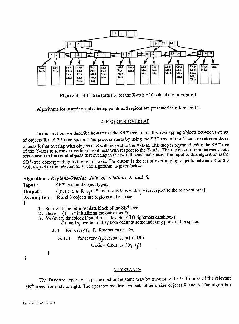
The Distance operator is perfonned in the same way by traversing the leaf nodes of the relevantSB+ -trees from left to right. The operator requires two sets of zero-size objects Rand S. The algorithm

3261SPIE Vol. 2670

given below finds ordered pairs (r, s), r in Rand s in S such that r and s are far apart by d units or less. Itrequires two data structures ArrR (length is size of R) and ArrS (length is size of S). Entries in both arraysare initialized to maximum integer values. When an indexing point ip is visited, for every point object r j of Rin the data block of ip, the entry ArrR[rjJ is assigned the value (ip+d). This is to indicate that all S objectsappearing in data blocks of indexing points on or before (ip+d) will be paired with r i in the output join set.The same operation is performed on S objects appearing in data blocks. (ip+d) is assigned to thecorresponding entries in ArrS so that objects of R can be paired with objects of S likewise. The algorithmguarantees that every tuple retrieved is unique with respect to the relevant axis. In addition, one traversal perlinked list of leaf nodes is enough to generate the Distance join for the corresponding axis.

Algorithm: Distance Join of relations Rand S.

Input: SB+ -tree, distance d, and object types.Assumption: Rand S objects are points in the space.

Output: {(ri,sj):rj E R ,Sj E S and the distance between ri and Sj is less than or equal to d with

respect to the relevant axis}.Local Structures:

ArrR is an array[rmin. .rrnax] of integer;ArrS is an array[srnin.. sma x] of integer;

{1. Oaxis= {};2.

for (every ri E [rmin..rmaxD ArrR[ri]= maxint;3.

for(everysjE [Smin'.Smax]) ArrS[sj]=maxint;4.

Start with the leftmost leaf node of the SB+ -tree5. for (ip=iPmin; ip<= iPmax; next ip){

5.1 for (every (ri,R,'p',pr) E ip.datablock) {ArrR[ri]= ip + d;

for (every Sj E [Smin..Smax] such that ip <= ArrS[Sj])

Oaxis= Oaxis U {(ri' Sj)}

5.2 for (every (Sj,S,'p',pr) E ip.datablock) {ArrS[SjJ= ip + d;

for (every rj E [rmjn..rmax] such that ip <= ArrR[rj])

Oaxis= Oaxis U {(rj, Sj)}

}

}

Figure 4 displays the contents of ArrR and ArrS at the relevant indexing points while perfonning theDistance spatial join operator between CmES and TOWNSmPS with respect to the X-axis (!:!.x = 3).

SPIt Vol. 2670/327

Cilios

c-o

Cc..:JC4..:JCo..:Ja-ICc.:J

a~

Co[::=]CO-.:JCc~Cd

~Cc $

a 8c.

Cilia

Co

~CO -I C-

eo I

Co ~

a I

c. -I

ODeS

Co~- 0 -I

c.-IC4 -c. sa 8

c, ,~

Citics

:: r Townships

~I :~Townsll;ps

TO§n "

To

To_poT8 §n -T,

Townships

y" §n -y, -

Towmhips

Ta§n -T' -

{}

ip=2

0..- -Ita. T,»

ip=6

0 0

Initially

Oak. V

ip=5 ip=7

CitiesCiti..Co

0Townsbjps

T'~l

n -T,

9

~

DooM 0 «a. T.~ (Co. T.~

(Cd. To). (Cd. To~'(Ct, To~(C.. To»

ip= 14

Execution of the Distance J om algorithm between Cities and Townships with respect to the X-axis (~x = 3)

Figure 4

6. DIRECfION

The Direction operator is ano~her spatial operator that can be performed using the SB + -tree. Itrequires two sets of objects R (a set of points), S (a set of regions), and the direction dir that is chosen fromthe set {NORTH, SOUTH, EAST, WEST}. One SB+-tree is needed to process this operator. When dir iseither EAST or WEST, the SB+-tree of the X-axis is searched. However, if dir is either NORTH orSOUTH, the SB + -tree of the Y-axis is searched. The list of leaf nodes of the SB + -tree is traversed from leftto right if dir is NORTH or EAST and from right to left if dir is SOUTH or WEST.

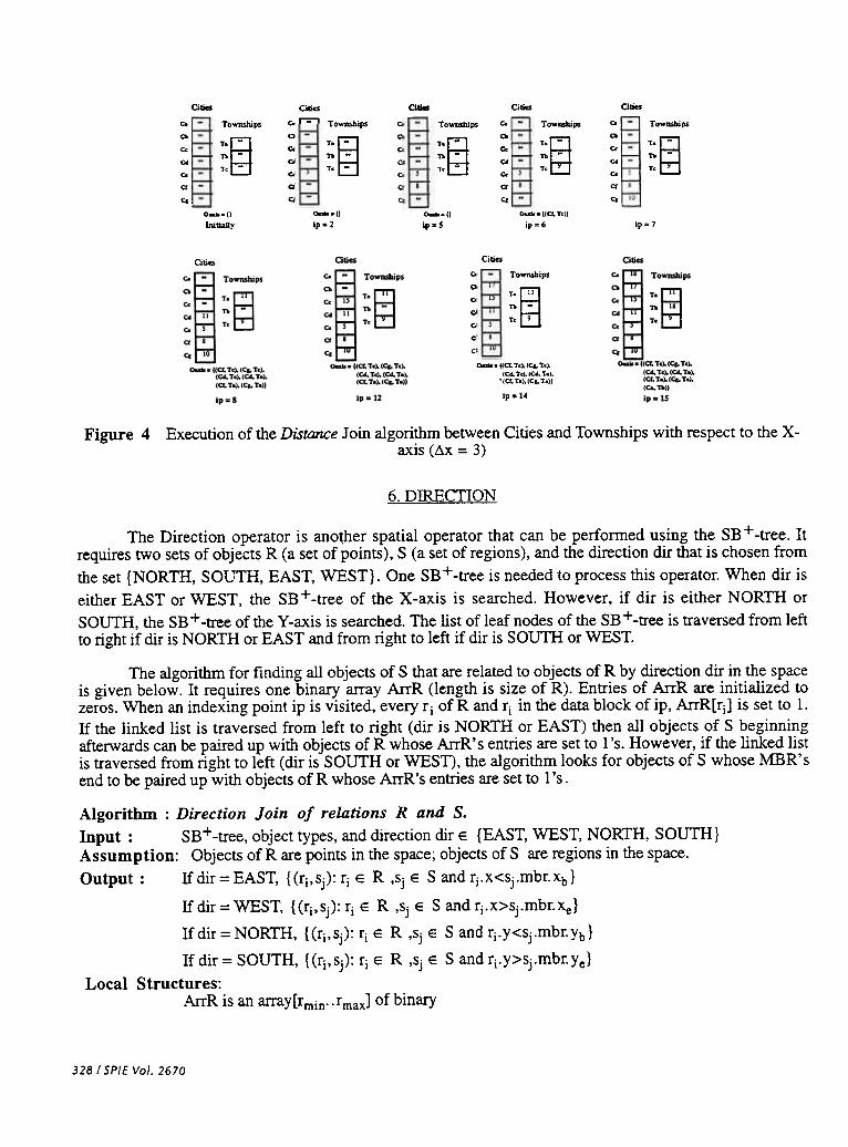
The algorithm for finding all objects of S that are related to objects of R by direction dir in the spaceis given below. It requires one binary array ArrR (length is size of R). Entries of ArrR are initialized tozeros. When an indexing point ip is visited, every rj of Rand rj in the data block of ip, ArrR[rj] is set to 1.If the linked list is traversed from left to right (dir is NORTH or EAST) then all objects of S beginningafterwards can be paired up with objects of R whose ArrR' s entries are set to 1 's. However, if the linked listis traversed from right to left (dir is SOUTH or WEST), the algorithm looks for objects of S whose :M:BR'send to be paired up with objects of R whose ArrR's entries are set to l's.

Algorithm: Direction Join of relations Rand S.Input: SB+-tree, object types, and direction dir E {EAST, WEST, NORTH, SOUTH}Assumption: Objects of R are points in the space; objects of S are regions in the space.

Output: Ifdir=EAST, {(rj,Sj):rjE R,SjE Sandrj.x<sj.mbr.xb}

Ifdir=WEST, {(rj,sj): rj E R ,Sj E Sand rj.x>sj.mbr.xe}

Ifdir = NORTH, {(rj,sj): rj E R ,Sj E Sand rj.y<sj.mbr.Yb}

If dir = SOUTH, {(rj,sj): rj E R ,Sj E Sand rj.y>sj.mbr.Ye}

Local Structures:ArrR is an array[rrnjn-. rrnax] of binary

328 I SPIE Vol. 2670

1. Oaxis= {};2. for (every rj E [rmjn. .rmaxJ) ArrR[rjJ= 0;

3. if (dir = EAST II dir = NORTH) {

3.1 Start with the leftmost data block of the SB+ -tree3.2 for (ip=iPmjn; ip<= iPmax; next ip){

for (every (sj,S,'b',pr) E ip.datablock)

for (every rj where ArrR[rjJ=I) Oaxis= Oaxis U {(rj' Sj)}

for (every (rj,R,'p',pr) E ip.datablock) ArrR[rjJ= 1;

}

}4. else if (dir == WEST II dir = SOUTH) {

4.1 Start with the rightmost leaf node of the SB+ -tree4.2 for (ip=iPmax; ip<= iPmjn; previous ip) {

for (every (sj,S,'e') E ip.datablock)

for (every rj where ArrR[rjJ=I) Oaxis= Oaxis U {(rj, Sj)}

for (every (rj,R,'p',pr) E ip.datablock) ArrR[rjJ= I;

}}

}

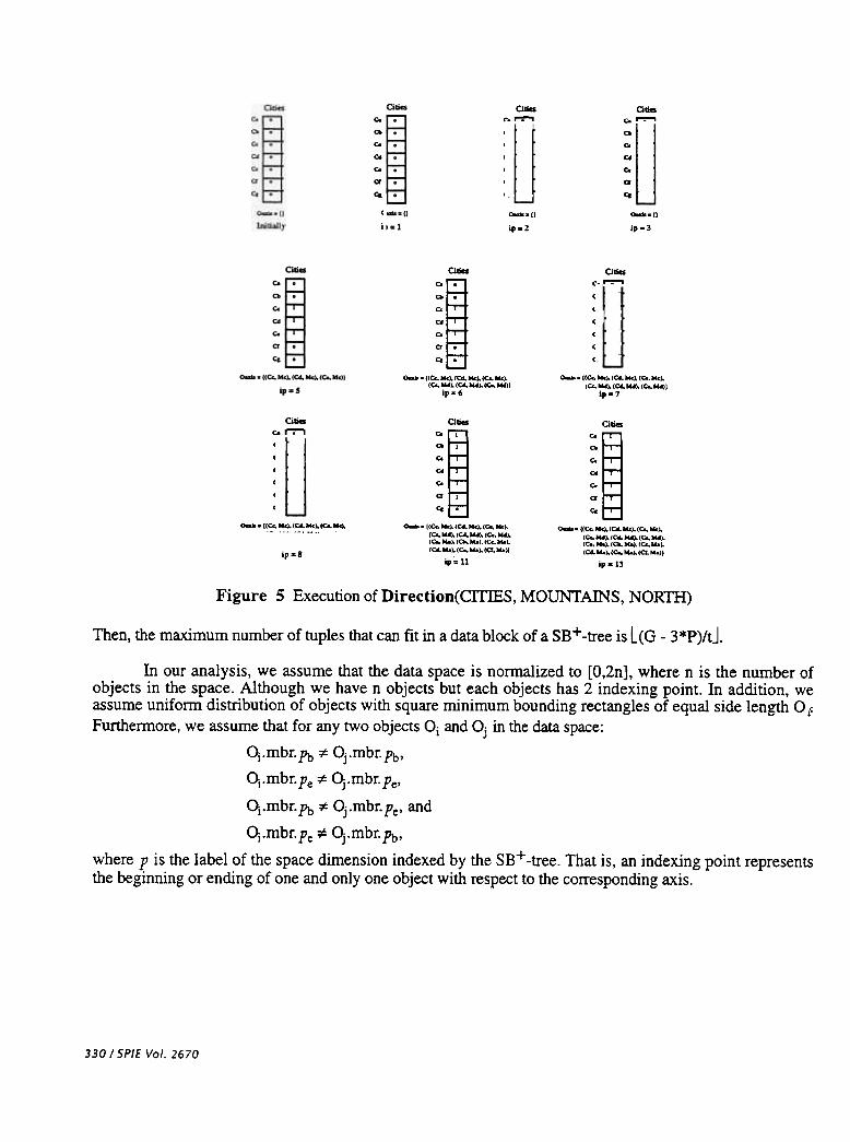
Figure 5 displays the contents of ArrR at the relevant indexing points while performing the query

Direction(CITIES, MOUNTAINS, NORTH).

7. COST MODEL

Here, we analyze the performance of the SB+ -tree with respect to the join operations: Regions-Overlap, Distance and Direction. Indexing points in leaf nodes are associated with pointers to a data blockscontaining tuples of the form: (Objid, reI, status,pr). In addition, each data block contains three pointers.The first pointer points to the data block associated with the previous indexing point. The second points tothe data block associated with the next indexing point. The third pointer points to overflow data blockassociated with the same indexing point. The following parameters will be used in our analysis:

mSB: degree of SB + -tree; mR: degree of R -tree;

X: size of indexing point; P: size of pointer, G: page size; D: Objid size;R: relation identification size; S: status code size; U: number of tuplesthat can fit in one datablock; n: number of objects; 0 f object side length;t: size of a tuple in a data block, t = CD + R + S + P); f fullness factor;tI/0: time required for a disk page I/O.

We have:U*t + 3*P ~ G

U*t ~ (G -3*P)

U ~ (G -3*P)/t.

SPIE Vol. 2670/329

OliosCo§co .Co .c.Co"-a-;-Co ,-;- ,

CitieoCor;-,co"':'""

Co-r-co-r-Co-r-or-:-Co ":'",

--.f)ipz3

c-oCo

~

c-oCo

0

il

o ()

ip52

aliosCo

0

c.coc.a

Co

0 (Cc., "'), (Cd, "'), (c., "'),cc., M4), (Cd, M4), (Co. "'"JJ

Ipz6

CilicsCa~Q I

Co

c.Co

a I

Cc .~'(Cc._(co."'~(Ca.-

(Cc. ...~ (co. Nd), (Co, 014))Ip.7

alia

Cor;-,allCc~~~Cc~

cr,c& -;-

ClIiosCo~a I

Co

c.Co

a I

C& .-'«Cc._'co._(Co,w.),

(Cc. M4), ,co (Co. M4),,Co, Ma)'(Q.Ma), (Cco Mo),(C4. Mo), (Co. Mo), (a. Mo»

ip= 11

--'I<c., Mc" (co. Mc" (Co,-

Cilia

~~--.«Cc,Mo),(~Mo),(Cc,Mo),

(Cc,MO),(~MO),(Cc,MO),(Co. w.), (co, No). (Cc, w.),C~ w.), (Co. No). ,a, w.»

ip -13ipz8

Figure 5 Execution of Direction(CrrIES, MOUNTAINS, NORTH)

Then, the maximum number of tuples that can fit in a data block of a SB+ -tree is LcG -3*P)/tJ.

In our analysis, we assume that the data space is normalized to [O,2n], where n is the number ofobjects in the space. Although we have n objects but each objects has 2 indexing point. In addition, weassume uniform distribution of objects with square minimum bounding rectangles of equal side length 0 fFurthermore, we assume that for any two objects OJ and OJ in the data space:

~ .mbr. Pb :t: OJ .mbr. Ph'

~ .mbr. Pe :t: q .mbr. Fe'

~.mbr'Ph:t: OJ.mbr'Pe' and

~ .mbr. Pe :t: OJ .mbr. Ph,

where P is the label of the space dimension indexed by the SB+ -tree. That is, an indexing point representsthe beginning or ending of one and only one object with respect to the corresponding axis.

330/ SPIt Vol. 2670

y

: : : I-; ; ; /

j.dotabloct01- ~ ::J,I

x

i .;.0111-0_0 f :i::f::::f 1:: ::~~:: f:J

I lo-;-.-o_oi--!o-i--'-i-'-!'-'_o'o_oi-o,

.;-;--j~\-=~-~ ~~odcFigure 6 2nX2n space

Figure 6 represents our view for the data space. The space is approximated by a grid of size 2nX2n.An object can start at some dashed line k and passes through k+l, k+2, ..., and ends at k+Of The

assumption is that these dashed lines are equally spaced.

Lets take the indexing point ip=i in the X-axis direction. We would like to estimate the size of thedata block associated with ip=i for i=O to 2n-l. All objects that pass through the line X=i will appear ini.datablock. The worst case happens when the indexing points (i-I), (i-2), ..., and (i-O~ represent thebeginning of objects in the X-axis direction.

Object staning at X=i-O (ends at X=i.

Object staning at X=i-°r-l passes through X=i and ends at X=i+l,

Object staIting at X=i-l passes through X=i and ends at X=i-l+O[

Therefore, the maximum number of objects that will appear in i.datablock is a f On the average, we can saythat a 12 objects will begin while the other a 12 objects will end at the indexing points (i-I), (i-2), ..., and (i-ad. The objects that begin at any of the listed indexing points will pass through X=i. As a result,i.datablock will contain a 12 tuples on the average. That is t*(O 12) is the average number of bytes that areactually occupied by each data block, where t is the size of the tuple. To enhance the performance of theSB+ -tree, we will cluster data blocks on disk pages. That is, for a page size of G, the number of data blocksthat can be clustered in one page is given as follows.

Number of data blocks per page = G/(t*a 12)= (2*G)/(t* ad.

The height of the SB + -tree hSB is one important factor in analyzing the perfonnance of the SB + -tree

with respect to most operators. Let fbe the fullness factor of nodes in SB+-tree, where Ie [0.5,1]. Tosimplify the analysis, we assume that the root has the same fullness factor as the other nodes. The numberof children of an internal node is f*mSB and the number of entries is .fmSB -1. The number of indexing

points in a leaf node is f*mSB -1. We assumed previously that there are 2n indexing points for n objects in

the space. Therefore,

SPIt Vol. 2670/331

number of leaf nodes in SB+ -tree = I -1n--1{*msB-l

and,

Regions-OverlapIn the algorithm given in section 3, step# 3 results in retrieving all the data blocks in an SB + -tree. As

per our assumption for the worst case, 2n data blocks are retrieved. From previous discussion, we showedthat (2G)/(t*O ~ blocks can be clustered in one page. The number of pages that need to be retrieved in order

to conduct the Region-Overlap join is given by the following lemma.

LemmaLet n be the total number of objects of relations R and S, 0 [is the average side length of the objects, t is the

tuple size in a data block, and G is the page size. The time needed to perform the Region-Overlap join of Rand S is

[(t*O tn)/G]*tI/O

ProofThe number of data blocks retrieved = 2n, and (20)/(t*0 p data blocks are clustered in one page. Therefore,

CRegion-Overlap = [211/((2G)/(t*0 p)]*tI/O

= [(t*O fn)/G]*tl/o

DistanceThis operator is used to perfom1 spatial join between two sets of points R and S. Assuming the

worst case where each set contributes by n/2 points, the maximum number of indexing points is n and thesize of each data block is one. The maximum number of leaf nodes in the tree is r n/(fmsB-l) 1 and thenumber of data blocks that can be clustered into one page is G/t. Consequently, the number of data blockpages that must be retrieved in order to perfom1 this join is n/(G/t)=(t*n)/G. The I/O requirements of theDistance join operator is indicated in step# 5 of the algorithm in section 4.5. Therefore, the time needed toperform the Distance join of R and S is

rr n/(fmsB-I) 1 + (t*n)/G]*tI/O

LemmaLet n be the total number of point objects of relations R and S, t is the tuple size in a data block, and G isthe page size. The time needed to perform the Distance join of R and S is

rf n/(j*msB-I) 1 + (t*n)/G]*tI/O

ProofIt follows from the previous discussion.

DirectionThis operator is used to perfonn spatial join between two relations R (a set of points) and S (a set of

332 I SPIt Vol. 2670

objects). Out assumption so far has been that the total number of objects is n, where each relation has n/2objects. Since R is a set of points, the maximum number of indexing points contributed by R is n/2.However, S is a set of regions and contributes to the set of indexing points by 2*(n/2)=n points in the worstcase. Therefore, the maximum number of indexing points is 3n/2. As a result, the maximum number of leafnodes in the tree is 13n/[2<.fmsB-l)]1 and the number of data block pages is

(3n/2)/[(2G)/(t*O p]=(3t*O tn)/( 4G).

In step# 3 or 4 of the algorithm in section 4.6, all leaf nodes and their data blocks are retrieved. Thetime needed to perform the Direction join of R and S is, [r3n/[2(f'mSB-l)]l + (3t*Otn)/(4G)]*tI/O

LemmaLet n be the total number of point objects of relations R and S, 0 [is the average side length of the non-zero

size objects, t is the tuple size in a data block, and G is the page size. The time needed to perform theDirection join of R and S is

[r 3n/[2(f'msB-l)] 1 + (3t*O !n)/(4G)]*tI/O

ProofIt follows from the previous discussion.

7. PERFORMANCE COMPARISON

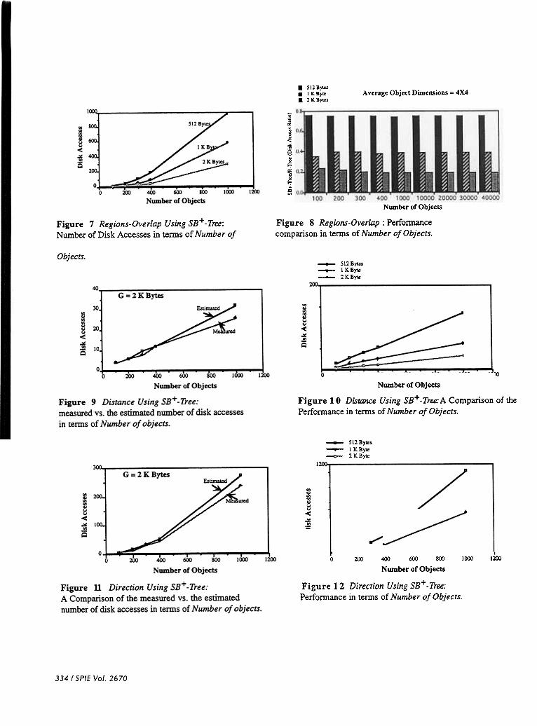
In this section, we study the performance of the SB + -tree with respect to the following operations:Regions-Overlap, Distance, and Direction. Unlike the k-d tree and the quadtree, the R-tree is similar to theSB+ -tree in that it is a paged-secondary memory structure. The performance of the SB + -tree and that of theR-tree is compared for the Regions-Overlap join. In order to achieve that, we have implemented theprevious operators on the SB + -tree and the R-tree in C. The experiments were performed for randomlygenerated objects on SUN-Workstations. The response times were obtained in terms of the number of I/Opages needed to be accessed to perform the queries. For our experiments, the area of the native space isfixed to lOOX1OO and for our estimated results, the fullness factor is taken to be 0.75. Figure 7 displays theanalytical performance of the SB+ -tree when performing the Regions-Overlap join for the page sizes: 512bytes, 1 K byte and 2 K byte. As we increase the page size, the height of the tree is less and more datablocks can be clustered in one page. Consequently, the performance of SB+ -tree is even better for largerpage sizes. Figure 8 demonstrates experimental results obtained for the disk access ratio of SB + -tree to R-tree in terms of number of objects. The Figure shows that for page size 512 Bytes, the ratio is 0.68. Theratio is even smaller for larger page sizes; 0.40 for G=1 K Byte and 0.25 for G=2 K Bytes.

Figure 9 and 11 show a comparison of the measured versus the estimated number of disk accesseswith respect to the Distance and Direction joins respectively using SB+ -tree. Figure 10 and 12experimentally compare the cost of processing both joins for different page sizes. Once again, increasing thepage size results in reducing the number of disk accesses required to process the query.

SPI E Vol. 2670/333

.SI2BY"".lKByII:.2 K By""

Average Object Dimensions = 4X4

~~g~~e~..]:-

='"

30000 40000100 400 1000

Number of Objects

Figure 8 Regions-Overlap: Performancecomparison in terms of Number of Objects.

200

300

Figure 7 Regions-Overlap Using SB+ -Tree:Number of Disk Accesses in temlS of Number of

Objects.-512 Bytcs---1 K BylO-2KBytc

1000

~..~~-<~~

Q

0"200 400 600 800 I I

Number of Objects

Figure 10 Distance Using SB+.Tree:A Comparison of thePerfonnance in tenDs of Number of Objects.

1000

1

ZOO

-512 ByIe$--1 KByIe--2KByIe

1<XX>]~ 800.~~ 600-<

~ ~-I

-~~~~::::;:::::;:::::::::0 200 400 600 800 J 000 J 200

Nwnber of Objects

Figure 12 Direction Using SB+ -Tree:

Perfonnance in tenDS of Number of Objects.

3341SPIE Vol. 2670

8 DISCUSSION AND CONCLUSIONS

In this paper, we discussed spatial join in databases. We defined the join operators: Regions-Overlap, Distance, and Direction. We presented the SB+ -tree as a data structure for accessing objects basedon their spatial attributes. The SB+ -tree is an enhancement for the B + -tree that can be used as an indexstructure for spaces containing point data as well as non-zero size objects. In order to index a k-dimensionalspace, we need k SB + -trees; one SB+ -tree is associated with every dimension. The advantage of the SB +-tree is that it is an upgrade for the B + -tree which allows commercial databases, that use B+ -tree, an accessmethod for spatial objects without a major change. We provided algorithms for conducting the joinoperations discussed in this paper using the SB + -tree. We can see that many of the existing spatial accessmethods stand still before some of the operations introduced in this paper. We also presented cost formulaefor processing join using SB + -tree. By simulation we demonstrated the superiority of SB+ -tree over the R-

tree in performing the Regions-Overlap join. The fact that entries within the nodes of the SB + -tree are sortedand that the SB + -tree guarantees one search path for query processing resulted in better response time

compared to that of the R-tree. It is worth noting that splitting nodes may produce null entries, but the SB +-tree remains balanced just as the B + -tree does, and for the same reason (i.e. the SB+ -tree increases in heightonly when the root splits).

9. REFERENCES

1. D. Ayala, P. Burnet, R. Juan and 1. Navazo, "Object representation by means of nonminimal divisionquadtree andoctree,"ACM Transactions on Graphics, Vol. 4, No.1, Jan. 1985, pp. 41-59.

2. T. Brinkhoff, H. Kriegel and B. Seeger, "Efficient Processing of Spatial Joins Using R-trees,"ProceedingsoftheACMSIGMOD Conference., May 1993, pp. 237-246.

3. N. Beckmann, H. Kriegel, R. Schneider and B. Seeger, "The R*-tree: An Efficient and RobustAccess Method for Points and Rectangles," Proceedings of the ACM SIGMOD Conference, May 1990, pp.322-331.

4. R. Elmasri and S. Navathe, Fundamentals of Database Systems, Benjamin/Cummings, 2nd edition,1994.

5. R.A. Finkel and J .L. Bentley, "Quad Trees: A Data Structure for Retrieval on Composite Keys," ActaInformatica, Vol. 4, No.1, 1974, pp. 1-9.

6. o. Gunther, "Efficient Computation of Spatial Joins", Proceedings of Data Engineering Conference,1993, pp. 50-59.

7. R.H. Guting, "An Introduction to Spatial Database Systems", VWB Journal, Vol. 3, No.4, 1994,pp. 357-399.

8. A. Guttman, "R-trees: A Dynamic Index Structure for Spatial Searching," Proceedings of the ACMSIGMOD Conference, June 1984, pp. 47-57.

9. R.H. Guting, R. Zicari and D.M. Choy "An algebra for structured office documents," ACMTransactions on Information Systems, Vol. 7,1989, pp. 123-157.

10. M. Kitsuregawa, L. Harada and M. Takagi, "Join Strategies on KD-Tree Indexed Relations,"Proceedings of Data Engineering Conference, 1989, pp.85-93.

11. A. T. Ibrahim, The SB + -Tree: An Index Structure or Spatial Data, Ph.D. Dissertation, Computer

Science Department, Wayne State University, Detroit, Michigan, 1995.12. J. Nievergelt, H. Hinterberger, and K. Sevcik, "The Grid File: An Adaptable, Symmetric Multi-Key

File Structure,"ACM TODS, Vol. 9, No.1, 1984, pp. 38-71.13. M.H. Overmars and Leeuwen, "Dynamic Multidimensional Data Structures Based on Quad- and K-d

Trees,"Acta Infonnatica, Vol. 17, No.3, 1982, pp. 267-285.14. J .A. Orenstein and T.H. Merette "A class of data structures for associative searching," Proceedings

SPIE Vol. 2670/335

of Third SIGACT News SIGMOD Symposium on the principles of Database Systems, 1984, pp.181-190.15. J.A. Orenstein, "Spatial Query Processing in an Object-Oriented Database System," Proceedings of

ACMSIGMOD Conference, 1989, pp. 326-333.16. J. T. Robinson, "The K-D-B-Tree : A Search for Large Multi-dimesional Dynamic Indexes,"

Proceedings of ACM SIGMOD Conference, 1981, pp. 10-18.17. D. Rotem, "Spatial Join Indices," Proceedings of Data Engineering Conference, 1991, pp. 500-509.18. H. Samet, The Design and Analysis of Spatial Data Structures, Addison-Wesley Publishing,

Reading, MA, 1990.19. T. Sellis, Roussopoulos and C. Faloutsos, "The R + -tree: A Dynamic Index for Multi-dimensional

Objects," Proceedings of the 13th VLDB Conference, 1987, pp. 507-518.

3361SPIE Vol. 2670