Retrieving atmospheric turbulence features from differential laser tracking motion data

Retrieving atmospheric turbulence features from differential

laser tracking motion data

Darıo G. Pereza, Angel Fernandeza, Gustavo Funesb, Damian Gulichb, and Luciano Zuninob,c

a Instituto de Fısica, Pontificia Universidad Catolica de Valparaıso (PUCV),23-40025 Valparaıso, Chile.

bCentro de Investigaciones Opticas (CIOp), C.C. 3, 1897 Gonnet, Argentina.cDepartamento de Ciencias Basicas, Facultad de Ingenierıa,

Universidad Nacional de La Plata (UNLP), 1900 La Plata, Argentina.

ABSTRACT

We have previously introduced the Differential Laser Tracking Motion Meter (DLTMM) [Proc. SPIE 7476,74760D (2009)] as a robust device to determine many optical parameters related to atmospheric turbulence. Itconsisted of two thin laser beams—whose separations can be modified—that propagate through convective air,then each random wandering was registered with position detectors, sampled at 800 Hz. The hypothesis that theanalysis of differential coordinates is less affected by noise induced by mechanical vibration was tested. Althoughwe detected a trend to the Kolmogorov’s power exponent with the turbulence increasing strength, we were unableto relate it to the Rytov variance. Also, analyzing the behaviour of the multi-fractal degree estimator (calculatedby means of multi-fractal detrended fluctuation analysis, MFDFA) at different laser-beam separations for thesedifferential series resulted in the appreciation of characteristic spatial scales; nevertheless, errors induced by thetechnique forbid an accurate comparison with scales estimated under more standard methods. In the present workwe introduce both an improved experimental setup and refined analyses techniques that eliminate many of theuncertainties found in our previous study. A new version of the DLTMM employs cross-polarized laser beams thatallows us to inspect more carefully distances in the range of the inner-scale, thus even superimposed beams canbe discriminated. Moreover, in this experimental setup the convective turbulence produced by electrical heaterspreviously used was superseded by a chamber that replicates isotropic atmospheric turbulence—anisotropicturbulence is also reproducible. Therefore, we are able to replicate the same state of the turbulent flow, specifiedby Rytov variance, for every separation between beams through the course of the experience. In this way, weare able to study the change in our MFDFA quantifiers with different strengths of the turbulence, and theirrelation with better known optical quantities. The movements of the two laser beams are recorded at 6 kHz; thisapparent oversampling is crucial for detecting the turbulence’s characteristics scales under improved MFDFAtechniques. The estimated characteristic scales and multi-fractal nature detected by this experiment providesinsight into the non-Gaussian nature of propagated light.

Keywords: multifractal detrended fluctuation analysis, Hurst exponent, differential beam wandering, angle-of-arrival, non-Kolmogorov turbulence

1. INTRODUCTION

As a result of the fluctuating nature of the refractive index in a turbulent medium any laser beam that propagatesthrough it experiments deflections. These displacements are always perpendicular to the initial unperturbeddirection of propagation, and arise from the beam phase fluctuations. This phenomenon is commonly known aslaser beam wandering because of the dancing the beam performs over a screen. Since it is very sensitive to theturbulence nature, it has been used in different experimental configurations to measure the characteristic scalesand parameters related to it.1–6

Further author information: (Send correspondence to D.G.P.)D.G.P.: E-mail: [email protected].: E-mail: [email protected]

Optics in Atmospheric Propagation and Adaptive Systems XV, edited by Karin Stein, John Gonglewski, Proc. of SPIE Vol. 8535, 853508 · © 2012 SPIE · CCC code: 0277-786/12/$18 · doi: 10.1117/12.974652

Proc. of SPIE Vol. 8535 853508-1

Downloaded From: http://proceedings.spiedigitallibrary.org/ on 11/02/2012 Terms of Use: http://spiedl.org/terms

In particular, Consortini and O’Donnell7, 8 introduced one of the simplest and less expensive techniquesavailable today, capable of capturing several parameters of the optical turbulence. It is based in a GeometricOptics (GO) model, developed by them, for the propagation of twin thin-beams through a turbulent media;particularly, for their covariances. Experimental measurements of these correlations allowed the determinationof the inner-, l0, and outer-scale, L0, of the turbulent media. Further improvements on this method providedalternative estimations of the outer-scale.9, 10 This technique is specifically useful when studying ground levelpropagation.

Nevertheless, these works were circumscribed to models for Obukhov-Kolmogorov turbulence, but throughthe years the presence of deviations from it have been determined; specifically, for ground-level turbulence whereConsortini’s scheme can be easily implemented.11, 12 Under the need to introduce more general statistical descrip-tions of the turbulent refractive index, we have introduced Levy fractional Brownian fields13–15 to describe thephase corrugations, and thus the angle-of-arrival. Also, experiments performed by us, on laser beam wanderingand wave-front propagation have shown the presence of memory effects reflected in some statistical quantifiers.Such as the wavelet entropy and Hurst exponent,16–19 the latter, we have shown, is proportional to the powerexponent in the non-Kolmogorov wave-front phase.15

The implications of a non-Kolmogorov turbulence on the wandering statistics for any propagation distancehave been recently studied by us.20 Specifically, we were most interested in short path propagation, and partiallyfilled paths: conditions frequently observed in the laboratory.

The purpose of this work is to experimentally check these results, and corroborate that the simple covariancesdefined by the GO approximation are insufficient to describe the state of turbulent media. New statisticalquantifiers are required to complete the classical methods: the MFDFA will provide insight in the developmentstate of the turbulence.

2. TWIN BEAM COVARIANCE FOR GENERALIZED SPECTRA FOR PARTIALLYFILLED PATHS

Consortini and O’Donnell’s model is devised to study thin beams propagating in turbulence along large paths.This approximation is not suited to analyse the small distances usually found in the laboratory. Moreover, it isunable to model deviations from the OK theory. Our extension of their work is capable of handling the situationswe have found in our experiment. First note, that on- and off-plane covariances obtained in Refs. [7, 8] can bereduced to adimensional forms separating the effects of the different scales from the geometric constrains of theproblem. Therefore, under the non-Kolmogorov von Karman (nKvK) model, the off-plane covariance results20

Bxpdq “ L5{2m

„ż 1

0

gnpu, δqˆ

2

3´ u ` u3

3

˙

du ´ p2ż 1

0

gnpu, δqˆ

u ` 2

3p

˙

du

, (1)

with p “ P {L the fraction of inactive turbulence (taking a region of length P ) in the propagation path of lengthL, Lm “ κmL represents the adimensional propagation distance, a function of κm “ 2π{ℓ0 the inner-scale cut-off,and

gnpu, δq “ sinpπHqΓp2H ` 2qπκ2H`2

m

C2n

ż 8

0

k exp`

´k2˘

pq2 ` k2qH`3{2

«

k3{2J3{2

`

kLm

?u2 ` δ2

˘

pu2 ` δ2q3{4

ff

dk (2)

where δ “ d{L is the separation between beams relative to the propagation distance, the relative separation.Observe that the second term in Eq. (1) can be thought as a correcting term function of p; moreover, when p issmall its contribution to the covariance is negligible. On the other hand, the on-plane covariance is functionallydependent of gn, so it can be defined from Eq. (1) and the covariance difference

∆pdq “ Bxpdq ´ Bypdq “

“ δ2L7{2m

„ż 1

0

hnpu, δqˆ

2

3´ u ` u3

3

˙

du ´ p2ż 1

0

hnpu, δqˆ

u ` 2

3p

˙

du

, (3)



with

hnpu, δq “ sinpπHqΓp2H ` 2qπκ2H`2

m

C2n

ż 8

0

k exp`

´k2˘

pq2 ` k2qH`3{2

«

k5{2J5{2

`

kLm

?u2 ` δ2

˘

pu2 ` δ2q5{4

ff

dk. (4)

In both definitions, gn and hn, are obtained from the adimensional form of the non-Kolmogorov von Karmanspectrum, the scale ratio q “ ℓ0{L0 controls the size of the inertial range, and the Hurst parameter H establishesthe degree of development of the turbulence, while C2

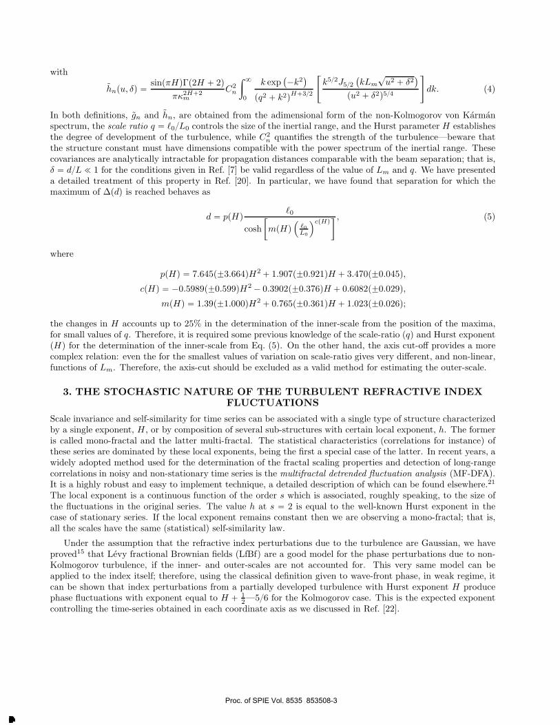
n quantifies the strength of the turbulence—beware thatthe structure constant must have dimensions compatible with the power spectrum of the inertial range. Thesecovariances are analytically intractable for propagation distances comparable with the beam separation; that is,δ “ d{L ! 1 for the conditions given in Ref. [7] be valid regardless of the value of Lm and q. We have presenteda detailed treatment of this property in Ref. [20]. In particular, we have found that separation for which themaximum of ∆pdq is reached behaves as

d “ ppHq ℓ0

cosh

„

mpHq´

ℓ0L0

¯cpHq , (5)

where

ppHq “ 7.645p˘3.664qH2 ` 1.907p˘0.921qH ` 3.470p˘0.045q,cpHq “ ´0.5989p˘0.599qH2 ´ 0.3902p˘0.376qH ` 0.6082p˘0.029q,

mpHq “ 1.39p˘1.000qH2 ` 0.765p˘0.361qH ` 1.023p˘0.026q;

the changes in H accounts up to 25% in the determination of the inner-scale from the position of the maxima,for small values of q. Therefore, it is required some previous knowledge of the scale-ratio (q) and Hurst exponent(H) for the determination of the inner-scale from Eq. (5). On the other hand, the axis cut-off provides a morecomplex relation: even the for the smallest values of variation on scale-ratio gives very different, and non-linear,functions of Lm. Therefore, the axis-cut should be excluded as a valid method for estimating the outer-scale.

3. THE STOCHASTIC NATURE OF THE TURBULENT REFRACTIVE INDEXFLUCTUATIONS

Scale invariance and self-similarity for time series can be associated with a single type of structure characterizedby a single exponent, H , or by composition of several sub-structures with certain local exponent, h. The formeris called mono-fractal and the latter multi-fractal. The statistical characteristics (correlations for instance) ofthese series are dominated by these local exponents, being the first a special case of the latter. In recent years, awidely adopted method used for the determination of the fractal scaling properties and detection of long-rangecorrelations in noisy and non-stationary time series is the multifractal detrended fluctuation analysis (MF-DFA).It is a highly robust and easy to implement technique, a detailed description of which can be found elsewhere.21

The local exponent is a continuous function of the order s which is associated, roughly speaking, to the size ofthe fluctuations in the original series. The value h at s “ 2 is equal to the well-known Hurst exponent in thecase of stationary series. If the local exponent remains constant then we are observing a mono-fractal; that is,all the scales have the same (statistical) self-similarity law.

Under the assumption that the refractive index perturbations due to the turbulence are Gaussian, we haveproved15 that Levy fractional Brownian fields (LfBf) are a good model for the phase perturbations due to non-Kolmogorov turbulence, if the inner- and outer-scales are not accounted for. This very same model can beapplied to the index itself; therefore, using the classical definition given to wave-front phase, in weak regime, itcan be shown that index perturbations from a partially developed turbulence with Hurst exponent H producephase fluctuations with exponent equal to H ` 1

2—5{6 for the Kolmogorov case. This is the expected exponent

controlling the time-series obtained in each coordinate axis as we discussed in Ref. [22].



4. EXPERIMENTAL SETUP

The experimental measurements were performed in controlled conditions: the turbulent media was created by aturbulator, a device introduced by Keskin et al.23 Briefly, the optical turbulence extending over a 37 cm channelis the product of the collision of two masses of air, one hot and one cold, that are pushed by identical fansthrough honeycombs placed opposite each other at the sides of this chamber. This device produces turbulencewith strength given by the structure constant, C2

n, in the range 2.93–8.63 ˆ 10´9 m´2{3.

d

Turbulator

LD

CCP

PCBS

M1

M2

MPBS

FPBS

D1

D2

P

P

A)

B)

Figure 1. The emitter platform produces two cross polarised beams running parallel to each other as they pass throughthe turbulator. The laser diode (LD) beam is collimated and pass trough a λ{4-wave plate (CCP) then the thin beamis split in two cross-polarised beams: a beam reflecting in two mirrors (M1 and M2), and a second on a movable pelliclebeam splitter (MPBS). These two thin beams emerge parallel to each other. A) for small distances the fixed pelliclebeam splitter allow detection of wandering for small separations of position detectors D1 and D2, the polarisers (P) forbidposition detection mixing. B) for separations over 20 mm both detectors receive direct light from the emitter platform.

As part of the emitter platform a 35mW laser diode (@635nm, DL5038-021, Thorlabs TLD001 driver) isemployed, and collimating optics is setup to maintain the beam waist around 3mm along the propagation path;additionally, a λ{4 wave plate turns it a circular polarised beam (CCP). As sketched in Figure 1, this laser beamis split by a 50{50 polarising cube beam splitter (PCBS), fixed to the platform. The two departing beams noware cross-polarised. The reflected beam has two more reflections (M1,M2) until exiting the emitter platform,while the transmitted beam reflects in a pellicle beam splitter (MPBS), fixed to a moving platform on a railsystem, exiting the platform parallel to the first one. This system provides separations between the beamsranging from 0 to 300 mm; ultimately, the maximum separation available is 100 mm because of the limited sizeof the optical windows of the turbulator. Once the beams output the turbulator, at the end of the propagationa second platform is setup to measure the wandering of both beams simultaneously. Two position sensitive



detectors, with an area of 1cm2 (UDT SC-10 D) measure the centroid position of the impinging laser beam—with relative accuracy of 2.5µm, so very small position deflections can be measured. The first detector (D1) wasmounted in a moving platform like the PBS splitter, but the second detector (D2) was placed out of the beamtrajectory, a fixed pellicle beam splitter (FPBS) reflected the beam back to D2. With this setup we avoidedthe physical constrains imposed by the size of the detectors; thus, allowing us to measure simultaneously thewandering of the two beams separated by distances under 20mm. We chose the following set of 25 distances:0, 1, 2, 3, 4, 5, 6, 7, 8, 18, 19, 20, 21, 22, 23, 24, 25, 30, 40, 50, 60, 70, 80, 90,and 100 millimetres. The total propagationdistance for the twin-beam is 1.29 m, but only 0.37 m are inside the turbulent medium, thus the factor from theinactive air is p » 0.71.

Both detectors were interfaced to a computer which allowed an acquisition rate of 6000 samples per second.Twenty five consecutive records of 60000 pairs of centroid laser beam coordinates, a total of 300,000 data, wereobtained for each separation distance between the two beams—each record was acquired in 50s. The fourcoordinates were stored in a hard disk, and the statistical analysis was performed afterwards.

Eight identical experiments were made at different turbulence strength, changing temperature differentialbetween the hot and cold air fluxes: 2.930ˆ 10´9p@40˝Cq, 4.830ˆ 10´9p@80˝Cq, 5.780ˆ 10´9p@100˝Cq, 6.731ˆ10´9p@120˝Cq, 7.206ˆ10´9p@130˝Cq, 7.681ˆ10´9p@140˝Cq, 8.156ˆ10´9p@150˝Cq and 8.631ˆ10´9p@160˝Cqm´2{3.For each intensity we collected the beam wandering data for each designated separation. Additionally, we haveperformed complete acquisitions for each separation studied with the hot source is off; thus, both mass of airjust collide generating turbulence where the perturbations to the refractive index are negligible. They can beconsidered as background measurements that quantify the mechanical, electronic, and other noises produced by

0 0.1 0.2 0.3 0.4 0.5 0.6 0.7 0.8

−0.1

0

0.1

0.2

0.3

0.4

0.5

0.6

0.7

0.8

0.9

0 0.1 0.2 0.3 0.4 0.5 0.6 0.7 0.8

−0.1

−0.05

0

0.05

0.1

0.15

0.2

0.25

0.3

0.35

0 0.1 0.2 0.3 0.4 0.5 0.6 0.7 0.8

−0.1

0

0.1

0.2

0.3

0.4

0.5

0.6

0.7

0.8

0.9

0 0.1 0.2 0.3 0.4 0.5 0.6 0.7 0.8−0.1

−0.05

0

0.05

0.1

0.15

0.2

0.25

0.3

0.35

0.4

δδ

norm

alisedB

y,B

xnorm

alized∆

∆T “ 40˝C ∆T “ 160˝C

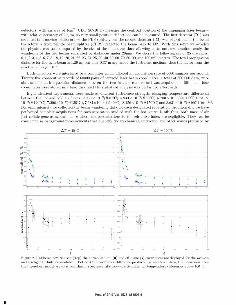
Figure 2. Unfiltered covariances: (Top) the normalised on- (�) and off-plane (‚) covariances are displayed for the weakestand stronger turbulence available. (Bottom) the covariance difference produced by unfiltered data, the deviations fromthe theoretical model are so strong that fits are unsatisfactory—particularly, for temperature differences above 100˝C.



this particular experimental arrangement.

5. RESULTS: MODEL COMPARISON

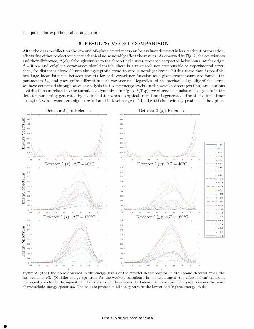
After the data recollection the on- and off-plane covariances can be evaluated; nevertheless, without preparation,effects due either to electronic or mechanical noise notably affect the results. As observed in Fig. 2, the covariancesand their difference, ∆pdq, although similar to the theoretical curves, present unexpected behaviours: at the origind “ 0 on- and off-plane covariances should match, there is a mismatch not attributable to experimental error;then, for distances above 30 mm the asymptotic trend to zero is notably slowed. Fitting these data is possible,but huge inconsistencies between the fits for each covariance function at a given temperature are found—theparameters Lm and q are quite different in each variance fit. Regardless of the mechanical quality of the setup,we have confirmed through wavelet analysis that some energy levels (in the wavelet decomposition) are spuriouscontributions unrelated to the turbulence dynamics. In Figure 3(Top), we observe the noise of the system in thedetected wandering generated by the turbulator when no optical turbulence is generated. For all the turbulencestrength levels a consistent signature is found in level range p´14,´4q: this is obviously product of the optical

-18 -18-16 -16-14 -14-12 -12-10 -10-8 -8-6 -6-4 -4-2 -20 0

0 0

0.05 0.05

0.10 0.10

0.15 0.15

0.20 0.20

0.25 0.25

0.30 0.30

0.35 0.35

0.40 0.40

0.45 0.45

0.18

0.18

0.16

0.16

0.14

0.14

0.12

0.12

0.10

0.10

0.08

0.08

0.06

0.06

0.04

0.04

0.02

0.02

0.18

0.18

0.16

0.16

0.14

0.14

0.12

0.12

0.10

0.10

0.08

0.08

0.06

0.06

0.04

0.04

0.02

0.02

J J

EnergySpectrum

EnergySpectrum

EnergySpectrum

Detector 2 (x): Reference Detector 2 (y): Reference

Detector 2 (x): ∆T “ 40˝C Detector 2 (y): ∆T “ 40˝C

Detector 2 (x): ∆T “ 160˝C Detector 2 (y): ∆T “ 160˝C

d“0

d“1

d“2

d“3

d“4

d“5

d“6

d“7

d“8

d“18

d“19

d“20

d“21

d“22

d“23

d“24

d“25

d“30

d“40

d“50

d“60

d“70

d“80

d“90

d“100

Figure 3. (Top) the noise observed in the energy levels of the wavelet decomposition in the second detector when thehot source is off. (Middle) energy spectrum for the weakest turbulence in our experiment; the effects of turbulence inthe signal are clearly distinguished. (Bottom) as for the weakest turbulence, the strongest analysed presents the samecharacteristic energy spectrum. The noise is present in all the spectra in the lowest and highest energy levels.



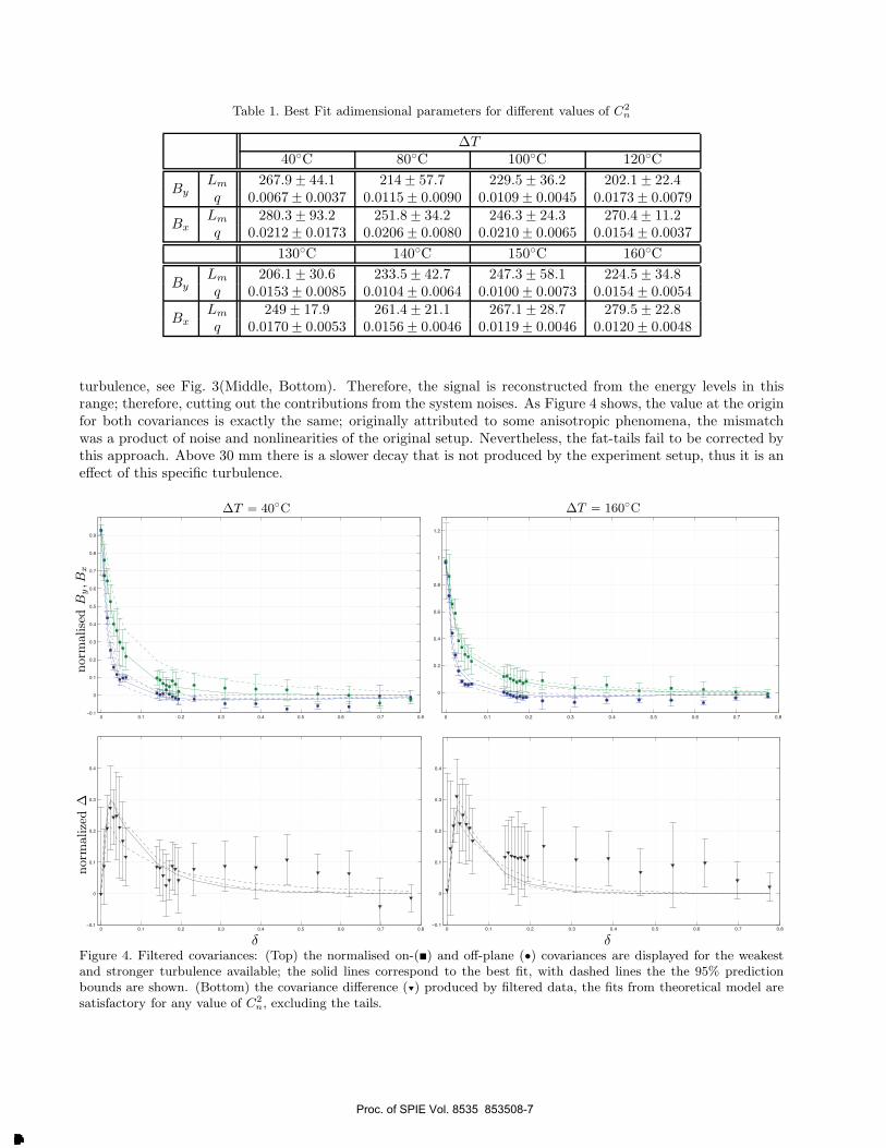
Table 1. Best Fit adimensional parameters for different values of C2

n

∆T

40˝C 80˝C 100˝C 120˝C

ByLm 267.9 ˘ 44.1 214 ˘ 57.7 229.5 ˘ 36.2 202.1 ˘ 22.4q 0.0067 ˘ 0.0037 0.0115 ˘ 0.0090 0.0109 ˘ 0.0045 0.0173 ˘ 0.0079

BxLm 280.3 ˘ 93.2 251.8 ˘ 34.2 246.3 ˘ 24.3 270.4 ˘ 11.2q 0.0212 ˘ 0.0173 0.0206 ˘ 0.0080 0.0210 ˘ 0.0065 0.0154 ˘ 0.0037

130˝C 140˝C 150˝C 160˝C

ByLm 206.1 ˘ 30.6 233.5 ˘ 42.7 247.3 ˘ 58.1 224.5 ˘ 34.8q 0.0153 ˘ 0.0085 0.0104 ˘ 0.0064 0.0100 ˘ 0.0073 0.0154 ˘ 0.0054

BxLm 249 ˘ 17.9 261.4 ˘ 21.1 267.1 ˘ 28.7 279.5 ˘ 22.8q 0.0170 ˘ 0.0053 0.0156 ˘ 0.0046 0.0119 ˘ 0.0046 0.0120 ˘ 0.0048

turbulence, see Fig. 3(Middle, Bottom). Therefore, the signal is reconstructed from the energy levels in thisrange; therefore, cutting out the contributions from the system noises. As Figure 4 shows, the value at the originfor both covariances is exactly the same; originally attributed to some anisotropic phenomena, the mismatchwas a product of noise and nonlinearities of the original setup. Nevertheless, the fat-tails fail to be corrected bythis approach. Above 30 mm there is a slower decay that is not produced by the experiment setup, thus it is aneffect of this specific turbulence.

0 0.1 0.2 0.3 0.4 0.5 0.6 0.7 0.8−0.1

0

0.1

0.2

0.3

0.4

0.5

0.6

0.7

0.8

0.9

0 0.1 0.2 0.3 0.4 0.5 0.6 0.7 0.8

0

0.2

0.4

0.6

0.8

1

1.2

0 0.1 0.2 0.3 0.4 0.5 0.6 0.7 0.8−0.1

0

0.1

0.2

0.3

0.4

0 0.1 0.2 0.3 0.4 0.5 0.6 0.7 0.8−0.1

0

0.1

0.2

0.3

0.4

δ

norm

alisedB

y,B

xnorm

alized∆

δ

∆T “ 40˝C ∆T “ 160˝C

Figure 4. Filtered covariances: (Top) the normalised on-(�) and off-plane (‚) covariances are displayed for the weakestand stronger turbulence available; the solid lines correspond to the best fit, with dashed lines the the 95% predictionbounds are shown. (Bottom) the covariance difference (İ) produced by filtered data, the fits from theoretical model aresatisfactory for any value of C2

n, excluding the tails.



Each of the eight turbulent strengths present similar values for the adimensional propagation distance andthe scale-ratio, see Table 1, but due to the tails huge uncertainties are observed. Moreover, as discussed inRef. [20] the free-space propagation should be relevant, but for the on- and off-plane covariances fits a good fitwas only obtained for p » 0.35 instead of 0.71, an important deviation from the experimental fraction. On theother hand, the maxima method proposed originally by Consortini et al.7 is quite stable under any circumstance.In this case, good fits for the covariance difference are found for p around 0.71. The inner-scale is determinedfrom Eq. (5) for the maxima given by the best fit, ℓ0 “ 0.69 ˘ 0.04 cm. Also, the outer-scale can be estimatedfrom these fits, and results L0 “ 13.21˘ 2.36 cm; this is to be expected since the width of the camera where theturbulent mixing occurs is 17 cm.

0 20 40 60 80 1000.2

0.4

0.6

0.8

1

1.2

0 20 40 60 80 1000.2

0.4

0.6

0.8

1

1.2

0 2 4 6 8 10 12

0.5

0.6

0.7

0.8

0.9

1

(3,0 .718)

mean 40–160˝C

∆T “ 40˝C

∆T “ 80˝C

∆T “ 100˝C

∆T “ 120˝C

∆T “ 130˝C

∆T “ 140˝C

∆T “ 150˝C

∆T “ 160˝C

∆T “ 0˝CReference off

HH

dd

B)

A)

Figure 5. A) Hurst exponent as a function of the difference d for the on-plane wandering series; the left image portrays thewhole range, on the right the zoomed region where inflection occurs. B) Hurst exponent as a function of the difference d

for the off-plane wandering series; the left image portrays the whole range, on the right the zoomed region where inflectionoccurs. Observe that both references have H values near 1{2.

To understand the peculiarities found in the classical analysis more powerful tools are needed. To this effect,we analyse the series produced by the DLTMM experiment with MFDFA3 as follows: we produce two differentialtime series from the detectors original pair, xtp0q ´ xtpdq and ytp0q ´ ytpdq, and split them in 10 series of 30, 000data-points each in order to obtain a mean value of the Hurst exponent, h p2q “ H (with error given by itsstandard deviation). The detrending algorithm employed in the estimation of H uses a polynomial of degree 3,



thus the acronym MFDFA3. The fitting range for the exponent estimation was carefully chosen studying thefluctuation functions and their log-log derivative.

Figure 5 shows the results of this procedure. For every given ∆T (associated with a unique C2n), the Hurst

exponent reveals a function of the beam separation. In both axis we observe values around 0.5 (brownian motion)for references; this is the noise of the system dynamics. For all the temperature differences studied (greater thanzero) the behaviour is exactly the same. Long-range correlations appear to occur for „ 20 mm and above,and with the given error bars one could guess this is the same phenomena observed for different temperatures.Moreover, values for the off-plane axis are slightly greater than those for on-plane axis indicating anisotropies(known to exist) in the turbulator.

Now, the saturation of the Hurst exponent is a phenomenon of the distance: the average curve starts at0.7, and reaches a minimum (around the 3 mm, see Fig. 5 left), then an inflection point occurs that leads toa saturation in H . We associate this change in convexity to the occurrence of a change in the dynamics ofthe optical turbulence. Under this method the determination of the inflection point should be related to theinner-scale. We proceed by fitting the averaged exponent with a rational functions (R-square 0.98), and estimatethe inflection distance. From this we obtain ℓ0 “ 0.620 ˘ 0.046 cm for the on-plane wandering series, andℓ0 “ 0.459 ˘ 0.026 cm for the off-plane series. Notoriously, the on plane scale is the closest to the previouslyestimated inner-scale.

On-plane H

Off-plane H

Fit for On-plane H

Fit for Off-plane H

Pred. Bnd. On-plane H

Pred. Bnd. Off-plane H

d

H

Figure 6. Fits for the averaged Hurst exponents estimated for each turbulence strength are displayed. The anisotropy isclearly observed, and the inflection points can be estimated.

6. CONCLUSIONS

We have presented a thorough exposition of the Geometrical Optics approach for non-Kolmogorov turbulence.It presents some drawbacks to note, from the theoretical point of view it is model dependent, and the exact valueof H is unknown. The experimental approach is more challenging, electronic and mechanical noise certainly



affects the correlations. Moreover, anisotropies and inhomogeneities are observed with larger separations, suchanisotropies are not caused by the experimental arrangement. Although this is inherent to the turbulent natureof the fluid dynamics inside the turbulator, real turbulence should commonly presents such anomalies. Therefore,additional information should be recollected to solve some of these issues, such as scintillation measurements. Inorder to have a more suitable interpretation of these results the GO model must be replaced by one based onthe physical optics.

Noises present in the system can be greatly mitigated by a wavelet filtering procedure. The signals obtainedafter filtering are more robust; particularly, the covariance difference can pass the best-fit procedure with R-squareabove 60%, and inner- and outer- estimated values are in accordance with expected values for this device—thevalues reported here are similar to those seen in Ref. [23]. Nevertheless, some inconsistencies remain, such as thefat tails observed in both covariances and the high correlation for d “ 0.

Finally, a new method for estimating the inner-scale is proposed: the determination of the inflection pointin the Hurst exponent estimated under the multifractal detrended fluctuation analysis. Not only successfullyprovides values for the inner-scale, but also provides the first hints to an anisotropic inner-scale in opticalturbulence. Lovejoy & Schertzer24 introduced an elliptical inner-scale to explain layered distribution of cloudsin the atmosphere. On the other hand, the exponent H obtained in this way differs from the expected values:once the threshold of the inner-scale has been exceeded the asymptotic values should be near 5{6, as discussedin Sec. 3. The excess in this value is unaccounted through classical models, or even single scale non-Kolmogorovextensions. Further research on whether this is the product of temporal correlations or the existence of a non-Gaussian statistics should be performed.

ACKNOWLEDGMENTS

This work was supported by Comision Nacional de Investigacion Cientıfica y Tecnologica (CONICYT, FONDE-CYT Grant No. 1100753, Chile), partially by Pontificia Universidad Catolica de Valparaıso (PUCV, Grant No.123.704/2010, Chile) and Consejo Nacional de Investigaciones Cientıficas y Tecnicas (CONICET, Argentina).

REFERENCES

1. J. H. Churnside and R. J. Lataitis, “Angle-of-arrival fluctuations of a reflected beam in atmospheric turbu-lence,” J. Opt. Soc. Am. A 4, pp. 1264–1272, July 1987.

2. E. Masciadri and J. Vernin, “Optical technique for inner-scale measurement: possible astronomical applica-tions,” Appl. Opt. 36, pp. 1320–1327, Feb. 1997.

3. J. Zhang and Z. Zeng, “Statistical properties of optical turbulence in a convective tank: experimentalresults,” J. Opt. A: Pure Appl. Opt. 3, pp. 236–241, 2001.

4. C. Innocenti and A. Consortini, “Refractive index gradient of the atmosphere at near ground levels,” J.

Mod. Optics 52(5), pp. 671–689, 2005.

5. M. S. Andreeva, A. V. Koryabin, V. A. Kulikov, and V. I. Shmalhausen, “Diagnostics of the scale ofturbulence using a divergent laser beam,” Moscow University Physics Bulletin 66(6), pp. 627–630, 2011.

6. M. S. Andreeva, N. G. Iroshnikov, A. B. Koryabin, A. V. Larichev, and V. I. Shmalgauzen, “Usage ofwavefront sensor for estimation of atmospheric turbulence parameters,” Optoelectronics, Instrumentation

and Data Processing 48(2), pp. 197–204, 2012.

7. A. Consortini and K. O’Donnell, “Beam wandering of thin parallel beams through atmospheric turbulence,”Waves in Random Media 3, pp. S11–S28, July 1991.

8. A. Consortini and K. O’Donnell, “Measuring the inner Scale of Atmospheric Turbulence by Correlation ofLateral Displacements of Thin Parallel Laser Beams,” Waves in Random Media 3, pp. 85–92, Apr. 1993.

9. A. Consortini, C. Innocenti, and G. Paoli, “Estimate method for outer scale of atmospheric turbulence,”Opt. Comm. 214, pp. 9–14, 2002.

10. Y. Y. Sun, A. Consortini, and Z. P. Li, “A new method for measuring the outer scale of atmosphericturbulence,” Waves in Random and Complex Media 17, pp. 1–8, 2007.

11. E. Golbraikh and N. S. Kopeika, “Behavior of structure function of refraction coefficients in different tur-bulent field,” Appl. Opt. 43, p. 615, Nov. 2004.

Proc. of SPIE Vol. 8535 853508-10


12. E. Golbraikh, H. Branover, N. S. Kopeika, and A. Zilberman, “Non-Kolmogorov atmospheric turbulenceand optical signal propagation,” Nonlin. Processes Geophys. 13, pp. 297–301, 2006.

13. D. G. Perez, L. Zunino, and M. Garavaglia, “A fractional Brownian motion model for the turbulent refractiveindex in lightwave propagation,” Opt. Comm. 242, pp. 57–63, Nov. 2004.

14. D. G. Perez, L. Zunino, and M. Garavaglia, “Modeling the turbulent wave-front phase as a fractionalBrownian motion: a new approach,” J. Opt. Soc. Am. A 21, pp. 1962–1969, Oct. 2004.

15. D. G. Perez and L. Zunino, “Generalized wave-front phase for non-Kolmogorov turbulence,” Optics Let-

ters 33, pp. 572–574, Mar. 2008.

16. L. Zunino, D. G. Perez, O. A. Rosso, and M. Garavaglia, “Characterization of Laser Propagation ThroughTurbulent Media by Quantifiers Based on the Wavelet Transform,” Fractals 12, pp. 223–233, June 2004.

17. L. Zunino, D. G. Perez, M. Garavaglia, and O. A. Rosso, “Characterization of laser propagation throughturbulent media by quantifiers based on the wavelet transform: dynamic study,” Physica A 364, pp. 79–86,2006.

18. G. Funes, D. Gulich, L. Zunino, D. G. Perez, and M. Garavaglia, “Behavior of the laser beam wanderingvariance with the turbulent path length,” Opt. Comm. 272, pp. 476–479, Apr. 2007.

19. D. Gulich, G. Funes, L. Zunino, D. G. Perez, and M. Garavaglia, “Angle-of-arrival variance’s dependenceon the aperture size for indoor convective turbulence,” Opt. Comm. 277, pp. 241–246, June 2007.

20. D. G. Perez and G. Funes, “Beam wandering statistics of twin thin laser beam propagation under generalizedatmospheric conditions.” 2012.

21. J. W. Kantelhardt, S. A. Zschiegner, E. Koscielny-Bunde, A. Bunde, S. Havlin, and H. E. Stanley, “Multi-fractal Detrended Fluctuation Analysis of Nonstationary Time Series,” Physica A 316, pp. 87–114, 2002.

22. D. G. Perez, L. Zunino, D. Gulich, G. Funes, and M. Garavaglia, “Turbulence characterization by studyinglaser beam wandering in a differential tracking motion setup,” Proc. SPIE 7476, p. 74760D, 2009.

23. O. Keskin, L. Jolissaint, and C. Bradley, “Hot-air optical turbulence generator for the testing of adaptiveoptics systems: principles and characterization,” Appl. Opt. 45, pp. 4888–4897, July 2006.

24. D. Schertzer and S. Lovejoy, “Physical Modeling and Analysis of Rain and Clouds by Anisotropic ScalingMultiplicative Processes,” J. Geophys. Res. 92, pp. 9692—-9714., 1987.

Proc. of SPIE Vol. 8535 853508-11


Retrieving atmospheric turbulence features from differential laser tracking motion data

Documents

Transcript of Retrieving atmospheric turbulence features from differential laser tracking motion data