Etudes Expérimentales en Turbulence d'Ondes - Laboratoire ...
224
Habilitation ` a Diriger des Recherches ´ Eric FALCON Universit´ e Paris Diderot – Paris 7 Laboratoire Mati` ere et Syst` emes Complexes Etudes Exp´ erimentales en Turbulence d’Ondes soutenue publiquement le 18 d´ ecembre 2008 `a 15h30 devant le Jury compos´ e de B. Castaing Professeur ` a l’ ´ Ecole Normale Sup´ erieure de Lyon Pr´ esident F. Charru Professeur ` a l’Universit´ e Paul Sabatier Toulouse III Rapporteur Y. Couder Professeur ` a l’Universit´ e Paris Diderot Rapporteur F. Dias Professeur ` a l’ ´ Ecole Normale Sup´ erieure de Cachan Rapporteur S. Fauve Professeur ` a l’ ´ Ecole Normale Sup´ erieure
-
Upload
khangminh22 -
Category
Documents
-
view
4 -
download
0
Transcript of Etudes Expérimentales en Turbulence d'Ondes - Laboratoire ...

Habilitation a Diriger des Recherches
Eric FALCON
Universite Paris Diderot – Paris 7Laboratoire Matiere et Systemes Complexes
Etudes Experimentales
en Turbulence d’Ondes
soutenue publiquement le 18 decembre 2008 a 15h30devant le Jury compose de
B. Castaing Professeur a l’Ecole Normale Superieure de Lyon PresidentF. Charru Professeur a l’Universite Paul Sabatier Toulouse III RapporteurY. Couder Professeur a l’Universite Paris Diderot RapporteurF. Dias Professeur a l’Ecole Normale Superieure de Cachan RapporteurS. Fauve Professeur a l’Ecole Normale Superieure

Avant-propos
Ce memoire presente une synthese de mes activites de recherche depuis l’obtention de maThese de Doctorat en juillet 1997. Cette these portait sur l’etude des milieux granulaires eten particulier sur divers comportements dynamiques resultants de la non linearite de la loi decontact de Hertz entre particules.
Depuis lors, j’ai travaille dans quatres laboratoires differents : au Laboratoire de la Phy-sique de la Matiere Condensee (LPMC) de l’Ecole Normale Superieure (ENS) pendant 1 an,puis au Laboratoire de Physique Statistique (LPS) de l’ENS pendant 2 ans, puis au Labora-toire de Physique de l’ENS Lyon pendant 6 ans, et actuellement au Laboratoire Matiere etSystemes Complexes (MSC) a l’Universite Paris – Diderot depuis plus d’un an.
Il serait vain de vouloir synthetiser toutes les sujets abordes depuis la These au risque depresenter une liste ou un catalogue des activites. J’ai plutot decide de presenter dans une partieprincipale mes activites en cours relatives a la « Turbulence d’Ondes ». Cette partie (chapitreA) fait le point sur le contexte, l’etat de l’art et les enjeux de cette thematique emergente, etpresente d’une facon originale et synthetique les principaux resultats obtenus. La redactiona volontairement ete la moins technique possible, avec une indroduction a la problematiqueet une vision la plus globale possible de l’ensemble des resultats obtenus permettant ainsi depointer les problemes ouverts et les perspectives de nos futurs travaux associes a la turbu-lence d’ondes. Les tires a part des publications presentes a la fin du chapitre permettent aulecteur d’acceder a plus de details, si besoin est, meme si le texte se suffit a lui-meme. Cettethematique avait debute par l’etude d’une nouvelle methode de mesure de hauteur de vaguesa la surface d’un fluide, qui m’avait eloigne un temps de la motivation initiale. En effet, ellem’a conduit a l’observation de phenomenes nouveaux relatifs aux ondes non-lineaires hydro-dynamiques qui feront l’objet du chapitre B « Ondes et Instabilites Hydrodynamiques » quiest moins detaille que le premier.
Meme si le fil conducteur de mes recherches reste la physique non-lineaire et la physiquestatistique hors equilibre, d’autres thematiques ont ete abordees depuis ma These. Les travauxconcernant la matiere condensee sont ainsi presentes sous forme d’une Annexe qui comportedeux chapitres. Le chapitre C expose les resultats obtenus sur le « Transport Electrique dansles Milieux Granulaires », et le chapitre D reporte mes activites relatives aux « Gaz Granu-laires Dissipatifs ». Ils font l’objet d’une presentation beaucoup plus synthetique que lors dupremier chapitre mais restent la-encore autonomes par rapport aux tires a part ajoutes en finde chaque chapitre.
Paris, Juillet 2008
3


Remerciements
Je tiens tout d’abord a remercier les membres du jury pour l’interet qu’ils ont porte ace travail, et en particulier Francois Charru, Yves Couder et Frederic Dias qui ont accepted’etre les rapporteurs de cette Habilitation a Diriger les Recherches. Je sais gre a BernardCastaing de m’avoir fait l’honneur de presider ce jury, et Stephan Fauve d’etre membre du jury.
Les travaux presentes proviennent de collaborations multiples dont je voudrais remercierici l’implication des personnes suivantes : B. Audit, S. Aumaıtre, D. Beysens, B. Castaing, S.Dorbolo, T. Dauxois, P. Evesque, S. Fauve, Y. Garrabos, C. Laroche, S. McNamara, B. Perrin,F. Palencia, F. Petrelis, S. Roux ; ainsi que les plus jeunes collaborateurs : U. Bortolozzo, F.Boyer, M. Creyssels, A. Didier, C. Falcon, et A. Merlen. Outre leurs participations a certainsdes travaux reunis ici, j’adresse ma profonde gratitude a deux « fideles » : S. Fauve pour sesremarques toujours pertinentes et profondes, ainsi que C. Laroche pour l’apport experimentaldu passionne qu’il est.
Je voudrais remercier le soutien financier des institutions suivantes sans qui ces travauxn’auraient pu etre possible : le Centre National de la Recherche Scientifique (CNRS), le CentreNational d’Etudes Spatiales (CNES), l’Agence Spatiale Europeenne (ESA), l’Agence Nationalde la Recherche (ANR 2007 Turbonde No BLAN07-3-197846), l’Action Concerte IncitativeJeune Chercheur (ACI 2001 No 21-31), l’Ecole Normale Superieure de Lyon, l’Ecole NormaleSuperieure, l’Universite Paris – Diderot, La Ville de Paris, le Ministere de l’EnseignementSuperieur et de la Recherche, et l’Union Europeenne.
Je tiens egalement a remercier ceux qui par leurs remarques, leurs commentaires ou bienleurs discussions m’ont permis d’apprendre bien des choses : outre les collaborateurs directs,certaines personnes des laboratoires de l’ENS (notamment de la piece « D24 »), de l’ENSLyon, et de MSC qui se reconnaıtront.
Je ne peux finir sans exprimer ma gratitude aux personnes des services techniques et ad-ministratifs (atelier, secretariat, informatique, bibliotheque) de leur precieuse aide sans quiun laboratoire ne fonctionnerait pas. Un grand merci aussi aux equipes techniques de la fusee-sonde Maxus 5 a Kiruna (Suede) et de Novespace (Vols paraboliques CNES/ESA en Airbus)a Bordeaux.
Je remercie aussi pour leur patience et leurs lectures attentives tous ceux qui ont contribuea la tache ingrate de correction du manuscrit.
Que mes amis et ma famille recoivent ici dans son ensemble la marque de ma reconnais-sance pour leur aide et leur gentillesse.
Enfin, je remercie Ingrid pour m’avoir soutenu et accompagne au quotidien avec patiencetout au long de ces travaux.
5


Table des matieres
Avant-propos 3
Remerciements 5
Curriculum vitæ et liste de publications 13
A Turbulence d’ondes 37A.1 Contextes et enjeux . . . . . . . . . . . . . . . . . . . . . . . . . . . . . . . . 37A.2 La turbulence d’ondes hydrodynamiques . . . . . . . . . . . . . . . . . . . . . 40A.3 Expose synthetique des principaux resultats . . . . . . . . . . . . . . . . . . . 42
A.3.1 Spectre et distribution d’amplitude des vagues . . . . . . . . . . . . . 42A.3.2 Intermittence en turbulence d’ondes . . . . . . . . . . . . . . . . . . . 44A.3.3 Fluctuations du flux d’energie . . . . . . . . . . . . . . . . . . . . . . . 48A.3.4 Turbulence d’ondes en impesanteur . . . . . . . . . . . . . . . . . . . . 51A.3.5 Turbulence d’ondes dans les ferrofluides . . . . . . . . . . . . . . . . . 53
A.4 Perspectives . . . . . . . . . . . . . . . . . . . . . . . . . . . . . . . . . . . . . 57References . . . . . . . . . . . . . . . . . . . . . . . . . . . . . . . . . . . . . . . . . 59A.5 Publications associees a ce chapitre . . . . . . . . . . . . . . . . . . . . . . . . 62A.6 Tires a part . . . . . . . . . . . . . . . . . . . . . . . . . . . . . . . . . . . . . 65
E. Falcon, C. Laroche & S. Fauve, Physical Review Letters 98, 094503 (2007) . 71E. Falcon, S. Fauve & C. Laroche, Physical Review Letters 98, 154501 (2007) . 75E. Falcon et al. Physical Review Letters 100, 064503 (2008) . . . . . . . . . . . 79C. Falcon, E. Falcon, U. Bortolozzo & S. Fauve, soumis a EPL (2008) . . . . . 83F. Boyer & E. Falcon, Physical Review Letters 101, 0244502 (2008) . . . . . . 87
B Ondes et instabilites hydrodynamiques 91B.1 Introduction . . . . . . . . . . . . . . . . . . . . . . . . . . . . . . . . . . . . . 91B.2 Ondes solitaires « depressions » a la surface d’un fluide . . . . . . . . . . . . . 91B.3 Precurseurs de Sommerfeld a la surface d’un fluide . . . . . . . . . . . . . . . 96B.4 Reflexion d’ondes internes . . . . . . . . . . . . . . . . . . . . . . . . . . . . . 99B.5 Stabilisation parametrique de l’instabilite de Rosensweig . . . . . . . . . . . . 102References . . . . . . . . . . . . . . . . . . . . . . . . . . . . . . . . . . . . . . . . . 102B.6 Publications associees a ce chapitre . . . . . . . . . . . . . . . . . . . . . . . . 104B.7 Tires a part . . . . . . . . . . . . . . . . . . . . . . . . . . . . . . . . . . . . . 105
E. Falcon, C. Laroche & S. Fauve, Physical Review Letters 89, 204501 (2002) . 111E. Falcon, C. Laroche & S. Fauve, Physical Review Letters 91, 064502 (2003) . 115T. Dauxois, A. Didier & E. Falcon, Physics of Fluids 16, 1936 (2004) . . . . . 119F. Petrelis, E. Falcon & S. Fauve, European Physical Journal B 15, 3 (2000) . . 123
7

Annexes - Milieux Granulaires 127
C Conduction electrique dans les milieux granulaires 129C.1 Resume synthetique des travaux . . . . . . . . . . . . . . . . . . . . . . . . . 129C.2 Publications associees . . . . . . . . . . . . . . . . . . . . . . . . . . . . . . . 134C.3 Tires a part . . . . . . . . . . . . . . . . . . . . . . . . . . . . . . . . . . . . . 137
E. Falcon, B. Castaing & M. Creyssels, European Phys. Journal B 38, 475 (2004)148E. Falcon, B. Castaing & C. Laroche, Europhysics Letters 65, 186 (2004) . . . 156E. Falcon, & B. Castaing, American Journal of Physics 73, 302–307 (2005) . . 163M. Creyssels et al, European Physical Journal E 23, 255 (2007) . . . . . . . . . 173S. Dorbolo et al., EPL 79, 54001 (2007) . . . . . . . . . . . . . . . . . . . . . . 178
D Gaz granulaires dissipatifs 181D.1 Resume synthetique des travaux . . . . . . . . . . . . . . . . . . . . . . . . . 181D.2 Publications associees . . . . . . . . . . . . . . . . . . . . . . . . . . . . . . . 184D.3 Tires a part . . . . . . . . . . . . . . . . . . . . . . . . . . . . . . . . . . . . . 187
E. Falcon, S. Fauve & C. Laroche, European Physical Journal B 9, 183 (1999) . 193E. Falcon et al. Physical Review Letters 83, 440 (1999) . . . . . . . . . . . . . 197S. McNamara & E. Falcon, Physical Review E 71 031302 (2005) . . . . . . . . 203E. Falcon et al., Europhysics Letters 74, 830 (2006) . . . . . . . . . . . . . . . 210
Articles de presse 211
Resume 224
8

9

10

« La Vague » de Camille Claudel, 1897.Onyx et bronze sur socle de marbre - 62 x 56 x 50 cm,
Paris, Musee Rodin, Photo : Ch. Baraja/Musee Rodin,
c© ADAGP Paris, 2008.
« Ma destine » de Victor Hugo, 1867.Plume et lavis d’encre brune, gouache, sur papier velin, 17,4 x 25,9 cm.
Paris, Maison de Victor Hugo, Inv. 927. c© PMVP
« en proie aux evenements comme vous aux vents, je constate leur demence apparente et leur logiqueprofonde ; je sens que la tempete est une volonte, et que ma conscience en est une autre, et qu’aufond elles sont d’accord ; et je persiste, et je resiste, [...] et je fais mon devoir, pas plus emu de la
haine que vous de l’ecume. »
Victor Hugo, Discours « Aux marins de la Manche » , 1870

12

CURRICULUM VITÆ
ET
PUBLICATIONS
Tous les articles cités sont téléchargeables sur http://www.msc.univ-paris7.fr/~falcon/
E R I C F A L C O N , M S C ,U N I V E R S I T E P A R I S - D I D E R O T

ERIC FALCON – HABILITATION A DIRIGER LES RECHERCHES
TA B L E D E S M AT I E R E S
I. CURRICULUM VITÆ..................................................................................................................................... 15
I.1. INFORMATIONS ADMINISTRATIVES ............................................................................................................. 16I.2. RÉSUMÉ CHRONOLOGIQUE DES ACTIVITÉS SCIENTIFIQUES........................................................................ 17
II. ENCADREMENT ET FORMATION........................................................................................................ 19
II.1. ENCADREMENT DE STAGES, THÈSES, POSTDOC .......................................................................................... 20II.2. ENSEIGNEMENT ........................................................................................................................................... 21II.3. ORGANISATION DE CONFÉRENCES .............................................................................................................. 21II.4. REVUES OU OUVRAGES DE VULGARISATION............................................................................................... 21II.5. ARTICLES DE PRESSE & AUDIOVISUEL........................................................................................................ 21
III. CONTRATS DE RECHERCHE................................................................................................................. 22
IV. ADMINISTRATION DE LA RECHERCHE ........................................................................................... 22
V. AUTRES RENSEIGNEMENTS ................................................................................................................. 23
V.1. PARTENAIRES ACADÉMIQUES...................................................................................................................... 23V.2. PLACE DE LA RECHERCHE AU SEIN DE L’UNITÉ.......................................................................................... 24V.3. MOBILITÉ..................................................................................................................................................... 24
VI. LISTE DES PUBLICATIONS .................................................................................................................... 25
VI.1. REVUES A COMITE DE LECTURE................................................................................................................... 26VI.2. THESES, LIVRES ........................................................................................................................................... 28VI.3. ACTES DE CONFÉRENCES ............................................................................................................................ 28VI.4. ARTICLES DE VULGARISATION ................................................................................................................... 29VI.5. ARTICLES DE PRESSE................................................................................................................................... 29VI.6. PRINCIPALES COMMUNICATIONS ................................................................................................................ 30

ERIC FALCON – HABILITATION A DIRIGER LES RECHERCHES
15
I. CURRICULUM VITÆ

ERIC FALCON – HABILITATION A DIRIGER LES RECHERCHES
16
I.1. INFORMATIONS ADMINISTRATIVES
Nom, prénom : FALCON Eric
Date de naissance : 15 Mars 1971 à Lyon 4ème
Adresse postale : Laboratoire Matière et Systèmes Complexes (MSC) , UMR 7057 CNRSUniversité Paris Diderot – Paris 7, Bâtiment Condorcet – Case 705610 rue A. Domon & L. Duquet, 75 205 Paris Cedex 13
Adresse électronique : [email protected]
Adresse Web : http://www.msc.univ-paris7.fr/~falcon/
Situation actuelle :
Depuis Déc. 2006 : Chargé de Recherche 1ère Classe du CNRS en Section 02, au LaboratoireMatière et Systèmes Complexes de l’Université Paris Diderot – Paris 7.
Autres expériences professionnelles :
2002-2006 : Chargé de Recherche 1ère Classe du CNRS, Laboratoire de Physique de l’ENS Lyon1999-2002 : Chargé de Recherche 2ème Classe du CNRS, Laboratoire de Physique de l’ENS Lyon
1997-1999 : Chercheur Post-doc (2 ans) du CNESau Laboratoire de Physique Statistique (LPS) de L’ENS Paris
1996-1997 : Chercheur Post-doc (1 an), Scientifique du Contingentau Laboratoire de la Physique de la Matière Condensée (LPMC) de l’ENS Paris
1993-1996 : Thèse de Doctorat préparée au Laboratoire de Physique de l’ENS Lyon
Distinctions professionnelles :
• Lauréat de la Médaille de Bronze du CNRS 2001• Lauréat du Prix Branly 2004
Cursus :
• Doctorat, Université Lyon I, mention « Très honorable avec les félicitations du Jury »(1997)
• DEA Physique Statistique et Phénomènes Non-Linéaires, ENS Lyon,mention Bien, 2ème /15 (1993)
• Magistère de Physique, ENS Lyon, mention « Bien » (1991 – 1993)• Maîtrise de Physique, ENS Lyon / Univ. Lyon I, mention « Assez Bien » (1992)

ERIC FALCON – HABILITATION A DIRIGER LES RECHERCHES
17
I.2. RESUME CHRONOLOGIQUE DES ACTIVITESSCIENTIFIQUES
Les références données dans ce paragraphe renvoient à la Liste des Publications du §VI
De 1993 à 1996, j'ai effectué ma thèse au Laboratoire de Physique de l'ENS Lyon. Mon travail a portésur l'étude des milieux granulaires et en particulier sur divers comportements dynamiques résultants de lanon-linéarité de la loi de contact de Hertz entre particules [1-3,1L,2L]. J’ai aussi mis en évidencel'apparition de nouvelles instabilités à la surface d'une poudre soumise à vibration [5,6].
À l'issue de ma thèse, j'ai travaillé un an, en 1996-97, sur le frottement solide au Laboratoire dePhysique de la Matière Condensée de l'ENS Paris. J'ai réalisé un montage expérimental original permettantd'effectuer des mesures dynamiques de frottement solide [4].
De 1997 à 1999, j'ai bénéficié d'une bourse post-doctorale du CNES pour travailler sur les régimescinétiques et d'instabilité des milieux granulaires vibrés au Laboratoire de Physique Statistique de l'ENSParis. J'ai obtenu empiriquement l'analogue d'une équation d'état pour un gaz granulaire dissipatif et j'aimis en évidence l'instabilité de l'état homogène de milieux granulaires vibrés, qui engendre la formationd'amas localisés de particules lorsque leur densité est suffisamment élevée [7-9,3L,1a]. En parallèle à cestravaux, j'ai mis en évidence la stabilisation paramétrique de l'instabilité de Rosensweig dans lesferrofluides [10].
En 2001, je suis lauréat de la médaille de Bronze du CNRS pour ces travaux.
Fin 1999, j’entre au CNRS à l'ENS Lyon où je débute une activitée sur les phénomènes de transportélectrique dans les milieux granulaires, et notamment sur l’Effet Branly (transition de conduction induitepar une onde électromagnétique). Ce effet datant de 1890 restait encore partiellement incompris. Aumoyen d’une expérience modèle (chaîne de billes), nous avons montré pour la première fois que l’originede cette transition résulte de l'échauffement Joule local des microcontacts entre grains jusqu'à l’apparitionde microsoudures [15,17,23,5L,3a]. Ces travaux ont été remarqués dans la presse [1v,2v,4v].
En 2004, je suis lauréat du Prix Branly pour ces travaux.
De 2002 à 2004, en parallèle aux travaux précédents sur les granulaires, je m’oriente vers une nouvellethématique : les ondes non linéaires hydrodynamiques. Nous avons obtenu la première observationd’ondes solitaires de type dépression à la surface d’une couche de fluide [11,2a] (étude remarquée par desarticles dans la presse scientifique Phys. Rev . Focus, Pour La Science). L’observation d’un nouveaurégime d’ondes transitoires de surface (précurseurs de Sommerfeld) [12] a aussi été réalisée, tout comme laréflexion d'ondes internes par un fond à l'intérieur d'un fluide stratifié [13,5a,6a], processus pouvantexpliquer les mélanges proches des fonds marins à l'intérieur des océans. Cette activité a été finançée parune ACI “Jeunes Chercheurs” que j’ai obtenue en 2001.
Entre 2004 et 2007, nous avons obtenu la première visualisation de la distribution des lignes decourant électrique au sein d’un milieu granulaire 2D (réseau de billes) et montré la nature quasi-1D de laconductivité électrique dans ce système 2D [22]. Nous avons aussi montré que l'évolution temporelle ducourant à travers une poudre métallique est très bruitée, et que ce bruit possède des propriétés d'invarianced'échelles et d'intermittence avec des différences et des similarités avec la turbulence dans les fluides[14,5L,4a,3v]. En régime alternatif, nous avons mis en évidence que la conduction électrique de la poudrerésulte de la large distribution des résistances de contacts entre grains, et ne fait pas intervenir de modèlemicroscopique de conduction, ni de paramètre lié au désordre du milieu [25].
Entre 2003 et 2007, j’ai montré numériquement [16,24,4L] avec S. McNamara qu’un modèle decoefficient de restitution dépendant de la vitesse d’impact entre particules est nécessaire pour pouvoirdécrire de façon réaliste un gaz granulaire dissipatif. L’étude des statistiques des collisions au sein de cesgaz granulaires a été réalisée expérimentalement en micro-gravité (vols paraboliques). Elle a permis demontrer notamment que la fréquence des collisions n’augmentait pas linéairement avec le nombre de

ERIC FALCON – HABILITATION A DIRIGER LES RECHERCHES
18
particules, comme pour un gaz classique, et que cette propriété résultait de la nature dissipative descollisions [18,19].
Fin 2006, je mute au Laboratoire « Matières et Systèmes Complexes » au sein des nouveaux locaux del’Université Paris Diderot – Paris 7 pour créer une nouvelle équipe (dans le groupe Dynamique desSystèmes Hors-Equilibre) basée sur une thématique émergente : la turbulence d’ondes. La premièreexpérience initiée dès 2005 à l’ENS-Lyon se poursuit à MSC. Depuis, nous avons observé les régimes deturbulence d’ondes de gravité et d’ondes capillaires à la surface d’un fluide [20]. Nous avons aussi rapportéla première observation d’intermittence en turbulence d’ondes [21]. En s’affranchissant des interactionsavec les ondes de gravité, nous avons étudié la turbulence d’ondes purement capillaires en microgravité[26]. Nous avons aussi mis en évidence l’existence de grandes fluctuations de puissance injectée dansfluide [27], non prises en compte au stade actuel des développements théoriques. La distribution de lapuissance injectée dans le fluide (mais aussi dans d’autres systèmes dissipatifs hors-équilibre [28]) est alorsbien décrite par un modèle simple de type Langevin. L’étude de la turbulence d’ondes continueactuellement et est finançée par une ANR blanche obtenu en 2007 dont je suis co-ordinateur avec deuxpartenaires (INLN Nice et LPS de l’ENS).

ERIC FALCON – HABILITATION A DIRIGER LES RECHERCHES
19
II. ENCADREMENT ET FORMATION

ERIC FALCON – HABILITATION A DIRIGER LES RECHERCHES
20
II.1. ENCADREMENT DE STAGES, THESES, POSTDOC
Post-doc :
2006 - 2007 : (1 an) Umberto Bortolozzo (Post-doc finançé par la Ville de Paris) :Sujet : Turbulence d’ondes.Actuellement : Post-doc bourse à l’INLN Sophia-Antipolis.⇒ article [27] du §VI
2005 : (3 mois) Stéphane Dorbolo (Post-doc finançé par l’Université de Liège et du FNRS) Sujet : Conduction électrique dans les milieux granulaires.Actuellement : en poste au FNRS à l’Univ. de Liège⇒ articles [22,23] du §VI
2005 – 2006 : (1 an) Alexandre Merlen (ATER à l’ENS Lyon) Sujet : Conduction électrique dans les milieux granulaires.Actuellement : en poste comme Maître de Conférences au L2MP à l’Univ. Sud Toulon Var⇒ articles [22,23] du §VI
Thésards :
2005 – 2008 : Thèse de doctorat de Claudio Falcón.Co-dirigée à 50% avec S. FauveSujet : Fluctuations de puissance injectée dans les systèmes dissipatifs hors-équilibre.⇒ articles [27,28] du §VI
2003 – 2006 : Thèse de doctorat de Mathieu Creyssels soutenue le 15 Sept. 2006 à l’ENS Lyon.Co-dirigée à 60% avec B. Castaing Sujet : Transport électrique dans les milieux granulairesActuellement : Agrégé préparateur au laboratoire de Physique de l’ENS Lyon⇒ articles [22,23,25,3a,4a,3v,4v] du §VI
Stagiaires :
2008 : Stage de M2 (4 mois) de Francois Boyer (Turbulence d’ondes à la surface d’un ferrofluide) ⇒ article [29]
2003 : Stage de DEA (3 mois) de Mathieu Creyssels (Transport électrique dans les milieux granulaires).Actuellement : Agrégé préparateur à l’ENS Lyon ⇒ article [15] du §VI
2002 : Stage de DEA (3 mois) d’Anthony Didier (Ondes internes hydrodynamiques ). Actuellement :professeur en lyçée à Vienne ⇒ article [13] du §VI
2001 : Stage de Maîtrise de Lucas Levrel (Etude de la dependence en fréquence de la conductivité électrique d’unemilieu granulaire 1D). Actuellement : Thèse soutenue en Décembre 2006 au Laboratoire de Physico-Chimie théorique de l’ESPCI
1999 : Stage DEA de François Pétrélis (Etude de la stabilisation paramétrique de l’instabilité de Faraday dans lesferrofluides). Actuellement : en poste au CNRS au LPS – ENS Paris. ⇒ article [10] du §VI
1998 : Stage de DEA d’Anne Cros (Etude du coefficient de restitution à basse vitesse d’impact). Actuellement : ?
Personnel ITA : Encadrement d’un IR1 CNRS (Claude Laroche) de 2000 – 2008.
ERIC FALCON – HABILITATION A DIRIGER LES RECHERCHES
21
II.2. ENSEIGNEMENT
Membre du Jury de stages de M1 ou M2 depuis 2007Juin 2005 : Membre du Jury pour le Prix du Projet Expérimental de Physique de Licence, Université
Claude-Bernard Lyon I 1995 – 96 : TP de Physique à l’Université Claude Bernard Lyon I (96 heures/an) 1994 – 95 : TP de Physique à l’Université Claude Bernard Lyon I (96 heures/an)
II.3. ORGANISATION DE CONFERENCES
Membre du comité local d’organisation du Congrès Général de la Société Française de Physique, 07 – 11Juillet 2003 à Lyon
II.4. REVUES OU OUVRAGES DE VULGARISATION
E. Falcon & B. Castaing, Pour La Science, 340, 58 - 64 (Février 2006)L'effet Branly livre ses secrets
E. Falcon & B. Castaing, Bulletin de la Société Française de Physique 148, 9 - 12 (2005)Propriétés électriques de la matière granulaire: "L'effet Branly continu"
E. Falcon, B. Castaing & M. Creyssels, Bulletin de la Société Française de Physique 149, 6 - 9 (2005)Propriétés électriques de la matière granulaire: Bruit et intermittence
II.5. ARTICLES DE PRESSE & AUDIOVISUEL
• Document de presse « 63e Campagne de vols paraboliques CNES/Novespace », p. 20 – 21, Mars2007 « Turbulence d’ondes à la surface d’un fluide en impesanteur par Eric Falcon »
• Press release from Novespace/CNRS 17 Sept. 2006 « Wave turbulence on a fuid surface inmicrogravity by E. Falcon »
• Interview télévisée de E. Falcon et M. Creyssels, enregistrée à Lyon et diffusée lors de l’Exposition sur leCentenaire de la découverte d’Edouard Branly, le 30 Juin 2005 au Musée de la Marine, Trocadéro, Paris
• Fiches signalétiques dans les hors-série « V.I.P. 2004-05 de la région Rhône-Alpes » du magazine“LyonMag” de Juin 2004 ; et « V.I.P. 2005-06 » de Juin 2005.

ERIC FALCON – HABILITATION A DIRIGER LES RECHERCHES
22
III. CONTRATS DE RECHERCHEPrincipaux contrats de recherche obtenus :
2008 : Contrat ECOS
2007 – 2011 : Responsable de l’ANR du Programme Blanc 2007 : TURBONDE « Turbulence d’ondeshydrodynamiques, élastiques et optiques »N° : BLAN07-3_197846Coordinateur : E. FalconPartenaire : S. Fauve (LPS, ENS, UMR 8550), S.Résidori (INLN Nice, UMR 6618)Montant : 480 000 €TTC
2007 : CNRS Mi-Lourd de 15 000 €HT
2006 : BQR de l’Université Paris 7 de 21 000€HT
2002 – 2004 : Responsable de l’ACI Jeunes chercheurs « Ondes Non Linéaires : Rôle combiné des NonLinéarités, du Désordre, de la Dispersion et de la Dissipation »Partenaire : T. Dauxois (ENS Lyon)Montant : 85 000€TT
IV. ADMINISTRATION DE LARECHERCHE
• Rapporteur dans les journaux internationaux à comité de lecture suivants:
Physical Review Letters,
EPL,
Physics of Fluids,
Physical Review E,
European Physical Journal B,
European Physical Journal E.
• Candidat en 2008 aux élections du Comité National du CNRS Section 02 Collège B1 : non élu 4èmesur 7 candidats (3 sièges à pourvoir)
• Candidat en 2004 aux élections du Comité National du CNRS Section 02 Collège B1 : non élu 5èmesur 8 candidats (3 sièges à pourvoir)
• 2000 – 2004 : Secrétaire du Bureau de la Section Rhône-Alpes de la Société Française de Physique
• 2004 – 2005 : Membre du Bureau de la Section Rhône-Alpes de la Société Française de Physique
• 2003 et 2004 : Responsable du séminaire d’Equipe “Traitements du Signal” du Laboratoire dePhysique de l’ENS Lyon
• 2000 – 2002 : Science en Fêtes: Particiation et conception d’expériences sur les granulaires

ERIC FALCON – HABILITATION A DIRIGER LES RECHERCHES
23
V. AUTRES RENSEIGNEMENTS
V.1. PARTENAIRES ACADEMIQUES
1° NOVESPACE et CNES
Partenaire : CNES et Novespace. Mise à disposition de l’Avion Airbus A300 Zéro-G permettant laréalisation de 90 paraboles en micro-gravité de 20 s chacunes.
• Responsable du projet « Turbulence d’ondes en microgravité » sélectionné par le CNES.2 campagnes de vols paraboliques effectués (Mars 2007 : CNES N°63, Sept. 2006 : CNES N°59).Renouvellement du certificat médical d’aptitude aux vols en micro-gravité (Juin 2006).
Responsable du projet: Eric Falcon, Equipe impliquée: U. Bortolozzo, C. Falcón, E. Falcon, S. Fauve
• Membre du projet « Gaz Granulaires en microgravité » sélectionné par le CNES.2 campagnes de vols paraboliques effectués (Avril & Nov. 2004 – CNES N°45 & N°40)Renouvellement du Certificat médical d’aptitude aux vols en micro-gravité (Mars 2004).
Responsables du projet: Y. Garrabos & P. Evesque
• Membre du projet « Statistique des collisions dans un gaz granulaire dissipatif en apesanteur » sélect. CNES3 campagnes de vols paraboliques effectués (Mai 2001, Mars 2002 & 2003 – ESA N°30, CNES N°25 etN°33).Responsables du projet: Y. Garrabos & P. Evesque
• Membre du projet « Forces non-linéaires d’origine acoustique » sélectionné par le CNES.1 campagne de vols paraboliques effectué ( Mars 2000 – CNES N°15).Certificat médical d’aptitude aux vols en micro-gravité (Février 2000).Responsable : S. Fauve
⇒ Depuis 2000, j’ai effectué 279 paraboles en impesanteur sur 4 projets differents au cours de 7campagnes.
2° Agence Spatiale Européenne (ESA)
2003 : Impliqué dans le module expérimental français embarqué à bord de la fusée sonde MAXUS 5lancée le 31 Mars 2003 de Kiruna (Suède). Ce projet (co-ordonné par Y. Garrabos & P. Evesque) a étésélectionné par l’ESA avec 4 autres modules européens pour participer à ce vol de 12 minutesd’impesanteur non habité. J’ai participé à la mission à Kiruna, la préparation de la conception du moduleet des expériences préliminaires en vols paraboliques (cf. ci dessus).
2004 – 2007 : Impliqué dans le Programme de Recherche de l’Agence Spatiale Européenne ESA – A02004 intitulé « Behavior of granular dissipative gas under vibration and cluster formation » co-ordonné parP. Evesque. Ce programme devrait deboucher sur la construction du module instrumental VIP-GRAN(VIbrational Phenomena in GRANular materials) qui sera envoyé dans la Station Spatiale InternationaleISS. Oct. 2007 : soummission à l’ESA du rapport d’activité et du Programme de Recherche ESA – A02004 mis-à-jour.

ERIC FALCON – HABILITATION A DIRIGER LES RECHERCHES
24
V.2. PLACE DE LA RECHERCHE AU SEIN DE L’UNITE
Je suis membre de l’équipe « Dynamique des Systèmes Hors-équilibre » au sein du LaboratoireMatière et Systèmes Complexes (MSC) UMR 7057 organisé en cinq équipes : « Dynamique desSystèmes Hors-équilibre », « Structure et dynamique des milieux complexes», « Physique du vivant »,« Biofluidique » et « Théorie ». L’effectif est composé de 84 permanents (20 CNRS, 44 enseignans-chercheurs, 20 IATOS/ITA) rattachés aux départements ST2I, MPPU et SDV.
Mes thèmes de recherche concernent les mileux granulaires, l’hydrodynamique non linéaire et laturbulence d’ondes. J’entretiens donc des liens privilégiés avec les membres de l’équipe « Dynamique desSystèmes Hors-équilibre » dont les thématiques sont proches des miennes, mais aussi avec certainsmembres de l’équipe « Théorie » par des discussions sur les systèmes dissipatifs amenés loin de l’équilibre,tels que la turbulence d’ondes et les milieux granulaires.
Enfin, mes principaux objectifs (voir § VI) sont là-encore cohérents avec les thématiques scientifiquesdu laboratoire, et pourront engendrer des discussions et/ou collaborations avec certains membres deséquipes du laboratoire.
V.3. MOBILITE
1996-1997: Post-doc (1 an) au Laboratoire de la Physique de la Matière Condensée de l’ENS Paris
1997-1999 : Post-doc (2 ans) au Laboratoire de Physique Statistique de L’ENS Paris UMR8550
1999-2006 : Chargé de Recherche au CNRS, Laboratoire de Physique de l’ENS Lyon UMR5672
Depuis 2007: CR au Laboratoire Matière et Systèmes Complexes de l’Université Paris Diderot UMR7057
Ma mutation a été concommitante avec l’ouverture fin 2006 des nouveaux locaux du Laboratoire“Matière et Systèmes Complexes” (MSC) à l’Université Paris Diderot – Paris 7. L’apport de cette mobilitéest de plusieurs ordres. Dans ces nouveaux locaux, j’ai débuté la construction d’un grand bassininstrumenté permettant l’étude de la turbulence d’ondes à la surface d’un fluide. Basée sur cettethématique émergente, j’ai fondé une nouvelle équipe au sein du groupe “Dynamique des Systèmes Hors-Equilibre” du laboratoire MSC. Il est aussi intéressant que cette mobilité s’inscrive dans la création d’unnouveau laboratoire. Elle a commencé à engendrer des collaborations internes à MSC entre les membresdes groupes “Dynamique des Systèmes Hors-Equilibre” et de “Théorie”. Pour réaliser à bien cettenouvelle thématique, j’ai obtenu divers soutiens financiers dont une ANR blanche 2007 que je co-ordonne.

ERIC FALCON – HABILITATION A DIRIGER LES RECHERCHES
25
VI. LISTE DES PUBLICATIONS
La couleur grisée correspond aux travaux relatifs à la thèse de doctoratTous les articles cités sont téléchargeables sur http://www.msc.univ-paris7.fr/~falcon/

ERIC FALCON – HABILITATION A DIRIGER LES RECHERCHES
26
VI.1. REVUES A COMITE DE LECTURE
1. C. Coste, E. Falcon & S. Fauve, Physical Review E 56, 6104-6117 (1997).Solitary waves in a chain of beads under Hertz contact
2. E. Falcon, C. Laroche, S. Fauve & C. Coste, European Physical Journal B 3, 45-57 (1998)Behavior of one inelastic ball bouncing repeatedly off the ground
3. E. Falcon, C. Laroche, S. Fauve & C. Coste, European Physical Journal B 5, 111-131 (1998)Collision of a 1-D column of beads with a wall
4. T. Baumberger, L. Bureau, M. Busson, E. Falcon, & B. Perrin, Review of Scientific Instruments69, 2416-2420 (1998)An inertial tribometer for measuring micro-slip dissipation at a solid-solid multicontact interface
5. K. Kumar, E. Falcon, K.M. Bajaj & J.K. Battacharjee, Physical Review E 59, 5176 (1999)Heap corrugation and hexagon formation of powder under vertical vibrations
6. E. Falcon, K. Kumar, K.M. Bajaj & S. Fauve, Physica A 270, 97-104 (1999)Shape of convective cell in Faraday experiment with fine granular materials
7. E. Falcon, S. Fauve & C. Laroche, European Physical Journal B 9, 183-186 (1999)Cluster formation, pressure and density measurements in a granular medium fluidized by vibrations
8. E. Falcon, S. Fauve & C. Laroche, Journal de Chimie Physique 96, 1111-1116 (1999)Experimental determination of a state equation for dissipative granular gases
9. E. Falcon, R. Wunenburger, P. Evesque, S. Fauve, C. Chabot, Y. Garrabos & D. Beysens,Physical Review Letters 83, 440-444 (1999)Cluster formation in a granular medium fluidized by vibrations in low gravity
10. F. Pétrélis, E. Falcon & S. Fauve, European Physical Journal B 15, 3-6 (2000)Parametric stabilization of the Rosensweig instability
11. E. Falcon, C. Laroche & S. Fauve, Physical Review Letters 89, 204501 (2002)Observation of depression solitary surface waves on a thin fluid layer
12. E. Falcon, C. Laroche & S. Fauve, Physical Review Letters 91, 064502 (2003)Observation of Sommerfeld precursors on a fluid surface
13. T. Dauxois, A. Didier & E. Falcon, Physics of Fluids 16, 1936-1941 (2004)Observation of near-critical reflection of internal waves in a stably stratified fluid
14. E. Falcon, B. Castaing & C. Laroche, Europhysics Letters 65, 186 –192 (2004) Turbulent electrical transport in Copper powders
15. E. Falcon, B. Castaing & M. Creyssels, European Physical Journal B 38, 475 - 483 (2004)Nonlinear electrical conductivity in a 1D granular medium

ERIC FALCON – HABILITATION A DIRIGER LES RECHERCHES
27
16. S. McNamara & E. Falcon, Physical Review E 71, 031302 (2005)Simulations of vibrated granular medium with impact velocity dependent restitution coefficient
17. E. Falcon & B. Castaing, American Journal of Physics 73, 302 - 307 (2005)Electrical conductivity in granular media and Branly's coherer: A simple experiment
18. E. Falcon, S. Aumaître, P. Evesque, F. Palencia, C. Lecoutre-Chabot, S. Fauve, D. Beysens& Y. Garrabos, Europhysics Letters 74, 830 – 836 (2006)Collision statistics in a dilute granular gas fluidized by vibrations in low gravity
19. M. Leconte, Y. Garrabos, E. Falcon, C. Lecoutre-Chabot, F. Palencia, P. Evesque, & D.Beysens, Journal of Statistical Mechanics - Theory and Experiment, P07012 (2006)Microgravity experiments on vibrated granular gas in a dilute regime : non classic statistics
20. E. Falcon, C. Laroche & S. Fauve, Physical Review Letters 98, 094503 (2007)Observation of gravity-capillary wave turbulence
21. E. Falcon, S. Fauve & C. Laroche, Physical Review Letters 98, 154501 (2007)Observation of intermittency in wave turbulence
22. M. Creyssels, S. Dorbolo, A. Merlen, C. Laroche, B. Castaing & E. Falcon,European Physical Journal E 23, 255 (2007)Some aspects of electrical conduction in granular systems of various dimensions
23. S. Dorbolo, A. Merlen, M. Creyssels, N. Vandewalle, B. Castaing & E. Falcon,EPL 79, 54001 (2007)
Effects of electromagnetic waves on the electrical properties of contacts between grains,
24. S. McNamara & E. Falcon, Powder Technology 182, 232 (2008) Simulation of dense granular gases without gravity with impact-velocity-dependent restitution coefficient
25. M. Creyssels, E. Falcon & B. Castaing, Physical Review B 77, 075135 (2008)Scaling of AC electrical conductivity of powders under compression
26. E. Falcon, S. Aumaître, C. Falcón, C. Laroche & S. Fauve, Physical Review Letters 100, 064503(2008) Fluctuations of energy flux in wave turbulence
27. C. Falcón, E. Falcon, U. Bortolozzo & S. Fauve, soumis à EPL (2008) Capillary wave turbulence on a spherical fluid surface in zero gravity
28. C. Falcón & E. Falcon, soumis à Physical Review E (2008)Fluctuations of energy flux in a simple dissipative out-of-equilibrium system
29. F. Boyer & E. Falcon, Physical Review Letters 101, 244502 (2008)Wave turbulence on the surface of a ferrofluid in a magnetic field

ERIC FALCON – HABILITATION A DIRIGER LES RECHERCHES
28
VI.2. THESES, LIVRES
1L. C. Coste, E. Falcon & S. Fauve, “Des géomatériaux aux ouvrages : expérimentations et modélisations”,in C. Petit, G. Pijaudier-Cabot & J.-M. Reynouard (Eds.), Hermes, Paris, 33-52 (1995).Propagations d'ondes non-linéaires dans une chaîne de billes en contact de Hertz.
2L. E. Falcon, Thèse de doctorat, Université Lyon I (1997).Comportements dynamiques associés au contact de Hertz : processus collectifs de collision et propagationd’ondes solitaires dans les milieux granulaires.
3L. E. Falcon, S. Fauve & C. Laroche, in “Granular Gases”, Vol. 564 of Lectures Notes in Physics, T.Pöschel & S. Luding (Eds.), Springer-Verlag, p. 244-253 (2001).An experimental study of a granular gas fluidized by vibrations
4L. S. McNamara & E. Falcon, in “Granular Gas Dynamics”, Vol. 624 of Lectures Notes in Physics, T.Pöschel & N. V. Brilliantov (Eds.), Springer, Berlin, p. 347-366 (2003).Vibrated granular media as experimentally realizable granular gases
5L. E. Falcon & B. Castaing, in Powders & Grains 2005, R.García-Rojo, H.J. Herrmann & S.McNamara, Eds. A.A.Balkema, Rotterdam, pp. 323 - 327 (2005)Electrical properties of granular matter: From “Branly effect” to intermittency
VI.3. ACTES DE CONFERENCES
1a. P. Evesque, E. Falcon, R. Wunenburger, S. Fauve, C. Lecoutre-Chabot, Y. Garrabos & D.Beysens, Proceedings of the 1st International Symposium on Microgravity Research and Applications inPhysical Sciences and Biotechnology, Sorrento (Italy), Sept. 10-15, 2000, ESA SP-454 (Ed.), p. 829-834(2001) : Gas-cluster transition of granular matter under vibration in microgravity
2a. E. Falcon, C. Laroche, & S. Fauve, 6ème Rencontre du Non-Linéaire Paris 2003, Non LinéairePub., Orsay, p. 119-124, (2003).Observation d'ondes solitaires dépressions à la surface d'une fine couche de fluide
3a. E. Falcon, B. Castaing & M. Creyssels, 7ème Rencontre du Non-Linéaire 2004, Non LinéairePub., Orsay, pp. 97-102 (2004)Transport électrique non linéaire dans les milieux granulaires 1D
4a. M. Creyssels, E. Falcon & B. Castaing, 8ème Rencontre du Non-Linéaire 2005, Non LinéairePub., Orsay, pp. 55-60 (2005)Bruit et intermittence du transport électrique dans les milieux granulaires
5a. L. Gostiaux, T. Dauxois & E. Falcon, 8ème Rencontre du Non-Linéaire 2005, Non LinéairePub., Orsay, pp. 103-108 (2005)Réflexion critique d'ondes internes de gravité en fluides stratifiés
6a. L. Gostiaux, T. Dauxois, E. Falcon & N. Garnier, Actes du Colloque Fluvisu 11, 7 juin 2005,Ecole Centrale Lyon, (2005)Mesure quantitative de gradients de densité en fluides stratifiés bidimensionnels

ERIC FALCON – HABILITATION A DIRIGER LES RECHERCHES
29
VI.4. ARTICLES DE VULGARISATION
1v. E. Falcon & B. Castaing, Pour La Science 340, 58 - 64 (Février 2006)L'effet Branly livre ses secretsArticle traduit en espagnole : Investigación y Ciencia (2006)
2v. E. Falcon & B. Castaing, Bulletin de la Société Française de Physique 148, 9 - 12 (2005)Propriétés électriques de la matière granulaire : “L'effet Branly continu”
3v. E. Falcon, B. Castaing & M. Creyssels, Bulletin de la Société Française de Physique 149, 6 - 9(2005)Propriétés électriques de la matière granulaire: Bruit et intermittence
4v. E. Falcon & M. Creyssels, Interview télévisée, enregistrée et diffusée lors de l’Exposition sur leCentenaire de la découverte d’Edouard Branly, Juin 2005 au Musée de la Marine, Trocadéro, Paris
VI.5. ARTICLES DE PRESSE*Article paru dans la presse scientifique : suite à F. Boyer & E. Falcon, PRL 101, 244502 (2008)
• “The New Wave” in Physics, 22 December 2008, by Jessica Thomas
• notifié comme Editors’ Suggestion in Physical Review Letters
* Document de presse « 63e Campagne de vols paraboliques CNES/Novespace Mars 2007 »« Turbulence d’ondes à la surface d’un fluide en impesanteur » par Falcon Eric, pages 20 – 21, Mars 2007
* Press release from Novespace/CNRS 17 Sept. 2006 : Wave turbulence on a fuid surface in microgravity
* Articles de presse :• Fiches signalétique dans les hors-série « V.I.P. 2003-04 de la région Rhône-Alpes » du
magazine “LyonMag” de Juin 2003 ; « V.I.P. 2004-05 » de Juin 2004 et « V.I.P. 2005-06 »de Juin 2005.
• European Space Agency News : “Bronze award for MiniTexus scientist”, 2 December 2002.• Lettre du SPM du CNRS N°38, p. 25, Janvier 2002.
* Articles parus dans la presse scientifique suite à Falcon et al., PRL 89, 204501 (2002)
• Pour La Science, N°304, Février 2003, p. 18. (en français)“La première onde solitaire en “creux”.”
• Sciscape, November 10, 2002, by Vincent Liu. (en chinois)物理:第一次驗證在流體表面消散孤立波理論的實驗
• Physical Review Focus, 29 October 2002 by Pam Frost Garder. (en anglais)“Wave of Depression”
* Articles parus dans la presse scientifique américaine suite à Falcon et al., PRL 83, 440 (July 1999):
• Science, Vol. 285, July 23, 1999, p. 251 by C. Holden in “Random Samples.”“Building theories on sand.”
• Science News, Vol. 156, n o 3, July 17, 1999, p. 38 by P. Weiss.“Vibrating grains form floating clumps.”

ERIC FALCON – HABILITATION A DIRIGER LES RECHERCHES
30
• UniSci (Daily University Science News site), July 12, 1999,“Granular Materials Tested In Outer Space For First Time.”
• Physics News, n o 438, July 09, 1999, by P. F. Schewe and B. Stein.“Clustering in granular gases.”
VI.6. PRINCIPALES COMMUNICATIONS
En gras : conférences invitées
1. Workshop “Oceanography and Mathematics”, ENS Paris, 26 – 28 January 2009Laboratory experiments on wave turbulence
2. 6th International Symposium of Bioscience and Nanotechnology, 7 – 10 November2008, Toyo University, Tokyo, JaponWave turbulence on a ferrofluid
3. Séminaire au Laboratoire de Physique des Solides, Orsay , 30 mai 2008.
4. Séminaire à l’IFREMER, Laboratoire de la Physique des Océans, Brest, 23 mai 2008.
5. Wave Turbulence Day, Royal Society & Warwick Turbulence Symposium, May 20,2008, Warwick University, Royaume-UniExperiments of wave turbulence on the surface of a fluid
6. Séminaire à GRASP (Group for Research and Applications in Statistical Physics), Université de Liège,28 Avril 2008, Liège, Belgique.Solitons et turbulence d’ondes hydrodynamiques
7. 4ème Rencontre du laboratoire Matière et Systèmes Complexes (MSC), 14 - 16 Avril 2008,Villers-Sur-Mer, FranceTurbulence d’ondes
8. Reunion ENS Cachan / MSC, 7 Avril 2008, MSC, France.
9. GDR Turbulence, 31 Mars – 2 Avril 2008, ENS, Lyon, France.Turbulence d’ondes à la surface d’un fluide
10. 11ème Rencontre du Non-Linéaire Paris 2008, 26-27 Mars 2008, IHP, Paris, France.Poster “Fluctuations de puissance injectée dans les systèmes dissipatifs hors équilibre”
11. Séminaire au FAST (Fluides, Automatique et Systèmes Thermiques), Orsay, 31 janvier 2008Turbulence d’ondes
12. Présentation lors de l’Evaluation du Laboratoire MSC par l’AERES, 16-17 janvier 2008La turbulence d’ondes au laboratoire
13. Séminaire à Saint – Gobain Recherche, Aubervilliers, 13 décembre 2007Turbulence d’ondes

ERIC FALCON – HABILITATION A DIRIGER LES RECHERCHES
31
14. Warwick Turbulence Symposium 2007, Workshop on Wave Turbulence, Sept. 17 – 21,2007, Warwick University & Hull University, Royaume-UniObservation of wave turbulence on a fluid surface
15. APS March Meeting, March 5–9, 2007, Denver, Colorado, USAComparison of the influence of a strong current and of a spark on the distribution of the resistance of a contactbetween two grains (Session B29 Dense Granular Flows and Jamming)
16. GDR Micropesanteur, Fontamentale & Appliquée, Fréjus 04-06 décembre 2006Turbulence d’ondes à la surface d’un fluide
17. Séminaire FIP (Formation interuniversitaire de Physique de l’ENS) à l’Ecole NormaleSupérieure, Paris 12 décembre 2006Turbulence d’ondes
18. European Space Agency Topical Team on « Vibration Induced Phenomena on GranularMatter in micro-gravity », ESA HQ, Paris, November 7, 2006
Statistical mechanics of a granular gas excited by vibration: from dilute to dense regimes andclustering
19. Workshop “Granular dynamics, jamming, rheology and instabilities”, Rennes 19-23 juin 2006Poster “Electrical properties of granular piles”
20. Colloque : “Ondes non linéaires : Quoi de neuf?”, 8 mars 2006, IHP, Paris, France Ondes à la surface d’un fluide : des ondes solitaires dépressions à la turbulence d’ondes
21. Conférence plénière à “Powders and Grains 2005”, July 18 – 22, 2005, Stuttgart, AllemagneElectrical properties of granular matter: From Branly effect to intermittency
22. 3ème Rencontre du laboratoire Matière et Systèmes Complexes (MSC), 13 - 15 Avril 2005,Villers-Sur-Mer, FranceOndes solitaires dépressions à la surface d'une couche de fluide
23. Séminaire à l’Ecole Supérieure de Physique et Chimie Industrielle, Paris, 10 Décembre 2004Propriétés électriques de la matière granulaire : “De l’effet Branly à l’intermittence”
24. Discours lors de la Cérémonie de Remise du Prix Branly 2004, 24 Novembre 2004, auMusée Branly, Jardin de l’Institut Catholique, Paris, France.Propriétés électriques de la matière granulaire : “De l’effet Branly à l’intermittence”
25. 7ème Rencontre du Non-Linéaire Paris 2004, 10-12 Mars 2004, IHP, Paris, France.“Transport électrique non linéaire dans les milieux granulaires 1D”
26. Congrès Général de la Société Française de Physique, 07-10 Juillet 2003, Lyon I, France.“Observation d'ondes solitaires dépressions à la surface d'une fine couche de mercure”
27. 6ème Rencontre du Non-Linéaire Paris 2003, 13-14 Mars 2003, IHP, Paris, France.“Observation d'ondes solitaires dépressions à la surface d'une fine couche de fluide”

ERIC FALCON – HABILITATION A DIRIGER LES RECHERCHES
32
28. Distinctions de physiciens de la région (J.-P. Wolf, A. Perez, E. Falcon, C. Seassal)organisée par la Section Rhône-Alpes de la Société Française de Physique, 29 Janvier2003, Univ. Lyon I, France.“De la chaîne de billes... aux milieux granulaires 3D vibrés en apesanteur”
29. Discours lors de la Cérémonie de Remise de Médailles de Bronze du CNRS(à E. Falcon et à J. Blichert-Toft), 29 Novembre 2002, à l’ENS Lyon, France.
30. “Granular Gases Conference”, Sept. 02–05, 2002, CECAM, Lyon, France.“The Variable Coefficient of Restitution and Granular Gases: Experiments and Simulations.”
31. Société GERAC, Groupe Thalès Technologies & Méthodes, 25 Juin 2001, Orsay, France. “Transport électrique dans les milieux granulaires.”
32. Ecole des Nouveaux Chargés de Recherche du Dép. SPM (ENCRE 2001), 07-14 Juin 2001,Autrans (Isère), France.
“Transport électrique dans les milieux granulaires.”
33. Ecole de Physique “ Wave propagation in diffusive and nonlinear media ”, 03-09 Sept. 2000,Institut d'Etudes Scientifiques de Cargèse, Corse, France.“Solitary waves in a chain of beads under Hertz contact - Nonlinearity and disorder.”
34. Conférencier invité au GDR N°2181 “ Milieux Divisés ”, 12 Mai 2000, ESPCI, Paris. “L'étude expérimentale des gaz granulaires dissipatifs.”
35. Meeting of the Topical Team “Vibrational Phenomena Under Micro-gravity ”, The EuropeanSpace Agency Headquarters, March 16, 2000, Paris, France.
“Cluster formation in a granular medium fluidized by vibration in low gravity.”
36. Journées du LPS, Ecole Normale Supérieure, 10-11 Mai 1999, Paris, France“Gaz granulaire excité par vibrations.”
37. “Granular Gases ” – 215th WE Heraeus Seminar, March 08–12, 1999, Bad Honnef,Allemagne.
“Cluster formation in a granular medium fluidized by vibration in low gravity.”
38. G.D.R. N°1020 “ Physique des Milieux Hétérogènes Complexes ”, École Supérieure dePhysique et Chimie Industrielle, 22 Janvier 1999, Paris, France.
“Cluster formation in a granular medium fluidized by vibration in low gravity.”
39. Séminaire au LPS de l'Ecole Normale Supérieure, 18 Novembre 1998, Paris, France“Des milieux granulaires modèles 1D aux gaz granulaires 3D.”
40. G.D.R. N°1185 CNES/CNRS “ Phénomènes critiques, Réactions chimiques et Milieuxhétérogènes en Micropesanteur ”, 10–14 Mai 1998, Saint–Pierre d’Oléron, France.
“Comportements dynamiques d’un gaz de sphères dures : expérience au sol et expérience en fusée sonde.”
41. Séminaire à l'Institut Non Linéaire de Nice, 28 Avril 1998, Sophia-Antipolis, France“Processus collectifs de collision et propagation d'ondes solitaires dans les milieux granulaires.”

ERIC FALCON – HABILITATION A DIRIGER LES RECHERCHES
33
42. Séminaire à l'Université de Rennes I, 21 Janvier 1998, Rennes, France.“Processus collectifs de collision et propagation d'ondes solitaires dans les milieux granulaires.”
43. Dry Granular Media Meeting, November 28th, 1997, Jussieu, Paris, France.“Behavior of one inelastic ball bouncing repeatedly off the ground.”
44. 17ème Rencontre de Physique Statistique de Paris, 30–31 Janvier 1997, École Supérieure dePhysique et Chimie Industrielles, Paris, France1 .
“Dynamique de la collision d’une colonne de N billes et le sol.”
45. Séminaire au LPMC de l'Ecole Normale Supérieure, 27 Janvier 1997, Paris, France.“Dynamique de la collision entrre une colonne de billes et un mur.”
46. Réseau Géomatériaux, Ecole Centrale de Lyon, 13 Juin 1996, Lyon, France.“Dynamique de la collision entrre une colonne de billes et un mur.”
47. Dynamics Days 1996: 7th Annual Informal Workshop, 10-13 July 1996, Lyon, France.“Solitary waves propagation in a chain of beads under Hertz contact.”
48. Colloque Géomatériaux 1995 : 2ème réunion annuelle, 11-15 Décembre 1995, Aussois, France.“Ondes solitaires dans une chaîne de billes en contact de Hertz.”
49. Ecole d'été sur les Milieux Granulaires, 18-28 Septembre 1995, Porquerolles, France.“Propagation d'onde dans une chaîne de billes.”
1Le titre de cette communication a été publiée dans Journal de Physique I, 7, 931 (1997)

34

« La grande vague de Kanagawa » de Katsushika Hokusai, 1831.
Premiere planche de la serie les 36 Vues du Mont Fuji,
Gravure sur bois coloree, 25.9 cm x 37.2 cm,
Metropolitan Museum of Art, New York.
35

36
Chapitre A
Turbulence d’ondes
A.1 Contextes et enjeux
Lorsque des ondes d’amplitudes suffisament grandes se propagent dans un milieu, leurs in-teractions peuvent engendrer des ondes de longueurs d’ondes differentes. Ce transfert d’energiea travers les differentes echelles spatiales peut s’effectuer sur une grande gamme de longueursd’ondes. Ce regime stationnaire hors equilibre s’appelle la turbulence d’ondes : l’energie dusysteme cascade dans les echelles a partir de l’echelle d’injection d’energie jusqu’a une pe-tite echelle ou l’energie est dissipee. La turbulence d’ondes concerne donc l’etude des pro-prietes dynamiques et statistiques d’un ensemble d’ondes en interaction non lineaire entreelles. L’archetype de la turbulence d’ondes est l’etude des vagues a la surface de l’ocean en-gendrees par le vent ou les courants marins. Mais, c’est un phenomene tres courant que l’onrencontre dans des situations variees sur des echelles tres differentes : ondes a la surface dela mer [1] et ondes internes dans les oceans [2], ondes d’Alfven dans le vent solaire [3], ondesradars dans l’ionosphere, ondes de spin dans les solides, ondes de Rossby en geophysique,ondes ioniques [4] et de Langmuir [5] dans les plasmas, ondes en optique non lineaire [6],ondes quantiques dans les condensats de Bose [7] ...
La turbulence d’ondes est donc un sujet interdisciplinaire qui implique differentes commu-nautes : atrophysique, geophysique, mathematique et differents domaines de la physique. Desles premiers developpements des outils theoriques par les mathematiciens et les physiciens,les premiers a s’y interesser furent les oceanographes et les meteorologues. Leurs motivationssont nombreuses : developper des modeles climatiques ou predire l’etat des mers avec plusde precision, produire de l’energie renouvelable a partir des vagues oceaniques comme sourced’energie alternative... A un niveau plus fondamental, le but est de comprendre les trans-ferts d’energie entre ondes non lineaires au moyen de lois generiques, quelque soit le milieuparticulier dans lequel ces ondes se propagent.
Contrairement au sens commun, l’analogie entre la turbulence d’ondes et la turbulencehydrodynamique au sein d’un fluide (turbulence 3D) ou au sein d’un film de fluide (turbu-lence 2D) est tres limitee. Bien qu’etant aussi gouvernee par les effets non lineaires et etudieesd’un point de vue statistique et non deterministe, la turbulence d’ondes est decrites par desequations fondamentalement differentes des equations de Navier et Stokes de la turbulenceusuelle. La turbulence d’ondes, dite turbulence faible1, est une theorie statistique des inter-actions faiblement non lineaire entre ondes. Elle fut devellopee a partir du milieu des annees1960, notamment par Hasselmann [8] et Zakharov [9, 10]. Si l’on considere une onde de vecteurd’onde ~k, de pulsation ωk, son energie E~k peut etre mise sous la forme,
E~k = n~k ωk (A.1)
1ou encore « weak turbulence (WT) theory » en anglais
37
avec n~k une quantite nommee « action d’onde2 » . La theorie WT permet alors d’exprimerl’evolution temporelle de la densite spectrale de l’action d’onde par une equation cinetique,
∂n~k∂t
= C~k −D~k + I~k. (A.2)
ou C~k est une integrale d’interaction entre ondes (analogue de l’integrale de collision duformalisme de Boltzmann de la theorie cinetique des gaz), un terme d’amortissement D~krepresentant la dissipation d’energie et un terme de forcage I~k modelisant l’injection d’energiea l’origine de l’apparition des ondes.
Contrairement aux equations de Navier et Stokes, des solutions stationnaires des equationscinetiques de la turbulence faible peuvent etre calculees analytiquement a l’equilibre ou dansun regime hors-equilibre en utilisant des methodes perturbatives. A l’equilibre (D~k = I~k ≡ 0),la solution est le spectre, dit de Rayleigh-Jeans, correspondant a l’equipartition d’energieparmis les modes3. Une solution hors-equilibre (D~k 6= 0, I~k 6= 0) est tractable lorsque l’echelled’injection d’energie (grande echelle) et l’echelle de dissipation (petite echelle) sont sup-posees largement separees, pour avoir un regime, dit inertiel, independant de l’injection etde la dissipation. L’eq. (A.2) possede alors une quantite conservee (le flux d’energie ε)4. Ledeveloppement au premier ordre non nul de l’integrale d’interaction permet alors de calculerde maniere exacte5 la densite spectrale d’action d’onde n~k ou la densite spectrale d’energieE~k telle que
E~k ∼ ε1/(N−1)k−α avec α > 1 . (A.3)
ou l’exposant du flux d’energie depend du processus d’interaction a N -ondes qui est lui memefixe par la relation de dispersion6. Cette solution hors-equilibre est appelee spectre de Za-kharov (ou spectre a la Kolmogorov par analogie avec le spectre obtenu dimensionnellementen turbulence usuelle). Ainsi, une « cascade d’energie » directe a lieu : par le biais des inter-actions non-lineaires entre ondes, le flux d’energie injecte a grande echelle est transfere versles echelles inferieures, ou il est finalement dissipe. Dans certains cas7, une solution de typecascade indirecte (des petites echelles au grandes echelles) est aussi predite ou la quantiteeconservee est l’action d’onde N ≡ ∫ n~kd~k et non plus le flux d’energie8. Ces spectres ont etecalcules exactement dans une grand majorite de systemes impliquant la dynamique des ondes[11].
Le domaine de validite de la theorie de turbulence faible est un probleme ouvert. Seshypotheses de derivation sont multiples :
– Une condition de faible non-linearite imposee par le calcul perturbatif. En pratique,cette condition correspond a des ondes d’amplitudes suffisantes mais pas trop. Ellen’est, par exemple, jamais verifiee a la transition entre differents regimes9.
– Les conditions aux limites sont supposees infinies : aucun effet de bords n’est pris encompte theoriquement, ce qui est tres rarement le cas experimentalement.
2Sa dimension est le produit d’une energie par un temps, soit une grandeur nommee action.3Similaire au spectre du corps noir en physique statistique, par exemple.4En multipliant l’eq. (A.2) par ωk et en integrant sur ~k, on obtient ε = ∂E
∂t= ∂
∂t
Rn~kωkd
~k.5Le calcul s’effectue sans probleme de fermeture des equations, a l’inverse de la turbulence hydrodynamique.6Le premier terme resonnant non nul pour les interactions entre ondes de gravites est un terme a N = 4
ondes, tandis que pour la capillarite N = 3.7Cela depend des proprietes de l’integrale de collision selon la relation de dispersion des ondes considerees.8C’est l’analogue en turbulence 2D de la conservation de l’enstrophie pour la cascade directe, et de la
conservation de l’energie pour la cascade indirecte.9Dans le cas hydrodynamique, lors du passage entre les spectres de gravite et du regime capillaire.
38

– Le quantite conservee (le flux d’energie) en turbulence d’ondes est supposee constanteet donc aucune fluctuation permise lors de la cascade dans les echelles.
– Le systeme est suppose isotrope, aucune direction n’etant favorisee et aucune structurecoherente10 n’intervient.
– Une separation entre les echelles d’injection et de dissipation d’energie signifiant qu’enpratique le forcage des ondes ne doit pas etre a toutes les echelles.
Toutes ces hypotheses sont assez restrictives, et nous verrons qu’elles sont toutes difficile-ment verifiables, et certaines non verifiees, experimentalement. Des resultats experimentauxquantitatifs aideront certainement a ameliorer les theories existantes en tenant compte deseffets additionels qui n’ont pas ete consideres jusqu’a lors. Cela permettra d’etudier commentcette theorie est violee hors de son domaine de validite, et pourra ainsi initier d’autres pistestheoriques. Actuellement, des travaux theoriques tentent de modeliser les effets de tailles finies[13, 14, 15, 16, 17]. L’influence de structures coherentes sur la dynamique commence a etreaussi prise compte theoriquement [18]. Depuis les 10 dernieres annees, des etudes theoriquesou numeriques vont au-dela des predictions sur les spectres et etudient notamment : les com-portements transitoires vers le regime stationnaire (ou turbulence d’ondes dites decroissantes)[19], la condensation des ondes classiques (et son analogie avec la condensation de Bose) [7, 21],l’introduction d’une dissipation empirique pour modeliser certains processus fortement nonlineaires (comme le deferlement de vagues) [22].
Malgre l’existence de nombreuses predictions theoriques exactes depuis plus de 40 ans,la turbulence d’ondes est a ce jour un domaine tres peu etudie experimentalement. La si-tuation est donc l’inverse de la turbulence hydrodynamique ou de tres nombreux resultatsexperimentaux existent, mais tres peu de resultats analytiques peuvent etre obtenus rigoureu-sement a partir des equations maıtresses. La communaute oceanographique et meteorologiquepossede de plus en plus de donnees in situ, aujourd’hui fournies par des mesures satellites, parballons sondes, altimetres, bouees de surface... [23, 24]. Cependant, ces systemes a grandesechelles dependent de nombreux parametres11 conduisant a des formulations semi-empiriquespour la densite spectrale d’energie [23]. Le vent a la surface des oceans induit aussi un forcagea toutes les echelles, et donc sans separation d’echelles comme imposee par la theorie. Lesexperiences a l’echelle du laboratoire sont beaucoup plus pertinentes pour regler et controlerprecisement les parametres du systeme. Cependant, de facon surprenante, de telles experiencesde laboratoire sont tres rares, et manquent crucialement pour pouvoir les comparer aux me-sures in situ, et aux resultats theoriques de la turbulence faible. Seules quelques experiencesde laboratoire ont ete realisees depuis 1996, toutes sur la turbulence d’ondes a la surface d’unfluide [25, 26, 27, 28]. Ces etudes se sont focalisees sur la mesure du spectre frequentiel desondes capillaires en relativement bon accord avec la prediction theorique de la turbulencefaible [10].
Nos travaux sur la turbulence d’ondes a la surface d’un fluide ont commences des 2005 auLaboratoire de Physique de l’ENS-Lyon puis au Laboratoire Matiere et Systemes Complexesde l’Universite Paris Diderot. Les principaux resultats seront decrits dans le § A.3. Nous avonsetudie le cas hydrodynamique de la turbulence d’ondes en forcant des ondes a la surface d’unfluide au moyen de batteurs. La pertinence de cette etude est d’etudier avec le meme systemedeux regimes differents de turbulence d’ondes, celle de gravite et celle de capillarite, qui sontcaracterisees par differentes interactions, 4 ondes et 3 ondes respectivement, conduisant a
10Par exemple en hydrodynamique, les tourbillons ou les deferlements de vagues.11En hydrodynamique, par exemple, le vent marin, le fetch, les courants marins...
39

differents spectres a la Kolmogorov. La transition entre ces spectres est aussi interessantepuisqu’elle montre des ecarts aux predictions theoriques. L’effet des parametres de forcagesur les spectres n’avait jamais ete reporte, ni l’existence d’une possible intermittence. Le fluxd’energie et ses fluctuations associees n’ont jamais ete mesures en turbulence d’ondes, bienqu’il soit le parametre cle puisqu’etant la quantite conservee en turbulence d’ondes. Une desmotivations a ete aussi de connaıtre les proprietes statistiques du flux d’energie necessairea maintenir un systeme dissipatif dans un regime stationnaire amene loin de l’equilibre. Cecontexte est plus general et ne se restreint pas uniquement au cas de la turbulence d’ondes.
Pour mener a bien ces etudes, nous avons obtenus en 2007 une ANR Blanche pour 4 ansavec deux partenaires : l’Institut Non Lineaire de Nice pour le domaine turbulence d’ondesen optique et le Laboratoire de Physique Statistique de l’ENS pour la turbulence d’ondesdans les plaques minces elastiques. Des experiences de turbulence d’ondes a la surface d’uneplaque mince viennent d’etre recemment realisees et montrent que le spectre d’energie est enfort desaccord avec les predictions de la turbulence faible [29, 30, 31].
A.2 La turbulence d’ondes hydrodynamiques
Les ondes a la surface d’un fluide sont en regime, dit d’ondes de gravite, lorsque leurlongueur d’onde λ est grande devant la longueur capillaire associe λc ≡ 2πlc = 2π
√γ/ρg ou
lc est la longueur capillaire, g est l’acceleration de la pesanteur, h la profondeur du fluide, ρsa densite et γ la tension de surface. Sinon, elles sont dans un regime capillaire. La transitionentre ces deux regimes intervient pour des longeurs d’ondes de l’ordre du centimetre pour del’eau, et cet ordre de grandeur est difficilement modifiable en utilisant d’autres liquides usuels.La relation de dispersion de ces ondes lineaires a la surface d’un fluide, suppose non visqueuxet de profondeur h, s’ecrit comme ω2(k) =
[gk + (γ/ρ)k3
]tanh (kh). Lorsque λ 2πh, le
regime est dit « en eau profonde12 » , et la relation de dispersion se reduit a
ω2 =(gk +
γ
ρk3
)(A.4)
En egalisant les 2 termes de droite de l’Eq. (A.4), on retrouve le nombre d’onde critiquede transition kc ≡ 1/lc entre les deux regimes. Si les ondes sont maintenant faiblement nonlineaires, l’application de la theorie de la turbulence faible a cette relation de dispersionconduit pour le spectre de puissance de hauteur des vagues13 a
Sgravη (ω) ∝ ε 13 g ω−4 pour les ondes de gravite [9] (A.5)
Scapη (ω) ∝ ε 12
(γ
ρ
) 16
ω−176 pour les ondes capillaires [10] (A.6)
Ces relations peuvent etre plus simplement derivees par analyse dimensionnelle. Dans lecas des ondes de gravite, les parametres a prendre en compte sont le spectre de puissanced’amplitude des vagues Sη, l’intensite de la pesanteur g, le flux d’energie injecte ε et lapulsation ω de dimensions : [Sη] = L2T ; [ε] = L3T−3 ; [g] = LT−2 ; [ω] = T−1. L’analyse
12En pratique, la condition tanh (kh) = 1 est verifiee a moins de 5% lorsque λ < 3.3h13En pratique, le spectre ou densite spectrale de puissance est estime sur un temps T comme le module au
carre de la transformee de Fourier de l’amplitude, η(t), des ondes selon Sη(ω) ≡ 1T
˛R T0η(t)e−iωtdt
˛2.
40

dimensionnelle permet de conclure si et seulement si la loi d’echelle entre Sgravη et ε est connue.Comme mentionne ci-dessus au § A.1, cette loi se reduit a la connaissance du nombre d’ondesN en interaction, c’est-a-dire l’ordre du premier terme non nul dans l’integrale d’interactionC~k de l’Eq. (A.2) : si les interactions resonnantes sont a N ondes, le spectre est proportionnela la puissance 1/(N − 1) du flux d’energie. Les interactions entre ondes de gravite sont desinteractions a 4 ondes, le spectre est donc proportionnel a ε1/3. Ces considerations prisesen compte, on obtient dimensionnellement le spectre frequentiel de hauteur des ondes degravite d’Eq. (A.6). On peut raisonner de meme pour les ondes capillaire avec l’hypothesed’interactions a 3 ondes. Ces calculs de turbulence d’ondes par analyse dimensionnelle existentdans un cadre plus general quelle que soit la relation de dispersion [18].
Les vagues a la surface de la mer sont essentiellement engendrees par le vent et par lescourants marins et ceci a toutes les echelles spatiales. Dans la litterature, les mesures in situdu spectre de hauteur des vagues varient considerablement, meme si certains articles semblentplutot converger vers une dependance en ω−4 [1], pouvant laisser presager un accord avec latheorie de turbulence faible [9] et les simulations numeriques [32] de turbulence d’ondes degravite. Or certains spectres sont ajustes par non moins de six parametres (existence d’uncourant, duree et longueur du vent, croissance et decroissance d’un orage, ...) [23] !
Lorsque la turbulence d’ondes de gravite n’est pas forcee par le vent, les mecanismes dela cascade d’energie changent dans le regime inertiel, tandis que la loi d’echelle du spectreest matiere a debat [32, 33, 34]. En effet, en supposant que Sη ne depende pas du fluxd’energie, Phillips a montre dimensionellement, des 1958, que Sη(ω) ∝ ε0g2ω−5 [35]. Celacorrespond a des ondes de gravite de tres fortes amplitudes dissipant toute la puissance injectee(par deferlement par exemple). Plus recemment, Kuznetsov a pris en compte la presencede « cusps » pouvant intervenir a la surface libre lorsque les vagues de grandes amplitudesatteignent leur forme asymptotique, dite de Stokes14 [36], et se propage sans deformation (i.e.en utilisant ω ∝ k au lieu de ω =
√gk). Si ces discontinuites de pente de vagues apparaissent
suivant des « aretes » (lignes 1D) alors Sη(ω) ∝ ω−4 [34]. Il est a noter que cette dependancefrequentielle en ω−4 est la meme que celle obtenue par la theorie de turbulence faible d’Eq.(A.5), meme si la physique sous-jacente est fondamentalement differente. De meme, si lesdiscontinuites de pente de vagues sont supposes etre des pics isoles (points de dimension zero)se propageant selon ω =
√gk, on retrouve le spectre de Phillips [35]. Tres recemment, des
developpements theoriques et numeriques tentent de prendre en compte la quantification dunombre d’onde k dans les systemes de taille finie qui peut fortement affecter les transfertsd’energie [13, 14, 15, 16, 17]. Pour les ondes de gravite dans un bassin de taille caracteristiqueL, Nazarenko predit notamment Sη(ω) ∝ ε0g5/2L−1/2ω−6 [16].
Experimentalement, le regime de turbulence d’ondes capillaires a ete observe par differentesmethodes optiques [25, 26, 27, 28] par excitation parametrique des ondes en faisant vibrer aune seule frequence l’ensemble de la cuve contenant le fluide. Il a ete rapporte que la hau-teur de la surface libre montre un spectre en loi de puissance de la frequence en ω−17/6 enaccord avec la theorie de turbulence faible [10] et les simulations [37]. Cette excitation n’estcependant pas la plus judicieuse possible, puisqu’elle engendre sur le spectre une serie depics15 d’amplitudes maximales decroissantes en loi de puissance de la frequence [25, 28, 39].L’exposant du spectre des pics ainsi determine est tres peu precis. Une recente etude a meme
14La pointe des vagues fait alors un angle a 120o.15Ces pics correspondent a la fois aux sous-harmoniques de l’excitation par instabilite de Faraday [38], et
aux harmoniques superieures de l’excitation par le processus d’interaction a 3-ondes de la turbulence d’ondes.
41

montre un exposant en desaccord a la prediction de la turbulence faible soulignant la diffi-culte d’atteindre un regime de turbulence d’ondes avec un forcage parametrique [39]. Notonsfinallement que de nouvelles experiences de turbulence d’ondes de gravite dans un grand canalviennent de voir le jour en Angleterre [40], et aux Pays-bas [41].
Container
Capacitivewire gauge
170 180 190 200 210 220-6-4-202468
1012
Time (s)
Sur
face
wav
e a
mpl
itude
η (
mm
)
Capacimeter Vibration
exciterVibrationexciter
Coil
F(t) v(t)
F(t)*v(t)
η(t)
Wave maker
Analogicmultiplier
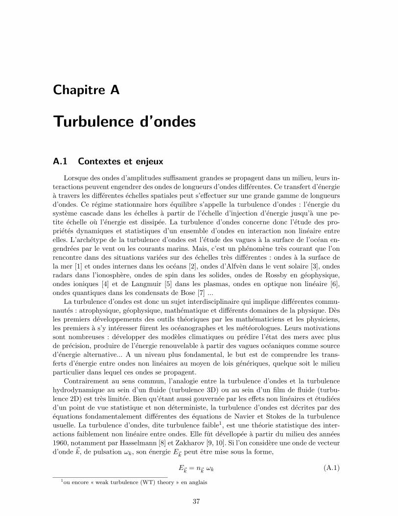
Force sensor
Fig. A.1: Schema et photo du dispositif experimental. Les deux batteurs se situent de partet d’autre du capteur capacitif mesurant la hauteur des vagues en un point. Taille de la cuve20 cm × 20 cm remplie d’eau ou de mercure.
A.3 Expose synthetique des principaux resultats
A.3.1 Spectre et distribution d’amplitude des vagues
Nous avons etudie la turbulence d’ondes a la surface d’un fluide. La majorite des experiencesa ete realisee avec de l’eau ou du mercure d’une profondeur de 2 cm. L’excitation se fait pardeux batteurs vibrant aleatoirement a basses frequences et la mesure de l’amplitude des vaguesse fait en un point au moyen d’une methode capacitive comme montre sur la Fig. A.1. Cetteenergie injectee au systeme par les grandes longueurs d’ondes est transferee vers les petitesstructures par l’intermediaire des non-linearites, dissipant l’energie par viscosite a la fin dela cascade. Ce processus de transfert est caracterise en mesurant le spectre frequentiel et ladistribution des fluctuations d’amplitudes des ondes.
Une evolution temporelle de la hauteur des vagues au cours du temps, η(t), est representeesur la Fig. A.2. Le signal est tres erratique et l’asymetrie observee est une signature duraidissement des vagues : les vagues avec des cretes de grandes amplitudes sont plus probablesque de profond creux. La transformee de Fourier d’un tel signal permet d’acceder a la densitespectrale de puissance de l’amplitude des vagues Sη(ω). Les ondes etant en interaction nonlineaires, on peut s’attendre a observer un regime de turbulence d’ondes, c’est-a-dire un spectreinvariant d’echelle.
Comme le montre la Fig. A.3, nous avons observe, pour la premiere fois, la transitionentre les regimes de turbulence d’ondes de gravite (a grandes echelles) et d’ondes capillaires(a petites echelles). Les spectres de ces deux regimes sont caracterises par des lois d’echelledifferentes (ou spectres « a la Kolmogorov »). Dans le regime capillaire, l’exposant de la loi depuissance avec la frequence est en accord avec la theorie de la turbulence faible d’Eq. (A.6) enω−17/6. Nos mesures de l’exposant du spectre des ondes capillaires sont beaucoup plus precises
42

170 180 190 200 210 220
6
4
2
0
2
4
6
8
10
12
Time (s)
Sur
face
wav
e am
plitu
de η
(m
m)
Fig. A.2: Evolution temporelle typique de la hauteur des vagues, η(t), pendant 50 s. 〈η〉 = 0.
que celles realisees precedemment [25, 26, 27, 28] du fait de leur forcage monochromatique denature parametrique (par instabilite de Faraday [38]). La transition entre les deux regimes alieu pour un nombre d’onde de l’ordre de l’inverse de la longueur capillaire lc. Pour la majoritedes fluides usuels, cela correspond a une frequence critique fc =
√g/2lc/π ' 20 Hz, c.-a-d. a
une longueur d’onde de l’ordre d’1 cm. Dans le regime de gravite, l’exposant du spectre estmesure etre dependant des parametres de forcage (l’amplitude et la gamme de frequences duforcage aleatoire) comme le montre la Fig. A.4, et donc en desaccord avec la prediction de laturbulence faible d’Eq. (A.6) en ω−4. Cette dependance est aussi observee sur la frequence detransition entre les deux regimes (voir l’encart de la Fig. A.4). Cette dependance de l’exposantdu spectre des ondes de gravite a ete depuis retrouve experimentalement dans un canal dedimension beaucoup grande que notre cuve [40]. L’origine de cette dependance reste actuel-lement un probleme ouvert. Elle pourrait provenir des effets de tailles finies de la cuve [40]. Ila aussi ete montre numeriquement que le spectre des ondes de gravite etait tres sensible a lacondensation d’ondes longues residuelles (ou « condensat » par analogie avec la condensationde Bose-Einstein en matiere condensee) [7, 21].
A faible forcage, la distribution de hauteur des vagues est bien decrite par une gaus-sienne (voir Fig. A.5). A suffisamment fort forcage, la distribution d’amplitudes des ondes esttrouvee asymetrique, montrant ainsi le caractere non-gaussien de la turbulence d’ondes. Cephenomene est bien connu des oceanographes qui mesures des distributions crete-a-creux desvagues s’ecartant d’une distribution de Rayleigh16 [23, 42]. Cette distribution a cependant peuete rapportee dans des experiences de laboratoire [43]. L’avantage est de pouvoir quantifierl’influence de certain parametre du systeme, telle la profondeur du fluide h, par exemple, quia tendance a augmenter cette asymetrie quand h diminue.
Reference :E. Falcon, C. Laroche & S. Fauve, Physical Review Letters 98, 094503 (2007)Observation of gravity-capillary wave turbulence
16Un processus gaussien a valeurs positives et negatives a une distribution de Rayleigh, P (x) ∼ xe−x2/σ2
,pour son amplitude crete-a-creux uniquement positive, σ etant l’ecart-type de la variable x.
43

Fig. A.3: Spectre de la hauteur des vagues montrant les regimes de turbulence d’ondes degravite et de capillarite. La transition entre les deux regimes a lieu pour λc = 2πlc ' 1 cm,ou lc est la longueur capillaire, i.e. pour une frequence ' 20 Hz. Les pointilles ont des pentesde −6.1 et −3.2. Forcage aleatoire de bande en frequences ≤ 4 Hz.
Fig. A.4: Pente des spectres de hauteur de vagues des regimes de turbulence d’ondes capillaires(symboles vides) et d’ondes de gravite (symboles pleins) en fonction de l’intensite UForcing etde la bande en frequence [() 0 a 4 Hz, (5) 0 a 5 Hz et () 0 a 6 Hz] du forcage aleatoire.Les traits pointilles sont les predictions theoriques de la turbulence faible [cf. Eqs. (A.5) &(A.6)]. Encart : Frequence de transition entre les deux regimes en fonction des parametres deforcage.
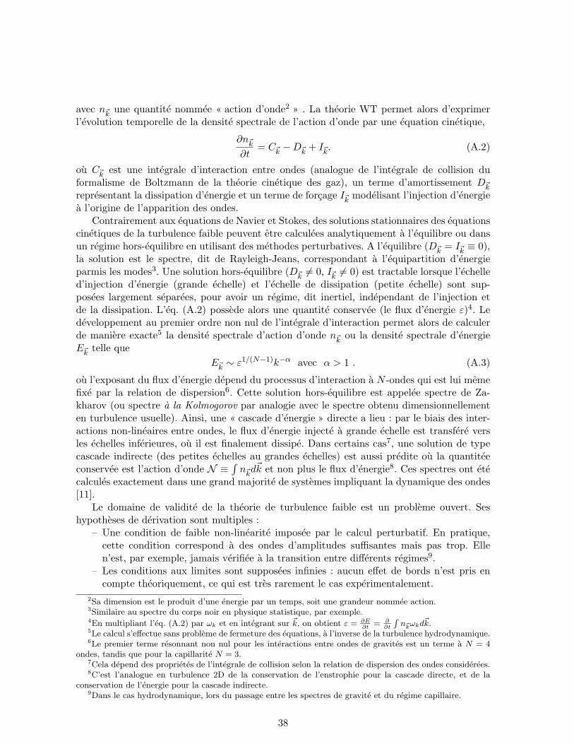
A.3.2 Intermittence en turbulence d’ondes
Une des images les plus frappantes de la turbulence hydrodynamique tri-dimensionnelleest l’apparition de bouffee intense de mouvement au sein de l’ecoulement fluide relativementcalme. Cela induit un comportement intermittent [44, 45]. En effet, on dit qu’un signal estintermittent lorsqu’il montre des evenements de plus en plus intense, lorsque on le sonde surdes temps de plus en plus courts, et donc lorsque la statistique du signal devient fortementnon gaussienne a petit temps. L’origine de la statistique non gaussienne en turbulence hy-drodynamique 3D a ete attribuee a la formation de structures coherentes, type vortex, desles premiers travaux de Batchelor et Townsend [44]. Cependant, le mecanisme physique de
44

−3 −2 −1 0 1 2 3 4 5
10−3
10−2
10−1
η / < η2 >1/2
Pro
babi
lity
Den
sity
Fun
ctio
ns
−5 0 5 1010
−3
10−2
10−1
100
η (mm)
PD
Fs
[ η ]
Fig. A.5: Encart : Fonctions de densite de probabilite asymetriques de la hauteur des vagues,η(t), pour differentes amplitudes croissantes du forcage (du noir au rouge). Principal : Distri-butions similaires adimensionnees par leurs ecart-types
√〈η2〉. Traits pointilles : Gaussiennede moyenne nulle et d’ecart-type 1.
l’intermittence est encore une question ouverte qui motive de tres nombreuses etudes en tur-bulence 3D [46]. L’intermittence a ete observee dans differents problemes de transport par unecoulement turbulent [scalaire passif, turbulence de Burgers (fluide fortement compressible)][47], en turbulence magnetohydrodynamique en geophysique [48] ou dans le vent solaire [49].Toutes ces observations ont eu lieu dans un systeme regi ou derive de la dynamique desequations de Navier-Stokes. L’observation d’intermittence dans d’autre systeme non modelisepar ces equations motiverait ainsi des explications nouvelles pour son origine.
−15 −10 −5 0 5 10 1510
−7
10−5
10−3
10−1
101
103
[η(t+τ) −2η(t) + η(t−τ)] / στ
PD
F(
[η(t
+τ)
−2η
(t)
+ η
(t−
τ)] /
στ )
τ = 6 msτ = 12 msτ = 18 msτ = 27 msτ = 50 msτ = 60 msτ = 80 msτ = 100 msGaussian
Fig. A.6: Fonctions de densite de probabilite des pentes locales des vagues [η(t+ τ)− 2η(t) +η(t−τ)]/στ a differentes echelles de temps 6 ≤ τ ≤ 100 ms (de haut en bas). Traits pointilles :Gaussienne de moyenne nulle et d’ecart-type 1. Temps de correlation : τc ' 63 ms. Les courbesont ete decallees verticalement pour plus de clarte.
Nous avons rapporte la premiere observation d’intermittence en turbulence d’ondes. Enmesurant les fluctuations temporelles de l’amplitude des vagues, η(t), en un point de la surfacedu fluide (cf. Fig. A.1), nous pouvons calculer les increments de la pente locale (ou vitesse)des vagues de gravite a une certaine echelle de temps τ : ∆η(τ) ≡ η(t+ τ)− 2η(t) + η(t− τ).
45
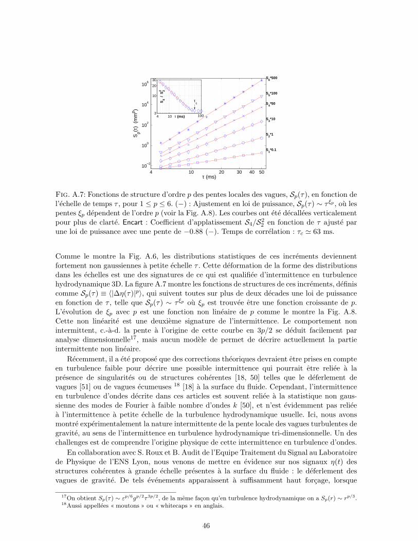
4 10 20 30 40 5010
−2
100
102
104
106
τ (ms)
Sp(τ
) (
mm
p )
3
10
20
30
τ (ms)
S4 /
S22
4 10 100
S6*500
S5*100
S4*50
S3*10
S2*1
S1*0.1
τc
Fig. A.7: Fonctions de structure d’ordre p des pentes locales des vagues, Sp(τ), en fonction del’echelle de temps τ , pour 1 ≤ p ≤ 6. (−) : Ajustement en loi de puissance, Sp(τ) ∼ τ ξp , ou lespentes ξp dependent de l’ordre p (voir la Fig. A.8). Les courbes ont ete decallees verticalementpour plus de clarte. Encart : Coefficient d’applatissement S4/S2
2 en fonction de τ ajuste parune loi de puissance avec une pente de −0.88 (−). Temps de correlation : τc ' 63 ms.
Comme le montre la Fig. A.6, les distributions statistiques de ces increments deviennentfortement non gaussiennes a petite echelle τ . Cette deformation de la forme des distributionsdans les echelles est une des signatures de ce qui est qualifiee d’intermittence en turbulencehydrodynamique 3D. La figure A.7 montre les fonctions de structures de ces increments, definiscomme Sp(τ) ≡ 〈|∆η(τ)|p〉, qui suivent toutes sur plus de deux decades une loi de puissanceen fonction de τ , telle que Sp(τ) ∼ τ ξp ou ξp est trouvee etre une fonction croissante de p.L’evolution de ξp avec p est une fonction non lineaire de p comme le montre la Fig. A.8.Cette non linearite est une deuxieme signature de l’intermittence. Le comportement nonintermittent, c.-a-d. la pente a l’origine de cette courbe en 3p/2 se deduit facilement paranalyse dimensionnelle17, mais aucun modele de permet de decrire actuellement la partieintermittente non lineaire.
Recemment, il a ete propose que des corrections theoriques devraient etre prises en compteen turbulence faible pour decrire une possible intermittence qui pourrait etre reliee a lapresence de singularites ou de structures coherentes [18, 50] telles que le deferlement devagues [51] ou de vagues ecumeuses 18 [18] a la surface du fluide. Cependant, l’intermittenceen turbulence d’ondes decrite dans ces articles est souvent reliee a la statistique non gaus-sienne des modes de Fourier a faible nombre d’ondes k [50], et n’est evidemment pas relieea l’intermittence a petite echelle de la turbulence hydrodynamique usuelle. Ici, nous avonsmontre experimentalement la nature intermittente de la pente locale des vagues turbulentes degravite, au sens de l’intermittence en turbulence hydrodynamique tri-dimensionnelle. Un deschallenges est de comprendre l’origine physique de cette intermittence en turbulence d’ondes.
En collaboration avec S. Roux et B. Audit de l’Equipe Traitement du Signal au Laboratoirede Physique de l’ENS Lyon, nous venons de mettre en evidence sur nos signaux η(t) desstructures coherentes a grande echelle presentes a la surface du fluide : le deferlement desvagues de gravite. De tels evenements apparaissent a suffisamment haut forcage, lorsque
17On obtient Sp(τ) ∼ εp/6gp/2τ3p/2, de la meme facon qu’en turbulence hydrodynamique on a Sp(r) ∼ rp/3.18Aussi appellees « moutons » ou « whitecaps » en anglais.
46

Fig. A.8: Exposants ξp des fonctions de strucure en fonction de l’ordre p. ξp est calcule apartir des pentes de la Fig. A.7, et est ajuste par (−−) ξp = c1p − c2
2 p2 avec c1 = 1.65 et
c2 = 0.2. Trait plein : Analyse dimensionnelle ξp = 3p/2.
650 750 850 950−10
−5
0
5
10
15
η (m
m)
Time (ms)650 750 850 950
−0.5
0
0.5
1
1.5
2
2.5
δη (
m/s
)
bBulge Crest
Toe
Fig. A.9: Deferlement typique d’une onde de gravite tres raide a fort forcage. Le front del’onde se situe sur le cote gauche. La courbe du haut (rouge) correspond a l’amplitude de lavague, et la courbe du bas (noir) a la pente de la vague.
l’acceleration verticale depasse un certain seuil. Ces deferlements s’observent directement surle signal de hauteur de vagues, et induisent une divergence de la pente locale des vagues(voir. Fig. A.9). L’evolution des fonctions de structures, a different forcage, en enlevant cesevenements de deferlement montre une attenuation de l’intermittence observee (la dependancenon lineaire de ξp avec p devient plus faible). Les deferlements d’ondes de gravite renforcentdonc l’intermittence, mais ne sont pas responsables de son origine qui est un probleme toujoursouvert. La dependance de l’exposant du spectre d’ondes de gravite avec le forcage ne peutpas aussi etre attribuee a ces structures coherentes. En effet, la pente a l’origine des courbesξp vs p est reliee a l’exposant du spectre et est independante de la presence ou non de cesevenements. L’origine de cette dependance est donc un probleme ouvert.
Generalement, pour tester les possibles proprietes d’intermittence d’un signal, la statis-tique de ses increments est calculee. Nous avons souligne avec S. Roux et B. Audit que pourdes signaux possedant des spectres assez raides, i.e. Sη(ω) ∼ ω−n avec n ≥ 3, les increments
47
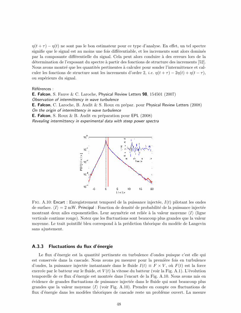
η(t+ τ)− η(t) ne sont pas le bon estimateur pour ce type d’analyse. En effet, un tel spectresignifie que le signal est au moins une fois differentiable, et les increments sont alors dominespar la composante differentielle du signal. Cela peut alors conduire a des erreurs lors de ladetermination de l’exposant du spectre a partir des fonctions de structure des increments [52].Nous avons montre que les quantites pertinentes a calculer pour sonder l’intermittence et cal-culer les fonctions de structure sont les increments d’ordre 2, i.e. η(t+ τ)− 2η(t) + η(t− τ),ou superieurs du signal.
References :E. Falcon, S. Fauve & C. Laroche, Physical Review Letters 98, 154501 (2007)Observation of intermittency in wave turbulenceE. Falcon, C. Laroche, B. Audit & S. Roux en prepar. pour Physical Review Letters (2008)On the origin of intermittency in wave turbulenceE. Falcon, S. Roux & B. Audit en preparation pour EPL (2008)Revealing intermittency in experimental data with steep power spectra
Fig. A.10: Encart : Enregistrement temporel de la puissance injectee, I(t) pilotant les ondesde surface. 〈I〉 = 2 mW. Principal : Fonction de densite de probabilite de la puissance injecteemontrant deux ailes exponentielles. Leur asymetrie est reliee a la valeur moyenne 〈I〉 (ligneverticale continue rouge). Notez que les fluctuations sont beaucoup plus grandes que la valeurmoyenne. Le trait pointille bleu correspond a la prediction theorique du modele de Langevinsans ajustement.
A.3.3 Fluctuations du flux d’energie
Le flux d’energie est la quantite pertinente en turbulence d’ondes puisque c’est elle quiest conservee dans la cascade. Nous avons pu mesurer pour la premiere fois en turbulenced’ondes, la puissance injectee instantanee dans le fluide I(t) ≡ F × V , ou F (t) est la forceexercee par le batteur sur le fluide, et V (t) la vitesse du batteur (voir la Fig. A.1). L’evolutiontemporelle de ce flux d’energie est montree dans l’encart de la Fig. A.10. Nous avons mis enevidence de grandes fluctuations de puissance injectee dans le fluide qui sont beaucoup plusgrandes que la valeur moyenne 〈I〉 (voir Fig. A.10). Prendre en compte ces fluctuations deflux d’energie dans les modeles theoriques de cascade reste un probleme ouvert. La mesure
48
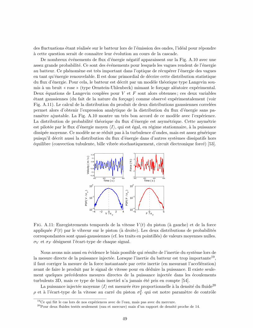
des fluctuations etant realisee sur le batteur lors de l’emission des ondes, l’ideal pour repondrea cette question serait de connaıtre leur evolution au cours de la cascade.
De nombreux evenements de flux d’energie negatif apparaissent sur la Fig. A.10 avec uneassez grande probabilite. Ce sont des evenements pour lesquels les vagues rendent de l’energieau batteur. Ce phenomene est tres important dans l’optique de recuperer l’energie des vaguesen tant qu’energie renouvelable. Il est donc primordial de decrire cette distribution statistiquedu flux d’energie. Pour cela, le batteur est decrit par un modele theorique type Langevin sou-mis a un bruit « rose » (type Ornstein-Uhlenbeck) mimant le forcage aleatoire experimental.Deux equations de Langevin couplees pour V et F sont alors obtenues ; ces deux variablesetant gaussiennes (du fait de la nature du forcage) comme observe experimentalement (voirFig. A.11). Le calcul de la distribution du produit de deux distributions gaussiennes correleespermet alors d’obtenir l’expression analytique de la distribution du flux d’energie sans pa-rametre ajustable. La Fig. A.10 montre un tres bon accord de ce modele avec l’experience.La distribution de probabilite theorique du flux d’energie est asymetrique. Cette asymetrieest pilotee par le flux d’energie moyen 〈I〉, qui est egal, en regime stationnaire, a la puissancedissipee moyenne. Ce modele ne se reduit pas a la turbulence d’ondes, mais est assez generiquepuisqu’il decrit aussi la distribution du flux d’energie dans d’autres systemes dissipatifs horsequilibre (convection tubulente, bille vibree stochastiquement, circuit electronique force) [53].
402 403 404 405
−0.15
−0.1
−0.05
0
0.05
0.1
0.15
Time ( s )
Vel
ocity
( m
/ s
)
402 403 404 405−4
−2
0
2
4
Time ( s )
For
ce (
N )
−4 −2 0 2 410
−4
10−2
100
V / σ V
PD
F(
V /
σ V
)
−5 0 510
−4
10−2
100
F / σ F
PD
F(
F /
σ F
)
Fig. A.11: Enregistrements temporels de la vitesse V (t) du piston (a gauche) et de la forceappliquee F (t) par le vibreur sur le piston (a droite). Les deux distributions de probabilitescorrespondantes sont quasi-gaussiennes (cf. les traits en pointilles) de valeurs moyennes nulles.σV et σF designent l’ecart-type de chaque signal.
Nous avons mis aussi en evidence le biais possible qui resulte de l’inertie du systeme lors dela mesure directe de la puissance injectee. Lorsque l’inertie du batteur est trop importante19,il faut corriger la mesure de la force instantanee par cette inertie (en mesurant l’acceleration)avant de faire le produit par le signal de vitesse pour en deduire la puissance. Il existe seule-ment quelques precedentes mesures directes de la puissance injectee dans les ecoulementsturbulents 3D, mais ce type de biais inertiel n’a jamais ete pris en compte [54].
La puissance injectee moyenne 〈I〉 est mesuree etre proportionnelle a la densite du fluide20
ρ et a l’ecart-type de la vitesse au carre du piston σ2V qui est notre parametre de controle
19Ce qui fut le cas lors de nos experiences avec de l’eau, mais pas avec du mercure.20Pour deux fluides testes seulement (eau et mercure) mais d’un rapport de densite proche de 14.
49

10 10010
−8
10−6
10−4
10−2
Frequency (Hz)
PS
D /
σ V2 (
s3 )
0 5 10 15 200
5
10
15
20
σV2 (cm/s)2
< I
> (
mW
)
4
Fig. A.12: Spectres de la hauteur des vagues divises par la variance de la vitesse du piston, σ2V ,
pour differentes amplitudes de forcage : σV = 2.1, 2.6, 3.5 et 4.1 cm/s. La ligne en pointillesa une pente de −5.5, tandis que la ligne en trait continu a une pente de −17/6. Encart : Lapuissance injectee moyenne 〈I〉 est trouve proportionnelle a σ2
V .
pour l’amplitude du forcage. Le transfert d’energie se produit par des interactions a 4 ondesdans le regime de gravite, et a 3 ondes dans le regime capillaire. Ainsi, si ces deux regimessont independants, la dependance du spectre Sη par rapport au flux d’energie moyen 〈I〉devrait montrer differentes lois d’echelle. Nos mesures montrent qu’une unique loi d’echelleen Sη ∼ 〈I〉 permet aux differents spectres gravito-capillaire obtenus a differents forcagesd’etre decrit par une seule coube maıtresse (voir Fig. A.12). Ce fort desaccord avec la theoriede turbulence faible [cf. Eqs. (A.5) & (A.6)] montre donc que les interactions entre les deuxregimes sont tres importantes bien qu’elles ne soient pas prises en compte theoriquement. Il estcependant a noter que l’energie injectee mesuree n’est pas exclusivement dediee a engendrerles ondes de surfaces, une fraction (qui reste a quantifier) contribue aussi a la creation detourbillons proches des batteurs, et au mouvement du fluide en profondeur a la base desbatteurs.
La distribution experimentale de puissance injectee moyennee sur un intervale de tempsτ , P (Iτ ) a aussi ete etudiee dans le cadre des theoremes des fluctuations de la physiquestatistique hors de l’equilibre (dits de Gallavotti-Cohen-Evans) [55]. Ce theoreme dit queP [+Iτ/〈I〉]P [−Iτ/〈I〉] ∼ e−β(τ)Iτ ou P [x] est la probabilite d’obtenir la valeur x et 1/β(τ) est associe al’energie du systeme. Les hypotheses du theoreme (notamment de reversibilite temporelle)ne sont generalement pas valides pour un systeme dissipatif. L’apparente verification de cetheoreme dans de nombreuses experiences precedentes [56, 57, 58, 59] provient des trop faiblesvaleurs des fluctuations Iτ/〈I〉 atteintes a grand τ [60, 61]. Notre systeme experimental deturbulence d’ondes permet d’atteindre des valeurs suffisamment grandes, et nous avons montrequ’elles ne verifiaient pas ce theoreme, mais etait bien decrite par un calcul analytique basesur une equation de Langevin force par un bruit blanc [62].
Nous avons aussi etudie experimentalement les fluctuations du flux d’energie dans un cir-cuit electronique RC en serie force par une tension stochastique. Ce systeme dissipatif horsequilibre modele permet de controler tres facilement les parametres du systeme21. Nous mon-trons que les grandes fluctuations obtenues ne suivent pas le theoreme des fluctuations meme
21Notamment, son taux d’amortissement 1/(RC).
50

−20 −10 0 10 20 30
10−4
10−3
10−2
10−1
100
I/<I>
PD
F(I
/<I>
)
Fig. A.13: Fluctuations de la puissance injectee I(t) dans un circuit electronique RC soumisa une tension aleatoire pour deux valeurs du taux d’amortissement (RC)−1 = 2000 et 200 Hz(resp. en bleu et en rouge). Comparaison entre experience (−) et la prediction du modele deLangevin (−−). Noter que, comme en turbulence d’ondes, plus le systeme est dissipatif plusla PDF de I(t) est asymetrique.
pour les temps de moyenne τ long. La distribution du flux d’energie montre en Fig. A.13ressemble fortement a celle de la Fig. A.10 de turbulence d’ondes, et se decrit d’ailleurs tresbien par le modele enonce plus haut (voir les pointilles Fig. A.13). Ce systeme electroniqueapparait donc comme l’un des plus simples pour comprendre certaines proprietes des fluctua-tions du flux d’energie partagee par d’autres systemes dissipatifs, tels que les gaz granulaires[56], la convection [58], ou la turbulence d’ondes.
References :E. Falcon, S. Aumaıtre, C. Falcon, C. Laroche & S. Fauve, Physical Review Letters 100, 064503(2008) Fluctuations of energy flux in wave turbulenceC. Falcon & E. Falcon, soumis a Physical Review E (2008)Fluctuations of energy flux in a simple dissipative out-of-equilibrium system
A.3.4 Turbulence d’ondes en impesanteur
Les experiences en microgravite permettent d’etudier les ondes purement capillaires surl’ensemble de la gamme experimentale de longueurs d’ondes sans etre pertubees par les effetsde gravite. Au sol, la limite superieure en longueur d’onde est la longueur capillaire, tandis quela limite inferieure est liee a la dissipation. Nos experiences de microgravite ont ete realiseeslors de deux campagnes CNES de vols paraboliques a bord d’un Airbus A300 en Septembre2006 et Mars 2007. Une campagne consiste en une session de 3 vols, chaque vol permettantla realisation de 30 paraboles de 22 secondes chacune de microgravite. Une gravite reduitepermet aussi d’etudier une couche de fluide en geometrie spherique sur laquelle des ondespeuvent se propager sans etre reflechies par des bords lateraux (voir le dispositif experimentalde la Fig. A.14).
51

Fig. A.14: Dispositif experimental pour l’etude de la turbulence d’ondes en impesanteur. Dansles phases de microgravite, le fluide recouvre toute la surface interne de la cellule soumises ades vibrations.
10 100 50010
−10
10−9
10−8
10−7
10−6
10−5
10−4
10−3
Frequency (Hz)
Pow
er S
pect
rum
Den
sity
( V
2 /
Hz
)
10 100 20010
−11
10−9
10−7
10−5
10−3
Frequency (Hz)
PS
D (
V 2
/ H
z )
Fig. A.15: Spectre de la hauteur des vagues en impesanteur pour deux forcages : aleatoireentre 0 et 6 Hz (courbe du bas), ou sinusoıdal a 3 Hz (courbe du haut). Les lignes en pointillesont des pentes de -3.1 (bas) et -3.2 (haut). Encart : Idem en presence de gravite. Deux loisde puissance apparaissent correspondant aux regimes de gravite (pente -5) et de capillarite(pente -3).
Nous avons observe en microgravite la turbulence d’ondes capillaires a la surface d’unecouche de fluide recouvrant toute la surface interne d’une cellule spherique. La figure A.15montre le spectre des ondes capillaires sur une large gamme de longueur d’ondes, notammentdans la zone ou les ondes de gravite etaient presentes lors d’experiences au sol. Ce spectre surdeux decades en frequence est trouve en bon accord avec la theorie de la turbulence faiblepredisant un exposant −17/6 ' −2.8 pour le regime capillaire [voir l’Eq. (A.6)]. Il est aussitrouve independant des parametres de forcages aleatoires ou periodiques a basses frequences.
Lorsque la cellule est vibree periodiquement a haute frequence, des motifs spheriquesbi-dimensionnels apparaissent a la surface du fluide tels que des lignes ou des hexagonessous-harmoniques (voir Figs. A.16). Leur dynamique est complexe et resulte d’une interac-tion entre deux instabilites (amplification parametrique de type Faraday [38] et mouvement
52

Fig. A.16: Ondes de surface engendrees en impesanteur a l’interieur d’une cellule transparentespherique (gauche) ou cylindrique (droite). Le fluide a l’interieur de la cellule mouille toutela surface et forme une couche homogene de fluide. Des motifs bidimensionnels (lignes ouhexagones) apparaissent a la surface de la couche spherique ou cylindrique de fluide (resp.ethanol et eau) sous un forcage sinusoıdal de 30 Hz.
de ballotement ou “sloshing”). Cette observation de motifs a la surface d’une couche fluideen geometrie courbe (sphere ou cylindre) n’avait jamais ete rapportee precedemment a notreconnaissance.
References :C. Falcon, E. Falcon, U. Bortolozzo & S. Fauve, soumis a EPL (2008)Capillary wave turbulence on a spherical fluid surface in zero gravity
A.3.5 Turbulence d’ondes dans les ferrofluides
Un ferrofluide est une suspension colloıdale de fines particules ferromagnetiques presentantun caractere a la fois liquide et fortement magnetique. Contrairement aux fluides usuels, larelation de dispersion des ondes a la surface d’un ferrofluide est non monotone et presente unminimum (dependant du champ magnetique B applique [63, 64]) qui est le siege d’instabilite.Au-dela d’un champ critique Bc, la surface libre du ferrofluide se deforme et un reseau depics statiques s’organise a sa surface (instabilite de Rosensweig) [65]. L’amplitude du champmagnetique B permet ainsi de piloter directement le caractere non monotone de la relationde dispersion des ondes qui secrit [66]
ω2 = gk − f [χ]ρµ0
B2k2 +γ
ρk3 (A.7)
ou µ0 = 4π × 10−7 H/m est la permeabilite magnetique du vide, et f [χ] une fonction connuede la susceptibilite magnetique du ferrofluide22. On peut ainsi facilement regler, avec le seul
22Plus precisement, χ(H) depend du champ magnetique H selon une loi connue dite de Langevin et doncimplicitement de l’induction magnetique B, puisque B = µ0(1 + χ)H. Par abus de langage dans le texte,l’induction magnetique B sera appele « champ magnetique » .
53

parametre de controle B, la relation de dispersion des ondes pour passer d’un systeme disper-sif (terme en k2 preponderant) a un systeme non dispersif (terme en k ou k3 dominant). Lespossibles predictions theoriques de la turbulence faible pour un systeme dispersif bidimen-sionnel est d’ailleurs matiere a debat [18, 70]. La turbulence d’ondes a la surface d’un fluidemagnetique presentera donc un comportement tres riche, selon que le systeme se trouve endessous du seuil, proche du seuil, ou au-dela du seuil de l’instabilite de Rosensweig.
Fig. A.17: Dispositif experimental pour l’etude de la turbulence d’ondes a la surface d’unferrofluide soumis a un champ magnetique continu perpendiculaire engendre par deux bobinesen serie. Les ondes a la surface du ferrofluide sont emises par un batteur plongeant dans lefluide pilote par un vibreur. La hauteur des vagues est mesuree locallement par une methodecapacitive.
Nous avons etudie la turbulence d’ondes a la surface d’un ferrofluide soumis a un champmagnetique normal (voir Fig. A.17). Ce sujet a debute mi-Janvier 2008 par le Stage de M2de 4 mois de Francois Boyer. Les resultats ont ete tres nombreux. Nous avons montre queles ondes de surface magnetiques apparaissent au-dessus d’un champ critique, mais inferieurau champ Bc de l’instabilite de Rosensweig. Le spectre de ces ondes magnetiques montre uneunique loi de puissance sur toute la gamme de frequence accessible au lieu des deux regimesgravito-capillaires observes sans champ magnetique applique (voir la Fig. A.18). On peutcalculer par analyse dimensionnelle le spectre de turbulence d’ondes magnetiques comme
Smagη (ω) ∼ εα(B2
ρµ0
) 2−3α2
ω−3 , (A.8)
L’exposant frequentiel attendu en ω−3 est tres proche de celui predit pour les ondes capillairesen ω−17/6, pour pouvoir etre discernable experimentalement sur la Fig. A.18. Cela conduitainsi a l’observation d’une seule pente « magneto-capillaire » . Contrairement au cas disper-sif [voir l’Eq. (A.5) & (A.6)], il est aussi notable que l’exposant frequentiel du spectre nedepende pas de l’exposant α du flux d’energie. Par contre, l’exposant α reste indeterminepar l’analyse dimensionnelle. En mesurant la loi d’echelle entre l’amplitude du spectre Smagη
et le champ magnetique B, on montre alors que α = 1/3, c’est-a-dire que la turbulenced’ondes magnetiques est un processus a 4-ondes. Ainsi, les variations de l’amplitude du spectremagnetique avec le champ nous ont permis d’etablir experimentalement l’expression completedu spectre de turbulence d’ondes magnetiques, qui n’a, a ce jour, fait l’objet d’aucune autreetude, ni experimentale, ni theorique.
54

3 10 100 40010
−6
10−4
10−2
100
102
Frequency (Hz)
Pow
er s
pect
rum
of η
( m
m2 /
Hz
)
B = 0.9 Bc
3 10 100 40010
−6
10−4
10−2
100
102
Frequency (Hz)
PS
D η
( m
m2 /
Hz
)
B = 0
Fig. A.18: Spectre de la hauteur des vagues, η(t), a la surface d’un ferrofluide pour deuxchamps magnetiques appliques. Encart : B = 0 : Regimes de turbulence d’ondes de graviteet d’ondes capillaires. Les lignes en pointilles ont des pentes de -4.6 et -2.9. La transition setrouve a fgc ' 20 Hz. Principal : B = 0.9Bc : Turbulence d’ondes magneto-capillaires. La ligneen pointilles a une pente de -3.3. La transition a ete abaissee vers fgc ' 5 Hz.
0 0.5 1 1.5 2
5
10
15
20
25
0.65
ft
fgc
fgm
fmc
Capillary Wave Turbulence
Gravity Wave
Turbulence
Magnetic Wave Turbulence
Ros
ensw
eig
inst
abili
ty
B / Bc
Cro
ssov
er fr
eque
ncie
s (H
z)
Fig. A.19: Frequences de transition entre les regimes de turbulence d’ondes de gravite, d’ondesmagnetiques et d’ondes capillaires en fonction du champ magnetique applique. Differentsparametres de forcage : (×) 1 a 4 Hz, () 1 a 5 Hz, et (+ ou ) 1 a 6 Hz. Les frequencesde transition theoriques fgc, fgm et fmc entre les differents regimes peuvent etre obtenuesanalytiquement a partir de l’Eq. (A.7). Par exemple, le point triple est donnee par ft =12π (g
3ργ )1/4 ' 10.8 Hz et f [χ]B2 = µ0
√ρgγ, soit B/Bc = 0.65 pour notre ferrofluide ou Bc est
le seuil de l’instabilite de Rosensweig.
Les domaines frequentiels d’existence des regimes de turbulence d’ondes de gravite, d’ondesmagnetiques et d’ondes capillaires ont ete mesures, ainsi que le point triple de coexistence deces 3 domaines (voir la Fig. A.19). Les courbes theoriques limitant ces differents domaines,ainsi que le point triple, sont calcules a partir de la relation de dispersion d’Eq. (A.7), et sonttrouves en tres bon accord avec l’experience sans parametre ajustable (voir les traits pleinssur la Fig. A.19).
Par ailleurs, la distribution statistique d’amplitude des vagues et leur evolution avec le
55

champ magnetique ont elles aussi ete etudiees : ces mesures confirment la nature non-lineairedes interactions entre ondes, hypothese fondatrice de la turbulence d’ondes, et montrentegalement un seuil d’existence des ondes magnetiques. Toutes ces analyses constituent unensemble coherent de resultats de turbulence d’ondes dans un systeme original.
Lorsque l’instabilite de reseau de pics statiques de Rosensweig est en place (a fort champmagnetique B ≥ Bc), nous avons etudie les interactions entre les ondes de surface et ladeformation du reseau de Rosensweig. Nous avons observe un phenomene nouveau. A faibleforcage periodique, le reseau hexagonal de pics n’est pas deforme, les pics sont animes de mou-vements oscillatoires autour de leur position d’equilibre statique (voir Fig. A.20a) ; lorsque leforcage depasse un certain seuil en deplacement, les pics n’ont plus de position moyenne fixe,sont animes d’un mouvement plus ou moins desordonne (selon l’ecart au seuil) et il se produitdes collisions « molles » engendrant la fusion de deux ou plusieurs pics (voir Fig. A.20b). On anomme ces deux comportements, respectivement, le regime elastique (a la maniere de phononsdans un reseau cristallin) et le regime fluide. Cette transition elastique-fluide a lieu lorsquel’amplitude du forcage depasse 10% de la distance entre les pics du reseau. Il est remarquablede constater que le seuil de rupture des reseaux cristallins, donne par le critere empiriquede Lindemann [67], est egalement de 10% de la distance entre les atomes. Des etudes plusapprofondies permettraient de preciser la nature de l’origine de ces similitudes et de decrireles interactions entre pics.
References :F. Boyer & E. Falcon, Physical Review Letters 101 0244502 (2008)Wave turbulence on the surface of a ferrofluid in a magnetic field
Fig. A.20: Interactions entre le reseau hexagonal de pics stationnaires de Rosensweig et lesondes de surface induites par la vibration d’un batteur (vues de dessus). A gauche : A faibleforcage, les pics oscillent autour de leurs positions moyennes (regime elastique). A droite :Lorsque le deplacement du batteur depasse une fraction de la distance entre pics, la « fusion »du reseau a lieu : les pics sont animes d’un mouvement desordonne. Cette transition elastique– fluide peut etre vue comme l’analogue de la fusion d’un reseau cristallin en physique dusolide.
56

A.4 Perspectives
Mes recherches pour les prochaines annees concerneront essentiellement l’etude de la tur-bulence d’ondes. Elles se realiseront dans le cadre de l’ANR « Turbulence d’ondes hydrody-namiques, elastiques et optiques », financement obtenu fin 2007 pour 4 ans.
On se propose d’etudier la turbulence d’ondes a la surface d’un fluide dans un grandbassin, nouvellement construit au laboratoire, de l’ordre de 2 m de diametre. L’excitationturbulente a la surface du fluide se fera par de nouveaux batteurs controles en deplacementpar l’intermediaire de servo-moteurs. Des sondes locales capacitives et optiques (vibrometrelaser) permettront la mesure temporelle de la hauteur des vagues (en differents endroits)avec la possibilite de faire des correlations dans l’espace reel. Cette experience a plus grandeechelle permettra de s’affranchir des effets de bords lies a la petite taille de nos precedentesexperiences. Elle permettra d’analyser l’effet de la quantification imposee par les conditionsaux bords sur les transferts d’energie entre modes et donc sur le spectre des ondes de gravite.Comprendre la dependance de l’exposant du spectre des ondes de gravite avec les parametresde forcage est en effet un des problemes ouverts.
La plupart des mesures in situ ou de laboratoire de turbulence d’ondes sont localiseesen espace, tandis que les predictions theoriques sont souvent relatives a l’espace de Fourier,telles que le spectre de puissance ou la distribution de probabilite de l’amplitude de Fourierde la composante de l’onde a un nombre d’onde k donne. Un challenge important seraitde developper une sonde directe dans l’espace de Fourier. Pour cela, une nouvelle methodeoptique developpee par une equipe de l’ESPCI (P. Cobelli & P. Petitjeans) permettra d’accedera la hauteur des vagues η(x, y, t) sur une certaine zone spatiale au cours du temps. Cettemethode non intrusive est basee sur la deformation d’une grille projetee sur la surface dufluide, ainsi que sa diffusion, par le ondes turbulentes a la surface du liquide (eau + peintureblanche). La comparaison avec l’image initiale non deformee permet de remonter au dephasageφ(x, y, t) et geometriquement a la hauteur η(x, y, t) des vagues jusqu’a des pentes 10 [68].D’autres methodes optiques basees sur la reflection, la refraction [69] ou l’absorption [25] delumiere par la surface ondulante existent mais ne permettent pas de mesurer la pente de vaguesfortement non lineaires. Ainsi, en collaboration avec l’equipe de l’ESPCI, nous pourrons ainsiacceder au spectre spatial des vagues Sη(k) au cours du temps, a la dependance temporellede l’amplitude de Fourier de chaque nombre d’ondes et leur distribution de probabilite, etainsi nous serons capable d’etudier comment se comporte les fluctuations de flux d’energieau cours du processus de cascade des grandes aux petites echelles. Il serait aussi interessantd’etudier la correlation entre differentes amplitudes de Fourier de differents vecteurs d’ondes.Les correlations entre triades resonnantes (capillarite) ou quartets resonnants (gravite) serontmesurees afin de mieux comprendre les processus dynamiques elementaires impliques dans lacascade d’energie.
Par ailleurs, l’existence d’une cascade inverse de gravite est predite theoriquement [9, 11]et numeriquement [21] mais n’a jamais ete observee experimentalement ; notre experience sepretera fort bien a cette etude.
Changer la profondeur de fluide est une facon de modifier la relation de dispersion desondes lineaires se propageant a sa surface. Les ondes de gravite en faible profondeur peuventdevenir en effet tres faiblement dispersives. Les predictions theoriques pour un systeme dis-persif voir faiblement dispersif est d’ailleurs matiere a debat [70]. L’absence de dispersionpourrait rendre caduque la theorie de turbulence faible, puisqu’elle implique des effets nonlineaires cumulatifs lors de la propagation d’ondes pouvant aller jusqu’a la formation d’ondes
57
de chocs. L’evolution des lois d’echelle des spectres d’ondes de gravite et de capillarite seraentreprise lorsque le systeme passera d’une limite eau profonde a une limite de faible profon-deur. Dans cette limite de faible profondeur, la turbulence faible predit des spectres beaucoupmoins raides qu’en eau profonde a la fois dans le regime de gravite [71] et de capillarite [72].L’evolution des distributions de probabilite des vagues sera aussi determinee. L’influence deces effets de prondeurs sur la turbulence d’ondes pourrait expliquer le melange du planctonsdans les lacs peu profonds [73].
Nous projetons aussi d’etudier la turbulence d’ondes decroissantes, dites aussi en declin,c’est-a-dire une fois que l’emission d’ondes est arretee. Cela permettrait de comprendrecomment l’energie est redistribuee a travers les modes au cours des transitoires, et com-ment a partir d’un regime transitoire, on tend vers le regime stationnaire de la turbulenced’ondes. Bien que des etudes theoriques et numeriques aient ete realisees en turbulence d’ondesmagnetohydrodynamiques pour des ondes d’Alfven ; a notre connaissance, une seul experiencea ete realisee en turbulence d’ondes capillaires decroissantes a la surface de l’hydrogene liquide[19].
La description du regime de transition entre ondes de gravite et ondes capillaires pose unedifficulte theorique dans la mesure ou il semble que les approximations utilisees pour decrirela turbulence d’ondes pourraient y etre invalides. Il est donc possible que la presence d’ondescapillaires a petite echelle affecte le spectre des ondes de gravite et inversement. Ceci demandecependant a etre confirme. Nous avons deja etudie le cas de la turbulence d’ondes en regimepurement capillaires lors d’experiences en microgravite. Afin d’isoler le regime de gravite eneliminant l’effet parasite du regime capillaire, une experience de turbulence d’ondes realiseesau voisinage du point critique liquide-vapeur sera aussi realisee au LPS de l’ENS dans le cadrede l’ANR. Des ondes de surface seront engendrees a l’interface entre un liquide et sa vapeur auvoisinage du point critique liquide-vapeur (CO2 vers 30o C a 70 bars). La tension de surfaces’y annule beaucoup plus rapidement que la difference de densite entre les deux phases, desorte que la capillarite devient negligeable par rapport a la gravite sur l’ensemble du spectre.En effet, en bout de spectre, les petites longueurs d’onde sont dissipees par viscosite avantd’avoir pu atteindre le regime capillaire. Nous pouvons ainsi etudier un regime pur d’ondesde gravite dans une experience de laboratoire.
Nous avons mis en evidence d’importantes fluctuations negatives de puissance injecteecorrespondant aux cas ou le fluide rend de l’energie a ce qui a permis d’engendrer les vagues.Un modele theorique simple de type Langevin nous a permis de decrire la distribution deprobabilite de la puissance injectee dans le fluide (mais aussi dans d’autres systemes dissi-patifs hors de l’equilibre). Fort de cette comprehension, une extension de ces travaux au casoceanographique pourraıt etre envisagee, notamment en ce qui concerne l’energie des vagues(energie houlomotrice) en tant qu’energie renouvelable.
La turbulence d’ondes de surface oceanique se fait en presence de tourbillons resultantsdes courants marins et des vents. Avec S. Aumaıtre (CEA Saclay), on se propose d’etudieren laboratoire l’influence des tourbillons sur la turbulence d’ondes. Pour cela, les ondes a lasurface d’un metal liquide conducteur traverse par un courant electrique interagiront avec destourbillons engendres magnetiquement par des aimants via les forces de Lorentz. Le meme dis-positif permettra aussi l’etude de la diffusion d’ondes de surface par un unique tourbillon (ana-logue hydrodynamique de la diffusion quantique de type Aharonov-Bohm), puis le problemeouvert qu’est la localisation d’energie des ondes de surface (lineaires ou non-lineaires) par ledesordre (reseau de tourbillons aleatoires).
Un autre motivation serait de comprendre le role d’une couche mince visqueuse (ajoutee a
58
la surface du fluide) sur le regime de turbulence d’ondes, et sa dispersion. Ce role est d’interetfondamental en oceanographie (degazages de bateaux...).
Des mesures de diffusion d’ondes radars par l’ocean ont ete realisees par Fabrice Ardhuindu SHOM (Service Hydrographique et Oceanographique de la Marine) sur une zone de 80km2 proche des cotes brestoises. Par decalage Doppler, la cartographie in situ de courants desurface et le spectre des vagues peuvent etre obtenues (via la 1re et 2e resonances de Bragg)[74]. Avec Louis Marie de l’IFREMER de Brest, une collaboration se met en place pour traiterces donnees existantes afin d’obtenir le spectre spatial bidimensionnel des vagues oceaniques.
L’etude de la turbulence d’ondes a la surface d’un ferrofluide initiee lors du stage deDEA de F. Boyer en Janv-Juillet 2008 sera continuee. La dependance de la pente du spectremagneto-capillaire avec le champ magnetique demeure une question ouverte, bien qu’elle nousait permis d’observer un seuil d’existence d’ondes magnetiques qui n’avait pas encore ete rap-porte. La transition elastique-fluide observee lors de l’interaction entre les ondes de surface etles pics statiques de l’instabilite de Rosensweig est a preciser, notamment l’analogie avec lesreseaux cristallins. Le regime « elastique » , type phonons, et le regime « desordonne » , typefluide, de nucleation et d’annihilation de pics seraient a etudier par des methodes d’analysesd’images multi-lagrangiennes, et permetraient de suivre certains pics pour comprendre leurdynamique d’interaction. En imposant un champ magnetique non plus perpendiculaire, maisparallele a la surface du ferrofluide, le terme quadratique additionel en B2k2 dans la relationde dispersion d’Eq. (A.7) serait effectif dans une seule direction rendant tres anisotrope lesysteme, et serait de signe positif supprimant ainsi l’instabilite de Rosensweig. Connaıtre lesspectres associes dans ce regime de turbulence d’ondes anisotrope serait interessant, puisquel’anisotropie n’est jamais prise en compte theoriquement. Par ailleurs, l’influence du termedispersif dans une seule direction du systeme permettrait d’atteindre un regime de turbulenced’ondes 1D faiblement dispersives, actuellement sujet de debat theoriquement [18, 70].
References
[1] Y. Toba, J. Ocean Soc. Jpn. 29, 209 (1973) ; K. K. Kahma, J. Phys. Oceanogr. 11, 1503(1981) ; G. Z. Forristall, J. Geophys. Res. 86, 8075 (1981) ; M. A. Donelan et al., Philos.Trans. R. Soc. London A 315, 509 (1985).
[2] Y. V. Lvov, K. L. Polzin & E. G. Tabak, Phys. Rev. Lett. 92, 128501 (2004).[3] R. Z. Sagdeev, Rev. Mod. Phys. 51, 1 (1979).[4] K. Mizuno & J. S. DeGroot, Phys. Fluids 26, 608 (1983).[5] J. D. Huba, P. K. Chaturvedi & K. Papadopoulos, Phys. Fluids 23, 1479 (1980) ; M. Y.
Yu & P. K. Shukla, Phys. Fluids 25, 573 (1982).[6] E. Kuznetsov, A. C. Newell & V. E. Zakharov, Phys. Rev. Lett. 67, 3243 (1991).[7] A. Dyachenko & G. Falkovitch, Phys. Rev. E54 5095 (1996) ; N. G. Berloff & B. V.
Svistunov, Phys. Rev. A 66, 013603 (2002) ; C. Connaughton et al., Phys. Rev. Lett.95 263901 (2005) ; S. Rica, Habilitation a Diriger les Recherches (Universite Pierre etMarie Curie, 2007).
[8] K. Hassselmann, J. Fluid Mech. 12, 481 (1962).[9] V. E. Zakharov & N. N. Filonenko, Sov. Phys. Dokl. 11, 881 (1967) ; V. E. Zakharov &
M. M. Zaslavsky, Izv. Atm. Ocean. Phys. 18, 747 (1982).
59
[10] V. E. Zakharov & N. N. Filonenko, J. App. Mech. Tech. Phys. 8, 37 (1967).
[11] V. E. Zakharov, V. L’vov & G. Falkovich Kolmogorov Spectra of Turbulence I (Springer-Verlag, Berlin, 1992)
[12] Nonlinear Waves and Weak Turbulence, Ed. by V. E. Zakharov, Series of AMS Trans-lations 2, Vol. 182 (American Mathematical Society, 1998)
[13] E. Kartashova, « Wave resonances in systems with discrete spectra » in [12] pp. 95–130
[14] V. E. Zakharov, A. O. Korotkevich, A. N. Pushkarev & A. I. Dyachenko, JETP Letters82, 487 (2005).
[15] M. Tanaka & N. Yokoyama, Fluid Dynam. Res. 34 199 (2006)
[16] S. Nazarenko, J. Stat. Mech. L02002 (2006)
[17] E. Kartashova, Phys. Rev. Lett. 98, 214502 (2007) ; E. Kartashova, S. Nazarenko, O.Rudenko, ArXiv.NLlin.0803.3308v2, a paraıtre dans Phys. Rev. E (2008)
[18] C. Connaughton, S. Nazarenko & A. C. Newell, Physica D 184 86 (2003).
[19] G. V. Kolmakov et al., Phys. Rev. Lett. 93, 074501 (2004) ; J. Low Temp. Phys. 145,311 (2006)
[20] B. Bigot, S. Galtier & H. Politano Phys. Rev. Lett. 100 074502 (2008)
[21] A. O. Korotkevitch, Phys. Rev. Lett. 101, 074504 (2008)
[22] V. E. Zakharov, A. O. Korotkevich, A. Pushkarev & D. Resio, Phys. Rev. Lett 99164501 (2007).
[23] M. K. Ochi, Ocean Waves (Cambridge University Press, Cambridge, 1998)
[24] The Wise Group, L. Cavaleri et al., Wave modelling - The state of art, Progress inOceanography 75, 603 (2007)
[25] W. B. Wright, R. Budakian & S. J. Putterman, Phys. Rev. Lett. 76, 4528 (1996) ; W.B. Wright, R. Budakian, D. J. Pine & S. J. Putterman, Science 278, 1609 (1997).
[26] R. G. Holt & E. H. Trinh, Phys. Rev. Lett. 77, 1274 (1996).
[27] M. Lommer & M. T. Levinsen J. Fluoresc. 12, 45 (2002) ; E. Henry, P. Alstrøm & M.T. Levinsen, Europhys. Lett. 52, 27 (2000).
[28] M. Yu. Brazhnikov, G. V. Kolmakov & A. A. Levchenko, Sov. Phys JETP 95, 447(2002) ; M. Yu. Brazhnikov et al., Europhys. Lett. 58, 510 (2002) ; G. V. Kolmakov etal. Phys. Rev. Lett. 93, 074501 (2004).
[29] N. Mordant, Phys. Rev. Lett. 100, 234505 (2008)
[30] A. Boudaoud, O. Cadot, B. Odille & C. Touze, Phys. Rev. Lett. 100, 234504 (2008)
[31] G. During, C. Josserand & S. Rica, Phys. Rev. Lett. 97, 025503 (2006).
[32] M. Onorato et al., Phys. Rev. Lett. 89, 144501 (2002) ; A. Pushkarev, D. Resio & V.Zakharov, Physica D 184 29 (2003) ; A. I. Dyachenko, A. O. Korotkevich & V. E.Zakharov, Phys. Rev. Lett. 92, 134501 (2004).
[33] S. A. Kitaigorodskii, J. Phys. Oceanogr. 13, 816 (1983).
[34] E. A. Kuznetsov, JETP Letters 80, 83 (2004).
[35] O. M. Phillips, J. Fluid Mech. 4 426 (1958).
[36] G. B. Whitham, Linear and Nonlinear Waves (John Wiley & Sons, New-York, 1999).
60

[37] A. N. Pushkarev & V. E. Zakharov, Phys. Rev. Lett. 76 3320 (1996).
[38] M. Faraday, Phil. Trans. R. Soc. London 52, 299 (1831).
[39] D. Snouck, M.-T. Westra & W. Van De Water, Turbulent parametic surface waves,preprint (2008)
[40] P. Denissenko, S. Lukaschuk & S. Nazarenko, Phys. Rev. Lett 99 014501 (2007)
[41] R. Savelsberg & W. Van De Water, Phys. Rev. Lett 99 034501 (2008) ; R. Savelsberg,A. Holten & W. Van De Water, Exp. Fluids 41 629 (2006)
[42] G. Z. Forristall, J. Phys. Oceanogr. 30 1931 (2000)
[43] M. Onorato et al, Phys. Rev. E 70 067302 (2004)
[44] G. K. Batchelor & A. A. Townsend, Proc. R. Soc. Lond. A 199, 238 (1949)
[45] A. N. Kolmogorov, J. Fluid Mech. 13, 82 (1962)
[46] A. Arneodo et al., Phys. Rev. Lett. 100, 254504 (2008) ; L. Chevillard & C. Meneveau,C. R. Mecanique 335, 187 (2007) ; Phys. Rev. Lett. 97, 174501 (2006)
[47] G. Falkovitch, K. Gawedzki, & M. Vergassola, Rev. Mod. Phys. 73, 913 (2001)
[48] P. De Michelis & G. Consolini, Ann. Geophys. 47, 1713 (2004)
[49] O. Alexandrova, Ph-D thesis, Universite Pierre et Marie Curie, Paris (2005) ; O. Alexan-drova, V. Carbone, P. Veltri, L. Sorriso-Valvo, Planetary & Space Science 55, 2224(2007)
[50] Y. Choi, Y. V. Lvov, S. Nazarenko & B. Pokorni, Phys. Lett. A, 339, 361 (2005)
[51] N. Yokoyama, J. Fluid Mech. 501, 169 (2004)
[52] A. Babiano, C. Basdevant & R. Sadourny, C. R. Acad. Sc. Paris 299, 495 (1984) (infrench) ; J. Atmos. Sci. 42, 941 (1985) & references therein.
[53] S. Aumaıtre et al., en preparation (2008)
[54] R. Labbe, J. F. Pinton & S. Fauve, J. Physique II 6, 1099 (1996) ; J. F. Pinton, P. C.W. Holdsworth & R. Labbe, Phys. Rev. E 60, R2452 (1999) ; J. H. Titon & O. Cadot,Phys. Fluids 15, 625 (2003).
[55] D. J. Evans, E. G. D. Cohen and G. P. Morriss, Phys. Rev. Lett. 71, 2401 (1993) ; G.Gallavotti and E. G. D. Cohen, Phys. Rev. Lett. 74, 2694 (1995).
[56] K. Feitosa and N. Menon, Phys. Rev. Lett. 92, 164301 (2004)
[57] S. Ciliberto and C. Laroche, J. Phys. IV (France) 8, Pr6-215 (1998)
[58] X.-D. Shang, P. Tong and K.-Q. Xia, Phys. Rev. E 72, 015301(R) (2005) ; X.-D. Shang,X.-L. Qiu, P. Tong and K.-Q. Xia, Phys. Rev. Lett. 90 074501 (2003)
[59] S. Ciliberto et al., Physica A 340, 240 (2004)
[60] S. Aumaıtre, S. Fauve, S. McNamara and P. Poggi, Eur. Phys. J. B, 19 449 (2001), S.Aumaıtre, J. Farago, and S. McNamara, Eur. Phys. J. B, 42 255 (2004) ; S. Aumaıtre,PhD thesis, Ecole Normale Superieure de Lyon, March 1999
[61] T. Gilbert, Europhys. Lett. 67, 172 (2004), A. Puglisi et al. Phys. Rev. Lett. 95, 110202(2005) ; P. Visco et al., Europhys. Lett. 72, 55 (2005)
[62] J. Farago, J. Stat. Phys. 107, 781 (2002) ; Physica A 331, 69 (2004).
61

[63] J. Broaweys, J.-C. Bacri, C. Flament, S. Neveu & R. Perzynski, Eur. Phys. J. B. 9, 335(1999) ; J. Broaweys, Ph-D Thesis, University Paris–Diderot (2000)
[64] J. P. Embs, C. Wagner, K. Knorr & M. Lucke, EPL 78 44003 (2007) ; H. W. Muller,J. Magn. Magn. Mater. 201 350 (1999) ; T. Mahr, A. Groisman & I. Rehberg J. Magn.Magn. Mater. 159, L45 (1996)
[65] M. D. Cowley & R. E. Rosensweig, J. Fluid Mech. 30, 671 (1967).[66] R. E. Rosensweig, Ferrohydrodynamics (Dover, New York, 1997) ; E. Blums, A. Cebers &
M. M. Maiorov, Magnetic Liquids (Walter de Gryuter & Co., Berlin, 1997) & referencestherein.
[67] J. M. Ziman, Principles of the Theory of Solids (2nd Ed., Cambridge University Press,Cambridge, 1972)
[68] P. Cobelli & P. Petitjeans, communication prive (2008)[69] F. Moisy, M. Rabaud & K. Salsac, soumis a Experiments in Fluids (2008)[70] A. C. Newell & P. J. Aucoin, J. Fluid Mech. 49 593 (1971), V. E. Zakharov & R. Z.
Sagdeev, Soviet Physics - Doklady 15 439 (1970) ; V. S. L’vov, Y. L’vov, A. C. Newell& V. Zakharov, Phys. Rev. E 56 391 (1997)
[71] V. E. Zakharov, Eur. J. Mech. B/Fluids 18, 327 (1999) ; V. E. Zakharov, « WeaklyNonlinear Waves on the Surface of an Ideal Finite Depth Fluid » in [12] pp. 167 – 197
[72] A. V. Kats & V. M. Kontorovich, J. App. Mech. Tech. Phys. 15, 810 (1974)[73] M. Rossi, communication prive (2008)[74] K.-W. Gurgel, H.-H. Essen & S. P. Kingsley, Coastal Engineering 37, 201 (1999) ; K.-W.
Gurgel, G. Antonischki, H.-H. Essen & T. Schlick Coastal Engineering 37, 219 (1999)
A.5 Publications associees a ce chapitre
E. Falcon, C. Laroche & S. Fauve, Physical Review Letters 98, 094503 (2007)Observation of gravity-capillary wave turbulence
E. Falcon, S. Fauve & C. Laroche, Physical Review Letters 98, 154501 (2007)Observation of intermittency in wave turbulence
E. Falcon, S. Aumaıtre, C. Falcon, C. Laroche & S. Fauve, Physical Review Letters 100, 064503(2008)Fluctuations of energy flux in wave turbulence
C. Falcon, E. Falcon, U. Bortolozzo & S. Fauve, soumis a EPL (2008)Capillary wave turbulence on a spherical fluid surface in zero gravity
C. Falcon & E. Falcon, soumis a Physical Review E (2008)Fluctuations of energy flux in a simple dissipative out-of-equilibrium system
F. Boyer & E. Falcon, Physical Review Letters 101, 0244502 (2008)Wave turbulence on the surface of a ferrofluid in a magnetic field
62

E. Falcon, C. Laroche, B. Audit & S. Roux en preparation pour Physical Review Letters (2008)On the origin of intermittency in wave turbulence
E. Falcon, S. Roux & B. Audit en preparation pour EPL (2008)Revealing intermittency in experimental data with steep power spectra
Articles de presse
Parus dans la presse scientifique suite a F. Boyer & E. Falcon, Phys. Rev. Lett. 101,0244502 (2008)
• « The New Wave » in Physics, 22 December 2008, by Jessica Thomas
• notifie comme Editors’ Suggestion in Physical Review Letters
63

64

A.6 Tires a part
65

66

Observation of Gravity-Capillary Wave Turbulence
Eric Falcon,1,* Claude Laroche,1 and Stephan Fauve2
1Laboratoire de Physique, Ecole Normale Superieure de Lyon, UMR 5672, 46, allee d’Italie, 69 007 Lyon, France2Laboratoire de Physique Statistique, Ecole Normale Superieure, UMR 8550, 24, rue Lhomond, 75 005 Paris, France
(Received 7 August 2006; published 2 March 2007)
We report the observation of the crossover between gravity and capillary wave turbulence on the surfaceof mercury. The probability density functions of the turbulent wave height are found to be asymmetric andthus non-Gaussian. The surface wave height displays power-law spectra in both regimes. In the capillaryregion, the exponent is in fair agreement with weak turbulence theory. In the gravity region, it depends onthe forcing parameters. This can be related to the finite size of the container. In addition, the scaling ofthose spectra with the mean energy flux is found in disagreement with weak turbulence theory for bothregimes.
DOI: 10.1103/PhysRevLett.98.094503 PACS numbers: 47.35.i, 05.45.a, 47.52.+j, 68.03.Cd
Wave turbulence, also known as weak turbulence, isobserved in various situations: internal waves in the ocean[1], surface waves on a stormy sea [2], Alfven waves inastrophysical plasmas [3], Langmuir waves [4] and ionwaves [5] in plasmas, spin waves in solids. It has beenalso emphasized that wave turbulence should play animportant role in nonlinear optics [6]. However, waveturbulence experiments are scarce. Most of them concerncapillary or gravity waves. For short wavelengths, capillarywave turbulence has been observed by optical techniques[7–10]. It has been reported that the height of the surfacedisplays a power-law frequency spectrum f17=6 in agree-ment with weak turbulence (WT) theory [11] and simula-tions [12]. For longer wavelengths, gravity waveturbulence has been mainly observed in situ (i.e., on thesea surface or in very large tanks) with wind-generatedwaves leading to power-law spectra f4 [2] in agreementwith isotropic WT theory [13] and simulations [14].However, when the turbulence is not forced by wind orby an isotropic forcing, mechanisms of energy cascade inthe inertial regime change, as well as the scaling law of thespectrum [14–16], and are still a matter of debate.
Besides scalings with respect to frequency or wavenumber, Kolmogorov-type spectra also depend on themean energy flux cascading from injection to dissipation.This dependence is related to the nature of nonlinear waveinteractions which are different in capillary (3-wave inter-actions) versus gravity (4-wave interactions) regimes[11,13]. To our knowledge, the mean energy flux has neverbeen measured in wave turbulence and no experiment hasbeen performed to study how spectra scale with .Matching the gravity and capillary spectra and WT theorybreakdown are other open questions [17,18]. We report inthis Letter how power-law spectra in the gravity and cap-illary ranges depend on the forcing parameters of surfacewaves. We measure the mean energy flux and show that,although the scaling of the spectra with respect to fre-quency looks in agreement with WT theory in some limits,their scaling on differ from theoretical predictions.
The experimental setup consists of a square plasticvessel, 20 cm side, filled with mercury up to a height h(h 18 mm in most experiments) (see Fig. 1). The prop-erties of the fluid are density, 13:5 103 kg=m3,kinematic viscosity, 1:15 107 m2=s and surfacetension 0:4 N=m. Contrary to the usual bulk excita-tion of waves by Faraday vibrations [7,8], surface wavesare generated by the horizontal motion of two rectangular(10 3:5 cm2) plunging Plexiglas wave makers driven bytwo electromagnetic vibration exciters (BK 4809) via apower supplied (Kepco Bop50-4A). The wave makers aredriven with random noise excitation, supplied by a functiongenerator (SR-DS345), and selected in a frequency range0–fdriv with fdriv 4 to 6 Hz by a low-pass filter (SR 640).This corresponds to wavelengths of surface waves largerthan 4 cm. This is in contrast with most previous experi-ments on capillary wave turbulence driven by one excita-tion frequency [7,8,10]. Surface waves are generated
Container
Capacitivewire gauge
170 180 190 200 210 220-6-4-202468
1012
Time (s)
Sur
face
wav
e a
mpl
itude
η (
mm
)
Capacimeter Vibration
exciterVibrationexciter
Coil
F(t) v(t)
F(t)*v(t)
η(t)
Wave maker
Analogicmultiplier
Force sensor
FIG. 1 (color online). Schematic view of the experimentalsetup showing a typical time recording of the surface waveheight, t, at a given location during 50 s. hi ’ 0.
PRL 98, 094503 (2007) P H Y S I C A L R E V I E W L E T T E R S week ending2 MARCH 2007
0031-9007=07=98(9)=094503(4) 094503-1 © 2007 The American Physical Society

2.2 cm inward from two adjacent vessel walls and the localdisplacement of the fluid in response to these excitations ismeasured 7 cm away from the wave makers. A capacitivewire gauge, perpendicular to the fluid surface at rest, ismade of an insulated copper wire, 0.1 mm in diameter. Theinsulation (a varnish) is then the dielectric of an annularcapacitor with the wire as the inner conductor and mercuryas the outer one. The capacitance is thus proportional to thefluid level. A low-cost homemade analogic multivibratorwith a response time 0.1 ms is used as a capacitance meterin the range 0–200 pF. The linear sensing range of thesensor allows waveheight measurements from 10 m upto 2 cm with a 20 mm=V sensitivity. Although resistanceor capacitance wire probes are widely used to get precisemeasurements of the level of quasistatic liquids, theirdynamical response in the case of a rapidly varying wavysurface is not well known due to possible meniscus effects[19]. Thus, we have first checked our results with mea-surements performed with eddy current displacementtransducers or with an optical determination of the localslope of the surface [20].
The mean energy flux injected by the wave makers anddissipated by viscosity is determined as follows. The ve-locity Vt of the wave maker is measured using a coilplaced on the top of the vibration exciter (see Fig. 1). Theinduced voltage generated by the moving permanent mag-net of the vibration exciter is proportional to the excitationvelocity. For a given excitation bandwidth, the rms valueV of the velocity fluctuations of the wave maker isproportional to the driving voltage Urms applied to thevibration exciter. The force Ft applied by the vibrationexciter to the wave maker is measured by a piezoresistiveforce transducer (FGP 10 daN). The power injected into thefluid by the wave maker is It FRtVt where FRtis the force applied by the fluid on the wave maker. Itgenerally differs from FtVt which is measured herebecause of the piston inertia. However, their time averagesare equal, thus hIi hFtVti.
A typical recording of the surface wave amplitude at agiven location is displayed in the inset of Fig. 1 as afunction of time. The wave amplitude is very erratic witha large distribution of amplitudes. The largest values of theamplitude are of the order of the fluid depth, whereas themean value of the amplitude is close to zero.
The probability density function (PDF) of the surfacewaveheight, , is found to be Gaussian at low forcingamplitude (not shown here), whereas it becomes asymmet-ric at high enough forcing (see Fig. 2). The positive rareevents such as high crest waves are more probable thandeep trough waves [21]. This can also be directly observedon the temporal signal t shown in the inset of Fig. 1. Asimilar asymmetrical distribution is observed when usingwater instead of mercury, although the meniscus has anopposite concavity. As shown in Fig. 2, the asymmetry isenlarged when the largest trough to crest amplitudes be-
come comparable to the height of the layer. However, itpersists in the limit of deep water waves. Note that themean value hi remains close to zero and the PDFs of thereduced variable =h2i1=2 roughly collapse (see inset ofFig. 2).
The power spectrum of the surface wave amplitude isrecorded from 4 Hz up to 200 Hz and averaged during2000 s. For small forcing, peaks related to the forcing andits harmonic are visible in the low frequency part of thespectrum in Fig. 3. At higher forcing, those peaks aresmeared out and a power law can be fitted. At higherfrequencies, the slope of the spectrum changes, and acrossover is observed near 30 Hz between two regimes.This corresponds to the transition from gravity to capillarywave turbulence. At still higher frequencies (greater than150 Hz), viscous dissipation dominates and ends the en-ergy cascade. For a narrower frequency band of excitation(0– 4 Hz), similar spectra are found but with a broaderpower law in the gravity range (see inset of Fig. 3). Whenthe two wave makers are driven with two noises withdifferent bandwidths, e.g., 0– 4 Hz and 0–6 Hz, the har-monic peak is no longer present, and gravity spectra dis-play a power law even at low driving amplitude.
For linear waves, the crossover between gravity andcapillary regimes corresponds to a wave number k of theorder of the inverse of the capillary length lc
=g
p,
i.e., to a critical frequency, fc g=2lc
p=, where g is the
acceleration of gravity. For mercury, lc 1:74 mm andfc ’ 17 Hz corresponding to a wavelength of the order of1 cm. The insets of Figs. 3 and 4 show a correct agreementin the case of a narrow driving frequency band. We also
−10 −5 0 5 10 1510
−3
10−2
10−1
100
η (mm)
Pro
babi
lity
Den
sity
Fun
ctio
ns
−4 −2 0 2 410
−3
10−2
10−1
η / < η2 >1/2
PD
Fs
[ η ]
FIG. 2 (color online). Probability density functions of thewaveheight, , for the maximum excitation amplitude (Urms 0:9 V) and for 6 different values of the fluid depth, from h 18,35, 55, 80, 110, to 140 mm (see the arrow). The frequency bandis 0 f 6 Hz. Inset: Same PDFs displayed using the reducedvariable =
h2i
p. Gaussian fit with zero mean and unit standard
deviation (dashed line).
PRL 98, 094503 (2007) P H Y S I C A L R E V I E W L E T T E R S week ending2 MARCH 2007
094503-2

observe that the crossover frequency increases with thedriving amplitude and with the width of the driving fre-quency band (see the inset of Fig. 4). This can be due to thefact that the above estimate of fc is only valid for linearwaves. The capillary length cannot be significantlychanged using other interfaces between simple liquidsand air. It is at an intermediate scale between the size of
the experiment and the dissipative length. In thislaboratory-scale experiment, this limits both the gravityand capillary regimes to less than a decade in frequency.With laboratory-scale experiments, we can study full rangegravity waves with a liquid-vapor interface close to itscritical point and full range capillary waves in a micro-gravity environment.
Surface wave turbulence is usually described as a con-tinuum of interacting waves governed by kineticlike equa-tions in case of small nonlinearity and weak waveinteractions. WT theory predicts that the surface-heightspectrum Sf, i.e., the Fourier transform of the autocor-relation function of t, is scale invariant with a power-law frequency dependence. Such a Kolmogorov-like spec-trum writes [11,13]
Sf / 1=2
1=6f17=6 for capillary waves;
Sf / 1=3gf4 for gravity waves;
(1)
where is the energy flux per unit surface and density[Sf has dimension L2T and has dimension L=T3]. Inboth regimes, these frequency power-law exponents arecompared in Fig. 4 with the slopes of surface-height spec-tra measured for different forcing intensities and band-widths. The experimental values of the scaling exponentof capillary spectra are close to the expected f2:8 scalingas already shown with one driving frequency [7,8,10] orwith noise [10]. Figure 4 shows that this exponent does notdepend on the amplitude and the frequency band of theforcing, within our experimental precision. For the gravityspectrum, no power law is observed at small forcing sinceturbulence is not strong enough to hide the first harmonicof the forcing (see Fig. 3). At high enough forcing, thescaling exponent of gravity spectra is found to increasewith the intensity and the frequency band (see Fig. 4). Forgravity waves, the predicted f4 scaling of Eq. (1) is onlyobserved for the largest forcing intensities and bandwidth(see Fig. 4). The dependence of the slope of the gravitywaves spectrum on the forcing characteristics can be as-cribed to finite size effects [22]. Similar results in thegravity range have been recently found in a much largertank with sinusoidal forcing [23].
We finally consider how those spectra scale with themean energy flux hIi=SP where hIi is the meanpower injected by the wave maker and SP is the area ofthe wave maker. With given V , we have first checked thathIi is proportional to SP and decreases by a factor 13 whenmercury is replaced by water. Our measurements also showthat hIi / 2
V with a proportionality coefficient of order10 W=m=s2 (see the inset of Fig. 5). We thus have /c2
V where c has the dimension of a velocity. If we assumethat should involve only large scale quantities, it cannotdepend on surface tension or viscosity. Then c is a char-acteristic gravity wave speed at large wave length. Thedependence of on c can be ascribed to finite size effects.
0 0.2 0.4 0.6 0.8−8
−7
−6
−5
−4
−3
−2
Urms
(V)
Spe
ctru
m s
lope
s
0.4 0.6 0.8 110
15
20
25
30
35
Urms
(V)
Cro
ssov
er fr
eque
ncy
(Hz)
FIG. 4. Slopes of surface-height spectra for gravity (solidsymbols) and capillary (open symbols) waves for different forc-ing bandwidths and intensities: () 0 to 4 Hz, (5) 0 to 5 Hz, and() 0 to 6 Hz. Power-law exponents of gravity wave spectrum(dash-dotted line) and capillary waves spectrum (dashed line) aspredicted by WT theory [Eq. (1)]. Inset: Crossover frequencybetween gravity and capillary regimes as a function of theforcing intensity and bandwidth.
10 100 20010
−10
10−8
10−6
10−4
10−2
Frequency (Hz)
Pow
er S
pect
ral D
ensi
ty (
V2 /
Hz)
10 100 20010
−10
10−8
10−6
10−4
10−2
Frequency (Hz)
PS
D (
V2 /
Hz)
4
4
gravity cascade
injection
dissipationcapillarycascade
crossover
FIG. 3 (color online). Power spectra of the surface waveheightfor two different driving voltages Urms 0:2 and 0.9 V (frombottom to top). The frequency band is 0 f 6 Hz. Dashedlines have slopes 4:3 and 3:2. Inset: The frequency band is0 f 4 Hz, and Urms 0:9 V. Dashed lines had slopes of6:1 and 2:8.
PRL 98, 094503 (2007) P H Y S I C A L R E V I E W L E T T E R S week ending2 MARCH 2007
094503-3

The inverse travel time of a wave within the tank or thefrequency difference between the discrete modes of thetank both scale with c. Discreteness also explains why aspectrum with enlarged peaks is observed in Fig. 4 at lowforcing in the gravity range. However, the large enoughvalues of required to observe power laws, are more than 1order of magnitude smaller than the critical fluxg=3=4 2200 cm=s3 corresponding to the break-down of weak turbulence [18].
The best choice in order to collapse our experimentalspectra on a single curve for different values of V isdisplayed in Fig. 5 where the power spectral density di-vided by 2
V is plotted versus f. Surprisingly, spectra arecollapsed on both the gravity and capillary ranges by thissingle scaling. Their dependence on the mean energy flux thus corresponds neither to prediction of WT theory for thecapillary regime (1=2) nor to the one related to the gravityregime (1=3) but is linear with . This discrepancy canresult from several reasons. First, the size of the containeris too small to reach a forcing-independent gravity regime.Second, capillary and gravity regimes probably interactsuch that it may be wrong to consider them independentlyas in Eq. (1). Third, we observed that the energy fluxstrongly fluctuates and takes both positive and negativeinstantaneous values much larger than its mean. The pos-sible effect of these fluctuations on wave turbulence de-serves further studies.
We thank F. Palierne for his help and B. Castaing, L.Biven, S. Nazarenko, and A. Newell for fruitful discus-sions. This work has been supported by the French
Ministry of Research (ACI 2001) and by the CNES.
*Permanent address: Matiere et Systemes Complexes,Universite Paris 7, CNRS UMR 7057, France.
[1] Y. V. Lvov, K. L. Polzin, and E. G. Tabak, Phys. Rev. Lett.92, 128501 (2004).
[2] Y. Toba, J. Oceanogr. Soc. Jpn. 29, 209 (1973); K. K.Kahma, J. Phys. Oceanogr. 11, 1503 (1981); G. Z.Forristall,J. Geophys. Res. Oceans Atmos. 86, 8075 (1981); M. A.Donelan et al., Phil. Trans. R. Soc. A 315, 509 (1985).
[3] R. Z. Sagdeev, Rev. Mod. Phys. 51, 1 (1979).[4] J. D. Huba, P. K. Chaturvedi, and K. Papadopoulos, Phys.
Fluids 23, 1479 (1980); M. Y. Yu and P. K. Shukla, Phys.Fluids 25, 573 (1982).
[5] K. Mizuno and J. S. DeGroot, Phys. Fluids 26, 608 (1983).[6] E. Kuznetsov, A. C. Newell, and V. E. Zakharov, Phys.
Rev. Lett. 67, 3243 (1991).[7] W. B. Wright, R. Budakian, and S. J. Putterman, Phys.
Rev. Lett. 76, 4528 (1996); W. B. Wright, R. Budakian,D. J. Pine, and S. J. Putterman, Science 278, 1609 (1997).
[8] M. Lommer and M. T. Levinsen, J. Fluoresc. 12, 45(2002); E. Henry, P. Alstrøm, and M. T. Levinsen,Europhys. Lett. 52, 27 (2000).
[9] R. G. Holt and E. H. Trinh, Phys. Rev. Lett. 77, 1274(1996).
[10] M. Yu. Brazhinikov, G. V. Kolmakov, and A. A.Levchenko, Sov. Phys. JETP 95, 447 (2002); M. Yu.Brazhinikov et al., Europhys. Lett. 58, 510 (2002); G. V.Kolmakov et al., Phys. Rev. Lett. 93, 074501 (2004).
[11] V. E. Zakharov and N. N. Filonenko, J. Appl. Mech. Tech.Phys. 8, 37 (1967).
[12] A. N. Pushkarev and V. E. Zakharov, Phys. Rev. Lett. 76,3320 (1996).
[13] V. E. Zakharov and N. N. Filonenko, Sov. Phys. Dokl. 11,881 (1967); V. E. Zakharov and M. M. Zaslavsky, Izv.Atmos. Oceanic Phys. 18, 747 (1982).
[14] M. Onorato et al., Phys. Rev. Lett. 89, 144501 (2002);A. Pushkarev, D. Resio, and V. Zakharov, Physica(Amsterdam) 184D, 29 (2003); A. I. Dyachenko, A. O.Korotkevich, and V. E. Zakharov, Phys. Rev. Lett. 92,134501 (2004).
[15] S. A. Kitaigorodskii, J. Phys. Oceanogr. 13, 816 (1983).[16] E. A. Kuznetsov, JETP Lett. 80, 83 (2004).[17] A. C. Newell and V. E. Zakharov, Phys. Rev. Lett. 69, 1149
(1992).[18] C. Connaughton, S. Nazarenko, and A. C. Newell, Physica
D (Amsterdam) 184, 86 (2003).[19] P. A. Lange et al., Rev. Sci. Instrum. 53, 651 (1982).[20] E. Falcon, C. Laroche, and S. Fauve, Phys. Rev. Lett. 89,
204501 (2002); Phys. Rev. Lett. 91, 064502 (2003).[21] V. P. Ruban, Phys. Rev. E 74, 036305 (2006).[22] V. E. Zakharov, A. O. Korotkevich, A. N. Pushkarev, and
A. I. Dyachenko, JETP Lett. 82, 487 (2005).[23] P. Denissenko, S. Lukaschuk, and S. Nazarenko, nlin.CD/
0610015.
10 10010
−8
10−6
10−4
10−2
Frequency (Hz)
PS
D /
σ V2 (
s3 )
0 5 10 15 200
5
10
15
20
σV2 (cm/s)2
⟨ I ⟩
(mW
)
4
FIG. 5 (color online). Spectra of the surface wave amplitudedivided by the variance 2
V of the velocity of the wave maker fordifferent forcing amplitudes, V 2:1, 2.6, 3.5, and 4:1 cm=s.The frequency band is 0 f 4 Hz. The dashed line has slope5:5 whereas the solid line has slope17=6. The mean injectedpower is displayed as a function of 2
V in the inset. The best fitgives a slope 11:5 W=m=s2.
PRL 98, 094503 (2007) P H Y S I C A L R E V I E W L E T T E R S week ending2 MARCH 2007
094503-4

Observation of Intermittency in Wave Turbulence
E. Falcon,1,* S. Fauve,1 and C. Laroche2
1Laboratoire de Physique Statistique, Ecole Normale Superieure, CNRS, 24, rue Lhomond, 75 005 Paris, France2Laboratoire de Physique, Ecole Normale Superieure de Lyon, CNRS, 46, allee d’Italie, 69 007 Lyon, France
(Received 27 December 2006; published 11 April 2007)
We report the observation of intermittency in gravity-capillary wave turbulence on the surface ofmercury. We measure the temporal fluctuations of surface wave amplitude at a given location. We showthat the shape of the probability density function of the local slope increments of the surface wavesstrongly changes across the time scales. The related structure functions and the flatness are found to bepower laws of the time scale on more than one decade. The exponents of these power laws increasenonlinearly with the order of the structure function. All these observations show the intermittent nature ofthe increments of the local slope in wave turbulence. We discuss the possible origin of this intermittency.
DOI: 10.1103/PhysRevLett.98.154501 PACS numbers: 47.35.i, 05.45.a, 47.52.+j
One of the most striking feature of turbulence is theoccurrence of bursts of intense motion within more quies-cent fluid flow. This generates an intermittent behavior[1,2]. One of the quantitative characterizations of intermit-tency is given by the probability density function (PDF) ofthe velocity increments between two points separated by adistance r. Starting from a roughly Gaussian PDF at inte-gral scale, the PDFs undergo a continuous deformationwhen r is decreased within the inertial range and developmore and more stretched exponential tails [3]. Deviationfrom the Gaussian shape can be quantified by the flatnessof the PDF. The origin of non-Gaussian statistics in threedimensional hydrodynamic turbulence has been ascribedto the formation of strong vortices since the early work ofBatchelor and Townsend [1]. However, the physicalmechanism of intermittency is still an open question thatmotivates a lot of studies in three dimensional turbulence[4]. Intermittency has also been observed in a lot of prob-lems involving transport by a turbulent flow for which theanalytical description of the anomalous scaling laws can beobtained [5].
It has been known since the work of Zakharov andcollaborators that weakly interacting nonlinear waves canalso display Kolmogorov-type spectra related to an energyflux cascading from large to small scales [6,7]. Thesespectra have been analytically computed using perturba-tion techniques, but can also be obtained by dimensionalanalysis using Kolmogorov-type arguments [8]. More re-cently, it has been proposed that intermittency correc-tions should also be taken into account in wave turbulence[9] and may be connected to singularities or coherentstructures [8,10] such as wave breaking [11] or whitecaps[8] in the case of surface waves. However, intermittencyin wave turbulence is often related to non-Gaussian statis-tics of low wave number Fourier amplitudes [10]; thus,it is not obviously related to small scale intermittency ofhydrodynamic turbulence. Surprisingly, there exist onlya small number of experimental studies on wave turbu-lence [12–16] compared to hydrodynamic turbulence,and to the best of our knowledge, no experimental
observation of intermittency has been reported in waveturbulence.
In this Letter, we report the observation of an intermit-tent behavior for gravity-capillary waves on the surface ofa layer of mercury. We show that we need to compute thesecond-order differences of the surface wave amplitude inorder to display intermittency. We observe that the shape oftheir probability density function changes strongly acrossthe time scales (from a Gaussian at large scales to astretched exponential shape at short scales). This short-scale intermittency is confirmed by computing the struc-ture functions for various time scales. The structure func-tions of order p (from 1 to 6) and the flatness are found tobe power laws of the time scale on more than one decade.The exponents of the power laws of the structure functionsare found to depend nonlinearly on p. All these observa-tions show the intermittent nature of the local slope incre-ments of the turbulent surface waves.
The experimental setup has already been described else-where [17]. It consists of a square vessel, 20 20 cm2,filled with mercury up to a height of 18 mm. Mercury ischosen because of its low kinematic viscosity (1 order ofmagnitude smaller than that of water), thus reducing wavedissipation. Note, however, that similar qualitative resultsto the ones reported here are found when changing mercuryby water. Surface waves are generated by the horizontalmotion of one rectangular (13 3:5 cm2) plungingPlexiglas wave maker driven by an electromagnetic vibra-tion exciter. The wave maker is driven with random noiseforcing, supplied by a function generator, and selected in afrequency range 0–6 Hz by a low-pass filter. The rms valueof the velocity fluctuations of the wave maker is propor-tional to the driving voltage Urms applied to the vibrationexciter. Surface waves are generated 3 cm inward from onevessel wall. The local vertical displacement of the fluid ismeasured, 7 cm away from the wave maker, by a capacitivesensor. The sensor allows wave-height measurements from10 m up to 2 cm.
A typical recording of the surface wave amplitude tat a given location is displayed in the inset of Fig. 1 as a
PRL 98, 154501 (2007) P H Y S I C A L R E V I E W L E T T E R S week ending13 APRIL 2007
0031-9007=07=98(15)=154501(4) 154501-1 © 2007 The American Physical Society

function of time. The surface strongly fluctuates with alarge distribution of amplitudes (see below). The meanvalue of the amplitude is close to zero. In order to charac-terize the statistical properties of such a signal (inset ofFig. 1), t is recorded by means of an acquisition cardwith a 1 kHz sampling rate during 3000 s, leading to 3106 points recorded. The power spectrum and the proba-bility density function are then computed.
At high enough forcing, the signature of a wave turbu-lence regime is observed [17]: a scale invariant spectrumwith two power-law frequency dependences (see Fig. 1)and an asymmetric PDF (see Fig. 2). The low frequencyspectrum part, f4:3, corresponds to the gravity regime,and the high frequency one, f2:8, corresponds to thecapillary regime. For the present characteristics of theforcing, both power-law exponents are in fair agreementwith weak turbulence theory predicting a power spectrumof the wave amplitudes f4 for gravity waves [6], andf17=6 for capillary waves [7]. However, the f4 scalinghas also been ascribed to cusps [18]. In addition, as em-phasized in [17], only the capillary regime is robust, theexponent for the gravity regime being strongly dependentof the forcing parameters. The crossover near 30 Hz cor-responds to the transition between gravity and capillarywave turbulence spectra. At still higher frequencies ( 150 Hz), viscous dissipation dominates and ends the cas-cade of energy injected from large scale forcing.
The statistical distribution of wave height at a givenlocation is displayed in Fig. 2. At high enough forcing, thePDF is no longer Gaussian, and becomes asymmetric. Thepositive rare events such as high crest waves are moreprobable than deep trough waves. This also can be directlyobserved on the temporal signal t in Fig. 1.
To test the intermittent properties of a stochastic sta-tionary signal t, one generally computes the increments
t t. The structure functions of thesignal sp hjjpi hjt tjpi are alsocomputed to seek a possible scaling behavior with the timelag [3], hi denoting a temporal average. However, if asignal has a steep power spectrum Ef fn with n > 3(e.g., in Fig. 1), the signal is then at least one time differ-entiable, and the increments are thus poorly informative(since they are dominated by the differentiable compo-nent), and s2 ht t2i 2 whatever n[19,20]. To test intermittency properties of such a signal, amore pertinent statistical estimator is related to the second-order differences of the signal, t 2t t [21]. The structure functions are thendefined as Sp hjjpi. Note that other more com-plex estimators exist based on wavelet analysis [22] or oninverse statistics [23].
The PDFs of the second-order differences of the surfacewave height , normalized to their respective standarddeviation , are plotted in Fig. 3 for different time lags6 100 ms, the correlation time of t being c ’63 ms. A shape deformation of the PDFs of = isobserved with the time lag . The PDF is nearly Gaussianat large . When is decreased from this integral scale, thePDF’s shape changes continuously, and strongly differsfrom a Gaussian (see the PDF’s tails in Fig. 3). This is adirect signature of intermittency. The extreme fluctuatingevents [large values of =] are all the more likelywhen the time scale is short. Thus, the signal of thesurface-wave amplitude displays intermittent bursts duringwhich the slope varies in an abrupt way within a short time.The second-order differences of the wave-amplitude signalare indeed related to intermittency of the local slope incre-ments of the surface waves.
10 10010
−6
10−4
10−2
100
Frequency (Hz)
Pow
er s
pect
rum
of η
( m
m2 /
Hz
)
1424 1426 1428 1430 1432 1434
−5
0
5
10
Time (s)
η (
mm
)
4 200
FIG. 1. Power spectrum of surface wave height, t. Dashedlines have slopes4:3 and2:8. Inset: Typical recording of tat a given location during 10 s. hi ’ 0. Forcing amplitudeUrms 0:4 V. Forcing frequency band 0 f 6 Hz.
−4 −2 0 2 4 610
−4
10−3
10−2
10−1
100
η / ση
PD
F(
η / σ
η )
FIG. 2. Probability density function of the normalized waveheight, t=. Standard deviation
h2i
p 2:6 mm,
flatness h4i=h2i2 4, and skewness h3i=h2i3=2 0:65.Gaussian fit with zero mean and unit standard deviation (dashedline). Same forcing parameters as in Fig. 1.
PRL 98, 154501 (2007) P H Y S I C A L R E V I E W L E T T E R S week ending13 APRIL 2007
154501-2

Figure 4 shows the structure functions Sp of thesecond-order differences of the wave amplitude as a func-tion of the time lag . For 5 50 ms, all the structurefunctions of order p (from 1 to 6) are found to be powerlaws of , Sp p , where p is an increasing functionof the order p. When * c, Sp is found to saturate(e.g., towards 2h2i, for p 2) as usual [3] (data notshown). To quantify the intermittency of the signal (i.e.,
the PDF shape deformation across the temporal scales), thedependence of the flatness, S4=S
22, as a function of is
displayed in the inset of the Fig. 4. At large , the flatness isclose to 3 (the value for a Gaussian) and increases up to 26at the shortest , corresponding to a much flatter PDF (seeFig. 3). The flatness is a power law of the time scale:S4=S
22
c with c 0:88 0:03.The evolution of the exponents p of the structure
functions as a function of p is shown in Fig. 5 from theslopes of the log-log curves in Fig. 4. p is found to be anonlinear function of p such that p c1p
c2
2 p2 with
c1 1:65 0:05 and c2 0:2 0:02. The value of c1 isrelated to the exponent of the low frequency spectrum,2c1 1 4:3 0:1. As said above, this value of c1
can be related to the cusps observed on the fluid surface.They correspond to discontinuities in the vertical velocityv of the surface, thus leading to f2 spectrum, i.e., hvt vt2i / . This leads to the dimensional estimatehjt 2t t jpi / pp=2 3p=2, infair agreement with the measurements for p 1 and 2(see Fig. 5). The nonlinearity of p (c2 0) is anotherdirect signature of intermittency [3]. This intermittency isobserved for 20 1= 200 Hz, that is, for the capil-lary wave regime. The so-called intermittency coeffi-cient c2 can also be deduced from the measurement ofthe flatness as a function of (inset of Fig. 4). Indeed,inserting the expression of p into F S4=S2
2 withSp
p leads to F 4c2 . Thus, our measurements
4 10 20 30 40 5010
−2
100
102
104
106
τ (ms)
Sp(τ
) (
mm
p )
3
10
20
30
τ (ms)
S4 /
S22
4 10 100
S6*500
S5*100
S4*50
S3*10
S2*1
S1*0.1
τc
FIG. 4 (color online). Structure functions Sp of the second-order differences of the wave amplitude as functions of the timelag , for 1 p 6 (as labeled). Solid line: Power-law fits,Sp p , where the slopes p depend on the order p (seeFig. 5). Curves have been shifted for clarity. Inset: FlatnessS4=S
22 as a function of . Solid line: Power-law fit with a slope
0:88. Correlation time c ’ 63 ms. Same forcing parametersas in Fig. 1.
0 1 2 3 4 5 60
1
2
3
4
5
6
Order p of the structure function
Exp
onen
t ξp
FIG. 5. Exponents p of the structure functions as a function ofp. p computed from the () second-order differences (from theslopes of Fig. 4), or from the () third-order differences, andfitted by (dashed line) p c1p
c2
2 p2 with c1 1:65 and
c2 0:2. Solid line: Dimensional analysis p 3p=2. () ~pcomputed from the first-order increments, and fitted by (dash-dotted line) ~p 0:85p. () Theoretical points (from the first-order increments) [24] and dimensional estimate ~p 11p=12(solid line).
−15 −10 −5 0 5 10 1510
−7
10−5
10−3
10−1
101
103
[η(t+τ) −2η(t) + η(t−τ)] / στ
PD
F(
[η(t
+τ)
−2η
(t)
+ η
(t−
τ)] /
στ )
τ = 6 msτ = 12 msτ = 18 msτ = 27 msτ = 50 msτ = 60 msτ = 80 msτ = 100 msGaussian
FIG. 3 (color online). Probability density functions of second-order differences of the wave height t 2t t= for different time lags 6 100 ms (from top tobottom). Gaussian fit with zero mean and unit standard deviation(dashed line). Correlation time c ’ 63 ms. Each curve has beenshifted for clarity. Same forcing parameters as in Fig. 1.
PRL 98, 154501 (2007) P H Y S I C A L R E V I E W L E T T E R S week ending13 APRIL 2007
154501-3

give c2 c=4 0:22 0:008, which is in agreementwith the value of c2 deduced from the exponents of thestructure functions. Note that this intermittency coefficientis robust when using a third-order increment processing(see diamonds in Fig. 5).
Figure 5 shows also the exponents ~p of the structurefunctions computed from the first-order differences of thesignal, hjt tjpi ~p , (open circles in Fig. 5).One can thus compare with theoretical predictions of weakturbulence [24] (solid circles in Fig. 5). Dimensional analy-sis for weak capillary wave turbulence gives ~p 11p=12(solid line). Although the experimentally measured slope isslightly smaller than 11=12 ’ 0:92, it is too close to 1 inorder to display intermittency just by computing the struc-ture functions from the signal increments. Indeed, as saidabove, since our signal spectrum is very steep, the signalincrements are poorly informative, and the exponents ~p ofthe structure functions of the signal increments are ex-pected to be such that ~p p [19,20]. This shows thatsecond-order differences should be computed in order totest intermittency properties.
We have reported that short-scale intermittency occurson the second-order differences of surface wave amplitude.As previously proposed, intermittency could be related tocoherent structures on the fluid surface [10], such as wavebreaking [11] or whitecaps [8]. Here, wave breaking orwhitecaps do not occur, but cusps are observed on the fluidsurface. However, we do not presently have a theory thatdetermines p for large p. We think that the observation ofsmall scale intermittency in our system that strongly differsfrom high Reynolds number hydrodynamic turbulence is ofprimary interest. It can indeed motivate explanations ofintermittency different than the ones considering the dy-namics of the Navier-Stokes equation or the existence ofcoherent structures. A more general explanation can berelated to the properties of the fluctuations of the energyflux that are shared by different systems displaying anenergy cascade.
We thank A. Newell for a series of lectures given atENS, and S. Roux, B. Audit, N. Mordant, and A. Newellfor fruitful discussions at the early stage of this work.
*Corresponding author.Permanent address: Matiere et Systemes Complexes,Universite Paris 7, CNRS UMR 7057, France.Email address: [email protected]
[1] G. K. Batchelor and A. A. Townsend, Proc. R. Soc. A 199,238 (1949).
[2] A. N. Kolmogorov, J. Fluid Mech. 13, 82 (1962).[3] U. Frisch, Turbulence (Cambridge University, Cambridge,
1995), and references therein.
[4] Y. Li and C. Meneveau, Phys. Rev. Lett. 95, 164502(2005); L. Chevillard et al., Phys. Rev. Lett. 95, 064501(2005); L. Chevillard and C. Meneveau, Phys. Rev. Lett.97, 174501 (2006).
[5] G. Falkovitch, K. Gawedzki, and M. Vergassola, Rev.Mod. Phys. 73, 913 (2001).
[6] V. E. Zakharov and N. N. Filonenko, Sov. Phys. Dokl. 11,881 (1967); V. E. Zakharov and M. M. Zaslavsky, Izv.,Atmos. Ocean. Phys. 18, 747 (1982).
[7] V. E. Zakharov and N. N. Filonenko, J. Appl. Mech. Tech.Phys. 8, 37 (1967).
[8] C. Connaughton, S. Nazarenko, and A. C. Newell, Physica(Amsterdam) 184D, 86 (2003).
[9] L. Biven, S. Nazarenko, and A. C. Newell, Phys. Lett. A280, 28 (2001); A. C. Newell, S. Nazarenko, and L. Biven,Physica (Amsterdam) 152–153D, 520 (2001); Y. V. Lvovand S. Nazarenko Phys. Rev. E 69, 066608 (2004).
[10] Y. Choi, Y. V. Lvov, S. Nazarenko, and B. Pokorni, Phys.Lett. A 339, 361 (2005).
[11] N. Yokoyama, J. Fluid Mech. 501, 169 (2004).[12] Y. Toba, J. Oceanogr. Soc. Jpn. 29, 209 (1973); K. K.
Kahma, J. Phys. Oceanogr. 11, 1503 (1981); G. Z.Forristall, J. Geophys. Res., Oceans Atmos. 86, 8075(1981); M. A. Donelan et al., Phil. Trans. R. Soc. A 315,509 (1985).
[13] W. B. Wright, R. Budakian, and S. J. Putterman, Phys.Rev. Lett. 76, 4528 (1996); W. B. Wright, R. Budakian,D. J. Pine, and S. J. Putterman, Science 278, 1609(1997).
[14] M. Lommer and M. T. Levinsen, J. Fluoresc. 12, 45(2002); E. Henry, P. Alstrøm, and M. T. Levinsen,Europhys. Lett. 52, 27 (2000).
[15] M. Yu. Brazhinikov, G. V. Kolmakov, and A. A.Levchenko, Sov. Phys. JETP 95, 447 (2002); M. Yu.Brazhinikov et al., Europhys. Lett. 58, 510 (2002); G. V.Kolmakov et al., Phys. Rev. Lett. 93, 074501 (2004).
[16] M. Onorato et al., Phys. Rev. E 70, 067302 (2004).[17] E. Falcon, C. Laroche, and S. Fauve, Phys. Rev. Lett. 98,
094503 (2007).[18] E. A. Kuznetsov, JETP Lett. 80, 83 (2004).[19] A. Babiano, C. Basdevant, and R. Sadourny, J. Atmos. Sci.
42, 941 (1985).[20] S. B. Pope, Turbulent Flows (Cambridge University,
Cambridge, England, 2000); A. S. Monin and A. M.Yaglom, Statistical Fluid Mechanics: Mechanics ofTurbulence (MIT, Cambridge, MA, 1975) Vol. 2; P. A.Davidson and B. R. Pearson, Phys. Rev. Lett. 95, 214501(2005).
[21] E. Falcon, S. Roux, and B. Audit (private communication);L. Biferale, M. Cencini, A. S. Lanotte, and D. Vergni,Phys. Fluids 15, 1012 (2003).
[22] J.-F. Muzy, E. Bacry, and A. Arneodo, Phys. Rev. E 47,875 (1993); Phys. Rev. Lett. 67, 3515 (1991).
[23] M. H. Jensen, Phys. Rev. Lett. 83, 76 (1999); L. Biferaleet al., Phys. Rev. Lett. 87, 124501 (2001).
[24] L. J. Biven, C. Connaughton, and A. C. Newell, Physica(Amsterdam) 184D, 98 (2003).
PRL 98, 154501 (2007) P H Y S I C A L R E V I E W L E T T E R S week ending13 APRIL 2007
154501-4

Fluctuations of Energy Flux in Wave Turbulence
Eric Falcon,1 Sebastien Aumaıtre,2 Claudio Falcon,3 Claude Laroche,1,3 and Stephan Fauve3
1Matiere et Systemes Complexes, Universite Paris Diderot-Paris 7, CNRS, 75 013 Paris, France2Service de Physique de l’Etat Condense, DSM, CEA-Saclay, CNRS, 91191 Gif-sur-Yvette, France
3Laboratoire de Physique Statistique, Ecole Normale Superieure, CNRS, 24, rue Lhomond, 75 005 Paris, France(Received 12 August 2007; published 15 February 2008)
We report that the power driving gravity and capillary wave turbulence in a statistically stationaryregime displays fluctuations much stronger than its mean value. We show that its probability densityfunction (PDF) has a most probable value close to zero and involves two asymmetric roughly exponentialtails. We understand the qualitative features of the PDF using a simple Langevin-type model.
DOI: 10.1103/PhysRevLett.100.064503 PACS numbers: 47.35.i, 68.03.Cd, 92.10.Hm
When a dissipative system is driven in a statisticallystationary regime by an external forcing, a given amountof power per unit mass, , is transferred from the drivingdevice to the system and is ultimately dissipated. In fullydeveloped turbulence, a flow is driven at large scales, andnonlinear interactions transfer kinetic energy toward smallscales where viscous dissipation takes place. In the inter-mediate range of scales (the inertial range), the key role ofthe energy flux has been first understood by Kolmogorov[1]. Using dimensional arguments, he derived the lawEk / 2=3k5=3 for the energy density Ek as a functionof the wave number k. Kolmogorov type spectra have beenderived analytically in wave turbulence, i.e., in varioussystems involving an ensemble of weakly interacting non-linear waves (see for instance [2] for a review). In all cases,it has been assumed that is a given constant parameter.However, it should be kept in mind that is not an inputparameter in most experiments or simulations of dissipa-tive systems. Its value is not externally controlled butdetermined by the impedance of the system. In addition,as we have already shown for a variety of different dis-sipative systems [3–5], the energy flux or related globalquantities strongly fluctuate in time although being aver-aged in space on the whole system or on its boundaries.These fluctuations should not be confused with small scaleintermittency which occurs in fully developed turbulence.The later is related to the spotness of dissipation in space[6], and its description does not involve a time dependent .
Here, we study the fluctuations of the injected power inwave turbulence. Gravity-capillary waves are generated ona fluid layer by low frequency random vibrations of a wavemaker. By measuring the applied force on the wave makerand its velocity, we determine the instantaneous power Itinjected into the fluid. We observe that it strongly fluctu-ates. Its most probable value is 0. rms fluctuations I up toseveral times the mean value hIi are observed, and theprobability density function (PDF) of I displays roughlyexponential tails for both positive and negative values of I.These negative values correspond to events for which therandom wave field gives back energy to the driving device.We show how fluctuations of the injected power depend on
the system size and on the mean dissipation, and we studytheir statistical properties.
The experimental setup, described in [7], consists of arectangular plastic vessel, with lateral dimensions 57 50or 20 20 cm2, filled with water or mercury (density 13.6times larger than water) up to a height, h 1:8 or 2.3 cm.Surface waves are generated by the horizontal motion of arectangular (LH cm2) plunging plastic wave makerdriven by an electromagnetic vibration exciter. We take1:2< L< 25 cm and H 3:5 cm. The wave maker isdriven with random noise excitation below 4 or 6 Hz.
The power injected into the wave field by the wavemaker is determined as follows. The velocity Vt of thewave maker is measured using a coil placed on the top ofthe vibration exciter. The voltage induced by the movingpermanent magnet of the vibration exciter is proportionalto Vt. The force FAt applied by the vibration exciter onthe wave maker is measured by a piezoresistive forcetransducer (FGP 10 daN). The time recordings of Vtand FAt together with their PDFs are displayed inFig. 1. Both Vt and FAt are Gaussian with zero mean
402 403 404 405
−0.15
−0.1
−0.05
0
0.05
0.1
0.15
Time ( s )
Vel
ocity
( m
/ s
)
402 403 404 405−4
−2
0
2
4
Time ( s )
For
ce (
N )
−4 −2 0 2 410
−4
10−2
100
V / σ V
PD
F(
V /
σ V
)
−5 0 510
−4
10−2
100
FA / σ
FA
PD
F(
FA /
σ F
A
)
FIG. 1 (color online). Time recordings of the velocity of thewave maker and the force applied to the wave maker by thevibration exciter. The fluid is mercury, with h 23 mm. BothPDFs are Gaussian (dashed lines) with zero mean value.
PRL 100, 064503 (2008) P H Y S I C A L R E V I E W L E T T E R S week ending15 FEBRUARY 2008
0031-9007=08=100(6)=064503(4) 064503-1 © 2008 The American Physical Society
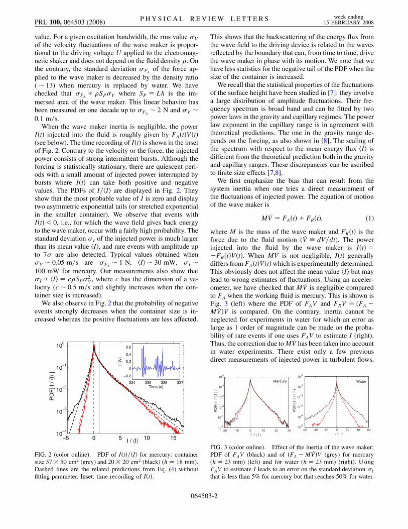
value. For a given excitation bandwidth, the rms value Vof the velocity fluctuations of the wave maker is propor-tional to the driving voltage U applied to the electromag-netic shaker and does not depend on the fluid density . Onthe contrary, the standard deviation FA of the force ap-plied to the wave maker is decreased by the density ratio( 13) when mercury is replaced by water. We havechecked that FA / SPV where SP Lh is the im-mersed area of the wave maker. This linear behavior hasbeen measured on one decade up to FA 2 N and V 0:1 m=s.
When the wave maker inertia is negligible, the powerIt injected into the fluid is roughly given by FAtVt(see below). The time recording of It is shown in the insetof Fig. 2. Contrary to the velocity or the force, the injectedpower consists of strong intermittent bursts. Although theforcing is statistically stationary, there are quiescent peri-ods with a small amount of injected power interrupted bybursts where It can take both positive and negativevalues. The PDFs of I=hIi are displayed in Fig. 2. Theyshow that the most probable value of I is zero and displaytwo asymmetric exponential tails (or stretched exponentialin the smaller container). We observe that events withIt< 0, i.e., for which the wave field gives back energyto the wave maker, occur with a fairly high probability. Thestandard deviation I of the injected power is much largerthan its mean value hIi, and rare events with amplitude upto 7 are also detected. Typical values obtained whenV 0:05 m=s are FA 1 N, hIi 30 mW, I 100 mW for mercury. Our measurements also show thatI / hIi cSP2
V , where c has the dimension of a ve-locity (c 0:5 m=s and slightly increases when the con-tainer size is increased).
We also observe in Fig. 2 that the probability of negativeevents strongly decreases when the container size is in-creased whereas the positive fluctuations are less affected.
This shows that the backscattering of the energy flux fromthe wave field to the driving device is related to the wavesreflected by the boundary that can, from time to time, drivethe wave maker in phase with its motion. We note that wehave less statistics for the negative tail of the PDF when thesize of the container is increased.
We recall that the statistical properties of the fluctuationsof the surface height have been studied in [7]: they involvea large distribution of amplitude fluctuations. Their fre-quency spectrum is broad band and can be fitted by twopower laws in the gravity and capillary regimes. The powerlaw exponent in the capillary range is in agreement withtheoretical predictions. The one in the gravity range de-pends on the forcing, as also shown in [8]. The scaling ofthe spectrum with respect to the mean energy flux hIi isdifferent from the theoretical prediction both in the gravityand capillary ranges. These discrepancies can be ascribedto finite size effects [7,8].
We first emphasize the bias that can result from thesystem inertia when one tries a direct measurement ofthe fluctuations of injected power. The equation of motionof the wave maker is
M _V FAt FRt; (1)
where M is the mass of the wave maker and FRt is theforce due to the fluid motion ( _V dV=dt). The powerinjected into the fluid by the wave maker is It FRtVt. When M _V is not negligible, It generallydiffers fromFAtVtwhich is experimentally determined.This obviously does not affect the mean value hIi but maylead to wrong estimates of fluctuations. Using an acceler-ometer, we have checked that M _V is negligible comparedto FA when the working fluid is mercury. This is shown isFig. 3 (left) where the PDF of FAV and FRV FA M _VV is compared. On the contrary, inertia cannot beneglected for experiments in water for which an error aslarge as 1 order of magnitude can be made on the proba-bility of rare events if one uses FAV to estimate I (right).Thus, the correction due toM _V has been taken into accountin water experiments. There exist only a few previousdirect measurements of injected power in turbulent flows,
−5 0 5 10 1510
−4
10−3
10−2
10−1
100
I / ⟨I⟩
PD
F[ I
/ ⟨I⟩
]
334 335 336 337
−0.2
0
0.2
0.4
0.6
Time (s)
I (W
)
FIG. 2 (color online). PDF of It=hIi for mercury: containersize 57 50 cm2 (grey) and 20 20 cm2 (black) (h 18 mm).Dashed lines are the related predictions from Eq. (4) withoutfitting parameter. Inset: time recording of It.
-20 -10 0 10 20 3010
-5
10 -4
10-3
10-2
10-1
100
I / ⟨ I ⟩
PD
F(
I / ⟨
I ⟩ )
Mercury
-60 -40 -20 0 20 40 6010
-5
10 -4
10 -3
10 -2
10 -1
100
I / ⟨ I ⟩
PD
F(
I / ⟨
I ⟩ )
Water
FIG. 3 (color online). Effect of the inertia of the wave maker:PDF of FAV (black) and of FA M _VV (grey) for mercury(h 23 mm) (left) and for water (h 23 mm) (right). UsingFAV to estimate I leads to an error on the standard deviation Ithat is less than 5% for mercury but that reaches 50% for water.
PRL 100, 064503 (2008) P H Y S I C A L R E V I E W L E T T E R S week ending15 FEBRUARY 2008
064503-2

and those type of inertial bias have never been taken intoaccount [9].
The PDFs of injected power for the same driving in thesame container for water and mercury are displayed inFig. 4. The asymmetry of the PDF is much larger withmercury. This is related to its larger mean energy flux, i.e.,mean dissipation, as shown below.
The qualitative features of the PDF of injected powercan be described with the following simple model. Guidedby our experimental observation of the linearity of FA inV , we assume that the force FR due to the fluid can beroughly approximated by a friction force MV where is a constant (the inverse of the damping time of the wavemaker). We are aware that a better approximation to theforce due to the fluid should involve both _V and an integralof Vt0 with an appropriate kernel. Thus, we only claimhere to give a heuristic understanding of the qualitativeproperties of the PDF of I. Modelling the forcing with anOrnstein-Uhlenbeck process, we obtain
_V V F; _F F ; (2)
where is the inverse of the correlation time of the appliedforce (F FA=M), and is a Gaussian white noise withhtt0i Dt t0. The PDF PV; F is the bivariatenormal distribution [10,11]
PV; F exp 1
21r2V
2
2V 2rVF
VF F2
2F
2VF1 r2p ; (3)
with F D=2
p, V
D=2
p, and r
= p
. Changing variables (V, F) to (~I FV I=M, F) and integrating over F gives
P~I exp r~I
1r2VF
VF1 r2p K0
j~Ij
1 r2VF
; (4)
where K0X is the zeroth order modified Bessel functionof the second kind. Using the method of steepest descent,this predicts exponential tails, PX 1=
jXj
p exprX
jXj, where X ~I=1 r2VF. In addition, we have
h~Ii D=2 rVF. Thus, (4) is determinedonce hIi, V , and F have been measured and can becompared to the experimental PDF without using anyfitting parameter. This is displayed with dashed lines inFig. 2. Taking into account the strong approximation madein the above model, we observe a good agreement in thelarger container. More importantly, this model captures thequalitative features of the PDF: its maximum for I 0 andthe asymmetry of the tails that is governed by the parame-ter r
=
p hIi=VFA. For given V and
FA , the larger is the mean energy flux, i.e., the dissipation,the more asymmetric is the PDF. For mercury, directdetermination of r from the measurement of hIi, V , andFA gives r 0:7 for the large container and r 0:6 forthe small one, in qualitative agreement with the differentasymmetry of the PDF in Fig. 2. Smaller values of r areachieved in water for which the dissipation is smaller. ThePDFs are more stretched for water, in particular, in thesmaller container.
We now consider the injected power averaged on a timeinterval
It 1
Z t
tIt0dt0: (5)
The PDFs of I for =c 1, 3, 11, and 50, where c is thecorrelation time of It, are displayed in Fig. 5. Theybecome more and more peaked around I ’ hIi as theyshould. However, one needs to average on a rather largetime interval ( 50c) in order to get a maximum proba-bility PI for I hIi (Fig. 5, bottom right). Then, theprobability of negative events become so small that almostnone can be observed. Figure 6 shows that the quantity, 1
log PI=hIiPI=hIi
, for different values of that has been pre-dicted to be linear in I=hIi when the hypothesis of the
−10 −5 0 5 1010
−4
10−3
10−2
10−1
100
Fluid effect
I / σ I
PD
F(
I / σ
I )
FIG. 4 (color online). Effect of fluid properties on the PDF ofthe injected power: (gray) mercury; (black): water (h 18 mm;20 20 cm2 container). Solid lines indicate the value of hIi=I .
−20 −10 0 10 2010
−4
10−3
10−2
10−1
100
τ / τc=1
I τ / ⟨ I ⟩
PD
F(
I τ /
⟨ I ⟩
)
−10 −5 0 5 10 1510
−4
10−3
10−2
10−1
100
I τ / ⟨ I ⟩
PD
F(
I τ /
⟨ I ⟩
) τ / τc=3
−2 0 2 410
−3
10−2
10−1
100
I τ / ⟨ I ⟩
PD
F(
I τ /
⟨ I ⟩
) τ / τc=11
0 0.5 1 1.5 2 2.510
−3
10−2
10−1
100
I τ / ⟨ I ⟩
PD
F(
I τ /
⟨ I ⟩
) τ / τc=50
FIG. 5 (color online). PDFs of the injected power I averagedon a time interval : 1, 3, 11, and 50c, where c 0:03 s isthe correlation time of It. Solid lines indicate the value of hIi(water, h 23 mm).
PRL 100, 064503 (2008) P H Y S I C A L R E V I E W L E T T E R S week ending15 FEBRUARY 2008
064503-3

fluctuation theorem (in particular time reversibility) arefulfilled [12,13]. As we clearly observe in Fig. 6, this isnot the case in general for dissipative systems. As alreadymentioned [4] and studied in details [14], the linear behav-ior reported in several experiments or numerical simula-tions results from the too small values of I=hIi that areprobed when c. Large enough values are obtained inthe present experiment, and the expected nonlinear behav-ior is thus reached. The shape of the curve in Fig. 6 is foundin good agreement with the analytical calculation [15]performed with a Langevin-type equation with white noise.
Finally, we emphasize that a fluctuating injected powerimplies fluctuations of the energy flux at all wave numbersin the energy cascade from injection to dissipation. In anysystem where an energy flux cascades from the injectedpower at large scales to dissipation at small scales, one hasfor the energy E< for wave numbers smaller than k withinthe inertial range, _E< It k; t R, where k; tis the energy flux at k toward large wave numbers. Thus,R10 hRR0id 0 in order to prevent the divergence ofhE2
<i. Dimensionally, this implies that 2k does not
depend on k [5], where is the standard deviation ofthe energy flux and k is its correlation time. If thisdimensional scaling is correct, fluctuations of the energyflux are expected to increase during the cascade from largeto small scales since k decreases (for instance, / k
1=3
for hydrodynamic turbulence). Such fluctuations have been
found numerically and experimentally in hydrodynamicturbulence [16]. To which extent, this is related or modifiedby small scale intermittency [17] remains an openquestion.
We acknowledge useful discussions with F. Petrelis.This work has been supported by ANR turbondeNo. BLAN07-3-197846 and by the CNES.
[1] A. N. Kolmogorov, Dokl. Akad. Nauk SSSR 30, 299(1941); reprinted in Proc. R. Soc. Lond. A 434, 15 (1991).
[2] C. Connaughton, S. Nazarenko, and A. C. Newell, PhysicaD (Amsterdam) 184, 86 (2003); V. Zakharov, F. Dias, andA. Pushkarev, Phys. Rep. 398, 1 (2004).
[3] S. Ciliberto, S. Douady, and S. Fauve, Europhys. Lett. 15,23 (1991); S. Aumaıtre, S. Fauve, and J. F. Pinton, Eur.Phys. J. B 16, 563 (2000); S. Aumaıtre and S. Fauve,Europhys. Lett. 62, 822 (2003).
[4] S. Aumaıtre, S. Fauve, S. McNamara, and P. Poggi, Eur.Phys. J. B 19, 449 (2001).
[5] S. Aumaıtre, J. Farago, S. Fauve, and S. McNamara, Eur.Phys. J. B 42, 255 (2004).
[6] A. N. Kolmogorov, J. Fluid Mech. 13, 82 (1962).[7] E. Falcon, C. Laroche, and S. Fauve, Phys. Rev. Lett. 98,
094503 (2007).[8] P. Denissenko, S. Lukaschuk, and S. Nazarenko, Phys.
Rev. Lett. 99, 014501 (2007).[9] R. Labbe, J. F. Pinton, and S. Fauve, J. Phys. II (France) 6,
1099 (1996); J. F. Pinton, P. C. W. Holdsworth, and R.Labbe, Phys. Rev. E 60, R2452 (1999); J. H. Titon andO. Cadot, Phys. Fluids 15, 625 (2003).
[10] See for instance, H. Risken, The Fokker-Planck Equation(Springer-Verlag, Berlin, 1996).
[11] Describing the PDF of the injected power using twocorrelated normal variables has also been proposedindependently by M. Bandi and C. Connaughton,arXiv:0710.1133.
[12] D. J. Evans, E. G. D. Cohen, and G. P. Morriss, Phys. Rev.Lett. 71, 2401 (1993); G. Gallavotti and E. G. D. Cohen,Phys. Rev. Lett. 74, 2694 (1995).
[13] J. Kurchan, J. Phys. A 31, 3719 (1998).[14] A. Puglisi et al., Phys. Rev. Lett. 95, 110202 (2005);
P. Visco et al., Europhys. Lett. 72, 55 (2005).[15] J. Farago, J. Stat. Phys. 107, 781 (2002); Physica A
(Amsterdam) 331, 69 (2004).[16] S. Cerutti and C. Meneveau, Phys. Fluids 10, 928 (1998);
B. Tao, J. Katz, and C. Meneveau, J. Fluid Mech. 457, 35(2002).
[17] E. Falcon, S. Fauve, and C. Laroche, Phys. Rev. Lett. 98,154501 (2007).
0 0.5 1 1.50
5
10
15
20
I τ / ⟨ I ⟩
log[
P(I
τ /
⟨ I ⟩)
/ P
(−I τ
/ ⟨ I
⟩) ]
/ τ
FIG. 6 (color online). Plot of 1 log PI=hIi
PI=hIifor 16< =c < 39
[=c 17 (*), 19.5 ( ), 22 (), 25 (), 28 (pentagram), 30.5(5), 33.5 (hexagram), 39 ()]. Langevin model of Ref. [15]: 4for I=hIi 1=3 (dashed line) and 7=4 3=2=4 for 1=3 (solid line) with 5 Hz.
PRL 100, 064503 (2008) P H Y S I C A L R E V I E W L E T T E R S week ending15 FEBRUARY 2008
064503-4

Capillary wave turbulence on a spherical fluid surface in zero gravity
C. Falcon,1 E. Falcon,2, ∗ U. Bortolozzo,1,2 and S. Fauve1
1Laboratoire de Physique Statistique, Ecole Normale Superieure,CNRS (UMR 8550) – 24, rue Lhomond, 75 005 Paris, France
2Laboratoire Matiere et Systemes Complexes (MSC), Universite Paris Diderot,CNRS (UMR 7057) – 10 rue A. Domon & L. Duquet, 75 013 Paris, France
(Dated: July 18, 2008)
We report the observation of capillary wave turbulence on the surface of a fluid layer in low gravityenvironment. In such conditions, the fluid covers all the internal surface of the spherical containerwhich is submitted to random forcing. The surface wave amplitude displays power-law spectrumover two decades in frequency, corresponding to wavelength from mm to a few cm. This spectrumis found in roughly good agreement with the wave turbulence theory. Such a large scale observationwithout gravity waves has never been reached during ground experiments. When the forcing isperiodic, two-dimensional spherical patterns are observed on the fluid surface such as subharmonicstripes or hexagons with wavelength satisfying the capillary wave dispersion relation.
PACS numbers: 47.35.Pq, 47.52.+j, 47.54.r, 81.70.Ha
Wave turbulence concerns the study of the dynami-cal and statistical properties of an ensemble of dispersivewaves with nonlinear interactions. Wave turbulence oc-curs at very different scales in a great variety of systems:surface or internal waves in oceanography [1, 2], Alfvenwaves in solar wind [3], plasmas [4], surface waves onelastic plates [5], spin waves in solids. Surprisingly, onlya few groups have performed laboratory experiments onthis subject so far, mainly focusing on wave turbulenceon fluid surface [6–10]. These wave turbulence experi-ments are scarce compared to numerous studies in hydro-dynamic turbulence, although various analytical resultshave been obtained in the framework of wave turbulenceor “weak turbulence” theory [11].
Gravity and capillary turbulent wave regimes on a fluidsurface are characterized by different Kolmogorov typespectra [10]. These two regimes influence each other andcoexist at different scales in the same experiment. Sinceenergy tranfers in capillary and gravity regimes are notgoverned by similar nonlinear processes, it is of primaryinterest to study a pure capillary wave regime. The im-portance of the gravity and the capillary effects is quan-tified by the ratio between the wavelength of the surfacewave, λ, and the capillary length, lc ≡
√γ/(ρg), where γ
and ρ are the surface tension and the density of the fluid,respectively, and g is the acceleration of gravity. Forusual fluids, lc is of the order of few mm, correspond-ing to a critical wavelength λc = 2πlc of the order of 1cm. Gravity waves are thus proeminent for wavelengthlarger than few cm. The capillary length cannot be sig-nificantly changed using other interfaces between simplefluids and air. It is in an intermediate range betweenthe size of the experiment and the dissipative length. Inusual laboratory-scale experiments, this limits both thegravity and capillary regimes to less than a decade infrequency. In a low gravity experiment, one can obtaincapillary waves at all wavelengths of the fluid container
of size L, provided that λc > L. We emphasize thatincreasing the capillary range toward large frequenciesusing better resolved measurements in ground experi-ments, without suppressing the development of gravitywaves, is not satisfactory. Gravity and capillary wavesindeed interact because the energy flux cascades amongthe different scales. In addition, it is predicted that weakturbulence for capillary waves breaks down at large scale,because the nonlinear time scale becomes comparable tothe linear one [12]. It is thus of interest to remove gravitywaves that may hide this phenomenon.
Here, we report the observation of the power spectrumdensity of the capillary wave turbulence regime over alarge range of wavelengths in zero gravity. The invariant-scale power spectrum is found in roughly good agreementwith weak turbulence theory. We also study parametricexcitation of a fluid in zero gravity by sinusoidally forcingits container. Although the so-called “Faraday instabil-ity” has been extensively studied with gravity [13–15],only one trial has been performed without gravity nearthe critical point [16]. We report here the first experi-mental observation of two-dimensional wave patterns ona spherical or cylindrical fluid surface in zero gravity. Ap-plications of this work could be extended to the latticewrapping on the curved surfaces as well as in condensedmatter such as in spherical crystallography [17]. In ad-dition, pattern formation in spherical geometry for ax-isymmetric systems is of obvious interest in the contextof geophysical and astrophysical fluid dynamics [18].
The experimental setup is sketched in Fig. 1. A con-tainer partially filled with a fluid is put down on a rail,and is submitted to vibrations by means of an elec-tromagnetic exciter (BK 4803) via a power amplifier(BK 2706). To study wave turbulence, the container isdriven with a random forcing, supplied by the source of adynamical analyzer (Agilent 35 670A), and low-pass fil-tered in the frequency range 0 - 6 Hz. This corresponds
Typeset by REVTEX

2
FIG. 1: Sketch of the experimental setup. In microgravityphases, the fluid covers all the internal surface of the containersubmitted to vibrations.
to wavelengths of surface waves larger than 1 cm in zerogravity. To study wave patterns, the container is drivenwith a sinusoidal forcing at frequency f0 in the range10 ≤ f0 ≤ 70 Hz, and amplitude d0 ∼ mm correspondingto a container acceleration 0.1 . a0 . 30g. The con-tainer geometry is either spherical (15 cm in diameter)or cylindrical (15 cm in diameter, 18 cm in length). Eachcontainer is made of a wetting material (Plexiglas cylin-der or glass sphere) to avoid that the fluid loses contactwith the internal wall of the container during the micro-gravity phases. According to its geometry, the containeris filled with 20 or 30 cl of fluid. This corresponds to anuniform fluid layer of roughly 5 mm depth covering allthe internal surface of the container during the micro-gravity phases. The fluid is either ethanol or water. Thelocal displacement of the fluid is measured with a capac-itive wire gauge, 0.1 mm in diameter, plunging into thefluid [10]. This sensor allows wave height measurementsfrom 10 µm up to 2 cm with a 0.1 ms response time. Apiezoelectric accelerometer (PCB) is screwed on the con-tainer to record its acceleration. A dynamical analyzeris used to record the power spectrum of the surface waveamplitude during each microgravity phase. The motionof the fluid surface is visualized with a Nikon camera andrecorded with a Sony video camera. Microgravity envi-ronment (about ±5 × 10⁻²g) is repetitively achieved byflying with the specially modified Airbus A300 Zero-Gaircraft through a series of parabolic trajectories whichresult in zero-gravity periods, each of 22 s. We observethat the fluid crawls up the sides of the container and cov-ers all the internal surface of the tank due to the capillaryforces. This takes roughly 1 s. Measurements have thusbeen recorded only on 18 s to eliminate these transients.Contrary to the common sense, no formation of a singlesphere of fluid is observed in the middle of the tank, dueto these capillary effects. An homogeneous fluid layer isformed on the internal surface of the tank, confining airin its center. When the container is submitted to a si-nusoidal forcing at frequency f0, surface wave patterns
FIG. 2: Two-dimensional cylindrical subharmonic wave pat-terns (hexagons) under a sinusoidal forcing at frequency f0 =30 Hz, and amplitude d0 = 0.29 mm leading to a 1.06g accel-eration. Cylindrical container filled with 30 cl of ethanol.
FIG. 3: Two-dimensional spherical subharmonic wave pat-terns under sinusoidal forcing at frequency f0 = 30 Hz, andamplitude d0 = 0.32 mm leading to a 1.16g acceleration.Spherical container filled with 20 cl of water.
appear as shown in Fig. 2 with a cylindrical container.These two-dimensional patterns are either stripes (notshown here) or hexagons (see Fig. 2) depending on thevibrating frequency. By using another container geome-try, one can also observe spherical patterns as shown inFig. 3.
To understand the mechanism of pattern formation,one records simultaneously the acceleration imposed tothe container, and the surface wave height as a function oftime. A typical power spectrum density of the containeracceleration is shown in the inset of Fig. 4. The mainpeak at f0 = 30 Hz corresponds to the driving frequency.The typical response of the fluid surface to this excita-tion is displayed in Fig. 4. The power spectrum of surfacewaves shows two main peaks: a subharmonic one closeto f0/2 ≃ 15 Hz, and a smaller one at f0 correspondingto a reminiscence of the driving frequency. The two-dimensional patterns are thus subharmonic ones. The
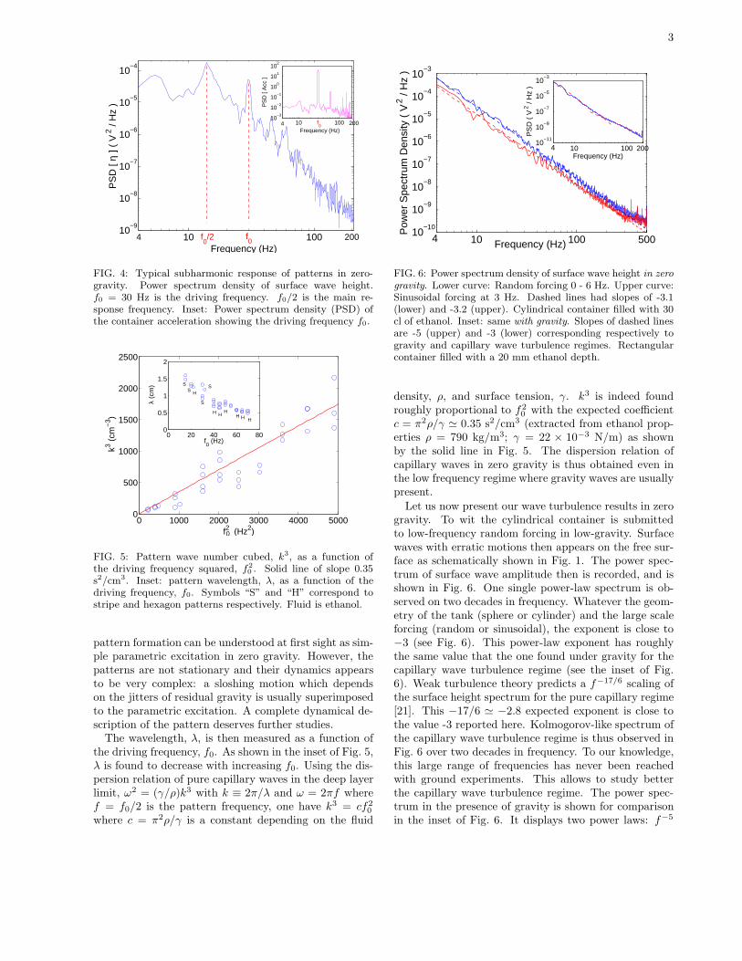
3
10 10010
−9
10−8
10−7
10−6
10−5
10−4
Frequency (Hz)
PS
D [
η ] (
V 2
/ H
z )
10 10010
−3
10−2
10−1
100
101
102
Frequency (Hz)
PS
D [
Acc
]
4 200 f0 f
0/2
4 200 f0
FIG. 4: Typical subharmonic response of patterns in zero-gravity. Power spectrum density of surface wave height.f0 = 30 Hz is the driving frequency. f0/2 is the main re-sponse frequency. Inset: Power spectrum density (PSD) ofthe container acceleration showing the driving frequency f0.
0 1000 2000 3000 4000 50000
500
1000
1500
2000
2500
f2 (Hz2)
k3 (
cm−
3 )
SS
S
0 20 40 60 800
0.5
1
1.5
2
f0 (Hz)
λ (
cm)
H HH
H
H H
S
S
SS
H
0
FIG. 5: Pattern wave number cubed, k3, as a function ofthe driving frequency squared, f2
0 . Solid line of slope 0.35s2/cm3. Inset: pattern wavelength, λ, as a function of thedriving frequency, f0. Symbols “S” and “H” correspond tostripe and hexagon patterns respectively. Fluid is ethanol.
pattern formation can be understood at first sight as sim-ple parametric excitation in zero gravity. However, thepatterns are not stationary and their dynamics appearsto be very complex: a sloshing motion which dependson the jitters of residual gravity is usually superimposedto the parametric excitation. A complete dynamical de-scription of the pattern deserves further studies.
The wavelength, λ, is then measured as a function ofthe driving frequency, f0. As shown in the inset of Fig. 5,λ is found to decrease with increasing f0. Using the dis-persion relation of pure capillary waves in the deep layerlimit, ω2 = (γ/ρ)k3 with k ≡ 2π/λ and ω = 2πf wheref = f0/2 is the pattern frequency, one have k3 = cf2
0
where c = π2ρ/γ is a constant depending on the fluid
10 100 50010
−10
10−9
10−8
10−7
10−6
10−5
10−4
10−3
Frequency (Hz)
Pow
er S
pect
rum
Den
sity
( V
2 /
Hz
)
10 100 20010
−11
10−9
10−7
10−5
10−3
Frequency (Hz)
PS
D (
V 2
/ H
z )
4
4
FIG. 6: Power spectrum density of surface wave height in zerogravity. Lower curve: Random forcing 0 - 6 Hz. Upper curve:Sinusoidal forcing at 3 Hz. Dashed lines had slopes of -3.1(lower) and -3.2 (upper). Cylindrical container filled with 30cl of ethanol. Inset: same with gravity. Slopes of dashed linesare -5 (upper) and -3 (lower) corresponding respectively togravity and capillary wave turbulence regimes. Rectangularcontainer filled with a 20 mm ethanol depth.
density, ρ, and surface tension, γ. k3 is indeed foundroughly proportional to f2
0 with the expected coefficientc = π2ρ/γ ≃ 0.35 s2/cm3 (extracted from ethanol prop-erties ρ = 790 kg/m3; γ = 22 × 10−3 N/m) as shownby the solid line in Fig. 5. The dispersion relation ofcapillary waves in zero gravity is thus obtained even inthe low frequency regime where gravity waves are usuallypresent.
Let us now present our wave turbulence results in zerogravity. To wit the cylindrical container is submittedto low-frequency random forcing in low-gravity. Surfacewaves with erratic motions then appears on the free sur-face as schematically shown in Fig. 1. The power spec-trum of surface wave amplitude then is recorded, and isshown in Fig. 6. One single power-law spectrum is ob-served on two decades in frequency. Whatever the geom-etry of the tank (sphere or cylinder) and the large scaleforcing (random or sinusoidal), the exponent is close to−3 (see Fig. 6). This power-law exponent has roughlythe same value that the one found under gravity for thecapillary wave turbulence regime (see the inset of Fig.6). Weak turbulence theory predicts a f−17/6 scaling ofthe surface height spectrum for the pure capillary regime[21]. This −17/6 ≃ −2.8 expected exponent is close tothe value -3 reported here. Kolmogorov-like spectrum ofthe capillary wave turbulence regime is thus observed inFig. 6 over two decades in frequency. To our knowledge,this large range of frequencies has never been reachedwith ground experiments. This allows to study betterthe capillary wave turbulence regime. The power spec-trum in the presence of gravity is shown for comparisonin the inset of Fig. 6. It displays two power laws: f−5
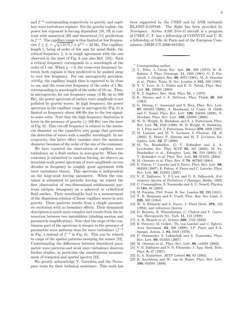
4
and f−3 corresponding respectively to gravity and capil-lary wave turbulence regimes. For the gravity regime, thepower law exponent is forcing dependent [10, 19] in con-trast with numerical [20] and theoretical [11] predictionsin f−4. The capillary range is thus limited at low frequen-cies f ≤ fc =
√g/(2π2lc) ∝ g3/4 ∼ 20 Hz. The capillary
length lc being of order of few mm for usual fluids, thecritical frequency fc is in rough agreement with the oneobserved in the inset of Fig. 6 (see also Ref. [10]). Sucha critical frequency corresponds to a wavelength of theorder of 1 cm. When g → 0, the cross-over frequency be-tween both regimes is then predicted to be pushed awayto very low frequency. For our microgravity precision,±0.05g, the capillary length then is expected to be closeto cm, and the cross-over frequency of the order of 1 Hz,corresponding to wavelength of the order of 10 cm. Thus,in microgravity, for our frequency range (4 Hz up to 500Hz), the power spectrum of surface wave amplitude is notpolluted by gravity waves. At high frequency, the powerspectrum in the capillary range in microgravity (Fig. 6) islimited at frequency about 400 Hz due to the low signal-to-noise ratio. Note that the high frequency limitation islower in the presence of gravity (≥ 100 Hz) (see the insetof Fig. 6). This cut-off frequency is related to the menis-cus diameter on the capacitive wire gauge that preventsthe detection of waves with a smaller wavelength. In mi-crogravity, this latter effect vanishes since the meniscusdiameter becomes of the order of the size of the container.
We have reported the observation of capillary waveturbulence on a fluid surface in zero-gravity. When thecontainer is submitted to random forcing, we observe aninvariant-scale power spectrum of wave amplitude on twodecades in frequency in roughly good agreement withwave turbulence theory. This spectrum is independenton the large-scale forcing parameter. When the con-tainer is submitted to periodic forcing, we report thefirst observation of two-dimensional subharmonic pat-terns (stripes, hexagons) on a spherical or cylindricalfluid surface. Their wavelengths lead to a measurementof the dispersion relation of linear capillary waves in zerogravity. These patterns results from a simple paramet-ric excitation with no boundary effects. Their dynamicaldescription is much more complex and results from the in-teraction between two instabilities (sloshing motion andparametric amplification). Note that the slope of the con-tinuous part of the spectrum is steeper in the presence ofparametric wave patterns than for wave turbulence (f−4
in Fig. 4 instead of f−3 in Fig. 6). This can be relatedto cusps of the spatial patterns sweeping the sensor [22].Understanding the differences between disordered para-metric wave patterns and weak wave turbulence deservesfurther studies, in particular the simultaneous measure-ment of temporal and spatial spectra [23].
We greatly acknowledge Y. Garrabos and the Noves-pace team for their technical assistance. This work has
been supported by the CNES and by ANR turbondeBLAN07-3-197846. The flight has been provided byNovespace. Airbus A300 Zero-G aircraft is a programof CNES. C. F. has a fellowship of CONYCIT and U. B.a fellowship of Ville de Paris and of the European Com-mission (MEIF-CT-2006-041594).
∗ Corresponding author[1] Y. Toba, J. Ocean Soc. Jpn. 29, 209 (1973); K. K.
Kahma, J. Phys. Oceanogr. 11, 1503 (1981); G. Z. For-ristall, J. Geophys. Res. 86, 8075 (1981); M. A. Donelanet al., Philos. Trans. R. Soc. London A 315, 509 (1985)
[2] Y. V. Lvov, K. L. Polzin and E. G. Tabak, Phys. Rev.Lett. 92, 128501 (2004)
[3] R. Z. Sagdeev, Rev. Mod. Phys. 51, 1 (1979)[4] K. Mizuno and J. S. DeGroot, Phys. Fluids 26, 608
(1983)[5] G. During, C. Josserand and S. Rica, Phys. Rev. Lett.
97, 025503 (2006), A. Boudaoud, O. Cadot, B. Odilleand C. Touze, Phys. Rev. Lett. 100, 234504 (2008), N.Mordant, Phys. Rev. Lett. 100, 234505 (2008).
[6] W. B. Wright, R. Budakian and S. J. Putterman, Phys.Rev. Lett. 76, 4528 (1996); W. B. Wright, R. Budakian,D. J. Pine and S. J. Putterman, Science 278, 1609 (1997)
[7] M. Lommer and M. T. Levinsen J. Fluoresc. 12, 45(2002); E. Henry, P. Alstrøm and M. T. Levinsen, Eu-rophys. Lett. 52, 27 (2000)
[8] M. Yu. Brazhnikov, G. V. Kolmakov and A. A.Levchenko, Sov. Phys JETP 95, 447 (2002); M. Yu.Brazhnikov et al., Europhys. Lett. 58, 510 (2002); G.V. Kolmakov et al. Phys. Rev. Lett. 93, 074501 (2004)
[9] M. Onorato et al. Phys. Rev. E 70, 067302 (2004)[10] E. Falcon, C. Laroche and S. Fauve, Phys. Rev. Lett. 98,
094503 (2007); E. Falcon, S. Fauve and C. Laroche, Phys.Rev. Lett. 98, 154501 (2007)
[11] V. E. Zakharov, V. S L’vov and G. E. Falkovitch, Kol-mogorov Spectra of Turbulence I (Springer, Berlin, 1992)
[12] C. Connaughton, S. Nazarenko and A. C. Newell, PhysicaD 184, 86 (2003)
[13] M. Faraday, Phil. Trans. R. Soc. London 52, 299 (1831).[14] T. B. Benjamin and F. Ursell, Proc. Roy. Soc Lond. A
225, 505 (1954).[15] W. S. Edwards and S. Fauve, J. Fluid Mech. 278, 123
(1994), and references therein.[16] D. Beysens, R. Wunenburger, C. Chabot and Y. Garra-
bos, Microgravity Sci. Tech. 11, 113 (1998)[17] A. R. Bausch et al., Science 299, 1716 (2003)[18] B. Futterer, M. Gellert, Th. von Larcher and C. Egbers,
Acta Astronaut. 62, 300 (2008); J.P. Poyet and E.A.Spiegel, Astron. J. 84, 1918 (1979).
[19] P. Denissenko, S. Lukaschuk and S. Nazarenko, Phys.Rev. Lett. 99, 014501 (2007)
[20] M. Onorato et al., Phys. Rev. Lett. 89, 144501 (2002)[21] V. E. Zakharov and N. N. Filonenko, J. App. Mech. Tech.
Phys. 8, 37 (1967).[22] E. A. Kuznetsov, JETP Letters 80, 83 (2004).[23] R. Savelsberg and W. van de Water, Phys. Rev. Lett.
100, 034501 (2008)

Wave Turbulence on the Surface of a Ferrofluid in a Magnetic Field
Francois Boyer and Eric Falcon*
Laboratoire Matiere et Systemes Complexes (MSC), Universite Paris Diderot, CNRS (UMR 7057)10 rue A. Domon & L. Duquet, 75 013 Paris, France
(Received 1 October 2008; published 11 December 2008)
We report the observation of wave turbulence on the surface of a ferrofluid mechanically forced and
submitted to a static normal magnetic field. We show that magnetic surface waves arise only above a
critical field. The power spectrum of their amplitudes displays a frequency-power law leading to the
observation of a magnetic wave turbulence regime which is experimentally shown to involve a 4-wave
interaction process. The existence of the regimes of gravity, magnetic and capillary wave turbulence is
reported in the phase space parameters as well as a triple point of coexistence of these three regimes. Most
of these features are understood using dimensional analysis or the dispersion relation of the ferrohy-
drodynamic surface waves.
DOI: 10.1103/PhysRevLett.101.244502 PACS numbers: 47.35.Tv, 47.27.i, 47.65.Cb
Wave turbulence is an out-of-equilibrium state wherewaves interact with each other nonlinearly throughN-waveresonance process. The archetype of wave turbulence is therandom state of ocean surface waves, but it appears invarious systems: capillary waves [1,2], plasma waves insolar winds, atmospheric waves, optical waves, and elasticwaves on thin plates [3]. Recent laboratory experiments ofwave turbulence have shown new observations such asintermittency [4], fluctuations of the energy flux [5], andfinite size effect of the system [2,6]. Some of these phe-nomena have recently been considered theoretically [7].Wave turbulence theory allows us to analytically derivestationary solutions for the wave energy spectrum as apower law of frequency or wave number [3]. The spectrumexponent and the number N of resonant waves depend onboth the wave dispersion relation and the dominant non-linear interaction. Several theoretical questions are open,notably about the validity domain of the theory [8], and thepossible existence of solutions for nondispersive systems[9]. In this context, finding an experimental system wherethe dispersion relation of the waves could be tuned by theoperator should be of primary interest to test the waveturbulence theory.
A ferrofluid is a suspension of nanometric ferromagneticparticles diluted in a liquid displaying striking properties:the Rosensweig instability [10], the labyrinthine instabil-ity, magnetic levitation [11]. In contrast with usual liquids,the dispersion relation of surface waves on a ferrofluiddisplays a minimum which depends on the amplitude ofthe applied magnetic field [12,13]. Thus, one can easilytune the dispersion relation of surface wave from a dis-persive to a nondispersive one with just one single controlparameter. To our knowledge, no experimental observationof wave turbulence on a magnetic fluid has been reported.Here, we study the wave turbulence on the surface of aferrofluid submitted to a normal magnetic field. We ob-serve for the first time a regime of magnetic wave turbu-
lence. We characterize this regime by measuring the powerspectrum and distribution of the magnetic wave amplitude.The experimental setup is shown in Fig. 1. It consists of
a cylindrical container, 12 cm in inner diameter and 4 cm indepth, filled with a ferrofluid up to a depth h ¼ 2 cm. Theferrofluid used is a ionic aqueous suspension synthesizedwith 8.5% by volume of maghemite particles (Fe2O3;7:6 0:36 nm in diameter) [14]. The properties of thismagnetic fluid are: density, ¼ 1324 kg=m3, surface ten-sion, ¼ 59 103 N=m, initial magnetic susceptibility,i ¼ 0:69, magnetic saturation Msat ¼ 16:9 103 A=m,and estimated dynamic viscosity 1:2 103 N s=m2. Thecontainer is placed between two horizontal coaxial coils,25 cm (respectively 50 cm) in inner (respectively in outer)diameter, 7 cm far apart. A dc current is supplied to thecoils in series by a power supply (50 V=35 A), the coilsbeing cooled with water circulation. The vertical magneticinduction generated is 99% homogeneous in the horizontalplane [12], and is up to 780 G. It is measured by a Hallprobe located in the center near the surface of the con-tainer. Surface waves are generated on the ferrofluid by thehorizontal motion of a rectangular plunging Teflon wavemaker driven by an electromagnetic vibration exciter. Thewave maker is driven with low-frequency random vibra-tions (typically from 1 to 5 Hz). The amplitude of thesurface waves ðtÞ at a given location is measured by a
FIG. 1 (color online). Experimental setup.
PRL 101, 244502 (2008) P HY S I CA L R EV I EW LE T T E R Sweek ending
12 DECEMBER 2008
0031-9007=08=101(24)=244502(4) 244502-1 2008 The American Physical Society
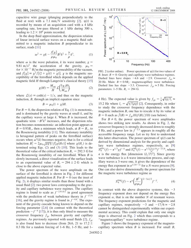
capacitive wire gauge (plunging perpendicularly to thefluid at rest) with a 7:1 mm=V sensitivity [2]. ðtÞ isrecorded by means of an acquisition card with a 4 kHzsampling rate, low-pass filtered at 1 kHz during 300 s,leading to 1:2 106 points recorded.
In the deep fluid approximation, the dispersion relationof linear inviscid surface waves on a magnetic fluid sub-mitted to a magnetic induction B perpendicular to itssurface, reads [11]
!2 ¼ gk f½0
B2k2 þ
k3; (1)
where ! is the wave pulsation, k its wave number, g ¼9:81 m=s2 the acceleration of the gravity, 0 ¼4 107 H=m the magnetic permeability of the vacuum,and f½ 2=½ð2þ Þð1þ Þ. is the magnetic sus-ceptibility of the ferrofluid which depends on the appliedmagnetic field H through Langevin’s classical theory [15]
ðHÞ ¼ Msat
HL3iH
Msat
; (2)
where LðxÞ cothðxÞ 1=x, and thus on the magneticinduction, B, through an implicit equation since
B ¼ 0ð1þ ÞH: (3)
For B ¼ 0, the dispersion relation of Eq. (1) is monotonic,and is dominated by the gravity waves at small k, and bythe capillary waves at large k. When B is increased, thequadratic term B2k2 increases, and the dispersion rela-tion becomes nonmonotonic: an inflection point appears atB ¼ 0:93Bc, then a minimum which leads, at B ¼ Bc, tothe Rosensweig instability [11]. This stationary instability(a hexagonal pattern of peaks on the ferrofluid surface)occurs when !2ðkÞ becomes negative, that is for a criticalinduction B2
c ¼ 20ffiffiffiffiffiffiffiffiffiffig
p=f½ðHcÞ where ðHcÞ is de-
termined using Eqs. (2) and (3) [10]. This leads to thetheoretical value of the critical induction Bc ¼ 292:3 G forthe Rosensweig instability of our ferrofluid. When B isslowly increased, a direct visualization of the surface leadsto an experimental value of Bc ¼ 294 2 G which isclose to the above expected value.
The power spectrum of the wave amplitude on thesurface of the ferrofluid is shown in Fig. 2 for differentapplied magnetic induction B. For B ¼ 0 (see the inset ofFig. 2), it displays similar results than those found with ausual fluid [2]: two power laws corresponding to the grav-ity and capillary turbulence wave regimes. The capillaryregime is found to scale as f2:90:1 in good agreement
with the prediction of weak turbulence theory in f17=6
[16], and the gravity regime is found in f4:6. The expo-nent of the gravity cascade being known to depend on theforcing parameter [2,6] (in contrast with the theoreticalprediction f4 [17]), it is thus only fitted to measure thecrossover frequency fgc between gravity and capillary
regimes. As previously reported with usual fluids [2], fgcis also found here to decrease (from 26.6, 21 to 17:20:3 Hz for a random forcing of 1–6 Hz, 1–5 Hz, and 1–
4 Hz). The expected value is given by fgc ¼ 1
ffiffiffiffiffiffiffiffiffiffiffiffi2g=lc
p ’15:2 Hz where lc ¼
ffiffiffiffiffiffiffiffiffiffiffiffiffiffiffiffi=ðgÞp
[2]. Consequently, in orderto study the crossover frequency dependence with themagnetic induction B, one has to rescale it by its value at
B ¼ 0 such as ~fðBÞ fgcð0ÞfðBÞ=fð0Þ (see below).For B 0, the power spectrum of wave amplitudes
shows two striking new results. As shown in Fig. 2, thecrossover frequency is strongly decreased down to roughly5 Hz, and a power law in f3:3 appears in roughly all theaccessible frequency range. Let us try first to understandthis latter observation. The power spectrum of ðtÞ can bederived by dimensional analysis for the gravity and capil-lary wave turbulence regimes, respectively, as [9]
Sgrav ðfÞ 1=3gf4 and S
cap ðfÞ 1=2ðÞ1=6f17=6, where
is the energy flux [dimension ðL=TÞ3]. Since gravitywave turbulence is a 4-wave interaction process, and cap-illary waves a 3-wave one, it gives the dependence of the
energy flux exponent in 1=ðN1Þ for a N-wave process [9].One can also derive dimensionally the power spectrum forthe magnetic wave turbulence regime as
Smag ðfÞ
B2
0
ð23Þ=2f3: (4)
In contrast with the above dispersive systems, this 3frequency exponent does not depend on the energy fluxexponent , that is on the number N of resonant waves.The frequency exponent predictions for the magnetic andcapillary regimes, respectively 3 and 17=6 ’ 2:8cannot be distinguished experimentally within our experi-mental accuracy. This could explain that only one singleslope is observed on Fig. 2 which thus corresponds to a‘‘magnetocapillary’’ wave turbulence regime.Figure 3 shows the frequency exponent of the magneto-
capillary spectrum when B is increased. For small B,
3 10 100 40010
−6
10−4
10−2
100
102
Frequency (Hz)
Pow
er s
pect
rum
of η
( m
m2 /
Hz
)
B = 0.9 Bc
3 10 100 40010
−6
10−4
10−2
100
102
Frequency (Hz)
PS
D η
( m
m2 /
Hz
)
B = 0
FIG. 2 (color online). Power spectrum of ðtÞ for two values ofB. Inset: B ¼ 0: Gravity and capillary wave turbulence regimes.Dashed lines have slopes 4:6 and 2:9. Crossover: fgc ’20 Hz. Main: B ¼ 0:9Bc: magnetocapillary wave turbulence.Dashed line has slope 3:3. Crossover: fgc ’ 5 Hz. Forcing
parameters: 1–5 Hz. Bc ¼ 294 G.
PRL 101, 244502 (2008) P HY S I CA L R EV I EW LE T T E R Sweek ending
12 DECEMBER 2008
244502-2
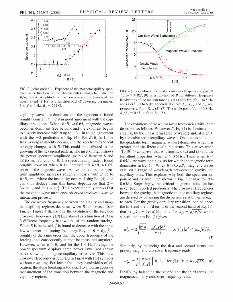
capillary waves are dominant and the exponent is foundroughly constant ’ 2:9 in good agreement with the cap-illary prediction. When B=Bc 0:65, magnetic wavesbecomes dominant (see below), and the exponent beginsto slightly increase with B up to 3:1 in rough agreementwith the 3 prediction of Eq. (4). For B=Bc 1, theRosensweig instability occurs, and the spectrum exponentstrongly changes with B. This could be attributed to thegrowing of the hexagonal pattern. The inset of Fig. 3 showsthe power spectrum amplitude (averaged between 8 and18 Hz) as a function of B. The spectrum amplitude is foundroughly constant when B is increased till B=Bc ’ 0:65,onset of the magnetic waves. Above this value, the spec-trum amplitude increases roughly linearly with B up toB=Bc ¼ 1 where the instability occurs. Using Eq. (4), onecan thus deduce from this linear dependence that 23 ¼ 1, and thus ¼ 1
3 . This experimentally shows that
the magnetic wave turbulence observed involves a 4-waveinteraction process.
The crossover frequency between the gravity and mag-netocapillary regimes decreases when B is increased (seeFig. 2). Figure 4 then shows the evolution of the rescaled
crossover frequency ~fðBÞ (see above) as a function of B for3 different frequency bandwidths of the random forcing.
When B is increased, ~f is found to decrease with the same
law whatever the forcing frequency. Beyond B ¼ Bc, ~f isroughly of the same order than the upper frequency of theforcing, and consequently cannot be measured anymore.However, when B> Bc and for the 1–6 Hz forcing, thepower spectrum displays three power laws (not shownhere) showing a magnetocapillary crossover. This newcrossover frequency is reported in Fig. 4 with () symbolswithout rescaling. For lower frequency bandwidths of vi-bration, the slope breaking is too small to allow an accuratemeasurement of the transition between the magnetic andcapillary regime.
The evolutions of these crossover frequencies with B aredescribed as follows. Whatever B, Eq. (1) is dominated, atsmall k, by the linear term (gravity waves) and, at high k,by the cubic term (capillary waves). One can assume thatthe quadratic term (magnetic waves) dominates when it isgreater than the linear and cubic terms. This arises whenf½B2 >0
ffiffiffiffiffiffiffiffiffiffig
p, that is, using Eqs. (2) and (3) and the
ferrofluid properties, when B> 0:65Bc. Thus, when B<0:65Bc, no wavelength exists for which the magnetic termdominates in Eq. (1). When B> 0:65Bc, magnetic wavesexist on a range of wavelength between the gravity andcapillary ones. This explains why both the spectrum ex-ponent and its amplitude shown in Fig. 3 change for B ’0:65Bc. Surprisingly, this critical magnetic induction hasnever been reported previously. The crossover frequenciesbetween the gravity, the magnetic and the capillary regimesare derived by balancing the dispersion relation terms eachto each. For the gravity-capillary transition, one balancesthe first and the third terms of the second hand of Eq. (1),
that is gkgc ¼ ð=Þk3gc, thus for kgc ¼ffiffiffiffiffiffiffiffiffiffiffiffig=
pwhich
substituted into Eq. (1) gives
!2gc ¼ 2
ffiffiffiffiffiffiffiffig3
s gf½B2
0; for f½B2 <0
ffiffiffiffiffiffiffiffiffiffig
p:
(5)
Similarly, by balancing the first and second terms, thegravity-magnetic crossover frequency reads
!2gm ¼
0g
f½3B6; for f½B2 >0
ffiffiffiffiffiffiffiffiffiffig
p: (6)
Finally, by balancing the second and the third terms, themagnetocapillary crossover frequency reads
0 0.5 1 1.52.8
2.9
3
3.1
3.2
3.3
3.4
0.62
Spe
ctru
m e
xpon
ent
B / Bc
0 0.2 0.4 0.6 0.8 1 1.20.01
0.015
0.02
0.025
0.03
0.035
0.04
0.65
Spe
ctru
m a
mpl
itude
( m
m2 /
Hz
)
B / Bc
FIG. 3 (color online). Exponent of the magnetocapillary spec-trum as a function of the dimensionless magnetic inductionB=Bc. Inset: Amplitude of the power spectrum (averaged be-tween 8 and 18 Hz) as a function of B=Bc. Forcing parameter:1 f 4 Hz. Bc ¼ 294 G.
0 0.5 1 1.5 2
5
10
15
20
25
Bt / B
c
ft
fgc
fgm
fmc
Capillary Wave Turbulence
Gravity Wave
Turbulence
Magnetic Wave Turbulence
Ros
ensw
eig
inst
abili
ty
B / Bc
Cro
ssov
er fr
eque
ncie
s (H
z)
FIG. 4 (color online). Rescaled crossover frequencies, ~fðBÞ fgcð0Þ fðBÞ=fð0Þ as a function of B for different frequency
bandwidths of the random forcing: () 1 to 4 Hz, (e) 1 to 5 Hz,and (+ or ) 1 to 6 Hz. Theoretical curves fgc, fgm, and fmc are,
respectively, from Eqs. (5)–(7). The triple point (ft ¼ 10:8 Hz,Bt=Bc ¼ 0:65) is from Eq. (8).
PRL 101, 244502 (2008) P HY S I CA L R EV I EW LE T T E R Sweek ending
12 DECEMBER 2008
244502-3
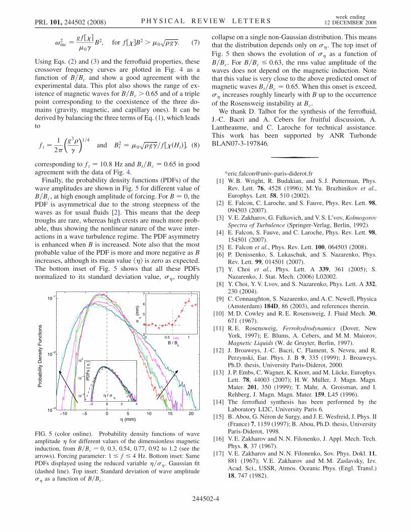
!2mc ¼ gf½
0B2; for f½B2 >0
ffiffiffiffiffiffiffiffiffiffig
p: (7)
Using Eqs. (2) and (3) and the ferrofluid properties, thesecrossover frequency curves are plotted in Fig. 4 as afunction of B=Bc and show a good agreement with theexperimental data. This plot also shows the range of ex-istence of magnetic waves for B=Bc > 0:65 and of a triplepoint corresponding to the coexistence of the three do-mains (gravity, magnetic, and capillary ones). It can bederived by balancing the three terms of Eq. (1), which leadsto
ft ¼ 1
2
g3
1=4
and B2t ¼ 0
ffiffiffiffiffiffiffiffiffiffig
p=f½ðHtÞ; (8)
corresponding to ft ¼ 10:8 Hz and Bt=Bc ¼ 0:65 in goodagreement with the data of Fig. 4.
Finally, the probability density functions (PDFs) of thewave amplitudes are shown in Fig. 5 for different value ofB=Bc, at high enough amplitude of forcing. For B ¼ 0, thePDF is asymmetrical due to the strong steepness of thewaves as for usual fluids [2]. This means that the deeptroughs are rare, whereas high crests are much more prob-able, thus showing the nonlinear nature of the wave inter-actions in a wave turbulence regime. The PDF asymmetryis enhanced when B is increased. Note also that the mostprobable value of the PDF is more and more negative as Bincreases, although its mean value hi is zero as expected.The bottom inset of Fig. 5 shows that all these PDFsnormalized to its standard deviation value, , roughly
collapse on a single non-Gaussian distribution. This meansthat the distribution depends only on . The top inset of
Fig. 5 then shows the evolution of as a function of
B=Bc. For B=Bc 0:63, the rms value amplitude of thewaves does not depend on the magnetic induction. Notethat this value is very close to the above predicted onset ofmagnetic waves Bt=Bc ¼ 0:65. When this onset is exceed, increases roughly linearly with B up to the occurrence
of the Rosensweig instability at Bc.We thank D. Talbot for the synthesis of the ferrofluid,
J.-C. Bacri and A. Cebers for fruitful discussion, A.Lantheaume, and C. Laroche for technical assistance.This work has been supported by ANR TurbondeBLAN07-3-197846.
*[email protected][1] W.B. Wright, R. Budakian, and S. J. Putterman, Phys.
Rev. Lett. 76, 4528 (1996); M.Yu. Brazhinikov et al.,Europhys. Lett. 58, 510 (2002).
[2] E. Falcon, C. Laroche, and S. Fauve, Phys. Rev. Lett. 98,094503 (2007).
[3] V. E. Zakharov, G. Falkovich, and V. S. L’vov, KolmogorovSpectra of Turbulence (Springer-Verlag, Berlin, 1992).
[4] E. Falcon, S. Fauve, and C. Laroche, Phys. Rev. Lett. 98,154501 (2007).
[5] E. Falcon et al., Phys. Rev. Lett. 100, 064503 (2008).[6] P. Denissenko, S. Lukaschuk, and S. Nazarenko, Phys.
Rev. Lett. 99, 014501 (2007).[7] Y. Choi et al., Phys. Lett. A 339, 361 (2005); S.
Nazarenko, J. Stat. Mech. (2006) L02002.[8] Y. Choi, Y. V. Lvov, and S. Nazarenko, Phys. Lett. A 332,
230 (2004).[9] C. Connaughton, S. Nazarenko, and A. C. Newell, Physica
(Amsterdam) 184D, 86 (2003), and references therein.[10] M.D. Cowley and R. E. Rosensweig, J. Fluid Mech. 30,
671 (1967).[11] R. E. Rosensweig, Ferrohydrodynamics (Dover, New
York, 1997); E. Blums, A. Cebers, and M.M. Maiorov,Magnetic Liquids (W. de Gruyter, Berlin, 1997).
[12] J. Broaweys, J.-C. Bacri, C. Flament, S. Neveu, and R.Perzynski, Eur. Phys. J. B 9, 335 (1999); J. Broaweys,Ph.D. thesis, University Paris-Diderot, 2000.
[13] J. P. Embs, C. Wagner, K. Knorr, and M. Lucke, Europhys.Lett. 78, 44003 (2007); H.W. Muller, J. Magn. Magn.Mater. 201, 350 (1999); T. Mahr, A. Groisman, and I.Rehberg, J. Magn. Magn. Mater. 159, L45 (1996).
[14] The ferrofluid synthesis has been performed by theLaboratory LI2C, University Paris 6.
[15] B. Abou, G. Neron de Surgy, and J. E. Wesfreid, J. Phys. II(France) 7, 1159 (1997); B. Abou, Ph.D. thesis, UniversityParis-Diderot, 1998.
[16] V. E. Zakharov and N.N. Filonenko, J. Appl. Mech. Tech.Phys. 8, 37 (1967).
[17] V. E. Zakharov and N.N. Filonenko, Sov. Phys. Dokl. 11,881 (1967); V. E. Zakharov and M.M. Zaslavsky, Izv.Acad. Sci., USSR, Atmos. Oceanic Phys. (Engl. Transl.)18, 747 (1982).
−10 −5 0 5 10 15 2010
−3
10−2
10−1
η (mm)
Pro
babi
lity
Den
sity
Fun
ctio
ns
−2 0 2 4
10−2
10−1
100
η / σ η
PD
Fs
[ η ]
0 0.5 13
4
5
6
7
B / Bc
σ η (
mm
)
0.63
FIG. 5 (color online). Probability density functions of waveamplitude for different values of the dimensionless magneticinduction, from B=Bc ¼ 0, 0.3, 0.54, 0.77, 0.92 to 1.2 (see thearrows). Forcing parameter: 1 f 4 Hz. Bottom inset: SamePDFs displayed using the reduced variable =. Gaussian fit
(dashed line). Top inset: Standard deviation of wave amplitude as a function of B=Bc.
PRL 101, 244502 (2008) P HY S I CA L R EV I EW LE T T E R Sweek ending
12 DECEMBER 2008
244502-4

87

88

« Vaguelettes » capillaires a la surface du mercure
« Canal a solitons », Parque das Nacoes, Lisboa (Portugal)
89

90

Chapitre B
Ondes et instabilites hydrodynamiques
B.1 Introduction
Le chapitre A precedent discutait des proprietes statistiques et dynamiques d’un ensembled’ondes a la surface d’un fluide interagissant faiblement entre elles (turbulence d’ondes). Nousnous focaliserons ici sur l’etude d’ondes sans interaction.
Dans le cas d’ondes de surface hydrodynamique, deux mecanismes conduisent au retour al’equilibre de la surface libre : la gravite qui s’oppose a la deviation de la surface par rapport al’horizontale et la tension de surface qui s’oppose a la courbure de l’interface. Nous montronsici que l’influence de la tension de surface engendre des phenomenes nouveaux aussi bienpour des ondes non lineaires localisees spatialement (ondes solitaires depressions) que pourdes ondes lineaires transitoires (precurseurs de Sommerfeld) a la surface d’un fluide. Dansce dernier cas, l’effet de la tension de surface est de rendre non monotone la relation dedispersion des ondes de surface en eau peu profonde. Cela induit alors un comportement richecomme nous l’avons deja vu au chapitre precedent pour la turbulence d’ondes a la surfaced’un ferrofluide.
Dans le cas des fluides stratifies en densite (eau sale), nous mettons en evidence uneinstabilite de retournement des lignes isodensites lors de la reflexion d’ondes internes degravite sur un fond incline. Ce nouvel effet pourrait expliquer le melange et la turbulenceobserves proche des fonds marins lors de la reflexion d’une onde interne.
D’autres types d’instabilite en competition peuvent engendrer des resultats etonnants. Parexemple, nous avons mis en evidence la stabilisation parametrique (instabilite de Faraday) del’instabilite de Rosensweig a la surface d’un ferrofluide soumis a un champ magnetique.
B.2 Ondes solitaires « depressions » a la surface d’un fluide
Une onde solitaire est une onde non lineaire localisee spatialement qui se propage sansdeformation sur une distance grande devant sa taille. Elle resulte d’un equilibre entre ladispersion et la non linearite. La premiere observation, il y a 150 ans, d’une onde solitairea la surface de l’eau par John Scott Russell [1], et a ete decrite par D. J. Korteweg et sonetudiant en these G. De Vries au moyen de l’equation Korteweg-de Vries [2], dite KdV, valableen faible profondeur1. Depuis, les ondes solitaires a la surface d’un fluide ont ete etudiees defacon extensive [3], et l’equation de KdV decrit de facon generique differents types d’ondessolitaires observees dans diverses situations : ondes de pression sanguine, ondes internes degravite en oceanographie, ondes dans les lignes electriques [4, 5], mais aussi en acoustique non
1c.-a-d., la hauteur du fluide h L, L etant la longueur typique de l’onde de surface.
91

lineaire [6], en magneto-acoustique [7], dans les plasmas ioniques [8], a la suface d’un solideelastique [9], dans les fibres optiques [10]... .
D. J. Korteweg et G. De Vries ont souligne dans leur article pionnier en 1895 que lesondes solitaires peuvent impliquer une perturbation localisee soit positive (elevation), soitnegative (creux ou depression) selon le signe de la dispersion. Cependant, depuis lors, seulesdes ondes solitaires elevations ont ete observees lorsque la gravite est dominante. Lorsque leseffets de tension de surface sont suffisants, il est connu que la dispersion peut changer designe si l’effet de la tension de surface. Les effets capillaires ont une tres forte influence sur lesondes solitaires KdV qui sont predites devenir des ondes depressions plutot qu’elevations [2].Tres curieusement, aucune observation de ces ondes solitaire en creux n’a ete rapporte depuiscette prediction de 1895 !
Nous avons observe pour la premiere fois la propagation d’ondes de surface solitaires detype depression a la surface d’une couche de mercure lorsque sa profondeur est suffisammentpetite devant la longueur capillaire. Au moyen d’une analyse quantitative precise, nous avonsmontre qu’elles avaient une vitesse subsonique dependante de leur amplitude et qu’elles gar-daient une forme auto-similaire bien qu’etant amorties par dissipation visqueuse. Ces resultatspublies a Phys. Rev. Lett. ont ete commentes dans la presse scientifique a Phys. Review Focus,Sciscape & Pour La Science.
Fig. B.1: Schema du dispositif experimental pour l’etude des ondes solitaires
Le dispositif experimental illustre sur la Fig. B.1 consiste en un canal horizontal de 1.5 m delong, et 7 cm de large, rempli de mercure jusqu’a une hauteur h : 2 ≤ h ≤ 8.5 mm. Les ondes desurface sont engendrees par une excitation impulsionnelle resultant du mouvement horizontald’un pave rectangulaire immerge dans le fluide et pilote par un vibreur electromagnetique. Lesondes sont engendrees a 1 cm du bord d’une des extremites du canal, et le deplacement localdu fluide en reponse a cette excitation est mesure par deux capteurs inductifs non intrusifs(capteurs de deplacement lineaire a courant de Foucault2). Les deux capteurs, de 3 mm dediametre, sont suspendus perpendiculairement a la surface du fluide au repos. Le premiercapteur est situe a 0.1 m du generateur d’ondes tandis que le second est monte sur un railmobile horizontal a une distance x du premier, 0 < x < 1.2 m. Le choix du mercure a etemotive par la possibilite d’utiliser la methode de mesure inductive, et aussi, du fait de sa
2Il est compose d’un circuit LC oscillant parcouru par un courant haute frequence produisant dans l’espaceenvironant un champ electromagnetique variable. Un objet metallique place dans cette zone est le siege decourants induits (dits de Foucault) s’opposant a l’induction de la bobine (loi de Lenz). La variation de soncoefficient d’auto-induction est proportionnel a la distance objet-capteur.
92

faible viscosite cinematique (un ordre de grandeur plus faible que pour l’eau), reduisant ainsiconsiderablement l’attenuation de l’onde.
-0.4 -0.2 0 0.2 0.4 0.6 0.8 1-0.08
-0.07
-0.06
-0.05
-0.04
-0.03
-0.02
-0.01
0
0.01
Am
plitu
de (
mm
)
Time (s)
(a)
-0.2 0 0.2 0.4 0.6 0.8 1-0.1
0
0.1
0.2
0.3
0.4
0.5
0.6
Am
plitu
de (
mm
)
Time (s)
(b)
Fig. B.2: Comparaison entre le profil experimental (−) et theorique (−−) d’Eq. (B.4) d’uneonde solitaire (a) depression et (b) elevation. Parametres d’ondes : (a) h = 2.12 mm,Bo=0.67, A0=0.064 mm, L = 8.2 mm, ε = 0.03, µ = 0.07, µ/ε = 2.2 ; (b) h = 5.6 mm,Bo=0.1, A0=0.57 mm, L = 9.8 mm, ε = 0.1, µ = 0.32, µ/ε = 3.2.
Comme nous l’avons vu precedemment, la relation de dispersion des ondes de surfacegravito-capillaires dans un fluide non visqueux de profondeur h s’ecrit
ω =
√(gk +
γ
ρk3
)tanh kh , (B.1)
ou ω = 2πf est la pulsation, k le nombre d’onde, ρ la densite, γ la tension de surface dufluide et g l’acceleration de la gravite. A partir de l’Eq.(B.1) et de la longueur capillaire,lc ≡
√γ/ (ρg), le nombre de Bond est defini comme
Bo ≡(lch
)2
=γ
ρgh, (B.2)
quantifiant les effets capillaires sur les effets de gravite. Dans l’approximation grande longueurd’onde (klc 1) et la limite « eau peu profonde » (kh 1), la vitesse des ondes lineaires desurface est cs =
√gh et la dispersion est petite. Quand la deflexion de la surface libre A(x, t)
est egalement petite, telle que les effets non-lineaires3 soient du meme ordre de grandeur queceux des effets dispersifs, elle est determinee au premier ordre par l’equation de Korteweg-deVries [2]
At +32cshAAξ +
12csh
2
(13− Bo
)Aξξξ = 0 , (B.3)
3L’origine de la non linearite ici est assez atypique. Habituellement en hydrodynamique, la non lineariteprovient du terme d’advection (v · grad)v dans le bilan de quantite de mouvement, v etant la vitesse d’uneparticule fluide. Pour les ondes de surface, la non linearite provient aussi du couplage entre les conditions auxlimites fixes au fond et libre a la surface, et est reliee au terme en ρv (ou ηv) de la conservation de la masse,η etant l’elevation de la surface libre.
93

dans le referentiel en mouvement, ξ ≡ x − ct. La solution onde solitaire gravito-capillaire del’Eq. (B.3) s’ecrit [2]
A(x, t) = A0 sech2
[x− ctL
], L ≡
√4 (1− 3Bo)h3
3A0(B.4)
avec c la vitesse de l’onde solitaire
c = cs
[1 +
A0
2h
], (B.5)
et L l’echelle de longeur de l’onde solitaire. Les Eqs. (B.4) et (B.5) montrent qu’il existeune famille continue de solutions a un parametre A0 (l’extremum de l’amplitude de l’onde).Lorsque 0 ≤ Bo < 1/3, les ondes solitaires sont predites du type elevation (A0 > 0) et sontobserves depuis longtemps, avec des vitesses supersoniques (nombre de Froude F ≡ c/cs > 1) ;tandis que, pour Bo > 1/3, nous devrions trouver des ondes du type depression (A0 < 0) avecdes vitesses subsoniques (F < 1). Malgre quelques tentatives [13, 14], aucune observationconcluante d’ondes solitaires depressions n’a ete effectuee jusqu’a present. Cette solution del’equation KdV ne doit pas etre confondue avec les ondes depressions oscillantes calculeesdans la limite de profondeur infinie [15], et recemment observees [16].
Le cas critique Bo = 1/3 correspond a hc ≈ 3 mm pour la majorite des liquides usuels. Nosexperiences ont ete realisees pour une fine couche de fluide depaisseur h de part et d’autre decette valeur critique4. Pour obtenir des ondes solitaires depressions (h < hc), le pave est tirevers l’arriere horizontalement afin d’engendrer une impulsion negative sur la surface du fluide.Pour les ondes elevations (h > hc), il est pousse vers l’avant pour engendrer une impulsionpositive. A une distance donnee de cette emission, le profil de la surface libre est enregistreet montre en Fig. B.2a pour une impulsion depression et en Fig. B.2b pour une impulsionelevation. Les deux enregistrements sont en bon accord avec les profils d’onde solitaire KdVdepression et elevation donnes par l’Eq. (B.4). Ce profil theorique ainsi que la vitesse del’onde solitaire [donne par l’Eq. (B.5)], n’impliquent aucun parametre ajustable des lors queson amplitude A0 est connu. De plus, les parametres associes aux ondes solitaires se trouventdans les gammes de validite necessaire pour l’obtention de l’equation KdV : faible dispersion(µ ≡ (h/L)2 1) et faible non linearite (ε ≡ |A|/h 1), les deux etant du meme ordre degrandeur (voir la legende de la Fig. B.2).
Pour h < hc, la propagation d’une onde depression est enregistree sur des distances allantde 10 a 110 fois sa taille typique L ≈ 1 cm. Comme le montre la Fig. B.3, les profils enregistressont en bon accord avec l’onde solitaire KdV depression tout au long de sa propagation. Ce-pendant, la premiere impulsion enregistree n’a pas eu suffisamment de temps pour atteindresa forme asymptotique, et que pour les derniers enregistrements, l’effet cumulatif de la dis-sipation conduit a une legere difference avec le profil KdV. Sur les distances intermediaires,l’encart de la Fig. B.3 montre qu’exprimes en variables −A/A0 et tc|A0|1/2, tous les resultats(−) se regroupent sur une seule courbe (−−) predite par l’Eq. (B.4). Cela signifie que l’im-pulsion se propage sans deformation sur une distance grande devant sa taille typique, en tresbon accord avec la solution de l’equation de KdV.
La vitesse de l’onde solitaire est mesuree, tout au long de sa propagation, en enregistrantle temps de vol entre minima (resp. maxima) successifs de l’amplitude A0 pour les impulsions
4Soit 2.1 ≤ h ≤ 8.5 mm correspondant a 0.04 ≤ Bo ≤ 0.67.
94

0 2 4 6 8
-0.1
-0.08
-0.06
-0.04
-0.02
0
Am
plitu
de (
mm
)
Time (s)
-30 -15 0 15 30-1
0
- A
/ A
0
t c |A0|1/2 (mm3/2)
Fig. B.3: Propagation d’une onde solitaire depression a differentes distances du generateurd’ondes de 0.1 a 1.1 m. (−−) : profils theoriques depression issus de l’Eq. (B.4) avec h = 2.12mm et A0 l’amplitude minimum de chaque profil experimental. Encart : ondes solitairesdepressions experimentales a 0.2, 0.3, 0.4 et 0.5 m en variables adimensionnees (−) compareesa la solution (−−) de l’Eq. (B.4).
depressions (resp. elevations). La vitesse adimensionnee, c/√gh (nombre de Froude F ), est
montree sur la Fig. B.4 en fonction de A0/h pour divers h correspondant a 0.04 ≤ Bo ≤ 0.67.Les symboles pleins (resp. ouverts) sont relatifs aux impulsions depressions (resp. elevations).Pour chaque hauteur correspondant a Bo > 1/3, la vitesse de l’onde depression est subsonique(F < 1) et croıt a mesure que l’impulsion se propage, tandis que pour 0 ≤ Bo < 1/3, la vitessede l’onde elevation est supersonique (F > 1) et decroıt avec le temps. Tous ces resultats seregroupent sur une unique ligne droite predite par l’Eq. (B.5) de pente 1/2 en variables sansdimension.
Nous avons observe des ondes de surface solitaires de type depression dans la limite « eaupeu profonde ». Nous avons trouve que leur forme et leur vitesse sont en bon accord avec lessolutions ondes solitaires KdV depressions. Aucun parametre ajustable n’a ete utilise lors decette comparaison. Bien que les ondes solitaires soient amorties par dissipation5, nous avonsmontre qu’elles gardaient, sur une longueur de propagation grande devant leur taille typique,une forme auto-similaire donnee par la famille continue de solution de l’equation KdV. Cetravail s’est poursuivit un temps en vue d’observer une eventuelle transition entre une ondesolitaire elevation vers une de type depression lorsque la profondeur du canal diminue avecla distance de propagation. Ces ondes solitaires une fois emises etant tres robustes, elles nechangent pas de type (e.g. d’elevation en depression) avec une diminution de profondeur,mais s’amortissent plus en irradiant des phonons. Comme l’a initie ce travail, on peut s’at-tendre a observer des ondes solitaires de type depression dans d’autres systemes gouvernespar l’equation de KdV.
Nous projetons dans un futur proche d’observer des ondes solitaires magnetiques se pro-pageant a la surface d’un fluide magnetique type ferrofluide. Au debut des annees 1980, uneequation de type KdV a en effet ete obtenue analytiquement en geometrie cylindrique en l’ab-sence de gravite [17]. Le terme dispersif depend du champ magnetique applique, le nombrede Bond magnetique quantifiant alors le rapport entre les effets magnetiques et ceux lies ala tension de surface. Une solution de type onde solitaire existe mais n’a jamais ete observee
5La dissipation a lieu par frottement visqueux sur le fond
95

-0.1 0 0.1 0.2 0.30.95
1
1.05
1.1
1.15
1.2
c / (
g*h)
1/2
Ao / h
Fig. B.4: Vitesse adimensionnee des ondes solitaires, c/√gh en fonction de leur amplitude
adimensionne A0/h comparee a la prediction theorique (−) de l’Eq. (B.5)). Ondes solitairesdepressions subsoniques : h = 2.12 (•) et 2.72 (F) mm. Ondes solitaires elevations superso-niques : h = 3.3 () ; 3.5 (C), 3.8 (∗), 4.5 (?), 4.6 (♦), 5.1(), 8.5(5) mm.
jusqu’a lors. Un barreau metallique conducteur soumis a un courant electrique de l’orde de50 A permettra d’engendrer un champ magnetique circulaire qui stabilisera une couche cylin-drique de ferrofluide a sa surface de quelques mm d’epaisseur. En envoyant une perturbationaxisymetrique a la surface du fluide magnetique, on devrait pouvoir observer une onde so-litaire magnetique de type elevation ou depression selon l’intensite du courant applique. Laforme, la vitesse et la largeur de l’onde solitaire seront comparees aux predictions analytiquesdependantes du champ magnetique applique.
B.3 Precurseurs de Sommerfeld a la surface d’un fluide
Une caracteristique de la propagation d’ondes lineaires en milieu dispersif est l’existencede precurseurs. Cette terminologie provient du fait qu’ils arrivent en general plus tot quele signal « principal ». Cette reponse transitoire est due a la propagation la plus rapide descomposantes hautes frequences du spectre de l’excitation initiale. Bien que predits des 1914par Sommerfeld et son etudiant Brillouin [18], les observations experimentales restent rares etqualitatives, et concernent principalement les ondes electromagnetiques (e.m.) dans un milieudielectrique [19]. De tels precurseurs de Sommerfeld ont aussi ete predits dans divers milieuxdispersifs, tels que biologique [20] ou viscoelastique [21], et ont ete recemment demontres etrerelie a la non-violation du principe de causalite d’Einstein lors de la propagation de signauxlumineux supraluminique dans des regions de dispersion « anormale6 » [22]. Cependant, ence qui concerne les ondes dans des fluides, l’observation de precurseurs est encore manquantemalgre plusieurs tentatives realisees avec des ondes acoustiques dans 3He superfluide [23] ouavec des ondes de pression dans un fluide contenu dans un tube a parois deformables [24].
Generallement, si nous regardons la propagation selon l’axe Ox d’une perturbation initialeζ0(x) dans un milieu dispersif, ζ(x, t) (e.g. la deformation de la surface libre) est formellementdonnee par l’integrale de Fourier ζ(x, t) =
∫ +∞−∞ ζo(k)eiφtdk, ou φ ≡ kx/t − ω(k), avec ω(k)
6La dispersion est dite anormale lorsque la vitesse de groupe excede la vitesse de phase. Pour les ondese.m., ce sont dans les zones d’absorption c.-a-d. vers les frequences de resonances lies aux electrons (uv), ions(infrarouge) ou molecules (micro-ondes) du materiau qui oscillent sous l’effet de l’onde e.m.
96
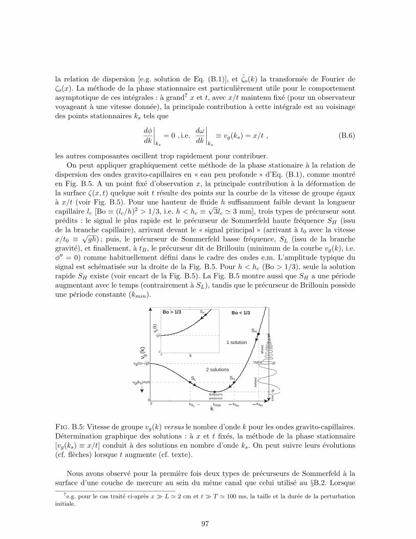
la relation de dispersion [e.g. solution de Eq. (B.1)], et ζo(k) la transformee de Fourier deζo(x). La methode de la phase stationnaire est particulierement utile pour le comportementasymptotique de ces integrales : a grand7 x et t, avec x/t maintenu fixe (pour un observateurvoyageant a une vitesse donnee), la principale contribution a cette integrale est au voisinagedes points stationnaires ks tels que
dφ
dk
∣∣∣∣ks
= 0 , i.e.dω
dk
∣∣∣∣ks
≡ vg(ks) = x/t , (B.6)
les autres composantes oscillent trop rapidement pour contribuer.On peut appliquer graphiquement cette methode de la phase stationaire a la relation de
dispersion des ondes gravito-capillaires en « eau peu profonde » d’Eq. (B.1), comme montreen Fig. B.5. A un point fixe d’observation x, la principale contribution a la deformation dela surface ζ(x, t) quelque soit t resulte des points sur la courbe de la vitesse de groupe egauxa x/t (voir Fig. B.5). Pour une hauteur de fluide h suffisamment faible devant la longueurcapillaire lc [Bo ≡ (lc/h)2 > 1/3, i.e. h < hc ≡
√3lc ' 3 mm], trois types de precurseur sont
predits : le signal le plus rapide est le precurseur de Sommerfeld haute frequence SH (issude la branche capillaire), arrivant devant le « signal principal » (arrivant a t0 avec la vitessex/t0 ≡
√gh) ; puis, le precurseur de Sommerfeld basse frequence, SL (issu de la branche
gravite), et finallement, a tB, le precurseur dit de Brillouin (minimum de la courbe vg(k), i.e.φ′′ = 0) comme habituellement defini dans le cadre des ondes e.m. L’amplitude typique dusignal est schematisee sur la droite de la Fig. B.5. Pour h < hc (Bo > 1/3), seule la solutionrapide SH existe (voir encart de la Fig. B.5). La Fig. B.5 montre aussi que SH a une periodeaugmentant avec le temps (contrairement a SL), tandis que le precurseur de Brillouin possedeune periode constante (kmin).
v g(k
)
k
ksL ksHkmin
vg(ks)≡x/t
vg(0)=√gh "signal"
00
Brillioun'sprecursor
behi
nd
ahea
d
time
Bo > 1/3 Bo < 1/3
SH
SHSL
v
00
g
SH
(k)
k
√gh
2 solutions
1 solution
t ot B
ksH
Fig. B.5: Vitesse de groupe vg(k) versus le nombre d’onde k pour les ondes gravito-capillaires.Determination graphique des solutions : a x et t fixes, la methode de la phase stationnaire[vg(ks) ≡ x/t] conduit a des solutions en nombre d’onde ks. On peut suivre leurs evolutions(cf. fleches) lorsque t augmente (cf. texte).
Nous avons observe pour la premiere fois deux types de precurseurs de Sommerfeld a lasurface d’une couche de mercure au sein du meme canal que celui utilise au §B.2. Lorsque
7e.g. pour le cas traite ci-apres x L ' 2 cm et t T ' 100 ms, la taille et la duree de la perturbationinitiale.
97
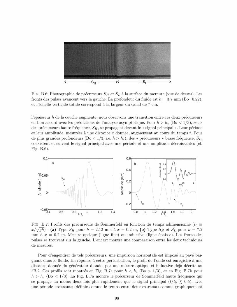
SH SL
Fig. B.6: Photographie de precurseurs SH et SL a la surface du mercure (vue de dessus). Lesfronts des pulses avancent vers la gauche. La profondeur du fluide est h = 3.7 mm (Bo=0.22),et l’echelle verticale totale correspond a la largeur du canal de 7 cm.
l’epaisseur h de la couche augmente, nous observons une transition entre ces deux precurseursen bon accord avec les predictions de l’analyse asymptotique. Pour h > hc (Bo < 1/3), seulsdes precurseurs haute frequence, SH , se propagent devant le « signal principal ». Leur periodeet leur amplitude, mesurees a une distance x donnee, augmentent au cours du temps t. Pourde plus grandes profondeurs (Bo < 1/3, i.e. h > hc), des « precurseurs » basse frequence, SL,coexistent et suivent le signal principal avec une periode et une amplitude decroissantes (cf.Fig. B.6).
0.4 0.6 0.8 1 1.2 1.4−0.05
0
0.05
0.1
Am
plitu
de (
mm
)
t / t0
SH
a
0.8 1 1.2 1.4 1.6 1.8 2
−0.2
0
0.2
0.4
0.6
Am
plitu
de (
mm
)
t / t0
1 1.5 2
−0.2
0
0.2
0.4
Am
plitu
de (
mm
)
t / t0
b
SL
SH
Fig. B.7: Profils des precurseurs de Sommerfeld en fonction du temps adimensionne (t0 ≡x/√gh) : (a) Type SH pour h = 2.12 mm a x = 0.2 m, (b) Type SH et SL pour h = 7.2
mm a x = 0.2 m. Mesure optique (ligne fine) ou inductive (ligne epaisse). Les fronts despulses se trouvent sur la gauche. L’encart montre une comparaison entre les deux techniquesde mesures.
Pour d’engendrer de tels precurseurs, une impulsion horizontale est impose au pave bai-gnant dans le fluide. En reponse a cette perturbation, le profil de l’onde est enregistre a unedistance donnee du generateur d’onde, par une mesure optique et inductive deja decrite au§B.2. Ces profils sont montres en Fig. B.7a pour h < hc (Bo > 1/3), et en Fig. B.7b pourh > hc (Bo < 1/3). La Fig. B.7a montre le precurseur de Sommerfeld haute frequence quise propage au moins deux fois plus rapidement que le signal principal (t/t0 & 0.5), avecune periode croissante (definie comme le temps entre deux extrema) comme graphiquement
98

predit dans l’encart de la Fig. B.5. Pour une profondeur suffisamment grande (Bo < 1/3) ceprecurseur rapide coexiste (cf. Fig. B.7b) avec un precurseur de Sommerfeld basse frequencequi apparaıt derriere le signal principal, avec une periode decroissante comme graphiquementpredite en Fig. B.5. De plus, l’amplitude du precurseur rapide SH est beaucoup plus faibleque SL (voir les echelles verticales des Figs. B.7a-b). La forme du precurseur dependant nota-blement de la transforme de Fourier de la perturabtion initiale, les largeurs spatiales les plusgrandes possedent alors les plus grandes amplitudes. Au-dela de ces accords qualitatifs, nousavons aussi obtenu un accord quantitatif : la periode de chaque precurseur est mesure le longde sa propagation, pour differentes hauteurs de fluide, et est trouvee en tres bon accord avecla periode theorique des precurseurs de Sommerfeld.
Une telle diversite de phenomenes transitoires est liee au caractere non monotone de la re-lation de dispersion des ondes a la surface d’un fluide d’Eq. (B.1), et notamment a l’existenced’un minimum de la courbe de vitesse de groupe vg(k) qui depend de la hauteur de fluide hselon kmin(h) ∼ √1− 3Bo. Les precurseurs les plus rapides se situent dans la limite faiblelongueur d’ondes ou les effets capillaires sont dominants (l’analogue de la dispersion « anor-male » pour les ondes e.m.) tandis que pour les seconds a plus grandes longueurs d’ondes,les effets de gravite ne sont plus negligeables (dispersion « normale »). Ces comportementssont interpretes dans le cadre de l’analyse, introduite pour la premiere fois par Sommerfeldet Brillouin, pour les ondes lineaires transitoires e.m. dans un milieu dielectrique. Nous sou-lignons que cette etude permet aussi de relier le concept de precurseur d’ondes e.m. auxphenomenes transitoires biens connus des ondes de surface hydrodynamique [25], ainsi qu’aleurs applications aux eruptions sous-marines [26].
B.4 Reflexion d’ondes internes
Les deux precedentes parties etaient centrees sur les ondes a la surface d’un fluide iso-tropre. La vitesse de l’onde depend alors de la longueur d’onde, mais pas de la direction depropagation, et l’energie de l’onde se propage perpendiculairement aux cretes (plans d’ondes)a la vitesse de groupe. Dans certains cas cependant, lorsque le fluide est anisotrope, l’energied’une onde peut se propager a une vitesse de groupe parallele aux cretes. C’est le cas desondes internes se propageant dans un milieu stratifie en densite, tel que les oceans (plus saleset donc plus dense en profondeur), l’atmosphere (moins dense avec l’altitude) ou les etoiles(densite augmente vers le centre). Dans le cas oceanographique, la densite croıt en generalde facon lineaire avec la profondeur (stratification lineaire due a la pression, aux salinitesdifferentes). Lorsqu’une particule fluide est deplacee de sa position d’equilibre, une force derappel (force de poussee d’Archimede proportionnelle au gradient de densite) apparaıt pourla ramener autour de sa position stable a la maniere d’une oscillateur harmonique (amorti parviscosite) de frequence propre, N , dit de Brunt-Vaisala : N =
√−(g/ρ0)∂ρ/∂z, ρ(z) etant ladensite du fluide a l’altitude z, g l’acceleration de la gravite, et ρ0 une densite de reference(eau pur). Dans les oceans, la periode 2π/N est de l’ordre de la fraction d’heure, tres grandedevant la periode des ondes sonores (fluide suppose ainsi incompressible). Dans un tel milieu,la relation de dispersion des ondes s’ecrit [27]
ω = ±N k⊥| −→k |
= ±N sinβ , (B.7)
99

ou ω est la pulsation, β l’angle du vecteur d’onde−→k avec la verticale, k⊥ ≡
√k2x + k2
y la
composante de−→k perpendiculaire a l’axe vertical z. Cette relation imlique des proprietes
atypiques et surprenantes pour les ondes internes :• C’est la frequence de l’onde, ω = 2πf , qui determine la direction de propagation de
l’onde, et non pas (comme habituellement) la longueur d’onde, qui est ici quelconque8.• Ces ondes sont dispersives et de pulsation inferieure a N .• La vitesse de groupe est perpendiculaire a la vitesse de phase, l’energie de l’onde se
propage donc parallelement a ses plans d’onde (voir Fig. B.8a) a la maniere d’une ondede cisaillement.
• β est aussi l’angle entre la vitesse de groupe et l’horizontal : les ondes internes de basse(haute) frequence se propage donc a un angle faible (eleve) par rapport a la horizontale.
Ainsi, lorsqu’on excite une onde interne, les rayons sont donnes par les directions de la vitessede groupe, formant une croix a 4 branches, chacune faisant un angle β avec l’horizontale (cf.Fig. B.8b).
(a)
vϕ
vg
g
vg
vϕ
ω
(b)
βg
Fig. B.8: (a) Vue schematique des plans de phase, de la vitesse de groupe vg, de la vitessede phase vφ et des mouvement des particules fluides d’une onde interne dans un milieu stra-tifie verticalement. (b) Visualisation d’ondes internes engendres par un cylindre horizontaloscillant. Les lignes noires et blanches representent des zones de phases constantes (creux etcretes), (Photo issue de la Ref. [28]).
(a)
vg
vg
(b)
Fig. B.9: (a) Vue schematique de la reflexion d’une onde interne d’angle incident β > γ (−),β < γ (− · −) et β = γ (−−). L’angle par rapport a l’axe vertical est conserve. (b) Vueschematique de la reflexion quasi-critique d’un faisceau d’ondes internes incident a β ' γmontrant la forte diminution de la longueur d’onde apres la reflexion. vg indique la directionde la vitesse de groupe.
8En effet, l’Eq. (B.7) est independante de| −→k |= 2π/λ
100
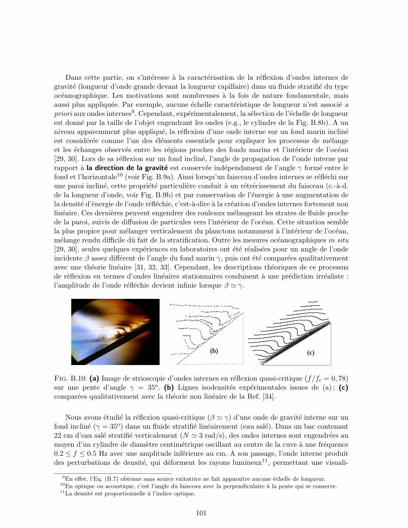
Dans cette partie, on s’interesse a la caracterisation de la reflexion d’ondes internes degravite (longueur d’onde grande devant la longueur capillaire) dans un fluide stratifie du typeoceanographique. Les motivations sont nombreuses a la fois de nature fondamentale, maisaussi plus appliquee. Par exemple, aucune echelle caracteristique de longueur n’est associe apriori aux ondes internes9. Cependant, experimentalement, la selection de l’echelle de longueurest donne par la taille de l’objet engendrant les ondes (e.g., le cylindre de la Fig. B.8b). A unniveau apparemment plus applique, la reflexion d’une onde interne sur un fond marin inclineest consideree comme l’un des elements essentiels pour expliquer les processus de melangeet les echanges observes entre les regions proches des fonds marins et l’interieur de l’ocean[29, 30]. Lors de sa reflexion sur un fond incline, l’angle de propagation de l’onde interne parrapport a la direction de la gravite est conservee independament de l’angle γ forme entre lefond et l’horizontale10 (voir Fig. B.9a). Ainsi lorsqu’un faisceau d’ondes internes se reflechi surune paroi incline, cette propriete particuliere conduit a un retrecissement du faisceau (c.-a-d.de la longueur d’onde, voir Fig. B.9b) et par conservation de l’energie a une augmentation dela densite d’energie de l’onde reflechie, c’est-a-dire a la creation d’ondes internes fortement nonlineaire. Ces dernieres peuvent engendrer des rouleaux melangeant les strates de fluide prochede la paroi, suivis de diffusion de particules vers l’interieur de l’ocean. Cette situation semblela plus propice pour melanger verticalement du planctons notamment a l’interieur de l’ocean,melange rendu difficile du fait de la stratification. Outre les mesures oceanographiques in situ[29, 30], seules quelques experiences en laboratoires ont ete realisees pour un angle de l’ondeincidente β assez different de l’angle du fond marin γ, puis ont ete comparees qualitativementavec une theorie lineaire [31, 32, 33]. Cependant, les descriptions theoriques de ce processusde reflexion en termes d’ondes lineaires stationnaires conduisent a une prediction irrealiste :l’amplitude de l’onde reflechie devient infinie lorsque β ' γ.
(b) (c)
Fig. B.10: (a) Image de strioscopie d’ondes internes en reflexion quasi-critique (f/fc = 0, 78)sur une pente d’angle γ = 35o. (b) Lignes isodensites experimentales issues de (a) ; (c)comparees qualitativement avec la theorie non lineaire de la Ref. [34].
Nous avons etudie la reflexion quasi-critique (β ' γ) d’une onde de gravite interne sur unfond incline (γ = 35o) dans un fluide stratifie lineairement (eau sale). Dans un bac contenant22 cm d’eau sale stratifie verticalement (N ' 3 rad/s), des ondes internes sont engendrees aumoyen d’un cylindre de diametre centimetrique oscillant au centre de la cuve a une frequence0.2 ≤ f ≤ 0.5 Hz avec une amplitude inferieure au cm. A son passage, l’onde interne produitdes perturbations de densite, qui deforment les rayons lumineux11, permettant une visuali-
9En effet, l’Eq. (B.7) obtenue sans source exitatrice ne fait apparaıtre aucune echelle de longueur.10En optique ou acoustique, c’est l’angle du faisceau avec la perpendiculaire a la pente qui se conserve.11La densite est proportionnelle a l’indice optique.
101

sation par une methode optique dite de strioscopie (ou Schlieren) du gradient de densite12.Proche de la reflexion quasi-critique (β ' γ, i.e. fc ' 0.3 Hz), nous observons que les lignesisodensites13, initiallement stable sans excitation, se courbent pour une excitation proche defc, et inverse leur courbure le long de la pente (cf. Fig. B.10a). C’est cette instabilite deretournement des lignes isodensites proche de la pente qui declenche alors le processus demelange entre strates. Nous avons caracterise cette instabilite en mesurant la position et lavitesse du front de retournement. Ces forts effets non lineaires predits theoriquement [34] ontde plus ete compares avec succes a la theorie non lineaire (voir Fig. B.10b-c), la ou le modelelineaire conduit a une singularite analytique.
B.5 Stabilisation parametrique de l’instabilite de Rosensweig
Nous avons vu au chapitre A que l’influence d’un champ magnetique sur la turbulenced’ondes a la surface d’un ferrofluide engendrait des phenomenes nouveaux particulierementinteressants. Nous avons aussi en projet (cf. §B.2) d’etudier son role sur la propagation d’uneonde solitaire se propageant a la surface d’un ferrofluide.
Ici, nous montrons experimentalement que l’instabilite de Rosensweig (instabilite station-naire d’une couche de ferrofluide soumis a un champ magnetique normal) peut etre inhibeepar amplification parametrique d’ondes a la surface du ferrofluide soumis a des vibrationsverticales (instabilite de Faraday). Les seuils de l’instabilite parametrique et de Rosensweigsont mesures dans l’espace des parametres : amplitude de l’acceleration de vibration et champmagnetique. Ces mesures et observations sont en accords quantitatifs avec un modele ana-lytique simple utilisant la theorie des fonctions de Mathieu. Ce modele permet de plus unedetermination experimentale de la susceptibilite magnetique du ferrofluide en fonction duchamp magnetique en bon accord avec la theorie classique de Langevin. Nous avons ainsimontre qu’un ferrofluide vibre soumis a un champ magnetique statique normal fournit uneconfiguration experimentale simple pour l’etude quantitative du mecanisme d’inhibition pa-rametrique d’une structuration spatiale etendue engendree par une instabilite hydrodyna-mique.
References
[1] J. S. Russell, Report on Waves in 1844 British Assn. Adv. Sci. Report, London, (1845)and in Proc. R. Soc. Edinburgh, p. 319 (1844).
[2] D. J. Korteweg and G. De Vries, Phil. Mag. 39, 422 (1895).
[3] J. L. Hammack and H. Segur, J. Fluid Mech. 65, 289 (1974).
[4] M. Peyrard & T. Dauxois Physique des Solitons (EDP Sciences, CNRS Ed., Paris 2004)
[5] M. Remoissenet Waves Called Solitons (Springer-Verlag, Berlin, 3rd Ed., 1999)
12Les phases des ondes sont convertis en intensite lumineuse par diffraction sur un bord : la lumiere courbeevers le haut (bas) est gardee (enlevee), resultant en un point lumineux (sombre). Cette methode est sensiblea l’angle des deviations des rayons (au gradient de densite).
13Bien que la strioscopie ne soit sensible qu’au gradient de densite, ces isodensites sont visibles ici car lemouvement oscillant a engendre par diffusion de particules (au bout d’un certain temps apres la reflexion) desdiscontinuites de gradient (en escalier), visibles par cette methode, et qui correspondent a des lignes isodensites.
102

[6] K. A. Naugol’nykh and L. A. Ostrovsky, Nonlinear wave processes in acoustics (Cam-bridge University Press, Cambridge, 1998).
[7] T. Kakutani, H. Ono, T. Taniuti and C.-C. Wei, J. Phys. Soc. Japan 24, 1159 (1968) ;T. Kakutani and H. Ono, ibid. 26, 1305 (1969).
[8] G. L. Lamb, Elements of soliton theory (John Wiley, New York, 1980).[9] A. M. Lomonosov, P. Hess and A. P. Mayer, Phys. Rev. Lett. 88, 076104 (2002).
[10] Y. S. Kivshar, Phys. Rev. A 42, 1757 (1990).[11] A. V. Fedorov, W. K. Melville and A. Rozenberg, Phys. Fluids 10, 1315 (1998).[12] D. M. Henderson and R. C. Lee, Phys. Fluids 29, 619 (1986).[13] T. B. Benjamin, Quarterly of Applied Mathematics 40, 231 (1982).[14] M. Z. Gak and E. Z. Gak in Nonlinear Oscillations, Waves and Vortices in Fluids In-
ternational Symposium (CSA, St-Petersburg, 1994).[15] M. S. Longuet-Higgins, J. Fluid Mech. 200, 451 (1989).[16] M. S. Longuet-Higgins and X. Zhang, Phys. Fluids 9, 1963 (1997).[17] V. G. Bashtovoi and R. A. Foigel, Magnetohydrodynamics 19, 160 (1983)[18] L. Brillouin, Wave Propagation And Group Velocity, Academic Press, Inc., Ny (1960)
incluant notamment la traduction en anglais de A. Sommerfeld, Ann. Physik (Leipzig)44, 177 (1914) ; L. Brillouin, ibid. 44, 203 (1914).
[19] P. Pleshko and I. Palocz, Phys. Rev. Lett. 22, 1201 (1969) ; D. D. Stancil, J. App. Phys53, 2658 (1982) ; J. Aaviksoo, J. Kuhl and K. Ploog, Phys. Rev. A 44, R5353 (1991)
[20] R. Albanese, J. Penn and R. Medina, J. Opt. Soc. Am. A 6, 1441–1446 (1989).[21] A. Hanyga, Pure Appl. Geophys. 159, 1749 (2002)[22] M. Mojahedi, E. Schamiloglu, F. Hegeler and K. J. Malloy, Phys. Rev. E 62, 5758 (2000) ;
A. P. Barbero, H. E. Hernandez-Figueroa and E. Recami, Phys. Rev. E 62, 8628 (2000) ;S. Chu and S. Wong, Phys. Rev. Lett. 48, 738 (1982), D. Mugnai, A. Ranfagni and R.Ruggeri, Phys. Rev. Lett. 84 4830 (2000).
[23] E. Varoquaux, G. A. Williams and O. Avenel, Phys. Rev. B 34, 7617 (1986).[24] I. Kececioglu, M. E. McClurken, R. D. Kamm and A. H. Shapiro, J. Fluid Mech. 109,
367 (1981) ; P. Flaud, D. Geiger and C. Oddou, J. Physique 47, 773 (1986).[25] J. E. Prins, Trans. Am. Geophys. Union 39, 865 (1958) pour les experiences d’ondes
de gravite ; H. C. Kranzer and J. B. Keller, J. Appl. Phys. 30, 398 (1959) ; H. Lamb,Hydrodynamics, Dover, NY (1945), pour la theorie.
[26] M. S. Smith and J. B. Sheperd, Natural Hazards 11, 75 (1994).[27] J. Lighthill, Waves in Fluids (Cambridge University Press, Cambridge, 1978)[28] P. K. Kundu, Fluid Mechanics (Academic Press, London, 1990)[29] K. L. Polzin, J. M. Toole, J. R. Ledwell & R. W. Schmitt, Science 76, 93-96 (1997).[30] C. C. Eriksen, J. Geophys. Res. 103, 2977-2994 (1998).[31] D. Cacchione, & C. Wunsch, J. Fluid Mech. 66, 223-239 (1974).[32] S. A. Thorpe, J. Fluid Mech. 178, 279-302 (1987).[33] E. E. McPhee-Shaw, & E. Kunze, J. Geophys. Res. 107 (C6), 10.1029/2001JC000801,
(2002).[34] T. Dauxois & W. R. Young, J. Fluid. Mech. 390, 271-295 (1999).
103

B.6 Publications associees a ce chapitre
T. Dauxois, A. Didier & E. Falcon, Physics of Fluids 16, 1936–1941 (2004)Observation of near-critical reflection of internal waves in a stably stratified fluid
E. Falcon, C. Laroche & S. Fauve, Physical Review Letters 91, 064502 (2003)Observation of Sommerfeld precursors on a fluid surface
E. Falcon, C. Laroche & S. Fauve, Physical Review Letters 89, 204501 (2002)Observation of depression solitary surface waves on a thin fluid layer
F. Petrelis, E. Falcon & S. Fauve, European Physical Journal B 15, 3–6 (2000)Parametric stabilization of the Rosensweig instability
Actes de conferences
E. Falcon, C. Laroche, & S. Fauve, 6e Rencontre du Non-Lineaire Paris 2003, Non-LineairePub., Orsay, p. 119–124, (2003)Observation d’ondes solitaires depressions a la surface d’une fine couche de fluide
L. Gostiaux, T. Dauxois & E. Falcon, 8eme Rencontre du Non-Lineaire 2005, Non LineairePub., Orsay, pp. 103-108 (2005)Reflexion critique d’ondes internes de gravite en fluides stratifies
L. Gostiaux, T. Dauxois, E. Falcon & N. Garnier, Actes du Colloque Fluvisu 11, Ecole CentraleLyon, (2005)Mesure quantitative de gradients de densite en fluides stratifies bidimensionnels
Articles de presse
Parus dans la presse scientifique suite a Falcon et al., PRL 89, 204501 (2002)
• Pour La Science, No 304, Fevrier 2003, p. 18. (en francais)« La premiere onde solitaire en “creux” »
• Sciscape, November 10, 2002, by Vincent Liu. (en chinois)
• Physical Review Focus, 29 October 2002 by Pam Frost Garder. (en anglais)“Wave of Depression”
104

B.7 Tires a part
105

106

Observation of Depression Solitary Surface Waves on a Thin Fluid Layer
Eric Falcon,1,* Claude Laroche,1 and Stephan Fauve2
1Laboratoire de Physique, Ecole Normale Superieure de Lyon, UMR 5672, 46, allee d’Italie, 69 007 Lyon, France2Laboratoire de Physique Statistique, Ecole Normale Superieure, UMR 8550, 24, rue Lhomond, 75 005 Paris, France
(Received 26 April 2002; published 23 October 2002)
We report the observation of depression solitary surface waves on a layer of mercury when its depth isthin enough compared to the capillary length. These waves, as well as the well known elevation solitarywaves, are studied with a new measurement technique using inductive sensors. The shape of the solitarywaves, their amplitude-dependent velocity, and their damping rates by viscosity are found in goodagreement with theoretical predictions.
DOI: 10.1103/PhysRevLett.89.204501 PACS numbers: 47.35.+i, 05.45.Yv, 68.03.Cd, 92.10.Hm
Since the first observation of a solitary wave on thefree-surface of water by Russell [1] and its interpretationusing the Korteweg–de Vries equation (KdV) [2], eleva-tion solitary waves in shallow water have been widelystudied in a quantitative way [3,4]. It has also been shownthat the KdV equation generically describes a large classof solitons observed in various situations: nonlinearwaves in acoustics [5], magneto-acoustic [6] or ion [7]plasma waves, elastic surface pulses [8], grey solitons inoptical fibers [9], and long flexural–gravity waves inwater under ice sheets [10]. It has been emphasized byKorteweg and de Vries in their early paper [2] that soli-tary waves may involve both a positive (elevation) or anegative (depression) localized perturbation, dependingon the sign of the dispersion. However, most quantitativestudies have reported the elevation solitary wave so far. Inthe case of waves on the surface of a fluid, only elevationsolitary waves can be observed in the long wavelengthlimit when gravity is dominant. For shorter wavelengths,when surface tension is no longer negligible, capillaryeffects have a drastic influence both on extended waves(observation of ripples or parasitic waves [11]) and onlocalized waves such as KdV solitary waves which arepredicted to become depression waves rather than eleva-tion ones. We report here the first observation of depres-sion solitary waves on a thin layer of mercury. By meansof an accurate quantitative analysis, they are shown tohave a subsonic amplitude-dependent velocity and tokeep a self-similar shape although damped by viscosity.
The experimental setup consists of a 1.5 m long hori-zontal Plexiglas channel, 70 mm wide, filled with mer-cury up to a height h: 2:12 h 8:5 mm. h is measuredwith 0:02 mm precision by means of a depth gaugeusing a micrometric linear positioner. The properties ofthe fluid are density, 13:5 103 kg=m3; surface ten-sion, 0:484 N=m; and dynamic viscosity, 1:5103 Ns=m2 [12]. Surface waves are generated by a sinu-soidal or impulsional excitation provided by the horizon-tal motion of rectangular plunging Teflon wavemakerdriven by an electromagnetic vibration exciter (Bruel &Kjær, type 4809). Waves are generated 10 mm inwardfrom one end of the channel, and the local displacement
of the fluid in response to this excitation is measured bytwo nonintrusive inductive sensors (eddy-current lineardisplacement gauge, Electro 4953 sensors). Both sensors,3 mm in diameter, are suspended perpendicular to thefluid surface at rest. They are put 2.5 mm (0.5 mm) abovethe surface when studying elevation solitary waves (de-pression solitary waves). The linear sensing range of thesensors allows distance measurements from the sensorhead to the fluid surface up to 2.5 mm with a 5 V=mmsensitivity. The first sensor is located 100 mm away fromthe wavemaker, whereas the second one is mounted on ahorizontal linear positioner at a distance x from the firstone, 0< x< 1:2 m. Although inductive sensors arewidely used to get precise measurements of the positionof plane metallic plates, their response in the case of awavy liquid surface was not known. Thus, we firstchecked our measurements with an optical determinationof the local slope of the surface: using a position sensitivedetector, we recorded the deflection of a laser beam by thesurface wave; the computation of the surface elevationfrom the optical signal was found in perfect agreementwith the direct inductive measurement of the shape of thewave [13]. Although the sensitivity of the optical tech-nique and its spatial resolution are better, the inductivemethod allows a direct measurement of the surface dis-placement and does not require signal processing. Besidessimplicity, this also gives more accurate measurements ofcomplex wave shapes because small errors may accumu-late due to the numerical integration necessary to processthe optical signal. Both techniques are not limited bytheir response time in the frequency range of surfacewaves. The choice of mercury was motivated by thepossible use of the inductive measurement techniqueand also because of its kinematic viscosity which is anorder of magnitude smaller than that of water, thusstrongly reducing wave dissipation.
We first measure the phase velocity and determine thedispersion relation of capillary-gravity surface waves inorder to check our measurement technique and to find thevalue of the surface tension . To wit, the shaker is drivensinusoidally at small amplitude at frequency f varyingfrom 5 to 25 Hz with a 0.1 Hz step. We measure the
VOLUME 89, NUMBER 20 P H Y S I C A L R E V I E W L E T T E R S 11 NOVEMBER 2002
204501-1 0031-9007=02=89(20)=204501(4)$20.00 2002 The American Physical Society 204501-1

relative phase difference between the signals givenby the two sensors by means of a lock-in amplifier as afunction of f. The phase velocity c is then obtained fromthe unwrapped phase f and the distance x 120 mmbetween the sensors: c 2fx=f. It is displayed inFig. 1 as a function of f for three different values of theheight. These data are in good agreement with the dis-persion relation neglecting viscosity
! gk
k3 tanhkh
q; (1)
between the pulsation ! 2f and the wave number k,provided that 0:4 N=m, g being the acceleration ofgravity. Note that this value of the surface tension is 17%lower than the tabulated one given above. This may resultfrom the presence of contaminants at the surface whichcould reduce the value of the ‘‘dynamic’’ surface tension
up to 30% with respect to the measured static value [14].Another independent check of Eq. (1) is displayed in theinset in Fig. 1: the wavelength c=f, as a function off obtained by the previous phase method, is compared toits direct measurement using a stroboscope.
From Eq. (1), we can define the capillary length, lc =g
p, and the Bond number, Bo lc=h
2. In the longwavelength approximation or ‘‘shallow water’’ limit(k ! 0), the linear wave velocity is cs
gh
pand dis-
persion is small. When the free-surface deflection Ax; tis also small, such that nonlinear effects have the sameorder of magnitude as dispersive ones, it is governed toleading order by the Korteweg–de Vries equation [2]
At 3
2
cshAA
1
6csh2
1
3 Bo
A 0; (2)
in the comoving reference frame, x ct. The soli-tary capillary-gravity wave solution of Eq. (2) reads [2]
Ax; t A0sech2
x ctL
; L
41 3Boh3
9A0
s;
(3)
with c the velocity of the solitary wave
c cs
1
A0
2h
; (4)
and L is the length scale of the solitary wave.Equations (3) and (4) show that there exists a continuousfamily of soliton solutions with parameter A0 (theextremum amplitude of the wave). Moreover, when0 Bo< 1=3, we get the previously observed elevationsolitary waves (A0 > 0) with supersonic speeds (Froudenumber F c=cs > 1), whereas when Bo > 1=3, weshould find depression waves (A0 < 0) with subsonicspeeds (F < 1). In the case Bo ’ 1=3, an additionalfifth-order dispersion term has to be taken into account
5 10 15 20 25
0.18
0.2
0.22
0.24
0.26
c φ (m
/s)
Frequency (Hz)
5 10 15 20 250
2
4
6
Frequency (Hz)
λ (c
m)
FIG. 1. Phase velocity vs f for h 3:3 ( ), 4.6( ), and 8 () mm. Solid lines represent !k=k derivedfrom Eq. (1) with 0:4 N=m for h 3:3 (lower curve),4.6 (middle), and 8 (upper) mm. Inset: Wavelength versus fwith additional stroboscopic measurements (same symbols asabove).
-0.4 -0.2 0 0.2 0.4 0.6 0.8 1-0.08
-0.07
-0.06
-0.05
-0.04
-0.03
-0.02
-0.01
0
0.01
Am
plitu
de (
mm
)
Time (s)
(a)
-0.2 0 0.2 0.4 0.6 0.8 1-0.1
0
0.1
0.2
0.3
0.4
0.5
0.6
Am
plitu
de (
mm
)
Time (s)
(b)
FIG. 2. (a) Free-surface profile of a depression solitary wave for h 2:12 mm and A0 0:064 mm, (b) elevation solitary waveprofile for h 5:6 mm and A0 0:57 mm. Solid lines are the time recordings of the fluid surface displacement measured by thesensor located at 300 (a) and 200 (b) mm from the wavemaker. Pulse fronts are located on the left side. Dashed lines are thetheoretical shapes of (a) depression [(b) elevation] KdVsolitons derived from Eq. (3) with 0:4 N=m, h 2:12 (5.6) mm, and A0
the minimal (maximal) amplitude of each experimental profile, leading to the following parameters of the wave: Bo 0:67,L 8:2 mm, 0:03, 0:07, = 2:2 (Bo 0:1, L 9:8 mm, 0:1, 0:32, = 3:2).
VOLUME 89, NUMBER 20 P H Y S I C A L R E V I E W L E T T E R S 11 NOVEMBER 2002
204501-2 204501-2

in Eq. (2), and, in this case, the solution for the fullhydrodynamic problem is still a matter of theoreticaldebate [15,16]. Despite some trials [15,17], no conclusiveobservation of the depression solitary waves has beenperformed so far. Note that this solution of the KdVequation should not be confused with oscillatory depres-sion waves computed in the limit of infinite depth [18]and recently observed [19].
We have performed an experimental study of solitarywaves for a fluid layer height in the range 2:12 h 8:5 mm; thus, 0:04 Bo 0:67. For mercury (lc 1:74 mm), the critical case Bo 1=3 corresponds tohc 3 mm. In order to generate solitary waves, we im-pulsionally drive the shaker. For h < hc (h > hc), thewavemaker is horizontally drawn back (pushed forward)in order to generate a negative (positive) pulse on the fluidsurface. At a given distance from the wave generator, thefree-surface profile is recorded and displayed in Fig. 2(a)for a depression pulse (h 2:12 mm) and in Fig. 2(b) foran elevation pulse (h 5:6 mm). Both recordings arein good agreement with the profiles of depression andelevation KdV solitary wave given by Eq. (3) with 0:4 N=m. Note that once A0 is known the theoreticalprofile as well as the velocity of the solitary wave givenby Eqs. (3) and (4) do not involve any adjustable parame-ter. The small oscillations observed before (after) thearrival of the pulse in Fig. 2(a) (2(b)) are identifiedwith forerunners (or precursors) [13] and with the usualphonon radiative tail, respectively. As indicated in thecaption of Fig. 2, those isolated pulses involve waveparameters that are in the range of validity required for
the derivation of Eq. (2), that is, corresponding to smalldispersion [ h=L2 1] and small nonlinearities( jAj=h 1), both of the same order of magnitude.
A depression pulse for h 2:12 mm is recorded at apropagation distance from the wavemaker ranging from10 to 110 times its typical size L 10 mm. As shown inFig. 3, the recorded profiles are in good agreement withthe KdV depression solitary wave all along the propaga-tion. Note, however, that the first recorded pulse had notenough time to reach its asymptotic shape, and that forthe last recordings, the cumulative effect of dissipationleads to a small difference from the KdV profile. In theintermediate range, the inset in Fig. 3 shows that, whenexpressed in the variables A=A0 and tcjA0j
1=2, all data( ) lie on a single curve ( ) predicted by Eq. (3).This means that the pulse propagates with no shapedeformation over a large distance with respect to itstypical size and in very good agreement with the profilederived from the KdV equation.
The solitary wave velocity is measured all along itspropagation by recording the time of flight between suc-cessive minima (maxima) of the amplitude A0 for depres-sion (elevation) pulses. The dimensionless pulse velocity,c=
gh
p(Froude number F), is displayed in Fig. 4 as a
function of A0=h for various h corresponding to 0:04 Bo 0:67. Full (open) symbols will be used afterwardsfor depression (elevation) pulses. For each height corre-sponding to Bo > 1=3, the velocity of the depressionwave is subsonic (F < 1) and increases as the pulse propa-gates, whereas for 0 Bo< 1=3, the velocity of theelevation wave is supersonic (F > 1) and decreases withtime. All data lie on a single straight line predicted byEq. (4), with slope 1=2 in the rescaled variables.
Finally, we study dissipative effects both on eleva-tion and depression solitary waves. The pulse amplitude
0 2 4 6 8
-0.1
-0.08
-0.06
-0.04
-0.02
0
Am
plitu
de (
mm
)
Time (s)
-30 -15 0 15 30-1
0
- A
/ A
0
t c |A0|1/2 (mm3/2)
FIG. 3. Propagation of a depression solitary wave for h 2:12 mm, recorded at distances from the wavemaker in therange 100 to 1100 mm with a 100 mm step. The time origin istriggered by the wavemaker. Dashed lines are the correspond-ing theoretical profiles of depression solitons derived fromEq. (3) with 0:4 N=m, h 2:12 mm, and A0 the minimalamplitude of each experimental profile. The inset displays therescaled experimental ( ) depression solitary waves at 200,300, 400, and 500 mm and the solution ( ) of Eq. (3).
-0.1 0 0.1 0.2 0.30.95
1
1.05
1.1
1.15
1.2
c / (
g*h)
1/2
Ao / h
FIG. 4. Dimensionless pulse velocity c=gh
pversus A0=h for
various experimental parameters: For depression solitarywaves, h 2:12 ( ) and 2:72 () mm. For elevation pulses,h 3:3 (), 3.5 (), 3.8 ( ), 4.5 ( ? ), 4.6 (), 5.1 ( ),8.5 ( 5 ) mm. (Full line of slope 0.5).
VOLUME 89, NUMBER 20 P H Y S I C A L R E V I E W L E T T E R S 11 NOVEMBER 2002
204501-3 204501-3

maximum (minimum), A0x, is displayed as a functionof the propagation distance x in the inset of Fig. 5 forelevation (depression) solitary waves. We observe thatA0x decreases exponentially with x, A0x A0jx0 expx=h, where h is the characteristic dampinglength. Figure 5 shows the dependence of with h ex-tracted from the slope of each linear curve in the inset. Inthe range, 2:12 h 8:5 mm, we find that / h3=2 bothfor depression and elevation solitary waves (see Fig. 5).This scaling can be understood as follows: for a smallviscosity fluid in the shallow water limit, we have h L where is the size of the viscous boundary layerclose to the bottom plate which gives the dominant con-tribution to the dissipation. From the ratio of the typicalkinetic energy of the flow to the dissipated power in theboundary layer, we get a typical damping time, / h= .This leads to the observed law, / cs / h3=2, if weassume that does not depend on h. The size of theboundary layer in our experiment certainly depends onthe way we generate the solitary wave, in particular, onthe characteristic time scale of the initial perturbation.When this dissipation is computed from the flow gener-ated by the KdV solitary wave alone [20], it usuallyunderestimates the measurements done previously forelevation solitary waves on shallow water [3,21].
In conclusion, we have reported the observation ofdepression solitary surface waves in the shallow waterlimit and found that their shape and velocity are in goodagreement with the ones predicted from the depression
KdV solitary wave solutions. We stress that no adjustableparameter has been used to fit the pulse shape. Althoughthe solitary waves are damped by viscous dissipation, wehave shown that they keep the self-similar shape given bythe continuous family of solutions of the KdVequation ona propagation length much larger than their typical scale.
We thank B. Castaing and F. Dias for discussions.
*Corresponding author.http://www.ens-lyon.fr/~efalcon/
[1] J. S. Russell, in Proc. R. Soc. Edinburgh 11, 319 (1844).[2] D. J. Korteweg and G. De Vries, London, Edinburgh
Dublin Philos. Mag. J. Sci. 39, 422 (1895).[3] J. L. Hammack and H. Segur, J. Fluid Mech. 65, 289
(1974).[4] A. Bettini, T. A. Minelli, and D. Pascoli, Am. J. Phys. 51,
977 (1983).[5] K. A. Naugol’nykh and L. A. Ostrovsky, Nonlinear Wave
Processes in Acoustics (Cambridge University,Cambridge, 1998).
[6] T. Kakutani, H. Ono, T. Taniuti, and C.-C. Wei, J. Phys.Soc. Jpn. 24, 1159 (1968); T. Kakutani and H. Ono, ibid.26, 1305 (1969).
[7] G. L. Lamb, Elements of Soliton Theory (Wiley, NewYork, 1980).
[8] A. M. Lomonosov, P. Hess, and A. P. Mayer, Phys. Rev.Lett. 88, 076104 (2002).
[9] Y. S. Kivshar, Phys. Rev. A 42, 1757 (1990).[10] T. Takizawa, J. Geophys. Res. 93, 5100 (1988); E. Parau
and F. Dias, J. Fluid Mech. 460, 281 (2002).[11] A.V. Fedorov, W. K. Melville, and A. Rozenberg, Phys.
Fluids 10, 1315 (1998); J. H. Chang, R. N. Wagner, andH. C. Yuen, J. Fluid Mech. 86, 401 (1978); G. Kuwabara,T. Hasegawa, and K. Kono, Am. J. Phys. 54, 1002 (1986).
[12] Handbook of Chemistry and Physics, edited by D. R.Lide (CRC Press, New York, 1999), 80th ed.
[13] E. Falcon, C. Laroche, and S. Fauve (unpublished).[14] D. M. Henderson and R. C. Lee, Phys. Fluids 29, 619
(1986).[15] T. B. Benjamin, Q. Appl. Math. 40, 231 (1982).[16] T. Kawahara, J. Phys. Soc. Jpn. 33, 260 (1972); J. K.
Hunter and J.-M. Vanden-Broeck, J. Fluid Mech. 134,205 (1983); J. A. Zufiria, J. Fluid Mech. 184, 183 (1987);A. R. Champneys, J.-M. Vanden-Broeck, and G. J. Lord,J. Fluid Mech. 454, 403 (2002).
[17] M. Z. Gak and E. Z. Gak, in Nonlinear Oscillations,Waves and Vortices in Fluids International Symposium(Center for Supercomputing Applications, St. Petersburg,1994).
[18] M. S. Longuet-Higgins, J. Fluid Mech. 200, 451 (1989).[19] M. S. Longuet-Higgins and X. Zhang, Phys. Fluids 9,
1963 (1997); X. Zhang, J. Fluid Mech. 289, 51 (1995).[20] G. H. Keulegan, J. Res. Natl. Bur. Stand. 40, 487 (1948);
J.W. Miles, J. Fluid Mech. 76, 251 (1976); R. S. Johnson,A Modern Introduction to the Mathematical Theory ofWater Waves (Cambridge University, Cambridge, 1997),pp. 365–374.
[21] P. D. Weidman and T. Maxworthy, J. Fluid Mech. 85, 417(1978), and references therein.
0 5 10 15 20 250
1
2
3
4
5
ζ (m
)
h3/2 (mm3/2)
0 0.4 0.8 1.20.1
1
Ao /
Ao
(x=
0)
x (m)
FIG. 5. Damping length versus h3=2 for depression solitarywaves [full symbols with h 2:12 ( ); 2.4 (); 2.54 (); 2.94() mm for various A0jx0 ( 6:2 102 A0jx0=h 4:3 102)] and for elevation pulses [at fixed A0jx0=h 0:106 ( ); 0.285 ( ) for various A0jx0 and h; at fixedA0jx0 1:3 mm () for various h; and at 0:1 A0jx0=h 0:33 ( ) for various A0jx0 and h]. The inset displays the semi-log plot of the normalized pulse amplitude A0x=A0jx0 as afunction of the distance x of propagation: for depression soli-tary waves (same legend as above); for elevation pulses withh 3:3 ( ); 4.6 ( ); 5.6 (); 8.2 ( ) mm at fixedA0jx0=h 0:106. Lines join the data points.
VOLUME 89, NUMBER 20 P H Y S I C A L R E V I E W L E T T E R S 11 NOVEMBER 2002
204501-4 204501-4

Observation of Sommerfeld Precursors on a Fluid Surface
Eric Falcon,1,* Claude Laroche,1 and Stephan Fauve2
1Laboratoire de Physique, Ecole Normale Superieure de Lyon, UMR 5672, 46, allee d’Italie, 69 007 Lyon, France2Laboratoire de Physique Statistique, Ecole Normale Superieure, UMR 8550, 24, rue Lhomond, 75 005 Paris, France
(Received 11 March 2003; published 7 August 2003)
We report the observation of two types of Sommerfeld precursors (or forerunners) on the surface of alayer of mercury. When the fluid depth increases, we observe a transition between these two precursorsurface waves in good agreement with the predictions of asymptotic analysis. At depths thin enoughcompared to the capillary length, high frequency precursors propagate ahead of the ‘‘main signal’’ andtheir period and amplitude, measured at a fixed point, increase in time. For larger depths, low frequency‘‘precursors’’ follow the main signal with a decreasing period and amplitude. These behaviors areunderstood in the framework of the analysis first introduced for linear transient electromagnetic wavesin a dielectric medium by Sommerfeld [Ann. Phys. (Leipzig) 44, 177 (1914)] and Brillouin [Ann. Phys.(Leipzig) 44, 203 (1914)].
DOI: 10.1103/PhysRevLett.91.064502 PACS numbers: 47.35.+i, 11.55.Fv, 68.03.Cd, 92.10.Hm
One feature of linear wave propagation in a dispersivemedium is the existence of precursors (or forerunners).This terminology traces back to the fact that they gen-erally arrive sooner than the ‘‘main’’signal. This transientresponse is due to the propagation of the fastest highfrequency components of the initial spectrum. Althoughpredicted as early as 1914 by Sommerfeld and Brillouin[1], experimental observations of forerunners are veryfew and only qualitative, mainly dealing with electro-magnetic (e.m.) waves in a dielectric medium in themicrowave [2] or optical [3] frequency range. SuchSommerfeld forerunners have also been predicted in vari-ous dispersive media such as biological [4] or viscoelastic[5] ones, and have been recently shown to be linked to thenonviolation of Einstein causality during superluminallight pulse propagation in the region of anomalous dis-persion [6]. However, for waves in fluids, the observationof forerunners is still lacking despite some effort per-formed with acoustic waves in superfluid 3He [7] orwith pressure waves in fluid-filled collapsible tubes [8].We report here the first observation of two types ofSommerfeld forerunners, which can or cannot coexist,on a thin layer of mercury. The nonmonotonous disper-sion relation of waves on the surface of a fluid lead to arich variety of such transient wave phenomena. In theshortwavelength limit, when capillary effects are domi-nant (the analogue to ‘‘anomalous’’ dispersion [9] for e.m.waves), only the fast high frequency components of theinitial excitation are observed arriving before the mainpulse, the so-called Sommerfeld precursor for e.m. waves.This transient is characterized by small amplitude andrapid oscillations (with respect to the main signal). Forlonger wavelengths, when gravity is no longer negligible(‘‘normal’’ dispersion), a slower low frequency precursoris also observed (no analogue exists for e.m. waves). Theforerunners are found in good agreement with the pre-dictions of asymptotic analysis based on the ‘‘stationary
phase method.’’ We note that this study also allows us toconnect the forerunner concept of electromagnetic wavesto the well-known hydrodynamic transient surface wavephenomena [10], and their applications to submarineeruptions [11].
The experimental setup consists of a 1.5 m long hori-zontal Plexiglas channel, 7 cm wide, filled with mercuryup to a height, h, where: 2 & h & 14 mm. h is measuredto a precision of 0:02 mm by means of a depth gaugeusing a micrometric linear positioner. The properties ofthe fluid are density, 13:5 103 kg=m3, dynamic vis-cosity, 1:5 103 Ns=m2 [12], and surface tension 0:4 N=m [13]. Surface waves are generated by animpulsional excitation provided by the horizontal motionof a rectangular plunging Teflon wave maker driven by anelectromagnetic vibration exciter. They are generated10 mm inward from one end of the channel and the localdisplacement of the fluid in response to this excitation ismeasured simultaneously by a nonintrusive inductivesensor and by an optical technique [13]. The inductivesensors, 3 mm in diameter, are suspended perpendicularlyto the fluid surface at rest. The linear sensing range of thesensors allows distance measurements from the sensorhead to the fluid surface up to 2.5 mm with a 5 V/mmsensitivity. An optical determination of the local slope ofthe surface is also performed. Using a position sensitivedetector, we have recorded the deflection of a laser beamby the surface wave; the computation of the surfaceelevation from the optical signal is in excellent agreementwith the direct inductive measurement of the shape of thewave [see insets of Figs. 3(b) and 3(c)]. Both sensors aremounted on a horizontal linear positioner at a distance xfrom the wave maker, 0< x< 1:2 m. The optical andinductive methods are complementary as the spatial reso-lution and the sensitivity of the optical technique arehigher, but the inductive technique provides a directmeasurement of the surface displacement and does not
P H Y S I C A L R E V I E W L E T T E R S week ending8 AUGUST 2003VOLUME 91, NUMBER 6
064502-1 0031-9007=03=91(6)=064502(4)$20.00 2003 The American Physical Society 064502-1
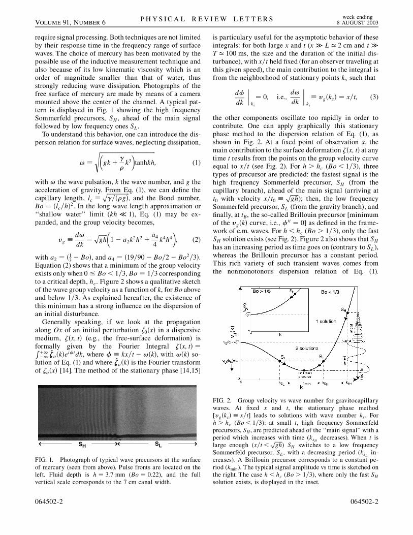
require signal processing. Both techniques are not limitedby their response time in the frequency range of surfacewaves. The choice of mercury has been motivated by thepossible use of the inductive measurement technique andalso because of its low kinematic viscosity which is anorder of magnitude smaller than that of water, thusstrongly reducing wave dissipation. Photographs of thefree surface of mercury are made by means of a cameramounted above the center of the channel. A typical pat-tern is displayed in Fig. 1 showing the high frequencySommerfeld precursors, SH, ahead of the main signalfollowed by low frequency ones SL.
To understand this behavior, one can introduce the dis-persion relation for surface waves, neglecting dissipation,
!
gk
k3tanhkh
s; (1)
with ! the wave pulsation, k the wave number, and g theacceleration of gravity. From Eq. (1), we can define thecapillary length, lc
=g
p, and the Bond number,
Bo lc=h2. In the long wave length approximation or
‘‘shallow water’’ limit (kh 1), Eq. (1) may be ex-panded, and the group velocity becomes,
vg d!dk
gh
p 1 a2k2h2
a44k4h4
; (2)
with a2 13 Bo, and a4 19=90 Bo=2 Bo2=3.Equation (2) shows that a minimum of the group velocityexists only when 0 Bo < 1=3, Bo 1=3 correspondingto a critical depth, hc. Figure 2 shows a qualitative sketchof the wave group velocity as a function of k, for Bo aboveand below 1=3. As explained hereafter, the existence ofthis minimum has a strong influence on the dispersion ofan initial disturbance.
Generally speaking, if we look at the propagationalong Ox of an initial perturbation 0x in a dispersivemedium, x; t (e.g., the free-surface deformation) isformally given by the Fourier Integral x; t R11 oke
itdk, where kx=t!k, with !k so-lution of Eq. (1) and where ok is the Fourier transformof ox [14]. The method of the stationary phase [14,15]
is particulary useful for the asymptotic behavior of theseintegrals: for both large x and t (x L ’ 2 cm and tT ’ 100 ms, the size and the duration of the initial dis-turbance), with x=t held fixed (for an observer traveling atthis given speed), the main contribution to the integral isfrom the neighborhood of stationary points ks such that
ddk
ks
0; i:e:;d!dk
ks vgks x=t; (3)
the other components oscillate too rapidly in order tocontribute. One can apply graphically this stationaryphase method to the dispersion relation of Eq. (1), asshown in Fig. 2. At a fixed point of observation x, themain contribution to the surface deformation x; t at anytime t results from the points on the group velocity curveequal to x=t (see Fig. 2). For h > hc (Bo < 1=3), threetypes of precursor are predicted: the fastest signal is thehigh frequency Sommerfeld precursor, SH (from thecapillary branch), ahead of the main signal (arriving att0 with velocity x=t0
gh
p); then, the low frequency
Sommerfeld precursor, SL (from the gravity branch), andfinally, at tB, the so-called Brillouin precursor [minimumof the vgk curve, i.e., 00 0] as defined in the frame-work of e.m. waves. For h < hc (Bo > 1=3), only the fastSH solution exists (see Fig. 2). Figure 2 also shows that SHhas an increasing period as time goes on (contrary to SL),whereas the Brillouin precursor has a constant period.This rich variety of such transient waves comes fromthe nonmonotonous dispersion relation of Eq. (1).
SH SL
FIG. 1. Photograph of typical wave precursors at the surfaceof mercury (seen from above). Pulse fronts are located on theleft. Fluid depth is h 3:7 mm (Bo 0:22), and the fullvertical scale corresponds to the 7 cm canal width.
FIG. 2. Group velocity vs wave number for gravitocapillarywaves. At fixed x and t, the stationary phase method[vgks x=t] leads to solutions with wave number ks. Forh > hc (Bo< 1=3): at small t, high frequency Sommerfeldprecursors, SH, are predicted ahead of the ‘‘main signal’’ with aperiod which increases with time (ksH decreases). When t islarge enough (x=t <
gh
p) SH switches to a low frequency
Sommerfeld precursor, SL, with a decreasing period (ksL in-creases). A Brillouin precursor corresponds to a constant pe-riod (kmin). The typical signal amplitude vs time is sketched onthe right. The case h < hc (Bo > 1=3), where only the fast SHsolution exists, is displayed in the inset.
P H Y S I C A L R E V I E W L E T T E R S week ending8 AUGUST 2003VOLUME 91, NUMBER 6
064502-2 064502-2

Finally, returning to the general case, one can have accessto the disturbance profile x; t which is given by theabove Fourier Integral. A Taylor series expansion of kin the neighborhood of ks leads to [14,15]
x; t ’Xks
0ks
2
tjdvg=dkjks j
scoskst =4: (4)
Thus, the shape of the precursor notably depends on theFourier transform of the initial disturbance, oks,whereas the temporal evolution of the precursor perioddepends only on the dispersion relation through ks.Therefore, the measured period can be easily comparedwith the theoretical prediction, whereas the prediction ofthe experimental profile requires the precise knowledge ofthe initial conditions. Note that, at the minimum of thegroup velocity where the Brillouin precursor is predicted,Eq. (4) is no longer valid, and the correct asymptoticbehavior is found by keeping higher orders in the Taylorseries for k [14,15].
We have performed an experimental study of precursorwaves for a fluid layer height in the range 2:12 h 13:75 mm; thus 0:02 Bo 0:67. For mercury (lc 1:74 mm), the critical caseBo 1=3 corresponds to hc 3 mm. A horizontal impulsion is imposed to initiate thesurface wave. In response to this initial disturbance, thefree-surface profile is recorded at a fixed distance fromthe wave generator, and displayed in Fig. 3(a) for h < hc(Bo > 1=3), and in Fig. 3(b) for h > hc (Bo < 1=3). Fig-ure 3(a) shows the high frequency Sommerfeld precursorwhich propagates at least 2 times faster than the mainsignal (t=t0 * 0:5), with an increasing period (defined asthe time between two successive extrema) as graphicallypredicted in the inset of Fig. 2. For a deep enough fluid(Bo < 1=3) this fast precursor coexists, as shown inFig. 3(b), with low frequency Sommerfeld precursorwhich appears behind the main signal, with a decreasingperiod as graphically predicted in Fig. 2. Moreover, theamplitude of the fast precursor, SH, is much smaller thanSL [see vertical scales in Fig. 3(a) and 3(b)]. This can beunderstood by assuming an initial normalized hump ofsection s, 0x s2=s2 x2, whose Fourier transformis 0k eks. eks being maximum for k 0, theprecursor SL with the larger spatial scale has the largeramplitude. For the same depth of fluid as in Fig. 3(b),Fig. 3(c) shows the profile of waves after 0.6 m of propa-gation. The fastest precursor has disappeared, and onlythe contribution due to the gravity branch, i.e., SL, isobserved. This is linked to the arguments given above,and also to viscous dissipation. The insets of Figs. 3(b) and3(c) show good agreement between optical and inductivemeasurements, except near the front wave where thesmall and fast SH forerunners are not resolved by theinductive method [see inset of Fig. 3(b)].
Finally, the period of each forerunner is measured allalong its propagation (0:2 x 0:8 m) by recording the
time between successive maxima of the amplitude. Theperiods are displayed in Fig. 4 as a function of t0=t (t0 x=
gh
p) for various fluid depths h corresponding to
0:02 Bo 0:67. For each height corresponding toBo 1=3, the SH precursor period increases as the wavespropagate. For 0 Bo < 1=3, both SH and SL precursorsare observed, and the period of SL decreases with time.
0.4 0.6 0.8 1 1.2 1.4−0.05
0
0.05
0.1
Am
plitu
de (
mm
)
t / t0
SH
a
0.8 1 1.2 1.4 1.6 1.8 2
−0.2
0
0.2
0.4
0.6
Am
plitu
de (
mm
)
t / t0
1 1.5 2
−0.2
0
0.2
0.4
Am
plitu
de (
mm
)
t / t0
b
SL
SH
0.8 1 1.2 1.4 1.6 1.8 2−0.2
−0.1
0
0.1
0.2
0.3
0.4
Am
plitu
de (
mm
)
t / t0
1 1.5 2− 0.2
0
0.2
0.4
Am
plitu
de (
mm
)
t / t0
SL
c
FIG. 3. Free-surface profiles of Sommerfeld precursors as afunction of dimensionless time (t0 x=
gh
p): (a) type SH for
h 2:12 mm at x 0:2 m; (b) type SH and SL for h 7:2 mmat x 0:2 m; and (c) type SL for h 7:2 mm, x 0:6 m.Inductive (c) or optical (a),(b) measurements. Pulse fronts arelocated on the left. The insets show a comparison between bothtechniques.
P H Y S I C A L R E V I E W L E T T E R S week ending8 AUGUST 2003VOLUME 91, NUMBER 6
064502-3 064502-3

We can map Fig. 4 on Fig. 2 with a 90o rotation andx=t=
gh
pcan then roughly be viewed as the group
velocity curve of the stationary mode ks as a functionof 1=ks. Therefore, Fig. 4 shows that SH precursor veloci-ties are supersonic [vgksH x=t >
gh
p], whereas SL
precursor is subsonic [vgksL<gh
p]. For each h, all the
data recorded at different x, lie on a single curve pre-dicted by Eq. (1), which is the parametric plot of 2 =!kas a function of vgk d!=dk for various values of k.Note that a Brillouin forerunner is never observed in ourexperiments, and SH disappear for large h (the absence of* and marks on Fig. 4). Note also the absence of SH forx=t=
gh
p< 1. Although they are predicted from Fig. 2,
they are much smaller than SL, and thus cannot be ob-served when they travel at the same velocity.
In conclusion, we have reported the observation ofSommerfeld forerunners in the shallow water limit ofsurface waves and found that their period is in goodagreement with theoretical predictions. An extension ofthis work, much easier to study in the context of hydro-dynamics than in the one of electromagnetism, is tounderstand how the dynamics of precursors are changedwhen the main signal amplitude is increased such thatnonlinear effects become important.
We thank B. Castaing for discussions. This work hasbeen supported by the French Ministry of Research underGrant ACI Jeunes Chercheurs 2001 and by the GDR‘‘Phenomenes hors equilibre’’ of CNRS.
*Corresponding author.Email address: [email protected] address: http://www.ens-lyon.fr/~efalcon/
[1] L. Brillouin, Wave Propagation And Group Velocity(Academic Press, Inc., New York, 1960), notably includ-ing the English translation of A. Sommerfeld, Ann. Phys.(Leipzig) 44, 177 (1914); L. Brillouin, ibid. 44, 203(1914).
[2] P. Pleshko and I. Palocz, Phys. Rev. Lett. 22, 1201 (1969);D. D. Stancil, J. Appl. Phys. 53, 2658 (1982).
[3] J. Aaviksoo, J. Kuhl, and K. Ploog, Phys. Rev. A 44,R5353 (1991).
[4] R. Albanese, J. Penn, and R. Medina, J. Opt. Soc. Am. A6, 1441–1446 (1989).
[5] A. Hanyga, Pure Appl. Geophys. 159, 1749 (2002).[6] M. Mojahedi, E. Schamiloglu, F. Hegeler, and K. J.
Malloy, Phys. Rev. E 62, 5758 (2000); A. P. Barbero,H. E. Hernandez-Figueroa, and E. Recami, Phys. Rev. E62, 8628 (2000); S. Chu and S. Wong, Phys. Rev. Lett. 48,738 (1982); D. Mugnai, A. Ranfagni, and R. Ruggeri,Phys. Rev. Lett. 84, 4830 (2000); L. J. Wang, A. Kuzmich,and A. Dogariu, Nature (London) 406, 277 (2000).
[7] E. Varoquaux, G. A. Williams, and O. Avenel, Phys.Rev. B 34, 7617 (1986), and references therein.
[8] I. Kececioglu, M. E. McClurken, R. D. Kamm, and A. H.Shapiro, J. Fluid Mech. 109, 367 (1981); P. Flaud,D. Geiger, and C. Oddou, J. Phys. (Paris) 47, 773(1986); T. B. Moodie and J. B. Haddow, J. Acoust. Soc.Am. 67, 446 (1980).
[9] The dispersion is called anomalous when the groupvelocity exceeds the phase velocity.
[10] J. E. Prins, Trans., Am. Geophys. Union 39, 865 (1958)for experiments; H. C. Kranzer and J. B. Keller, J. Appl.Phys. 30, 398 (1959); H. Lamb, Hydrodynamics (Dover,New York, 1945), for Cauchy-Poisson problem of waterwaves generated by sudden disturbances of the freesurface.
[11] M. S. Smith and J. B. Shepherd, Natural Hazards 11, 75(1994).
[12] Handbook of Chemistry and Physics, edited by D. R.Lide (CRC Press, Boca Raton, Florida, 1999), 80th ed.
[13] E. Falcon, C. Laroche, and S. Fauve, Phys. Rev. Lett. 89,204501 (2002).
[14] G. B. Whitham, Linear and Nonlinear Wave (John Wiley& Sons, Inc., New York, 1974); J. D. Jackson, ClassicalElectrodynamics (John Wiley & Sons, New York, 1998),3rd ed.
[15] H. Jeffreys and B. Jeffreys, Methods of MathematicalPhysics (Cambridge University Press, Cambridge, 1956),3rd ed., pp. 498–518; T. H. Havelock, The Propagationof Disturbances in Dispersive Media (CambridgeUniversity Press, Cambridge, 1914); J. J. Stoker, WaterWaves (Interscience Publishers, Inc., New York, 1957);V. I. Karpman, Nonlinear Waves in Dispersive Media(Pergamon Press, New York, 1975).
FIG. 4. Period of Sommerfeld precursors SH and SL as afunction of x=t=
gh
pfor various heights h 2:12 for de-
pression (5) or elevation (4) pulses, 3.4 (), 5.6 (),7.2 (), 10.4 (), 13.75 (*) mm with 0:2 x 0:8 m. Foreach value of h, the theoretical Sommerfeld (solid line) andBrillouin (dashed line) precursor periods are extracted fromEq. (1) (see text for details).
P H Y S I C A L R E V I E W L E T T E R S week ending8 AUGUST 2003VOLUME 91, NUMBER 6
064502-4 064502-4

Observation of near-critical reflection of internal waves in a stablystratified fluid
Thierry Dauxois,a) Anthony Didier, and Eric Falconb)
Laboratoire de Physique, E´cole Normale Supe´rieure de Lyon, UMR-CNRS 5672, 46 alle´e d’Italie,69007 Lyon, France
~Received 22 April 2003; accepted 10 February 2004; published online 29 April 2004!
An experimental study is reported of the near-critical reflection of internal gravity waves oversloping topography in a stratified fluid. An overturning instability close to the slope and triggeringthe boundary-mixing process is observed and characterized. These observations are found in goodagreement with a recent nonlinear theory. ©2004 American Institute of Physics.@DOI: 10.1063/1.1711814#
I. INTRODUCTION
The reflection of near-critical internal waves over slop-ing topography plays a crucial role in determining exchangesbetween the coastal ocean and the adjacent deep waters. Di-rect measurements of mixing in the ocean, using tracers,1
have vindicated decades of phenomenological and theoreti-cal inferences. In particular, these measurements have shownthat most of the vertical mixing is not taking place inside theocean, but close to the boundaries and topographic features.2
These results have directed attention to the possible role ofinternal wave reflection in the boundary-mixing process.
Internal waves have different properties of reflectionfrom a rigid boundary than do sound or light waves.3 Insteadof following the familiar Snell’s law, internal waves reflectoff a boundary such that the angle with respect to gravitydirection is preserved upon reflection~Fig. 1!. This peculiarreflection law leads to a concentration of the reflected energydensity into a narrow ray tube upon reflection as displayed inFig. 1. Theoretical descriptions of this reflection processhave been framed largely in terms of linear and stationarywave dynamics.3,4 However, when the slope angle,g, isequal to the incident wave angle,b, these restrictions lead toan unrealistic prediction: The reflected rays lie along theslope with an infinite amplitude and a vanishing group ve-locity. Theoretical results have recently healed this singular-ity by taking into account the role of transience andnonlinearity.5
Following preliminary oceanographic measurements,6,7
Eriksen8 has beautifully observed, near the bottom of a steepflank of a tall North Pacific Ocean seamount, an internalwave reflection process leading to a clear departure from aGarett–Munk model9 for wave frequencies at which ray andbottom slopes match. Several experimental facilities10–15
have therefore been dedicated to the understanding of theinternal wave reflection and associated instabilities.
However, results of a controlled laboratory experimentclose to the critical conditions are still lacking since previous
ones with a moving paddle10,11,13at one end of a very longtank, or by the vibration of the tank itself,14 does not gener-ate a clear incident wave beam as needed for a careful study.In addition, a direct comparison with the recent and completenonlinear theory near the critical reflection would be pos-sible. Finally, the goal is to improve the understanding of thepossible mixing mechanism near the sloping topography ofocean as very recently initiated by MacPhee and Kunze16 byexhibiting the instability mechanisms leading to mixing. Thepaper is organized as follows. The experimental setup is de-scribed and carefully explained in Sec. II. The main experi-mental results are presented in Sec. III, and comparisonswith the theory is also provided. Finally, Sec. IV containsconclusions and perspectives.
II. EXPERIMENTAL SETUP
The experimental setup consists of a 38 cm long Plexi-glas tank, 10 cm wide, filled up to 22 cm height with alinearly salt-stratified water obtained by the ‘‘double bucket’’method.17 The choice of salt, sodium nitrate (NaNO3) snow,is motivated due to its highly solubility in water leading to asalty water viscosity close to the fresh one. Moreover, thissalt allows to reach a strong stratification: The fluid density@1&r(z)<1.2 g/cm3# measured at different altitudes(22>z.0 cm) by a conductimetric probe leads to a linearvertical density profile of slopedr/dz.20.0104 g/cm4. Arectangular Plexiglas sheet, 3 mm thick and 9.6 cm wide~toallow exchange of water! is introduced at one end of the tankwith an angleg535° with respect to the horizontal tankbottom~see Fig. 1! to create the reflective sloping boundary.
Internal waves are generated by a sinusoidal excitationprovided by the vertical motion of a horizontal PVC plung-ing cylinder ~3.1 cm in diameter and 9.4 cm long!. The cyl-inder is located roughly midway between the base tank andthe free surface. This wave maker is driven by an electro-magnetic vibration exciter powered by a low frequencypower supply. Optical measurements confirm18 that the cyl-inder motion is sinusoidal without distortions for vibrationalfrequencies 0.2< f <0.5 Hz and maximal displacement am-plitudes,App, up to 8.5 mm~peak to peak!.
a!Electronic mail: [email protected]!Electronic mail: [email protected]
PHYSICS OF FLUIDS VOLUME 16, NUMBER 6 JUNE 2004
19361070-6631/2004/16(6)/1936/6/$22.00 © 2004 American Institute of Physics
Downloaded 30 Apr 2004 to 140.77.240.18. Redistribution subject to AIP license or copyright, see http://pof.aip.org/pof/copyright.jsp

The well-known and nonintuitive dispersion relation ofinternal waves in an incompressible, inviscid and linearlystratified fluid reads19
v56Nk'
uku56N sinb, ~1!
wherek' is the component ofk perpendicular to thez axis,N5A2(g/r0)]r/]z is the constant buoyancy~or Brunt–Vaisala! frequency,r(z) the fluid density at altitudez, g5981 cm/s2 the acceleration of gravity, andr0.1 g/cm3 areference density. Thus, from Eq.~1!, the wave frequency,v52p f , determines the inclination angleb of the phasesurfaces with the vertical, and not the magnitude of the wavevectork. From Eq.~1!, b is also the angle between the groupvelocity cg5]v/]k and the horizontal, sincecg'k. Thus, fora given stratification and frequency, internal waves of low~higher! frequency propagate at low~steeper! angle.
The outward radiation of energy is thus along fourbeams oriented at an angleb with the horizontal, the familiarSt. Andrews Cross structure.20 The beam propagating di-rectly toward the slope has been singled out by adding a gridon the surface of water. This grid strongly damps the threeother wave beams that propagate towards the free surface,and thereby prevents reflection of such beams. A planar wavepattern consisting of parallel rays is thus generated from thewave maker. Although it is well-known that the spatial spec-trum of waves generated by an oscillating cylinder islarge,15,21,22 it has been experimentally checked that thedominant wavelength is approximately equal to the cylinderdiameter~see later!. Moreover, measurements confirm thatthe low vibrational amplitudes of cylinder do not stronglyinfluence the wavelength generated.
Different visualization methods are used to study the re-flection mechanism of such internal gravity waves by aboundary layer. First, the usual shadowgraph technique23 al-lows visualization of the qualitative and global two-dimensional evolution of the incident and reflected waves. Itinvolves projecting a point source of light through stratifiedwater onto a screen behind the tank. The optical refractiveindex variations induced by the fluid density variations, al-lows one to observe isodensity lines~or isopycnals! on thescreen, located perpendicularly to the light source and paral-
lel to the longest wall tank. It is therefore possible to mea-sure the group velocity angle,b, and the phase velocityvw ofthe incident wave. For various frequencies of excitation,0.2< f <0.5 Hz, the angleb of the St. Andrews Cross ismeasured on a screen leading to a linear relation betweenvand sinb as predicted by Eq.~1! with a slope ofN53.160.1 rad/s, for the stratified fluid prepared as earlier. Thisvalue is in good agreement with the earlier static one ob-tained from the density profile with a conductimetric probe.The cutoff frequency is thenf c5N/(2p).0.5 Hz. By timeof flight measurements between signals delivered by twophotodiodes, 1 cm apart, each of 7 mm2 area, located behindthe tank along the propagation direction, a valuevw50.660.4 cm/s was obtained for an excitation frequencyf50.25 Hz. When these signals are crosscorrelated by meansof a spectrum analyzer, the averaged dephasing time leads tovw50.760.3 cm/s, close to the previous value. The wave-length of the incident wave is thusl5vw / f .3 cm, corre-sponding as expected to the oscillating cylinder’s diameter.However, neither this shadowgraph technique nor one23 us-ing passive tracers~fluorescein dye! is sufficiently sensitiveto observe quantitative and local internal wave propertiesclosed to the reflective boundary layer.
Accordingly, the classical Schlieren method23,24 of visu-alization has been used. Let us just note that behind the tank,the light beam is refocused by a lens a small distance after aslit ~instead of the usual knife blade to increase contrast! tofilter the rays. The slit is oriented orthogonally to the slopegenerating straight horizontal fringe lines in the case of noexcitation. The image of the observation field~strongly de-pendent of the 7.5 cm diameter lens! is focused on the screenby a last lens. The internal wave, producing density distur-bances, causes lines to distort, this distorting line patternbeing recorded by a camera. Note that this experimentaltechnique is sensitive to the index gradient, and therefore tothe density gradient,orthogonalto the slit, i.e., parallel to theslope.
III. EXPERIMENTAL RESULTS AND COMPARISONWITH THEORY
The Schlieren technique allows one to carefully observequantitative and local internal wave properties during thereflection process. Critical reflection arises when an incidentwave beam with an angle of propagationb reflects off theslope of angleg.b, the reflected wave being then trappedalong the plane slope. This corresponds to a critical fre-quency f c5N sing.0.2860.01 Hz, N being equal to 3.160.1 rad/s for all experiments. It is possible to observe thatthe isodensity lines~isopycnals!, initially horizontal withoutexcitation, are bent for an excitation nearf c (0.78< f / f c
<1.14), and fold over themselves along the length of theslope. Figure 2 shows a time sequence of constant densitysurfaces, depicting sequential snapshots of the flow through-out one period of its development.
These pictures strikingly show the distortion of theisopycnals in the slightly subcritical case withf / f c50.78. Inpanel~a!, the density disturbance is very small and one canobserve essentially the initial horizontal background stratifi-
FIG. 1. Schematic view of the reflection process when the incident wavenearly satisfies the critical conditiong'b. The group velocity of the re-flected wave makes a very shallow angle with the slope.cg indicates theincident and reflected group velocities. The reflection law leads to a concen-tration of the energy density into a narrow ray tube.
1937Phys. Fluids, Vol. 16, No. 6, June 2004 Observation of near-critical reflection
Downloaded 30 Apr 2004 to 140.77.240.18. Redistribution subject to AIP license or copyright, see http://pof.aip.org/pof/copyright.jsp

cation. This background stratification, usually obtained withdye fluorescein, should be invisible with this Schlierenmethod. However, as previously reported by MacPhee andKunze,16 the comparison between shadowgraph and fluores-cein dye visualizations allows to identify these lines with
isopycnals. In panel~b!, the disturbance generated by theincident wave breaking against the slope begins to ‘‘fold-up’’the isopycnals. As time progresses@see panel~c!#, waveoverturning develops around a front: The buoyancy becomesstatically unstable. This overturned region climbs along the
FIG. 2. ~Color! Schlieren pictures showing the slightly subcritical reflection (f / f c50.78) of an internal wave on a slope, during one incident wave periodT.The slope~thick black line! has an angleg535°. The incident wave plane comes in from the left~inclined black region near the top left corner between blueand yellow regions!. The reflected wave plane is hardly noticeable. Wave maker vibrational frequency and peak to peak amplitude are, respectively,f50.22 Hz andApp56.7 mm.
1938 Phys. Fluids, Vol. 16, No. 6, June 2004 Dauxois, Didier, and Falcon
Downloaded 30 Apr 2004 to 140.77.240.18. Redistribution subject to AIP license or copyright, see http://pof.aip.org/pof/copyright.jsp

slope as time continues, and the folded isopycnals collapseinto turbulence that mixes the density field within the break-ing region @see panel~d!#. The maximum thickness of thisreflected disturbance is of the order of 5 mm, and decreaseswith time as theoretically predicted.5 Finally, the flow beginsto relaminarize@panel~e!#. One can check that panels~a! and~f! are almost identical, showing that the flow is entirelyrestratified@panel~f!# after one period of excitation.
Figure 2 has been analyzed with an image processingsoftware ~Scion-Image! to extract the isopycnals from thepictures. A typical experimental result for the distortion ofisopycnals is reported in Fig. 3~a!, and is compared with atheoretical result in Fig. 3~b!. The analytic solution of thedensity field of the initial value problem in the critical casereads5
r5r0H 12N2
g Fz cosg2cBAukusin2~2b!
2v1G J , ~2!
where
B5At
zJ1 sin@v1t2ukusin~b1g!x#, ~3!
J1[J1~2A2v1 cos2 bukutz!, ~4!
J1(•) being the Bessel function,v1 is the positive solutionof Eq. ~1!, c is the maximum amplitude of the streamfunc-tion, andx is the horizontal coordinate. Figure 3 shows agood qualitative agreement between experimental and theo-retical results, the value for the timet being arbitrarily cho-sen. Far from the slope, the density disturbance is very smalland one sees essentially the initial background stratification.Closer to the slope, the disturbance folds up the isopycnals,and this produces a region of static instability.
Recording several isopycnals and using image process-ing, it is also possible to follow the temporal evolution of asingle isopycnalduring its overturning. As this phenomenonis periodic with a periodT51/f , it is possible to reconstructfrom this temporal evolution the density profile picture at agiven time t. This allows one to follow the position, andtherefore the propagation velocity of the front along theslope at different times. The front is defined as the inflexionpoint @represented by the star in Fig. 3~b!# of the followedisopycnal. Figure 4~a! shows, during two periods, the isopy-cnal front position,xf , along the slope as a function of time.The periodic evolution of this front position is clearly ob-
served, and the local slope of the curves in Fig. 4~a! allowsone to roughly measure the front velocity,v f , as a functionof time, as reported in Fig. 4~b!.
The front velocity from its creation to its collapsing in-creases from 0.5 up to 3 cm/s. The front has thus travelledroughly 4 cm in one period (;4.5 s). This leads to an aver-aged front velocity in agreement with the phase speed mea-surement obtained from the shadowgraph visualizations~seeSec. II!.
The wave maker frequency is now increased up tof50.32 Hz, to have an incident plane wave tilted with anangleb steeper than the slope angleg. In this slightly super-critical case (f / f c51.14), intrusions are still observed, butthe density field does not fold up so abruptly and does notlead anymore to overturning instability~see Fig. 5!. Exceptthe value of the frequencyf , all others parameter valueshave been kept identical to the ones in Fig. 2. The instant ofthis snapshot has been chosen when the isopycnal distortionis the largest. This distortion is clearly far from leading to anoverturning instability as encountered in the subcritical caseof Fig. 2~c!: The reflected wave is not trapped along theslope in the boundary layer, and consequently the isopycnalsare not overturned. Moreover the density front velocity ismeasured roughly constant, 0.5 cm/s, during two periods ofvibration. Both differences confirm that the singularity ap-pears only in the critical case.5
FIG. 3. ~a! Experimental isopycnals extracted from a region of Fig. 2~c!. ~b!Theoretical isopycnals from Eq.~2!. The star indicates the position of thefront.
FIG. 4. Temporal evolution of the isopycnal front position~a! and velocity~b! along the slope, during two periods of vibration.T.4.5 s, f / f c50.78,andApp56.7 mm.
1939Phys. Fluids, Vol. 16, No. 6, June 2004 Observation of near-critical reflection
Downloaded 30 Apr 2004 to 140.77.240.18. Redistribution subject to AIP license or copyright, see http://pof.aip.org/pof/copyright.jsp

Eur. Phys. J. B 15, 3–6 (2000) THE EUROPEANPHYSICAL JOURNAL Bc©
EDP SciencesSocieta Italiana di FisicaSpringer-Verlag 2000
Rapid Note
Parametric stabilization of the Rosensweig instability
F. Petrelis, E. Falcona, and S. Fauveb
Laboratoire de Physique Statistiquec, Ecole Normale Superieure, 24 rue Lhomond, 75231 Paris Cedex 05, France
Received 29 November 1999
Abstract. We report an experimental study of the inhibition of the instability generated by a magneticfield applied perpendicularly to the surface of a magnetic fluid (the Rosensweig instability), by verticalvibrations of the fluid container. Our measurements are in quantitative agreement with a simple analyticalmodel using the theory of Mathieu functions.
PACS. 47.20.-k Hydrodynamic stability – 75.50.Mm Magnetic liquids – 47.35.+i Hydrodynamics waves– 47.54.+r Pattern selection; pattern formation
Parametric stabilization is a well known phenomenonin the theory of the Mathieu oscillator [1]. A canonicalexample is the inverted pendulum, whose unstable up-right position could be stabilized by vertically vibratingits point of suspension; this physical mechanism has beenused in various devices, for instance the Paul trap that al-lows the confinement of an electric charge in a quadrupolartime periodic electric field [2]. Parametric stabilization hasbeen also observed in fluid dynamics, the most impressiveexample being the inhibition of the Rayleigh-Taylor insta-bility: a horizontal fluid layer could be stabilized above another one of smaller density, by vertically vibrating theircontainer [3]. However, this requires a container with arather small horizontal extension because modes with alarge enough wavelength are not parametrically stabilized.It has been predicted recently that the Rosensweig insta-bility, i.e. the stationary instability of a layer of ferrofluidsubmitted to a normal magnetic field [4], could be inhib-ited by vertical vibrations with an appropriate choice ofthe fluid and vibration parameters [5]. We report the ex-perimental observation of this effect and determine theparametric and Rosensweig instability thresholds in pa-rameter space (acceleration amplitude and frequency andmagnetic induction). We understand most of our observa-tions with a simple analytical model using the theory ofMathieu functions.
The experimental setup consists of a vertically vibrat-ing cylindrical vessel, 8.5 cm in inner diameter and 1 cmin depth. An electromagnetic vibration exciter (BK4810)
a Present address: Laboratoire de Physique, Ecole NormaleSuperieure de Lyon, 46 allee d’Italie, 69364 Lyon Cedex 07,France
b e-mail: [email protected] CNRS, UMR 8550
drives the container sinusoidally in the frequency rangefrom 30 to 70 Hz. The vertical acceleration amplitude,A, is measured by means of a piezoelectric accelerom-eter (BK4393V). The container is filled with 25 ml to37 ml of magnetic fluid APG512A, Lot. N F5136C(Ferrofluidics), corresponding to a depth h of ferrofluidfrom h = 4.4 mm to h = 6.5 mm. The proper-ties of the fluid are: density, ρ = 1.26 g/cm3, sur-face tension, γ = 35 × 10−3 N/m, initial magneticsusceptibility, χi = 1.4, saturation moment, Msat =300 gauss, and dynamic viscosity, η = 75 mPa s [6].The whole setup is placed between a pair of Helmholtzcoils, 16 cm (resp. 36 cm) in inner (resp. outer) diameter,8.4 cm far apart. A DC current up to 6 A is supplied to thecoils by a generator (KEPCO BOP36-6M). The magneticinduction is measured by means of a Hall probe (HP1755),located in the center near the surface of the vessel, and isfound to be a linear function of the applied current witha 50 gauss/A slope. This slope is independent of the pres-ence of the ferrofluid and the electromagnetic exciter. Ourcontrol parameters are the applied magnetic induction B,the driving frequency f , and the dimensionless accelera-tion amplitude Γ = A/g0 ranging from 0 to 10, whereg0 = 9.81 m/s2 is the acceleration due to gravity. Themotions of the free–surface of the ferrofluid are visualizedwith a video camera mounted above the center of the ves-sel. A typical pattern at large enough vibration amplitudeand magnetic field is displayed in Figure 1. The hexag-onal pattern is generated by the Rosensweig instability.The modulation visible on the lines between two adjacenthexagons correspond to subharmonic waves generated bythe Faraday instability.
Experiments are conducted at a fixed value of the driv-ing frequency, by increasing or decreasing Γ (resp. B)

4 The European Physical Journal B
Fig. 1. Photograph of the fluid surface seen from above.
at a fixed value of B (resp. Γ ). Figure 2 shows thethresholds for the subharmonic Faraday instability andthe Rosensweig instability versus the dimensionless accel-eration Γ and the magnetic induction B at an excitationfrequency f = 40 Hz. Two measurements of Γ (respec-tively B) are performed, one just below onset when theinterface is flat, and the other just above onset, when pat-terns are present. Their difference gives the error bars onthe critical acceleration and magnetic induction measure-ments, ±1 m/s2, respectively ±2 gauss.
Without parametric excitation, the magnetic induc-tion threshold for the Rosensweig instability is Bc =151± 2 gauss in agreement with the theoretical value (seebelow). The instability nucleates in the center of the cellbecause the magnetic field is slightly larger there, andgenerates an hexagonal pattern. It is known to be a sub-critical instability but our measurements are not preciseenough to study the corresponding hysteresis cycle. It isclear from Figure 2 that parametric excitation can delaythe Rosensweig instability onset to larger values of thecritical magnetic induction Bc(Γ ), i.e. stabilizes the flatsurface. The instability wavenumber kc stays roughly con-stant along the marginal curve Bc(Γ ). The increase thatone may expect because of the increase of Bc(Γ ) with Γis too small with respect to the quantization imposed bythe lateral boundaries.
In the absence of magnetic field, the flat surface under-goes the Faraday instability when the vertical vibration,i.e. Γ , is large enough. At a given excitation frequency,the critical acceleration ΓF for instability onset increaseswhen the viscosity and/or the wavenumber increase, be-cause both terms lead to an increase of the dissipation inthe deep layer limit [9]. The generated pattern takes theform of a standing plane wave because of the large enoughvalue of the dissipation [10]. It is clear from Figure 2 thatthe onset of the Faraday instability is delayed when a ver-tical magnetic field is applied. The instability wavenumberis also an increasing function of the magnetic induction (itincreases roughly by a factor 2 along the marginal curveΓF(B)). This results from the modification of the wavedispersion relation by the magnetic field (see Eq. (1) inthe discussion below). Since bulk dissipation in the fluidincreases proportionally to the square of the wavenumber,the critical acceleration ΓF(B) increases with B.
Figure 2 shows that the marginal stability curves donot depend on the fluid volume i.e. on the depth of thefluid layer because we are in the large depth limit (kh1). Thus, the modification of the shape of the meniscus
1
2
3
4
5
6
0 50 100 150 200
Γ
B (Gauss)
Faraday instability
Flat free-surfaceRosensweig
instability
Tricritical point
Fig. 2. Stability thresholds for the Faraday instability and theRosensweig instability as a function of the dimensionless accel-eration Γ and the magnetic induction B. Excitation frequencyf = 40 Hz; volume of ferrofluid: 25 ml (•), 35 ml (). Thesolid line corresponds to equation (8) without any adjustableparameter.
of the ferrofluid under the action of the magnetic fieldand the corresponding slight variation of the height of thelayer, cannot contribute to the increase of ΓF(B) withB. It is not necessary either to invoke the dependence ofthe rotational viscosity of the ferrofluid on the magneticfield [8].
The point where the marginal curves of the Rosensweigand Faraday instabilities intersect, (Γt, Bt), can be calleda tricritical point using the language of phase transitions.The Rosensweig instability cannot be stabilized by para-metric forcing for B > Bt. The phase diagram displayedin Figure 2 remains qualitatively unchanged (up to a shiftof the marginal curves) when the vibration frequency isvaried in the range 30 < f < 70 Hz. No stabilizationof the Rosensweig instability is observed when the fre-quency is too low. The high frequency limit is due tothe limited power of our vibration exciter. The linear sta-bility of a vertically vibrated layer of viscous ferrofluidsubmitted to a vertical magnetic field has been recentlystudied by Muller [5]. His calculations showed that theRosensweig instability can be parametrically stabilized athigh enough shaking frequency, in agreement with our ex-perimental observations. The threshold of the Faraday in-stability looks almost not affected by the magnetic fieldamplitude (Fig. 7a of his paper) whereas we observe thatit increases because of the change in wavenumber due tothe magnetic field. This is due to the resolution of his plot;a slight increase does exist [11].
We next consider the dependence of the marginal sta-bility curves of Figure 2 on the excitation frequency f .Figure 3 shows that the critical dimensionless acceleration,Γc(B), for the inhibition of the Rosensweig instability gen-erated by a fixed magnetic induction B, is a linear functionof f . The frequency dependence of the coordinates of thetricritical point, (Γt, Bt), is displayed in Figure 4. BothΓt and Bt are increasing functions of f in our frequencyrange.
Most of these experimental results can be understoodin a simple way using the inviscid theory of the Faraday

F. Petrelis et al.: Parametric stabilization of the Rosensweig instability 5
30 40 50 60 701
2
3
4
5
6
Frequency f (Hz)
Γ c
Fig. 3. Critical dimensionless acceleration, Γc, for inhibitingthe Rosensweig instability, as a function of the driving fre-quency, f , for various values of the applied magnetic inductionB = 155 (), 163 (?), 165 (5) and 175 () gauss. Solid (resp.dot–dashed) lines from bottom to top correspond to equa-tion (8) (resp. Eq. (11)) for the same values of B. Dashedlines are linear fits of the experimental data for B = 165 and175 gauss. The volume of ferrofluid is 25 ml. The agreementbetween experiments and theory is good up to B = 163 gauss.
instability [12], taking into account the modification ofthe surface wave dispersion relation due to the appliedmagnetic field. We consider the interface between anhorizontally unbounded ferrofluid layer of height hand air at atmospheric pressure. The fluid is assumedincompressible, of density ρ and is submitted to a staticmagnetic induction B perpendicular to its surface.We consider the deep layer approximation which isfulfilled for wavenumbers k such that kh 1. Neglect-ing the fluid viscosity leads to the dispersion relation [4,6],
ω20(k) =
[g0k − χ2
ρµ0(2 + χ)(1 + χ)B2k2 +
γ
ρk3
], (1)
where ω0 is the eigenfrequency in the absence of driving,µ0 = 4π× 10−7 H/m is the magnetic permeability of vac-uum, and χ is the magnetic susceptibility of the ferrofluidwhich depends on the applied magnetic field, H, throughLangevin’s classical theory [6]
χ(H) =Msat
µ0H
[coth
(3µ0Hχi
Msat
)− Msat
3µ0Hχi
], (2)
and therefore on the magnetic induction, B, through animplicit equation since
B = µ0(1 + χ)H. (3)
In a static normal magnetic induction, the surface ofthe magnetic fluid undergoes a stationary instability, theso–called Rosensweig instability, when ω2
0(k) becomesnegative [4,6]. This condition gives the magnetic induc-tion threshold, Bc,
B2c = 2µ0
√ρgγ
(2 + χ)(1 + χ)χ2
, (4)
where χ(Hc) is determined by solving equations (2) to-gether with (3) and (4). Equation (4) yields the critical
3
4
5
6
7
8
25 30 35 40 45 50
Γ t
Frequency f (Hz)
(a)
175
180
185
190
195
200
205
210
215
25 30 35 40 45 50
Bt(G
auss
)Frequency f (Hz)
(b)
Fig. 4. (a) Dimensionless acceleration, Γt, and (b) magneticinduction, Bt, at the tricritical point (see Fig. 2) versus thedriving frequency. The volume of ferrofluid is 25 ml.
induction, Bc = 152 gauss, in agreement with our experi-mental value in the absence of driving.
When the fluid is vertically vibrated, the effectivegravity becomes g(t) = g0 + A cos(2πft), where A andf are the driving acceleration amplitude and frequency.Linear stability analysis [12] shows that an eigenmode ofwavenumber k of the surface deformation ζ, obeys thefollowing Mathieu equation,
∂2ζ
∂t2+ ω2
0ζ = Akζ cos(2πft) . (5)
Setting τ = πft, α = −Ak/(πf)2 and β = ω20/(πf)2,
we transform (5) into the standard form of the Mathieuequation,
∂2ζ
∂τ2+ (β + α cos 2τ) ζ = 0 . (6)
Analysis of (6) in the α–β plane yields a set of unstableand stable regions limited by α(β) curves correspondingto periodic solutions of (6), called Mathieu functions,which can be expressed in term of series of trigonometricfunctions [1]. In the vicinity of the (α = 0, β = 0) point,the marginal curves of stability, α(β), reduce to [1]
β ' −α2
8+
7α4
2048, (7)
which corresponds in the (Γ , B) plane to the marginalstability curve of the Rosensweig instability near (Γ = 0,B = Bc) (see Fig. 2). Since β is a function of thewavenumber k, we assume that the minimum, kmin, ofthe function β(k), i.e. of ω2
0(k), governs the behavior of
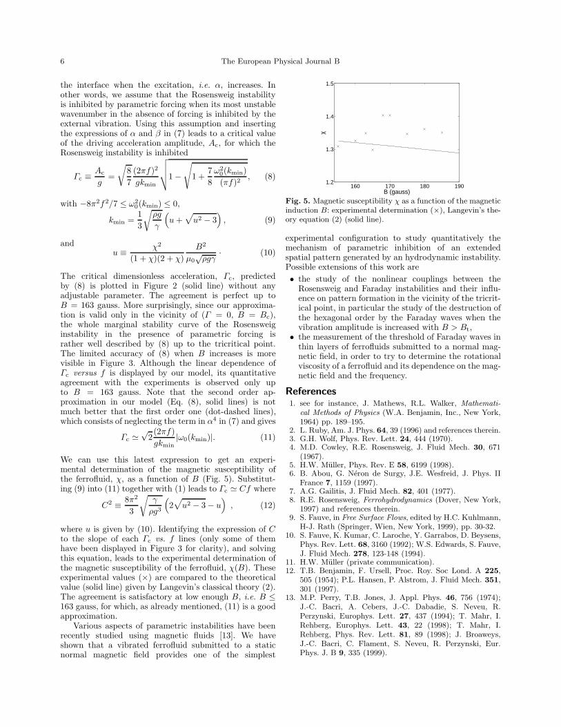
6 The European Physical Journal B
the interface when the excitation, i.e. α, increases. Inother words, we assume that the Rosensweig instabilityis inhibited by parametric forcing when its most unstablewavenumber in the absence of forcing is inhibited by theexternal vibration. Using this assumption and insertingthe expressions of α and β in (7) leads to a critical valueof the driving acceleration amplitude, Ac, for which theRosensweig instability is inhibited
Γc ≡ Ac
g=
√87
(2πf)2
gkmin
√√√√1−√
1 +78ω2
0(kmin)(πf)2
, (8)
with −8π2f2/7 ≤ ω20(kmin) ≤ 0,
kmin =13
√ρg
γ
(u+
√u2 − 3
), (9)
andu ≡ χ2
(1 + χ)(2 + χ)B2
µ0√ρgγ· (10)
The critical dimensionless acceleration, Γc, predictedby (8) is plotted in Figure 2 (solid line) without anyadjustable parameter. The agreement is perfect up toB = 163 gauss. More surprisingly, since our approxima-tion is valid only in the vicinity of (Γ = 0, B = Bc),the whole marginal stability curve of the Rosensweiginstability in the presence of parametric forcing israther well described by (8) up to the tricritical point.The limited accuracy of (8) when B increases is morevisible in Figure 3. Although the linear dependence ofΓc versus f is displayed by our model, its quantitativeagreement with the experiments is observed only upto B = 163 gauss. Note that the second order ap-proximation in our model (Eq. (8), solid lines) is notmuch better that the first order one (dot-dashed lines),which consists of neglecting the term in α4 in (7) and gives
Γc '√
2(2πf)gkmin
|ω0(kmin)|. (11)
We can use this latest expression to get an experi-mental determination of the magnetic susceptibility ofthe ferrofluid, χ, as a function of B (Fig. 5). Substitut-ing (9) into (11) together with (1) leads to Γc ' Cf where
C2 ≡ 8π2
3
√γ
ρg3
(2√u2 − 3− u
), (12)
where u is given by (10). Identifying the expression of Cto the slope of each Γc vs. f lines (only some of themhave been displayed in Figure 3 for clarity), and solvingthis equation, leads to the experimental determination ofthe magnetic susceptibility of the ferrofluid, χ(B). Theseexperimental values (×) are compared to the theoreticalvalue (solid line) given by Langevin’s classical theory (2).The agreement is satisfactory at low enough B, i.e. B ≤163 gauss, for which, as already mentioned, (11) is a goodapproximation.
Various aspects of parametric instabilities have beenrecently studied using magnetic fluids [13]. We haveshown that a vibrated ferrofluid submitted to a staticnormal magnetic field provides one of the simplest
160 170 180 1901.2
1.3
1.4
1.5
B (gauss)
χ
Fig. 5. Magnetic susceptibility χ as a function of the magneticinduction B: experimental determination (×), Langevin’s the-ory equation (2) (solid line).
experimental configuration to study quantitatively themechanism of parametric inhibition of an extendedspatial pattern generated by an hydrodynamic instability.Possible extensions of this work are• the study of the nonlinear couplings between the
Rosensweig and Faraday instabilities and their influ-ence on pattern formation in the vicinity of the tricrit-ical point, in particular the study of the destruction ofthe hexagonal order by the Faraday waves when thevibration amplitude is increased with B > Bt,• the measurement of the threshold of Faraday waves in
thin layers of ferrofluids submitted to a normal mag-netic field, in order to try to determine the rotationalviscosity of a ferrofluid and its dependence on the mag-netic field and the frequency.
References1. see for instance, J. Mathews, R.L. Walker, Mathemati-
cal Methods of Physics (W.A. Benjamin, Inc., New York,1964) pp. 189–195.
2. L. Ruby, Am. J. Phys. 64, 39 (1996) and references therein.3. G.H. Wolf, Phys. Rev. Lett. 24, 444 (1970).4. M.D. Cowley, R.E. Rosensweig, J. Fluid Mech. 30, 671
(1967).5. H.W. Muller, Phys. Rev. E 58, 6199 (1998).6. B. Abou, G. Neron de Surgy, J.E. Wesfreid, J. Phys. II
France 7, 1159 (1997).7. A.G. Gailitis, J. Fluid Mech. 82, 401 (1977).8. R.E. Rosensweig, Ferrohydrodynamics (Dover, New York,
1997) and references therein.9. S. Fauve, in Free Surface Flows, edited by H.C. Kuhlmann,
H-J. Rath (Springer, Wien, New York, 1999), pp. 30-32.10. S. Fauve, K. Kumar, C. Laroche, Y. Garrabos, D. Beysens,
Phys. Rev. Lett. 68, 3160 (1992); W.S. Edwards, S. Fauve,J. Fluid Mech. 278, 123-148 (1994).
11. H.W. Muller (private communication).12. T.B. Benjamin, F. Ursell, Proc. Roy. Soc Lond. A 225,
505 (1954); P.L. Hansen, P. Alstrom, J. Fluid Mech. 351,301 (1997).
13. M.P. Perry, T.B. Jones, J. Appl. Phys. 46, 756 (1974);J.-C. Bacri, A. Cebers, J.-C. Dabadie, S. Neveu, R.Perzynski, Europhys. Lett. 27, 437 (1994); T. Mahr, I.Rehberg, Europhys. Lett. 43, 22 (1998); T. Mahr, I.Rehberg, Phys. Rev. Lett. 81, 89 (1998); J. Broaweys,J.-C. Bacri, C. Flament, S. Neveu, R. Perzynski, Eur.Phys. J. B 9, 335 (1999).

123

124

Annexes - Milieux Granulaires
125


127

128

Chapitre C
Conduction electrique dans les milieuxgranulaires
C.1 Resume synthetique des travaux
Introduction
Les phenomenes de transport electrique dans les milieux granulaires sont peu etudies bienqu’ils constituent d’anciens problemes. En 1890, Edouard Branly decouvre la transition deconduction electrique (isolant – conducteur) d’une poudre metallique oxydee lorsqu’une ondeelectromagnetique est emise dans son voisinage. Bien que ce phenomene fut a l’origine despremieres transmissions radio sans fils vers 1900, il reste depuis lors partiellement incompris.Une transition similaire est aussi observee lorsqu’une source electrique continue est directe-ment appliquee a l’echantillon et depasse un certain seuil. Des fluctuations de sa resistanceapparaıssent aussi au cours du temps sous certaines conditions. Nous nous proposons ici decomprendre ces phenomenes de transport electrique dans les milieux granulaires en nous ba-sant sur une experience modele avec une chaıne de billes, puis avec un reseau bidimensionnelde billes, et enfin avec de la poudre metallique. Nous chercherons a demeler les effets locaux(contacts entre grains) des effets collectifs (tel le desordre typique d’un granulaire) respon-sables de ces phenomenes. La comprehension de ses phenomenes permettrait a terme d’utiliserla conductivite electrique comme une sonde pour connaıtre la rheologie des milieux granu-laires.
La conduction electrique dans les milieux granulaires metalliques est un probleme com-plexe dependant d’un nombre important de parametres globaux relatifs a l’assemblee degrains (distribution de forme, de taille, de pression, ...), et locaux relatifs au contact entredeux grains (degre d’oxydation, etat de surface, rugosite ...). Certains de ces parametres ap-paraissent comme des contributions secondaires : par exemple, la percolation ne peut pasetre evoquee pour expliquer la transition de conduction puisque Branly l’avait aussi ob-serve pour un contact unique entre deux grains. De meme, l’action a distance de l’etincelleelectromagnetique peut etre dans une premiere etape remplacee par l’application directe d’unesource electrique bien controlable au milieu granulaire. Dans une premiere etape, nous avonsdonc reduit deliberement le nombre de parametres, sans perdre en generalite. Ces travauxsont rapidement decrits ci-dessous. Pour plus de details, nous renvoyons le lecteur aux publi-cations ci-jointes.
129

PVC
Computer
Forc
e
U, I, R
0 x
For
cese
nsor
+-
Displac
emen
t
Stepper Motor 1 N
F < 500 N
I
Fig. C.1: Schema de l’experience pour l’etude de la conduction electrique d’une chaıne debilles. 1 ≤ N ≤ 40 billes en acier de 8 mm de diametre. Un courant I est applique et latension U ou la resistance R=U/I est mesuree pour une contrainte appliquee F < 500 N.
0 0.2 0.4 0.6 0.8 10
1
2
3
4
5
6Usat
I (A)
U (
V)
0 2 40
2
4
6Usat
Umax
I * R2 (V)
U (
V)
R1
~ 1
0 kΩ
R2 ~ few Ω
retu
rn retu
rn
forw
ard
saturation
Imax
F = 56 NF = 100 NF = 220 N
Metal
R1 ~ 104 Ω R2 ~ fews Ω
I Oxide film
Metal
Apparentcontat area
Electricalcontact area
Microcontact
Weldedmicrocontact
Low current I High current I
Fig. C.2: A gauche : Caracteristique U - I pour une chaıne de 14 billes montrant la transitionde conduction, la tension de saturation a partir de laquelle les microcontacts entre billesse soudent, et, en encart, les trajectoires de retours bien decrites par un modele electro-thermique. A droite : Vue schematique de la creation de ponts metalliques due a la soudurelocale des microcontacts.
De « l’effet Branly » a l’intermittence
Dans un premier temps, nous avons etudie le transport electrique dans une chaıne debilles metalliques directement soumise a une source electrique continue (voir Fig. C.1). Lescontacts entre billes ne sont pas metalliques du fait de la presence d’un film isolant (oxydeou contaminant) a leur surface. Nous observons une transition d’un etat isolant a un etatconducteur lorsque le courant applique augmente. Les caracteristiques tension – courant (U- I) sont symetriques avec une partie ohmique reversible suivie par une partie non lineaireirreversible saturant a une tension critique de l’ordre de 0.4 V par contact (voir Fig. C.2).Nous montrons, pour la premiere fois, que cette transition de conduction ou « effet Branlycontinu » resulte de l’echauffement local des microcontacts entre chaque bille jusqu’a l’ap-parition de microsoudures : l’ecoulement des lignes de courant a travers ces petites zonesengendre leur echauffement local qui conduit a une augmentation de leurs aires de contact,et donc de leur conduction. Des temperatures de l’ordre de 1000o C s’y etablissent, allantjusqu’a la fusion des microcontacts, meme pour une tension appliquee aussi faible que 0.4 V.Basee sur un mecanisme de temperature et de tension auto-regulee, une expression analy-
130
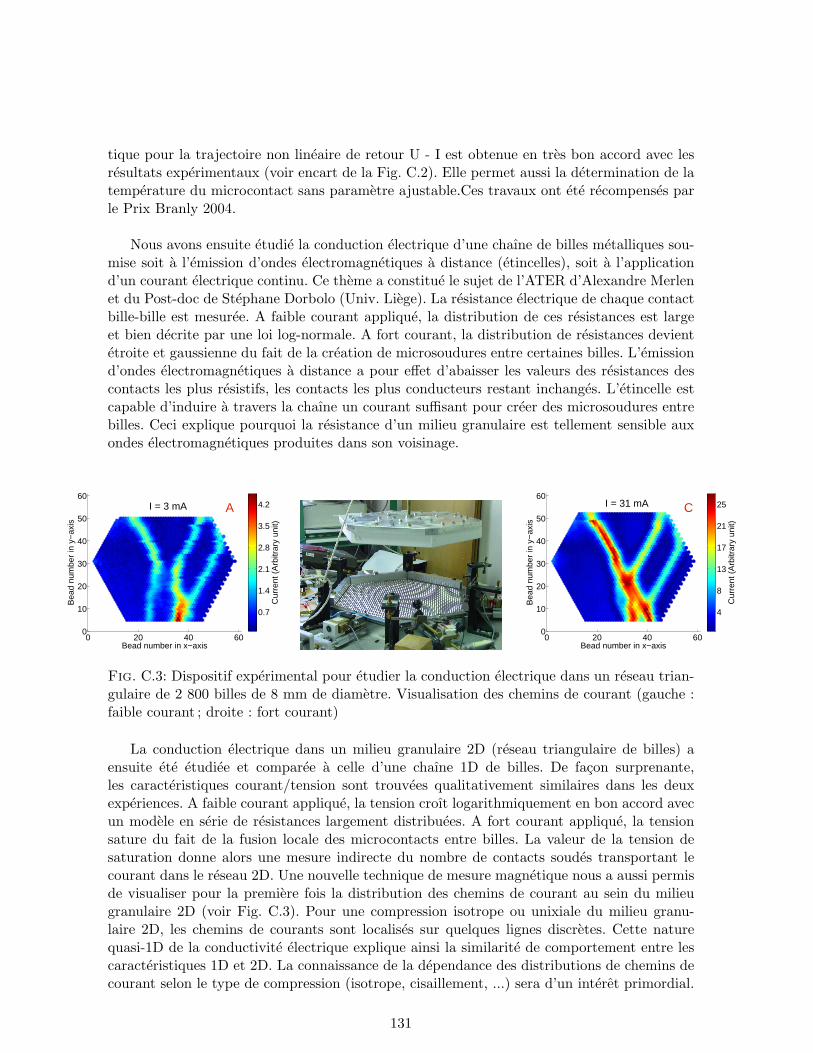
tique pour la trajectoire non lineaire de retour U - I est obtenue en tres bon accord avec lesresultats experimentaux (voir encart de la Fig. C.2). Elle permet aussi la determination de latemperature du microcontact sans parametre ajustable.Ces travaux ont ete recompenses parle Prix Branly 2004.
Nous avons ensuite etudie la conduction electrique d’une chaıne de billes metalliques sou-mise soit a l’emission d’ondes electromagnetiques a distance (etincelles), soit a l’applicationd’un courant electrique continu. Ce theme a constitue le sujet de l’ATER d’Alexandre Merlenet du Post-doc de Stephane Dorbolo (Univ. Liege). La resistance electrique de chaque contactbille-bille est mesuree. A faible courant applique, la distribution de ces resistances est largeet bien decrite par une loi log-normale. A fort courant, la distribution de resistances devientetroite et gaussienne du fait de la creation de microsoudures entre certaines billes. L’emissiond’ondes electromagnetiques a distance a pour effet d’abaisser les valeurs des resistances descontacts les plus resistifs, les contacts les plus conducteurs restant inchanges. L’etincelle estcapable d’induire a travers la chaıne un courant suffisant pour creer des microsoudures entrebilles. Ceci explique pourquoi la resistance d’un milieu granulaire est tellement sensible auxondes electromagnetiques produites dans son voisinage.
0 20 40 600
10
20
30
40
50
60
Bead number in x−axis
Bea
d nu
mbe
r in
y−
axis
AI = 3 mA
Cur
rent
(A
rbitr
ary
unit)
0.7
1.4
2.1
2.8
3.5
4.2
0 20 40 600
10
20
30
40
50
60
Bead number in x−axis
Bea
d nu
mbe
r in
y−
axis
I = 31 mA C
Cur
rent
(A
rbitr
ary
unit)
4
8
13
17
21
25
Fig. C.3: Dispositif experimental pour etudier la conduction electrique dans un reseau trian-gulaire de 2 800 billes de 8 mm de diametre. Visualisation des chemins de courant (gauche :faible courant ; droite : fort courant)
La conduction electrique dans un milieu granulaire 2D (reseau triangulaire de billes) aensuite ete etudiee et comparee a celle d’une chaıne 1D de billes. De facon surprenante,les caracteristiques courant/tension sont trouvees qualitativement similaires dans les deuxexperiences. A faible courant applique, la tension croıt logarithmiquement en bon accord avecun modele en serie de resistances largement distribuees. A fort courant applique, la tensionsature du fait de la fusion locale des microcontacts entre billes. La valeur de la tension desaturation donne alors une mesure indirecte du nombre de contacts soudes transportant lecourant dans le reseau 2D. Une nouvelle technique de mesure magnetique nous a aussi permisde visualiser pour la premiere fois la distribution des chemins de courant au sein du milieugranulaire 2D (voir Fig. C.3). Pour une compression isotrope ou unixiale du milieu granu-laire 2D, les chemins de courants sont localises sur quelques lignes discretes. Cette naturequasi-1D de la conductivite electrique explique ainsi la similarite de comportement entre lescaracteristiques 1D et 2D. La connaissance de la dependance des distributions de chemins decourant selon le type de compression (isotrope, cisaillement, ...) sera d’un interet primordial.
131

3.9 4 4.1 4.2 4.3-3
-2
-1
Time (s)
I -
< I
> (
µA)
Fig. C.4: A gauche : Schema du dispositif experimental pour l’etude de la conductionelectrique d’une poudre metallique (500 000 particules de cuivre de 100 µm). A droite : Bruitde courant dans de la poudre de cuivre sous une tension appliquee de l’ordre du Volt.
10-4
10-2
100
102
104
10-13
10-10
10-7
10-4
Frequency (Hz)
Pow
er s
pect
rum
(m
A2
/ Hz
)
-10 -5 0 5 1010
-6
10-5
10-4
10-3
10-2
10-1
100
δ Iτ / σ
PD
F(δ
I τ / σ)
τ = 0.00036 sτ = 0.021 sτ = 7.3 sGaussian
Fig. C.5: A gauche : Spectre de puissance de ces fluctuations de courant de la Fig. C.3montrant une invariance d’echelle sur plus de 4 decades en frequence. A droite : Fonction dedensite de probabilite (PDF) des increments de courant montrant l’intermittence de ce bruit,pour differentes echelles de temps testees.
Nous avons ensuite etudie la conduction electrique dans une poudre metallique (voir Fig.C.4). Ce theme a constitue le sujet de la these de Mathieu Creyssels de 2003 a 2006. Unechantillon de poudre de cuivre presente une resistance electrique elevee (1 MΩ) due a lacouche d’oxyde presente sur les grains (diametre moyen 100 µm). Nous observons que sescaracteristiques courants–tensions sont non lineaires, et une instabilite apparaıt, d’un etatisolant vers un etat conducteur, a relativement faible tension appliquee. Nous montrons que leseuil de la transition correspond toujours a la meme puissance dissipee de l’ordre de 10−4 Wquelle que soit la contrainte appliquee, suggerant ainsi une instabilite thermique de faconcoherente avec l’experience 1D ci-dessus, mais de facon plus complexe. Les dilatations degrains engendrees sont alors estimees a quelque 10 nm. Des fluctuations temporelles sont deplus observees (voir Fig. C.5), et sont alors caracterisees avec les outils developpes en tur-bulence hydrodynamique. Nous montrons alors que ces fluctuations possedent d’interessantesproprietes d’invariance d’echelle (sur 4 decades en temps - voir Fig. C.5) et d’intermittence
132
(voir Fig. C.5). Cette intermittence et les fluctuations de courant associees proviennent dedilatations thermiques creant ou detruisant localement les contacts electriques a toutes lesechelles spatiales (de la taille du grain a la taille de l’echantillon). Ces etonnants phenomenesd’auto-similarite sont ainsi relies aux effets collectifs de la matiere granulaire.
Nous avons entrepris par la suite la mesure de la resistance et de la capacite electriqued’une poudre metallique en regime alternatif AC. Quelle que soit la valeur de la pressionmecanique appliquee a la poudre, les courbes de resistance en fonction de la frequence seplacent sur une courbe maıtresse apres une remise a l’echelle appropriee. La meme proprieteest observee pour la capacite. Un modele 1D montre que la forte dependance frequentiellede la resistance et de la capacite macroscopique de l’echantillon est une consequence de ladistribution large des resistances de contacts entre grains. Aucun modele de conduction mi-croscopique, ni aucun parametre lie au desordre du milieu granulaire n’est suppose. Ce modelesimple permettrait aussi d’expliquer la dependance frequentielle universelle de la conducti-vite (“Universal Dielectric Response”) d’autres systemes heterogenes (melanges aleatoires deconducteurs et d’isolants, composes de polymeres).
Lors de mon premier post-doc en 1998 au Laboratoire de la Physique de la MatiereCondensee a l’ENS Paris, nous avions deja ete confrontes au role des microcontacts a la sur-face d’un solide. Nous avions etudie le frottement entre deux solides macroscopiques, rugueuxa l’echelle du micron, formant une interface multicontacts, c.-a-d. discontinue et constitueed’une population dispersee de contacts. Ce travail a ete entrepris afin de mieux comprendreles phenomenes physiques qui sont a l’origine de la dissipation d’energie dans un contact nonlubrifie, notamment le role de l’elasticite des microcontacts et leurs ruptures dans le processusdissipatif qu’est le frottement. Nous avions mis au point un montage experimental ayant pourobjet de caracteriser la reponse d’une interface solide-solide a une contrainte de cisaillementcyclique, entre l’etat de repos et le glissement macroscopique des deux corps en contact. Cedispositif permet de mesurer les deplacements, inferieurs au micron, d’un patin pose sur unepiste et sollicite par une force tangentielle cyclique dont l’amplitude reste inferieure a la forcenecessaire a sa mise en glissement macroscopique. La mesure des deplacements du patin parrapport a la piste permet d’acceder d’une part a la composante elastique de la reponse enphase avec l’excitation, et d’autre part a la composante dissipative en quadrature avec l’exci-tation. Les resultats obtenus mettent en evidence la reponse elastique, lineaire et non lineaire,des microcontacts de l’interface, ainsi que la dissipation d’energie, pour differentes frequenceset amplitudes maximales de la force de cisaillement. L’analyse spectrale de la reponse dupatin a un bruit blanc a mis en evidence un pic de resonance correspondant a la resonancedu systeme consistue du patin et des microcontacts de taille micrometrique.
133

C.2 Publications associees
Articles
M. Creyssels, E. Falcon & B. Castaing, Physical Review B 77, 075135 (2008)Scaling of AC electrical conductivity of powders under compression
M. Creyssels, S. Dorbolo, A. Merlen, C. Laroche, B. Castaing & E. Falcon, European PhysicalJournal E 23, 255 (2007)Some aspects of electrical conduction in granular systems of various dimensions
S. Dorbolo, A. Merlen, M. Creyssels, N. Vandewalle, B. Castaing & E. Falcon, EPL 79, 54001(2007)Effects of electromagnetic waves on the electrical properties of contacts between grains
E. Falcon, & B. Castaing, American Journal of Physics 73, 302–307 (2005)Electrical conductivity in granular media and Branly’s coheror : A simple experiment
E. Falcon, B. Castaing & C. Laroche, Europhysics Letters 65, 186–192 (2004)“Turbulent” electrical transport in Copper powders
E. Falcon, B. Castaing & M. Creyssels, European Physical Journal B 38, 475–483 (2004)Nonlinear electrical conductivity in a 1D granular medium
T. Baumberger, L. Bureau, M. Busson, E. Falcon, & B. Perrin, Review of Scientific Instruments69, 2416–2420 (1998)An inertial tribometer for measuring micro-slip dissipation at a solid-solid multicontact interface
Revues
E. Falcon, & B. Castaing, Bulletin de la Societe Francaise de Physique 148, 9 - 12 (2005)Proprietes electriques de la matiere granulaire : « L’effet Branly continu »
E. Falcon, B. Castaing & M. Creyssels, Bulletin de la Societe Francaise de Physique 149, 6 - 9(2005)Proprietes electriques de la matiere granulaire : Bruit et intermittence
Actes de conferences
E. Falcon & B. Castaing, in Powders & Grains 2005, R.Garcıa-Rojo, H.J. Herrmann & S.McNamara, Eds. A.A.Balkema, Rotterdam, pp. 323 - 327 (2005)Electrical properties of granular matter : From “Branly effect” to intermittency
M. Creyssels, E. Falcon, & B. Castaing, 8e Rencontre du Non-Lineaire Paris 2005, Non-LineairePub., Orsay, p. 55-60 (2005)
134

Bruit et intermittence du transport electrique dans les milieux granulaires
E. Falcon, B. Castaing & M. Creyssels, 7e Rencontre du Non-Lineaire Paris 2004, Non-LineairePub., Orsay, p. 97–102, (2004)Transport electrique non lineaire dans les milieux granulaires 1D
Articles de vulgarisation
E. Falcon & B. Castaing, Pour La Science 340, 58 - 64 (Fevrier 2006)L’effet Branly livre ses secrets
E. Falcon & M. Creyssels, Interview televisee, enregistree et diffusee lors de l’Exposition sur leCentenaire de la decouverte d’Edouard Branly, le 30 Juin 2005 au Musee de la Marine, Tro-cadero, Paris
135

136

C.3 Tires a part
137

138
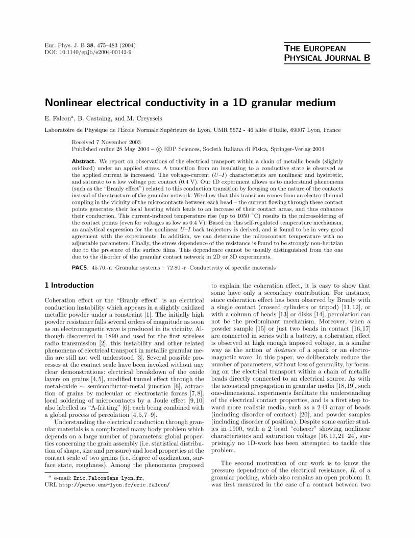
Eur. Phys. J. B 38, 475–483 (2004)DOI: 10.1140/epjb/e2004-00142-9 THE EUROPEAN
PHYSICAL JOURNAL B
Nonlinear electrical conductivity in a 1D granular medium
E. Falcona, B. Castaing, and M. Creyssels
Laboratoire de Physique de l’Ecole Normale Superieure de Lyon, UMR 5672 - 46 allee d’Italie, 69007 Lyon, France
Received 7 November 2003Published online 28 May 2004 – c© EDP Sciences, Societa Italiana di Fisica, Springer-Verlag 2004
Abstract. We report on observations of the electrical transport within a chain of metallic beads (slightlyoxidized) under an applied stress. A transition from an insulating to a conductive state is observed asthe applied current is increased. The voltage-current (U–I) characteristics are nonlinear and hysteretic,and saturate to a low voltage per contact (0.4 V). Our 1D experiment allows us to understand phenomena(such as the “Branly effect”) related to this conduction transition by focusing on the nature of the contactsinstead of the structure of the granular network. We show that this transition comes from an electro-thermalcoupling in the vicinity of the microcontacts between each bead – the current flowing through these contactpoints generates their local heating which leads to an increase of their contact areas, and thus enhancestheir conduction. This current-induced temperature rise (up to 1050 C) results in the microsoldering ofthe contact points (even for voltages as low as 0.4 V). Based on this self-regulated temperature mechanism,an analytical expression for the nonlinear U–I back trajectory is derived, and is found to be in very goodagreement with the experiments. In addition, we can determine the microcontact temperature with noadjustable parameters. Finally, the stress dependence of the resistance is found to be strongly non-hertziandue to the presence of the surface films. This dependence cannot be usually distinguished from the onedue to the disorder of the granular contact network in 2D or 3D experiments.
PACS. 45.70.-n Granular systems – 72.80.-r Conductivity of specific materials
1 Introduction
Coheration effect or the “Branly effect” is an electricalconduction instability which appears in a slightly oxidizedmetallic powder under a constraint [1]. The initially highpowder resistance falls several orders of magnitude as soonas an electromagnetic wave is produced in its vicinity. Al-though discovered in 1890 and used for the first wirelessradio transmission [2], this instability and other relatedphenomena of electrical transport in metallic granular me-dia are still not well understood [3]. Several possible pro-cesses at the contact scale have been invoked without anyclear demonstrations: electrical breakdown of the oxidelayers on grains [4,5], modified tunnel effect through themetal-oxide ∼ semiconductor-metal junction [6], attrac-tion of grains by molecular or electrostatic forces [7,8],local soldering of microcontacts by a Joule effect [9,10]also labelled as “A-fritting” [6]; each being combined witha global process of percolation [4,5,7–9].
Understanding the electrical conduction through gran-ular materials is a complicated many body problem whichdepends on a large number of parameters: global proper-ties concerning the grain assembly (i.e. statistical distribu-tion of shape, size and pressure) and local properties at thecontact scale of two grains (i.e. degree of oxidization, sur-face state, roughness). Among the phenomena proposed
a e-mail: [email protected],URL http://perso.ens-lyon.fr/eric.falcon/
to explain the coheration effect, it is easy to show thatsome have only a secondary contribution. For instance,since coheration effect has been observed by Branly witha single contact (crossed cylinders or tripod) [11,12], orwith a column of beads [13] or disks [14], percolation cannot be the predominant mechanism. Moreover, when apowder sample [15] or just two beads in contact [16,17]are connected in series with a battery, a coheration effectis observed at high enough imposed voltage, in a similarway as the action at distance of a spark or an electro-magnetic wave. In this paper, we deliberately reduce thenumber of parameters, without loss of generality, by focus-ing on the electrical transport within a chain of metallicbeads directly connected to an electrical source. As withthe acoustical propagation in granular media [18,19], suchone-dimensional experiments facilitate the understandingof the electrical contact properties, and is a first step to-ward more realistic media, such as a 2-D array of beads(including disorder of contact) [20], and powder samples(including disorder of position). Despite some earlier stud-ies in 1900, with a 2 bead “coherer” showing nonlinearcharacteristics and saturation voltage [16,17,21–24], sur-prisingly no 1D-work has been attempted to tackle thisproblem.
The second motivation of our work is to know thepressure dependence of the electrical resistance, R, of agranular packing, which also remains an open problem. Itwas first measured in the case of a contact between two

476 The European Physical Journal B
conductors, submitted to a force, F , in order to determinethe real area of contact [25]. Indeed, careful attentionwas paid to initially break any oxide layers at the sur-face [25], or to work with noble metals [26], or specificsurface coatings [27] in order to get reproducible resultswhich follow; R ∼ 1/F 1/3, in agreement with the elasticHertz law. However, when superficial oxide and/or impu-rity layers are present, this scaling is found again to be apower law but with an exponent greater than 1. This hasbeen observed in a 3D packing of steel beads [28,29] un-der weak (elastic) compression, or for strongly compressedpowders [30]. This anomalous exponent is ascribed eitherto a superficial contaminant film [28,29], or a combinaisonof a contaminant film and the degree of contact disorderin the packing [28]. Here again, a 1D experiment shouldallow to answer if this exponent is driven by contact prop-erties since the effect of contact disorder is absent.
2 Experimental setup
The experimental setup is sketched in Figure 1. It consistsof a chain of 50 identical stainless-steel beads, each 8 mmin diameter, with a tolerance of 4 µm on diameter,and 2 µm on sphericity [31]. The physical properties ofthe beads are summarized in Table 1. The beads aresurrounded by an insulating framework of polyvinylchlo-ride (PVC). It consists of two parts, each one 30 mm high,40 mm wide and 400 mm long, with a straight channelhaving a squared section with 8.02 mm sides milled inthe lower part to contain the beads. A very small clear-ance of 2/100 mm is provided in the channel, so thatthe beads move freely along the chain axis but not inthe perpendicular direction. A static force F is appliedto the chain of beads by means of a piston (8 mm diam-eter duralumin cylinder), and is measured with a staticforce sensor (FGP Instr. 1054) with a 6.1 mV/N sensitiv-ity in the range from 1 to 500 N. A 1.8 degree steppermotor (RS 440-442) fitted to a gearhead (gear ratio 25:1)is linked to an endless screw, with a 1 mm thread, in or-der to axially move the piston and the force sensor witha 0.2 µm/step precision. The number of motor steps ismeasured with a counter (Schlumberger 2721) to deter-mine the piston displacement necessary to reach a spe-cific force. Electrical contacts between the chain and theelectrical source are made by soldering leads on particularbeads, and the measurements are performed in a four-wireconfiguration. Note that the lowest resistance of the wholechain (about 3 Ω) is always found much higher than theelectrode or the stainless steel bulk material. The beadnumber N between both electrodes is varied from 1 to 41by moving the electrode beads within the chain. DC volt-age (resp. current) source is supplied to the chain by asource meter (Keithley K2400) which also gives a mea-sure of the current (resp. voltage). The maximum poweroutput is 22 W (210 V at 0.105 A or 21 V at 1.05 A).During a typical experiment, we chose to supply the cur-rent (10−6 ≤ I ≤ 1 A) and to simultaneously measure thevoltage V and the resistance R. The current is suppliedduring a short time (1 s) in order to avoid possible Jouleheating of continuous measurements. We note that similar
Fig. 1. Schematics of experimental setup.
Table 1. Relevant mechanical and electrical properties ofstainless steel beads used in the chain (norms: AISI 420C,AFNOR Z40C13, grade IV) [31] or for another stainless steeltype (AISI 304) [32].
Signification Value
r Bead radius 4 mm± 2 µm [31]Ra Roughness 0.1–0.2 µm [31]ρ Density 7750 kg/m3 [31]ν Poisson’s ratio 0.27E Young’s modulus 1.95 × 10¹¹ N/m2 [32]ρel Electrical resistivity 20 C 72 µΩ cm [32]
650 C 116 µΩcm [32]λ Thermal conductivity 20 C 16.2 W/(Km) [32]
500 C 21.5 W/(Km) [32]Tmel Approx. melting point 1425 C [32]
results have been found when repeating experiments withimposing the voltage (10−2 ≤ U ≤ 2 × 10² V) and mea-suring current and resistance. The results reported hereare highly reproducible.
3 Mechanical behaviour
The relation between the force F applied on two identicalspheres and the distance of approach δ of their centersis given by linear elasticity through the so-called Hertzlaw [33],
F =E√
2r
3(1− ν2)δ3/2, (1)
and the “apparent” radius of the circular contact by [33]
A =[3(1− ν2)
4ErF
]1/3
, (2)
E being the Young’s modulus, ν the Poisson’s ratioand r the radius of the beads. For stainless steel beadsused in the chain (see bead properties in Tab. 1), when Franges from 10 to 500 N, equation (1) leads to a rangeof deformations δ between two beads from 2 to 20 µm,and equation (2) to a range of the contact radii A from 40to 200 µm.
Figure 2 shows the total chain displacement δtot as afunction of F . As expected, there is good agreement withthe F 2/3 Hertz law for our range of F . The departure atlow F is linked to the fact that δtot includes the pistondisplacement x0, needed to bring all the beads in contact,
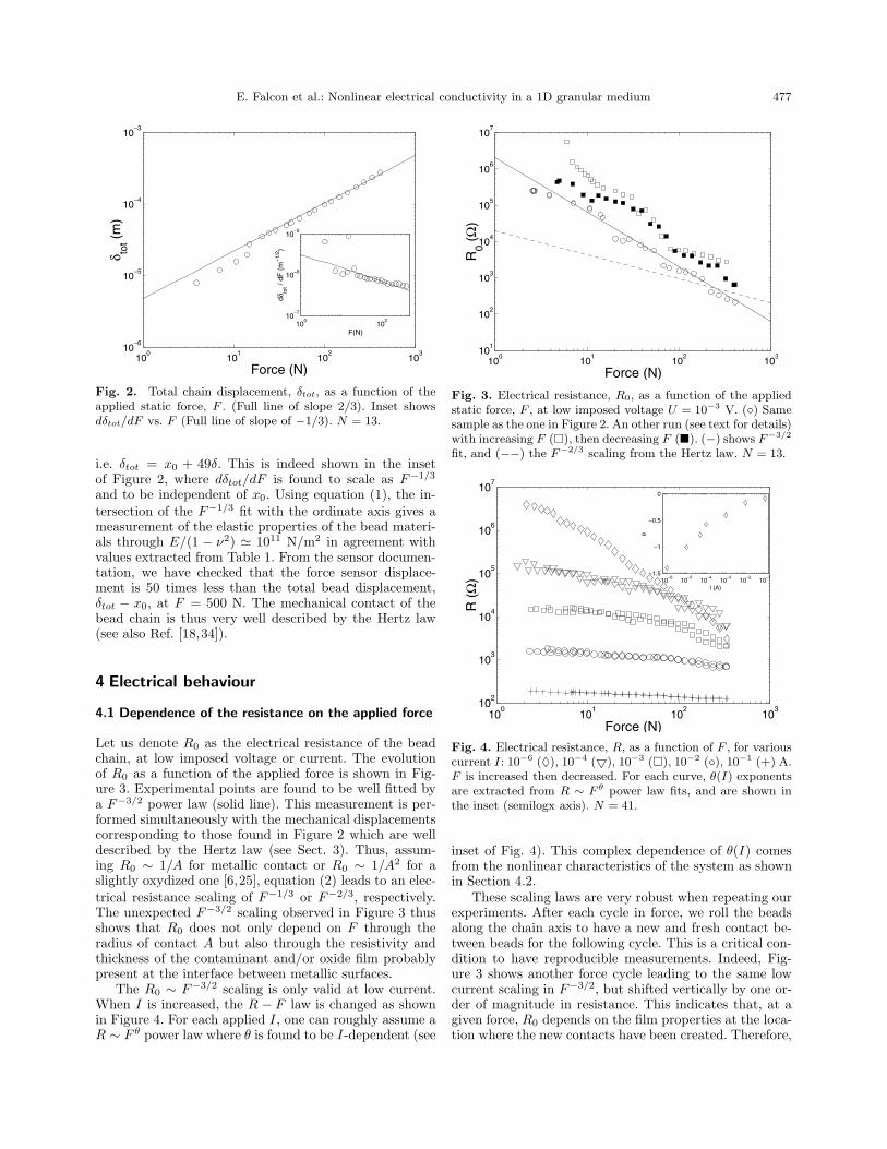
E. Falcon et al.: Nonlinear electrical conductivity in a 1D granular medium 477
100
101
102
103
10−6
10−5
10−4
10−3
Force (N)
δ tot (
m)
100
102
10−7
10−6
10−5
F(N)
dδto
t / dF
(m
−1/
2 )
Fig. 2. Total chain displacement, δtot, as a function of theapplied static force, F . (Full line of slope 2/3). Inset showsdδtot/dF vs. F (Full line of slope of −1/3). N = 13.
i.e. δtot = x0 + 49δ. This is indeed shown in the insetof Figure 2, where dδtot/dF is found to scale as F−1/3
and to be independent of x0. Using equation (1), the in-tersection of the F−1/3 fit with the ordinate axis gives ameasurement of the elastic properties of the bead materi-als through E/(1 − ν2) 1011 N/m2 in agreement withvalues extracted from Table 1. From the sensor documen-tation, we have checked that the force sensor displace-ment is 50 times less than the total bead displacement,δtot − x0, at F = 500 N. The mechanical contact of thebead chain is thus very well described by the Hertz law(see also Ref. [18,34]).
4 Electrical behaviour
4.1 Dependence of the resistance on the applied force
Let us denote R0 as the electrical resistance of the beadchain, at low imposed voltage or current. The evolutionof R0 as a function of the applied force is shown in Fig-ure 3. Experimental points are found to be well fitted bya F−3/2 power law (solid line). This measurement is per-formed simultaneously with the mechanical displacementscorresponding to those found in Figure 2 which are welldescribed by the Hertz law (see Sect. 3). Thus, assum-ing R0 ∼ 1/A for metallic contact or R0 ∼ 1/A2 for aslightly oxydized one [6,25], equation (2) leads to an elec-trical resistance scaling of F−1/3 or F−2/3, respectively.The unexpected F−3/2 scaling observed in Figure 3 thusshows that R0 does not only depend on F through theradius of contact A but also through the resistivity andthickness of the contaminant and/or oxide film probablypresent at the interface between metallic surfaces.
The R0 ∼ F−3/2 scaling is only valid at low current.When I is increased, the R − F law is changed as shownin Figure 4. For each applied I, one can roughly assume aR ∼ F θ power law where θ is found to be I-dependent (see
100
101
102
103
101
102
103
104
105
106
107
Force (N)
R0 (
Ω)
Fig. 3. Electrical resistance, R0, as a function of the appliedstatic force, F , at low imposed voltage U = 10−3 V. () Samesample as the one in Figure 2. An other run (see text for details)with increasing F (), then decreasing F (). (−) shows F−3/2
fit, and (−−) the F−2/3 scaling from the Hertz law. N = 13.
100
101
102
103
102
103
104
105
106
107
Force (N)
R (
Ω) 10
−610
−510
−410
−310
−210
−1−1.5
−1
−0.5
0
I (A)
θ
Fig. 4. Electrical resistance, R, as a function of F , for variouscurrent I : 10−6 (♦), 10−4 (), 10−3 (), 10−2 (), 10−1 (+) A.F is increased then decreased. For each curve, θ(I) exponentsare extracted from R ∼ F θ power law fits, and are shown inthe inset (semilogx axis). N = 41.
inset of Fig. 4). This complex dependence of θ(I) comesfrom the nonlinear characteristics of the system as shownin Section 4.2.
These scaling laws are very robust when repeating ourexperiments. After each cycle in force, we roll the beadsalong the chain axis to have a new and fresh contact be-tween beads for the following cycle. This is a critical con-dition to have reproducible measurements. Indeed, Fig-ure 3 shows another force cycle leading to the same lowcurrent scaling in F−3/2, but shifted vertically by one or-der of magnitude in resistance. This indicates that, at agiven force, R0 depends on the film properties at the loca-tion where the new contacts have been created. Therefore,
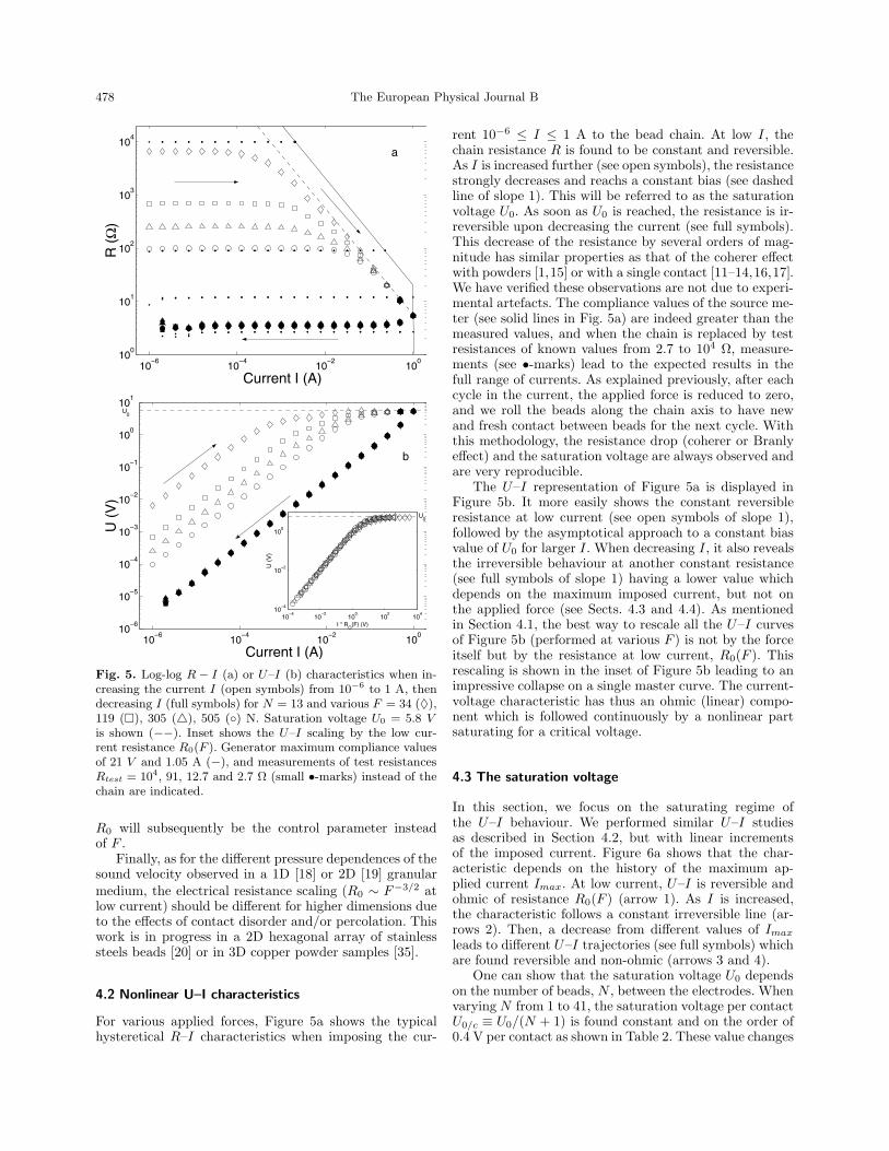
478 The European Physical Journal B
10−6
10−4
10−2
100
100
101
102
103
104
Current I (A)
R (
Ω)
a
10−6
10−4
10−2
100
10−6
10−5
10−4
10−3
10−2
10−1
100
101
U0
Current I (A)
U (
V)
10−4
10−2
100
102
104
10−4
10−2
100
U0
I * RO
(F) (V)
U (
V)
b
Fig. 5. Log-log R− I (a) or U–I (b) characteristics when in-creasing the current I (open symbols) from 10−6 to 1 A, thendecreasing I (full symbols) for N = 13 and various F = 34 (♦),119 (), 305 (), 505 () N. Saturation voltage U0 = 5.8 Vis shown (−−). Inset shows the U–I scaling by the low cur-rent resistance R0(F ). Generator maximum compliance valuesof 21 V and 1.05 A (−), and measurements of test resistancesRtest = 104, 91, 12.7 and 2.7 Ω (small •-marks) instead of thechain are indicated.
R0 will subsequently be the control parameter insteadof F .
Finally, as for the different pressure dependences of thesound velocity observed in a 1D [18] or 2D [19] granularmedium, the electrical resistance scaling (R0 ∼ F−3/2 atlow current) should be different for higher dimensions dueto the effects of contact disorder and/or percolation. Thiswork is in progress in a 2D hexagonal array of stainlesssteels beads [20] or in 3D copper powder samples [35].
4.2 Nonlinear U–I characteristics
For various applied forces, Figure 5a shows the typicalhysteretical R–I characteristics when imposing the cur-
rent 10−6 ≤ I ≤ 1 A to the bead chain. At low I, thechain resistance R is found to be constant and reversible.As I is increased further (see open symbols), the resistancestrongly decreases and reachs a constant bias (see dashedline of slope 1). This will be referred to as the saturationvoltage U0. As soon as U0 is reached, the resistance is ir-reversible upon decreasing the current (see full symbols).This decrease of the resistance by several orders of mag-nitude has similar properties as that of the coherer effectwith powders [1,15] or with a single contact [11–14,16,17].We have verified these observations are not due to experi-mental artefacts. The compliance values of the source me-ter (see solid lines in Fig. 5a) are indeed greater than themeasured values, and when the chain is replaced by testresistances of known values from 2.7 to 104 Ω, measure-ments (see •-marks) lead to the expected results in thefull range of currents. As explained previously, after eachcycle in the current, the applied force is reduced to zero,and we roll the beads along the chain axis to have newand fresh contact between beads for the next cycle. Withthis methodology, the resistance drop (coherer or Branlyeffect) and the saturation voltage are always observed andare very reproducible.
The U–I representation of Figure 5a is displayed inFigure 5b. It more easily shows the constant reversibleresistance at low current (see open symbols of slope 1),followed by the asymptotical approach to a constant biasvalue of U0 for larger I. When decreasing I, it also revealsthe irreversible behaviour at another constant resistance(see full symbols of slope 1) having a lower value whichdepends on the maximum imposed current, but not onthe applied force (see Sects. 4.3 and 4.4). As mentionedin Section 4.1, the best way to rescale all the U–I curvesof Figure 5b (performed at various F ) is not by the forceitself but by the resistance at low current, R0(F ). Thisrescaling is shown in the inset of Figure 5b leading to animpressive collapse on a single master curve. The current-voltage characteristic has thus an ohmic (linear) compo-nent which is followed continuously by a nonlinear partsaturating for a critical voltage.
4.3 The saturation voltage
In this section, we focus on the saturating regime ofthe U–I behaviour. We performed similar U–I studiesas described in Section 4.2, but with linear incrementsof the imposed current. Figure 6a shows that the char-acteristic depends on the history of the maximum ap-plied current Imax. At low current, U–I is reversible andohmic of resistance R0(F ) (arrow 1). As I is increased,the characteristic follows a constant irreversible line (ar-rows 2). Then, a decrease from different values of Imax
leads to different U–I trajectories (see full symbols) whichare found reversible and non-ohmic (arrows 3 and 4).
One can show that the saturation voltage U0 dependson the number of beads, N , between the electrodes. Whenvarying N from 1 to 41, the saturation voltage per contactU0/c ≡ U0/(N + 1) is found constant and on the order of0.4 V per contact as shown in Table 2. These value changes

E. Falcon et al.: Nonlinear electrical conductivity in a 1D granular medium 479
0 0.2 0.4 0.6 0.8 10
1
2
3
4
5
6
Current I (A)
U (
V)
a
1
2
3 3 4
4
0 200 400 600 800 1000 1200 1400 16000
1
2
3
4
5
6U
0
I * RO
(F) (V)
U (
V)
10−2
100
102
0
1
2
3
4
5
6
I * RO
(F) (V)
U (
V)
b V
0
Fig. 6. (a) U–I characteristics (in linear axes) showing thesaturation voltage, U0 = 5.8 V, when increasing the current Iin the range 1 mA ≤ I ≤ Imax (open symbols), then decreas-ing I (full symbols) for various F = 32 (), 125 (), 321 ()and 505 (♦) N with Imax = 1 A, and for F = 211 N () withImax = 0.5 A. Measurement of test resistance Rtest = 2.7 Ω(small •-marks) instead of the chain. (b) Same open symbolsas (a) rescaled by R0(F ) in linear or semilogx axes (inset). Ad-ditional F = 13 N () is shown. Solid line show empirical fitof Guthe [17]. N = 13.
when replacing all stainless steel beads with others of an-other material, U0/c 0.2 V for bronze beads and 0.3 Vfor brass beads (see Tab. 2). Therefore, U0/c dependsslightly on the bead material (see also Refs. [16,17,22]),but does not depend on the bead radius [16] nor on thegas surrounding the beads [22,24]. Moreover, the non-linear saturation bias U0 does not depend explicitly onthe force F . This means that when the previous charac-teristics obtained for different F are rescaled by R0(F ),all U–I curves collapse as shown in Figure 6b on lin-ear or semilog (see inset of Fig. 6b) axes. This satura-tion bias was first observed in 1901 by Guthe [17] fortwo beads in contact. He suggested an empirical fit of
Table 2. Saturation voltage, U0, for various bead numbers, N ,in the chain and for different bead materials. Nc ≡ (N + 1) isthe number of bead-bead contacts.
Materials Nc U0 (V) U0/Nc (V)
Stainless Steel 02 0.75 0.37
Stainless Steel 14 5.8 0.41
Stainless Steel 42 16.5 0.39
Brass 14 4.4 0.31
Bronze 14 3 0.21
the form U = U0[1 − exp (−IR0/U0)] which does not de-scribe our data (see solid line in the inset of Fig. 6b). Ifwe use a more complex fit, U = U0[1− exp (−IR0/U0)
α]βwith αβ = 1 as used in percolation studies [36], thisleads to a better description but with one adjustable pa-rameter. However, no satisfactory physical description hasbeen proposed for such characteristics and the conductionmechanisms involved. In Section 5, we suggest a physicalinterpretation for U0/c based on an electro-thermal cou-pling within the microcontacts. Finally, we note that thesaturation voltage has not been reported in higher dimen-sional systems, although these systems exhibit a nonlinearand irreversible U–I characteristics (e.g. in 3D polydis-perse packing of beads [37] or in 2D metallic packing ofpentagons [38]).
4.4 Symmetry properties of the U–I characteristics
Due to contaminants and/or oxide layers probably presenton the bead surfaces, a contact between two beads can bedescribed as a Metal/Oxide/Oxide/Metal contact. If theconduction through this contact is ionic or electronic, weexpected that the Oxide/Oxide interface has less influencethan the Metal/Oxide one. In this case, the conduction viaa bridge between metals through the oxide should thuslead to an ionic or electronic accumulation on one sideof the contact. When the saturation voltage is reached, itshould affect differently the two sides, breaking the origi-nal symmetry. This broken symmetry should be observedby an asymmetrical characteristic U–I, when reversing theapplied current to the chain.
However, when the current is reversed and applied tothe chain, Figure 7 clearly shows a symmetrical curveU(I) = −U(−I). At low applied current, U–I is reversibleand ohmic (solid arrow 1), then it nonlinearly reachesthe irreversible saturation regime (solid arrow 2) for in-creasing I up to Imax+ = 1 A, and finally follows anonlinear and reversible back trajectory (solid arrow 3)when I is decreased to 1 mA. When reversing the cur-rent up to Imax− = −1 A, the characteristic follows thisreversible non-ohmic line symmetrically (solid arrows 4and 5). We can thus conclude that the important inter-face is the Oxide/Oxide interface in this case.
We now repeat the experiment (see ♦-marks) up toa different Imax+ = 0.5 A. It leads to a different backtrajectory (dashed arrow 3) which is again symmetrical
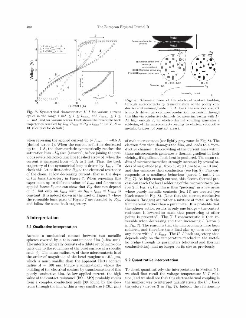
480 The European Physical Journal B
Fig. 7. Symmetrical characteristics U–I for various currentcycles in the range 1 mA ≤ I ≤ Imax+ and Imax− ≤ I ≤−1 mA, and for various forces. Inset shows the reversible backtrajectories rescaled by R0b. Umax ≡ R0b ∗ Imax 3.5 V. N =13. (See text for details.)
when reversing the applied current up to Imax− = −0.5 A(dashed arrow 4). When the current is further decreasedup to −1 A, the characteristic symmetrically reaches thesaturation bias −U0 (see ♦-marks), before joining the pre-vious reversible non-ohmic line (dashed arrow 5), when thecurrent is increased from −1 A to 1 mA. Thus, the backtrajectory of this symmetrical loop is driven by |Imax|. Tocheck this, let us first define R0b as the electrical resistanceof the chain, at low decreasing current, that is, the slopeof the back trajectory in Figure 7. When repeating thisexperiment up to different values of Imax and for variousapplied forces F , one can show that R0b does not dependon F , but only on Imax such as R0b ∗ Imax ≡ Umax isconstant. It is indeed shown in the inset of Figure 7 wherethe reversible back parts of Figure 7 are rescaled by R0b,and follow the same back trajectory.
5 Interpretation
5.1 Qualitative interpretation
Assume a mechanical contact between two metallicspheres covered by a thin contaminant film (∼few nm).The interface generally consists of a dilute set of microcon-tacts due to the roughness of the bead surface at a specificscale [6]. The mean radius, a, of these microcontacts is ofthe order of magnitude of the bead roughness ∼0.1 µm,which is much smaller than the apparent Hertz contactradius A ∼ 100 µm. Figure 8 schematically shows thebuilding of the electrical contact by transformation of thispoorly conductive film. At low applied current, the highvalue of the contact resistance (kΩ – MΩ) probably comesfrom a complex conduction path [39] found by the elec-trons through the film within a very small size (0.1 µm)
Fig. 8. Schematic view of the electrical contact buildingthrough microcontacts by transformation of the poorly con-ductive contaminant/oxide film. At low I , the electrical contactis mostly driven by a complex conduction mechanism throughthis film via conductive channels (of areas increasing with I).At high enough I , an electro-thermal coupling generates asoldering of the microcontacts leading to efficient conductivemetallic bridges (of constant areas).
of each microcontact (see lightly grey zones in Fig. 8). Theelectron flow then damages the film, and leads to a “con-ductive channel”: the crowding of the current lines withinthese microcontacts generates a thermal gradient in theirvicinity, if significant Joule heat is produced. The mean ra-dius of microcontacts then strongly increases by several or-ders of magnitude (e.g., from ai 0.1 µm to af ∼ 10 µm),and thus enhances their conduction (see Fig. 8). This cor-responds to a nonlinear behaviour (arrow 1 until 2 inFig. 7). At high enough current, this electro-thermal pro-cess can reach the local soldering of the microcontacts (ar-row 2 in Fig. 7); the film is thus “piercing” in a few areaswhere purely metallic contacts (few Ω) are created (seeblack zones in Fig. 8). [Note that the current-conductivechannels (bridges) are rather a mixture of metal with thefilm material rather than a pure metal. It is probable thatthe coherer action results in only one bridge – the contactresistance is lowered so much that puncturing at otherpoints is prevented]. The U–I characteristic is then re-versible when decreasing and then increasing I (arrow 3in Fig. 7). The reason is that the microcontacts have beensoldered, and therefore their final size af does not varyany more with I < Imax. The U–I back trajectory thendepends only on the temperature reached in the metal-lic bridge through its parameters (electrical and thermalconductivities), and no longer on its size as previously.
5.2 Quantitative interpretation
To check quantitatively the interpretation in Section 5.1,we shall first recall the voltage–temperature U–T rela-tion, and we shall see that this electro-thermal coupling isthe simplest way to interpret quantitatively the U–I backtrajectory (arrows 3 in Fig. 7). Indeed, the relationship

E. Falcon et al.: Nonlinear electrical conductivity in a 1D granular medium 481
between the voltage-drop across the contact U , the cur-rent I and the microcontact radius a is strongly modifiedcompared to the classical constricted case, U/I = ρel/2a,derived without taking into account the significant heatproduction within the microcontact.
Assume a microcontact between two clean metal-lic conductors (thermally insulated at uniform temper-ature T0, with no contaminant or tarnish film at thecontact). Such a clean microcontact is generally called a“spot”. If an electrical current flowing through this spotis enough to produce Joule heating, then a steady-statetemperature distribution is quickly reached (∼ µs) in thecontact vicinity. The maximum temperature Tm is locatedat the contact, and is linked to the voltage-drop U by theKohlrausch’s equation [6,40,41]
U2 = 8∫ Tm
T0
λρel dT, (3)
where, ρel is the electrical resistivity and λ the thermalconductivity, both being dependent on the temperature T .However, for many conductors, the Wiedemann-Franz lawstates that [6,41,42]
λρel = LT, (4)
where L = π2k2/(3e2) = 2.45×10⁻⁸ V2/K2 is the Lorentzconstant, k the Boltzmann’s constant, and e the electroncharge. This is a consequence that the electron scatteringtime contributes to both the electrical conductivity andthe heat conductivity. Combining equations (3) and (4)yields for the local heating;
T 2m − T 2
0 =U2
4L. (5)
This relationship shows that the maximum tempera-ture Tm reached at the contact is independent of thecontact geometry and of the materials in contact! Thisis a consequence that both the electrical and thermalconductivities are related to the conduction electronsthrough equation (4). However, the temperature distri-bution within the bridge depends on the geometry [42].A voltage near 0.4 V across a constriction thus leadsfrom equation (5) to a contact temperature near 1050 Cfor a bulk temperature T0 = 20 C. This means thatU 0.3−0.4 V leads to contact temperatures that exceedthe softening or/and the melting point of most conduc-tive materials [42]. Efficient conductive metallic bridges(or “hot spots”) are therefore created by microsoldering.Moreover, equation (5) shows that the parameter deter-mining the spot temperature is the voltage-drop acrossthe contact, not the magnitude of the current: this ex-plains why the experimental saturation voltage U0/c isthe relevant parameter in Section 4. In addition, when Uapproaches U0/c, the local heating of microcontacts isenough, from equation (5), to soft them (mainly at theirperipheries [42]). Then, their contact areas increase thusleading to a decrease of local resistances, and thus stabiliz-ing the voltage, the contact temperatures and the contact
areas, since the current is fixed. The phenomenon is there-fore self-regulated in voltage and temperature.
Let us now specify the temperature dependence for thethermal and electrical conductivity in the case of an alloyor a pure metal. For an alloy, some defects are present inthe bulk metal, and contribute to the electrical conduc-tivity (but have no influence on the Eq. (4) [6]). The elas-tic scattering of the conductive electrons with the metalphonons and with the defects is random, and thus thecorresponding scattering frequencies add up. This leadsto the Mathiessen’s rule: the total resistivity is the sum ofa temperature dependent resistivity due to the scatteringwith phonons and a residual resistance at zero tempera-ture due to defects such as
ρel(T ) ≡ α(T + βT0) (6)
where α = 6.98 × 10⁻¹⁰ Ω m/K and β = 2.46 are ex-tracted from the stainless steel resistivity in Table 1, andT0 = 293 K is the room temperature. This defines aneffective temperature linked to the defects Tdef ≡ βT0.Note that for pure metals, α = ρ0/T0, β = 0 (since onlythe “phonon resistivity” contributes), and thus from equa-tion (4), λ(T ) = λ0 = LT0/ρ0, where ρ0 and λ0 are theelectrical resistivity and thermal conductivity of the puremetal at T0.
One can analytically solve the electro-thermal problemfor the general case of an alloy, i.e. with ρel(T ) and λ(T )as in equations (4) and (6), as shown in the appendix:
– the isothermal temperature Tm at the contact surfaceas a function of the voltage U is
Tm =
√T 2
0 +U2
4LN2c
, (7)
– the normalized current IR0b through the contacts onlydepends on this temperature Tm (i.e. on U) such as
IR0b = 2T0Nc
√L(1 + β)
∫ θ0
0
cos θ
β cos θ0 + cos θdθ, (8)
where θ0 ≡ arccos (T0/Tm).
We remind the reader that Tm does not depend on thematerial properties, or the microcontact geometry, butonly on the room temperature, T0, the number of bead-bead contacts in the chain, Nc ≡ N + 1, and the Lorentzconstant L. IR0b has an additional parameter β relatedto the defects in the material. For pure metals, i.e withα = ρ0/T0 and β = 0 in equation (6), equation (8) sim-plifies to the well-known explicit expression with no ad-justable parameter [6,40]
IR0b = 2NcT0
√L arctan[T ∗
m(2 + T ∗m)], (9)
where T ∗m ≡ (Tm − T0)/T0.
The normalized U–I back trajectory (i.e., IR0b as afunction of U) is displayed in Figure 9. Here, the exper-imental results of Figure 7 are compared with the the-oretical solutions for an alloy (Eq. (8)) calculated with

482 The European Physical Journal B
0 1 2 3 40
1
2
3
4
5
6
I * R0b
(V)
U (
V)
Umax
U0
0 300 600 900 12000
1
2
3
4
5
6U
0
U (
V)
Tm
(oC)
Fig. 9. Comparison between experimental U–I back trajec-tories of Figure 7 (symbols), and theoretical curves for analloy (Eq. (8)) with stainless steel properties [β = 3 (−) orβ = 2.46 (· · · )], and for a pure metal (−.−) (Eq. (9)). Insetshows the theoretical maximum temperature, Tm (Eq. (7)),reached in one contact when the chain is submitted to a volt-age U . N = 13.
AISI 304 stainless steel properties, and for a pure metal(Eq. (9)). A very good agreement is shown between the ex-perimental results and the electro-thermal theory, notablyfor the alloy case. Qualitatively, the alloy solution has abetter curvature than the pure metal one. The agreementis quantitatively excellent when choosing β = 3 insteadof 2.46 (the β value for AISI 304 stainless steel), sincethe β value for the bead material (AISI 420 stainless steel)is unknown, but should be close. This gives a measurementof the effective temperature due to the defects Tdef = 3T0.During this experimental back trajectory, the equilibriumtemperature, Tm, on a microcontact is also deduced fromequation (7) with no adjustable parameter (see inset ofFig. 9). Therefore, when the saturation voltage is reached(U0 = 5.8 V), Tm is close to 1050 C which is enoughto soften or to melt the microcontacts. Our implicit mea-surement of the temperature is equivalent to use a resistivethermometer. When very high voltage (more than 500 V)is applied to a monolayer of aluminium beads, direct visu-alization with an infrared camera has been performed byVandembroucq et al. [9].
6 Conclusion
We have reported the observation of the electrical trans-port within a chain of oxidized metallic beads under ap-plied static force. A transition from an insulating to aconductive state is observed as the applied current is in-creased. The U–I characteristics are nonlinear, hysteretic,and saturate to a low voltage per contact (0.4 V). Elec-trical phenomena in granular materials related to thisconduction transition such as the “Branly effect” werepreviously interpreted in many different ways but with-
out a clear demonstration. Here, we have shown thatthis transition, triggered by the saturation voltage, comesfrom an electro-thermal coupling in the vicinity of themicrocontacts between each bead. The current flowingthrough these spots generates local heating which leadsto an increase of their contact areas, and thus enhancestheir conduction. This current-induced temperature rise(up to 1050 C) results in the microsoldering of contacts(even for so low voltage as 0.4 V). Based on this self-regulated temperature mechanism, an analytical expres-sion for the nonlinear U–I back trajectory is derived, andis found in very good agreement with the data. It also al-lows the determination of the microcontact temperatureall through this reverse trajectory, with no adjustable pa-rameter. Finally, the stress dependence of the resistanceis strongly found non-hertzian underlying a contributiondue to the surface films.
We thank D. Bouraya for the realization of the experimen-tal setup, and G. Kamarinos for sending us references [4,5].L.K.J. Vandamme and E. Guyon are grateful for the fruitfuldiscussions.
Appendix A
Assume a single plane contact (of any shape) betweentwo identical conductors (of large dimensions comparedto the contact ones) submitted to a constant current I.The electrical power dissipated by the Joule effect is as-sumed totally drained off by thermal conduction in theconductors. This thermal equilibrium and Ohm’s law leadto the potential ϕ at the isotherm T in the contactvicinity [6,40,42],
ϕ2(T ) = 2∫ Tm
T
ρel(T ′)λ(T ′)dT ′, (10)
where Tm is the maximum temperature occurring in thecontact plane, λ the thermal conductivity and ρel theelectrical resistivity of the conductor. Denote by R0b, the“cold” contact resistance presented to a current low en-ough not to cause any appreciable rise in the tempera-ture at the contact (the conductor bulk being at the roomtemperature T0). The relation between the current flow-ing through the contact and the maximum temperatureproduced is then [40]
IR0b = 2ρel(T0)∫ Tm
T0
λ(T )ϕ(T )
dT. (11)
Note that the dependence on temperature of the right-hand side of equation (11) arises solely from the presenceof material parameters, and that only R0b depends on thecontact geometry. Solving this equation for the generalcase of λ(T ) and ρel(T ) such as in equations (4) and (6).Substituting equations (4) and (6) in the so-called “ϕ–T ”relation (the Kohlrausch’s Eq. (10)) leads to equation (7)

E. Falcon et al.: Nonlinear electrical conductivity in a 1D granular medium 483
for Nc contacts in series, since ϕ(T0) ≡ U/2. Substitutingequations (4) and (6) in equation (11) yields to
IR0b = 2√
LT0(1 + β)∫ Tm
T0
T/T0β+T/T0
Tm
√1− (T/Tm)2
dT. (12)
Making the change of variable θ ≡ arccos (T/Tm), equa-tion (12) reduces to
IR0b = 2√
LT0(1 + β)∫ θ0
0
cos θ
cos θ + β cos θ0dθ, (13)
with θ0 ≡ arccos (T0/Tm). For Nc contacts in series, equa-tion (13) leads to equation (8).
References
1. E. Branly, C.R. Acad. Sci. Paris 111, 785 (1890) (inFrench)
2. R. Bridgman, Physics World Dec., pp. 29–33 (2001)3. E. Falcon, B. Castaing, C. Laroche, Europhys. Lett. 65,
186 (2004)4. G. Kamarinos, P. Viktorovitch, M. Bulye-Bodin, C.R.
Acad. Sci. Paris 280, 479 (1975) (in French)5. G. Kamarinos, A. Chovet, Bruit, fluctuations et insta-
bilite de conduction irreversible dans les poudres de metauxde transition, in Proceed. SEE: Conducteurs Granulaires,edited by E. Guyon, pp. 181–184, Paris, 1990 (in French)
6. R. Holm, Electric Contacts, 4th edn. (Springer Verlag,Berlin, 2000)
7. R. Gabillard, L. Raczy, C.R. Acad. Sci. Paris 252, 2845(1961) (in French)
8. G. Salmer, Etude experimentale et theorique duphenomene de coheration dans les milieux metalliques al’etat pulverulent, Ph.D. thesis, Universite de Lille, Lille,1966 (in French)
9. D. Vandembroucq, A.C. Boccara, S. Roux, J. Phys. IIIFrance 7, 303 (1997)
10. S. Dorbolo, M. Ausloos, N. Vandewalle, Phys. Rev. E 67,040302(R) (2003)
11. E. Branly, C.R. Acad. Sci. Paris 134, 1197 (1902) (inFrench)
12. E. Branly, C.R. Acad. Sci. Paris 134, 347 (1902) (inFrench)
13. E. Branly, C.R. Acad. Sci. Paris 128, 1089 (1899) (inFrench)
14. E. Branly, C.R. Acad. Sci. Paris 127, 219 (1898) (inFrench)
15. T. Calzecchi-Onesti, Nuovo Cim. 16, 58 (1884);T. Calzecchi-Onesti, Nuovo Cim. 17, 35 (1885) (in Italian),also in J. Phys. 5, 573 (1886)
16. K.E. Guthe, A. Trowbridge, Phys. Rev. 11, 22 (1900)17. K.E. Guthe, Phys. Rev. 12, 245 (1901)18. C. Coste, E. Falcon, S. Fauve, Phys. Rev. E 56, 6104
(1997)19. B. Gilles, C. Coste, Phys. Rev. Lett. 90, 174302 (2003)20. E. Falcon, B. Castaing, C. Laroche, Electrical conductivity
in a 2D granular medium (unpublished)21. D.L. Sengupta, T.K. Sarkar, D. Sen, Proc. of the IEEE
86, 235 (1998) (and references therein)22. M.A. Fisch, J. Phys. 3, 350 (1904) (in French)23. M.A. Blanc, J. Phys. 4, 743 (1905) (in French)24. P. Weiss, J. Phys. 5, 462 (1906) (in French)25. F.P. Bowden, D. Tabor, Proc. Roy. Soc. Lond. A 169, 391
(1939); see also F.P. Bowden, D. Tabor, The Friction andLubrification of Solids (Clarendon Press, Oxford, 1950)
26. R.W. Wilson, Proc. R. Soc. Lond. B 68, 625 (1955)27. L. Boyer, S. Noel, F. Houze, J. Phys. D 21, 495 (1988)28. M. Ammi, T. Travers, D. Bideau, A. Gervois, J.-C.
Messager, J.-P. Troadec, J. Phys. 49, 221 (1988)29. X. Zhuang, J.D. Goddard, A.K. Didwania, J. Comp. Phys.
121, 331 (1995)30. K.J. Euler, J. Power Sources 3, 117 (1978)31. Marteau & Lemarie. Specialist of beads. Product Catalogue32. Stainless Steel AISI 304 properties at CERN
http://atlas.web.cern.ch/Atlas/GROUPS/Shielding/
jfmaterial.htm
33. K.L. Johnson, Contact Mechanics (Cambridge Univ.Press, Cambridge, 1985)
34. E. Falcon, C. Laroche, S. Fauve, C. Coste, Eur. Phys. J.B 5, 111 (1998)
35. M. Creyssels, B. Castaing, E. Falcon, Pressure dependenceof the electrical resistance in copper powder (unpublished)
36. A.K. Gupta, A.K. Sen, Phys. Rev. B 57, 3375 (1998)37. S. Dorbolo, M. Ausloos, N. Vandewalle, Appl. Phys. Lett.
81, 936 (2002)38. S. Dorbolo, M. Ausloos, N. Vandewalle, Eur. Phys. J. B
34, 201 (2003)39. V. Da Costa, Y. Henry, F. Bardou, M. Romeo,
K. Ounadjela, Eur. Phys. J. B 13, 297 (2000)40. J.A. Greenwood, J.B.P. Williamson, Proc. Roy. Soc. A
246, 13 (1958)41. R.S. Timsit, Electrical contact resistance: Fundamental
principles, in Electrical Contacts, Principles andApplications, edited by P. Slade (Marcel Dekker,New York, 1999), p. 1
42. L. Fechant, Le Contact Electrique : Phenomenes Physiqueset Materiaux, Vol. 2 (Hermes, Paris, 1996) (in French)

148

Europhys. Lett., 65 (2), pp. 186–192 (2004)DOI: 10.1209/epl/i2003-10071-9
EUROPHYSICS LETTERS 15 January 2004
“Turbulent” electrical transport in copper powders
E. Falcon(∗), B. Castaing and C. LarocheLaboratoire de Physique, Ecole Normale Superieure de LyonUMR 5672 - 46, allee d’Italie, 69007 Lyon, France
(received 28 February 2003; accepted in final form 6 November 2003)
PACS. 45.70.-n – Granular systems.PACS. 05.40.-a – Fluctuation phenomena, random processes, noise, and Brownian motion.PACS. 72.80.-r – Conductivity of specific materials.
Abstract. – Compressed copper powder has a very large electrical resistance (1MΩ), due tothe oxide layer on grains (100µm). We observe that its voltage-current U -I characteristics arenonlinear, and undergo an instability, from an insulating to a conductive state at relatively smallapplied voltages. Current through the powder is then noisy, and the noise has interesting self-similar properties, including intermittency and scale invariance. We show that heat dissipationplays an essential role in the physics of the system. One piece of evidence is that the instabilitythreshold always corresponds to the same Joule dissipated power whatever the applied stress.In addition, we observe long-time correlations which suggest that thermal expansion locallycreates or destroys contacts, and is the driving mechanism behind the instability and noiseobserved in this granular system.
Introduction. – For over a century [1], electrical transport in metallic powders has gen-erated interest [2]. These powders have fascinating properties, such as extreme sensitivityto electromagnetic waves, highly nonlinear U -I characteristics, hysteresis, and 1/f noise, forwhich fully satisfactory explanations are still lacking. The experiments presented here weremotivated by the work of Kamarinos et al. [3] on compressed copper powders. These authorsobserved an insulating-to-conducting transition at rather low pressure-dependent voltages,associated with strong 1/f noise. Just above the conduction transition threshold, we ob-serve slow temporal evolution of the powder resistance with a noisy component. Electricalbreakdown of the oxide layers on grains has been invoked [3, 4] for the transition, but thisexplanation is unsatisfactory, for we observe that the noise involves both increasing and de-creasing the electrical resistance of the powder. In this letter, we show that this electricalnoise has interesting scale-invariant properties. Scale invariance [5] occurs for various physicalsignals: turbulent velocity [6], financial stock market data [7], earthquake energy release [5],or worldwide information traffic [8]. One of the goals of this study is to use the analytictools developed for turbulent signals in the case of this granular system. We shall focus thecomparison on two aspects: The statistics of current increments, I(t+ τ)− I(t), depending onthe tested time scale τ , and the correlations between the amplitudes of these increments. This
(∗) E-mail: [email protected]; URL: http://perso.ens-lyon.fr/eric.falcon/
c© EDP Sciences
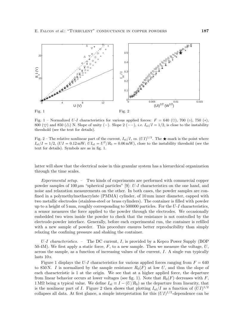
E. Falcon et al.: “Turbulent” conductance in copper powders 187
0 4 8 120
10
20
U (V)
RoI
(V)
Fig. 1
0 0.005 0.01 0.0150
0.1
0.2
0.3
0.4
0.5
(UI)1/2 (W1/2)
I nl /
I
Fig. 2
Fig. 1 – Normalized U -I characteristics for various applied forces: F = 640 (), 700 (), 750 (∗),800 () and 850 () N. Slope of unity (−). Slope 2 (−−), i.e. Inl/I = 1/2, is close to the instabilitythreshold (see the text for details).
Fig. 2 – The relative nonlinear part of the current, Inl/I, vs. (UI)1/2. The -mark is the point whereInl/I = 1/2, (UI = 0.12mW; UInl = U2/R0 = 0.06mW), close to the instability threshold (see thetext for details). Symbols are as in fig. 1.
latter will show that the electrical noise in this granular system has a hierarchical organizationthrough the time scales.
Experimental setup. – Two kinds of experiments are performed with commercial copperpowder samples of 100 µm “spherical particles” [9]: U -I characteristics on the one hand, andnoise and relaxation measurements on the other. In both cases, the powder samples are con-fined in a polymethylmethacrylate (PMMA) cylinder, of 10 mm inner diameter, capped withtwo metallic electrodes (stainless-steel or brass cylinders). The container is filled with powderup to a height of 5 mm, roughly corresponding to 500000 particles. For the U -I characteristics,a sensor measures the force applied to the powder through the electrodes. We occasionallyembedded two wires inside the powder to check that the resistance is not controlled by theelectrode-powder interface. Generally, before each experimental run, the container is refilledwith a new sample of powder. This procedure ensures better reproducibility than simplyrelaxing the confining pressure and shaking the container.
U -I characteristics. – The DC current, I, is provided by a Kepco Power Supply (BOP50-4M). We first apply a static force, F , to a new sample. Then we measure the voltage, U ,across the sample, as a function of increasing values of the current, I. A single run typicallylasts 10 s.
Figure 1 displays the U -I characteristics for various applied forces ranging from F = 640to 850 N. I is normalized by the sample resistance R0(F ) at low U , and thus the slope ofeach characteristic is 1 at the origin. We see that at a higher applied force, the departurefrom linear behavior occurs at lower voltages (see fig. 1). Note that R0(F ) decreases with F ,1 MΩ being a typical value. We define Inl ≡ I − (U/R0) as the departure from linearity, thatis the nonlinear part of I. Figure 2 then shows that plotting Inl/I as a function of (UI)1/2
collapses all data. At first glance, a simple interpretation for this (UI)1/2-dependence can be

188 EUROPHYSICS LETTERS
developed. Indeed, developing I in powers of U such as
I = (U/R0) + cU2
yieldsInl/I R0cU cR
3/20 (UI)1/2.
However, due to the symmetry of the system, c should be zero. Thus, this interpretation doesnot hold. We prefer to focus on the main observation: The relative nonlinear component ofthe current, Inl/I, seems to depend only on the total dissipated power in the sample, UI. Aninterpretation along these lines will be proposed in what follows.
Transition and relaxation. – In a new series of experiments, the PMMA cylinder is filledwith 5 mm of powder, then vibrated and embedded in a cylindrical brass press with 5 mmthick walls. The pressure on the sample is generated by means of the lid press acting as ascrew. At constant low voltage (U 0.5 V), the sample resistance, R0, is monitored duringthe stepwise pressing of the sample until a maximum pressure, Pm, is reached. R0 is foundto decrease with increasing Pm, and to reach a value ranging from 100 kΩ to 500 kΩ, at theend of the pressing process (half an hour later). We then let the system relax for one day.After checking that R0 and Pm are constant in time, a fixed voltage, U , is suddenly appliedto the sample, and the current, I, is monitored. If U is smaller than a threshold value Uc, thesample is in a weakly conducting state with very slow temporal evolutions of I, if any. WhenU > Uc, an instability occurs. I rapidly increases at constant U which can be interpretedas the resistance relaxing down. The larger U is, the faster the resistance relaxes. Similarfeatures have been observed by Kamarinos et al. [3].
When the above experiment is repeated for different values of Pm, it shows that both Uc andR0 depend on Pm. However, the critical ratio U2
c /R0 is found to be independent of the appliedpressure, with a value close to 0.07 mW. This value is close to the point where Inl/I = 1/2(see -mark in fig. 2). All these observations suggest that this spontaneous transition from aninsulating to conducting state is a thermal instability. To further characterize the phenomenonobserved for U > Uc, let us make three remarks:
– Due to the strong sample pressure, vibrations have no effect; even a strong jolt appliedto the press has no visible consequence on the signal.
– We occasionally followed the relaxation down to a resistance of 500 Ω, which is almostthree orders of magnitude lower than the initial one R0; however, this resistance remainsmuch higher than a metallic contact would produce between the grains, no matter howsmall the contact [2].
– The temporal evolution of the current, at constant U > Uc, is not monotonic. Bothincreasing and decreasing events occur for the current. However, the former dominateand control the global evolution. This is contradictory to what would result from acascading electrical breakdown for the oxide layers, as supposed by Kamarinos et al. [3].
Finally, we observe that the direction of the global evolution of the resistance dependson the applied voltage. As shown in fig. 3, we first apply to the sample a voltage U = 4 V(U2/R0 = 0.1 mW > U2
c /R0), which triggers the relaxation. Half an hour later, we decreaseU to 0.5 V, and the conductance goes down. Two hours later, we increase U to 3.5 V and wesee that the conductance goes up again. Consequently, with a well-chosen applied voltage, wecan obtain an approximately constant conductance. Note that these observations are coherentwith the last item above. We exploit them in what follows.
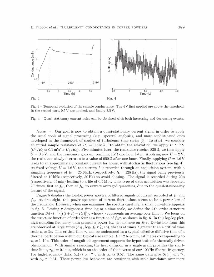
E. Falcon et al.: “Turbulent” conductance in copper powders 189
0.5 1 1.5 2 2.5
0.5
1
1.5
2
Time (h)
Con
duct
ance
(m
S)
4V 0.5V 3.5V
Fig. 3
3.9 4 4.1 4.2 4.3-3
-2
-1
Time (s)
I-<
I> (
µ A
)
Fig. 4
Fig. 3 – Temporal evolution of the sample conductance. The 4V first applied are above the threshold.In the second part, 0.5V are applied, and finally 3.5V.
Fig. 4 – Quasi-stationary current noise can be obtained with both increasing and decreasing events.
Noise. – Our goal is now to obtain a quasi-stationary current signal in order to applythe usual tools of signal processing (e.g., spectral analysis), and more sophisticated onesdeveloped in the framework of studies of turbulence time series [6]. To start, we consideran initial sample resistance of R0 = 0.5 MΩ. To obtain the relaxation, we apply U 7 V(U2/R0 0.1 mW > U2
c /R0). Five minutes later, the resistance reaches 830 Ω, we then applyU = 0.5 V, and the resistance goes up, reaching 1 kΩ one hour later. Applying now U = 2 V,the resistance slowly decreases to a value of 950 Ω after one hour. Finally, applying U = 1.6 Vleads to an approximately constant current for hours, with stochastic fluctuations (see fig. 4).At fixed voltage U = 1.6 V, the current I is recorded through an acquisition system, with asampling frequency of fH = 25.6 kHz (respectively, fL = 128 Hz), the signal being previouslyfiltered at 10 kHz (respectively, 50 Hz) to avoid aliasing. The signal is recorded during 20 s(respectively, 65 min) leading to a file of 0.5 Mpt. This type of data acquisition was repeated20 times, first at fH, then at fL, to extract averaged quantities, due to the quasi-stationarityfeature of the signal.
Figure 5 displays the log-log power spectra of filtered signals of current recorded at fL andfH. At first sight, this power spectrum of current fluctuations seems to be a power law ofthe frequency. However, when one examines the spectra carefully, a small curvature appearsin fig. 5. Letting τ designate a time lag or a time scale, we define the i-th–order structurefunction Si(τ) = 〈[I(t + τ)− I(t)]i〉, where 〈·〉 represents an average over time t. We focus onthe structure function of order four as a function of fHτ , as shown in fig. 6. In this log-log plot,high sampling frequency data present a power law dependence on fHτ . Deviations from thisare observed at large times (e.g., log2 fHτ 16), that is at times τ greater than a critical timescale τc 3 s. This critical time τc can be understood as a typical effective diffusive time of athermal pertubation within our typical size sample, L 2.5–5 mm, estimates corresponding toτc 1–10 s. This order-of-magnitude agreement supports the hypothesis of a thermally drivenphenomenon. With similar reasoning the heat diffusion in a single grain provides the short-time limit, τinf 0.1 ms, which is on the order of the inverse of our 10 kHz filtered frequency.For high-frequency data, S4(τ) ∝ τα4 , with α4 0.57. The same data give S2(τ) ∝ τα2 ,with α2 0.31. These power law behaviors are consistent with scale invariance over more

190 EUROPHYSICS LETTERS
10-4
10 -2
100
102
104
10 -13
10 -10
10 -7
10 -4
Frequency (Hz
Pow
er S
pect
rum
(m
A2 /H
z)
Fig. 5
5 10 15 20 2510
-15
10 -13
10 -11
10 -9
log2(f
Hτ)
S4 (
mA
4 )Fig. 6
Fig. 5 – Average power spectra of current fluctuations sampled at low () and high () frequencies.
Fig. 6 – The fourth moment of current differences, S4(τ), vs. the nondimensional time scale, fHτ .Same symbols as in fig. 5.
than 3 decades in time. Intermittency, corresponding to α4 < 2α2, appears more clearly fromthe direct examination of probability density functions, and correlations, in the next sections.Here, α4 and 2α2 differ only by one standard error.
Probability density functions. – We concentrate now on the high-frequency part of thesignal, which presents nice scale invariance properties for τinf < τ < τc. Figure 7 shows,for three different τ , the probability density functions (PDF) of current differences, δIτ (t) =I(t + τ) − I(t), normalized to their respective root mean square, σ. The exact shape of thesePDF is rather sensitive to the statistics (see PDF tails in fig. 7), and would have led tosmoother curves with a greater quantities of data. However, two remarks can be made in thelight of what is known for velocity signals in turbulence [6]:
– The PDF shape changes with the time scale τ —this is a direct signature of intermittency,as S4 cannot be proportional to S2
2 and thus α4 = 2α2.
– Current difference PDF are symmetric —time reversal, which a priori should not beinvoked here, is the only symmetry able to lead to this behavior. Turbulent velocitydifferences have a skewed PDF, S3 being proportional to the dissipated power [6]. How-ever, even in turbulence, global quantities, like the total dissipated power (equivalent towhat we measure here), have rather symmetric time difference PDF [10].
Multiplicative cascade. – A signal with scale invariance is called self-similar since itsstatistical properties can be described by the same laws at various scales. If the shape oftime difference PDF changes across scales with a self-similar law of deformation, this signal isgenerally described either in terms of a “multifractal set of singularities”, or a “multiplicativecascade” across scales, both approaches being considered equivalent [11]. In the “multiplicativecascade”, a given scale (e.g., average gradients on a time interval) conditions smaller scales(e.g., smaller intervals within this one) in a random Markovian way. It induces not onlyintermittency (evolution of distribution shape across scales), but also long-range correlations
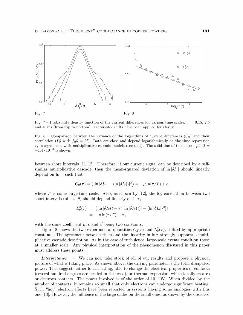
E. Falcon et al.: “Turbulent” conductance in copper powders 191
-10 -5 0 5 1010
-6
10 -4
10 -2
100
δ Iτ / σ
PDF(
δ I τ /
σ)
Fig. 7
4 8 12-0.01
0.01
0.03
log2(f
Hτ)
L22 (τ)
C2 (τ)
Fig. 8
Fig. 7 – Probability density function of the current differences for various time scales: τ = 0.15, 2.5and 40ms (from top to bottom). Factor-of-2 shifts have been applied for clarity.
Fig. 8 – Comparison between the variance of the logarithms of current differences (C2) and theircorrelation (L2
θ with fHθ = 22). Both are close and depend logarithmically on the time separationτ , in agreement with multiplicative cascade models (see text). The solid line of the slope −µ ln 2 =−1.4 · 10−3 is shown.
between short intervals [11, 12]. Therefore, if our current signal can be described by a self-similar multiplicative cascade, then the mean-squared deviation of ln |δIτ | should linearlydepend on ln τ , such that
C2(τ) =⟨[ln |δIτ | − 〈ln |δIτ |〉]2
⟩= −µ ln(τ/T ) + c,
where T is some large-time scale. Also, as shown by [12], the log-correlation between twoshort intervals (of size θ) should depend linearly on ln τ ,
L2θ(τ) =
⟨[ln |δIθ(t + τ)| ln |δIθ(t)| − 〈ln |δIθ|〉2]
⟩= −µ ln(τ/T ) + c′,
with the same coefficient µ, c and c′ being two constants.Figure 8 shows the two experimental quantities C2(τ) and L2
θ(τ), shifted by appropriateconstants. The agreement between them and the linearity in ln τ strongly supports a multi-plicative cascade description. As in the case of turbulence, large-scale events condition thoseat a smaller scale. Any physical interpretation of the phenomenon discussed in this papermust address these points.
Interpretation. – We can now take stock of all of our results and propose a physicalpicture of what is taking place. As shown above, the driving parameter is the total dissipatedpower. This suggests either local heating, able to change the electrical properties of contacts(several hundred degrees are needed in this case), or thermal expansion, which locally createsor destroys contacts. The power involved is of the order of 10−4 W. When divided by thenumber of contacts, it remains so small that only electrons can undergo significant heating.Such “hot” electron effects have been reported in systems having some analogies with thisone [13]. However, the influence of the large scales on the small ones, as shown by the observed
192 EUROPHYSICS LETTERS
logarithmic correlations, cannot be taken into account by such a local process. Therefore,thermal expansion seems to be the mechanism driving the instability and the associated noise.
In this spirit, we attempt to show the correspondence between the formal multiplicativecascade and electrical conduction in our powder. Since the contact distribution in a powderis very inhomogeneous, one would also expect an inhomogeneous current distribution. ThusJoule heating should create inhomogeneous increasing stresses in the powder. Very smallthermal expansion can result in dramatic changes in the current paths, thus in the distributionof this Joule heating, and so on. Such events can occur at any scale, ranging from the size of thesample and the grain size. The large-scale events should influence the small ones, as suggestedby our study. A full confirmation of this idea requires longer carefully controlled studies.
Conclusion. – The results of this work are twofold. First, we show that the sponta-neous decrease in resistance of a copper powder sample above a voltage threshold is due to athermal instability, and not to electrical breakdown, as had previously been proposed. Thisconclusion results from the observation that dissipated power drives the phenomenon, in spiteof the probable smallness of the induced temperature inhomogeneities. Second, we proposea procedure yielding an interesting self-similar process in this non-equilibrium system. Oursystem displays both intermittency and multiplicative cascade-like two-point correlations, inways that are interesting to compare and contrast with the archetypical case of turbulence.
∗ ∗ ∗
We wish to thank O. Michel for his exciting ideas, P. Metz and D. Bouraya for elec-tronical and technical support, andG. Kamarinos, T. Lopez Rios and L. K. J. Vandammefor discussions. Thanks are also due to V. Bergeron, L. Chevillard and M. Marder forhelp in improving the manuscript.
REFERENCES
[1] Branly E., C. R. Acad. Sc. Paris, 111 (1890) 785 (in French).[2] Holm R., Electric Contacts Handbook, 3rd edition, Vol. IV (Springer Verlag, Berlin) 1958,
pp. 398-406. Note that this section has been removed since the 4th edition.[3] Kamarinos G., Viktorovitch P. and Buyle-Bodin M., C. R. Acad. Sc. Paris, 280 (1975)
479; Kamarinos G. and Chovet A., Conducteurs Granulaires, Proceedings SEE, edited byGuyon E. (Palais de la Decouverte, Paris) 1990, pp. 181-184 (both in French).
[4] Vandembroucq D., Boccara A. C. and Roux S., J. Phys. III, 7 (1997) 303.[5] Dubrulle B., Graner F. and Sornette D. (Editors), Scale Invariance and Beyond (EDP
Science & Springer) 1997.[6] Frisch U., Turbulence (CUP, Cambridge) 1995.[7] Sornette D., Why Stock Markets Crash: Critical Events in Complex Financial Systems
(Princeton University Press, Princeton) 2003.[8] Park K. and Willinger W. (Editors), Self-similar Network Traffic and Performance Evalua-
tion (Wiley) 2000.[9] CU 006025, Goodfellow Product Catalogue, 1998, see also http://www.goodfellow.com/.[10] Pinton J. F., private communication.[11] Chainais P., PhD Thesis, ENS Lyon (2001) (in French).[12] Delour J., Muzy J. F. and Arneodo A., Eur. Phys. J. B, 23 (2001) 243.[13] Fedorovich R. D., Kiyayev O. E., Naumovets A. G., Pilipchak K. N. and Tomchuk
P. M., Phys. Low-Dim. Struct., 1 (1994) 83.

156

Electrical conductivity in granular media and Branly’s coherer:A simple experiment
Eric Falcona) and Bernard CastaingLaboratoire de Physique, E´cole Normale Supe´rieure de Lyon, UMR 5672, 46, alle´e d’Italie,69 007 Lyon, France
~Received 25 May 2004; accepted 15 November 2004!
We show how a simple laboratory experiment can illustrate certain electrical transport properties ofmetallic granular media. At a low critical external voltage, a transition from an insulating to aconductive state is observed. This transition comes from an electro-thermal coupling in the vicinityof the microcontacts between grains where microwelding occurs. Our apparatus allows us to obtainan implicit determination of the microcontact temperature, which is analogous to the use of aresistive thermometer. The experiment also helps us explain an old problem, Branly’s coherer effect,which was used as a radio wave detector for the first wireless radio transmission, and is based onthe sensitivity of the conductivity of metal filings to an electromagnetic wave. ©2005 American
Association of Physics Teachers.
@DOI: 10.1119/1.1848114#
I. INTRODUCTION
The coherer or Branly effect is an electrical conductioninstability that appears in a slightly oxidized metallic powderunder a constraint.1 The initial high powder resistance fallsirreversibly by several orders of magnitude as soon as anelectromagnetic wave is produced in its vicinity. The effectwas discovered in 1890 by E. Branly1 and is related to otherphenomena. For instance, a transition from an insulatingstate to a conducting state is observed as the external sourceexceeds a threshold voltage~the dc Branly effect!; temporalfluctuations and slow relaxations of resistance also occur un-der certain conditions.2
Although these electrical transport phenomena in metallicgranular media were involved in the first wireless radiotransmission near 1900, they still are not well understood.Several possible processes at the contact scale have beeninvoked without a clear verification: electrical breakdown ofthe oxide layers on grains,3 the modified tunnel effectthrough the metal-oxide/semiconductor-metal junction,4 theattraction of grains by molecular or electrostatic forces,5 andlocal welding of microcontacts by a Joule heating effect.4,6,7
A global process of percolation within the grain assemblyalso has been invoked.3,5,6
Our goal in this paper is to understand the dc Branly effectby means of an experiment with a chain of metallic beads.8
Our focus is on the local properties~the contacts betweengrains! instead of the collective properties. We also discussthe history of the electrical and thermal properties of nonho-mogeneous media such as granular media, as well as theinfluence of electromagnetic waves on their conductance.9
After a brief review of the history of the coherer effect inSec. II, we introduce in Sec. III A an experiment that can beeasily done in a standard physics laboratory. We present ourresults in Sec. III B, followed by a qualitative and quantita-tive interpretation of the conduction transition mechanism inSecs. III C and III D. Our conclusions are given in Sec. IV.
II. A BRIEF HISTORICAL REVIEW
In 1887, shortly after the publication of Maxwell’s theoryof electromagnetism, experiments performed by H. Hertzclearly demonstrated the free space generation and propaga-
tion of electromagnetic waves. He noticed that sparks~highfrequency electromagnetic waves of the order of 100 MHz!could induce arcing across a wire loop containing a smallgap, a few meters away.10,11
This discovery was anticipated by many people; P. S.Munk observed in 1835 the permanent increase of the elec-trical conductivity of a mixture of metal filings resultingfrom the passage of a discharge current of a Leyden jar.12 In1879 D. E. Hughes observed a similar phenomenon for aloose contact formed of a carbon rod resting in the groovesin two carbon blocks, and with a tube filled with metallicgranules~a microphone because it was first designed to de-tect acoustic waves!. Hughes appears to have discovered theimportant fact that such a tube was sensitive to electricsparks at a distance as indicated by its sudden change inconductivity. At the time, the Royal Society of London wasnot convinced, and his results were published some 20 yearslater,13 a long time after the discovery of hertzian waves. In1884 T. Calzecchi-Onesti performed experiments on the be-havior of metallic powders under the action of various elec-tromotive forces, and observed a considerable increase of thepowder conductivity by successively opening and closing acircuit containing an induction coil and a tube with filings.14
The action of nearby electromagnetic waves on metallicpowders was observed and extensively studied by Branly in1890.1 When metallic filings are loosely arranged betweentwo electrodes in a glass or ebonite tube, they have a veryhigh initial resistance of many megohms due to an oxidelayer likely present on the particle surfaces. When an electricspark was generated at a distance away, the resistance wassuddenly reduced to several ohms. This conductive state re-mained until the tube was tapped restoring the resistance toits earlier high value. Because the electron was not known atthis time ~it was discovered in 1897!,15 Branly called hisdevice a ‘‘radio conductor’’ to recall that ‘‘the powder con-ductivity increased under the influence of the electric radia-tions from the spark;’’ the meaning of the prefix ‘‘radio’’ atthis time was ‘‘radiant’’ or ‘‘radiation.’’ He performed otherexperiments with various powders, lightly or tightly com-pressed, and found that the same effect occurred for twometallic beads in contact, and for two slightly oxidized steel
302 302Am. J. Phys.73 ~4!, April 2005 http://aapt.org/ajp © 2005 American Association of Physics Teachers

or copper wires lying across each other with light pressure.16
This loose or imperfect contact was found to be extremelysensitive to a distant electric spark.
This discovery caused a considerable stir when O. Lodgein 1894 repeated and extended Hertz’s experiments by usinga Branly tube, a much more sensitive detector than the wireloop used by Hertz.11,14 Lodge improved the Branly tube sothat it was a reliable, reproducible detector, and automated itby tapping on the tube with a slight mechanical shock. Lodgecalled this electromagnetic wave detector a ‘‘coherer’’ fromthe Latincohaerere, which means ‘‘stick together.’’ He saidthat the filings ‘‘coherered’’ under the action of the electro-magnetic wave and needed to be ‘‘decoherered’’ by a shock.Later, Branly and Lodge focused their fundamental researchon mechanisms of powder conductivity, and not on practicalapplications such as wireless communications. However,based on using the coherer as a wave detector, the first wire-less telegraphy communications were transmitted in 1895 byG. Marconi, and independently by A. S. Popov.12,14,17Popovalso used the coherer to detect atmospheric electrical dis-charges at a distance.
Lodge first hypothesized that the metallic grains werewelded together by the action of the voltages that are in-duced by electromagnetic waves.14 According to some, in-cluding Lodge himself,14,18 the grains became dipoles andattracted each other by electrostatic forces, inducing grains tostick together, thus forming conductive chains. A shockshould be enough to break these fragile chains and to restorethe resistance to its original value. Branly did not believe thishypothesis, and to demonstrate that motion of the grains wasnot necessary, he immersed the particles in wax or resin. Healso used a column of six steel balls or disks, which were afew centimeters in diameter. Because the coherer effect per-sisted, he thought that the properties of the dielectric be-tween the grains played an important role. In 1900, Gutheand Trowbridge performed similar experiments with twoballs in contact.19 However, the invention by de Forest of thetriode in 1906, the first vacuum tube~an audion!, supplantedthe coherer as a receiver, and Branly’s effect sank intooblivion without being fully understood.
In the beginning of the 1960s, a group in Lille becameinterested in this old problem. They suggested that attractivemolecular forces keep the particles in contact even after theremoval of the applied electrostatic field.5 In the 1970s, nu-merous papers considered the conductivity of granular mate-rials for batteries, but they did not focus on the electricalconduction transition.20 In 1975, a group in Grenoble sug-gested a mechanism of electrical breakdown of the oxidelayer on the grain surfaces and investigated the associated1/f resistance noise.3 In 1997, the conduction transition wasobserved by direct visualization~with an infrared camera! ofthe conduction paths when a very high voltage (.500 V)was applied to a monolayer of aluminum beads.6 More re-
cently, the action at a distance of sparks was investigated.7
For additional information about the history of the coherer,see Refs. 21 and 22.
III. ELECTRICAL CONDUCTIVITY OF A CHAINOF METALLIC BEADS
Understanding the electrical conduction transition ingranular materials is a complicated problem that depends onmany parameters: the statistical distribution of the shape andsize of the grains, the applied force, and the local propertiesat the contact scale of two grains, that is, the degree of oxi-dization, surface state, and roughness. Among the phenom-ena proposed to explain the coherer effect, it is easy to showthat some have only a secondary contribution. For instance,because the coherer effect was observed by Branly with asingle contact between two grains,16 percolation cannot bethe dominant mechanism. Moreover, when two beads in con-tact are connected in series with a battery, a coherer effect isobserved at a sufficiently high imposed voltage,19 in a waysimilar to the action at a distance of a spark or an electro-magnetic wave. We will reduce the number of parameters,without loss of generality, by focusing on electrical transportwithin a chain of metallic beads directly connected to a dcelectrical source.
A. Experimental setup
The experimental setup is sketched in Fig. 1. It consists ofa chain of 50 identical stainless steel beads,23 each 8 mm indiameter, and 0.1mm in roughness. The beads are sur-rounded by an insulating medium of polyvinylchloride. Astatic forceF<500 N is applied to the chain of beads bymeans of a stepper motor, and is measured with a static forcesensor. The number of motor steps is measured with acounter to determinex, the total deformation of the chainthat is necessary to reach a specific force. During a typicalexperiment, we supply a current (1026 A<I<1 A) and si-multaneously measure the voltageU, and thus the resistanceR5U/I . Similar results have been found by repeating theexperiment with an applied voltage and measuringI and thusR. The number of beadsN between the two electrodes isvaried from 1 to 41 by moving the electrode beads within thechain. The lowest resistance of the entire chain~a few ohms!is always found to be much higher than that of the electrodeand the stainless steel bulk material.
B. Experimental results
The mechanical behavior of the bead chain is found to bein very good agreement with the nonlinear Hertz law~givenby linear elasticity!, that is Fx3/2. This result leads to anestimate of the typical range of the deformation between two
Fig. 1. Schematics of experimental setup.
303 303Am. J. Phys., Vol. 73, No. 4, April 2005 Eric Falcon and Bernard Castaing

beads as 2–20mm, and of the apparent contact radius,A, of40–200mm, whenF ranges from 10 to 500 N.
The electrical behavior is much more remarkable than themechanical one. Because no particular precautions weretaken, an insulating film~oxide or contaminant!, a few na-nometers thick, is likely present at the bead-bead contact.When the applied current to the chain is increased, we ob-serve a transition from an insulating to a conductive state asshown in Fig. 2. At low applied current and fixed force, thevoltage–currentU – I characteristic is reversible and ohmic~see arrow 1 in Fig. 2! with a high, constant resistance,R0 .This resistance (R0.104– 107 V) at low current depends ina complex way on the applied force and on the contaminantfilm properties~resistivity and thickness! at the contact loca-tion. The value ofR0 is determined by the slope of theU – Iplot at low current. AsI is increased further, the resistance
strongly decreases, corresponding to a biasU0 independentof I ~see arrow 2!. As soon as this saturation voltageU0 isreached, theU – I characteristic is irreversible if the currentis decreased~see arrow 3!. The resistance reached at lowdecreasing current,R0b ~the order of 1–10V!, depends onthe previously applied maximum current,I max. Note that thenonlinear return trajectory is reversible upon again increas-ing the current,I , and also is symmetrical when the currentapplied to the chain is reversed~see arrows 4 and 5!. Fordifferent applied forcesF and different values ofI max, weshow that the return trajectories depend only onI max andfollow the same reverse trajectory whenU is plotted versusIR0b ~see the inset in Fig. 2!. The values ofR0b are deter-mined by the slopes of theU – I return trajectories at low anddecreasing current~see Fig. 2!.
The decrease of the resistance by several orders of mag-nitude~from R0 to R0b) is similar to that of the coherer effectwith powders1 and with a single contact.16,19 Note that aftereach cycle of the current, the applied force is reduced tozero, and we roll the beads along the chain axis to form newcontacts for the next cycle. With this procedure, the fall ofthe resistance~the coherer or Branly effect! and the satura-tion voltage are always observed and are very reproducible.
The saturation voltageU0 is independent of the appliedforce, but depends on the number of beads between the elec-trodes. The saturation voltage per contactUc[U0 /(N11) isfound to be constant when the number of beadsN is variedfrom 1 to 41 and is on the order of 0.4 V per contact. How-ever, this saturation voltage depends slightly on the beadmaterial (Uc.0.4 V for stainless steel beads,.0.2 V forbronze beads, and 0.3 V for brass beads!, but is of the sameorder of magnitude.8
C. Qualitative interpretation
Assume a mechanical contact between two metallicspheres covered by a thin contaminant film (;few nm). Theinterface generally consists of a dilute set of microcontactsdue to the roughness of the bead surface.4 The mean radius,a, of these microcontacts is of the order of magnitude of thebead roughness;0.1 mm, which is much smaller than theapparent Hertz contact radiusA;100 mm. Figure 3 sche-
Fig. 2. Symmetrical characteristics of a chain ofN513 beads for variousforcesF and for various current cycles in the range2I max<I<1Imax. ~s,!!: I 50→1 A→21 A→0, and ~L! I 50→0.5 A→20.5 A→21 A→0.A saturation voltage appears forU0.5.8 V corrresponding to a saturationvoltage per contactU0 /(N11).0.4 V. The inset shows the reversible re-turn trajectories rescaled byR0b . Umax[R0b* Imax.3.5 V.
Fig. 3. Schematic of the electrical contact creationthrough microcontacts by transformation of the poorlyconductive contaminant/oxide film. At low currentI ,the electrical contact is mostly driven by a complexconduction mechanism through this film via conductivechannels~of areas increasing withI ). At high enoughI ,an electro-thermal coupling generates a welding of themicrocontacts leading to efficient conductive metallicbridges~of constant area!.
304 304Am. J. Phys., Vol. 73, No. 4, April 2005 Eric Falcon and Bernard Castaing

matically shows the creation of good electrical contacts bythe transformation of this poorly conductive film. At lowapplied currents, the high value of the contact resistance~kV–MV! probably comes from a complex conduction pathfound by the electrons through the film within the very smallsize (!0.1 mm) of each microcontact~see light gray zonesin Fig. 3!. The electrons damage the film and lead to a ‘‘con-ductive channel:’’ the crowding of the current lines withinthese microcontacts generates a thermal gradient in their vi-cinity if significant Joule heat is produced. The mean radiusof the microcontacts then strongly increases by several or-ders of magnitude~for example, froma!0.1 mm to a;10 mm), and thus enhances their conduction~see Fig. 3!.This increase of the radius is responsible for the nonlinearbehavior of theU – I characteristic~arrow 1→2 in Fig. 2!.At high enough current, this electro-thermal process can leadto local welding of the microcontacts~arrow 2 in Fig. 2!; thefilm is thus pierced in a few places where purely metalliccontacts~few V! are created~see the black zones in Fig. 3!.@Note that the current-carrying channels~bridges! are a mix-ture of metal and the film material rather than a pure metal. Itis likely that the coherer action results in only one bridge—the contact resistance is lowered so much that piercing atother points is prevented.# The U – I characteristic is revers-ible whenI is decreased and then increased~arrow 3 in Fig.2!. The reason is that the microcontacts have been welded,and therefore their final size does not vary any more forI,I max. TheU – I reverse trajectory then depends only on thetemperature reached in the metallic bridge and no longerdepends on the bridge size as for the initial trajectory.
D. Quantitative interpretation
We now check the interpretation in Sec. III C quantita-tively. Assume a microcontact between two clean metallicconductors~thermally insulated at the uniform temperatureT0 , with no contaminant or tarnish film on their surfaces!.Such a clean microcontact is called a ‘‘spot.’’ If an electricalcurrent flowing through this spot is enough to produce Jouleheating~assumed to be totally dissipated by thermal conduc-tion in the conductors!, then a steady-state temperature dis-tribution is quickly reached (;ms) in the contact vicinity.The maximum temperature reached,Tm , is located at thecontact, and is related to the potential,w, at the isotherm,T,by the Kohlrausch equation4,24
w2~T!52ET
Tml~T8!r~T8!dT8, ~1!
wherel(T) is the thermal conductivity andr(T) is the elec-trical resistivity of the conductor, both depending on the tem-peratureT. Thermal equilibrium means that the heat flux,l(T)“T, across the isothermal surfaces,S, is due to theelectrical power,Iw(T), wherew(T) is the potential betweenone of the conductors and the contact (w(T0)56U/2). Thisthermal equilibrium,Iw(T)52**Sl“(T).dS, and the cur-rent densityj52“(w)/r, thus giveswdw57lrdT, whichleads by integration to Eq.~1!.
For many conductors, the Wiedemann–Franz law statesthat4
lr5LT, ~2!
where L5p2k2/(3e2)52.4531028 V2/K2 is the Lorentzconstant,k is the Boltzmann constant, ande is the electroncharge. If we combine Eqs.~1! and ~2! with w(T0)56U/2, we can express the relation betweenTm and the ap-plied voltage,U, as
Tm2 2T0
25U2
4L. ~3!
Equation ~3! shows that the maximum temperatureTmreached at the contact is independent of the contact geometryand of the materials in contact because both the electricalresistivity,r(T), and the thermal conductivity,l(T), are dueto the conduction electrons, which leads to the temperaturedependence given by Eq.~2!.
A voltage near 0.4 V across a contact leads, from Eq.~3!and the value ofL, to a contact temperature near 1050 °C(Tm51320 K) for a bulk temperature 20 °C (T05290 K). Avoltage U.0.3– 0.4 V thus leads from Eq.~3! to contacttemperatures that exceed the melting point of most conduct-ing materials. Efficient metallic bridges are therefore createdby microwelding. Beyond the quantitative agreement withthe experimental saturation voltageUc ~see Sec. III B andFig. 2!, Eq. ~3! also explains whyUc is the relevant param-eter in the experiments in Sec. III B, and not the magnitudeof the current. In addition, whenU approachesUc ~see Fig.2!, the local heating of the microcontacts is enough, from Eq.~3!, to melt them. Then their contact areas increase, thusleading to a decrease of the local resistance. WhenUc isreached, the microcontacts are welded, thus stabilizing thecontact areas, the voltage, and the contact temperatures. Thephenomenon is therefore self-regulated in voltage and tem-perature.
Our quantitative model describes only the electrical be-havior of a welded contact, that is, when the saturation volt-age is reached. It describes the reversibleU – I reverse tra-jectory~when this contact is cooled by decreasing the currentfrom I max, then eventually reheated by increasingI .) Thecontact area is assumed to be constant because the contacthas been welded, andI ,I max.
Let us derive the analytical expression of the nonlinearU – I reverse trajectory.8 We introduce the ‘‘cold’’ contactresistanceR0b present at currents sufficiently low so as to notcause any appreciable rise in the temperature at the contact.The bulk conductor is at the room temperatureT0 , with anelectrical resistivityr05r(T0). The derivation ofR0b in-volves the same equipotential surfaces during a change be-tween the cold state~denoted by a star! w!, and the ‘‘hot’’statew(T): the same current thus involves the same currentdensity in both states, and thus“(w!)/r05“(w)/r(T).Note that an equipotential also is an isothermal. At thermalequilibrium, this equation and the differential expression ofEq. ~1! give
dw!
r05
dw
r~T!57
l~T!
w~T!dT. ~4!
We use Ohm’s law and integrate Eq.~4! between the isother-mal surfacesT0 andTm and find24
IR0b
r052E
T0
Tm l~T!
w~T!dT. ~5!
305 305Am. J. Phys., Vol. 73, No. 4, April 2005 Eric Falcon and Bernard Castaing

The factor of 2 arises from heat flowing in parallel on bothsides of the contact, whereas the current uses these both sidesin series. The temperature dependence of the thermal con-ductivity, l(T), and electrical conductivity,r(T), of the ma-terial in contact is given by Eq.~2! and
r~T!5r0@11a~T2T0!#, ~6!
wherea is the temperature coefficient of the electrical resis-tivity.
Equations~2! and ~6! let us find explicit expressions forl(T) and w(T) which can be substituted in Eq.~5!. Thereverse trajectoryIR0b depends only on the temperatureTm
~that is, onU)
Tm5AT021
U2
4L~N11!2 ~7!
and finally gives~see the Appendix in Ref. 8 for the details!
IR0b52~N11!AL
a E0
u0 cosu
@~aT0!2121#cosu01cosudu,
~8!
where u0[arccos(T0 /Tm) and N11 is the number of con-tacts in series in the chain. Note that onlyR0b depends on thecontact geometry, and its value is easily determined experi-mentally ~see Sec. III B!.
Because for pure metals (a21.T0),25 the right-hand sideof Eq. ~8! does not depend explicitly on the geometry of thecontact or on the metal used for the contact. However, foralloys the right-hand side of Eq.~8! depends ona, the tem-perature coefficient of the electrical resistivity of the alloy.This additional parameter is related to the presence of defectsin the material. The normalizedU – I reverse trajectory~thatis, U as a function ofIR0b in the inset of Fig. 2! is comparedin Fig. 4 with the theoretical solutions, Eq.~8!, for puremetals and for a stainless steel alloy. Very good agreement isfound between the experimental results and the electro-
thermal theory, especially for the alloy. Qualitatively, the al-loy solution is closer to the experimental data than the solu-tion for a pure metal. The agreement is even quantitativelyexcellent~see the solid line in Fig. 4!. For this comparison,the valuea21 is equal to 4T0 instead of 3.46T0 ~the a21
value for AISI 304 stainless steel!,26 because the value ofa21 for the bead material~AISI 420 stainless steel! is un-known, but should be close to 3.46T0 . During the experi-mental reverse trajectory, the equilibrium temperature,Tm ,of a microcontact also is deduced from Eq.~7! with no ad-justable parameters~see the inset in Fig. 4!. Therefore, whenthe saturation voltage is reached (U055.8 V), Tm is close to1050 °C which is enough to soften or melt the microcontactsbetween theN513 beads of the chain. We could say that ourimplicit measurement of the maximum temperature~basedon the temperature dependence of the material conductivi-ties! is equivalent to the use of a resistive thermometer.
IV. CONCLUSIONS
Electrical phenomena in granular materials related to theelectrical conduction transition such as the Branly effecthave been interpreted in many different ways but without aclear demonstration. We have reported the observation ofelectrical transport through a chain of oxidized metallicbeads under an applied static force. A transition from aninsulating to a conducting state is observed as the appliedcurrent is increased. TheU – I characteristics are nonlinear,hysteretic, and saturate to a low voltage per contact(.0.4 V). From this simple experiment, we have shown thatthe transition triggered by the saturation voltage arises froman electro-thermal coupling in the vicinity of the microcon-tacts between each bead. The current flowing through thesespots generates local heating which leads to an increase oftheir contact areas, and thus enhances their conduction. Thiscurrent-induced temperature rise~up to 1050 °C) results inthe microwelding of contacts~even for a voltage as low as0.4 V!. Based on this self-regulated temperature mechanism,an analytical expression for the nonlinearU – I reverse tra-jectory was derived, and was found to be in good agreementwith the data. The theory also allows for the determination ofthe microcontact temperature through the reverse trajectorywith no adjustable parameters. We could attempt to directlyvisualize this process with a microscope or infrared camera.But for this purpose a very powerful electrical source mustbe applied, far in excess of that necessary to produce truecoherer phenomena~see, for example, Ref. 6!.
ACKNOWLEDGMENTS
We thank D. Bouraya for the realization of the experimen-tal setup, and Madame M. Tournon-Branly, the granddaugh-ter of E. Branly, for discussions.
a!Electronic mail: [email protected]; url: http://perso.ens-lyon.fr/eric.falcon/
1E. Branly, ‘‘Variations de conductibilite´ sous diverses influences e´lec-triques,’’ C. R. Acad. Sci. Paris111, 785–787~1890!.
2E. Falcon, B. Castaing, and C. Laroche, ‘‘Turbulent electrical transport incopper powders,’’ Europhys. Lett.65, 186–192~2004!.
3G. Kamarinos, P. Viktorovitch, and M. Bulye-Bodin, ‘‘Instabilite´s de con-duction dans les poudres me´talliques,’’ C. R. Acad. Sci. Paris280, 479–481 ~1975!.
4R. Holm, Electrical Contacts~Springer-Verlag, Berlin, 2000!, 4th ed.5R. Gabillard and L. Raczy, ‘‘Sur une explication possible de l’effet
Fig. 4. Comparison between the experimentalU – I reverse trajectories ofFig. 2 ~symbols! and theoretical curves from Eq.~8! for an alloy with stain-less steel properties@a2154T0 ~—! or 3.46T0 ~¯!#, and for a pure metal@a215T0 ~—.—!#. The inset shows the theoretical maximum temperature,Tm , from Eq.~7!, reached for one contact when the chain ofN513 stainlesssteel beads is submitted to a voltageU.
306 306Am. J. Phys., Vol. 73, No. 4, April 2005 Eric Falcon and Bernard Castaing

Branly,’’ C. R. Acad. Sci. Paris252, 2845–2847~1961!; G. Salmer and R.Gabillard, ‘‘Sur la rapidite´ de fonctionnement du cohe´reur de Branly,’’ C.R. Acad. Sci. Paris262, 1043–1046~1966!.
6D. Vandembroucq, A. C. Boccara, and S. Roux, ‘‘Breakdown patterns inBranly’s coheror,’’ J. Phys. III7, 303–310~1997!.
7S. Dorbolo, M. Ausloos, and N. Vandewalle, ‘‘Reexamination of theBranly effect,’’ Phys. Rev. E67, 040302-1–4~2003!.
8E. Falcon, B. Castaing, and M. Creyssels, ‘‘Nonlinear electrical conduc-tivity in a 1D granular medium,’’ Eur. Phys. J. B38, 475–483~2004!.
9B. Taylor, ‘‘Historical inspiration sparks off experimentation with coher-ers,’’ Phys. Educ.39, 126–127~2004!.
10H. Hertz,Electric Waves~Macmillan and Co., London, 1893! ~reprinted byDover, 1962!.
11D. T. Emerson, ‘‘The stage is set: Developments before 1900 leading topractical wireless communication,’’ Globecom Meeting of the IEEE, SanAntonio, TX, 2001,^http://www.tuc.nrao.edu/;demerson/ssetq.pdf&.
12L. N. Kryzhanoski, ‘‘A history of the invention of and research on thecoherer,’’ Sov. Phys. Usp.35, 334–338~1992!.
13D. E. Hughes, ‘‘Prof. D. E. Hughes’s researches in wireless telegraphy,’’The Electrician, May 5, 40–41~1899!, ^http://godel.ph.utexas.edu/;tonyr/electrician.pdf&.
14J. A. Fleming,The Principles of Electric Wave Telegraphy~Longmans,Green and Co., London, 1906!, pp. 353–417, and references therein.
15J. F. Blatt,Principles of Physics~Allyn and Bacon, Boston, 1989!, 3rd ed.16E. Branly, ‘‘Radioconducteurs a` contact unique,’’ C. R. Acad. Sci. Paris
134, 347–349~1902!; ‘‘Resistance e´lectrique au contact de deux disquesd’un meme metal,’’ C. R. Acad. Sci. Paris127, 219–223~1898!; ‘‘Radio-conducteurs a` billes metalliques,’’ C. R. Acad. Sci. Paris128, 1089–1095~1899!.
17R. Bridgman, ‘‘Guglielmo Marconi: Radio star,’’ Phys. World14, 29–33~2001!.
18T. Tommasina, ‘‘Sur un curieux phe´nomene d’adhe´rence des limailles me´t-alliques sous l’action du courant e´lectrique,’’ C. R. Acad. Sci. Paris127,1014–1016 ~1898!; O. J. Lodge, ‘‘On the sudden acquisition ofconducting-power by a series of discrete metallic particles,’’ Philos. Mag.37, 94 ~1894!.
19K. Guthe and A. Trowbridge, ‘‘On the theory of the coherer,’’ Phys. Rev.11, 22–39 ~1900!; K. Guthe, ‘‘On the action of the coherer,’’ibid. 12,245–253~1901!.
20K. J. Euler, ‘‘The conductivity of compressed powders. A review,’’ J.Power Sources3, 117–136~1978!.
21R. Holm, ‘‘On the history of the coherer invention,’’Electric ContactsHandbook~Springer-Verlag, Berlin, 1958!, 3rd ed., Sec. IV, pp. 398–406;R. Gabillard, ‘‘The Branly coherer and the first radiodetectors . . . For-bears of transistor?,’’ L’onde Electrique71, 7–11 ~1991!; see also theBranly museum athttp://museebranly.isep.fr& and Refs. 11, 12, and 14.
22V. J. Phillips, ‘‘The ‘‘Italian Navy coherer’’ affair: A turn-of-the-centuryscandal,’’ Proc. IEEE86, 248–258~1998!; see Ref. 17.
23We used AISI 420. AISI alloy specifications are defined by the AmericanIron and Steel Institute.
24J. A. Greenwood and J. B. P. Williamson, ‘‘Electrical conduction in solids.II. Theory of temperature-dependent conductors,’’ Proc. R. Soc. London,Ser. A246, 13–31~1958!.
25R. C. Weast,CRC Handbook of Chemistry and Physics~CRC, Boca Raton,FL, 1981!, 60th ed.
26Stainless Steel AISI 304 specifications at CERN,^http://atlas.web.cern.ch/Atlas/GROUPS/Shielding/jfmaterial.htm
Crystal Set Tuner. This crystal set tuner is home-built and has many of the characteristics shown in the Department of Commerce Circular of the Bureauof Standards, Bulletin No. 121, ‘‘Construction and Operation of a Two-Circuit Radio Receiving Equipment with Crystal Detector,’’ issued July 17, 1922. Therest of the radio consisted of a crystal detector~a crystal of galena with a fine wire or cat’s whisker resting gently on its surface to make the rectifying contact!and a pair of magnetic earphones. The device is in the Greenslade Collection.~Photograph and notes by Thomas B. Greenslade, Jr., Kenyon College!
307 307Am. J. Phys., Vol. 73, No. 4, April 2005 Eric Falcon and Bernard Castaing

DOI 10.1140/epje/i2006-10186-9
Eur. Phys. J. E 23, 255–264 (2007) THE EUROPEANPHYSICAL JOURNAL E
Some aspects of electrical conduction in granular systems ofvarious dimensions
M. Creyssels1, S. Dorbolo2, A. Merlen1, C. Laroche1, B. Castaing1, and E. Falcon1,a
1 Laboratoire de Physique, Ecole Normale Superieure de Lyon, CNRS, 46 allee d’Italie, 69 007 Lyon, France2 GRASP Photopole, Physics Department, Universite de Liege, B-4000 Liege, Belgium
Received 2 November 2006 and Received in final form 14 May 2007Published online: 5 July 2007 – c© EDP Sciences / Societa Italiana di Fisica / Springer-Verlag 2007
Abstract. We report on measurements of the electrical conductivity in both a 2D triangular lattice ofmetallic beads and in a chain of beads. The voltage/current characteristics are qualitatively similar in bothexperiments. At low applied current, the voltage is found to increase logarithmically in good agreementwith a model of widely distributed resistances in series. At high enough current, the voltage saturates dueto the local welding of microcontacts between beads. The frequency dependence of the saturation voltagegives an estimate of the size of these welded microcontacts. The DC value of the saturation voltage (≃ 0.4 Vper contact) gives an indirect measure of the number of welded contact carrying the current within the2D lattice. Also, a new measurement technique provides a map of the current paths within the 2D latticeof beads. For an isotropic compression of the 2D granular medium, the current paths are localized in fewdiscrete linear paths. This quasi-onedimensional nature of the electrical conductivity thus explains thesimilarity between the characteristics in the 1D and 2D systems.
PACS. 45.70.-n Granular systems – 72.80.-r Conductivity of specific materials – 81.05.Rm Porous mate-rials; granular materials
1 Introduction
Granular materials are ubiquitous in nature and have beenextensively studied mostly since the 1990s [1]. However,transport phenomena within granular media such as soundpropagation [2,3], heat transfer [4,5] and electrical con-duction [6] are not so much addressed.
Electrical conduction within metallic granular mediais a very old problem. In 1890 E. Branly discovered theextreme sensitivity of the conductivity of metal fillings toan electromagnetic wave [7]. Although this effect was in-volved in the first wireless radio transmission near 1900,it is still not well understood (see Ref. [8] for a review).Except some sporadic works in the 1960-70s [9,10], theelectrical conduction in granular media prompts renewedinterest only since recently. Some works revisited the ac-tion of nearby electromagnetic wave (Branly effect) [11,12], others focused on the effect of an electrical sourcedirectly imposed on the system [8,13,14]. Both perturba-tions lead to a transition from an insulating state to a con-ductive state of the granular medium. Using a 1D modelgranular system, it has been shown that the transition ofconduction is related to the local welding of the microcon-
a Present address: Matiere et Systemes Complexes, Univer-site Paris-Diderot, Paris 7, CNRS, 75 013 Paris, France; e-mail:[email protected]
tacts between grains when the applied voltage reaches acritical value [8,14].
Electrical conduction within granular media also dis-plays other astonishing properties: stochastic current fluc-tuations [10,15–17], slow relaxations [17], percolation [18,19]. Some of these electrical properties of metallic granu-lar packings can be due to the extreme sensitivity of theintergrain electrical resistance to the nature of the grainsurface [20]. One could even suspect completely irrepro-ducible behaviours, fully dependent on the history andminute details of the material. Curiously enough, genericand reproducible behaviours can be observed in some cir-cumstances.
This paper attempts to describe some of these genericbehaviours. To wit, two model granular systems will becompared: a 1D linear chain and a 2D lattice of beadsunder an applied stress. Surprisingly, the voltage/currentcharacteristics are qualitatively similar in both experi-ments. Here, we also report the first experimental mapshowing the current distribution within a 2D granularmedium. Note that direct infrared visualizations and nu-merical simulations of temperature distribution exist [13,21], as well as various 2D models of random resistor net-work [22]. This work is a first step towards more complexsystems, some questions being still open, e.g., the stressdependence of the electrical resistance of a granular pack-ing [23].

256 The European Physical Journal E
Fig. 1. Sketch of the 2D experimental setup (top view). Thereal size of each side of the hexagonal lattice is 31 beads.
2 Experimental setup
The 2D experimental setup is sketched in Figure 1.Stainless-steel beads, 8mm in diameter (with a ±4µmtolerance [24]), are confined in an hexagonal cell betweentwo horizontal plates of Teflon (PTFE) in order to achievelow friction between beads and framework. The beads areplaced on a triangular lattice. The total number of beadsis 2792, and the size of the lattice side is 31 beads. Threesides of the hexagon are fixed, while the others may moveindependently along their normal direction. As shown inFigure 1, an horizontal stress can be applied either in onesingle direction or isotropically with the help of a feedbackloop [3]. The isotropic compression is created by compress-ing in the three directions by means of 3 linear motors,whereas the compression in one single direction is createdwith one motor, the two other ones being kept fixed. Themaximum force applied on each side is limited to 80N.The applied force on each lattice side is measured by threestatic force sensors. In the following, only an isotropicstress is applied. Each side of the hexagon is electrically in-sulated, except both faces perpendicular to the y-axis (seeFig. 1). A DC current source is supplied to both electrodesby a source meter (Keithley 2400) which also gives a mea-surement of the voltage drop. The current is injected tothe lattice side and not to only one bead. During a typicalrun, a current I is applied in the range 10−6 ≤ I ≤ 0.1A,and the voltage U (or the resistance R ≡ U/I) is simulta-neously measured. The current is supplied during a timeshorter than 1 s in order to avoid possible DC Joule heat-ing. Similar results are found in experiments conducted byimposing the voltage (10−2 ≤ U ≤ 200V) and measuringthe current (or the resistance).
In this 2D experiment, the map of current paths ismonitored by means of a magnetic field sensor (Barting-ton Inst. Mag-03) [25]. Current flow through a conductor
generates a magnetic field B perpendicular to the axis ofthe conductor (Œrsted experiment) and proportional tothe current strength (Biot and Savart law). The sensorsensitivity is of the order of 500µT. To avoid the inter-ference from the Earth’s magnetic field, a high-frequency(≈ 10 kHz) current is applied to the bead lattice by meansof the source of a lock-in amplifier. A typical currentmap is obtained as follows. The thick Teflon lid (40mmin thickness) is replaced by a thin hexagonal glass plate(8mm in thickness) in order to achieve the magnetic mea-surement. A small stress ∼ 1N is imposed on each sideto settle the contacts. The glass plate is then tightenedon the beads network by means of 6 screws and a bar(parallel to the x-axis) to avoid a possible buckling of thenetwork at larger force. We first apply an isotropic stresson the 2D network (≤ 80N by side). The system is thenallowed to relax for one hour in order to avoid possible me-chanical drift. A voltage is then applied to both electrodesparallel to the x-axis (see Fig. 1), the total current beingmeasured with an ammeter (Keithley). We wait until thecurrent is stabilized. The magnetic sensor then is placedabove the glass plate and is parallelly moved along the x-axis (orthogonally to the current direction) into grooves ofthe plate, from bead to bead along each of the 60 lines ofbeads. In the vicinity of each bead, the value of B is thenmeasured with the lock-in amplifier. We have checked thatthis value is proportional to the current averaged withina radius of two adjacent beads. One hour is necessary toperform the whole current map.
The one-dimensional experiment consists of a chain ofstainless steel beads, 8mm in diameter (with a ±4µm tol-erance [24]), submitted to a fixed stress. The number ofbeads, N , in the chain can be varied from N = 2 to 40. Acurrent, I, is injected to the chain, and the voltage U ofthe whole chain is simultaneously measured (in the sameway as in the 2D experiment) as well as the voltage, Ui,between each beads by means of multimeter/switch sys-tem (Keithley 2700 with multiplexer module 7702). The1D experimental setup has been already described else-where [14].
Note that for both experiments, after each cycle ofcurrent, new contacts between each bead are needed toobtain reproducible measurements for the next cycle [14].To wit, the applied force is reduced to zero, and we rollthe beads which creates new contacts for the next cycle.
3 Voltage/current characteristics: saturationvoltage
The typical electrical characteristic of a 1D chain of beadsis schematically displayed in Figure 2 which can be sum-marized as follows [8,14]. For a given applied current I,the measured U(I) depends on the history of the imposedcurrent. Whenever the current remained below the valueI since the last renewal of contacts, the behaviour of thecontact is designated as “up-characteristic”. On the otherhand, once a larger current has been injected, the be-haviour is “down-characteristic”. Down-characteristics are
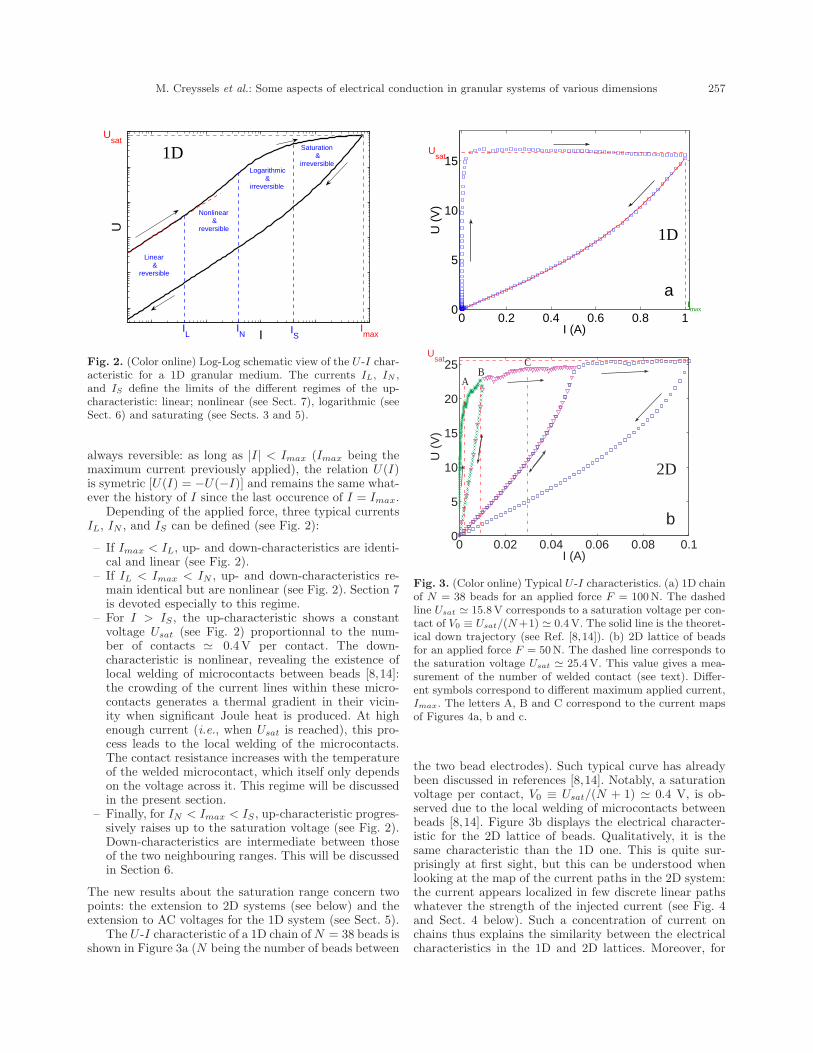
M. Creyssels et al.: Some aspects of electrical conduction in granular systems of various dimensions 257
I
UU
sat
IN I
S I
max
Logarithmic&
irreversible
Saturation &
irreversible
Nonlinear &
reversible
Linear &
reversible
IL
1D
Fig. 2. (Color online) Log-Log schematic view of the U -I char-acteristic for a 1D granular medium. The currents IL, IN ,and IS define the limits of the different regimes of the up-characteristic: linear; nonlinear (see Sect. 7), logarithmic (seeSect. 6) and saturating (see Sects. 3 and 5).
always reversible: as long as |I| < Imax (Imax being themaximum current previously applied), the relation U(I)is symetric [U(I) = −U(−I)] and remains the same what-ever the history of I since the last occurence of I = Imax.
Depending of the applied force, three typical currentsIL, IN , and IS can be defined (see Fig. 2):
– If Imax < IL, up- and down-characteristics are identi-cal and linear (see Fig. 2).
– If IL < Imax < IN , up- and down-characteristics re-main identical but are nonlinear (see Fig. 2). Section 7is devoted especially to this regime.
– For I > IS , the up-characteristic shows a constantvoltage Usat (see Fig. 2) proportionnal to the num-ber of contacts ≃ 0.4V per contact. The down-characteristic is nonlinear, revealing the existence oflocal welding of microcontacts between beads [8,14]:the crowding of the current lines within these micro-contacts generates a thermal gradient in their vicin-ity when significant Joule heat is produced. At highenough current (i.e., when Usat is reached), this pro-cess leads to the local welding of the microcontacts.The contact resistance increases with the temperatureof the welded microcontact, which itself only dependson the voltage across it. This regime will be discussedin the present section.
– Finally, for IN < Imax < IS , up-characteristic progres-sively raises up to the saturation voltage (see Fig. 2).Down-characteristics are intermediate between thoseof the two neighbouring ranges. This will be discussedin Section 6.
The new results about the saturation range concern twopoints: the extension to 2D systems (see below) and theextension to AC voltages for the 1D system (see Sect. 5).
The U -I characteristic of a 1D chain of N = 38 beads isshown in Figure 3a (N being the number of beads between
0 0.2 0.4 0.6 0.8 10
5
10
15
1D
a
Usat
I (A)
U (
V)
Imax
0 0.02 0.04 0.06 0.08 0.10
5
10
15
20
25
2D
b
Usat
I (A)
U (
V)
AB
C
Fig. 3. (Color online) Typical U -I characteristics. (a) 1D chainof N = 38 beads for an applied force F = 100 N. The dashedline Usat ≃ 15.8 V corresponds to a saturation voltage per con-tact of V0 ≡ Usat/(N +1) ≃ 0.4 V. The solid line is the theoret-ical down trajectory (see Ref. [8,14]). (b) 2D lattice of beadsfor an applied force F = 50 N. The dashed line corresponds tothe saturation voltage Usat ≃ 25.4 V. This value gives a mea-surement of the number of welded contact (see text). Differ-ent symbols correspond to different maximum applied current,Imax. The letters A, B and C correspond to the current mapsof Figures 4a, b and c.
the two bead electrodes). Such typical curve has alreadybeen discussed in references [8,14]. Notably, a saturationvoltage per contact, V0 ≡ Usat/(N + 1) ≃ 0.4 V, is ob-served due to the local welding of microcontacts betweenbeads [8,14]. Figure 3b displays the electrical character-istic for the 2D lattice of beads. Qualitatively, it is thesame characteristic than the 1D one. This is quite sur-prisingly at first sight, but this can be understood whenlooking at the map of the current paths in the 2D system:the current appears localized in few discrete linear pathswhatever the strength of the injected current (see Fig. 4and Sect. 4 below). Such a concentration of current onchains thus explains the similarity between the electricalcharacteristics in the 1D and 2D lattices. Moreover, for

258 The European Physical Journal E
0 20 40 600
10
20
30
40
50
60
Bead number in x−axis
Bea
d nu
mbe
r in
y−
axis
I = 31 mA C
Cur
rent
(A
rbitr
ary
unit)
4
8
13
17
21
25
0 20 40 600
10
20
30
40
50
60
Bead number in x−axis
Bea
d nu
mbe
r in
y−
axis
BI = 11 mAC
urre
nt (
Arb
itrar
y un
it)
2
4
5
7
9
11
0 20 40 600
10
20
30
40
50
60
Bead number in x−axis
Bea
d nu
mbe
r in
y−
axis
AI = 3 mA
Cur
rent
(A
rbitr
ary
unit)
0.7
1.4
2.1
2.8
3.5
4.2
Fig. 4. (Color online) Visualization of the current path net-work in an 2D hexagonal packing of metallic beads. The ap-plied voltage increases from bottom to top (corresponding toa total current of I = 3, 11 and 31 mA and denoted by theletters A, B, and C in Fig. 3b). An isotropic stress is createdby applying a 20N force on each upper side. The size of thelattice side is 31 beads. The upper part has not been measured(bead number in the y-axis ≥ 52). Colorbar scales are differentin the 3 plots.
the 2D lattice, the 25.4V saturation voltage (see Fig. 3b)gives a number of 64± 1 welded contacts when comparedto the V0 ≡ 0.4± 0.01V per contact of the 1D chain. Thisestimate is in good agreement with the dimensions of thehexagon (31 beads per side). Thus, as in the 1D system,the saturation voltage is also a measurement of the num-ber of welded contact in the 2D system.
4 Visualization of current paths in a 2Dgranular medium
Figures 4a, b and c show the evolution of the current mapswhen the applied voltage increases. These three maps cor-respond to the letters A, B and C in the U -I charac-teristic diagram of Figure 3b, that is, to the nonlinearand saturation regime. The current mainly appears con-centrated in few discrete paths as shown in Figure 4a.When the voltage increases, most of these paths are en-hanced, whereas few ones disappear (see Fig. 4b). Forhigher applied voltage, the previous paths are stronglyenhanced, and a bridge between two paths is even cre-ated (see Fig. 4c). For the highest applied voltage, thetotal current decreases from 31 to 20mA (during the 1hour measurement) due to thermal drift, and the stressdecreases of roughly 10%. The typical observation of thecurrent paths is generic to various stresses within our ex-perimental range, and is not reduced to a small range ofcompression. The effect of the stress strength on the cur-rent path evolution will be described in a future work.
The current maps of Figure 4 show that the currentpaths mainly appear concentrated on linear chains. Thesepreferred paths are reminiscent of stress concentrations(the so-called “force chains”) carrying an external loadimposed on granular systems [26–28]. The spatial dis-tribution of these force chains depends strongly on thetype of loading (isotropic or uniaxial compression, or pureshear) [28]. Only the isotropic case is described here. Sincethe contact resistances strongly vary with the applied force(much more than for an assumed elastic or plastic contact,see Fig. 3 of Ref. [14]), this could explain the similaritybetween force chains and “electrical chains”. However, asshown below, the contact resistances are also widely dis-tributed for a given force. This random distribution of re-sistances could also lead to the concentration of current onpercolating backbones [18]. The chains of maximum cur-rent thus would not be those of maximum stress, exceptmaybe at very high loading. However, we did not performa simultaneous measurement of force and current maps.Since the resistance distribution is broad, we probe morethe contact network (the least resistance paths) than theforce network.
5 Frequency dependence of the saturationvoltage
Let us now examine the AC electrical response of the 1Dchain. As far as the saturation voltage is concerned, twoextreme cases can be considered:

M. Creyssels et al.: Some aspects of electrical conduction in granular systems of various dimensions 259
– Either the contact temperature can follow the voltagevariations across a contact. Then the 0.4V per contactcorresponds to the peak amplitude of the AC voltageacross a contact. For a sine like variation in the voltage,the rms value of the saturation voltage is 0.4/
√2 ≃
0.28V per contact. The temperature variations occurat twice the frequency of the voltage. This doublingtemperature frequency stems from the dependence ofthe contact temperature on the square of the voltage(see below).
– Or the temperature cannot follow the voltage varia-tions due to the specific heat of the material. Then, the0.4V is the rms saturation voltage across the contact.
To discuss the intermediate regime between these twoextreme cases, let us introduce the influence of the spe-cific heat in the thermal budget. We approximate the tem-perature T and voltage U fields as spherically symmetricaround the center of the metallic bridge. Half of the Jouleheating goes in each bead. The current flowing from theleft to the right bead, and considering the right bead, wedefine u as the (negative) difference between the potentialat distance r and the potential at the center. Far from thecenter, T = T0 and u = −U/2. At the center (r = 0),T = T (0) and u = 0. The total heat flow at distance r is
−λ2πr2 ∂T
∂r, (1)
where λ is the heat conductivity. The total current I isindependent of r and is
I = −2πr2
ρ
∂u
∂r, (2)
where ρ is the electrical resistivity. Joule heating withinthe considered bead at distance less than r is then
−uI =2πr2
ρ
u∂u
∂r. (3)
The thermal budget then becomes
−λr2 ∂T
∂r=
r2
ρ
u∂u
∂r−
∫ r
0
Cr′2∂T (r′)
∂tdr′ , (4)
where C is the specific heat of the bead material. Usingthe relation λρ = LT (see Refs. [8,14]), where L ≃ 2.5 ×10⁻⁸ V2/K2 is the Lorentz number, equation (4) can bewritten as
T∂T
∂r= −u∂u
L∂r+
T
λr2
∫ r
0
Cr′2∂T (r′)
∂tdr′ . (5)
Integrating equation (5) from r = 0 to ∞ gives
T (ℓ)2−T (0)2 = −u2
L+
∫ ℓ
0
2T
λr2
∫ r
0
Cr′2∂T (r′)
∂tdr′dr (6)
or, with Tm ≡ T (0),
T 2m − T 2
0 =U2
4L−
∫ ∞
0
2T
λr2
∫ r
0
Cr′2∂T (r′)
∂tdr′dr . (7)
0 0.2 0.4 0.6 0.8 1 1.2
0.26
0.28
0.3
0.32
0.34
Irms
(A)
Urm
s / (N
+1)
(
V)
1D
Fig. 5. (Color online) Comparison between the AC character-istics measured at 1MHz () in the chain of N = 9 beads, andthe model (solid line) from equation (11) with A = 1.15 µm/A.Only the top part of the experimental curve is shown here tofocus on the saturation regime.
This is the modified Kohlrausch equation due to the sec-ond term on the right-hand side of equation (7) takingthe temporal dependence into account. For details on theKohlrausch equation at the thermal equilibrium, see ref-erences [6,29] for generality, or references [8,14] for thisproblem. The influence of this last term is examined inAppendix A for a sinusoidal voltage U = U0 cos ωt. Wethen find
T 2m − T 2
0 =U2
0
8L[1 + θ(ω) cos(2ωt− φ(ω))] , (8)
where
θ(ω) =1√
1 + G(ω)2; G(ω) =
4a
5
√2ω
κ, (9)
a = ρI0/πU0 being of the order of the radius of the metal-lic bridge (see App. A). I = I0 cos ωt is the first (andmain) harmonics of the current, κ and φ being introducedin Appendix A.
As explained in [8,14], the maximum value of T 2m, is
fixed to V 20 /4L by the softening of the metallic bridge,
with V0 ≃ 0.4V. Substituting this variable into equa-tion (8) leads to the rms saturation voltage
U2rms ≡
U20
2=
V 20
1 + θ(ω)= V 2
0
√1 + (32a2ω/25κ)
1 +√
1 + (32a2ω/25κ).
(10)Defining Irms ≡ I0/
√2 and A ≡ 8ρ/(5πV0), the AC
current-voltage characteristics for one contact then be-comes
U2rms = V 2
0
√1 + (A2I2
rmsω/κ)1 +
√1 + (A2I2
rmsω/κ). (11)
Figure 5 shows a comparison between measurementsat 1MHz (-symbols) and equation (11) (solid line). For

260 The European Physical Journal E
0.001 0.01 0.1 1 100
5
10
15 1D
a
I (mA)
U (
V)
0.02 0.2 20
5
10
15
202D
b
I (mA)
U (
V)
Fig. 6. (Color online) Zoom of the U -I characteristics in Fig-ure 3 on a semi-log plot focusing on small currents. (a) 1D and(b) 2D experiment. (solid line): fits U ∝ ln I.
this comparison, ω = 2πf with f = 1MHz, and thevalue chosen for A = 1.15µm/A is within 30% of thatobtained (≃ 0.9µm/A) from the physical properties ofthe stainless-steel beads used in the chain (see App. A).V0 = Usat/(N +1) ≃ 0.42V is given by the DC saturationmeasurements. The uncertainties in the measurements donot allow to claim for a full agreement. However, it is clearthat the model gives an order-of-magnitude estimate forthe frequency effects, and a good explanation of the pro-gressive character of the saturation in such conditions.It also confirms the size of the metallic bridge invokedto explain the saturation plateau: namely a ≃ 50 nm forI = 10−1 A, and proportional to the current I.
6 Up-characteristics for IN < I < IS
Let us now focus on the intermediate range of the DCapplied current IN < I < IS (see Fig. 2). In this case, thevoltage across the 1D chain of beads progressively growsup to the saturation voltage. For this current range, thecharacteristic of the Figure 3a is shown in a semi-log plot
Fig. 7. Cumulative distribution function of the resistance of achain of N = 17 beads for 480 realizations (in a semi-log plot):before () and after () the saturation regime (see Fig. 3a).〈R〉 = 38.3 Ω before (0.29 Ω after), and σR = 154.5 Ω before(0.22 Ω after).
in Figure 6a. It can be modeled over roughly two decadesas
U ∝ ln I. (12)
Only an inhomogeneity of resistances occurs betweenbeads along the chain. In the 2D experiment, there areboth stress [26–28] and resistance inhomogeneities. How-ever, a similar logarithmic characteristic is also observedwith the 2D experiment for this range of current, as shownin Figure 6b.
We argue that it is simply due to the wide distribu-tion of contact resistances between beads. The rough ar-gument is the following. When the current is progressivelyraised from zero, the contacts with the largest resistancesreach the saturation voltage first. Consequently, a furtherincrease of the current does not result in voltage increasefor each of these contacts. On the other hand, the contactswith the lowest resistances do not contribute either to thetotal rise in voltage. Thus this rise is due to the contactswhose resistance is such that they are close to the satura-tion voltage V0. This resistance is thus V0/I. For a varia-tion of current δI, their voltage increase is δU = (V0/I)δI.By integration, this leads to the log dependence of equa-tion (12) in qualitative agreement with the observationdisplayed in Figure 6.
A direct measurement of the cumulative distributionof resistances in the chain confirms this broad distributionof contact resistances between beads (see Figs. 7 and 8).Figure 7 shows in a semi-log plot the typical cumulativedistribution function of the total resistance of a chain of17 beads during 480 realizations. The distribution is broadbefore the saturation regime, and narrower after the sat-uration. The inset of Figure 8 shows the values of theresistance between 2 beads during 600 realizations beforethe saturation regime. These values are spread on morethan 3 decades. The cumulative distribution function ofthe logarithms of resistances is well fitted (solid line in
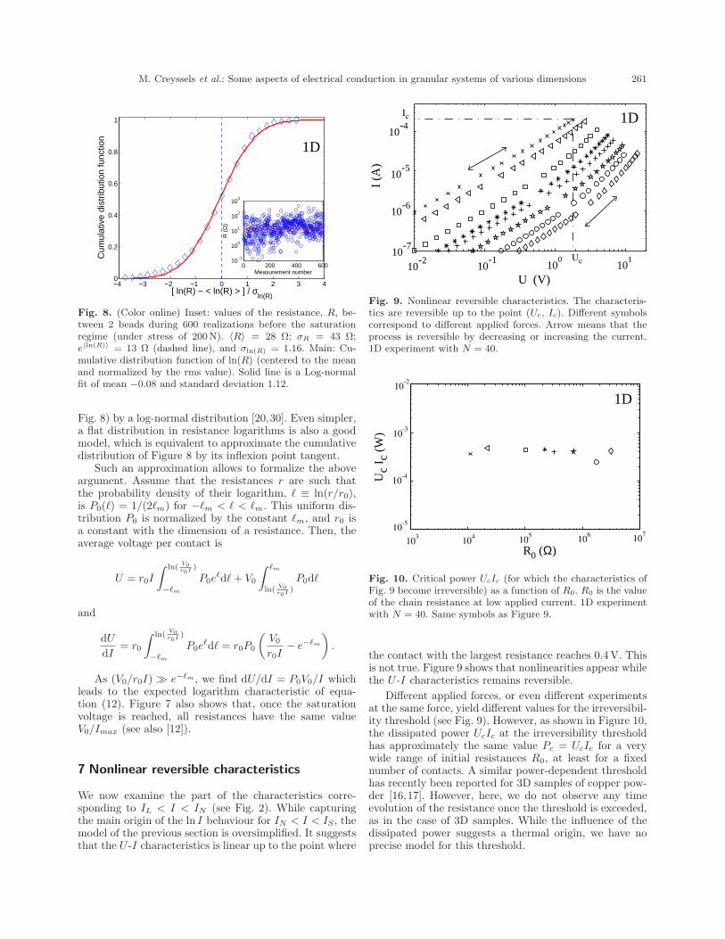
M. Creyssels et al.: Some aspects of electrical conduction in granular systems of various dimensions 261
−4 −3 −2 −1 0 1 2 3 40
0.2
0.4
0.6
0.8
1
[ ln(R) − < ln(R) > ] / σln(R)
Cum
ulat
ive
dist
ribut
ion
func
tion
1D
0 200 400 60010
−1
100
101
102
103
Measurement number
R (
Ω)
Fig. 8. (Color online) Inset: values of the resistance, R, be-tween 2 beads during 600 realizations before the saturationregime (under stress of 200N). 〈R〉 = 28 Ω; σR = 43 Ω;e〈ln(R)〉 = 13 Ω (dashed line), and σln(R) = 1.16. Main: Cu-mulative distribution function of ln(R) (centered to the meanand normalized by the rms value). Solid line is a Log-normalfit of mean −0.08 and standard deviation 1.12.
Fig. 8) by a log-normal distribution [20,30]. Even simpler,a flat distribution in resistance logarithms is also a goodmodel, which is equivalent to approximate the cumulativedistribution of Figure 8 by its inflexion point tangent.
Such an approximation allows to formalize the aboveargument. Assume that the resistances r are such thatthe probability density of their logarithm, ℓ ≡ ln(r/r0),is P0(ℓ) = 1/(2ℓm) for −ℓm < ℓ < ℓm. This uniform dis-tribution P0 is normalized by the constant ℓm, and r0 isa constant with the dimension of a resistance. Then, theaverage voltage per contact is
U = r0I
∫ ln(V0r0I )
−ℓm
P0eℓdℓ + V0
∫ ℓm
ln(V0r0I )
P0dℓ
and
dU
dI= r0
∫ ln(V0r0I )
−ℓm
P0eℓdℓ = r0P0
(V0
r0I− e−ℓm
).
As (V0/r0I) ≫ e−ℓm , we find dU/dI = P0V0/I whichleads to the expected logarithm characteristic of equa-tion (12). Figure 7 also shows that, once the saturationvoltage is reached, all resistances have the same valueV0/Imax (see also [12]).
7 Nonlinear reversible characteristics
We now examine the part of the characteristics corre-sponding to IL < I < IN (see Fig. 2). While capturingthe main origin of the ln I behaviour for IN < I < IS , themodel of the previous section is oversimplified. It suggeststhat the U -I characteristics is linear up to the point where
10-4
U (V)
I (A
)
10-5
10-6
10-7
10-2
10-1 10
010
1
Ic
Uc
1D
Fig. 9. Nonlinear reversible characteristics. The characteris-tics are reversible up to the point (Uc, Ic). Different symbolscorrespond to different applied forces. Arrow means that theprocess is reversible by decreasing or increasing the current.1D experiment with N = 40.
R0 (Ω)
Uc
I c (
W) 10-3
10-2
10-4
10-5
103
104
105
106
107
1D
Fig. 10. Critical power UcIc (for which the characteristics ofFig. 9 become irreversible) as a function of R0. R0 is the valueof the chain resistance at low applied current. 1D experimentwith N = 40. Same symbols as Figure 9.
the contact with the largest resistance reaches 0.4V. Thisis not true. Figure 9 shows that nonlinearities appear whilethe U -I characteristics remains reversible.
Different applied forces, or even different experimentsat the same force, yield different values for the irreversibil-ity threshold (see Fig. 9). However, as shown in Figure 10,the dissipated power UcIc at the irreversibility thresholdhas approximately the same value Pc = UcIc for a verywide range of initial resistances R0, at least for a fixednumber of contacts. A similar power-dependent thresholdhas recently been reported for 3D samples of copper pow-der [16,17]. However, here, we do not observe any timeevolution of the resistance once the threshold is exceeded,as in the case of 3D samples. While the influence of thedissipated power suggests a thermal origin, we have noprecise model for this threshold.

262 The European Physical Journal E
102
U (V)
R0
I -
U (
V)
101
100
10-1
10-2
10-1 100 101
1D
Fig. 11. Normalized nonlinear part of the current as a functionof the voltage U . The logarithmic slope is close to 2.33 ≃ 7/3.1D experiment with N = 40 beads. Same symbols as Figure 9.
100
101
10−2
10−1
100
101 3D
U (V)
R0I −
U (
V)
Fig. 12. Normalized nonlinear part of the current as a functionof the voltage U . The logarithmic slope is 7/3. 3D experimentwith copper powder from reference [16]. Symbols correspondsto different forces applied to the powder sample ranging from640 to 850N.
In order to characterize the nonlinearity, we plot R0I−U versus U in Figure 11, that is, the nonlinear part ofthe current, normalized by the initial resistance at lowapplied current, R0. The logarithmic plot stresses a powerlaw behaviour of this nonlinear part as
R0I − U ∼ Uα. (13)
The power law exponent α is always found close to 2.3 ≃7/3 whatever the applied force. Let us now use previousdata from 3D experiments with Copper powder [16], andplot R0I − U versus U as in Figure 12. Here also we finda similar power-law behaviour of the nonlinear part withroughly the same exponent α than the one found for the1D experiment of Figure 11.
The situation for 3D Copper powder samples will beclarified in [31]. Let us add a few comments about the
interplay between the irreversibility threshold occuringat a constant dissipated power (Pc), and the saturationthreshold (U = 0.4V per contact). At the former one,U2 < R0Pc, which means that, for sufficiently small initialresistance R0, it will occur before the saturation. However,for large enough R0 (small applied forces), it should occurafter. This is impossible, as our explanation of the satura-tion implies the irreversibility. Indeed, in such situations,we observed that the voltage U can cross the saturationvalue, and continue to grow until the irreversibility occurs.
8 Conclusion
We have reported experiments on the electrical con-ductivity in 1D and 2D model granular media. Theresults reported here serve both to confirm previousinterpretations and to raise new questions. In both 1Dand 2D systems at low current, the wide distributionof contact resistances results in a logarithmic behaviourfor the voltage/current characteristics. At high enoughcurrent, the dependence of the saturation voltage on theAC frequency confirms the model of the metallic bridge,including the order of magnitude of its size. In the 2Dsystem, both the voltage/current characteristic and themap of the current paths show the quasi–one-dimensionalnature of the electrical conductivity within a 2D granularmedium. The knowledge of the dependence of the currentpath distribution on different types of loads (e.g., pureshear, isotropic compression, . . . ) will be of primaryinterest. Another extension of this work is to understandthe nonlinear reversible behaviour of the characteristicobserved at very low current in the 1D system. Themost remarkable feature is that the nonlinear part ofthe current is a power law of the voltage with the sameexponent that the one found in previous 3D experiments.
A part of this work was supported by the French Ministry ofResearch under Grant ACI Jeunes Chercheurs 2001. S.D. isan FNRS research associate, and gratefully acknowledges thehospitality of the Physics Laboratory at the ENS Lyon. Wethank J.-F. Pinton and H.-C. Nataf for lending us the magneticfield sensor.
Appendix A.
Our goal is to approximately solve the Kohlrausch modi-fied equation (7)
T (0)2 − T 20 =
U2
4L−
∫ ∞
0
2T
λr2
∫ r
0
Cr′2∂T (r′)
∂tdr′dr (A.1)
with U = U0 cos ωt.To wit, we shall use a low-frequency approximation
for T (r) in the integrals. The imposed voltage across thecontact is U = U0 cos ωt. Thus, u = −(U0/2)f(r) cos ωtand I = I0 cos ωt. Substituting these two equations into

M. Creyssels et al.: Some aspects of electrical conduction in granular systems of various dimensions 263
equation (2) gives
I0 =U0π
ρr2 ∂f
∂r.
Neglecting the temperature dependence of ρ, we definea = r2∂f/∂r, a constant length which is of the order ofthe radius of the metallic bridge. As f = 1 for r = ∞, theabove relation integrates as f = 1 − (a/r) which is validfor r ≫ a. For r = 0, f = 0. We shall thus use the ansatz
f(r) = 1− a
r + a=
r
r + a.
Let us now limit ourselves to the first harmonics in 2ω,that is
T (r) = T∞ [h0(r) + θ(ω)h1(r) cos(2ωt− φ(ω))] (A.2)
with h0(0) = 1, φ(0) = 0, θ(0) = 1 and θ(∞) = 0.There are several approximations here. We assume
φ(ω) is independent of r, and h1 independent of ω. How-ever, φ(ω) is probably larger when r increases, as thevolume of the involved material (∝ r3) is larger. In thesame way, h1(r) is probably smaller at large r for small ωthan for large ω. Both effects have the result to effectivelylimit the integral to r smaller than the diffusion lengthℓD. We thus take them into account by putting the up-per limit in r to ℓD =
√κ/2ω, with κ ≡ λ/C, λ being
the thermal conductivity and C the specific heat of thebead material. For stainless steel: λ = 16.2Wm−1K−1,C = 3.9 × 10⁶ Jm−3K−1, κ = 4.1 × 10⁻⁶ m2s−1 andρ = 72× 10−8 Ωm.
Within the same approximations, at low frequency,equations (6) and (7) then become
T (r)2 − T 20 =
U20
8L(1− f2)(1 + cos 2ωt) =
T 2∞h2
0 + 2T 2∞h0h1 cos(2ωt)− (T 2
0 − T 2∞h2
1/2).
Neglecting the last term, we obtain
T 2∞ =
U20
8L; h0 =
√1− f2; h1 = h0/2.
Looking only at the 2ω terms, equation (A.1) thenbecomes
θ(ω) cos[2ωt−φ(ω)] = cos(2ωt)+G(ω)θ(ω) sin[2ωt−φ(ω)]
with
G(ω) = 4ω∫ ℓD
0
h0(r)λr2
∫ r
0
Cr′2h1(r′)dr′dr ,
or
G(ω) ≃ 2ω
κ
∫ ℓD
0
h0(r)r2
∫ r
0
r′2h0(r′)dr′dr . (A.3)
It thus gives
θ(ω) =1√
1 + G(ω)2. (A.4)
Keeping only the dominant term in equation (A.3),thus taking h0 ≃
√2a/r, that is∫ r
0
r′2h0(r′)dr′ ≃ 2√
2a
5r5/2 ,
we finally obtain
G ≃ 2ω
κ
4a
5ℓD =
4a
5
√2ω
κ.
References
1. R. Garcia-Rojo, H.J. Herrmann, S. McNamara (Editors),Powders and Grains 2005 (Taylor & Francis Group, Lon-don, 2005) and references therein.
2. J.D. Goddard, Proc. R. Soc. London, Ser. A 430, 105(1990); C. Liu, S.R. Nagel, Phys. Rev. B 48, 15646 (1993);C. Coste, E. Falcon, S. Fauve, Phys. Rev. E 56, 6104(1997); E. Falcon, C. Laroche, S. Fauve, C. Coste, Eur.Phys. J. B 5, 111 (1998); X. Jia, C. Caroli, B. Velicky,Phys. Rev. Lett. 82, 1863 (1999).
3. B. Gilles, C. Coste, Phys. Rev. Lett. 90, 174302 (2003).4. G.K. Batchelor, R.W. O’Brien, Proc. R. Soc. London, Ser.
A 355, 313 (1977); J.-C. Geminard, D. Bouraya, H. Gay-vallet, Eur. Phys. B 48, 509 (2005).
5. K. Chen et al., Nature 442, 257 (2006).6. R. Holm, Electric Contacts, 4th ed. (Springer Verlag,
Berlin, 2000); R.S. Timsit, Electrical Contacts, Principlesand Applications, edited by P. Slade (Marcel Dekker, NewYork, 1999).
7. E. Branly, C. R. Acad. Sci. Paris 111, 785 (1890) (inFrench).
8. E. Falcon, B. Castaing, Am. J. Phys. 73, 302 (2005).9. R. Gabillard, L. Raczy, C. R. Acad. Sci. Paris 252, 2845
(1961); 262, 1043 (1966).10. G. Kamarinos, P. Viktorovitch, M. Bulye-Bodin, C. R.
Acad. Sci. Paris 280, 479 (1975) (in French); G. Kamari-nos, A. Chovet, in Proceedings SEE: Conducteurs Granu-laires, edited by E. Guyon (Palais de la Decouverte, Paris,1990) p. 181 (in French).
11. S. Dorbolo, M. Ausloos, N. Vandewalle, Phys. Rev. E 67,040302(R) (2003).
12. S. Dorbolo, A. Merlen, M. Creyssels, N. Vandewalle, B.Castaing, E. Falcon, submitted to Europhys. Lett. (2007).
13. D. Vandembroucq, A.C. Boccara, S. Roux, J. Phys. III 7,303 (1997).
14. E. Falcon, B. Castaing, M. Creyssels, Eur. Phys. J. B 38,475 (2004).
15. D. Bonamy et al., Europhys. Lett. 51, 614 (2000); N. Van-dewalle, C. Lenaerts, S. Dorbolo, Europhys. Lett. 53, 197(2001).
16. E. Falcon, B. Castaing, C. Laroche, Europhys. Lett. 65,186 (2004).
17. M. Creyssels, PhD Thesis, Ecole Normale Superieure deLyon, 2006 (in French).
18. V. Ambegaokar, S. Cochran, J. Kurkijarvi, Phys. Rev. B8, 3682 (1973).
19. K.K. Bardhan, Physica A 241, 267 (1997) and referencestherein; J.P. Troadec, D. Bideau, J. Phys. (Paris) 42, 113(1981) (in French).

264 The European Physical Journal E
20. V. Da Costa et al., Eur. Phys. J. B 13, 297 (2000).21. J. Zhang, A. Zavaliangos, Discrete Element Simulation
of Transient Thermo electrical Phenomena in ParticulateSystem, in Granular Material-Based Technologies, MRSFall Meeting 2002, Boston, MA, December 2-6, 2002,edited by S. Sen, M.L. Hunt, A.J. Hurd, Proc. MRS,Vol. 759 (MRS, 2002).
22. A. Vojta, T. Vojta, J. Phys.: Condens. Matter 8, L461(1996); S. Roux, H.J. Herrmann, Europhys. Lett. 4, 1227(1987).
23. F.P. Bowden, D. Tabor, Proc. Roy. Soc. London, Ser.A 169, 391 (1939); K.J. Euler, J. Power Sources 3, 117(1978); M. Ammi et al., J. Phys. (Paris) 49, 221 (1988); X.Zhuang, J.D. Goddard, A.K. Didwania, J. Comput. Phys.121, 331 (1995).
24. Marteau & Lemarie, Specialist of beads. Product Cata-logue.
25. See Mag-03MC Fluxgate Sensor Operation Manual inhttp://www.gmw.com.
26. P. Dantu, Geotechnique 18, 50 (1968) (in French); A.Drescher, G. De Josselin De Jong, J. Mech. Phys. Solids20, 337 (1972); T. Travers et al., J. Phys. (Paris) 49, 939(1988); D.W. Howell, R.P. Behringer, C. Veje, Phys. Rev.Lett. 82, 5241 (1988).
27. F. Radjai, D.E. Wolf, M. Jean, J.-J. Moreau, Phys. Rev.Lett. 80, 61 (1998).
28. M.J. Majmudar, R.P. Behringer, Nature 435, 1079 (2005)and references therein.
29. J.A. Greenwood, J.B.P. Williamson, Proc. Roy. Soc. Lon-don, Ser. A 246, 13 (1958).
30. M. Evans, N. Hastings, B. Peacock, Statistical Distribu-tions (John Wiley & Sons, 1993).
31. M. Creyssels, E. Falcon, B. Castaing, unpublished.

September 2007
EPL, 79 (2007) 54001 www.epljournal.org
doi: 10.1209/0295-5075/79/54001
Effects of electromagnetic waves on the electrical properties ofcontacts between grains
S. Dorbolo1, A. Merlen
2, M. Creyssels
2, N. Vandewalle
1, B. Castaing
2 and E. Falcon3
1GRASP-Photopole, Physics Department, University of Liege - B-4000 Liege, Belgium2 Laboratoire de Physique, Ecole Normale Superieure de Lyon - 46 allee d’Italie, 69 007 Lyon, France3Matiere et Systemes Complexes, Universite Paris-Diderot - Paris 7, CNRS - Paris, France
received 1 June 2007; accepted in final form 5 July 2007published online 27 July 2007
PACS 45.70.-n – Granular systemsPACS 72.80.-r – Conductivity of specific materialsPACS 81.05.Rm – Porous materials; granular materials
Abstract – A DC electrical current is injected through a chain of metallic beads. The electricalresistance of each bead-bead contacts is measured. At low current, the distribution of theseresistances is large and log-normal. At high enough current, the resistance distribution becomessharp and Gaussian due to the creation of microweldings between some beads. The action ofnearby electromagnetic waves (sparks) on the electrical conductivity of the chain is also studied.The spark effect is to lower the resistance values of the more resistive contacts, the best conductiveones remaining unaffected by the spark production. The spark is able to induce through the chaina current enough to create microweldings between some beads. This explains why the electricalresistance of a granular medium is so sensitive to the electromagnetic waves produced in its vicinity.
Copyright c© EPLA, 2007
The electrical resistance of a granular assembly is verysensitive to a large variety of external perturbation. Theglobal electrical resistance can be indeed modified bya mechanical shock or stress, by a thermal dilatation,by aging [1], by applying an electrical current [2,3],or by producing electromagnetic perturbation in itsvicinity [4]. The two last sources of perturbation are themost unexpected. The relation between the voltage andthe current injected through a granular material has beendebated for a long time. It has been shown at the end ofthe XIX century that a huge decrease of resistance occurswhen a current is injected through metallic fillings [5]. Theresistance drops over several order of magnitude whenthe current reaches a given threshold. Almost during thesame period, Branly discovered that an electromagneticwave (e.g., spark production in the air) is able to modifythe electrical resistance of a granular heap at distance [4].This remarkable phenomenon is at the origin of thedevelopment of the wireless transmission. These problemshave been recently revisited because the mechanisms arestill not completely elucidated [6]. Moreover the electricalproperties could be a smart way to probe the internalstructure of the mechanical arches through a granularpile. When an electrical current is injected through a pile,it percolates according to the least resistance pathway
which has a topological dimension of 1. One of thechallenges is to determine the exact role of the networkcompared to the role of one single contact with respect tothe imposed perturbation.The relation between DC current and voltage has been
described for a one-dimensional (1D) chain of metallicbeads [2], in a 2D configuration [7,8] or in a 3D packing[9,10]. As reported in these works, the electrical propertiesof the bead assembly strongly depend on the electricalhistory of the granular pile. The voltage is not univocallydetermined by the current because of irreversible processessuch as microwelding occuring between the beads [2]. Someworks have also revisited the influence of sparks on theelectrical resistance of a 3D packing of lead beads (Branlyeffect) [11] and theoretically [12].The aim of this paper is to study the effect of either
a high current or an electromagnetic perturbation on theresistance of one single bead-bead contact. By performingthe experiments several times, a large number of contactswill be considered in order to establish the distributionof the resistances before and after the application of theperturbation. The comparison of both situations will allowto determine the behavior of one single contact.The experimental setup is shown in fig. 1. Seventeen
stainless steel beads (8mm of diameter) are placed in a
54001-p1
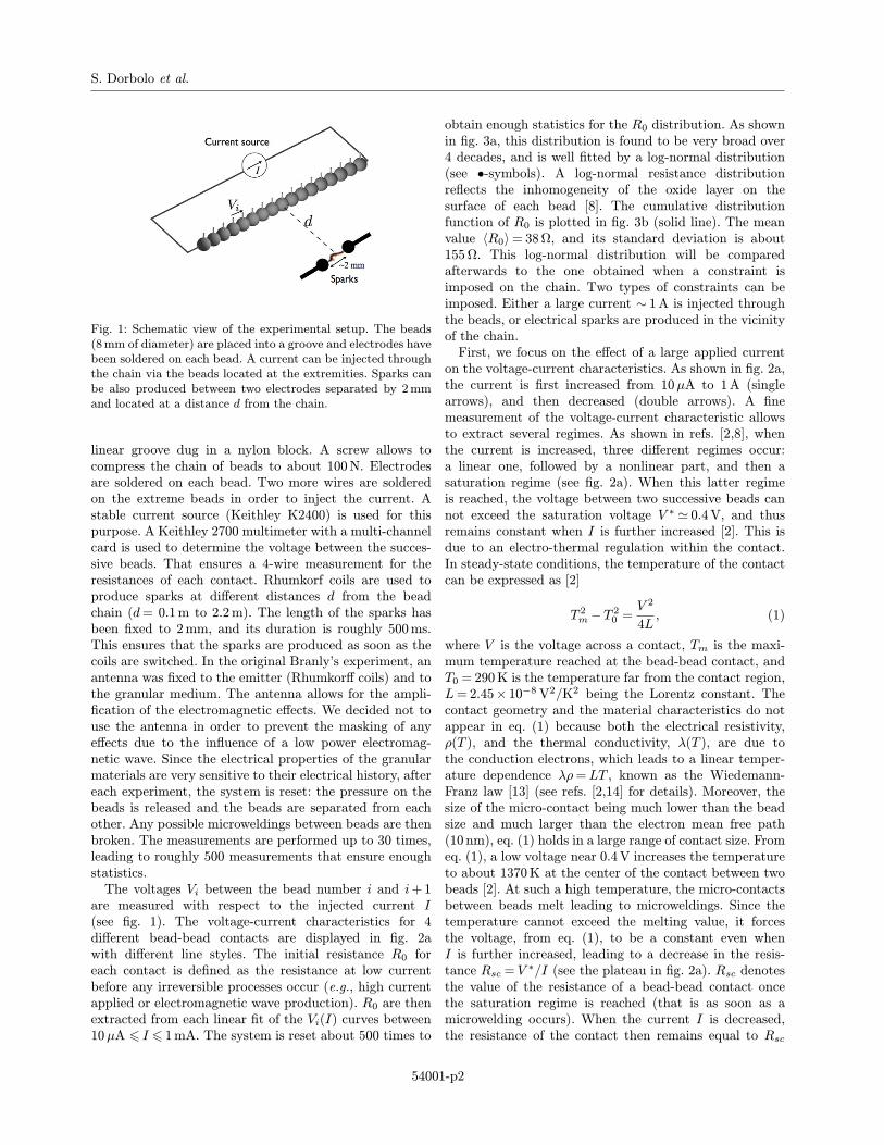
S. Dorbolo et al.
Fig. 1: Schematic view of the experimental setup. The beads(8mm of diameter) are placed into a groove and electrodes havebeen soldered on each bead. A current can be injected throughthe chain via the beads located at the extremities. Sparks canbe also produced between two electrodes separated by 2mmand located at a distance d from the chain.
linear groove dug in a nylon block. A screw allows tocompress the chain of beads to about 100N. Electrodesare soldered on each bead. Two more wires are solderedon the extreme beads in order to inject the current. Astable current source (Keithley K2400) is used for thispurpose. A Keithley 2700 multimeter with a multi-channelcard is used to determine the voltage between the succes-sive beads. That ensures a 4-wire measurement for theresistances of each contact. Rhumkorf coils are used toproduce sparks at different distances d from the beadchain (d= 0.1m to 2.2m). The length of the sparks hasbeen fixed to 2mm, and its duration is roughly 500ms.This ensures that the sparks are produced as soon as thecoils are switched. In the original Branly’s experiment, anantenna was fixed to the emitter (Rhumkorff coils) and tothe granular medium. The antenna allows for the ampli-fication of the electromagnetic effects. We decided not touse the antenna in order to prevent the masking of anyeffects due to the influence of a low power electromag-netic wave. Since the electrical properties of the granularmaterials are very sensitive to their electrical history, aftereach experiment, the system is reset: the pressure on thebeads is released and the beads are separated from eachother. Any possible microweldings between beads are thenbroken. The measurements are performed up to 30 times,leading to roughly 500 measurements that ensure enoughstatistics.The voltages Vi between the bead number i and i+1
are measured with respect to the injected current I(see fig. 1). The voltage-current characteristics for 4different bead-bead contacts are displayed in fig. 2awith different line styles. The initial resistance R0 foreach contact is defined as the resistance at low currentbefore any irreversible processes occur (e.g., high currentapplied or electromagnetic wave production). R0 are thenextracted from each linear fit of the Vi(I) curves between10µA I 1mA. The system is reset about 500 times to
obtain enough statistics for the R0 distribution. As shownin fig. 3a, this distribution is found to be very broad over4 decades, and is well fitted by a log-normal distribution(see •-symbols). A log-normal resistance distributionreflects the inhomogeneity of the oxide layer on thesurface of each bead [8]. The cumulative distributionfunction of R0 is plotted in fig. 3b (solid line). The meanvalue 〈R0〉= 38Ω, and its standard deviation is about155Ω. This log-normal distribution will be comparedafterwards to the one obtained when a constraint isimposed on the chain. Two types of constraints can beimposed. Either a large current ∼ 1A is injected throughthe beads, or electrical sparks are produced in the vicinityof the chain.First, we focus on the effect of a large applied current
on the voltage-current characteristics. As shown in fig. 2a,the current is first increased from 10µA to 1A (singlearrows), and then decreased (double arrows). A finemeasurement of the voltage-current characteristic allowsto extract several regimes. As shown in refs. [2,8], whenthe current is increased, three different regimes occur:a linear one, followed by a nonlinear part, and then asaturation regime (see fig. 2a). When this latter regimeis reached, the voltage between two successive beads cannot exceed the saturation voltage V ∗ 0.4V, and thusremains constant when I is further increased [2]. This isdue to an electro-thermal regulation within the contact.In steady-state conditions, the temperature of the contactcan be expressed as [2]
T 2m−T 20 =V 2
4L, (1)
where V is the voltage across a contact, Tm is the maxi-mum temperature reached at the bead-bead contact, andT0 = 290K is the temperature far from the contact region,L= 2.45× 10⁻⁸V2/K2 being the Lorentz constant. Thecontact geometry and the material characteristics do notappear in eq. (1) because both the electrical resistivity,ρ(T ), and the thermal conductivity, λ(T ), are due tothe conduction electrons, which leads to a linear temper-ature dependence λρ=LT , known as the Wiedemann-Franz law [13] (see refs. [2,14] for details). Moreover, thesize of the micro-contact being much lower than the beadsize and much larger than the electron mean free path(10 nm), eq. (1) holds in a large range of contact size. Fromeq. (1), a low voltage near 0.4V increases the temperatureto about 1370K at the center of the contact between twobeads [2]. At such a high temperature, the micro-contactsbetween beads melt leading to microweldings. Since thetemperature cannot exceed the melting value, it forcesthe voltage, from eq. (1), to be a constant even whenI is further increased, leading to a decrease in the resis-tance Rsc = V
∗/I (see the plateau in fig. 2a). Rsc denotesthe value of the resistance of a bead-bead contact oncethe saturation regime is reached (that is as soon as amicrowelding occurs). When the current I is decreased,the resistance of the contact then remains equal to Rsc
54001-p2

Effects of electromagnetic waves on the electrical properties of contacts between grains
Fig. 2: Typical current-voltage characteristics for 4 single contacts within the bead chain (different line styles). (a) Effect of astrong applied current: I is first increased from 10µA to 1A, then is decreased to 10µA. (b) Effect of sparks: I is first increasedfrom 10µA to 1mA, then sparks are produced at 1m from the chain. The influence of the sparks is shown by the discontinuityin two curves. Afterwards, I is increased up to 1A before being set back to 10µA. The single (respectively, double) arrowsdenote an increase (respectively, decrease) of the current. All the 4 curves collapse on each other when the current is decreased.The horizontal dashed line shows the saturation voltage V ∗ 0.4 V (see text).
Fig. 3: (a) Probability density functions (PDF) of the resistance R0 at low current (•), the resistance Rsc after the injectionof a current of 1A (), and the resistance Rsp after the production of sparks at 1m from the chain (). The curves representthe log-normal distribution fit of R0 (−) and Rsp (· · ·), while a Gaussian is fitted to Rsc (−−). The distribution of this latterhas been plotted on a linear scale in the inset. (b) The cumulative distribution functions (CDF) of R0 (−), Rsc (−−), and Rsp(· · ·) are shown on the same semi-log plot. The impact of sparks on the distribution is clearly visible between the R0 (−) andRsp (· · ·) CDFs: only the resistance values of the more resistive contacts have been decreased.
(see double arrows in fig. 2a). The distribution of thecontact resistances Rsc after the passage of a current of1A is shown in fig. 3a (see -symbols). The distributionis found to be very narrow, and is roughly fitted by aGaussian (see dashed line in fig. 3a and in the inset).
The mean value is 〈Rsc〉= 0.29Ω. Since the distribution isvery narrow, all the contacts can be viewed as electricallyequivalent. The large current has generated microweldingsbetween some beads and has thus erased their initiallyhigh resistive values. A finer description of the distribution
54001-p3
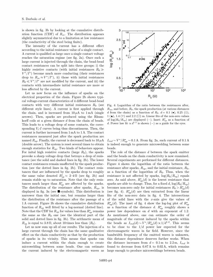
S. Dorbolo et al.
is shown in fig. 3b by looking at the cumulative distrib-ution function (CDF) of Rsc. The distribution appearsslightly asymmetrical due to a limitation at low resistance(the conductivity of the steel being finite).The intensity of the current has a different effect
according to the initial resistance value of a single contact.A current is qualified as large once a single contact voltagereaches the saturation regime (see fig. 2a). Once such alarge current is injected through the chain, the bead-beadcontact resistances can be split into three groups: i) thehighly resistive contacts (with initial resistances R0V ∗/I∗) become much more conducting (their resistancesdrop to Rsc ≈ V ∗/I∗), ii) those with initial resistancesR0 V ∗/I∗ are not modified by the current, and iii) thecontacts with intermediate initial resistance are more orless affected by the current.Let us now focus on the influence of sparks on the
electrical properties of the chain. Figure 2b shows typi-cal voltage-current characteristics of 4 different bead-beadcontacts with very different initial resistances R0 (seedifferent style lines). A current is first applied throughthe chain, and is increased from 10µA to 1mA (singlearrows). Then, sparks are produced using the Rhum-korff coils at a given distance d from the chain of beads.This leads to a voltage drop of some contacts, the corre-sponding Vi-I curves being thus discontinuous. Then, thecurrent is further increased from 1mA to 1A. The contactresistances measured just after the spark production arenamed Rsp. Finally, the current is decreased back to 10µA(double arrow). The system is reset several times to obtainenough statistics for Rsp. Two kinds of behaviors appear.For inital high resistive contacts (large R0), the sparksprovoke a sharp voltage drop that betrays a drop of resis-tance (see the solid and dashed lines in fig. 2b). The lowercontact resistances remain unaffected by the spark produc-tion (see the dotted lines in fig. 2b). The contact resis-tances that are influenced by the sparks drop to roughlythe same value denoted R∗sp 2–4Ω (see fig. 2b) andremain stable up to saturation. Note that the only resis-tances much larger than R∗sp are affected by the sparks.The distribution of the resistance after sparks, Rsp, isdisplayed in fig. 3a (see -symbols). This distribution isnarrower than the initial one, but remains larger thanthe distribution of the resistance after the passage of a1A current. Figure 3b shows the cumulative distributionfunction of Rsp well fitted by a log-normal (dotted line).Note that the CDF forRsp for values less than R
∗sp remains
the same as the R0 one (see the identical part of thesolid and dotted lines in fig. 3b). The arithmetic mean ofRsp is equal to 3.8Ω, about 10 times less than 〈R0〉.Let us now sum up all of our results. The injection of a
large current through the chain has the same qualitativeeffect on the chain conductivity as that by the productionof sparks in its vicinity. This means that sparks caninduce a current within the chain enough to createmicrowelding between some beads. One can estimatethe current induced by the electromagnetic waves as
Fig. 4: Logarithm of the ratio between the resistances after,Rsp, and before, R0, the spark production (at various distancesd from the chain) as a function of R0. d= 0.1 (•), 0.25 (♦),1 (), 1.4 () and 2.2 () m. Linear fits of the non-zero valuesof log(R0/Rsp) are displayed (−). Inset: R∗sp as a function ofd. Power law fit ∝ d1.2 is shown (−) as a guide for the eyes.
Iind ∼ V ∗/R∗sp ∼ 0.1A. From fig. 2a, such current of 0.1Ais indeed enough to generate microwelding between somebeads.The role of the distance d between the spark emitter
and the beads on the chain conductivity is now examined.Several experiments are performed for different distances.Figure 4 shows the logarithm of the ratio between theresistance after sparks, Rsp, and the initial resistance, R0,as a function of the logarithm of R0. Thus, when theresistance is not affected by sparks, log(R0/Rsp) equalszero. As said above, R∗sp(d) is the lowest resistance thatsparks are able to change. Thus, for a fixed d, log(R0/Rsp)becomes non-zero only for initial resistances R0 >R
∗sp(d)
(see fig. 4). R∗sp(d) are then extracted from the linearfits of the non-zero data in fig. 4. The intersectionsof the solid lines with the x-axis give the values ofR∗sp(d). The inset of fig. 4 show the log-log plot of R∗spas a function of the distance d. R∗sp roughly shows apower law dependence on d with an exponent of 1.2.As mentioned above, one can estimate the order ofmagnitude of the current induced by the sparks withinthe beads as Iind(d)∼ V ∗/R∗sp(d)∝ 1/d1.2. This seemsto be close to the 1/d power law expected for theelectromagnetic waves in far field. However, since thebandwidth frequency of the emitted waves is unknown,this distance dependence deserves further works. Whenthe distance increases from d= 0.1m to 2.2m, Iind isfound to decrease from 0.87A to 0.02A, which remainslarge enough to produce microweldings between beads.
54001-p4
Effects of electromagnetic waves on the electrical properties of contacts between grains
The infuence of either a high DC current or an electro-magnetic perturbation on the electrical properties of achain of beads has been studied. The distribution of thebead-bead resistances before the perturbation is a log-normal over 4 decades. Applying a high current transformsthis distribution to a narrow Gaussian owing to thecreation of microwelding between the contacts. Whensparks are produced in the chain vicinity, only bead-bead resistances larger than a threshold value R∗sp areaffected by the electromagnetic waves. R∗sp is roughlyproportional to the distance between the chain and thespark emitter. Spark emission acts as a DC current whichintensity inversely depends on the distance between thesparks and the contact. This induced current is enough tocreate microweldings between some contacts. Generally,a granular packing has a huge contact number. Highlyresistive contacts are thus likely. Since only the largestresistances are influenced by sparks, this explains why theconductivity of a granular network is so sensitive to theaction of nearby electromagnetic waves.
∗ ∗ ∗
SD thanks FNRS for financial support and gratefullyacknowledges the hospitality of the Physics Laboratory atENS-Lyon. Part of this work was supported by the FrenchMinistry of Research under Grant ACI 2001. Dr A. V.Orpe (Clark University) is thanked for his comments.The authors would like to thank C. Laroche for his
helpful comments in the elaboration of the experimentalset-up.
REFERENCES
[1] Dorbolo S., Ausloos M., Vandewalle N. andHoussaM., J. Appl. Phys., 94 (2003) 7835.
[2] Falcon E., Castaing B. and Creyssels M., Am. J.Phys., 73 (2005) 302.
[3] Vandembroucq D., Boccara A. and Roux S., J. Phys.III, 7 (1997) 303.
[4] Branly E., C. R. Acad. Sci. Paris, 111 (1890) 785.[5] Calzecchi-Onesti T., Nuovo Cimento, 16 (1884) 58.[6] Falcon E. and Castaing B., Pour la Science, 340(2006) 58; Guyon E., Physica A, 357 (2005) 150.
[7] Dorbolo S., Ausloos M. and Vandewalle N., Eur.Phys. J. B, 34 (2003) 201.
[8] Creyssels M., Dorbolo S., Merlen A., Laroche C.,Castaing B. and Falcon E., to be published in Eur.Phys. J. E (2007); Creyssels M., PhD Thesis, ENS-Lyon, France, 2006.
[9] Dorbolo S., Ausloos M. and Vandewalle N., Appl.Phys. Lett., 81 (2002) 936.
[10] Falcon E., Castaing B. and Laroche C., Europhys.Lett., 65 (2004) 186.
[11] Dorbolo S., Ausloos M. and Vandewalle N., Phys.Rev. E, 67 (2003) 040302 R.
[12] Hirlimann C., cond-mat/0703495 (2007).[13] Holm R., Electrical Contacts, 4th edition (Springer-
Verlag, Berlin) 2000.[14] Greenwood J. A. and Williamson J. B. P., Proc. R.
Soc. London, Ser. A, 246 (1958) 13.
54001-p5

178

179

180
Chapitre D
Gaz granulaires dissipatifs
D.1 Resume synthetique des travaux
Introduction
Depuis les predictions de Maxwell et Boltzmann en 1860-70, il est bien connu que lesmolecules d’un gaz bougent de facon erratique avec une distribution de vitesse gaussienne.Cela permet de decrire les proprietes de transport des gaz moleculaires. Cependant, cettetheorie cinetique n’est plus valable si les interactions entre particules sont dissipatives ou sielles dependent de leur vitesses. Un exemple bien connu de gaz dissipatif est le gaz granulaire.
Les proprietes macroscopiques d’un gaz granulaire sont intimement liees a la physique descollisions entre grains et a l’absence d’agitation thermique. Puisque les collisions entre parti-cules granulaires sont inelastiques, il faut alors continument fournir de l’energie a ce systeme(par vibration mecanique) pour le maintenir dans un etat stationnaire hors equilibre. Cetteinelasticite des collisions conduit a des regimes dynamiques particulierement interessants.Nous avons notamment mis en evidence une transition entre un etat fluidise homogene spa-tialement, un « gaz » , et un phenomene d’agregation ou « amas » de particules soumises a desexcitations vibratoires, lorsque le nombre de particules augmente. Ce type de comportementresulte de l’inelasticite des collisions qui peuvent dissiper en un temps fini l’energie cinetiqued’un groupe de particules. Ces travaux ont donne lieu a des commentaires tres positifs dansScience, Science News, Daily University Science News et Physics News.
Dans le regime cinetique, du fait de l’inelasticite des collisions, nous avons montre experi-mentalement que la pression et la temperature d’un tel gaz granulaire obeissent a une equationd’etat qui differe qualitativement de celle d’un gaz classique. Nous avons ensuite montrenumeriquement qu’un modele de coefficient de restitution dependant de la vitesse d’impactentre grains est necessaire pour retrouver l’ensemble de ces resultats experimentaux a la foisqualitativement et quantitativement. Nous avons aussi etudie la statistique des fluctuationsde pression d’un gaz granulaire dissipatif. Ces travaux sont rapidement decrits ci-dessous.Pour plus de details, nous renvoyons le lecteur aux publications ci-jointes.
Du gaz a l’amas granulaire
Du fait de la dissipation d’energie intervenant principalement au cours des collisionsinelastiques, un « gaz » granulaire dissipatif ne peut etre decrit a la maniere d’un gaz usuel aumoyen de la theorie cinetique d’un gaz de sphere dure. Un tel « gaz » dissipatif est obtenu enmettant en mouvement un ensemble de billes a l’aide d’un piston oscillant dans un cylindre
181

ba
Fig. D.1: Experience au sol : Transition entre un « gaz » granulaire dissipatif et un « amas »dense de particules lorsque le nombre de particules augmente de (a) 500 a (b) 2000. Le pistonvibrant est en bas (non visible). Diametre des billes en acier 2 mm. Diametre du tube 52 mm.
vertical. Afin d’acceder a l’analogue de l’equation d’etat du gaz usuel, un deuxieme piston,se trouvant a la partie superieure du cylindre, est soit fixe a une hauteur donnee (experiencea volume constant), soit se stabilise a une hauteur donnee sous l’effet des chocs des billes(experience a pression constante). Nous avons mesure, d’une part, la pression moyenne Pexercee par les billes (resp. le volume Ω) en fonction du nombre de particules N , et des pa-rametres de vibration a Ω (resp. P ) fixe et, d’autre part, la densite locale de billes en fonctionde l’altitude. Lorsque le nombre de billes est superieur a un nombre critique, une transitionapparaıt entre un regime ou les particules ont un mouvement desordonne et un regime decomportement collectif ou les particules rebondissent a la maniere d’un corps solide (voir Fig.D.1). Pour Ω (resp. P ) fixe, la pression (resp. le volume) passe par un maximum pour unnombre critique de particules, avant de decroıtre lorsque le nombre de billes augmente. Cescomportements, differents de ceux des gaz usuels, proviennent de la dissipation d’energie dueaux collisions inelastiques. Cependant, comme pour un gaz usuel, « l’atmosphere » ou la den-site de particules decroıt exponentiellement suffisamment loin du piston, mais sur des echellesde longueur tres differentes. De facon independante, les mesures de pression, de volume et lesqueues exponentielles des profils de densite permettent alors d’avoir acces a la dependancede la temperature granulaire1, T , avec la vitesse d’excitation, V , selon T ∼ V θ(N) ou θ esttrouvee etre une fonction decroissante de N , determinee empiriquement. Nous avons doncmontre, pour la premiere fois, que la loi PΩ ∼ T avec T ∼ V θ(N), ou θ(N) a ete obtenu par3 mesures independantes sous des conditions experimentales differentes, fournit une equationd’etat empirique acceptable pour un gaz granulaire dissipatif dans le regime cinetique. Cetravail explique les resultats numeriques conflictuels anterieurs pour la determination de lavaleur de l’exposant θ.
En collaboration avec Sean McNamara de l’Universite de Stuttgart, nous avons realise dessimulations numeriques bidimensionnelles d’un milieu granulaire fortement vibre en presencede gravite. Nous avons introduit un modele de coefficient de restitution dependant de la vitesse
1La temperature granulaire est definie par ananolgie avec la tempeature d’un gaz usuel comme etant l’energiecinetique des particules divisee par le nombre de particules.
182

d’impact entre deux particules. Cette dependance permet de tenir compte des deformationsviscoelastiques et plastiques des particules intervenant respectivement a petites et grandesvitesses. Nous avons montre que l’utilisation de ce modele de coefficient de restitution estnecessaire pour que nos simulations soient en accord avec les experiences ci-dessus. Nous me-surons numeriquement les exposants en loi de puissance de la temperature granulaire, de lafrequence de collision, de l’impulsion et de la pression du gaz avec la vitesse de piston vibrant.Lorsque le systeme evolue d’un etat gazeux homogene, a basse densite de particules, vers unetat en amas, a haute densite, ces exposants decroıssent continument avec le nombre de par-ticules en accord avec l’observation experimentale. L’utilisation de ce modele de coefficient derestitution conduit aussi a des nouveaux comportements. En l’absence de gravite, on observenumeriquement qu’un amas « lache » de particules apparaıt proche du mur oppose au pistonvibrant et agit comme un amortisseur pour les particules les plus rapides conduisant alors ades exposants anormaux : la pression exercee sur les murs devient independante du nombrede particules N , et est proportionnelle a la vitesse du piston V ; la frequence de collision a laparoi vibrante devient independante de N et V . Tous ces resultats different de facon signifi-cative de la theorie cinetique classique de sphere dure inelastique, ainsi que des precedentessimulations numeriques principalement basees sur un coefficient de restitution constant.
a
b
Fig. D.2: Experience en impesanteur : Transition d’un gaz granulaire a un amas dense departicules lorque le nombre de particules dans les cellules augmente. De droite a gauche :1500, 3000 et 4500 particules. Deux phases differentes du cycle de vibration sont montrees :(a) vitesse de la cellule maximum vers le haut et (b) maximum vers le bas. Diametre desbilles en bronze 0.3 mm. Chaque cellule est cubique d’1 cm3.
La mise en amas observee dans l’experience au sol decrite ci-dessus n’exclut toutefois pasun possible phenomene de resonance entre son temps de vol sous gravite et la periode devibration. Les fusees-sondes2 Mini-Texus 5 et Maxus 5, ont ete lancees respectivement en1998 et en 2003 a Esrange (Suede) afin d’etudier cette transition gaz – amas en microgravite.A son bord, trois cellules (resp. sept cellules), avec des densites de billes differentes, ont etesoumises a des vibrations sinusoıdales d’amplitude et de frequence variables. L’interet de lamicrogravite est de se placer dans une situation experimentale ou les collisions sont le seul
2Ce sont des fusees de l’ESA de 12 tonnes et de 16 metres de haut qui atteignent leur apogee a 710 km(resp. 150 km) d’altitude, avant de permettre au 5 modules experimentaux embarques d’avoir 12 min (resp. 3min) de microgravite (a 10−4g pres) au cours de sa chute libre.
183
mecanisme d’interaction. L’enregistrement video a montre que lorsque la densite du milieuaugmente, l’etat fluidise homogene spatialement ( « gaz » ) n’est plus stable et un remar-quable phenomene d’agregation de particules se produit, sous la forme d’un amas immobile,au sein de la cellule (voir Fig. D.2). C’est la premiere observation convaincante qui montrequ’un ensemble de particules solides en mouvement erratique, interagissant seulement parl’intermediaire de collisions inelastiques, peut engendrer la formation d’un « amas » dense departicules.
Entre 2000 et 2003, cinq campagnes de vols paraboliques3 en microgravite ont ete realiseesa bord de l’Airbus A300 Zero-G afin d’etudier la statistique des collisions d’un gaz granulairedilue fluidise par des vibrations. Nous avons mesure, pour la premiere fois en geometrie 3D,la loi d’echelle du nombre des collisions a une paroi de la cellule, et celle de la distributiondes impulsions des particules en fonction de la vitesse de vibration du piston et du nombre departicules presentes dans l’enceinte. Nous montrons que la frequence de collisions a la paroin’evolue pas lineairement avec le nombre de particules et que la distribution des vitesses ala paroi possede une queue exponentielle. Nous avons souligne que ces resultats different defacon significative de la theorie cinetique d’un gaz usuel, et sont deux consequences impor-tantes de la nature inelastique des collisions.
D.2 Publications associees
Articles
E. Falcon, S. Fauve & C. Laroche, European Physical Journal B 9, 183–186 (1999)Cluster formation, pressure and density measurements in a granular medium fluidized by vibrations
E. Falcon, S. Fauve & C. Laroche, Journal de Chimie Physique 96, 1111–1116 (1999)Experimental determination of a state equation for dissipative granular gases
E. Falcon, R. Wunenburger, P. Evesque, S. Fauve, C. Chabot, Y. Garrabos & D. Beysens,Physical Review Letters 83, 440–444 (1999)Cluster formation in a granular medium fluidized by vibrations in low gravity
S. McNamara & E. Falcon, Physical Review E 71 031302 (2005)Simulations of vibrated granular medium with impact velocity dependent restitution coefficient
E. Falcon, S. Aumaıtre, P. Evesque, F. Palencia, C. Chabot, S. Fauve, D. Beysens & Y.Garrabos, Europhysics Letters 74, 830 (2006)Collision statistics in a dilute granular gas fluidized by vibrations in low gravity
M. Leconte, Y. Garrabos, E. Falcon, C. Lecoutre-Chabot, F. Palencia, P. Evesque, & D.Beysens, Journal of Statistical Mechanics - Theory and Experiment, P07012 (2006)Microgravity experiments on vibrated granular gas in a dilute regime : non classic statistics
3Une campagne consiste en une session de 3 vols, chaque vol permettant la realisation de 30 paraboles de22 secondes chacune de microgravite (a 5×10⁻²g pres).
184
S. McNamara & E. Falcon, Powder Technology 182, 232 (2008)Simulation of dense granular gases without gravity with impact-velocity-dependent restitution co-efficient
Chapitre de Livres
E. Falcon, S. Fauve & C. Laroche, in “Granular Gases”, Vol. 564, Lectures Notes in Physics,T. Poschel & S. Luding (Eds.), Springer-Verlag, pp. 244–253 (2001)An experimental study of a granular gas fluidized by vibrations
S. McNamara & E. Falcon, in “Granular Gas Dynamics”, Vol. 624, Lectures Notes in Physics,T. Poschel & N. V. Brilliantov (Eds.), Springer, Berlin, p. 341–361 (2003)Vibrated granular media as experimentally realizable granular gases
Actes de conferences
P. Evesque, E. Falcon, R. Wunenburger, S. Fauve, C. Lecoutre-Chabot, Y. Garrabos & D.Beysens, Proceedings of the 1st International Symposium on Microgravity Research and Applica-tions in Physical Sciences and Biotechnology, Sorrento (Italy), Sept. 10-15, 2000, ESA SP-454(Ed.), p. 829–834 (2001)Gas-cluster transition of granular matter under vibration in microgravity
Articles de presse
Parus dans la presse scientifique americaine suite a Falcon et al., PRL 83, 440 (July 1999)
• Science, Vol. 285, July 23, 1999, p. 251 by C. Holden in “Random Samples.”Building theories on sand.
• Science News, Vol. 156, No 3, July 17, 1999, p. 38 by P. Weiss.Vibrating grains form floating clumps.
• UniSci (Daily University Science News site), July 12, 1999.Granular Materials Tested In Outer Space For First Time.
• Physics News, No 438, July 09, 1999, by P. F. Schewe and B. Stein.Clustering in granular gases.
• European Space Agency News : Bronze award for MiniTexus scientist, 2 December 2002.
185

186

D.3 Tires a part
187

188

Eur. Phys. J. B 9, 183–186 (1999) THE EUROPEANPHYSICAL JOURNAL Bc©
EDP SciencesSocieta Italiana di FisicaSpringer-Verlag 1999
Rapid Note
Cluster formation, pressure and density measurementsin a granular medium fluidized by vibrations
E. Falcon1,a, S. Fauve1, and C. Laroche2
1 Laboratoire de Physique Statistique, Ecole Normale Superieure, 24 rue Lhomond, 75231 Paris Cedex 05, France2 Laboratoire de Physique, Ecole Normale Superieure de Lyon, 46 allee d’Italie, 69364 Lyon Cedex 07, France
Received 1 February 1999
Abstract. We report experimental results on the behavior of an ensemble of inelastically colliding particles,excited by a vibrated piston in a vertical cylinder. When the particle number is increased, we observe atransition from a regime where the particles have erratic motions (“granular gas”) to a collective behaviorwhere all the particles bounce like a nearly solid body. In the gas-like regime, we measure the density ofparticles as a function of the altitude and the pressure as a function of the number N of particles. Theatmosphere is found to be exponential far enough from the piston, and the “granular temperature”, T ,dependence on the piston velocity, V , is of the form T ∝ V θ, where θ is a decreasing function of N . Thismay explain previous conflicting numerical results.
PACS. 45.70.-n Granular systems – 83.70.Fn Granular solids – 05.20.Dd Kinetic theory –83.10.Pp Particle dynamics
Granular matter is an interdisciplinary subject, involvingsoil mechanics (rheology), powder technology [1,2], geo-physics (dunes [3], ice floes [4]), astrophysics (planetaryrings [5]) and statistical physics of dissipative media [6,7].Recently, considerable attention has been devoted to therole of the inelasticity of the collisions in vibrated granularmedia, the so-called driven “granular gas” for which thestationary state results from the balance between dissi-pation by inelastic collisions and power input by externalvibrations. While over the years many attempts based onkinetic theory [8–11] have been made to describe such dis-sipative granular gases, no agreement has been found sofar both with experiments [12,13] and numerical simula-tions [13–15], for the dependence of the “granular tem-perature” with the parameters of vibration [16–18]. Theaim of this study was to guess possible gas-like state equa-tions for such dissipative granular gas and to observe newkinetic behaviors which trace back to the inelasticity ofcollisions.
We report an experimental study of a “gas” of inelas-tically colliding particles, excited by vertical vibrations.When the vibration is strong enough and the numberof particles is low enough, the particles display ballisticmotion between successive collisions like molecules in agas (see Fig. 1a). At constant external driving, we showthat the pressure passes through a maximum for a critical
a e-mail: [email protected]
ba
Fig. 1. Transition from a dissipative granular gas to a densecluster: (a) N = 480; (b) N = 1920, respectively correspondingto roughly 1 and 4 particle layers at rest. The parameters ofvibration are f = 20 Hz and A = 40 mm. The driving pistonis at the bottom (not visible), the inner diameter of the tubebeing 52 mm.
number of particles before decreasing for large N . We alsomeasure density profiles and extract granular temperaturefrom them. When the density of the medium is increased,the gas-like state is no longer stable but displays the for-mation of a dense cluster bouncing like a nearly solid body(see Fig. 1b).

184 The European Physical Journal B
0 500 1000 1500 2000 25000
0.05
0.1
0.15
0.2
0.25
N
P /
f 2 (P
a s−
2 )
Fig. 2. Mean pressure P rescaled by f2 as a function of N .From the upper (×-marks) to the lower (hexagrams) curve,vibration frequency f varies from 10 to 20 Hz with a 1 Hz step.For all these experiments, h − h0 = 5 mm and A = 25 mm.One single layer of particles at rest corresponds to N = 600.Lines join the data points.
The experiment consists of a transparent cylindricaltube, 60 mm in inner diameter, filled from 20 to 2640 stain-less steel spheres, 2 mm in diameter, roughly correspond-ing to no more than 5 particle layers at rest. An electri-cal motor, with eccentric transformer from rotational totranslational motion, drives the particles sinusoidally witha 25 or 40 mm amplitude, A, in the frequency range from 6to 20 Hz. A lid in the upper part of the cylinder, is eitherfixed at a given height, h (constant-volume experiment)or is stabilized at a given height hm due to the bead col-lisions (constant-pressure experiment). Heights h and hmare defined from the lower piston at full stroke.
Time averaged pressure measurements have been doneas follows. Initially, a counterweight of mass m = 46 gbalances the lid mass. The piston drives stainless steelspheres in erratic motions in all directions (see Fig. 1a).Particles are hitting the lid all the time, so that to keepit at a given height h we have to hold the lid down bya given force, Mg, where M is the mass of a weight weplace on the lid and g the acceleration of gravity. At afixed h, i.e. at a constant-volume, Figure 2 shows the timeaveraged pressure Mg/S exerted on the lid as a functionof the number N of beads in the container, for differentfrequencies of vibration, S being the area of the tube cross-section. At constant external driving, i.e. at fixed f andA, the pressure passes through a maximum for a criticalvalue of N roughly corresponding to 0.8 particle layers atrest. This critical number is independent on the vibrationfrequency. A further increase of the number of particlesleads to a decrease in the mean pressure underlying thatmore and more energy is dissipated by inelastic collisions.Note that gravity has a small effect in these measurementsthat are performed for V 2 gh, where V = 2πfA is themaximum velocity of the piston. For N such that one hasless than one particle layer at rest, most particles are invertical ballistic motion between the piston and the lid.Thus, the mean pressure increases roughly proportionallyto N . When N is increased such that one has more than
0 500 1000 1500 2000 25000
2
4
6
8
10
N
Exp
ansi
on, h
m −
h0 (
cm)
Fig. 3. Maximal bed expansion, hm − h0, as a function of N ,for various frequencies f of vibration. From the lower (-marks)to the upper (-marks) curve, f varies from 7 to 20 Hz with a1 Hz step and A = 25 mm. One single layer of particles at restcorresponds to N = 600. Lines join the data points.
one particle layer at rest, interparticle collisions becomemore frequent. The energy dissipation is increased andthus the pressure decreases. In the low density regime (lessthan two particles layers at rest) the mean pressure scaleslike the square of the piston velocity, V 2.
We now consider the bed expansion under the influ-ence of collisions on a circular wire mesh lid placed ontop of the beads leaving a clearance of about 0.5 mm be-tween the edge of the lid and the tube one. Due to thebead collisions, the lid is stabilized at a given height hmfrom the piston at full stroke. Although the lid mass isroughly 50 times smaller than the total mass of beads,the lid proves to be quite stable and remains horizontal.The expansion, hm−h0, of the bed is displayed in Figure 3as a function of N for different vibration frequencies. h0
is the bed height at rest. At fixed f , the expansion passesthrough a maximum for a critical value of N roughly cor-responding to 0.6 particle layers at rest. This critical num-ber is independent on the vibration frequency. When N isfurther increased, the expansion decreases showing, as forpressure measurements, an increase in dissipated energyby inelastic collisions. Note that the height hm of the gran-ular gas is much larger than for pressure measurements ofFigure 2. Consequently, gravity is obviously important.Moreover, for a given N , the number of interparticle col-lisions is larger than for the pressure measurements. Onecannot consider that most particles are in ballistic motionbetween the piston and the lid, and thus the V 2 scaling isno longer observed.
As already found experimentally in 1-D [13] and3-D [19,20] and numerically [13,21], we observe that, atN fixed, the granular medium exhibits (not shown here)a sudden expansion at a critical frequency correspondingto a bifurcation similar to that exhibited by a single ballbouncing on a vibrating plate [13,19]. Moreover, we findthat this critical frequency depends on the number of lay-ers, n. When n increases above 0.4, a transition from the1-D-like behavior to a 3-D one is observed: the expansionat the critical frequency becomes less abrupt and tends toincrease regularly with f .
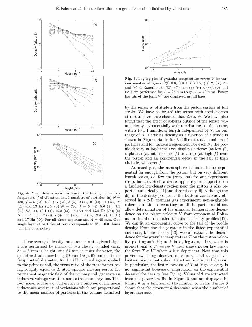
E. Falcon et al.: Cluster formation in a granular medium fluidized by vibrations 185
0 4 8 1210
0
101
102
Height (cm)
Den
sity
(ar
b. u
nit)
(a)
0 4 8 1210
0
101
102
Height (cm)
Den
sity
(ar
b. u
nit)
(b)
0 4 8 1210
0
101
102
103
Height (cm)
Den
sity
(ar
b. u
nit)
(c)
Fig. 4. Mean density as a function of the height, for variousfrequencies f of vibration and 3 numbers of particles: (a) N =480; f = 5 (), 6 (+), 7 (×), 8 (), 9 (∗), 10 (2), 11 (3), 12(4) and 13 Hz (5); (b) N = 720; f = 5 (), 5.6 (+), 7.1(×), 8.6 (), 10.1 (∗), 12.2 (2), 14 (3) and 15.2 Hz (4); (c)N = 1440; f = 7 (), 8 (+), 10 (×), 11.4 (), 12.8 (∗), 15 (2)and 17 Hz (3). For all these experiments, A = 40 mm. Onesingle layer of particles at rest corresponds to N = 480. Linesjoin the data points.
Time averaged density measurements at a given heightz are performed by means of two closely coupled coils,δz = 5 mm in height, and 64 mm in inner diameter, thecylindrical tube now being 52 mm (resp. 62 mm) in inner(resp. outer) diameter. An 1.5 kHz a.c. voltage is appliedto the primary coil, the turns ratio of the transformer be-ing roughly equal to 2. Steel spheres moving across thepermanent magnetic field of the primary coil, generate aninductive voltage variation across the secondary one. Thisroot mean square a.c. voltage ∆e is a function of the meaninductance and mutual variations which are proportionalto the mean number of particles in the volume delimited
1 2 3 4 510
−2
10−1
100
V (m s−1)
T (
arb.
uni
t)
Fig. 5. Log-log plot of granular temperature versus V for var-ious number of layers: (5) 0.8, (2) 1, () 1.2, (3) 2, (×) 2.4and (∗) 3. Experiments (2), (3) and (∗) (resp. (5), () and(×)) are performed for A = 25 mm (resp. A = 40 mm). Powerlaw fits of the form V θ are displayed in full lines.
by the sensor at altitude z from the piston surface at fullstroke. We have calibrated the sensor with steel spheresat rest and we have checked that ∆e ∝ N . We have alsofound that the effect of spheres outside of the sensor vol-ume decays exponentially with the distance to the sensor,with a 10± 1 mm decay length independent of N , for ourrange of N . Particles density as a function of altitude isshown in Figures 4a–4c for 3 different total numbers ofparticles and for various frequencies. For each N , the pro-file density in log-linear axes displays a decay (at low f),a plateau (at intermediate f) or a dip (at high f) nearthe piston and an exponential decay in the tail at highaltitude, whatever f .
As usual gas, the atmosphere is found to be expo-nential far enough from the piston, but on very differentlength scales, i.e. few cm (resp. km) for our experiment(resp. for air). Such a dense upper region supported ona fluidized low-density region near the piston is also re-ported numerically [21] and theoretically [6]. Although thedip in the density profiles at the bottom was already ob-served in a 2-D granular gas experiment, non-negligiblecoherent friction force acting on all the particles did notallow determination of the granular temperature depen-dence on the piston velocity V from exponential Boltz-mann distributions fitted to tails of density profiles [12].We can fit an exponential curve to the tail of the profiledensity. From the decay rate α in the fitted exponentialand using kinetic theory [12], we can extract the depen-dence for the granular temperature T on the piston veloc-ity: plotting as in Figure 5, in log-log axes, −1/α, which isproportional to T , versus V then shows power law fits ofthe form T ∝ V θ where θ is n dependent. Note that thispower law, being observed only on a small range of ve-locities, one cannot rule out another functional behavior.In particular, the faster increase of T at high velocity isnot significant because of imprecision on the exponentialdecay of the density (see Fig. 4). Values of θ are extractedfrom the power law fits in Figure 5 and are displayed inFigure 6 as a function of the number of layers. Figure 6shows that the exponent θ decreases when the number oflayers increases.

186 The European Physical Journal B
0.5 1 1.5 2 2.5 30
0.5
1
1.5
2
2.5
n
θ
Fig. 6. Evolution of the θ exponent in T ∝ V θ as a function ofthe number of layers, n. The V 3/2 scaling (2-mark) for n = 1is from reference [24] performed in low gravity. See the text fordetails.
The dependence of the granular temperature on thepiston velocity has been addressed in various papers, us-ing kinetic theory [12,18] and hydrodynamics models [16].A V 2 scaling law has been predicted in low-density regimeand a V 4/3 in high-density one [22], whereas a transitionfrom V 2 to V 3/2 is reported numerically when the granu-lar medium is not enough fluidized [17]. When n increasesuntil one layer, others numerical simulations have reporteda continuous dependence from θ = 2 to θ = 3/2 [15,23], whereas no dependence has been observed in a 2-Dexperiment from height of center of mass measurements(see Fig. 14 of [12] or Ref. [23]). For 0 < n ≤ 1, ourresults are thus in agreement with the ones in reference[15,23] and extend them for n > 1, since the exponent al-most vanishes for large n (see Fig. 6). Note that our previ-ous V 3/2 scaling found in low-gravity for n = 1 [24] is thuscoherent with those results (see the 2-mark in Fig. 6). Forsmall n, θ slowly decreases from its value θ = 2 predictedby kinetic theory, as n is increased. For large n, the gran-ular temperature is almost independent of V , thus θ ' 0.One of the simplest empirical law fitting this behavior isθ = tanh(n− nc) with nc = 2 (full line in Fig. 6).
The particle aggregation phenomenon displayed inFigure 1b seems similar to the various clustering phe-nomena observed numerically [25]. A cluster formationhas been also observed in a 2-D experiment, with ahorizontally shaken layer of particles, but the coherentfriction force acting on all the particles was far frombeing negligible [26]. We have shown in this paper that a3-D granular gas excited by a vibrating piston displaysa transition from a kinetic regime with an exponential
atmosphere far enough from the piston, to a cluster thatbounces as a nearly solid body, when the particle densityis increased.
This work was supported by grants from the Centre Nationald’Etudes Spatiales (C.N.E.S.) through contract 96/0318. E.F.was supported by a postdoctoral grant from the C.N.E.S.
References
1. W.A. Gray, G.T. Rhodes, Powder Technol. 6, 271 (1972).2. B. Thomas, M.O. Mason, Y.A. Liu, A.M. Squires, Powder
Technol. 57, 267 (1989).3. R.A. Bagnold, The physics of blown sand and desert dunes
(Methuen, London, 1954).4. H.H. Shen, W.D. Hibler, M. Lepparanta, J. Geophys. Res.
92, 7085 (1987).5. P. Goldreich, S. Tremaine, Ann. Rev. Astrophys. 20, 249
(1982); M. Higa, M. Arakawa, N. Maeno, Planet. SpaceSci. 44, 917 (1996) and references therein.
6. D.A. Kurtze, D.C. Hong, Physica A 256, 57 (1998).7. D.R.M. Williams, Aust. J. Phys. 50, 425 (1997).8. P.K. Haff, J. Fluid Mech. 134, 401 (1983).9. C.K.K. Lun, S.B. Savage, Acta Mech. 63, 15 (1986).
10. S.B. Savage, J. Fluid Mech. 194, 457 (1988).11. C.S. Campbell, Annu. Rev. Fluid Mech. 22, 57 (1990).12. S. Warr, J.M. Huntley, G.T.H. Jacques, Phys. Rev. E 52,
5583 (1995).13. S. Luding et al., Phys. Rev. E 49, 1634 (1994).14. S. Luding, H.J. Herrmann, A. Blumen, Phys. Rev. E 50,
3100 (1994).15. S. Luding, Phys. Rev. E 52, 4442 (1995).16. J. Lee, Physica A 219, 305 (1995).17. S. McNamara, S. Luding, Phys. Rev. E 58, 813 (1998).18. V. Kumaran, Phys. Rev. E 57, 5660 (1998).19. C.E. Brennen, S. Ghosh, C.R. Wassgren, J. Appl. Mech.
63, 156 (1996).20. M.L. Hunt, S. Hsiau, K.T. Hong, J. Fluids Eng. 116, 785
(1994).21. Y. Lan, A.D. Rosato, Phys. Fluids 7, 1818 (1995).22. J.M. Huntley, Phys. Rev. E 58, 5168 (1998).23. H.J. Herrmann, S. Luding, Continuum Mech. Thermodyn.
10, 189 (1998).24. E. Falcon et al., Cluster formation in a granular medium
fluidized by vibrations in low gravity, Phys. Rev. Lett. (toappear).
25. M.A. Hopkins, M.Y. Louge, Phys. Fluids A 3, 47 (1991); S.McNamara, W.R. Young, Phys. Fluids A 4, 496 (1992); I.Goldhirsch, G. Zanetti, Phys. Rev. Lett. 70, 1619 (1993).
26. A. Kudrolli, M. Wolpert, J.P. Gollub, Phys. Rev. Lett. 78,1383 (1997).

VOLUME 83, NUMBER 2 P H Y S I C A L R E V I E W L E T T E R S 12 JULY 1999
Cluster Formation in a Granular Medium Fluidized by Vibrations in Low Gravity
Éric Falcon,1,* Régis Wunenburger,2 Pierre Évesque,3 Stéphan Fauve,1 Carole Chabot,2
Yves Garrabos,2 and Daniel Beysens4
1Laboratoire de Physique Statistique, École Normale Supérieure, 24 rue Lhomond, 75 005 Paris, France2Institut de Chimie et de la Matière Condensée de Bordeaux, avenue du Docteur A. Schweitzer, 33 608 Pessac, France
3Laboratoire M.S.2M., École Centrale Paris, 92 295 Chatenay-Malabry Cedex, France4D.R.F.M.C., Commissariat à l’Énergie Atomique Grenoble, 38 054 Grenoble Cedex 9, France
(Received 24 November 1998)
We report an experimental study of a “gas” of inelastically colliding particles, excited by vibrationsin low gravity. In the case of a dilute granular medium, we observe a spatially homogeneous gaslikeregime, the pressure of which scales like the 32 power of the vibration velocity. When the density ofthe medium is increased, the spatially homogeneous fluidized state is no longer stable but displays theformation of a motionless dense cluster surrounded by low particle density regions.
PACS numbers: 45.70.–n, 81.70.Ha, 83.10.Pp, 83.70.Fn
Vibrated granular media display striking fluidlike prop-erties: convection and heaping [1,2], period doubling in-stabilities [3], and parametric extended [4] or localized[5] surface waves. When the vibration is strong enough,the granular medium undergoes a transition to a fluidizedstate. It looks like a gas of particles that can be describedusing kinetic theory [6]. The “granular temperature,” i.e.,the mean kinetic energy per particle, is determined by thebalance between the power input due to the external vibra-tion and dissipation by inelastic collisions. Fluidizationby vibrations has been studied experimentally [7,8] andnumerically [8,9], but no agreement has been found so farfor the dependence of the granular temperature on the am-plitude and the frequency of external vibrations [10–12].
One of the most interesting properties of such “granu-lar gases” is the tendency to form clusters. Althoughthis has probably been known since the early observa-tion of planetary rings [13], there exist only a few recentlaboratory experiments. One experiment, with a horizon-tally shaken two-dimensional layer of particles, displayeda cluster formation, but the coherent friction force actingon all the particles was far from being negligible [14].We performed a similar three-dimensional experiment inthe laboratory and observed clustering, but we could notrule out the possibility of a resonance mechanism betweenthe time of flight under gravity and the excitation fre-quency [15]. Various cluster types in granular flows havealso been observed numerically [16]. The mechanismsof cluster formation are an active subject of research thatstill deserves more study because of its relevance to tech-nical, astrophysical [17], or geophysical [18] applicationsof granular media. At a more fundamental level, it is of aprimary interest to understand the new qualitative behav-iors due to inelasticity of collisions, i.e., nonconservationof energy, in kinetic theory.
In this Letter, we report a study of the kinetic regimesof a granular medium, fluidized by vibrating its containerin a low gravity environment. The motivation for lowgravity is to achieve an experimental situation in which
inelastic collisions are the only interaction mechanism.The aim of the experiment is to observe new phenomenawhich result from the inelasticity of the collisions andare thus absent in a usual gas. In the dilute case, weshow that the pressure of a granular gas scales like the32 power of the vibration velocity. When the densityof the medium is increased, we observe for the firsttime that an ensemble of solid particles in erratic motioninteracting only through inelastic collisions can generatethe formation of a motionless dense cluster.
The Mini-Texus 5 space probe was launched fromEsrange (Northern Sweden) on a Nike-Improved Orionrocket with three cubic containers on board,1 cm3 ininner volume, with clear sapphire walls. Each cell isfilled, respectively, with 0.281, 0.562, and 0.8915 g of0.3 0.4 mm in diameter bronze spheres (solid fractions:3.2%, 6.4%, and 10.1%). Thus, the total number of par-ticles in each cell is about 1420, 2840, and 4510, respec-tively, corresponding to roughly 1, 2, and 3 particle layersat rest. An electrical motor, with eccentric transformerfrom rotational to translational motion, drives the vesselssinusoidally at frequencyf and maximal displacementamplitudeA in the ranges 1 to 60 Hz and 0.1 to 2.5 mm,respectively. The vibrational parameters during the timeline are listed in Table I. Motion of particles is visual-ized and recorded by an SWM039 CCD camera, fixed inthe frame of the space probe, that captures742 3 582pixel images with an 40 ms exposure time. Each cell isilluminated by a light-emitting diode at a right angle tothe observation during 1 ms with a frequency detuning of2 Hz with respect to the drive signal. Accelerations aremeasured by piezoelectric accelerometers (PCB 356A08)screwed in the shaft in a triaxial way. Typical outputsensitivities in the vibrational direction and in the perpen-dicular directions are, respectively, 0.1 and1 Vg, withg 9.81 m s22 the acceleration of gravity. A piezoelec-tric pressure sensor (PCB 106B50), 1.53 cm in diameter,is fixed on the “top” of each cell. The accelerome-ter orientation, in the direction of vibration, is such that
440 0031-90079983(2)440(4)$15.00 © 1999 The American Physical Society
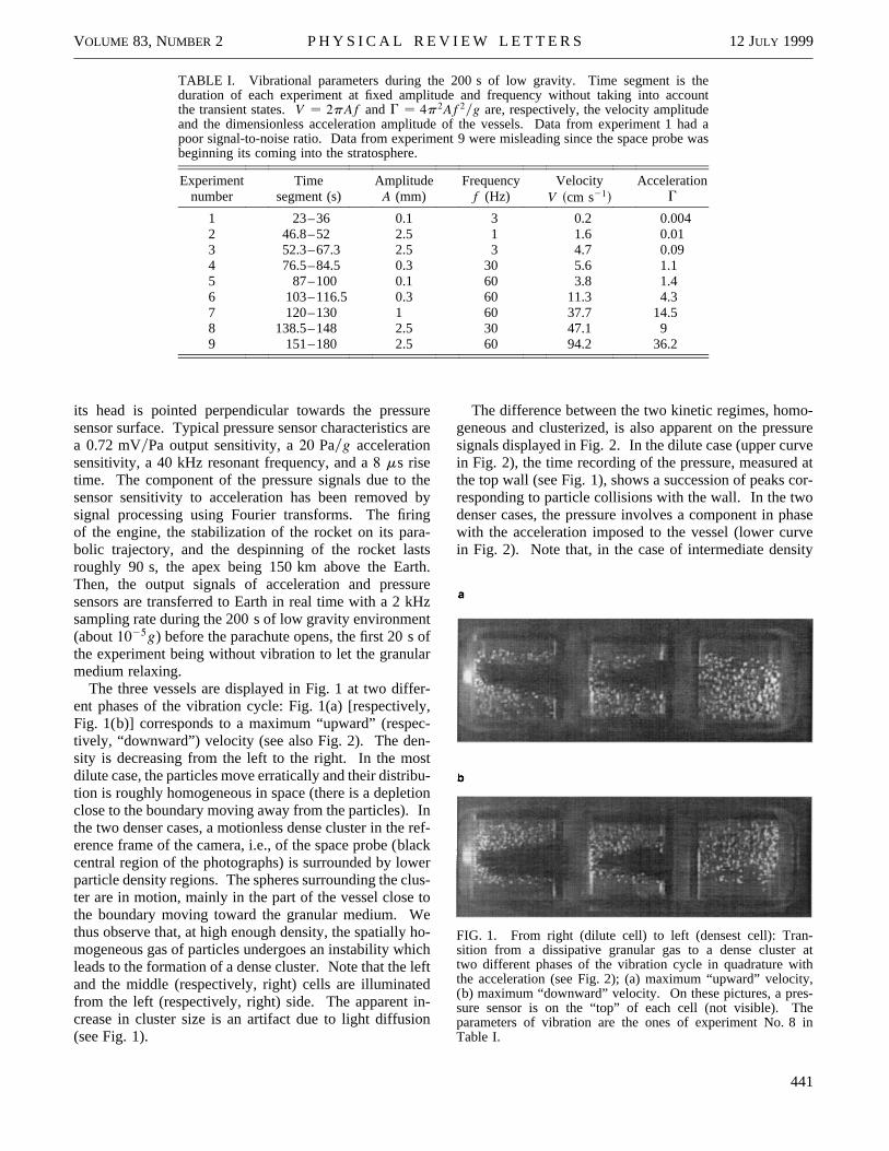
VOLUME 83, NUMBER 2 P H Y S I C A L R E V I E W L E T T E R S 12 JULY 1999
TABLE I. Vibrational parameters during the 200 s of low gravity. Time segment is theduration of each experiment at fixed amplitude and frequency without taking into accountthe transient states. V 2pAf and G 4p2Af2g are, respectively, the velocity amplitudeand the dimensionless acceleration amplitude of the vessels. Data from experiment 1 had apoor signal-to-noise ratio. Data from experiment 9 were misleading since the space probe wasbeginning its coming into the stratosphere.
Experiment Time Amplitude Frequency Velocity Accelerationnumber segment (s) A (mm) f (Hz) V cm s21 G
1 23–36 0.1 3 0.2 0.0042 46.8–52 2.5 1 1.6 0.013 52.3–67.3 2.5 3 4.7 0.094 76.5–84.5 0.3 30 5.6 1.15 87–100 0.1 60 3.8 1.46 103–116.5 0.3 60 11.3 4.37 120–130 1 60 37.7 14.58 138.5–148 2.5 30 47.1 99 151–180 2.5 60 94.2 36.2
its head is pointed perpendicular towards the pressuresensor surface. Typical pressure sensor characteristics area 0.72 mVPa output sensitivity, a 20 Pag accelerationsensitivity, a 40 kHz resonant frequency, and a 8 ms risetime. The component of the pressure signals due to thesensor sensitivity to acceleration has been removed bysignal processing using Fourier transforms. The firingof the engine, the stabilization of the rocket on its para-bolic trajectory, and the despinning of the rocket lastsroughly 90 s, the apex being 150 km above the Earth.Then, the output signals of acceleration and pressuresensors are transferred to Earth in real time with a 2 kHzsampling rate during the 200 s of low gravity environment(about 1025g) before the parachute opens, the first 20 s ofthe experiment being without vibration to let the granularmedium relaxing.
The three vessels are displayed in Fig. 1 at two differ-ent phases of the vibration cycle: Fig. 1(a) [respectively,Fig. 1(b)] corresponds to a maximum “upward” (respec-tively, “downward” ) velocity (see also Fig. 2). The den-sity is decreasing from the left to the right. In the mostdilute case, the particles move erratically and their distribu-tion is roughly homogeneous in space (there is a depletionclose to the boundary moving away from the particles). Inthe two denser cases, a motionless dense cluster in the ref-erence frame of the camera, i.e., of the space probe (blackcentral region of the photographs) is surrounded by lowerparticle density regions. The spheres surrounding the clus-ter are in motion, mainly in the part of the vessel close tothe boundary moving toward the granular medium. Wethus observe that, at high enough density, the spatially ho-mogeneous gas of particles undergoes an instability whichleads to the formation of a dense cluster. Note that the leftand the middle (respectively, right) cells are illuminatedfrom the left (respectively, right) side. The apparent in-crease in cluster size is an artifact due to light diffusion(see Fig. 1).
The difference between the two kinetic regimes, homo-geneous and clusterized, is also apparent on the pressuresignals displayed in Fig. 2. In the dilute case (upper curvein Fig. 2), the time recording of the pressure, measured atthe top wall (see Fig. 1), shows a succession of peaks cor-responding to particle collisions with the wall. In the twodenser cases, the pressure involves a component in phasewith the acceleration imposed to the vessel (lower curvein Fig. 2). Note that, in the case of intermediate density
FIG. 1. From right (dilute cell) to left (densest cell): Tran-sition from a dissipative granular gas to a dense cluster attwo different phases of the vibration cycle in quadrature withthe acceleration (see Fig. 2); (a) maximum “upward” velocity,(b) maximum “downward” velocity. On these pictures, a pres-sure sensor is on the “ top” of each cell (not visible). Theparameters of vibration are the ones of experiment No. 8 inTable I.
441
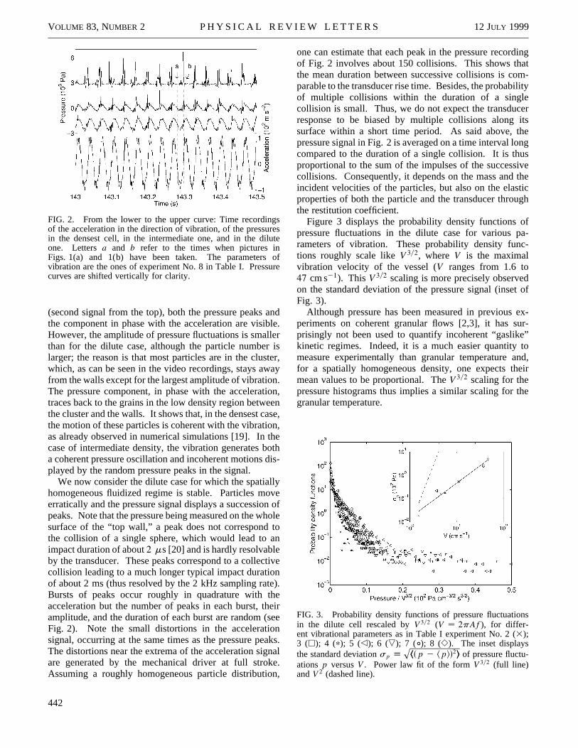
VOLUME 83, NUMBER 2 P H Y S I C A L R E V I E W L E T T E R S 12 JULY 1999
FIG. 2. From the lower to the upper curve: Time recordingsof the acceleration in the direction of vibration, of the pressuresin the densest cell, in the intermediate one, and in the diluteone. Letters a and b refer to the times when pictures inFigs. 1(a) and 1(b) have been taken. The parameters ofvibration are the ones of experiment No. 8 in Table I. Pressurecurves are shifted vertically for clarity.
(second signal from the top), both the pressure peaks andthe component in phase with the acceleration are visible.However, the amplitude of pressure fluctuations is smallerthan for the dilute case, although the particle number islarger; the reason is that most particles are in the cluster,which, as can be seen in the video recordings, stays awayfrom the walls except for the largest amplitude of vibration.The pressure component, in phase with the acceleration,traces back to the grains in the low density region betweenthe cluster and the walls. It shows that, in the densest case,the motion of these particles is coherent with the vibration,as already observed in numerical simulations [19]. In thecase of intermediate density, the vibration generates botha coherent pressure oscillation and incoherent motions dis-played by the random pressure peaks in the signal.
We now consider the dilute case for which the spatiallyhomogeneous fluidized regime is stable. Particles moveerratically and the pressure signal displays a succession ofpeaks. Note that the pressure being measured on the wholesurface of the “ top wall,” a peak does not correspond tothe collision of a single sphere, which would lead to animpact duration of about 2 ms [20] and is hardly resolvableby the transducer. These peaks correspond to a collectivecollision leading to a much longer typical impact durationof about 2 ms (thus resolved by the 2 kHz sampling rate).Bursts of peaks occur roughly in quadrature with theacceleration but the number of peaks in each burst, theiramplitude, and the duration of each burst are random (seeFig. 2). Note the small distortions in the accelerationsignal, occurring at the same times as the pressure peaks.The distortions near the extrema of the acceleration signalare generated by the mechanical driver at full stroke.Assuming a roughly homogeneous particle distribution,
one can estimate that each peak in the pressure recordingof Fig. 2 involves about 150 collisions. This shows thatthe mean duration between successive collisions is com-parable to the transducer rise time. Besides, the probabilityof multiple collisions within the duration of a singlecollision is small. Thus, we do not expect the transducerresponse to be biased by multiple collisions along itssurface within a short time period. As said above, thepressure signal in Fig. 2 is averaged on a time interval longcompared to the duration of a single collision. It is thusproportional to the sum of the impulses of the successivecollisions. Consequently, it depends on the mass and theincident velocities of the particles, but also on the elasticproperties of both the particle and the transducer throughthe restitution coefficient.
Figure 3 displays the probability density functions ofpressure fluctuations in the dilute case for various pa-rameters of vibration. These probability density func-tions roughly scale like V 32, where V is the maximalvibration velocity of the vessel (V ranges from 1.6 to47 cm s21). This V 32 scaling is more precisely observedon the standard deviation of the pressure signal (inset ofFig. 3).
Although pressure has been measured in previous ex-periments on coherent granular flows [2,3], it has sur-prisingly not been used to quantify incoherent “gaslike”kinetic regimes. Indeed, it is a much easier quantity tomeasure experimentally than granular temperature and,for a spatially homogeneous density, one expects theirmean values to be proportional. The V 32 scaling for thepressure histograms thus implies a similar scaling for thegranular temperature.
FIG. 3. Probability density functions of pressure fluctuationsin the dilute cell rescaled by V 32 (V 2pAf), for differ-ent vibrational parameters as in Table I experiment No. 2 (3);3 (); 4 (); 5 (); 6 (); 7 (±); 8 (). The inset displaysthe standard deviation sp
pp 2 p2 of pressure fluctu-
ations p versus V . Power law fit of the form V 32 (full line)and V 2 (dashed line).
442

VOLUME 83, NUMBER 2 P H Y S I C A L R E V I E W L E T T E R S 12 JULY 1999
Using dimensional analysis, the granular temperature,i.e., the mean kinetic energy per particle, EN , scales like
EN
mf2A2F
√e, N ,
AL
,RL
!, (1)
where m is the mass and F is an arbitrary functionof R, the radius of the particles, L, the length of thevessel, e, the restitution coefficient, A and N . Notethat one should take into account different restitutioncoefficients for the particle-particle and the wall-particlecollisions, but that this does not modify the frequencydependence of the granular temperature. Consequently,in low gravity, one expects the granular temperature orthe mean pressure to be proportional to the square ofthe vibration frequency. This is not compulsory in thepresence of gravity because an additional dimensionlessparameter Af2g is involved in Eq. (1). Indeed, aprevious experiment [7], numerical simulations [8–10],kinetic theory [7,12,21] and hydrodynamic models [11],all involving gravity, have found different scaling lawsfor the granular temperature, in the range V 43 V 2.
Our measurements in low gravity imply that anotherdimensionless parameter involving a new velocity scaleshould be considered in Eq. (1). The dependence of therestitution coefficient on the impact velocity provides thisadditional parameter. In our velocity range, the restitu-tion coefficient varies from 0.97 to 0.87 as the velocity isincreased [22]. Dissipative effects thus increase with ve-locity which leads to a smaller increase of the granulartemperature with velocity than for a constant restitution co-efficient. To be more specific, one can combine the resultof kinetic theory, EN ~ V 21 2 e with a viscoelasticmodel for the restitution coefficient, 1 2 e ~ Va [20] toexplain that the scaling exponent of the granular tempera-ture as a function of the velocity is smaller than 2.
In conclusion, we have reported a 3D experiment of agranular medium fluidized by sinusoidal vibrations in lowgravity environment. When the density of the granularmedium is increased, we clearly show that an ensembleof particles in erratic motion interacting only throughinelastic collisions spontaneously generates the formationof a motionless dense cluster.
We thank S. Aumaıtre for discussions. This work hasbeen supported by the European Space Agency (France)and the Centre National d’Études Spatiales (France). Theflight has been provided by E.S.A. The experiment mod-ule has been constructed by D.A.S.A. (Germany), Ferrari(Italy), and Techno System (Italy). Mini-Texus 5 sound-ing rocket is a program of E.S.A. We gratefully ac-
knowledge the Texus team for its kind technical assis-tance. E. F. was supported by a postdoctoral grant fromthe C.N.E.S.
*Corresponding author.Email address: [email protected]
[1] M. O. Faraday, Philos. Trans. R. Soc. London 52, 299(1831); J. Walker Sci. Am. 247, No. 3, 166 (1982);P. Évesque and J. Rajchenbach, Phys. Rev. Lett. 62, 44(1989); B. Thomas and A. M. Squires, Phys. Rev. Lett.81, 574 (1998).
[2] C. Laroche, S. Douady, and S. Fauve, J. Phys. (Paris) 50,699 (1989).
[3] S. Douady, S. Fauve, and C. Laroche, Europhys. Lett. 8,621 (1989).
[4] S. Fauve, S. Douady, and C. Laroche, J. Phys. (Paris),Colloq. 50, C3-187 (1989).
[5] P. B. Umbanhowar, F. Melo, and H. L. Swinney, Nature(London) 382, 793 (1996).
[6] J. T. Jenkins and S. B. J. Savage, Fluid Mech. 130, 187(1983); C. S. Campbell, Annu. Rev. Fluid Mech. 22, 57(1990).
[7] S. Warr, J. M. Huntley, and G. T. H. Jacques, Phys. Rev. E52, 5583 (1995).
[8] S. Luding et al., Phys. Rev. E 49, 1634 (1994).[9] S. Luding, H. J. Herrmann, and A. Blumen, Phys. Rev. E
50, 3100 (1994).[10] S. McNamara and S. Luding, Phys. Rev. E 58, 813 (1998).[11] J. Lee, Physica (Amsterdam) 219A, 305 (1995).[12] V. Kumaran, Phys. Rev. E 57, 5660 (1998).[13] P. Goldreich and S. Tremaine, Annu. Rev. Astron.
Astrophys. 20, 249 (1982).[14] A. Kudrolli, M. Wolpert, and J. P. Gollub, Phys. Rev. Lett.
78, 1383 (1997).[15] S. Fauve, E. Falcon, and C. Laroche, CNES Report
No. 95/0256, 1996 (unpublished).[16] M. A. Hopkins and M. Y. Louge, Phys. Fluids A 3, 47
(1991); S. McNamara and W. R. Young, Phys. Fluids A 4,496 (1992); I. Goldhirsch and G. Zanetti, Phys. Rev. Lett.70, 1619 (1993).
[17] F. G. Bridges, A. Hatzes, and D. N. C. Lin, Nature (Lon-don) 309, 333 (1984).
[18] H. H. Shen, W. D. Hibler, and M. Leppäranta, J. Geophys.Res. 92, 7085 (1987).
[19] S. McNamara and J. L. Barrat, Phys. Rev. E 55, 7767(1997).
[20] E. Falcon, C. Laroche, S. Fauve, and C. Coste, Eur. Phys.J. B 3, 45 (1998).
[21] J. M. Huntley, Phys. Rev. E 58, 5168 (1998).[22] C. V. Raman, Phys. Rev. 12, 442 (1918); W. Goldsmith,
Impact (Arnold, London, 1960).
443

Simulations of vibrated granular medium with impact-velocity-dependent restitution coefficient
Sean McNamara1,* and Eric Falcon2,†
1Centre Européen de Calcul Atomique et Moléculaire, 46, allée d’Italie, 69 007 Lyon, France2Laboratoire de Physique, École Normale Supérieure de Lyon, UMR 5672, 46, allée d’Italie, 69 007 Lyon, France
sReceived 30 November 2004; published 24 March 2005d
We report numerical simulations of strongly vibrated granular materials designed to mimic recent experi-ments performed in both the presence and the absence of gravity. The coefficient of restitution used heredepends on the impact velocity by taking into account both the viscoelastic and plastic deformations ofparticles, occurring at low and high velocities, respectively. We show that this model with impact-velocity-dependent restitution coefficient reproduces results that agree with experiments. We measure the scaling ex-ponents of the granular temperature, collision frequency, impulse, and pressure with the vibrating pistonvelocity as the particle number increases. As the system changes from a homogeneous gas state at low densityto a clustered state at high density, these exponents are all found to decrease continuously with increasingparticle number. All these results differ significantly from classical inelastic hard sphere kinetic theory andprevious simulations, both based on a constant restitution coefficient.
DOI: 10.1103/PhysRevE.71.031302 PACS numberssd: 45.70.2n, 05.20.Dd, 05.45.Jn
I. INTRODUCTION
The past decade has seen the publication of many experi-mentalf1–3g, numericalf3–5g, and theoreticalf1,6–8g stud-ies of strongly vibrated granular media. This problem is in-teresting because vibrated granular media are simple butnontrivial examples of nonequilibrium steady states and theonly way to experimentally realize granular gasesf9g. How-ever, numerous questions remain about the link between ex-periments on one hand, and theory and simulations on theother. Most numerical and theoretical studies were not in-tended to be compared with experiments. Therefore, theyhave parameter values far from the experimental ones, andnone of them predict even the most basic features of theexperimental results.
In this paper, we bridge the gap between experiments andnumerics by presenting simulations of strongly vibratedgranular materials designed to mimic recent experiments per-formed in both the presencef10g and the absencef11g ofgravity. We present simulations that resemble the experi-ments for a large range of parameters. We show that twoparameters are especially important for the agreement be-tween experiment and simulation. First of all, the coefficientof restitution has to be dependent on the particle impact ve-locity by taking into account both the viscoelastic and plasticdeformations of particles occurring at low and high veloci-ties, respectively. Most previous numerical studies consideronly a constant restitution coefficientf3–5g; a few studieswith slight velocity dependencesdue to only the viscoelasticcontributiond f12g. Second, it is important to explicitly con-sider the number of particlesN. Studying only one value ofN or comparing results obtained at differentN can lead tointerpretive difficulties.
Beyond these agreements between experiments and oursimulations, we find results that differ significantly fromclassical inelastic hard sphere kinetic theory and previoussimulations. We measure the scaling exponents of the granu-lar temperature, collision frequency, impulse, and pressurewith the vibrating piston velocity as the particle number in-creases, in both the presence and absence of gravity. Weshow that the system undergoes a smooth transition from ahomogeneous gas state at low density to a clustered state athigh density.
The paper has the following structure. In Sec. II, wepresent a description of the simulationssnotably the model ofimpact-velocity-dependent restitution coefficient, and the in-fluence of other simulations parametersd. Section III providesa comparison of simulations and experimentssshowing theimportance of the variable coefficient of restitution and theparticle numberd, and the results of the scaling exponents.Section III C focus on the influence of other simulations pa-rameterssbed height, box size, particle rotations, gravityd.Finally, in Sec. IV we summarize our results.
II. DESCRIPTION OF THE SIMULATIONS
A. The variable coefficient of restitution
The greatest difference between our simulations and theprevious numerical studies of vibrated granular mediaf3–5gis that we use a restitution coefficient that depends on impactvelocity. The restitution coefficientr is the ratio between therelative normal velocities before and after impact. In previ-ous simulations of strongly vibrated granular media, the co-efficient of restitution is considered to be constant and lowerthan 1. However, for a century, it has been shown fromimpact experiments thatr is a function of the impact velocityv f13–17g. Indeed, for metallic particles, whenv is largesv*5 m/s f14gd, the colliding particles deform fully plasti-cally and r ~v−1/4 f13–15g. Whenv&0.1 m/sf14g, the de-formations are elastic with mainly viscoelastic dissipation,ands1−rd~v1/5 f15–18g. Such velocity-dependent restitution
*Permanent address: I.C.P., Universität Stuttgart, 70569 Stuttgart,Germany.
†Email address: [email protected];URL:http//perso.ens-lyon.fr/eric.falcon/
PHYSICAL REVIEW E 71, 031302s2005d
1539-3755/2005/71s3d/031302s6d/$23.00 ©2005 The American Physical Society031302-1
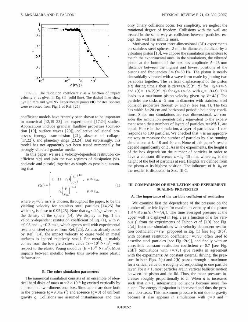
coefficient models have recently been shown to be importantin numerical f12,19–23g and experimentalf17,24g studies.Applications include granular fluidlike propertiessconvec-tion f19g, surface wavesf20gd, collective collisional pro-cesses senergy transmissionf21g, absence of collapsef17,22gd, and planetary ringsf23,24g. But surprisingly, thismodel has not apparently yet been tested numerically forstrongly vibrated granular media.
In this paper, we use a velocity-dependent restitution co-efficient rsvd and join the two regimes of dissipationsvis-coelastic and plasticd together as simply as possible, assum-ing that
rsvd =51 − s1 − r0dS vv0D1/5
, v ø v0,
r0S vv0D−1/4
, v ù v0,6 s1d
wherev0=0.3 m/s is chosen, throughout the paper, to be theyielding velocity for stainless steel particlesf14,25g forwhich r0 is close to 0.95f25g. Note thatv0,1/Îr wherer isthe density of the spheref14g. We display in Fig. 1 thevelocity-dependent restitution coefficient of Eq.s1d, with r0=0.95 andv0=0.3 m/s, which agrees well with experimentalresults on steel spheres from Ref.f25g. As also already notedby Ref. f14g, the impact velocity to cause yield in metalsurfaces is indeed relatively small. For metal, it mainlycomes from the low yield stress valuesY,109 N/m2d withrespect to the elastic Young modulussE,1011 N/m2d. Mostimpacts between metallic bodies thus involve some plasticdeformation.
B. The other simulation parameters
The numerical simulation consists of an ensemble of iden-tical hard disks of massm<3310−5 kg excited vertically bya piston in a two-dimensional box. Simulations are done bothin the presencesg=9.8m/s2d and absencesg=0d of uniformgravity g. Collisions are assumed instantaneous and thus
only binary collisions occur. For simplicity, we neglect therotational degree of freedom. Collisions with the wall aretreated in the same way as collisions between particles, ex-cept the wall has infinite mass.
Motivated by recent three-dimensionals3Dd experimentson stainless steel spheres, 2 mm in diameter, fluidized by avibrating pistonf10g, we choose the simulation parameters tomatch the experimental ones: in the simulations, the vibratedpiston at the bottom of the box has amplitudeA=25 mmsdistance between the highest and lowest positions of thepistond and frequencies 5ø f ø50 Hz. The piston is nearlysinusoidally vibrated with a wave form made by joining twoparabolas together. The vertical displacement of the pistonzstd during time t then is zstd=sA/2dst2− t0
2d for −t0ø tø t0andzstd=−sA/2dst2− t0
2d for t0ø tø3t0 with to=1/s4fd. Thisleads to a maximum piston velocity given byV=4Af. Theparticles are disksd=2 mm in diameter with stainless steelcollision properties throughv0 and r0 ssee Fig. 1d. The boxhas widthL=20 cm and horizontal periodic boundary condi-tions. Since our simulations are two dimensional, we con-sider the simulation geometrically equivalent to the experi-ment when their numbers of layers of particles,n=Nd/L, areequal. Hence in the simulation, a layer of particlesn=1 cor-responds to 100 particles. We checked thatn is an appropri-ate way to measure the number of particles by also runningsimulations atL=10 and 40 cm. None of this paper’s resultsdepend significantly onL. As in the experiments, the heighthof the box depends on the number of particles in order tohave a constant differenceh−h0=15 mm, whereh0 is theheight of the bed of particles at rest. Heights are defined fromthe piston at its highest position. The influence ofh−h0 onthe results is discussed in Sec. III C.
III. COMPARISON OF SIMULATION AND EXPERIMENT:SCALING PROPERTIES
A. The importance of the variable coefficient of restitution
We examine first the dependence of the pressure on thenumber of particle layers for maximum velocity of the piston1&V&5 m/s sV=4Afd. The time averaged pressure at theupper wall is displayed in Fig. 2 as a function ofn for vari-ous f: from the experiments of Falconet al. f10g fsee Fig.2sadg, from our simulations with velocity-dependent restitu-tion coefficientr =rsvd proposed in Eq.s1d fsee Fig. 2sbdg,with constant restitution coefficientr =0.95, often used todescribe steel particlesfsee Fig. 2scdg, and finally with anunrealistic constant restitution coefficientr =0.7 fsee Fig.2sddg. Simulations with r =rsvd give results in agreementwith the experiments: At constant external driving, the pres-sure in both Figs. 2sad and 2sbd passes through a maximumfor a critical value ofn roughly corresponding to one particlelayer. Forn,1, most particles are in vertical ballistic motionbetween the piston and the lid. Thus, the mean pressure in-creases roughly proportionally ton. When n is increasedsuch thatn.1, interparticle collisions become more fre-quent. The energy dissipation is increased and thus the pres-sure decreases. This maximum pressure is not due to gravitybecause it also appears in simulations withg=0 and r
FIG. 1. The restitution coefficientr as a function of impactvelocity v, as given in Eq.s1d ssolid lined. The dashed lines showv0=0.3 m/s andr0=0.95. Experimental pointssPd for steel sphereswere extracted from Fig. 1 of Ref.f25g.
S. McNAMARA AND E. FALCON PHYSICAL REVIEW E71, 031302s2005d
031302-2

=rsvd. Furthermore, the maximum persists wheng is in-creased above 9.8 m/s2. For nù4 and for certain frequen-cies, a resonance appears in Fig. 2sbd which is controlled bythe ratio between the vibration period and the particle flighttime under gravity,Îg/h/ f. Turning our attention to Fig.2scd, we see that settingr =0.95 independently of impactvelocity gives pressure qualitatively different from experi-ments. The difference between Figs. 2sbd and 2scd can beunderstood by considering a high velocity collisionse.g.,v=1 m/sd. In Fig. 2sbd, this collision has a restitution coeffi-cient of r =rs1 m/sd<0.7 ssee Fig. 1d, whereas in Fig. 2scd,r is fixed at 0.95 for all collisions. This means that for equalcollision frequencies, dissipation is much stronger forr=rsvd than for r =0.95, because the high velocity collisionsdominate the dissipation. Stronger dissipation leads to lowergranular temperatures and thus to lower pressures.
We can check this interpretation by changing the constantrestitution coefficient tor =0.7 and then comparing it tor=rsvd. In these two cases, the high velocity collisions willhave roughly the same restitution coefficient. We indeed ob-served a pressure that decreases for largen for constantr=0.7 fsee Fig. 2sddg. Therefore, surprisingly, constantr =0.7reproduces more precisely the experimental pressure mea-
surements than constantr =0.95, even thoughr =0.95 or 0.9is often given as the restitution coefficient of steel. However,if we look at other properties, we see thatr =0.7 and r=rsvd give very different predictions.
For example, in Fig. 3, we show two snapshots from twodifferent simulations one withr =rsvd and another withr=0.7, both withn=3 in the presence of gravity. Whenr=rsvd, the particles are concentrated in the upper half of thechamber, but they are evenly spread in the horizontal direc-tion fsee Fig. 3sadg. The system is hotter and less dense nearthe vibrating wall, and colder and denser by the oppositewall. But, whenr =0.7, the majority of the particles are con-fined to a tight cluster, pressed against the upper wall, coex-isting with low density regionsfsee Fig. 3sbdg. This instabil-ity has already been reported numericallyf26g, although formuch different parameterssconstant restitution coefficientr=0.96, thermal walls, no gravity, and largend. However,nothing like this was seen experimentally. Therefore, if oneis seeking information about particle positions,r =0.7 givesincorrect results even though it gives acceptable results forthe pressure. We conclude, therefore, that the only way tosuccessfully describe all the properties in all situations is touse a velocity-dependent restitution coefficient model.
FIG. 2. Time averaged pressureP on the top of the cell as a function of particle layern for various vibration frequenciesf. sadExperimental results fromf10g for stainless steel beads 2 mm in diameter, withA=25 mm, 10ø f ø20 Hz with a 1 Hz stepsfrom bottom totopd andh−h0=5 mm.sbd Numerical simulation where the coefficient of restitutionrsvd is given by Eq.s1d. scd Numerical simulation witha coefficient of restitution of 0.95, independent of impact velocity.sdd Numerical simulation with a coefficient of restitution of 0.7,independent of impact velocity. The simulationssbd, scd, and sdd are 2D with gravity, done for 2 mm disks, withA=25 mm, 10ø fø30 Hz with a 2 Hz stepsfrom bottom to topd andh−h0=15 mm. In the simulations, the two-dimensional pressure is given in N/m.
SIMULATIONS OF VIBRATED GRANULAR MEDIUM… PHYSICAL REVIEW E 71, 031302s2005d
031302-3

B. The importance of the particle number
Many authors have postulated that the pressure on theupper wall P sor granular temperatureTd is related to thepiston velocityV throughP,T~Vu. However, it is not clearwhat the correct “scaling exponent”u should be. This ques-tion has been addressed several times in the past, without aclear resolution of the questionf5–8g. For example, kinetictheory f1,7g and hydrodynamic modelsf8g predict T~V2
whereas numerical simulationsf3,4g or experimentsf1–3ggive T~Vu, with 1øuø2. These studies were done at singlevalues ofn. In this section, we show that it is very importantto explicitly consider the dependence of the scaling expo-nents onn. We also consider the effect of gravity and avariable coefficient of restitution. Doing so enables us toexplain and unify all previous works.
At the upper wall, we measured numerically the collisionfrequencyNc and the mean impulsion per collisionDI forvarious frequencies of the vibrating wall and numbers ofparticles in the box, withr =rsvd or with r =0.95, in the pres-ence or absence of gravity. The time averaged pressure onthe upper wall can be calculated from these quantities using
P = NcDI/L. s2d
sBy conservation of momentum, the time averaged pressureon the lower wall is justP plus the weight of the particlesNmg/L.d The total kinetic energy of the system is also mea-sured to have access to the granular temperature,T. Nc, DI,P, andT are all found to fit with power laws inVu for ourrange of piston velocities. Figure 4 showsu exponents ofNc,DI, P, andT as a function ofn. Wheng=0 andr is constantfsee Fig. 4sadg, we haveP,V2, DI ,V, andNc,V for all n.We call these relations the classical kinetic theory scaling.This scaling can be established by simple dimensional analy-sis when the vibration velocityV provides the only timescale in the system. This is the case forg=0 andr indepen-dent of velocity. However, in the experiments, two additionaltime scales are provided, one by gravity and the other by the
velocity-dependent restitution coefficient. Numerical simula-tions can separate the effects of these two time scales on thescaling exponentsu. This is done in Fig. 4sbd fwhereg=0but r =rsvdg and Fig. 4scd fwherer is constant butgÞ0g. Inboth figures, all the exponents become functions ofn. How-ever, the time scale linked tor =rsvd leads to much moredramatic departure from the classical scaling. After consid-ering the two time scales separately, let us consider the casecorresponding to most experiments, where both gravity andr =rsvd are presentfsee Fig. 4sddg. The similarity betweenthis figure and Fig. 4sbd confirms that the velocity-dependentrestitution coefficient has a more important effect than thegravity. Furthermore, only the variation of the restitution co-efficient with the particle velocity explains the experimentperformed in low gravityf11g. This experiment gives aV3/2
pressure scalingfP symbol on Fig. 4sbdg for n=1 and amotionless clustered state forn.2. Only the simulation withr =rsvd can reproduce these resultsfsee Fig. 4sbdg whereasconstantr simulations leads to the classical scalingfP~V2,see Fig. 4sadg and only a gaseous state for alln shown in thefigure.
As shown in Fig. 4, it is thus very important to explicitlyconsider the dependence ofu on n. In all cases, except theunrealistic case of Fig. 4sad, u depends onn. To our knowl-edge, the only experimentf10g to systematically investigatethis effect shows thatT~Vusnd, with u continuously varyingfrom u=2 whenn→0, as expected from kinetic theory, tou.0 for largen due to the clustering instability. These ex-perimentsf10g performed under gravitysshown in Fig. 5d arewell reproduced by the simulations of Fig. 4sdd. In bothcases, the observed pressure and granular temperature scal-ing exponents strongly decrease with increasingn.
We finish this section by noting two curious facts aboutFig. 4. First of all, in Fig. 4sbd fg=0 andr =rsvdg, u<1 forthe pressure and temperature whenn.2. This is the sign ofa different robust scaling regime whereP andT~V1, whichwill be the topic of a future paper. Second, in Fig. 4sdd fgÞ0 and r =rsvdg, the scaling exponents are not shown fornù3, because the dependence ofP, T, Nc, andDI on V is nolonger a simple power law.sMore precisely, we do not plot apoint on Fig. 4 whenuln sXobservedd−ln sXfittedduù0.25 for anyof the 11 simulations used to calculate the exponent—seecaption.d The power law breaks down because there is aresonance between the time of flight of the cluster undergravity and the vibration period.
C. The influence of other parameters
In this section, we review the influence of the other simu-lation parameterssbox size, particle rotations, gravity, andthe vibration parametersd, and show that it is not possible toreproduce the experimental curves in Fig. 2sad unless onesetsr =rsvd or r =0.7.
Performing simulations for 5øh−h0ø50 mm shows thatthe shapes of the curvesP vs n in Figs. 2sbd and 2scd remainthe same. Forr =rsvd fFig. 2sbdg increasingh−h0 shifts themaximum toward smaller values ofn and decreases in am-plitude. The only exception occurs when the box height ap-proaches the particle diameter, i.e.,h−h0=5 mm, where the
FIG. 3. Snapshots from the simulations withn=3, gravity gÞ0, driving frequencyf =30 Hz, andh−h0=15 mm. The upperwall is stationary, and the lower wall is the piston, which is at itslowest position in both snapshots. The horizontal boundaries areperiodic sindicated by dashed linesd. Gravity points downward.sadr =rsvd, as given in Eq.s1d, andsbd constantr =0.7. In sbd we see atight cluster which was not observed in the experiments.
S. McNAMARA AND E. FALCON PHYSICAL REVIEW E71, 031302s2005d
031302-4

maximum disappears. Consideringr =0.95 leads to similarconclusions.
To eliminate the possibility that the experimental curvecan be reproduced by taking into account particle rotations,we performed simulations withr =0.95 and various values ofthe tangential restitution coefficientrt. This parameter is de-fined as the ratio between the tangential components of thepre- and postcollision relative velocities. Perfectly smoothspheres correspond tort=−1. Whenrt=1, the tangential rela-tive velocity is reversed by the collision. These two valuesurtu=1 correspond to energy conservation. Energy is dissi-pated for −1, rt,1, rt=0 corresponding to maximum en-ergy dissipation. Whenurtu is close to 1, theP vs n curves arealmost unchanged. Whenrt is close to 0, the curves becomenearly flat forn.2.
Throughout this paper, we have used the piston vibrationvelocity V to characterize the vibration. It is important topoint out thatV is not the only way to do this. One could alsouse the maximum piston accelerationG. WhenG is close tog, it controls the behavior of the system, i.e., adjustingA andf while keepingG constant does not change the system’s
FIG. 4. The exponentsu as a function ofn which give the scaling of the granular temperatureT sLd, collision frequencyNc spd, meanimpulsionDI snd, and pressureP ssd. All these quantities are proportional toVusnd. Without gravity,sad for r =0.95 andsbd for r =rsvd. Withgravity, scd for r =0.95 andsdd for r =rsvd. The exponents are obtained by fixingn and performing 11 simulations, varyingf from10 to 30 Hz. Then lnsXd swhereX is the quantity being consideredd is plotted against lnsVd. The resulting curve is always nearly a straightline fexcept forn.3 in sdd—see textg, and the exponent is calculated from a least squares fit. The pressure scaling pointsPd on sbd is fromthe experimentf11g performed in low gravity. See Fig. 3sad for typical snapshot corresponding ton=3, gÞ0 andr =rsvd.
FIG. 5. Experimental data performed under gravity from Ref.f10g: The exponentsusnd of time averaged pressureshd fsee Fig.2sadg, and kinetic energy extracted from density profilessd or vol-ume expansionsLd measurements. These data should be comparedwith the simulations of Fig. 4sdd.
SIMULATIONS OF VIBRATED GRANULAR MEDIUM… PHYSICAL REVIEW E 71, 031302s2005d
031302-5
behavior much. But in the simulations presented here,G@g, and the system’s behavior is controlled byV. This canbe checked by multiplying the frequency by 10 while divid-ing A by 10, thus keepingV the sameswhile G increases byan order of magnituded. Doing so changes the pressure onlyby about 20%. Therefore,V is the correct parameter to de-scribe the vibration for the simulations considered here.
IV. CONCLUSIONS
In this paper, we brought simulations of a strongly vi-brated granular medium as close as possible to the experi-ments. We showed that the use of a velocity-dependent co-efficient of restitution reproduces results that agree withexperiments. It is especially important to take into accountplastic deformations that cause the restitution coefficient todecrease rapidly with increasing impact velocity. Indeed, therestitution coefficient for strongly vibrated steel spheres is
very far from the constant values ofr =0.95 or 0.9 that areoften cited in simulations as typical for steel spheres. Chang-ing the box size or the gravitational acceleration and includ-ing particle rotation do not modify this conclusion. We alsonoted that it is very important to take into account the num-ber of particle layersn. The dependence of the pressureP onthe piston velocityV changes withn. It is not accurate tospeak of “a” scaling exponent for the pressure in terms ofV:this exponent depends continuously onn, and does not existat high densitysn.3d under gravity, due to the clusteringinstability.
ACKNOWLEDGMENTS
We thank Stéphan Fauve for fruitful discussions. The au-thors gratefully acknowledge the hospitality of the ENS-Lyon physics department, which made this collaborationpossible.
f1g S. Warr, J. M. Huntley, and G. T. H. Jacques, Phys. Rev. E52,5583 s1995d.
f2g X. Yang and D. Candela, Phys. Rev. Lett.85, 298 s2000d; R.D. Wildman, J. M. Huntley, and D. J. Parker, Phys. Rev. E63,061311s2001d.
f3g S. Ludinget al., Phys. Rev. E49, 1634s1994d.f4g S. Luding, H. J. Herrmann, and A. Blumen, Phys. Rev. E50,
3100s1994d; S. Luding,ibid. 52, 4442s1995d; H. J. Herrmannand S. Luding, Continuum Mech. Thermodyn.10, 189s1998d.
f5g S. McNamara and S. Luding, Phys. Rev. E58, 813 s1998d.f6g J. M. Huntley, Phys. Rev. E58, 5168s1998d.f7g V. Kumaran, Phys. Rev. E57, 5660s1998d.f8g J. Lee, Physica A219, 305 s1995d.f9g Granular Gases, edited by T. Pöschel and S. Luding, Lectures
Notes in Physics Vol. 564sSpringer-Verlag, Berlin, 2001d.f10g E. Falcon, S. Fauve, and C. Laroche, inGranular GasessRef.
f9gd, pp. 244–253; E. Falcon, S. Fauve, and C. Laroche, Eur.Phys. J. B9, 183 s1999d; J. Chim. Phys.96, 1111s1999d.
f11g E. Falconet al., Phys. Rev. Lett.83, 440 s1999d.f12g N. V. Brilliantov and T. Pöschel, Phys. Rev. E61, 5573
s2000d; S. J. Moon, J. B. Swift, and H. L. Swinney,ibid. 69,011301s2004d.
f13g C. V. Raman, Phys. Rev.12, 442 s1918d; D. Tabor, Proc. R.Soc. London, Ser. A192, 247 s1948d; W. Goldsmith,ImpactsArnold, London, 1960d.
f14g K. L. Johnson,Contact MechanicssCambridge UniversityPress, Cambridge, U.K., 1985d.
f15g L. Labous, A. D. Rosato, and R. N. Dave, Phys. Rev. E56,
5717 s1997d.f16g G. Kuwabara and K. Kono, Jpn. J. Appl. Phys., Part 126,
1230 s1987d.f17g E. Falcon, C. Laroche, S. Fauve, and C. Coste, Eur. Phys. J. B
3, 45 s1998d; see also references therein.f18g J.-M. Hertzsch, F. Spahn, and N. V. Brilliantov, J. Phys. II5,
1725 s1995d; J. Schäfer, S. Dippel, and D. E. Wolf, J. Phys. I6, 5 s1996d; S. Ludinget al., Phys. Rev. E50, 4113s1994d.
f19g C. Salueña, T. Pöschel, and S. E. Esipov, Phys. Rev. E59,4422 s1999d.
f20g C. Bizonet al., Phys. Rev. Lett.80, 57 s1998d.f21g T. Pöschel and N. V. Brilliantov, Phys. Rev. E63, 021505
s2001d.f22g D. Goldmanet al., Phys. Rev. E57, 4831s1998d.f23g H. Salo, J. Lukkari, and J. Hänninen, Earth, Moon, Planets43,
33 s1988d; F. Spahn, U. Schwarz, and J. Kurths, Phys. Rev.Lett. 78, 1596 s1997d; H. Salo, in Granular GasessRef. f9gdpp. 330–349.
f24g F. G. Bridges, A. Hatzes, and D. N. C. Lin, NaturesLondond309, 333 s1984d; A. Hatzes, F. G. Bridges, and D. N. C. Lin,Mon. Not. R. Astron. Soc.231, 1091s1988d; K. D. Supulver,F. G. Bridges, and D. N. C. Lin, Icarus113, 188 s1995d; M.Higa, M. Arakawa, and N. Maeno, Planet. Space Sci.44, 917s1996d.
f25g J. M. Lifshitz and H. Kolsky, J. Mech. Phys. Solids12, 35s1964d.
f26g M. Argentina, M. G. Clerc, and R. Soto, Phys. Rev. Lett.89,044301s2002d.
S. McNAMARA AND E. FALCON PHYSICAL REVIEW E71, 031302s2005d
031302-6

Europhys. Lett., 74 (5), pp. 830–836 (2006)DOI: 10.1209/epl/i2005-10589-8
EUROPHYSICS LETTERS 1 June 2006
Collision statistics in a dilute granular gas fluidizedby vibrations in low gravity
E. Falcon1(∗), S. Aumaıtre
2, P. Evesque
3, F. Palencia
4,
C. Lecoutre-Chabot4, S. Fauve
2, D. Beysens
4 and Y. Garrabos4
1 Laboratoire de Physique, ENS Lyon, UMR 5672 CNRS46 allee d’Italie, 69007 Lyon, France2 LPS, ENS Paris, UMR 8550 CNRS - 24 rue Lhomond, 75005 Paris, France3 Laboratoire MSSMat, Ecole Centrale Paris, UMR 8579 CNRS92295 Chatenay-Malabry, France4 ESEME-CEA-CNRS, ICMCB, 87 av. Schweitzer, Universite Bordeaux 133608 Pessac Cedex, France
received 28 October 2005; accepted in final form 11 April 2006published online 10 May 2006
PACS. 45.70.-n – Granular systems.PACS. 81.70.Ha – Testing in microgravity environments.PACS. 45.50.-j – Dynamics and kinematics of a particle and a system of particles.
Abstract. – We report an experimental study of a dilute “gas” of inelastically colliding parti-cles excited by vibrations in low gravity. We show that recording the collision frequency togetherwith the impulses on a wall of the container gives access to several quantities of interest. Weobserve that the mean collision frequency does not scale linearly with the number N of particlesin the container. This is due to the dissipative nature of the collisions and is also directly relatedto the non-extensive behaviour of the kinetic energy (the granular temperature is not intensive).
Introduction. – Since Maxwell and Boltzmann predictions in 1860-70, it is well knownthat molecules of a gas move erratically with a Gaussian velocity distribution, as experimen-tally verified later [1]. This allows thermodynamic and transport properties of molecular gasesto be described. However, these kinetic theory results do not hold if the particle interactionsare dissipative or depend on their velocities (e.g., in relativistic plasmas [2]). A well-knownexample of dissipative gas is the granular gas (see [3,4] for a recent collection of papers). Sincecollisions between granular particles are inelastic, a continuous input of energy (by vibratinga piston or the container) is required to reach a nonequilibrium steady state. In this regime,granular matter sometimes seems to behave like an molecular gas in which particles follow er-ratic motions, but several experiments have displayed striking different properties: Instabilityof the homogeneous density state leading to cluster formation [5–7], non-Gaussian nature ofthe velocity distribution [8], anomalous scaling of the pressure [7, 9]. These effects have beenalso numerically simulated and some of them have been theoretically understood [10].
(∗) E-mail: [email protected], URL: http://perso.ens-lyon.fr/eric.falcon/
c© EDP SciencesArticle published by EDP Sciences and available at http://www.edpsciences.org/epl or http://dx.doi.org/10.1209/epl/i2005-10589-8

E. Falcon et al.: Collision statistics in a dilute granular gas etc. 831
Table I – Vibration parameters during each parabola. V = 2πAf and Γ = 4π2Af2/g are, respectively,the maximal piston velocity and the dimensionless acceleration. The number of collisions Nw on thesensor is detected during θ = 16 s of low gravity to avoid transient states.
N A f V Γ Nw Symbols(mm) (Hz) (m/s) in fig. 3
12 0.92 40 0.23 5.9 2591 ×12 0.65 59.7 0.24 9.3 2605 12 0.88 80 0.44 22.7 5756 •12 0.64 90.9 0.37 21.4 4617 +24 0.96 40 0.24 6.2 5097 ∗24 0.67 59.7 0.25 9.6 4078 ♦24 0.89 80 0.44 22.8 8362 36 0.44 40 0.11 2.8 2538 36 0.67 59.7 0.25 9.7 6496 penta.36 0.89 80 0.44 22.8 9744 36 0.69 90.9 0.39 22.9 9741 ×48 0.42 40 0.11 2.7 2728 ×48 0.69 59.7 0.26 9.9 8650 hexa.48 0.89 80 0.45 22.9 10906 48 0.73 90.9 0.41 24.2 12512
In this paper, we report a 3D experiment of a dilute granular medium fluidized by sinu-soidal vibrations in a low-gravity environment. The motivation for low gravity is to achievean experimental situation in which inelastic collisions are the only interaction mechanism, andwhere only one “input” variable (the inverse vibration frequency) has the dimension of time [6].This eliminates possible resonances between the time of flight of a particle under gravity andthe period of vibration. The aim is to observe new phenomena which result from the inelastic-ity of the collisions, thus absent in molecular gases. We first study the scaling of the collisionfrequency with a container wall with respect to the vibration velocity, V , and the particle num-ber, N . We also measure the time lag distribution between successive collisions with the walland the impulse distribution. We show in particular that two measurements display signifi-cant differences from the behaviours observed in molecular gases: the scalings of the collisionfrequency and of the particle impulse distribution with N . The scaling of the granular temper-ature with V has been extensively investigated [3], but there exists only one 2D experiment forthe scaling with N [11]. We emphasize that velocity distributions in granular gases have beenmeasured so far only for nearly 2D geometries. In the 3D case, it is much easier to measure thedistribution of impact velocities at a boundary as done here. This measurement involves a sim-ilar information content and can be easily compared to molecular dynamics simulations [12].
Experimental setup. – A fixed transparent Lexan tube, D = 12.7mm in inner diameterand L = 10mm in height, is filled with N steel spheres, d = 2mm in diameter. Experimentshave been performed with N = 12, 24, 36 and 48, respectively corresponding to n = 0.3, 0.6,0.9 and 1.2 particle layers at rest (packing fraction from 0.04 to 0.18). A piezoelectric forcesensor (PCB 200B02), 12.7mm in diameter, is fixed at the top of the cell in order to recordthe particle collisions with the upper wall. A piston made of duralumin, 12mm in diameter, isdriven sinusoidally at the bottom of the cell by an electromagnetic shaker. The frequency f isin the range 40 to 91Hz and the maximal displacement amplitude A is varied from 0.4 to 2mm.The vibration parameters during the time line are listed in table I. Vibration amplitudes aremeasured by piezoelectric accelerometers (PCB 356A08) screwed in the shaft in a triaxial way.

832 EUROPHYSICS LETTERS
9 9.05 9.1 9.15 9.2 9.25
−60
−40
−20
0
20
40
60
I (ar
b. u
nit)
Time (s)
9.09 9.091−5
0
5
10
15
500 µs
Fig. 1 – Typical time recording of the force sensor (impulse response I(t)) during 10 periods ofvibration showing 106 collisions. Inset: zoom of this signal during 1.3ms showing two detectedcollision peaks () and the typical damping time of the oscillatory response of the sensor. Theparameters of vibration are: N = 12, f = 40Hz, A = 1.96mm (not listed in table I).
Typical output sensitivities in the vibration direction and in the perpendicular directions are,respectively, 0.1 and 1 V/g, where g = 9.81m/s2 is the acceleration of gravity. Typical forcesensor characteristics are a 11.4mV/N output sensitivity, a 70 kHz resonant frequency, anda 10µs rise time. Low-gravity environment (about ±5 × 10⁻²g) is repetitively achieved byflying with the specially modified Airbus A300 Zero-G aircraft through a series of parabolictrajectories which result in low-gravity periods, each of 20 s. An absolute acceleration sensorallows the detection of the low-gravity phases and the automatic increment of the vibrationparameters after each parabola. The output signals of force, respectively accelerations, arestored on a computer on 16 bits at a 2MHz sampling rate, respectively, on 12 bits at 10 kHz.
Detection of collisions. – A typical time recording of the force sensor shows a successionof peaks corresponding to particle collisions, as displayed in fig. 1 for 10 periods of vibration.Bursts of peaks roughly occur in phase with the vibration but the number of peaks in eachburst and their amplitude are random (see fig. 1). A peak corresponds to the collision ofa single sphere, which leads to an almost constant impact duration from 5 to 6µs for ourrange of particle velocities v (assumed of the order of V ). Indeed, Hertz’s law of contactbetween a sphere of radius R and a plane made of same material, leads to a duration ofcollision τ = Y R/v1/5, where Y = 6.9 × 10⁻³ (s/m)4/5 for steel [13]. The signal recordedby the sensor corresponds to an impulse response, I(t). Each peak due to a collision is thusfollowed by an oscillatory tail at the sensor resonance frequency (roughly 100 kHz) dampedover 500µs (see inset of fig. 1). A thresholding technique is applied to the signal in order todetect the collisions. We have to discard a time interval of 100µs around each detected peakin order to avoid counting the first maxima of each oscillatory tail as additional collisions.Thus an additional weak collision occurring in the oscillatory tail due to the previous one maybe missed by our detection process. However, the discarded time interval is small comparedto the mean time lag (a few ms) between successive collisions if their statistics is assumedPoissonian (see below). Consequently, the probability of possibly discarded collisions is small.

E. Falcon et al.: Collision statistics in a dilute granular gas etc. 833
0 0.1 0.2 0.3 0.4 0.5 0.60
20
40
60
80
100
V (m/s)
ν w / N
0.6
(Hz)
Fig. 2 – Collision frequency rescaled by the number of particles, νw/N0.6, as a function of V forN = 12 () and (); 24 (♦); 36 (); 48 (). -marks are from a previous set of experiments atfixed N = 12 for 15 different velocities which are not listed in table I. Solid line corresponds to thefit νw/N0.6 = V/l0, where l0 5.9mm.
Collision frequency scaling. – The number of collisions Nw with the top wall (i.e., thesensor) is obtained by the previous thresholding technique, for each parameter listed in table I,during θ = 16 s of low gravity to avoid possible transient states. For a fixed number of particles,N , fig. 2 shows that the collision frequency, νw = Nw/θ, is proportional to the maximal pistonvelocity, V , for 0.1 ≤ V ≤ 0.5m/s. As also shown in fig. 2, νw ∝ V Nα, with α = 0.6 ± 0.1for our range of N . This result strongly differs from the kinetic theory of molecular gasesfor which νw varies linearly with N . It cannot be explained either in the very dilute limit(Knudsen regime). Indeed, assuming that each particle mostly collides with the boundariesof the container and does not interact with others, leads to νw ∝ V N/[2(L − d)]. Thereforeparticles do interact significantly with each other through inelastic collisions. We will showbelow that this anomalous scaling is a consequence of the dissipative nature of collisions. Notealso that this scaling law with N has been recently recovered in 2D numerical simulations [12].It thus appears to be a robust and generic behaviour of granular gases as we will explain below.
Time lag distribution. – The probability density functions (PDF) of the time lag ∆tbetween two successive collisions with the top wall is displayed in fig. 3 for 4 different valuesof N and various parameters of vibration. These PDFs are found to decrease exponentiallywith ∆t and to scale like V for our range of V . This exponential distribution for the time lagstatistics is the expected one for Poissonian statistics. As already shown for the data of fig. 2,these PDFs can be collapsed by the N0.6 rescaling. We also observe in fig. 3 that even thelargest values of ∆tV are smaller than L. In our range of N , the Knudsen number, K = l/L,is in the range 0.1–1, where l is the mean free path, l = Ω/(Nπd2), Ω being the containervolume. We are thus in a transition regime from a Knudsen regime to a kinetic regime. Itcorresponds to a crossover between the very dilute regime for which each particle mostlycollides with the boundaries (l of order L independent of N), to the kinetic regime (l inverselyproportional to N). Finally, if the amplitude of vibration, A, is not negligible with respect toL (i.e., A/L ≥ 0.17), the time lag distributions are no longer exponential (not shown here).

834 EUROPHYSICS LETTERS
0 5 1010
−4
10−2
100
N=12
∆ t V (mm)
PDF(
∆ t
V )
0 5 1010
−4
10−2
100
N=24
∆ t V (mm)
PDF(
∆ t
V )
0 1 2 3 4 510
−4
10−2
100
N=36
∆ t V (mm)
PDF(
∆ t
V )
0 1 2 3 4 510
−4
10−2
100
N=48
∆ t V (mm)
PDF(
∆ t
V )
Fig. 3 – Probability density functions of the time lag ∆t between two successive collisions rescaledby V (V = 2πAf), for N = 12, 24, 36 and 48 particles, and for different vibration parameters (seesymbols in table I).
0 50 100 15010
−5
10−3
10−1
N=12
I / V (a.u.)
PDF(
I /
V )
0 50 100 15010
−5
10−3
10−1
N=24
I / V (a.u.)
PDF(
I /
V )
0 50 100 15010
−5
10−3
10−1
N=36
I / V (a.u.)
PDF(
I /
V )
0 50 100 15010
−5
10−3
10−1
N=48
I / V (a.u.)
PDF(
I /
V )
Fig. 4 – Probability density functions of the impulse I of the impacts on the sensor rescaled by V ,for different vibration parameters. Symbols are the same as in fig. 3.

E. Falcon et al.: Collision statistics in a dilute granular gas etc. 835
Impulse distribution. – The PDFs of the maxima I of the impacts recorded in fig. 1 aredisplayed in fig. 4 for 4 different values ofN and various parameters of vibration. Note that thelow-impulse events are not resolved because of noise. Indeed, we expect that the PDFs vanishfor I = 0. We first observe that they scale like V , for our range of V (see fig. 4). Second,they display exponential tails with a slope increasing with the particle number N . Third,the PDF for different values of N can be roughly collapsed when I is scaled like V/Nβ withβ ≈ 0.8±0.2. This shows that the mean particle velocity v near the wall scales like v ∝ V/Nβ ,which gives for the granular temperature near the wall, Tw ∝ V 2/N2β (see below). Finally,we observe that the shape of the distributions of I also differ from kinetic theory of moleculargas. They display an exponential tail instead of the Gaussian one. Note however, that it hasbeen observed many times that a universal shape of the bulk velocity distribution do not existfor granular gases. In particular, a significant effect of side walls has been reported [8].
Discussion and concluding remarks. – The experimental results obtained on the collisionfrequency and the distribution of impulse at the wall are related and can be used to extractinformation on various quantities of interest. Indeed, keeping only quantities that depend onV and N , we have νw ∝ ρwv ∝ ρwI, where ρw is the particle density at the wall. Thus, weget ρw ∝ Nα+β and Tw ∝ V 2N−2β . The density of particles close to the wall opposite tothe piston increases faster than N (α + β = 1.4± 0.3) because the density gradient becomeslarger when N increases. Indeed, it is well known that the granular temperature decreasesaway from the piston because of inelastic collisions. Thus, the density has to increase in orderto keep the pressure P constant (in zero-gravity environment). We also have from the stateequation for a dilute gas, P ∝ ρwTw ∝ V 2Nα−β .The dependence on N of the collision frequency can be understood as follows: we have
νw ∝ ρwv. In a molecular gas, ρw ∝ N and v is fixed by the thermostat and does not dependon N , thus we have νw ∝ N . In a granular gas, v or the total kinetic energy E are determinedfrom the balance between the injected power by the vibrating piston and the dissipated oneby inelastic collisions. For a dilute gas with a restitution coefficient r very close to 1 such thatthe density is roughly homogeneous (ρw ∝ N), E does not depend on N , and thus v ∝ 1/√N .Thus, we get νw ∝ √
N [12]. In the present experiment, both the scaling of the density andthe one of the mean velocity differ from this limit case, because gradients of density andgranular temperature cannot be neglected. However, the prediction in the limit r 1 givesa good approximation to the observed scaling of the collision frequency. This shows that agranular gas driven by a vibrating piston strongly differs from a molecular gas in contact witha thermostat even in the limit r 1.
∗ ∗ ∗
We thank P. Chainais and S.McNamara for discussions. This work has been supportedby the European Space Agency and the Centre National d’Etudes Spatiales. The flight hasbeen provided by Novespace. Airbus A300 Zero-G aircraft is a program of CNES and ESA.We gratefully acknowledge the Novespace team for their kind technical assistance.
REFERENCES
[1] Miller R. C. and Kush P., Phys. Rev., 99 (1955) 1314.[2] Landau L. and Lifshitz E., Fluid Mechanics, 2nd edition, Vol. 6 (Pergamon) 1995.[3] Poschel T. and Luding S. (Editors), Granular Gases, Lect. Notes Phys., Vol. 564 (Springer-Verlag, Berlin) 2001, and references therein.

836 EUROPHYSICS LETTERS
[4] Poschel T. and Brilliantov N. V. (Editors), Granular Gas Dynamics, Lect. Notes Phys.,Vol. 624 (Springer-Verlag, Berlin) 2003, and references therein.
[5] Kudrolli A., Wolpert M. and Gollub J. P., Phys. Rev. Lett., 78 (1997) 1383.[6] Falcon E. et al., Phys. Rev. Lett., 83 (1999) 440.[7] Falcon E., Fauve S. and Laroche C., Eur. Phys. J. B, 9 (1999) 183; J. Chim. Phys., 96(1999) 1111; in ref. [3], pp. 244.
[8] Rouyer F. and Menon N., Phys. Rev. Lett., 85 (2000) 3676; Losert W. et al., Chaos, 9(1999) 682; Olafsen J. S. and Urbach J. S., Phys. Rev. E, 60 (1999) R2468; Kudrolli A.
and Henry J., Phys. Rev. E, 62 (2000) R1489; Van Zon J. S. et al., Phys. Rev. E, 70 (2004)040301(R).
[9] McNamara S. and Falcon E., in ref. [4], pp. 347; Phys. Rev. E, 71 (2005) 031302.[10] For a recent review, see, for instance, Goldhirsch I., Annu. Rev. Fluid Mech., 35 (2003) 267
and references therein.[11] Warr S., Huntley J. M. and Jacques G. T. H., Phys. Rev. E, 52 (1995) 5583.[12] Aumaıtre S. and Fauve S., Phys. Rev. E, 73 (2006) 010302(R).[13] Falcon E., Laroche C., Fauve S. and Coste C., Eur. Phys. J. B, 3 (1998) 45.

210

Articles de presse
211

212

Science News Online (7/17/99): References for "Vibrating grains ... http://www.sciencenews.org/pages/sn_arc99/7_17_99/fob6ref.htm
1 sur 2 18/06/04 15:14
The Weekly Newsmagazine of Science
Volume 156, Number 3 (July 17, 1999)
References & Sources<<Back to Contents
Vibrating grains form floating clumps
A new rocket-borne microgravity experiment shows that granular materials that are shaken intoa cloud in a closed box can spontaneously gather into motionless lumps.
References:
Falcon, É., et al. 1999. Cluster formation in a granular medium fluidized byvibrations in low gravity. Physical Review Letters 83(July 12):440.
Further Readings:
Perkins, S. 1998. Whither heapeth the dancing sands? Science News 153(Feb.7):95.
Peterson, I. 1996. Shaken bead beds show pimples and dimples. Science News150(Aug. 31):135.
Images and more information on studies of granular materials by Éric Falcon andcolleagues can be found at http://www.lps.ens.fr/recherche/physique-non-lineaire.
Sources:
Éric FalconÉcole Normale SupérieureLaboratoire de Physique Statistique24, rue l'Homond75 231 Paris Cedex 05France
Jerry P. GollubHaverford CollegePhysics Department370 Lancaster AvenueHaverford, PA 19041
Stefan LudingInstitut fuer Computeranwendungen 1Pfaffenwaldring 2770569 StuttgartGermany
From Science News, Vol. 156, No. 3, July 17, 1999, p. 38. Copyright © 1999, Science Service.
Back to Top
HomeSearchFeedback
Table of ContentsOnline ArchiveOrder Back Issues
Science News BooksSubscribeAddress Changes

214

Physics News Update Number 438 - Story CLUSTERING IN G... http://perso.ens-lyon.fr/eric.falcon/physnews.html
1 sur 1 18/06/04 15:10
Site IndexSite IndexPhysics News UpdateThe American Institute of Physics Bulletin of Physics News
Number 438 (Story #1), July 9, 1999 by Phillip F. Schewe and Ben Stein
CLUSTERING IN GRANULAR GASES Granular materials (e.g., salt, sand, sugar) share properties with solids (they support a load) and liquids (they pour) but have unique properties of their own owing to the complex ways in which thousands to millions of grains collide with each other. Tounderstand better the ways in which grains move and organize themselves, it would be nice if gravitational interactions could be minimized so that only inter-grain and grain-wall interactions were important. For this reason, French researchers (Eric Falcon, Ecole Normale Superieure,011-33-1-44-323501, [email protected]) resorted to outer space. They have performed the firstexperiment with vibrated granular media in a low-gravity environment. On board a sounding rocket,inelastic frictional collisions among the grains themselves and with the container walls were the only interaction mechanisms at work. Once fluidized (agitated) the grains formed a uniform gas. At higherdensities, though, the grains formed dense, motionless, 3-dimensional clusters surrounded bylow-density regions. (Falcon et al., Physical Review Letters, 12 July 1999.)
Physics News UpdateEmail: [email protected]
Phone: 301-209-3090
Click on Logo to Return to AIP Home Page© 2000 American Institute of PhysicsOne Physics Ellipse, College Park, MD 20740-3843Email: [email protected] Phone: 301-209-3100; Fax: 301-209-0843

Granular Materials Tested In Outer Space For First Time http://perso.ens-lyon.fr/eric.falcon/unisci.html
1 sur 1 18/06/04 15:11
University Science
Granular Materials Tested In Outer Space For First Time
Granular materials such as salt, sand, and sugar share properties with solids (theysupport a load) and liquids (they pour). But they also have unique properties of their own because of the complex ways in which thousands to millions of grains collide with each other and with the walls of their container.
To better understand the ways in which grains move and organize themselves, it would be helpful to minimize gravitational interactions so that only inter-grain and grain-wall interactions were important.
To achieve this, French researcher Eric Falcon, Ecole Normale Superieure, and colleagues resorted to outer space, where they performed the first experiment with vibrated granular media in a low-gravity environment, according to the American Institute of Physics Physics News Update Number 438.
On board a sounding rocket, inelastic frictional collisions among the grains themselves and with the container walls were the only interaction mechanisms at work.
Once fluidized (agitated), the grains formed a uniform gas. But at higher densities, the grains formed dense, motionless 3-dimensional clusters surrounded by low-density regions. Details are spelled out by Falcon et al in Physical Review Letters, 12 July 1999.
12-Jul-1999
Click for Related Stories
For More Science Coverage: UniSci Science and Research Newshttp://unisci.com
Search UniSci ArchivesEnter Keyword(s) and Click Search Button
Archives have been maintained since January 1, 1998.
© 1995-1999 UniSci. All rights reserved.

News
Bronze award for MiniTexus scientist
On 27 November 2002, French scientist Dr Eric Falcon received a bronze medal from the French National Centre for Scientific Research (CNRS). The medal was awarded for his research in the field of granular dynamics and in particular for an experiment carried out on the ESA sponsored
sounding rocket flight MiniTexus-5.
2 December 2002
MiniTexus is a sounding rocket programme initiated in 1993 to satisfy a demand from the science community for a period of weightlessness lasting 3 to 4 minutes. At the time, MiniTexus filled a gap in the available duration of weightless conditions offered by ESA by means of drop-towers (4 seconds), parabolic flights (20 seconds), the Texus and Maser sounding rockets (6 minutes) and the Maxus sounding rocket (12-13 minutes). The MiniTexus-5 flight was launched on 11 February 1998, from the Esrange facility at Kiruna in northern Sweden. Dr Eric Falcon (30) and his colleagues from the Physics Laboratory at the École Normale Supérieure de Lyon, France, were the first to conduct an experiment looking at granular gases under conditions of weightlessness.
By flying the experiment on the MiniTexus sounding rocket, the effect of gravity on the behaviour of granular gases was virtually eliminated. The findings, published in the in 1999, suggest a behaviour that could have played a fundamental role in the formation of planetary rings.
Physical Review Letters
Dr Eric Falcon will be flying a new experiment on the Maxus-5 sounding rocket flight scheduled for the end of March next year.
Related links
• CNRS (http://www.cnrs.fr/)
• Eric Falcon (http://www.ens-lyon.fr/~efalcon/)
• ESA's ISS utilisation website (http://www.spaceflight.esa.int/users/index.cfm)
18/06/04 15:48ESA - Human Spaceflight - Research in space - Bronze award for MiniTexus scientist
Page 1 sur 1http://www.esa.int/export/esaHS/ESAG4K7708D_research_2.html

Eric Falcon - PourLaScience (Février 2003) http://perso.ens-lyon.fr/eric.falcon/PourLaScience.html
1 sur 1 18/06/04 15:11
Extrait de la revue "Pour La Science" (N°304, Février 2003)

/ /
Pre
viou
s S
tory
Nex
t Sto
ryJu
ly -
Dec
embe
r 20
02 A
rchi
ve
(issu
e of
11
Nov
embe
r 20
02)
Phy
s. R
ev. L
ett.
, 204
501
89
29
Oct
ob
er 2
002
Titl
e an
d A
utho
rs
Wav
es o
f D
epre
ssio
n
A r
esea
rch
team
has
cre
ated
the
first
la
bora
tory
exa
mpl
e of
a d
epre
ssio
n so
litar
y w
ave
on a
liqu
id s
urfa
ce. S
olita
ry
wav
es m
aint
ain
a co
nsta
nt s
hape
as
they
tr
avel
with
littl
e di
ssip
atio
n, b
ut o
nly
"ele
vatio
n" w
aves
hav
e be
en m
ade
in
fluid
s in
the
past
. Dep
ress
ion
wav
es w
ere
pred
icte
d ov
er a
cen
tury
ago
but
req
uire
sp
ecia
l con
ditio
ns to
pro
duce
. The
team
us
ed a
new
mag
netic
indu
ctiv
e se
nsor
te
chni
que
to d
etec
t the
wav
es o
n liq
uid
mer
cury
an
dre
port
sth
ere
sults
inth
epr
int i
ssue
of
. 11
Nov
embe
rPRL
Unl
ike
the
up-a
nd-d
own,
sin
usoi
dal
beha
vior
of a
nor
mal
wav
e, a
sol
itary
w
ave-
-or
solit
on--
trav
els
thro
ugh
a m
ater
ial a
s on
ly a
n "u
p" o
r a
"dow
n"
wav
e. It
kee
ps it
s sh
ape,
eve
n at
larg
e am
plitu
des,
bec
ause
the
spee
d of
wav
es
in th
e m
ediu
m d
epen
ds o
n fr
eque
ncy
in
just
the
right
way
.
Éric
Fal
con
and
his
colle
ague
s at
Éco
le
Nor
mal
e S
upér
ieur
e in
Par
is a
nd L
yon
orig
inal
ly s
et u
p th
eir
indu
ctan
ce m
easu
rem
ent t
echn
ique
as
an im
prov
ed w
ay to
st
udy
fluid
turb
ulen
ce. T
he in
duct
ion
sens
or d
etec
ts m
otio
n of
a n
earb
y co
nduc
tor
the
sam
e w
ay a
n el
ectr
ic g
uita
r pi
ck-u
p se
nses
vib
ratin
g m
etal
str
ings
: T
he s
enso
r ge
nera
tes
an e
lect
rom
agne
tic fi
eld
and
dete
cts
the
degr
ee to
whi
ch
that
fiel
d is
dis
rupt
ed.
Whi
le s
tudy
ing
elev
atio
n so
liton
s in
mer
cury
to te
st th
e ne
w s
yste
m, F
alco
n ca
me
acro
ss a
n 18
95 p
redi
ctio
n of
the
exis
tenc
e of
dep
ress
ion
solit
ons,
but
onl
y in
flui
ds o
f ext
rem
ely
shal
low
dep
th. "
It w
as a
sur
pris
e to
me,
" he
rec
alls
. "W
hen
I w
as a
stu
dent
I fo
llow
ed le
ctur
es a
nd r
ead
cour
se b
ooks
that
sta
ted
that
sol
itary
w
aves
can
not b
e de
pres
sion
wav
es."
So
he to
ok o
n th
e cr
eatio
n of
dep
ress
ion
wav
es a
s a
chal
leng
e.
J.C
. E
ilbe
ck a
nd
D.B
. D
un
can
/He
rio
t-W
att
Un
iv.
Sol
itary
wav
es c
an
trav
el lo
ng d
ista
nces
with
out
chan
ging
sh
ape.
The
ir di
scov
ery
in a
can
al in
183
4 w
asin
1995
(abo
ve,
clic
kfo
r).
New
exp
erim
ents
with
m
ercu
ry d
emon
stra
te t
hat
they
can
als
o ex
ist
as "
depr
essi
on"
wav
es.
Un
sto
pp
able
wav
e.
re-e
nact
edla
rger
imag
e
11 N
ovem
ber
18/0
6/04
15
:24
Wav
es o
f D
epre
ssio
n
Page
1 s
ur 2
http
://f
ocus
.aps
.org
/sto
ry/v
10/s
t20
One
of t
he b
igge
st e
xper
imen
tal h
urdl
es in
volv
ed s
prea
ding
an
ultr
athi
n, e
ven
laye
r of
mer
cury
in th
e sh
allo
w p
last
ic te
st c
hann
el, F
alco
n sa
ys. T
he m
etal
is s
o co
hesi
ve th
at it
tend
s to
pul
l bac
k fr
om th
e si
des
of a
con
tain
er to
form
larg
e dr
ops.
The
ulti
mat
e so
lutio
n, d
evis
ed b
y te
am m
embe
r C
laud
e La
roch
e, w
as to
di
g gr
oove
s in
to th
e si
des
of th
e ch
anne
l bot
tom
, run
ning
par
alle
l to
the
desi
red
wav
e di
rect
ion,
to a
ncho
r th
e m
ercu
ry in
pla
ce.
The
res
earc
hers
vib
rate
d a
rect
angu
lar
wav
e m
aker
in h
oriz
onta
l pul
ses
acro
ss
the
surf
ace
of th
e m
ercu
ry. T
houg
h th
e de
pres
sion
sol
itons
wer
e ev
entu
ally
da
mpe
d by
vis
cosi
ty, t
hey
mai
ntai
ned
the
shap
e an
d ve
loci
ty r
equi
red
by th
e st
anda
rd s
olito
n eq
uatio
ns a
s th
ey tr
avel
ed a
cros
s th
e ch
anne
l.
Sur
ajit
Sen
, of t
he S
tate
Uni
vers
ity o
f New
Yor
k at
Buf
falo
, cal
ls th
e ac
hiev
emen
t "a
com
men
dabl
e fe
at, g
iven
that
sur
face
tens
ion,
den
sity
, gra
vity
, and
cha
nnel
he
ight
mus
t con
spire
to m
ake
a su
stai
nabl
e de
pres
sion
pos
sibl
e."
Chr
is E
ilbec
k,
a m
athe
mat
icia
n at
Her
iot-
Wat
t Uni
vers
ity in
Edi
nbur
gh, r
emar
ks th
at "
It's
nice
to
see
care
ful e
xper
imen
ts, s
ince
muc
h so
liton
res
earc
h is
pur
ely
theo
retic
al."
He
is g
lad
to s
ee "
a ne
w tw
ist t
o th
e so
liton
sto
ry."
--P
am F
rost
Gor
der
Pam
Fro
st G
orde
r is
a f
reel
ance
sci
ence
writ
er in
Col
umbu
s, O
H.
Éric
Fal
con,
Cla
ude
Laro
che,
and
Sté
phan
Fau
ve
(issu
e of
11
Nov
embe
r 20
02)
Ob
serv
atio
n o
f D
epre
ssio
n S
olit
ary
Su
rfac
e W
aves
on
a
Th
in F
luid
Lay
er
Phy
s. R
ev. L
ett.
, 204
501
89
/ /
Pre
viou
s S
tory
Nex
t Sto
ryJu
ly -
Dec
embe
r 20
02 A
rchi
ve
© 2
002,
The
. A
ll rig
hts
rese
rved
.A
mer
ican
Phy
sica
l Soc
iety
[][
][][
] []
Foc
us A
rchi
veP
NU
Ind
exIm
age
Inde
xF
ocus
Sea
rch
Con
tact
Us
18/0
6/04
15
:24
Wav
es o
f D
epre
ssio
n
Page
2 s
ur 2
http
://f
ocus
.aps
.org
/sto
ry/v
10/s
t20

220

221


Resume
De nouveaux phenomenes en physique non lineaire et en physique statistique hors del’equilibre sont decrits dans ce manuscrit. Il est centre sur l’etude experimentale de la turbu-lence d’ondes en interaction non lineaire. Apres avoir presente les enjeux et un etat des lieuxde cette thematique emergente, nous presenterons nos principaux resultats sur la turbulenced’ondes a la surface d’un fluide : la caracterisation des regimes de turbulence d’ondes degravite et d’ondes capillaires, la premiere observation d’intermittence en turbulence d’ondes,l’existence de grandes fluctuations de la puissance injectee dans le fluide, l’observation de laturbulence d’ondes purement capillaires en microgravite et la turbulence d’ondes magnetiquesa la surface d’un ferrofluide. Nous presenterons ensuite d’autres travaux relatifs aux ondes non-lineaires hydrodynamiques tels que l’observation d’ondes solitaires « depressions » a la surfaced’un fluide, de precurseurs hydrodynamiques, de l’inhibition de l’instabilite de Rosensweig parl’instabilite parametrique de Faraday. Dans une annexe au manuscrit, nous presenterons lesresultats anterieurs obtenus sur l’etude des milieux granulaires. Une partie sera consacreea la conduction electrique d’un milieu granulaire, ainsi que l’etude de l’effet Branly, et unedeuxieme partie s’interessera aux proprietes des gaz granulaires dissipatifs pilotees par lescollisions inelastiques entre grains.
Abstract
This manuscript reports new phenomena in nonlinear physics and out-of-equilibrium statisti-cal physics. It is focus on experimental studies of wave turbulence with nonlinear interactions.We first lay out the context and a survey of this new field of research. Then, our main re-sults about wave turbulence on the surface of a fluid will be described : caracterisation ofthe gravity and capillary wave turbulence regimes, the first observation of intermittency inwave turbulence, the occurence of strong fluctuations of injected power in the fluid, the ob-servation of a pure capillary wave turbulence in low gravity environment and of magneticwave turbulence on the surface of a ferrofluid. Then, we will present others works about non-linear hydrodynamics waves such that the observation of depression solitary waves on a fluidsurface, of hydrodynamics forerunners, of the inhibition of the Rosensweig instability by theparametric Faraday instability. In an appendix to the manuscript, we will introduce someprevious results on the study of granular media. A first part will be devoted to the electricalconduction within a granular medium, as well as on the study of the Branly effect ; and asecond part will concern with the properties of dissipative granular gases which are driven bythe inelastic collisions between grains.