Effects of Crossflow Turbulence - Scholarship@Western

Western University Western University

Scholarship@Western Scholarship@Western

Electronic Thesis and Dissertation Repository

4-15-2021 10:30 AM

Flow Visualization Study of Wake-Stabilized Diffusion Flames in a Flow Visualization Study of Wake-Stabilized Diffusion Flames in a

Crossflow: Effects of Crossflow Turbulence Crossflow: Effects of Crossflow Turbulence

Diya Cui, The University of Western Ontario

Supervisor: Kopp, Gregory A., The University of Western Ontario

A thesis submitted in partial fulfillment of the requirements for the Master of Science degree in

Civil and Environmental Engineering

© Diya Cui 2021

Follow this and additional works at: https://ir.lib.uwo.ca/etd

Part of the Other Civil and Environmental Engineering Commons

Recommended Citation Recommended Citation Cui, Diya, "Flow Visualization Study of Wake-Stabilized Diffusion Flames in a Crossflow: Effects of Crossflow Turbulence" (2021). Electronic Thesis and Dissertation Repository. 7779. https://ir.lib.uwo.ca/etd/7779

This Dissertation/Thesis is brought to you for free and open access by Scholarship@Western. It has been accepted for inclusion in Electronic Thesis and Dissertation Repository by an authorized administrator of Scholarship@Western. For more information, please contact [email protected].

https://ir.lib.uwo.ca/

https://ir.lib.uwo.ca/etd

https://ir.lib.uwo.ca/etd?utm_source=ir.lib.uwo.ca%2Fetd%2F7779&utm_medium=PDF&utm_campaign=PDFCoverPages

http://network.bepress.com/hgg/discipline/257?utm_source=ir.lib.uwo.ca%2Fetd%2F7779&utm_medium=PDF&utm_campaign=PDFCoverPages

https://ir.lib.uwo.ca/etd/7779?utm_source=ir.lib.uwo.ca%2Fetd%2F7779&utm_medium=PDF&utm_campaign=PDFCoverPages

mailto:[email protected]

ii

Abstract

Effects of crosswind turbulence on the mechanisms and flow structures affecting emissions

from non-premixed wake stabilized flames from elevated stacks are investigated. In the

current work, two conditions of upstream crossflow are tested to investigate the effects of

turbulence on the flame, including the turbulent flow with enhanced freestream turbulence

that is generated by a passive grid placed upstream of the burner, and smooth flow with

ambient turbulence for baseline comparisons. The experimental method of Mie scattering

flow visualization is used to investigate the effects of turbulence. The addition of freestream

turbulence has been found to make changes to the flame characteristics and the development

of vortical structures in the separated shear layer, which are closely associated with increases

in combustion inefficiency. The fuel stripping mechanism was proposed to be responsible for

inefficient combustion; a few bits of unburnt fuels are observed to be drawn through adjacent

flame pockets, and finally are ejected away from the underside of flame without combustion.

The Mie scattering images combined with combustion inefficiency data indicated the bypass-

transition in the shear layer plays an important role in the fuel stripping mechanism.

Keywords: Freestream turbulence; non-premixed flame; Mie scattering flow visualization;

separated shear layers; gas flares.

iii

Lay Summary

Global warming driven by greenhouse gas (GHG) emissions is a serious problem that causes

climate change. GHG emissions in Canada increased by 20.9% (126 megatonnes of CO2

equivalent) between 1990 and 2018. One major cause is emission from upstream oil and gas

production. Flaring is an environmentally friendly and safe waste gas disposal method.

Flaring CH4 (methane) greatly reduces the global warming effects because CH4 has a global

warming potential 25 times higher than CO2 (carbon dioxide) based on 100-year effects

(Johnson, Kostiuk, & Spangelo, 2011). However, gas flaring is not 100% efficient;

incomplete combustion causes unburned fuels to be released into the atmosphere, which are

harmful to the environment and human health.

The pollutant emissions from gas flaring have become critical in recent years. Many

researchers studied the effects of smooth crosswind velocities on combustion inefficiency, but

the fundamental understanding of the effects of crosswind atmospheric turbulence is

incomplete. In the current work, the effects of crosswind turbulence are investigated. It is

found from flame images that the turbulent flow can change the flame shape and appearance,

as well as vortices in the shear layer regions. Those changes are closely related to the

mechanism leading to combustion inefficiency.

iv

Acknowledgements

I would like to thank many people for their continuous supports and assistance throughout my

graduate study life.

Firstly, I would like to thank my supervisor, Professor Gregory Alan Kopp, who has always

been supportive with his patience, specialized knowledge, and contributive suggestions.

Professor Kopp continuously guided and encouraged me to pursue my goals on the right

track. I gained lots of support from him not only in my studies but also in my life especially in

the time of the COVID-19 breakout. By talking with him via weekly Zoom meetings helped

me relieve stress in both study and daily life.

I also express my sincere gratitude to the rest of people who contribute to my research work. I

thank, Tanjil, who provided lots of helpful ideas and assistance during the experiments;

Darcy, who designed and build up initial flare systems; Brian, who always stayed online to

answer my tons of questions about flares and provided professional ideas to solve problems. I

acknowledge the support of Carleton University research team members, Damon and

Professor Matthew Johnson. Without their help, my experiments cannot be performed. I also

thank my research team members Jason, Jinlin, and Shiyu who assisted me in getting started

with the Laser system.

I would like to thank my friends I’ve met in London for their company. Last but not the least,

I thank my family for their unconditional love and full supports throughout my life.

v

Table of Contents Abstract ................................................................................................................................. ii

Lay Summary ....................................................................................................................... iii

Acknowledgements .............................................................................................................. iv

List of Tables ...................................................................................................................... vii

List of Figures .................................................................................................................... viii

Nomenclature ....................................................................................................................... xi

Chapter 1 ................................................................................................................................1

1 Overview ........................................................................................................................1

1.1 Background ..............................................................................................................1

1.2 Objectives and Approach ..........................................................................................3

1.3 Contributions ............................................................................................................3

Chapter 2 ................................................................................................................................4

2 Literature Review ...........................................................................................................4

2.1 Jets in Crossflow ......................................................................................................4

2.1.1 Vortical Structures.............................................................................................5

2.1.2 Influence of Reynolds Number (Re) and Freestream Turbulence on the

Separated Shear Layer .................................................................................................. 12

2.2 Flares in Crossflow ................................................................................................. 14

2.2.1 Classification of Wake-stabilized Jet Diffusion Flame ..................................... 16

2.3 Combustion Efficiency ........................................................................................... 19

2.3.1 Fuel Stripping Mechanism ............................................................................... 21

2.4 Effects of Crossflow Turbulence on Flares ............................................................. 25

Chapter 3 .............................................................................................................................. 27

3 Experimental Methodology ........................................................................................... 27

3.1 Experimental Approach .......................................................................................... 27

3.1.1 Mie Scattering ................................................................................................. 28

3.2 Closed-Loop Wind Tunnel ..................................................................................... 29

3.3 Gas Compositions .................................................................................................. 30

3.4 Experimental Apparatus ......................................................................................... 31

3.4.1 Passive Grids ................................................................................................... 31

3.4.2 Burner ............................................................................................................. 32

3.4.3 Gas Delivery System ....................................................................................... 34

vi

3.4.4 Mie Scattering Imaging Components ............................................................... 35

3.5 Image Acquisition .................................................................................................. 37

3.6 Flow Conditions ..................................................................................................... 38

3.6.1 Velocity and Momentum Ratios ...................................................................... 38

3.6.2 Boundary Layer Velocity Profiles ................................................................... 39

3.6.3 Grid Turbulence .............................................................................................. 40

3.6.4 Turbulence Energy .......................................................................................... 41

Chapter 4 .............................................................................................................................. 46

4 Results and Discussions ................................................................................................ 46

4.1 Observations of Flame Appearance ........................................................................ 46

4.1.1 The Effects of Crossflow ................................................................................. 46

4.1.2 The Effects of Freestream Turbulence ............................................................. 54

4.2 Shear Layer Region ................................................................................................ 56

4.2.1 Observed Flow Patterns in Shear Layer ........................................................... 56

4.2.2 The Effects of Freestream Turbulence on the Shear Layer ............................... 62

4.3 Discussion on Effects of Turbulence Based on Mean Flame Images ....................... 69

4.4 A Proposed Fuel Stripping Mechanism ................................................................... 73

4.5 Limitations of Results ............................................................................................. 76

Chapter 5 .............................................................................................................................. 77

5 Conclusions and Recommendations .............................................................................. 77

5.1 Conclusions ............................................................................................................ 77

5.2 Recommendations for Future Work ........................................................................ 79

References ............................................................................................................................ 80

Appendix A .......................................................................................................................... 84

Additions images for each flow condition ............................................................................. 84

Appendix B .......................................................................................................................... 90

Determine a cutoff pixel value to get mean flame images ..................................................... 90

Curriculum Vitae .................................................................................................................. 92

vii

List of Tables

Table 1. Flare Gas Composition ............................................................................................ 31

Table 2. Stack Dimension ..................................................................................................... 33

Table 3. Jet-to-Crossflow Momentum and Velocity Ratios for Uj = 2 m/s ............................. 38

Table 4. Comparison of flame length of Cases A and D for different crossflow velocities. .... 71

viii

List of Figures

Figure 1. Schematics of transverse jet injected from the wall, and four types of vortical

structures (from Smith & Mungal (1998), which is modified from Fric & Roshko (1994))......6

Figure 2. Side (top) and corss-sectional (bottom) view of vortical structure obersved by Fric

& Roshko (1994). ...................................................................................................................7

Figure 3. Structure of “hovering vortex” above upstream shear layer observed by Kelso et al.,

(1996). ....................................................................................................................................9

Figure 4. The interpretation of developed vortex structure from Lim et al., (2001). ............... 10

Figure 5. Shear layer vorticity ωy measured via PIV (from Gestinger et al., 2014). ............... 12

Figure 6. (a) Lifted diffusion flame (b) Wake stabilized diffusion flame (Huang & Chang,

1994b). ................................................................................................................................. 16

Figure 7. Six different flame modes observed by Huang & Wang (1999). (a) R=0.04, down-

wash flame; (b) R=0.16, crossflow dominated flame; (c) R=0.70, crossflow dominated flame;

(d) R=2.47, transitional flame; (e) R=4.32, jet dominated flame; (f) R=12.6, strong jet flame.

............................................................................................................................................. 18

Figure 8. Schematic of (a) Type I flame (b) Type II flame and (c) Type III flame sketched by

Majeski (2000). (a) and (b) are identified from Gollahalli & Nanjundappa (1995). (c) is

extended type flame by Majeski (2000). ............................................................................... 19

Figure 9. Effects of crossflow turbulence on combustion inefficiency (Johnson & Kostiuk,

2002a). ................................................................................................................................. 21

Figure 10. Three-zone wake stabilized flame structure (Johnson et al., 2001)........................ 22

Figure 11. Schematic of proposed fuel stripping mechanism (Johnson & Kostiuk, 2000). ..... 23

Figure 12. Color images of diffusion flame taken via Mie scattering visualization method

(Johnson & Kostiuk, 2002b). ................................................................................................ 24

Figure 13. Interaction of incident light and fluid flow (Merzkirch, 1987). ............................. 27

Figure 14. Scattered light intensity for olive oil in air (left: dp= 2 𝜇m and right: dp= 20 𝜇m)

(Crowder, 2016). .................................................................................................................. 29

Figure 15. Top View of Closed-loop Wind Tunnel (Hossain, 2019). ..................................... 30

Figure 16. Front view of the passive grid (marked dimensions in inch). ................................ 31

Figure 17. Schematic of burner. ............................................................................................ 33

Figure 18. Schematic of fuel delivery system. ....................................................................... 35

ix

Figure 19. Mie scattering visualization system setup. ............................................................ 36

Figure 20. Boundary layer velocity profiles. ......................................................................... 40

Figure 21. Turbulence intensity profile. ................................................................................ 41

Figure 22. Power spectral density of the measured velocity at the burner height and von

Kármán spectra of two full-scale conditions given by equation 2.9. ...................................... 44

Figure 23. The whole view of flame. 𝑈∞= 2m/s, J=0.66. (a) Case A: ambient turbulence. (b)

Case D: enhanced FST.......................................................................................................... 48

Figure 24. The whole view of flame. U∞= 4m/s, J=0.16. (a) Case A: ambient turbulence. (b)








Figure 28. Streak Mie scattering images of shear layer region for Case A. U∞ = 2m/s. J = 0.66.

............................................................................................................................................. 58


............................................................................................................................................. 60


............................................................................................................................................. 61

Figure 31. Streak Mie scattering images of shear layer region for Case D. U∞ = 2m/s. J = 0.66.

............................................................................................................................................. 63


............................................................................................................................................. 64


............................................................................................................................................. 65

Figure 34. Comparison of break down location between Case A and Case D. ....................... 66

Figure 35. Comparison of vortex sizes between Case A and Case D. .................................... 66

Figure 36. Indication showing how size of vortex is measured. ............................................. 67

Figure 37. Mean Flame Images. ............................................................................................ 70

x

Figure 38. Flame length. ....................................................................................................... 72

Figure 39. An example showing fuel stripping process. ........................................................ 73

Figure 40. Combustion inefficiency for Case D (image courtesy of Damon Burtt and Matthew

Johnson). .............................................................................................................................. 75

Figure A1. A sequence of full-view flames showing change of flame appearance with time.

(a)-(d): Case A. (e)-(h): Case D. U∞=2m/s. J=0.66. Frame Rate=30fps. ................................ 85








(a)-(d): Case A. (e)-(h): Case D. U∞=10m/s. J=0.03. Frame Rate=30fps. .............................. 89

Figure B1. Derivative of image histogram. ........................................................................... 90

Figure B2. Mean images with two different cutoff intensity. (a) the mean flame with the lower

cutoff intensity value. (b) the mean flame with the higher cutoff intensity value. .................. 91

xi

Nomenclature

Notation and symbols

d Inner diameter of burner stack

D Outer diameter of burner stack

f Frequency, s-1

Iu Turbulence intensity

J Jet-to-crossflow momentum flux ratio

L Flame length

Lx Integral length scale, m

R Jet-to-crossflow velocity ratio

M Mesh size of the passive grid, m

Rej Jet flow Reynolds number

Re∞ Crossflow Reynolds number

S Jet-to-crossflow density ratio

u’ Fluctuating velocity, m/s

𝑈𝑚𝑒𝑎𝑛 Mean velocity, m/s

𝑈𝑗 Jet flow velocity, m/s

𝑈∞ Crossflow velocity, m/s

Greek Symbols

𝜂 Combustion efficiency

𝑣 Kinematic viscosity, m2/s

𝜌j Density of fuel jet flow, kg/m3

𝜌∞ Density of crossflow, kg/m3

Abbreviations

FST Freestream turbulence

JIC Jets in crossflow

KH Kelvin-Helmholtz

1

Chapter 1

1 Overview

1.1 Background

The case of a diffusion flame burning in a crossflow is widely used in practical applications.

One of the more important applications is gas flaring. Flaring is the process of burning

unwanted flammable gases, which is a common and safe waste gas disposal method for gas or

oil production fuel (Johnson et al., 2011). The main products generated from flaring are water

vapor and carbon dioxide (CO2). Comparing with directly venting natural gas (CH4) to the

atmosphere, flaring can greatly reduce global warming effects because CH4 has a global

warming potential 25 times higher than CO2 by considering 100-year effects (Ismail &

Umukoro, 2012). However in the real world, the combustion efficiency, which is defined as

the measure of how effective the fuel is oxidized to CO2, is not 100%. In the process of

inefficient combustion, products other than CO2 and water vapor are emitted, which include

carbon monoxide (CO), soot, volatile organic compounds and unburnt fuel (Johnson et al.,

2011). Those undesirable products increase global warming potential and have a negative

effect on the environment and human health. Factors affecting combustion efficiency include

gas flow rate, crossflow velocity, and heating value of fuel (Johnson et al., 2011). Non-

premixed fuels are ignited at the tip of a burner, and combustion occurs as the fuel reacts with

air in the crossflow. Greater mixing of fuel and air leads to a higher combustion efficiency

(Fawole et al., 2016).

The volume of gas flaring increase dramatically in recent years in Canada, and the issues of

pollutant emissions associated with gas flaring have become critical. The FlareNet Strategic

Network funded by the Natural Sciences and Engineering Research Council (NSERC)

addresses these challenging problems. The overall objective is “to provide a quantitative

understanding of flare generated pollutant emissions, new quantitative measurement

techniques, and vital methods to assess pollutant emissions and climate impact” (NSERC

FlareNet Strategic Network, 2016). Different groups of researchers collaborate on this

network to solve problems from five highly integrated themes. Experiments are mainly

2

performed at two facilities: the intermediate-scale Flare facility at the Carleton University and

the Boundary Layer Wind Tunnel (BLWT) facility at the University of Western Ontario.

The University of Western Ontario provides the BLWT facility mainly to perform

experiments to study Theme 3: The Effects of Turbulent Crosswinds. The closed-loop wind

tunnel with a large test section (5 m wide and 4 m high) is ideal for burning flares. The test

section has a wave tank space below the moveable floor panels, which can be filled with

water to study the interaction of wind and waves. Currently this space is used to construct the

burner and ignition systems below the moveable floor panels (the test section is above the

floor). The literature shows that combustion efficiency is greatly affected by crosswind. The

fuel stripping mechanism proposed by Johnson and Kostiuk (2001) is considered as the main

factor leading to a decrease in efficiency for flares especially flares that are in wake-stabilized

mode at low jet-to-crossflow momentum flux ratios. A few previous studies have investigated

effects of crosswind on the performance of flares. Johnson & Kostiuk (2000, 2002a)

addressed the concerns over combustion efficiency by elucidating the affecting parameters

and developing a parametric model to predict combustion efficiencies of flares; however, the

parameters defining the crossflow turbulence were not quantitatively considered.

Wind in the atmosphere is turbulent, and limited experimental data show crossflow turbulence

does affect the measured efficiency (Johnson & Kostiuk, 2002a). A knowledge gap exists due

to a lack of systematic studies and experiments to simulate the effects of boundary layer

turbulence on flares. To address problems associated with incomplete combustion caused by

the turbulent crosswind, it is of great importance to study the associated flows (crossflow and

jet flow) and their interactions. So, the focus of current work is on to study flares from the

perfective of fluid mechanics. Testing will be conducted with reduced scale flares subjected to

a turbulent crossflow generated by a passive grid in order to understand the underlying

mechanisms leading to incomplete combustion. The first phase of the study of fluid dynamics

is by means of flow visualization, which is the main tool for the current study.

3

1.2 Objectives and Approach

Understanding the pollutant emissions from gas flaring has become critical in recent years.

Many researchers state that laminar crosswind velocities affect flame structure and

combustion inefficiencies, but a fundamental understanding of the effects of crosswind

turbulence on flare performance is incomplete. As such, the overarching objective of this

thesis is to investigate the effects of crosswind turbulence on the mechanisms and flow

structures affecting emissions from non-premixed flames, particularly the details of the fuel-

stripping mechanism proposed by Johnson and Kostiuk (2001).

To achieve the experimental goals, the effects of high turbulence conditions need to be

examined for a range of jet-to-crosswind velocity ratios. The laminar crossflow will also be

tested for baseline comparisons. Two approaches are used. Firstly, high-frame-rate flame

imaging analysis is used to investigate effects of turbulence on the flame characteristics

including the shear layer vortical structures and flame patterns. Second, the Mie scattering

flow visualization method will be used to track unburnt fuel, which provides the means to

understand the interaction of the fuel jet, the crossflow, and unburnt fuels, as well as to

elucidate the fuel stripping mechanism for combustion inefficiencies proposed by Johnson

and Kostiuk (2001). As such, the remainder of the thesis only focuses on fluid mechanics

aspects of the problem.

1.3 Contributions

This project requires team collaboration to make the whole system work. Each researcher

works on different tasks, which can contribute to the overall project success. Researchers who

have made significant contributions related to current work are (i) Darcy Corbin, a research

engineer for the FlareNet network, (ii) the research team from Carleton University (Damon

Burtt and Prof. Matthew Johnson), and (iii) the research team from University of Western

Ontario (MD Mahbub Hossain and the author). Darcy Corbin designed and built the initial

fuel delivery system and the burner. Damon Burtt and Prof. Mathew Johnson controlled the

combustion system and measured combustion efficiency. MD Mahbub Hossain designed the

passive grid. The author modified the fuel delivery system for generating seeding particles

using methane and designed the Mie scattering visualization system. All researchers were

involved to conduct the experiments.

4

Chapter 2

2 Literature Review

2.1 Jets in Crossflow

The study of transverse jet flow or jet in cross flow (JIC) can help understand some physical

characteristics of flaring. The transverse jet flow can be described as a momentum jet injected

flush or elevated from the injection wall. This flow has been experimentally studied for over

a century including notable studies by Keffer & Baines (1963), Fric & Roshko (1994), Kelso

et al. (1996), Smith & Mungal (1997), Karagozian (2014), and many other researchers. The

two independent flows, the jet flow and the crossflow, interact and mix with each other,

which increases the complexity of the physical behavior (Camussi et al., 2002). There are

several main flow structures identified by Fric & Roshko (1994), which will be discussed in

the next section.

The shape and centerline trajectory of the reacting jet in the crossflow are similar to a non-

reacting jet in crossflow (Kostiuk et al., 2004). However, the buoyancy effects and heat

released from combustion can result in some differences (Gollahalli et al., 1975). Many

studies in the literature focus on characterizing flame length, centerline trajectory, and flame

structure (e.g., Gollahalli et al. (1975), Huang & Chang (1994a, 1994b), Gollahalli &

Nanjundappa (1995), Kostiuk et al. (2000), Majeski et al. (2004)). Johnson & Kostiuk (2000,

2002a, and 2002b) investigated the combustion efficiencies and developed a parametric

model to predict combustion efficiencies for flows with different parameters. This current

work will mainly focus on the effects of crosswind turbulence.

The jet flow can be either issued from a circular exit from a ground wall or an elevated tube or

nozzle. Both types of transverse jets can be described as the injection of a jet in the upward

direction into the crossflow. The jet flow bends in the direction of the crosswind. Some

parameters that are used to characterize transverse jet flow are jet-to-crossflow momentum

flux ratio (𝐽), jet-to-crossflow velocity ratio (R), jet-to-crossflow density ratio (S), crossflow

Reynolds number (Reꚙ), and jet flow Reynolds number (Rej). Those parameters are defined

as,

5

𝐽 =

𝜌𝑗𝑈𝑗2

𝜌∞𝑈∞2

2.1

𝑅 =

𝑈𝑗

𝑈∞

2.2

𝑆 =

𝜌𝑗

𝜌∞

2.3

𝑅𝑒∞ =

𝑈∞𝑑

𝑣∞

2.4

𝑅𝑒𝑗 =

𝑈𝑗𝑑

𝑣𝑗

2.5

where 𝑈∞ and 𝜌∞ are the velocity and density of the crossflow, 𝑈𝑗 and 𝜌𝑗 are the velocity and

density of jet flow, 𝑑 is the diameter of jet exit, and 𝑣∞ and 𝑣𝑗 are the viscosity of crossflow

and jet flow respectively.

2.1.1 Vortical Structures

Research of elevated transverse jets has received less attention than wall-issued transverse

jets. In common, they both have a complex structure due to interaction of two streams of

flow: jet flow and crossflow flow. Fric & Roshko (1994) classified four types of vortical

structures from studying wall-issued transverse jet with velocity ratios, 2 ≤ 𝑅 ≤ 4, which are

illustrated in Figure 1: shear layer (ring vortices), wake structures, horseshoe vortices and

counter-rotating vortex pair (CVP). In the case of a wall-issued transverse jet, interaction

among the several flow regions is important: crossflow, jet flow, wall boundary layer and jet

wake. The jet wake refers to the region in the downstream of jet, between the bent jet column

and the injection wall.

6

Figure 1. Schematics of transverse jet injected from the wall, and four types of vortical

structures (from Smith & Mungal (1998), which is modified from Fric & Roshko (1994)).

Horseshoe vortices are located near the injection wall, and are formed in front of the jet exit

and around the jet “column”. The horseshoe vortices are interesting when they are formed by

jet flow rather than solid objects. Kelso & Smits (1995) found that these types of horseshoe

vortices start to oscillate for some specific flow conditions, and the oscillation frequency is

related to the frequency of periodic motion in the wake.

The vortical structures in the jet wake are also different from those in the wake behind the

circular cylinder in terms of formation mechanism. It is known that the crossflow flow

separates from cylinder surface while flowing around the circular cylinder, accompanied by

alternating vortex structure shedding from either side of cylinder, which is known as “vortex

shedding”. Fric & Roshko (1994) proposed a wake structure formation mechanism called

“separation event roll-up” marked by two arrows as indicated in Figure 2. Figure 2 shows the

side view of wake structure and the cross-sectional view of near wall flow structure.

7

Figure 2. Side (top) and cross-sectional (bottom) view of vortical structure observed by Fric

& Roshko (1994).

By using smoke as a marker, the wake vortices were found to originate from the crossflow

wall boundary layer. The separation of crossflow boundary layer occurs on alternating sides

of the downstream of jet. At the location of occurrence of separation, the vorticity in the

boundary layer is freely entrained and stretched by the jet in the downstream direction. It can

be seen from Figure 2 that the vortical wake structures (in the side view image) are formed by

“separation event roll-up” vertically lifted from wall and extended into the bent jet flow. This

pattern is most obvious for flow with velocity ratios, 4 ≤ 𝑅 ≤ 6. Smith & Mungal (1997)

studied the jet in crossflow with a wide velocity ratio range, 5 ≤ 𝑅 ≤ 200, and they found the

8

wake structures still exist as R ≥ 10 even as high as R = 200. Gopalan et al. (2004) discussed

the structure of a transverse jet at low velocity ratios, 0.5 ≤ 𝑅 ≤ 2.5. For R<2, a semi-

cylindrical vortical layer instead of wake structure was generated behind the jet. This structure

is formed by stretching vorticity in the backside of jet, which is different from the viewpoint

that wake vortices come from crossflow boundary layer for R>2. For the jet flow injected

from an elevated nozzle or pipe, the effects of crossflow wall boundary layer are less

important. The flow structure is affected by the additional wake region that is formed in the

lee side of stack (stack wake). A different feature is observed by Andreopoulos (1989), which

is called “downwash”. As the flow separates from the stack, negative pressure behind stack

draws the crossflow into the wake region and bends the jet flow downward. The downwash

effect was enhanced as R was reduced.

The CVP is an important feature in both far and near fields. The development of CVP with

induced crossflow could enhance the mixing rate (Broadwell & Breidenthal, 1984). Smith &

Mungal (1997) stated only CVP in the near field, where the CVP form, enhance mixing.

Cortelezzi et al. (2001) found for the jet in crossflow, a small amount of jet flow was ejected

from vorticity isosurface downstream of the jet column, as more crossflow fluids were

entrained into the jet region. The entrainment of crossflow into the lee side of jet flow was

enhanced with formation of CVP, which indicates the formation of CVP potentially leads to

greater mixing of jet flow and crossflow (Cortelezzi et al., 2001). Fric (1990) suggested the

sources of vorticity in CVP were from vorticity generated inside the nozzle or pipe.

Cortelezzi et al. (2001) stated that the CVP was formed by tilting, folding and rolling of jet

shear layer vortex rings. Kelso et al. (1996) also found that ring-like shear layer roll-up that

was initiated by the unstable “hovering vortex” above the jet exit as indicated in Figure 3

caused the formation of CVP.

9

Figure 3. Structure of “hovering vortex” above upstream shear layer observed by Kelso et al.,

(1996).

Lim et al. (2001) argued CVP was not formed by folding of ring-like vortices, whereas the

formation of CVP can inhibit the shear layer rolling into vortex rings. Figure 4 shows the

sketch that Lim et al. (2001) proposed for how the near-field structure develops. CVP is

initiated on the sides of the jet flow near the exit, which prevents the rolling of the shear layer

on the sides. Two rows of loops (upstream loop and lee-side loop) were stretched by CVP as

convect downstream, and, at last, the “arms” of vortex loops merge with the vorticity of CVP

(Lim et al., 2001). They suspected that the loop “arms” appeared to be the “hovering vortex”

described by Kelso et al. (1996). For low velocity ratios, R<1, the lee-side loops disappear

and the upstream loops point downstream instead of upstream. This change in sign of vorticity

is supposed to be closely connected with different structures of JIC at low velocity ratios.

Other researchers also identified that the velocity ratios can affect the vorticity structure.

Camussi et al. (2002) found that the dominating sign of vorticity changed from positive (jet-

like structure) to negative (wake-like structure) with the transition at R≈3. Andreopoulos

(1989) also observed this change in sign of vorticity for elevated transverse jet, which

happened approximately at R≅1 (critical transition value).

10

Figure 4. The interpretation of developed vortex structure from Lim et al., (2001).

The instability in the separating shear layer is an important and dominate feature in the near-

field where the most intense interactions between the jet flow and crossflow occur. Many

researchers accept that the shear layer instability is developed from a Kelvin-Helmholtz (KH)

instability, which is found in plane mixing layers. The KH vortices are identified as high

frequency patches in time history of velocity signals, which also show intermittent features.

Kelso et al. (1996) found that the laminar jet shear layer was rolled up by KH vortices by 3

pipe diameter above the jet exit for 𝑅𝑒∞= 940. The KH vortices started to appear closer to the

jet exit with an increase in 𝑅𝑒∞ until a critical point, the shear layer rolled up periodically

starting near or within the jet exit (Kelso et al., 1996). Apart from KH instability mechanism,

there exists some different opinions from other researchers. Camussi et al. (2002) studied JIC

in water tunnel at low jet Reynolds number (𝑅𝑒𝑗 = 100) and proposed the destabilization

mechanism. They discussed that the shear layer vortices were formed due to “waving of jet

flow’ rather than KH instability. Moussa et al. (1977) proposed the instability within the shear

layer was an extension of vorticity rings generated inside the pipe.

11

Megerian et al. (2007), Davitian et al. (2010), Getsinger et al. (2012, 2014), and Karagozian

(2014) stated the shear layer changed from convectively unstable to globally unstable as R

was reduced below a critical value (𝑅𝑐𝑟𝑖𝑡𝑖𝑐𝑎𝑙). The term “convectively unstable” means the

disturbances are wiped out from the source. In contrast, the term “globally unstable” indicates

the entire flow field becomes self-excited. The jet issued from elevated nozzles at 𝑅𝑒𝑗=1800

had a lower 𝑅𝑐𝑟𝑖𝑡𝑖𝑐𝑎𝑙 (≈1.2) than the flush-ejected jet 𝑅𝑐𝑟𝑖𝑡𝑖𝑐𝑎𝑙 (≈3.5) (Megerian et al., 2007).

The elevated jet experiences “coflow”, which is the flow outside of nozzle with the same

direction of jet at low R. The coflow effect is enhanced with increasing crossflow velocity,

which reduces the strength of shear layer instability and has a stabilizing influence (Megerian

et al., 2007). As a result, the elevated jet shear layer instability transits to a globally unstable

mode at lower R compared to the flush jet. For convectively unstable flow (high R), the initial

instability dominates in the near field of jet exit with fundamental frequency, f0. With the

distance further away from the jet exit, the subharmonic mode of frequency f0/2 is

strengthened and is associated with the appearance of vortex pairing in the upstream shear

layer (Gesinger et al., 2012). As R deceases (flow transition to globally unstable), the

fundamental mode remains strong, which restrains the vortex pairing process. Gesinger et al.

(2012) observed flow with low density ratios below a critical value experienced a different

globally unstable mode by lowering R. The vortex pairing process is enhanced as S is reduced

to reach a globally unstable mode. Gesinger et al. (2012) used the method of particle image

velocimetry (PIV) to measure the velocity and vorticity. Figure 5 shows dimensionless

spanwise vorticity (𝜔𝑦) in the plane across the centerline of the jet nozzle for flow conditions

at a constant 𝑅𝑒𝑗=1800 and varying 𝑅𝑒∞ produced a range of 𝐽 (S=1). As 𝐽 is deceased, the

location of shear layer rollup start point moves more closer to the jet exit and eventually right

at jet exit at very low 𝐽 (𝐽 <2).

12

Figure 5. Shear layer vorticity ωy measured via PIV (from Gestinger et al., 2014).

2.1.2 Influence of Reynolds Number (Re) and Freestream Turbulence on the

Separated Shear Layer

The shear layer separated at the leading edge of the burner tip is expected to be greatly

affected by 𝑅𝑒 and freestream turbulence, like other bluff body shear layers. The bluff body

shear layer experiences transition from laminar to turbulent flow in the subcritical Reynolds

number regime from 350 to 2×105 (Khabbouchi et al., 2014). The KH instability plays an

important role in development of a shear layer. For the conditions without freestream

turbulence, KH vortices are observed to present within the shear layer after separation, and

along the distance downstream, vortices paired to form larger vortices that convect

downstream and subsequently break down into random turbulence (Khabbouchi et al., 2014).

From previous studies on shear layer separated from circular cylinders, the KH instability

13

with frequency 𝑓𝐾𝐻 , normalized by the von Kármán vortex shedding frequency, 𝑓𝑉𝐾 , was

found to have a power-law dependence on --, i.e., 𝑓𝐾𝐻 /𝑓𝑉𝐾 ∝ Ren. This frequency ratio scaling

was initially proposed by Bloor (1964), who identified the boundary thickness at the

separation point as the length scale of the shear layer with the freestream velocity as the

velocity scale. Accordingly, the value of the exponent, n, was found to be 0.5. Prasad &

Williamson (1997) argued that the momentum thickness at the “transition point” and velocity

at separation point would be more proper to scale the shear layer; thus, the exponent, n, was

determined to be 0.69.

The transition point can be defined in different ways, but all are used to describe a streamwise

location in which the transition features can be clearly identified. Sato (1956) determined that

the transition point occurred at the location where turbulence energy started to increase

rapidly. Lander et al. (2018) defined the transition point as a point where KH instability

growth saturated. The measured values of the exponent, n, vary among different experiments

for circular cylinder. Prasad & Williamson (1997) proposed that Re induced variation of the

base pressure, shedding frequency and movement of transition point can affect the KH

instability frequency. Khabbouchi et al. (2014) found values of exponent, n, increased with

the addition of freestream turbulence. The values of exponent, n, increased by 15% with

freestream turbulence intensity (Iu , definition in 2.4) increased from 0.25% to 3.4%, and n

cannot be identified as turbulence intensity was further increased above 6.2% (Khabbouchi et

al., 2014). They also developed a model, for Re > 104, to show “an increase in Iu is equivalent

to an increase in Re” based on their effects on 𝑓𝐾𝐻 /𝑓𝑉𝐾 .

Re and freestream turbulence can influence the transition process of separated shear layer.

Kim et al. (2000) observed from instantaneous laser tomographic images taken for JICF that

the near-field structures changed due to an increased 𝑅𝑒∞. The critical Reynold number

corresponding to this structure change was found between 1050 and 2100 (Kim et al., 2000).

The flow with high 𝑅𝑒∞ above critical Reynolds number is characterized by random

turbulence motion in the near field where an organized roll-up of KH vortices was observed in

low 𝑅𝑒∞ flow. The vortex pairing and breakdown process can also be identified with

harmonics of KH instability frequency in spectra of streamwise velocity fluctuations.

Khabbouchi et al. (2014) stated the freestream turbulence accelerates vortex break down into

14

turbulence within a short distance after separation so that vortex paring was significantly

prohibited. Lander et al. (2018) observed, for a square prism, that the “transition point”

where exponential growth of KH instability stopped moved closer to the separation point as

Re was increased. At high Re, the vortices are much smaller and prone to cluster as a group.

The similar phenomenon of vortices cluster were observed by Lander et al. (2016) who

studied effects of turbulent flow on shear layer separated from a square prism; they found the

conventional transition was bypassed with the addition of freestream turbulence. Instead of

formation and pairing of KH vortices over a distance from the separation, multiple small KH

vortices amalgamate right after the separation. The larger vortex formed by small vortices

moves downstream and then breaks into cluster retaining a counterclockwise circulation that

entrains fluid on the side surface. The earlier grouping of KH vortices and entrainment of

freestream fluids bring the shear layer closer to the body. In addition, the breakup of vortex

also moves closer to the separation point. The maximum local vorticity determined from

mean flow analysis shows the freestream turbulence only affect the initial development of the

shear layer, the differences of vorticity between cases with and without freestream turbulence

are negligible after transition to random turbulence.

2.2 Flares in Crossflow

Flares in crossflow or reacting jets in crossflow exhibit some other phenomena and features.

Flaring includes emergency flaring and process flaring for different purposes and operating

conditions (Kostiuk et al., 2014). Emergency flaring is used to burn unexpectedly high

volumes of gas at very high flow rates (Kostiuk et al., 2014). Process flaring tends to

continuously burn downstream oil or gas at relatively low flow rates involving a range of

solution gas flares, which is focus of this study. The solution gas is a collection of gases

dissolved in the oil that come out of solution at atmospheric pressure and temperature. The

combustion for solution gas flares occurs when an injected jet of fuel mixes with oxygen in

air. Installing an ignitor near the jet exit can help to continuously ignite the flared gas.

Reacting jets can be basically classified into two categories: premixed flame and non-

premixed flame (or diffusion flame). In a premixed flame, the fuel mixes with an oxidizer

before reaching the combusting environment. In a non-premixed flame, the fuel, without prior

15

mixing with an oxidizer combines with oxygen in the air during diffusion. As non-premixed

condition is usually used in solution gas flaring (Corbin, 2014), the current study will focus

on a discussion of non-premixed diffusion flames.

A reacting jet, in crossflows can be classified into two main categories based on flame

phenomenon with respect to changes in jet-to-wind momentum flux ratio (𝐽): lifted jet

diffusion flame and wake-stabilized jet diffusion flame (or non-lifted flame). The lifted flame

describes the phenomenon that the flame base is lifted from the burner tip. The lifted flame as

indicated in Figure 6 can be found at high J or R. As the crossflow velocities increase (J

decreases), the flame base remains attached to the burner. Huang & Chang (1994b) noticed

that an increase in fuel jet velocities may lead to liftoff of the flame base when the crossflow

velocities are below a critical value. However, the flame can never be lifted by increasing the

jet velocities if the crossflow velocities are above the critical value (Huang & Chang, 1994b).

It is also noticed (see Figure 6) that lifted flames and non-lifted flames both contain blue and

yellow color flame. The blue flame always indicates an intense mixing of fluid and air

(Gollahalli et al., 1975).

16

Figure 6. (a) Lifted diffusion flame (b) Wake stabilized diffusion flame (Huang & Chang,

1994b).

2.2.1 Classification of Wake-stabilized Jet Diffusion Flame

The wake stabilized flame has been grouped into sub-categories (Huang & Wang (1994b,

1999), Gollahalli & Nanjundappa (1995), and Majeski (2000)). Huang & Wang (1994b)

initially identified six flame modes at crossflow velocities from 4.5m/s to 10.5 m/s, which

include down-washed flames, flashing flames, developing flames, dual flames, flickering

flames and pre-blowoff flames. These six flame modes are identified based on changes in

subtle physical appearance and behaviours. However, it is difficult to distinguish and identify

each flame mode due to ambiguous boundaries between modes.

Huang and Wang (1999) redefined the classification of propane gas jet flame in crossflow in

terms of jet-to-crossflow momentum ratios for clarity as down-wash (𝐽 <0.1), crossflow

dominated (0.1< 𝐽 <1.6), transitional (1.6< 𝐽 <3.0), jet dominated (3.0< 𝐽 <10), and strong jet

17

(𝐽 >10) modes (Figure 7). The cross flow velocity is fixed with 𝑅𝑒∞ of 2074 falling in the

subcritical regime. Figure 7 shows the images of vertical plane across the centerline of burner

using the TiCl4 Mie scattering visualization method. The TiCl4 vapor in the fuel will react

with combustion products of water vapor, which produce TiO2 particles. With blue laser light

illuminating TiO2 particles, the reacting zone is marked by the blue colour. The yellow zone

indicates there exists radiation of soot. In the down-wash flame (Figure 7(a)), the jet flow is

completely deflected by cross stream and a small recirculation region is observed near the lee-

side of the burner tip. After transition to a crossflow-dominated flame (Figure 7(b)), the jet

flow is still too weak to withstand the cross stream, and the down wash area becomes larger

due to a large amount of jet fluid is entrained into this region to support combustion (Huang &

Wang, 1999). In this region, the yellow flame area (soot-radiating region) increases as 𝐽

decreases (Figure 7(c)). The shear layer develops and the vortex structure starts to generate

along the upstream shear layer with forward-direction rolling up. The transitional flame is

characterized by a reduction of the down-wash area (Figure 7(d)). The direction of vorticity

cannot be distinguished as both directions of vorticity are found in this mode. The phenomena

of necking is observed in the transitional flame. In jet-dominated flame, the downwash area

continues decreasing, and the rolling direction of vortices in the shear layer change from

forward to backward (Figure 7(e)). The recirculation region disappears in the strong-jet flame

mode (Figure 7(f)).

18

Figure 7. Six different flame modes observed by Huang & Wang (1999). (a) R=0.04, down-

wash flame; (b) R=0.16, crossflow dominated flame; (c) R=0.70, crossflow dominated flame;

(d) R=2.47, transitional flame; (e) R=4.32, jet dominated flame; (f) R=12.6, strong jet flame.

Gollahalli & Nanjundappa (1995) classified flames in a simpler way as Type I and Type II.

Type II flame consists three zones: downwash recirculation attached to the lee side of burner

(zone 1), axisymmetric flame tail (zone 2), and junction of zone 1 and zone 2 (zone 3, similar

to “neck” observed by Huang & Wang, 1999). Type I flame is characterized with extinction

of zone 2 and zone 3. Majeski (2000) added Type III flame which the circulation vortex

disappears in the downwash region. The schematic of those three types of flame are shown in

Figure 8.

19

Figure 8. Schematic of (a) Type I flame (b) Type II flame and (c) Type III flame sketched by

Majeski (2000). (a) and (b) are identified from Gollahalli & Nanjundappa (1995). (c) is

extended type flame by Majeski (2000).

2.3 Combustion Efficiency

Combustion efficiency is an important parameter to evaluate the performance of combustion.

In the real world, combustion cannot convert 100% of the carbon in the fuel to carbon

dioxide. By considering that only gaseous products are produced, the incomplete combustion

of hydrocarbon fuel or fuel blend can be defined as (Corbin, 2015),

𝐶𝑥𝐻𝑦 + 𝑂2 = 𝑏𝐶𝑂2 + 𝑑𝐻2𝑂 + 𝑒𝐶𝑂 + 𝑓𝐶𝐻4 + ∑ 𝑔𝑚,𝑛𝐶𝑚𝐻𝑛

𝑚,𝑛

2.6

20

The products may contain carbon monoxide (CO), unburnt methane (CH4) and other unburnt

fuels (CmHn). There are some different ways to define combustion efficiency. One of widely

used way is carbon conversion efficiency (η), which is defined based on overall carbon mass

balance as (Kostiuk et al., 2004),

𝜂[%] =𝑀𝑎𝑠𝑠 𝑅𝑎𝑡𝑒 𝑜𝑓 𝐶𝑎𝑟𝑏𝑜𝑛 𝑖𝑛 𝑡ℎ𝑒 𝐹𝑜𝑟𝑚 𝑜𝑓 𝐶𝑂2 𝑃𝑟𝑜𝑑𝑢𝑐𝑒𝑑 𝑏𝑦 𝑡ℎ𝑒 𝐹𝑙𝑎𝑚𝑒

𝑀𝑎𝑠𝑠 𝑅𝑎𝑡𝑒 𝑜𝑓 𝐶𝑎𝑟𝑏𝑜𝑛 𝑖𝑛 𝑡ℎ𝑒 𝐹𝑜𝑟𝑚 𝑜𝑓 𝐻𝑦𝑑𝑟𝑜𝑐𝑎𝑟𝑏𝑜𝑛 𝐹𝑢𝑒𝑙 𝐸𝑥𝑖𝑠𝑡𝑖𝑛𝑔 𝑡ℎ𝑒 𝐹𝑙𝑎𝑚𝑒 2.7

In this study, the term “combustion efficiency” will refer to “carbon conversion efficiency”

throughout the discussion. In addition, combustion inefficiency will be represented as (1−𝜂).

The number of research studies on combustion inefficiency of jet diffusion flame in the

literature is limited. Recent research work conducted by Johnson & Kostiuk (2000, 2002a)

focused on the effects of physical parameters including jet and crossflow velocities, fuel type,

burner diameter and specific energy content of the fuel mixture (Johnson & Kostiuk (2000,

2002a)). Johnson & Kostiuk (2000) found that the Richardson number defined as the ratio of

buoyancy force to momentum, can predict combustion inefficiency. The combustion

efficiency profiles for each types of fuels are found to vary with 𝑈𝑗1/3

𝑈∞⁄ rather than R.

Johnson & Kostiuk (2002a) developed a parameter model to evaluate the combustion

inefficiency as,

(1 − 𝜂) ∙ (𝐿𝐻𝑉𝑚𝑎𝑠𝑠)3 = 𝐴 ∙ exp (𝐵𝑈∞

(𝑔𝑉𝑗𝑑𝑜)13

) 2.8

where 𝐿𝐻𝑉𝑚𝑎𝑠𝑠 is lower heating value, 𝑑𝑜 is burner tube diameter, and A and B are constant

coefficients. The values of A and B are different for natural gas compared with propane and

ethane. The effects of crosswind turbulence were also investigated. Figure 9 shows the carbon

conversion inefficiency versus crosswind velocities for laminar and turbulent flow with

turbulence intensity of around 5%. It is clear that the combustion inefficiency is higher with

21

turbulent flow for all crosswind velocities tested. At crossflow velocities 𝑈∞ lower than 3

m/s, the differences of combustion inefficiency between two cases are small. The differences

increase when crossflow velocities are increased, but the increases are not linear. Even though

the experimental data for turbulent crossflow are limited, we can still suspect the crosswind

turbulence could make some differences on flaring performance.

Figure 9. Effects of crossflow turbulence on combustion inefficiency (Johnson & Kostiuk,

2002a).

2.3.1 Fuel Stripping Mechanism

The compositional analysis of combustion products in the wind tunnel shows that unburnt

hydrocarbon is in the form of fuel (Kostiuk et al., 2000). Johnson & Kostiuk (2000) proposed

that the unburnt fuel was “stripped” from the fuel jet before combustion. Johnson et al. (2001)

used a fast flame ionization detector probe to measure hydrocarbon concentration at several

22

locations around “three-zone” wake stabilized flame. The three-zone flame structure is shown

in Figure 10.

Figure 10. Three-zone wake stabilized flame structure (Johnson et al., 2001).

Results show that most unburnt fuels are ejected from underside of the flame especially in the

junction (Zone 2) (Johnson & Kostiuk, 2000). A schematic of the proposed fuel stripping

mechanism is shown in Figure 11, which consists of a time sequence of the stripping process.

The fuel packet in the upstream shear layer travels between two adjacent “flame pockets”, and

finally is stripped away from the underside of flame without burning (Johnson & Kostiuk,

2000). The interaction of recirculation vortex and shear layer vortices plays an important role

in fuel stripping mechanism. It is also found increasing crossflow velocity can result in higher

mean hydrocarbon concentration at locations below the flame.

Uꚙ

23

Figure 11. Schematic of proposed fuel stripping mechanism (Johnson & Kostiuk, 2000).

Additionally, the Mie scattering visualization method was used to successfully verify the fuel

stripping mechanism (Johnson & Kostiuk, 2002b). Figure 12 shows the color images of flame

at 𝑈𝑗= 1 m/s and 𝑈∞ from 1 m/s to 5 m/s. The unburnt fuels show in green color. KH vortices

start to appear in the upper shear layer after flame transits to wake –stabilized mode and size

of vortices decrease with crossflow velocities increase. At 𝑈∞=3.5 m/s, vortex pairing occurs

in the upper shear layer at a short distant away from the burner. As crossflow velocities

increase to 5 m/s, vortices in the shear layer seem to become further smaller, and unburnt fuel

recognized as green dots is clearly seen to escape from underside of the flame. Johnson &

Kostiuk (2002b) proposed that coherent bits of unburnt fuel from upper shear layer were

24

transported and stretched by the mean flow induced by the vortex behind the burner, and were

forced through discrete flame pockets without combustion. It is noted that all experiments

mentioned here are performed in laminar crossflow; thus there exists a critical lack of data for

the conditions of turbulent crossflow. Turbulence effects are barely understood.

Figure 12. Color images of diffusion flame taken via Mie scattering visualization method

(Johnson & Kostiuk, 2002b).

25

2.4 Effects of Crossflow Turbulence on Flares

Turbulent flow, regardless of reacting or non-reacting, is usually characterized by turbulence

intensity, and turbulence time and length scales. The turbulence intensity (𝐼𝑢) can be

determined by root mean square (r.m.s.) of fluctuating velocity (𝑢′) over mean velocity (�̅�) as,

𝑢′ = 𝑢 − �̅� 2.9

𝐼𝑢 =√𝑢′2̅̅ ̅̅

�̅�

2.10

The integral time scale (I) can be evaluated by integrating correlation (𝜌(𝜏)) of streamwise

velocity fluctuations as indicated in equation 2.11 where 𝜏 is time lag. For a process with

high frequency, the correlation will drop fast, leading to small integral time scales.

𝐼 = ∫ 𝜌(𝜏)𝑑𝜏

∞

0

2.11

𝜌(𝜏) =

𝑢′(𝑡)𝑢′(𝑡 + 𝜏)̅̅ ̅̅ ̅̅ ̅̅ ̅̅ ̅̅ ̅̅ ̅̅ ̅̅

𝑢′2̅̅ ̅̅

2.12

By assuming Taylor’s Hypothesis of “frozen turbulence”, the integral length scale (𝐿𝑥) can be

estimated via equation 2.13. The integral length scale usually indicates the size of eddies that

contain the most of turbulence kinetic energy.

𝐿𝑥 ≅ �̅� ∫ 𝜌(𝜏)𝑑𝜏

∞

0

2.13

The previous experimental work from Hossain (2019) showed the effects of crossflow

turbulence on physical characteristics of combusting methane-rich jets. A passive grid was

built to generate turbulence, and two levels of turbulent crossflow were simulated by

changing the position of grids relative to the burner tube. The detail information of simulated

turbulence will be discussed in the next section. From images taken for a wide range of jet-to-

crossflow momentum flux ratios (0.03≤ 𝐽 ≤10.51), three types of flame are identified based

on 𝐽: crossflow dominated flame (𝐽 ≤0.66), transitional flame (0.66< 𝐽 <2.63), and jet

dominated flame (𝐽 ≥2.63). The flame length refers to the distance from the burner exit center

to flame tip. The flame edge was found from 10% probability occurrence of flame from

26

averaged image analysis. It was observed that turbulent crossflow caused an 8-10% reduction

in flame length except for strong crossflow velocities (Hossain, 2019). The recirculation

region in the lee side of burner decreases with enhanced crossflow turbulence. Due to

decreases in both flame length and recirculation region area, a reasonable guess would be

some fuel are ejected without combustion. But this speculation cannot be verified just in terms

of flame images.

For the current study, the Mie scattering method will be applied to elucidate the mechanism

that an amount of fuel are stripped away from combusting for turbulent flow. The details of

Mie scattering method will be discussed in the next chapter.

27

Chapter 3

3 Experimental Methodology

3.1 Experimental Approach

Flame patterns are often experimentally studied by flow visualization. The flow visualization

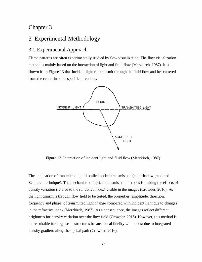
method is mainly based on the interaction of light and fluid flow (Merzkirch, 1987). It is

shown from Figure 13 that incident light can transmit through the fluid flow and be scattered

from the center in some specific directions.

Figure 13. Interaction of incident light and fluid flow (Merzkirch, 1987).

The application of transmitted light is called optical transmission (e.g., shadowgraph and

Schileren technique). The mechanism of optical transmission methods is making the effects of

density variation (related to the refractive index) visible in the images (Crowder, 2016). As

the light transmits through flow field to be tested, the properties (amplitude, direction,

frequency and phase) of transmitted light change compared with incident light due to changes

in the refractive index (Merzkirch, 1987). As a consequence, the images reflect different

brightness for density variation over the flow field (Crowder, 2016). However, this method is

more suitable for large scale structures because local fidelity will be lost due to integrated

density gradient along the optical path (Crowder, 2016).

28

Light scattering can be classified into two types: elastic scattering and inelastic scattering. For

the elastic scattering, the wavelength of scattered light (𝜆𝑠) is equal to wavelength of incident

light (𝜆𝑖) (e.g., Rayleigh and Mie scattering); whereas for the inelastic scattering, 𝜆𝑠>𝜆𝑖 (e.g.,

fluorescence). With the arrival of lasers, many combustion experiments are conducted with

laser as a light source. Planar laser-induced fluorescence (PLIF) are often used to identify

reaction zone and burnt fuel via detectable molecules in flames. Selected molecules can be

excited by a specific laser light from ground level to a higher energy level from which they

can decay back to the ground level by spontaneous emission of photons (fluorescence) that

can be collected at a right angle (Merzkirch, 1987). The objective of this study is to track

unburnt fuel; thus, Mie scattering is selected as the experimental method. The theory and

limitations will be discussed in this section.

3.1.1 Mie Scattering

Mie scattering (Mie solution or Lorenz-Mie) is the solution to Maxwell’s equation, which is

applied for scattering of spherical particles where the particle size is larger than the

wavelength of the incident light, i.e., 𝑑𝑝 𝜆⁄ > 1. The scattered light intensity (𝐼𝑠𝑐) depends on

particle concentration (c), particle diameter (𝑑𝑝), scattering angle (𝜃), wavelength of incident

light (𝜆𝑖), and refractive index of the particles relative to that of surrounding medium (n)

(Beverley et al., 2007). The same particles have different scattering intensities in different

surrounding medium due to effects of n. The scattering intensity is linearly proportional to

particle concentration. The Mie scattering intensity increases with an increase in particle

diameter, which is found to be proportional to the area of particle, i.e., 𝑑𝑝2 (Smith & Neal,

2016). Figure 14 shows a polar distribution of scattered light intensity for different sizes of

olive oil droplets in air. The intensity of 20 𝜇m-diameter particle is about square times larger

than 2 𝜇m-diameter particle at corresponding location. The scattering angle can greatly affect

scattering intensity. It is clear form Figure 14 that most of light is scattered in the forward

direction (0° ≤ 𝜃 ≤ 45°). Less light is scattered at angle of 90° in which images are taken.

The low intensity will influence the performance if the noise level is comparably high.

29

Figure 14. Scattered light intensity for olive oil in air (left: dp= 2 𝜇m and right: dp= 20 𝜇m)

(Crowder, 2016).

The Mie scattering method with seeding oil particles is an important tool in studies of

combustion and flame. It has been widely used to find flame fronts where burnt and unburnt

gases are separated including studies of Abbasi-Atibeh & Bergthorson (2019), Kheirkhah &

Gulder (2014), and Thevenie et al. (1996). The oil droplets, which acted as seeding particles

to the fuel, evaporate as they approach the high temperature region. The unburnt fuels at low

temperature are marked by scattering of seeding oil droplets.

3.2 Closed-Loop Wind Tunnel

The experiments were conducted in the closed-looped Boundary Layer Wind Tunnel II at The

University of Western Ontario, which includes two test sections: high-speed section and low-

speed section, as shown in Figure 15. Current experiments were conducted in the low-speed

section with a length of 52 meters. A 289 horsepower (hp) motor is placed downstream of

high-speed section (Figure 15), which introduces air into the tunnel and produces crosswind

speeds up to around 10 m/s on the low speed. The crossflow air passes a perforated screen

that is used to reduce velocity fluctuation before entering the contraction section. The

contraction section also helps reduce velocity fluctuation in order to ensure the test section is

exposed to uniform and low-turbulence flow (turbulence intensity less than 1%). With

30

contraction added, the test section is 3.6 m × 3.65 m (height × width) in cross-section. A

stack was placed 26 m downstream of the perforated screen. The crossflow velocities

upstream of the stack for current experiments were varied from 2 m/s to 10 m/s. The 2-part

hinged door was located at the end of low-speed section. Due to accumulation of combustion

products by each test, the test durations are limited. The 2-part hinged door is opened after

four sets of experiments to make sure the wind tunnel was free of exhaust combustion

products. In addition, the wind tunnel temperature increases after several sets of experiments,

so an amount of time was required to let the wind tunnel cool down.

Figure 15. Top View of Closed-loop Wind Tunnel (Hossain, 2019).

3.3 Gas Compositions

The methane-based flare gases used in current work contain six different components that are

representative of compositions from the Alberta upstream oil and gas industry (Conrad &

Johnson, 2019). The flare gas compositions were selected based on median flare gas

compositions that were derived from 2016 Alberta Energy Regulator data (Conrad & Johnson,

2019). The flare gas compositions are summarized in Table 1,

31

Table 1. Flare Gas Composition.

Components Species Volume Fraction (%)

Methane (CH4) 86.03

Ethane (C2H6) 6.81

Propane (C3H8) 2.35

Butane (C4H10) 1.99

Nitrogen (N2) 1.61

Carbon Dioxide (CO2) 1.21

3.4 Experimental Apparatus

3.4.1 Passive Grids

A passive grid was used to produce different levels of turbulence. The passive grid made of

wood (bi-planer grid) as shown in Figure 16 was designed by Hossain (2019). The

performance of the passive grid depends on three main factors: bar thickness (b), mesh size

(M) (distance between the centerline of two adjacent bars) and relative distance from the grid

to the location of interest (X).

Figure 16. Front view of the passive grid (marked dimensions in inch).

32

As crossflow passed through the bars of grid, turbulence was generated by shedding of

vortices downstream (Vita et al., 2018). In the region near the grid, the length scale is in the

order of the bar thickness, and the turbulence decays rapidly with distance downstream where

the flow is fully developed in the far field. The turbulent kinetic energy is found to be affected

by bar drag forces. More drag forces lead to higher initial turbulence production and higher

turbulence dissipation rate downstream. The ratio of bar thickness to mesh size (b/M) can

affect the drag, which in turn affects the turbulent energy. For the passive grid used in the

current experiments as shown in Figure 16, the ratio b/M was set to 0.2, with bar thickness of

4 inches (0.1016 m) and mesh size of 20 inches (0.508 m). The details on the design and build

of passive grids can be found in the work of Hossain (2019). The passive grid was placed at

the location, X = 10 M upstream of the stack to achieve enhanced freestream turbulence

approaching the burner.

3.4.2 Burner

The burner can be mainly divided into four parts including the diffusion chamber, settling

chamber, converging nozzle, and burner stack as shown in Figure 17. The flare gases enter the

chamber with a diffuser disk at the burner base in which the multiple gases can be effectively

mixed. Then the mixture goes through the settling chamber containing three mesh screens that

can make gas mixture homogeneous. The opening sizes of mesh screens were in decreasing

order from upstream to downstream.

33

Figure 17. Schematic of burner.

The tube size with nominal diameter of 1 inch was used as a burner stack for current

experiments. The 1 inch burner stack has the same dimension as 1” NPS SCH 40 pipe

(Nominal Pipe Size Schedule standard, 40 indicates the wall thickness represented in NPS

SCH). The detail dimensions of three stacks are listed in Table 2. The length of burner stack

(h) extending from the ground was fixed at 1.45 meters.

Table 2. Stack Dimension.

Burner Inner Diameter (d) Outer Diameter (D)

1 inch 1.049 inch (26.64mm) 1.173 inch (29.78mm)

34

3.4.3 Gas Delivery System

The fuel delivery system was initially designed by Darcy Corbin and then modified for the

current Mie scattering experiments. The schematic of the system is shown in Figure 18 which

consists of gas supplies, pressure regulators, mass flow controllers (MFCs), valves, and an

atomizer. Six Bronkhorst MFCs were used to separately control the flow of six pure gases to

maintain a fixed composition ratio, with one additional MFC used to control the methane

gases used to generate seeding particles. All gases were contained in pressurized cylinders,

and each was incorporated with a pressure regulator that can provide constant pressure.

For Mie scattering experiments, a certain amount of methane flow was used to atomize oil to

generate droplets as seeding particles. The rest of the methane flow bypassed the atomizer,

and was sent directly to the burner. The percentage of methane (86.03%) remains constant for

all experimental conditions. The required amount of methane depends on the fuel velocities,

and can be controlled by the mass flow controller that allows a flow range of 5 - 250 standard

liter per minute (SLPM). The methane supply line that is used to generate seeding particles

has a pressure supplied at around 20 pounds per square in gauge (PSIG). The Laskin nozzle

oil atomizer model 9637-6 (six-nozzle) supplied from TSI company was used for current

experiments. The end of nozzles immersed in the oil and pressurized gas exited through four

holes equally spaced around the nozzle acting as four jets. The pressure difference at the jet

exits leads to generation of tiny bubbles. The shearing effects of jet on the oil break up oil

streams into fine droplets carried inside bubbles that are drawn towards the oil surface. An

impactor plate inside the atomizer blocks large particles; small particles with an average

diameter in the order of micrometers escape from the gap and are ejected from the exit.

Solenoid valves were installed to remotely open or close inlet of nozzles to easily adjust the

seeding flow rate. In addition, a pressure transducer assisted in maintaining a relatively

constant supply pressure at around 20 PSIG. The seeded methane flow was mixed with other

gases via a Tee-fitting and sent to the burner all together.

35

Figure 18. Schematic of fuel delivery system.

3.4.4 Mie Scattering Imaging Components

The laser light sheet used to image the flame was created by a dual-head YLF laser with the

wavelength of 532nm working at the maximum energy level 30 mJ/pulse. The laser is located

1.5 meters downstream of the burner closed to the side wall. The photography and the front-

view schematic of the laser system setup are shown in Figure 19. The laser beam that has a

diameter of around 5cm at the exit was reflected off a 45˚ mirror that is located along the

centerline of the burner. Then the laser beam went through a combination of optics including

two cylindrical lenses so that the laser beam diverges into two directions. Two cylindrical

lenses with a focal length of -14mm give the primary expansion of light in the streamwise

direction (x). The angle of divergence is approximately 50 degrees, which forms a wide light

sheet in the xy-plane. The source of laser was placed around 1.5 meters downstream of the

burner, which gives intense laser light within the measurement domain so that the structures

of shear layer can be presented more clearly. The drawback of placing the laser closer to the

36

burner is making the background bright and greenish around the source of laser. Some

features of light scattering of seeding particles nearby may be lost. The average thickness of

the light sheet within the measurement domain is around 5 cm.

Figure 19. Mie scattering visualization system setup.

The Basler acA1920-155 uc CMOS color camera (complementary metal oxide

semiconductor) was used to capture Mie scattering images of flame. The images are taken

with a spatial resolution of 1920 × 1200 pixels. The lens has a fixed focal length of 16 mm

and adjustable aperture (f#) F1.4 to F16. The aperture was adjusted to the lowest number F1.4,

which allows an increased amount of light to pass into camera sensors. The working distance

(WD) from the camera to the image plane is around 1.6 m. With sensor size (physical size of

the sensor) 11.3 mm × 7.1 mm (width × height), the field of view (FOV) of width and height

can be calculated with equation 3.1, yielding 1.13 m × 0.71m (width × height).

𝐹𝑂𝑉 = 𝑊𝐷 ×

𝑠𝑒𝑛𝑠𝑒𝑟 𝑠𝑖𝑧𝑒

𝑓𝑜𝑐𝑎𝑙 𝑙𝑒𝑛𝑔𝑡ℎ

3.1

Passive grid

Burner

Pitot

tube

Optics

Laser head

37

The camera was mounted to a frame with a vertical rail on the side wall (perpendicularly to

the laser sheet) so that the camera can be moved vertically up and down to the right position

for different test conditions. There are eight different positions to place the camera with the

first position located around 60 cm above the ground, and raised by 15 cm for every increased

position.

3.5 Image Acquisition

A code developed in LabVIEW software was used to capture flame images at high frame

rates, which is 30 frames per second (fps) for two cameras mounted on the side wall. The

exposure time of each camera is 500 µs, which is short enough without blurring the flames in

photos. Each run of test duration was 60 seconds; thus the total number of 1800 images were

captured for each experimental condition. The images taken have three color channels (RGB):

red, green, and blue, and each channel consists 1920 × 1200 pixels. The color digital camera

outputs 8 bits of each of red, green and blue data for each pixel that has 256 light intensity

levels available in the range from 0 to 255.

Synchronization of multiple cameras was achieved using hardware triggering. A sequence of

5V TTL digital signals at 30 Hz was generated and sent to all cameras so that images were

acquired simultaneously. In the meanwhile, the same sequence of signals acting as external

triggers were sent to a delay generator that was used to fire the laser. The firing of the laser

was delayed for 50 ns while receiving the signals from the delay generator, leading to the

pulse of laser light synchronized with the opening of cameras.

38

3.6 Flow Conditions

3.6.1 Velocity and Momentum Ratios

In the current experiments, a crossflow with two different levels of turbulence were tested to

investigate the importance of turbulence effects. The two cases with different turbulence

levels are:

Case A: ambient turbulence (no passive grid upstream of burner)

Case D: enhanced freestream turbulence (passive grid is placed at 10M upstream of

burner)

For each case of turbulence conditions, a fixed fuel jet velocity of 2 m/s was tested in five

different mean crosswind velocities (2, 4, 6, 8, 10 m/s). The total number of conditions is 5

for each case. The jet to crossflow velocity ratios R are varied from 0.2 to 1.0 (0.2 ≤ R ≤ 1.0),

as shown in Table 3. The crossflow Reynolds number (Re∞) based on crossflow velocities and

burner diameter were altered from approximately 3.6 × 103 to 1.8 × 104. The density of the

fuel is 0.79 kg/m3 that is measured at standard temperature and pressure (273.15K and 101.3

Pa).

Table 3. Jet-to-Crossflow Momentum and Velocity Ratios for Uj = 2 m/s.

𝑈∞(m/s) Velocity Ratio, R Momentum Ratio, J

2 1.00 0.66

4 0.50 0.16

6 0.33 0.07

8 0.25 0.04

10 0.20 0.03

39

3.6.2 Boundary Layer Velocity Profiles

Velocity profiles were taken via a Cobra Probe at a sampling frequency of 1250 Hz. The

Cobra Probe is a 4-hole pressure probe, which can measure time-varying 3-component

velocity as well as local static pressure. The probe has been already calibrated by the supplier.

The limitation of the Cobra Probe is that it only can measure the velocities greater than 2 m/s,

and will show errors for velocities below 2 m/s. A Pitot-static tube was used to control the

cross flow velocities as well as to cross check the velocities measured by the Cobra Probe.

Velocities were measured at several positions from 10 cm above the floor nearly up to the

burner tip (y =10 - 140 cm and h = 145 cm). Figure 20 shows normalized mean streamwise

velocity profile (U/U∞) in the boundary layer above the floor for two different turbulence

cases. It is observed that velocities reach around 95% of freestream velocity at the vertical

location around y = 0.2 h for both Case A and Case D. Velocities at vertical location above

0.2 h remain almost constant with variation less than 5% of freestream velocities so the

effects of velocity gradients on the flame is negligible. The uniformity of mean streamwise

velocities across the wind tunnel was checked by Hossain (2019). The flow approaching the

center plane of wind tunnel is at a relative uniform velocity compared with the flow near the

wind tunnel side walls at 1.2 meters height. The velocities at the location within 30cm away

from two side walls falls to 90% - 95% of freestream velocity. The velocities far away from

walls (>30cm) varies ±3% of freestream velocity.

40

Figure 20. Boundary layer velocity profiles.

3.6.3 Grid Turbulence

As discussed in Section 3.4.1, the performance of the turbulence produced by the passive grid

greatly depends on the distance relative to the grid since the turbulence intensity decays with

distance downstream. The relation of grid turbulence data with distance downstream of

passive grid can be found in Hossain (2019). The turbulence intensity profiles for both Case A

and Case D at the location upstream of burner are shown in Figure 21. Figure 21 shows the

turbulence intensity reaches a relatively stable value at vertical location 0.4 h above the

ground plane. The values of turbulence intensities calculated for Case A and Case D at the

burner height are 0.75% and 9.14%, respectively. The integral length scale representing the

length scale of largest eddies at the measured location. Size of eddies increases with distance

away from the grid (Hossain, 2019). The length scales normalized by burner diameter (Lx/d)

of Case D was determined to be 5.6.

41

Figure 21. Turbulence intensity profile.

3.6.4 Turbulence Energy

The turbulent kinetic energy is distributed over a spectrum of scales. The total turbulent

kinetic energy (K) contained in the flow is defined as

𝐾 =

1

2(𝑢′2̅̅ ̅̅ + 𝑣′2̅̅ ̅̅ + 𝑤′2̅̅ ̅̅ ̅) 3.2

where 𝑢′, 𝑣′ and 𝑤′ are the three fluctuating velocity components.

The turbulent flow consists of a spectrum of a wide range of scales, which can be interpreted

as different sizes of eddies (l). Large eddies in the flow contain most of turbulent kinetic

energy. An important characteristic of turbulent flow is energy dissipation. As described by

Richardson “Big whirls have little whirls that feed on their velocity, and little whirls have

lesser whirls and so on to viscosity” (Pope, 2015). That means large eddies extract kinetic

energy from mean flow, and produce smaller eddies through non-linear interactions leading to

energy transfer to slightly smaller eddies. This process goes on until the viscous effects

42

become important to small-scale motions, then kinetic energy contained in the smallest eddies

is dissipated into thermal energy due to viscous forces. The turbulent kinetic energy spectrum

is always represented as a function of frequency, f (or wave number, 𝜅 = 2𝜋/𝑙) that relate to

different scales in the flow (Davidson, 2014). The energy spectrum at high Reynolds number

is characterized by three regions with various length scales l, which are:

Energy-containing range. Large turbulent eddies extract energy from mean flow so

that the turbulence kinetic energy is increased, which is called “production”. Most

energy is contained in the eddies in the range of largest size, and characterized by

length scale 𝑙𝑥, velocity scale 𝑢0 that is on the order of r.m.s. of 𝑢′ comparable to

mean velocity, with time scale 𝜏0 = 𝑙𝑥/𝑢0. The effects of viscosity are not significant

because Reynolds number of large eddies is large in this range, which indicates the

viscous force is relatively small. Energy is transferred as the large eddies break into

smaller eddies.

Dissipation range. For sufficiently small scale eddies, the rate at which energy

received is nearly balanced with rate at which energy dissipated (𝜀). The small scale

motion is, therefore, affected by two parameters, energy dissipation 𝜀 and viscosity 𝑣.

The viscous effects are mainly in charge of dissipation into thermal energy. The small

scale eddies at dissipation rate are described by Kolmogorov scales in terms of 𝜀 and 𝑣

that are defined in equations 3.3, 3.4, and 3.5, which are derived based on the

Reynolds number of unity (Pope, 2015). Kolmogorov argued “small scale turbulent

motions are statistically isotropic”, which indicates the motions are similar for all

sufficiently high Reynolds number turbulent flow.

Length scale: 𝜂 = (𝑣3

𝜀)

14

3.3

Velocity scale: 𝑢𝜂 = (𝜀𝑣)14 3.4

Time scale: 𝜏𝜂 = (𝑣

𝜀)

12 3.5

43

Inertial subrange. Transfer of energy mainly happens in this range in which Reynolds

number is still large. The motions of scales in this range are mainly determined by

inertial effects. The eddy sizes are between integral length scales and Kolmogorov

scales, which is Taylor microscales.

The rate of energy transferred can be scaled as 𝑢02/𝜏0(= 𝑢0

3/𝑙𝑥). Because the dissipation rate

(𝜀) is balanced with energy transfer rate, the ratio of large eddies to the Kolmogorov scale

eddies can be estimated as in equations 3.6, 3.7, and 3.8 (Pope, 2015),

𝑢0

𝑢𝜂= 𝑢0(𝜀𝑣)−

14 = 𝑢0 (

𝑣𝑢03

𝑙𝑥)

−14

= (𝑢0𝑙𝑥

𝑣)

14

= 𝑅𝑒14 3.6

𝑙𝑥

𝑙𝜂= 𝑙0 (

𝑣3

𝜀)

−14

= 𝑙𝑥 (𝑣3𝑙0

𝑢03 )

−14

𝑣0 = (𝑣3

𝑢03𝑙𝑥

3)

−14

= 𝑅𝑒34 3.7

𝜏0

𝜏𝜂= 𝜏0 (

𝑣𝑙𝑥

𝑢03 )

−12

=𝑙𝑥

𝑢0(

𝑢03

𝑣𝑙𝑥)

12

= (𝑢0𝑙𝑥

𝑣)

12

= 𝑅𝑒12 3.8

It is noted form equation 3.7 that the ratio 𝑙𝑥 𝑙𝜂⁄ is reduced with an increase in Reynolds

number. At high Reynolds number, the smallest eddies in flow are much smaller compared

with 𝑙𝑥. In addition, the vorticity, 𝜔, of eddies is reversely proportional to the time scale; thus,

the ratio of Kolmogorov eddies vorticity to large eddies vorticity (𝜔𝜂/𝜔0) is 𝑅𝑒1 2⁄ . As a

result, the most intense vorticity is associated with the smallest eddies in the flow.

The von Kármán spectra is commonly used to represent the turbulence over the full scale

range. The shape of the von Kármán spectra depends on the turbulence intensity and integral

length scale. The von Kármán spectral equation is given as (ESDU 85020)

𝑓𝑆𝑢𝑢(𝑓)

𝜎𝑢2

=4 (

𝑓𝑙𝑥

�̅� )

[1 + 70.8 (𝑓𝑙𝑥

�̅� )2

]

5/6 2.9

44

where 𝜎𝑢 is standard deviation of streamwise velocity u and 𝑆𝑢𝑢(𝑓) is spectral density

function of u components. In this study, 𝑙𝑥 and 𝜎𝑢 are computed based on ESDU 8250.

Figure 22. Power spectral density of the measured velocity at the burner height and von

Kármán spectra of two full-scale conditions given by equation 2.9.

In Hossain (2019), two target full-scale scenarios from ESDU 85020 were selected to be

compared with experimental conditions of wind tunnel. Figure 22 shows measured

normalized power spectra density (PSD) and von Kármán spectra given by equation 2.9. Case

B (Iu = 3.72% and Lx = 0.32 m) and Case C (Iu = 5.78% and Lx = 0.23 m) are two different

turbulence cases corresponding to two full-scale scenarios as indicated in Figure 22. In the

previous experiments including both Case B and Case C, the turbulence kinetic energy starts

to drop significantly at the scale of burner diameter where the energy level is low. Due to

importance of keeping energy high at length scale of burner diameter, the passive grid was

moved closer to the burner (Case D), so that the overall energy levels were increased

including energy at the scale of burner, but energy levels decrease rapidly for scales smaller

45

than the burner diameter. The rapid loss of energy is associated with Re∞ (~ 103-104) not

being high enough to generate small scale eddies. It is noticed from Figure 22 that the scales

in energy containing range are in the order of 102-103. Based on equation 3.7, the ratio of

smallest eddies to largest eddies in the flow should be approximately 102-103 (Re∞ ~ 103-104).

The Reynolds number is low, and the motion is affected by viscosity. Therefore the rapid

drop-off was observed at scales fd/U∞ ~ 100. Figure 22 also shows the power spectra taken at

location of burner exit for current experimental conditions Case A. Case A represents the case

without a passive grid placed inside the wind tunnel, the energy levels are sufficiently low at

all scales compared to Case D.

46

Chapter 4

4 Results and Discussions

4.1 Observations of Flame Appearance

This section mainly discusses two factors affecting the flame appearance. In Section 4.1.1, the

characteristics of the visible flame are discussed for each flow condition, as well as changes

with an increase in crossflow velocity. The discussion only examines the effects of crossflow

velocities in Section 4.1.1; effects of freestream turbulence are addressed in Section 4.1.2.

4.1.1 The Effects of Crossflow

Several changes of flame characteristics were observed for both Case A and Case D as

crossflow velocities were increased (i.e., J was reduced). In the current study, the flame base

remains attached to the burner for the entire range of conditions, which indicates that only

wake-stabilized flame will be discussed below. As discussed in Section 2.2.1, the wake

stabilized flames can be further grouped into different types or modes based on overall

appearance, based on changes of crossflow velocity. Flames observed in current experiments

are Type I and Type II flames, as described by Gollahalli & Nanjundappa (1995) and Johnson

and Kostiuk (2000). Type III flames were not observed in current study. Type II flames are

characterized by a three-zone structure, as indicated in Figure 10 (Johnson and Kostiuk,

2000): Zone 1(the planar recirculation zone that stands behind the burner stack, which is also

known as downwash), Zone 3 (axisymmetric main tail of flame), and Zone 2 (junction of Zone

1 & 3, the main color of flame is blue in the transition zone). Type I flames are characterized

by the extinction of the flame tail. Most flames are identified to be Type II, except for

crossflow velocities of 10 m/s. Even though the other four conditions have the same type of

flame, there still exists significant differences among each of them.

Figure 23 shows flames at the lowest crossflow velocities of 2 m/s (J = 0.66). A small amount

of fuel is drawn downward into the downwash region and burns, enclosing a small yellow

flame at the backside of the burner. The flame firstly shrinks in the y direction and then

expands with downstream distance. The thinnest part of the flame can be identified as a

47

junction, which is marked in Figure 23. The phenomenon is also called the “neck” that was

observed by Huang & Wang (1999), which is an important feature to identify the flame as

being in a transitional mode from the jet-dominated mode to the crossflow-dominated mode.

The neck is observed around 3 d downstream of burner followed by initial blue part of flame

tail. The flame after Zone 2 expands slightly in the y direction and burns in large detached

pockets in Zone 3.

(a) Case A, U∞ = 2 m/s

Small

yellow

flame

Junction, also

known as “neck”

Detached flame

pocket

48

Figure 23. The whole view of flame. 𝑈∞= 2m/s, J=0.66. (a) Case A: ambient turbulence. (b)

Case D: enhanced FST.

At crossflow velocities of 4 m/s (J = 0.16) and 6 m/s (J = 0.07) as shown in Figure 24 and

Figure 25, increased amounts of fuels are trapped into the leeside of the burner stack and burn

so that the area of downwash increases. This is due to the enhanced negative pressure behind

the burner stack with an increase in crossflow velocity. The differences between pressure in

the lee side of burner stack (𝑃) and freestream (𝑃∞) can be determined as,

𝑃 − 𝑃∞ = 𝐶𝑝 ×

1

2𝜌𝑈∞

2 3.1

Equation 3.1 shows that increases of pressure differences are proportional to 𝑈∞2 , which

means intense suction brings more fuels burning in the near weak region. In addition, the

pressure differences are also affected by the pressure coefficient, 𝐶𝑝, which is dependent on

freestream Reynolds number and freestream turbulence. The Reynolds number for all current

(b) Case D, U∞ = 2 m/s

Small

yellow

flame

Junction

Detached flame

pocket

49

experimental conditions falls into the subcritical regime. The pressure coefficient at the base

(−𝐶𝑝𝑏) and drag increase in this Re regime because of forward movement of “transition

point” in the separated shear layer (Roshko, 1993). In addition, the junction zone seems to be

extinct as J is reduced to 0.07 (Figure 25). It is hard to find the necking phenomenon from

individual images. The flame tail becomes narrower and narrower as crossflow velocities are

increased, and does not expand as wide as crossflow velocities of 2 m/s. The length of the

flame tail increases as crossflow velocity is increased from 2 m/s to 4 m/s. It seems that the

length of flame reaches the maximum value between 4 m/s and 6 m/s because the length of

flame tail starts to decrease in this range.


Large

downwash area

50





Smaller downwash area

compared to Case A

Junction zone

(neck) is not

obvious

51



At higher crossflow velocities of 8 m/s (J = 0.04) and 10 m/s (J = 0.03) as shown in Figure 26

and Figure 27, most parts of flame are trapped in the downwash region. The junction zone

completely disappears and the flame tail becomes almost entirely blue. The blue color of

flame tail represents an intense mixing of air and fuel. A large amount of air is entrained in

the reaction zone so that the fuels are diluted beyond the lean limits, and the combustion

becomes unstable. Gollahalli & Nanjundappa (1995) proposed that the lean limit process is

mainly responsible for local extinction of flame. The yellow/orange flame zone behind the

burner stack becomes shorter in the x direction but is stretched in the y direction.

Apart from changes of each zone of flames with crossflow velocity discussed above, another

important change is the flame pockets over the length of flame. It is clear that flame pockets

disappear with extinction of flame tail for both Case A and Case D. For the conditions with

flame pockets, it is difficult to quantify the number of flame pockets changing with crossflow

velocities due to limited conditions of tests taken. But, based on observations from a sequence


Flame length is

reduced

52

of individual images, the number of flame pockets tends to increase when the flame length is

reduced after reaching peak. This explains the observations of flame length reduction.

Because the fuel supply rate is unchanged for all crossflow conditions, it is assumed that the

flame surface area does change too much due to assumption of insignificant changes of

oxygen entrained to mix with fuels. An increase in number of flame pockets leads to an

increase in flame surface area; thus balanced by a reduction in flame length.


Extinction of

junction

53




(a) Case A, U∞ = 10 m/s

Flame tail is

entirely blue

54



4.1.2 The Effects of Freestream Turbulence

Several differences to the flame appearance are observed with the addition of freestream

turbulence. Firstly, it is noticed that at the same crossflow velocities, both length of flame tail

and/or downwash area are reduced for the Case D compared to Case A. For crossflow

velocities larger than 4m/s, fuel from the burner is drawn by low pressure into the separated

flow on the lee side of the stack. Figures in Section 4.1.1 show the downwash area is

obviously smaller for flow with turbulence, which indicates the base pressure suction is

relatively lower. The possible reason is that the freestream turbulence interacts with the

separated shear layer from burner stack and brings it closer to the burner stack leading to a

narrower wake region. This results in a reduction in pressure differences between upstream

and downstream of the burner stack.

(b) Case D, U∞ = 10 m/s

55

Compared with flames in crossflow with freestream turbulence, the flames without effects of

turbulence are more stable and integrated as a whole flame. A sequence of images for each

condition is shown in Appendix A. The Case A flames appear to break off into flame pockets

at the distance further away from the burner compared to flames from Case D. For example,

at crossflow velocity of 4 m/s (Figure A2 in Appendix A), Case A flames burn in flame

pockets at location x = 30-35 d; whereas Case D flames start to break into flames pockets at

location x = 15-25 d. The length of flame tail is obviously shortened for Case D flames, which

compensate with an increased number of detached flame pockets. The averaged flame length

will be analyzed in Section 4.3. Another noticeable difference is that most of flame pockets

formed in Case D are completely detached. The spaces between adjacent flame pockets are

larger, which can be especially noticed between Cases A and D (such as for U∞ = 6 m/s

indicated in the last group of images in Figure A3 in Appendix A). In contrast, the flame

pockets from Case A are close to each other or continuous.

In addition, an interesting observation is made for the effects of turbulence is that flames

undergo “flapping” motion in the y direction. This feature was also observed in non-reacting

jets in crossflow, which is identified as “waving of jet” (or destabilization of jet flow), and is

driven by counter-rotating vortex pair in the downstream of flow (Camussi et al., 2002). The

destabilization was found to be strongly affected by velocity ratios, and the differences are

recognized to originate from a streamline of the jet exit (Camussi et al., 2002). The current

study does not involve measurements of the velocity field, so the waving of flame tail can

only be recognized from individual images that cannot be compared among each other in

terms of streamlines. However, the waving of flame tail is not observed for the flames from

Case A for all conditions, which are completely different from Case D flames. The Case A

flames are much more stable and stay in place, which means the flames do not move up and

down in the y direction. Further descriptions of flame flapping can be found in Appendix A

(Figure A2, U∞ = 4 m/s).

56

4.2 Shear Layer Region

This section discusses the observations from the shear layer region. Section 4.2.1 describes

the observed structures in the shear layer for different crossflow conditions for flames in

crossflow without turbulence (Case A). Section 4.2.2 discusses the observation for flames

from Case D, which is affected by enhanced FST. The differences are clarified between Case

A and Case D due to effects of turbulence.

4.2.1 Observed Flow Patterns in Shear Layer

Shear layer vortices are readily apparent in the upper side of flame. The vortices in the

separated shear layer downstream of the burner tip are like Kelvin-Helmholtz (KH) vortices

generated in plane mixing layers. These vortices are created by vertical shear stress between

two flows (air and fuel) of different densities and velocities. The KH like vortices are also

found in JIC, but there is one clear difference between JIC and flare in crossflow: most

researchers studying JIC found vorticities were generated in both the upper and lower of the

jet flow, which are usually called ring-like vortices. Only a few studies stated the lee-side

vortices disappear at low velocity ratios (Lim et al., 2001). For the flare in crossflow, lee-side

vortices were not found in any flow conditions even at high R or J in literature. The vortical

structures of the upper side of flame are strongly dependent on crossflow velocities, similar to

non-reacting jet in crossflow.

The most obvious change with crossflow velocity is the change in direction of rotation of the

vortices. Studies on JIC by Lim et al. (2001) showed the upstream vortex loops were pointed

downstream (clockwise direction) at velocity ratio, R ≤ 1, instead of upstream

(counterclockwise direction) at large R. The counterclockwise rolling vortices in shear layers

that have jet-like structures were found to have the same sign of vorticity (positive) as vortices

generated inside the pipe (Andreopoulos, 1989). Several researchers discussed the vorticity in

the boundary layer on the inside of the tube was of great importance in generation of jet-like

structures in the shear layer. As crossflow velocities are increased, the wake-like structures

(clockwise rolling vortices) carrying negative vorticity start to appear together with jet-like

vortices. This special structure is named as mushroom-type vortices.

57

In the current experiments between crossflow flow velocities of 2 m/s and 10 m/s,

unidirectional counterclockwise vortices are not observed in the shear layer. There exists a

regime at a crossflow velocity of 2 m/s where both jet-like and wake-like vortices are present,

similar to those observed by Huang & Chang (1994a) and Huang & Lan (2005). Figure 28

shows the streak Mie scattering images of shear layer region for Case A at U∞ = 2 m/s.

Images were taken at frame rates of 30 fps so that the interval time among each image is

0.033 seconds. The evolution of a single vortex circled in streak images is clearly present in

Figure 28.

58


Figures (a)-(b): the initial development of the circled vortex evolved from the burner tip.

Figures (d)-(f): the circled vortex gradually develops into “mushroom-like” shape as time

evolves. Figures (g)-(i): the “mushroom-like” vortex starts to fade away with right part

disappearing firstly. In figure (e), the circled vortex cannot be found, which breaks into small

random turbulence.

(a)

(b)

(c)

(d)

(e)

(f)

(g)

(h)

(i)

59

The circled vortex, firstly, evolves from the tip of the burner as indicated in Figure 28(a) and

(b), then it starts to rotate downstream with clockwise direction. Up to this point, the vortex

just travels a short distance downstream and only has one rotating direction. While convecting

further downstream (Figure 28(d)), the vortex tends to turn into the mushroom-type structure

at the location where the flame is bent by the crosswind towards streamwise direction. The

mushroom type vortex is made of two parts: one remains clockwise on the right side and the

other develops in the opposite direction on the left side. This vortex remains coherent and

convects downstream until a location around 2-3d away from center of burner. Then, the right

part of the mushroom fades away. Finally, the coherent structure breaks into random

turbulence further downstream. For the current condition, the vortex is dominated by vorticity

in a counterclockwise direction, especially in the downstream area of the shear layer.

For the higher crossflow velocity of 4 m/s (i.e., J = 0.16), the size of vortices becomes smaller

and occur in a very organized pattern. Those well-organized structures are similar to coherent

structures in the plane mixing layer observed by Roshko (1976). Figure 29 shows streak Mie

scattering images of shear layer region. The coherent structures are of a scale comparable to

burner diameter and rotate in the clockwise direction to the downstream distance. The single

vortex remains integrated as one over a long distance, and then begins to be stretched in the x

direction. The scale of vortices slowly grow and each vortex is evenly distributed before

stretching and elongation. Two or more stretched vortices amalgamate at a distance of

approximately 3d away from the burner. The loosely formed large-scale vortex continues

rotating downstream with a lack of circumferential coherence.

60


Figures (a)-(c): the circled vortex is stretched in streamwise direction. Figure (d): several

vortices amalgamate to form a large structure without concentrated core that is shown in

figure (e). Figure (f): the loosely formed large structure convects downstream.

As crossflow velocities are increased above 6 m/s (i.e., J is reduced below 0.07), the

development of structures is similar to the transition process of shear layer separated from

bluff body, as discussed in Lander et al. (2016). Figure 30 shows streak images of the shear

layer region at crossflow velocity of 8 m/s. The KH vortices are clearly present along the

initial region of the shear layer. The width of shear layer increases with downstream distance.

The growth is the result of vortex pairing process. It is found adjacent vortices interact with

each other and rotate into a larger vortex that continues rotating in the clockwise direction.

The large vortex breaks into small dispersed cores before diffusion into the flame.

(a)

(b)

(c)

(d)

(e)

(f)

61


Figure (a): pairing of two individual vortices circled starts. Figures (b) and (c): pairing

continuous, forming a relatively large vortex. Figure (d): lager vortex rotates to downstream

area. The dispersed cores pointed by arrows in figures (c) and (d) are caused by breakdown of

the former lager vortex.

(b)

(c)

(d)

(a)

62

4.2.2 The Effects of Freestream Turbulence on the Shear Layer

Section 4.2.1 mainly discussed the development of coherent structures in the separated shear

layer for different crossflow velocities. The examples in the discussions are all from cases

with ambient turbulence (Case A). Similar structures are also observed in corresponding cases

with enhanced freestream turbulence (Case D). But there are some obvious differences in the

shear layer region between Case A and Case D due to the effects of enhanced FST.

Figure 31 shows streak images of shear layer region at crossflow velocity of 2 m/s (i.e., J =

0.66). The mushroom-type vortices maintain the shape with two parts travelling for a longer

downstream distance, unlike Case A, for which the right part of mushroom-vortices disappear

quickly at the location where the jet flow turns in the streamwise direction. Instead, the

clockwise rotating part continues developing downstream with a higher strength than the

counterclockwise rotating part on the left side. The counterclockwise part is probably initiated

by negative velocity gradient in y direction within the shear layer. With freestream turbulence,

the velocity in y direction may increase faster resulting in an increased velocity gradient,

decreasing the strength of counterclockwise rotating vortices. The increased strength of the

right part may entrain freestream air into fuels and bring the shear layer closer to the flame

body.

63


Figures (a) and (b): The vortex rotates into “mushroom-like’ structure. Figures (c)-(f): the

right side of mushroom type vortex rotates into the next vortex to from another mushroom

type vortex; the left side of vortices keep pointing upstream while convecting downstream.

Figure 32 shows sequential images of flame D with enhanced FST for a crossflow velocity of

4 m/s (J = 0.16). For this case, it is noticed the motion of vortices becomes random; the size

of vortices and the space between each other are varied from image to image at the same

location. The vortex pairing (or amalgamation) of several vortices is clearly observed, which

occurs near the burner exit. In the conditions without enhanced FST (Case A) at the same

momentum flux ratio, vortex amalgamation happens at a distance further from the burner. The

loosely-formed via vortex pairing large vortex convects downstream and loses its coherence.

The length of shear layer is significantly shortened for Case D compared to Case A due to the

(a)

(b)

(c)

(d)

(e)

(f)

64

rapid breakdown of coherent structures and diffusion of turbulence into the flame. Another

important feature clearly observed from those images is that the shear layer undergoes

“flapping motion” together with the flame body. The blue arrow marked in the sequential

images indicates the movement of shear layer (also shown for 𝑈∞ = 6 m/s in Figure A3 in

Appendix A). The movement of shear layer is like a wave, which may be the reason why

vortices are not evenly distributed like for Case A. The waving of the shear layer are also

observed in other conditions from Case D. The dependence of crossflow velocities is difficult

to be solved with visualization only. As the crossflow velocity is further increased to a higher

value, i.e., 𝑈∞ = 6, 8, and 10 m/s, the pairing of vortex moves closer to the burner tip. In some

images, pairing or amalgamation of vortices occurs right above the burner exit as illustrated in

Figure 33. Changes of shear layer region are not obvious from observations of individual

images for 𝑈∞ ≥ 6 m/s.


Figure (a): multiple vortices amalgamate. Figures (b)-(c): the loosely formed structure

convects downstream. Figure (d): breakdown of vortices as pointed by the arrow in white

color. Figure (d): vortex pair occurs near the burner exit.

(a)

(b)

(c)

(d)

(e)

65


Figures (a) and (c): single vortex distributed along the shear layer. Figures (b) and (d): vortex

pairing occurs just above the burner tip where arrows pointed.

The “transition point” in the current study is defined as the location where breakdown of

coherent structures into dispersed cores occurs. Figure 34 shows the transition point changes

with crossflow velocities for both turbulent cases. The transition shows the dependence of

Re∞. The development of structures in the shear layer observed in the current study is mainly

controlled by crosswind because the fuel jet velocity remains unchanged. It is observed that

the transition point moves upstream as crossflow velocity is increased. The transition may

also depend on the jet-to-crossflow momentum flux ratio. The fuel jet flow could affect the

coherent structures on the upper side of the flame. Testing with a range of jet velocities should

be done to further investigate the dependence of transition. The transition points also occur

earlier with the effects of turbulence for each crossflow velocity. The earlier transition is

probably caused by bypass-transition, which will be revisited in Section 4.3.

(a)

(b)

(c)

(d)

66

Figure 34. Comparison of break down location between Case A and Case D.

Figure 35. Comparison of vortex sizes between Case A and Case D.

67

Figure 36. Indication showing how size of vortex is measured.

From earlier observations and discussions, it was discussed that the FST affects the growth of

the shear layer significantly. The growth can be roughly quantified with scales of vortices

within the shear layer. Figure 35 shows mean size of vortices along the shear layer in x

direction. The mean size of vortices at each location shown in Figure 35 is calculated based

on vortices within distance ± 0.25 d (x=0 is the center of burner stack). The size of vortices is

measured in pixel size. From observations of vortices in the shear layer, the shapes of vortices

are closed to a round circle except for U∞ =2 m/s. The shape of coherent structures varies

significantly, which makes it difficult to be measured. So the size of vortices are only

measured for crossflow velocities from 4 m/s to 10m/s. The size of vortices can be estimated

to be the diameter of the circle. The way to measure the vortices is consistent, which is

measured from one side of edge to another across the center of vortex along the trajectory of

the shear layer, as indicated in Figure 36.

Figure 35 illustrates that the size of the vortices decrease with crossflow velocities increased

from 4 m/s to 10 m/s for both Case A and Case D. For Case A, the growth of vortices is

continuous, however, the decrease of vortex size occurs for Case D (such as U∞ = 6 m/s and

10 m/s), which may indicate that the large vortex formed in the upstream breaks into smaller

vortices. The growth of vortices with streamwise direction x for Case D is irregular. The

decreases and increases in mean size of vortices may be due to breakdown and amalgamation

of vortices. For U∞ = 4 m/s, the size of vortices are similar between Cases A and D. The

Trajectory of

shear layer

Size of individual

vortex

68

amalgamation of vortices for Case A occurs later, at location x = 3-3.5 d. For the rest of the

conditions (i.e., U∞ = 6, 8, and 10 m/s), the size of vortices for Case D are mostly larger than

Case A, probably due to earlier pairing or amalgamation of vortices.

In summary, the following observations are identified with the addition of enhanced FST:

i. The separated shear layer becomes unstable, an associated with randomization of

vortex pairing. The shear layer undergoes a “flapping” motion, up and down in y

direction together with the flame body.

ii. The coherent structures are not highly concentrated, which may due to small-scale

turbulence superimposed on the large-scale structures. For conditions without FST, the

vortices are evenly distributed and have relatively clear cores.

iii. The event of vortex pairing occurs earlier.

iv. The transition point moves upstream, and the overall length of the shear layer is

reduced. Conversely, the shear layer tends to extend further downstream for flames

from Case A.

69

4.3 Discussion on Effects of Turbulence Based on Mean Flame

Images

The mean flame images are calculated from around 1500 images taken for each experimental

condition. It is noticed that pixel intensity of each image include content of flame, Mie

scattering from laser light, and the green background that comes from radiation of laser light.

While part of background of laser light is filtered, the area around the flame body and shear

layer cannot be processed too much because the intensity values between background and Mie

scattering from seeding particles are too close. In the current study, the mean images are

mainly used to observe the features of mean structures of flame or shear layer. To obtain the

mean images, the first step is image binarization, which is to convert RGB coloured images to

binary (elements greater than a threshold are converted to values of 1 and lower than that are

converted to 0). Then a cutoff value determined from the distribution of pixel values and is

used to distinguish flame and Mie scattering from background for each individual images.

The pixel value of the mean image is determined from the possibility of occurrence of flame

or Mie scattering. Figure 37 shows the mean images for each condition. The three different

intensity levels of gray-scale from dark to bright represent the possibility is higher than 10%,

50%, and 90%.

Case A, U∞ = 2m/s

Case D, U∞ = 2m/s

70

Figure 37. Mean Flame Images.

Case A, U∞ = 4m/s

Case A, U∞ = 6m/s

Case A, U∞ = 10m/s

Case A, U∞ = 8m/s

Case D, U∞ = 4m/s

Case D, U∞ = 10m/s

Case D, U∞ = 8m/s

Case D, U∞ = 6m/s

71

The most obvious change with the addition of enhanced FST is the flame shape. The same

conclusion is made from individual images: both flame length and downwash area are

reduced. It is much clearer from the mean images that the planar area is overall reduced.

Based on assumption that, if the flow rate is kept constant, the flame surface will not change

too much, the mechanism leading to a great reduction of visible flame may be due to fuel

ejection without combustion.

The flame length is determined from 10% probability occurrence of a flame at each pixel

from the mean flame images. The length is measured from the center of the burner exit to the

edge of the 10% contour. The mean flame images used to determine the flame length are

binarized with a higher cutoff value than the one used to generate mean images in Figure 37.

The reason is that pixel intensity of shear layer closes to the background. In order to avoid the

shear layer being erased, a lower cutoff is selected. To determine the flame length, a higher

cutoff value is used to completely segment the flame from the background. The method of

how the cutoff value is chosen is discussed in detail in Appendix B.

Figure 38 shows flame length changes with U∞. The trend of change of flame length with

crossflow velocities are the same for Cases A and D: the length firstly increases as U∞ is

increased from 2 to 4 m/s reaching the peak between 4 and 6 m/s, and then starts to decrease.

The differences between Case A and Case D are not consistent for different crossflow

velocities, which are listed in Table 4. The maximum differences are 35.4% at U∞ = 6m/s. As

U∞ was increased 8 and 10 m/s, the differences between two cases are reduced. At U∞ =

10m/s, the flame length for both cases are almost equal to each other. This is due to extinction

of flame tail with the flame trapped in the downwash area.

Table 4. Comparison of flame length of Case A and Case D for different crossflow velocities.

U∞, m/s 2 4 6 8 10

Differences 14.4% 22.5% 35.4% 28.9% 10.4%

72

Figure 38. Flame length.

Another observation made due to the effects of FST is that the trajectory of the shear layer is

bought closer to the flame body. It is noticed the shear layer is closely attached to the flame

for U∞ ≥ 6 m/s. This is speculated to be associated with bypass-transition behavior, which is

also described in Lander et al. (2016). From observations from individual images of flame in

crossflow with enhanced FST (Figure 33), the transition process in the shear layer is changed.

The FST that is distorted by the burner is likely to be enhanced and amplified in the shear

layer region near the stagnation point (burner tip). As a result, the initial development of KH

vortices is bypassed, promoting and accelerating breakdown of organized vortices into

random turbulence. The pairing or amalgamation of vortices occurs earlier, right after the

separation. The movement of vortex pairing to the upstream can maintain the initial part of

shear attached to the flame. From analysis of the instantaneous flow field on separated shear

layer from a square prism by Lander et al. (2016), freestream fluid is entrained between

adjacent vortices, which cause the locus of vorticity closer to the body. This may be able to

explain the observation that the shear layer closely attached to the flame, as found here.

73

4.4 A Proposed Fuel Stripping Mechanism

Based on all observations from the previous three sections, a fuel stripping mechanism that is

responsible for combustion inefficiencies for flames in crossflow with turbulence may be

initially proposed. Figure 39 shows an example to speculate how the unburnt fuels are

stripped away from the flame without participating in the combustion process. It is can be

seen from Figure 39(a) to Figure 39(b), the flame tail starts to split into partially detached

parts. Unburnt fuels appear as green dots can be observed between detached parts of flame.

With the timing of the combustion process, flame parts become completely detached and

space between them increases. A few bits of (green) unburnt fuels, circled in the Figure 39,

are drawn through these spaces, and finally are ejected away from the underside of the flame.

In contrast, hot combustion products are lifted due to buoyancy effects.

Figure 39. An example showing fuel stripping process.

(a)

(c)

(d)

(b)

Flame spilt into

separate parts

starts

Green unburnt fuels

travels through flame

Space between

separate parts increases Unburnt fuel bites are

drawn downwards

Hot combustion

products are lifted

Entrainment of

freestream air

Green unburnt fuels exists

between detached parts

74

The ejected bursts of unburnt fuels are periodic, which probably has a close relation with

coherent structures in the separated shear layer. As large vortices are formed by vortex pairing

rotate in a clockwise direction, air is entrained among the vortices into the reaction area. An

increased amount of air dilutes the fuel beyond the lean limit, which may be the reason for

local extinction of flame (present of discrete flame parts). At the same time, bits of unburnt

fuels are likely to be drawn into the space which is free of flame. Those fuel bits maintain

coherence to help them escape from combustion. In addition, the recirculation zone behind the

burner stack may also be involved in this fuel stripping process. As suggested by Johnson &

Kostiuk (2002b), the mean flow induced by the standing vortex transport and stretch the

coherent structures in the shear layer down to the underside of flame without burning, which

cannot be clearly observed in the current experiments.

Figure 40 shows the plot of combustion inefficiency changes with crossflow velocities for

Case D. It is noticed the increases of inefficiency with crossflow is not linear. After the

crossflow velocities are increased above 4m/s, the slope increases significantly, which

indicates combustion inefficiency is more sensitive to higher crossflow velocities. Recall that

as the crossflow velocities are increased from 2 m/s to 4m/s, the vortices in the shear layer

change completely. For crossflow of 2 m/s, there exists a region where both negative and

positive vorticity are present in the shear. For the rest of conditions, flow is dominated by

negative vorticity. One possible guess for low combustion inefficiency at U∞ = 2 m/s is the

counterclockwise rotating vortices balanced with clockwise rotating vortices so that

entrainment of air is reduced. The shear layer is lifted away from the flame as shown in mean

flame images (Figure 37). At crossflow velocity of 4 m/s, even though the most vortices are

observed to rotate forward (negative vorticity), the shear layer is still lifted from flame but is

brought a little bit closer compared with U∞ = 2 m/s. For U∞ ≥ 6 m/s at which combustion

inefficiencies are increased faster with U∞, the shear layer is attached to the burner, which is

considered as a result of bypass transition occurring in the shear layer. Therefore the bypass

transition could be an important mechanism for a large increase in combustion inefficiencies.

75

Figure 40. Combustion inefficiency for Case D (image courtesy of Damon Burtt and Matthew

Johnson).

76

4.5 Limitations of Results

Two main limitations of the results are recognized. The first limitation is with respect to the

scales of turbulence, which is discussed in Section 3.6.4. The critical scales (frequencies,

fd/U∞) of turbulence having a profound impact on the aerodynamic mechanism are in the

range, 0.1< fd/U∞ <10. From the energy spectral analysis (Figure 22), it is found that the wind

field does not match the full-scale von Kármán spectra well, particularly for normalized

frequencies larger than an order of 1, where the turbulent energy drops significantly. Thus, the

potential effects of turbulence may be underestimated. A second limitation is the reduced size

of flare for current lab-based experiments compared to real-world flares. The typical size of

flare stacks utilizing for flaring in the field in Alberta is nominally four inches constructed

from 4-inch NPS SCH 40 pipe (Kostiuk et al., 2004). The scaled-down burner stack of 1-inch

using in current experiments was machined to keep the ratio of inner diameter to outer

diameter constant so that geometric similarity is achieved. The common height of burner

stack used at sites is about 10 meters (Kostiuk et al., 2004). The stack height above the floor

in the wind tunnel is 1.45 meters. The equivalent height corresponding to real conditions

should be approximately 3.2 meters; thus only the top portion of full-size flares is studied.

Those two limitations may cause some effects on the current experimental results.

The main conclusion of the current study is that the bypass transition of the shear layer is an

important factor leading to increasing combustion inefficiency. Additionally, the proposed

fuel stripping mechanism resulting in emissions of unburnt fuel is closely related to the

development of coherent structures in the shear layer region. The bypass transition occurs for

momentum flux ratios lower than 0.07. The detailed contents of results applied in a full-scale

stack in the atmospheric boundary layer may be altered due to two limitations mentioned

above, but it is believed the underlying mechanism would still hold for flares in the field. To

verify experimental results, field tests and measurements should be conducted for an accurate

estimate of flare performance in reality. Theme 5, one of five themes of research of the

FlareNet project focus on the field measurements, which has the main objective to support the

model tests in the other parts of the FlareNet network.

77

Chapter 5

5 Conclusions and Recommendations

5.1 Conclusions

Wake stabilized diffusion flames are studied via the method of Mie scattering flow

visualization. A fixed fuel jet velocity of 2m/s was tested in five different mean crosswind

velocities (2, 4, 6, 8, 10 m/s), which are in a range of jet-to-crossflow momentum flux ratios,

J, from 0.03 to 0.66. Two conditions of upstream crossflow were tested to investigate the

effects of turbulence on the flame: Case D has enhanced FST (Iu= 9.14%) that is generated by

a passive grid placed in the upstream of burner; Case A has ambient turbulence (Iu < 1%) for a

baseline comparison. The overall flame structures and appearance, as well as vortical

structures in the separated shear layer from the burner tip, were varied with changes to the

crossflow velocities. More importantly, the addition of enhanced FST made a change for each

crossflow velocity, which are closely associated with increases in combustion inefficiency.

Several observations are made in terms of flame appearance. Some similarities were observed

for Case A and Case D with changing of momentum flux ratios. The flame length initially

increases and then decreases with a decrease of J, reaching a maximum value in the range

0.07<J<0.16. As J is reduced below 0.04, most fuels were trapped into the downwash area

and burn there to form a large yellow recirculation zone. Noticeable differences between Case

A and Case D were also observed, which are caused by turbulence. The flame length was

reduced with effects of turbulence for all J tested in current study. The maximum reduction of

flame length is 35% at J = 0.07. The difference of flame length is reduced as the flames were

trapped in downwash area. It was observed that flames burn in detached pockets, the pockets

started to be formed earlier for Case D. A “flapping” type of motion also occurred in flames

from Case D, which was not observed in Case A.

The vortices within the shear layer region change significantly over the range of conditions

taken in the current study. Mushroom-type like vortices were observed at relatively higher J

of 0.66 for both Case A and Case D. As J was reduced below 0.16, vortices observed in shear

layer were similar to vortices in the plane mixing layer. The growth of shear layer is

78

accompanied by events of vortex pairing. With effects of turbulence, vortex pairing and

breakdown of large vortex into random turbulence occurred earlier. The trajectory of shear

layer for U∞ ≥ 6 m/s from Case D moved closer to the flame body owing to a bypass-

transition. Via the bypass-transition, larger vortices formed by earlier amalgamation of small

vortices entrain the freestream air into the flame, thereby bringing the shear layer closely

attached to the flame body. The shear layer in flames from Case D also underwent a

“flapping” motion together with flame tail.

The fuel stripping mechanism that was initially proposed by Johnson and Kostiuk (2001) was

also recognized to be responsible for high combustion inefficiency observed for flames with

enhanced FST. Unburnt bits of fuel were observed between adjacent flame pockets, which

were on the way to escape from burning. Those coherent bites of unburnt fuels were proposed

to originate from vortices in the shear layer. From the data of combustion inefficiency (Figure

40), a large increase in inefficiency was observed for U∞ ≥ 6 where bypass-transition

occurred. It is speculated the bypass-transition in the shear layer plays an important role in the

fuel stripping mechanism that leads to incomplete combustion. A much smaller area of flames

from Case D can also assist in supporting the fuel stripping mechanism, which means an

amount of fuels remained unburnt are ejected away from the flame leading to a reduction of

flame area.

79

5.2 Recommendations for Future Work

The analysis of current work is based on Mie scattering visualization of wake stabilized

diffusion flame. Mie scattering imaging technique has been successfully applied to track

unburnt fuels, which provides a clue for a proposal of the fuel stripping mechanism that is

responsible for combustion inefficiency.

To further test hypothesis of the fuel stripping mechanism, it is recommended to use other

experimental methods to study fluid dynamics such as particle image velocimetry (PIV).

Measuring the velocity field in the shear layer region can help to quantify the shear layer

thickness thus to measure the growth rate of the shear layer. Furthermore, the development of

coherent structures in the shear layer can be studied from analysis of vorticity and turbulence

kinetic energy.

For future study, an active grid will be used instead of the passive grid so that the freestream

flow downstream of the active grid can develop into turbulent flow with higher turbulence

intensity and Reynolds number. The energy spectra for turbulent flow will be extended to the

high-frequency regime.

80

References Andreopoulos. (1985). On the structure of jets in a crossflow. Journal of Fluid Mechanics,

157, 163-197.

Andreopoulos, J. (1989). Wind tunnel experiments on cooling tower plumes: part 1-in

uniform crossflow. Journal of Heat Transfer, 111, 941-948.

Andreopoulos, J., & Rodi, W. (1984). Experimental investigation of jets in a crossflow.

Journal of FLuid Mechanics, 138, 93-127.

Atibeh, E., & Bergthorson, J. (2019). Differential difussion effects in counter-flow premixed

hydrogen-enriched methane and propane flames. Proceeding of the Combustion

Institute, 37, 2399-2406.

Bloor, M. (1964). The transition to turbulence in the wake of a circular cylinder. Journal of

Fluid Mechanics, 290-304.

Broadwell, J., & Breidenthal, R. (1984). Structure and mixing of a transverse jet in

incompressible flow. Journal of Fluid Mechanics, 148, 405-412.

Camussi, R., Guj, G., & Stella, A. (2002). Experimental study of a jet in a crossflow at very

low Reynolds number. Journal of Fluid Mechanics, 454, 113-144.

Corbin, D. (2014). Methodology and experiments to determine soot and NOx yields from a

vertical lab-scale flare burning Alkane-mixtures and Ethylene. Ottawa: Carleton

University.

Corbin, D. J., & Johnson, M. (2014). Detailed expressions and methodologies for measuring

flare combustion efficiency, species emission rates, and associated uncertainties.

Industrial and Engineering Chemistry Research, 53(49), 19359-19369.

Cortelezzi, L., & Karagozian, A. (2001). On the formation of the counter-rotating vortex pair

in transverse jets. Jounal of Fluid Mrchanics, 446, 347-373.

Crowder, J. P. (2016). Flow Visualization. In R. Johnson, Hansbook of Fluid Dynamics (2nd

ed., pp. 50(1)-50(26)). Boca Raton: CRC Press.

Davidson, L. (2014). Fluid mechanics, turbulent flow and turbulence modeling. Goteborg:

Chalmers University of Technology.

Davitian, J., Getsinger, D., Hendrickson, C., & Karagozian, A. R. (2010). Transition to global

instability in transverse-jet shear layers. Journal of Fluid Mechanics, 661, 294-315.

ESDU 85020. (2010). Bracknell: IHS Global Limited.

Fawole, O. G., Cai, X.-M., & MacKenzie, A. (2016). Gas flaring and resultant air pollution: A

review focusing on black carbon. Emvironmental Poluution, 216, 182-197.

Fric, T. (1990). Structure in the near field of the transverse jet. Ann Arbor: ProQuest.

81

Fric, T., & Roshko, A. (1994). Vortical structure in the wake of a transverse jet. Journal of

Fluid Mechanics, 279, 1-47.

Getsinger, D. (2012). Shear layer instabilities and mixing in variable density rtansverse jet

flows. Ann Arbor: ProQuest.

Getsinger, D., Gevorkyan, L., Smith, O., & Karagozian, A. (2014). Structural and stability

characteristics of jets in crossflow. Journal of Fluid Mechanics, 760, 342-367.

Getsinger, D., Hendrickson, C., & Karagozian, A. (2012). Shear layer instability in low-

density transverse jets. Experiments in FLuids, 53, 783-801.

Gollahalli, S., & Nanjundappa, B. (1995). Burner wake stabilized gas jet flames in cross-flow.

Combustion Science and Technology, 109, 327-346.

Gollahalli, S., Brzustowski, T., & Sullivan, H. (1975). Characteristics of a turbulent propane

diffusion flame in a crpss-wind. Transactions of the Canadian Society for Mechanical

Engineering, 3, 205-214.

Gopalan, S., Abraham, B., & Katz. (2004). The structure of a jet in cross flow at low velocity

ratios. Physics of Fluids, 16(6), 2067-2087.

Hossain, M. M. (2019). The effects of turbulence cross-winds on combusting jets at low

velocity ratios. London: The University of Western Ontario.

Huang, R., & Chang, J. (1994a). Coherent structure in a combusting jet in crossflow. AIAA

Journal, 32(6), 1120-1125.

Huang, R., & Chang, J. (1994b). The stability and visualization flame and flow structures of a

combusting jet in cross flow. Combustion and Flame, 98, 267-278.

Huang, R., & Wang, S. (1999). Characteristic flow modes of wake-stabilized jet flames in a

transverse air stream. Combustion and Flame, 117, 59-77.

Ismail, S. O., & Umukoro, E. G. (2012). Global Impact of Gas Flaring. Energy and Power

Engineering, 4, 290-302.

Johnson, M. W. (2001). A fuel stripping mechanism for wake-stabiliazed jet diffusion flames

in crossflow. Combustion Science and Technology, 169, 155-174.

Johnson, M., & Kostiuk, L. (2000). Efficiencies of low-momentum jet diffusion flames in

crosswinds. Combustion and Flame, 123, 189-200.

Johnson, M., & Kostiuk, L. (2002a). A paramertic model for the efficiency of a flare in

crosswind. Proceedings of the Combustion Institute, 29, 1943-1950.

Johnson, M., & Kostiuk, L. (2002b). Visualization of the fuel stripping mechanism for wake-

Stabilized diffusion flames in a crossflow. IUTAM Symposium on Turbulent Mixing

and Combustion, 295-303.

82

Johnson, M., Kostiuk, L., & Spangelo, J. (2011). A characterization of solution gas flaring in

Alberta. Journal of the Air & Waste Management Association, 51(8), 1167-1177.

Karagozian, A. R. (2014). The jet in crossflow. Physics of fluids, 26, 1-17.

Keffer, J., & Baines, W. (1963). The round turbulent jet in a crosswind. Journal of Fluid

Mechanics, 15(4), 481-496.

Kelso, R., Lim, T., & Perry, A. (1996). An experimental study of round jets in cross-flow.

Journal of Fluid Mechanics, 306, 111-144.

Khabbouchi, I., Fellouah, H., Ferchichi, M., & Guellouz, M. (2014). Effects offree-stream

turbulence and Reynolds number on the separated shear layer from acircular cylinder.

Journal of Wind Engineering and Industrial Aerodynamics, 135, 46-56.

Khsirkhah, S., & Gulder, O. (2015). Consumption speed and burning velocity in counter-

gradient and gradient difussion regimes of tyrbulent premixed combustion.

Combustion and Flames, 162, 1422-1439.

Kim, K., Kim, S., & Yoon, S. (2000). PIV measurements of the flow and turbulent

characteristics of a round jet in crossflow. Journal of Visualization, 3, 157-164.

Kostiuk, L., Johnson, M., & Thomas, G. (2014). University of Alberta flare research project

final report. Alberta: University of Alberta Press.

Lander, D., Letchford, C., Amitay, M., & Kopp, G. (2016). Influence of the bluff body shear

layers on the wake of a square prism in a turbulent flow. Physical Review Fluids , 1-

28.

Lander, D., Moore, D., Letchford, C., & Amitay, M. (2018). Scalling of square-prism shear

layers. Journal of Fluid Mechanics, 849, 1096-1119.

Lim, T., New, T., & Luo, S. (2001). On the development of large-scale structures of a jet

normal to a cross flow. Physics of Fluids, 13, 770-775.

Majeski, A. (2000). Size and shape of low momentum jet diffusion flames in cross flow.

Ottawa: National Library of Canada.

Majeski, A., Wilson, D., & Kostiuk, L. W. (2004). Predicting the length of low-momentum jet

diffusion flames in crossflow. Combustion Science and Technology, 176, 2001-2025.

Megerian, S., Davitian, J., Alves, L. S., & Karagozian, A. (2007). Transverse-jet shear-layer

instabilities. Part 1. Experimental studies. Journal of Fluid Mechanics, 593, 93-129.

Merzkirch, M. (1987). Flow Visualization (2nd ed.). Orlando: Academic Press.

Moussa, Z., Trischka, J. W., & Eskinazi, S. (1977). The near field in the mixing of a round jet

with a cross-stream. Journal of Fluid Mechanics, 80, 49-80.

83

NSERC FlareNet Strategic Network. (2016). Quantifying & Reducing Impacts of Globa Gas

Flaring . Retrieved from https://www.flarenet.ca

Pope, S. B. (2015). Turbulent Flows. Daryaganj: Cambridge University Press.

Prasad, A., & Williamson, C. (1997). The instability of the shear layer separating from a bluff

body. Journal of Fluid Mechanics, 333, 375-402.

Roshko, A. (1976). Structure of turbulent shear flow: a new look. AIAA Journal, 14(10), 76-

78.

Roshko, A. (1993). Perspetive on bluff body aerodynamics . Journal of Wind Engineering and

Industrial Aerodynamicas , 79-100.

Sato, H. (1956). Experimental investigation on the transition of laminar separated layer.

Journal of the Physical Society of Japan, 11, 702-709.

Smith, B., & Neal, D. (2016). Particle Image Velocimetry. In W. J. Jochard, Hand Book of

Fluid Dynamics (2nd ed., pp. 48(1)-48(27)). Boca Raton: CRC Press.

Smith, S., & M.G., M. (1998). Mixing, structure and scaling of the jet in crossflow. Journal of

Fluid Mechanics, 357, 83-122.

Thevenin, D., Rolon, J., Renard, P., Kendrick, D., Veynante, D., & Scandel, S. (1996).

Structure of a non-premixed flame interaction with counterrotating vortices. Twenty

Sixth Symposium (International) on Combustion, 1079-1086.

Tropea, C., Yarin, A., & Foss, Y. (Eds.). (2007). Springer Handbook of Experimental Fluid

Mechanics . New York: Springer.

Vita, G., Hemida, H., Andrianne, T., & Baniotopoulos, C. (2018). Generating atmospheric

turbulence using passive grids in an expansion test section of a wind tunnel. Journal of

Wind Engineering and Industrial Aerodynamics, 178, 91-104.

84

Appendix A

Additions images for each flow condition In this section, the streak images of flames are shown for each condition, which illustrates

variation of flame appearance with time. The frame rate are 30 fps for all conditions so that

each individual image is separated by a fixed time interval. Figure A1, Figure A2, Figure A3,

Figure A4, and Figure A5 shows crossflow velocities of 2, 4, 6, 8, and 10 m/s, respectively.

Each figure includes four images of Case A flames on the left side and four images of Case D

flames on the right side. As times involves, the differences of how flames develops are

present between Case A and Case D, which are stated below in detail for each crossflow

velocity.

85


(a)-(d): Case A. (e)-(h): Case D. U∞=2m/s. J=0.66. Frame Rate=30fps.

X/d X/d

Integrated as a whole

flame, no flame pockets

formed.

(a) Case A

(b) Case A

(c) Case A

(d) Case A

(e) Case D

(f) Case D

(g) Case D

(h) Case D

Flame pocket starts

to be formed

Flame pocket starts

to be formed

Detached

flame pockets

Completely

detached

Continue burning

downstream

86



X/d X/d

The same line is drawn

along the flame body

for all four images

The flame body nearly

move in y direction

Flame pocket is formed

earlier compared to U∞

of 2 m/s

Flame pocket is formed

earlier compared to U∞

of 2 m/s

The downward “wave”

is initiated near to the

burner tip

The same “wave”

draws the flame down

The “wave” continues

moving downstream

The “wave” seems to

break up the flame

87

Figure A3. A sequence of full-view flames showing change of flame appearance with time. (a)-

(d): Case A. (e)-(h): Case D. U∞=6m/s. J=0.07. Frame Rate=30fps.

X/d X/d

The size of

flame pockets

are decreased

Bites of unburnt fuels

diffuse in green color

into the flame

Bites of unburnt are

drawn downwards

with wave

Shear layer is closely

attached to the flame body

Shear layer flaps together

with flame body

Flame tail breaks into

separate parts with

larger space between

The distance between

adjacent flame pocket

are small

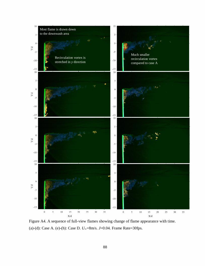
88



X/d X/d

Most flame is drawn down

to the downwash area

Recirculation vortex is

stretched in y direction

Much smaller

recirculation vortex

compared to case A

89



X/d X/d

Larger recirculation

vortex

Size of recirculation

vortex is reduced

Distinction of yellow

flame tail

90

Appendix B

Determine a cutoff pixel value to get mean flame images

As discussed in Section 3.5, images taken for flames have three color channels (RGB): red,

green, and blue. The color digital camera outputs 8 bits of each of red, green, and blue data

for each pixel that has 256 light intensity, ranging from 0 to 255. Each color image is firstly

converted to the grayscale image, which also has pixel intensity from 0 to 255. Figure B1

shows the derivative of image histogram. The image histogram is the graph representing the

number of pixels (y-axis) versus pixel intensity (x-axis). It is noted that each image has a total

pixel number of 1920 × 1200. As discussed in Section 4.3, two cutoff values (marked in

Figure B1) of pixel intensity were selected based on different purposes. The lower cutoff

intensity represents the contents of both flame and the shear layer as well as part of

background. At the higher cutoff intensity, the background is entirely filtered out but a part of

the shear layer is also removed. Figure B2 shows the two images with lower and higher cutoff

intensity values.

Figure B1. Derivative of image histogram.

Lower cutoff intensity at which the

magnitude of derivative of pixel

number does not change significantly.

Higher cutoff intensity at which the

magnitude of derivative of pixel

number is lower than 500.

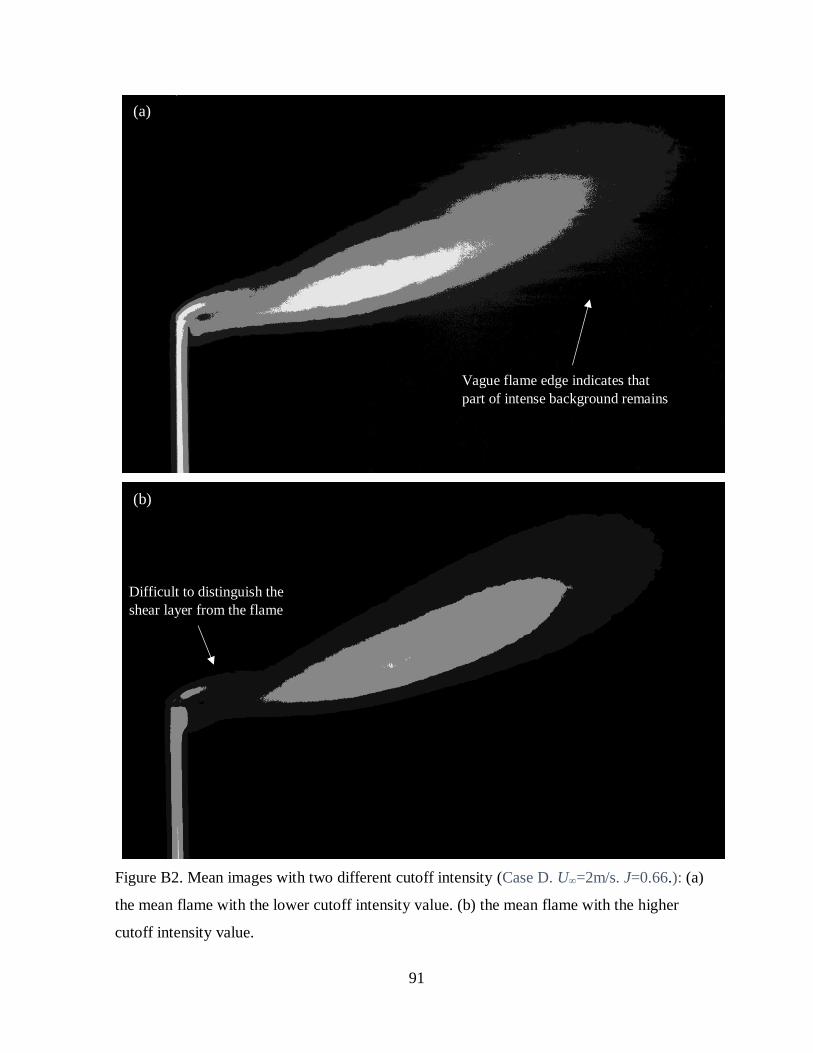
91

Figure B2. Mean images with two different cutoff intensity (Case D. U∞=2m/s. J=0.66.): (a)

the mean flame with the lower cutoff intensity value. (b) the mean flame with the higher

cutoff intensity value.

Difficult to distinguish the

shear layer from the flame

Vague flame edge indicates that

part of intense background remains

(b)

(a)

92

Curriculum Vitae

Name Diya Cui

Post-secondary

Education and

Degrees

University of Manitoba

Winnipeg, Manitoba, Canada

2014-2018, BSc

University of Western Ontario

London, Ontario, Canada

2018-2021, MESc

Honors and

Awards

University of Manitoba Faculty of Engineering Dean’s Honor List

2014-2018

University of Manitoba Undergraduate Research Awards

2016, 2017

Undergraduate Research Awards (NSERC)

2018

Western Graduate Research Scholarship

2018-2021

Related Work

Experience

Research Assistance

University of Western Ontario

2018-2021

Teaching Assistance

The University of Western Ontario

2019-2020

Effects of Crossflow Turbulence - Scholarship@Western

Documents

Transcript of Effects of Crossflow Turbulence - Scholarship@Western