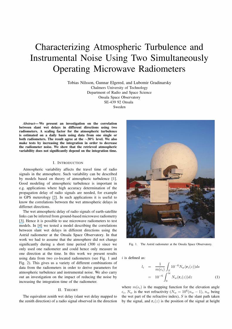
Characterizing Atmospheric Turbulence andInstrumental Noise Using Two Simultaneously

Operating Microwave RadiometersTobias Nilsson, Gunnar Elgered, and Lubomir Gradinarsky

Chalmers University of TechnologyDepartment of Radio and Space Science

Onsala Space ObservatorySE-439 92 Onsala

Sweden

Abstract— We present an investigation on the correlationbetween slant wet delays in different directions using tworadiometers. A scaling factor for the atmospheric turbulenceis estimated on a daily basis using data from one single orboth radiometers. The result agree at the ∼30% level. We alsomake tests by increasing the integration in order to decreasethe radiometer noise. We show that the retrieved atmosphericvariability does not significantly depend on the integration time.

I. INTRODUCTION

Atmospheric variability affects the travel time of radiosignals in the atmosphere. Such variability can be describedby models based on theory of atmospheric turbulence [1].Good modeling of atmospheric turbulence is important ine.g. applications where high accuracy determination of thepropagation delay of radio signals are needed, for examplein GPS meterology [2]. In such applications it is useful toknow the correlations between the wet atmospheric delays indiffernet directions.

The wet atmospheric delay of radio signals of earth-satellitelinks can be inferred from ground-based microwave radiometry[3]. Hence it is possible to use microwave radiometers to testmodels. In [4] we tested a model describing the correlationsbetween slant wet delays in different directions using theAstrid radiometer at the Onsala Space Observatory. In thatwork we had to assume that the atmosphere did not changesignificantly during a short time period (300 s) since weonly used one radiometer and could hence only measure inone direction at the time. In this work we present resultsusing data from two co-located radiometers (see Fig. 1 andFig. 2). This gives us a variety of different combinations ofdata from the radiometers in order to derive parameters foratmospheric turbulence and instrumental noise. We also carryout an investigation on the impact of reducing the noise byincreasing the integration time of the radiometer.

II. THEORY

The equivalent zenith wet delay (slant wet delay mapped tothe zenith direction) of a radio signal observed in the direction

Fig. 1. The Astrid radiometer at the Onsala Space Observatory.

i is defined as:

li =1

m(εi)

∫

S

10−6Nw(ri(z))ds

= 10−6

∫ ∞

0

Nw(ri(z))dz (1)

where m(εi) is the mapping function for the elevation angleεi, Nw is the wet refractivity (Nw = 106(nw − 1), nw beingthe wet part of the refractive index), S is the slant path takenby the signal, and ri(z) is the position of the signal at height

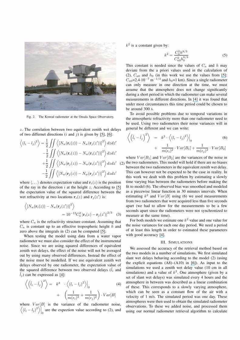
Fig. 2. The Konrad radiometer at the Onsala Space Observatory.

z. The correlation between two equivalent zenith wet delaysof two differnet directions (i and j) is given by [5], [6]:⟨

(li − lj)2⟩

=1

2

∫∫ ⟨[Nw(ri(z))−Nw(rj(z

′))]2⟩dzdz′

−1

2

∫∫ ⟨[Nw(ri(z))−Nw(ri(z

′))]2⟩dzdz′

+1

2

∫∫ ⟨[Nw(rj(z))−Nw(ri(z

′))]2⟩dzdz′ (2)

−1

2

∫∫ ⟨[Nw(rj(z))−Nw(rj(z

′))]2⟩dzdz′

where 〈. . . 〉 denotes expectation value and ri(z) is the positionof the ray in the direction i at the height z. According to [5]the expectation value of the squared difference between thewet refractivity at two locations ri(z) and rj(z

′) is:⟨

[Nw(ri(z))−Nw(rj(z′))]

2⟩

= 10−12C2n |ri(z)− rj(z

′)|2/3 (3)

where Cn is the refractivity structure constant. Assuming thatCn is constant up to an effective tropospheric height h andzero above the integrals in (2) can be computed [5].

When testing the model using data from a water vaporradiometer we must also consider the effect of the instrumentalnoise. Since we are using squared differences of equivalentzenith wet delays, the effect of the noise will not be averagedout by using many observed differences. Instead the effect ofthe noise must be modelled. If we use equivalent zenith wetdelays observed by one radiometer, the expectation value ofthe squared difference between two observed delays (li andlj) can be expressed as [4]:⟨(

li − lj)2⟩

= k2 ·⟨

(li − lj)2⟩∣∣∣

0(4)

+

(1

m(εi)2+

1

m(εj)2

)· V ar[B]

where V ar[B] is the variance of the radiometer noise,⟨(li − lj)2

⟩∣∣∣0

are the expection value according to (2), and

k2 is a constant given by:

k2 =C2nh

8/3

C2n0h

8/30

(5)

This constant is needed since the values of Cn and h maydeviate from the a priori values used in the calculation of(2), Cn0 and h0 (in this work we use the values from [5]:Cn0=2.4·10−7 m−1/3 and h0=1 km). Since a single radiometercan only measure in one direction at the time, we mustassume that the atmosphere does not change significantlyduring a short period in which the radiometer can make severalmeasurements in different directions. In [4] it was found thatunder most circumstances this time period could be chosen tobe around 300 s.

To avoid possible problems due to temporal variations inthe atmospheric refractivity more than one radiometer need tobe used. Using two radiometers their noise variances will ingeneral be different and we can write:⟨(

li − lj)2⟩

= k2 ·⟨

(li − lj)2⟩∣∣∣

0(6)

+1

m(εi)2· V ar[B1] +

1

m(εj)2· V ar[B2]

where V ar[B1] and V ar[B2] are the variances of the noise inthe two radiometers. This model will hold if there are no biasesbetween the two radiometers in the equivalent zenith wet delay.This can however not be expected to be the case in reality. Inthis work we dealt with this problem by estimating a slowlytime varying bias between the radiometers before making thefit to model (6). The observed bias was smoothed and modeledas a piecewise linear function in 30 minutes intervals. Whenestimating k2 and V ar[B] using (6) we used measurementsfrom two radiometers that were acquired less than five secondsapart (we had to allow for the measurements to be a fewseconds apart since the radiometers were not synchronized tomeasure at the same time).

For both models we estimate one k2 value and one value forthe noise variances for each one day period. We need a periodof at least this length in order to estimated these parameterswith good accuracy [4].

III. SIMULATIONS

We assessed the accuracy of the retrieval method based onthe two models in a number of simulations. We first simulatedslant wet delays behaving according to the model (2) (usingthe explicit equations (A8)–(A10) in [6]). As input to thesimulations we used a zenith wet delay value (10 cm in allsimulations) and a value of k2. One atmosphere (given by aset of slant wet delays) was simulated every 4 hours and theatmosphere in between was described as a linear combinationof these. This corresponds to a slowly varying atmosphere,which can be seen as a constant flow of the air with avelocity of 1 m/s. The simulated period was one day. Theseatmospheres were then used to obtain the simulated radiometerobservations. To these we added noise, and processed themusing our normal radiometer retrieval algorithm to calculate

0 2 4 6 8 10 120

5

10

15

20

k2

Ret

. k2

0 2 4 6 8 10 120

0.1

0.2

0.3

k2

Ret

. Var

[B] c

m2

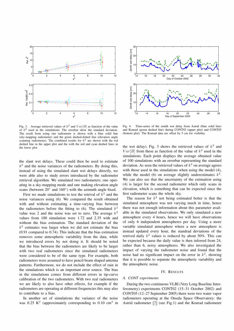
Fig. 3. Average retrieved values of k2 and V ar[B] as function of the valueof k2 used in the simulations. The errorbar show the standard deviation.The result from using one radiometer is shown with a blue solid line(sky-mapping radiometer) and the green dashed-dotted line (elevation anglescanning radiometer). The combined results for k2 are shown with the reddashed line in the upper plot and the with the red and cyan dashed lines inthe lower plot.

the slant wet delays. These could then be used to estimatek2 and the noise variances of the radiometers. By doing this,instead of using the simulated slant wet delays directly, wewere able also to study errors introduced by the radiometerretrieval algorithm. We simulated two radiometers; one oper-ating in a sky-mapping mode and one making elevation anglescans (between 20◦ and 160◦) with the azimuth angle fixed.

First we made simulations to test the retrival of k2 and thenoise variances using (6). We compared the result obtainedwith and without estimating a time-varying bias betweenthe radiometers before the fitting to (6). The simulated k2

value was 2 and the noise was set to zero. The average k2

values from 100 simulation were 1.72 and 2.35 with andwithout the bias estimation. The standard deviation of thek2 estimates was larger when we did not estimate the bias(0.91 compared to 0.74). This indicate that the bias estimationremoves some atmospheric variability from the data, whilewe introduced errors by not doing it. It should be notedthat the bias between the radiometers are likely to be largerwith two real radiometers since the simulated radiometerswere considered to be of the same type. For example, bothradiometers were assumed to have pencil beam shaped antennapatterns. Furthermore, we do not include the effect of rain inthe simulations which is an important error source. The biasin the simulations comes from different errors in tip-curvecalibration of the two radiometers. With two real radiometerswe are likely to also have other effects, for example if theradiometers are operating at different frequencies this may alsoto contribute to a bias.

In another set of simulations the variance of the noisewas 0.25 K2 (approximately corresponding to 0.10 cm2 in

14 16 18 20 22 24 26 28 30 320

10

20

30

Day of October 2002

Zeni

th w

et d

elay

[cm

]

12 14 16 18 20 22 24 26 280

10

20

30

Day of September 2005

Zeni

th w

et d

elay

[cm

]

Fig. 4. Time-series of the zenith wet delay from Astrid (blue solid line)and Konrad (green dashed line) during CONT02 (upper plot) and CONT05(bottom plot). The Konrad data are offset by 5 cm for visibility.

the wet delay). Fig. 3 shows the retrieved values of k2 andV ar[B] from these as function of the value of k2 used in thesimulations. Each point displays the average obtained valueof 100 simulations with an errorbar representing the standarddeviation. As seen the retrieved values of k2 on average agreeswith those used in the simulations when using the model (4),while the model (6) on average slightly underestimates k2.We can also see that the uncertainty of the estimation using(4) is larger for the second radiometer which only scans inelevation, which is something that can be expected since thefirst radiometer scans the whole sky.

The reason for k2 not being estimated better is that thesimulated atmosphere was not varying much in time, hencethere was not enough information about this parameter avail-able in the simulated observations. We only simulated a newatmosphere every 4 hours, hence we will have observationsof only 6 independent atmospheres per day. Using a morevariable simulated atmosphere where a new atmosphere isinstead updated every hour, the standrad deviations of theretrived daily k2 values is reduced by about 50%. This canbe expected because the daily value is then inferred from 24,rather than 6, noisy atmospheres. We also investigated theimpact of varying the radiometer noise and found that thenoise had no significant impact on the error in k2, showingthat it is possible to separate the atmospheric variability andthe atmospheric noise.

IV. RESULTS

A. CONT experiments

During the two continuous VLBI (Very Long Baseline Inter-ferometry) experiments CONT02 (15–31 October 2002) andCONT05 (12–27 September 2005) there were two water vaporradiometers operating at the Onsala Space Observatory: theAstrid radiometer [7] (see Fig.1) and the Konrad radiometer

14 16 18 20 22 24 26 28 30 32−5

0

5

Bia

s K

onra

d −

Ast

rid [c

m]

Day of September 2005

12 14 16 18 20 22 24 26 28−5

0

5

Bia

s K

onra

d −

Ast

rid [c

m]

Day of September 2005

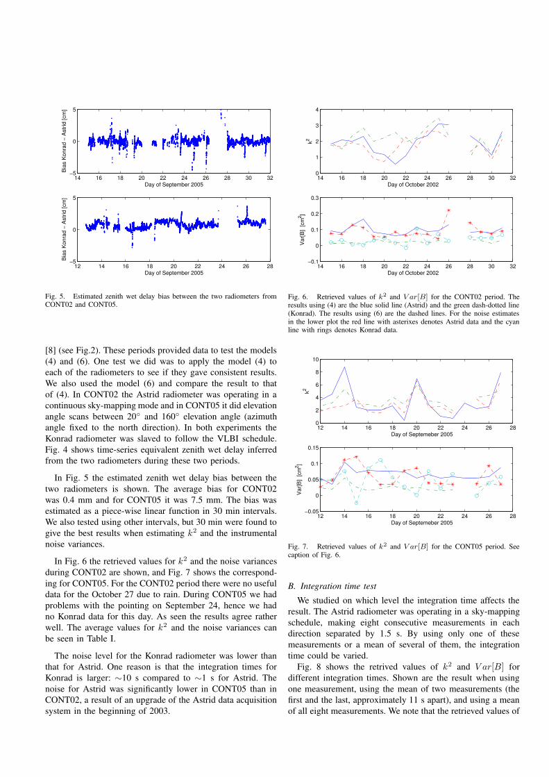
Fig. 5. Estimated zenith wet delay bias between the two radiometers fromCONT02 and CONT05.

[8] (see Fig.2). These periods provided data to test the models(4) and (6). One test we did was to apply the model (4) toeach of the radiometers to see if they gave consistent results.We also used the model (6) and compare the result to thatof (4). In CONT02 the Astrid radiometer was operating in acontinuous sky-mapping mode and in CONT05 it did elevationangle scans between 20◦ and 160◦ elevation angle (azimuthangle fixed to the north direction). In both experiments theKonrad radiometer was slaved to follow the VLBI schedule.Fig. 4 shows time-series equivalent zenith wet delay inferredfrom the two radiometers during these two periods.

In Fig. 5 the estimated zenith wet delay bias between thetwo radiometers is shown. The average bias for CONT02was 0.4 mm and for CONT05 it was 7.5 mm. The bias wasestimated as a piece-wise linear function in 30 min intervals.We also tested using other intervals, but 30 min were found togive the best results when estimating k2 and the instrumentalnoise variances.

In Fig. 6 the retrieved values for k2 and the noise variancesduring CONT02 are shown, and Fig. 7 shows the correspond-ing for CONT05. For the CONT02 period there were no usefuldata for the October 27 due to rain. During CONT05 we hadproblems with the pointing on September 24, hence we hadno Konrad data for this day. As seen the results agree ratherwell. The average values for k2 and the noise variances canbe seen in Table I.

The noise level for the Konrad radiometer was lower thanthat for Astrid. One reason is that the integration times forKonrad is larger: ∼10 s compared to ∼1 s for Astrid. Thenoise for Astrid was significantly lower in CONT05 than inCONT02, a result of an upgrade of the Astrid data acquisitionsystem in the beginning of 2003.

14 16 18 20 22 24 26 28 30 320

1

2

3

4

k2

Day of October 2002

14 16 18 20 22 24 26 28 30 32−0.1

0

0.1

0.2

0.3

Var

[B]

[cm

2 ]

Day of October 2002

Fig. 6. Retrieved values of k2 and V ar[B] for the CONT02 period. Theresults using (4) are the blue solid line (Astrid) and the green dash-dotted line(Konrad). The results using (6) are the dashed lines. For the noise estimatesin the lower plot the red line with asterixes denotes Astrid data and the cyanline with rings denotes Konrad data.

12 14 16 18 20 22 24 26 280

2

4

6

8

10

k2

Day of Septemeber 2005

12 14 16 18 20 22 24 26 28−0.05

0

0.05

0.1

0.15

Var

[B]

[cm

2 ]

Day of Septemeber 2005

Fig. 7. Retrieved values of k2 and V ar[B] for the CONT05 period. Seecaption of Fig. 6.

B. Integration time test

We studied on which level the integration time affects theresult. The Astrid radiometer was operating in a sky-mappingschedule, making eight consecutive measurements in eachdirection separated by 1.5 s. By using only one of thesemeasurements or a mean of several of them, the integrationtime could be varied.

Fig. 8 shows the retrived values of k2 and V ar[B] fordifferent integration times. Shown are the result when usingone measurement, using the mean of two measurements (thefirst and the last, approximately 11 s apart), and using a meanof all eight measurements. We note that the retrieved values of

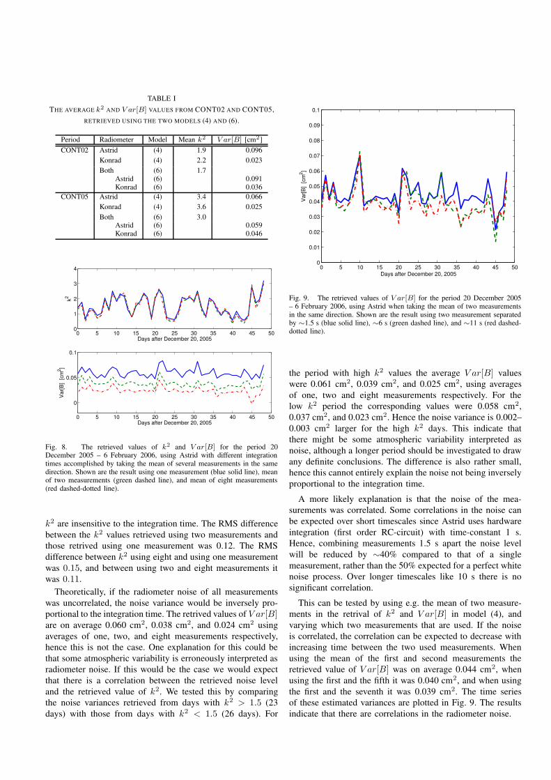
TABLE ITHE AVERAGE k2 AND V ar[B] VALUES FROM CONT02 AND CONT05,

RETRIEVED USING THE TWO MODELS (4) AND (6).

Period Radiometer Model Mean k2 V ar[B] [cm2]CONT02 Astrid (4) 1.9 0.096

Konrad (4) 2.2 0.023Both (6) 1.7

Astrid (6) 0.091Konrad (6) 0.036

CONT05 Astrid (4) 3.4 0.066Konrad (4) 3.6 0.025Both (6) 3.0

Astrid (6) 0.059Konrad (6) 0.046

0 5 10 15 20 25 30 35 40 45 500

1

2

3

4

Days after December 20, 2005

k2

0 5 10 15 20 25 30 35 40 45 50

0

0.05

0.1

Var

[B]

[cm

2 ]

Days after December 20, 2005

Fig. 8. The retrieved values of k2 and V ar[B] for the period 20December 2005 – 6 February 2006, using Astrid with different integrationtimes accomplished by taking the mean of several measurements in the samedirection. Shown are the result using one measurement (blue solid line), meanof two measurements (green dashed line), and mean of eight measurements(red dashed-dotted line).

k2 are insensitive to the integration time. The RMS differencebetween the k2 values retrieved using two measurements andthose retrived using one measurement was 0.12. The RMSdifference between k2 using eight and using one measurementwas 0.15, and between using two and eight measurements itwas 0.11.

Theoretically, if the radiometer noise of all measurementswas uncorrelated, the noise variance would be inversely pro-portional to the integration time. The retrived values of V ar[B]are on average 0.060 cm2, 0.038 cm2, and 0.024 cm2 usingaverages of one, two, and eight measurements respectively,hence this is not the case. One explanation for this could bethat some atmospheric variability is erroneously interpreted asradiometer noise. If this would be the case we would expectthat there is a correlation between the retrieved noise leveland the retrieved value of k2. We tested this by comparingthe noise variances retrieved from days with k2 > 1.5 (23days) with those from days with k2 < 1.5 (26 days). For

0 5 10 15 20 25 30 35 40 45 500

0.01

0.02

0.03

0.04

0.05

0.06

0.07

0.08

0.09

0.1

Var

[B]

[cm

2 ]

Days after December 20, 2005

Fig. 9. The retrieved values of V ar[B] for the period 20 December 2005– 6 February 2006, using Astrid when taking the mean of two measurementsin the same direction. Shown are the result using two measurement separatedby ∼1.5 s (blue solid line), ∼6 s (green dashed line), and ∼11 s (red dashed-dotted line).

the period with high k2 values the average V ar[B] valueswere 0.061 cm2, 0.039 cm2, and 0.025 cm2, using averagesof one, two and eight measurements respectively. For thelow k2 period the corresponding values were 0.058 cm2,0.037 cm2, and 0.023 cm2. Hence the noise variance is 0.002–0.003 cm2 larger for the high k2 days. This indicate thatthere might be some atmospheric variability interpreted asnoise, although a longer period should be investigated to drawany definite conclusions. The difference is also rather small,hence this cannot entirely explain the noise not being inverselyproportional to the integration time.

A more likely explanation is that the noise of the mea-surements was correlated. Some correlations in the noise canbe expected over short timescales since Astrid uses hardwareintegration (first order RC-circuit) with time-constant 1 s.Hence, combining measurements 1.5 s apart the noise levelwill be reduced by ∼40% compared to that of a singlemeasurement, rather than the 50% expected for a perfect whitenoise process. Over longer timescales like 10 s there is nosignificant correlation.

This can be tested by using e.g. the mean of two measure-ments in the retrival of k2 and V ar[B] in model (4), andvarying which two measurements that are used. If the noiseis correlated, the correlation can be expected to decrease withincreasing time between the two used measurements. Whenusing the mean of the first and second measurements theretrieved value of V ar[B] was on average 0.044 cm2, whenusing the first and the fifth it was 0.040 cm2, and when usingthe first and the seventh it was 0.039 cm2. The time seriesof these estimated variances are plotted in Fig. 9. The resultsindicate that there are correlations in the radiometer noise.

V. CONCLUSIONS

The results from the two CONT experiments agree ratherwell in general. The observed difference between the retrivedvalues of k2 is at the level which can be expected fromthe simulation results. The agreement between the k2 valuesretrieved using one radiometer in model (4) as in [4] and usingtwo radiometers and model (6) indicates that the method usingonly one radiometer and assuming no significant variations intime on timescales <300 s works well.

As seen the noise variances retrived using (4) were ratherconstant during respective period. The noise for Astrid waslower during CONT05 than during CONT02, which wasexpected due to an upgrade of the radiometer in 2003. Thisagrees well with the result in [4]. The noise variances retrievedusing (6) varies much more, especially those from CONT05.This can be expected from the simulation results which showthat the uncertainty of the noise retrieved using this model arelarger than the noise retrieved using (4), especially when k2

is large (note that k2 is larger in CONT05 than in CONT02).There are some days where the results are not consistent. Onereason for the disagreement on 20–21 October 2002 may bethat much of the data on this day were not usable due torain. Hence the results for these days are based on less datathan for other days and can be expected to be more uncertain.Another explanation is that Konrad was slaved to the VLBIschedule and this may not be an optimum schedule to obtaindata to be used to investigate correlations between slant wetdelays in different directions. In CONT05 the Astrid did onlydo elevation angle scans, hence did not map the whole sky asin CONT02. This is likely to have degraded the results andmay be one explanation for the noise during CONT05 retrivedby model (6) being more variable. Instrumental differencesbetween the two radiometers are likely impact the results. Forexample the two radiometers have different beamwidths (6◦

for Astrid and 3◦ for Konrad) and this can be exected to affectthe result at some level.

The investigation regarding the integration time shows thatthe value of k2 estimated using (4) is relatively independent ofthe integration time. Hence an increase of the integration timeto at least ∼10 s (and hence decrease the noise) will not leadto any significant loss of information about the atmosphere interms of the model parameters estimated in this work.

ACKNOWLEDGMENT

We are grateful to Carsten Rieck for his help getting theKonrad radiometer operating during the CONT05 experiment.This work was supported by the Swedish National SpaceBoard.

REFERENCES

[1] V. I. Tatarskii, The Effects of the Turbulent Atmosphere on Wave Propa-gation. Jerusalem: Israel Program for Scientific Translations, 1971.

[2] P. Fang, M. Bevis, Y. Bock, S. Gutman, and D. Wolfe, “GPS meteorology:Reducing systematic errors in geodetic estimates for zenith delay,”Geophys. Res. Lett., vol. 25, pp. 3583–3586, 1998.

[3] G. Elgered, “Tropospheric radio-path delay from ground-based mi-crowave radiometry,” in Atmospheric Remote Sensing by MicrowaveRadiometry, M. Janssen, Ed. John Wiley & Sons, 1993, pp. 215–258.

[4] T. Nilsson, L. Gradinarsky, and G. Elgered, “Correlations between slantwet delays measured by microwave radiometry,” IEEE Trans. Geosci.Remote Sensing, vol. 43, pp. 1028–1035, 2005.

[5] R. N. Treuhaft and G. E. Lanyi, “The effect of the dynamic wet tropo-sphere on radio interferometric measurements,” Radio Science, vol. 22,pp. 251–265, 1987.

[6] T. R. Emardson and P. O. J. Jarlemark, “Atmospheric modelling in GPSanalysis and its effect on the estimated geodetic parameters,” Journal ofGeodesy, vol. 73, p. 322, 1999.

[7] G. Elgered and P. O. J. Jarlemark, “Ground-based microwave radiometryand long term observations of atmospheric water vapor,” Radio Sci.,vol. 33, no. 3, pp. 707–717, 1998, 98RS00488.

[8] B. Stoew and C. Rieck, “Dual channel water vapour radiometer develop-ment,” in Proceedings of the 13th Working Meeting on European VLBIfor Geodesy and Astrometry, W. Schluter and H. Hase, Eds., Bundesamtfur Kartographie und Geodasie., Wettzell, 1999.