Optical Spectroscopy with Very Large Telescope:

Instrumental Development and Data InterpretationThe case of the Rocky-Planets Finder ESPRESSO and Spectral

Characterization of BL Lac Objects

Marco Landoni

Department of Mathematics and Physics

University of Insubria - Como

A thesis submitted for the degree of

Doctor of Philosophy in Astronomy and Astrophysics

26th November 2013

Supervisor: Dr. Filippo M. Zerbi

co-Supervisors: Prof. Aldo Treves

Prof. Renato Falomo

The sudden liberation of our thinking on the very structure of the physical world

was overwhelming

Chien-Shiung Wu on 60Co β-decay P violation experiment.

ii

Abstract

This PhD thesis is focused on one of the main research area in mod-

ern Astrophysics: the spectroscopy. Within the current framework of

observational astronomy, I carried out the Thesis aiming at the fig-

ure of Instrument Scientist who acts as a junction between astronomer

and design engineers joining the science and technology in order to

contribute to a more consolidated and optimised design of new instru-

mentations for large experiments.

For this reason, in this Thesis I will present two main parts of my PhD

activities that have characterised my entire doctoral training. In par-

ticular, I will first introduce ESPRESSO, the Echelle SPectrograph for

Rocky Exoplanet and Stable Spectroscopic Observations, which will be

a new generation extra stable spectrograph at the European Southern

Observatory (ESO) Very Large Telescope (VLT). ESPRESSO will be a

spectrograph mainly optimised for finding rocky planet orbiting main

sequence G stars in the habitable zone through the Radial Velocity

(RV) method. I will outline my contribution to ESPRESSO in Chap-

ter 2 where I illustrate simulations on the expected performances of

the detectors used by a main part of the instrument: the Front End

Unit. This subsystem is responsible to stabilise the field and pupil of

ESPRESSO through active optics and to collect the light from the four

telescope and inject it through fiber feeding the spectrograph. I also

outline the design of the Exposure Meter of the instrument which is

in charge to continuously monitoring the exposure in order to evaluate

a critical value, called Mean Time of Exposure (MTE), which is used

in order to correct the measured Radial Velocity for the relative Earth

motion at the time of observation. For the first time, the exposure will

be monitored chromatically allowing a better characterisation of the

behaviour of the MTE and of the overall observation simultaneously.

In Chapter 3 I focus on pure astrophysical research based on spec-

troscopy of a particular class of Active Galatic Nuclei: the BL Lacertae

Objects. These objects are characterised by a strong non-thermal emis-

sion which arises from the accreting nucleus. For this reason, spectral

features (when present) are extremely diluted making the determina-

tion of their redshifts a challenging task. With the adoption of FORS2

spectrograph, in low resolution, at 10mt class VLT I completed a survey

of these objects started few years ago and I derived from the complete

sample a conspicuous number of properties of the class, including the

characterisation of their line-of-sight Mg II absorber systems. More-

over, I will outline the results obtained from observation of a small sub-

sample of strong FERMI γ-rays (and in certain cases VHE emitters)

source with ESO X-SHOOTER which combines medium resolution (R

∼ 4000) and large spectral range. In particular, for the source PKS

0048-097 the determination of its redshift for the first time allowed to

deeply investigate its Spectral Energy Distribution and the close envi-

ronment of the object. The spectra of the other sources in the sample

are also illustrated and explicated for particular interesting objects.

Contents

Contents v

List of Figures ix

Nomenclature xviii

1 Introduction 1

2 ESPRESSO: the Echelle SPectrograph for Rocky Exoplanet and

Stable Spectroscopic Observations. Design of the Front End and

Exposure Meter subsystems 5

2.1 Introduction . . . . . . . . . . . . . . . . . . . . . . . . . . . . . . . 5

2.1.1 Exoplanets detection main techniques: Transit and Radial

Velocity methods . . . . . . . . . . . . . . . . . . . . . . . . 6

2.1.1.1 An example of planet detection through radial ve-

locity method. . . . . . . . . . . . . . . . . . . . . 10

2.1.2 ESPRESSO: a general overview of the instrument . . . . . . 12

2.1.2.1 Design concept . . . . . . . . . . . . . . . . . . . . 12

2.1.2.2 Wavelength calibration . . . . . . . . . . . . . . . . 14

2.1.2.3 Coude train and Front End subsystem - feeding the

spectrograph with scientific lights . . . . . . . . . . 14

2.1.2.4 Foreseen ESPRESSO mode . . . . . . . . . . . . . 15

2.1.2.5 A scientific Pandora box . . . . . . . . . . . . . . . 17

2.2 State of the art at Paranal: Test campaign activities and data analysis 19

2.2.1 Introduction . . . . . . . . . . . . . . . . . . . . . . . . . . . 19

v

CONTENTS

2.2.2 Setup configuration @VLT . . . . . . . . . . . . . . . . . . . 20

2.2.2.1 Temperature and wind measurement setup . . . . . 20

2.2.2.2 PSF and image stability through the tunnels . . . . 22

2.2.3 Data analysys . . . . . . . . . . . . . . . . . . . . . . . . . . 24

2.2.3.1 PSF model . . . . . . . . . . . . . . . . . . . . . . 24

2.2.4 Results . . . . . . . . . . . . . . . . . . . . . . . . . . . . . . 27

2.2.4.1 Image quality and relationship with Paranal envi-

ronment . . . . . . . . . . . . . . . . . . . . . . . . 28

2.2.5 Conclusions . . . . . . . . . . . . . . . . . . . . . . . . . . . 33

2.3 Front-End Subsystem: stabilisation of the field . . . . . . . . . . . . 34

2.3.1 Introduction . . . . . . . . . . . . . . . . . . . . . . . . . . . 34

2.3.2 CCD detector simulation and radiometry . . . . . . . . . . . 35

2.3.2.1 Determination of optical parameters . . . . . . . . 37

2.3.3 Radiometric quantities . . . . . . . . . . . . . . . . . . . . . 37

2.3.4 Pinhole slit simulation . . . . . . . . . . . . . . . . . . . . . 40

2.3.5 The algorithm architecture . . . . . . . . . . . . . . . . . . . 41

2.3.5.1 Phase (1) - CCD generation . . . . . . . . . . . . . 41

2.3.5.2 Phase (2) - Guiding algorithm . . . . . . . . . . . . 42

2.3.6 CCDs under evaluation . . . . . . . . . . . . . . . . . . . . . 43

2.3.6.1 Bright objects cases - Results . . . . . . . . . . . . 47

2.3.6.2 Faint object cases - Results . . . . . . . . . . . . . 49

2.3.6.3 Parametric evaluation for faint object guiding . . . 52

2.4 Design of the Exposure Meter subsystem . . . . . . . . . . . . . . . 58

2.4.1 General Introduction . . . . . . . . . . . . . . . . . . . . . . 58

2.4.2 Simulations on the expected performances . . . . . . . . . . 61

2.4.2.1 Flux received and star model . . . . . . . . . . . . 65

2.4.2.2 Sky model . . . . . . . . . . . . . . . . . . . . . . . 66

2.4.2.3 dpdλ

dispersion function . . . . . . . . . . . . . . . . 66

2.4.2.4 PSF model of the Exposure Meter optics . . . . . . 67

2.4.2.5 Fiber image . . . . . . . . . . . . . . . . . . . . . . 67

2.4.2.6 Image on the focal plane . . . . . . . . . . . . . . . 69

2.4.2.7 Slit loss and dependence on seeing . . . . . . . . . 69

2.4.2.8 CCD configuration . . . . . . . . . . . . . . . . . . 70

vi

CONTENTS

2.4.2.9 Detector simulation for performances evaluation . . 70

2.4.3 Simulations results and expected performances . . . . . . . . 72

2.4.3.1 First scientific case - 10 cm s−1 RV accuracy . . . . 76

2.4.3.2 Second scientific case - 1 m s−1 RV accuracy . . . . 80

2.4.3.3 Third scientific case - 10 m s−1 RV accuracy . . . . 82

2.4.3.4 Multimode setup - An introduction to 5 m s−1 RV

accuracy case . . . . . . . . . . . . . . . . . . . . . 83

3 Application of spectroscopy to BL Lacertae objects: from low to

medium-high resolution. The case of FORS2 and X-Shooter 85

3.1 An introduction to AGN . . . . . . . . . . . . . . . . . . . . . . . . 85

3.1.1 What is an AGN ? . . . . . . . . . . . . . . . . . . . . . . . 85

3.1.2 Emission mechanism - Thermal emission from accretion disk,

broad line and narrow line regions . . . . . . . . . . . . . . . 88

3.1.2.1 Broad line region . . . . . . . . . . . . . . . . . . . 89

3.1.2.2 The narrow-line region . . . . . . . . . . . . . . . . 94

3.2 The case of BL Lacertae objects . . . . . . . . . . . . . . . . . . . . 96

3.2.1 Characteristic of the BL Lacs optical spectra . . . . . . . . . 97

3.3 Observing BL Lacs with FORS2@ESO-VLT. The completion of the

sample . . . . . . . . . . . . . . . . . . . . . . . . . . . . . . . . . . 98

3.3.1 Introduction . . . . . . . . . . . . . . . . . . . . . . . . . . . 98

3.3.2 The sample . . . . . . . . . . . . . . . . . . . . . . . . . . . 100

3.3.3 The complete BLL@FORS2 sample observed at FORS2-ESO

VLT . . . . . . . . . . . . . . . . . . . . . . . . . . . . . . . 103

3.3.4 Immediate results . . . . . . . . . . . . . . . . . . . . . . . . 108

3.3.4.1 The BL Lac mean spectrum . . . . . . . . . . . . . 125

3.3.5 The relativistic optical beaming factor δ . . . . . . . . . . . 127

3.3.6 Statistical properties of the whole sample . . . . . . . . . . . 131

3.3.7 Intervening Mg II system on BL Lac objects observed with

FORS2 . . . . . . . . . . . . . . . . . . . . . . . . . . . . . . 132

3.4 Medium resolution spectroscopy of bright BL Lac objects with ESO-

XSHOOTER . . . . . . . . . . . . . . . . . . . . . . . . . . . . . . 134

3.4.1 Introduction . . . . . . . . . . . . . . . . . . . . . . . . . . . 134

vii

CONTENTS

3.4.2 The sample, observation and data reduction . . . . . . . . . 135

3.4.3 The case of FERMI γ-ray BL Lac PKS 0048-097 observed

with XSHOOTER . . . . . . . . . . . . . . . . . . . . . . . 136

3.4.3.1 Introduction . . . . . . . . . . . . . . . . . . . . . 136

3.4.3.2 Spectral analysys . . . . . . . . . . . . . . . . . . . 138

3.4.3.3 Intervening MgII and PKS 0048-097 close environ-

ment . . . . . . . . . . . . . . . . . . . . . . . . . . 141

3.4.3.4 Spectral Energy Distribution of PKS 0048-097 . . . 143

3.4.4 Other objects observed. Preliminary results . . . . . . . . . 145

3.4.4.1 Introduction . . . . . . . . . . . . . . . . . . . . . 145

3.4.4.2 The spectra and basic properties . . . . . . . . . . 145

3.4.4.3 The peculiar case of MH 2136-428 . . . . . . . . . 159

3.5 Future perspective. Spectroscopy of BL Lacs in the E-ELT era . . . 164

3.5.1 Introduction . . . . . . . . . . . . . . . . . . . . . . . . . . . 164

3.5.2 Simulation of BL Lac spectra observed by E-ELT . . . . . . 164

4 ESPRESSO: Foreseen science and outlook 169

5 Conclusions 173

Appendix A - List of publication 175

References 185

viii

List of Figures

2.1 Transit of a planet detected on the host star [Ribas et al., 2008]. . . 6

2.2 Pictorial representation of the transit method. . . . . . . . . . . . . 7

2.3 Pictorial representation of a planet around a pulsar detected with

the Pulsar Timing technique. . . . . . . . . . . . . . . . . . . . . . 8

2.4 An example of radial velocity plot versus time obtained after an ob-

servation campaign on the host star (freely taken from en.wikipedia.org

Doppler Spectroscopy). . . . . . . . . . . . . . . . . . . . . . . . . . 9

2.5 Radial velocity and planet mass limit detection as a function of

distance from G2V solar like host star. Pepe et al 2013 in press. . . 12

2.6 Sketch of the ESPRESSO spectrograph optical layout [Spano et al.,

2012] . . . . . . . . . . . . . . . . . . . . . . . . . . . . . . . . . . . 13

2.7 Coude Train of ESPRESSO and optical path through the telescope

and the tunnels [Cabral et al., 2012]. . . . . . . . . . . . . . . . . . 15

2.8 Top view of the Front-End and the arrival of the four UT beam at

the CCL [Riva et al., 2012] . . . . . . . . . . . . . . . . . . . . . . . 16

2.9 All-sky spatial dipole with the combined VLT (squares) and Keck

(circles) α measurements from Webb et al. (2011). Triangles are

measures in common to the two telescopes. The blue dashed line

shows the equatorial region of the dipole. . . . . . . . . . . . . . . . 18

2.10 Configuration for the proposed environmental tests. . . . . . . . . . 20

2.11 Anemometer used for wind measurements. . . . . . . . . . . . . . . 21

2.12 Temperature data logger used for temperature measurements. . . . 21

2.13 Optical setup for the image quality measurement at the end side of

the delay tunnel. . . . . . . . . . . . . . . . . . . . . . . . . . . . . 24

ix

LIST OF FIGURES

2.14 An example of the PSF of the laser beam recorded by the camera.

Horizontal bars represent the area of interest for the full readout

while vertical bar is the preliminary computation of the centroid

performed by the onboard software of the camera. . . . . . . . . . . 25

2.15 An example of the PSF of the laser beam recorded by the camera af-

ter the application of gaussian PSF model. Courtesy: ESO Paranal

(Document ESO: VLT-TRE-ESP-13520) . . . . . . . . . . . . . . . 27

2.16 Image displacement acquired during the night between 12 and 13 of

July 2011. . . . . . . . . . . . . . . . . . . . . . . . . . . . . . . . . 28

2.17 Comparison between image displacement and temperatures behav-

ior. Wind line (solid blue) refers to the wind temperature at the

level of the anemometer. . . . . . . . . . . . . . . . . . . . . . . . . 30

2.18 Correlation between temperature and the wind speed. . . . . . . . . 30

2.19 Image displacement acquired during the night between 13 and 14 of

july 2011 (closed configuration) . . . . . . . . . . . . . . . . . . . . 31

2.20 Measured FWHM during the 12 to 13 night. Note that spikes are

due to non-convergence of the fitting algorithm on bad recorded

image. . . . . . . . . . . . . . . . . . . . . . . . . . . . . . . . . . . 32

2.21 Standard deviation of the Full Width at half maximum of the image

on 10 minutes wide bins . . . . . . . . . . . . . . . . . . . . . . . . 32

2.22 Measured FWHM during the 13 to 14 night in closed ducts config-

uration. Note that spikes are due to non-convergence of the fitting

algorithm on bad recorded image. . . . . . . . . . . . . . . . . . . . 33

2.23 Subsampling of the spot position. Red dots are experimental data

while the yellow ones are the subsample interpolation in order to

better characterise the behaviour of the image displacement on the

detector . . . . . . . . . . . . . . . . . . . . . . . . . . . . . . . . . 36

2.24 Quantum Efficiency of a sample of three different TCCD and ESPRESSO

System Efficiency (updated at Final Design Review (May 2013). . . 38

2.25 CCD Sony ICX285 detector Quantum Efficiency. This detector is

the baseline for the technical CCD for the ESPRESSo system. . . . 39

2.26 Simulation of a scientific object on the TCCD (no noises considered). 40

2.27 Scheme of the guiding algorithm . . . . . . . . . . . . . . . . . . . . 44

x

LIST OF FIGURES

2.28 Workflow of the guiding algorithm. Integration time is computed

according to the magnitude of the target and the neutral density

filter installed in front of the camera. For instance, table 2.5 gives

two general template cases. . . . . . . . . . . . . . . . . . . . . . . . 45

2.29 Experimental data recorded in Paranal during the observational

campaign in July 2011 . . . . . . . . . . . . . . . . . . . . . . . . . 46

2.30 Perturbations applied to all the configurations: X displacement

(top), Y displacement (middle), Seeing variation (Down). The units

of the displacement are linear and must be corrected recalling that

they are recorder with a F/10 camera. . . . . . . . . . . . . . . . . 46

2.31 Simulation results on guiding an object with mv ∼ 10. Third and

fourth panels show the residual left after the correction of the guid-

ing system . . . . . . . . . . . . . . . . . . . . . . . . . . . . . . . . 48

2.32 An example of a simulated Front End technical CCD observing

object with mv ∼ 10 for guiding. . . . . . . . . . . . . . . . . . . . . 49

2.33 Histrograms of the error during a simulation on guiding bright ob-

jects. Left upper panel - Histogram of the error as recorded on

Paranal on X axis. Right upper panel - Histogram of the error as

recorded in Paranal on Y axis. Lower panels represent error after

the application of the guiding algorithm . . . . . . . . . . . . . . . 50

2.34 Simulation results on guiding an object with mv = 20. . . . . . . . . 53

2.35 Histograms of the residuals during a simulation on guiding faint

objects. Panel legends are the same of Figure 2.33 . . . . . . . . . . 54

2.36 Pictorial representation of the position of the spot with respect to

the requirement (solid circle). . . . . . . . . . . . . . . . . . . . . . 55

2.37 Results of the guiding algorithm performances against detector dark

current magnification. The dark current in the legend is in units of

e- px−1 s−1. . . . . . . . . . . . . . . . . . . . . . . . . . . . . . . . 55

2.38 RMS error on positioning against detector dark current magnifica-

tion. The dark current in the legend is in units of e- px−1 s−1. . . . 56

2.39 Results of the guiding algorithm performances against QE degrada-

tion. . . . . . . . . . . . . . . . . . . . . . . . . . . . . . . . . . . . 56

2.40 RMS error on positioning against QE degradation. . . . . . . . . . . 57

xi

LIST OF FIGURES

2.41 ESPRESSO Exposure meter general overall schema. . . . . . . . . 62

2.42 ESPRESSO exposure meter 3D general view. . . . . . . . . . . . . . 63

2.43 ESPRESSO Exposure meter overall efficiency (this curve also con-

siders the whole efficiency of ESPRESSO and includes the Sony ICX

285 detector efficiency) . . . . . . . . . . . . . . . . . . . . . . . . 63

2.44 ESPRESSO Exposure meter light extraction schema. . . . . . . . . 64

2.45 ESPRESSO Exposure meter overall optical setup. . . . . . . . . . . 65

2.46 ESPRESSO Exposure meter ray tracing function. This function

allows to known the absolute position (in mm respect to the centre

of the CCD) of the image against λ with respect to the dispersion

axis. . . . . . . . . . . . . . . . . . . . . . . . . . . . . . . . . . . . 67

2.47 ESPRESSO Exposure meter PSF function against λ. . . . . . . . . 68

2.48 ESPRESSO Exposure meter PSF function against λ in a pictorial

representation. . . . . . . . . . . . . . . . . . . . . . . . . . . . . . 68

2.49 Seeing vs slit efficiency curve adopted for simulations of the Expo-

sure meter . . . . . . . . . . . . . . . . . . . . . . . . . . . . . . . . 70

2.50 Simulation of a spectrum obtained in the exposure meter for a M

star of mv = 15 assuming seeing of ∼ 1.00′′. . . . . . . . . . . . . . 73

2.51 Simulation for the exposure time vs magnitude in multiUT mode. . 74

2.52 Simulation for the exposure time vs magnitude in singleUT mode. . 74

2.53 Flow chart for the strategy adopted for the scientific simulation.

Each simulation is repeated 100 times in order to investigate general

statistical properties . . . . . . . . . . . . . . . . . . . . . . . . . . 75

2.54 ESPRESSO Exposure Meter channels . . . . . . . . . . . . . . . . . 75

2.55 Behavior of the perturbation as seen on the CCD aboard the Ex-

posure Meter . . . . . . . . . . . . . . . . . . . . . . . . . . . . . . 77

2.56 Behavior of the perturbation as seen on the CCD aboard the Ex-

posure Meter . . . . . . . . . . . . . . . . . . . . . . . . . . . . . . 78

2.57 ESPRESSO Exposure Meter performance for 10cm/s goal withmv =

10 with perturbations on the system or atmosphere . . . . . . . . . 78

2.58 ESPRESSO Exposure Meter performances against a chromatic per-

turbation on the red part (cloud passing through) . . . . . . . . . . 80

xii

LIST OF FIGURES

2.59 ESPRESSO Exposure Meter performance for 1m/s scientific goal.

No perturbations are applied to the system . . . . . . . . . . . . . . 81

2.60 ESPRESSO Exposure Meter performance for 1m/s scientific goal

with perturbations applied to the system . . . . . . . . . . . . . . . 81

2.61 ESPRESSO Exposure Meter performance for 10 m/s scientific goal

without perturbation . . . . . . . . . . . . . . . . . . . . . . . . . . 83

2.62 ESPRESSO Exposure Meter r.m.s. error on the three channel in

multi-UT configuration . . . . . . . . . . . . . . . . . . . . . . . . . 84

3.1 Effective potential of a test particle test with mass M in orbit around

a Schwarchild Black Hole. . . . . . . . . . . . . . . . . . . . . . . . 86

3.2 ISCO in function of the black hole spin a. . . . . . . . . . . . . . . 87

3.3 Spectral energy distribution of the radio quiet QSO Mkn586. The

UV bump due to thermal radiation generated by the accretion disk

is clearly visible in the region 1015 - 1015 Hz. . . . . . . . . . . . . . 88

3.4 Emission lines in the BLR superposed on different spectrum of QSOs

with different absolute luminosities. . . . . . . . . . . . . . . . . . . 90

3.5 Multiepoch spectrum of the QSO NGC1097 where double peaked

broad Hα is clearly spot. . . . . . . . . . . . . . . . . . . . . . . . . 91

3.6 Narrow line region line profile asymmetry. This structure suggests

flows of matter in the active nucleus [Lutz et al., 2000]. . . . . . . 94

3.7 Narrow line region line spectrum (NIR and FIR) example from the

AGN NGC1078 [Lutz et al., 2000]. . . . . . . . . . . . . . . . . . . 95

3.8 Optical spectrum of the BL Lac object (2214-313) in which the fea-

tures associated to its host galaxy are clearly detected (z = 0.460).

See Landoni et al 2013, Sbarufatti et al 2009. . . . . . . . . . . . . 99

3.9 Flux calibrated (upper panel) and normalized (lower panel) spec-

trum of 1553+113. The spectrum is lacking any intrinsic spectral

feature. Absorptions from our galaxy ISM are labeled in green. The

telluric absorption are marked. See Landoni et al 2013, Sbarufatti

et al 2009. . . . . . . . . . . . . . . . . . . . . . . . . . . . . . . . . 99

xiii

LIST OF FIGURES

3.10 Top panel: V-magnitude distribution of the observed BLLs in the

sample selected adopting the criteria described in the text. Bottom:

Fraction of objects of known redshift as a function of the magnitude.

Further details and references are reported in Sbarufatti et al. [2006]

and Landoni et al. [2013]. . . . . . . . . . . . . . . . . . . . . . . . 101

3.11 Spectra of BLLs sources. Top panel: flux calibrated spectra. Nor-

malized spectra on bottom. Telluric bands are indicated by ⊕,

spectral lines are marked by line identification, absorption features

from interstellar medium of our galaxy are labeled by ISM, diffuse

interstellar bands by DIB. The flux density is in units of 10−16 erg

cm−2 s−1 A−1. . . . . . . . . . . . . . . . . . . . . . . . . . . . . . 109

3.12 continued . . . . . . . . . . . . . . . . . . . . . . . . . . . . . . . . 110

3.13 continued . . . . . . . . . . . . . . . . . . . . . . . . . . . . . . . . 111

3.14 continued . . . . . . . . . . . . . . . . . . . . . . . . . . . . . . . . 112

3.15 continued . . . . . . . . . . . . . . . . . . . . . . . . . . . . . . . . 113

3.16 continued . . . . . . . . . . . . . . . . . . . . . . . . . . . . . . . . 114

3.17 continued . . . . . . . . . . . . . . . . . . . . . . . . . . . . . . . . 115

3.18 Spectra of QSOs or confirmed non-BLLs sources. Top panel: flux

calibrated spectra. Normalized spectra on bottom. Telluric bands

are indicated by ⊕, spectral lines are marked by line identification,

absorption features from interstellar medium of our galaxy are la-

beled by ISM, diffuse interstellar bands by DIB. The flux density is

in units of 10−16 erg cm−2 s−1 A−1. . . . . . . . . . . . . . . . . . . 116

3.19 continued . . . . . . . . . . . . . . . . . . . . . . . . . . . . . . . . 117

3.20 Spectral decomposition (rest frame) for the objects RBS 0337, MS

0622.5-5256, RX J1117.0+2014 and RBS 1899. The solid line shows

the fitted spectrum while dots is the observed one. . . . . . . . . . . 120

3.21 Mean spectrum of BL Lac objects obtained combining the 23 ob-

jects of our campaign in which intrinsic spectral features are de-

tected. The first panel reports the mean spectrum assuming for the

continuum a power-law with index α = 0.90 (which corresponds to

the mean spectral index of the whole BL Lac sample). In the second

panel normalised spectrum is shown. . . . . . . . . . . . . . . . . . 125

xiv

LIST OF FIGURES

3.22 Relation between the thermal disk continuum and MgII emission

line luminosity (see Decarli et al. [2011] for details). . . . . . . . . . 128

3.23 Optical beaming factor for the sources observed in the campaign.

Red dashed line indicates the lower limit value calculated through

Equation 3.27 assuming z = 0.70. Filled blue circle are the δ of

bona-fide BL Lac objects with Mg II emission line while the open

magenta circle are the beaming factor for other intermediate sources

(classified as confirmed non-BL Lacs). Dotted line delimit the area

of the EW-δ plane where the source are of intermediate nature be-

tween pure QSO(δ ∼ 1)and BL Lacs(δ >4). . . . . . . . . . . . . . 130

3.24 Incidence rate dNdz

of Mg II absorbers with 0.6 A < EW λ2796 <

1.0 A (top) and EW λ2796 > 1.0 A (bottom). Figure from [Zhu

and Menard, 2013]. . . . . . . . . . . . . . . . . . . . . . . . . . . . 133

3.25 ESO XSHOOTER data reduction pipeline workflow schema (cour-

tesy ESO XShooter User manual, Version 2.0) . . . . . . . . . . . . 137

3.26 PKS0048-097 overall mean spectrum. Atmospheric absorption are

labelled by ⊕ while calibration artefacts (detectable in the two-

dimensional image of the spectrum) are marked with ∆. Emission

lines above ∼ 3-σ confidence intervals of the SNR of the spectrum

are marked with a single vertical line. The expected position of Hβ

at z = 0.635 is marked with a dashed line. . . . . . . . . . . . . . . 139

3.27 PKS 0048-097 [OII] emission line at 6096 A, [O III] at 8189 A pol-

luted by many resolved atmospheric absorption, and H α emission

line at 10751 A. The vertical dotted lines represent the expected

position of the three emission lines assuming the redshift z = 0.635,

while the dashed one indicates the position of the barycenter. The

red dotted line is the fit to the continuum. . . . . . . . . . . . . . . 140

3.28 PKS 0048-097 Mg II absorption features at z = 0.154 associated

with a spiral galaxy at 50 Kpc projected distance from the BL Lac. 141

xv

LIST OF FIGURES

3.29 An R band image (FoV of 1.1′×1.1′) of the BL Lac object PKS 0048-

097 obtained with NTT and SUSI (Melnick et al) by Falomo [1996a]

that shows its close enviroment. The spiral galaxy G1 (panel b) is

the Mg II intervening system detected in the very blue part of the

spectrum while the Galaxy G2 is a foreground object with respect to

the absorption. The panel (a) in the figure shows a deconvolution of

the image. The small object nearby PKS 0048-097 is most probably

a background galaxy. Panel (c) shows the image of galaxy G1 after

the model subtraction, while panel (d) reports the average radial

brightness profile of galaxy G1. . . . . . . . . . . . . . . . . . . . . 142

3.30 PKS 0048-097 spectral energy distribution. The dashed line is the

intrinsic SED model, while the solid line represent the flux absorbed

by EBL interaction. Green points are from ASDC archive. Red

points represent Swift UVOT and XRT data. FERMI spectra FGL1

and FGL2 are indicated, respectively, by blue and green points.

The parameters of the model are γmin = 500, γb = 8.5 × 103, and

γmax = 5 × 105, in addition to n1 = 2, n2 = 4.1, B = 0.46 G,

K = 3.7× 104, R = 8.2× 1015 cm, and δ = 25. For descriptions of

the observations and details of the model, see Tavecchio et al. [2010]. 144

3.31 PKS 1553+113 UVB arm (normalised spectrum). Horizontal lines

models the echelon orders of the instrument. . . . . . . . . . . . . . 146

3.32 PKS 1553+113 VIS arm (normalised spectrum). Same legend of

previous figure. . . . . . . . . . . . . . . . . . . . . . . . . . . . . . 147

3.33 PKS 1553+113 NIR arm (normalised spectrum) . . . . . . . . . . . 148

3.34 H1722+119 UVB arm (normalised spectrum) . . . . . . . . . . . . . 149

3.35 H1722+119 VIS arm (normalised spectrum) . . . . . . . . . . . . . 150

3.36 H1722+119 NIR arm (normalised spectrum) . . . . . . . . . . . . . 151

3.37 MH2136-428 UVB arm (normalised spectrum) . . . . . . . . . . . . 152

3.38 MH2136-428 VIS arm (normalised spectrum) . . . . . . . . . . . . . 153

3.39 MH2136-428 NIR arm (normalised spectrum) . . . . . . . . . . . . 154

3.40 PKS 2554-204 UVB arm (normalised spectrum) . . . . . . . . . . . 155

3.41 PKS 2254-204 VIS arm (normalised spectrum) . . . . . . . . . . . . 156

3.42 PKS 2254-204 NIR arm (normalised spectrum) . . . . . . . . . . . . 157

xvi

LIST OF FIGURES

3.43 H 2136-428 Ca II systems detected toward the line of sight. Galatic

H and K Ca II bands are marked by the label ISM. . . . . . . . . . 159

3.44 MH 2136-428 Ca II systems and ISM K Band de-blend fit. Dashed

blue line and dotted red line are respectively the fit for deblending

K ISM band and Ca II H band absorption system. The weighted

reduced χ2 for the model is 0.92 with 30 degrees of freedom. The

r.m.s. overall error is 0.02. . . . . . . . . . . . . . . . . . . . . . . . 160

3.45 MH 2136-428 close environment from ESO NTT. The Ca II inter-

vening system detected in the XSHOOTER spectrum arises in the

surrounding nebulosity of NGC 7097 at 100 Kpc projected distance

from the background BL Lac. S1 and S2 are satellites of NGC 7097

at the same redshift. . . . . . . . . . . . . . . . . . . . . . . . . . . 161

3.46 MH 2136-428 HST Advanced Camera for Surveys (ACS) snapshot

image. The integration time is 780s and adopted filter is F625W.

The plate scale is 0.025′′ per pixel and the FoV is about 15′′x15′′.

The image clearly shows the presence of a faint galaxy at 3.2′′ NW

from the BL Lac (labelled as G1). . . . . . . . . . . . . . . . . . . . 163

3.47 Aperture effect for different slit dimension projected on the sky.

Details are reported in Sbarufatti et al. [2006] . . . . . . . . . . . . 165

3.48 First panel: simulation of a BL Lac spectrum with V = 17, S/N

= 2000, z = 0.40 and N/H = 100. Aperture correction is 0.35 .

Second panel: simulation for a BL Lac spectrum with V = 20, S/N

= 500, N/H = 40, z = 0.70 and aperture correction of 0.50. For

both cases the exposure time is 3600 s and the adopted slit is a 1′′

x 1′′. The efficiency of the spectrograph is considered similar to the

VLT-FORS2. The solid black line is the BL Lac overall spectrum

while dashed line is the power law associated to the non thermal

emission. Blue dotted line is the superposed host galaxy template

spectrum. . . . . . . . . . . . . . . . . . . . . . . . . . . . . . . . . 166

xvii

LIST OF FIGURES

4.1 XSH-UVB spectrum simulation (SNR 25). Left panel: detection

of Ly-α absorption with EW = 100 mA, b ∼ 100 km s−1. Center:

Ly-α feature with EW = 200 mA, b ∼ 50 km s−1. Right: Ly-α

system with EW = 50 mA, b ∼ 100 km s−1. Dotted line is the best

fit. . . . . . . . . . . . . . . . . . . . . . . . . . . . . . . . . . . . . 171

xviii

Chapter 1

Introduction

The present Thesis work concerns Observational Astronomy as it is in recent time

considered in the framework of state-of-the-art Astrophysics. In Observational

Astronomy nowadays Science and Technology are intimately linked, in a certain

sense in the same way Particle Physics Experiments have been carried out in the

last decades. The examples of Very High Energy Astrophysics collaborations, such

as MAGIC or VERITAS, where astronomers and engineers work strictly together

at the same experiment sharing the knowledge of technology and science aimed at

the same research target are noticeable, not to mention experiments in accelera-

tors. Such a symbiosis clearly appears during the design of a new instrument (in

particular during the conceptual phase) when the Top Level Requirement must be

elaborated in order to assess the expected performance, feasibility and reliability

of the new system. This phase requires a mutual translation of the requirements

and the specifications between the point of view of the engineer ad the frame of

reference of the Astronomers.

There is a figure, namely the Instrument Scientist, who acts within large instru-

mental projects as the junction figure between astronomers, who think in term of

scientific results and expected performance, and design engineers who declinate

the requirements in terms of construction parameters such as optical efficiency,

mechanical stability, etc . In the concurrent conceptual design phase, when as-

tronomers and engineers are called to work side by side, the Instrument Scientist

is called to bridge the science and the technology so to ease the process and con-

1

tribute to a more solid and viable design.

The present Thesis summarises the Work I have done in my PhD path, i.e. in the

last and conclusive phase of my University education. I found already in the early

phases of this path the figure of the Instrument Scientist intriguing and interesting

and I decided to invest my energies in forming myself along this guideline. For this

reason, with the help of my Thesis Supervisors, I decided to keep a dual interest for

purely scientific arguments on one side an technological development on the other

side, both however in the common area of Astronomical Spectroscopy in order to

make a synthesis possible.

In details, I first used low to medium/high resolution spectroscopy to study the

properties of a population of BL Lacertae objects which are a particular class of

Active Galatic Nuclei (AGN). This work is a part of even larger project, started

few years ago, aimed at derive as much as possible redshifts using 10mt class

telescope equipped with modern instrumentations. Thanks to the availability of

high quality FORS2 spectroscopic data, I first completed the ZBLLAC survey

(http://archive.oapd.inaf.it/zbllac/) collecting the spectra of additional 33 sources

deriving 5 new redshifts. Moreover, merging all data available from the complete

survey I carried out the characterisation of intervening Mg II absorption systems

toward the line of sight of BL Lacs and I studied the non thermal properties of

the whole sample. The study of Mg II intervening system allowed to clear the

fog around a long lived hint on the great excess of Mg II absorption lines in the

spectra of BL Lacs. In fact, the survey showed that the number of intervening

system is compatible with those expected from dNdz

derived from QSOs spectra .

During the PhD I have been trained also on the use and interpretation of data

collected with the most recent X-SHOOTER spectrograph at ESO-VLT. In de-

tails, I reduced XSHOOTER spectra (collected in service mode) for 5 well known

FERMI γ-rays sources deriving the redshift of PKS 0048-097 allowing the study

its close environment, its spectral energy distribution from radio to γ-rays and the

beaming factor.

From the point of view of advanced technology for astronomical instrumentation,

I participated to the definition and design of two subsystem of the third genera-

tion VLT spectrograph ESPRESSO : the Front End Unit, which is responsible to

collect the light from the telescope and feed the spectrograph through fiber, and

2

the Exposure Meter unit which is in charge to evaluate the mean time of exposure

exploited for the correction of the radial velocity according to flux weighted time

of exposure. In details, I have studied the properties of CCD detectors aimed at

implementing detailed simulation of the various detectors in order to assess their

characteristics suiting both astronomical and engineering requirements. Finally,

in the design of the Front End Unit system I also contributed in the definition of

the guiding algorithm system which is in charge to stabilise the field during the

exposure in order reach 10 cm s−1 radial velocity accuracy.

3

Chapter 2

ESPRESSO: the Echelle

SPectrograph for Rocky

Exoplanet and Stable

Spectroscopic Observations.

Design of the Front End and

Exposure Meter subsystems

2.1 Introduction

In this section the ESPRESSO instrument will be introduced. The design and

definitions are updated at the Final Design Review process that took place on

May 2013. Parts of this introduction is freely taken from ESO Messenger Article

”ESPRESSO - An Echelle SPectrograph for Rocky Exoplanets Search and Stable

Spectroscopic Observations” from Pepe et al 2013 (in press) of which I am a

coauthor.

4

2.1.1 Exoplanets detection main techniques: Transit and

Radial Velocity methods

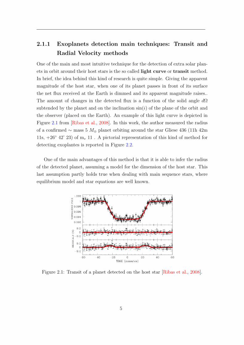
One of the main and most intuitive technique for the detection of extra solar plan-

ets in orbit around their host stars is the so called light curve or transit method.

In brief, the idea behind this kind of research is quite simple. Giving the apparent

magnitude of the host star, when one of its planet passes in front of its surface

the net flux received at the Earth is dimmed and its apparent magnitude raises..

The amount of changes in the detected flux is a function of the solid angle dΩ

subtended by the planet and on the inclination sin(i) of the plane of the orbit and

the observer (placed on the Earth). An example of this light curve is depicted in

Figure 2.1 from [Ribas et al., 2008]. In this work, the author measured the radius

of a confirmed ∼ mass 5 M⊕ planet orbiting around the star Gliese 436 (11h 42m

11s, +26 42’ 23) of mv 11 . A pictorial representation of this kind of method for

detecting exoplantes is reported in Figure 2.2.

One of the main advantages of this method is that it is able to infer the radius

of the detected planet, assuming a model for the dimension of the host star. This

last assumption partly holds true when dealing with main sequence stars, where

equilibrium model and star equations are well known.

Figure 2.1: Transit of a planet detected on the host star [Ribas et al., 2008].

5

Figure 2.2: Pictorial representation of the transit method.

However, this photometry-based method has two major disadvantages. Plan-

etary transits are only observable for planets whose orbits happen to be aligned

with the observation site (telescope). As a rule of thumb, the probability of a

planetary orbital plane being directly on the line-of-sight to a host star is the ratio

of the diameter of the star to the diameter of the orbit (in small stars, the radius of

the planet is also an important factor). About 10 percent of planets with small or-

bits have such alignment, and the fraction decreases for planets with larger orbits.

However, adopting surveys able to study large areas of sky containing thousands

or even hundreds of thousands of stars at once, transit surveys can in principle find

extrasolar planets at a reasonable rate. For instance, GAIA [Lindegren and Perry-

man, 1996], Kepler [Koch et al., 1998] or CoRoT [Baglin et al., 2006] missions are

or will be used for this kind of activity. The second issue that afflicts the transit

method is a high rate of false detections. For instance, the detection of a planet

orbiting a red giant branch star could be tricky. In fact, while planets around these

stars are much more likely to transit due to the larger size, these transit signals

are hard to separate from the main star’s brightness light curve as red giants have

frequent pulsations in brightness with a period of few hours to days. Red giant

stars are also much more luminous and transiting planets block much smaller per-

centage of light coming from these stars. On the contrary, planets can completely

occult a white dwarf which would be easily detectable from Earth. However, due

to their small sizes, chance of a planet aligning such a stellar remnant is extremely

small as explained before.

In the latter case, a successful method has been exploited for detection of plan-

6

Figure 2.3: Pictorial representation of a planet around a pulsar detected with thePulsar Timing technique.

ets around pulsars. In particular, since the intrinsic rotation period of a pulsar is

so regular (P), slight anomalies in the timing of its observed radio pulses can be

used to track the pulsar’s motion. Like an ordinary star, a pulsar will move in its

own small orbit if it has a planet. Calculations based on pulse-timing observations

can then reveal the parameters of that orbit. For instance in 1992 Aleksander

Wolszczan and Dale Frail used this method to discover planets around the pulsar

PSR 1257+12. [Wolszczan and Frail, 1992]. The detection was quickly confirmed,

making it the first confirmation of planets outside the Solar System.

Nevertheless, the state-of-the-art method able to detect planets orbiting around

their host stars is the radial velocity method which is based essentially on the

doppler spectroscopy (see e.g. [Baranne et al., 1979; Cochran and Hatzes, 1994;

Mayor and Queloz, 1995; Mayor et al., 1992]). In brief, this method exploits the

relative shifts of absorption lines in the star spectrum in order to derive a pro-

jected line of sight radial velocity that, combined with other observables, gives the

detection and basic properties (such as the mass) of the orbiting planet. Giving

a series of observations of the host star spectrum, periodic variations may be de-

7

tected measuring the wavelength of characteristic spectral absorption lines that

increases and decreases regularly over a period of time. An example of this proce-

dure usually yields a radial velocity plot that is reported in Figure 2.4.

Figure 2.4: An example of radial velocity plot versus time obtained after an ob-servation campaign on the host star (freely taken from en.wikipedia.org DopplerSpectroscopy).

The main problem with radial velocity method is that it can only measure velocity

component along the line-of-sight, and so depends on a measurement (or estimate)

of the inclination of the planet’s orbit to finally determine the planet’s mass. If the

orbital plane of the planet happens to line up with the line-of-sight of the observer

the measured variation in the star’s radial velocity is the true value. In the case

the orbital plane is tilted away from the line-of-sight, then the true effect of the

planet on the motion of the star will be greater than the measured variation in

the star’s radial velocity, which is only the component along the line-of-sight. As

a result, the planet’s true mass will be higher than expected.

To correct for this effect, and so determine the true mass of an extrasolar planet,

radial-velocity measurements can be combined with astrometric observations, which

track the movement of the star across the plane of the sky, perpendicular to the

line-of-sight. Astrometric measurements allows researchers to check whether ob-

8

jects that appear to be high mass planets are more likely to be stellar or sub-stellar

objects.

2.1.1.1 An example of planet detection through radial velocity method.

In this example the mass of planet 51 Pegasi (b) orbiting its host star is derived.

The radial velocity curve depicted in Figure 2.4 is derivated using Doppler spec-

troscopy to observe the radial velocity of the star which is being orbited by the

planet (in a circular orbit). This star velocity shows a periodic variance of ±1

m s−1 [Mayor and Queloz, 1995], suggesting an orbiting mass that is creating a

gravitational pull on this star. From Kepler’s third law of planetary motion, the

observed period of the planet’s orbit around the star (equal to the period of the

observed variations in the star spectrum) can be used to determine the distance

planet from the star (r) adopting the equation:

r3 =GMstar

4π2P 2star (2.1)

where Pstar is the star observed period and Mstar is the mass of the host star itself,

usually derived from stellar equilibrium models. The velocity of the planet around

the star can be calculated using Newton’s law of gravitation and the classical

definition of centripetal force as expressed in the following equation

VPlanet =√GMstar/r (2.2)

The mass of the orbiting planet can be found from its calculated velocity adopting

the formula:

Mplanet =MstarVstarVplanet

(2.3)

where Vstar is the velocity of parent star. The observed Doppler velocity, K =

Vstar sin(i), where i is the inclination of the planet’s orbit to the line perpendicular

to the line-of-sight. Thus, assuming a value for the inclination of the orbit and for

the mass of the star, the observed changes in the radial velocity of the can be used

to calculate the mass of the extrasolar planet. In Table 2.1 are given some details

on physical observable of known planets orbiting a sun-like star (∼ G2V spectral

9

class and a mass of ∼ 1 M) .

Planet Mass Distance (AU) Radial velocityJupiter 1 28.4 m s−1

Jupiter 5 12.7 m s−1

Neptune 0.1 4.8 m s−1

Neptune 1 1.5 m s−1

Super-Earth (5 M⊕) 0.1 1.4 m s−1

Alpha Centauri Bb (1.13 ± 0.09 M⊕) 0.004 0.51 m s−1

Super-Earth (5 M⊕) 1 0.45 m s−1

Earth 1 0.09 m s−1

Table 2.1: Planets physical observables and relative measurements.

Planet Type MA (AU) Period RV (m s−1) Spectrograph:51 Pegasi b Hot Jupiter 0.05 4.23 d 55.9 First-generation55 Cancri d Gas giant 5.77 14.29 y 45.2 First-generationJupiter Gas giant 5.20 11.86 y 12.4 First-generationGliese 581c Super-Earth 0.07 12.92 d 3.18 Second-generationSaturn Gas giant 9.58 29.46 y 2.75 Second-generationα Centauri Bb Terrestrial 0.04 3.23 d 0.510 Second-generationNeptune Ice giant 30.10 164.79 y 0.281 Third-generationEarth Habitable 1.00 365.26 d 0.089 ESPRESSOPluto Dwarf 39.26 246.04 y 0.00003 Not detectable

Table 2.2: Known planets and required spectrograph to detect through the radialvelocity method (data taken from exoplanets.org).

As shown in Table 2.2 the needed of even more resolved spectrograph is becom-

ing even more compelling in order to study the physical properties and environment

of habitable terrestrial planets around main sequence solar like stars. This facts

is also supported by Figure 2.5 that shows the correlation between the radial ve-

locity sensitivity to minimum detectable planet mass, assuming a solar like G2V

host star.

10

Figure 2.5: Radial velocity and planet mass limit detection as a function of distancefrom G2V solar like host star. Pepe et al 2013 in press.

2.1.2 ESPRESSO: a general overview of the instrument

2.1.2.1 Design concept

ESPRESSO [Pepe et al., 2010] is a fibre-fed, cross-dispersed, high-resolution,

echelle spectrograph. The telescope light is fed to the instrument via a so-called

Coude-Train optical system and within the adoption of optical fibres. ESPRESSO

is located in the Combined-Coude Laboratory (incoherent focus) at the European

Southern Observatory (ESO) Paranal site, where a front-end unit can combine the

light from up to 4 Unit Telescopes (UT) of the Very Large Telescope (VLT). The

target and sky light enter the instrument simultaneously through two separate

fibres, which form together the slit of the spectrograph. The full spectrum of an

observed scientific object has a wavelength coverage from 380 nm to 780 nm on two

large 92 mm x 92 mm CCDs with 10-µm pixels. A very simple sketch of the optical

layout is shown in Figure 2.6 . The aimed precision of 10 cm/sec RMS requires

measuring spectral line position changes of 2 nm (physical) in the CCD plane. In

order to improve as much as we can the stability and thermal-expansion, the CCD

package is made of Silicon Carbide. The package of the CCDs, the surrounding

11

mechanics and precision temperature control inside the cryostat head and its cool-

ing system, as well as the thermal stability and the homogeneous dissipation of the

heat locally produced in the CCDs during operation are of critical importance.

Figure 2.6: Sketch of the ESPRESSO spectrograph optical layout [Spano et al.,2012]

ESPRESSO is designed to be an ultra-stable spectrograph capable of reaching

radial-velocity precisions of the order of 10 cm s−1, one order of magnitude better

than its predecessor HARPS [Mayor et al., 2003]. This instrument is therefore

designed with a totally fixed configuration and for the highest thermo-mechanical

stability. The spectrograph optics is mounted in a tri-dimensional optical bench

specifically designed to keep the optical system within the thermo-mechanical tol-

erances required for high-precision RV measurements. The bench is mounted in

a vacuum vessel in which 10-5-mbar class vacuum is maintained during the entire

duty cycle of the instrument. The temperature at the level of the optical system is

required to be stable at the mK level in order to avoid both short-term drift and

long-term mechanical instabilities. Such an ambitious requirement is obtained by

locating the spectrograph in a multi-shell active thermal enclosure system. Each

shell will improve the temperature stability by a factor 10, thus getting from typ-

ically Kelvin-level variations in the Combined Coude Laboratory (CCL) down to

mK stability inside the vacuum vessel and on the optical bench.

12

2.1.2.2 Wavelength calibration

All spectrograph observation through plates or modern CCDs need to be wavelength-

calibrated in order to assign to each detector pixel the correct wavelength with a

repeatability of the order of ∆λλ∼ 10−1. A necessary condition for this step is the

availability of a suitable spectral wavelength reference. While in other spectro-

graph the wavelength calibration is assed through consolidated standard spectral

lamps (such as thorium argon) none of them provide a spectrum sufficiently wide,

rich, stable and uniform for this purpose. Therefore, the source for the calibration

and simultaneous reference adopted for ESPRESSO is a Laser Frequency Comb

(LFC) (see e.g. [Murphy et al., 2007]).

2.1.2.3 Coude train and Front End subsystem - feeding the spectro-

graph with scientific lights

ESPRESSO is an instrument designed for the incoherent combined focus of the

VLT. Although foreseen in the original plan, such a focus has never been im-

plemented at the VLT. For this reason, the implementation of a Coude Train is

mandatory in order to materialise a focus in the CCL, 40 m far away from the

UTs [Cabral et al., 2012]. Unlike any other instrument built so far, ESPRESSO

will receive light from any of the four UTs. The light of the single UT sched-

uled to work with ESPRESSO is then fed into the spectrograph (1-UT mode).

Alternatively, the combined light of all the UTs can be fed into ESPRESSO simul-

taneously (4-UT mode). The Coude Train picks up the light with a prism at the

level of the Nasmyth-B platform and roots the beam through the UT mechanical

structure down to the UT Coude room, and farther to the CCL along the exist-

ing incoherent light ducts (see Figure 2.7 ). The selected concept to convey the

light of the telescope from the Nasmyth Focus (B) to the entrance of the tunnel

in the Coude Room (CR) below each UT unit is based on a set of 6 prisms (with

some power). The light is directed from the UTs Coude room towards the CCL

using 2 big lenses. The beams from the four UTs converge into the CCL, where

mode selection and beam conditioning is obtained thanks to the fore-optics of the

Front-End subsystem [Riva et al., 2012].

The Front-End transports the beam received from the Coude, once corrected for

13

Figure 2.7: Coude Train of ESPRESSO and optical path through the telescopeand the tunnels [Cabral et al., 2012].

atmospheric dispersion by the ADC, to the common focal plane on which the

heads of the fibre-to-spectrograph feeding are located. While performing such a

beam conditioning the Front-End applies pupil and field stabilization (explained

in details in this chapter of the Thesis). They are achieved via two independent

control loops each composed of a technical camera and a tip-tilt stage. Another

dedicated stage delivers a focusing function. In addition, the Front-End provides

the mean to inject calibration light (white and spectral sources) into spectrograph

fibre if and when needed. A top view of the Front-End arrangement is shown in

Figure 2.8 .

2.1.2.4 Foreseen ESPRESSO mode

ESPRESSO will have three instrumental modes: singleHR, singleUHR and mul-

tiMR. Each mode will be available with two different detector read-out modes

optimized for low and high-SNR measurements, respectively. In high-SNR (high-

precision) measurements the second fiber will be fed with the simultaneous refer-

ence, while in the case of faint objects it shall be preferred to feed the second fiber

14

Figure 2.8: Top view of the Front-End and the arrival of the four UT beam at theCCL [Riva et al., 2012]

with sky light. The extreme precision, mandatory for the scientific tasks, will be

obtained by adopting and improving concepts implemented in the state-of-the-art

HARPS. The light is fed to the spectrograph by means of the front-end unit into

optical fibres that scramble the light and provide excellent illumination stability

to the spectrograph. The target fibre can be fed either with the light from the

astronomical object or the calibration sources. The reference fibre will receive

either sky light (faint source mode) or calibration light (bright source mode). In

the latter case - the famous simultaneous-reference technique adopted in HARPS

- it will be possible to track instrumental drifts down to the cm s−1 level. It is

assumed that in this mode the measurement is photon-noise limited and detector

read-out noise negligible. In the faint-source mode, instead, detector noise and

sky background may become significant. In this case, the second fibre will allow

to measure the sky background, while a slower read-out and high binning factor

will reduce the detector noise. Table 2.3 summarise the expected performance of

the overall instruments.

15

Parameter/Mode singleHR multiMR singleUHRWavelength range 380-780 nm 380-780 nm 380-780 nmResolving power 134.000 59.000 225.000Aperture on sky 1.0′′ 4x1.0′′ 0.5′′

Spectral sampling (average) 4.5 pixels 5.5 pixels (bin x2) 2.5 pixelsSpatial sampling per slice 9.0 (4.5) pixels 5.5 pixels (bin x4) 5.0 pixelsSimultaneous reference Yes (no sky) Yes (no sky) Yes (no sky)Sky subtraction Yes (no sim. ref.) Yes (no sim. ref.) Yes (no sim. ref.)Total efficiency 11% 11% 5%RV precision < 10 cm s−1 ∼ 1 m s−1 < 10 cm s−1

Table 2.3: Summary of ESPRESSO’s instrument modes and corresponding per-formances.

2.1.2.5 A scientific Pandora box

Thanks to its high resolution and stability ESPRESSO will be able to investigate

the presence and the basics physical parameters of terrestrial habitable exoplanets

around main sequence star from F2V to M4V. In fact, ESPRESSO, being capable

of achieving a precision of 10 cm s−1 in terms of radial velocity, will be able to

register the signals of Earth-like and massive Earths in the habitable zones (i.e.,

in orbits where water is retained in the liquid form on the planet surface) around

nearby solar-type stars and stars smaller than the Sun. For instance, we recall

that our planet pulls a velocity amplitude of 9 cm s−1 onto the Sun, a G2V main

sequence star.

Nevertheless, this kind of research is only a tiny fraction of the astrophysical

science that this new instrument could be carry on. In particular, it could be

possible to study (confirm or deny) the variation of the α fine structure constant

and/or variation of the proton-electron ratio mass ratio (µ). At the present mo-

ment, Earth-based experiments have revealed no variation in their values. Hence

its status as truly constants is amply justified. With the advent of 10-m class tele-

scopes observations of spectral lines of intervening system in the spectra of distant

quasars gave the first hints that the fine structure constant might change its value

over time, being lower in the past by about 6 ppm (Webb et al., 1999; Murphy et

al., 2004). The addition of other 143 VLT-UVES absorbers have revealed a 4-σ

16

Figure 2.9: All-sky spatial dipole with the combined VLT (squares) and Keck(circles) α measurements from Webb et al. (2011). Triangles are measures incommon to the two telescopes. The blue dashed line shows the equatorial regionof the dipole.

evidence for a dipole-like variation in α across the sky at the 10 ppm level (King,

2012). This results is shown in Figure 2.9 .

Finally, it will be also possible to study the chemical composition of stars in local

galaxies and the metal abundance in the so-called metal poor stars. The most

metal poor stars in the Galaxy are probably the most ancient fossil records of the

chemical composition and thus can provide clues on the pre-Galactic phases and

on the stars which synthesized the first metals. Masses and yields of POP III stars

can be inferred from the observed elemental ratios in the most metal poor stars

[Heger and Woosley, 2010]. ESPRESSO, both in the 1-UT and 4-UT mode will

be able to provide spectra with a sufficient resolution and signal to noise ratio for

an reliable chemical analysis.

17

2.2 State of the art at Paranal: Test campaign

activities and data analysis

2.2.1 Introduction

As reported in the general description of the instrument, the light coming from the

4 UTs of the VLT are combined in the Coude Combined Laboratory through the

Front End unit. However, the path that the light have to span in order to reach

the CCL will most likely induce a deformation on the wavefront and/or tip-tilt on

the spot at the focal plane. In order to understand the environmental behaviour

where the instrument will be installed and operated, an extensive campaign has

been coordinated with the European Souther Observatory ESO. In particular, the

following test scheme have been implemented:

• Wind speed in 2 of the VLT incoherent ducts and in P3 / P4 Coude Room

passage

• Temperature record in:

– Nasmyth platform

– Coude Room

– Combined Coude Laboratory

• PSF stability of the image at CCL

• Image position stability (tip/tilt) at CCL

The elaboration of the aforementioned information will provide the following

information relevant for the optimal optical coupling efficiency between the VLTs

Units and ESPRESSO:

• Estimation of the required tip-tilt correction for the Front End Unit

• Air flux in the incoherent ducts

• Temperature record at different times in the year

• Influence of the ducts on the image quality at the CCL

18

2.2.2 Setup configuration @VLT

We describe in this section the setup for the measurement of temperature, wind

and PSF. Further details can be found in Avila G. & Landoni M. , Coude Room

CCL environmental tests. ESO VLT-TRE-ESP-13520.

2.2.2.1 Temperature and wind measurement setup

Temperature measurements were recorded with compact portable devices. Figure

2.12 shows the picture of the sensor. It is an USB Data logger from ATP Messtech-

nik GmbH. In addition to temperature they provide relative humidity measure-

ments and dew point. They are PC programmable and provide the recorded data

in plain text or cvs formats. The resolution is 0.1 degree. Three of them were

placed at most relevant points: at the Nasmyth platform to measure the open air

temperature, in the middle of the Coude Room and in the middle of the CCL as

indicated in Figure 2.10.

UT NasmythPlatform

Coude Room Incoherent Duct CCL

Temp. Sensor 1

Temp. Sensor 2

Temp. Sensor 3

Anemometer

Objective +CCD cameraCollimator

Figure 2.10: Configuration for the proposed environmental tests.

Wind measurements were taken with hot wire anemometers (Hitzedraht-Anemometer

PCE-423). They can record very slow fluxes (0.02 m/s) but the big drawback is

that they are unidirectional. Figure 2.11 shows the anemometer controller and

head. They are not programmable and the recording mode have been fixed to one

19

Figure 2.11: Anemometer used for wind measurements.

Figure 2.12: Temperature data logger used for temperature measurements.

20

measurement per second. In order to detect a substantial chimney effect along the

tube between P1 and P4 two anemometers will be installed (see Figure 2.10): one

at the Nasmyth folded focus where there is a small hole to pass the beam and a

second at the passage to the CR, just above M9 (VLT Interferometer). In partic-

ular, if the temperature in each Coude Room is not the same, the wind flux might

be different for each duct that reaches the Coude Combined Laboratory. Conse-

quently the wind speed should be measured for all incoherent ducts. Moreover,

since different configurations for the tunnels might be considered, the following

configuration for the measurement have been evaluated:

• The incoherent duct is open on both sides and all the coherent ducts (VLTI)

are closed. Note that the coherent ducts are closed only on the Delay Line

side when the VLTI is not in operation. The incoherent apertures from the

CR are always open.

• The incoherent duct is closed on both sides.

• In all the cases the wind sensor has to be placed at around 50 cm inside the

duct end.

Note that in the case of UT1 and UT4, where the incoherent ducts intersect the

coherent ones, there might be some turbulence at the intersections even if the

incoherent ducts are sealed.

2.2.2.2 PSF and image stability through the tunnels

The turbulences that arises inside the tunnel cannot be simulated by a Kolmogorv

model [Kolmogorov, 1941] since it considers that the turbulence at small scales are

statistically isotropic. However, this assumption holds only for very high Reynolds

number.

Re =Fiνi

(2.4)

where Fi are the inertial forces and νi the non-conservative field of forces due to vis-

cosity. Assuming a flow inside a cylindrical tunnel in a newtonian approximation,

21

the Reynold numbers turns out to be

Re =ρvL

µ(2.5)

where ρ is the density of the fluid (kg m−3), L is the characteristic linear dimension,

v is the vector fluid velocity and µ is the kinematic viscosity (m2 s−1). If a fluid is

transported through a pipe (as in the case of the air inside the duct tunnels) the

flow is said to be turbulent if Re > 4000 while, for Re < 2300 the flow is laminar.

The region between 2300 and 4000 is called critical Reynolds number and the flow

is said to be in transition between the two regimes.

In the case of the VLT ducts, stratified or laminar fluxes similar to the ones in

the VLT-I ducts are expected. A major technique for measuring the image qual-

ity would be the adoption of a Shack Hartman wavefront sensor, similar to that

applied for adaptive optics. In particular, for a given number of short exposures

(of the order of seconds or less) it provides an appropriate average map of the

wavefront described by the Zernike coefficients. The point spread function (PSF)

and therefore the full width half maximum (FWHM) may be deduced.

However this method requires considerable equipment which is not available

in the Coude Combined Laboratory. For this reason, a simplified method has

been proposed instead: the image of a point-like source (optical single mode fibre)

generated in the Coude Room is directly recorded in the CCL with a fast CCD

camera. The FWHM is directly measured on the image for different short exposure

times. The barycentre or the photocenter of individual images records the tip-tilt

low movement of the star.

Figure 2.13 reports the laboratory setup for the intended measurements. On

the left side of the delay line an optical fiber of ∼ 10 µm is feeded by a quasi

monochromatic light source. A small F/5 telescope opens the ligth beam which

is then collimated through a long focal lens. After a path of ∼ 60 meters the

ligth reaches a simple optics (objective) F/10 that focalize the spot on a CCD

camera. It is important to note that a 10 µm fiber on F/10 corresponds roughly

to 0.026′′ on the sky. Since at the Paranal the median seeing (no adaptive optics

considered) is about 0.70′′ [Sarazin et al., 2008] the spot on the detector can be

22

Laser / LED Image grabberand PC

CCD camera

Duct

ObjectiveCollimatorFi

bre

Coude Room CCL

Figure 2.13: Optical setup for the image quality measurement at the end side ofthe delay tunnel.

reasonable considered as a PSF of a point-like source.

2.2.3 Data analysys

2.2.3.1 PSF model

As noted in the previous chapter, the fiber image should give at the focal plane

a good approximation of a the point spread function of an unresolved source.

However, as shown in Figure 2.14 the radial profile of the spot is quite similar

to a Gaussian Beam profile. A Gaussian beam profile [Svelto, 2010] is a beam

of electromagnetic radiation in which the transverse electric field and intensity

(irradiance) distributions are described by mean of approsimation of Gaussian

functions. These beams are popular when describing the spread function of lasers,

as in the case of our experimental setup. In particular, giving the electric field as

E(r, z) = E0w0

w(z)exp

( −r2

w2(z)− ikz − ik r2

2R(z)+ iζ(z)

), (2.6)

23

X pixel

Y pi

xel

20 40 60 80 100 120 140

50

100

150

200

20

40

60

80

100

120

140

160

180

200

Student Version of MATLAB

Figure 2.14: An example of the PSF of the laser beam recorded by the camera.Horizontal bars represent the area of interest for the full readout while vertical baris the preliminary computation of the centroid performed by the onboard softwareof the camera.

24

where r is the radial distance from the center axis of the beam,

z is the axial distance from the beam’s narrowest point (the ”waist”),

i is the imaginary unit,

k = 2π/λ is the wave number (in rad m),

E0 = |E(0, 0)|,w(z) is the radius at which the field amplitude and intensity drop to 1/e and 1/e2

of their axial values,

w0 = w(0) is the waist size,

R(z) is the radius of curvature of the beam’s wavefronts,

ζ(z) is the Gouy phase shift

the intensity at radius r in spherical coordinates is given by the equation

I(r, z) =|E(r, z)|2

2η= I0

(w0

w(z)

)2

exp

(−2r2

w2(z)

), (2.7)

where I0 is the intensity at the center of the beam and η is the characteristic

impedance of the medium in which the beam propagates. In our case, the tightness

of the beam itself at F/10 allows to properly approximate the spot profile to a true

point-like PSF after the application of a low passband filter. The point-like PSF

is described by the equation

I(q) ≈ I ′0 exp

(−q2

2σ2

), (2.8)

where FWHM = 2√

2 ln 2 σ ≈ 2.3 σ. and q is the distance from the center of the

beam. In the case of Gaussian beam profile, 2w =√

2 FWHM√ln 2

= 1.699 × FWHM

where 2w is the full width at half maximum at 1e

that, for tight beams (0.02′′),

encompasses about the 99% of the irradiated power. Figure 2.15 shows the result

of the adopted approximation. The mean systematical error on the PSF FWHM

error is about 20%.

Each recorded image, with a frequency of about 1 Hz, is then reduced through

standard MIDAS procedures [Banse et al., 1988]. The data reduction includes

standard bias subtraction, cosmic ray removal (if needed). When the raw image is

reduced, a gaussian fit is applied adopting the CENTER/GAUSS MIDAS recipe.

The position of the spot on the detector, instead, is directly recorded by the

25

Figure 2.15: An example of the PSF of the laser beam recorded by the cameraafter the application of gaussian PSF model. Courtesy: ESO Paranal (DocumentESO: VLT-TRE-ESP-13520)

detector. Each proposed value for the photometric barycenter computed by the

camera itself has been cross-checked with the position proposed by MIDAS after

the data reduction.

2.2.4 Results

The campaign (repeated both in the winter and summer chilean seasons) has

collected a huge amount of raw data (in particular in terms of FITS image of

the image behaviour). The summer data acquisition includes temperatures, wind

speed and image displacement (only x and y positions) while in the winter one

the image quality (FWHM) has been acquired too. The results are here summa-

rized with significant examples evaluating both the image displacement and the

image quality. The overall behaviour of the Paranal enviroment will be helpful to

understand:

• How to design the ESPRESSO Front End unit in terms of stabilization of

the field (guiding algorithm).

26

• Definitively point out the needed of adaptive optics at the level of the in-

strument (or telescope directly)

2.2.4.1 Image quality and relationship with Paranal environment

The data analysiys immediately shows that image displacement due to air flows

in the ducts has mainly two features. First of all there are some spikes which raise

during the whole night and, moreover, a slightly drift along the overall time is also

apparent. The image displacements measured in all the campaigns are essentially

along the vertical direction. This could drive to inferr that a layered thermal

stratification of the air exists at the level of the tunnel, instead of a pure turbulent

one.

Figure 2.16: Image displacement acquired during the night between 12 and 13 ofJuly 2011.

Figure 2.16 shows an explicative behavior of the centroid displacement during

the night. On X axis is represented the time expressed in hours, while in Y is

reported the components of the image displacement in microns. As said before,

27

spikes with displacement of tenth of microns are present. The spikes are sudden

event that last usually few minutes; however some of them takes even half an

hour. On the other hand it is possible to notice that during the night there are

also some plateau where the image is very stable. The characteristics spikes in

that night show that the maximum peak within 1 sec is around 50µm (the average

is around 23µm). According to the optical configuration, the plate scale is ∼ 390

µm arcsec−1 . For this reasons, the displacement on the sky turns out to be 0.12′′

projected on the sky. The stability requirement budget error for the positioning,

in order to cope with the ESPRESSO scientific goals, is 0.05′′ rms.

Now, suppose to observe a star of mv = 8.00 in the Johnson UVB V filter. The

required exposure time in order to reach, at the level of the recorder spectrum, an

accuracy on the radial velocity of about few cm s−1 is about 30 minutes. If the

exposure starts just before a spike happens, the rms error on the position will be

∼ 0.2′′ which is a factor ∼ 5 above the maximum accetable error on the position of

the target on the slit. For this reason, an active control of the field position must

be implemented at the level of the front end of the instrument.

The displacement of the PSF has also been correlated with temperature and

wind recorder by the instruments adopted as explained in the setup configuration.

In Figure 2.17 are shown both the temperatures behavior and the image displace-

ment. A strong correlation between the temperature (taken in proximity of the

anemometer) at the entrance of the tunnel into the CCL and PSF tilts seems to

appear. Between h2.00 and h4.00 there are both plateau in the temperature and

in the displacement while when the temperature starts shacking the spikes of the

displacement raise up. From the same figure no strong correlation seems to exist

with the other temperature acquired in different location at the VLT.

As expected, the temperature fluctuations are strictly correlated to the wind

speed changing that could drive to the conclusion that there is a strict interaction

between the turbulence into the tunnel and the vertical displacement of the image

(see Figure 2.19). In order to better characterise the turbolence features, a closed

configuration for the tunnel has been assesed to evaluate the effect on the image

stability. Maintaining the previous setup for the detectors (except for the vertical

axis of the camera), both the entrance and the exit of the delay line have been

28

Figure 2.17: Comparison between image displacement and temperatures behav-ior. Wind line (solid blue) refers to the wind temperature at the level of theanemometer.

Figure 2.18: Correlation between temperature and the wind speed.

29

then sealed.

In Figure 2.19 is shown the image displacement in the closed configuration. Note

that in this configuration the camera has been rotated along the optical axis of

90 degree due to technical reasons. This clearly demonstrate that during the

night there is a predominant displacement along the vertical axis respect to the

horizontal one, as detected in the open configurations.

Figure 2.19: Image displacement acquired during the night between 13 and 14 ofjuly 2011 (closed configuration)

From the comparison between open and closed configuration it is clear that

the second one shows that the image position is more stable and reliable. The

maximum peak-to-valley displacement during a spike is around 35µm which is

roughly half of the open configuration.

Regarding the image quality in terms of FWHM of the PSF the data analysys

shows that it is quite stabile along the nigths. The behaviour is shown in Figure

2.21

As in the case of image displacement, the PSF of the image has been evaluated

also in the closed configuration which provides benefits also to the image quality

behavior as shown in Figure 2.22

30

Figure 2.20: Measured FWHM during the 12 to 13 night. Note that spikes aredue to non-convergence of the fitting algorithm on bad recorded image.

Figure 2.21: Standard deviation of the Full Width at half maximum of the imageon 10 minutes wide bins .

31

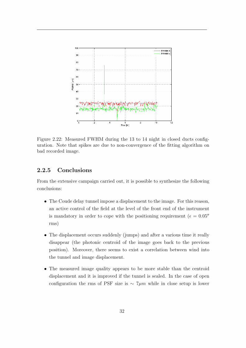
Figure 2.22: Measured FWHM during the 13 to 14 night in closed ducts config-uration. Note that spikes are due to non-convergence of the fitting algorithm onbad recorded image.

2.2.5 Conclusions

From the extensive campaign carried out, it is possible to synthesize the following

conclusions:

• The Coude delay tunnel impose a displacement to the image. For this reason,

an active control of the field at the level of the front end of the instrument

is mandatory in order to cope with the positioning requirement (ε = 0.05′′

rms)

• The displacement occurs suddenly (jumps) and after a various time it really

disappear (the photonic centroid of the image goes back to the previous

position). Moreover, there seems to exist a correlation between wind into

the tunnel and image displacement.

• The measured image quality appears to be more stable than the centroid

displacement and it is improved if the tunnel is sealed. In the case of open

configuration the rms of PSF size is ∼ 7µm while in close setup is lower

32

than ∼ 3µm. For the purposes of ESPRESSO the behaviour of the PSF

clearly indicates that no adaptive optics is required to fulfill the instrument

requirements. Nevertheless, the closed-tunnel setup is overall better than the

open one, in terms of centroid stability and also in PSF size stability and

dimension which is directly correlated to the image quality.

2.3 Front-End Subsystem: stabilisation of the

field

2.3.1 Introduction

The observation campaign in Paranal, illustrated in the previous section, clearly

demonstrated that the image stability at the end of the Coude Train system is

not sufficient to guarantee an error on the position accuracy (with respect to the

fiber entrance which acts as slit) well below 0.05′′, which is the evaluated require-

ment for the positioning system in order to reach the stability for the purposes of

ESPRESSO (RV stability and SNR directly correlated to severe slit loss in case of

bad guiding). For this reason, the aim of the Front End System is the stabilisation

of the delivered field and pupil of the telescope and the entire Coude Train. This

task is crucial since it allows the entire ESPRESSO to reach the required perfor-

mances in terms of stability of the image. The stabilisation algorithm is based on

active optics (piezo tip-tilt devices) that will correct low spatial order perturbation

(tip tilt) and not high spatial order perturbation since the image quality (in terms

of FWHM) is reasonably stable for the purpose of the spectrograph as investigated

before.

We will illustrate the following main topics.

• A parametric detector simulator has been set up in order to evaluate the

performances of different detector, commercial ones (such as Sony or Kodak

detectors) and scientific (e2v or Hamamatzu). In detail the CCD characteris-

tics like RON dark current, QE has been investigated to exploit the expected

performance on the sky for the different products.

• A robust version of the centroid calculation based on the computation of

33

the barycenter adopting Proportional and Integral controller architecture in

order to increase the stability of the whole guiding system will be used.

2.3.2 CCD detector simulation and radiometry

In order to exploit the behaviour of the detector and the stabilisation algorithm

performance expected on the sky, a numerical model for CCD simulation has been

setup. In particular, in the numerical model, the CCDs are essentially charac-

terised by the following parameters:

• Pixel size (µm).

• Number of pixel of the detector (e.g. 511x511).

• Read out noise (in e-).

• Dark Current (in e- sec−1 px−1).

• Quantum efficiency (on the ESPRESSO spectral range).

• Saturation level (in e- pixel−1) and ADU saturation level.

The main part of the simulation algorithm lies in the generation of the noises,

which are function of the parameter of the TCCD. In the next paragraph, we ex-

plain the main steps required to simulate an integration of the TCCD in order to

validate the Positioning and Guiding Algorithm. In particular, the stabilisation

algorithm will be evaluated adopting the displacement obtained through exper-

imental data recorded in Paranal and illustrated in the previous section. Since

those measurements have been recored at 1 Hz, to simulate the real displacement

of the image a linear interpolation between one step and the following has been

considered. The 1 sec of exposure is then realized by adding 10 images of 0.1sec

with the displacement obtained by the linear interpolation illustrated in the pic-

torial representation of Figure 2.23.

Moreover, the following theoretical assumption are assumed to hold during

each simulation:

34

Figure 2.23: Subsampling of the spot position. Red dots are experimental datawhile the yellow ones are the subsample interpolation in order to better characterisethe behaviour of the image displacement on the detector

• The PSF (since only point like source are considered) is a Gaussian func-

tion. In particular, consider the following formula for the spot that it will

be sampled on the simulated CCD. f(x, y) = A exp(−(

(x−xo)22σ2x

+ (y−yo)22σ2y

)).,

where A is the peak in photon s−1 of the function, x0 and y0 represent the

displacement (in pixel unit) of the spot with respect to the origin of the

reference system..

• The spot is symmetric. In particular, we considere a perfect symmetry of

the spot but the algorithm could guide also with an asymmetric one.

• The reference flux is considered to be constant over the ESPRESSO wave-

lengths and is 1000 photons sec−1 cm−2 A−1, assuming an object with ap-

parent magnitude mv = 0. This assumption is reasonable since bolometric

correction for different star spectral class (from B to M) slightly modify the

bolometric flux received at the level of the Front End stabilisation algorithm

subsystem.

• The magnitude of the star is constant during the observation (this holds

true for the most scientific objects that ESPRESSO will observe).

35

2.3.2.1 Determination of optical parameters

This paragraph describes the main optical parameters calculated by the algorithm

in order to perform the simulation of the CCD. In particular, the plate scale of

the system will be calculated as

PS =F ×D206265

× 1000 µm arcsec−1 (2.9)

where F is defined as F-number times the diameter of the telescope in mm and

1000 is a proportional constant in order to obtain the PS as µm arcsec−1. When

the plate scale is constrained, the PSF of the scientific object is simulated as a

Gaussian spot. Since the Gaussian function is determined by its variance in the X

and Y direction it is necessary to estimate their value that are function of seeing,

pixel size and Plate scale. In particular, they are defined as

σx = σy =PS × seeing

2.35× pixelsizeµm (2.10)

where the seeing is given in arc sec and pixelsize is the dimension of the pixel in

µm. Moreover, if a binning (only squared) is assumed the dimension of the pixel

is multiplied by the binning factor.

2.3.3 Radiometric quantities

For each simulation, it is mandatory to estimate how many photons can reach

the ESPRESSO Front-End up to the pinhole slit which is responsible to inject

the received light into the fiber. Here below are reported the equations that are

used in order to perform the estimation, assuming that the scientific object is fully

described by its relative visual magnitude (V filter). The received flux between λ

and λ + dλ is calculated as follow

dφ

dλ= φ? × η(λ)× ηESPRESSO(λ) (2.11)

where φ? is the object flux in photons sec−1 cm−2 A−1 calculated from its apparent

magnitude in V band, η(λ) is the CCD Quantum Efficiency and ηESPRESSO(λ) is

36

the efficiency of the whole ESPRESSO instruments up to the Front End technical

CCD. Figure 2.24 shows the diagram of the Quantum efficiency of three different

detectors. The solid dashed line represents the estimated efficiency of ESPRESSO

system as defined in the PDR document. Figure 2.25 shows the quantum efficiency

of the Sony ICX 285 detector which is the baseline one for ESPRESSO (on FDR,

May 2013).

Integrating all over the wavelengths that ESPRESSO will observe, the total

number of photon per unit area is expressed as:

φsciObj =

∫ 8000

3800

φ? × ηESPRESSO(λ)× η(λ)dλ (2.12)

Figure 2.24: Quantum Efficiency of a sample of three different TCCD andESPRESSO System Efficiency (updated at Final Design Review (May 2013).

For each pixel of the CCD, it is mandatory to compute the flux received from

the star. In particular, adopting the formula

Npxphoton =

∫ xmax

xmin

∫ ymax

ymin

A exp

(−(

(x− xo)2

2σ2x

+(y − yo)2

2σ2y

))dxdy (2.13)

where x and y are the CCD cartesian coordinates and σx and σy are calculated

as explained before. The constant A is defined as φbolometric2σxσyπ

ph sec−1 while X0 and

Y0 represent the displacement of the Gaussian spot respect to the center of the

37

3500 4000 4500 5000 5500 6000 6500 7000 7500 8000 85000.2

0.25

0.3

0.35

0.4

0.45

0.5

0.55

0.6

0.65

0.7

Wavelenght

QE

effic

ienc

y

fitted curve

Student Version of MATLAB

Figure 2.25: CCD Sony ICX285 detector Quantum Efficiency. This detector is thebaseline for the technical CCD for the ESPRESSo system.

TCCD. The Φbolometric factor is calculated according to Equation 2.12. Note that

the double integral is not calculated using an iterative numerical method but using

geometric assumptions for the computation of the volume. This is implemented

in order to improve the cost of computation.

Finally, the sky background must be evaluated since, for faint objects, the exposure

time of the detector aboard the frond end are about 17 sec and the contribution

from sky photons is not negligible. Starting from the definition of surface bright-

ness

Sv = mv + 2.5 log10A (2.14)

the magnitude of each pixel is the computed as

mpixelb = Sv − 2.5 log10

(pixelsizePS

)2

(2.15)

The median sky brightness in V band has been assumed as 21.00 mag arcsec−2,

which is a quite good compromise on different lunar phases.

38

Band U B V R IMagnitude 22.28 22.64 21.61 20.87 19.71

Table 2.4: ESO Paranal observatory mean sky brightness (courtesy EuropeanSouthern Observatory

2.3.4 Pinhole slit simulation

In ESPRESSO the slit on the sky is made through the adoption of a pinhole

mirror of 1′′ diameter project on the sky (High Resolution mode) and it is also the

interface for the fiber injection. On the simulation of the CCD the slit is simulated

as a circle with radius equal to 1′′ on the sky centered in the middle of the CCD

(which is reasonable the reference point for the system in the simulation). Figure

2.26 shows an example of a simulated CCD (with no noises) in which a star with

mv = 15 it is integrated for 0.2 sec, assuming seeing of 1′′.

Figure 2.26: Simulation of a scientific object on the TCCD (no noises considered).

39

2.3.5 The algorithm architecture

In order to evaluate the behaviour of the front end and the technical CCD used

for stabilise the field, there are two main phases in the simulations that have been

carried out. The first phase (1) regards the generation of the detector image,

adopting the theoretical framework explained in the previous section, while the

second (2) is only on the evaluation of the guiding algorithm.

2.3.5.1 Phase (1) - CCD generation

Let be n the exposure time (in second) and assume that the physical displacement

of the spot (respect to the center of the CCD) are subsampled as explained. For

further details on exposure times, representative cases are given in Table 2.5. As

a rule of thumb, the integration time of the technical CCD is computed according

to the magnitude of the target (n ∝ (2.51)−mv) and to the neutral density filter

applied on the filter wheel installed in front of the camera

• Build up n × 10 CCD in which each pixel contains the flux from the

scientific object integrated for 0.1 s. The spot of the scientific object is placed

in the position XCCD = Xphys(i) − ∆X, Y CCD = Yphys(i) − ∆Y , where

∆X and ∆Y are the current correction (zero for the first step) and Xphys and

Yphys are the absolute spot physical displacement data recorded in Paranal.

We do not considered high frequency image blur due to scintillation effect

from Kolmogorov perturbation (for further details see the next section).

• Sum up the n*10 CCD

• Add the sky contribution on each pixel to the summed CCDs (here in

after this sum will be referred only as CCD). The flux (for each pixel) from

the sky is calculated as explained in the previous paragraph, considering n

as exposure time.

• Subtract the hole contribution in the center of the CCD

• Generate the dark current signal for each pixel adding a number in

which the parameter of the e- sec−1 px−1 is the value of the dark current

(from datasheet if available).

40

• Generate the photon noise replacing the flux calculated (λ t) value of

each pixel of the CCD with one drawn from a Poisson distribution (N) in

which the parameter of the PDF is the current value of the pixel.

Pr(N = k) =e−λt(λt)k

k!(2.16)

• Generate the readout noise adding a mask to the CCD generated as

a Normal random number with µ = 0 and rms equal to the RON value

reported in the datasheet.

• For each pixel check the saturation level. If the pixel exceeds the maxi-

mum number of electrons allowed in the potential well its value will be fixed

at the saturation threshold (reported in the CCD datasheet).

• Apply the ADC conversion of the CCD and check if the ADU is satu-

rated. For this reason, the value of each pixel in converted from e- to ADU

through the ccd-gain factor (e- ADU−1). In case of saturation, the value of

the pixel is forced to 2ADUbits , where ADUbits are the number of bits available

to the electronics of CCD for the readout.

2.3.5.2 Phase (2) - Guiding algorithm

In this phase, the CCD generated in Phase(1) is given as the input for the guiding

algorithm under evaluation.

• Performe a standard σ-clipping on the CCD in order to enhance the signal-

to-noise ratio of the image. In particular, in this steps the background is

subtracted since only pixels above a certain threshold are considered, while

the others below the threshold are forced to be zero. In this way, the photo-

center is calculated without systematic deviation introduced by the detector

and background biases. The threshold is computed in a small region of the

CCD away from the target in order to give a reasonable estimation of the

background used for the computation of previous step.

41

• Calculate the centroid adopting the canonical baricenter formula for the X

and Y coordinate (XBARY and YBARY ).

• Calculate error in the X and Y position as ∆XERR = XBARY − XREF and

∆YERR = YBARY − YREF where XREF and YREF are the reference desired

position (for the simulation it is the center of the hole which is coincident

with the center of the TCCD).

• Update the integral error (Integral error) and the total integration time.

• Update the correction position X and Y adopting a P.I. control architec-

ture, where Kp is the proportional constant and Ki is the integral constant

according to equation

X(t+ 1) = X(t) +Kp ×Xerr +Ki × IntegralErrorXTOTALIntegrationT ime

(2.17)

Y (t+ 1) = Y (t) +Kp × Yerr +Ki × IntegralErrorYTOTALIntegrationT ime

(2.18)

• Step to point 1, Phase (1), if the integration in not yet completed.

Figure 2.27 and 2.28 shows the block diagram and the general workflow of the

analysis.

2.3.6 CCDs under evaluation

Different technical CCDs have been evaluated starting from the high performance

e2v-detector, implemented in most of scientific instruments, that has the drawback

of a USB and Ethernet interface moving to less performing detectors (Kodak and

Sony) that also enable the Ethernet GIGE vision interface. We have considered

two different template cases in order to stress the performances of the detector

both in high and low speed acquisition range. Based onto scientific goal a bright

and a faint object template case has been defined basically to identify requirements

for RON dark current and Quantum Efficiency.

42

Figure 2.27: Scheme of the guiding algorithm

The displacement disturbances adopted are relative to the experimental data mea-

sured in Paranal during the second observational campaign (see Figure 2.29 and

2.30). In particular the most severe condition has been taken into account.

Faint object Bright objectsApparent Magnitude mv = 20 0 ≤ mv ≤ 8Scientific exposure time ∼ 45 mins (10 m s−1 RV acc.) 1 to 20 mins (10 cm s−1)Number of corrections 100 100 or betterCorrection period 18 s 0.1s or betterSky brightness 21 mag arcsec−2 21 mag arcsec−2

rms error max < 0.05 < 0.05 or better

Table 2.5: Template case adopted for the algorithm evaluation.

To evaluate the algorithm performances the most severe displacement recored

in Paranal has been considered. In addition we added a non-physical step vari-

ation of the seeing which overestimates its real possible modification. However,

for sake of simplicity no image blur due to scintillation has been considered since

we take into account only the integrated effect of the Kolmogorov perturbation

spectrum on the image quality which directly reflects into the size of the seeing

disk. The barycenter algorithm is anyway quite insensitive to any real seeing vari-

ation. Figure 2.30 illustrates the real system situation taken into account. For

43

Figure 2.28: Workflow of the guiding algorithm. Integration time is computedaccording to the magnitude of the target and the neutral density filter installed infront of the camera. For instance, table 2.5 gives two general template cases.

44

Figure 2.29: Experimental data recorded in Paranal during the observational cam-paign in July 2011

Figure 2.30: Perturbations applied to all the configurations: X displacement (top),Y displacement (middle), Seeing variation (Down). The units of the displacementare linear and must be corrected recalling that they are recorder with a F/10camera.

45

instance, an improvement (next steps) of the model will be achieved through the

introduction of the scintillation model described by Kolmogorov spectrum of at-

mospheric perturbation. For each simulation carried out, the following parameter

will be calculated in order to infer the general behaviour of the algorithm:

• Maximum error (correction residual) displacement

• Average error in order to be sure that no systematic effects are injected by

the guiding system

• RMS on the mean error vector , where the mean error vector is defined as

( ∑Ni ex(i)

N∑Ni ey(i)

N

)(2.19)

and the modulus, defines as√σ2x + σ2

y must be lower than 0.05′′ in order to

guarantee the required precision.

It is also important here to stress the fact that the guiding errors (or correction

residuals) which are referred throughout the Chapter are the quantity (expressed

in arc sec or linear unit1) which are left after the application of the correction

computed by the system. In particular ε = Xref −Xactual, where ε is the residual

(as explained above), Xref is the desired position and Xactual is the actual position

of the object on the slit.

2.3.6.1 Bright objects cases - Results

When guiding the field through a bright target object, the performance of the

algorithm are always shot noise limited and, for each detector under evaluation,

the RMS error on the position is far below the desired accuracy (ε ∼ 0.003 or less).

In fact, considering the signal-to-noise ratio CCD equation [Howell, 2006]

S

N=

N?√N? + npix(Nsky +ND +N2

R)(2.20)

1In F/8, which is the optical layout of the front end unit, the plate scale is ∼ 310 µm arcsec−1

46

where N? are the counts received from the target object, npix is the number of pixel

considered, Nsky are the photons falling on the CCD from the sky background, ND

are the counts due to dark current and NR are the read out noise per pixel. In

the case of very low magnitude, Nsky, ND and NR are negligible when compared

to N? so the snr equation turns out to be

S

N=

N?√N?

∝√N? (2.21)

and the resulting image is said to be shot noise limited. For this reason, the

detector characteristic such as the readout noise or the dark current are negligible

and the overall performance of the system are only affected by the quantized nature

of the light. In order to cope with very bright magnitude, the Front End guiding

system is equipped with a filter wheel that will be configured with 5 neutral density

filters with Optical depth OD of 1, 2, 3, 4 and 5. For example, in Table 2.6 is

shown the configuration for the filter wheel against target magnitude.

0 500 1000 150064

65

66

67

Time [0.1s]

Posi

tion

on d

etec

tor (

X)

0 500 1000 150063.5

64

64.5

Time [0.1s]Posi

tion

on d

etec

tor (

Y)

0 500 1000 1500−0.05

0

0.05

Time [s]

Erro

r on

X (a

rcse

c)

0 500 1000 1500−0.05

0

0.05

Time [s]

Erro

r on

Y (a

rcse

c)

Student Version of MATLAB

Figure 2.31: Simulation results on guiding an object with mv ∼ 10. Third andfourth panels show the residual left after the correction of the guiding system

As shown in Figure 2.31 the residuals induced by the guiding systems are

negligible with respect to actual displacement, although severe perturbation are

applied to the system. Measurements and consequent action on the PI controller

are shot noise limited. In particular Box 3 and 4 of Figure 2.31 report the residuals

47

Figure 2.32: An example of a simulated Front End technical CCD observing objectwith mv ∼ 10 for guiding.

mv 20th-2th 11-9th 8-7th 6-4h 3-2 1-0OD * 1 2 3 4 5ExpTime 0.1s to 17s 0.1 0.1 0.1 0.1 0.1

Table 2.6: CCD readout times and Neutral density filter configuration for brightobjects. Binning 2x2 is assumed. Gain 3.2 e-/ADU is also considered.

of guiding systems after the application of correction. Figure 2.32 shows a pictorial

representation of a simulated CCD as seen aboard the Front End guiding system

while results of the entire simulation are given in Table 2.7. The results are also

reported through histograms in Figure 2.33.

2.3.6.2 Faint object cases - Results

When the Front End Unit has to cope with faint object for guiding task the situa-

tion is more challenging. In particular, starting from the SNR equation (Equation

2.20) for mv ≥ 18 the image recorded at the level of the detector begin to be

background and readout noise dominated. For instance, if the sky brightness is

roughly the same reported in Table 2.3.3 an exposure of 1 second (assuming a

detector with 6.45 µm and 2x2 binning) imprint ∼ 14 e- on the detector. For

48

0 0.1 0.2 0.3 0.40

100

200

300

400

500

600

Paranal error on X−0.04 −0.02 0 0.02 0.04

0

50

100

150

200

250

300

350

Paranal error on Y

−0.04 −0.02 0 0.02 0.040

200

400

600

800

1000

Guiding error on X−0.04 −0.02 0 0.02 0.04

0

200

400

600

800

1000

Guiding error on Y

Student Version of MATLAB

Figure 2.33: Histrograms of the error during a simulation on guiding bright objects.Left upper panel - Histogram of the error as recorded on Paranal on X axis. Rightupper panel - Histogram of the error as recorded in Paranal on Y axis. Lowerpanels represent error after the application of the guiding algorithm

49

Coordinate Quantity Measured value

x Max residual 0.05′′

Mean residual 5.8′′ × 10−6

y Max residual 0.026′′

Mean residual 3.8′′ × 10−7

Overall residual RMS Residual vector 0.0057′′

Table 2.7: Algorithm performance evaluation for object with mv ∼ 10 (brightcase).

the faintest considered magnitude (mv ∼ 20) the typical exposure times for the

technical CCD of the Front End are about ∼ 17 secs (which is calculated con-

sidering the typical scientifical exposure time and the required SNR ratio of the

image obtained at the TCCD in order to perform guiding) the flux received from

the sky is ∼ 240 e- . The baseline detector (Sony ICX-285) possesses a full well

capacity of ∼ 20.000 e-, a readout noise of 8 e- and a negligible dark current

(≤ 0.003e−s−1px−1). For this reason ∼ 1% of the full well capacity is occupied

by the background that it is also a factor 30 with respect to the readout noise.

Another crucial quantity that significantly affects the overall performance at faint

magnitude is the detector quantum efficiency. As noted in the previous section,

the guiding of bright object is a straightforward task and the CCD characteristic

only affect marginally the overall performance. Nevertheless, this assumption does

still not hold at higher magnitude. For all of these reasons, simulations have been

carried out with the baseline Sony ICX 285 detector and its parameters. Moreover,

additional simulations have been performed modifying the basic CCD parameter

(starting from an high level one e2v detector, see Figure 2.24) in order to inves-

tigate (and, possibly, mitigate) the consequent effect on the system. Finally, it is

worthy to note that the detector considered (ICX 285AL) possesses in the camera

implementation choosed (BigEye G132G cooled) the on-chip binning in only one

direction (vertical). When guiding faint objects, the CCDs of the Front End Unit

are configured in order to achieve a 2x2 binning in order to reduce the effect of

50

the readout noise. In this case, since only one direction is directly binned on chip

the readout noise considered during simulation is ∼√

2RON in order to take into

account a quadrature summation of the noise during the binning off chip (which

is implemented with a FPGA aboard the camera).

In Figure 2.36, 2.35 and in the pictorial representation of Figure 2.36 we report

the obtained result for the guiding algorithm when a faint object mv = 20 is

considered. Table 2.8 illustrates the performances obtained after running.

Coordinate Quantity Measured value

x Max residual 0.90′′

Mean residual 1.0′′ × 10−3

y Max residual 0.06′′

Mean residual 8.0′′ × 10−4

Overall residual RMS Residual vector 0.0310′′

Table 2.8: Algorithm performance evaluation for object with mv ∼ 20 (faintestcase).

2.3.6.3 Parametric evaluation for faint object guiding

An additional analysis has been carried out in order to quantify the effect of

different quantum efficiency and detector dark current onto the algorithm perfor-

mance. Considering the previous results, we focus the attention on the faint-object

(mv ∼ 20) template case which is the most critical one. In particular, dark cur-

rent and quantum efficiency peak will be parametrically modified in order to

asses a detailed analysis on the performances. It must be reminded here that the

measured displacements used to evaluate the guiding performance refer only to

the tunnels for incoherent light combination between Coude Room and CCL, as

illustrated in the previous chapter. Results are presented in Figure 2.37, 2.38, 2.39

and 2.40.

51

0 2000 4000 6000 8000 10000 12000 14000 1600062

64

66

68

70

Time [arbitrary units]

Para

nal p

ositi

on (p

x) X

0 2000 4000 6000 8000 10000 12000 14000 1600063

64

65

66

Time [arbitrary units]

Para

nal p

ositi

on (p

x) Y

0 5000 10000 15000

−0.1

0

0.1

0.2

Time [arbitrary units]

Erro

r (ar

csec

) X

0 2000 4000 6000 8000 10000 12000 14000 16000−0.1

−0.05

0

0.05

0.1

Time [arbitrary units]

Erro

r (ar

csec

) X

Student Version of MATLAB

Figure 2.34: Simulation results on guiding an object with mv = 20.

52

−0.1 0 0.1 0.2 0.30

500

1000

1500

2000

2500

3000

3500

Paranal error on X−0.04 −0.02 0 0.02 0.04 0.06

0

1000

2000

3000

4000

5000

Paranal error on Y

−0.1 −0.05 0 0.05 0.1 0.150

1000

2000

3000

4000

5000

Guiding error on X−0.1 −0.05 0 0.05 0.10

1000

2000

3000

4000

5000

Guiding error on Y

Student Version of MATLAB

Figure 2.35: Histograms of the residuals during a simulation on guiding faintobjects. Panel legends are the same of Figure 2.33

.

53

62 63 64 65 66 67 68 6961

62

63

64

65

66

67

CCD x

CC

D y

Positioning requirementCentroid position: Correction OFFCentroid Position: Correction ON

Student Version of MATLAB

Figure 2.36: Pictorial representation of the position of the spot with respect tothe requirement (solid circle).

Figure 2.37: Results of the guiding algorithm performances against detector darkcurrent magnification. The dark current in the legend is in units of e- px−1 s−1.

54

Figure 2.38: RMS error on positioning against detector dark current magnification.The dark current in the legend is in units of e- px−1 s−1.

Figure 2.39: Results of the guiding algorithm performances against QE degrada-tion.

55

Figure 2.40: RMS error on positioning against QE degradation.

56

2.4 Design of the Exposure Meter subsystem

2.4.1 General Introduction

When a spectrum of a star is obtained in order to measure its radial velocity,

defined as Vrad = V (t) × sin(i) , it must be corrected taking into account the

relative speed of the observer which is at rest with respect to the Earth. For this

reason, the spectroscopic shift zobs measured by an Earth-bound observer must

be converted to the corresponding barycentric shift zB that would be measured

by an observer at rest relative to the Solar System barycenter (SSB) and at zero

gravitational potential. In the case of ESPRESSO, the key problem is to know

to which precision the transformation can be computed and what are the main

factors limiting the accuracy. Movements of the SSB relative to the Galactic center

and the Local group are not considered here.

The general formula connecting observed and barycentric shifts [Lindegren and

Dravins, 2003] is given by

1 + zb = (1 + zobs)×(

1− Φobs

c2− |~vobs|

2c2

)−1

×(

1 +~k · ~vobsc

)(2.22)

where

1. Φobs is the gravitational potential measured at the location of the observer.

2. ~vobs is the velocity vector of the observer respect to the Solar System barycen-

ter.

3. ~k is a unit vector pointing from the observer to the target.

The stellar coordinates (expressed in < α, δ >) must be known much better than

0.35′′, otherwise varying systematic errors on the line of sight and thus on the

barycentric correction will be introduced on yearly time scale. While the coordi-

nate can be assumed to be known in general to much better than 0.35′′ the mean

time of the exposure (which is flux weighted) must be known with accuracy in order

to perform the correction according to the 1-momentum of the time of exposure.

The 1st momentum of a function is generally defined as µ′n =∫∞−∞(x− c)n f(x) dx.

57

Given that definition, the Mean Time of Exposure (MTE) is defined as

MTE =

∫ TSTE

tf(t)dt∫ TSTE

f(t)dt(2.23)

where t is the time, f(t) is the measured flux at time t and TS, TE are the start

time and the end time of the scientific exposure. MTE might be very different

form just the mean value of TS and TE, especially when the atmospheric condi-

tions change significantly during the exposure. In other planet-finder spectrograph

like HARPS North and HARPS South the correction is assessed using a simple

exposure meter based on a photomultiplier counter and no chromatic effects are

investigated. In the case of ESPRESSO, the Exposure Meter is made by two main

components: a simple grating (150 lines/mm) and a technical camera equipped

with a CCD. In particular, the grating disperses the small portion of the scientific

light that feeds the exposure meter and the MTEs are calculated on, let’s say,

three different channels (which are a slices of the spectrum obtained at the level

of the CCD) following the formulas

MTE1 =

∫ TSTE

tf1(t)dt∫ TSTE

f1(t)dt(2.24)

MTE2 =

∫ TSTE

tf2(t)dt∫ TSTE

f2(t)dt(2.25)

MTE3 =

∫ TSTE

tf3(t)dt∫ TSTE

f3(t)dt(2.26)

where f1(t), f2(t) and f3(t) is the integrated measured flux on the relative channel

on the spectrum. The number of channels considered in this Chapter has been

tuned according to two main parameters. The first one is the wavelength cov-

erage, which is 4000 - 8000 angstroms that yields a sampling of about 1300 A

per channel. This value is sufficient to have a reasonable spectral sampling and

enough signal to maintain the error on the computed MTE below the specific.

Nevertheless, since both dimensions and numbers of channels are software tunable

a further development of this Thesis could be the investigation of a greater number

58

of channels and/or their dynamical adjustment according to target magnitude or

scientific objectives.

The adoption of multi-channel MTE allows to obtain a very precise measurement

of the MTE according not only to the spectral type of star that it is observed

but also against chromatic atmosphere perturbation. In particular, as reported in

the following sections, the MTE could vary significantly between the three chan-

nels. The most challenging situation is materialised when the scientific object is

observed under sky condition in which a thin cloud passes in front of the target.

In this case, the MTE could be significantly different in the blue and red region

of the spectrum. In fact, assuming that the covering factor is reasonable, the flux

received in the blue part of the spectrum is roughly constant while in the mid-

dle/near infrared region the luminosity is significantly dimmed. This dimming is

caused by a reduced atmosphere transmission efficiency, due to absorption of red-

der photons by molecules of the water vapor in the thin clouds. For this reason,

the use of a simple spectrum at the level of the exposure meter allows to capture

variation of the MTE according to the wavelength, significantly reducing the error

on the RV, in comparison to the calculation of the MTE only on integrated (white)

light as shown in the results section of this chapter.

The design of the ESPRESSO exposure meter has been assessed in order to

comply with the requirement of radial velocity precision measurement. In partic-

ular, starting from three top level requirement of accuracy (10 cm s−1 single UT

high resolution, 1 m s−1 single UT high resolution, 5 m s−1 for multi-UT and 10

m s−1 single UT high resolution) the exposure meter design allow to maintain the

error induced on the measurement of MTE below the photonic accuracy reached

at the level of the scientific echelle spectrum. For example, suppose to observe an

mv = 8 class-G star with the scientific goal to measure the shift of its absorption

lines on the photosphere with an accuracy of 10 cm s−1. The MTE calculated by

the Exposure Meter must be below the error induced on the scientific spectrum of

the star by the photonic accuracy and, for this reason, the measure on the scientific

spectrum will only be shot-noise limited.

59

The Exposure Meter (shown in Figure 2.42) works on the same spectral band

of the scientific Echelle grating[Spano et al., 2012]. In particular, the spectral

bandwidth is 380nm to ∼ 800nm. However, from 380nm to 400 nm the exposure

meter is completely blind due to a pass band filter that is required by the exposure

meter diffraction grating in order to avoid the overlap of the orders with m > 1.

The total efficiency of the exposure meter (which includes atmosphere, telescope,

slit losses and fiber link efficiency) is presented Figure 2.43. The calculation also

considers the quantum efficiency of the Sony ICX285, which is the baseline detec-

tor. The optical design of this small subsystem is very similar to that of other

spectrographs. The Exposure meter receives the light from the fiber link that will

feed ESPRESSO. This extra light comes due to the fact that the F/number of the

fibers and that of the spectrograph are different. This situation yields a phenom-

ena called Focal Ratio Degradation (FRD). In particular, about 3% of the light

coming from the fiber will never reach the echelle of ESPRESSO and would be oth-

erwise lost. Briefly, as reported in Figure 2.44, the photons coming from the fiber

are extracted by the adoption of a small crowned mirror designed to match the

halo of FRD (2) and then are focused onto a bundle of fibers (3) that reproduces

the same fiber interface entrance on both sides. The recovered light will then feed

the exposure meter. In Figure 2.45 the general optical layout aboard the exposure

meter is shown. A very general pictorial representation of the subsystem is given

in Figure 2.41. The collimator is a standard Edmund triplet (30229 A.1) made out

by N-F2 and N-BK7, and the refocusing is obtained through the same objective.

A Richardson disperser grating will be mounted into the collimated beam, while

a filter wheel will be equipped with neutral filter in order to cope with different

star brightnesses. As pointed out before ,in order to cut the blue wavelength up

to 400nm a custom coating will be assessed in order to avoid order overlapping.

The useful Exposure meter bandwidth will be then ∼ 400-800nm.

2.4.2 Simulations on the expected performances

In order to characterise the expected performance of the Exposure Meter on the

on-sky regime a long series of simulation have been carried out. This section

presents the theoretical background in order to understand it and the obtained

60

Figure 2.41: ESPRESSO Exposure meter light extraction schema.

61

Figure 2.42: ESPRESSO exposure meter 3D general view.

Figure 2.43: ESPRESSO Exposure meter overall efficiency (this curve also con-siders the whole efficiency of ESPRESSO and includes the Sony ICX 285 detectorefficiency)

62

Figure 2.44: ESPRESSO Exposure meter light extraction schema.

63

Figure 2.45: ESPRESSO Exposure meter optical setup.

results which confirm the feasibility of the designed instrument for the on sky

regime.

2.4.2.1 Flux received and star model

Stars are modeled as a blackbody radiatior. In particular, the differential flux

recevied between λ and λ + dλ is computed as

dφ = B(λ, T )× ExpMefficiency(λ)× λ

hc× φ? × 10

−mv2.5 dλ (2.27)

where B(λ, T ) is the Plank law (in units of erg cm−2 s−1 cm−1) defined as

Bλ(T ) =2hc2

λ5

1

ehc

λkBT − 1(2.28)

and φ? is a normalisation constant such that the differential flux density at 5550

A is 1000 photons s−1 cm−2 A −1 for a 0th magnitude star in the V Band

64

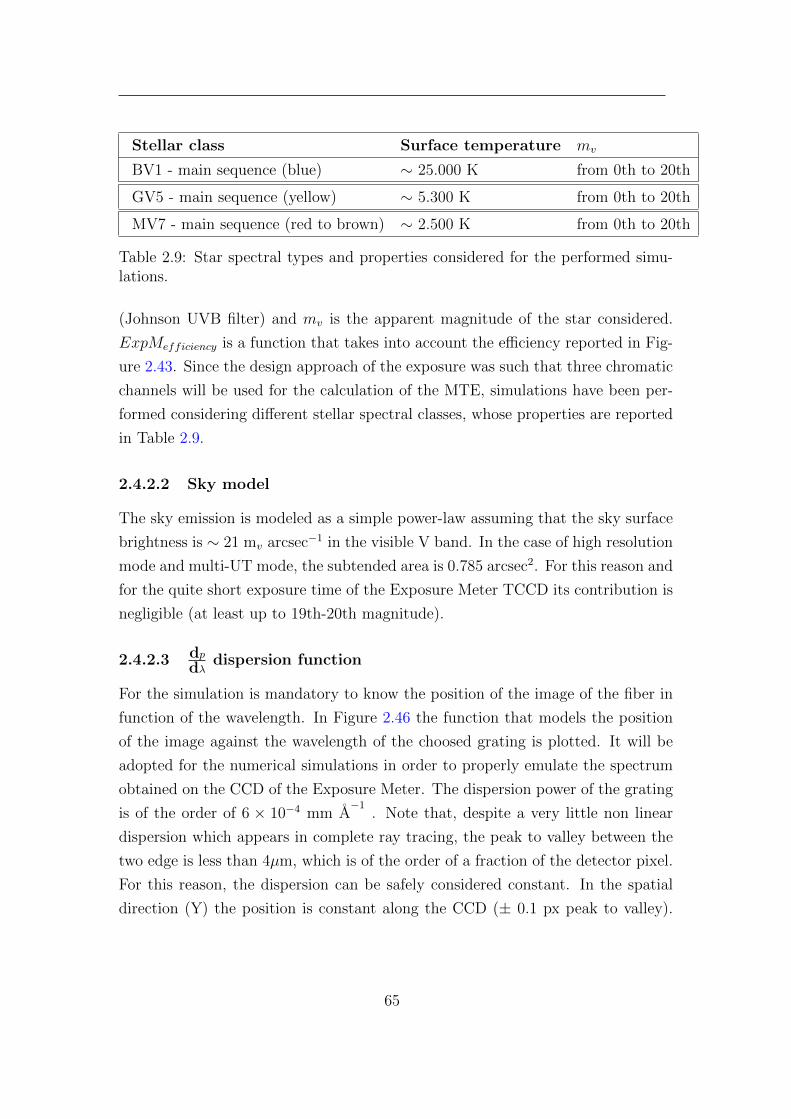
Stellar class Surface temperature mv

BV1 - main sequence (blue) ∼ 25.000 K from 0th to 20th

GV5 - main sequence (yellow) ∼ 5.300 K from 0th to 20th

MV7 - main sequence (red to brown) ∼ 2.500 K from 0th to 20th

Table 2.9: Star spectral types and properties considered for the performed simu-lations.

(Johnson UVB filter) and mv is the apparent magnitude of the star considered.

ExpMefficiency is a function that takes into account the efficiency reported in Fig-

ure 2.43. Since the design approach of the exposure was such that three chromatic

channels will be used for the calculation of the MTE, simulations have been per-

formed considering different stellar spectral classes, whose properties are reported

in Table 2.9.

2.4.2.2 Sky model

The sky emission is modeled as a simple power-law assuming that the sky surface

brightness is ∼ 21 mv arcsec−1 in the visible V band. In the case of high resolution

mode and multi-UT mode, the subtended area is 0.785 arcsec2. For this reason and

for the quite short exposure time of the Exposure Meter TCCD its contribution is

negligible (at least up to 19th-20th magnitude).

2.4.2.3 dpdλ

dispersion function

For the simulation is mandatory to know the position of the image of the fiber in

function of the wavelength. In Figure 2.46 the function that models the position

of the image against the wavelength of the choosed grating is plotted. It will be

adopted for the numerical simulations in order to properly emulate the spectrum

obtained on the CCD of the Exposure Meter. The dispersion power of the grating

is of the order of 6 × 10−4 mm A−1

. Note that, despite a very little non linear

dispersion which appears in complete ray tracing, the peak to valley between the

two edge is less than 4µm, which is of the order of a fraction of the detector pixel.

For this reason, the dispersion can be safely considered constant. In the spatial

direction (Y) the position is constant along the CCD (± 0.1 px peak to valley).

65

Figure 2.46: ESPRESSO Exposure meter ray tracing function. This functionallows to known the absolute position (in mm respect to the centre of the CCD)of the image against λ with respect to the dispersion axis..

For all of these reasons, the function could be assumed to be of the form

dp

dλ∼ 6× 10−4 mm A

−1(2.29)

2.4.2.4 PSF model of the Exposure Meter optics

Through the adoption of ray tracing (Zemax analysis) the point spread function of

the Exposure Meter has been evaluted. The PSF is quite stable though different

wavelength but slightly differences appear (in the order of few pixels). The PSF is

reasonably assumed to be gaussian. In particular, Figure 2.47 illustrates the PSF

dimension (in um) while Figure 2.48 shows what appears on the detector when an

impulsive signal (Dirac delta-function) is applied in front of the overall exposure

meter optics.

2.4.2.5 Fiber image

The image of the fiber for the considered case (Multi UT mode, Ultra High resolu-

tion 1UT or High resolution 1UT) is modeled through the drawing of the relative

polygon on the detector matrix. They are reported in Table 2.10:

66

Figure 2.47: ESPRESSO Exposure meter PSF FWHM function against λ ina pictorial representation. The slightly difference between the three ESPRESSOmodes are apparent due to different optical path through the overall ExposureMeter subsystem to the detector.

Figure 2.48: ESPRESSO Exposure meter PSF function against λ in a pictorialrepresentation.

67

Mode Description Image

Single 1UT UHR mode Octagonal fiber of 70 µm

Single 1UT HR mode Octagonal fiber of 140 µm

Multi-UT mode Rectangular fiber of ∼ 280 µm

Table 2.10: Image fibers on the focal plane and configuration.

2.4.2.6 Image on the focal plane

At the level of the detector the images of the fibers reported in Table 2.10 must be

corrected for the PSF function described in the previous sections. The equation1takes into account the canonical definition of convolution in a discrete domain:

Imagedetector(i, j) = Imagefiber⊗PSF (λ) =

j=+∞∑

j=−∞

i=+∞∑

i=−∞Image(i, j)×PSF (m−i,m−j)

(2.30)

2.4.2.7 Slit loss and dependence on seeing

The seeing at wavelength λ follows the formula

S(λ) = S5500A

(λ

5500A)−

16 (2.31)

where S5500 is the seeing measured at 5500A. This relation obviously affects the

amount of light that enter the spectrograph since the subtended slit is a pinhole

of ∼ 1′′ for the High Resolution mode. For the simulation a mean seeing of 1′′ is

assumed (up to mv ∼ 15, for mv greater than 15 ∼ 0.80′′ seeing is assumed) and

the efficiency due to slit-loss is considered. For instance, at 5500 A the efficiency

for a seeing of 1′′ is about 50%. In other words, only 50% of the scientific light is

1The ∞ obiouvsly appears in the theoretical definition. It will be substituted with thedetector dimensions.

68

Figure 2.49: Seeing vs slit efficiency curve adopted for simulations

able to reach the spectrograph while the remnant photons are back reflected for

the guiding system Landoni et al. [2012b]; Riva et al. [2012]. The seeing-efficiency

curve is reported in Figure 2.49. The behaviour has been assessed in two ways,

numerical and analytical, in order to ensure a good estimation of the slit loss

related to seeing effect. The analytical expression for the slit loss is given by the

Equation 2.32.

f = 1− 1

exp(√

log 2 ΦfSPΦs

)2 (2.32)

where Φf is the pinhole diameter, Φs is the seeing and SP is scale plate of the

optical system.

2.4.2.8 CCD configuration

The frequency for the readout of the technical CCD of the Exposure Meter has

been evaluated taking into account noises from the detector, accuracy on the mea-

surement on the flux and computational overhead. In Table 2.11 are reported the

readout frequencies adopted for the simulation that are a baseline for the on-sky

regime (note that T is the exposure time of scientific object).

2.4.2.9 Detector simulation for performances evaluation

This section presents the algorithm adopted to generate a generic image of the

Exposure Meter CCD detector. The result is used in order to evaluate the per-

formance of the overall system. For numerical reason, the spectrum is simulated

69

RV UTs mv limit Read frequency CCD gain and bin

10 cm s−1 1UT - mv 10 T/1000 or less High , 2x2 bin1 m s−1 1UT - mv 15 T/100 or less Low , 2x2 bin10 m s−1 1UT - mv 20 T/10 Low, 2x2 bin5 m s−1 multiUT - mv 20 T/10 ∗ (nUT ) Low, 2x2 bin

Table 2.11: CCD configuration for the Exposure meter. T is the scientific exposuretime and nUT is the number of UTs considered in the case of multiUT observationmode

dividing in bin of ∼ 20A. Starting from the definition of the received differential

flux, wavelength dispersion and PSF a CCD is generated as follow:

1. Compute the number of photon received from the scientific object in a bin

of 20 A by the integration of Equation 2.27. In particular, the total number

of photon received in a 20 A wide bin is

phstartbin =

∫ binend

binstart

B(λ, T )× ExpMefficiency(λ)× λ

hc× φ? × 10−

mv2.5 dλ (2.33)

2. Compute the number of photon received in a bin of a 20 A from the sky by

the integration of the formula

phstartbin =

∫ binend

binstart

2× 10−17 × ExpMefficiency(λ)× λ

hc× φ? × 10−

mv2.5 dλ

(2.34)

The differential flux of 10−17 erg cm−2 s−1 A−1 correspond to the mean sky

background level at ESO Paranal .

3. Draw the image of a fiber (according to which mode is under simulation, see

Table 2.10) in the detector at the position binstart+binend2

adopting the relation

( λ∆λ

) reported in Figure 2.46 and imposing that the total number of counts

is such that it is equal to the number of scientific photon plus the photons

received from the sky (energy conservation). Uniform illumination of the

fiber image is assumed.

70

4. Apply Equation 2.30 in order to convolve the drawn image with the instru-

mental PSF response at wavelength binstart+binend2

5. Add the result to the overall image (which contains the draws of each fiber

in their proper positions).

6. Repeat from step 1 until binend = 8000 A.

7. Apply the binning adopting a resize of the image.

8. Multiply the overall results for the integration time considered.

At this point, the image generated is saved and stored for further computation

(in particular for the theoretical MTE, that must be compared with the measured

one after detector noises) and the noises from the detector are generated in the

same way that it is explained in Section 2.3.5.1. In Figure 2.50 it is reported

the result of the simulation of the Exposure Meter detector for an MV5 spectral

type class with apparent magnitude mv = 15. The first panel shows the obtained

detector at the end of the generation (with noises) while the second panel shows

the extracted spectrum (in ADU).

2.4.3 Simulations results and expected performances

The performance of the exposure meter, in terms of accuracy and precision of the

MTE calculation, has been evaluated starting from the most common scientific

cases requirement. In particular, the simulation framework has been stressed in

two different situations: a zero order evaluation in which it is assumed to

observe the scientific target with no perturbation at the level of the atmosphere

or on the instrument itself and a second order evaluation in which a chromatic

perturbation is considered. As noted in the previous sections, when a chromatic

perturbation occurs, the received flux is dimmed especially in the red part of the

received light. This situation is typical when observing the target through a thin

cloud.

As an overall consideration, the flow diagram of Figure 2.53 reports in detail

how a generic simulation of a scientific exposure has been implemented. Briefly,

knowing the required exposure time for reaching desired radial velocity accuracy,

71

Figure 2.50: Simulation of a spectrum obtained in the exposure meter for a Mstar of mv = 15 assuming seeing of ∼ 1.00′′

the TCCDs of the Exposure meter are read out (in this case, simulated) and stored

for the final computation of the MTE. The integration times (readout frequencies)

of the TCCD are investigated in Table 2.11. In particular, the accuracy on RMS

radial velocity on the scientific spectrum is defined as

rms(m s−1)photon =K

S/N5500A

(2.35)

where K is a constant which depend on the characteristic of the spectrograph (e.g.

resolution, detector noises, etc.). For instance, as a rule of thumb, in the case of

HARPS [Mayor et al., 2003] for a G2V star a RV of ∼ 1 m s−1 is reached when

the S/N is about 100 per pixel, as illustrated by Equation 2.35 assuming K = 100.

The approximate exposure time vs magnitudes are depicted in Figure 2.52 and

Figure 2.51 (Pepe et al 2013, ESO Messenger in press). In particular, Figure 2.52

refers to 1UT mode while Figure 2.51 to multiUT (4) configuration mode.

Finally, the simulation software performs the calculation of the MTEs in each

72

Figure 2.51: Simulation for the exposure time vs magnitude in multiUT mode.Purple solid line represent texp = 60 s, blue is texp = 1200 s and red is texp = 3600s.

Figure 2.52: Simulation for the exposure time vs magnitude in singleUT mode.Legend is the same of Figure 2.51

73

Figure 2.53: Flow chart for the strategy adopted for the scientific simulation.Each simulation is repeated 100 times in order to investigate general statisticalproperties.

Figure 2.54: ESPRESSO Exposure Meter channels.

channel on ideal ccd (noise free) in order to evaluate its actual value, and on real

ccd with relative noises (as explained in the previous sections). The differences

between the actual value and the simulated one (after noises) is then converted

in RV accuracy error induced by the exposure meter assuming that, in the worst

case, an error of 0.6s corresponds to 1 cm/s in the RV measurement. This is, of

course, the worst case since the value depends on the declination of the target.

For the simulation, dependences on < α, δ > are not investigated.

Simulations are repeated 100 times in order to investigate the r.m.s. error

and the general behaviour of the system. The channels, which simulations refer

74

to, are indicated by the pictorial representation of Figure 2.54. We stress again

the fact that the dispersion axis is inverted at the level of the focal plane in

which the detector lies (from red to blue). It is also important here to recall

the general aim and algorithm behind each simulation. In particular, starting

from the scientific exposure time (T ) needed to reach the photonics accuracy in

function of the magnitude target (see e.g. Figures 2.51, 2.52) n noise-free images

with integration time of Tn

(see Table 2.11) are generated (and possibly blurred

in case of perturbation). Then, the MTE (which is the actual noise free value) is

computed. The n CCD images passes throughout the chain of all noises that must

be considered (photon noise, dark current, RON, etc) following the simulation

procedure also adopted in par. 2.3.5. The MTE is then calculated on the actual

(noisy) CCD images. The difference between the actual value of MTE and the

measured one is then computed and converted in RV error according to the fact

that 0.6s of error is about 1 cm s−1 on the measured star RV. The overall process

is repeated 100 times in order to investigate statistical properties (in terms of

rms, for example). Results are presented both in tabular and graphical format.

The data reduction of CCDs frames is assumed to be easy to compute and no

particular tasks are considered at this level of approximation. In particular, for

each frame the background is computed in a small region away from the spectrum

(median value of about 10x10 pixels) and then it is subtracted from the overall

frame. The fluxes in each channel (used for the computation of the MTE) are then

obtained summing up pixels belonging to that channel (column of the CCD). In

order to enhance the SNR for very faint sources it is suggested to use only the

central 3 or 5 lines of the spatial axis of CCD since their SNR is sufficient enough

for the computation of MTE. As in the case of aperture photometry, trying add

more pixels for faint sources also increase the noises although much more signal is

contained in the aperture.

2.4.3.1 First scientific case - 10 cm s−1 RV accuracy

In order to evaluate the performance of the designed Exposure Meter for the 10

cm/s scientific goal, the simulations start with the assumption of the integration

time needed for reach this accuracy at the level of the scientific spectrum (from

75

Figure 2.55: Behavior of the perturbation as seen on the CCD aboard the Expo-sure Meter.

now, referred as photonic accuracy). In particular, the limit magnitude for the 10

cm/s is mv = 10 since the required integration time for the photonic accuracy of

10 cm/s is about 1.6 hours. For mv < 10 the error induced on the calculation of

the MTE by the Exposure Meter is negligible (<< 1 cm/s) and the accuracy on

the scientific spectrum is always shot-noise limited. Moreover, for magnitude mv

< 2 the exposure meter is not required since the integration time should be very

short (less than 10 seconds). However, since in the optical design a filter wheel has

been implemented the Exposure Meter could be used with a read out frequency

limited by the maximum sampling frequency of the camera (12 fps, for instance)

or less if needed.

For mv = 10, the limit case, two simulation has been assessed. In the first one,

no perturbation are applied on the system or on the atmosphere. Results are

presented in Figure 2.57 and 2.58 and Table 2.12 and 2.13 . In particular, for

the 100 simulations the error induced by the Exposure Meter on the channels are

presented in the boxes of Figure 2.57 for the spectral type B,G and M investigated

while r.m.s. error are tabulated in Table 2.12 and 2.13 . The second case considers a

chromatic perturbation modelled by the function of Figure 2.55 where its behaviour

can be seen. The effect of the perturbation on the spectra at the level of the

exposure meter, plotted against time, could be spotted in Figure 2.56. The second

order simulations carried out also adopt symmetric perturbation in time, in order

to better emulate the actual sky condition on different exposures.

76

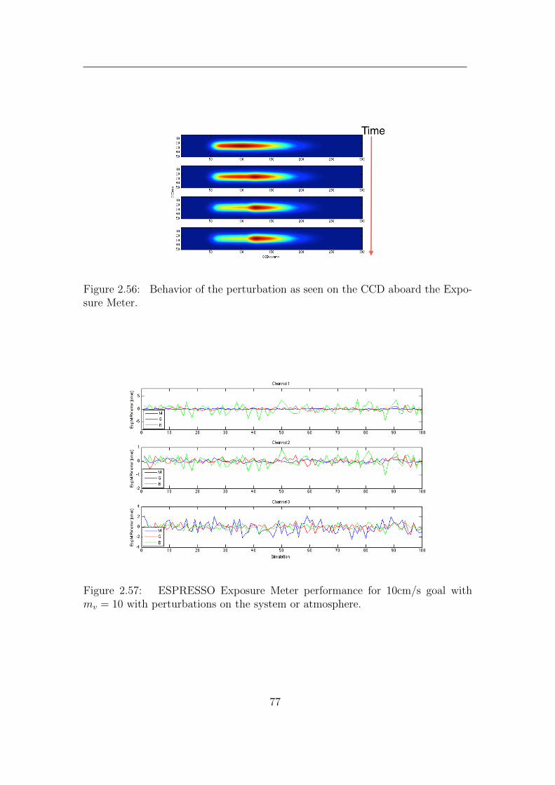
Figure 2.56: Behavior of the perturbation as seen on the CCD aboard the Expo-sure Meter.

Figure 2.57: ESPRESSO Exposure Meter performance for 10cm/s goal withmv = 10 with perturbations on the system or atmosphere.

77

Channel / Spectral type B G Mr.m.s error on Channel 1 1.2 cm/s 0.5 cm/s 0.1 cm/sr.m.s error on Channel 2 0.3 cm/s 0.2 cm/s 0.2 cm/sr.m.s error on Channel 3 0.4 cm/s 0.5 cm/s 1.3 cm/s

Table 2.12: Root mean square error for 10cm s−1 scientific goal, mv = 10 and noperturbation on the system

Channel / Spectral type B G Mr.m.s error on Channel 1 2.5 cm/s 0.8 cm/s 0.1 cm/sr.m.s error on Channel 2 0.3 cm/s 0.3 cm/s 0.2 cm/sr.m.s error on Channel 3 0.5 cm/s 0.6 cm/s 1.5 cm/s

Table 2.13: Root mean square error for 10cm s−1 scientific goal, mv = 10 withperturbation applied on the system

Is a chromatic exposure meter a must-have device ? Comparison

between spectrum and white light

It is now important to note that the use of the small spectrum at the level of the

exposure meter significantly reduce the error on the MTE when such a perturba-

tion occurs at the level of the atmosphere. In particular, if the MTE is calculated

only on the integrated white light for this simulation it gives a value of 2.9377e+03

s. The MTE, since a perturbation occurred, is obviously different from the simple

half value of the integration time (which is 3000s in this case).

However, when inspecting the MTE on channel 1(red) and channel 3 (blue) the

results are significantly different since in the red band less light reached the instru-

ment due to the perturbation (note that the situation could be exactly symmetric

if the perturbation occurs in the blue part instead of happening in the red one. In

detail, MTE(Ch1) = 2.6550e+03 and MTE(Ch3) ∼ 3000s. Now, comparing the

MTE on channel1 with the MTE on white light gives a difference of ∼ 282 s that

corresponds to a worst case error of ∼ 4.7 m/s. For this reason, the correction of

the relative shift of a stellar absorption line in the red region of the spectrum using

only the MTE calculated on the integrated light would cause an error of several

meters per second. These kind of consideration also apply for the next simulations

of 1m/s and 10 m/s of scientific goals. In the case of multi-UT mode no perturba-

78

Figure 2.58: ESPRESSO Exposure Meter performances against a chromatic per-turbation on the red part (cloud passing through).

tion are applied since the light comes from different arms of the instrument and

the sky conditions could also be slightly different.

2.4.3.2 Second scientific case - 1 m s−1 RV accuracy

As in the previous case, two kind of simulations have been carried out. For 1 m

s−1 the limit magnitude is mv = 15 since the exposure time needed to reach the

desired accuracy is about 1.5 hours. For magnitude mv < 15 the error induced

by the exposure meter is negligible in comparison to the requirement of the 1 m

s−1 accuracy and, in any case, the error induced by this subsystem is lower than

the photonic precision reached at the level of the scientific spectrum. Results are

reported in Figures 2.59, 2.60 and Tables 2.14, 2.15.

The adoption of a spectrum, as illustrated in the previous scientific case, re-

duced significantly the error when the chromatic perturbation occurred. In par-

ticular, if the system only adopt the MTE on the integrated white light, the error

on the red part of the spectrum for inaccurate Earth-motion correction would be

of about several meters per second.

79

Figure 2.59: - ESPRESSO Exposure Meter performance for 1m/s scientific goal.No perturbations are applied to the system

Figure 2.60: - ESPRESSO Exposure Meter performance for 1m/s scientific goalwith perturbations applied to the system

80

Channel / Spectral type B G Mr.m.s error on Channel 1 0.30 m/s 0.1 m/s 0.05 m/sr.m.s error on Channel 2 0.1 m/s 0.05 m/s 0.1 m/sr.m.s error on Channel 3 0.12 m/s 0.15 m/s 0.2 m/s

Table 2.14: Root mean square error for 1 m s−1 scientific goal, mv = 15 withoutperturbation applied on the system

Channel / Spectral type B G Mr.m.s. error on Channel 1 0.37 m/s 0.20 m/s 0.1 m/sr.m.s. error on Channel 2 0.10 m/s 0.10 m/s 0.2 m/sr.m.s. error on Channel 3 0.10 m/s 0.15 m/s 0.25 m/s

Table 2.15: Root mean square error for 1 m s−1 scientific goal, mv = 15 withperturbation applied on the system

2.4.3.3 Third scientific case - 10 m s−1 RV accuracy

For the 10 m s−1 accuracy scientific case the limit magnitude is about 19-20 (worst

case considered for the simulation). For brighter object (e.g. mv = 16, 18) the error

induced by the exposure meter in its channels is negligible (less than 1 m s−1)

compared to the photonic accuracy reached at the level of the scientific spectrum.

For this reason, the measurements are shot noise limited and not affected by the

error that occurs on the MTE computed by adopting the designed Exposure Meter.

Since, in this case, the requirements are quite loose and reasonable perturbations

affects the MTE for an amount that is less than 10 m s−1 only a zero order

simulation has been carried out. Results are reported in Figure 2.61 and Table

2.16.

Channel / Spectral type B G Mr.m.s error on Channel 1 2.5 m/s 2.2 m/s 0.7 m/sr.m.s error on Channel 2 1.0 m/s 0.95 m/s 1 m/sr.m.s error on Channel 3 1.5 m/s 2.0 m/s 3 m/s

Table 2.16: Root mean square error for 10 m s−1 scientific goal, mv ∼ 20 withoutperturbation applied on the system

81

Figure 2.61: - ESPRESSO Exposure Meter performance for 10 m/s scientific goalwithout perturbation

2.4.3.4 Multimode setup - An introduction to 5 m s−1 RV accuracy

case

In the case of multi-UT observation mode, the spectrograph and the exposure

meter collect the light from the scientific target from more than 1 telescope. For

this reason, the flux received is n-times that received from only one UT. As a

representative case, a simulation for an mv = 20 object has been carried out. In

particular, in order to reach a photonic accuracy of 5 m s−1 an exposure of 3h is

required with only one UT. This integration time is quite high in comparison to

a typical exposure time in an Observation Block (less than 2 hours). However,

adopting 4-UT configuration the time needed is reduced by a factor of 4 since 4

telescopes feed the spectrograph simultaneously. In Figure 2.62 and Table 2.17 are

reported the errors induced by the exposure meter with a configuration of 4-UT,

adopting parameters reported in Table 2.11.

Channel / Spectral type B G Mr.m.s error on Channel 1 3.2 m/s 3.0 m/s 1.1 m/sr.m.s error on Channel 2 1.6 m/s 2.4 m/s 2.0 m/sr.m.s error on Channel 3 1.6 m/s 2.8 m/s 3.0 m/s

Table 2.17: ESPRESSO Exposure Meter r.m.s. error on the three channel inmulti-UT configuration

82

Figure 2.62: - ESPRESSO Exposure Meter r.m.s. error on the three channel inmulti-UT configuration

83

Chapter 3

Application of spectroscopy to BL

Lacertae objects: from low to

medium-high resolution. The case

of FORS2 and X-Shooter

3.1 An introduction to AGN

3.1.1 What is an AGN ?

Active galactic nuclei (AGN) are astrophysical sources characterised by a strong

emission of electromagnetic radiation. The power of which is of the order of 1042 -

1048 erg s−1. The emitting region is extremely compact and usually its volume is

about 1 pc3. The radiation is emitted across the overall electromagnetic spectrum,

from radio to Very High Energy (VHE) γ-rays. For the brightest sources the

bolometric luminosity is of the order 1047 erg s−1. According to the Eddington

luminosity,

Lbol ≤ LEdd =4πGM•mpc

σt(3.1)

which implies that M•≥ 7× 108 M. The gravitational radius Rs for this mass

is Rs = 2GMc2

that turns out to be Rs = 2.1 × 1014 cm. This value is compa-

rable with the one reported for the emitting region estimated through the time

84

Figure 3.1: Effective potential of a test particle test with mass M in orbit arounda Schwarchild Black Hole.

scale variability of the source (assuming causality connection). For this reason,

the currently accepted paradigm for AGN emission is that the released power is

supported by the accretion of matter onto a Super Massive Black Hole (SMBH)

which dissipates its potential gravitational energy . If the central black hole has a

mass M•, the energy released per unit mass is then

∆Eacc =GM

Risco

(3.2)

where Risco is the inner stable circular orbit. Assuming a spherical Schwarchild

metric, it is safe to assume Risco ∼ Rgrav = 2GMc2

and the energy released per

unit mass is ∆E = ε∆Mc2 ∼ 0.1mc2. The mass-energy conversion efficiency ε is

maximum when a highly rotating Kerr black hole with angular momentum J is

consider. In this case, the energy released per unit mass would be ∆E ∼ 0.40∆Mc2

(see also Figures 3.2, 3.2).

It is also important to note that the inner stable circular orbit is also a function

of the Black Hole spin, as illustrated in Figure 3.2.

For QSOs objects, where typical luminosities are of the order of L∼ 1046 erg s−1

85

Figure 3.2: ISCO in function of the black hole spin a.

the accretion rate requires ∆M of 1 M yr−1 while for X-ray binaries luminosites

are of the order of L∼ 1039 erg s−1 implying 10−7 M yr−1. The mass accretion rate

is also related, as illustrated in previous equations, to the Eddington Luminosity.

In fact, ∆M is related to the accretion luminosity as ∆M = Laccεc2

. The maximum

luminosity is related to the Eddington luminosity, which is the maximum power

sustained by the AGN (balance between force due to radiation pressure and force

of gravity). For this reason, combining equations one obtains

∆M =Laccεc2

<4πGMmp

εcσt(3.3)

which implies that the black hole growth is governed by the equation M ≤M0etτ

M(t) ≤M0etτ (3.4)

where τ is the Salpeter growth time defined as

τ =εcσt

4πGmp

∼ 5× 107yr (3.5)

86

3.1.2 Emission mechanism - Thermal emission from accre-

tion disk, broad line and narrow line regions

Figure 3.3: Spectral energy distribution of the radio quiet QSO Mkn586. The UVbump due to thermal radiation generated by the accretion disk is clearly visible inthe region 1015 - 1015 Hz.

In general, the optical to UV spectrum of QSOs and AGN is dominated by

thermal emission deriving from the accretion disk which is formed by accreted

matter. The material, spiralling through the disk, releases gravitational energy

and angular momentum before reaching the event horizon. The energy loss due

to viscosity and friction could be safely modelled as an ensable of thin ring, all

emitting as blackbody radiator. In particular, the energy released between r and

r + dr in the elementary interval time dt is

dE

dt=

3GM∆M

4πr3×(

1−(rinr

)1/2)

(3.6)

Integrating all over the radii one has

L =

∫ +∞

rISCO

2πr3GM∆M

8πr3×(

1−(rinr

)1/2)

dr (3.7)

87

According to the Virial Theorem, the total emitted luminosity could also be ex-

pressed as

L =1

2

GM∆M

rinerg s−1 (3.8)

which simply states that half of the power released from accretion goes into radi-

ation produced by friction in the accretion disk. As spotted before, each disk of

radii dr emits as a blackbody radiator. For this reson, the luminosity of the disk

between r and r + dr is

dL =GM∆M

2rdr = 2(2πrdr)σT 4(r) (3.9)

The temperature T (r) is could then be expresses ad

T (r) =

(3GM∆M

8πσR3int

) 14(Rint

r

) 34

K (3.10)

Differentiating T (r) with respect to dr it is possible to estimate the accretion disk

temperature. In particular

Tdisk(r) =dT (r)

dr= 0 =

(24c6∆M

125πσG2M2

) 14

=

(95c5

125kσGM

1

ε

LdiskLEddington

) 14

(3.11)

Considering a Kerr black hole with maximum angular momentum J , Rint ∼ 58RSchw

and a typical mass of a SMBH (∼ 108 M) Tdisk ∼ 7× 105K. At the level of the

spectrum, the contribution of the accretion disk could be spotted by the so called

big blue bump that can be easily observed in QSOs UV spectra. An example of

a SED where the big blue bump is clearly detectable is reported in Figure 3.3.

The size of the emitting region in common Active Galatic Nuclei is of the order of

our Solar System, producing the light of a nearly a trillion (1012 ) stars in a very

small compact region. This evaluation is also obtained through the study of short

time-scale variability of the nuclei brightness.

3.1.2.1 Broad line region

In the accepted paradigm of AGN structure, the accretion disk is surrounded by

relative cold gaseous halos which generate emission lines by fluorescence in gas

88

clouds surrounding the central black hole. In fact, in most AGNs the UV, visible

or infrared spectra show broad line component (1000 ≤ FWHM 20000 ≤ km s−1)

typical of photoionized gases at T ∼ 104 K. The average of different spectra of

AGNs shows that BLR lines are extremely similar over a wide range of luminosity

as illustrated in Figure 3.4.

48

Luminosity Effects•

Average line spectra of AGNs are amazingly similar over a wide range of luminosity.

•

Exception: Baldwin Effect–

Relative to continuum, C IV

O1549 is weaker in more luminous objects

–

Origin unknown 6'66FRPSRVLWHVE\OXPLQRVLW\9DQGHQ

%HUN

HWDOFigure 3.4: Emission lines in the BLR superposed on different spectrum of QSOswith different absolute luminosities.

The broad line profiles could also be exploited in order to study kinematics

properties of the source since, for the most part, the profiles tell us about the

kinematic of the BLR itself. For instance, a very common technique based on

Virial Theorem allows to estimate the mass of the central engine starting from

the profile of the BLR which reflect the dynamic of the gravitational potential

(related to the FWHM velocity ∆v) of the central black hole, as illustrated in

Equation 3.12 (where R is the BLR radius which can be inferred from multiple

scale relations, see e.g. Kaspi et al. [2005]).

Moreover, a relatively small subset of AGNs show double-peaked BLR profiles

that are characteristic of rotation (see Figure 3.5). This characteristic tell us that

89

Double-Peaked Emission Lines•

A relatively small subset of AGNs have double-peaked profiles that are characteristic of rotation.–

Tendency to appear in low accretion-rate objects

–

Disks are not simple; non-axisymmetric.

–

Sometimes also seen in difference or rms spectra.

1*&6WRUFKL%HUJPDQQHWDOFigure 3.5: Multiepoch spectrum of the QSO NGC1097 where double peaked broad

Hα is clearly spot.

probably accretion disks are not symmetric or axisymmetric.

M• ∝∆V 2R

G(3.12)

As explained, emission lines in the BLR are generated through the photoion-

ization of the gas from the continuum generated by the accretion disk. Since no

forbidden lines are detectable in the BLR densities are quite high, of the order of

1010 ne cm−3. The ionization level of the BLR is usually defined as :

U =1

nec

∫ +∞

13.6eV

Fνhνdν (3.13)

U depends on the intrinsic luminosity of the source Fν , on the distance from the

ionizing source and on the density ne of free electrons. The ionization parameter

could also be derived through indirect mesaurement. In particular, it may be

derived from the intensity ratio of the [OIII] λ5007 and [OII] λ3727 [Penston

et al., 1990]. In details, considering the equation of ionization balance for species

90

i one has

N0i =

1

4πr2Ne

∫ +∞

νi

Lνhν

ανiαidν = N+

i Neαi (3.14)

The ratio of number of particles in the ionized state, to that in the non-ionized

state is thus

N+i

N0i

=1

4πr2Ne

∫ +∞

vi

Lνhν

ανiαidν (3.15)

The recombination coefficients, αi are independent of photon frequency. Defining

a ionization parameter Γ which is species-independent as

Γ =1

4πr2Nec

∫ +∞

νo

Lνhνdν (3.16)

With this model, it is possible to refer to the ratio of ionization, which is species

dependent, as

N+i

N0i

=ανiαicΓ (3.17)

The integral in 3.16 is the number of ionizing photons coming from the source.

When divided by 4πr2, this becomes the surface density of ionizing photons. In

the case where Ne ∼ Np, this density of photons is then compared with the density

of material. In other words, Γ describes how many ionizing photons there are per

atom.

Γ =Q(H0)

4πr2cNH

∼ 〈Nph〉〈NH〉

(3.18)

Broad lines typically seen in quasars only occur for permitted and semi-permitted

transitions. In addition to the emission lines of the hydrogen (Lyman and Balmer

series) and helium, the commonly ions include

• Permitted lines of lithium-like ions (from s-shell electrons). For instance, the

strongest lines are C IV λ1549, N V λ1240, O VI λ1035, Mg II λ2798, and

Si IV λ1400.

• Permitted lines of Fe II that are usually blended due to instrument resolu-

tion and instrinsically high density at high temperature which cause doppler

91

broadening and blending. In the broad line region, forbidden lines are sup-

pressed. Combining this fact with the presence of semiforbidden lines places

a constrain on the density of the BLR. The density of the broad line region

is estimated to be of the order of 108 or 109 atom cm−3.

The temperature of the BLR is assumed to be Te ∼ 15000 K. This value is derived

from the ratio of Fe III and Fe II, adopting the Saha equation, and from the

simultaneous presence of the C III] λ 1909 and absence of C III λ977. The mass

and the size of the BLR can be estimated in the following way (for sake of simplicity

we will referr to Hβ hydrogen transition). The luminosity of the Hβ emission line

is defined as

L(Hβ) = NeNpαeffHβhνHβfV (3.19)

where f is the filling factor and V the considered volume. The total mass of the

ionized gas is thus

M = (NpmH +NHemHe)fV ∼ 1.3NpmHfV (3.20)

Combining Equation 3.19 and 3.20 the total mass of the BLR is thus defined as

M = 1.3mHL(Hβ)

NeαeffHβ hνHβ

(3.21)

A typical luminosity for the Hβ emission line is L(Hβ) = 109L. Assuming Ne ∼109 cm−3 the BLR mass turns out to be 40 M. The volume in which this mass

of gas is contained is

V =4

3πr3 =

M

1.4NpmHf(3.22)

The typical radius for the BLR can be also derivated from the equations illustrated

before. In particular, R is defined as

R ∼ 0.015f−13

(109

Ne

) 23

pc (3.23)

Operationally, the BLR radius could also be obtained through the adoption of

scaling relation involving continuum luminosity (e.g λLλ at λ = 5100A, see e.g.

92

Kaspi et al. [2005]). Assuming median value, one has that the BLR size is therefore

only a few tenths of a light year which is unresolvable also with modern telescopes

and innovative instrumentation.

3.1.2.2 The narrow-line region

The Narrow Line Region is located between 10 pc e 1 Kpc from the accreting black

hole. Dispersion velocites inferred from the FWHM of the lines are quite variable

but, in general, they are below 1000 km s−1. A lot of forbidden lines are present in

the NLR spectrum, suggesting the idea that the NLR is a low density region. The

gaseous content in the narrow line region is in general optically thick (τ >> 1).

Nevertheless, in some objects, the high ratio He II λ4686 Hβ allow also to inferr

that optically thin NLR clouds could also exist. The mean electron density and

temperature are of the order of 103 - 104 cm?3 and ∼ 1.5 × 104 K. The ionization

parameter, defined as in the case of BLR, is of the order of 10−2. The NLR is

Broad/Narrow-Line Regions

The Narrow Line Region

The NLR spectrumoptical and UV lines

permitted,semi-forbidden andforbidden lines

IR lines

coronal lines

line profilesline asymmetry (flows)

Broad/Narrow-Line Regions: AGN J.P. Torres-Papaqui Physics of AGN 40 / 41

Figure 3.6: Narrow line region line profile asymmetry. This structure suggestsflows of matter in the active nucleus [Lutz et al., 2000].

organized as a stratified structure. In the inner region, the photoionization of the

low density gaseous nebule is only due to the central accreting black hole. The most

93

intense emission lines that could be measured in the spectrum are the doublet [OIII]

λλ 5007, 4959, [NII] and [SII]. The external region is called Extended Emission

Line Region (EELR). The kinematic deduced from the structure of the narrow

emission lines reflets the potential of the galaxy itself and not the gravitational

potential well of the central black hole, as in the case of the Broad Line region.

It is worth noticily that in some cases, the profile of the emission lines from NLR

are found to be asymmetric suggesting that ouflows due to winds could be present

(see Figure 3.6).

Broad/Narrow-Line Regions

The Narrow Line Region

The NLR spectrumoptical and UV lines

permitted,semi-forbidden andforbidden lines

IR lines

coronal lines

line profilesline asymmetry (flows)

Broad/Narrow-Line Regions: AGN J.P. Torres-Papaqui Physics of AGN 39 / 41

Figure 3.7: Narrow line region line spectrum (NIR and FIR) example from theAGN NGC1078 [Lutz et al., 2000].

As in the case of the Broad Line Region, the mass of NLR can be estimated

from numerous diagnostic ratios measured through properies of the emission lines

(see e. g. [Peterson, 1997]). In particular, typical densities of the NLR are of the

order of 10−3−5 atom cm−3 and its total mass is of the order of several million of

solar masses. A sample spectrum of NLR is shown in Figure 3.7.

94

3.2 The case of BL Lacertae objects

BL Lac objects are a particular class of AGN essentially characterized by [Peterson,

1997]

• Absence or extreme weakness of spectral features in the optical spectrum.

• Flat radio spectrum

• Large and rapid variability in all spectral bands

• High optical polarization

• Large X and γ-ray luminosities

• Superluminal motion

BL Lacs are grouped with Flat Spectrum Radio Quasars (FSRQ), due to the

same characteristics, except for line weakness, into the blazar class. The common

structure of all radio-loud AGNs [Urry and Padovani, 1995] is thought to be given

by a central SMBH, surrounded by an accretion disk and ionized gas clouds, which

emit the spectral lines. As explained in the previous paragraph, these clouds are

divided into a Broad Line Region (BLR), closer to the black hole, and a Narrow

Line Region (NLR), at a greater distance. On the same plane of the accretion

disk, an optically thick torus of gas and dust is also present. The black hole also

powers a relativistic jet, orthogonal to the accretion disk, which accounts for the

large scale radio emission. In this scenario, a BL Lac is seen when the line of sight

is close to the jet direction. The relativistic beaming of the radiation emitted in

the jet easily explains the main characteristics of this class (e.g. the rapid and

large variability, the high polarization, the superluminal motions). Their spectral

energy distribution (SED) is characterized by two broad peaks. The low energy

maximum is usually explained as the synchrotron emission by a population of

highly relativistic electrons accellerated in the relativistic jet, while the higher

energy one is interpreted as Inverse Compton emission of the same population

of electrons interacting with seed photons produced from the synchrotron radia-

tion (Synchrotron Self Compton, SSC) or photons from the external environment

(External Compton), depending on the model [Ghisellini et al., 1998].

95

3.2.1 Characteristic of the BL Lacs optical spectra

The main characteristic of the optical spectrum of BL Lacs is that the lines (from

the BLR, NLR or from its host galaxy) can be very faint, if present at all. For

this reason the first definition of the class required that the equivalent width (EW)

of the strongest emission line should be less than 5A rest frame . This definition

has been often criticized as arbitrary, because it does not correspond to intrinsic

physical differences in the objects. In fact Scarpa and Falomo [1997] showed that

in blazars emission line properties vary smoothly across the 5A limit. Several

others classification criteria where proposed for BL Lacs. For example, Plotkin

et al. [2010] adopted a limit on the intensity of the CaII continuum break around

4000A (CaII break < 25 %) when selecting BL Lacs from the SDSS while Landt

et al. [2004] adopts the relative strength of [OII] and [OIII] narrow lines, but the

question is still open.

Nevertheless, the extreme weakness (or absence) of the lines is easily explained by

the emission mechanism model mentioned above. The light from the host galaxy,

which has been found to be a giant elliptical with Mr = −22.80± 0.10 [Sbarufatti

et al., 2005a] responsible of the absorption lines, and the radiation from the BLR

and NLR (emission lines) in first approximation are emitted isotropically, while

the non-thermal continuum emitted by the jet is doppler-enhanced (δ) due to

relativistic effect (Preceived = δ4Pemitted). When the line of sight is aligned with the

jet and the beaming increases, the line flux remains constant, while the continuum

flux increase reducing the equivalent width of spectral lines. Another paradigm

usually taken into account for explaining the absence of the emission lines from

the Broad Line Region is based on a particular kind of accretion disk, which is

radiatively inefficient. This kind of disk is called ADAF, Advection Dominated

accretion Flow which essentially postulates that most of the accretion power is

not released in the disk (which is geometrically thick and optically thin) but it is

carried away in a direct accretion beyond the event horizon. Further details could

be found in Narayan and Yi [1994] and references therein.

96

3.3 Observing BL Lacs with FORS2@ESO-VLT.

The completion of the sample

3.3.1 Introduction

As illustrated before, BL Lac objects are a particular class of Active Galactic Nuclei

(AGN) characterized by a quasi featureless optical spectra. Their emission is in

fact strongly dominated by the non-thermal continuum arising from the relativistic

jet aligned towards the line of sight of the observer. The featureless nature of their

optical spectra makes the determination of their redshifts (and, as a consequence

of their distance) a very challenging task. Deep imaging studies of BL Lac objects

carried out using both ground based and space observatories show that they are

hosted in luminous giant ellipticals (see e.g. Urry et al. [2000] , Falomo et al.

[2000], Sbarufatti et al. [2005a]). For this reason, in addition to the non thermal

emission, there is always a thermal contribution due to the stellar component of

the host galaxy. Sometimes, like in other AGN, some emission lines generated

by fluorescence in gas clouds surrounding the central black hole, can be present.

Finally as in the case of QSOs, absorption lines due to intervening gas in the halo

of foreground galaxies can be observed in the spectra of BL Lacs (e.g. Stocke and

Rector [1997]). In this latter case, if the BL Lac object does not exhibits other

intrinsic features the intervening absorptions put a lower limit to the redshift of

the source.

In the past decade a number of projects were carried out to determine the redshift

of BL Lac objects. Most of these works were based on optical spectra collected

with 4 m class telescopes, and are therefore limited by relatively low signal-to-

noise ratio, low spectral resolution and limited wavelength range (e.g. Falomo

et al. [1993b]; Stickel et al. [1993]; Veron-Cetty and Veron [1993]; Falomo et al.

[1994b]; Falomo [1996b]; Landt et al. [2001]; Rector and Stocke [2001]).

The detectability of spectral features depends on the brightness of the nuclear

source. During low brightness states, intrinsic absorption features can be more eas-

ily revealed, while during high states one can better discover intervening absorption

systems. Nevertheless, the strong contribution from the non-thermal continuum,

illustrated in the previous paragraph, drastically lowers the equivalent width of the

97

Figure 3.8: Optical spectrum of the BL Lac object (2214-313) in which the featuresassociated to its host galaxy are clearly detected (z = 0.460). See Landoni et al2013, Sbarufatti et al 2009.

Figure 3.9: Flux calibrated (upper panel) and normalized (lower panel) spectrumof 1553+113. The spectrum is lacking any intrinsic spectral feature. Absorptionsfrom our galaxy ISM are labeled in green. The telluric absorption are marked. SeeLandoni et al 2013, Sbarufatti et al 2009.

98

intrinsic spectral features making their detection challenging. For these reasons,

more systematic work aimed at obtain high signal-to-noise spectra of BL Lacs was

started [Sbarufatti et al., 2006]. In particular, exploiting the capabilities of FORS1

and FORS2 at the 8-m Very Large Telescopes (VLT) of the European Southern

Observatory (ESO) spectra for a sample of 69 objects, extracted from the lists of

BL Lacs by Padovani & Giommi Sedentary Survey [Padovani and Giommi, 1995]

, have been secured. This high quality spectroscopic data forms the first collec-

tion of homogeneous and high quality spectra of BL Lacs from which a number of

properties (in addition to the redshift or a redshift lower limit) can be extracted

(the work in part reported in this Thesis).

Figure 3.8 and Figure 3.9 show examples of optical spectra for two BL Lacs

objects . In the first case we report the spectrum of the well known TeV source

PG1553+113 obtained with VLT + FORS2. As shown, no intrinsic features are

apparent yielding this powerful source with an unknown redshift. In the second

case, the absorption features of the host galaxy (CaII H K and the stellar G Band)

of 2214-313 are detected with high confidence allowing us to derive a firm value for

the redshift of the source (more details can be found in this Thesis and on website

archive.oapd.inaf.it/zbllac/).

The content of this Chapter is published in the article ESO Very Large Tele-

scope Optical Spectroscopy of BL Lacertae Objects. IV. New Spectra

and Properties of the Full Sample (Landoni et al. [2013] ) aimed to com-

plete the survey mentioned before and to derive the overall properties of the class

from the complete sample. Throughtout the Thesis, we consider the following

cosmological parameters: H0 = 70 km s−1 Mpc−1, Ωm = 0.27 and ΩΛ = 0.73.

3.3.2 The sample

The sample of BLLs (and candidates) observed with the ESO Very Large Telescope

has been selected from two extended catalog of BLLs: the Padovani & Giommi

(1995) [Padovani and Giommi, 1995] collection and the Sedentary Survey (SS;

Giommi et al. [1999], Giommi et al. [2005]). The first list contains all objects

identified as BLLs, belonging to the complete samples existing at the time of its

compilation, selected in the radio, optical, and X-ray bands (e.g., the 1 Jy survey,

99

Stickel et al. [1991]; Palomar-Green survey [PG]; Extended Medium Sensitivity

Survey [EMSS]). It also includes sources from the Hewitt and Burbidge [1993] and

[Veron-Cetty and Veron, 2003] catalogs. More details are given in Landoni et al.

[2013] and Sbarufatti et al. [2006].

Figure 3.10: Top panel: V-magnitude distribution of the observed BLLs in thesample selected adopting the criteria described in the text. Bottom: Fraction ofobjects of known redshift as a function of the magnitude. Further details andreferences are reported in Sbarufatti et al. [2006] and Landoni et al. [2013].

According to the 11th Veron-Cetty catalog of AGN objects [Veron-Cetty and

Veron, 2003] at the time of the first scheduling of the overall campaign in 2003,

797 sources were known as candidate or confirmed BL Lacs and 313 objects of

the list were left without a reliable measure of their redshift. In order to select

sources well observable from the Paranal site only the sources with δ < 15 were

been considered. With this cutoff a total of 169 BL Lacs objects still remains of

unknown redshift. From this set, objects with apparent magnitude V < 21 were

selected in order to secure an acceptable SNR ratio spectrum for each source. The

campaign obtained time for the observation of 88 sources, selected combining the

100

∼ 155 objects well observable with FORS2 from the catalogs mentioned above.

In Figure 3.10 we report a synthetic statistic about the distribution of the BLL

observed magnitude versus the redshift hit rate for redshift bin.

101

3.3.3 The complete BLL@FORS2 sample observed at FORS2-ESO VLT

Source Name z V α SNR References

PKS 0019+058 > 0.49 18.10 0.65 120 Sbarufatti et al 2009 - AJ 137:337-346

PKS 0047+023 >0.82 19 0.61 80 Sbarufatti et al 2006 AJ 132:1-19

PKS 0048-09 >0.30 16.10 0.95 250 Sbarufatti et al 2006 AJ 132:1-19

GC 0109+224 >0.10 14.9 0.85 200 This work

GC 0109+224 > 0.25 14.80 0.82 380 Sbarufatti et al 2009 - AJ 137:337-346

RBS 0231 > 0.41 18.90 1.00 20 Sbarufatti et al 2009 - AJ 137:337-346

PKS 0140-059 > 0.46 19.20 0.45 65 This work

1RXS J022716.6+020154 0.457 18.90 0.83 100 Sbarufatti et al 2005 AJ 129:559-566

RBS 0337 0.232 16.50 1.30 130 This work

PKS 0302-623 1.350 18.30 150 This work

PKS 0306+102 0.862 21.20 0.47 20 Sbarufatti et al 2005 AJ 129:559-566

1RXS J031615.0-26074 0.443 18.10 1.20 130 Sbarufatti et al 2005 AJ 129:559-566

PKS 0338-214 0.223 17.90 0.27 210 Sbarufatti et al 2005 AJ 129:559-566

RBS 0499 > 0.45 19.10 1.00 40 This work

PKS 0410-519 1.254 17.40 70 This work

PKS 0420+022 2.278 18.80 90 Sbarufatti et al 2006 AJ 132:1-19

PKS 0422+00 >0.31 16.30 0.88 230 Sbarufatti et al 2006 AJ 132:1-19

PKS 0426-380 1.105 18.60 0.70 100 Sbarufatti et al 2005 AJ 129:559-566

PKS 0439-299 > 0.68 20.80 0.30 30 This work

102

PKS 0443-387 0.537 17.30 140 This work

RBS 0589 >0.45 17.50 1.20 130 This work

ZS 0506+056 > 0.15 16 0.92 200 This work

PMN J0529-3555 0.323 20.20 30 This work

PKS 0539-543 1.191 17.90 70 This work

1RXS J055806.6-383829 0.302 16.80 1.21 280 Sbarufatti et al 2005 AJ 129:559-566

PKS 0607-605 1.1 18.10 50 This work

MS 0622.5-5256 0.513 19.90 0.90 45 This work

PKS 0627-199 >0.63 19.30 0.56 50 Sbarufatti et al 2006 AJ 132:1-19

PKS 0723-00 0.127 16.00 250 Sbarufatti et al 2006 AJ 132:1-19

PKS 0735+17 > 0.18 16.30 0.84 160 This work

PKS 0808+019 1.148 18.40 0.93 140 Sbarufatti et al 2005 AJ 129:559-566

OJ-131 0.539 17.90 0.44 100 This work

PKS 0823-223 >0.911 15.70 0.47 220 Sbarufatti et al 2009 - AJ 137:337-346

H0841+1256 >2.48 18.10 100 Sbarufatti et al 2006 AJ 132:1-19

1WGA J1012.2+063 0.727 17.60 0.80 200 Sbarufatti et al 2005 AJ 129:559-566

RX J1022.7-0112 > 0.30 17.10 1.34 100 This work

RX J1023.9-4336 > 0.24 16.30 1.28 200 This work

PKS 1057-79 0.581 16.20 0.73 90 Sbarufatti et al 2009 - AJ 137:337-346

PKS B1056-113 > 0.27 17.20 0.66 100 This work

1ES 1106+244 > 0.37 18.70 0.78 40 This work

RX J1117.0+2014 0.140 16.50 0.98 130 This work

103

PKS 1145-676 0.210 18.60 80 Sbarufatti et al 2009 - AJ 137:337-346

OM 280 > 0.20 16.10 0.79 100 Sbarufatti et al 2009 - AJ 137:337-346

1ES 1212+078 0.137 17.40 1.17 100 Sbarufatti et al 2006 AJ 132:1-19

RX J1241.8-1455 > 0.32 17.30 1.05 140 This work

1ES 1239+069 > 0.47 18.70 1.00 50 This work

1ES 1248-296 0.382 19.50 0.92 50 Sbarufatti et al 2006 AJ 132:1-19

PKS 1250-33 0.856 20.10 0.48 30 Sbarufatti et al 2005 AJ 129:559-566

PKS 1256-229 0.481 17.90 0.31 170 Sbarufatti et al 2005 AJ 129:559-566

4C 12.46 > 0.37 18.20 0.43 70 This work

1ES 1320+084N 1.50 19.00 50 Sbarufatti et al 2006 AJ 132:1-19

PKS 1349-439 >0.39 16.90 0.82 240 Sbarufatti et al 2006 AJ 132:1-19

OQ 012 > 0.63 18.60 0.29 120 Sbarufatti et al 2009 - AJ 137:337-346

OQ 240 > 0.10 14.60 1.00 170 This work

1RXS J144505.9-032613 > 0.51 17.70 1.21 100 Sbarufatti et al 2006 AJ 132:1-19

1RXS J150343.0 154107 >0.38 17.90 1.52 40 Sbarufatti et al 2006 AJ 132:1-19

OR 103 1.833 16.40 150 This work

RBS 1478 > 0.50 19.20 0.95 50 This work

PKS 1519-273 1.297 17.80 0.51 170 Sbarufatti et al 2005 AJ 129:559-566

PMN J1539-0658 > 0.80 19.90 0.50 50 Sbarufatti et al 2009 - AJ 137:337-346

HB89 1553+113 >0.09 13.90 0.84 250 Sbarufatti et al 2006 AJ 132:1-19

H1722+119 >0.17 14.80 1.30 350 Sbarufatti et al 2006 AJ 132:1-19

PKS 1815-553 1.633 21.40 10 This work

104

PKS 1830-589 > 0.45 18.10 0.65 100 Sbarufatti et al 2009 - AJ 137:337-346

PKS 2012-017 >0.94 17.70 0.49 130 Sbarufatti et al 2006 AJ 132:1-19

OW 080 > 0.47 18.80 0.42 90 This work

1RXS J213151.7-251602 >0.86 19.00 1.28 70 Sbarufatti et al 2006 AJ 132:1-19

RBS 1752 0.448 17.80 1.45 90 Sbarufatti et al 2009 - AJ 137:337-346

PKS 2131-021 1.284 19.20 0.29 80 Sbarufatti et al 2006 AJ 132:1-19

MH 2133-449 >0.98 19.70 1.02 60 Sbarufatti et al 2006 AJ 132:1-19

MH 2136-428 >0.24 15.60 0.84 490 Sbarufatti et al 2006 AJ 132:1-19

OX 183 0.870 19.50 0.16 50 This work

RX J22174-3106 0.460 19.70 0.90 50 Sbarufatti et al 2006 AJ 132:1-19

PKS 2223-114 0.997 21.40 0.31 20 Sbarufatti et al 2006 AJ 132:1-19

PKS 2233-148 > 0.65 18.50 0.15 170 Sbarufatti et al 2006 AJ 132:1-19

RBS 1899 > 0.53 19.20 0.93 60 This work

RBS 1915 0.243 17.30 1.09 160 Sbarufatti et al 2009 - AJ 137:337-346

PKS 2254-204 >0.47 17.10 0.86 220 Sbarufatti et al 2006 AJ 132:1-19

1RXS J231027.0-371926 >1.03 19.60 1.15 80 Sbarufatti et al 2006 AJ 132:1-19

RX J2319.6+1611 > 0.97 17.80 0.96 100 This work

1ES 2322-409 > 0.16 16.50 0.84 60 This work

MS 2342.7-1531 >1.03 21.50 1.02 20 Sbarufatti et al 2006 AJ 132:1-19

TXS 2346+052 0.419 18.70 0.06 80 Sbarufatti et al 2009 - AJ 137:337-346

1RXS J235730.1-171801 >0.85 18.10 1.44 150 Sbarufatti et al 2006 AJ 132:1-19

1RXS J235730.1-171801 > 0.63 17.90 1.40 110 Sbarufatti et al 2009 - AJ 137:337-346

105

PKS 2354-021 0.812 20.40 0.67 30 Sbarufatti et al 2005 AJ 129:559-566

Table 3.1: BL Lacs candidate source observed from ESO

VLT with FORS2 spectrograph.

106

The spectra of the sources reported in Table 3.1 were obtained in Service Mode

using the FOcal Reducer and a low dispersion Spectrograph (FORS2, Seifert et al.

[2000]). The observations of the last run which this Thesis refers to (labelled as

This Work in Table 3.1) took place between April 2008 and June 2008 at VLT-UT1

(Antu) and from September 2008 to February 2009 at VLT-UT2 (Kueyen). The

spectrograph was configured with a 300V+I grism with a slit of 2′′ achieving the

spectral range of 3800 - 8300 A with a dispersion of ∼ 3.2 A pixel−1. The seeing

during the observation was in the range 0.65′′-2.50′′ with an average of 1.20′′ (rms

∼ 0.4′′ ). Although these observations were carried on in 2008, the data processing

started in late 2010 due to problems related to flat field calibrations.

Data reduction was performed using the IRAF package with the adoption of stan-

dard procedures. In particular, for each target we performed bias subtraction, flat

fielding and bad pixels or cosmic rays rejection. For each object we obtained from

2 to 6 individual exposure frames that were then combined into a single average

image. The wavelength calibration was achieved using the spectra of a Helium

Neon Argon lamp reaching an accuracy of ∼ 3 A rms. Even though the overall

program did not require photometric conditions during observations, checking the

weather database at Paranal, the sky was clear during most of the time. This

enabled us to flux calibrate our spectra using standard stars [Oke, 1990].

The flux calibration was assessed through the relative photometric calibration of

the acquisition image and the overall uncertainty is ∆m ∼ 0.1 mag (rms). Fi-

nally, each spectrum has been de-reddened applying the extinction law described

in Cardelli et al. [1989] assuming the EB−V values computed by [Schlegel et al.,

1998].

3.3.4 Immediate results

In this section I will refer to the objects observed during Period P81 and P82.

For the other objects of the sample reported in Table 3.1 see [Sbarufatti et al.,

2005b]; [Sbarufatti et al., 2006]; [Sbarufatti et al., 2009] and [Landoni et al., 2013]

for overall further details. From the spectroscopic point of view we consider as

bona-fide BL Lac the sources that either have a featureless spectrum or in which

their intrinsic features have equivalent width (EW) < 5 A. Based on this classifi-

107

Figure 3.11: Spectra of BLLs sources. Top panel: flux calibrated spectra. Nor-malized spectra on bottom. Telluric bands are indicated by ⊕, spectral lines aremarked by line identification, absorption features from interstellar medium of ourgalaxy are labeled by ISM, diffuse interstellar bands by DIB. The flux density isin units of 10−16 erg cm−2 s−1 A−1.

108

Figure 3.12: continued

109

Figure 3.13: continued

110

Figure 3.14: continued

111

Figure 3.15: continued

112

Figure 3.16: continued

113

Figure 3.17: continued

114

Figure 3.18: Spectra of QSOs or confirmed non-BLLs sources. Top panel: fluxcalibrated spectra. Normalized spectra on bottom. Telluric bands are indicatedby ⊕, spectral lines are marked by line identification, absorption features frominterstellar medium of our galaxy are labeled by ISM, diffuse interstellar bands byDIB. The flux density is in units of 10−16 erg cm−2 s−1 A−1.

115

Figure 3.19: continued

116

cation we confirm the BL Lac nature for 25 objects . Their spectra are reported

in Figure 3.11 to Figure 3.17 while confirmed non-BL Lac spectra are shown in

Figure 3.18 to Figure 3.19. All BL Lac spectra can be accessed at the website

http://www.oapd.inaf.it/zbllac/ In particular, 20 sources have no intrinsic

lines, 3 of them show weak absorption features arising from their host galaxy and

other 3 show weak narrow emission lines. For only one object (OX 183) a weak

broad emission line is apparent. We identify spectral features arising from the

source or from intervening systems with the atomic species (if applicable) while

the Diffused Interstellar Bands are marked with the label DIB. Telluric absorption

are indicated by the symbol ⊕. The identification of the lines, their equivalent

width, full width at half maximum and redshift estimation are given in Table 3.2

for BL Lac objects and in Table 3.3 for the other sources.

As explained in the Introduction of this chapter, the emission of BL Lac objects in

the optical region is well characterised by a superposition of a non-thermal com-

ponent, arising from the accreting nucleus, and a thermal one that originates from

its host galaxy. In particular, the emission from the nucleus can be described by

a power-law model Fλ ∝ λ−α while the galaxy contribution can be modeled by an

elliptical galaxy template spectrum with Mhost = -22.90 ± 0.50 [Sbarufatti et al.,

2005a]. For the objects that do not present host galaxy absorption features we fit-

ted the continuum adopting a single power law, while for the BL Lac where galactic

absorption are detected we performed the fit by adding the host galaxy template

contribution, following procedure described in [Sbarufatti et al., 2006];[Sbarufatti

et al., 2009]. Resulting power law indexes are reported in Table 3.2. The mean

value is αmean = 0.87 ± 0.35 which is consistent with result for power law indexes

obtained in [Sbarufatti et al., 2005b]; [Sbarufatti et al., 2006];[Sbarufatti et al.,

2009] (αmean = 0.90 ± 0.40). Following the procedure described in [Sbarufatti

et al., 2005b] we measured the minimum detectable equivalent width (EWmin) for

each spectrum. All the candidate in the spectrum with EW above the minimum

value has been carefully identified and cross checked with the original bidimen-

sional frames (which are 2 or more per each source). Spectral parameters, line

properties and relative identification and minimum equivalent width for the BL

Lac objects investigated in this Thesis are reported in Table 3.2.

For the objects in which no spectral features are detectable (e.g. the case of BLL

117

OQ 240) we applied the procedure fully illustrated in Sbarufatti et al. [2005b] Sbar-

ufatti et al. [2006] in order to infer a lower limit on the redshift of each source.

Assuming that the BL Lac host galaxy is a giant elliptical with Mhost = -22.90±0.50

if one measures the minimum equivalent width and the R nucleus apparent mag-

nitude it is possibile to derive a lower limit on the z of the source adopting the

equation

EWobs =(1 + z)× EW0

1 + ρ/A(z)(3.24)

where EWobs is the observed minimum equivalent width, EW0 is the equivalent

width of the feature in the host galaxy template of Kinney et al. [1996], ρ is the

nucleus-to-host flux ratio, z is the redshift and A(z) is the aperture correction.

The lower limits are reported in Table 3.2 . Spectral decompositions for BL Lacs

with detected host galaxies are reported in Figure 3.20.

118

Figure 3.20: Spectral decomposition (rest frame) for the objects RBS 0337, MS0622.5-5256, RX J1117.0+2014 and RBS 1899. The solid line shows the fittedspectrum while dots is the observed one.

119

Object z α R EWmin Line ID λ zline Type FWHM kms−1 EWobs(A)

GC 0109+224 > 0.10 0.85 14.20 0.11

PKS 0140-059 > 0.46 0.45 18.50 0.45

RBS 0337 0.232 1.30 16.00 0.35

Ca II 4850 0.233 g +0.60± 0.15

Ca II 4889 0.232 g +0.55± 0.15

G Band 5304 0.232 g +0.80± 0.13

Mg I 6375 0.233 g +1.00± 0.18

RBS 0499 > 0.45 1.00 18.60 0.65

PKS 0439-299 > 0.68 0.30 20.10 1.00

Mg II (?) 4708 [0.68] i +2.15± 0.50

RBS 0589 > 0.45 1.20 17.00 0.20

ZS 0506+056 > 0.15 0.92 15.30 0.18

MS 0622.5-5256 0.513 1.00 19.30 0.65

Ca II 5953 0.513 g +1.50± 0.20

Ca II 6002 0.513 g +1.45± 0.20

G Band 6501 0.512 g +1.40± 0.40

PKS 0735+17 > 0.18 0.84 15.70 0.20

OJ-131 0.539 0.44 17.20 0.25

[O II] 5736 0.539 e 1200± 150 −1.15± 0.30

H β 7481 0.539 e 1100± 100 −0.70± 0.15

[O III] 7703 0.538 e 1250± 100 −2.50± 0.20

RX J1022.7-0112 > 0.30 1.34 16.60 0.20

120

RX J1023.9-4336 > 0.24 1.28 15.80 0.12

PKS B1056-113 > 0.27 0.66 16.50 0.20

1ES 1106+244 > 0.37 0.78 18.20 0.65

RX J1117.0+2014 0.140 1.40 16.10 0.40

[O II] 4245 0.139 e 1200± 120 −1.20± 0.20

Ca II 4489 0.140 g +0.70± 0.15

Ca II 4522 0.140 g +0.60± 0.10

G Band 4908 0.140 g +0.70± 0.20

Na I Blend 6710 0.139 g +1.10± 0.40

RX J1241.8-1455 > 0.32 1.05 16.80 0.20

1ES 1239+069 > 0.47 1.00 18.10 0.35

4C-12.46 > 0.37 0.43 17.60 0.30

OQ-240 > 0.10 1.00 14.20 0.15

RBS 1478 > 0.50 0.95 18.60 0.50

OW-080 > 0.47 0.42 18.10 0.25

OX-183 0.870 0.16 18.70 0.50

Mg II 5236 0.870 e 4400± 300 −5.80± 1.60

[O II] 6970 0.870 e 1100± 200 −3.50± 0.70

RBS 1899 > 0.53 0.93 18.60 0.45

RX J2319.6+1611 > 0.97 0.96 17.20 0.25

Mg II (?) 5527 [0.97] i +1.50± 0.30

1ES 2322-409 > 0.16 0.84 15.90 0.32

Table 3.2: Spectral line parameters for the BL Lac objects.

121

Object1 α R LineID λ zline Type FWHM kms−1 EWobs(A)

PKS 0302-623 1.350 17.70

C III] 4485 1.349 e 5500 ± 300 −20.00± 2.00

Mg II (?) 5756 [1.056] i +2.50± 0.30

Mg II 6585 1.350 e 7000 ± 300 −35.00± 8.00

PKS 0410-519 1.254 17.10

C III] 4300 1.252 e 5200 ± 300 −63.50± 5.00

Mg II 6310 1.253 e 3400 ± 300 −48.00± 6.00

PKS 0443-387 0.537 16.80

Mg II 4298 0.535 e 7400 ± 500 −53.50± 3.00

[Ne V] 5143 0.537 e 1100 ± 100 −0.60± 0.20

[Ne V] 5268 0.537 e 1500 ± 200 −2.60± 0.30

[O II] 5730 0.537 e 1200 ± 100 −2.50± 0.20

[Ne III] 5946 0.537 e 2000 ± 300 −5.30± 0.60

H ε 6098 0.537 e 1200 ± 200 −1.70± 0.30

H δ 6304 0.537 e 1050 ± 150 −0.90± 0.20

H γ 6670 0.537 e 5300 ± 400 −30.00± 3.00

H β 7455 0.534 e 5300 ± 400 −30.00± 3.00

[O III] 7697 0.537 e 1100 ± 100 −35.00± 8.00

PMN J0529-3555 0.323 19.20

Mg II 3705 0.323 e 6400 ± 400 −90.30± 10

1Description of columns: (1) Object fication (5) Barycenter of the line (6) Redshift of the line; (7) Line type e: emission line fromBL Lac; g: absorption line from BL Lac host galaxy; i: absorption line from intervening system; (8) Full Width at half maximum; (9)Measured equivalent width

122

Ca II 5206 0.323 g +4.60± 0.70

Ca II 5250 0.323 g +4.50± 0.50

G Band 5689 0.323 g +4.50± 0.50

[O III] 6560 0.323 e 1300 ± 100 −4.70± 0.80

[O III] 6623 0.323 e 1100 ± 200 −9.80± 1.20

PKS 0539-543 1.191 17.60

C II] 5097 1.191 e 3200 ± 300 −1.40± 0.30

Mg II 6135 1.191 e 4000 ± 400 −50.00± 8.00

PKS 0607-605 1.100 17.30

C III] 4000 1.095 e 3400 ± 300 −30.90± 3.00

Mg II 5880 1.100 e 4000 ± 300 −45.50± 4.00

[O II] 7821 1.100 e 1100 ± 100 −13.50± 2.00

OR 103 1.833 15.70

Mg II (?) 3778 [0.349] i +2.80± 0.5

C IV 4393 1.834 e 5200 ± 300 −13.50± 2.00

C III] 5410 1.833 e 4800 ± 400 −5.00± 0.70

PKS 1815-553 1.633 20.80

C III] 5030 1.634 e 6800 ± 600 −92.00± 13.00

Mg II 7370 1.632 e 6100 ± 400 −115.00± 15.00

Table 3.3: Spectral measurement for objects that are not

classified as bona fide BL Lacs (QSOs for example)

.

123

3.3.4.1 The BL Lac mean spectrum

Figure 3.21: Mean spectrum of BL Lac objects obtained combining the 23 objectsof our campaign in which intrinsic spectral features are detected. The first panelreports the mean spectrum assuming for the continuum a power-law with indexα = 0.90 (which corresponds to the mean spectral index of the whole BL Lacsample). In the second panel normalised spectrum is shown.

124

Ion1 λ EW FWHM (kms−1) EW range FWHM range NobsNtot

Type

C III] 1909 1.20± 0.10 4000 ± 350 [1.30; 1.90] [2000; 4000] 3/4 e

Mg II 2800 1.00± 0.20 3500 ± 200 [0.30; 3.20] [1900; 6100] 9/13 e

[O II] 3727 0.30± 0.10 1300 ± 200 [0.10; 2.50] [1000; 4700] 9/18 e

Ca II 3934 0.80± 0.20 [0.30; 6.10] 12/17 g

Ca II 3968 0.65± 0.10 [0.40; 4.20] 12/17 g

G Band 4305 0.75± 0.10 [0.42; 4.00] 12/17 g

H β 4862 0.25± 0.10 [0.50; 3.00] 2/14 g

[O III] 5007 0.50± 0.10 1100 ± 200 [0.80; 1.47] [500; 2400] 3/14 e

Mg I 5162 0.90± 0.20 [0.26; 14.00] 3/12 g

Na I 5892 0.40± 0.10 [1.00; 3.00] 2/6 g

H α 6563 0.90± 0.15 1300 ± 200 * * 1/3 e

Table 3.4: Mean BLL spectrum parameters.

In order to better characterise the spectrum of BL Lac objects, we constructed

a mean optical spectrum combining the normalized spectra of the 23 sources,

belonging to the whole sample, with z measured through intrinsic emission or

absorption lines. In details, for each spectrum we first carefully removed spectral

regions contaminated by telluric, interstellar medium or intervening absorption

system (such as the Mg II, see next sections) and then we corrected the spectrum

to rest frame reference by adopting the measured z. We finally averaged the spectra

according to their signal-to-noise ratio. The obtained mean spectrum is reported

in Figure 3.21 and it covers the spectral range 1800 A ∼ 6700 A, rest frame. The

first panel shows the mean spectrum assuming for the continuum a power-law with

index α = 0.90 while the normalised spectrum is reported in the bottom panel.

We measured the spectral features detectable on the average spectrum reporting

the line identification, equivalent width and full width at half maximum in Table

3.4. It is important to point out that, due to the large difference in BL Lacs of the

1Description of columns: (1) Ion identification; (2) Rest frame wavelength; (3) Measuredequivalent width (4) Full width at half maximum (5) Equivalent width measurement range (6)Full width at half maximum measurement range (7) Ratio between number of detections andnumber of spectra in which the line could be measures (8) Type of line: e: emission line fromBL Lac; g: absorption line from BL Lac host galaxy;

125

ratio between the non-thermal emission and the thermal one associated to stellar

component arising from their host galaxy, the mean BL Lac spectrum cannot be

considered as representative as that of QSOs. Nevertheless, it illustrates emission

or absorption lines that could be measured in individual objects. In particular,

absorption lines from the host galaxy are always present in the spectrum but their

detectability depends both on SNR ratio and on the nucleus-to-host ratio of the

source. The emission lines instead could be missing .

3.3.5 The relativistic optical beaming factor δ

The emission mechanism of BL Lac objects is essentially dominated by the non-

thermal emission which arises from synchrotron photons generated by the relativis-

tic jet. Due to its high Γ = 1√1−β2

Lorentz factor and considering the low angle

subtended by the cone of the jet and the line of sight, the relativistic doppler

beaming δ = 1Γ(1−cosθ) plays an important role in the understating of the physics

behind these kind of source. In fact, as a first property, it must to be recalled that

the received power from the jet is relativistic, boosted according to the formula

Preceived = δ4Pemitted. In various emission model mechanism (see e.g. Tavecchio

et al. [1998]) the δ doppler factor is derived from theorical assumption on the ra-

diative region mixed up with observable physical quantities, such as X-ray fluxes,

SED, etc.

For instance, in the radio emission, the relativistic beaming of the jet is revealed

in BL Lac in the frequent appearance of jets with superluminal velocities. This

is also required in high energy emissions (in γ-rays) by the short time scale of

variability, which can be accommodated in a standard SSC model (e.g. Tavecchio

et al. [1998]) only invoking large Doppler beaming factors. In order to derive a

relativistic doppler factor calculated from the observable quantities in the optical

band and following the unified model of Active Galactic Nuclei, we assume that the

optical emission arising from the nuclear component is basically the superposition

of a two major component. The thermal emission of luminosity Lth, associated

with a disk structure, and a non thermal one Lnth, which dominates the output

received power in BL Lac objects. Since the former component is assumed to be

isotropic (at least in a first rough approximation) and the latter supposedly is

126

6 R. Decarli et al.

Figure 2. The continuum to line luminosity ratios for H! (left panel) and Mg ii (right panel). Data are taken from Shen et al. (2010).For the sake of clarity, in the Mg ii plots, only 1 object out of 5 is shown. Contours enclosing > 10, 20, 40, 80, . . . objects are also plotted.Dash lines show the average ratios. The plot region used to compute it for H! is marked with dotted lines. The faint end of the continuumluminosity distribution in the optical wavelengths is clearly deviating from the 1-to-1 relation, because of the contribution of the hostgalaxy starlight. The same is not true in the UV range, where the host galaxy contribution is negligible throughout the luminosity rangeof interest, and a clear linear correlation appears.

is then estimated through the (redshift-dependent) relationfound in Decarli et al. (2010b):

logMBH

Mbulge= (0.28 ± 0.06)z ! (2.91 ± 0.06) (6)

We therefore can estimate f from the ratio between theimage-based estimate of MBH and the one obtained fromequation 1, using FWHM instead of vBLR:

f =

!MBH(image)

MBH(virial)=

!GMBH(image)

RBLRFWHM2(7)

Tables 1 and 2 list the main measured and derived quan-tities for the blazar and reference samples.

4 RESULTS AND DISCUSSION

In Figure 3 we compare the MBH estimates obtained in thevirial assumption, assuming f = 1, with the bulge mass in-ferred from the host galaxy luminosity. It is apparent thatblazars, and specifically BL Lac objects, show smaller virialMBH values than quasars for a given host galaxy mass, i.e.,higher values of f are required for blazars. We note that theredshift-dependent evolution of the MBH/Mhost scaling re-lation has not been applied at this stage. The bulge massrange of blazars and quasars sampled in this study is thesame, so no explicit bias due to the host galaxy is expectedto a!ect our results. The same is true if we divide our sampleaccording to the broad line width: No obvious segregationin terms of bulge mass is observed. Most importantly, when

we pick up pure BL Lac objects (with broad line Equiv-alent Width EW<10 A4), we automatically select blazarsamong those showing the largest deviations between MBH

and Mbulge, as expected if we assume that BL Lac objectsshow the smallest inclination angles amongst blazars.

Figure 4 shows the f values as a function of the lineFWHM. As already noted in Decarli et al. (2008b), an anti-correlation between f and FWHM is apparent. This sup-ports the idea of a flat geometry viewed at di!erent inclina-tion angles. In particular, only few objects with f > 2 haveFWHM>4000 km/s, and no one of them has FWHM>5000km/s. It is also apparent that blazars have, on average,higher f than quasars. Namely, "fBLLacs# = 6.9 ± 2.3,"fblazars# = 5.6 ± 1.3 and "fquasars# = 2.0 ± 0.3, with allthe BL Lac objects having f $> 2. All these indications sup-port a flat geometry of the BLR, with smaller inclinationangles for blazars and BL Lacs in particular.

Further evidence of this appears from the distributionof sources in the f–EW plane. As shown in Figure 2, theluminosity ratio between broad lines and continua is almostconstant in the average quasar population (see also the anal-ysis in Risaliti, Salvati & Marconi 2010). In BL Lac objects,the continuum emission from the jet contaminates the op-tical spectrum, so that the ratio between the line flux and

4 Here we slightly relaxed the usual EW<5 A threshold in orderto include BL Lac and 3C279. We note that, in order to studybroad emission lines, we are biased towards spectra collected dur-ing relatively faint states of the continuum emission of BL Lacobjects.

Figure 3.22: Relation between the thermal disk continuum and MgII emission lineluminosity (see Decarli et al. [2011] for details).

127

beamed, we can define as beaming factor (see e.g. Farina et al. [2012]; Landoni

et al. [2012a])

δopt =Ltot

Lthermal(3.25)

where Ltot = Lthermal + LNonThermal. We further assume that the thermal com-

ponents (accretion disk) of BL Lac objects can be described as that of quasars.

The large collection of Type I AGN spectra available in the SDSS allows to find

relations between the broad line luminosity Lline and the continuum (thermal)

luminosity for Type I quasars. They are generally expressed in the form

logλLλ(λref )

Lline= K (3.26)

For simplicity, we refer only to Mg II relation (see Figure 3.22) since it is the

tightest one (K = 1.91 ± 0.26, λref = 3000, see Decarli et al. [2011]; Shaw et al.

[2012]). Taking into account the contribution of the cosmological redshift and

combining Equation 3.25 and 3.26 with the usual defintion of the Equivalent Width

, one has

δ = (1 + z)× λref10K × EW (3.27)

δ is obviously equal to ∼1, within the dispersion, in the case Type I quasar. When

a broad Mg II line is observed in a BL Lac object Eq. 3.27 gives an estimate of the

beaming. If no emission line is detected one can still use Eq. 3.27 and from the

upper limit on the equivalent width deduce a lower limit on δ. We suppose that

the redshift is such that the relation can be applied because the Mg II emission

line is within band of observation and we also consider the positive 1-σ dispersion

on the relation, which yields K = 2.17 . In particular, for featureless BL Lacs we

assume z ∼ 0.7 while for the BL Lac in which the redshift is known we use the

actual value for the redshift. The wide-spread criterion of defining a BL Lac a

Type I AGN with line EW < 5, which was adopted also in this paper, therefore

translates through Eq. 3.27 in δ & 4 which is a more physical definition. In other

words, the criteria illustrated in the equation simply states that in BL Lacs the

non thermal output power is at least a factor 4 higher than the thermal one.

In Figure 3.23 we show the lower limit relation expressed in Eq. 3.27 for the

beaming factor of BL Lacs with no broad emission lines (dashed line) and the

128

Figure 3.23: Optical beaming factor for the sources observed in the campaign.Red dashed line indicates the lower limit value calculated through Equation 3.27assuming z = 0.70. Filled blue circle are the δ of bona-fide BL Lac objects withMg II emission line while the open magenta circle are the beaming factor for otherintermediate sources (classified as confirmed non-BL Lacs). Dotted line delimitthe area of the EW-δ plane where the source are of intermediate nature betweenpure QSO(δ ∼ 1)and BL Lacs(δ >4).

129

actual value of δ for the sources in which the broad Mg II emission line is detected

(filled blue circle). We note that ∼ 7 BL Lac candidates considered in our complete

sample have spectral properties that do not completely satisfy the criterion for BL

Lac classification. On the other hand, these objects differ also from the typical

spectrum of Type I AGN. Interesting enough they have their optical beaming

factor (open magenta circle of Figure 3.23) much larger of that of quasar, where

δ should be ∼ 1, suggesting a substantial non-thermal emission from the nucleus

which indicates that the objects are indeed of intermediate nature between BL Lac

and quasars.

3.3.6 Statistical properties of the whole sample

Thanks to the high quality optical spectra, we confirmed as bona-fide BL Lacs 69

sources while 15 have been classified as QSOs or FSRQs. The remaining 4 objects

are stars (in particular 1 main sequence star and three white dwarf misclassified

in the original catalogs).

For the sources that have been classified as bona-fide BL Lac we were able to

measured a spectroscopic redshift for 23 of them. In particular, in 12 sources we

clearly detected the absorption features from their host galaxy and in 15 objects

emission lines are observable. Broad emission lines (such as Mg II or C III]) are

detected in only 10 BL Lacs.

We measured the luminosity of Mg II emission lines in all the sources in which the

line is detected. The mean value is logL(MgII) ∼ 42.40 ± 0.30, where L(MgII)

is in erg s−1 . This value is lower of an order of magnitude of that of quasars

which is logL(MgII) ∼ 43.60 ± 0.45 [Shen et al., 2011] but the dispersions are

rather larger. For the remaining 46 sources we inferred a redshift lower limit as

illustrated in the previous section .

The full dataset, with spectra and line identification, is also available in electronic

form at the website http://www.oapd.inaf.it/zbllac/.

130

3.3.7 Intervening Mg II system on BL Lac objects ob-

served with FORS2

In 1997 Stocke and Rector [1997] claimed that a strong excess of a factor ∼ 4

on the number of Mg II intervening system is apparent in the spectra of BL Lac

objects, with respect to those of quasars. Since BL Lac objects are extragalactic

sources it is reasonable to expect that their spectra could present absorption fea-

tures from intervening systems but a strong excess of Mg II system could appear

as a selection effect and/or an intrinsically properties of the source. A more exotic

explanation involves the gravitational lensing of the BL Lac source. As reported

in Stocke and Rector [1997] BL Lac objects with foreground Mg II absorbers could

be microlensed by stars associated with the absorbing gas. The background AGN

is a radio-loud quasar associated with its common emission line but the action

of the foreground stellar screen is to preferentially amplify the continuum of the

background source.

In order to confirm or partially reject this claimed excess we analysed our FORS2

BL Lac sample aimed to characterise the Mg II detected intervening systems. In

our sample there are 7 confirmed BL Lacs objects in which absorption systems

are detected. These absorptions are interpreted as Mg II intervening systems on

our line of sight toward the BL Lac. In particular, the total number of absorbing

systems is Nobs = 8, partly associated with BL Lacs with unknown redshift. The

most natural interpretation is that the features are due to intervening MgII at λrest

= 2800. The features associated to intervening Mg II systems are observable in

our sample in the redshift interval zmin ∼ 0.5 and zmax ∼ 1.5 . The total number

of BL Lacs we consider is nt = 69 (23 with redshift measured and 46 lower limits

on z) and those which have z < zmin are 13. Therefore, excluding sources with

z < zmin the number of BL Lacs which can contribute to the observed absorptions

is at most 56. On the other hand the minimum number which for sure contributes

to the statistics of the absorbers is 8, which are the observed systems associated

to BL Lacs in our sample, plus the number of BL Lacs without intervening ab-

sorptions with z > zmin that are 20.

Following Zhu and Menard [2013], who consider QSOs in the SDSS, for an arbi-

trary pointing direction the normalised mean number of MgII absorbers with EW

131

& 1 A is nQ ∼ 0.40 in the redshift range given above. This value is obtained

numerically integrating the curve reported in Figure 3.24 bottom panel. Within

The JHU-SDSS Mg II Catalog 11

Fig. 11.— Incidence rate dN/dz of Mg II absorbers with 0.6 A < W !27960 < 1.0 A (top) and W !2796

0 > 1.0 A (bottom). The blue pointsare from the present study based on SDSS data are our measurements at moderate redshifts, while the green points show near-infraredmeasurements from Matejek & Simcoe (2012). The blue solid lines show the global fit of Eq. 5 to all !2N/!z!W !2796

0 data points. In the

lower panel, the dashed line shows the best-fit cosmic star formation history by Hopkins & Beacom (2006), scaled to match dN/dz A atz ! 1.5.

lar mass and star formation rate. Rubin et al. (2010)extended the analysis to lower redshift at 0.7 < z < 1.5and reached a similar conclusion. More recently, usingstacked spectra of background galaxies, Bordoloi et al.(2011) studied the radial and azimuthal distribution ofMg II gas of galaxies at 0.5 < z < 0.9. They showed thatblue galaxies have a significantly larger average Mg IIequivalent width at close galactocentric radii than redgalaxies. They also showed that the average Mg II equiv-alent width is larger at larger azimuthal angle, indicatingthe presence of a strongly bipolar outflow aligned withthe disk rotation axis. Our results further support theconnection between strong Mg II absorbers and star for-mation, across a wide range of redshifts.

5. SUMMARY

The Mg II !!2796, 2803 absorption line doublet probeslow-ionization and neutral gas in the Universe. We havedeveloped a generic and fully-automatic algorithm todetect absorption lines in the spectra of astronomicalsources. The estimation of the flux continuum is basedon nonnegative matrix factorization (NMF), a vector de-composition technique similar to principal componentanalysis (PCA) but with the additional requirement ofnonnegativity. We then applied this algorithm to a sam-ple of about 100,000 quasar spectra from the SDSS DR7

dataset. Our results are summarized as follows:

• We detected 40, 429 Mg II absorbers, with 35, 752intervening systems, defined as zabs < zQSO ! 0.04,

corresponding to a !v >" 12, 000 km s!1. Thisdoubles the size of previously published Mg II cat-alogs. The dataset is available at:http://www.pha.jhu.edu/~gz323/jhusdss.Future updates including new data releases can befound at the same address.

• We determined the completeness and purity ofour line detection algorithm and validated it withthe visually-inspected Pittsburgh Mg II catalog(Quider et al. 2011, based on the SDSS DR4 sub-set).

• We measured the di"erential incidence rate"2N/"z"W!2796

0 of Mg II absorbers: the restequivalent width distribution of systems with W0 >0.6 A is well-represented by an exponential at allredshifts. The shape of this distribution changesfor weaker absorbers. Combining our SDSS-basedresults and near-infrared measurements of Mg IIabsorbers by Matejek & Simcoe (2012) we intro-duced a new parametrization of the di"erential in-cidence rate "2N/"z"W!2796

0 of Mg II absorbers

Figure 3.24: Incidence rate dNdz

of Mg II absorbers with 0.6 A < EW λ2796 < 1.0

A (top) and EW λ2796 > 1.0 A (bottom). Figure from [Zhu and Menard, 2013].

these assumptions we expect that the number of Mg II absorption systems is 11<

Nexp<22. Since in our sample we observe Nobs = 8 intervening systems we do

not confirm the suggestion of Stocke and Rector [1997] and we conclude that ab-

sorbers related to BL Lacs are not more numerous than those associated to QSOs.

Moreover, since the distribution of Mg II intervening system for BL Lac appears

to be similar of those of quasars, the number of observed absorption system could

suggest that the BL Lacs without z in our sample should have low value for their

redshift, in order to comply with the discussed statistical properties for intervening

system.

132

3.4 Medium resolution spectroscopy of bright BL

Lac objects with ESO-XSHOOTER

3.4.1 Introduction

As illustrated in the previous section, observation with a 8 mt class telescope

equipped with a low/medium resolution spectrograph allowed to measure redshift

for a conspicuous percentage of BL Lacs for which the z were unknown when ob-

served with other telescopes (4 mt for instance). Nevertheless, some γ-ray TeV

bright sources were left without z also with 8-mt FORS2 spectra.

A first solution of this problem is to increase the SNR ratio of the observed spectra

using even larger telescopes or perform spectroscopy in the NIR band of the elec-

tromagnetic spectrum. This approach is suitable both for higher redshift sources,

where rest frame optical and UV emission lines from the active nucleus and absorp-

tion lines from the host move in the observed NIR band, and for low-intermediate

redshift sources, where strong emission and absorption lines are available to mea-

sure precisely the redshift. For all of these reasons, we decided to observe a small

subset of bright γ-ray sources with XSHOOTER [Vernet et al., 2011] spectrograph

at ESO-VLT.

Sbarufatti et al 2009 proposed a filler program, to be carried out under non-

optimal seeing condition, aimed at the observation of 6 sources selected following

the criteria : (a) sources confirmed as featureless BL Lacs by VLT+FORS optical

spectroscopy; (b) source lacking high S/N IR spectroscopy in the literature; (c)

source detected in the γ-ray or TeV domain. An additional observational con-

straint requires that the selected sources must have δ < 20o and 14 < mv <17 in

order to ensures high S/N spectra with reasonable exposure times.

VLT equipped with XSHOOTER observations produced for the first time UV to

NIR spectroscopy for these sources. The high expected S/N allowed the detection

of faint spectral features. The UV part of the spectrum has been used to model the

non-thermal continuum that is subtracted from the optical and IR spectra in order

to maximize our capability to detect host galaxy spectral lines. In the case of a

featureless spectrum we determinate a more stringent redshift lower limit exploit-

ing the fact that host galaxies are candles, as done for our previous VLT+FORS

133

Date(a)1 Seeing(b) Channel(c) Slit(d) R(e) texp(f) N (g) SNR(h)

UVB 1.6′′ × 11′′ 3300 2720 4 3405 Jul 2010 1.22 VIS 1.5′′ × 11′′ 5400 2460 6 32

NIR 1.5′′ × 11′′ 3500 1440 6 28UVB 1.6′′ × 11′′ 3300 2720 4 24

18 Aug 2010 0.84 VIS 1.5′′ × 11′′ 5400 2460 6 24NIR 1.5′′ × 11′′ 3500 1440 6 24

Table 3.5: Journal of Observations of PKS0048-097

Date(a) Seeing(b) Channel(c) Slit(d) R(e) texp(f) N (g) SNR(h)

UVB 1.6′′ × 11′′ 3300 410 4 15028 Apr 2010 1.80 VIS 1.5′′ × 11′′ 5400 410 6 130

NIR 1.5′′ × 11′′ 3500 410 6 80

Table 3.6: Journal of Observations of PG 1553+113

observations. More details are reported in the Proposal P85-43030 (PI: Sbarufatti

B.).

3.4.2 The sample, observation and data reduction

The following sources, with the reported setup, have been observed with ESO-

XSHOOTER at the Very Large Telescope.

We obtained UVB (3100-5500 A), Optical (5600-10.000 A) and near-IR (10.100-

15.000 A) spectra of the each target using the ESO Very Large Telescope (UT2

- Kueyen) equipped with X-Shooter in Service Mode. The spectra were secured

using the Nodding configuration for the instrument, according to the Journal of

Observations reported from Table 3.5 to Table 3.8.

The data reduction was carried out using the X-Shooter Data Reduction Pipeline

(version 2.0.0, see Goldoni et al. [2006]) in Polynomial Mode adopting the config-

Date(a) Seeing(b) Channel(c) Slit(d) R(e) texp(f) N (g) SNR(h)

UVB 1.6′′ × 11′′ 3300 240 4 6028 Apr 2010 1.80 VIS 1.5′′ × 11′′ 5400 240 6 60

NIR 1.5′′ × 11′′ 3500 240 6 50

Table 3.7: Journal of Observations of H 1722+119

134

Date(a) Seeing(b) Channel(c) Slit(d) R(e) texp(f) N (g) SNR(h)

UVB 1.6′′ × 11′′ 1360 240 4 5028 Apr 2010 1.80 VIS 1.5′′ × 11′′ 1360 240 6 45

NIR 1.5′′ × 11′′ 3500 1360 6 30UVB 1.6′′ × 11′′ 1360 240 4 50

05 May 2010 1.80 VIS 1.5′′ × 11′′ 1360 240 6 45NIR 1.5′′ × 11′′ 3500 1360 6 30

Table 3.8: Journal of Observations of PKS2254-204

uration recommended by ESO.

In particular, for each observation, we calculated the Master Bias Frames and Mas-

ter Flat Frames for each channel selecting carefully the proper slit values reported

in Table 3.5 - 3.8. We also obtained the bidimensional mapping required by the

pipeline software stack to resample the Echelle Orders. Finally, for each chan-

nel, we computed the sensitivity functions required by the pipeline to calibrate in

flux the spectra. We normalized in relative units the obtained spectra in order to

proper juxtapose the three arms.

In case of multiple observation (PKS 0048-097 and PKS 2254-204) since no signifi-

cant spectral differences were apparent between the two spectra we averaged them

in order to improve the overall signal-to-noise ratio. For instance, the XSHOOTER

Pipeline Workflow schema, taken from the Official ESO User Manual, is reported

in Figure 3.25.

3.4.3 The case of FERMI γ-ray BL Lac PKS 0048-097 ob-

served with XSHOOTER

3.4.3.1 Introduction

PKS 0048-097 (mV = 15) is a bright, strongly variable [Pica and Smith, 1983]

and best studied BL Lac object [Falomo et al., 1993a, 1994a; Stickel et al., 1993;

Wills et al., 1992]. Despite many spectroscopical studies [Sbarufatti et al., 2006;

Stickel et al., 1993] it remains one of the few bright sources with unknown red-

shift. Imaging studies of the source were unable to detect its host galaxy [Falomo,

1996a]. Moreover, the upper limits to the brightness of the host galaxy derived

135

ESO X-Shooter Pipeline User ManualDoc: VLT-MAN-ESO-14650-4840Issue: Issue 12.0Date: DatePage: 47 of 140

Figure 9.1: The X-Shooter calibration cascade (physical mode).Figure 3.25: ESO XSHOOTER data reduction pipeline workflow schema (courtesyESO XShooter User manual, Version 2.0)

136

Table 3.9: Measurements of spectral lines observed (referred to the mean spectrumof each arm). The observed λ column is referred to the barycenter of the line.

Line λ z FWHM EW[A] [km s−1] [A]

Mg II 2796.35 3228.20 ± 0.20 0.1544 ± 0.0001 0.59 ± 0.16Mg II 2803.53 3236.60 ± 0.20 0.1544 ± 0.0001 0.45 ± 0.12[O II] 3727.40 6096.20 ± 1 0.635 ± 0.0004 680 ± 100 0.79 ± 0.39[O III] 5006.84 8189.20 ± 1 0.635 ± 0.0004 400 ± 100 0.92 ± 0.44Hα 6562.80 10751.10 ± 5 0.638 ± 0.001 1900 ± 130 3.00 ± 1.20

from Optical and NIR imaging suggest lower limits to the redshift of z > 0.3, even

z > 0.5 [Falomo, 1996a; Kotilainen et al., 1998]. Nevertheless, the observation of

the source with XSHOOTER allowed us both to measure a firm redshift for this

well known source and to study the close environment of the BL Lac. In particular,

in Figure 3.26, we show the mean spectrum of PKS 0048-097 obtained after the

complete data reduction with X-SHOOTER.

3.4.3.2 Spectral analysys

PKS 0048-097 clear shows that its continuum is dominated by the contribution

of non-thermal emission, which can be described by a power law of the form

F (λ) = λ−α (α ∼ 0.9). In addition to many telluric absorption lines, it is possible

to clearly detect the intervening Galactic absorption of Ca II (EW 0.16 A - 0.05 A)

and Na I (EW 0.10 A - 0.07 A). The flux calibration was cross checked using the

relative photometric calibration of the acquisition image. The R band magnitude

of PKS 0048-097 is found to be 17.3± 0.3, which corresponds to a low brightness

of the source. In the literature, the R magnitude of the source is reported to be

between 14.74 and 16.22 (Fan and Lin [2000]). In this case, the combination of

the high quality instrumentation, in terms of throughput and spectral resolution,

and the low brightness of the source clearly favoured the detection of the faint

emission lines.

Starting from the spectrum reported in Figure 3.26 we searched for intrinsic

emission or absorption features above or below ∼ 3σ SNR ratio of the spectrum

with the additional condition that the features are clearly detectable in both in-

137

Figure 3.26: PKS0048-097 overall mean spectrum. Atmospheric absorption arelabelled by ⊕ while calibration artefacts (detectable in the two-dimensional imageof the spectrum) are marked with ∆. Emission lines above ∼ 3-σ confidenceintervals of the SNR of the spectrum are marked with a single vertical line. Theexpected position of Hβ at z = 0.635 is marked with a dashed line.

138

Figure 3.27: PKS 0048-097 [OII] emission line at 6096 A, [O III] at 8189 A pollutedby many resolved atmospheric absorption, and H α emission line at 10751 A. Thevertical dotted lines represent the expected position of the three emission linesassuming the redshift z = 0.635, while the dashed one indicates the position of thebarycenter. The red dotted line is the fit to the continuum.

139

dividual spectra and do not correspond to obvious defects in the two-dimensional

image. This procedure detected three emission lines (see Figure 3.26 and 3.27 and

Table 3.9) at λ = 6096A , λ = 8189A, and λ = 10751A. The line at λ = 6096A

was tentatively detected by Rector and Stocke [2001] (EW 0.3 A). It is important

at this point to stress the fact that no previous near-IR observation of comparable

spectral resolution was present in the literature. We identify the first two lines as

[O II] (λ0 = 3727A) and [O III] (λ0 = 5007A) from which a consistent redshift of

z = 0.635 is derived. The third emission line (λ = 10751A) is identified as Hα,

which corresponds to z = 0.638. The small velocity difference (∼ 600 km s−1)

measured between the redshifts derived from these narrow and broad emission

lines is not uncommon in quasars (see e.g. Boroson [2005]). We therefore assume

that a reliable estimate of the redshift of PKS 0048-097 is z = 0.635.

3.4.3.3 Intervening MgII and PKS 0048-097 close environment

In the UV part of the spectrum (around λ ∼ 3200) two narrow absorption fea-

tures at λλ 3228.20 A 3236.60 A (see Figure 3.28) are clearly detectable and the

straightforward interpretation of this absorption system is an intervening Mg II

absorption system at redshift z = 0.154. To search for objects associated with

this absorption, we investigated the environment around the target using a high-

resolution deep image of the field, in the R band, obtained with ESO NTT and

SUSI [Falomo, 1996a].

Figure 3.28: PKS 0048-097 Mg II absorption features at z = 0.154 associated witha spiral galaxy at 50 Kpc projected distance from the BL Lac.

140

Figure 3.29: An R band image (FoV of 1.1′ × 1.1′) of the BL Lac object PKS 0048-097 obtained with NTT andSUSI (Melnick et al) by Falomo [1996a] that shows its close enviroment. The spiral galaxy G1 (panel b) is the MgII intervening system detected in the very blue part of the spectrum while the Galaxy G2 is a foreground objectwith respect to the absorption. The panel (a) in the figure shows a deconvolution of the image. The small objectnearby PKS 0048-097 is most probably a background galaxy. Panel (c) shows the image of galaxy G1 after themodel subtraction, while panel (d) reports the average radial brightness profile of galaxy G1.

141

The close companion galaxy (mR = 22.5) that is 2.5′′ east of PKS 0048-097

(see panel (a) of Figure 3.29) and previously detected by Falomo et al. [1990] is too

faint to be associated with the absorption system at z = 0.154 and it is probably a

background galaxy. The spiral galaxy G1 (mr = 19.2) at ∼ 23′′ north-west of the

BL Lac corresponding to a 50 kpc projected distance at redshift z = 0.154 [Stickel

et al., 1993] is the obvious galaxy associated with the observed Mg II absorption.

This galaxy ( Mr = −20.57) is found to have a disturbed morphology (see panel

(b), (c), and (d) of Figure 3.29) after model subtraction and a scale length of

∼ 5 Kpc. This is a rare case-study of absorption system at low redshift (see e.g.

Kacprzak et al. [2011]) in which the counterpart can be reliably investigated using

an imaging analysis. The column density inferred from the Mg II features by

adopting the Voigt profile-fitting method is logNaMgII = 13.20 atoms cm−3.

3.4.3.4 Spectral Energy Distribution of PKS 0048-097

PKS 0048-097 is a well known γ-ray emitter observed with FERMI in the band 100

MeV - 10 GeV and it is high energy spectrum could be well accommodated by the

adoption of a single power law (α0 = 2.38± 0.24). Assuming the extrapolation of

this power law measured with FERMI to the TeV band, we calculated the expected

emission after correction for the EBL absorption [Domınguez et al., 2011] and based

on the derived redshift. The EBL interaction reduces the intrinsic flux above 50

GeV by a factor of 1.7 and above 300 GeV by a factor of 60.

In Figure 3.30, we reported the overall spectral energy distribution (SED) of

PKS 0048-097 collected for multifrequency data by Tavecchio et al. [2010]. We

fitted the data using a standard leptonic one-zone model considering synchrotron

and synchrotron self-Compton (SSC) radiation mechanism (see Tavecchio et al.

[1998, 2010]). We report two curves: the dashed line shows the intrinsic emission,

while the solid one takes into account the absorption by EBL photons, assuming

the estimate of Domınguez et al. [2011]. Despite adopting different approaches and

methods, models for the EBL are in significant agreement in the spectral region

interesting for absorption of GeV-TeV photons (see discussion and comparison in

Domınguez et al. [2011]). The one-zone models satisfactorily reproduce the SED

above the IR band, below which the emission is self-absorbed in the region that

142

Figure 3.30: PKS 0048-097 spectral energy distribution. The dashed line is theintrinsic SED model, while the solid line represent the flux absorbed by EBL inter-action. Green points are from ASDC archive. Red points represent Swift UVOTand XRT data. FERMI spectra FGL1 and FGL2 are indicated, respectively, byblue and green points. The parameters of the model are γmin = 500, γb = 8.5×103,and γmax = 5× 105, in addition to n1 = 2, n2 = 4.1, B = 0.46 G, K = 3.7× 104,R = 8.2× 1015 cm, and δ = 25. For descriptions of the observations and details ofthe model, see Tavecchio et al. [2010].

143

we consider. The emission at lower frequencies is therefore produced in a more

distant, transparent, region of the jets, and is irrelevant to the modelling of the

high frequency SED.

3.4.4 Other objects observed. Preliminary results

3.4.4.1 Introduction

In this section we illustrate the reduced spectrum obtained for the other objects

in the XSHOOTER observed sample. These results will be published in a paper

in preparation (Landoni et al 2014). Briefly, for the TeV sources PG 1553+113

and H1722+119 we found that their spectra are completely featureless. Also the

FERMI source PKS 2254-204 shows a completely non-thermal dominated spectra.

The same consideration apply for MH 2136-428 but, in this case, an intervening

Ca II H-K band system at z ∼ 0.008 allows to study environment of the source.

3.4.4.2 The spectra and basic properties

Here below we report the normalised spectra of each of the sources. Spectral

measurements on each source are reported in Table 3.10. In particular, we report

also the minimum equivalent width which must be compared with those measured

on FORS2 spectra. In the case of XSHOOTER, the EWmin are about a factor

∼ 10 lower than those measured with FORS2. This will allow us (in the mentioned

forthcoming paper) to derive stringent lower limit for their redshift applying the

procedure described in [Sbarufatti et al., 2006].

144

Figure 3.31: PKS 1553+113 UVB arm (normalised spectrum). Horizontal lines models the echelon orders of theinstrument.

145

Figure 3.32: PKS 1553+113 VIS arm (normalised spectrum). Same legend of previous figure.

146

Figure 3.33: PKS 1553+113 NIR arm (normalised spectrum)

147

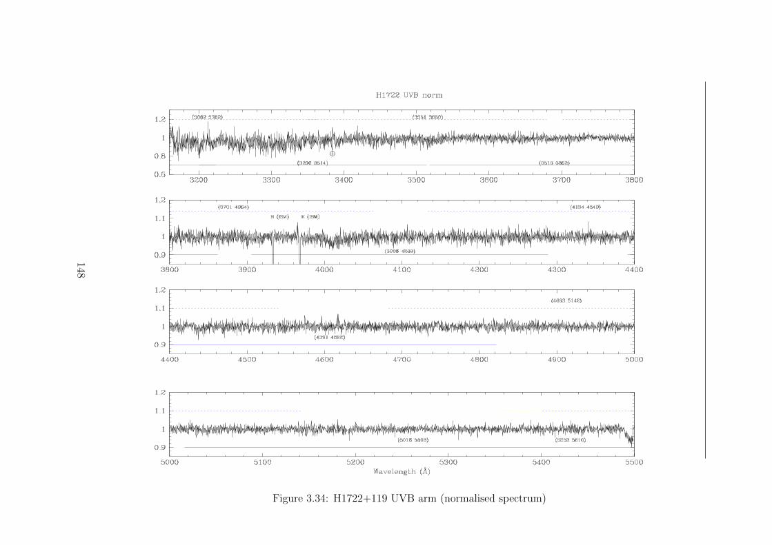
Figure 3.34: H1722+119 UVB arm (normalised spectrum)

148

Figure 3.35: H1722+119 VIS arm (normalised spectrum)

149

Figure 3.36: H1722+119 NIR arm (normalised spectrum)

150

Figure 3.37: MH2136-428 UVB arm (normalised spectrum)

151

Figure 3.38: MH2136-428 VIS arm (normalised spectrum)

152

Figure 3.39: MH2136-428 NIR arm (normalised spectrum)

153

Figure 3.40: PKS 2554-204 UVB arm (normalised spectrum)

154

Figure 3.41: PKS 2254-204 VIS arm (normalised spectrum)

155

Figure 3.42: PKS 2254-204 NIR arm (normalised spectrum)

156

Object1 z α R EWmin Line ID λ zλ Type EW

PG 1553+113 0.82 14.00 0.06 U - 0.05 V - 0.31 N

Ca II (ISM) 3933.30 - g 0.37 ± 0.02

Ca II (ISM) 3968.10 - g 0.22 ± 0.02

Na I (ISM) 5889.20 - g 0.30 ± 0.03

Na I (ISM) 5895.30 - g 0.20 ± 0.03

H 1722+119 0.80 14.40 0.13 U - 0.07 V - 0.20 N

Ca II (ISM) 3933.40 - g 0.45 ± 0.02

Ca II (ISM) 3968.20 - g 0.30 ± 0.02

Na I (ISM) 5889.20 - g 0.62 ± 0.03

Na I (ISM) 5895.30 - g 0.50 ± 0.05

MH 2136-428 > 0.008 0.65 15.60 0.05 U - 0.05 V - 0.31 N

Ca II (ISM) 3933.40 - g 0.14 ± 0.02

Ca II (ISM) 3968.20 - g 0.10 ± 0.04

Ca II (H) 3966.40 0.0084 i 0.15 ± 0.02

Ca II (K) 4001.20 0.0084 i 0.10 ± 0.02

PKS 2254-204 0.70 17.10 0.10 U - 0.10 V - 0.30 N Ca II (ISM) 3933.40 - g 0.20 ± 0.05

Ca II (ISM) 3967.70 - g 0.10 ± 0.04

Table 3.10: Spectral parameters for the XSH objects

1(1) Object name; (2) average redshift (or lower limit); (3) power-law spectral index; (4) R magnitude measured on the spectrum;(5) Minimum equivalent width detectable in the three arms (U = UVB, V = VIS and N = NIR); (6) Line identification (7) Barycenterof the line (8) Redshift of the line; (9) Line type e: emission line from BL Lac; g: absorption line from BL Lac host galaxy; i: absorptionline from intervening system; (11) Measured equivalent width

157

3.4.4.3 The peculiar case of MH 2136-428

MH 2136-428 is a bright BL Lac object (mr = 15.36) discovered by Hawkins et al.

[1991] through its strong optical variability (∆m ∼ 1.0). The source appeared

in an optical survey carried out in 1977, with the UK 1.2 Schmidt telescope,

aimed at detect quasars on the ESO/SERC field . The survey yielded two BL Lac

objects selected on their optical variability, highly polarisation and radio loudness

(including MH 2136-428).

Figure 3.43: H 2136-428 Ca II systems detected toward the line of sight. GalaticH and K Ca II bands are marked by the label ISM.

Previous spectroscopical studies of this source (Hawkins et al. [1991], Sbarufatti

et al. [2006] and Shaw et al. [2013]) failed to detect intrinsic or absorption lines

leaving the object completely featureless.

The XSHOOTER spectrum also shows that the overall spectrum of MH 2136-

428 exhibit a strongly dominated non-thermal continuum that arises from the

active nucleus which can be firmly described by a single power-law of the form

F (λ) = λ−α, where α ∼ 0.70. The measured spectral index is well consistent with

previous observation of this source [Sbarufatti et al., 2006]. The lack of intrinsic

spectral features (Sbarufatti et al. [2006], Shaw et al. [2013]) in the large spectral

158

band 3200 - 15.0000 A is also confirmed.

Figure 3.44: MH 2136-428 Ca II systems and ISM K Band de-blend fit. Dashedblue line and dotted red line are respectively the fit for deblending K ISM bandand Ca II H band absorption system. The weighted reduced χ2 for the model is0.92 with 30 degrees of freedom. The r.m.s. overall error is 0.02.

However, we clearly detected two narrow absorption lines above ∼ 3-σ of the

signal-to-noise ratio at 3966.40 A and 4001.40 A that we interpret as intervening

system on the line of sight of MH 2136-428 (Figure 3.43). The first one is blended

with the Ca II K band absorption that arises in our Galaxy. In order to measure

the properties of both lines we fitted them with two gaussian profiles, assuming a

159

model for the Ca II K band absorption derived from observations of other BL Lacs

objects with X-Shooter in the same program. The results of the fitting procedure

is reported in Figure 3.44. The most straightforward interpretation considering

the ratio of the wavelength is a Ca II intervening system at z = 0.0085. The close

environment which also confirms the interpretation is illustrated in Figure 3.45.

Figure 3.45: MH 2136-428 close environment from ESO NTT. The Ca II inter-vening system detected in the XSHOOTER spectrum arises in the surroundingnebulosity of NGC 7097 at 100 Kpc projected distance from the background BLLac. S1 and S2 are satellites of NGC 7097 at the same redshift.

We also found that this BL Lac was imaged with the Advanced Camera for

Surveys (ACS) aboard the Hubble Space Telescope [Ubeda and et al., 2012] using

the High Resolution Channel (HRC). In particular, two frames have been acquired

adopting the filter F625W for a total integration time of 780s. In Figure 3.46

we report the field of view around MH 2136-428. We measured the apparent

magnitude of the source that turns out to be mF625W ∼ 16.00. The image of the

BLL is unresolved, as confirmed by the comparison with the point spread function

derived with TinyTim [Krist et al., 2011]. The analysis of the image carried out

160

with AIDA [Uslenghi and Falomo, 2011] also reveals that no significant extended

surround nebulosity due to BLL host galaxy is detectable, leaving the radial surface

brightness of the source best fitted only by the PSF model. Furthermore, at ∼ 3′′

North-West from the BL Lac a faint spiral galaxy (labelled as G1 in Figure 3.46)

is clearly detected. The apparent magnitude of G1 is mG1 = 20.90 and the relative

surface brightness profile is well fitted by a Sersic profile yielding a Reff of ∼ 1′′.

From the expected absolute magnitude of typical spiral galaxies we reasonably

infer that the redshift of G1 is 0.40 ≤ zG1 ≤ 0.60. Within this assumption, its

absolute magnitude is −21.70 ≤ MG1V ≤ −20.00 and the projected distance from

MH 2136-428 turns out to be 20 ≤ d ≤ 30 kpc. We searched for possible Mg II

absorption feature imprinted by G1 in the BL Lac spectrum. No absorption lines

compatible with the Mg II doublet transition above the instrumental sensitivity

(EWmin ∼ 0.03 A) are revealed in the range ∼ 3900 - 4500 A. Although we do not

know if G1 is a foreground or background object, the absence of Mg II absorption

(if G1 is foreground with respect to BL Lac) it is not unexpected since, as noted

by Chen et al. [2010], about 40% of isolated galaxy at ρ ≤ 100h−1 kpc from a

background QSO do not imprint Mg II spectral signature in its spectrum.

161

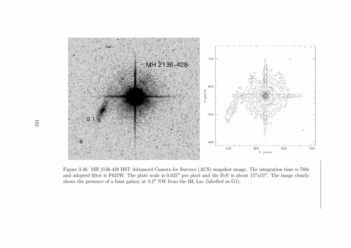
Figure 3.46: MH 2136-428 HST Advanced Camera for Surveys (ACS) snapshot image. The integration time is 780sand adopted filter is F625W. The plate scale is 0.025′′ per pixel and the FoV is about 15′′x15′′. The image clearlyshows the presence of a faint galaxy at 3.2′′ NW from the BL Lac (labelled as G1).

162

3.5 Future perspective. Spectroscopy of BL Lacs

in the E-ELT era

3.5.1 Introduction

In the spectrum of a BL Lac object the absorption lines associated to the stellar

components of the host galaxy are always present. On the other hand, their de-

tectability depends both on the S/N ratio and on the nucleus to host ratio (N/H)

of the source. With the state of the art 8-mt class telescopes and modern instru-

mentation it is possible to obtain spectra with S/N about 100 and R ∼ 2000 for

object of V ∼ 17 (assuming exposure time of ∼ 1 hour). For sources with V & 20

the situation is even worse since the S/N typically drops below 50. This limits

the capability to detect the host galaxy features either for the sources with high

intrinsic N/H ratio and for faint objects. In this chapter we illustrated that it is

possible to overcome the problem either increasing the SNR ratio or the spectral

resolution as in the case of X-SHOOTER.

For this reason, in order to significantly improve these limits, a future 40-mt class

telescope like the European Extreme Large Telescope (E-ELT) is mandatory to

investigate these kind of objects. In particular, the adoption of even larger tele-

scope equipped with low resolution FORS2-like spectrograph allows to study the

host galaxy features in the spectra of BL Lacs in which the nucleus to host ratio

is extremely high. In this section it will be illustrated how E-ELT equipped with

a FORS2 like spectrograph could detected host galaxy features for high N/H ratio

sources with different magnitude and redshift assuming reasonable exposure times.

3.5.2 Simulation of BL Lac spectra observed by E-ELT

Assuming that the BL Lac spectrum is the sum of a non thermal emission, modelled

with a power law, and a stellar component described by a giant elliptical galaxy

[Kinney et al., 1996] we performed the simulation of two cases. We consider an

exposure time of 3600 s and a spectrograph with a dispersion of ∼ 1.0 A / pixel,

with an efficiency similar to the VLT-FORS2. We take into account a standard

galaxy characterised by Mr = −23 and Reff = 10 kpc. We adopted an aperture

163

correction for a slit of 1′′ x 1′′, similarly to the aperture effect correction fully

described in Sbarufatti et al. [2006]. Briefly, the fraction of starlight lost δmag

due to slit effect depends on the redshift of the object and in the simulations this

fact is taken into account assuming that N/H ratio apparent at the level of the

spectrograph is higher than the N/H ratio intrinsic of the source. We adopted an

aperture effect A(z) described by curves reported in Figure 3.47 .

resulting from the depression of the continuum caused by theenvelope ofmany unresolved narrow absorption features. Higherresolution spectra of the object in the spectral range 4200–58008are needed to distinguish between the two possibilities.1210+121: Hazard & Murdoch (1977) proposed that this ob-

ject was the optical counterpart of a radio source in the MolongoCatalogue (Sutton et al. 1974); the separation was, however,1600. Zotov & Tapia (1979) reported large optical variability andpolarization, apparently reinforcing the identification. Baldwinet al. (1973) found a featureless optical spectrum. Our VLT spec-trum clearly shows that the source is a type B star in our Galaxy.1212+078: Our VLT spectrum clearly shows the presence of

a strong thermal component due to the host. We detected Ca iikk3934, 3968,G band k4305, Mg i k5175, and H! k6563 in emis-sion at z ! 0:137, confirming the redshift estimated by Perlmanet al. (1996). The contribution of the nonthermal component isvisible in the bluest part of the spectrum. The best-fit decom-position of the spectrum gives ! ! 1:17 for the nonthermal com-ponent andMR ! "22:0 for the host. Although this is somewhatfainter than expected for a BL Lac host galaxy, we cannot ex-clude the possibility that part of the light did not enter in the slit,given the low redshift and the consequent large apparent size ofthe host.

Fig. 5.—Top: Simulated BL Lac spectrum at z ! 0:5 (solid line), obtained as the composition of a nonthermal power law (dashed line) and an elliptical galaxyspectrum (magnified 5 times, dotted line), with nucleus-to-host ratio of 5. Bottom: Simulated spectrum, if observed with S/N ! 30 (left) or S/N ! 300 (right).

Fig. 6.—Aperture effect correction A(z) as a function of the redshift for ap-erture sizes 200 ; 1200 (dashed line), 200 ; 600 (solid line), and 200 ; 300 (dotted line).Seeing is assumed to be #100.

SBARUFATTI ET AL.14 Vol. 132

Figure 3.47: Aperture effect for different slit dimension projected on the sky.Details are reported in Sbarufatti et al. [2006]

The results of the simulations are presented in Figure 3.48 . In the first case

(top panel), the E-ELT can obtain a spectrum with S/N ∼ 2000 for an object

with V = 17 and z = 0.40. The features associated to the host galaxy are clearly

detectable with an intrinsic N/H up to 100 in the band 5200 - 6200 A. The second

simulation (bottom panel) is carried out assuming V = 20 and z = 0.70. In this

case, the S/N ratio of the spectrum is ∼ 500 and the intrinsic N/H ratio limit

reached is ∼ 40. We note that the use of the E-ELT allows to increase the S/N

ratio of the spectra of a factor ∼ 20 for the first case and ∼ 10 for the latter respect

to typical S/N ratios reached with the VLT.

In the light of these results, we are confident that the advent of 40-mt telescope

164

Figure 3.48: First panel: simulation of a BL Lac spectrum with V = 17, S/N= 2000, z = 0.40 and N/H = 100. Aperture correction is 0.35 . Second panel:simulation for a BL Lac spectrum with V = 20, S/N = 500, N/H = 40, z = 0.70and aperture correction of 0.50. For both cases the exposure time is 3600 s and theadopted slit is a 1′′ x 1′′. The efficiency of the spectrograph is considered similarto the VLT-FORS2. The solid black line is the BL Lac overall spectrum whiledashed line is the power law associated to the non thermal emission. Blue dottedline is the superposed host galaxy template spectrum.

165

instrumentation can significantly decrease the fraction of BL Lacs that are still

left without z.

166

Chapter 4

ESPRESSO: Foreseen science andoutlook

According to the latest schedule, ESPRESSO will be commissioned at the Very

Large Telescope in Paranal in late 2016. A lot of science, as explained in the

introduction of this Thesis, will be carried out through the adoption of this revo-

lutionary instrument which, for the first time, will deliver a 16mt equivalent class

telescope on the Earth. In this small Chapter I want to present the outlook for a

foreseen scientific project in which I want to be involved. As reported in Chapter 3

I spent a lot of time in my PhD studying the optical spectral properties of BL Lac.

As in the case of PKS 0048-097 or in a lot of sources in the ZBLLAC campaign

intervening systems on the line of sight are apparent, but in only few cases deeply

investigations of the physical condition of the absorbing gas are possible. This

is caused in part due to low resolution (which is not sufficient to resolve singu-

lar absorption in the clouds or derive stringent physical parameters) and due to

low SNR especially with high z sources. This issue is directly linked with a new

project carried on in collaboration with my supervisors Prof. A. Treves and Prof.

R. Falomo. In particular, at the moment of the submission of this Thesis we are

issuing a proposal at ESO-XSHOOTER aimed at obtaining high quality spectra

of candidate high-redshift BL Lacs. Thanks to superior quality of spectroscopical

XSHOOTER data we want to confirm the BL Lac nature of the candidates and

exploiting their Ly-α absorber at z ≥ 1.70 in order to firmly constraint their red-

shift and study the distribution of the absorbers toward the line of sight of BL

Lacs.

167

In details, the confirmed high-redshift BL Lac objects will allow us to probe the

cosmic evolution of the class which is a 20 years controversial issue. In fact, BL

Lac objects form an elusive class of low power AGN that, contrary to the case of

QSOs, appear to not evolve or anti-evolve with the cosmic time. Moreover, the

claimed evolution appears to be dependent on the wavelength range adopted for

surveys. In particular, radio selected BL Lacs seem to be positively evolving as

in the case of QSOs while those selected in the X-ray band appear to anti-evolve

with the cosmic time. This issue is mainly induced by very paucity of high red-

shift objects. Using the complete SDSS optically selected sample of BL Lacs (see

e.g. [Plotkin et al., 2010]) we selected 6 BL Lac candidates with possibly z ≥ 1.6

to obtain good SNR and high spectral resolution over a wide spectral range with

X-SHOOTER. The existence of BL Lacs at high redshift in the adopted survey

would disprove the proposed anti evolution picture yielding a direct confirmation

that the recent proposed anti evolution of the class is strongly biased by selection

effects (see e.g. [Giommi et al., 2012]). In order to assess the feasibility of this ob-

servations, we simulated the spectrum of a BL Lac object in which Ly-α absorbers

are present according to the signal to noise ratio obtained from the ESO Expo-

sure Time Calculator (ETC). The adopted values for the simulations are similar

to those observed using HST/COS observation of Lyman-α detected intervening

systems toward the line-of-sight of the BL Lac PKS 1553+113 [Danforth et al.,

2010] and results are reported in Figure 4.1.

Nevertheless, the faint magnitude of the sources (V ∼ 19) allow to obtain

reasonable but not excellent signal-to-noise ratio. Moreover, the medium resolution

does not allow to deeply probe any structure on absorption features (multiple

systems at the same redshift or resolve different clouds that cause the absorption

itself). The advent of ESPRESSO in 4-UT mode will allow to obtain an higher (or

comparable) SNR (at least a factor of 2 assuming same exposure time) combining

the high resolution suitable for the investigation of complex absorber structure.

Despite of the fact that, high resolution spectrographs are currently available at

10 mt class telescopes (e.g. UVES@VLT) they are limited to magnitude around

V = 18 if desired SNR would be ∼ 20-30. With the advent of ESPRESSO in

4-UT mode the limit magnitude will be pushed away with the great advantage to

maintain reasonable overall exposure times. For example, according to the most

168

Figure 4.1: XSH-UVB spectrum simulation (SNR 25). Left panel: detection ofLy-α absorption with EW = 100 mA, b ∼ 100 km s−1. Center: Ly-α feature withEW = 200 mA, b ∼ 50 km s−1. Right: Ly-α system with EW = 50 mA, b ∼ 100km s−1. Dotted line is the best fit.

recent Exposure Time Calculator for ESPRESSO a SNR of 20 is reached 1 hour

in for an object of 20th magnitude. This value should be compared with that

obtained with UVES ETC which is less than 10 for the same object. On the light

of these considerations, we are confident that the advent of this new generation

spectrograph in the VLT era will allow for the first time to study from the ground

faint sources at high redshift with the greatly benefit of combining high resolution

and suitable SNR ratio to deeply investigate intervening absorbers (and associated

system) toward the line of sight of this elusive class of objects.

169

Chapter 5

Conclusions

Aimed at achieve the basic knowledge behind the professional figure of the Instru-

ment Scientist

I presented in this Thesis the results of my work on the application of low and

medium/high resolution spectroscopy to the study of a particular class of Active

Galatic Nuclei, the BL Lacertae objects. The work was specially aimed to the in-

terpretation of spectroscopic observations and consequent redshift determination.

In details I completed the analysis and interpretation of a a survey started few

years ago (www.oapd.inaf.it/zbllac/). Through this work I learned how to use

and how to scientifically interpret data obtained with ESO-FORS2 (a first gener-

ation spectrograph) and ESO-X-SHOOTER.

I also presented in this thesis my personal contribution to the definition and design

of a new ultra high resolution spectrograph for planet finding and cosmological

research: ESPRESSO@VLT. Through this activity I learned how to work in a

large Instrumental Project where I contributed with simulations of the expected

performance of the Front End Subsystem and Exposure Meter Subsystem, to be

compared with the top level astronomical requirements for the instrument.

The most relevant result, in terms of personal formation, of my PhD educational

path resides in the synergy between the aforementioned areas, which allowed me

to achieve the basic formation as an Instrument Scientist, the professional figure

I aim to for the future.

170

Appendix A - List of publication

Title: On the redshift of the bright BL Lacertae object PKS 0048-097

Authors: Landoni, M.; Falomo, R.; Treves, A.; Sbarufatti, B.; Decarli, R.; Tavec-

chio, F.; Kotilainen, J.

Publication: Astronomy & Astrophysics, Volume 543, id.A116, 5 pp.

Publication Date: 07/2012

Origin: EDP Sciences

Astronomy Keywords: BL Lacertae objects: individual: PKS 0048-097, galax-

ies: active

DOI: 10.1051/0004-6361/201219114

Bibliographic Code: 2012A&A...543A.116L

Abstract: Aims: We attempt to determine the spectroscopic redshifts of bright

BL Lac objects, which have proven difficult to measure.

Methods: We use the spectra acquired using the newly available spectrograph

X-Shooter at the European Southern Observatory Very Large Telescope, which

combines high resolution with a large wavelength range, to obtain ultraviolet to

near-infrared spectra of BL Lacs.

Results: Our observations of PKS 0048-097 detect three emission lines, which per-

mit us to derive a redshift z = 0.635. Moreover, we discover a Mg II absorption

system at z = 0.154 that is associated with a foreground spiral galaxy a 50 kpc of

projected distance.

Conclusions: The measured redshift allows us to discuss the optical beaming factor

and the absorption of the high energy spectrum by the extragalactic background

light.

171

Title: ESO Very Large Telescope Optical Spectroscopy of BL Lacertae Objects.

IV. New Spectra and Properties of the Full Sample

Authors: Landoni, M.; Falomo, R.; Treves, A.; Sbarufatti, B.; Barattini, M.;

Decarli, R.; Kotilainen, J.

Publication: The Astronomical Journal, Volume 145, Issue 4, article id. 114, 12

pp. (2013). (AJ Homepage)

Publication Date: 04/2013

Origin: IOP

Astronomy Keywords: BL Lacertae objects: general, instrumentation: spec-

trographs, quasars: absorption lines

DOI: 10.1088/0004-6256/145/4/114

Bibliographic Code: 2013AJ....145..114L

Abstract: We present the last chapter of a spectroscopy program aimed at deriv-

ing the redshift or a lower limit to the redshift of BL Lac objects using medium-

resolution spectroscopy. Here we report new spectra for 33 BL Lac object can-

didates obtained in 2008-2009, confirming the BL Lac nature of 25 sources and

obtaining new redshifts for 5 objects. These new observations are combined with

our previous data in order to construct a homogeneous sample of 70 BL Lac ob-

jects with high-quality spectroscopy. All these spectra can be accessed at the Web

site http://www.oapd.inaf.it/zbllac/. The average spectrum, beaming properties

of the full sample, discussion of intervening systems, and future perspectives are

addressed.

Title: Spectroscopy of Optically Selected BL Lac Objects and their gamma-ray

emission

Authors: Sandrinelli, A.; Treves, A.; Falomo, R.; Farina, E. P.; Foschini, L.;

Landoni, M.; Sbarufatti, B.

Publication: eprint arXiv:1310.1837 (AJ in press)

Publication Date: 10/2013

Keywords: Astrophysics - Cosmology and Extragalactic Astrophysics

Comment: Accepted for publication in AJ

Bibliographic Code: 2013arXiv1310.1837S (AJ, in press)

172

Abstract: We present Very Large Telescope optical spectroscopy of nine BL Lac

objects of unknown redshift belonging to the list of optically selected radio loud BL

Lacs candidates. We explore their spectroscopic properties and the possible link

with gamma ray emission. From the new observations we determine the redshift

of four objects from faint emission lines or from absorption features of the host

galaxy. In three cases we find narrow intervening absorptions from which a lower

limit to the redshift is inferred. For the remaining two featureless sources, lower

limits to the redshift are deduced from the very absence of spectral lines. A search

for gamma counterpart emission shows that six out of nine are Fermi gamma-ray

emitters with two new detections. Our analysis suggests that most of the BL Lac

still lacking of redshift information are most probably located at high redshift.

Title: Speckle observations with PISCO in Merate (Italy) - XII. Astrometric

measurements of visual binaries in 2011

Authors: Scardia, M.; Prieur, J.-L.; Pansecchi, L.; Argyle, R. W.; Span, P.; Riva,

M.; Landoni, M.

Publication: Monthly Notices of the Royal Astronomical Society, Volume 434,

Issue 4, p.2803-2813 (MNRAS Homepage)

Publication Date: 10/2013

Origin: OUP

Astronomy Keywords: techniques: interferometric, astrometry, binaries: close,

binaries: visual

DOI: 10.1093/mnras/stt1140

Bibliographic Code: 2013MNRAS.434.2803S

Abstract: We present relative astrometric measurements of visual binaries, made

in 2011 with the Pupil Interferometry Speckle camera and COronagraph (PISCO)

at the 102-cm Zeiss telescope of the Brera Astronomical Observatory in Merate

(Italy). Our observing list contains orbital couples as well as binaries whose motion

is still uncertain. We obtained new measurements of 469 objects, with angular

separations in the range 0.14-8.1 arcsec, and an average accuracy of 0.02 arcsec.

The mean error on the position angles is 0.7. Most of the position angles were

173

determined without the usual 180 deg ambiguity with the application of triple-

correlation techniques and/or by inspection of the long integration files. Thanks

to a new low-magnification option included in PISCO, we have been able to observe

fainter stars than previously. The limiting magnitude of our instrumentation on

the Zeiss telescope is now close to mV = 10-12, which permits the observation

of some red dwarfs. Finally, we present new revised orbits for ADS 8739, 9182

Aa,Ab, 9626 Ba,Bb, 12880 and 14412, partly derived from those observations.

The corresponding estimated values for the masses of those systems are compatible

with the spectral types.

Title: Supernova 2013fj in Pgc 68419 = Psn J22152851+1534041

Authors: Ciabattari, F.; Mazzoni, E.; Parker, S.; Brimacombe, J.; Zanutta, A.;

Landoni, M.; Bianco, A.; Spiro, S.; Benetti, S.; Pastorello, A.; Cappellaro, E.;

Tomasella, L.; Ochner, P.; Turatto, M.

Publication: Central Bureau Electronic Telegrams, 3654, 1 (2013). Edited by

Green, D. W. E.

Publication Date: 09/2013

Origin: CBAT

Objects: 2013fj

Bibliographic Code: 2013CBET.3654....1C

Title: ESPRESSO front end opto-mechanical configuration

Authors: Riva, M.; Landoni, M.; Zerbi, F. M.; Mgevand, D.; Cabral, A.; Cris-

tiani, S.; Delabre, B.

Publication: Ground-based and Airborne Instrumentation for Astronomy IV.

Proceedings of the SPIE, Volume 8446, article id. 84469E, 7 pp. (2012). (SPIE

Homepage)

Publication Date: 09/2012

Origin: SPIE

174

Comment: ISBN: 9780819491473

DOI: 10.1117/12.924978

Bibliographic Code: 2012SPIE.8446E..9ER

Abstract: This paper presents the Espresso Front End mechanical and opti-

cal configuration. ESPRESSO, Echelle SPectro-graph for Rocky Exoplanets and

Stable Spectroscopic Observations, will combine the efficiency of modern echelle

spectrograph design with extreme radial-velocity precision. It will be installed on

ESO’s VLT and it is expected to achieve a gain of two magnitudes with respect

to its predecessor HARPS. The instrumental radial-velocity precision will also be

improved to reach cm/s level. The Front End is a modular subsystem that collects

the light coming from the Coude Trains of all the Four Telescope Units (UT), pro-

vides Field and Pupil stabilisation via piezoelectric tip tilt devices and inject the

beam into the Spectrograph fiber. The Front End will also inject the calibration

light coming from the calibration unit. There will be four Front End modules, one

per UT. A rotary Stage will provide the toggling between different observation

mode: Single UT Ultra High resolution (SUT-UHR), Single UT High resolution

(SUT-HR) and multiple UTS Mid Resolution (MUT-MR). The field and pupil

guiding is obtained through a reimaging system that elaborates the halo of the

light out of the Injection Fiber and a telescope pupil beacon. A dedicated guiding

algorithm has been studied in order to provide proper image stability even with

faint objects (mv=20).

Title: ESPRESSO front-end guiding algorithm

Authors: Landoni, M.; Riva, M.; Zerbi, F. M.; Mgevand, D.; Cabral, A.; Cris-

tiani, S.

Publication: Software and Cyberinfrastructure for Astronomy II. Proceedings of

the SPIE, Volume 8451, article id. 84512X, 14 pp. (2012). (SPIE Homepage)

Publication Date: 09/2012

Origin: SPIE

Comment: ISBN: 9780819491527

DOI: 10.1117/12.924980

Bibliographic Code: 2012SPIE.8451E..2XL

175

Abstract: This paper presents the Espresso Front End Guiding Algorithm. ESPRESSO,

the Echelle SPectrograph for Rocky Exoplanets and Stable Spectroscopic Obser-

vations, will be installed on ESO’s Very Large Telescope (VLT). The Front End

(FE) is the subsystem that collects the light coming from the Coud Trains of all

the Four Telescope Units (UTs), provides Field and Pupil stabilisation via piezo-

electric tip tilt devices and inject the beams into the Spectrograph fibers. The

field and pupil guiding is obtained through a re-imaging system that elaborates

the halo of the light out of the Injection Fiber and a telescope pupil beacon. The

first guiding algorithm that we evaluated splits the FP in four areas and computes

the sum of the photon counting of each pixel in that area. The unbalancing of the

photon sums will give the centroid misalignment information that will be handled

by the Instrument Control Software (ICS). Different algorithms and controllers

architectures have been evaluated and implemented in order to select a strategy

that enables the FE to guide up to 20 apparent magnitude in V band.

Title: ESPRESSO: the ultimate rocky exoplanets hunter for the VLT

Authors: Mgevand, Denis; Zerbi, Filippo M.; Cabral, Alexandre; Di Marcanto-

nio, Paolo; Amate, Manuel; Pepe, Francesco; Cristiani, Stefano; Rebolo, Rafael;

Santos, Nuno C.; Dekker, Hans; Abreu, Manuel; Affolter, Michael; Avila, Ger-

ardo; Baldini, Veronica; Bristow, Paul; Broeg, Christopher; Carvas, Pedro; Cirami,

Roberto; Coelho, Joo.; Comari, Maurizio; Conconi, Paolo; Coretti, Igor; Cupani,

Guido; D’Odorico, Valentina; De Caprio, Vincenzo; Delabre, Bernard; Figueira,

Pedro; Fleury, Michel; Fragoso, Ana; Genolet, Ludovic; Gomes, Ricardo; Gon-

zalez Hernandez, Jonay; Hughes, Ian; Iwert, Olaf; Kerber, Florian; Landoni,

Marco; Lima, Jorge; Lizon, Jean-Louis; Lovis, Christophe; Maire, Charles; Man-

netta, Marco; Martins, Carlos; Moitinho, Andr; Molaro, Paolo; Monteiro, Manuel;

Rasilla, Jos Luis; Riva, Marco; Santana Tschudi, Samuel; Santin, Paolo; Sos-

nowska, Danuta; Sousa, Sergio; Span, Paolo; Tenegi, Fabio; Toso, Giorgio; Vanzella,

Eros; Viel, Matteo; Zapatero Osorio, Maria Rosa

Publication: Ground-based and Airborne Instrumentation for Astronomy IV.

Proceedings of the SPIE, Volume 8446, id. 84461R-84461R-15 (2012). (SPIE

Homepage)

176

Publication Date: 09/2012

Origin: SPIE

Comment: ISBN: 9780819491473

DOI: 10.1117/12.924602

Bibliographic Code: 2012SPIE.8446E..1RM

Abstract: ESPRESSO, the VLT rocky exoplanets hunter, will combine the effi-

ciency of modern echelle spectrograph with extreme radial-velocity precision. It

will be installed at Paranal on ESO’s VLT in order to achieve a gain of two magni-

tudes with respect to its predecessor HARPS, and the instrumental radial-velocity

precision will be improved to reach 10 cm/s level. We have constituted a Consor-

tium of astronomical research institutes to fund, design and build ESPRESSO on

behalf of and in collaboration with ESO, the European Southern Observatory. The

project has passed the preliminary design review in November 2011. The spec-

trograph will be installed at the so-called ”Combined Coud Laboratory” of the

VLT, it will be linked to the four 8.2 meters Unit Telescopes (UT) through four

optical ”Coud trains” and will be operated either with a single telescope or with

up to four UTs. In exchange of the major financial and human effort the building

Consortium will be awarded with guaranteed observing time (GTO), which will

be invested in a common scientific program. Thanks to its characteristics and the

ability of combining incoherently the light of 4 large telescopes, ESPRESSO will

offer new possibilities in many fields of astronomy. Our main scientific objectives

are, however, the search and characterization of rocky exoplanets in the habitable

zone of quiet, near-by G to M-dwarfs, and the analysis of the variability of fun-

damental physical constants. In this paper, we present the ambitious scientific

objectives, the capabilities of ESPRESSO, the technical solutions for the system

and its subsystems, enlightening the main differences between ESPRESSO and

its predecessors. The project aspects of this facility are also described, from the

consortium and partnership structure to the planning phases and milestones.

Title:ESPRESSO Front End Exposure Meter - A chromatic approach to radial

velocity correction

Authors: Marco Landoni , Marco Riva , Francesco Pepe , Paolo Conconi , Filippo

177

M. Zerbi , Alexandre Cabral , Stefano Cristiani and Denis Megevand

Publication: SPIE Optics and Photonics 2013 in press

Publication Date: In press

Origin: SPIE

DOI: 10.1117/12.2023227

Abstract: This paper presents the Espresso Exposure Meter (EM) implemen-

tation. ESPRESSO, the Echelle SPectrograph for Rocky Exoplanets and Stable

Spectroscopic Observations, will be installed on ESOs Very Large Telescope (VLT).

The light coming from the Telescope through a Coud Focus4 of all the Four Tele-

scope Units (UTs) will be collected by the Front End Unit that provides Field

and Pupil stabilisation and injects the beams into the Spectrograph fibers. An

advanced Exposure Meter system will be used to correct RadialVelocity (RV) ob-

tained from the scientific spectrum for the Earth relative motion. In this work we

will present the performance of an innovative concept for the Exposure Meter sys-

tem based on a Charge Coupled Device (CCD) with a chromatic approach for the

calculation of the Mean Time of Exposure (MTE). The MTE is a crucial quantity

used for the correction of RV for the Earth relative motion during the exposure.

In particular, splitting the light in different chromatic channels on the CCD, we

will probe for potential chromatic effects on the calculation of the MTE in each

channel and how they could be used in order to perform the correction of RV. The

paper is accompanied by a fully described numerical analysis that keeps into view

a key performance evaluation for different stellar spectral types (B to M spectral

main sequence classes).

Title: ESPRESSO APSU: simplify the life of pupil slicing

Authors: Conconi, P.; Riva, M.; Pepe, F.; Zerbi, F. M.; Cabral, A.; Cristiani, S.;

Megevand, D.; Landoni, M.; Span, P.

Publication: Proceedings of the SPIE, Volume 8842, id. 88420P 9 pp. (2013).

(SPIE Homepage)

Publication Date: 09/2013

Origin: SPIE

Comment: ISBN: 9780819496928

178

DOI: 10.1117/12.2024843

Bibliographic Code: 2013SPIE.8842E..0PC

Abstract: This paper presents the Espresso Anamorphic pupil Slicer (APSU) im-

plementation. ESPRESSO, the Echelle SPectrograph for Rocky Exoplanets and

Stable Spectroscopic Observations, will be installed on ESOs Very Large Telescope

(VLT). In this work we will present the design and trade-off for the pupil slicing

system introduced in order to increase the resolving power, effectively decreas-

ing slit width. Its based onto simplified optical component that introduce large

anamorphism while keeping low aberrations by means of cylindrical optics. We

describe here the trade-off between slicing through two adjacent squared doublets

and two achromatic prisms.

179

References

A. Baglin, M. Auvergne, L. Boisnard, T. Lam-Trong, P. Barge, C. Catala,

M. Deleuil, E. Michel, and W. Weiss. CoRoT: a high precision photometer for

stellar ecolution and exoplanet finding. In 36th COSPAR Scientific Assembly,

volume 36 of COSPAR Meeting, page 3749, 2006. 7

K. Banse, D. Ponz, C. Ounnas, P. Grosbol, and R. Warmels. The MIDAS Image

Processing System. In L. B. Robinson, editor, Instrumentation for Ground-

Based Optical Astronomy, page 431, 1988. 26

A. Baranne, M. Mayor, and J. L. Poncet. CORAVEL - A new tool for radial

velocity measurements. Vistas in Astronomy, 23:279–316, 1979. doi: 10.1016/

0083-6656(79)90016-3. 8

T. Boroson. Blueshifted [O III] Emission: Indications of a Dynamic Narrow-Line

Region. AJ, 130:381–386, August 2005. doi: 10.1086/431722. 141

A. Cabral, A. Moitinho, J. Coelho, J. Lima, G. Avila, B.-A. Delabre, R. Gomes,

D. Megevand, F. Zerbi, P. Di Marcantonio, C. Lovis, and N. C. Santos.

ESPRESSO: design and analysis of a Coude-train for a stable and efficient

simultaneous optical feeding from the four VLT unit telescopes. In Society

of Photo-Optical Instrumentation Engineers (SPIE) Conference Series, volume

8444 of Society of Photo-Optical Instrumentation Engineers (SPIE) Conference

Series, September 2012. doi: 10.1117/12.926093. ix, 14, 15

J. A. Cardelli, G. C. Clayton, and J. S. Mathis. The relationship between infrared,

optical, and ultraviolet extinction. ApJ, 345:245–256, October 1989. doi: 10.

1086/167900. 108

180

REFERENCES

H.-W. Chen, J. E. Helsby, J.-R. Gauthier, S. A. Shectman, I. B. Thompson, and

J. L. Tinker. An Empirical Characterization of Extended Cool Gas Around

Galaxies Using Mg II Absorption Features. ApJ, 714:1521–1541, May 2010. doi:

10.1088/0004-637X/714/2/1521. 162

W. D. Cochran and A. P. Hatzes. A high-precision radial-velocity survey for

other planetary systems. APSS, 212:281–291, February 1994. doi: 10.1007/

BF00984532. 8

C. W. Danforth, B. A. Keeney, J. T. Stocke, J. M. Shull, and Y. Yao. Hubble/COS

Observations of the Lyα Forest Toward the BL Lac Object 1ES 1553+113. ApJ,

720:976–986, September 2010. doi: 10.1088/0004-637X/720/1/976. 170

R. Decarli, M. Dotti, and A. Treves. Geometry and inclination of the broad-line

region in blazars. MNRAS, 413:39–46, May 2011. doi: 10.1111/j.1365-2966.

2010.18102.x. xv, 128, 129

A. Domınguez, J. R. Primack, D. J. Rosario, F. Prada, R. C. Gilmore, S. M.

Faber, D. C. Koo, R. S. Somerville, M. A. Perez-Torres, P. Perez-Gonzalez, J.-

S. Huang, M. Davis, P. Guhathakurta, P. Barmby, C. J. Conselice, M. Lozano,

J. A. Newman, and M. C. Cooper. Extragalactic background light inferred from

AEGIS galaxy-SED-type fractions. MNRAS, 410:2556–2578, February 2011.

doi: 10.1111/j.1365-2966.2010.17631.x. 143

R. Falomo. Host galaxy and close environment of BL Lacertae objects. MNRAS,

283:241–250, November 1996a. xvi, 136, 138, 141, 142

R. Falomo. Host galaxy and close environment of BL Lacertae objects. MNRAS,

283:241–250, November 1996b. 98

R. Falomo, J. Melnick, and E. G. Tanzi. On the close environment of BL Lacertae

objects. Nature, 345:692–694, June 1990. doi: 10.1038/345692a0. 143

R. Falomo, M. Bersanelli, P. Bouchet, and E. G. Tanzi. The optical to near-infrared

emission of BL Lac objects - Simultaneous observations. AJ, 106:11–27, July

1993a. doi: 10.1086/116616. 136

181

REFERENCES

R. Falomo, M. Bersanelli, P. Bouchet, and E. G. Tanzi. The optical to near-infrared

emission of BL Lac objects - Simultaneous observations. AJ, 106:11–27, July

1993b. doi: 10.1086/116616. 98

R. Falomo, R. Scarpa, and M. Bersanelli. Optical spectrophotometry of blazars.

ApJ Supplement Series, 93:125–143, July 1994a. doi: 10.1086/192048. 136

R. Falomo, R. Scarpa, and M. Bersanelli. Optical spectrophotometry of blazars.

ApJ Letters, 93:125–143, July 1994b. doi: 10.1086/192048. 98

R. Falomo, R. Scarpa, A. Treves, and C. M. Urry. The Hubble Space Telescope

Survey of BL Lacertae Objects. III. Morphological Properties of Low-Redshift

Host Galaxies. ApJ, 542:731–739, October 2000. doi: 10.1086/317044. 98

J. H. Fan and R. G. Lin. Optical Variability and Periodicity Analysis for Blazars.

I. Light Curves for Radio-selected BL Lacertae Objects. ApJ, 537:101–122, July

2000. doi: 10.1086/308996. 138

E. P. Farina, R. Decarli, R. Falomo, A. Treves, and C. M. Raiteri. The optical

spectrum of PKS 1222+216 and its black hole mass. MNRAS, 424:393–398, July

2012. doi: 10.1111/j.1365-2966.2012.21209.x. 129

G. Ghisellini, A. Celotti, G. Fossati, L. Maraschi, and A. Comastri. A theoretical

unifying scheme for gamma-ray bright blazars. MNRAS, 301:451–468, December

1998. doi: 10.1046/j.1365-8711.1998.02032.x. 96

P. Giommi, M. T. Menna, and P. Padovani. The sedentary multifrequency survey

- I. Statistical identification and cosmological properties of high-energy peaked

BL Lacs. MNRAS, 310:465–475, December 1999. doi: 10.1046/j.1365-8711.1999.

02942.x. 100

P. Giommi, S. Piranomonte, M. Perri, and P. Padovani. X-ray/radio data of high

energy peaked BL Lacs (Giommi+, 2005). VizieR Online Data Catalog, 343:

40385, January 2005. 100

P. Giommi, P. Padovani, G. Polenta, S. Turriziani, V. D’Elia, and S. Piranomonte.

A simplified view of blazars: clearing the fog around long-standing selection

182

REFERENCES

effects. MNRAS, 420:2899–2911, March 2012. doi: 10.1111/j.1365-2966.2011.

20044.x. 170

P. Goldoni, F. Royer, P. Francois, M. Horrobin, G. Blanc, J. Vernet, A. Modigliani,

and J. Larsen. Data reduction software of the X-shooter spectrograph. In Society

of Photo-Optical Instrumentation Engineers (SPIE) Conference Series, volume

6269 of Society of Photo-Optical Instrumentation Engineers (SPIE) Conference

Series, July 2006. doi: 10.1117/12.669986. 135

M. R. S. Hawkins, P. Veron, R. W. Hunstead, and A. M. Burgess. Two BL Lacertae

objects discovered through their optical variability. A&A, 248:421–425, August

1991. 159

A. Heger and S. E. Woosley. Nucleosynthesis and Evolution of Massive Metal-free

Stars. ApJ, 724:341–373, November 2010. doi: 10.1088/0004-637X/724/1/341.

18

A. Hewitt and G. Burbidge. A revised and updated catalog of quasi-stellar objects.

ApJ Supplement Series, 87:451–947, August 1993. doi: 10.1086/191811. 101

S . Howell. Handbook of CCD astronomy - Second edition. 2006. 47

G. G. Kacprzak, C. W. Churchill, E. J. Barton, and J. Cooke. Halo Gas and

Galaxy Disk Kinematics of a Volume-limited Sample of Mg II Absorption-

selected Galaxies at z ˜ 0.1. ApJ, 733:105, June 2011. doi: 10.1088/0004-637X/

733/2/105. 143

S. Kaspi, D. Maoz, H. Netzer, B. M. Peterson, M. Vestergaard, and B. T. Jannuzi.

The Relationship between Luminosity and Broad-Line Region Size in Active

Galactic Nuclei. ApJ, 629:61–71, August 2005. doi: 10.1086/431275. 90, 94

A. L. Kinney, D. Calzetti, R. C. Bohlin, K. McQuade, T. Storchi-Bergmann, and

H. R. Schmitt. Template Ultraviolet to Near-Infrared Spectra of Star-forming

Galaxies and Their Application to K-Corrections. ApJ, 467:38, August 1996.

doi: 10.1086/177583. 119, 164

183

REFERENCES

D. G. Koch, W. Borucki, L. Webster, E. Dunham, J. Jenkins, J. Marriott, and

H. J. Reitsema. Kepler: a space mission to detect earth-class exoplanets. In P. Y.

Bely and J. B. Breckinridge, editors, Society of Photo-Optical Instrumentation

Engineers (SPIE) Conference Series, volume 3356 of Society of Photo-Optical

Instrumentation Engineers (SPIE) Conference Series, pages 599–607, August

1998. 7

A. Kolmogorov. The Local Structure of Turbulence in Incompressible Viscous

Fluid for Very Large Reynolds’ Numbers. Akademiia Nauk SSSR Doklady, 30:

301–305, 1941. 22

J. K. Kotilainen, R. Falomo, and R. Scarpa. The host galaxies of BL Lac objects

in the near-infrared. A&A, 336:479–489, August 1998. 138

J. E. Krist, R. N. Hook, and F. Stoehr. 20 years of Hubble Space Telescope

optical modeling using Tiny Tim. In Society of Photo-Optical Instrumentation

Engineers (SPIE) Conference Series, volume 8127 of Society of Photo-Optical

Instrumentation Engineers (SPIE) Conference Series, September 2011. doi:

10.1117/12.892762. 161

M. Landoni, R. Falomo, A. Treves, B. Sbarufatti, R. Decarli, F. Tavecchio, and

J. Kotilainen. On the redshift of the bright BL Lacertae object PKS 0048-097.

A&A, 543:A116, July 2012a. doi: 10.1051/0004-6361/201219114. 129

M. Landoni, M. Riva, F. M. Zerbi, D. Megevand, A. Cabral, and S. Cristiani.

ESPRESSO front-end guiding algorithm. In Society of Photo-Optical Instrumen-

tation Engineers (SPIE) Conference Series, volume 8451 of Society of Photo-

Optical Instrumentation Engineers (SPIE) Conference Series, September 2012b.

doi: 10.1117/12.924980. 70

M. Landoni, R. Falomo, A. Treves, B. Sbarufatti, M. Barattini, R. Decarli, and

J. Kotilainen. ESO Very Large Telescope Optical Spectroscopy of BL Lacertae

Objects. IV. New Spectra and Properties of the Full Sample. AJ, 145:114, April

2013. doi: 10.1088/0004-6256/145/4/114. xiv, 100, 101, 108

H. Landt, P. Padovani, E. S. Perlman, and P. Giommi. The Emission Line Prop-

erties of DXRBS Blazars. In P. Padovani and C. M. Urry, editors, Blazar

184

REFERENCES

Demographics and Physics, volume 227 of Astronomical Society of the Pacific

Conference Series, page 73, 2001. 98

H. Landt, P. Padovani, E. S. Perlman, and P. Giommi. A physical classification

scheme for blazars. MNRAS, 351:83–100, June 2004. doi: 10.1111/j.1365-2966.

2004.07750.x. 97

L. Lindegren and D. Dravins. The fundamental definition of “radial velocity”.

A&A, 401:1185–1201, April 2003. doi: 10.1051/0004-6361:20030181. 58

L. Lindegren and M. A. C. Perryman. GAIA: Global astrometric interferometer

for astrophysics. A&A, 116:579–595, May 1996. 7

D. Lutz, E. Sturm, R. Genzel, A. F. M. Moorwood, T. Alexander, H. Netzer, and

A. Sternberg. ISO-SWS Spectroscopy of NGC 1068. ApJ, 536:697–709, June

2000. doi: 10.1086/308972. xiii, 94, 95

M. Mayor and D. Queloz. A Jupiter-mass companion to a solar-type star. Nature,

378:355–359, November 1995. doi: 10.1038/378355a0. 8, 10

M. Mayor, A. Duquennoy, J.-L. Halbwachs, and J.-C. Mermilliod. CORAVEL

Surveys to Study Binaries of Different Masses and Ages. In H. A. McAlister

and W. I. Hartkopf, editors, IAU Colloq. 135: Complementary Approaches to

Double and Multiple Star Research, volume 32 of Astronomical Society of the

Pacific Conference Series, page 73, 1992. 8

M. Mayor, F. Pepe, D. Queloz, F. Bouchy, G. Rupprecht, G. Lo Curto, G. Avila,

W. Benz, J.-L. Bertaux, X. Bonfils, T. Dall, H. Dekker, B. Delabre, W. Eck-

ert, M. Fleury, A. Gilliotte, D. Gojak, J. C. Guzman, D. Kohler, J.-L. Lizon,

A. Longinotti, C. Lovis, D. Megevand, L. Pasquini, J. Reyes, J.-P. Sivan, D. Sos-

nowska, R. Soto, S. Udry, A. van Kesteren, L. Weber, and U. Weilenmann. Set-

ting New Standards with HARPS. The Messenger, 114:20–24, December 2003.

13, 73

M. T. Murphy, T. Udem, R. Holzwarth, A. Sizmann, L. Pasquini, C. Araujo-

Hauck, H. Dekker, S. D’Odorico, M. Fischer, T. W. Hansch, and A. Manescau.

High-precision wavelength calibration of astronomical spectrographs with laser

185

REFERENCES

frequency combs. MNRAS, 380:839–847, September 2007. doi: 10.1111/j.

1365-2966.2007.12147.x. 14

R. Narayan and I. Yi. Advection-dominated accretion: A self-similar solution.

ApJ Letters, 428:L13–L16, June 1994. doi: 10.1086/187381. 97

J. B. Oke. Faint spectrophotometric standard stars. AJ, 99:1621–1631, May 1990.

doi: 10.1086/115444. 108

P. Padovani and P. Giommi. The connection between x-ray- and radio-selected

BL Lacertae objects. ApJ, 444:567–581, May 1995. doi: 10.1086/175631. 100

M. V. Penston, A. Robinson, D. Alloin, I. Appenzeller, I. Aretxaga, D. J. Axon,

T. Baribaud, P. Barthel, S. A. Baum, C. Boisson, A. G. de Bruyn, J. Clavel,

L. Colina, M. Dennefeld, A. Diaz, M. Dietrich, F. Durret, J. E. Dyson, P. Gond-

halekar, E. van Groningen, P. Jablonka, N. Jackson, W. Kollatschny, E. Lau-

rikainen, A. Lawrence, J. Masegosa, I. McHardy, E. J. A. Meurs, G. Miley,

M. Moles, P. O’Brien, C. O’Dea, A. del Olmo, A. Pedlar, J. Perea, E. Perez,

I. Perez-Fournon, J. Perry, G. Pilbratt, M. Rees, I. Robson, P. Rodriguez-

Pascual, J. M. Rodriguez Espinosa, M. Santos-Lleo, R. Schilizzi, G. Stasinska,

G. M. Stirpe, C. Tadhunter, E. Terlevich, R. Terlevich, S. Unger, V. Vila-Vilaro,

J. Vilchez, S. J. Wagner, M. J. Ward, and G. J. Yates. The extended narrow

line region of NGC 4151. I - Emission line ratios and their implications. A&A,

236:53–62, September 1990. 91

F. A. Pepe, S. Cristiani, R. Rebolo Lopez, N. C. Santos, A. Amorim, G. Avila,

W. Benz, P. Bonifacio, A. Cabral, P. Carvas, R. Cirami, J. Coelho, M. Comari,

I. Coretti, V. de Caprio, H. Dekker, B. Delabre, P. di Marcantonio, V. D’Odorico,

M. Fleury, R. Garcıa, J. M. Herreros Linares, I. Hughes, O. Iwert, J. Lima,

J.-L. Lizon, G. Lo Curto, C. Lovis, A. Manescau, C. Martins, D. Megevand,

A. Moitinho, P. Molaro, M. Monteiro, M. Monteiro, L. Pasquini, C. Mordasini,

D. Queloz, J. L. Rasilla, J. M. Rebordao, S. Santana Tschudi, P. Santin, D. Sos-

nowska, P. Spano, F. Tenegi, S. Udry, E. Vanzella, M. Viel, M. R. Zapatero

Osorio, and F. Zerbi. ESPRESSO: the Echelle spectrograph for rocky exo-

planets and stable spectroscopic observations. In Society of Photo-Optical In-

186

REFERENCES

strumentation Engineers (SPIE) Conference Series, volume 7735 of Society of

Photo-Optical Instrumentation Engineers (SPIE) Conference Series, July 2010.

doi: 10.1117/12.857122. 12

B . Peterson. An introduction to Active Galatic Nuclei. 1997. 95, 96

A. J. Pica and A. G. Smith. Optical variability, absolute luminosity, and the

Hubble diagram for QSOs. ApJ, 272:11–25, September 1983. doi: 10.1086/

161257. 136

R. M. Plotkin, S. F. Anderson, W. N. Brandt, A. M. Diamond-Stanic, X. Fan,

P. B. Hall, A. E. Kimball, M. W. Richmond, D. P. Schneider, O. Shemmer,

W. Voges, D. G. York, N. A. Bahcall, S. Snedden, D. Bizyaev, H. Brewington,

V. Malanushenko, E. Malanushenko, D. Oravetz, K. Pan, and A. Simmons.

Optically Selected BL Lacertae Candidates from the Sloan Digital Sky Survey

Data Release Seven. AJ, 139:390–414, February 2010. doi: 10.1088/0004-6256/

139/2/390. 97, 170

T. A. Rector and J. T. Stocke. The Properties of the Radio-Selected 1 Jy Sample

of BL Lacertae Objects. AJ, 122:565–584, August 2001. doi: 10.1086/321179.

98, 141

I. Ribas, A. Font-Ribera, and J.-P. Beaulieu. A ˜5 M⊕ Super-Earth Orbiting GJ

436? The Power of Near-Grazing Transits. ApJ, 677:L59–L62, April 2008. doi:

10.1086/587961. ix, 6

M. Riva, M. Landoni, F. M. Zerbi, D. Megevand, A. Cabral, S. Cristiani, and

B. Delabre. ESPRESSO front end opto-mechanical configuration. In Society

of Photo-Optical Instrumentation Engineers (SPIE) Conference Series, volume

8446 of Society of Photo-Optical Instrumentation Engineers (SPIE) Conference

Series, September 2012. doi: 10.1117/12.924978. ix, 14, 16, 70

M. Sarazin, J. Melnick, J. Navarrete, and G. Lombardi. Seeing is Believing: New

Facts about the Evolution of Seeing on Paranal. The Messenger, 132:11–17,

June 2008. 23

187

REFERENCES

B. Sbarufatti, A. Treves, and R. Falomo. Imaging Redshifts of BL Lacertae Ob-

jects. ApJ, 635:173–179, December 2005a. doi: 10.1086/497022. 97, 98, 118

B. Sbarufatti, A. Treves, R. Falomo, J. Heidt, J. Kotilainen, and R. Scarpa. ESO

Very Large Telescope Optical Spectroscopy of BL Lacertae Objects. I. New

Redshifts. AJ, 129:559–566, February 2005b. doi: 10.1086/427138. 108, 118,

119

B. Sbarufatti, A. Treves, R. Falomo, J. Heidt, J. Kotilainen, and R. Scarpa. ESO

Very Large Telescope Optical Spectroscopy of BL Lacertae Objects. II. New

Redshifts, Featureless Objects, and Classification Assessments. AJ, 132:1–19,

July 2006. doi: 10.1086/503031. xiv, xvii, 100, 101, 108, 118, 119, 136, 145, 159,

165

B. Sbarufatti, S. Ciprini, J. Kotilainen, R. Decarli, A. Treves, A. Veronesi, and

R. Falomo. European Southern Observatory Very Large Telescope Optical Spec-

troscopy of BL Lacertae Objects. III. An Extension of the Sample. AJ, 137:

337–346, January 2009. doi: 10.1088/0004-6256/137/1/337. 108, 118

R. Scarpa and R. Falomo. Are high polarization quasars and BL Lacertae objects

really different? A study of the optical spectral properties. A&A, 325:109–123,

September 1997. 97

D. J. Schlegel, D. P. Finkbeiner, and M. Davis. Maps of Dust Infrared Emission for

Use in Estimation of Reddening and Cosmic Microwave Background Radiation

Foregrounds. ApJ, 500:525, June 1998. doi: 10.1086/305772. 108

W. Seifert, I. Appenzeller, W. Fuertig, O. Stahl, E. Sutorius, W. Xu, W. Gaessler,

R. Haefner, H.-J. Hess, W. Hummel, K.-H. Mantel, W. Meisl, B. Muschielok,

K. Tarantik, H. E. Nicklas, G. Rupprecht, C. Cumani, T. Szeifert, and J. Spy-

romilio. Commissioning of the FORS instruments at the ESO VLT. In M. Iye and

A. F. Moorwood, editors, Society of Photo-Optical Instrumentation Engineers

(SPIE) Conference Series, volume 4008 of Society of Photo-Optical Instrumen-

tation Engineers (SPIE) Conference Series, pages 96–103, August 2000. 108

M. S. Shaw, R. W. Romani, G. Cotter, S. E. Healey, P. F. Michelson, A. C. S.

Readhead, J. L. Richards, W. Max-Moerbeck, O. G. King, and W. J. Potter.

188

REFERENCES

Spectroscopy of Broad-line Blazars from 1LAC. ApJ, 748:49, March 2012. doi:

10.1088/0004-637X/748/1/49. 129

M. S. Shaw, R. W. Romani, G. Cotter, S. E. Healey, P. F. Michelson, A. C. S.

Readhead, J. L. Richards, W. Max-Moerbeck, O. G. King, and W. J. Potter.

Spectroscopy of the Largest Ever γ-Ray-selected BL Lac Sample. ApJj, 764:135,

February 2013. doi: 10.1088/0004-637X/764/2/135. 159

Y. Shen, G. T. Richards, M. A. Strauss, P. B. Hall, D. P. Schneider, S. Snedden,

D. Bizyaev, H. Brewington, V. Malanushenko, E. Malanushenko, D. Oravetz,

K. Pan, and A. Simmons. A Catalog of Quasar Properties from Sloan Digital

Sky Survey Data Release 7. ApJ Supplement Series, 194:45, June 2011. doi:

10.1088/0067-0049/194/2/45. 131

P. Spano, B. Delabre, H. Dekker, F. Pepe, F. M. Zerbi, P. Di Marcantonio, S. Cris-

tiani, and D. Megevand. Very high-resolution spectroscopy: the ESPRESSO

optical design. In Society of Photo-Optical Instrumentation Engineers (SPIE)

Conference Series, volume 8446 of Society of Photo-Optical Instrumentation En-

gineers (SPIE) Conference Series, September 2012. doi: 10.1117/12.925947. ix,

13, 61

M. Stickel, P. Padovani, C. M. Urry, J. W. Fried, and H. Kuehr. The complete

sample of 1 Jansky BL Lacertae objects. I - Summary properties. ApJ, 374:

431–439, June 1991. doi: 10.1086/170133. 101

M. Stickel, J. W. Fried, and H. Kuehr. The complete sample of 1 Jy BL Lac

objects. II - Observational data. A&A, 98:393–442, May 1993. 98, 136, 143

J. T. Stocke and T. A. Rector. An Excess of Mg II Absorbers in BL Lacertae

Objects. ApJ Letters, 489:L17, November 1997. doi: 10.1086/310962. 98, 132,

133

O . Svelto. Principles of lasers. 2010. 24

F. Tavecchio, L. Maraschi, and G. Ghisellini. Constraints on the Physical Param-

eters of TeV Blazars. ApJ, 509:608–619, December 1998. doi: 10.1086/306526.

127, 143

189

REFERENCES

F. Tavecchio, G. Ghisellini, G. Ghirlanda, L. Foschini, and L. Maraschi. TeV BL

Lac objects at the dawn of the Fermi era. MNRAS, 401:1570–1586, January

2010. doi: 10.1111/j.1365-2966.2009.15784.x. xvi, 143, 144

L. Ubeda and et al. Advanced Camera for Surveys Instrument Handbook for Cycle

21 v. 12.0. December 2012. 161

C. M. Urry and P. Padovani. Unified Schemes for Radio-Loud Active Galactic

Nuclei. PASP, 107:803, September 1995. doi: 10.1086/133630. 96

C. M. Urry, R. Scarpa, M. O’Dowd, R. Falomo, J. E. Pesce, and A. Treves. The

Hubble Space Telescope Survey of BL Lacertae Objects. II. Host Galaxies. ApJ,

532:816–829, April 2000. doi: 10.1086/308616. 98

M. Uslenghi and R. Falomo. AIDA: a software package for 2D model fitting

analysis of astronomical images. In Society of Photo-Optical Instrumentation

Engineers (SPIE) Conference Series, volume 8135 of Society of Photo-Optical

Instrumentation Engineers (SPIE) Conference Series, September 2011. doi:

10.1117/12.913305. 162

J. Vernet, H. Dekker, S. D’Odorico, L. Kaper, P. Kjaergaard, F. Hammer,

S. Randich, F. Zerbi, P. J. Groot, J. Hjorth, I. Guinouard, R. Navarro,

T. Adolfse, P. W. Albers, J.-P. Amans, J. J. Andersen, M. I. Andersen,

P. Binetruy, P. Bristow, R. Castillo, F. Chemla, L. Christensen, P. Con-

coni, R. Conzelmann, J. Dam, V. de Caprio, A. de Ugarte Postigo, B. De-

labre, P. di Marcantonio, M. Downing, E. Elswijk, G. Finger, G. Fischer,

H. Flores, P. Francois, P. Goldoni, L. Guglielmi, R. Haigron, H. Hanenburg,

I. Hendriks, M. Horrobin, D. Horville, N. C. Jessen, F. Kerber, L. Kern,

M. Kiekebusch, P. Kleszcz, J. Klougart, J. Kragt, H. H. Larsen, J.-L. Li-

zon, C. Lucuix, V. Mainieri, R. Manuputy, C. Martayan, E. Mason, R. Maz-

zoleni, N. Michaelsen, A. Modigliani, S. Moehler, P. Møller, A. Norup Sørensen,

P. Nørregaard, C. Peroux, F. Patat, E. Pena, J. Pragt, C. Reinero, F. Rigal,

M. Riva, R. Roelfsema, F. Royer, G. Sacco, P. Santin, T. Schoenmaker, P. Spano,

E. Sweers, R. Ter Horst, M. Tintori, N. Tromp, P. van Dael, H. van der Vliet,

L. Venema, M. Vidali, J. Vinther, P. Vola, R. Winters, D. Wistisen, G. Wul-

190

REFERENCES

terkens, and A. Zacchei. X-shooter, the new wide band intermediate resolution

spectrograph at the ESO Very Large Telescope. A&A, 536:A105, December

2011. doi: 10.1051/0004-6361/201117752. 134

M.-P. Veron-Cetty and P. Veron. Spectroscopic observations of sixteen BL Lacertae

candidates. A&A, 100:521–529, September 1993. 98

M.-P. Veron-Cetty and P. Veron. A catalogue of quasars and active nuclei: 11th

edition. A&A, 412:399–403, December 2003. doi: 10.1051/0004-6361:20034225.

101

B. J. Wills, D. Wills, M. Breger, R. R. J. Antonucci, and R. Barvainis. A survey

for high optical polarization in quasars with core-dominant radio structure -

Is there a beamed optical continuum? ApJ, 398:454–475, October 1992. doi:

10.1086/171869. 136

A. Wolszczan and D. A. Frail. A planetary system around the millisecond pulsar

PSR1257 + 12. Nature, 355:145–147, January 1992. doi: 10.1038/355145a0. 8

G. Zhu and B. Menard. The JHU-SDSS Metal Absorption Line Catalog: Redshift

Evolution and Properties of Mg II Absorbers. ApJ, 770:130, June 2013. doi:

10.1088/0004-637X/770/2/130. xv, 132, 133

191

Acknowledgements

Only formal

I would like to thank all of my supervisors (rigorously only in alphabetic

order) Renato Falomo, Aldo Treves and Filippo Zerbi who followed and

helped me from the first day to the end of this long journey. It is also a

pleasure to thank all the other people in OABr Merate while a special

mention goes to Marco Riva for all of our long discussion and the overall

support. I am also grateful to Paolo Di Marcantonio (OATs) for the

careful reading of a significant part of this manuscript. Moreover, I

have to be indebt with Francesco Pepe (Geneva Observatory) for the

extremely professionalism in his review of the Thesis as commissary.

His fruitful comments greatly helped to improve the quality of my

work. Next, many thanks goes also to the other astrophysics students

in Como (especially to Emanuele and Angela) and obviously I could not

forget all my friends that supported me during these 9 years. Finally,

I thank my family and parents for their continuos and unconditioned

support.