arX

iv:a

stro

-ph/

0611

502v

2 2

9 Ju

n 20

07

A Telescope Search for Decaying Relic Axions

Daniel Grin1, Giovanni Covone2, Jean-Paul Kneib3, Marc Kamionkowski1, Andrew Blain1, and Eric Jullo4

1California Institute of Technology, Mail Code 130-33, Pasadena, CA 911252INAF - Osservatorio Astronomico di Capodimonte, Naples, Italy

3Laboratoire d’Astrophysique de Marseilles, Traverse du Siphon, 13012 Marseilles, France and4European Southern Observatory, Santiago, Chile

A search for optical line emission from the two-photon decay of relic axions was conducted inthe galaxy clusters Abell 2667 and 2390, using spectra from the VIMOS (Visible Multi-ObjectSpectrograph) integral field unit at the Very Large Telescope. New upper limits to the two-photoncoupling of the axion are derived, and are at least a factor of 3 more stringent than previous upperlimits in this mass window. The improvement follows from larger collecting area, integration time,and spatial resolution, as well as from improvements in signal to noise and sky subtraction madepossible by strong-lensing mass models of these clusters. The new limits either require that thetwo-photon coupling of the axion be extremely weak or that the axion mass window between 4.5eV and 7.7 eV be closed. Implications for sterile-neutrino dark matter are briefly discussed also.

PACS numbers: 14.80.Mz,98.62.Sb,98.65.Cw,95.35.+d,14.60.St

I. INTRODUCTION

Axions are an obvious dark-matter candidate in someof the most conservative extensions of the standard modelof particle physics. The magnitude of the charge-parity(CP) violating term in QCD is tightly constrained byexperimental limits to the electric dipole moment of theneutron, presenting the strong CP problem [1, 2, 3, 4].Fine tuning can be avoided through the Peccei-Quinn(PQ) mechanism, in which a new symmetry (the Peccei-Quinn symmetry) is introduced, along with a new pseu-doscalar particle, the axion. These ingredients dynami-cally drive the CP violating term to zero [5, 6, 7]. Viamixing with pions, axions pick up a mass, which is setby the PQ scale [6].

Below a mass of 10−2 eV, axions will be producedthrough coherent oscillations of the PQ pseudoscalar,yielding a population of cold relics that dominate thedark-matter density [7, 8, 9]. Above this mass, axionswill be in thermal equilibrium at early times [7, 8]. Un-less ma ∼> 15 eV, the resulting relic density is insufficientto account for all the dark matter, but high enough thataxions will be a nontrivial fraction of the dark matter [7].In either case, axions might be detectable through theircouplings to standard-model particles.

The couplings of the axion are set by the PQ scaleand the specific axion model [6, 7, 10]. In theDine-Fischler-Srednicki-Zhitnitski (DFSZ) axion model,standard-model fermions carry PQ charge, and so ax-ions couple to photon pairs both via electrically chargedstandard-model leptons and via mixing with pions [11,12]. In hadronic axion models, such as the Kim-Shifman-Vainshtein-Zakharov (KSVZ) axion model [13, 14], ax-ions do not couple to standard-model quarks or leptonsat tree level. In KSVZ models, axions couple to gluonsthrough triangle diagrams involving exotic fermions, topions via gluons, and to photons via mixing with pions.

Constraints to the two-hadron couplings of axionscome from stellar evolution arguments, from the dura-

tion of the neutrino burst from SN1987A, and from theupper limit to their cosmological density [6, 7, 15, 16,17, 18, 19]. Upper limits to the two-photon coupling ofthe axion come from searches for solar axions [20], fromupper limits to the intensity of the diffuse extragalacticbackground radiation (DEBRA) [21, 22], and from upperlimits to x-ray and optical emission by galaxies and clus-ters of galaxies [8, 23, 24]. Recent searches for vacuumbirefringence report evidence for the existence of a lightboson [25, 26, 27, 28, 29, 30, 31], though in a region ofparameter space already constrained by null solar axionsearches [20, 32, 33].

The two-photon coupling of the axion will lead tomonochromatic line emission from axion decays to pho-ton pairs. Although the lifetime of the axion is muchlonger than a Hubble time, the dark-matter density in agalaxy cluster is sufficiently high that optical line emis-sion due to the decay of cluster axions could be detected.This line emission should trace the density profile of thegalaxy cluster. Telescope searches for this emission werefirst suggested in Ref. [34]. In Ref. [8], this sugges-tion was extended to thermally produced axions. A tele-scope search for this emission was first attempted in Refs.[23, 24], in which a null search imposed upper limits tothe two-photon coupling of the axion in the mass window3 eV ≤ ma ≤ 8 eV. Less stringent constraints have beenobtained in searches for decaying galactic axions[23, 35].

In the past few years, high-precision cosmic microwavebackground (CMB) and large-scale-structure (LSS) mea-surements have become available and allowed new con-straints to axion parameters in this mass range. In par-ticular, axions in the few-eV mass range behave like hotdark matter and suppress small-scale structure in a man-ner much like neutrinos of comparable masses. Refer-ence [36] shows that such arguments lead to an axion-mass bound ma ≤ 1.05 eV. Still, given uncertaintiesand model dependences, it is important in cosmology tohave several techniques as verification. For example, inextended, low-temperature (∼ MeV) reheating models

2

[37, 38, 39], light relics like axions and neutrinos are pro-duced non-thermally and have suppressed abundances,evading CMB/LSS bounds, but may still show up in tele-scope searches for axion decay lines [40]. Finally, otherdark-matter candidates may show up in such searches;the sterile neutrino [41, 42, 43, 44] is one example, whichwe will discuss below. We are thus motivated to re-visitthe searches of Refs. [23, 24] and see whether new tele-scopes, techniques, and observations may yield improve-ments.

Refs. [23, 24] preceded the advent of observations ofgravitational lensing by galaxy clusters, however, and sothe cluster mass density profiles assumed were not mea-sured directly, but derived using x-ray data and assump-tions about the dynamical state of the clusters. Theconstraints reported in Refs. [23, 24] depend on theseassumptions. Today, gravitational-lensing data can beused to determine cluster density profiles, independentof dynamical assumptions [45]. Thus, by using lensingmass maps and by applying the larger collecting areasof modern telescopes, cluster constraints to axions canboth be tightened, and made robust. The high spatialresolution of integral field spectroscopy allows the use oflensing mass maps to extract the component of intraclus-ter emission that traces the cluster mass profile. Clustermass models can be used to derive an optimal spatialweighting of the data, thus focusing on parts of the clus-ter where the highest signal is expected.

To this end, we have conducted a search for opticalline emission from the two-photon decays of thermallyproduced axions1. We used spectra of the galaxy clus-ters Abell 2667 (A2667) and Abell 2390 (A2390) obtainedwith the Visible Multi-Object Spectrograph (VIMOS) In-tegral Field Unit (IFU), which has the largest field ofview of any instrument in its class [46]. VIMOS is a spec-trograph mounted at the third unit (Melipal) of the VeryLarge Telescope (VLT), part of the European SouthernObservatory (ESO) in Chile [47]. In our analysis, we usemass models of the clusters derived from strong-lensingdata, obtained with the Hubble Space Telescope (HST),using the Wide Field Planetary Camera #2 (WFPC-2).

We obtain new upper limits to the two-photon couplingof the axion in the mass window 4.5 eV ≤ ma ≤ 7.7 eV(set by the usable wavelength range of the VIMOS IFU)of ξ ≤ 0.003 − 0.017. The two-photon coupling of theaxion, ξ, is defined in Eq. (3) and discussed in SectionII. Although we search a smaller axion mass range thanRefs. [23, 24], our upper limits improve on past work by afactor of 2.1−7.1, depending on the candidate axion massand how the limits of Ref. [23, 24] are rescaled to correct

1 Based on observations made with ESO Telescopes at the ParanalObservatories (program ID 71.A-3010), and on observationsmade with the NASA/ESA Hubble Space Telescope, obtainedfrom the data archive at the Space Telescope Institute. STScI isoperated by the association of Universities for Research in As-tronomy, Inc. under the NASA contract NAS5-26555.

for today’s best-fit cosmological parameters and more ac-curate cluster mass profiles. Our data rule out the canon-ical KSVZ and DFSZ models in the 4.5 eV− 7.7 eV win-dow. However, theoretical uncertainties in quark massesand pion couplings may allow for a much wider range ofvalues of ξ than the canonical KSVZ and DFSZ modelsallow, as emphasized by Ref. [48], thus motivating thesearch for axions with smaller values of ξ.

A quick estimate shows that our level of improvementis not unexpected: The collecting area of the VLT is afactor of (8.1/2.1)2 greater than the 2.1m telescope atKitt Peak National Observatory (KPNO) used in Ref.[24]. Our integration time is a factor of 10.8 ksec/3.6 ksecgreater. The IFU allows us to cover 3.4 times as muchof the field of view as the spectrographs used at KPNO.Thus we estimate that our collecting area should be afactor of ∼ 160 higher than that of Ref. [24]. If there isno signal, and if we are noise limited, we would expect aconstraint to flux that is a factor of ≃ 13 more stringentthan that of Ref. [24], and, since Iλ ∝ ξ2, upper limits toξ that are ≃ 3.5 times more stringent than those reportedin Ref. [24].

We begin by reviewing the relevant theory and proceedto describe our observations. We then summarize ourdata analysis technique. The new limits to axion parame-ter space are then discussed along with other constraints.We conclude by pointing out the potential of conductingsuch work with higher redshift clusters. For consistencywith the assumptions used to derive the strong-lensingmaps used in our analysis, we assume a ΛCDM cosmologyparameterized by h = 0.71, Ωm = 0.30, and ΩΛ = 0.70,except where explicitly noted otherwise.

II. THEORY

To predict the expected intensity of the optical sig-nal due to axion decay, given the mass distribution of agalaxy cluster, we need to know the total mass densityin axions. If ma ≥ 10−2 eV, standard thermal freeze-outarguments show that the mass density of thermal axionstoday is

Ωah2 =

ma,eV

130, (1)

where ma,eV is the axion mass in units of eV [7, 8, 23].Thermal axions in our mass range of interest, which

become nonrelativistic when 4.5 eV ≤ T ≤ 7.7 eV,will have a velocity dispersion today of 〈v2

a/c2〉1/2 =4.9 × 10−4m−1

a,eV, low enough that axions will bind to

galaxy clusters [8, 23]. The maximum axionic mass frac-tion xmax

a of a cluster is [23, 49]

xmaxa = 1.2 × 10−2m4

a,eVa2250σ1000, (2)

where σ1000 is the velocity dispersion of the cluster inunits of 1000 km s−1, and a250 is the cluster core radius inunits of 250 h−1 kpc. For ma,eV > 3 and typical cluster

3

values, there is ample phase space to accommodate anaxionic mass fraction of xa = Ωa/Ωm.

Axions decay to two photons via two channels. In one,axions couple to neutral pions through their two-gluoncoupling and two QCD vertices. These pions then de-cay to photon pairs through QED triangle anomaly dia-grams. In the other mechanism, axions couple directly tostandard-model fermions through triangle anomaly dia-grams, which then couple to photon pairs through QEDvertices. The total decay rate is derived by taking thesum of the matrix elements for these two processes, andthen incorporating the relevant kinematic factors, yield-ing an axion lifetime of [6, 23]

τ = 6.8 × 1024ξ−2m−5a,eV s,

where ξ ≡ 4

3(E/N − 1.92 ± 0.08) . (3)

The values of E and N depend on the axion model cho-

sen, but by parameterizing τ in terms of ξ, we are ableto obtain model independent upper limits to ξ. The neg-ative sign comes from interference between the differentchannels for the two-photon decay of axions. The uncer-tainty in the theoretical value of ξ comes from uncertain-ties in the quark masses and pion-decay constant, andmay in fact be larger than indicated by Eq. (3). A com-plete cancellation of the axion’s two-photon coupling ispossible for KSVZ models, in which E/N = 2, and evenfor DFSZ axion models, in which E/N = 8/3 [48]. It isthus hasty to claim that an upper limit on ξ truly rulesout axions; it always pays to keep looking.

The rest-frame wavelength of the axion-decay line isλa = 24, 800A/ma,eV, and the line width is dominatedby Doppler broadening. If the axion has a cosmologicaldensity given by Eq. (1) and its mass fraction in thecluster is xa, then the observer-frame specific intensityfrom axion decay is

Iλo = 2.68 × 10−18 ×m7

a,eVξ2Σ12 exp[

− (λr − λa)2c2/

(

2λ2aσ

2)

]

σ1000(1 + zcl)4S2(zcl)cgs, (4)

where λo denotes wavelength in the observer’s restframe, λr = λo/(1 + zcl), cgs denotes units of

specific intensity (ergs cm−2 s−1 A−1

arcsec−2),S(zcl) ≡ da(zcl)/

[

c/(

100 km s−1 Mpc−1)]

is a di-mensionless angular-diameter distance, and Σ12 ≡Σ/

(

1012M⊙pixel−2)

is the normalized surface mass den-sity of the cluster. If for some reason (e.g., low-temperature reheating [40]), the cosmological axion massdensity is lower than indicated by Eq. (1), then the in-tensity in Eq. (4) is decreased accordingly.

The cluster mass density was determined by fitting pa-rameterized potentials to the locations of gravitationallylensed arcs. In our mass maps, one pixel is ∼ 0.5 arcsecacross. The intensity predicted by Eq. (4) is comparablewith that of the night-sky continuum, and so it is crucialto obtain a good sky subtraction when searching for anaxion-decay line in clusters. Fortunately, the spatial de-pendence of the cluster density and the expected signalprovides a natural way to separate the background froman axion signal, as discussed in Section IVB.

III. OBSERVATIONS

A. Imaging Data

To construct the lensing models used in our analy-sis and to mask out IFU fibers corresponding to clus-ter galaxies and other bright sources, we used images of

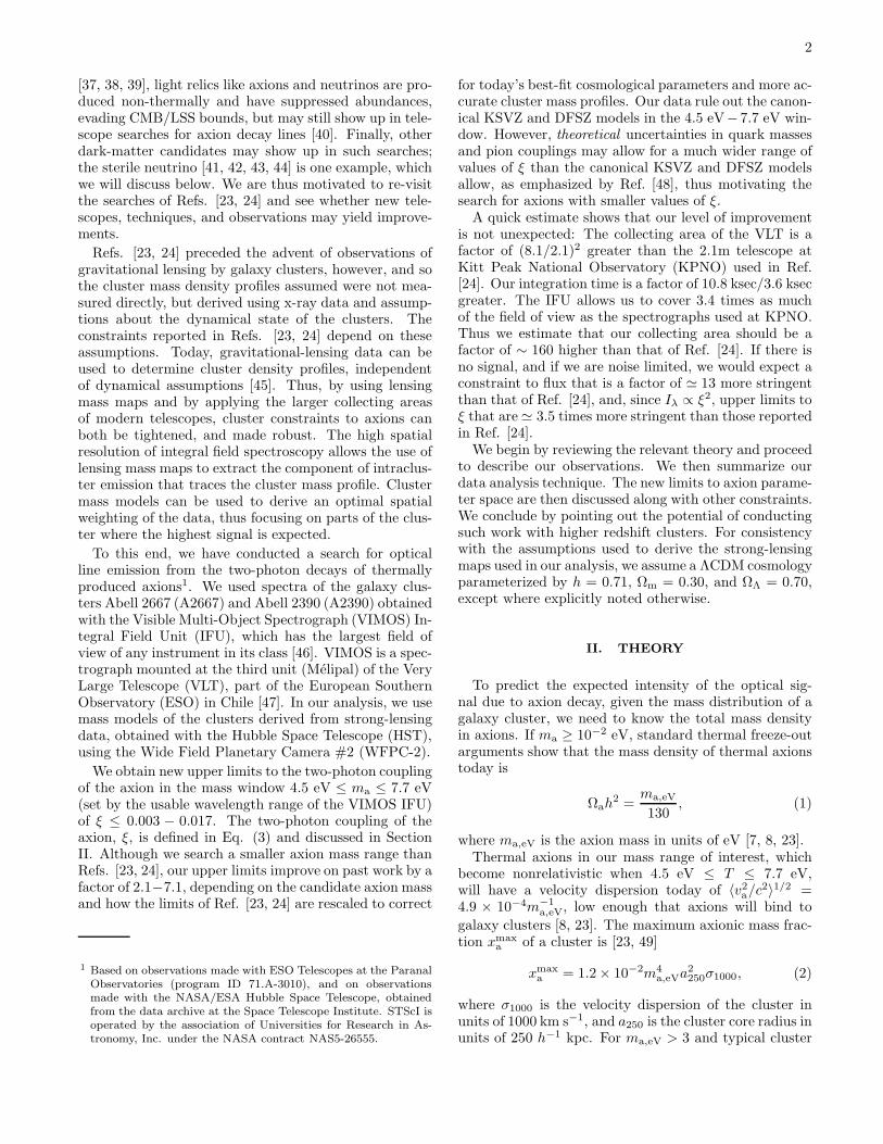
A2667 and A2390 obtained with the HST and the VLT.The cluster A2667 was observed with HST on October10-11, 2001, using WFPC-2 in the F450W, F606W, andF814W filters, with total exposure times of 12.0 ksec,4.00 ksec, and 4.00 ksec, respectively [50]. The clusterA2390 was observed with HST on December 10, 1994,using WFPC-2 in the F555W and F814W filters and to-tal exposure times of 8.40 ksec and 10.5 ksec [51]. Af-ter pipeline processing, standard reduction routines wereused with both clusters to combine the frames and re-move cosmic rays. Figs. 1 and 2 are images of the clustercores, with iso-mass contours overlaid from our best-fitlensing models.

On May 30 and June 1, 2001, near-infrared J-bandand H-band observations of A2667 were obtained withISAAC on the VLT [50]. The total exposure times for theJ and H band ISAAC data were 7.93 ksec and 6.53 ksec,respectively. The final seeing was 0.51′′ and 0.58′′ in theJ and H bands, respectively.

B. VIMOS Spectra

The massive galaxy clusters A2667 and A2390 wereobserved with VIMOS, between June 27 and 30, 2003[50, 51]. The IFU is one of three modes available on VI-MOS, and consists of 4 quadrants, each containing 1600fibers. We used an instrumental setup in which each fibercovered a region of 0.67′′ in diameter. A single pointingcovered a 54′′ × 54′′ region of the sky. Roughly 10% of

4

FIG. 1: Image of the Abell 2667 cluster core imaged with HSTin the F450W, F606W, and F814W filters. The white (thinyellow) square shows the IFU field of view, which is 54”×54”.North is to the top and east is to the left. Note the stronglymagnified gravitational arc north-east of the central galaxy.The white curves correspond to iso-mass contours from thelens model; the dark gray (red) line is the critical line at theredshift of the giant arc. The field of view is centered onαJ2000=23:52:28.4, δJ2000=−26:05:08. At a redshift of z =0.233, the angular scale is 3.661 kpc/arcsec.

FIG. 2: Image of the Abell 2390 cluster core imaged withHST in the F450W, F606W, and F814W filters. The white(thin yellow) squares correspond to the IFU field of view indifferent pointings. The white curves correspond to iso-masscontours from the lens model. The dark gray (red) line is thecritical line at the redshift of the giant arc, labelled 1. Eachsquare is 54” × 54”. North is to the top and east is to theleft. The field of view is centered on αJ2000=21:53:36.970,δJ2000=+17:41:44.66. At a redshift of z = 0.228, the angularscale is 3.601 kpc/arcsec.

the IFU field of view is unresponsive because of incom-plete fiber coverage. A low resolution blue (LR-Blue)grism was used, covering the wavelength range 3500Ato 7000A with spectral resolution R ≈ 250 and disper-sion 5.355A/pixel. The FWHM of the axion-decay lineis 195A σ1000 m−1

a,eV, and so the LR-Blue grism can re-solve this line, without spreading a faint signal over toomany wavelength pixels. Unfortunately, because spectrafrom contiguous pseudo-slits (sets of 400 spectra) on theCCD overlap, the first and last 50 pixels on most of theraw spectra are unusable, reducing the spectral range to4000A − 6800A, corresponding to an axion mass-rangeof 4.5 ≤ ma,eV ≤ 7.7 at the nearly identical redshifts(z ≈ 0.23) of the two clusters. Further observationaldetails are discussed in Ref. [50].

The total exposure time for each cluster was 10.8 ksec(4 × 2.70 ksec exposures). Calibration frames were ob-tained after each of the exposures, and a spectrophoto-metric standard star was observed. In order to compen-sate for the presence of a small set of bad fibers, we usedan offset between consecutive exposures. At a redshiftof z = 0.233 (A2667), the IFU covers a physical regionof 198 kpc × 198 kpc in the plane of the cluster. At aredshift of z = 0.228 (A2390), the IFU covers a physicalregion of 195 kpc × 195 kpc.

C. Reduction of IFU data

If axions exist and are present in the halos of massivegalaxy clusters, a distinct spectral feature will appear inVIMOS-IFU data. At a rest-frame wavelength λa, wewill observe a spatially extended emission line whose in-tensity traces the projected dark-matter density. Reveal-ing such a faint, spatially extended signal requires greatcare in correcting for fiber efficiency and in subtractingthe sky background, because the instrument itself canimpose spatial variation in the sky background throughvarying IFU fiber efficiency.

The VIMOS-IFU data were reduced using the VIMOSInteractive Pipeline Graphical Interface (VIPGI), andthe authors’ own routines [52]. References [47, 50] giveboth a detailed description of the methods and an as-sessment of the quality of VIPGI data reduction. Thereduction steps that precede the final combination of thedithered exposures into a single data cube are performedon a quadrant by quadrant basis. The main steps are thefollowing [47, 50, 52, 53, 54]: extract spectra from the rawCCD data at each pointing, calibrate wavelength, removecosmic rays, determine fiber efficiencies, subtract the skybackground, and calibrate flux.

The exposures were bias subtracted. Cosmic-ray hitswere removed with an efficient automatic routine basedon a σ-clipping algorithm, which exploits the fact thatcosmic-ray hits show strong spatial gradients on the CCD[47], in contrast to the smoother spatial behavior of gen-uine emission lines. In Ref. [24], spectra were obtainedusing a limited number of long-slit exposures, so the re-

5

moval of a small number of incorrectly identified cosmic-ray hits could thwart a search for line emission fromdecaying axions. An axion-decay line, however, mustsmoothly track the density profile of the cluster. Ourspectra are highly spatially-resolved, and so cosmic-rayhits can be removed safely using our cleaning algorithm.Using the raw CCD spectral traces, we verified that thesignals removed by the cleaning algorithm bore the dis-tinctive visual signatures of cosmic-ray hits.

VIPGI usually determines fiber efficiencies by normal-izing to the flux of bright sky lines; this technique yieldeddata cubes with prominent bright and dark patches (eachcovering ∼ 20× 20 fibers). It is conceivable that an acci-dental correlation of these patches with the cluster den-sity profile could lead to a spurious axion signal. To avoidthis possibility, we measured fiber efficiency using highsignal to noise continuum arc-lamp exposures (analogousto flat-fielding for images and henceforth referred to asflat-fielding). The resulting flat-fielded data cubes weremuch less patchy, and were thus used for all subsequentanalysis.

The VIMOS IFU does not have a dedicated set offibers to determine the sky-background level. VIPGI usu-ally determines the sky statistically at each wavelength.VIPGI first groups the fibers in each quadrant into threesets according to the shape of a user selected sky-emissionline, and then takes the statistical mode of the counts ineach set and subtracts it from the counts measured ineach fiber in the set [52]. Although axions (and thustheir decay luminosity) trace the centrally peaked den-sity profile of the cluster, the average decay luminositywould be wiped out by this procedure, and lead to a spu-rious depression in measurements of ξ. The sky subtrac-tion implemented in VIPGI is thus unsuitable for ouraxion search and was not applied. A customized sky-subtraction was applied, as discussed in Section IVB.

Flux is calibrated separately for each IFU quadrant,using observations of a standard star. Finally, the fourfully reduced exposures are combined. The final datacube for A2667 is made of 6806 spatial elements, eachone containing a spectrum from 3500A to 7000A, andcovers a sky area of 0.83 arcmin2, centered 5 arcsec south-west of the brightest cluster galaxy. The final data cubefor A2390 is made of 24, 645 spatial elements, each onecontaining a spectrum from 3500A to 7000A, and coversa sky area of 3.11 arcmin2, centered 15 arcsec north-east of the brightest cluster galaxy. The median spectralresolution is ≃ 18A. For further discussion of the processused to generate the data cubes, see Refs. [47, 50].

After producing data cubes in VIPGI, we passed thesedata cubes to a secondary routine that searches foremission from axion decay and estimates the noise inour spectra. The most obvious source of error is Pois-son counting noise. The number of photons observedat wavelength λ in the jth spatial bin is just Nλ,j =E [Fλ,j/(hc/λ)] δtδλδA, where δA = 51.2m2 is the col-

lecting area of the Melipal telescope, δλ = 5.355A is thedispersion of a single VIMOS spectral pixel, δt is the

integration time, Fλ,j is the flux in the jth pixel at wave-length λ, and E is the end to end mean efficiency ofVIMOS mounted at Melipal. The Poisson counting noiseis δNλ,j ≈

√

Nλ,j , and so δIλ,j ≈ Iλ,j/√

Nλ,j . A sec-ondary error source is flux contamination from neighbor-ing pixels. To include this error, we use the 5% estimateof Ref. [47], calculate the ‘leakage’ contribution to noiseat each pixel by taking the mean flux of all the nearestneighboring pixels, and multiply it by 5%. We also usetime-logged measurements of the CCD bias and dark-current, with the appropriate integration time, to calcu-late the additional noise from these sources2. Finally weestimate the flat-fielding noise using the rms differencebetween different sets of efficiency tables. These errorsare added in quadrature to obtain a data cube of theestimated errors in specific intensity.

In Refs. [23, 24], slit locations were chosen to avoidthe locations of known galaxies, as well as regions thatshowed statistical evidence for faint galaxies [55]. Like-wise, we masked out IFU fibers that fell on the locationsof individual bright sources. Bright sources were identi-fied in each cluster image by tagging pixels where the im-age intensity exceeded the median by more than 1σ andmasking IFU fibers that fell on these pixels. Practically,this means that 40% of the fibers in each data cube areleft unmasked. The images used to generate this maskare broadband, and so this masking technique will notmask out an axion-decay signal. The accidental inclu-sion of galaxies could conceivably lead us to erroneouslyattribute their emission to axion decay. This is unlikely,given that the spectra of cluster galaxies are dominatedby continuum emission and line absorption. If we seean indication of emission due to line decay, however, wemay have to revise our masking criteria to take accountof this possibility. As we shall see later, we imposed up-per limits to axion decay, and can safely use the chosenmasking criterion. The resulting masks were visually in-spected to verify that most of the masked fibers fall neargalaxies. To extract the density dependent component ofthe cluster spectra, we apply a mass map obtained fromgravitational lensing observations.

IV. ANALYSIS

A. Strong Lensing and Cluster Mass Maps

To model the mass distribution of A2667 and A2390,we used both a cluster mass-scale component (represent-ing the contribution of the dark-matter halo and the intr-acluster medium) and cluster-galaxy mass components asin Refs. [45, 56]. Cluster galaxies were selected accord-ing to their redshift (when available, in the inner clusterregion covered with VIMOS spectroscopy) or their color,

2 http://www.eso.org/observing/dfo/quality/VIMOS/toc.html.

6

thus selecting galaxies belonging to the cluster red se-quence. For A2667, ISAAC images were used to deter-mine J-H colors, whereas for A2390, HST images wereused to determine I-V colors. The lensing contributionfrom more prominent foreground galaxies was also in-cluded, rescaling their lensing properties using the ap-propriate redshift.

All model components were parameterized using asmoothly truncated pseudo-isothermal mass distributionmodel (PIEMD) [57], which avoids both the unphysicalcentral-density singularity and the infinite spatial extentof the singular isothermal model.

The galaxy mass components were chosen to have thesame position, ellipticity and orientation as their corre-sponding images. The K-band luminosity of the galaxieswas computed, assuming a typical E/S0 spectral energydistribution (redshifted but uncorrected for evolution ofconstituent stellar populations). Their masses were esti-mated using the K-band luminosity, calculated assuminga global mass to light ratio (M/L) and the Faber-Jacksonrelation [58]. The final mass model is made of 70 com-ponents, including the large scale cluster halo and theindividual galaxies.

Using the LENSTOOL ray-tracing code [59] with theHST images, we iteratively implemented the constraintsfrom the gravitational lenses. Lensing mass models withχ2 ≤ 1 were found by fitting the ellipticity, orientation,center, and mass parameters (velocity dispersion, coreradius, and truncation radius) of the cluster scale com-ponent, as well as the truncation radius and velocity dis-persion of the ensemble of cluster galaxies, using scalingrelations for early-type galaxies [60]. Cluster galaxy red-shifts were measured using the IFU data [50]. The brightcentral galaxy and several galaxies near the locations ofstrong-lensing arcs were modeled separately from the en-semble. The resulting cluster density maps for A2667and A2390 are shown in Figs. 3 and 4 [50, 51]. Statisti-cal errors in the mass model parameters were propagatedthrough the relevant code to produce a fiber by fiber mapof statistical errors in Σ. These maps were then used toweight different IFU fibers and thus maximize the signalto noise ratio of any putative line emission from axiondecay.

B. Extraction of One Dimensional Spectra

Using density maps of A2667 and A2390, we can op-timally weight averages over fibers to maximize the con-tribution from high density regions of the cluster. Thismaximizes the signal to noise ratio of our axion searchby emphasizing IFU fibers where maximum signal fromaxion decay is expected. These maps allow us to separateemission correlated with the mass profile of the cluster,which could be due to axion decay, from a sky back-ground that we assume to be spatially homogeneous. Ourtechnique is an IFU generalization of the long-slit ‘on-off’sky-subtraction technique presented in Refs. [23, 24].

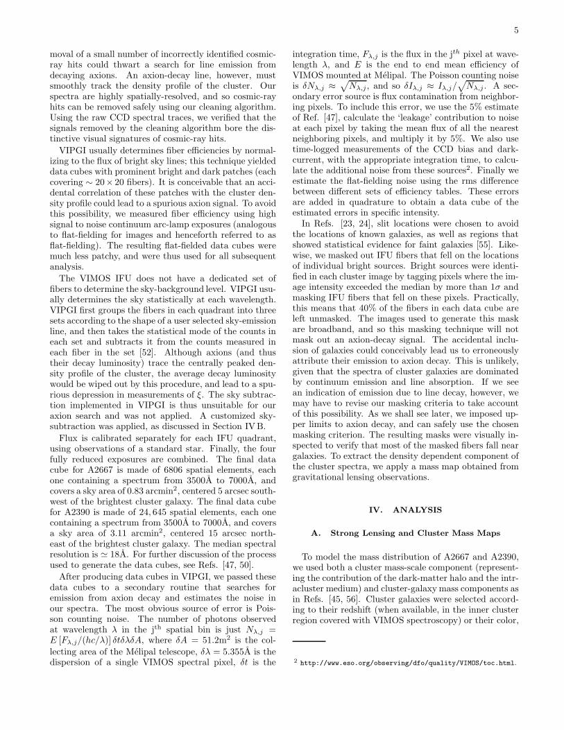
FIG. 3: Mass map of A2667. The intensity of the image scaleswith density (in units of 1012M⊙ pix−2), where 1 pix = 0.50”.A density scale is provided on the bottom of the image. Thehorizontal extent of this map is 222.6′′. The vertical extentis 200.0′′ . The thick black line indicates the spatial extent ofthe IFU head on the mass map.

The real sky background is certainly not perfectly homo-geneous, but by making this assumption, we are beingmaximally conservative. With our reduction method,any density correlated spatial dependence in the skybackground will show up as putative emission from ax-ion decay. If evidence for a signal is seen, we will haveto be careful to avoid being confused by sky line emis-sion. The projected surface density of the cluster at thelocation in the lens plane associated with the ith fiberis denoted Σ12,i. Assuming that the only spatially de-pendent signal comes from axions, we can then modelthe actual intensity Imod

λ,i at a given wavelength λ and

spatial pixel i as Imodλ,i = 〈Iλ/Σ12〉Σ12,i + bλ, where bλ

represents the contribution of a spatially homogeneoussky signal, and Iλ,i is the specific intensity in the ith

fiber at wavelength λ. Since the signal from axion decayis bounded from above by the total component of thesignal proportional to Σ12,i, a measurement of 〈Iλ/Σ12〉will either provide evidence of axion decay, or impose anupper limit on 〈Iλ/Σ12〉axion. Using a simple linear fit toseparate the sky background from signal, we extract thearray 〈Iλ/Σ12〉 from each cluster data cube.

At a small number of wavelengths, this yielded nega-tive (unphysical) values for one or both fitted parameters.To avoid this, we fit for 〈Iλ/Σ12〉 and bλ, subject to theobvious constraints 〈Iλ/Σ12〉 ≥ 0 and bλ ≥ 0, estimat-ing errors σλ,i as described in Section III C. Estimatederrors in Σ12 were also included in the fit. Residualsfrom the best fit are due to flux noise, imperfect maskingof galaxies, and variations in fiber efficiency unaccounted

7

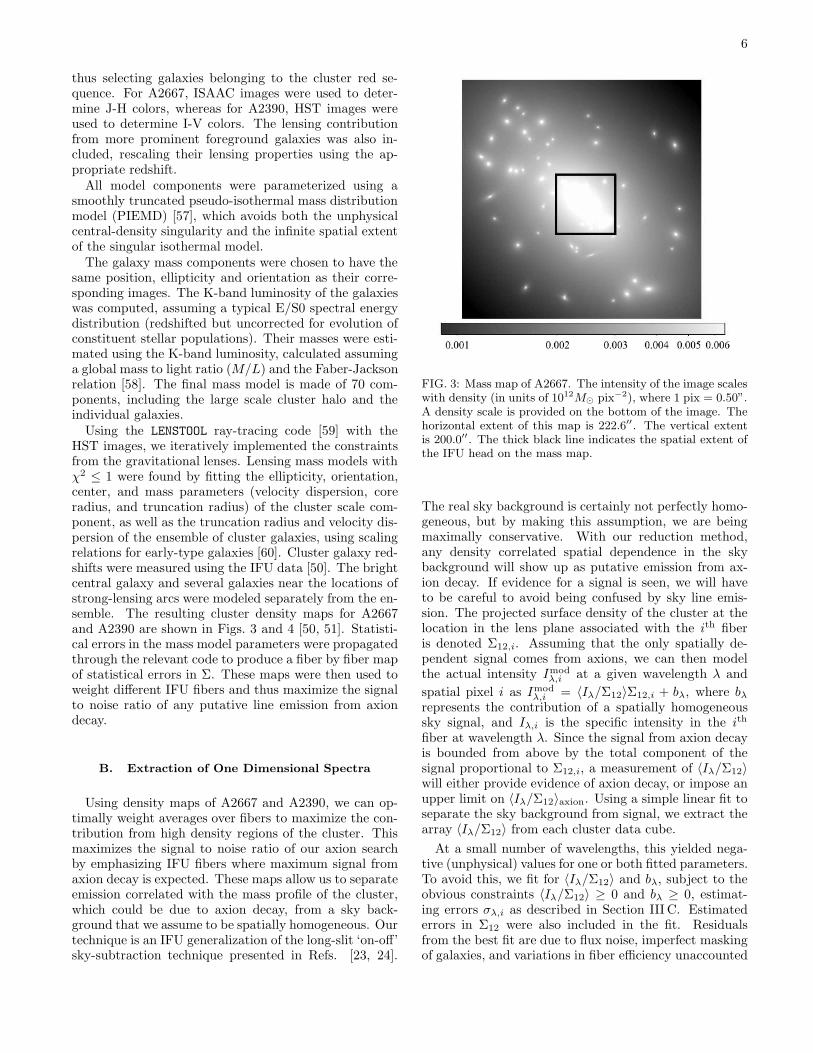
FIG. 4: Mass map of A2390. The intensity of the image scaleswith density (in units of 1012M⊙ pix−2), where 1 pix = 0.50”.A density scale is provided on the bottom of the image. Thehorizontal spatial extent of the map is 157.5”. The verticalextent is 150.0′′. The thick black lines indicate IFU pointingsused to construct our data cubes.

for by the flat-fielding procedure. As can be seen directlyfrom the unconstrained linear-least-squares solutions forthe parameters 〈Iλ/Σ12〉 and bλ, this procedure placeshigher weights on those VIMOS fibers that fall on higherdensity portions of the cluster. In essence, we used ourknowledge of the cluster density profile to extract onlythe information that interests us, namely, that part of theemission that is correlated with the cluster’s mass densityprofile. At some wavelengths, the best fit is 〈Iλ/Σ12〉 = 0with very low noise. We verified that these wavelengthscoincide with those at which a naive linear fit yieldednegative values for 〈Iλ/Σ12〉. Thus there is no evidencefor density correlated emission at these wavelengths. Atthese wavelengths, the emission due to axion decay isbounded from above by the brightness of the sky back-ground, and so we used 〈Iλ/Σ12〉 ≤ bλ/〈Σ12〉 to obtaina conservative upper limit on the flux. Decaying axionswill produce line emission, so it might seem that an ad-ditional continuum subtraction might be in order. Thecontinuum component of the sky background, however,is already subtracted using the techniques discussed, andan additional continuum subtraction step would be erro-neously aggressive.

As a test of our sky-subtraction technique, we alsoreimplemented the sky-subtraction technique of Ref. [24]and implemented an ‘on-off’ subtraction by definingfibers further than 23′′ (A2667) or 72′′ (A2390) from thecluster center (defined by the highest density point in thedensity maps) as ‘sky’ fibers, spatially averaging the fluxof these sky fibers at each wavelength, and subtractingthe resulting sky spectrum from each pixel in the ‘on’

cluster region. In this case, sky emission was directly es-timated from the data rather than modeled. In this case,the best fit for the signal is given by

⟨

Iλ

Σ12

⟩

=

∑

iIλ,iΣ12,i

σ2λ,i

∑

i

Σ212,i

σ2λ,i

, (5)

where i is a label for the density at the location of a givenIFU fiber, and σλ,i is the error in the specific intensity.

In the case of A2667, even the fibers furthest from thecluster center fall on portions of the cluster where emis-sion due to axion decays will be of the same order ofmagnitude as at the center. The sky-subtraction tech-nique of Ref. [24] is thus entirely inappropriate for ourdata on A2667, as it will subtract out a substantial frac-tion of any signal and return unjustifiably stringent limitsto emission from axion decay.

For A2390, the effective field of view is much larger,and so the emission expected from axion decays in theouter fibers is much less. Over most of the wavelengthrange of our data for A2390, the different sky-subtractiontechniques agreed to within a factor of two, leading usto believe that our sky-subtraction technique is trust-worthy. We used the value for 〈Iλ/Σ12〉 obtained usingour sky-subtraction technique, as it is desirable to usethe same sky-subtraction method for both clusters tobe self-consistent. Equation (5) and the correspondingbest-fit result in the constrained case essentially yieldone-dimensional cluster spectra, rescaled by the clus-ter density, as shown in Figs. 5 and 6. The specificintensity values in Fig. 5 were obtained by multiply-ing the best-fit values of 〈Iλ/Σ12〉 from Eq. (5) by the

mean 〈Σ12〉 =(

∑

i Σ12,i/σ2λ,i

)

/(

∑

i 1/σ2λ,i

)

. The plot-

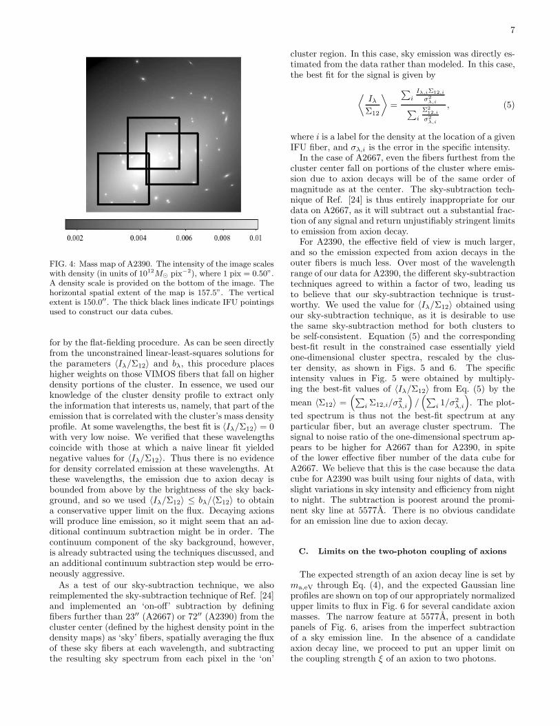
ted spectrum is thus not the best-fit spectrum at anyparticular fiber, but an average cluster spectrum. Thesignal to noise ratio of the one-dimensional spectrum ap-pears to be higher for A2667 than for A2390, in spiteof the lower effective fiber number of the data cube forA2667. We believe that this is the case because the datacube for A2390 was built using four nights of data, withslight variations in sky intensity and efficiency from nightto night. The subtraction is poorest around the promi-nent sky line at 5577A. There is no obvious candidatefor an emission line due to axion decay.

C. Limits on the two-photon coupling of axions

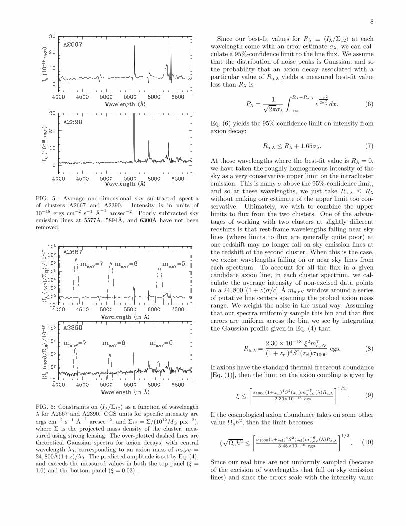
The expected strength of an axion decay line is set byma,eV through Eq. (4), and the expected Gaussian lineprofiles are shown on top of our appropriately normalizedupper limits to flux in Fig. 6 for several candidate axionmasses. The narrow feature at 5577A, present in bothpanels of Fig. 6, arises from the imperfect subtractionof a sky emission line. In the absence of a candidateaxion decay line, we proceed to put an upper limit onthe coupling strength ξ of an axion to two photons.

8

FIG. 5: Average one-dimensional sky subtracted spectraof clusters A2667 and A2390. Intensity is in units of

10−18 ergs cm−2 s−1 A−1

arcsec−2. Poorly subtracted skyemission lines at 5577A, 5894A, and 6300A have not beenremoved.

FIG. 6: Constraints on 〈Iλ/Σ12〉 as a function of wavelengthλ for A2667 and A2390. CGS units for specific intensity are

ergs cm−2 s−1 A−1

arcsec−2, and Σ12 = Σ/(1012M⊙ pix−2),where Σ is the projected mass density of the cluster, mea-sured using strong lensing. The over-plotted dashed lines aretheoretical Gaussian spectra for axion decays, with centralwavelength λ0, corresponding to an axion mass of ma,eV =24, 800A(1+z)/λ0. The predicted amplitude is set by Eq. (4),and exceeds the measured values in both the top panel (ξ =1.0) and the bottom panel (ξ = 0.03).

Since our best-fit values for Rλ ≡ 〈Iλ/Σ12〉 at eachwavelength come with an error estimate σλ, we can cal-culate a 95%-confidence limit to the line flux. We assumethat the distribution of noise peaks is Gaussian, and sothe probability that an axion decay associated with aparticular value of Ra,λ yields a measured best-fit valueless than Rλ is

Pλ =1√

2πσλ

∫ Rλ−Ra,λ

−∞e

−x2

2σ2λ dx. (6)

Eq. (6) yields the 95%-confidence limit on intensity fromaxion decay:

Ra,λ ≤ Rλ + 1.65σλ. (7)

At those wavelengths where the best-fit value is Rλ = 0,we have taken the roughly homogeneous intensity of thesky as a very conservative upper limit on the intraclusteremission. This is many σ above the 95%-confidence limit,and so at these wavelengths, we just take Ra,λ ≤ Rλ

without making our estimate of the upper limit too con-servative. Ultimately, we wish to combine the upperlimits to flux from the two clusters. One of the advan-tages of working with two clusters at slightly differentredshifts is that rest-frame wavelengths falling near skylines (where limits to flux are generally quite poor) atone redshift may no longer fall on sky emission lines atthe redshift of the second cluster. When this is the case,we excise wavelengths falling on or near sky lines fromeach spectrum. To account for all the flux in a givencandidate axion line, in each cluster spectrum, we cal-culate the average intensity of non-excised data pointsin a 24, 800 [(1 + z)σ/c] A ma,eV window around a seriesof putative line centers spanning the probed axion massrange. We weight the noise in the usual way. Assumingthat our spectra uniformly sample this bin and that fluxerrors are uniform across the bin, we see by integratingthe Gaussian profile given in Eq. (4) that

Ra,λ =2.30 × 10−18 ξ2m7

a,eV

(1 + zcl)4S2(zcl)σ1000cgs. (8)

If axions have the standard thermal-freezeout abundance[Eq. (1)], then the limit on the axion coupling is given by

ξ ≤[

σ1000(1+zcl)4S2(zcl)m

−7a,eV(λ)Ra,λ

2.30×10−18 cgs

]1/2

. (9)

If the cosmological axion abundance takes on some othervalue Ωah

2, then the limit becomes

ξ√

Ωah2 ≤[

σ1000(1+zcl)4S2(zcl)m

−6a,eV(λ)Ra,λ

3.48×10−16 cgs

]1/2

. (10)

Since our real bins are not uniformly sampled (becauseof the excision of wavelengths that fall on sky emissionlines) and since the errors scale with the intensity value

9

at a given wavelength, we make a small correction to thisexpected value. Specifically,

Ra,λ =2.68 × 10−18 ξ2m7

a,eV

(1 + zcl)4S2(zcl)

∑

j∈Tλ

Gj

σ2j

∑

j∈Tλ

1σ2

j

cgs,

where Gj = e−

(λj /(1+zcl)−λa)2c2

2σ2λ2a , (11)

Tλ is the set of all non-excised wavelengths lying withinthe bin centered at wavelength λ, and j labels wave-lengths. The quality of sky background subtraction mayvary as a result of spatial and temporal variations in thesky background from night to night. If it is not due toaxion decay, the density correlated emission might alsogenuinely vary between clusters. The quantity Ra,λ, how-ever, will by definition be independent of these factors. Asimple error weighted mean of the upper limits obtainedfrom the two clusters would thus erroneously increase theupper limit placed on ξ. If two clusters yield differentbest-fit values for Rλ, Ra,λ must be bounded from aboveby the lesser of these two. By comparing upper limitsto Rλ obtained from A2390 with those obtained fromA2667 and choosing the lowest value at each wavelength,we obtained the maximum values of Ra,λ consistent withthe data. We then applied Eq. (11) to obtain an upperlimit on ξ consistent with the spectra of both clusters.To account for variation in the upper limits to ξ aris-ing from systematic errors in the cluster mass profiles,we repeated the preceding analysis, drawing Σ12,i fromthe best-fit NFW (Navarro, Frenk, and White) and Kingprofiles to the cluster mass profiles.

Analytic expressions for the volumetric and surfacemass density for NFW and King profiles are reviewedin Appendix A. We determined the mass profile pa-rameters (a and σ for King profiles, c and σ for NFWprofiles) by fitting to our strong-lensing density maps.Using these different density profiles and assuming thatthe mass fraction in axions is xa = Ωah

2/(Ωmh2), weobtain limits to ξ. The cluster density at the locationof a given IFU fiber varies from profile to profile, andso different fibers receive higher weights when a one-dimensional spectrum is extracted. This explains thevariation in upper limits to ξ that arises when differentdensity profiles are assumed. We show the most conser-vative (with respect to choice of density profile) limit onξ (assuming the thermal-freezeout abundance of axions)at each candidate axion mass in Fig. 7. The upper limitsto ξ in adjacent points along the ma,eV axis are corre-lated due to overlapping bins. The narrow black arrowsnear ma,eV = 5.43 and 4.83 mark sharp night-sky lines

at λ = 5577A and λ = 6300A, where sky subtractionis unreliable and useful limits to ξ cannot be obtained.Limits on ξ and specific intensity at the putative line cen-ter are displayed for several candidate masses in Table I.Our data rule out the canonical DFSZ and KSVZ axionmodels in the mass window 4.5 ≤ ma,eV ≤ 7.7, as seenin Fig. 8. However, theoretical uncertainties motivatethe search for axions with values of ξ smaller than those

TABLE I: Upper limits to central line intensity and ξ at sev-eral candidate axion masses, derived directly from sky sub-tracted spectra of A2667 and A2390.

ma,eV 〈Iλ/Σ12〉 〈Σ12〉 (cgs) ξ

4.5 1.83 × 10−19 7.17 × 10−3

5 6.04 × 10−19 9.00 × 10−3

6 8.74 × 10−19 5.72 × 10−3

6.5 9.91 × 10−19 4.60 × 10−3

7 9.13 × 10−19 3.41 × 10−3

7.5 1.11 × 10−18 2.95 × 10−3

7.65 8.96 × 10−19 2.47 × 10−3

allowed by the canonical KSVZ and DFSZ models.If we relax the assumption that the cosmological ax-

ion abundance be given by Eq. (1), then our null searchimplies the bound, shown in Fig. 9, to the combinationξ(Ωah

2)1/2. We see that if ξ ∼ 10−1, as is the case inthe KSVZ model, then our results imply an upper limitΩah

2 ∼< 10−4 in our mass range, roughly two orders ofmagnitude stronger than CMB/LSS limits [36], whichprobe densities down to Ωah

2 ∼ 10−2.

D. Revision of past telescope constraints to axions

As can be seen from Eq. (4), and from the factthat the mass fraction of the cluster in axions is xa =Ωah

2/(Ωmh2), the upper limit on ξ derived from a givenupper limit on flux depends on the cluster mass modelused and the cosmological parameters assumed. Refer-ences [23, 24] date to a time when the observationallyfavored cosmology was sCDM (Standard Cold Dark Mat-ter: h = 0.5, Ωm = 1.0, ΩΛ = 0). Moreover, the Kingprofiles assumed in those analyses of A2218, A2256, andA1413 were based on available x-ray emission profiles ofthe chosen clusters [23, 24] (and references therein). Theadvent of modern x-ray instruments has improved x-ray-derived cluster mass profiles, and gravitational-lensingstudies have allowed measurements of cluster mass pro-files, free of the dynamical assumptions required to ob-tain a density profile from an x-ray temperature map.The quoted upper limits of Refs. [23, 24] must thus berescaled, and we have done so up to an ambiguity in slitplacement for A2218; details are discussed in Appendix Band the rescaled limits from past work are shown along-side our own in Fig. 7. Our limits improve on the rescaledlimits of Ref. [23, 24] by a factor of 2.1 − 7.1. Our fi-nal measurement of 〈Iλ/Σ12〉 is only noise limited at asmall fraction (≃ 10%) of the available wavelength range.The dominant uncertainty is systematic and comes fromsky subtraction. The expected improvement estimated inthe introduction assumed that we are limited by Poissonnoise in the measured flux, and is thus naive.

Previous cluster searches for axions used long-slit spec-troscopy. Our use of IFU data is novel, and it is conceiv-

10

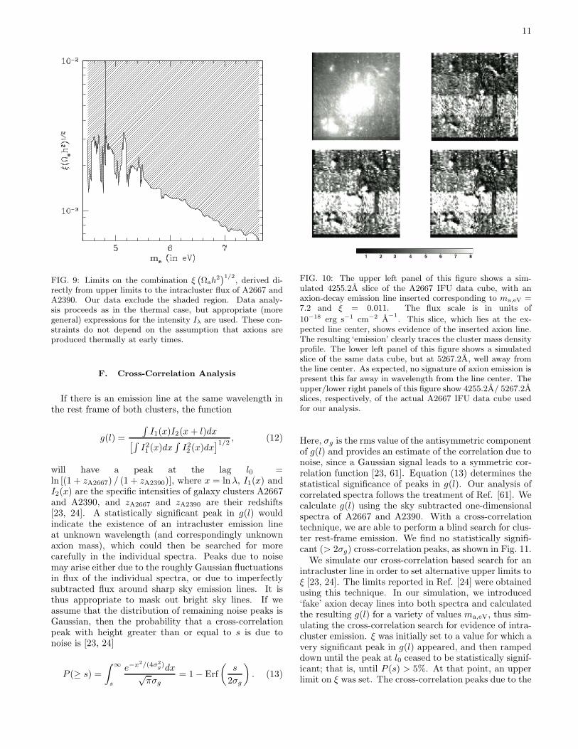
FIG. 7: Upper limits to the two-photon coupling parameter ξof the axion, derived directly from upper limits to the intra-cluster flux of A2667 and A2390. Our data exclude the shadedregion. The solid and dashed lines show the upper limits re-ported in Refs. [23, 24], adjusted (optimistically and pes-simistically) for differences between today’s best-fit measure-ments of the cosmological parameters/cluster mass profilesand the assumptions in Refs. [23, 24]. Details are discussedin Appendix B. The mass range 4.5 eV ≤ ma ≤ 7.7 eV arisesfrom the 4000A–6800A usable wavelength range of VIMOS,which is smaller than that of the KPNO spectrograph used inRef. [24]. The narrow black arrows near 5.43 eV and 4.83 eVmark the sharp night-sky lines at 5577A and 6300A, wheresky subtraction is unreliable and useful limits to ξ cannot beobtained. The shaded exclusion region is derived by applyingthe cluster density profile (strong-lensing map, best-fit NFWprofile, or best-fit King profile) at each candidate axion massthat yields the most conservative upper limit on ξ.

able that peculiarities of the data-reduction techniquesused in IFU spectroscopy may affect the sensitivity of oursearch. To explore this possibility, we have conducted asimulation.

E. Simulation of Analysis Technique

We simulate axion-decay emission in our data cube forA2667, using Eq. (4) and our lensing derived projecteddensity maps. We did this at a range of 10 candidateaxion masses spanning the full mass range of our search.We used 3 or 4 different values of ξ at each candidatemass. The first value was chosen to be slightly below(5−10%) the limit on ξ set by preceding techniques, whilethe second was chosen to be slightly above the upperlimit. The third and fourth values were chosen to be inconsiderable (factors of 2 and 10, respectively) excess ofthe upper limit. For all simulated axion masses, visualinspection of the data cube yields clear evidence for the

FIG. 8: Comparison of existing limits to the two-photon cou-pling of a 4.5 eV− 14 eV axion with the projected sensitivityof our proposed observations of lensing cluster RDCS 1252(z = 1.237). Flux limits and density profiles were assumedto be the same as those of A2667/A2390. The best existingupper limits to ξ in the higher mass window come from lim-its to the Diffuse Extragalactic Background Radiation (DE-BRA), and were rescaled for consistency with today’s best-fitΛCDM parameters and recent measurements [21, 22]. Thelimits reported in this and previous work, derived using opti-cal spectroscopy of galaxy clusters, are shown for comparison[23, 24]. Regions inaccessible due to night-sky emission linesare marked with narrow black arrows. The two solid horizon-tal lines indicate the predictions of the DFSZ and KSVZ axionmodels; the downward arrows indicate that ξ is theoretically

uncertain.

inserted line when ξ exceeds the imposed upper limit.An example is shown in Fig. 10. After inspecting thedata cubes visually, we applied the routines used for thepreceding analysis to produce one-dimensional spectrafor each cube. We then applied the same routine used toextract upper limits to ξ to recover the simulated ξ value.When the simulated value of ξ exceeded the upper limit,we recovered the correct answer in all cases to a precisionof 5 − 10%. This leads us to believe that our techniqueis robust and our upper limits reliable. References [23,24] supplement upper limits to ξ derived directly fromflux limits with limits obtained from a cross-correlationanalysis. We do the same, using our data on A2667 andA2390.

11

FIG. 9: Limits on the combination ξ`

Ωah2´1/2

, derived di-rectly from upper limits to the intracluster flux of A2667 andA2390. Our data exclude the shaded region. Data analy-sis proceeds as in the thermal case, but appropriate (moregeneral) expressions for the intensity Iλ are used. These con-straints do not depend on the assumption that axions areproduced thermally at early times.

F. Cross-Correlation Analysis

If there is an emission line at the same wavelength inthe rest frame of both clusters, the function

g(l) =

∫

I1(x)I2(x + l)dx[∫

I21 (x)dx

∫

I22 (x)dx

]1/2, (12)

will have a peak at the lag l0 =ln [(1 + zA2667) / (1 + zA2390)], where x = lnλ, I1(x) andI2(x) are the specific intensities of galaxy clusters A2667and A2390, and zA2667 and zA2390 are their redshifts[23, 24]. A statistically significant peak in g(l) wouldindicate the existence of an intracluster emission lineat unknown wavelength (and correspondingly unknownaxion mass), which could then be searched for morecarefully in the individual spectra. Peaks due to noisemay arise either due to the roughly Gaussian fluctuationsin flux of the individual spectra, or due to imperfectlysubtracted flux around sharp sky emission lines. It isthus appropriate to mask out bright sky lines. If weassume that the distribution of remaining noise peaks isGaussian, then the probability that a cross-correlationpeak with height greater than or equal to s is due tonoise is [23, 24]

P (≥ s) =

∫ ∞

s

e−x2/(4σ2g)dx√

πσg= 1 − Erf

(

s

2σg

)

. (13)

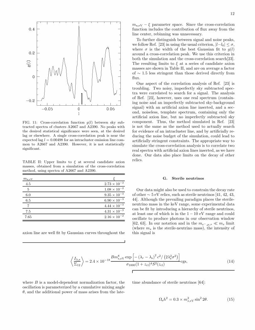
FIG. 10: The upper left panel of this figure shows a sim-ulated 4255.2A slice of the A2667 IFU data cube, with anaxion-decay emission line inserted corresponding to ma,eV =7.2 and ξ = 0.011. The flux scale is in units of

10−18 erg s−1 cm−2 A−1

. This slice, which lies at the ex-pected line center, shows evidence of the inserted axion line.The resulting ‘emission’ clearly traces the cluster mass densityprofile. The lower left panel of this figure shows a simulatedslice of the same data cube, but at 5267.2A, well away fromthe line center. As expected, no signature of axion emission ispresent this far away in wavelength from the line center. Theupper/lower right panels of this figure show 4255.2A/ 5267.2Aslices, respectively, of the actual A2667 IFU data cube usedfor our analysis.

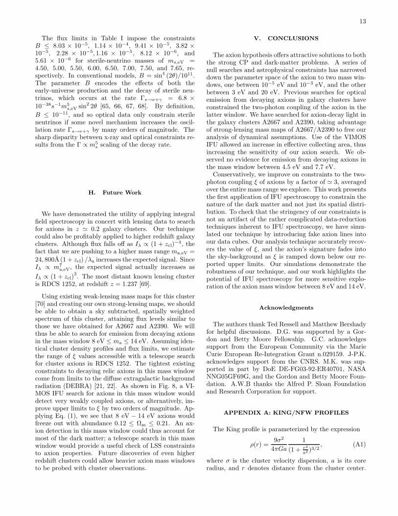
Here, σg is the rms value of the antisymmetric componentof g(l) and provides an estimate of the correlation due tonoise, since a Gaussian signal leads to a symmetric cor-relation function [23, 61]. Equation (13) determines thestatistical significance of peaks in g(l). Our analysis ofcorrelated spectra follows the treatment of Ref. [61]. Wecalculate g(l) using the sky subtracted one-dimensionalspectra of A2667 and A2390. With a cross-correlationtechnique, we are able to perform a blind search for clus-ter rest-frame emission. We find no statistically signifi-cant (> 2σg) cross-correlation peaks, as shown in Fig. 11.

We simulate our cross-correlation based search for anintracluster line in order to set alternative upper limits toξ [23, 24]. The limits reported in Ref. [24] were obtainedusing this technique. In our simulation, we introduced‘fake’ axion decay lines into both spectra and calculatedthe resulting g(l) for a variety of values ma,eV, thus sim-ulating the cross-correlation search for evidence of intra-cluster emission. ξ was initially set to a value for which avery significant peak in g(l) appeared, and then rampeddown until the peak at l0 ceased to be statistically signif-icant; that is, until P (s) > 5%. At that point, an upperlimit on ξ was set. The cross-correlation peaks due to the

12

FIG. 11: Cross-correlation function g(l) between sky sub-tracted spectra of clusters A2667 and A2390. No peaks withthe desired statistical significance were seen, at the desiredlag or elsewhere. A single cross-correlation peak is near theexpected lag l = 0.00498 for an intracluster emission line com-mon to A2667 and A2390. However, it is not statisticallysignificant.

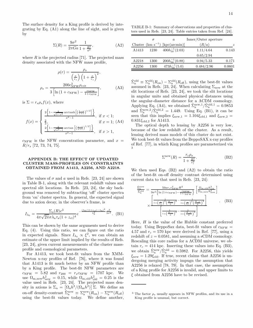
TABLE II: Upper limits to ξ at several candidate axionmasses, obtained from a simulation of the cross-correlationmethod, using spectra of A2667 and A2390.

ma,eV ξ

4.5 2.73 × 10−2

5 1.08 × 10−2

6.0 9.35 × 10−3

6.5 6.90 × 10−3

7 4.44 × 10−3

7.5 4.31 × 10−3

7.65 2.16 × 10−2

axion line are well fit by Gaussian curves throughout the

ma,eV − ξ parameter space. Since the cross-correlationfunction includes the contribution of flux away from theline center, rebinning was unnecessary.

To further distinguish between signal and noise peaks,we follow Ref. [23] in using the usual criterion, |l−l0| ≤ σ,where σ is the width of the best Gaussian fit to g(l)around a cross-correlation peak. We use this criterion inboth the simulation and the cross-correlation search[23].The resulting limits to ξ at a series of candidate axionmasses are shown in Table II, and are on average a factorof ∼ 1.5 less stringent than those derived directly fromflux.

One aspect of the correlation analysis of Ref. [23] istroubling. Two noisy, imperfectly sky subtracted spec-tra were correlated to search for a signal. The analysisof Ref. [23], however, uses one real spectrum (contain-ing noise and an imperfectly subtracted sky-backgroundsignal) with an artificial axion line inserted, and a sec-ond, noiseless, template spectrum, containing only theartificial axion line, but no imperfectly subtracted skycomponent. Thus, the method simulated in Ref. [23]is not the same as the method used to actually searchfor evidence of an intracluster line, and by artificially re-ducing the noise budget of the simulation, could lead toartificially stringent constraints. The appropriate way tosimulate the cross-correlation analysis is to correlate tworeal spectra with artificial axion lines inserted, as we havedone. Our data also place limits on the decay of otherrelics.

G. Sterile neutrinos

Our data might also be used to constrain the decay rateof other ∼ 5 eV relics, such as sterile neutrinos [41, 42, 43,44]. Although the prevailing paradigm places the sterile-neutrino mass in the keV range, some experimental datacan be fit by introducing a hierarchy of sterile neutrinos,at least one of which is in the 1− 10 eV range and couldoscillate to produce photons in our observation window[62, 63]. In our notation and in the me−,µ,τ ≪ ms limit(where ms is the sterile-neutrino mass), the intensity ofthis signal is

⟨

Iλ,s

Σ12

⟩

= 2.4 × 10−18Bm8

s,eV exp[

− (λr − λs)2c2/

(

2λ2sσ

2)

]

σ1000(1 + zcl)4S2(zcl)cgs, (14)

where B is a model-dependent normalization factor, theoscillation is parameterized by a cumulative mixing angleθ, and the additional power of mass arises from the late-

time abundance of sterile neutrinos [64]:

Ωsh2 = 0.3 × m2

s,eV sin2 2θ. (15)

13

The flux limits in Table I impose the constraintsB ≤ 8.03 × 10−5, 1.14 × 10−4, 9.41 × 10−5, 3.82 ×10−5, 2.28 × 10−5, 1.16 × 10−5, 8.12 × 10−6, and5.61 × 10−6 for sterile-neutrino masses of ms,eV =4.50, 5.00, 5.50, 6.00, 6.50, 7.00, 7.50, and 7.65, re-spectively. In conventional models, B = sin4 (2θ)/1011.The parameter B encodes the effects of both theearly-universe production and the decay of sterile neu-trinos, which occurs at the rate Γs→ν+γ = 6.8 ×10−38s−1m5

s,eV sin2 2θ [65, 66, 67, 68]. By definition,

B ≤ 10−11, and so optical data only constrain sterileneutrinos if some novel mechanism increases the oscil-lation rate Γs→ν+γ by many orders of magnitude. Thesharp disparity between x-ray and optical constraints re-sults from the Γ ∝ m5

s scaling of the decay rate.

H. Future Work

We have demonstrated the utility of applying integralfield spectroscopy in concert with lensing data to searchfor axions in z ≃ 0.2 galaxy clusters. Our techniquecould also be profitably applied to higher redshift galaxyclusters. Although flux falls off as Iλ ∝ (1 + zcl)

−4, thefact that we are pushing to a higher mass range ma,eV =

24, 800A (1 + zcl) /λa increases the expected signal. SinceIλ ∝ m7

a,eV, the expected signal actually increases as

Iλ ∝ (1 + zcl)3. The most distant known lensing cluster

is RDCS 1252, at redshift z = 1.237 [69].

Using existing weak-lensing mass maps for this cluster[70] and creating our own strong-lensing maps, we shouldbe able to obtain a sky subtracted, spatially weightedspectrum of this cluster, attaining flux levels similar tothose we have obtained for A2667 and A2390. We willthus be able to search for emission from decaying axionsin the mass window 8 eV ≤ ma ≤ 14 eV. Assuming iden-tical cluster density profiles and flux limits, we estimatethe range of ξ values accessible with a telescope searchfor cluster axions in RDCS 1252. The tightest existingconstraints to decaying relic axions in this mass windowcome from limits to the diffuse extragalactic backgroundradiation (DEBRA) [21, 22]. As shown in Fig. 8, a VI-MOS IFU search for axions in this mass window woulddetect very weakly coupled axions, or alternatively, im-prove upper limits to ξ by two orders of magnitude. Ap-plying Eq. (1), we see that 8 eV − 14 eV axions wouldfreeze out with abundance 0.12 ≤ Ωm ≤ 0.21. An ax-ion detection in this mass window could thus account formost of the dark matter; a telescope search in this masswindow would provide a useful check of LSS constraintsto axion properties. Future discoveries of even higherredshift clusters could allow heavier axion mass windowsto be probed with cluster observations.

V. CONCLUSIONS

The axion hypothesis offers attractive solutions to boththe strong CP and dark-matter problems. A series ofnull searches and astrophysical constraints has narroweddown the parameter space of the axion to two mass win-dows, one between 10−5 eV and 10−3 eV, and the otherbetween 3 eV and 20 eV. Previous searches for opticalemission from decaying axions in galaxy clusters haveconstrained the two-photon coupling of the axion in thelatter window. We have searched for axion-decay light inthe galaxy clusters A2667 and A2390, taking advantageof strong-lensing mass maps of A2667/A2390 to free ouranalysis of dynamical assumptions. Use of the VIMOSIFU allowed an increase in effective collecting area, thusincreasing the sensitivity of our axion search. We ob-served no evidence for emission from decaying axions inthe mass window between 4.5 eV and 7.7 eV.

Conservatively, we improve on constraints to the two-photon coupling ξ of axions by a factor of ≃ 3, averagedover the entire mass range we explore. This work presentsthe first application of IFU spectroscopy to constrain thenature of the dark matter and not just its spatial distri-bution. To check that the stringency of our constraints isnot an artifact of the rather complicated data-reductiontechniques inherent to IFU spectroscopy, we have simu-lated our technique by introducing fake axion lines intoour data cubes. Our analysis technique accurately recov-ers the value of ξ, and the axion’s signature fades intothe sky-background as ξ is ramped down below our re-ported upper limits. Our simulations demonstrate therobustness of our technique, and our work highlights thepotential of IFU spectroscopy for more sensitive explo-ration of the axion mass window between 8 eV and 14 eV.

Acknowledgments

The authors thank Ted Ressell and Matthew Bershadyfor helpful discussions. D.G. was supported by a Gor-don and Betty Moore Fellowship. G.C. acknowledgessupport from the European Community via the MarieCurie European Re-Integration Grant n.029159. J-P.K.acknowledges support from the CNRS. M.K. was sup-ported in part by DoE DE-FG03-92-ER40701, NASANNG05GF69G, and the Gordon and Betty Moore Foun-dation. A.W.B thanks the Alfred P. Sloan Foundationand Research Corporation for support.

APPENDIX A: KING/NFW PROFILES

The King profile is parameterized by the expression

ρ(r) =9σ2

4πGa

1

(1 + r2

a2 )3/2, (A1)

where σ is the cluster velocity dispersion, a is its coreradius, and r denotes distance from the cluster center.

14

The surface density for a King profile is derived by inte-grating by Eq. (A1) along the line of sight, and is givenby

Σ(R) =9σ2

2πGa

1

1 + R2

a2

, (A2)

where R is the projected radius [71]. The projected massdensity associated with the NFW mass profile,

ρ(r) =ρs

(

rrs

)(

1 + rrs

)2 ,

ρs =200c3

NFWρcrit

3[

ln (1 + cNFW) − cNFW

1+cNFW

] , (A3)

is Σ = rsρsf(x), where

f(x) =

2

1− 2√1−x2

arctanhh

( 1−x1+x )1/2

i

ff

x2−1 , if x < 1;23 , if x = 1;

2

1− 2√x2

−1arctan

h

(x−1x+1 )

1/2i

ff

x2−1 , if x > 1,

(A4)

cNFW is the NFW concentration parameter, and x =R/rs [72, 73, 74, 75].

APPENDIX B: THE EFFECT OF UPDATEDCLUSTER MASS-PROFILES ON CONSTRAINTSOBTAINED FROM A1413, A2256, AND A2218.

The values of σ and a used in Refs. [23, 24] are shownin Table B-1, along with the relevant redshift values andspectral slit locations. In Refs. [23, 24], the sky back-ground was removed by subtracting ‘off’ cluster spectrafrom ‘on’ cluster spectra. In general, the expected signaldue to axion decay, in the observer’s frame, is

Iλ0 =Σa(R)c3

4π√

2πσλaτa(1 + zcl)4e− (λ0/(1+zcl)−λa)2

λ2a

c2

2σ2 . (B1)

This can be shown by the same arguments used to deriveEq. (4). Using this ratio, we can figure out the ratioin expected signals. Since Iλ0 ∝ ξ2, we can obtain anestimate of the upper limit implied by the results of Refs.[23, 24], given current measurements of the cluster mass-profile and cosmological parameters.

For A1413, we took best-fit values from the XMM-Newton x-ray profiles of Ref. [76], where it was foundthat A1413 is fit much better by an NFW profile thanby a King profile. The best-fit NFW parameters arecNFW = 5.82 and r200 = rscNFW = 1707 kpc. Weuse Ωm,newh2

new = 0.15, while Ωm,oldh2old = 0.25 is the

value used in Refs. [23, 24]. The projected mass den-sity in axions is Σa =

[

Ωah2/(Ωmh2)

]

Σ. We define an

on-off density-contrast Σnewa ≡ Σnew

a (Ron) − Σnewa (Roff)

using the best-fit values today. We define another,

TABLE B-1: Summary of observations and properties of clus-ters used in Refs. [23, 24]. Table entries taken from Ref. [24].

σ a Inner/Outer aperture

Cluster (km s−1) [kpc(arcmin)] (R/a) z

A1413 1230 400h−1

50(2.03) 1.11/4.64 0.143

0.65/2.94

A2218 1300 200h−1

50(0.88) 0.94/5.33 0.171

A2256 1300 473h−1

50(5.0) 0.484/2.96 0.0601

Σolda ≡ Σold

a (Ron) − Σolda (Roff), using the best-fit values

assumed in Refs. [23, 24]. When calculating Σnew at theslit locations of Refs. [23, 24], we took the slit locationsin angular units and obtained physical distances usingthe angular-diameter distance for a ΛCDM cosmology.Applying Eq. (A4), we obtained Σnew,1

a /Σold,1a = 0.9853

and Σnew,2a /Σold,2

a = 1.449. Using Eq. (B1), it can beseen that this implies ξnew,1 = 1.104ξold,1 and ξnew,2 =0.831ξold,2 for A1413.

The optical depth to lensing by A2256 is very low,because of the low redshift of the cluster. As a result,lensing derived mass models of this cluster do not exist.We took best-fit values from the BeppoSAX x-ray profilesof Ref. [77], in which King profiles are parameterized via3

Σnew(R) =rcρs

1 + R2

r2c

. (B2)

We then used Eqs. (B2) and (A2) to obtain the ratioof the best-fit on-off density contrast determined usingcurrent data to that used in Refs. [23, 24]:

Σnewa

Σolda

=50arcc3

NFWH2

9σ2n

ln (1+cNFW)− cNFW1+cNFW

o

[

Ωm,oldh2old

Ωm,newh2new

]

×

2

4

1

1+( arc

)2(Rona )2 − 1

1+( arc )2(Roff

a )2

3

5

2

4

1

1+(Rona )

2 − 1

1+(Roffa )

2

3

5

. (B3)

Here, H is the value of the Hubble constant preferredtoday. Using BeppoSax data, best-fit values of cNFW =4.57 and rc = 570 kpc were derived in Ref. [77], using aredshift of z = 0.0581, and assuming a sCDM cosmology.Rescaling this core radius for a ΛCDM universe, we ob-tain rc = 414 kpc. Inserting these values into Eq. (B3),

we obtain Σnewa /Σold

a = 0.5982. For A2256, this yieldsξnew = 1.29ξold. If true, recent claims that A2256 is un-dergoing merging activity impugn the assumption thatA2256 is relaxed [78, 79]. In that case, the assumptionof a King profile for A2256 is invalid, and upper limits toξ obtained from A2256 have to be revised.

3 The factor ρs usually appears in NFW profiles, and its use in aKing profile is unusual, but correct.

15

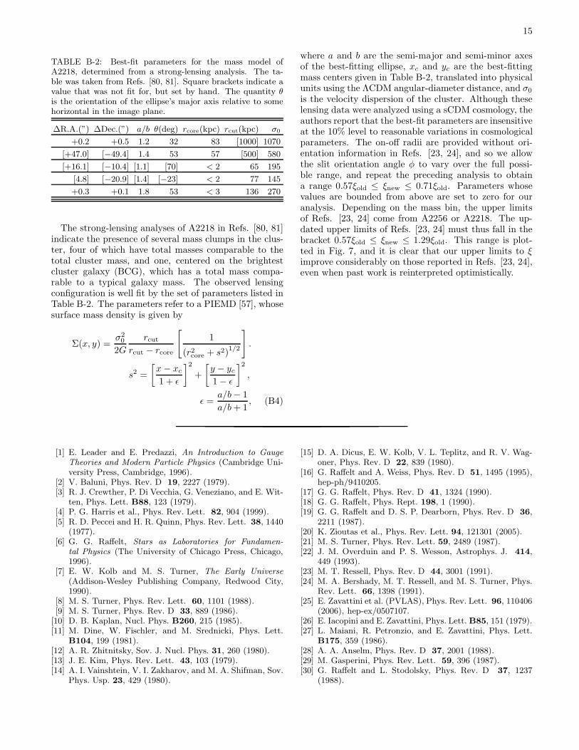
TABLE B-2: Best-fit parameters for the mass model ofA2218, determined from a strong-lensing analysis. The ta-ble was taken from Refs. [80, 81]. Square brackets indicate avalue that was not fit for, but set by hand. The quantity θis the orientation of the ellipse’s major axis relative to somehorizontal in the image plane.

∆R.A.(”) ∆Dec.(”) a/b θ(deg) rcore(kpc) rcut(kpc) σ0

+0.2 +0.5 1.2 32 83 [1000] 1070

[+47.0] [−49.4] 1.4 53 57 [500] 580

[+16.1] [−10.4] [1.1] [70] < 2 65 195

[4.8] [−20.9] [1.4] [−23] < 2 77 145

+0.3 +0.1 1.8 53 < 3 136 270

The strong-lensing analyses of A2218 in Refs. [80, 81]indicate the presence of several mass clumps in the clus-ter, four of which have total masses comparable to thetotal cluster mass, and one, centered on the brightestcluster galaxy (BCG), which has a total mass compa-rable to a typical galaxy mass. The observed lensingconfiguration is well fit by the set of parameters listed inTable B-2. The parameters refer to a PIEMD [57], whosesurface mass density is given by

Σ(x, y) =σ2

0

2G

rcut

rcut − rcore

[

1

(r2core + s2)

1/2

]

.

s2 =

[

x − xc

1 + ǫ

]2

+

[

y − yc

1 − ǫ

]2

,

ǫ =a/b − 1

a/b + 1, (B4)

where a and b are the semi-major and semi-minor axesof the best-fitting ellipse, xc and yc are the best-fittingmass centers given in Table B-2, translated into physicalunits using the ΛCDM angular-diameter distance, and σ0

is the velocity dispersion of the cluster. Although theselensing data were analyzed using a sCDM cosmology, theauthors report that the best-fit parameters are insensitiveat the 10% level to reasonable variations in cosmologicalparameters. The on-off radii are provided without ori-entation information in Refs. [23, 24], and so we allowthe slit orientation angle φ to vary over the full possi-ble range, and repeat the preceding analysis to obtaina range 0.57ξold ≤ ξnew ≤ 0.71ξold. Parameters whosevalues are bounded from above are set to zero for ouranalysis. Depending on the mass bin, the upper limitsof Refs. [23, 24] come from A2256 or A2218. The up-dated upper limits of Refs. [23, 24] must thus fall in thebracket 0.57ξold ≤ ξnew ≤ 1.29ξold. This range is plot-ted in Fig. 7, and it is clear that our upper limits to ξimprove considerably on those reported in Refs. [23, 24],even when past work is reinterpreted optimistically.

[1] E. Leader and E. Predazzi, An Introduction to Gauge

Theories and Modern Particle Physics (Cambridge Uni-versity Press, Cambridge, 1996).

[2] V. Baluni, Phys. Rev. D 19, 2227 (1979).[3] R. J. Crewther, P. Di Vecchia, G. Veneziano, and E. Wit-

ten, Phys. Lett. B88, 123 (1979).[4] P. G. Harris et al., Phys. Rev. Lett. 82, 904 (1999).[5] R. D. Peccei and H. R. Quinn, Phys. Rev. Lett. 38, 1440

(1977).[6] G. G. Raffelt, Stars as Laboratories for Fundamen-

tal Physics (The University of Chicago Press, Chicago,1996).

[7] E. W. Kolb and M. S. Turner, The Early Universe

(Addison-Wesley Publishing Company, Redwood City,1990).

[8] M. S. Turner, Phys. Rev. Lett. 60, 1101 (1988).[9] M. S. Turner, Phys. Rev. D 33, 889 (1986).

[10] D. B. Kaplan, Nucl. Phys. B260, 215 (1985).[11] M. Dine, W. Fischler, and M. Srednicki, Phys. Lett.

B104, 199 (1981).[12] A. R. Zhitnitsky, Sov. J. Nucl. Phys. 31, 260 (1980).[13] J. E. Kim, Phys. Rev. Lett. 43, 103 (1979).[14] A. I. Vainshtein, V. I. Zakharov, and M. A. Shifman, Sov.

Phys. Usp. 23, 429 (1980).

[15] D. A. Dicus, E. W. Kolb, V. L. Teplitz, and R. V. Wag-oner, Phys. Rev. D 22, 839 (1980).

[16] G. Raffelt and A. Weiss, Phys. Rev. D 51, 1495 (1995),hep-ph/9410205.

[17] G. G. Raffelt, Phys. Rev. D 41, 1324 (1990).[18] G. G. Raffelt, Phys. Rept. 198, 1 (1990).[19] G. G. Raffelt and D. S. P. Dearborn, Phys. Rev. D 36,

2211 (1987).[20] K. Zioutas et al., Phys. Rev. Lett. 94, 121301 (2005).[21] M. S. Turner, Phys. Rev. Lett. 59, 2489 (1987).[22] J. M. Overduin and P. S. Wesson, Astrophys. J. 414,

449 (1993).[23] M. T. Ressell, Phys. Rev. D 44, 3001 (1991).[24] M. A. Bershady, M. T. Ressell, and M. S. Turner, Phys.

Rev. Lett. 66, 1398 (1991).[25] E. Zavattini et al. (PVLAS), Phys. Rev. Lett. 96, 110406

(2006), hep-ex/0507107.[26] E. Iacopini and E. Zavattini, Phys. Lett. B85, 151 (1979).[27] L. Maiani, R. Petronzio, and E. Zavattini, Phys. Lett.

B175, 359 (1986).[28] A. A. Anselm, Phys. Rev. D 37, 2001 (1988).[29] M. Gasperini, Phys. Rev. Lett. 59, 396 (1987).[30] G. Raffelt and L. Stodolsky, Phys. Rev. D 37, 1237

(1988).

16

[31] R. Rabadan, A. Ringwald, and K. Sigurdson, Phys. Rev.Lett. 96, 110407 (2006), hep-ph/0511103.

[32] E. Masso and J. Redondo, JCAP 0509, 015 (2005), hep-ph/0504202.

[33] P. Jain and S. Mandal, Int. J. Mod. Phys. D15, 2095(2006), astro-ph/0512155.

[34] T. W. Kephart and T. J. Weiler, Phys. Rev. Lett. 58,171 (1987).

[35] Y. N. Gnedin, S. N. Dodonov, V. V. Vlasyuk, O. I. Spiri-donova, and A. V. Shakhverdov, Mon. Not. R. Astron.Soc. 306, 117 (1999).

[36] S. Hannestad, A. Mirizzi, and G. Raffelt, JCAP 0507,002 (2005), hep-ph/0504059.

[37] G. F. Giudice, E. W. Kolb, and A. Riotto, Phys. Rev. D64, 023508 (2001), hep-ph/0005123.

[38] G. F. Giudice, E. W. Kolb, A. Riotto, D. V. Semikoz,and I. I. Tkachev, Phys. Rev. D 64, 043512 (2001), hep-ph/0012317.

[39] M. Kawasaki, K. Kohri, and N. Sugiyama, Phys. Rev.Lett. 82, 4168 (1999), astro-ph/9811437.

[40] D. Grin et al., in preparation.[41] S. Dodelson and L. M. Widrow, Phys. Rev. Lett. 72, 17

(1994), hep-ph/9303287.[42] A. D. Dolgov and S. H. Hansen, Astropart. Phys. 16, 339

(2002), hep-ph/0009083.[43] X.-D. Shi and G. M. Fuller, Phys. Rev. Lett. 82, 2832

(1999), astro-ph/9810076.[44] T. Asaka, M. Shaposhnikov, and A. Kusenko, Phys. Lett.

B638, 401 (2006), hep-ph/0602150.[45] J.-P. Kneib, R. S. Ellis, I. Smail, W. J. Couch, and

R. M. Sharples, Astrophys. J. 471, 643 (1996), astro-ph/9511015.

[46] O. Le Fevre et al., The Messenger 111, 18 (2003).[47] A. Zanichelli et al., Publ. Astron. Soc. Pac. 117, 1271

(2005), astro-ph/0509454.[48] T. Moroi and H. Murayama, Phys. Lett. B440, 69

(1998), hep-ph/9804291.[49] S. Tremaine and J. E. Gunn, Phys. Rev. Lett. 42, 407

(1979).[50] G. Covone, J.-P. Kneib, G. Soucail, J. Richard, E. Jullo,

and H. Ebeling, Astron. Astrophys. 456, 409 (2006),astro-ph/0511332.

[51] E. Jullo et al., in preparation.[52] M. Scodeggio et al., Publ. Astron. Soc. Pac. 117, 1284

(2005), astro-ph/0409248.[53] S. D’Odorico et al., The Messenger 113, 26 (2003).[54] K. Horne, Publ. Astron. Soc. Pac. 98, 609 (1986).[55] M. Bershady, electronic correspondence.[56] G. P. Smith et al., Mon. Not. R. Astron. Soc. 359, 417

(2005), astro-ph/0403588.[57] A. Kassiola and I. Kovner, Astrophys. J. 417, 450

(1993).[58] S. M. Faber and R. E. Jackson, Astrophys. J. 204, 668

(1976).[59] J.-P. Kneib, Ph.D. Thesis (1993).[60] P. Natarajan and J.-P. Kneib, Mon. Not. R. Astron. Soc.

287, 833 (1997), astro-ph/9609008.[61] J. Tonry and M. Davis, Astron. J. 84, 1511 (1979).[62] A. de Gouvea, Phys. Rev. D 72, 033005 (2005), hep-

ph/0501039.[63] A. de Gouvea and C. Pena-Garay, Phys. Rev. D 64,

113011 (2001), hep-ph/0107186.[64] K. Abazajian, G. M. Fuller, and M. Patel, Phys. Rev. D

64, 023501 (2001), astro-ph/0101524.[65] P. B. Pal and L. Wolfenstein, Phys. Rev. D 25, 766

(1982).[66] A. De Rujula and S. L. Glashow, Phys. Rev. Lett. 45,

942 (1980).[67] K. Abazajian, G. M. Fuller, and W. H. Tucker, Astro-

phys. J. 562, 593 (2001), astro-ph/0106002.[68] V. D. Barger, R. J. N. Phillips, and S. Sarkar, Phys. Lett.

B352, 365 (1995), hep-ph/9503295.[69] P. Rosati, R. della Ceca, C. Norman, and R. Giacconi,

Astrophys. J. Lett. 492, L21 (1998), astro-ph/9710308.[70] M. Lombardi et al., Astrophys. J. 623, 42 (2005), astro-

ph/0501150.[71] J. Binney and S. Tremaine, Galactic dynamics (Prince-

ton University Press, Princeton, 1987).[72] J. F. Navarro, C. S. Frenk, and S. D. M. White, Mon.

Not. R. Astron. Soc. 275, 720 (1995), astro-ph/9408069.[73] J. F. Navarro, C. S. Frenk, and S. D. M. White, Astro-

phys. J. 462, 563 (1996), astro-ph/9508025.[74] J. F. Navarro, C. S. Frenk, and S. D. M. White, Astro-

phys. J. 490, 493 (1997), astro-ph/9611107.[75] C. O. Wright and T. G. Brainerd, Astrophys. J. 534, 34

(2000), astro-ph/9908213.[76] E. Pointecouteau, M. Arnaud, and G. W. Pratt, Astron.

Astrophys. 435, 1 (2005), astro-ph/0501635.[77] S. Ettori, S. De Grandi, and S. Molendi, Astron. Astro-

phys. 391, 841 (2002), astro-ph/0206120.[78] U. G. Briel et al., Astron. Astrophys. 246, L10 (1991).[79] M. Sun, S. S. Murray, M. Markevitch, and A. Vikhlinin,

Astrophys. J. 565, 867 (2002), astro-ph/0103103.[80] J.-P. Kneib et al., Astrophys. J. 471, 643 (1996), astro-

ph/9511015.[81] G. P. Smith et al., Mon. Not. R. Astron. Soc. 359, 417

(2005), astro-ph/0403588.