a spatial telescope to detect nearby exoplanets using astrometry
249
HAL Id: tel-01362947 https://tel.archives-ouvertes.fr/tel-01362947 Submitted on 9 Sep 2016 HAL is a multi-disciplinary open access archive for the deposit and dissemination of sci- entific research documents, whether they are pub- lished or not. The documents may come from teaching and research institutions in France or abroad, or from public or private research centers. L’archive ouverte pluridisciplinaire HAL, est destinée au dépôt et à la diffusion de documents scientifiques de niveau recherche, publiés ou non, émanant des établissements d’enseignement et de recherche français ou étrangers, des laboratoires publics ou privés. NEAT : a spatial telescope to detect nearby exoplanets using astrometry Antoine Crouzier To cite this version: Antoine Crouzier. NEAT: a spatial telescope to detect nearby exoplanets using astrometry. Astro- physics [astro-ph]. Université de Grenoble, 2014. English. NNT : 2014GRENY053. tel-01362947
-
Upload
khangminh22 -
Category
Documents
-
view
1 -
download
0
Transcript of a spatial telescope to detect nearby exoplanets using astrometry

HAL Id: tel-01362947https://tel.archives-ouvertes.fr/tel-01362947
Submitted on 9 Sep 2016
HAL is a multi-disciplinary open accessarchive for the deposit and dissemination of sci-entific research documents, whether they are pub-lished or not. The documents may come fromteaching and research institutions in France orabroad, or from public or private research centers.
L’archive ouverte pluridisciplinaire HAL, estdestinée au dépôt et à la diffusion de documentsscientifiques de niveau recherche, publiés ou non,émanant des établissements d’enseignement et derecherche français ou étrangers, des laboratoirespublics ou privés.
NEAT : a spatial telescope to detect nearby exoplanetsusing astrometry
Antoine Crouzier
To cite this version:Antoine Crouzier. NEAT : a spatial telescope to detect nearby exoplanets using astrometry. Astro-physics [astro-ph]. Université de Grenoble, 2014. English. �NNT : 2014GRENY053�. �tel-01362947�

THÈSEPour obtenir le grade de
DOCTEUR DE L’UNIVERSITÉ DE GRENOBLESpécialité : Astronomie & Astrophysique
Arrêté ministériel : 7 août 2006
Présentée par
Antoine Crouzier
Thèse dirigée par Fabien Malbet
préparée au sein l’Institut de Planétologie et d’Astrophysique deGrenobleet de l’Ecole Doctorale de Physique de Grenoble
NEAT: un télescope spatial pourdétecter des exoplanètes prochespar astrométrie.NEAT: a spatial telescope to detect nearby ex-oplanets using astrometry
Thèse soutenue publiquement le 17 décembre 2014,devant le jury composé de :
Dr. Xavier DelfosseAstronome, Institut de Planétologie et d’Astrophysique de Grenoble, PrésidentProf. Olivier GuyonProfesseur, University of Arizona, RapporteurProf. Didier QuelozProfesseur, University of Cambridge, RapporteurProf. Paul KamounProfesseur, Thalès Aliena Space, ExaminateurDr. Nicolas GuerinauDocteur ingénieur, Office National d’Etudes et de Recherches Aérospatiales,ExaminateurIng. Jean-Michel Le DuigouIngénieur, Centre National d’Etudes Spatiales, ExaminateurDr. Fabien MalbetDirecteur de recherche CNRS, Institut de Planétologie et d’Astrophysique deGrenoble, Directeur de thèse
Contents
Acknowledgements 5
I Introduction 71 Context . . . . . . . . . . . . . . . . . . . . . . . . . . . . . . . . . . 7
1.1 The beginning of a new field: exoplanetology . . . . . . . . . . 81.2 Exoplanet detection and characterization techniques . . . . . . 111.3 Understanding planetary formation and searching for life out-
side of the Solar System . . . . . . . . . . . . . . . . . . . . . 182 Space borne missions and ground based instruments for exoplanet
science . . . . . . . . . . . . . . . . . . . . . . . . . . . . . . . . . . . 192.1 Transits . . . . . . . . . . . . . . . . . . . . . . . . . . . . . . 192.2 Radial velocities . . . . . . . . . . . . . . . . . . . . . . . . . . 202.3 Imaging, coronagraphy and nulling interferometry . . . . . . . 212.4 The case for µas astrometry . . . . . . . . . . . . . . . . . . . 21
3 Astrometry, exoplanets and NEAT . . . . . . . . . . . . . . . . . . . 243.1 Historical presentation of Astrometry . . . . . . . . . . . . . . 243.2 The recent developments . . . . . . . . . . . . . . . . . . . . . 263.3 Exoplanet detection using astrometry . . . . . . . . . . . . . . 27
4 My contribution in the context of NEAT . . . . . . . . . . . . . . . . 334.1 NEAT mission: science case and optimization . . . . . . . . . 334.2 NEAT lab demo . . . . . . . . . . . . . . . . . . . . . . . . . . 34
II NEAT mission 351 Presentation of NEAT . . . . . . . . . . . . . . . . . . . . . . . . . . 35
1.1 Principle of the pointed differential astrometric measure . . . 361.2 Single epoch astrometric accuracy of NEAT . . . . . . . . . . 371.3 How NEAT reaches µas accuracy? . . . . . . . . . . . . . . . . 381.4 Error budget . . . . . . . . . . . . . . . . . . . . . . . . . . . 41
2 Optimization of the number of visits per target . . . . . . . . . . . . 422.1 Description of the model . . . . . . . . . . . . . . . . . . . . . 422.2 Numerical results . . . . . . . . . . . . . . . . . . . . . . . . . 452.3 Discussion . . . . . . . . . . . . . . . . . . . . . . . . . . . . . 46
3 Construction of the catalog of NEAT targets and references . . . . . . 473.1 The NEAT catalogs . . . . . . . . . . . . . . . . . . . . . . . . 473.2 Creation of the NEAT columns . . . . . . . . . . . . . . . . . 49
4 Statistical analysis of the NEAT catalogs . . . . . . . . . . . . . . . . 494.1 Availability of reference stars . . . . . . . . . . . . . . . . . . 494.2 Astrometric signal in HZ versus stellar mass . . . . . . . . . . 504.3 Crossmatch with already known exoplanets . . . . . . . . . . . 51
5 Allocation strategies and science yields . . . . . . . . . . . . . . . . . 54
2

6 Conclusion . . . . . . . . . . . . . . . . . . . . . . . . . . . . . . . . . 57
IIINEAT lab demo: concept, specifications, design and test results 581 Foreword . . . . . . . . . . . . . . . . . . . . . . . . . . . . . . . . . . 582 High level specifications and concept . . . . . . . . . . . . . . . . . . 593 Specifications . . . . . . . . . . . . . . . . . . . . . . . . . . . . . . . 61
3.1 Mechanical supports and environment . . . . . . . . . . . . . 623.2 Detector/pixel specifications . . . . . . . . . . . . . . . . . . . 623.3 Pseudo stars specifications . . . . . . . . . . . . . . . . . . . . 633.4 Metrology specifications . . . . . . . . . . . . . . . . . . . . . 63
4 Critical design constraints . . . . . . . . . . . . . . . . . . . . . . . . 644.1 Nyquist sampling of pseudo stars and pupil size . . . . . . . . 644.2 Photometric relations . . . . . . . . . . . . . . . . . . . . . . . 64
5 Design . . . . . . . . . . . . . . . . . . . . . . . . . . . . . . . . . . . 715.1 Overview . . . . . . . . . . . . . . . . . . . . . . . . . . . . . 725.2 Sub-systems . . . . . . . . . . . . . . . . . . . . . . . . . . . . 725.3 Baffles . . . . . . . . . . . . . . . . . . . . . . . . . . . . . . . 805.4 Parameters and components summary . . . . . . . . . . . . . 80
6 Compliance and tests . . . . . . . . . . . . . . . . . . . . . . . . . . . 836.1 Photometric budgets . . . . . . . . . . . . . . . . . . . . . . . 836.2 Diffraction limited PSF . . . . . . . . . . . . . . . . . . . . . . 836.3 Safe operation of the CCD: temperature and critical pressure . 866.4 Mechanical and thermal stability . . . . . . . . . . . . . . . . 886.5 Individual components tests . . . . . . . . . . . . . . . . . . . 896.6 CCD calibration results . . . . . . . . . . . . . . . . . . . . . 896.7 Compliance table . . . . . . . . . . . . . . . . . . . . . . . . . 97
IVNEAT lab demo: data analysis methods and simulations 1021 Introduction . . . . . . . . . . . . . . . . . . . . . . . . . . . . . . . . 1022 Data analysis: methods . . . . . . . . . . . . . . . . . . . . . . . . . . 104
2.1 Overview . . . . . . . . . . . . . . . . . . . . . . . . . . . . . 1042.2 Dark and flat fields . . . . . . . . . . . . . . . . . . . . . . . . 1042.3 Metrology . . . . . . . . . . . . . . . . . . . . . . . . . . . . . 1062.4 Pseudo stars . . . . . . . . . . . . . . . . . . . . . . . . . . . . 112
3 Results on simulated data . . . . . . . . . . . . . . . . . . . . . . . . 1143.1 Metrology . . . . . . . . . . . . . . . . . . . . . . . . . . . . . 1143.2 Pseudo stars . . . . . . . . . . . . . . . . . . . . . . . . . . . . 117
V NEAT lab demo: results and conclusions 1191 Result on actual data . . . . . . . . . . . . . . . . . . . . . . . . . . . 119
1.1 Dark and flat fields . . . . . . . . . . . . . . . . . . . . . . . . 1201.2 Metrology . . . . . . . . . . . . . . . . . . . . . . . . . . . . . 1251.3 Pseudo stars . . . . . . . . . . . . . . . . . . . . . . . . . . . . 130
2 Conclusions on the data analysis . . . . . . . . . . . . . . . . . . . . . 1422.1 Metrology . . . . . . . . . . . . . . . . . . . . . . . . . . . . . 1422.2 Flat fields . . . . . . . . . . . . . . . . . . . . . . . . . . . . . 1422.3 Stray light . . . . . . . . . . . . . . . . . . . . . . . . . . . . . 1432.4 Centroids (plus corrections from flat and metrology) . . . . . . 143
VIConclusions and perspectives 146
3

1 The NEAT/Theia mission concepts and the science case for µas as-trometry . . . . . . . . . . . . . . . . . . . . . . . . . . . . . . . . . . 1461.1 Results for the science case . . . . . . . . . . . . . . . . . . . . 1461.2 The new mission concept: Theia . . . . . . . . . . . . . . . . . 1471.3 Future use of the catalog of targets and references . . . . . . . 1471.4 Improvements on the catalogs of targets and references and
yield simulator . . . . . . . . . . . . . . . . . . . . . . . . . . 1481.5 Near and mid-term perspectives in exoplanetology . . . . . . . 149
2 The NEAT lab demo . . . . . . . . . . . . . . . . . . . . . . . . . . . 1502.1 General feedback on the project and teamwork aspects . . . . 1502.2 Possible improvements for the NEAT lab demo . . . . . . . . 1512.3 Lessons learned for the NEAT lab demo . . . . . . . . . . . . 1542.4 Future applications of the NEAT demo experiment . . . . . . 156
3 After my PhD... . . . . . . . . . . . . . . . . . . . . . . . . . . . . . . 157
APPENDICES 158
A Animations 158
B Analysis of JPL data 1601 Flat fields . . . . . . . . . . . . . . . . . . . . . . . . . . . . . . . . . 1602 Metrology . . . . . . . . . . . . . . . . . . . . . . . . . . . . . . . . . 1613 Pseudo stars . . . . . . . . . . . . . . . . . . . . . . . . . . . . . . . . 163
C Table of reference documents 165
D Components references 166
E NEAT demo user manual 1671 Folder naming convention . . . . . . . . . . . . . . . . . . . . . . . . 1672 The work environment . . . . . . . . . . . . . . . . . . . . . . . . . . 1673 Reminder: list of operations . . . . . . . . . . . . . . . . . . . . . . . 1694 The data cube creation routine: from row data to fits files . . . . . . 174
4.1 Introduction . . . . . . . . . . . . . . . . . . . . . . . . . . . . 1744.2 createFitsCubes.m: list of operations . . . . . . . . . . . . . . 175
5 Python example command file . . . . . . . . . . . . . . . . . . . . . . 1776 Tutorial: mounting directories with SSH tunnel manager and Macfusion1797 Metrology switch configuration . . . . . . . . . . . . . . . . . . . . . 180
F NEAT memo: Creation and exploitation of the NEAT catalog 182
G Tests on individual components 217
H Size of the diffraction spot and Nyquist sampling 228
I Coherent and incoherent stray light 230
Glossary 232
Bibliography 235
4
Acknowledgements
First of all I thank my PhD advisor Fabien Malbet for his continuous supportthroughout the 3 years of my PhD. From the dynamic weekly meetings duringthe first year that got the neat lab demonstration experiment (neat-demo) on goodtracks to the final stage when he helped me to take control over the experiment, hismanagement has been critical for a good unfolding of my PhD.
I acknowledge the labex OSUG@2020 and . . . . . .CNES (Centre National d’Etudes Spa-tiales) for financing the neat-demo experiment and . . . . . .CNES and TAS (Thales AleniaSpace) for funding my PhD.
I also thank Arianne Lancon, for putting me in contact with Fabien Malbet, whichhelped me to find a thesis in very good agreement with my personal interests.
I am very grateful to all the people that contributed to the neat-demo: withoutmany of them the latter simply would not have been possible. Most of the neat-demo team is from . . . . . .IPAG (Institut de Planetologie et d’Astrophysique de Grenoble):Pierre Kern, Francois Henault, Eric Stadler, Noel Ventura, Guillermo Martin, AlainDelboulbe, Olivier Preis, Philippe Feautrier, Sylvain Lafrasse. We also had manystudents that contributed to the neat-lab demo though their internships. So I givemy thanks to Etienne Behar, Morgan Saint-Pe, Jan Dupont and Sandra Potin aswell.
I thank in particular the people from the . . . . .CEA (Commissariat a l’Energie Atomiqueet aux Energies Alternatives), who have designed and made the readout electronics ofthe camera, a crucial part of the neat lab demonstration. Their team was composedof Christophe Cara, Modeste Donati and Eric Doumayrou. I give special thanks toAlain Leger from the . . . .IAS (Institut d’Astrophysique Spatiale) which has supportedus from the very beginning and throughout our progress, in regard to various aspectsof the experiment.
I am especially grateful to Mike Shao, Bijan Nemati, Chengxing Zhai, Inseob Hahnand Debra Shimoda for hosting me into their team during my two month visit atJPL and taking the time to answer many of my questions. During these two months,my work with them on the . . . . . . . .VESTA experiment (very similar to our neat-demo one)brought me invaluable experience.
I also thank the administration and IT support from IPAG, and in particular Lau-rence Platel, for the continuous support with the administrative hurdles and fordefending me against our sometime merciless and grumpy IT support team.
And last but not least, I thank mom and dad for their support, Faustine Cantaloubefor the penguin, Alexandre Charmasson without which this thesis would have beenmuch quicker to write, Justine Lanier for the numerous giggling sessions, David
5

Gillier for its legendary troubleshooting skills and the awesome beverages, Jacques
Kluska for the food and Fabien Antonioz for feeding the ’s but not only
(pretty much everything top and bot) !
Et merci la nature !
6
Chapter I
Introduction
In my thesis, I have developed techniques and made analysis to contribute to theproposition of a space telescope that is able to detect and characterize planetarysystems around nearby stars. In the first chapter I will first introduce the fieldof exoplanetology, i.e. the detection of planets outside the solar system, beforepresenting the space telescope itself and the technique it uses: astrometry. I willclose the chapter by explaining precisely what was my contribution in this context.
Note to the reader: words defined in the glossary appear in a sans serif italics fontfor their first occurrence in the text. Some acronyms are also defined in the glossary,they are signaled by a . . . . . . .dotted. . . . . . . . . .underline. For electronic versions1, a tool-tip function-ality is available for these acronyms: their full name are displayed when hoveringthe mouse over them.
1 Context
For thousands of years, humans have gazed in awe at the night sky, pondering aboutthe possibility of life elsewhere in the universe. Since a refractive telescope waspointed to a sky for the first time centuries ago [Galilei, 1610], our knowledge ofthe heavens has increased dramatically. We have discovered that we live in a galaxypopulated with billions of stars like the Sun and that there are billions of galaxies inthe observable universe [Johnson., 2013]. For a long time, we could only speculate onthe existence of planets around other stars than the Sun (i.e. exoplanets), possiblyhosting life like the Earth. We live in exciting times: astronomers have recentlybecome able to detect planets around other stars: the question of habitable worldsaround other stars and extra-terrestrial life is more than ever before on the agenda.In this first section I will introduce the field of exoplanet detection and explain whyit is relevant to the questions of the formation of planets and of extra-terrestrial life.
1This manuscript also includes a few animated figures (grouped in appendix A), they are onlycompatible with Adobe� Reader�.
7

Chapter I: Introduction
0
200
400
600
800
1000
1200
1400
1600
1800
1990 1995 2000 2005 2010Year
Num
ber o
f con
firm
ed e
xopl
anet
s
Figure I.1: Cumulative histogram of the number of confirmed exoplanets,sorted by year of discovery, from 1989 to 2014 (Credit: exoplanet.eu database,updated: 12/07/2014). The histogram starts before 1992 because the databaseincludes a prior discovery [Latham et al., 1989] of an object with a high and uncertainmass, it could be a planet or a very low mass star depending on the orientation ofthe orbit, see radial velocities in section 1.2.1 for detailed explanations. The highnumber of new exoplanets in 2014 comes from the Kepler mission [Rowe et al., 2014].
1.1 The beginning of a new field: exoplanetology
1.1.1 The technical challenge
The discovery and confirmation of the very first planets around other stars thanthe Sun, around a pulsar [Wolszczan and Frail, 1992] (confirmed only in 1997) andaround a main sequence star [Mayor and Queloz, 1995] (confirmed in 1995) markedthe beginning or a new era in astrophysics. A new field was born and the race forexoplanets begun. Since then, the number of known exoplanets has escalated quicklythanks to an ever accelerating rate of discovery, as shown by Fig. I.1. Accordingto the exoplanet.eu database [Schneider et al., 2011], at the end of 2013, the totalnumber of known exoplanets reached the symbolic milestone of one thousand. Theincrease of the number of detections is due to the diversification of the detectiontechniques used and the improved sensitivity of each one of them. As the number ofdetections rose, the statistical biases became well understood and we realized thatexoplanets are ubiquitous in our Galaxy: a significant proportion of stars do haveplanets [Wolfgang and Laughlin, 2011] [Bonfils et al., 2013].
The reason behind this late but quick development is linked to the difficulty ofdetecting exoplanets, which is a consequence of the great distance between starsand of the large size and luminosity ratio between stars and planets. The averagedistance between the stars in the Milky Way is of the order of the parsec (pc): thestellar density in the solar neighborhood is 0.15 pc−3 [Gliese, 1956]. One pc is about200 000 times the distance between the Earth and the Sun, while the Earth is 10billion times fainter than the Sun [Guyon et al., 2006], [Woolf and Angel, 1998].Looking for an Earth around another nearby star is analogous to looking for a fireflynext to a light house, observed from hundreds of kilometers away.
Table I.1 gives the planet/star radius, mass and luminosity ratios and angular sepa-rations for different kinds of planets around a Sun-like star. The angular separation
8

1. Context
Table I.1: Radius, mass, luminosity ratios and angular separations (rad) betweenan exoplanet and a Sun-like star.
Radius ratio Mass ratio Angular separation Luminosity ratio
Hot giant 5× 10⁻⁸ rad 10−6
Temperate giant 10−1 10−3 5× 10⁻⁷ rad 10−8
Cold giant 5× 10⁻⁶ rad 10−10
Hot Earth 10−8
Temperate Earth 10−2 3× 10⁻⁶ same as above 10−10
Cold Earth 10−12
(in radians) is equal to the ratio of the orbital distance over the distance to the starand the Solar System (here we assume that the host star is at 10 pc). The differenttypes of exoplanet considered are: giants (mass and radius of Jupiter) and Earths(1 M⊕, 1 R⊕), at different orbital distances. The adjectives hot, temperate andcold correspond respectively to orbital distances of 0.1, 1 and 10 astronomical units(. . . .AU). The cold giant is thus a Jupiter at the position of Saturn and the temper-ate Earth is an analogue of the Earth (an exo-Earth). The radius ratio, mass ratioand angular separation are trivial to calculate, the luminosities are scaled from the10−10 value for an Earth, assuming [1/planet orbital distance]2 and [planet radius]2
dependencies. The luminosity ratio is given in the visible wavelength and assumethat the planet luminosity is dominated by reflection of starlight, so it effectivelyexcludes self-luminous hot Young planets [Oppenheimer and Hinkley, 2009]. ThisTable is useful as a starting point when comparing different detection methods: itquantifies the technical barrier associated with each case (type of planet/detectionmethod).
Even in the favorable cases the technical challenge of exoplanet detection is daunt-ing, that is why the instruments at our disposal only recently reached the requiredperformances. In order to mitigate the distance, mass and luminosity problemsastronomers use various techniques to detect exoplanets in addition to trying toobtain images of them. Several indirect detection methods have been developed,namely: radial velocities, astrometry on the host star, transits and gravitationallenses [Wright and Gaudi, 2013]. The last decade has witnessed a spectacular im-provement of all these detection techniques, which resulted in a large number ofdiscoveries and a great diversity of known exoplanets [Udry and Santos, 2007] [Per-ryman, 2000].
1.1.2 The push towards terrestrial habitable planets
Since about 2005 enough progress has been made to be able to detect terrestrialplanets in the so called “habitable zone” (. . .HZ) of their host star: in the exoplanet.eudatabase there are already a few planets of about 10 M⊕ that have been discoveredby radial velocities at this date, and their number increase quickly afterwards. Thisis very well illustrated by the animated version of Fig. I.2. The first super-Eartharound a main sequence M star was soon announced [Rivera et al., 2005], and shortyafter a super-Earth in habitable zone (also an M star) [Udry et al., 2007]. This isextremely interesting because it brings us closer to finding life outside of the SolarSystem. Indeed, when looking for exoplanets that could harbor life, we consider two
9

Chapter I: Introduction
conditions:
• The planet must be in the . . .HZ, i.e. at the right distance (not too hot nor toocold) from the star so it can have liquid water on the surface. Being in . . .HZdoes not ensure the presence of life and being outside the . . .HZ does not excludethe possibility of Earth-like life or any other lifeforms, but planets in . . .HZ arefor sure very good candidates for astronomers to look for signs of life in theiratmospheres [Rampino and Caldeira, 1994].
• The mass of the planet must be less than 10 M⊕. This is the threshold atwhich a planet is likely to be rocky like Earth with a thin atmosphere. Planetswith a rocky core and more massive than 10 M⊕ attract a lot of gas duringtheir formation and end up as gas giant with a high pressure and opaqueatmosphere, like Neptune for example [Mordasini et al., 2010]. Obviously,such planets are not hospitable for Earth-like life. There is also a minimummass required: very small planets suffer quick atmospheric loss, because oftheir low escape velocities [Lammer et al., 2008]. Tectonic activity may alsohave a critical role in stabilizing the climate by controlling the CO2-carbonatecycle [Kump et al., 2000] and small rocky planets tend to lose tectonic activitymore quickly. Because of this, it is unlikely that a planet smaller than roughly0.3 M⊕ would be habitable [Raymond et al., 2007]. But this lower mass limithas little practical consequences yet because we seldom detect planets smallerthan the Earth.
Figure I.2 is a period-planetary mass diagram of the confirmed exoplanets. Keepin mind that the diversity of host stars is not explicit in Fig. I.2. The host starshave not the same spectral type (i.e. different masses) and this is another importantparameter to consider for a detection. The figure shows the existence of very diverseworlds, from small rocky planets of 0.5 M⊕ to giants several times more massivethan Jupiter, with orbits from a few hours to thousands of years. Each detectiontechnique has a different sensitivity to the parameters involved, this explains whythe planets are grouped by detection techniques into distinct populations on thediagram.
As time goes on, each technique gains in sensitivity and the corresponding populationcan spread to a larger range of periods and to lower masses. One important thingto notice about mass is that it is almost always technically easier to detect a giantplanet than a small one. Small planets are abundant and giants are rare, so thenumber of detected giant planets is mainly limited by their occurrence rate (andthe number of stars we can survey) whereas the number of small planets is limitedby our ability to identify their signal in noisy data [Howard et al., 2012]. On thecontrary, for the period of the planets, the detection techniques have different regionsof optimal sensitivity: they are complementary. Aggregating the results from all ofthem allow us to have a much more complete view. In the next section we will seehow each detection technique works, what are the advantages and drawback of eachone of them and what are their preferred regions of the parameter space, relative tothe planet periods and the host star mass.
10
1. Context
10−1
100
101
102
103
104
105
106
10−5
10−4
10−3
10−2
10−1
100
101
102
Planet orbital period (day)
Pla
net m
ass (
Jupiter
mass)
Known exoplanets in 2014
HZ for M stars K stars G starsF stars
10 Earth mass (terrestrial limit)
Earth mass
Jupiter mass
Me
V E
Ma
J
S
U N
Me
V E
Ma
J
S
U N
Me
V E
Ma
J
S
U N
Me
V E
Ma
J
S
U N
Me
V E
Ma
J
S
U N
Me
V E
Ma
J
S
U N
Me
V E
Ma
J
S
U N
Me
V E
Ma
J
S
U N
Me
V E
Ma
J
S
U N
Me
V E
Ma
J
S
U N
Me
V E
Ma
J
S
U N
Me
V E
Ma
J
S
U N
Me
V E
Ma
J
S
U N
Me
V E
Ma
J
S
U N
Me
V E
Ma
J
S
U N
Me
V E
Ma
J
S
U N
Me
V E
Ma
J
S
U N
Me
V E
Ma
J
S
U N
Me
V E
Ma
J
S
U N
Me
V E
Ma
J
S
U N
Me
V E
Ma
J
S
U N
Me
V E
Ma
J
S
U N
Me
V E
Ma
J
S
U N
TransitsRadial velocitiesImaging or interferometryMicrolensingAstrometrypulsar
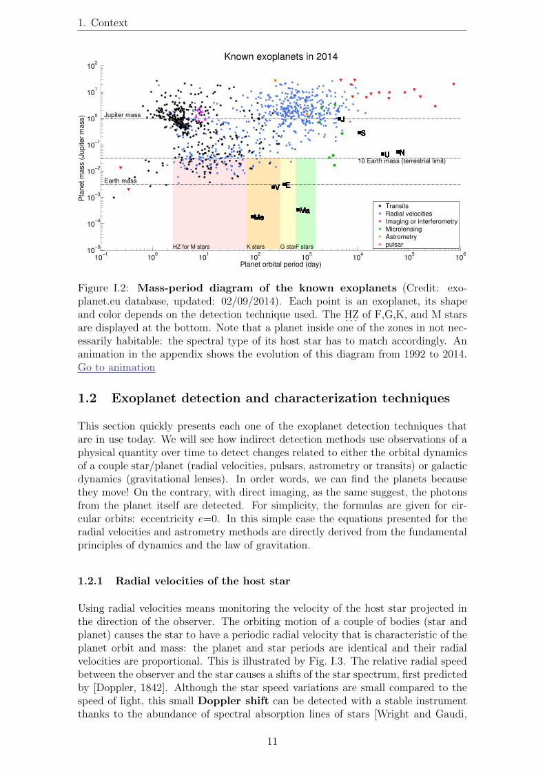
Figure I.2: Mass-period diagram of the known exoplanets (Credit: exo-planet.eu database, updated: 02/09/2014). Each point is an exoplanet, its shapeand color depends on the detection technique used. The . . .HZ of F,G,K, and M starsare displayed at the bottom. Note that a planet inside one of the zones in not nec-essarily habitable: the spectral type of its host star has to match accordingly. Ananimation in the appendix shows the evolution of this diagram from 1992 to 2014.Go to animation
1.2 Exoplanet detection and characterization techniques
This section quickly presents each one of the exoplanet detection techniques thatare in use today. We will see how indirect detection methods use observations of aphysical quantity over time to detect changes related to either the orbital dynamicsof a couple star/planet (radial velocities, pulsars, astrometry or transits) or galacticdynamics (gravitational lenses). In order words, we can find the planets becausethey move! On the contrary, with direct imaging, as the same suggest, the photonsfrom the planet itself are detected. For simplicity, the formulas are given for cir-cular orbits: eccentricity e=0. In this simple case the equations presented for theradial velocities and astrometry methods are directly derived from the fundamentalprinciples of dynamics and the law of gravitation.
1.2.1 Radial velocities of the host star
Using radial velocities means monitoring the velocity of the host star projected inthe direction of the observer. The orbiting motion of a couple of bodies (star andplanet) causes the star to have a periodic radial velocity that is characteristic of theplanet orbit and mass: the planet and star periods are identical and their radialvelocities are proportional. This is illustrated by Fig. I.3. The relative radial speedbetween the observer and the star causes a shifts of the star spectrum, first predictedby [Doppler, 1842]. Although the star speed variations are small compared to thespeed of light, this small Doppler shift can be detected with a stable instrumentthanks to the abundance of spectral absorption lines of stars [Wright and Gaudi,
11

Chapter I: Introduction
����������
Figure I.3: Illustration of the star/planet orbital dynamic (image modifiedfrom wikipedia). An observer situated in the plane of the image sees wavelengthshifts in the spectrum of the star: as the planet moves on its orbit, the star movesin the opposite direction. Go to animation
���������
�������������
�
���������
Figure I.4: Definition of the inclinaison i (as used in radial velocities).
2013].
The amplitude of the radial velocity signal is given by Eq. (I.1):
A = 0.09m.s−1 × MPlanet
M⊕×�MStar
M�
�−1
�
R
1AU
�− 12
× sin i (I.1)
Where MPlanet is the exoplanet mass, R is the exoplanet semi major axis, MStar isthe mass of the observed host star and i is the inclination (see Fig. I.4). The constant0.09 m.s−1 correspond to the signal of an exo-Earth around a Sun.
By looking at Eq. (I.1), one can see that radial velocities are best adapted to smallmass stars and small period planets (small orbits) seen on an edge-on configuration(i = 90◦). For face-on configurations (i = 0◦), no signal is detected. For statisticson a large number of detections, unknown inclinations are not a problem: face-onconfigurations are less frequent and the statistical bias due to the sin i term is low.However for a given individual case, it is often not possible to be certain of theplanet mass when information on the inclination is not available: only the productMPlanet
M⊕sin(i) is known.
1.2.2 Pulsar timing
Pulsars are highly magnetized residual cores of dead stars which are spinning veryquickly. They emit regular radio signals as they spin, they are very accurate naturalclocks [Matsakis et al., 1997]. The same Doppler effect that occurs in radial velocitiesis affecting the pulsar signal in the exact same way: the time between the pulseschanges with the speed relative to the observer.
12

1. Context
1.2.3 Astrometry of the host star
Astrometry measures the motion of the star on the plane of the celestial sphere.Just like for the radial velocities, the presence of a planet causes the star to havean orbit which is characteristic of the planet, called reflex motion or wobble. Thestar lateral position is measured instead of its radial velocity. This is also illustratedby the Fig. I.3. An observer perpendicular to the orbital plane would sees the starwobbling, but this angular motion at real scale is very small. The angular amplitudeof the astrometric signal is given by Eq. I.2:
A = 3µas× MPlanet
M⊕×
�MStar
M�
�−1
× a
1AU×
�D
1pc
�−1
(I.2)
Where D is the distance between the Sun and the observed star, MPlanet is theexoplanet mass, a is the exoplanet semi major axis and MStar is the mass of theobserved host star. The constant 3 µas (3 × 10⁻⁶ arcseconds) corresponds to thesignal of an exo-Earth observed from a distance of 1 pc.
Astrometry of the host star is best adapted to intermediate period planets (near . . .HZ)and longer, as long as the period does not exceed the time span of the observations.The astrometric signal is stronger for small stars (all other parameters being equal)but for detection of planets in . . .HZ, the method is more sensitive for massive stars,as the habitable zone is in this case further away from the star, as we will see in thechapter II. At last, astrometry works best with a face-on geometric configurations,but edge-on systems are also detected. Note that it is also possible to do astrometrydirectly on the planets if they are detected by direct imaging. In this manuscriptwhen we simply refer to astrometry, we implicitly mean astrometry of the hoststar. Section 3 will give a much more detailed presentation of astrometry.
1.2.4 Transits
����
�����������������������������
�������������
���������������
����
������
Figure I.5: Schematic of a transit.
The transit method looks at the decrease in apparent brightness of an host star as anexoplanet transits between the star and the observer. This is illustrated by Fig. I.5.
The depth of a transit (the relative decrease in luminosity of the host star) dependson the relative radius of the star and the planet:
ρ =
�Rplanet
Rstar
�2
(I.3)
13
Chapter I: Introduction
If we refer to Table I.1, we have a straightforward estimation of the depth of thetransit of an exo-Earth (around a Sun-like star): 10−4. Furthermore, to see a planetwhich has a random orientation transiting, the geometric configuration must be suchthat the planet passes by chance between the observer and the star, the probability(for a circular orbit of semi major axis a) is given by Eq. I.4 [Winn, 2010]:
Ptransit =Rstar +Rplanet
a≈ Rstar
a(I.4)
Where Rstar is the diameter of the star and a the orbital distance. In most cases theplanet is much smaller than the star and the approximation in equation I.4 is valid.The geometric probability of transit decrease with the orbital distance. The numberof transits seen in a given time span also decrease with the orbital period. In orderto confirm a transit detection one has to see at least 3 transit events: the longestperiod that can be detected is only 1
3of the time span of the observations [Koch
et al., 2010]. This makes transits best suitable for short periods (or small orbits).However, exo-Earth detection is possible (transit probability of 0.5%) provided anadequate time span of more than 3 years of observations is available for large numberof stars.
It is sometimes possible to obtain the mass of planets or to discover other nontransiting planets with transits alone, when planets are in resonance or have veryclose orbital periods. In this cases they perturb each other and produce Transittiming variations (TTV). The amplitude of the perturbations depends on the massesand periods of the planets. If both planets transits and show visible TTV, bothmasses can be known, otherwise we mainly have additional information about thenon transiting planet[Holman and Murray, 2005].
There is a secondary event, which is frequently found in association with transits:the eclipse, which happens when the planet disappears when passing behind thestar. Some systems can have only a transit or an eclipse, if the orbit is not circular.The effect of the eclipse is similar (a relative decrease in luminosity) but it is harderto detect because the planet has a much lower irradiance (W.m−2) than the star.
1.2.5 Gravitational microlensing
����� ������������������ ������������
����������
����
����������������������������
�����������������������������������
�������������
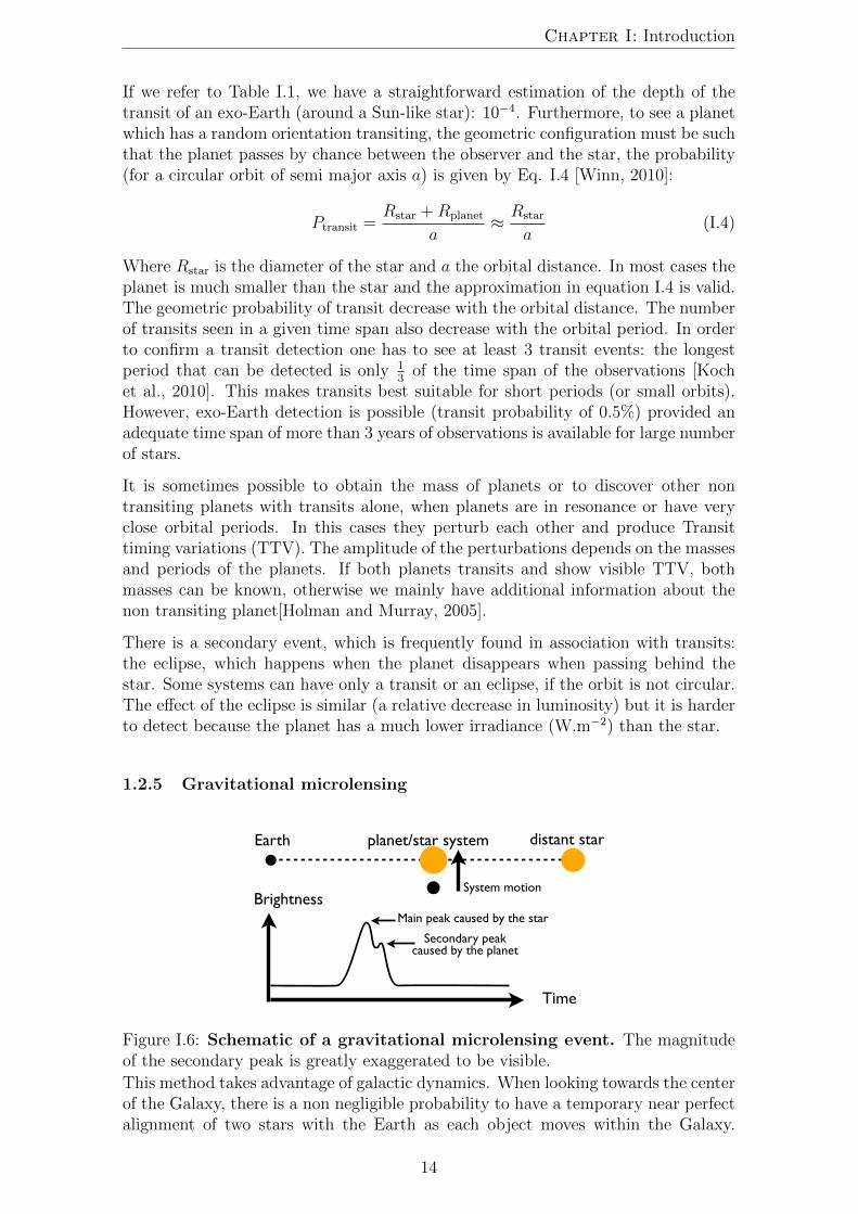
Figure I.6: Schematic of a gravitational microlensing event. The magnitudeof the secondary peak is greatly exaggerated to be visible.
This method takes advantage of galactic dynamics. When looking towards the centerof the Galaxy, there is a non negligible probability to have a temporary near perfectalignment of two stars with the Earth as each object moves within the Galaxy.
14
1. Context
When the chance alignment occurs, the star at the back (in the galactic center) ismagnified by the one that is closer to the observer, producing a light curve roughlyshaped like a bell. If a planet is present around the closer star, it will producea secondary intensity peak that can be detected (Fig. I.6). Inverting this curvegives information about the planet mass and orbital distance. This method has anoptimal sensitivity from 1 to 10 . . . .AU from the host star [Gaudi, 2012]. Until now thismethod has been relatively marginal and has the obvious disadvantage of not beingreproducible: chance alignments only occur once. Furthermore, detections are hardto follow-up with other techniques because they occur at great distances (typicallythousands of parsecs).
1.2.6 Direct imaging
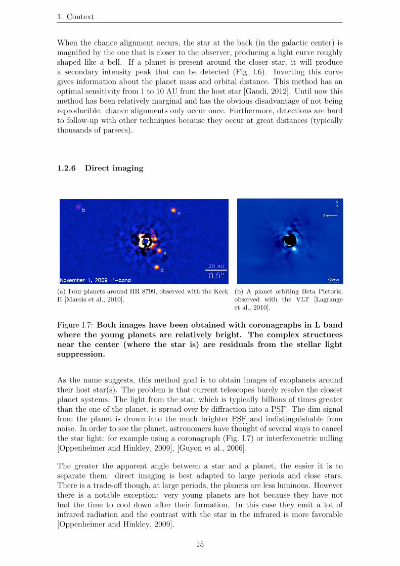
(a) Four planets around HR 8799, observed with the KeckII [Marois et al., 2010].
(b) A planet orbiting Beta Pictoris,observed with the VLT [Lagrangeet al., 2010].
Figure I.7: Both images have been obtained with coronagraphs in L bandwhere the young planets are relatively bright. The complex structuresnear the center (where the star is) are residuals from the stellar lightsuppression.
As the name suggests, this method goal is to obtain images of exoplanets aroundtheir host star(s). The problem is that current telescopes barely resolve the closestplanet systems. The light from the star, which is typically billions of times greaterthan the one of the planet, is spread over by diffraction into a . . . . .PSF. The dim signalfrom the planet is drown into the much brighter . . . . .PSF and indistinguishable fromnoise. In order to see the planet, astronomers have thought of several ways to cancelthe star light: for example using a coronagraph (Fig. I.7) or interferometric nulling[Oppenheimer and Hinkley, 2009], [Guyon et al., 2006].
The greater the apparent angle between a star and a planet, the easier it is toseparate them: direct imaging is best adapted to large periods and close stars.There is a trade-off though, at large periods, the planets are less luminous. Howeverthere is a notable exception: very young planets are hot because they have nothad the time to cool down after their formation. In this case they emit a lot ofinfrared radiation and the contrast with the star in the infrared is more favorable[Oppenheimer and Hinkley, 2009].
15
Chapter I: Introduction
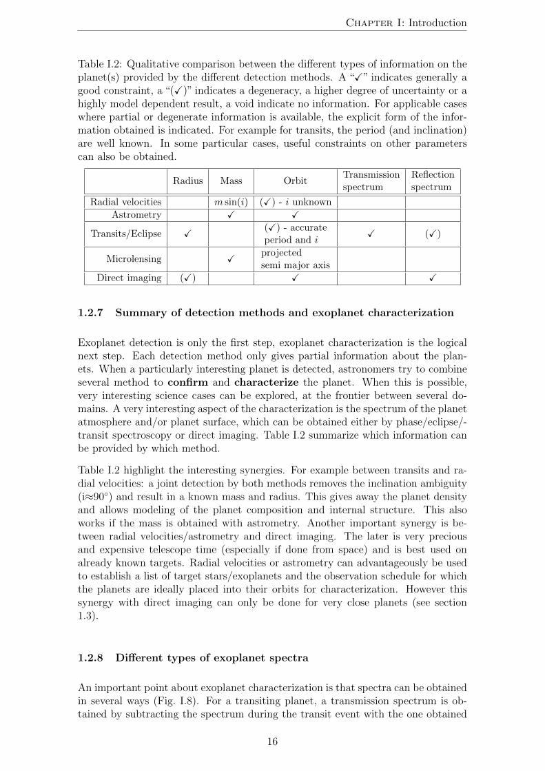
Table I.2: Qualitative comparison between the different types of information on theplanet(s) provided by the different detection methods. A “�” indicates generally agood constraint, a “(�)” indicates a degeneracy, a higher degree of uncertainty or ahighly model dependent result, a void indicate no information. For applicable caseswhere partial or degenerate information is available, the explicit form of the infor-mation obtained is indicated. For example for transits, the period (and inclination)are well known. In some particular cases, useful constraints on other parameterscan also be obtained.
Radius Mass OrbitTransmissionspectrum
Reflectionspectrum
Radial velocities m sin(i) (�) - i unknown
Astrometry � �
Transits/Eclipse � (�) - accurateperiod and i
� (�)
Microlensing � projectedsemi major axis
Direct imaging (�) � �
1.2.7 Summary of detection methods and exoplanet characterization
Exoplanet detection is only the first step, exoplanet characterization is the logicalnext step. Each detection method only gives partial information about the plan-ets. When a particularly interesting planet is detected, astronomers try to combineseveral method to confirm and characterize the planet. When this is possible,very interesting science cases can be explored, at the frontier between several do-mains. A very interesting aspect of the characterization is the spectrum of the planetatmosphere and/or planet surface, which can be obtained either by phase/eclipse/-transit spectroscopy or direct imaging. Table I.2 summarize which information canbe provided by which method.
Table I.2 highlight the interesting synergies. For example between transits and ra-dial velocities: a joint detection by both methods removes the inclination ambiguity(i≈90◦) and result in a known mass and radius. This gives away the planet densityand allows modeling of the planet composition and internal structure. This alsoworks if the mass is obtained with astrometry. Another important synergy is be-tween radial velocities/astrometry and direct imaging. The later is very preciousand expensive telescope time (especially if done from space) and is best used onalready known targets. Radial velocities or astrometry can advantageously be usedto establish a list of target stars/exoplanets and the observation schedule for whichthe planets are ideally placed into their orbits for characterization. However thissynergy with direct imaging can only be done for very close planets (see section1.3).
1.2.8 Different types of exoplanet spectra
An important point about exoplanet characterization is that spectra can be obtainedin several ways (Fig. I.8). For a transiting planet, a transmission spectrum is ob-tained by subtracting the spectrum during the transit event with the one obtained
16

1. Context
� ��
��������������������� ����������������
�������
�������
Figure I.8: Schematic of the different types of spectra of an exoplanet. Theleft part is the case without a coronagraph, only the total light from the star plus theplanet is seen but one can have a differential spectra of the planet by comparing datafrom different orbital positions: (1,2) → transit atmospheric transmission spectra,(4,5) → eclipse reflection spectra, (2,3,4) → phase reflection spectra (no transit noreclipse needed). The right part is the case with a coronagraph: the star light isattenuated and the light/spectrum of the planet is observed directly.
before or after2. For a planet close to a edge-on configuration, one can in principlealso compute a phase reflection spectrum3. It can be obtained by subtracting spectraat different orbital phases of a planet orbit, because the planet is seen alternativelyalmost fully illuminated (day side) and almost entirely dark (night side), the planetdoes not have to transit and no coronagraph is needed in this case. However, ifseveral planets are presents, their phase signals are blended together. If there is aneclipse, a better reflection spectra can be obtained. In any case, a big inconvenientwith transmission spectra and phase/eclipse reflection spectra is the photon noisefrom the star, given that the signal to noise ratio (. . . . .SNR) for a given wavelengthchannel λ) is:
SNR = Nγ,λsignal/
�Nγ,λ
total (I.5)
Where Nγ,λsignal and Nγ,λ
total are the number of photons respectively from the spectralfeature to detect and from the star. While feasible in principle, obtaining usefuleclipse/phase reflection spectra often results in an unrealistic integration times forsmall planets, because the signal/star photon ratio is very low and the photon starnoise only goes down as the square root of the time4, transmission is only slightlyeasier. In this regard, direct imaging has a huge advantage: because the photon fluxfrom the star is suppressed or strongly attenuated, the . . . . .SNR of a reflection spectrumfor a given target and given telescope diameter is larger than with differential spectraobtained with transits, eclipses or phase curves.
2The transmission spectrum is the star light passing through the planet atmosphere. Thisspectrum carries information about the exoplanet atmospheric composition.
3The reflexion spectrum is the star light reflected by the planet surface. This spectrum carriesinformation about the exoplanet atmospheric composition and its surface reflectivity as a functionof wavelength
4Using the JWST, the upcoming world best space based observatory, detection of spectralfeatures of super-Earth around small stars (lowest hanging fruits in the terrestrial mass regime)would use 2% of the 5 year mission [Belu et al., 2011]
17

Chapter I: Introduction
1.3 Understanding planetary formation and searching forlife outside of the Solar System
The direct consequence of the improvement of exoplanet detection techniques is to fillthe mass/period parameter space. This is very important as it will help astronomersanswer the two following fundamental questions: how do planets form? is there lifeoutside of the Solar System? But how exactly are exoplanet detections related thosetwo questions?
1.3.1 Planetary formation
In order to develop accurate planetary formation models, astrophysicists need datato constrain the models results. In particular, the discovery of the first “hot Jupiter”(a giant gaseous planet on a very small orbit) has made the field evolve very rapidly:new models to explain inward planetary migration of gas giants were developed.Before, as only the Solar System planet were known, hot gas giants were only hy-pothetical. We are now filling the mass/period parameter space so well that we canstart to look at the effect of the star mass as well. The data is now sufficient toreconstruct unbiased distributions of exoplanets for many parameters (planet mass,planet period, star mass) and additional detections are helping to increase the ac-curacy and the span of the distributions. These statistical results are key to refineour understanding of planetary formation [Udry and Santos, 2007].
1.3.2 Life outside the Solar System
Even though small planets (in mass and in size) are the hardest to detect, in someaspects they are also the most interesting. We now arrive at a point were severalmethods are becoming sensitive enough to detect terrestrial mass planets (i.e. lessthan 10 M⊕) at periods that places them in . . .HZ, where we have a chance to find liquidwater at the planetary surface. These terrestrial planets in . . .HZ, which I will simplycall habitable planets by abuse of terminology5, are the places most conducive tothe emergence of life known to date (other than the Earth) [Rampino and Caldeira,1994]. They are places where we can hope to find complex life-forms outside theSolar System. The first step is to detect the closest of these habitable planets, toknow where they are in our solar neighbourhood. Then, the next step is to try toget a spectra of their surface and atmosphere in order to confirm habitability andinfer the presence of biological activity if it exists. In order for this second step tobe possible by direct imaging using present or near future technology, the planetsmust be very close, on the order of 10 pc or less [Cockell et al., 2009] [Belu et al.,2011]. In this regard, µas astrometry offers a unique opportunity to find the closestplanet systems including the habitable ones: the reasons behind this are developedin section 2.4.
5Being terrestrial and in . . .HZ does not ensures habitability, knowledge of atmospheric density andcomposition is required to confirm habitability. Strictly speaking, they should be called“potentiallyhabitable”.
18

2. Space borne missions and ground based instruments for exoplanet science
2 Space borne missions and ground based instru-
ments for exoplanet science
In this part I present the landscape of recent/planned space missions and of recen-t/planned ground instruments, in the exoplanet field. I compare the role of themost successful exoplanet detection techniques and explore their potential for thefuture of exoplanetology and the search for life. The technical challenge of habitableexoplanet detection is so difficult that so far a large part of the related activities arespace missions, with the notable exceptions of radial velocities and coronagraphs onvery large telescopes.
2.1 Transits
Observations of transits from the ground is very difficult because atmospheric effectshave so far limited the accuracy of the photometric curves to a few parts per onethousandth: with this accuracy it is only possible to detect giant planets for Sun-likestars. Numerous new ground surveys, like for example, MEarth [Berta et al., 2011],ExTra6, MASCARA (the Multi-site All-Sky CAmeRA) [Snellen et al., 2012], NGTS(Next-Generation Transit Survey) [Wheatley et al., 2013] are trying to improve thecalibration methods with reference stars in order to increase the photometric accu-racy and generally focus on low mass stars where the transit depth is larger. Some ofthem should be sensitive to terrestrial planets around M stars. On the other hand,space transits missions already have had great success: two have been completedand several others are in preparation. . . . . . .CNES (Centre National d’Etudes Spatiales),in collaboration with . . . . .ESA (European Space Agency) launched in December 2006a small sized space telescope (Ø 0.27m) called . . . . . . . . .COROT (COnvection ROtation etTransits Planetaires) [Auvergne et al., 2009] that observed transits during for 5 years.In March 2009, . . . . . . .NASA (National Aeronautics and Space Administration) launcheda much bigger telescope (Ø 1.4m): the Kepler7 spacecraft which has monitored afixed field of 150,000 stars continuously over 5 years [Koch et al., 2010]. Both mis-sions were very successful, although the number of detections is much higher forKepler thanks to its very large size and wide field of view. It has found thousandsof exoplanet candidates, more than 4200 according to the . . . . . . .NASA exoplanet archive8
[Akeson et al., 2013].
Kepler has a very interesting characteristic: it was designed to detect transits ofplanets with radius down to 0.5 R⊕, which are terrestrial (the limit between gasgiant and terrestrial is around 2 R⊕). Although transits are less likely to occurfor planets of large periods, the number of stars observed is large enough to yielda significant number of terrestrial and habitable planets. After correction for theincompleteness of the transit detection and the transit probability biases, it has beenestimated that 22±8% of Sun-like stars harbor Earth-size planets orbiting in theirhabitable zones [Petigura et al., 2013].
6Xavier Bonfils, Priv. comm. A presentation is available on the . . . . .ESO (European SouthernObservatory) website: http://www.eso.org/sci/meetings/2014/exoelt2014/presentations/
Bonfils.pdf7Kepler is not an acronym. The spacecraft was named after the scientist Johannes Kepler
(1571-1630), best known for his laws of planetary motion.8updated: 25/06/2014, http://exoplanetarchive.ipac.caltech.edu/http://
exoplanetarchive.ipac.caltech.edu/
19

Chapter I: Introduction
The limitation of these missions arises from the very nature of the transits. In orderto detect lots of planets with a practical instrument design, a constant field has beenmonitored for long periods, thus making the search space a cone containing only asmall fraction of the sky. Consequently the target stars are thousands of parsecsaway. The habitable exoplanets detected by Kepler and . . . . . . . . .COROT are unlikely tobe directly observable for a long time: as explained in section 1.3 the reasonabledistance limit for spectroscopy of habitable exoplanet is about 10 pc.
Other mission concepts are trying to address this issue by looking at transits on thewhole sky. In this case, we may have some chance of finding some close enough hab-itable planets: it depends on ηEarth, on how far we are willing to probe and on luck.But with a transit probability of 0.5%, we will miss most of the closest exo-Earths.CHEOPS (CHaracterising ExOPlanets Satellite) [Broeg et al., 2013], TESS (Transit-ing Exoplanet Survey Satellite) [Ricker et al., 2010] and . . . . . . . .PLATO (Planetary Transitsand Oscillations of stars) [Rauer et al., 2013] are missions in preparation that willlook for transits around close and bright stars. EChO (Exoplanet Characterisa-tion Observatory) [Tinetti et al., 2012] and . . . . . . .JWST (James-Webb Space Telescope)[Clampin, 2008] are respectively proposed and planned missions to carry out transitspectroscopy: the idea is to compare spectra before and during the transits andeclipses to obtain transmission and reflection spectra.
2.2 Radial velocities
Radial velocity on the host star gives information on the orbit and mass of the planet,with one remaining ambiguity though, the angle of the plane of the orbit relativeto the observer. This information can sometimes be obtained by other methods if agood habitable exoplanet candidate is found. The spectral signature of the planet isalso present in the data even if the final signal is strongly dominated by the signalof the star. It is thus in principle possible to distinguish the two signals when thesignal to noise ratio is good enough. However, because of the contrast problem, itis unlikely that the spectrum of an habitable planet will be directly observed (i.e.without canceling of the light of the star first).
A major advantage of radial velocities is that they are possible from the ground,so they are relatively cheap. They are a lot of RV spectrographs in service today,and a significant fraction of them are accurate enough to look for exoplanets. Themost notable ones in service today are . . . . . . . .HARPS (High Accuracy Radial VelocityPlanet Searcher) operating at La Silla Observatory and NIRSPEC [McLean et al.,1998] on the Keck II telescope. The precision of the instruments is about 1m/s.Next generation spectrographs will reach a precision of 0.1m/s, but at this pointthe dominant source of noise will be the star themselves and not the instruments[Mayor et al., 2003]. ESPRESSO (Echelle SPectrograph for Rocky Exoplanet- andStable Spectroscopic Observations) [Pepe et al., 2014] is an instrument that will beinstalled on the . . . . .VLT (Very Large Telescope).
Radial velocities are already capable of detecting habitable super-Earths aroundM type stars. With future spectrographs, more habitable planets will be detectedlikely ranging from 1M⊕ or less around very low mass stars to super Earths aroundSun-like stars. But it is unclear whether radial velocities will succeed to go downto exo-Earths around Sun-like stars (0.1 m/s). It depends on the extent to whichastronomers are able to filter the stellar noise out of the data [Dumusque, 2010].
20
2. Space borne missions and ground based instruments for exoplanet science
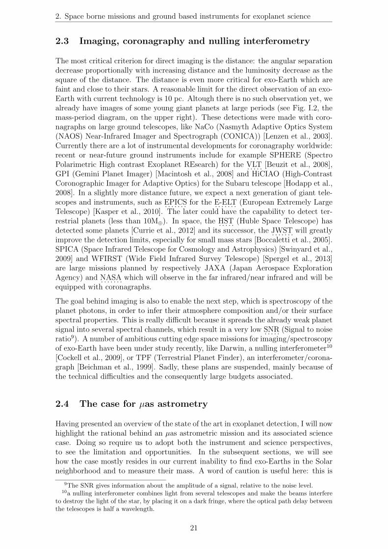
2.3 Imaging, coronagraphy and nulling interferometry
The most critical criterion for direct imaging is the distance: the angular separationdecrease proportionally with increasing distance and the luminosity decrease as thesquare of the distance. The distance is even more critical for exo-Earth which arefaint and close to their stars. A reasonable limit for the direct observation of an exo-Earth with current technology is 10 pc. Altough there is no such observation yet, wealready have images of some young giant planets at large periods (see Fig. I.2, themass-period diagram, on the upper right). These detections were made with coro-nagraphs on large ground telescopes, like NaCo (Nasmyth Adaptive Optics System(NAOS) Near-Infrared Imager and Spectrograph (CONICA)) [Lenzen et al., 2003].Currently there are a lot of instrumental developments for coronagraphy worldwide:recent or near-future ground instruments include for example SPHERE (SpectroPolarimetric High contrast Exoplanet REsearch) for the . . . . .VLT [Beuzit et al., 2008],GPI (Gemini Planet Imager) [Macintosh et al., 2008] and HiCIAO (High-ContrastCoronographic Imager for Adaptive Optics) for the Subaru telescope [Hodapp et al.,2008]. In a slightly more distance future, we expect a next generation of giant tele-scopes and instruments, such as . . . . . . .EPICS for the . . . . . . .E-ELT (European Extremely LargeTelescope) [Kasper et al., 2010]. The later could have the capability to detect ter-restrial planets (less than 10M⊕). In space, the . . . . .HST (Huble Space Telescope) hasdetected some planets [Currie et al., 2012] and its successor, the . . . . . . .JWST will greatlyimprove the detection limits, especially for small mass stars [Boccaletti et al., 2005].SPICA (Space Infrared Telescope for Cosmology and Astrophysics) [Swinyard et al.,2009] and WFIRST (Wide Field Infrared Survey Telescope) [Spergel et al., 2013]are large missions planned by respectively JAXA (Japan Aerospace ExplorationAgency) and . . . . . . .NASA which will observe in the far infrared/near infrared and will beequipped with coronagraphs.
The goal behind imaging is also to enable the next step, which is spectroscopy of theplanet photons, in order to infer their atmosphere composition and/or their surfacespectral properties. This is really difficult because it spreads the already weak planetsignal into several spectral channels, which result in a very low . . . . .SNR (Signal to noiseratio9). A number of ambitious cutting edge space missions for imaging/spectroscopyof exo-Earth have been under study recently, like Darwin, a nulling interferometer10
[Cockell et al., 2009], or TPF (Terrestrial Planet Finder), an interferometer/corona-graph [Beichman et al., 1999]. Sadly, these plans are suspended, mainly because ofthe technical difficulties and the consequently large budgets associated.
2.4 The case for µas astrometry
Having presented an overview of the state of the art in exoplanet detection, I will nowhighlight the rational behind an µas astrometric mission and its associated sciencecase. Doing so require us to adopt both the instrument and science perspectives,to see the limitation and opportunities. In the subsequent sections, we will seehow the case mostly resides in our current inability to find exo-Earths in the Solarneighborhood and to measure their mass. A word of caution is useful here: this is
9The SNR gives information about the amplitude of a signal, relative to the noise level.10a nulling interferometer combines light from several telescopes and make the beams interfere
to destroy the light of the star, by placing it on a dark fringe, where the optical path delay betweenthe telescopes is half a wavelength.
21
Chapter I: Introduction
written in mid 2014 and the field is evolving so rapidly that some arguments maybecome invalid in a not so distant future!
2.4.1 Current limitations of radial velocities
We have already approached the limitations of radial velocities in section 2.2. Nextgeneration instruments will reach a precision of 0.1 m/s, which is precisely thelevel required for an exo-Earth. However, below 1 m/s, the stellar noise is muchlarger than the instruments’ for most stars. The case of Alpha Centauri Bb isemblematic to the challenged posed by stellar noise. Alpha Cen Bb is a planet witha signal amplitude of 0.51 m/s, recently discovered with the HARPS spectrograph[Dumusque et al., 2012]. It is the closest Sun-like star from the Sun, it is very quietand it has had the lion’s share of the HARPS program observation time with atotal of 459 observations over three years. For Sun-like stars, it hardly gets betterthan this! In spite of this, in order to make the detection possible, multiple signalswith amplitudes larger than 0.5 m/s have been removed by various signal processingtechniques. The signals have been attributed to other phenomenons, such as stellarspots, rotation and jitter. But this very complex processing has raised some doubtsand the planet existence is somewhat contested [Hatzes, 2013]. At this level ofprecision, the slightest error in processing can result in a false apparent signal.
Radial velocities work much better for small mass stars, where the signal in . . .HZ is
larger for two reasons: first the signal scales directly withMplanet
Mstar, and secondly the
. . .HZ is closer to the star (short periods/small semi major axis planets give off largerRV signals). Around M stars, the detection is so much easier that RVs have alreadydetected terrestrial planets in the habitable zone. But for solar type stars, we simplydo not know if radial velocities will be able to separate the planet from the stellarnoise, down to 1M⊕ in . . .HZ.
2.4.2 Current limitations of transits
Transits look very promising in the near future. With PLATO, TESS, the JSWT andEChO, we will soon discover many more transiting planets closer than what Keplerhas already found and we will have better quality transiting and eclipse spectra,down to a few Earth masses [Tinetti et al., 2012] [Deming et al., 2009]. However themajor limitation in the case of very close stars is the geometric transit probability.There are only about 400 Sun-like stars (F, G and K spectral types) closer than20 pc. Assuming a frequency of habitable planets of about 10 to 20% (result fromKepler) and with a transit probability of 0.5% for an earth analog, there may beno nearby transiting exo-Earth (around a Sun-like star) to detect at all. This willnot prevent PLATO and TESS to successfully survey bright stars over all the sky,to look for close-by transiting stars. But these missions will work with many moretargets to overcome the transit probability and mostly look at targets further outthan 20 pc.
In the case of M stars, transit become much more advantageous.The terrestrialplanets are not only more easily detectable thanks to a larger
Rplanet
Rstarratio, but also
the geometric transit probability of a planet in . . .HZ is about 2 to 5%. And on top ofthat, M stars are much more numerous than higher mass stars. The MEarth catalog,which is mostly complete up to 20 pc, indicates a cumulative count of about 600 M
22

2. Space borne missions and ground based instruments for exoplanet science
stars at that distance [Dittmann et al., 2014]. The frequency of habitable planetsaround M stars is estimated at about 40% [Bonfils et al., 2013]: this means thatseveral of them transit around nearby M dwarfs. The goal of many ground surveysis precisely these very interesting nearby low mass stars.
But not being able to suppress the star light is a problem because of the planet/starcontrast: the information obtained by differential spectroscopy is strongly impairedby the photon noise from the star. Direct imaging with a coronagraph can tackle thisproblem, as we have explained in section 1.2.7. Such a gain will be a determinantfactor when looking for biomarkers. That brings us to the next part: direct imaging.
2.4.3 Current limitations of direct imaging
Direct imaging has the capability of both finding our closest neighbors and do-ing spectroscopy to characterize their atmospheres and surface properties. So whynot simply directly detect the planets, skipping radial velocities or astrometry alto-gether?
The first issue is that we currently know very few suitable target stars for directimaging of habitable planets. While young and long period planets have alreadybeen imaged, habitable planets are much harder. For the latter, angular separationand contrast requirements restrict us close stars: a reasonable distance limit toconsider is 10 pc [Guyon et al., 2006]. Any large mission or survey aiming at aspectroscopic characterization much first find where the planets are by spendingsome time exploring almost blindly, relying mostly on the stellar parameters forprior target selection. If a survey mission can be launched as a medium sized mission(that is what NEAT aims to be) and the coronagraph needs to be a large mission, itmakes a lot of sense to have a pre-established list of targets to optimize the designand the utilization of the most costly instrument.
The second issue is that a detection by direct imaging alone gives a very poorconstraint on the planet mass. The radius can be estimated by a model, but theresult depends on the assumed planet albedo. Mass limits can be estimated fromthe radius, using more models and/or mass-radius scatter diagrams of exoplanetsfor which both quantities have been measured. But in the end all we have areapproximative mass limits that are highly model dependent.
2.4.4 Summary
Significant progress in the ability to filter stellar noise down to 0.1 m/s on longtimescales (year or more) with radial velocities would seriously undermine the moti-vation for an µas astrometric mission, but this does not seem very likely to happenin the short term. For the case of close stars, the effort behind neat can be seen as aworkaround the stellar noise problem: the astrophysical noise problem is traded foranother one, which is instrumental. Transits constitute a valuable parallel avenueof exploration, which has its own merits but cannot correctly address our very closeSun-like neighbors: when looking nearby, we find ourselves cornered in the samepart of the parameter space than radial velocities: M stars.
An astrometric solution also has the additional merit of increasing the diversity ofexoplanet detection techniques, which brings advantages via the complementaries of
23

Chapter I: Introduction
���� ���� ���� ��� ��� ��� �
����������������������
���
���
���
�
��������������������������������������������
�������
������
������
��������������������
�������
��������
��������������������������������������������
���� ����������������������������
����������� ����������
���������
�������
�����������������
�����������������������������������
�������
�������
Figure I.9: Astrometric signal of exo-Earth in HZ vs. IWA for nearest F,G and K stars.
methods, for example concerning the orbital periods and the inclination of the sys-tems. Thorough observations of nearby stars by astrometry (at µas accuracy), radialvelocities and direct imaging combined would yield very detailed knowledge of closeplanetary systems. This second aspect would help toward a better comprehensionof planetary formation.
Concerning a space coronagraph mission, a precursor astrometric mission would pavethe way by making it less risky, easier to prepare and enhancing its scientific yield,because target locations and characteristics would be known beforehand. Above all,it would provide a reliable measure of the planetary masses.
Figure I.9 show the astrometric signal of exo-Earths in HZ versus the inner workingangle (IWA) for the nearest A, F, G K and M stars (at less than 20 pc). With anastrometric accuracy of 0.5 µas and an IWA smaller than 150 mas, one can combineastrometry and direct imaging for 12 of the easiest targets.
3 Astrometry, exoplanets and NEAT
3.1 Historical presentation of Astrometry
Astrometry is the oldest of all astronomical sciences. It consists in the study ofpositions and motions of the celestial objects. The first astrometric observation onlyneeds the naked eye as an instrument: some of the brightest objects are movingacross the sky relative to the fixed sphere of stars and this is in fact the origin
24

3. Astrometry, exoplanets and NEAT
of the word “planets” (from Greek “asteres planetai” i.e. wandering stars). TheBabylonians are the first civilization known to have left written evidence of extensivestudies of the path of the celestial bodies and star catalogs. By inferring fromthese basic observations and using some mathematics, the Babylonians producedremarkably accurate ephemerides [Aaboe, 1974]. They predicted in particular solareclipses, daytime durations or the variations of the number of days between two newmoons.
Astrometry then continued in the West with the Greeks: Eudoxus (370 BC), Timo-charis of Alexandria and Aristillus (300 BC) and then Hipparchus (135 BC) createdother star catalogs [Aaboe, 2001]. Hipparchus made his measurements using an as-trolabe and obtained the positions of at least 850 stars with an accuracy of about 20arcmin [Lankford, 1997]. He discovered the precession of the equinoxes by comparinghis catalog to Timocharis’ and Aristillus’. After that there was very little improve-ment until the late 16th century. Finally, in 1586, the Danish astronomer TychoBrahe achieved measurements with 30” accuracy using a quadrant [Kovalevsky andSeidelmann, 2001]. Although the final precision of the catalog is 2’ instead of 30”because the atmosphere refraction causes systematic errors which were not takeninto account correctly, this was a huge step forward. At this point, the precisionof the instrument (not considering the atmospheric systematics) is limited by theresolution of the eye.
The first practical refracting telescopes were build in 1608, then followed the reflec-tive telescopes in 1668, by Isaac Newton. Observation with telescopes allowed subarcsecond astrometry, leading to the discovery of the aberration of light [Bradley,1727] and the nutation of the Earth’s axis [Bradley, 1753], and to the measurement ofthe first parallax [Bessel, 1838]. Although different setups were used for astrometry,the most common way to measure the parallaxes and separations between doublestars was a telescope equipped with a filar micrometer. The latter is a reticle thathas two fine parallel wires or threads that can be moved by the observer using amicrometer screw. By placing one wire over one object of interest and moving theother to a second object, the distance between the two objects at the focal plane canbe measured with the micrometer portion of the instrument. Note that the objectsmust be close enough to be in the field of view and that the measure is differential(it needs two objects). The differential accuracy obtained depends on the telescopediameter but can reach a few dozen of miliarcseconds.
The invention of photographic plates allowed to capture and archive images of thesky. The great advantages of the photographic plates were not so much in terms ofaccuracy, but because much dimmer objects could be observed (with long exposuretimes) and a large volume of data can be processed and archived. Photographicplates/films were experimented with as early as 1790 by Thomas Wedgwood [Hirsch,1999] and people quickly realized their potential for astronomy. However, theybecame widely used only about 100 years later, when their sensitivity and theirusage was practical for astronomy. Finally, in the 1980s, . . . . .CCDs (Charged-CoupledDevice11) replaced photographic plates and reduced errors to 1 mas. Automaticcontrol of the instruments coupled with . . . . .CCDs allowed the creation of the moderncatalogs with even larger numbers of stars.
11CCDs are microelectronic devices that are sensitive to light. They operate by shifting chargesbetween each sensitive element, called pixel. They are widely used in digital cameras.
25

Chapter I: Introduction
3.2 The recent developments
The digital revolution has given us all the key technologies to enable space missionsand ground surveys: automated data acquisition, instrument control, data transferto Earth, data processing pipelines, data distribution and archiving. For astrom-etry, this has culminated into the . . . . . . . . . .Hipparcos (HIgh Precision PARallax COllectingSatellite12) [van Leeuwen, 1997] and . . . . .Gaia (Global Astrometric Interferometer forAstrophysics13) [Lindegren et al., 2008] space missions. Hipparcos has yielded theparallaxes of 100,000 close stars with an accuracy of 1 mas, which will very soon besuperseded by Gaia with the parallaxes of 1,000,000,000 stars with an accuracy upto 7 µas. The success of . . . . . . . . . .Hipparcos and the exquisite accuracy expected from Gaiaare largely due to the fact that being in space, these missions are not impeded byatmospheric turbulence.
However access to space is quite recent and still very expensive, atmospheric tur-bulence has not prevented astronomers from trying accurate astrometry from theground and persevering despite severe hiccups. The last two centuries are plaguedwith a history of exoplanet detections by astrometry on the host star [Boss, 2009],such as the infamous planets around 61 Cygni and Lalande 21185 which have neverbeen confirmed. The recurrent reason of these false positives is an underestimationof systematic errors. More recently, astrometry with large ground-base telescopes(2-8 m class) has been more successful. It was initially though that the precisionwas limited to about 1 mas, due to the atmospheric image motion which comes fromthe expression σ = θ/D2/3, where D is the telescope diameter and θ the angularseparation between the stars [Lindegren, 1980]. It was later found that by usinga grid composed of many reference stars, the expression (asymptotically) becomesσ = θ11/6/D3/2 [Lazorenko, 2002]. This opens the possibility of narrow angle rela-tive astrometry better than 100 µas over a field of view of 1’, which is a significantimprovement over . . . . . . . . . .Hipparcos and sufficient to detect giant exoplanets around nearbystars [Sahlmann et al., 2013a].
Ground instruments have reached accuracies up to 50 µas with FORS2 for example[Lazorenko et al., 2009] and we have now some solid astrometric evidence of exoplan-ets [Sahlmann et al., 2013c]. Another powerful technique that was been developedfor astrometry is interferometry on duals stars, with instruments like PTI (Palomartestbed interferometer) [Colavita et al., 1999] and PRIMA (Phase Referenced Imag-ing and Microarcsecond Astrometry) [van Belle et al., 2008]. Interferometry on dualstars can accurately measure separations, up to a few dozen of µas (its work betterfor small separations, under 1”). The progress made from the time of Hipparcosuntil now is summed up in Fig. I.10. In the next section I will talk specifically inmore details about exoplanet detection by astrometry on the host star.
12Hipparcos was a scientific mission of ESA (1989-1993). It was the first space mission devotedto precision astrometry, it measured the parallaxes of 100,000 close and bright stars with anaccuracy of 1mas. The name of the mission is an obvious reference to the ancient Greek astronomerHipparchus.
13Gaia is a scientific mission of ESA launched in december 2013, for a planned duration of 5years. It is expected to measure the position of 1 billion objects with an accuracy going from 7micro arcseconds (for magnitude V=10) to hundreds of micro arcseconds (V=20). Gaia works bydirect imaging: although it was first planned as an interferometer, this design was abandoned butthe name was kept.
26

3. Astrometry, exoplanets and NEAT
���
���
���
����
����
����
����
����
����
����
����� ��� ���� ����
���
���
����
��������������������������������
��������������������������
������������������������������������
������������������������
�������������������������
����������������
���������������������������
����������������������
������������������
��������������������
����������������
��������������
����
�����������������������������
Figure I.10: 2000 years of astrometry: from Hipparchus to Hipparcos. Thisplot shows the progress of astrometric measurements versus time. Each dot representthe accuracy obtained after a new breakthrough. On the left the labels indicate theangular amplitude of several phenomena.
3.3 Exoplanet detection using astrometry
3.3.1 Astrometric signal
This concept was briefly presented in section 1.2.3, more details will be given here.I recall the principle: the presence of a planet causes the star to have an orbit whichis characteristic of the planet. For a circular orbit, the amplitude of the astrometricsignal is:
A = 3µas× MPlanet
M⊕×�MStar
M�
�−1
× a
1AU�
D
1pc
�−1
Given the very small angular signal generated by planets compared to our currenttechnical capabilities, and the 1/D signal amplitude scaling, astrometry is limitedto close stars [Malbet et al., 2010]. The signal of an exo-Earth at 10 pc is obviousto derive from this equation: 0.3 µas. This is a really tiny angle, it is the apparentangle of 0.5 mm on the Moon (seen from the Earth). Yet this is the accuracy thatmust be reached if one is to detect an exo-Earth in the solar neighborhood: thiswill become obvious when making the NEAT catalog of target stars (chapter II),from the Hipparcos catalog [Perryman and ESA, 1997]. A minimal distance of 10pc is highly desirable to have a reasonable number of target stars and detectedplanets regarding the two scientific goals we have already mentioned (understandingplanetary formation and searching for life outside of the Solar System). The firstgoal requires enough detections for meaningful statistics. For the second one, theidea is to detect at least a few habitable planets, dozens if possible.
27

Chapter I: Introduction
Figure I.11: Example of accurate multi-epoch astrometric observation. Atfirst sight, the star motion fits well with a model that includes the proper motion(indicated by the red arrow) and the parallax. The residuals (of parallax and propermotion) are shown blown up in the upper right rectangle, where we see the astro-metric signature of a dwarf star companion. The orbital motion is indicated by thegreen arrow. Figure from [Sahlmann et al., 2013b].
3.3.2 Different types of astrometry
There are two different types of astrometry: absolute and relative. The first kind hasbeen carried out by Hipparcos and will be continued by Gaia. The spacecraft, beingadvantageously placed in space, have continuous access to the sky over large anglesand work in scanning mode. They spin continuously and compare the position ofstars in two field of view separated by a large angle (106◦ for Gaia). This kind of datacan be processed to find an absolute (global) astrometric solution for all stars. Onthe opposite, relative astrometry only needs a limited field of view, this is the kindof astrometry that is being done with ground telescopes, for example with PRIMAor FORS2 [Lazorenko et al., 2009]. In this case, the position of a target star iscompared against the position of other reference stars in the field. These are usuallymore distant, weaker and more numerous, they provide a practical way to constructa constant frame of reference for measuring the target star position. The advantageof this approach is that systematic noise (for example due to the atmosphere) oftenaffects the reference and the target in almost the same way: this makes possible toreach an accuracy (for the target) that competes with global space astrometry, fora few pointed targets of particular interest. In the end, both kinds can in principlebe used to detect exoplanets, the determinant factor being the final accuracy of themeasurements.
3.3.3 Examples of astrometric observations
Whether global or differential, multi-epoch astrometric observations of a star enableus to see its motion projected on the celestial sphere. An example of multi-epochdifferential astrometric observations is presented in Fig. I.11 in relative equatorial
28

3. Astrometry, exoplanets and NEAT
����
����
����
����
����
����
����
����
��������
−� −� �� �� ��−�
−�
��
��
��
��������
��������
Figure I.12: Orbit of the Sun between 2000 and 2040. The astrometric signal(in distance units) generated is the sum of the images of the orbits of each planetscaled down by a factor Mplanet/Mstar. The final motion is dominated by Jupiterand Saturn and it’s amplitude is on the order of magnitude of the Sun diameter.For the Earth, the signal is about 2000 times smaller.
coordinates. The nutation, precession and aberration of light disappear thanks todifference with references stars. The trajectory looks like a cycloid: the observedmotion is in first approximation a combination of the proper motion (uniform con-stant speed move) and the parallax (sinusoidal back and forth motion with a periodof one year). Hypothetical planetary signals would be much smaller and would notbe directly visible on the figure.
If the astrometric accuracy is good enough and several planets are present around astar, the residuals from a proper motion, parallax and eventual stellar companionsfit (like in Fig. I.11) would show even smaller wobbles that look like Fig. I.12.
3.3.4 Retrieving the planet orbits
In order to find the planets in the sum of astrometric signals, one can use a Fourieranalysis to detect each planet, one at a time. Each planet has an orbit which isidentical to the orbit with a different period: it is not possible for two planetsto have identical or close periods, or else the planetary system would be unstablebecause close encounters would occurs between the planets [Davies et al., 2013]. Soby fitting the perturbation associated with each period until only noise is left, onecan in principle fit all of the system planets with statically significant signal (i.e.above the detection threshold) one by one. Of course, another condition is thatthe number of measurements must be greater than the number of parameters, orthe inversion problem is degenerate. Figure I.13 shows the parameters necessary tocharacterize an orbit. In total 7 parameters are needed to uniquely specify a starorbital motion caused by one planet: the planet mass plus the six Kepler orbitalelements [Bate et al., 1971]. So the number of parameters needed to characterizeNplanets from a multi-epochs astrometric observation of a single star is: Nparam =5+7Nplanets. The first 5 base parameters are: position (right ascension/declination),proper motion (right ascension/declination) and parallax. If star companions arepresent, the orbital motion adds 7 parameters per companion.
29

Chapter I: Introduction
���������
��������������
�����
��������������
�
ν
Ω
ω �������������������
��
������������������
Figure I.13: Illustration of the Kepler orbital parameters. The parameters
are: semimajor axis a, eccentricity e =�1−
�ba
�2, inclination i, longitude of the
ascending node Ω, argument of periapsis ω and true anomaly ν.
A complete fit with real data, from proper motion and parallax to terrestrial planetsorbits is quite tricky to do properly. In order to demonstrate the feasibility of thewhole process and to check for degeneracies, a double blind test was conducted in2009 by . . . . . . .NASA [Traub et al., 2009]. A set multi epoch astrometric and radial velocitydata for single stars was generated by a first team, then other teams analyzed thesignals to try to detect the planets and characterize their orbits and masses, of coursewithout knowing the planets simulated by the first team. The conclusions of thetest are:
• The presence of giant planets does not prevent the detection of the smallerones.
• There is sharp change at . . . . .SNR14 = 6, where the completeness of detectionis around 50%, and is close to 100% for . . . . .SNR > 10. These were theoreticalpredictions and are well confirmed by the experiment.
• The parameters can be retrieved from the data with reasonable errors (lessthan 10% for the most important parameters like mass and period, with a
. . . . .SNR > 10).
• The degeneracy between the parameters is in general low, except in some par-ticular configurations, for example near edge-on inclinations can be confusedwith high eccentricity.
• As orbital periods start to exceed the astrometric data time span, the detectionthreshold raises and the problem becomes degenerate (for the outer planets).In this case, partial orbits can still be fitted and this does not affect the de-tection of short period planets. Some loose parameters with large error barsor only upper/lower bounds are obtained for the large period planets.
• Radial velocities measurements are an important complement to astrometricones.
Another blind test has been started in February 2014 in Europe by the . . . . . . .NEAT consor-tium (managed by Guillem Anglada). In this study we have added some refinements,we only give the relative positions of the reference stars and the target star. Thisallows simulating noise on the references (this was neglected in the previous double
14The . . . . .SNR is defined here as the ratio between the astrometric signal as given by Eq. I.2 andthe differential astrometric accuracy noise between two epochs.
30

3. Astrometry, exoplanets and NEAT
blind test): even if they are further away, reference stars can have companions orgiant planets that will be detectable and will introduce errors on the target.
The double blind phase of the test ended the 08/10/2012, the teams have officiallyhanded their results on the blind data set (priv. comm.). From a first analysis ofthe results, we can already draw the following conclusions:
• The presence of noise around the reference stars did not change significantlythe results compared to the previous double blind test, detection thresholdsare close to theoretical predictions (SNR ≈ 6).
• Very noisy reference stars (usually with giant planets around them) can beeasily spotted and dealt with, at least by removing them from the astrometricsolution.
3.3.5 Noise of astrophysical nature
At last, in order for the detection to be possible, the astrophysical astrometric noisemust be smaller than the astrometric signal (or can be calibrated out). Indeed, starsare active objects and present several features on their surface that have differentbrightness and change in time. All of these dynamical features rotate with thestar, in particular dark spots, when going from on side to the other, introduce anastrometric jitter by moving the effective barycenter of light. Several studies havetried to quantify these effects and found that even for an exo-Earth around a Sunanalog, the astrometric jitter is smaller than the signal except for very active stars[Makarov et al., 2010], at least 5 times more active than the Sun [Lagrange et al.,2011].
3.3.6 Summary
To summarize, all the following conditions must be fulfilled in order to enable thedetection of an exoplanet by astrometry on the host star:
• . . . . .SNR of 6.
• Number of observations greater than Nparam = 5+7Nplanets to avoid degeneracy
• Time span longer than the planet period
• Astrophysical astrometric noise smaller than the astrometric signal (true forexo-Earths around most main sequence stars)
3.3.7 The near future: giant planets with Gaia
. . . . .Gaia, which has been launched in december 2013 and should complete its nominalmission within 5 years, will find thousands of giant exoplanets by astrometry [Lin-degren et al., 2008]. The reason why Hipparcos did not find any planets unlike Gaiais because its accuracy is just above the critical threshold (Fig. I.10: Hipparcos isslightly above “Jupiter at 10 pc”). On the opposite, Gaia has the capability to de-tect giant exoplanets around stars up to a few hundreds of parsecs (several hundredthousand stars). Even though giants planets are fairly rare, by the sheer number ofstars surveyed, Gaia will have a huge impact on our knowledge of exoplanets.
31

Chapter I: Introduction
3.3.8 Next generation astrometric instrument concepts
Unfortunately Gaia accuracy will fall short of detecting exo-Earth around our closestneighboors. Gaia was conceived to look at very faint stars and saturation of itsdetectors will prevent to reach the photon limit for stars below magnitude 6. Forbright stars, the noise floor is expected to be at best 7 µas [Lindegren et al., 2008].
Here are a few interesting space-borne mission concepts that have been studied orproposed to succeed to Gaia:
Corono-astrometry This concept combines coronagraphic imaging with astromet-ric measurements [Guyon et al., 2012]. Both measurements are done simultane-ously with a single telescope: the central part of the field enters a coronagraph,while the outer part is imaged by a wide field camera. The large outer fieldgive access to reference stars. The primary mirror is marked with small dotsarranged in a regular grid that creates diffraction spikes. The spikes can beused to calibrate of the FoV distortion and measure the position of the centralstar.
SIM (Space Interferometry Mission) SIM is an optical interferometer capableof µas accuracy that was developed at the JPL [Goullioud, 2010]. The interfer-ometer configuration is of the Michelson type: the beams from two telescopes(50 cm in diameter separated by a distance of 6.5 m) is recombined to createinterference fringes.
NEAT (Nearby Earth Astrometric Telescope) NEAT was proposed in 2010at the ESA call for M class missions [Malbet et al., 2012]. It is an astrometricoptical imager in a very simple optical configuration: only one (primary) mirrorand a detector at the focal plane. The mirror and the detector are 40 m apartand on-board two spacecraft flying in formation. This design with only oneoptical surface allows for a minimal distortion of the FoV, advantageous forµas astrometry.
. . . . . .STEP (Search for Terrestrial Extrasolar Planets) . . . . . .STEP15 is a mission of CAS(Chinese Academy of Science) / NSSC (National Space Science Center) se-lected as part of the advanced research project in the Chinese Strategic PioneerProgram (SPP) on Space Science. STEP is a pointed astrometric mission sim-ilar to NEAT but it uses a compact configuration with several mirrors[Chen,2014]. The telescope has to be equipped with metrology systems for the CCDand the mirrors to enable µas astrometry.
Despite the interest of the exoplanet community, none of the 3 first projects is ac-tually scheduled to fly in the near future. The SIM-Lite was canceled by NASAafter the the Astro2010 Decadal Report, despite a successful technology demonstra-tion. The corono-astrometry is still at an early phase of numerical simulation / labdemonstration [Guyon et al., 2013], and NEAT was proposed to ESA in 2010 inthe framework of the call for M3 missions in the Cosmic Vision plan [Malbet et al.,2012], but it was not selected to fly. At last, if STEP is approved to enter phase B
15STEP is a mission of CAS (Chinese Academy of Science) / NSSC (National Space ScienceCenter) selected as part of the advanced research project in the Chinese Strategic Pioneer Program(SPP) on Space Science. STEP is a pointed astrometric mission similar to NEAT but it uses acompact configuration with several mirrors. If approved to enter phase B around 2015, STEPshould be planned for launch in 2020.
32

4. My contribution in the context of NEAT
around 2015, it should be planned for launch in 2020.
4 My contribution in the context of NEAT
The research is organized into two main axis: the first one is fairly general andrelative to the assessment and the optimization of a NEAT-like mission from thescience perspective. A very important aspect of this is the creation of a catalog ofpotential targets stars and the discussion of how one should select the final targetsand allocate the observation time between them. The second one is the demonstra-tion of the feasibility of the detection of nearby Earth-like exoplanets by astrometry,based on the design of the NEAT mission: the NEAT lab demonstration.
4.1 NEAT mission: science case and optimization
An important aspect of the mission, which is closely related to the science case, isthe selection of the target stars. Given that the NEAT mission has not been selectedyet, it would be an overkill to establish a complete/final list of targets. However, itis quite useful to start with an approximative one, which can be constructed easilyfrom the readily available Hipparcos catalog. Such a list can be used to estimatethe detection threshold for each star and the total science yield as a function ofthe total observing time available and its allocation between the targets. Using thislist as a tool, we will discuss the trade-offs between the two scientific objectivesof NEAT. This will be second part of the chapter II (after the presentation of theNEAT instrument). Part of this work has been used as a contribution to the µ-NEAT proposal in 2012 (an adaptation of NEAT as a S class mission) and for theNEAT double blind test.
A delicate question that has been glossed over is section 3.3 (Exoplanet detectionusing astrometry) is: what should be the number of epochs (i.e. instrument visits)per target? We have seen that too few visits can result in an under-constrainedproblem if they are too many planets around a given target star (5 + 7Nplanets
parameters per star are needed). On the other hand, one can not simply decide touse a arbitrarily large margin for the number of visits because a real instrument willlose precious photon collecting time whenever it has to change target (or “slew”).Additionally, for the NEAT instrument in the formation flying configuration, fuelhas to be used every time the target is changed. More visits per target means thatthe total number of reconfigurations has to increase which results in either:
• a longer slewing time (to decrease fuel use per reconfiguration): the effectivetime spent staring at the stars and hence the number of collected photons issmaller, so the telescope is less efficient
• or more fuel is used: the telescope is more massive/more expensive
As the number of planets is not known prior to the observations, one has to use aassume a value (plus an eventual margin) estimated from established results fromother detection methods. The last part of the chapter II will explain how to findthe optimal number of visits.
33

Chapter I: Introduction
4.2 NEAT lab demo
Figure I.14: Picture of the NEAT demo experiment in its vacuum chamber.The testbed imitates the configuration of the NEAT mission and has two main sub-systems. The first one produces the pseudo stars: a blackbody light source is fedinto a large core fiber and lights-up a pinhole mask in the object plane, which isimaged by a mirror on the . . . . .CCD. The second sub-system is the metrology, it projectsyoung fringes on the . . . . .CCD. The fringes are created by two single mode fibers facingthe . . . . .CCD and fixed on the mirror.
The rational behind a sub-µas astrometric survey of nearby stars has been describedin section 2.4. We will see in chapter II that the 0.3 µas accuracy required to detectan exo-Earth up to 10 pc, given the chosen configuration (diameter of 1 meter,focal distance of 40 meters, pixel size of 10 microns), corresponds to a need tocontrol focal plane calibration errors to roughly 5 µpixels. Although this numbercan slightly vary depending on the number of measurements per target star and theerror budget allocation choice, for the proof of principle we will stick to the baselinespecification which is 5 µpixels at Nyquist sampling. Given that the NEAT missionfeasibility is dependent on this calibration method, which is a first of its kind, it hasto be demonstrated in the lab, prior to being applied in space. This is the reasonwhy . . . . . .CNES (Centre National d’Etudes Spatiales16) has financed the NEAT demoexperiment (Fig. I.14), which has been assembled and operated at . . . . . .IPAG (Institutde Planetologie et d’Astrophysique de Grenoble).
This experiment is the core of this thesis and is the object of chapters III, IVand V. Chapter III presents the testbed and its specifications, the tree productand the test results (critical individual components and sub-systems), chapter IVexplains how the data is analyzed and chapter V gives the final experiment results.A positive conclusion from this experiment is critical to reinforce the credibility offuture NEAT/µ-NEAT proposals.
16CNES is the French Space Agency. Established in 1961 and headquartered in Paris, its currentannual budget is about 1.9 billion euros (2012).
34

Chapter II
NEAT mission
This chapter is linked to two critical aspects of the thesis. The first one is awarenessof the broad context and scientific issues that lie behind the mission concept. As thefield is evolving very quickly, it is necessary to understand the implication of newdiscoveries and to stay open minded. It is possible for a given mission concept tobecome less interesting or even obsolete within a few years, or on the contrary moreinteresting, as new missions are selected and discoveries unfold.
The second aspect is the participation to the calls for space missions. Writing pro-posals is a time consuming and delicate exercise that relies on the availability ofhigh quality technical content, in order to advocate for a specific mission concept.Putting in this chapter my work related to the NEAT mission concept and its sci-entific case is a good way to organize and archive content for later use. The initialproposal of NEAT in 2010 (ESA call for M3) occurred before my PhD, but I haveparticipated into a µ-NEAT proposal in 2012 (ESA call for S class missions) andthe next opportunity is the upcoming ESA call for M4 missions with a deadline forproposals mid January 2015. The consortium of the former NEAT mission will makea new proposal for a mission called Theia. The content of this chapter will providevery useful material to contribute for this new proposal.
1 Presentation of NEAT
The design of the NEAT mission is way out of the scope of this document. A . . . . . .CNESphase 0 study which objective was to study the trade-offs between different missionsdesigns was in preparation, but it was unfortunately canceled after the selectionof . . . . . . . .PLATO, which changed the priorities for the . . . . . .CNES. Figure II.1 illustrates 3different possible configurations: the first one is the formation flying as presentedin the NEAT proposal, the second one is a study by NASA called EXAM, with a0.6 m primary mirror and a 20 m deployable boom, the third one is more standard,it is a compact three mirror configuration (called KOSCH). The mission that wasproposed to ESA in 2010 was based on the formation flying configuration [Malbetet al., 2012], it is the only one that has been studied extensively by the NEATconsortium to this date. In the subsequent discussions, formation flying will beconsidered as the default option.
The mission objective is to find most of the exoplanets in our Solar neighbourhood
35
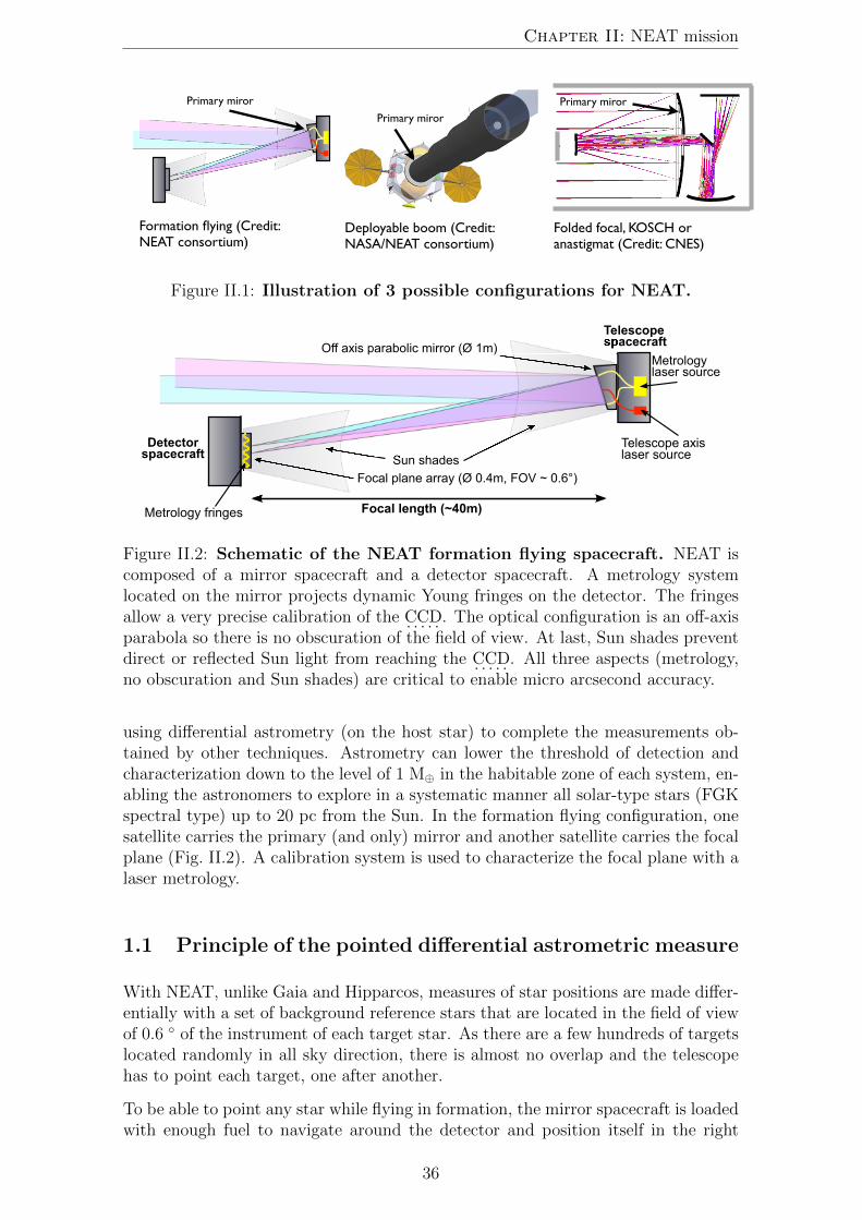
Chapter II: NEAT mission
�������������
�������������
�����������������������������������������
����������������������������������������������
������������������������������������������������
�������������
Figure II.1: Illustration of 3 possible configurations for NEAT.
Sun shades
Off axis parabolic mirror (Ø 1m)
Detectorspacecraft
Telescopespacecraft
Focal plane array (Ø 0.4m, FOV ~ 0.6°)
Focal length (~40m)
Metrologylaser source
Telescope axislaser source
Metrology fringes
Figure II.2: Schematic of the NEAT formation flying spacecraft. NEAT iscomposed of a mirror spacecraft and a detector spacecraft. A metrology systemlocated on the mirror projects dynamic Young fringes on the detector. The fringesallow a very precise calibration of the . . . . .CCD. The optical configuration is an off-axisparabola so there is no obscuration of the field of view. At last, Sun shades preventdirect or reflected Sun light from reaching the . . . . .CCD. All three aspects (metrology,no obscuration and Sun shades) are critical to enable micro arcsecond accuracy.
using differential astrometry (on the host star) to complete the measurements ob-tained by other techniques. Astrometry can lower the threshold of detection andcharacterization down to the level of 1 M⊕ in the habitable zone of each system, en-abling the astronomers to explore in a systematic manner all solar-type stars (FGKspectral type) up to 20 pc from the Sun. In the formation flying configuration, onesatellite carries the primary (and only) mirror and another satellite carries the focalplane (Fig. II.2). A calibration system is used to characterize the focal plane with alaser metrology.
1.1 Principle of the pointed differential astrometric measure
With NEAT, unlike Gaia and Hipparcos, measures of star positions are made differ-entially with a set of background reference stars that are located in the field of viewof 0.6 ◦ of the instrument of each target star. As there are a few hundreds of targetslocated randomly in all sky direction, there is almost no overlap and the telescopehas to point each target, one after another.
To be able to point any star while flying in formation, the mirror spacecraft is loadedwith enough fuel to navigate around the detector and position itself in the right
36

1. Presentation of NEAT
�����������
���������������
��������������������������������
�����������������������������������
������������������������
(a) Schematic of the focal plane of NEAT.
�����������������
��������������� ����������
������
����������������
����������������
���������������
����������������
����������������
����������������
�������������������������
������
��������������
�������������
��������������
���������������
���������������
����������������
����������������
����������������
����������������
����������������
����������������
����������������
����������������
����
�
�
(b) Example of field of view around thetarget Upsilon Andromeda.
Figure II.3: Explanation of the focal plane operation. After the two space-craft have repositioned correctly, the mirror is oriented to place the target star onthe dedicated central fixed . . . . .CCD. The best 8 reference stars compatible with theconfiguration are selected and each mobile . . . . .CCD moves to its assigned reference star.
configuration every time the target is changed. When the satellites are in position,8 mobile platforms position themselves on the location of reference stars, as describedin Fig. II.3. When in position, data is acquired for a few hours (mostly dependingon the target priority ranking and the brightness of the reference stars). During thistime, the altitude and the relative positions of each spacecraft are stabilized. Thefinest corrections are done with tip-tilt actuators on the primary mirror, in orderto freeze the centroids positions on the same pixels during data acquisition. Thecomplete sequence of events is shown in Table II.4. The stability requirement forthe centroids relative to the pixels depends on the accuracy obtained after the focalplane calibration and the data processing. The NEAT lab demonstration, which isthe core of this thesis, will explore this aspect (chapters IV and V).
1.2 Single epoch astrometric accuracy of NEAT
The baseline specification for NEAT sets the detection limit at 0.3 µas at the endof the mission, corresponding to an exo-Earth at 10 pc, with an . . . . .SNR of 6. Thistranslates into a final multi epoch accuracy of
σf =0.3µas
6= 0.05µas (II.1)
We have seen that the minimal number of single epoch measurements required isNparam = 5 + 7Nplanets. From here we assume an average of 3 planets detectedper star1 which yields Nparam = 26. We then conservatively assume an effective
1The recent exoplanet detection with . . . . . . . .HARPS and Kepler have allowed us to estimate thedistribution of exoplanet for a broad range of masses and periods [Wolfgang and Laughlin, 2011][Alibert et al., 2013b]. Given the detection limits of NEAT, we estimate that it will detect inaverage less than 3 planets per star.
37
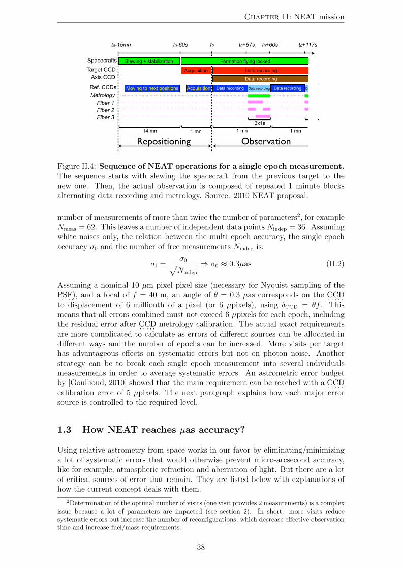
Chapter II: NEAT mission
���
�����������������������
�����������������������
��������������
��������������
����������
���������
���������������������
��������������
��������
���������
�������������������������
�����������
���� �������
�� ������ ������ �������
�����������������������
������������������������
�������������
���������
�����������
����
������������� �����������
Figure II.4: Sequence of NEAT operations for a single epoch measurement.The sequence starts with slewing the spacecraft from the previous target to thenew one. Then, the actual observation is composed of repeated 1 minute blocksalternating data recording and metrology. Source: 2010 NEAT proposal.
number of measurements of more than twice the number of parameters2, for exampleNmeas = 62. This leaves a number of independent data points Nindep = 36. Assumingwhite noises only, the relation between the multi epoch accuracy, the single epochaccuracy σ0 and the number of free measurements Nindep is:
σf =σ0�Nindep
⇒ σ0 ≈ 0.3µas (II.2)
Assuming a nominal 10 µm pixel pixel size (necessary for Nyquist sampling of the
. . . . .PSF), and a focal of f = 40 m, an angle of θ = 0.3 µas corresponds on the . . . . .CCDto displacement of 6 millionth of a pixel (or 6 µpixels), using δCCD = θf . Thismeans that all errors combined must not exceed 6 µpixels for each epoch, includingthe residual error after . . . . .CCD metrology calibration. The actual exact requirementsare more complicated to calculate as errors of different sources can be allocated indifferent ways and the number of epochs can be increased. More visits per targethas advantageous effects on systematic errors but not on photon noise. Anotherstrategy can be to break each single epoch measurement into several individualsmeasurements in order to average systematic errors. An astrometric error budgetby [Goullioud, 2010] showed that the main requirement can be reached with a . . . . .CCDcalibration error of 5 µpixels. The next paragraph explains how each major errorsource is controlled to the required level.
1.3 How NEAT reaches µas accuracy?
Using relative astrometry from space works in our favor by eliminating/minimizinga lot of systematic errors that would otherwise prevent micro-arcsecond accuracy,like for example, atmospheric refraction and aberration of light. But there are a lotof critical sources of error that remain. They are listed below with explanations ofhow the current concept deals with them.
2Determination of the optimal number of visits (one visit provides 2 measurements) is a complexissue because a lot of parameters are impacted (see section 2). In short: more visits reducesystematic errors but increase the number of reconfigurations, which decrease effective observationtime and increase fuel/mass requirements.
38
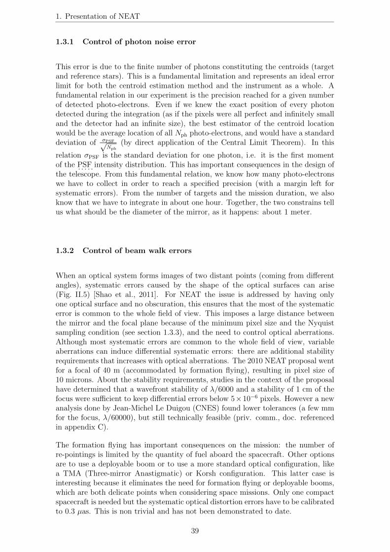
1. Presentation of NEAT
1.3.1 Control of photon noise error
This error is due to the finite number of photons constituting the centroids (targetand reference stars). This is a fundamental limitation and represents an ideal errorlimit for both the centroid estimation method and the instrument as a whole. Afundamental relation in our experiment is the precision reached for a given numberof detected photo-electrons. Even if we knew the exact position of every photondetected during the integration (as if the pixels were all perfect and infinitely smalland the detector had an infinite size), the best estimator of the centroid locationwould be the average location of all Nph photo-electrons, and would have a standarddeviation of σPSF√
Nph
(by direct application of the Central Limit Theorem). In this
relation σPSF is the standard deviation for one photon, i.e. it is the first momentof the . . . . .PSF intensity distribution. This has important consequences in the design ofthe telescope. From this fundamental relation, we know how many photo-electronswe have to collect in order to reach a specified precision (with a margin left forsystematic errors). From the number of targets and the mission duration, we alsoknow that we have to integrate in about one hour. Together, the two constrains tellus what should be the diameter of the mirror, as it happens: about 1 meter.
1.3.2 Control of beam walk errors
When an optical system forms images of two distant points (coming from differentangles), systematic errors caused by the shape of the optical surfaces can arise(Fig. II.5) [Shao et al., 2011]. For NEAT the issue is addressed by having onlyone optical surface and no obscuration, this ensures that the most of the systematicerror is common to the whole field of view. This imposes a large distance betweenthe mirror and the focal plane because of the minimum pixel size and the Nyquistsampling condition (see section 1.3.3), and the need to control optical aberrations.Although most systematic errors are common to the whole field of view, variableaberrations can induce differential systematic errors: there are additional stabilityrequirements that increases with optical aberrations. The 2010 NEAT proposal wentfor a focal of 40 m (accommodated by formation flying), resulting in pixel size of10 microns. About the stability requirements, studies in the context of the proposalhave determined that a wavefront stability of λ/6000 and a stability of 1 cm of thefocus were sufficient to keep differential errors below 5×10−6 pixels. However a newanalysis done by Jean-Michel Le Duigou (CNES) found lower tolerances (a few mmfor the focus, λ/60000), but still technically feasible (priv. comm., doc. referencedin appendix C).
The formation flying has important consequences on the mission: the number ofre-pointings is limited by the quantity of fuel aboard the spacecraft. Other optionsare to use a deployable boom or to use a more standard optical configuration, likea TMA (Three-mirror Anastigmatic) or Korsh configuration. This latter case isinteresting because it eliminates the need for formation flying or deployable booms,which are both delicate points when considering space missions. Only one compactspacecraft is needed but the systematic optical distortion errors have to be calibratedto 0.3 µas. This is non trivial and has not been demonstrated to date.
39

Chapter II: NEAT mission
�� �� ��
Figure II.5: Illustration of the “beam walk” problem (term coined by MikeShao). Configuration 1 is NEAT-like, there is no obscuration. Configuration 2has some obscuration on part of the field: the purple beam footprint is only halfof the mirror and is affected by different systematic errors than the green one.Configuration 3 has two mirrors: the beams have not the same footprint on thesecondary mirror, they are also affected by different systematic errors. A TMAconfiguration with a central obscuration by the secondary would suffer from theissues of configurations 2 and 3.
A Chinese mission called . . . . . .STEP (Search for Terrestrial Extrasolar Planets3) [Chen,2014] uses the configuration with several mirrors. A possibility to calibrate thebeam walk errors is to use globular clusters4: moving and/or rotating the clusterin the field of view gives the information needed to fit the optical distortion field.Additionally, more metrology systems have to be used to monitor changes of theoptical surfaces. So there is a trade-off between a configuration with a single opticalsurface (which has to accommodate a long focal), and a TMA or Korsch (which hasto use more calibrations).
In this thesis we work on the basis of the default NEAT configuration (formationflying). We assume that the beam walk problem can be solved by an appropriatespacecraft design and concentrate our efforts on the characterization of errors causedby the detector. However the beam walk issue is a major point to consider for anykind of µas astrometric mission: the formation flying configuration brings a lot ofinconveniences. Demonstrating µas calibration of a TMA or Korsch configurationis highly desirable.
1.3.3 Pixelation errors and focal plane calibration
The . . . . .CCD introduce errors related to the pixels, which are of several types. First,each pixel integrate the signal over a surface, and if the centroid is not at leastNyquist sampled (more than 2 pixels per λf/D), it will introduce sampling errors.Moreover, inter pixel variations also introduce some errors, even when the centroidsare properly sampled: pixels have different dark currents, sensitivities, they are notregularly spaced and the quantum efficiency (QE) profile within each pixel is notuniform. While the dark current and the sensitivity variations are usually calibratedwith darks and flat fields, at our level or precision we have to take into account allthe parameters. This is the role of the interferometric metrology system located onmirror spacecraft, with has fibers positioned on the mirror edge and pointed towards
3STEP is a mission of CAS (Chinese Academy of Science) / NSSC (National Space ScienceCenter) selected as part of the advanced research project in the Chinese Strategic Pioneer Program(SPP) on Space Science. STEP is a pointed astrometric mission similar to NEAT but it uses acompact configuration with several mirrors. If approved to enter phase B around 2015, STEPshould be planned for launch in 2020.
4A globular cluster is a compact group of up to one million stars
40

1. Presentation of NEAT
the detector
Two fibers are turned-on at a time to project Young fringes on the detector and adifferential phase modulation between the fibers is used to make the fringes dynam-ically sweep the focal plane. The basic principle is the following: each pixel sees asinusoidal signal whose characteristics (amplitude, offset, frequency and phase) giveinformation about the pixel sensitivity and location. Another important aspect ofthe metrology is related to the mobile . . . . .CCDs: by knowing the relative location ofeach pixel, one is able to measure the position of each reference star . . . . .CCD with avery high accuracy, by averaging individual pixel positions. This is critical to themission, as these positions must be known to a few micropixels. The metrologyfringes act like a ruler. The fringe pattern produced by the metrology is at the firstorder proportional to:
I(x, y) ∝ 2I20
�1 + cos
�φ0 +Δφ(t) +
2π(xBx + yBy)
λL
��(II.3)
Where I0 is the intensity for one fiber, φ0 is the origin phase, Δφ(t) is the phasemodulation applied between the two fibers and Bx and By are the (x,y) coordinatesof the baseline between the fibers.
The signal seen by each pixel is the convolution of the . . . . .PRF (Pixel Response func-tion5) and the fringe pattern along the modulation direction, which is perpendicularto the fringes. If the modulation is regular (Δφ(t) = 2πft), the pixel signals arepure sinusoids.
The phase difference between the measurement and the phase expected from thespatial fit gives the pixel offset. More elaborate models using several bases canobtain more information and probe the . . . . .PRF, inside the pixel. Simulations havebeen done, they showed that µpixel can be reached, provided that the . . . . .PRF arewell characterized [Zhai et al., 2011]. This was only a short introduction about thetheoretical principle of the calibration. The NEAT lab demo is an experiment todemonstrate this calibration technique, it is the core of this thesis. The algorithmsused to analyze the data are presented in chapter IV.
1.4 Error budget
An detailed error budget, accounting instrument systematic error has been developedin the framework of the NEAT proposal of 2010 by Renaud Goullioud (priv. comm.).The document is listed in appendix C. Figure II.6 is the high level summary of theerror budget.
5A PRF is a function representing a pixel sensitivity to light (or quantum efficiency) in theCCD plane.
41
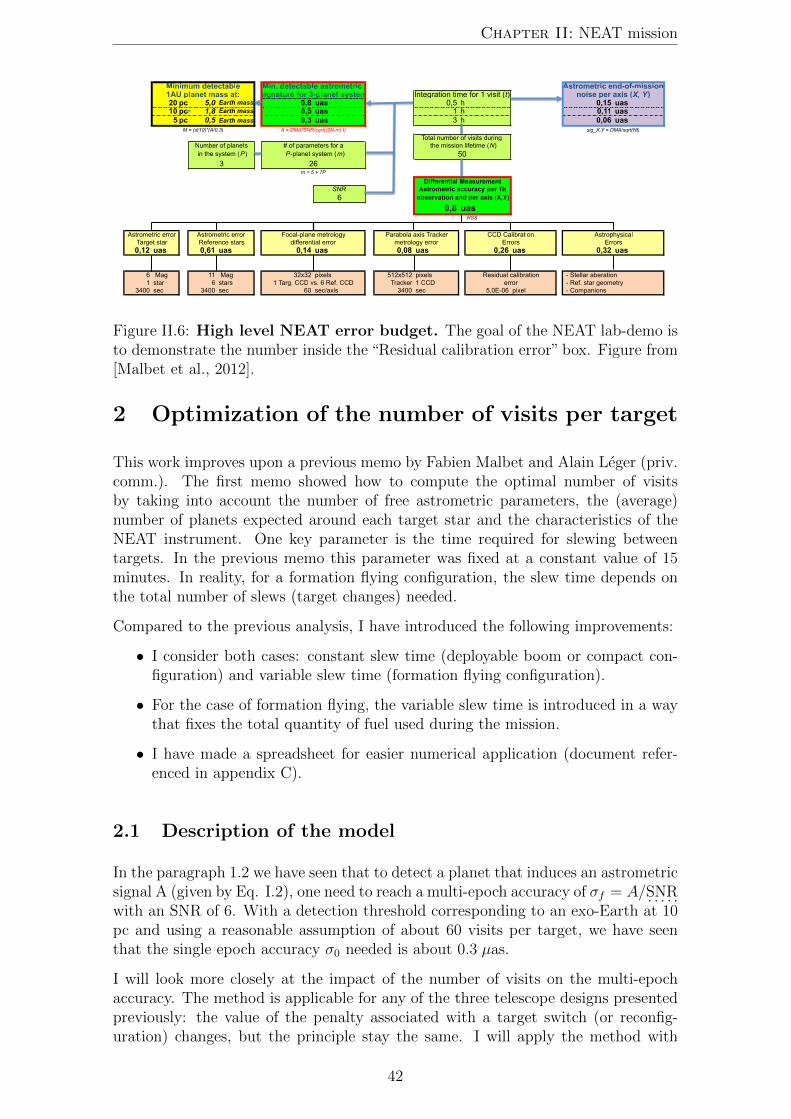
Chapter II: NEAT mission
�� �� ��� ����� ���� ��� ��� ��� ���� ������ �� ��� ���������� ��� ��� � � ���� ����� �� ��� ���������� ��� ��� � ���� ����
����
������
���� ��� ���� ��� ���� ��� ���� ��� ���� ��� ���� ���
� ���� �� ���� ����� ������ ������� ������� ���� � ����� ������� �����
���� ��� ���� ��� �� �������� ���� ��� ������� �����
�������������������
������������������������������������������������������
���������������������������������������������������
��������������������������������������
���������������������������������������
���������������
�
����������������������������������������������������������
���
����������� �������������������������������� ���������������������
��
������������������������
���������������������������������
�
�������������������������������������������������������
��
����������
���������������������������������������������������������
�����������������������������������������������
����������������������
����������������������������������
�������������������������������������
��������������������������������������������
�����������������������������������������
Figure II.6: High level NEAT error budget. The goal of the NEAT lab-demo isto demonstrate the number inside the “Residual calibration error” box. Figure from[Malbet et al., 2012].
2 Optimization of the number of visits per target
This work improves upon a previous memo by Fabien Malbet and Alain Leger (priv.comm.). The first memo showed how to compute the optimal number of visitsby taking into account the number of free astrometric parameters, the (average)number of planets expected around each target star and the characteristics of theNEAT instrument. One key parameter is the time required for slewing betweentargets. In the previous memo this parameter was fixed at a constant value of 15minutes. In reality, for a formation flying configuration, the slew time depends onthe total number of slews (target changes) needed.
Compared to the previous analysis, I have introduced the following improvements:
• I consider both cases: constant slew time (deployable boom or compact con-figuration) and variable slew time (formation flying configuration).
• For the case of formation flying, the variable slew time is introduced in a waythat fixes the total quantity of fuel used during the mission.
• I have made a spreadsheet for easier numerical application (document refer-enced in appendix C).
2.1 Description of the model
In the paragraph 1.2 we have seen that to detect a planet that induces an astrometricsignal A (given by Eq. I.2), one need to reach a multi-epoch accuracy of σf = A/ . . . . .SNRwith an SNR of 6. With a detection threshold corresponding to an exo-Earth at 10pc and using a reasonable assumption of about 60 visits per target, we have seenthat the single epoch accuracy σ0 needed is about 0.3 µas.
I will look more closely at the impact of the number of visits on the multi-epochaccuracy. The method is applicable for any of the three telescope designs presentedpreviously: the value of the penalty associated with a target switch (or reconfig-uration) changes, but the principle stay the same. I will apply the method with
42

2. Optimization of the number of visits per target
different numerical constants depending on which configuration we consider.
First I list the notations and equations that will be useful for this discussion. Whenapplicable I also give the values used for numerical application:
• The number of parameters needed to fit p planets around a given target star:m = 5+7p. We have seen previously that this value is not well known becauseit depends on the number of detectable planets per star. For NEAT we assumep = 3 ⇒ m = 26.
• The number of visits per target: Nvis. This is the number we want to optimize.We know that it will be more than 26 (number of free parameters) and lessthan a few hundreds (too much time spent switching between targets).
• The time effectively spent observing a target during a visit (i.e. collecting the“science” photons): T .
• The number of measurements per visit: α. In our case this number is ondebate. Some people think that since we have 2D measurements Nmeas =2Nvis whereas others think that the x and y measurements are not strictlyindependent yielding to Nmeas = Nvis. The NEAT double blind test shouldprovide useful insight. Here we will useNmeas = αNvis with α = 2 for numericalimplementation.
• The number of independent measurements: Nindep = αNvis−m. This is simplythe number of measurements minus the number of free astrometric parameters(m).
• The number of NEAT targets in the main science program: Ntargets = 200.
• The number of slews (i.e. a telescope reconfiguration, to change target):Nslews = NvisNtargets.
• The duration of a slew: h. This number can be a constant or depend of thenumber of visits per target (for formation flying).
• The total time spent on a target (observation + slews): T ∗ = Nvis(T + h)
Let us determine h as a function of the number of visits (formation flying case). ForNEAT the reconfiguration time is typically 15 to 30 minutes, but the exact durationwill depend on the number of visits. Each reconfiguration uses fuel, which is asignificant part of the satellite total mass and therefore cost! As for this exercise wewant to change only Nvis and keep all other things equal, a fixed among of availablefuel also means a fixed among of delta-v (noted ΔVtot)
6. If each reconfigurationhas to use in average ΔVtot/Nvis, then more of them will make each one longer, butby how much?
To answer this question I will consider a very simple model: I neglect any finepropulsion adjustment and I simply consider that the reconfiguration consist of twoimpulses (one to start moving the spacecraft, one to stop at the new configuration).
6In astrodynamics the delta-v (literally “change in velocity”) is a measure of the amount of workthat is needed to change from one trajectory to another by making an orbital maneuver, in unitsof speed. Delta-v is produced by the use of propellant by reaction engines to produce a thrust thataccelerates the spacecraft.
43
Chapter II: NEAT mission
In this case, the average time required to change target is:
h =Nslews
G1
=NvisNtargets
G1
=Nvis
G2
(II.4)
where G1,2 are constants related to ΔVtot. They can be estimated from the nominalparameters used in the 2011 NEAT proposal. For example, for 20000 slews of 15min yield: G1 = 1333 min−1 and G2 = G1/Ntargets = 6.67 min−1.
Note that in our case (formation flying), the slew time also depends on the focallength and on the angular separation between the targets. There is a case to bemade for optimization of average slew time by going faster (using more fuel) whenthe targets are further apart. But we can apply all the principles we have discussedabove to the sum (or average) speed of “optimized” slews: if we use twice as muchΔV holding the slew time distribution constant, the total slew time is halved. Therelations we have defined above are valid for any slew time distribution.
Now I write the equations between number of visits, the duration of visits, thenumber of parameters and the multi/single epoch accuracies:
σf =σ0�Nindep
(II.5)
=σ0√
αNvis −m(II.6)
=σT0�
T/T0
√αNvis −m
(II.7)
Here σT0 is the precision that NEAT can reach in one single observation which lastT0. From a previous NEAT error budget [Goullioud, 2010] we know that typicallyσT0 = 0.8 µas for T0 = 1 h. This is indeed mandatory if NEAT is to reach itsadvertised scientific goals. In Eq. II.7, we have implicitly defined σ0 =
σT0√T/T0
.
There is a critical hidden assumption in this last relation: it is that systematicerrors, for example due to the instrument and calibration residuals, can also beaveraged as the square root of the time spend on a target within a single epoch.
Now that I have defined all the relations I need, I will search for the minimum ofT ∗ as a function of T . This is equivalent to optimize Nvis because these two relatedquantities are the only variables in the expression of T ∗ (provided that h is alsoexpressed as a function of T ). In the end we will obtain the number of visits thatoptimizes the total time spent on a target, for a given multi epoch accuracy andfixed quantity of propellant fuel.
First let us express Nvis as a function of T using Eq. II.7:
Nvis =1
α×�T0
T
�σT0
σf
�2
+m
�=
1
α×�B
T+m
�(II.8)
I have introduced the constant B = T0
�σT0
σf
�2
(for the sake of simplicity). I now
replace Nvis in the definition of T ∗.
T ∗ =1
α×
�B
T+m
�(T + h) (II.9)
44

2. Optimization of the number of visits per target
Now consider two cases for h:
Case 1: h is a constant, this is valid for deployable boom and folded focal configurations
dT ∗
dT= − 1
α
�B
T 2
�[T + h] +
1
α
�B
T+m
�(II.10)
dT ∗
dT= 0 ⇔ B(T + h)
T 2=
B
T+m (II.11)
⇒ Topt =
�Bh
m(II.12)
Case 2: h = Ntargets/G2, this is valid for the formation flying configuration
T ∗ =�BT+m
� �T + 1
αG2(BT+m)
�(II.13)
= B + B2
αG2T 2 +2mBαG2T
+mT + m2
αG2(II.14)
dT ∗
dT=
1
α
� −2B2
αG2T 3+m+
−2mB
αG2T 2
�(II.15)
dT ∗
dT= 0 ⇔ αmG2T
3 − 2mBT − 2B2 = 0 (II.16)
The root of this 3rd degree polynomial exists and is unique because there is noquadratic term. An analytical formula of the solution exists but we will spare our-selves its expression which is rather cumbersome. The table II.1 sums up the numeri-cal results for different values of h, calculated by an excel spreadsheet (Nvisits_optimal.xls).We consider 4 different scenarios:
1. Compact configuration (folded focal, one spacecraft: quick reconfiguration,h=3 min)
2. A deployable boom (assumes h=15 min for a reconfiguration, to account forboom inertia)
3. Formation flying, large delta-v (uses an average value of h=15 min from theNEAT proposal of 2010)
4. Formation flying, low delta-v (assumes half the delta-V than the NEAT 2010proposal: average value of h=30 min)
2.2 Numerical results
Table II.1 shows the optimal visits duration and numbers of visits for different slewtimes durations and types (constant / variable).
45

Chapter II: NEAT mission
Table II.1: Slew time versus optimal visit duration and number of visits.
Scenario h T Nvis
1 3 min (constant) 0.702 h 1952 15 min (constant) 1.57 h 95
3 15 min average (= Nvis
G2) 1.96 h 78
4 30 min average (= Nvis
G2) 2.51 h 64
2.3 Discussion
The goal was to investigate wherever the optimal number of visit is far from thereasonable assumption of about 60 visits, and to see if different constraints on hchange the optimum significantly. When using the simplest approach for NEAT(scenario 2, h=15 min and is not adjusted for the number of visits), we findNvis = 95.This was the approach used by the initial memo from Fabien Malbet and Alain Leger.The result reflects the trade-off between wanting to split the photons into as manyepochs as possible (to make αNvis � m) and losing effective photon collecting timefor every additional visit. Of course, we see that when the slew penalty is muchsmaller (scenario 1), optimal Nvis increases to 195.
The critical difference between scenario 2 and 3 is taking into account the fact thatwith formation flying, if there are less visits, more gas can be used per slew, so slewsare shorter, so more time is available for photon collecting. This is an additionalincentive to have less visits, and as expected, this results in a lower optimal numberof visits: 78 versus 95. Scenario 4 is a test to see how the Nvis optimum is sensible toΔVtot. The result of 64 visits indicates that the mission can accommodate a tighterconstraint on fuel without loosing too much photon collecting time (6400 hours ofslewing instead of 3900, for a total of 22000 hours).
On the other hand, the optimum is very sensitive to σf . For scenario 3, changingσf from 0.05 µas to 0.025 µas changes the optimal number of visits to 119, this isalmost a linear increase. This means that there is also a case for choosing an optimalnumber of visits which is different for each target. Remember that 0.05 µas is theσf needed for an exo-Earth at 10 pc... NEAT will not observe only Suns at 10 pc!
But having different numbers of visits per target has to be considered together withyet another very important kind of optimization: the order in which the stars aretargeted to minimize the total angular separation. And to top it all, there are alsothe issues of having good (regular?) time samplings and the solar exclusion angle.All these problems have to be solved together, with the additional constraint thatit would be highly desirable to adapt the number of visits at the end of the missionin function of the number of planets already detected. If we find a very interestingsystem, no doubt we will want to come back more often before the mission is over.Obviously the whole problem is not trivial to solve and one would have to thinkof some simplifications and/or using numerical simulations to obtain a workablesolution.
One interesting idea with formation flying could be to dedicate a ΔV reserve (a few%) to an end of mission “slow mode”. At the end or after the nominal five yearmission, the spacecraft would only observe the few most promising targets (mostlikely a dozen), the ones which have habitable planets and are high priority targets
46
3. Construction of the catalog of NEAT targets and references
for direct detection/spectroscopic characterization, or stars for which there are po-tential (habitable) planets with signals slightly below the detection threshold (highfalse alarm probability). This would be an attempt to confirm near-detections andimprove the knowledge about the orbital parameters of interesting detections. Thereis an additional interesting benefit to have a long temporal baseline by prolongingthe mission: the knowledge of the true anomaly of habitable planets at the date oftheir direct detection would be greatly improved. With so few targets, the spacecraftcould accommodate very slow slews and use very little fuel, it would spend a longtime on each star and obtain exquisite accuracy per epoch. The approach is verylow risk: if prolonging the mission in this way is not thought to be worth it afterall, the ΔV reserve can simply be burned (quickly) in the continuity of the nominalmission.
To conclude the section, I will make some remarks about how to improve the model.In our flexible h scenarios, we have considered to have a strict 1/Nvis dependency. Amore accurate model would include a fixed overtime to account for the fine propul-sion adjustment needed to enter the static formation flying configuration and themetrology calibration that must take place before data can be acquired.
3 Construction of the catalog of NEAT targets
and references
3.1 The NEAT catalogs
This part will explain how the NEAT catalogs are constructed. Of course we arenot talking here of a complete and definitive catalog of targets for an actual NEATmission, but only an approximative catalog which is a tool to:
• obtain statistical information about the target and references
• test time allocation strategies by comparing their yields
The list of target stars of an actual mission would have several differences:
• The Hipparcos catalog is not complete for K and M stars up to 20 pc. A listbased on the Gaia survey, which should be available before 2017, would bepreferable.
• The main science program is specifically aimed at main sequence stars, sonearby stars would likely be checked against spectral miss-classification andany star found outside of the main sequence removed from the list.
• Close multiple stars should have a special treatment. It may be possible to usetheir relative orbits as a kind of reference resulting in an exquisite accuracy. Onthe other hand, overlap of their PSFs will make data reduction more complex.The final accuracy depends on the separation between them, the instrumentdesign and the processing. We have not explored this delicate issue significantlyyet. Depending or whether a given binary turns out to be more or less suitablefor exoplanet detection, one might want to spend more or less time than forsingle stars on them. To be accurate, one should also take into account thatboth can be observed at the same time.
47
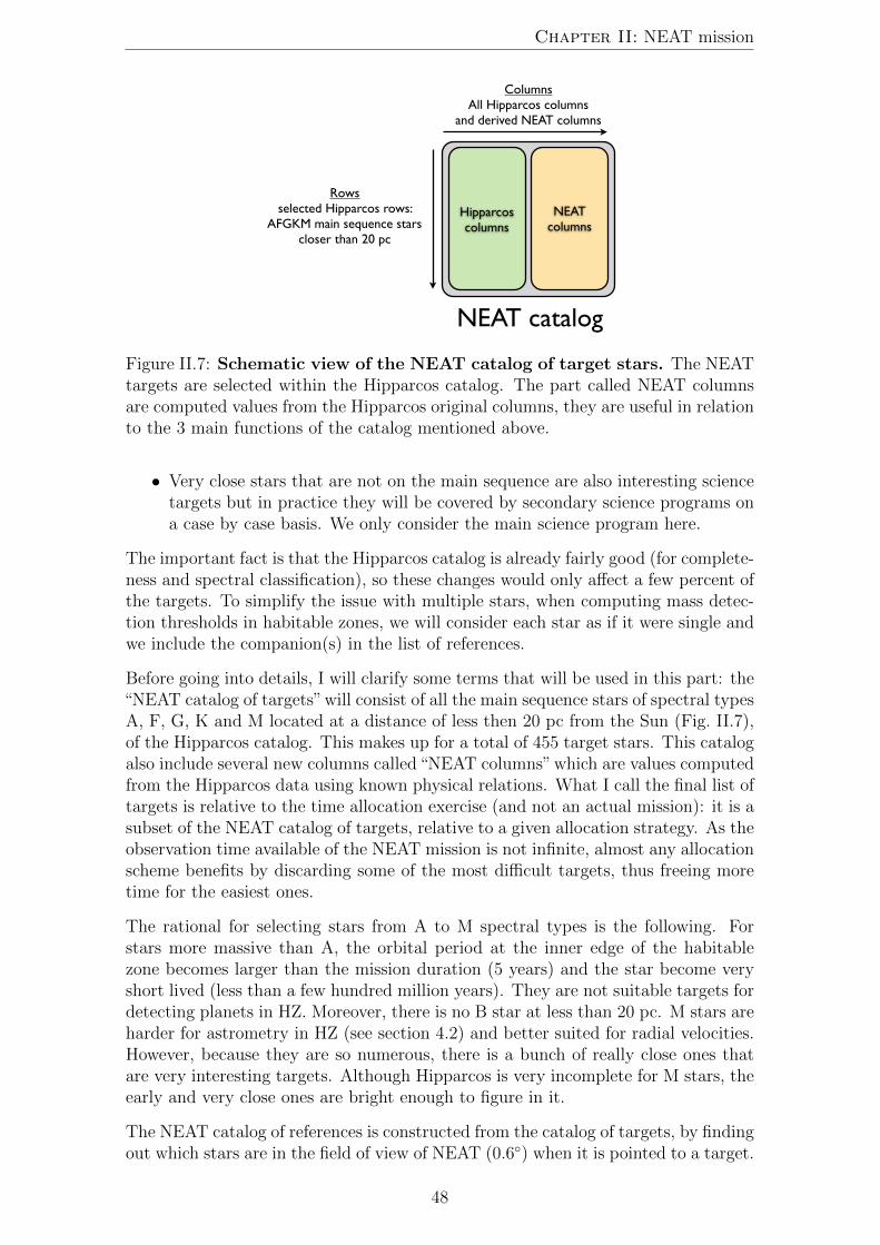
Chapter II: NEAT mission
�����������������
������������
������������
������������������������������
������������������������������������������
�����������������������������
������������������������
Figure II.7: Schematic view of the NEAT catalog of target stars. The NEATtargets are selected within the Hipparcos catalog. The part called NEAT columnsare computed values from the Hipparcos original columns, they are useful in relationto the 3 main functions of the catalog mentioned above.
• Very close stars that are not on the main sequence are also interesting sciencetargets but in practice they will be covered by secondary science programs ona case by case basis. We only consider the main science program here.
The important fact is that the Hipparcos catalog is already fairly good (for complete-ness and spectral classification), so these changes would only affect a few percent ofthe targets. To simplify the issue with multiple stars, when computing mass detec-tion thresholds in habitable zones, we will consider each star as if it were single andwe include the companion(s) in the list of references.
Before going into details, I will clarify some terms that will be used in this part: the“NEAT catalog of targets”will consist of all the main sequence stars of spectral typesA, F, G, K and M located at a distance of less then 20 pc from the Sun (Fig. II.7),of the Hipparcos catalog. This makes up for a total of 455 target stars. This catalogalso include several new columns called“NEAT columns”which are values computedfrom the Hipparcos data using known physical relations. What I call the final list oftargets is relative to the time allocation exercise (and not an actual mission): it is asubset of the NEAT catalog of targets, relative to a given allocation strategy. As theobservation time available of the NEAT mission is not infinite, almost any allocationscheme benefits by discarding some of the most difficult targets, thus freeing moretime for the easiest ones.
The rational for selecting stars from A to M spectral types is the following. Forstars more massive than A, the orbital period at the inner edge of the habitablezone becomes larger than the mission duration (5 years) and the star become veryshort lived (less than a few hundred million years). They are not suitable targets fordetecting planets in HZ. Moreover, there is no B star at less than 20 pc. M stars areharder for astrometry in HZ (see section 4.2) and better suited for radial velocities.However, because they are so numerous, there is a bunch of really close ones thatare very interesting targets. Although Hipparcos is very incomplete for M stars, theearly and very close ones are bright enough to figure in it.
The NEAT catalog of references is constructed from the catalog of targets, by findingout which stars are in the field of view of NEAT (0.6◦) when it is pointed to a target.
48

4. Statistical analysis of the NEAT catalogs
This is done by crossmatching7 the NEAT catalog of targets with a subset of theTycho catalog which contain all stars suitable as references. The process I usedto create both catalogs using Topcat8 is explained in details in a memo untitled“Creation and exploitation of the NEAT catalog” where I describe the operationsstep by step, in the form of a tutorial. Here I will briefly explain how the criticalNEAT columns are calculated, then I will focus on the results. For more details Iinvite the reader to refer to the memo which can be found in the appendix F.
3.2 Creation of the NEAT columns
For our purposes, the needed columns are (for each star): distance, bolometric lu-minosity, mass and the distances of the inner and outer edges of the . . .HZ. The mainpoint of this is to determine the amplitude of the astrometric signals of planets (of agiven mass) located at the inner and outer edge of the . . .HZ. The distance is directlyobtained from the Hipparcos parallax. The bolometric luminosity (L) is derivedfrom the V and B band magnitudes and relations with the effective temperature[Flower, 1996]. The mass (M) is estimated using the following general relation:L ∝ M3.5. The locations of the . . .HZ edges are given for two types of limits: themaximum greenhouse/runaway greenhouse limits (pessimistic), and the early Marsand recent Venus limits (more optimistic) based on [Kasting et al., 1993].
We now have all the information to calculate the amplitude of the astrometric signalof an hypothetical exo-Earth in a circular orbit at any one of the four . . .HZ edgesdefined earlier. We can simply scale it from the one of the Earth/Sun couple, viathe following equation:
A = 3µas× MPlanet
M⊕×�MStar
M�
�−1
× R
1AU�
D
1pc
�−1
The astrometric signals of an exo-Earth at this four orbital distances is the infor-mation that we store in the columns, the signal for any planetary mass is trivial toobtain from there: it scales proportionally with Mplanet/M⊕.
4 Statistical analysis of the NEAT catalogs
4.1 Availability of reference stars
From the catalog of the reference stars, we can determine the distribution of thesize of the groups of reference stars and the distribution of the equivalentmagnitudes. A “group” consists of the reference stars associated with one NEATtarget. The equivalent magnitude is the magnitude of a star which flux would beequal to the sum of the flux of the references. In the error budget associated withthe NEAT proposal, we have assumed 6 reference stars of magnitude 11 per target
7A “crossmatch” between two catalogs of astronomical sources is a process usually used toidentify which objects are in both catalogs by comparing their positions on the sky, with a specifiedtolerance. Here I make a slightly diverted usage of the crossmatch to find which objects are in agiven field of view, by using a tolerence equal to the radius of the FoV.
8TOPCAT is an interactive graphical viewer and editor for tabular data, specialized for astro-nomical data, developed by Mark Taylor.
49
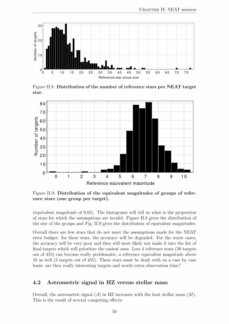
Chapter II: NEAT mission
0 5 1 0 1 5 2 0 2 5 3 0 3 5 4 0 4 5 5 0 5 5 6 0 6 5 7 0 7 5Reference star group size
0
1 0
2 0
3 0
Num
ber
of t
arge
ts
Figure II.8: Distribution of the number of reference stars per NEAT targetstar.
0 1 2 3 4 5 6 7 8 9 1 0
Reference equivalent magnitude
0
1 0
2 0
3 0
4 0
5 0
6 0
7 0
8 0
Num
ber
of t
arge
ts
Figure II.9: Distribution of the equivalent magnitudes of groups of refer-ence stars (one group per target).
(equivalent magnitude of 9.05). The histograms will tell us what is the proportionof stars for which the assumptions are invalid. Figure II.8 gives the distribution ofthe size of the groups and Fig. II.9 gives the distribution of equivalent magnitudes.
Overall there are few stars that do not meet the assumptions made for the NEATerror budget: for these stars, the accuracy will be degraded. For the worst cases,the accuracy will be very poor and they will most likely not make it into the list offinal targets which will prioritize the easiest ones. Less 4 reference stars (30 targetsout of 455) can become really problematic, a reference equivalent magnitude above10 as well (3 targets out of 455). These stars must be dealt with on a case by casebasis: are they really interesting targets and worth extra observation time?
4.2 Astrometric signal in HZ versus stellar mass
Overall, the astrometric signal (A) in HZ increases with the host stellar mass (M).This is the result of several competing effects:
50

4. Statistical analysis of the NEAT catalogs
1. The star luminosity increase with the mass: L ∝ M3.8
2. The orbital distance of the HZ increase with the luminosity: R(HZ) ∝ L0.5
3. The albedo of the planet is higher for bluer light (it moves the HZ slightlycloser to the star)
4. The ratioMplanet
Mstaris smaller
The net effect of 1 and 2 is an increase of the astrometric signal (A ∝ M1.9). Thisis somewhat attenuated by 3 (but it is a weak effect). We can take the albedo intoaccount by defining an effective luminosity Leff ≈ L−α and we obtain for 1, 2 and3: A ∝ M1.9−α/2. The effect of 4 is to subtract 1 to the total power. So we finallyobtain: A ∝ M0.9−α/2. This relation is approximative, as we have used severalapproximated power laws: the L = f(M) relationship breaks down for M stars (thelimit is around 0.43 M�) and the albedo effect is in our case modeled by a piecewiselinear function. In reality the exact albedo effect will be non linear and specific toeach planet.
Figure II.10 shows the astrometric signal in HZ versus the stellar mass. In orderto separate the effects of the distance and the stellar mass, Fig. II.11 shows theastrometric signal in HZ (µas) multiplied by the distance to the Sun (pc) versus thestellar mass. This is equivalent to moving all the targets at a distance of 1 pc fromthe Sun.
Figure II.11 confirms that the spectral effect is weak and that the astrometric signalin HZ increase with stellar mass, roughly as M0.63 (⇒ α = 0.54) 9. This result isimportant, it tells us that astrometry is complementary with radial velocities whensearching for planets in the habitable zone. Indeed, for radial velocities, exoplanetdetection in HZ becomes harder when the stellar mass increases. There is an impor-tant caveat that must be noted here: the increase in astrometric signal with stellarmass goes with a period increase. The temporal baseline must be larger than theperiod to fully take advantage of the increased signal amplitude. For stars later thanA, the orbital period at the inner edge of the HZ becomes larger than 5 years (thenominal duration of the NEAT mission).
4.3 Crossmatch with already known exoplanets
In order to to know which of the NEAT targets already have known exoplanetsaround them, I crossmatch the NEAT catalog of targets with the subset for exo-planets located at less than 20 pc from the Sun. The exoplanets are taken from theexoplanet.eu database (1821 exoplanets). The results of the crossmatch are given inTable II.2 and Fig. II.12. Table II.2 tells several interesting facts:
• Among the 1821 exoplanets candidates, only 126 are located at less than 20pc.
• The fraction of main sequence stars that have known exoplanets is not signif-icantly higher than the fraction for all stars. We have not put a particularlystrong emphasis on main sequence stars in past surveys.
• The known systems have in average 1.7 planet(s): we have mostly found iso-lated exoplanets because of detection biases.
• We expect on average several planets per star, around almost every star: manymore exoplanets are yet to be discovered in our solar neighborhood.
9Extrapolating from the following data points: (M=0.42, A=2.0) and (M=2.0, A=6.0).
51
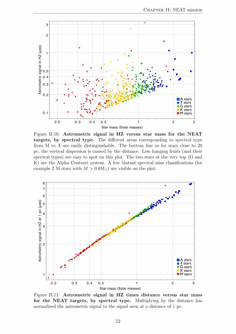
Chapter II: NEAT mission
��� ��� ��� ��� � � �
������������������������
���
���
���
���
���
�
�
�
������������������������������
�����������������������������������
Figure II.10: Astrometric signal in HZ versus star mass for the NEATtargets, by spectral type. The different areas corresponding to spectral typefrom M to A are easily distinguishable. The bottom line os for stars close to 20pc, the vertical dispersion is caused by the distance. Low hanging fruits (and theirspectral types) are easy to spot on this plot. The two stars at the very top (G andK) are the Alpha Centauri system. A few blatant spectral miss classifications (forexample 2 M stars with M > 0.8M�) are visible on the plot.
��� ��� ��� ��� � � �
������������������������
�
�
�
�
�
�
�
�
��������������������������������������
�����������������������������������
Figure II.11: Astrometric signal in HZ times distance versus star massfor the NEAT targets, by spectral type. Multiplying by the distance hasnormalized the astrometric signal to the signal seen at a distance of 1 pc.
52

4. Statistical analysis of the NEAT catalogs
Table II.2: Number of stars with known exoplanets (updated 02/09/2014).Two different star subsets are compared: the first one is all Hipparcos stars closerthan 20 pc (934 stars) and the second one is the NEAT catalog of targets (455 stars).The “Exoplanet count” tells how many exoplanets have been successfully associatedwith a Hipparcos host star, the “Star count” tells how many Hipparcos stars host atleast one known exoplanet. There is a small fraction of exoplanets for which no hoststar is found, they are most likely around M stars that are too faint for Hipparcos.
Hipparcos subset Exoplanet count Exoplanet count (%) Star count Star count (%)All stars < 20 pc
113/126 90% 64/934 6.9%
Main sequenceAFGKM stars < 20 pc
74/126 59% 39/455 8.6%
���������������������������������������������������
�������������
� �� ��
���
Figure II.12: 3D representation of the catalog of the NEAT catalog oftargets, by spectral type (updated 02/09/2014). The stars are crossmatchedwith the list of known exoplanets, the ones with at least one known exoplanet inorbit are circled. There are 10 A, 62 F, 97 G, 192 K and 94 M stars.
53

Chapter II: NEAT mission
5 Allocation strategies and science yields
In the NEAT catalog, we have constructed estimations of the astrometric signal ofplanets in HZ (AHZ), instrumental accuracy as a function of time (σtarget/h) and theobservation time needed to detect an Earth in HZ around a given target (TexoEarth).The accuracy is given in units of µas.h−0.5. This is because it increases as the squareroot of the number of photons, which is proportional to time. The accuracy alsotakes into account the brightness of the target stars and the reference stars. For mosttargets the photon noise of the reference stars is the limiting factor, but sometimesthe opposite can be true. This is important to take all these factors into accountto have a reliable estimation of the observation time needed to detect astrometricsignatures around each star and to rank them properly by increasing difficulty. Thedetailed reasoning to define the columns is explained in the neat catalog memo.
The fundamental approximation that enables this analysis is that we forget the com-plex considerations about how to optimize the number of visits, their duration andthe number of slews required. We retain only the total time of effective observationper target (excluding slew time from this total). The approximation is valid becausethe number of epochs per target, number of data points per epoch or integration timeper data point all increase the accuracy roughly as a power 0.5 when the number ofindependent measurements is larger than the number of free parameters.
The planetary systems are based on a list of 344 synthesized planetary systems kindlyprovided by Yann Alibert, they were originally generated for the NEAT double blindtest (for non-blind test runs). The planet systems are randomly assigned to targetstars. For detailed informations about the population synthesis model, refer to[Alibert et al., 2013a]. The fundamental assumptions of the planet synthesis modelare:
• Maximum of 10 planets per system• Star mass of 1M�• Alpha disk model (1+1D model, azimuthal symmetry, α = 2× 10⁻³)• Migration model based on [Mordasini et al., 2011] and [Dittkrist et al., 2014]• Disk properties (mass and lifetime) should be similar to observations
The analysis consists in distributing the total effective observation time among thetargets: once we have done that, the relations and models mentioned above are usedto derive the planet yield (any planet with a SNR > 6 is considered to be detected).Based on the content of the NEAT proposal of 2010, the total observing time is22000 hours. Six time allocation scenarios have been tested. Figure II.13 shows thetime distribution corresponding to each scenario. This analysis is carried out witha matlab script (observational_strategy_yield.m).
The 6 bar plots highlight the trade-offs between the allocation schemes. The dif-ference between 1, 2 and 3 is that we increasingly concentrate more time on easytargets. 1 yields more giant planets than 2, but slightly less terrestrial ones. How-ever when we reduce the number of targets too much (3), we obtain less giant butalso less terrestrial planets. In this case we have already spent a fair amount of timeon the easy targets in 2, so the additional observation time around these do notcompensate for the planet loss of the “medium” targets (ranked 100 to 200).
The idea behind schemes 4, 5 and 6 is too see whether having an unequal distributiontime can yield better results. We test several possibilities:
54
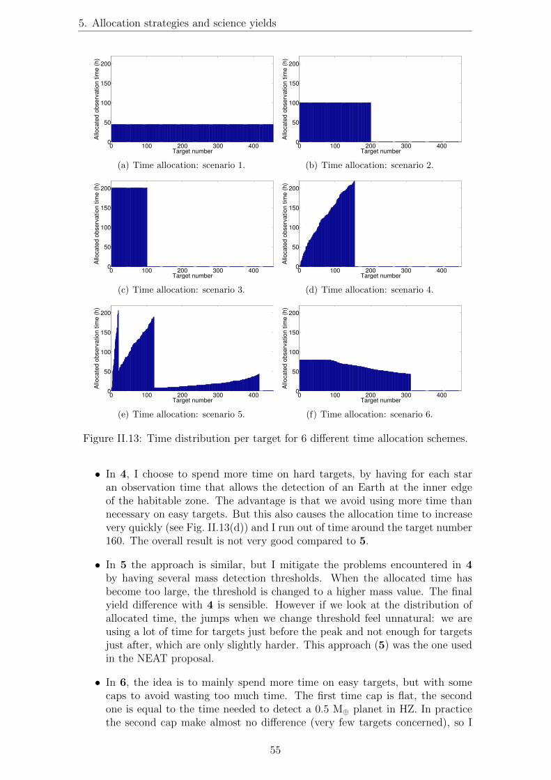
5. Allocation strategies and science yields
0 100 200 300 4000
50
100
150
200
Target number
Allo
cate
d o
bserv
ation tim
e (
h)
(a) Time allocation: scenario 1.
0 100 200 300 4000
50
100
150
200
Target number
Allo
cate
d o
bserv
ation tim
e (
h)
(b) Time allocation: scenario 2.
0 100 200 300 4000
50
100
150
200
Target number
Allo
cate
d o
bserv
ation tim
e (
h)
(c) Time allocation: scenario 3.
0 100 200 300 4000
50
100
150
200
Target number
Allo
cate
d o
bserv
ation tim
e (
h)
(d) Time allocation: scenario 4.
0 100 200 300 4000
50
100
150
200
Target number
Allo
cate
d o
bserv
ation tim
e (
h)
(e) Time allocation: scenario 5.
0 100 200 300 4000
50
100
150
200
Target number
Allo
cate
d o
bserv
ation tim
e (
h)
(f) Time allocation: scenario 6.
Figure II.13: Time distribution per target for 6 different time allocation schemes.
• In 4, I choose to spend more time on hard targets, by having for each staran observation time that allows the detection of an Earth at the inner edgeof the habitable zone. The advantage is that we avoid using more time thannecessary on easy targets. But this also causes the allocation time to increasevery quickly (see Fig. II.13(d)) and I run out of time around the target number160. The overall result is not very good compared to 5.
• In 5 the approach is similar, but I mitigate the problems encountered in 4by having several mass detection thresholds. When the allocated time hasbecome too large, the threshold is changed to a higher mass value. The finalyield difference with 4 is sensible. However if we look at the distribution ofallocated time, the jumps when we change threshold feel unnatural: we areusing a lot of time for targets just before the peak and not enough for targetsjust after, which are only slightly harder. This approach (5) was the one usedin the NEAT proposal.
• In 6, the idea is to mainly spend more time on easy targets, but with somecaps to avoid wasting too much time. The first time cap is flat, the secondone is equal to the time needed to detect a 0.5 M⊕ planet in HZ. In practicethe second cap make almost no difference (very few targets concerned), so I
55

Chapter II: NEAT mission
ignore it and only apply the first one. For harder targets, the time spent isproportional to 1
TexoEarthα . Around harder targets, we reduce the time spent:we only hope to detect massive super-Earth and giant planets.
In the end the simulation indicates that 6 finds the most terrestrial exoplanets. Itseems to be a good compromise for splitting time between easy and hard targets,because a significant fraction of the giant planets are detected (55%), not very farfrom the maximum obtained with 1 (75%).
0
1000
2000
3000
Nu
mb
er
of
pla
ne
ts
2.5 % 36.1 %
34/1382
44/122
8.7 % 63.7 %
35/404 45/718 %
63.6 %
91/1145
140/220
5.5 %
55.5 %
160/2931
229/413
cold/terHZ/ter
hot/tercold/gas
HZ/gashot/gas
tot. ter
tot. gas
Simulated planetsDetected planets
Figure II.14: Exoplanet yields for allocation scheme number 6.
10−2
10−1
100
101
102
10−2
10−1
100
101
102
103
104
Planet semi major axis (AU)
Pla
net m
ass (
Eart
h m
ass)
10 Earth mass (terrestrial limit)
1 Earth mass
planet not detected (<0.3µas)
hot planet
temperate planet
cold planet
Figure II.15: Mass period diagram of the NEAT mission simulated exo-planet yield.
56

6. Conclusion
6 Conclusion
I have shown that with an accuracy on the order of 0.7 µas.h−0.5, and with a missionduration of 5 years, NEAT is capable of finding dozens of nearby habitable planets,the closest of which would be the best targets for direct imaging and spectroscopiccharacterization. I have presented a process from which one can:
• Create catalogs of target and reference stars for a pointed astrometric missionaiming at detecting nearby exo-Earths
• Acquire various statistics about the reference stars and in particular check ifthe hypothesis made in the NEAT error budget are correct
• Estimate the science yield of the mission, as a function of mission and telescopeparameters, the distribution of the observation time between the targets
Because the process is documented at each step, parts of the process can be modifiedand easily adapted to work with the rest of it. A new input catalog can be used (forexample from Gaia), the error budget can be updated and the planet populationsynthesis model can be improved or swapped for an empirical one based on observa-tions only. Some parameters require only minimal work to update the final result:the time allocation scheme and mission duration can be changed in the final scriptbefore execution. The NEAT catalog of target and references and all the associatedtools will be very valuable to provide content for the incoming Theia proposal.
57
Chapter III
NEAT lab demo: concept,specifications, design and testresults
1 Foreword
Before going into details, I will have a word about the management of the NEATlab demonstration. From the start, a project-like approach was taken, to be able togo through the specification, design, procurement, assembling, test and operationphase of the testbed within the 3 years limited by my working contract with CNES:this time framework is rather short for an academic research project with such anambitious and unprecedented goal. To minimize costs and delays and maximize flex-ibility, we have chosen to take advantage of the local resources (mainly mechanical,optical and IT manpower and expertise) by locally designing and manufacturing asmuch components as we could. Having a small and modular experiment was veryimportant for us.
One of the main difficulties in organizing the project was dealing with the limitedand somewhat unpredictable availability of the people. The NEAT lab demo being asmall project, we would typically require people to work in average for 10 to 20% oftheir time for us, but we had occasionally the need for stronger commitments to solvespecific problems. Of course the availability and need for specific manpower wouldnot always coincide. The initial standard planning approach using a Gantt-like toolquickly revealed to be impractical. The solution that was adopted was to use a lowlevel of planning but to increase communication, follow up and feedback. Duringthe design, commissioning, assembling and testing phases we had weekly meetingsand we used a “snapshot spreadsheet” to visualize the current state of the project.It proved to be a very convenient tool, it was very easy to update and allowed usto quickly identify priorities by giving us a good overview about the state of theproject. The spreadsheet is more relevant to the design and test phases and will bepresented in the appropriate place (section 5: design overview).
Many people from . . . . . .IPAG, IAS (Institut d’Astrophysique Spatiale) and CEA (Com-missariat a l’Energie Atomique et aux Energies Alternatives) have brought theirexpertise and made the NEAT testbed a reality. Here is the list of people ar-ranged by domains, to help identify who worked on what: Pierre Kern, Francois
58

2. High level specifications and concept
Henault, Alain Leger (optics, error budget), Eric Stadler, Noel Ventura (Mechanics),Guillermo Martin, Alain Delboulbe (Metrology) , Olivier Preis (lab environment),Christophe Cara, Modeste Donati, Christophe Doumayrou, Philippe Feautrier (CCDand readout electronics) and Sylvain Lafrasse (IT).
To conclude this section, I have to mention the . . . . . . . .VESTA experiment (ValidationExperiment for Solar-system STaring Astrometry1), which team was composed ofMike Shao, Bijan Nemati, Chengxing Zhai and Inseob Hahn. In summer 2012, Ispent two months at JPL working on a high accuracy astrometric testbed: . . . . . . . .VESTA.This visit and the interaction with the team was very beneficial to me, I was ableto acquire invaluable experience on the design, the operation and the data analysisof the astrometric testbed. As a result we were able to anticipate a lot of issueswhen designing our own experiment in Grenoble. A lot of specifications of our ownexperiment are based on the experience gained at the JPL.
2 High level specifications and concept
The primary goal of the NEAT lab demonstration is to show that centroiding can bedone at the required accuracy, 5×10−6 pixel, with the help of a calibration systemand provided that some eventual conditions (that are to be discovered) are met.Obtaining such a performance would validate the fact that systematic errors causedby the pixels can indeed be controlled down to 5×10−6 pixels and are not a showstopper for the detection of nearby exo-Earths with NEAT as it was proposed at the2010 . . . . .ESA call for M class missions.
Additionally, even if this ultimate goal of 5×10−6 pixel accuracy is not reached,the lab demonstration has other important goals that would be very beneficial tosubsequent NEAT proposals and more broadly astrometric and transit missions.The most important aspect is the quantitative understanding of all the systematicerror sources that must be corrected for to improve the accuracy, from pixels tomicro pixels. Another critical aspect is the impact of the observational strategy onthe final accuracy: one can chose to move the CCD to a lot of different places toaverage pixel errors, or to come back to precisely the same positions every time tosubtract the systematic errors. In fact it might be possible to come up with a wayof obtaining astrometric measurements with a precision greater than 0.3 µas even ifthe pixel calibration does not reach the accuracy of 5×10−6 pixel.
In order to explore all the aspects mentioned above in the most sensible manner,the NEAT lab demo mimics the configuration of the NEAT instrument very closely:the concept shown in Fig. III.1 is the starting point from which we derive at firstthe specifications and then the complete design of the testbed.
1VESTA is a high accuracy astrometry testbed that was operated at the JPL, it was very similarto and preceded the NEAT lab demonstration.
59

Chapter III: NEAT lab demo: concept, specifications, design and test results
������������������
�����������������������������������
����������������������������������������
�����
���������������
�����
������
��������������
�����������������
�������������
������������������
��
��
�
�������������������
��
��
θ
Figure III.1: Concept for the NEAT lab demo (top view, not to scale).The elements associated with the metrology, the pseudo stars and the mechanicalsupports are respectively in red, blue and grey/green. The (X,Y,Z) axis indicated onthe figure will be used consistently throughout the document to indicate directions.
The concept includes numerous key elements that are grouped into 4 sub-systems:
Metrology It produces Young fringes on the detector, they are used for calibration,just like in the case of the spacecraft. We use single mode fibers (SMF), theirtips are seen as punctual sources by the detector.
Pseudo stars On the NEAT instrument, an off axis parabola focuses the targetand reference stars (which are punctual objects optically located at infinity)on the detector. Here we have to use a slightly different configuration wherethe stars are produced artificially, hence the name of “pseudo stars”. Thedevice that produces them has to be located inside the available space, whichis a cuboid of dimensions 0.3×0.3×0.8 m. Just like for the NEAT instrument,using only one optical surface and having no obscuration in the field of viewis critical. The optical configuration is thus with a “real object at a finitedistance”. The specification of this system has to be such that the pseudostars on the detector have no significant difference than ones that would beproduced by real stars.
Light detector It will be a . . . . .CCD or a CMOS.
Mechanical supports and environment control This broad category regroupall mechanical supports and environment control system, in particular it in-cludes the vacuum chamber, which has crucial functionalities. Generally speak-ing, it reproduces the mechanical and thermal stability of space, at least par-tially. It is very important to have very little or no pressure inside the chamberto decrease the effect of atmospheric turbulence. Additionally, it allows thedetector to work at a lower temperature, which would be impossible at at-mospheric pressure because of water condensation or ice deposition. This isneeded to control the level of dark current as most detectors do not workoptimally at ambient temperature.
The maximum dimensions of the optical bench (0.3×0.3×0.8 m) originated at firstfrom the size of a vacuum chamber at IAS, in which the experiment was to beinstalled. The precise dimensions later became irrelevant because we decided toassemble and operate the testbed directly at IPAG, but we continued with the same
60

3. Specifications
Table III.1: Notations.Parameter Notationdistance mirror to CCD Ldistance mirror to pseudo star objects L0
min/max wavelength of pseudo stars λmin/λmax
diameter of the entrance pupil Dmirror focal length fseparation between pseudo stars objects spseudo stars pinhole diameter doff axis angle (pseudo stars) θmetrology source wavelength λm
metrology baseline Bpixel size edetector frame format (N ×N pixels) N
numbers. From an optical point of view, the scale can be chosen arbitrarily as we willsee in the pseudo stars specifications (pixel size and Nyquist sampling condition).But as it turns out, working at this scale was a very good trade-off: the optical andmechanical elements are readily available and large enough to be easily manipulatedby hand, yet they are small enough to keep costs under control. In the end we havean affordable and flexible system.
Another critical aspect is the mobility of the detector. In order to rigorously de-termine the accuracy of the calibration, we have to be able to induce a commontranslation motion of several pixels on all the pseudo stars. With a smaller dis-placement (or no displacement at all), one would greatly underestimate the residualnoise after calibration because the biases caused by the pixels would be stronglycorrelated. On the other hand, for other kinds of analysis, it is interesting to comeback to precisely the same positions, so the translation stage should also be accu-rate, to a fraction of a pixel (10% or better). Understanding why we do all thesedifferent types of analysis and what kind of information will bring each one is quitesubtle and cannot be detailed here (see section 2.4: analysis of pseudo star data).To conclude this part I recall that what we want to characterize in this experiment isthe error caused by the pixels and not those caused by the optics. For our purposesthis second part of the problem is assumed to be solved by either formation flying, adeployable boom or an advanced calibration of the optics. Table III.1 summarize thenotations for the critical dimensions and parameters that will be used consistentlythroughout this document.
3 Specifications
In this section we list the specifications for each sub-system of the testbed, whichhave been obtained by a wide variety of methods. Some are straightforward conse-quences of the concept or high level specifications. Whenever possible and practicalwe have performed calculations to obtain precise quantitative specifications. Butlacking this, we have at times relied on the experience gained at the JPL with the
. . . . . . . .VESTA experiment, used guesstimates and/or helped our decisions based on thecontent of the NEAT proposal of 2010. At last, these specifications are not exhaus-
61

Chapter III: NEAT lab demo: concept, specifications, design and test results
tive: there are a lot of uncertain areas. In particular, the validity of the error budgetsdepends on the data analysis methods used. Moreover, our understanding of errorpropagations has evolved while we have explored the data. We will see in section1.3 (data analysis of pseudo stars) that we had to deal with quite nasty surpriseswhen looking at the real data.
3.1 Mechanical supports and environment
Mechanical supports:
• The optical bench inside the vacuum chamber (plus all the components in-stalled on it) fits into a cuboid of dimensions 0.3×0.3×0.8 m.
• The relative positions of the pseudo stars objects and the mirror are con-strained by a zerodur bench with a coefficient of thermal expansion lower than1× 10−7.
• The relative position of the pseudo stars (image) and the detector is stable onthe X,Y and Z axis to 0.01e (to avoid blurring effects)
• The light detector is installed on a translation stage, allowing motor controlledtranslation in the X and Y direction, with a resolution smaller than 0.1e.Accurate translation (< 0.1mm) in the Z direction is also possible, at leastmanually, to adjust the focal point. The resolution on the Z axis is sufficientto have a defocus effect smaller than 1% of the PSF width. Coarse tip-tilt(rotations on X and Y axis) is possible, at least manually.
Vacuum chamber:
• The chamber withstands vacuum (P < 1mbar).
• The sealing quality allows a critical pressure threshold Pcrit to be reached andmaintained without pumping for at least a few hours. The critical pressurethreshold Pcrit is such that it allows the detector to safely operate at a tempera-ture TCCD, corresponding to a dark current < dcrit (see detector specifications).The correspondence between Pcrit and TCCD is given by the P-T phase diagramof water (this is necessary to avoid the formation of ice or dew on the detector).
Environment:
• Sufficient precautions are taken to provide a dust free environment for the un-protected detector, during data acquisition or modification of the configurationinside the vacuum chamber.
• The temperature of the detector is stable to at least 0.1◦C over one hour.
3.2 Detector/pixel specifications
We have to use an off-the-shelve CMOS or . . . . .CCD in order to limit costs. The modelhas to accommodate the following constraints:
• Read noise of less than 10 electrons.
• High product “frame rate × effective well size”, because we want to be able torun the experiment in a “reasonable time” (at most 1 hour, ideally a few min-utes). The number of pseudo star and metrology photons needed for 5×10⁻⁶
62
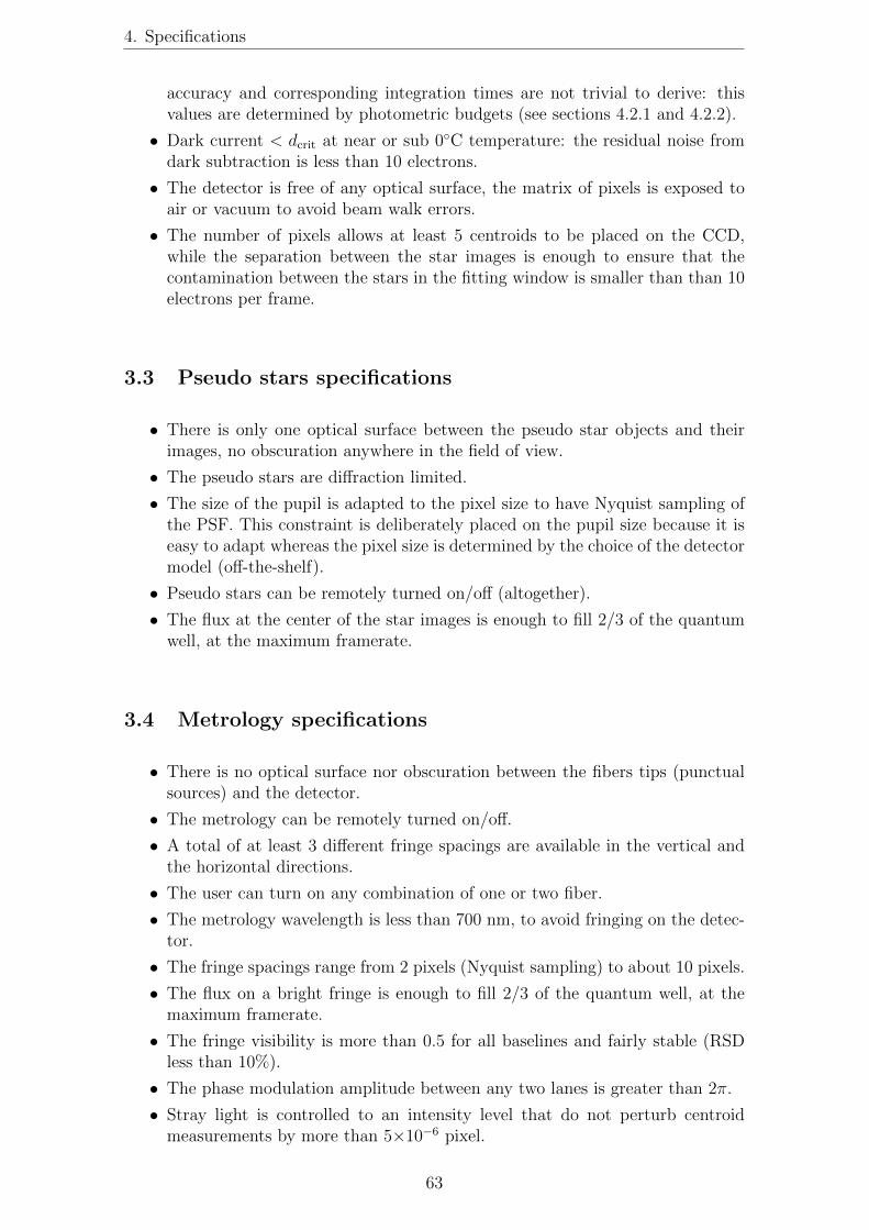
4. Specifications
accuracy and corresponding integration times are not trivial to derive: thisvalues are determined by photometric budgets (see sections 4.2.1 and 4.2.2).
• Dark current < dcrit at near or sub 0◦C temperature: the residual noise fromdark subtraction is less than 10 electrons.
• The detector is free of any optical surface, the matrix of pixels is exposed toair or vacuum to avoid beam walk errors.
• The number of pixels allows at least 5 centroids to be placed on the CCD,while the separation between the star images is enough to ensure that thecontamination between the stars in the fitting window is smaller than than 10electrons per frame.
3.3 Pseudo stars specifications
• There is only one optical surface between the pseudo star objects and theirimages, no obscuration anywhere in the field of view.
• The pseudo stars are diffraction limited.
• The size of the pupil is adapted to the pixel size to have Nyquist sampling ofthe PSF. This constraint is deliberately placed on the pupil size because it iseasy to adapt whereas the pixel size is determined by the choice of the detectormodel (off-the-shelf).
• Pseudo stars can be remotely turned on/off (altogether).
• The flux at the center of the star images is enough to fill 2/3 of the quantumwell, at the maximum framerate.
3.4 Metrology specifications
• There is no optical surface nor obscuration between the fibers tips (punctualsources) and the detector.
• The metrology can be remotely turned on/off.
• A total of at least 3 different fringe spacings are available in the vertical andthe horizontal directions.
• The user can turn on any combination of one or two fiber.
• The metrology wavelength is less than 700 nm, to avoid fringing on the detec-tor.
• The fringe spacings range from 2 pixels (Nyquist sampling) to about 10 pixels.
• The flux on a bright fringe is enough to fill 2/3 of the quantum well, at themaximum framerate.
• The fringe visibility is more than 0.5 for all baselines and fairly stable (RSDless than 10%).
• The phase modulation amplitude between any two lanes is greater than 2π.
• Stray light is controlled to an intensity level that do not perturb centroidmeasurements by more than 5×10−6 pixel.
63

Chapter III: NEAT lab demo: concept, specifications, design and test results
4 Critical design constraints
4.1 Nyquist sampling of pseudo stars and pupil size
In order to comply rigorously with the Nyquist sampling requirement, one has touse the shortest wavelength of the pseudo star light spectrum. Using a “midband”average wavelength as reference could result in under-sampling of part of the signaland aliasing. The choice of this minimum wavelength λmin is somewhat arbitrary asthe detector spectral response curve does not necessarily have a steep cut-off profile.We will use a conservative estimate of the minimum wavelength by requiring thatthe quantum efficiency for λ < λmin is less than 10% of the peak efficiency. We keepthe option to add a filter to the white source later if aliasing proves to be an issue.This also means that the detector coating for the NEAT demo and NEAT missionshould have a spectral profile with a steep cut-off.
In the NEAT-demo optical configuration the size of the diffraction spot is related tothe pupil size which is the mirror diameter, and the distance between the mirror andthe detector rather than the focal length (see appendix H for a quick justification).Thus the Nyquist sampling condition is:
2e ≤ Lλmin
D(III.1)
4.2 Photometric relations
The goal of the next two sections is to determine the pseudo star and metrologyintegration times needed to reach the targeted accuracy and what are the conditionsfor which each light source (metrology and pseudo stars) have sufficient fluxes toefficiently fill the pixels quantum wells. Keep in mind that we are looking for ordersof magnitudes here, not parts per million. We will use a lot of approximations toget simpler expressions.
Table III.2 lists the notations introduced for these photometric budgets. A visualsummary of the photometric relations and where they physically apply in the ex-periment is shown in Fig. III.2. We have initially considered two possibilities for thepseudo stars: either a pinhole mask combined with a MMF or a bundle of SMF. Forthe sake of clarity and simplicity, I the summary I only show the relations for theMMF case which was the one to be implemented. After the summary, I present indetails how I:
• get from the photometric result per say (the photo-electron flux for the bright-est pixels, noted Fmax/pix) to the final integration time, by defining a sourceoptimality factor (this part is common for metrology and pseudo stars).
• determine the number of photons needed for the metrology and the pseudostars (Ne−).
• obtain each relation, following the light path step by step from the sources tothe detector, for the pseudo stars (section 4.2.1) and the metrology (section4.2.2).
The numerical applications with the parameters used in the design are shown inspreadsheets (see section 6.1), here we only derive the analytical expressions. The
64
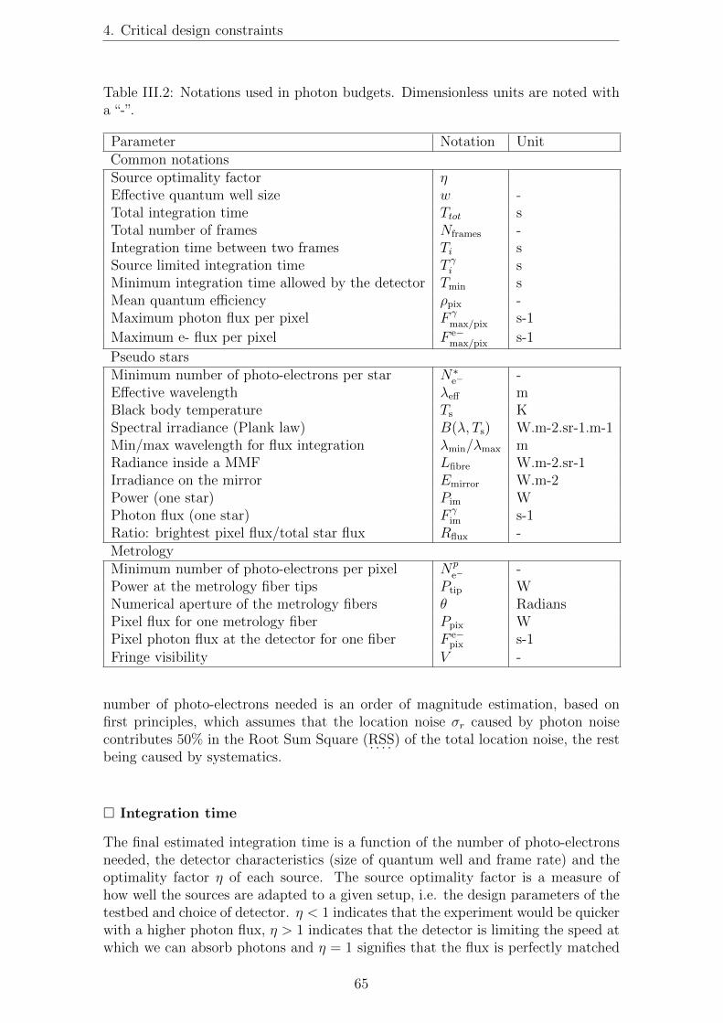
4. Critical design constraints
Table III.2: Notations used in photon budgets. Dimensionless units are noted witha “-”.
Parameter Notation UnitCommon notationsSource optimality factor ηEffective quantum well size w -Total integration time Ttot sTotal number of frames Nframes -Integration time between two frames Ti sSource limited integration time T γ
i sMinimum integration time allowed by the detector Tmin sMean quantum efficiency ρpix -Maximum photon flux per pixel F γ
max/pix s-1
Maximum e- flux per pixel F e−max/pix s-1
Pseudo starsMinimum number of photo-electrons per star N∗
e− -Effective wavelength λeff mBlack body temperature Ts KSpectral irradiance (Plank law) B(λ, Ts) W.m-2.sr-1.m-1Min/max wavelength for flux integration λmin/λmax mRadiance inside a MMF Lfibre W.m-2.sr-1Irradiance on the mirror Emirror W.m-2Power (one star) Pim WPhoton flux (one star) F γ
im s-1Ratio: brightest pixel flux/total star flux Rflux -MetrologyMinimum number of photo-electrons per pixel Np
e− -Power at the metrology fiber tips Ptip WNumerical aperture of the metrology fibers θ RadiansPixel flux for one metrology fiber Ppix WPixel photon flux at the detector for one fiber F e−
pix s-1Fringe visibility V -
number of photo-electrons needed is an order of magnitude estimation, based onfirst principles, which assumes that the location noise σr caused by photon noisecontributes 50% in the Root Sum Square (. . . .RSS) of the total location noise, the restbeing caused by systematics.
� Integration time
The final estimated integration time is a function of the number of photo-electronsneeded, the detector characteristics (size of quantum well and frame rate) and theoptimality factor η of each source. The source optimality factor is a measure ofhow well the sources are adapted to a given setup, i.e. the design parameters of thetestbed and choice of detector. η < 1 indicates that the experiment would be quickerwith a higher photon flux, η > 1 indicates that the detector is limiting the speed atwhich we can absorb photons and η = 1 signifies that the flux is perfectly matched
65

Chapter III: NEAT lab demo: concept, specifications, design and test results
Fe−max/pix=
⇢pix F
γmax/pix=
Rflux ⇢
pix F
γim
������������������
����������
�������������
������������
�����������
���
��������������������������
���������������
������
��������������
�����������������
�������������
������������������
�����������������
Fγim
=Pim
λeff
hc
Pim
=E
mirro
r Smirro
r=
Lfibre⇡d2
4L0
⇡D
2
4
()
Emirro
r=
Lfibre
⇡d2
4L0
di
iLfibre=
T
Zλm
ax
λm
in
B(λ,T
s )dλ≈
T(λ
max −
λmin )×
B(λ
eff,T
s )
Ptip
Ppix ≈
2Ptip e
2
⇡✓2L
2
Fe−pix=
⇢pix P
pix λ
met
hc
≈2P
tip e2λ
⇢pix
⇡✓2L
2hc
Fe−max/pix ≈
2(1
+V)F
e −pix
���������������
����������������
�����
�������������������
��������������
�������������������
�����
�������������������
Tγi=
wF
e−max/pix
�����������������
�������������
�����������������
⌘=
Tmin
Tγi
with
Ti=
⇢Tminif⌘>
1Tm
in⌘
if⌘<
1
Ttot=
Nfra
mes T
i
�����
������
���
������
����
��������
���
������������������������������
�
������������������������
����������������������
Nfra
mes=
Rflux N
∗e −
w
Nfra
mes=
Npe −
wV
���������������������
������������
��
��������������
���������
Figu
reIII.2:
Photometric
budgetsu
mmary.Theelem
ents
associated
with
themetrology,
thepseu
dostars
areresp
ectivelyin
redan
dblue.
Relation
sin
grayare
validfor
both
.Therelation
sthat
givethephotom
etricresu
ltsper
say(photo-electron
fluxfor
thebrigh
testpixels,
Fe−max/pix )
arefram
edin
red/b
lue.
66

4. Critical design constraints
with the detector characteristics. By definition, η = 1 is when the pixels that receivethe most flux are filled at 2/3 of the detector quantum well size at the maximumframe rate. This proportion is a safety factor to avoid being too close to saturationand risking non-linear response. We note w this effective electron capacity, equal to2/3 of the detector full quantum well.
The time needed to reach the targeted accuracy is:
Ttot = NframesTi, with Ti =
⇢Tmin if η > 1Tmin
⌘if η < 1
(III.2)
where Nframes is the total number of frames and Ti the integration time between twoframes. The value of Nframes is linked to the number of photo-electrons needed perpixel or per centroid for respectively the metrology and the pseudo stars. We havealso introduced the variable Tmin: it is the minimum read time for one frame (inverseof the maximum frame rate of the detector), it is fixed by the model of the detectorand the design of the readout electronics. We consider that if the light source is thelimiting factor, the integration time Ti is expanded by a factor 1/η (slower framerate) so that the 2/3 filling factor still stands. If η > 1 the total time is not shorterbecause in this case we must attenuate the flux of the source to avoid having morethan w electrons per pixel per frame.
In practice we first calculate T γi , the source/photon limited integration time. Then
we have η = Tmin
T γi
and we can deduce the final Ti.
4.2.1 Pseudo star photometric relations
� Number of photo-electrons
For the centroids, the photon location noise is σ∗r = 3.5 × 10⁻⁶ (50% . . . .RSS of
5 × 10⁻⁶). We note the minimum number of photo-electrons for each pseudo starN∗
e− , it verifies: σ∗r = σPSF√
N∗e−. Here σPSF is expressed in units of pixels. If we ap-
proximate the Airy profile with a Gaussian of standard deviation σ = 0.42λL/D2,we obtain: σPSF = 0.84 pixel (because of the Nyquist sampling condition) whichyields N∗
e− = 5.7× 10¹⁰.
We now consider two cases: the pseudo star objects are either SMF tips or a pinholemask back-lighted by a very large core MMF fiber.
� SMF case: photon flux on the image plane
The power coupled from a black body source to a SMF is approximated by:
Pfibre = Tλ2eff ×
Z λmax
λmin
B(λ, Ts)dλ ≈ Tλ2eff × (λmax − λmin)× B(λeff , Ts) (III.3)
In this relation T is an optical coefficient transmission, Ts is the black body temper-ature, B is the plank law and λeff is defined as: λmax+λmin
2.
2This value of 0.42 is obtained by least square fit of a Gaussian on the central lob of the Airydisk.
67

Chapter III: NEAT lab demo: concept, specifications, design and test results
The power arriving on the detector in one spot is the output of one SMF, multipliedby the mirror coupling coefficient, i.e. the fraction of the light collected by themirror, in the Gaussian beam case: Pim = Pfibre × ρmirror,Gaussian. The conversionto a photon flux in the focal plane is done via the following relation: F γ
im = Pimλeff
hc.
� SMF case: Mirror coupling coefficient (Gaussian beam)
The pseudo stellar sources are fiber tips and emit Gaussian beams that reflect on themirror and are sent on the image plane. The mirror collects only a small fractionof the light because the NA of the fibre is larger than the apparent angle of thepupil (seen from the object point). As a result only the central part of the beam iscollected. The losses due to the mirror surface reflectivity which are typically a fewpercent are neglected.
According to the Gaussian beam model, the intensity of the light at the point (r, z)is
I(r, z) = I0
�w0
w(z)
�2
exp
�−2r2
w2(z)
�(III.4)
r is the distance to optical axis and z is the distance between the source and theprojection on the optical axis.
In the expression above, we have w(z) = w0
�1 +
�zzR
�2
. As we are in the far field
regime, we can simplify this expression: w(z) = w0 × zzR
≈ λ⇡w0
z = θz. We haveintroduced theta, the numerical aperture of the fiber.
To calculate the coefficient ρmirror, we have to integrate the intensity over the pupil:
Ptransmitted =
Z φ=2⇡
φ=0
Z r=R=D/2
r=0
I0
�w0
w(z)
�2
exp
�−2r2
w2(z)
�rdrdφ
=π
2× I0 × w2
0
�1− exp
�−2R2
w2(z)
��
= P0
�1− exp
�−2R2
w2(z)
��(III.5)
P0, which is the total power of the beam, appears in this expression. Thus we have:
ρmirror,Gaussian =Ptransmitted
P0
= 1− exp
�−1
2
�D
θL0
�2�
(III.6)
where L0 is the distance between the sources and the mirror.
� MMF case: photon flux on the image plane
The radiance (W.m-2.sr-1) inside the MMF is conserved, it is the same as the blackbody source that was injected.
Lfibre = T
Z λmax
λmin
B(λ, Ts)dλ ≈ T (λmax − λmin)× B(λeff , Ts) (III.7)
68
4. Critical design constraints
The radiance of each pinhole is also the same as the fiber radiance because the holesare close to the fiber extremity, compared to the fiber diameter: the fiber tip is seenas an infinite plane. We assume that the pinholes diameters are large enough sowe can neglect diffraction (we will see later in the design that it is the case). Theirradiance (W.m−2) of one pinhole on the mirror depends on its solid angle, seenfrom the mirror, is: Emirror = Lfibre
⇡d2
4L0. The power per pinhole collected by the
mirror, which is also the power in one pseudo star image is:
Pim = EmirrorSmirror = Lfibreπd2
4L0
πD2
4(III.8)
This last result can also be obtained by directly using the definition of the opticaletendue:Pim = LfibreG. The conversion to a photon flux in the CCD plane is done via thefollowing relation:
F γim = Pim
λeff
hc(III.9)
� Maximum photon flux per pixel
The intensity at the center of an airy disk peaks at I0 = P0⇡D2
4λ2L2 , with P0 the totalpower transmitted through the pupil, D the diameter of the pupil, L the distancepupil to image plane. We chose D to be at Nyquist sampling: D = λL
2e. The flux
on the central pixel is upper-bounded by:
I0×e2 = P0×π(λL)2
4λ2L24e2×e2 =
π
16P0 = RfluxP0 ≈ 0.20P0 (only at Nyquist sampling)
(III.10)
Thus, the maximum flux of photon per pixel is: F γmax/pix = RfluxF
γim. The coefficient
Rflux is the ratio of the flux on the central pixel pixel versus the total flux of thecentroid. The value of 0.20 is valid for a monochromatic source. In the polychromaticcase, as the Nyquist sampling is for λ = λmin, for larger wavelengths the centroid willbe oversampled, i.e. spread on more pixels. As a consequence, the polychromaticRflux coefficient will be slightly lower.
� Source limited integration time:
T γi = w
F e−max/pix
with F e−max/pix = ρpixF
γmax/pix = RfluxρpixF
γim.
I have introduced ρpix, as the mean quantum efficiency of the detector’s pixels be-tween λmin and λmax.
Finally, the expression of T γi is:
T γi =
w
ρpixFγimRflux
(III.11)
69
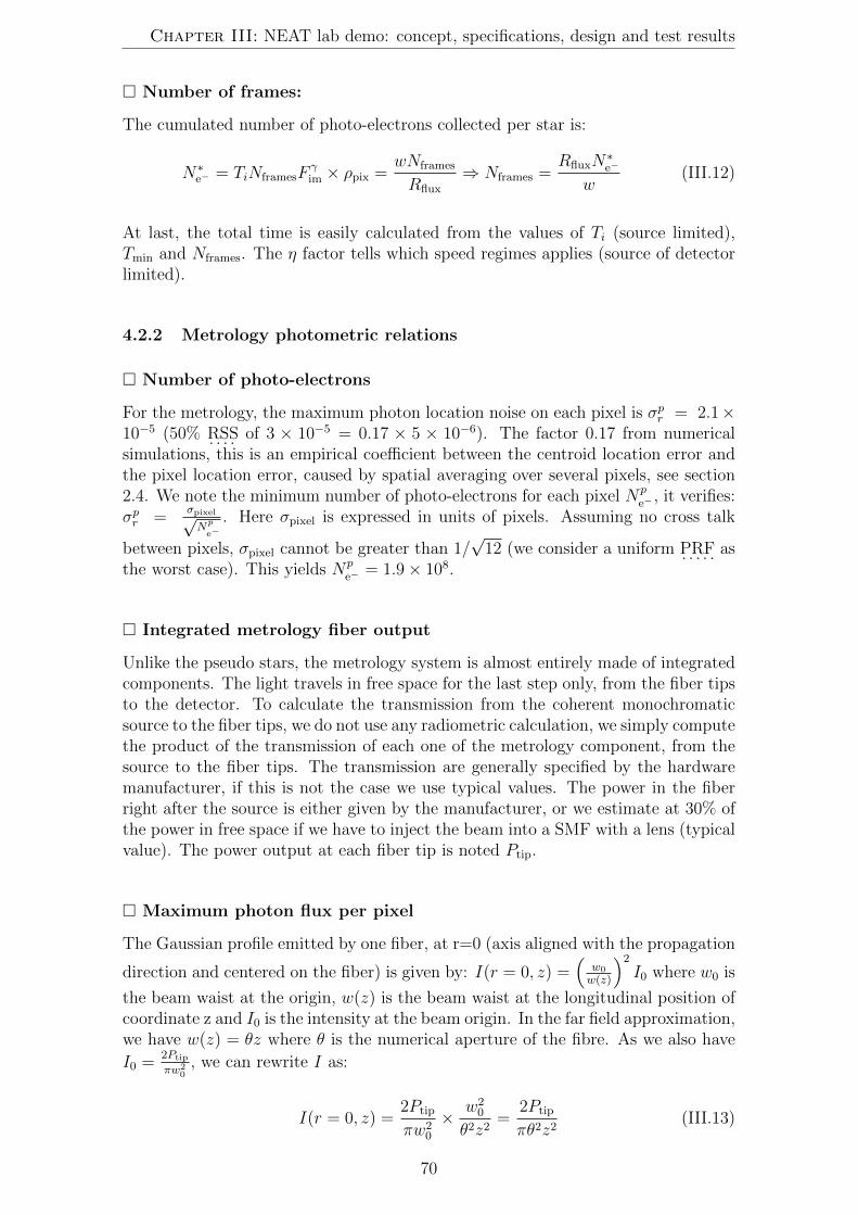
Chapter III: NEAT lab demo: concept, specifications, design and test results
� Number of frames:
The cumulated number of photo-electrons collected per star is:
N∗e− = TiNframesF
γim × ρpix =
wNframes
Rflux
⇒ Nframes =RfluxN
∗e−
w(III.12)
At last, the total time is easily calculated from the values of Ti (source limited),Tmin and Nframes. The η factor tells which speed regimes applies (source of detectorlimited).
4.2.2 Metrology photometric relations
� Number of photo-electrons
For the metrology, the maximum photon location noise on each pixel is σpr = 2.1×
10−5 (50% . . . .RSS of 3 × 10−5 = 0.17 × 5 × 10−6). The factor 0.17 from numericalsimulations, this is an empirical coefficient between the centroid location error andthe pixel location error, caused by spatial averaging over several pixels, see section2.4. We note the minimum number of photo-electrons for each pixel Np
e− , it verifies:σpr =
σpixel√Np
e−. Here σpixel is expressed in units of pixels. Assuming no cross talk
between pixels, σpixel cannot be greater than 1/√12 (we consider a uniform . . . . .PRF as
the worst case). This yields Npe− = 1.9× 10⁸.
� Integrated metrology fiber output
Unlike the pseudo stars, the metrology system is almost entirely made of integratedcomponents. The light travels in free space for the last step only, from the fiber tipsto the detector. To calculate the transmission from the coherent monochromaticsource to the fiber tips, we do not use any radiometric calculation, we simply computethe product of the transmission of each one of the metrology component, from thesource to the fiber tips. The transmission are generally specified by the hardwaremanufacturer, if this is not the case we use typical values. The power in the fiberright after the source is either given by the manufacturer, or we estimate at 30% ofthe power in free space if we have to inject the beam into a SMF with a lens (typicalvalue). The power output at each fiber tip is noted Ptip.
� Maximum photon flux per pixel
The Gaussian profile emitted by one fiber, at r=0 (axis aligned with the propagation
direction and centered on the fiber) is given by: I(r = 0, z) =�
w0
w(z)
�2
I0 where w0 is
the beam waist at the origin, w(z) is the beam waist at the longitudinal position ofcoordinate z and I0 is the intensity at the beam origin. In the far field approximation,we have w(z) = θz where θ is the numerical aperture of the fibre. As we also have
I0 =2Ptip
⇡w20, we can rewrite I as:
I(r = 0, z) =2Ptip
πw20
× w20
θ2z2=
2Ptip
πθ2z2(III.13)
70
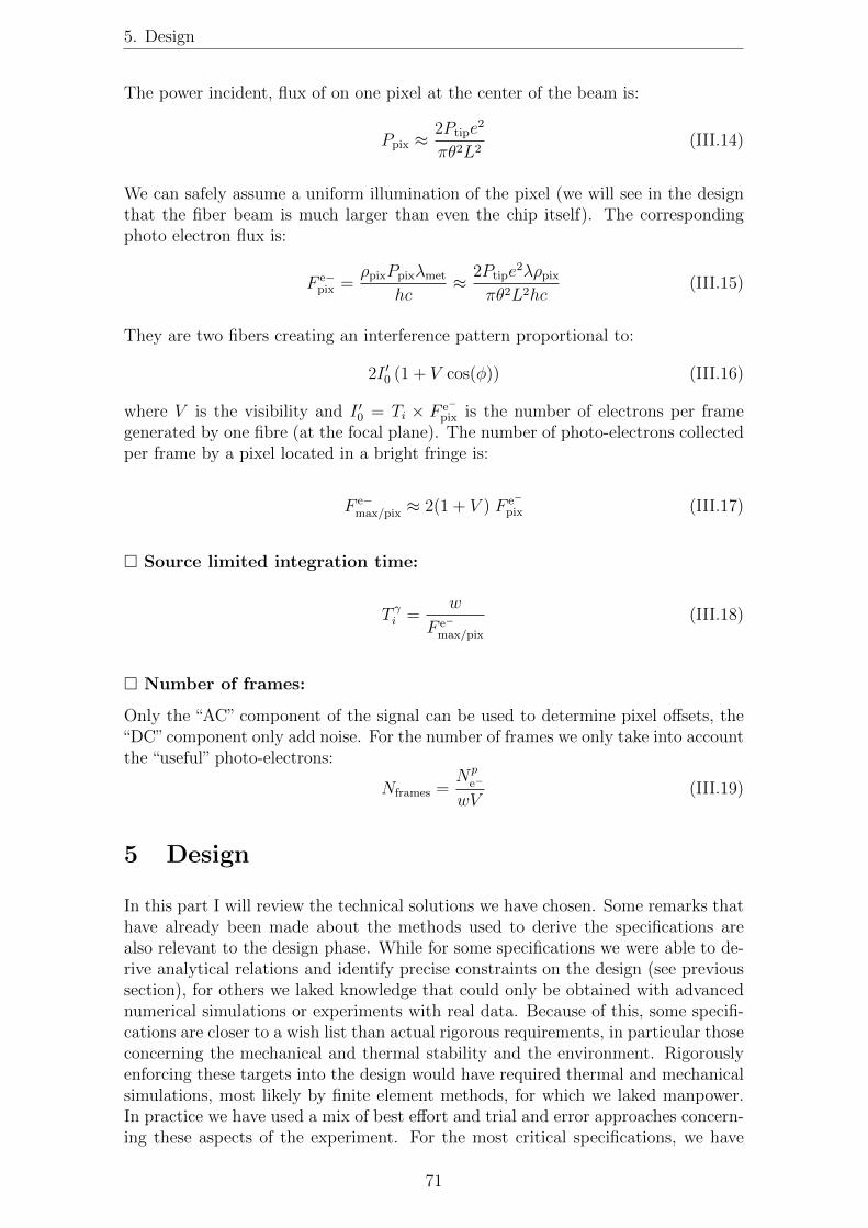
5. Design
The power incident, flux of on one pixel at the center of the beam is:
Ppix ≈2Ptipe
2
πθ2L2(III.14)
We can safely assume a uniform illumination of the pixel (we will see in the designthat the fiber beam is much larger than even the chip itself). The correspondingphoto electron flux is:
F e−pix =
ρpixPpixλmet
hc≈ 2Ptipe
2λρpixπθ2L2hc
(III.15)
They are two fibers creating an interference pattern proportional to:
2I �0 (1 + V cos(φ)) (III.16)
where V is the visibility and I �0 = Ti × F e−pix is the number of electrons per frame
generated by one fibre (at the focal plane). The number of photo-electrons collectedper frame by a pixel located in a bright fringe is:
F e−max/pix ≈ 2(1 + V ) F e−
pix (III.17)
� Source limited integration time:
T γi =
w
F e−max/pix
(III.18)
� Number of frames:
Only the “AC” component of the signal can be used to determine pixel offsets, the“DC”component only add noise. For the number of frames we only take into accountthe “useful” photo-electrons:
Nframes =Np
e−
wV(III.19)
5 Design
In this part I will review the technical solutions we have chosen. Some remarks thathave already been made about the methods used to derive the specifications arealso relevant to the design phase. While for some specifications we were able to de-rive analytical relations and identify precise constraints on the design (see previoussection), for others we laked knowledge that could only be obtained with advancednumerical simulations or experiments with real data. Because of this, some specifi-cations are closer to a wish list than actual rigorous requirements, in particular thoseconcerning the mechanical and thermal stability and the environment. Rigorouslyenforcing these targets into the design would have required thermal and mechanicalsimulations, most likely by finite element methods, for which we laked manpower.In practice we have used a mix of best effort and trial and error approaches concern-ing these aspects of the experiment. For the most critical specifications, we have
71

Chapter III: NEAT lab demo: concept, specifications, design and test results
���
�����������������
��������������������������
�����������
�������
����������������
��������������������
�������������������
����������������������������
��������������������
�����
Figure III.3: Optical bench inside the vacuum chamber.
done extensive measurements to check the performances of particular componentsor sub-parts of the whole experiment (section 6).
The trial an error method has been particularly essential in investigating stray lightissues. We based our initial design mainly on my experience at the JPL, but theconditions for the NEAT-demo were substantially different than for . . . . . . . .VESTA (muchsmaller vacuum chamber). The initial results were not satisfactory and we havethen tested 4 different baffles. An initial memo was written but it is now completelyoutdated (as we have since learned a lot by experimentation) and at the date ofcompletion of this manuscript, we are still actively investigating the issue and wehave no definitive conclusions about how to control the stray light down to therequired level. In this chapter we present the version 4 of the baffle which has beenin use for most of the data that is presented in chapter IV.
5.1 Overview
Now let me give an overview of the design through some schematics: Fig. III.3 is alabeled picture of the interior of the vacuum chamber. Figure III.4 is the product treeof the testbed components. The high level categories are organized by functionality.
Our tool of choice to monitor our progress during the design, assembling and testphases of the experiment was the so-called“snapshot spreadsheet”, shown by Fig. III.5.One can see that at the time of this snapshot (07/05/2013) most of the componentshad been designed and procured, we were mostly checking their normal operationand we had also begun the tests.
5.2 Sub-systems
I will now present the most important sub-systems, by functional groups or one ata time. I will mostly describe them from a functional and qualitative point of view.
72
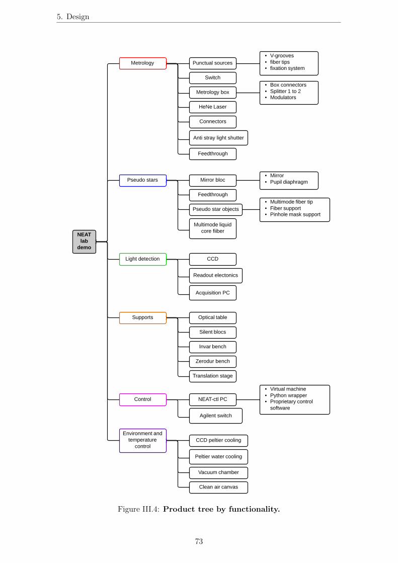
5. Design
Figure III.4: Product tree by functionality.
73
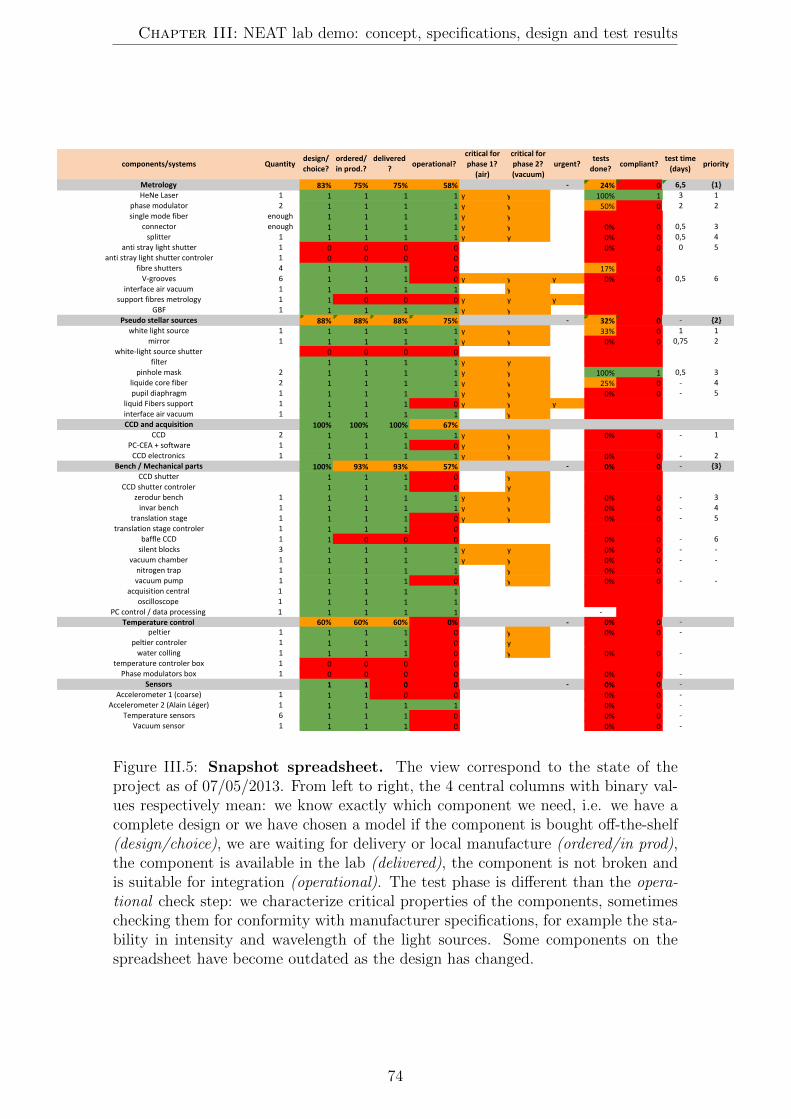
Chapter III: NEAT lab demo: concept, specifications, design and test results
components/systems Quantitydesign/1choice?
ordered/1in1prod.?
delivered? operational?
critical1for1phase11?1(air)
critical1for1phase12?1(vacuum)
urgent?tests1done? compliant?
test1time1(days) priority
Metrology 83% 75% 75% 58% C 24% 0 6,5 {1}HeNe Laser 1 1 1 1 1 y y 100% 1 3 1
phase$modulator 2 1 1 1 1 y y 50% 0 2 2single$mode$fiber enough 1 1 1 1 y y
connector enough 1 1 1 1 y y 0% 0 0,5 3splitter 1 1 1 1 1 y y 0% 0 0,5 4
anti$stray$light$shutter 1 0 0 0 0 0% 0 0 5anti$stray$light$shutter$controler 1 0 0 0 0
fibre$shutters 4 1 1 1 0 17% 0VBgrooves 6 1 1 1 0 y y y 0% 0 0,5 6
interface$air$vacuum 1 1 1 1 1 ysupport$fibres$metrology 1 1 0 0 0 y y y
GBF 1 1 1 1 1 y yPseudo1stellar1sources 88% 88% 88% 75% C 32% 0 B {2}white$light$source 1 1 1 1 1 y y 33% 0 1 1
mirror 1 1 1 1 1 y y 0% 0 0,75 2whiteBlight$source$shutter 0 0 0 0
filter 1 1 1 1 y ypinhole$mask 2 1 1 1 1 y y 100% 1 0,5 3
liquide$core$fiber 2 1 1 1 1 y y 25% 0 B 4pupil$diaphragm 1 1 1 1 1 y y 0% 0 B 5
liquid$Fibers$support 1 1 1 1 0 y y yinterface$air$vacuum 1 1 1 1 1 yCCD1and1acquisition 100% 100% 100% 67%
CCD 2 1 1 1 1 y y 0% 0 B 1PCBCEA$+$software 1 1 1 1 0 y yCCD$electronics 1 1 1 1 1 y y 0% 0 B 2
Bench1/1Mechanical1parts 100% 93% 93% 57% C 0% 0 B {3}CCD$shutter 1 1 1 0 y
CCD$shutter$controler 1 1 1 0 yzerodur$bench 1 1 1 1 1 y y 0% 0 B 3invar$bench 1 1 1 1 1 y y 0% 0 B 4
translation$stage 1 1 1 1 0 y y 0% 0 B 5translation$stage$controler 1 1 1 1 0
baffle$CCD 1 1 0 0 0 0% 0 B 6silent$blocks 3 1 1 1 1 y y 0% 0 B B
vacuum$chamber 1 1 1 1 1 y y 0% 0 B Bnitrogen$trap 1 1 1 1 1 y 0% 0vacuum$pump 1 1 1 1 0 y 0% 0 B B
acquisition$central 1 1 1 1 1oscilloscope 1 1 1 1 1
PC$control$/$data$processing 1 1 1 1 1 BTemperature1control 60% 60% 60% 0% C 0% 0 B
peltier 1 1 1 1 0 y 0% 0 Bpeltier$controler 1 1 1 1 0 ywater$colling 1 1 1 1 0 y 0% 0 B
temperature$controler$box 1 0 0 0 0Phase$modulators$box 1 0 0 0 0 0% 0 B
Sensors 1 1 0 0 C 0% 0 BAccelerometer$1$(coarse) 1 1 1 0 0 0% 0 B
Accelerometer$2$(Alain$Léger) 1 1 1 1 1 0% 0 BTemperature$sensors 6 1 1 1 0 0% 0 B
Vacuum$sensor 1 1 1 1 0 0% 0 B
Figure III.5: Snapshot spreadsheet. The view correspond to the state of theproject as of 07/05/2013. From left to right, the 4 central columns with binary val-ues respectively mean: we know exactly which component we need, i.e. we have acomplete design or we have chosen a model if the component is bought off-the-shelf(design/choice), we are waiting for delivery or local manufacture (ordered/in prod),the component is available in the lab (delivered), the component is not broken andis suitable for integration (operational). The test phase is different than the opera-tional check step: we characterize critical properties of the components, sometimeschecking them for conformity with manufacturer specifications, for example the sta-bility in intensity and wavelength of the light sources. Some components on thespreadsheet have become outdated as the design has changed.
74

5. Design
5.2.1 Light detector and readout electronics
The detector is a crucial part of our experiment. Our final choice was the “CCD39-01” from e2v3. The readout electronics and software have been developed and testedby the . . . . .CEA. The CCD 39-01 is a back illuminated visible CCD, with a frame sizeof 80 by 80 pixels. The physical pixel size is 24 µm (making for a total sensitivearea of 1,92 by 1,92 mm). To enable high frame rate operation (up to 1000 Hz),the chip has 4 amplifiers, i.e. the imaging area is split into 4 square areas which wecall quadrants, of 40 by 40 pixels. Each quadrant has a separate readout channel(different wires and electronics components). This has important implications forthe data analysis.
There is a lot more I could say about the CCD, but I am not going to give moredetails here. Several documents contain relevant information on many aspects: thereadout electronics are extensively documented in the “NEATRO” document pro-vided by the . . . . .CEA (see appendix C). Practical information on how to operate theCCD and how the CCD raw data is converted into fits files is found in the NEATuser manual (appendix E). At last, the section 6.6 summarizes the result of thestandard characterization of the CCD (photon transfer curve, linearity, dark currentand readout noise).
5.2.2 Metrology
��������������
���������������
�����������������
������������������
����������������
�����������������
�����������������
������������������������������
������
������������
�������������������������
����������
��������������
������������������������
��
����
Figure III.6: Schematic of the metrology. The axis are indicated on the figure: Zis aligned with the optical axis, X and Y are aligned with the horizontal and verticaldirections within the focal plane.
The metrology is made of integrated components from the laser to the bases (seeFig. III.6). The source for the metrology is a HeNe laser. Its light is split into twofibers, which are fed into two lithium niobate phase modulators to apply a periodicphase shift between the lanes. This configuration ensures that the phase modulationis applied between the two point sources constituting each base. A switch can beused to select any combination of one or zero fibers on the mirror and most com-binations of two fibers. During the metrology calibration phase, two vertically andhorizontally aligned fibers are selected successively to project respectively horizontal
3e2v is a private British company specialized in semiconductors, radio-frequency applicationsand medical and spatial imaging.
75
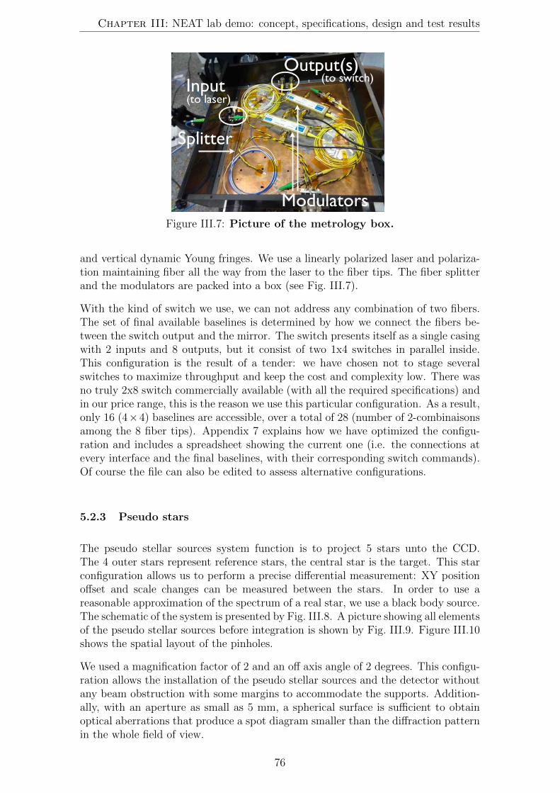
Chapter III: NEAT lab demo: concept, specifications, design and test results
��������������
��������
����������
�����������
����������
Figure III.7: Picture of the metrology box.
and vertical dynamic Young fringes. We use a linearly polarized laser and polariza-tion maintaining fiber all the way from the laser to the fiber tips. The fiber splitterand the modulators are packed into a box (see Fig. III.7).
With the kind of switch we use, we can not address any combination of two fibers.The set of final available baselines is determined by how we connect the fibers be-tween the switch output and the mirror. The switch presents itself as a single casingwith 2 inputs and 8 outputs, but it consist of two 1x4 switches in parallel inside.This configuration is the result of a tender: we have chosen not to stage severalswitches to maximize throughput and keep the cost and complexity low. There wasno truly 2x8 switch commercially available (with all the required specifications) andin our price range, this is the reason we use this particular configuration. As a result,only 16 (4×4) baselines are accessible, over a total of 28 (number of 2-combinaisonsamong the 8 fiber tips). Appendix 7 explains how we have optimized the configu-ration and includes a spreadsheet showing the current one (i.e. the connections atevery interface and the final baselines, with their corresponding switch commands).Of course the file can also be edited to assess alternative configurations.
5.2.3 Pseudo stars
The pseudo stellar sources system function is to project 5 stars unto the CCD.The 4 outer stars represent reference stars, the central star is the target. This starconfiguration allows us to perform a precise differential measurement: XY positionoffset and scale changes can be measured between the stars. In order to use areasonable approximation of the spectrum of a real star, we use a black body source.The schematic of the system is presented by Fig. III.8. A picture showing all elementsof the pseudo stellar sources before integration is shown by Fig. III.9. Figure III.10shows the spatial layout of the pinholes.
We used a magnification factor of 2 and an off axis angle of 2 degrees. This configu-ration allows the installation of the pseudo stellar sources and the detector withoutany beam obstruction with some margins to accommodate the supports. Addition-ally, with an aperture as small as 5 mm, a spherical surface is sufficient to obtainoptical aberrations that produce a spot diagram smaller than the diffraction patternin the whole field of view.
76

5. Design
��������������������
�����
�����������������������
��������������������������
����
�������
���������
���������
���������
���������
Figure III.8: Schematic of the pseudo stars sources.
������������������������
�����������������
�����������
����������������
Figure III.9: Pseudo stars before integration in the vacuum chamber. Thelower metal bench is made of invar (low dilatation material). The translucent yel-lowish glass block is the zerodur bench and has an ultra-low dilatation coefficientlower than 10−7K−1. On the left side of the zerodur bench: the pinhole mask thatis back lighted by the liquid core fiber. On the right side: the mirror block with thediaphragm (in black). One can also see invar rails on the top of the mirror block,their function is to hold the metrology fibres in the V-grooves located between them.
��
�
�
σ�
σ�
��
Figure III.10: Layout of the pinholes on the mask. The holes are arranged likethe dots for the number 5 on a dice, with 4 outer stars forming a square and one(representing the target) in the center. We have introduced small offsets, noted asσx/y on the figure, to prevent the stars from falling into the same fractional positionsrelative to the pixels.
77

Chapter III: NEAT lab demo: concept, specifications, design and test results
5.2.4 Flat field
Note the absence of specifications for this system. We had initially planned to derivethe flat field using single metrology fibers. However, stray light is much harder tocontrol in coherent light than in incoherent light. If we note I0 the direct intensityfrom the light source and I0 the stray light intensity after (multiple) reflection(s), the
perturbation in coherent light is ∝�
I1I0
instead of directly proportional to I1I0
(see
appendix I). We have only added this system in the latter stages of the experiment(after the first light). The design of the system and choice of the components wasderived mostly on an experimental basis.
This system is very simple, is consists of a high power broadband white light LED(400 to 700 nm) connected to a multimode fiber which tip is taped on the mirrorblock and oriented toward the CCD. The light source is located outside the vacuumchamber, a custom made feed-through enables operation in vacuum. For experimen-tal tests and reliability (by redundancy), we have two fibers with respectively 200um and 365 um diameter cores.
The main reason for having a multimode fiber is the luminous flux needed to operatethe CCD in a photon noise limited regime and to accumulate photons at a recent rate,resulting in a total integration time similar to the other systems (a few minutes). Wedid not found suitable commercially available light sources within our price rangethat could deliver enough light to the CCD: with a SMF, a superluminescent type ofsource is required. There are possible issues when using a MMF rather than a SMFbecause of speckles produced by the fiber which we try to evaluate experimentally.
5.2.5 Mechanical supports and lab environment
Figure III.11 is a picture of the lab were you can see the vacuum chamber on theoptical table, inside the canvas. We use a standard optical table with pneumaticsuspension. The picture illustrate the design approach pretty well: we have stackedfour stages of vibration damping in order to stabilize the core of the experiment:in addition to the table suspension, the vacuum chamber is installed on dampingsupports, the invar bench inside the chamber is installed on silent blocks (anotherkind of damping support) and there is a last stage of damping between the invarand the zerodur bench.
The canvas is equipped with a casing at the top (Fig. III.11) that provides filteredand clean air in close proximity of the detector (vacuum chamber, metrology andoptical table). This is important to avoid dust contamination on the detector as allprotections have to be removed during normal operation. This setup is very conve-nient because it allows us to open the chamber at anytime and make modificationsto the configuration inside without worrying about dust contamination. Operationsinvolving the CCD can be done in immediate proximity (on the optical table), with-out having to use a clean room. We still have to be somewhat careful about dustoutside the canvas: it can still be brought inside by direct contact. We use lab coats,shoe covers and mob caps inside the lab. The air conditioning system (located underthe roof, not visible in the picture) also filters the air and works slightly overpressureto avoid air leaks from the outside.
The temperature is stabilized at several stages: first for the whole lab with the air
78
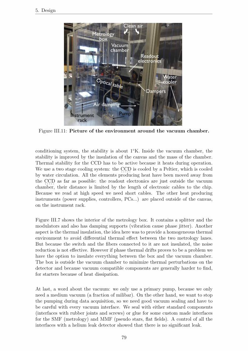
5. Design
��������������
�������������������
���������������
����
�������������
������������
���������
�������������
�����������
�������
Figure III.11: Picture of the environment around the vacuum chamber.
conditioning system, the stability is about 1◦K. Inside the vacuum chamber, thestability is improved by the insulation of the canvas and the mass of the chamber.Thermal stability for the CCD has to be active because it heats during operation.We use a two stage cooling system: the . . . . .CCD is cooled by a Peltier, which is cooledby water circulation. All the elements producing heat have been moved away fromthe . . . . .CCD as far as possible: the readout electronics are just outside the vacuumchamber, their distance is limited by the length of electronic cables to the chip.Because we read at high speed we need short cables. The other heat producinginstruments (power supplies, controllers, PCs...) are placed outside of the canvas,on the instrument rack.
Figure III.7 shows the interior of the metrology box. It contains a splitter and themodulators and also has damping supports (vibration cause phase jitter). Anotheraspect is the thermal insulation, the idea here was to provide a homogeneous thermalenvironment to avoid differential thermal effect between the two metrology lanes.But because the switch and the fibers connected to it are not insulated, the noisereduction is not effective. However if phase thermal drifts proves to be a problem wehave the option to insulate everything between the box and the vacuum chamber.The box is outside the vacuum chamber to minimize thermal perturbations on thedetector and because vacuum compatible components are generally harder to find,for starters because of heat dissipation.
At last, a word about the vacuum: we only use a primary pump, because we onlyneed a medium vacuum (a fraction of milibar). On the other hand, we want to stopthe pumping during data acquisition, so we need good vacuum sealing and have tobe careful with every vacuum interface. We seal with either standard components(interfaces with rubber joints and screws) or glue for some custom made interfacesfor the SMF (metrology) and MMF (pseudo stars, flat fields). A control of all theinterfaces with a helium leak detector showed that there is no significant leak.
79

Chapter III: NEAT lab demo: concept, specifications, design and test results
5.3 Baffles
We have used 4 baffle versions so far:
v1: initial design, aluminum tube with 4 circular vanes. The initial design(v1) was generating 4 visible bright spots (several % above the flat field level,a few pixel width) in white and laser light. The cause was attributed be-yond any doubt to reflections on the baffle edges. Each circular edge eachvane corresponded to one spot, and their positions were linked to the baffleorientation.
v2: a baffle made of paper sheets. This was an attempt to have a better qual-ity baffling by replacing the bright aluminum edges by black paper. In thisversion they were only two vanes, one in the middle of the vacuum chamberand one close to the detector. A paper sheet has a thickness of typically 100µm, about the same as the baffle edges. The bright spots were not visibleanymore but analysis of data quality indicated almost no difference with thepaper baffle and no baffle at all, whereas the first version of the baffle wasalready improving the signal.
v3: same as v1, with improved bevels for the vanes edges. Version 3 is mod-ified from the first one, bevel precision was improved and the width of thevanes edges was measured under microscope to be about 50 µm instead ofthe previous 100 µm. However this improvement was the best we could dowith our local mechanical equipment and still not sufficient. The baffle wasalso suffering from a very tight field of view. Narrow angular tolerances andunreliable translation stage tip tilt resulted in a constant need to check thebaffle orientation.
v4: plastic tube, razor blades, modular design. Version 4 is build from a largertube. The new design addresses the issues with the previous versions. Theoptical apertures are made with razor blades, which provide a very fine opticaledge (<1µm). The design is modular, to allow quick modifications if required:each new vane consist of a holder piece, on which the razor blades are attached.Vanes can be positioned anywhere inside the baffle and be inserted/removedfor modification. For better performance, most interior surfaces are coveredwith a light absorbing material (“metal velvet” acktar�).
Figures III.12, III.13 and III.14 are pictures of the different baffles inside the vacuumchamber. Figure III.15 is the optical schematic for the baffle v4. It shows how thebaffle was designed with respect to avoid critical reflections. Figure III.16 shows theFoVs of baffles v1/v3 and v4 on the mirror block.
5.4 Parameters and components summary
The values we have chosen for the design parameters previously introduced in section2 as notations are presented by Table III.3. The components that have been boughtoff-the-shelf and their references are presented in a table in appendix D. For thecomponents that have been the object of a tender, we refer the reader to the list ofreference documents (appendix C).
80

5. Design
Figure III.12: Baffle v1/3.
Figure III.13: Baffle v2. The picture is taken in front of the chip, just behind theouter vane inside the vacuum chamber. The small square inside the bright area isthe sensitive area of the chip. The black square around the bright area next to thechip is the inner vane.
Figure III.14: Baffle v4.
81

Chapter III: NEAT lab demo: concept, specifications, design and test results
������������������������������������
������
�������������������������
����
���
������������������������������������ �� ��
�����
��
��
��
��
������������
����
�� �
��
�����
Figure III.15: Optical schematic for the baffle v4. No ray can reach the detectorafter only one reflection, expect for on the vane edges, which are very thin (razorblades edges).
�����
����
����������������
������������
��������������
����������������
Figure III.16: Fields of view of baffle v1/v3 and v4.
82
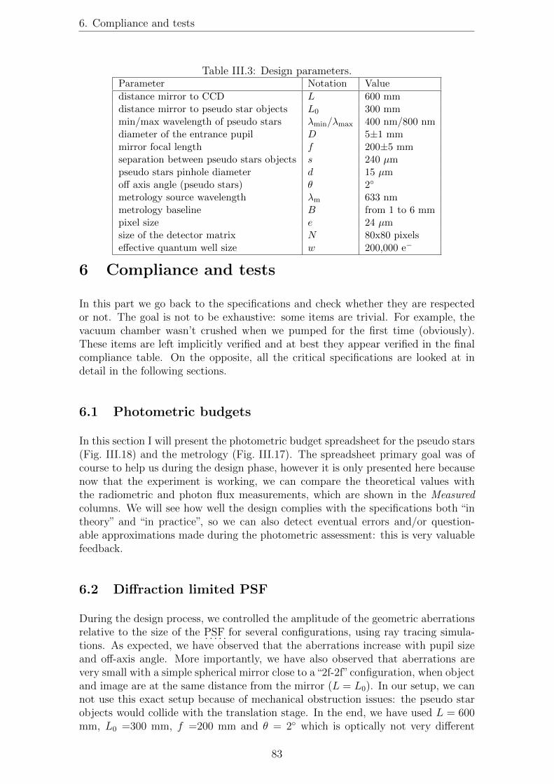
6. Compliance and tests
Table III.3: Design parameters.Parameter Notation Value
distance mirror to CCD L 600 mmdistance mirror to pseudo star objects L0 300 mmmin/max wavelength of pseudo stars λmin/λmax 400 nm/800 nmdiameter of the entrance pupil D 5±1 mmmirror focal length f 200±5 mmseparation between pseudo stars objects s 240 µmpseudo stars pinhole diameter d 15 µmoff axis angle (pseudo stars) ✓ 2◦
metrology source wavelength λm 633 nmmetrology baseline B from 1 to 6 mmpixel size e 24 µmsize of the detector matrix N 80x80 pixelseffective quantum well size w 200,000 e−
6 Compliance and tests
In this part we go back to the specifications and check whether they are respectedor not. The goal is not to be exhaustive: some items are trivial. For example, thevacuum chamber wasn’t crushed when we pumped for the first time (obviously).These items are left implicitly verified and at best they appear verified in the finalcompliance table. On the opposite, all the critical specifications are looked at indetail in the following sections.
6.1 Photometric budgets
In this section I will present the photometric budget spreadsheet for the pseudo stars(Fig. III.18) and the metrology (Fig. III.17). The spreadsheet primary goal was ofcourse to help us during the design phase, however it is only presented here becausenow that the experiment is working, we can compare the theoretical values withthe radiometric and photon flux measurements, which are shown in the Measuredcolumns. We will see how well the design complies with the specifications both “intheory” and “in practice”, so we can also detect eventual errors and/or question-able approximations made during the photometric assessment: this is very valuablefeedback.
6.2 Diffraction limited PSF
During the design process, we controlled the amplitude of the geometric aberrationsrelative to the size of the . . . . .PSF for several configurations, using ray tracing simula-tions. As expected, we have observed that the aberrations increase with pupil sizeand off-axis angle. More importantly, we have also observed that aberrations arevery small with a simple spherical mirror close to a“2f-2f”configuration, when objectand image are at the same distance from the mirror (L = L0). In our setup, we cannot use this exact setup because of mechanical obstruction issues: the pseudo starobjects would collide with the translation stage. In the end, we have used L = 600mm, L0 =300 mm, f =200 mm and θ = 2◦ which is optically not very different
83
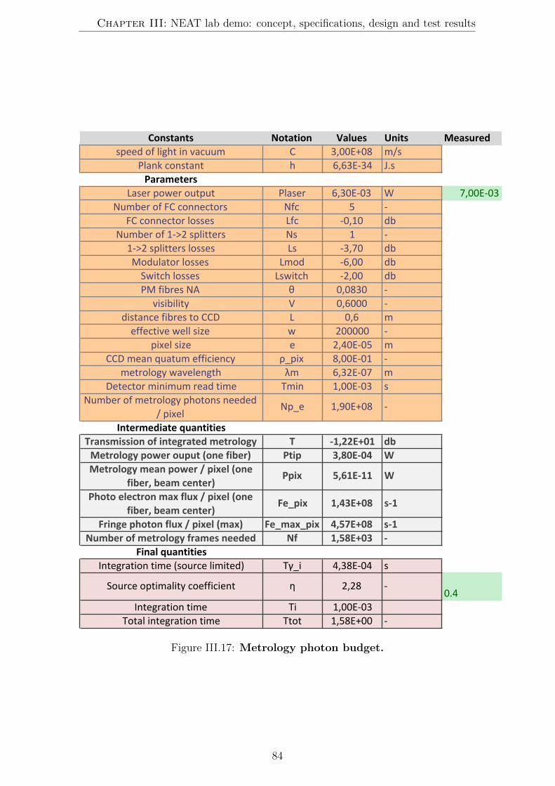
Chapter III: NEAT lab demo: concept, specifications, design and test results
Constants Notation Values Units Measuredspeed%of%light%in%vacuum C 3,00E+08 m/s
Plank%constant h 6,63E>34 J.sParameters
Laser%power%output Plaser 6,30E>03 W 7,00E>03Number%of%FC%connectors Nfc 5 >
FC%connector%losses Lfc >0,10 dbNumber%of%1>>2%splitters Ns 1 >1>>2%splitters%losses Ls >3,70 dbModulator%losses Lmod >6,00 dbSwitch%losses Lswitch >2,00 dbPM%fibres%NA θ 0,0830 >
visibility V 0,6000 >distance%fibres%to%CCD L 0,6 meffective%well%size w 200000 >
pixel%size e 2,40E>05 mCCD%mean%quatum%efficiency ρ_pix 8,00E>01 >
metrology%wavelength λm 6,32E>07 mDetector%minimum%read%time Tmin 1,00E>03 s
Number%of%metrology%photons%needed%/%pixel
Np_e 1,90E+08 >
Intermediate4quantitiesTransmission4of4integrated4metrology T :1,22E+01 dbMetrology4power4ouput4(one4fiber) Ptip 3,80E:04 WMetrology4mean4power4/4pixel4(one4
fiber,4beam4center)Ppix 5,61E:11 W
Photo4electron4max4flux4/4pixel4(one4fiber,4beam4center)
Fe_pix 1,43E+08 s:1
Fringe4photon4flux4/4pixel4(max) Fe_max_pix 4,57E+08 s:1Number4of4metrology4frames4needed Nf 1,58E+03 :
Final4quantitiesIntegration%time%(source%limited) Tγ_i 4,38E>04 s
Source%optimality%coefficient η 2,28 >0.4
Integration%time Ti 1,00E>03Total%integration%time Ttot 1,58E+00 >
Figure III.17: Metrology photon budget.
84

6. Compliance and tests
Constants'and'parameters Notation Values Units MeasuredPhysical'constants
speed%of%light%in%vacuum C 3,00E+08 m/sPlank%constant h 6,63E>34 J.s
Boltzman%constant kb 1,38E>23 m2.kg.s>2.K>1Parameters
effective%wavelength λeff 6,00E>07 mwavelength%width Δλ 4,00E>07 m
entrance%pupil%diameter D 5,00E>03 mdistance%pseudo%stellar%sources%to%CCD L0 3,00E>01 m
distance%mirror%to%CCD L 6,00E>01 moptics%+%fibres%transmission T 7,00E>01 >CCD%quantum%efficiency ρ_pix 8,00E>01 >
effective%quantum%well%size w 2,00E+05 >minimum%read%time Tmin 1,00E>03 s
ratio%central%pixel%flux/centroid%flux Rflux 2,00E>01 >Number%of%photon>electrons%needed Ne> 5,70E+10 >
Parameters'(SMF)SMF%NA NA 0,13 >
White%source%temperature Ts 3,00E+03 KBlack%body%emissivity ε 1,00E+00 >Parameters'(MMF)pinhole%diameter d 1,50E>05 m
Intermediate'quantitiesNumber'of'frames'needed Nf 5,70E+04 G
Black'body'spectral'irradiance SIbb 5,13E+11 W.mG3.srG1Black'body'irradiance Ibb 2,05E+05 W.mG2.srG1
Intermediate'quantities'(SMF)SMF'power'(one'fibre) Psmf 5,17EG08 W 2,00E>07
ρmirror ρSMF 8,18EG03 Gflux'on'CCD'(one'spot) P_im_smf 4,24EG10 W
photon'flux'on'CCD'(one'spot) Fγ_im_smf 1,28E+09 sG1photoGelectron'flux'on'CCD'(one'spot) FeG_im_smf 1,02E+09 sG1
Intermediate'quantities'(MMF)Fiber'irradiance L_fiber 1,44E+05 W.mG2.srG1
pinhole'power'(one'pinhole) Phole 2,54EG05 WIrradiance'on'mirror E_mirror 8,47EG05 W.mG2flux'on'CCD'(one'spot) P_im_mmf 1,66EG09 W 3,30E>09
photon'flux'on'CCD'(one'spot) Fγ_im_mmf 5,02E+09 sG1photoGelectron'flux'on'CCD'(one'spot) FeG_im_mmf 4,01E+09 sG1
Final'quantities'(SMF)%Integration%time%(source%limited) Tγ_i_smf 9,78E>04 sSource%optimality%coefficient η 1,02 >
Integration%time Ti 1,00E>03s
Total%integration%time Ttot 5,70E+01 sFinal'quantities'(MMF)
White%source%exposure%time Tγ_i_mmf 2,49E>04 sSource%optimality%coefficient η 4,01 > 0.8
Integration%time Ti 1,00E>03 s
Total%integration%time Ttot 5,70E+01 s
Figure III.18: Pseudo stars photon budget.
85
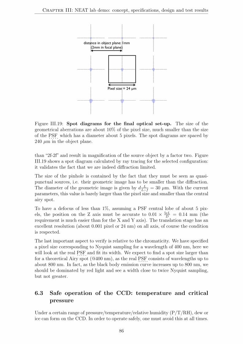
Chapter III: NEAT lab demo: concept, specifications, design and test results
�����������
�
�
������������������
�������������������������������������������������
Figure III.19: Spot diagrams for the final optical set-up. The size of thegeometrical aberrations are about 10% of the pixel size, much smaller than the sizeof the . . . . .PSF which has a diameter about 5 pixels. The spot diagrams are spaced by240 µm in the object plane.
than “2f-2f” and result in magnification of the source object by a factor two. FigureIII.19 shows a spot diagram calculated by ray tracing for the selected configuration:it validates the fact that we are indeed diffraction limited.
The size of the pinhole is contained by the fact that they must be seen as quasi-punctual sources, i.e. their geometric image has to be smaller than the diffraction.The diameter of the geometric image is given by d L
L−f= 30 µm. With the current
parameters, this value is barely larger than the pixel size and smaller than the centralairy spot.
To have a defocus of less than 1%, assuming a PSF central lobe of about 5 pix-els, the position on the Z axis must be accurate to 0.01 × 5eL
D= 0.14 mm (the
requirement is much easier than for the X and Y axis). The translation stage has anexcellent resolution (about 0.001 pixel or 24 nm) on all axis, of course the conditionis respected.
The last important aspect to verify is relative to the chromaticity. We have specifieda pixel size corresponding to Nyquist sampling for a wavelength of 400 nm, here wewill look at the real . . . . .PSF and fit its width. We expect to find a spot size larger thanfor a theoretical Airy spot (@400 nm), as the real . . . . .PSF consists of wavelengths up toabout 800 nm. In fact, as the black body emission curve increases up to 800 nm, weshould be dominated by red light and see a width close to twice Nyquist sampling,but not greater.
6.3 Safe operation of the CCD: temperature and criticalpressure
Under a certain range of pressure/temperature/relative humidity (P/T/RH), dew orice can form on the CCD. In order to operate safely, one must avoid this at all times.
86

6. Compliance and tests
The exact conditions at which dew or ice will from on the CCD in the P/T/RHparameter space are complex to determine, that is why we make simplifications.First, we only consider a limited number of modes of operation obtained by choosinga combination of P/T parameters values: we can work in air (P=1 bar) or vacuum(P<Pcrit) and at ambient (∼ 25◦C), cool (17◦C) or cold (-10◦C) temperature.
The table III.4 gives the possible modes of operation among all 6 possibilities definedabove.
Table III.4: Table of possible P/T operation modes for the CCDT = 25◦C T = 17◦C T = −10◦C
P=1 bar � � ×P < Pcrit � � �
In practice, we will retain 4 modes:
1. In air, ambient temperature. Although far from ideal, it is possible to operatein air with no cooling at all. Operating the CCD will heat it slightly, to around25◦C. In this mode, the equilibrium temperature of the CCD will be high andunstable, dark current and read noise may be high and variable. This is usefulif one want to have images very quickly.
2. In air, cool temperature (TCCD = 17◦C)
3. In vacuum, cool temperature (TCCD = 17◦C)
4. In vacuum, cold temperature (TCCD = −10◦C). This setup is expected to givethe best performances: the CCD is specified for operation at this temperature.
These 4 possible modes allow us to explore both the effect of a large change of TCCD
or P on the experiment, and gives us a way to either have the best data quality,or to have data more quickly. We have the choice to go into vacuum or not: thisis important constraint to keep in mind in case one want to do experiments whichinvolve manual handling inside the vacuum chamber, such as stray light tests. In thiscase, pumping and pressurization are needed between each different configuration.If one wants to operate at -10◦C, vacuum is required and the same thing applies.
Now we have to check the requirement specified for the vacuum chamber and thepump: a pressure threshold Pcrit can be reached and maintained without pumpingfor at least a few hours. The critical pressure threshold Pcrit is such that is allows thedetector to safely operate at a temperature TCCD, corresponding to a dark current< dcrit (see detector specifications).
Pumping tests with the vacuum chamber showed that pressures of less than 0.1mbar can be reached and maintained for about a day. Cooling tests showed thatTCCD = −10◦C can be reached easily and quickly by using a water temperatureof 8◦C. From the PT phase diagram of water, we know that at -10◦C, water onlybecomes solid for pressures higher than 2 mbars. To have some margins, we havedefined the critical pressure P = 0.5 mbar. This is the point at which the circuitbreaker will automatically shut down the cooling systems. We also define anothercritical pressure threshold (Plow) that needs to be reached before the circuit breakercan be armed, lower than the first threshold to form an hysteresis cycle. We havefixed Plow = 0.2 mbar to allow for some pressure increase in all case.
87

Chapter III: NEAT lab demo: concept, specifications, design and test results
0 5 10 15 20−2
0
2
4x 10
−4 X position
rela
tive
X p
ositio
n (
pix
el)
batch number
(a) Relative X positions (pixel), versustime.
0 5 10 15 20−2
−1
0
1
2x 10
−3 Y position
rela
tive
Y p
ositio
n (
pix
el)
batch number
(b) Relative Y positions (pixel), versustime.
Figure III.20: The position of each centroid is shown relative to its position att=0. The horizontal units are batches of frames, i.e. packets of averaged frames foreach position measurement. Batches consists of 4000 frames equivalent to 5 seconds(framerate is 800 Hz), so the total duration of the stability measurement is 100 sec.Horizontal motion (X axis) shows an oscillating pattern, whereas vertical motion ismore linear and could be caused by thermal effects.
We have solved the case for safe operation mode n◦4 (T = −10◦C and P < 0.5 mbar).What about the other 3? The PT phase diagram of water also tells us that operationin mode n◦3 is even safer. This is also true for any temperature above -10◦C, as longas (P < 0.5 mbar). For mode number 2, we are at atmospheric pressure, the safelimit is given by the dew point, with depends on the RH. In temperate climates, itis very rare to have dew points above 15◦C, so we have conservatively set the limitat 17◦C. Of course, operation at (moderately) higher temperatures is also safe.
6.4 Mechanical and thermal stability
The mechanical stability of the testbed was measured by recording the motion ofthe pseudo stars relative to the CCD versus time. We are interested in timescales oftypically one minute, this is the time needed to for photon noise to reach 5 × 10⁻⁶
pixel with the pseudo stars. Figures III.20(a) and III.20(b) show the position ofeach one of the 5 centroids, respectively on the horizontal and vertical directions.The amplitudes are less than 3× 10−3 pixel PtV, below the 0.01 pixel specified.
The thermal stability was measured in two different sets of conditions: at 17◦C inair, or at -10◦C in vacuum, while the CCD is recording data (to be in the mostrealistic conditions). There are several thermal sensors in the chamber, here we usethe one closest to the CCD. The probe is fixed on the copper block that makes athermal mass with the CCD chip (the two are connected with thermal paste). FigureIII.21(a) and III.21(b) show the temperature versus time at respectively 17◦C and-10◦C. The thermal stabilities are respectively 2.5 × 10⁻³ and 2.6 × 10⁻³, both arebelow the specification (0.1◦C).
88
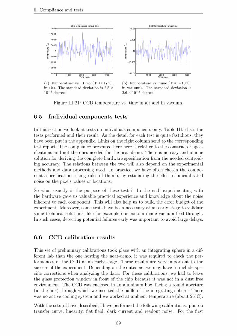
6. Compliance and tests
0 1000 2000 3000 400016.992
16.994
16.996
16.998
17
17.002
17.004
17.006
17.008CCD temperature versus time
Tem
pera
ture
(°C
)
Time (sec)
(a) Temperature vs. time (T ≈ 17◦C,in air). The standard deviation is 2.5 ×10⁻³ degree.
0 1000 2000 3000 4000−10.01
−10.005
−10
−9.995
−9.99CCD temperature versus time
Tem
pera
ture
(°C
)
Time (sec)
(b) Temperature vs. time (T ≈ −10◦C,in vacuum). The standard deviation is2.6× 10−3 degree.
Figure III.21: CCD temperature vs. time in air and in vacuum.
6.5 Individual components tests
In this section we look at tests on individuals components only. Table III.5 lists thetests performed and their result. As the detail for each test is quite fastidious, theyhave been put in the appendix. Links on the right column send to the correspondingtest report. The compliance presented here here is relative to the constructor spec-ifications and not the ones needed for the neat-demo. There is no easy and uniquesolution for deriving the complete hardware specification from the needed centroid-ing accuracy. The relations between the two will also depend on the experimentalmethods and data processing used. In practice, we have often chosen the compo-nents specifications using rules of thumb, by estimating the effect of uncalibratednoise on the pixels values or locations.
So what exactly is the purpose of these tests? In the end, experimenting withthe hardware gave us valuable practical experience and knowledge about the noiseinherent to each component. This will also help us to build the error budget of theexperiment. Moreover, some tests have been necessary at an early stage to validatesome technical solutions, like for example our custom made vacuum feed-through.In such cases, detecting potential failures early was important to avoid large delays.
6.6 CCD calibration results
This set of preliminary calibrations took place with an integrating sphere in a dif-ferent lab than the one hosting the neat-demo, it was required to check the per-formances of the CCD at an early stage. These results are very important to thesuccess of the experiment. Depending on the outcome, we may have to include spe-cific corrections when analyzing the data. For these calibrations, we had to leavethe glass protection window in front of the chip because it was not in a dust freeenvironment. The CCD was enclosed in an aluminum box, facing a round aperture(in the box) through which we inserted the baffle of the integrating sphere. Therewas no active cooling system and we worked at ambient temperature (about 25◦C).
With the setup I have described, I have performed the following calibrations: photontransfer curve, linearity, flat field, dark current and readout noise. For the first
89

Chapter III: NEAT lab demo: concept, specifications, design and test results
Table III.5: List of tests of individual components.
Componenttested
Test name / Test ID Compl. Specification / Result Link toTable
Laser HeNe1.5mW
Intensity stability / 1 Yes 1× 10⁻³ / 9.5× 10⁻⁵ TABLE
Laser HeNe1.5mW
Polarization linearity /2
Yes 1000:1 / 5400:1 TABLE
Laser HeNe1.5mW
Polarisation angularstability / 3
NS NS / [0.038; 0.24]◦ TABLE
Laser HeNe1.5mW
Stabilization time / 4 No 30 min / 60-70 min TABLE
Laser HeNe1.5mW
Wavelength stability /5
No 2× 10⁻⁹ / 1.5× 10⁻⁸ TABLE
Liquid corefiber
Plug interface leakage /6
Yes Air tight / Air tight TABLE
Liquid corefiber
Degassing / 7 Yes Air tight / Air tight TABLE
Integrated-optical phasemodulators
Attenuation / 8 Yes 6 db / 5.94 db TABLE
Halogenlight sources
White light source sta-bility / 9
NS NS / 8% TABLE
two calibrations I used a conventional dark subtraction (subtraction of an averageddark to each frame), prior to the processing. Some results are just indicative andcannot be directly applied for the neat-demo data analysis, in particular flat fields(because of the window), dark current and read noise (because of the temperature).Fortunately, they can be repeated in the neat-demo lab inside the vacuum chamberif necessary, albeit the flat will have to be without the integrating sphere.
Dark current and readout noise have been tested again inside the vacuum chamberat lower temperatures and are presented in this section as well. Numerous otherflat fields have been measured inside the chamber, but they are much more closelyrelated to the data analysis and are presented in the chapter V.
� Notations
To briefly explain the principle of each calibration, I will use the following notations:
• Signal (in counts) on the CCD: S = kN0 + Soffset
• Temporal variance of the signal: σ2S = k2s20 + k2s2r
with:
• k: gain (ADU/e-)
• N0: number of photo-electrons generated
• Soffset: electronic offset (in ADU)
• sr: readout noise (in e-)
• s0: photo-electron shot noise (in e-)
Additionally, I note the exposure time for one frame: Texp (i.e. the inverse of theframe rate). The colors on the plots (green, blue, red, black) correspond to onequadrant each.
90

6. Compliance and tests
6.6.1 Photon transfer curve (integrating sphere)
� Theory
The photon transfer curve is a plot of the temporal variance of the pixels versusthe dark-subtracted signal, for different flat fields with different exposure times ordifferent exposure intensities.
As we have s20 = N0 =S−Soffset
k, we can write:
σ2S = k2s2r + k2(S − Soffset)
So plotting σ2S versus S − Soffset will allow us to recover:
• k2: the slope of the linear fit
• k2s2r: the value for N0 = 0
Strictly speaking, one cannot really obtain S − Soffset, because the dark currentrealization is different in the dark data than in the flat field data. These relationsare only valid when the residual noise from dark subtraction (i.e. dark noise) isnegligible compared to the photon noise. In practice we have 4 photon transfercurves, one for each quadrant of the CCD, because the electronics are different foreach one. We define for each quadrant a 10×10 pixel window in which we do thecalibration for every pixel and average the results afterwards. Spatial averaging inthis manner increases the precision of the calibration. The great advantage of thismethod is that it does not require knowledge of the absolute exposure luminance orexposure time.
If we use different exposure intensities (with a constant frame rate), the point atwhich the linear fit crosses the vertical axis is not only the readout noise, but the sumof the dark and readout noises. In this case the extrapolated value correspond to anull intensity but not to a null exposure time. Whether we vary the frame rate orthe intensity, the measure of the readout noise is intrinsically unreliable, because itis extrapolated from data which is dominated by photon noise. To properly measuredark and readout noise we use other sets of experiments, where we do not exposethe detector to light.
� Method and results
We have taken two sets of measurements (Fig. III.22 and Fig. III.23). The lines arelinear least square fits (one fit per quadrant).
Set 1 (11/06/2013): this first curve was performed by changing the luminance (theintegrating sphere is equipped with a shutter that can be open between 0 and 100%).The frequency was low enough (100 Hz) so that the A/D converter could reach closeto 65000 counts with the shutter fully open. The gain is close to 10 for all quadrants(fit between 0 and 27000 counts). The noise reaches its maximum value for 27000counts. This is because we are reaching saturation (the size of the quantum wells isabout 30000 counts). We notice 2 outliers in green around a “signal - dark” of 5000counts.
Set 2 (14/06/2013): this second curve was performed in the same way, but thistime the frequency was increased to 200 Hz. The goal was to obtain the maximum
91
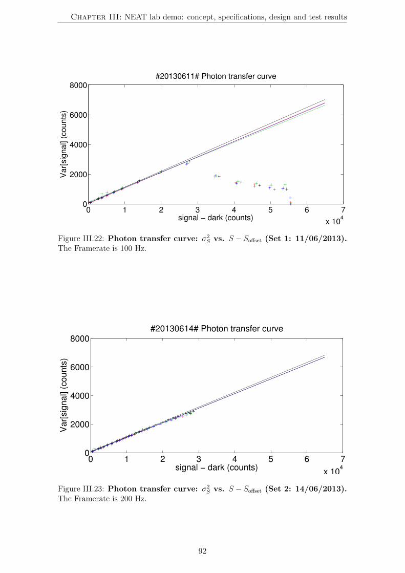
Chapter III: NEAT lab demo: concept, specifications, design and test results
0 1 2 3 4 5 6 7
x 104
0
2000
4000
6000
8000#20130611# Photon transfer curve
signal − dark (counts)
Va
r[sig
na
l] (
co
un
ts)
Figure III.22: Photon transfer curve: σ2S vs. S − Soffset (Set 1: 11/06/2013).
The Framerate is 100 Hz.
0 1 2 3 4 5 6 7
x 104
0
2000
4000
6000
8000#20130614# Photon transfer curve
signal − dark (counts)
Var[
sig
nal] (
counts
)
Figure III.23: Photon transfer curve: σ2S vs. S − Soffset (Set 2: 14/06/2013).
The Framerate is 200 Hz.
92

6. Compliance and tests
number of data points between 0 and 30000 counts (saturation level), to obtain abetter fit.
For the second set, the fit was done between 0 and 24000 counts because for highervalues there is visible deviation from linearity. The values found for k, for quadrant1 to 4 are respectively: 0.10142, 0.10099, 0.10146, 0.10344. All values are close to0.1 ADU/pixel. If we express the gain in units of e-/ADU, we obtain a value ofabout 10. In the subsequent discussions we will use a factor of 10 to convert fromADU to e-.
The values for a null illumination are respectively: 45, 71, 44, 76. This yield noisevalues (noted s) of:
7ADU < ks < 9ADU
⇒ 70e− < s < 90e−
These values of noise are the sum of the read noise and the dark current noise (at200 Hz).
6.6.2 Linearity (integrating sphere)
� Theory
To test the linearity we plot S − Soffset versus the exposure time. We keep theluminance constant and we change the framerate (thus changing also the exposuretime). The clock of the CCD is very accurate and we know the exposure time witha precision of a few nanoseconds.
S = kN0 + Soffset = kTexpF + Soffset, where F is the flux of photons/sec/pixel.
We are not interested in knowing F but in looking at the deviation of the pointsfrom a perfect line (S−Soffset vs. Texp). We however need to have a very stable flux:we need it more stable than the non-linearity we aim to measure. After plotting thefit, we plot the fit residuals and then the relative residuals. The maximum of theselast residuals gives the difference to perfect linearity.
� Method and results
First we have checked the . . . . .RSD of the flux emitted by the lamp used during thecalibration. A tool was available to export recorded flux data, we have determinedthat on the timescale of 1 minute needed for the calibration, the flux . . . . .RSD wassmaller than 10−4. For the linearity test itself, the position of the shutter was set tohave about 27000 counts (close to saturation) for the largest exposure time used (5ms). We have used frames rates ranging from 200 Hz to 977 Hz.
Figure III.24 is a plot of the dark subtracted signal versus the exposure time. FigureIII.25 is a plot of (absolute) residuals of Fig. III.24 in counts. Figure III.26 is a plotof (relative) residuals of Fig. III.24 in counts.
The maximum is at 0.2% (for an exposure time of 3.3 ms). All the values are alsoabove -0.1%. In conclusion for this test, no quadrant deviate of more than 0.2%from the linear response, when averaging a zone of 10 by 10 pixels.
93

Chapter III: NEAT lab demo: concept, specifications, design and test results
0 0.002 0.004 0.006 0.008 0.010
2
4
6x 10
4 #20130614# Linearity curve
exposure time (s)
sig
na
l −
da
rk (
co
un
ts)
Figure III.24: Linearity curve: S − Soffset vs. Texp.
1 1.5 2 2.5 3 3.5 4 4.5 5
x 10−3
−40
−20
0
20
40#20130614# Linearity curve, residuals
exposure time (s)
linear
fit re
sid
uals
(counts
)
Figure III.25: Linearity test: absolute residuals (counts).
1 1.5 2 2.5 3 3.5 4 4.5 5
x 10−3
−2
−1
0
1
2x 10
−3 #20130614# Linearity curve, relative residuals
exposure time (s)
rela
tive lin
ear
fit re
sid
uals
(counts
)
Figure III.26: Linearity test: relative residuals (counts).
94

6. Compliance and tests
6.6.3 Flat field (integrating sphere)
#20130614# Differential flatrelative photon noise: 0.0082449
20 40 60
20
40
60
0.98
0.99
1
1.01
1.02
1.03
(a) Differential flat field. The pho-ton noise indicated in the figure title is atheoretical value calculated from the av-erages of each dark-subtracted flat usedin the process. It corresponds roughlyto the granularity (within quadrants) wesee in the image.
#20130614# Differential flat corrected flatphoton noise: 75.4462 counts
20 40 60
20
40
60
1.396
1.398
1.4
1.402
1.404
x 104
(b) Differential flat corrected flatfield. The photon noise is a theoreti-cal value. It corresponds roughly to thesmall scale granularity of the image.
Figure III.27: Flat fields.
Here we test the pixel response non uniformity (PRNU), by temporally averagingthe pixel counts. Figure III.27(a) is a differential flat: it is the difference between aflat with high flux (near saturation) and a flat with low flux (near dark). We usethis differential method to have the most linear response possible. The variationsare caused by differences in sensitivity between the pixels and photon noise, butwe integrate for a time long enough to ensure that the latter is smaller than thesensitivity differences.
There are very clear variations between each quadrant, with systematic biases nearthe edges (more sensitive pixels) and smaller biases forming spots inside the quad-rants. However the interpretation is ambiguous: the variations can also be causedby the protection window. FigureIII.27(b) is a flat with a medium flux divided bythe previous flat. The result has a very smooth profile, the residual inhomogeneitiesseen here are caused by photon shot noise and variations of non linearity betweenthe pixels.
There are no significant changes in non linearity between the pixels in the center ofthe chip. This shows that the linearity results are valid over all the central area.There seem to be a small gradient between the middle and the edges, of the sameorder than the non linearity of individual pixels: 0.3% (from 1.398 to 1.402 × 10⁴
counts). Given the small magnitude of the effect, it is hard to tell if this is areal change in non linearity or it has a different cause. Overall, the linearity can beconsidered to be very good. Very close to the edges we see larger biases, in particularthe top and bottom rows, but they can be easily cropped without losing much space.
6.6.4 Dark current and readout noise
� Theory
95

Chapter III: NEAT lab demo: concept, specifications, design and test results
In absence of light, the residual signal (in counts) on the CCD is caused by thermalelectrons, plus the offset: S = kFdarkTexp + Soffset, where Fdark is the rate of ther-mally generated electrons (so called dark current), expressed in e-/pixel/s. Withoutphotons, the temporal variance of the signal is: σ2
S = k2s2r + k2Fdarkt.
To obtain the dark current we plot S as a function of Texp. The slope of the fit givesFdark. To obtain the readout noise we plot σ2
S as a function of Texp. The readoutnoise is at the intersection of the linear fit with the vertical axis.
� Method and results
Both measurements are obtained from the same set of measurements, which are darkfields at a range of different frame rates. The dark current and the readout noise canbe very sensitive to temperature, so we should not take the results obtained withthe integrating sphere setup at face value. These first results (set 1: 14/06/2013)are obtained at ambient temperature, plus a few degrees because the CCD heatsup during operation to around 25◦C. The cooling is only passive, through air andthe aluminum box enclosure. The two other sets (set 2: 30/09/2014 and set 3:02/10/2014) have been obtained inside the vacuum chamber with active cooling atrespective temperatures of 17◦C and -10◦C (stable to 2.5 mK). For each data set, Ishow the plots from which I derive the dark current and readout noise estimations.
In all sets the data was obtained by using different frame rates ranging from 50 Hzto 977 Hz with the lamp of the integrating sphere or any other light source shut-off(our setups prevent any visible light from arriving to the detector when the lampsare off). For the dark current estimation (Fig. III.28 III.29 and III.30), pixel countvalues are averaged temporally and spatially over a 10 × 10 pixel zone at the centerof each quadrant. For the readout noise (Fig. III.31, III.32 and III.33), we use thesame data and compute the temporal standard deviation (for each exposure time).The noise values are also averaged spatially over zones of 10 × 10 pixels. On theplots the readout noises are given (for each quadrant) by the intersection of the fitand the vertical axis (null exposure time).
In the CCD39 product sheet, the dark currents are specified for Vss=9V (in ourexperiment we use Vss=8V4). At 25,17 and -10◦C, their respective values are specifiedat 70000, 40000 and 3000 e-/pixel/s. According to the plots, the dark current isabout 90000 e-/pixel/s at 25◦C, 30000 e-/pixel/s at 17◦C and negligible at -10◦C(the value is too small to be measured). From the data, we confirm that:
• At 25◦C / 200 Hz, the dark variance is about 450 e- or 45 counts, which is toosmall to affect the precision of the photon transfer calibration (Y values rangefrom 0 to 3000 counts).
• At 17◦C, the dark noise for the lower frame rate we use (100 Hz), is ≈√300 ≈
17e−, smaller than the measured read noise (50 e- or more).
The measured readout noise is typically about 5 counts / 50 e-, significantly higherthan the initial specification (1 count / 10 e-). Generally speaking, a readout noiseof 50 e- should not have any tangible consequence for our experiment: for a fluxas low as 10000 e-/frame, the photon noise will be 100 e-, already larger than the
4Vss is one of the critical CCD control voltages, defined by the readout electronics design.
96
6. Compliance and tests
readout noise. For all kinds of measurement (flat, metrology, pseudo stars) we havebeen able to fill a significant fraction of the quantum wells, typically 1/3 (i.e. 100000e-) or more.
On the other hand we have observed something that is potentially problematic: theCCD exhibits some worrying instabilities with respect to its readout noise. Some-times the readout noise within one quadrant increases to a much higher level, whichcan be as high as 30 counts. Figure III.33 illustrates this: one of the quadrants hasa noise of about 20 counts (at all frequencies), whereas all the others are at about5. The data was taken for a CCD temperature of -10◦C (in vacuum), after 8 hoursof continuous acquisition to allow for the temperature of the electronic equipmentto be very stable. On Fig. III.32, the readout noise levels are high for some couplesof quadrants / framerates.
The CCD control interface come with a handy “quick look” utility, which displaytwo images in real time, one is the number of counts and the other one shows thenoise calculated over 25 frames. The instabilities have thus been observed in realtime, and of course the level of noise derived in the calibration presented above iscompatible with the quick look indicator (so we have no reason not to trust it!).From what we have seen during the experiments, we can say the following about theinstabilities:
• They appears quite frequently, they make up for typically 50% of the time theCCD is operating
• They appears/disappears slowly, ramping up/down for several minutes
• Once stabilized, the readout noise can also stay constant for hours
• Rebooting the CCD and its electronics most often does not change the readoutnoise levels.
• The readout noise level in the anomalous quadrant often stabilizes somewherebetween 10 and 20 counts, but it can be as high as 30 counts.
• It does not always affect the same quadrant.
• It has been observed on all chips (we have several science qualified copies ofthe CCD chip, the chip in the chamber has been swapped several times).
Unfortunately we have been unable to pin down a convincing cause for the insta-bilities. A level of noise of 30 counts is much more consequent: it is comparableto the photon noise for a high flux: about 1/3 of the full quantum well. One canspeculate about the nature of this additional noise: if it is not white Gaussian noise,it could compromise the experiment success. We will remain alert of this aspectwhen analyzing the data.
6.7 Compliance table
I will conclude this chapter by some remarks about the non compliance/complianceof some parameters and their potential impact on the experiment.
Dust free environment Dust control worked quite well overall, we however hadone instance were some dust was deposited unto the CCD. Large dust particlesbecame visible on the CCD (they induced large effective QE drops, of several
97

Chapter III: NEAT lab demo: concept, specifications, design and test results
0 0.005 0.01 0.015 0.029600
9700
9800
9900
10000
10100#20130614# Dark current VS Texp
exposure time (s)
da
rk c
urr
en
t (c
ou
nts
)
Figure III.28: Dark current vs. exposure time (set 1: 14/06/2013, T ≈25◦C). The slope is the dark current per pixel.
0 0.005 0.01 0.015 0.029500
9600
9700
9800#20140930# Dark current VS Texp
exposure time (s)
da
rk c
urr
en
t (c
ou
nts
)
Figure III.29: Dark current vs. exposure time (set 2: 30/09/2014, T =17◦C). The slope is the dark current per pixel.
0 0.005 0.01 0.015 0.029600
9700
9800
9900#20141002# Dark current VS Texp
exposure time (s)
da
rk c
urr
en
t (c
ou
nts
)
Figure III.30: Dark current vs. exposure time (set 3: 02/10/2014, T =−10◦C). The slope is the dark current per pixel.
98
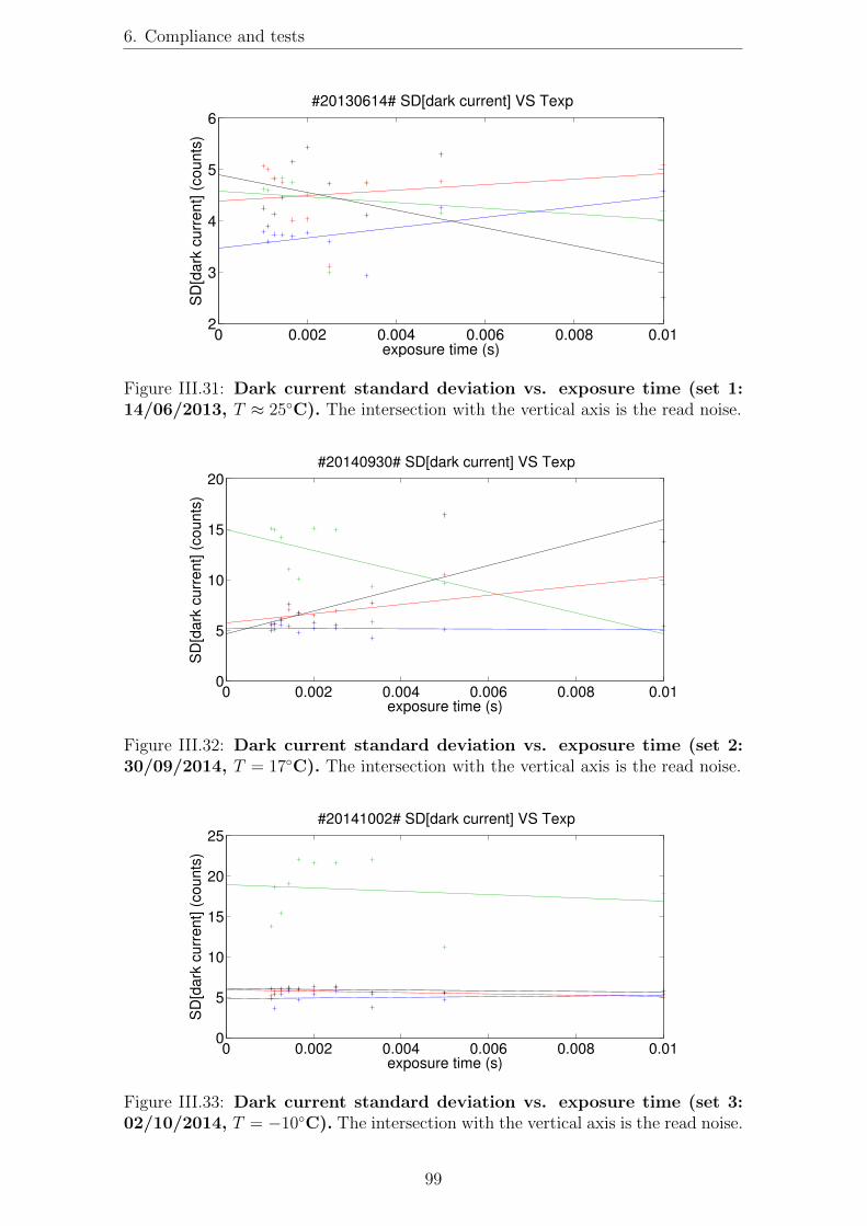
6. Compliance and tests
0 0.002 0.004 0.006 0.008 0.012
3
4
5
6#20130614# SD[dark current] VS Texp
exposure time (s)
SD
[da
rk c
urr
en
t] (
co
un
ts)
Figure III.31: Dark current standard deviation vs. exposure time (set 1:14/06/2013, T ≈ 25◦C). The intersection with the vertical axis is the read noise.
0 0.002 0.004 0.006 0.008 0.010
5
10
15
20#20140930# SD[dark current] VS Texp
exposure time (s)
SD
[da
rk c
urr
en
t] (
co
un
ts)
Figure III.32: Dark current standard deviation vs. exposure time (set 2:30/09/2014, T = 17◦C). The intersection with the vertical axis is the read noise.
0 0.002 0.004 0.006 0.008 0.010
5
10
15
20
25#20141002# SD[dark current] VS Texp
exposure time (s)
SD
[da
rk c
urr
en
t] (
co
un
ts)
Figure III.33: Dark current standard deviation vs. exposure time (set 3:02/10/2014, T = −10◦C). The intersection with the vertical axis is the read noise.
99

Chapter III: NEAT lab demo: concept, specifications, design and test results
Table III.6: Notations.
# Criterion Specification Measured/Design Comp.?
Detector and environment
1 Stability of pseudo star images 1× 10⁻²e 3× 10⁻³e Yes
2 Translation stage resolution X/Y 0.1e 1× 10⁻³e Yes
3 Translation stage resolution Z 1.4× 10⁻⁴ m 2.4× 10⁻⁸ m Yes
4 X/Y rotationManualcoarse rotation
Motorizedrotation
Yes
5 Critical pressureP < 0.5 mbarfor several hours
- Yes
6 Dust free environment Best effort - -
7 Detector temperature stability 0.1 K over 1 h2.6× 10−3Kover 1 h
Yes
8 Read noise 10 e- 40 to 300 e- No
9Pseudo stars andmetrology integration times
less than afew minutes
see phot.budgets (6.1)
Yes
10 Dark noise 10 e- @ Tcrit20 e- @ 17◦C5 e- @ -10◦C
Yes
Pseudo stars
11 Geometric aberrations Diffraction limited see section 6.2 Yes
12 Spatial sampling Nyquist sampling see section 4.1 Yes
Metrology
13Number of baselinesfor each direction
3+ metrologybaselines
4 metrologybaselines
Yes
14 Fringe visibility V > 0.5 V � 0.5 Yes
15 Phase modulation > 2⇡ > 6⇡ Yes
% over one or a few pixels). We were able to remove most of them by blowingnitrogen unto the CCD, but a few small particles stayed on the chip, producingQE drops of about 1%. The CCD was not removed from the vacuum chamberduring this incident and we were doing the usual kinds of modifications insidethe chamber (baffle changes, stray light tests). Dust could have been broughtby contact inside the chamber, but we do not know the exact cause, i.e. howit got unto the CCD.
Readout noise Readout issues have been extensively described in section 6.6.4. Iwill only give a brief summary here. The readout noise was specified at 10 e-,but the measurements showed a “baseline” level of about 40-50 e-. Howeverthis later readout noise level is still small compared to the photon noise in theconditions of our experiment. The instability of the readout noise level is muchmore concerning, it can ramp up to about 300 e-. If this noise is not strictlywhite and Gaussian this could have a serious impact on the experiment.
Dark noise The dark noise level is only slightly higher than the specification, evenat 17◦C (20 e- for 10 e-). In any case it is smaller than the readout noise andit should not have any impact on the experiment, even when we are in air andwe cannot go at low temperatures.
Integration time The photo-electron fluxes measured by the detector are lower bymore than a factor 2 than the values predicted by the photometric assessment,for both the metrology and the pseudo stars. However the integration time
100

6. Compliance and tests
does not become problematic at all (still a few minutes), because they weremargins for the sources (the predicted values were detector-limited). Themeasured values are still fairly close to the detector limit.
101

Chapter IV
NEAT lab demo: data analysismethods and simulations
1 Introduction
1.1 Error models
In this chapter I present the methods we have used to analyze different types of data(stars, metrology and flats) and quantify the accuracy of the centroid measurements.In addition to the data reduction process itself which yields pixel and star positionsfrom raw images, our set of tools also included an analytic error model by FrancoisHenault and numeric models that I developed myself.
The analytic error model resulted in a spreadsheet with which we can understanderror propagation quantitatively and determine some specifications on the stabilityor calibration accuracy needed on some error sources like pixel QE, offsets or laserintensity. Numerical models have been used for debugging, checking the data pro-cessing for artifacts and characterizing errors that are hard to assess analytically. Toenable all this, numerical models are merged with the standard data analysis usinga “Y” architecture (see Fig. IV.1).
For actual data, additional processing steps are required (preprocessing): a dark sub-traction and a possible flat calibration (the later is optional). This distinct treatmentis necessary because the synthetic data model is quite simple. Photo-electron countsare directly converted from a photon count estimation by an homogeneous scalingfactor. It does not simulate all the potentially complex behaviors of the CCD andits electronics. But the core of the processing (the most complex part) i.e. the fringefit and derivation of pixel position for metrology data and the PSF re-sampling forpseudo star data, is common to synthetic and actual data. This is critical becauseis allows:
• A reliable debugging of this complex part. When synthetic data is injected,the exact solution is known and is used to determine true errors (computedsolutions minus the exact ones). Under ideal conditions (no noise), the trueerror should be close to zero, within the numerical precision. Every time timea significant modification is made to the core, one can quickly re-check theprocessing by switching between ideal and actual data.
102

1. Introduction
�����������������
��������������
������������������������������������
������������������������������
���������� ������������
�������
Figure IV.1: Data and model flow diagram. The pseudo star and metrologydata analysis scripts both follow this architecture. An option setting parameter canbe used to switch between synthetic and actual data.
• Characterization of artifacts introduced by the processing. True errors can stillbe determined when any kind of perturbation(s) (random noises or systemat-ics) are added to the synthetic data. One can determine the conditions underwhich the resulting accuracy is compatible with the experiment objective.
• Confirmation and extension of the analytical model. With the same kindof process (true error analysis), applied in Monte Carlo simulations, one cantest each noise source separately, possibly for different noise amplitudes, andfind empirical relations between the noise sources and the final accuracy. Theconsistency between the analytical and numerical models can be checked andmore complex noise sources can also be characterized.
1.2 Units and rules of thumb
Before going into the subject, a word about the units we will use to express theperformances of the testbed: we mainly express distances and standard deviations
. . .SD in units of pixels, sometimes implicitly to simplify the notation. We will also userelative standard deviations (. . . . .RSD), so beware of confusing the two !
I will present a lot of maps of pixel properties (QEs, offsets, read noise etc, over anarea of 80 by 80 pixels). For some maps the spatial standard deviation is calculatedas part of the analysis pipeline and indicated in the title, but most often this is notthe case. There is however a useful rule of thumb that can be used to estimate theSD for white Gaussian noise: the peak to valley (PtV) variation, which is given bythe max/min values of the color scale legend, is equal to about 6 to 7 times the SD(it is defined by extreme values and thus varies randomly by about 20%). Whenlooking at the difference between two maps, the effective SD is increased by a factor√2, the difference, to a factor 8.5 to 10. In the case of the comparison between two
flat fields, for example to estimate photon noise, the rule of thumb is very easy toapply: the noise is about 0.1 times the PtV given by the color scale.
In section 3.2, we derive coefficients between the amplitude some types of noise andthe error on the centroid, which are also rules of thumb. Combining both rules gives
103
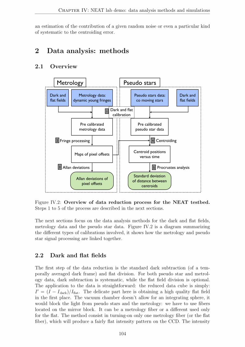
Chapter IV: NEAT lab demo: data analysis methods and simulations
an estimation of the contribution of a given random noise or even a particular kindof systematic to the centroiding error.
2 Data analysis: methods
2.1 Overview
�������������������������������������
����������������������������������
���������������������
�����������������
�������������������������������
������������������������������
�����������
�������������������
���������������������������������
���������������������������������������
���������
������������������
��������� �������������
� �
�� ����������������
�
������������������
�����������������������������
�����������������������
Figure IV.2: Overview of data reduction process for the NEAT testbed.Steps 1 to 5 of the process are described in the next sections.
The next sections focus on the data analysis methods for the dark and flat fields,metrology data and the pseudo star data. Figure IV.2 is a diagram summarizingthe different types of calibrations involved, it shows how the metrology and pseudostar signal processing are linked together.
2.2 Dark and flat fields
The first step of the data reduction is the standard dark subtraction (of a tem-porally averaged dark frame) and flat division. For both pseudo star and metrol-ogy data, dark subtraction is systematic, while the flat field division is optional.The application to the data is straightforward: the reduced data cube is simply:I � = (I − Idark)/Iflat. The delicate part here is obtaining a high quality flat fieldin the first place. The vacuum chamber doesn’t allow for an integrating sphere, itwould block the light from pseudo stars and the metrology: we have to use fiberslocated on the mirror block. It can be a metrology fiber or a different used onlyfor the flat. The method consist in turning-on only one metrology fiber (or the flatfiber), which will produce a fairly flat intensity pattern on the CCD. The intensity
104

2. Data analysis: methods
������������������ �������������������������
����������������������������������������
Figure IV.3: Flat field processing. (1) Image after dark subtraction, temporalnormalization, temporal averaging and spatial normalization. (2) The relative gainbetween the quadrants have been compensated, assuming continuity of the inten-sity between the quadrants. (3) The image had been divided by its low pass filtercomponent to obtain. (4) The quadrant relative gains are added back into the data,this is the “final flat” that will can be used for the centroids or the metrology. Theimages used here have a very poor quality (good for illustration purposes), of coursewe use better ones to derive the actual flat field.
profile produced is a Gaussian beam whose waist of about 10 cm is much largerthan the CCD field (2 mm). So what is seen by the detector is an intensity gradientwith an eventual slight curvature, which has to be “detrended”. The method usedto obtain the flat field is illustrated by Fig. IV.3.
The first step of the flat field processing consist of:
• Dark subtraction
• Temporal normalization: each frame is scaled to have an average flux equal tothe average intensity level of the first frame
• Calculation of theoretical photon noise and measured photon noise
• Temporal averaging to obtain a mean frame
• Spatial normalization: the mean frame is normalized, the average pixel valueis set to 1
An important point is that we expect the flat to be much better with incoherent light,unlike the metrology fringes. Coherent light produces relative intensity variations∝
�I1/I0 instead of ∝ I1/I0 because of interferences (I0 is the intensity of the fiber,
I1 is the intensity of a parasite reflection). The interference pattern can be quitecomplex and have spatial features unresolved by the pixels if the angular separationis too large, so it can not be properly detrended. This is the case for example forreflections on the edges of the stop apertures of the baffle.
105
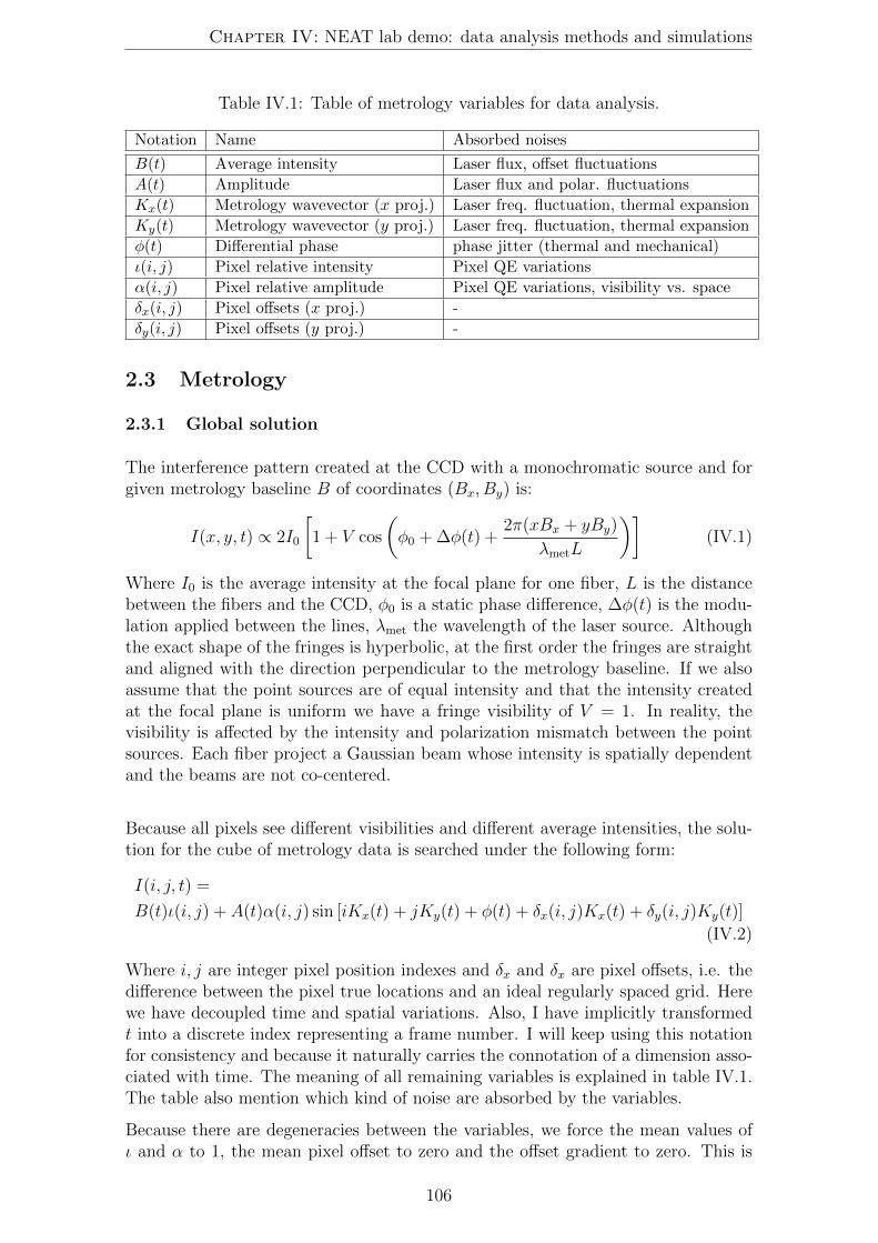
Chapter IV: NEAT lab demo: data analysis methods and simulations
Table IV.1: Table of metrology variables for data analysis.
Notation Name Absorbed noises
B(t) Average intensity Laser flux, offset fluctuations
A(t) Amplitude Laser flux and polar. fluctuations
Kx(t) Metrology wavevector (x proj.) Laser freq. fluctuation, thermal expansion
Ky(t) Metrology wavevector (y proj.) Laser freq. fluctuation, thermal expansion
φ(t) Differential phase phase jitter (thermal and mechanical)
ι(i, j) Pixel relative intensity Pixel QE variations
α(i, j) Pixel relative amplitude Pixel QE variations, visibility vs. space
δx(i, j) Pixel offsets (x proj.) -
δy(i, j) Pixel offsets (y proj.) -
2.3 Metrology
2.3.1 Global solution
The interference pattern created at the CCD with a monochromatic source and forgiven metrology baseline B of coordinates (Bx, By) is:
I(x, y, t) ∝ 2I0
�1 + V cos
�φ0 +Δφ(t) +
2π(xBx + yBy)
λmetL
��(IV.1)
Where I0 is the average intensity at the focal plane for one fiber, L is the distancebetween the fibers and the CCD, φ0 is a static phase difference, Δφ(t) is the modu-lation applied between the lines, λmet the wavelength of the laser source. Althoughthe exact shape of the fringes is hyperbolic, at the first order the fringes are straightand aligned with the direction perpendicular to the metrology baseline. If we alsoassume that the point sources are of equal intensity and that the intensity createdat the focal plane is uniform we have a fringe visibility of V = 1. In reality, thevisibility is affected by the intensity and polarization mismatch between the pointsources. Each fiber project a Gaussian beam whose intensity is spatially dependentand the beams are not co-centered.
Because all pixels see different visibilities and different average intensities, the solu-tion for the cube of metrology data is searched under the following form:
I(i, j, t) =
B(t)ι(i, j) + A(t)α(i, j) sin [iKx(t) + jKy(t) + φ(t) + δx(i, j)Kx(t) + δy(i, j)Ky(t)]
(IV.2)
Where i, j are integer pixel position indexes and δx and δx are pixel offsets, i.e. thedifference between the pixel true locations and an ideal regularly spaced grid. Herewe have decoupled time and spatial variations. Also, I have implicitly transformedt into a discrete index representing a frame number. I will keep using this notationfor consistency and because it naturally carries the connotation of a dimension asso-ciated with time. The meaning of all remaining variables is explained in table IV.1.The table also mention which kind of noise are absorbed by the variables.
Because there are degeneracies between the variables, we force the mean values ofι and α to 1, the mean pixel offset to zero and the offset gradient to zero. This is
106
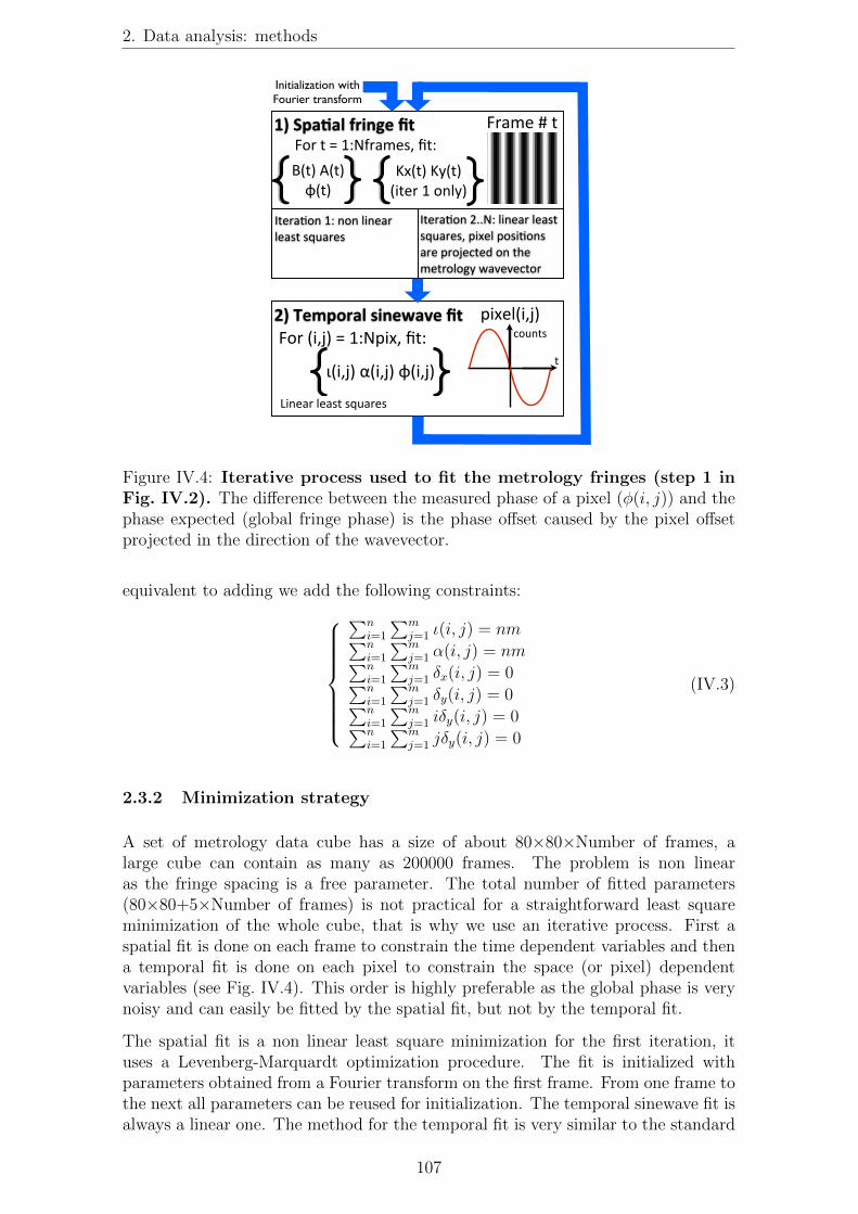
2. Data analysis: methods
B(t) A(t) φ(t)
1) Spa'al fringe fit
2) Temporal sinewave fit
For t = 1:Nframes, fit:Frame # t
pixel(i,j)For (i,j) = 1:Npix, fit:
t
counts
Kx(t) Ky(t)(iter 1 only)
Linear least squares
ι(i,j) α(i,j) φ(i,j)
IteraFon 1: non linear least squares
IteraFon 2..N: linear least squares, pixel posiFons are projected on the metrology wavevector
��������������������������������������
Figure IV.4: Iterative process used to fit the metrology fringes (step 1 inFig. IV.2). The difference between the measured phase of a pixel (φ(i, j)) and thephase expected (global fringe phase) is the phase offset caused by the pixel offsetprojected in the direction of the wavevector.
equivalent to adding we add the following constraints:
�ni=1
�mj=1 ι(i, j) = nm�n
i=1
�mj=1 α(i, j) = nm�n
i=1
�mj=1 δx(i, j) = 0�n
i=1
�mj=1 δy(i, j) = 0�n
i=1
�mj=1 iδy(i, j) = 0�n
i=1
�mj=1 jδy(i, j) = 0
(IV.3)
2.3.2 Minimization strategy
A set of metrology data cube has a size of about 80×80×Number of frames, alarge cube can contain as many as 200000 frames. The problem is non linearas the fringe spacing is a free parameter. The total number of fitted parameters(80×80+5×Number of frames) is not practical for a straightforward least squareminimization of the whole cube, that is why we use an iterative process. First aspatial fit is done on each frame to constrain the time dependent variables and thena temporal fit is done on each pixel to constrain the space (or pixel) dependentvariables (see Fig. IV.4). This order is highly preferable as the global phase is verynoisy and can easily be fitted by the spatial fit, but not by the temporal fit.
The spatial fit is a non linear least square minimization for the first iteration, ituses a Levenberg-Marquardt optimization procedure. The fit is initialized withparameters obtained from a Fourier transform on the first frame. From one frame tothe next all parameters can be reused for initialization. The temporal sinewave fit isalways a linear one. The method for the temporal fit is very similar to the standard
107

Chapter IV: NEAT lab demo: data analysis methods and simulations
linearizion technique used on a sinewave whose period is known. The differenceis that we instead know the phase of the 2D carrier sinewave (not including pixeloffsets) at each pixel and for each frame. After normalization to average frameintensity and average frame amplitude, the signal is a pure sinewave with a constantoffset whose phase carries information on the pixel location projected along themodulation direction:
I(i, j, t) = ι(i, j) + α(i, j) sin [φ(t) + φ(i, j)] = ai,j sin(φ(t)) + bi,j cos(φ(t)) + ci,j(IV.4)
� Linear temporal fit
A least square minimization of the sum:
Si,j =N−1�
t=0
[I(i, j, t)− ai,j sin(φ(t))− bi,j cos(φ(t))− ci,j]2 (IV.5)
yields the values for a, b and c from which α(i, j), φ(i, j) and ι(i, j) are derived foreach pixel: this is the temporal fit. We obtain pixel phases:
φ(i, j) = iKx(t) + jKy(t) + δx(i, j)Kx(t) + δy(i, j)Ky(t) (IV.6)
Also knowing the metrology wavevector (see Fig. IV.5), we derive the projectedphase offsets: δx(i, j)Kx + δy(i, j)Ky (for this final step K is assumed constant),from which we have the spatial offset. The detail for the linearization of the fit isexplained below.
��
������
������������
����
����
�
Figure IV.5: Definition of the wave vector. For a given metrology orientation,the wave vector is defined as: �K = (Kx(t), Ky(t)) for a plane wave of the form:I(x, y, t) ∝ sin(xKx(t) + yKy(t) + φ(t)). The wave vector is by definition perpen-dicular to the fringes and aligned with the modulation direction, i.e. the apparentmotion of the fringes when the phase changes. The default distance unit is the pixel,so the magnitude of the vectors is | �K| = 2π/λ, with lambda in pixel units.
We want to fit a pure sinewave, and just like in the usual case when the frequency isknown, the fit can be linearized. Instead we know the phase of the carrier wave foreach point in time (i.e. frame), but the principle is the same. As long as we knowthe true phase, the fit works even if sampling points are not evenly spaced in timeor if the phase has jitter. The first step is to rewrite the sinewave and decompose itinto cos and sin components, which has already been done in Eq. (IV.4). We haveintroduced three coefficients (a, b, c) ∈ R3. The equality is obtained when a, b, cverify:
108
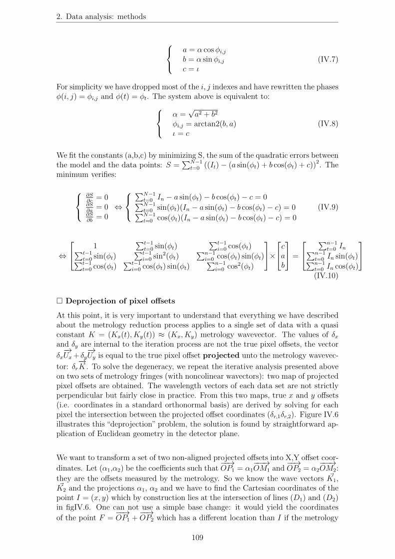
2. Data analysis: methods
a = α cosφi,j
b = α sinφi,j
c = ι(IV.7)
For simplicity we have dropped most of the i, j indexes and have rewritten the phasesφ(i, j) = φi,j and φ(t) = φt. The system above is equivalent to:
α =√a2 + b2
φi,j = arctan2(b, a)ι = c
(IV.8)
We fit the constants (a,b,c) by minimizing S, the sum of the quadratic errors betweenthe model and the data points: S =
�N−1t=0 ((It)− (a sin(φt) + b cos(φt) + c))2. The
minimum verifies:
∂S∂c
= 0∂S∂a
= 0∂S∂b
= 0⇔
�N−1t=0 In − a sin(φt)− b cos(φt)− c = 0�N−1t=0 sin(φt)(In − a sin(φt)− b cos(φt)− c) = 0�N−1t=0 cos(φt)(In − a sin(φt)− b cos(φt)− c) = 0
(IV.9)
⇔
1�t−1
t=0 sin(φt)�t−1
i=0 cos(φt)�t−1t=0 sin(φt)
�t−1i=0 sin
2(φt)�n−1
i=0 cos(φt) sin(φt)�t−1t=0 cos(φt)
�t−1i=0 cos(φt) sin(φt)
�n−1i=0 cos2(φt)
×
cab
=
�n−1t=0 In�n−1
t=0 In sin(φt)�n−1t=0 In cos(φt)
(IV.10)
� Deprojection of pixel offsets
At this point, it is very important to understand that everything we have describedabout the metrology reduction process applies to a single set of data with a quasiconstant K = (Kx(t), Ky(t)) ≈ (Kx, Ky) metrology wavevector. The values of δxand δy are internal to the iteration process are not the true pixel offsets, the vector
δx−→Ux+ δy
−→Uy is equal to the true pixel offset projected unto the metrology wavevec-
tor: δr−→K . To solve the degeneracy, we repeat the iterative analysis presented above
on two sets of metrology fringes (with noncolinear wavectors): two map of projectedpixel offsets are obtained. The wavelength vectors of each data set are not strictlyperpendicular but fairly close in practice. From this two maps, true x and y offsets(i.e. coordinates in a standard orthonormal basis) are derived by solving for eachpixel the intersection between the projected offset coordinates (δr,1δr,2). Figure IV.6illustrates this “deprojection” problem, the solution is found by straightforward ap-plication of Euclidean geometry in the detector plane.
We want to transform a set of two non-aligned projected offsets into X,Y offset coor-
dinates. Let (α1,α2) be the coefficients such that−−→OP1 = α1
−−−→OM1 and
−−→OP2 = α2
−−−→OM2:
they are the offsets measured by the metrology. So we know the wave vectors �K1,�K2 and the projections α1, α2 and we have to find the Cartesian coordinates of thepoint I = (x, y) which by construction lies at the intersection of lines (D1) and (D2)in figIV.6. One can not use a simple base change: it would yield the coordinates
of the point F =−−→OP1 +
−−→OP2 which has a different location than I if the metrology
109

Chapter IV: NEAT lab demo: data analysis methods and simulations
−2 −1 0 1 2−2
−1
0
1
2
(D2)
(D1)
M1
M2
P1
P2
F
I
0
Figure IV.6: Illustration of the deprojection problem.−−−→OM1 and
−−−→OM2 are the
wave vectors normalized to a length of one pixel. The points P1 and P2 are themeasured offsets, i.e. the projections of the true pixel offset (point I), unto the linesgenerated by the wave vectors. The axis units are in pixels. Simply summing theprojected offsets gives a wrong answer (point F ).
baselines are not orthogonal.
Let the coordinates of the normalized wave vectors be kx,1, ky,1, kx,2, ky,2, for respec-tively metrology cube 1 (first baseline/orientation) and cube 2 (second baseline/ori-entation). The direction vectors of lines (D1) and (D2) are noted cx/y,1/2 and havetrivial relations with the wave vectors coordinates:
cx,1 = ky,1cy,1 = −kx,1cx,2 = ky,2cy,2 = −kx,2
(IV.11)
The lines (D1) and (D2) are passing thought respectively P1 = (dx,1, dy,1) and P2 =(dx,2, dy,2), of coordinates:
dx,1 = kx,1α1
dy,1 = ky,1α1
dx,2 = kx,2α2
dy,2 = ky,2α2
(IV.12)
The parametric equation of line (D1), passing thought P1, of direction vector (cx,1, cy,1),is: ⇢
x = cx,1t+ dx,1y = cy,1t+ dy,1
(IV.13)
110
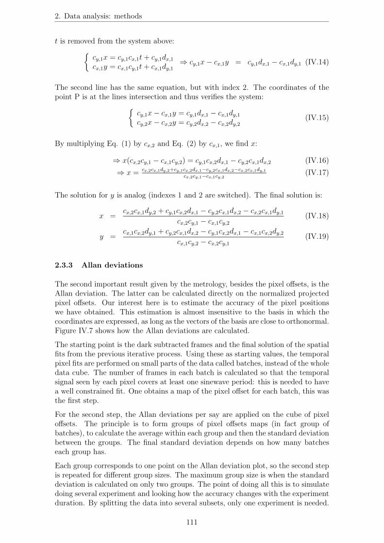
2. Data analysis: methods
t is removed from the system above:
⇢cy,1x = cy,1cx,1t+ cy,1dx,1cx,1y = cx,1cy,1t+ cx,1dy,1
⇒ cy,1x− cx,1y = cy,1dx,1 − cx,1dy,1 (IV.14)
The second line has the same equation, but with index 2. The coordinates of thepoint P is at the lines intersection and thus verifies the system:
⇢cy,1x− cx,1y = cy,1dx,1 − cx,1dy,1cy,2x− cx,2y = cy,2dx,2 − cx,2dy,2
(IV.15)
By multiplying Eq. (1) by cx,2 and Eq. (2) by cx,1, we find x:
⇒ x(cx,2cy,1 − cx,1cy,2) = cy,1cx,2dx,1 − cy,2cx,1dx,2 (IV.16)
⇒ x = cx,2cx,1dy,2+cy,1cx,2dx,1−cy,2cx,1dx,2−cx,2cx,1dy,1cx,2cy,1−cx,1cy,2
(IV.17)
The solution for y is analog (indexes 1 and 2 are switched). The final solution is:
x =cx,2cx,1dy,2 + cy,1cx,2dx,1 − cy,2cx,1dx,2 − cx,2cx,1dy,1
cx,2cy,1 − cx,1cy,2(IV.18)
y =cx,1cx,2dy,1 + cy,2cx,1dx,2 − cy,1cx,2dx,1 − cx,1cx,2dy,2
cx,1cy,2 − cx,2cy,1(IV.19)
2.3.3 Allan deviations
The second important result given by the metrology, besides the pixel offsets, is theAllan deviation. The latter can be calculated directly on the normalized projectedpixel offsets. Our interest here is to estimate the accuracy of the pixel positionswe have obtained. This estimation is almost insensitive to the basis in which thecoordinates are expressed, as long as the vectors of the basis are close to orthonormal.Figure IV.7 shows how the Allan deviations are calculated.
The starting point is the dark subtracted frames and the final solution of the spatialfits from the previous iterative process. Using these as starting values, the temporalpixel fits are performed on small parts of the data called batches, instead of the wholedata cube. The number of frames in each batch is calculated so that the temporalsignal seen by each pixel covers at least one sinewave period: this is needed to havea well constrained fit. One obtains a map of the pixel offset for each batch, this wasthe first step.
For the second step, the Allan deviations per say are applied on the cube of pixeloffsets. The principle is to form groups of pixel offsets maps (in fact group ofbatches), to calculate the average within each group and then the standard deviationbetween the groups. The final standard deviation depends on how many batcheseach group has.
Each group corresponds to one point on the Allan deviation plot, so the second stepis repeated for different group sizes. The maximum group size is when the standarddeviation is calculated on only two groups. The point of doing all this is to simulatedoing several experiment and looking how the accuracy changes with the experimentduration. By splitting the data into several subsets, only one experiment is needed.
111
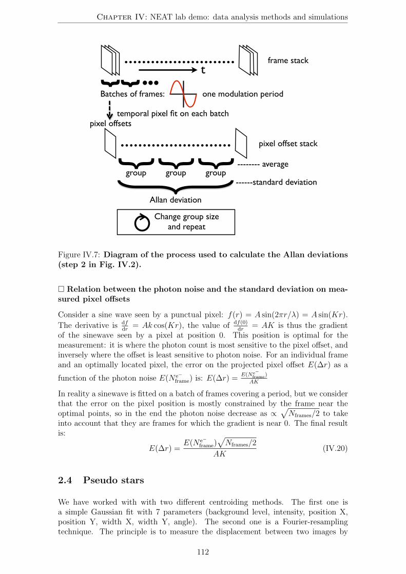
Chapter IV: NEAT lab demo: data analysis methods and simulations
������������������������� �����������
�
�������������
�������������������������������������������������������
�������������������������������
������������������������� ������������������
�
�����
����������������
�����
�����������������
�����
�
������������������������
����������������������������
� ���
Figure IV.7: Diagram of the process used to calculate the Allan deviations(step 2 in Fig. IV.2).
� Relation between the photon noise and the standard deviation on mea-sured pixel offsets
Consider a sine wave seen by a punctual pixel: f(r) = A sin(2πr/λ) = A sin(Kr).
The derivative is dfdr
= Ak cos(Kr), the value of df(0)dr
= AK is thus the gradientof the sinewave seen by a pixel at position 0. This position is optimal for themeasurement: it is where the photon count is most sensitive to the pixel offset, andinversely where the offset is least sensitive to photon noise. For an individual frameand an optimally located pixel, the error on the projected pixel offset E(Δr) as a
function of the photon noise E(N e−frame) is: E(Δr) =
E(Ne−frame)
AK
In reality a sinewave is fitted on a batch of frames covering a period, but we considerthat the error on the pixel position is mostly constrained by the frame near theoptimal points, so in the end the photon noise decrease as ∝
�Nframes/2 to take
into account that they are frames for which the gradient is near 0. The final resultis:
E(Δr) =E(N e−
frame)�Nframes/2
AK(IV.20)
2.4 Pseudo stars
We have worked with with two different centroiding methods. The first one isa simple Gaussian fit with 7 parameters (background level, intensity, position X,position Y, width X, width Y, angle). The second one is a Fourier-resamplingtechnique. The principle is to measure the displacement between two images by
112

2. Data analysis: methods
resampling with phase ramp in the Fourier domain. We use the following propertyof the Fourier transform (noted F):
F [PSF(x− x0, y − y0)] = exp [−i2π(x0x+ y0y)]F [PSF(x, y)] (IV.21)
In pratice, I use Eq. (IV.22) as a way to translate the resample the second . . . . .PSFat the location of the first one. The vector (x0, y0) for which the residual imagebetween the first . . . . .PSF and the resampled second . . . . .PSF is minimal (in the least squaresens) is the displacement. Thus the vector (x0, y0) is found by minimization of theexpression:
�
x,y
�F [PSF1(x, y)]− exp [−i2π(x0x+ y0y)]F
�PSF2(x, y)
��2(IV.22)
When done on Nyquist sampled data, it is equivalent to a perfect interpolation.Another advantage of this method is that we are essentially using the data itself toreconstruct the PSF and we do not need a model of the PSF in the first place, thusavoiding potential errors caused by a model/data PSF mismatch. But this methodhas a drawback: it only gives relative motion. In order to know the distance fromone centroid to another, we have to use an autocorrelation between two distinctcentroids. However, because we have an optical configuration with only one opticalsurface and no obscuration of the field of view, the PSF is expected to be nearlyinvariant. The errors of this process should be mainly caused by the pixels, whichcan be calibrated by the metrology.
To take the pixel offsets into account, a intermediate step is added. Before calculat-ing the offset with Eq. (IV.22), we correct the PSFs by finding its theoretical shapefor null offsets P0(i, j). Eq. (IV.22) is then applied between the P0(i, j) correspond-ing to each PSF. This is done by using the CCD model, generated from the pixeloffsets. A least square minimization is done on the product between:
• An oversampled version of P0 obtained by zero padding in the Fourier domain• The part of the CCD model (concatenation of PRFs) corresponding to theactive fitting window
More precisely, the residuals are the difference between the data and the product wehave defined above. To efficiently evaluate the residuals, in an manner practical foriterative optimization, the function returns a residual array with the same samplingthan the original PSF, by summing the product array over each pixel.
The last step is the SD analysis of the centroid positions, with or without Procrustesanalysis. At this point we have a measure of the coordinates of each centroid versusthe time, for one or more positions on the CCD. We perform several types of analysis.For the first type (lets call it quasistatic), we monitor the centroids locations versustime at a fixed position: we do not use the motors of the translation stage. We canthen calculate the SD of the distances between the outer centroids and the centralone. This measure is sensible to some environmental factors such as mechanicalstability, air turbulence etc... but if the centroid positions are stable enough, thepixel errors are nearly constant and therefore do not affect the measures significantly.The centroids motion are caused by mechanical vibrations and are typically less thanone 1% of a pixel. A complete Procrustes analysis is actually not needed to obtainthis particular result, only the translation is compensated.
113
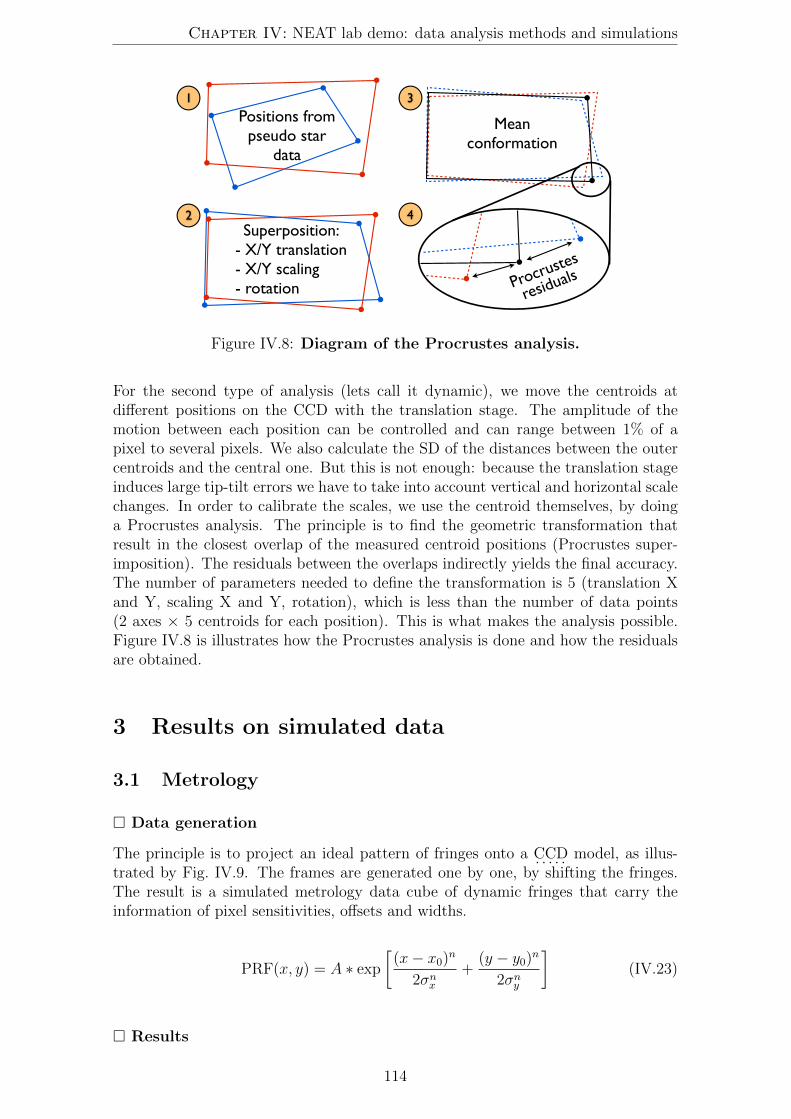
Chapter IV: NEAT lab demo: data analysis methods and simulations
������������������������������������������������������
�����������������
�������������������������������
�����������
���������
�
�
�
�
Figure IV.8: Diagram of the Procrustes analysis.
For the second type of analysis (lets call it dynamic), we move the centroids atdifferent positions on the CCD with the translation stage. The amplitude of themotion between each position can be controlled and can range between 1% of apixel to several pixels. We also calculate the SD of the distances between the outercentroids and the central one. But this is not enough: because the translation stageinduces large tip-tilt errors we have to take into account vertical and horizontal scalechanges. In order to calibrate the scales, we use the centroid themselves, by doinga Procrustes analysis. The principle is to find the geometric transformation thatresult in the closest overlap of the measured centroid positions (Procrustes super-imposition). The residuals between the overlaps indirectly yields the final accuracy.The number of parameters needed to define the transformation is 5 (translation Xand Y, scaling X and Y, rotation), which is less than the number of data points(2 axes × 5 centroids for each position). This is what makes the analysis possible.Figure IV.8 is illustrates how the Procrustes analysis is done and how the residualsare obtained.
3 Results on simulated data
3.1 Metrology
� Data generation
The principle is to project an ideal pattern of fringes onto a . . . . .CCD model, as illus-trated by Fig. IV.9. The frames are generated one by one, by shifting the fringes.The result is a simulated metrology data cube of dynamic fringes that carry theinformation of pixel sensitivities, offsets and widths.
PRF(x, y) = A ∗ exp�(x− x0)
n
2σnx
+(y − y0)
n
2σny
�(IV.23)
� Results
114
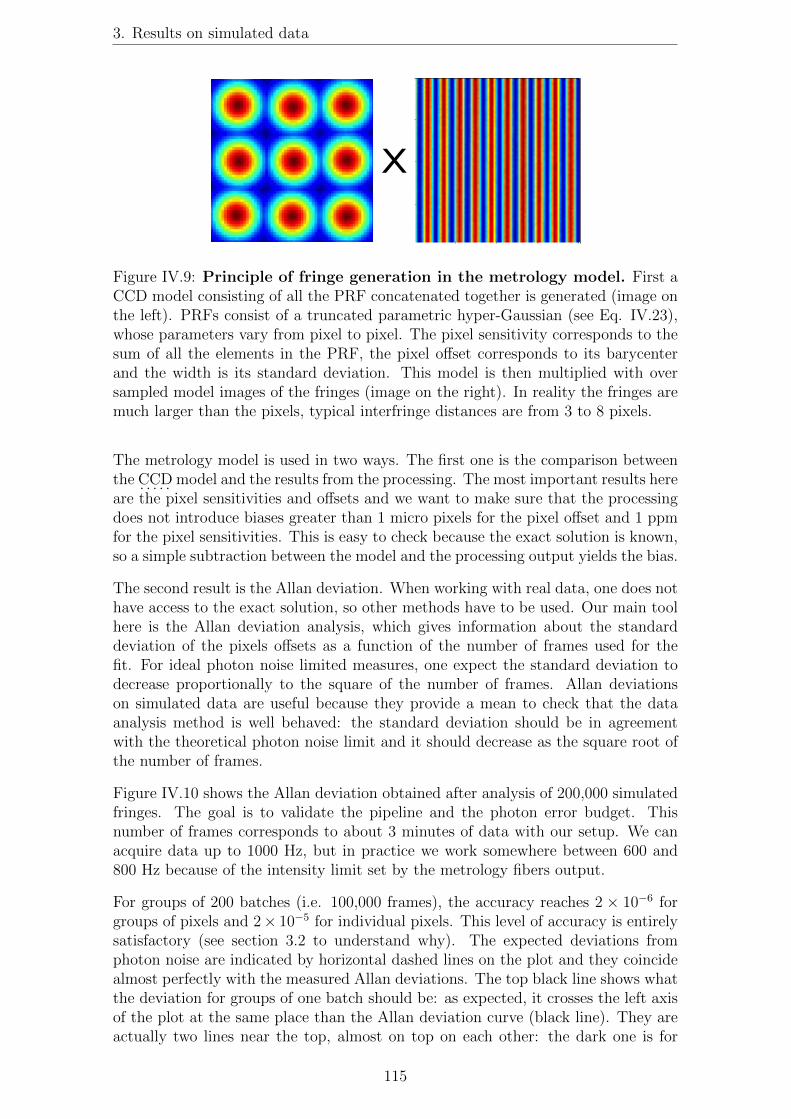
3. Results on simulated data
�
Figure IV.9: Principle of fringe generation in the metrology model. First aCCD model consisting of all the PRF concatenated together is generated (image onthe left). PRFs consist of a truncated parametric hyper-Gaussian (see Eq. IV.23),whose parameters vary from pixel to pixel. The pixel sensitivity corresponds to thesum of all the elements in the PRF, the pixel offset corresponds to its barycenterand the width is its standard deviation. This model is then multiplied with oversampled model images of the fringes (image on the right). In reality the fringes aremuch larger than the pixels, typical interfringe distances are from 3 to 8 pixels.
The metrology model is used in two ways. The first one is the comparison betweenthe . . . . .CCD model and the results from the processing. The most important results hereare the pixel sensitivities and offsets and we want to make sure that the processingdoes not introduce biases greater than 1 micro pixels for the pixel offset and 1 ppmfor the pixel sensitivities. This is easy to check because the exact solution is known,so a simple subtraction between the model and the processing output yields the bias.
The second result is the Allan deviation. When working with real data, one does nothave access to the exact solution, so other methods have to be used. Our main toolhere is the Allan deviation analysis, which gives information about the standarddeviation of the pixels offsets as a function of the number of frames used for thefit. For ideal photon noise limited measures, one expect the standard deviation todecrease proportionally to the square of the number of frames. Allan deviationson simulated data are useful because they provide a mean to check that the dataanalysis method is well behaved: the standard deviation should be in agreementwith the theoretical photon noise limit and it should decrease as the square root ofthe number of frames.
Figure IV.10 shows the Allan deviation obtained after analysis of 200,000 simulatedfringes. The goal is to validate the pipeline and the photon error budget. Thisnumber of frames corresponds to about 3 minutes of data with our setup. We canacquire data up to 1000 Hz, but in practice we work somewhere between 600 and800 Hz because of the intensity limit set by the metrology fibers output.
For groups of 200 batches (i.e. 100,000 frames), the accuracy reaches 2 × 10⁻⁶ forgroups of pixels and 2× 10⁻⁵ for individual pixels. This level of accuracy is entirelysatisfactory (see section 3.2 to understand why). The expected deviations fromphoton noise are indicated by horizontal dashed lines on the plot and they coincidealmost perfectly with the measured Allan deviations. The top black line shows whatthe deviation for groups of one batch should be: as expected, it crosses the left axisof the plot at the same place than the Allan deviation curve (black line). They areactually two lines near the top, almost on top on each other: the dark one is for
115

Chapter IV: NEAT lab demo: data analysis methods and simulations
100
101
102
10−6
10−5
10−4
Number of batches per group (500 frames per batch) − 0.83 sec per batch
Sta
nd
ard
de
via
tio
ns b
etw
ee
n g
rou
ps (
pix
el)
Allan deviation of pixels and blocs of pixels # 20140603 # 2−79x5−84 # vertical
167 sec
measured photon noise (pixels, 1 batch)expected std from photon noise (pixels, 1 batch)
(blocs, 1 batch)
(pixels, largest group)
(blocs, largest group)Ind. pixels (data)Ind. pixels average (data)
Ind. pixel average (white gaussian noise)
Blocs average (data)Blocs average (white gaussian noise)
Figure IV.10: Allan deviations of simulated data. The amplitude, visibility andphoton noise of simulated fringes are adjusted to values typical of real experiment(B = 10000 counts, A = 6000 counts, 1 count = 10 photons). Additional sources ofnoise are simulated, such as laser intensity (1 × 10⁻² RSD), fringe phase (1 × 10⁻²
radian SD) and pixel QE (1× 10⁻⁵ RSD). The plot shows deviations for individualspixels (plain red), their average deviation (plain black) and the average for blocks of10 by 10 pixels in (plain blue). The dotted black and blue curves are for a cube ofwhite noise whose standard deviation is matched to the data for groups of 1 batch.Averaging Allan deviations over pixels or blocks is important because they tendto be noisy (plain red) when the final deviation is derived from very few groups.Horizontal dotted blue and black lines are various estimations of the photon limit.
theoretical photon noise, the red one is for measured photon noise using the firstframe of the data cube. No red noises or read noise was included in the model. Inthe real experiment the read noise is negligible compared to photon noise.
Figure IV.11 shows maps of the difference between the measured pixel offsets and thetrue solution (pixel offset simulation input) for different values of pixel QE RSD. Thisis the ultimate metric to check the accuracy of the result, because biases constant intime are not visible in the Allan deviation. For low pixel QE RSD (< 1× 10⁻⁵), thestandard deviation of 2×10⁻⁵ seen in Fig. IV.11 is coherent with the value given byAllan deviation (i.e. the photon noise floor). However, tests with higher values ofpixel QE RSD show residual spatial bias above photon noise floor, while the Allandeviation is unaffected. This is an eventual point to improve, but a good pre-flatcalibration of the actual metrology data can in principle take care of this problem.
In conclusion, although a small bias could persist if the metrology data is not prop-erly flat calibrated (ideally to an accuracy of 1 × 10⁻⁵), the Allan deviations arenot affected and are a good way to control for the presence of correlated noise. Thecomparison between simulations and actual data will give us clues about what kindof noises are present in the data.
116
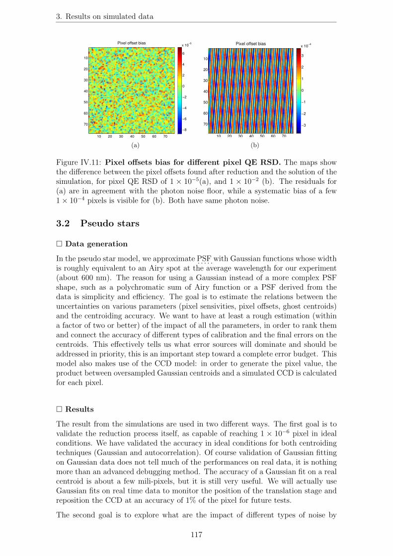
3. Results on simulated data
Pixel offset bias
10 20 30 40 50 60 70
10
20
30
40
50
60
70
−8
−6
−4
−2
0
2
4
6
x 10−5
(a)
Pixel offset bias
10 20 30 40 50 60 70
10
20
30
40
50
60
70 −3
−2
−1
0
1
2
3
x 10−4
(b)
Figure IV.11: Pixel offsets bias for different pixel QE RSD. The maps showthe difference between the pixel offsets found after reduction and the solution of thesimulation, for pixel QE RSD of 1 × 10⁻⁵(a), and 1 × 10⁻² (b). The residuals for(a) are in agreement with the photon noise floor, while a systematic bias of a few1× 10−4 pixels is visible for (b). Both have same photon noise.
3.2 Pseudo stars
� Data generation
In the pseudo star model, we approximate . . . . .PSF with Gaussian functions whose widthis roughly equivalent to an Airy spot at the average wavelength for our experiment(about 600 nm). The reason for using a Gaussian instead of a more complex PSFshape, such as a polychromatic sum of Airy function or a PSF derived from thedata is simplicity and efficiency. The goal is to estimate the relations between theuncertainties on various parameters (pixel sensivities, pixel offsets, ghost centroids)and the centroiding accuracy. We want to have at least a rough estimation (withina factor of two or better) of the impact of all the parameters, in order to rank themand connect the accuracy of different types of calibration and the final errors on thecentroids. This effectively tells us what error sources will dominate and should beaddressed in priority, this is an important step toward a complete error budget. Thismodel also makes use of the CCD model: in order to generate the pixel value, theproduct between oversampled Gaussian centroids and a simulated CCD is calculatedfor each pixel.
� Results
The result from the simulations are used in two different ways. The first goal is tovalidate the reduction process itself, as capable of reaching 1 × 10−6 pixel in idealconditions. We have validated the accuracy in ideal conditions for both centroidingtechniques (Gaussian and autocorrelation). Of course validation of Gaussian fittingon Gaussian data does not tell much of the performances on real data, it is nothingmore than an advanced debugging method. The accuracy of a Gaussian fit on a realcentroid is about a few mili-pixels, but it is still very useful. We will actually useGaussian fits on real time data to monitor the position of the translation stage andreposition the CCD at an accuracy of 1% of the pixel for future tests.
The second goal is to explore what are the impact of different types of noise by
117

Chapter IV: NEAT lab demo: data analysis methods and simulations
Table IV.2: Results from pseudo stars model. The error on pseudo stars measuredlocations is always in pixel units.Error type Error normalization / definition Error on centroid
Pixel sensitivity: σQE average pixel sensitivity = 1 0.5 σQE
Photon noise: σph
relative photon noisecalculated for the pixelwith the highest value
0.75 σph
Pixel offset: σoffsetoffset expressedin pixel units
0.15 σoffset
Pixel read noise: σread
relative read noisecalculated for the pixelwith the highest value
1.1 σread
Ghost centroids: σghost
ghost intensity relative to the maincentroid, ghost located randomlywithin 2 pixels of the star center
1.2 σghost
injecting them one at a time into the simulated data, in Monte Carlo simulations.Because we use Gaussian PSFs, in these simulations we can directly compare theinput centroid locations with the fit results, thus relying on absolute positions (asopposed to distances) and we can also skip the Procrustes analysis. We have usedthe model to estimate the relations between the uncertainties on various parameters(pixel sensivities, pixel offsets, ghost centroids) and the centroiding accuracy, theresults are summarized in Table IV.2.
Another useful aspect of these Monte Carlo simulations is the estimation of theproportion of random star position error that is absorbed by the Procrustes super-simposition. Among 10 observables, we allow for a fit with 5 degrees of freedom (2translation, 2 scaling, 1 rotation), which will inevitably lead us to underestimate thefinal noise. Simulations have showed that Procrustes supersimposition only decreasethe error by about 20%. When we express the final accuracy after the Procrustessupersimposition we correct the estimation for this factor.
We can draw interesting conclusions from these relations. In order to reach an errorof 5× 10⁻⁶ on the centroid, one only needs to calibrate the pixels positions to about3 × 10−5 and the accuracy of the flat field has to be better than 1 × 10⁻⁵. Theexperience is very sensitive to the presence of a ghost centroid near the real one: itsintensity must be lower than 4× 10⁻⁶ times the main centroid intensity.
118

Chapter V
NEAT lab demo: results andconclusions
During the progression of the experiment, we had a lot of discussion with JPL wherea similar experiment (VESTA) was carried out and we exchanged data (both ways).To validate the data processing and to better understand the nature of the errors,we have compared the result of our analysis with theirs on some of their data. Thecomplete analysis of JPL data began only a few weeks ago and is at a preliminarystage. The data has some differences, like having only two centroids instead of 5,some adaptations of the processing are required.
We did not get feedback about the result they have obtained with our data yet.However, we have completed a equivalent analysis of their data set. The final accu-racy is not in complete agreement, in particular after the last part of their analysiswhich consisted in making groups of positions. They have moved the centroids byincrements of a fraction of a pixel only: in the final analysis, the 30 positions arearranged into 3 groups of 10 (group are made on the basis of proximity). The resultare nevertheless already very interesting, they are presented presented in appendixB. This will avoid confusion with data from our own experiment.
1 Result on actual data
Before presenting the results, I must explain why the analysis may seem incomplete,in particular the metrology. There are major hardware issues that remain to besolved. Nearly all the elements needed to solve the problems have been supplied andthe bench is being upgraded so there is no need to try to work around the problems.Here is the list of issues that are being solved:
• One of the CCD quadrants showed an anomalous behavior, with a standarddeviation on the pixel offsets up to 10 times higher than the rest of the CCD.The cause of this behavior is uncertain, however the problem disappeared whenthe chip was swapped with another one. Unfortunately a quadrant of the newchip died very quickly, we had to put the previous chip back without a completeset of data in vacuum to work with. The third (and last) copy of the chip hasbeen transfered from CEA to IPAG and will be installed soon. Until then, tomitigate the issue we have restricted the Allan deviation analysis to parts of
119

Chapter V: NEAT lab demo: results and conclusions
Dark (mean frame) # 20141002
20 40 60 80
20
40
60
9600
9650
9700
9750
9800
(a)
Dark (mean frame) # 20141002
20 40 60 80
20
40
60
9500
9550
9600
9650
9700
(b)
Figure V.1: Mean dark frames at 100 Hz at 17◦C (left) and -10◦C (right).The darks have each 3000 frames, the theoretical SD of the pixel values are 0.1 count(the final error is dominated by the quantification).
the CCD unaffected by the problem. However, when calculating all the pixeloffsets (we need the complete map for centroid corrections), there is a concernthat errors from the bad quadrant can propagate into other quadrants.
• The metrology fiber tips have been damaged. A new system is being installed.When the data presented here was taken, only two baselines (one vertical, onehorizontal) were available. The horizontal baseline is with the new system,the vertical baseline is with the old one. We can look for differences in thequality of the data between the vertical and the horizontal direction with Allandeviations, but we can not compare pixel maps obtained with different sets ofbaselines.
1.1 Dark and flat fields
1.1.1 Darks
Figure V.1 shows typical dark frames at 17 and -10◦C. To illustrate the readout noiseinstability issue (refer to section 6.6.4 for a detailed description of the issue), Fig.V.2 shows two darks taken in identical conditions. When an instability appears, thehigh noise is usually restricted to one quadrant and the noise level is fairly variablefor different pixels within this quadrant. The stability of the dark over long timescales (a minute) is good in the sens that the SD is not higher than the readoutnoise. This is equivalent to say that there is no drift.
1.1.2 Flat fields
Our setup for flat fields consists of two multimode fibers of respective diameters of200 and 360 um attached to the mirror and pointing in the direction of the detector.The light source is a broadband high power LED (400 to 700 nm), plugged to eitherone of the fibers (fiber swapping is manual). The duration of the flat fields is adaptedto reach roughly the same photon noise with either fiber: it has to be longer withthe smaller fiber. In practice we obtain relative photon noises of less than 2× 10⁻⁵
for integration times of 360 and 180 seconds (on respectively 200 and 360 um fibers).
120

1. Result on actual data
Dark temporal SD # 20141006
20 40 60 80
20
40
60
4
6
8
10
12
(a)
Dark temporal SD # 20141006
20 40 60 80
20
40
60
3
4
5
6
7
(b)
Figure V.2: Temporal noise in dark data cubes. The cubes have been taken inidentical conditions: -10◦C, 100 Hz framerate, 30 seconds of acquisition (about 3000frames in total).
Simulations have showed that the relative errors on pixel QEs has to be less than1×10−5 to reach the ultimate accuracy goal on the centroids. With a relative photonnoise of 2×10⁻⁵, we can in principle get very close to the ultimate requirement (in thebest case). But we have to also quantify the systematics errors, and we will see thatin practice they are a slightly higher than the photon noise. To estimate the qualityof the flat field, we use several comparison techniques. First, by comparing two flatfields taken in the exact same conditions (one after the other), we expect to see thephoton noise, provided that the setup is stable enough. We can also estimate thephoton noise directly from one flat field because we know the acquisition parameters(number of frames, number of photons per frame), so we can check that the two areconsistent. Secondly, some systematics can be estimated by using fibers located atdifferent places on the mirror, moving them or by translating the CCD between twoflats.
If stray light is generated by the baffle or other elements within the vacuum cham-ber, moving the CCD or the fibers will change the stray light intensity distribution.When moving the fibers, we are also sensitive to systematics caused by the fiberthemselves, their tips and their orientation, such as differences in illumination gra-dient or speckles. Speckles can indeed appear for multimode fibers, even in whitelight (they will be strongly attenuated). To investigate the effect of speckles, we cansimply move the part of the fiber which is located outside of the vacuum chamber(between the source and the vacuum plug) between two flat fields, or scramble itduring the acquisition.
Figure V.3 shows the raw images that were obtained using the 200 um and 360um fibers located on the mirror (step 1). Figure V.4 shows the flat fields at step2 (after quadrant normalization). Figure V.5 shows the flat fields at step 3 (afterlow pass filter normalization). Figure V.6 shows the final flat fields taking accountthe quadrant gains. Figures V.7(a), V.7(b), V.8(a) and V.9(a) shows the differencebetween 200 um / 360 um flats for respectively: raw flat images, after step 2, afterstep 3 and after step 4. All these flats come from the same data set (30/09/2014)and were taken in the same conditions (100 Hz, 17◦C).
The first flat difference on Fig. V.7(a) is affected by various systematics at the
121

Chapter V: NEAT lab demo: results and conclusions
raw flat1
20 40 60 80
20
40
60
0.96
0.98
1
(a) 200 um Multimode fiber.
raw flat2
20 40 60 80
20
40
60
0.97
0.98
0.99
1
1.01
(b) 360 um Multimode fiber.
Figure V.3: Raw flat fields.
flat1 (Q−normalized)
20 40 60 80
20
40
60
0.96
0.98
1
(a) 200 um Multimode fiber.
flat2 (Q−normalized)
20 40 60 80
20
40
60
0.97
0.98
0.99
1
1.01
(b) 360 um Multimode fiber.
Figure V.4: Quadrant normalized flat fields.
flat1 (Q / irradiance normalized)
20 40 60 80
20
40
600.97
0.98
0.99
1
(a) 200 um Multimode fiber.
flat2 (Q / irradiance normalized)
20 40 60 80
20
40
600.97
0.98
0.99
1
(b) 360 um Multimode fiber.
Figure V.5: Quadrant / irradiance normalized flat fields.
final flat1
20 40 60 80
20
40
60
0.96
0.98
1
(a) 200 um Multimode fiber.
final flat2
20 40 60 80
20
40
600.97
0.98
0.99
1
1.01
(b) 360 um Multimode fiber.
Figure V.6: Final flat fields.
122
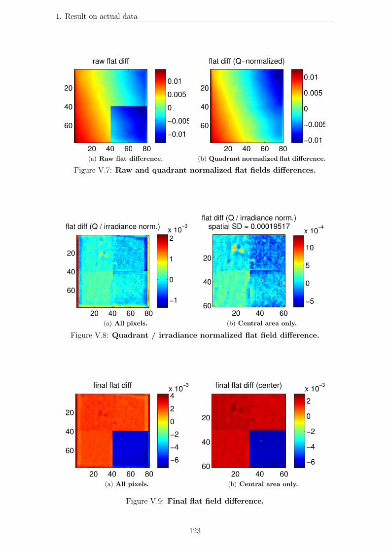
1. Result on actual data
raw flat diff
20 40 60 80
20
40
60
−0.01
−0.005
0
0.005
0.01
(a) Raw flat difference.
flat diff (Q−normalized)
20 40 60 80
20
40
60
−0.01
−0.005
0
0.005
0.01
(b) Quadrant normalized flat difference.
Figure V.7: Raw and quadrant normalized flat fields differences.
flat diff (Q / irradiance norm.)
20 40 60 80
20
40
60
−1
0
1
2x 10
−3
(a) All pixels.
flat diff (Q / irradiance norm.)spatial SD = 0.00019517
20 40 60
20
40
60−5
0
5
10
x 10−4
(b) Central area only.
Figure V.8: Quadrant / irradiance normalized flat field difference.
final flat diff
20 40 60 80
20
40
60
−6
−4
−2
0
2
4x 10
−3
(a) All pixels.
final flat diff (center)
20 40 60
20
40
60−6
−4
−2
0
2
x 10−3
(b) Central area only.
Figure V.9: Final flat field difference.
123

Chapter V: NEAT lab demo: results and conclusions
same time (gradient and the quadrant differences are visible). After correction forquadrant gains (Fig. V.7(b)), the dominant effect becomes the gradient differencebetween the two fibers. Once the irradiance (W.m-2) has been normalized, yet moresubtle effects are visible. On Fig. V.8 systematic biases are visible at a level of afew parts per thousand. Weird systematics often appear near the edges of the CCD,so we often compare the flats over the central region of the CCD only, by croppingthe outer 10 pixels on each side (Fig. V.8(b)). On the latter figure, we ideally wantto see only photon noise left. If this is the case, it means what after corrections, theflat field is close to the photon limit, with the caveat that we have not introducedcommon distortions for both flats during the processing.
The final flat difference (Fig. V.9) is affected by quadrant gains instabilities whichare not constant (relative to one another). This can be caused by thermal drifts of thereadout electronic components which are located in an aluminum box outside of thevacuum chamber. The box temperature is not regulated. At the interface betweenquadrants, the relative pixel gains are only stable to about 1%. The consequencesof this are the following:
• We will avoid putting centroid too close to quadrants edges. Error propagationindicates that if we do not do this we will introduce errors up to 5×10−3 pixel.
• We will still apply the final flat fields to the data. In case the fitting windowfor the stars slightly overlaps with another quadrant, this will keep the QEerror near the fitting window edge to about 1%. This is important because wehave to put centroids near quadrant edges to avoid ghosts (see section 1.3).
• When trying to estimate smaller systematics, we always correct for the quad-rant gains. In practice we want to correct for both quadrant gains and irradi-ance, so we can either compare the flat field at step (3) of the processing, oruse final flat fields (which are saved into files) and allow for a re-normalizationof the quadrants before calculating the difference. We also use the central areaonly to get rid of the systematics near the CCD edges.
The series of flat fields we have presented in Fig. V.3 to V.9(a) was affected bya lot of systematics. It was chosen mainly because it illustrates very well whatkinds of systematics are in the data, and why we need the processing to removethe largest effects (quadrant gains and gradient) to see them. On subsequent tests,we have done more tests and we have clearly identified at least one other source ofsystematic errors. Figure V.10 shows differences between flat fields obtained withthe 360 um fiber (central area), where the CCD was moved between the flats andwith or without shielding the mirror.
When the CCD is moved we see negative/positive ghost pairs, corresponding tothe ghost start and end positions. When the CCD is immobile and the mirror isshielded, we only see the positive part. For From these tests we conclude that aghost is produced by the mirror, by the conjugate reflection between the CCD andthe pinhole mask. We initially planned for a shutter that would shield the mirrorduring metrology and flat field data acquisition to avoid this specific stray lightreflection but the shutter was never installed because its motor was not functioningproperly.
In another set of tests (all done with the same fiber, 360 um core), we have tried toquantify eventual systematics caused by speckles (Fig. V.11). Scrambling seems tohelp and bending the fiber seems to have some effects, however the results are not
124
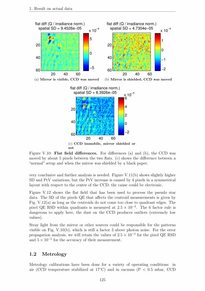
1. Result on actual data
flat diff (Q / irradiance norm.)spatial SD = 9.4526e−05
20 40 60
20
40
60−5
0
5
x 10−4
(a) Mirror is visible, CCD was moved
flat diff (Q / irradiance norm.)spatial SD = 4.7304e−05
20 40 60
20
40
60 −2
−1
0
1
x 10−4
(b) Mirror is shielded, CCD was moved
flat diff (Q / irradiance norm.)spatial SD = 8.3926e−05
20 40 60
20
40
60−2
0
2
4
6x 10
−4
(c) CCD immobile, mirror shielded ornot
Figure V.10: Flat field differences. For differences (a) and (b), the CCD wasmoved by about 5 pixels between the two flats. (c) shows the difference between a“normal” setup and when the mirror was shielded by a black paper.
very conclusive and further analysis is needed. Figure V.11(b) shows slightly higherSD and PtV variations, but the PtV increase is caused by 4 pixels in a symmetricallayout with respect to the center of the CCD: the cause could be electronic.
Figure V.12 shows the flat field that has been used to process the pseudo stardata. The SD of the pixels QE that affects the centroid measurements is given byFig. V.12(a) as long as the centroids do not come too close to quadrant edges. Thepixel QE RSD within quadrants is measured at 2.5 × 10⁻³. The 6 factor rule isdangerous to apply here, the dust on the CCD produces outliers (extremely lowvalues).
Stray light from the mirror or other sources could be responsible for the patternsvisible on Fig. V.10(b), which is still a factor 3 above photon noise. For the errorpropagation analysis, we will retain the values of 2.5 × 10⁻³ for the pixel QE RSDand 5× 10⁻⁵ for the accuracy of their measurement.
1.2 Metrology
Metrology calibrations have been done for a variety of operating conditions: inair (CCD temperature stabilized at 17◦C) and in vacuum (P < 0.5 mbar, CCD
125
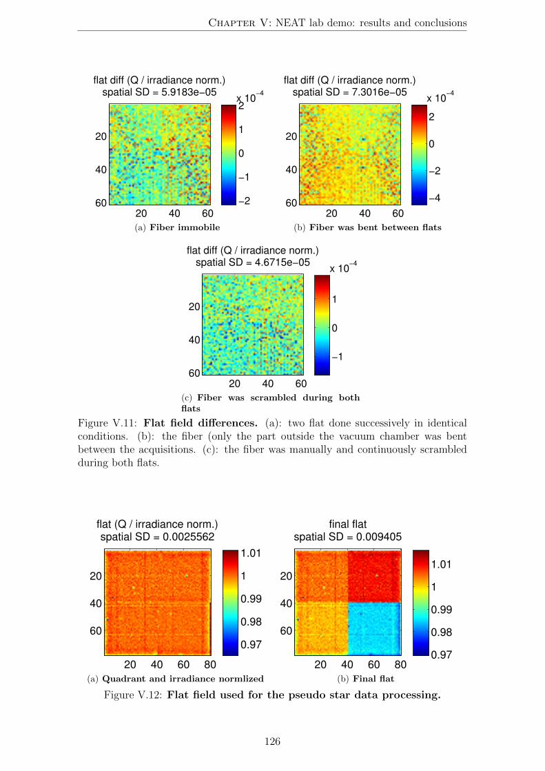
Chapter V: NEAT lab demo: results and conclusions
flat diff (Q / irradiance norm.)spatial SD = 5.9183e−05
20 40 60
20
40
60 −2
−1
0
1
2x 10
−4
(a) Fiber immobile
flat diff (Q / irradiance norm.)spatial SD = 7.3016e−05
20 40 60
20
40
60−4
−2
0
2
x 10−4
(b) Fiber was bent between flats
flat diff (Q / irradiance norm.)spatial SD = 4.6715e−05
20 40 60
20
40
60
−1
0
1
x 10−4
(c) Fiber was scrambled during bothflats
Figure V.11: Flat field differences. (a): two flat done successively in identicalconditions. (b): the fiber (only the part outside the vacuum chamber was bentbetween the acquisitions. (c): the fiber was manually and continuously scrambledduring both flats.
flat (Q / irradiance norm.)spatial SD = 0.0025562
20 40 60 80
20
40
60
0.97
0.98
0.99
1
1.01
(a) Quadrant and irradiance normlized
final flatspatial SD = 0.009405
20 40 60 80
20
40
60
0.97
0.98
0.99
1
1.01
(b) Final flat
Figure V.12: Flat field used for the pseudo star data processing.
126

1. Result on actual data
temperature stabilized at -10◦C) for different metrology baselines. In air I haveused different setups for stray light. For a complete characterization of the pixeloffsets in each direction we need two non collinear baselines. It is best to haveperpendicular baselines, in practice the baselines are nearly perpendicular, one isroughly vertical and the other roughly horizontal. Note that the terms designatingthe baselines (vertical/horizontal) corresponds to their physical alignment in thevacuum chamber. As the images of the data cube are displayed with a 90◦ rotationcompared to the physical layout of the pixels, the vertical baseline corresponds tothe vertical fringes and vice versa in the horizontal direction.
To avoid having too many plots, instead of showing the full Allan deviation curve,I will sometimes only mention numerical values which correspond to the measurednoise for the largest group size (largest integration time). On the plot it correspondsto the end of the (black and blue) curves on the right side.
1.2.1 Allan deviation in air, 17◦C, baffle v3, vertical baseline, one quad-rant (upper left).
100
101
10−6
10−5
10−4
10−3
Number of batches per group (500 frames per batch) − 0.83 sec per batch
Sta
nd
ard
de
via
tio
ns b
etw
ee
n g
rou
ps (
pix
el)
Allan deviation of pixels and blocs of pixels # 20140519 # 2−42x5−45 # vertical
8 sec
measured photon noise (pixels, 1 batch)expected std from photon noise (pixels, 1 batch)
(blocs, 1 batch)
(pixels, largest group)
(blocs, largest group)
Ind. pixels (data)Ind. pixels average (data)
Ind. pixel average (white gaussian noise)
Blocs average (data)Blocs average (white gaussian noise)
Figure V.13: Allan deviations of pixels and blocks of pixels.
Figure V.13 shows the Allan deviation obtained the 19/05/2014. This result waspresented in the SPIE 2014 paper (it was the best measure obtained by then). Onlyone quadrant was used in this analysis to avoid having pixels from the“bad quadrant”in the data.
They are noticeable differences with the simulated data. Firstly the level of noise ishigher than the expected photon noise limit by a factor 2.5. Secondly, the gain ofspatial averaging (blocks of pixels) is slightly less the expected factor of 10. Thirdly,tests on larger data sets (up to 50000 frames) show degraded accuracy: the two
127

Chapter V: NEAT lab demo: results and conclusions
symptoms mentioned above worsen (worse spatial averaging, larger gap with the-oretical photon noise) and the standard deviation does not fall as quickly. Thisindicates the presence of spatial and temporal red noise.
For this particular data set, we have also have looked at the impact of stray light onAllan deviations and found interesting results. A test without the baffle (all otherthings constant) yielded: Allan deviation of 3×10⁻⁴ for pixels (versus 2×10⁻⁴) and2× 10−4 only for groups of pixels (with baffle 3× 10⁻⁵). Tests with a baffle made ofpaper sheets have shown similar result than with no baffle.
1.2.2 Allan deviation in vacuum, -10◦C, baffle v4, vertical baseline, twoquadrants (left).
100
101
10−6
10−5
10−4
10−3
Number of batches per group (500 frames per batch) − 2.50 sec per batch
Sta
ndard
devia
tions b
etw
een g
roups (
pix
el)
Allan deviation of pixels and blocs of pixels # 20141006 # 2−78x5−42 # vertical # fiber44
25 sec
measured photon noise (pixels, 1 batch)expected std from photon noise (pixels, 1 batch)
(blocs, 1 batch)
(pixels, largest group)
(blocs, largest group)
Ind. pixels (data)Ind. pixels average (data)
Ind. pixel average (white gaussian noise)
Blocs average (data)Blocs average (white gaussian noise)
Figure V.14: Allan deviations of pixels and blocks of pixels.
Figure V.14 shows the Allan deviations obtained the 06/10/2014 on a vertical base-line. These results are nearly identical to the previous ones (photon noise higherthan expected, accuracy gets worse with more frames).
1.2.3 Allan deviation in vacuum, -10◦C, baffle v4, horizontal baseline,two quadrants (left).
Figure V.15 shows the Allan deviations obtained the 06/10/2014 on a horizontalbaseline. The fiber holding system is different for these fibers, it was changed becausethe previous system had damaged fiber tips. With the new system, fibers are gluedinside holes in an invar bar and the tips are polished. With the old system, fiber tipswere put into Zerodur V-grooves located on the mirror. The new system is much
128
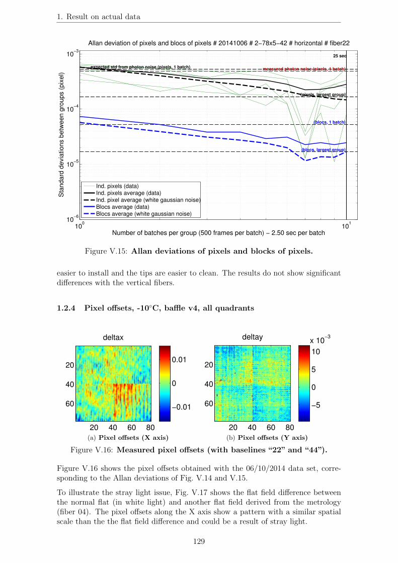
1. Result on actual data
100
101
10−6
10−5
10−4
10−3
Number of batches per group (500 frames per batch) − 2.50 sec per batch
Sta
nd
ard
de
via
tio
ns b
etw
ee
n g
rou
ps (
pix
el)
Allan deviation of pixels and blocs of pixels # 20141006 # 2−78x5−42 # horizontal # fiber22
25 sec
measured photon noise (pixels, 1 batch)expected std from photon noise (pixels, 1 batch)
(blocs, 1 batch)
(pixels, largest group)
(blocs, largest group)
Ind. pixels (data)Ind. pixels average (data)
Ind. pixel average (white gaussian noise)
Blocs average (data)Blocs average (white gaussian noise)
Figure V.15: Allan deviations of pixels and blocks of pixels.
easier to install and the tips are easier to clean. The results do not show significantdifferences with the vertical fibers.
1.2.4 Pixel offsets, -10◦C, baffle v4, all quadrants
deltax
20 40 60 80
20
40
60−0.01
0
0.01
(a) Pixel offsets (X axis)
deltay
20 40 60 80
20
40
60 −5
0
5
10
x 10−3
(b) Pixel offsets (Y axis)
Figure V.16: Measured pixel offsets (with baselines “22” and “44”).
Figure V.16 shows the pixel offsets obtained with the 06/10/2014 data set, corre-sponding to the Allan deviations of Fig. V.14 and V.15.
To illustrate the stray light issue, Fig. V.17 shows the flat field difference betweenthe normal flat (in white light) and another flat field derived from the metrology(fiber 04). The pixel offsets along the X axis show a pattern with a similar spatialscale than the the flat field difference and could be a result of stray light.
129
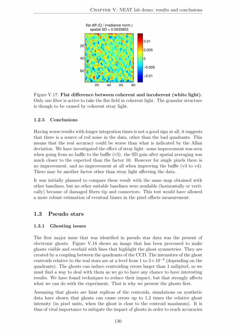
Chapter V: NEAT lab demo: results and conclusions
flat diff (Q / irradiance norm.)spatial SD = 0.0035853
20 40 60 80
20
40
60
−0.01
−0.005
0
0.005
0.01
Figure V.17: Flat difference between coherent and incoherent (white light).Only one fiber is active to take the flat field in coherent light. The granular structureis though to be caused by coherent stray light.
1.2.5 Conclusions
Having worse results with longer integration times is not a good sign at all, it suggeststhat there is a source of red noise in the data, other than the bad quadrants. Thismeans that the real accuracy could be worse than what is indicated by the Allandeviation. We have investigated the effect of stray light: some improvement was seenwhen going from no baffle to the baffle (v3): the SD gain after spatial averaging wasmuch closer to the expected than the factor 10. However for single pixels there isno improvement, and no improvement at all when improving the baffle (v3 to v4).There may be another factor other than stray light affecting the data.
It was initially planned to compare these result with the same map obtained withother baselines, but no other suitable baselines were available (horizontally or verti-cally) because of damaged fibers tip and connectors. This test would have alloweda more robust estimation of eventual biases in the pixel offsets measurement.
1.3 Pseudo stars
1.3.1 Ghosting issues
The first major issue that was identified in pseudo star data was the present ofelectronic ghosts. Figure V.18 shows an image that has been processed to makeghosts visible and overlaid with lines that highlight the ghost symmetries. They arecreated by a coupling between the quadrants of the CCD. The intensities of the ghostcentroids relative to the real stars are at a level from 1 to 3×10⁻³ (depending on thequadrants). The ghosts can induce centroiding errors larger than 1 milipixel, so wemust find a way to deal with them as we go to have any chance to have interestingresults. We have found techniques to reduce their impact, but that strongly affectswhat we can do with the experiment. That is why we present the ghosts first.
Assuming that ghosts are faint replicas of the centroids, simulations on syntheticdata have shown that ghosts can cause errors up to 1.2 times the relative ghostintensity (in pixel units, when the ghost is close to the centroid maximum). It isthus of vital importance to mitigate the impact of ghosts in order to reach accuracies
130

1. Result on actual data
Figure V.18: Image of the ghost centroids. There are 3 main stars in the image.It has been processed: the fitting windows (11 by 11 for this test) are replaced by theresiduals and the values below 0 and above 100 are truncated. The residuals insidethe fitting windows are caused by the centroids motion (this image is extracted froma video). The two brightest ghosts (circled in pink) are defects in the pinhole mask,they are faint but real pseudo stars. They are however co moving the main starsand thus always stays outside of the fitting window. The problematic ghosts arethe smaller ones, which are caused by coupling between quadrants during the CCDreadout. Their symmetries with respect to the main stars are indicated by black lines(dotted for central symmetry, plain for reflection symmetry). The dotted white lineindicates the limits between quadrants. These ghosts can cross the fitting windowswhen moving the CCD with the translation stage and bias the measurements. Someghosts are rather faint, they might not be seen on black and white printed paper.
better than a few milipixels. One can think of two kinds of strategies to mitigatethe problem: either getting rid of the ghosts or avoiding them (putting them as faraway from the centroids as possible). In practice the ghosts have sometimes morecomplex and extended shapes, as shown by Fig. V.19 and Fig. V.20, which is a dataset obtained when trying to calibrate the ghosts. A single centroid was moved todifferent places in an attempt to calibrate the ghosts: the hope was that the ghostswould be very stable within a quadrant and could easily be subtracted out, but itturned out not to be the case. Another set of data with 16 positions taken at -10◦Chas shown more stable ghosts, but still not constant within all the quadrant and withsome halos. Also the cause of the improvement is not necessarily the temperaturebut could be linked to the readout noise instabilities instead. During a pseudo starmeasurement, they is no guaranty that wide ghosts can not appear.
(a) Getting rid of the ghosts
To eliminate the ghosts, we have tried to identify the cause of the problem. Afterconsultation with an expert, we have suspected a resistive type of coupling to beresponsible. Our main tentative to solve the issue has consisted in lowering theimpedance of the ground wire of the chip. The “flex rigid”, i.e. the flexible cable
131

Chapter V: NEAT lab demo: results and conclusions
(a) Position 1 (b) Position 2
(c) Position 3 (d) Position 4
(e) Position 5 (f) Position 6
(g) Position 7 (h) Position 8
Figure V.19: Ghosts for one centroid at 8 different positions on the CCD(positions 1 to 8).
132
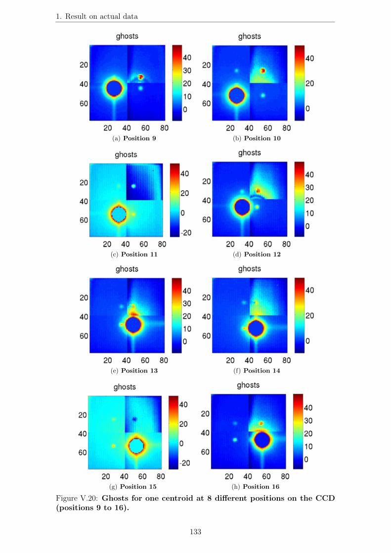
1. Result on actual data
(a) Position 9 (b) Position 10
(c) Position 11 (d) Position 12
(e) Position 13 (f) Position 14
(g) Position 15 (h) Position 16
Figure V.20: Ghosts for one centroid at 8 different positions on the CCD(positions 9 to 16).
133

Chapter V: NEAT lab demo: results and conclusions
connecting the chip and the readout electronics (outside the vacuum chamber) wasretro-fitted with a large and low-impedance ground connection. More precisely, thenew connection was a copper adhesive tape manually welded to the chip mass pins.However the tests indicated no change of the ghosts intensities after the intervention.
Another idea was to tamper with the CCD voltage controls and see if it has anyeffect on the ghosts. In order to be able to do this in an interactive manner, anew advanced type of quicklook was developed and included in a new version ofthe labview acquisition/control program. This new utility allow a visualization ofthe ghosts in real time, by performing a quick processing. The processing consistin an offset for each quadrant that bring their background levels to the same value(using either a median pixel count value, or the maximums in the distributions ofcounts), and min/max thresholds for pixel counts values. Truncation of pixel valuesis essential to bring the dynamic of the image to values typical of ghost intensities.Simply displaying counts on a log scale is not as good because it still attributesa large part of the color scale to the central part of the centroids. The result ofthis test was that some values result in significantly lower ghost intensities (abouta factor 5 for the brightest ghosts), but it also produces large noisy halos aroundsome ghosts (like in Fig. V.19, positions 4 to 8). This makes the ghosts impossibleto avoid while the relative intensity is still too high to completely ignore them.
(b) Avoiding the ghosts
To avoid the ghosts, we restrict ourselves to a smaller set of positions. Because thedistance between the outer stars is about 40 pixels (the width of one quadrant),avoiding ghosts for one star tends to make ghosts avoided for all stars, by symmetryof the configuration. This is illustrated by Fig. V.21(a): even though there are15 ghosts and 5 stars on a 80x80 pixels, there are some positions for which noghost is under a star. In a real configuration, stars are not perfectly aligned withthe vertical/horizontal direction (this depends on the mask insertion). If the miss-alignment is too large, the number of available positions decrease. Figure V.21(b)shows a map of the correct pixels for the position of the central star. For all theblack pixels, there is no ghost closer to 6 pixels of a star (condition on the euclideandistance between the centers of both ghosts and stars) or closer to 6 pixels from theedge of the CCD.
Thanks to the real time ghost visualization mode, at any time we can in principlecheck that all the ghosts are visible and not under a centroid, before even taking data.Unfortunately, the pinhole mask was damaged when trying to find a good alignmentof the centroids. Multiple optical ghosts are crowding the field and preventing aneasy identification of the electronic ones (Fig. V.22). New pinhole masks have beenordered and will solve this problem.
(c) Ghosts: course of action
An early test of centroid accuracy with centroids both CCD voltage controls (“nor-mal” and “low ghosts” voltages), where the centroid where in avoiding ghosts posi-tions did not show any difference any accuracy (accuracy of 1× 10−3 pixel in bothcases). From this test we have concluded that at this stage the ghosts were not thelargest error factor.
134

1. Result on actual data
(a) Illustration of a good ghost con-figuration, caused by symmetries.Real stars are in black, ghosts are in red.
Positions without ghosts
20 40 60 80
20
40
60
80 0
0.5
1
(b) Map of the ghost avoiding star positions:central star on black pixels. The map was gen-erated using the relative star positions measured witha real pinhole mask, where the stars have a 20◦ missalignment.
Figure V.21: How to avoid ghosts.
For the time being, the course of action is to use the standard (and supposedlyoptimal) CCD voltage controls and to only use positions where the ghosts are knownto be far from the centroids, as indicated by Fig. V.21(b). This produces ghostswith relative intensities of a few parts per thousand but which are most of the timewithout large halos. When the new pinhole masks will be available, a better controlon the ghosts positions and shapes in real time will be possible.
1.3.2 Quasistatic and dynamic analysis of star positions (-10◦C, in vac-uum)
On real data, we perform both types of analysis for each setup (quasistatic anddynamic). Each setup produces a data set which consist of several data cubes (oneper position of the translation stage). We typically use 2 to 12 different positions,depending on where we allow the centroid to be placed. Because the CCD is only 80by 80 pixels with 4 quadrants, we have much fewer positions available if we want toavoid putting the central star at the limit between two quadrants or near ghosts andmoving from one quadrant to another. The quasistatic analysis only need one datacube (one position) to work, for analysis we simply split the cube into batches. Thedata set that we present here has 12 positions, 3 on each quadrant. Figure V.23(a)shows where we have put the central star for the 12 measurements. The positions areapproximative to about 1 pixel, the position control was done manually by lookingat the image of the stars with the quick look utility. A visual fine tuning is neededbecause the translation stage has asymmetric motion speeds and directions and noposition control indicator (open control loop). Figure V.23(b) is an image of thestars for one of the positions.
(a) Quasistatic analysis
135

Chapter V: NEAT lab demo: results and conclusions
ghosts
20 40 60 80
20
40
60
−20
0
20
40
60
80
100
Figure V.22: Optical ghosts caused by mask damage. The peak value of thestars is at 20000 counts: the dynamic of the image is limited to 0-0.5%.
�
��
��
� �� ��
�
�
�
�
��
��
� ��
����
(a) The positions used for the differ-ential star position analysis, numberedfrom 1 to 12.
Pseudo stars average image
20 40 60 80
20
40
60 0.5
1
1.5
2
x 104
(b) Images of stars for position 8.
Figure V.23: Illustration of the pseudo star data set.
For this analysis the CCD is not moved, the relative apparent motion is caused byvibrations and photon noise. There is an important rule of thumb to keep in mind,derived from the following facts:
• Mechanical stability tests have shown that the positions of star are stable toσmotion = 3× 10−3 pixels over 100 sec
• The dynamical analysis (next paragraph) shows that even without calibration(of pixels QEs or positions), the differential accuracy when moving over severalpixels is better than σcentroid = 1× 10−3 pixel
• In order to have uncorrelated errors on the centroid, it has to be moved byseveral pixels
Thus, the differential errors between centroid location should be lower than: σmotion×σcentroid = 3 × 10−6 pixels (we have taken a safety margin here by considering thaterrors can become independent for a motion as small as one pixel). This tells us
136
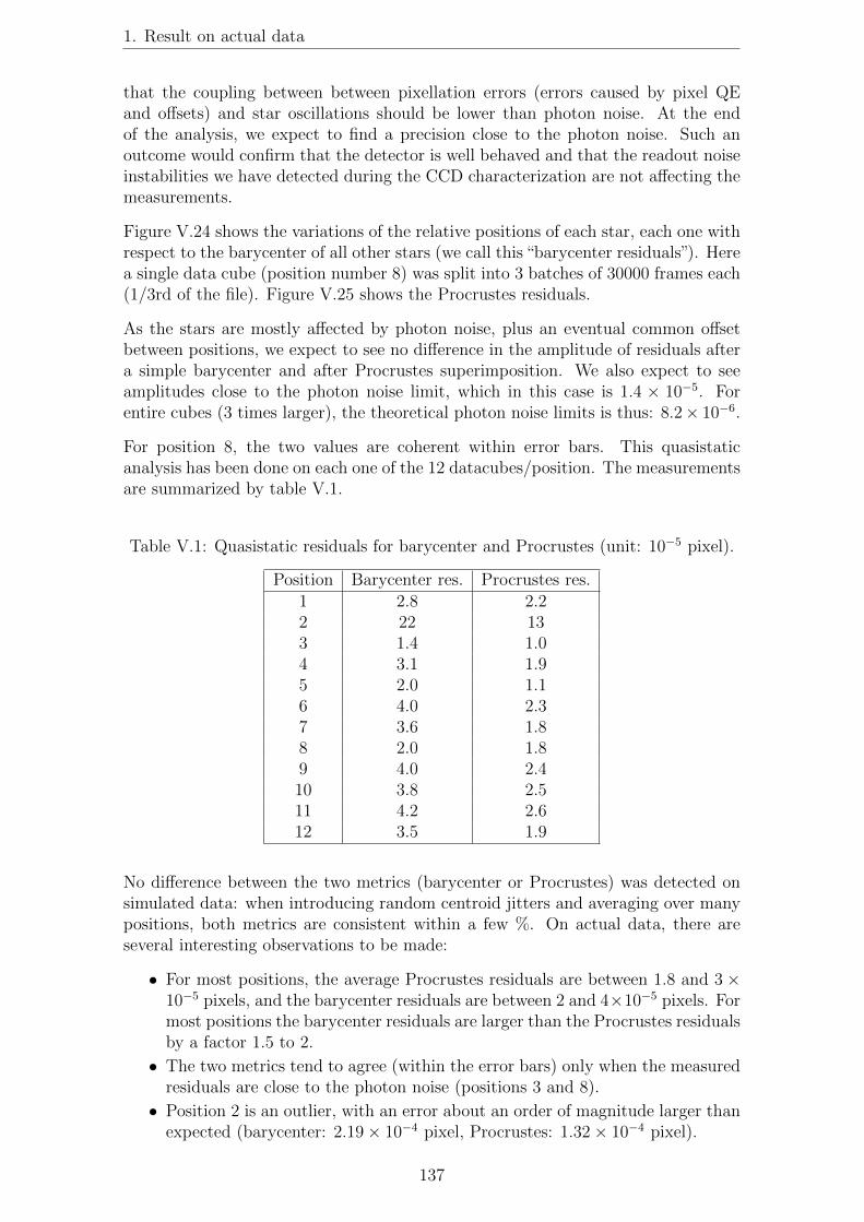
1. Result on actual data
that the coupling between between pixellation errors (errors caused by pixel QEand offsets) and star oscillations should be lower than photon noise. At the endof the analysis, we expect to find a precision close to the photon noise. Such anoutcome would confirm that the detector is well behaved and that the readout noiseinstabilities we have detected during the CCD characterization are not affecting themeasurements.
Figure V.24 shows the variations of the relative positions of each star, each one withrespect to the barycenter of all other stars (we call this “barycenter residuals”). Herea single data cube (position number 8) was split into 3 batches of 30000 frames each(1/3rd of the file). Figure V.25 shows the Procrustes residuals.
As the stars are mostly affected by photon noise, plus an eventual common offsetbetween positions, we expect to see no difference in the amplitude of residuals aftera simple barycenter and after Procrustes superimposition. We also expect to seeamplitudes close to the photon noise limit, which in this case is 1.4 × 10⁻⁵. Forentire cubes (3 times larger), the theoretical photon noise limits is thus: 8.2× 10⁻⁶.
For position 8, the two values are coherent within error bars. This quasistaticanalysis has been done on each one of the 12 datacubes/position. The measurementsare summarized by table V.1.
Table V.1: Quasistatic residuals for barycenter and Procrustes (unit: 10−5 pixel).
Position Barycenter res. Procrustes res.1 2.8 2.22 22 133 1.4 1.04 3.1 1.95 2.0 1.16 4.0 2.37 3.6 1.88 2.0 1.89 4.0 2.410 3.8 2.511 4.2 2.612 3.5 1.9
No difference between the two metrics (barycenter or Procrustes) was detected onsimulated data: when introducing random centroid jitters and averaging over manypositions, both metrics are consistent within a few %. On actual data, there areseveral interesting observations to be made:
• For most positions, the average Procrustes residuals are between 1.8 and 3×10−5 pixels, and the barycenter residuals are between 2 and 4×10−5 pixels. Formost positions the barycenter residuals are larger than the Procrustes residualsby a factor 1.5 to 2.
• The two metrics tend to agree (within the error bars) only when the measuredresiduals are close to the photon noise (positions 3 and 8).
• Position 2 is an outlier, with an error about an order of magnitude larger thanexpected (barycenter: 2.19× 10−4 pixel, Procrustes: 1.32× 10−4 pixel).
137
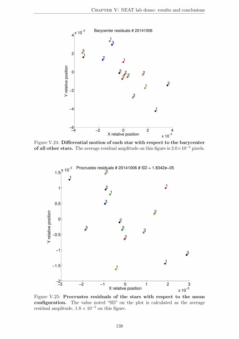
Chapter V: NEAT lab demo: results and conclusions
−4 −2 0 2 4
x 10−5
−6
−4
−2
0
2
4x 10
−5
1
1
1
1
1
22
2
2
23
3
3
3
3
X relative position
Y r
ela
tive
po
sitio
n
Barycenter residuals # 20141006
Figure V.24: Differential motion of each star with respect to the barycenterof all other stars. The average residual amplitude on this figure is 2.0×10−5 pixels.
−3 −2 −1 0 1 2 3
x 10−5
−2
−1.5
−1
−0.5
0
0.5
1
1.5x 10
−5
1
1
1
1
1
2
2
2
2
2
33
3
3
3
X relative position
Y r
ela
tive
po
sitio
n
Procrustes residuals # 20141006 # SD = 1.8342e−05
Figure V.25: Procrustes residuals of the stars with respect to the meanconfiguration. The value noted “SD” on the plot is calculated as the averageresidual amplitude, 1.8× 10⁻⁵ on this figure.
138

1. Result on actual data
We are unsure of the cause of this observations, it could be linked to an instabilityof the ghosts or an instability of the readout noise (even at 30 counts the readoutnoise must be non Gaussian to become significantly larger than photon noise).
(b) Dynamic analysis
For this analysis the stars are moved together by translation of the CCD of about3 pixels between each position. Figure V.26 shows the Procrustes residuals of thecentral star, for all 12 positions (without flat field nor metrology calibration). Theaverage residual distance, calculated over all centroids and positions is 1.8± 0.14×10⁻³. Figure V.27 shows the Procrustes residuals for all the stars for positions 7 to9 (without flat field nor metrology calibration). In this case, the average residualdistance, calculated over all centroids and positions is 3.6±0.59×10⁻⁴. For the samepositions, with flat field calibration, the accuracy is 2.8± 0.45× 10⁻⁴ (Fig. V.28).
One can see that the for the central star (in black), the residuals of the 12 positionsare clustering into 4 groups of 3 positions, which corresponds to the central star onthe same quadrant. The position of the clusters are symmetric with the relativepositions of the quadrants on which the central star was placed. It indicates thata systematic error is introduced when the central star goes from one quadrant tothe next. A possible explanation is that there are larger or smaller than averagegaps between the pixels at the quadrants limits. Gaps seem to appear in-betweenquadrants in the maps of measured pixels offsets (see Fig. V.16 in the metrologyresults).
The error bar on the magnitude of the Procrustes residuals is computed by assum-ing that the stars are affected by random Gaussian offsets: it takes into accountthe number of centroids and positions over which the averaged residual distance isobtained. It implicitly assumes that the errors are homogeneous over the CCD. Theerror is only meaningful as a lower bound, in practice the variation of the estimatedaccuracy is dominated by what kinds of systematics are introduced into the data, byquadrants and ghosts, which are not (spatially) homogeneous at all. The amplitudeof the residuals depends on where the stars are.
The accuracy (estimated as the average amplitude of Procrustes residuals) was de-termined for each group of 3 positions for which the central star is always on thesame quadrant. The best result was obtained for the positions 7, 8 and 9. Theaccuracies for each set of 3 positions (with flat field calibration only) are:
• Positions 1,2,3: 8.2± 1.3× 10⁻⁴
• Positions 4,5,6: 4.0± 0.63× 10⁻⁴
• Positions 7,8,9: 2.8± 0.45× 10⁻⁴
• Positions 10,11,12: 1.2± 0.19× 10⁻³
The magnitude of the changes are much larger than the expected random errors fora CCD with homogeneous spatial properties. The large differences are likely to becaused by ghosts positioning. We have used the set of positions 7,8,9 only to testwhether the calibrations improve the accuracy. Table V.2 summarizes the resultsfor all configurations (relative to the types of calibrations used).
The conclusion comes easily: the flat calibration improves the accuracy, whereas themetrology does not. It is not surprising given the fact that we have checked the flat
139

Chapter V: NEAT lab demo: results and conclusions
−6 −4 −2 0 2 4
x 10−3
−2
−1.5
−1
−0.5
0
0.5
1
1.5
2
2.5x 10
−3
11
1
1
1
22
2
2
2
3
3
3
3
3
4
4
4
4
4
5
5
5
5
56
6
6
6
6
7
7
7
7
78
8
8
8
8
99
9
9
910
1010
10
10
11
11
11
11
11
12
12
12
12
12
X relative position
Y r
ela
tive
po
sitio
n
Procrustes residuals # 20141006 # SD = 0.0018072
Figure V.26: Procrustes residuals of the stars with respect to the meanconfiguration (for 12 positions).
Table V.2: Accuracies with different types of calibrations (unit: 10−5 pixel).
- No flat flatNo metrology 3.6± 0.59× 10⁻⁴ 2.8± 0.45× 10⁻⁴
Metrology 5.9± 0.94× 10⁻⁴ 4.3± 0.69× 10⁻⁴
field for systematics down to a level of 5× 10−5 pixels, whereas the metrology couldnot be verified in the same manner because of hardware issues.
140

1. Result on actual data
−4 −3 −2 −1 0 1 2 3 4
x 10−4
−8
−6
−4
−2
0
2
4
6
8x 10
−4
11
1
1
1
2
2
2
2
2
3
3
3
3
3
X relative position
Y r
ela
tive p
ositio
n
Procrustes residuals # 20141006 # SD = 0.00036664
Figure V.27: Procrustes residuals of the stars with respect to the meanconfiguration (for 3 positions, no calibration).
−6 −4 −2 0 2 4
x 10−4
−4
−3
−2
−1
0
1
2
3
4x 10
−4
1
1
1
1
1
2
2
2
2
2
33
3
3
3
X relative position
Y r
ela
tive
po
sitio
n
Procrustes residuals # 20141006 # SD = 0.00028083
Figure V.28: Procrustes residuals of the stars with respect to the meanconfiguration (3 positions, flat calibration).
141

Chapter V: NEAT lab demo: results and conclusions
2 Conclusions on the data analysis
2.1 Metrology
The most obvious and disappointing conclusion of our experiment is that correctionof pixel offsets from metrology measurements did not work. It seems that we havemeasured pixel offsets to about a bit better than a percent, but we expect true pixeloffsets to have a SD of only 1.5×10⁻³ (from JPL data), so we have in fact measuredmostly noise. The cause of these bad metrology measurements is an unidentifiedsource of red noise in metrology data, specific to our testbed. Several observationspoint to this conclusion:
• Allan deviations of our metrology data become worse when more frames areused.
• The metrology calibration did improve the accuracy for simulated data (downto 10−6 pixel) and for data from the VESTA experiment (down to 1.8× 10⁻⁴
pixel).
• Allan deviation on VESTA data is photon limited for the horizontal fringes.
The nature of the red noise in metrology data is unclear, so far we have consideredthe following possibilities:
Stray light inside the baffle or the vacuum chamber. We have made tests inthis direction and observed that when removing the baffle spatial averagingoffsets over zones of pixels was less effective. However the effect on individualpixel offsets was not sensible.
Ghost fringes and CCD instabilities. Just like there are ghost images of thestars symmetrical with respect with the quadrants, there may be ghosts fringesat a level of a few parts per thousand. These are much harder to detect becauseall the CCD is illuminated at once and constantly moving: one can not simplyintegrate for a long time to see them though photon noise. Attempts to detectsystematics from videos of pixel offset residuals (displayed versus time) did notshow anything obvious, except for the anomalous quadrant. Simulations haveshown that ghosts fringes at a few part per thousand do affect Allan deviationand slightly bias the final pixel offsets, but it does not look like red noise(integrating longer is still beneficial) and the biases are smaller than what weobserve on real data.
Damaged fiber tips. Although we have checked visually that all 4 beams for thefiber tips that were used for the metrology data where clean, we still see astray light pattern on the map of pixel offsets on the X axis which is similarwhich the patterns obtained with damaged fiber tips.
2.2 Flat fields
A positive point of the experiment is the accuracy of the flat field, for which we havemade great progress. The new flat field system provides a very good accuracy, whichhas been tested for systematics down to a level of 5× 10⁻⁵ (relative errors). This isvery close to the specification required to reach the final objective. Because of the
142

2. Conclusions on the data analysis
difference between expected and observed errors from flat field (see Fig. V.29), theaccuracy of the calibration may already be sufficient.
The most notable improvement was brought by switching from laser light to whitelight. This is also a positive change from a spectral point of view, the spectrumof the light is more similar to the pseudo stars (although not identical, we havea white LED instead of the tungsten filament). We expect an eventual spectraldependency of the pixel QE to be less visible with the new system. The flat systemwould be even better with a supercontinuum source with a SMF (to eliminate thepossibility of speckles), but with the current results, there is no strong need for acostly supercontinuum source.
Further improvements were visible when upgrading the baffling inside the vacuumchamber. Systematic effects caused by stray light could either be detected directlyor by looking at difference between flat fields. Although flat fields were in practicethe most successful mode for identifying stray light sources, we have also sometimesused flats from metrology fibers or both. An improvement of data quality for asource of stray light detected with either mode is likely to be beneficial to bothsystems because all the fibers (multimode and singlemode) are close to each otherand are thus likely to be affected by the same stray light sources. Because of this,the conclusions about stray light are presented separately.
2.3 Stray light
With the metrology and the flat field systems, we have identified and taken care ofthe following stray light reflections:
• On the zerodur bench. We have placed an array made with black paper andrazor blades to solve this issue.
• On the piece holding the liquid core fiber (for the pseudo stars). Severalrazor blades have been placed on this piece to prevent direct reflections fromoccurring.
• On the edge of baffle vanes. The new vanes made with razor blades have solvedthis problem (baffle v4).
• Conjugate reflection between the pinhole mask and the CCD, caused by themirror. A stray light shutter has been installed in front of the mirror.
2.4 Centroids (plus corrections from flat and metrology)
Figure V.29 summarizes the results obtained on simulated and actual data into asingle picture, by comparing the relative error levels. The leftmost column shows therelative amplitude of the main sources of errors, estimated from actual testbed data.The values are indicated in accordance to their definitions in table IV.2 (section3.2), they are either dimensionless or in pixel units). The coefficients of the secondcolumn also correspond to the results presented in the former table, they are theresults of Monte Carlo simulations on synthetic data. The rightmost column arethe accuracies measured for the pseudo stars in different configurations (for actualdata).
143
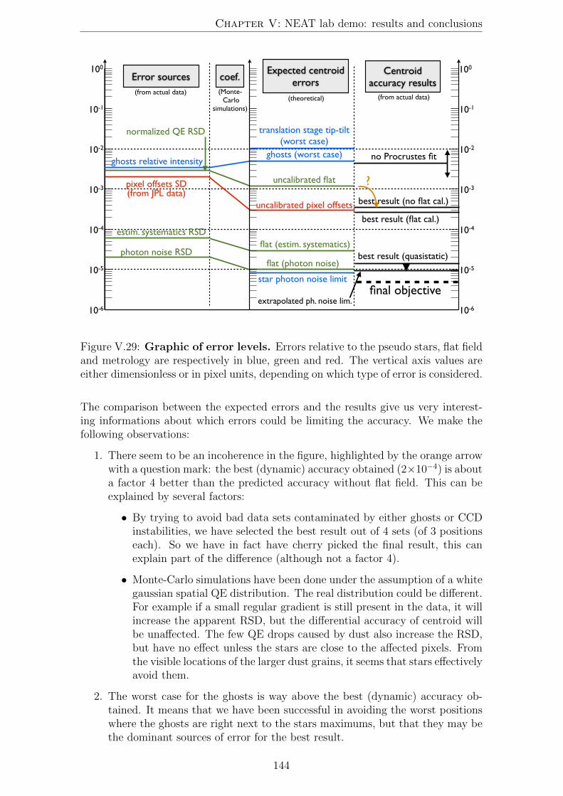
Chapter V: NEAT lab demo: results and conclusions
���
����
����
����
����
����
����
���
����
����
����
����
����
����
������������������������
������������������
�������������������
��������������������������
����������������
�������������������������
����������������������
���������������������������������������
�������������������������
�����������������
����������������
����������������������
��������������������������������
�������������������������������
���������������
���������������������
�������������������������
�����������������������
����������������
��������������
��������������
������������
�
�������������������������������������������������
���������������������������
Figure V.29: Graphic of error levels. Errors relative to the pseudo stars, flat fieldand metrology are respectively in blue, green and red. The vertical axis values areeither dimensionless or in pixel units, depending on which type of error is considered.
The comparison between the expected errors and the results give us very interest-ing informations about which errors could be limiting the accuracy. We make thefollowing observations:
1. There seem to be an incoherence in the figure, highlighted by the orange arrowwith a question mark: the best (dynamic) accuracy obtained (2×10⁻⁴) is abouta factor 4 better than the predicted accuracy without flat field. This can beexplained by several factors:
• By trying to avoid bad data sets contaminated by either ghosts or CCDinstabilities, we have selected the best result out of 4 sets (of 3 positionseach). So we have in fact have cherry picked the final result, this canexplain part of the difference (although not a factor 4).
• Monte-Carlo simulations have been done under the assumption of a whitegaussian spatial QE distribution. The real distribution could be different.For example if a small regular gradient is still present in the data, it willincrease the apparent RSD, but the differential accuracy of centroid willbe unaffected. The few QE drops caused by dust also increase the RSD,but have no effect unless the stars are close to the affected pixels. Fromthe visible locations of the larger dust grains, it seems that stars effectivelyavoid them.
2. The worst case for the ghosts is way above the best (dynamic) accuracy ob-tained. It means that we have been successful in avoiding the worst positionswhere the ghosts are right next to the stars maximums, but that they may bethe dominant sources of error for the best result.
144

2. Conclusions on the data analysis
3. The best dynamic accuracy fall very close to the level predicted without pixeloffset calibration. It is very tempting to conclude that the dominant source oferror are the uncalibrated pixel offsets. It may not be the case because:
• The pixel offsets have not been properly measured in our experiment, theestimation of the QE RSD is actually based on JPL data.
• Just like for the flat field, the QE spatial distribution may not be whiteand Gaussian, resulting in a wrong coefficient between the RSD and theexpected errors on centroids.
145

Chapter VI
Conclusions and perspectives
In this chapter I will review the results that have been obtained for both the as-trophysical aspect (section 1) and instrumentation aspect (section 2) and I will putthem in the broader context of exoplanet research.
Given the current situation with the testbed, the founding of my PhD was extendedto the end of 2014 in a last effort to improve the performances. At the date ofcompletion of this manuscript, the new metrology is at last operational on all fibersand new tests will tell if the stray light control has improved the quality of the dataor not. However the troublesome issue of ghosts will be hard to workaround in theremaining time. The surest way to deal with the ghost problem would be to changeeither the CCD and its readout electronics or the translation stage and to use onlytwo centroids on one quadrant. Regretfully, these major changes are not possiblewithin the timeframe of a PhD, which are subject to a rather strict limitation of 3years in France.
Concerning the astrophysical aspect of the Thesis, which has to do with the NEATmission concept and its science case, there are also a lot of possibilities that havebeen left unexplored. The time limit is a strong constraint in this case as well and ithas prevented me from doing some interesting refinements. Fortunately, the Theiaproposal comes at the right time and in this context I will be able to capitalize onthe work already done and expand it a little bit.
1 The NEAT/Theia mission concepts and the sci-
ence case for µas astrometry
1.1 Results for the science case
Based or the error budget of the NEAT mission1, which corresponds to a typicaldifferential astrometric accuracy of 0.7 µas.h−0.5, I have shown that NEAT is capableof finding dozens of nearby habitable planets. The closest of these would be the besttargets for direct imaging and spectroscopic characterization. I have presented aprocess from which one can:
1Error budget by Renaud Goullioud, referenced in appendix C
146

1. The NEAT/Theia mission concepts and the science case for µas astrometry
• Create catalogs of target and reference stars for a pointed astrometric missionaiming at detecting nearby exo-Earths
• Acquire various statistics about the reference stars and in particular check ifthe hypothesis made in the NEAT error budget are correct
• Estimate the science yield of the mission, as a function of mission and telescopeparameters, the distribution of the observation time between the targets
1.2 The new mission concept: Theia
The 4th ESA call for M class missions has been made, the deadline for the proposalshas been set to January the 15th. The former NEAT consortium will propose arevised version of the NEAT mission called Theia [Malbet et al., 2014].
One of the main critics of the NEAT proposal was relative to the cost estimation.To address the cost issue, the new Theia design will use a slightly downscaled mirror(about 0.6 to 0.8 m of diameter instead of 1 m). Formation flying was also a delicatepoint and will stay that way. As of now, µas astrometry with a TMA configurationis not demonstrated and we think that formation flying is still our preferred option(main design). A deployable boom design can still be presented as a backup option.
The exoplanet community is in a delicate situation for this new . . . . .ESA call, as two tran-sit exoplanet missions have already been selected by . . . . .ESA (. . . . . . . .PLATO and CHEOPS),in addition to another one of . . . . . . .NASA (TESS). To have a better chance of being posi-tively received, the Theia proposal will set aside more than 70% of its mission timefor other objectives than exoplanets, like dark matter study, dynamics of the galaxy,stellar clusters and extreme astrophysical objects, astrometry of Solar System aster-oids, measure of relativistic multipolar light deflection around Jupiter.
1.3 Future use of the catalog of targets and references
The work that has been done on the scientific case and the error budget of NEAThas to be updated to assess the exoplanet science case of Theia. With a smallermirror and about 15 to 30% of the mission time dedicated to exoplanets, which is adrastic reduction compared to NEAT, what science can we do?
To answer this question, we can use a combination of three tools:
The NEAT/Theia catalog of target of references The catalog can be directlyreused, the stars have not changed!
The Theia error budget The error budget has to be updated to the new Theiaparameters.
A planet population model Here they are several possibilities. We can for ex-ample use the planet population model from [Alibert et al., 2013a], the samethat was used for the NEAT double blind test. This model is mostly theoreticaland based on planet formation and migration simulations. Another possibilityis to use a distribution based on the results from the Kepler mission. Thefirst model is interesting because it provides information for a very large spaceof planet parameters, the second model is expected to be more reliable and
147

Chapter VI: Conclusions and perspectives
conservative in the number of predicted detections if we restrict the analysisto the actual Kepler detection space and do not extrapolate.
This combination of tools is very powerful. Not only it can answer the initial ques-tion, it is possible to go into finer details, like for example:
• For a given mission time how many stars can we survey, at which accuracy?
• What will the exoplanet yield look like (in terms of parameters distribution)?
• Depending on the number of habitable planets we aim to detect, what is theminimal fraction of the mission needed for exoplanets?
• What is the best trade-off between the number of targets searched for exo-planets and the accuracy, relative to the yield?
• Can we optimize the yield by changing the time distribution between thetargets?
1.4 Improvements on the catalogs of targets and referencesand yield simulator
There are numerous improvements possible for the catalogs of targets and references,in some areas very significant simplifications had to be made. Further studies areneeded to make progress on some particular points.
Complete the catalog of targets with M stars Very close (early) M stars areinteresting to observe with NEAT, exoplanets in their HZ can be detected byastrometry. There is a large overlap with radial velocities in this case, but insome ways it is an advantage: the detection power increase when combiningthe two methods, which is also a very good way to confirm eventual detectionsand to better separate the stellar noise from the planetary signals. Thesefew stars would constitute a very valuable case study of how to extract theplanet signals from the steallar noise. Habitable exoplanets around these starscould be observed with future giant telescopes. We have realized that quite afew M stars are missing in Fig. I.9 (for example Barnard star, with a visiblemagnitude of 9.5, should be visible near the top!). These stars are not inthe catalog because the filter used to determine stars that are on the mainsequence is too restrictive.
Better way to filter main sequence stars The filter used to select main sequencestars is tricky to define. We have used the following types of regular expres-sions (here for F stars): matches(SpType,"^F.*(IV-V|[^I]V)"). It considersmain sequence stars the ones which contain the following string in their Sp-Type columns: “IV-V”, “V” or “V” plus some flags before or after it, and ofcourse it excludes “VI”. For stars with two components (separated by a “+”sign), we should ideally base the selection on the main component. However,errors will be made if the secondary component only is main sequence: withthis regular expression, the star will be included in the list. The problem isthat it is not possible to use a “\” sign in the regular expression (it causesan error in Topcat), it this therefore impossible to get the needed escaped“+” in the regular expression. The spectral type of Barnard star indicated byHipparcos is “sdM4”, which explains why it was not in the final catalog. We
148

1. The NEAT/Theia mission concepts and the science case for µas astrometry
have also lost Sirius A (SpType: “A0m...”). Close M stars can also be found inthe MEarth catalog [Dittmann et al., 2014], with more suitable spectral types.Another way of filtering the main sequence stars that could be more reliablewould be to use their position on the HR diagram.
Update the catalogs with the Gaia survey When the Gaia survey will be re-leased, more precise parallaxes will be known, compared to the Hipparcos ones.This will make a big difference for the reference stars: we will have more infor-mation about their true distances. Both the targets and the references starscatalogs could be derived from the Gaia survey. It will also include all theclosest M stars that are of interest for our astrometric survey.
Refine the columns calculations The current method to obtain the astrometricsignal in HZ is approximative. A number of refinements can be made, such as:
• Using a piecewise power law, instead of simply L ∝ M3.8. This is impor-tant when we consider M stars.
• Updating the HZ inner and outer edges with the latest published results[Kopparapu et al., 2013].
Improve the error estimation for reference stars The photon noise from thereference stars is calculated as a function of the sum of the fluxes of all referencestars. A more realistic estimation has to take into account the geometricconfiguration of the reference stars. For example if there is only one brightreference star, rotation errors will be larger.
Take into account multiple stars Companions are always counted as valid ref-erence stars. This is an optimistic assumption: for small separations, it couldbe impossible to obtain accurate measurements of the centroids for each com-ponent. In this case the astrometric solution is actually harder than for asingle star, the orbital parameters of the close binary have to be subtractedaccurately before the planets can be detected.
Improve the integration and automation of the tool The current version re-lies a lot on Topcat and uses lots of different tools. The consequence is thatin order to run a new simulation with different parameters, everything has tobe done and checked manually (there are dozens of steps), this is impractical.The issue can be mitigated by exporting the catalogs of targets and referencesbefore making all the NEAT new columns. The equivalent reference flux cal-culation and all remaining columns would then be calculated automatically bya script.
1.5 Near and mid-term perspectives in exoplanetology
Three transit missions, namely TESS, CHEOPS and PLATO have been selectedfor launch within the next 10 years. These missions will be nicely complementedby Gaia which will find thousands of longer period giant planets (with the bestsensitivity for timescales of a few years) and direct imaging for young bodies evenfurther away. This will give us a very rich picture of the distribution of planets andwe will have a more comprehensive view of planet formation. We will also havethe JWST to do follow-up transit spectroscopy on the most interesting targets andwe have a chance of detecting biomarkers with it, for the easiest ones. However
149

Chapter VI: Conclusions and perspectives
this kind of science will be near the limit of technical capabilities and we will in alllikelihood not be able to make a detailed study of an exo-Earth around a Sun-likestar with the JWST, unless we get lucky and get a very close habitable transitingplanet.
In the meantime, ground-based transits and RV surveys around low mass stars mayfind very close habitable Earth and super-Earths, which would be prime targets fortransit/coronagraphic spectroscopy. It is also interesting to note that in the case ofnon-transiting habitable planets around M stars, coronagraphic spectroscopy withthe next generation of ground-based giant telescopes (ELTs) is more advantageousthan in space and should be the first method to obtain spectra of terrestrial habitableplanets [Guyon and Martinache, 2013]. The small separations between the stars andthe planets and the need to observe in the near infrared result in the need for a verylarge pupil. It will be interesting to see how much further can the accuracy bepushed for the RV method.
In the longer term, coronagraphs (ground based as well as space born) will offer ahigher potential to find and spectroscopically characterize the closest targets becausethey can be much less sensible to the photon noise from the star (we have explainedthis in section 1.2.8). So far, astrometry has only played a marginal role in theexoplanet research. Although Gaia will only detect giant exoplanets, when themission will be completed (around 2019), the number of exoplanets detections byastrometry is expected to be more than all other methods combined [Perryman et al.,2014]. On can hope that it will bring astrometry to the forefront of the researchwhen considering future missions.
2 The NEAT lab demo
2.1 General feedback on the project and teamwork aspects
A lot of people have worked together to make the NEAT lab demo possible and I amvery grateful to all of them. I interacted with people from various backgrounds andspecialties (researchers, engineers, interns, mechanics, opticians, electricians. . . ), inorder to design and build the NEAT testbed. Overall, the teamwork has been anenjoyable and rewarding experience. I have been able to gain in autonomy through-out the process and interact more directly and more effectively with everyone. Afterthe testbed was assembled, I was able to manage the upgrades on the testbed andits operation myself and this was very satisfying.
Another positive aspect of the work is my collaboration with JPL. My first experi-ence at the JPL on the VESTA team, which was composed of Mike Shao, ChengxingZhai, Bijan Nemati and Inseob Hahn, provided me invaluable experience for ourtestbed. Our collaboration was been very fruitful and is still ongoing. In this con-text, we have recently exchanged testbed data (in both ways, JPL data to Grenobleand vice versa) and have some teleconferences to discuss the results. Comparativeanalysis of both data sets will help us to improve the processing and to understandand deal with specific noises in the data. We are also planning a trip to IPAG forChengxing Zhai at the end of November: we will work together on the NEAT demotestbed during one week.
150

2. The NEAT lab demo
The project approach has been a good way to put things together rather quickly.We were able to design and assemble the testbed within 2 years: first light on bothmetrology and pseudo stars was obtained in July 2013, leaving more than one yearto work with an operational testbed. Yet the final objective is very ambitious and wehad to face unanticipated difficulties which have strongly limited the performancesso far. In the next part I will talk about the many kinds of upgrades we can do onthe testbed: there are interesting smaller upgrades that can be done before the endof the year.
2.2 Possible improvements for the NEAT lab demo
The final accuracy obtained from the experiment at this stage is not particularlythrilling. We are far from having demonstrated accuracy down to 5 × 10⁻⁶, whichwould allow detection of exoplanets in habitable zone of nearby stars with the NEATconcept. Our experiment has been impeded by a range of issues, that when combinedtogether, makes it hard to make significant progress. The main dilemma is that wewant less pseudo stars to avoid being plagued by electronic ghosts, but we need all5 stars to correct the tip-tilt of the translation stage. Despite the disappointingresults, there are multiple interesting avenues for improvements.
2.2.1 Averaging errors over several detector positions
The first important aspect to mention for the experiment is the possibility to averagethe systematic errors caused by pixels over several positions. This is very interest-ing, because the same technique can be applied for an actual mission as well. Wehave vaguely made a reference to this in chapter 2, where we have said: “Anotherstrategy can be to break each single epoch measurement into several individualsmeasurements in order to average systematic errors”. In the particular case of errorscaused by pixels, the mitigation strategy would be done by taking data on multiplelocations on the CCD (for a single epoch). In the case of a space telescope as wellas with our experiment, we can apply a common translation to generate in principleas many positions as we want, in practice limited by the size of the detector. Thefinal measure of the relative positions is obtained by averaging over all the detectorpositions.
For a real instrument, the number of positions that can be averaged per epoch woulddepend on many parameters. For NEAT, it would be possible to use hundreds ofpositions, because a single epoch measurement lasts typically several hours and asmall tip-tilt of the mirror can be used to apply the common translation motion veryquickly (500 Hz feedback loop for the position of the target star). If one acceptsthe assumption can systematic errors can be averaged efficiently by this technique,the final requirement is relaxed by a factor of 10 (to 5× 10⁻⁵ instead of 5× 10⁻⁶) ifwe average over 100 positions. The accuracy currently obtained is not that far fromthis value !
Even more interesting, we can in theory try to quantify how well this error averagingmethod works in our experiment: do we obtain the full expected accuracy gainof 1/
�Ndetector positions? Instead of looking directly at Procrustes residuals of each
position, we can look at Procrustes residuals between the relative stars positionsaveraged for several detector positions. Unfortunately, with the current setup, we
151
Chapter VI: Conclusions and perspectives
have access to very few positions (to avoid ghosts) and we had to work with only3 positions, which make the grouping described above impossible. If we can get tometrology to work properly, it should be possible to compensate for errors seen whenthe central star change quadrant (if pixel offsets between quadrant are indeed theircause). With 12 positions in a single analysis, we can make 3 groups of 4 positions,thus potentially gaining a factor of 2 in accuracy. However it will be hard push muchfurther, certainly not to 100 positions.
2.2.2 Hardware upgrades
There are numerous improvements that would be very beneficial for the testbed,the first of which is to change the detector and its electronics for a model with onlyone quadrant and with a stable readout noise. However this change is not realisticto make in the remaining timeframe (the current CCD, its readout took electronicsand the related software about 1 year to be developed and installed). I will presentsmall modifications that can be done before the end of the year first, I will talkabout more consequent modifications afterwards.
(a) Small upgrades
Bundle of SMF instead of pinhole mask. The current pseudo star system ismade from a pinhole mask, back illuminated by a large liquid core multimodefiber. In this configuration, it is not possible to illuminate the stars one at atime (it is all stars or nothing). By replacing this system with a a bundle ofSMF it will be possible to control every star independently, at least manuallywith the fiber connectors. By illuminating the stars one by one, we can checkthe ghosts much more easily (and even estimate their stability) because we donot have to deal with the signals of other stars on top of it. Having no photonnoise to deal with, we can quickly calibrate the ghosts for each position ifneeded.
Vantablack lining. The current material we are using to cover the interior of thebaffle is a black coating called “metal velvet” (acktar�). It has a reflectancecoefficient of 1% in the visible. We have contacted Surrey Nanosystems whichhave recently commercialized a new high performance black coating calledVantablack, which a reflectance coefficient of 0.04%, and will soon receive thenew sample. The new coating is very expensive though and we will not haveenough of it to cover all the baffle interior, this is more for experimentation.
Better stray light control neat the chip. There is a small very bright area aroundthe chip ( 0.3 cm2, see Fig. VI.1), a Zemax stray light model has indicatedthat it could be by far the dominant contributor to stray light inside the baffle,we are thinking of covering this area with a black material (the Vantablackwould be well adapted for this). However the operation is dangerous and thearea can not be completely covered because of the CCD bounding.
Installation of a shutter. In order to limit stray light during the flat field andmetrology measurements, we will put the stray light shutter in place, like itwas supposed to be from the beginning. We had concerns that the conjugatereflection with the mirror would affect the metrology, however a test with ashield on the mirror indicated that it is not the cause for the problematic red
152

2. The NEAT lab demo
������
����������������������
������
�����
�����������
����������������������
�����
������
Figure VI.1: Picture of the bright area around the chip.
noise we currently see (no major difference was observed in the Allan deviationswith/without the shield). So far the only confirmed effect in on the flat field.
(b) Major upgrades
Translation stage The current translation stage produces large tip-tilt jitter whentranslating the centroids (it is inherent to its design), this produces plate scalechanges between the detector positions. Consequently, it is necessary to have5 centroids to remove the platescale from the data. With a very stable stage,one would have the option to use only two centroid and look at the distancesprojected in the X and Y axis. This was done at he JPL, they initially has 3centroids, but turned off one of them because of electronic ghosts and workedwith only two.
Changing the CCD The testbed would benefit greatly from having a CCD withone quadrant only. Data processing would become much easier and several ma-jor problems would go away (ghosts, relative quadrant instabilities, anomalousquadrants).
2.2.3 Analysis and software upgrades
There are countless improvement that can be made to the matlab code, here I willonly mention the most critical ones in our situation:
1. The analysis of differential centroid accuracy used relative positions only andcan be coupled with the old method of measuring position (with Gaussian fits)which give an absolute position in the CCD index frame. This can be useful toplot variations in relative position versus absolute position on the CCD. Thisfunction will be useful to check that mechanical vibrations are nominal for alldata cubes: for one data cube used in our analysis (pseudo stars at position 2),the precision is far from photon noise. Possible causes are a CCD instabilityor a mechanical instability.
153
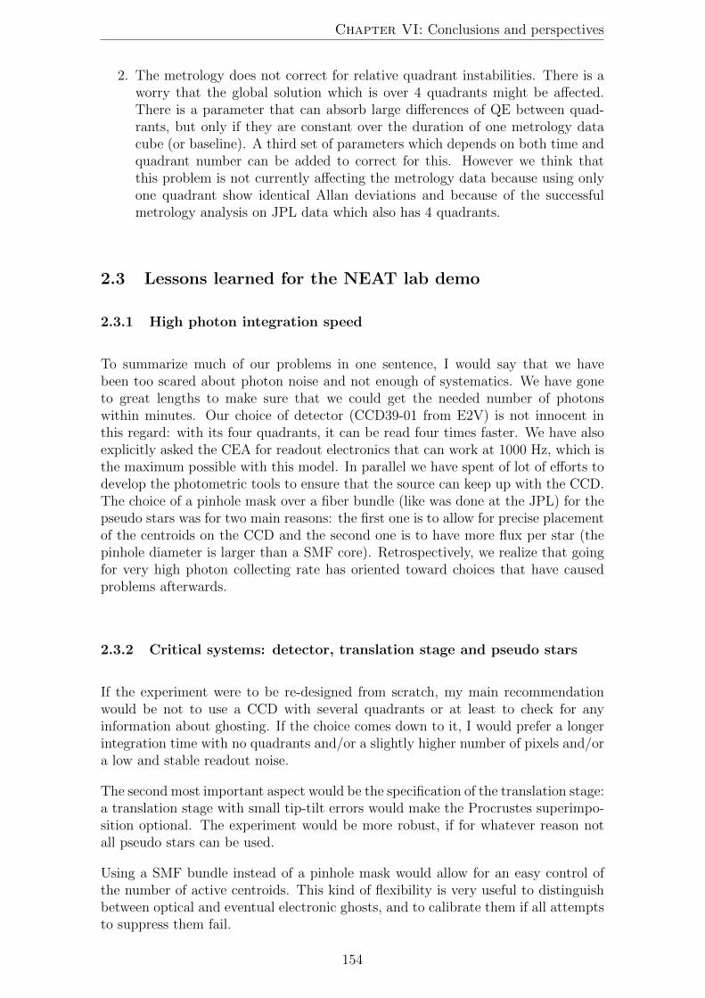
Chapter VI: Conclusions and perspectives
2. The metrology does not correct for relative quadrant instabilities. There is aworry that the global solution which is over 4 quadrants might be affected.There is a parameter that can absorb large differences of QE between quad-rants, but only if they are constant over the duration of one metrology datacube (or baseline). A third set of parameters which depends on both time andquadrant number can be added to correct for this. However we think thatthis problem is not currently affecting the metrology data because using onlyone quadrant show identical Allan deviations and because of the successfulmetrology analysis on JPL data which also has 4 quadrants.
2.3 Lessons learned for the NEAT lab demo
2.3.1 High photon integration speed
To summarize much of our problems in one sentence, I would say that we havebeen too scared about photon noise and not enough of systematics. We have goneto great lengths to make sure that we could get the needed number of photonswithin minutes. Our choice of detector (CCD39-01 from E2V) is not innocent inthis regard: with its four quadrants, it can be read four times faster. We have alsoexplicitly asked the CEA for readout electronics that can work at 1000 Hz, which isthe maximum possible with this model. In parallel we have spent of lot of efforts todevelop the photometric tools to ensure that the source can keep up with the CCD.The choice of a pinhole mask over a fiber bundle (like was done at the JPL) for thepseudo stars was for two main reasons: the first one is to allow for precise placementof the centroids on the CCD and the second one is to have more flux per star (thepinhole diameter is larger than a SMF core). Retrospectively, we realize that goingfor very high photon collecting rate has oriented toward choices that have causedproblems afterwards.
2.3.2 Critical systems: detector, translation stage and pseudo stars
If the experiment were to be re-designed from scratch, my main recommendationwould be not to use a CCD with several quadrants or at least to check for anyinformation about ghosting. If the choice comes down to it, I would prefer a longerintegration time with no quadrants and/or a slightly higher number of pixels and/ora low and stable readout noise.
The second most important aspect would be the specification of the translation stage:a translation stage with small tip-tilt errors would make the Procrustes superimpo-sition optional. The experiment would be more robust, if for whatever reason notall pseudo stars can be used.
Using a SMF bundle instead of a pinhole mask would allow for an easy control ofthe number of active centroids. This kind of flexibility is very useful to distinguishbetween optical and eventual electronic ghosts, and to calibrate them if all attemptsto suppress them fail.
154

2. The NEAT lab demo
2.3.3 Metrology
The integrated metrology system, from the source to right before the fiber tips hasbeen working well. Our choice to have everything in integrated polarization main-taining components (i.e. everything is fibered) results in a practical and compactsolution. A possible interesting alternative (also with only integrated components)would have been to use circular polarization with fiber stretchers for the phase mod-ulation. The advantages of this configuration over the current one: there is no needto manually align fiber tips axis and the attenuation is lower. Our phase modulatorshave indeed a rather strong attenuation (6 db), this has lead us towards a high powerlaser (22 mW). However the most problematic metrology issue we had to solve waswith the fiber tip holders. In our case their design is potentially critical (becauseof the baseline stability requirement) but not trivial. Because the first design wasover-specified for stability and used zerodur V-grooves we were unable to clean thefiber tips and the installation was very tricky (it took weeks!). In the end thesepractical considerations made us change the design.
2.3.4 Real time feedback
On the more positive points, there are things that have been tremendously useful,such as the quick look utility. Having the possibility to investigate and get rid of themost trivial issues in real time was a major advantage and allowed us to solve someproblems very quickly. The actual version of the quick-look has a normal (count)display and a temporal noise display, which are both useful. Along the way we havealso added a mode to detect ghosts and a remote command that can be used toexport a small cube of 25 images into a file. The latter functionality can be used bythe user to implement any kind of tricky signal processing on the raw image in quasireal time that would help solve a particular unanticipated issue. In our case we haveused it to build an iterative procedure that can reposition the translation stage to anaccuracy of 0.01 pixel. I would highly recommend to plan for these functionalitiesright from the start on any future similar experiment.
2.3.5 System automation
Another positive point was the almost complete automation of the system. Mostof the systems are controllable from a single interface, that presents itself as a veryconvenient Python wrapper. Thanks to the labview remote control interface, theCCD can also be controlled from the same interface. The only system that is notremotely controllable is the flat field source (because it was added at a very latestage), but flats can easily be taken manually at the beginning of the sequence.Unfortunately, various specific concerns prevent us from taking full advantage of thesystem and running in a completely automated mode, we need to at least be therefor some basic checks. The various issues are the stability of the readout noise, thepositions and sizes of the ghosts and the stray light shutter which can sometimesget stuck mid position.
155

Chapter VI: Conclusions and perspectives
2.3.6 Stray light
Stray light proved to be very hard to control. Given our very strict requirement onstray light for coherent metrology light, an integrated approach from the start wouldhave been more effective. In our experiment, many difficulties originated from thesmall size of the vacuum chamber and our choice to work with a very small off-axisangle to minimize geometrical aberrations on pseudo stars. There are a lot of ofphysical elements near the line of sight between the mirror and the CCD, includingthe walls of the vacuum chamber.
We were able to significantly improve the situation with a baffle and by shielding thephysical elements in the baffle FoV, this was sufficient for the flat field in incoherentwhite light. However, the stray light effect on the metrology which uses coherentlight is larger and is a likely cause for the red noise that limits the accuracy of thepixel offset measurement. In the VESTA experiment, at least one of the metrologybaselines has very good properties, which could be the consequence of good straylight control. It would be interesting to understand precisely how this was achieved(I currently have no details about the stray light control on VESTA for this dataset).
2.3.7 Numerical simulations
Numerical simulations proved to be an indispensable tool to debug and validate thedata analysis process and to refine our understanding of error propagation of allnoise sources. We have used stray light simulations very late in the experiment andwe have paid a heavy price for it. The integration of simulated data into the analysisprocess was done in a straightforward manner with a system of option parametersbecause I was working alone on the code most of the time. However the code israther complex and the system of option parameters has been pushed to its limits.In the context of a larger project, a better way to organize and document the codewould be needed, especially if several people are working together. One student hasdone an internship on data simulations for the NEAT lab demo and contributed toparts of the code, for example for the simulation of PSFs. I was not able to take fulladvantage of this work because of the lack of organization and documentation in ourrespective source codes and our lack of programming experience and best practices.
2.4 Future applications of the NEAT demo experiment
The issues we have encountered are however not fundamental and can be overcome:we have made numerous possible suggestions. There is also the interesting possibilityof averaging the residuals calibration errors, which we could not explore also becauseof the ghosts. Decreasing the calibration requirement by a factor 10 would resultin a much easier task. As a matter of fact, an accuracy better than 5 × 10⁻⁵
has already been demonstrated at the JPL (priv. comm.2). Short of reaching theultimate NEAT accuracy, there are other interesting applications for our experimentwhich have lower requirements.
2More information is available on a two-wheel Kepler white paper by Shao et al.http://keplerscience.arc.nasa.gov/K2/docs/WhitePapers/Shao_etal_Kepler_2Wheel.pdf
156

3. After my PhD...
On-board astrometry for spacecraft navigation in the Solar System The con-cept is to provide a way for a spacecraft navigating in the solar system to au-tonomously measure its position by performing astrometry on asteroids. Themore accurate the astrometry, the more accurate the estimated position. Thiswas the primary goal of the VESTA experiment, the requirement was set at2× 10−5 pixel (priv. comm.).
Detector calibration for accurate photometry Astrometry measures the av-erage photon location, whereas photometry is the total number of photons.Correction for the biases caused by the pixel QEs and offsets in the first casealso works in the other. There are several transits missions that will fly soonand that could benefit from a ground calibration. Space mission achieve goodphotometric accuracy by having a very stable pointing, but this does not workon long timescales because of relative star motions (proper motion, parallax,stellar aberration). A fine calibration of the CCD could at least recover most ofthe photometric accuracy on long time scales and at best relax the requirementfor high pointing stability if a full calibration can be relied upon.
Fine characterization of detectors A very wide application is simply the char-acterization of detectors (CCD and CMOS) in general. Manufacturers arelikely to be interested by a method that can accurately measure the propertiesof their products, as it can give them ways to control or improve them.
3 After my PhD...
One of the key motivations that drove me to work on NEAT is the detection ofclose habitable worlds. I will follow with great interest how the field evolves in thefuture and I hope I will have the opportunity to take part in new discoveries bydoing a postdoc related to exoplanets. In the current context, there will be manyopportunities to work on transit missions or coronagraphy.
Regarding transit missions, one way to contribute would be to assess the benefitsof a detector calibration for the accuracy of the mission, based on the results of theNEAT-demo and VESTA experiments. For coronagraphy, experience with detectorsand optical simulations will be a useful asset to work on laboratory testbeds. Mywork with the catalogs of targets/references and the exoplanet yield simulationsis also a good starting point to get more deeply involved in the scientific aspects.Another possibility for me is relative to the astrometry on the Gaia mission: I couldtry to integrate the DPAC (Data Processing and Analysis Consortium).
157

Appendix A
Animations
This section contains animations relative to some figures. These animations are onlycompatible with Adobe� Reader� which can be downloaded for free here.
Figure A.1: Animation showing the exoplanets discoveries year by yearon the mass-period diagram, from 1992 to 2013. As time goes on, one cansee that less and less massive planets are discovered: starting from 2004, we findmore and more planets with masses below 10M⊕, which are likely to be terrestrial.Go back to figure
158
10−1
100
101
102
103
104
105
106
10−5
10−4
10−3
10−2
10−1
100
101
102
Planet orbital period (day)
Pla
net m
ass (
Jupiter
mass)
Known exoplanets in 1992
HZ for M stars K stars G starsF stars
10 Earth mass (terrestrial limit)
Earth mass
Jupiter mass
Me
V E
Ma
J
S
U N
TransitsRadial velocitiesImaging or interferometryMicrolensingAstrometrypulsar

0.
Figure A.2: Illustration of the star/planet orbital dynamic (Credit:wikipedia). Go back to figure
159

Appendix B
Analysis of JPL data
In the context of our collaboration with the . . . . . . . .VESTA team at the JPL, they havekindly provided us with their data set from the 02/10/2012, which was the final oneused to demonstrate the VESTA performance at a level of 2× 10−5 pixel accuracy.
The data set includes:
• Two flat fields taken with a superluminous source• Metrology measurements on a vertical and horizontal baseline, plus associateddarks
• Pseudo star measurements for 30 different positions, with a common centroidtranslation of 3 pixels in the horizontal direction, plus associated darks
1 Flat fields
Figure B.1 shows the difference between the two normalized flat fields (at “step 3”,quadrant and irradiance normalized). Figure B.2 shows the normalized flat field(also quadrant and irradiance normalized). Figure B.3 shows the final flat.
flat diff (Q / irradiance norm.)spatial SD = 0.00052214
20 40 60 80
20
40
60 −2
0
2
x 10−3
(a) All pixels.
flat diff (Q / irradiance norm.)spatial SD = 0.00044867
20 40 60
20
40
60
−2
0
2x 10
−3
(b) Central area only.
Figure B.1: Quadrant / irradiance normalized flat field difference.
160

2. Metrology
flat (Q / irradiance norm.)spatial SD = 0.029291
20 40 60 80
20
40
60
0.6
0.7
0.8
0.9
1
(a) All pixels.
flat (Q / irradiance norm., center)spatial SD = 0.0017376
20 40 60
20
40
60 0.98
0.99
1
(b) Central area only.
Figure B.2: Quadrant / irradiance normalized flat field.
final flatspatial SD = 0.031352
20 40 60 80
20
40
60
0.6
0.7
0.8
0.9
1
(a) All pixels.
final flat (center)spatial SD = 0.011253
20 40 60
20
40
600.98
0.99
1
1.01
(b) Central area only.
Figure B.3: Final flat field.
2 Metrology
Figures B.4 and B.5 show the Allan deviations for respectively the vertical andhorizontal directions. Figures B.6 and B.7 show the pixel offsets respectively on theX and Y axis.
161

Chapter B: Analysis of JPL data
100
10−6
10−5
10−4
Number of batches per group (500 frames per batch) − 2.50 sec per batch
Sta
ndard
devia
tions b
etw
een g
roups (
pix
el)
Allan deviation of pixels and blocs of pixels # 20121002 # 2−79x5−84 # vertical # fiber15
23 sec
measured photon noise (pixels, 1 batch)expected std from photon noise (pixels, 1 batch)
(blocs, 1 batch)
(pixels, largest group)
(blocs, largest group)
Ind. pixels (data)Ind. pixels average (data)
Ind. pixel average (white gaussian noise)
Blocs average (data)Blocs average (white gaussian noise)
Figure B.4: Allan deviations of pixels and blocs of pixels.
100
10−6
10−5
10−4
Number of batches per group (500 frames per batch) − 2.50 sec per batch
Sta
nd
ard
de
via
tio
ns b
etw
ee
n g
rou
ps (
pix
el)
Allan deviation of pixels and blocs of pixels # 20121002 # 2−79x5−84 # horizontal # fiber17
23 sec
measured photon noise (pixels, 1 batch)expected std from photon noise (pixels, 1 batch)
(blocs, 1 batch)
(pixels, largest group)
(blocs, largest group)
Ind. pixels (data)Ind. pixels average (data)
Ind. pixel average (white gaussian noise)
Blocs average (data)Blocs average (white gaussian noise)
Figure B.5: Allan deviations of pixels and blocs of pixels.
162

3. Pseudo stars
deltax
20 40 60 80
20
40
60
−0.01
0
0.01
(a) All pixels.
deltax (center)
20 40 60
20
40
60−10
−5
0
5
x 10−3
(b) Central area.
Figure B.6: Measured pixel offsets along the X axis.
deltay
20 40 60 80
20
40
60
−0.2
−0.1
0
(a) All pixels.
deltay (center)
20 40 60
20
40
60−5
0
5
10x 10
−3
(b) Central area
Figure B.7: Measured pixel offsets along the Y axis.
3 Pseudo stars
The quasistatic analysis yielded precisions between 1.5 × 10⁻⁴ and 5 × 10⁻⁵ (forcubes split into 3 batches, the photon noise extrapolated to the whole cube is abouttwice as low). This is consistent with the photon noise expected from the numberof counts (5× 10⁻⁵ on each star).
For the dynamic analysis, Fig. B.8 shows the variations of the projected distancesbetween the centroids, in the X and Y plane (with flat and metrology correctionsactive). Table B.1 gives the final accuracy for different calibrations configurations.By grouping of all positions into 3 bins and averaging the centroids positions, theaccuracy was increased to 1× 10⁻⁴.
Table B.1: Accuracies with different types of calibrations.
- No flat flatNo metrology 2.99× 10⁻⁴ 1.90× 10⁻⁴
Metrology 2.82× 10⁻⁴ 1.72× 10⁻⁴
163

Chapter B: Analysis of JPL data
−4 −3 −2 −1 0 1 2 3 4
x 10−4
−3
−2
−1
0
1
2
3
4x 10
−4
1
2
3
4
56
7
8
9
10
111213
14
15
X relative position
Y r
ela
tive p
ositio
n
Distance residuals # 20121002 # SD = 0.00018822
Figure B.8: Variations of the projected distances between the centroids.The numbers next to the dots correspond to the number of the star position onthe CCD. The value noted “SD” on the plot is calculated as the average residualdistance, 1.8× 10⁻⁴ on this figure.
164
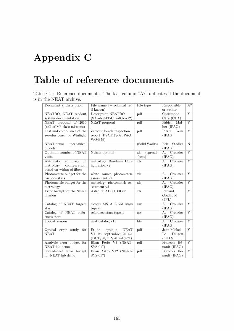
Appendix C
Table of reference documentsTable C.1: Reference documents. The last column “A?” indicates if the documentis in the NEAT archive.
Document(s) description File name (+technical ref.if known)
File type Responsibleor author
A?
NEATRO, NEAT readoutsystem documentation
Description NEATRO(SAp-NEAT-CCa-00xx-12)
pdf ChristopheCara (CEA)
Y
NEAT proposal of 2010(call of M3 class missions)
NEAT proposal pdf Fabien Mal-bet (IPAG)
Y
Test and compliance of thezerodur bench by Winlight
Zerodur bench inspectionreport (PVC1179-A IPAGWO4379)
pdf Pierre Kern(IPAG)
Y
NEAT-demo mechanicalmodels
- (Solid Works) Eric Stadler(IPAG)
N
Optimum number of NEATvisits
Nvisits optimal xls (spread-sheet)
A. Crouzier(IPAG)
Y
Automatic summary ofmetrology configuration,based on wiring of fibers
metrology Baselines Con-figuration v2
xls A. Crouzier(IPAG)
Y
Photometric budget for thepseudos stars
white source photometricassessment v2
xls A. Crouzier(IPAG)
Y
Photometric budget for themetrology
metrology photometric as-sessment v2
xls A. Crouzier(IPAG)
Y
Error budget for the NEATmission
AstroFF AEB 1000 v2 xls RenaudGoullioud(JPL)
Y
Catalog of NEAT targetsstar
closest MS AFGKM starstopcat
csv A. Crouzier(IPAG)
Y
Catalog of NEAT refer-ences stars
reference stars topcat csv A. Crouzier(IPAG)
Y
Topcat session neat catalog v11 fits A. Crouzier(IPAG)
Y
Optical error study forNEAT
Etude optique NEATV1 25 septembre 2014-1(DCT/SI/OP/2014-15571)
pdf Jean-MichelLe Duigou(CNES)
Y
Analytic error budget forNEAT lab demo
Bilan Perfo V3 (NEAT-SYS-017)
pdf Francois He-nault (IPAG)
Y
Spreadsheet error budgetfor NEAT lab demo
Bilan Astro V12 (NEAT-SYS-017)
pdf Francois He-nault (IPAG)
Y
165

Appendix D
Components referencesTable D.1: Component references.
Sub-system Component Manufacturer Product reference
Metrology
HeNe laser 1.5 mW Thorlabs HRS015HeNe laser 21 mW Thorlabs HNL210L-ECFiber splitter (PM) Thorlabs PMC630-50B-APCSwitch (PM) Leoni EOL2x8Fiber patch cables (PM) Thorlabs P3-630PM-FC
Modulators JenoptikIntegrated Optical PhaseModulator - PM 635
Light detectorCCD e2v CCD39-01Readout electronics CEA custom made
Pseudo stars
Light source:-halogen bulb-power supply-housing-condenser-shutter
Lot-Oriel
-LSB111/5-LSN111-LSH102-LSC111-LSZ160/161
Liquid core fiber Lot-Oriel LLG210/LLG211Pinhole mask Winlight Optics/FEMTO-ST custom madeDiaphragm IPAG custom made
Supports
Translation stage:-structure and motors-controlers
-New Focus-New Focus
-9053-8752/8753
Zerodur bench Winlight optics custom made
ControlData Acquisition andwitch Unit
Agilent 34970A
Environment andtemperaturecontrol
Pressure gauge Agilent Varian AGC-100
Vacuum chamberOutillage MecaniqueGenerale (OMG)
custom made
Canvas:-structure-air filter
-Faure Automatisme-ADS laminaire
-custom made-custom made
Peltier:-chip-controler
-TEC Laird Technologies-Keithley
-UT11,12,F2,3030-2510 TEC SourceMeter
Water cooler Thermo scientific Accel 500 LT
Flat field
Light source:-LED-controler-power supply
Thorlabs-MWWHF1-LEDD1B-TPS001
Multimode opticalfibers 200/365 µm
Thorlabs 10230A/10410A
OthersInverter Riello UPS DVR 50/80/110Oscilloscope Agilent Agilent 1000 Series
166

Appendix E
NEAT demo user manual
1 Folder naming convention
In order to sort and retrieve files more easily, the raw data, fits cubes and alsoeventual plots produced from data of a given day are placed in folders with datetags in the following format: “YYYYMMDD” (for example “20140401” if you haveacquired data on the first of April in 2014). Every time the “YYYYMMDD” tagappears in this manual, it means “the actual date tag corresponding to the data”.
2 The work environment
� Lab environment
Figure E.1 is a simplified plan (roughly scaled) to help you identify the physicalelements and devices that are mentioned throughout this manual and it tells wherethey are located in the lab. Here we only shown the most important (high level)ones. In particular we do not list what is installed on the instrumentation rack.Almost any device that isn’t mentioned on the plan is on the rack, but there arequite easy to identify.
� Electrical wiring
Electrical devices are split into groups A and B for security reasons, as shown byfig. E.2. The group A can be protected behind a circuit breaker when the shortcircuit switch is open. This allows for safe operation at CCD cold temperature: itthe even of a pressure or power loss, all electric devices of group A are powered off(see section 6.3). Power will not come back at the same time than the mains, it hasto be re-established manually. The experiment is thus put in a stable state untilwe make sure it can be safely resumed. The group B is protected by the inverter,which will maintain power for about 15 minutes in the event of a power loss. Thiswill give time to shut down computers properly.
� Network spaces and architecture
167
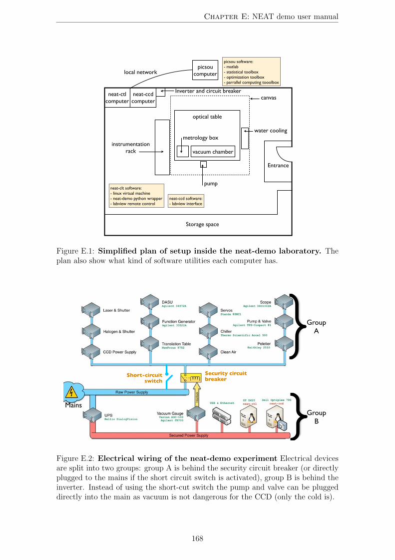
Chapter E: NEAT demo user manual
��������
�������������
����������������
����������������
��������������������
�������������
��������������
�������������
��������������
�������������
������
����
�������������
�������������������������������������������������������������������������������������������
�������������������������������������
�������������������������������������������������������������������������������������������������
����������������������������
Figure E.1: Simplified plan of setup inside the neat-demo laboratory. Theplan also show what kind of software utilities each computer has.
������
������
�����
������������������������
��������������������������������������������������
������
Figure E.2: Electrical wiring of the neat-demo experiment Electrical devicesare split into two groups: group A is behind the security circuit breaker (or directlyplugged to the mains if the short circuit switch is activated), group B is behind theinverter. Instead of using the short-cut switch the pump and valve can be pluggeddirectly into the main as vacuum is not dangerous for the CCD (only the cold is).
168

3. Reminder: list of operations
A lot of different network resources have been used in addition to the 3 computersalready mentioned. The multiplicity of the tools has created an working environmentthat is rather disintegrated (as in the opposite of integrated). In order to createa unique and functional archive most of the important files and documents havebeen gathered into the so called “neat-demo archive”. However, the archive is notcompletely exhaustive and it can be advantageous to access some resources directly.All the existing resources are listed below.
Neat-demo Twiki pages A subset of the Twiki pages for NEAT are exclusivelyfor Neat-demo:http://ipag.osug.fr/twiki/bin/view/Ipag/Projets/Neat/LabDemo/WebHome.This resource has been used for project management as it offers many differ-ent functions, such as maintaining lists of actions, sharing meetings reports,attaching documentation files... Of particular interest is the logbook page:http://ipag.osug.fr/twiki/bin/view/Ipag/Projets/Neat/LabDemo/CahierDeManip.It contains detailed reports of what was modified on the neat testbed and whatkind of data has been acquired (with the CCD39) on a daily basis. This spacebeing properly backed-up and web based, it is not copied in the Neat-demoarchive. An IPAG ID is needed to access the resource.
Neat-demo workspace This is a disk space of a size of 500 GB available via theIPAG local network (not backed-up). It was used to share large files betweenNeat-demo crew members. Access to this space also requires an IPAG ID andcan be a bit tricky (see tutorial 6).
Personal workspace Everyone at IPAG has about 15 GB of personal workspace(backed-up on a weekly basis). Workspaces can be accessed from almost anymachine: my personal workspace was used to host the matlab scripts whichare executed by picsou. The final version of the code has been copied in theNeat-demo archive.
Picsou hard drive Picsou has been equipped with 3 hard drives in a RAID5 con-figuration (not backed-up). The volume of available data is 2TB. Raw datafiles are first transfered to picsou and fits cube are generated. Data securityis assured because the fits can be rebuild from the raw data files conserved onneat-ccd.
forge.osug.fr SVN repository includes Documentation wiki pages http://forge.osug.fr/trac/IPAG-neat. The repository was also used to host the matlabscripts and allow users to share source files (for example with the interns).However the space has reached maximal capacity and I am now working aloneso the code is not up to date.
3 Reminder: list of operations
� Foreword
This section contains the list of operations needed to acquire data, in different cases.We have defined 4 possible modes to operate the CCD (see section 6.3), they arereminded here:
1. In air, ambient temperature. Although far from ideal, it is possible to operate
169

Chapter E: NEAT demo user manual
in air with no cooling at all. Operating the CCD will heat it slightly, to around25◦C. In this mode, the equilibrium temperature of the CCD will be high andunstable, dark current and read noise may be high and variable. This is usefulif one want to have images very quickly.
2. In air, cool temperature (TCCD = 17◦C)3. In vacuum, cool temperature (TCCD = 17◦C)4. In vacuum, cold temperature (TCCD = −10◦C). This setup is expected to give
the best performances: the CCD is specified for operation at this temperature.
Cold operation in air is not possible because of possible formation of dew or iceon the CCD.
In addition to this, there is a remote control system that makes it possible to controlthe labview interface via a python script: to enable this remote control, execute thecorresponding step.
The list of operations below is the most complete one, corresponding to mode number4 with the remote control. Some operations are optional as they depend on the
chosen mode: they are noted with a icon.
� List of operations
1. Pump the vacuum chamber down to 0.2 mbar
• Seal the vacuum chamber
• Plug the electric power supplies of the vacuum pump and the valve di-rectly on the mains
• Wait until the pressure has decreased to at least 0.2 mbar (this will takeabout 4 hours)
• Unplug the pump and the valve
• Engage the circuit breaker and then switch off the short circuit: group
A is now protected by the circuit breaker (needed only for cold tempera-ture)
The valve is normally closed: it will stay open when powered and willautomatically close if the pull is plugged or if the power goes out.
The pump should always be off while taking data to avoid vibration andincrease stability. The vacuum sealing is good enough to retain proper vacuum(P < 0.5 mbar) for about a day.
The circuit breaker is a protection against a loss of pressure and mustalways be used when operating the CCD at low temperatures (T < 17◦C).In the event of a loss of vacuum (i.e. quick pressure increase), cooling mustbe stopped immediately to let the CCD warm up. If the CCD is kept coolunder high atmospheric pressure, dew and/or ice will form on the chip andcould damage it. The circuit breaker can only be engaged when the pressureis less than 0.2 mbar and will automatically cut power off if pressure increaseto more than 0.5 mbar. Details about this issue are explained in section 6.3.
2. Turn on all devices
• Water cooler (set T=18◦C/8◦C)• Peltier controller (set T=17◦C/-10◦C)
170
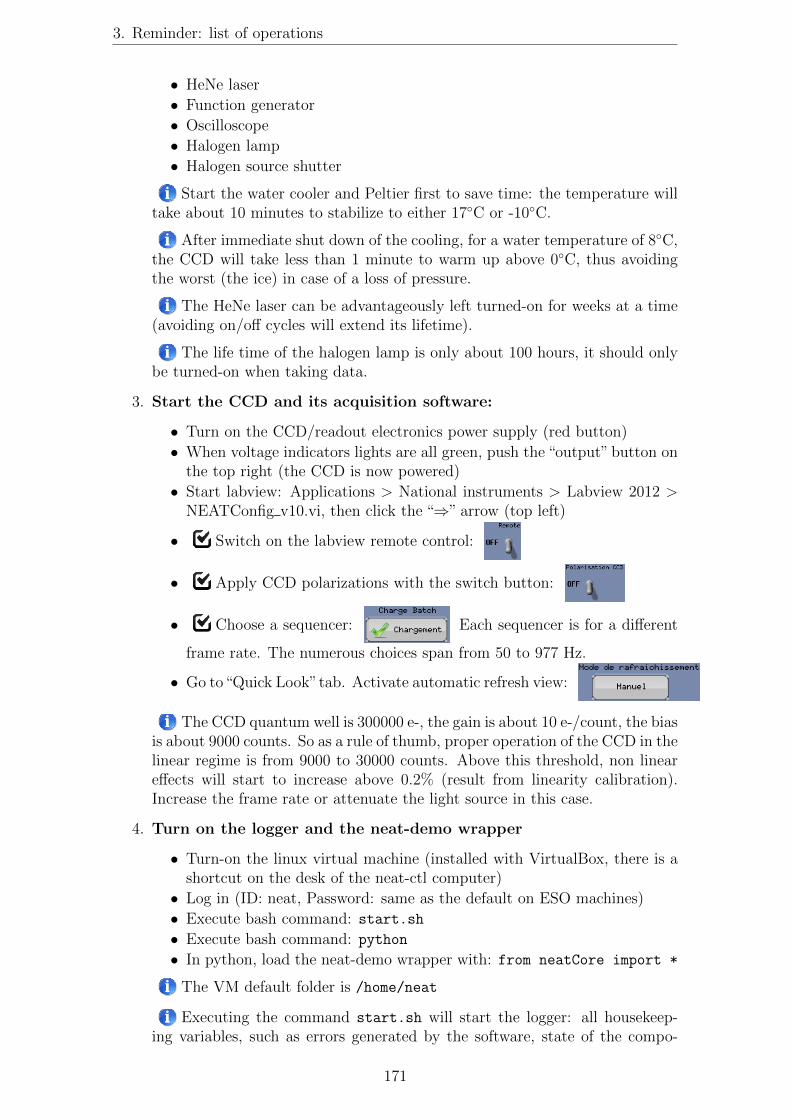
3. Reminder: list of operations
• HeNe laser
• Function generator
• Oscilloscope
• Halogen lamp
• Halogen source shutter
Start the water cooler and Peltier first to save time: the temperature willtake about 10 minutes to stabilize to either 17◦C or -10◦C.
After immediate shut down of the cooling, for a water temperature of 8◦C,the CCD will take less than 1 minute to warm up above 0◦C, thus avoidingthe worst (the ice) in case of a loss of pressure.
The HeNe laser can be advantageously left turned-on for weeks at a time(avoiding on/off cycles will extend its lifetime).
The life time of the halogen lamp is only about 100 hours, it should onlybe turned-on when taking data.
3. Start the CCD and its acquisition software:
• Turn on the CCD/readout electronics power supply (red button)
• When voltage indicators lights are all green, push the “output” button onthe top right (the CCD is now powered)
• Start labview: Applications > National instruments > Labview 2012 >NEATConfig v10.vi, then click the “⇒” arrow (top left)
• Switch on the labview remote control:
• Apply CCD polarizations with the switch button:
• Choose a sequencer: Each sequencer is for a different
frame rate. The numerous choices span from 50 to 977 Hz.
• Go to“Quick Look”tab. Activate automatic refresh view:
The CCD quantum well is 300000 e-, the gain is about 10 e-/count, the biasis about 9000 counts. So as a rule of thumb, proper operation of the CCD in thelinear regime is from 9000 to 30000 counts. Above this threshold, non lineareffects will start to increase above 0.2% (result from linearity calibration).Increase the frame rate or attenuate the light source in this case.
4. Turn on the logger and the neat-demo wrapper
• Turn-on the linux virtual machine (installed with VirtualBox, there is ashortcut on the desk of the neat-ctl computer)
• Log in (ID: neat, Password: same as the default on ESO machines)
• Execute bash command: start.sh
• Execute bash command: python
• In python, load the neat-demo wrapper with: from neatCore import *
The VM default folder is /home/neat
Executing the command start.sh will start the logger: all housekeep-ing variables, such as errors generated by the software, state of the compo-
171
Chapter E: NEAT demo user manual
nents, pressure inside the chamber and temperatures (by 3 different probes) arerecorded in a time tagged folder on the VM: home/neat/YYYY-MM-DD_HH/MM/SS.
If the remote control has been switched on in labview before executingstart.sh, the remote control is now active.
Labview remote control and neat-demo python wrappers are grouped intothe neatCore python library, the documentation can be found at the followingaddress:https://forge.osug.fr/trac/IPAG-neat. A python file of command exam-ples can be found in the virtual machine default folder or in the appendix5.
For better usability, once the VM has started, you can access it froman ssh connection: ssh -X [email protected] -p 2222.This can be useful if for example you want to work on python script files withyour favorite text editor.
5. Record data
• Turn on/off the relevant hardware to have either a flat, metrology or starsimages
• For each data cube: chose a duration and click:
• Organize all the data and put it in a folder named YYYYMMDD
• Or: use the remote interface to acquire data
By default data is created on the neat-ccd machine in the folder: /mnt/s-db/PCIeData.
It is strongly advised to create one folder per data cube/acquisition (seefits generation in section 4).
The flat field source is not included with the neat-demo wrapper, thebroadband white LED has to be turned on and off manually. If you want tohave a flat field in an automated sequence, take it manually at the beginningor the end of it.
To validate a new acquisition duration, you have to type a new numberand then push ENTER.
6. Power CCD off and shut down labview
• Switch off the CCD polarisations:
• Shut down the remote control if active:
– Switch off the python remote control client first: neatCore.controlCamera("P","")
– Switch off the remote control in labview last:
• Exit labview: . This will also stop the C acquisition process.
Switching off the CCD polarisations can also be done via the remote con-trol.
Do not forget to switch off the CCD polarisation before closing labview.You should be able cut the power off to the CCD without damage, but thesafest process is to switch off polarisations first.
172

3. Reminder: list of operations
7. Exit the neat-demo wrapper, save logs and turn off the logger
• Exit python with: quit()
• Execute bash command: stop.sh
• Enter your login and password (this is needed to save logs)
8. Return to ambient temperature
• Shut the Peltier controller off
• Shut the water cooler off
9. Return to atmospheric pressure
• Before proceeding further, check that the temperature has returnedabove 17◦C
• Disengage the circuit breaker and switch the power outlet of group
A from the circuit breaker to mains
• Plug the valve to open it
• Use the nitrogen pressurized bottle when starting to fill the vacuum cham-ber
• Complete with air to 1 bar
10. Shut down all remaining devices
Of course, in case other acquisitions are planned in the near future somedevices can safely be left powered or in sleep mode, such as the laser, computersor even the virtual machine.
Don’t ever forget to turn off the halogen lamp ! If you leave it on overthe week end you are good to replace it with a new one (experience speakinghere).
11. Transfer the data to picsou
• execute bash command: ssh -X picsou
• execute bash command:rsync -rv [email protected]:’/mnt/sdb/PCIeDATA/YYYYMMDD’
/picsou/SHARED/dataNEAT/rawDataCCD39. This command will synchro-nize the picsou folder and add new data in case previous data was alreadytaken and transfered.
It is easier to execute the data transfer form picsou, network rules at IPAGmight prevent it if attempted from another machine.
12. Generate the fits data cubes
• if not already done, execute bash command: ssh -X picsou
• execute bash command: matlab&
• open script file: createFitsCubes.m
• update the variable directory with actual date tag (YYYYMMDD)
• execute the script
Information about the generation of the fits and what kind of issues mayarise is found in section 4.
173

Chapter E: NEAT demo user manual
� Conclusion
Although the complete list of operation is long, depending on the needs of the user,a lot of operations can be skipped or swapped, in particular for tests (when not invacuum and cold). The critical points to remember are:
• Never operate at cold temperature if not below 0.5 mbar, use circuit breakerwhen CCD is cold
• However the chamber can be safely left in vacuum and with the pump on atany time (cold is dangerous, not vacuum)
• Switch off CCD polarisation before closing labview
• If a bug or crash occurs, always restart the software in the same order aspresented
• Do not leave the halogen lamp on overnight
Happy experimentation !
4 The data cube creation routine: from row data
to fits files
4.1 Introduction
The acquisition system made by the CEA generates two data files labeled V3 andV4, each one containing multiplexed data from two quadrants. Before having usableimages, the data has to be extracted from these two files (called “raw data files”),checked, reorganized and stored in a proper data cube which consists of stackedframes. Dimensions 1 and 2 of the cube are pixel rows and columns and the thirddimension is time. This process is taken care of by a matlab script called “create-FitsCubes.m”. This section describe every step of the process, it contains importantpractical information related to the creation of these cubes and to the acquisitionsystem. Such information will be needed if problems arise with the acquisition sys-tem for any reason, most likely if new versions are developed. There were a lot ofissues with the early versions of the acquisitions system and there are still someminor issues left. In any case it is advisable that anyone acquiring data andproducing fits from them reads this information at least once to have abasic understanding of what is happening and what the caveats are. Forextensive information about the acquisition system, refer to the NEATRO documen-tation (doc ref.: SAp-NEAT-CCa-00xx-12).
First a word about the rational behind the acquisition system: the CCD readingelectronics have been developed specifically to enable a very high frame-rate. Thatis why the data comes-in through two separate channels, referred to as V3 and V4.Each channel corresponds to 2 CCD quadrants, the CCD being split into 4 differentquadrants. At the end of an acquisition, two “raw data files” (one per channel) aresaved on the hard drive. The file corresponding to the channel V3 contains thequadrants 1 and 2, the file corresponding to the channel V4 contains the quadrants3 and 4 (see Fig. E.3).
174

4. The data cube creation routine: from row data to fits files
����������������������
����������������������
����������������������
����������������������
��������������������������
�������������
��������������������������
�����������������������
���
�������������
���
�������������
Figure E.3: Schematic of the CCD quadrants and their relation to thedata in V3 and V4 files. Quadrants and reading directions of the CCD39. Ineach quadrant the reading occurs row by row. The outer row is read (red arrows)and then all the columns of the quadrant are shifted (green arrow). The process isrepeated until all the quadrant has been read. The pixels of quadrants (1,2) and(3,4) are multiplexed and sent respectively into channels V3 and V4.
Important remark: the result presented by Fig. E.3 was deduced by reconstruct-ing the “potato” (see Fig. E.5). It is in contradiction with the information given bythe NEATRO documentation (Fig. 13, “construction des trames”): quadrant 3 and4 are swapped. It is possible to reconstruct an image where quadrants 3 and 4 areflipped and swapped, but this breaks the potato and the potato cannot lie...
The usage of the “createFitsCubes.m” script is quite simple: one simply needs toupdate the variable directory to match the name of the folder containing the newraw data before executing it. It is implicitly assumed that all the raw data to beprocessed has been stored and sorted within a folder named in the following format:“YYYYMMDD”. At first the script will recursively search for all pairs of raw datafile within the folder and its sub-folders and memorize theirs paths. It will thenattempt to process each pair, and if successful, a .fits data cube will be created atthe same location than the pair. The name of the fits is derived from common partin the names of the pairs, which is a time tag. It is strongly recommended to placeeach raw data file pair into a separate folder with a more explicit name in orderto facilitate ulterior access to data when loading files for “science” analysis. Thefunction “loadFitsCube” can be used to load a data cube automatically without theneed to know its complete name with the cumbersome time tag. It relies on thefolder name (given as argument) and extension name (known to be .fits), but it canonly work properly if there is a unique fits cube into the folder.
4.2 createFitsCubes.m: list of operations
� Find the pairs of V3/V4 raw data files
The “raw data files” are named in the following pattern:Year_Month_Day_Hour_Min_Sec_Mode_Channel.bin
175

Chapter E: NEAT demo user manual
They should be put into subdirectories, sorted by acquisition-pairs (V3/V4 pairs)by the user. The program first task is to identify and list the pairs of files to beprocessed. The following operations are done on each pair separately.
� Drop the first 50 frames
On one of the channels, one of the first 50 half frames is often incomplete, the reasonof this is linked to the acquisition starting phase but the precise cause has not beenfound, so to workaround this problem we simply get rid of the first 50 frames of eachraw data file.
� Check the file structure
Given the high speed of the transfer, it is possible that some frames are incomplete,for example if there was a buffer overflow caused by a lack of CPU time during theacquisition. So we check the size of all the half frames inside the file. This functionhas also been very useful to debug the system. The structure of the half frames isdescribed by Fig. E.4.
�������
��� ��� ��� ��������������������������
������������������
�������������������
�����������
������������������������������������������������������
�������������������� �������������������������������������
�������
��������������������
���������������
���������������
��������������������
������������������������
�������������������
������������������������
�����������
������������������ ������������� ������������� ������������������
�����������������
������������
������������
�����������������
���������������� ���������������� ���������������� ����������������
���������������� ���������������� ���������������� ����������������
�� �� �� ��
���������������
���������������
���������������
���������
���� � � �
Figure E.4: Structure of a half-frame (2 multiplexed quadrants) in the rawdata files.The expected size of one half-frame is 2× 40× 44 uint16, i.e. 3520× 2 =7040 bytes plus a header of 24 bytes and a trailer of 4 bytes. So its total size is7068B. The last byte visible on the figure is suppressed by the acquisition card.Credit: CEA, Description NEATRO.
In case an abnormal frame is encountered, i.e. the length between the headers isnot right, the program will only save the frames before the abnormal one and awarning will be generated. One recurrent issue that has not been resolved is thefollowing: when processing large data cubes (� 2.5GB), an abnormal frame is alwaysencountered near the end of the file. In practice files larger than 2.5 GB can not becreated because of this, although the original specification was a maximum size of4GB. The cause of this problem has never been found.
� Synchronise the frames between V3 and V4
When the files are saved, the OS can introduce some delay (a few milliseconds)between channels V3 and V4. It means that for each (V3,V4) pair of files there is
176
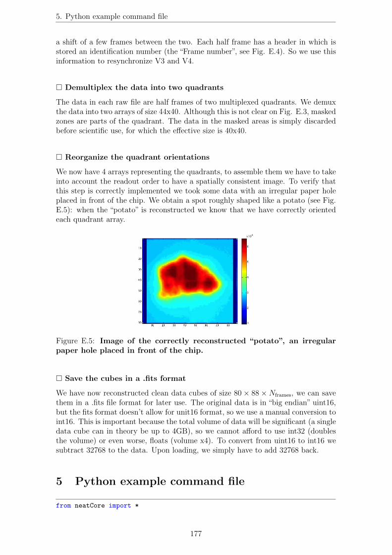
5. Python example command file
a shift of a few frames between the two. Each half frame has a header in which isstored an identification number (the “Frame number”, see Fig. E.4). So we use thisinformation to resynchronize V3 and V4.
� Demultiplex the data into two quadrants
The data in each raw file are half frames of two multiplexed quadrants. We demuxthe data into two arrays of size 44x40. Although this is not clear on Fig. E.3, maskedzones are parts of the quadrant. The data in the masked areas is simply discardedbefore scientific use, for which the effective size is 40x40.
� Reorganize the quadrant orientations
We now have 4 arrays representing the quadrants, to assemble them we have to takeinto account the readout order to have a spatially consistent image. To verify thatthis step is correctly implemented we took some data with an irregular paper holeplaced in front of the chip. We obtain a spot roughly shaped like a potato (see Fig.E.5): when the “potato” is reconstructed we know that we have correctly orientedeach quadrant array.
Figure E.5: Image of the correctly reconstructed “potato”, an irregularpaper hole placed in front of the chip.
� Save the cubes in a .fits format
We have now reconstructed clean data cubes of size 80 × 88 ×Nframes, we can savethem in a .fits file format for later use. The original data is in “big endian” uint16,but the fits format doesn’t allow for unit16 format, so we use a manual conversion toint16. This is important because the total volume of data will be significant (a singledata cube can in theory be up to 4GB), so we cannot afford to use int32 (doublesthe volume) or even worse, floats (volume x4). To convert from uint16 to int16 wesubtract 32768 to the data. Upon loading, we simply have to add 32768 back.
5 Python example command file
from neatCore import *
177
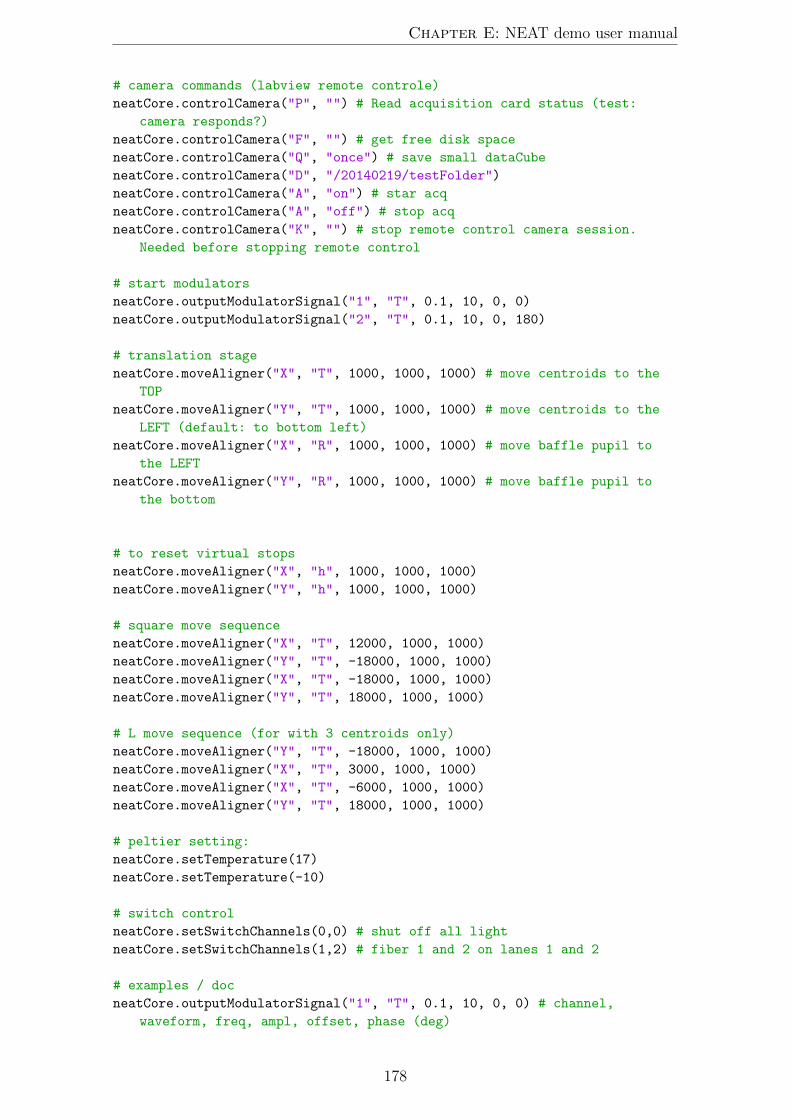
Chapter E: NEAT demo user manual
# camera commands (labview remote controle)
neatCore.controlCamera("P", "") # Read acquisition card status (test:
camera responds?)
neatCore.controlCamera("F", "") # get free disk space
neatCore.controlCamera("Q", "once") # save small dataCube
neatCore.controlCamera("D", "/20140219/testFolder")
neatCore.controlCamera("A", "on") # star acq
neatCore.controlCamera("A", "off") # stop acq
neatCore.controlCamera("K", "") # stop remote control camera session.
Needed before stopping remote control
# start modulators
neatCore.outputModulatorSignal("1", "T", 0.1, 10, 0, 0)
neatCore.outputModulatorSignal("2", "T", 0.1, 10, 0, 180)
# translation stage
neatCore.moveAligner("X", "T", 1000, 1000, 1000) # move centroids to the
TOP
neatCore.moveAligner("Y", "T", 1000, 1000, 1000) # move centroids to the
LEFT (default: to bottom left)
neatCore.moveAligner("X", "R", 1000, 1000, 1000) # move baffle pupil to
the LEFT
neatCore.moveAligner("Y", "R", 1000, 1000, 1000) # move baffle pupil to
the bottom
# to reset virtual stops
neatCore.moveAligner("X", "h", 1000, 1000, 1000)
neatCore.moveAligner("Y", "h", 1000, 1000, 1000)
# square move sequence
neatCore.moveAligner("X", "T", 12000, 1000, 1000)
neatCore.moveAligner("Y", "T", -18000, 1000, 1000)
neatCore.moveAligner("X", "T", -18000, 1000, 1000)
neatCore.moveAligner("Y", "T", 18000, 1000, 1000)
# L move sequence (for with 3 centroids only)
neatCore.moveAligner("Y", "T", -18000, 1000, 1000)
neatCore.moveAligner("X", "T", 3000, 1000, 1000)
neatCore.moveAligner("X", "T", -6000, 1000, 1000)
neatCore.moveAligner("Y", "T", 18000, 1000, 1000)
# peltier setting:
neatCore.setTemperature(17)
neatCore.setTemperature(-10)
# switch control
neatCore.setSwitchChannels(0,0) # shut off all light
neatCore.setSwitchChannels(1,2) # fiber 1 and 2 on lanes 1 and 2
# examples / doc
neatCore.outputModulatorSignal("1", "T", 0.1, 10, 0, 0) # channel,
waveform, freq, ampl, offset, phase (deg)
178

6. Tutorial: mounting directories with SSH tunnel manager and Macfusion
neatCore.moveAligner("Y", "R", 10000, 1000, 1000) # axis, T/R, Nsteps,
motor acc, motor speed
6 Tutorial: mounting directories with SSH tunnel
manager and Macfusion
In this tutorial we ssh tunnel to jupiter and mount the neat workspace locally. Butthe same method can be applied to all network spaces accessible through an sshtunnel.
1. Connect manually to the ssh to verify that you have the access rights
- if login from outside the lab, connect to janus first:ssh -X @janus.obs.ujf-grenoble.fr
- connection to the neat space with:ssh -X @jupiter.obs.ujf-grenoble.fr
2. Creation of your public key
This will avoid having to enter your password everytime you connect, followthe instructions here:http://ipag.osug.fr/twiki/bin/view/Trash/Intranet/InfoDocAgentSsh
3. SSH Tunnel manager
Download link: http://www.macupdate.com/app/mac/10128/ssh-tunnel-manager
Configuration:- Click on the button configuration- Create a new profile
• Nom: NEAT demo• Hote: janus.obs.ujf-grenoble.fr• Port: 22• Redirections locales: Port: 2022, Hote distant: jupiter.obs.ujf-grenoble.fr,Port: 22
- Go into ”Options”and select: Connection automatique / Gerer l’authentification/ Activer la compression
4. Mac fusion
If not already installed, install macfuse first:download link for macfuse: http://code.google.com/p/macfuse/download link for macfusion: http://macfusionapp.org/
Configuration:- click on ”+” to create a new SSHFS mount point- click on edit:
• SSH:
– Host: localhost– User name: your username
179

Chapter E: NEAT demo user manual
– Password: your password– Path: /data/neat/
• SSH Advanced:
– Port: 2022– Enable Compression: Yes– Follow Symbolic Links: Yes– Extra options: -o idmap=user -o uid=yourUID -o gid=yourGID
• Mac fusion:
– Mount Point: /Users/username/dirname (example)– Volume Name: dirname (example)
7 Metrology switch configuration
The fibers are separated into two groups: 4 are vertically aligned and 4 are hori-zontally aligned (see Fig. E.6). As we do not use diagonal baselines, we want tomax out the number of accessible baselines within each group. For this we have toconnect 2 fibers from each “sub-switch” (1x4) to each group of 4 fibers. Within eachgroup, we will have 4 baselines available, over a total of 6 (number of 2-combinaisonsamong the 4 fiber tips) that would have been possible with a truly 2x8 switch. Theother possibilities are obviously less interesting, if instead of 2/2 we go with a 3/1or 4/0 mixing between the switch and the groups, we end up with respectively 3 or0 available baselines within the groups.
When doing a 2/2 mixing, we have in principle 24 possible cabling configurations(4!) for each group, but only 6 of them are non equivalent (they will change whichbaselines are available in the end), a lot of them are redundant and will only resultin a permutation of switch command. The easiest way to think about it is thefollowing: for each group of 4 fibers one has to select a first impossible baseline (2fibers tips among 4). These two fibers are set to come from the same sub-switch andthe corresponding baseline is eliminated. The other two fibers of the same groupalso are coming from the same sub-witch and are also eliminated. The 4 remainingcombinations are all accessible.
180

7. Metrology switch configuration
Inputs: Outputs:
Switch.side Plug.side Plug.side Mirror.side H4 H3 H2 H1S3 10 10 V1 V4 Note:.i.=.λL/B.=>.B=λL/iT3 2 2 V2 V3 L.(m) 0,6T4 3 3 V3 V2 λ.(m) 6,33EL07S4 4 4 V4 V1 pixel.size.(m) 2,40EL05S1 5 5 H1T2 6 6 H2T1 7 7 H3S2 8 8 H4
Switch'Name
Mirror'Name
X.Coord. Y.coord. Xcoord'1
Xcoord'2
YCoord'1
Ycoord'2
X'diff
Y'diff
Dist i active?
S3 V1 0 3,7 V1 V2 S3 T3 0 0 3,7 4,7 0 1 1 15,83 1T3 V2 0 4,7 V1 V3 S3 T4 0 0 3,7 7,7 0 4 4 3,96 1T4 V3 0 7,7 V1 V4 S3 S4 0 0 3,7 9,7 0 6 6 2,64 0S4 V4 0 9,7 V2 V3 T3 T4 0 0 4,7 7,7 0 3 3 5,28 0S1 H1 3,7 0 V2 V4 T3 S4 0 0 4,7 9,7 0 5 5 3,17 1T2 H2 4,7 0 V3 V4 T4 S4 0 0 7,7 9,7 0 2 2 7,91 1T1 H3 7,7 0 H1 H2 S1 T2 3,7 4,7 0 0 1 0 1 15,83 1S2 H4 9,7 0 H1 H3 S1 T1 3,7 7,7 0 0 4 0 4 3,96 1
H1 H4 S1 S2 3,7 9,7 0 0 6 0 6 2,64 0H2 H3 T2 T1 4,7 7,7 0 0 3 0 3 5,28 0H2 H4 T2 S2 4,7 9,7 0 0 5 0 5 3,17 1H3 H4 T1 S2 7,7 9,7 0 0 2 0 2 7,91 1
Mirror'bloc'(seen'face'on)
Baselines Switch'outputs
<====>
This.file.contains.the.current.metrology.baseline.configuration,.this.includes.both.the.set.of.connections.after.the.switch.and.in.the.vacuum.chamber
Possible.upgrade:.switch.4.with.3.and.5.with.6.between.the.switch.and.the.plugswitch.command:.setSwitchChannel(Ti,Si)
Final.connection.configuration Switch./.Baselines.table
Configuration.between.the.switch.and.the.chamber
Connection.configuration.inside.the.vacuum.chamber,.as.noted.on.fiber.
Fibers.fixed.on.the.mirror,.as.noted.on.their.connectors
Interfringe.(i)PLUG
Figure E.6: Metrology configuration spreadsheet. It summarize all the practi-cal information needed about the current metrology configuration: how the connec-tors/fibers are paired between the switch and the vacuum plug, after the vacuumplug inside the vacuum chamber, what are the final baselines interfringe distancesand what are the corresponding switch commands.
181

Appendix F
NEAT memo: Creation andexploitation of the NEAT catalog
182

NEAT Memo NEAT-sci-001
Orig. : A. CrouzierDest. : NEAT consortiumDate : 16-09-2014Version : v4
Subject : Creation and exploitation of the NEAT catalogs
Memo version history
• 25-Jan-2012 (v1): initial writing
• 29-May-2012 (v2): addition of the section for HZ calculation
• 01-Jun-2012 (v3): reorganization of the sections
• 16-09-2014 (v4): major update, change of main sequence selection criteria (broadertolerances), addition of observational strategies
Scope
The targets of the NEAT mission are the Sun-like stars in our close neighborhood. Theycorrespond more precisely to the main sequence stars of spectral types A, F, G, K and M thatare located at a distance of less then 20 pc from the Sun.
The goal of this memo is to describe the sequence of commands I used to create the NEATcatalog of targets with the program Topcat. This catalog is defined as the A, F, G, K andM main sequence stars, located at less than 20 pc from the Sun, in the Hipparcos catalog. Wewill also define the NEAT catalog of references stars from the NEAT catalog of targets.Other sections will show how one can use Topcat and the newly defined NEAT catalogs tocheck for sample completeness and to obtain statistics about the target and reference stars.
Topcat is a spreadsheet application for astronomical catalogs, developed by Mark Taylor.It offers the possibility to define catalog subsets and has a nice set of visualization tools. It canbe downloaded for free from this webpage: http://www.star.bris.ac.uk/~mbt/topcat/.
Acronyms
BC Bolometric Correction
1 / 34
0.
Appendix F - NEAT Memo: Creation and exploitation of the NEAT catalog
183

Nearby Earth Astrometric Telescope Ref: NEAT-sci-001Version : v4
Creation and exploitation of the NEATcatalogs
Date : 16-09-2014Page : 2 / 34
HZ Habitable zoneNEAT Nearby Earth Astrometric Telescope
SciDAVis Scientific Data Analysis and VisualizationSNR Signal to Noise Ratio
TOPCAT Tool for OPerations on Catalogues And Tables
Reference documents, files, catalogs and papers
• NEAT: a spatial telescope to detect nearby exoplanets using astrometry (PhD manuscriptof Antoine Crouzier)
• NEAT Proposal of 2010• TOPCAT Reference manual• Hiparcos catalog - available on Vizier• Tycho2 catalog - available on Vizier• The exoplanet catalog of “The Extrasolar Planets Encyclopaedia”• Transformations from Theoretical Hertzsprung-Russell Diagrams to Color-Magnitude
Diagrams: Effective Temperatures, B-V Colors, and Bolometric Corrections (Flower,1996)
• The B-V / BC / Teff relation for main sequence stars, subgiants, and giants (Flower,1996) - available on Vizier
• Target star catalogue for Darwin Nearby Stellar sample for a search for terrestrial planets(Kaltenegger et al., 2010).
• Habitable Zones around Main Sequence Stars (Kasting et al., 1993)• Physical Parameters of the Stars (Schmidt-Kaler, 1982)• NEAT error budget (Renaud Goullioud, priv comm.)• Spreadsheet for calculation of NEAT photon noise limit: neat_photon_limit.xls• Planet population synthesis model (Alibert et al., 2013).• List of synthetic exoplanet systems: CD2133_ltev.dat.• Matlab script (calculation of exoplanet yields): observational_strategy_yields.m• Python script (calculation of reference equivalent magnitude): process_ref_stars.py
Chapter F: NEAT memo: Creation and exploitation of the NEAT catalog
Appendix F - NEAT Memo: Creation and exploitation of the NEAT catalog
184
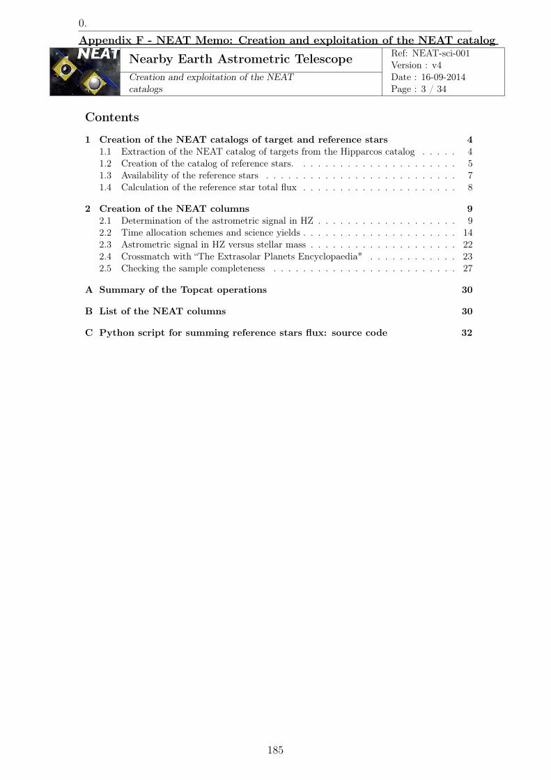
Nearby Earth Astrometric Telescope Ref: NEAT-sci-001Version : v4
Creation and exploitation of the NEATcatalogs
Date : 16-09-2014Page : 3 / 34
Contents
1 Creation of the NEAT catalogs of target and reference stars 41.1 Extraction of the NEAT catalog of targets from the Hipparcos catalog . . . . . 41.2 Creation of the catalog of reference stars. . . . . . . . . . . . . . . . . . . . . . 51.3 Availability of the reference stars . . . . . . . . . . . . . . . . . . . . . . . . . . 71.4 Calculation of the reference star total flux . . . . . . . . . . . . . . . . . . . . . 8
2 Creation of the NEAT columns 92.1 Determination of the astrometric signal in HZ . . . . . . . . . . . . . . . . . . . 92.2 Time allocation schemes and science yields . . . . . . . . . . . . . . . . . . . . . 142.3 Astrometric signal in HZ versus stellar mass . . . . . . . . . . . . . . . . . . . . 222.4 Crossmatch with “The Extrasolar Planets Encyclopaedia" . . . . . . . . . . . . 232.5 Checking the sample completeness . . . . . . . . . . . . . . . . . . . . . . . . . 27
A Summary of the Topcat operations 30
B List of the NEAT columns 30
C Python script for summing reference stars flux: source code 32
0.
Appendix F - NEAT Memo: Creation and exploitation of the NEAT catalog
185

Nearby Earth Astrometric Telescope Ref: NEAT-sci-001Version : v4
Creation and exploitation of the NEATcatalogs
Date : 16-09-2014Page : 4 / 34
1 – Creation of the NEAT catalogs of target and reference stars
1.1 – Extraction of the NEAT catalog of targets from the Hipparcos cata-log
The NEAT catalog of targets will consist of all the main sequence stars of spectral typesA, F, G, K and M located at a distance of less then 20 pc from the sun (see Fig. 1). What Icall the final list of targets will be a sub sample of this pre selection, relative to the exerciseof observation time allocation. The final selection will prioritize the targets with the highestastrometric signals, so depending on the observational strategy, a fraction of the stars is likelyto be excluded.
�����������������
������������
������������
������������������������������
������������������������������������������
�����������������������������
������������������������
Figure 1: Schematic view of the NEAT catalog of target stars. The NEAT targets are selectedwithin the Hipparcos catalog. The part called NEAT columns are computed values from the Hipparcosoriginal columns.
Unfortunately Topcat does not offer the possibility to save a list of commands. Instead thefull session, including all the Hipparcos data, has to be saved in a fits-plus file, which can havea substantial size (hundreds of mega bytes in our case), this constraint limits the possibility toshare the Topcat sessions. To mitigate this problem, I will describe in details the commandsI used to define the NEAT catalog.
To begin, the NEAT catalog is created from a subset of stars from the Hipparcos catalog.In order to manipulate the data more easily, several subsets will be defined. Additionally,we have to download the Hipparcos catalog from the vizier portal because we need to addRA2000 and DEC2000 columns.
This is done with the following sequence of actions:
• Search for the Hipparcos catalog in Vizier.• In the catalog list select All (so you will be also downloading the tycho catalog, which
is the last table).• On the Preferences window on the left, tick All columns, set max to unlimited, set
the format to VOTable and verify that the J2000 box is active in the Compute menu.
Chapter F: NEAT memo: Creation and exploitation of the NEAT catalog
Appendix F - NEAT Memo: Creation and exploitation of the NEAT catalog
186
Nearby Earth Astrometric Telescope Ref: NEAT-sci-001Version : v4
Creation and exploitation of the NEATcatalogs
Date : 16-09-2014Page : 5 / 34
• Click Query selected Tables and save the tables on the hard drive.• In Topcat, open the Load New Table dialog box via the menu File > Load table.• Click on the System Browser icon and load the catalogs.• Select the Hipparcos main catalog: l/239/hip_main (it is the first table in the Table
List).• Click the tool Display row subsets.• Click the tool Define a new subset... in the window showing the list of subsets• Type a condition in the column Algebraic expression
The last two actions are repeated for each new subset. Each subset is defined by its ownalgebraic expression. Here is the list of all the subsets I chose to create:
• A first subset named closest_stars containing all the Hipparcos stars closer than 20pc, using the following expression: Plx > 50
• One subset for each sun-like spectral type (A, F, G, K and M), among the closest stars.For example, for the main sequence F stars, the subset name is: closest_MS_F_starsand the expression is:_2 && matches(SpType,"^F.*(IV-V|[^I]V)")
• One subset named closest_MS_FGK_stars, this is the union of the three subsets above.The expression is:_2 && (matches(SpType,"^F.*(IV-V|[^I]V)")||matches(SpType,"^G.*(IV-V|[^I]V)")||matches(SpType,"^K.*(IV-V|[^I]V)"))
• One subset named closest_MS_AFGKM_stars with the A,F,G,K and M main sequencestars closer than 20 pc. This is the NEAT catalog of targets. The expression is:_2 && (matches(SpType,"^A.*(IV-V|[^I]V)")||matches(SpType,"^F.*(IV-V|[^I]V)")||matches(SpType,"^G.*(IV-V|[^I]V)")||matches(SpType,"^K.*(IV-V|[^I]V)")||matches(SpType,"^M.*(IV-V|[^I]V)"))
The (IV-V|[^I]V) part in the regular expression mean that we accept selected all mainsequence stars (or between main sequence and sub-giant). For stars with two components(separated by a “+” sign), we should ideally base the selection on the main component. How-ever, errors will be made if the secondary component only is main sequence: with this regularexpression, the star will be included in the list. The problem is that it is not possible to usea “\” sign in the regular expression (it causes an error in Topcat), it this therefore impossibleto get the needed escaped “+” in the regex.
“_2” refers to the second subset (“_1” is referring to the full Hipparcos catalog itself). Bydoing this, each spectral class can be easily manipulated. You should now have 351 stars inthe closest_MS_FGK_stars subset and 455 in the closest_MS_AFGKM_stars subset.
1.2 – Creation of the catalog of reference stars.
One strong requirement of NEAT is the availability of the reference stars. The field of view ofNEAT is limited to about 0.6◦ because of the aberrations. For each target star, NEAT needsat least 6 reference stars of Vmag < 11 in the field of view to reach its specified accuracy. Thereference stars are ideally quiet and immobile stars, used for differential astrometry measure-ments. In practice they are mostly K giants at long distances. Ideally, the reference starsshould fill the following list of conditions:
0.
Appendix F - NEAT Memo: Creation and exploitation of the NEAT catalog
187

Nearby Earth Astrometric Telescope Ref: NEAT-sci-001Version : v4
Creation and exploitation of the NEATcatalogs
Date : 16-09-2014Page : 6 / 34
• Magnitude lower than 11• Not too noisy...
Stars too close, too active or with giant planets could show excessive noise and be unsuitableto be used as references. In practice, we only have knowledge about the magnitude in Tychoand some targets critically lack reference stars. It is important to keep all we can find1. Also,the shape of the NEAT detector is square, which authorizes the use of some reference starslocated between 0.6◦ and 0.84◦2. So we will use the whole Tycho catalog, with a threshold ofeither 0.6 or 0.84◦. We will also calculate a magnitude equivalent to the sum of the flux fromthe reference stars to estimate the reference star photon noise for each target (some targetsmight have a lot of references stars but only faint ones).
The reference stars are found by cross-matching the NEAT catalog (closest_MS_AFGKM_starssubset) with the Tycho catalog. The list of conditions above can be applied to filter out allthe stars that are unsuitable (for example to reject stars with Vmag < 13). It is necessary toapply at least the condition !NULL_Vmag: some stars have unknown/null magnitudes and willcrash the script (section 1.4) unless they are filtered out. Here is the list of the correspondingoperations in Topcat:
• Select the Tycho catalog (“l/239/tyc_main").
• Create a “reference_stars" subset of the Tycho catalog with the conditions of your choice(for example Vmag < 13 && !NULL_Vmag).
• Crossmatch the NEAT catalog (“closest_MS_AFGKM_stars" subset) with the “refer-ence_stars" subset. Use the following parameters:
– Max Error 0.3 or 0.42◦
– Table 1: Hipparcos main catalog
– RA column (for Table 1): _RAJ2000 - degrees
– Dec column (for Table 1): _RAJ2000 - degrees
– Table 2: Tycho main catalog
– RA column (for Table 2): _RAJ2000 - degrees
– Dec column (for Table 2): _RAJ2000- degrees
– Match selection: Best match for each Table 2 row
– Join type: 1 and 2
• Eventually plot the results on a sphere (to visually verify the RAs and DECs)
You should obtain a crossmatch table containing 6466 reference stars (for 0.84◦ FoV andwith Vmag < 13). Click on the tool Display Table Metadata and in front of the raw Name,
1Tycho is magnitude limited to about Vmag = 12− 13. It is not complete after Vmag = 11, but still have alot of stars between 11 and 13. These stars will be our backup reference is we lack brighter one and we willnot be flooded with stars too faint to be useful.
2With only 0.6◦ of FoV, the first result indicated that a significant proportion of target have few referencestars (4 or less). Using 0.84◦ improves the result quite dramatically for some stars. We will overestimate thenumber of available references stars in some rare cases (not all references close to 0.84◦ can be used). Butseeing how to best place a square FoV can not be solved with Topcat, it would require tricky programminginstead.
Chapter F: NEAT memo: Creation and exploitation of the NEAT catalog
Appendix F - NEAT Memo: Creation and exploitation of the NEAT catalog
188

Nearby Earth Astrometric Telescope Ref: NEAT-sci-001Version : v4
Creation and exploitation of the NEATcatalogs
Date : 16-09-2014Page : 7 / 34
change the value Joined to Tycho reference stars crossmatch. This will help distinguishall the different crossmatches.
The current method used to select the reference stars is very crude. For a real mission,other criteria should be used to filter out unsuitable reference stars. A minimum distance (forexample 1 kpc) and a condition on the activity of the stars could be added. The parallax ofthe Tycho catalog can not be used as the errors are typically several dozen of mas (as a result,distances of more than one hundred parsec are not measured properly). An alternative toestimate the distance would be to use the H-R diagram... or to wait for Gaia. The statisticswe will obtain are close to a best case scenario for the number of reference stars because Tychois 99% complete to magnitude 11.
1.3 – Availability of the reference stars
Now that we have a catalog of the reference stars, we want to know the distribution of thesize of the groups of reference stars, each group being all the reference stars associatedwith one NEAT target. This is a bit tricky to do this with Topcat: using directly the informa-tion of the column count in the crossmatch results to plot an histogram doesn’t yield correctresults. This is because for a group of n stars, each reference star will contribute one count.Consequently, in the final distribution, a group of size n will be counted n times.
To tackle this problem, do the following sequence of actions:
• Open the menu Joins > Internal match..
• Select the reference stars crossmatch in Table.
• Chose the option Eliminate all but first of each group.
• Leave all the other options unchanged and click ok.
• Change the name of the new crossmatch table to:Histogram group size reference stars
Now you can plot the histogram of the distribution of the number of reference stars for eachNEAT target stars. Click on the Histogram tool, then change the X-axis to GroupSize-1.The -1 eliminates the target stars from the group (it was counted with the reference stars).The result is shown in the fig. 2.
Remark: The internal match discards the stars that are not in groups, i.e. for which noreference star is available. They do not appear in Fig. 2. By doing an internal match with theoption Eliminate All Grouped Rows you will find how many targets are without reference(0 for 0.84◦ FoV and with Vmag < 13).
Conclusions
Though in average the number of reference is good, there is a significant fraction of theNEAT targets (about 100 of 340) that have only 4 available references stars or less (with afield of 0.6◦ and a Vmag limit of 11). This could affect the ability of NEAT to find planetsaround these stars.
0.
Appendix F - NEAT Memo: Creation and exploitation of the NEAT catalog
189

Nearby Earth Astrometric Telescope Ref: NEAT-sci-001Version : v4
Creation and exploitation of the NEATcatalogs
Date : 16-09-2014Page : 8 / 34
0 5 1 0 1 5 2 0 2 5 3 0 3 5 4 0 4 5 5 0 5 5 6 0 6 5 7 0 7 5Reference star group size
0
1 0
2 0
3 0
Num
ber
of t
arge
ts
Figure 2: Distribution of the number of reference stars per NEAT target star.
1.4 – Calculation of the reference star total flux
The total flux of the reference stars is useful to estimate the integration time requirement foreach target star and for a given astrometric signal and mass detection threshold.
It is not straightforward to obtain this quantity with Topcat: we have a catalog of thereference stars, which are organized in groups that also include the target star. We havethe visible magnitude of all the stars of each group and we want to “sum" the magnitudesto find an equivalent magnitude which flux corresponds to the sum of the flux of the ref-erence stars. The problem is that Topcat does not provide a way to perform this specificoperation. So we will export the catalogs of the reference stars and the target stars as .csvfiles and run a python script through them. The catalog of the reference stars is calledreference_stars_topcat.csv and the catalog of the subset of main sequence AFGKM NEATtargets is called closest_MS_AFGKM_stars_topcat.csv. To create these files,select the ap-propriate table and subset, then use the menu File > Save Table(s)/Session, select the.csv format, enter the name and hit save.
The operations applied in the python script is summarised here:
• Get all the targets’ hipparcos IDs from the catalog of targets
• Loop though the catalog of references and identify the targets stars among them
• Loop though the catalog of reference stars, sum the flux of all the reference stars (ex-cluding the targets) and calculate the equivalent magnitudes
• Add the equivalent magnitudes into the catalog of targets
The equivalent magnitude is the magnitude of a star which flux would be the sum of thereference star flux. We note F0 the reference star flux for the visible magnitude. We have:
M = −2.5 log (F/F0) ⇔ F = F0 × 10−M/2.5
⇒�
i
Fi = F0
�
i
10−Mi/2.5 ⇒ Meq = −2.5 log
��
i
10−Mi/2.5
�
Chapter F: NEAT memo: Creation and exploitation of the NEAT catalog
Appendix F - NEAT Memo: Creation and exploitation of the NEAT catalog
190

Nearby Earth Astrometric Telescope Ref: NEAT-sci-001Version : v4
Creation and exploitation of the NEATcatalogs
Date : 16-09-2014Page : 9 / 34
After running the script a new csv file is created: closest_MS_AFGKM_targets_topcat_out.csv.Import the file back into the list of table via the menu File > Load. The new column EqRefMaghas been added.
Figure 3 is an histogram of the equivalent magnitudes. The NEAT error budget assumed6 stars of magnitude 11 (equivalent magnitude of 9.05). The histogram confirms that thisis a sound assumption: nearly all the target have enough bright reference stars to verify“equivalent” Vmag < 9.05.
0 1 2 3 4 5 6 7 8 9 1 0
Reference equivalent magnitude
0
1 0
2 0
3 0
4 0
5 0
6 0
7 0
8 0
Num
ber
of t
arge
ts
Figure 3: Distribution of the equivalent magnitudes of groups of reference stars (one groupper target).
2 – Creation of the NEAT columns
In this second part we will add a lot of NEAT columns to the catalog of targets. Some ofthem can in principle be added before the column eq_ref_mag has been added. But the latteris integrated into a new table (closest_MS_AFGKM_targets_topcat_out.csv, different fromthe original Hipparcos subset). So any column created before has to be created again, ora crossmatch much be performed to merge the two tables. The simplest way to avoid theproblem is to create the closest_MS_AFGKM_targets_topcat_out.csv table first (with theeq_ref_mag column), and to create all other NEAT columns later.
2.1 – Determination of the astrometric signal in HZ
2.1.1 – Introduction
The goal of this subsection is to add a new column specifying the astrometric signal of anEarth mass planet in the HZ of the target stars. The amplitude of the astrometric signal
0.
Appendix F - NEAT Memo: Creation and exploitation of the NEAT catalog
191
Nearby Earth Astrometric Telescope Ref: NEAT-sci-001Version : v4
Creation and exploitation of the NEATcatalogs
Date : 16-09-2014Page : 10 / 34
yielded by an exoplanet at a distance D, of mass MPlanet, with a semi major axis R around astar of mass MStar is given by:
A = 3µas× MPlanet
MEarth×
�MStar
MSun
�−1
× R(AU)
1AU�D(pc)
1pc
�−1
(1)
From that formula one can see that a star mass increase with have the following effects onthe signal:
• Greater star/planet mass ratio (decreases the signal)
• Greater star luminosity ⇒ further away HZ ⇒ greater semi major axis (increases thesignal)
Note that the mass and the spectral type are strongly correlated, so changes in the starsemission spectrum have to be taken into account. The additional effects, implicit in theformula above, that happen when the mass increase are listed below:
• Blue shifted spectrum ⇒ Greater normalized solar flux factor ⇒ closer HZ ⇒ smallersemi major axis (decreases the signal).
• Greater semi major axis ⇒ Period increase
• Increase of the target stellar flux.
The normalized solar flux factor is a coefficient taking into account the overlap of the stellaremission and the planetary albedo. The values of this coefficient for different spectral typesare found in the literature (Kasting et al., 1993). The overall effect is a moderate negativefeedback on the variation of the HZ location with the mass: for more blue and luminous stars,the albedo is higher, so the net energy input is a bit smaller than expected.
The period also has an influence on the detection threshold. Because of the nature of themission, for periods longer than the mission during the minimum planet mass required fordetection increases, despite an increasing astrometric signal: in this case only a portion ofthe orbit will be sampled so a larger SNR is required. But in our case study this parameterdoesn’t matter much: even for F stars the planet period at the HZ outer edge barely exceed5 years.
Finally, if the stellar flux is larger, the precision of the astrometric measurements willincrease more rapidly with the integration time (noted T): the location error on the measuredcentroid of the target will be σmeasure ∝ 1√
TFstarHowever in the case of NEAT which is
differential astrometry, the photon noise of the much fainter reference stars dominates in mostcases. This means that the final precision will be almost insensitive of the target star flux,but will depend on: the astrometric signal, the photon noise of the reference stars and theintegration time.
The overall effect of the host star mass on the astrometric signal in HZ is a bit tricky todetermine. The result is that the astrometric signal increase with the stellar mass, see section2.3 for details.
Another important parameter I haven’t mentioned yet is the distance, but it is easilyderived from the Hipparcos parallax. The last parameter, the planet mass, can not be knowbefore the observations. We will normalize by the Earth mass: the signal for any mass iseasily obtained by scaling by the ratio: Mplanet
MEarth.
Chapter F: NEAT memo: Creation and exploitation of the NEAT catalog
Appendix F - NEAT Memo: Creation and exploitation of the NEAT catalog
192

Nearby Earth Astrometric Telescope Ref: NEAT-sci-001Version : v4
Creation and exploitation of the NEATcatalogs
Date : 16-09-2014Page : 11 / 34
2.1.2 – Determination of Dist, L, HZin, HZout, and Mass
To determine the astrometric signal in habitable zone, we will determine the following interme-diate quantities: the distance, the bolometric luminosity, the HZ inner and outer boundaries,and the star mass for each NEAT target star (respectively noted Dist, L, HZin, HZout, andMass). Figure 4 shows how L, HZin, HZout, and Mass are derived. The detailed descriptionsof the process for each quantity are presented below.
���
��
��
������
�������������������������������������
�����������������������
�������������������������������
�����������������������������������
����������������������������
�������������������������������
������������������������������
�������������
��� ����
�������������
�������������
�������������� ����
� � ��������
�
�
������� � �
�����−��
����
�����
�����������������
Figure 4: How the luminosity, HZ boundaries and the stellar mass are derived. The blueboxes represent added columns to the catalogues and the green boxes represent data tables.
� How to obtain the distance
The distance is obtained directly from the hipparcos parallax. Add a new column for thedistance by doing the following actions in Topcat:
• Select the Hipparcos main catalog (l 239 hip main, closest_stars_AFGKM subset) ORclosest_MS_AFGKM_targets_topcat_out.csv in the Table List.
• Click the tool Display column metadata
• Click the tool Add a new column
• Name it Dist and enter the following expression: 1000/Plx
� How to obtain the luminosity
0.
Appendix F - NEAT Memo: Creation and exploitation of the NEAT catalog
193

Nearby Earth Astrometric Telescope Ref: NEAT-sci-001Version : v4
Creation and exploitation of the NEATcatalogs
Date : 16-09-2014Page : 12 / 34
This work is based mostly on the following publication: Transformations from TheoreticalHertzsprung-Russell Diagrams to Color-Magnitude Diagrams: Effective Temperatures, B-VColors, and Bolometric Corrections (Flower, 1996). In order to complete the first step, down-load the main sequence “Teff, B-V and BC" table from the same author (the data is accessiblevia Vizier). It is necessary to download the data and perform an interpolation manually be-cause the BC = P(B-V) relation doesn’t exist in the publication (it only gives the log(Teff) =P(B-V) and the log(Teff) = P(BC) polynomial relations).
I downloaded the data in a csv format and loaded it in SciDAVis (a free application forScientific Data Analysis and Visualization). I performed with the latter a polynomial inter-polation (order 10 i.e. 11 DoF). The resulting fit looks very good, the χ2 value of the fit is0.0004. The table 1 gives the coefficients of the polynomial (P = a0 + a1X + a2X
2 + ...).
Coefficient Value Errora0 -0,1784538504862980 0,0040439753600725a1 2,9023636120332208 0,0358593758682318a2 -12,3188141929402839 0,1468192147338562a3 20,9310264552908833 0,7901640483937037a4 -22,5026837177971153 1,7789678865741207a5 63,6149604337794230 3,6915037287900767a6 -177,5417213564442136 11,9138718837156965a7 249,9150285256258428 16,1324092451378540a8 -182,6519997569876352 11,0043353138590163a9 67,4220567552053751 3,7755649838561576a10 -9,9870014580361062 0,5193285281379360
Table 1: Polynomial coefficients of the relation BC = P (B − V ).
With these coefficients I can now complete the first step and add a BC column to theAFGKM subset:
BC -0.1784538+2.9023636*$39-12.318814*pow($39,2)+20.931026*pow($39,3)-22.50268371*pow($39,4)+63.6149604*pow($39,5)-177.541721356*pow($39,6)+249.915028525*pow($39,7)-182.6519997*pow($39,8)+67.42205675*pow($39,9)-9.98700145*pow($39,10)
In the above expression, $39 refers to the B-V column. It is required that one addressesthis column by its ID because it has a “-" in its name.
One last thing to do is to verify that all the targets have a B-V index in the inter-polated range. This can be done by creating a new subset with the following expression:_8 && $39 < 1.8 && $39 > -0.35 and noting that the number of rows is unchanged (_8
is the FGKM susbset). From this point, it is very straightforward to obtain the luminosity insolar units, by creating two other columns:
MB Vmag+BC-5*ln(100/Plx)/ln(10)
L pow(10,(4.75-MB)/2.5)
Remark: The value of 4.75 in the formula above is the solar absolute bolometric magnitude.
Chapter F: NEAT memo: Creation and exploitation of the NEAT catalog
Appendix F - NEAT Memo: Creation and exploitation of the NEAT catalog
194

Nearby Earth Astrometric Telescope Ref: NEAT-sci-001Version : v4
Creation and exploitation of the NEATcatalogs
Date : 16-09-2014Page : 13 / 34
� How to obtain the boundaries of the habitable zone
First of all I extract some data from a table (Schmidt-Kaler, 1982). I need only the rowsF0, G2 and M0 and the following columns: spectral type and log(Teff). Then I add thefollowing columns: B-V, Seff IN, Seff OUT. All this is done manually by feeding the values ina spreadsheet (the final table size is only 3 rows by 7 columns). The table is shown on Fig. 5.
NOTE:&B(V&=&a&+&b*log(Teff)+c(log(Teff))^2+…
Spectral)type Teff log(Teff) B2V)(poly) Seff)IN Seff)OUT B2V)(graphic)
Coefficients F0 7194,48978 3,857 2685,6903264 1,90 0,46 0,293,979145 G2 5861,38165 3,768 2550,8516149 1,41 0,36 0,62(0,654499 M0 3845,91782 3,585 2342,7309295 1,05 0,27 1,591,74069(4,608815 Line)coefficient A)IN A)OUT B)IN B)OUT6,7926 1 21,4848485 20,3030303 2,330606061 0,54787879(5,39691 2 20,371134 20,0927835 1,640103093 0,417525772,19297(0,359496
Spectral)type Teff log(Teff) B2V)(poly) Seff)IN Seff)OUT B2V)(graphic)F0 7194,48978 3,857 2685,6903264 2,00 0,41 0,29G2 5861,38165 3,768 2550,8516149 1,76 0,32 0,62M0 3845,91782 3,585 2342,7309295 1,60 0,24 1,59
Line)coefficient A)IN A)OUT B)IN B)OUT1 20,7272727 20,2727273 2,210909091 0,489090912 20,1649485 20,0824742 1,862268041 0,37113402
Maximum&greenhouse&and&runaway&greenhouse&limits
Early&Mars&and&recent&Venus&limits
Figure 5: The Seff versus B-V table. The spreadsheet also gives the values of the A and Bcoefficients of the S
IN/OUTeff = A
IN/OUT1/2 × (B − V ) +B
IN/OUT1/2 relations.
The values in the B-V column are found by using the relation B-V = P(log(Teff)) (Flower,1996). Since there is obviously a problem when using the polynomial coefficients from thepaper, I simply used the plots of the publication to graphically obtain the B-V values.
The values in the Seff columns are found in a publication from Kastings (Kasting et al.,1993). They performed climate simulations to determine the width and the locations of theHZ. Note that the concept of HZ remains very fuzzy, as it depends strongly on which modeland hypothesis one relies. Here we use two sets of limits: the runaway greenhouse/maximumgreenhouse limits and the recent venus/early mars ones.
These limits were calculated for F0, G2 and M0 spectra and should be updated for allspectral sub classes (Kaltenegger, Segura and Kasting in prep). So when more values for Seffwill become available, it will be possible to add rows to the table and perform a polynomialinterpolation. In the meantime, with only 3 data points available to calibrate the relation (SeffIN, Seff OUT) = f(B-V) I chose to use a piecewise linear function (Seff = A× (B−V )+B).
Assuming the following notations for Seff IN in the table:
B-V Seff INx1 y1x2 y2x3 y3
the coefficients A et B are given by: A1 = (y2−y1)/(x2−x1) and B1 = (y1x2−y2x1)/(x2−x1), for the first segment. Similarly we have A2 = (y3 − y2)/(x3 − x2) and B2 = (y2x3 −y3x2)/(x3 − x2) for the 2nd segment. The coefficient for Seff OUT are calculated in the sameway. After replacing A1/2 and B1/2 by their numerical values (see Fig. 5), we obtain thefollowing expressions:
0.
Appendix F - NEAT Memo: Creation and exploitation of the NEAT catalog
195
Nearby Earth Astrometric Telescope Ref: NEAT-sci-001Version : v4
Creation and exploitation of the NEATcatalogs
Date : 16-09-2014Page : 14 / 34
SeffIn1 $39<0.62? -1.484*$39+2.330 : -0.371*$39+1.640
SeffOut2 $39<0.62? -0.273*$39+0.489 : -0.082*$39+0.371
SeffIn1 $39<0.62? -1.484*$39+2.330 : -0.371*$39+1.640
SeffOut2 $39<0.62? -0.273*$39+0.489 : -0.082*$39+0.371
The columns indexes 1 and 2 are for different types of habitable zone limits (they are notrelated to A1/A2 B1/B2 which simply results from the piecewise nature of the fits). For all thecolumns related to the HZ, the index 1 is for the runaway greenhouse/maximum greenhouselimits whereas the index 2 is for the recent venus/early mars limits ((Kasting et al., 1993)).
Finally the inner and outer edges of the habitable zones are given by the following for-mula(Kasting et al., 1993):
d = 1AU �L/L�Seff
�0.5
(2)
So the expression for the edges of the HZ columns will be:
HZIn1 pow(L/SeffIn1,0.5)
HZIn2 pow(L/SeffIn2,0.5)
HZOut1 pow(L/SeffOut1,0.5)
HZOut2 pow(L/SeffOut2,0.5)
� How to obtain the star mass
The star mass can be obtained in at least two ways: the first way is to use the informationcontained on the exoplanet encyclopedia. The drawback of this method is that the mass willonly be available for the NEAT target stars that have already known exoplanets around them(92 stars out of 385). The other method is to use the relation L = M 3.8. The problem withthis second method is that its very approximative. It is nevertheless necessary to estimate themass of all the target stars in order to know how much integration time must be allocated toreach the habitable zone. The column is created as follows:
Mass pow(L,1.0/3.8)
We know have all the columns needed to derive the astrometric signal at the HZ boundariesand the Earth flux equivalent position, the inner working angles of the respective circular orbitsand their orbital periods. All columns are listed in appendix B. Only the astrometric signalsare useful for the next section (observation strategy and science yields), but the other columnscan be useful to explore various aspect by plotting the data, such as inner working angle fordirect imaging or deriving RV amplitude signals.
2.2 – Time allocation schemes and science yields
In this section we explore different ways of distributing the observation time between thetargets and the effect on the science yield of the mission.
Chapter F: NEAT memo: Creation and exploitation of the NEAT catalog
Appendix F - NEAT Memo: Creation and exploitation of the NEAT catalog
196
Nearby Earth Astrometric Telescope Ref: NEAT-sci-001Version : v4
Creation and exploitation of the NEATcatalogs
Date : 16-09-2014Page : 15 / 34
2.2.1 – Relation between minimum detectable signal and integration time
In order to carry on our analysis we need a relation between the minimum astrometric signaldetectable (Amin) and the integration time (T ) for each target. We will need the relation inboth ways:
• With T = f(Amin): we can rank the targets by order of increasing “difficulty”. Thedifficulty is defined as the integration time required to detect a terrestrial mass planetat the inner edge of the habitable zone.
• With Amin = f(T ): for a given integration time, we know the detection limit. For anypair of target star/simulated planetary system, we can easily determine which planetswould be detected.
An error model for NEAT, with the knowledge of the visible magnitude of the target starand the magnitude equivalent to the sum of associated reference stars allows us to find foreach target a relation between its observation time and the minimum detectable signal. Themodel is mainly based on the photon noise limit of the NEAT instrument. The photon noiselimit can be estimated with a spreadsheet, using fundamental laws (see reference document:neat_photon_limit.xls). The steps used to estimate the photon limit are:
1. The total visible photon flux of the Sun (photon.s−1.m−2) is calculated. This is doneusing the plank function and a numerical integration among 41 wavelength channels,from 400 to 810 nm. After the stellar spectral irradiances (W.m−1) are converted intoa photon flux for each channel, the sum of all channels gives the total photon flux.
2. The photon flux is expressed as a function of distance (in pc) from the Sun and themirror size.
3. The flux is converted into a photo-electron flux (e-.s−1).
4. The fundamental limit on the (angular) accuracy of the centroid is given by: 0.42λeff
D√
Ne−.
The factor 0.42 is the standard deviation of the best Gaussian fit to an Airy spot centrallob (this is an optimistic assumption, we ignore the wings). In practice the PSF ispolychromatic: longer wavelengths have larger standard deviations and vice versa. Thephoton budget per channel indicates that red channels have more photons. To safely takeinto account out these effects we use the maximum wavelength (810 nm) as a reference.
To verify the method, I have used the same star brightness than the NEAT error budget: Iassume a G2 target star of Vmag = 6 and 6 references stars of Vmag = 11. The reference starstotal flux is equivalent of one star of Vmag = 9.05. As a common reference I also assume anintegration time of one hour. I find that the photon noise of the target star (σtarget) and thereference stars (σref) are respectively 0.09 µas.h−0.5 and 0.36 µas.h−0.5.
There are significant differences with the NEAT error budget, they can explain why the pho-ton noise limits we find are smaller. Indeed, the error budget yields: σtarget = 0.12 µas.h−0.5,σref = 0.61 µas.h−0.5 for references, plus σsystematics = 0.44 µas.h−0.5 for instrument system-atics. The notable differences are:
• K0 stars (target and references) are used instead of G2
0.
Appendix F - NEAT Memo: Creation and exploitation of the NEAT catalog
197

Nearby Earth Astrometric Telescope Ref: NEAT-sci-001Version : v4
Creation and exploitation of the NEATcatalogs
Date : 16-09-2014Page : 16 / 34
• Wavelength integration is over 8 channels, from 450 to 950 nm• CCD quantum efficiency is specified per channel, not only averaged• A lot of other error sources are taken into account, instrumental and astrophysical errors
like metrology calibration, stellar aberration...• The method to derive the centroid accuracy from the number of collected photon is
different
For our purposes, we will use the more conservative values of the NEAT error budget. Wewill adjust the multi epoch accuracy σf for the brightness of target (baseline flux F 0
target) andreference stars (baseline flux F 0
ref) and for the integration time T (in hours) in the followingway:
σ2f =
�σ2target
F 0target
Ftarget+ σ2
ref
F 0ref
Fref+ σ2
systematics
�× 1
T= σ2
target/h
1
T(3)
The fundamental point is the square root increase of the accuracy with the number of collectedphotons, either because we have more flux or we integrate longer. Moreover, we consider thatmost systematics can be averaged out by taking many data points, eventually several perepoch. We can now determine for each target the sum of errors σtarget/h, normalized for aone hour integration. In Eq. 3: the value of σtarget/h as a function of the target and referenceequivalent magnitudes is:
σtarget/h =
�10
Vmag.target−6
2.5 σ2target + 10
Vmag.ref−9.05
2.5 σ2ref + σ2
systematics (4)
The column is created as follows:
SigmaH pow(0.0144*pow(10,(Vmag-6)/2.5)+0.372*pow(10,(EqRefMag-9.05)/2.5)+0.194,0.5)
The minimum detectable astrometric signal is for an SNR of 6:
Amin = 6σf = 6σtarget/h
�1
T(5)
The inverse relation is:
T = 36σ2target/h
A2min
(6)
The column for the target “difficulty” (integration time needed for an exo-Earth at theinner edge of HZ) is created with:
TexoEarth 36*pow(SigmaH,2)/pow(AIn1,2)
Note that I have made implicit assumptions to obtain this simple result. I have forgottenthe complex considerations about how to optimize the number of visits, their duration andthe number of slews required (these are addressed in the manuscript). I retain only thetotal time of effective observation per target (excluding slew time from this total). Theapproximation can be made because the number of epochs per target, number of data pointsper epoch or integration time per data point all increase the accuracy roughly as the power 0.5when the number of independent measurements is larger than the number of free parameters.Concerning systematic errors, we assume that we have enough epochs per target and datapoints per epoch to verify the number given by the error budget. There are a lot of possiblecaveats to this simplistic approach, here is a list of important ones I can think of:
Chapter F: NEAT memo: Creation and exploitation of the NEAT catalog
Appendix F - NEAT Memo: Creation and exploitation of the NEAT catalog
198

Nearby Earth Astrometric Telescope Ref: NEAT-sci-001Version : v4
Creation and exploitation of the NEATcatalogs
Date : 16-09-2014Page : 17 / 34
• We assume that systematic errors are averaged by having many epochs. On a realinstrument, this will not be the case for all kinds of systematics.
• The NEAT error budget assumes the same number of visits for every target. In a realmission, the number of visits could be different for each target and could also depend onthe number of planet detected before the end of the mission. If we find a very interestingsystem, no doubt we will come back more often before the mission is over. Moreover, inthe manuscript we have determined that the optimal number of visits depends on thefinal accuracy desired.
• We have not considered the impact of giant exoplanets (M > MJupiter) around referencestars. They would increase the total number of parameters on the global solution. Thereis also the option of removing noisy reference stars from the global solution (in this casethe reference equivalent magnitude increases). We expect to find giant planets aroundabout 10% of stars, so depending on the rejection criteria, the number of useful referencestars might be slightly lower than expected and/or some reference stars will be morenoisy.
2.2.2 – Impact of the time allocation scheme
Having decoupled the total integration time from the number and durations of visits, fromnow on I only consider the total effective observing time (slew time not included). Based onthe content of the NEAT proposal, I fix the total effective observation time at Ttot = 20000hours (subtracting about 10% of the total time from the proposal to account for slew time).I analyze different scenarios for the time allocation scheme. This is done via a matlab script:observational_strategy_yield.m.
1. All NEAT catalog targets (455 stars) are selected. The observation time is distributedequally.
2. The 200 easiest stars are selected. The observation time is distributed equally.
3. The 100 easiest stars are selected. The observation time is distributed equally.
4. Time allocated equal to TexoEarth: more observation time is allocated for harder targets.Cumulative time stops at Ttot.
5. The observation time is distributed to reach specific mass detection thresholds in habit-able zone. Several categories are defined manually. For the closest stars, a threshold ofMlim = 0.5 M⊕ at the inner edge of the HZ is used to calculate the time allocated. Whenthe time needed becomes too large, the threshold is changed to 1 M⊕ (2nd category).Same thing for the last category (Mlim = 5 M⊕). The boundaries between the categoriesare placed so that all the observation time is used after at least 400 targets.
6. Time allocated equal to C1TexoEarthα , with a maximum time threshold of Ttot
C2. So slightly
more time is allocated for easier targets. The constant C1 determines at which targetwe stop allocating a constant fraction of time and we start to decrease. The constant C2
determines the maximum time threshold for easy targets. The constant α determines thespeed at which we decrease the allocated time with increasing difficulty. The numericalvalues are: C1 = 957, C2 = 250 and α = 0.5.
0.
Appendix F - NEAT Memo: Creation and exploitation of the NEAT catalog
199

Nearby Earth Astrometric Telescope Ref: NEAT-sci-001Version : v4
Creation and exploitation of the NEATcatalogs
Date : 16-09-2014Page : 18 / 34
0 100 200 300 4000
50
100
150
200
Target number
Allo
cate
d o
bserv
ation tim
e (
h)
(a) Time allocation: scenario 1.
0 100 200 300 4000
50
100
150
200
Target number
Allo
cate
d o
bserv
ation tim
e (
h)
(b) Time allocation: scenario 2.
0 100 200 300 4000
50
100
150
200
Target number
Allo
cate
d o
bserv
ation tim
e (
h)
(c) Time allocation: scenario 3.
0 100 200 300 4000
50
100
150
200
Target number
Allo
cate
d o
bserv
ation tim
e (
h)
(d) Time allocation: scenario 4.
0 100 200 300 4000
50
100
150
200
Target number
Allo
cate
d o
bserv
ation tim
e (
h)
(e) Time allocation: scenario 5.
0 100 200 300 4000
50
100
150
200
Target number
Allo
cate
d o
bserv
ation tim
e (
h)
(f) Time allocation: scenario 6.
Figure 6: Time distribution per target for 6 different time allocation schemes.
Figure 6 shows the time distribution corresponding to each scenario.
Figures 7 and 8 are bar graphs of predicted exoplanet yields. The yield simulation isbased on a list of 344 synthesized planetary systems kindly provided by Yann Alibert, theywere originally generated for the NEAT double blind test (for non-blind test runs). Fordetailed informations about the population synthesis model, refer to (Alibert et al., 2013).The fundamental assumptions of the planet synthesis model are:
• Maximum of 10 planets per system• Star mass of 1M�• Alpha disk model (1+1D model, azimuthal symmetry, α = 2× 10⁻³)• Migration model based on (Mordasini et al., 2011) and (Dittkrist et al., 2014)• Disk properties (mass and lifetime) should be similar to observations
The yields are obtained by averaging 100 random permutations. With only one permutationthe results vary too much (by several percents for a yield of about 8% for terrestrial planetin HZ, for example). The variability is introduced when we randomly assign the planetary
Chapter F: NEAT memo: Creation and exploitation of the NEAT catalog
Appendix F - NEAT Memo: Creation and exploitation of the NEAT catalog
200
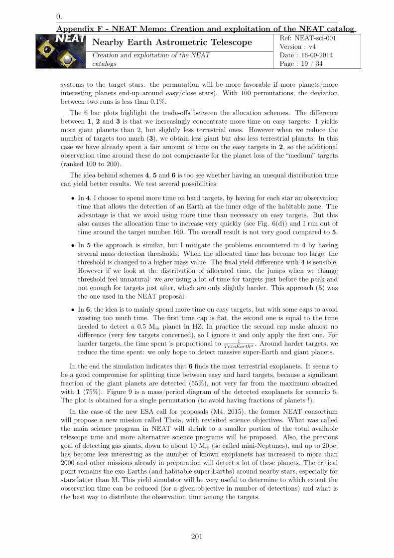
Nearby Earth Astrometric Telescope Ref: NEAT-sci-001Version : v4
Creation and exploitation of the NEATcatalogs
Date : 16-09-2014Page : 19 / 34
systems to the target stars: the permutation will be more favorable if more planets/moreinteresting planets end-up around easy/close stars). With 100 permutations, the deviationbetween two runs is less than 0.1%.
The 6 bar plots highlight the trade-offs between the allocation schemes. The differencebetween 1, 2 and 3 is that we increasingly concentrate more time on easy targets. 1 yieldsmore giant planets than 2, but slightly less terrestrial ones. However when we reduce thenumber of targets too much (3), we obtain less giant but also less terrestrial planets. In thiscase we have already spent a fair amount of time on the easy targets in 2, so the additionalobservation time around these do not compensate for the planet loss of the “medium” targets(ranked 100 to 200).
The idea behind schemes 4, 5 and 6 is too see whether having an unequal distribution timecan yield better results. We test several possibilities:
• In 4, I choose to spend more time on hard targets, by having for each star an observationtime that allows the detection of an Earth at the inner edge of the habitable zone. Theadvantage is that we avoid using more time than necessary on easy targets. But thisalso causes the allocation time to increase very quickly (see Fig. 6(d)) and I run out oftime around the target number 160. The overall result is not very good compared to 5.
• In 5 the approach is similar, but I mitigate the problems encountered in 4 by havingseveral mass detection thresholds. When the allocated time has become too large, thethreshold is changed to a higher mass value. The final yield difference with 4 is sensible.However if we look at the distribution of allocated time, the jumps when we changethreshold feel unnatural: we are using a lot of time for targets just before the peak andnot enough for targets just after, which are only slightly harder. This approach (5) wasthe one used in the NEAT proposal.
• In 6, the idea is to mainly spend more time on easy targets, but with some caps to avoidwasting too much time. The first time cap is flat, the second one is equal to the timeneeded to detect a 0.5 M⊕ planet in HZ. In practice the second cap make almost nodifference (very few targets concerned), so I ignore it and only apply the first one. Forharder targets, the time spent is proportional to 1
TexoEarthα . Around harder targets, wereduce the time spent: we only hope to detect massive super-Earth and giant planets.
In the end the simulation indicates that 6 finds the most terrestrial exoplanets. It seems tobe a good compromise for splitting time between easy and hard targets, because a significantfraction of the giant planets are detected (55%), not very far from the maximum obtainedwith 1 (75%). Figure 9 is a mass/period diagram of the detected exoplanets for scenario 6.The plot is obtained for a single permutation (to avoid having fractions of planets !).
In the case of the new ESA call for proposals (M4, 2015), the former NEAT consortiumwill propose a new mission called Theia, with revisited science objectives. What was calledthe main science program in NEAT will shrink to a smaller portion of the total availabletelescope time and more alternative science programs will be proposed. Also, the previousgoal of detecting gas giants, down to about 10 M⊕ (so called mini-Neptunes), and up to 20pc,has become less interesting as the number of known exoplanets has increased to more than2000 and other missions already in preparation will detect a lot of these planets. The criticalpoint remains the exo-Earths (and habitable super Earths) around nearby stars, especially forstars latter than M. This yield simulator will be very useful to determine to which extent theobservation time can be reduced (for a given objective in number of detections) and what isthe best way to distribute the observation time among the targets.
0.
Appendix F - NEAT Memo: Creation and exploitation of the NEAT catalog
201
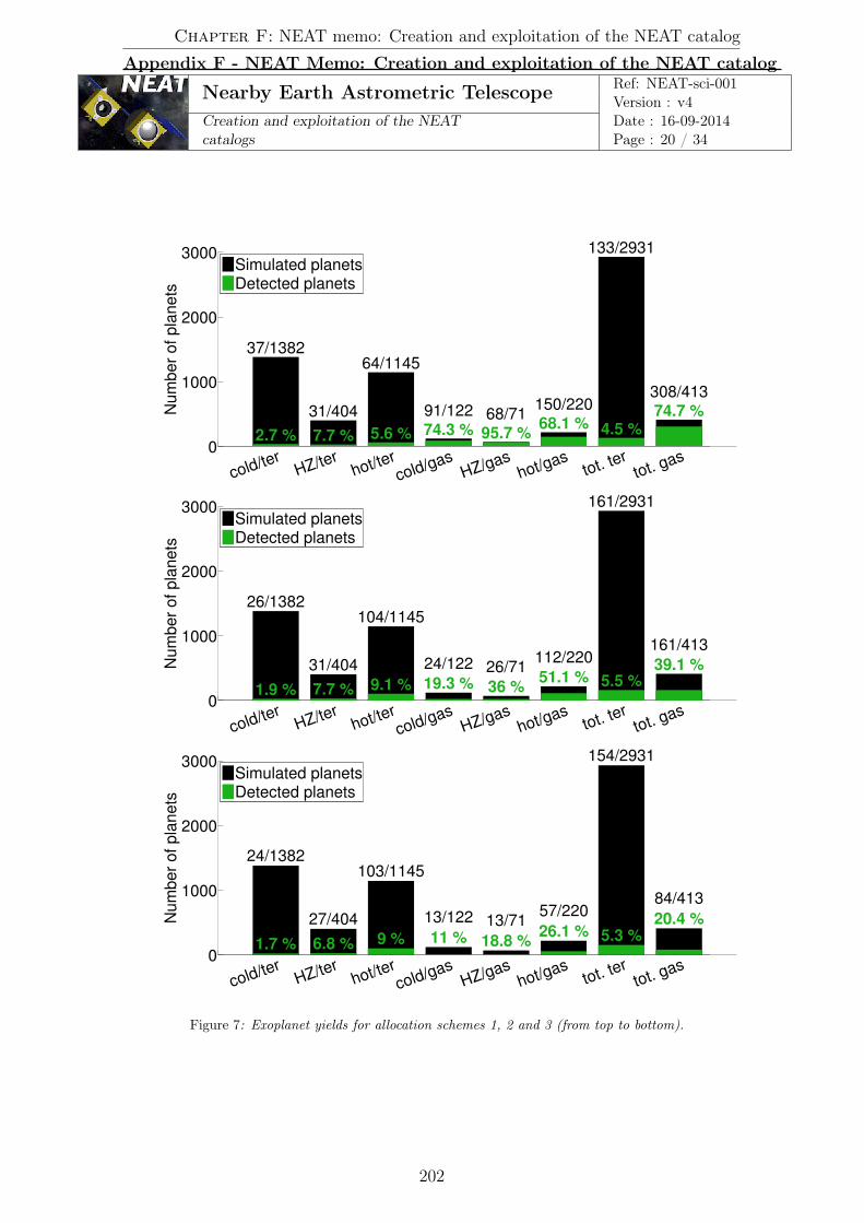
Nearby Earth Astrometric Telescope Ref: NEAT-sci-001Version : v4
Creation and exploitation of the NEATcatalogs
Date : 16-09-2014Page : 20 / 34
0
1000
2000
3000
Nu
mb
er
of
pla
ne
ts
2.7 % 74.3 %
37/1382
91/122
7.7 % 95.7 %
31/404 68/71
5.6 %68.1 %
64/1145
150/220
4.5 %
74.7 %
133/2931
308/413
cold/terHZ/ter
hot/tercold/gas
HZ/gashot/gas
tot. ter
tot. gas
X−Axis Label
Simulated planetsDetected planets
0
1000
2000
3000
Nu
mb
er
of
pla
ne
ts
1.9 %19.3 %
26/1382
24/122
7.7 % 36 %
31/404 26/719.1 %
51.1 %
104/1145
112/220
5.5 %
39.1 %
161/2931
161/413
cold/terHZ/ter
hot/tercold/gas
HZ/gashot/gas
tot. ter
tot. gas
Simulated planetsDetected planets
0
1000
2000
3000
Nu
mb
er
of
pla
ne
ts
1.7 %11 %
24/1382
13/122
6.8 % 18.8 %
27/404 13/719 %
26.1 %
103/1145
57/220
5.3 %
20.4 %
154/2931
84/413
cold/terHZ/ter
hot/tercold/gas
HZ/gashot/gas
tot. ter
tot. gas
Simulated planetsDetected planets
Figure 7: Exoplanet yields for allocation schemes 1, 2 and 3 (from top to bottom).
Chapter F: NEAT memo: Creation and exploitation of the NEAT catalog
Appendix F - NEAT Memo: Creation and exploitation of the NEAT catalog
202

Nearby Earth Astrometric Telescope Ref: NEAT-sci-001Version : v4
Creation and exploitation of the NEATcatalogs
Date : 16-09-2014Page : 21 / 34
0
1000
2000
3000
Nu
mb
er
of
pla
ne
ts
1.6 %16.8 %
22/1382
21/122
6.1 % 28.5 %
25/404 20/717.9 %
39.9 %
90/1145
88/220
4.7 %
31.1 %
137/2931
128/413
cold/terHZ/ter
hot/tercold/gas
HZ/gashot/gas
tot. ter
tot. gas
X−Axis Label
Simulated planetsDetected planets
0
1000
2000
3000
Nu
mb
er
of
pla
ne
ts
2.3 % 59.5 %
31/1382
73/122
7.2 % 89.5 %
29/404 64/717.4 %
66.3 %
85/1145
146/220
5 %
68.3 %
145/2931
282/413
cold/terHZ/ter
hot/tercold/gas
HZ/gashot/gas
tot. ter
tot. gas
Simulated planetsDetected planets
0
1000
2000
3000
Nu
mb
er
of
pla
ne
ts
2.5 % 36.1 %
34/1382
44/122
8.7 % 63.7 %
35/404 45/718 %
63.6 %
91/1145
140/220
5.5 %
55.5 %
160/2931
229/413
cold/terHZ/ter
hot/tercold/gas
HZ/gashot/gas
tot. ter
tot. gas
Simulated planetsDetected planets
Figure 8: Exoplanet yields for allocation schemes 4, 5 and 6 (from top to bottom).
0.
Appendix F - NEAT Memo: Creation and exploitation of the NEAT catalog
203

Nearby Earth Astrometric Telescope Ref: NEAT-sci-001Version : v4
Creation and exploitation of the NEATcatalogs
Date : 16-09-2014Page : 22 / 34
10−2
10−1
100
101
102
10−2
10−1
100
101
102
103
104
Planet semi major axis (AU)
Pla
ne
t m
ass (
Ea
rth
ma
ss)
10 Earth mass (terrestrial limit)
1 Earth mass
planet not detected (<0.3µas)
hot planet
temperate planet
cold planet
Figure 9: Mass period diagram of the NEAT mission simulated exoplanet yield.
2.3 – Astrometric signal in HZ versus stellar mass
Overall, the astrometric signal (A) in HZ increases with the host stellar mass (M). This isthe result of several competing effects:
1. The star luminosity increase with the mass: L ∝ M 3.8
2. The orbital distance of the HZ increase with the luminosity: R(HZ) ∝ L0.5
3. The albedo of the planet is higher for bluer light (it moves the HZ slightly closer to thestar)
4. The ratio Mplanet
Mstaris smaller
The net effect of 1 and 2 is an increase of the astrometric signal (A ∝ M 1.9). This issomewhat attenuated by 3 (but it is a weak effect). We can take the albedo into account bydefining an effective luminosity Leff ≈ L−α and we obtain for 1, 2 and 3: A ∝ M1.9−α/2. Theeffect of 4 is to subtract 1 to the total power. So we finally obtain: A ∝ M 0.9−α/2. Thisrelation is approximative, as we have used several approximated power laws: the L = f(M)relationship breaks down for M stars (the limit is around 0.43 M�) and the albedo effect is inour case modeled by a piecewise linear function. In reality the exact albedo effect will be nonlinear and specific to each planet.
Figure 10 shows the astrometric signal in HZ versus the stellar mass. In order to separatethe effects of the distance and the stellar mass, Fig. 11 shows the astrometric signal in HZ(µas) multiplied by the distance to the Sun (pc) versus the stellar mass. This is equivalent tomoving all the targets at a distance of 1 pc from the Sun.
Figure 11 confirms that the spectral effect is weak and that the astrometric signal in HZincrease with stellar mass, roughly as M 0.63 (⇒ α = 0.54) 3. This result is important, it tells
3Extrapolating from the following data points: (M=0.42, A=2.0) and (M=2.0, A=6.0).
Chapter F: NEAT memo: Creation and exploitation of the NEAT catalog
Appendix F - NEAT Memo: Creation and exploitation of the NEAT catalog
204
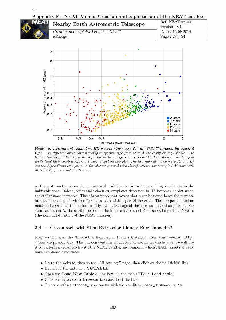
Nearby Earth Astrometric Telescope Ref: NEAT-sci-001Version : v4
Creation and exploitation of the NEATcatalogs
Date : 16-09-2014Page : 23 / 34
��� ��� ��� ��� � � �
������������������������
���
���
���
���
���
�
�
�
������������������������������
�����������������������������������
Figure 10: Astrometric signal in HZ versus star mass for the NEAT targets, by spectraltype. The different areas corresponding to spectral type from M to A are easily distinguishable. Thebottom line os for stars close to 20 pc, the vertical dispersion is caused by the distance. Low hangingfruits (and their spectral types) are easy to spot on this plot. The two stars at the very top (G and K)are the Alpha Centauri system. A few blatant spectral miss classifications (for example 2 M stars withM > 0.8M�) are visible on the plot.
us that astrometry is complementary with radial velocities when searching for planets in thehabitable zone. Indeed, for radial velocities, exoplanet detection in HZ becomes harder whenthe stellar mass increases. There is an important caveat that must be noted here: the increasein astrometric signal with stellar mass goes with a period increase. The temporal baselinemust be larger than the period to fully take advantage of the increased signal amplitude. Forstars later than A, the orbital period at the inner edge of the HZ becomes larger than 5 years(the nominal duration of the NEAT mission).
2.4 – Crossmatch with “The Extrasolar Planets Encyclopaedia"
Now we will load the “Interactive Extra-solar Planets Catalog", from this website: http://www.exoplanet.eu/. This catalog contains all the known exoplanet candidates, we will useit to perform a crossmatch with the NEAT catalog and pinpoint which NEAT targets alreadyhave exoplanet candidates.
• Go to the website, then to the “All catalogs” page, then click on the “All fields" link• Download the data as a VOTABLE• Open the Load New Table dialog box via the menu File > Load table• Click on the System Browser icon and load the table• Create a subset closest_exoplanets with the condition: star_distance < 20
0.
Appendix F - NEAT Memo: Creation and exploitation of the NEAT catalog
205
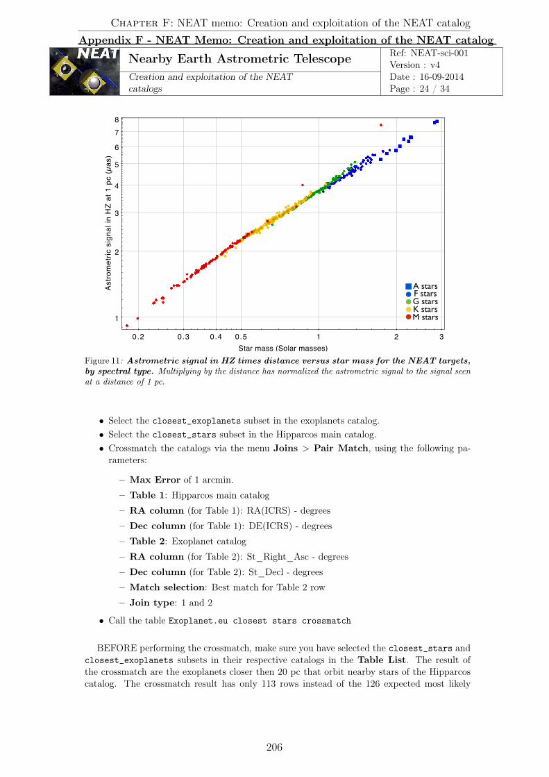
Nearby Earth Astrometric Telescope Ref: NEAT-sci-001Version : v4
Creation and exploitation of the NEATcatalogs
Date : 16-09-2014Page : 24 / 34
��� ��� ��� ��� � � �
������������������������
�
�
�
�
�
�
�
�
��������������������������������������
�����������������������������������
Figure 11: Astrometric signal in HZ times distance versus star mass for the NEAT targets,by spectral type. Multiplying by the distance has normalized the astrometric signal to the signal seenat a distance of 1 pc.
• Select the closest_exoplanets subset in the exoplanets catalog.• Select the closest_stars subset in the Hipparcos main catalog.• Crossmatch the catalogs via the menu Joins > Pair Match, using the following pa-
rameters:
– Max Error of 1 arcmin.
– Table 1: Hipparcos main catalog
– RA column (for Table 1): RA(ICRS) - degrees
– Dec column (for Table 1): DE(ICRS) - degrees
– Table 2: Exoplanet catalog
– RA column (for Table 2): St_Right_Asc - degrees
– Dec column (for Table 2): St_Decl - degrees
– Match selection: Best match for Table 2 row
– Join type: 1 and 2
• Call the table Exoplanet.eu closest stars crossmatch
BEFORE performing the crossmatch, make sure you have selected the closest_stars andclosest_exoplanets subsets in their respective catalogs in the Table List. The result ofthe crossmatch are the exoplanets closer then 20 pc that orbit nearby stars of the Hipparcoscatalog. The crossmatch result has only 113 rows instead of the 126 expected most likely
Chapter F: NEAT memo: Creation and exploitation of the NEAT catalog
Appendix F - NEAT Memo: Creation and exploitation of the NEAT catalog
206
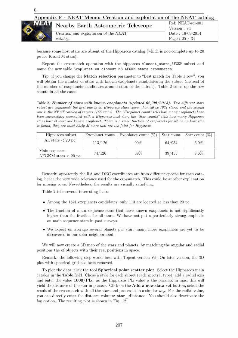
Nearby Earth Astrometric Telescope Ref: NEAT-sci-001Version : v4
Creation and exploitation of the NEATcatalogs
Date : 16-09-2014Page : 25 / 34
because some host stars are absent of the Hipparcos catalog (which is not complete up to 20pc for K and M stars).
Repeat the crossmatch operation with the hipparcos closest_stars_AFGKM subset andname the new table Exoplanet.eu closest MS AFGKM stars crossmatch.
Tip: if you change the Match selection parameter to “Best match for Table 1 row", youwill obtain the number of stars with known exoplanets candidates in the subset (instead ofthe number of exoplanets candidates around stars of the subset). Table 2 sums up the rowcounts in all the cases.
Table 2: Number of stars with known exoplanets (updated 02/09/2014). Two different starssubset are compared: the first one is all Hipparcos stars closer than 20 pc (934 stars) and the secondone is the NEAT catalog of targets (455 stars). The “Exoplanet count” tells how many exoplanets havebeen successfully associated with a Hipparcos host star, the “Star counts” tells how many Hipparcosstars host at least one known exoplanet. There is a small fraction of exoplanets for which no host staris found, they are most likely M stars that are too faint for Hipparcos.
Hipparcos subset Exoplanet count Exoplanet count (%) Star count Star count (%)All stars < 20 pc 113/126 90% 64/934 6.9%
Main sequenceAFGKM stars < 20 pc 74/126 59% 39/455 8.6%
Remark: apparently the RA and DEC coordinates are from different epochs for each cata-log, hence the very wide tolerance used for the crossmatch. This could be another explanationfor missing rows. Nevertheless, the results are visually satisfying.
Table 2 tells several interesting facts:
• Among the 1821 exoplanets candidates, only 113 are located at less than 20 pc.
• The fraction of main sequence stars that have known exoplanets is not significantlyhigher than the fraction for all stars. We have not put a particularly strong emphasison main sequence stars in past surveys.
• We expect on average several planets per star: many more exoplanets are yet to bediscovered in our solar neighborhood.
We will now create a 3D map of the stars and planets, by matching the angular and radialpositions the of objects with their real positions in space.
Remark: the following step works best with Topcat version V3. On later version, the 3Dplot with spherical grid has been removed.
To plot the data, click the tool Spherical polar scatter plot. Select the Hipparcos maincatalog in the Table field. Chose a style for each subset (each spectral type), add a radial axisand enter the value 1000/Plx: as the Hipparcos Plx value is the parallax in mas, this willyield the distance of the star in parsecs. Click on the Add a new data set button, select theresult of the crossmatch with all the stars and process it in a similar way. For the radial value,you can directly enter the distance column: star_distance. You should also deactivate thefog option. The resulting plot is shown in Fig. 12.
0.
Appendix F - NEAT Memo: Creation and exploitation of the NEAT catalog
207
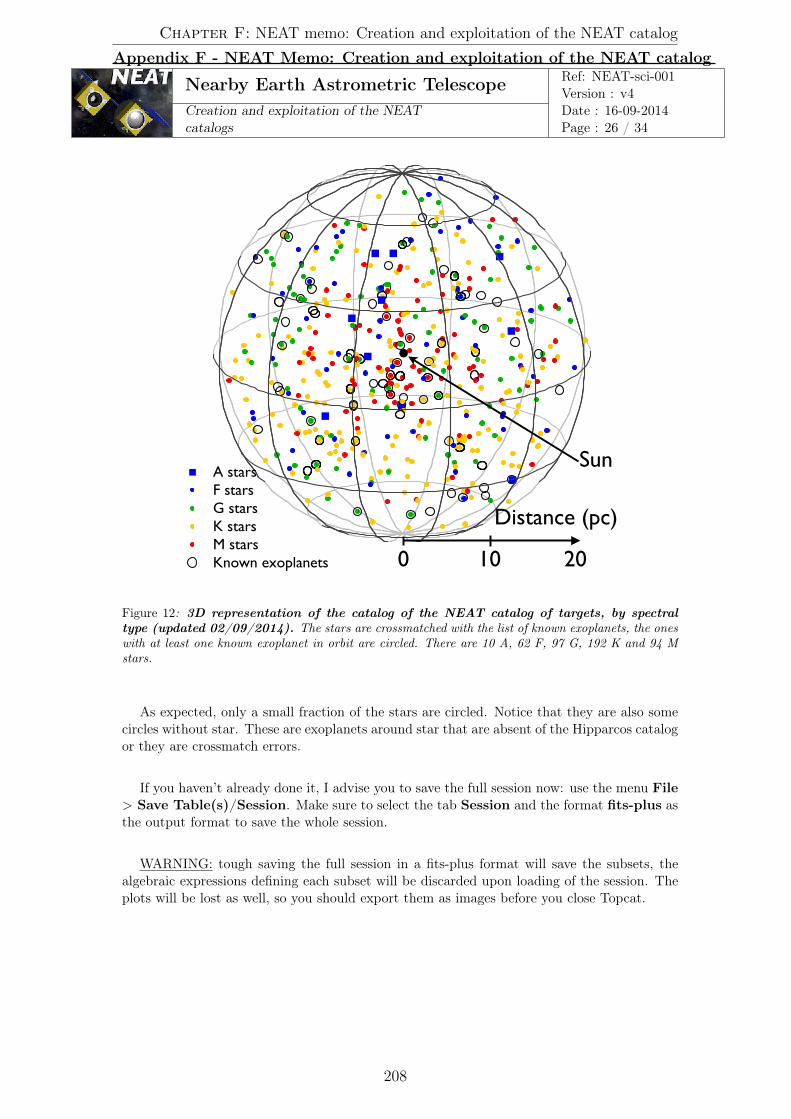
Nearby Earth Astrometric Telescope Ref: NEAT-sci-001Version : v4
Creation and exploitation of the NEATcatalogs
Date : 16-09-2014Page : 26 / 34
���������������������������������������������������
�������������
� �� ��
���
Figure 12: 3D representation of the catalog of the NEAT catalog of targets, by spectraltype (updated 02/09/2014). The stars are crossmatched with the list of known exoplanets, the oneswith at least one known exoplanet in orbit are circled. There are 10 A, 62 F, 97 G, 192 K and 94 Mstars.
As expected, only a small fraction of the stars are circled. Notice that they are also somecircles without star. These are exoplanets around star that are absent of the Hipparcos catalogor they are crossmatch errors.
If you haven’t already done it, I advise you to save the full session now: use the menu File> Save Table(s)/Session. Make sure to select the tab Session and the format fits-plus asthe output format to save the whole session.
WARNING: tough saving the full session in a fits-plus format will save the subsets, thealgebraic expressions defining each subset will be discarded upon loading of the session. Theplots will be lost as well, so you should export them as images before you close Topcat.
Chapter F: NEAT memo: Creation and exploitation of the NEAT catalog
Appendix F - NEAT Memo: Creation and exploitation of the NEAT catalog
208

Nearby Earth Astrometric Telescope Ref: NEAT-sci-001Version : v4
Creation and exploitation of the NEATcatalogs
Date : 16-09-2014Page : 27 / 34
2.5 – Checking the sample completeness
By looking at the 3D representation of the NEAT catalog, it is clear that the M stars are notevenly distributed. They are mostly located within 10 pc of the sun. There is obviously aproblem of completeness for the M stars: the most distant M stars seams to be absent of theHipparcos catalog because their magnitudes are too high.
So I ask the following: are all the F, G and K stars closer than 20 pc present in theHipparcos catalog ? To answer this, one can simply plot the histogram of the number of starsversus the distance.
Add new subsets of main sequence F,G,K and M stars closer than 100 pc in the mainHipparcos table. For example for F stars:-name: close_MS_F_stars-condition: Plx > 10 && matches(SpType,"^F.*(IV-V|[^I]V)")
Assuming an homogeneous distribution of the stars in the solar neighbourhood, the numberof stars in a radius r is: n = α × 4/3⇡r3, where α is the mean density of stars, thus: dn =α × 4⇡r2dr. An histogram of the stars count versus the distance (in log axis) is in fact arepresentation of log dn
dr versus log r. Since we have: log dndr = 2 log r + 2 log 4⇡α, we expect
to see a slope of 2 for the short distances, where the Hipparcos catalog is complete. Thebreakpoint in the slope indicate where the catalog is not complete anymore.
In order to see the breakpoints, other subsets are defined. The procedure is the same thanthe one that was used to define the NEAT catalog, expect that the distance is limited to 1kpc(as a result almost all the Hipparcos stars are included). The final histograms are shown inFig. 13 and 14
� Conclusion
One can assume near completeness of the Hipparcos catalog for the FGK main sequencestars (the completeness breakpoints are all well further than 20 pc). The same is not true for Mstars, because they are much fainter. These results are consistent with the existing literature,a completeness study was performed to assess the completeness of the Darwin catalog (whichwas also build from the Hipparcos catalog): “Excluding the M stars from the estimate leads toa high completeness at 20 pc and 30 pc of 97% and 76% respectively, based on the estimatednumber of stars per volume using the 10 pc RECONS data set." (Kaltenegger et al., 2010).
The incompleteness issue is of little practical importance for the main science programbecause Hipparcos is 99.9% complete to magnitude 10, and measures around fainter starswould be strongly impaired by high photon noise (it becomes larger than reference photonnoise). To summarize: the NEAT catalog is volume limited for F,G and K stars at 20 pc, andmagnitude limited for M stars (around Vmag = 10).
0.
Appendix F - NEAT Memo: Creation and exploitation of the NEAT catalog
209

Nearby Earth Astrometric Telescope Ref: NEAT-sci-001Version : v4
Creation and exploitation of the NEATcatalogs
Date : 16-09-2014Page : 28 / 34
���
���
���
�������
���
���
���
�������
���
���
���
�������
������ ��� ��� ��� ���� ��� ��� ��� ��� ����
�������������
���������������
����������������������������������������������������
����������������
��������������
Figure 13: Histogram of the distribution of the F, G and K stars versus the distance. Wecan see that the completeness breakpoint locations are different for each spectral type: 40 pc for K stars,60 pc for G stars and further away for F stars. This pattern was expected since the hotter a star is,the larger it’s luminosity is. The values for distances less than 10 pc can be ignored (the number ofstars in these beans is too small).
���
���
���
���
���
���������
��������
���
������ ��� ��� ��� ���� ��� ��� ��� ��� ����
�������������
���������������
����������������������������������������������������
���������
�������
Figure 14: Histogram of the distribution of the M stars versus the distance. The sample isquite small (75 stars). One can see that the slope is less than 2 for this histogram: although there isan upward trend for distances less than 20 pc, the sample is clearly incomplete (not even at 10 pc!).
Chapter F: NEAT memo: Creation and exploitation of the NEAT catalog
Appendix F - NEAT Memo: Creation and exploitation of the NEAT catalog
210

Nearby Earth Astrometric Telescope Ref: NEAT-sci-001Version : v4
Creation and exploitation of the NEATcatalogs
Date : 16-09-2014Page : 29 / 34
References
Alibert, Y., Carron, F., Fortier, A., Pfyffer, S., Benz, W., Mordasini, C., and Swoboda, D.:2013, Astronomy and Astrophysics 558, A109
Dittkrist, K.-M., Mordasini, C., Klahr, H., Alibert, Y., and Henning, T.: 2014, Astronomyand Astrophysics 567, A121
Flower, P. J.: 1996, APJ 469, 355Kaltenegger, L., Eiroa, C., and Fridlund, C. V. M.: 2010, APSS 326, 233Kasting, J. F., Whitmire, D. P., and Reynolds, R. T.: 1993, Icarus 101, 108Mordasini, C., Dittkrist, K.-M., Alibert, Y., Klahr, H., Benz, W., and Henning, T.: 2011,
in A. Sozzetti, M. G. Lattanzi, and A. P. Boss (eds.), IAU Symposium, Vol. 276 of IAUSymposium, pp 72–75
Schmidt-Kaler: 1982, in Astronomy and Astrophysics (eds.), Stars and star clusters, Vol. 2b,SpringerMaterials
0.
Appendix F - NEAT Memo: Creation and exploitation of the NEAT catalog
211

Nearby Earth Astrometric Telescope Ref: NEAT-sci-001Version : v4
Creation and exploitation of the NEATcatalogs
Date : 16-09-2014Page : 30 / 34
A – Summary of the Topcat operations
• Load the hipparcos and tycho catalog (all the tables), with the computed J2000 coordi-nates in a VOTable format
• In the main Hipparcos table, define the following subsets
– closest_stars: Plx > 50
– closest_MS_A_stars: _2 && matches(SpType, "^A.*V$")
– closest_MS_F_stars: _2 && matches(SpType, "^F.*V$")
– closest_MS_G_stars: _2 && matches(SpType, "^G.*V$")
– closest_MS_K_stars: _2 && matches(SpType, "^K.*V$")
– closest_MS_M_stars: _2 && matches(SpType, "^M.*V$")
– closest_MS_FGK_stars:
_2 && (matches(SpType,"^F.*V$")||matches(SpType,"^G.*V$")||matches(SpType,"^K.*V$"))
– closest_MS_AFGKM_stars:
_2 && (matches(SpType,"^A.*V$")||matches(SpType,"^F.*V$")||matches(SpType,"^G.*V$")||matches(SpType,"^K.*V$")||matches(SpType,"^M.*V$"))
• Select the Tycho table and perform a crossmatch with Hipparcos to find the referencestars.Change table name to: Tycho reference stars crossmatchExport table as: reference_stars_topcat.csv
• Export the closest_MS_AFGKM_stars subset as closest_MS_AFGKM_stars_topcat.csv,run the script and import the new table with the new magnitude column.
• Select the closest_MS_AFGKM_stars subset and create all the “NEAT" columns (seethe list in section B)
• For completeness only: create the close main sequence F, G, K and M stars subsets inthe main Hipparcos table (stars closer than 100 pc).
• Re create the A, F, G, K and M main sequence stars subsets in the closest_MS_AFGKM_stars_topcat.csvtable.
B – List of the NEAT columns
� Columns prior to sum of reference stars flux (by script) .
These columns can be created either before or after the equivalent reference star magnitudeis added.
Dist 1000/Plx
Chapter F: NEAT memo: Creation and exploitation of the NEAT catalog
Appendix F - NEAT Memo: Creation and exploitation of the NEAT catalog
212

Nearby Earth Astrometric Telescope Ref: NEAT-sci-001Version : v4
Creation and exploitation of the NEATcatalogs
Date : 16-09-2014Page : 31 / 34
BC -0.1784538+2.9023636*$39-12.318814*pow($39,2)+20.931026*pow($39,3)-22.50268371*pow($39,4)+63.6149604*pow($39,5)-177.541721356*pow($39,6)+249.915028525*pow($39,7)-182.6519997*pow($39,8)+67.42205675*pow($39,9)-9.98700145*pow($39,10)
MB Vmag+BC-5*ln(100/Plx)/ln(10)L pow(10,(4.75-MB)/2.5)
Mass pow(L,1.0/3.8)SeffIn1 $39<0.62? -1.484*$39+2.330 : -0.371*$39+1.640
SeffOut1 $39<0.62? -0.303*$39+0.547 : -0.092*$39+0.417SeffIn2 $39<0.62? -0.727*$39+2.211: -0.165*$39+1.862
SeffOut2 $39<0.62? -0.273*$39+0.489 : -0.082*$39+0.371HZIn1 pow(L/SeffIn1,0.5)HZIn2 pow(L/SeffIn2,0.5)
HZOut1 pow(L/SeffOut1,0.5)HZOut2 pow(L/SeffOut2,0.5)
AIn1 3/Mass*HZIn1/DistAIn2 3/Mass*HZIn2/Dist
AOut1 3/Mass*HZOut1/DistAOut2 3/Mass*HZOut2/Dist
AEarthFlux 3/Mass*pow(L,0.5)/DistAMid1 (AIn1+AOut1)/2AMid2 (AIn2+AOut2)/2
IWAIn1 HZIn1/DistIWAIn2 HZIn2/Dist
IWAOut1 HZOut1/DistIWAOut2 HZOut2/Dist
IWAEarthFlux pow(L,0.5)/DistIWAMid1 (IWAIn1+IWAOut1)/2IWAMid2 (IWAIn2+IWAOut2)/2
TIn1 pow(pow(HZIn1,3)/Mass,0.5)Tin2 pow(pow(HZIn2,3)/Mass,0.5)
TOut1 pow(pow(HZOut1,3)/Mass,0.5)TOut2 pow(pow(HZOut2,3)/Mass,0.5)
� Columns after sum of reference stars flux (by script) .
These columns can only be created after the equivalent reference star magnitude is added.
SigmaH pow(0.0144*pow(10,(Vmag-6)/2.5)+0.372*pow(10,(EqRefMag-9.05)/2.5)+0.194,0.5)TexoEarth 36*pow(SigmaH,2)/pow(AIn1,2)
0.
Appendix F - NEAT Memo: Creation and exploitation of the NEAT catalog
213
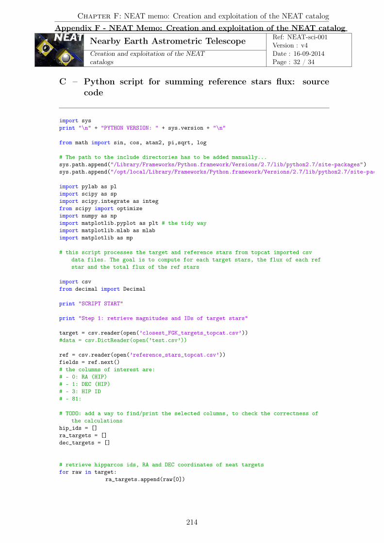
Nearby Earth Astrometric Telescope Ref: NEAT-sci-001Version : v4
Creation and exploitation of the NEATcatalogs
Date : 16-09-2014Page : 32 / 34
C – Python script for summing reference stars flux: sourcecode
import sysprint "\n" + "PYTHON VERSION: " + sys.version + "\n"
from math import sin, cos, atan2, pi,sqrt, log
# The path to the include directories has to be added manually...sys.path.append("/Library/Frameworks/Python.framework/Versions/2.7/lib/python2.7/site-packages")sys.path.append("/opt/local/Library/Frameworks/Python.framework/Versions/2.7/lib/python2.7/site-packages
import pylab as plimport scipy as spimport scipy.integrate as integfrom scipy import optimizeimport numpy as npimport matplotlib.pyplot as plt # the tidy wayimport matplotlib.mlab as mlabimport matplotlib as mp
# this script processes the target and reference stars from topcat imported csvdata files. The goal is to compute for each target stars, the flux of each refstar and the total flux of the ref stars
import csvfrom decimal import Decimal
print "SCRIPT START"
print "Step 1: retrieve magnitudes and IDs of target stars"
target = csv.reader(open(’closest_FGK_targets_topcat.csv’))#data = csv.DictReader(open(’test.csv’))
ref = csv.reader(open(’reference_stars_topcat.csv’))fields = ref.next()# the columns of interest are:# - 0: RA (HIP)# - 1: DEC (HIP)# - 3: HIP ID# - 81:
# TODO: add a way to find/print the selected columns, to check the correctness ofthe calculations
hip_ids = []ra_targets = []dec_targets = []
# retrieve hipparcos ids, RA and DEC coordinates of neat targetsfor raw in target:
ra_targets.append(raw[0])
Chapter F: NEAT memo: Creation and exploitation of the NEAT catalog
Appendix F - NEAT Memo: Creation and exploitation of the NEAT catalog
214

Nearby Earth Astrometric Telescope Ref: NEAT-sci-001Version : v4
Creation and exploitation of the NEATcatalogs
Date : 16-09-2014Page : 33 / 34
dec_targets.append(raw[1])hip_ids.append(raw[3])
ra_targets.pop(0)dec_targets.pop(0)hip_ids.pop(0)
print(’hip_ids = ’)print(hip_ids)
print "Step 2: find which tychos stars are the targets"# finds which entry in the tychos ref stars is the targettyc_ids = [0]*len(hip_ids)ref_star_mageq = [99]*len(hip_ids) # equivalent magnitude of ref stars
counts = 0
for i in range(len(hip_ids)):dist = 3600.0**2ref = csv.reader(open(’reference_stars_topcat.csv’))ref.next()for raw in (ref):
# print(’hip_id = ’ + hip_ids[i])# print(’raw = ’ + raw[3])# print(’ ’)
if int(raw[3]) == int(hip_ids[i]):counts = counts +1new_dist = (float(raw[81])-float(ra_targets[i]))**2 +
(float(raw[82])-float(dec_targets[i]))**2if new_dist < dist:
tyc_ids[i] = raw[84]dist = new_dist
print(’counts = ’)print(counts)print(’tyc_ids = ’)print(tyc_ids)
print(’size tyc_ids = ’)print(len(tyc_ids))
vmag_hip = []vmag_tyc = []sep = []print "Step 3: verification of the matching between the hipparcos targets and the
tychos matches found "# TODO: add a verification step: verify that the parameters for the identified
hipparcos targets in the list of references have the same hipparcos/tychosparameters. Count the good matches. Plot the values of hip params VS tyc params
for i in range(len(tyc_ids)):ref = csv.reader(open(’reference_stars_topcat.csv’))ref.next()for raw in ref:
if raw[84] == tyc_ids[i]:
0.
Appendix F - NEAT Memo: Creation and exploitation of the NEAT catalog
215
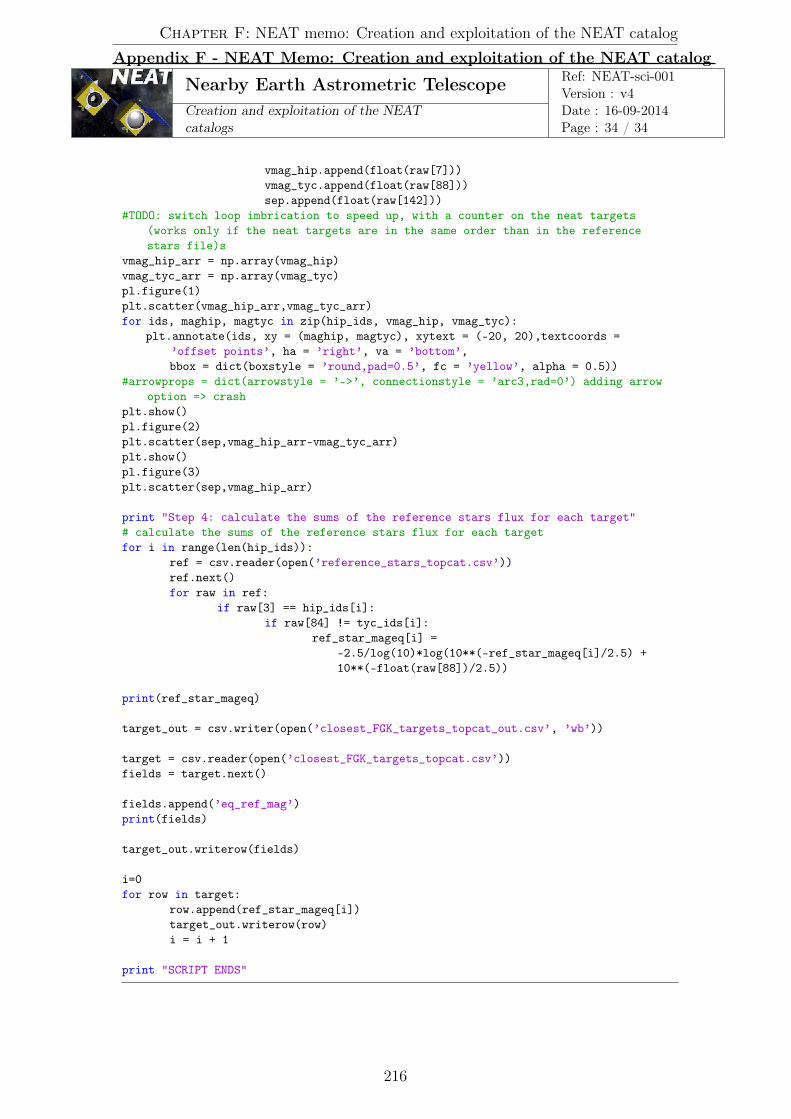
Nearby Earth Astrometric Telescope Ref: NEAT-sci-001Version : v4
Creation and exploitation of the NEATcatalogs
Date : 16-09-2014Page : 34 / 34
vmag_hip.append(float(raw[7]))vmag_tyc.append(float(raw[88]))sep.append(float(raw[142]))
#TODO: switch loop imbrication to speed up, with a counter on the neat targets(works only if the neat targets are in the same order than in the referencestars file)s
vmag_hip_arr = np.array(vmag_hip)vmag_tyc_arr = np.array(vmag_tyc)pl.figure(1)plt.scatter(vmag_hip_arr,vmag_tyc_arr)for ids, maghip, magtyc in zip(hip_ids, vmag_hip, vmag_tyc):
plt.annotate(ids, xy = (maghip, magtyc), xytext = (-20, 20),textcoords =’offset points’, ha = ’right’, va = ’bottom’,bbox = dict(boxstyle = ’round,pad=0.5’, fc = ’yellow’, alpha = 0.5))
#arrowprops = dict(arrowstyle = ’->’, connectionstyle = ’arc3,rad=0’) adding arrowoption => crash
plt.show()pl.figure(2)plt.scatter(sep,vmag_hip_arr-vmag_tyc_arr)plt.show()pl.figure(3)plt.scatter(sep,vmag_hip_arr)
print "Step 4: calculate the sums of the reference stars flux for each target"# calculate the sums of the reference stars flux for each targetfor i in range(len(hip_ids)):
ref = csv.reader(open(’reference_stars_topcat.csv’))ref.next()for raw in ref:
if raw[3] == hip_ids[i]:if raw[84] != tyc_ids[i]:
ref_star_mageq[i] =-2.5/log(10)*log(10**(-ref_star_mageq[i]/2.5) +10**(-float(raw[88])/2.5))
print(ref_star_mageq)
target_out = csv.writer(open(’closest_FGK_targets_topcat_out.csv’, ’wb’))
target = csv.reader(open(’closest_FGK_targets_topcat.csv’))fields = target.next()
fields.append(’eq_ref_mag’)print(fields)
target_out.writerow(fields)
i=0for row in target:
row.append(ref_star_mageq[i])target_out.writerow(row)i = i + 1
print "SCRIPT ENDS"
Chapter F: NEAT memo: Creation and exploitation of the NEAT catalog
Appendix F - NEAT Memo: Creation and exploitation of the NEAT catalog
216
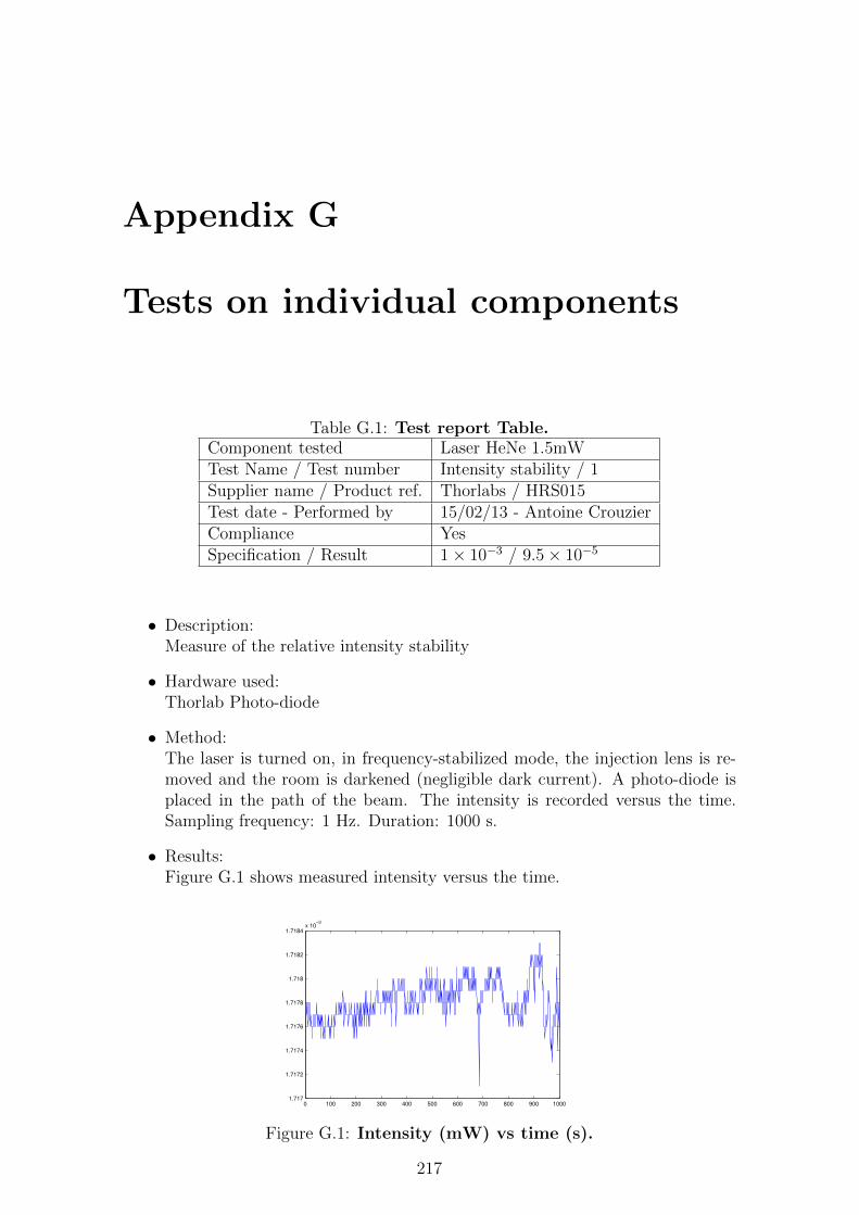
Appendix G
Tests on individual components
Table G.1: Test report Table.Component tested Laser HeNe 1.5mWTest Name / Test number Intensity stability / 1Supplier name / Product ref. Thorlabs / HRS015Test date - Performed by 15/02/13 - Antoine CrouzierCompliance YesSpecification / Result 1× 10⁻³ / 9.5× 10⁻⁵
• Description:Measure of the relative intensity stability
• Hardware used:Thorlab Photo-diode
• Method:The laser is turned on, in frequency-stabilized mode, the injection lens is re-moved and the room is darkened (negligible dark current). A photo-diode isplaced in the path of the beam. The intensity is recorded versus the time.Sampling frequency: 1 Hz. Duration: 1000 s.
• Results:Figure G.1 shows measured intensity versus the time.
0 100 200 300 400 500 600 700 800 900 10001.717
1.7172
1.7174
1.7176
1.7178
1.718
1.7182
1.7184x 10
−3
Figure G.1: Intensity (mW) vs time (s).
217
Chapter G: Tests on individual components
• Remarks:Idark = 0 nW
• Conclusion:For a duration of 1000 sec, with a 1 Hz sampling: RSD(intensity) = 9.5×10⁻⁵
Table G.2: Test report Table.Component tested Laser HeNe 1.5mWTest Name / Test number Polarization linearity / 2Supplier name / Product ref. Thorlabs / HRS015Test date - Performed by 15/02/13 - Antoine CrouzierCompliance YesSpecification / Result 1000:1 / 5400:1
• Description:Measure of the linearity of the polarization at the laser output. The linearityRpol is defined as the following ratio: intensity of straight polarization
intensity of circular polarization.
• Hardware used:Two polarizers: Glan–Thompson crystals, theoretical rejection ratio of 100000:1. Thorlab Photo-diode.
• Method:The laser is on and in frequency-stabilized mode, the injection lens is removed.The room is darkened (negligible dark current).
1. The laser beam is blocked and the resulting“dark intensity” is noted Idark.
2. The polariser extinction ratio is measured by placing the two polarizersin the path of the laser beam. The first polarizer is aligned with thelaser main axis (by searching the maximum). The second polarizer isalso aligned with the polarization (same method) and Ipara is measured.The angle of the second polariser is changed by 90◦ (by searching theminimum) and Iperp is measured. The ratio between the intensity ofeach case (after dark subtraction) gives the rejection ratio. It gives themaximum value of Rpol that can be obtained by this measure.
Rejection ratio = Ipara−IdarkIperp−Idark
3. The second polarizer is removed (only one is left in front of the laser).The angle of the polariser is tuned to find the maximum of intensity Imax.The angle of the polarizer is tuned to find the minimum of intensity Imin.We obtain Rpol =
Imax−IdarkImin−Idark
.
• Results:Read noise photo-detector (no light): ± 3nWIdark < 1 nWIpara = 1.337 mWIperp = 45± 3 nW⇒ Rejection ratio > 3.0× 10⁴ ± 10%Imax = 1.371mWImin = 248± 3 nW⇒ Rpol = 5400 : 1± 1%
218

0.
• Remarks:After using a sheet of paper to block the part of the beam visible on the leftof the photo-detector (outside of the integrating area): Iperp = 10 nW. Someinternal reflections or alignment problems inside the polarizers are creatingstray light on the photo-detector. The pattern of these off-axis reflectionschanges with the alignment. We conclude that we have only obtained a lowerbound of the rejection ratio, however the value is sufficiently high for ourpurposes (Rejection ratio � Rpol).
• Conclusion:Polarization ratio = 5400 : 1± 1%.
Table G.3: Test report Table.Component tested Laser HeNe 1.5mWTest Name / Test number Polarisation angular stability / 3Supplier name / Product ref. Thorlabs / HRS015Test date - Performed by 15/02/13 - Antoine CrouzierCompliance NSSpecification / Result NS / [0.038; 0.24]◦
• Description:Measure of the angular stability of the polarization versus time
• Hardware used:One polarizer: Glan–Thompson crystal, theoretical rejection ratio of 100 000:1.Thorlab Photo-diode.
• Method:The laser is on and in frequency-stabilized mode, the injection lens is removed.The room is darkened (negligible dark current).
1. The beam is blocked and the “dark intensity” is noted Idark
2. The intensity is measured after the linear polarizer placed in front ofthe laser output. The polarizer is set with an angle of 90◦ between thelaser polarization and the transmitting axis by searching the minimum oftransmission. The value of the intensity I(t) is recorded versus the time.Sampling rate = 1 Hz. Duration = 100 s.
3. The intensity is measured after the linear polarizer placed in front ofthe laser output. The polarizer is set with an angle of 0◦ between thelaser polarization and the transmitting axis by searching the maximumof transmission. The value of the intensity I �(t) is recorded versus thetime. Sampling rate = 1 Hz. Duration = 100 s.
Is it quite troublesome to get back to the variation of the polarization anglefrom only this intensity measurement. The contributions from the circularityof the laser polarization and the miss-alignment angle of the polarizer have tobe separated. Here we consider a model where the polarization is (slightly)elliptical and constant with time. The electric field after the polarizer is thesum of the projections of the minor and major axis (with are out of phase by180◦) along the polarizer transmitting axis:
�E = Ex cos(t) cos(dθ(t) + φ) �ux + Ey sin(t) sin(dθ(t) + φ) �uy
219

Chapter G: Tests on individual components
where:
◦ Ex is the electric field amplitude along the minor polarization axis of thelaser
◦ Ey is the electric field amplitude along the major polarization axis of thelaser
◦ φ is the static miss-alignment between the polarizer transmitting axis andthe laser major axis
◦ dθ(t) is the random variation of the laser polarization angle at a time t.
Let us define Φ = dθ(t) + φ. Given the setup and the previous results, we cansafely assume Φ � 0.02 rad, so we can write: I(t) ≈ Ex2(1 − Φ2)2 + Ey2Φ2.The intensity I(t) is minimum when Φ = 0. The variations of I(t) are infirst approximation caused by the change in the projection of Ey because:E2
y � E2x (from previous tests, we have already determined Ex2 = Imin and
Ey2 = Imax).
Assuming that the miss-alignment angle is small (dθ(t) � φ):
I(t) ≈ Imin + Imax (dθ(t))2 ≈ I(t)min + Imax (dθ(t))
2 (G.1)
⇒ |dθ(t)| =
�I(t)− I(t)min
Imax
(G.2)
Assuming that the miss-alignment angle is large (dθ(t) ≤ φ):
I(t) ≈ Imin + Imaxφ2 + Imax (2dθ(t)φ) ≈ I(t)mean + Imax (2dθ(t)φ)(G.3)
⇒ dθ(t) =I(t)− I(t)mean
2φImax
(G.4)
In our setup we feed the laser into two modulators that select a linear polar-ization. So what we are really interested in is the level of intensity fluctuationsafter selecting the main polarization (I �(t)). Then the fluctuations can becompared to laser intensity fluctuations and we can simply assess how muchpolarization instability contributes into overall intensity fluctuations. In factI �(t) gives us the stability of the intensity and the polarization combined.
• Results:Figure G.2 shows I(t). Figure G.3 shows dθ(t). Figure G.4 shows I �(t).
0 10 20 30 40 50 60 70 80 90 1002.56
2.57
2.58
2.59
2.6
2.61
2.62
2.63
2.64
2.65x 10
−7
Figure G.2: I(t) (W) vs time (s). These points are used to calculate dθ(t).
220

0.
0 10 20 30 40 50 60 70 80 90 1000
0.5
1
1.5
2
2.5x 10
−3
Figure G.3:�
I(t)−I(t)min
Imaxvs time(s).
0 100 200 300 400 500 600 700 800 900 10001.441
1.4412
1.4414
1.4416
1.4418
1.442
1.4422x 10
−3
Figure G.4: I’(t) (W) versus time (s). .
For a duration of 100 sec, with a sampling of 1 Hz:
– RSD(I(t)) = 9.3× 10⁻³.
– RSD(I �(t)) = 1.3× 10⁻⁴
– If dθ(t) � φ: RSD(|dθ(t)|) = 6.7× 10⁻⁴rad = 0.038◦
– If dθ(t) ≤ φ, the worst case is when we assume φ = 8×10⁻³ rad, becausewe find
SD[dθ(t)] =RSD[I(t)]Mean[I(t)]
2φImax
= 4.3× 10⁻³ rad = 0.24◦ (G.5)
We know this to be the worst case because if assume lower values for φ,we quickly obtain dθ(t) ≥ φ, which contradicts the hypothesis.
• Remarks:Idark = 0Imax = 1.371mW (known from other tests)
• Conclusion:The intensity variations observed after the polarizer are dominated by intensityvariation only (the RSD of the intensity before and after selection of the mainaxis with a polarizer are respectively 9.5×10⁻⁵ and 1.3×10⁻⁴, the difference isnot significant and could be simply due to changes in the amplitude of thermalfluctuations between the two measures.
The angle of the polarization is fairly stable, for a duration of 100 sec: STD(dθ) <0.24◦
221
Chapter G: Tests on individual components
Test report:
Table G.4: Test report Table.Component tested Laser HeNe 1.5mWTest Name / Test number Stabilization time / 4Supplier name / Product ref. Thorlabs / HRS015Test date - Performed by 13/02/13 - Antoine CrouzierCompliance NoSpecification / Result 30 min / 60-70 min
• Description:Measure of the stabilization time
• Hardware used:Clock
• Method:The laser is turned on and the time after which the LED stops blinking isnoted.
• Results:The laser stabilized between 60 and 70 minutes after being turned on.
• Remarks:
• Conclusion:The laser can take longer than the time given by the constructor to stabilize(not critical).
Test report:
Table G.5: Test report Table.Component tested Laser HeNe 1.5mWTest Name / Test number Wavelength stability / 5Supplier name / Product ref. Thorlabs / HRS015Test date - Performed by 18/02/13 - Antoine CrouzierCompliance NoSpecification / Result 2× 10⁻⁹ / 1.5× 10⁻⁸
• Description:Measure of the wavelength stability
• Hardware used:HiFinesse spectrometer: http://www.highfinesse.com/en/wavelengthmeter/ws6.phpTheoretical resolution: better than 1× 10⁻⁶
• Method:The laser is turned ON, in frequency-stabilized mode and injected into a (nonPM) fiber. The fiber is fed into a lambda meter. The wavelength is recordedversus the time. Sampling rate: 10 Hz. Lambda meter integration time: 100ms. Duration = 3000 seconds.
222

0.
• Results:A wavelength of -4 on the data log indicates that the laser was saturated, thishappens because the intensity is not stable and the exposure time becomestoo high. Only the first part of the data (before saturation) is shown below.The deviation is greater for longer time scales: slow drifts occur. This can bedue to thermal variations.
0 0.5 1 1.5 2 2.5 3 3.5
x 107
632.9914
632.9915
632.9915
632.9916
632.9916
632.9917
632.9918
632.9918
632.9918
Figure G.5: Wavelength (nm) vs time (ms). There are 30000 points onthis plot, at a sampling rate of 10Hz, the total duration is 3000 seconds.Relative STD = 9.5× 10⁻⁸.
1 1.02 1.04 1.06 1.08 1.1 1.12
x 106
632.9916
632.9916
632.9916
632.9916
632.9916
632.9917
632.9917
Figure G.6: Figure 2: Wavelength (nm) vs time (ms). There are 1000points on this plot, at a sampling rate of 10Hz, the total duration is 100seconds. Wavelength RSD: 1.5 × 10⁻⁸. The deviation is smaller becauseit was dominated by large variations in large time scales in the previousset of data points: on short time scale the laser is more stable.
• Remarks:
• Conclusion:For a duration of 100 sec, RSD(wavelength)= 1.5 × 10⁻⁸. Although the fi-nal values found are not compatible with the constructor specification, thiscould be caused by the resolution of the spectrometer used. The measuredwavelength stability should however be enough for our application.
223

Chapter G: Tests on individual components
Table G.6: Test report Table.Component tested Liquid core fiberTest Name / Test number Plug interface leakage / 6Supplier name / Product ref. Oriel / Liquid light guides - LLG210/LLG211Test date - Performed by 18/02/13 - Antoine Crouzier and Eric StadlerCompliance YesSpecification / Result Air tight / Air tight
• Description:Air Leakage inside the fiber when interfaced with a vacuum plug
• Hardware used:Leakage detector. Plug.
• Method:The fiber is inserted into the plug, the plug is connected to the leakage detector,the vacuum is made and the leakage rate is tested with helium.
• Results:No significant leakage was detected (< 1×10⁻¹⁰ mBar on the leakage manome-ter).
• Remarks:The joint had to be maintained in place manually, so the leakage has beentested reliably only for a short time (a few seconds).
• Conclusion:No significant leakage was detected inside the fiber. The fiber still works afterthe operation.
Table G.7: Test report Table.Component tested Liquid core fiberTest Name / Test number Degassing / 7Supplier name / Product ref. Oriel / Liquid light guides - LLG210/LLG211Test date - Performed by 21/12/12 - Antoine CrouzierCompliance YesSpecification / Result Air tight / Air tight
• Description:Behavior of the fiber into vacuum, degassing .
• Hardware used:Vacuum stove
• Method:The fiber is put into vacuum, its integrity and transmission are checked afterpassage into vacuum. The quantity of gas released by the fiber is measuredcoarsely.
The fiber is first placed into vacuum for several days to be cleaned. After thatthe pump of the vacuum stove is stopped and the pressure increase is measuredversus the time. This pressure increase correspond to the leaks of the stoveplus the residual degassing of the fiber.
224

0.
Because the vacuum stove is not airtight, additional actions are taken:
◦ the valve between the stove and the pomp is closed before stopping thepomp
◦ the pressure increase is also measured without the fiber
• Results:Measure 1: With fiber, after 3 days + 14 hours of vacuum cleaning:T (min) 0 0,5 1,5 2,5 3 4 4,5 5 35 177P (mbar) 6 7 8 9 10 11 12 13 54 285
Leaking rates:F(5 min) = 1.5 mbar/minF(35min) = 1.37 mbar/minF(177min) = 1.57 mba/min
Measure 2: Without fiberT (min) 0 0,3 0,6 0,8 1 1,5 2 2,5 3 4 5 98P (mbar) 14 15 16 17 18 20 22 25 27 32 36 780
Leaking rates:F(5min) = 4.4 mbar/minF(98 min) = 7.81 mbar/min
Measure 3: Without fiberT (min) 0 0,5 1 1,5 2 2,5 3 3,5 4 4,5 5 121P (mbar) 7 8 9 10 11 11 12 13 14 15 16 147
Leaking rates:F(5min) = 1.8 mbar/minF(121 min) = 1.16 mbar/min
• Remarks:For the measure 2 the door was first pressed against the frame before locking.This apparently resulted in a much higher leaking rate. The leaking ratechanges with time, it seems to decrease first and increase afterwards. The leakwas 1 mbar/sec at the end of the measure 2.
• Conclusion:The fiber still works after being put into vacuum, a visual inspection showsno damages and it still transmits light properly (the change in transmission isnot noticeable to the naked eye).
The deviation on the leaking rate of the door (at 5 minutes) is 1.83 mbar/min.It is greater than the leaking rate measured with the fiber inside. The degassingrate can be anywhere between 0 and 1.5 mbar/min. Assuming a volume of 200L, we can only say that the degassing rate is less than 0.3 L/min. A cryostatis needed to obtain a useful measure.
225

Chapter G: Tests on individual components
Table G.8: Test report Table.Component tested Integrated-optical phase modulatorsTest Name / Test number Attenuation / 8Supplier name / Product ref. Jenoptik / PM 635Test date - Performed by 06/03/13 - Antoine CrouzierCompliance YesSpecification / Result 6 db / 5.94 db
• Description:Measure of the intensity attenuation.
• Hardware used:Laser source. Fibers and connectors. Photo-diode.
• Method:The light is fed from the fibered HeNe laser into the photodiode, the inten-sity levels are compared when the modulator is out (Iref) and in (Imodulator)the chain. The transmission is T = Imodulator
Iref. The attenuation is: A(db) =
10 log(−T ). Because no fiber was available, the splitter was used between thelaser and the photo-diode/the modulator.
• Results:Iref = 255± 5 nWImodulator = 65± 2 nW⇒ T = 0.255⇒ A = 5.94 db
With the modulator plugged, the intensity was varying between 0 nW anda maximum of about 65 nW when the fiber was moved. This is consistentwith a modulator that selects only a linear polarization: the flux is maximumwhen the polarization at the end of the fiber is (by chance) aligned with thetransmitting axis.
• Remarks:
• Conclusion:A=5.94 db. It May be advantageous to use a PM fiber between the laserand the splitter, it can reduce the difficulty of obtaining a configuration withthe main polarization axis aligned with each modulator. To avoid having abad and/or variable visibility, we must insure that after the separation inthe splitter, the polarization in both lanes is aligned with each respectivemodulator and that the setup is stable mechanically and thermally.
Table G.9: Test report Table.Component tested Halogen light sourcesTest Name / Test number White light source stability / 9Supplier name / Product ref. Lot-Oriel / LSB111/5Test date - Performed by 15/02/13 - Antoine Crouzier and Jan DupontCompliance NSSpecification / Result NS / 8%
226

0.
• Description:Measure of the power output and intensity stability after coupling into theliquid core fibers.
• Hardware used:Thorlab photo-diode. Liquid core fibers.
• Method:
1. The white source is injected into the liquid core fiber, the extremity ofthe fiber is placed a few millimeters in front of the photo-diode. Theintensity I(t) is measured versus time.
2. We add the“optical filter”provided with the lamp. The maximum outputlevel is measured, then we place a second liquid core fiber in front of thefirst fiber. We measure again the intensity.
• Results:At the output of the first fiber: Imax = 8.25 mW, at the output of the secondfiber Imax = 5.17 mW.
Figure G.7 shows the measured intensity versus time.
0 1000 2000 3000 4000 5000 6000 7000 8000 9000 100000.023
0.0235
0.024
0.0245
0.025
0.0255
Figure G.7: Intensity (W) vs time (s).
• Remarks:
• Conclusion:The intensity of the light steadily increased by 8% during the first 1000 secondsafter turning on the lamp. The short scale fluctuation amplitude is about 0.2%of the total intensity.
The total power collected after filtering and coupling into one liquid fiber is8.25 W. The coupling ratio between the two liquid fibers is 63%.
227

Appendix H
Size of the diffraction spot andNyquist sampling
The aim of this appendix is to determine the size of the diffraction spot in the NEATdemo optical configuration (“real object”/“real image”). We will use the notion of“equivalent focal”. Figure H.1 shows an equivalent optical set-up, where the mirroris replaced with two thin lenses of focal lengths f1 = F1O1 and f2 = O2F2 (with1/f1 + 1/f2 = 1/f) and an intermediary stop aperture between them.
�� ��
�� �� ����
���������
�
Figure H.1: Equivalent optical set up.
Let be A the location of the pseudo star objects, A� the location of their image.We have the relation 1/OA + 1/OA� = 1/f . By choosing f1 = OA and f2 = OA�,we have the artificial stars at the focus of the first lens of the equivalent system. Acollimated beam of light is sent by the lens L1 unto the diaphragm. So the diffractionpattern at infinity (before L2) is an Airy pattern, which is imaged at the focus oflens L2. The light distribution at the detector plane is:
I(θ) ∝ I0
�J1
�⇡DrLλ
�⇡DrLλ
�2
With r the distance to the optical axis in cylindrical coordinates. The maximumspatial frequency of this Airy pattern is λL
D(and the first zero is at r = 1.22λL
D). So
compared to a configuration with real stars at infinity, we have simply replaced f
228

0.
by the “equivalent focal” L and the Nyquist sampling condition is:
2e ≤ Lλmin
D(H.1)
229
Appendix I
Coherent and incoherent straylight
In the case of incoherent light, we have: . . . . .SNR ∝ I1I0, where I0 is the light intensity
from the source we want to observe (direct path) and I1 is the stray light intensity,i.e. after reflection(s) inside the vacuum chamber or the baffle.
The stray light is a much more sensitive issue when the light is coherent: consider thefringe pattern created by two beams of respective intensities I0 and I1, the resultingintensity can be written as:
I0 + I1 + 2�I0I1 cos(2πδ12(M))
Here δ12(M) is the path-length difference between the beams 1 and 2 and the pointM. Now we place ourselves in the case I0 >> I1, where I0 is the main beam and I1is the stray light (the intensity, after (multiple) reflection(s), on the CCD).
In this case we have . . . . .SNR = I02√I0I1
= 12
�I0I1: I0 is the intensity created by the main
beam and 2√I0I1 is the secondary fringe pattern created by the stray light. This
means that this kind of stray light must be taken care off very minutely.
230
Glossary
M⊕ Unit of mass equal to the mass of the Earth (M⊕ = 5.97219× 1024 kg). 9, 230M� Unit of mass equal to the mass of the Sun (M� = 1.988× 1030 kg). 230R⊕ Unit of length equal to the radius of the Earth (R⊕ = 6.371m). 9, 19, 230R� Unit of length equal to the radius of the Sun (R� = 6.955× 10⁵m). 230
arcmin The arcminute (arcmin/amin) is a unit of angle commonly used by as-tronomers, it is equal to 1/60th of a degree. It can also be noted with asingle prime symbol: 1’ = 1 arcmin. 25, 230
as The arcsecond (arcsec/as) is a unit of angle commonly used by astronomers, itis equal to 1/3600th of a degree. It can also be noted with a double primesymbol: 1” = 1 as. 13, 230
bolometric luminosity The bolometric luminosity of a star is a logarithmic measureof its total energy emission, integrated over all wavelengths. 49, 230
confirmed exoplanet Exoplanet detection is delicate. Very often, the data availableis only indicative of a planet, but not sufficient to be sure of its existence. Thishappens if the detection threshold barely exceeds the noise, or if the possibilityof another physical explanation cannot be excluded. Both cases can lead tofalse detections: the literature is full of examples of retracted planets. A stan-dard practice is to classify detections into exoplanet candidates and confirmedexoplanets. Typically, we consider that an exoplanet is confirmed when weestimate that the probability of a false detection is below 1%, otherwise it isonly a candidate. In order to confirm a candidate, one can try to acquire moreaccurate data or detect the same planet with a different method. 10, 230
exo-Earth An exo-Earth is using in this manuscript to designate an habitable Earth-like planet around a sun like star. More precisely this means a similar planetarymass, orbital distance and ellipticity and that the host star has a mass similarto the sun. 9, 12, 230
exoplanet An exoplanet (portmanteau of extrasolar planet), is a planet outside ofthe Solar System. 8, 230
exoplanet candidate see confirmed exoplanet 19, 20, 230
inclination The inclination of an orbit is the angle between the vector normal tothe orbital plane and a reference. In the case of radial velocities, the referenceis the direction of the observer. 12, 230
main sequence The main sequence is the state in which stars spend most of theirtime during their life cycle. The simplified life cycle for a Sun-like star is:formation (by collapse of a gas could), pre-main sequence stage (at this stagethe star is contracting and mainly powered by gravitational collapse), mainsequence (hydrogen fusion maintain the star is quasi-equilibrium), giant phase
231

Glossary
(fusion of heavier elements) and finally ejection of the outer layer and formationof a dense stellar remnant. The Sun is in the middle of its main sequence. 8,230
pc The parsec (pc) is a distance unit commonly used by astronomers. One pc isthe distance at which one astronomical unit (distance Earth to Sun) has anapparent angle of 1 arc second, i.e. 1/3600th of a degree. 1 pc = 3.08567758×10¹⁶ m = 3.26 light years. 8, 13, 230
pulsar A pulsar (portmanteau of pulsating star) is a highly magnetized, rapidlyrotating neutron star. A neutron star is a type of very dense stellar remnantthat can result from the death of a massive star, it is almost entirely composedof neutrons. 8, 230
spectral type The spectral type of a star is related to its surface temperature (Har-vard classification). Star surface temperatures are strongly correlated to theirmass and luminosities. In first approximation, spectral types can be directlymapped onto mass/luminosity/temperature ranges. The more massive thestars, the hotter and the more luminous they are. 10, 230
super Earth An exoplanet of a mass between 1 M⊕ and 10 M⊕. 20, 230Acronyms:
AU: Astronomical Unit. The AU is a distance unit commonly used by astronomers.One astronomical unit is 1.495978707×10¹¹m, roughly the average distance betweenthe Earth and the sun.
CCD: Charged-Coupled Device. CCDs are microelectronic devices that are sensi-tive to light. They operate by shifting charges between each sensitive element, calledpixel. They are widely used in digital cameras.
CEA: Commissariat a l’Energie Atomique et aux Energies Alternatives. CEA is afrench public research organism in the fields or energy, defense, information technol-ogy, health sciences. Its current annual budget is about 4.7 billion euros (2012).
CNES: Centre National d’Etudes Spatiales. CNES is the French Space Agency.Established in 1961 and headquartered in Paris, its current annual budget is about1.9 billion euros (2012).
COROT: COnvection ROtation et Transits Planetaires. COROT is a space mis-sion of CNES (2006-2011) with contributions from ESA and the German AerospaceCenter (DLR). COROT has done precise photometry on stars, for stellar seismologyand for detecting transisting exoplanets.
EELT: European Extremely Large Telescope. The E-ELT is a planned ground-based extremely large telescope for the optical/near-infrared range, to be completedby 2022 by ESO on a mountain top in Cerro Armazones, Chile. The primary mirrorwill have a diameter of 39 meters, fragmented into 798 hexagonal segments, each ofthem 1.45 meters wide.
EPICS: Exoplanet Imaging Camera and Spectrograph. EPICS is a proposed in-strument for the European ELT, dedicated to the detection and characterization ofExoplanets using direct imaging, spectroscopy and polarimetry.
232
0. Glossary
ESA: European Space Agency. ESA is an intergovernmental organization dedicatedto the exploration of space, with 20 member states (all in Europe). Established in1975 and headquartered in Paris, it currently has an annual budget of about 4.28billion euros (2013).
ESO: European Southern Observatory. ESO is an intergovernmental research orga-nization for astronomy. Since its creation in 1962, ESO provides astronomers accessto the southern sky with state-of-the-art observatories located in northern Chile.The annual member state contributions to ESO are approximately 130 million euros(2013).
Gaia: Global Astrometric Interferometer for Astrophysics. Gaia is a scientific mis-sion of ESA launched in december 2013, for a planned duration of 5 years. It isexpected to measure the position of 1 billion objects with an accuracy going from7 micro arcseconds (for magnitude V=10) to hundreds of micro arcseconds (V=20).Gaia works by direct imaging: although it was first planned as an interferometer,this design was abandoned but the name was kept.
HARPS: High Accuracy Radial Velocity Planet Searcher. HARPS is a high-precision echelle spectrograph installed in 2002 on ESO’s 3.6 m telescope at LaSilla Observatory in Chile. Its state of the art precision of 1m/s allows to detecthabitable super-Earth by radial velocities.
HST: Huble Space Telescope. The HST is a space telescope (diameter of 2.4 m)that was launched in 1990 and is still in operation today.
HZ: Habitable Zone. The habitable zone (around a given star) is the range of or-bital distances (or periods) where planets can have liquid water on their surface. Weconsider that this condition is the best proxy for “favorable to life as we know it onEarth”.
Hipparcos: HIgh Precision PARallax COllecting Satellite. Hipparcos was a scien-tific mission of ESA (1989-1993). It was the first space mission devoted to precisionastrometry, it measured the parallaxes of 100,000 close and bright stars with anaccuracy of 1mas. The name of the mission is an obvious reference to the ancientGreek astronomer Hipparchus.
IAS: Institut d’Astrophysique Spatiale.
IPAG: Institut de Planetologie et d’Astrophysique de Grenoble.
JPL: Jet Propulsion laboratory. JPL is a federally funded research and developmentcenter and NASA field center located in La Canada Flintridge, California, UnitedStates.
JWST: James-Webb Space Telescope. The James-Webb space telescope is an un-derway NASA project, with contribution from ESA and CSA (Canadian SpaceAgency), planned for launch in 2018. The telescope is a scientific successor to theHubble Space Telescope and the Spitzer Space Telescope. The design is optimized
233

Glossary
for observations in the infrared with passive cooling. Its diameter of 6.5m will makeit the largest infrared observatory ever sent into orbit: it will have an unprecedentedresolution and sensitivity from visible red to mid-infrared.
MMF: Multi Mode Fiber.
NASA: National Aeronautics and Space Administration. NASA is the agency of theUnited States government that is responsible for the nation’s civilian space programand for aeronautics and aerospace research. Established in 1958 and headquarteredin Washington D.C., its current annual budget is about 18 billion US dollars (2013).
NEAT: Nearby Earth Astrometric Telescope. NEAT is a concept of M class spacemission proposed to ESA in 2010. The concept is a space telescope to detect nearbyexoplanets by astrometric detection of the wobble of the host star.
PLATO: Planetary Transits and Oscillations of stars. PLATO is a space missionof ESA planned for 2024 which will survey up to a million star to find transitingrocky exoplanets, down to the Earth size.
PRF: Pixel Response function. A PRF is a function representing a pixel sensitivityto light (or quantum efficiency) in the CCD plane.
PSF: Point Spread Function. The PSF of an imaging instrument (for instance atelescope) is the light distribution pattern at its focal plane when exposed to a pointsource. In practice stars are quasi-perfect point sources because their apparent di-ameter is well below the resolution of any current telescope.
RSD: Relative Standard Deviation. The RSD is the absolute value of the coefficientof variation. The latter is defined as the ratio of the standard deviation to the mean.
RSS: Root of Sum of Squares. RSS is a mathematical formula, in statistics it canbe used to calculate the deviation of a sum of independent random variables ofknown deviations. When making error budgets, it is used to add several indepen-dent sources of errors.
SD: Standard Deviation.
SMF: Single Mode Fiber.
SNR: Signal to noise ratio. The SNR gives information about the amplitude of asignal, relative to the noise level.
STEP: Search for Terrestrial Extrasolar Planets. STEP is a mission of CAS (Chi-nese Academy of Science) / NSSC (National Space Science Center) selected as partof the advanced research project in the Chinese Strategic Pioneer Program (SPP) onSpace Science. STEP is a pointed astrometric mission similar to NEAT but it usesa compact configuration with several mirrors. If approved to enter phase B around2015, STEP should be planned for launch in 2020.
VESTA: Validation Experiment for Solar-system STaring Astrometry. VESTA is a
234

0. Glossary
high accuracy astrometry testbed that was operated at the JPL, it was very similarto and preceded the NEAT lab demonstration.
VLT: Very Large Telescope. The VLT is a telescope operated since 1998 by theEuropean Southern Observatory on Cerro Paranal in the Atacama Desert of north-ern Chile. It consists of four individual telescopes, each with a primary mirror 8.2m in diameter, which can be used either separately or together as an interferometerto achieve very high angular resolution.
235

Bibliography
A. Aaboe. Scientific Astronomy in Antiquity. Philosophical Transactions of theRoyal Society, 276, 1974. doi: 10.1098/rsta.1974.0007.
Asger H. Aaboe. Episodes from the Early History of Astronomy. Springer, 2001.ISBN 9780387951362.
R. L. Akeson, X. Chen, D. Ciardi, M. Crane, J. Good, M. Harbut, E. Jackson, S. R.Kane, A. C. Laity, S. Leifer, M. Lynn, D. L. McElroy, M. Papin, P. Plavchan, S. V.Ramırez, R. Rey, K. von Braun, M. Wittman, M. Abajian, B. Ali, C. Beichman,A. Beekley, G. B. Berriman, S. Berukoff, G. Bryden, B. Chan, S. Groom, C. Lau,A. N. Payne, M. Regelson, M. Saucedo, M. Schmitz, J. Stauffer, P. Wyatt, andA. Zhang. The nasa exoplanet archive: Data and tools for exoplanet research.Publications of the Astronomical Society of the Pacific, 125:989–999, August 2013.
Y. Alibert, F. Carron, A. Fortier, S. Pfyffer, W. Benz, C. Mordasini, and D. Swo-boda. Theoretical models of planetary system formation: mass vs. semi-majoraxis. Astronomy and Astrophysics, 558:A109, October 2013a.
Y. Alibert, F. Carron, A. Fortier, S. Pfyffer, W. Benz, C. Mordasini, and D. Swo-boda. Theoretical models of planetary system formation: mass vs. semi-majoraxis. Astronomy and Astrophysics, 558:A109, October 2013b. doi: 10.1051/0004-6361/201321690.
M. Auvergne, P. Bodin, L. Boisnard, J.-T. Buey, S. Chaintreuil, G. Epstein,M. Jouret, T. Lam-Trong, P. Levacher, A. Magnan, R. Perez, P. Plasson,J. Plesseria, G. Peter, M. Steller, D. Tiphene, A. Baglin, P. Agogue, T. Appour-chaux, D. Barbet, T. Beaufort, R. Bellenger, R. Berlin, P. Bernardi, D. Blouin,P. Boumier, F. Bonneau, R. Briet, B. Butler, R. Cautain, F. Chiavassa, V. Costes,J. Cuvilho, V. Cunha-Parro, F. de Oliveira Fialho, M. Decaudin, J.-M. Defise,S. Djalal, A. Docclo, R. Drummond, O. Dupuis, G. Exil, C. Faure, A. Gabori-aud, P. Gamet, P. Gavalda, E. Grolleau, L. Gueguen, V. Guivarc’h, P. Guter-man, J. Hasiba, G. Huntzinger, H. Hustaix, C. Imbert, G. Jeanville, B. Joh-lander, L. Jorda, P. Journoud, F. Karioty, L. Kerjean, L. Lafond, V. Lapeyrere,P. Landiech, T. Larque, P. Laudet, J. Le Merrer, L. Leporati, B. Leruyet,B. Levieuge, A. Llebaria, L. Martin, E. Mazy, J.-M. Mesnager, J.-P. Michel,J.-P. Moalic, W. Monjoin, D. Naudet, S. Neukirchner, K. Nguyen-Kim, M. Ol-livier, J.-L. Orcesi, H. Ottacher, A. Oulali, J. Parisot, S. Perruchot, A. Piacentino,L. Pinheiro da Silva, J. Platzer, B. Pontet, A. Pradines, C. Quentin, U. Rohbeck,G. Rolland, F. Rollenhagen, R. Romagnan, N. Russ, R. Samadi, R. Schmidt,N. Schwartz, I. Sebbag, H. Smit, W. Sunter, M. Tello, P. Toulouse, B. Ul-mer, O. Vandermarcq, E. Vergnault, R. Wallner, G. Waultier, and P. Zanatta.
236
0. BIBLIOGRAPHY
The CoRoT satellite in flight: description and performance. Astronomy andAstrophysics, 506:411–424, October 2009.
R.R. Bate, D.D. Mueller, and J.E. White. Fundamentals of Astrodynamics. DoverBooks on Aeronautical Engineering Series. Dover Publications, 1971. ISBN9780486600611.
C. A. Beichman, N. J. Woolf, and C. A. Lindensmith. The Terrestrial Planet Finder(TPF): a NASA Origins Program to search for habitable planets. 1999.
A. R. Belu, F. Selsis, J.-C. Morales, I. Ribas, C. Cossou, and H. Rauer. Pri-mary and secondary eclipse spectroscopy with JWST: exploring the exoplanetparameter space. Astronomy and Astrophysics, 525:A83, January 2011. doi:10.1051/0004-6361/201014995.
Z. K. Berta, D. Charbonneau, J. Irwin, C. Burke, J. Dittman, E. Falco, E. Newton,P. Nutzman, A. A. West, and M. Zastrow. The MEarth Project: Characterizingthe Nearest M Dwarfs while Searching for Transiting, Habitable Exoplanets. InAmerican Astronomical Society Meeting Abstracts 218, page 306.03, May 2011.
F. W. Bessel. Bestimmung der Entfernung des 61sten Sterns des Schwans.Astronomische Nachrichten, 16, 1838. doi: 10.1002/asna.18390160502.
J.-L. Beuzit, M. Feldt, K. Dohlen, D. Mouillet, P. Puget, F. Wildi, L. Abe,J. Antichi, A. Baruffolo, P. Baudoz, A. Boccaletti, M. Carbillet, J. Charton,R. Claudi, M. Downing, C. Fabron, P. Feautrier, E. Fedrigo, T. Fusco, J.-L. Gach,R. Gratton, T. Henning, N. Hubin, F. Joos, M. Kasper, M. Langlois, R. Lenzen,C. Moutou, A. Pavlov, C. Petit, J. Pragt, P. Rabou, F. Rigal, R. Roelfsema,G. Rousset, M. Saisse, H.-M. Schmid, E. Stadler, C. Thalmann, M. Turatto,S. Udry, F. Vakili, and R. Waters. SPHERE: a planet finder instrument for theVLT. In Society of Photo-Optical Instrumentation Engineers (SPIE) ConferenceSeries, volume 7014 of Society of Photo-Optical Instrumentation Engineers (SPIE)Conference Series, August 2008.
A. Boccaletti, P. Baudoz, J. Baudrand, J. M. Reess, and D. Rouan. Imaging exo-planets with the coronagraph of JWST/MIRI. Advances in Space Research, 36:1099–1106, 2005.
X. Bonfils, X. Delfosse, S. Udry, T. Forveille, M. Mayor, C. Perrier, F. Bouchy,M. Gillon, C. Lovis, F. Pepe, D. Queloz, N. C. Santos, D. Segransan, and J.-L.Bertaux. The HARPS search for southern extra-solar planets. XXXI. The M-dwarfsample. Astronomy and Astrophysics, 549:A109, January 2013.
Alan Boss. The Crowded Universe : The Search for Living Planets. Basic Books,2009. ISBN 0-465-00936-0.
James Bradley. A Letter from the Reverend Mr. James Bradley Savilian Professorof Astronomy at Oxford, and F.R.S to Dr. Edmond Halley, Astronom. Reg. &c.giving an account of a new discovered motion of the Fix’d Stars. PhilosophicalTransactions of the Royal Society, 35:637–661, 1727.
James Bradley. A Letter to the Right Honourable George Earl of Macclesfield con-cerning an Apparent Motion Observed in Some of the Fixed Stars. PhilosophicalTransactions of the Royal Society, 1753.
237

BIBLIOGRAPHY
C. Broeg, A. Fortier, D. Ehrenreich, Y. Alibert, W. Baumjohann, W. Benz,M. Deleuil, M. Gillon, A. Ivanov, R. Liseau, M. Meyer, G. Oloffson, I. Pagano,G. Piotto, D. Pollacco, D. Queloz, R. Ragazzoni, E. Renotte, M. Steller, andN. Thomas. CHEOPS: A transit photometry mission for ESA small missionprogramme. In European Physical Journal Web of Conferences, volume 47 ofEuropean Physical Journal Web of Conferences, page 3005, April 2013.
D. Chen. STEP mission: high-precision space astrometry to search for terrestrialexoplanets. Journal of Instrumentation, 9:C04040, April 2014.
M. Clampin. Status of the James Webb Space Telescope (JWST). In Society ofPhoto-Optical Instrumentation Engineers (SPIE) Conference Series, volume 7010of Society of Photo-Optical Instrumentation Engineers (SPIE) Conference Series,August 2008.
C. S. Cockell, A. Leger, M. Fridlund, T. M. Herbst, L. Kaltenegger, O. Absil, C. Be-ichman, W. Benz, M. Blanc, A. Brack, A. Chelli, L. Colangeli, H. Cottin, V. Coudedu Foresto, W. C. Danchi, D. Defrere, J.-W. den Herder, C. Eiroa, J. Greaves,T. Henning, K. J. Johnston, H. Jones, L. Labadie, H. Lammer, R. Launhardt,P. Lawson, O. P. Lay, J.-M. LeDuigou, R. Liseau, F. Malbet, S. R. Martin,D. Mawet, D. Mourard, C. Moutou, L. M. Mugnier, M. Ollivier, F. Paresce,A. Quirrenbach, Y. D. Rabbia, J. A. Raven, H. J. A. Rottgering, D. Rouan, N. C.Santos, F. Selsis, E. Serabyn, H. Shibai, M. Tamura, E. Thiebaut, F. Westall,and G. J. White. Darwin-A Mission to Detect and Search for Life on ExtrasolarPlanets. Astrobiology, 9:1–22, February 2009. doi: 10.1089/ast.2007.0227.
M. M. Colavita, J. K. Wallace, B. E. Hines, Y. Gursel, F. Malbet, D. L. Palmer, X. P.Pan, M. Shao, J. W. Yu, A. F. Boden, P. J. Dumont, J. Gubler, C. D. Koresko,S. R. Kulkarni, B. F. Lane, D. W. Mobley, and G. T. van Belle. The PalomarTestbed Interferometer. The Astrophysical Journal, 510:505–521, January 1999.doi: 10.1086/306579.
T. Currie, J. Debes, T. J. Rodigas, A. Burrows, Y. Itoh, M. Fukagawa, S. J. Kenyon,M. Kuchner, and S. Matsumura. Direct Imaging Confirmation and Character-ization of a Dust-enshrouded Candidate Exoplanet Orbiting Fomalhaut. TheAstrophysical Journal Letters, 760:L32, December 2012.
M. B. Davies, F. C. Adams, P. Armitage, J. Chambers, E. Ford, A. Morbidelli,S. N. Raymond, and D. Veras. The long-term dynamical evolution of planetarysystems. ArXiv e-prints, November 2013.
D. Deming, S. Seager, J. Winn, E. Miller-Ricci, M. Clampin, D. Lindler, T. Greene,D. Charbonneau, G. Laughlin, G. Ricker, D. Latham, and K. Ennico. Discov-ery and Characterization of Transiting Super Earths Using an All-Sky Tran-sit Survey and Follow-up by the James Webb Space Telescope. Publicationsof the Astronomical Society of the Pacific, 121:952–967, September 2009. doi:10.1086/605913.
K.-M. Dittkrist, C. Mordasini, H. Klahr, Y. Alibert, and T. Henning. Impacts ofplanet migration models on planetary populations. Effects of saturation, coolingand stellar irradiation. Astronomy and Astrophysics, 567:A121, July 2014.
238

0. BIBLIOGRAPHY
J. A. Dittmann, J. M. Irwin, D. Charbonneau, and Z. K. Berta-Thompson. Trigono-metric Parallaxes for 1507 Nearby Mid-to-late M Dwarfs. The AstrophysicalJournal, 784:156, April 2014.
Christian Doppler. On the coloured light of the binary stars and some other starsof the heavens. 1842.
X. Dumusque. Radial Velocity Stellar Noise and Impact for the Detection of OtherEarths. In Astronomy of Exoplanets with Precise Radial Velocities, page 11,August 2010.
X. Dumusque, F. Pepe, C. Lovis, D. Segransan, J. Sahlmann, W. Benz, F. Bouchy,M. Mayor, D. Queloz, N. Santos, and S. Udry. An Earth-mass planet orbitingAlpha Centauri B. Nature, 491:207–211, November 2012.
P. J. Flower. Transformations from Theoretical Hertzsprung-Russell Diagrams toColor-Magnitude Diagrams: Effective Temperatures, B-V Colors, and BolometricCorrections. APJ, 469:355, September 1996. doi: 10.1086/177785.
Galileo Galilei. Sidereus Nuncius (The Sidereal Messenger). Thomas Baglioni, 1610.
B. S. Gaudi. Microlensing Surveys for Exoplanets. Annual Review of Earth andPlanetary Sciences, 50:411–453, September 2012.
W. Gliese. Dichte, Hertzsprung-Russell-Diagramm und Geschwindigkeitsverteilungder Sterne innerhalb 20 Parsec. Zeitschrift fur Astrophysik, 39:1–35, 1956.
R. Goullioud. SIM Lite Instrument Description, Operation, and Performance. InV. Coude du Foresto, D. M. Gelino, and I. Ribas, editors, Pathways TowardsHabitable Planets, volume 430 of Astronomical Society of the Pacific ConferenceSeries, page 450, October 2010.
R. Goullioud. Neat error budget. Private communication, 2010.
O. Guyon and F. Martinache. How Extremely Large Telescopes (ELTs) will Ac-quire the First Spectra of Rocky Habitable Planets. In American AstronomicalSociety Meeting Abstracts, volume 221 of American Astronomical Society MeetingAbstracts, page 419.05, January 2013.
O. Guyon, E. A. Pluzhnik, M. J. Kuchner, B. Collins, and S. T. Ridgway. The-oretical Limits on Extrasolar Terrestrial Planet Detection with Coronagraphs.Astrophysical Journal Supplement Series, 167:81–99, November 2006. doi:10.1086/507630.
O. Guyon, E. Bendek, S. M. Ammons, M. Shao, S. Shaklan, R. A. Woodruff, R. Be-likov, and T. Milster. Characterization of habitable exoplanets with simultane-ous coronagraphy and astrometry with a single aperture telescope. In Society ofPhoto-Optical Instrumentation Engineers (SPIE) Conference Series, volume 8442of Society of Photo-Optical Instrumentation Engineers (SPIE) Conference Series,September 2012. doi: 10.1117/12.927196.
O. Guyon, J. A. Eisner, R. Angel, N. J. Woolf, E. A. Bendek, T. D. Milster, S. M.Ammons, M. Shao, S. Shaklan, M. Levine, B. Nemati, F. Martinache, J. Pitman,R. A. Woodruff, and R. Belikov. Simultaneous Exoplanet Characterization andDeep Wide-field Imaging with a Diffractive Pupil Telescope. The AstrophysicalJournal, 767:11, April 2013.
239

BIBLIOGRAPHY
A. P. Hatzes. The Radial Velocity Detection of Earth-mass Planets in the Presenceof Activity Noise: The Case of Alpha Centauri Bb. The Astrophysical Journal,770:133, June 2013.
Robert Hirsch. Seizing the Light: A History of Photography. McGraw-Hill, 1999.
K. W. Hodapp, R. Suzuki, M. Tamura, L. Abe, H. Suto, R. Kandori, J. Morino,T. Nishimura, H. Takami, O. Guyon, S. Jacobson, V. Stahlberger, H. Yamada,R. Shelton, J. Hashimoto, A. Tavrov, J. Nishikawa, N. Ukita, H. Izumiura,M. Hayashi, T. Nakajima, T. Yamada, and T. Usuda. HiCIAO: the Subaru Tele-scope’s new high-contrast coronographic imager for adaptive optics. In Society ofPhoto-Optical Instrumentation Engineers (SPIE) Conference Series, volume 7014of Society of Photo-Optical Instrumentation Engineers (SPIE) Conference Series,July 2008. doi: 10.1117/12.788088.
M. J. Holman and N. W. Murray. The Use of Transit Timing to Detect Terrestrial-Mass Extrasolar Planets. Science, 307:1288–1291, February 2005.
A. W. Howard, G. W. Marcy, S. T. Bryson, J. M. Jenkins, J. F. Rowe, N. M. Batalha,W. J. Borucki, D. G. Koch, E. W. Dunham, T. N. Gautier, III, J. Van Cleve,W. D. Cochran, D. W. Latham, J. J. Lissauer, G. Torres, T. M. Brown, R. L.Gilliland, L. A. Buchhave, D. A. Caldwell, J. Christensen-Dalsgaard, D. Ciardi,F. Fressin, M. R. Haas, S. B. Howell, H. Kjeldsen, S. Seager, L. Rogers, D. D.Sasselov, J. H. Steffen, G. S. Basri, D. Charbonneau, J. Christiansen, B. Clarke,A. Dupree, D. C. Fabrycky, D. A. Fischer, E. B. Ford, J. J. Fortney, J. Tarter,F. R. Girouard, M. J. Holman, J. A. Johnson, T. C. Klaus, P. Machalek, A. V.Moorhead, R. C. Morehead, D. Ragozzine, P. Tenenbaum, J. D. Twicken, S. N.Quinn, H. Isaacson, A. Shporer, P. W. Lucas, L. M. Walkowicz, W. F. Welsh,A. Boss, E. Devore, A. Gould, J. C. Smith, R. L. Morris, A. Prsa, T. D. Morton,M. Still, S. E. Thompson, F. Mullally, M. Endl, and P. J. MacQueen. PlanetOccurrence within 0.25 AU of Solar-type Stars from Kepler. The AstrophysicalJournal Supplement, 201:15, August 2012.
James R Johnson. Comprehending the Cosmos, a Macro View of the Universe.Thomas Baglioni, 2013. ISBN 978-1-477-64969-5.
M. Kasper, J.-L. Beuzit, C. Verinaud, R. G. Gratton, F. Kerber, N. Yaitskova,A. Boccaletti, N. Thatte, H. M. Schmid, C. Keller, P. Baudoz, L. Abe, E. Aller-Carpentier, J. Antichi, M. Bonavita, K. Dohlen, E. Fedrigo, H. Hanenburg,N. Hubin, R. Jager, V. Korkiakoski, P. Martinez, D. Mesa, O. Preis, P. Rabou,R. Roelfsema, G. Salter, M. Tecza, and L. Venema. EPICS: direct imagingof exoplanets with the E-ELT. In Society of Photo-Optical InstrumentationEngineers (SPIE) Conference Series, volume 7735 of Society of Photo-OpticalInstrumentation Engineers (SPIE) Conference Series, July 2010.
J. F. Kasting, D. P. Whitmire, and R. T. Reynolds. Habitable Zones around MainSequence Stars. Icarus, 101:108–128, January 1993. doi: 10.1006/icar.1993.1010.
D. G. Koch, W. J. Borucki, G. Basri, N. M. Batalha, T. M. Brown, D. Caldwell,J. Christensen-Dalsgaard, W. D. Cochran, E. DeVore, E. W. Dunham, T. N.Gautier, III, J. C. Geary, R. L. Gilliland, A. Gould, J. Jenkins, Y. Kondo, D. W.Latham, J. J. Lissauer, G. Marcy, D. Monet, D. Sasselov, A. Boss, D. Brownlee,J. Caldwell, A. K. Dupree, S. B. Howell, H. Kjeldsen, S. Meibom, D. Morrison,
240

0. BIBLIOGRAPHY
T. Owen, H. Reitsema, J. Tarter, S. T. Bryson, J. L. Dotson, P. Gazis, M. R.Haas, J. Kolodziejczak, J. F. Rowe, J. E. Van Cleve, C. Allen, H. Chandrasekaran,B. D. Clarke, J. Li, E. V. Quintana, P. Tenenbaum, J. D. Twicken, and H. Wu.Kepler Mission Design, Realized Photometric Performance, and Early Science.The Astrophysical Journal Letters, 713:L79, April 2010.
R. K. Kopparapu, R. Ramirez, J. F. Kasting, V. Eymet, T. D. Robinson, S. Ma-hadevan, R. C. Terrien, S. Domagal-Goldman, V. Meadows, and R. Deshpande.Habitable Zones around Main-sequence Stars: New Estimates. The AstrophysicalJournal, 765:131, March 2013. doi: 10.1088/0004-637X/765/2/131.
Jean Kovalevsky and P. Kenneth Seidelmann. Fundamentals of astrometry. Cam-bridge University Press, 2001. ISBN 0521642167.
L. R. Kump, S. L. Brantley, and M. A. Arthur. Chemical Weathering, AtmosphericCO2, and Climate. Annual Review of Earth and Planetary Sciences, 28:611–667,2000. doi: 10.1146/annurev.earth.28.1.611.
A.-M. Lagrange, M. Bonnefoy, G. Chauvin, D. Apai, D. Ehrenreich, A. Boccaletti,D. Gratadour, D. Rouan, D. Mouillet, S. Lacour, and M. Kasper. A Giant PlanetImaged in the Disk of the Young Star Beta Pictoris. Science, 329:57–, July 2010.
A.-M. Lagrange, N. Meunier, M. Desort, and F. Malbet. Using the Sun to estimateEarth-like planets detection capabilities . III. Impact of spots and plages on astro-metric detection. AAP, 528:L9, April 2011. doi: 10.1051/0004-6361/201016354.
H. Lammer, J. F. Kasting, E. Chassefiere, R. E. Johnson, Y. N. Kulikov, and F. Tian.Atmospheric Escape and Evolution of Terrestrial Planets and Satellites. SpaceScience Reviews, 139:399–436, August 2008.
John Lankford. History of astronomy: an encyclopedia. Taylor & Francis, 1997.ISBN 081530322X.
D. W. Latham, R. P. Stefanik, T. Mazeh, M. Mayor, and G. Burki. The unseencompanion of HD114762 - A probable brown dwarf. Nature, 339:38–40, May 1989.doi: 10.1038/339038a0.
P. F. Lazorenko. Differential image motion at non-Kolmogorov distortions of the tur-bulent wave-front. Astronomy and Astrophysics, 382:1125–1137, February 2002.doi: 10.1051/0004-6361:20011671.
P. F. Lazorenko, M. Mayor, M. Dominik, F. Pepe, D. Segransan, and S. Udry.Precision multi-epoch astrometry with VLT cameras FORS1/2. Astronomy andAstrophysics, 505:903–918, October 2009.
R. Lenzen, M. Hartung, W. Brandner, G. Finger, N. N. Hubin, F. Lacombe,A.-M. Lagrange, M. D. Lehnert, A. F. M. Moorwood, and D. Mouillet.NAOS-CONICA first on sky results in a variety of observing modes. InM. Iye and A. F. M. Moorwood, editors, Instrument Design and Performancefor Optical/Infrared Ground-based Telescopes, volume 4841 of Society ofPhoto-Optical Instrumentation Engineers (SPIE) Conference Series, pages 944–952, March 2003.
L. Lindegren. Atmospheric limitations of narrow-field optical astrometry. Astronomyand Astrophysics, 89:41–47, September 1980.
241
BIBLIOGRAPHY
L. Lindegren, C. Babusiaux, C. Bailer-Jones, U. Bastian, A. G. A. Brown, M. Crop-per, E. Høg, C. Jordi, D. Katz, F. van Leeuwen, X. Luri, F. Mignard, J. H. J.de Bruijne, and T. Prusti. The Gaia mission: science, organization and presentstatus. In W. J. Jin, I. Platais, and M. A. C. Perryman, editors, IAU Symposium,volume 248 of IAU Symposium, pages 217–223, July 2008.
B. A. Macintosh, J. R. Graham, D. W. Palmer, R. Doyon, J. Dunn, D. T. Gavel,J. Larkin, B. Oppenheimer, L. Saddlemyer, A. Sivaramakrishnan, J. K. Wallace,B. Bauman, D. A. Erickson, C. Marois, L. A. Poyneer, and R. Soummer. TheGemini Planet Imager: from science to design to construction. In Society ofPhoto-Optical Instrumentation Engineers (SPIE) Conference Series, volume 7015of Society of Photo-Optical Instrumentation Engineers (SPIE) Conference Series,July 2008.
V. V. Makarov, D. Parker, and R. K. Ulrich. Astrometric Jitter of the Sun as aStar. ApJ, 717:1202–1205, July 2010. doi: 10.1088/0004-637X/717/2/1202.
F. Malbet, A. Sozzetti, P. Lazorenko, R. Launhardt, D. Segransan, F. Delplancke,N. Elias, M. W. Muterspaugh, A. Quirrenbach, S. Reffert, and G. van Belle.Review from the Blue Dots Astrometry Working Group. In V. Coude du Foresto,D. M. Gelino, and I. Ribas, editors, Pathways Towards Habitable Planets, volume430 of Astronomical Society of the Pacific Conference Series, page 84, October2010.
F. Malbet, R. Goullioud, P. Lagage, A. Leger, M. Shao, A. Crouzier, and consortiumNEAT. Neat: a space born astrometric mission for the detection and characteri-zation of nearby habitable planetary systems. Proc. of SPIE, 8442, 2012.
F. Malbet, A. Leger, M. Shao, R. Goullioud, P.-O. Lagage, A. G. A. Brown, C. Cara,G. Durand, C. Eiroa, P. Feautrier, B. Jakobsson, E. Hinglais, L. Kaltenegger,L. Labadie, A.-M. Lagrange, J. Laskar, R. Liseau, J. Lunine, J. Maldonado,M. Mercier, C. Mordasini, D. Queloz, A. Quirrenbach, A. Sozzetti, W. Traub,O. Absil, Y. Alibert, A. H. Andrei, F. Arenou, C. Beichman, A. Chelli, C. S. Cock-ell, G. Duvert, T. Forveille, P. J. V. Garcia, D. Hobbs, A. Krone-Martins, H. Lam-mer, N. Meunier, S. Minardi, A. Moitinho de Almeida, N. Rambaux, S. Raymond,H. J. A. Rottgering, J. Sahlmann, P. A. Schuller, D. Segransan, F. Selsis, J. Sur-dej, E. Villaver, G. J. White, and H. Zinnecker. High precision astrometry missionfor the detection and characterization of nearby habitable planetary systems withthe Nearby Earth Astrometric Telescope (NEAT). Experimental Astronomy, 34:385–413, October 2012.
F. Malbet, A. Crouzier, A. Leger, M. Shao, and R. Goullioud. NEAT: ultra-precisedifferential astrometry to characterize planetary systems with Earth-mass exo-planets in the vicinity of our Sun. In Society of Photo-Optical InstrumentationEngineers (SPIE) Conference Series, volume 9143 of Society of Photo-OpticalInstrumentation Engineers (SPIE) Conference Series, August 2014.
C. Marois, B. Zuckerman, Q. M. Konopacky, B. Macintosh, and T. Barman. Imagesof a fourth planet orbiting HR 8799. Nature, 468:1080–1083, December 2010. doi:10.1038/nature09684.
D. N. Matsakis, J. H. Taylor, and T. M. Eubanks. A statistic for describing pulsarand clock stabilities. Astronomy and Astrophysics, 326:924–928, October 1997.
242
0. BIBLIOGRAPHY
M. Mayor and D. Queloz. A Jupiter-mass companion to a solar-type star. Nature,378:355–359, November 1995. doi: 10.1038/378355a0.
M. Mayor, F. Pepe, D. Queloz, F. Bouchy, G. Rupprecht, G. Lo Curto, G. Avila,W. Benz, J.-L. Bertaux, X. Bonfils, T. Dall, H. Dekker, B. Delabre, W. Eck-ert, M. Fleury, A. Gilliotte, D. Gojak, J. C. Guzman, D. Kohler, J.-L. Lizon,A. Longinotti, C. Lovis, D. Megevand, L. Pasquini, J. Reyes, J.-P. Sivan, D. Sos-nowska, R. Soto, S. Udry, A. van Kesteren, L. Weber, and U. Weilenmann. SettingNew Standards with HARPS. The Messenger, 114:20–24, December 2003.
I. S. McLean, E. E. Becklin, O. Bendiksen, G. Brims, J. Canfield, D. F. Figer,J. R. Graham, J. Hare, F. Lacayanga, J. E. Larkin, S. B. Larson, N. Leven-son, N. Magnone, H. Teplitz, and W. Wong. Design and development of NIR-SPEC: a near-infrared echelle spectrograph for the Keck II telescope. In A. M.Fowler, editor, Infrared Astronomical Instrumentation, volume 3354 of Society ofPhoto-Optical Instrumentation Engineers (SPIE) Conference Series, pages 566–578, August 1998.
C. Mordasini, H. Klahr, Y. Alibert, W. Benz, and K.-M. Dittkrist. Theory of planetformation. ArXiv e-prints, December 2010.
C. Mordasini, K.-M. Dittkrist, Y. Alibert, H. Klahr, W. Benz, and T. Henning.Application of recent results on the orbital migration of low mass planets: con-vergence zones. In A. Sozzetti, M. G. Lattanzi, and A. P. Boss, editors, IAUSymposium, volume 276 of IAU Symposium, pages 72–75, November 2011.
B. R. Oppenheimer and S. Hinkley. High-Contrast Observations in Optical andInfrared Astronomy. Annual Review of Astronomy and Astrophysics, 47:253–289,September 2009. doi: 10.1146/annurev-astro-082708-101717.
F. Pepe, P. Molaro, S. Cristiani, R. Rebolo, N. C. Santos, H. Dekker, D. Megevand,F. M. Zerbi, A. Cabral, P. Di Marcantonio, M. Abreu, M. Affolter, M. Aliv-erti, C. Allende Prieto, M. Amate, G. Avila, V. Baldini, P. Bristow, C. Broeg,R. Cirami, J. Coelho, P. Conconi, I. Coretti, G. Cupani, V. D’Odorico, V. DeCaprio, B. Delabre, R. Dorn, P. Figueira, A. Fragoso, S. Galeotta, L. Genolet,R. Gomes, J. I. Gonzalez Hernandez, I. Hughes, O. Iwert, F. Kerber, M. Lan-doni, J.-L. Lizon, C. Lovis, C. Maire, M. Mannetta, C. Martins, M. Monteiro,A. Oliveira, E. Poretti, J. L. Rasilla, M. Riva, S. Santana Tschudi, P. Santos,D. Sosnowska, S. Sousa, P. Spano, F. Tenegi, G. Toso, E. Vanzella, M. Viel,and M. R. Zapatero Osorio. ESPRESSO: The next European exoplanet hunter.Astronomische Nachrichten, 335:8, January 2014.
M. Perryman, J. Hartman, G. A. Bakos, and L. Lindegren. Astrometric ExoplanetDetection with Gaia. The Astrophysical Journal, 797:14, December 2014. doi:10.1088/0004-637X/797/1/14.
M. A. C. Perryman. Extra-solar planets. Reports on Progress in Physics, 63:1209–1272, August 2000.
M. A. C. Perryman and ESA, editors. The HIPPARCOS and TYCHO catalogues.Astrometric and photometric star catalogues derived from the ESA HIPPARCOSSpace Astrometry Mission, volume 1200 of ESA Special Publication, 1997.
243
BIBLIOGRAPHY
E. A. Petigura, A. W. Howard, and G. W. Marcy. Prevalence of Earth-size planetsorbiting Sun-like stars. Proceedings of the National Academy of Science, 110:19273–19278, November 2013.
M. R. Rampino and K. Caldeira. The Goldilocks Problem: Climatic Evolutionand Long-Term Habitability of Terrestrial Planets. Annual Review of Earth andPlanetary Sciences, 32:83–114, 1994.
H. Rauer, C. Catala, C. Aerts, T. Appourchaux, W. Benz, A. Brandeker,J. Christensen-Dalsgaard, M. Deleuil, L. Gizon, M.-J. Goupil, M. Gudel, E. Janot-Pacheco, M. Mas-Hesse, I. Pagano, G. Piotto, D. Pollacco, N. C. Santos, A. Smith,J. C., Suarez, R. Szabo, S. Udry, V. Adibekyan, Y. Alibert, J.-M. Almenara,P. Amaro-Seoane, M. Ammler-von Eiff, M. Asplund, E. Antonello, W. Ball,S. Barnes, F. Baudin, K. Belkacem, M. Bergemann, G. Bihain, A. C. Birch,X. Bonfils, I. Boisse, A. S. Bonomo, F. Borsa, I. M. Brandao, E. Brocato, S. Brun,M. Burleigh, R. Burston, J. Cabrera, S. Cassisi, W. Chaplin, S. Charpinet, C. Chi-appini, R. P. Church, S. Csizmadia, M. Cunha, M. Damasso, M. B. Davies,H. J. Deeg, R. F. Dlaz, S. Dreizler, C. Dreyer, P. Eggenberger, D. Ehrenre-ich, P. Eigmuller, A. Erikson, R. Farmer, S. Feltzing, F. de Oliveira Fialho,P. Figueira, T. Forveille, M. Fridlund, R. A. Garcia, P. Giommi, G. Giuffrida,M. Godolt, J. Gomes da Silva, T. Granzer, J. L. Grenfell, A. Grotsch-Noels,E. Gunther, C. A. Haswell, A. P. Hatzes, G. Hebrard, S. Hekker, R. Helled,K. Heng, J. M. Jenkins, A. Johansen, M. L. Khodachenko, K. G. Kislyakova,W. Kley, U. Kolb, N. Krivova, F. Kupka, H. Lammer, A. F. Lanza, Y. Lebreton,D. Magrin, P. Marcos-Arenal, P. M. Marrese, J. P. Marques, J. Martins, S. Mathis,S. Mathur, S. Messina, A. Miglio, J. Montalban, M. Montalto, M. J. P. F. G. Mon-teiro, H. Moradi, E. Moravveji, C. Mordasini, T. Morel, A. Mortier, V. Nascim-beni, R. P. Nelson, M. B. Nielsen, L. Noack, A. J. Norton, A. Ofir, M. Oshagh,R.-M. Ouazzani, P. Papics, V. C. Parro, P. Petit, B. Plez, E. Poretti, A. Quirren-bach, R. Ragazzoni, G. Raimondo, M. Rainer, D. R. Reese, R. Redmer, S. Reffert,B. Rojas-Ayala, I. W. Roxburgh, S. Salmon, A. Santerne, J. Schneider, J. Schou,S. Schuh, H. Schunker, A. Silva-Valio, R. Silvotti, I. Skillen, I. Snellen, F. Sohl,S. G. Sousa, A. Sozzetti, D. Stello, K. G. Strassmeier, M. Svanda, G. M. Szabo,A. Tkachenko, D. Valencia, V. van Grootel, S. D. Vauclair, P. Ventura, F. W.Wagner, N. A. Walton, J. Weingrill, S. C. Werner, P. J. Wheatley, and K. Zwintz.The PLATO 2.0 Mission. ArXiv e-prints, October 2013.
S. N. Raymond, T. Quinn, and J. I. Lunine. High-Resolution Simulations of TheFinal Assembly of Earth-Like Planets. 2. Water Delivery And Planetary Habit-ability. Astrobiology, 7:66–84, March 2007. doi: 10.1089/ast.2006.06-0126.
G. R. Ricker, D. W. Latham, R. K. Vanderspek, K. A. Ennico, G. Bakos, T. M.Brown, A. J. Burgasser, D. Charbonneau, M. Clampin, L. D. Deming, J. P. Doty,E. W. Dunham, J. L. Elliot, M. J. Holman, S. Ida, J. M. Jenkins, J. G. Jernigan,N. Kawai, G. P. Laughlin, J. J. Lissauer, F. Martel, D. D. Sasselov, R. H. Schingler,S. Seager, G. Torres, S. Udry, J. N. Villasenor, J. N. Winn, and S. P. Worden.Transiting Exoplanet Survey Satellite (TESS). In American Astronomical SocietyMeeting Abstracts #215, volume 42 of Bulletin of the American AstronomicalSociety, page 450.06, January 2010.
E. J. Rivera, J. J. Lissauer, R. P. Butler, G. W. Marcy, S. S. Vogt, D. A. Fischer,T. M. Brown, G. Laughlin, and G. W. Henry. A 7.5 Mearth Planet Orbiting the
244

0. BIBLIOGRAPHY
Nearby Star, GJ 876. The Astrophysical Journal, 634:625–640, November 2005.doi: 10.1086/491669.
J. F. Rowe, S. T. Bryson, G. W. Marcy, J. J. Lissauer, D. Jontof-Hutter, F. Mul-lally, R. L. Gilliland, H. Issacson, E. Ford, S. B. Howell, W. J. Borucki, M. Haas,D. Huber, J. H. Steffen, S. E. Thompson, E. Quintana, T. Barclay, M. Still,J. Fortney, T. N. Gautier, III, R. Hunter, D. A. Caldwell, D. R. Ciardi, E. De-vore, W. Cochran, J. Jenkins, E. Agol, J. A. Carter, and J. Geary. Validationof Kepler’s Multiple Planet Candidates. III. Light Curve Analysis and Announce-ment of Hundreds of New Multi-planet Systems. The Astrophysical Journal, 784:45, March 2014.
J. Sahlmann, P. F. Lazorenko, A. Merand, D. Queloz, D. Segransan, and J. Woillez.Astrometric detection of exoplanets from the ground. In Society of Photo-OpticalInstrumentation Engineers (SPIE) Conference Series, volume 8864 of Society ofPhoto-Optical Instrumentation Engineers (SPIE) Conference Series, September2013a.
J. Sahlmann, P. F. Lazorenko, A. Merand, D. Queloz, D. Segransan, and J. Woillez.Astrometric detection of exoplanets from the ground. In Society of Photo-OpticalInstrumentation Engineers (SPIE) Conference Series, volume 8864 of Society ofPhoto-Optical Instrumentation Engineers (SPIE) Conference Series, September2013b. doi: 10.1117/12.2023929.
J. Sahlmann, P. F. Lazorenko, D. Segransan, E. L. Martın, D. Queloz, M. Mayor,and S. Udry. Astrometric orbit of a low-mass companion to an ultracool dwarf.Astronomy and Astrophysics, 556:A133, August 2013c.
J. Schneider, C. Dedieu, P. Le Sidaner, R. Savalle, and I. Zolotukhin. Defining andcataloging exoplanets: the exoplanet.eu database. Astronomy and Astrophysics,532:A79, August 2011.
M. Shao, R. Goulliard, J. Marr, B. nemati, C. Zhai, J. Catanzerite, andX. Pan. Astrometric Detection Exo-Earths with a Small Telescope. In AmericanAstronomical Society Meeting Abstracts 217, volume 43 of Bulletin of theAmerican Astronomical Society, page 425.01, January 2011.
I. A. G. Snellen, R. Stuik, R. Navarro, F. Bettonvil, M. Kenworthy, E. de Mooij,G. Otten, R. ter Horst, and R. le Poole. Ground-based search for the brightesttransiting planets with the Multi-site All-Sky CAmeRA: MASCARA. In Societyof Photo-Optical Instrumentation Engineers (SPIE) Conference Series, volume8444 of Society of Photo-Optical Instrumentation Engineers (SPIE) ConferenceSeries, September 2012. doi: 10.1117/12.925178.
D. Spergel, N. Gehrels, J. Breckinridge, M. Donahue, A. Dressler, B. S. Gaudi,T. Greene, O. Guyon, C. Hirata, J. Kalirai, N. J. Kasdin, W. Moos, S. Perl-mutter, M. Postman, B. Rauscher, J. Rhodes, Y. Wang, D. Weinberg, J. Cen-trella, W. Traub, C. Baltay, J. Colbert, D. Bennett, A. Kiessling, B. Macintosh,J. Merten, M. Mortonson, M. Penny, E. Rozo, D. Savransky, K. Stapelfeldt, Y. Zu,C. Baker, E. Cheng, D. Content, J. Dooley, M. Foote, R. Goullioud, K. Grady,C. Jackson, J. Kruk, M. Levine, M. Melton, C. Peddie, J. Ruffa, and S. Shaklan.WFIRST-2.4: What Every Astronomer Should Know. ArXiv e-prints, May 2013.
245

BIBLIOGRAPHY
B. Swinyard, T. Nakagawa, P. Merken, P. Royer, T. Souverijns, B. Vandenbussche,C. Waelkens, P. Davis, J. Di Francesco, M. Halpern, M. Houde, D. Johnstone,G. Joncas, D. Naylor, R. Plume, D. Scott, A. Abergel, S. Bensammar, J. Braine,V. Buat, D. Burgarella, P. Cais, H. Dole, L. Duband, D. Elbaz, M. Gerin, M. Gi-ard, J. Goicoechea, C. Joblin, A. Jones, J. P. Kneib, G. Lagache, S. Madden,R. Pons, F. Pajot, D. Rambaud, L. Ravera, I. Ristorcelli, L. Rodriguez, S. Vives,A. Zavagno, N. Geis, O. Krause, D. Lutz, A. Poglitsch, W. Raab, J. Stegmaier,E. Sturm, R. Tuffs, H. M. Lee, B.-C. Koo, M. Im, S. Pak, W. Han, J.-H.Park, U.-W. Nam, H. Jin, D.-H. Lee, I.-S. Yuk, S. Lee, Y. Aikawa, N. Ari-moto, Y. Doi, K. Enya, M. Fukagawa, R. Furusho, S. Hasegawa, M. Hayashi,M. Honda Kanagawa, S. Ida, Imanishi, Masatoshi, S.-i. Inutsuka, H. Izumiura,H. Kamaya, H. Kaneda, T. Kasuga, H. Kataza, K. Kawabata, M. Kawada,H. Kawakita, T. Kii, J. Koda, T. Kodama, E. Kokubo, Keiji Komatsu, H. Mat-suhara, T. Matsumoto, S. Matsuura, T. Miyata, M. Miyata, Hiroshi, H. Na-gata, T. Nagata, T. Nakajima, K. Naoto, R. Nishi, A. Noda, A. Okamoto, Y. K.Okamoto, K. Omukai, T. Onaka, T. Ootsubo, M. Ouchi, H. Saito, Y. Sato, S. Sako,T. Sekiguchi, H. Shibai, H. Sugita, K. Sugitani, H. Susa, T.-s. Pyo, M. Tamura,Y. Ueda, M. Ueno, T. Wada, J. Watanabe, T. Yamada, I. Yamamura, N. Yoshida,K. Yoshimi, Y. Yui, M. Benedettini, R. Cerulli, A. Di Giorgio, S. Molinari, R. Or-fei, S. Pezzuto, L. Piazzo, P. Saraceno, L. Spinoglio, T. de Graauw, P. de Korte,F. Helmich, H. Hoevers, R. Huisman, R. Shipman, F. van der Tak, P. van derWerf, W. Wild, J. Acosta-Pulido, J. Cernicharo, J. Herreros, J. Martin-Pintado,F. Najarro, I. Perez-Fourmon, J. Ramon Pardo, F. Gomez, N. Castro Rodriguez,P. Ade, M. Barlow, D. Clements, M. Ferlet, H. Fraser, D. Griffin, M. Griffin,P. Hargrave, K. Isaak, R. Ivison, M. Mansour, J. Laniesse, P. Mauskopf, D. Mo-rozov, S. Oliver, A. Orlando, M. Page, C. Popescu, S. Serjeant, R. Sudiwala,D. Rigopoulou, I. Walker, G. White, S. Viti, B. Winter, J. Bock, M. Bradford,M. Harwit, and W. Holmes. The space infrared telescope for cosmology andastrophysics: SPICA A joint mission between JAXA and ESA. ExperimentalAstronomy, 23:193–219, March 2009.
G. Tinetti, J. P. Beaulieu, T. Henning, M. Meyer, G. Micela, I. Ribas, D. Stam,M. Swain, O. Krause, M. Ollivier, E. Pace, B. Swinyard, A. Aylward, R. vanBoekel, A. Coradini, T. Encrenaz, I. Snellen, M. R. Zapatero-Osorio, J. Bouw-man, J. Y.-K. Cho, V. Coude de Foresto, T. Guillot, M. Lopez-Morales, I. Mueller-Wodarg, E. Palle, F. Selsis, A. Sozzetti, P. A. R. Ade, N. Achilleos, A. Adriani,C. B. Agnor, C. Afonso, C. Allende Prieto, G. Bakos, R. J. Barber, M. Barlow,V. Batista, P. Bernath, B. Bezard, P. Borde, L. R. Brown, A. Cassan, C. Cavarroc,A. Ciaravella, C. Cockell, A. Coustenis, C. Danielski, L. Decin, R. De Kok, O. De-mangeon, P. Deroo, P. Doel, P. Drossart, L. N. Fletcher, M. Focardi, F. Forget,S. Fossey, P. Fouque, J. Frith, M. Galand, P. Gaulme, J. I. G. Hernandez, O. Gras-set, D. Grassi, J. L. Grenfell, M. J. Griffin, C. A. Griffith, U. Grozinger, M. Guedel,P. Guio, O. Hainaut, R. Hargreaves, P. H. Hauschildt, K. Heng, D. Heyrovsky,R. Hueso, P. Irwin, L. Kaltenegger, P. Kervella, D. Kipping, T. T. Koskinen,G. Kovacs, A. La Barbera, H. Lammer, E. Lellouch, G. Leto, M. Lopez Morales,M. A. Lopez Valverde, M. Lopez-Puertas, C. Lovis, A. Maggio, J. P. Maillard,J. Maldonado Prado, J. B. Marquette, F. J. Martin-Torres, P. Maxted, S. Miller,S. Molinari, D. Montes, A. Moro-Martin, J. I. Moses, O. Mousis, N. NguyenTuong, R. Nelson, G. S. Orton, E. Pantin, E. Pascale, S. Pezzuto, D. Pinfield,E. Poretti, R. Prinja, L. Prisinzano, J. M. Rees, A. Reiners, B. Samuel, A. Sanchez-Lavega, J. S. Forcada, D. Sasselov, G. Savini, B. Sicardy, A. Smith, L. Stixrude,
246

0. BIBLIOGRAPHY
G. Strazzulla, J. Tennyson, M. Tessenyi, G. Vasisht, S. Vinatier, S. Viti, I. Wald-mann, G. J. White, T. Widemann, R. Wordsworth, R. Yelle, Y. Yung, andS. N. Yurchenko. EChO. Exoplanet characterisation observatory. ExperimentalAstronomy, 34:311–353, October 2012. doi: 10.1007/s10686-012-9303-4.
W. Traub, E. Ford, G. Laughlin, H. Levison, D. Lin, S. Raymond, V. Makarov,S. Casertano, D. Fischer, J. Kasdin, M. Muterspaugh, M. Shao, C. Beichman,A. Boss, A. Gould, and J. Marr. Overview of the sim-rv double-blind simulation todetect earths in multi-planet systems. In American Astronomical Society MeetingAbstracts #213, volume 41 of Bulletin of the American Astronomical Society,page #300.01, Jan 2009.
S. Udry and N. C. Santos. Statistical Properties of Exoplanets. Annual Review ofAstronomy and Astrophysics, 45:397–439, September 2007. doi: 10.1146/annurev.astro.45.051806.110529.
S. Udry, X. Bonfils, X. Delfosse, T. Forveille, M. Mayor, C. Perrier, F. Bouchy,C. Lovis, F. Pepe, D. Queloz, and J.-L. Bertaux. The HARPS search for southernextra-solar planets. XI. Super-Earths (5 and 8 Mearth) in a 3-planet system.Astronomy and Astrophysics, 469:L43–L47, July 2007. doi: 10.1051/0004-6361:20077612.
G. T. van Belle, J. Sahlmann, R. Abuter, M. Accardo, L. Andolfato, S. Brillant,J. de Jong, F. Derie, F. Delplancke, T. P. Duc, C. Dupuy, B. Gilli, P. Gitton,P. Haguenauer, L. Jocou, A. Jost, N. di Lieto, R. Frahm, S. Menardi, S. Morel, J.-M. Moresmau, R. Palsa, D. Popovic, E. Pozna, F. Puech, S. Leveque, A. Ramirez,N. Schuhler, F. Somboli, S. Wehner, and Espri Consortium. The VLTI PRIMAFacility. The Messenger, 134:6–11, December 2008.
F. van Leeuwen. The HIPPARCOS Mission. Space Science Reviews, 81:201–409,August 1997.
P. J. Wheatley, D. L. Pollacco, D. Queloz, H. Rauer, C. A. Watson, R. G. West,B. Chazelas, T. M. Louden, S. Walker, N. Bannister, J. Bento, M. Burleigh,J. Cabrera, P. Eigmuller, A. Erikson, L. Genolet, M. Goad, A. Grange, A. Jordan,K. Lawrie, J. McCormac, and M. Neveu. The Next Generation Transit Sur-vey (NGTS). In European Physical Journal Web of Conferences, volume 47 ofEuropean Physical Journal Web of Conferences, page 13002, April 2013. doi:10.1051/epjconf/20134713002.
J. N. Winn. Transits and Occultations. ArXiv e-prints, January 2010.
A. Wolfgang and G. Laughlin. Combining Kepler and HARPS Exoplanet Occur-rence Rates to Infer the Period-Mass-Radius Distribution of Super-Earths/Sub-Neptunes. AGU Fall Meeting Abstracts, page F6, December 2011.
A. Wolszczan and D. A. Frail. A planetary system around the millisecond pulsarPSR1257 + 12. Nature, 355:145–147, January 1992. doi: 10.1038/355145a0.
Neville Woolf and J. Roger Angel. ASTRONOMICAL SEARCHES FOR EARTH-LIKE PLANETS AND SIGNS OF LIFE. Annual Review of Astronomy andAstrophysics, 36:507–537, September 1998. doi: 10.1146/annurev.astro.36.1.507.
247

BIBLIOGRAPHY
JasonT. Wright and B.Scott Gaudi. Exoplanet detection methods. In TerryD.Oswalt, LindaM. French, and Paul Kalas, editors, Planets, Stars and StellarSystems, pages 489–540. Springer Netherlands, 2013. ISBN 978-94-007-5605-2.doi: 10.1007/978-94-007-5606-9 10.
C. Zhai, M. Shao, R. Goullioud, and B. Nemati. Micro-pixel accuracy centroiddisplacement estimation and detector calibration. Royal Society of LondonProceedings Series A, 467:3550–3569, 2011.
248