Optical and Infrared Photometry of the Nearby Type Ia Supernovae 1999ee, 2000bh, 2000ca, and 2001ba
53
arXiv:astro-ph/0311439v1 18 Nov 2003 Optical and Infrared Photometry of the Nearby Type Ia Supernovae 1999ee, 2000bh, 2000ca, and 2001ba Kevin Krisciunas, 1,2 Mark M. Phillips, 1 Nicholas B. Suntzeff, 2 S. E. Persson, 3 Mario Hamuy, 3 Roberto Antezana, 5 Pablo Candia, 2 Alejandro Clocchiatti, 8 Darren L. DePoy, 12 Lisa M. Germany, 4 Luis Gonzalez, 5 Sergio Gonzalez, 2 Wojtek Krzeminski, 1 Jos´ e Maza, 5 Peter E. Nugent, 9 Yulei Qiu, 6 Armin Rest, 2 Miguel Roth, 1 Maximilian Stritzinger, 10 L.-G. Strolger, 7 Ian Thompson, 3 T. B. Williams, 11 and Marina Wischnjewsky 5,13 1 Las Campanas Observatory, Carnegie Observatories, Casilla 601, La Serena, Chile 2 Cerro Tololo Inter-American Observatory, National Optical Astronomy Observatory, 14 Casilla 603, La Serena, Chile 3 Observatories of the Carnegie Institution of Washington, 813 Santa Barbara St., Pasadena, CA 91101-1292 4 European Southern Observatory, Casilla 19001, Santiago, Chile 5 Departmento de Astronom ´ ia, Universidad de Chile, Casilla 36-D, Santiago, Chile 6 National Astronomical Observatories, Chinese Academy of Sciences, Beijing 100012 7 Space Telescope Science Institute, 3700 San Martin Drive, Baltimore, MD 21218 8 Univ. Cat´ olica de Chile, Astronom ´ ia y Astrofisica, Casilla 104, Santiago 22, Chile 9 Lawrence Berkeley Laboratory, 1 Cyclotron Road, MS 50-F, Berkeley, California 94720 10 Max-Planck-Institut f¨ ur Astrophysik, Karl-Schwarzschild-Str. 1, 85741 Garching, Germany 11 Rutgers University, Dept. of Physics and Astronomy, 136 Frelinghuysen Rd., Piscataway, NJ 08855-0849 12 Department of Astronomy, The Ohio State University, 140 West 18th Avenue, Columbus, OH 43210 13 Deceased kkrisciunas, arest, [email protected] sgh, [email protected] mmp, wojtek, [email protected] [email protected] [email protected] [email protected] [email protected] 14 The National Optical Astronomy Observatory is operated by the Association of Universities for Research in Astronomy, Inc., under cooperative agreement with the National Science Foundation.
Transcript of Optical and Infrared Photometry of the Nearby Type Ia Supernovae 1999ee, 2000bh, 2000ca, and 2001ba

arX
iv:a
stro
-ph/
0311
439v
1 1
8 N
ov 2
003
Optical and Infrared Photometry of the Nearby Type Ia
Supernovae 1999ee, 2000bh, 2000ca, and 2001ba
Kevin Krisciunas,1,2 Mark M. Phillips,1 Nicholas B. Suntzeff,2 S. E. Persson,3 Mario
Hamuy,3 Roberto Antezana,5 Pablo Candia,2 Alejandro Clocchiatti,8 Darren L. DePoy,12
Lisa M. Germany,4 Luis Gonzalez,5 Sergio Gonzalez,2 Wojtek Krzeminski,1 Jose Maza,5
Peter E. Nugent,9 Yulei Qiu,6 Armin Rest,2 Miguel Roth,1 Maximilian Stritzinger,10 L.-G.
Strolger,7 Ian Thompson,3 T. B. Williams,11 and Marina Wischnjewsky5,13
1Las Campanas Observatory, Carnegie Observatories, Casilla 601, La Serena, Chile2Cerro Tololo Inter-American Observatory, National Optical Astronomy
Observatory,14 Casilla 603, La Serena, Chile3Observatories of the Carnegie Institution of Washington, 813 Santa Barbara St.,
Pasadena, CA 91101-12924European Southern Observatory, Casilla 19001, Santiago, Chile
5Departmento de Astronomia, Universidad de Chile, Casilla 36-D, Santiago, Chile6 National Astronomical Observatories, Chinese Academy of Sciences, Beijing 100012
7Space Telescope Science Institute, 3700 San Martin Drive, Baltimore, MD 212188Univ. Catolica de Chile, Astronomia y Astrofisica, Casilla 104, Santiago 22, Chile
9Lawrence Berkeley Laboratory, 1 Cyclotron Road, MS 50-F, Berkeley, California 9472010Max-Planck-Institut fur Astrophysik, Karl-Schwarzschild-Str. 1, 85741 Garching,
Germany11Rutgers University, Dept. of Physics and Astronomy, 136 Frelinghuysen Rd., Piscataway,
NJ 08855-084912Department of Astronomy, The Ohio State University, 140 West 18th Avenue, Columbus,
OH 4321013Deceased
kkrisciunas, arest, [email protected]
sgh, [email protected]
mmp, wojtek, [email protected]
14The National Optical Astronomy Observatory is operated by the Association of Universities for Research
in Astronomy, Inc., under cooperative agreement with the National Science Foundation.

– 2 –
rantezan, lgonzale, [email protected]
mhamuy, persson, [email protected]
ABSTRACT
We present near infrared photometry of the Type Ia supernova 1999ee; also,
optical and infrared photometry of the Type Ia SNe 2000bh, 2000ca, and 2001ba.
For SNe 1999ee and 2000bh we present the first-ever SN photometry at 1.035 µm
(the Y -band). We present K-corrections which transform the infrared photom-
etry in the observer’s frame to the supernova rest frame. Using our infrared
K-corrections and stretch factors derived from optical photometry, we construct
JHK templates which can be used to determine the apparent magnitudes at
maximum if one has some data in the window −12 to +10 d with respect to
T(Bmax). Following up previous work on the uniformity of V minus IR loci of
Type Ia supernovae of mid-range decline rates, we present unreddened loci for
slow decliners. We also discuss evidence for a continuous change of color at a
given epoch as a function of decline rate.
Subject headings: supernovae, photometry; supernovae
1. Introduction
Type Ia supernovae (SNe) are well known to the cognoscenti as standardizable candles
for determining extragalactic distances. They are considered to be the explosions of CO white
dwarfs in binary systems. Using optical light curves, Phillips (1993), Hamuy et al. (1996a),
and Phillips et al. (1999) established the relationship between the absolute magnitudes at
maximum and the decline rates of these SNe. The characteristic parameter is ∆m15(B), the
number of magnitudes that the SN declines in the first 15 days after B-band maximum.15
Riess, Press, & Kirshner (1996), Riess et al. (1998), and Jha, Riess, & Kirshner (2004)
have elaborated three versions of the Multicolor Light Curve Shape (MLCS) method. This
15The method actually uses the B-, V - and I-band light curves to obtain a characteristic value of ∆m15(B).

– 3 –
method now correlates the light curve shapes in UBV RI with the absolute magnitudes. In
the MLCS method the characteristic parameter is ∆, the number of V -band magnitudes
that a Type Ia SN at maximum is brighter than (∆ < 0), or fainter than (∆ > 0) a fiducial
object of MV (max) = −19.47 on a scale where H0 = 63 km s−1 Mpc−1 . Finally, the stretch
method of Perlmutter et al. (1997) is used to stretch or shrink B- and V -band light curves
in the time axis to match a fiducial.16 Since brighter SNe are more slowly declining, the
stretch factor is less than 1.0 for the intrinsically brighter SNe, and greater than 1.0 for the
intrinsically fainter ones. Typically, ∆m15(B) = 1.1 corresponds to ∆ = 0 and stretch factor
s = 1.0.
While the optical light curves of most Type Ia SNe fit into some kind of an ordering
scheme, with the marked increase of SN discoveries in the past few years, more and more
objects are being found which do not fit the patterns. SN 1999ac was a slow riser, fast
decliner (Labbe et al. 2001, Phillips et al. 2003). SN 2000cx was a fast riser, slow decliner
and had unusually blue B − V colors after T(Bmax) + 30 d (Li et al. 2001, Candia et
al. 2003). Recently, Li et al. (2003) describe the even stranger SN 2002cx, which had
premaximum spectra like SN 1991T (the classical hot Type Ia SN), a luminosity like SN
1991bg (the classic sub-luminous object), a slow late-time decline, and unidentified spectral
lines. These “pathological” examples should motivate breakthroughs in the modeling of
Type Ia SNe, allowing us to understand better the more normal objects.
Following the pioneering papers of Elias et al. (1981, 1985) and the photometry of
SN 1986G (Frogel et al. 1987), essentially no infrared light curves of Type Ia SNe were
obtained until the appearance of SN 1998bu. (See Meikle 2000 for a compilation of all
the IR photometry available three years ago.) In 1999 two of us (MMP and NBS) started
regular observing campaigns at Las Campanas Observatory and Cerro Tololo Inter-American
Observatory to obtain optical and infrared light curves of supernovae, primarily Type Ia’s.
For this we have used mainly the LCO 1-m Swope telescope and the CTIO 1-m Yale-AURA-
Lisbon-Ohio (YALO) telescope.
In this paper we report optical and infrared photometry of the Type Ia SNe 2000bh,
2000ca, and 2001ba. We present infrared photometry of SN 1999ee. Previous extensive
UBV RIz optical photometry of SN 1999ee has been published by Stritzinger et al. (2002).
A significant fraction of the data reported in this paper was obtained for the Supernova
16The stretch method does not work with R-and I-band light curves, except around T(Bmax), because of
the shoulder in the R-band light curves and the secondary maximum in the I-band ones. See Fig. 10 below.
For roughly 90 percent of Type Ia SNe, the strength of the secondary hump is correlated with ∆m15(B)
(Krisciunas et al. 2001), hence with the absolute magnitudes at maximum.

– 4 –
Optical and Infrared Survey (SOIRS), a project organized and carried out in 1999 and 2000
(Hamuy principal investigator). See Hamuy et al. (2001) for further details. SOIRS also
included a photographic search for supernovae carried out at Cerro El Roble (Maza 1979).
Amongst SOIRS discoveries are three of the four SNe reported here. We note that the optical
and IR photometry and spectroscopy of SN 1999ee (one of the prime SOIRS targets) is the
largest such dataset ever obtained for a Type Ia SN.
2. Observations
2.1. Photometric Calibration
Supernova light curves can be derived from images taken on photometric and non-
photometric nights thanks to the use of digital array detectors. This works providing that
calibration has been done on some photometric nights, and it assumes that the exposures are
long enough for any variations of transparency of the sky covered by the digital array to even
out. In our experience this works better for optical photometry than infrared photometry.
In the latter the field of view is usually quite small, and one takes many short exposures
while dithering the position of the telescope. If the sky is non-photometric, only the center
of the subsequently constructed mosaic is useable. Thus, one hopes to have an appropriately
bright field star or two close to the SN so that data from all nights can be utilized.
One of our concerns is whether observing through clouds affects the photometric colors:
are clouds grey? Serkowski (1970) demonstrated that U −B, B − V , and V −R colors were
affected less than 0.01 mag even though he was observing through up to eight magnitudes
of cloud cover. Walker et al. (1971) and Olsen (1983) reported similar reassuring results.
As is common, we have tied the optical photometry of our SNe to the UBV RI standards
of Landolt (1992a). This allows us to calibrate the field stars near the SNe. However, the
spectra of SNe are unlike spectra of normal stars, so ideally one would then devise a set
of corrections to place the SN photometry on a particular photometric system, such as
that of Bessell (1990). Stritzinger et al. (2002) attempted this with their extensive optical
photometry of SN 1999ee, but in the end decided not to apply any corrections, citing “rather
disappointing” results. By contrast, Krisciunas et al. (2003) were much more encouraged
with their similar endeavors with SN 2001el. We used optical data obtained with the CTIO
1.5-m telescope, the CTIO 0.9-m telescope, and the YALO 1-m telescope. We were able to
devise corrections for the B- and V -bands which placed the photometry on the Bessell filter
system, tightened up the light curves, and eliminated a known source of systematic error
in the B − V light curves. However, if we had applied our derived corrections for the R-

– 5 –
and I-bands, the light curves derived from imagery obtained on different telescopes would
have actually been pulled further apart, not tightened up. Hence, such corrections were not
applied to the R and I photometry.
For the calibration of the photometry presented here we used a combination of aperture
photometry within the iraf17 environment and analysis using point spread function (psf)
magnitudes obtained with either daophot (Stetson 1987, 1990) or John Tonry’s version of
vista (Terndrup, Lauer, & Stover 1984). Field star magnitudes were typically determined
via aperture photometry, while instrumental magnitudes of the SNe were psf magnitudes.
When necessary we performed image subtraction using a script written by Brian Schmidt
and based on the algorithm of Alard & Lupton (1998).
Much of the IR photometry presented in this paper was obtained from imagery obtained
with the LCO 1-m and LCO 2.5-m telescopes. The LCO 1-m infrared camera utilizes a
Rockwell 256 × 256 NICMOS-3 HgCdTe array, giving a plate scale of 0.60 arcsec pixel−1.
The LCO 2.5-m data for SN 1999ee were obtained with the cirsi camera, giving a plate
scale of 0.20 arcsec pixel−1. The LCO 2.5-m data for SNe 2000bh, 2000ca, and 2001ba were
obtained with a camera containing a similar Rockwell array to that in the 1.0-m camera,
but with a plate scale of 0.35 arcsec pixel−1.
A majority of the J- and H-band of SN 1999ee was obtained with the optical and
infrared camera andicam on the YALO 1-m telescope. The infrared camera contained a
1024 × 1024 HgCdTe array by Rockwell, giving a plate scale of 0.22 arcsec pixel−1. The
optical camera in andicam, which was used for the SN 2001ba observations presented here,
utilized a Loral 2048 × 2048 CCD, giving a plate scale of 0.30 arcsec pixel−1.
It was with the LCO 1-m telescope that Persson et al. (1998) established their system
of IR standards. Thus, no corrections need to be made to our LCO photometry to place it
on the Persson system. For the reduction of the YALO photometry to the Persson system
we used color terms derived from observations of Persson standards made in February 2000.
For YALO J the color term is −0.043 ± 0.005, scaling J−H . For YALO H the color term is
+0.015 ± 0.005, scaling J−H . For YALO K the color term is −0.003 ± 0.005, scaling J−K.
For the case of our YALO IR photometry of SN 1999ee, we also used spectra of SN 1999ee
(Hamuy et al. 2002) and appropriate filter profiles to correct the YALO photometry for the
non-stellar spectral energy distribution of the SN.
17iraf is distributed by the National Optical Astronomy Observatory, which is operated by the Association
of Universities for Research in Astronomy, Inc., under cooperative agreement with the National Science
Foundation.

– 6 –
In the case of z-band photometry, Hamuy (2001, Appendix B) gives synthetic z-band
magnitudes of 20 spectrophotometric standards (Stone & Baldwin 1983), quoting uncer-
tainties of ± 0.02 mag. For more information on the z-band filter see Schneider, Gunn, &
Hoessel (1983). We made UBV RIz observations of the SN 2000bh and 2000ca fields from
29 January to 1 February 2003, along with some of these spectrophotometric standards and
Landolt (1992a) fields, to calibrate the z-band photometry of the SNe. (Additional BV RI
calibration was obtained from images of May 2000, when these two SNe were active.) Details
of the z-band calibration are given in Appendix A.
The Y -band at 1.035 µm is a new photometric band whose prime advantages are de-
scribed by Hillenbrand et al. (2002). It is a relatively clean atmospheric window. Y -band
photometry should be relatively independent of the specific IR detector, relatively insensi-
tive to differences in transparency vs. wavelength and nightly variations of water vapor at a
given site. For a tabulation and graphical representation of the Y -band filter transmission,
see Table 1 and Fig. 1, respectively, of Hillenbrand et al. (2002).
If we derive Y -band values for Vega, Sirius, and the Sun (see Appendix A of Krisciunas
et al. 2003), we obtain the following linear transformation:
(Y − Ks) = −0.013 + 1.614 (Js − Ks) , (1)
where Js (“J-short”) and Ks (“K-short”) are the equivalent magnitudes in the system of
Persson et al. (1998). Many of the Persson et al. standards have Js − Ks colors in between
those of Vega and the Sun, so we may rely on interpolation for the presumed Y −Ks colors.
Of various Persson et al. stars observed by us in the Y -band, we note that P9183 has Y =
12.459, according to Eq. 1, while Hillenbrand et al. (2002) give Y = 12.296 ± 0.030, which is
0.16 mag (5.4-σ) brighter than our interpolated value. For P9155 Eq. 1 predicts Y = 12.285,
while Hillenbrand et al. (2002) give Y = 12.363 ± 0.05, which is 0.08 mag fainter or 1.8-σ
different.
We derived the Y -band magnitudes of the field stars listed in Table 1 using observations
taken on 6 nights (1999ee) and 3 nights (2000bh), respectively, with 3 to 5 Persson stars per
night, whose Y -band magnitudes we derived using Eq. 1, rather than relying on only one
Persson star per night whose Y magnitude happens to be given by Hillenbrand et al. Our
Y -band photometry of SNe may be subject to systematic errors, on the order of 0.03 mag,
perhaps larger. In any case, for the first time we present Y -band light curves of Type Ia
SNe.
The field star magnitudes given by us in Table 1 were checked against the corresponding
2MASS values using simbad. Limiting ourselves to field stars brighter than magnitude 15,

– 7 –
beyond which 2MASS data have large uncertainties, we find that our Js-band magnitudes
are systematically fainter than 2MASS by 0.014 mag, with a 1-σ scatter of ± 0.026 mag.
For H our field star magnitudes are systematically fainter by 0.028 mag, with σH = ± 0.046
mag. For Ks our field star magnitudes are 0.030 fainter than 2MASS, with σK = ± 0.059
mag. Thus, there are no serious systematic differences between our field star photometry
and 2MASS values.
2.2. SN 1999ee
The Type Ia SN 1999ee was discovered on 1999 October 7.15 UT (JD 2,451,458.65)
by Wischnjewsky as part of the SOIRS project and reported by Maza et al. (1999). It
was located 10 arcsec east and 10 arcsec south of the core of the SA(rs)bc-type galaxy IC
5179. CCD photometry reported by Stritzinger et al. (2002) was begun the following day;
these authors give JD 2,451,469.1 ± 0.5 as the time of B-band maximum. Our infrared
observations were begun on JD 2,451,461.6, some 7.5 days before T(Bmax). From optical
data only, using analysis similar to that of Phillips et al (1999), Stritzinger et al. (2002)
derived AV = 0.94 ± 0.16 for SN 1999ee. Extensive spectroscopy of this SN is discussed by
Hamuy et al. (2002).
While observations of SN 1999ee were ongoing, another SN exploded in the same galaxy,
the Type Ib/c SN 1999ex. It was discovered by Martin et al. (1999) on 1999 November 9.51
UT. Stritzinger et al. (2002) were able to detect SN 1999ex in pre-discovery images as early
as 30 October UT. We will present infrared photometry of this SN in another paper.
In Table 1 we give infrared photometry of some of the field stars near IC 5179. The
mean values are based on data taken on six photometric nights. We retain the numbering
scheme of Stritzinger et al. (2002). Star 3 is clearly the best field star for calibration of the
SN light curves, as it is close enough to the SN to be on the detector at all times that the
SN was. Star 1 of Stritzinger et al. was saturated on many of our LCO 1-m frames, so we
have not used it as a secondary standard. Star 9 is quite faint and star 6 is at the very edge
of the IR mosaics, in which case it is only useful on photometric nights. Star 17 exhibited
evidence of some level of variability. Because we decided to tie the photometry of SN 1999ee
to star 3 only, we have added in quadrature 0.03, 0.02, 0.02, and 0.02 mag, respectively, to
uncertainties of the resulting Y , Js, H , and Ks photometry.
In Table 2 we give IR photometry of SN 1999ee from LCO, and in Table 3 we give
the YALO data along with corrections to the photometric system of Persson et al. (1998).
For the LCO and YALO imagery we derived the photometry from psf magnitudes, using

– 8 –
photometric templates obtained on 2000 November 15-17 UT, more than 394 days after
the time of B-band maximum. We assume SN 1999ee had faded away sufficiently after 13
months that there are no serious systematic errors resulting from the image subtraction.
Given that SN 1999ee had faded by 4.9 mag in the Y-band by 2000 April 28 and that it
was not detectable in Js, H, or Ks in late April of 2000, the mid-November 2000 templates
should be acceptable.
The YALO J and H photometry has been corrected to the system of Js and H mag-
nitudes of Persson et al. (1998) using the method described by Stritzinger et al. (2002) and
Krisciunas et al. (2003). We used actual spectra of SN 1999ee described by Hamuy et al.
(2002). Fig. 6 of Krisciunas et al. (2003) shows the derived filter corrections, which are
added to the YALO IR photometry to place it on the system of Persson et al. (1998). These
corrections amount to as much as 0.13 mag, and from 10 to 30 d after T(Bmax) make the
YALO J and H magnitudes brighter.
The derivation of the filter corrections involves the construction of effective filter trans-
mission profiles, each of which includes (as a function of wavelength) the atmospheric trans-
mission, the nominal filter transmission, aluminum reflections for the telescope and within
the instrument, window transmission for the instrument, dichroic transmission (if the in-
strument contains one), and the quantum efficiency of the detector. The effective filter
transmission is meant to mimic the natural system of the observations. This natural system
is transformed to the standard system of Persson et al. (1998) using color terms measured
elsewhere.
As a consistency check, the J-band color term from synthetic photometry of Vega,
Sirius, and the Sun is −0.037 (scaling J −H), which compares well to the actual color term
from observations of Persson et al. (1998) standards of −0.043. For the H-band the color
term from synthetic photometry is +0.020, also scaling J − H , which compares well with
the actual value from observations of stars of +0.015. These tests show that our model
bandpasses provide a reasonable match to the actual YALO bandpasses.
In Fig. 1 we show near-infrared light curves of SN 1999ee. In all infrared bands the
time of maximum was about 4 days prior to T(Bmax).
The reader will note that the corrected YALO photometry still does not quite agree with
the LCO photometry. From about 15 to 20 days after T(Bmax) the corrected YALO values
are still fainter than the LCO values. We discovered that we could reconcile the two sets of
data if we shifted the YALO J filter 225 A to longer wavelengths and shifted the YALO H
filter 200 A to shorter wavelengths. The synthetic color term for H (+0.035) would still be
in reasonable agreement with the actual value (+0.015), given uncertainties of 0.01 to 0.02,

– 9 –
but for the J-band there would be considerable disagreement (−0.112 vs. −0.043). This
shows that a simple wavelength shift does not account for the differences in the photometry
and that the shape of the model bandpasses must be different than the actual ones, or that
the spectrophotometry of SN 1999ee is in error. The conservative user of our photometry
should give greater weight to the LCO photometry, since it was primarily taken with the
very telescope used to set up the photometric system of Persson et al. (1998).
2.3. SN 2000bh
SN 2000bh was discovered on 2000 April 5.23 UT (JD 2,451,639.73) by Antezana as
part of the SOIRS project. The discoverey was reported by Maza et al. (2000a). SN 2000bh
was located 8 arcsec west and 11 arcsec south of the nucleus of ESO 573-14. A spectrum
taken on April 7 UT by L. Ho revealed it to be a Type Ia SN near maximum light.
Fig. 2 shows the field of SN 2000bh and the nearby field stars.
Infrared photometry of some of the fields stars near SN 2000bh is to be found in Table
1. Optical photometry of the nearby field stars is given in Table 4. Optical and infrared
photometry of SN 2000bh is given in Tables 5 and 6, respectively. Because stars 2 and 3
were at the edges of the IR mosaics, we have tied the IR photometry to stars 1 and 11 only.
In Fig. 3 we show the optical and IR light curves of SN 2000bh. We have added BV I
fits derived using the ∆m15 method (Phillips et al. 1999).
We find from analysis similar to Phillips et al. (1999) that ∆m15(B) = 1.16 ± 0.10,
T(Bmax) = JD 2,451,635.29 ± 0.28, E(B − V )host = 0.02 ± 0.03, and m−M = 35.01 ± 0.08
on the Freedman et al. (2001) distance scale.
In Fig. 3 we also show near infrared light curves of SN 2000bh. If the behavior of
SN 2000bh were like other Type Ia SNe, its IR maxima occurred about JD 2,451,632, some
8 d before the start of our observations. We note the extremely deep dip in the Js-band
light curve. We also note that the H-band secondary maximum must have been comparable
in brightness to the first H-band maximum; this is similar to the behavior of SN 2001el
(Krisciunas et al. 2003).
2.4. SN 2000ca
SN 2000ca was discovered as part of the SOIRS project by Antezana on 2000 April
28.18 UT (JD 2,451,662.68) roughly 1 arcsec east and 5 arcsec north of the nucleus of ESO

– 10 –
383-32. The discovery was reported by Maza et al. (2000b). A spectrum taken by Aldering
& Conley (2000) on April 29.3 UT revealed SN 2000ca to be a Type Ia SN near maximum
light. From the ratio of Si II lines at 580 and 610 nm, Aldering & Conley suggested that
this SN was slightly hotter and more luminous than normal; also, that the equivalent width
(0.02 nm) due to Na D at the redshift of the host galaxy indicated modest extinction by the
host galaxy.
Fig. 4 shows the field of SN 2000ca and the nearby field stars.
Infrared photometry of some of the fields stars near SN 2000ca is given in Table 1.
Optical photometry of the nearby field stars is given in Table 4. Optical and infrared
photometry of SN 2000ca is to be found in Tables 7 and 8, respectively. For the most
part we found that photometry based on image subtraction was very close (0.01 mag) to
photometry based on psf magnitudes without image subtraction, but to be on the safe side
we preferred to derive our results from image subtractions.
The optical photometry was derived using image subtraction templates obtained with
the CTIO 1.5-m telescope on 2003 February 1 UT. Infrared photometry based on images
taken with the LCO 1-m telescope was derived using subtraction templates obtained on 2003
March 9 UT. Infrared photometry based on images taken with the LCO 2.5-m telescope was
obtained from psf magnitudes without the use of Js- and H-band subtraction templates.
In Fig. 5 we show UBV RIz optical and JsH light curves of SN 2000ca. We find
from analysis similar to Phillips et al. (1999) that ∆m15(B) = 0.98 ± 0.05, T(Bmax) = JD
2,451,666.22 ± 0.54, E(B−V )host = 0.00 ± 0.03, and m−M = 34.91 ± 0.08 on the Freedman
et al. (2001) distance scale.
2.5. SN 2001ba
SN 2001ba was discovered by Chassagne (2001) from images taken on 2001 April 27.8
and 28.7 UT (Julian Dates 2,452,027.3 and 2,452,028.2). It was located 19 arcsec east and
22 arcsec south of the nucleus of MCG-05-28-1. A spectrum by Nugent & Wang (2000)
obtained on April 30 UT revealed it to be a Type Ia SN near maximum light.
Fig. 6 shows SN 2001ba and the nearby field stars. Optical and infrared photometry
of the field stars is given in Tables 4 and 1, respectively. The field stars were calibrated
from observations with the LCO 1-m telescope. All of the optical data of SN 2001ba itself
were obtained with the YALO 1-m telescope. From 20 nights of YALO data we determined
mean color coefficients, using our LCO calibration of the field stars near SN 2001ba as local

– 11 –
“standards”. We then used these mean color terms to determine photometric zero points
for the transformation of the instrumental psf magnitudes of the SN to standardized values.
This resulted in the smoothest possible light curves.
Optical photometry from the YALO 1-m telescope is given in Table 9. IR photometry
from the LCO 1-m and 2.5-m telescopes is given in Table 10. The optical and infrared light
curves of SN 2001ba are shown in Fig. 7.
We find from analysis similar to Phillips et al. (1999) that ∆m15(B) = 0.97 ± 0.05,
T(Bmax) = JD 2,452,034.48 ± 0.68, E(B − V )host = 0.04 ± 0.03, and m−M = 35.55 ± 0.07
on the Freedman et al. (2001) distance scale.
We have not devised filter corrections to place the YALO optical photometry of SN 2001ba
on the system of Bessel (1990). As explained in our paper on SN 2001el (Krisciunas et al.
2003), the B − V colors in the tail of the color curve will likely be “too red” by ≈ 0.1 mag
as a result. This systematic difference was taken into account when calculating E(B −V )tail
as part of the ∆m15 analysis.
3. Discussion
3.1. Determining maximum magnitudes in the infrared
It is well known that the optical light curves of Type Ia SNe show various patterns. For
example, if we order the light curves of different Type Ia SNe by the decline rate parameter
∆m15(B), the MLCS luminosity parameter ∆ or the Perlmutter et al. (1997) stretch factor,
we see that the secondary hump in the I-band decreases in strength and occurs closer to the
time of B-band maximum as we move from slower to faster decliners. Narrower light curves
in B and V have weaker I-band secondary humps (Hamuy et al. 1996b). For the fastest
decliners such as SNe 1991bg and 1999by there is no secondary hump at all (Garnavich et
al. 2001, and references therein). For the R-band one typically sees a “shoulder” in the light
curves of the slow decliners, but no shoulder for the fast decliners.
Elias et al. (1985), Meikle (2000), Krisciunas et al. (2000), Verdugo et al. (2002), and
Phillips et al. (2003) have sought templates for the JHK light curves, with mixed results.
Candia et al. (2003) also give some JHK light curves, ordered by ∆m15(B). Along with the
data presented in this paper, we can state that the morphology of the infrared light curves
does not change with the same obvious pattern as the R-band and I-band light curves.
Roughly speaking, the time of the secondary J-band hump moves to earlier phases for faster
decliners. The strength of the dip in the J-band light curves roughly two weeks after T(Bmax)

– 12 –
and the strength of the secondary hump following are not a monotonic function of ∆m15(B).
Also, the flatness of the H-band light curves 10 days after T(Bmax) is not a simple function
of ∆m15(B).
Given the available data, we have not yet devised a method of fitting the JHK light
curves from t = −12 to +60 days with respect to the B-band maximum. However, we show
here that there are stretchable templates that appear to fit the infrared light curves within
≈13 days of the times of the infrared maxima.
First it is necessary to correct the infrared photometry from the observer’s frame to the
SN rest frame. See Appendix B for details on the infrared K-corrections. These corrections
are given in Table 11 and are to be subtracted from the data to correct them for the Doppler
shifting of the spectral energy distributions of the SNe with respect to the filter profiles.
Jha (2002, Fig. 3.8) gives new relationships between ∆m15(B) and the stretch parame-
ters for V and B. The reader will note that the stretch parameter s is defined as the factor by
which one stretches a template to match a V - or B-band light curve. If we seek a template,
we seek values of s−1 to apply to light curves.
Using values of ∆m15(B) from Phillips et al. (1999), Krisciunas et al. (2001, 2003),
Strolger et al. (2002), and this paper, we calculated the inverse stretch factors (s−1) from
the V - and B-band regressions of Jha (2002), averaging the two for each object. The objects
in question were SNe 1980N, 1986G, 1998bu, 1999aw, 1999ee, 2000ca, 2001ba, and 2001el.
All of these objects were observed overlapping the times of IR maxima, or shortly thereafter.
This made it easy to estimate the maximum infrared magnitudes.
Our templates use “stretched time” as the time coordinate. We transformed the dates
of the observations to (Julian Date − T(Bmax)) times s−1 and took out the cosmological
time dilation by dividing by (1 + z), where z is the redshift.
In Fig. 8 we show the superimposition of the K-corrected, stretched J-band light curves
with respect to maximum light. While the dispersion increases significantly after t = +10
d, the stretched light curves show very uniform behavior overlapping the time of maximum.
In Fig. 9 we show the JHK templates overlapping the time of the infrared maxima.
The rms residuals of the third order polynomial fits are ± 0.062, 0.080, and 0.075 mag,
respectively, for J , H , and K. In Table 12 we give polynomial coefficients so that the reader
may use the fits shown in Fig. 9 for the extrapolation to maximum light for other supernovae.
The reader might naturally wonder: does the stretch method work at all for the I-band?
In Fig. 10 we show the data for SNe 1998bu, 1999aw, 1999ee, 2000ca, 2001ba, and 2001el
treated in the same manner as our JHK data. Clearly, the stretch method does work at the

– 13 –
time of the I-band maximum. The rms scatter in the plot is only ± 0.045 mag.
We are particularly encouraged by results shown in Fig. 9, because they give us a tool
with which to estimate the maximum infrared magnitudes of other Type Ia SNe which have
many fewer data points in the window of stretched time from −12 to +10 days. In particular,
Krisciunas, Phillips, & Suntzeff (2003) use the extinction-corrected maximum magnitudes of
the template objects listed above, along with data of several other Type Ia SNe to produce
JHK Hubble diagrams. They further show that there are no obvious decline rate relations
if we plot the resultant absolute magnitudes of the SNe vs. ∆m15(B). Thus, Type Ia SNe
in the infrared may be standard candles when at maximum brightness.
3.2. Color curves and extinction
Until recently, extinction corrections for SNe have primarily been calculated from a
B − V color excess and an assumed value of RV , where AV = RV × E(B − V ). Standard
Galactic dust gives RV = 3.08 ± 0.15 (Sneden et al. 1978). But there is no universal value
of RV . For example, in the case of SN 1999cl Krisciunas et al. (2000) found that RV = 1.8.
Similarly, Hough et al. (1987) found that RV = 2.4 ± 0.13 may be appropriate for the dust
in NGC 5128, the host of SN 1986G. Now that supernovae are regularly observed at optical
and infrared wavelengths, we can use a variety of color indices to calculate AV , perhaps with
fewer worries about systematic errors.
In our first paper on optical and IR photometry of Type Ia SNe (Krisciunas et al.
2000) we constructed unreddened loci of objects with mid-range decline rates. These loci
were based on very few data points per object. However, the well sampled photometry of
SN 2001el and color curves based on a generic Hoflich model (Krisciunas et al. 2003, §3.4)
showed that our original V − H and V − K unreddened loci contain no serious systematic
errors. This is to say that our empirical color curves and the synthetic color curves based
on a SN model are consistent with each other. As stated by Krisciunas et al. (2003), the
agreement is better than the accuracy of the model. The bottom line is that we believe the
unreddened loci derived by Krisciunas et al. (2000) allow us to determine AV to better than
0.1 mag for Type Ia SNe of mid-range decline rates.
Over the past four years we have obtained enough well sampled infrared light curves
of Type Ia SNe that we may now construct the unreddened loci for Type Ia SNe which are
slow decliners. Also, we can address the question of the “uniformity” of the color curves for
the slow decliners. Candia et al. (2003) gave preliminary V − J and V −H loci for the slow
decliners. What follows supercedes that work.

– 14 –
Krisciunas et al. (2000, 2001) previously considered objects of relatively low redshift
z . 0.01). Since we are now investigating objects up to z = 0.038, it is necessary first of all
to apply K-corrections to the V JHK data. For the V -band data we interpolated the values
in Table 4 of Hamuy et al. (1993). For JHK we used the values presented here in Table 11.
If we adopt the values of Aλ / AV = 0.282, 0.190, and 0.114 for the J-, H-, and K-bands,
respectively, given by Cardelli, Clayton, & Mathis (1989; Table 3, column 5) and assign an
uncertainty of 20 percent to each ratio (to account for some range of dust properties in other
galaxies), it follows that:
AV = (1.393 ± 0.110) E(V − J) . (2)
AV = (1.235 ± 0.058) E(V − H) . (3)
AV = (1.129 ± 0.029) E(V − K) . (4)
In Fig. 11 we show dereddened V minus near infrared colors of 1999aa, 1999aw, 1999ee,
1999gp, 2000ca, and 2001ba, whose decline rates ranged from ∆m15(B) = 0.81 to 1.00.18 Our
adopted values of AV were derived from the optical light curves using the method of Phillips
et al. (1999), and our values of V minus IR color excesses were derived using Eqs. 2 to 4.
The data shown in Fig. 11 are corrected for K-terms, extinction and time dilation.
In Table 13 we give least-squares regressions to subsets of the data shown in Fig. 11.
The reader should pay particular attention to the range of time over which we feel the fits
are valid.
From −8 . t . +9.5 d the dereddened V − J colors get monotonically bluer. The
scatter about the line is only ± 0.067 mag. Thus, from the available data, V − J colors of
slow decliners may be regarded as “uniform” over this range of time with respect to B-band
maximum. However, at t = +9.5 d the dispersion of V − J colors increases significantly.
In Fig. 11 we show as dashed lines the fourth order fits to the V −H and V −K colors
of eight SNe of mid-range decline rates considered by Krisciunas et al. (2000). Coefficients
to generate these polynomials are given in Table 14. These loci are consistent with Peter
Hoflich’s modeling presented in our paper on SN 2001el (Krisciunas et al. 2003, §3.4). One
18In the case of SN 1999aa we use the updated value (J. L. Prieto, private communication) of ∆m15(B)
= 0.81 ± 0.04 based on the data of Krisciunas et al. (2000) and Jha (2002).

– 15 –
obvious thing to note about the slow decliners is that they have V − H and V − K colors
which are bluer than those of the mid-range decliners. At the time of B-band maximum the
slow decliners are 0.243 and 0.230 mag bluer, respectively, in these two color indices.
In the case of V −H colors, a fourth order fit to the dereddened colors of SNe 1999aw,
1999ee, 1999gp, 2000ca, and 2001ba exhibits a scatter of ± 0.062 mag with a reduced χ2 of
1.9 prior to t = +8.5 d. However, the scatter from +8.5 ≤ t ≤ +27 d is ± 0.15 mag with
χ2ν = 12. Thus, V − H colors of slow decliners may be considered “uniform” within 8 or 9
days of T(Bmax), but not afterwards.
Our dereddened V −K colors of slow decliners do not exhibit any epoch over which the
rms scatter is less than ± 0.1 mag. The V −K colors of SN 1999ee, for example, are roughly
0.3 mag redder than those of SN 2001ba, and these two objects have quite similar B-band
decline rates. While the formal scatter of the fourth order fit to the data of SNe 1999aa,
1999aw, 1999ee, 1999gp, and 2001ba is ± 0.138 mag, we do not think that the available
data allow us to assert that the V −K colors of the slow decliners are particularly uniform.
The reader should notice from Table 11 that the K-corrections are quite large for the LCO
Ks-band and a strong function of the redshift. Some of the spread of the V −K colors shown
in the bottom panel of Fig. 11 may be due to differences in the K-band spectra of the SNe,
which is to say that our K-corrections, based on SN 1999ee but applied to different objects,
may add systematic error to the results. See Figs. 7 and 8 of Hamuy et al. (2002) for a
comparison of spectra of different SNe. Some of the spread of the photometry must be due
to the uncertainties of the reddening coefficients in Eqs. 2 to 4.
We wish to consider if there is evidence of a continuous change of V minus IR colors
at some epoch. One can often determine a maximum magnitude more accurately than
the time of maximum. As a result, we show in Fig. 12 the dereddened colors Vmax − Jmax,
Vmax−Hmax, and Vmax−Kmax.19 The objects considered are SNe 1980N (Hamuy et al. 1991),
1981B (Buta & Turner 1983), 1998bu (Suntzeff et al. 1999, Jha et al. 1999), Phillips et al.
2003), 1999ee (Stritzinger et al. 2002), 2000bh, 2000bk (Krisciunas et al. 2001), 2000ca,
2001ba, and 2001el (Krisciunas et al. 2003). We also consider SNe 1994D (Richmond et al.
1995), 1999gp and 2000ce (Krisciunas et al. 2001), which had very few data points in the
[−12,+10] day window. The IR data can be found in the papers cited, in Meikle (2000), and
in the tables of this paper.
Since relatively few SNe are discovered early enough to measure their infrared maxima
19The reader will note that because the V −band maximum of a Type Ia SN occurs on average about five
to six days after the IR maximum, the colors plotted in Fig. 12 are unphysical in the sense that they do not
correspond to observations that can be made at a single moment in time.

– 16 –
directly, we plot in Fig. 13 the interpolated V − J and V − H colors 6 days after B-band
maximum. The regression lines weighted by the errors of the points are:
(V − J)t=+6 = (−1.837 ± 0.148) + (0.570 ± 0.138) × ∆m15(B) . (5)
(V − H)t=+6 = (−1.836 ± 0.169) + (0.650 ± 0.157) × ∆m15(B) . (6)
The rms residual of the V − J fit is ± 0.125 mag, with a reduced χ2 value of 1.22, while for
V −H , σ(rms) = ± 0.146 mag and χ2ν = 1.32. The scatter corresponds to to an uncertainty
in AV of ± 0.18 mag, or ± 0.06 mag in E(B − V ). This is comparable to the advertised
accuracy of determining extinction and reddening with the ∆m15 method.
As time goes on our growing database will allow us to make plots analogous to Figs.
12 and 13 which will include only those objects with small host extinction and whose light
curves were well sampled at maximum. These two preliminary figures can be interpreted to
mean that there is evidence for a continuous change of V − J and V −H color as a function
of decline rate. V − K data may eventually show a similar trend.
Regarding V minus IR loci for the mid-range decliners and the slow decliners, the
presently available data can be looked at two ways. It is equally valid to average the data
of several objects over some range of decline rates, or to assert qualitatively that there is
a continuous change of color as a function of decline rate at some epoch earlier than t =
+9 d. The idea of continuous color variation as a function of decline rate is more pleasing
aesthetically, because one would think that cosmic explosions exhibit a continuous range of
energies, temperatures, and opacities.
4. Conclusions
In this paper we presented well sampled light curves for four Type Ia SNe. This includes
the first-ever SN data published at 1.03 µm, though the Y -band data lack a firm basis in
calibration. Given that the maxima in the infrared light curves occur typically 3 to 4 days
before the time of B-band maximum, it is a considerable challenge to obtain light curves
that cover the IR maxima. We achieved this in the cases of SNe 1999ee, 2000ca, and 2001ba.
We have now observed a sufficient number of Type Ia SNe near the time of maximum
that we can investigate the question of uniform templates for the infrared. If we stretch the
light curves in the time domain according to stretch factors based on the B- and V -band

– 17 –
relationships of Jha (2002, Fig. 3.8), we obtain reasonably uniform templates from −12
to +10 days after maximum (in “stretched days”). The rms uncertainties of the fits are
± 0.062, 0.080, and 0.075 mag in J , H , and K, respectively. This allows us to determine
the maximum magnitudes of other Type Ia SNe as long as we have some data in the −12 to
+10 d window, and the light curves are not obviously “abnormal” (e.g. like SN 2000cx).
Primarily on the basis of observations carried out at CTIO and Las Campanas since
the beginning of 1999, we can now draw the V minus IR color curves for Type Ia SNe
which are mid-range decliners and slow decliners. We can utilize the present observational
data, backed up by modeling for the mid-range decliners (Krisciunas et al. 2003, §3.4), to
determine the extinction suffered by these objects. This is true even for highly reddened
objects that occurred in galaxies with different dust properties than we measure for the dust
in our Galaxy.
The motivation behind using IR data is that extinction is considerably lower than in
the optical, and if we know the intrinsic V minus IR colors of Type Ia SNe, then we can
determine AV by slightly scaling the V minus IR color excesses. This should give us more
accurate extinction corrections compared to deriving B − V color excesses and scaling them
by an assumed value of RV . However, while we can enumerate unreddened loci for Type Ia
SNe of mid-range and slow decline rates, for the slow decliners the “uniformity” of V − J
and V −H color is limited to within nine days of the time of B-band maximum, just about
what we found for the construction of our JHK templates.
The available data can also be used as evidence that there is a continuous change of
V minus IR color at t = +6 d vs. the decline rate. The Vmax−Jmax and Vmax−Hmax colors
are further evidence that Type Ia SNe are progressively redder as a function of decline rate.
Given that we already have evidence for a spectroscopic sequence as function of temperature
(Nugent et al. 1995), the further calibration of the optical-IR color relationships will be
relevant to SN modeling.
As large scale surveys of the sky are planned and implemented, we can and should make
use of the light curve and color templates presented here to derive the maximum magnitudes
of Type Ia SNe and correct the data for the effects of dust along the line of sight. Since
Type Ia SNe are the most important distance indicator at redshifts z > 0.01, we may further
solidify the foundation of the cosmological distance ladder with these useful cosmic beacons.
We made extensive use of the NASA/IPAC Extragalactic Database (NED). We also
made use of the simbad database, operated at CDS, Strasbourg, France. We thank the
Space Telescope Science Institute for the following support: HST GO-07505.02A; HST GO-
08177.06 (the High-Z Supernova Team survey); HST GO-08641.07A was provided by NASA

– 18 –
through a grant from the Space Telescope Science Institute, which is operated by the Asso-
ciation of Universities for Research in Astronomy, Inc., under NASA contract NAS5-26555.
We thank STScI for the salary support for PC from grants GO-09114 and GO-09421. We
thank Arlo Landolt for many useful discussions. Our late colleague Robert Schommer was a
strong supporter of the YALO 1-m telescope, with which we have obtained a large amount of
supernova data. KK thanks LCO and NOAO for funding part of his postdoctoral position.
A. Calibration of z-band Photometry
Hamuy (2001, Appendix B) gives synthetic z-band magnitudes of 20 of the spectropho-
tometric standards of Stone & Baldwin (1983). Using the V RI photometry of 17 of these
stars given by Landolt (1992b), we obtain the following regression:
(R − z) = (−0.0416 ± 0.0069) + (0.7627 ± 0.0140) (V − I) , (A1)
with an rms residual of ± 0.020 mag. The range of V − I color of this sample is −0.266 to
+0.769.
From 10 to 12 November 2001 and 30 January to 1 February 2003 we imaged a number
of Landolt (1992a) fields in V RIz using the CTIO 1.5-m telescope and also imaged some of
the Stone-Baldwin standards. In Fig. 14 we show the R − z vs. V − I colors.
The solid line in Fig. 14 is that of Eq. A1 above. Over a similar color range of the
Stone-Baldwin standards, the rms scatter of R − z colors of the Landolt (1992a) standards
is ± 0.039 mag. Some of this larger scatter is due to three stars whose points lie noticeably
above the line: Rubin 149C, SA95-96, and Rubin 152E. We offer no explanation for these
deviations, but note that these three stars have B − V colors like those of stars of spectral
type A.
Somewhere around V − I = 1.00 there is a change of slope. From the points with
V − I > 0.97 we find:
(R − z) = (−0.0196 ± 0.0289) + (0.7191 ± 0.0217) (V − I) , (A2)
with an rms residual of ± 0.030 mag.
Naturally, if one wishes to calibrate z-band photometry, it is best to use the Stone-
Baldwin standards, but with the three exceptions noted above, there is a rather tight rela-
tionship between the R − z and V − I colors of Landolt (1992a) standards.

– 19 –
B. Infrared K-corrections
The K-corrections for the near-infrared bands JsHKs have been calculated in the man-
ner described in Hamuy et al. (1993). The K-correction is given with the usual sign conven-
tion: mi(z = 0) = mi(z) −Ki(z) where mi(z) is the magnitude as observed at the telescope
and mi(z = 0) is the corrected magnitude as if it were observed in the frame of the super-
nova. Optical K-corrections are typically positive and an increasing function in z because
the optical flux of most sources increases towards the red. The K-correction vanishes for
Fλ ∝ λ−1 independent of the filter. Since the near-IR flux tends to decrease as function
of wavelength, most of the near-IR K-corrections are negative. The K-corrections are not
as monotonic in z as in the optical because large nebular emission features dominate the
continuum flux.
These K-corrections are based on 11 spectra of a single supernova, SN 1999ee (Hamuy
et al. 2002), spanning days −9 to +41 from T(Bmax). The spectra were corrected to zero
heliocentric velocity from the observed velocity of v = 3498 km s−1. Each spectrum was
inspected by eye. For the regions between the J/H and H/K bands where there is significant
water absorption, a simple linear interpolation was made. In some cases, we extended the
spectrum on a given date by logrithmic interpolation between the spectra bracketing the
given spectrum in time. This was generally done to extend a spectrum slightly to the red in
order for the spectrum to overlap “unredshifted” filter curve.
The filter transmission functions were calculated from the filter curves given in Persson
et al. (1998) for the Js, H , and Ks filters. These filter functions were mulitplied by a
standard atmosphere at airmass = 1 (to introduce the saturated telluric absorption), two
aluminum reflections (to mimic the telescope mirrors), three aluminum reflections (to mimic
the internal reflective optics), and a typical quantum efficieny of a Rockwell HgCdTe detector.
The remaining optical element − the Dewar window − was ignored. The product of these
curves defines the natural system of the Persson et al. standards.
Because these K-corrections are based on a single supernova, these tables should be
used with caution for supernovae that have significantly different spectral features than
SN 1999ee.
REFERENCES
Alard, C., & Lupton, R. H. 1998, ApJ, 503, 325
Aldering, G., & Conley, A. 2000, IAU Circ., 7413

– 20 –
Bessell, M. S. 1990, PASP, 102 118
Buta, R. J., & Turner, A. 1983, PASP, 95, 72
Candia, P., Krisciunas, K., Suntzeff, N. B., et al. 2003, PASP, 115, 277
Cardelli, J. A., Clayton, G. C., & Mathis, J. S. 1989, ApJ, 345, 245
Chassagne, R. 2001, IAU Circ., 7614
Elias, J. H., Frogel, J. A., Hackwell, J. A., & Persson, S. E. 1981, ApJ, 251, L13
Elias, J. H., Matthews, G., Neugebauer, G., & Persson, S. E. 1985, ApJ, 296, 379
Freedman, W. L., Madore, B. F., Gibson, B. K., et al. 2001, ApJ, 553, 47
Frogel, J. A., Gregory, B., Kawara, K., Laney, D., Phillips, M. M., Terndrup, D., Vrba, F.,
& Whitford, A. E. 1987, ApJ, 315, L129
Garnavich, P. M., Bonanos, A. Z., Jha, S., et al. 2001, ApJ, in press (astro-ph/0105490)
[NOTE to editor: This paper has actually not been revised, accepted and published
as of 12 November 2003.]
Hamuy, M. 2001, University of Arizona Dissertation
Hamuy, M., Phillips, M. M., Maza, J., Wischnjewsky, M., Uomoto, A., Landolt, A. U., &
Khatwani, R. 1991, AJ, 102, 208
Hamuy, M., Phillips, M. M., Wells, L. A., & Maza, J. 1993, PASP, 105, 787
Hamuy, M., Phillips, M. M., Suntzeff, N. B., et al. 1996a, AJ, 112, 2408
Hamuy, M., Phillips, M. M., Suntzeff, N. B., Schommer, R. A., Maza, J., Smith, R. C., Lira,
P., & Aviles, R. 1996b, AJ, 112, 2438
Hamuy, M., Pinto, P. A., Maza, J., et al. 2001, ApJ, 558, 615
Hamuy, M., Maza, J. Phillips, M. M., et al. 2002, AJ, 124, 417
Hillenbrand, L. A., Foster, J. B., Persson, S. E., & Matthews, K. 2002, PASP, 114, 708
Hough, J. H., Bailey, J. A., Rouse, M. F., & Whittet, D. C. B. 1987, MNRAS, 227, 1P
Jha, S. 2002, Harvard University Dissertation
Jha, S., Garnavich, P. M., Kirschner, R. P., et al. 1999, ApJS, 125, 73

– 21 –
Jha, S., Riess, A. G., & Kirshner, R. P. 2004, in preparation
Krisciunas, K., Hastings, N. C., Loomis, K., McMillan, R., Rest, A., Riess, A. G., & Stubbs,
C. 2000, ApJ, 539, 658
Krisciunas, K., Phillips, M. M., Stubbs, C., et al. 2001, AJ, 122, 1616
Krisciunas, K., Suntzeff, N. B., Candia, P., et al. 2003, AJ, 125, 166
Krisciunas, K., Phillips, M. M., & Suntzeff, N. B. 2003, in preparation
Labbe, E. et al. 2001, BAAS, 33, 1370
Landolt, A. U. 1992a, AJ, 104, 340
Landolt, A. U. 1992b, AJ, 104, 372
Li, W. D., Filippenko, A. V., Gates, E., et al. 2001, PASP, 113, 1178
Li, W. D., Filippenko, A. V., Chornock, R., et al. 2003, PASP, 115, 453
Martin, R., Williams, A., Woodings, S. Biggs, J., & Verveer, A. 1999, IAU Circ., 7310
Maza, J. 1979, Texas Workshop on Type I Supernovae, 7
Maza, J., Hamuy, M., Wischnjewsky, M., Gonzalez, L., Candia, P., & Lidman, C. 1999,
IAU Circ., 7272
Maza, J., Hamuy, M., Antezana, R., Gonzalez, L., Phillips, M. M., Williams, T. B., & Ho,
L. C. 2000a, IAU Circ., 7397
Maza, J., Hamuy, M., Antezana, R., Gonzalez, L., Zuniga, A., & Roth, M. 2000b, IAU Circ.,
7409
Meikle, W. P. S. 2000, MNRAS, 314, 782
Nugent, P., & Wang, L. 2001, IAU Circ., 7614
Nugent, P., Phillips, M. M., Baron, E., Branch, D., & Hauschildt, P. 1995, Astrophys. Lett.,
455, 147
Olsen, E. H. 1983, A&AS, 54, 55
Perlmutter, S., et al. 1997, ApJ, 483, 565

– 22 –
Persson, S. E., Murphy, D. C., Krzeminski, W., Roth, M., & Rieke, M. J. 1998, AJ, 116,
2475
Phillips, M. M. 1993, ApJ, 413, L105
Phillips, M. M., Lira, P., Suntzeff, N. B., Schommer, R. A., Hamuy, M., & Maza, J. 1999,
AJ, 118, 1766
Phillips, M M., et al. 2003, in From Twilight to Highlight – The Physics of Supernovae,
ESO/MPA/MPE Workshop, 29-31 July 2002, p. 193
Richmond, M. W., Treffers, R. R., Filippenko, A. V., et al. 1995, AJ, 109, 2121
Riess, A. G., Press, W. H., & Kirshner, R. P. 1996, ApJ, 473, 88
Riess, A. G., Filippenko, A. V., Challis, P., et al. 1998, AJ, 116, 1009
Schneider, D. P., Gunn, J. E., & Hoessel, J. G. 1983, ApJ, 264, 337
Serkowski, K. 1970, PASP, 82, 908
Sneden, C., Gehrz, R. D., Hackwell, J. A., York, D. G., & Snow, T. P. 1978, ApJ, 223, 168
Stetson, P. 1987, PASP, 99, 191
Stetson, P. 1990, PASP, 102, 932
Stone, R. P. S., & Baldwin, J. A. 1983, MNRAS, 204, 347
Stritzinger, M., Hamuy, M., Suntzeff, N. B., et al. 2002, AJ, 124, 2100
Strolger, L.-G., Smith, R. C., Suntzeff, N. B., et al. 2002, AJ, 124, 2905
Suntzeff, N. B., Phillips, M. M., Covarrubias, R., et al. 1999, AJ, 117, 1175
Terndrup, D. M., Lauer, T. R., & Stover, R. 1984, Lick Obs. Tech. Rep., No. 33
Verdugo Olivares, M., Krisciunas, K., Suntzeff, N. B., Phillips, M. M., & Candia, P. 2002,
BAAS, 34, 1305
Walker, G. A. H., Andrews, D. H., Hill, G., Morris, S. C., Smyth, W. G., & White, J. R.
1971, Pub. Dominion Astophys. Obs., 13, 415
This preprint was prepared with the AAS LATEX macros v5.0.

– 23 –
Table 1. Infrared Photometry of Field Stars
Field star Y Js H Ks Nobsa
1999ee 3 14.066 (0.008) 13.646 (0.008) 13.039 (0.010) 12.756 (0.014) 6 6 6 6
. . . 6 15.400 (0.006) 15.025 (0.010) 14.410 (0.023) 14.204 (0.028) 4 6 6 6
. . . 9 17.686 (0.049) 16.954 (0.024) 16.359 (0.033) 16.220 (0.045) 5 5 6 5
. . . 17 14.531 (0.016) 14.080 (0.022) 13.500 (0.008) 13.231 (0.019) 6 6 6 6
2000bh 1 14.329 (0.007) 14.070 (0.004) 13.627 (0.005) 13.533 (0.011) 4 8 8 6
. . . 2 14.507 (0.016) 14.227 (0.007) 13.728 (0.009) 13.702 (0.017) 4 8 8 6
. . . 3 13.267 (0.022) 12.796 (0.022) 12.239 (0.011) 12.003 (0.009) 4 7 9 6
. . . 11 14.171 (0.015) 13.952 (0.004) 13.590 (0.005) 13.495 (0.010) 4 8 8 6
2000ca 1 · · · 14.135 (0.019) 13.802 (0.033) · · · 0 4 6 0
. . . 3 · · · 16.231 (0.051) 15.896 (0.007) · · · 0 4 6 0
2001ba 1 · · · 14.679 (0.007) 14.339 (0.010) 14.323 (0.016) 0 4 4 3
. . . 2 · · · 16.363 (0.017) 16.065 (0.037) 16.060 (0.047) 0 4 4 3
. . . 20 · · · 15.862 (0.005) 15.460 (0.037) 15.455 (0.025) 0 4 4 3
aNumber of observations that were used to determine the weighted means, for filters Y ,
Js, H , and Ks, respectively.

– 24 –
Table 2. LCO Infrared Photometry of SN 1999ee
JDa Y Js H Ks Telescopeb
461.59 · · · 14.964 (0.022) 15.117 (0.024) 14.859 (0.041) 1
462.56 14.899 (0.032) 14.804 (0.022) 15.082 (0.024) 14.808 (0.041) 1
463.55 14.788 (0.032) 14.797 (0.022) 15.016 (0.024) · · · 1
464.56 14.733 (0.032) 14.669 (0.022) 14.934 (0.024) 14.667 (0.036) 1
465.52 14.811 (0.032) 14.676 (0.022) 14.993 (0.025) 14.572 (0.034) 1
467.52 14.880 (0.032) 14.817 (0.022) 15.000 (0.026) 14.626 (0.043) 1
468.53 14.928 (0.032) 14.797 (0.022) 15.121 (0.026) 14.592 (0.042) 1
477.50 · · · · · · 15.312 (0.026) · · · 2
478.51 · · · 15.716 (0.024) · · · · · · 2
479.52 · · · · · · 15.411 (0.028) · · · 2
481.48 · · · · · · 15.391 (0.028) · · · 2
482.57 15.534 (0.033) 16.175 (0.026) 15.348 (0.030) 14.748 (0.046) 1
483.56 15.588 (0.032) 16.289 (0.030) 15.349 (0.027) 14.809 (0.060) 1
484.54 15.464 (0.032) 16.355 (0.026) 15.259 (0.027) 14.918 (0.039) 1
485.50 · · · 16.325 (0.033) 15.179 (0.034) · · · 1
486.53 15.416 (0.032) 16.314 (0.028) 15.259 (0.026) 14.853 (0.046) 1
487.55 15.419 (0.032) 16.228 (0.026) 15.128 (0.026) 14.972 (0.046) 1
488.55 15.347 (0.032) 16.285 (0.024) 15.161 (0.025) 14.961 (0.052) 1
489.56 15.279 (0.031) 16.240 (0.026) 15.176 (0.025) 14.934 (0.050) 1
661.88c · · · > 19.00 > 18.64 > 17.00 1
662.86 19.64 (+0.26,−0.21) · · · · · · · · · 1
aJulian Date minus 2,451,000.
b1 = LCO 1-m. 2 = LCO 2.5-m.
cThe data of Julian Date 2,451,661 are 3-σ upper limits.

– 25 –
Table 3. YALO Infrared Photometry of SN 1999ee and Filter Correctionsa
JDb J ∆ J H ∆ H
461.60 15.006 (0.026) 0.042 15.147 (0.034) 0.003
462.57 14.880 (0.026) 0.044 15.071 (0.030) 0.001
464.62 14.743 (0.027) 0.052 15.004 (0.031) −0.003
466.64 14.709 (0.026) 0.058 15.032 (0.030) −0.008
468.63 14.800 (0.025) 0.065 15.103 (0.028) −0.012
470.64 14.915 (0.025) 0.068 15.186 (0.028) −0.018
472.65 15.072 (0.025) 0.048 15.297 (0.031) −0.033
475.64 15.343 (0.029) 0.019 15.354 (0.033) −0.042
478.66 15.745 (0.033) −0.008 15.407 (0.037) −0.044
480.66 16.121 (0.030) −0.025 15.520 (0.042) −0.044
482.63 16.383 (0.033) −0.041 15.500 (0.037) −0.044
484.57 16.487 (0.030) −0.057 15.445 (0.033) −0.045
486.64 16.528 (0.040) −0.070 15.356 (0.032) −0.053
488.64 16.521 (0.032) −0.083 15.254 (0.034) −0.060
490.65 16.518 (0.031) −0.096 15.230 (0.033) −0.067
492.63 16.411 (0.032) −0.088 15.252 (0.038) −0.071
495.60 16.271 (0.031) −0.055 15.189 (0.033) −0.070
497.55 16.209 (0.034) −0.055 15.161 (0.034) −0.058
498.55 16.164 (0.034) −0.064 15.195 (0.036) −0.045
499.57 16.047 (0.029) −0.074 15.111 (0.031) −0.030
500.55 15.978 (0.034) −0.084 15.185 (0.030) −0.019
501.53 15.963 (0.030) −0.087 15.161 (0.029) −0.014
503.53 15.878 (0.030) −0.098 15.314 (0.036) −0.003
504.54 15.899 (0.029) −0.103 15.268 (0.033) 0.002
505.53 15.922 (0.027) −0.107 15.435 (0.038) 0.009
507.59 16.124 (0.028) −0.117 15.513 (0.039) 0.018
508.55 16.216 (0.033) −0.122 15.537 (0.045) 0.023
511.55 16.466 (0.039) −0.131 15.792 (0.043) 0.033
513.60 16.552 (0.048) −0.131 15.971 (0.055) 0.033
515.60 16.797 (0.038) −0.131 15.975 (0.042) 0.033

– 26 –
Table 3—Continued
517.54 16.887 (0.040) −0.131 16.067 (0.044) 0.033
519.54 17.129 (0.047) −0.131 16.128 (0.054) 0.033
521.59 17.263 (0.063) −0.131 16.208 (0.070) 0.033
aThe photometry corrections of columns 3 and 5, when
added to the data given in columns 2 and 4, respectively,
place the YALO JH data on the JsH system of Persson et
al. (1998). These corrections were derived from spectra of
SN 1999ee (Hamuy et al. 2002) and appropriate filter trans-
mission functions.bJulian Date minus 2,451,000.

–27
–
Table 4. Optical Photometry of Field Stars
Field star U B V R I z
2000bh 1 16.946 (0.018) 16.480 (0.006) 15.617 (0.006) 15.133 (0.006) 14.692 (0.006) 14.511 (0.023)
. . . 2 16.827 (0.017) 16.609 (0.006) 15.805 (0.006) 15.330 (0.006) 14.856 (0.006) 14.662 (0.020)
. . . 3 20.063 (0.068) 18.737 (0.020) 17.024 (0.006) 15.786 (0.007) 14.222 (0.008) 13.642 (0.062)
. . . 4 · · · 16.674 (0.006) 15.799 (0.006) 15.300 (0.006) 14.801 (0.006) 14.590 (0.027)
. . . 5 16.319 (0.027) 16.373 (0.006) 15.773 (0.006) 15.408 (0.006) 15.040 (0.006) 14.898 (0.017)
. . . 10 18.743 (0.023) 17.474 (0.008) 16.225 (0.006) 15.449 (0.006) 14.749 (0.006) 14.449 (0.033)
. . . 11 16.241 (0.031) 16.021 (0.014) 15.292 (0.006) 14.885 (0.006) 14.501 (0.009) 14.353 (0.023)
2000ca 1 15.576 (0.019) 15.745 (0.012) 15.225 (0.010) 14.898 (0.013) 14.556 (0.013) 14.415 (0.018)
. . . 2 15.026 (0.025) 14.990 (0.014) 14.408 (0.012) 14.061 (0.014) 13.719 (0.013) 13.593 (0.018)
. . . 3 18.386 (0.011) 18.246 (0.007) 17.554 (0.006) 17.128 (0.020) 16.754 (0.009) 16.564 (0.028)
. . . 4 16.977 (0.011) 16.922 (0.009) 16.270 (0.008) 15.892 (0.009) 15.521 (0.011) 15.353 (0.022)
. . . 5 16.775 (0.092) 16.787 (0.010) 16.167 (0.008) 15.805 (0.009) 15.450 (0.011) 15.310 (0.022)
. . . 6 16.401 (0.020) 15.946 (0.008) 15.062 (0.006) 14.567 (0.006) 14.081 (0.008) 13.863 (0.007)
. . . 7 17.935 (0.026) 18.141 (0.007) 17.721 (0.006) 17.411 (0.012) 17.089 (0.013) 16.965 (0.053)
2001ba 1 · · · 16.517 (0.024) 15.894 (0.017) 15.505 (0.023) 15.152 (0.024) · · ·
. . . 2 · · · 18.069 (0.033) 17.499 (0.023) 17.147 (0.026) 16.789 (0.028) · · ·
. . . 3 · · · 15.967 (0.023) 15.197 (0.016) 14.768 (0.022) 14.338 (0.023) · · ·
. . . 4 · · · 17.982 (0.031) 16.990 (0.020) 16.440 (0.023) 15.897 (0.024) · · ·
. . . 5 · · · 17.908 (0.030) 16.944 (0.019) 16.384 (0.023) 15.860 (0.024) · · ·
. . . 6 · · · 17.571 (0.028) 16.768 (0.019) 16.331 (0.023) 15.862 (0.024) · · ·
. . . 7 · · · 16.623 (0.024) 15.607 (0.016) 15.042 (0.022) 14.553 (0.023) · · ·
. . . 8 · · · 15.818 (0.023) 15.131 (0.016) 14.741 (0.022) 14.337 (0.023) · · ·
. . . 9 · · · 15.938 (0.023) 15.258 (0.016) 14.899 (0.022) 14.535 (0.023) · · ·
. . . 10 · · · 16.228 (0.024) 15.709 (0.016) 15.411 (0.022) 15.095 (0.023) · · ·
. . . 11 · · · 16.940 (0.025) 16.024 (0.017) 15.568 (0.022) 15.170 (0.023) · · ·

–28
–
Table 4—Continued
. . . 14 · · · 16.150 (0.024) 15.254 (0.016) 14.761 (0.022) 14.276 (0.023) · · ·
. . . 17 · · · 14.767 (0.023) 13.952 (0.016) 13.558 (0.015) 13.120 (0.030) · · ·
. . . 19 · · · 16.105 (0.024) 15.412 (0.016) 15.034 (0.022) 14.670 (0.023) · · ·
. . . 20 · · · 17.866 (0.031) 17.176 (0.021) 16.781 (0.024) 16.361 (0.025) · · ·

–29
–
Table 5. Optical Photometry of SN 2000bh
JDa U B V R I z Telescopeb
641.72 · · · 16.284 (0.018) 16.103 (0.010) · · · 16.513 (0.010) · · · 2
642.68 · · · 16.405 (0.013) 16.155 (0.015) · · · 16.592 (0.011) · · · 2
643.62 16.632 (0.060) 16.483 (0.012) 16.192 (0.012) 16.108 (0.012) 16.633 (0.012) 16.399 (0.020) 1
661.78 · · · 18.335 (0.035) 17.186 (0.012) 16.810 (0.012) 16.841 (0.012) · · · 2
675.57 · · · 19.120 (0.013) 18.009 (0.012) 17.549 (0.012) 17.366 (0.012) 17.023 (0.020) 2
676.61 · · · 19.183 (0.013) 18.047 (0.012) 17.609 (0.012) 17.430 (0.012) · · · 2
677.62 · · · 19.213 (0.026) 18.108 (0.014) 17.661 (0.018) 17.476 (0.012) 17.244 (0.020) 2
680.75 · · · 19.310 (0.057) 18.190 (0.016) · · · 17.425 (0.020) 2
681.58 · · · 19.296 (0.027) 18.237 (0.013) 17.822 (0.010) 17.700 (0.014) 17.412 (0.026) 2
682.52 · · · 19.326 (0.031) 18.234 (0.012) 17.843 (0.012) 17.757 (0.015) · · · 2
683.57 · · · 19.330 (0.026) 18.285 (0.035) 17.874 (0.011) 17.770 (0.015) 17.608 (0.027) 2
684.57 · · · 19.355 (0.023) 18.304 (0.012) 17.916 (0.010) 17.824 (0.011) 17.584 (0.021) 2
aJulian Date minus 2,451,000.
b1 = ESO NTT 3.6-m. 2 = CTIO 0.9-m.
– 30 –
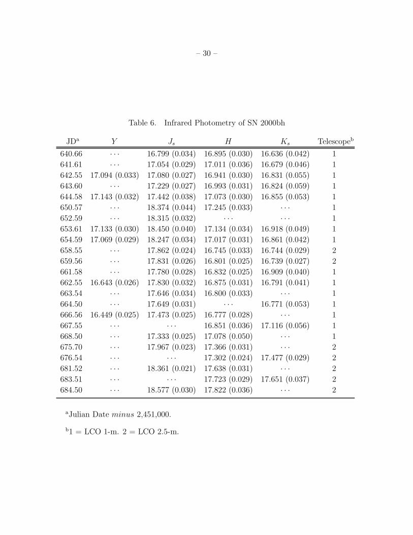
Table 6. Infrared Photometry of SN 2000bh
JDa Y Js H Ks Telescopeb
640.66 · · · 16.799 (0.034) 16.895 (0.030) 16.636 (0.042) 1
641.61 · · · 17.054 (0.029) 17.011 (0.036) 16.679 (0.046) 1
642.55 17.094 (0.033) 17.080 (0.027) 16.941 (0.030) 16.831 (0.055) 1
643.60 · · · 17.229 (0.027) 16.993 (0.031) 16.824 (0.059) 1
644.58 17.143 (0.032) 17.442 (0.038) 17.073 (0.030) 16.855 (0.053) 1
650.57 · · · 18.374 (0.044) 17.245 (0.033) · · · 1
652.59 · · · 18.315 (0.032) · · · · · · 1
653.61 17.133 (0.030) 18.450 (0.040) 17.134 (0.034) 16.918 (0.049) 1
654.59 17.069 (0.029) 18.247 (0.034) 17.017 (0.031) 16.861 (0.042) 1
658.55 · · · 17.862 (0.024) 16.745 (0.033) 16.744 (0.029) 2
659.56 · · · 17.831 (0.026) 16.801 (0.025) 16.739 (0.027) 2
661.58 · · · 17.780 (0.028) 16.832 (0.025) 16.909 (0.040) 1
662.55 16.643 (0.026) 17.830 (0.032) 16.875 (0.031) 16.791 (0.041) 1
663.54 · · · 17.646 (0.034) 16.800 (0.033) · · · 1
664.50 · · · 17.649 (0.031) · · · 16.771 (0.053) 1
666.56 16.449 (0.025) 17.473 (0.025) 16.777 (0.028) · · · 1
667.55 · · · · · · 16.851 (0.036) 17.116 (0.056) 1
668.50 · · · 17.333 (0.025) 17.078 (0.050) · · · 1
675.70 · · · 17.967 (0.023) 17.366 (0.031) · · · 2
676.54 · · · · · · 17.302 (0.024) 17.477 (0.029) 2
681.52 · · · 18.361 (0.021) 17.638 (0.031) · · · 2
683.51 · · · · · · 17.723 (0.029) 17.651 (0.037) 2
684.50 · · · 18.577 (0.030) 17.822 (0.036) · · · 2
aJulian Date minus 2,451,000.
b1 = LCO 1-m. 2 = LCO 2.5-m.

–31
–
Table 7. Optical Photometry of SN 2000ca
JDa U B V R I z Telescopeb
663.76 15.336 (0.032) 15.870 (0.015) 15.859 (0.012) 15.759 (0.023) 16.081 (0.019) 16.022 (0.022) 1
664.77 15.367 (0.054) 15.910 (0.030) 15.850 (0.031) 15.825 (0.019) 16.045 (0.011) 15.963 (0.021) 2
669.71 · · · 15.881 (0.054) 15.874 (0.019) 15.779 (0.015) 16.145 (0.028) · · · 3
672.76 15.882 (0.044) 16.050 (0.011) 15.941 (0.012) 15.900 (0.021) 16.392 (0.021) · · · 2
675.62 16.109 (0.040) 16.218 (0.021) 16.074 (0.012) 16.094 (0.012) 16.625 (0.011) 16.396 (0.021) 2
676.69 · · · 16.315 (0.018) 16.098 (0.022) 16.153 (0.012) 16.681 (0.010) 16.400 (0.023) 2
677.68 16.293 (0.028) 16.402 (0.018) 16.168 (0.012) 16.236 (0.012) 16.756 (0.011) 16.443 (0.023) 2
681.69 · · · 16.803 (0.024) 16.446 (0.012) 16.493 (0.016) 16.930 (0.012) 16.430 (0.026) 2
682.69 · · · 16.979 (0.024) 16.527 (0.015) 16.531 (0.012) 16.948 (0.015) 16.446 (0.019) 2
683.70 17.163 (0.052) 17.048 (0.020) 16.549 (0.012) 16.541 (0.012) 16.896 (0.013) 16.392 (0.026) 2
699.63 · · · 18.485 (0.018) 17.393 (0.012) 16.947 (0.012) 16.756 (0.010) · · · 2
705.59 · · · 18.781 (0.023) 17.715 (0.021) 17.305 (0.012) 17.113 (0.019) · · · 2
711.61 · · · 18.913 (0.035) 17.934 (0.032) 17.549 (0.023) 17.448 (0.024) · · · 2
730.53 · · · 19.243 (0.025) 18.455 (0.016) 18.193 (0.022) 18.352 (0.031) · · · 2
738.54 · · · 19.374 (0.053) 18.634 (0.041) 18.441 (0.023) 18.622 (0.036) · · · 2
745.50 · · · 19.481 (0.039) 18.823 (0.023) 18.621 (0.050) 18.832 (0.041) · · · 2
752.54 · · · 19.536 (0.028) 19.007 (0.020) 18.902 (0.031) 19.188 (0.076) · · · 2
757.51 · · · 19.758 (0.043) 19.137 (0.027) 19.031 (0.036) 19.431 (0.072) · · · 2
aJulian Date minus 2,451,000.
b1 = ESO NTT 3.6-m. 2 = CTIO 0.9-m. 3 = LCO 1-m.

– 32 –
Table 8. Infrared Photometry of SN 2000ca
JDa Js H Telescopeb
663.70 16.392 (0.045) 16.850 (0.048) 1
664.63 16.425 (0.031) 16.711 (0.087) 1
665.73 16.364 (0.029) 16.815 (0.057) 1
666.72 16.572 (0.041) 16.841 (0.033) 1
667.68 16.572 (0.037) 16.834 (0.031) 1
668.72 16.588 (0.037) 16.923 (0.040) 1
675.53 17.356 (0.043) 16.964 (0.028) 2
677.74 17.668 (0.046) 16.904 (0.032) 2
681.59 18.003 (0.046) 17.002 (0.028) 2
684.54 18.042 (0.045) 16.813 (0.028) 2
687.68 17.849 (0.046) 16.738 (0.025) 2
688.47 17.774 (0.058) · · · 2
aJulian Date minus 2,451,000.
b1 = LCO 1-m. 2 = LCO 2.5-m.

– 33 –
Table 9. Optical Photometry of SN 2001ba
JDa B V I
2030.60 16.551 (0.018) 16.586 (0.027) 16.691 (0.018)
2031.56 16.465 (0.020) 16.542 (0.029) 16.709 (0.017)
2032.59 16.461 (0.015) 16.498 (0.023) 16.679 (0.019)
2033.58 16.451 (0.019) 16.471 (0.027) 16.686 (0.021)
2034.59 16.445 (0.016) 16.465 (0.031) 16.746 (0.024)
2037.58 16.558 (0.022) 16.524 (0.028) 16.872 (0.033)
2038.56 16.679 (0.069) 16.509 (0.061) 16.796 (0.129)
2040.61 16.701 (0.033) 16.610 (0.033) 17.041 (0.040)
2042.59 16.777 (0.034) 16.674 (0.034) 17.119 (0.046)
2045.71 17.112 (0.051) 16.734 (0.059) 17.304 (0.122)
2046.57 17.171 (0.021) 16.847 (0.032) 17.508 (0.037)
2047.57 17.233 (0.088) · · · 17.455 (0.136)
2048.66 17.431 (0.030) 16.951 (0.037) 17.566 (0.066)
2049.54 17.462 (0.023) 17.069 (0.026) 17.567 (0.037)
2051.53 17.745 (0.031) 17.138 (0.029) · · ·
2053.50 17.934 (0.023) 17.260 (0.028) 17.494 (0.035)
2054.54 18.083 (0.026) 17.339 (0.032) · · ·
2055.55 18.208 (0.036) 17.373 (0.033) 17.467 (0.040)
2057.50 18.389 (0.027) 17.486 (0.033) 17.405 (0.031)
2059.52 18.482 (0.047) 17.629 (0.049) 17.377 (0.049)
2060.52 · · · 17.640 (0.075) 17.213 (0.074)
2061.61 18.884 (0.071) 17.648 (0.044) 17.351 (0.038)
2063.53 18.908 (0.044) 17.986 (0.039) · · ·
2064.50 19.005 (0.083) 17.872 (0.062) 17.528 (0.071)
2066.50 · · · 17.974 (0.073) 17.406 (0.064)
2067.51 19.240 (0.055) 18.101 (0.045) 17.527 (0.068)
2068.50 19.292 (0.054) 18.093 (0.044) 17.540 (0.056)
2069.50 19.349 (0.061) 18.275 (0.046) 17.627 (0.060)
2070.49 19.290 (0.071) 18.363 (0.057) 17.721 (0.063)
2072.48 · · · 18.406 (0.079) · · ·
2075.49 19.706 (0.128) · · · · · ·
2077.48 · · · · · · 18.042 (0.085)
2079.54 · · · 18.632 (0.073) 18.133 (0.105)

– 34 –
Table 9—Continued
2080.51 · · · · · · 18.261 (0.075)
2082.49 19.626 (0.078) 18.846 (0.065) 18.339 (0.086)
2083.51 · · · 18.810 (0.114) · · ·
2086.48 · · · 18.698 (0.068) · · ·
2087.49 · · · · · · 18.317 (0.077)
2088.48 · · · · · · 18.534 (0.109)
2090.46 20.140 (0.222) · · · · · ·
2091.48 · · · 18.948 (0.098) 18.534 (0.086)
aJulian Date minus 2,450,000.
Table 10. Infrared Photometry of SN 2001ba
JDa Js H Ks Telescopeb
2028.58 17.027 (0.033) · · · · · · 1
2029.56 16.998 (0.023) 17.240 (0.040) 17.187 (0.062) 1
2030.53 · · · 17.251 (0.038) · · · 1
2031.54 16.992 (0.018) 17.332 (0.045) 17.161 (0.081) 1
2032.58 16.994 (0.029) 17.310 (0.057) 17.061 (0.064) 1
2044.57 18.362 (0.053) 17.920 (0.056) · · · 1
2045.52 18.671 (0.045) 17.777 (0.077) 17.441 (0.029) 1
2047.53 18.977 (0.082) 17.941 (0.075) 17.525 (0.087) 1
2048.48 19.115 (0.136) · · · · · · 1
2049.54 18.742 (0.095) 17.855 (0.108) 17.422 (0.093) 1
2052.55 18.872 (0.076) 17.771 (0.048) 17.554 (0.116) 1
2055.54 18.525 (0.061) 17.837 (0.107) 17.246 (0.073) 1
2057.54 18.514 (0.052) 17.437 (0.045) 17.389 (0.079) 1
2061.56 18.314 (0.031) 17.448 (0.056) · · · 2
2068.46 18.006 (0.029) 17.485 (0.029) · · · 2
2069.46 18.021 (0.035) 17.516 (0.027) · · · 2
aJulian Date minus 2,450,000.
b1 = LCO 1-m. 2 = LCO 2.5-m.

Table 11. K-corrections for Type Ia Supernovae in LCO Near Infrared Bandsa
tb\ z 0.005 0.010 0.015 0.020 0.025 0.030 0.035 0.040 0.045 0.050 0.060 0.070 0.080 0.090 0.100 0.150
Js:
−8.57 −0.012 −0.023 −0.034 −0.044 −0.055 −0.066 −0.078 −0.090 −0.103 −0.116 −0.141 −0.164 −0.185 −0.204 −0.221 −0.321
1.40 −0.007 −0.015 −0.021 −0.027 −0.034 −0.041 −0.047 −0.053 −0.058 −0.062 −0.066 −0.066 −0.064 −0.061 −0.061 −0.119
4.51 −0.003 −0.007 −0.010 −0.012 −0.014 −0.018 −0.023 −0.026 −0.028 −0.030 −0.031 −0.027 −0.022 −0.017 −0.017 −0.090
8.38 −0.008 −0.016 −0.023 −0.030 −0.037 −0.042 −0.048 −0.052 −0.055 −0.058 −0.058 −0.056 −0.057 −0.062 −0.077 −0.241
15.39 −0.013 −0.030 −0.045 −0.062 −0.082 −0.101 −0.122 −0.146 −0.171 −0.194 −0.239 −0.286 −0.339 −0.407 −0.485 −0.878
19.42 −0.019 −0.039 −0.061 −0.084 −0.109 −0.133 −0.158 −0.184 −0.213 −0.241 −0.300 −0.366 −0.442 −0.533 −0.625 −1.058
22.40 −0.023 −0.047 −0.072 −0.099 −0.127 −0.155 −0.184 −0.216 −0.249 −0.283 −0.354 −0.434 −0.523 −0.623 −0.723 −1.164
27.46 −0.034 −0.069 −0.104 −0.137 −0.173 −0.206 −0.242 −0.280 −0.321 −0.361 −0.448 −0.540 −0.642 −0.752 −0.862 −1.319
31.43 −0.028 −0.058 −0.089 −0.121 −0.153 −0.187 −0.222 −0.260 −0.300 −0.343 −0.436 −0.540 −0.648 −0.757 −0.871 −1.328
41.42 −0.028 −0.064 −0.105 −0.149 −0.196 −0.244 −0.294 −0.347 −0.403 −0.459 −0.561 −0.656 −0.756 −0.861 −0.973 · · ·
H:
−8.57 −0.008 −0.016 −0.025 −0.033 −0.042 −0.051 −0.060 −0.070 −0.079 −0.088 −0.106 −0.125 −0.144 −0.166 −0.191 −0.373
0.39 −0.004 −0.007 −0.010 0.007 0.007 0.016 0.004 −0.001 −0.006 −0.013 −0.030 −0.049 −0.077 −0.108 −0.146 −0.397
1.40 0.002 0.005 0.008 0.011 0.013 0.013 0.011 0.007 0.002 −0.005 −0.021 −0.041 −0.069 −0.102 −0.141 −0.400
4.51 0.008 0.017 0.028 0.038 0.048 0.054 0.057 0.061 0.063 0.065 0.061 0.049 0.024 −0.007 −0.045 −0.290
8.38 0.004 0.011 0.021 0.034 0.047 0.060 0.073 0.087 0.102 0.115 0.133 0.136 0.122 0.098 0.072 −0.071
15.39 0.015 0.034 0.056 0.082 0.109 0.139 0.170 0.203 0.234 0.263 0.315 0.354 0.384 0.404 0.420 0.549
19.42 0.015 0.035 0.062 0.093 0.126 0.158 0.189 0.218 0.244 0.267 0.306 0.338 0.367 0.393 0.420 0.622
22.40 0.017 0.039 0.065 0.096 0.129 0.162 0.194 0.222 0.249 0.273 0.312 0.346 0.376 0.406 0.436 0.652
27.46 0.011 0.026 0.045 0.069 0.098 0.122 0.144 0.163 0.180 0.196 0.225 0.257 0.281 0.304 0.338 0.607
31.43 −0.002 0.002 0.012 0.024 0.038 0.051 0.061 0.068 0.075 0.080 0.089 0.097 0.104 0.117 0.145 0.344
41.42 −0.014 −0.023 −0.026 −0.025 −0.022 −0.018 −0.015 −0.012 −0.010 −0.006 0.001 0.010 0.023 0.046 0.082 0.338
Ks:
−8.57 −0.012 −0.024 −0.036 −0.048 −0.058 −0.070 −0.082 −0.095 −0.106 −0.117 −0.143 −0.170 −0.195 −0.221 −0.246 −0.367
0.39 −0.021 −0.047 −0.074 −0.102 −0.130 −0.158 −0.189 −0.219 −0.248 −0.275 −0.330 −0.382 −0.433 −0.475 −0.517 −0.706
1.40 −0.025 −0.053 −0.082 −0.112 −0.143 −0.175 −0.208 −0.239 −0.269 −0.300 −0.362 −0.421 −0.477 −0.530 −0.580 −0.813
4.51 −0.033 −0.072 −0.113 −0.155 −0.194 −0.231 −0.269 −0.308 −0.344 −0.374 −0.435 −0.492 −0.546 −0.601 −0.649 −0.851
8.38 −0.036 −0.079 −0.122 −0.162 −0.202 −0.240 −0.279 −0.315 −0.350 −0.387 −0.450 −0.504 −0.553 −0.593 −0.629 −0.797
15.39 −0.033 −0.066 −0.097 −0.127 −0.157 −0.187 −0.216 −0.241 −0.265 −0.287 −0.329 −0.365 −0.398 −0.433 −0.474 −0.696
22.40 −0.018 −0.035 −0.051 −0.066 −0.080 −0.092 −0.099 −0.105 −0.106 −0.108 −0.117 −0.130 −0.148 −0.179 −0.216 −0.534
27.46 −0.002 −0.006 −0.015 −0.021 −0.027 −0.024 −0.011 −0.003 0.004 0.008 0.026 0.016 −0.015 −0.058 −0.099 −0.460
31.43 −0.004 −0.012 −0.024 −0.036 −0.043 −0.043 −0.036 −0.025 −0.015 −0.006 0.005 −0.013 −0.043 −0.071 −0.100 −0.581
41.42 −0.004 −0.013 −0.024 −0.036 −0.048 −0.047 −0.036 −0.023 −0.012 −0.006 0.007 0.000 −0.020 −0.028 −0.036 −0.373
aThe following corrections are subtracted from the photometric data to correct them to the observer’s frame (redshift z = 0.00).
bTime t is the number of days since B-band maximum.

Table 12. Fitting Supernova Light Curves at Maximuma
Coeff ∆J ∆H ∆K
a0 0.080 0.050 0.042
a1 0.5104699E−01 0.2509234E−01 0.2728437E−01
a2 0.7064257E−02 0.1852107E−02 0.3194500E−02
a3 −0.2579062E−03 −0.3557824E−03 −0.4139377E−03
aThe differential magnitudes with respect to maximum are of
the form: ∆ mag = a0 + Σ(ai × ti), where t is the number of days
since B-band maximum, scaled according to the mean of the B-
and V -band inverse stretch factors s−1 from Jha (2000, Fig. 3.8)
and divided by (1 + z). The fits are valid from −12 to +10 d of
“stretched time”.
Table 13. V minus Infrared Loci for Slowly Declining Type Ia Supernovaea
Parameter \ color index V − J V − H V − K
a0 −0.902(0.005) −1.194 −0.971
a1 −0.07136(0.00104) −0.4793682E−01 −0.4089032E−01
a2 0.4647584E−02 0.3613656E−02
a3 0.8813858E−04 0.6178713E−04
a4 −0.5205402E−05 −0.3648954E−05
Rangeb [−8,+9.5] [−8,+8.5] [−8,+27]
rms residual ± 0.067 ± 0.062 ± 0.138
χ2ν 3.5 1.9 4.9
aThe range of ∆m15(B) is 0.81 to 1.00. The fits are of the form: V − [J, H, K] = a0
+ Σ(ai × ti), where t is the number of days since B-band maximum, corrected for time
dilation but not stretch.bThe range in days with respect to B-band maximum for which the fit is most valid.
36

Table 14. V minus Infrared Loci for Type Ia Supernovae of Mid-Range Decline Ratesa
Parameter \ color index V − H V − K
a0 −0.951 −0.741
a1 −0.5383673E−01 −0.5071254E−01
a2 0.5913753E−02 0.3281215E−02
a3 0.1155147E−03 0.2158419E−03
a4 −0.7144163E−05 −0.8056540E−05
Rangeb [−9,+27] [−9,+27]
rms residual ± 0.093 ± 0.105
χ2ν 4.2 3.9
aKrisciunas et al. (2000, Table 9) gave hinged two-line fits to
the color curves. Actual data are redder at t = +6 d than the two-
line fits. Here we give fourth order polynomial fits to the same
extinction-corrected data. The fits are of the form: V − [J, H, K]
= a0 + Σ(ai × ti), where t is the number of days since B-band
maximum.bThe range in days with respect to B-band maximum for which
the fit is most valid.
37

Fig. 1.— Near infrared photometry of SN 1999ee. For Js and H the Las Campanas data are
red filled in symbols, while the YALO data are filled in with blue. The YALO data include
filter-based corrections to place them on the system of Persson et al. (1998) used at Las
Campanas Observatory.
Fig. 2.— Finding chart for SN 2000bh. North is up and east to the left. The image is 6.5
arcmin on a side. It is a V-band image obtained on the CTIO 0.9-m telescope. The SN is
indicated by the short line.
Fig. 3.— Optical and infrared photometry of SN 2000bh. We have added BV I fits derived
using the ∆m15 method of Phillips et al. (1999).
Fig. 4.— Similar to Fig. 2, but for SN 2000ca.
Fig. 5.— Optical and infrared photometry of SN 2000ca.
Fig. 6.— Similar to Fig. 2, but for SN 2001ba. This V-band image was obtained with the
Las Campanas 2.5-m telescope.
Fig. 7.— Optical and infrared photometry of SN 2001ba.
Fig. 8.— J-band light curves of 8 Type Ia SNe, normalized to maximum brightness and
stretched in the time axis according to inverse stretch factors derived from Fig. 3.8 of Jha
(2002). We have also take out the time dilation. The key to the symbols is: 1980N (solid
dots), 1986G (large open squares), 1998bu (larger open circles), 1999aw (X’s), 1999ee (LCO
data = small open squares, corrected YALO data = triangles), 2000ca (pinched in squares),
2001ba (stars), 2001el (smaller open circles).
Fig. 9.— JH maxima of 8 Type Ia SNe and K-band maxima of 6 Type Ia SNe. The time
axis is “stretched days” (see Fig. 8 and the text). We also give third order polynomial fits.
Fig. 10.— I-band data of SNe 1998bu, 1999aw, 1999ee, 2000ca, 2001ba, and 2001el. The
data are stretched in the time axis in a manner similar to Figs. 8 and 9.
Fig. 11.— V minus IR colors of Type Ia SNe with decline rates 0.81 ≤ ∆m15(B) ≤ 1.00. The
data are K-corrected, and have been corrected for extinction due to dust and time dilation,
but not stretch. The solid line in the top plot shows the range of uniformity of V − J . The
dashed lines in the bottom two plots are the loci for mid-range decliners (Krisciunas et al.
2000, 2003). The solid lines in the bottom two plots are fourth order polynomial fits to the
data from −8 to +27 days with respect to B-band maximum. On the whole the random
errors of the photometry are on the order of the size of the points, or smaller. In the cases
38

of SNe 1999gp and 1999aw we show the considerably larger error bars. The points are color
coded as follows: SN 1999aa (magenta); 1999aw (red), 1999ee (blue), 1999gp (cyan), 2000ca
(green), and 2001ba (yellow).
Fig. 12.— Dereddened colors of Type Ia SNe vs. the decline rate parameter ∆m15(B). The
(green) triangles correspond to objects which have few infrared observations in the [−12,+10]
day window, so their IR maxima are not as well determined; these objects were not used for
the regression lines shown.
Fig. 13.— Dereddened V − J and V − H colors of Type Ia SNe at 6 days after the time of
the B-band maxima, vs. the decline rate parameter ∆m15(B).
Fig. 14.— R − z vs. V − I colors for spectrophotometric standards (Stone & Baldwin
1983; open circles) and for Landolt (1992a) standards. The z magnitudes of Stone-Baldwin
standards were taken from Hamuy (2001, Appendix B); the solid line is a fit to data for
these stars. The dashed line is a fit to points with V − I > 0.97. Three particular stars are
Rubin 149C (open squares), SA95-96 (diamond), and Rubin 152E (X’s). See text for further
details.
39

460 470 480 490 500 510 520
Julian Date [2,451,000 + ...]
12
14
16
18
mag
nitu
de +
off
set
SN 1999ee
Js
H-1
Y+2
Ks-2
Krisciunas et al. Fig. 1
40

Krisciunas et al. Fig. 2
41

630 640 650 660 670 680 690
Julian Date [2,451,000 + ...]
10
15
20
mag
nitu
de +
off
set
Ks-8
H-7
Js-6
Y-4
z-2.5
R-1
I-2
V
B+1SN 2000bh
Krisciunas et al. Fig. 3
42

Krisciunas et al. Fig. 4
43

660 680 700 720 740 760
Julian Date [2,451,000 + ...]
10
15
20
mag
nitu
de +
off
set
H-6
Js-5
z-3
I-2
R-1
V
B+1
U+2
SN 2000ca
Krisciunas et al. Fig. 5
44

Krisciunas et al. Fig. 6
45

30 40 50 60 70 80 90
Julian Date [2,452,000 + ...]
10
15
20
mag
nitu
de +
off
set
Ks-6
H-5
Js-4
I-1
V
B+1
SN 2001ba
Krisciunas et al. Fig. 7
46

Krisciunas et al. Fig. 8

0
0.5
1
0
0.5
1
-10 0 10
Time since B-band maximum
0
0.5
1
J
H
K
Krisciunas et al. Fig. 9
48

-10 0 10
Time since B-band maximum (stretched days)
0
0.5
1
∆ I
Krisciunas et al. Fig. 10
49
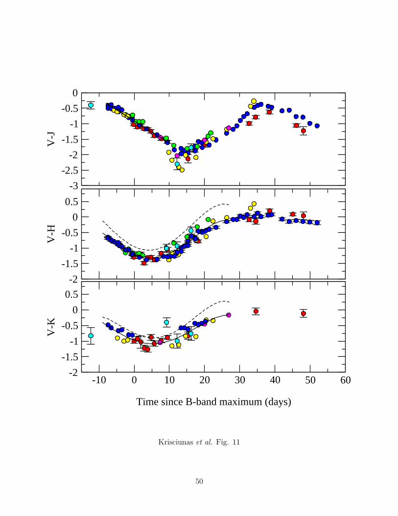
-3
-2.5
-2
-1.5
-1
-0.5
0
V-J
-2
-1.5
-1
-0.5
0
0.5
V-H
-10 0 10 20 30 40 50 60
Time since B-band maximum (days)
-2
-1.5
-1
-0.5
0
0.5
V-K
Krisciunas et al. Fig. 11
50

-1-0.8-0.6-0.4-0.2
00.2
Vm
ax-J
max
-1.6-1.4-1.2
-1-0.8-0.6-0.4
Vm
ax-H
max
0.8 1 1.2 1.4 1.6 1.8
∆ m15
(B)
-1.4-1.2
-1-0.8-0.6-0.4-0.2
Vm
ax-K
max
Krisciunas et al. Fig. 12
51

0.8 1 1.2 1.4 1.6 1.8
-1.6
-1.4
-1.2
-1
-0.8
-0.6
V-J
0.8 1 1.2 1.4 1.6 1.8
∆ m15
(B)
-1.6
-1.4
-1.2
-1
-0.8
-0.6
V-H
t = +6 d
t = +6 d
Krisciunas et al. Fig. 13
52
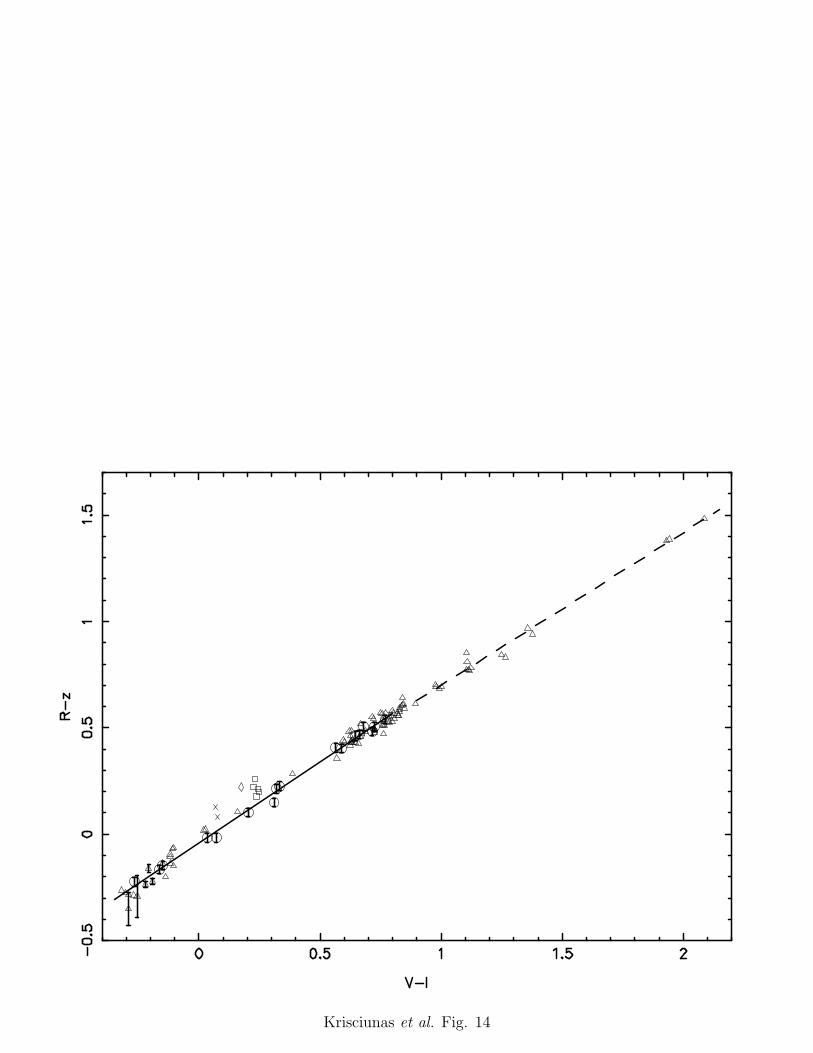
Krisciunas et al. Fig. 14