* * *

ABSOLUTE MAGNITUDE ANALYSIS OF THE SCP UNION SUPERNOVAE

ECM paper XIII by Luciano Lorenzi

56th Annual Meeting of the Italian Astronomical Society

EWASS 2012 - European Week of Astronomy and Space Science -

Rome - Pontificia Universita Lateranense, 1-6 July 2012

ABSTRACT

After analysing the trend of 14 high-z normal points 〈MB〉 versus the

mean redshift 〈z〉 > 0.55 or the corresponding Hubble depths D = c〈z〉/H0

and light space r in H.u. of SCP Union supernovae (Kowalski et al. 2008),

listed in Table 2 of the ECM paper IX (Sait2010 in Naples), a trend analysis

of another 15 and 30 normal points of the Hubble Magnitude M and a new

absolute magnitude M∗, at increasing 〈z〉 ≡ z0 corresponding to a different

series of z bins, leads to the discovery of the anomalous behaviour of the

SNe luminosity in the nearby Universe in comparison with the more regular

magnitude trend of the deep Universe SNe. When the low-z normal points

are excluded, the best fittings make it possible to extrapolate both the

SNe Ia absolute magnitude M0 at a central redshift z0 → 0 and a few final

solutions of the SNe Ia 〈M〉 and 〈M∗〉. The new value M0 = −17.9 ± 0.1

confirms the ADDENDUM NOTE - October 2011 - of paper XI. All the

plots and graphical fittings of this analysis appear in the Appendix ”Check

atlas of the ECM paper XIII figures”. The magnitude anomaly of the low

〈z〉 points is here interpreted as due to a deficiency in the used magnitude

formulas; these produce a maximum peak of deviation, with a resulting

systematic ∆M ≈ 1 in the depth range 0.04 � 〈z〉 � 0.08. That is a proof of

the Universe rotation within the limits of the expansion center model.

1

1. Introduction

The data of the present analysis of the SNe Ia absolute magnitude are all taken from the SCP

Union Compilation (SCPU: Kowalski et al. 2008). In particular this large ”Union” sample reports

redshifts and blue apparent magnitudes of 398 SNe Ia, or of 307 SNe Ia after selection cuts,

including the distant supernovae recently observed with HST. On the grounds of the strengthening

perturbation effect of theM scattering at decreasing z < 0.5 (cf. paper XI), jointly with the results

of paper XI ADDENDUM NOTE, new 〈MB〉 fittings limited to normal points with 〈z〉 > 0.5 from

the paper IX Table 2 have been explored. After the successful check, 30 new normal points from

the data of all 398 SCPU SNe have been constructed, in order to better analyse the SN magnitude

trend at different Hubble depths. The main construction and analysis of the magnitude normal

points does not involve the expansion center model or ECM. In other words the main experimental

results obtained, the SNe absolute magnitude value M0 and the trend of the Hubble Magnitude

M , can be considered both model independent and able to confirm once again the expansion

center model. In particular the new findings provide astronomical evidence for cosmic rotation

around the expansion center, in accordance with the limits of the ECM which formally, as one

must recall, implies a rigid rotation of the very nearby Universe (cf. paper VII).

All the plots and graphical fittings of this analysis appear in the Appendix ”Check atlas of

the ECM paper XIII figures”. Moreover, as we deal only with blue magnitudes, the pedicel B

becomes superfluous; thus the convention MB ≡M is adopted within the present paper XIII.

The cited papers I-II-V-VI-VII-VIII-IX-X-XI-XII are those of the author’s references: Lorenzi

1999a→2012c.

2

2. Analysis and discussion

After the preliminary analysis on the first SCP Union data set in paper IX, here a further more pre-

cise analysis is carried out, so as to distinguish the normal luminosity behaviour of the supernovae

Ia of the deep Universe from the SNe magnitude trend of the nearby Universe.

2.1 Fitting 14 High-z SNe M normal points

In paper XI we found evidence for a clear perturbation effect of the SNe ∆M at z � 0.5. In order

to avoid possible interference effects, here a new model independent analysis of the normal points

in paper IX Table 2 is undertaken and limited to 14 high-z mean Hubble Magnitudes 〈M〉, those

with z-bin normal redshifts 〈z〉 > 0.55. If a first, second and third degree polynomial is applied

to the fitting of the 〈M〉 plot versus 〈z〉, the statistical coefficients of determination R2 result to

be 0.9720, 0.9967, 0.9974, respectively. The best fitting is clearly the cubic one. Therefore, after

adopting the identity between the z-bin normal redshift and the central redshift z0, that is

〈z〉 ≡ z0 (1)

and the normal equation of the Hubble Magnitude

〈M〉 = 〈mmax

B 〉 − 5〈log [cz(1 + z)]〉+ 5 logH0 − 25 (2)

, the line equation of the normal Hubble Magnitude 〈M〉 as a function of the central

redshift z0 becomes

〈M〉 = A0 +A1z0 +A2z2

0+A3z

3

0(3)

with

A0 = −17.96 A1 = −4.117 A2 = +3.197 A3 = −0.9463 (4)

from the automatic cubic fitting (cf. Figure 1 in Appendix) whose coefficient of determination

results to be R2 = 0.9974.

Note that the previous eq. (2) of the normal points 〈M〉 is the same normal M equation (21)

of paper IX, while the Hubble Magnitude M of an individual source with redshift z and apparent

magnitude m is by definition

M =m− 5 log [D · (1 + z)]− 25 (5)

3

where D = cz/HX = cz0/H0 is the Hubble depth according to the expansion center Universe (cf.

the ECM papers V-VI-IX-X-XI-XII).

Together with the successful cubic fitting (3) of 14 high-z normal Hubble Magnitudes 〈M〉

versus the normal redshift 〈z〉, it is possible to carry out a successful linear fitting of the same

14 〈M〉 points versus the corresponding central light space values r = r(z0) listed in column 8 of

paper IX Table 2. In this case the normal Hubble Magnitude 〈M〉 is represented by the equation

〈M〉 = C0 +C1r (6)

with

C0 = −17.80 C1 = −0.002200 (7)

from the automatic linear fitting (cf. Figure 2 in Appendix) whose coefficient of determination

results to be R2 = 0.9951.

The result of two fittings can be summarized as follows:

M0∼= 〈M〉(z0 → 0) = A0 ∼= 〈M〉(r → 0) = C0 (8)

Of course M0 represents the absolute magnitude of a hypothetical supernova Ia with a central

redshift z0 → 0. As the Hubble Magnitude M is clearly an apparent absolute magnitude at

increasing Hubble depths, so its standard value for D→ 0 must necessarily coincide with the true

intrinsic absolute magnitude, that is Mα (cf. paper XII).

The conclusion of the preliminary analysis of the SNe Ia absolute magnitudes, based on the

high-z normal points with 〈z〉 > 0.55 of the paper IX Table 2, leads to the new result

M0 = 〈Mα〉(z0 → 0) ∼= −17.9 (9)

The previous value of M0 agrees with the new absolute magnitude inferred from the 〈M∗

B〉

relationship of eq. (A3) in the ADDENDUM NOTE - October 2011 - of paper XI.

2.2 Construction of 30 new normal points by 398 SCPU SNe data

The normal points of paper IX Table 2 refer to excessively large z-ranges to be able to represent

accurately the SNe Hubble Magnitude trend at the low redshifts of the nearby Universe. Therefore,

in order to improve the analysis, we need smaller z bins. The following Table 1 and Table 2,

referring to the nearby and deep Universe respectively, collect 30 new normal points, based on

398 SCPU supernovae. These two tables were constructed according to the same procedure as

4

paper IX Table 2. In particular the first 5 columns both of Table 1 and Table 2 contain numerical

values derived from the observed z and mmax

B listed within the SCPU compilation (Kowalski et al.

2008); the values referring to each z bin are in the order: z range; number N of the SNe included

in the normal point; unweighed mathematical mean 〈m〉 of the corresponding SNe magnitudes

mmax

B ; mean Hubble Magnitude 〈M〉 resulting from the normal eq. (2) applied to the bin, with

H0 = 70 assumed; mathematical mean of the observed redshifts of the z bin, according to the

position 〈z〉 ≡ z0 of eq. (1). The 6th column holds the value of the Hubble Magnitude of a

supernova Ia, with z = 〈z〉 ≡ z0 and m = 〈m〉 ≡ m0 assumed (cf. paper XII), according to the

paper IX formula (19) (also called ECM M(z0) equation):

M(z0) = m0 − 5 log [cz0 · (1 + z0)] + 5 logH0 − 25 (10)

Fitting the points M(z0) plotted versus z0 or r(z0) leads to the line equation, M(z0) or

M(r), representing the central Hubble Magnitude of the supernovae Ia.

The last two columns, 7th and 8th, include two other central quantities, the light space r(z0)

and the new absolute magnitude M∗(z0), corresponding to the assumed central redshift z0 ≡ 〈z〉

and the central magnitude m0 ≡ 〈m〉. Let us recall the ECM calculation procedure of r(z0), that

applied in section 2.1 of paper IX and section 4 of paper X:

z0 =x

3

(1 + x

1− x

)⇒ x = x(z0) =

3H0r(z0)

c⇒ r(z0) =

cx(z0)

3H0(11)

According to the contents of paper XI ADDENDUM NOTE, the previous r(z0), whose values

are listed in column 7th of Table 1 and 2, allow the introduction of a new central luminosity

distance, that is

D∗L(z0) = r(z0) · (1 + z0)2 (12)

together with the new absolute magnitude of a supernova Ia, always with z = 〈z〉 ≡ z0 and

m = 〈m〉 ≡ m0 assumed, as follows:

M∗(z0) =m0 − 5 log[r(z0) · (1 + z0)

2]− 25 (13)

Fitting the points M∗(z0) plotted versus z0 or r(z0) leads to the line equation, M∗(z0) or

M∗(r), representing the new central absolute magnitude of the supernovae Ia.

5

Table 1

z range N 〈m〉 〈M〉 〈z〉 ≡ z0 M(z0) r(z0) M∗(z0)

0 < z ≤ 0.010 16 14.24 −18.14± 0.36 0.007 −18.24 29 −18.09

0 < z ≤ 0.015 33 14.60 −18.44± 0.21 0.010 −18.58 40 −18.48

0.005 ≤ z ≤ 0.020 50 14.99 −18.63± 0.11 0.013 −18.75 52 −18.64

0.010 ≤ z ≤ 0.025 45 15.46 −18.75± 0.11 0.016 −18.81 63 −18.60

0.015 ≤ z ≤ 0.030 40 15.90 −18.86± 0.10 0.021 −18.92 80 −18.72

0.020 ≤ z ≤ 0.050 39 16.63 −19.07± 0.06 0.032 −19.14 116 −18.84

0.025 ≤ z ≤ 0.100 42 17.19 −19.14± 0.05 0.044 −19.28 152 −18.91

0.030 ≤ z ≤ 0.150 37 17.77 −19.15± 0.05 0.059 −19.38 193 −18.90

0.035 ≤ z ≤ 0.200 39 18.42 −19.16± 0.05 0.083 −19.51 250 −18.91

0.040 ≤ z ≤ 0.250 42 19.50 −19.09± 0.06 0.129 −19.48 340 −18.68

0.045 ≤ z ≤ 0.300 52 20.04 −19.09± 0.06 0.163 −19.51 395 −18.60

0.050 ≤ z ≤ 0.350 66 20.81 −19.15± 0.06 0.220 −19.49 473 −18.43

0.10 ≤ z ≤ 0.40 74 21.80 −19.13± 0.06 0.291 −19.24 552 −18.02

0.15 ≤ z ≤ 0.45 100 22.20 −19.18± 0.05 0.341 −19.26 598 −17.96

0.20 ≤ z ≤ 0.50 120 22.51 −19.21± 0.05 0.382 −19.26 632 −17.90

6

Table 2

z range N 〈m〉 〈M〉 〈z〉 ≡ z0 M(z0) r(z0) M∗(z0)

0.25 ≤ z ≤ 0.55 131 22.72 −19.26± 0.04 0.419 −19.31 660 −17.90

0.30 ≤ z ≤ 0.60 142 22.87 −19.32± 0.04 0.450 −19.36 682 −17.91

0.35 ≤ z ≤ 0.65 143 23.10 −19.37± 0.04 0.495 −19.40 711 −17.90

0.40 ≤ z ≤ 0.70 138 23.25 −19.44± 0.04 0.533 −19.47 733 −17.93

0.45 ≤ z ≤ 0.75 118 23.43 −19.48± 0.04 0.574 −19.51 756 −17.93

0.50 ≤ z ≤ 0.80 98 23.61 −19.55± 0.04 0.623 −19.57 781 −17.96

0.55 ≤ z ≤ 0.85 91 23.82 −19.60± 0.04 0.680 −19.62 808 −17.97

0.60 ≤ z ≤ 0.90 79 24.03 −19.62± 0.04 0.730 −19.64 829 −17.94

0.65 ≤ z ≤ 0.95 68 24.25 −19.68± 0.04 0.797 −19.69 855 −17.96

0.70 ≤ z ≤ 1.00 62 24.42 −19.71± 0.04 0.851 −19.72 875 −17.96

0.75 ≤ z ≤ 1.10 60 24.52 −19.74± 0.04 0.885 −19.75 886 −17.97

0.80 ≤ z ≤ 1.20 56 24.62 −19.79± 0.05 0.927 −19.80 900 −18.00

0.85 ≤ z ≤ 1.30 44 24.77 −19.86± 0.06 0.996 −19.88 921 −18.05

z ≥ 0.9 43 25.01 −19.88± 0.06 1.082 −19.91 944 −18.05

z ≥ 0.95 34 25.13 −19.89± 0.07 1.123 −19.92 955 −18.04

Formally the eq. (13) of M∗(z0) (whose high-z values are listed in column 8th of the above

Table 2) is different from eq. (A2) of 〈M∗〉 in paper XI (whose high-z values are listed in column

8th of that Table A0), that is the normal equation of the new absolute magnitude, here

called 〈M∗〉, as follows

〈M∗〉 = 〈m〉 − 5〈log[rz(1 + z)

2]〉 − 25 (14)

where rz is the light space resulting from the ECM z equation (cf. eq. (4) of paper IX).

Fitting the normal points 〈M∗〉 plotted versus z0 or 〈rz〉 leads to the line equation, 〈M∗〉(z0)

or 〈M∗〉(〈rz〉), representing the new normal absolute magnitude of the supernovae Ia.

Numerically, we find a small difference between 〈M∗〉 and M∗(z0), about 0.03 magnitudes on

average at high z, that is

〈M∗〉(z0)−M∗(z0) ≈ 0.03 (15)

Thus the usefulness of the new central absolute magnitude M∗(z0) is confirmed.

7

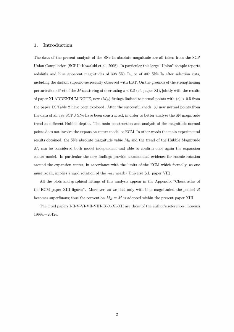
2.3 Plotting 30 values of SNe 〈M〉, M(z0), M∗(z0) versus z0 and r(z0)

The 30 values of 〈M〉, M(z0), M∗(z0) in Table 1 and 2 from SCPU data of 398 SNe allow the

construction of the corresponding 6 plots, versus z0 ≡ 〈z〉 and r(z0) respectively. These diagrams

appear in the Appendix ”Check atlas of the ECM paper XIII figures”. In particular Figure 3

presents the plot of 30 SNe Ia normal Hubble Magnitudes 〈M〉 versus the mean redshift 〈z〉,

Figure 4 the plot of 30 SNe Ia normal Hubble Magnitudes 〈M〉 versus the ECM r(z0), Figure 5

the plot of 30 SNe Ia central Hubble Magnitudes M(z0) versus z0, Figure 6 the plot of 30 SNe Ia

central Hubble Magnitudes M(z0) versus the ECM r(z0), Figure 7 the plot of 30 SNe Ia central

absolute magnitudesM∗(z0) versus z0, Figure 8 the plot of 30 SNe Ia central absolute magnitudes

M∗(z0) versus the ECM r(z0).

2.4 The magnitude anomaly of the SNe Ia at low 〈z〉

Even at first sight the plots of the Appendix Figures 3-4-5-6-7-8 highlight the magnitude anomaly

of the low 〈z〉 points. In other words these six diagrams give clear empirical evidence for the

normal luminosity behaviour of the supernovae Ia of the deep Universe in comparison with the

SNe magnitude trend of the nearby Universe. Such a distinction has been emphasized through

the separation of the 30 normal points into two groups of 15 points each. Table 1 collects 15

normalized-central supernovae Ia which appear to be affected by the magnitude anomaly with

individual redshifts z ≤ 0.5, while Table 2 collects other 15 normalized-central supernovae Ia based

on individual redshifts z ≥ 0.25. In particular it is remarkable to see in Fig. 7 a significant linear

trend (almost constant) of the central absolute magnitudes M∗(z0) after high normal redshifts,

with 〈z〉 � 0.4. Thus a preliminary cut-off redshift limit between the nearby Universe affected by

the magnitude anomaly and the unperturbed deep one is here fixed at z = 0.25 and corresponding

〈z〉 > 0.4. But the discovered variation of the SNe Ia luminosity may be only apparent, because

there is no astrophysical explanation able to reproduce intrinsically the observed maximum peak

in the depth range 0.04 � 〈z〉 � 0.08, with a resulting ∆M ≈ 1 (cf. Figures 3-5-7 in Appendix).

2.5 Astronomical evidence for cosmic rotation

An interpretation of the observed magnitude anomaly can be found in paper VII ”Cosmic mechan-

ics of the nearby Universe within the expansion center model with angular momentum conserved”.

In other words the negative collapse of the SNe M at 〈z〉 ≈ 0.06 and 〈z〉 ≡ z0 � 0.4 is here con-

8

sidered to be a proof of the cosmic rotation, which not even the ECM Hubble law (cf. papers

V-VI-IX-XI) includes. Consequently the related magnitude formula, owing to the inclusion of dis-

torted Hubble depths D = cz0/H0 = cz/HX or light spaces r as inferred from the ECM Hubble

law, should give also distorted values of SNe 〈M〉, M(z0), M∗(z0) to a wide Galaxy entourage,

including the Huge Void (Bahcall & Soneira 1982) and the expansion center at R0 ≈ 260 Mpc

from the Local Group (cf. papers I-II and author 1991). Indeed, only the very nearby Universe,

at z0 � 0.007 or D � 30 Mpc, should be somewhat independent from the cosmic rotation, owing

to the Galilean relativity effect within the ECM rigid rotation; on the other hand also the normal

or central points of the deep Universe, at 〈z〉 ≡ z0 � 0.4 or D � 1000 Mpc, result to be negligibly

affected by the cosmic rotation, probably thanks to a better statistical merging of the individual

z points. Here we must remark that, according to the rotating Universe calculated in paper VII,

the transversal velocity of the Galaxy, R0ϑ0 ≈ 6× 109cm/s, is more than three times the radial

velocity, R0 ≈ 1.8 × 109cm/s. Then the observed redshift z from the Milky Way must also be

linked to a relative motion of differential rotation, which however is inconsistent with the ECM

rigid rotation. In conclusion the magnitude anomaly of the SNe Ia at low 〈z〉 may be technically

interpreted as due to a deficiency in the used magnitude formulas, which produce a maximum

peak of deviation, with a resulting systematic ∆M ≈ 1 at 0.04 � 〈z〉 � 0.08, that is in the Hubble

depth range 170 Mpc � D � 350 Mpc.

2.6 Fitting 15 values of High-z SNe 〈M〉, M(z0), M∗(z0) versus z0 and r

As a consequence of the previous results, a correct analysis of the SNe Ia absolute magnitudes

(cf. eqs. 2-5-10-13) must necessarily be limited to the data of Table 2, that of a deep Universe

whose magnitude anomaly seems to be negligible within the limits of the present astronomical

measurements.

Fitting the 15 points 〈M〉 (cf. Table 2) plotted versus z0 and r(z0) leads to the line equations,

〈M〉(z0) and 〈M〉(r), representing the normal Hubble Magnitude of the supernovae Ia, as a func-

tion of the central redshift z0 and light space r(z0). The solutions from the following automatic

cubic and linear fittings (cf. Figures 9-10 in Appendix)

〈M〉(z0) = A0 +A1z0 +A2z2

0+A3z

3

0(16)

〈M〉(r) = C0 +C1r(z0) (17)

, whose corresponding coefficients of determination result to be R2 = 0.9948 and R2 = 0.9950,

9

respectively, give the values:

A0 = −18.26 A1 = −3.351 A2 = +2.636 A3 = −0.8485 (18)

C0 = −17.86 C1 = −0.002138 (19)

Fitting the 15 pointsM(z0), (cf. Table 2) plotted versus z0 and r(z0) leads to the line equations,

M(z0) and M(r), representing the central Hubble Magnitude of the supernovae Ia, as a function

of the central redshift z0 and light space r(z0). The solutions from the following automatic cubic

and linear fittings (cf. Figures 11-12 in Appendix)

M(z0) = A0 +A1z0 +A2z2

0 +A3z3

0 (20)

M(r) = C0 +C1r(z0) (21)

, whose corresponding coefficients of determination result to be R2 = 0.9939 and R2 = 0.9923,

respectively, give the values:

A0 = −18.38 A1 = −3.188 A2 = +2.681 A3 = −0.9603 (22)

C0 = −17.95 C1 = −0.002061 (23)

Fitting the 15 points M∗(z0)(cf. Table 2) plotted versus z0 and r(z0) leads to the line equa-

tions, one of M∗(z0) and two of M∗(r), representing the new central absolute magnitude of the

supernovae Ia, as a function of the central redshift z0 and light space r(z0). The solutions from

one quadratic and two linear automatic fittings (cf. Figures 13-14-15 in Appendix)

M∗(z0) = A0 +A1z0 +A2z2

0 (24)

M∗(z0) = A0 +A1z0 (25)

M∗(r) = C0 +C1r(z0) (26)

, whose corresponding coefficients of determination result to be R2 = 0.8883, R2 = 0.8772 and

R2 = 0.8353, respectively, give the values:

A0 = −17.87 A1 = −0.02420 A2 = −0.1199 (27)

A0 = −17.81 A1 = −0.2071 (28)

C0 = −17.57 C1 = −4.831E − 04 (29)

10

2.7 A final solution for the SNe Ia 〈M〉 and 〈M∗〉

Each solution in the previous sections has given an extrapolated value of the absolute magnitude

〈Mα〉(z0 → 0) asM0 =A0 orM0 = C0. Thus the solution here adopted for the absolute magnitude

M0 of the supernovae Ia, from the mathematical mean of the 9 values listed above, is the following:

M0 = −17.9± 0.1 (30)

Once the starting point has been fixed at this M0 = −17.9, a solution of the SNe Ia 〈M〉 and

〈M∗〉 can be found taking into account only the best normal points, that is the core of

the available data, those based on z bins with individual z ≥ 0.4 and a number N ≥ 60 as a

minimum limit for the SNe included in the normal point. In particular the choice for 〈M〉 includes

9 normal points from paper IX Table 2 and the 4 ECM normal points here listed in Table 3, while

that for 〈M∗〉 includes only the 4 ECM normal points of Table 3.

Fitting the plot of the 9 core points 〈M〉 from paper IX Table 2 and the starting point

M0 = −17.9, both versus 〈z〉 ≡ z0 and r(z0), leads to the line equations, 〈M〉(z0) and 〈M〉(r),

representing the normal Hubble Magnitude of the supernovae Ia, as a function of the

central redshift z0 and light space r(z0). The solutions of the following automatic cubic and linear

fittings (cf. Figures 16-18 in Appendix)

〈M〉(z0) = A0 +A1z0 +A2z2

0+A3z

3

0(31)

〈M〉(r) = C0 +C1r(z0) (32)

, whose corresponding coefficients of determination result to be R2 = 0.99992 and R2 = 0.9996

respectively, give the values:

A0 = −17.900 A1 = −4.2618 A2 = +3.2507 A3 = −0.90878 (33)

C0 = −17.90 C1 = −0.002091 (34)

The parallel check solutions based only on the 9 points 〈M〉 without M0 = −17.9 (cf. Figures

17-19 in Appendix) give R2 = 0.9974 and R2 = 0.9943, with A0 = −18.11 and C0 = −17.75,

respectively.

An alternative solution is based on the 4 ECM normal points of Table 3, which was constructed

by combining the core points from paper XI Table 0 with those from paper XI Table A0.

11

Table 3

N z bin 〈z〉 〈m〉 〈rz〉 〈Mz〉 〈M∗〉

200 0.4 ≤ z < 1.4 0.677 23.763 793.0 −19.567 −17.928

149 0.5 ≤ z < 1.4 0.756 24.052 830.4 −19.650 −17.951

107 0.6 ≤ z < 1.4 0.837 24.339 865.6 −19.719 −17.961

75 0.7 ≤ z < 1.4 0.919 24.627 898.9 −19.773 −17.954

Fitting the plot of the 4 ECM points 〈Mz〉 of Table 3 and the starting point M0 = −17.9,

both versus 〈z〉 ≡ z0 and 〈rz〉, leads to the line equations, 〈Mz〉(z0) and 〈Mz〉(〈rz〉), representing

the ECM normal Hubble Magnitude of the supernovae Ia, as a function of the central

redshift z0 and light space 〈rz〉. The solutions of the following automatic cubic and linear fittings

(cf. Figures 20-22 in Appendix)

〈Mz〉(z0) = A0 +A1z0 +A2z2

0 +A3z3

0 (35)

〈Mz〉(〈rz〉) = C0 +C1〈rz〉 (36)

, whose corresponding coefficients of determination result to be R2 = 1.0000 and R2 = 0.99990

respectively, gives the values:

A0 = −17.900 A1 = −4.0675 A2 = +2.8270 A3 = −0.67334 (37)

C0 = −17.901 C1 = −0.0020968 (38)

The parallel check solutions based only on the 4 points 〈Mz〉 without M0 = −17.9 (cf. Figures

21-23 in Appendix) give R2 = 0.9999 and R2 = 0.9954, with A0 = −18.12 and C0 = −18.03,

respectively.

Indeed, the high reliability of the 4 ECM normal points of Table 3 is clearly shown by the

very precise solutions above listed, which result to be very near to those derived from the previous

9 points 〈M〉 from paper IX Table 2. Consequently these 4 ECM normal points are here

considered pilot points also for finding a better trend of the new absolute magnitude M∗ of the

supernovae Ia.

Fitting only the plot of the 4 core points 〈M∗〉 listed in Table 3 (excluding the starting point

M0 = −17.9), both versus 〈z〉 ≡ z0 and 〈rz〉, leads to the line equations, 〈M∗〉(z0) and 〈M

∗〉(〈rz〉),

representing the new normal absolute magnitude of the supernovae Ia, as a function of

12

the central redshift z0 and light space 〈rz〉, with 〈M∗〉(z0) ≡ 〈M∗〉(〈rz〉) ≡ 〈Mα〉(z0) assumed.

The solutions from both the automatic linear fittings (cf. Figures 24-25 in Appendix), that is

〈M∗〉(z0) = A0 +A1z0 (39)

and

〈M∗〉(〈rz〉) = C0 +C1〈rz〉 (40)

, whose corresponding coefficients of determination result to be R2 = 0.6237 and R2 = 0.6564

respectively, give the values:

A0 = −17.86 A1 = −0.1084 (41)

C0 = −17.73 C1 = −0.0002541 (42)

The 6 previous fittings carried out without the starting point M0 = −17.9 give again an

extrapolated absolute magnitude 〈Mα〉(z0 → 0) as M0 = A0 or M0 = C0. Hence the computed

solution for the absolute magnitude M0 of the supernovae Ia, from the mathematical mean of the

6 values listed above, is here confirmed to be the following:

M0 = −17.93± 0.08 (43)

Finally, the solutions here proposed for the SNe 〈M〉 and 〈M∗〉 permit the computation of

both the total M spread and the absolute magnitude Mα when Mα ≡M∗ is assumed, according

to paper XII and paper X Appendix. Table 4 lists 5 spread values (in second, fourth and sixth

column) following the 3 solutions (33)(37)(41), calculated at the 5 different 〈z〉 ≡ z0 of the first

column. In addition Table 4 also reports the relativistic value of the deceleration parameter which

results by applying the total spread of the extrapolated Hubble Magnitudes 〈M〉(z0) and 〈Mz〉(z0)

at z0 = 0.001 into the q0 formula (24) of paper XII (or A19 of paper X).

Table 4

z0 〈M〉(z0)−M0 q0 〈Mz〉(z0)−M0 q0 〈M∗〉(z0)−A0

0.001 −0.004259 +2.92 −0.004065 +2.74 −0.000109

0.01 −0.04229 −0.04039 −0.00108

0.1 −0.3946 −0.3792 −0.0108

0.5 −1.432 −1.411 −0.0542

1 −1.920 −1.914 −0.1084

13

2.8 The new absolute magnitude M∗

At the end of this magnitude analysis, the coincidence between the intrinsic absolute magnitude

Mα with the new absolute magnitude M∗ (cf. paper XII - paper XI Addendum Note - paper X

Appendix) must also be shown theoretically, summed up in the identity

Mα ≡M∗ = m− 5 logDL − 25 (44)

with

DL = r · (1 + z)2 = r0 · (1 + z) (45)

as a new formulation of the luminosity distance DL, which differs from relativistic cosmology

in that, here, the light space r = −c∆t is a physical distance, representing the space run by light

during the past travel time ∆t = t − t0, in place of the relativistic proper distance rpr at the

emission epoch t (cf. section 2 of paper VIII, IX and X).

Mathematically, such light-space r in eq. (45) is the same r we find in Milne’s cosmology

(Rowan-Robinson 1996) as the distance at the emission epoch; however the ”cosmic medium”

(CM), with respect to which light moves at constant speed c = λ/T , is expanding as does the

whole Universe. Consequently, also λ and T increase, because of the CM expansion with the

constancy of c. As a result, the light-space r is larger than the distance at the emission epoch,

although its value in light-time represents a measure of that past epoch t.

The same, r0 = r · (1 + z) in eq. (45) seems to substitute the relativistic proper distance at

the present epoch t0, while its meaning has yet to be found within expansion center cosmology.

In conclusion the physical demonstration of eq. (45) is possible, but such a task must belong

rigorously to the theoreticians.

14

3. Conclusions

The present paper, after the parallel ”Evidence for a high deceleration of the relativistic Universe”

(paper XII), is the latest in a series of 5 ECM papers based on the fundamental SCP Union data.

Now let us try to summarize a few new concluding statements, in addition to the 13 listed in

section 5 of the previous ”Dipole analysis...” (paper XI) :

13) The magnitude anomaly of the SCP Union supernovae at low redshifts, with an observed

maximum peak of ∆M ≈ 1 in the range 0.04 � 〈z〉 � 0.08 (cf. Figures 3-5-7 in Appendix), is the

most important finding in the present paper XIII ;

14) The negative collapse of the SNe M at 〈z〉 ≈ 0.06 in a range 0.007 � 〈z〉 � 0.4 is

here considered to be structural and due to the cosmic rotation, which should be able to affect

significantly the usual magnitude formulas for a wide Galaxy entourage, including the Huge Void

(Bahcall & Soneira 1982) and the expansion center at R0 ≈ 260 Mpc (cf. ECM papers I-II and

author 1991);

15) Once the perturbation zone on the SNe M is removed, the luminosity analysis of high

z SNe Ia has allowed the extrapolation of the corresponding absolute magnitude M0 value at a

central redshift z0 → 0. The final result is M0 = −17.93± 0.08 ;

16) The extrapolated trend of the normal Hubble Magnitude 〈M〉 of the supernovae Ia at

low central redshifts z0 ≡ 〈z〉 � 1, according to 〈M〉 = 〈m〉 − 5〈log [D(1 + z)]〉 − 25 with D =

cz/HX ≡ cz0/H0, presents a sharp negative increase with z0, which clearly contrasts with the

almost constant trend due to a relativistic q0 ≈ −1 (cf. paper XII and paper X Appendix);

17) The new ECM absolute magnitude of the supernovae Ia, that M∗ based on a luminosity

distance DL = rz · (1 + z)2 where rz = −c(t − t0) is the light space resulting from the ECM

z equation as space run by light at constant speed c into the expanding ”cosmic medium” or

Hubble flow, shows here a slowly increasing negative trend, that is: 〈M∗〉 = −17.9−0.1×z0, with

z0 ≡ 〈z〉 assumed;

18) Two precise values of the determination coefficient, that is R2 = 0.99992 and R2 = 1.0000,

from the final cubic fittings of 〈M〉(z0) and 〈Mz〉(z0) respectively, give the corresponding total M

spread in Table 4 a high accuracy. As a consequence, the more reliable value of the relativistic

deceleration parameter q0 here results to be about +3 ;

15

19) The intrinsic absolute magnitude Mα is here found to coincide with the new absolute

magnitude M∗, that is Mα ≡M∗, based both on empirical and theoretical results;

20) After the strong experimental evidence for the expansion center and some mechanical in-

vestigations about the Universe as a whole, according to the ECM papers series, this paper XIII

presents a noteworthy observational proof of the cosmic rotation, that is the magnitude anomaly

of the nearby supernovae Ia. Thus Gamow (1946) was right to propose a ”Rotating Universe?”

to Einstein, however unsuccessfully (cf. Kragh 1996). Actually there are other important astro-

nomical proofs on the topic (cf. Longo 2011). The conclusion might be in favour of a Big Bang

as a Big Crush, when the ECM cosmic mechanics with angular momentum conserved (cf. paper

VII and VIII) is applied even to Lemaıtre primitive atom (1946).

Acknoledgements

The present analysis has been made possible thanks to the SCP Union Compilation.

Specifically the author would like to express his gratitude to the Italian Astronomical Society

and the President Roberto Buonanno, for the constant attention given to the ECM research.

16

REFERENCES

Bahcall, N.A. & Soneira, R.M. 1982, ApJ 262, 419 (B&S)

Gamow, G. 1946, ”Rotating Universe?”, Nature, 158, 549

Kowalski, M. et al. 2008, arXiv:0804.4142v1 [astro-ph] 25 Apr 2008→ApJ 686, 749

Kragh, H. 1996, ”Cosmology and Controversy”, Princeton University Press

Lemaıtre, G. 1946, ”L’Hypothese de l’atom primitif”, Neuchatel, Griffon

Longo, M.J. 2011, arXiv:1104.2815v1 [astro-ph.CO] 14 Apr 2011

Lorenzi, L. 1991, ”The huge void of Bahcall & Soneira as a possible great expander”,

Contributo N. 1, Centro Studi Astronomia - Mondovı, Italy

1999a, astro-ph/9906290 17 Jun 1999,

in 2000 MemSAIt, 71, 1163 (paper I: reprinted in 2003, MemSAIt, 74)

1999b, astro-ph/9906292 17 Jun 1999,

in 2000 MemSAIt, 71, 1183 (paper II: reprinted in 2003, MemSAIt, 74)

2003b, MemSAIt Suppl. 3,

http://sait.oat.ts.astro.it/MSAIS/3/POST/Lorenzi poster.pdf (paper V)

2004, MemSAIt Suppl. 5, 347 (paper VI)

2008, www.sait.it, Archivio Eventi, 2008-LII Congresso Nazionale della SAIt,

http://terri1.oa-teramo.inaf.it/sait08/slides/I/ecmcm9b.pdf (paper VII)

2009, www.sait.it, Archivio Eventi, 2009-LIII Congresso Nazionale della SAIt,

http://astro.df.unipi.it/sait09/presentazioni/AulaMagna/08AM/lorenzi.pdf (p.VIII)

2010, arXiv: 1006.2112v3 [astro-ph.CO] 17 Jun 2010

LIV Congresso Nazionale della SAIt - Naples, May 4-7, 2010 (paper IX)

2011a, arXiv: 1105.3697v3 [astro-ph.CO] 23 Nov 2011

LV Congresso Nazionale della SAIt - Palermo, May 3-6, 2011 (paper X)

2011b, arXiv: 1105.3699v3 [astro-ph.CO] 28 Oct 2011

LV Congresso Nazionale della SAIt - Palermo, May 3-6, 2011 (paper XI)

2012a (paper XII: parallel paper)

Rowan-Robinson M. 1996, ”Cosmology” Clarendon Press - Oxford

17

4. Appendix

4.1 Check atlas of the ECM paper XIII figures

All the plots and graphical fittings of this ”Absolute magnitude analysis of the SCP Union super-

novae” appear in the following check atlas of 25 figures and their corresponding legends.

The atlas uses Hubble units; therefore the abscissa as light space r(z0) or 〈rz〉 is in Megaparsecs,

while 〈z〉 ≡ z0 is normal redshift and the ordinate is magnitude.

In the cartesian plane (x, y) of Figures 1-2-9-10-11-12-13-14-15-16-17-18-19-20-21-22-23-24-25,

the resulting fitting equations, as y = f(x), are included, together with the value of the coefficient

of determination R2.

The diagrams of Figures 3-4-5-6-7-8 highlight the magnitude anomaly of the low 〈z〉 points.

In particular Figure 7, that presents the plot of 30 SNe new central absolute magnitudesM∗(z0)

versus 〈z〉 = z0 from SCP Union data of 398 supernovae Ia, gives clear empirical evidence for

the normal luminosity behaviour of the supernovae Ia of the deep Universe in comparison with

the SNe Ia magnitude trend of the nearby Universe, where we can see a maximum peak of M∗

deviation, with a resulting systematic ∆M∗ ≈ 1 at 0.04 � 〈z〉 � 0.08, that is in the Hubble depth

range 170 Mpc � D � 350 Mpc. Note that the distance of the expansion center from the Local

Group at the present epoch t0 results to be R0 ≈ 260 Mpc, according to the ECM.

Lastly, the high reliability of the core points in Table 3 is clearly shown by the plots and precise

fittings of Figures 20-21-22-23. Thus these 4 ECM normal points become pilot points also in

Figures 24-25, to represent two linear trends of the new normal absolute magnitude 〈M∗〉 of the

supernovae Ia.

18

Fig. 1 : - Plot and cubic fitting of 14 SNe M normal points versus <z> 0.55 of the ECM paper IX Table 2 from SCPU data

y = -9.463E-01x3 + 3.197E+00x

2 - 4.117E+00x - 1.796E+01

R2 = 9.974E-01

-20

-19.5

-19

-18.5

-18

-17.5

0 0.2 0.4 0.6 0.8 1 1.2

<z>

<M

>

Fig. 2 : - Plot and linear fitting versus r=r(z0) of 14 SNe M normal points of the ECM paper IX Table 2 from SCPU data

y = -2.200E-03x - 1.780E+01

R2 = 9.951E-01

-20

-19.5

-19

-18.5

-18

-17.5

0 100 200 300 400 500 600 700 800 900 1000

r(z0)

<M

>

Fig. 3 : - Plot of 30 SNe normal Hubble Magnitudes <M> versus the mean redshift <z> from SCPU data of 398 SNe

-20

-19.5

-19

-18.5

-18

-17.5

0 0.2 0.4 0.6 0.8 1 1.2

<z>

<M

>

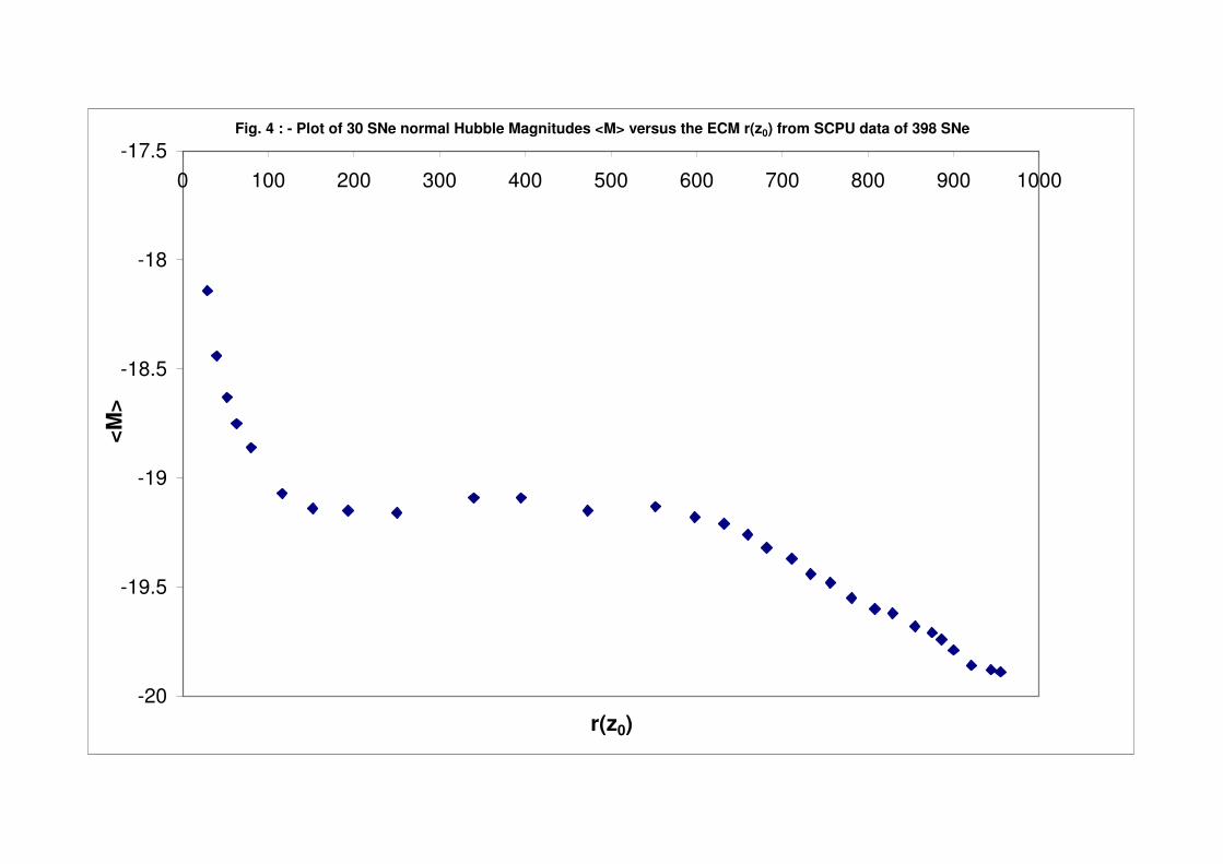
Fig. 4 : - Plot of 30 SNe normal Hubble Magnitudes <M> versus the ECM r(z0) from SCPU data of 398 SNe

-20

-19.5

-19

-18.5

-18

-17.5

0 100 200 300 400 500 600 700 800 900 1000

r(z0)

<M

>

Fig. 5 : - Plot of 30 SNe central Hubble Magnitudes M(z0) versus the mean redshift <z>=z0 from SCPU data of 398 SNe

-20

-19.5

-19

-18.5

-18

-17.5

0 0.2 0.4 0.6 0.8 1 1.2

<z>

M(z

0)

Fig. 6 : - Plot of 30 SNe central Hubble Magnitudes M(z0) versus the ECM r(z0) from SCPU data of 398 SNe

-20

-19.5

-19

-18.5

-18

-17.5

0 100 200 300 400 500 600 700 800 900 1000

r(z0)

M(z

0)

Fig. 7 : - Plot of 30 SNe new central absolute magnitudes M*(z0) versus <z>=z0 from SCPU data of 398 SNe

-19.5

-19

-18.5

-18

-17.5

-17

0 0.2 0.4 0.6 0.8 1 1.2

<z>

M*(

z0)

Fig. 8 : - Plot of 30 SNe new central absolute magnitudes M*(z0) versus the ECM r(z0) from SCPU data of 398 SNe

-19.5

-19

-18.5

-18

-17.5

-17

0 100 200 300 400 500 600 700 800 900 1000

r(z0)

M* (z

0)

Fig. 9 : - Plot and cubic fitting of 15 SNe normal Hubble Magnitudes M versus <z> > 0.4 from SCPU data

y = -8.485E-01x3 + 2.636E+00x

2 - 3.351E+00x - 1.826E+01

R2 = 9.948E-01

-20

-19.5

-19

-18.5

-18

-17.5

0 0.2 0.4 0.6 0.8 1 1.2

<z>

<M

>

Fig. 10 : - Plot and linear fitting of 15 SNe normal Hubble Magnitudes <M> versus the ECM r(z0) from SCPU data

y = -2.138E-03x - 1.786E+01

R2 = 9.950E-01

-20

-19.5

-19

-18.5

-18

-17.5

0 100 200 300 400 500 600 700 800 900 1000

r(z0)

<M

>

Fig. 11 : - Plot and cubic fitting of 15 SNe central Hubble Magnitudes M(z0) versus <z>=z0 > 0.4 from SCPU data

y = -9.603E-01x3 + 2.681E+00x

2 - 3.188E+00x - 1.838E+01

R2 = 9.939E-01

-20

-19.5

-19

-18.5

-18

-17.5

0 0.2 0.4 0.6 0.8 1 1.2

<z>

M(z

0)

Fig. 12 : - Plot and linear fitting of 15 SNe central Hubble Magnitudes M(z0) versus the ECM r(z0) from SCPU data

y = -2.061E-03x - 1.795E+01

R2 = 9.923E-01

-20

-19.5

-19

-18.5

-18

-17.5

0 100 200 300 400 500 600 700 800 900 1000

r(z0)

M(z

0)

Fig. 13 : - Plot and parabolic fitting of 15 SNe new central absolute magnitudes M*(z0) versus <z> > 0.4 from SCPU data

y = -1.199E-01x2 - 2.420E-02x - 1.787E+01

R2 = 8.883E-01

-19.5

-19

-18.5

-18

-17.5

-17

0 0.2 0.4 0.6 0.8 1 1.2

<z>

M* (z

0)

Fig. 14 : - Plot and linear fitting of 15 SNe new central absolute magnitudes M*(z0) versus <z>=z0 > 0.4 from SCPU data

y = -2.071E-01x - 1.781E+01

R2 = 8.772E-01

-19.5

-19

-18.5

-18

-17.5

-17

0 0.2 0.4 0.6 0.8 1 1.2

<z>

M* (z

0)

Fig. 15 : - Plot and linear fitting of 15 SNe M*(z0) versus the ECM r(z0) from SCPU data of 398 SNe

y = -4.831E-04x - 1.757E+01

R2 = 8.353E-01

-19.5

-19

-18.5

-18

-17.5

-17

0 100 200 300 400 500 600 700 800 900 1000

r(z0)

M* (z

0)

Fig. 16 : - Plot and cubic fitting of 9 SNe M normal points +1 versus <z>=z0 of the ECM paper IX from SCPU data

y = -9.0878E-01x3 + 3.2507E+00x

2 - 4.2618E+00x - 1.7900E+01

R2 = 9.9992E-01

-20

-19.5

-19

-18.5

-18

-17.5

0 0.2 0.4 0.6 0.8 1 1.2

<z>

<M

>

Fig. 17 : - Plot and cubic fitting of 9 SNe M normal points versus <z>=z0 of the ECM paper IX from SCPU data

y = -4.339E-01x3 + 2.146E+00x

2 - 3.416E+00x - 1.811E+01

R2 = 9.974E-01

-20

-19.5

-19

-18.5

-18

-17.5

0 0.2 0.4 0.6 0.8 1 1.2

<z>

<M

>

Fig. 18 : - Plot and linear fitting of 9 SNe M normal points +1 versus r(z0) of the ECM paper IX from SCPU data

y = -2.091E-03x - 1.790E+01

R2 = 9.996E-01

-20

-19.5

-19

-18.5

-18

-17.5

0 100 200 300 400 500 600 700 800 900 1000

r(z0)

<M

>

Fig. 19 : - Plot and linear fitting of 9 SNe M normal points versus r(z0) of the ECM paper IX from SCPU data

y = -2.260E-03x - 1.775E+01

R2 = 9.943E-01

-20

-19.5

-19

-18.5

-18

-17.5

0 100 200 300 400 500 600 700 800 900 1000

r(z0)

<M

>

Fig. 20 : - Plot and cubic fitting of 4 SNe core points <Mz> +1 versus <z>=z0 of the ECM Table 3 from SCPU data

y = -6.7334E-01x3 + 2.8270E+00x

2 - 4.0675E+00x - 1.7900E+01

R2 = 1.0000E+00

-20

-19.5

-19

-18.5

-18

-17.5

0 0.2 0.4 0.6 0.8 1 1.2

<z>

<M

z>

Fig. 21 : - Plot and cubic fitting of 4 SNe core points <Mz> versus <z>=z0 of the ECM Table 3 from SCPU data

y = -2.331E-01x3 + 1.771E+00x

2 - 3.230E+00x - 1.812E+01

R2 = 9.999E-01

-20

-19.5

-19

-18.5

-18

-17.5

0 0.2 0.4 0.6 0.8 1 1.2

<z>

<M

z>

Fig. 22 : - Plot and linear fitting of 4 SNe core points <Mz> +1 versus <rz> of the ECM Table 3 from SCPU data

y = -2.0968E-03x - 1.7901E+01

R2 = 9.9990E-01

-20

-19.5

-19

-18.5

-18

-17.5

0 100 200 300 400 500 600 700 800 900 1000

<rz>

<M

z>

Fig. 23 : - Plot and linear fitting of 4 SNe core points <Mz> versus <rz> of the ECM Table 3 from SCPU data

y = -1.950E-03x - 1.803E+01

R2 = 9.954E-01

-20

-19.5

-19

-18.5

-18

-17.5

0 100 200 300 400 500 600 700 800 900 1000

<rz>

<M

z>

Fig. 24 : - Plot and linear fitting of 4 SNe pilot points <M*> versus <z>=z0 of the ECM Table 3 from SCPU data

y = -1.084E-01x - 1.786E+01

R2 = 6.237E-01

-19.5

-19

-18.5

-18

-17.5

-17

0 0.2 0.4 0.6 0.8 1 1.2

<z>

<M

* >

Fig. 25 : - Plot and linear fitting of 4 SNe pilot points <M*> versus r(z0) of the ECM Table 3 from SCPU data

y = -2.541E-04x - 1.773E+01

R2 = 6.564E-01

-19.5

-19

-18.5

-18

-17.5

-17

0 100 200 300 400 500 600 700 800 900 1000

r(z0)

<M

* >