arX

iv:0

902.

0979

v1 [

astr

o-ph

.CO

] 5

Feb

200

9

Cosmic Core-Collapse Supernovae from Upcoming Sky Surveys

Amy Lien and Brian D. Fields

Department of Astronomy, University of Illinois, Urbana, IL

ABSTRACT

Large synoptic (repeated scan) imaging sky surveys are poised to observe enormous

numbers of core-collapse supernovae. We quantify the discovery potential of such sur-

veys, and apply our results to upcoming projects, including DES, Pan-STARRS, and

LSST. The latter two will harvest core-collapse supernovae in numbers orders of mag-

nitude greater than have ever been observed to date. These surveys will map out the

cosmic core-collapse supernova redshift distribution via direct counting, with very small

statistical uncertainties out to a redshift depth which is a strong function of the survey

limiting magnitude. This supernova redshift history encodes rich information about

cosmology, star formation, and supernova astrophysics and phenomenology; the large

statistics of the supernova sample will be crucial to disentangle possible degeneracies

among these issues. For example, the cosmic supernova rate can be measured to high

precision out to z ∼ 0.5 for all core-collapse types, and out to redshift z ∼ 1 for Type

IIn events if their intrinsic properties remain the same as those measured locally. A

precision knowledge of the cosmic supernova rate would remove the cosmological un-

certainties in the study of the wealth of observable properties of the cosmic supernova

populations and their evolution with environment and redshift. Because of the tight link

between supernovae and star formation, synoptic sky surveys will also provide precision

measurements of the normalization and z <∼ 1 history of cosmic star-formation rate in

a manner independent of and complementary to than current data based on UV and

other proxies for massive star formation. Furthermore, Type II supernovae can serve as

distance indicators and would independently cross-check Type Ia distances measured in

the same surveys. Arguably the largest and least-controlled uncertainty in all of these

efforts comes from the poorly-understood evolution of dust obscuration of supernovae

in their host galaxies; we outline a strategy to determine empirically the obscuration

properties by leveraging the large supernova samples over a broad range of redshift.

We conclude with recommendations on how best to use (and to tailor) these galaxy

surveys to fully extract unique new probes on the physics, astrophysics, and cosmology

of core-collapse explosions.

Subject headings: core-collapse supernovae; supernova evolution; galaxy surveys

– 2 –

1. Introduction

A new generation of deep, large-area, synoptic (repeated-scan) galaxy surveys is coming online

and is poised to revolutionize cosmology in particular and astrophysics in general. The scanning

nature of these surveys will open the way for a systematic study of the celestial sphere in the

time domain. In particular, ongoing and planned surveys are sensitive to the transient cosmos on

timescales from hours to years, and to supernova flux limits down to 24mag and sometimes fainter.

As we will see, these capabilities will reap a huge harvest in cosmic supernovae and will offer a new

and direct probe of the cosmic supernova history out to high redshifts.

In the past decade, supernovae in nearby and distant galaxies have come to play crucial role

for cosmology, via the use of Type Ia explosions as “standardizable” candles (e.g., Phillips 1993;

Riess et al. 1996). These powerful beacons are detectable out to very high redshift and thus reveal

the cosmic expansion history for much of the lifetime of the universe; the stunning result has been

the detection of the acceleration of the Universe and the inference that dark energy of some form

dominates the mass-energy content of the cosmos today (e.g., Riess et al. 1998; Perlmutter et al.

1999; Astier et al. 2006; Wood-Vasey et al. 2007). The detection of large numbers of Type Ia

supernovae over a large redshift range, and their use as cosmological probes, represents a major

focus of future galaxy surveys (e.g., Wang et al. 2004).

While studies of supernova Type Ia (thermonuclear explosions) justly receive enormous atten-

tion due to their cosmological importance, there has been relatively little focus on the detection of

the more numerous population of core-collapse supernovae. These explosions of massive stars show

great diversity in their observed properties, e.g. including several varieties of Type II events, but also

Types Ib and Ic events. Despite their heterogeneous nature, some core-collapse events may nonethe-

less provide standardized candles, via their early lightcurves whose nature is set by the physics of

their expanding photospheres (Kirshner & Kwan 1974; Baron et al. 2004; Dessart & Hillier 2005,

see below). Moreover, core-collapse events are of great intrinsic importance for cosmology, astro-

physics, and particle physics. These events play a crucial role in cosmic energy feedback processes

and thus in the formation and evolution of galaxies and of cosmological structure.

Synoptic surveys tuned for Type Ia events will also automatically detect core-collapse super-

novae. Indeed, as survey coverage and depth increase, they will, for the first time, image a large

fraction of all unobscured cosmic core-collapse supernovae out to moderate redshift. These pho-

tometric detections of supernovae and their light curves will shed new light on a wide variety of

problems spanning cosmology, particle astrophysics, and supernova studies. Moreover, these data

will “come for free” so long as surveys include core-collapse events in their analysis pipelines.

For example, Madau et al. (1998) already pointed out the link between the cosmic star forma-

tion history and the cosmic supernova history, and showed that when integrated over all redshifts,

the all-sky supernova event rate is enormous, ≃ 5 − 15 events/sec in their estimate. Upcoming

synoptic surveys will probe most or all of the sky at great depth, and thus are positioned to ob-

serve a large fraction of these events. Consequently, these surveys will reveal the history of cosmic

– 3 –

supernovae via directly counting their numbers as a function of redshift.

Already, recent and ongoing surveys have begun to detect core-collapse supernovae. However,

to date, surveys have focused on Type Ia events, and thus core-collapse discovery and observation

has been a serendipitous or even accidental byproduct of SNIa searches. As a result of these surveys,

the supernova discovery rate is accelerating, and the current all-time, all-Type supernova count is

∼ 5000 since SN1006.1 Thus core-collapse data is currently sparsely analyzed and reported in an

uneven manner. This situation will drastically improve in the near future, when the supernova count

increase by large factors, culminating in up to ∼ 100,000 core-collapse events seen by LSST annually.

In this paper we therefore will anticipate this future, rather than make extensive comparison with

the present data though we will make quantitative contact with current results.

Our work draws upon several key analyses. The thorough and elegant work of Dahlen & Fransson

(1999) laid out the framework for rates and observability of cosmic supernovae of all types. Their

work assembled a large body of supernova data and applied it to make rate and discovery predic-

tions for the wide variety of star formation histories and normalizations viable at that time, with

a particular focus on forecasts for very high redshift (out to z ∼ 5) observable by the infrared

James Webb Space Telescope. Sullivan et al. (2000) estimated the rates for supernovae lensed by

the matter distribution–particularly rich clusters–along the line of sight; these objects further ex-

tend the reach of infrared searches, and identified a possible supernova candidate from Hubble Space

Telescope archival images of an intermediate-redshift cluster. Gal-Yam et al. (2002) made similar

calculations of the infrared observability of supernovae, and identified additional events in archival

data. Gal-Yam & Maoz (2004) and Oda & Totani (2005) presented forecasts for then-upcoming

ground-based surveys. These studies considered all cosmic supernovae, but with a focus on Type Ia

events, specifically with an eye towards revealing the Type Ia delay time as well as a parameterized

characterization of the cosmic star formation history based on Type Ia counts. In addition, these

first studies reasonably chose to emphasize near-term (i.e., now-completed or ongoing) relatively

modest surveys, or on future space-based missions such as SNAP, with little to no study of the

impact of large synoptic surveys. Moreover, while these works included dust extinction effects in

host galaxies, but because of their focus on Type Ia events, they did not study the possibility of a

redshift evolution in extinction (Mannucci et al. 2007).

We build on the important studies of Dahlen & Fransson (1999), Gal-Yam et al. (2002); Gal-Yam & Maoz

(2004), and Oda & Totani (2005) in several respects: (1) we explore the promise of synoptic sur-

veys and forecast the very large numbers of supernovae they will find; (2) we focus on less-studied

core-collapse events; (3) we incorporate the (pessimistic) possibility of strong dust evolution of

Mannucci et al. (2007) which is a dominant obstacle to observing massive star death at high red-

shifts; (4) we present a strategy for empirically calibrating the obscuration properties across a broad

range of redshift by studying the evolution of the supernova luminosity function; and (5) we study

the unique opportunities that become available with the large supernova harvest of synoptic sur-

1 Central Bureau for Astronomical Telegrams (2008); see also http://www.cfa.harvard.edu/iau/lists/Supernovae.html

– 4 –

veys; in particular, we show how the cosmic supernova rate can be recovered based on core-collapse

counts, without assumption as to its functional form.

Our goal in this paper is to explore the impact synopic surveys will make on core-collapse

supernova astrophysics and cosmology. We summarize key upcoming surveys in §2. In §3 we

review expectations for the CSNR, core-collapse supernova observables, and the effect of cosmic

dust and its evolution. We combine these inputs in §4 where we forecast the core-collapse supernova

discovery potential for upcoming surveys. We quantify in detail the strong dependence of the

supernova harvest on the survey limiting magnitude, which we find to be the key figure of merit

for supernova studies. We discuss some of the supernova science payoff in §6, and conclude in §7

with some recommendations for synoptic surveys.

2. Synoptic Surveys

Current and future sky surveys build on the pioneering approach of the Sloan Digital Sky

Survey (SDSS; York et al. 2000). Following SDSS, these surveys will produce high-quality digital

photometric maps of large regions of the celestial sphere. The powerful innovation the new surveys

to extend the original SDSS approach into the time domain. Each program will scan part of their

survey domain frequently, with revisit periods of days and in some cases even hours, and maintain

this systematic effort throughout the survey’s multi-year operating lifespans. The result will be

unprecedented catalogs of transient phenomena over timescales from hours to years. These surveys

are thus ideal for supernova discovery and matched to supernova light curve evolution timescales;

the result will be a revolution in our observational understanding of supernovae.

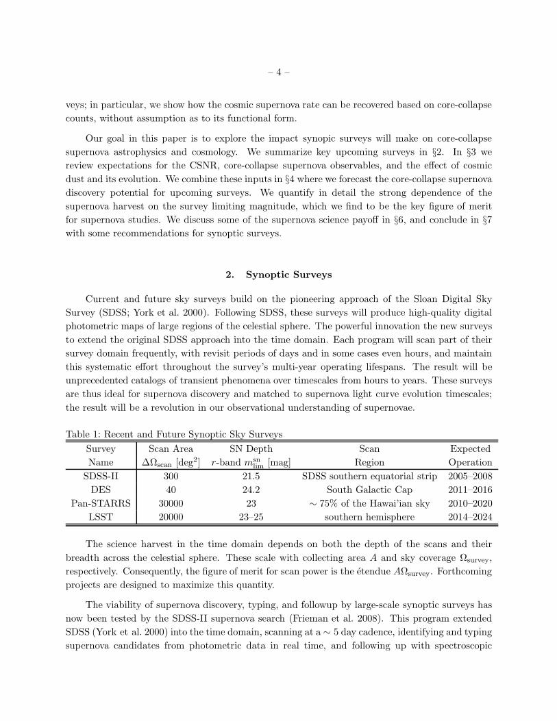
Table 1: Recent and Future Synoptic Sky Surveys

Survey Scan Area SN Depth Scan Expected

Name ∆Ωscan [deg2] r-band msnlim [mag] Region Operation

SDSS-II 300 21.5 SDSS southern equatorial strip 2005–2008

DES 40 24.2 South Galactic Cap 2011–2016

Pan-STARRS 30000 23 ∼ 75% of the Hawai’ian sky 2010–2020

LSST 20000 23–25 southern hemisphere 2014–2024

The science harvest in the time domain depends on both the depth of the scans and their

breadth across the celestial sphere. These scale with collecting area A and sky coverage Ωsurvey,

respectively. Consequently, the figure of merit for scan power is the etendue AΩsurvey. Forthcoming

projects are designed to maximize this quantity.

The viability of supernova discovery, typing, and followup by large-scale synoptic surveys has

now been tested by the SDSS-II supernova search (Frieman et al. 2008). This program extended

SDSS (York et al. 2000) into the time domain, scanning at a ∼ 5 day cadence, identifying and typing

supernova candidates from photometric data in real time, and following up with spectroscopic

– 5 –

confirmation. This survey will serve as a testbed for the larger future campaigns. It is thus very

important and encouraging that SDSS-II has reported the discovery of 403 confirmed supernovae

in the first two seasons of operation (Sako et al. 2008). The search algorithms and followup were

focused on Type Ia events, for which light curves and spectra have been recovered over 0.05 <

z < 0.35; human input was used for supernova typing, but automated routines appear promising

and will be essential for larger surveys. Follow-up spectroscopy (Zheng et al. 2008) yields accurate

supernova and host-galaxy redshifts (σsnz ≈ 0.005 and σgal

z ≈ 0.0005); host-galaxy contamination is

found to be well-addressed by χ2 fitting and a principal component analysis.

Table 1 lists several major current and future synoptic surveys, and gives the values or current

estimates of their performance characteristics. The msnlim values are derived from the survey 5σ

detections for single visit exposures, which have been corrected 1mag shallower as noted above.

SDSS-II (Frieman et al. 2008) is recently completed, as discussed above; we adopt an r-band lim-

iting magnitude of 21.5mag (J. Frieman, private communication). The Dark Energy Survey (DES;

The Dark Energy Survey Collaboration 2005) will push down to msnlim ∼ 24.2mag in r-band; as

we will see below, this will already enormously increase the supernova harvest. Finally, look-

ing out farther into the next decade, Pan-STARRS (Jewitt 2003; Tonry 2003) and then LSST

(The LSST Collaboration 2007; Tyson 2002) will introduce a huge leap in both sky coverage and

in depth. These ambitious projects represent a culmination of the synoptic survey approach, and

we will make a particular effort to examine their potential for supernova science.

For our analysis, we will characterize each survey with four parameters

1. the survey supernova depth, i.e., single exposure limiting magnitude msnlim for supernova de-

tection when used in scan mode; this is set by collecting area (and monitoring time)

2. the total survey scanning sky coverage, i.e., solid angle ∆Ωscan

3. the scan revisit time (“cadence”) τvisit

4. the total monitoring time ∆tobs, which (for a single cadence) is proportional to the total

number ∆tobs/τvisit of visits

For a fixed survey design and lifetime, these parameters are not independent, since exposure time

comes at the expense of sky coverage and number of visits.

There are numerous challenges and complexities in the process of extracting supernovae and

their redshifts from surveys (and for sorting out their types; see, e.g., Dahlen & Goobar 2002;

Poznanski et al. 2007; Kim & Miquel 2007; Kunz et al. 2006; Blondin & Tonry 2007; Wang 2007).

Tonry et al. (2003) gives thorough discussion of these issues with emphasis on Type Ia events;

see also Dahlen & Fransson (1999), Gal-Yam & Maoz (2004) and Oda & Totani (2005), and the

SDSS-II papers (Frieman et al. 2008; Sako et al. 2008; Zheng et al. 2008).

Our simple survey parameterization cannot capture all of these subtleties, not do we intend it

– 6 –

to; rather, we wish our treatment to provide a rough illustration of the surveys’ potential for core-

collapse detection and science. Consequently, our parameter choices should be viewed as typical

effective values, which may be different from (and weaker than) the raw survey specifications.

For example, supernova identification and typing requires knowledge of the light curve. Thus,

one cannot only observe the supernova at peak brightness, but also follow it after (and ideally be-

fore). Tonry (2003) recommends following the supernova for least δm = 1mag below peak brightness;

we will adopt this value as well. Thus, the effective supernova detection depth is msnlim = mmax−δm,

where mmax is the survey scan depth (i.e., depth for a single exposure).

Note also that some upcoming surveys (such as DES) will only repeatedly scan a fraction of the

sky which they map; but only the scanned regions will host the discovery of supernovae and other

transients. Also, some surveys (e.g., Pan-STARRS and LSST) envision multiple periodicities and

associated limiting magnitudes; for simplicity we will here chose conservative depths for the values

given in Table 1, to be consistent with the advertised scanning sky coverage. Thus one should bear

in mind that in our analysis we have chosen the minimal parameterization one could use, which give

only a simplified and idealized sketch of the real surveys. Given this, and the ongoing planning of

future survey characteristics, our forecasts for the surveys’ supernova results should be understood

as indicative of the order of magnitude expected, but not as high-precision predictions.

3. Core-Collapse Supernovae in a Cosmic Context

3.1. The Cosmic Core-Collapse Supernova Rate: Expectations

The total cosmic supernova rate (hereafter CSNR)

RSN[z(tem)] ≡dNSN

dVcom dtem(1)

is the number of events per comoving volume per unit time tem in the emission frame (i.e., cosmic

time dilation effects in the observer’s z = 0 frame are not included). The total rate, and the various

differential rates below, can of course be specialized to distinguish different groups of supernovae

classified by intrinsic type and/or dependence on local environment.

The present data on high-redshift core-collapse supernovae are too poor to construct an accu-

rate CSNR. But the CSNR is intimately related to cosmic star-formation rate ρ⋆ = dM⋆/dVcomdt

(Madau et al. 1998). The connection is

RSN =XSN

〈mSN〉ρ⋆ (2)

where XSN is the fraction, by mass, of stars which become supernovae, and 〈mSN〉 is the average

supernova progenitor mass (see Appendix A). A key point is that due to the short core-collapse

progenitor lifetimes the two rates scale linearly, RSN ∝ ρ⋆. The constant of proportionality depends

– 7 –

on the initial mass function (IMF). If the IMF changes with time (or environment) this complicates

the picture. In producing quantitative estimates we will follow most studies in assuming time-

independent IMF. Thus the supernova/star-formation rate proportionality is a constant fixed for

all time, namely RSN/ρ⋆ = 0.00915M−1⊙

(Appendix A).

Uncertainties in the cosmic rates for both supernovae and star-formation remain considerable.

As illustrated in detail by (Strigari et al. 2005), the cosmic star-formation rate is known to rise

sharply towards redshift z ∼ 1. In this low-to-moderate redshift regime, the shape of the rate versus

redshift is fairly well known, but as emphasized by Hopkins & Beacom (2006) the normalization

remains uncertain to within a factor ∼ 2. At higher redshifts, the rate becomes even more uncertain,

largely due to the paucity of data and also to uncertainties in our knowledge of the degree of dust

obscuration. It is also worth noting that most studies to date directly or indirectly use massive

stars as proxies for star formation. Consequently, the rate for cosmic massive star formation–and

for cosmic supernovae–is less uncertain and IMF-dependent than the total rate.

To illustrate the effects of these uncertainties on the synoptic survey supernova harvest, we have

adopted two possible CSNR forms. These appear in Figure 1, which shows the expected supernovae

rate assuming a perfect environment (i.e. no dust extinction, etc). The solid curve in Figure 1(a)

is the CSNR derived from the cosmic star-formation rate of Cole et al. (2001) with parameters

fitted by Hopkins & Beacom (2006) (hereafter the “benchmark” CSNR). This rate sharply rises to

a peak at z ∼ 2.5, followed a strong but less rapid declines out to high redshift. To investigate

the impact of the falloff from the peak, we also show in the broken curve an alternate CSNR due

to current observational data fitted by Botticella et al. (2008) (hereafter the “alternative” CSNR).

This rate also rise to redshift z ∼ 0.5, though with a different slope; we somewhat arbitrarily set

the alternative rate to a constant at z > 0.5 where the data are unclear; in any case we will find

that few events from this high-redshift regime will be accessible to the all-sky surveys which are

our focus.

Synoptic surveys will measure several observables associated with cosmic supernovae: their

numbers and location, and some portion of their light curves in different bands. Spectroscopic

redshifts of host galaxies can also be determined (when visible; see §6.5). Using the number counts

and redshift indicators, one can deduce an observed core-collapse rate, per unit redshift and per

unit time and solid angle. This observed rate distribution directly encodes the CSNR via

dNSN

dΩdtobsdz=

dNSN

dVcomdtem

dtemdtobs

dVcom

dΩdz= RSN(z)

r2com

1 + z

drcom

dz(3)

where Vcom is the comoving volume and rcom(z) is the comoving distance out to redshift z. The

1 + z factor corrects for time dilation via dtobs = (1 + z)dtem.

Figure 1(b) shows the all-sky cumulative frequency of cosmic supernovae for an observer at

z = 0, i.e.,

dNSN

dt(< z)all−sky = 4π

∫ z

0

dNSN

dΩdtobsdzdz′ = 4π

∫ z

0RSN(z′)

r2com

1 + z′drcom

dz′dz′ (4)

– 8 –

Fig. 1.— (a) Top panel: Possible cosmic core-collapse supernova rates as a function of redshift.

The solid curve is the result calculated based on the Cole et al. (2001) cosmic star-formation rate;

the broken curve is based on current supernova data (Botticella et al. 2008); see Appendix A. (b)

Bottom panel: The idealized, all-sky cumulative rate of all supernovae observed over redshift 0 to

z, for an observer with no faintness limit and with no dust extinction anywhere along the line of

sight.

– 9 –

These curves give the total rate of observed cosmic supernova explosions out to redshift z for

an idealized observer monitoring the entire sky out to unlimited depth and without any dust

obscuration anywhere along the line of sight.

All of these idealizations will fail, some of them drastically, for real observational programs.

Nevertheless, one cannot help but be tantalized by the enormous explosion frequencies indicated

in Figure 1(b). With our benchmark CSNR, out to redshift z = 1, something like ∼ 1 supernova

explodes per second somewhere in the sky. Out to redshift z = 2, this rate increases to ∼ 6

events/sec. Clearly, even with a small detection efficiency, synoptic surveys are poised to discover

core-collapse supernovae in numbers far exceeding all supernovae in recorded history to date.

For numerical results in Figure 1 and throughout this paper, we adopt a flat cosmology with

Ωm = 0.3 and ΩΛ = 0.7. For the Hubble constant we adopt the value H0 = 71 km s−1 Mpc−1, i.e.,

h = 0.71 where H0 = 100 h km s−1 Mpc−1. These values are consistent with recent determinations

using WMAP and large-scale structure (Spergel et al. 2007).

3.2. The Effect of Dust Obscuration

The enormous inventory of cosmic supernovae is not, unfortunately, fully observable even

for arbitrarily deep surveys. In a realistic environment there are several factors which will hide

the supernovae from us; dust extinction is one of the most important, and probably the most

uncertain. Core-collapse supernovae mostly explode within regions of vigorous star formation

which are thus likely to be dusty environments. Consequently, we expect that some core-collapse

supernovae will be obscured to the point where they are not detected in synoptic surveys. The

fraction of supernovae lost to dust obscuration, and particularly the possible redshift dependence

of this extinction, represents a crucial systematic error which must be addressed before one can use

survey data to infer information about supernova populations and their cosmic rates.

For the purposes of our present estimates of survey supernova yields, we follow the approach of

Mannucci et al. (2007). These authors characterize losses due to dust extinction and/or reddening

in the host galaxies via a fraction αdust(z) of undetected events at each redshift. This fraction could

in principle differ for the various core-collapse types; for the present treatment we will assume it is

the same for all such events. As core-collapse statistics become available from surveys, this issue

can and should be revisited; more on this below. and in §5. The resulting fraction of detected

supernovae is thus the complement fdust(z) = 1− αdust(z), which measures the reduced supernova

detection efficiency in the presence of dust. Expressed as an effective extinction A for the supernova

population at z, we have Aeff (z) = −1.086 ln fdust.

Mannucci et al. (2007) estimate the fraction of missing supernovae by comparing the observed

detections in the optical with those in radio and near-IR. They conclude that dust evolution is very

strong; this becomes a dominant limitation to the discovery of core-collapse events at high redshift.

In the local universe, Mannucci et al. (2007) find that the vast majority of the events occurring in

– 10 –

massive starbursts (luminous infrared galaxies) are missed. Because these galaxies harbor only a

small fraction of the local supernova population, the overall optically missing fraction at z = 0 is

estimated to be rather modest: αdust = 5 − 10% . If, however, high-redshift star formation occurs

in starburst environments (i.e., luminous and ultra-luminous galaxies, which are highly extincted;

see e.g. Smail et al. 1997; Hughes et al. 1998; Perez-Gonzalez et al. 2003; Le Floc’h et al. 2005;

Choi et al. 2006) then the fraction of missing events rises sharply with redshift. Multiwavelength

observations of light from pre-supernova massive stars also supports the idea of increasing dust

obscuration at high redshift. Adelberger & Steidel (2000) find that ultraviolet light from massive

stars in z ∼ 3 galaxies is mostly reprocessed by dust into thermal submillimeter emission, so that

the observable galaxy luminosities have Lsub−mm/LUV ∼ 1 − 100.

Mannucci et al. (2007) estimate the portion of supernovae which will be “catastrophic losses”

to severe extinction, and propose that the missing fraction can be described by a linear relation

αdust(z) = 0.05 + 0.28z for the core-collapse supernovae for redshift z<2. Thus, the fraction of the

supernovae which remain optically detectable is fdust(z) = 1 − αdust(z) = 0.95 − 0.28z for z < 2.

At higher redshift, Chen et al. (2007) and Gnedin et al. (2008) argue that fdust is small; they find

limits consistent with fdust = 0.02 for these redshifts.

We will smoothly match these two estimates, and adopt a fraction of the supernovae which

can be detected after dust extinction of

fdust(z) =

0.95 − 0.28z , z < 3.3

0.02 , z ≥ 3.3(5)

For these values of fdust, the effective extinction varies from Aeff = 0.056mag at z = 0 to Aeff =

4.25mag at z ≥ 3.3. In practice, we will find that cosmological dimming of supernovae beyond z ∼ 1

is itself so large that surveys up to and including LSST will see relatively few events, so that the

details of the adopted dust model in this regime will not affect our conclusions.

The strong redshift evolution of dust obscuration in the empirical Mannucci et al. (2007) model

deserves comment. From a physical point of view, the rise in dust losses α(z) towards high redshift

implies that at earlier times, the birth environments of supernovae are significantly more enshrouded

than those now. This interesting result itself deserves a deeper elucidation, one which will likely be

easier to formulate and test in the presence of survey supernova data. From more practical point

of view, our adoption of a model wherein dust losses grow rapidly with z should yield conservative

(or at least not optimistic) predictions for the supernova harvest at large redshifts. That is, if it

turns out that host galaxy effects do not change rapidly with cosmic time so that the efficiency of

supernova detection remains close to the high local value, then our rate predictions at z ∼ 1 would

be boosted by a factor of ∼ 1.5.

Note also that fdust as Mannucci et al. (2007) and we have defined it characterizes the observ-

able portion of the ensemble of supernovae at a particular redshift. Implicitly, individual supernovae

are treated as either detectable or not, i.e., dust effects are considered negligible or total; our cal-

culation treats total, catastrophic losses of supernovae using this fdust formalism. We separately

– 11 –

include the effect of partial extinction due to dust, where the apparent magnitude of supernova

is reduced but still visible, as discussed in the next section. Of course in reality, all supernovae

will experience some level of extinction in their host galaxies, with the distribution of host-galaxy

extinctions changing with redshift. A more detailed study of dust effects on supernovae (and uses

of supernovae to quantify and calibrate these effects) would be of interest for further investigation;

see discussion in §5.

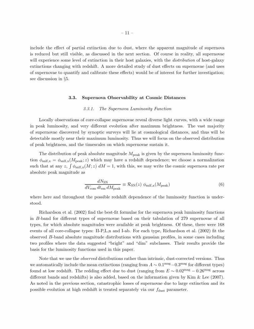
3.3. Supernova Observability at Cosmic Distances

3.3.1. The Supernova Luminosity Function

Locally observations of core-collapse supernovae reveal diverse light curves, with a wide range

in peak luminosity, and very different evolution after maximum brightness. The vast majority

of supernovae discovered by synoptic surveys will lie at cosmological distances, and thus will be

detectable mostly near their maximum luminosity. Thus we will focus on the observed distribution

of peak brightness, and the timescales on which supernovae sustain it.

The distribution of peak absolute magnitude Mpeak is given by the supernova luminosity func-

tion φsnlf,x = φsnlf,x(Mpeak; z) which may have a redshift dependence; we choose a normalization

such that at any z,∫

φsnlf,x(M ; z) dM = 1, with this, we may write the cosmic supernova rate per

absolute peak magnitude as

dNSN

dVcom dtem dMpeak≡ RSN(z) φsnlf,x(Mpeak) (6)

where here and throughout the possible redshift dependence of the luminosity function is under-

stood.

Richardson et al. (2002) find the best-fit formulae for the supernova peak luminosity functions

in B-band for different types of supernovae based on their tabulation of 279 supernovae of all

types, for which absolute magnitudes were available at peak brightness. Of these, there were 168

events of all core-collapse types: II-P,L,n and I-ab. For each type, Richardson et al. (2002) fit the

observed B-band absolute magnitude distributions with gaussian profiles, in some cases including

two profiles where the data suggested “bright” and “dim” subclasses. Their results provide the

basis for the luminosity functions used in this paper.

Note that we use the observed distributions rather than intrinsic, dust-corrected versions. Thus

we automatically include the mean extinctions (ranging from A ∼ 0.1mag−0.3mag for different types)

found at low redshift. The redding effect due to dust (ranging from E ∼ 0.02mag − 0.26mag across

different bands and redshifts) is also added, based on the information given by Kim & Lee (2007).

As noted in the previous section, catastrophic losses of supernovae due to large extinction and its

possible evolution at high redshift is treated separately via our fdust parameter.

– 12 –

We adjust the Richardson et al. (2002) distributions in two ways. First, we converted from

their Hubble constant of h = 0.6 ot our adopted value h = 0.71. More importantly, we assume

that each gaussian is a good representation of the data around the peak, but we do not allow

the wings to extend arbitrarily far. Instead, we cut off the distributions at |M − Mmean| > 2.5σ,

where no data exist in the Richardson et al. (2002) sample. We introduce these cutoffs in order to

avoid extrapolating to very rare, bright events which in a large survey could extend the redshift

reach considerably. Below (§4.2) we discuss the effect of this cutoff and its effect on the predicted

supernova redshift range.

3.4. Supernova Discovery in Magnitude-Limited Surveys

Surveys will discover supernovae monitor lightcurves in one or more passbands Here we will

adopt the SDSS ugriz photometric system, which uses AB magnitudes (Fukugita et al. 1996).

The light curve of any supernova will suffer redshifting and time dilation effects. For passband

x we put

mx − Mx = 5 log

(

dL(z)

d0

)

+ Kx(z) + Ax(z) ≡ µ(z) + Kx(z) − 1.086 ln fdust (7)

with dL the luminosity distance and µ(z) is the usual distance modulus with d0 = 10 pc. The dust

extinction A is included via the factor fdust (eq. 5). The K-correction accounts for redshifting of

the supernova spectrum, and is discussed in Appendix C.

As noted above, at each redshift the effect of dust will be to obscure some fraction of supernovae.

The remaining unobscured events will have apparent x-filter magnitudes of mx = Mx+µ(z)+Kx(z).

The expected mx distribution thus reflects the underlying distribution of absolute magnitudes Mx.

Since the Richardson et al. (2002) supernova luminosity function we use is in the B-band, we need

to find the corresponding B-band magnitude in order to find the right corresponding number of

supernovae; this transformation to mB is straightforward and is given by mx = mB + ηxB, where

ηxB = −2.5 log

∫ xf

xiF (λ)Sx(λ)dλ

∫ Bf

BiF (λ)SB(λ)dλ

+ zeropoint correction (8)

is a color index which translates between the x and B magnitudes in the rest frame, and zeropoint

correction is the correction for different zeropoint of the SDSS magnitude system and the Johnson

magnitude system. For the spectral shapes F (λ) we use the prescriptions of Dahlen & Fransson

(1999) as described in Appendix C.

The absolute x-band magnitude distribution of unobscured supernovae at redshift z is φsnlf,x[Mx−

ηxB ], where φsnlf,x is the luminosity function in B-band as tabulated by Richardson et al. (2002).

Therefore the distribution of a certain type of supernova apparent magnitudes mx in x-filter is

φsnlf,x[mx − µ(z) − Kx(z) − ηxB], Thus the fraction of all (unobscured) supernovae at z which

– 13 –

fall within the survey x-band magnitude limit msnlim is a sum over the luminosity functions for all

core-collapse types:

fmaglim(z) =∑

types

∫ msn

limxφsnlf,x[mx − µ(z) − Kx(z) − ηxB ] dm

∫

φsnlf,x(m) dm

=∑

types

∫ msn

lim−µ(z)−Kx(z)−ηxB φsnlf,x(m

′) dm′

∫

φsnlf,x(m) dm

≡ fsnlf [< Mlim(z,msnlim)]

which is the cumulative fraction of supernovae whose absolute magnitude is brighter than

Mlim(z,msnlim) = msn

lim − µ(z) − Kx(z) − ηxB (9)

To develop some intuition, suppose the supernova peak brightnesses lie in a range Mpeak ∈

(Mbright,Mdim), and ignore for now the effects of dust. Then for low redshifts such that the absolute

magnitude limit Mlim from eq. (9) is fainter than Mdim, we can expect to see all supernovae, and

fmaglim = 1. For these redshifts, we can study the entire supernova luminosity function and test

whether it varies with redshift. On the opposite extreme, for high redshifts such that Mlim is dimmer

than Mbright we can see no supernovae, so fmaglim = 0; this then defines the survey redshift cutoff (for

fixed msnlim). Finally, for intermediate z such that msn

lim−Mdim < µ(z)+Kx(z)+ηxB < msnlim−Mbright,

we have 0 < fmaglim < 1; over these redshifts the survey samples the bright end of the supernova

luminosity function.

Both magnitude limit and dust extinction reduce the expected supernova detection, and do so

independently of each other. Consequently, we can find the net supernova detection probability by

simply taking the product of the individual factors:

fdetect(z;msnlim) = fmaglim(z;msn

lim) fdust(z) (10)

Figure 2 shows the resulting detectable fraction of supernovae. The left panel shows the shape

of fmaglim for the g and r bands. At redshifts close to zero, fmaglim ≈ 1 which means that almost

all supernovae are detected in the local universe. And it approaching to zero at high redshift,

which reflects the fact that no supernovae can be detected at high redshift because of the survey

deepness. Note that g and r bands are competitive for msnlim ≤ 24, but for higher msn

lim, fmaglim in

g-band drops a lot faster than those in r-band especially around z ∼ 0.4, which is cause by the

effect of K-correction. The figure also shows that for higher msnlim, fmaglim decays less rapidly. The

right panel shows fdetect for different msnlim, using our adopted dust model (eq. 5). We see fdetect

shows the same trend as fmaglim except the detectable fraction is reduced due to dust and we can no

longer observe all supernovae even in the local universe. It is also clear to see that going to fainter

msnlim significantly boosts the detectable fraction at high redshift. For msn

lim = 23mag, fdetectable is

almost zero at redshift z ∼ 1 for both g and r bands. But going to msnlim = 26mag, ∼ 55% of the

supernovae at redshift z ∼ 1 remain visible both the g and r bands.

– 14 –

Fig. 2.— (a) The fraction of supernovae detected based on different survey deepness in g and r

bands, with msnlim ranging from 21mag down to 27mag; effects of dust obscuration are not included.

(b) As in (a), but including the effects of dust obscuration strongly evolving with redshift as modeled

by eq. (5).

This means that deeper surveys (and/or scanning modes in which smaller areas are scanned

more deeply) will probe supernovae out to much higher redshifts. Deep survey modes will also

probe a much wider regime of the supernova luminosity function and light curves over a broad

range of cosmic epochs, thus testing for redshift evolution in supernova properties. The clear lesson

is that the scan msnlim is critical in determining the quality and reach of the supernova science. In

particular, we urge that scans strategies include modes which push > 1mag deeper than the all-sky

depth.

3.4.1. Supernova Light Curves

The observed population of core-collapse supernovae shows a broad range of timescales and

time histories in their decline from peak brightness (e.g., Doggett & Branch 1985; Leibundgut & Suntzeff

2003). The amplitude and time behavior of these curves encodes a wealth of information about

the underlying physics of the supernovae as well as their interaction with the circumstellar and

interstellar medium.

Empirically, light curves broadly fall into phenomenological categories, those whose magnitudes

decline in a relatively steep, linear way (Type II-L) and those which linger near peak brightness

with a relative plateau in magnitude (Type II-P). Patat et al. (1993) compiled 51 Type II light

curves, and analysis in Patat et al. (1994) showed that plateau-type supernovae typically decline

from peak brightness at rates which vary the range (0.7mag − 3.1mag)/100 days, while linear-type

– 15 –

events typically have (3.9mag − 5.7mag)/100 days. Unfortunately, the lightcurves available at the

time of these studies were poorly sampled near the peak itself, where the behavior is most critical

for our purposes.

Fortunately, subsequent data, particularly using Swift, gives a clearer picture of the early light

curves for a few events. For plateau event SN 2005cs, data in Pastorello et al. (2006) show that

∼ 15 days after peak brightness, the supernova dimming was strongly depending on passband:

∆M15(U) ≃ 1.8mag, ∆M15(B) ≃ 0.7mag, ∆M15(V ) ≃ 0.18mag, and ∆M15(R) ∼ 0.1mag. Another

Type II-P event, SN 2006bp, after ∼ 13 days declined by ∼ 1mag in U , but within errors was

essentially constant in B and V (Dessart et al. 2008). For Type Ib, the recent event SN 2008D was

seen from shock breakout (Modjaz et al. 2008); after dropping from this brief initial outburst, the

flux increased for ∼ 15 days to a maximum. Afterwards, the brightness decline rates lengthen with

wavelength, with a drop of ∆M ∼ 1mag after ∼ 10 days in U -band, but after about 15 and 20 days

in B and V respectively.

These multicolor data show that brightness decline in V and longer passbands comparable to

if not slower than the typical range of ∆M15 ∼ 1mag−2mag found in Type Ia events (Phillips 1993).

This implies that surveys timed for Type Ia discovery will automatically be well-suited and possibly

even better-sampled for core-collapse events. In particular, we will find below that the r and also

g passbands are the most promising for survey supernova detections. Thus, if cosmic supernovae

follow the behavior of these local events, we expect that the light curves will remain within, e.g.,

∆m ≃ 0.5mag of peak brightness (a factor 1.5 in flux) for a timescale of at least a week. In some

cases this timescale will be longer, and possibly also with detections in the rising phase.

For synoptic surveys to detect core-collapse supernovae near their peak brightness, the cadence

needs to be shorter than the (observer-frame) brightness decline time. Thus weekly revisits are

sufficient for marginal detections, and cadences of ∼ 3 − 4 days will often see the event three or

more times. In the cases of plateau events, the supernova should remain near peak brightness

for many such revisit times. Furthermore, due to cosmological time dilation effects, the observed

brightness decline timescale τobs = (1 + z)τrest is increased by a factor of 1 + z, which extends the

detection window and offers a greater opportunity to recover a well-sampled lightcurve. Also, we

see that color evolution is not strong in V and R bands. The UV and blue do fade more rapidly,

and the supernova reddening depends on the type. For events where bluer rest-frame colors are

available, this might be a useful means of photometrically determining supernova type.

4. The Cosmic Core-Collapse Supernova Rate: Forecasts for Synoptic Surveys

In this section we will work out general formalism for supernova observations by synoptic

surveys. We then apply this formalism to specific current and proposed surveys

– 16 –

4.1. Connecting Cosmic Supernovae and Survey Observables

4.1.1. General Formalism

It is useful to define a differential supernova detection rate per unit redshift, solid angle, and

apparent magnitude in x-band:

dNSN,obs,x

dtobs dz dΩ dm= RSN(z)

r(z)2

1 + z

dr

dzfdust(z) φsnlf,x[mx − µ(z) − Kx(z) − ηxB] (11)

This expression adds the effects of supernova luminosity (cf eq. 6) and of dust obscuration (eq. 5)

to the ideal rate of eq. (3). Throughout, we will for simplicity refer to the entire core-collapse

supernova population, but the formalism could equally well distinguish the various core-collapse

types, and compute the rates of each. An example of such a treatment is the Scannapieco et al.

(2005) study of the rate and detectability of pair-instability supernovae.

The differential rate in eq. (11) relates the observables in a synoptic survey to underlying

properties of cosmic supernovae. As such, a wealth of information can be recovered by a good

statistical sample of supernovae over a redshift range: one probe different terms and their underlying

physics. For example, at fixed z, the range of observed supernova magnitudes in x-band mx probes

the supernova peak luminosity function φsnlf,x(M ; z) at magnitudes Mx = mx−µ(z)−Kx(z)−ηxB .

Comparing these results at different redshifts with local determinations can reveal any redshift-

and/or environment-dependence in the core-collapse supernova luminosity function.

Another aspect of cosmic supernovae probed by synoptic surveys, and central focus of this

paper, is the cosmic supernova rate. Whereas the supernova luminosity function can be determined

from the distribution of supernova magnitudes at the same redshift, the cosmic supernova rate

comes from the distribution of supernova counts across different redshifts. The observed differential

rate for supernovae of all magnitudes in the x-band is

ΓSN,obs,x(z) ≡dNSN,obs,x

dtobs dz dΩ=

∫ msn

lim

dmdNSN,obs,x

dtobs dz dΩ dm= RSN(z) fdetect,x(z;msn

lim)r(z)2

1 + z

dr

dz(12)

Note that this is the idealized rate of eq. (3) reduced by the detection in x-band fdetect,x.

One can get a sense of the orders of magnitude in play via the definition of a dimensionful

scale factor

ΓSN,0 = RSN(0) d3H = 7.2 × 106 events yr−1 sr−1

(

RSN(0)

10−4 yr−1 Mpc−3

)

(13)

= 0.22 events sec−1 sr−1

(

RSN(0)

10−4 yr−1 Mpc−3

)

(14)

= 2.2 × 103 events yr−1 deg−2

(

RSN(0)

10−4 yr−1 Mpc−3

)

(15)

We may then define a dimensionless distance u(z) = r(z)/dH , with dH = c/H0 the Hubble length,

– 17 –

Fig. 3.— The cosmic supernova detection rate in r-band, expressed in number of events per solid

angle per time, shown a function of redshift. The curve labeled “unobscured” ignores both effects

of dust extinction or the flux limit of the survey (i.e., fdetect = 1). The curve labeled “with dust”

includes dust extinction only, but with msnlim = ∞. The remaining curves are for surveys with msn

lim

as labeled, and include dust extinction. Note that the vertical axis is shown both in units of events

per second per steradian (left scale) and events per year per square degrees (right scale).

and write

ΓSN,obs(z) = ΓSN,0RSN(z)

RSN(0)

u(z)2

1 + z

du

dzfdetect,x(z,msn

lim) (16)

Figure 3 plots the observed supernova rate ΓSN,obs per solid angle in r-band. For comparison,

we show the idealized cases of msnlim = ∞ and fdust = 0, as well as realistic cases in the presence of

dust and with different msnlim. The amplitudes of the curves in Figure 3 confirm the large numbers

of events expected from eq. (13).

The shapes of the curves can also be readily understood. At low redshifts, the surveys see most

of the supernovae that occur–i.e., the entire luminosity function is sampled; cf Figure 2. Hence at

small z, the supernova sample is simply limited by the cosmic volume within z: Γ ∝ dVcom/dz ∼

– 18 –

r2com drcom/dz ∼ z2 Thus the detection rate initially rises quadratically with z; this volume effect

is essentially independent of survey magnitude limit, as we see by the overlap of the curves in this

regime.

In the high redshift limit, several effects act to suppress supernova detectability. At z > 1, rcom

rapidly saturates at the comoving horizon scale, and nearly all observable cosmic volume is sampled;

in this regime, the volume factor decreases as dVcom/dz ∼ drcom/dz ∼ 1/H(z) ∼ (1 + z)−3/2. In

addition, time dilation effects become large and add another factor of (1 + z)−1. For these reasons,

even the idealized (unobscured, msnlim = ∞) rate drops. Moreover, in some models (such as that of

Cole et al. 2001), the CSNR itself is intrinsically expected to drop after a peak, perhaps somewhere

in the range z ∼ 1 − 3. On top of this, the effects of dust obscuration become large at z >∼ 1 and

removes further supernovae in this range. Finally, a finite survey magnitude limit truncates still

more events at high z.

The combination of the low-redshift rise and high-redshift drop acts to create a peak in su-

pernova detectability. The position of the peak is sensitive to the CSNR itself, and the details of

dust obscuration. But the peak position and amplitude are also both very sensitive to the survey

magnitude limit; both rise sharply as survey depth msnlim increases. This illustrates a key conclusion

which will be manifest in several other ways below: for discovery of core-collapse supernovae at

high redshifts, the most important aspect of a synoptic survey is its limiting magnitude; investment

in deep scan modes (msnlim > 24 mag) will reap substantial rewards.

Figure 4 shows the same supernova rate redshift distribution as in Fig. 3, but for the five ugriz

passbands with SDSS filters and efficiencies. For each band we fix msnlim = 24mag. We see that the

discovery rate is the highest in r for essentially all redshifts, with g-band counts very nearly the

same except around the peak at 0.2 <∼ z <∼ 0.6. The relative smallness of the counts in other bands

traces back predominantly to low detector efficiency in i and z, and redshifting effects for u. The

upshot is that for synoptic surveys, r and g bands are (in that order) clearly the most promising

for supernova search.

We have thus far shown the total supernova rate redshift distribution, summed over all core-

collapse subtypes. Figure 5 illustrates how the different subtypes contribute to the aggregate. Here

we fix msnlim = 24mag and show results for the r and g bands. It is worth recalling that we have

assumed the low-redshift Richardson et al. (2002) determination of luminosity functions and type

distributions holds for all redshifts. In this scenario, we see that in both bands, Type IIn events

give the largest contribution to the signal at z >∼ 0.3, and totally dominate the counts at z >∼ 0.6.

This is expected, since it is the intrinsically brightest core-collapse subtype. Thus the redshift reach

of supernova discovery (and associated results such as the CSNR) in synoptic surveys will depend

sensitively on nature Type IIn events at z >∼ 0.6. It will thus be crucial to determine whether

these events show evolution in their luminosity function and/or relative fraction of core-collapse

events with redshift (e.g., via metallicity effects). Also, it is worth noting that the Richardson et al.

(2002) luminosity function we have used is relatively narrow. As noted recently by Cooke (2008),

– 19 –

Fig. 4.— Number of supernovae per year per solid angle per redshift with msnlim = 24mag in different

bands.

some Type IIn events have now been observed with luminosities far above the range of values we

consider. If so, then the redshift range of synoptic surveys could thus extend significantly further

than in our estimates.

Figure 5 further predicts that the other core-collapse types should have observably distinct

redshift ranges in different bands, again assuming no evolution in luminosity function or type

distribution. The upper panels of Fig. 5 show the individual subtype detection rates, as well as

their sum. Type II-L events have simlilar behavior in both r and g bands, peaking at z ∼ 0.45

then rapidly dropping off. Although Type II-P events are the largest core-collapse subtype in the

Richardson et al. (2002) sample, they are also by far the intrinsically dimmest, ∼ 1mag − 3mag

fainter than the other types. We thus find that Type II-P have a smaller redshift range than Type

II-L and IIn events. The counts and redshift range of Type Ib and Ic events are notably different

in the two passbands. This traces to the effects of UV lineblanketing which removes blue flux; thus

at high redshift the K-correction first shifts photons out of the g band, with the r-band signal

surviving until higher redshift. Note also that the “bright” and “normal” Type Ib and Ic events

– 20 –

Fig. 5.— Supernova rate redshift distribution, as in Fig. 4, broken down by core-collapse type.

Results shown for (a) r band, and (b) g band; both have msnlim = 24mag. Top panels: detection rate

distribution per subtype; bottom panels: fraction of each subtype rate relative to the total. We see

that intrinsically bright Type IIn events dominate the counts at high redshift (z & 0.5) and thus

determine the redshift reach for core-collapse discovery.

lead to the double-peaked structure in their redshift distribution.

The lower panels of Fig. 5 shows our forecast for subtype fraction detected as a function of

redshift, i.e., the ratio of each subtype rate to the total. At z = 0, the subtype fractions go to

the observed local values we have adopted from Richardson et al. (2002), as required by our model

design. For z ∼ 0 − 0.2, we see that all subtypes make significant contributions tot the total,

and thus for this redshift range, the sharp rise in the total detection rate (top panel) is due to

contributions from all subtypes. The features around the maximum in the total rate (z ∼ 0.2−0.5)

are due to the interplay between the rise of the Type IIn events and the successive dropout of the

other types. Finally, we see that for z ∼ 0.5, Type IIn events essentially completely set the total

rate.

Because the highest-redshift detections will be dominated by Type IIn events, the nature of

and evolution of this subtype will play a crucial role in setting the high-redshift impact of surveys

for core-collapse events, as also pointed out by Cooke (2008). As we have noted, intrinsic evolution

of the Type IIn fraction of core-collapse events would directly change–and be written into–the high-

redshift signal. But at present, the uncertainties are very large even when evolution issues are set

aside. Namely, published data are as yet very uncertain concerning the local, z ≈ 0 fraction of core-

collapse events which explode as Type IIn. Our forecasts use the Richardson et al. (2002) sample

– 21 –

which finds 9 Type IIn events out of 72 core-collapse events, for a fraction of 12.5%. However, this

discovery fraction are very uncertain. For example, the prior work of Dahlen & Fransson (1999)

compiled their own core-collapse discovery statistics, and adopted a Type IIn event fraction of 2%,

while noting that Cappellaro et al. (1997) recommend a Type IIn fraction of ∼ 2 − 5%. Because

the high-redshift core-collapse detections will be dominated by Type IIn events, if these values

better reflect the intrinsic fraction, this would dramatically reduce our predicted detection rates for

z >∼ 0.5 by factors of ∼ 2 − 6, and thus also reduce the maximum redshift at which core-collapse

events can be seen in surveys. Clearly, the small numbers available when all of these compilations

were made render the Type IIn fraction estimates uncertain; indeed, to a lesser extent the estimates

for the more common core-collapse types suffer similar problems.

In light of the uncertainties in the Richardson et al. (2002) and prior compilations, it is worth

noting that considerably more supernova data already exists. A detailed, systematic study of the

luminosity function and intrinsic subtype fractions of local events would be of the utmost value for

forecasts of the sort we have presented. Moreover, precise and accurate local measurements will

play an essential role as a basis of comparison for the future medium- to high-redshift data, in order

to empirically probe for evolution within and among the core-collapse subtypes.

4.1.2. Unveiling the Cosmic Core-Collapse Supernova Rates

As noted above, synoptic surveys will revolutionize our understanding of the CSNR because

they will directly determine the rate through counting. We now are in a position to determine

the supernova counts for realistic (magnitude-limited, dust-obscured) surveys. Using these, we can

demonstrate how the CSNR can be extracted. We can further determine its statistical uncertainty

and the impact of survey depth and sky coverage.

Consider a survey with scan area ∆Ωscan and limiting magnitude msnlim, the total number of

supernovae seen in x-band in time ∆tobs, in a small redshift bins of width ∆z = zf −zi ≪ 1 centered

around z = (zf + zi)/2 is

∆NSN,obs,x = ∆Ωscan∆tobs ∆z ΓSN,obs,x(z) (17)

= ∆Ωscan∆tobs ∆z ΓSN,0,xRSN(z)

RSN(0)

u(z)2

1 + z

du

dzfdetect,x(z;msn

lim) (18)

Thus we see that the cosmic supernova rate is directly encoded in our binned data. This means we

can use the binned data to extract the supernova rate:

RSN(z) =1

∆Ωscan

1

∆z

1 + z

u(z)2dz

dufdetect,x(z;msn

lim)−1 ∆NSN,obs,x

d3H ∆tobs,x

(19)

this result is a major goal of this paper. Physically, we see that as we accumulate supernovae, i.e.,

as ∆NSN,obs fills out the redshift range accessible to the survey, we obtain an ever better measure

of the SN rate.

– 22 –

We can also compute the statistical uncertainty in the CSNR derived from counts in surveys.

The statistical error arises from the counting statistics in the supernova number. Expressing this

as a fractional error, we have

σ(RSN)

RSN=

σ(∆NSN,obs,x)

∆NSN,obs,x≈

1√

∆NSN,obs,x

(20)

But from eq. (18), we see that ∆NSN,obs,x scales linearly with the product of detected fraction and

survey sky coverage, as well as monitoring time and redshift bin width. Thus we find the CSNR

statistical error should scale as

σ(RSN)

RSN=

1√

∆Ωscan∆tobs ∆z ΓSN,obs,x(z)(21)

∝1

√

fdetect,x(z;msnlim)∆tobs ∆Ωscan

(22)

Consequently, for a fixed redshift bin size ∆z, the CSNR accuracy grows with the product ∆tobs ∆Ωscan,

and implicitly with msnlim via the detection fraction. Thus survey sky coverage and magnitude limit

(i.e., collecting area) enter together, and we see the payoff of a large survey etendue.

Thus, we can find the survey properties. needed to achieve any desired precision in the CSNR

at some redshift z. For a fixed msnlim and thus fdetect, monitoring time and sky coverage enter

together as the product ∆tobs ∆Ωscan. Figure 6 shows the needed monitoring time ∆tobs ∆Ωscan to

measure the CSNR to a statistical precisions of σstat(RSN)/RSN = 10%, and with different survey

msnlim in r-band. In both panels we choose ∆z = 0.1 for the redshift bin size. The two panels show

our baseline and alternative CSFR. From these figures we can see that these two different adopted

CSNR behaviors both yield very similar results for the survey CSNR detectability.

Again the shapes of the curves can be understood. As shown in eq. (21), that the precision at

each bin scales inversely with the supernova differential redshift distribution as Γobs(z)−1/2. Not

surprisingly therefore, the least monitoring is needed to measure the CSNR for z near the peak in

the redshift distribution On the other hand, redshifts in the high- and low-redshift tails of ΓSN,obs

require increasing monitoring, eventually to the point of unfeasibility.

Figure 6 makes clear that increasing msnlim brings a huge payoff reducing the needed monitoring

∆t ∆Ωscan. To achieve a σ(RSN)/RSN < 10% precision at redshift z = 1, the monitoring becomes

about 1000 times smaller in r-band if we increase msnlim from 23mag to 26mag. Clearly, for any survey,

increasing msnlim will drastically shorten the observing time needed for the high redshift supernovae.

In practice, given fixed survey lifetimes, this means that msnlim sets the maximum redshift reach over

which the survey may determine the CSNR (via eq. 9).

– 23 –

4.2. Forecasts for Synoptic Surveys

For a given survey with a fixed scanning sky coverage ∆Ωscan, we can determine the total

number of supernovae expected in each redshift bin. We can also forecast the accuracy of the

resulting survey determination of the CSNR. Namely, we can turn our sky coverage–monitoring

time result (Figure 6) into a specific prediction for the needed time to determine the CSNR to

a given precision. In practice, this amounts to a determination of the redshift range over which

different surveys can measure the CSNR. Our detailed predictions appear in Appendix B; here we

summarize the results.

Fig. 6.— Survey CSNR discovery parameter, i.e., the product of survey monitoring time and sky

coverage ∆t ∆Ω needed to measure the CSNR to a specified precision. Data are binned in redshift

units of ∆z = 0.1 vs. redshift. Top panel: discovery parameter needed to reach 10 % precision with

our benchmark CSNR. Bottom panel: discovery parameter needed to reach 10 % precision with the

alternative CSNR seen in Fig. 1.

– 24 –

Several main lessons emerge from considerations of specific surveys. When Pan-STARRS and

LSST are online, these surveys will collect a core-collapse supernova harvest far larger than the

current set of events ever reported. This alone will make synoptic surveys a transformational point

in the study of supernovae.

Moreover, synoptic surveys will detect core-collapse events over a wide redshift ranges. Table

2 summarizes the supernova redshift ranges correspond to the most likely msnlim of the surveys. The

total supernova harvest depends sensitively on the survey depth, and in Appendix B the sensitivity

to msnlim is shown. To determine the redshift ranges shown in Table 2, we set an (arbitrary) lower

limit on the number of total supernova counts at Nmin = 10. We choose a lower redshift limit zmin

such the cumulative survey supernova count in one year is Nsurvey(< zmin) = Nmin. Similarly, the

upper limit zmax is set by N(> zmax) = Nmin is the number of supernovae detected within redshift

z = zmin within a year.

As seen in Tables 2 and 3, the future surveys will find abundant supernovae over a wide

redshift range. At low redshifts, the surveys will detect nearly all of the supernovae within the

nearby cosmic volume accessible in their sky coverage. So surveys with a large ∆Ωscan, such as

LSST and Pan-STARRS, have zmin which does not depends on msnlim. For DES, ∆Ωscan is not

as large, so that the number of supernovae brighter than msnlim = 21mag does not accumulate to

N(< zmin)=10 until zmin=0.081. But for depths fainter than msnlim = 24mag, the survey does become

volume-limited and the supernova counts accumulate to 10 at the same redshift. The upper limit

of the redshift zmax depends not only on sky coverage but also survey depth. For planned survey

depths, DES will gather core-collapse supernovae to about z ≃ 1.20; LSST will extend to z ∼ 0.89,

and could go further in modes with smaller sky coverage but deeper exposure.

The large supernova counts and wide redshift ranges together mean that surveys will, by

direct counting, map out the CSNR to high precision out to high redshifts. Future surveys should

easily achieve 10% statistical precision for the CSNR for redshifts around which the survey’s counts

peak. We see that, with msnlim = 23mag, LSST will reach out to z ∼ 0.89, presuming that the

relative fraction of the brightest, farthest-reaching events (of Type IIn and Ic) do not evolve with

redshift. If so, then by direct counting future survey should witness the sharp CSNR rise. With

deeper exposures and corresponding increases in redshift reach, surveys could begin to test for the

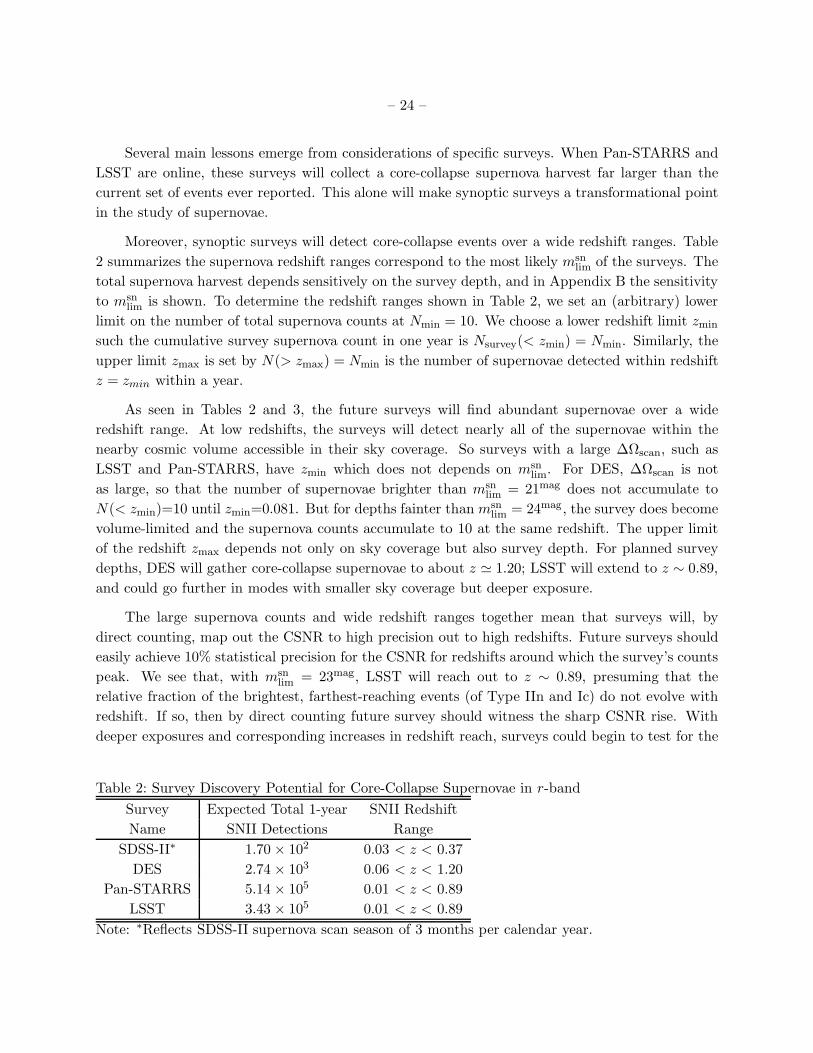
Table 2: Survey Discovery Potential for Core-Collapse Supernovae in r-band

Survey Expected Total 1-year SNII Redshift

Name SNII Detections Range

SDSS-II∗ 1.70 × 102 0.03 < z < 0.37

DES 2.74 × 103 0.06 < z < 1.20

Pan-STARRS 5.14 × 105 0.01 < z < 0.89

LSST 3.43 × 105 0.01 < z < 0.89

Note: ∗Reflects SDSS-II supernova scan season of 3 months per calendar year.

– 25 –

behavior of the CSNR above z = 1, a regime that is currently poorly understood.

Both the survey yields of supernova discoveries, as well as their redshift ranges, are strong

functions of survey depth. As shown in Table 3 of Appendix B, each magnitude increase in survey

depth yields a large enhancement (a factor ∼ 3) in total supernova counts. This in turn leads to

large enhancements in redshift range, and thus in the range over which the CSNR is measured. As

shown in Appendix B, increased monitoring time needed to achieve higher msnlim will come at some

cost, though this will be partially offset by the higher supernova yield in a deeper exposure. Finally,

for the large population of low-redshift supernovae, deeper surveys will lead to better lightcurve

determination, allow for a more accurate photometry over a larger brightness range and thus longer

timescales.

As noted in §3.3.1, our fiducial results are for supernova peak magnitudes whose luminosity

functions (each of which is one or two gaussians for each core-collapse type) are nonzero only

within |M − Mmean| < 2.5σ away from the mean. This arbitrary cutoff is meant as a compromise

which shows the effect of nonzero width of the luminosity functions, without extrapolating too

far into the tails in which there is as yet no data. To give a feel for the sensitivity of our results

to the assumed luminosity function width we repeated our analysis for luminosity functions with

larger and narrower |M − Mmean| ranges, (but with fixed observed intrinsic σ). We find that

the total supernova counts vary less than 0.88% when |M − Mmean| ranges from 2σ to 3σ; this

insensitivity reflects the fact that the bulk of supernova counts are from events near the means of

the distribution. One the other hand, we found that the maximum observed supernova redshift (and

thus the depth to which one can probe the CSNR) is very sensitive to the choice of |M − Mmean|.

For example, the LSST maximum supernova redshift in 1 year is zsn,max = 0.89 for our fiducial

choice of |M −Mmean| = 2.5σ, as seen in Table 2. On the other hand for |M −Mmean| = 2σ and 3σ,

we find zsn,max = 0.73 and 1.06, respectively. Here rare, intrinsically bright events determine the

redshift reach, and the deeper the luminosity function reaches into the bright-end tail, the larger

the resulting zsn,max. Thus we would expect the intrinsically brightest events, of Type Ibc and

Type IIn, to give the greatest redshift reach. Indeed, Cooke (2008) has recently illustrated how

Type IIn events can be mapped out to z > 2 by ground-based 8 meter-class telescopes.

Of course, all of our forecasts assume that the luminosity functions of each supernova type,

and the relative frequencies among the supernova types, all remain unchanged at earlier epochs.

However, it is entirely plausible and even likely that these properties could evolve, e.g., with metal-

licity and/or environment. These effects are likely to be crucial in determining the true redshift

reach of future sky surveys, and thus predictions such as ours will improve only as real supernova

data becomes available with good statistics at ever-increasing redshifts, and one can directly con-

strain and/or measure evolutionary effects. Moreover, the relatively small sample sizes available

to Richardson et al. (2002) could well lead to underestimates of the true range of luminosities of

each type. For example, (Gezari et al. 2008) very recently report of an unusually bright Type II-L

event, SN 2008es, with peak magnitude MB ≃ −22.2, far outside of the absolute magnitude range

we have adopted for this subtype.

– 26 –

Indeed, the enormous statistics gathered by future surveys will allow for cross-checks and

empirical determination of other evolutionary and systematic effects. A major such effect is dust

obscuration, to which we now turn.

5. Dust Obscuration: Disentangling the Degeneracies and Probing High-Redshift

Star-Forming Environments

The loss of some supernovae due to dust obscuration must be understood accurately and

quantitatively in order to take full advantage of the large data samples of supernovae which are

detected. As noted above in §3.2, currently we have very limited knowledge of supenova extinction

and particularly its evolution, and most of what is reliably known is based on empirical studies

of supernova counts. Precisely for this reason, future surveys offer an opportunity to address this

problem in great detail by leveraging the enormous numbers of supernovae of all types, seen over

a wide range of redshifts and in a wide range of environments. Here we sketch a procedure for

recovering this information.

Future surveys will produce well-populated distributions of supernovae; these encode informa-

tion about extinction and reddening due to dust. Specifically, in redshift bin ∆z around z one can

measure, often with very high statistical accuracy, the apparent magnitude distribution for each

subtype of core-collapse events. These distributions can be made for all bands, but as we have

shown, detections and/or light curve information will be most numerous in r and g bands; we will

focus on these for the purposes of discussion. Within a redshift bin, the distance modulus µ is

fixed, and the light curve and associated K-correction should reflect intrinsic variations within the

core-collapse subtype.

Thus, for a given core-collapse subtype and redshift z, one can construct histograms of r and

g peak magnitudes. From redshift and supernova type, one can compute the distance modulus and

K-correction, and use these to infer, for each event, the dust-obscured peak magnitude Mdust ≡

mobs −µ(z)−K(z) = Mpeak + A where Mpeak is the intrinsic peak magnitude for the event, and A

is the extinction for this event in its host galaxy. By comparing two passbands we can also evaluate

colors, for example g − r = Mg,peak − Mr,peak + E(g − r), where E(g − r) is the reddening. In

general, within a redshift bin we expect the A and E to vary on an event-by-event basis, reflecting

the properties of dust along the particular line of sight through the particular host galaxy.

Invaluable insight into these issues comes from the Hatano et al. (1998) analysis of extinction

in observation of local supernovae. These authors argue that the data are consistent with very

strong dependence of extinction with the inclination of the host galaxy; this alone guarantees that

A must vary strongly from event to event even within subtypes. Hatano et al. (1998) also argue

that the variation of dust column with galactic radius also suggests that extinction is responsible

for the paucity of supernovae at small radii. (Shaw 1979). Finally, Hatano et al. (1998) also point

out that core-collapse events are more extincted than Type Ia events because the Ia’s have a higher

– 27 –

scale height and thus are more likely to occur in less extincted regions.

On an event-by-event basis, intrinsic light curve and color evolution are degenerate with dust

evolution. However, the large sample size may allow for a physically motivated empirical approach

to lifting this degeneracy. If on theoretical grounds we can assume that at least one core-collapse

subtype has negligible intrinsic evolution in its lightcurve, then for that subtype M and K are

effectively known and moreover are constant across events in a particular redshift bin. In this

case, the apparent magnitude and color distributions can be directly translated into distributions

of extinction and reddening. By comparing these distributions (or e.g., their means and variances)

across different redshifts, one directly probes dust evolution.

Moreover, if one can use one core-collapse subtype as an approximate “standard distribution”

from which to extract dust properties, one might press further by assuming that other core-collapse

events will be born in similar environments and thus encounter similar extinction and reddening.

One can thus use the empirically determined dust evolution to statistically infer the degree of

intrinsic lightcurve variation in the other core-collapse subtypes.

If subtype can be firmly established, comparison of magnitude distributions of different core-

collapse subtypes allows for a purely empirical approach. namely, one can compare the evolution

of the magnitudes distributions of different subtypes. One could first provisionally treat each

supernova subtype as a “standard distribution” with no intrinsic evolution; then for each subtype

one would infer dust extinction and reddening at each redshift. It is reasonable to expect that

the different subtypes sample the same dust properties, as long as the host environments are

not systematically different for the different subtypes (all of which arise in massive-star-forming

environments). Indeed, Nugent et al. (2006) have performed such an analysis to use V − I colors

of Type II-P events to infer reddening for events out to z ∼ 0.3.

A comparison of the dust extinction inferred the different subtypes amounts to a test for

intrinsic variation. With information from multiple subtypes, it may be possible to isolate dust

effects common to all, and intrinsic variation peculiar to each subtype. For example, if one subtype

distribution evolves significantly more than another (e.g., one subtype variance grows more than

another) then the difference in variance must be intrinsic, and that the lesser variance is an upper

limit to the variance due to dust effects.

The ability to empirically measure extinction depends on the intrinsic width of the A(z) dis-

tribution, and on surveys’ ability to probe this distribution. At low redshift, Hatano et al. (1998)

find a wide (> 1mag) range of extinctions, much of which they attribute to inclination which will

remain an issue at higher redshift. On the other hand, as a given survey pushes to higher redshift,

progressively less of the distribution is observable. For the case of LSST, we see in Fig. 10 that

with msnlim = 23mag the least obscured events are visible out to redshift z ∼ 1, while those which

have suffered Ar = 1mag of extinction would correspond to the msnlim = 22mag curves, which reach

to about z ∼ 0.5. Thus over this shallower redshift range, extinction can be probed in detail, but

with a narrowing observable range at higher redshift.

– 28 –

If future surveys can empirically determine effects of dust evolution, this would not only remove

a major “nuisance parameter” for supernova and cosmology science, but also gain information

of intrinsic interest. Namely, we will learn about the cosmic distribution and evolution of host

environments of supernovae and thus of star formation.

6. Discussion

The large amount of core-collapse supernovae observed by synoptic surveys will yield a wealth

of data and enormous science returns. Here we sketch some of these.

6.1. Survey Impact on the Cosmic Supernova and Star Formation Histories

As we have indicated in the previous section, synoptic surveys will determine cosmic core-

collapse supernova rate with high precision out to high redshifts. Moreover, with the large number

of supernova counts, and with light curves and host environments known, the total cosmic core-

collapse redshift history can be subdivided according to environment and/or supernova type. For

example, with photometric data alone one can determine to high accuracy correlations between

supernova rate and host galaxy luminosity and Hubble type. One can compare supernova rates

in field galaxies versus those in galaxy groups and clusters. Using galaxy morphology one can

investigate correlations between supernovae and galaxy mergers. With the addition of spectroscopic

information one can also search for correlations with host galaxy metallicity.

The CSNR is also tightly related to the cosmic star-formation rate. Therefore with the high

precision CSNR, and assuming an unchanging initial mass function, one can make a similarly precise

measure of the cosmic star-formation rate. On the other hand, one can test for environmental

and/or redshift variations in the initial mass function, by comparing the supernova rates based on

direct survey counts with the star-formation rates determined via UV and other proxies.

In addition to core-collapse explosions, synoptic surveys will of course by design also discover

a similarly huge number of Type Ia supernovae. Thus the Type Ia supernova rates can be com-

pared to those for core collapse events. As has been widely noted (e.g., Gal-Yam & Maoz 2004;

Watanabe et al. 1999; Oda & Totani 2005; Scannapieco & Bildsten 2005, and references therein)

this will yield information about the distribution of time delays between the core-collapse and ther-

monuclear events. Moreover, one can explore differences in the environmental correlations for the

two supernova types (and subtypes).

– 29 –

6.2. Survey Supernovae as Distance Indicators: the Expanding Photosphere

Method

Type Ia supernovae have become the premier tool for distance determinations at cosmological

scales, thanks to their regular light curves, high peak brightnesses, and relatively less dusty environ-

ments. Nevertheless, given the importance of the cosmic distance scale, and the ongoing need for

systematic crosschecks and calibration, it is worthwhile to consider other methods. Core-collapse

events offer just such a method, via the expanding photosphere/expanding atmosphere method.

This method was originally conceived by Baade (1926) and Wesselink (1946) for study of

Cephieds; Kirshner & Kwan (1974) applied the Baade-Wesselink method to supernovae. The key

to the technique is to exploit the simple kinematics of a newborn supernova remnant: the freely-

expanding photosphere grows in size as R = vt. Thus, for purely blackbody emission, the luminosity

grows with size (i.e., time) as L = 4πR2σT 4. With good sampling to measurements time t since

explosion, and spectroscopic inference of v and T , one can recover the luminosity. In principle,

therefore, one can use the explosion as a standard candle.

In practice, this method has been slow to mature. Until recently, the agreement with inde-

pendent distance measures has been only good to within a factor ∼ 2 (e.g., Vinko & Takats 2007).

The complex (out of local thermodynamic equilibrium) spectra of supernovae has proved difficult to

adequately model. However, recently important advances have been made in the radiation transfer

modeling of young supernova remnants and its fitting to spectra of local supernovae (Baron et al.

2004; Dessart & Hillier 2005, 2008). Because of this, the expanding photosphere (or more prop-

erly, expanding atmosphere) method now appears to be reaching consistency with other distance

measures; this method now shows agreement approaching the ∼ 10% level. Similar pecision now

seems possiblue using a separate, empirical method (Hamuy & Pinto 2002) which exploits the ob-

served correlation between luminosity and expansion velocity of Type II-P events. This opens up

core-collapse supernovae as alternative distance indicators. Indeed, several group (Nugent et al.

2006; Poznanski et al. 2007; Olivares 2008) have already applied this method to various collections

of Type II-P observations, yielding tight Hubble diagrams out to z ∼ 0.3.

To use this method as it is currently envisioned, follow-up spectroscopy is mandatory for each

event (see §6.5), with photometric surveys identifying the candidates. Obviously, for the largest

surveys, in practice only a tiny fraction of core-collapse events could be studied in a (separate)

spectroscopic campaign, particularly given that the most common core-collapse types are intrinsi-

cally dimmer than Type Ia events and thus require longer exposures to obtain spectra. Followup

requirements thus are the limiting factor for the use of core-collapse events as distance indicators.

The situation for Type Ia supernovae is better-studied and also potentially more hopeful.

Recent work (Poznanski et al. 2007; Kim & Miquel 2007; Kunz et al. 2006; Blondin & Tonry 2007;

Wang 2007; Kuznetsova et al. 2008; Sako et al. 2008) suggests that photometric redshifts of Type Ia

events near maximum light could be obtained with sufficient precision (give a low-redshift training

set) to provide useful dark energy constraints without spectroscopy. Whether photometric-based

– 30 –

distances can be derived for core-collapse events with sufficient accuracy remains to be seen. It

nevertheless seems to us a worthy object of further study. In this context it is worth noting that DES

plans to do followup spectroscopy on ∼ 25% of Type Ia events (The Dark Energy Survey Collaboration

2005). We suggest that at least some modest fraction of this follow-up time be dedicated to core-

collapse monitoring.

6.3. Other Science with Cosmic Supernovae

The physics, astrophysics, and cosmology of cosmic core-collapse supernovae is a fertile topic;

with our detectability study in hand, a wide variety of problems present themselves. Here we sketch

these out; we intend to return to these in future publications.

The huge harvest of core-collapse events will open new windows onto other aspects of supernova

physics. For example, the physics of black hole formation in supernovae, and the neutron-star/black

hole divide, remain important open questions. Balberg & Shapiro (2001) have estimated the rates

of events with observable signatures of black hole formation; LSST should provide a fertile testing

ground for these predictions.

The elaboration of the cosmic history and specific sites of high-redshift supernovae will also

offer unique new information about supernova “ecology” – i.e., feedback and cycling of energy, mass,

and metals into the surrounding environment. For example, large surveys will offer the opportunity

to study supernova rates as a function of host galaxy and galaxy clustering, shedding new light

onto large-scale star formation and its connection with galaxy evolution. Moreover, DES and other

surveys will discover an enormous number of rich galaxy clusters; the occurrence of both Type Ia

and core-collapse events in clusters will offer important new insight into the origin of the very high

metallicity of intracluster gas (Maoz & Gal-Yam 2004; Maoz et al. 2005).

Core-collapse supernovae also are the sources, directly or indirectly, of high-energy radiation

of various kinds. For example, supernovae act as accelerators of cosmic rays. These in turn

interact with interstellar matter to produce high-energy γ-rays. Pavlidou & Fields (2002) used

then-available estimates of the cosmic star-formation rate to show that this γ-ray signal has a

characteristic feature, and makes a significant part of the extragalactic γ-ray background around ∼ 1

GeV. With the successful launch of the high-energy γ-ray observatory GLAST, this component of

the γ-ray background may for the first time be clearly identified. Regardlessly, a sharper knowledge

of the cosmic supernova rate (and thus cosmic-ray injection rate) will work in concert with GLAST

observations to probe the history of cosmic rays throughout the universe.

– 31 –

6.4. Comparison with Type Ia Survey Requirements

The characteristic of Type Ia supernovae are in general very similar to the core-collapse su-

pernovae. Hence the observational requirements for their identification in synoptic surveys are also

very similar. The rest-frame, full-width at half-maximum timescale for Type Ia supernovae is ∼ 20

days. Therefore surveys will need a scan cadence of a few days in order to get a well-sampled light

curve. For example, the Pan-STARRS strategy for Type Ia discovery is to sample the light curve

every 4 days (Tonry et al. 2003; Tonry 2003). As we have discussed, this sampling frequency is

also suitable for the core-collapse supernovae which the time scale of the light curve also last a few

weeks.

6.5. Redshifts and Typing from Photometry and Followup Spectroscopy

Survey supernovae become scientifically useful only when one can establish, at the very least,

their redshift and whether they are core collapse or Type Ia. Since followup spectroscopy will

not be possible for the large numbers of future events, photometric redshifts will be needed. For

events in which a host galaxy is clearly visible, one can use photometric redshifts of the hosts.

Here one is helped by the ability of surveys to stack all of the many (non-supernova) exposures to

obtain a much deeper image than those with the supernovae. Once the host redshift is know, the

supernova type must be determined. Baysean analysis techniques and software (Dahlen & Goobar

2002; Poznanski et al. 2007) have been developed to distinguish both Type Ia and core-collapse

events. These authors find that type discrimination depends crucially on the accuracy with which

the redshift is known. For spectroscopic redshifts, their methods is extremely accurate, and for

photometric redshifts the method is still quite good, though in this case misclassifications can reach

15 − 25% depending on σphoto−z.

Followup spectroscopy on a subset of events will be essential to calibrate the accuracy of the

photometric typing (and host redshifts). In particular, spectroscopy will be invaluable in identifying

and quantifying catastrophic failures in the typing algorithms; on the basis of these it may be

possible to refine the routines. As noted in the previous section, followup is also required for any

events one hopes to use in distance determinations.

For events without clear host galaxies and without followup, one must resort to photometric

redshifts and typing based on the supernova light curve itself, in whatever bands are available. It is

not clear that this can be done with any reliability on an event-by-event basis As Poznanski et al.

(2007) emphasize, one might make statistical statements about the types and redshifts of the entire

class of “hostless” events. Here spectroscopic followup will be essential, not only for determining

the supernova redshift but also the nature of the underlying host.

– 32 –

7. Conclusions and Recommendations for Synopic Surveys

The next ten years will witness a revolution in our observational knowledge of core-collapse

supernovae. Synoptic sky surveys will reap an enormous harvest of these events, with tens of

thousands discovered in the near future, culminating with of order 100,000 seen annually by LSST.

These data will reveal the supernova distribution in space and time over much of cosmic history.

The needed observations are naturally a part of the scanning nature of these surveys, and require

only that core-collapse events be included in the data analysis pipeline.

The potential science impact of this unprecedented supernova sample is enormous. We have

discussed ways in which the photometric supernova data alone will contribute in significant and

unique ways to cosmology and astroparticle physics, as well as to studies of core-collapse and

supernova evolution themselves. We illustrate one such application by demonstrating how to recover

the cosmic supernova rate from the redshift distribution of supernova counts in synoptic surveys.

The large datasets ensure that the statistical error will be very low, and the first large surveys will

rapidly determine the CSNR to precision exceeding that of current data based on observation of

massive-star proxies.

With the addition of spectroscopic followup observations, the survey-identified core-collapse

supernovae can be used as distance indicators. Thanks to recent advances in the phenomenology

of supernova spectra and the modelling of their expanding atmospheres, the early light curves

provide standardizable candles. This expanding photosphere/atmosphere method could provide a

cross-check for the cosmic distance scale as inferred from Type Ia supernovae.

To summarize our recommendations for synoptic surveys, in order to capitalize on this poten-

tial:

1. Include core-collapse supernovae (all Type II as well as Types Ib and Ic) in the data analysis

pipeline.

2. Include a scanning mode in which the depth msnlim is as large as possible, in order to maximize

the supenova redshift range. Surveys which modes which probe down to msnlim = 26mag could

discover many supernovae (both core-collapse and Type Ia) approaching redshift z ∼ 2.

3. Adopt scanning cadence of revisits every ∼ 4 days, in order to capture core-collapse events

at peak brightness, and to obtain a well-sampled lightcurve. This timescale also appropriate

for Type Ia events.

4. Allocate some followup spectroscopy to core-collapse events. This will calibrate photometric

Type Ia/core-collapse typing and typing among core-collapse subtypes, and will be particu-

larly crucial for probing the nature of events in which a host galaxy is not seen.

We close by re-emphasizing that these recommendations require only modest efforts in anal-

ysis, little to no modification of the strategies already in place for Type Ia searches, and some

– 33 –

commitment of followup spectroscopy. Thus a small extra investment of resources will reap hand-

some scientific rewards as we open our eyes to the incessant rise and fall of these beacons marking

massive star death throughout the cosmos.

It is a pleasure to thank Joe Mohr, Vasiliki Pavlidou, Tijana Prodanovic, Jon Thaler, Yun

Wang, David Weinberg, and Michael Wood-Vasey for valuable discussions. We are particularly

indebtted to Josh Frieman, Avishay Gal-Yam, John Beacom, and David Branch for detailed con-

structive feedback on an earlier draft, which has greatly improved this paper.

Note: In the final stages of writing this paper we became aware of the work of Young et al.

(2008). These authors discuss core collapse rates in sky surveys, with a focus on events in low-

metallicity environments. Where it is possible to compare and when we adopt their parameters

(particularly msnlim), our analyses seem to be in broad agreement.

A. Appendix: The Supernova/Star-Formation Connection

The star-formation rate and supernova rate for any astrophysical site are intimately related.

Moreover, in many applications such as ours the timescales of interest are much longer than the

∼ few Myr supernova progenitor lifetimes. In this case, the star-formation rate and supernova

rates are proportional. This is expressed above in eq. (2). The constant of proportionality can be

obtained from the initial mass function ξ(m). In stellar mass range (m,m + dm) the number of

new stars is proportional to ξ(m) dm, while the mass of new stars is m ξ(m) dm. Thus the number

of supernovae per unit new star mass–i.e., the conversion between star-formation and supernova

rates–isRSN

ρ⋆=

∫

SN ξ(m) dm∫

m ξ(m) dm=

∫

SN ξ(m) dm∫

SN m ξ(m) dm

∫

SN m ξ(m) dm∫

m ξ(m) dm=

XSN

〈m〉SN(A1)

where XSN =∫

SN m ξ dm/∫

m ξ dm is the mass fraction of new stars that will go into supernovae,

and 〈m〉SN =∫

SN m ξ(m) dm/∫

SN ξ(m) dm is the mean supernova progenitor mass. For illustration,

consider a Salpeter IMF ξ(m) ∝ m−2.35 over mass range (0.5M⊙, 100M⊙) and ξ(m) ∝ m−1.5 for the

low mass range (0.1M⊙, 0.5M⊙) (Baldry & Glazebrook 2003, their “Salpeter A” mass function). We

also take supernova progenitors to lie in the mass range mSN ∈ (8M⊙, 50M⊙). This gives XSN =

0.15,〈m〉SN ≈ 15.95M⊙, and thus a star-formation/supernova conversion factor XSN/〈m〉SN =

0.00914M−1⊙

. The uncertainty here is significant, probably about a factor of 2.

The cosmic star-formation rate can be estimated from a number of observables tied to massive

(i.e., short-lived thus “instantaneous”) star-formation. Proxies often adopted are the UV and/or

Hα luminosity densities (Madau et al. 1996). Of these, UV light has a more direct connection with

massive stars, but is also affected more by the dust extinction than the Hα light (Strigari et al.

2005). Most cosmic star-formation studies find a sharp increase in the rate up to z = 1, but there

– 34 –

remains a large uncertainty of the star formation rate at higher redshift. In this paper, we adopt

the Cole et al. (2001) fitting formula for the cosmic star-formation rate

ρcole⋆ =

a + bz

1 + (z/c)dhM⊙ yr−1 Mpc−3 (A2)

where(a, b, c, d) = (0.017, 0.13, 3.3, 5.3), which are one of the best-fitted parameters according

to current observing data found by Hopkins & Beacom (2006). Using the conversion factor of

Hopkins & Beacom (2006) and our adopted Hubble constant, this gives a local rate of RSN(0) =

1.1× 10−4 SNII Mpc−3 yr−1. The benchmark CC SNe rate rises to a peak around z = 2.5 and then

slowly declines at high redshift.

To illustrate the impact of different star formation, we also did all calculations with an alter-

native CSNR. Here we normalize to the current observed, counting-based CSNR (Botticella et al.

2008), and take the shape from the a fitting function of the Hippelein et al. (2003) star formation

rate. We also lower the rate by 30% because we want the alternative CSNR to be as much different

as the benchmark CSNR as possible and Hopkins & Beacom (2006) suggested that the uncertainty

of the normalization of the star formation rate is about 30%. The differences between this and our

fiducial rate gives a sense of the current rough but not perfect agreement between the CSNR as

inferred indirectly from progenitor light (sometimes reprocessed) and directly from counting.

B. Appendix: Supernova Predictions for Upcoming Synoptic Surveys

Table 3: Sensitivity to survey depth in r band, for fixed sky coverage.

msnlim DES Pan-STARRS LSST

[mag] Total SNe Redshifts Total SNe Redshifts Total SNe Redshifts

21 4.32 × 101 0.081 < z < 0.18 3.24 × 104 0.007 < z < 0.36 2.16 × 104 0.008 < z < 0.36

22 1.86 × 102 0.066 < z < 0.38 1.40 × 105 0.007 < z < 0.56 9.32 × 104 0.008 < z < 0.56

23 6.86 × 102 0.064 < z < 0.66 5.14 × 105 0.007 < z < 0.89 3.43 × 105 0.008 < z < 0.89

24 2.19 × 103 0.063 < z < 1.10 1.64 × 106 0.007 < z < 1.34 1.10 × 106 0.008 < z < 1.33

25 6.32 × 103 0.063 < z < 1.62 4.74 × 106 0.007 < z < 1.88 3.16 × 106 0.008 < z < 1.88

26 1.55 × 104 0.063 < z < 2.17 1.16 × 107 0.007 < z < 2.48 7.73 × 106 0.008 < z < 2.47

27 3.17 × 104 0.063 < z < 2.68 2.38 × 107 0.007 < z < 3.08 1.58 × 107 0.008 < z < 3.08

Figures 7–10 show the supernova forecasts for different surveys. For each we show the expected

annual supernova harvest ∆Nobs(z) as a function of redshift, with the sky coverage held fixed to

the values in Table 1. The count distribution across redshift bins are directly proportional to the

differential supernova rate distribution ΓSN,obs(z), via eq. (18). Thus the shapes the curves follow

those of ΓSN,obs(z) as seen in Figure 4 an explained in the accompanying discussion.

Figures 7–10 also show the survey scan time required for these data to constrain the cosmic star-

formation rate in each redshift bin to within a statistical precision σ(RSN)/RSN = 10%. We have

– 35 –

seen (eq. 20) that the precision at each bin is inverse with the counts, σ(RSN)/RSN = 1/√

∆Nobs(z).

Thus these panels show trends in which monitoring time decreases with the counts per bin. This

mirrors the behavior shown in Figure 6 and explained in the surrounding discussion.

Table 3 shows the effect of survey limiting magnitude on redshift range and total supernova

harvest in the r-band. We see that each unit increase ∆msnlim = 1mag in survey depth yields a large

enhancement, in the total supernovae seen. The supernova numbers increase by a factor 4.3 when

going from msnlim = 21mag to 22mag to factor of 2.0 when going from 26mag to 27mag. Of course, there

is a tradeoff in the needed exposure. For the faintest objects at the highest redshifts, background

noise dominates, and monitoring time grows by a factor (102/5)2 ∼ 6.3 per magnitude. Thus,

including a narrower but deeper survey mode will likely yield fewer supernovae, but if judiciously

implemented, this tradeoff may be worth the additional redshift coverage.

Fig. 7.— Sloan Digital Sky Survey (SDSS-II). All the results plotted here are using the benchmark

CSNR. Top panel: The number of supernovae observed in one scan season of 3 months per year, in

redshift bins of with ∆z = 0.1. Results are shown for a fixed scan sky coverage ∆Ωscan = 300 deg2,

and the survey depth as labeled. Bottem panel: The monitoring time ∆t needed in order to

determine the cosmic supernova rate to a 10% precision.

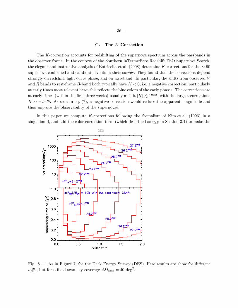
– 36 –

C. The K-Correction

The K-correction accounts for redshifting of the supernova spectrum across the passbands in

the observer frame. In the context of the Southern inTermediate Redshift ESO Supernova Search,

the elegant and instructive analysis of Botticella et al. (2008) determine K-corrections for the ∼ 90

supernova confirmed and candidate events in their survey. They found that the corrections depend

strongly on redshift, light curve phase, and on waveband. In particular, the shifts from observed V

and R bands to rest-frame B-band both typically have K < 0, i.e, a negative correction, particularly

at early times most relevant here; this reflects the blue colors of the early phases. The corrections are

at early times (within the first three weeks) usually a shift |K| <∼ 1mag, with the largest corrections

K ∼ −2mag. As seen in eq. (7), a negative correction would reduce the apparent magnitude and

thus improve the observability of the supernovae.

In this paper we compute K-corrections following the formalism of Kim et al. (1996) in a

single band, and add the color correction term (which described as ηxB in Section 3.4) to make the

Fig. 8.— As in Figure 7, for the Dark Energy Survey (DES). Here results are show for different

msnlim, but for a fixed scan sky coverage ∆Ωscan = 40 deg2.

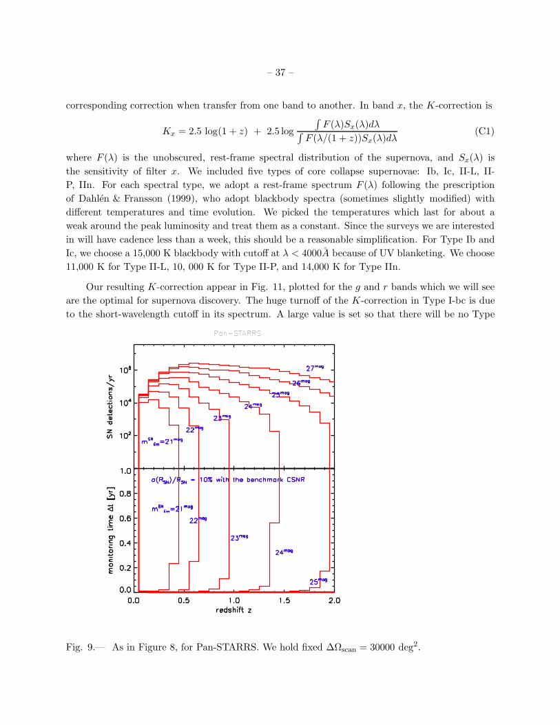
– 37 –

corresponding correction when transfer from one band to another. In band x, the K-correction is

Kx = 2.5 log(1 + z) + 2.5 log

∫

F (λ)Sx(λ)dλ∫

F (λ/(1 + z))Sx(λ)dλ(C1)

where F (λ) is the unobscured, rest-frame spectral distribution of the supernova, and Sx(λ) is

the sensitivity of filter x. We included five types of core collapse supernovae: Ib, Ic, II-L, II-

P, IIn. For each spectral type, we adopt a rest-frame spectrum F (λ) following the prescription

of Dahlen & Fransson (1999), who adopt blackbody spectra (sometimes slightly modified) with

different temperatures and time evolution. We picked the temperatures which last for about a

weak around the peak luminosity and treat them as a constant. Since the surveys we are interested

in will have cadence less than a week, this should be a reasonable simplification. For Type Ib and

Ic, we choose a 15,000 K blackbody with cutoff at λ < 4000A because of UV blanketing. We choose

11,000 K for Type II-L, 10, 000 K for Type II-P, and 14,000 K for Type IIn.

Our resulting K-correction appear in Fig. 11, plotted for the g and r bands which we will see

are the optimal for supernova discovery. The huge turnoff of the K-correction in Type I-bc is due

to the short-wavelength cutoff in its spectrum. A large value is set so that there will be no Type

Fig. 9.— As in Figure 8, for Pan-STARRS. We hold fixed ∆Ωscan = 30000 deg2.

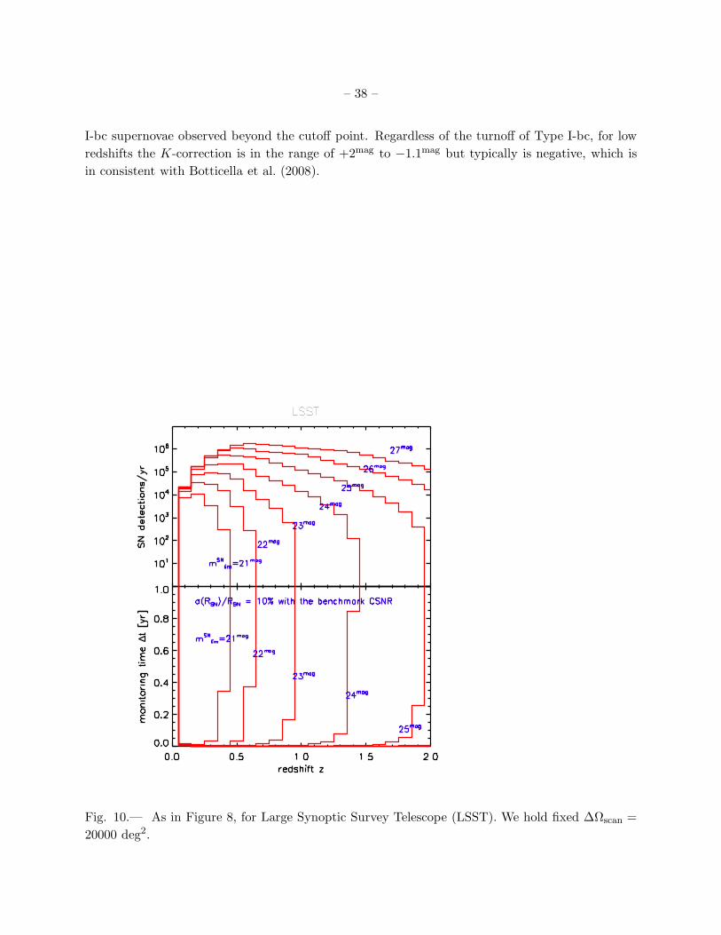
– 38 –

I-bc supernovae observed beyond the cutoff point. Regardless of the turnoff of Type I-bc, for low

redshifts the K-correction is in the range of +2mag to −1.1mag but typically is negative, which is

in consistent with Botticella et al. (2008).

Fig. 10.— As in Figure 8, for Large Synoptic Survey Telescope (LSST). We hold fixed ∆Ωscan =

20000 deg2.

– 39 –

Fig. 11.— K-correction of the four types of supernovae(I-bc,II-L,II-P,II-N) in g and r bands (green

lines for g-band and red lines for r-band). The sharp upturn in the Ibc correction reflects a cutoff

in the supernova spectrum due to UV line blanketing; see discussion in text.

REFERENCES

Adelberger, K. L., & Steidel, C. C. 2000, ApJ, 544, 218

Astier, P., et al. 2006, A&A, 447, 31

Baade, W. 1926, Astronomische Nachrichten, 228, 359

Balberg, S., & Shapiro, S. L. 2001, ApJ, 556, 944

Baldry, I. K., & Glazebrook, K. 2003, ApJ, 593, 258

Baron, E., Nugent, P. E., Branch, D., & Hauschildt, P. H. 2004, ApJ, 616, L91

Blondin, S., & Tonry, J. L. 2007, ApJ, 666, 1024

Botticella, M. T., et al. 2008, A&A, 479, 49

– 40 –

Cappellaro, E., Turatto, M., Tsvetkov, D. Y., Bartunov, O. S., Pollas, C., Evans, R., & Hamuy,

M. 1997, A&A, 322, 431

Central Bureau for Astronomical Telegrams http://www.cfa.harvard.edu/iau/cbat.html

Chen, H.-W., Prochaska, J. X., & Gnedin, N. Y. 2007, ApJ, 667, L125

Choi, P. I., et al. 2006, ApJ, 637, 227

Cole, S., et al. 2001, MNRAS, 326, 255

Cooke, J. 2008, ApJ, 677, 137

The Dark Energy Survey Collaboration 2005, ArXiv e-prints, arXiv:astro-ph/0510346

Dahlen, T., & Fransson, C. 1999, A&A, 350, 349

Dahlen, T., & Goobar, A. 2002, PASP, 114, 284

Dessart, L., & Hillier, D. J. 2005, A&A, 439, 671

Dessart, L., & Hillier, D. J. 2008, MNRAS, 383, 57

Dessart, L., et al. 2008, ApJ, 675, 644

Doggett, J. B., & Branch, D. 1985, AJ, 90, 2303

Frieman, J. A., et al. 2008, AJ, 135, 338

Fukugita, M., Ichikawa, T., Gunn, J. E., Doi, M., Shimasaku, K., & Schneider, D. P. 1996, AJ,

111, 1748

Gal-Yam, A., & Maoz, D. 2004, MNRAS, 347, 942

Gal-Yam, A., Maoz, D., & Sharon, K. 2002, A New Era in Cosmology, 283, 289

Gezari, S., et al. 2008, arXiv:0808.2812

Gnedin, N. Y., Kravtsov, A. V., & Chen, H.-W. 2008, ApJ, 672, 765

Hamuy, M., & Pinto, P. A. 2002, ApJ, 566, L63

Hatano, K., Branch, D., & Deaton, J. 1998, ApJ, 502, 177

Hippelein, H., et al. 2003, A&A, 402, 65

Hopkins, A. M., & Beacom, J. F. 2006, ApJ, 651, 142

Hughes, D. H., et al. 1998, Nature, 394, 24

– 41 –

Jewitt, D. 2003, Pan-STARRS Science Goals: Science Overview, URL

http://pan-starrs.ifa.hawaii.edu/project/science/precodr.html

Kim, A., Goobar, A., & Perlmutter, S. 1996, PASP, 108, 190

Kim, S. S., & Lee, M. G. 2007, PASP, 119, 1449

Kim, A. G., & Miquel, R. 2007, Astroparticle Physics, 28, 448

Kirshner, R. P., & Kwan, J. 1974, ApJ, 193, 27

Kuznetsova, N., et al. 2008, ApJ, 673, 981

Kunz, M., Bassett, B. A., & Hlozek, R. 2006, ArXiv e-prints, arXiv:astro-ph/0611004

Le Floc’h, E., et al. 2005, ApJ, 632, 169

Leibundgut, B., & Suntzeff, N. B. 2003, Supernovae and Gamma-Ray Bursters, 598, 77

The Large Synoptic Survey Telescope Collaboration 2007, Science Requirements Document

http://www.lsst.org/Science/docs/SRD.pdf

Madau, P., Ferguson, H. C., Dickinson, M. E., Giavalisco, M., Steidel, C. C., & Fruchter, A. 1996,

MNRAS, 283, 1388

Madau, P., della Valle, M., & Panagia, N. 1998, MNRAS, 297, L17

Mannucci, F., Della Valle, M., & Panagia, N. 2007, MNRAS, 377, 1229

Maoz, D., & Gal-Yam, A. 2004, MNRAS, 347, 951

Maoz, D., Waxman, E., & Loeb, A. 2005, ApJ, 632, 847

Modjaz, M., et al. 2008, ArXiv e-prints, 805, arXiv:0805.2201

Nugent, P., et al. 2006, ApJ, 645, 841

Oda, T., & Totani, T. 2005, ApJ, 630, 59

Olivares, F. 2008, arXiv:0810.5518

Pastorello, A., et al. 2006, MNRAS, 370, 1752

Patat, F., Barbon, R., Cappellaro, E., & Turatto, M. 1993, A&AS, 98, 443

Patat, F., Barbon, R., Cappellaro, E., & Turatto, M. 1994, A&A, 282, 731

Pavlidou, V., & Fields, B. D. 2002, ApJL, 575, L5

– 42 –

Perez-Gonzalez, P. G., Zamorano, J., Gallego, J., Aragon-Salamanca, A., & Gil de Paz, A. 2003,

ApJ, 591, 827

Perlmutter, S., et al. 1999, ApJ, 517, 565

Phillips, M. M. 1993, ApJ, 413, L105

Poznanski, D., Maoz, D., & Gal-Yam, A. 2007, AJ, 134, 1285

Richardson, D., Branch, D., Casebeer, D., Millard, J., Thomas, R. C., & Baron, E. 2002, AJ, 123,

745

Riess, A. G., Press, W. H., & Kirshner, R. P. 1996, ApJ, 473, 88

Riess, A. G., et al. 1998, AJ, 116, 1009

Sako, M., et al. 2008, AJ, 135, 348

Scannapieco, E., & Bildsten, L. 2005, ApJ, 629, L85

Scannapieco, E., Madau, P., Woosley, S., Heger, A., & Ferrara, A. 2005, ApJ, 633, 1031

Shaw, R. L. 1979, A&A, 76, 188

Smail, I., Ivison, R. J., & Blain, A. W. 1997, ApJ, 490, L5

Spergel, D. N., et al. 2007, ApJS, 170, 377

Strigari, L. E., Beacom, J. F., Walker, T. P., & Zhang, P. 2005, Journal of Cosmology and Astro-

Particle Physics, 4, 17

Sullivan, M., Ellis, R., Nugent, P., Smail, I., & Madau, P. 2000, MNRAS, 319, 549

Suntzeff, N. B., Smith, R. C.,Hamuy, M., Phillips, M. M., & Tyson, T. 2004, Bulletin of the

American Astronomical Society, 36, 1530

Tonry, J. 2003, Pan-STARRS Science Goals: Supernova Science, URL

http://pan-starrs.ifa.hawaii.edu/project/science/precodr.html

Tonry, J. L., et al. 2003, ApJ, 594, 1

Tyson, J.A. and the LSST Collaboration, 2002, Proc. SPIE Int.Soc.Opt.Eng. 4836, 10

Vinko, J., & Takats, K. 2007, ArXiv e-prints, 704, arXiv:0704.0552

Wang, Y. 2007, ApJ, 654, L123

Wang, Y., Kostov, V., Freese, K., Frieman, J. A., & Gondolo, P. 2004, Journal of Cosmology and

Astro-Particle Physics, 12, 3

– 43 –

Watanabe, K., Hartmann, D. H., Leising, M. D., & The, L.-S. 1999, ApJ, 516, 285

Wesselink, A. J. 1946, Bull. Astron. Inst. Netherlands, 10, 91

Wood-Vasey, W. M., et al. 2007, ApJ, 666, 694

York, D. G., et al. 2000, AJ, 120, 1579

Young, D. R., Smartt, S. J., Mattila, S., Tanvir, N. R., Bersier, D., Chambers, K. C., Kaiser, N.,

& Tonry, J. L. 2008, ArXiv e-prints, 807, arXiv:0807.3070

Zheng, C., et al. 2008, AJ, 135, 1766

This preprint was prepared with the AAS LATEX macros v5.2.