Damage Assessment and Collapse Simulations of Structures ...
234
Damage Assessment and Collapse Simulations of Structures under Extreme Loading Conditions by Thanh Do Ngoc A dissertation submitted in partial satisfaction of the requirements for the degree of Doctor of Philosophy in Engineering - Civil and Environmental Engineering in the Graduate Division of the University of California, Berkeley Committee in charge: Professor Filip C. Filippou, Chair Professor Anil K. Chopra Professor Panayiotis Papadopoulos Spring 2017
-
Upload
khangminh22 -
Category
Documents
-
view
0 -
download
0
Transcript of Damage Assessment and Collapse Simulations of Structures ...

Damage Assessment and Collapse Simulationsof Structures under Extreme Loading Conditions
by
Thanh Do Ngoc
A dissertation submitted in partial satisfaction of the
requirements for the degree of
Doctor of Philosophy
in
Engineering - Civil and Environmental Engineering
in the
Graduate Division
of the
University of California, Berkeley
Committee in charge:
Professor Filip C. Filippou, ChairProfessor Anil K. Chopra
Professor Panayiotis Papadopoulos
Spring 2017

Damage Assessment and Collapse Simulationsof Structures under Extreme Loading Conditions
Copyright 2017by
Thanh Do Ngoc

1
Abstract
Damage Assessment and Collapse Simulationsof Structures under Extreme Loading Conditions
by
Thanh Do Ngoc
Doctor of Philosophy in Engineering - Civil and Environmental Engineering
University of California, Berkeley
Professor Filip C. Filippou, Chair
This dissertation presents a family of new beam-column element models which are basedon damage-plasticity and are suitable for the damage assessment and the collapse simulationof structures.
First, a new 1d hysteretic damage model based on damage mechanics is developed that re-lates any two work-conjugate response variables such as force-displacement, moment-rotationor stress-strain. The strength and stiffness deterioration is described by a damage variablewith continuous evolution. The formulation uses a criterion based on the hysteretic energyand the maximum absolute deformation value for the damage initiation with a cumulativeprobability distribution function for the damage evolution. The damage evolution functionis extended to accommodate the sudden strength and stiffness degradation of the force-deformation relation due to brittle fracture. The model shows excellent agreement withthe hysteretic response of an extensive set of reinforced concrete, steel, plywood, and ma-sonry specimens. In this context it is possible to relate the model’s damage variable to thePark-Ang damage index so as to benefit from the extensive calibration of the latter againstexperimental evidence.
The 1d damage model is then extended to the development of beam-column elementsbased on damage-plasticity. In these models the non-degrading force-deformation relationin the effective space is described by a linear elastic element in series with two rigid-plasticsprings with linear kinematic and isotropic hardening behavior. The first model, the seriesbeam element, assumes that the axial response is linear elastic and uncoupled from theflexural response. The second model, the NMYS column element, uses an axial-flexureinteraction surface for the springs to account for the inelastic axial response and capture theeffect of a variable axial load on the flexural response. A novel aspect of the beam-columnformulation is that the inelastic response is monitored at two locations that are offset fromthe element ends to account for the spread of inelasticity for hardening response and thesize of the damage zones for softening response. The plastic hinge offsets account for theresponse coupling between the two element ends.

2
The implementation of the damage-plasticity elements with the return-mapping algo-rithm ensures excellent convergence characteristics for the state determination. The pro-posed elements compare favorably in terms of computational efficiency with more sophisti-cated models with fiber discretization of the cross section while achieving excellent agreementin the response description for homogeneous metallic structural components. The excellentaccuracy is also confirmed by the agreement with experimental results from more than 50steel specimens under monotonic and cyclic loading. The models are able to describe ac-curately the main characteristics of steel members, including the accumulation of plasticdeformations, the cyclic strength hardening in early cycles, the low-cycle fatigue behavior,and the different deterioration rates in primary and follower half cycles. With the plasticaxial energy dissipation accounted for in the damage loading function, the damage-plasticitycolumn model captures the effect of a variable axial force on the strength and stiffness dete-rioration in flexure, the severe deterioration under high axial compression, the nonsymmetricresponse under a variable axial force, and the very large plastic axial and flexural deforma-tions before column failure. The validation studies point out the dependence of the strengthand stiffness deterioration on the section compactness, the element slenderness, the axialforce history, and the axial shortening of the columns. A regression analysis is then used toestablish guidelines for the damage parameter selection in relation to the geometry and theboundary conditions of the structural member.
The proposed damage-plasticity frame elements are deployed in an analysis frameworkfor the large-scale simulation and collapse assessment of structural systems. The capabilitiesof the modeling approach are demonstrated with the case study of an 8-story 3-bay specialmoment-resisting steel frame that investigates various aspects of the structural collapse be-havior, including the global and local response under strength and stiffness deterioration, themagnitude and distribution of the local damage variables, and the different types of collapsemechanism. The study proposes new local and global damage indices, which are better suitedfor the collapse assessment of structures than existing engineering demand parameters likethe maximum story drift. The incremental dynamic analysis of the 8-story moment frameunder a suite of earthquake ground motions confirms the benefits of the proposed damage in-dices for the collapse assessment of structures. The study shows that an aftershock as strongas the main shock increases the collapse margin ratio by as much as 30% and requires morestringent design criteria for protecting the building from collapse that currently specified.
The study compares different modeling aspects for the archetype building to assess thebenefits of the proposed beam-column elements, such as the ability to account for the memberdamage, the offset location of the plastic hinges, the inelastic axial response, the axial-flexureinteraction, and the sudden strength and stiffness deterioration due to brittle fracture ofthe structural member. The study concludes that the proposed family of beam-columnelements holds great promise for the large scale seismic response simulation of structuralsystems with strength and stiffness deterioration, because of their computational efficiencyand excellent accuracy. Consequently, the proposed models should prove very useful forthe damage assessment and the collapse simulation of structures under extreme loadingconditions.

i
Contents
Contents i
List of Figures v
List of Tables x
1 Introduction 11.1 Motivation . . . . . . . . . . . . . . . . . . . . . . . . . . . . . . . . . . . . . 11.2 Literature Review . . . . . . . . . . . . . . . . . . . . . . . . . . . . . . . . . 2
1.2.1 Damage models . . . . . . . . . . . . . . . . . . . . . . . . . . . . . . 21.2.2 Beam-column models . . . . . . . . . . . . . . . . . . . . . . . . . . . 41.2.3 Damage assessment of structures . . . . . . . . . . . . . . . . . . . . 7
1.3 Objectives and Scope . . . . . . . . . . . . . . . . . . . . . . . . . . . . . . . 91.4 Dissertation Outline . . . . . . . . . . . . . . . . . . . . . . . . . . . . . . . 91.5 Preliminaries . . . . . . . . . . . . . . . . . . . . . . . . . . . . . . . . . . . 10
1.5.1 Continuum damage mechanics . . . . . . . . . . . . . . . . . . . . . . 101.5.2 Basic coordinate system for plane frame elements . . . . . . . . . . . 11
2 Hysteretic Damage Model 122.1 Introduction . . . . . . . . . . . . . . . . . . . . . . . . . . . . . . . . . . . . 122.2 Formulation . . . . . . . . . . . . . . . . . . . . . . . . . . . . . . . . . . . . 12
2.2.1 Constitutive relation in effective space . . . . . . . . . . . . . . . . . 132.2.2 Damage loading function. . . . . . . . . . . . . . . . . . . . . . . . . 152.2.3 Damage evolution law . . . . . . . . . . . . . . . . . . . . . . . . . . 17
2.3 Effect of Damage Parameters . . . . . . . . . . . . . . . . . . . . . . . . . . 192.4 Illustrative example . . . . . . . . . . . . . . . . . . . . . . . . . . . . . . . . 222.5 Validation Studies . . . . . . . . . . . . . . . . . . . . . . . . . . . . . . . . . 25
2.5.1 Reinforced concrete columns . . . . . . . . . . . . . . . . . . . . . . . 252.5.2 Steel beam-column joints . . . . . . . . . . . . . . . . . . . . . . . . . 272.5.3 Low-cycle fatigue of steel components . . . . . . . . . . . . . . . . . . 272.5.4 Effect of load histories on plywood shearwalls response . . . . . . . . 302.5.5 Degrading behavior of structural systems . . . . . . . . . . . . . . . . 31

ii
2.6 Damage Variables . . . . . . . . . . . . . . . . . . . . . . . . . . . . . . . . . 412.6.1 Comparison with Park-Ang index . . . . . . . . . . . . . . . . . . . . 412.6.2 Damage states . . . . . . . . . . . . . . . . . . . . . . . . . . . . . . . 44
2.7 Damage Evolution Law for Brittle Failure . . . . . . . . . . . . . . . . . . . 46
3 Damage-Plasticity Beam Model 493.1 Series Beam Element . . . . . . . . . . . . . . . . . . . . . . . . . . . . . . . 50
3.1.1 Formulation . . . . . . . . . . . . . . . . . . . . . . . . . . . . . . . . 503.1.2 Plastic hinge offset . . . . . . . . . . . . . . . . . . . . . . . . . . . . 543.1.3 State determination: Return-mapping algorithm . . . . . . . . . . . . 553.1.4 Model parameters . . . . . . . . . . . . . . . . . . . . . . . . . . . . . 62
3.2 Examples of Series Beam Element . . . . . . . . . . . . . . . . . . . . . . . . 653.2.1 Pushover analysis of portal frame . . . . . . . . . . . . . . . . . . . . 653.2.2 General bending of simply-supported beam . . . . . . . . . . . . . . . 663.2.3 Reduced beam section (RBS) connections . . . . . . . . . . . . . . . 70
3.3 Damage-Plasticity Beam Element . . . . . . . . . . . . . . . . . . . . . . . . 803.3.1 Effective response . . . . . . . . . . . . . . . . . . . . . . . . . . . . . 803.3.2 Damage loading function . . . . . . . . . . . . . . . . . . . . . . . . . 813.3.3 Damage evolution law . . . . . . . . . . . . . . . . . . . . . . . . . . 82
3.4 Examples of Damage-Plasticity Beam Element . . . . . . . . . . . . . . . . . 833.4.1 Simply-supported beam . . . . . . . . . . . . . . . . . . . . . . . . . 833.4.2 Portal frame . . . . . . . . . . . . . . . . . . . . . . . . . . . . . . . . 86
3.5 Validation Studies . . . . . . . . . . . . . . . . . . . . . . . . . . . . . . . . . 913.5.1 Simulation of steel components . . . . . . . . . . . . . . . . . . . . . 913.5.2 Regression analysis for parameter identification . . . . . . . . . . . . 923.5.3 Parameter sensitivity . . . . . . . . . . . . . . . . . . . . . . . . . . . 94
3.6 Damage Evolution with Brittle Failure . . . . . . . . . . . . . . . . . . . . . 983.6.1 Formulation . . . . . . . . . . . . . . . . . . . . . . . . . . . . . . . . 983.6.2 Validation studies . . . . . . . . . . . . . . . . . . . . . . . . . . . . . 99
4 Damage-Plasticity Column Element 1014.1 NMYS Column Element . . . . . . . . . . . . . . . . . . . . . . . . . . . . . 102
4.1.1 Force-deformation relation . . . . . . . . . . . . . . . . . . . . . . . . 1024.1.2 Plastic hinge offset . . . . . . . . . . . . . . . . . . . . . . . . . . . . 1064.1.3 Return mapping algorithm . . . . . . . . . . . . . . . . . . . . . . . . 1074.1.4 Model parameters . . . . . . . . . . . . . . . . . . . . . . . . . . . . . 1104.1.5 Example 1: Cantilever column . . . . . . . . . . . . . . . . . . . . . . 1144.1.6 Example 2: Four-story three-bay frame . . . . . . . . . . . . . . . . . 121
4.2 Damage-Plasticity Column Element . . . . . . . . . . . . . . . . . . . . . . . 1264.2.1 Formulation . . . . . . . . . . . . . . . . . . . . . . . . . . . . . . . . 1264.2.2 Implementation . . . . . . . . . . . . . . . . . . . . . . . . . . . . . . 1294.2.3 Model parameters . . . . . . . . . . . . . . . . . . . . . . . . . . . . . 131
iii
4.3 Illustrative Example . . . . . . . . . . . . . . . . . . . . . . . . . . . . . . . 1314.3.1 Monotonic response . . . . . . . . . . . . . . . . . . . . . . . . . . . . 1314.3.2 Cyclic response . . . . . . . . . . . . . . . . . . . . . . . . . . . . . . 133
4.4 Comparison with Other Column Models . . . . . . . . . . . . . . . . . . . . 1344.4.1 Concentrated plasticity without N -M interaction . . . . . . . . . . . 1354.4.2 Distributed plasticity . . . . . . . . . . . . . . . . . . . . . . . . . . . 136
4.5 Validation Studies . . . . . . . . . . . . . . . . . . . . . . . . . . . . . . . . . 1434.5.1 Columns by Lignos [56] . . . . . . . . . . . . . . . . . . . . . . . . . . 1434.5.2 Columns by MacRae [59] . . . . . . . . . . . . . . . . . . . . . . . . . 1474.5.3 Columns by Newell and Uang [66] . . . . . . . . . . . . . . . . . . . . 1494.5.4 Remarks on parameter Ci . . . . . . . . . . . . . . . . . . . . . . . . 150
5 Case Study: 8-story Steel Moment Frame 1525.1 Archetype Building . . . . . . . . . . . . . . . . . . . . . . . . . . . . . . . . 1525.2 Structural Model . . . . . . . . . . . . . . . . . . . . . . . . . . . . . . . . . 154
5.2.1 Element models . . . . . . . . . . . . . . . . . . . . . . . . . . . . . . 1545.2.2 Mass, damping, nonlinear geometry . . . . . . . . . . . . . . . . . . . 1555.2.3 Member naming convention . . . . . . . . . . . . . . . . . . . . . . . 155
5.3 Static Response . . . . . . . . . . . . . . . . . . . . . . . . . . . . . . . . . . 1555.4 Ground motions . . . . . . . . . . . . . . . . . . . . . . . . . . . . . . . . . . 1565.5 Dynamic Response . . . . . . . . . . . . . . . . . . . . . . . . . . . . . . . . 158
5.5.1 Local damage distribution . . . . . . . . . . . . . . . . . . . . . . . . 1585.5.2 Collapse mechanism . . . . . . . . . . . . . . . . . . . . . . . . . . . 1625.5.3 Other response distribution . . . . . . . . . . . . . . . . . . . . . . . 1645.5.4 Further remarks . . . . . . . . . . . . . . . . . . . . . . . . . . . . . . 166
5.6 Global Damage Index . . . . . . . . . . . . . . . . . . . . . . . . . . . . . . . 1675.6.1 Formulation . . . . . . . . . . . . . . . . . . . . . . . . . . . . . . . . 1675.6.2 Localized Damage Region . . . . . . . . . . . . . . . . . . . . . . . . 1695.6.3 Comparison with maximum story drift . . . . . . . . . . . . . . . . . 1715.6.4 Damage-base limit states . . . . . . . . . . . . . . . . . . . . . . . . . 1725.6.5 Case study: collapse assessment with aftershocks . . . . . . . . . . . 174
5.7 Effect of Modeling Assumptions . . . . . . . . . . . . . . . . . . . . . . . . . 1775.7.1 Effect of element damage . . . . . . . . . . . . . . . . . . . . . . . . . 1775.7.2 Effect of plastic hinge offsets . . . . . . . . . . . . . . . . . . . . . . . 1795.7.3 Axial-flexure interaction . . . . . . . . . . . . . . . . . . . . . . . . . 181
5.8 Consideration of Element Brittle Failure . . . . . . . . . . . . . . . . . . . . 1885.8.1 Background . . . . . . . . . . . . . . . . . . . . . . . . . . . . . . . . 1885.8.2 Calibration of model parameters . . . . . . . . . . . . . . . . . . . . . 1905.8.3 Pushover analysis . . . . . . . . . . . . . . . . . . . . . . . . . . . . . 1905.8.4 Dynamic analysis . . . . . . . . . . . . . . . . . . . . . . . . . . . . . 1905.8.5 Further remarks . . . . . . . . . . . . . . . . . . . . . . . . . . . . . . 194

iv
6 Concluding Remarks 1966.1 Summary . . . . . . . . . . . . . . . . . . . . . . . . . . . . . . . . . . . . . 1966.2 Conclusions . . . . . . . . . . . . . . . . . . . . . . . . . . . . . . . . . . . . 197
6.2.1 Hysteretic damage model . . . . . . . . . . . . . . . . . . . . . . . . . 1976.2.2 Damage-plasticity beam and column elements . . . . . . . . . . . . . 1986.2.3 Damage assessment of steel moment-frames . . . . . . . . . . . . . . 199
6.3 Recommendations for Further Study . . . . . . . . . . . . . . . . . . . . . . 201
Bibliography 202
A Alterative Damage Evolution Functions 211A.1 Beta Distribution . . . . . . . . . . . . . . . . . . . . . . . . . . . . . . . . . 211A.2 Lognormal distribution . . . . . . . . . . . . . . . . . . . . . . . . . . . . . . 212
B Mathematical Derivations 215B.1 Plastic Consistency Parameter . . . . . . . . . . . . . . . . . . . . . . . . . . 215B.2 Algorithmic Tangent . . . . . . . . . . . . . . . . . . . . . . . . . . . . . . . 215
B.2.1 Series beam model . . . . . . . . . . . . . . . . . . . . . . . . . . . . 215B.2.2 NMYS column model . . . . . . . . . . . . . . . . . . . . . . . . . . . 216
C Thermodynamics Framework 218

v
List of Figures
1.1 Coordinate systems for plane frame elements: (a) global coordinate system, (b)local coordinate system, (c) basic system . . . . . . . . . . . . . . . . . . . . . . 11
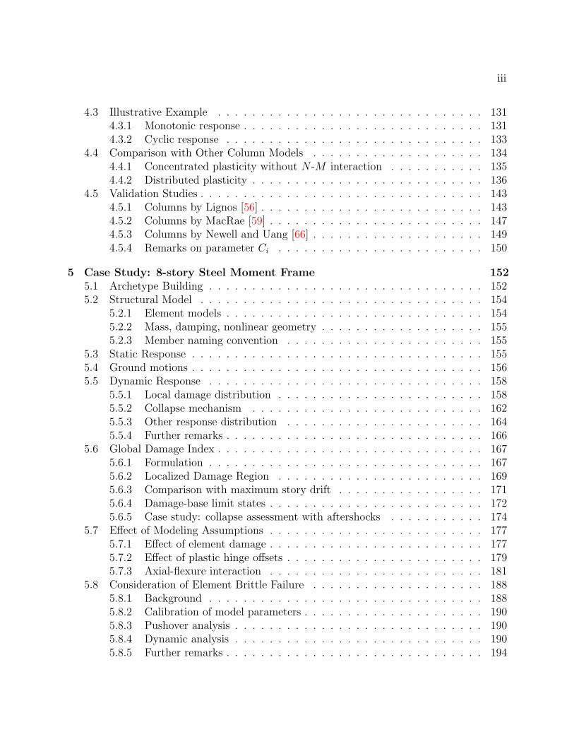
2.1 Relation between effective and true response . . . . . . . . . . . . . . . . . . . . 132.2 Selected force-deformation relations in effective space . . . . . . . . . . . . . . . 142.3 Effect of px and py on the reloading response of the hysteretic model . . . . . . 152.4 Illustration of ψt and ψc and of the effect of the parameter Cwc . . . . . . . . . . 162.5 Effect of parameters d±p on the damage evolution . . . . . . . . . . . . . . . . . 182.6 FEMA force-deformation envelope . . . . . . . . . . . . . . . . . . . . . . . . . 212.7 Effect of damage parameters on force-deformation relation . . . . . . . . . . . . 212.8 Sample cyclic response of proposed model . . . . . . . . . . . . . . . . . . . . . 222.9 Evolution of damage variables d± under cyclic loading . . . . . . . . . . . . . . 232.10 Stiffness degradation under cyclic loading with decreasing magnitudes . . . . . . 242.11 Simulations of reinforced concrete columns . . . . . . . . . . . . . . . . . . . . . 262.12 Simulations of steel beam-column assemblages . . . . . . . . . . . . . . . . . . . 282.13 Simulation of steel cantilever beams under cyclic loading . . . . . . . . . . . . . 292.14 Numerical and experimental correlation for plywood shear walls . . . . . . . . . 302.15 Simulation of beam-to-column shear tab connections (S1 system) . . . . . . . . 322.16 Simulation of pre-Northridge non-ductile welded steel beam-column connections
(system S2) . . . . . . . . . . . . . . . . . . . . . . . . . . . . . . . . . . . . . . 342.17 Simulation of post-Northridge ductile steel beam-column connections (system S3) 352.18 Simulation of stiff, non-ductile concentrically braced steel frame (system S4) . . 362.19 Simulation of stiff, non-ductile masonry wall with pronounced pinching (system
S5) . . . . . . . . . . . . . . . . . . . . . . . . . . . . . . . . . . . . . . . . . . . 372.20 Simulation of lightly reinforced concrete column with limited-ductility (system S7) 382.21 Monotonic response and comparison of Park-Ang damage index with damage
variable d+ . . . . . . . . . . . . . . . . . . . . . . . . . . . . . . . . . . . . . . 422.22 Cyclic response and comparison of damage index dPA with damage variable d+ . 432.23 Effect of parameters Cwc and Ccd on damage index dPA and damage variable d+ 432.24 Response of steel beam-column subassemblages under cyclic load protocols . . . 442.25 Comparison of damage evolution in specimen LS2 . . . . . . . . . . . . . . . . . 452.26 Damage evolution with brittle failure . . . . . . . . . . . . . . . . . . . . . . . . 47

vi
2.27 Simulations of steel beam with brittle failure . . . . . . . . . . . . . . . . . . . . 48
3.1 Series beam element . . . . . . . . . . . . . . . . . . . . . . . . . . . . . . . . . 503.2 Equilibrium and compatibility relations of series beam model . . . . . . . . . . . 513.3 Yield envelope of series element . . . . . . . . . . . . . . . . . . . . . . . . . . . 523.4 Scenarios of plastic deformation increments: (a) only fi active, (b) only fj active,
(c) both fi and fj active . . . . . . . . . . . . . . . . . . . . . . . . . . . . . . . 533.5 Series beam element with plastic hinge offset . . . . . . . . . . . . . . . . . . . . 543.6 Moment interpolation between the hinge locations and the element ends . . . . 543.7 Return-mapping algorithm for series element . . . . . . . . . . . . . . . . . . . . 593.8 Two-step identification of active surfaces . . . . . . . . . . . . . . . . . . . . . . 613.9 Violation of Kuhn-Tucker condition due to incorrect active β’s . . . . . . . . . 613.10 Evolution of yield surfaces: (a) kinematic hardening with Hkr > 0, and (b)
isotropic hardening with Hir > 0 . . . . . . . . . . . . . . . . . . . . . . . . . . 633.11 Sample cyclic response with linear kinematic and isotropic hardening . . . . . . 643.12 Effect of offset on flexural response of a cantilever beam . . . . . . . . . . . . . 653.13 Structural model of portal frame . . . . . . . . . . . . . . . . . . . . . . . . . . 653.14 Pushover response of portal frame with EPP element behavior . . . . . . . . . . 673.15 Simply-supported beam with proportional end rotations . . . . . . . . . . . . . 683.16 Calibration of post-yield hardening parameter: (a) with target deformation vtarget,
(b) with fictitious moment M∗p . . . . . . . . . . . . . . . . . . . . . . . . . . . . 69
3.17 Moment-rotation relation of simply-supported beam under monotonic loading . 703.18 Moment-rotation relation of simply-supported beam under cyclic loading . . . . 713.19 Modeling approaches for reduced-beam sections: (a) 3 linear-elastic beams with
2 zero-length springs, (b) 2 linear-elastic beams with 1 series beam without offset,(c) 1 series beam with offset . . . . . . . . . . . . . . . . . . . . . . . . . . . . . 72
3.20 Moment-rotation of beam with RBS: (a) ρ = 0.5, χ = 0.05, λ = 0.6, (b) ρ = −0.5,χ = 0.05, λ = 0.8, (c) ρ = −0.5, χ = 0.1, λ = 0.6 . . . . . . . . . . . . . . . . . 73
3.21 Effect of hinge offset on portal frame response: static response . . . . . . . . . . 743.22 Structural model of 3-story moment frame . . . . . . . . . . . . . . . . . . . . . 763.23 Collapse mechanisms of 3-story 1-bay moment frame: (a) 1-story, (b) 2-story, (c)
full 3-story . . . . . . . . . . . . . . . . . . . . . . . . . . . . . . . . . . . . . . . 763.24 Response comparison of design alternatives . . . . . . . . . . . . . . . . . . . . . 773.25 Response comparison of RBS designs . . . . . . . . . . . . . . . . . . . . . . . . 783.26 Member response at the beam-column joint in the 1st story . . . . . . . . . . . 793.27 Equilibrium and compatibility relations of plastic-damage beam model . . . . . 803.28 Degrading moment-rotation relation of simply-supported beam under monotonic
loading . . . . . . . . . . . . . . . . . . . . . . . . . . . . . . . . . . . . . . . . . 853.29 Degrading moment-rotation relation of simply-supported beam under cyclic loading 873.30 Dynamic response of portal frame . . . . . . . . . . . . . . . . . . . . . . . . . . 883.31 Girder moment-rotation and damage evolution in model M1 . . . . . . . . . . . 893.32 Girder moment-rotation and damage evolution in model M2 . . . . . . . . . . . 90

vii
3.33 Moment-rotation relation of steel specimens LS1 and LS3 [111] . . . . . . . . . . 923.34 Variation in the limit coefficient Cd1 with the section compactness and member
slender . . . . . . . . . . . . . . . . . . . . . . . . . . . . . . . . . . . . . . . . . 933.35 Cyclic load protocols for cantilever beam . . . . . . . . . . . . . . . . . . . . . . 943.36 Reference cyclic response under different loading histories . . . . . . . . . . . . . 953.37 Sensitivity analysis: CUREE loading . . . . . . . . . . . . . . . . . . . . . . . . 963.38 Sensitivity analysis: NF loading . . . . . . . . . . . . . . . . . . . . . . . . . . . 973.39 Moment-rotation relation of steel specimens with brittle failure . . . . . . . . . . 100
4.1 NMYS column element . . . . . . . . . . . . . . . . . . . . . . . . . . . . . . . . 1024.2 Yield surfaces . . . . . . . . . . . . . . . . . . . . . . . . . . . . . . . . . . . . . 1044.3 NMYS column element with plastic hinge offset . . . . . . . . . . . . . . . . . . 1064.4 Geometric illustration of return-mapping algorithm at corner point . . . . . . . 1104.5 Effect of yield surface parameters . . . . . . . . . . . . . . . . . . . . . . . . . . 1134.6 Effect of hardening parameters on yield envelope . . . . . . . . . . . . . . . . . 1144.7 Cantilever column: (a) structure and loading, (b) concentrated plasticity (CP)
model, (c) distributed plasticity (DP) model . . . . . . . . . . . . . . . . . . . . 1154.8 Monotonic response of cantilever column with EPP behavior . . . . . . . . . . . 1164.9 Cyclic response of cantilever column with EPP response . . . . . . . . . . . . . 1184.10 Cyclic response of cantilever column with EPP response (continued) . . . . . . . 1194.11 Cyclic response of cantilever column with hardening behavior, χ = 0 . . . . . . . 1214.12 Cyclic response of cantilever column with hardening behavior, , χ = 0.2 . . . . . 1224.13 Four-story three-bay moment-resisting frame . . . . . . . . . . . . . . . . . . . . 1234.14 Global dynamic response of four-story three-bay steel moment frame . . . . . . 1244.15 Local dynamic response of four-story three-bay steel moment frame . . . . . . . 1254.16 Cantilever column: (a) Structure and loading, (b) Idealized model . . . . . . . . 1324.17 Monotonic response of cantilever column under different levels of axial force . . 1324.18 Cyclic response comparison: (a) variable axial force N/Np = −0.4 ∓ 0.3, (b)
constant axial force N/Np = −0.4 . . . . . . . . . . . . . . . . . . . . . . . . . . 1334.19 Modeling approaches for response simulation of a cantilever column: (a) Structure
and loading, (b) Model CP, (c) Model CP0, (d) Model DP . . . . . . . . . . . . 1344.20 Response comparison of model CP and model CP0 . . . . . . . . . . . . . . . . 1364.21 Comparison of cyclic response with variable axial compression . . . . . . . . . . 1374.22 Sample stress-strain relation . . . . . . . . . . . . . . . . . . . . . . . . . . . . . 1384.23 Comparison of cyclic response of cantilever column . . . . . . . . . . . . . . . . 1384.24 Numbering of fibers in cross-section of DP model . . . . . . . . . . . . . . . . . 1394.25 Sample fiber response under N/Np = 0 . . . . . . . . . . . . . . . . . . . . . . . 1404.26 Sample fiber response under N/Np = -0.2 . . . . . . . . . . . . . . . . . . . . . 1414.27 Damage measures of DP model . . . . . . . . . . . . . . . . . . . . . . . . . . . 1424.28 Comparison of damage variables DCP and DDP . . . . . . . . . . . . . . . . . . 1424.29 Response under constant axial compression and monotonic lateral displacement 1444.30 Effect of axial load level on cyclic response of steel column . . . . . . . . . . . . 145

viii
4.31 Effect of variable axial load on cyclic response of steel column . . . . . . . . . . 1454.32 Axial shortening of steel column under constant axial load . . . . . . . . . . . . 1464.33 Cyclic response of steel columns under constant axial load . . . . . . . . . . . . 1474.34 Damage evolution of steel column specimens . . . . . . . . . . . . . . . . . . . . 1484.35 Cyclic response of steel column under variable axial compression . . . . . . . . . 149
5.1 Archetype eight-story three-bay special moment frame . . . . . . . . . . . . . . 1535.2 Typical floor model of the eight-story three-bay moment frame . . . . . . . . . . 1555.3 Pushover response: load distribution and normalized base shear vs roof drift . . 1565.4 Story drift and shear distribution . . . . . . . . . . . . . . . . . . . . . . . . . . 1575.5 Damage distribution at RD = 0.045 . . . . . . . . . . . . . . . . . . . . . . . . . 1575.6 Elastic response spectrum of the far-field ground motions, ξ = 2.5% . . . . . . . 1595.7 Response distribution and deformed shape (FF4, SF = 6.60) . . . . . . . . . . . 1605.8 Response of 1st story exterior columns (FF4, SF = 6.60): (a) Flexural response
at base, (b) Plastic axial deformation, (c) Damage evolution . . . . . . . . . . . 1615.9 Response distribution and deformed shape (FF1, SF = 5.00) . . . . . . . . . . . 1615.10 Response of 1st story exterior columns (FF1, SF = 5.0): (a) Flexural response at
base, (b) Plastic axial deformation, (c) Damage evolution . . . . . . . . . . . . . 1625.11 Girder response of 1st floor girders (FF4, SF = 6.6) . . . . . . . . . . . . . . . . 1635.12 Deformed shape with weak-story collapse mechanism: (a) FF14, SF = 9.0, (b)
FF1, SF = 5.6 . . . . . . . . . . . . . . . . . . . . . . . . . . . . . . . . . . . . . 1635.13 Story DR and shear distribution of a one-story mechanism (FF14, SF = 9.0) . . 1645.14 Time history of the average floor rotations . . . . . . . . . . . . . . . . . . . . . 1655.15 Distribution of floor acceleration . . . . . . . . . . . . . . . . . . . . . . . . . . 1655.16 Dynamic response under FF9 . . . . . . . . . . . . . . . . . . . . . . . . . . . . 1665.17 Illustration of column indices, joint indices, and floor indices . . . . . . . . . . . 1685.18 Typical configuration of a story mechanism . . . . . . . . . . . . . . . . . . . . . 1695.19 Damage indices and localized damage region (FF1, SF = 5.6) . . . . . . . . . . 1705.20 Comparison of damage index DG and maximum story drift . . . . . . . . . . . . 1715.21 Incremental dynamic analysis curve in terms of story drift and damage index . . 1725.22 Comparison of max drift ratio DR and damage index DG at different limit states:
(a) Life safety, (b) Collapse prevention, (c) Collapse . . . . . . . . . . . . . . . . 1735.23 Probability of different damage limit states . . . . . . . . . . . . . . . . . . . . . 1745.24 Acceleration history of FF1 record with aftershock . . . . . . . . . . . . . . . . 1755.25 Collapse probability with and without consideration of aftershocks . . . . . . . . 1765.26 Comparison of dynamic response in model R and model A . . . . . . . . . . . . 1785.27 Dynamic response without element damage (FF14, SF = 12.15) . . . . . . . . . 1795.28 Comparison of model R and model B: average roof translation . . . . . . . . . . 1795.29 Comparison of model R and model B: 1st story drift . . . . . . . . . . . . . . . 1805.30 Comparison of model R and model B: collapse mechanisms . . . . . . . . . . . . 1815.31 Comparison of model R and model B: damage distribution . . . . . . . . . . . . 182

ix
5.32 Comparison of model R and model CA: story drift and deformed shape (FF17,SF = 9.40) . . . . . . . . . . . . . . . . . . . . . . . . . . . . . . . . . . . . . . 183
5.33 Comparison of model R and model CA: effect of column shortening (FF17, SF =9.40) . . . . . . . . . . . . . . . . . . . . . . . . . . . . . . . . . . . . . . . . . . 184
5.34 Comparison of model R and model CA: local column response (FF17, SF = 9.40) 1855.35 Comparison of model R and model CA: damage distribution (FF17, SF = 9.40) 1865.36 Comparison of model R and model CB: story drift and deformed shape (FF2, SF
= 7.92) . . . . . . . . . . . . . . . . . . . . . . . . . . . . . . . . . . . . . . . . 1875.37 Comparison of model R and model CB: local column response and damage dis-
tribution (FF2, SF = 7.92) . . . . . . . . . . . . . . . . . . . . . . . . . . . . . . 1895.38 Pushover analysis response with sudden strength deterioration . . . . . . . . . . 1915.39 Comparison of model R and model D: 1st story drift . . . . . . . . . . . . . . . 1925.40 Comparison of model R and model D: 1st story column response . . . . . . . . . 1935.41 1st story drift ratio under FF19, SF = 6.93 . . . . . . . . . . . . . . . . . . . . 1945.42 Local response and damage distribution under FF19, SF = 6.93 . . . . . . . . . 195
A.1 Effect of β1 and β2 on the beta CDF . . . . . . . . . . . . . . . . . . . . . . . . 212A.2 Effect of µ and σ on the lognormal CDF . . . . . . . . . . . . . . . . . . . . . . 213A.3 Simulation of concrete uniaxial response . . . . . . . . . . . . . . . . . . . . . . 214

x
List of Tables
2.1 State determination algorithm of hysteretic damage model . . . . . . . . . . . . 202.2 Parameters used in simulations of reinforced concrete columns . . . . . . . . . . 252.3 Parameters used in simulations of steel beam-column joints . . . . . . . . . . . . 272.4 Parameters for the simulations of the degrading hysteretic behavior of structural
components . . . . . . . . . . . . . . . . . . . . . . . . . . . . . . . . . . . . . . 402.5 Correlation of damage measures and limit states for specimen LS2 . . . . . . . . 46
3.1 State determination algorithm of series beam model with plastic hinge offset . . 583.2 Design alternatives of 3-story frame . . . . . . . . . . . . . . . . . . . . . . . . . 793.3 State determination algorithm of damage-plasticity beam model . . . . . . . . . 843.4 Regression coefficients for parameter calibration . . . . . . . . . . . . . . . . . . 933.5 Sensitivity ranking of damage parameters . . . . . . . . . . . . . . . . . . . . . 983.6 Parameters for the simulations of steel beams with brittle damage . . . . . . . . 99
4.1 Elastic predictor algorithm . . . . . . . . . . . . . . . . . . . . . . . . . . . . . . 1114.2 Plastic correction algorithm: closest point projection . . . . . . . . . . . . . . . 1124.3 Unit comparison of beam and column models . . . . . . . . . . . . . . . . . . . 1144.4 State determination algorithm of damage-plasticity column model . . . . . . . . 1304.5 Comparison of Ci and Cd1 in column simulations . . . . . . . . . . . . . . . . . 150
5.1 Member sizes for eight-story three-bay moment resisting frame . . . . . . . . . . 1535.2 Parameters of reduced beam sections . . . . . . . . . . . . . . . . . . . . . . . . 1545.3 Far-field ground motion information . . . . . . . . . . . . . . . . . . . . . . . . . 158

xi
Acknowledgments
First and foremost, I would like to express my deep gratitude to my advisor, Professor FilipFilippou, for the unique opportunity to embark on this challenging and rewarding journey inthe last five years at Berkeley. I truly appreciate his constant guidance and encouragement,and especially his incredible energy and patience as he helped me improve my writing. Hisdedication to high-quality research and teaching is unparalleled. I am also very gratefulfor the honor to serve as his graduate student instructor in the Structural Analysis andNonlinear Structural Analysis courses.
I would like to thank Professor Anil Chopra and Professor Panayiotis Papadopoulos foragreeing to serve on my qualifying exam and dissertation committee and for their valuablecomments to improve the thesis. I am also grateful for the other members on my qualifyingexam committee: Professor Khalid Mosalam and Professor John Strain.
I would like to thank Ms. Shelley Okimoto for her valuable advice throughout my stayat Berkeley.
I would like to thank my former advisor at University of the Pacific, Dr. Camilla Saviz,for her encouragement, continuous support, and lifelong mentoring. I am very fortunate tohave met and worked with such a dedicated and passionate mentor.
I would like to express my gratitude to all my friends, in particular, my friends at Univer-sity of the Pacific and at University of California, Berkeley. One way or the other, you havemade my journey particularly memorable. Your lifelong friendship and warm welcomingmakes me truly feel this is my ’home away from home.’
Finally, my deepest appreciation goes to family. I thank you for your infinite patienceespecially during the preparation of this dissertation and other difficult times. Without yourunconditional love and support, it would be impossible for me to become who I am today.I would like to dedicate my accomplishments to you. You have been, and forever will be, acrucial part of my journey.

1
Chapter 1
Introduction
1.1 Motivation
Over the last decades, we are continuously reminded of the lack of resilience in thebuilt-environment by earthquakes, tsunamis, hurricanes, that cause intolerable structuraldamage, economic loss, and significant loss of lives. These hazards pose a constant threat tothe resilience of our community. In particular, the seismic hazard has caused severe dam-age to a wide variety of structural types, ranging from reinforced concrete (RC), masonry,wood, to steel, which is widely believed to exhibit superior performance during earthquakes.Damage in steel structures, even though not as severe as in other structural types such asRC structures, also results in significant economic loss and thus deserves more attention.One example of serious damage in steel structures is the Cordova building during the PrinceWilliam Sound, Alaska earthquake in 1964. Damage to this six-story steel frame was concen-trated in the first story where a number of wide flange columns buckled due to the high axialforces. Another example of a severely damaged steel structure is the Pino Suarez Complexduring the Mexico City earthquake in 1985. In this case, the large brace forces induced axialoverstress in the columns and lead to column buckling, and in turns, the collapse of a 21-story building. A detailed discussion on past performance of steel moment-frame buildingsin earthquake can be found in the FEMA 355E report [107].
To prevent structural collapse and enhance the community resilience in a multi-hazardenvironment, it is critical to understand the deterioration in structures so that proper pre-vention and/or mitigation practices can be undertaken. For the purpose, often times anumerical model is employed to simulate the structural response and quantify the level ofdamage. However, as will be discussed in detail in the remaining of this dissertation, manyexisting models have serious limitations in the accuracy and the efficiency.
Due to the above limitations, the major challenge in this generation is two-fold: first,to establish an accurate, efficient, and reliable analytical framework to quantify the perfor-mance of existing and new structures under extreme loading conditions both predictivelyand retrospectively; and second, to develop the design and retrofit guidelines to improve the

CHAPTER 1. INTRODUCTION 2
system resilience against the effect of manmade and natural hazards. The framework con-sists of several critical components: (1) a damage model to predict the structural responseand assess the damage states and collapse fragility, (2) a probabilistic model to evaluatethe multi-hazard risks, and (3) a financial model to estimate the repair/replacement cost aswell as the necessary recovery time for the structure to be fully operational. The analysispermits a resilient design for a new building or an economical retrofitting scheme for anexisting structure with optimal use of available resources.
This dissertation addresses the first major component of this interdisciplinary framework:to develop efficient and accurate damage models for the response simulation and damageassessment of structural systems in a multi-hazard environment.
1.2 Literature Review
The following review of relevant literature is presented in three parts: the first addressesthe existing deterioration models, the second reviews some notable beam and column ele-ment models, and the third discusses the engineering demand parameters commonly used indamage evaluation of components and structures.
1.2.1 Damage models
The assessment of structural resilience depends on the analytical description of the dam-age evolution under a sequence of extreme cyclic loading conditions. Existing models ofmaterial damage fall into three broad categories:
(a) Rigorously formulated 3d material constitutive models based on continuum damagemechanics (CDM) that describe the evolution of the strength and stiffness deterio-ration. These models focus on local response simulations of structural components,which however, make their high computational cost unsuitable for the simulation ofstructural systems under multi-hazard scenarios.
(b) Hysteretic models with strength and stiffness deterioration rules. These models can, inturn, be divided into polygonal and smooth response description models. The first typeassumes piece-wise linear response between events corresponding to cracking, yieldingand ultimate capacity. The second type uses algebraic or differential equations togenerate a smooth hysteretic response with a gradual transition from the elastic tothe inelastic range. These models are simpler than the ones in the first category andare widely used in practice. However, they exhibit some limitations in the damagedescription of components, such as in the degradation in primary and follower halfcycles, the unloading stiffness deterioration, the lack of a consistent damage measure,among others.
(c) Damage index models. These models establish a damage index for quantifying compo-nent damage. The damage index calibration is based on experimental measurements

CHAPTER 1. INTRODUCTION 3
and observations or on analytical results with some of the hysteretic models under (b).The models, however, do not explicitly describe the degrading hysteretic response asthe models under (a) and (b), and thus, lacks the correlation between the structuralresponse and the damage states.
Examples of CDM models are those by Simo and Ju [91], Lemaitre [54], and Huang [38]for ductile materials, and those by Mazars and Pijaudier-Cabot [62] and Wu and Faria [110]for concrete materials. The cyclic void growth model (CVGM) by Rice and Tracey [83] andthe model by Kanvinde and Deierlein [44] also fall in this category. Because these modelsfocus on local response simulations of structural components, their high computational costmakes them unsuitable for the simulation of structural systems under multi-hazard scenarios.
Models in the second category can be further classified into to groups: polygonal modelsand smooth models. Polygonal hysteretic models are relatively easy to formulate, but of-tentimes depend on many rules limiting their generality and making their consistency andnumerical robustness challenging. Several such models have been proposed over the yearsstarting with Clough [17] and Takeda et al. [98]. The force-deformation relation of the for-mer represents the stiffness degradation by adjusting the reloading behavior to target themaximum previous displacement in the loading direction and is often referred to as the peak-oriented model. Takeda’s model uses a trilinear envelope to distinguish the cracking fromthe yield moment of a reinforced concrete component and is characterized by a more complexunloading and reloading peak-oriented behavior than Clough’s model. The three-parametermodel by Park, Reinhorn, and Kunnath [72, 81] uses a pivot rule to describe the stiffnessdeterioration and includes strength degradation based on the hysteretic energy at unload-ing. The model by Song and Pincheira [94] relates the strength and stiffness deterioration tothe maximum deformation at the most recent inelastic excursion in the opposite direction.Finally, the model by Ibarra et al. [39] uses a piecewise linear monotonic backbone relationand four deterioration modes: strength, post-capping, unloading stiffness, and acceleratedreloading stiffness. [57] reports the extensive calibration of this model. Because of theirformulation polygonal models accommodate strength and stiffness deterioration as discreteupdates at the instant of load or deformation reversal.
Smooth hysteretic models are more computationally involved than polygonal models butare more consistent and numerically robust. A prominent example of this group is themodel of Bouc [11] and its extension by Wen [108] and Baber et al. [9, 8]. Sivaselvan andReinhorn [93] and Ray and Reinhorn [80] demonstrated the ability of smooth hystereticmodels to accommodate a continuous strength and stiffness deterioration through the useof rate equations for the strength and stiffness evolution. Sivaselvan and Reinhorn [93] alsoproposed an elegant framework for combining basic polygonal and smooth hysteretic modelsin parallel or in series with the intent of assigning one suitable component to a correspondingphysical mechanism like plastic yielding, slip, friction, etc.
Park and Ang [73] proposed an early damage model with the damage index as the linearcombination of the normalized maximum deformation and the normalized hysteretic energy.In contrast, the model by Kratzig [49] uses the normalized hysteretic energy of each load

CHAPTER 1. INTRODUCTION 4
cycle to establish the damage index of the component. To account for the dependenceof damage on the deformation history, Kratzig distinguishes the energy dissipation of aprimary half cycle (PHC) that extends the deformation envelope from a follower half cycle(FHC) that remains within the current extreme deformations. Mehanny and Deierlein [64]adopted the idea of PHC and FHC but based the damage index on the maximum plasticdeformations instead of hysteretic energy. Rahnama and Krawinkler [79] proposed a damageindex as an exponential function of the normalized energy dissipation in each load cycle.Finally, Bozorgnia and Bertero [12] suggested a modification of the Park-Ang damage indexto discount damage in the elastic range. They also introduced a weight coefficient for thecontribution of the deformation ductility relative to the energy dissipation.
1.2.2 Beam-column models
The following review of the existing beam and column elements is presented in two parts.First, the element models without strength and stiffness deterioration are discussed. Then,the discussion focuses on the models that account for the deterioration in the response.
1.2.2.1 Element models with nondegrading response
Existing nondegrading beam-column models can be classified into three main categories:
(a) Continuum models: this approach requires a discretization of the structural modeland is common in finite element analysis. These models specify a stress-strain relationfor the material response and focus on the local behavior of structural components.However, the high computational cost limits their use in large-scale simulations ofstructural systems.
(b) Distributed plasticity models: the element response is monitored at several sectionsalong the element length. The models permit plastic hinges to form at any sectionand account directly for the interaction of the element response, such as axial, flexure,shear, torsion, and warping. The section response is determined from a stress-resultantmodel [24] or a fiber-based model. The latter can, in turn, be divided into elementswith a displacement- and a force-based or a mixed formulation.
(c) Concentrated plasticity models: the inelastic behavior is concentrated in the nonlinearplastic hinges typically located at the element ends. The hysteretic behavior of theplastic hinges are given by a moment-rotation relation.
Distributed plasticity elements based on the displacement-formulation adopt a similarapproach in standard finite element method and utilize displacement interpolation functionsto relate the section deformations to the element deformations [112]. Since the relation isapproximate, several elements are required to describe accurately the nonlinear elementresponse. Distributed plasticity elements based on the force- or mixed-formulation, on the

CHAPTER 1. INTRODUCTION 5
other hand, use force interpolation functions to relate the section forces to the element forces.Since equilibrium is satisfied exactly, the force-based formulation only requires one elementto describe accurately the nonlinear behavior and permits fewer degrees of freedom in thestructural model. Further discussion on the advantages of the force-based elements can befound in Spacone et al. [95], Neunhoffer and Filippou [65], Taylor et al. [102].
One of the earliest concentrated plasticity models is the two-component element pro-posed by Clough, Benuska, and Wilson [17]. It consists of a linear elastic-perfectly plasticcomponent in parallel with a linear elastic component and is able to represent a post-yieldlinear hardening behavior in the flexural response. Another notable model in this categoryis the one-component element by Giberson [30], which consists of a linear elastic componentin series with two nonlinear springs located at the element ends. The springs assume arigid-plastic with linear hardening behavior and are activated when the moment exceeds theplastic flexural capacity. Both the one-component and the two-component models assume alinear elastic axial response that is uncoupled from the flexural behavior. The models havebeen extended to accommodate the axial-flexure interaction in the plastic hinge response[37, 76]. Concentrated plasticity models are widely used in response simulations of struc-tural components of different materials, including steel [67, 67, 75, 70, 37, 76], reinforcedconcrete [100], and concrete-filled steel tubes [34, 48].
Concentrated plasticity models compare favorably to continuum and distributed plas-ticity models in the numerical efficiency but also exhibit several limitations. First, despitethe effort to account for the response interaction, the challenge to capture sufficiently thecoupling of complex element response remains. Second, many concentrated plasticity modelsexplicitly specify a zero-length rotational spring element and require additional nodes anddegrees of freedom at the interface between the spring and the elastic beam element. Thisproblem can be resolved by specifying the plastic hinges implicitly in the element state deter-mination [77, 48]. Moreover, the approximatation of the rigid-plastic behavior in the plastichinges with a large elastic stiffness leads to numerical nonconvergence under dynamic load-ing and unreasonable sensitivity of the dynamic response to the damping models, especiallywhen the initial stiffness is used in Rayleigh damping [15].
1.2.2.2 Element models with degrading response
The element models with degrading response are based on the models with nondegradingresponse in Section 1.2.2.1 and specify the deterioration in three main manners: (1) in thematerial stress-strain relation or in the section moment-curvature relation of a fiber-basedelement, (2) in the zero-length spring’s moment-rotation relation of a concentrated plasticitymodel, and (3) in the force-deformation relation of a concentrated plasticity model.
(1) Degrading material stress-strain and section moment-curvatureA degrading stress-strain relation for the material response is specified in continuum mod-
els and distributed plasticity models. The material models are typically based on continuumdamage mechanics (CDM), such as those listed in category (a) in Section 1.2.1. These ele-

CHAPTER 1. INTRODUCTION 6
ments account for the coupling of complex element response and capture the deterioration atthe local material level. However, in addition to the high computational cost, the elementsare susceptible to mesh inobjectivity [20].
To resolve this issue, many regularization techniques have been proposed, such as byColeman and Spacone [18], Addessi and Ciampi [2]. Another approach is the beam withhinge element by Scott et al. [86, 87], and Ribeiro et al. [82]. The element consists of threesegments: an interior elastic beam element and two plastic hinge segments at the elementends with a specified plastic hinge length, and adopts a proper numerical integration scheme.To represent the deterioration in the element response, a degrading stress-strain relation canbe specified for the material response in each fiber, or alternatively, a degrading moment-curvature relation can be specified for the section response.
A recent approach to describe the column strength and stiffness deterioration is the fiberhinge element by Kasai et al. [46]. The inelastic behavior is localized at the column baseand modeled by the zero-length fiber hinge element, which is discretized into fibers with adegrading stress-strain relation.
(2) Degrading spring moment-rotationOne of the most common approaches to simulate strength deterioration is to define a
degrading moment-rotation relation for the zero-length rotational springs at the ends of aconcentrated plasticity beam-column element. This approach is recommended in ATC-72guidelines for modeling of tall buildings [61]. The moment-rotation relation can adopt anydeterioration hysteretic model summarized in 1.2.1.
Besides the same drawbacks as in the concentrated plasticity models with nondegradingresponse, these models fail to capture the effect of a variable axial force on the strengthdeterioration in flexure, which is critical in tall structures where the columns are subjectedto high axial forces from the overturning effect.
(3) Degrading element force-deformationAn efficient approach to incorporate deterioration in concentrated plasticity formulation
is to adopt the continuum damage mechanics concept [41, 54]. These element models employa nondegrading force-deformation relation to describe the response without strength deteri-oration, and define some criteria for damage initiation and growth to represent the strengthand stiffness deterioration in the element response.
Some of the earliest models in this category include the work by Cipolina et al. [16],Florez-Lopez [28], and Inglesis et al. [40]. The models adopted a simple bilinear force-deformation with kinematic hardening for the base response and proposed different damageevolution laws for steel and reinforced concrete (RC) components based on experimentalmeasurements of steel and RC cantilever specimens under cyclic loading. Faleiro et al. [26]proposed an element model that uses an energy variable to describe the damage initiationand growth. Kaewkulchai et al. [42] formulated a beam-column element with a multi-linearforce-deformation relation that adopted the Mroz’s hardening rule and a damage variableresembling the Park-Ang damage index to investigate the progressive collapse of structures.

CHAPTER 1. INTRODUCTION 7
One limitation of the existing models is in the criteria for damage initiation and growth.Models that adopt an elastic energy variable to govern the damage evolution fail to capturethe low-cycle fatigue behavior due to repeated cycles between the same range of deforma-tion values. Other models that are based on the cumulative plastic deformations do notdistinguish the two deterioration rates in the primary and the follower half cycles.
1.2.3 Damage assessment of structures
The engineering demand parameters (EDP) commonly used for damage assessment ofstructures can be classified into two categories: the parameters of the structural responseand the damage indices derived from a damage index model. Each category can, in turn, bedivided into the local and the global parameters that relate to the local and global response,respectively [21, 109].
1.2.3.1 Structural response
Local parameters are related to the response of each individual member. The mostcommon local response for collapse assessment is the plastic hinge rotation [4]. Krishnan[52] studied the plastic hinge distribution to interpret the collapse mechanisms of tall steelmoment-frames. The local plastic rotations are used to define the non-simulated collapsemodes of the structures in FEMA P695 [4]. Once the plastic rotation in any member reaches athreshold, the structure triggers a non-simulated mechanism. Other important local damageindicators include the fiber stress-strain and the element force-deformation. These parame-ters are critical to detect the local limit states, including cracking, yielding, buckling [21].
Global parameters account for the contributions from all members to the behavior of oneor several stories/floors. The most widely used global response for collapse assessment isthe maximum story drift and residual drift [3]. The maximum drift is typically used as themain EDP to evaluate the structural collapse fragility, often times through an incrementaldynamic analysis [105]. Other important global damage indicators include the peak momentsand shear forces, and the maximum floor velocity and acceleration [21].
1.2.3.2 Damage indices
Damage indices may be defined locally for an individual member or globally for an en-tire structure [109]. Many damage models have been proposed up to date to quantify themember’s damage state based on the displacement amplitude, the energy dissipation, thenumber of loading cycles, or a combination thereof. Some representative models for the localdamage indices are summarized in Section 1.2.1. The main disadvantages of many existinglocal damage indices are two-fold [109]: (1) the lack of parameter calibration against differentdamage states of various structural types, and (2) the ability to address various componentfailure mechanisms besides the flexural modes, such as the failure of steel columns under thecombined axial and flexural effects.

CHAPTER 1. INTRODUCTION 8
The overall damage state of a structure depends on both the distribution and the severityof the localized damage. The global damage indices may be defined as weighted average ofthe local damage indices or from the variation in the structural characteristics, such asthe modal properties [109]. Different formulation have been proposed to formulate the globaldamage indices from the local damage indices in Section 1.2.1 across the structure with someweight distributions. Two most widely used approaches to quantify the contribution fromeach member are based on the local damage itself and the local energy absorption, such as inPark et al. [73, 71], Kunnath et al. [53], Bracci et al. [13]. These weighted average methodsare simple to implement; however, they inherit many limitations of the local damage indices[109]. Moreover, a comparison is necessary to assess different weighing alternatives.
The global damage indices can also be evaluated in terms of the local damage indicesin the element models that are based on continuum damage mechanics such as those inSection 1.2.2.2(1) and Section 1.2.2.2(3). Faleiro et al. [26] defined a member damage indexin terms of a ratio of the damaged and undamaged free energy variables in the elementresponse. To account for the contribution of the member deterioration to the global response,the model evaluated the sum of the damaged free energy among all elements and the sum ofthe corresponding undamaged free energy, then the global damage index was defined in termsof the ratio of the two quantities. The damage indices were demonstrated in the simulationof a two-story RC frame under quasi-static cyclic loading. Hanganu et al. [35] and Scottaet al. [88] employed a distributed plasticity model with a degrading material stress-strainrelation to examine the damage states of RC structures. The damage indices were calibratedagainst experimental data of RC cantilever columns and compared to the limit states criteriain FEMA 356 [3] through a nonlinear dynamic analysis of a RC frame.
Another approach to detect the damage evolution is to examine the change in the modalproperties. DiPasquale and Cakmak [23, 22] proposed thee softening indices to reflect thestructural damage state in term of three periods: the period of the undamaged structure,the maximum period, and the period of the damaged structure. The studies showed thatthe softening indices correlate well with the stiffness deterioration of a structure and areconsistent with several other damage indices, such as the Park-Ang damage index [73].However, the formulation based solely on the fundamental period neglects the critical impactof the higher modes and the distribution of damage within the structure [109]. An alternativeapproach is to examine the fundamental and the higher mode shapes as well as the variationsin the flexibility coefficients, such as in the work by Raghavendrachar and Aktan [78].
The next definition of global damage indices is associated with the economic loss. Thismethodology does not directly relate to the structural response as the other approaches;however, it has an important implication in damage mitigation practices and resilience as-sessment of structures. Hasselman and Wiggins [36] used a damage ratio to quantify theglobal damage state, which is defined as the ratio of the repair cost to the replacement cost.Based on the data from the 1971 San Fernando earthquake, the study proposed a log-logrelationship between the damage ratio and the interstory drift. Gunturi and Shah [33] pro-posed the global damage as a collective measure of three main components: the structuraldamage, the nonstructural damage, and the content damage, which are dependent on the

CHAPTER 1. INTRODUCTION 9
Park-Ang damage index, the maximum story drift, and the maximum floor acceleration. Amajor challenge of the financial damage indices is the need for an extensive validation withdata in real events and, to some extent, the subjective nature of the financial loss estimation.
1.3 Objectives and Scope
This dissertation develops new damage models for the response simulation and damageassessment of structures under extreme loading conditions. The main objectives of the studyare as follows:
(1) To present a new hysteretic damage model based on damage mechanics to describebetter the continuous strength and stiffness deterioration in structural components.
(2) To implement the damage formulation in the development of efficient and accuratebeam and column elements for modeling of steel components.
(3) To generalize the concentrated plasticity frame elements with the plastic hinge offsetsto describe the coupling of the inelastic zones at the element ends.
(4) To calibrate the model parameters against experimental data of steel beams andcolumns under various loading scenarios. The calibration permits a regression analysisto establish a set of guidelines for the parameter identification.
(5) To investigate the dynamic response and collapse behavior of steel special momentframes (SMF). The new element models are deployed in the response simulation of an8-story 3-bay SMF under a suite of ground motions up to collapse.
(6) To highlight the unique features of the proposed element models in the collapse simu-lations and identify limitations of existing models commonly used in practice.
(7) To examine the brittle failure in the element and how the failure sequence influencesthe collapse behavior, force redistribution, and the local and global response.
(8) To formulate new global damage indices from the local element damage variables toassist in the damage assessment of structures.
(9) To introduce the concept of Localized Damage Region (LDR) to identify the mostprobable story collapse mechanisms in SMFs.
1.4 Dissertation Outline
The dissertation is organized into 6 chapters and 3 appendices, each of which addressesone or several objectives outlined in the previous section.

CHAPTER 1. INTRODUCTION 10
Chapter 1 discusses the motivation for the study and presents a detailed literature reviewof relevant topics. The chapter concludes with a brief review of continuum damage mechanicsand the basic coordinate system of 2d frame elements.
Chapter 2 presents a new hysteretic damage model. The chapter starts with a detaileddescription of the model formulation and parameters, followed by a series of validationexamples to showcase its capabilities to capture a vast range of hysteretic behaviors anddamage evolution. The chapter concludes with a comparison of the model’s damage variablewith an existing damage index model commonly used in practice.
Chapter 3 and 4 present new damage-plasticity beam and column elements, respectively.Each chapter starts with the element formulation and the state determination in a nonde-grading configuration, followed by a discussion of the damage formulation in the elementresponse. Simulations of components and structures are presented to validate the modelcapabilities. To facilitate the parameter identification, detailed guidelines for the parametercalibration are presented at the end of each chapter.
Chapter 5 incorporates the new damage models in a simulation of an 8-story 3-bay steelspecial moment-resisting frame (SMF). The chapter investigates the static and dynamicresponse of the archetype building up to collapse. The chapter presents new damage indicesand discusses its implementation in damage evaluation and collapse assessment of steel SMFs.Finally, the reference structural model is compared against several alternatives to examinedifferent modeling assumptions.
Chapter 6 summarizes the key findings in the present study, highlights some limitationsof the current models, and offers recommendations for future development.
Appendix A offers further discussion on the selection of the statistical function for thedamage evolution law, then introduces two useful statistical functions as alternatives. Ap-pendix B presents the mathematical derivations of the return-mapping algorithm and thealgorithmic tangent of the element models. Appendix C discusses the thermodynamic frame-work of the damage formulation.
1.5 Preliminaries
1.5.1 Continuum damage mechanics
The proposed models in this dissertation are based on the theory of effective stress andequivalent strain in continuum damage mechanics (CDM) [41]. The theory relates the ma-terial response in the true physical configuration to the response in an effective undamagedstate. With a bar denoting the variables in the effective space, the equivalent strain hypoth-esis postulates the equality of the true strain ε with the effective strain ε:
ε = ε (1.1)
The effective stress theory then states that the actual stress σ and the effective stress σ at agiven strain are related through a damage variable d as is the stiffness E and E in the two

CHAPTER 1. INTRODUCTION 11
configurations:
σ = (1− d)σ (1.2)
E = (1− d)E (1.3)
1.5.2 Basic coordinate system for plane frame elements
In Chapter 3 and Chapter 4, the element force-deformation relation is defined in a basicsystem to accommodate the nonlinear geometry under large displacements. The study adoptsthe corotational formulation, which defines a reference rigid coordinate system that rotateswith the element as it deforms and distinguishes the element deformations from the rigid bodymotion. Equilibrium in the element free body is satisfied in the deformed configuration, withthe element basic forces defined relative to the chord in its position under large displacements.The static and kinematic variables for a frame element are shown in the global coordinatesystem p− u in Figure 1.1(a), in the local p− u coordinate system in Figure 1.1(b), and inthe basic system q− v in Figure 1.1(c). Transformation of the basic element forces to theend forces in the global coordinate system is possible with the direction cosines of the chordorientation in the deformed configuration.
This dissertation limits the element formulation to 2d response and neglects the biaxialbending and torsion effect. The element models relate the basic forces q = [qa, qi, qj]
T to the
basic deformations v = [va, vi, vj]T . qa and va denote the axial force and axial deformation,
while qi − vi and qj − vj represent the flexural force and flexural deformation at end i andend j, respectively.
(c)qi
qj
vi vj
qa , va
i
j
(b)p1 , u1
p2 , u2
p3 , u3
p4 , u4
p5 , u5p6 , u6
xy
i
j
p1 , u1
p2 , u2
p3 , u3
p4 , u4
p5 , u5 p6 , u6
x
y
i
j
(a)
Figure 1.1: Coordinate systems for plane frame elements: (a) global coordinate system, (b)local coordinate system, (c) basic system

12
Chapter 2
Hysteretic Damage Model
This chapter presents a hysteretic damage model for the response simulation of structuralcomponents with strength and stiffness deterioration under cyclic loading. The model isbased on 1d continuum damage mechanics and relates any two work-conjugate responsevariables such as force-displacement, moment-rotation or stress-strain. The strength andstiffness deterioration is described by a continuous damage variable. The formulation usesa criterion based on the hysteretic energy and the maximum absolute deformation valuefor damage initiation with a cumulative probability distribution function for the damageevolution. A series of structural component response simulations showcase the ability of themodel to describe different types of hysteretic behavior. The relation of the model’s damagevariable to the Park-Ang damage index is also discussed.
2.1 Introduction
2.2 Formulation
The continuum damage mechanics (CDM) theory uses damage as an internal variable dto describe the stress-strain relation at the material level and provides a physical motivationfor this choice [41]. For the modeling of structural components, Cipolina [16], Florez-Lopez[40] and Faleiro et al. [26] extended the formulation to stress resultants by showing thata damage-based model for stress resultants is thermodynamically consistent with the CDMmaterial model and gives results that are consistent with experimental observations [26].
Consequently, the proposed hysteretic damage model is presented in the general contextof any two work-conjugate variables s and e, where s denotes the stress or stress resultantand e the corresponding strain or deformation. The following description refers to s as forceand e as deformation, but the model can be used for force-displacement, moment-rotation,moment-curvature, or stress-strain hysteretic relations.
The formulation consists of three independent parts: (1) the force-deformation relationin the effective space defining a boundary to serve as the upper bound of the true response

CHAPTER 2. HYSTERETIC DAMAGE MODEL 13
under positive deformations and as the lower bound of the true response under negativedeformations; (2) the damage loading function describing the trigger and the accumulation ofthe energy dissipation, which is then used in the third component, the damage evolution law,to establish the damage variable d. The latter controls the strength and stiffness deteriorationof the force-deformation relation by reducing the effective force s to the true force s.
Deformation0 2 4 6 8 10
Forc
e
0
20
40
60
80Effective force, s
_
True force, s = (1 - d) s_
Strengthdegradation
E
E: Effective stiffness
E : True stiffness
_
_
Figure 2.1: Relation between effective and true response
Figure 2.1 illustrates the interplay of the model components: first the relation betweenthe effective force s and the deformation is defined, as represented by the long dash line inthe figure. Given the effective force-deformation relation the damage loading function servesas the criterion for damage growth. It is defined in terms of the energy dissipation in theeffective force-deformation space. Finally, the damage evolution law relates the value of thedamage loading function to the damage variable d which is used to reduce the effective forces to the true force s and the effective unloading stiffness E to the true unloading stiffnessE. A solid red line depicts the resulting relation between the deformation and the trueforce in Figure 2.1. The threshold of damage initiation coincides with the yield point of theeffective force-deformation relation in the figure, but can it be set to any value, since it is anindependent parameter of the damage evolution law.
The following subsections describe each component of the hysteretic damage model indetail.
2.2.1 Constitutive relation in effective space
The force-deformation relation in effective space serves as the boundary of the degradingresponse. While any suitable relation can be used for the purpose, the following discussionfocuses on two representative relations: (i) the Giuffre, Menegotto, Pinto (GMP) modelwith isotropic hardening [27], and (ii) a simple bilinear model with elastic unloading anda bilinear reloading path that describes either ”pinching” or the Bauschinger effect of the

CHAPTER 2. HYSTERETIC DAMAGE MODEL 14
hysteretic relation. The GMP model is suitable for metallic components with symmetric hys-teretic behavior under positive and negative deformations and with pronounced Bauschingereffect in the reloading response, while the simple bilinear model is suitable for componentswith asymmetric monotonic behavior in tension and compression, and for components withbilinear reloading following an elastic unloading, particularly those exhibiting ”pinching”.
The first model in effective space describes a smooth hysteretic relation with a gradualtransition from the elastic to the plastic behavior. The model requires the following param-eters: the elastic stiffness E, the yield strength sy, the hardening ratio b, the parameter rcontrolling the transition from the elastic to the plastic branch, two parameters cR1 and cR2
controlling the evolution of parameter r, and four parameters a1, a2, a3, a4 describing theisotropic hardening behavior, two for the response under positive forces and two under nega-tive forces. [27] presents details of the formulation and the numerical state determination ofthe model. Here, the model is extended to accommodate asymmetric hardening and reload-ing behavior with different values for parameters b, r, cR1, cR2 for the response under positiveand negative forces. Figure 2.2(a) shows the force-deformation relation of the model for twoand a half cycles with one incomplete load reversal under negative deformation. Units arenot displayed since these are not pertinent to the discussion. The hardening modulus Eh inFigure 2.2(a) is the product of the elastic stiffness E and the hardening ratio b [27].
(a) GMP model (b) Bilinear hysteretic model
-10 -5 0 5 10Deformation
-60
-30
0
30
60
Forc
e
Eh sy
E
0
1
2
3
4
5
6
7
-10 -5 0 5 10Deformation
-60
-30
0
30
60
Forc
e
spE2p
E1p
sn
E1n
E2n
CP
0
1 2, 7
3
45
6
8
9
Figure 2.2: Selected force-deformation relations in effective space
The second force-deformation relation in effective space has two bilinear curves with in-dependent parameters for accommodating asymmetric behavior in tension and compression,as Figure 2.2(b) shows. Each bilinear curve depends on three parameters: the yield strengthsy, the elastic modulus E1, and the post-yield modulus E2. The subscript p or n refers to thebilinear curve under a positive or negative deformation, respectively. Unloading takes placewith the modulus E1 of the corresponding backbone curve, while reloading takes place from

CHAPTER 2. HYSTERETIC DAMAGE MODEL 15
the point of complete unloading to the maximum or minimum deformation for a positiveor negative deformation increment, respectively. The reloading path is bilinear with thefirst branch connecting the point of complete unloading with an intermediate point px andpy, and the second branch connecting the latter with the point of maximum or minimumprevious deformation. Asymmetric reloading behavior is possible with different reloadingparameters in tension (pxp and pyp) than in compression (pxn and pyn). Figure 2.2(b) illus-trates an asymmetric reloading response with pinching behavior for reloading in the positivedirection, and a Bauschinger effect for reloading in the negative direction. The intermediatepoint coordinates px and py are defined relative to the deformation and force range of thereloading path: px = py results in a linear peak-oriented reloading path in Figure 2.3(a),px < py describes a reloading behavior similar to the Bauschinger effect of metallic materialsin Figure 2.3(b), and px > py describes ”pinching” behavior in Figure 2.3(c).
Deformation-0.15 -0.075 0 0.075 0.15
Forc
e
-60
-30
0
30
60
Deformation-0.15 -0.075 0 0.075 0.15
Forc
e
-60
-30
0
30
60
(a) px = py = 1 (b) px = 0.3, py = 0.6 (c) px = 0.9, py = 0.1
-0.15 -0.075 0 0.075 0.15
Forc
e-60
-30
0
30
60
Deformation
Figure 2.3: Effect of px and py on the reloading response of the hysteretic model
2.2.2 Damage loading function.
The damage loading function represents the criterion for damage growth. In the proposedmodel this criterion is defined in terms of the energy dissipation in the effective force space.Because structural components may exhibit different damage evolution under a positive forcethan under a negative force, it is important that the damage loading function distinguishesbetween the energy dissipation under positive force states from that under negative forcestates. To accomplish this the following definition separates the positive effective force s+
from the negative effective force s−:
s± =s± |s|
2(2.1)
Consequently, s+ is equal to s for s ≥ 0 and equal to zero otherwise. In contrast, s− is equalto s for s ≤ 0 and is equal to zero otherwise.

CHAPTER 2. HYSTERETIC DAMAGE MODEL 16
(a) Determination of ψt and ψc (b) Half cycle with partial and full energy dissipation
e
s+ > 0
s- < 0
ψt > 0
ψc > 0
1
0
2
3
4
5
6emin
emax
s
eemax
emin
Cwc < 1Cwc = 1
1
2, 7
3
4
5
6
8s
Figure 2.4: Illustration of ψt and ψc and of the effect of the parameter Cwc
The damage loading function is expressed in terms of two variables ψt and ψc in Fig-ure 2.4 representing the energy dissipation under positive effective forces and negative effec-tive forces, respectively. These are defined by the integral of the product of s+ or s− withthe deformation increment (e)dτ over the pseudo-time variable τ
ψt(t) =
t∫t0
C+wc(e) s
+(e) e(τ) dτ (2.2)
ψc(t) =
t∫t0
C−wc(e) s
−(e) e(τ) dτ (2.3)
e denotes the deformation derivative with respect to the pseudo-time τ , t0 denotes the timeat the start of loading, and t denotes the pseudo-time at the current state. Figure 2.4(b)shows that the constants C±
wc in the integrals of Equation (2.2) and Equation (2.3) serveas weights of the energy dissipation increment for differentiating the effect of deformationsexceeding the previous extreme values from the effect of deformations within the extremevalues. Denoting with emin the minimum and emax the maximum previous deformation theweights Cwc are defined by:
Cwc(e) =
1 if e < emin or e > emax
0 ≤ Cwc ≤ 1 if emin ≤ e ≤ emax
(2.4)
Cwc in Equation (2.2) and Equation (2.3) thus represents the effect of primary and followerhalf cycles in [49] and [63] on the energy dissipation with continuous updating of the energy

CHAPTER 2. HYSTERETIC DAMAGE MODEL 17
dissipation variables as opposed to the discrete updating at the end of each half cycle inmany earlier models.
The separation of the energy dissipation into contributions under positive and negativeeffective forces in Equation (2.2) and Equation (2.3) offers the opportunity to account forthe coupling effect that the energy dissipation in one loading direction has on the damagein the opposite loading direction, as exhibited by the hysteretic behavior of different typesof structural components, e.g. concrete shear walls [77]. To include this coupling effect twoenergy dissipation variables ψ+ and ψ− are introduced as the linear combination of ψt andψc in the following form: (
ψ+
ψ−
)=
[1 C+
cd
C−cd 1
](ψtψc
)(2.5)
In this definition C±cd are damage coupling parameters with C+
cd ≥ 0 weighing the contributionof the energy dissipation under negative forces on the energy variable ψ+ and C−
cd ≥ 0 weigh-ing the contribution of the energy dissipation under positive forces on the energy variableψ−.
To complete the definition of the damage loading function the energy threshold ψ± fordamage growth needs to be defined. The maximum previous energy dissipation serves thispurpose with the definition:
ψ±(t) = maxψ±(τ) t0 ≤ τ < t (2.6)
Consequently, the damage loading function is defined by:
g±(t) = ψ±(t)− ψ±(t) (2.7)
Damage growth occurs when g±(t) > 0.
2.2.3 Damage evolution law
The third component of the hysteretic damage model is the damage evolution law thatrelates the energy dissipation variables ψ±(t) to the damage variable d. Noting that thedamage variable d in CDM ranges from 0 at damage initiation to 1 at complete loss ofstrength, the damage evolution law requires the definition of a threshold energy ψ±
d0 fordamage initiation and a limit (ultimate) energy ψ±
d1 at complete loss of strength. Theseenergies are defined as multiples of the corresponding energy at yield initiation ψ±
y accordingto:
ψ±d0 = C±
d0ψ±y (2.8)
ψ±d1 = C±
d1ψ±y (2.9)
where C±d0 and C±
d1 are model parameters. Cd0 = 0 implies that the damage evolution startswith the virgin material, while Cd0 = 1 implies that the damage initiation coincides with the

CHAPTER 2. HYSTERETIC DAMAGE MODEL 18
yield point of the effective force-deformation relation. The greater Cd0 > 1 is, the more thedamage initiation is delayed after yielding. The parameters C±
d1 play the same role as thedeformation ductility at the complete strength loss of the component.
With the introduction of the threshold and the limit energy the energy dissipation canbe normalized according to:
ψ± =ψ± − ψ±
d0
ψ±d1 − ψ
±d0
(2.10)
with ψ± denoting the normalized energy dissipation of the component.Noting that the damage variable d ranges from 0 to 1 it is convenient to tap into the vast
array of cumulative probability distribution functions (CDF) for the damage evolution lawwith the normalized energy ψ in Equation (2.10) taking the place of the random variableand the damage variable d the place of the cumulative probability.
0 0.2 0.4 0.6 0.8 10
0.2
0.4
0.6
0.8
1
dp1 = 0.1 = 0.5 = 1 = 4 = 8
dp1dp1dp1dp1
d
0 0.2 0.4 0.6 0.8 1
d
0
0.2
0.4
0.6
0.8
1
dp2
= 0.5 = 1 = 4 = 8
dp2dp2dp2dp2
= 0.1
(a) Effect of dp1 for dp2 = 1y y
(b) Effect of dp2 for dp1 = 1
Figure 2.5: Effect of parameters d±p on the damage evolution
Among possible CDFs the proposed model uses the beta CDF [101] for the damageevolution law, because it seems to match better the degradation of structural componentsand fits the analytical form of the model well. With it the dependence of the damage variabled on the normalized energy dissipation ψ becomes:
d± = FB(ψ±, β±1 , β
±2 ) (2.11)
where FB is the beta CDF with its parameters β1 and β2. The latter can be assigned differentvalues for the damage evolution under ψ+ than under ψ−, as reflected by the superscripts.

CHAPTER 2. HYSTERETIC DAMAGE MODEL 19
For better identification of the effect of the parameters β1 and β2 on the damage evolutionit is useful to introduce the following relations:
dp1 = β2/β1 (2.12)
dp2 = min(β1, β2) (2.13)
The parameter dp1 thus represents the ratio of β2 to β1, while the parameter dp2 is equalto the smaller of β1 and β2. Figure 2.5 shows the benefit of this parameter change in theinterpretation of the parameter effect on the damage evolution. Figure 2.5(a) shows the effectof dp1 on the damage evolution under constant dp2 = 1. The value dp1 = 1 corresponds to
a uniform rate of damage accumulation with normalized energy dissipation ψ, while a valuedp1 > 1 biases the damage rate accumulation toward the early stages of energy dissipation,and a value of dp1 < 1 biases it toward the later stages. Figure 2.5(b) shows the effect ofdp2 on the damage evolution under constant dp1 = 1. The value dp2 = 1 corresponds to a
uniform rate of damage accumulation with normalized energy dissipation ψ, while a valuedp2 > 1 concentrates the damage accumulation in the middle range of energy dissipation anda value dp2 < 1 concentrates it in the early and late stages. It is evident from Figure 2.5 thatthe parameters dp1 and dp2 afford considerable flexibility in the description of the damageevolution.
Upon determination of the damage variables d± with the damage evolution law in Equa-tion (2.11) the true force s results from the linear combination of the positive effective forces+ and the negative effective force s− after multiplication with the respective damage vari-ables
s =(1− d+
)s+ +
(1− d−
)s− (2.14)
The model formulation can be shown to be thermodynamically consistent. The statedetermination of the damage model evaluates the force sn at step n given the deformationen and the history variables at step n− 1. Table 2.1 summarizes the algorithm.
2.3 Effect of Damage Parameters
Following the model description it is helpful to showcase the effect of the model param-eters on the strength and stiffness deterioration of the hysteretic behavior. The followingdiscussion also aims at facilitating the parameter selection by demonstrating the responsesensitivity of the model to a range of parameter values. The discussion uses the backboneenvelope in Figure 2.6 for the effective force-deformation relation. This choice is motivatedby the recommendation of the FEMA study in [19] for the response description of differentstructural component types. The multi-linear envelope in Figure 2.6 consisting of the elasticrange, the strength hardening range, two strength softening ranges, and the residual strengthplateau can be adjusted to match the backbone envelope of different structural componenttypes: to this end one or both strength softening ranges may be present while the strengthhardening range and the residual strength plateau may be missing from the envelope [19].

CHAPTER 2. HYSTERETIC DAMAGE MODEL 20
1. State determination in effective space
Evaluate sn and internal variables
2. Energy variables
Identify C±wc in (2.4)
Compute ψt and ψc in (2.2)-(2.3)
Evaluate ψ+ and ψ− in (2.5)
3. Damage loading functions
Identify ψ± in (2.6)
Evaluate g± in (2.7)
IF g∗ < 0 with ∗ = ’+’, ’-’ THEN:
No damage growth, go to Step 4a
ELSE:
Damage accumulates, go to Step 4b
4a. No damage loading: d∗n = d∗n−1
4b. Damage loading
Evaluate ψ∗ in (2.10)
Update d∗n in (2.11)
5. Update sn in (2.14)
Table 2.1: State determination algorithm of hysteretic damage model
The following parameter study sets the residual strength plateau to zero, since this has littlebearing on the parameter influence of the response.
The damage threshold coefficient Cd0 in Equation (2.8) controls the damage initiationand affects the post-yield range prior to the onset of strength softening, as Figure 2.7(a)shows: a higher Cd0 value delays the onset of damage and increases the range of the post-yield hardening range. The limit (ultimate) damage coefficient Cd1 in Equation (2.9) controlsthe energy at complete strength loss thus affecting the ultimate deformation ductility andthe strength softening behavior: a higher Cd1 increases the ultimate deformation at completeloss of strength in Figure 2.7(b) thus reducing the rate of strength softening. The damageevolution parameters dp1 and dp2 in Equation (2.12)-Equation (2.13) affect the rate of dam-age accumulation. Figure 2.7(c)-(d) illustrate their effect on the response, as discussed inconnection with Figure 2.5: dp1 controls the bias of damage growth between the early andlate response stages, while dp2 controls the evolution of the rate of damage growth withenergy dissipation.

CHAPTER 2. HYSTERETIC DAMAGE MODEL 21
Deformation e
Nor
mal
ized
forc
e s/
s y
A
BC
D
E F
G
Figure 2.6: FEMA force-deformation envelope
0 5 10 15Normalized deformation e/ey
0
0.2
0.4
0.6
0.8
1
1.2
Nor
mal
ized
forc
e s/
s y
Cd0 = 1Cd0 = 5Cd0 = 15
(a) Cd0
0 5 10 15Normalized deformation e/ey
0
0.2
0.4
0.6
0.8
1
1.2
Nor
mal
ized
forc
e s/
s y
dp2 = 0.2dp2 = 1dp2 = 3
(d) dp2
(b) Cd1
(e) Cwc (f) Ccd
0 10 20 30 400
0.2
0.4
0.6
0.8
1
1.2Cd1 = 50Cd1 = 100Cd1 = 150
Nor
mal
ized
forc
e s/
s y
Normalized deformation e/ey
0 5 10 15Normalized deformation e/ey
0
0.2
0.4
0.6
0.8
1
1.2dp1 = 0.3dp1 = 1.0dp1 = 5.0
Nor
mal
ized
forc
e s/
s y
0 1 2 3 4 5 6 7-1
-0.5
0
0.5
1
Normalized deformation e/ey
Nor
mal
ized
forc
e s/
s y
Cwc = 0.05Cwc = 0.25
Monotonic
-5 0 5 10-1
-0.5
0
0.5
1
Nor
mal
ized
forc
e s/
s y
Normalized deformation e/ey
Ccd = 0Ccd = 1
Monotonic
Figure 2.7: Effect of damage parameters on force-deformation relation
The cyclic degradation coefficient Cwc in Equation (2.4) controls the contribution of theenergy dissipation under follower half cycles on the damage growth: while a value of Cwc = 0neglects completely this contribution, a value of Cwc = 1 accounts for it fully and results inmore severe strength and stiffness degradation under cyclic loading. Figure 2.7(e) shows theeffect of two typical values of Cwc on the strength and stiffness deterioration of the hysteretic

CHAPTER 2. HYSTERETIC DAMAGE MODEL 22
response. Later correlation studies show that this range of values covers the hystereticbehavior of most specimens. Finally, the damage coupling coefficient Ccd in Equation (2.5)controls the effect of the energy dissipation under a positive effective force on the damagevariable for the response under a negative effective force and vice versa. Figure 2.7(f) showsthe behavior of the model for two limit values of Ccd: for Ccd = 0 the energy dissipation undera positive force has no effect on the strength and stiffness deterioration under a negative forceand vice versa. For Ccd = 1 the energy dissipation under a positive force is accounted forfully in the determination of the damage variable for the response under a negative forceand the same is true for the energy dissipation under a negative force for the response undera positive force.
2.4 Illustrative example
-0.16 -0.08 0 0.08 0.16Deformation
-60
-30
0
30
60
Forc
e
0
1 23, 20
4
56, 10, 14
7, 11
8 12
9, 13
15, 17
16
18
19
21
-0.16 -0.08 0 0.08 0.16Deformation
-60
-30
0
30
60Fo
rce
0
12
3
4
56
7, 11
8
9, 13
10
12
1415, 17
16
18
19
2021
(a) Effective response without damage (b) True response with damage
Figure 2.8: Sample cyclic response of proposed model
The following example illustrates the hysteretic behavior of the proposed model. Theexample uses the bilinear model of Figure 2.2(b) for the effective force-deformation relationwith the following parameters: syp = 45, E1p = 4,500, E2p = 150, syn = -50, E1n = 5,000,E2n = 100. Under cyclic reloading, the selection of px = py ensures a straight reloading pathfrom the point of complete unloading to the largest previous deformation in the oppositedirection. Figure 2.8(a) shows the force-deformation relation in the effective space withoutdamage, while Figure 2.8(b) shows the evolution of strength and stiffness deterioration ofthe hysteretic force-deformation relation under the imposed cyclic deformation history. Theparameters for the damage loading function are C±
d0 = 5, C±d1 = 100, C±
wc = 0.2, C±cd = 0.25,
while the parameters for the damage evolution law are [d±p1; d±p2] = [2; 1.5].

CHAPTER 2. HYSTERETIC DAMAGE MODEL 23
The onset of damage after yielding at load point (LP) 1 occurs at LP 2 because of theselection of Cd0 greater than 1. The strength reduction between LP 2 and 3 is evident. Theeffect of the energy dissipation up to LP 4 is evident in the strength reduction between LP4, 5 and 6 because of the value for the damage coupling parameter C−
cd set at 0.25 for thecase in hand.
The proposed hysteretic damage model accommodates both types of degradation inFEMA P440A [19]: the cyclic or between-cycle degradation, which describes the loss ofstrength and stiffness from one cycle to the next, and the in-cycle degradation, which de-scribes the loss of strength and stiffness within a cycle. The former is evident in the strengthand stiffness reduction between LP 6, 10 and 14, and between LP 8 and 12. The latter isevident in the continuous strength reduction between LP 2 and 3, and between LP 5 and 6.Moreover, it is evident in the model response when the deformation exceeds the maximumprevious value in the same direction, as is the case between LP 14 and 18, and between LP20 and 21.
-0.16 -0.08 0 0.08 0.16Deformation
0
0.2
0.4
0.6
0.8
d +
2
3
812
20
21
5
6
14
18
711
4
1
913
10
15, 17 1619
-0.16 -0.08 0 0.08 0.16Deformation
0
0.2
0.4
0.6
0.8
d -
1 2 345
6 7 8910 11 121314
15, 17 16
18 19 2021
(a) Positive damage variable d + (b) Negative damage variable d -
Figure 2.9: Evolution of damage variables d± under cyclic loading
Figure 2.9 shows the evolution of the positive damage variable d+ in Figure 2.9(a) andof the negative damage variable d− in Figure 2.9(b) for the load history in Figure 2.8. Therate of increase of the positive damage variable d+ is highest when the positive deformationexceeds the maximum previous value as is the case between LP 2 and 3, and between LP 20and 21 in Figure 2.9(a). The same is true for the negative damage variable d− between LP 5and 6, and between LP 14 and 18 in Figure 2.9(b). The non-zero damage coupling parameterCcd causes the increase of the positive damage variable d+ under negative deformationsbetween LP 5 and 6, and between LP 14 and 18 in Figure 2.9(a) albeit at a slower ratebecause of the selection C+
cd = 0.25. The same is true for the negative damage variable d−
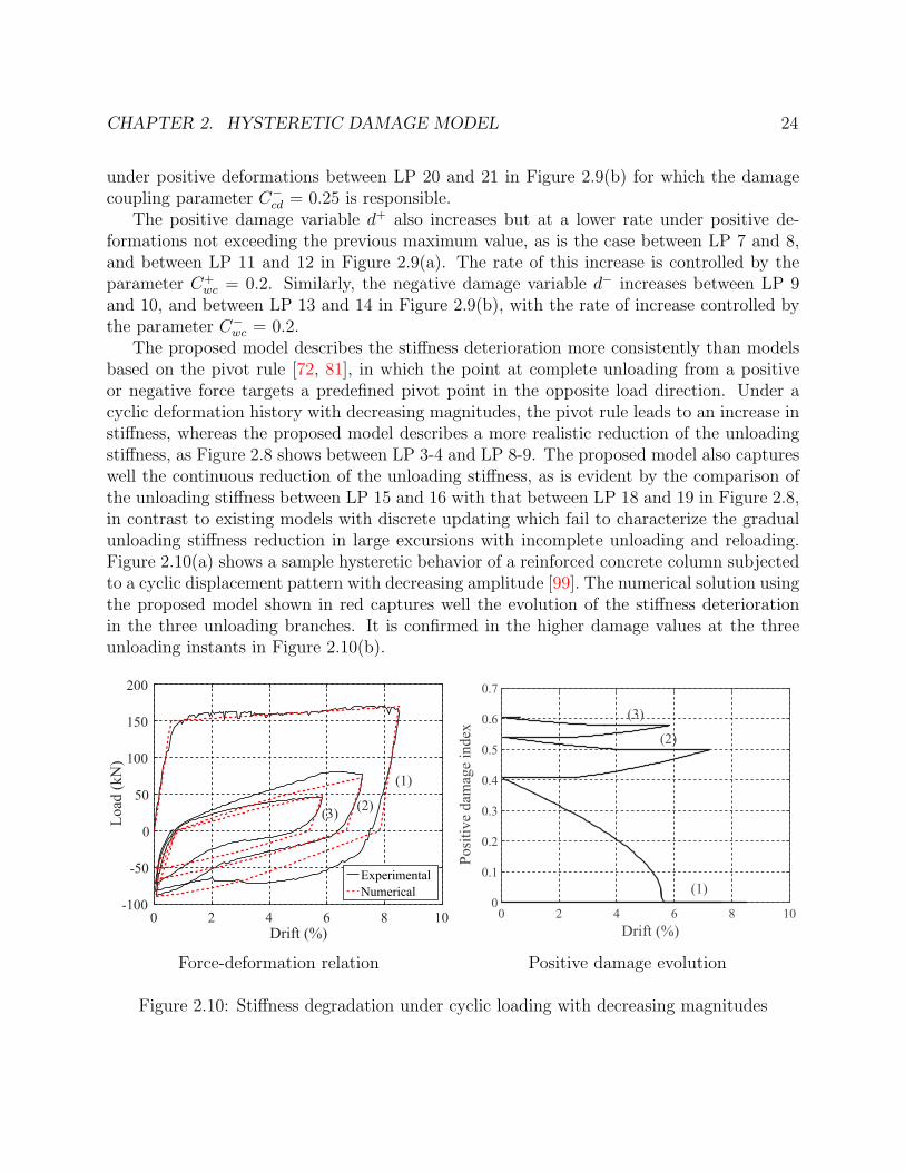
CHAPTER 2. HYSTERETIC DAMAGE MODEL 24
under positive deformations between LP 20 and 21 in Figure 2.9(b) for which the damagecoupling parameter C−
cd = 0.25 is responsible.The positive damage variable d+ also increases but at a lower rate under positive de-
formations not exceeding the previous maximum value, as is the case between LP 7 and 8,and between LP 11 and 12 in Figure 2.9(a). The rate of this increase is controlled by theparameter C+
wc = 0.2. Similarly, the negative damage variable d− increases between LP 9and 10, and between LP 13 and 14 in Figure 2.9(b), with the rate of increase controlled bythe parameter C−
wc = 0.2.The proposed model describes the stiffness deterioration more consistently than models
based on the pivot rule [72, 81], in which the point at complete unloading from a positiveor negative force targets a predefined pivot point in the opposite load direction. Under acyclic deformation history with decreasing magnitudes, the pivot rule leads to an increase instiffness, whereas the proposed model describes a more realistic reduction of the unloadingstiffness, as Figure 2.8 shows between LP 3-4 and LP 8-9. The proposed model also captureswell the continuous reduction of the unloading stiffness, as is evident by the comparison ofthe unloading stiffness between LP 15 and 16 with that between LP 18 and 19 in Figure 2.8,in contrast to existing models with discrete updating which fail to characterize the gradualunloading stiffness reduction in large excursions with incomplete unloading and reloading.Figure 2.10(a) shows a sample hysteretic behavior of a reinforced concrete column subjectedto a cyclic displacement pattern with decreasing amplitude [99]. The numerical solution usingthe proposed model shown in red captures well the evolution of the stiffness deteriorationin the three unloading branches. It is confirmed in the higher damage values at the threeunloading instants in Figure 2.10(b).
0 2 4 6 8 10Drift (%)
-100
-50
0
50
100
150
200
ExperimentalNumerical
Load
(kN
)
(1)
(2)(3)
Force-deformation relation
0 2 4 6 8 10Drift (%)
0
0.1
0.2
0.3
0.4
0.5
0.6
0.7
Posi
tive
dam
age
inde
x
(3)
(2)
(1)
Positive damage evolution
Figure 2.10: Stiffness degradation under cyclic loading with decreasing magnitudes
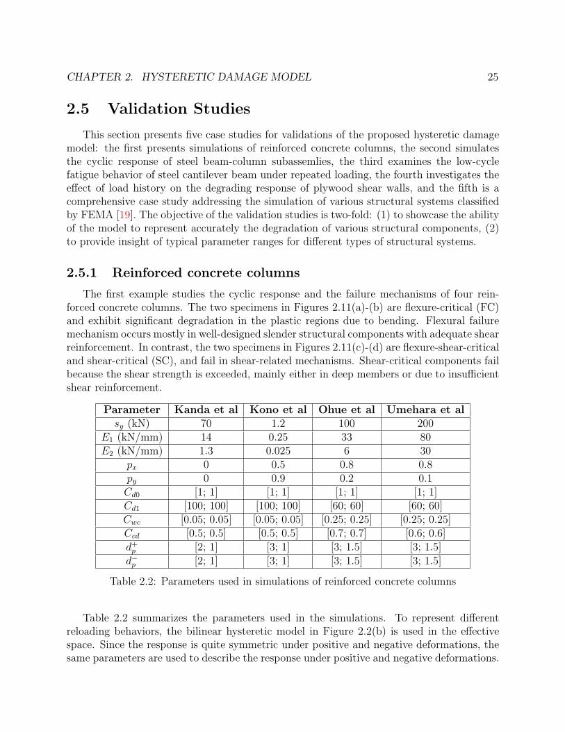
CHAPTER 2. HYSTERETIC DAMAGE MODEL 25
2.5 Validation Studies
This section presents five case studies for validations of the proposed hysteretic damagemodel: the first presents simulations of reinforced concrete columns, the second simulatesthe cyclic response of steel beam-column subassemlies, the third examines the low-cyclefatigue behavior of steel cantilever beam under repeated loading, the fourth investigates theeffect of load history on the degrading response of plywood shear walls, and the fifth is acomprehensive case study addressing the simulation of various structural systems classifiedby FEMA [19]. The objective of the validation studies is two-fold: (1) to showcase the abilityof the model to represent accurately the degradation of various structural components, (2)to provide insight of typical parameter ranges for different types of structural systems.
2.5.1 Reinforced concrete columns
The first example studies the cyclic response and the failure mechanisms of four rein-forced concrete columns. The two specimens in Figures 2.11(a)-(b) are flexure-critical (FC)and exhibit significant degradation in the plastic regions due to bending. Flexural failuremechanism occurs mostly in well-designed slender structural components with adequate shearreinforcement. In contrast, the two specimens in Figures 2.11(c)-(d) are flexure-shear-criticaland shear-critical (SC), and fail in shear-related mechanisms. Shear-critical components failbecause the shear strength is exceeded, mainly either in deep members or due to insufficientshear reinforcement.
Parameter Kanda et al Kono et al Ohue et al Umehara et alsy (kN) 70 1.2 100 200
E1 (kN/mm) 14 0.25 33 80E2 (kN/mm) 1.3 0.025 6 30
px 0 0.5 0.8 0.8py 0 0.9 0.2 0.1Cd0 [1; 1] [1; 1] [1; 1] [1; 1]Cd1 [100; 100] [100; 100] [60; 60] [60; 60]Cwc [0.05; 0.05] [0.05; 0.05] [0.25; 0.25] [0.25; 0.25]Ccd [0.5; 0.5] [0.5; 0.5] [0.7; 0.7] [0.6; 0.6]d+p [2; 1] [3; 1] [3; 1.5] [3; 1.5]
d−p [2; 1] [3; 1] [3; 1.5] [3; 1.5]
Table 2.2: Parameters used in simulations of reinforced concrete columns
Table 2.2 summarizes the parameters used in the simulations. To represent differentreloading behaviors, the bilinear hysteretic model in Figure 2.2(b) is used in the effectivespace. Since the response is quite symmetric under positive and negative deformations, thesame parameters are used to describe the response under positive and negative deformations.

CHAPTER 2. HYSTERETIC DAMAGE MODEL 26
The different reloading behaviors are reflected in the reloading parameters px and py. Forspecimen STC2 in Figure 6(a), px = py captures the typical peak-oriented reloading behaviorcommonly observed in reinforced concrete components. For specimen L1N60 in Figure 6(b),px < py describes the Bauschinger effect due to a high reinforcement ratio. For specimen4D13RS in Figure 6(c) and specimen CUW in Figure 6(d), px > py captures the pronouncedpinching behavior due to sliding, slip, and shear failure.
Displacement (mm)-60 -30 0 30 60
Forc
e (k
N)
-100
-50
0
50
100ExperimentalNumerical
(a) Kanda et al, STC2 [43]
Displacement (mm)-40 -20 0 20 40
Forc
e (M
N)
-1.6
-0.8
0
0.8
1.6ExperimentalNumerical
(b) Kono et al, L1N60 [10]
Displacement (mm)-18 -9 0 9 18
Forc
e (k
N)
-120
-60
0
60
120ExperimentalNumerical
(c) Ohue, 4D13RS [69]
Displacement (mm)-18 -9 0 9 18
Forc
e (k
N)
-300
-150
0
150
300ExperimentalNumerical
(d) Umehara, CUW [103]
Figure 2.11: Simulations of reinforced concrete columns
In all specimens, the threshold coefficient Cd0 = 1 indicates the onset of degradation uponreinforcement yielding. The damage parameters distinguish well the degrading behaviors ofFC and SC columns. The limit coefficient Cd1 for the FC specimens (Cd1 = 100) is higherthan for the SC specimens (Cd1 = 60) to indicate a higher ductility capacity of the FCcolumns. A relatively high cyclic degradation coefficient (Cwc = 0.25) and damage coupling

CHAPTER 2. HYSTERETIC DAMAGE MODEL 27
coefficient (Ccd = 0.6–0.7) seem to capture adequately the rapid strength deterioration undercyclic shear.
2.5.2 Steel beam-column joints
Figure 2.12 compares the experimental and the numerical load-displacement of four steelbeam-column subassemblages. This example selects the GMP model in Figure 2.2(a) todescribe the effective response.
The model captures well the smooth transition from the elastic to the plastic range andthe Bauschinger effect in the reloading response. This is achieved with the reloading param-eter r that varies within a relatively small range between 4–5. The threshold coefficientsC±d0 are greater than 1 for all specimens so that strength degradation initiates after yielding.
The relatively high displacement ductility of the steel specimens is reflected in the limitcoefficients C±
d1 in the range between 100–125. The damage evolution parameters d±p1 be-tween 4–5 and d±p2 = 1 capture well the degradation rate in the softening range. The cycliccoefficients Cwc and the damage coupling coefficients Ccd simulate accurately the strengthand stiffness degradation due to cyclic loading. Similar damage parameters are specified forthe positive and negative response due to symmetric degrading behavior. One exception isa higher d+p1 than d−p1 in specimen UCSD-3R to capture the more severe deterioration underpositive forces.
Parameter EERC-RN2 EERC-RN3 UCSD-1R UCSD-3RE (kip/in) 100 100 100 100sy (kip) 150 150 130 140
b 0.04 0.05 0.045 0.045r 4 5 4 4Cd0 [3; 3] [2; 2] [3; 3] [3; 3]Cd1 [125; 125] [100; 100] [100; 100] [120; 120]Cwc [0.12; 0.12] [0.1; 0.1] [0.15; 0.15] [0.15; 0.15]Ccd [0.5; 0.5] [0.5; 0.5] [0.5; 0.5] [0.5; 0.5]d+p [4.2; 1] [5; 1] [4.5; 1] [5; 1]
d−p [4.2; 1] [5; 1] [4.5; 1] [3; 1]
Table 2.3: Parameters used in simulations of steel beam-column joints
2.5.3 Low-cycle fatigue of steel components
To study the low-cycle fatigue behavior, the experimental campaign by Krawinkler [51]furnishes measurements of the hysteretic behavior for steel components. Three identicalcantilever steel beams are selected for the response simulation: specimen B24 is subject toa monotonic deformation history, and specimens B25 and B28 to cyclic load protocols.

CHAPTER 2. HYSTERETIC DAMAGE MODEL 28
-8 -4 0 4 8Deflection (in)
-150
-100
-50
0
50
100
150
Forc
e (k
ip)
ExperimentalNumerical
(a) EERC-RN2
-8 -4 0 4 8Deflection (in)
-150
-100
-50
0
50
100
150
Forc
e (k
ip)
ExperimentalNumerical
(b) EERC-RN3
-6 -3 0 3 6Deflection (in)
-150
-100
-50
0
50
100
150
Forc
e (k
ip)
ExperimentalNumerical
(c) UCSD-1R
-6 -3 0 3 6Deflection (in)
-150
-100
-50
0
50
100
150Fo
rce
(kip
)
ExperimentalNumerical
(d) UCSD-3R
Figure 2.12: Simulations of steel beam-column assemblages
The subsequent simulations use the GMP model in Figure 2.2(a) to describe the effec-tive force-deformation relation. The same parameters are specified to reflect the symmetricgeometry and properties of the specimens under positive and negative deformations. Thefollowing parameters are satisfactory for specimen B24 in Figure 2.13(a): E = 28, sy = 9.8,b = 0.04, r = 4, Cd0 = 5, Cd1 = 150, dp1 = 3, dp2 = 1.5. The selection of Cd0 greater than 1 istypical for steel components to indicate that the strength reduction initiates after yielding.The values of Cd1, dp1 and dp2 are also representative of steel components. The numericalsolution matches rather well the post-yield response of the specimen. The evolution of thehysteretic energy in Figure 2.13(a2) confirms that the numerical solution agrees rather wellwith the experimental result.
Next, the cyclic test B25, which consists of several cycles at a constant displacement

CHAPTER 2. HYSTERETIC DAMAGE MODEL 29
0 0.5 1 1.5 2Deflection (in)
0
2
4
6
8
10
12
Load
(kip
)
ExperimentalNumerical
(a1) B24: Force-deformation
-0.8 -0.4 0 0.4 0.8
-10
-5
0
5
10
Deflection (in)Lo
ad (k
ip)
ExperimentalNumerical
(b1) B25: Force-deformation
-1 -0.5 0 0.5 1
-10
-5
0
5
10
Load
(kip
)
Deflection (in)
ExperimentalNumerical
(c1) B28: Force-deformation
0 0.5 1 1.5 2Deflection (in)
0
5
10
15
20
Ener
gy (k
ip-in
)
2.5
ExperimentalNumerical
(a2) B24: Hysteretic energy
0 200 400 600 800 1000Pseudo-time
-15
-10
-5
0
5
10
15
Load
(kip
)
ExperimentalNumerical
(b2) B25: Force time history
0 100 200 300 400-15
-10
-5
0
5
10
15
ExperimentalNumerical
Pseudo-time
Load
(kip
)(c2) B28: Force time history
Figure 2.13: Simulation of steel cantilever beams under cyclic loading
amplitude, facilites the calibration of the cyclic degradation coefficient Cwc and the damagecoupling coefficient Ccd. The numerical force-deformation relation with Cwc = 0.14 andCcd = 0.5 in Figure 2.13(b) compares reasonably well with the experimental measurements.One limitation is the inadequate representation of the rapid strength degradation in the lasthalf cycle. The parameters dp1 and dp2 of the damage evolution function could be modifiedto concentrate more damage at larger energy dissipation. The discrepancy also suggeststhat the selection of the limit coefficient Cd1 = 150 may not be accurate enough. Insteada slightly lower value may represent better the rapid degradation and the lower ductilitycapacity. Nonetheless, the force time history in Figure 2.13(b2) confirms that the proposeddamage model captures adequately the peak forces in the half cycles.
To validate the calibration, the same parameters are used to simulate the response of an-other identical specimen under a different cyclic deformation history. Figure 2.13(c) showsthe force-deformation relation for specimen B28, which is subjected to a cyclic deformationhistory with larger amplitudes. The numerical solution agrees well with the experimentalresult albeit with the same limitations as previously discussed. Although the model under-estimates the strength in compression, the numerical solution shows a consistent pattern ofstrength degradation in reasonable agreement with the experiment, as the force time historyin Figure 2.13(c2) shows.

CHAPTER 2. HYSTERETIC DAMAGE MODEL 30
2.5.4 Effect of load histories on plywood shearwalls response
Drift (mm)-150 -75 0 75 150
Load
(kN
)
-40
-20
0
20
40
ExperimentalNumerical
Drift (mm)-200 -100 0 100 200
Load
(kN
)
-50
-25
0
25
50
ExperimentalNumerical
(a) ISO loading protocol (b) CUREE loading protocol
Drift (mm)-120 -60 0 60 120
Load
(kN
)
-40
-20
0
20
40
ExperimentalNumerical
(c) SPD loading protocol (d) NF loading protocol
Drift (mm)-100 0 100 200
Load
(kN
)
-50
-25
0
25
50
ExperimentalNumerical
Figure 2.14: Numerical and experimental correlation for plywood shear walls
To study the model response under different load histories the experimental campaignby Gatto and Uang [29] furnishes measurements of the hysteretic behavior for four identicalplywood shear walls under different deformation histories corresponding to the ISO, CUREE,SPD and NF loading protocol. For the first three protocols the loading consists of groups ofdisplacement cycles of either constant or variable amplitude from one cycle to the next withgradually increasing average amplitude of the group as loading progresses. The NF loadingprotocol consists of several cycles with small but ever increasing displacement amplitudefollowed by very few large displacement cycles of increasing amplitude to simulate the effect

CHAPTER 2. HYSTERETIC DAMAGE MODEL 31
of near-fault ground motions [50].Figure 2.14 shows the numerical results for the plywood shear walls under the four load
histories. The proposed damage model uses the bilinear hysteretic model in Figure 2.2(b) torepresent the force-deformation relation of the plywood shear wall in the effective space. Thesame parameters are used for the effective response under positive and negative deformationswith the following properties: syp = 17 kN, E1p = 1.7 kN/mm, E2p = 0.6 kN/mm, syn =-17 kN, E1n = 1.7 kN/mm, E2n = 0.6 kN/mm. To account for the pronounced pinching ofthe hysteretic force-displacement relation during reloading the control point coordinates ofthe bilinear reloading branch are selected as px = 0.9, py = 0.2, very similar to the valuesfor systems S1, S2 and S5 in Table 2.4. The same reloading parameters are used in bothloading directions.
The parameters of the damage loading function are C±d0 = 1, C±
d1 = 200, C±wc = 0.15,
and C±cd = 0.2, with the parameters of the damage evolution law set as [d±p1; d
±p2] = [2.25; 1].
These parameters are kept the same for the analysis of the plywood shear walls under thefour load histories.
The comparison of the numerical results with the experimental measurements show satis-factory agreement for the evolution of the strength and stiffness deterioration of the plywoodshear walls under the four load histories. The agreement is particularly good for the SPDload history Figure 2.14(c) and quite good for the NF load history in Figure 2.14(d). Theability of the model to capture the non-symmetric damage evolution between positive andnegative deformations in Figure 2.14(d) is noteworthy since this type of loading proved chal-lenging for earlier models. The underestimation of the actual deterioration in the early cyclesunder the ISO load protocol in Figure 2.14(a) and the overestimation of the deteriorationunder the CUREE load protocol in Figure 2.14(b) suggest that the energy dissipation ofdisplacement cycles with large amplitude may have a stronger impact on the deteriorationthan the energy of displacement cycles with small amplitude which are quite numerous inthe CUREE protocol for simulating the effect of far field ground motions. This leads to theconclusion that a value for the damage evolution law parameter d±p2 greater than 1 may be amore suitable choice than the selected value d±p2=1, which corresponds to the damage variabled being proportional to the normalized energy dissipation in Figure 2.5(b). As noted already,no effort is made in this study to optimize the selection of parameters for best fit, which isleft for further study with parameter identification methods. The extensively calibrated hys-teretic model by Ibarra et al. [39] shows similar discrepancies between the numerical and theexperimental results for the early cycles of the ISO and CUREE load history underscoringthe importance of further study for the calibration of the damage evolution law.
2.5.5 Degrading behavior of structural systems
To further showcase the ability of the proposed damage model to represent the hystereticbehavior of different structural component types, the comprehensive study of the effectsof strength and stiffness degradation on the seismic response of structural systems in theframework of the FEMA P440A Recommendations is used as a reference [19]. The capacity

CHAPTER 2. HYSTERETIC DAMAGE MODEL 32
boundary curves of the FEMA P440A Recommendations inform the parameter selection forthe damage loading function and for the damage evolution law of each structural component.The following structural components are used in the correlation studies: a typical gravityframe, subsequently referred to as system S1, a non-ductile moment frame (S2), a ductilemoment frame (S3), a stiff non-ductile system (S4), a stiff and highly-pinched non-ductilesystem (S5), and a limited ductility moment frame (S7). These categories of hystereticbehavior follow the classification in the FEMA P440A Recommendations.
2.5.5.1 System S1 - Typical Gravity Frame
The capacity boundary for a typical gravity frame is characterized by a sudden strengthdrop of 45% of the yield strength of the component following yielding [19]. This capacityboundary is representative of the moment-rotation relation of a beam-to-column shear tabconnection in Figure 2.15(b), as established by experiments such as those by Liu and Astaneh[58]. The observed strength degradation of these connections is caused by the closing of thegap between the beam and the column flange causing the bearing strength failure of the boltsin the shear tab and eventually leading to the shear connection failure [58]. The responseunder positive and negative deformation does not appear to be the same, but the FEMAP440A Recommendations do not discuss the matter.
Rotation (rad)-0.15 -0.075 0 0.075 0.15
Mom
ent (
MN
m)
-2
-1
0
1
2Effective responseTrue response
Rotation (rad)-0.15 -0.075 0 0.075 0.15
Mom
ent (
MN
m)
-1
0
1
2ExperimentalNumerical
(a) Relation between effective and true response (b) Numerical and experimental correlation
Figure 2.15: Simulation of beam-to-column shear tab connections (S1 system)
Figure 2.15(a) shows the bilinear hysteretic model in Figure 2.2(b) for the effectivemoment-rotation relation of the shear tab connections with the values reported in the col-umn under the label S1 in Table 2.4. The values sy, E1 and E2 under a positive rotation aredifferent from the values under a negative rotation to do justice to the observed response inFigure 2.15(b). The same is true for the damage parameters Cd0 and Cd1 for the damageinitiation and the damage limit, respectively. To account for the pronounced pinching of the

CHAPTER 2. HYSTERETIC DAMAGE MODEL 33
hysteretic moment-rotation relation during reloading, the relative control point coordinatesof the bilinear reloading branch are selected as px = 0.90 and py = 0.20. Furthermore, theparameter dp2 of the damage evolution law is selected to account for the sudden strengthloss and the subsequent reduced strength plateau of the connections. In accordance withFigure 2.5 the smaller the value of dp2 is relative to 1 the sharper the early drop, particularlyif it is weighted with a value of dp1 larger than 1. Accordingly, d+p2 = 0.1 and d−p2 = 0.3 areselected along with d+p1 = 1 and d−p2 = 2. Figure 2.15(a) shows the resulting true responseaccording to Equation (2.14) for the cyclic deformation history of the experimental results.The true response of the damage model compares quite favorably with the experimentalmeasurements in Figure 2.15(b), particularly with regard to the strength degradation of theconnection.
2.5.5.2 System S2 - Non-Ductile Moment Frame
The capacity boundary for a non-ductile moment frame is characterized by a very sharpstrength drop to 15% of the yield strength of the component following yielding [19]. Thestrength plateau at this strength extends from a relative drift of 3% to the ultimate drift of6%. This capacity boundary is representative of older steel and concrete structures [19], suchas the steel moment-resisting frames with pre-Northridge welded beam-column connections,in which connection fracture leads to the sudden strength drop, and reinforced concreteframes with inadequate column and joint confinement as well as poor detailing of the re-inforcement, in which the sudden strength drop is related to the shear failure of columnsand joints. Figure 2.16(b) shows the measured moment-rotation relation of a pre-Northridgewelded steel beam-to-column connection from the experiments by Stojadinovic and Goel[96]. The response under positive and negative moment is not the same, but the FEMAP440A Recommendations do not discuss the matter.
Figure 2.16(a) shows the bilinear hysteretic model in Figure 2.2(b) for the effectivemoment-rotation relation of the non-ductile welded steel beam-column connection with thevalues reported in the column under the label S2 in Table 2.4. The values sy, E1 and E2
under a positive rotation are only slightly different from the values under a negative rotationto account for the observed response in Figure 2.16(b). The damage parameter Cd0 is set to1 for positive and negative deformations to reflect the fact that damage initiates at the onsetof yielding. The significant difference in the resulting true response in Figure 2.16(a) and (b)arises from the large difference in the value of the damage limit parameter Cd1 (Table 2.4):it is set to 10 under positive deformations and to 200 under negative deformations. Thelow value of C+
d1 represents very well the rapid strength loss of the fracturing connections inFigure 2.16(b). To account for the asymmetric reloading behavior, different control pointcoordinates are selected for the two bilinear reloading branches with pxp = 0.1 and pyp = 0.4representing the evident Bauschinger effect under positive moments, and pxn = 0.95 andpyn = 0.1 describing the pronounced pinching under negative moments.
The parameter dp2 of the damage evolution law is selected again to account for the suddenstrength loss of the connections under positive rotations. In accordance with Figure 2.5 the

CHAPTER 2. HYSTERETIC DAMAGE MODEL 34
(a) Relation between effective and true response (b) Numerical and experimental correlation
-0.03 -0.015 0 0.015 0.03-8
-4
0
4
8
Rotation (rad)
Mom
ent x
10-3
(kip
-in)
Effective responseTrue response
-0.03 -0.015 0 0.015 0.03-8
-4
0
4
8
Rotation (rad)
Mom
ent x
10-3
(kip
-in)
ExperimentalNumerical
Figure 2.16: Simulation of pre-Northridge non-ductile welded steel beam-column connections(system S2)
smaller the value of dp2 is relative to 1 the sharper the early drop, particularly if it is weightedwith a value of dp1 larger than 1. Accordingly, d+p2 = 0.05 is selected along with d+p1 = 4.In contrast, the parameters of the damage evolution law under negative deformations areleft to the default values of 1 (Table 2.4). Figure 2.16(a) shows the resulting true responseaccording to Equation (2.14) for the cyclic deformation history of the experimental results.The true response of the damage model is consistent with the experimental measurementsfor all cycles in Figure 2.16(b) with regard to the strength deterioration under positiveand negative moments. The Bauschinger effect under reloading in the positive directionis consistent with the experimental observations for all cycles. In contrast, the pinchingof the hysteretic moment-rotation relation during reloading in the negative direction is onlycaptured well in the late cycles. To improve these results, the future extension of the bilinearhysteretic model should consider relating the coordinates of the reloading control point tothe damage evolution.
2.5.5.3 System S3 - Ductile Moment Frame
The capacity boundary for a ductile moment frame consists of 4 linear segments: the lin-ear elastic range is followed by the strength hardening segment with stiffness equal to 2% ofthe initial stiffness, which is then followed by a strength softening segment over the deforma-tion range from 4% to 6%, and a residual strength plateau up to the ultimate deformationof 8%. This capacity boundary is representative of newer steel and concrete structures,such as the post-Northridge steel special moment-resisting frames with ductile beam-columnconnections and well detailed reinforced concrete moment resisting frames [19].
Figure 2.17(b) shows the measured moment-rotation relation of a post-Northridge welded

CHAPTER 2. HYSTERETIC DAMAGE MODEL 35
(a) Relation between effective and true response (b) Numerical and experimental correlation
-0.08 -0.04 0 0.04 0.08-40
-20
0
20
40
Rotation (rad)
Mom
ent x
10-3
(kip
-in)
Effective responseTrue response
-0.08 -0.04 0 0.04 0.08
-30
-15
0
15
30
Rotation (rad)
Mom
ent x
10-3
(kip
-in)
ExperimentalNumerical
Figure 2.17: Simulation of post-Northridge ductile steel beam-column connections (systemS3)
beam-column connection with reduced beam section from the experiments by Venti and En-gelhardt [106]. Because all metallic components show a Bauschinger effect during reloading,the effective response is based on the GMP model in Figure 2.2(a). To accommodate thediscrepancy in the hardening and reloading behavior under positive and negative moments,the parameter values for b, r, cR1, cR2 for the positive branch are different from those for thenegative branch. The relatively large r+ = 7 and r− = 10 in combination with c+R2 = 0.75and c−R2 = 1 result in full hysteresis loops with large energy dissipation capacity. The param-eters c+R1 = 0.82 and c−R1 = 0.85 make the transition from elastic to plastic behavior moregradual as the deformation amplitude increases. Figure 2.17(a) shows the cyclic behavior ofthe model in the effective space.
The model captures the asymmetric onset of strength deterioration in Figure 2.17(b)with a value for the damage threshold parameter under positive deformations C+
d0 = 22that differs from that of the same parameter under negative deformations C−
d0 = 11. Bothvalues indicate that strength reduction initiates after significant plastic deformation. Thehigh values of C±
d1 = 150 represent very well the significant ductility of the steel component.The asymmetric strength degradation is captured by selecting two values for the damageparameter dp2, with d−p2 under negative moment less than 1 for describing an early strengthreduction, while d+p2 is equal to 1. Both dp1 values are set equal to 2 slightly biasing thestrength reduction to smaller normalized energy dissipation values according to Figure 2.5.Figure 2.17(a) shows the resulting true response for the cyclic deformation history of thespecimen. Except for the reloading response in the last cycle, the true response of the damagemodel compares very well with the experimental results in Figure 2.17(b) with regard to thereloading behavior and the strength and stiffness deterioration under the cyclic load history.

CHAPTER 2. HYSTERETIC DAMAGE MODEL 36
2.5.5.4 System S4 - Stiff, Non-Ductile System
The capacity boundary for a relatively stiff lateral force-resisting system is characterizedby the significant and rapid strength loss to 30% of the yield strength at a deformation of0.4% [19]. The strength loss is followed by an extensive strength plateau from a deformationof 2% to the ultimate deformation of 8%. This capacity boundary is representative ofconcentrically braced steel frames that experience a significant and rapid strength loss dueto brace buckling at a small lateral drift [19].
(a) Relation between effective and true response (b) Numerical and experimental correlation
-5 -2.5 0 2.5 5Displacement (in)
-600
-300
0
300
600
Forc
e (k
ip)
Effective responseTrue response
-5 -2.5 0 2.5 5Displacement (in)
-600
-300
0
300
600
Forc
e (k
ip)
ExperimentalNumerical
Figure 2.18: Simulation of stiff, non-ductile concentrically braced steel frame (system S4)
Figure 2.18 shows the force-displacement relation of a concentrically braced steel framefrom the experiments by Uriz and Mahin [104]. To capture the Bauschinger effect duringreloading, the GMP model in Figure 2.2(a) is used for the effective force-deformation relation.Similar to specimen S3, a large value for parameters r± = 10 and c±R2 = 0.5 describes a fullhysteresis loop in the first cycle with a relatively sharp transition from the elastic to theplastic range. In contrast to the ductile response of specimen S3, a high value for theparameters c±R1 = 0.96 is used to extend the gradual transition range during reloading andrepresents well the reloading stiffness deterioration after buckling initiation.
Slightly different values for the damage threshold coefficients, C+d0 = 35 and C−
d0 = 30,are selected to simulate the asymmetric onset of strength deterioration under positive andnegative deformation. Similar to the steel specimen S3, the values indicate that strengthreduction initiates after significant plastic deformation. A damage parameter value dp2 lessthan 1 with d+p2 = 0.5 and d−p2 = 0.3 in combination with a d±p1 value greater than 1 capturesvery well the rapid strength deterioration after buckling initiation at the end of the secondloading cycle. The severe cyclic degradation and the damage coupling under positive andnegative deformations for the non-ductile system are reflected in relatively high values for Cwcand Ccd, with C±
wc = 0.27 and C±cd = 0.50. Figure 2.18(b) shows that overall the resulting

CHAPTER 2. HYSTERETIC DAMAGE MODEL 37
true response compares rather well with the experimental measurements in regard to theevolution of the strength and stiffness degradation of the non-ductile concentric steel bracedframe, even though the model slightly overestimates the measured strength in the first cycleunder negative deformation.
2.5.5.5 System S5 - Stiff, Non-Ductile System with Pronounced Pinching
The capacity boundary for a relatively stiff, non-ductile system consists of 4 linear seg-ments: the linear elastic range is followed by the strength hardening segment with highrelative stiffness, which is then followed by two strength softening segments up to the ulti-mate deformation of 6% [19]. This capacity boundary is representative of non-ductile ma-sonry walls and concrete frames with masonry infill with the elastic range corresponding tothe pre-cracking response and the steep strength hardening segment to the post-crackingresponse until yielding [19]. Figure 2.19(b) shows the measured force-displacement relationof a masonry wall from the experiments by Shing [90].
(a) Relation between effective and true response (b) Numerical and experimental correlation
Displacement (in)-2 -1 0 1 2
Forc
e (k
ip)
-80
-40
0
40
80Effective responseTrue response
Displacement (in)-2 -1 0 1 2
Forc
e (k
ip)
-60
-30
0
30
60ExperimentalNumerical
Figure 2.19: Simulation of stiff, non-ductile masonry wall with pronounced pinching (systemS5)
Figure 2.19(a) shows the shows the bilinear hysteretic model in Figure 2.2(b) for theeffective force-displacement relation of the masonry wall. Because the experimental responseunder positive and negative deformations is quite similar, the same parameters are used forthe effective force-deformation relation under positive and negative deformations. The sameis true for all damage parameters of the model except for dp1. The column under label S5in Table 2.4 lists the parameter values for the true response in Figure 2.19(a). The damagethreshold coefficient C±
d0 is set equal to 1 to indicate that the onset of strength reductionfor the masonry wall coincides with the yielding of the reinforcement. The relatively lowdisplacement ductility of the system is reflected in the limit damage parameter value C±
d1

CHAPTER 2. HYSTERETIC DAMAGE MODEL 38
= 80. To account for the pronounced pinching of the hysteretic force-displacement relationduring reloading the control point coordinates of the bilinear reloading branch are selectedas px = 0.80 and py = 0.20. The selection of the value of 0.15 for the cyclic degradationcoefficient C±
wc appears to capture well the effect of the energy dissipation during followercycles of the deformation history. The true response of the damage model compares ratherwell with the experimental measurements in Figure 2.19(b) in regard to the evolution of thestrength and stiffness deterioration of the masonry wall. The hysteretic behavior also showsreasonable agreement.
2.5.5.6 System S7 - Limited Ductility Moment Frame
The capacity boundary for a structural component of limited ductility consists of 4 lin-ear segments: the linear elastic range is followed by the yield plateau with limited ductility,which is then followed at a deformation of 2% by a strength softening segment that termi-nates at 20% of the yield strength of the component. This is followed, in turn, by a shortresidual strength plateau up to the ultimate deformation of 6% [19]. This capacity bound-ary is representative of older lightly reinforced concrete columns and beam-column jointswith inadequate confinement that are susceptible to shear failure [19]. Figure 2.20(b) showsthe measured force-displacement relation of a lightly reinforced concrete column from theexperiments by Sezen and Moehle [89].
(a) Relation between effective and true response (b) Numerical and experimental correlation
-80 -40 0 40 80Displacement (in)
-350
-175
0
175
350
Forc
e (k
ip)
ExperimentalNumerical
-80 -40 0 40 80Displacement (in)
-350
-175
0
175
350
Forc
e (k
ip)
Effective responseTrue response
Figure 2.20: Simulation of lightly reinforced concrete column with limited-ductility (systemS7)
Figure 2.20(a) shows the the shows the bilinear hysteretic model in Figure 2.2(b) forthe effective force-displacement relation of the lightly reinforced concrete column. Becausethe experimental response under positive and negative deformations is practically the same,the same parameters are used for the effective force-deformation relation under positive and

CHAPTER 2. HYSTERETIC DAMAGE MODEL 39
negative deformations. The same is true for the damage parameters of the model, which arelisted in the column under label S7 in Table 2.4. To account for the yield plateau of limitedductility, a small value of E2p = E2n = 0.4 is assigned to the strain hardening stiffness. Forthe same reason the damage threshold coefficient C±
d0 is set equal to 10 to delay the onsetof damage until an energy dissipation of 10 times the yield energy. The low displacementductility of the system is reflected in the limit damage parameter value C±
d1 = 40. Theselection of the value of 0.5 for the damage parameter d±p2 in combination with the valueof 2.1 for the damage parameter d±p1 is meant to capture the rapid strength deteriorationfollowing the onset of damage. To account for the pronounced pinching of the hysteretic force-displacement relation during reloading the control point coordinates of the bilinear reloadingbranch are selected as px = 0.50 and py = 0.10 under positive and negative deformations. Theselection of the value of 0.25 for the cyclic degradation coefficient C±
wc appears to capture wellthe effect of the energy dissipation during follower cycles of the deformation history. Equallyimportant is the effect of the energy dissipation under positive moments and of the energydissipation under negative moments on the strength reduction in the opposite direction, asreflected in the relatively high value of the coupling damage parameter C±
cd = 0.5. WhileFigure 2.20(a) only includes the nonlinear material response of the specimen, the numericalresponse in Figure 2.20(b) superimposes the additional force contribution from the nonlineargeometry effect under the axial force of the column, which is noticeable as negative stiffnessduring the early reloading stage under large deformations. Figure 2.20(b) shows that theresulting true response compares quite favorably with the experimental measurements inregard to the evolution of the strength and stiffness degradation of the lightly reinforcedconcrete column. The hysteretic behavior also seems to be adequately captured.
2.5.5.7 Conclusions from the simulations of degrading behavior
The preceding simulations demonstrate the flexibility of the proposed damage model forthe simulation of the hysteretic behavior of different structural component types. Table 2.4summarizes the parameters for the simulations. The top 16 rows of the table contain theparameters of the force-deformation relation in effective space. The effective response withthe GMP model in Figure 2.2(a) requires 14 parameters: the initial stiffness E, the yieldstrength sy, the hardening ratios b±, the reloading parameters r±, c±R1, c
±R2, and the isotropic
hardening parameters a1, a2, a3, a4. The first two parameters are the same under positiveand negative deformations. The default values a2 = a4 = 0 are assumed in all simulations torepresent the onset of isotropic hardening behavior at the start of the deformation history.
The strength envelope for the bilinear hysteretic model in Figure 2.2(b) requires 6 mate-rial parameters, 3 for the envelope under positive deformations and 3 for the envelope undernegative deformations. These are the yield strength sy, the initial modulus E1, and the post-yield modulus E2. Furthermore, the bilinear hysteretic model requires four more parametersfor the coordinates of the control point for the bilinear reloading branch in Figure 2.2(b), pxpand pyp in the positive reloading direction and pxn and pyn in the negative reloading direc-tion. These can be used for the description of the Bauschinger effect in metallic structural

CHAPTER 2. HYSTERETIC DAMAGE MODEL 40
components or for the description of pinching in structural members with sliding, slip andshear deformations.
Parameter S1 S2 S3 S4 S5 S7E - - 6,000 2,167 - -sy - - 28 580 - -
[b+; b−] - - [0.0125; 0] [0.005; 0.005] - -[r+; r−] - - [7; 10] [10; 10] - -
[c+R1; c−R1] - - [0.82; 0.85] [0.96; 0.96] - -
[c+R2; c−R2] - - [0.75; 1] [0.5; 0.5] - -
[a1; a3] - - [0.025; 0.025] [0.05; 0.05] - -[a2; a4] - - [0; 0] [0; 0] - -syp 1.6 7.5 - - 45 310E1p 53.3 730 - - 300 31E2p -5.0 50 - - 14.3 0.4syn -0.6 -6.6 - - -45 -310E1n 120 660 - - 300 31E2n 6.7 100 - - 14.3 0.4
[pxp; pyp] [0.9; 0.2] [0.1; 0.4] - - [0.8; 0.2] [0.5; 0.1][pxn; pyn] [0.9; 0.2] [0.95; 0.1] - - [0.8; 0.2] [0.5; 0.1]Cd0 [3; 10] [1; 1] [22; 11] [37; 31] [5; 5] [10; 10]Cd1 [120; 200] [10; 200] [150; 150] [110; 110] [80; 80] [40; 40]Cwc [0.05; 0.05] [0.25; 0.25] [0.14; 0.14] [0.27; 0.27] [0.15; 0.15] [0.25; 0.25]Ccd [0.30; 0.30] [0.50; 0.50] [0.36; 0.36] [0.50; 0.50] [0.20; 0.20] [0.50; 0.50]
[d+p1; d+p2] [1.0; 0.1] [4.5; 0.05] [2.0; 1.0] [1.5; 0.5] [2.0; 1.5] [2.1; 0.5]
[d−p1; d−p2] [2.0; 0.3] [1.0; 1.0] [2.0; 0.75] [3; 0.3] [1.5; 1.5] [2.1; 0.5]
Table 2.4: Parameters for the simulations of the degrading hysteretic behavior of structuralcomponents
Most parameters of the effective response correspond to mechanical properties of thestructural components, such as the initial stiffness and the yield strength, and can, therefore,be readily established. The hardening or softening post-yield behavior can also be readilyestablished for typical structural components. Observations about the reloading behaviorof a structural component are used for the selection of the parameters px and py: the case0 ≤ py < px ≤ 1 represents pinching behavior, while the case 0 ≤ px < py ≤ 1 representsreloading behavior mimicking the Bauschinger effect. The selection px = py results in alinear reloading branch from the point of complete unloading to the maximum previousdeformation under a force of opposite sign. While any px = py ≤ 1 is equally suited for thepurpose, the discussion makes reference to px = py = 1 for this case.
The remaining 12 parameters control the evolution of strength and stiffness deterioration

CHAPTER 2. HYSTERETIC DAMAGE MODEL 41
and have a clear physical meaning. Of these 4 are relatively easy to establish from thecapacity boundary of a structural component: the threshold damage parameter C±
d0 andthe limit damage parameter C±
d1. The determination of the remaining 8 parameters shouldideally be based on formal parameter identification methods. Such a formal process is beyondthe scope of this study. Moreover, the correlation studies of the numerical results with theexperimental measurements show that very satisfactory agreement results with a relativelyconsistent set of values for these parameters across a wide spectrum of observed hystereticbehavior of structural components. This conclusion is supported by the small range ofvariation for the numerical values of Ccd and Cwc in Table 2.4. The same is also true for thevalues of dp, particularly after consideration of Figure 2.5.
While the agreement between numerical simulations and experimental results in Fig-ure 2.15-Figure 2.20(d) can certainly be improved, the description for the evolution of thestrength and stiffness deterioration seems very satisfactory. The small variation of the pa-rameters Ccd, Cwc in Table 2.4 and the direct relation of the parameters dp to the damageevolution according to Figure 2.5 implies that a selection of values within the range of Ta-ble 2.4 is likely to result in a very satisfactory representation of the observed hystereticbehavior.
2.6 Damage Variables
2.6.1 Comparison with Park-Ang index
The purpose of the following discussion is two-fold: first to show that the damage variabled of the proposed model can be calibrated to give an assessment of the damaged state of astructural component that is consistent with the well known damage index by Park-Ang forstandard cases of structural component characteristics and loading, and second to highlightthe flexibility and some of the capabilities of the proposed formulation by pointing outspecific cases where the damage variable deviates from the Park-Ang damage index. It isworth pointing out at the outset that alternative damage indices such as the one proposed byMehanny and Deierlein [63], or, improvements of the Park-Ang index such as the proposalby Bozorgnia and Bertero could have been used for the comparison without changing theessence of the argument.
The Park-Ang (PA) damage index dPA [73] is the linear combination of the maximumdeformation em and the hysteretic energy dissipation E
dPA =emeu
+β
syeu
∫dE (2.15)
where eu is the deformation capacity under monotonic loading. This damage index has beenextensively calibrated and is referenced often in seismic response studies. Because the originalproposal does not distinguish between the effect of positive and negative deformations, thefollowing discussion is limited to cases with symmetric response. Because the proposed

CHAPTER 2. HYSTERETIC DAMAGE MODEL 42
model accounts for the effect of two damage variables on the hysteretic response accordingto Equation (2.14), the following discussion is limited to load histories with the largestexcursion of each cycle occurring under positive deformations, so that the Park-Ang indexcan be compared with the damage variable d+.
(a) Monotonic response (b) Comparison of damage evolution after calibration
0 10 20 30Normalized deformation e/ey
0
0.25
0.5
0.75
1
Nor
mal
ized
forc
e s/
s y
0 10 20 30Normalized deformation e/ey
0
0.2
0.4
0.6
0.8
1
Damage index dPADamage variable d+
Dam
age
inde
x/va
riabl
e
Figure 2.21: Monotonic response and comparison of Park-Ang damage index with damagevariable d+
At the outset of the comparison the following parameters are selected for the proposedmodel: E2p/E1p = 0.05, Cd0 = 0, Cd1 = 100, dp1 = 1.5, dp2 = 0.8. While the first and thirdparameter are arbitrary, Cd0 is set equal to zero to match the assumption of the Park-Angindex that damage initiates even under elastic deformation, which may not be realistic formany structural components [12]. The selection of the parameters dp1 and dp2 is so that thedamage evolution law of the model is almost linear with increasing deformation to matchthe linear evolution of the Park-Ang damage index. This parameter selection results in thenormalized force-deformation response in Figure 2.21(a) for the bilinear hysteretic modelin Figure 2.2(b) for the effective force-deformation relation. The dPA parameters in Equa-tion (2.15), i.e. the ultimate deformation eu and the energy dissipation parameter β, are thenselected to match the damage evolution of the model in Figure 2.21(a): with the selectioneu/ey = 32 where ey is the yield deformation and β = 0.15, dPA and d+ are practically thesame in Figure 2.21(b). The Park-Ang damage index dPA varies linearly with the normalizeddeformation e/ey. As already noted, the damage evolution law parameters dp1 and dp2 werespecifically selected to match this linear variation as closely as possible. Figure 2.5, however,shows the considerable flexibility of the proposed model in the description of the damageevolution by variation of these parameters.
After calibrating the monotonic response of the proposed model to match the Park-Angdamage index, it is possible to select the parameters Cwc and Ccd of the model that affectthe damage evolution under cyclic loading to give a good agreement with the Park-Ang
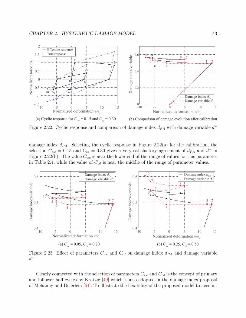
CHAPTER 2. HYSTERETIC DAMAGE MODEL 43
(a) Cyclic response for Cwc = 0.15 and Ccd = 0.30 (b) Comparison of damage evolution after calibration
-10 -5 0 5 10 15Normalized deformation e/ey
-1.5
-1
-0.5
0
0.5
1
1.5
2
Nor
mal
ized
forc
e s/
s y
Effective responseTrue response
0
1 2
3
45
6
7
89
10
-10 -5 0 5 10 15Normalized deformation e/ey
0
0.2
0.4
0.6
Dam
age
inde
x/va
riabl
e
1
234
578910
6
Damage index dPADamage variable d+
Figure 2.22: Cyclic response and comparison of damage index dPA with damage variable d+
damage index dPA. Selecting the cyclic response in Figure 2.22(a) for the calibration, theselection Cwc = 0.15 and Ccd = 0.30 gives a very satisfactory agreement of dPA and d+ inFigure 2.22(b). The value Cwc is near the lower end of the range of values for this parameterin Table 2.4, while the value of Ccd is near the middle of the range of parameter values.
(a) Cwc = 0.05, Ccd = 0.20
-10 -5 0 5 10 15Normalized deformation e/ey
0.4
0.5
0.6
Dam
age
inde
x/va
riabl
e
Damage index dPADamage variable d+
23
4
56
78910
-10 -5 0 5 10 15Normalized deformation e/ey
0.4
0.5
0.6
Dam
age
inde
x/va
riabl
e
Damage index dPADamage variable d+
3 2
4
56 7
89
10
(b) Cwc = 0.25, Ccd = 0.50
Figure 2.23: Effect of parameters Cwc and Ccd on damage index dPA and damage variabled+
Clearly connected with the selection of parameters Cwc and Ccd is the concept of primaryand follower half cycles by Kratzig [49] which is also adopted in the damage index proposalof Mehanny and Deierlein [64]. To illustrate the flexibility of the proposed model to account
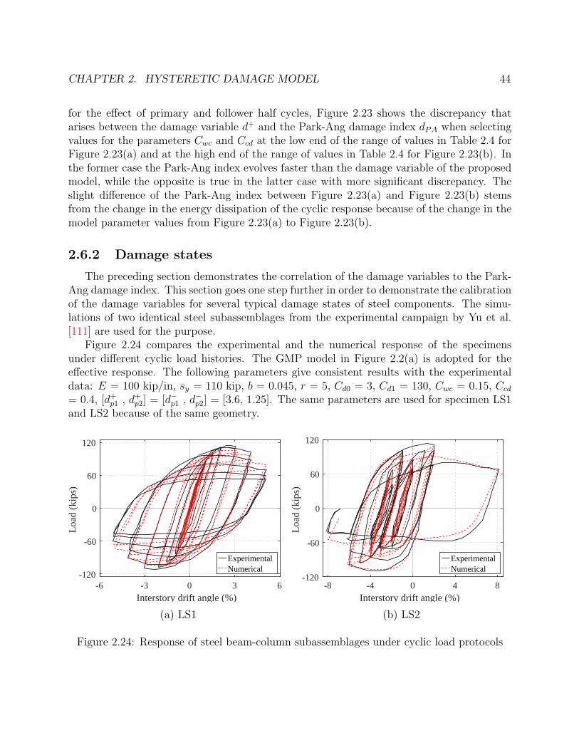
CHAPTER 2. HYSTERETIC DAMAGE MODEL 44
for the effect of primary and follower half cycles, Figure 2.23 shows the discrepancy thatarises between the damage variable d+ and the Park-Ang damage index dPA when selectingvalues for the parameters Cwc and Ccd at the low end of the range of values in Table 2.4 forFigure 2.23(a) and at the high end of the range of values in Table 2.4 for Figure 2.23(b). Inthe former case the Park-Ang index evolves faster than the damage variable of the proposedmodel, while the opposite is true in the latter case with more significant discrepancy. Theslight difference of the Park-Ang index between Figure 2.23(a) and Figure 2.23(b) stemsfrom the change in the energy dissipation of the cyclic response because of the change in themodel parameter values from Figure 2.23(a) to Figure 2.23(b).
2.6.2 Damage states
The preceding section demonstrates the correlation of the damage variables to the Park-Ang damage index. This section goes one step further in order to demonstrate the calibrationof the damage variables for several typical damage states of steel components. The simu-lations of two identical steel subassemblages from the experimental campaign by Yu et al.[111] are used for the purpose.
Figure 2.24 compares the experimental and the numerical response of the specimensunder different cyclic load histories. The GMP model in Figure 2.2(a) is adopted for theeffective response. The following parameters give consistent results with the experimentaldata: E = 100 kip/in, sy = 110 kip, b = 0.045, r = 5, Cd0 = 3, Cd1 = 130, Cwc = 0.15, Ccd= 0.4, [d+p1 , d+p2] = [d−p1 , d−p2] = [3.6, 1.25]. The same parameters are used for specimen LS1and LS2 because of the same geometry.
-6 -3 0 3 6Interstory drift angle (%)
-120
-60
0
60
120
Loa
d (k
ips)
ExperimentalNumerical
(a) LS1
-8 -4 0 4 8Interstory drift angle (%)
-120
-60
0
60
120
Loa
d (k
ips)
ExperimentalNumerical
(b) LS2
Figure 2.24: Response of steel beam-column subassemblages under cyclic load protocols

CHAPTER 2. HYSTERETIC DAMAGE MODEL 45
To illustrate the deterioration in the specimens, Figures 2.25(a)-(b) plot the evolutionof the damage variables in the simulation of specimen LS2 and compare it with the Park-Ang damage index. Six load points (LP) are identified corresponding to important eventsobserved during the experiment. Between LP 1 and LP 2 the specimen is subjected to alarge negative displacement leading to pronounced yielding and the initiation of buckling.Between LP 2 and LP 3, the specimen undergoes small cycles without exceeding the previousminimum and maximum displacements and experiences pronounced buckling. Between LP3 and LP 4 the specimen is subjected to a large positive displacement causing severe damagewith a fatigue crack in the bottom flange at the reduced beam section (RBS). Between LP4 and LP 5, the displacement reverses to the negative direction. The previous minimumdisplacement is exceeded at LP 5, and the specimen continues to load into the negativedisplacement range to LP 6, where large cracks develop through the flange thickness causinga fracture failure.
-8 -4 0 4 8Interstory drift (%)
0
0.1
0.2
0.3
0.4
0.5
0.6
0.7
Dam
age
varia
ble
12
3
456
(a) Positive damage
-8 -4 0 4 8Interstory drift (%)
0
0.1
0.2
0.3
0.4
0.5
0.6
0.7
Dam
age
varia
ble
1
2
3
456
(b) Negative damage
-10 -5 0 5 10Interstory drift (%)
0
0.2
0.4
0.6
0.8
Dam
age
inde
x/va
riabl
e
Damage index dPADamage variable
(c) Damage comparison
Figure 2.25: Comparison of damage evolution in specimen LS2
For a direct comparison with the Park-Ang damage index [73], Figure 2.25(c) plots asingle damage variable d that represents both the positive and negative damage variablesd±. For simplicity, this damage variable is taken as the maximum of the positive and negativedamage variables d = max(d+, d−). As expected from the comparison study in Section 2.6.1,the damage variable d and the Park-Ang damage index dPA are consistent for this standardcase. Table 2.5 correlates the observed events with the corresponding damage values.
The correlation gives rise to the following damage thresholds:
• d = 0.0–0.2: yielding of panel zone, beam flange and web
• d = 0.2–0.4: initiation of buckling leading to some strength deterioration
• d = 0.4–0.6: crack propagation and significant strength degradation
• d = 0.6–1.0: failure through fracture

CHAPTER 2. HYSTERETIC DAMAGE MODEL 46
Limit stateDamagevariable
Park-Angindex
Damagelevel
Panel zone yielding 0.02 0.08 LightBeam bottom flange yielding 0.2 0.2 ModerateNotable buckling 0.3 0.3 ModerateFatigue crack in bottom flange RBS 0.55 0.51 SevereCracks through flange thickness and fracture 0.63 0.57 Severe
Table 2.5: Correlation of damage measures and limit states for specimen LS2
It is instructive to extend the calibration to a wider variety of specimens and load histo-ries. This task is, however, beyond the scope of this work and left for future studies.
2.7 Damage Evolution Law for Brittle Failure
Often times fracture initiates and the structural components undergo a drastic reduc-tion in strength and stiffness. The damage evolution function based on the CDF of thebeta distribution accounts for such sudden strength deterioration through the selection ofparameters Cd0, Cd1, dp1, dp2. With a small difference in the values for Cd0 and Cd1, thelimit energy ψd1 is very close to the threshold ψd0 and the damage evolution is rapid. Suit-able values for dp1 and dp2 accelerate damage in certain deformation ranges, for example,dp1 > 1 and dp2 < 1 leads to rapid damage accumulation in early cycles. Both methods arereasonable for simulating brittle response but they have certain limitations. In the former,the damage initiation coincides with the onset of the brittle failure, which implies that themodel is unable to describe the gradual damage prior to fracture. In the latter, since thedamage evolution law is a smooth function, it is unable to distinguish the distinct behaviorsin the damage accumulation pre- and post-fracture.
To address these issues, a composite damage evolution law is proposed. The compositefunction introduces two energy variables ψf and ψu that satisfy ψd0 ≤ ψf < ψu ≤ ψd1. ψf isthe energy at which fracture takes place and ψu is the ultimate energy at complete strengthloss. The energy variables can be normalized to give the condition 0 ≤ ψf < ψu ≤ 1.Different values can be specified for the variables under positive and negative moments atend i and end j, and for brevity, the superscript ± and the subscript i and j have beendropped. The damage evolution in the preceding sections is modified to account for therapid strength degradation following fracture:
d =
FB
(ψ, β1, β2
), 0 ≤ ψ ≤ ψf
FB
(ψf , β1, β2
)+
1− FB(ψf , β1, β2
)ψu − ψf
(ψ − ψf
), ψf < ψ ≤ ψu
1, ψu < ψ ≤ 1
(2.16)

CHAPTER 2. HYSTERETIC DAMAGE MODEL 47
In Equation (2.16) the damage evolution consists of three segments. When the energy ψis less than the fracture energy ψf , the damage evolution follows the cumulative distributionfunction (CDF) of the beta distribution similar to the formulation without brittle damage.When the energy ψ exceeds the fracture threshold ψf but is less than the ultimate threshold
ψu, the damage variable increases linearly to 1 at ψ = ψu. At higher energy, the strengthis completely lost and the damage variable remains equal to 1. Figure 2.26 shows the threesegments of the damage evolution.
0 10
1
Dam
age
varia
ble
d
ˆNormalized energy y
yf yu
(1)
(2)
(3)
FB= (yf , b1, b2)ˆ
Figure 2.26: Damage evolution with brittle failure
To illustrate the proposed damage evolution law for brittle failure, the following presentssimulations of steel cantilever beams under repeated cyclic loading from the experiments byKrawinkler [51]. Two specimens selected for the simulations are B13 and B18. Note thatthree other specimens from the same experimental campaign have been simulated in 2.5.3 toinvestigate the low-cycle fatigue phenomenon: B24, B25, and B28. The two groups B1 andB2 exhibit vastly different behaviors. While the specimens in group B2 experience gradualdeterioration due to local buckling in beam flanges, the specimens in group B1 fail fromcrack propagation at weldments with relatively higher rate of deterioration [51].
The following damage parameters are used in the simulation of B13 and B18: Cd0 = 10,Cd1 = 300, Cwc = 0.13, Ccd = 0.3, [dp1, dp2] = [3, 1.5], ψf = 0.078, ψu = 0.1. These parametersresult in the damage evolution that is consistent with the distinct deterioration patterns inthe B1 and B2 groups. For specimens in group B1, the slow crack propagation in the earlycycles causes little deterioration for a larger number of cycles in the beginning, but as thecrack approaches its critical size, the specimens show rapid strength reduction. On the otherhand, for specimens in group B2, strength reduction due to local flange buckling initiatesearlier but the deterioration rate is more gradual [51]. Such behaviors are captured by thethreshold coefficient Cd0 and the limit coefficient Cd1, which are higher in the simulation ofspecimens in group B1 than in group B2. The higher Cd0 allows damage to initiate laterwhile the higher Cd1 results in more ductile response prior to the onset of fracture.

CHAPTER 2. HYSTERETIC DAMAGE MODEL 48
-3 -1.5 0 1.5 3Deflection (in)
-10
-5
0
5
10
Load
(kip
)
ExperimentalNumerical
(a) B13: load-displacement
-3 -2 -1 0 1 2 3Deflection (in)
0
0.2
0.4
0.6
0.8
1
Dam
age
vari
able
(b) B13: damage evolution
-1.6 -0.8 0 0.8 1.6Deflection (in)
-10
-5
0
5
10
Load
(kip
)
ExperimentalNumerical
(c) B18: load-displacement
-1.5 -1 -0.5 0 0.5 1 1.5Deflection (in)
0
0.1
0.2
0.3
0.4
0.5
0.6
Dam
age
vari
able
(d) B18: damage evolution
Figure 2.27: Simulations of steel beam with brittle failure
Figure 2.27 shows the load-displacement relation and the evolution of the positive damagevariable d+ for specimens B13 and B18. The model also simulates well the limited deteri-oration prior to the onset of fracture. The damage evolution function in Equation (2.16)with ψf = 0.078 and ψu = 0.1 captures accurately the sharp strength reduction in bothspecimens during the last half cycle. The distinct deterioration rates prior and post-fractureare evident in the damage evolution in Figure 2.27(b) and (d).
More extensive calibration is required to identify practical values for the parameters ψfand ψu and correlate them with physical properties of components. Nonetheless, the excellentresults in the case study show that the model has significant promise in the hystereticresponse simulation of structural members susceptible to brittle failure.
49
Chapter 3
Damage-Plasticity Beam Model
This chapter extends the 1d hysteretic damage model in Chapter 2 to formulate a newbeam element based on damage-plasticity for the response simulation and damage assess-ment of steel structures under extreme load conditions. First, the series beam element basedon resultant plasticity and the serial springs formulation is introduced to describe the nonde-grading force-deformation relation in the effective space. The inelastic response is monitoredat two locations offset from the element ends to account for the spread of inelasticity forhardening response and the size of the damage zones for softening response. The plastic hingeoffsets accommodate the response coupling between the two element ends and represent moreaccurately the post-yield hardening behavior.
The damage formulation allows the beam element to describe the main characteristicsof steel components, including the accumulation of plastic deformations, the cyclic strengthhardening in early cycles, the low-cycle fatigue behavior, the distinct deterioration rates inprimary and follower half cycles. The damage evolution function is extended to accommodatethe sudden strength and stiffness deterioration from element brittle failure.
The chapter concludes with an extensive parameter calibration for more than 50 steelcomponents under monotonic and cyclic load histories. A regression analysis is then usedto establish guidelines for the damage parameter selection in relation to the geometry andthe boundary conditions of the structural member. The validation studies indicate thedependence of the strength and stiffness deterioration on the section compactness and theelement slenderness. The proposed model compares favorably in terms of computationalefficiency with more sophisticated models with fiber discretization of the cross section whileachieving excellent agreement in the response description for homogeneous metallic structuralcomponents. The implementation of the damage-plasticity elements with the return-mappingalgorithm ensures excellent convergence characteristics for the state determination. Becauseof the computational efficiency and excellent accuracy, the proposed beam element holdsgreat promise for the large scale seismic response simulation of structural systems withstrength and stiffness deterioration and should prove very useful in the damage assessmentand the collapse simulation of structures under extreme loading conditions.
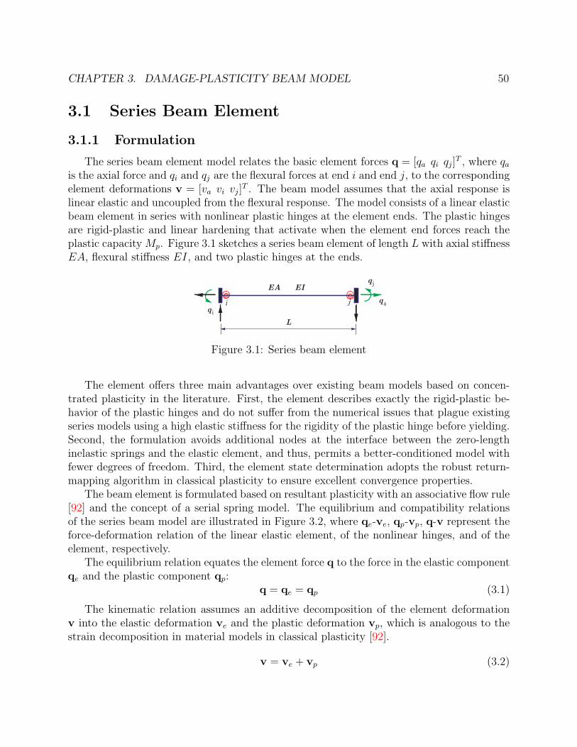
CHAPTER 3. DAMAGE-PLASTICITY BEAM MODEL 50
3.1 Series Beam Element
3.1.1 Formulation
The series beam element model relates the basic element forces q = [qa qi qj]T , where qa
is the axial force and qi and qj are the flexural forces at end i and end j, to the correspondingelement deformations v = [va vi vj]
T . The beam model assumes that the axial response islinear elastic and uncoupled from the flexural response. The model consists of a linear elasticbeam element in series with nonlinear plastic hinges at the element ends. The plastic hingesare rigid-plastic and linear hardening that activate when the element end forces reach theplastic capacity Mp. Figure 3.1 sketches a series beam element of length L with axial stiffnessEA, flexural stiffness EI, and two plastic hinges at the ends.
q i
q jEA EI
qa
L
i j
Figure 3.1: Series beam element
The element offers three main advantages over existing beam models based on concen-trated plasticity in the literature. First, the element describes exactly the rigid-plastic be-havior of the plastic hinges and do not suffer from the numerical issues that plague existingseries models using a high elastic stiffness for the rigidity of the plastic hinge before yielding.Second, the formulation avoids additional nodes at the interface between the zero-lengthinelastic springs and the elastic element, and thus, permits a better-conditioned model withfewer degrees of freedom. Third, the element state determination adopts the robust return-mapping algorithm in classical plasticity to ensure excellent convergence properties.
The beam element is formulated based on resultant plasticity with an associative flow rule[92] and the concept of a serial spring model. The equilibrium and compatibility relationsof the series beam model are illustrated in Figure 3.2, where qe-ve, qp-vp, q-v represent theforce-deformation relation of the linear elastic element, of the nonlinear hinges, and of theelement, respectively.
The equilibrium relation equates the element force q to the force in the elastic componentqe and the plastic component qp:
q = qe = qp (3.1)
The kinematic relation assumes an additive decomposition of the element deformationv into the elastic deformation ve and the plastic deformation vp, which is analogous to thestrain decomposition in material models in classical plasticity [92].
v = ve + vp (3.2)

CHAPTER 3. DAMAGE-PLASTICITY BEAM MODEL 51
qqp
ve vp
v
vevp
Mp Mp
qe
+ =
Figure 3.2: Equilibrium and compatibility relations of series beam model
The constitutive law of the elastic component relates the force q to the elastic deformationve through the elastic stiffness ke:
q = keve = ke (v − vp) (3.3)
The following discusses the three main aspects of the element formulation: the yieldfunction, the flow rules, and the hardening rules.
Yield functionTwo yield functions fi and fj describe the admissible force state of the response at end
i and end j, respectively. fi and fj are functions of three history variables: the element
forces q, the back-forces qb = [qb,a qb,i qb,j]T describing the kinematic hardening behavior,
and the internal variables α = [αi αj]T governing the isotropic hardening behavior. With
Mp = [Mp,i Mp,j]T denoting the plastic flexural capacities and Hi,i and Hi,j denoting the
isotropic hardening modulus of the response at end i and j, the yield functions fi and fj aregiven by:
fi (q,qb,α) = |qi − qb,i| − (Mp,i +Hi,iαi) (3.4)
fj (q,qb,α) = |qj − qb,j| − (Mp,j +Hi,jαj) (3.5)
While the model accommodates unequal plastic capacities at the two ends, the samecapacity Mp,i = Mp,j = Mp is used in this study, which is a reasonable assumption for steelcomponents. Figure 3.3 plots the two initial yield surfaces defined by the yield functions fiand fj in the (qi, qj) force space and the four unit normals n±
i and n±j . The yield envelope
consists of four lines qi = ±Mp and qj = ±Mp.The normal n to the yield envelope is given by:
n = [ni nj] =
[∂fi∂q
∂fj∂q
]=
0 0sign (qi − qb,i) 0
0 sign (qj − qb,j)
(3.6)

CHAPTER 3. DAMAGE-PLASTICITY BEAM MODEL 52
qi
fj = 0
fj = 0
fi = 0 fi = 0
+Mp
qj
+Mp
-Mp
-Mp
ni+
ni-
nj+
nj-
Figure 3.3: Yield envelope of series element
The yield functions in Equations (3.4)–(3.5) can be written more compactly as follows:
f (q,qb,α) = nT (q− qb)− (Mp + Hiα) (3.7)
where Hi is a diagonal 2×2 isotropic hardening matrix with the isotropic hardening moduliHi,i and Hi,j on the diagonal. It is noteworthy that the yield envelope given by fi and fj inEquations (3.4)–(3.5) is nonsmooth with four singular points on the boundary of the elasticdomain.
Flow rulesThe associative flow rule describes the evolution of the plastic deformation vp. To account
for the singularity at the corners, the Koiter’s rule [47] states that the plastic deformationrate vp, or equivalently, the plastic deformation increment ∆vp, is a linear combination ofthe normals ni and nj:
vp = βini + βjnj = nβ (3.8)
where β = [βi βj]T is a vector of the consistency parameters.
Figure 3.4 illustrates three scenarios of the plastic deformation increment. In Fig-ure 3.4(a), only the yield surface defined by fi is ’active’, that is, βi > 0 and βj = 0 andthe plastic deformation increment is colinear to the normal ni. In Figure 3.4(b), only theyield surface defined by fj is ’active’, that is, βj > 0 and βi = 0 and the plastic deformationincrement is colinear to the normal nj. In Figure 3.4(c), both yield surfaces are ’active’ andthe plastic deformation increment depends on both ni and nj.
Hardening rulesThe rate of the internal variable α and the back-force qb are given as functions of the

CHAPTER 3. DAMAGE-PLASTICITY BEAM MODEL 53
∆vp = βjnj+
∆vp = βini+
βini+
βjnj+∆vp = βini
++ βjnj+
(a) (b) (c)
Figure 3.4: Scenarios of plastic deformation increments: (a) only fi active, (b) only fj active,(c) both fi and fj active
consistency parameters β:
α = β (3.9)
qb = Hknβ (3.10)
where Hk is a 3×3 diagonal matrix with ’0’ and the kinematic hardening moduli Hk,i andHk,j on the diagonal.
The consistency parameter β and the yield function f satisfy the unilateral constraintsknown as the Kuhn-Tucker condition:
β ≥ 0 and f ≤ 0 and βmfm = 0, m = i, j (3.11)
The consistency condition asserts additional loading/unloading conditions for the yieldsurfaces:
βmfm = 0, m = i, j (3.12)
Given the deformation rate v, the consistency parameter β can be evaluated as follows:
β =[nT (ke + Hk) n + Hi
]−1nTkev (3.13)
The expresion of the tangent stiffness upon plastic loading is:
kt = ke − ken[nT (ke + Hk) n + Hi
]−1nTke (3.14)
The derivation of the consistency parameters and the tangent stiffness can be found inAppendix B.

CHAPTER 3. DAMAGE-PLASTICITY BEAM MODEL 54
3.1.2 Plastic hinge offset
The series beam element in Section 3.1 is generalized by placing the two nonlinear springsat distances χi = ci/L and χj = cj/L from the ends. Figure 3.5 sketches the series beamelement of length L, axial stiffness EA and flexural stiffness EI composed of a linear elasticbeam element in series with two offset rigid-plastic plastic hinges in the interior of theelement. While the model permits different offset ratios χi and χj at the two ends, forsimplicity a symmetric placement of the plastic hinges χi = χj = χ is used in the remainingof the dissertation.
q i
q j
c i c j
EA EI
qa
L
i j
Figure 3.5: Series beam element with plastic hinge offset
The governing relations in Equations (3.1)–(3.3) still apply. It is noteworthy that theplastic force qp and plastic deformation vp are associated with the response at the elementends, and the plastic response is activated when the moment reaches the plastic capacity Mp
at the hinge location. In the absence of element loading, the moment distribution is linearalong the beam span, and the hinge moments Mi and Mj can be linearly interpolated fromthe element flexural forces qi and qj, as Figure 3.6 shows.
-qp,i
qp,j
Mi
Mjχjχi
LL L
Figure 3.6: Moment interpolation between the hinge locations and the element ends
The moment interpolation matrix bp is defined based on the plastic hinge offset χ:
bp =
1 0 00 χ χ0 χ 1− χ
(3.15)

CHAPTER 3. DAMAGE-PLASTICITY BEAM MODEL 55
The force and deformation of the plastic hinges qh–vh can be related to the plastic forceand deformation qp–vp through the force interpolation matrix bp:
qh = bpqp (3.16)
vp = bTp vh (3.17)
where qh = [N , Mi, Mj]T denotes the axial force and the bending moments at the plastic
hinge locations and vh = [θa, θi, θj]T are the corresponding hinge axial deformations and
rotations. Due to the assumption of linear elastic axial response, the axial deformation inthe plastic hinges θa is zero.
The yield functions in Equation (3.7) become:
f = nT (bpq− qb)− (Mp + Hiα) (3.18)
where the normal n can be evaluated as:
n =
0 0sign [(χ− 1)qi + χqj − qb,i] 0
0 sign [−χqi + (1− χ)qj − qb,j]
(3.19)
It is evident in Equation (3.19) that the plastic hinge offsets couple the forces at the twoelement ends.
The same hardening rules in Equations (3.9)–(3.10) are adopted for the evolution of theback-force qb, and the internal variable α. The plastic deformation rate vp is then given bythe interpolation matrix bp, the normal to the yield surface n, and the consistency parameterβ:
vp = bTp nβ (3.20)
The consistency parameter β have the following expression:
β =[nT(bpkeb
Tp + Hk
)n + Hi
]−1nkev (3.21)
and the tangent stiffness kt is given by:
kt = ke − kebTp n[nT(bpkeb
Tp + Hk
)n + Hi
]−1nTbpke (3.22)
The series beam model in Section 3.1.1 is a special case with χ = 0. It is possible toextend the formulation with more than two plastic hinges to accommodate various inelasticphenomenon, such as shear and bond-slip; however, it is left for future studies.
3.1.3 State determination: Return-mapping algorithm
Given the deformation vn at the current step n and the previous history variables, thestate determination of the element model evaluates the end force qn, the internal hardening

CHAPTER 3. DAMAGE-PLASTICITY BEAM MODEL 56
variable qb,n and αn, the plastic deformation vp,n, and the tangent stiffness kt. The ele-ment state determination is based on the return-mapping algorithm in classical multisurfaceplasticity.
The algorithm starts with an elastic predictor assuming that the deformation incrementis entirely elastic, and evaluates the trial force qtr, the trial back-force qtrb , and the trialinternal variable αtr:
qtr = ke (vn − vp,n−1) (3.23)
qtrb = qb,n−1 (3.24)
αtr = αn−1 (3.25)
The trial normal to the yield surface ntr can be expressed as:
ntr =
0 0sign
[(χ− 1)qtri + χqtrj − qtrb,i
]0
0 sign[−χqtri + (1− χ)qtrj − qb,j
] (3.26)
The trial yield function f tr is evaluated from the trial force and state variables:
f tr =(ntr)T
(bpqtr − qtrb )− (Mp + Hiα
tr) (3.27)
If both yield functions are positive, f tri > 0 and f trj > 0, the trial force state is admissibleand the element response is elastic. The trial elastic state is accepted and the end force qnequals to the trial value qtr:
qn = qtr (3.28)
Similarly, the state variables are equal to the corresponding trial values:
qb,n = qtrb (3.29)
αn = αtr (3.30)
vp,n = vp,n−1 (3.31)
and the tangent stiffness kt is equal to the elastic stiffness ke:
kt = ke (3.32)
If at least one yield condition is violated, f tri ≥ 0 and/or f trj ≥ 0, plastic correction isrequired to adjust the force back to the admissible domain. A yield surface m is considered’active’ if the consistency parameter βm > 0 and the corresponding yield function fm = 0after the correction with m = i, j. The selection of active surfaces satisfies two constraintsof the Kuhn-Tucker conditions after the plastic correction: (1) the consistency parameterβ is positive, (2) the yield function f defined by the corrected variables qn, qb,n, and αnare non-positive, that is, the point (qi, qj) does not fall outside the admissible domain inthe force space upon correction. The identification of the active yield surfaces involves twosteps:

CHAPTER 3. DAMAGE-PLASTICITY BEAM MODEL 57
(1) Both yield surfaces are assumed active, the trial consistency parameter βtr is evaluated:
βtr =[nT(bpkeb
Tp + Hk
)n + Hi
]−1f tr (3.33)
(2) Enforcing the Kuhn-Tucker conditions, the active surfaces can be shown to correspondto the positive trial consistency parameters βtr.
m ∈ Jact = i, j | βtrm > 0 (3.34)
where Jact denotes the indices of the active yield surfaces.
To account only for the active constraints, the normal ntr is revised to include only theactive yield surfaces. For example, if both yield surfaces are active, ntr =
[ntri ntrj
]. If only
the yield surface at end i is active, ntr = ntri .
ntr =[ntrm], m ∈ Jact (3.35)
Similarly, the trial yield function f tr and the isotropic hardening modulus Hi are revisedto reflect the active yield surfaces. For example, if only the yield surface at end i is active,f tr = f tri and Hi = Hi,i.
f tr =[f trm], m ∈ Jact (3.36)
Hi = Hi (Jact,Jact) (3.37)
With the modifications in Equation (3.35)–(3.37) to include only the active surface(s),the consistency parameters β can then be evaluated as follows:
β =[nT(bpkeb
Tp + Hk
)n + Hi
]−1f tr (3.38)
The plastic deformations vp, the internal variables α and the back-forces qb are thenupdated:
vp,n = vp,n−1 + bTp nβ (3.39)
qb,n = qb,n−1 + Hknβ (3.40)
αn = αn−1 + β (3.41)
The force qn is updated from the trial value qtr as follows:
qn = qtr − kebTp nβ (3.42)
Finally the tangent stiffness kt is given in Equation (3.22). Table 3.1 summarizes thestate determination algorithm of the general series beam model with offsets.
Figure 3.7 is a graphical illustration of the returning-mapping scheme for an elementresponse under the assumption of an elasto-plastic behavior and no plastic hinge offset forsimplicity. The shaded region is the elastic domain with fi < 0 and fj < 0. Plastic correctionis required when the trial force qtr falls outside this region. Note that the force correctionis ∆q = qtr − q = kenβ = βikeni + βjkenj, which is a linear combination of keni and kenj.The area outside the elastic domain can be divided into three regions A, B, C separated bythese vectors, as shown in Figure 3.7(a).

CHAPTER 3. DAMAGE-PLASTICITY BEAM MODEL 58
Given: end deformations vn and history variables at step n− 1
Required : state variables at step n
1. Elastic predictor:
Evaluate qtr, qtrb , αtr in (3.23)–(3.25)
Evaluate ntr in (3.26)
2. Check of plastic process:
Evaluate f tr in (3.27)
IF f tri < 0 and f trj < 0 THEN:
Elastic update, go to Step 3
ELSE:
Plastic correction, go to Step 4
ENDIF
3. Elastic update:
Update qb,n, αn, vp,n in (3.29)–(3.31)
Update qn, kt in (3.28) and (3.32)
EXIT
4. Identification of active yield surfaces in two steps
Assume both surfaces are active and evaluate trial βtr in (3.33)
Identify active surfaces Jact that correspond to positive βtr
5. Consistency parameters β:
Update ntr, f tr, Hi in (3.35)–(3.37)
Compute β in (3.38)
6. State variables update:
Update vp,n in (3.39)
Update qb,n, αn in (3.40)–(3.41)
7. Element end forces and tangent stiffness:
Update qn in (3.42)
Evaluate kt in (3.22)
Table 3.1: State determination algorithm of series beam model with plastic hinge offset

CHAPTER 3. DAMAGE-PLASTICITY BEAM MODEL 59
keni+
kenj+kenj
+
keni+
keni-
keni-
kenj- kenj
-
B CC
BC C
A
A
(a) Regions in qi − qj space
keni+
kenj+kenj
+
keni+
keni-
keni-
kenj- kenj
-
qtr
q
qtr
q
(b) Region A: only βi active
keni+
kenj+kenj
+
keni+
keni-
keni-
kenj- kenj
-
qtr
q
qtr
q
(c) Region B: only βj active
keni+
kenj+kenj
+
keni+
keni-
keni-
kenj- kenj
-
qtr
q
qtr
q
qtr
q
qtr
q
(d) Region C: both βi and βj active
Figure 3.7: Return-mapping algorithm for series element

CHAPTER 3. DAMAGE-PLASTICITY BEAM MODEL 60
(i) Region A: This region corresponds to a positive trial yield function at end i, f tri > 0,and is defined by the area outside the yield envelope between vectors ken
+i for qi > 0
and between vectors ken−i for qi < 0. If the trial force qtr falls in this region, only
the yield surface at end i is active, i.e. the consistency parameter βi > 0 and βj = 0.The normal ntr = ntri in Equation (3.35) and the plastic deformation increment ∆vpis parallel to the normal ni of the yield surface fi = 0. The force correction ∆q isparallel to keni. The corrected force q gives fi = 0 and fj < 0. The plastic correctionscheme is shown in Figure 3.7(b).
(ii) Region B: This region corresponds to a positive trial yield function at end j, f trj > 0,and is defined by the area outside the yield envelope between vectors ken
+j for qj > 0
and between vectors ken−j for qj < 0. If the trial force qtr falls in this region, only
the yield surface at end j is active, i.e. the consistency parameter βj > 0 and βi = 0.The normal ntr = ntrj in Equation (3.35) and the plastic deformation increment ∆vpis parallel to the normal nj of the yield surface fj = 0. The force correction ∆q isparallel to kenj. The corrected force q gives fi < 0 and fj = 0. The plastic correctionscheme is shown in Figure 3.7(c).
(iii) Region C: This region is defined by the area outside the yield envelope and betweenthe vectors ken
±i and ken
±i in the same quadrant of the force space. If the trial force
qtr falls in this region, both yield surfaces are active, i.e. the consistency parameters
βi > 0 and βj > 0. The normal ntr =[ntri ntrj
]Tin Equation (3.35). The plastic
deformation increment ∆vp is a linear combination of the normals ni and nj. Thecorrection process adjusts the force q to the ’corner’ of the admissible domain andgives fi = 0 and fj = 0. The plastic correction scheme is shown in Figure 3.7(d).
(iv) Along the common edges between two regions, A & C and B & C, the correctionscheme is similar to the scheme in regions A and B, respectively. The only differenceis that upon the correction process, the force q targets the singular point of the yieldenvelope and gives fi = fj = 0.
The force correction processes in Figures 3.7(b)–(d) results from the two-step scheme inthe previous discussion. An example is shown in Figure 3.8. In the first step, both surfacesare assumed active and the trial force qtr is projected to the nearest corner in the quadrantin Figure 3.8(a). The trial consistency parameters βtr can be interpreted as the projectionof the force increment ∆q to vectors keni and kenj. In the second step, since βtrj < 0,only the yield surface i is active and the force correction is adjusted accordingly as shown inFigure 3.8(b).
It is important to point out that the signs of the trial yield functions f tr are not sufficientto identify the active surfaces. For example, if only one trial yield function is positive, f tri > 0and f trj < 0, it is not guaranteed that only the surface i is active, βi > 0 and βj = 0. Theforce correction affects both qi and qj due to the coupling terms in the elastic stiffness ke, andcould activate the surface j after the correction, fj > 0, and thus violates the Kuhn-Tucker

CHAPTER 3. DAMAGE-PLASTICITY BEAM MODEL 61
keni+
kenj+
qtr
βjtrkenj
+
βitrkeni
+
q
fj = 0
fi = 0
(a) Step 1: Evaluate βtr
keni+
kenj+
qtr
βikeni+
qfj = 0
fi = 0
(b) Step 2: Update active surfaces
Figure 3.8: Two-step identification of active surfaces
condition. Figure 3.9 illustrates two scenarios in which determining the active surfaces basedsolely on the signs of the trial yield functions is erroneous.
keni+
kenj+
qtr βjkenj+
βikeni+
q fj = 0
fi = 0
(a) βi < 0
keni-
kenj+
qtr
q
βjkenj+
fj = 0
fi = 0
(b) fi > 0
Figure 3.9: Violation of Kuhn-Tucker condition due to incorrect active β’s
In the first scenario in Figure 3.9(a), the trial force qtr gives a positive value for bothtrial yield functions f tri > 0 and f trj > 0. If both surfaces are assumed active, the correctionbrings the force qtr to the corner to satisfy fi = fj = 0. However, this projection of theforce increment ∆q onto vectors keni and kenj indicates that βi < 0, and thus violates the

CHAPTER 3. DAMAGE-PLASTICITY BEAM MODEL 62
Kuhn-Tucker condition that requires positive consistent parameters β. In this scenario, thetrial force qtr lies in region B in Figure 3.7(a), which shall only activate surface j even thoughf tri > 0.
In the second scenario in Figure 3.9(b), the trial force qtr gives f tri < 0 and f trj > 0. Ifthe active surfaces are based on signs of the trial yield functions, only surface j is activeand the force correction is parallel to kenj. However, the correction gives fi > 0 and bringsthe force qtr outside the admissible domain. This violates the Kuhn-Tucker condition thatrequires the yield functions to remain nonpositive, f ≤ 0. In this scenario, the trial forceqtr lies in region C in Figure 3.7(a), which shall activate both surfaces i and j even thoughf tri < 0.
3.1.4 Model parameters
The series beam element requires 7 parameters: the Young modulus E, the cross-sectionalarea A, the moment of inertia I, the flexural plastic capacity Mp, the kinematic hardeningratio Hkr, the isotropic hardening ratio Hir, and the offset parameter χ. Since the first 4parameters are readily available from the material properties and the member geometry, thissection addresses the last 3 parameters.
3.1.4.1 Hardening parameters Hkr and Hir
The kinematic hardening ratio Hkr and the isotropic hardening ratio Hir are directlyrelated to the kinematic hardening modulus Hk and the isotropic hardening modulus Hi interms of the flexural stiffness under antisymmetric bending 6EI/L:
Hk = Hkr6EI
L(3.43)
Hi = Hir6EI
L(3.44)
Figure 3.10 illustrates the evolution of the yield surface with linear isotropic and kinematichardening from fn−1 to fn. The end forces evolve from an elastic state qn−1 to a plastic stateqn. Kinematic hardening translates the yield surface while isotropic hardening expands orcontracts the yield surface in the force space.
Figures 3.10(a1)-(a2) illustrate the evolution of the yield envelope in the case of kinematichardening with Hkr > 0. In Figure 3.10(a1) only the yield surface j is active, βj > 0, andthe yield envelope translates parallel to the normal nj. The force qn gives fn,i < 0 andfn,j = 0. In Figure 3.10(a2) both yield surfaces i and j are active, βi > 0 and βj > 0, andthe translation of the yield envelope is a linear combination of both ni and nj. The force qntargets the corner of the new yield surfaces, implying that fn,i = 0 and fn,j = 0.
Figures 3.10(b1)-(b2) illustrate the evolution of the yield envelope in the case of isotropichardening with Hir > 0. In Figure 3.10(b1) only the yield surface i is active, βi > 0, andthe yield envelope expands in the direction parallel to the normal ni. The force qn gives
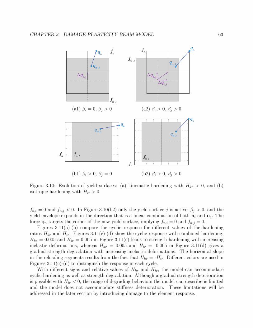
CHAPTER 3. DAMAGE-PLASTICITY BEAM MODEL 63
qn
qn-1
∆qb,j
fn-1
fn
(a1) βi = 0, βj > 0
qn
qn-1
∆qb,i
∆qb,j
fn-1
fn
(a2) βi > 0, βj > 0
qn
qn-1
fn-1fn
(b1) βi > 0, βj = 0
qn
qn-1
fn-1
fn
(b2) βi > 0, βj > 0
Figure 3.10: Evolution of yield surfaces: (a) kinematic hardening with Hkr > 0, and (b)isotropic hardening with Hir > 0
fn,i = 0 and fn,j < 0. In Figure 3.10(b2) only the yield surface j is active, βj > 0, and theyield envelope expands in the direction that is a linear combination of both ni and nj. Theforce qn targets the corner of the new yield surface, implying fn,i = 0 and fn,j = 0.
Figures 3.11(a)-(b) compare the cyclic response for different values of the hardeningratios Hkr and Hir. Figures 3.11(c)-(d) show the cyclic response with combined hardening:Hkr = 0.005 and Hir = 0.005 in Figure 3.11(c) leads to strength hardening with increasinginelastic deformations, whereas Hkr = 0.005 and Hir = -0.005 in Figure 3.11(d) gives agradual strength degradation with increasing inelastic deformations. The horizontal slopein the reloading segments results from the fact that Hkr = -Hir. Different colors are used inFigures 3.11(c)-(d) to distinguish the response in each cycle.
With different signs and relative values of Hkr and Hir, the model can accommodatecyclic hardening as well as strength degradation. Although a gradual strength deteriorationis possible with Hir < 0, the range of degrading behaviors the model can describe is limitedand the model does not accommodate stiffness deterioration. These limitations will beaddressed in the later section by introducing damage to the element response.

CHAPTER 3. DAMAGE-PLASTICITY BEAM MODEL 64
-0.04 -0.02 0 0.02 0.04Deformation
-1.5
-1
-0.5
0
0.5
1
1.5
M=M
p
Hkr = 0.01Hkr = 0.03Hkr = 0.05
(a) Kinematic hardening
-0.06 -0.03 0 0.03 0.06Deformation
-1.5
-1
-0.5
0
0.5
1
1.5
M=M
p
Hir = 0.002Hir = 0.005Hir = 0.01
(b) Isotropic hardening
-0.08 -0.04 0 0.04 0.08Deformation
-2
-1
0
1
2
M=M
p
(c) Hkr = 0.005, Hir = 0.005
-0.08 -0.04 0 0.04 0.08Deformation
-1
-0.5
0
0.5
1M
=Mp
(d) Hkr = 0.005, Hir = −0.005
Figure 3.11: Sample cyclic response with linear kinematic and isotropic hardening
3.1.4.2 Offset parameter
The offset parameter χ represents the location of the plastic hinges from the elementends and ranges from χ = 0 for the hinges at the element ends to χ = 0.5 for the hingesat the element midspan. Figure 3.12 compares the flexural force-deformation relation at thebase of a cantilever beam subjected to a monotonically increasing transverse load at the freeend for different offset parameter χ = 0, 0.05, 0.1. For the linear moment distribution in thiscase study, the offset parameter χ increases the yield moment at the base. This strengthincrease results from the extrapolation of moment from the hinge locations to the elementends, with a larger offset leading to a higher moment amplification.
The ability of the plastic hinge offsets to describe the coupling of the inelastic zones atthe element ends is demonstrated in the following section.

CHAPTER 3. DAMAGE-PLASTICITY BEAM MODEL 65
0 0.0025 0.005 0.0075 0.01Deformation
0
0.5
1
1.5
M/M
p
χ = 0χ = 0.05χ = 0.1
Figure 3.12: Effect of offset on flexural response of a cantilever beam
3.2 Examples of Series Beam Element
3.2.1 Pushover analysis of portal frame
This example compares the series beam element to a more sophisticated element basedon distributed plasticity in a simple structure under a standard load pattern. The steelportal frame in Figure 3.13 is used for illustration. The columns are subjected to an axialcompression of Pv = 160 kips, which is 10% of the column axial plastic capacity Np torepresent the effect of gravity loading on the portal frame. The frame is subjected to amonotonically increasing lateral displacement at the girder level.
L = 20 ft
H = 14 ft W21x111W21x111
W21x93
Pv Pv
Integration points
A A Section A-A
Figure 3.13: Structural model of portal frame
The column and beam elements assume an elastic-perfectly-plastic (EPP) behavior. The

CHAPTER 3. DAMAGE-PLASTICITY BEAM MODEL 66
corotational formulation is used to account for the nonlinear geometry. Each column ismodeled with a force-based distributed beam-column element with 4 integration points alongthe length and 9 fibers in each cross section: 2 in each flange and 5 in the web. The idealizedmodel of the column and its discritization scheme is shown in Figure 3.13. The distributedplasticity model is used to capture the axial-flexure interaction in the columns.
For comparison, two different models are used to simulate the girder: (1) Model M1 usinga force-based beam-column element with the same discretization scheme as the columns,and (2) Model M2 using the series beam element. In this example, no plastic hinge offset isspecified in the girder, χ = 0.
Figure 3.14 compares the global and the local response in the two models. The base shear-lateral drift relation in Figure 3.14(a) is practically identical. Both models can capture thelinear elastic segment at small drifts, followed by the gradual yielding and transition toplastic behavior, and the linear softening range. The negative stiffness in Figure 3.14(a)indicates the effect of the column axial force under the large lateral displacement.
The girder response in the two models are shown in Figure 3.14(b). While the elasticresponse is identical, the plastic behavior shows slight discrepancies between the models.Model M1 gives a smooth transition from the elastic to the plastic range due to the gradualyielding of the fibers. In contrast, model M2 exhibits an abrupt yielding when the girdermoment reaches the plastic capacity Mp. The yield moment in model M1 is slightly smallerthan in model M2 due to a small axial force in the girder that reduces the flexural yieldstrength. The series beam element in model M2 neglects the axial-flexure interaction, andthus, does not capture this strength reduction. However, the discrepancy is negligible (within2%).
The response of the left column is shown in Figures 3.14(c)–(d). It is noteworthy thateven though the two models use the same column element, the column response show slightdiscrepancies due to the differences in the girder response. The girder in model M2 yieldsat a higher moment, which leads to a higher transverse shear and imposes a higher axialforce demand on the columns. Consequently, the columns in model M2 yield at a smallermoment.
One advantage of the concentrated plasticity over the distributed plasticity approach isthe improvement in the numerical efficiency because model M1 requires state determinationand storage of all fiber response whereas model M2 only monitors the response at the elementends. The running time of model M2 is 2 times faster than model M1 in this simple example.
3.2.2 General bending of simply-supported beam
The objectives of this example are two-fold: (1) to illustrate the calibration of the hard-ening parameters, and (2) to showcase the ability of the plastic hinge offsets to couple theinelastic response at the element ends and describe accurately the hardening response. Forthe purposes, the study uses a simply-supported beam with a bilinear moment-curvaturerelation that is subjected to proportional rotations at two ends. The 10-ft beam, shown inFigure 3.15, is made of a W30x173 steel profile with fy = 50 ksi yield strength. The imposed

CHAPTER 3. DAMAGE-PLASTICITY BEAM MODEL 67
0 0.05 0.1 0.15 0.2Average roof drift (rad)
0
0.2
0.4
0.6
Nor
mal
ized
she
ar, V
/W
M1M2
(a) Base shear - lateral drift
-0.2 -0.15 -0.1 -0.05 0Flexural deformation
-1
-0.8
-0.6
-0.4
-0.2
0
Flex
ural
forc
e, M
/Mp
M1M2
(b) Girder left end moment
0 0.05 0.1 0.15 0.2Flexural deformation
0
0.2
0.4
0.6
0.8
1
Flex
ural
forc
e, M
/Mp
M1M2
(c) Left column base moment
0 1 2 3Flexural deformation
x10-30
0.2
0.4
0.6
0.8
Flex
ural
forc
e, M
/Mp
M1M2
(d) Left column top moment
Figure 3.14: Pushover response of portal frame with EPP element behavior
rotation ratio is ρ = vj/vi, where vi and vj are the element deformations at the left andright end of the beam, respectively. The following evaluates the moment distribution underdifferent rotation ratio ρ ranging from −1 to 1. ρ = −1 represents a uniform moment andcurvature distribution while ρ = 1 corresponds to antisymmetric bending.
For comparison, three different alternatives are used to model the beam:
(1) Model DP : represents the distributed plasticity formulation. This model uses oneEuler-Bernoulli force-based distributed plasticity beam-column element with 3 inte-gration points along its length. Each cross section is discretized into 9 fibers: 2 ineach flange and 5 in the web. The number of elements and integration points have

CHAPTER 3. DAMAGE-PLASTICITY BEAM MODEL 68
v i
L = 10 ft
v j
Figure 3.15: Simply-supported beam with proportional end rotations
been calibrated to give sufficient accuracy in the numerical response. The fiber stress-strain constitutive relation adopts the bilinear plasticity model with linear kinematichardening Hk = 1.5%E and no isotropic hardening Hi = 0.
(2) Model CP1 : represents the concentrated plasticity formulation without plastic hingeoffsets. A kinematic hardening ratio Hkr = 2.5% is used to describe the post-yieldhardening behavior. No plastic hinge offset is specified, χ = 0.
(3) Model CP2 : represents the concentrated plasticity formulation with plastic hingeoffsets. This model is similar to model CP1 except the kinematic hardening ratioHkr = 1% and the offset χ = 0.065.
Figure 3.16(a) illustrates the calibration of the hardening parameter Hkr in model CP1.To account for the gradual yielding and a slightly higher yield strength than the nominal valueMp in model DP, the hardening parameter in model CP1 is calibrated to match the momentat a target rotation value vtarget under antisymmetric bending with equal end deformationsρ = 1. In this example, vtarget = 0.03 is used, which results in the hardening parameterHkr = 2.5%.
Another common approach, shown in Figure 3.16(b), is to introduce a constant ’fictitiousplastic moment’M∗
p higher than the nominal valueMp. The stiffness transition initiates whenthe moment reaches the ’fictitious’ yield strength M∗
p to accommodate the higher strengthduring the gradual yielding. However, this approach does not capture the coupling of theresponse at the element ends that changes the fictitious moment M∗
p under different rotationratios ρ. This limitation can be addressed with the plastic hinge offsets, as will be shown inthe following discussion.
Figure 3.17 compares model DP and models CP1 and CP2 in the monotonic moment-rotation at both two element ends under three rotation ratios ρ = 0.5, ρ = −0.5, and ρ = −1.Each curve is denoted by the model name followed by the element end, for instance, ’DP-i’represents the moment-rotation relation at end i in model DP. Model CP1 captures ratherwell the response under antisymmetric bending with ρ = 0.5 in Figure 3.17(a). However, itis evident in Figures 3.17(b)-(c) that Hkr = 2.5% gives excessive hardening under symmetricbending with ρ = −0.5 and ρ = −1. Model CP1 underestimates the moment at rotationssmaller than the target value while it overestimates the moment beyond the target rotation.

CHAPTER 3. DAMAGE-PLASTICITY BEAM MODEL 69
Rotation
Mp
Mom
ent
ReferenceNumericalvtarget
Rotation
Mp
ReferenceNumerical
Mp*
Mom
ent
(a) (b)
Figure 3.16: Calibration of post-yield hardening parameter: (a) with target deformationvtarget, (b) with fictitious moment M∗
p
The moment-rotation relation in model CP2 under different rotation ratios is shownin Figures 3.17(d)-(f). The plastic hinge offsets couple the response at the element endsand capture better the variation in the yield strength under different rotation ratios. Theresponse under antisymmetric bending is almost identical to model DP while the responseunder symmetric bending shows a better agreement than model CP1.
Calibration of the hardening parameter in model CP2 with plastic hinge offsets is per-formed in two steps: (1) calibrate the hardening ratio Hkr to match the post-yield responsegiven by the DP model under ρ = 1, and (2) identify the fictitious yield moment M∗
p , thenevaluate the offset parameter χ = 1/2 −Mp/2M
∗p . The offsets offer more flexibility in the
parameter calibration. While model CP1 has the kinematic hardening ratio Hkr as the onlydegree of freedom to calibrate the hardening response, model CP2 has two, which are thekinematic hardening ratio Hkr and the offset parameter χ. The additional parameter allowsmodel CP2 to avoid the rather arbitrary target rotation in model CP1.
Next the beam ends are subjected to a proportional cyclic rotation history with a fixedrotation ratio ρ = vi/vj. The rotation at end j follows a cyclic pattern with the followingpeak rotation values: 0.01, −0.01, 0.02, −0.02, 0.04, −0.04. Figure 3.18 compare model DPwith model CP1 and CP2, respectively, in the moment-rotation at both ends for 3 casesρ = 1, 0.5,−0.5. Same parameters in the monotonic cases are used in the simulations. Itis evident that the plastic hinge offsets capture very well the coupling of the response atthe two ends and describe more consistently the post-yield hardening behavior. It is alsonoteworthy that the both CP models are significantly more efficient than model DP with afactor of 5–10 times reduction in the computation time.

CHAPTER 3. DAMAGE-PLASTICITY BEAM MODEL 70
0 0.01 0.02 0.03 0.04 0.05Rotation
0
0.25
0.5
0.75
1
1.25
1.5
Nor
mal
ized
mom
ent M
/Mp
DP-iCP1-iDP-jCP1-j
(a) ρ = 0.5, χ = 0
-0.03 0 0.03 0.06Rotation
-1.5
-1
-0.5
0
0.5
1
1.5
Nor
mal
ized
mom
ent M
/Mp
DP-iCP1-iDP-jCP1-j
(b) ρ = −0.5, χ = 0
-0.06 -0.04 -0.02 0 0.02 0.04 0.06Rotation
-1.5
-1
-0.5
0
0.5
1
1.5
Nor
mal
ized
mom
ent M
/Mp
DP-iCP1-iDP-jCP1-j
(c) ρ = −1, χ = 0
0 0.01 0.02 0.03 0.04 0.05Rotation
0
0.25
0.5
0.75
1
1.25
1.5
Nor
mal
ized
mom
ent M
/Mp
DP-iCP2-iDP-jCP2-j
(d) ρ = 0.5, χ = 0.065
-0.03 0 0.03 0.06Rotation
-1.5
-1
-0.5
0
0.5
1
1.5
Nor
mal
ized
mom
ent M
/Mp
DP-iCP2-iDP-jCP2-j
(e) ρ = −0.5, χ = 0.065
-0.06 -0.03 0 0.03 0.06Rotation
-1.5
-1
-0.5
0
0.5
1
1.5
Nor
mal
ized
mom
ent M
/Mp
DP-iCP2-iDP-jCP2-j
(f) ρ = −1, χ = 0.065
Figure 3.17: Moment-rotation relation of simply-supported beam under monotonic loading
3.2.3 Reduced beam section (RBS) connections
In earthquake-resistant design of steel structures, reduced beam sections (RBS) inten-tionally move the plastic hinges away from the beam ends. Properties of the RBS dependon two main parameters: (1) location of the RBS from the beam ends, and (2) design ofthe RBS such as the radius cut. The latter reduces the strength at the RBS relative to thenominal section strength along the beam span.
In practice, a beam with RBS is usually modeled by 3 elastic beams in series with 2nonlinear springs at the RBS locations as shown in Figure 3.19(a). This modeling approach,so-called model A, requires 6 nodes for the assembly, 4 of which locate at the interfacebetween the elastic beams and the plastic hinges, and as a result, generate additional globaldofs. The moment-rotation relation of the plastic hinges is specified by the user. Ideally, thehinges are rigid-plastic, but in practice, they are often approximated as semi rigid-plastic witha very large initial stiffness. This proposition is known to give rise to numerical problems,including excessive damping forces and violation of equilibrium at degrees of freedom (dofs)with no inertial forces [15].
An improved modeling approach, so-called model B, shown in Figure 3.19(b), is a serialassembly of 2 exterior linear elastic beam elements and 1 interior inelastic beam element

CHAPTER 3. DAMAGE-PLASTICITY BEAM MODEL 71
-0.04 -0.02 0 0.02 0.04Rotation
-1.5
-1
-0.5
0
0.5
1
1.5
Nor
mal
ized
mom
ent M
/Mp
DPCP1
(a) χ = 0, ρ = 1, end i
-0.04 -0.02 0 0.02 0.04Rotation
-1.5
-1
-0.5
0
0.5
1
1.5
Nor
mal
ized
mom
ent M
/Mp
DPCP1
(b) χ = 0, ρ = 0.5, end i
-0.04 -0.02 0 0.02 0.04Rotation
-1.5
-1
-0.5
0
0.5
1
1.5
Nor
mal
ized
mom
ent M
/Mp
DPCP1
(c) χ = 0, ρ = −0.5, end i
-0.04 -0.02 0 0.02 0.04Rotation
-1.5
-1
-0.5
0
0.5
1
1.5
Nor
mal
ized
mom
ent M
/Mp
DPCP1
(d) χ = 0, ρ = 1, end j
-0.02 -0.01 0 0.01 0.02Rotation
-1.5
-1
-0.5
0
0.5
1
1.5
Nor
mal
ized
mom
ent M
/Mp
DPCP1
(e) χ = 0, ρ = 0.5, end j
-0.02 -0.01 0 0.01 0.02Rotation
-1.5
-1
-0.5
0
0.5
1
1.5
Nor
mal
ized
mom
ent M
/Mp
DPCP1
(f) χ = 0, ρ = −0.5, end j
-0.04 -0.02 0 0.02 0.04Rotation
-1.5
-1
-0.5
0
0.5
1
1.5
Nor
mal
ized
mom
ent M
/Mp
DPCP2
(g) χ = 0.065, ρ = 1, end i
-0.04 -0.02 0 0.02 0.04Rotation
-1.5
-1
-0.5
0
0.5
1
1.5
Nor
mal
ized
mom
ent M
/Mp
DPCP2
(h) χ = 0.065, ρ = 0.5, end i
-0.04 -0.02 0 0.02 0.04Rotation
-1.5
-1
-0.5
0
0.5
1
1.5
Nor
mal
ized
mom
ent M
/Mp
DPCP2
(i) χ = 0.065, ρ = −0.5, end i
-0.04 -0.02 0 0.02 0.04Rotation
-1.5
-1
-0.5
0
0.5
1
1.5
Nor
mal
ized
mom
ent M
/Mp
DPCP2
(j) χ = 0.065, ρ = 1, end j
-0.02 -0.01 0 0.01 0.02Rotation
-1.5
-1
-0.5
0
0.5
1
1.5
Nor
mal
ized
mom
ent M
/Mp
DPCP2
(k) χ = 0.065, ρ = 0.5, end j
-0.02 -0.01 0 0.01 0.02Rotation
-1.5
-1
-0.5
0
0.5
1
1.5
Nor
mal
ized
mom
ent M
/Mp
DPCP2
(l) χ = 0.065, ρ = −0.5, end j
Figure 3.18: Moment-rotation relation of simply-supported beam under cyclic loading

CHAPTER 3. DAMAGE-PLASTICITY BEAM MODEL 72
c i c j
L
j
21 3
i 4 5
j
21 3
i
(a)
j
1
i
(b)
(c)
Figure 3.19: Modeling approaches for reduced-beam sections: (a) 3 linear-elastic beams with2 zero-length springs, (b) 2 linear-elastic beams with 1 series beam without offset, (c) 1 seriesbeam with offset
with plastic hinges at the ends. The state determination of the plastic hinges are performedimplicitly in the inelastic element. This method requires 4 nodes, 2 of which locate in thebeam interior between the elastic elements and the inelastic element. In the subsequentdiscussion, the series beam element with the plastic hinges at the element ends is selectedto represent the inelastic element in model B. The exact representation of the rigid-plasticbehavior in model B avoids the numerical problems in model A.
A more direct approach, so-called model C, is proposed here to use 1 beam element withplastic hinge offsets, as shown in Figure 3.19(c). As opposed to model A and B, model Cdoes not require additional nodes and dofs at the interface between the plastic hinges andthe elastic beam. The RBS design is reflected in two parameters in model C: the offsetparameter χ and the strength modification factor λ. The offset χ indicates the RBS locationat distance c = χL from the element ends. The strength modification factor λ gives themoment capacity at the RBS relative to the nominal strength Mp with 0 < λ ≤ 1.
The simply-support beam under general bending in Section 3.2.2 is revisited but withreduced sections in the beam interior. Figure 3.20 compares the moment-rotation relationat the beam ends and at the hinge locations for three load scenarios using model B andmodel C. All parameters in the two models are the same except for the hardening ratio Hkr.To describe the same post-yield hardening stiffness Hk in Equation (3.43), the kinematic
hardening ratios in model B, H(B)kr , and in model C, H
(C)kr , are proportional to the flexural
stiffness:H
(B)kr
H(C)kr
=EI/L(B)
EI/L(C)=
1
1− 2χ(3.45)
This modification accounts for the different flexural stiffness EI/L in the two modelsdue to the element length: while the element in model C has length L, the interior beamin model B has length (1 − 2χ)L. The adjustment in Equation (3.45) ensures the samehardening response in the two models regardless of the RBS location. It is evident that

CHAPTER 3. DAMAGE-PLASTICITY BEAM MODEL 73
0 0.02 0.04 0.06Rotation
0
0.2
0.4
0.6
0.8
1
Mom
ent M
/Mp
Model C, end iModel B, end iModel C, end jModel B, end j
(a1) Case 1: end response
-0.03 0 0.03 0.06Rotation
-1
-0.5
0
0.5
1
Mom
ent M
/Mp
Model C, end iModel B, end iModel C, end jModel B, end j
(b1) Case 2: end response
-0.03 0 0.03 0.06Rotation
-1
-0.5
0
0.5
1
Mom
ent M
/Mp
Model C, end iModel B, end iModel C, end jModel B, end j
(c1) Case 3: end response
0 0.02 0.04 0.06Plastic rotation
0
0.2
0.4
0.6
0.8
1
Mom
ent M
/Mp
Model C, end iModel B, end iModel C, end jModel B, end j
(a2) Case 1: hinge response
-0.02 0 0.02 0.04 0.06Plastic rotation
-1
-0.5
0
0.5
1
Mom
ent M
/Mp
Model C, end iModel B, end iModel C, end jModel B, end j
(b2) Case 2: hinge response
-0.02 0 0.02 0.04 0.06Plastic rotation
-1
-0.5
0
0.5
1
Mom
ent M
/Mp
Model C, end iModel B, end iModel C, end jModel B, end j
(c2) Case 3: hinge response
Figure 3.20: Moment-rotation of beam with RBS: (a) ρ = 0.5, χ = 0.05, λ = 0.6, (b)ρ = −0.5, χ = 0.05, λ = 0.8, (c) ρ = −0.5, χ = 0.1, λ = 0.6
the two models give identical response. The rigid-plastic response at the plastic hinges areaccurately represented by proposed beam model.
The following subsections present two case studies: a portal frame and a three-storyframe. The structure in both examples have RBS in the beam interior. The objective is toshowcase the effect of the hinge offset location and the strength reduction at the RBS on thestructural response.
3.2.3.1 Example 1: Portal frame
The first example illustrates the effect of the plastic hinge offsets and the strength reduc-tion on the sequence of yielding at a beam-column joint and its effect on the local and globalresponse. For the purpose, a portal frame with height H = 14 ft and bay width L = 20 ftis used. The columns and girders are made of W21x111 and W24x104 wide flange section,respectively. The columns are subjected to an axial compression of Pv = 160 kips, which is10% of the column axial plastic capacity Np to represent the effect of gravity loading on theportal frame. Three RBS designs are considered: (i) λ = 0.8, χ = 0.1, (ii) λ = 0.7, χ = 0.1,(iii) λ = 0.8, χ = 0.05, and compared to the reference design without RBS: λ = 1, χ = 0. In

CHAPTER 3. DAMAGE-PLASTICITY BEAM MODEL 74
this example, the columns and girders are simulated by the proposed beam-column model.The element response is elasto-plastic. Figure 3.21 plots the base shear against the lateraldrift, the left column response at the base and the top, and the girder response at the leftend in a pushover analysis.
0 0.05 0.1 0.15 0.2Roof drift ratio
0.56
0.58
0.6
0.62
0.64
0.66
0.68
Nor
mal
ized
shea
r, V
/W
χ = 0.05, λ = 0.8χ = 0.1, λ = 0.7χ = 0.1, λ = 0.8χ = 0, λ = 1
0.25
(a) Base shear
0 0.05 0.1 0.15 0.2 0.25Flexural deformation
0.85
0.9
0.95
1
Flex
ural
forc
e, M
/Mp
χ = 0.05, λ = 0.8χ = 0.1, λ = 0.7χ = 0.1, λ = 0.8χ = 0, λ = 1
(b) Column base moment
0 0.05 0.1 0.15 0.2 0.25Flexural deformation
0.85
0.9
0.95
1
Flex
ural
forc
e, M
/Mp
χ = 0.05, λ = 0.8χ = 0.1, λ = 0.7χ = 0.1, λ = 0.8χ = 0, λ = 1
(c) Column top moment
-0.25 -0.2 -0.15 -0.1 -0.05 0-1
-0.95
-0.9
-0.85
-0.8
-0.75
-0.7χ = 0.05, λ = 0.8χ = 0.1, λ = 0.7χ = 0.1, λ = 0.8χ = 0, λ = 1
Flex
ural
forc
e, M
/Mp
Flexural deformation
(d) Girder left moment
Figure 3.21: Effect of hinge offset on portal frame response: static response
Without the RBS, yielding occurs at the base and the top of the columns while thegirder remains elastic. This results from the smaller capacity Mp,g in the girder relative tothe capacity Mp,c in the column that is reduced due to the axial forces. Column yielding istypically undesirable and avoided in earthquake-resistant design. Figure 3.21 suggests thatwhile the column base yields in all four cases, the response at the top and in the girder vary

CHAPTER 3. DAMAGE-PLASTICITY BEAM MODEL 75
with the RBS parameters. The response with χ = 0.1, λ = 0.8, shown in blue in Figure 3.21,is identical to the reference response without RBS, that is, the columns yield while the girderis elastic. In the alternative RBS designs with χ = 0.1, λ = 0.7 (in red), and with χ = 0.05,λ = 0.8 (in black), the girder induces plastic rotations while the column tops remain elastic.The parameters are selected ensure the amplified moment at the girder end is below thecapacity of the columns. These designs efficiently divert the inelastic behavior away fromthe beam-column interface. For the same RBS location, a lower RBS capacity reduces themoment at the beam ends, and in turns, the moment at the top of the columns and thelateral base shear. Moreover, for the same RBS capacity, a smaller displacement of the RBSfrom the column face lowers the amplified end moments, which in turns reduces the momentat the column tops and the lateral base shear. Therefore, the two cases χ = 0.1, λ = 0.7and χ = 0.05, λ = 0.8 give a smaller base shear than the case χ = 0.1, λ = 0.8.
3.2.3.2 Example 2: Collapse mechanism of 3-story frame
This example demonstrates the RBS connection as an effective design alternative to pre-vent a weak story mechanism and examines the effect of different RBS designs on the collapsemechanisms. A 3-story 1-bay frame with a fundamental period of 1.12 sec in Figure 3.22is used for illustration. The frame is modeled with distributed plasticity elements for thecolumns and concentrated plasticity elements for the girders. Each column is represented byone forced-based element with four integration points along the column height to account forthe axial-flexure interaction. Each section in the column is discretized into 9 layers, 2 in eachflange and 5 in the web. Each girder is modeled by one series beam element. This exampleassumes an elastic-perfectly plastic behavior in the element response and neglects the effectof floor slabs on the member strength and stiffness as well as the shear deformations in thepanel zones.
Columns and girders are of wide flange sections: W21x73 in the 1st and 2nd floor girders,W21x57 in the girder at the roof level, W24x84 in the 1st and 2nd story columns, and W24x76in the 3rd story columns. Pushover analysis with a lateral load distribution proportionalto the fundamental mode shape is performed to assess the structural performance. Thestructure forms a 1-story collapse mechanism at large roof drifts, as shown in Figure 3.23(a),with significant plastic deformations at the base of the 1st-story columns, in the 1st-floorgirders, and especially, at the top end of the 1st-story columns.
The weak-story mechanism is highly undesirable and shall be avoided in design. Toenhance the structural performance at collapse, several design alternatives are proposed.One approach is to modify the column design to utilize larger sections. Two such alternativesare considered for comparison: model MC1 uses W24x94 sections for the 1st story columns,while model MC2 uses W24x94 sections for both the 1st and the 2nd story columns. In bothmodels, other members are the same as in the original design, which shall be referred as thereference model MR hereafter. The key design parameters of the models are summarized inTable 3.2. With larger column sections, the collapse behavior is improved, that is, modelMC1 initiates a 2-story mechanism and model MC2 forms a full mechanism involving all

CHAPTER 3. DAMAGE-PLASTICITY BEAM MODEL 76
Integration points
Section A-A
A A
15’
15’
15’
30’
Figure 3.22: Structural model of 3-story moment frame
three stories. Figure 3.23 plots the 3-fold magnified deformed shape of models MR, MC1,MC2, respectively, at the instant of 20% reduction in the maximum base shear. Increasingthe column capacity reduces the adverse effect of column hinging by accumulating moreplastic deformations in the girders instead of the columns.
(a) (b) (c)
Figure 3.23: Collapse mechanisms of 3-story 1-bay moment frame: (a) 1-story, (b) 2-story,(c) full 3-story
Figure 3.24 compares the pushover response of the three models. As expected, modelsMC1 and MC2 show higher base shear than model MR due to the increased column strength.The collapse mechanism is reflected in the slope of the softening segment in the plot ofbase shear versus roof drift in Figure 3.24(a). Under the same gravity load, the geometric

CHAPTER 3. DAMAGE-PLASTICITY BEAM MODEL 77
stiffness contribution is the highest in the 1-story mechanism and the smallest in the full3-story mechanism; therefore, at collapse model MR shows the steepest softening segmentwhile model MC2 has the flattest softening slope. As expected, the softening slope in modelMC1 and MC2 is approximately 2 and 3 times the slope in model MR, respectively. Thedifferent collapse mechanisms are also evident in the interstory drift distribution at 0.04 roofdrift ratio in Figure 3.24(b).
0 0.01 0.02 0.03 0.04Average roof drift ratio
0
0.02
0.04
0.06
0.08
0.1
0.12
Nor
mal
ized
shea
r, V
/W
MRMC1MC2
(a) Normalized base shear
0.02 0.03 0.04 0.05 0.06 0.07 0.08 0.09Interstory drift ratio
0
1
2
3
Stor
y
MRMC1MC2
(b) Drift distribution
Figure 3.24: Response comparison of design alternatives
The design refinement reflects the widely-used ’strong column - weak beam’ concept,which requires the capacity of the columns to exceed the girders at a beam-column joint toavoid excessive column hinging. The criteria enforces the ratio SCWB to be greater thanunity:
SCWB =
∑M∗
pc∑M∗
pb
≥ 1 (3.46)
where∑M∗
pc is the sum of the projections of the nominal flexural strength of the columnsabove and below the joint to the beam centerline with a reduction for the axial force in thecolumns.
∑M∗
pb is the sum of the projections of the expected flexural strength of the beamsat the plastic hinge locations to the column centerline. Similar to the AISC recommendations,the nominal beam yield strength is amplified by Ry = 1.5 factor, which is the ratio of theexpected yield stress to the specified minimum yield stress. In this case study, the SCWBratio at a beam-column joint on the 1st story in models MR, MC1, MC2 are 1.30, 1.39, 1.47,respectively. The result suggests that the criteria SCWB >1 is not sufficient to prohibit theundesirable weak story collapse mechanisms.
Another approach to enhance the design of steel structures is to utilize reduced beamsections (RBS) in girders. Three alternative designs are considered with varying RBS location

CHAPTER 3. DAMAGE-PLASTICITY BEAM MODEL 78
χ and strength λ relative to the nominal strength of the original section. Model MO1 hasχ = 0.08 and λ = 0.75 while model MO2 has higher RBS strength capacity λ = 0.8 andmodel MO3 specifies a farther offset χ = 0.095 from the beam-column interface. The keydesign parameters of the models are summarized in Table 3.2.
Figure 3.25 compares the pushover response of the three alternative designs with RBSand the reference model MR. All three models with RBS give smaller peak base shearthan the reference model because of the strength reduction in the girders due to the RBS.The softening behavior suggests that models MR, MO2, and MO3 have the same collapsemechanism whereas model MO1 shows a different behavior. This observation is reinforced inthe interstory drift distribution at 0.04 roof drift ratio. While models MR, MO2, and MO3form a 1-story mechanism as evident in the excessive drift in the 1st-story relative to theupper levels, model MO3 indicates a full 3-story mechanism with a relatively regular driftdistribution across the building height.
0 0.01 0.02 0.03 0.04Average roof drift ratio
0
0.02
0.04
0.06
0.08
0.1
Nor
mal
ized
she
ar, V
/W
MRMO1MO2MO3
(a) Normalized base shear
0.02 0.03 0.04 0.05 0.06 0.07 0.08 0.09Interstory drift ratio
0
1
2
3St
ory
MRMO1MO2MO3
(b) Drift distribution
Figure 3.25: Response comparison of RBS designs
Figure 3.26 plots the force-deformation response at the beam-column joint on the 1st storyto illustrate the force redistribution in the two distinct collapse mechanisms. In models MR,MO2, MO3, the 1st-story column exhibits significant plastic deformations at the top endwhile the 1st-floor girder accumulates less. The two members show distinct behavior as the1-story mechanism is triggered, in which the column continues to load inelastically whereasthe girder unloads elastically. Less column plastic deformations are induced in models MO2and MO3 than in model MR due to the smaller girder end moment, which attracts relativelymore plastic deformations in the girder and less in the columns. On the other hand, in modelMO1, the 1st story column remains elastic while significant plastic deformations are inducedin the 1st floor girders. Plastic hinges only form in the girders and at the base of the 1ststory columns, which gives rise to the full 3-story mechanism.

CHAPTER 3. DAMAGE-PLASTICITY BEAM MODEL 79
0 0.01 0.02 0.03 0.04 0.05 0.06Flexural deformation
0
0.2
0.4
0.6
0.8
Flex
ural
forc
e, M
/Mp
MRMO1MO2MO3
(a) 1st story column top
-0.04 -0.03 -0.02 -0.01 0Flexural deformation
-1
-0.8
-0.6
-0.4
-0.2
0
Flex
ural
forc
e, M
/Mp
MRMO1MO2MO3
(b) 1st floor girder
Figure 3.26: Member response at the beam-column joint in the 1st story
The case study suggests that the RBS has a significant effect on the collapse behavior ofsteel moment frames. In this example, the RBS design in model MO1 is effective to avoid theundesirable weak story mechanism, while model MO2 and MO3 are not. The latter two notonly fail to safeguard against the undesirable story mechanism but also weaken the structuredue to the reduced strength at the RBS. The results lead to an important implication inframe design, that is, the RBS must be properly designed to avoid the large extrapolatedmoment from the RBS to the girder end that is still unable to prevent the excessive columnplastic deformations.
Model1st storycolumn
2nd storycolumn
3rd storycolumn
λRBS χRBS SCWB Mechanism
MR W24x84 W24x84 W24x76 1 0 1.30 1-storyMC1 W24x94 W24x84 W24x76 1 0 1.39 2-storyMC2 W24x94 W24x94 W24x76 1 0 1.47 fullMO1 W24x84 W24x84 W24x76 0.75 0.08 1.30 fullMO2 W24x84 W24x84 W24x76 0.80 0.08 1.30 1-storyMO3 W24x84 W24x84 W24x76 0.75 0.095 1.30 1-story
Table 3.2: Design alternatives of 3-story frame

CHAPTER 3. DAMAGE-PLASTICITY BEAM MODEL 80
3.3 Damage-Plasticity Beam Element
This section adopts the 1d damage hysteretic model in Chapter 2 to the series beamelement in the preceding sections to describe the strength and stiffness deterioration in theelement behavior. The moment and rotation in the plastic hinges, Mi − θi at end i andMj − θj at end j, are the work-conjugate variables that govern the damage accumulation,which are analogous to the force s and the deformation e in the 1d formulation.
Figure 3.27 illustrates the equilibrium and the compatibility conditions for the elementresponse in the effective space and the true space. The effective response is represented bythe black line and the true response is shown in red. In both configurations, under the sameforce q, the element end deformation v is the sum of the elastic deformation ve and theplastic deformation vp, in which the latter is defined as the permanent deformation uponcomplete elastic unloading. The damage variable d reduces the forces in both the elastic andthe plastic components to enforce equilibrium q = qe = qp at the element ends. While theelastic component unloads at a reduced stiffness than the initial elastic stiffness, the plasticcomponent unloads vertically due to the rigid-plastic behavior.
qqpqe
+ =
qeqp q
∆q=dq
ktkt
ve vp v=ve+vp
keke
Figure 3.27: Equilibrium and compatibility relations of plastic-damage beam model
The following subsections describe the three parts of the element formulation in detail:(1) an undamaged response in the effective space, (2) a damage loading function, and (3) adamage evolution law; and highlight the key differences from the 1d damage model.
3.3.1 Effective response
The effective response describes the relation between the effective end forces q to theend deformations v. While any force-deformation relation q–v of a beam element can beused, this study adopts the series beam element with plastic hinge offsets in Section 3.1 todescribe the constitutive relation in the effective space. The overscore symbol represents thevariables in the effective space, for instance, the effective moments at the hinge locations are
M =[Mi Mj
]T.

CHAPTER 3. DAMAGE-PLASTICITY BEAM MODEL 81
3.3.2 Damage loading function
The damage loading function describes the relation between the variables in the effectivespace with the energy dissipation that controls the damage evolution. In the proposedelement model, the bending moment at the plastic hinges, Mi and Mj, and the plastic hingerotations, θi and θj, are the work-conjugate variables that govern the damage accumulationanalogous to the force s and the deformation e in the 1d damage model. To accommodate theasymmetrical response under positive and negative moments, the model isolates the positiveeffective moments M+ and the negative effective moments M−:
M± =M± |M|
2(3.47)
where |M| =[|Mi| |Mj|
]Trepresents the magnitude of the effective hinge moments, M+ =[
M+i M+
j
]Tand M− =
[M−
i M−j
]Tare the positive and the negative components of the
effective hinge moments, respectively. The positive effective moment at hinge i, M+i , is equal
to Mi for Mi > 0 and zero otherwise. Similarly, the negative effective moment at hinge i,M−
i , is equal to Mi for Mi < 0 and zero otherwise.The damage loading function is expressed in terms of two variables ψ+ and ψ− represent-
ing the energy dissipation under positive effective moments and negative effective moments,respectively.
ψ+ =
(ψ+i
ψ+j
)ψ− =
(ψ−i
ψ−j
)(3.48)
The energy variables are defined by the integral of the product of M+ or M− with therotation increment dθ. Equations (3.49)–(3.50) give the expressions of the positive energyψ+i and ψ+
j , and the negative energy ψ−i and ψ−
j , where the subscript m represents end iand j. Similar to the 1d damage formulation, the energy variables ψ depend on the cyclicdegradation parameters C±
wc,m and the damage coupling coefficients C±cd,m:
ψ+m =
∫C+wc,mM
+mdθm + C+
cd,m
∫C−wc,mM
−mdθm (3.49)
ψ−m =
∫C−wc,mM
−mdθm + C−
cd,m
∫C+wc,mM
+mdθm (3.50)
The coefficient Cwc serves as a weight of the energy dissipation increment for differen-tiating the effect of the rotations exceeding the previous extreme values from the effect ofthe rotations within the extreme values. Denoting with θm,min the minimum and θm,max themaximum previous hinge rotation, the weight Cwc,m is defined as:
Cwc,m =
1 if θm < θm,min or θm > θm,max
0 ≤ Cwc,m ≤ 1 if θm,min ≤ θm ≤ θm,max
(3.51)

CHAPTER 3. DAMAGE-PLASTICITY BEAM MODEL 82
In Equations (3.49)–(3.50), C±cd,m are the damage coupling parameters with C+
cd,m ≥ 0weighing the contribution of the energy dissipation under negative moments on the energyvariable ψ+
m, and C−cd,m ≥ 0 weighing the contribution of the energy dissipation under positive
moments on the energy variable ψ−m.
It is noteworthy that in the element formulation, the energy variables ψ± in Equations(3.49)–(3.50) depend on the plastic hinge rotation θ, and in turns, the plastic deformationvp. This is different than the 1d damage formulation in which the energy dissipation ψ isdepend on the total deformation e.
The model defines the energy thresholds ψ±m:
ψ±m(t) = maxψ±(τ) t0 ≤ τ < t (3.52)
where τ is a pseudo-time variable and t is the current pseudo-time.Four damage loading functions g+i , g−i , g+j , g−j compare the energy variables ψ± in Equa-
tions (3.49)–(3.50) with the corresponding thresholds ψ±m in Equation (3.52). Damage grows
when the energy exceeds the threshold value.
g±m = ψ±m − ψ±
m, m = i, j (3.53)
3.3.3 Damage evolution law
The element model computes four damage variables for the positive and negative responseat the two plastic hinges:
d =[d+ d−] =
[d+i d−id+j d−j
](3.54)
The damage evolution law relates the damage variables d to the energy dissipation vari-ables ψ± in Equations (3.49)–(3.50). The evolution law requires a definition of the energythresholds ψ±
d0 corresponding to an undamaged state and the energy limits ψ±d1 corresponding
to a complete loss of strength. These energies are expressed as multiples of the yield energyψy of a cantilever beam:
ψy,m =M2
p,mL
6EI(3.55)
where Mp is the plastic flexural capacity, EI is the element flexural stiffness, and L is theelement length.
With Cd0 and Cd1 denoting the damage threshold coefficient and the damage limit coef-ficient, the energy thresholds ψ±
d0 and the energy limits ψ±d1 are given as:
ψ±d0,m = C±
d0,mψy,m (3.56)
ψ±d1,m = C±
d1,mψy,m (3.57)
It is convenient to normalize the energy variables ψ± in terms of the energy thresholdsand energy limits:
ψ±m =
ψ±m − ψ±
d0,m
ψ±d1,m − ψ
±d0,m
(3.58)

CHAPTER 3. DAMAGE-PLASTICITY BEAM MODEL 83
The cumulative distribution function (CDF) of the beta distribution is used to evaluatethe element damage variables d:
d±m = FB
(ψ±m, β
±1,m, β
±2,m
)(3.59)
where FB denotes the CDF of the beta distribution and β1 and β2 are the parameters of theCDF. Similar to the 1d damage formulation, to better identify the effect of the parameters onthe damage evolution, the damage evolution law introduces two damage evolution parametersdp1 and dp2 defined as the ratio and the smaller of the two original parameters β1 and β2.
The true moments M result from linear combinations of the positive and negative effectivemoments, M+ and M− after multiplication with the respective damage variables:
Mm =(1− d+m
)M+
m +(1− d+m
)M−
m m = i, j (3.60)
The true flexural end forces qf = [qi, qj] are extrapolated from the moments at the hingelocations to the element ends:
qf = b−1pf M (3.61)
where bpf denotes a subset of the moment interpolation matrix bp without the axial terms.Note that the damage-plasticity beam formulation assumes that the axial response is linearelastic and uncoupled from the flexural response. Consequently, the axial force qa in the truespace is equal to the effective axial force:
qa = qa =EA
Lva (3.62)
Finally, the tangent stiffness kt is the derivative of the true end forces qn with respectto the end deformations vn. Table 3.3 summarizes the state determination of the damage-plasticity beam model.
3.4 Examples of Damage-Plasticity Beam Element
3.4.1 Simply-supported beam
This example extends the case study of the simply-supported beam under general bendingin Section 3.2.2 by introducing damage to the element behavior. The objectives are two-fold:(1) to showcase the ability of plastic hinge offsets to describe the coupling of plasticity anddamage in the element response, and (2) to compare the proposed damage-plasticity beamelement to a distributed plasticity element with a degrading stress-strain relation in thematerial response. The example compares the moment-rotation relation using the followingthree models to simulate the beam: (1) Model CP1: a damage-plasticity beam elementwithout plastic hinge offset χ = 0, (2) Model CP2: a damage-plasticity beam element withplastic hinge offset, and (3) Model DP: a distributed plasticity element with force-basedformulation.

CHAPTER 3. DAMAGE-PLASTICITY BEAM MODEL 84
Given: end deformations vn and history variables at step n− 1
Required : state variables at step n
1. State determination in effective space:
Procedure for the series beam model in Table 3.1
Outputs: qn, vp,n, αn, qb,n, M, θ
2. Decomposition of Mn into M+n and M−
n in (3.47)
3. Energy variables ψ±i,n and ψ±
j,n (3.49)–(3.50)
4. Damage loading functions:
Evaluate the energy threshold ψ±i,n and ψ±
j,n in (3.52)
Evaluate damage loading functions g±i and g±j in (3.53)
5. Check of damage for each of the four damage loading functions:
IF g ≤ 0, THEN
Damage unloading, go to 6a
ELSE
Damage loading, go to 6b
6a. Damage unloading:
Update d±i,n = d±i,n−1 and d±j,n = d±j,n−1
Go to 7
6b. Damage loading:
Compute normalized energy ψ±i and ψ±
j in (3.58)
Evaluate d±i,n and d±j,n in (3.59)
Go to 7
7. End forces and tangent stiffness:
Update the hinge moments Mn from M±n and d±
n in (3.60)
Update the end forces qn in (3.61)–(3.62)
Evaluate the tangent stiffness kt
Table 3.3: State determination algorithm of damage-plasticity beam model
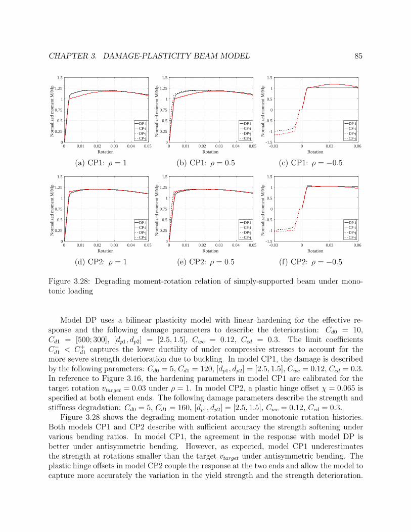
CHAPTER 3. DAMAGE-PLASTICITY BEAM MODEL 85
0 0.01 0.02 0.03 0.04 0.05Rotation
0
0.25
0.5
0.75
1
1.25
1.5
Nor
mal
ized
mom
ent M
/Mp
DP-iCP-iDP-jCP-j
(a) CP1: ρ = 1
0 0.01 0.02 0.03 0.04 0.05Rotation
0
0.25
0.5
0.75
1
1.25
1.5
Nor
mal
ized
mom
ent M
/Mp
DP-iCP-iDP-jCP-j
(b) CP1: ρ = 0.5
-0.03 0 0.03 0.06Rotation
-1.5
-1
-0.5
0
0.5
1
1.5
Nor
mal
ized
mom
ent M
/Mp
DP-iCP-iDP-jCP-j
(c) CP1: ρ = −0.5
0 0.01 0.02 0.03 0.04 0.05Rotation
0
0.25
0.5
0.75
1
1.25
1.5
Nor
mal
ized
mom
ent M
/Mp
DP-iCP-iDP-jCP-j
(d) CP2: ρ = 1
0 0.01 0.02 0.03 0.04 0.05Rotation
0
0.25
0.5
0.75
1
1.25
1.5
Nor
mal
ized
mom
ent M
/Mp
DP-iCP-iDP-jCP-j
(e) CP2: ρ = 0.5
-0.03 0 0.03 0.06Rotation
-1.5
-1
-0.5
0
0.5
1
1.5
Nor
mal
ized
mom
ent M
/Mp
DP-iCP-iDP-jCP-j
(f) CP2: ρ = −0.5
Figure 3.28: Degrading moment-rotation relation of simply-supported beam under mono-tonic loading
Model DP uses a bilinear plasticity model with linear hardening for the effective re-sponse and the following damage parameters to describe the deterioration: Cd0 = 10,Cd1 = [500; 300], [dp1, dp2] = [2.5, 1.5], Cwc = 0.12, Ccd = 0.3. The limit coefficientsC−d1 < C+
d1 captures the lower ductility of under compressive stresses to account for themore severe strength deterioration due to buckling. In model CP1, the damage is describedby the following parameters: Cd0 = 5, Cd1 = 120, [dp1, dp2] = [2.5, 1.5], Cwc = 0.12, Ccd = 0.3.In reference to Figure 3.16, the hardening parameters in model CP1 are calibrated for thetarget rotation vtarget = 0.03 under ρ = 1. In model CP2, a plastic hinge offset χ = 0.065 isspecified at both element ends. The following damage parameters describe the strength andstiffness degradation: Cd0 = 5, Cd1 = 160, [dp1, dp2] = [2.5, 1.5], Cwc = 0.12, Ccd = 0.3.
Figure 3.28 shows the degrading moment-rotation under monotonic rotation histories.Both models CP1 and CP2 describe with sufficient accuracy the strength softening undervarious bending ratios. In model CP1, the agreement in the response with model DP isbetter under antisymmetric bending. However, as expected, model CP1 underestimatesthe strength at rotations smaller than the target vtarget under antisymmetric bending. Theplastic hinge offsets in model CP2 couple the response at the two ends and allow the model tocapture more accurately the variation in the yield strength and the strength deterioration.

CHAPTER 3. DAMAGE-PLASTICITY BEAM MODEL 86
Not only does the softening range is closely captured, the response prior to softening isdescribed more consistently. The improvement in the response simulation under symmetricbending ρ = −0.5 is significant with the plastic hinge offsets.
To conclude the comparison study, the following compares the degrading moment-rotationwith and without the plastic hinge offsets under cyclic loading. It is evident in Figure 3.29that the plastic hinge offsets and the damage parameters capture well the response underboth antisymmetric bending and symmetric bending scenarios.
3.4.2 Portal frame
The objectives of this example are two-fold: (1) to evaluate the local and the globalresponse of a simple structure with and without strength deterioration in the girder, and(2) to investigate the effect of cyclic degradation on the force-deformation relation and thedamage evolution in the element response. This example examines the dynamic response ofa steel portal frame with height H = 14 ft and bay width L = 20 ft in Figure 3.13 under theLA30 ground motion. Following the ’strong column-weak beam’ concept, damage is assumedto accumulate in the girder while the columns have an elasto-plastic behavior. To account forthe axial-flexure interaction, each column is modeled with a force-based distributed beam-column element with 4 integration points along the length and 9 fibers in each cross section: 2in each flange and 5 in the web. The girder is modeled with the proposed damage-plasticitybeam element. To investigate the effect of element damage and cyclic degradation, threemodels with different girder response are examined:
• Model M0 : The girder response is elasto-plastic without strength deterioration.
• Model M1 : The damage parameters are Cd0 = 0, Cd1 = 120, [dp1, dp2] = [2.5, 1.5],Cwc = 0.1, Ccd = 0.3. The threshold coefficient Cd0 = 0 implies damage initiation atthe onset of yielding. The cyclic degradation coefficient Cwc and the coupling coefficientCcd indicate a relatively mild level of strength and stiffness deterioration due to cyclicloading.
• Model M2 : Same as model M1, but the parameters that govern the cyclic degradationare higher: Cwc = 0.3 and Ccd = 0.6 to describe more severe deterioration in the girderresponse.
It is evident in Figure 3.30 that the element damage has a significant impact on thedynamic behavior of the portal frame. The time history of the lateral displacement in Fig-ure 3.30(a) shows higher displacement amplification with more severe strength and stiffnessdeterioration in the girder. While model M0 and M1 result in residual displacements in thenegative direction, model M2 induces residual displacements in the opposite direction.
Figures 3.30(b)-(d) highlight the effect of cyclic degradation on the local response in thegirder. Figure 3.30(b) plots the moment-rotation relation in model M0 and model M1 to

CHAPTER 3. DAMAGE-PLASTICITY BEAM MODEL 87
-0.04 -0.02 0 0.02 0.04Rotation
-1.5
-1
-0.5
0
0.5
1
1.5
Nor
mal
ized
mom
ent M
/Mp
DPCP
(a) χ = 0, ρ = 1, end i
-0.04 -0.02 0 0.02 0.04Rotation
-1.5
-1
-0.5
0
0.5
1
1.5
Nor
mal
ized
mom
ent M
/Mp
DPCP
(b) χ = 0, ρ = 0.5, end i
-0.04 -0.02 0 0.02 0.04Rotation
-1.5
-1
-0.5
0
0.5
1
1.5
Nor
mal
ized
mom
ent M
/Mp
DPCP
(c) χ = 0, ρ = −0.5, end i
-0.04 -0.02 0 0.02 0.04Rotation
-1.5
-1
-0.5
0
0.5
1
1.5
Nor
mal
ized
mom
ent M
/Mp
DPCP
(d) χ = 0, ρ = 1, end j
-0.02 -0.01 0 0.01 0.02Rotation
-1.5
-1
-0.5
0
0.5
1
1.5
Nor
mal
ized
mom
ent M
/Mp
DPCP
(e) χ = 0, ρ = 0.5, end j
-0.02 -0.01 0 0.01 0.02Rotation
-1.5
-1
-0.5
0
0.5
1
1.5
Nor
mal
ized
mom
ent M
/Mp
DPCP
(f) χ = 0, ρ = −0.5, end j
-0.04 -0.02 0 0.02 0.04Rotation
-1.5
-1
-0.5
0
0.5
1
1.5
Nor
mal
ized
mom
ent M
/Mp
DPCP
(g) χ = 0.065, ρ = 1, end i
-0.04 -0.02 0 0.02 0.04Rotation
-1.5
-1
-0.5
0
0.5
1
1.5
Nor
mal
ized
mom
ent M
/Mp
DPCP
(h) χ = 0.065, ρ = 0.5, end i
-0.04 -0.02 0 0.02 0.04Rotation
-1.5
-1
-0.5
0
0.5
1
1.5
Nor
mal
ized
mom
ent M
/Mp
DPCP
(i) χ = 0.065, ρ = −0.5, end i
-0.04 -0.02 0 0.02 0.04Rotation
-1.5
-1
-0.5
0
0.5
1
1.5
Nor
mal
ized
mom
ent M
/Mp
DPCP
(j) χ = 0.065, ρ = 1, end j
-0.02 -0.01 0 0.01 0.02Rotation
-1.5
-1
-0.5
0
0.5
1
1.5
Nor
mal
ized
mom
ent M
/Mp
DPCP
(k) χ = 0.065, ρ = 0.5, end j
-0.02 -0.01 0 0.01 0.02Rotation
-1.5
-1
-0.5
0
0.5
1
1.5
Nor
mal
ized
mom
ent M
/Mp
DPCP
(l) χ = 0.065, ρ = −0.5, end j
Figure 3.29: Degrading moment-rotation relation of simply-supported beam under cyclicloading

CHAPTER 3. DAMAGE-PLASTICITY BEAM MODEL 88
0 10 20 30 40 50Time (sec)
-0.1
-0.05
0
0.05
0.1
Drif
t rat
io
M0M1M2
(a) Lateral displacement time history
-0.02 0 0.02 0.04 0.06
Flexural deformation
-1
-0.5
0
0.5
1
Flex
ural
forc
e, M
/Mp
M0M1
(b) Girder response with and without damage
-0.05 0 0.05Flexural deformation
-1
-0.5
0
0.5
1
Flex
ural
forc
e, M
/Mp
M1M2
(c) Girder response with cyclic degradation
-0.06 -0.04 -0.02 0 0.02 0.04 0.06Plastic flexural deformation
0
0.05
0.1
0.15
0.2
0.25
0.3
0.35
Dam
age
varia
ble
M1M2
(d) Girder damage evolution
Figure 3.30: Dynamic response of portal frame
study the effect of element damage. Model M1 shows a wider range of rotation in the hystere-sis loops, which leads to more excessive lateral drift in the negative direction. Figure 3.30(c)compares the moment-rotation relation in model M1 and model M2 to examine the effectof cyclic degradation. As expected from the lateral displacement time history, the rotationsin the two cases depart to opposite directions. Higher values of Cwc and Ccd lead to a morepronounced strength reduction especially in the follower cycles, which are numerous in thisground motion. Figure 3.30(d) compares the evolution of a damage variable at the girderleft end in model M1 and model M2, which is taken as the higher of the two variables d+iand d−i . In model M2, the higher values of the damage parameters result in 35% strength
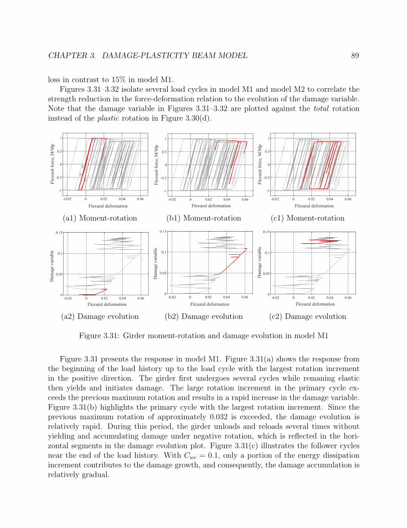
CHAPTER 3. DAMAGE-PLASTICITY BEAM MODEL 89
loss in contrast to 15% in model M1.Figures 3.31–3.32 isolate several load cycles in model M1 and model M2 to correlate the
strength reduction in the force-deformation relation to the evolution of the damage variable.Note that the damage variable in Figures 3.31–3.32 are plotted against the total rotationinstead of the plastic rotation in Figure 3.30(d).
-0.02 0 0.02 0.04 0.06
Flexural deformation
-1
-0.5
0
0.5
1
Flex
ural
forc
e, M
/Mp
a
a
(a1) Moment-rotation
-0.02 0 0.02 0.04 0.06
Flexural deformation
-1
-0.5
0
0.5
1
Flex
ural
forc
e, M
/Mp
(b1) Moment-rotation
-0.02 0 0.02 0.04 0.06
Flexural deformation
-1
-0.5
0
0.5
1
Flex
ural
forc
e, M
/Mp
(c1) Moment-rotation
-0.02 0 0.02 0.04 0.06Flexural deformation
0
0.05
0.1
0.15
Dam
age
varia
ble
(a2) Damage evolution
-0.02 0 0.02 0.04 0.06
Flexural deformation
0
0.05
0.1
0.15
Dam
age
varia
ble
(b2) Damage evolution
-0.02 0 0.02 0.04 0.06
Flexural deformation
0
0.05
0.1
0.15
Dam
age
varia
ble
(c2) Damage evolution
Figure 3.31: Girder moment-rotation and damage evolution in model M1
Figure 3.31 presents the response in model M1. Figure 3.31(a) shows the response fromthe beginning of the load history up to the load cycle with the largest rotation incrementin the positive direction. The girder first undergoes several cycles while remaning elasticthen yields and initiates damage. The large rotation increment in the primary cycle ex-ceeds the previous maximum rotation and results in a rapid increase in the damage variable.Figure 3.31(b) highlights the primary cycle with the largest rotation increment. Since theprevious maximum rotation of approximately 0.032 is exceeded, the damage evolution isrelatively rapid. During this period, the girder unloads and reloads several times withoutyielding and accumulating damage under negative rotation, which is reflected in the hori-zontal segments in the damage evolution plot. Figure 3.31(c) illustrates the follower cyclesnear the end of the load history. With Cwc = 0.1, only a portion of the energy dissipationincrement contributes to the damage growth, and consequently, the damage accumulation isrelatively gradual.

CHAPTER 3. DAMAGE-PLASTICITY BEAM MODEL 90
-0.08 -0.06 -0.04 -0.02 0 0.02
Flexural deformation
-1
-0.5
0
0.5
1
Flex
ural
forc
e, M
/Mp
(a1) Moment-rotation
-0.08 -0.06 -0.04 -0.02 0 0.02
Flexural deformation
-1
-0.5
0
0.5
1
Flex
ural
forc
e, M
/Mp
(b1) Moment-rotation
-0.08 -0.06 -0.04 -0.02 0 0.02
Flexural deformation
-1
-0.5
0
0.5
1
Flex
ural
forc
e, M
/Mp
(c1) Moment-rotation
-0.08 -0.06 -0.04 -0.02 0 0.02
Flexural deformation
0
0.05
0.1
0.15
0.2
0.25
0.3
0.35
Dam
age
varia
ble
(a2) Damage evolution
-0.08 -0.06 -0.04 -0.02 0 0.02
Flexural deformation
0
0.05
0.1
0.15
0.2
0.25
0.3
0.35
Dam
age
varia
ble
(b2) Damage evolution
-0.08 -0.06 -0.04 -0.02 0 0.02
Flexural deformation
0
0.05
0.1
0.15
0.2
0.25
0.3
0.35
Dam
age
varia
ble
(c2) Damage evolution
Figure 3.32: Girder moment-rotation and damage evolution in model M2
Figure 3.32 presents the moment-rotation and the damage evolution in model M2. Fig-ure 3.32(a) shows the response from the beginning of the load history to the load cycle withthe largest rotation increment in the negative direction. The large rotation increment in theprimary cycle results in a rapid damage growth. In contrast to model M1 with mild cyclicdegradation, the element damage accumulates relatively earlier and induces a significantdisplacement increment in the opposite direction. Figure 3.32(b) highlights the follower halfcycles in which the previous maximum rotation magnitude is not exceeded. The girder isreloading in the negative rotation direction with a few instances of unloading and reloadingwithout accumulating further damage. The deterioration rate is quite rapid in these fol-lower cycles because of the high cyclic degradation parameter Cwc. Figure 3.32(c) illustratesthe follower half cycles near the end of the load history. In contrast to the load cycles inFigure 3.32(b), damage accumulates from the rotation reversals in both loading directions.
In summary, based on the comparison of the global and the local response, it is importantto account for the strength and stiffness deterioration in the element behavior. The cyclicdegradation proves to have a significant impact on the dynamic behavior of structures,especially in this case study with a ground motion record with numerous cycles. Moreover,the damage-plasticity model captures well the distinct deterioration rates in primary andfollower half cycles.

CHAPTER 3. DAMAGE-PLASTICITY BEAM MODEL 91
3.5 Validation Studies
A database with more than 50 experiments of steel wide-flange components is assembledfor the validation of the proposed damage-plasticity beam model. The geometry of specimensin the database satisfies the following conditions:
5 ≤ bf/2tf ≤ 8 30 ≤ h/tw ≤ 55 35 ≤ Lb/ry ≤ 120 (3.63)
where bf is the flange width, tf is the flange thickness, h is the fillet-to-fillet web depth, twis the web thickness, Lb is the unbraced length, and ry is the radius of gyration about theweak axis of the cross section.
A calibration study is performed to showcase the capabilities of the model to capture themeasured degrading response as well as to correlate the model’s damage parameters withphysical properties of specimens, such as the geometry and material properties. Based onthe response comparison, a multivariate regression analysis is performed to derive empiricalfunctions for the damage parameters. These functions establish a set of guidelines for theparameter selection.
The section first illustrates the simulation of a sample steel specimen from the database.Then, a multivariate regression analysis is presented to derive the empirical formulae for theparameters. The study concludes with a parameter sensitivity analysis to identify the extentto which each parameter affects the numerical solutions.
3.5.1 Simulation of steel components
The experimental campaign by Yu et al. [111] provides measurements of the hystereticbehavior of two identical steel beam-to-column subassemblages under different deformationhistories, referred to as experiment LS1 and LS3. The load protocol of specimen LS1 is astandard symmetrical cyclic history consisting of groups of displacement cycles with con-stant amplitudes from one cycle to the next with gradually increasing average amplitude ofthe group as loading progresses. The deformation history of specimen LS3 consists of sev-eral small cycles with variable and gradually increasing amplitudes followed by a few largedisplacement pulses. The LS1 deformation history represents the effect of far-field groundmotions while the LS3 protocol simulates the effect of near-fault ground motions on thehysteretic behavior of steel components.
Figure 3.33 shows the numerical results for the steel assembly under the two load histories.The series beam model in Section 3.1 describes the force-deformation relation in the effectivespace with the kinematic hardening ratio Hkr = 0.015 and isotropic hardening ratio Hir =0.002. Although the plastic hinge offset could capture better the yield strength in the earlycycles, no hinge offset is specified, χ = 0, for simplicity. In this simulation the CDF of thebeta distribution in Section 3.3.3 is used. The damage parameters are Cd0 = 5, Cd1 = 130,dp1 = 3, dp2 = 1.5, Cwc = 0.14, Ccd = 0.4. Same parameters are specified for the positive andnegative response to account for the symmetrical degrading behavior of the steel specimen.

CHAPTER 3. DAMAGE-PLASTICITY BEAM MODEL 92
-0.05 -0.025 0 0.025 0.05Rotation
-1
-0.5
0
0.5
1
q=q p
ExperimentalNumerical
(a) Specimen LS1
0 0.025 0.05Rotation
-1
-0.5
0
0.5
1
q=q p
ExperimentalNumerical
(b) Specimen LS3
Figure 3.33: Moment-rotation relation of steel specimens LS1 and LS3 [111]
The damage threshold coefficient Cd0 > 0 indicates damage initiation after significantplastic deformations in the steel specimens. The numerical solution simulates well the cyclichardening behavior in the early cycles following yielding of the specimen. The limit coefficientCd1 = 130 appears to capture sufficiently the ductility capacity of the specimen in both loadcases. The damage evolution parameter dp1 > 1 in combination with dp2 > 1 describeconsistently the deterioration rate in both specimens. These values for dp1 and dp2 appearto be typical for steel specimens with ductile respone and high energy dissipation capacity.The cyclic coefficient Cwc and the couplding coefficient Ccd are able to capture the strengthand stiffness degradation due to repeated load reversals.
One limitation in the response comparison is the inadequate representation of the Bauschingereffect in the reloading behavior. A possible solution is to use a different element model inthe effective space to account for the gradual smooth transition from the elastic to plasticbehavior, such as to adopt the generalized plasticity [7, 48]; however, this is not pursuedfurther here. Nonetheless, the model simulates consistently the gradual strength and stiff-ness degradation of the specimen under both loading scenarios and the agreement with theexperimental results is acceptable.
3.5.2 Regression analysis for parameter identification
The simulations of the specimens in the database indicate an evident correlation betweenthe model’s damage parameters and the section compactness and the specimen slendernes.These properties are reflected in: (1) the flange width-to-thickness ratio bf/2tf , (2) the webdepth-to-thickness ratio h/tw, and (3) the slenderness ratio Lb/ry. Figure 3.34 illustrates thevariation in the limit coefficient Cd1 with the section compactness bf/2tf and h/tw and the

CHAPTER 3. DAMAGE-PLASTICITY BEAM MODEL 93
slenderness ratio Lb/ry. The ductility capacity governed by the limit coefficient Cd1 showsthe strongest correlation with the slenderness of the components.
5 5.5 6 6.5 7 7.5 8bf/2tf
100
150
200
250
300
Cd1
(a) Cd1 vs. bf/2tf
30 35 40 45 50 55h/tw
100
150
200
250
300
Cd1
(b) Cd1 vs. h/tw
40 60 80 100 120Lb/ry
100
150
200
250
300
Cd1
(c) Cd1 vs. Lb/ry
Figure 3.34: Variation in the limit coefficient Cd1 with the section compactness and memberslender
The value of a damage parameter can be evaluated empirically using the folowing ex-pression, where X represents the parameter Cd0, Cd1, dp1, dp2, Cwc, Ccd.
X = α0.
(bf2tf
)α1
.
(h
tw
)α2
.
(Lbry
)α3
(3.64)
The objective is to identify the coefficients α0, α1, α2, α3 to best fit the value of parameterX obtained from the simulations. Taking the natural logarithm of both sides, Equation (3.64)can be rewritten in a standard form of a linear multivariate regression problem:
lnX = lnα0 + α1 ln
(bf2tf
)+ α2
(h
tw
)+ α3
(Lbry
)(3.65)
Table 3.4 lists the coefficients of the multivariate linear regression for the damage param-eters.
Parameter α0 α1 α2 α3
Cd0 37.44 0.2439 -0.3799 -0.0149Cd1 2640 -0.6246 0.0122 -0.3631Cwc 0.0166 0.0104 0.0723 0.4190Ccd 0.0818 -0.1156 0.1328 0.3044dp1 2.092 0.0114 0.1321 -0.0485dp2 1.306 -0.0518 -0.0770 0.1148
Table 3.4: Regression coefficients for parameter calibration

CHAPTER 3. DAMAGE-PLASTICITY BEAM MODEL 94
3.5.3 Parameter sensitivity
For each damage parameter X, define the error ρX as the relative difference between thepredicted value Xp using Equation (3.64) and the ’exact’ value Xe from the simulation:
ρX =(Xp −Xe)
Xe
(3.66)
then the minimum value ρX,min and the maximum ρX,max give the boundary for the error inthe prediction of parameter X.
0 5 10 15 20Half cycle
-0.08
-0.04
0
0.04
0.08
Rota
tion
(a) CUREE
0 2 4 6 8 10 12Half cycle
-0.06
-0.03
0
0.03
0.06
0.09
0.12
Rota
tion
(b) NF
Figure 3.35: Cyclic load protocols for cantilever beam
To evaluate the sensitivity of the numerical solution to the damage parameters, theproposed damage-plasticity beam model simulates the force-deformation relation of a steelW30x99 cantilever beam subjected to two different cyclic load patterns: the CUREE protocoland the NF protocol [50]. The CUREE protocol consists of groups of displacement cycleswith gradually increasing average amplitude as the loading progresses. The NF protocolconsists of several cycles of small but ever increasing displacement amplitude followed byvery few large displacement pulses of increasing amplitude. The former simulates the effectof far-field ground motions and the latter represents the effect of near-fault ground motions.
In each load scenario, the numerical solution that uses the regression expression in Equa-tion (3.64) for the parameter identification is selected as the reference response. For eachparameter, while the remaining parameters are fixed, the numerical solution is reevaluatedat Xmin = (1 + ρX,min)Xr and Xmax = (1 + ρX,max)Xr, where Xr is the parameter value inthe reference solution. These account for the uncertainty in the parameter estimation andprovide an upper bound and a lower bound for the numerical response. Figure 3.36 shows the

CHAPTER 3. DAMAGE-PLASTICITY BEAM MODEL 95
-0.06 -0.04 -0.02 0 0.02 0.04 0.06Deformation
-1
-0.5
0
0.5
1
M=M
p
(a) CUREE
-0.04 0 0.04 0.08 0.12Deformation
-1
-0.5
0
0.5
1
M=M
p
(b) NF
Figure 3.36: Reference cyclic response under different loading histories
reference force-deformation relation in the two load scenarios and Figures 3.37–3.38 presentthe numerical solutions evaluated at different parameter values.
The change in the damage variable d = max(d+, d−) at the end of the load history isselected to quantify the effect of the parameters on the numerical solutions. Note that whileother measures can be used for the comparison, this study makes use of the damage variabled because: (i) the damage variable is closely related to the energy dissipation, which is acommon damage measure in performance-based design, (ii) the damage variable is readilyavailable from the model state determination. The error εmin is defined as the relativedifference in the damage variable d at Xmin and the error εmax corresponds to Xmax.
εmin =dmin − dr
drεmax =
dmax − drdr
(3.67)
where dmin and dmax correspond to the damage variable d in the solution at Xmin and Xmax,respectively, and dr represents the damage variable d in the reference case. A positive εoverestimates the damage variable d and predicts more severe strength and stiffness deterio-ration in the response. A smaller magnitude of ε indicates that the response is less sensitiveto the variation in the parameter value.
Table 3.5 summarizes the relative errors in the two load patterns. In each load scenario,the response sensitivity to the parameters is ranked based on the range of error ∆ε =|εmax − εmin|. The response is most sensitive to the parameter of rank ’1’ and least sensitiveto the parameter of rank ’6’.
In both load scenarios, the numerical solution is most sensitive to the limit coefficientCd1. It is noteworthy that the excessive error in the damage variable of almost +25% in theNF load pattern corresponds to a ρmin = +30% overestimation in the value of Cd1. However,
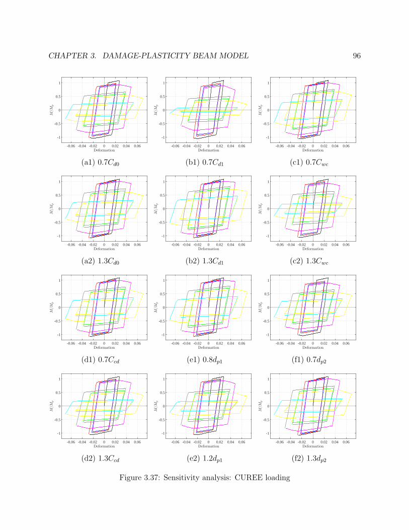
CHAPTER 3. DAMAGE-PLASTICITY BEAM MODEL 96
-0.06 -0.04 -0.02 0 0.02 0.04 0.06Deformation
-1
-0.5
0
0.5
1
M=M
p
(a1) 0.7Cd0
-0.06 -0.04 -0.02 0 0.02 0.04 0.06Deformation
-1
-0.5
0
0.5
1
M=M
p
(b1) 0.7Cd1
-0.06 -0.04 -0.02 0 0.02 0.04 0.06Deformation
-1
-0.5
0
0.5
1
M=M
p
(c1) 0.7Cwc
-0.06 -0.04 -0.02 0 0.02 0.04 0.06Deformation
-1
-0.5
0
0.5
1
M=M
p
(a2) 1.3Cd0
-0.06 -0.04 -0.02 0 0.02 0.04 0.06Deformation
-1
-0.5
0
0.5
1
M=M
p
(b2) 1.3Cd1
-0.06 -0.04 -0.02 0 0.02 0.04 0.06Deformation
-1
-0.5
0
0.5
1
M=M
p(c2) 1.3Cwc
-0.06 -0.04 -0.02 0 0.02 0.04 0.06Deformation
-1
-0.5
0
0.5
1
M=M
p
(d1) 0.7Ccd
-0.06 -0.04 -0.02 0 0.02 0.04 0.06Deformation
-1
-0.5
0
0.5
1
M=M
p
(e1) 0.8dp1
-0.06 -0.04 -0.02 0 0.02 0.04 0.06Deformation
-1
-0.5
0
0.5
1
M=M
p
(f1) 0.7dp2
-0.06 -0.04 -0.02 0 0.02 0.04 0.06Deformation
-1
-0.5
0
0.5
1
M=M
p
(d2) 1.3Ccd
-0.06 -0.04 -0.02 0 0.02 0.04 0.06Deformation
-1
-0.5
0
0.5
1
M=M
p
(e2) 1.2dp1
-0.06 -0.04 -0.02 0 0.02 0.04 0.06Deformation
-1
-0.5
0
0.5
1
M=M
p
(f2) 1.3dp2
Figure 3.37: Sensitivity analysis: CUREE loading

CHAPTER 3. DAMAGE-PLASTICITY BEAM MODEL 97
-0.04 0 0.04 0.08 0.12Deformation
-1
-0.5
0
0.5
1
M=M
p
(a1) 0.7Cd0
-0.04 0 0.04 0.08 0.12Deformation
-1
-0.5
0
0.5
1
M=M
p
(b1) 0.7Cd1
-0.04 0 0.04 0.08 0.12Deformation
-1
-0.5
0
0.5
1
M=M
p
(c1) 0.7Cwc
-0.04 0 0.04 0.08 0.12Deformation
-1
-0.5
0
0.5
1
M=M
p
(a2) 1.3Cd0
-0.04 0 0.04 0.08 0.12Deformation
-1
-0.5
0
0.5
1
M=M
p
(b2) 1.3Cd1
-0.04 0 0.04 0.08 0.12Deformation
-1
-0.5
0
0.5
1
M=M
p(c2) 1.3Cwc
-0.04 0 0.04 0.08 0.12Deformation
-1
-0.5
0
0.5
1
M=M
p
(d1) 0.7Ccd
-0.04 0 0.04 0.08 0.12Deformation
-1
-0.5
0
0.5
1
M=M
p
(e1) 0.8dp1
-0.04 0 0.04 0.08 0.12Deformation
-1
-0.5
0
0.5
1
M=M
p
(f1) 0.7dp2
-0.04 0 0.04 0.08 0.12Deformation
-1
-0.5
0
0.5
1
M=M
p
(d2) 1.3Ccd
-0.04 0 0.04 0.08 0.12Deformation
-1
-0.5
0
0.5
1
M=M
p
(e2) 1.2dp1
-0.04 0 0.04 0.08 0.12Deformation
-1
-0.5
0
0.5
1
M=M
p
(f2) 1.3dp2
Figure 3.38: Sensitivity analysis: NF loading

CHAPTER 3. DAMAGE-PLASTICITY BEAM MODEL 98
CUREE NFParameter
εmin εmax Ranking εmin εmax RankingCd0 +1.15% -1.25% 6 +1.95% -2.08% 6Cd1 +15.48% -16.77% 1 +23.14% -19.57% 1Cwc -11.11% +8.01% 2 -4.54% +4.17% 3Ccd -5.72% +4.77% 4 -3.64% +3.40% 4dp1 -9.79% +6.67% 3 -12.38% +9.28% 2dp2 -3.58% +2.94% 5 -2.51% +2.35% 5
Table 3.5: Sensitivity ranking of damage parameters
only 4 among more than 50 specimens yield an error ρ between ±20% and ±30% while theothers are within ±20% and give the maximum error ε of approximately 15%. This stillindicates that the model is most sensitive to Cd1 but the error in the prediction is far morereasonable.
The ranking of the damage evolution parameter dp1 and the cyclic degradation parameterCwc are switched in the two load patterns. The error ∆ε for parameter dp1 is relatively highin both load cases whereas the error ∆ε for parameter Cwc is more significant in the CUREEprotocol than in the NF protocol. Effect of the displacement history on the cyclic degradationis evident in the ranking of the cyclic degradation parameter Cwc. Cyclic degradation issignificant in the CUREE protocol due to the numerous cycles with complete load reversalsin contrast to the NF protocal with a displacement history that biases to one direction andconsists of many incomplete cycles with little damage accumulation.
The model is least sensitive to the damage threshold coefficient Cd0 and followed by thesecond damage evolution parameter dp2. The effect of the damage threshold Cd0 is mainly inthe early cycles up to the onset of strength softening and less pronounced in the subsequentcycles. The negligible variation in the damage variable suggests that it is sufficient to specifyconstant values for Cd0 and dp2 so as to reduce the number of parameters to be calibrated.
3.6 Damage Evolution with Brittle Failure
3.6.1 Formulation
To account for the sudden strength and stiffness deterioration in the event of brittlefailure, the damage evolution law in Section 2.7 is adopted. The damage evolution functionis shown in Figure 2.26. The damage evolution law introduces two energy variables: ψ±
f and
ψ±u that satisfy the constraint ψd0 ≤ ψ±
f < ψ±u ≤ ψd1. ψ±
f is the energy at which fracturetakes place and ψ±
u is the ultimate energy at complete strength loss. The energy variablescan be normalized to give the condition 0 ≤ ψf < ψu ≤ 1. Different values can be specifiedfor the variables under positive and negative moments at end i and end j, and for brevity the

CHAPTER 3. DAMAGE-PLASTICITY BEAM MODEL 99
superscript ± and the subscript i and j are dropped. The damage variables d± are evaluatedfrom a composite function in Equation (2.16).
3.6.2 Validation studies
The section presents four simulations of steel cantilever beam specimens that exhibitbrittle damage at large inelastic deformations. The damage-plasticity beam element with thedamage evolution that accommodates the brittle damage is used in all simulations. Table 3.6lists the damage parameters in each case, including the threshold coefficient Cd0, the limitcoefficient Cd1, the evolution parameters dp1 and dp2, the cyclic degradation coefficient Cwc,
the damage coupling coefficient Ccd, the normalized fracture energy ψf , and the normalized
ultimate energy ψu.
Parameter Popov, EERC-3 Uang, DC3 Ricles, 1E Engelhardt, 3BCd0 8 7 5 7Cd1 110 200 140 170Cwc 0.10 0.15 0.15 0.13Ccd 0.40 0.40 0.50 0.40dp1 3 3 3 3dp2 1.5 1.5 1.5 1.5
ψf 0.15 0.11 0.28 0.27
ψu 0.20 0.12 0.33 0.30
Table 3.6: Parameters for the simulations of steel beams with brittle damage
Figure 3.39(a) shows the measured moment-rotation of the specimen EERC-3 from theexperimental campaign by Popov [74]. The specimen is made of a W18x50 steel cantileverbeam with a pre-Northridge connection. Figure 3.39(b) shows the measured moment-rotationof the steel specimen DC3 from the experiments by Uang [31] of a W27x194 beam section.Figure 3.39(c) shows the response of the specimen 1E from the experimental campaignby Ricles [84] with a W36x150 beam section. Figure 3.39(d) shows the response of thespecimen 3B from the experiments by Engelhardt [25] with a W36x150 beam section andweld connection.
The proposed model simulates quite accurately the strength degradation pre- and post-fracture in the specimens. The first two specimen show negligible damage prior to the onset offracture whereas the latter two specimens show a gradual strength and stiffness degradationbefore the onset of severe strength deterioration in the last cycle. The relatively low fractureenergy parameter ψf in the first two specimen captures the drastic strength reduction at alower normalized energy level with limited previous accumulated damage.
The specimens represent two distinct types of failure mechanisms observed in steel com-ponents under cyclic loading [51]. The first mechanism is related to crack propagation at

CHAPTER 3. DAMAGE-PLASTICITY BEAM MODEL 100
-0.05 -0.025 0Rotation
-1
-0.5
0
0.5
1
q=q p
ExperimentalNumerical
(a) Popov, EERC-3 [74]
-0.025 0 0.025Rotation
-1
-0.5
0
0.5
1
q=q p
ExperimentalNumerical
(b) Uang, DC3 [31]
-0.05 -0.025 0 0.025Rotation
-1
-0.5
0
0.5
1
q=q p
ExperimentalNumerical
(c) Ricles, 1E [84]
-0.025 0 0.025Rotation
-1
-0.5
0
0.5
1
q=q p
ExperimentalNumerical
(d) Engelhardt, 3B [25]
Figure 3.39: Moment-rotation relation of steel specimens with brittle failure
weldments, in which little deterioration is induced for a number of cycles in the beginning,then as the crack approaches its critical size, the specimens show rapid strength reduction.The second mechanism typically involves local buckling and leads to more gradual deterio-ration prior to the brittle failure. As evident in the response simulation of the two specimensin Figure 3.39, the composite evolution function accommodates well both types of degradingbehavior.

101
Chapter 4
Damage-Plasticity Column Element
This chapter extends the 1d hysteretic damage model in Chapter 2 to formulate a newcolumn element based on damage-plasticity for the response simulation and damage assess-ment of steel structures under extreme load conditions, especially when the axial forces aresignificant. First, the NMYS column element based on resultant plasticity and the serialsprings formulation is introduced to describe the nondegrading force-deformation relationin the effective space. The model accounts for the axial-flexure interaction in a yield enve-lope with consistent associative flow rules and linear hardening laws. Similar to the beamformulation in Chapter 3, plastic hinge offsets are introduced to approximate the spread ofinelasticity and enhance the simulation of the post-yield hardening response. The implemen-tation of the damage-plasticity element with the return-mapping algorithm ensures excellentconvergence characteristics for the state determination.
With the plastic axial energy dissipation accounted for in the damage loading function,the damage-plasticity column model captures the effect of a variable axial force on thestrength and stiffness deterioration in flexure, the severe deterioration under high axial com-pression, the nonsymmetric response under variable axial forces, and the excessive plasticaxial and flexural deformations near column failure. The damage-plasticity model comparesfavorably in terms of computational efficiency with more sophisticated models with fiberdiscretization of the cross section while achieving excellent agreement in the response de-scription for homogeneous metallic structural components. The excellent accuracy is alsoconfirmed by the agreement with experimental results from column specimens under thecombined effect of axial and bending in various load scenarios. Because of the computa-tional efficiency and excellent accuracy, the proposed column element holds great promisefor the large scale seismic response simulation of structural systems with strength and stiff-ness deterioration and should prove very useful in the damage assessment and the collapsesimulation of structures under extreme loading conditions.
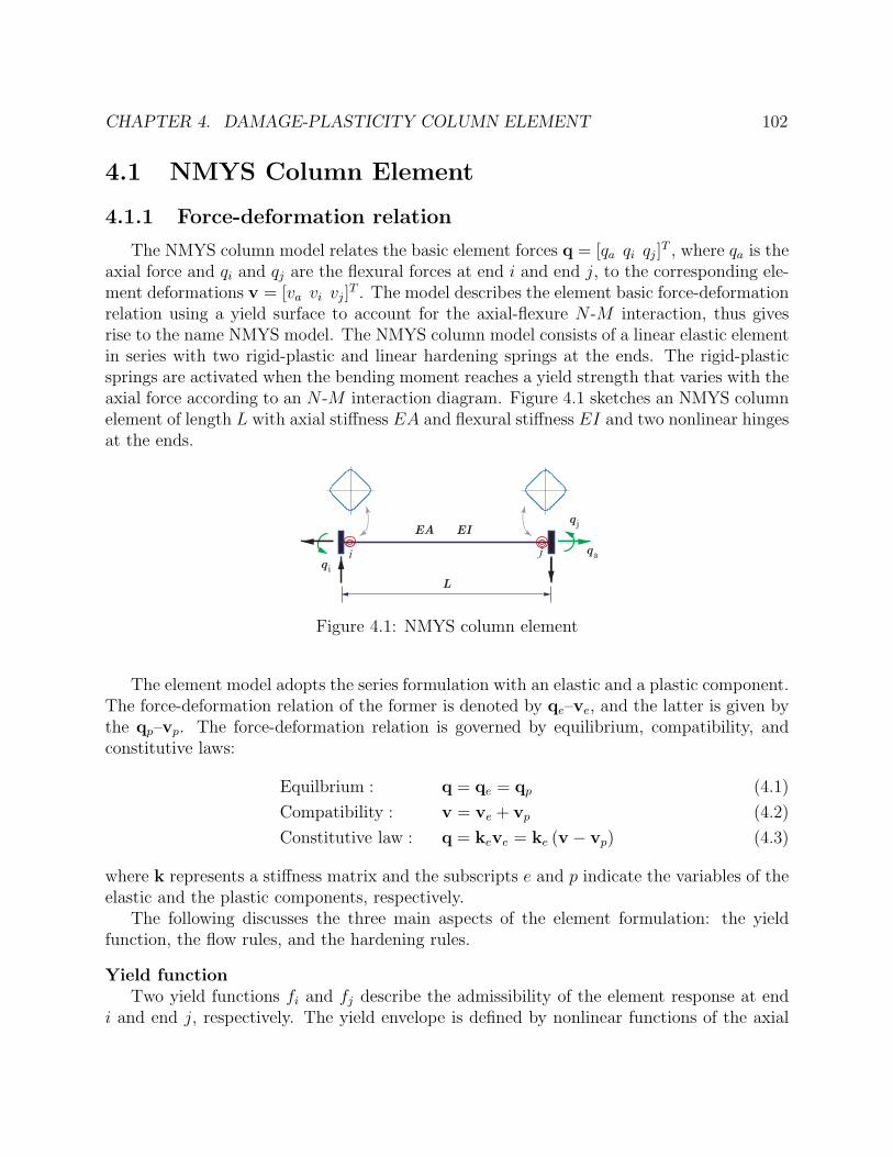
CHAPTER 4. DAMAGE-PLASTICITY COLUMN ELEMENT 102
4.1 NMYS Column Element
4.1.1 Force-deformation relation
The NMYS column model relates the basic element forces q = [qa qi qj]T , where qa is the
axial force and qi and qj are the flexural forces at end i and end j, to the corresponding ele-ment deformations v = [va vi vj]
T . The model describes the element basic force-deformationrelation using a yield surface to account for the axial-flexure N -M interaction, thus givesrise to the name NMYS model. The NMYS column model consists of a linear elastic elementin series with two rigid-plastic and linear hardening springs at the ends. The rigid-plasticsprings are activated when the bending moment reaches a yield strength that varies with theaxial force according to an N -M interaction diagram. Figure 4.1 sketches an NMYS columnelement of length L with axial stiffness EA and flexural stiffness EI and two nonlinear hingesat the ends.
q i
q jEA EI
qa
L
i j
Figure 4.1: NMYS column element
The element model adopts the series formulation with an elastic and a plastic component.The force-deformation relation of the former is denoted by qe–ve, and the latter is given bythe qp–vp. The force-deformation relation is governed by equilibrium, compatibility, andconstitutive laws:
Equilbrium : q = qe = qp (4.1)
Compatibility : v = ve + vp (4.2)
Constitutive law : q = keve = ke (v − vp) (4.3)
where k represents a stiffness matrix and the subscripts e and p indicate the variables of theelastic and the plastic components, respectively.
The following discusses the three main aspects of the element formulation: the yieldfunction, the flow rules, and the hardening rules.
Yield functionTwo yield functions fi and fj describe the admissibility of the element response at end
i and end j, respectively. The yield envelope is defined by nonlinear functions of the axial

CHAPTER 4. DAMAGE-PLASTICITY COLUMN ELEMENT 103
basic force qa and the flexural basic forces qi and qj:
fi =
∣∣∣∣qa − qb,aNp
∣∣∣∣c1 +
∣∣∣∣qi − qb,iMp
∣∣∣∣c2 + c3
∣∣∣∣qa − qb,aNp
∣∣∣∣c4 ∣∣∣∣qi − qb,iMp
∣∣∣∣c5 − (1 +Hip,iαi) (4.4)
fj =
∣∣∣∣qa − qb,aNp
∣∣∣∣c1 +
∣∣∣∣qj − qb,jMp
∣∣∣∣c2 + c3
∣∣∣∣qa − qb,aNp
∣∣∣∣c4 ∣∣∣∣qj − qb,jMp
∣∣∣∣c5 − (1 +Hip,jαj) (4.5)
With the subscripts i and j dropped for brevity, qb are the back-forces that govern thekinematic hardening behavior, Np and Mp are the axial and flexural plastic capacities, Hip
is an isotropic hardening parameter, α is an internal variable that governs the isotropichardening behavior, and c1, c2, c3, c4, c5 are coefficients of the yield envelope. While it ispossible to specify different coefficients c1 to c5 to distinguish the response at the two ends,this study limits to symmetrical yielding behavior and assumes the same coefficients at bothends.
In the case of elastic-perfectly-plastic response, the hardening parameters and variablesare irrelevant: qb,a = 0 and qb,i = qb,j = 0, Hip,i = Hip,j = 0, αi = αj = 0. In a purelyaxial force state, yielding initiates when the axial force reaches the plastic axial capacity,qa = ±Np, qi/j = 0. In a purely flexural force state, yielding initiates when the bendingmoment reaches the plastic flexural capacity, qa = 0, qi/j = ±Mp. Figure 4.2(a) plots theyield envelope defined by two surfaces fi = 0, fj = 0 in the force space N -Mi-Mj. The redsurface corresponds to fi = 0 and the blue surface corresponds to fj = 0. The admissiblestate is defined by the region inside both envelopes. Figure 4.2(b) shows a projection of thesame envelope on the N -Mi plane. This is a 2d representation of the yield surface fi = 0.The yield envelope in Figure 4.2 is given by the following parameters: c1 = 2, c2 = 2,c3 = 3.5, c4 = 2.5, c5 = 1.5.
Flow rulesThe associative flow rule describes the evolution of the plastic deformation vp in terms
of the normals ni and nj to the yield envelopes. The normals ni and nj are derivatives ofthe yield functions fi and fj with respect to the end force q, respectively. To account for thesingularities at the interface between the two yield surfaces, the Koiter’s rule expresses theplastic deformation increment, or equivalently, the plastic deformation rate vp as a linearcombination of the normals ni and nj [47].
vp = βini + βjnj = nβ (4.6)
where β = [βi βj]T are the plastic consistency parameters. Since the axial and the flexural
terms in Equations (4.4)–(4.5) are coupled, except for the pure bending force state, in generalthe element accummulates plastic axial deformations as yielding progresses. Consequently,the column model describes an elastic-plastic axial response as opposed to the linear elasticbehavior in the beam model.

CHAPTER 4. DAMAGE-PLASTICITY COLUMN ELEMENT 104
N/Np
Mi/Mp
Mj/Mp
fi = 0
fj = 0
(a) fi = fj = 0 in N -Mi-Mj space
-1 -0.5 0 0.5 1Mi/Mp
-1
-0.5
0
0.5
1
N/N
p(b) fi = 0 in N -Mi plane
Figure 4.2: Yield surfaces
The consistency condition imposes plastic loading and unloading constraints on the twoyield surfaces during plastic flow f = 0:
βmfm = 0, m = i, j (4.7)
Plastic unloading corresponds to zero consistency parameters βi = βj = 0 and negativeincrements of the yield function values fi < 0 and fj < 0. Plastic loading occurs whenthe consistency parameters are positive, βi > 0 and/or βj > 0, while the yield functionsremain constant fi = 0 and/or fj = 0. During plastic loading, a yield surface is ’active’ ifthe corresponding consistency parameter is positive β > 0, and otherwise, ’inactive’ if theconsistency parameter is zero β = 0. Identification of active yield surfaces of the columnmodel is an iterative process and will be discussed in subsequent sections. If only the yieldenvelope at end i is active, βi ≥ 0, βj = 0, and the plastic deformation increment is colinearwith the normal to the surface i: vp = βini. If both envelopes are active, βi > 0 andβj > 0, and the plastic deformation increment is a linear combination of both normals:vp = βini + βjnj.
Hardening rulesThe evolution of the internal variable α and the back-force qb are described as functions
of the consistency parameters β:
α = β (4.8)
qb = Hknβ (4.9)

CHAPTER 4. DAMAGE-PLASTICITY COLUMN ELEMENT 105
where Hk is a 3×3 kinematic hardening matrix with the hardening moduli of the axial andflexural response on the diagonal.
Finally, the Kuhn-Tucker conditions enforce unilateral constraints on the consistencyparameter β and the yield functions f = [fi fj]
T .
β ≥ 0 and f ≤ 0 and βmfm = 0, m = i, j (4.10)
Remarks on model formulation:The NMYS column model and the series beam model share many common features in
the formulation. Both elements are classified as concentrated plasticity and are based onthe series formulation with an elastic component in connection with two rigid-plastic andlinear hardening springs. Both models adopt the associative flow rules and the Koiter’s ruleto account for multi-surface plasticity. The hardening rules of the two models are identical.The column element inherits similar positive features as the series beam element in Chapter 3:exact representation of the rigid-plastic hinge behavior, implicit state determination of theplastic hinge to avoid additional nodes and global degrees of freedom (dofs) at the interfacebetween the elastic component and the plastic hinges, robust and efficient return-mappingalgorithm.
The main difference between the models, which is also a major advantage of the proposedcolumn model over several other commonly used concentrated plasticity column models inpractice, is the ability to describe an inelastic axial response and to account for the effectof the axial force on the flexural yield strength. The beam model neglects the axial-flexureinteraction and assumes a linear elastic axial response, whereas the NMYS column modelaccounts for the coupling and captures the axial plastic deformation and the elastic-linearhardening axial behavior. These assumptions are justified by a negligible axial force in beammembers and a relatively large axial force in column members.
The yield functions of the beam model in Equations (3.4)–(3.5) have unit of bendingmoments, whereas the yield functions of the column model in Equations (4.4)–(4.5) aredimensionless because the element basic forces are normalized by the respective plastic ca-pacities. The yield envelope of the beam model is defined by linear functions of the flexuralforces qi and qj, whereas the yield envelope of the column model is given by nonlinear func-tions of both the axial force qa and the flexural forces qi and qj. Consequently, the statedetermination of the column model is iterative.
It is noteworthy that the yield envelope of the beam model is a special case of Equations(4.4)–(4.5). With the coefficient c1 assumes a very large value and c2 = 1, c3 = 0, the yieldfunction in Equations (4.4)–(4.5) becomes:
fm =
∣∣∣∣qm − qb,mMp
∣∣∣∣− (1 +Hip,mαm) m = i, j (4.11)
Multiplying Equation (4.11) by Mp and denoting Hi,m = MpHip,m, the yield functionbecomes:
f ∗m = |qm − qb,m| − (Mp +Hi,mαm) m = i, j (4.12)

CHAPTER 4. DAMAGE-PLASTICITY COLUMN ELEMENT 106
which is the same as the yield function of the beam model in Equations (3.4)–(3.5)Another discrepancy between the models is the definition of the isotropic hardening
parameter, which will be addressed in Section 4.1.4.
4.1.2 Plastic hinge offset
The formulation in Section 4.1.1 places the rigid-plastic springs at the element ends. Sim-ilar to the series beam model, this section introduces the plastic hinge offset to concentratethe inelastic behavior at a distance away from the column ends. The objectives of the plastichinge offset are two-fold: (1) to account for the spread of plasticity from the column endsinto the interior region, and (2) to simulate more accurately the column post-yield hardeningresponse.
q i
q jEA EI
qa
L
c i c j
Figure 4.3: NMYS column element with plastic hinge offset
Assume the nonlinear springs are offset by the same distance ci = cj from the elementends, the model defines the offset parameter χ = ci/L = cj/L where L is the elementlength. The force interpolation matrix bp is introduced to evaluate the response at thespring locations:
bp =
1 0 00 χ− 1 χ0 −χ 1− χ
(4.13)
The normal and flexural forces in the plastic hinge qh = [N Mi Mj]T , and the corre-
sponding hinge normal and flexural deformations vh = [θa θi θj]T are expressed in terms of
the plastic forces qp and plastic deformations vp:
qh = bpqp (4.14)
vp = bTp vh (4.15)
With the plastic hinge offsets, the yield functions are defined for the spring force qhinstead of the element end force q in Equations (4.4)–(4.5). For consistency, the back-forces

CHAPTER 4. DAMAGE-PLASTICITY COLUMN ELEMENT 107
Nb, Mb,i, Mb,j follow the sign convention of internal axial force and bending moment. Theyield functions are given as follows:
fi =
∣∣∣∣Ni −Nb
Np
∣∣∣∣c1 +
∣∣∣∣Mi −Mb,i
Mp
∣∣∣∣c2 + c3
∣∣∣∣Ni −Nb
Np
∣∣∣∣c4 ∣∣∣∣Mi −Mb,i
Mp
∣∣∣∣c5 − (1 +Hip,iαi) (4.16)
fj =
∣∣∣∣Nj −Nb
Np
∣∣∣∣c1 +
∣∣∣∣Mj −Mb,j
Mp
∣∣∣∣c2 + c3
∣∣∣∣Nj −Nb
Np
∣∣∣∣c4 ∣∣∣∣Mi −Mb,j
Mp
∣∣∣∣c5 − (1 +Hip,jαj) (4.17)
The original formulation in 4.1.1 with two plastic hinges at the element ends is a specialcase with χ = 0. The next subsection presents the state determination of the NMYS columnelement model.
4.1.3 Return mapping algorithm
The state determination of the NMYS column model uses an iterative return-mappingalgorithm to determine the element end force qn and other variables at step n from theend deformation vn and the history variables. First, an elastic predictor assumes no plasticdeformation increment and gives a trial force qtr:
qtr = ke (vn − vp,n−1) (4.18)
The trial axial force N tr and bending moments M tri and M tr
j at the spring locations arecomputed from the trial force qtr according to Equation (4.14). The trial internal variableαtr and the back-force qtrb assume the values from the previous step n− 1:
αtr = αn−1 (4.19)
qtrb = qb,n−1 (4.20)
The trial variables qtr, αtr, qtrb are used to evaluate the trial yield functions f tr in Equa-tions (4.16)–(4.17). If both trial yield functions return a negative value, f tri < 0 and f trj < 0,the elastic assumption is valid and the trial variables are accepted.
qn = qtr (4.21)
αn = αtr (4.22)
qb,n = qtrb (4.23)
vp,n = vp,n−1 (4.24)
Otherwise, if at least one trial yield function returns a nonnegative value, f tri ≥ 0 and/orf trj ≥ 0, plastic correction is required. The correction uses the closest point projectionalgorithm and evaluates the variables at step n by applying the Newton-Ralphson schemeiteratively to reduce the residuals of the variable increments and enforce the Kuhn-Tuckerconditions [92].
CHAPTER 4. DAMAGE-PLASTICITY COLUMN ELEMENT 108
With the superscripts denoting the iteration number, the following residuals are defined:Rvp for the plastic deformation vp, Rf for the yield function f , Rα for the internal variableα, and Rb for the back-force qb.
R(k)vp = −v(k)
p,n + vp,n−1 + bTp n(k)β(k) (4.25)
R(k)f = f
(q(k)n ,α(k)
n ,q(k)b,n
)(4.26)
R(k)α = −α(k)
n +αn−1 + β(k) (4.27)
R(k)b = −q
(k)b,n + qb,n−1 + Hkn
(k)β(k) (4.28)
The residual vector R is defined as:
R = [Rvp Rf Rα Rb]T (4.29)
At each iteration the goal is to reduce the residuals to zero:
R(k) = 0 (4.30)
The iterations solve for the state variable x that represents the consistency parameter β,the end force q, the internal variable α, and the back-force qb.
x = [β q α qb]T (4.31)
The dimension of vectors R and x vary with the number of active yield surfaces. Whilethe dimension of Rvp and Rb are 3× 1, the residuals Rα and Rf are 1× 1 if only one surfaceis active and 2 × 1 if both are active. Similarly for the variable vector x, the dimension ofthe element end force q and the back-force qb are 3 × 1 while the consistency parameter βand the internal variable α are 1× 1 or 2× 1.
A yield surface fm is considered ’active’ if the respective consistency parameter βm > 0.The iterative procedure starts with an initial set of trial active constraints defined by J
(0)act.
J(0)act = m ∈ i, j | f trm ≥ 0 (4.32)
The subsequent iterations modify this initial set and iteratively enforce the Kuhn-Tuckerconditions. At each iteration, the set of active yield surfaces Jact is updated as follows:
(i) Let J(k−1)act denote the set of active yield surfaces at iteration k−1. If there exists indices
m not in J(k−1)act such that the yield functions violate the admissibility, f
(k−1)m > 0,
include m in J(k−1)act and repeat the iteration.
(ii) The increment of the consistency parameters ∆β(k−1)m , m ∈ J
(k−1)act is computed by
solving the linearized residual equations (4.30).
(iii) Update β(k)m = β
(k−1)m + ∆β
(k−1)m for m ∈ J
(k−1)act . If β
(k)m < 0 for some m ∈ J
(k−1)act ,
remove these constraints from the active set J(k−1)act and restart the iteration with the
new active constraints. Otherwise, set J(k)act = J
(k−1)act and proceed to the next iteration.

CHAPTER 4. DAMAGE-PLASTICITY COLUMN ELEMENT 109
The Newton-Raphson iterations start with the intial consistency parameters β(0) = 0and the initial state variables equal to the trial values.
q(0) = qtr (4.33)
α(0) = αtr (4.34)
q(0)b = qtrb (4.35)
At iteration k, the Newton-Raphson scheme requires the Jacobian matrix J(k−1), definedas the derivative of the residual R with respect to the variable x evaluated at x(k−1).
J(k−1) =∂R
∂x=
∂Rvp
∂β
∂Rvp
∂q
∂Rvp
∂α
∂Rvp
∂qb∂Rf
∂β
∂Rf
∂q
∂Rf
∂α
∂Rf
∂qb∂Rα
∂β
∂Rα
∂q
∂Rα
∂α
∂Rα
∂qb∂Rb
∂β
∂Rb
∂q
∂Rb
∂α
∂Rb
∂qb
at x = x(k−1) (4.36)
Equation (4.30) is linearized to solve for the increment of the state variable ∆x(k−1)
0 ≈ R(k) = R(k−1) +∂R
∂x∆x(k−1) (4.37)
∆x(k−1) = −J(k−1)\R(k−1) (4.38)
The model variable at iteration k, x(k), is updated from the history value x(k−1) and theincrement ∆x(k−1).
x(k) = x(k−1) + ∆x(k−1) (4.39)
With the new variable x(k), the yield function f (k) is evaluated. The iterations repeat withthe updated active surfaces based on the consistency parameter β(k). The plastic correctionalgorithm terminates when the residual norms are less than the specified tolerance values,‖R(k−1)
w ‖ < tolw, where w ∈ vp, f, α, b. Separate residual norms are checked againstdifferent tolerances for unit consistency and to avoid nonconvergence due to significant dis-crepancies between the residual norms when evaluating ‖R‖.
It is noteworthy that the element end force qn can also be updated from the trial forceqtr as follows:
qn = qtr − ke∆vp = qtr − kebTp nβ (4.40)
In view of Equation (4.40), the consistency parameters β can be regarded as the con-travariant components of the force correction ∆q = qtr − qn along the vectors keb
Tp ni and
kebTp nj. Figure 4.4 gives a graphical illustration of the return mapping algorithm for a simple

CHAPTER 4. DAMAGE-PLASTICITY COLUMN ELEMENT 110
case with an elasto-plastic element behavior and no plastic hinge offset. Figure 4.4(a) plotsa cross-section of the yield surfaces fi = 0 and fj = 0 in the plane defined by vectors keb
Tp ni
and kebTp nj evaluated at an intersection point. The region defined by fi > 0 and fj > 0 can
be divided into 3 subregions Γi, Γj, Γij. The condition β1 > 0 and β2 > 0 corresponds tosubregion Γij. In an iteration, if the trial force falls into this subregion, both surfaces areactive. Conversely, region Γi gives βi > 0 but βj < 0, and region Γj gives βj > 0 but βi < 0.If the trial force falls into Γi or Γj, only one constraint is active although both yield functionsare positive. The return-mapping procedure in subregions Γij and Γj is shown in Figures4.4(b)-(c), respectively. This illustration demonstrates that the sign of the yield function fis insufficient to determine the set of active surfaces.
fi < 0fj < 0
fi = 0
fj = 0 kebpTni
kebpTnj
Γij
Γi
Γj
(a) Definition of Γi, Γj, Γij
fi < 0fj < 0
fi = 0
fj = 0 kebpTni
kebpTnj
qtrβi > 0
βj > 0
(b) Γij: βi > 0 and βj > 0
fi < 0fj < 0
fi = 0
fj = 0 kebpTni
kebpTnj
qtr
βj > 0
βi < 0
(c) Γj: βi < 0 and βj > 0
Figure 4.4: Geometric illustration of return-mapping algorithm at corner point
The state determination of the NMYS column model is summarized in Tables 4.1–4.2: theelastic predictor in Table 4.1 and the iterative plastic correction in Table 4.2. The algorithmictangent kt is the derivative of the end force qn with respect to the end deformation vn. Aderivation of the tangent is presented in Appendix B.
4.1.4 Model parameters
Parameters of the NMYS model can be classified into three main categories:
(1) Parameters of the geometry and material properties : the Young modulus E, the cross-sectional area A, the moment of inertia I, the axial and flexural plastic capacities Np
and Mp. These 5 parameters depend solely on the specimen geometry and materialproperties and do not require calibration;
(2) Parameters of the yield envelope: coefficients c1, c2, c3, c4, c5 of the yield functions,presented in Section 4.1.4.1.

CHAPTER 4. DAMAGE-PLASTICITY COLUMN ELEMENT 111
1. Elastic predictor:
Evaluate qtr, qtrb , αtr
Evaluate trial spring forces N tr, M tri , M tr
j
2. Check of plastic process:
Evaluate f tr in Equations (4.16)–(4.17)
IF f tri < 0 and f trj < 0 THEN:
Update qb,n, αn, vp,n
Update qn, kt
EXIT
ELSE Initialization for plastic correction:
Initialize J(0)act = m ∈ i, j | f trm > 0
Initialize q(0)n , α
(0)n , q
(0)b,n, f (0), v
(0)p,n
Initialize β(0) = 0
Set k = 1 and go to Table 4.2
ENDIF
Table 4.1: Elastic predictor algorithm
(3) Hardening parameters : the kinematic hardening ratio Hkr and the isotropic hardeningparameter Hip, presented in Section 4.1.4.2.
4.1.4.1 Yield surface parameters
Figure 4.5 illustrates the effect of 5 parameters c1, c2, c3, c4, c5 on the yield envelope,which shows the projection of the 3d N -Mi-Mj surface onto N -Mi and/or N -Mj planes.The response with c1 = 2, c2 = 2, c3 = 4, c4 = 2, c5 = 2 is used as a reference in all fiveplots. In each plot, one coefficient varies from 1 to 20 while the others remain equal to therespective reference values. Due to symmetry, it is sufficient to show the envelope in onlyone quadrant.
Increasing c1, c2, c4, c5 makes the yield envelope more convex, whereas increasing c3makes the envelope more concave. As c3 varies, changes to the yield envelope is symmetricalabout the reference axis N/Np = M/Mp, whereas c1 and c2, c4 and c5 give asymmetricalchanges to the yield envelope. The yield envelope is relatively less sensitive to c1 and c2 thanc3, c4, c5. Therefore, it is recommended to calibrate the latter three coefficients first.

CHAPTER 4. DAMAGE-PLASTICITY COLUMN ELEMENT 112
1. Check of yield functions:
Evaluate the spring forces N(k−1)n , M
(k−1)i,n , M
(k−1)j,n from q
(k−1)n
Evaluate yield function f(k−1)m , for m = i, j
IF ∃m /∈ J(k−1)act : f
(k−1)m > 0 THEN:
For all m, reset J(k−1)act = J
(k−1)act ∪ m and repeat 1
ELSE:
Go to 2
ENDIF
2. Evaluation of residuals:
Evaluate R(k−1) = [Rvp Rf Rα Rb]T
IF ‖R(k−1)w ‖ < tolw, w ∈ vp, f, α, b, THEN:
Update qn, αn, qb,n and go to 7
ELSE:
Go to 3
ENDIF
3. Evaluation of force and internal variable increments:
Evaluate the Jacobian J(k−1)
Evaluate the increments ∆x(k−1) = [∆β ∆q ∆α ∆qb]T
4. Check of active constraints:
Update β(k) = β(k−1) + ∆β(k−1)
IF β(k)m < 0, m ∈ J
(k−1)act , THEN:
Reset J(k−1)act = m ∈ J
(k−1)act | β(k)
m > 0Go to 2
ELSE:
Go to 5
5. Update of forces and internal variables:
Update x(k) to obtain β(k)n,m, q
(k)n , α
(k)n,m, q
(k)b,n, m ∈ J
(k−1)act
Set J(k)act = J
(k−1)act
6. Set k − 1← k and go to 1
7. Evaluate the tangent stiffness kt
Table 4.2: Plastic correction algorithm: closest point projection

CHAPTER 4. DAMAGE-PLASTICITY COLUMN ELEMENT 113
0 0.2 0.4 0.6 0.8 10
0.2
0.4
0.6
0.8
1
M/Mp
N/N
p
c1 = 1c1 = 2c1 = 5c1 = 10c1 = 20
(a) Parameter c1
0 0.2 0.4 0.6 0.8 10
0.2
0.4
0.6
0.8
1
c2 = 1c2 = 2c2 = 5c2 = 10c2 = 20
M/Mp
N/N
p
(b) Parameter c2
0 0.2 0.4 0.6 0.8 10
0.2
0.4
0.6
0.8
1
M/Mp
N/N
p
c3 = 1c3 = 2c3 = 5c3 = 10c3 = 20
(c) Parameter c3
0 0.2 0.4 0.6 0.8 10
0.2
0.4
0.6
0.8
1
N/N
p
c4 = 1c4 = 2c4 = 5c4 = 10c4 = 20
M/Mp
(d) Parameter c4
0 0.2 0.4 0.6 0.8 1M/Mp
0
0.2
0.4
0.6
0.8
1
N/N
p
c5 = 1c5 = 2c5 = 5c5 = 10c5 = 20
(e) Parameter c5
Figure 4.5: Effect of yield surface parameters
4.1.4.2 Hardening parameters
The hardening behavior of the NMYS column element is governed by 2 parameters: thekinematic hardening ratio Hkr and the isotropic hardening parameter Hip. The dimensionlessratio Hkr describes the kinematic hardening behavior and translates the yield envelope asplastic deformations accumulate. The hardening ratio Hkr relates to the hardening modulusHk of the plastic hinge moment-rotation relation through the flexural stiffness 6EI/L underantisymmetric bending with equal end deformations:
Hk =6EI
LHkr (4.41)
The isotropic hardening parameter Hip describes the istropic hardening behavior andexpands or contracts the yield envelope as plastic deformations accumulate. It is noteworthythat the isotropic hardening parameter Hip in Equations (4.4)–(4.5) is not equivalent to theisotropic hardening ratio Hir in the series beam formulation in Chapter 3. Table 4.3 comparesthe units of relevant variables in the beam and the column models. The variables are inunit of force, deformation, or a combination thereof, or dimensionless (’1’ in Table 4.3).In the series beam model, the isotropic hardening ratio Hir is dimensionless, whereas in

CHAPTER 4. DAMAGE-PLASTICITY COLUMN ELEMENT 114
the NMYS column model, the isotropic hardening parameter Hip has dimension [force−1 ×deformation−1] .
Variable(s) Beam model Column modelfi, fj force 1ni, nj 1 force−1
vp deformation deformationβi, βj deformation force × deformationαi, αj deformation force × deformation
Hir or Hip 1 force−1 × deformation−1
Table 4.3: Unit comparison of beam and column models
Figure 4.6 illustrates the effect of the hardening behavior on the yield envelope. Thekinematic hardening in Figure 4.6(a) translates the envelope while preserving the initialshape. The isotropic hardening with Hip > 0 in Figure 4.6(b) expands the yield envelope.It is noteworthy that the shape of the yield envelope changes during the expansion or con-traction.
-1.5 -1 -0.5 0 0.5 1 1.5-1.5
-1
-0.5
0
0.5
1
1.5
N/N
p
M/Mp
(a) Kinematic hardening
-1.5 -1 -0.5 0 0.5 1 1.5-1.5
-1
-0.5
0
0.5
1
1.5
N/N
p
M/Mp
(b) Isotropic hardening
Figure 4.6: Effect of hardening parameters on yield envelope
4.1.5 Example 1: Cantilever column
The first example examines the response of a cantilever column under a combined effectof axial forces and bending moments. The column, shown in Figure 4.7, is 10 ft in length and

CHAPTER 4. DAMAGE-PLASTICITY COLUMN ELEMENT 115
has a W24x162 steel profile with a yield strength fy = 50 ksi. For comparison, two elementmodels are used to simulate the column response: a concentrated plasticity model (CP) anda distributed plasticity model (DP) . The objectives of this example are three-fold: (1) tocalibrate the yield surface parameters c1 to c5 of the NMYS model, (2) to highlight the effectof the axial-flexure interaction on the yielding behavior, and (3) to validate the accuracy andefficiency of the NMYS model in comparison to the more sophisticated distributed plasticityapproach.
N
Uh
H = 10ft W24x162
(a) (b)
Integration points
(c)
Figure 4.7: Cantilever column: (a) structure and loading, (b) concentrated plasticity (CP)model, (c) distributed plasticity (DP) model
In model DP, one force-based distributed plasticity element is used with 4 integrationpoints along the column height. Each section is discretized into 9 fibers: 2 in each flangeand 5 in the web. The Gauss-Lobatto integration rule is used along the element lengthand the mid-point rule in each cross section. The material constitutive relation assumes abilinear elastic-plastic response [92]. In model CP, one NMYS element is used to simulatethe column. The parameters E, A, I, Np, and Mp are specified based on the geometry andmaterial properties.
The following presents two case studies with different assumptions of the column behavior.
4.1.5.1 Elastic-perfectly-plastic element behavior
In the first case study, the column assumes an elastic-perfectly-plastic (EPP) behavior.In both models, same flexural deformations are increased monotonically under constant axialcompressions, whose values range from 20% to 80% the plastic axial capacity, N/Np = −0.2,−0.4, −0.6, −0.8. The yield surface coefficients c1 to c5 in the NMYS model are calibratedagainst the yield envelope given by model DP. Two response variables are compared in themodels: the plastic axial deformation and the flexural yield strength.

CHAPTER 4. DAMAGE-PLASTICITY COLUMN ELEMENT 116
The following coefficients are found to describe well the yield envelope: c1 = 2, c2 = 2,c3 = 2.95, c4 = 2, c5 = 1.33. Without hardening, the yield function in Equations (4.4)–(4.5)becomes:
fm =
(Nm
Np
)2
+
(Mm
Mp
)2
+ 2.95
(Nm
Np
)2(Mm
Mp
)1.33
− 1 (4.42)
where m = i, j indicates the element end.Figure 4.8(a) compares the normalized axial force N/Np against the axial deformation
va and Figure 4.8(b) plots the normalized bending moment Mi/Mp at end i against the cor-responding flexural deformation vi. The response comparison gives rise to two observations.First, the axial shortening given by the two models agree rather well, especially under themoderate axial load levels N/Np = −0.4 and N/Np = −0.6. Model CP underestimates theaxial deformation under the small axial load level N/Np = −0.2 and the high axial loadlevel N/Np = −0.8; however, the discrepancies are within 15% the response in model DP,which are acceptable considering the small deformation values. The satisfactory agreementsuggests that the associative flow rule and the Koiter’s rule are reasonable to describe theevolution of plastic deformations in steel components.
-2 -1.5 -1 -0.5 0Axial deformation (%)
-1
-0.8
-0.6
-0.4
-0.2
0
Axi
al fo
rce
N/N
p
DPCP
(a) Axial force-deformation
0 0.05 0.1 0.15 0.2Drift ratio
0
0.2
0.4
0.6
0.8
1
Flex
ural
forc
e M
/Mp
DPCP
(b) Flexural force-deformation
Figure 4.8: Monotonic response of cantilever column with EPP behavior
Second, the yield surface coefficients capture very well the axial-flexure interaction. Fig-ure 4.8(b) proves that the variation in the yield moment is consistent between the twomodels. The response deviates slightly at the transtion from the elastic to the plastic range:while model DP describes a gradual yielding with a smooth curve, model CP shows suddenyielding with an abrupt stiffness transition. However, the discrepancies are minor and thetwo models are identical in the elastic and the post-yield response.
Next, the column is subjected to a number of load histories to further validate theaccuracy of the NMYS element model. Figures 4.9–4.10 compare the column response in 6

CHAPTER 4. DAMAGE-PLASTICITY COLUMN ELEMENT 117
load scenarios. For each load case (LC), three comparisons are shown: the load path on theaxial-flexure interaction diagram N -M , the axial response qa/Np − va/L, and the flexuralresponse at the base (end i) qi/Mp − vi.
(1) LC1: shown in Figure 4.9(a). The column is subjected to a constant axial compressionN/Np = −0.4 and a cyclic lateral displacement at the free end that consists of sym-metric cycles about the undeformed configuration with increasing amplitudes from onecycle to the next. This cyclic displacement pattern is representative of far-field groundmotions, and thus shall be referred to as the FF pattern in subsequent discussions.Except for the stiffness transition at yield initiation, the two models give essentiallyidentical response.
(2) LC2: shown in Figure 4.9(b). The column is subjected to the FF pattern and a variableaxial load history N/Np = −0.2 ∓ 0.4. First, an axial compression N/Np = −0.2 isimposed to represent the effect of gravity loading. Then the axial load varies fromN/Np = −0.6 to N/Np = +0.2 to represent the variation due to overturning effect.The axial compression is ”in-phase” with the lateral displacement, that is, the columnis compressed more with higher lateral displacement in the positive direction. Theevolution of the axial deformation agrees well in early cycles and slightly deviateswith increasing inelastic deformations. However, the discrepancies are relatively minorand model CP captures well the overall behavior. Model CP is able to simulate theasymmetrical flexural response under positive and negative moments due to the variableaxial force. The satisfactory match in the load path confirms the model accuracy.
(3) LC3: shown in Figure 4.9(c). The column is subjected to a constant axial compressionN/Np = −0.2 and a cyclic lateral displacement history that consists of several largepulses and load reversals biased to one direction. This pattern is representative of near-field ground motions, and thus shall be referred to as the NF pattern in subsequentdiscussions. As expected from the observation in Figure 4.8(a), model CP underesti-mates the axial deformation under small axial compression N/Np = −0.2. However,model CP captures well the flexural response and the overall axial deformation evolu-tion.
(4) LC4: shown in Figure 4.9(d). The column is subjected to the NF pattern and avariable axial load history N/Np = −0.2∓0.4 same as LC2. Similar observations hold,including the consistency in the axial and the flexural response and slight discrepanciesin the axial deformation. Same as LC2, model CP captures well the effect of the axialforce variation on the column yielding.
(5) LC5: shown in Figure 4.9(e). The column is subjected to the FF pattern and a variableaxial force history that ranges from N/Np = −0.6 to N/Np = +0.2. First, a referenceconstant axial compression N/Np = −0.2 is imposed, then the axial force oscillatesabout this value with increasing amplitude as loading progresses. As opposed to LC2

CHAPTER 4. DAMAGE-PLASTICITY COLUMN ELEMENT 118
-1 -0.5 0 0.5 1M=Mp
-1
-0.5
0
0.5
1
N=N
p
DPCP
(a1) LC1: N -M
-8 -6 -4 -2 0Axial deformation (%)
-0.5
-0.4
-0.3
-0.2
-0.1
0
Nor
mal
ized
axi
al f
orce
N/N
p
DPCP
(a2) LC1: axial response
-0.06 -0.04 -0.02 0 0.02 0.04 0.06Drift ratio
-0.8
-0.4
0
0.4
0.8
Nor
mal
ized
mom
ent M
/Mp
DPCP
(a3) LC1: flexural response
-1 -0.5 0 0.5 1M=Mp
-1
-0.5
0
0.5
1
N=N
p
DPCP
(b1) LC2: N -M
-4 -3 -2 -1 0Axial deformation (%)
-0.6
-0.4
-0.2
0
0.2
Nor
mal
ized
axi
al f
orce
N/N
p
DPCP
(b2) LC2: axial response
-0.06 -0.04 -0.02 0 0.02 0.04 0.06Drift ratio
-1
-0.5
0
0.5
1
Nor
mal
ized
mom
ent M
/Mp
DPCP
(b3) LC2: flexural response
-1 -0.5 0 0.5 1M=Mp
-1
-0.5
0
0.5
1
N=N
p
DPCP
(c1) LC3: N -M
-2.5 -2 -1.5 -1 -0.5 0Axial deformation (%)
-0.2
-0.15
-0.1
-0.05
0DPCP
(c2) LC3: axial response
-0.02 0 0.02 0.04 0.06Drift ratio
-1
-0.5
0
0.5
1
Nor
mal
ized
mom
ent M
/Mp
DPCP
(c3) LC3: flexural response
-1 -0.5 0 0.5 1M=Mp
-1
-0.5
0
0.5
1
N=N
p
DPCP
(d1) LC4: N -M
-2 -1.5 -1 -0.5 0Axial deformation (%)
-0.6
-0.4
-0.2
0
0.2
Nor
mal
ized
axi
al f
orce
N/N
p
DPCP
(d2) LC4: axial response
-0.02 0 0.02 0.04 0.06 0.08Drift ratio
-1
-0.5
0
0.5
1
Nor
mal
ized
mom
ent M
/Mp
DPCP
(d3) LC4: flexural response
Figure 4.9: Cyclic response of cantilever column with EPP response

CHAPTER 4. DAMAGE-PLASTICITY COLUMN ELEMENT 119
-1 -0.5 0 0.5 1M=Mp
-1
-0.5
0
0.5
1
N=N
p
DPCP
(e1) LC5: N -M
-4 -3 -2 -1 0Axial deformation (%)
-0.6
-0.4
-0.2
0
0.2
Nor
mal
ized
axi
al f
orce
N/N
p
DPCP
(e2) LC5: axial response
-0.06 -0.04 -0.02 0 0.02 0.04 0.06Drift ratio
-1
-0.5
0
0.5
1
Nor
mal
ized
mom
ent M
/Mp
DPCP
(e3) LC5: flexural response
-1 -0.5 0 0.5 1M=Mp
-1
-0.5
0
0.5
1
N=N
p
DPCP
(f1) LC6: N -M
-1.5 -1 -0.5 0Axial deformation (%)
-0.6
-0.4
-0.2
0
0.2
Nor
mal
ized
axi
al f
orce
N/N
p
DPCP
(f2) LC6: axial response
-0.02 0 0.02 0.04 0.06 0.08Drift ratio
-1
-0.5
0
0.5
1
Nor
mal
ized
mom
ent M
/Mp
DPCP
(f3) LC6: flexural response
Figure 4.10: Cyclic response of cantilever column with EPP response (continued)
and LC4, the axial compression is ”out-of-phase” with the lateral displacement, thatis, as the lateral displacement increases in the positive direction, the axial compressiondecreases and switches to tension in later cycles. Consequently, compared to LC2 andLC4, the flexural force-deformation relation exhibits a different trend in which theresponse under negative moments softens with increasing negative deformations.
(6) LC6: shown in Figure 4.9(f). The column is subjected to the NF pattern and thevariable axial force history in LC5. The agreement in the two models is excellent..
Similar to the comparison between the DP and the CP beam models in Chapter 3, theNMYS column model outperforms the DP model in numerical efficiency with a factor of 2–3times reduction in the computation time. Convergence in the NMYS model is quadratic andis achieved within 3–4 iterations per load step for a tolerance of 1e−16.
It is noteworthy that the simulations neglect the geometric nonlinearity and assumelinear geometry. This is hypothetical because for such excessive lateral displacement valuesin these load cases, the effect of axial force is significant and nonlinear geometry mustbe accounted for to accurately represent the column behavior. However, for illustrationpurposes, the assumption of linear geometry is reasonable to focus only on the materialnonlinearity. Moreover, since the two models are subjected to the same axial force histories

CHAPTER 4. DAMAGE-PLASTICITY COLUMN ELEMENT 120
and show negligible discrepancies in the response, the above conclusions are expected to holdunder nonlinear geometry.
4.1.5.2 Hardening element behavior
The second case study evaluates the NMYS element in the presence of hardening behaviorto demonstrate the effect of the plastic hinge offsets χ. The same column in Figure 4.7 issubjected to a constant axial compression and a cyclic lateral displacement at the free end.Six levels of axial force are considered: N/Np = 0, −0.1, −0.2, −0.4, −0.6, −0.8. Theeffect of the axial force at large displacement values is accounted for by the corotationalformulation and is reflected in the post-yield stiffness reduction with increasing axial forcelevels.
Model DP assumes no isotropic hardening Hi = 0 and a kinematic hardening Hk = 2%E.The normalized base moment Mi/Mp are plotted against the horizontal drift ratio for twocases of plastic hinge offsets: no offset χ = 0 in Figure 4.11 and with offsets χ = 0.2 inFigure 4.12. In model CP, the isotropic hardening parameter Hip = 0, while the kinematichardening ratio Hkr = 0.0175 for χ = 0 and Hkr = 0.0075 for χ = 0.2. Similar to thecalibration in the series beam model in Chapter 3, without offsets, the kinematic hardeningratio Hkr is calibrated to match the moment at a target drift ratio, which is 0.1 in this casestudy. With offsets, the hardening ratio Hkr is selected to match the post-yield stiffnessobserved in model DP.
The response without plastic hinge offsets in Figure 4.11 shows that model CP captureswell the reduction in the yield moment as the axial force increases. Similar to model DP, theNMYS element exhibits a behavior analogous to isotropic hardening, that is, the momentincreases as the column cycles between same deformation values and accumulates plasticdeformations. This phenomenon is evident during early cycles after the first yield initiationand more pronounced under higher axial compression. Overall, model CP without plastichinge offsets offers a reasonable approximation of the ’exact’ response given by model DP. Thecomparison, however, also identifies some limitations. Although the moment at the targetrotation is captured well in all cases of axial force, model CP underestimates the momentat smaller rotations than the target value. Moreover, the excessive post-yield hardeningexacerbates the discrepancies, especially under higher axial force levels.
Figure 4.12 proves that the plastic hinge offsets enhance model CP’s response tremen-dously. Although model CP does not capture exactly the moment at every load reversalparticularly under high axial compression N/Np = −0.6 and N/Np = −0.8, the agreementbetween model CP and DP is significantly improved. The column response under low tomoderate axial compression, i.e. less than 50% the plastic axial capacity, which is typicalin low- to mid-rise moment frames, is represented very well by the proposed NMYS elementwith offsets. Model CP captures satisfactorily the post-yield hardening even at high axialcompression N/Np = −0.8. However, some discrepancies remain, such as the insufficientrepresentation of the Bauschinger effect in the reloading response and the strength increasedue to cyclic loading under high axial force. The first limitation results from the assumption

CHAPTER 4. DAMAGE-PLASTICITY COLUMN ELEMENT 121
-0.1 -0.05 0 0.05 0.1Drift ratio
-2
-1
0
1
2
Flex
ural
forc
e M
/Mp
DPCP
(a) N/Np = 0, χ = 0
-0.1 -0.05 0 0.05 0.1-2
-1
0
1
2
Drift ratioFl
exur
al fo
rce
M/M
p
DPCP
(b) N/Np = −0.1, χ = 0
-0.1 -0.05 0 0.05 0.1-2
-1
0
1
2
Drift ratio
Flex
ural
forc
e M
/Mp
DPCP
(c) N/Np = −0.2, χ = 0
-0.1 -0.05 0 0.05 0.1-2
-1
0
1
2
Drift ratio
Flex
ural
forc
e M
/Mp
DPCP
(d) N/Np = −0.4, χ = 0
-0.1 -0.05 0 0.05 0.1-2
-1
0
1
2
Drift ratio
Flex
ural
forc
e M
/Mp
DPCP
(e) N/Np = −0.6, χ = 0
-0.1 -0.05 0 0.05 0.1-2
-1
0
1
2
Drift ratio
Flex
ural
forc
e M
/Mp
DPCP
(f) N/Np = −0.8, χ = 0
Figure 4.11: Cyclic response of cantilever column with hardening behavior, χ = 0
of linear hardening, which could be addressed by introducing a nonlinear hardening rule toaccommodate the gradual yielding, such as with generalized plasticity [7]. The second limi-tation suggests that a nonassociative flow rule may be explored to improve the descriptionof the yield envelope evolution.
4.1.6 Example 2: Four-story three-bay frame
The second example evaluates the response of the NMYS column model and its interac-tion with other elements in a structural model. The study selects the four-story three-baysteel special moment frame (SMF) in Figure 4.13, which is adapted from the PG-2RSAperformance group in the NIST study of FEMA P695 Methodology [68]. The columns andgirders are wide-flange sections whose sizes are shown in Figure 4.13. The fundamental pe-riod obtained from an eigenvalue analysis of the structure is 1.62 sec. This is rather high fora four-story frame, but is adopted here to be consistent with the NIST report [68].
In this study, the girders and columns assume an elastic-perfectly-plastic (EPP) behavior.The effect of gravity loading is accounted for with constant axial compression on the columns.Two models are used to simulate the dynamic response of the SMF:

CHAPTER 4. DAMAGE-PLASTICITY COLUMN ELEMENT 122
-0.1 -0.05 0 0.05 0.1-2
-1
0
1
2
Drift ratio
Flex
ural
forc
e M
/Mp
DPCP
(a) N/Np = 0, χ = 0.2
-0.1 -0.05 0 0.05 0.1-2
-1
0
1
2
Drift ratioFl
exur
al fo
rce
M/M
p
DPCP
(b) N/Np = −0.1, χ = 0.2
-0.1 -0.05 0 0.05 0.1-2
-1
0
1
2
Drift ratio
Flex
ural
forc
e M
/Mp
DPCP
(c) N/Np = −0.2, χ = 0.2
-0.1 -0.05 0 0.05 0.1-2
-1
0
1
2
Drift ratio
Flex
ural
forc
e M
/Mp
DPCP
(d) N/Np = −0.4, χ = 0.2
-0.1 -0.05 0 0.05 0.1-2
-1
0
1
2
Drift ratio
Flex
ural
forc
e M
/Mp
DPCP
(e) N/Np = −0.6, χ = 0.2
-0.1 -0.05 0 0.05 0.1-2
-1
0
1
2
Drift ratio
Flex
ural
forc
e M
/Mp
DPCP
(f) N/Np = −0.8, χ = 0.2
Figure 4.12: Cyclic response of cantilever column with hardening behavior, , χ = 0.2
(1) Model DP: Each girder and column is represented by a force-based distributed plas-ticity beam-column element with 4 integration points along the element length. Eachcross section is discretized into 12 layers: 3 in each flange and 6 in the web. The bilin-ear elastic-plastic material model is adopted with hardening parameters Hk = Hi = 0to represent the fiber stress-strain relation.
(2) Model CP: Each girder is represented by a series beam element with Hkr = Hir = 0.Each column is represented by a NMYS column element with Hkr = 0, Hip = 0. Noplastic hinge offset is specified in the members, χ = 0, which gives sufficient accuracyfor a cantilever column with EPP element behavior, as the example in Section 4.1.5shows.
Both models assume rigid beam-column connections and neglect the effect of floor slabsand shear deformations in panel zones at the beam-column interface. Rayleigh dampingis used with the damping matrix proportional to the mass matrix and the tangent stiffnessmatrix. The damping coefficients are obtained from the first and the third mode of vibrationwith a damping ratio of 2.5%. The corotational formulation is used to account for thenonlinear geometry effect.

CHAPTER 4. DAMAGE-PLASTICITY COLUMN ELEMENT 123
W24x103 W24x103W24x103 W24x103
W24x103 W24x103W24x103 W24x103
W24x62 W24x62 W24x62 W24x62
W24x62 W24x62 W24x62 W24x62
20 ft 20 ft 20 ft
13 ft
13 ft
13 ft
15 ft
W21x73 W21x73 W21x73
W21x73 W21x73 W21x73
W21x57 W21x57 W21x57
W21x57 W21x57 W21x57
Figure 4.13: Four-story three-bay moment-resisting frame
The frame is subjected to the LA30 record. Figure 4.14 shows the global response of theSMF: the average 1st story drift in Figure 4.14(a) and the average roof drift in Figure 4.14(b).The models give identical response up to the major pulse at approximately 12 sec leading toa considerable drift increment. The response following the pulse deviates slightly; however,the discrepancies are negligible. Model CP captures well the main characteristics of theresponse, for instance, the residual drift is biased to the negative direction near the end ofthe load history.
Figures 4.14(c)-(d) show the distribution of the story drift ratios (DR) and the flooraccelerations at the instant of respective maximum value attained. Both models give asimilar story drift distribution and indicate the maximum DR of roughly 5.2% in the 3rdstory. The floor acceleration distribution shows discrepancies in the bottom two floors: whilemodel DP suggests a higher acceleration in the 2nd floor, model CP predicts a higher value inthe 1st story. However, this does not significantly affect the accuracy because the differenceis quite small and model CP captures well the maximum acceleration on the 3rd floor, whichis more relevant in damage assessment of the SMF. The excessive 3rd story drift and flooracceleration relative to the others suggests a potential weak story mechanism that involvesthe 3rd story members and induces high plastic deformations at these locations.
Next, the local element response is examined. This study adopts the following namingconvention for a member: ’X1-X2-X3-X4’, where the first three terms identify the memberand the last term specifies the element end. X1 represents the member type: ’C’ for a

CHAPTER 4. DAMAGE-PLASTICITY COLUMN ELEMENT 124
0 10 20 30 40 50Time (sec)
-0.02
-0.01
0
0.01
0.02
0.03
0.04
Ave
rage
flo
or d
rift
(ra
d)
DPCP
(a) 1st floor translation
0 10 20 30 40 50Time (sec)
-0.02
-0.01
0
0.01
0.02
0.03
0.04
Ave
rage
flo
or d
rift
(ra
d)
DPCP
(b) Roof translation
0 0.01 0.02 0.03 0.04 0.05 0.06Interstory drift (rad)
0
1
2
3
4
Stor
y
DPCP
(c) Interstory drift distribution
-0.8 -0.6 -0.4 -0.2 0Floor acceleration (g)
0
1
2
3
4St
ory
DPCP
(d) Floor acceleration distribution
Figure 4.14: Global dynamic response of four-story three-bay steel moment frame
column and ’G’ for a girder. X2 represents the member location in the vertical direction,which equals the number of floor or story from the ground. X3 represents the memberlocation in the lateral direction, which is the column line or the bay number from left toright. X4 indicates the element end: ’T’ for the top and ’B’ for the bottom end of a column,’L’ for the left and ’R’ for the right end of a girder. For instance, C-1-3-B refers to the baseof the first-story column that is the third from left, and G-2-1-R refers to the right end ofthe leftmost girder on the second-floor.
Figure 4.15 presents the response of several representative columns and girders, includingthe N -M load path as well as the axial and the flexural response.

CHAPTER 4. DAMAGE-PLASTICITY COLUMN ELEMENT 125
-1 -0.5 0 0.5 1M/Mp
-0.35
-0.3
-0.25
-0.2
-0.15
-0.1
-0.05
0
N/N
p
DPCP
(a) C-1-1: N -M
-0.5 -0.4 -0.3 -0.2 -0.1 0Axial deformation (%)
-0.35
-0.3
-0.25
-0.2
-0.15
-0.1
-0.05
0
Col
umn
axia
l for
ce, N
/Np
DPCP
(b) C-1-1: axial
-0.02 -0.01 0 0.01 0.02 0.03Flexural deformation
-1
-0.5
0
0.5
1
Col
umn
flex
ural
for
ce, M
/Mp
DPCP
(c) C-1-1-B: flexural
-1 -0.5 0 0.5M/Mp
-0.15
-0.1
-0.05
0
N/N
p
DPCP
(d) C-2-3: N -M
-0.05 -0.04 -0.03 -0.02 -0.01 0Axial deformation (%)
-0.15
-0.1
-0.05
0
Col
umn
axia
l for
ce, N
/Np
DPCP
(e) C-2-3: axial
-5 0 5Flexural deformation #10-3
-1
-0.5
0
0.5
Col
umn
flex
ural
for
ce, M
/Mp
DPCP
(f) C-2-3-B: flexural
-1 -0.5 0 0.5 1M/Mp
-0.25
-0.2
-0.15
-0.1
-0.05
0
N/N
p
DPCP
(g) C-3-1: N -M
-0.25 -0.2 -0.15 -0.1 -0.05 0Axial deformation (%)
-0.25
-0.2
-0.15
-0.1
-0.05
0
Col
umn
axia
l for
ce, N
/Np
DPCP
(h) C-3-1: axial
0 0.01 0.02 0.03Flexural deformation
-1
-0.5
0
0.5
1
Col
umn
flex
ural
for
ce, M
/Mp
DPCP
(i) C-3-1-B: flexural
-0.03 -0.02 -0.01 0 0.01 0.02Flexural deformation
-1
-0.5
0
0.5
1
Gir
der
flex
ural
for
ce, M
/Mp DP
CP
(j) G-1-1-L: flexural
-0.02 -0.01 0 0.01 0.02Flexural deformation
-1
-0.5
0
0.5
1
Gir
der
flex
ural
for
ce, M
/Mp DP
CP
(k) G-2-3-L: flexural
-0.02 -0.01 0 0.01 0.02Flexural deformation
-1
-0.5
0
0.5
1
Gir
der
flex
ural
for
ce, M
/Mp DP
CP
(l) G-3-1-L: flexural
Figure 4.15: Local dynamic response of four-story three-bay steel moment frame

CHAPTER 4. DAMAGE-PLASTICITY COLUMN ELEMENT 126
(i) C-1-1: The agreement between the models in Figures 4.15(a)-(c) is excellent. ModelCP is able to capture the variable axial compression of up to 35% the plastic axialcapacity. The model describes well the asymmetric yield strength under positive andnegative moments. The load cycles under negative moments correspond to higheraxial compression, and in turns, smaller flexural yield strength according to the N -Minteraction diagram.
(ii) C-2-3: Model CP accurately predicts the column elastic state throughout the loadhistory, which is evident in the load path inside the initial yield envelope. Both modelsgive consistent axial response with a compression of up to 15% the plastic axial capacity.
(iii) C-3-1: Despite the overestimation in the axial shortening of 0.05% the element length,model CP gives an excellent estimate of the axial force level and the flexural force-deformation relation. The model is able to capture the smaller flexural yield strengthdue to higher axial compression under negative moments. The axial compression inC-3-1 is higher than C-2-3 because the overturning effect exerts additional compressionon the left columns as the structure leans permanently to the left direction relative tothe ground.
(iv) G-1-1, G-2-3, G-3-1: Model CP describes accurately the flexural force-deformationrelations and the spread of yielding up to the higher floors. In this case, the yieldstrength is practically equal to the nominal strength Mp, which supports the assump-tion to neglect the axial-flexure interaction in the series beam model.
4.2 Damage-Plasticity Column Element
4.2.1 Formulation
The damage-plasticity column element adopts the damage mechanics concepts to describethe continuous strength and stiffness degradation in the column response. The frameworkfor the formulation is similar to the beam element in Section 3.3 and consists of threemain components: a constitutive relation in effective space, a damage loading function,and a damage evolution law. The following discussion highlights the key aspects of eachcomponent.
4.2.1.1 Effective response
A major difference between the damage-plasticity formulation of the beam and the col-umn models is the force-deformation relation in the effective space. While the beam modelneglects the axial-flexure interaction due to small axial force in girder members, the columnmodel accounts for this coupling effect. Although any force-deformation relation with N -Minteraction could be used, this study adopts the NMYS column model in Section 4.1 todescribe the effective response.

CHAPTER 4. DAMAGE-PLASTICITY COLUMN ELEMENT 127
4.2.1.2 Damage loading function
The damage loading function describes the relation between the variables in the effectivespace and the energy dissipation that controls the damage evolution. In the proposed elementmodel, the effective force and deformation in the plastic hinges N − θa, Mi − θi, Mj − θjare the work-conjugate variables that govern the damage accumulation, which are analogousto the effective force s and the deformation e in the 1d damage model in Chapter 2. Toaccomodate asymmetrical response under positive and negative forces, the model isolatesthe positive and the negative components of the effective forces qh in the plastic hinge:
q±h =
N±
M±i
M±j
=1
2
NMi
Mj
± 1
2
|N ||Mi||Mj|
(4.43)
where |qh| =[|N | |Mi| |Mj|
]Trepresents the magnitude of the effective hinge forces, q+
h =[N+ M+
i M+j
]Tand q−
h =[N− M−
i M−j
]Tare the positive and the negative components
of the effective hinge forces, respectively.The model assumes damage accumulation is governed by the energy dissipation. It is
instructive to distinguish the energy dissipation due to the axial and flexural response. Tothis end, the axial energy variables ψ±
a and the flexural energy variables ψ±f are defined
as integrals of the product of the effective hinge force with the corresponding deformationincrement and scaled by two coefficients Cwc and Ccd:
ψ±a,m = C±
i,m
∫C±wc,mN
−dθa (4.44)
ψ±f,m =
∫C±wc,mM
±mdθm + C±
cd,m
∫C∓wc,mM
∓mdθm (4.45)
where m = i, j. Similar to the 1d damage formulation in Chapter 2, C±wc,i and C±
wc,j are thecyclic degradation coefficients that determine the weight of the energy increment based onthe current deformation relative to the previous maximum and minimum deformations. Cwcequals to 1 if the deformation exceeds the previous extreme values, and less than 1 otherwise.With θm,max and θm,min denoting the maximum and minimum rotations at spring m = i, j,the cyclic degradation coefficient is defined as:
Cwc,m =
1 if θm < θm,min or θm > θm,max
0 ≤ Cwc,m ≤ 1 if θm,min ≤ θm ≤ θm,max
(m = i, j) (4.46)
C±cd,i and C±
cd,j are the damage coupling coefficients that govern the effect of the response
in one loading direction on the damage accumulation in the other direction. C±i,i and C±
i,j arethe axial-flexure interaction coefficients that govern the effect of the axial response on thedamage accumulation.

CHAPTER 4. DAMAGE-PLASTICITY COLUMN ELEMENT 128
Then, the total energy variables ψ± consist of the contribution from the axial responseψ±a and the flexural response ψ±
f :
ψ±m = ψ±
a,m + ψ±f,m (m = i, j) (4.47)
It is noteworthy that only the axial compression N− contributes to the energy variablesψ± to account for the strength degradation due to buckling of steel members under highcompression. It is also worth pointing out that in the element formulation, the energyvariables ψ± depend on the plastic hinge deformation θ. This is different than the 1ddamage formulation in Chapter 2 in which the energy dissipation ψ depends on the totaldeformation e.
The damage formulation requires the energy threshold variables ψ±m to initiate the damage
growth and defined as the previous maximum energy dissipation ψ±m:
ψ±m(t) = maxψ±(τ) t0 ≤ τ < t (m = i, j) (4.48)
Finally, four damage loading functions for the two plastic hinges g±i and g±j are given as:
g±m = ψ±m − ψ±
m, (m = i, j) (4.49)
4.2.1.3 Damage evolution law
The damage evolution law evaluates four damage variables, d+i and d−i for the positiveand negative moments at spring i, and d+j and d−j for the positive and negative momentsat spring j, based on the energy dissipation variables ψ± in Equation (4.47). The damageevolution law of the column element is similar to the 1d damage formulation in Chapter 2 andthe damage-plasticity beam model in Chapter 3. The following highlights the key aspects ofthe formulation.
The evolution law requires a definition of the energy thresholds ψ±d0 corresponding to an
undamaged state and the energy limits ψ±d1 corresponding to a complete loss of strength.
These energy variables are expressed as multiples of the yield energy ψy of a cantilevercolumn without axial force:
ψy,m =M2
p,mL
6EI(4.50)
where Mp is the nominal plastic flexural capacity, EI is the element flexural stiffness, and Lis the element length.
With Cd0 and Cd1 denoting the damage threshold coefficient and the damage limit coef-ficient, the energy thresholds ψ±
d0 and the energy limits ψ±d1 are given as:
ψ±d0,m = C±
d0,mψy,m (4.51)
ψ±d1,m = C±
d1,mψy,m (4.52)

CHAPTER 4. DAMAGE-PLASTICITY COLUMN ELEMENT 129
The energy variables ψ±i and ψ±
j in Equation (4.47) are normalized with respect to thethreshold and the limit energy variables ψd0 and ψd1:
ψ±m =
ψ±m − ψ±
d0,m
ψ±d1,m − ψ
±d0,m
(4.53)
Similar to the damage-plasticity beam formulation, the damage variables can be evaluatedwith two evolution functions. The first evolution function adopts the cumulative distributionfunction (CDF) of the beta distribution. The function modifies the original parameters ofthe CDF of the beta distribution and introduces two parameters dp1 and dp2, same as thedamage model in Chapter 2 and Chapter 3.
d±m = FB
(ψ±m, β
±1,m, β
±2,m
)(4.54)
where FB denotes the CDF of the beta distribution and β1 and β2 are the parameters ofthe CDF. Similar to the 1d damage formulation Chapter 2, to better identify the effect ofthe parameters on the damage evolution, the damage evolution law introduces two damageevolution parameters dp1 and dp2 defined as the ratio and the smaller of the two originalparameters β1 and β2.
The second evolution law is a composite function similar to the formulation in Section 2.7.This evolution function accommodates sudden strength degradation due to brittle failure.
d±m =
FB
(ψ±m, β1, β2
), 0 ≤ ψ±
m ≤ ψf
FB
(ψf , β1, β2
)+
1− FB(ψf , β1, β2
)ψu − ψf
(ψ±m − ψf
), ψf < ψ±
m ≤ ψu
1, ψu < ψ±m ≤ 1
(4.55)
While the axial force N is equal to the value in the effective space N , the true momentsMi and Mj result from linear combinations of the positive and negative effective momentsand the damage variables:
Mm =(1− d+m
)M+
m +(1− d+m
)M−
m m = i, j (4.56)
The true force q at the element ends are obtained from an extrapolation of the truespring force qh:
q = b−1p qh (4.57)
4.2.2 Implementation
The state determination of the damage-plasticity column model is summarized in Tables4.1–4.2.

CHAPTER 4. DAMAGE-PLASTICITY COLUMN ELEMENT 130
Given: end deformations vn and history variables at step n− 1
Required : state variables at step n
1. State determination in effective space:
Procedure for the series beam model in Tables 4.1–4.2
Outputs: qn, vp,n, αn, qb,n, qh, vh
2. Decomposition of qh into q+h and q−
h
3. Energy variables ψ±i,n and ψ±
j,n with contribution from the axial term
4. Damage loading functions:
Evaluate the energy threshold ψ±i,n and ψ±
j,n
Evaluate damage loading functions g±i and g±j
5. Check of damage for each of the four damage loading functions:
IF g ≤ 0, THEN
Damage unloading, go to 6a
ELSE
Damage loading, go to 6b
6a. Damage unloading:
Update d±i,n = d±i,n−1 and d±j,n = d±j,n−1
Update ψ±i,n = ψ±
i,n−1 and ψ±j,n = ψ±
j,n−1
Go to 7
6b. Damage loading:
Compute normalized energy ψ±i and ψ±
j
Evaluate d±i,n and d±j,n
Update ψ±i,n = ψ±
i,n and ψ±j,n = ψ±
j,n
Go to 7
7. End forces and tangent stiffness:
Update the hinge force qh from q±h
Update the end forces qn from qh
Evaluate the tangent stiffness kt
Table 4.4: State determination algorithm of damage-plasticity column model

CHAPTER 4. DAMAGE-PLASTICITY COLUMN ELEMENT 131
4.2.3 Model parameters
Parameters of the damage-plasticity column model are classified into two main categories:
(i) Parameters of the effective constitutive relation: These parameters vary with the ele-ment model in the effective space. In this study we select the NMYS column elementwith the following parameters: Young modulus E, cross-sectional area A, moment ofinertia I, plastic axial capacity Np, plastic flexural capacity Mp, kinematic hardeningratio Hkr, isotropic hardening parameter Hip. The first 5 parameters depend on thegeometry and material properties and do not require calibration.
(ii) Damage parameters : threshold coefficient Cd0, limit coefficient Cd1, evolution param-eters dp1 and dp2, cyclic degradation coefficient Cwc, coupling coefficient Ccd, axial-flexure interaction coefficient Ci. For each damage parameter, 4 different values canbe specified for the response under positive and negative forces at spring i and j. Thefirst 6 parameters are also present in the damage-plasticity beam model in Chapter 3,and only the last parameter is unique for the column model. The subsequent sectionsfocus on the axial-flexure coefficient Ci and its effect on the strength and stiffnessdegradation under a combined axial and flexural action.
4.3 Illustrative Example
The following example studies the response of a W24x131 cantilever column in Fig-ure 4.16 under a constant or variable axial force in combination with a monotonic or cycliclateral displacement history at the free end. The objective is two-fold: (1) to illustrate thecapabilities of the damage-plasticity column element, and (2) to investigate the effect of theaxial-flexure interaction coefficient Ci on the strength and stiffness degradation. The columnis modeled by one damage-plasticity column element with the following parameters: c1 = 2,c2 = 2, c3 = 3.5, c4 = 2, c5 = 2; Hkr = 0.02, Hip = 1.5e−4; C±
d0 = 0, C±d1 = 200, [d±p1, d
±p2] =
[2.8, 1.3], C±wc = 0.1, C±
cd = 0.3, Ci = 2.
4.3.1 Monotonic response
First the column is subjected to a monotonic lateral displacement history and five sepa-rate cases of constant axial force N/Np = 0, −0.2, −0.4, −0.6, +0.4. The moment-rotationrelation in Figure 4.17(a) shows that the strength deterioration is the least severe undertension N/Np = +0.4 and most severe under high compression N/Np = −0.8. As the axialcompression increases, (i) yielding initiates at a smaller moment, and (ii) the strength degra-dation is more severe. The yield strength reduction directly stems from the N -M interactionenvelope. The more severe degradation results from an increase in the energy variable ψ inEquation (4.47), with the superscript ’+’ dropped for brevity. As the axial compressionincreases, the increase in the axial energy ψa overcomes the decrease in the flexural energyψf and leads to an overall increase in the total energy ψ.

CHAPTER 4. DAMAGE-PLASTICITY COLUMN ELEMENT 132
N
Uh
H = 8ft W24x131
(a) (b)
Figure 4.16: Cantilever column: (a) Structure and loading, (b) Idealized model
0 0.05 0.1 0.15 0.2Rotation
0
0.2
0.4
0.6
0.8
1
Mom
ent M
/Mp
N/Np = 0N/Np = - 0.2N/Np = - 0.4N/Np = - 0.6N/Np = +0.4
(a) Moment-rotation
0 0.05 0.1 0.15 0.2Rotation
0
0.1
0.2
0.3
0.4
0.5
0.6
0.7
Nor
mal
ized
ene
rgy
TotalFlexuralAxial
(b) N/Np = −0.2
0 0.05 0.1 0.15 0.2Rotation
0
0.2
0.4
0.6
0.8
1
Nor
mal
ized
ene
rgy
TotalFlexuralAxial
(c) N/Np = −0.6
Figure 4.17: Monotonic response of cantilever column under different levels of axial force
Under the constant axial tension N/Np = +0.4, the column yields at the same strengthas under the compression N/Np = −0.4 because of the symmetry in the N -M yield envelope.The column under tension, however, exhibits higher ductility than the other cases becausethe axial energy variable ψa neglects the tensile force N+ and only considers the compressiveforce N− in Equation (4.44).
The evolution of the total energy ψ and the contributions from the axial and the flexuralresponse are demonstrated in Figure 4.17(b)-(c). The contribution from the axial responseincreases with the level of axial compression and ψa ≈ ψf under N/Np = −0.6. It is clearin Equation (4.47) that ψa is proportional to the axial-flexure interaction coefficient Ci. Ahigher value of Ci leads to a higher value of ψa and, consequently, more severe strengthdeterioration. Ci must be selected properly to avoid excessive strength deterioration dueto a high value of Ci as well as an unrealistic increase in ductility under a higher axial

CHAPTER 4. DAMAGE-PLASTICITY COLUMN ELEMENT 133
compression due to a low value of Ci.
4.3.2 Cyclic response
-4 -3 -2 -1 0Axial deformation (%)
-0.7
-0.6
-0.5
-0.4
-0.3
-0.2
-0.1
0
N=N
p
(a1) Axial force - deformation
-0.06 -0.04 -0.02 0 0.02 0.04 0.06Rotation
-1
-0.5
0
0.5
1
M=M
p
(a2) Moment - rotation
-0.06 -0.04 -0.02 0 0.02 0.04 0.06Rotation
0
0.2
0.4
0.6
0.8
Dam
age
varia
ble
PositiveNegative
(a3) Damage evolution
-4 -3 -2 -1 0Axial deformation (%)
-0.4
-0.3
-0.2
-0.1
0
N=N
p
(b1) Axial force - deformation
-0.06 -0.04 -0.02 0 0.02 0.04 0.06Rotation
-1
-0.5
0
0.5
1
M=M
p
(b2) Momoment - rotation
-0.06 -0.04 -0.02 0 0.02 0.04 0.06Rotation
0
0.2
0.4
0.6
0.8
Dam
age
varia
ble
PositiveNegative
(b3) Damage evolution
Figure 4.18: Cyclic response comparison: (a) variable axial force N/Np = −0.4 ∓ 0.3, (b)constant axial force N/Np = −0.4
The same cantilever column is subjected to a cyclic lateral displacement history at thefree end and two separate axial load scenarios. The lateral displacement follows a cyclicpattern with drift ratios of 2%, 4%, 6%, in which the cycles are repeated once at each driftratio. In the first axial load case, the axial compression remains constant N/Np = −0.4.In the second load case, the column is subjected to a variable axial load history. Thecolumn is first subjected to an axial compression of N/Np = −0.4, then a variable quantity∓0.3Np is superimposed to represent the overturning effect in multi-story frames. Theaxial compression and lateral displacement are in-phase, that is, the axial force varies fromN/Np = −0.7 at the maximum positive drift to N/Np = −0.1 at the maximum negativedrift in each load cycle.
Figure 4.18 compares the column response in the two load patterns. Under the vari-able axial load, yielding takes place under a higher axial force than in the constant axialforce scenario. Consequently, the yield moment is slightly lower, as Figures 4.18(a2)-(b2)

CHAPTER 4. DAMAGE-PLASTICITY COLUMN ELEMENT 134
show. While the moment-rotation relation is relatively symmetrical under the constant axialforce, the response is asymmetrical in the variable load pattern. The higher axial compres-sion under positive rotations leads to more pronounced strength and stiffness degradation.The asymmetrical degrading behavior is also reflected in the damage evolution in Figures4.18(a3)-(b3). The constant axial load gives comparable positive and negative damage vari-ables d+ and d−, whereas under the variable axial load, the positive damage variable d+ ishigher. The positive damage variable d+ in the variable load case exceeds both the dam-age variables d+ and d− under constant compression, which implies that it is important toaccount for the variable axial forces for more accurate damage assessment of steel columns.
It is noteworthy that with a higher value of Ci, the effect of axial compression wouldbe amplified and the asymmetry in the moment-rotation relation and the damage evolutionunder variable axial forces would become more pronounced.
4.4 Comparison with Other Column Models
This section uses the same cantilever column in the Section 4.3 to compare the responseof the damage-plasticity column element with two other column models commonly used inpractice. Figure 4.19 illustrates the three modeling approaches in this comparison study: (i)Model CP with the proposed damage-plasticity column element, (ii) Model CP0 with a con-centrated plasticity element without N -M interaction, and (ii) Model DP with a distributedplasticity element.
NUh
H = 8ft W24x131
(a) (b)
Integration points
(c)
N/Np N/Np
M/MpM/Mp
(d)
Figure 4.19: Modeling approaches for response simulation of a cantilever column: (a) Struc-ture and loading, (b) Model CP, (c) Model CP0, (d) Model DP
Model CP0 assumes the axial force-deformation relation is linear elastic and the axialresponse is uncoupled from the flexural response, that is, the axial force does not affect the

CHAPTER 4. DAMAGE-PLASTICITY COLUMN ELEMENT 135
yield strength and the strength deterioration. In this study, the damage-plasticity beamelement in Chapter 3 is selected to represent this modeling approach. Model CP0 adoptsthe damage loading function and the evolution law in Chapter 3 to describe the strengthsoftening in the stress-resultants.
Model DP uses 3 displacement-based distributed plasticity beam-column element to rep-resent the cantilever column. Each element monitors the response at three sections alongthe element length, each of which is, in turns, discretized into 9 fibers: 2 in each flange and5 in the web. The discretization scheme is calibrated a-priori to give consistent solutionswith an equivalent model with one force-based element. The model adopts the 1d hystereticdamage model in Chapter 2 with a bilinear elastic-plastic model for the stress-strain relationthe effective space [92].
4.4.1 Concentrated plasticity without N-M interaction
In the first example, the column assumes an elasto-plastic behavior in the effective spaceand is subjected to a variable axial force N/Np = −0.2 ∓ 0.3 and a cyclic displacementpattern with lateral drift ratios of +1%, −2%, +4%, −6% at the end of the half cycles. Thesame damage parameters are specified in the two models. Figure 4.20(a)-(b) compares theflexural response in the two models with and without damage. Due to the axial force, theyield moment is smaller in model CP than in model CP0. The variable axial force patternresults in the asymmetrical moment-rotation relation under positive and negative rotations inmodel CP, whereas the response in model CP0 is relatively symmetrical. Figure 4.20(c)-(d)compare the load path in both the effective space and the true space on an N -M interactiondiagram defined by the yield surface parameters c1 = 2, c2 = 2, c3 = 3.5, c4 = 2, c5 =2. In the effective space, while model CP describes consistently the variation in the yieldstrength under variable axial forces and the load path remains on the envelope as plastic flowoccurs, model CP0 does not capture the strength reduction and the load path penetratesthe envelope. In both models, strength degradation shifts the load path horizontally towardthe y-axis while maintaining the axial force to preserve equilibrium.
In the second example, the column assumes a linear kinematic hardening response andis subjected to a cyclic lateral displacement history with drift ratio amplitude of 2% and4% and a variable axial load N/Np = −0.3 ± 0.4. The axial force ranges from N/Np =+0.1 at the end of a half cycle in the negative direction to N/Np = −0.7 in the positivedirection. The modification factor λ = 0.76 is adopted to represent the constant strengthreduction in model CP0 to match model CP at the first yield initiation, which correpondsto N/Np = −0.38 and M/Mp = 0.76.
Figure 4.21 compares the column response with and without damage in the two models.In model CP, the effect of the variable axial force on the effective response is evident inFigure 4.21(a) with the smaller moment under positive rotations due to the higher axialcompression. Model CP0 fails to capture the variable axial force and gives a symmetricaleffective response. The response comparison with damage in Figures 4.21(c)–(d) emphasizes

CHAPTER 4. DAMAGE-PLASTICITY COLUMN ELEMENT 136
-0.06 -0.04 -0.02 0 0.02 0.04Rotation
-1
-0.5
0
0.5
1
M/M
p
Effective responseTrue response
(a) Moment-rotation: Model CP
-0.06 -0.04 -0.02 0 0.02 0.04Rotation
-1
-0.5
0
0.5
1
M/M
p
Effective responseTrue response
(b) Moment-rotation: Model CP0
-1 -0.5 0 0.5 1M/Mp
-0.6
-0.4
-0.2
0
0.2
N/N
p
Effective responseTrue response
(c) Load path: Model CP
-1 -0.5 0 0.5 1-0.6
-0.4
-0.2
0
0.2Effective responseTrue response
M/Mp
N/N
p
(d) Load path: Model CP0
Figure 4.20: Response comparison of model CP and model CP0
the limitation of the model without the N -M interaction. Model CP0 overestimates thestrength under positive rotations and underestimates the strength under negative rotations.
4.4.2 Distributed plasticity
In this case study, the cantilever column is subjected to a cyclic displacement historywith drift ratios +2%, −2%, +4%, −4%, +6%, −6%, in which each amplitude is repeatedonce. Two levels of constant axial force are considered: N/Np = 0 (no axial force) andN/Np = −0.2. In contrast to the elasto-plastic effective response in the previous case study,

CHAPTER 4. DAMAGE-PLASTICITY COLUMN ELEMENT 137
-0.04 -0.02 0 0.02 0.04Rotation
-1
-0.5
0
0.5
1
M=M
p
(a) Effective response: Model CP
-0.04 -0.02 0 0.02 0.04Rotation
-1
-0.5
0
0.5
1
M=M
p
(b) Effective response: Model CP0
-0.04 -0.02 0 0.02 0.04Rotation
-1
-0.5
0
0.5
1
M=M
p
(c) Degrading response: Model CP
-0.04 -0.02 0 0.02 0.04Rotation
-1
-0.5
0
0.5
1
M=M
p
(d) Degrading response: Model CP0
Figure 4.21: Comparison of cyclic response with variable axial compression
this example assumes a post-yield linear hardening behavior.The following parameters are specified in model CP: Hkr = 0.018, Hip = 1.5e−4, χ = 0,
C±d0 = 10, C±
d1 = 300, [d±p1, d±p2] = [2.5, 1.5], C±
wc = 0.12, C±cd = 0.3, and Ci = 4. In model
DP, the parameters of the effective response are the yield stress sy = 50 ksi, kinematichardening modulus Hk = 2.2%E, and isotropic hardening modulus Hi = 0.15%E. Thedamage parameters are C±
d0 = 10, [C+d1, C
−d1] = [650; 380], [d±p1, d
±p2] = [2.5, 1.5], C±
wc = 0.12,C±cd = 0.3. A smaller value is specified for the negative limit coefficient, C−
d1 < C+d1, to
represent a more rapid degradation in the fiber stress-strain relation due to local bucklingunder high compressive stresses. Figure 4.22 shows a sample cyclic stress-strain relation.

CHAPTER 4. DAMAGE-PLASTICITY COLUMN ELEMENT 138
-0.08 -0.06 -0.04 -0.02 0 0.02 0.04 0.06Strain (in/in)
-60
-30
0
30
60
Stre
ss (
ksi)
Figure 4.22: Sample stress-strain relation
Figure 4.23 shows that model CP replicates very well the response of model DP underN/Np = 0. Model CP underestimates the increase in the bending moment from cyclichardening in the early cycles under N/Np = −0.2. The description of the hardening behaviorcan be improved with a plastic hinge offset from the column base to modify the yield strength.However, this is not pursued further in this study. Nonetheless, model CP captures ratherwell the strength and stiffness deterioration in the column response in both load scenarios.
-0.06 -0.03 0 0.03 0.06Drift ratio
-1.5
-1
-0.5
0
0.5
1
1.5
Nor
mal
ized
mom
ent M
/Mp
DPCP
(a) N/Np = 0
-0.06 -0.04 -0.02 0 0.02 0.04 0.06Drift ratio
-1.5
-1
-0.5
0
0.5
1
1.5
Nor
mal
ized
mom
ent M
/Mp
DPCP
(b) N/Np = −0.2
Figure 4.23: Comparison of cyclic response of cantilever column
It is noteworthy that similar values for C±d0, C
±wc, C
±cd, d
±p1, d
±p2 are used in both models,
while the values for the limit coefficient C±d1 are different. The key distinction in the two

CHAPTER 4. DAMAGE-PLASTICITY COLUMN ELEMENT 139
models is that while the parameters of model CP describe directly the force-deformationrelation of the ’global’ stress-resultants, the parameters of model DP describe the stress-strain relation of the ’local’ fibers, which are then integrated in the sections and along theelement length to evaluate the ’global’ response. For a direct comparison of the damageevolution, a single ’damage index’ is derived for each model to represent the level of strengthand stiffness deterioration at the base of the cantilever column.
Model CP defines the damage index DCP as a combination of the two damage variablesd+ and d− that represent the strength and stiffness deterioration under positive and negativemoments.
DCP =d+w+ + d−w−
w+ + w− (4.58)
where the integration weights w± are equal to the corresponding damage variables d±.In model DP, the following notations are defined: the fiber damage variables d±f , the
section damage variables d±s , and the element damage variables d±e . The fiber damagevariables d±f are readily available from the material state determination, while the sectiondamage variables d±s and the element damage variables d±e are given by integration of thefiber response, as Figure 4.27 illustrates. Figure 4.24 illustrates the section discretization atthe column base.
S1S2S3
F2 F3 F4 F5 F6
Uh
F7F1 F9F8
Figure 4.24: Numbering of fibers in cross-section of DP model
Figure 4.25 and Figure 4.26 plot representative stress-strain relation and the fiber damagevariables df in fiber F1, F4, F9 at the column base without axial force N/Np = 0 and withaxial force N/Np = −0.2, respectively. In the former scenario, the strain history is relativelysymmetric, whereas in the latter case, the initial compression leads to an asymmetric strainhistory biased toward the compression side. With the axial compression, the fiber dam-age state is asymmetric with higher strength and stiffness deterioration under compressivestresses. These observations highlight that the axial compression has a tremendous impacton the fiber behavior as well as the global response.
Let nIP denote the number of fibers in a section and w±f the integration weights rep-
resenting the contribution of each fiber to the section damage variables d±s . The section

CHAPTER 4. DAMAGE-PLASTICITY COLUMN ELEMENT 140
-0.05 -0.025 0 0.025 0.05Strain (in/in)
-60
-40
-20
0
20
40
60
Stre
ss (
ksi)
(a1) F1, stress-strain
-0.01 -0.005 0 0.005 0.01Strain (in/in)
-60
-40
-20
0
20
40
60
Stre
ss (
ksi)
(b1) F4, stress-strain
-0.05 -0.025 0 0.025 0.05Strain (in/in)
-60
-40
-20
0
20
40
60
Stre
ss (
ksi)
(c1) F9, stress-strain
-0.05 -0.025 0 0.025 0.05Strain (in/in)
0
0.2
0.4
0.6
0.8
Dam
age
varia
ble
PositiveNegative
(a2) F1, damage evolution
-0.01 -0.005 0 0.005 0.01Strain (in/in)
0
0.01
0.02
0.03
0.04
0.05
0.06
Dam
age
varia
ble
PositiveNegative
(b2) F4, damage evolution
-0.05 -0.025 0 0.025 0.05Strain (in/in)
0
0.2
0.4
0.6
0.8
Dam
age
varia
ble
PositiveNegative
(c2) F9, damage evolution
Figure 4.25: Sample fiber response under N/Np = 0
damage variables d±s are defined as weighted averages of the fiber damage:
d+s =
nIP∑f=1
d+f w+f
nIP∑f=1
w+f
d−s =
nIP∑f=1
d−f w−f
nIP∑f=1
w−f
(4.59)
where w±f = 1 is assumed in this study to imply equal contributions from the fibers.
The element damage variables d±e are defined as weighted averages of the section damagevariables along the element length. Let w±
s denote the integration weights representingthe contribution of each section to the element damage d±e . To account for the damagelocalization in a particular section, the coefficients w±
s are assumed equal to d±s to assignmore weights to the heavily damaged sections.
d+e =
nIP∑s=1
d+s w+s
nIP∑s=1
w+s
d−e =
nIP∑s=1
d−s w−s
nIP∑s=1
w−s
(4.60)

CHAPTER 4. DAMAGE-PLASTICITY COLUMN ELEMENT 141
-0.08 -0.06 -0.04 -0.02 0 0.02Strain (in/in)
-60
-30
0
30
60
Stre
ss (
ksi)
(a1) F1, stress-strain
-0.05 -0.04 -0.03 -0.02 -0.01 0Strain (in/in)
-50
-25
0
25
50
Stre
ss (
ksi)
(b1) F4, stress-strain
-0.08 -0.06 -0.04 -0.02 0 0.02Strain (in/in)
-60
-30
0
30
60
Stre
ss (
ksi)
(c1) F9, stress-strain
-0.08 -0.06 -0.04 -0.02 0 0.02Strain (in/in)
0
0.2
0.4
0.6
0.8
1
Dam
age
vari
able
PositiveNegative
(a2) F1, damage evolution
-0.05 -0.04 -0.03 -0.02 -0.01 0Strain (in/in)
0
0.1
0.2
0.3
0.4
Dam
age
vari
able
PositiveNegative
(b2) F4, damage evolution
-0.08 -0.06 -0.04 -0.02 0 0.02Strain (in/in)
0
0.2
0.4
0.6
0.8
1
Dam
age
vari
able
PositiveNegative
(c2) F9, damage evolution
Figure 4.26: Sample fiber response under N/Np = -0.2
The damage indices D±DP are weighted averages of the element damage variables d±e
among all ne elements:
D+DP =
ne∑e=1
d+e w+e
ne∑e=1
w+e
D−DP =
ne∑e=1
d−e w−e
ne∑e=1
w−e
(4.61)
where w±e denote the integration weights of the positive and the negative response. The
weights are assumed equal to the corresponding damage variables, w+e = d+e and w−
e = d−e .Finally, a single global damage index DDP is defined by combining the positive and the
negative variables D±DP .
DDP =D+DPw
+DP +D−
DPw−DP
w+DP + w−
DP
(4.62)
where w±DP denotes the integration weights of the positive and the negative damage variables
and are set equal to the corresponding damage variables.Figure 4.27 illustrates the relation between the global and local damage variables in
model DP, with the superscript ± of the damage variables and integration weights droppedfor brevity.

CHAPTER 4. DAMAGE-PLASTICITY COLUMN ELEMENT 142
(df+ , df
- )
(ds+ , ds
- ) (de+ , de
- )
ds = ∑ df wf
∑ wfDDP =
∑ de we
∑ we
DDP
de = ∑ ds ws
∑ ws
Figure 4.27: Damage measures of DP model
Figure 4.28 shows the same trend in the evolution of the damage indices DDP and DCP .Both exhibit several instants with rapid ’jumps’ as well as those with slower damage accu-mulation. The former correspond to the primary cycles in which the previous minimum ormaximum deformation is exceeded and the latter correspond to the follower cycles with thecurrent deformation bounded by the previous minimum or maximum values. The excellentagreement in Figure 4.28 implies the equivalence in the damage description in the two modelsand justifies the use of damage mechanics for stress-resultants.
0 2 4 6 8 10 12Pseudo-time
0
0.1
0.2
0.3
0.4
0.5
Dam
age
varia
ble
DDP DCP
N/Np = -0.2
N/Np = 0
Figure 4.28: Comparison of damage variables DCP and DDP
It is noteworthy to point out that the goal of this example is to showcase the capabilityof the proposed model to replicate the response of a more sophisticated model widely usedin practice. The comparison, however, does not strive to prove or disprove the validity of theproposed model based on the advantages or the limitations of the distributed plasticity mod-els. A detailed study of the distributed plasticity models is beyond the scope of this study.The validation of the proposed model is discussed in the next section through calibrationsagainst experimental measurements of steel columns.

CHAPTER 4. DAMAGE-PLASTICITY COLUMN ELEMENT 143
4.5 Validation Studies
This section presents three case studies to validate the proposed damage-plasticity columnelement against experimental results of steel column components. The simulations investi-gate the model’s ability to describe the effect of the axial load variation on the strengthand stiffness degradation as well as on the axial shortening. In all three cases, the testconfiguration involves wide-flange steel columns that are restrained at one or both ends andsufficiently supported to prevent out-of-plane movement. The columns are subjected to con-stant or variable axial compression and cyclic lateral displacements at one end. The casestudies do not strive for exhaustive accuracy in the simulations but attempt to convey tothe readers the new element model’s potential to capture sufficiently the unique hystereticbehaviors of steel columns up to failure.
4.5.1 Columns by Lignos [56]
Two sets of cantilever column specimens, W14x82 and W16x89, from the experimentalcampaign by Lignos et al. [56] are selected in this case study. The parameters used inthe simulations of the W16x89 column are: c1 = 2, c2 = 2, c3 = 2.95, c4 = 2, c5 = 1.33,Hkr = 0.01 and Hip = 5e − 4, χ = 0, Cd0 = 15, Cd1 = 200, Cwc = 0.15, Ccd = 0.6,[dp1, dp2] = [3.5, 1.5], Ci = 2.75. Same damage parameters are used to simulate the responseof the W14x82 column, except for the limit coefficient Cd1 = 205 and the axial-flexureinteraction coefficient Ci = 2.5.
4.5.1.1 Monotonic response
Figure 4.29 compares the monotonic moment-rotation of the two column sections underdifferent level of constant axial compression. The numerical solutions are shown in dashedlines and the experimental results are in solid lines.
The column model is able to capture the yield strength of different column sections andunder different axial load levels. Under the same compression N/Np = −0.3, the W14x82column has a smaller yield strength than the W16x89 column due to the section geometry.For the same W16x89 column section, the yield strength decreases as the axial compressionincreases from N/Np = −0.3 to N/Np = −0.5. This is captured well by the N -M yieldenvelope.
The model describes well the different ductility capacities of the W14x82 and W16x89columns under the same axial compression N/Np = −0.3. This results from the fact that theW14x82 section is more compact than the W16x89 section. This is captured with a highervalue of the limit coefficient Cd1 and a lower value of the axial-flexure interaction coefficientCi for the W14x82 specimen.
For the W16x89 column, the axial-flexure interaction coefficient Ci = 2.75 captures quitewell the strength reduction due to the increase in axial compression. In the softening range,however, the numerical model underestimates the damage underN/Np = −0.5. This suggests

CHAPTER 4. DAMAGE-PLASTICITY COLUMN ELEMENT 144
0 0.025 0.05 0.075 0.1Rotation
0
0.25
0.5
0.75
1
Mom
ent (
MN
-m)
ExperimentalNumerical
W16x89N= -0.3Np
W16x89N= -0.5Np
W14x82N= -0.3Np
Figure 4.29: Response under constant axial compression and monotonic lateral displacement
that to improve the result, instead of specifying a constant value for Ci, the parameter couldbe defined as a function of the axial response, for instance, Ci increases under higher axialcompression. This is not pursued further and left for future investigation. As expected,the numerical solutions also show discrepancies in the transition from the elastic to theplastic range, which is a typical limitation of the linear hardening assumption. This can beaddressed by introducing a nonlinear hardening rule, such as with generalized plasticity [7].
4.5.1.2 Effect of axial load level on damage
The W14x82 column is subjected to a cyclic lateral displacement history under twoseparate cases of constant axial compression: N/Np = −0.5 and N/Np = −0.75. The sameparameters in the monotonic cases are used for the simulations. The yield surface coefficientscapture the yield strength reduction with increasing axial compression. The significant post-yield cyclic hardening in the first few cycles in both load cases are simulated relatively wellby the isotropic hardening parameter Hip and the damage threshold coefficient Cd0 to delaythe onset of strength deterioration. The axial-flexure interaction coefficient Ci allows themodel to sufficiently distinguish the ductility capacity in the two load scenarios.
Although the numerical solutions do not capture exactly the strength at some load re-versals, the unloading stiffness in the last few cycles, and the brittle failure in the last cycle,overall the damage-plasticity column model represents well the main characteristics of theresponse in Figure 4.30. To simulate the sharp strength reduction in the last half cycle, thedamage evolution law could be modified to accommodate the sudden damage increment dueto the brittle failure. This is, however, beyond the scope of this study.

CHAPTER 4. DAMAGE-PLASTICITY COLUMN ELEMENT 145
-0.05 -0.025 0 0.025 0.05
-1
-0.5
0
0.5
1
ExperimentalNumerical
Rotation
Mom
ent M
/Mp
(a) W14x82, N/Np = −0.5
-0.04 -0.02 0 0.02 0.04-1
-0.5
0
0.5
1
ExperimentalNumerical
Rotation
Mom
ent M
/Mp
(b) W14x82, N/Np = −0.75
Figure 4.30: Effect of axial load level on cyclic response of steel column
4.5.1.3 Effect of axial load history on damage
The W16x89 column is subjected to two separate axial load patterns: (1) the axialcompression remains constant throughout the load history at 50% the plastic axial capacityN/Np = −0.5, and (2) the column is first subjected to the same axial compression N/Np =−0.5, then the compression varies from 25% the plastic capacity N/Np = −0.25 to 75% thecapacity N/Np = −0.75.
-0.04 -0.02 0 0.02 0.04-1
-0.5
0
0.5
1
ExperimentalNumerical
Rotation
Mom
ent M
/Mp
(a) W16x89, N/Np = −0.5
-0.04 -0.02 0 0.02 0.04-1
-0.5
0
0.5
1
ExperimentalNumerical
Rotation
Mom
ent M
/Mp
(b) W16x89, N/Np = −0.5± 0.25
Figure 4.31: Effect of variable axial load on cyclic response of steel column

CHAPTER 4. DAMAGE-PLASTICITY COLUMN ELEMENT 146
Figure 4.31 compares the moment-rotation relation in the two load scenarios. The numer-ical solution simulates rather well the asymmetrical response under the variable axial force.Compared to the constant load case in Figure 4.31(a), the response under variable axialforce shows less degradation under positive rotations and more degradation under negativerotations.
The model, however, underestimates the positive moments in the variable load pattern.This observation implies that under positive rotations, the model overestimates the axialcontribution ψ+
a to the total energy dissipation ψ+, and in turns, overestimates the positivedamage variable d+. As recommended in the monotonic load case, to enhance the accuracy,the interaction coefficient Ci may be defined as an evolutionary function of the axial forcelevel.
4.5.1.4 Axial shortening
The axial shortening has a tremendous impact on the column strength and stiffness de-terioration as well as the global stability [60, 97]. The plastic axial deformation contributesto the axial energy, and ultimately affects the total energy and the damage variables. Fig-ure 4.32 shows the axial shortening of the W14x82 column under a relatively high axialcompression N/Np = −0.75.
-0.04 -0.02 0 0.02 0.04Rotation
-6
-5
-4
-3
-2
-1
0
Axi
al s
hort
enin
g (%
)
ExperimentalNumerical
Figure 4.32: Axial shortening of steel column under constant axial load
The numerical solution captures very well the experimental response up to a rotationof 0.02 and underestimates the axial deformation in the last two half cycles, in which thecolumn exhibits substantial shortening at the onset of fracture. The discrepancies in the axialshortening at the end of the load history is approximately 1% the column height, which isrelatively minor.

CHAPTER 4. DAMAGE-PLASTICITY COLUMN ELEMENT 147
4.5.2 Columns by MacRae [59]
This case study investigates the cyclic response of the steel cantilever columns from theexperimental campaign by MacRae [59]. Four axial compression levels are selected for thesimulations: N/Np = −0.3,−0.5,−0.6,−0.8. The columns are referred to as C3, C5, C6,C8, which correspond to the axial compression level.
-5 -2.5 0 2.5 5Horizontal drift ratio (%)
-300
-200
-100
0
100
200
300
Loa
d (k
N)
ExperimentalNumerical
(a) N/Np = −0.3
-4 -2 0 2 4Horizontal drift ratio (%)
-200
-100
0
100
200
Loa
d (k
N)
ExperimentalNumerical
(b) N/Np = −0.5
-3 -1.5 0 1.5 3Horizontal drift ratio (%)
-200
-100
0
100
200
Loa
d (k
N)
ExperimentalNumerical
(c) N/Np = −0.6
-2 -1 0 1 2Horizontal drift ratio (%)
-150
-100
-50
0
50
100
150
Loa
d (k
N)
ExperimentalNumerical
(d) N/Np = −0.8
Figure 4.33: Cyclic response of steel columns under constant axial load
The following parameters are used to simulate the response of the four specimens: c1= 2, c2 = 3, c3 = 4, c4 = 2, c5 = 2.5, Hkr = 0.02, Hip = 2e − 4, χ = 0, Cd0 = 10,Cd1 = 175, Cwc = 0.15, Ccd = 0.5, Ci = 3. Figure 4.33 plots the load-drift relation for thefour load cases. Overall, the element model captures the reduction in strength, stiffness,

CHAPTER 4. DAMAGE-PLASTICITY COLUMN ELEMENT 148
and displacement ductility with increasing axial compression with reasonable accuracy. Thepost-yield cyclic hardening behavior in early cycles prior to softening is represented betterin the cases with lower axial compression. The model predicts particularly well the peakstrength under N/Np = −0.3 and N/Np = −0.5, but underestimates the peak positive loadunder high axial compression N/Np = −0.8. The discrepancies in the case of high axialcompression N/Np = −0.8 supports the earlier suggestion to specify the damage parametersas evolutionary functions of the damage states instead of as constants.
Figure 4.34(a) plots the evolution of the positive damage variable d+ under N/Np = −0.3.The red dashed lines in Figure 4.34(a) represent two envelopes for the damage variables. Theenvelope on the right indicates the maximum values for the positive damage variable d+ andthe envelope on the right corresponds to the maximum values for the negative damage vari-able d−. The envelopes show two distinct characteristics in primary and follower cycles. Inprimary cycles, damage evolves as the cumulative maximum or minimum drift ratios increase,which is reflected in the diagonal segments of the damage envelopes. In follower cycles, dam-age evolves as the cumulative maximum or minimum drift ratios remain unchanged, whichis reflected in the vertical segments of the damage envelopes. The damage increment in eachvertical segment represents the amount of cyclic degradation due to repeated load cycles.
-6 -3 0 3 6Horizontal drift ratio (%)
0
0.1
0.2
0.3
0.4
0.5
0.6
0.7
Dam
age
vari
able
Positive damage d+Damage Envelope
(a) Damage envelopes of specimen C3
0 1 2 3 4 5Horizontal drift ratio (%)
0
0.1
0.2
0.3
0.4
0.5
0.6
0.7
Dam
age
vari
able
C3C5C6C8
(b) Comparison of damage evolution
Figure 4.34: Damage evolution of steel column specimens
Figure 4.34(b) compares the positive damage envelope in the four load patterns. Underthe same drift ratio, the higher axial compression induces more severe damage. Alternatively,to reach the same damage level, the column under a smaller axial compression can withstanda higher drift ratio. This implies a more gradual degradation and higher ductility capacityunder smaller axial forces. It is noteworthy that the column failure when the experimentsterminated corresponds to a damage value of approximately 0.6 in all four specimens. Thissuggests a possible damage threshold to represent the failure of steel columns.

CHAPTER 4. DAMAGE-PLASTICITY COLUMN ELEMENT 149
4.5.3 Columns by Newell and Uang [66]
This example studies the strength and stiffness deterioration in stockier columns. Twocolumn sections W14x176 and W14x233 from the experimental program by Newell andUang [66] are selected for illustration. Both column ends are restrained with base platesand strengthened by haunch stiffeners. First, a compression of N/Np = −0.15 is imposedto represent the effect of gravity loading. Then, the lateral drift and variable axial force areapplied in-phase to reach a target axial force. The specimens are designated by the crosssection size and the target axial load. For instance, W14x176-55 refers to the W14x176column under a variable axial force pattern with the maximum target of 55% the plasticaxial capacity: N/Np = −0.15± 0.4.
-0.1 -0.05 0 0.05 0.1-1.5
-1
-0.5
0
0.5
1
1.5
Mom
ent M
/Mp
Rotation
ExperimentalNumerical
(a1) W14x176-55
-0.1 -0.05 0 0.05 0.1-1.5
-1
-0.5
0
0.5
1
1.5
Mom
ent M
/Mp
Rotation
ExperimentalNumerical
(b1) W14x176-75
-0.1 -0.05 0 0.05 0.1Rotation
0.4
0.6
0.8
1
Mom
ent M
/Mp
ExperimentalNumerical
W14x176-55
W14x176-75
(c1) W14x176
-0.08 -0.04 0 0.04 0.08-1.5
-1
-0.5
0
0.5
1
1.5
Mom
ent M
/Mp
Rotation
ExperimentalNumerical
(a2) W14x233-35
-0.1 -0.05 0 0.05 0.1Rotation
-1.5
-1
-0.5
0
0.5
1
1.5
Mom
ent M
/Mp
ExperimentalNumerical
(b2) W14x233-55
-0.1 -0.05 0 0.05 0.10.4
0.7
1
1.3
Rotation
Mom
ent M
/Mp
W14x233-35
W14x233-55ExperimentalNumerical
(c2) W14x233
Figure 4.35: Cyclic response of steel column under variable axial compression
It was reported that during the tests, the load pattern was modified because the axialforce and the lateral drift were not applied in-phase due to limitations of the experimentalsetup. It was verified analytically, however, that both the modified and the original protocolsgive comparable response at the end of each half cycle when the target axial force and driftare obtained [66]. In this study, the original protocol is adopted. Due to the discrepanciesin the load patterns, only the force at the end of each half cycle is relevant for comparison.The following parameters are used in the simulations: Hkr = 0.05, Hir = 3e−5, χ = 0,

CHAPTER 4. DAMAGE-PLASTICITY COLUMN ELEMENT 150
Cd0 = 10, [dp1, dp2] = [3, 1.5], Ccd = 0.6, Cwc = 0.15. For specimen W14x176, Cd1 = 220 andCi = 1.5, and for specimen W14x233, Cd1 = 270 and Ci = 1. Figures 4.35(a)-(b) comparethe bending moment at the end of each half cycle for the four specimens. Figure 4.35(c)highlight the magnitude of the moment under positive and negative drift ratios normalizedby the corresponding plastic capacity.
The comparison gives rise to three observations. First, the strength reduction due to thehigher axial compression is less pronounced in stockier columns with a more compact crosssection. This is evident in Figure 4.35(c) as the black curves are above the red curves forboth specimens and the deviation between the two is smaller for the W14x233 specimens.The model captures this feature with a higher limit coefficient Cd1 and a smaller axial-flexureinteraction coefficient Ci for the W14x233 specimens. Second, the different ductility capacityin the two columns is captured sufficiently by the model. While the W14x176 columns reachthe peak strength and exhibit strength softening at drift ratio of 0.07, the W14x233 columnsdo not show strength reduction even at large drift ratios. Third, the asymmetrical responsedue to the variable axial load history is less pronounced than observed in the previous casestudies, implying that the effect of axial forces on the strength deterioration is less significantin stockier columns. This is reflected in the relatively low values of the axial-flexure inter-action coefficient Ci. The numerical solutions, however, slightly underestimate the negativemoments and overestimate the positive moments. This suggests that separate coefficientsC+i and C−
i for the response under positive and negative moments may be worthwhile.
4.5.4 Remarks on parameter Ci
The section concludes with a discussion on the axial-flexure interaction coefficient Ci.Table 4.5 lists the parameter values and summarizes the relevant properties of the columnspecimens in the previous simulations.
Section bf/2tf h/tw Lb/ry Cd1 Ci
W14x233 4.6 10.7 43.9 270 1W14x176 6.0 13.7 44.8 220 1.5W14x82 5.9 22.4 59.5 205 2.5W16x89 5.9 27 59.3 200 2.75W10x49 8.9 23.1 34.1 185 3
Table 4.5: Comparison of Ci and Cd1 in column simulations
The validation studies show that the effect of the axial response on the element damagevaries with the cross sections and the geometry of the column specimens. Stocky columnswith more compact cross sections appear to be less affected by the axial compression. It isevident that the value of Ci is higher for a less compact section and for a more slender column.This observation suggests that the axial-flexure interaction coefficient Ci is closely related tothe limit coefficient Cd1, which governs the ultimate ductility capacity of the column element.

CHAPTER 4. DAMAGE-PLASTICITY COLUMN ELEMENT 151
A regression analysis is performed to relate the two parameters and suggests the followingrelation:
ln(Ci) = 17.383− 3.114 ln(Cd1) (4.63)
with an R-value of 0.939, which ensures sufficient confidence in the correlation.The relation in Equation (4.63) is derived from the calibration of 5 column specimens
under monotonic and cyclic displacement patterns in combination with constant and variableaxial forces. It is instructive to extend the correlation studies to cover a broader rangeof column specimens and load histories. Nonetheless, Equation (4.63) allows for the firstestimate of the model parameters, which are in satisfactory agreement with the availabletest data.

152
Chapter 5
Case Study: 8-story Steel MomentFrame
In this chapter, the damage-plasticity beam and column elements in the preceding chap-ters are deployed in an analysis framework for the large-scale simulation and collapse as-sessment of structural systems. The capabilities of the modeling approach are demonstratedwith the case study of an 8-story 3-bay special moment-resisting steel frame that investigatesvarious aspects of the structural collapse behavior, including the global and local responseunder element strength and stiffness deterioration, the magnitude and distribution of thelocal element damage variables, and the different types of collapse mechanism. The chapteris organized as follows. First, the archetype structure and its idealized numerical modelare described. The static and dynamic behaviors of the structure are discussed, with a fo-cus on the continuous element strength deterioration and the response redistribution due todamage accumulation. The study proposes new local and global damage indices, which arebetter suitable for the collapse assessment of structures than existing engineering demandparameters like the maximum story drift. The incremental dynamic analysis of the 8-storymoment frame under a suite of earthquake ground motions highlights the benefits of theproposed damage indices for the collapse assessment of structures. The study shows thatan aftershock as strong as the main shock increases the collapse margin ratio by as much as30% and requires more stringent design criteria for protecting the building from collapse thatcurrently specified. Finally, the study compares different modeling aspects for the archetypebuilding to highlight the benefits of the proposed beam-column elements.
5.1 Archetype Building
This study examines the static and dynamic behavior of an eight-story three-bay steelspecial moment frame (SMF). The frame is adapted from the PG-2RSA performance groupin the NIST evaluation of the FEMA P-695 methodology [68]. Figure 5.1 shows the planview and the elevation view of the SMF. The columns and girders are wide-flange sections

CHAPTER 5. CASE STUDY: 8-STORY STEEL MOMENT FRAME 153
with the dimensions summarized in Table 5.1. The sections are designed for the seismicdesign category (SDC) Dmax in accordance the AISC 341-05 strength requirements [5] andthe ASCE/SEI 7-05 seismic requirements [1]. Reduced beam section (RBS) connections areused in the girders following the AISC 358-05 recommendations [6]. The fundamental periodfrom eigenvalue analysis of the SMF is 2.29 sec [68], which seems rather high for a mid-risestructure. To be consistent with the design specified in the NIST report, this value is adoptedin the subsequent analyses.
Tributary area for gravity loading
140’
100’
3@20
’
3@20’Special moment frame
(a) Plan view of archetype building
15 ft
13 ft
13 ft
13 ft
13 ft
13 ft
13 ft
13 ft
20 ft 20 ft 20 ft
(b) Frame elevation view
Figure 5.1: Archetype eight-story three-bay special moment frame
Story Elevation (in.) Beam SizeExterior
Column SizeInterior
Column Size1 166.55 W30x108 W24x131 W24x1622 322.55 W30x116 W24x131 W24x1623 478.55 W30x116 W24x131 W24x1624 634.55 W27x94 W24x131 W24x1625 790.55 W27x94 W24x131 W24x1316 946.55 W24x84 W24x131 W24x1317 1102.55 W24x84 W24x94 W24x948 1258.55 W21x68 W24x94 W24x94
Table 5.1: Member sizes for eight-story three-bay moment resisting frame

CHAPTER 5. CASE STUDY: 8-STORY STEEL MOMENT FRAME 154
5.2 Structural Model
5.2.1 Element models
5.2.1.1 Girder model
Each girder is modeled with the beam element based on damage-plasticity in Chapter 3.Plastic hinge offsets are specified and the yield strength at the reduced sections is lower thanthe nominal value to simulate the response of RBSs. Table 5.2 summarizes the strengthreduction factor λ and the hinge offset ratio χ at the reduced sections used in the analysis.The kinematic hardening ratio Hkr = 0.025 and the isotropic hardening ratio Hir = 0.002are used. The damage parameters are specified based on the section compactness h/tw andbf/tf and the member slenderness Lb/ry in accordance with the guidelines for the parameteridentification in Chapter 3.
Beam Size Strength reduction, λ Hinge offset, χW30x116 0.805 0.074W30x108 0.808 0.074W27x94 0.802 0.068W24x84 0.798 0.061W21x68 0.797 0.055
Table 5.2: Parameters of reduced beam sections
5.2.1.2 Column model
Each column is modeled with the column element based on damage-plasticity in Chapter 4to capture the effect of variable axial forces on the yielding and deterioration in the flexuralresponse. The kinematic hardening ratio Hkr = 0.025 and the isotropic hardening parameterHip = 1.5e−4 are specified. The parameters c1, c2, c3, c4, c5 are calibrated to match the yieldenvelope given by an equivalent distributed plasticity model. For the W24 column sections,the following values give sufficient accuracy c1 = 2.1, c2 = 2, c3 = 2.95, c4 = 2, c5 = 1.335.The damage parameters are specified in accordance with the guidelines for the parameteridentification in Chapter 3 and Chapter 4.
5.2.1.3 Assumptions
To simplify the graphical illustration, a single damage variable d = max(d+, d−) is usedto represent the strength and stiffness deterioration in each plastic hinge of a beam-columnelement. The damage variable d is cumulative over the range [0, 1] and has similar char-acteristics as the two damage variables d+ and d−. Other combinations of the two damagevariables d+ and d− may be worthwhile exploring in future studies.

CHAPTER 5. CASE STUDY: 8-STORY STEEL MOMENT FRAME 155
The primary focus of this study is on modeling of the deterioration in the columns andgirders, and thus, other contributions to the global strength and stiffness deterioration arenot accounted for. For instance, the panel zones are assumed to induce negligible sheardeformations and strength deterioration. The effect of floor slabs on the element yieldstrength and flexural stiffness is also neglected. Figure 5.2 illustrates the model of a typicalfloor. Rigid joint offsets are specified to account for the member clear span.
Beam element
Columnelement
Rigid joint offset
P.H.offset
Plastic hinge (P.H.)
Figure 5.2: Typical floor model of the eight-story three-bay moment frame
5.2.2 Mass, damping, nonlinear geometry
A lumped mass model is adopted for the subsequent dynamic analyses. Rayleigh dampingis used with the damping matrix proportional to the constant mass matrix and the tangentstiffness matrix for a damping ratio of 2.5%. The corotational formulation is used to accountfor the nonlinear geometry effect. Inflexible leaning columns are specified adjacent to theSMF to capture the P-∆ effect from the additional tributary gravity on the perimeter frame.
5.2.3 Member naming convention
The same naming convention as Section 4.1.6 is used. For example, C-3-1-T refers to thetop end of the 3rd story exterior column on the left, G-1-2-R refers to the right end of the1st floor girder in the second bay from the left.
5.3 Static Response
A pushover analysis is conducted under the factored gravity loads and the monotonicallyincreasing lateral forces with distribution proportional to the fundamental mode shape, asFigure 5.3(a) shows. Figure 5.3(b) plots the base shear normalized by the weight of thestructure against the average roof drift. The limited ductility capacity is evident in therelatively rapid strength reduction over a small range of drift ratio values.
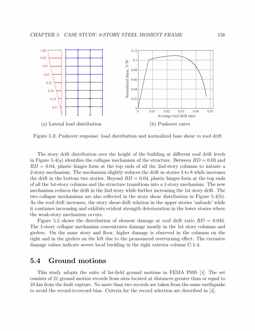
CHAPTER 5. CASE STUDY: 8-STORY STEEL MOMENT FRAME 156
1.00
0.92
0.81
0.67
0.52
0.38
0.24
0.11
(a) Lateral load distribution
0 0.01 0.02 0.03 0.04 0.05Average roof drift ratio
0
0.02
0.04
0.06
0.08
0.1
0.12
Nor
mal
ized
shea
r, V
/W(b) Pushover curve
Figure 5.3: Pushover response: load distribution and normalized base shear vs roof drift
The story drift distribution over the height of the building at different roof drift levelsin Figure 5.4(a) identifies the collapse mechanism of the structure. Between RD = 0.03 andRD = 0.04, plastic hinges form at the top ends of all the 2nd-story columns to initiate a2-story mechanism. The mechanism slightly reduces the drift in stories 3 to 8 while increasesthe drift in the bottom two stories. Beyond RD = 0.04, plastic hinges form at the top endsof all the 1st-story columns and the structure transitions into a 1-story mechanism. The newmechanism reduces the drift in the 2nd story while further increasing the 1st story drift. Thetwo collapse mechanisms are also reflected in the story shear distribution in Figure 5.4(b).As the roof drift increases, the story shear-drift relation in the upper stories ’unloads’ whileit continues increasing and exhibits evident strength deterioration in the lower stories wherethe weak-story mechanism occurs.
Figure 5.5 shows the distribution of element damage at roof drift ratio RD = 0.045.The 1-story collapse mechanism concentrates damage mostly in the 1st story columns andgirders. On the same story and floor, higher damage is observed in the columns on theright and in the girders on the left due to the pronounced overturning effect. The excessivedamage values indicate severe local buckling in the right exterior column C-1-4.
5.4 Ground motions
This study adopts the suite of far-field ground motions in FEMA P695 [4]. The setconsists of 21 ground motion records from sites located at distances greater than or equal to10 km from the fault rupture. No more than two records are taken from the same earthquaketo avoid the record-to-record bias. Criteria for the record selection are described in [4].

CHAPTER 5. CASE STUDY: 8-STORY STEEL MOMENT FRAME 157
0 0.05 0.1 0.15Interstory drift (rad)
0
1
2
3
4
5
6
7
8
Stor
y
RD = 0.01RD = 0.02RD = 0.025RD = 0.03RD = 0.035RD = 0.04RD = 0.045
(a) Story drift distribution
0 0.05 0.1 0.15Interstory drift (rad)
0
0.02
0.04
0.06
0.08
0.1
0.12
Nor
mal
ized
she
ar, V
/W
1 story2 story3 story4 story5 story6 story7 story8 story
(b) Story shear distribution
Figure 5.4: Story drift and shear distribution
0.370.02
0.410.07
0.560.24
0.990.97
0.00 0.020.350.35
0.21 0.18 0.20 0.19 0.14
Figure 5.5: Damage distribution at RD = 0.045
Table 5.3 summarizes the main properties of the 21 far-field ground motions from thePEER database [14], including the record name, year, and station, the magnitude Mw, andthe peak ground acceleration PGA.
Figure 5.6 plots the elastic response spectrum for the 21 ground motion records with 2.5%damping ratio. The median of the pseudo-acceleration on the spectrum is also highlightedin the figure.

CHAPTER 5. CASE STUDY: 8-STORY STEEL MOMENT FRAME 158
ID Name Year Mw Station PGA(g)FF1 Northridge 1994 6.7 Beverley Hills - Mulhol 0.52FF2 Northridge 1994 6.7 Canyon County - WCL 0.48FF3 Duzce, Turkey 1999 7.1 Bolu 0.82FF4 Hector Mine 1999 7.1 Hector 0.34FF5 Imperial Valley 1979 6.5 Delta 0.35FF6 Imperial Valley 1979 6.5 El Centro Array #11 0.38FF7 Kobe, Japan 1995 6.9 Nishi-Akashi 0.51FF8 Kobe, Japan 1995 6.9 Shin-Osaka 0.24FF9 Kocaeli, Turkey 1999 7.5 Duzce 0.36FF10 Kocaeli, Turkey 1999 7.5 Arcelik 0.22FF11 Landers 1992 7.3 Yermo Fire Station 0.24FF12 Landers 1992 7.3 Coolwater 0.42FF13 Loma Prieta 1989 6.9 Capitola 0.53FF14 Loma Prieta 1989 6.9 Gilroy Array #3 0.56FF15 Manjil, Iran 1990 7.4 Abbar 0.51FF16 Superstition Hills 1987 6.5 El Centro Imp. Co. 0.36FF17 Superstition Hills 1987 6.5 Poe Road 0.45FF18 Chi-Chi, Taiwan 1999 7.6 CHY101 0.44FF19 Chi-Chi, Taiwan 1999 7.6 TCU045 0.51FF20 San Fernando 1971 6.6 LA - Hollywood 0.21FF21 Friuli, Italy 1976 6.5 Tolmezzo 0.35
Table 5.3: Far-field ground motion information
5.5 Dynamic Response
This section investigates the dynamic behavior of the archetype SMF subjected to the 21ground motions magnified by a scale factor SF. This study uses a collapse criteria based onthe maximum story drift DR. Because there are cases in which the structure stabilizes afterit experiences an excessive story drift, global collapse initiates when the maximum story DRexceeds 10% and continues to grow thereafter. In the following discussion, the displacementsand accelerations are measured relative to the ground.
5.5.1 Local damage distribution
The location and the magnitude of the damage variables within the structure indicatewhere severe damage concentrates and offer insight into the collapse mechanisms. In par-ticular, the symmetry of the damage distribution is indicative of the overturning effect dueto the relative motion of the structure. For illustration, this section examines the local re-sponse of the members on the first story where damage is most severe: the exterior columns

CHAPTER 5. CASE STUDY: 8-STORY STEEL MOMENT FRAME 159
0 0.5 1 1.5 2 2.5Period T (sec)
0
0.5
1
1.5
2
2.5
3
Pseu
do-A
ccel
erat
ion
(g)
IndividualMedian
(a) Individual records
0 0.5 1 1.5 2 2.5Period T (sec)
0
0.2
0.4
0.6
0.8
1
1.2
Pseu
do-A
ccel
erat
ion
(g)
(b) Median value
Figure 5.6: Elastic response spectrum of the far-field ground motions, ξ = 2.5%
C-1-1 and C-1-4, and the girders G-1-1 and G-1-3. The following subsections compare twoscenarios with a nonsymmetric and a symmetric damage evolution in the exterior columnsand discuss the damage distribution in the girders.
5.5.1.1 Nonsymmetric column damage
A nonsymmetric damage distribution results from the considerable discrepancies in theplastic energy dissipation in the columns of the same story. Such discrepancies are typicallydue to the larger drift in one direction that amplifies the overturning effect and induces moreplastic axial deformations in the columns on one side than on the other. In a special case, thestructure initiates a weak-story mechanism and permanent deformations in one dominantdirection, which exacerbates the discrepancies in the column plastic axial deformations, andin turn, leads to a nonsymmetric damage distribution.
Figure 5.7 shows the response under the Hector Mine record at Hector station (FF4) withscale factor SF = 6.6. A large pulse at t = 7 sec initiates a 2-story mechanism, as evidentin the excessive drifts in the bottom two stories in Figure 5.7(a), and leads to a one-sidedrelative motion in the positive direction. The damage distribution is highly nonsymmetricwith higher damage on the right side of the structure. The high damage value at the baseof C-1-4 indicates severe local buckling in the column. It is noteworthy that the damage inthe interior columns is relatively mild because of the higher ductility of the larger sectionsize. Moreover, damage in the interior columns is more symmetric due to the reduced effectof the overturning moment.
Figure 5.8 compares the response at the base of the 1st story exterior columns C-1-1 on theleft and C-1-4 on the right. The comparison of the moment-rotation relation in Figure 5.8(a)

CHAPTER 5. CASE STUDY: 8-STORY STEEL MOMENT FRAME 160
0 10 20 30 40Time (sec)
0
0.05
0.1
0.15
Stor
y dr
ift ra
tio
1 story2 story
3 story4 story
5 story6 story
7 story8 story
(a) Story drift distribution
0.45
0.02
0.40
0.01
0.42
0.02
0.78
0.33
0.07 0.10 0.12
0.02
0.39
0.74 0.66 0.65 0.65 0.61 0.62
0.12 0.05 0.07 0.06 0.02 0.03
0.01 0.00 0.01 0.00
0.01 0.02 0.02 0.02 0.03 0.01
0.01 0.01 0.00 0.00 0.01 0.00
0.00 0.00 0.00 0.00
(b) Final damage profile
Figure 5.7: Response distribution and deformed shape (FF4, SF = 6.60)
leads to two observations: (1) the columns accumulate similar flexural deformations, and (2)the strength and stiffness deterioration is more pronounced in C-1-4 than in C-1-1. Thefirst observation suggests that the axial deformations govern the discrepancies in the columnresponse. Due to the relative motion of the structure causing permanent deformations inthe positive direction, the overturning effect induces higher compression and more excessiveplastic axial deformations on C-1-4, as Figure 5.8(b) shows. The evolution of the plastic axialdeformations in Figure 5.8(b) correlates well with the damage evolution in Figure 5.8(c).After the large pulse at t = 7 sec triggers the weak-story mechanism, the accumulation ofplastic axial deformations in C-1-4 accelerates due to the overturning effect and leads tohigher damage increments than in C-1-1.
5.5.1.2 Symmetric column damage
A symmetric damage distribution results from the negligible discrepancies in the plasticenergy dissipation in the columns when the ground motion induces relatively equal largedrifts in both directions. Two scenarios resulting in a symmetric damage distribution are:(1) the ground motion has relatively small intensity that induces minor discrepancies in thecolumn plastic deformations, and (2) the impact of axial forces from the overturning effecton the column response is relatively small, which is typical in low-rise to mid-rise structures.
Figure 5.9 shows the response under the Northridge record at Beverly Hills station (FF1)with a scale factor SF = 5.0. The evolution of the story drifts in Figure 5.9(a) indicatescomparable drifts in the two directions, with the maximum positive drift ratio of 0.06 and themaximum negative drift ratio of −0.07. The damage distribution in Figure 5.9(b) is rathersymmetric, with the damage in C-1-4 (d = 0.51) practically equal to the damage in C-1-1
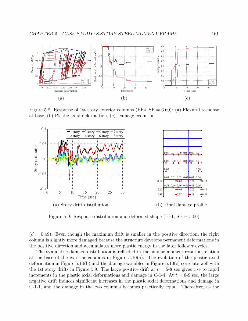
CHAPTER 5. CASE STUDY: 8-STORY STEEL MOMENT FRAME 161
0 0.02 0.04 0.06 0.08 0.1 0.12Flexural deformation
-1
-0.5
0
0.5
1
Mom
ent,
M/M
p
C-1-1C-1-4
(a)
0 10 20 30 40Time (sec)
-2
-1.5
-1
-0.5
0
Plas
tic a
xial
def
orm
atio
n (%
) C-1-1C-1-4
(b)
0 10 20 30 40Time (sec)
0
0.1
0.2
0.3
0.4
0.5
0.6
0.7
0.8
Dam
age
varia
ble
C-1-1C-1-4
(c)
Figure 5.8: Response of 1st story exterior columns (FF4, SF = 6.60): (a) Flexural responseat base, (b) Plastic axial deformation, (c) Damage evolution
0 5 10 15 20 25 30Time (sec)
-0.1
-0.05
0
0.05
0.1
Stor
y dr
ift ra
tio
1 story2 story
3 story4 story
5 story6 story
7 story8 story
(a) Story drift distribution
0.49
0.11
0.27
0.03
0.28
0.03
0.51
0.16
0.12 0.07 0.08 0.130.56 0.46 0.46 0.46 0.46 0.46
0.05 0.01 0.02 0.02 0.03 0.04
0.00 0.00
0.01 0.00 0.01 0.00 0.00 0.01
0.01 0.01 0.00 0.00 0.00 0.01
(b) Final damage profile
Figure 5.9: Response distribution and deformed shape (FF1, SF = 5.00)
(d = 0.49). Even though the maximum drift is smaller in the positive direction, the rightcolumn is slightly more damaged because the structure develops permanent deformations inthe positive direction and accumulates more plastic energy in the later follower cycles.
The symmetric damage distribution is reflected in the similar moment-rotation relationat the base of the exterior columns in Figure 5.10(a). The evolution of the plastic axialdeformation in Figure 5.10(b) and the damage variables in Figure 5.10(c) correlate well withthe 1st story drifts in Figure 5.9. The large positive drift at t = 5-8 sec gives rise to rapidincrements in the plastic axial deformations and damage in C-1-4. At t = 8-9 sec, the largenegative drift induces significant increases in the plastic axial deformations and damage inC-1-1, and the damage in the two columns becomes practically equal. Thereafter, as the

CHAPTER 5. CASE STUDY: 8-STORY STEEL MOMENT FRAME 162
structure forms a 2-story mechanism and leans permanently to the right, C-1-4 graduallyaccumulates more plastic axial deformations and exceeds slightly the damage in C-1-1 at theend of the ground motion. The discrepancies, however, are negligible in this case.
-0.06 -0.04 -0.02 0 0.02 0.04 0.06Flexural deformation
-1
-0.5
0
0.5
1
Mom
ent,
M/M
p
C-1-1C-1-4
(a)
0 5 10 15 20 25 30Time (sec)
-1.6
-1.4
-1.2
-1
-0.8
-0.6
-0.4
-0.2
0
Plas
tic a
xial
def
orm
atio
n (%
) C-1-1C-1-4
(b)
0 5 10 15 20 25 30Time (sec)
0
0.1
0.2
0.3
0.4
0.5
0.6
Dam
age
varia
ble
C-1-1C-1-4
(c)
Figure 5.10: Response of 1st story exterior columns (FF1, SF = 5.0): (a) Flexural responseat base, (b) Plastic axial deformation, (c) Damage evolution
5.5.1.3 Girder damage
Since the axial forces in the girders are relatively small, girder damage depends entirelyon the flexural response, and in particular, on the plastic flexural deformations. If thecolumns on the same story experience similar axial deformations, which typically leads to asymmetric column damage pattern, the plastic flexural deformations in the adjacent girdersare comparable and the girder damage distribution is symmetric. Otherwise, if the differ-ential plastic axial deformations in the columns are significant, the floor rotation imposesdifferent rotation demand on the adjacent girders and results in a nonsymmetric damagepattern. In general, however, the damage discrepancies in girders on the same floor are lesspronounced than in the columns due to the relatively small differences in the plastic flexuraldeformations.
Figure 5.11 illustrates a slightly nonsymmetric girder damage distribution between G-1-1-L and G-1-3-R under FF4 with SF = 6.6. The global response and local response in the1st-story columns are shown in Figure 5.7 and Figure 5.8. Since more plastic deformationsare accumulated in C-1-4 than in C-1-1, less plastic deformations are developed in G-1-3than in G-1-1, and as a result, the strength deterioration in G-1-3 is less pronounced, asevident in the moment-rotation relation in Figure 5.11(a).
5.5.2 Collapse mechanism
For all 21 ground motions, the structure forms either a 1-story or a 2-story collapsemechanism. The deformed shape with fivefold magnification in Figure 5.12 shows a 1-story

CHAPTER 5. CASE STUDY: 8-STORY STEEL MOMENT FRAME 163
-0.12 -0.1 -0.08 -0.06 -0.04 -0.02 0 0.02
Flexural deformation
-1
-0.5
0
0.5
1
M/M
p
G-1-1G-1-3
(a) Flexural response
-0.1 -0.08 -0.06 -0.04 -0.02 0 0.02
Plastic flexural deformation
0
0.1
0.2
0.3
0.4
0.5
0.6
0.7
0.8
Dam
age
varia
ble
G-1-1G-1-3
(b) Damage evolution
Figure 5.11: Girder response of 1st floor girders (FF4, SF = 6.6)
mechanism under the Loma Prieta record at Gilroy Array station (FF14) with scaled factorSF = 9.0, and a 2-story mechanism under the Northridge record at Beverly Hills station(FF1) with scaled factor SF = 5.6. In addition to the local damage variables discussed inthe preceeding section, the following examines two global variables that are indicative of aweak-story collapse mechanism: the story drifts and the floor rotations.
(a) One-story mechanism (b) Two-story mechanism
Figure 5.12: Deformed shape with weak-story collapse mechanism: (a) FF14, SF = 9.0, (b)FF1, SF = 5.6
Figure 5.13(a) plots the evolution of the story drifts under FF14, SF = 9.0. The 1st storydrift ratio increases drastically near the end of the ground motion and is well-separated from

CHAPTER 5. CASE STUDY: 8-STORY STEEL MOMENT FRAME 164
the other stories, which is indicative of a 1-story collapse mechanism. The 1-story mechanisminduces significant damage to the structural members in the 1st story and negligible damagein the upper stories. This is reflected in the more pronounced deterioration in the 1st storyshear in Figure 5.13(b) relative to the 2nd story shear in Figure 5.13(c).
0 5 10 15 20 25Time (sec)
-0.2
-0.15
-0.1
-0.05
0
0.05
Stor
y dr
ift ra
tio
1 story2 story
3 story4 story
5 story6 story
7 story8 story
(a) Story DR distribution
-0.15 -0.1 -0.05 0Story drift ratio
-0.15
-0.1
-0.05
0
0.05
0.1
0.15
Nor
mal
ized
stor
y sh
ear,
V/W
(b) 1st story shear vs DR
-0.08 -0.06 -0.04 -0.02 0Story drift ratio
-0.15
-0.1
-0.05
0
0.05
0.1
0.15
Nor
mal
ized
stor
y sh
ear,
V/W
(c) 2nd story shear vs DR
Figure 5.13: Story DR and shear distribution of a one-story mechanism (FF14, SF = 9.0)
The floor rotation results from the difference in the column axial deformations on thesame story and adopts a positive convention for the counter-clockwise direction. Figure 5.14shows two distinct trends in the distribution of the average floor rotation. In the first case,the floor rotation distribution under FF4 with SF = 6.6 in Figure 5.14(a) gives rise to twoobservations. First, all floor rotations remain negative and gradually increase in magnitude.This behavior implies that the structure undergoes permanent relative motion to the rightuntil collapse. Second, the rotations from the 2nd floor to the 8th floor are practically thesame and well-separated from the 1st floor. Since rotations are cumulative as elevationincreases, the difference in the rotation between adjacent floors is the relative rotation dueto diffential shortening in the columns between the floors. This suggests that the overturningeffect is significant in the bottom two stories and negligible in the upper stories, which impliesa 2-story mechanism consistent with the observation from the dynamic analysis.
The second case in Figure 5.14(b) examines the floor rotations under FF1 with SF =3.2. In contrast to the first case, the floor rotations alternate in signs with relatively smallmagnitude and remain stable until the end of the ground motion. This behavior implies thatthe structure oscillates in both directions and does not collapse. The rotations on differentfloors are more evenly distributed, which implies that the stories contribute similarly to thetotal roof rotation and a weak-story mechanism is not likely.
5.5.3 Other response distribution
5.5.3.1 Plastic hinges
In contrast to the pushover analysis, the dynamic analysis indicates a wider spread ofplastic hinges in almost all elements up to the roof level. This observation leads to two

CHAPTER 5. CASE STUDY: 8-STORY STEEL MOMENT FRAME 165
0 10 20 30 40Time (sec)
-0.5
-0.4
-0.3
-0.2
-0.1
0
0.1
0.2
Ave
rage
floo
r rot
atio
n (%
) 1 story2 story
3 story4 story
5 story6 story
7 story8 story
(a) FF4, SF = 6.60
0 5 10 15 20 25 30Time (sec)
-0.2
-0.15
-0.1
-0.05
0
0.05
0.1
0.15
0.2
Ave
rage
floo
r rot
atio
n (%
)
1 story2 story
3 story4 story
5 story6 story
7 story8 story
(b) FF1, SF = 3.20
Figure 5.14: Time history of the average floor rotations
implications: (1) for flexible structures, which is typically the case for most tall buildings, thehigher mode effect is important, and (2) the constant lateral force distribution proportionalto the fundamental mode shape in pushover analysis might not represent sufficiently theforce distribution in the dynamic analysis.
5.5.3.2 Lateral inertial forces
As opposed to a constant load pattern in the pushover analysis, the lateral force dis-tribution varies in the dynamic analysis. To illustrate some commonly observed patterns,Figure 5.15 plots the distribution of the average lateral floor acceleration at various instantsfor 3 different ground motions.
-2 -1.5 -1 -0.5 0 0.5 1 1.5Floor acceleration (g)
0
1
2
3
4
5
6
7
8
Stor
y
t = 5 st = 7 st = 10 st = 15 st = 20 s
(a) FF17, SF = 9.40
-3 -2 -1 0 1 2Floor acceleration (g)
0
1
2
3
4
5
6
7
8
Stor
y
t = 12.9 st = 16.7 st = 19.5 st = 23.9 st = 27.3 s
(b) FF12, SF = 8.10
-1 -0.5 0 0.5 1 1.5Floor acceleration (g)
0
1
2
3
4
5
6
7
8
Stor
y
t = 5.0 st = 8.7 st = 15.0 st = 20.0 st = 30.0 s
(c) FF1, SF = 3.20
Figure 5.15: Distribution of floor acceleration

CHAPTER 5. CASE STUDY: 8-STORY STEEL MOMENT FRAME 166
In the first case in Figure 5.15(a), the inertial force distribution is rather irregular. Lo-cation of the maximum acceleration varies and the sign alternates with increasing eleva-tion. This pattern emphasizes the impact of the higher modes. In the second case inFigure 5.15(b), the distribution is relatively uniform over the building height. In the thirdcase in Figure 5.15(c), the inertial force distribution is a combination of the two: irregularwith alternating signs in the beginning and more uniform as the ground motion progresses.
The magnitude of the inertial forces reduces toward the end of shaking due to two reasons:(1) the reduction in the ground motion intensity near the end, and (2) the damage localizationin the structure due to the strength deterioration in the element response.
5.5.4 Further remarks
0 5 10 15 20 25Time (sec)
-0.08
-0.06
-0.04
-0.02
0
0.02
0.04
Stor
y dr
ift ra
tio
SF = 2.50SF = 3.00
SF = 3.50SF = 4.00
SF = 4.50
(a) 1st story drift
-0.08 -0.06 -0.04 -0.02 0 0.02 0.04Story drift ratio
0
1
2
3
4
5
6
7
8
Stor
y
SF = 2.50SF = 3.00SF = 3.50SF = 4.00SF = 4.50
(b) Distribution at max drift
0 0.05 0.1 0.15Story drift ratio
0
0.2
0.4
0.6
0.8
1
1.2
1.4
1.6
Sa (g
)
(c) IDA curve
0.03 0.01 0.02 0.20
0.08
0.03
0.04 0.02 0.02 0.02 0.01 0.00
0.00 0.00 0.00
(d) Damage profile, SF = 2.5
0.58
0.45
0.22
0.01
0.20
0.00
0.25
0.030.000.10 0.01 0.01
0.04
0.07
0.30 0.28 0.33 0.33 0.41 0.32
0.02 0.02 0.04 0.04 0.05 0.03
0.03 0.00 0.02 0.02 0.00
0.01 0.00 0.02 0.02 0.00
(e) Damage profile, SF = 4.5
Figure 5.16: Dynamic response under FF9
This section examines the story drifts and damage distribution under the same groundmotion with different scale factors to investigate the effect of ground motion intensity on

CHAPTER 5. CASE STUDY: 8-STORY STEEL MOMENT FRAME 167
the dynamic behavior. The response under the Kocaeli record at Duzce station (FF9) withscale factor SF ranging from 2.5 to 4.5 is selected for illustration. The time history of the1st story drift in Figure 5.16(a) shows that the permanent deformation changes direction asthe scale factor varies. Figure 5.16(b) plots the drift distribution when the maximum valueis attained. Two important observations arise: (1) for the same ground motion, the storywhere the highest drift value is attained varies with the ground motion intensity, and (2)the maximum drift does not increase monotonically with the ground motion intensity. Thesecond remark is shown in the relation of the maximum drift and the spectral accelerationSa in Figure 5.16(c). The change in the relative motion direction leads to the nonmonotonicrelation and explains the ’resurrection’ phenomenon observed in the literature in which thestructure regains stability as the ground motion intensity increases.
Figures 5.16(d)–(e) highlights the effect of the ground motion intensity on the damagedistribution. For SF = 2.5, the maximum drift is attained in the positive direction and theright columns are more damaged, whereas for SF = 4.5, the maximum drift is attained inthe negative direction and the damage in the left columns is more severe.
5.6 Global Damage Index
The preceeding sections suggest a close correlation between the local damage variablesand the global response. This section derives a global damage index from the local damagevariables to assist in the assessment of the global damaged states. The section starts withthe formulation of the global damage index and an example to illustrate the satisfactorycorrelation to the collapse mechanisms. The section proceeds with a comparison study withthe maximum story drift, which is the most common Engineering Demand Parameter (EDP)for damage assessment of structures. Based on the comparison, three limit states of steelstructures are identified in terms of the damage values. The section concludes with a casestudy to demonstrate the use of the proposed damage index in the collapse assessment ofthe archetype structure under an earthquake sequence.
5.6.1 Formulation
Figure 5.17 illustrates four damage indices: the column top and bottom indices, the jointindices, and the floor indices.
The column top index of the k-th story, D(k)t , is defined as a weighted average of the
damage variables d(el)t at the top end of column element el on the k-th story. Similarly, the
column base index of the k-th story, D(k)b , is defined as a weighted average of the damage
variables d(el)b at the base of column element el on the k-th story.
D(k)t =
∑w
(el)t d
(el)t∑
w(el)t
D(k)b =
∑w
(el)b d
(el)b∑
w(el)b
(5.1)

CHAPTER 5. CASE STUDY: 8-STORY STEEL MOMENT FRAME 168
Dt(k)
Dt(k-1)
(a) Column top index
Db(k+1)
Db(k)
(b) Column base index
DJ
(c) Joint index
DF(k+1)
DF(k)
(d) Floor index
Figure 5.17: Illustration of column indices, joint indices, and floor indices
where w(el)t serves as weight for the damage variable d
(el)t and w
(el)b is the weight for the
damage variable d(el)b . w
(el)t = w
(el)b = 1 is adopted in this study.
The joint index at the k-th node, D(k)j , is defined as a weighted average of the damage
variables d(el) at the end of element el adjacent to node k:
D(k)j =
∑w(el)d(el)∑w(el)
(5.2)
where w(el) serves as weight for the damage variable d(el); w(el) = 1 is adopted in this study,implying that the joint index is the mean of the respective local damage variables.
The floor index of the k-th floor, D(k)f , is defined as a weighted average of the joint indices
Dj on floor k:
D(k)f =
∑WjDj∑Wj
(5.3)
where Wj serves as weight for the joint index Dj and Wj = 1 is adopted in this study.Finally, the global damage index, DG, is defined as the weighted average of the floor
indices Df :
DG =W
(1)b D
(1)b +
∑W
(k)f D
(k)f
W(1)b +
∑W
(k)f
(5.4)

CHAPTER 5. CASE STUDY: 8-STORY STEEL MOMENT FRAME 169
where D(1)b and W
(1)b are the 1st-story column base index and the corresponding weight, and
D(k)f and W
(k)f are the floor index and the corresponding weight. The weight is assumed equal
to the respective damage index, W(1)b = D
(1)b , W
(k)f = D
(k)f to emphasize the contribution of
the floors with more severe deterioration.
5.6.2 Localized Damage Region
When a story mechanism initiates, the structure deforms as multiple blocks: one ’active’block with highly inelastic element behavior and several adjacent ’passive’ blocks with elasticor mildly inelastic element behavior. A localized damaged region (LDR) is defined as the’active’ block, which is a collection of elements over one or more stories with significantlyhigher damage than in the other elements outside the block. The LDR is characterized by ahigh column top index Dt and a high column base index Db at the upper and lower edges ofthe block, and relatively high floor indices Df on the intermediate floors within the LDR.
Dt,max
Db,max
LDR
‘Passive’
block
‘Passive’
block
‘Active’
block
Figure 5.18: Typical configuration of a story mechanism
Figure 5.18 illustrates a possible weak-story collapse mechanism of a five-story two-bayframe. The element ends with relatively high damage and plastic deformations are shownwith red circles. The LDR consists of the 2nd and 3rd stories and is restricted betweenthe column bases with the highest damage index Db and the column tops with the highestdamage index Dt. The LDR has significant story drifts, vertical floor translations, andfloor rotations due to the excessive element deformations, as opposed to the limited elementdeformations in the adjacent ’passive’ blocks.
The following example demonstrates the correlation of the LDR and the collapse behav-iors of the structure. Figure 5.19 shows the distribution of the column top and base damageindices and the floor indices for the archetype eight-story SMF under FF1 with SF = 5.6.It is noteworthy that the global damage indices Dt, Db, Df have lower values than the localelement damage variables because the former are averages of the latter and account also forthe undamaged element ends. The LDR consists of members in the bottom 2 stories and

CHAPTER 5. CASE STUDY: 8-STORY STEEL MOMENT FRAME 170
D(2)t = 0.27
D(1)b = 0.61
D(1)F = 0.30
Localized damagedregion (LDR)
(a) Localized damage region
D(8)F = 0
D(7)F = 0
D(6)F = 0
D(5)F = 0.00
D(4)F = 0.00
D(3)F = 0.00
D(2)F = 0.06
D(1)F = 0.30
(b) Floor indices
D(1)t = 0.13
D(2)t = 0.27
D(3)t = 0
D(4)t = 0
D(5)t = 0
D(6)t = 0
D(7)t = 0
D(8)t = 0
(c) Column top indices
D(1)b = 0.61
D(2)b = 0
D(3)b = 0
D(4)b = 0
D(5)b = 0
D(6)b = 0
D(7)b = 0
D(8)b = 0
(d) Column base indices
Figure 5.19: Damage indices and localized damage region (FF1, SF = 5.6)
satisfies all three conditions: (1) the upper edge corresponds to the maximum column top
index D(2)t = 0.27 on the 2nd story, (2) the lower edge corresponds to the minimum column
base damage D(1)b = 0.61 on the 1st story, and (3) the floor indices between the two edges
are relatively high D(1)f = 0.3. The LDR is consistent with the 2-story mechanism observed
for this ground motion.

CHAPTER 5. CASE STUDY: 8-STORY STEEL MOMENT FRAME 171
5.6.3 Comparison with maximum story drift
Figure 5.20(a) plots the global damage index DG against the maximum story drift ratioDR. Each data point corresponds to a dynamic analysis under one of the 21 far-field groundmotions with a scale factor SF . For clarity, lines are drawn to connect the data points fromthe same ground motion. The figure zooms in the response up to collapse and leaves out thedata points beyond collapse in which the structure is unstable and the maximum story driftbecomes unbounded. The damage index DG initiates at DR ≈ 0.025 and varies essentiallylinearly with the story drift DR up to DR ≈ 0.15 when the structure becomes unstable.Due to the weak-story mechanism, both the story drift and the damage are excessive in theLDR, which explain the correlation of the two variables.
0 0.05 0.1 0.15Interstory drift
0
0.1
0.2
0.3
0.4
0.5
0.6
Glo
bal d
amag
e in
dex
(a) DG vs DR
0 5 10 15 20 25Time (sec)
0
0.01
0.02
0.03
0.04
0.05
0.06
0.07
0.08
Drif
t rat
io
LP1 LP2
LP3 LP4 LP5
(b) Maximum story drift
0 5 10 15 20 25Time (sec)
0
0.05
0.1
0.15
0.2
0.25
0.3
0.35
Dam
age
inde
x
LP1LP2
LP3
LP4LP5
(c) Global damage index
Figure 5.20: Comparison of damage index DG and maximum story drift
To distinguish the two variables, Figure 5.20(b)-(c) plots the evolution of the maximumstory drift ratio DR and the global damage index DG under FF12 and SF = 6.9. Thestory drift shows two significant increments at load point (LP) 1 and 3 when the previousmaximum or minimum drift value is exceeded, while remains constant between LP1 and LP2and after LP3. The maximum story drift is able to capture the large earthquake pulses thatcause excessive drift increments but fails to account for the damage accumulation in followerhalf cycles after the maximum drift is attained. In contrast, the global damage index DG notonly predicts the rapid damage growth between LP2 and LP3, but also captures the gradualdamage accumulation during the load reversal from LP1 to LP2 and during the followercycles after LP3. The global damage index is cumulative and attains its maximum value atthe end of the ground motion, which is critical for ground motions with longer duration andnumerous cycles.
Figure 5.21 plots the two variables against the ground motion intensity, which is repre-sented by the spectral acceleration Sa evaluated at the fundamental period of the archetypestructure. This plot is known as the incremental dynamic analysis (IDA) curve [105] andtypically used in collapse assessment of structures. It is noteworthy that the maximum storydrift DR does not always vary monotonically with the ground motion intensity because it

CHAPTER 5. CASE STUDY: 8-STORY STEEL MOMENT FRAME 172
does not account for the direction of motion. In contrast, the global damage index DG variesmonotonically with the ground motion intensity.
0 0.05 0.1 0.15 0.2Interstory drift
0
0.5
1
1.5
2
Sa (
g)
(a) Max story drift
0 0.2 0.4 0.6 0.8Global damage index
0
0.5
1
1.5
2
Sa (
g)
(b) Global damage index
Figure 5.21: Incremental dynamic analysis curve in terms of story drift and damage index
It is noteworthy that the proposed global and local damage measures correlate wellwith both the global and the local response variables. In particular, the damage variablesaccount for the plastic axial deformation, which is critical in collapse simulations but typicallyneglected in practice due to limitations of available column models. Therefore, the proposeddamage formulation is a rational way to bridge from the local to the global response andavoids separate limit state checks that are commonly used in practice.
5.6.4 Damage-base limit states
This subsection calibrates the global damage index DG against the maximum story driftratio DR to define three limit states of the archetype structure in terms of damage: lifesafety (LS), collapse prevention (CP), and collapse (CL). FEMA 356 [3] associates the LSlimit state with a story drift value DR = 0.025 and the CP limit state with DR = 0.05.A drift ratio between DR = 0.1 and DR = 0.15 has been widely adopted for the CL limitstate [4]. These story drift values correspond to the following damage thresholds at the limitstates of the 8-story frame:
(1) Life safety (LS): DG = 0.01. Damage initiates in several elements after sufficientplastic deformations. The story drift is relatively small and a story mechanism is notpresent.
(2) Collapse prevention (CP): DG = 0.1. Significant plastic deformations are accumulatedin several elements and the strength and stiffness deterioration is moderate, especially

CHAPTER 5. CASE STUDY: 8-STORY STEEL MOMENT FRAME 173
in the 1st and 2nd stories. The structure forms a localized damage region (LDR) andinitiates a weak-story mechanism.
(3) Collapse (CL): DG = 0.4 Elements in the LDR undergo significant plastic deforma-tions and severe damage due to local buckling and/or brittle failure. Differential col-umn shortening results in considerable floor rotations. The weak-story mechanism ispronounced with significant story drifts.
0 0.2 0.4 0.6 0.8Global damage index
0
0.5
1
1.5
2
Spec
tral a
ccel
erat
ion,
Sa
(g) DR = 0.025
DG = 0.01
(a1)
0 0.2 0.4 0.6 0.8Global damage index
0
0.5
1
1.5
2Sp
ectra
l acc
eler
atio
n, S
a (g
) DR = 0.05DG = 0.1
(b1)
0 0.2 0.4 0.6 0.8Global damage index
0
0.5
1
1.5
2
Spec
tral a
ccel
erat
ion,
Sa
(g) DR = 0.1
DG = 0.4
(c1)
0 5 10 15 20GM record no.
0
0.1
0.2
0.3
0.4
0.5
0.6
0.7
Spec
tral a
ccel
erat
ion,
Sa
(g) DR = 0.025
DG = 0.01
(a2)
0 5 10 15 20GM record no.
0
0.2
0.4
0.6
0.8
1
1.2
1.4
Spec
tral a
ccel
erat
ion,
Sa
(g) DR = 0.05
DG = 0.1
(b2)
0 5 10 15 20GM record no.
0
0.5
1
1.5
2Sp
ectra
l acc
eler
atio
n, S
a (g
) DR = 0.1DG = 0.4
(c2)
Figure 5.22: Comparison of max drift ratio DR and damage index DG at different limitstates: (a) Life safety, (b) Collapse prevention, (c) Collapse
Figures 5.22(a)–(c) compare the damage index DG and the maximum story drift ratio DRat the three limit states on the IDA curves in terms of the damage index DG. Figure 5.22(d)–(e) compare the ground motion intensity at the three limit states defined by the two responsevariables. The red circles correspond to the limit states in terms of the story drift andthe blue circles in terms of the damage index. The slight discrepancies in the spectralacceleration Sa at the LS limit state suggest that a smaller damage threshold may providea more consistent result, and indeed, DG = 0.075 gives better agreement. However, this isnot pursued here because the small damage value implies an impractical level of accuracy.The value DG = 0.01 is selected to represent an arbitrary small threshold when the global

CHAPTER 5. CASE STUDY: 8-STORY STEEL MOMENT FRAME 174
damage index DG begins to accumulate. At the CP and the CL limit states, the agreementbetween the two criteria is satisfactory.
0 0.5 1 1.5Spectral acceleration, Sa (g)
0
0.2
0.4
0.6
0.8
1
Prob
abili
ty o
f exc
eeda
nce
DG = 0.01DG = 0.1DG = 0.4
Figure 5.23: Probability of different damage limit states
Figure 5.23 compares the fragility curves for the three limit states defined in terms ofthe proposed damage index. The curves are constructed from the IDA results and assumethat the fragility function follows the cumulative distribution function of the log-normaldistribution. The fragility curves permits an estimation of the structural damage state for agiven ground motion intensity so that measures for damage mitigation can be undertaken.
5.6.5 Case study: collapse assessment with aftershocks
The following case study illustrates an application of the proposed global damage index inthe damage assessment of structures in the event of aftershocks. The archetype 8-story frameis subjected to a series of ground motions consisting of a main shock and an aftershock. Anincremental dynamic analysis is performed and the global damage index is used to assess thechange in the damaged states and the collapse fragility of the structure with considerationof aftershocks.
5.6.5.1 Ground motions
Characterization of aftershocks involves two major sources of uncertainties: the probableintensity and the location of the aftershock relative to the main shock. Both can createdifferent damaging effects to the structure. Another critical aspect is when the aftershockoccurs after the main shock. This has an important implication in repair of damaged build-ings, that is, whether it is more practical to repair immediately after the main shock andperhaps again following the aftershock, or to repair after the aftershock provided that thestructure survives the main shock. These complex issues are beyond the scope of this study.

CHAPTER 5. CASE STUDY: 8-STORY STEEL MOMENT FRAME 175
For this preliminary study, the following assumptions are made: (1) the main shock is amongthe 21 far-field ground motions in the preceeding sections; (2) the aftershock is identical tothe main shock, and consequently, has the same spectral shape and energy content; (3)the effect of free vibration after the MS is neglected and the aftershock follows the mainshock immediately; (4) the effect of the aftershock location is not accounted for; and (5) theground motions are scaled by the same factor in the main shock and the aftershock for theincremental dynamic analysis.
0 10 20 30 40 50 60Time (s)
-0.5
-0.25
0
0.25
0.5
Acc
eler
atio
n (g
)
Main shockAftershock
Figure 5.24: Acceleration history of FF1 record with aftershock
The simplifications, in particular (2)-(5), might not give the most realistic representationof the AS; however, they are sufficient for the current study. Moreover, the selection of theaftershock as large as the main shock has been done in design practice and found to giveconfidence to engineers, public officials, and owners as they already have a clear idea of whatthe structure undergoes in the main shock. Figure 5.24 illustrates the ground accelerationhistory of the MS and aftershock sequence, in which the MS is the FF1 record with SF = 1.
5.6.5.2 Collapse probability
Figures 5.25(a)–(b) plot the collapse probability against a ground motion intensity mea-sure and a target demand parameter, respectively, in two cases: (1) if only the main shockis considered (MS), and (2) both the main shock and the aftershock are considered (MS +AS).
The fragility curves in Figure 5.25(a) suggest that under the same spectral accelerationSa, the aftershock leads to a considerable increase in the collapse risk: from 20% under MSto 45% under MS + AS, 40% under MS to 75% under MS + AS. The aftershock also resultsin a roughly 30% increase in the collapse margin ratio, which is proportional to the groundmotion intensity corresponding to a 50% collapse probability [4].

CHAPTER 5. CASE STUDY: 8-STORY STEEL MOMENT FRAME 176
0.4 0.6 0.8 1 1.2 1.4 1.60
0.2
0.4
0.6
0.8
1
MSMS + AS
Spectral acceleration (g)
Col
laps
e pr
obab
ility
(a) Ground motion intensity
0 0.2 0.4 0.6 0.80
0.2
0.4
0.6
0.8
1
MSMS + AS
Col
laps
e pr
obab
ility
Damage index
(b) Damage index after main shock
Figure 5.25: Collapse probability with and without consideration of aftershocks
Figure 5.25(b) implies a substantial increase in the collapse risk if an aftershock follows.For example, the structure does not collapse with DG = 0.2 at the end of the main shock;however, if an aftershock follows, the collapse risk increases significantly with a 80% prob-ability. In another example, the threshold DG = 0.4 at the end of the main shock is themedian damage level corresponding to a 50% collapse probability if only the main shock isaccounted for; however, if an aftershock follows, this damage level almost ensures collapsewith a 98% probability. Figure 5.25(b) suggests that to target a 50% collapse probability, thestructure is designed for a damage threshold DG = 0.4 if only the main shock is accountedfor. However, if the aftershock is also considered, the target damage threshold becomesDG = 0.13, which implies that the structure is designed for the CP limit state instead of theCL limit state at the end of the main shock. Due to the substantial increase in the collapseprobability and the more stringent requirements of the allowable damage when aftershocksare present, the study recommends that aftershocks should be considered in the dynamicanalysis and design of structures. The structure should be ’red-tagged’ once the damageindex exceeds the CP limit state threshold DG = 0.1 to account for the possible followingaftershock.
It is instructive to compare the collapse fragility of the structure under aftershocks usingother commonly used damage measures, such as the maximum story drift and the residualstory drift. This task will be pursued in future studies.

CHAPTER 5. CASE STUDY: 8-STORY STEEL MOMENT FRAME 177
5.7 Effect of Modeling Assumptions
The proposed damage-plasticity element models account for three characteristic featuresthat capture complex global and local behavior up to collapse: (1) the strength and stiffnessdeterioration of the element response, (2) the plastic hinge offsets, and (3) the inelastic axialforce-deformation relation and the effect of variable axial forces on the flexural behavior. Inpractice, one or several aspects are often neglected in the simulations due to limitations ofavailable models. In this section, the structural model in the preceeding sections is used asa reference (model R) to compare against three alternatives that represent commonly-usedexisting models:
• Model A: same as Model R, but the element response does not account for damage.The element behavior is linear elastic with linear kinematic and isotropic hardening.
• Model B : same as Model R, but no plastic hinge offset is specified. The model doesnot explicitly simulate the RBS connections.
• Model C : same as Model R, but the column response does not account for the inelas-tic axial behavior and the axial-flexural interaction. To replicate this behavior, thedamage-plasticity beam element in Chapter 3 is used to model the columns.
The comparison addresses two objectives: (1) to evaluate the change in the dynamic re-sponse of the archetype SMF in the absence of the aboved features in the element models, (2)to identify potential limitations of the existing element models and highlight the advantagesof the proposed models in collapse assessment of SMFs.
5.7.1 Effect of element damage
The response under the Loma Prieta record at Gilroy Array station (FF14) is usedto distinguish model R and model A. With the strength and stiffness deterioration, thestructure collapses at SF = 9.0 compared to SF = 12.15 if no element damage is accountedfor. Figure 5.26 compares the global and local response of the two models under the sameground motion intensity SF = 9.0. The average lateral roof drifts are almost identical upto t = 15 sec whereas the 1st story drifts deviate substantially after t = 5 sec. In contrastto model A, model R shows a drastic increase in the 1st story drifts and indicates the lossof global stability. The residual story drift distribution in Figure 5.26(c) implies a 1-storycollapse mechanism with excessive 1st story drift in model R and a stable structure withnegligible deformations in model A.
Figures 5.26(d)-(f) highlight the local response of the members in the 1st story. ModelA captures well the yield strength and the response prior to softening because both modelsuse the same elements to describe the nondegrading response, but misses the strength andstiffness deterioration under cyclic loading. Without the strength and stiffness deterioration,less plastic axial deformation is accumulated in the columns, as evident in the axial response

CHAPTER 5. CASE STUDY: 8-STORY STEEL MOMENT FRAME 178
0 5 10 15 20 25Time (sec)
-0.04
-0.03
-0.02
-0.01
0
0.01
0.02
Ave
rage
roof
drif
t rat
io
Model RModel A
(a) Roof drift
0 5 10 15 20 25Time (sec)
-0.2
-0.15
-0.1
-0.05
0
0.05
Stor
y dr
ift ra
tio
Model RModel A
(b) 1st story drift
-0.2 -0.15 -0.1 -0.05 0 0.050
1
2
3
4
5
6
7
8 Model RModel A
Interstory drift
Stor
y
(c) Story drift distribution
-2 -1.5 -1 -0.5 0Axial deformation (%)
-0.8
-0.6
-0.4
-0.2
0
0.2
Col
umn
axia
l for
ce, N
/Np
Model RModel A
(d) C-1-1 axial response
-0.15 -0.1 -0.05 0Flexural deformation
-1.5
-1
-0.5
0
0.5
1
Col
umn
flexu
ral f
orce
, M/M
p
Model RModel A
(e) C-1-1-B flexural response
0 0.02 0.04 0.06 0.08Flexural deformation
-1
-0.5
0
0.5
1
1.5
Gird
er fl
exur
al fo
rce,
M/M
p
Model RModel A
(f) G-1-3-R flexural response
Figure 5.26: Comparison of dynamic response in model R and model A
of C-1-1 in Figure 5.26(d). Model A gives stable hysteresis loops for the column moment-rotation relation and overlooks the severe strength reduction in C-1-1, as Figure 5.26(e)shows. Discrepancies in the girder response are less pronounced in Figure 5.26(f) becausethe damage in the girders is relatively mild.
Figure 5.27 shows the response of model A at SF = 12.15 to demonstrate the differentcollapse behavior when element damage is not accounted for. The story drift distribution inFigure 5.27(a) suggests that the structure is subjected to a large pulse at t = 5 sec leadingto a 2-story mechanism with excessive drifts in the bottom two stories. In contrast to thecollapse behavior of model R at SF = 9.0, the structure does not lose stability but stabilizeswith smaller story drifts as the ground motion progresses. Figure 5.27(b) compares the storydrift distribution at the instant of maximum story drift and at the end of the ground motionto highlight the structural stability in the absence of element damage. The global response isalso reflected in the floor rotation distribution in Figure 5.27(c), which shows large positiverotations with the bottom two floors in the early cycles followed by stable oscillations withsmall amplitudes in later cycles.

CHAPTER 5. CASE STUDY: 8-STORY STEEL MOMENT FRAME 179
0 10 20 30 40Time (sec)
-0.2
-0.15
-0.1
-0.05
0
0.05
Stor
y dr
ift ra
tio
1 story2 story
3 story4 story
5 story6 story
7 story8 story
(a) Story drift ratio
-0.15 -0.1 -0.05 0 0.05Interstory drift
0
1
2
3
4
5
6
7
8
Stor
y
Max driftFinal
(b) Story drift distribution
0 10 20 30 40Time (sec)
-0.2
0
0.2
0.4
0.6
0.8
Ave
rage
floo
r rot
atio
n (%
) 1 story2 story
3 story4 story
5 story6 story
7 story8 story
(c) Average floor rotation
Figure 5.27: Dynamic response without element damage (FF14, SF = 12.15)
5.7.2 Effect of plastic hinge offsets
Model B uses the same beam and column elements as the reference model R but doesnot explicitly simulate the RBS connections. No plastic hinge offset is specified in thegirders: the offset parameter χ = 0 and the section strength factor λ = 1. To investigatethe impact of the plastic hinge offsets, this section compares the two models using threerepresentative ground motions: (1) Imperial Valley record at Delta station (FF5) with scalefactor SF = 2.7, (2) San Fernando record at LA-Hollywood station (FF20) with scale factorSF = 6.84, (3) Duzce record at Bolu station (FF3) with scale factor SF = 6.12.
Global responseFigure 5.28 compares the average roof translation and suggests moderate discrepancies
between the two models. The RBSs enhance the structural performance by reducing theroof drift under FF5 but show no benefit under FF20 and FF3.
0 20 40 60Time (sec)
-0.06
-0.05
-0.04
-0.03
-0.02
-0.01
0
0.01
Ave
rage
roof
drif
t rat
io (r
ad)
Model RModel B
(a) FF5, SF = 2.7
0 20 40 60 80Time (sec)
-0.05
-0.04
-0.03
-0.02
-0.01
0
0.01
0.02
Ave
rage
roof
drif
t rat
io
Model RModel B
(b) FF20, SF = 6.84
0 10 20 30 40Time (sec)
-0.04
-0.02
0
0.02
0.04
0.06
Ave
rage
roof
drif
t rat
io
Model RModel B
(c) FF3, SF = 6.12
Figure 5.28: Comparison of model R and model B: average roof translation
The 1st story drift in Figure 5.29 offers further insight of the model response. Under
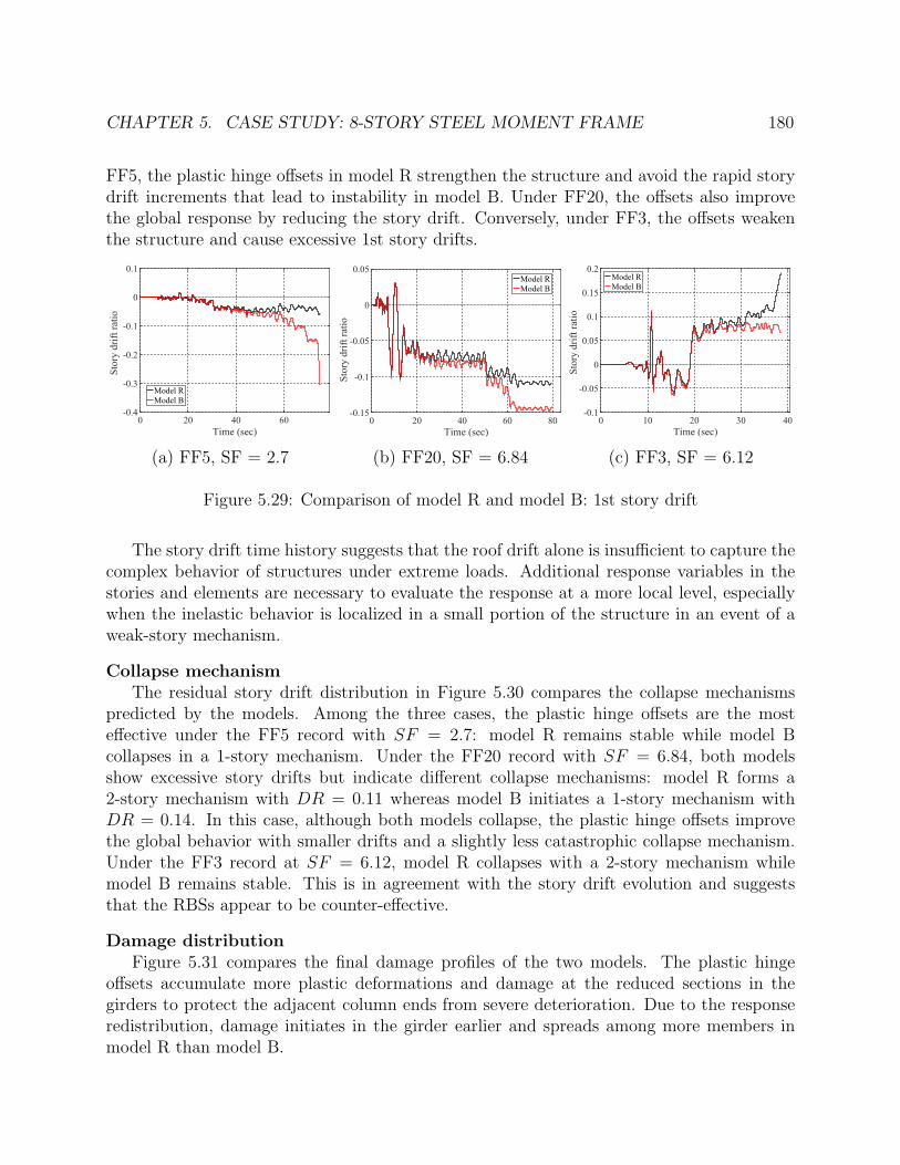
CHAPTER 5. CASE STUDY: 8-STORY STEEL MOMENT FRAME 180
FF5, the plastic hinge offsets in model R strengthen the structure and avoid the rapid storydrift increments that lead to instability in model B. Under FF20, the offsets also improvethe global response by reducing the story drift. Conversely, under FF3, the offsets weakenthe structure and cause excessive 1st story drifts.
0 20 40 60Time (sec)
-0.4
-0.3
-0.2
-0.1
0
0.1
Stor
y dr
ift ra
tio
Model RModel B
(a) FF5, SF = 2.7
0 20 40 60 80Time (sec)
-0.15
-0.1
-0.05
0
0.05
Stor
y dr
ift ra
tio
Model RModel B
(b) FF20, SF = 6.84
0 10 20 30 40Time (sec)
-0.1
-0.05
0
0.05
0.1
0.15
0.2
Stor
y dr
ift ra
tio
Model RModel B
(c) FF3, SF = 6.12
Figure 5.29: Comparison of model R and model B: 1st story drift
The story drift time history suggests that the roof drift alone is insufficient to capture thecomplex behavior of structures under extreme loads. Additional response variables in thestories and elements are necessary to evaluate the response at a more local level, especiallywhen the inelastic behavior is localized in a small portion of the structure in an event of aweak-story mechanism.
Collapse mechanismThe residual story drift distribution in Figure 5.30 compares the collapse mechanisms
predicted by the models. Among the three cases, the plastic hinge offsets are the mosteffective under the FF5 record with SF = 2.7: model R remains stable while model Bcollapses in a 1-story mechanism. Under the FF20 record with SF = 6.84, both modelsshow excessive story drifts but indicate different collapse mechanisms: model R forms a2-story mechanism with DR = 0.11 whereas model B initiates a 1-story mechanism withDR = 0.14. In this case, although both models collapse, the plastic hinge offsets improvethe global behavior with smaller drifts and a slightly less catastrophic collapse mechanism.Under the FF3 record at SF = 6.12, model R collapses with a 2-story mechanism whilemodel B remains stable. This is in agreement with the story drift evolution and suggeststhat the RBSs appear to be counter-effective.
Damage distributionFigure 5.31 compares the final damage profiles of the two models. The plastic hinge
offsets accumulate more plastic deformations and damage at the reduced sections in thegirders to protect the adjacent column ends from severe deterioration. Due to the responseredistribution, damage initiates in the girder earlier and spreads among more members inmodel R than model B.

CHAPTER 5. CASE STUDY: 8-STORY STEEL MOMENT FRAME 181
-0.3 -0.25 -0.2 -0.15 -0.1 -0.05Story drift ratio
0
1
2
3
4
5
6
7
8
Stor
y
Model RModel B
(a) FF5, SF = 2.7
-0.14 -0.12 -0.1 -0.08 -0.06 -0.04 -0.02Story drift ratio
0
1
2
3
4
5
6
7
8
Stor
y
Model RModel B
(b) FF20, SF = 6.84
0.05 0.1 0.15 0.2Story drift ratio
0
1
2
3
4
5
6
7
8
Stor
y
Model RModel B
(c) FF3, SF = 6.12
Figure 5.30: Comparison of model R and model B: collapse mechanisms
Under FF5, in model R, only the base of C-1-1 is significantly damaged while the damagein other members are relatively mild. The damage profile suggests that no member fails fromsevere local buckling and the structure does not initiate a weak-story collapse mechanism.In contrast, damage in model B localizes at both ends of all the 1st story columns and isrelatively negligible elsewhere. The high damage values imply severe local buckling thatleads to column failure, and subsequently, a 1-story collapse mechanism.
Under FF20, in model R, the highest damage locates at the base of the 1st story columns,the top end of the 2nd story columns, and the 1st floor girders. On the other hand, in modelB, damage concentrates at the top and bottom of the 1st story columns. The damageprofiles are consistent with the collapse mechanisms observed in the two models: a 2-storymechanism in model R and a 1-story mechanism in model B.
Under FF3, in model R, the highest damage concentrates at the base of the 1st storycolumns, the top of the 2nd story columns, and the 1st floor girders. The high damage valuesindicate severe local buckling at these locations and a 2-story collapse mechanism. Damagein model B localizes at the base of the 1st story columns, the top of C-1-4, and the 1st floorgirders. The damage distribution indicates a potential 1-story mechanism. It is noteworthythat in contrast to the first two ground motions, in this case the column damage in model Ris higher because the excessive girder damage leads to the weak-story collapse mechanism,which in turns accelerates the damage accumulation in these columns.
5.7.3 Axial-flexure interaction
To further investigate the effect of variable axial forces on the strength and stiffnessdeterioration in the flexural response, two variations of model C are examined:
• Model CA: no strength reduction in the columns.
• Model CB: the column strength is reduced based on the FEMA P695 recommen-dations [4]. The strength reduction in a column is determined from the axial-flexure

CHAPTER 5. CASE STUDY: 8-STORY STEEL MOMENT FRAME 182
0.51
0.38
0.14 0.12 0.18
0.02
0.04
0.16 0.12 0.20 0.20 0.26 0.18
0.03 0.04 0.05 0.05 0.08 0.03
0.01 0.02 0.02 0.02 0.02 0.01
0.03 0.07 0.08 0.08 0.07 0.04
0.03 0.05 0.04 0.03 0.05 0.03
0.02 0.02 0.02 0.02 0.03 0.02
(a) FF5, SF = 2.7: Model R
1.00
1.00
0.99
0.88
0.98
0.83
1.00
0.920.37
0.28 0.01 0.000.05 0.08 0.08 0.15 0.07
0.00 0.01
0.00 0.00 0.00 0.00
(b) FF5, SF = 2.7: Model B
0.87
0.49
0.43 0.40 0.49
0.010.07
0.60 0.24 0.19 0.17
0.79 0.74 0.81 0.80 0.84 0.79
0.04 0.06 0.07 0.07 0.10 0.05
0.00 0.01 0.01 0.01
0.01 0.00 0.03 0.01 0.02 0.01
0.00 0.01 0.02
(c) FF20, SF = 6.84: Model R
1.00
1.00
0.66
0.38
0.59
0.24
0.70
0.330.30
0.30 0.04 0.030.01
0.04
0.19 0.11 0.23 0.21 0.26 0.19
0.00 0.01 0.00 0.01 0.00
(d) FF20, SF = 6.84: Model B
0.87
0.15
0.78
0.06
0.80
0.09
0.95
0.43
0.69 0.63 0.670.020.85
1.00 1.00 1.00 1.00 1.00 1.00
0.04 0.03 0.03 0.03 0.05 0.02
0.00 0.00
0.00 0.01 0.00
0.01 0.00 0.00 0.01
0.00 0.00
(e) FF3, SF = 6.12: Model R
0.64
0.27
0.48
0.10
0.52
0.14
0.84
0.55
0.17 0.10 0.130.020.27
0.30 0.24 0.28 0.26 0.27 0.26
0.00
(f) FF3, SF = 6.12: Model B
Figure 5.31: Comparison of model R and model B: damage distribution

CHAPTER 5. CASE STUDY: 8-STORY STEEL MOMENT FRAME 183
interaction envelope for a constant axial force Pgrav + 0.5PE, where Pgrav is the gravityload and PE is the maximum axial force imposed on the column that results from thelateral forces in pushover analysis.
Model CB gives rise to two important observations: (1) theoretically the calibrationshall be performed for each individual column because the column axial force varies betweenstories as well as among members on the same story due to the overturning effect, (2) sincethe lateral forces are applied in one direction in the pushover analysis, the overturning effectexerts higher axial forces and implies higher strength reduction to the columns of one sideof the building. Conversely, the lateral force direction in dynamic analysis varies, and thus,the assumption of the direction in pushover analysis could result in inaccurate estimation ofthe column strength. To account for the variable load direction, on each floor, the strengthreduction in the exterior columns is conservatively selected based on the higher axial forceamong the two, and the same procedure applies to the interior columns. With these tworemarks, model CB requires preprocessing to calibrate the column strength 16 times, i.e. forone exterior and one interior column on each story.
The following discussion highlights the dynamic response of the models in comparison tothe reference model.
Model CAThe response under FF17 with SF = 9.4 highlights the key differences in model R and
model CA. Figure 5.32 plots the evolution and the distribution of the story drifts. Theevolution of the drift in the 1st story and at the roof level indicates that model CA remainsstable while model R loses stability. The residual deformations in model CA are relativesmall and do not initiate a weak-story mechanism whereas model R collapses in a 2-storymechanism with considerable drifts in the bottom 2 stories.
0 5 10 15 20Time (sec)
-0.03
-0.02
-0.01
0
0.01
0.02
0.03
0.04
Ave
rage
roof
drif
t rat
io
Model RModel CA
(a) Average roof translation
0 5 10 15 20Time (sec)
-0.1
-0.05
0
0.05
0.1
0.15
0.2
0.25
Stor
y dr
ift ra
tio
Model RModel CA
(b) 1st story drift
-0.05 0 0.05 0.1 0.15 0.20
1
2
3
4
5
6
7
8Model RModel CA
Interstory drift
Stor
y
(c) Story drift distribution
Figure 5.32: Comparison of model R and model CA: story drift and deformed shape (FF17,SF = 9.40)
In addition to the excessive lateral drifts, the inelastic axial response allows model R tosimulate the significant shortening when the columns are severely damaged, and in turns, the

CHAPTER 5. CASE STUDY: 8-STORY STEEL MOMENT FRAME 184
0 5 10 15 20Time (sec)
-7
-6
-5
-4
-3
-2
-1
0
Avg
. ver
tical
tran
slat
ion
(%)
Model RModel CA
(a) Average 1st floor vertical translation
0 5 10 15 20Time (sec)
-0.4
-0.3
-0.2
-0.1
0
0.1
0.2
Ave
rage
flo
or r
otat
ion
(%)
Model RModel CA
(b) Average 1st floor rotation
Figure 5.33: Comparison of model R and model CA: effect of column shortening (FF17, SF= 9.40)
considerable vertical floor displacement and floor rotation, as illustrated in Figures 5.33(a)-(b). The vertical translation shown in Figure 5.33(a) is given as the average displacementsat the top end of the columns on the same story normalized by the column height. ModelCA does not capture the plastic axial deformation in the columns and only accounts for theelastic axial deformation, which is relatively negligible, and thus, fails to describe the floorvertical translations as observed in model R. Consequently, the differential axial deformationsin model CA are relatively small and lead to insignificant floor rotations. Variations in thefloor rotation with alternating signs and small amplitudes imply that the structure oscillatesabout the undeformed configuration without initiating permanent relative displacements inone dominant direction or a weak-story mechanism.
Figure 5.34 shows the response of left exterior column in the 1st story. Figure 5.34(a)shows the load path at the column base during the first 3 inelastic half cycles in whichthe column yields and accumulates plastic deformations. The axial and flexural forces arenormalized by the respective plastic capacities and superimposed on the initial yield envelope.At the first instant, model R yields at 0.8Mp due to an axial compression −0.25Np, whereasmodel CA yields at the nominal strength Mp. At the second instant, both models yieldat a similar strength −0.9Mp under practically no axial force. After several elastic loadreversals the models yield the third time, at which model R yields at −0.7Mp under anaxial compression −0.5Np and model CA yields at a slightly higher strength than Mp. Itis evident that under a small axial force, model CA gives reasonable approximations of thecolumn yield strength while it overestimates the strength as the axial force increases.
Figures 5.34(b)-(e) compare the flexural and axial response of C-1-1. Model CA fails tocapture the excessive strength and stiffness deterioration in the column hysteretic behavior

CHAPTER 5. CASE STUDY: 8-STORY STEEL MOMENT FRAME 185
-1 -0.5 0 0.5 1M/Mp
-0.6
-0.4
-0.2
0
0.2
N/N
p
Model RModel CA
1
2
3
(a) C-1-1 N -M path (partial)
-0.05 0 0.05 0.1 0.15 0.2Flexural deformation
-1
-0.5
0
0.5
1
Flex
ural
forc
e, M
/Mp
Model RModel CA
(b) C-1-1-B flexural response
-1.5 -1 -0.5 0Axial deformation (%)
-0.6
-0.4
-0.2
0
0.2
Axi
al fo
rce,
N/N
p
Model RModel CA
(c) C-1-1 axial response
0 5 10 15 20Time (sec)
-0.1
-0.05
0
0.05
0.1
0.15
0.2
Plas
tic fl
exur
al d
efor
mat
ion
Model RModel CA
(d) C-1-1-B plas. flexural def.
0 5 10 15 20Time (sec)
-1.4
-1.2
-1
-0.8
-0.6
-0.4
-0.2
0
Plas
tic a
xial
def
orm
atio
n (%
)
Model RModel CA
(e) C-1-1-B plas. axial def.
0 5 10 15 20Time (sec)
0
0.2
0.4
0.6
0.8
1
Col
umn
dam
age
Model RModel CA
(f) C-1-1-B damage evolution
Figure 5.34: Comparison of model R and model CA: local column response (FF17, SF =9.40)
and the significant increments in the flexural deformation near the end of the ground mo-tion. As expected, the two models differ significantly in the axial response. While modelCA gives a linear elastic response with limited axial deformations, model R captures theaccumulation of the plastic axial deformations as the column yields. The differences in theplastic deformations are reflected in the evolution of the damage variables in the two models,as Figure 5.34(f) shows.
The damage distribution at the end of the ground motion in Figures 5.35(a)-(b) are con-sistent with the global and the local response. While model R indicates a 2-story mechanismwith damage concentration in the members of the lower two stories, model CA suggests adifferent mechanism with damage localized in the girders. The symmetry of the damagedistribution also distinguishes the two models and emphasizes the effect of the axial forceon the element damage. In model CA, without the inelastic axial behavior, damage in thecolumns depends solely on the flexural response. On the same floor, the elements accumulatethe same plastic flexural deformations, and thus, leading to the symmetric damage pattern.The inelastic axial response and the axial-flexural interaction allow model R to capture thenonsymmetric damage distribution due to the considerable overturning effect.

CHAPTER 5. CASE STUDY: 8-STORY STEEL MOMENT FRAME 186
0.93
0.31
0.85
0.04
0.86
0.07
1.00
0.83
0.53 0.46 0.49
0.08
0.800.99 0.99 0.99 0.99 0.98 0.96
0.12 0.10 0.09 0.09 0.10 0.08
0.00 0.01 0.02 0.02 0.03 0.00
0.02 0.03 0.03 0.03 0.03 0.01
0.02 0.03 0.01 0.01 0.03 0.01
0.00 0.04 0.00 0.00 0.04 0.00
0.02 0.02
(a) Damage profile: Model R
0.32 0.27 0.27 0.32
0.04 0.07 0.07 0.03
0.67 0.62 0.63 0.62 0.62 0.67
0.24 0.24 0.17 0.17 0.24 0.24
0.06 0.10 0.07 0.07 0.10 0.06
0.06 0.08 0.07 0.07 0.08 0.05
0.04 0.06 0.03 0.03 0.06 0.04
0.02 0.05 0.01 0.01 0.05 0.02
0.02 0.02
(b) Damage profile, Model CA
Figure 5.35: Comparison of model R and model CA: damage distribution (FF17, SF = 9.40)
Model CBWith the modification based on the FEMA P695 recommendations [4], in contrast to
model CA, model CB overestimates the yield strength reduction and the element damage.For all ground motions, model CB requires a lower scale factor SF to trigger collapse,which implies that the model overestimates the collapse fragility of the SMF. The responseunder the Northridge record at Canyon County station (FF2) is representative of the groundmotion suite and distinguishes well the two models. Figure 5.36 plots the roof drift and the1st story drift as well as the residual deformed shape under FF2 with SF = 7.92. The driftsare almost identical up to t = 7 sec then start to deviate. Near the end of the ground motion,the 1st story drift in model CB grows rapidly and leads to a 1-story collapse mechanism, asevident in the deformed shape at t = 12 sec in Figure 5.36(d). In contrast, in model R, thestructure remains stable and does not initiate a weak-story mechanism. It is noteworthy thatthe deformed shape in model CB shows significant vertical translation of the floors, whichresults from the excessive lateral story drifts. In each story, the column axial deformationsare uniform and the floor remains practically horizontal. In contrast, in model R, eventhough the vertical translation is less pronounced, the floor rotation is evident due to thediscrepancies in the shortening of the columns in a story.
Figure 5.37 shows the response of C-1-1 and the damage distribution to further distinguishthe two models. Figure 5.37(a) shows the load path at the column base during the first 3inelastic half cycles in which the column yields and accumulates plastic deformations. Theaxial and flexural forces are normalized by the respective plastic capacities and superimposedon the initial yield envelope. At the first instant, model R yields at 0.8Mp under an axialcompression −0.25Np. On the other hand, model CB yields at 0.6Mp, which results from thestrength reduction due to a constant axial force according to FEMA P695 recommendations.

CHAPTER 5. CASE STUDY: 8-STORY STEEL MOMENT FRAME 187
0 2 4 6 8 10 12Time (sec)
-0.04
-0.02
0
0.02
0.04
Ave
rage
roof
drif
t rat
io
Model RModel CB
(a) Average roof translation
0 2 4 6 8 10 12Time (sec)
-0.05
0
0.05
0.1
0.15
0.2
0.25
Stor
y dr
ift ra
tio
Model RModel CB
(b) 1st story drift
(c) Deformed shape: Model R (d) Deformed shape, Model CB
Figure 5.36: Comparison of model R and model CB: story drift and deformed shape (FF2,SF = 7.92)
At the second instant, model R yields at a strength slightly lower than Mp under a smallaxial compression −0.05Np, while model CB again yields at roughly 0.6Mp. At the thirdinstant, model R yields under a negative moment with a slightly smaller magnitude than−Mp at axial force −0.12Np, whereas model CB yields at −0.6Mp. It is evident that theconstant axial force Pgrav + 0.5PE underestimates the column yield strength under the effectof variable axial force.
Figures 5.37(b)-(e) compare the flexural and axial response of C-1-1. Model CB over-estimates the element damage and shows excessive strength and stiffness deterioration in

CHAPTER 5. CASE STUDY: 8-STORY STEEL MOMENT FRAME 188
the column hysteretic behavior. The flexural deformation grows drastically near the end ofthe ground motion implying the loss of column stability. As expected, the two models differtremendously in the axial response. While model CB gives a linear elastic response with lim-ited axial deformation, the damage-plasticity element in model R captures the plastic axialdeformations accumulated as the column yields. In model R, the plastic axial deformationsare different in the members on the two sides of the structure and lead to the floor rotationsas shown in the deformed shape in Figure 5.36(c). The discrepancies in the models arereflected in the damage evolution in the column. Figure 5.37(f) plots the damage variabled defined as the higher of the positive and the negative damage variables d+ and d− at thebase of the column.
As expected, model CB shows more severe damage in the 1st story columns than model R.In contrast, the damage in the 1st floor girders is higher in model R, which implies differentload redistribution mechanisms in the two models. In model CB, the high damage valuesindicate severe local buckling at both ends of the 1st story columns and leads to a 1-storycollapse mechanism. Model R shows severe local buckling at the base of the 1st story exteriorcolumns and the 1st floor girders, moderate damage at the base of 1st story interior columns,and mild to no damage in other members. This damage distribution suggests a possible 2-story mechanism, however, the damage values at the top end of the 2nd story columns arerelatively small to trigger a weak story mechanism. It is evident that the column strengthmodification in model CB weakens the structure and concentrates damage in a smaller region.Moreover, without the inelastic axial behavior, the column damage in model CB dependssolely on the flexural response. On the same floor, the same plastic flexural deformationsresult in a symmetric damage pattern. In contrast, the inelastic axial response and theaxial-flexure interaction allow model R to capture the nonsymmetric damage distribution tobetter identify the more vulnerable locations within the structure.
5.8 Consideration of Element Brittle Failure
5.8.1 Background
Due to software limitations, the FEMA P695 methodology [4] does not explicitly simulatethe sudden strength deterioration in the element behavior, and instead, uses componentlimit checks to account for the non-simulated modes. FEMA recommends that if the plasticrotation in any plastic hinge exceeds θp = 0.063, the component is assumed to fracture.FEMA P695 recommends that global collapse takes place if fracture occurs in any elementor the story drift exceeds the collapse limit, whichever occurs first. One limitation of thismethodology is that it overestimates the true collapse probability because failure of oneelement does not necessarily result in global collapse. Moreover, the method does not addressthe response redistribution in the structure in the event of an element failure, which is a veryimportant characteristic of the structural behavior. To address these limitations, anotherstructural model of the eight-story SMF, so-called model D, is developed using the same

CHAPTER 5. CASE STUDY: 8-STORY STEEL MOMENT FRAME 189
-1 -0.5 0 0.5 1M/Mp
-0.6
-0.5
-0.4
-0.3
-0.2
-0.1
0
0.1
N/N
p
Model RModel CB
1
23
(a) C-1-1 N -M path (partial)
-0.05 0 0.05 0.1 0.15 0.2 0.25Flexural deformation
-1
-0.5
0
0.5
1
Flex
ural
for
ce, M
/Mp
Model RModel CB
(b) C-1-1-B flexural response
-2 -1.5 -1 -0.5 0Axial deformation (%)
-0.8
-0.6
-0.4
-0.2
0
0.2
Axi
al f
orce
, N/N
p
Model RModel CB
(c) C-1-1 axial response
0 2 4 6 8 10 12Time (sec)
-0.05
0
0.05
0.1
0.15
0.2
0.25
Plas
tic fl
exur
al d
efor
mat
ion
Model RModel CB
(d) C-1-1-B plas. flexural def.
0 2 4 6 8 10 12Time (sec)
-2
-1.5
-1
-0.5
0
Plas
tic a
xial
def
orm
atio
n (%
)
Model RModel CB
(e) C-1-1-B plas. axial def.
0 2 4 6 8 10 12Time
0
0.2
0.4
0.6
0.8
1
Col
umn
dam
age
Model RModel CB
(f) C-1-1-B damage evolution
0.65
0.20
0.49
0.06
0.49
0.05
0.75
0.21
0.18 0.15 0.16 0.27
0.65 0.61 0.62 0.62 0.60 0.62
0.10 0.07 0.07 0.07 0.11 0.09
0.00 0.00 0.02
0.00 0.00 0.00
(g) Damage profile: Model R
1.00
1.00
0.92
0.88
0.92
0.88
1.00
1.00
0.11 0.03 0.03 0.11
0.30 0.29 0.29 0.29 0.29 0.30
0.00 0.00
0.00
(h) Damage profile, Model CB
Figure 5.37: Comparison of model R and model CB: local column response and damagedistribution (FF2, SF = 7.92)
CHAPTER 5. CASE STUDY: 8-STORY STEEL MOMENT FRAME 190
elements as in model R, but the damage evolution is modified to account for the suddenstrength deterioration in the element response.
5.8.2 Calibration of model parameters
To describe the sudden strength reduction in the element response, the composite damageevolution function in Section 2.7 is adopted. The following values are specified for theevolution law: the normalized fracture energy ψf = 0.14 and the normalized ultimate energy
ψu = 0.18. These values are calibrated so that the plastic energy at the onset of brittlefailure ψ = ψf corresponds to the target plastic rotation θp = 0.063 under a constant axialcompression of 0.3Np. This axial force level is chosen to match the median axial force levelin the columns of the SMF subjected to the ground motion suite.
5.8.3 Pushover analysis
Figure 5.38(a) compares the base shear in model D and model R. It is noteworthy thatthe pushover curve of model D is jagged with sudden reduction in the base shear. Eachdrop corresponds to an instant of element fracture, and the relatively flat plateaus betweenthe drops indicate the force redistribution after the element failure. Four important eventsare identified on the pushover curve of model D. The first event A corresponds to the firstfracture at the base of C-1-4. Up to this point, both models have identical response, and thus,the same maximum base shear Vmax. Thereafter, due to the accelerated element strengthreduction, the normalized base shear in model D remains smaller. The second event B takesplace shortly after A and corresponds to the onset of fracture at the top end of C-1-4. Thethird event C occurs at a roof drift ratio of 0.035 when the base of C-1-3 fractures andleads to the rapid drop in the base shear. The fourth event D follows almost immediately asfracture initiates at the base of C-1-1 and C-1-2. The roof drift reaches its maximum valueof 0.036 then slightly decreases as the structure loses stability and the base shear quicklydrops to zero.
The fracturing sequence is confirmed in the response of the 1st story columns in Fig-ure 5.38(b). Fracture of an element leads to a significant drop in the column moment. Asfracture progresses among the 1st story columns, the forces redistribute and lead to slightincreases in the force demand in the top ends of C-1-1, C-1-2, C-1-3 as Figure 5.38(b) shows.
5.8.4 Dynamic analysis
Model D is subjected to the same 21 far-field ground motions with increasing intensityuntil collapse. Response under the following two representative cases illustrate the effect ofelement sudden strength deterioration: (1) the Landers record at Coolwater station (FF12)with scale factor SF = 5.4, and (2) the Superstition Hills record at Poe Road station (FF17)with scale factor SF = 7.2.

CHAPTER 5. CASE STUDY: 8-STORY STEEL MOMENT FRAME 191
0 0.01 0.02 0.03 0.04 0.05Average roof drift ratio
0
0.02
0.04
0.06
0.08
0.1
0.12
Nor
mal
ized
shea
r, V
/W
Model RModel D
AB
C
D
(a) Pushover curve
0 0.01 0.02 0.03 0.04Roof drift ratio
0
0.5
1
1.5
Flex
ural
forc
e, M
/Mp
C-1-1-BC-1-2-BC-1-3-BC-1-4-B
AB
C
D
C-1-1-TC-1-2-TC-1-3-TC-1-4-T
(b) 1st story column response
Figure 5.38: Pushover analysis response with sudden strength deterioration
Global responseFigure 5.39 compares the 1st story drifts in the two models. The 1st story is selected
because most inelastic phenomena are expected to localize in this region. For each groundmotion, the instants of element fracturing are identified, which correspond to the damagevariable d exceeding the threshold 0.6. Model D exhibits many similar behaviors under thetwo ground motions. In both cases, the drifts become excessive and indicate the loss ofglobal stability. The first fracture occurs at the base of the exterior column under higheraxial compression. Subsequent cycles lead to failure of both exterior columns, excessive storydrifts, and then failure at the base of the interior columns. The structure technically collapsesat this point as it is no longer able to resist lateral forces at the base. Failure at the top of the1st story columns follows shortly and accentuates the 1-story mechanism. Conversely, underboth ground motions, model R suggests a stable structure without a weak-story mechanism.
The two cases FF12 and FF17, however, differ in the relative motion history of thestructure. After the first event, under FF12, the structure switches direction and leanspermanently to the right, whereas under FF17, the structure maintains in the same direction.Under FF12, as the structure deforms in the opposite direction after the first exterior columnfractures, the overturning effect imposes higher axial compression on the remaining 1st storyexterior column, making it more susceptible to fracture. The load reversal with a largedrift amplitude in FF12 accentuates the strength deterioration in the exterior columns andinitiates collapse faster than in FF17.
Local responseFigures 5.40(a)-(b) show the response of the exterior column C-1-1 and the interior col-
umn C-1-2 under FF12. The two models give identical response up to the first event because

CHAPTER 5. CASE STUDY: 8-STORY STEEL MOMENT FRAME 192
0 5 10 15 20Time (sec)
-0.05
0
0.05
0.1
0.15
0.2
0.25
Stor
y dr
ift ra
tio
Model RModel DA
BC
DE
(B)(A) (C)
(D) (E)
-0.1
(a) FF12, SF = 5.4
0 5 10 15Time (sec)
-0.05
0
0.05
0.1
0.15
0.2
0.25
Stor
y dr
ift ra
tio
Model RModel D
A B
CE
(A) (B) (C) (D)
(b) FF17, SF = 7.2
Figure 5.39: Comparison of model R and model D: 1st story drift
the damage evolution is the same until the plastic energy ψ reaches the fracture plastic energylimit ψf and initiates the brittle failure. In model D, both the exterior and interior columnsexperience a sharp strength reduction due to excessive plastic deformations during primaryhalf cycles, in which the deformation exceeds the previous maximum value. The exteriorcolumn fails at a smaller plastic flexural deformation amplitude than the interior column dueto the higher axial compression and plastic axial deformations from the overturning effect.
Figures 5.40(c)-(d) compare the response of the two exterior columns C-1-1 and C-1-4under FF17. In model D, both columns fracture and lose all the strength capacity, but inslightly different manners due to the relative motion of the structure. The high axial force and

CHAPTER 5. CASE STUDY: 8-STORY STEEL MOMENT FRAME 193
-0.06 -0.04 -0.02 0 0.02 0.04 0.06Flexural deformation
-1
-0.5
0
0.5
1
Col
umn
flex
ural
for
ce, M
/Mp
Model RModel D
(a) FF12: C-1-1-B
-0.05 0 0.05 0.1 0.15 0.2Flexural deformation
-1
-0.5
0
0.5
1
Col
umn
flex
ural
for
ce, M
/Mp
Model RModel D
(b) FF12: C-1-2-B
-0.05 0 0.05 0.1Flexural deformation
-1
-0.5
0
0.5
1
Col
umn
flex
ural
for
ce, M
/Mp
Model RModel D
(c) FF17: C-1-1-B
-0.05 0 0.05 0.1Flexural deformation
-1
-0.5
0
0.5
Col
umn
flex
ural
for
ce, M
/Mp
Model RModel D
(d) FF17: C-1-4-B
Figure 5.40: Comparison of model R and model D: 1st story column response
plastic deformations accelerate the damage growth in C-1-4, and the column undergoes rapiddamage increments within a single primary cycle. On the other hand, C-1-1 is subjectedto a lower axial demand and the damage accumulation is relatively more gradual. Thestrength reduction occurs in multiple subsequent follower half cycles, which explains thelonger duration to trigger global collapse in FF17 than FF12.
The case studies highlight the limitations in the FEMA P695 recommendation of theplastic rotation limit θp = 0.063 for the non-simulated collapse mode. First, the criteria doesnot account for the plastic axial deformations and fails to distinguish the failure modes ofthe columns from the girders. Second, the constant plastic rotation limit θp does not account

CHAPTER 5. CASE STUDY: 8-STORY STEEL MOMENT FRAME 194
for the effect of cyclic degradation, which causes the substantial low-cycle fatigue behaviorin follower half cycles. Therefore, the proposed element model addresses the limitations ofthe FEMA P695 criteria and offers a more rational and consistent approach to capture thenon-simulated collapse mode.
5.8.5 Further remarks
0 20 40 60 80Time (sec)
-0.02
0
0.02
0.04
0.06
0.08
0.1
0.12
Stor
y dr
ift ra
tio
Model RModel D
A
B(A) (B)
Figure 5.41: 1st story drift ratio under FF19, SF = 6.93
The study concludes with an example to illustrate the complex dynamic response withbrittle failure in one or several elements. The 1st story drift under the Chi-Chi record atTCU045 station (FF19) with scale factor SF = 6.93 is shown in Figure 5.41. It is interestingthat even with column failure, model D gives smaller drifts than model R. Only two majorevents occur in model D: fracture at the base of C-1-4 at roughly t = 40 sec and then at thetop end of C-1-4 at t = 45 sec. The frame then undergoes a large number of cycles withoutsevere damage in other members. The structure does not lose both exterior columns underthis ground motion, which is the key driver for the instability under FF12 and FF17.
The local element response and the damage distribution in Figure 5.42 offer furtherinsight of the dynamic behavior. The response of C-1-4 in Figure 5.42(a) is vastly differentin the two models. Model D shows a significant strength reduction in a primary half cycle,whereas model R shows relatively less severe damage. In contrast, the response of C-1-1 inFigure 5.42(b) is very similar in the two models with only a slight discrepancy in the damagevalue at the base: d = 0.3 in model R and d = 0.4 in model D. The response of G-1-1 inFigure 5.42(c) shows more plastic deformations and damage in model R. The damage profileof model D indicates higher damage in the 1st story columns and lower damage in the othermembers relative to model R. In this case, the girder damage governs the global behaviorand leads to an unfavorable response in model R.

CHAPTER 5. CASE STUDY: 8-STORY STEEL MOMENT FRAME 195
0 0.02 0.04 0.06 0.08 0.1Flexural deformation
-1
-0.5
0
0.5
Col
umn
flex
ural
for
ce, M
/Mp
Model RModel D
(a) C-1-4-B
0 0.02 0.04 0.06 0.08 0.1Flexural deformation
-0.5
0
0.5
1
Col
umn
flex
ural
for
ce, M
/Mp
Model RModel D
(b) C-1-1-B
-0.08 -0.06 -0.04 -0.02 0Flexural deformation
-1
-0.5
0
0.5
1
Gir
der
flex
ural
for
ce, M
/Mp
Model RModel D
(c) G-1-1-L
0.30
0.01
0.27
0.01
0.30
0.02
0.71
0.36
0.01 0.03 0.04
0.03
0.21
0.41 0.31 0.33 0.31 0.29 0.26
0.04 0.00 0.01 0.01 0.00
(d) Model R
0.40
0.03
0.25
0.01
0.36
0.03
1.00
1.00
0.01 0.02
0.15
0.15
0.31 0.23 0.25 0.23 0.20 0.15
0.03 0.00 0.01 0.00 0.00
(e) Model D
Figure 5.42: Local response and damage distribution under FF19, SF = 6.93
Discrepancies in the local response are attributed to the force redistribution among themembers. As fracture progresses, additional forces are exerted on the adjacent members.The simulation result suggests as that as C-1-4 fractures in model D, the additional demandis mainly distributed to the adjacent 1st story columns instead of the 1st floor girders.Further study is required to examine alternative load paths, such as to distribute the responsepartially to both the columns and the girders.

196
Chapter 6
Concluding Remarks
6.1 Summary
The objective of this dissertation is the development of a family of beam-column elementmodels which are based on damage-plasticity and are suitable for the damage assessmentand the collapse simulation of structures.
First, a new hysteretic damage model based on damage mechanics is developed that re-lates any two work-conjugate response variables such as force-displacement, moment-rotationor stress-strain. The strength and stiffness deterioration is described by a damage variablewith continuous evolution. The formulation uses a criterion based on the hysteretic energyand the maximum absolute deformation value for the damage initiation with a cumulativeprobability distribution function for the damage evolution. The damage evolution functionis extended to accommodate the sudden strength and stiffness degradation of the force-deformation relation due to brittle fracture. The model shows excellent agreement withthe hysteretic response of an extensive set of reinforced concrete, steel, plywood, and ma-sonry specimens. In this context it is possible to relate the model’s damage variable to thePark-Ang damage index so as to benefit from the extensive calibration of the latter againstexperimental evidence.
The 1d damage model is then extended to the development of beam-column elementsbased on damage-plasticity. In these models the non-degrading force-deformation relationin the effective space is described by a linear elastic element in series with two rigid-plasticsprings with linear kinematic and isotropic hardening behavior. The first model, the seriesbeam element, assumes that the axial response is linear elastic and uncoupled from theflexural response. The second model, the NMYS column element, uses an axial-flexureinteraction surface for the springs to account for the inelastic axial response and capture theeffect of a variable axial load on the flexural response. A novel aspect of the beam-columnformulation is that the inelastic response is monitored at two locations that are offset fromthe element ends to account for the spread of inelasticity for hardening response and thesize of the damage zones for softening response. The plastic hinge offsets account for the

CHAPTER 6. CONCLUDING REMARKS 197
response coupling between the two element ends. The proposed models assume that damageis governed by the plastic energy dissipation and the maximum absolute deformation valuesin the plastic hinges. In the column model, the plastic energy dissipation accounts forthe interaction between the axial and the flexural response during the degrading hystereticbehavior. The excellent accuracy of the proposed models is confirmed with the agreementwith experimental results from more than 50 steel specimens under monotonic and cyclicloading. The models are able to describe accurately the main characteristics of steel members,including the accumulation of plastic deformations, the cyclic strength hardening in earlycycles, the low-cycle fatigue behavior, and the different deterioration rates in primary andfollower half cycles.
The proposed damage-plasticity frame elements are deployed in an analysis framework forthe large-scale simulation and collapse assessment of structural systems. Pushover analysisand dynamic analyses under a suite of 21 far-field ground motions are performed on an8-story, 3-bay moment resisting steel frame to investigate various aspects of the dynamicbehavior of the structure under high ground motion intensity, including the local damagedistribution, the distribution of various response variables, and the characteristics of thecollapse mechanism. The study proposes new local and global damage indices, which arebetter suited for the collapse assessment of structures than existing engineering demandparameters like the maximum story drift, and culminates with the definition of key limitstates for steel structures in terms of the new damage indices.
To account for the damage distribution over a portion of the structure, the LocalizedDamage Region (LDR) is introduced to accurately identify the most probable collapse mecha-nisms consistent with the observed simulated results. Then, an incremental dynamic analysisof the archetype structure under an earthquake sequence is used to highlight the consistencyof the proposed damage indices for the collapse assessment of multi-story frames.
The study compares different modeling aspects for the archetype building to assess thebenefits of the proposed beam-column elements, such as the ability to account for the memberdamage, the offset location of the plastic hinges, the inelastic axial response, the axial-flexureinteraction, and the sudden strength and stiffness deterioration due to brittle fracture of thestructural member.
6.2 Conclusions
6.2.1 Hysteretic damage model
• The modular formulation of the damage model accommodates any force-deformationrelation for the non-degrading effective response and any function for the damageevolution law. Moreover, the proposed formulation is thermodynamically consistent.
• The correlation studies of the proposed hysteretic damage model with an extensive setof experimental data for the hysteretic behavior of steel, reinforced concrete, masonry,

CHAPTER 6. CONCLUDING REMARKS 198
and plywood specimens under different load histories demonstrate its ability to describeaccurately different types of hysteretic behavior with a consistent set of parameters.
• The continuous updating of the damage variables d+ and d− on the basis of a continuousdamage evolution law matches the continuous strength and stiffness degradation ofstructural members under cyclic load reversals in contrast to models with discreteupdates at the end of each half cycle.
• The damage variables give an assessment of the damaged state of a structural memberthat is consistent with well-known damage indices and can thus benefit from the exten-sive calibration of the latter against a large database of experimental observations. Thecomparison of the damage variables with the Park-Ang damage index, in particular,under different load histories highlights the flexibility of the proposed formulation andits ability to overcome some limitations of this well known index in agreement withrecent proposals for its improvement.
6.2.2 Damage-plasticity beam and column elements
• Because the series beam model and the NMYS column model account directly for therigid-plastic behavior of the plastic hinges, they do not suffer from the numerical issuesthat plague existing series models that use a high elastic stiffness to simulate the rigidityof the inelastic spring before yielding. Because the series spring formulation doesnot require additional nodes at the interface between the zero-length inelastic springand the elastic element, it is characterized by a better-conditioned, robust numericalresponse.
• The plastic hinge offsets represent well the spread of inelasticity and describe accuratelythe post-yield hardening response and the coupling between the response at the elementends. Moreover, the plastic hinge offsets are ideally suitable for the modeling of girderswith reduced beam section (RBS) connections with a single element.
• By adopting the resultant-plasticity concept in connection with the 1d hysteretic dam-age model, the proposed beam and column element models are able to describe thecharacteristic hysteretic behavior of steel components, including the accumulation ofplastic deformations, the cyclic strength hardening in early cycles, the low-cycle fatiguebehavior, and the different deterioration rates in primary and follower half cycles.
• The two proposed damage evolution laws, a smooth cumulative distribution functionand a composite function that includes a sudden change, capture well the most typicaldegrading response of steel members: the gradual deterioration captures the strengthloss due to local buckling, while the sudden strength and stiffness loss captures thebrittle fracture of the member or its connection.

CHAPTER 6. CONCLUDING REMARKS 199
• With the inclusion of the plastic axial energy dissipation in the damage loading func-tion, the damage-plasticity column model captures the effect of a variable axial forceon the strength and stiffness deterioration in flexure, the severe deterioration underhigh axial compression, the nonsymmetric response under a variable axial force, andthe large plastic axial and flexural deformations near column failure.
• The correlation studies of the proposed beam-column models with data from morethan 50 wide-flange steel specimens under monotonic and cyclic loading give regressionequations for the selection of the damage parameters in relation to the web and flangecompactness and the member slenderness.
• The proposed beam-column models compare favorably in terms of computational ef-ficiency with more sophisticated models with fiber discretization of the cross sectionwhile achieving excellent agreement in the response description for homogeneous metal-lic structural components. The implementation of the damage-plasticity elementswith the return-mapping algorithm ensures excellent convergence characteristics forthe state determination.
• The proposed beam-column models strike a balance between accuracy and numericalefficiency to meet the challenge of large-scale simulations of steel multi-story framesunder seismic excitations.
6.2.3 Damage assessment of steel moment-frames
The pilot study of an 8-story, 3-bay moment resisting steel frame leads to the followingconclusions:
• The pushover analysis with a load distribution that follows the fundamental modeof vibration according to FEMA P695 gives unreliable results regarding the plastichinge distribution and the collapse mechanism unless the influence of higher modes isincluded, especially for tall buildings.
• A weak-story collapse mechanism is reflected in the concentration of high plastic de-formations in the element response, severe story shear deterioration, relatively largerotations of the floors above the weak stories, and excessive story drifts in one or severalstories of multi-story moment resisting frames.
• The magnitude and the distribution of the element damage variables offer insight intothe local element response and the global structural behavior. A nonsymmetric damagedistribution, typical of a structure with a weak story mechanism, results from excessivestory drifts in one dominant direction inducing higher plastic axial deformations in thecolumns on one side of the building. In contrast, a symmetric damage distribution isindicative of a more stable structure and occurs when the magnitude of the maximum

CHAPTER 6. CONCLUDING REMARKS 200
positive and negative story drift is about the same and the plastic axial deformationsare comparable in the columns on both sides of the building.
• The proposed global and local damage indices are cumulative and monotonically in-creasing with the ground motion intensity. This characteristic allows the damage in-dices to capture more accurately the continuous damage evolution of the structure andoffer several advantages over commonly used EDPs such as the maximum story drift,which only captures the maximum value. Moreover, the damage indices are highlydependent on the plastic axial deformation, which is critical in the collapse assessmentof multi-story buildings but is often neglected in seismic response analyses.
• By correlating the proposed global damage index with the maximum story drift threelimit states are identified for the damage evaluation of steel moment-resisting frames:life safety, collapse prevention, and collapse.
• The Localized Damage Region (LDR), which is established directly from the damagedistribution, is able to identify the most probable collapse mechanism of the structurein agreement with the results of several dynamic response simulations.
• The incremental dynamic analysis of the archetype structure under an earthquake se-quence demonstrates the capabilities of the damage indices and emphasizes the impor-tant influence of aftershocks in the collapse of multi-story frames. With an aftershockas strong as the main shock, the collapse margin ratio increases by as much as 30%.
• Neglecting the strength and stiffness deterioration of structural members leads to anunderestimation of the collapse fragility and to the inability to predict the actualcollapse mechanism.
• The plastic hinge offsets play an important role in the seismic response of the multi-story frames under high ground motion intensities. The dynamic response with offsetplastic hinges for simulating RBS connections in the girders of the multi-story framegives contradictory results: (1) On the one hand, the RBS connections improve thedynamic behavior of the structure and prevent collapse at an intensity that results in aweak-story collapse mechanism for the frame without the RBS connections; (2) On theother hand, the RBS reduces the lateral strength of the multi-story frame and leadsto a significant damage accumulation in the RBS connection that leads to early globalcollapse.
• Neglecting the column strength reduction due to the axial-flexure interaction leads toan underestimation of the collapse fragility and an inaccurate prediction of the collapsemechanism. In contrast, the calibration of the column strength based on the constantaxial force recommendation in FEMA P695 leads to an overestimation of the collapsefragility.
CHAPTER 6. CONCLUDING REMARKS 201
• Column models with linear elastic axial response fail to capture the pronounced verticalfloor translations, the floor rotations, and the nonsymmetric damage distribution whena weak-story collapse mechanism arises.
• The sudden strength and stiffness deterioration due to brittle fracture of the memberleads to the redistribution of forces and plastic deformations in adjacent elements,and in turn, to the progressive failure of the corresponding members of the structuralmodel. As a result, significant damage is localized in a smaller region as the structurethat initiates a weak-story mechanism and leads to higher collapse fragility.
6.3 Recommendations for Further Study
This dissertation develops an analytical framework for the large-scale simulation andcollapse assessment of structural systems and showcases its potential in the pilot study ofthe 8-story moment frame in Chapter 5. It is recommended to extend the study to differentsteel structures to cover a range of building configurations common in earthquake resistantdesign practice. It is also recommended to explore the impact of different ground motioncharacteristics on the damage evolution of structures. A thorough investigation of commonmodeling assumptions regarding damping is also important. Finally, it is recommended tocorrelate the damaged variables and the associated damage states to economic losses so asto extend the study to the resilience assessment of structures under one or more extremeevents in sequence.
There is, naturally, room for further investigation of the proposed hysteretic damagemodel and the beam-column element models. Areas of further study are:
• Different constitutive models for the force-deformation relation in the effective forcespace may be better suited for the variety of structural systems with materials rangingfrom steel and reinforced concrete to timber and masonry. Similarly, different damageevolution functions may provide a better description for the damage evolution of thesematerials.
• The inclusion of the damage parameter evolution in terms of non-mechanical effects,such as fire, environmental conditions, and chemical exposure, can help extend theproposed framework to the evaluation of structures under multi-hazard risk scenarios.
• The inclusion of the axial strength deterioration under significant flexural damage inthe column model can improve the assessment of the collapse risk of multi-story framesunder seismic excitations.

202
Bibliography
[1] ASCE/SEI 7-05. “Minimum design loads for buildings and other structures”. In:American Society of Civil Engineers Virginia, USA. 2006.
[2] Daniela Addessi and Vincenzo Ciampi. “A regularized force-based beam element witha damage-plastic section constitutive law”. In: International Journal for NumericalMethods in Engineering 70.5 (2007), p. 610.
[3] Federal Emergency Management Agency. Prestandard and Commentary for the Seis-mic Rehabilitation of Buildings. Tech. rep. Report FEMA 356, Federal EmergencyManagement Agency, Washington, D.C., 2000.
[4] Federal Emergency Management Agency. Quantification of Building Seismic Perfor-mance Factors. Tech. rep. Report FEMA P-695, Federal Emergency ManagementAgency, Washington, D.C., 2009.
[5] ANSI AISC. “AISC 341-05”. In: Seismic provisions for structural steel buildings.Chicago (IL): American Institute of Steel Construction (2005).
[6] AISC ANSI. “Aisc 358–05 prequalified connections for special and intermediate steelmoment frames for seismic applications”. In: American Institute of Steel ConstructionInc., Chicago (2005).
[7] Ferdinando Auricchio and Robert L Taylor. “Two material models for cyclic plasticity:nonlinear kinematic hardening and generalized plasticity”. In: International Journalof Plasticity 11.1 (1995), pp. 65–98.
[8] Thomas T Baber and Mohammad N Noori. “Random vibration of degrading, pinchingsystems”. In: Journal of Engineering Mechanics 111.8 (1985), pp. 1010–1026.
[9] Thomas T Baber and Yi-Kwei Wen. “Random vibration hysteretic, degrading sys-tems”. In: Journal of the Engineering Mechanics 107.6 (1981), pp. 1069–1087.
[10] Hakim Bechtoula, Susumu Kono, and Fumio Watanabe. “Experimental and analyticalinvestigations of seismic performance of cantilever reinforced concrete columns undervarying transverse and axial loads”. In: Journal of Asian Architecture and BuildingEngineering 4.2 (2005), pp. 467–474.
[11] R Bouc. “Forced vibration of mechanical systems with hysteresis”. In: Proceedings ofthe Fourth Conference on Nonlinear Oscillation, Prague, Czechoslovakia. 1967.

BIBLIOGRAPHY 203
[12] Yousef Bozorgnia and Vitelmo V Bertero. “Damage spectra: characteristics and ap-plications to seismic risk reduction”. In: Journal of Structural Engineering 129.10(2003), pp. 1330–1340.
[13] JM Bracci et al. “Deterministic model for seismic damage evaluation of reinforced con-crete structures”. In: National Center for Earthquake Engineering Research, TechnicalReport NCEER-89-0033, State University of New York at Buffalo (1989).
[14] Brian Chiou et al. “NGA project strong-motion database”. In: Earthquake Spectra24.1 (2008), pp. 23–44.
[15] Anil K Chopra and Frank McKenna. “Modeling viscous damping in nonlinear re-sponse history analysis of buildings for earthquake excitation”. In: Earthquake Engi-neering & Structural Dynamics 45.2 (2016), pp. 193–211.
[16] A Cipollina, A Lopez-Inojosa, and J Florez-Lopez. “A simplified damage mechanicsapproach to nonlinear analysis of frames”. In: Computers & Structures 54.6 (1995),pp. 1113–1126.
[17] Ray W Clough. Effect of stiffness degradation on earthquake ductility requirements.Tech. rep. UCB/SESM-1966/16, Department of Civil Engineering, University of Cal-ifornia Berkeley, Berkeley, CA, 1966.
[18] J Coleman and Enrico Spacone. “Localization issues in force-based frame elements”.In: Journal of Structural Engineering 127.11 (2001), pp. 1257–1265.
[19] Applied Technology Council. Effects of Strength and Stiffness Degradation on SeismicResponse. Tech. rep. Report ATC 62/FEMA P440A, Federal Emergency ManagementAgency, Washington, D.C., 2009.
[20] Rene De Borst et al. Nonlinear finite element analysis of solids and structures. JohnWiley & Sons, 2012.
[21] Derya Deniz. “Stochastic prediction of collapse of building structures under seismicexcitations”. PhD thesis. University of Illinois, Urbana-Champaign, 2014.
[22] E DiPasquale and AS Cakmak. “Detection of seismic structural damage using parameter-based global damage indices”. In: Probabilistic Engineering Mechanics 5.2 (1990),pp. 60–65.
[23] Edmondo DiPasquale and Ahmet S Cakmak. Identification of the serviceability limitstate and detection of seismic structural damage. National Center for EarthquakeEngineering Research, 1988.
[24] Sherif El-Tawil and Gregory G Deierlein. “Stress-resultant plasticity for frame struc-tures”. In: Journal of engineering mechanics 124.12 (1998), pp. 1360–1370.
[25] MD Engelhardt and Thomas A Sabol. “Testing of welded steel moment connectionsin response to the Northridge earthquake”. In: Northridge Steel Update 1 (1994).
[26] J Faleiro, S Oller, and AH Barbat. “Plastic-damage analysis of reinforced concreteframes”. In: Engineering Computations 27.1 (2010), pp. 57–83.

BIBLIOGRAPHY 204
[27] Filip C Filippou, Egor Paul Popov, and Vitelmo Victorio Bertero. Effects of bonddeterioration on hysteretic behavior of reinforced concrete joints. Tech. rep. ReportUCB/EERC-83-19, Department of Civil and Environmental Engineering, Universityof California, Berkeley, CA, 1983.
[28] Julio Florez-Lopez. “Frame analysis and continuum damage mechanics”. In: EuropeanJournal of Mechanics-A/Solids 17.2 (1998), pp. 269–283.
[29] Kip Gatto and Chia-Ming Uang. “Effects of loading protocol on the cyclic response ofwoodframe shearwalls”. In: Journal of Structural Engineering 129.10 (2003), pp. 1384–1393.
[30] Melbourne Fernald Giberson. “The response of nonlinear multi-story structures sub-jected to earthquake excitation”. PhD thesis. California Institute of Technology, 1967.
[31] Chad S Gilton and Chia-Ming Uang. “Cyclic response and design recommendationsof weak-axis reduced beam section moment connections”. In: Journal of StructuralEngineering 128.4 (2002), pp. 452–463.
[32] VS Gopalaratnam and Surendra P Shah. “Softening response of plain concrete indirect tension”. In: ACI Journal proceedings. Vol. 82. 3. ACI. 1985.
[33] Surya Kumar V Gunturi and Haresh C Shah. “Mapping structural damage to mone-tary damage”. In: Structural Engineering in Natural Hazards Mitigation: ASCE. 1993,pp. 1331–1336.
[34] Jerome F Hajjar and Brett C Gourley. “A cyclic nonlinear model for concrete-filledtubes. I: Formulation”. In: Journal of Structural Engineering 123.6 (1997), pp. 736–744.
[35] Alex D Hanganu, Eugenio Onate, and Alex H Barbat. “A finite element methodologyfor local/global damage evaluation in civil engineering structures”. In: Computers &Structures 80.20 (2002), pp. 1667–1687.
[36] TK Hasselman and JH Wiggins. “Earthquake damage to high-rise buildings as afunction of interstory drift”. In: Proc. 3rd Int. Earthquake Microzonation Conf. 1982,pp. 883–894.
[37] Said I Hilmy and John F Abel. “Material and geometric nonlinear dynamic analysisof steel frames using computer graphics”. In: Computers & structures 21.4 (1985),pp. 825–840.
[38] Yuli Huang. “Simulating the inelastic seismic behavior of steel braced frames includingthe effects of low-cycle fatigue”. PhD thesis. University of California, Berkeley, 2009.
[39] Luis F Ibarra, Ricardo A Medina, and Helmut Krawinkler. “Hysteretic models thatincorporate strength and stiffness deterioration”. In: Earthquake Engineering & Struc-tural Dynamics 34.12 (2005), pp. 1489–1511.
[40] Pether Inglessis et al. “Model of damage for steel frame members”. In: Engineeringstructures 21.10 (1999), pp. 954–964.

BIBLIOGRAPHY 205
[41] LM Kachanov. “On rupture time under condition of creep”. In: Izvestia AkademiNauk USSR, Otd. Techn. Nauk, Moskwa 8 (1958), pp. 26–31.
[42] Griengsak Kaewkulchai and Eric B Williamson. “Beam element formulation and solu-tion procedure for dynamic progressive collapse analysis”. In: Computers & Structures82.7 (2004), pp. 639–651.
[43] Makoto Kanda et al. “Analytical study on elasto-plastic hysteretic behaviors of re-inforced concrete members”. In: Transactions of the Japan Concrete Institute 10.1(1988), pp. 257–264.
[44] AM Kanvinde and GG Deierlein. “Cyclic void growth model to assess ductile fractureinitiation in structural steels due to ultra low cycle fatigue”. In: Journal of EngineeringMechanics 133.6 (2007), pp. 701–712.
[45] I Demir Karsan and James O Jirsa. “Behavior of concrete under compressive load-ings”. In: Journal of the Structural Division (1969).
[46] Kazuhiko Kasai, Tran-Tuan Nam, and Bruce F Maison. “Structural collapse correla-tive analysis using phenomenological fiber hinge elements to simulate two-directionalcolumn deteriorations”. In: Earthquake Engineering & Structural Dynamics 45.10(2016), pp. 1581–1601.
[47] Warner Tjardus Koiter. General theorems for elastic-plastic solids. North-HollandAmsterdam, 1960.
[48] Svetlana M Kostic, Filip C Filippou, and Biljana Deretic-Stojanovic. “Generalizedplasticity model for inelastic RCFT column response”. In: Computers & Structures168 (2016), pp. 56–67.
[49] WB Kratzig, IF Meyer, and K Meskouris. “Damage evolution in reinforced concretemembers under cyclic loading”. In: Structural Safety and Reliability. American Societyof Civil Engineers. 1989, pp. 795–804.
[50] Helmut Krawinkler. “Loading histories for cyclic tests in support of performanceassessment of structural components”. In: The 3rd International Conference on Ad-vances in Experimental Structural Engineering, San Francisco. 2009.
[51] Helmut Krawinkler et al. Recommendations for Experimental Studies on The SeismicBehavior of Steel Components and Materials. 1983.
[52] Swaminathan Krishnan and Matthew Muto. “Mechanism of collapse of tall steelmoment-frame buildings under earthquake excitation”. In: Journal of Structural En-gineering 138.11 (2012), pp. 1361–1387.
[53] Sashi K Kunnath, Andrei M Reinhorn, and Young J Park. “Analytical modeling ofinelastic seismic response of R/C structures”. In: Journal of Structural Engineering116.4 (1990), pp. 996–1017.
[54] Jean Lemaitre. A Course on Damage Mechanics. Springer Science & Business Media,2012.

BIBLIOGRAPHY 206
[55] Dimitrios Lignos. Sidesway Collapse of Deteriorating Structural Systems Under Seis-mic Excitations. ProQuest, 2008.
[56] Dimitrios Lignos, Julien Cravero, and Ahmed Mohamed Ahmed Elkady. “Experi-mental Investigation of the Hysteretic Behavior of Wide-Flange Steel Columns underHigh Axial Load and Lateral Drift Demands”. In: Proceedings of the 11th PacificStructural Steel Conference (PSSC). EPFL-CONF-222730. 2016.
[57] Dimitrios G Lignos and Helmut Krawinkler. “Deterioration modeling of steel com-ponents in support of collapse prediction of steel moment frames under earthquakeloading”. In: Journal of Structural Engineering 137.11 (2010), pp. 1291–1302.
[58] Judy Liu and Abolhassan Astaneh-Asl. “Moment-rotation parameters for compositeshear tab connections”. In: Journal of Structural Engineering 130.9 (2004), pp. 1371–1380.
[59] Gregory A MacRae. “The seismic response of steel frames”. PhD thesis. Universityof Canterbury. Civil Engineering, 1989.
[60] Gregory A MacRae et al. “Axial shortening of steel columns in buildings subjectedto earthquakes”. In: Bulletin of the New Zealand Society for Earthquake Engineering42.4 (2009), p. 275.
[61] JO Malley et al. “Modeling and Acceptance Criteria for Seismic Design and Analysisof Tall Buildings”. In: Applied Technology Council (2010).
[62] Jacky Mazars and Gilles Pijaudier-Cabot. “Continuum damage theory-Applicationto concrete”. In: Journal of Engineering Mechanics 115.2 (1989), pp. 345–365.
[63] SSF Mehanny. “Modeling and assessment of seismic performance of composite frameswith reinforced concrete columns and steel beams”. PhD thesis. Stanford University,1999.
[64] SSF Mehanny and GG Deierlein. “Seismic damage and collapse assessment of com-posite moment frames”. In: Journal of Structural Engineering 127.9 (2001), pp. 1045–1053.
[65] Ansgar Neuenhofer and Filip C Filippou. “Evaluation of nonlinear frame finite-elementmodels”. In: Journal of structural engineering 123.7 (1997), pp. 958–966.
[66] James D Newell and Chia-Ming Uang. “Cyclic behavior of steel wide-flange columnssubjected to large drift”. In: Journal of structural engineering 134.8 (2008), pp. 1334–1342.
[67] NC Nigam. “Yielding in framed structures under dynamic loads”. In: Journal of theEngineering Mechanics Division 96.5 (1970), pp. 687–709.
[68] GCR NIST. “GCR 10-917-8 (2010) Evaluation of the FEMA P-695 Methodology forQuantification of Building Seismic Performance Factors”. In: National Institute ofStandards and Technology, Gaithersburg, MD (2011).

BIBLIOGRAPHY 207
[69] Minoru Ohue and Nihon Konkurıto Kogaku Kyokai. Behavior of RC Short ColumnsFailing in Splitting Bond-Shear Under Dynamic Lateral Loading. Japan Concrete In-stitute, 1985.
[70] James G Orbison, William McGuire, and John F Abel. “Yield surface applicationsin nonlinear steel frame analysis”. In: Computer Methods in Applied Mechanics andEngineering 33.1 (1982), pp. 557–573.
[71] YJ Park, A HS Ang, and YK Wen. “Damage-limiting seismic design of buildings”.In: Earthquake Spectra 3.1 (1987), pp. 1–26.
[72] Young J Park, Andrei M Reinhorn, and Sashi K Kunnath. IDARC: Inelastic damageanalysis of reinforced concrete frame-shear-wall structures. Tech. rep. NCEER-87-0008, State University of New York at Buffalo, Buffalo, NY, 1987.
[73] Young-Ji Park and Alfredo H-S Ang. “Mechanistic seismic damage model for rein-forced concrete”. In: Journal of Structural Engineering 111.4 (1985), pp. 722–739.
[74] Egor Paul Popov and Roy M Stephen. “Cyclic loading of full-size steel connections”.In: American Iron and Steel Institute 21 (1972).
[75] Frank L Porter and Graham H Powell. Static and dynamic analysis of inelastic framestructures. University of California, College of Engineering, Earthquake EngineeringResearch Center, 1971.
[76] Graham H Powell and Paul Fu-Song Chen. “3D beam-column element with gener-alized plastic hinges”. In: Journal of Engineering Mechanics 112.7 (1986), pp. 627–641.
[77] Graham Harcourt Powell. Modeling for Structural Analysis: Behavior and Basics.Computers and Structures, 2010.
[78] Madhwesh Raghavendrachar and Ahmet E Aktan. “Flexibility by multireferenceimpact testing for bridge diagnostics”. In: Journal of Structural Engineering 118.8(1992), pp. 2186–2203.
[79] Mohsen Rahnama and Helmut Krawinkler. Effects of soft soil and hysteresis model onseismic demands. Tech. rep. John A. Blume Earthquake Engineering Center ReportNo. 108. Department of CEE, Stanford University, 1993.
[80] Tathagata Ray and Andrei M Reinhorn. “Enhanced smooth hysteretic model with de-grading properties”. In: Journal of Structural Engineering 140.1 (2012), p. 04013028.
[81] Andrei M Reinhorn et al. IDARC2D version 7.0: A Program for the Inelastic DamageAnalysis of Structures. 2009.
[82] Filipe LA Ribeiro et al. “Deterioration modeling of steel moment resisting framesusing finite-length plastic hinge force-based beam-column elements”. In: Journal ofStructural Engineering 141.2 (2014), p. 04014112.

BIBLIOGRAPHY 208
[83] J R Rice and Dennis Michael Tracey. “On the ductile enlargement of voids in triaxialstress fields”. In: Journal of the Mechanics and Physics of Solids 17.3 (1969), pp. 201–217.
[84] James M. Ricles et al. Developement of seismic guidelines for deep-column steel mo-ment connections. Tech. rep. ATLSS Report No. 04-13, Lehigh University, Bethlehem,PA, USA, 2004.
[85] Maria Grazia Santoro and Sashi K Kunnath. “Damage-based RC beam element fornonlinear structural analysis”. In: Engineering Structures 49 (2013), pp. 733–742.
[86] Michael H Scott and Gregory L Fenves. “Plastic hinge integration methods for force-based beam–column elements”. In: Journal of Structural Engineering 132.2 (2006),pp. 244–252.
[87] Michael H Scott and Keri L Ryan. “Moment-rotation behavior of force-based plastichinge elements”. In: Earthquake Spectra 29.2 (2013), pp. 597–607.
[88] Roberto Scotta et al. “Global damage indexes for the seismic performance assessementof RC structures”. In: Earthquake Engineering & Structural Dynamics 38.8 (2009),pp. 1027–1049.
[89] Halil Sezen and Jack P Moehle. “Shear strength model for lightly reinforced concretecolumns”. In: Journal of Structural Engineering 130.11 (2004), pp. 1692–1703.
[90] P Benson Shing. Response of single-story reinforced masonry shear walls to in-planelateral loads. Tech. rep. Report No. 3.1(a)–2, Department of Eivil, Environmental andArchitectural engineering, University of Colorado, Boulder, CO, 1991.
[91] J. C. Simo and J. W. Ju. “Strain- and stress-based continuum damage models: Part I -Formulation”. In: International Journal of Solids and Structures 23.7 (1987), pp. 821–840.
[92] Juan C Simo and Thomas JR Hughes. Computational Inelasticity. Vol. 7. SpringerScience & Business Media, 2006.
[93] Mettupalayam V Sivaselvan and Andrei M Reinhorn. “Hysteretic models for dete-riorating inelastic structures”. In: Journal of Engineering Mechanics 126.6 (2000),pp. 633–640.
[94] Jong-Keol Song and JoseA Pincheira. “Spectral displacement demands of stiffness-and strength-degrading systems”. In: Earthquake Spectra 16.4 (2000), pp. 817–851.
[95] Enrico Spacone, Vincenzo Ciampi, and Filip C Filippou. A beam Element for SeismicDamage Analysis. Vol. 92. 7. Earthquake Engineering Research Center, University ofCalifornia, 1995.
[96] Bozidar Stojadinovic et al. “Parametric tests on unreinforced steel moment connec-tions”. In: Journal of Structural Engineering 126.1 (2000), pp. 40–49.

BIBLIOGRAPHY 209
[97] Y Suzuki and DG Lignos. “Large scale collapse experiments of wide flange steel beam-columns”. In: 8th International Conference on Behavior of Steel Structures in SeismicAreas (STESSA). 2015.
[98] Toshikazu Takeda, Mete Avni Sozen, and N Norby Nielsen. “Reinforced concrete re-sponse to simulated earthquakes”. In: Journal of the Structural Division 96.12 (1970),pp. 2557–2573.
[99] Hiroshi Takemura and Kazuhiko Kawashima. “Effect of loading hysteresis on ductilitycapacity of reinforced concrete bridge piers”. In: Journal of Structural Engineering43 (1997), pp. 849–858.
[100] Haruo Takizawa and Hiroyuki Aoyama. “Biaxial effects in modelling earthquake re-sponse of R/C structures”. In: Earthquake Engineering & Structural Dynamics 4.6(1976), pp. 523–552.
[101] Wilson H Tang and A Ang. Probability Concepts in Engineering: Emphasis on Appli-cations to Civil & Environmental Engineering. Wiley, 2007.
[102] RL Taylor et al. “A mixed finite element method for beam and frame problems”. In:Computational Mechanics 31.1 (2003), pp. 192–203.
[103] Hidetaka Umehara. “Shear strength and deterioration of short reinforced concretecolumns under cyclic deformations.” In: Dissertation Abstracts International PartB: Science and Engineering[DISS. ABST. INT. PT. B- SCI. & ENG.]. 43.3 (1982),p. 1982.
[104] P Uriz and S Mahin. “Seismic performance of concentrically braced steel frame build-ings”. In: Proceedings, 13th World Congress on Earthquake Engineering. 2004.
[105] Dimitrios Vamvatsikos and C Allin Cornell. “Incremental dynamic analysis”. In:Earthquake Engineering & Structural Dynamics 31.3 (2002), pp. 491–514.
[106] M Venti and MD Engelhardt. Brief report of steel moment connection test, specimenDBBW (Dog Bone–Bolted Web). Tech. rep. Phase 2 Report, SAC Joint Venture, 1999.
[107] SAC Joint Venture. “State of the Art Report on Past Performance of Steel Moment-Frame Buildings in Earthquakes”. In: SAC Rep. No. FEMA 355e, Federal EmergencyManagement Agency, Washington, DC (2000).
[108] Yi-Kwei Wen. “Method for random vibration of hysteretic systems”. In: Journal ofthe Engineering Mechanics 102.2 (1976), pp. 249–263.
[109] Martin S Williams and Robert G Sexsmith. “Seismic damage indices for concretestructures: a state-of-the-art review”. In: Earthquake spectra 11.2 (1995), pp. 319–349.
[110] Jian Ying Wu, Jie Li, and Rui Faria. “An energy release rate-based plastic-damagemodel for concrete”. In: International Journal of Solids and Structures 43.3 (2006),pp. 583–612.

BIBLIOGRAPHY 210
[111] Qi Song Yu, Chad Gilton, and Chia-Ming Uang. Cyclic Response of Rbs MomentConnections: Loading Sequence and Lateral Bracing Effects. Vol. 99. 13. Dept. ofStructural Engineering, Univ. of California, San Diego, 2000.
[112] Olgierd Cecil Zienkiewicz and Robert Lee Taylor. The finite element method. Vol. 3.McGraw-hill London, 1977.

211
Appendix A
Alterative Damage EvolutionFunctions
The wealth of cumulative distribution functions (CDFs) in statistics permits a wide rangeof damage evolution characteristics. Further study is necessary to evaluate the capabilitiesand applications of the CDFs. This appendix presents two representative functions that couldbe potential alternatives for the proposed damage evolution functions in this dissertation.The first function is the CDF of the beta distribution. This function is similar to theproposed function in Chapter 2 but with the original parameters of the statistical function.The second function is the CDF of the lognormal distribution, which is shown to describewell the uniaxial hysteretic behavior of concrete material.
A.1 Beta Distribution
Figure A.1 plots the damage variable d if the original CDF of the beta distribution isused to describe the damage evolution.
d = FB
(ψ, β1, β2
)(A.1)
where FB is the CDF of the beta distribution, ψ is the normalized energy variable in (2.10),and β1 and β2 are the shape parameters of the CDF.
Figure A.1(a) demonstrates the effect of β1 for β2 = 1 and Figure A.1(b) showcases theeffect of β2 for β1 = 1. Similar to the damage evolution adopted in Chapter 2, β1 = β2 = 1describes a linear damage evolution with the energy variable. β1 < 1 gives faster deteriorationrate in the early stage of the energy dissipation whereas β1 > 1 concentrates the damagegrowth in the later stage. The effect of β2 shows a similar behavior, with β2 > 1 correspondingto faster deterioration rate in the early stage of the energy dissipation whereas β2 < 1representing more damage growth in the later stage.
It is noteworthy that since there exists a one-to-one conversion of the parameters inthe two functions, both can describe exactly the same damage evolution. However, the

APPENDIX A. ALTERATIVE DAMAGE EVOLUTION FUNCTIONS 212
0 0.2 0.4 0.6 0.8 1A
0
0.2
0.4
0.6
0.8
1
d
-1 = 0.1
-1 = 0.5
-1 = 1
-1 = 4
-1 = 8
(a) Effect of β1 for β2 = 1
0 0.2 0.4 0.6 0.8 1A
0
0.2
0.4
0.6
0.8
1
d
-2 = 0.1
-2 = 0.5
-2 = 1
-2 = 4
-2 = 8
(b) Effect of β2 for β1 = 1
Figure A.1: Effect of β1 and β2 on the beta CDF
transformation in the modified CDF in Equations (2.12)−(2.13) allow the paramaters dp1 anddp2 to have distinct effects on the deterioration rate. Therefore, the parameter identificationin the modified CDF is more convenient.
A.2 Lognormal distribution
The CDF of the lognormal distribution, or lognormal CDF for short, has two parameters,the location parameter µ and scale parameter σ. In contrast to the beta distribution, thedomain of the lognormal CDF is (0,+∞), and thus, the normalized energy variable ψ ismodified as follows:
ψ =ψ − ψd0ψd0
(A.2)
It is clear that ψ is positive but does not have an upperbound as when the beta distri-bution is utilized. The damage variable d is evaluated from the lognormal CDF, FL, thenormalized energy ψ in Equation (A.2), and the two parameters µ and σ.
d = FL
(ψ, µ, σ
)(A.3)
Figure A.2 illustrates the effect of µ and σ on the force-deformation relation and thedamage evolution. With σ remains fixed, at the same deformation value, a higher µ givesa smaller damage value d, and as a result, a higher force value. On the other hand, for afixed µ value, a higher σ concentrates more damage during the earlier stage and less damageduring the later stage. Consequently, a higher σ leads to a smaller peak strength attainedat a higher deformation value.

APPENDIX A. ALTERATIVE DAMAGE EVOLUTION FUNCTIONS 213
0 5 10 15Deformation e/ey
0
0.5
1
1.5
2
2.5
3
Forc
e s/
sy
= 1.0 = 2.0 = 2.5 = 3.0 = 4.0
(a) Effect of µ on force-deformation
0 5 10 15Deformation e/ey
0
0.2
0.4
0.6
0.8
1
Dam
age
= 1.0 = 2.0 = 2.5 = 3.0 = 4.0
(b) Effect of µ on damage
0 5 10 15Deformation e/ey
0
0.5
1
1.5
2
Forc
e s/
sy
= 0.5 = 1.0 = 1.5 = 2.0 = 2.5
(c) Effect of σ on force-deformation
0 5 10 15Deformation e/ey
0
0.2
0.4
0.6
0.8
1D
amag
e
= 0.5 = 1.0 = 1.5 = 2.0 = 2.5
(d) Effect of σ on damage
Figure A.2: Effect of µ and σ on the lognormal CDF
It is noteworthy that the effect of parameters µ and σ of the lognormal CDF on the dam-age evolution resembles the parameters dp1 and dp2 in Figure 2.5. An attractive feature ofthe lognormal CDF is the ability to describe the ’skewness’ in the force-deformation relation.This property is particularly powerful to represent the stress-strain relation in concrete ma-terial in compression. As an illustration,Figure A.3 compares the numerical response usingthe lognormal CDF for the damage evolution function against the experimental response ofconcrete in uniaxial tension [32] and in uniaxial compression [45].
The preliminary work shows excellent promise in the lognormal CDF for the responsesimulations of reinforced concrete structures. Further studies are necessary to calibrate
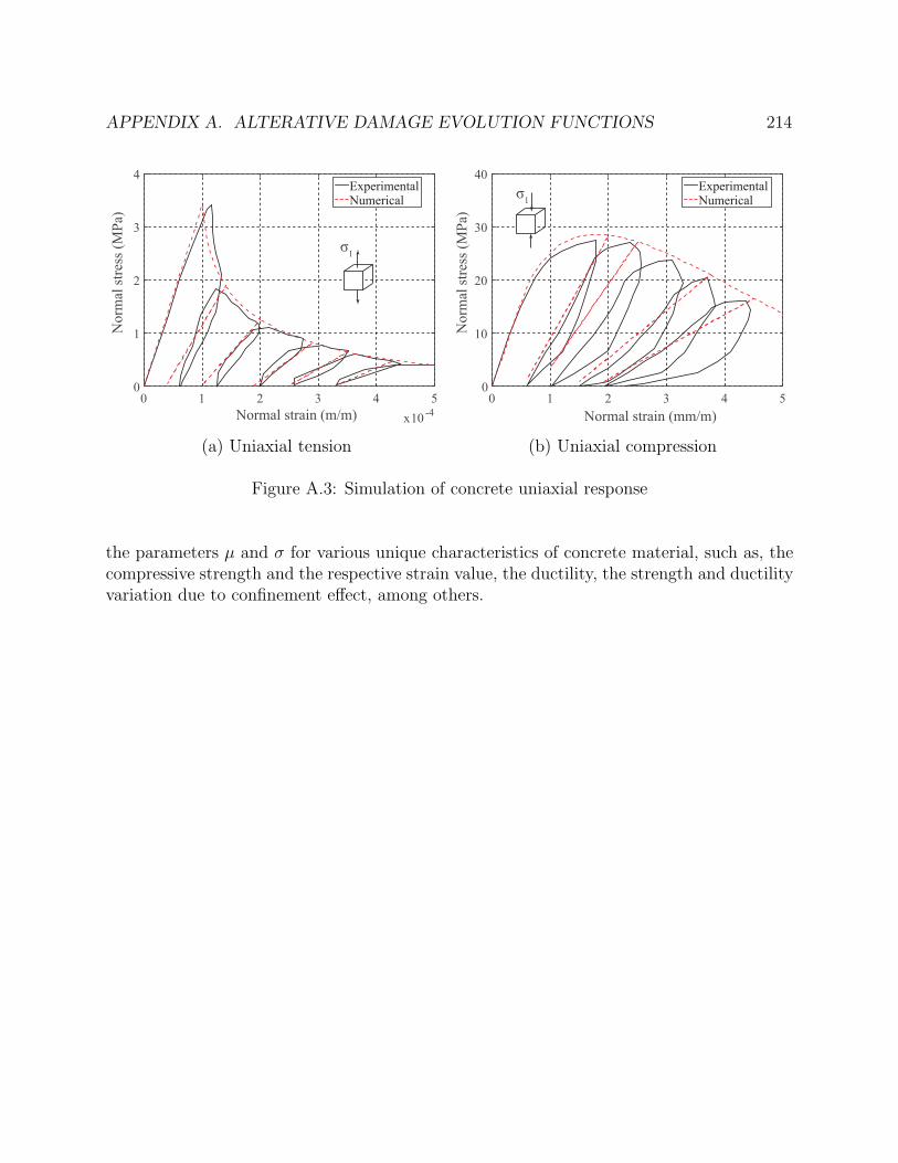
APPENDIX A. ALTERATIVE DAMAGE EVOLUTION FUNCTIONS 214
Normal strain (m/m) x10 -40 1 2 3 4 5
Nor
mal
stre
ss (M
Pa)
0
1
2
3
4ExperimentalNumerical
σ1
(a) Uniaxial tension
Normal strain (mm/m)0 1 2 3 4 5
Nor
mal
stre
ss (M
Pa)
0
10
20
30
40ExperimentalNumericalσ1
(b) Uniaxial compression
Figure A.3: Simulation of concrete uniaxial response
the parameters µ and σ for various unique characteristics of concrete material, such as, thecompressive strength and the respective strain value, the ductility, the strength and ductilityvariation due to confinement effect, among others.

215
Appendix B
Mathematical Derivations
B.1 Plastic Consistency Parameter
This section derives the plastic consistency parameter β in the return-mapping algo-rithm of the series beam element model state determination in Section 3.1.3. In the plasticcorrection at step n, the yield function n can be expressed in the following form:
fn = nT (bpqn − qb,n)− (Mp + Hiαn)
= nT[bp(qtr − keb
Tp nβ
)−(qtrb + Hknβ
)]−[Mp + Hi
(αtr + β
)]=[nT (bpq
trn − qtrb )− (Mp + Hiα
tr)]−[nT(bpkeb
Tp + Hk
)n + Hi
]β (B.1)
(B.2)
Similar to the return-mapping algorithm in classical plasticity, the normals in the trialand the correction step are equal n = ntr. Consequently, the term in the square bracket inEquation (B.2) gives the value of the trial yield function f tr. Finally, set the yield functionn to its target value 0:
0 = f tr −[nT(bpkeb
Tp + Hk
)n + Hi
]β (B.3)
one obtains the expression of the plastic consistency parameter β in Equation (3.38).
B.2 Algorithmic Tangent
This section derives the tangent stiffness of the series beam element and the NMYScolumn element.
B.2.1 Series beam model
This subsection presents the derivation of the tangent stiffness of the series beam modelgiven in Equation (3.22). Starting with the final form of the element forces qn in Equa-

APPENDIX B. MATHEMATICAL DERIVATIONS 216
tion (3.42), the tangent kt is evaluated as follows:
kt =∂qn∂vn
=∂qtr
vn− keb
Tp n
∂β
∂vn(B.4)
The partial derivative of the trial force qtr with respect to the deformation vn gives theelastic stiffness ke due to the assumption of a trial elastic step:
∂qtr
vn= ke (B.5)
Using the expression of the plastic consistency parameter β in Equation (3.38) and notethat:
∂f tr
vn= nTbp
∂qtr
vn= nTbpke (B.6)
the partial derivative of β with respect to the deformation vn is:
∂β
∂vn=[nT(bpkeb
Tp + Hk
)n + Hi
]−1nTbpke (B.7)
The partial derivatives in Equations (B.5) and (B.7) are subtituted into (B.4), and theexpression in Equation (3.22) for the tangent stiffness can be recovered.
B.2.2 NMYS column model
Diffentiating the residuals in Equation (4.28) to arrive at the following system of equa-tions:
dv
0
0
0
=
∂Rv
∂q
∂Rv
∂∆β
∂Rv
∂α
∂Rv
∂qb
∂Rα
∂q
∂Rα
∂∆β
∂Rα
∂α
∂Rα
∂qb
∂Rb
∂q
∂Rb
∂∆β
∂Rb
∂α
∂Rb
∂qb
∂f
∂q
∂f
∂∆β
∂f
∂α
∂f
∂qb
dq
d∆β
dα
dqb
(B.8)
The Jacobian matrix can be partitioned into four submatrices:
J =
[Frr Frc
Fcr Fcc
](B.9)

APPENDIX B. MATHEMATICAL DERIVATIONS 217
where the block matrices are:
Frr =∂Rv
∂qFrc =
[∂Rv
∂∆β,∂Rv
∂α,∂Rv
∂qb
](B.10)
Fcr =
[∂Rα
∂q,∂Rb
∂q,∂f
∂q
]TFcc =
∂Rα
∂∆β
∂Rα
∂α
∂Rα
∂qb
∂Rb
∂∆β
∂Rb
∂α
∂Rb
∂qb
∂f
∂∆β
∂f
∂α
∂f
∂qb
(B.11)
One approach to obtain the tangent stiffness kt is to first find the flexibility matrixf = ∂v/∂q and then invert the flexibility for the stiffness. The flexibility f is derived fromstatic condensation of Equation (B.8):
f =∂v
∂q=(Frr − FrcFcc
−1Fcr
)−1(B.12)
One drawback of this apprroach, however, is the issue of inverting a singular matrixduring static condensation. For instance, in case of an elasto-plastic response with Hip = 0and Hkr = 0, then Fcc becomes singular.
An alternative to find the tangent stiffness without directly using static condensation isto adopt the Woodbury formula:
(A + UCV)−1 = A−1 −A−1U(C−1 + VA−1U
)−1VA−1 (B.13)
The expression of the tangent stiffness matrix becomes:
k =∂q
∂v= Frr
−1 + Frr−1Frc
(Fcc − FcrFrr
−1Frc
)−1FcrFrr
−1 (B.14)

218
Appendix C
Thermodynamics Framework
A free energy potential per unit volume, Φ, can be defined as a function of the elasticdeformation ee, the plastic deformation ep, the damage variable d, and some hardeningvariables γ. The free energy potential is assumed to be decomposed into the elastic potentialΦe, the plastic potential Φp, and the hardening potential Ω. The elastic potential Φe dependson the elastic deformation ee and damage index d, while the plastic potential Φp is a functionof the plastic deformation ep and damage index d. The hardening potential Ω is dependenton the hardening variables γ. The elastic and plastic potentials are proportional to theircounterparts in the effective space, Φe and Φp.
Φ(ee, ep, d, γ) = Φe(ee, d) + Φp(ep, d) + Ω(γ)
= (1− d)Φe(ee) + (1− d)Φp(ep) + Ω(γ) (C.1)
According to the second principle of thermodynamics, any irreversible process shall pro-duce non-negative energy dissipation. The condition applies for all admisible process and isgiven by the Clausius-Dulhem inequality:
se− Φ ≥ 0 (C.2)
The inequality in Equation (C.2) can be rewritten as:
se−(∂Φ
∂ee+
∂Φ
∂dd+
∂Φ
∂γγ
)≥ 0 (C.3)
Rearranging the terms in Equation (C.3) gives:(s− ∂Φ
∂e
)e− ∂Φ
∂dd− ∂φ
∂γγ ≥ 0 (C.4)
Imposing a constraint on the deformation field, the first term in equation (C.4) leads tothe constitutive relation:
s =∂Φ
∂e(C.5)

APPENDIX C. THERMODYNAMICS FRAMEWORK 219
The second and third terms in equation (C.4) invoke the nonnegativity of the energydissipation:
−∂Φ
∂dd ≥ 0 (C.6)
−∂Φ
∂γγ ≥ 0 (C.7)
In Equation (C.6), define ψ as the conjugate to the damage index d as:
ψ = −∂Φ
∂d= Φe + Φp (C.8)
Equation (C.8) suggests that ψ is an energy variable and is related to the energy dissipa-tion in the effective space. The damage conjugate ψ, usually referred to as the energy releaserate in the literature, is the key variable that governs the damage evolution. This observationis consistent with the formulation in Chapter 2, in which the energy variable is evaluated inEquations (2.2)−(2.3). Therefore, the proposed damage formulation is thermodynamicallyconsistent.