arX

iv:1

101.

2037

v4 [

astr

o-ph

.GA

] 25

Aug

201

1Astronomy & Astrophysicsmanuscript no. Dust˙MC˙20juillet2011 c© ESO 2011August 26, 2011

Planck Early Results. XXV. Thermal dust in nearby molecularclouds

Planck Collaboration: A. Abergel46, P. A. R. Ade70, N. Aghanim46, M. Arnaud57, M. Ashdown55,4, J. Aumont46, C. Baccigalupi68, A. Balbi28,A. J. Banday74,7,62, R. B. Barreiro52, J. G. Bartlett3,53, E. Battaner76, K. Benabed47, A. Benoıt45, J.-P. Bernard74,7, M. Bersanelli25,40, R. Bhatia5,

J. J. Bock53,8, A. Bonaldi36, J. R. Bond6, J. Borrill61,71, F. R. Bouchet47, F. Boulanger46, M. Bucher3, C. Burigana39, P. Cabella28,J.-F. Cardoso58,3,47, A. Catalano3,56, L. Cayon18, A. Challinor49,55,9, A. Chamballu43, L.-Y Chiang48, C. Chiang17, P. R. Christensen65,29,

D. L. Clements43, S. Colombi47, F. Couchot60, A. Coulais56, B. P. Crill53,66, F. Cuttaia39, L. Danese68, R. D. Davies54, R. J. Davis54, P. deBernardis24, G. de Gasperis28, A. de Rosa39, G. de Zotti36,68, J. Delabrouille3, J.-M. Delouis47, F.-X. Desert42, C. Dickinson54, K. Dobashi14,S. Donzelli40,50, O. Dore53,8, U. Dorl62, M. Douspis46, X. Dupac32, G. Efstathiou49, T. A. Enßlin62, H. K. Eriksen50, F. Finelli39, O. Forni74,7,

M. Frailis38, E. Franceschi39, S. Galeotta38, K. Ganga3,44, M. Giard74,7, G. Giardino33, Y. Giraud-Heraud3, J. Gonzalez-Nuevo68,K. M. Gorski53,78, S. Gratton55,49, A. Gregorio26, A. Gruppuso39, V. Guillet46, F. K. Hansen50, D. Harrison49,55, S. Henrot-Versille60, D. Herranz52,S. R. Hildebrandt8,59,51, E. Hivon47, M. Hobson4, W. A. Holmes53, W. Hovest62, R. J. Hoyland51, K. M. Huffenberger77, A. H. Jaffe43, A. Jones46,

W. C. Jones17, M. Juvela16, E. Keihanen16, R. Keskitalo53,16, T. S. Kisner61, R. Kneissl31,5, L. Knox20, H. Kurki-Suonio16,34, G. Lagache46,J.-M. Lamarre56, A. Lasenby4,55, R. J. Laureijs33, C. R. Lawrence53, S. Leach68, R. Leonardi32,33,21, C. Leroy46,74,7, M. Linden-Vørnle11,

M. Lopez-Caniego52, P. M. Lubin21, J. F. Macıas-Perez59, C. J. MacTavish55, B. Maffei54, N. Mandolesi39, R. Mann69, M. Maris38,D. J. Marshall74,7, P. Martin6, E. Martınez-Gonzalez52, S. Masi24, S. Matarrese23, F. Matthai62, P. Mazzotta28, P. McGehee44, P. R. Meinhold21,

A. Melchiorri24, L. Mendes32, A. Mennella25,38, S. Mitra53, M.-A. Miville-Deschenes46,6, A. Moneti47, L. Montier74,7, G. Morgante39,D. Mortlock43, D. Munshi70,49, A. Murphy64, P. Naselsky65,29, P. Natoli27,2,39, C. B. Netterfield13, H. U. Nørgaard-Nielsen11, F. Noviello46,D. Novikov43, I. Novikov65, S. Osborne73, F. Pajot46, R. Paladini72,8, F. Pasian38, G. Patanchon3, O. Perdereau60, L. Perotto59, F. Perrotta68,

F. Piacentini24, M. Piat3, S. Plaszczynski60, E. Pointecouteau74,7, G. Polenta2,37, N. Ponthieu46, T. Poutanen34,16,1, G. Prezeau8,53, S. Prunet47,J.-L. Puget46, W. T. Reach75, R. Rebolo51,30, M. Reinecke62, C. Renault59, S. Ricciardi39, T. Riller62, I. Ristorcelli74,7, G. Rocha53,8, C. Rosset3,J. A. Rubino-Martın51,30, B. Rusholme44, M. Sandri39, D. Santos59, G. Savini67, D. Scott15, M. D. Seiffert53,8, P. Shellard9, G. F. Smoot19,61,3,

J.-L. Starck57,10, F. Stivoli41, V. Stolyarov4, R. Sudiwala70, J.-F. Sygnet47, J. A. Tauber33, L. Terenzi39, L. Toffolatti12, M. Tomasi25,40, J.-P. Torre46,M. Tristram60, J. Tuovinen63, G. Umana35, L. Valenziano39, L. Verstraete46, P. Vielva52, F. Villa39, N. Vittorio28, L. A. Wade53, B. D. Wandelt47,22,

D. Yvon10, A. Zacchei38, and A. Zonca21

(Affiliations can be found after the references)

Received 9 January 2011/ Accepted 23 June 2011

ABSTRACT

Planck allows unbiased mapping of Galactic sub-millimetre and millimetre emission from the most diffuse regions to the densest parts of molecularclouds. We present an early analysis of the Taurus molecularcomplex, on line-of-sight-averaged data and without component separation. Theemission spectrum measured byPlanck andIRAS can be fitted pixel by pixel using a single modified blackbody.Some systematic residuals aredetected at 353 GHz and 143 GHz, with amplitudes around−7% and+13%, respectively, indicating that the measured spectra are likely morecomplex than a simple modified blackbody. Significant positive residuals are also detected in the molecular regions and in the 217 GHz and100 GHz bands, mainly caused by to the contribution of theJ = 2 → 1 andJ = 1 → 0 12CO and13CO emission lines. We derive maps of thedust temperatureT , the dust spectral emissivity indexβ, and the dust optical depth at 250µm τ250. The temperature map illustrates the coolingof the dust particles in thermal equilibrium with the incident radiation field, from 16–17 K in the diffuse regions to 13–14 K in the dense parts.The distribution of spectral indices is centred at 1.78, with a standard deviation of 0.08 and a systematic error of 0.07.We detect a significantT − β anti-correlation. The dust optical depth map reveals the spatial distribution of the column density of the molecular complex from the densestmolecular regions to the faint diffuse regions. We use near-infrared extinction and Hi data at 21-cm to perform a quantitative analysis of the spatialvariations of the measured dust optical depth at 250µm per hydrogen atomτ250/NH. We report an increase ofτ250/NH by a factor of about 2between the atomic phase and the molecular phase, which has astrong impact on the equilibrium temperature of the dust particles.

Key words. ISM: general, dust, extinction, clouds - Submillimeter: ISM

1. Introduction

Planck 1 (Tauber et al. 2010; Planck Collaboration 2011a) is thethird-generation space mission to measure the anisotropy of the

1 Planck (http://www.esa.int/Planck ) is a project of the EuropeanSpace Agency (ESA) with instruments provided by two scientific con-sortia funded by ESA member states (in particular the lead countriesFrance and Italy), with contributions from NASA (USA) and telescopereflectors provided by a collaboration between ESA and a scientific con-sortium led and funded by Denmark.

cosmic microwave background (CMB). It observes the sky innine frequency bands covering 30–857GHz with high sensitiv-ity and angular resolution from 3′ to 5′. The Low FrequencyInstrument (LFI; Mandolesi et al. 2010; Bersanelli et al. 2010;Mennella et al. 2011) covers the 30, 44, and 70 GHz bands withamplifiers cooled to 20 K. The High Frequency Instrument (HFI;Lamarre et al. 2010; Planck HFI Core Team 2011a) covers the100, 143, 217, 353, 545, and 857 GHz bands with bolome-ters cooled to 0.1 K. Polarisation is measured in all but thehighest two bands (Leahy et al. 2010; Rosset et al. 2010). A

1

Planck Collaboration: Thermal dust in nearby molecular clouds

combination of radiative cooling and three mechanical cool-ers produces the temperatures needed for the detectors and op-tics (Planck Collaboration 2011b). Two data processing centres(DPCs) check and calibrate the data and make maps of the sky(Planck HFI Core Team 2011b; Zacchei et al. 2011).Planck’ssensitivity, angular resolution, and frequency coverage make it apowerful instrument for Galactic and extragalactic astrophysicsas well as cosmology. Early astrophysics results are given inPlanck Collaboration, 2011h–u. This paper presents the early re-sults of the analysis of Planck/HFI observations of the Taurusmolecular cloud.

IRAS provided a complete view of the interstellar matter inour Galaxy in four photometric bands from 12 to 100µm withangular resolution of about 4′. The 12, 25, and 60µm bandsare mainly sensitive to the emission of the smallest interstel-lar grains. They are aromatic hydrocarbons (large molecules)and amorphous hydrocarbon grains that undergo stochastic heat-ing upon photon absorption, and tend to emit most of theirenergy at wavelengths shortward of 100µm. The large parti-cles have dimensions of the order of 100 nm and make up thebulk of the dust mass. They are in equilibrium between ther-mal emission and absorption of UV and visible photons fromincident radiation. Only oneIRAS band, at 100µm, is dom-inated by the emission of this dust component. DIRBE andFIRAS on boardCOBE produced all-sky maps at longer wave-lengths, with angular resolution lower thanIRAS (40′ and 7,respectively), which allowed the measurement of dust temper-atures and spectral indices. The dust temperature was foundto be on average∼17.5 K (with a spectral emissivity indexβ = 2) in the diffuse atomic medium (Boulanger et al. 1996)and to be lower in molecular clouds with no embedded brightstars (Lagache et al. 1998). Small patches of molecular cloudshave been observed in more detail from the ground by theJCMT (Johnstone & Bally 1999), by balloon-borne experimentsPRONAOS (Ristorcelli et al. 1998), Archeops (Desert et al.2008a) and BLAST (Netterfield et al. 2009), and from space bySpitzer (e.g., Flagey et al. 2009) andHerschel (e.g., Andre et al.2010; Motte et al. 2010; Abergel et al. 2010; Juvela et al. 2011).

With Planck, the whole sky emission of thermal dust ismapped from the submillimetre to the millimetre range, withangular resolution comparable toIRAS. We have complete andunbiased surveys of molecular clouds not only in terms of spa-tial coverage, but also in terms of spatial content of the data.Unlike ground or ballon observations, the maps contain all an-gular scales above the diffraction limit without spatial filtering.This is extremely important for Galactic science, because the in-terstellar matter contains a large range of intricate spatial scales.Moreover, the emission is measured with unprecedented signal-to-noise ratio down to the faintest parts surrounding the brightand dense regions. Up to now, the rotational transitions of car-bon monoxide (CO) were the main tracer of the interstellar mat-ter in molecular clouds. WithPlanck thermal dust becomes anew tracer. The spectral coverage and the sensitivity allowforeach line of sight precise measurements of the temperature,ofthe spectral emissivity index, and of the optical depth, indepen-dent of the excitation conditions.

Molecular clouds present a wide range of physical conditions(illumination, density, star-forming activity), so are ideal targetsfor studying the emission properties of dust grains and their evo-lution. The goal of this paper is to discuss the results of theearlyanalysis of HFI maps of the Taurus complex, which is one of thenearest giant molecular clouds (d = 140 pc, from Kenyon et al.1994) with low-mass star-forming activity.

First we present the HFI data and the ancillary observationsused for this paper (Sect. 2). Then we describe the emission spec-trum of thermal dust measured by HFI andIRAS, and discussthe validity of the measured spectra fitting with one single modi-fied blackbody (Sect. 3). Maps of the dust temperature and of thespectral emissivity index are analysed in Sect. 4. Then in Sect. 5we discuss the evolution of the dust optical depth/column den-sity conversion factor (τ/NH) from the atomic diffuse regions tothe molecular regions.

2. Observations

2.1. HFI data

We used the DR2 release of the HFI maps presented in Fig. 1 andbegin with Healpix (Gorski et al. 2005) withNside= 2048 (pixelsize 1.′7). The data processing and calibration are described inPlanck HFI Core Team (2011b). An important step is the re-moval of the CMB through a needlet internal linear combinationmethod.

The systematic calibration accuracy of HFI is summarized inTable 1 (from Planck HFI Core Team 2011a). For the two bandsat 857 and 545 GHz, the gain calibration is performed usingFIRAS data. The CMB dipole is used at lower frequencies. Thesystematic errors on the gain calibration are 7% for the 857 and545 GHz bands, respectively (estimated using the dispersion indifferent regions of the sky), and about 2% for the other bands.

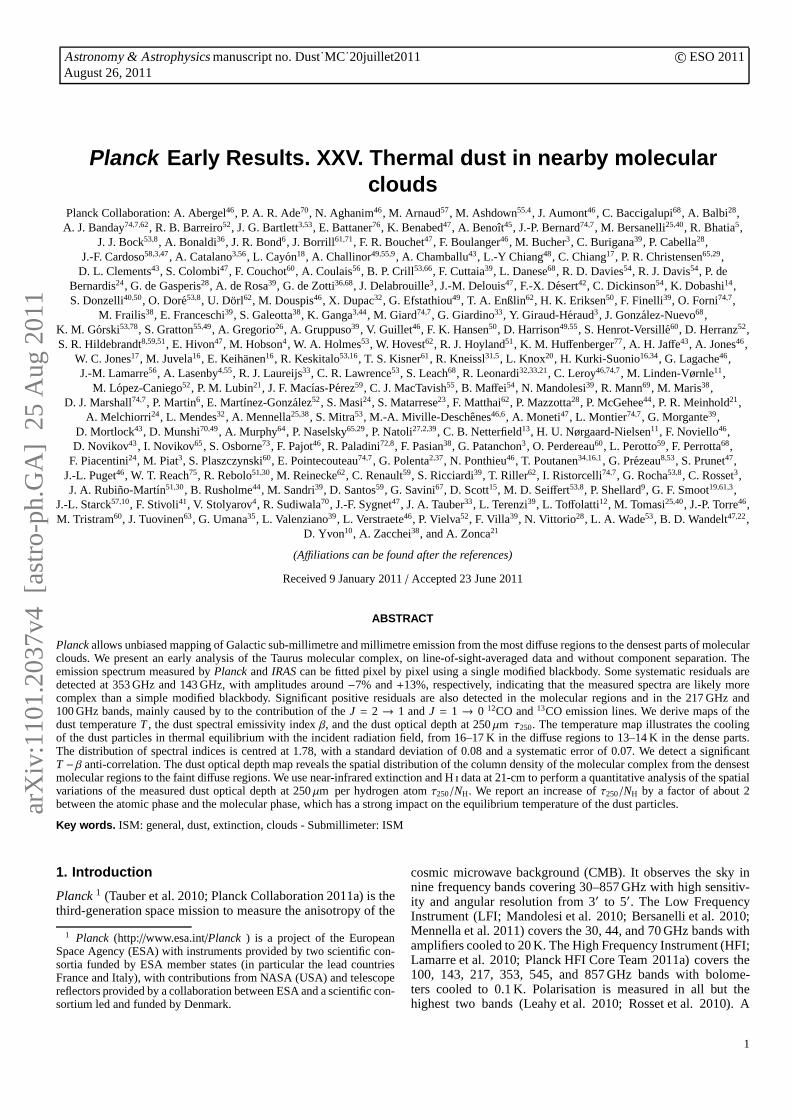
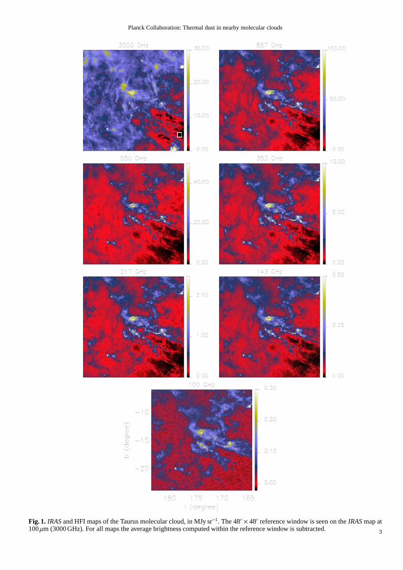
We estimated the statistical noise as follows (see alsoAppendixB of Planck Collaboration 2011t, for details). Twoin-dependent maps of the sky have been computed by the DPC fromthe first- and second-half ring of each pointing period. Becausethe coverage is identical for these two maps, the standard de-viation of their half difference,σHR, is equal to the standarddeviation of the average map. For all bands, we compared thecomputed value ofσHR with the standard deviationσref of theDR2 map computed within a reference 48′ × 48′ window cen-tered atl = 165.43, b = −21.06, chosen in the lowest part ofthe map (white square in the first image of Fig. 1). Obviously,the values ofσref give only upper limits on the statistical noisebecause of the contributions of CMB residuals, and of cosmicinfrared background (CIB) and thermal dust fluctuations that in-crease with increasing frequencies. Table 1 shows that for the100, 143, and 217 GHz bands,σHR is almost identical toσref.Therefore we conclude that

1. the standard deviation of CMB residuals is lower than thestatistical noise in all bands;

2. the standard deviation of the CIB anisotropies (CIBA) ap-pears lower than the measured statistical noise in the 100,143, and 217 GHz bands (which is compatible with the CIBAmeasurements in Planck Collaboration 2011n);

3. the computed values ofσHR give realistic estimates of thestatistical noise.

For this early analysis, we used a constant statistical noise ineach band, taken equal to the values ofσHR in Table 1.

2.2. Ancillary data

We combined thePlanck maps with IRAS maps at 100µm(3000 GHz), using the IRIS (Improved Reprocessing of theIRAS Survey) data computed by Miville-Deschenes & Lagache(2005). The statistical noise of the 100µm maps is about0.06 MJy sr−1 per pixel (pixel size of 1.8′), while the system-atic error in the gain calibration from DIRBE is estimated to

2

Planck Collaboration: Thermal dust in nearby molecular clouds

Fig. 1. IRAS and HFI maps of the Taurus molecular cloud, in MJy sr−1. The 48′ × 48′ reference window is seen on theIRAS map at100µm (3000 GHz). For all maps the average brightness computed within the reference window is subtracted. 3

Planck Collaboration: Thermal dust in nearby molecular clouds

Table 1.Calibration accuracy, statistical noise, standard deviation within the reference window (white square in the3000 GHzpanelof Fig. 1), median brightnesses, and average spectrum within the reference window.

Frequency (GHz) 100 143 217 353 545 857 3000Calibration accuracy 2% 2% 2% 2% 7% 7% 13.5%Statistical noise fromσHR (MJy sr−1) 0.014 0.0086 0.018 0.038 0.049 0.074σref (MJy sr−1) 0.013 0.0078 0.019 0.050 0.13 0.35 0.37Median brightness (MJy sr−1) 0.042 0.094 0.41 1.67 6.37 17.46 13.9Reference spectrum (MJy sr−1) 0.010 0.027 0.11 0.43 1.48 4.1 4.8

be 13.5% (from Miville-Deschenes & Lagache 2005). For theTaurus molecular cloud, the 100µm brightness is in the range1–20 MJy sr−1, so the statistical noise translates into relative er-rors in the range 0.03–6%, well below the systematic error onthe gain.

The atomic gas was traced on large scales using the Hi dataat 21 cm taken with the Leiden/Dwingeloo 25-m telescope withan angular resolution of 36′ by Hartmann & Burton (1997). Thevelocity spacing was 1.03 km s−1, and the local standard of rest(LSR) velocity range was−450< VLS R < 400 km s−1. The datawere corrected for contamination from stray light radiation tothe 0.07 K sensitivity level (Hartmann et al. 1996).

The large-scale survey in the12CO (J = 1 → 0) emissionline taken by Dame et al. (2001) with the CfA telescope wasused to trace the molecular gas. The beam width was 8.8′ ±0.2′.For the observations of the Taurus molecular cloud, the samplingdistance was equal to 7.5′, the channel width is 0.65 km s−1 andthe channel rms noise was 0.25 K. The data cubes were trans-formed into the velocity-integrated intensity of the line (WCO)by integrating the velocity range where the CO emission issignificantly detected using the moment method proposed byDame et al. (2001). The statistical noise level of theWCO mapis typically 1.2 K km s−1.

In order to analyse the central region of the Taurus molecularcloud with the13CO J = 1→ 0 emission lines, we also used theFCRAO survey of 98 deg2 conducted with an angular resolution47′′ (Narayanan et al. 2008; Goldsmith et al. 2008). We appliedthe error beam scaling factor recently proposed by Pineda etal.(2010), so that the intensities of the CfA and FCRAO surveys ofthe12CO emission line are compatible. The statistical noise perpixel (with pixel size of 0.33′) of the velocity-integrated inten-sity maps is about 0.4 K km s−1 for the13CO line.

The column density can also be traced from the near-infrared(NIR) extinction using the 2MASS point source catalogue (e.g.,Dobashi et al. 2005; Pineda et al. 2010). For comparison withHFI data, we used the extinction map of the central part ofthe Taurus molecular cloud recently created by Pineda et al.(2010) and shown in Fig. 2. It is Nyquist-sampled with an an-gular resolution of 200′′, and corrected for the contribution ofatomic gas to the total extinction. Using the extinction curveof Weingartner & Draine (2001) and adopting the standard ra-tio of selective to total extinctionRV=3.1 for the diffuse ISM(Savage & Mathis 1979), the infrared colours are converted tovisible extinctionAV or column densitiesNH (= AV ×1.87×1021

cm2). Because the number of background stars used to computethe extinction decreases with increasing extinction, the error inAV increases from about 0.2 mag at low extinctions (AV = 0–1 mag) to 0.5 mag at high extinctions (AV ∼ 10 mag), with anaverage error of 0.29 mag. For higher extinctions (AV > 10 mag)the extinction map only gives lower limits.

Fig. 3. Spectrum of one pixel in the non-molecular region:crosses, total brightnessItot; triangles, average brightnessIrefwithin the reference 48′ × 48′ window (seen on the 3000 GHzpanel of Fig. 1); squares,Itot− Iref; and diamonds, CIB spectrumat the central frequency of the HFI filters from 857 to 217 GHz,from Fixsen et al. (1998).

3. Emission spectrum of thermal dust

3.1. Reference spectrum

The combination ofIRAS andPlanck data provides the spectralenergy distribution (SED) from 3000 GHz (100µm) to 100 GHz(3 mm) for each pixel of the maps. The CMB has been removedfrom the maps we use. The maps could contain some CMB resid-ual, but with an amplitude lower than the statistical noise evenin the low frequency channels (see Sect. 2.1).

In all bands, the maps contain Galactic and non-Galacticemission that is not associated with the Taurus complex.Therefore, we subtracted for all maps the average brightnesscomputed within the reference 48′ × 48′ window, chosen in thefaintest region (white square in the first image of Fig. 1 and cen-tral coordinates given above in Sect. 2.1) of the map. This isil-lustrated for one pixel in Fig. 3. The average spectrum in thereference window is also shown in Fig. 3, together with the CIBspectrum (from FIRAS data by Fixsen et al. 1998) at the centralfrequencies of the HFI filters. We see that the reference spec-trum is mainly caused by Galactic atomic emission (there is nodetected emission within the12CO J = 1 → 0 line), since theCIB contributes not more than 5–10%.

In order to derive the dust optical depth per column densityin the atomic phase (Sect. 5.2), the emission measured within thesame reference window will be subtracted from the Hi data.

4

Planck Collaboration: Thermal dust in nearby molecular clouds

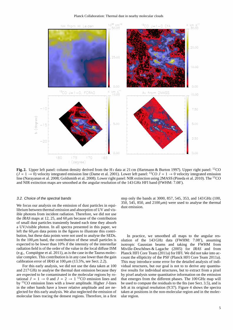
Fig. 2. Upper left panel: column density derived from the Hi data at 21 cm (Hartmann & Burton 1997). Upper right panel:12CO(J = 1→ 0) velocity integrated emission line (Dame et al. 2001). Lower left panel:13CO J = 1→ 0 velocity integrated emissionline (Narayanan et al. 2008; Goldsmith et al. 2008). Lower right panel: NIR extinction using 2MASS (Pineda et al. 2010). The13COand NIR extinction maps are smoothed at the angular resolution of the 143 GHz HFI band (FWHM: 7.08′).

3.2. Choice of the spectral bands

We focus our analysis on the emission of dust particles in equi-librium between thermal emission and absorption of UV and vis-ible photons from incident radiation. Therefore, we did notusetheIRAS maps at 12, 25, and 60µm because of the contributionof small dust particles transiently heated each time they absorba UV/visible photon. In all spectra presented in this paper, weleft the 60µm data points in the figures to illustrate this contri-bution, but these data points were not used to analyse the SEDs.In the 100µm band, the contribution of these small particles isexpected to be lower than 10% if the intensity of the interstellarradiation field is of the order of the value in the local diffuse ISM(e.g., Compiegne et al. 2011), as is the case in the Taurus molec-ular complex. This contribution is in any case lower than thegaincalibration error ofIRAS at 100µm (13.5%, see Sect. 2.2).

For this early analysis, we did not use the data taken at 100and 217 GHz to analyse the thermal dust emission because theyare expected to be contaminated in the molecular regions by ro-tational J = 1 → 0 andJ = 2 → 1 12CO emission lines andby 13CO emission lines with a lower amplitude. HigherJ-linesin the other bands have a lower relative amplitude and are ne-glected for this early analysis. We also neglected the emission ofmolecular lines tracing the densest regions. Therefore, ina first

step only the bands at 3000, 857, 545, 353, and 143 GHz (100,350, 545, 850, and 2100µm) were used to analyse the thermaldust emission.

In practice, we smoothed all maps to the angular res-olution of the 143 GHz data (FWHM: 7.08′), assumingisotropic Gaussian beams and taking the FWHM fromMiville-Deschenes & Lagache (2005) forIRAS and fromPlanck HFI Core Team (2011a) for HFI. We did not take into ac-count the ellipticity of the PSF (Planck HFI Core Team 2011a).This may introduce some error for the detailed analysis of indi-vidual structures, but our goal is not to to derive any quantita-tive results for individual structures, but to extract froma pixelby pixel analysis some quantitative information on the emissionthat emerges from the different phases. The 100 GHz map willbe used to compute the residuals to the fits (see Sect. 3.5), and isleft at its original resolution (9.′37). Figure 4 shows the spectrataken at positions in the non-molecular region and in the molec-ular region.

5

Planck Collaboration: Thermal dust in nearby molecular clouds

Fig. 4. SED of two pixels (top: non-molecular region, bottom:molecular region). The squares are data, the solid line is the fittedmodel, and the crosses are the fitted model integrated withinthebands. The fits are performed using the 100µm, 857, 545, 353and 143 GHz bands (red squares), and using the statistical noisediscussed in Sect. 2, which is too low to be visible on the figure.Significant excess in the 217 and 100 GHz bands caused by12COand13CO emissions are detected in the molecular spectrum. The60µm data points are not used to analyse the SED because of thecontribution of small dust particles transiently heated each timethey absorb a UV/visible photon.

3.3. Principle of fitting

In this early analysis, the fitting function is a single and opticallythin modified blackbody:

Iν = τν0 ×

(

ν

ν0

)β

× Bν(T ), (1)

whereτν0 is the dust optical depth at frequencyν0, β is the spec-tral emissivity index,Bν is the Planck function, andT the dusttemperature. All quantitative values of the dust optical depth willbe given at the frequencyν0 = 1200 GHz (250µm) to be compa-rable to previous analyses, and we defineτν0 = τ250.

The three computed parameters for each pixel areT , β, andτ250. We used the IDL MPFIT routine, which performs weightedleast-squares curve fitting of the data (Markwardt 2009) tak-ing into account the noise (statistical noise or calibration un-certainty) for each spectral band. We applied colour-correctionfactors computed using version 1 of the transmission curves(Planck HFI Core Team 2011a).

The goal of this adjustment is to reduce the properties of theSED measured for each line of sight to the set of three param-etersT, β, andτ250. The temperature, spectral emissivity index,and optical depth of the emitting dust particles along the line ofsight can obviously vary, so the fitted values of the three param-eters, while representing some average properties, cannotgivethe complete picture of the dust particles located along that lineof sight. Moreover, we assumed that the spectral emissivityin-dexβ of the measured spectra is constant from far-infrared (FIR)to millimetre wavelengths. The spectral emissivity index of dustemission may vary due to temperature-dependent mechanismsat low temperatures, including free-charge carrier processes,two-phonon difference processes, and absorption mechanismsin two-level systems (Agladze et al. 1996; Meny et al. 2007).Moreover, the measured spectra can be broadened around thepeak of the modified blackbody in the submillimeter (submm)because of the contribution of dust at different temperatures.Thus, the spectral emissivity indexβ of the measured spectracould increase from the submm to the millimeter, as illustratedby Shetty et al. (2009b).

3.4. Example of spectra. Systematic errors on theparameters derived from the fit

Figure 4 is an illustration of the fitting for two pixels, one taken ata position with detected CO emission (within the12CO J = 1→0 line), the other at a position with no detected CO emission.Weused for the fitting the statistical noise for HFI andIRAS datadiscussed in Sect. 2, taking into account the smoothing of themap at the angular resolution of the 143 GHz band.

Simulations have been performed to understand and to quan-tify the propagation of the calibration errors, the statisticalnoise, and the CIBA in the determination ofT, β, andτ250 (seeAppendixA for details). The calibration errors propagate intosystematic errors inT, β, andτ250 of about 0.7 K, 0.07, and 18%,respectively. We have also shown that the statistical noiseandthe CIBA propagates into statistical noise levels inT , β, andτ250in the range 0.1–1 K, 0.025–0.25 and 2–20%, respectively, de-pending on the 100µm brightness (10–1 MJy sr−1). Moreover,both for systematic errors and statistical noises, the three param-eters are strongly correlated or anti-correlated (Fig. A.1).

The two spectra of Fig. 4 show that to first order, a sin-gle modified blackbody gives a reasonable representation oftheSED measured byIRAS and HFI. Obviously by increasing thenumber of free parameters in our fit (e.g., by using two modifiedblackbodies with different temperatures and spectral indices) itis possible to improve the fits significantly, but this is not ourgoal in this early paper. We used exactly the same method to fitthe spectra for all pixels of the map to derive the temperaturemap and the spectral emissivity index map shown in Fig. 7.

3.5. Analysis of the residuals

The fit residuals allow us to assess the limitations of using asingle modified blackbody to fit the data. As seen in Sect. 3.2,fits were made to the 3000, 857, 545, 353, and 143 GHz dataall smoothed to the angular resolution of 143 GHz. The residualmap at 100 GHz was computed from the difference between thesynthetic spectra smoothed at the 100 GHz resolution and thedata at 100 GHz. The residual map of the fitting in all bands isshown in Fig. 5. Figure 6 shows the relative residual map (resid-ual map divided by measured map).

6

Planck Collaboration: Thermal dust in nearby molecular clouds

Fig. 5.Same as Fig 1 for the fit residuals. The bottom right image is the COJ = 1→ 0 integrated emission from Dame et al. (2001).The units are K km s−1.

7

Planck Collaboration: Thermal dust in nearby molecular clouds

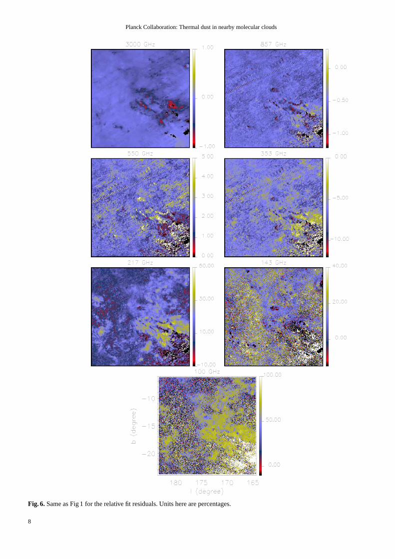
Fig. 6.Same as Fig 1 for the relative fit residuals. Units here are percentages.

8

Planck Collaboration: Thermal dust in nearby molecular clouds

3.5.1. Residuals for the five fitted bands

We see in Fig. 6 that the relative residuals are distributed aroundzero and below 1–3% for the 3000, 857, and 545 Hz bands. Onthe other hand, the residuals at 353 GHz are systematically neg-ative, with a median relative amplitude about−7%, while theresiduals at 143 GHz are systematically positive, with a medianrelative amplitude about+13%. As can be seen in Figs. 5 and 6,these residuals are spatially correlated with the measuredbright-ness, so they are related to the emission spectrum of the dustparticles located in the complex.

We have seen in Sect. 2.1 (Table 1, fromPlanck HFI Core Team 2011a) that the calibration errorsare estimated to be 13.5% at 3000 GHz (100µm), 7% at 857 and545 GHz, and 2% at 353 and 143 GHz. These numbers translateinto systematic errors of about 5% and 4% on the 353 and143 GHz brightnesses (computed from the fit of the five bands),respectively. We conclude in this early analysis that the negativeresiduals at 353 GHz (with a median amplitude about−7%)and the positive residuals at 143 GHz (with a median amplitudeabout+13%) are not caused by calibration errors. The negativeresiduals at 353 GHz could be caused by a broadening of themeasured spectra around the peak of the modified blackbody(3000–545GHz spectral range) because of the contribution ofdust at different temperatures along the line of sight. On theother hand, the positive residuals at 143 GHz suggest a flatteningof the emission spectra at low frequencies.

3.5.2. Residuals at 217 and 100 GHz

As shown in Fig. 5, there is a striking spatial correlation betweenthe residual maps at 100 GHz and 217 GHz and the map of theintegrated emission of the12CO J = 1→ 0 emission line. Thisconfirms that 100 GHz and 217 GHz residuals are dominated bya contamination by CO molecular lines (mainly12CO, but also13CO and other isotopes and molecules in the densest regions).However, we have seen above that the measured dust spectra aremore complex than a single modified blackbody from 3000 GHzto 100 GHz, so the residuals computed at 100 GHz and 217 GHzin this early analysis and shown in Fig. 5 are only indicativeofthe CO emission.

4. Analysis of the dust temperature and spectralemissivity index maps.

4.1. Dust temperature map

The dust temperature map is shown in Fig. 7. The black regionsare artifacts: they correspond to low values of the temperature(below 12 K) caused by statistical noise and CIBA in the faintregions (withI (100µm) < 1 MJy sr−1, as also illustrated in oursimulations presented in Fig. A.2). Excluding these regions andsome residual stripping in the faintest regions with amplitudesaround 0.15 K, most of the variations seen on the temperaturemap are real because their amplitude is higher than the noisecomputed from our simulations (about 0.1–1 K forI (100µm) =10− 1 MJy sr−1, from Fig A.2).

At least three regions with different temperature distribu-tions can be identified in the temperature map (Fig. 7) and itshistogram (Fig. 8):

– the outer parts of the molecular cloud (with no detected12COemission), with temperatures∼ 16–17.5K;

– the molecular cloud with detected12CO emission but no de-tected13CO emission, with temperatures∼ 15–17 K;

Fig. 9. Correlation between the spectral emissivity index andthe dust temperature. Upper panel: for all pixels. Lower panel:for pixels in the molecular region with detected CO emissionandI (100µm) > 10 MJy sr−1. The solid and dashed lines showthe relations deduced fromArcheops (Desert et al. 2008b) andPRONAOS (Dupac et al. 2003), respectively.

– the densest parts of the molecular cloud with detected13COemission which coincide with the well-known dense fila-ments, with temperatures∼ 13–16 K.

Most of the differences between theIRAS map at 100µm and theHFI maps (Fig. 1) are caused by temperature variations. Exceptin diffuse regions with uniform illumination and constant dusttemperature, this demonstrates thatIRAS maps at 100µm usedalone cannot properly probe the gas column density. Comparabletemperature variations have also been found by Flagey et al.(2009) in the central region of our field (average temperatureabout 14.5 K with a dispersion of 1 K) by combiningSpitzer160µm andIRAS 100µm maps and assuming a constant valueof β equal to 2.

9

Planck Collaboration: Thermal dust in nearby molecular clouds

Fig. 7.Left panel: dust temperature map. Right panel: spectral emissivity index map.

Fig. 8. Dust temperature and spectral emissivity index histograms: black, all pixels; green, pixels without detected12CO emission;red, pixels with detected12CO emission but no detected13CO emission in the central molecular region covered by Pineda et al.(2010); and blue, pixels in the central molecular region with detected13CO emission.

4.2. Spectral emissivity index map

The spectral emissivity index presents a symmetric distribution(Fig. 8) with average and median values both equal to 1.78 and astandard deviationσβ = 0.08. The standard deviation caused bystatistical noise and CIBA estimated from our simulations is inthe range 0.025–0.25 forI (100µm) = 10−1 MJy sr−1 (Fig A.2).Moreover, we can see in Fig. 7 and more explicitly in the firstpanel of Fig. 9 that there is a some anti-correlation betweenTandβ. The higher values ofβ (> 1.8) are found in the coldest(about 14 K) structures.

We show in AppendixA and it was also discussed in de-tail by Shetty et al. (2009a,b) that the instrumental errorsalwaysproduce intrinsic anti-correlation betweenT andβ. A significantfraction of the anti-correlation seen in Fig. 9 could be caused bynoise. However, high values ofβ generally correspond to brightregions. This is illustrated in the second panel of Fig. 9, whichshows theT − β correlation diagram for pixels in the molecularregion with detected CO emission andI (100µm) > 10 MJy sr−1:theT − β anti-correlation is still visible, with an amplitude sig-nificantly higher to what is expected from the contribution of thestatistical noise and the CIBA computed from simulations (greenpoints in the first panel of Fig. A.1).

Previous observations of thermal dust emission at FIR tomillimetre wavelengths in a variety of Galactic regions indi-cate an anti-correlation between the fitted values of the spectralemissivity indexβ and the dust temperature, from PRONAOSdata for T = 12 − 20 K (Dupac et al. 2003),Archeops datafor T = 7 − 27 K (Desert et al. 2008b), andHerschel data forT = 10− 30 K (e.g., Anderson et al. 2010; Paradis et al. 2010).We see in Fig. 9 that theT − β anti-correlation we find is steeperthan the relation deduced from PRONAOS, but comparable tothe relation deduced fromArcheops. ThisT−β anti-correlation isfor line-of-sight-averaged data and reveals an intrinsic propertyof the emission spectrum of the dust particles (e.g., Meny etal.2007; Boudet et al. 2005). The amplitude of the anti-correlationmay be higher for the emission spectrum of the dust particlesthan for line-of-sight-averaged data because in the general casethere is a combination of dust temperatures in each line of sight.

4.3. Comparison with other Planck results and dust models

As shown in Planck Collaboration (2011t), both FIRAS andHFI+IRAS spectra of the local diffuse ISM can be well-fit bya modified blackbody withT = 17.9 K andβ = 1.8. Morever,median values ofT = 17.7 K and β = 1.8 are also found at

10

Planck Collaboration: Thermal dust in nearby molecular clouds

b > 10 in the all-sky analysis using the 3000, 857, and 545 GHzbands (Planck Collaboration 2011o). These two results are fullycompatible with our distribution of spectral emissivity indices(Fig. 8) centred on 1.78 with a standard deviation of 0.08. Wealso saw in Sect. 3.4 that the systematic error inβ is estimated tobe 0.07.

We compare here our results to the dust mod-els of Draine & Li (2007) and Compiegne et al.(2011), which were computed with the DustEM tool(http://www.ias.u-psud.fr/DUSTEM). As far as the proper-ties of thermal dust are concerned, silicates are the samein both models, whereas the carbon grains are taken to begraphite (Draine & Li 2007), or hydrogenated amorphous car-bon (Compiegne et al. 2011). We first computed dust emissionmodels for all grain types in the diffuse ISM, i.e., heated bythe standard interstellar radiation field (ISRF) of Mathis et al.(1983). Next, we generated simulated data points by taking theflux densities of our model spectra in the bands at 100µm, 857,545, 353 and 143 GHz. We then applied our fitting procedureto these simulated band flux densities. Fitting the model ofDraine & Li (2007) yieldsT ≃ 19.6 K and β ≃ 1.67. Thelatter value is intermediate between that obtained from fitsforsilicates (1.57) and graphite (1.93) alone. Fitting the model ofCompiegne et al. (2011) yieldsT ≃ 20.5 K andβ ≃ 1.52 (seeFig. 10). Individual fits for silicates and amorphous carbongivesimilar values ofβ. We note that the highest residuals from asingle modified blackbody are found between 150 and 300µm,in the spectral gap betweenIRAS and HFI (Fig. 10).

For both the Draine & Li (2007) and Compiegne et al.(2011) models, the fitted values ofβ are slightly below the cen-tral value found in the Taurus molecular cloud (1.78, with a sys-tematical error of 0.07). However, it is worth noting that toac-count for the FIRAS spectrum of the diffuse ISM, Li & Draine(2001) decreasedβ from 2.1 to 1.6 in the absorption efficiencyof silicates at wavelengths above 250µm. If we do not ap-ply this correction and simply extrapolate the absorption ef-ficiency of silicates as a single power law withβ = 2.1 forλ ≥ 30 µm, our fit providesT ≃ 19.4 K and β ≃ 1.73 forthe model of Compiegne et al. (2011), andT ≃ 18.2 K andβ ≃ 1.97 for the model of Draine & Li (2007). The value ofβobtained with the Compiegne et al. (2011) model is then com-patible with the observations. Finally, the dust temperature de-rived from the Compiegne et al. (2011) model is significantlyhigher than the value of 17.9 K found by Planck Collaboration(2011t) in diffuse clouds: this is because the amorphous carbonof Compiegne et al. (2011) absorbs the ISRF in the near-IR (be-tween 1 and 10µm) more efficiently than graphite or silicates.

This first comparison of thePlanck data and recent dust mod-els shows that the emission of thermal dust can be representedas a first approximation by a single modified blackbody with aconstant spectral emissivity indexβ.

5. Dust optical depth per unit column density

We have seen in the previous section that the spectral cover-age ofPlanck/HFI allows for the measurement of the dust tem-perature and of the spectral emissivity indexβ for each line ofsight. The third adjustable parameter is the dust optical depth at250µm, τ250. To allow a direct comparison of dust optical depthresults with the otherPlanck Early Results papers, we fitted thedata using only the bands at 3000, 857, and 545 GHz, holdingβ

fixed at 1.8. Compared to fits with five bands (including 353 and143 GHz), the fitted optical depths do not change by more thanabout 10%.

For the first time we have an unbiased map of the opticaldepth of thermal dust in a molecular complex from the most dif-fuse regions to the densest parts. The optical depth map in Fig. 11has a dynamic range greater than 100. The statistical error andthe systematic noise inτ250 are estimated to be about 1–10% and12%, respectively, using the method described in AppendixA(but with a fixed value ofβ = 1.8, and considering fitting of onlythe three bands at 3000, 857, 545 GHz).

5.1. Independent tracers of the column density

5.1.1. Atomic phase

The column density of the atomic gas is traced using the Hidata at 21 cm taken with the Leiden/Dwingeloo 25-m telescopewith an angular resolution of 36′ (Hartmann & Burton 1997).In the optically thin hypothesis, the velocity-integratedemis-sion can be converted to column density using the classical fac-tor 1 K−1 km−1 s = 1.81 × 1018 cm−2. However, the Hi emis-sion is subject to self-absorption in the cold neutral medium(CNM), and NH can be underestimated. An exact calculationrequires knowledge of the density profiles of the CNM com-ponents along each line of sight. This estimate has been per-formed by Heiles & Troland (2003) by measuring the emis-sion/absorption of the 21-cm line against a number of con-tinuum sources. Correction factors around 1.25 are found inthe Taurus/Perseus region. In our case, the precise correctionpixel by pixel for each line of sight is not possible. We testedthe simple correction method discussed in Planck Collaboration(2011t), which assumes a constant spin temperatureTS (this isnot really justified becauseTS varies from the warm neutral me-dia (WNM) to the CNM). Correction factors of about 1.1–1.5are obtained forTS = 100 K. In this early analysis we decided toapply a constant multiplicative correction factor of 1.25,with aconservative uncertainty of 20%, to derive from the Hi data thecolumn density map for the atomic phase (Fig. 2). In any case,we checked that a different choice for the correction method doesnot affect the quantitative analysis of the dust optical depth perunit column density in the molecular phase (see below).

The Taurus molecular cloud is 15 from the Galactic Planeand contains large-scale emission associated with backgroundatomic gas with LSR velocities from−50 km s−1 to 0 km s−1.This explains the north-south Galactic gradient in the HFI andIRAS maps (Fig. 1) and also in the dust optical depth map(Fig. 11). An east-west gradient caused by a filamentary struc-ture that extends away from the Galactic plane and crosses theeastern part of Taurus is also detected, with velocity in thesamerange as the velocity in the12CO J = 1→ 0 emission line, i.e.,from∼ 0 km s−1 to ∼ 15 km s−1 (Narayanan et al. 2008).

5.1.2. Molecular phase

The column density associated with the molecular regions canbe traced with the NIR extinction map of Pineda et al. 2010(Fig. 2), which gives the extinction caused by dust associ-ated with the non-atomic component. Special care is taken byPineda et al. (2010) to remove the overall extinction associatedwith H i located between the background stars used and the Earth(0.3 mag), and also the extinction associated with the widespreadH i emission (0.12 mag).

The J = 1 → 0 line of 12CO is a widely-used tracer ofthe molecular phase. However, this line is sensitive to variationsin abundance (depletion in densest regions, formation and de-struction), excitation conditions, and radiative transfer effects

11

Planck Collaboration: Thermal dust in nearby molecular clouds

Fig. 10. Left panel: fit of the DustEM model of Compiegne et al. (2011)for the diffuse ISM heated by the standard interstellarradiation field (ISRF) of Mathis et al. (1983). The black solid line is the model, the squares are the model in the photometric bandsat 100µm, 857, 545 and 143 GHz, and the red solid line is the fitted spectrum. Right panel: relative residuals of the fit. The solidline is the continuous model and the triangles are the model in the photometric bands. The dashed line shows the relative residualsof the fit for the Draine & Li (2007) model. The increase of the residuals at wavelengths below 100µm is caused by the contributionof transiently heated small particles.

Fig. 11.Maps of the dust optical depth at 250µm (1200GHz). Left panel: total optical depth derived from the pixel-by-pixel fit ofthe HFI and IRAS data. Right panel : optical depth map of the molecular phase alone (the optical depth associated with the atomicphase has been removed, see Sect. 5.3).

(the line is generally optically thick), which explains thedif-ference between maps of integrated12CO (J = 1 → 0) emis-sion (Dame et al. 2001; Fig. 2) and our dust optical depth map(Fig. 11). A detailed comparison between the NIR extinctionandthe integrated emission of the12CO (J = 1 → 0) line has beenpresented by Pineda et al. (2010). In this paper, our strategy is touse the NIR extinction map of Pineda et al. (2010) as a quanti-tative tracer of the column density of the molecular phase. Wealso used the12CO (J = 1 → 0) integrated emission map ofDame et al. (2001), which covers the whole complex, to defineregions containing (or not containing) molecular material.

5.2. Dust optical depth per unit column density in the atomicmedium

To measure the dust optical depth at 250µm per unit columndensityτ250/NH in the atomic phase, we used the column den-

sity map derived from Hi data presented in Fig. 2. We subtractedfrom this map the averaged column density computed withinthe reference window (see Sect. 3.1). Then we smoothed ourdust optical depth map (Fig. 11) to the angular resolution oftheH i data (FWHM 36′) assuming Gaussian beams. We also se-lected all pixels with no detected CO emission, using the12COJ = 1 → 0 map smoothed to the Hi resolution and with thecriterionWCO < 0.5 K km s−1.

The dust optical depth at 250µm τ250 as a function of theatomic column density for the selected pixels is shown in Fig. 12.The relationship presents some dispersion, which may be owingto the uncertainties in the Hi opacity correction (estimated tobe 20 %, see Sect. 5.1.1), to the statistical noise in the computedvalues ofτ250 (about 1–10%, see above), and also to the contri-bution of some molecular material not detected on the12CO sur-vey. However, the relationship appears linear over the fullrangeof column density from 1× 1020 cm−2 to 3× 1021 cm−2, with a

12

Planck Collaboration: Thermal dust in nearby molecular clouds

Fig. 12.Dust optical depth at 250µm as a function of the atomiccolumn density, for pixels with no detected CO emission. Thered line shows the result of the linear regression:τ250 = 1.14×10−25× NH + 4.1× 10−5.

Fig. 13. Dust optical depth at 250µm as a function of the col-umn densityNH computed from the NIR extinction map ofPineda et al. 2010 (shown on the lower right panel of our Fig. 2),for pixels with detected CO emission (W (CO) > 3 K km s−1).The black line shows the result of the linear regression:τ250 =

2.32× 10−25× NH − 1.44× 10−4.

slope ofτ250/NH = 1.14± 0.2× 10−25 cm2. The uncertainty ofτ250/NH takes into account the uncertainty in the opacity correc-tion of H i data, the statistical noise and the systematic error inthe dust optical depth map (12%).

We conclude that the value ofτ250/NH computed in theatomic medium in the Taurus region appears to be consistentwith the standard value for the diffuse ISM, 1× 10−25 cm2

(Boulanger et al. 1996).

5.3. Dust optical depth per unit column density in themolecular phase

In order to measureτ250/NH in the molecular phase, we need tosubtract the dust optical depth associated with the atomic phasefrom the dust optical depth map. In this paper the atomic gas istraced using Hi data, which have an angular resolution of 36′,which is significantly lower thanPlanck/HFI. However, the lo-cal densities are higher in the molecular phase than in the atomicone, so we can consider that in lines of sight containing detectedCO emission the small scale spatial fluctuations in the dust op-tical depth maps are dominated by density fluctuations in themolecular phase. Consequently, first we computed the opticaldepth map of the dust associated to the atomic medium aloneτ250,HI by multiplying the Hi column density by the value ofτ250/NH found in the previous section. Then we subtracted theτ250,HI map from the dust optical depth map to obtain the mapof the optical depth of the dust associated to the molecular phase(Fig. 11). We see that the north-south and east-west gradients de-tectable in the total dust optical depth map have disappeared, asexpected.

The dust optical depth at 250µm τ250 in the molecular phaseas a function of the column densityNH computed from the NIRextinction map of Pineda et al. 2010 (shown in the lower rightpanel of our Fig. 2) is presented in Fig. 13. The statistical andsystematic errors onτ250 are estimated to be about 1–10% and12%, respectively (see Sect. 5). The statistical error onNH is inthe range 0.2− 0.5× 1021 cm2 for NH = 0− 20× 1021 cm2 (seeSect. 2.2, and taking into account the smoothing at the angu-lar resolution of the 143 GHz HFI band). The systematic erroron NH is additive and is mainly caused by the uncertainty onthe zero level from the correction of the extinction associated tothe atomic phase located between the background stars and theEarth, and is estimated to be 0.5− 1× 1021 cm2 by Pineda et al.2010.

We see in Fig. 13 that theτ250− NH relationship appears lin-ear. The dispersion is mainly caused by the statistical errors onNH (0.2− 0.5× 1021 cm2) andτ250 (1–10%). The slope gives ameasurement of the dust optical depth per unit column densityin the molecular phaseτ250/NH = 2.32± 0.3× 10−25. The uncer-tainty takes into account the statistical error onτ250 andNH, andthe systematic error onτ250 (12%).

Theτ250-NH linear relationship presents a faint non-zero pos-itive residualNH (τ250 = 0) ≃ 6× 1020 cm2 compatible with theuncertainty on the zero level of theNH map.

5.4. Discussion

5.4.1. Previous observations

The possibility of a higher value ofτ250/NH in dense cloudsthan in the diffuse ISM has been a long-standing question(Ossenkopf & Henning 1994; Henning et al. 1995). This was notunexpected, as dust grains must go through coagulation pro-cesses in dense environments, which tends to increaseτ/NH(e.g., Ossenkopf & Henning 1994; Stognienko et al. 1995). Lowgrain temperatures (∼ 13 K) have been observed also with thePRONAOS balloon in relatively diffuse clouds, the translucentPolaris Flare (Bernard et al. 1999) and one molecular filament(for AV >∼ 2) in the Taurus molecular cloud (Stepnik et al. 2003).As demonstrated by the authors, this low temperature cannotbeexplained by the effect of extinction alone: one needs to increasethe value ofτ250/NH (with NH derived from the NIR extinction)

13

Planck Collaboration: Thermal dust in nearby molecular clouds

by a factor of about 3 compared to the standard value for thediffuse ISM of 1× 10−25 cm2.

An increase ofτ250/NH in the FIR by a factor≥ 1.5–4 (always with NH derived from the NIR extinction) hasbeen detected from ISOPHOT observations of several high-latitude translucent clouds (Cambresy et al. 2001; Burgo et al.2003; Ridderstad et al. 2006; Kiss et al. 2006; Lehtinen et al.2007) and TMC-2 (Burgo & Laureijs 2005), bySpitzer obser-vations of the Perseus molecular cloud (Schnee et al. 2008) andof the Taurus molecular cloud (Flagey et al. 2009), and morerencentely byHerschel observations of Galactic dense cores(Juvela et al. 2011). Because the decrease in temperature isgen-erally observed to be associated with a decrease of the 60µmover 100µm intensity ratio, which traces the abundance of smallgrains relative to that of big grains, coagulation has oftenbeeninvoked to explain this emissivity increase (Bernard et al.1999;Stepnik et al. 2003; Cambresy et al. 2005).

However, the increase ofτ250/NH with increasing columndensity is not systematically observed. No excess is detectedin the Corona Australis molecular cloud fromSpitzer/MIPS orAPEX/Laboca data using also the NIR extinction as a tracerof the column density (Juvela et al. 2009). Finally, contradic-tory results have also been obtained using the12CO (J =

1 → 0) emission line to trace the column density. For in-stance, Roman-Duval et al. (2010) found that the deviationsbetween CO surface density and FIR emission (measured byHerschel/SPIRE andSpitzer/MIPS) are more probably causedby H2 envelopes not traced by CO and therefore not accountedin the column density, than by gas-to-dust ratio orτ250/NHvariations. On large scales, Paradis et al. (2009) concludefromDIRBE, Archeops, and WMAP data that the dust that gives anexcess ofτ250/NH in the submm may recover its diffuse ISMvalue in the millimetre. This contradicts current scenarios of dustcoagulation, for which a constant emissivity increase overthewhole FIR-submm wavelength range is predicted for aggregatesof astronomical silicate grains. Dust optical constants inthe FIR-submillimetre range, however, are not well constrained by labo-ratory studies.

In any case, instruments beforePlanck never had the angularresolution, appropriate spectral coverage, sensitivity,and map-ping capability to perform full and unbiased surveys of the ther-mal dust emission within individual complexes, from the mostdiffuse regions to the densest parts. The key observational ques-tions are: where and on which angular scale do the dust proper-ties evolve in the ISM. Resolving these questions is the firststepin understanding the physical processes that regulate the opticalproperties of thermal dust.

5.4.2. Planck results

We have seen in Sections 5.2 and 5.3 that the averaged value ofthe dust optical depth at 250µm per unit column densityτ250/NHincreases from 1.14± 0.2 × 10−25 cm2 in the atomic phase to2.32±0.3×10−25 cm2 in the molecular phase. It is interesting tonote that the same value ofτ250/NH was found by Flagey et al.(2009) in the molecular central region of the Taurus complexfrom IRAS 100µm andSpitzer 160µm maps.

In the molecular phase, theτ250-NH relationship appears lin-ear forNH = 0−15×1021 cm2 (Fig. 13), so the value ofτ250/NHdoes not appear to depend on the column densityNH. However,the value ofτ250/NH for dust particles located in dense regionscould be higher, due to different effects:

1. Because there is no embedded heating star, the distributionof dust temperatures along a “cold” line of sight, with alow value of the measured temperature, should be gener-ally broader than along lines of sight with higher measuredtemperatures. Moreover, the measured temperatures for coldlines of sight are always warmer than the average tempera-ture along that line of sight, so the values ofτ250 for coldlines of sight may underestimate the average values for dustparticles2 (see also Cambresy et al. 2001; Lehtinen et al.2007; Schnee et al. 2008).

2. As seen in Sect. 2.2, the NIR extinction map is convertedinto column density using the standard ratio of selective tototal extinctionRV = 3.1 corresponding to the diffuse ISM.However,RV is expected to increase at high densities (withtypical extinctionAV > 3), up to about 4.5 owing to graingrowth by accretion and coagulation (Whittet et al. 2001).This increase lowers the column densities derived from theextinction. Therefore the computed values ofτ250/NH couldbe systematically underestimated in dense regions.

The increase ofτ250/NH by a factor around 2 between the atomicphase and the molecular phase obviously tends to decrease theequilibrium temperature of the dust particles. For constant in-tensity of the incident radiation field and at a first order, thetemperature of the dust particles should follow the relationshipT α (τ250/NH)−1/(4+β), which gives forβ = 1.8 a decrease of2 K for dust at 17 K. However, the radiation field is attenuatedin dense regions, and radiative transfer effects must be consid-ered for a complete analysis of the spatial variations of thedusttemperature, which is beyond the scope of this paper.

6. Conclusions

Combined withIRAS maps at 100µm (3000 GHz), HFI mapsat 857, 545, 353, and 143 GHz allow the precise measurementof the emission spectrum of thermal dust with unprecedentedsensitivity from the faintest atomic regions to the densestpartsof the Taurus molecular complex.

While the dust particles located along the lines of sight haveno reason to be at the same temperature and may have differ-ent optical properties, we find that for each pixel of the map themeasured spectra are reasonably fitted with a single modifiedblackbody, which gives one dust temperature, one spectral emis-sivity index, and one dust optical depth per pixel. However,themodified blackbody can be slightly broadened around the peakof the spectrum because of the range of dust temperature alongthe line of sight, which explains the negative residuals found at353 GHz (around−7%). On the other hand, the positive resid-uals at 143 GHz (around+13%) could be attributed to a slightdecrease of the spectral emissivity index at low frequency.

The dust temperature map we derive from the pixel-by-pixelfits provides a spectacular description of the cooling of thether-mal dust across the whole complex from about 17.5 K to about13 K. These variations can be caused by variations of both theexcitation conditions and the optical properties of the dust parti-cles.

The spectral emissivity index map we derive presents signif-icant spatial variations, from 1.6 to 2. The distribution iscen-tred on 1.78, with systematic error estimated to be 0.07. We

2 For the same reason, we can also conclude that the inverse correla-tion of τ250/NH with T is robust against the unavoidable combination ofdust temperature on the line of sight, and reveals a real anti-correlationof τ250/NH andT for the dust particles.

14

Planck Collaboration: Thermal dust in nearby molecular clouds

have checked that the synthetic spectra computed with the post-Spitzer dust models of Draine & Li (2007) and Compiegne et al.(2011) have almost identical values of their spectral emissivityindexes. Slightly higher values (> 1.8) are found in the coldest(about 14 K) structures, and we detect aT − β anti-correlationthat cannot be explained by the statistical noise and the CIBA.

We also derive a dust optical depth map with a very high dy-namic range, which reveals the spatial distribution of the columndensity of the molecular complex from the densest molecularre-gions to the faint diffuse regions. Using the NIR extinction as anindependant tracer of the column density, we report an increaseof the measured dust optical depth at 250µm per unit columndensity in the molecular phase by a factor of about 2 comparedto the value found in the diffuse atomic ISM. The increase of op-tical depth per unit column density for the dust particles could beeven higher in dense regions, owing to radiative transfer effectsand the increase ofRV in dense regions.

Acknowledgements. A description of the Planck Collaboration and a list ofits members, indicating which technical or scientific activities they have beeninvolved in, can be found at http://www.rssd.esa.int/Planck. We thank GopalNarayanan and Jorge Pineda for providing FCRAO and NIR extinction data,and the referee, Paul Goldsmith, for very helpful comments.

ReferencesAbergel, A., Arab, H., Compiegne, M., et al. 2010, A&A, 518,L96+Agladze, N. I., Sievers, A. J., Jones, S. A., Burlitch, J. M.,& Beckwith, S. V. W.

1996, ApJ, 462, 1026Anderson, L. D., Zavagno, A., Rodon, J. A., et al. 2010, A&A,518, L99+Andre, P., Men’shchikov, A., Bontemps, S., et al. 2010, A&A, 518, L102+Bernard, J.-P., Abergel, A., Ristorcelli, I., et al. 1999, A&A, 347, 640Bersanelli, M., Mandolesi, N., Butler, R. C., et al. 2010, A&A, 520, A4+Boudet, N., Mutschke, H., Nayral, C., et al. 2005, ApJ, 633, 272Boulanger, F., Abergel, A., Bernard, J., et al. 1996, A&A, 312, 256Burgo, C. D. & Laureijs, R. J. 2005, MNRAS, 360, 901Burgo, C. D., Laureijs, R. J.,Abraham, P., & Kiss, C. 2003, MNRAS, 346, 403Cambresy, L., Boulanger, F., Lagache, G., & Stepnik, B. 2001, A&A, 375, 999Cambresy, L., Jarrett, T. H., & Beichman, C. A. 2005, A&A, 435, 131Compiegne, M., Verstraete, L., Jones, A., et al. 2011, A&A,525, A103+Dame, T. M., Hartmann, D., & Thaddeus, P. 2001, ApJ, 547, 792Desert, F., Macıas-Perez, J. F., Mayet, F., et al. 2008a,A&A, 481, 411Desert, F., Macıas-Perez, J. F., Mayet, F., et al. 2008b,A&A, 481, 411Dobashi, K., Uehara, H., Kandori, R., et al. 2005, PASJ, 57, 1Draine, B. T. & Li, A. 2007, ApJ, 657, 810Dupac, X., Bernard, J., Boudet, N., et al. 2003, A&A, 404, L11Fixsen, D. J., Dwek, E., Mather, J. C., Bennett, C. L., & Shafer, R. A. 1998, ApJ,

508, 123Flagey, N., Noriega-Crespo, A., Boulanger, F., et al. 2009,ApJ, 701, 1450Goldsmith, P. F., Heyer, M., Narayanan, G., et al. 2008, ApJ,680, 428Gorski, K. M., Hivon, E., Banday, A. J., et al. 2005, ApJ, 622, 759Hartmann, D. & Burton, W. B. 1997, Atlas of Galactic Neutral Hydrogen, ed.

Hartmann, D. & Burton, W. B.Hartmann, D., Kalberla, P. M. W., Burton, W. B., & Mebold, U. 1996, A&AS,

119, 115Heiles, C. & Troland, T. H. 2003, ApJ, 586, 1067Henning, T., Michel, B., & Stognienko, R. 1995, Planetary and Space Science v.

43, 43, 1333Johnstone, D. & Bally, J. 1999, ApJ, 510, L49Juvela, M., Pelkonen, V., & Porceddu, S. 2009, A&A, 505, 663Juvela, M., Ristorcelli, I., Pelkonen, V.-M., et al. 2011, A&A, 527, A111+Kenyon, S. J., Dobrzycka, D., & Hartmann, L. 1994, AJ, 108, 1872Kiss, C., Abraham, P., Laureijs, R. J., Moor, A., & Birkmann, S. M. 2006,

MNRAS, 373, 1213Lagache, G., Abergel, A., Boulanger, F., & Puget, J. 1998, A&A, 333, 709Lamarre, J., Puget, J., Ade, P. A. R., et al. 2010, A&A, 520, A9+

Leahy, J. P., Bersanelli, M., D’Arcangelo, O., et al. 2010, A&A, 520, A8+Lehtinen, K., Juvela, M., Mattila, K., Lemke, D., & Russeil,D. 2007, A&A, 466,

969Li, A. & Draine, B. T. 2001, ApJ, 554, 778Mandolesi, N., Bersanelli, M., Butler, R. C., et al. 2010, A&A, 520, A3+Markwardt, C. B. 2009, in Astronomical Society of the PacificConference

Series, Vol. 411, Astronomical Society of the Pacific Conference Series, ed.D. A. Bohlender, D. Durand, & P. Dowler, 251–+

Mathis, J. S., Mezger, P. G., & Panagia, N. 1983, A&A, 128, 212Mennella et al. 2011, Planck early results 03: First assessment of the Low

Frequency Instrument in-flight performance (Submitted to A&A)Meny, C., Gromov, V., Boudet, N., et al. 2007, A&A, 468, 171Miville-Deschenes, M. & Lagache, G. 2005, ApJS, 157, 302Motte, F., Zavagno, A., Bontemps, S., et al. 2010, A&A, 518, L77+Narayanan, G., Heyer, M. H., Brunt, C., et al. 2008, ApJS, 177, 341Netterfield, C. B., Ade, P. A. R., Bock, J. J., et al. 2009, ApJ,707, 1824Ossenkopf, V. & Henning, T. 1994, A&A, 291, 943Paradis, D., Bernard, J.-P., & Meny, C. 2009, A&A, 506, 745Paradis, D., Veneziani, M., Noriega-Crespo, A., et al. 2010, A&A, 520, L8+Penin, A., Lagache, G., Noriega-Crespo, A., et al. 2011, submittedPineda, J. L., Goldsmith, P. F., Chapman, N., et al. 2010, ApJ, 721, 686Planck Collaboration. 2011a, Planck early results 01: The Planck mission

(Submitted to A&A)Planck Collaboration. 2011b, Planck early results 02: The thermal performance

of Planck (Submitted to A&A)Planck Collaboration. 2011c, Planck early results 07: The Early Release

Compact Source Catalogue (Submitted to A&A)Planck Collaboration. 2011d, Planck early results 08: The all-sky early Sunyaev-

Zeldovich cluster sample (Submitted to A&A)Planck Collaboration. 2011e, Planck early results 09: XMM-Newton follow-up

for validation of Planck cluster candidates (Submitted to A&A)Planck Collaboration. 2011f, Planck early results 10: Statistical analysis of

Sunyaev-Zeldovich scaling relations for X-ray galaxy clusters (Submitted toA&A)

Planck Collaboration. 2011g, Planck early results 11: Calibration of the localgalaxy cluster Sunyaev-Zeldovich scaling relations (Submitted to A&A)

Planck Collaboration. 2011h, Planck early results 12: Cluster Sunyaev-Zeldovich optical Scaling relations (Submitted to A&A)

Planck Collaboration. 2011i, Planck early results 13: Statistical properties ofextragalactic radio sources in the Planck Early Release Compact SourceCatalogue (Submitted to A&A)

Planck Collaboration. 2011j, Planck early results 14: Early Release CompactSource Catalogue validation and extreme radio sources (Submitted to A&A)

Planck Collaboration. 2011k, Planck early results 15: Spectral energy distri-butions and radio continuum spectra of northern extragalactic radio sources(Submitted to A&A)

Planck Collaboration. 2011l, Planck early results 16: The Planck view of nearbygalaxies (Submitted to A&A)

Planck Collaboration. 2011m, Planck early results 17: Origin of the submillim-iter excess dust emission in the Magellanic Clouds (Press)

Planck Collaboration. 2011n, Planck early results 18: The power spectrum ofcosmic infrared background anisotropies (Submitted to A&A)

Planck Collaboration. 2011o, Planck early results 19: All-sky temperature anddust optical depth from Planck and IRAS — constraints on the “dark gas” inour Galaxy (Submitted to A&A)

Planck Collaboration. 2011p, Planck early results 20: New light on anomalousmicrowave emission from spinning dust grains (Submitted toA&A)

Planck Collaboration. 2011q, Planck early results 21: Properties of the interstel-lar medium in the Galactic plane (Submitted to A&A)

Planck Collaboration. 2011r, Planck early results 22: The submillimetre proper-ties of a sample of Galactic cold clumps (Submitted to A&A)

Planck Collaboration. 2011s, Planck early results 23: The Galactic cold corepopulation revealed by the first all-sky survey (Submitted to A&A)

Planck Collaboration. 2011t, Planck early results 24: Dustin the diffuse inter-stellar medium and the Galactic halo (Submitted to A&A)

Planck Collaboration. 2011u, Planck early results 25: Submillimiter and mil-limeter emissions of molecular clouds as observed by Planck(Submitted toA&A)

Planck Collaboration. 2011v, The Explanatory Supplement to the Planck EarlyRelease Compact Source Catalogue (ESA)

Planck HFI Core Team. 2011a, Planck early results 04: First assessment of theHigh Frequency Instrument in-flight performance (Submitted to A&A)

Planck HFI Core Team. 2011b, Planck early results 06: High FrequencyInstrument data processing (Submitted to A&A)

Ridderstad, M., Juvela, M., Lehtinen, K., Lemke, D., & Liljestrom, T. 2006,A&A, 451, 961

Ristorcelli, I., Serra, G., Lamarre, J. M., et al. 1998, ApJ,496, 267Roman-Duval, J., Israel, F. P., Bolatto, A., et al. 2010, A&A, 518, L74Rosset, C., Tristram, M., Ponthieu, N., et al. 2010, A&A, 520, A13+Savage, B. D. & Mathis, J. S. 1979, ARA&A, 17, 73Schnee, S., Li, J., Goodman, A. A., & Sargent, A. I. 2008, ApJ,684, 1228Shetty, R., Kauffmann, J., Schnee, S., & Goodman, A. A. 2009a, ApJ, 696, 676Shetty, R., Kauffmann, J., Schnee, S., Goodman, A. A., & Ercolano, B. 2009b,

ApJ, 696, 2234Stepnik, B., Abergel, A., Bernard, J.-P., et al. 2003, A&A, 398, 551Stognienko, R., Henning, T., & Ossenkopf, V. 1995, A&A, 296,797

15

Planck Collaboration: Thermal dust in nearby molecular clouds

Tauber, J. A., Mandolesi, N., Puget, J., et al. 2010, A&A, 520, A1+Weingartner, J. C. & Draine, B. T. 2001, ApJ, 548, 296Whittet, D. C. B., Gerakines, P. A., Hough, J. H., & Shenoy, S.S. 2001, ApJ,

547, 872Zacchei et al. 2011, Planck early results 05: Low Frequency Instrument data

processing (Submitted to A&A)

Appendix A: Error propagation - simulation of thefitting

A.1. Principle of the simulations

We performed Monte-Carlo simulations to understand thepropagation of the calibration errors, the statistical noise, andthe CIBA in the determination of the dust temperatureT , thespectral emissivity indexβ, and the dust optical depthτ250 at250µm from the fit to a single modified blackbody of the fivebands at 3000 GHz (100µm), 857, 545, 353, and 143 GHz(Sect. 3.3). In practice, we computed 1000 synthetic spectrawith the same values ofT andβ (T = 17 K andβ =1.8) at thecentral frequency of the five bands. We take a fixed value of thedust optical depth (τ250 = 1) to study the calibration errors, andfixed values of the brightness at 100µm to study statisticalnoise and CIBA. Then we randomnly add some error for eachband computed using a Gaussian distribution with a standarddeviationσ (and mean of 0) equal to the assumed noise.Finally, we apply our fitting procedure, and obtain for eachsimulation a set of 1000 values ofT, β, andτ250. For thedifferent simulations we conducted, the standard deviationsobtained for each parameters are given in Table A.1, whileFig. A.1 shows the correlations between the three parameters.

A.2. Calibration errors

In order to study the propagation of calibration errors, we tookstandard deviations of the simulated noise equal to thecalibration errors presented in Sect. 2.1. For the two HFI bandsat 545 and 857 GHz, we assumed that the calibration errors arefully correlated between the two bands, so in the simulationwetook the same realization of the simulated Gaussian noise. Incontrast, the calibration error at 143 GHz is not correlatedwiththe calibration error of the two high frequency bands.The fitted values ofT andβ computed for the 1000 syntheticspectra are presented in Fig. A.1 (black symbols). We observethe classical anti-correlation intrinsic to the noise identified byseveral authors (e.g., Shetty et al. 2009b). The dust opticaldepth at 250µm τ250 is also anti-correlated withT owing to thetemperature dependance of the Planck function. Finallyτ250 iscorrelated withβ, as expected, since bothT–β andT–τ250 areanti-correlated.To first order, we can consider that for each band the calibrationerror is constant over the maps, so the errors onT, β, andτ250(Fig. A.1 and Table A.1) systematically affect (in the samedirection for all pixels) the three parameters derived fromthefits. Obviously, these calculations are preliminary, sinceothersystematic effects are neglected, but they give for this earlyanalysis an estimate for the systematic errors on the threeparametersT, β, andτ250, which are derived from the data.

A.3. Statistical errors and CIB anisotropies

The statistical noise on the data is considered to beun-correlated both spatially and spectrally. We take standarddeviations of the simulated noise equal to the statistical noise

Fig. A.1. Correlation between the fitted values ofT , β, andτ250for 1000 simulated spectra at 100µm 857, 545, and 143 GHz(350, 545, and 2100µm) with T = 17 K, β = 1.8, andτ250 = 1:black, with systematic errors on the gains; red and green, withstatistical noise and CIBA withI (100µm) = 1 and 10 MJy sr−1,respectively. Relative values are given forτ250.

used for the pixel-per-pixel fitting of the data at 100µm, 857,545, and 143 GHz presented in Sect. 2. We also take intoaccount the noise caused by the CIBA, using the standarddeviations measured byPlanck/HFI (Planck Collaboration2011n) andIRAS at 100µm (Penin et al. 2011).The correlation diagrams of Fig. A.1 and the standarddeviations given in Table A.1 show that the effects of thestatistical noise and CIBA have a smaller amplitude than theeffects of the systematic errors, but they depend on the absolutebrightness, as illustrated in Fig. A.2. It is interesting tonote that

16

Planck Collaboration: Thermal dust in nearby molecular clouds

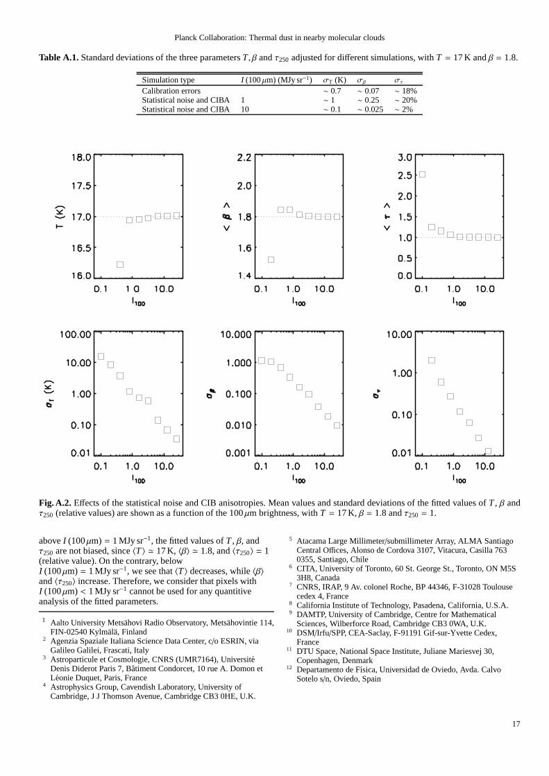
Table A.1.Standard deviations of the three parametersT, β andτ250 adjusted for different simulations, withT = 17 K andβ = 1.8.

Simulation type I (100µm) (MJy sr−1) σT (K) σβ στ

Calibration errors ∼ 0.7 ∼ 0.07 ∼ 18%Statistical noise and CIBA 1 ∼ 1 ∼ 0.25 ∼ 20%Statistical noise and CIBA 10 ∼ 0.1 ∼ 0.025 ∼ 2%

Fig. A.2. Effects of the statistical noise and CIB anisotropies. Mean values and standard deviations of the fitted values ofT , β andτ250 (relative values) are shown as a function of the 100µm brightness, withT = 17 K, β = 1.8 andτ250 = 1.

aboveI (100µm) = 1 MJy sr−1, the fitted values ofT , β, andτ250 are not biased, since〈T 〉 ≃ 17 K, 〈β〉 ≃ 1.8, and〈τ250〉 = 1(relative value). On the contrary, belowI (100µm) = 1 MJy sr−1, we see that〈T 〉 decreases, while〈β〉and〈τ250〉 increase. Therefore, we consider that pixels withI (100µm) < 1 MJy sr−1 cannot be used for any quantitiveanalysis of the fitted parameters.

1 Aalto University Metsahovi Radio Observatory, Metsahovintie 114,FIN-02540 Kylmala, Finland

2 Agenzia Spaziale Italiana Science Data Center, c/o ESRIN, viaGalileo Galilei, Frascati, Italy

3 Astroparticule et Cosmologie, CNRS (UMR7164), Universit´eDenis Diderot Paris 7, Batiment Condorcet, 10 rue A. Domon etLeonie Duquet, Paris, France

4 Astrophysics Group, Cavendish Laboratory, University ofCambridge, J J Thomson Avenue, Cambridge CB3 0HE, U.K.

5 Atacama Large Millimeter/submillimeter Array, ALMA SantiagoCentral Offices, Alonso de Cordova 3107, Vitacura, Casilla 7630355, Santiago, Chile

6 CITA, University of Toronto, 60 St. George St., Toronto, ON M5S3H8, Canada

7 CNRS, IRAP, 9 Av. colonel Roche, BP 44346, F-31028 Toulousecedex 4, France

8 California Institute of Technology, Pasadena, California, U.S.A.9 DAMTP, University of Cambridge, Centre for Mathematical

Sciences, Wilberforce Road, Cambridge CB3 0WA, U.K.10 DSM/Irfu/SPP, CEA-Saclay, F-91191 Gif-sur-Yvette Cedex,

France11 DTU Space, National Space Institute, Juliane Mariesvej 30,

Copenhagen, Denmark12 Departamento de Fısica, Universidad de Oviedo, Avda. Calvo

Sotelo s/n, Oviedo, Spain

17

Planck Collaboration: Thermal dust in nearby molecular clouds

13 Department of Astronomy and Astrophysics, University ofToronto, 50 Saint George Street, Toronto, Ontario, Canada

14 Department of Astronomy and Earth Sciences, Tokyo GakugeiUniversity, Koganei, Tokyo 184-8501, Japan

15 Department of Physics & Astronomy, University of BritishColumbia, 6224 Agricultural Road, Vancouver, British Columbia,Canada

16 Department of Physics, Gustaf Hallstromin katu 2a, University ofHelsinki, Helsinki, Finland

17 Department of Physics, Princeton University, Princeton, NewJersey, U.S.A.

18 Department of Physics, Purdue University, 525 NorthwesternAvenue, West Lafayette, Indiana, U.S.A.

19 Department of Physics, University of California, Berkeley,California, U.S.A.

20 Department of Physics, University of California, One ShieldsAvenue, Davis, California, U.S.A.

21 Department of Physics, University of California, Santa Barbara,California, U.S.A.

22 Department of Physics, University of Illinois atUrbana-Champaign, 1110 West Green Street, Urbana, Illinois,U.S.A.

23 Dipartimento di Fisica G. Galilei, Universita degli Studidi Padova,via Marzolo 8, 35131 Padova, Italy

24 Dipartimento di Fisica, Universita La Sapienza, P. le A. Moro 2,Roma, Italy

25 Dipartimento di Fisica, Universita degli Studi di Milano,ViaCeloria, 16, Milano, Italy

26 Dipartimento di Fisica, Universita degli Studi di Trieste, via A.Valerio 2, Trieste, Italy

27 Dipartimento di Fisica, Universita di Ferrara, Via Saragat 1, 44122Ferrara, Italy

28 Dipartimento di Fisica, Universita di Roma Tor Vergata, Via dellaRicerca Scientifica, 1, Roma, Italy

29 Discovery Center, Niels Bohr Institute, Blegdamsvej 17,Copenhagen, Denmark

30 Dpto. Astrofısica, Universidad de La Laguna (ULL), E-38206 LaLaguna, Tenerife, Spain

31 European Southern Observatory, ESO Vitacura, Alonso de Cordova3107, Vitacura, Casilla 19001, Santiago, Chile

32 European Space Agency, ESAC, Planck Science Office, Caminobajo del Castillo, s/n, Urbanizacion Villafranca del Castillo,Villanueva de la Canada, Madrid, Spain

33 European Space Agency, ESTEC, Keplerlaan 1, 2201 AZNoordwijk, The Netherlands

34 Helsinki Institute of Physics, Gustaf Hallstromin katu 2, Universityof Helsinki, Helsinki, Finland

35 INAF - Osservatorio Astrofisico di Catania, Via S. Sofia 78,Catania, Italy

36 INAF - Osservatorio Astronomico di Padova, Vicolodell’Osservatorio 5, Padova, Italy

37 INAF - Osservatorio Astronomico di Roma, via di Frascati 33,Monte Porzio Catone, Italy

38 INAF - Osservatorio Astronomico di Trieste, Via G.B. Tiepolo 11,Trieste, Italy

39 INAF/IASF Bologna, Via Gobetti 101, Bologna, Italy40 INAF/IASF Milano, Via E. Bassini 15, Milano, Italy41 INRIA, Laboratoire de Recherche en Informatique, Universite

Paris-Sud 11, Batiment 490, 91405 Orsay Cedex, France42 IPAG: Institut de Planetologie et d’Astrophysique de Grenoble,

Universite Joseph Fourier, Grenoble 1/ CNRS-INSU, UMR 5274,Grenoble, F-38041, France

43 Imperial College London, Astrophysics group, BlackettLaboratory, Prince Consort Road, London, SW7 2AZ, U.K.

44 Infrared Processing and Analysis Center, California Institute ofTechnology, Pasadena, CA 91125, U.S.A.

45 Institut Neel, CNRS, Universite Joseph Fourier GrenobleI, 25 ruedes Martyrs, Grenoble, France

46 Institut d’Astrophysique Spatiale, CNRS (UMR8617) UniversiteParis-Sud 11, Batiment 121, Orsay, France

47 Institut d’Astrophysique de Paris, CNRS UMR7095, UniversitePierre & Marie Curie, 98 bis boulevard Arago, Paris, France

48 Institute of Astronomy and Astrophysics, Academia Sinica,Taipei,Taiwan

49 Institute of Astronomy, University of Cambridge, Madingley Road,Cambridge CB3 0HA, U.K.

50 Institute of Theoretical Astrophysics, University of Oslo, Blindern,Oslo, Norway

51 Instituto de Astrofısica de Canarias, C/Vıa Lactea s/n, La Laguna,Tenerife, Spain

52 Instituto de Fısica de Cantabria (CSIC-Universidad de Cantabria),Avda. de los Castros s/n, Santander, Spain

53 Jet Propulsion Laboratory, California Institute of Technology, 4800Oak Grove Drive, Pasadena, California, U.S.A.

54 Jodrell Bank Centre for Astrophysics, Alan Turing Building,School of Physics and Astronomy, The University of Manchester,Oxford Road, Manchester, M13 9PL, U.K.

55 Kavli Institute for Cosmology Cambridge, Madingley Road,Cambridge, CB3 0HA, U.K.

56 LERMA, CNRS, Observatoire de Paris, 61 Avenue del’Observatoire, Paris, France

57 Laboratoire AIM, IRFU/Service d’Astrophysique - CEA/DSM -CNRS - Universite Paris Diderot, Bat. 709, CEA-Saclay, F-91191Gif-sur-Yvette Cedex, France

58 Laboratoire Traitement et Communication de l’Information, CNRS(UMR 5141) and Telecom ParisTech, 46 rue Barrault F-75634Paris Cedex 13, France

59 Laboratoire de Physique Subatomique et de Cosmologie,CNRS/IN2P3, Universite Joseph Fourier Grenoble I, InstitutNational Polytechnique de Grenoble, 53 rue des Martyrs, 38026Grenoble cedex, France

60 Laboratoire de l’Accelerateur Lineaire, Universite Paris-Sud 11,CNRS/IN2P3, Orsay, France

61 Lawrence Berkeley National Laboratory, Berkeley, California,U.S.A.

62 Max-Planck-Institut fur Astrophysik, Karl-Schwarzschild-Str. 1,85741 Garching, Germany

63 MilliLab, VTT Technical Research Centre of Finland, Tietotie 3,Espoo, Finland

64 National University of Ireland, Department of ExperimentalPhysics, Maynooth, Co. Kildare, Ireland

65 Niels Bohr Institute, Blegdamsvej 17, Copenhagen, Denmark66 Observational Cosmology, Mail Stop 367-17, California Institute

of Technology, Pasadena, CA, 91125, U.S.A.67 Optical Science Laboratory, University College London, Gower

Street, London, U.K.68 SISSA, Astrophysics Sector, via Bonomea 265, 34136, Trieste,

Italy69 SUPA, Institute for Astronomy, University of Edinburgh, Royal

Observatory, Blackford Hill, Edinburgh EH9 3HJ, U.K.70 School of Physics and Astronomy, Cardiff University, Queens

Buildings, The Parade, Cardiff, CF24 3AA, U.K.71 Space Sciences Laboratory, University of California, Berkeley,

California, U.S.A.72 Spitzer Science Center, 1200 E. California Blvd., Pasadena,

California, U.S.A.73 Stanford University, Dept of Physics, Varian Physics Bldg,382 Via

Pueblo Mall, Stanford, California, U.S.A.74 Universite de Toulouse, UPS-OMP, IRAP, F-31028 Toulouse cedex

4, France75 Universities Space Research Association, Stratospheric

Observatory for Infrared Astronomy, MS 211-3, Moffett Field, CA94035, U.S.A.

76 University of Granada, Departamento de Fısica Teorica y delCosmos, Facultad de Ciencias, Granada, Spain

77 University of Miami, Knight Physics Building, 1320 Campo SanoDr., Coral Gables, Florida, U.S.A.

78 Warsaw University Observatory, Aleje Ujazdowskie 4, 00-478Warszawa, Poland

18