Characterization of the systematic effects on the Planck/HFI ...
336
HAL Id: tel-01677257 https://tel.archives-ouvertes.fr/tel-01677257 Submitted on 8 Jan 2018 HAL is a multi-disciplinary open access archive for the deposit and dissemination of sci- entific research documents, whether they are pub- lished or not. The documents may come from teaching and research institutions in France or abroad, or from public or private research centers. L’archive ouverte pluridisciplinaire HAL, est destinée au dépôt et à la diffusion de documents scientifiques de niveau recherche, publiés ou non, émanant des établissements d’enseignement et de recherche français ou étrangers, des laboratoires publics ou privés. Characterization of the systematic effects on the Planck/HFI instrument, propagation and impact on science data Alexandre Sauve To cite this version: Alexandre Sauve. Characterization of the systematic effects on the Planck/HFI instrument, propa- gation and impact on science data. Astrophysics [astro-ph]. Université Paul Sabatier - Toulouse III, 2016. English. NNT : 2016TOU30362. tel-01677257
-
Upload
khangminh22 -
Category
Documents
-
view
3 -
download
0
Transcript of Characterization of the systematic effects on the Planck/HFI ...
HAL Id: tel-01677257https://tel.archives-ouvertes.fr/tel-01677257
Submitted on 8 Jan 2018
HAL is a multi-disciplinary open accessarchive for the deposit and dissemination of sci-entific research documents, whether they are pub-lished or not. The documents may come fromteaching and research institutions in France orabroad, or from public or private research centers.
L’archive ouverte pluridisciplinaire HAL, estdestinée au dépôt et à la diffusion de documentsscientifiques de niveau recherche, publiés ou non,émanant des établissements d’enseignement et derecherche français ou étrangers, des laboratoirespublics ou privés.
Characterization of the systematic effects on thePlanck/HFI instrument, propagation and impact on
science dataAlexandre Sauve
To cite this version:Alexandre Sauve. Characterization of the systematic effects on the Planck/HFI instrument, propa-gation and impact on science data. Astrophysics [astro-ph]. Université Paul Sabatier - Toulouse III,2016. English. NNT : 2016TOU30362. tel-01677257
THÈSETHÈSEEn vue de l’obtention du
DOCTORAT DE L’UNIVERSITÉ DE TOULOUSE
Délivré par : l’Université Toulouse 3 Paul Sabatier (UT3 Paul Sabatier)
Présentée et soutenue le 5 Décembre 2016 par :Alexandre Sauvé
Caractérisation des effets systématiques de l’instrument Planck/HFI,propagation et impact sur les données scientifiques
JURYPeter VON BALLMOOS Professeur d’Université Président du JuryAnthony BANDAY Directeur de Recherche Co-directeur de thèseFrançois COUCHOT Directeur de Recherche Membre du JuryKeith GRAINGE Professeur d’Université RapporteurLudovic MONTIER Ingénieur de Recherche Directeur de thèseMichel PIAT Maître de Conférences Membre du JuryIsabelle RISTORCELLI Chargée de Recherche Membre du JuryLouis RODRIGUEZ Ingénieur Rapporteur
École doctorale et spécialité :SDU2E : Astrophysique, Sciences de l’Espace, Planétologie
Unité de Recherche :IRAP / CNRS (UMR 5277)
Directeur(s) de Thèse :Ludovic MONTIER et Anthony BANDAY
Rapporteurs :Louis RODRIGUEZ et Keith GRAINGE


iii
Declaration of AuthorshipI, Alexandre Sauvé, declare that this thesis titled, “Caractérisation des effets systématiquesde l’instrument Planck/HFI, propagation et impact sur les données scientifiques” and thework presented in it are my own. I confirm that:
• This work was done wholly or mainly while in candidature for a research degree at thisUniversity.
• Where any part of this thesis has previously been submitted for a degree or any otherqualification at this University or any other institution, this has been clearly stated.
• Where I have consulted the published work of others, this is always clearly attributed.
• Where I have quoted from the work of others, the source is always given. With theexception of such quotations, this thesis is entirely my own work.
• I have acknowledged all main sources of help.
• Where the thesis is based on work done by myself jointly with others, I have madeclear exactly what was done by others and what I have contributed myself.
Signed:
Date:

v
RésuméUniversité Paul Sabatier
Sciences de l’Univers de l’Environnement et de l’Espace
Docteur en philosophie
Caractérisation des effets systématiques de l’instrument Planck/HFI,propagation et impact sur les données scientifiques
par Alexandre Sauvé
Planck est un satellite de l’ESA lancé en 2009, il représente la troisième génération d’ob-servatoires spatiaux dans l’ère de la cosmologie de précision. Sa mission était de cartographierle fond diffus cosmologique (CMB) avec une extrême précision (∆T/T < 10−5). Le niveaude précision requis nécessite un niveau de contrôle extrêmement élevé des effets systéma-tiques introduits par les instruments embarqués. Il se trouve qu’une combinaison inattendued’éléments a conduit à une amplification de l’impact des effets de non linéarité introduitspar le composant de numérisation des données scientifiques de l’instrument HFI, conduisantà l’introduction d’un des effets systématiques les plus difficiles à maîtriser. Ce manuscritprésente le travail qui a conduit à la caractérisation et à la correction de cette non-linéarité.
Tout d’abord la modélisation de la réponse thermique complexe des détecteurs bolo-métriques sous intensité modulée est présentée. Puis la caractérisation de la réponse desdétecteurs et de l’électronique de lecture est réalisée via l’utilisation du signal produit parl’impact des particules cosmiques sur les détecteurs. Dans un deuxième temps, les étapesmenant à la caractérisation de précision des composants de numérisation sont détaillée. Pourpouvoir corriger l’effet de non-linéarité sur les données scientifiques, la chaîne complète del’électronique de lecture est modélisée en prenant en compte la réponse des détecteurs sousintensité modulée et les effets non-linéaires du composant de numérisation avec le bruit. Enplus de cela, il a fallu tenir compte du signal parasite complexe généré par le compresseur del’étage de refroidissement cryogénique à 4 K, son inclusion dans la correction est détaillée.Ceci a mené à une correction qui a réduit l’impact de cet effet d’un ordre de grandeur sur lecatalogue des données Planck de 2015. Finalement une étude est menée pour mesurer l’im-pact de cet effet de non-linéarité sur l’analyse scientifique de la Galaxie en polarisation et surla cosmologie à travers le spectre de puissance angulaire du CMB. Une étude préliminaireest menée pour la détection de l’annihilation de nuages d’antimatière survivant à l’époquede la recombinaison en utilisant la carte d’effet Sunyaev-Zeldovich de Planck, et commentcette détection est affectée par la stratégie de scan de Planck.

vii
AbstractUniversité Paul Sabatier
Sciences de l’Univers de l’Environnement et de l’Espace
Doctor of Philosophy
Caractérisation des effets systématiques de l’instrument Planck/HFI,propagation et impact sur les données scientifiques
by Alexandre Sauvé
Planck is an ESA spacecraft launched in 2009, it is the third generation of spatial ob-servatory in the era of precision cosmology. Its mission goal was to map with an exquisiteprecision (∆T/T < 10−5) the Cosmic Microwave Background (CMB). The required level ofaccuracy needs an unusually high level control of the systematic effects introduced by theon-board instruments. However, an unexpected conjunction of elements has enhanced thenonlinearity introduced by the chip performing the digitization of science data by the HFIinstrument. It resulted in the most challenging systematic effect to deal with. It is presentedhere the work performed to characterize and correct for this nonlinear effect.
First a detailed modeling of the complex thermal response of the bolometer detectorsunder AC biasing is presented. The detector response is then further characterized by usingthe signal produced by cosmic particles. Second, the steps leading to the in-flight accuratecharacterization of the digitization chip are detailed. To correct for the nonlinear effect onscience data, the full electronics readout chain response is modeled, taking into account thedetector response under AC biasing and the nonlinear effect of the digitization chip withthe noise. Furthermore, the complex parasitic signal originating from the 4 K cryogenicstage mechanical cooler has also to be taken into account. The provided correction hasbeen applied with success to the HFI data 2015 release reducing the effect by an order ofmagnitude. Finally it is studied how the nonlinearity effect of the digitization componentaffects the galactic and cosmological scientific analysis through the angular power spectrumof the CMB. A preliminary study is performed for the detection of surviving antimatterclouds annihilating with matter at the epoch of recombination with the Planck map ofSunyaev-Zeldovich effect, and how it is affected by the scanning strategy of the spacecraft.

ix
AcknowledgementsCe travaille de thèse s’est déroulé sur plus de trois ans, et avant toute autre chose je dois
remercier mon fils qui du haut de ses sept ans a été extrêmement bienveillant à mon égardmalgrès les très nombreuses heures que j’ai passé devant un écran au lieu de jouer avec lui.
Cette thèse est co-financée par le CNES et la société Noveltis, je tiens à les remercier etplus particulièrement Olivier Lamarle ainsi que Philippe Bru d’avoir accepté de me prendresous leur aile.
Je remercie mon directeur de thèse Ludovic Montier de m’avoir offert l’opportunité deréaliser cette thèse ainsi que son énergie indéfectible pour débloquer tout les problèmes quiont pu se présentér sur le chemin. Il a souffert avec beaucoup d’abnégation pour la relecturedes deux articles que j’ai rédigé durant ces trois annés ainsi que ce manuscrit avec monanglais approximatif qui n’aime pas les “s”. Mon co-directeur de thèse Anthony Banday aégalement été d’un grand soutien et a toujours su fournir des réponses précises et des conseilspertinents chaque fois que j’en avais besoin.
J’ai une pensée particulière pour François Couchot qui a porté à bout de bras l’équipeADC pendant plusieurs années avec sa nonchalance et sa bonne humeur qui lui vont sibien. Il m’a donné de nombreux conseils et appris énormément, il a notamment porté à maconnaissance la méthode des Lagrange Multipliers qui a débouché sur la correction d’ADCutilisé pour les données Planck 2015. Mais surtout il m’a fait découvrir le P’tit Cahoua duBd St-Marcel, ce qui n’a pas de prix!
Dans le travail sur les ADC j’ai également eu beaucoup de plaisir à échanger avec Guil-laume Patanchon, les discussions qu’on a eu étaient très animées et constructives.
Je tiens également à remercier toute l’équipe du café matinal (et bénévole) de l’IRAPsans qui rien de tout ceci n’aurait été possible!
The development of Planck has been supported by: ESA; CNES and CNRS/INSU-IN2P3-INP (France); ASI, CNR, and INAF (Italy); NASA and DoE (USA); STFC andUKSA (UK); CSIC, MICINN and JA (Spain); Tekes, AoF and CSC (Finland); DLR andMPG (Germany); CSA (Canada); DTU Space (Denmark); SER/SSO (Switzerland); RCN(Norway); SFI (Ireland); FCT/MCTES (Portugal); and PRACE (EU). A description of thePlanck Collaboration and a list of its members, including the technical or scientific activitiesin which they have been involved, can be found at http://www.rssd.esa.int/index.php?project=PLANCK&page=PlanckCollaboration.

xi
Contents
Declaration of Authorship iii
Résumé v
Abstract vii
Acknowledgements ix
Introduction Générale 1
1 Introduction 71.1 Context . . . . . . . . . . . . . . . . . . . . . . . . . . . . . . . . . . . . . . . 7
1.1.1 History of the Universe . . . . . . . . . . . . . . . . . . . . . . . . . . 71.1.2 The Cosmic Microwave Background . . . . . . . . . . . . . . . . . . . 7
Anisotropies . . . . . . . . . . . . . . . . . . . . . . . . . . . . . . . . . 8The angular power spectrum . . . . . . . . . . . . . . . . . . . . . . . 9
1.1.3 Observational history of the CMB in brief . . . . . . . . . . . . . . . . 111.2 The Planck spacecraft . . . . . . . . . . . . . . . . . . . . . . . . . . . . . . . 12
1.2.1 overview . . . . . . . . . . . . . . . . . . . . . . . . . . . . . . . . . . . 12Mission goals . . . . . . . . . . . . . . . . . . . . . . . . . . . . . . . . 12History . . . . . . . . . . . . . . . . . . . . . . . . . . . . . . . . . . . 12Characteristics of the HFI instrument . . . . . . . . . . . . . . . . . . 13
1.2.2 Scanning strategy . . . . . . . . . . . . . . . . . . . . . . . . . . . . . 131.2.3 The cooling system . . . . . . . . . . . . . . . . . . . . . . . . . . . . . 141.2.4 HFI Systematics . . . . . . . . . . . . . . . . . . . . . . . . . . . . . . 17
Major sources of systematics . . . . . . . . . . . . . . . . . . . . . . . 181.2.5 The Calibration and Performance Validation (CPV) phase . . . . . . . 191.2.6 The HFI Electronic Readout Chain . . . . . . . . . . . . . . . . . . . . 19
Overview . . . . . . . . . . . . . . . . . . . . . . . . . . . . . . . . . . 20HFI detectors biasing . . . . . . . . . . . . . . . . . . . . . . . . . . . 20Amplification and balance of detectors signal . . . . . . . . . . . . . . 20Digitization by the ADC : the fast samples . . . . . . . . . . . . . . . 21Signal summation . . . . . . . . . . . . . . . . . . . . . . . . . . . . . 21Compression . . . . . . . . . . . . . . . . . . . . . . . . . . . . . . . . 22
1.3 Data processing . . . . . . . . . . . . . . . . . . . . . . . . . . . . . . . . . . . 221.3.1 overview . . . . . . . . . . . . . . . . . . . . . . . . . . . . . . . . . . . 22
Time ordered data . . . . . . . . . . . . . . . . . . . . . . . . . . . . . 221.3.2 Production of HFI sky maps . . . . . . . . . . . . . . . . . . . . . . . 26
1.4 Polarization-Sensitive bolometers (PSB) of HFI . . . . . . . . . . . . . . . . . 271.5 Planck results . . . . . . . . . . . . . . . . . . . . . . . . . . . . . . . . . . . . 28
1.5.1 Study of our Galaxy . . . . . . . . . . . . . . . . . . . . . . . . . . . . 28Polarization properties of dust grains . . . . . . . . . . . . . . . . . . . 28Dust as a tracer of Galactic magnetic field . . . . . . . . . . . . . . . . 28
xii
1.5.2 The Sunyaev-Zeldovich (SZ) effect . . . . . . . . . . . . . . . . . . . . 30Clusters of galaxies . . . . . . . . . . . . . . . . . . . . . . . . . . . . . 31Matter-Antimatter annihilation . . . . . . . . . . . . . . . . . . . . . . 32
1.5.3 Cosmology . . . . . . . . . . . . . . . . . . . . . . . . . . . . . . . . . 331.6 Lessons learned . . . . . . . . . . . . . . . . . . . . . . . . . . . . . . . . . . . 34
I Readout Response 37
2 time transfer function analytical model 392.1 Context . . . . . . . . . . . . . . . . . . . . . . . . . . . . . . . . . . . . . . . 39
2.1.1 Definition of the time transfer function . . . . . . . . . . . . . . . . . . 392.1.2 Characterization . . . . . . . . . . . . . . . . . . . . . . . . . . . . . . 40
Thermal response model . . . . . . . . . . . . . . . . . . . . . . . . . . 40Calibration of the HFI thermal response . . . . . . . . . . . . . . . . . 40Degeneracy with the scanning beam . . . . . . . . . . . . . . . . . . . 41
2.2 Discussion of the AC paper . . . . . . . . . . . . . . . . . . . . . . . . . . . . 412.2.1 Motivations . . . . . . . . . . . . . . . . . . . . . . . . . . . . . . . . . 412.2.2 AC paper content . . . . . . . . . . . . . . . . . . . . . . . . . . . . . 432.2.3 Constraints for the LFER model . . . . . . . . . . . . . . . . . . . . . 43
2.3 Test of the analytical model against HFI data . . . . . . . . . . . . . . . . . . 442.3.1 Fit setups . . . . . . . . . . . . . . . . . . . . . . . . . . . . . . . . . . 442.3.2 Results . . . . . . . . . . . . . . . . . . . . . . . . . . . . . . . . . . . 45
Setup 1 . . . . . . . . . . . . . . . . . . . . . . . . . . . . . . . . . . . 45Setup 2 . . . . . . . . . . . . . . . . . . . . . . . . . . . . . . . . . . . 45Setup 3 . . . . . . . . . . . . . . . . . . . . . . . . . . . . . . . . . . . 45
2.4 Perspectives . . . . . . . . . . . . . . . . . . . . . . . . . . . . . . . . . . . . . 462.4.1 ADC nonlinearity correction . . . . . . . . . . . . . . . . . . . . . . . 462.4.2 Three thermal component model . . . . . . . . . . . . . . . . . . . . . 462.4.3 The disc form factor thermal model . . . . . . . . . . . . . . . . . . . 46
2.5 Conclusions . . . . . . . . . . . . . . . . . . . . . . . . . . . . . . . . . . . . . 49
3 Glitches exploitation 513.1 Introduction . . . . . . . . . . . . . . . . . . . . . . . . . . . . . . . . . . . . . 51
Glitches origin . . . . . . . . . . . . . . . . . . . . . . . . . . . . . . . 51Characterization of the glitch families . . . . . . . . . . . . . . . . . . 51
3.1.1 Relation with the time transfer function . . . . . . . . . . . . . . . . . 53The continuous Finite Impulse Response (FIR) . . . . . . . . . . . . . 53
3.2 Building glitch templates . . . . . . . . . . . . . . . . . . . . . . . . . . . . . 563.2.1 Formalism . . . . . . . . . . . . . . . . . . . . . . . . . . . . . . . . . . 56
Projection of glitches in Euclidean space . . . . . . . . . . . . . . . . . 56Glitch selection . . . . . . . . . . . . . . . . . . . . . . . . . . . . . . . 57Glitch normalization . . . . . . . . . . . . . . . . . . . . . . . . . . . . 58Noise radius . . . . . . . . . . . . . . . . . . . . . . . . . . . . . . . . . 58Visualization of the glitch cloud . . . . . . . . . . . . . . . . . . . . . . 58
3.2.2 Glitch templates reconstruction with the capillarity method . . . . . . 59Localisation of starting point . . . . . . . . . . . . . . . . . . . . . . . 60Path following . . . . . . . . . . . . . . . . . . . . . . . . . . . . . . . 61
3.2.3 Estimation of the continuous FIR . . . . . . . . . . . . . . . . . . . . . 62Reconstruction of the continuous FIR . . . . . . . . . . . . . . . . . . 62Bias and uncertainties . . . . . . . . . . . . . . . . . . . . . . . . . . . 62
xiii
3.3 Applications . . . . . . . . . . . . . . . . . . . . . . . . . . . . . . . . . . . . . 643.3.1 Validation of the the empirical time transfer function model . . . . . . 643.3.2 Analysis of thermal properties of detectors . . . . . . . . . . . . . . . 653.3.3 High frequency transfer function constraints . . . . . . . . . . . . . . . 65
Motivation . . . . . . . . . . . . . . . . . . . . . . . . . . . . . . . . . 66Model of the glitch FIR . . . . . . . . . . . . . . . . . . . . . . . . . . 66Results . . . . . . . . . . . . . . . . . . . . . . . . . . . . . . . . . . . 66
3.4 Perspectives . . . . . . . . . . . . . . . . . . . . . . . . . . . . . . . . . . . . . 683.5 Conclusions . . . . . . . . . . . . . . . . . . . . . . . . . . . . . . . . . . . . . 69
II ADC characterization and correction 71
4 ADC chip characterization 754.1 Historical overview of the ADC issue . . . . . . . . . . . . . . . . . . . . . . . 75
On-ground qualification : the back-door is open . . . . . . . . . . . . . 75The variable gain mystery . . . . . . . . . . . . . . . . . . . . . . . . . 76ADC nonlinearity evidence from fast samples histograms . . . . . . . . 77Dipole size compared to ADC nonlinear features . . . . . . . . . . . . 77The beginning of my contribution . . . . . . . . . . . . . . . . . . . . 78
4.2 Understanding the ADC of HFI . . . . . . . . . . . . . . . . . . . . . . . . . . 794.2.1 Basics of a Successive Approximation Register (SAR) ADC . . . . . . 79
MSB and LSB . . . . . . . . . . . . . . . . . . . . . . . . . . . . . . . 79Algorithm . . . . . . . . . . . . . . . . . . . . . . . . . . . . . . . . . . 79Architecture . . . . . . . . . . . . . . . . . . . . . . . . . . . . . . . . 79A non-ideal capacitive array . . . . . . . . . . . . . . . . . . . . . . . . 80
4.2.2 ADC nonlinearity characterization in general . . . . . . . . . . . . . . 80Quantization noise . . . . . . . . . . . . . . . . . . . . . . . . . . . . . 81Transfer function and Code Transition Points (CTP) . . . . . . . . . . 82Differential NonLinearity (DNL) . . . . . . . . . . . . . . . . . . . . . 82Integral NonLinearity (INL) . . . . . . . . . . . . . . . . . . . . . . . . 84DNL estimation with ramp . . . . . . . . . . . . . . . . . . . . . . . . 84DNL estimation with Gaussian noise . . . . . . . . . . . . . . . . . . . 85
4.2.3 Target accuracy for INL characterization . . . . . . . . . . . . . . . . 854.3 INL estimation from cold fast samples . . . . . . . . . . . . . . . . . . . . . . 87
4.3.1 Slow thermal variations . . . . . . . . . . . . . . . . . . . . . . . . . . 874.3.2 Estimation of INL with Gaussians . . . . . . . . . . . . . . . . . . . . 874.3.3 Results of the INL estimation . . . . . . . . . . . . . . . . . . . . . . . 894.3.4 Fit of generic SAR nonlinearity model . . . . . . . . . . . . . . . . . . 91
4.4 INL estimations from HFI electronics flight spare . . . . . . . . . . . . . . . . 924.4.1 Experimental setup . . . . . . . . . . . . . . . . . . . . . . . . . . . . . 934.4.2 Data acquisition . . . . . . . . . . . . . . . . . . . . . . . . . . . . . . 944.4.3 Estimation of INL from Setup B . . . . . . . . . . . . . . . . . . . . . 944.4.4 The 64-code periodic pattern . . . . . . . . . . . . . . . . . . . . . . . 954.4.5 Uncertainty estimation for the EOL sequence . . . . . . . . . . . . . . 96
4.5 SPICE model approach . . . . . . . . . . . . . . . . . . . . . . . . . . . . . . . 974.5.1 Workplan . . . . . . . . . . . . . . . . . . . . . . . . . . . . . . . . . . 974.5.2 DAC architecture of the 7809LPRP . . . . . . . . . . . . . . . . . . . . 98
4.6 Cardiff full scale acquisition . . . . . . . . . . . . . . . . . . . . . . . . . . . . 994.6.1 Acquisition setup . . . . . . . . . . . . . . . . . . . . . . . . . . . . . . 994.6.2 64 codes periodicity . . . . . . . . . . . . . . . . . . . . . . . . . . . . 100
xiv
4.7 INL estimation from in-flight warm data . . . . . . . . . . . . . . . . . . . . . 1014.7.1 The EOL sequence . . . . . . . . . . . . . . . . . . . . . . . . . . . . . 101
EOL warmup . . . . . . . . . . . . . . . . . . . . . . . . . . . . . . . . 101HFI DPU reboot versus LFI requirements . . . . . . . . . . . . . . . . 102EOL sequence . . . . . . . . . . . . . . . . . . . . . . . . . . . . . . . 102ADC scale coverage with ibias parameter . . . . . . . . . . . . . . . 104Gaussian noise and channel gamp parameter . . . . . . . . . . . . . . . 104
4.7.2 INL estimation with maximum likelihood . . . . . . . . . . . . . . . . 105Signal model for EOL sequence . . . . . . . . . . . . . . . . . . . . . . 105Likelihood function . . . . . . . . . . . . . . . . . . . . . . . . . . . . . 106Free parameters . . . . . . . . . . . . . . . . . . . . . . . . . . . . . . 107INL estimation method . . . . . . . . . . . . . . . . . . . . . . . . . . 107
4.7.3 INL uncertainty . . . . . . . . . . . . . . . . . . . . . . . . . . . . . . 1084.8 Validation of a candidate INL . . . . . . . . . . . . . . . . . . . . . . . . . . . 109
4.8.1 The smooth histogram method . . . . . . . . . . . . . . . . . . . . . . 1104.8.2 The raw gain method . . . . . . . . . . . . . . . . . . . . . . . . . . . 110
ADC nonlinearity correction of fast samples . . . . . . . . . . . . . . . 111Cold fast samples model of signal response . . . . . . . . . . . . . . . 111Calculating the raw gain . . . . . . . . . . . . . . . . . . . . . . . . . . 112Overcoming the 4 K lines bias . . . . . . . . . . . . . . . . . . . . . . 112Stability of the raw gain over the mission . . . . . . . . . . . . . . . . 113
4.9 Perspectives . . . . . . . . . . . . . . . . . . . . . . . . . . . . . . . . . . . . . 1154.9.1 Avoiding ADC nonlinearity . . . . . . . . . . . . . . . . . . . . . . . . 115
Increasing signal dynamic . . . . . . . . . . . . . . . . . . . . . . . . . 115Using analog integration . . . . . . . . . . . . . . . . . . . . . . . . . . 117DPU correction . . . . . . . . . . . . . . . . . . . . . . . . . . . . . . . 117
4.9.2 New track for the INL estimation . . . . . . . . . . . . . . . . . . . . . 1184.10 Conclusions . . . . . . . . . . . . . . . . . . . . . . . . . . . . . . . . . . . . . 118
5 Correction of science data 1215.1 Principle . . . . . . . . . . . . . . . . . . . . . . . . . . . . . . . . . . . . . . . 1215.2 Analog signal model . . . . . . . . . . . . . . . . . . . . . . . . . . . . . . . . 122
5.2.1 Slow sky signal variations . . . . . . . . . . . . . . . . . . . . . . . . . 1225.2.2 Signal Model . . . . . . . . . . . . . . . . . . . . . . . . . . . . . . . . 1235.2.3 The raw gain . . . . . . . . . . . . . . . . . . . . . . . . . . . . . . . . 123
Estimation with a Principal Component Analysis (PCA) . . . . . . . . 123Inference of the relative error on the raw gain . . . . . . . . . . . . . . 124
5.2.4 The raw constant . . . . . . . . . . . . . . . . . . . . . . . . . . . . . . 125Deglitching . . . . . . . . . . . . . . . . . . . . . . . . . . . . . . . . . 125Characterization the raw constant parameter . . . . . . . . . . . . . . 127Per ring binning . . . . . . . . . . . . . . . . . . . . . . . . . . . . . . 127
5.2.5 Iterative estimation of the parameters . . . . . . . . . . . . . . . . . . 1285.3 Digitization with noise . . . . . . . . . . . . . . . . . . . . . . . . . . . . . . . 129
5.3.1 Noise model . . . . . . . . . . . . . . . . . . . . . . . . . . . . . . . . . 1295.3.2 summation of noisy fast samples . . . . . . . . . . . . . . . . . . . . . 1305.3.3 Estimation of the fast samples noise RMS . . . . . . . . . . . . . . . . 131
5.4 Science data transfer function . . . . . . . . . . . . . . . . . . . . . . . . . . . 1325.4.1 Separation of modulation half periods . . . . . . . . . . . . . . . . . . 1325.4.2 Transfer function expression . . . . . . . . . . . . . . . . . . . . . . . . 1335.4.3 Correction of science data . . . . . . . . . . . . . . . . . . . . . . . . . 1345.4.4 Validation of the transfer function with simulation . . . . . . . . . . . 134
xv
Application to simulations at full mission scale . . . . . . . . . . . . . 1355.5 Validation of the correction . . . . . . . . . . . . . . . . . . . . . . . . . . . . 137
5.5.1 Formalism . . . . . . . . . . . . . . . . . . . . . . . . . . . . . . . . . . 1375.5.2 Production of PBRs with the 1D drizzling algorithm . . . . . . . . . . 137
The 1D drizzling projection . . . . . . . . . . . . . . . . . . . . . . . . 137Filtering effect of the 1D drizzling . . . . . . . . . . . . . . . . . . . . 138Half parity PBRs . . . . . . . . . . . . . . . . . . . . . . . . . . . . . . 139
5.5.3 The half parity gain observable . . . . . . . . . . . . . . . . . . . . . . 1395.5.4 The half parity sum observable . . . . . . . . . . . . . . . . . . . . . . 1405.5.5 Impact of ADC nonlinearity correction on bogopix gains . . . . . . . 1415.5.6 Simulations . . . . . . . . . . . . . . . . . . . . . . . . . . . . . . . . . 142
Simulation setup . . . . . . . . . . . . . . . . . . . . . . . . . . . . . . 142Nulltest . . . . . . . . . . . . . . . . . . . . . . . . . . . . . . . . . . . 144ADC nonlinearity effect validation . . . . . . . . . . . . . . . . . . . . 146Half parity observable characterization . . . . . . . . . . . . . . . . . . 146Frequency domain . . . . . . . . . . . . . . . . . . . . . . . . . . . . . 146
5.6 Conclusions . . . . . . . . . . . . . . . . . . . . . . . . . . . . . . . . . . . . . 147
6 4 K lines 1496.1 Characterization of 4 K lines . . . . . . . . . . . . . . . . . . . . . . . . . . . 149
6.1.1 Origin . . . . . . . . . . . . . . . . . . . . . . . . . . . . . . . . . . . . 1496.1.2 Impact on ADC nonlinearity observables . . . . . . . . . . . . . . . . . 1506.1.3 4 K lines on science data . . . . . . . . . . . . . . . . . . . . . . . . . 151
Spectral distribution on TOIs . . . . . . . . . . . . . . . . . . . . . . . 151Estimation of 4 K lines with the 18 samples chunks method . . . . . . 151Drift over the mission . . . . . . . . . . . . . . . . . . . . . . . . . . . 153Sub-ring variations . . . . . . . . . . . . . . . . . . . . . . . . . . . . . 155Cross channel correlations . . . . . . . . . . . . . . . . . . . . . . . . . 159Modulation by the sorption cooler bed switching . . . . . . . . . . . . 159
6.1.4 4 K lines on fast samples . . . . . . . . . . . . . . . . . . . . . . . . . 162The 4 K lines window problematic . . . . . . . . . . . . . . . . . . . . 162The CPV fast samples sequences . . . . . . . . . . . . . . . . . . . . . 164Estimation of unfolded 4 K lines harmonics : the forrest . . . . . . . . 164Time domain drift over CPV 1 and CPV 2 . . . . . . . . . . . . . . . 167Spectral drift over CPV 1 and CPV 2 . . . . . . . . . . . . . . . . . . 167
6.2 Inclusion of 4 K lines in the ADC nonlinearity correction . . . . . . . . . . . 1696.2.1 Updated analog signal model . . . . . . . . . . . . . . . . . . . . . . . 1696.2.2 Updated science data transfer function . . . . . . . . . . . . . . . . . . 1696.2.3 Simulations . . . . . . . . . . . . . . . . . . . . . . . . . . . . . . . . . 170
Simulation of the 4 K lines effect on correction . . . . . . . . . . . . . 170Susceptibility of ADC nonlinearity to 4 K lines harmonics . . . . . . . 171
6.3 Estimation of parameters for 2013 data release . . . . . . . . . . . . . . . . . 1726.3.1 Breaking degeneracy with the half parity sum . . . . . . . . . . . . . . 1726.3.2 Using even modulation harmonics from CPV . . . . . . . . . . . . . . 1746.3.3 Parameters estimation using the Lagrange multipliers method . . . . . 1756.3.4 2013 correction results . . . . . . . . . . . . . . . . . . . . . . . . . . . 176
Quantification of the improvement . . . . . . . . . . . . . . . . . . . . 178Analysis with the half parity 9-gain observable . . . . . . . . . . . . . 178
6.4 Alternative parameters estimation for 2015 correction . . . . . . . . . . . . . 1816.4.1 Characterization of science data transfer function parameters . . . . . 181
Setup of the MH algorithm . . . . . . . . . . . . . . . . . . . . . . . . 181
xvi
Generation of transitions with folding constraints . . . . . . . . . . . . 184Analysis of the MCMCs . . . . . . . . . . . . . . . . . . . . . . . . . . 186Stability of the raw constant over the mission . . . . . . . . . . . . . . 187
6.4.2 The global raw constant method . . . . . . . . . . . . . . . . . . . . . 189Global raw constant model . . . . . . . . . . . . . . . . . . . . . . . . 189Estimation of the global raw constant parameter . . . . . . . . . . . . 190Results . . . . . . . . . . . . . . . . . . . . . . . . . . . . . . . . . . . 191
6.5 Conclusions and perspectives . . . . . . . . . . . . . . . . . . . . . . . . . . . 192
III Propagation of systematics on science 195
7 Propagation of ADC nonlinearity to science 1977.1 ADC impact on Galactic polarization . . . . . . . . . . . . . . . . . . . . . . 197
7.1.1 Simulation . . . . . . . . . . . . . . . . . . . . . . . . . . . . . . . . . 1977.1.2 Degeneracy with the bandpass mismatch (BPM) effect . . . . . . . . . 199
7.2 ADC impact on CMB science . . . . . . . . . . . . . . . . . . . . . . . . . . . 2007.2.1 Half-parity methodology . . . . . . . . . . . . . . . . . . . . . . . . . . 201
Principle . . . . . . . . . . . . . . . . . . . . . . . . . . . . . . . . . . 201Production of HPD maps . . . . . . . . . . . . . . . . . . . . . . . . . 201Characterization of the ADC effect on the TT spectrum with a simulation202Multi-component Noise model for science data . . . . . . . . . . . . . 204Comparison with half-ring difference (HRD) map . . . . . . . . . . . . 206
7.2.2 Analysis of ADC nonlinearity impact on science . . . . . . . . . . . . 207Photometric calibration . . . . . . . . . . . . . . . . . . . . . . . . . . 207Impact on the TT spectrum . . . . . . . . . . . . . . . . . . . . . . . . 209
7.2.3 Impact in polarization . . . . . . . . . . . . . . . . . . . . . . . . . . . 2097.3 Conclusions . . . . . . . . . . . . . . . . . . . . . . . . . . . . . . . . . . . . . 211
8 Preliminary study for the detection of primordial matter-antimatter an-nihilation with Planck data 2138.1 Introduction . . . . . . . . . . . . . . . . . . . . . . . . . . . . . . . . . . . . . 213
8.1.1 Context . . . . . . . . . . . . . . . . . . . . . . . . . . . . . . . . . . . 2138.1.2 The Planck tSZ-map . . . . . . . . . . . . . . . . . . . . . . . . . . . . 216
8.2 Characterization of the scanning strategy leakage . . . . . . . . . . . . . . . . 2168.2.1 Angular power spectrum split in the co/cross-scan directions . . . . . 2168.2.2 Application of the co/cross-scan harmonic decomposition to the tSZ-map2178.2.3 Characterization of the scanning strategy leakage with simulations . . 217
8.3 Conclusions and perspectives . . . . . . . . . . . . . . . . . . . . . . . . . . . 218
Conclusions et perspectives 223
Conclusions and perspectives 229
A Building the analytical response in frequency domain of AC biased bolome-ters 235
B SPIE Astronomical Telescope + Instrumentation proceeding 263
C HFI ADC chip specifications design sheet 281

xvii
D Orsay ground calibration datasets 285
E Schematics of the Cardif setup 287
F Sorption cooler schematic and sensors 289
G DMC objects Location 293
H Transfer function of the DPU summation 295H.1 Parasitic wave description . . . . . . . . . . . . . . . . . . . . . . . . . . . . . 295H.2 Raw samples integration effect . . . . . . . . . . . . . . . . . . . . . . . . . . 296H.3 Raw samples integration TF for 4K lines . . . . . . . . . . . . . . . . . . . . . 296

xix
List of Figures
1.1 History of the Universe . . . . . . . . . . . . . . . . . . . . . . . . . . . . . . . 81.2 Spherical harmonics functions . . . . . . . . . . . . . . . . . . . . . . . . . . . 101.3 Angular power spectrum of the CMB . . . . . . . . . . . . . . . . . . . . . . . 101.4 The horn antenna used to make the first CMB detection . . . . . . . . . . . . 111.5 Comparison of CMB results from COBE, WMAP and Planck . . . . . . . . . 121.6 Planck mission time-line . . . . . . . . . . . . . . . . . . . . . . . . . . . . . . 131.7 Planck Scanning strategy . . . . . . . . . . . . . . . . . . . . . . . . . . . . . 141.8 Cutaway view of Planck, with the temperatures of key components in flight . 151.9 Thermal architecture of the HFI focal plane . . . . . . . . . . . . . . . . . . . 161.10 Thermal variations of the bolometer plate temperature over the mission . . . 171.11 Schematic of the HFI readout electronic chain . . . . . . . . . . . . . . . . . . 191.12 Functional view of in-flight signal processing . . . . . . . . . . . . . . . . . . . 211.13 Example of raw science data TOI . . . . . . . . . . . . . . . . . . . . . . . . . 231.14 Example of Phased Binned Ring . . . . . . . . . . . . . . . . . . . . . . . . . 231.15 HFI 143 GHz intensity sky maps at different stages of processing . . . . . . . 241.16 Overview of the HFI data processing pipeline . . . . . . . . . . . . . . . . . . 251.17 Example of an HFI PSB . . . . . . . . . . . . . . . . . . . . . . . . . . . . . . 271.18 Planck full sky maps from the 9 frequency bands . . . . . . . . . . . . . . . . 291.19 Polarized emission of foreground components . . . . . . . . . . . . . . . . . . 301.20 All-sky view of the angle of polarization at 353 GHz . . . . . . . . . . . . . . 311.21 Visualization of SZ effects for the cluster Abell 2319 . . . . . . . . . . . . . . 321.22 The cluster Abel 2319 as seen in the Planck y-map . . . . . . . . . . . . . . . 331.23 CMB intensity map at 5′ resolution . . . . . . . . . . . . . . . . . . . . . . . . 34
2.1 Thermal response of the time transfer function . . . . . . . . . . . . . . . . . 412.2 Scanning beam map . . . . . . . . . . . . . . . . . . . . . . . . . . . . . . . . 422.3 Analytical model fit setup 1: data = raw gain only . . . . . . . . . . . . . . . 472.4 Analytical model fit setup 2: data = raw gain + TF . . . . . . . . . . . . . . 472.5 Analytical model fit setup 3: data = TF only . . . . . . . . . . . . . . . . . . 472.6 Thermal model with three components . . . . . . . . . . . . . . . . . . . . . . 482.7 Thermal filtering profile for two 100 GHz channels . . . . . . . . . . . . . . . 482.8 Thermal dissipation with a disc model for the link to the heat sink . . . . . . 49
3.1 Glitch rate versus SREM measurements and number of sun spots . . . . . . . 523.2 Examples of glitches on demodulated science data . . . . . . . . . . . . . . . 523.3 HFI bolometers annotated with glitch energy deposit locations . . . . . . . . 543.4 Glitch families . . . . . . . . . . . . . . . . . . . . . . . . . . . . . . . . . . . 543.5 Simulation of glitch from energy deposit at different phases within the mod-
ulation period . . . . . . . . . . . . . . . . . . . . . . . . . . . . . . . . . . . . 553.6 Simulation of the continuous FIR . . . . . . . . . . . . . . . . . . . . . . . . . 563.7 Glitch normalization with pseudo energy . . . . . . . . . . . . . . . . . . . . . 573.8 Example of 2D projection of glitch cloud . . . . . . . . . . . . . . . . . . . . . 593.9 Example of glitches in start location configuration . . . . . . . . . . . . . . . . 603.10 2D representation of path following . . . . . . . . . . . . . . . . . . . . . . . . 61
xx
3.11 Examples of continuous FIR reconstructed with glitch dat . . . . . . . . . . . 633.12 Comparison of short glitch FIR with two early time transfer function model
candidates . . . . . . . . . . . . . . . . . . . . . . . . . . . . . . . . . . . . . . 643.13 Comparison of glitch families with the optical time transfer function . . . . . 653.14 Fit residuals values for different free parameters selection of the LFER model 673.15 Example of fits of a short2 glitch with the LFER model . . . . . . . . . . . . 67
4.1 Example of on-ground qualification test for an HFI ADC . . . . . . . . . . . 764.2 Survey sky map differences before and after time variable gain correction . . 774.3 Histogram of the ADC output values over the HFI mission . . . . . . . . . . . 784.4 Example of SAR operation with a 4-bit ADC . . . . . . . . . . . . . . . . . . 804.5 Simplified n-bit SAR ADC architecture. . . . . . . . . . . . . . . . . . . . . 814.6 A 16-bit example of a capacitive DAC. . . . . . . . . . . . . . . . . . . . . . 814.7 Example of a non ideal ADC transfer function . . . . . . . . . . . . . . . . . 834.8 Example DNL and INL . . . . . . . . . . . . . . . . . . . . . . . . . . . . . . 834.9 Normal CDF annotated with quantization step size . . . . . . . . . . . . . . . 864.10 DC level variations over the mission on a per ring basis . . . . . . . . . . . . 874.11 Example of fast samples periods selection for local INL reconstruction . . . . 884.12 Example of INL and DNL built from cold fast samples . . . . . . . . . . . . . 894.13 Absolute error estimate for quantization step size built from cold fast samples 904.14 Generic SAR model fit results of the 11 first most significant bits for two
channels. . . . . . . . . . . . . . . . . . . . . . . . . . . . . . . . . . . . . . . 924.15 Photo of the HFI electronics flight spare taken at IAS in February 2012 . . . 934.16 Histogram of fast samples for flight spare channel FS60 . . . . . . . . . . . . 954.17 LCF drift on the INL for channel FS60 . . . . . . . . . . . . . . . . . . . . . . 964.18 Resulting DNL and INL for FS60 after LCF component removal . . . . . . . 974.19 Resulting DNL and INL for FS60 after LCF component removal (Zoom) . . . 974.20 Visualization of the 64-code periodic pattern . . . . . . . . . . . . . . . . . . 984.21 Correlation of DNL yielded by Setup A and B . . . . . . . . . . . . . . . . . . 994.22 Diagram of the 7809LPRP DAC . . . . . . . . . . . . . . . . . . . . . . . . . 1004.23 Fullscale INL estimated from Cardiff measurements . . . . . . . . . . . . . . . 1014.24 INL with the 64-code pattern and jumps each 64 codes removed . . . . . . . 1024.25 Temperature of the detectors plate during the first two month of EOL warmup1034.26 Histogram of the fast samples acquired over the EOL sequence . . . . . . . . 1034.27 Variation of the REU temperature over the mission . . . . . . . . . . . . . . . 1044.28 Signal shape for a warm detector . . . . . . . . . . . . . . . . . . . . . . . . . 1054.29 Estimated INL for the ADC of the channel 00_100-1a . . . . . . . . . . . . . 1094.30 Histogram of fast samples corrected for ADC nonlinearity . . . . . . . . . . . 1114.31 Raw gains calculated with fast samples periods from different science data bins1134.32 Effect of ADC nonlinearity correction on raw gain stability over the HFI mis-
sion for channel 03_143-1a (unbiased) . . . . . . . . . . . . . . . . . . . . . . 1144.33 Estimation of ADC nonlinearity from raw gain consistency over HFI mission 1164.34 Functional diagram of readout electronics with increased signal dynamic . . . 1174.35 Functional diagram of readout electronics with analog integration . . . . . . . 1174.36 Functional diagram of readout electronics with in-flight ADC correction . . . 118
5.1 Simplified model of the HFI readout electronics with ADC nonlinearity . . . 1215.2 Typical signal dynamic of the solar dipole on channel 10_143-2a . . . . . . . 1225.3 Principal Component Analysis outputs for channel 00_100-1a . . . . . . . . . 1245.4 Example of raw gains estimated with a PCA . . . . . . . . . . . . . . . . . . 1255.5 Relative error of raw gains estimated from asymmetry . . . . . . . . . . . . . 126
xxi
5.6 Example of glitch on a fast samples period . . . . . . . . . . . . . . . . . . . . 1275.7 raw constant drift over the HFI mission for the channel 42-143-6 . . . . . . . 1285.8 Effect of noise on the ADC transfer function . . . . . . . . . . . . . . . . . . . 1305.9 PDF of the squared residuals for fast samples periods fit . . . . . . . . . . . . 1325.10 PDF of the squared residuals for fast samples periods compared with simulations1335.11 Correction parameters shifted to the first fast samples integration index for
channel 01_100-1b . . . . . . . . . . . . . . . . . . . . . . . . . . . . . . . . . 1335.12 Science data transfer function for both modulation parities on channel 01_100-1b1345.13 Simulation at fast samples level of the readout chain with nonlinear ADC . . 1365.14 Simulation of ADC nonlinearity correction residuals for parity zero . . . . . . 1365.15 The 1D drizzling projection . . . . . . . . . . . . . . . . . . . . . . . . . . . . 1375.16 Transfer function modulus of the 1D drizzling in the HFI configuration . . . . 1385.17 Example of PBRs produced with the 1D drizzling . . . . . . . . . . . . . . . . 1405.18 Correlation plot between PBRs produced from each modulation parity . . . . 1415.19 ADC observable: the half parity gain relative difference . . . . . . . . . . . . 1425.20 Half parity gain observable for all channels . . . . . . . . . . . . . . . . . . . 1435.21 ADC observable: the half parity sum standard deviation . . . . . . . . . . . . 1445.22 Bogopix gains . . . . . . . . . . . . . . . . . . . . . . . . . . . . . . . . . . . . 1445.23 Simulation of ADC nonlinearity effect over the full mission . . . . . . . . . . 1455.24 Simulation of ADC nonlinearity effect in frequency domain . . . . . . . . . . 147
6.1 The 4K mechanical compressors, prior to integration to the spacecraft . . . . 1506.2 Correlation plots between the 4 K lines level and ADC nonlinearity observables1526.3 4 K lines on science data TOI spectra . . . . . . . . . . . . . . . . . . . . . . 1536.4 Difference between the 4 K lines removal by cutfreq and a manual version . 1546.5 Estimation of 4 K lines with the 18 samples chunks method . . . . . . . . . . 1556.6 4 K lines drift throughout the mission . . . . . . . . . . . . . . . . . . . . . . 1556.7 4 K lines amplitude drift in time on science data for all channels . . . . . . . 1566.8 4 K lines at sky circle time scale averaged on all channels . . . . . . . . . . . 1576.9 4 K lines at sky circle time scale averaged on all channels . . . . . . . . . . . 1576.10 DFT of 4 K lines amplitudes all over the mission at one minute time resolution1586.11 4 K lines correlation matrices for full sky survey 1 . . . . . . . . . . . . . . . 1606.12 4 K lines correlation matrices for full sky survey 2 . . . . . . . . . . . . . . . 1606.13 4 K lines correlation matrices for survey 3 . . . . . . . . . . . . . . . . . . . . 1616.14 4 K lines correlation matrices for survey 4 . . . . . . . . . . . . . . . . . . . . 1616.15 Schematic of the LFI 20 K sorption cooler . . . . . . . . . . . . . . . . . . . . 1626.16 Comparison of sorption cooler helium pressure and 4 K lines variations . . . . 1636.17 Estimated periodicity of the 4 K lines shortest modulation . . . . . . . . . . . 1636.18 Example of contiguous fast samples periods from the CPV2 sequence . . . . . 1656.19 Spectral distribution of the unfolded 4 K lines during the CPV 2 sequence . . 1666.20 Spectral distribution of the unfolded 4 K lines for all channels grouped by belt
during the CPV 2 sequence . . . . . . . . . . . . . . . . . . . . . . . . . . . . 1666.21 Reconstructed time domain 4 K lines periods for CPV 1 and CPV 2 . . . . . 1686.22 Variation of the time domain unfolded 4 K lines period between CPV 1 and
CPV 2 . . . . . . . . . . . . . . . . . . . . . . . . . . . . . . . . . . . . . . . . 1686.23 Spectral drift over CPV 1 and CPV 2 . . . . . . . . . . . . . . . . . . . . . . 1696.24 Simulation of 4 K lines impact on ADC nonlinearity using half parity gain
observable . . . . . . . . . . . . . . . . . . . . . . . . . . . . . . . . . . . . . . 1716.25 Spectrum of ADC nonlinearity susceptibility Sg to unfolded 4 K lines . . . . 1736.26 Even modulation harmonics templates from CPV . . . . . . . . . . . . . . . . 1746.27 Abacus of the DPU summation transfer function in frequency domain . . . . 176
xxii
6.28 Estimates of unfolded 4 K lines harmonics . . . . . . . . . . . . . . . . . . . . 1776.29 Removal of 4 K lines from the averaged fast samples period . . . . . . . . . . 1776.30 ADC nonlinearity observables for the Planck 2013 data release . . . . . . . . 1796.31 ADC nonlinearity 9-gain observables for the Planck 2013 data release . . . . . 1806.32 Half parity 9-gain observables for all HFI detector channels (no correction) . 1826.33 Half parity 9-gain observables for all HFI detector channels (2013 correction) 1836.34 Schematic view of the folded vector complement for the transition . . . . . . 1856.36 Burn in period of the MCMC . . . . . . . . . . . . . . . . . . . . . . . . . . . 1876.37 Likelihood of harmonic values with tight prior on amplitudes . . . . . . . . . 1886.38 Likelihood of harmonics values with relaxed prior on amplitudes . . . . . . . 1886.39 Likelihood with only 7 harmonics . . . . . . . . . . . . . . . . . . . . . . . . . 1886.40 Consistency of half period sum residuals over the mission . . . . . . . . . . . 1896.41 Consistency of the raw constant over the mission . . . . . . . . . . . . . . . . 1906.42 half parity sum of the global raw constant . . . . . . . . . . . . . . . . . . . . 1916.43 ADC nonlinearity residuals after correction with the global raw constant pa-
rameter set . . . . . . . . . . . . . . . . . . . . . . . . . . . . . . . . . . . . . 1926.44 ADC nonlinearity observables calculated with the 2015 parameter set . . . . 193
7.1 Functional diagram for the simulation of ADC nonlinearity residuals in polar-ization . . . . . . . . . . . . . . . . . . . . . . . . . . . . . . . . . . . . . . . . 198
7.2 Simulation of polarization maps at 353 GHz . . . . . . . . . . . . . . . . . . . 1987.3 Simulation of ADC nonlinearity residuals on polarization maps at 353 GHz . 1997.4 Simulation of ADC nonlinearity effect on polarization fraction and angle at
353 GHz . . . . . . . . . . . . . . . . . . . . . . . . . . . . . . . . . . . . . . . 1997.5 Dust leakage correction maps 353 GHz . . . . . . . . . . . . . . . . . . . . . . 2007.6 Half-parity difference map principle . . . . . . . . . . . . . . . . . . . . . . . . 2017.7 HPD maps before and after ADC nonlinearity correction . . . . . . . . . . . . 2027.8 TT power spectrum calculated with HPD maps . . . . . . . . . . . . . . . . . 2037.9 TT power spectrum calculated with simulated HPD maps . . . . . . . . . . . 2037.10 Simulation of the HPD noise spectrum at TOI level . . . . . . . . . . . . . . 2047.11 Functional diagram for the multi-component noise model of science data . . . 2057.12 Validation of the multi-component noise model on science data TOI . . . . . 2057.13 Comparison with the TT spectrum of the HRD map . . . . . . . . . . . . . . 2077.14 ADC nonlinearity error compared to the solar dipole amplitude . . . . . . . . 2087.15 Impact of ADC nonlinearity on the scientific analysis of the TT spectrum . . 2097.17 TT EE and BB spectra of ADC nonlinearity residuals estimated from HPD
maps of 143 GHz channels . . . . . . . . . . . . . . . . . . . . . . . . . . . . . 212
8.1 Expected patterns for the interfaces between matter and antimatter . . . . . 2148.2 Constraints on ABC domain size from gamma observations . . . . . . . . . . 2158.3 Planck map of the Compton parameter . . . . . . . . . . . . . . . . . . . . . . 2198.4 Leakage of the scanning strategy in the tSZ-map . . . . . . . . . . . . . . . . 2198.5 Spherical harmonics selection for co-scan / cross-scan directions . . . . . . . . 2208.6 Co/cross-scan angular power spectra of the tSZ-map . . . . . . . . . . . . . . 2208.7 Co/cross-scan harmonic decomposition in a small region of the tSZ-map . . . 221

xxiii
List of Tables
2.1 Results of the raw gain and 2015 time transfer function fit using the analyt-ical model on channel 00_100-1a. The time constant of the second thermalcomponent is calculated with τ2ϕ = Gs02/C02 by extrapolation of the singlecomponent formula. . . . . . . . . . . . . . . . . . . . . . . . . . . . . . . . . 45
3.1 Cases of free parameter considered . . . . . . . . . . . . . . . . . . . . . . . . 663.2 . . . . . . . . . . . . . . . . . . . . . . . . . . . . . . . . . . . . . . . . . . . . 68
4.3 gamp parameter . . . . . . . . . . . . . . . . . . . . . . . . . . . . . . . . . . . 105
6.1 dates of the fast samples CPV sequences . . . . . . . . . . . . . . . . . . . . . 1646.2 Global raw constant parameter sets produced in 2015 . . . . . . . . . . . . . . 191
G.1 DMC objects location for detectors channels. The bc label is meant to bereplaced by the 2 characters channel code. . . . . . . . . . . . . . . . . . . . 293


xxv
List of Abbreviations
ADC Analog to Digital ConverterADU Analog Digital UnitCMB Cosmic Microwave BackgroundCPV Calibration Performance ValidationCTP Code Transition PointDAC Digital to Analog ConverterDFT Discrete Fourier TransformDNL Differential Non LinearityDPC Data Processing CenterFPU Focal Plane UnitHFI High Frequency InstrumentINL Integral Non LinearityLFI Low Frequency InstrumentLSB Least Significant BitPAU Pre Amplifier UnitPLA Planck Legacy ArchivePSB Polarization Sensitive BolometerPDF Probability Density FunctionREU Readout Electronic UnitRMS Root Mean SquareSWB Spider Web BolometerSZ Sunyaev Zeldovich (effect)TF Transfer Function


xxvii
List of Symbols
P power W (J s−1)ω angular frequency rad≡ equivalent to binary operator' asymptotically equivalent binary operator≈ is approximately binary operator∝ is proportional to binary operator〈x〉 average value of x unary operator

1
Introduction générale
Pour bien définir le fond du sujet qui nous intéresse commençons par un tour d’horizon de lathéorie sur la formation de notre Univers qui décrit le mieux les observations. Selon la théoriede l’inflation, l’Univers a connu une période d’expansion très rapide après l’instant initial duBig Bang pendant ses premières 10−32 s. Dans les instants qui ont suivi, la matière et l’anti-matière se sont formées, leur annihilation réciproque a donné naissance à la la majeure partiedes photons du fond diffus cosmologique (CMB), mais une légère asymétrie dans le rapportdes deux en faveur de la matière a fait que cette dernière domine dans l’Univers moderne.Environ 380 000 ans après l’instant initial, l’expansion qui a suivi l’inflation a suffisammentrefroidis le plasma dense et chaud de matière baryonique et de photons pour permettre larecombinaison des protons avec les électrons libres et former des atomes d’hydrogène ma-joritairement. C’est à cette époque qu’on appelle la recombinaison que le CMB est émis,ses photons n’étant plus soumis à la diffusion Compton sur les électrons libres ont pu sepropager jusqu’à nous en ayant un minimum d’interactions avec la matière. La période quia suivi s’appelle l’age de l’obscurité. C’est pendant ce temps que la matière a commencé às’effondrer sur elle même à cause de l’instabilité gravitationnelle et que les premières grandesstructures de l’Univers se sont formées. Par la suite la première lumière émise par les galaxiesnaissantes et la quasars a de nouveau ionisé l’hydrogène, c’est l’époque de la réionisation, cequi a eu pour effet de diffuser à nouveau une fraction des photons du CMB à grande échelleangulaire sur les électrons de nouveau libres.
Le CMB se présente de nos jours comme une émission uniforme sur le ciel avec un spectrede corps noir à la température de 2.7255 K. Si on fait abstraction du dipôle solaire dû à l’ef-fet Doppler de notre vitesse relative dans le référentiel du CMB, apparaissent de petitesvariations de températures de l’ordre de ∆T = 1× 10⁻⁵ K, qu’on appelle les anisotropies.Ces anisotropies qu’on qualifie de primaires sont principalement dues aux oscillations acous-tiques adiabatiques produites par la compétition entre la gravité et la pression des photonsà l’époque où le CMB a été émis. Elles présentent une distribution caractéristique dans leursamplitudes et leurs échelles angulaires qu’on mesure avec le spectre de puissance angulaire.Ce spectre de puissance angulaire est très bien décrit avec les six paramètres du modèlecosmologique ΛCDM (Cold Dark Matter) qui fournit une estimation précise de la densitéde matière et d’énergie dans l’Univers mais nécessite l’introduction d’énergie sombre et dematière sombre n’interagissant pas avec la matière ordinaire. Une petite fraction des pho-tons du CMB sont polarisés par deux types de perturbations, les premières sont scalaireset proviennent des variations de densité de matière dues aux oscillations acoustiques, ce quiproduit de la polarisation avec une orientation radiale ou circulaire qu’on appelle les modes-Een polarisation. Les secondes sont dues aux ondes gravitationnelles générées pendant l’infla-tion. Elles se manifestent également par des modes-E ainsi que par de la polarisation avecune orientation tourbillonnante qu’on appelle les modes-B en polarisation. Il y a une autrecatégorie d’anisotropies qu’on qualifie de secondaires et qui sont dues aux interactions sub-séquentes à l’émission du CMB et qui sont principalement : l’effet de lentille gravitationnellegénéré par les amas de galaxies, l’effet Sunyaev-Zeldovich (SZ) lié à la diffusion Comptoninverse des photons du CMB sur le gaz d’électrons chauds des amas de galaxies, et aussi ladiffusion Thompson de ces mêmes photons par les électrons libres dus à la réionisation.
La première détection accidentelle du CMB a été effectuée en 1964 par les radio astro-nomes Arno Penzias et Robert Woodrow Wilson avec une antenne à cornet de 6 m de large.
2
La radiation observée prise d’abord pour un biais était isotrope sur tout le ciel et ne pré-sentait pas de fluctuations diurnes ou saisonnières. Puis le satellite COBE lancé en 1989 amesuré avec l’instrument FIRAS que le CMB avait un spectre qui correspondait parfaite-ment à celui d’un corps noir à une température de 2.726 K. L’instrument DMR à son borda également effectué la première observation des anisotropies et a trouvé qu’elles avaientune distribution Gaussienne, mais il n’avait cependant pas la résolution angulaire suffisantepour résoudre le premier pic acoustique du spectre de puissance angulaire. Son successeur,le satellite WMAP a véritablement marqué le début de l’ère de la cosmologie de précisionen réduisant de façon remarquable le nombre de paramètres cosmologiques à six par l’in-termédiaire au modèle ΛCDM qui reproduisait avec une très bonne précision le spectre depuissance angulaire du CMB. Afin de séparer l’émission des avant-plans galactiques du CMB,opération qu’on appelle la séparation de composantes, il a observé le ciel dans cinq bandesde fréquences (23, 33, 41, 61 et 94 GHz).
Passons maintenant au dernier satellite en date axé sur la cosmologie. Planck est unsatellite de l’ESA bénéficiant d’une large collaboration internationale. Lancé en 2009, il acartographié le ciel avec ses deux instruments complémentaires HFI et LFI pendant 30 mois,avec pour mission de déterminer la géométrie et le contenu de l’Univers, et de comparerles observations avec les théories sur la naissance et l’évolution de l’Univers. Le minimumrequis pour la mission était de deux couvertures complètes du ciel en un an, il a fonctionnéà la perfection en étendant sa mission nominale à 30 mois et en produisant cinq couverturescomplètes du ciel avec ses deux instruments. Après épuisement de ses réserves d’hélium(4He) pour le refroidissement du plan focal, l’instrument LFI qui pouvait fonctionner à plushaute température à continué sa couverture du ciel sur une grande partie de l’année 2013.Le décommissionnemment de Planck a eu lieu le 23 Octobre 2013, date à laquelle il a étédéplacé sur une orbite de rebut.
Le travail présenté dans ce manuscrit est axé sur l’instrument HFI, et ce sera donc lescaractéristiques de ce dernier qui seront détaillées ci-après. HFI a observé le ciel dans sixbandes de fréquences (100, 143, 217, 353, 545 et 857 GHz) avec une résolution angulaireallant de 10′ à 5′. La couverture spectrale de HFI a été optimisée pour la séparation decomposantes, et est particulièrement bien adaptée à l’étude de l’effet SZ qui se manifeste surle CMB dans une gamme de fréquences autour de 217 GHz. Les 54 détecteurs bolométriquesde HFI ont été manufacturés par JPL/Caltech et sont refroidis à 0.1 K.
Les observations ont été faites au second point de Lagrange du système Soleil-Terre et lechemin suivi par l’axe de rotation du satellite est défini relativement au plan de l’écliptique,il correspond à un mouvement en longitude qui permet de conserver une orientation anti-solaire. Planck a observé le ciel avec des balayages circulaires à la vitesse de rotation de untour par minute. Les balayages circulaires sont particulièrement bien adaptés à l’étude duCMB car ils permettent une analyse naturelle des signaux d’origine cosmologique et d’unepartie de ceux induits par l’instrument.
Le système de refroidissement du satellite a assuré les performances des détecteurs enles refroidissant à 0.1 K avec une grande stabilité. Le refroidissement passif a été particu-lièrement bien exploité avec un système d’ailettes ayant une forte émissivité à l’extérieuret une faible émissivité sur la face interne. La descente en température à 0.1 K est assuréepar trois étages de refroidissement actifs. Le refroidissement de l’étage à 20 K a été assurépar un circuit fermé contenant de l’hydrogène, absorbé et désorbé par un matériaux spéci-fique, et produisant des températures en dessous de 20 K par expansion de Joule-Thompson(JT). L’étage suivant à 4 K a été basé lui aussi sur un circuit fermé fonctionnant à l’héliumsur le principe de l’expansion de JT. Celui-ci utilise un compresseur mécanique tournant à20 Hz dont les vibrations sont amorties par un système électronique, cependant le blindagecontre les perturbations électro-magnétiques étant insuffisant il a laissé fuir un signal para-site caractéristique surnommé lignes 4K et qui sera traité plus loin en détails. Finalement
3
le refroidissement à 0.1 K se fait par dilution d’3He dans de l’4He, ce système a produit unetempérature très stable avec des variations qui ont été seulement de l’ordre de 1× 10⁻⁴ K,excepté pendant les éruptions solaires les plus intenses dont le flux de particules réchauffaitle plan focal.
Passons maintenant aux effets systématique principaux de l’instrument HFI qui sont aucœur de ce travail. Par effet systématique on entend toute déviation du signal par rapport àun instrument avec une fonction de réponse angulaire de l’optique parfaitement Gaussienneet un bruit parfaitement blanc et Gaussien. Ces effets systématiques se rencontrent a priorisur la fonction de réponse angulaire de l’optique qui n’est pas parfaitement Gaussienne, etla réponse temporelle de la chaîne de détection dont l’estimation sur les données de vol dé-génèrent l’une avec l’autre. La réponse temporelle a été particulièrement difficile à étalonneravec les données de vol à cause d’un excès de réponse à basse fréquence des bolomètres.Ceci a été problématique pour l’étalonnage photométrique qui se fait sur la modulation duCMB par la rotation de la terre autour du soleil pendant la mission, qu’on appelle le dipôleorbital, et qui apparaît sur le signal à une fréquence de 16 mHz. Mais il y a de nombreusesautres sources d’effets systématiques comme les glitches causés par les dépôts d’énergie desparticules traversant les détecteurs sont aussi une source de bruit non-Gaussien. Ceux-cidoivent être enlevés du signal, mais on verra qu’ils peuvent également fournir de précieusescontraintes sur la réponse temporelle des détecteurs et sur le filtrage de l’électronique delecture. L’effet le plus difficile à traiter qui a été rencontré vient du composant de numéri-sation du signal (ADC), et a été amplifié par une combinaison de plusieurs facteurs : unefaible dynamique du signal numérisé, un équilibrage du signal analogique qui a fait que lanumérisation se faisait exactement sur le défaut le plus important du composant, suivi parla sommation dans l’unité de traitement (DPU) des échantillons détruisant l’informationnécessaire à la correction de la non-linéarité de l’ADC. Un autre effet à prendre en compteviens du compresseur de l’étage à 4 K dont les parasites se combinent au signal numérisé parl’ADC et qui rendent la correction de la non-linéarité de l’ADC beaucoup plus compliquée.
La chaîne électronique de lecture des détecteurs est un élément important pour poser lecontexte de la correction de la non-linéarité de l’ADC. Il y a en fait 54 chaînes de lecture,une pour chaque détecteur, leur rôle est de produire les données scientifiques à un débit de180 échantillons par seconde. Les détecteurs de HFI sont alimentés par un courant carré quiest produit grâce à une tension triangulaire dérivée par deux condensateurs. Une capacitéparasite apparaît à cause de la longueur des câbles entre le bolomètre et le boîtier JFETqui fait l’adaptation d’impédance. Cette capacité parasite complexifie énormément la mo-délisation de la réponse du bolomètre, et nécessite l’ajout sur l’alimentation du détecteurd’une tension carée de compensation du courant de fuite qu’elle génère. Pour diminuer ladynamique du signal un signal carré en opposition de phase est ajouté au signal à la sortiedu détecteur dans le boîtier de l’électronique de lecture (REU). Suite à cela, le signal devienttrès plat, ce qui est un élément critique pour la capture du signal brillant de la galaxie etdes planètes sans saturation de l’électronique. Cependant la numérisation de ce signal platse fait ensuite au centre de l’échelle de l’ADC, la partie qui contient le défaut le plus im-portant du composant, ce qui maximise l’impact de la non-linéarité de l’ADC. Le signalmodulé est en fait numérisé à la fréquence de 7200 Hz, les 40 échantillons par demi-périodede la modulation sont ensuite sommés pour produire le signal scientifique à 180 Hz. Cetteétape de sommation est importante pour améliorer le rapport signal sur bruit des donnéeset diminuer le volume des données car la bande passantes allouée à la télémétrie est limitée.Cependant en sommant les échantillons produit par l’ADC, qu’on appelle des codes, leurvaleur exacte est perdue en même temps que les harmoniques du parasite de l’étage à 4 Kayant une fréquence supérieure à celle de la modulation sont repliées. Une partie importantede ce manuscrit sera consacré à la tâche difficile d’estimer les valeurs perdues pour corrigerde l’effet de non-linéarité de l’ADC.
4
Le traitement des données scientifiques est organisé en trois niveaus qui sont : L1 où labase de données exploitable par les outils informatiques est constituée, L2 où est réalisé letraitement proprement dit des données scientifiques dans le domaine temporel pour la pro-duction des catalogues des cartes du ciel, et L3 où est effectuée la séparation de composanteset la production des catalogues de données. Un niveau supplémentaire LS correspond auxsimulations. Le reste du travail présenté sera localisé sur le L2, et plus particulièrement lacorrection de l’effet de non-linéarité qui est la toute première opération effectuée pour le trai-tement des données scientifiques. Les données scientifiques proprement dites sont organiséesen fonction de l’horodatage au moment de leur capture sous forme d’objets qu’on appelleTOI (Time Ordered Input). Les TOI sont découpées par zones de pointage stable d’une duréeapproximative de 45 minutes qu’on appelle des ring. Les données d’un ring peuvent être pro-jetées en fonction de leur phase à l’intérieur du cercle balayé pour produire un PBR (PhaseBinned Ring) qui est un objet intermédiaire de la production des cartes et dont le niveau debruit est réduit d’un facteur racine du nombre de tours effectués sur le ring considéré.
La production des cartes nécessite la suppression des glitches et la correction des effetssystématiques comme celui de l’ADC et du compresseur de l’étage à 4 K. Les données sontensuite déconvoluées de la réponse temporelle de la chaîne de détection, puis le pointage as-socié est reconstitué avec la fonction de réponse angulaire de l’optique. S’ensuit la calibrationphotométrique des détecteurs puis la projections des cartes au format HEALPix qui est unepixellisation de la sphère adapté au calcul de leur spectre de puissance angulaire. Une carteHEALPix à la résolution nominale contient environ 50× 106 pixels.
Une partie des détecteurs de HFI, les PSB, sont sensibles à la polarisation linéaire dela lumière. Pour cela ils sont constitués de deux grilles superposées associées chacune àun canal différent et sensibles à des directions orthogonales de la polarisation. Il faut enfait trois directions différentes pour reconstituer les paramètres de Stokes (I,Q, U) de lapolarisation. A cet effet, il y a toujours deux PSB associés à la même fréquence mais avecdes orientations relatives de 45 sur la même ligne de balayage du plan focal. Une desproblématiques majeure de ce type d’architecture de détecteur est que l’étalonnage relatifdes canaux utilisés conjointement pour produire les paramètres de Stokes doit être trèsprécis. Dans ce cas, la non-linéarité introduite par l’ADC est un facteur limitant important,on voit donc qu’il faudra une très bonne maîtrise de cet effet systématique dans le cadre dela polarisation.
Voyons maintenant comment HFI participe à l’étude de notre Galaxie. Le milieu inter-stellaire contient des grains de poussière qui présentent une grande diversité de formes etde tailles. Plusieurs mécanismes sont impliqués dans l’émission de lumière polarisée par cesgrains, la connaissance de ces mécanismes est encore partielle et ils sont toujours activementétudiés. Cependant deux éléments dominants ressortent : la rotation des grains et leur ali-gnement le long des lignes de champ magnétique. Cette rotation est aujourd’hui plutôt bienexpliquée par un mécanisme qu’on appelle alignement du moment par pression radiative,c’est à dire que le grain dont la surface est irrégulière se comporte comme une éolienne quela pression de radiation non-isotrope des photons fait tourner. Ces grains une fois alignéspar le champ magnétique ambiant produisent une émission thermique polarisée visible parHFI. Un autre mécanisme produit de la polarisation par absorption sélective de la lumièredes étoiles dans les longueurs d’ondes du visible et de l’UV proche mais n’est pas visible parPlanck. Notre Galaxie a un champ magnétique cohérent à grande échelle et donc l’émissionthermique polarisée des grains est un outil unique d’étude de ce champ. De plus des modes-Ben polarisation sont produits par la poussière, il est donc impératif de bien caractériser cerayonnement pour observer les mode-B produits par les ondes gravitationnelles primordialessur le CMB.
L’effet SZ qui a été évoqué plus haut est un outil performant pour l’étude des amas degalaxies dont la répartition de masse présente un grand intérêt pour la compréhension de
5
la formation des premières grandes structures de l’Univers jeune. Il se présente sous deuxformes : un effet dit thermique produit par diffusion Compton inverse (tSZ) sur le gas d’élec-trons chauds rencontré dans les amas de galaxies, et un effet dit cinétique (kSZ) lié à la vitessede ces mêmes amas mais qui est de second ordre. Avec les données de Planck on peut produirela carte de l’effet tSZ sur le ciel complet qu’on appelle la carte de paramètre Compton. Cettecarte est un outil puissant d’étude et de détection des amas. En effet, l’effet SZ ne dépendspas du redshift et fournit des contraintes qu’on peut combiner avec les observations dansles longueurs d’ondes des rayons-X pour déterminer la masse des amas. Cette analyse peutêtre complémentée avec le spectre de puissance angulaire de la carte de paramètre Comptoncar il a été montré que la fonction de répartition de masse des amas peut également êtrecontrainte avec ce spectre de puissance angulaire, ce qui est particulièrement bien adapté aucas de Planck où on a une résolution angulaire faible mais une grande statistique grâce à lacouverture complète du ciel.
Pour finir sur les résultats, la mission Planck a été globalement couronnée de succès après4 années d’opérations. Planck a renforcé le modèle cosmologique ΛCDM en améliorant laprécision sur ses paramètres qui favorise un Univers plat dont la courbure est compatibleavec zéro. L’analyse des données de la mission Planck n’a pas encore permit de détecterla signature des ondes gravitationelles sur le CMB, mais l’analyse conjointe avec l’équipeBICEP2/KECK a été fructueuse en permettant de poser une limite supérieure au rapporttenseur sur scalaire à r < 0.12. Ceci a été permit par la couverture complète du ciel à lafréquence de 353 GHz où la poussière thermique a son pic d’émission polarisée et qui permetde caractériser les modes-B qu’elle émet et qui entrent en compétition avec ceux du CMB.Le travail sur les effets systématiques présenté dans ce manuscrit a participé à améliorer laprécision de ces résultats.

7
Chapter 1
Introduction
1.1 Context
1.1.1 History of the Universe
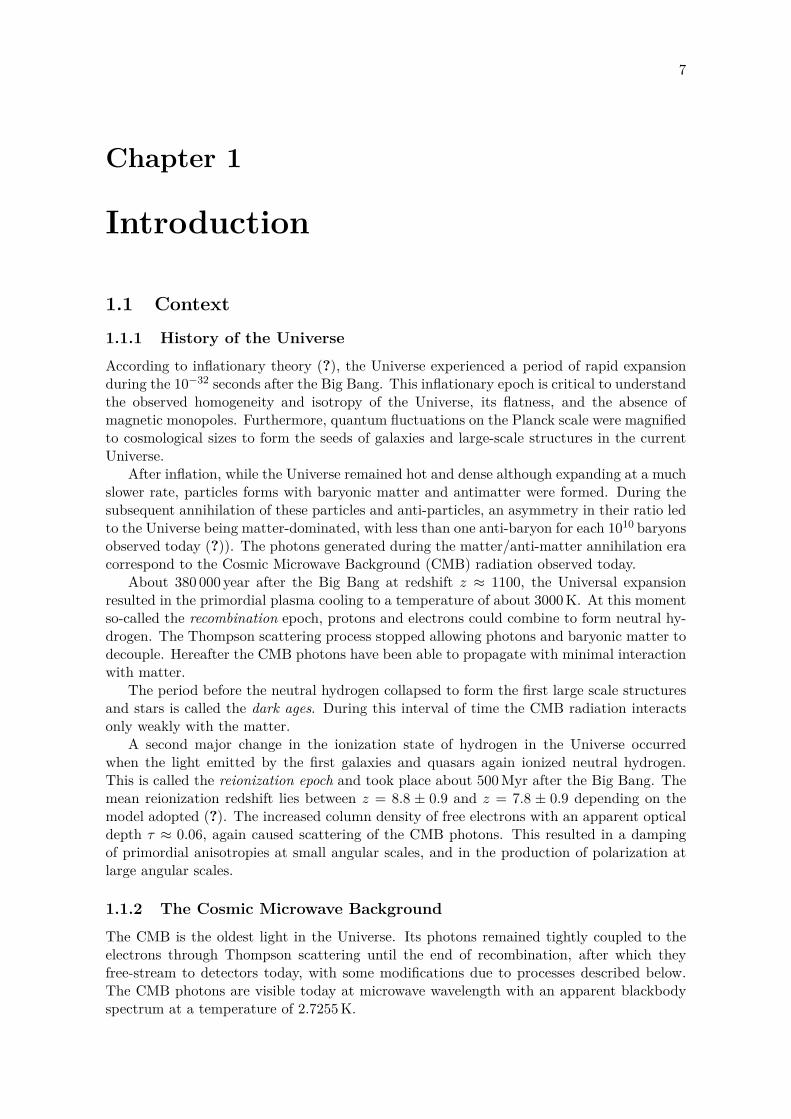
According to inflationary theory (?), the Universe experienced a period of rapid expansionduring the 10−32 seconds after the Big Bang. This inflationary epoch is critical to understandthe observed homogeneity and isotropy of the Universe, its flatness, and the absence ofmagnetic monopoles. Furthermore, quantum fluctuations on the Planck scale were magnifiedto cosmological sizes to form the seeds of galaxies and large-scale structures in the currentUniverse.
After inflation, while the Universe remained hot and dense although expanding at a muchslower rate, particles forms with baryonic matter and antimatter were formed. During thesubsequent annihilation of these particles and anti-particles, an asymmetry in their ratio ledto the Universe being matter-dominated, with less than one anti-baryon for each 1010 baryonsobserved today (?)). The photons generated during the matter/anti-matter annihilation eracorrespond to the Cosmic Microwave Background (CMB) radiation observed today.
About 380 000 year after the Big Bang at redshift z ≈ 1100, the Universal expansionresulted in the primordial plasma cooling to a temperature of about 3000 K. At this momentso-called the recombination epoch, protons and electrons could combine to form neutral hy-drogen. The Thompson scattering process stopped allowing photons and baryonic matter todecouple. Hereafter the CMB photons have been able to propagate with minimal interactionwith matter.
The period before the neutral hydrogen collapsed to form the first large scale structuresand stars is called the dark ages. During this interval of time the CMB radiation interactsonly weakly with the matter.
A second major change in the ionization state of hydrogen in the Universe occurredwhen the light emitted by the first galaxies and quasars again ionized neutral hydrogen.This is called the reionization epoch and took place about 500 Myr after the Big Bang. Themean reionization redshift lies between z = 8.8 ± 0.9 and z = 7.8 ± 0.9 depending on themodel adopted (?). The increased column density of free electrons with an apparent opticaldepth τ ≈ 0.06, again caused scattering of the CMB photons. This resulted in a dampingof primordial anisotropies at small angular scales, and in the production of polarization atlarge angular scales.
1.1.2 The Cosmic Microwave Background
The CMB is the oldest light in the Universe. Its photons remained tightly coupled to theelectrons through Thompson scattering until the end of recombination, after which theyfree-stream to detectors today, with some modifications due to processes described below.The CMB photons are visible today at microwave wavelength with an apparent blackbodyspectrum at a temperature of 2.7255 K.
8 Chapter 1. Introduction
CMB
Planck
Opaque Transparent
History of the Universe
Age of the Universe
Radiu
s of th
e V
isib
le U
niv
ers
e
Inflation Generates Two Types of Waves
Free Electrons Scatter Light
Earliest Time Visible with Light
Density Waves
Gravitational Waves
Infla
tion
Prot
ons
Form
ed
Nuc
lear
Fus
ion
Beg
ins
Nuc
lear
Fus
ion
Ends
Cos
mic
Mic
row
ave
Bac
kgro
und
Neu
tral
Hyd
roge
nFo
rms
Mod
ern
Uni
vers
e
Big Bang
Waves Imprint CharacteristicIntensity & Polarization Signals
0 10−32 s 1 µs 0.01 s 3 min 375,000 yrs 13.8 Billion yrs
Qua
ntum
Fl
uctu
atio
ns
500 Millions yrs
Dar
k Age
s
Firs
t Sta
rs F
orm
1 Billion yrsRei
oniz
atio
n Er
a
Rei
oniz
atio
n Com
plet
e
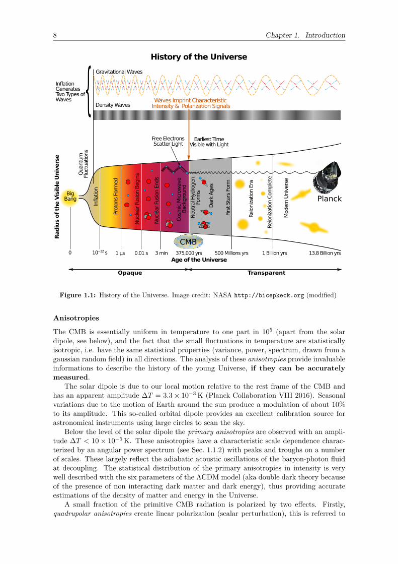
Figure 1.1: History of the Universe. Image credit: NASA http://bicepkeck.org (modified)
Anisotropies
The CMB is essentially uniform in temperature to one part in 105 (apart from the solardipole, see below), and the fact that the small fluctuations in temperature are statisticallyisotropic, i.e. have the same statistical properties (variance, power, spectrum, drawn from agaussian random field) in all directions. The analysis of these anisotropies provide invaluableinformations to describe the history of the young Universe, if they can be accuratelymeasured.
The solar dipole is due to our local motion relative to the rest frame of the CMB andhas an apparent amplitude ∆T = 3.3× 10⁻³ K (Planck Collaboration VIII 2016). Seasonalvariations due to the motion of Earth around the sun produce a modulation of about 10%to its amplitude. This so-called orbital dipole provides an excellent calibration source forastronomical instruments using large circles to scan the sky.
Below the level of the solar dipole the primary anisotropies are observed with an ampli-tude ∆T < 10× 10−5 K. These anisotropies have a characteristic scale dependence charac-terized by an angular power spectrum (see Sec. 1.1.2) with peaks and troughs on a numberof scales. These largely reflect the adiabatic acoustic oscillations of the baryon-photon fluidat decoupling. The statistical distribution of the primary anisotropies in intensity is verywell described with the six parameters of the ΛCDM model (aka double dark theory becauseof the presence of non interacting dark matter and dark energy), thus providing accurateestimations of the density of matter and energy in the Universe.
A small fraction of the primitive CMB radiation is polarized by two effects. Firstly,quadrupolar anisotropies create linear polarization (scalar perturbation), this is referred to
1.1. Context 9
as polarization E-modes. Secondly, the inflation is theorized to have generated gravitationalwaves which, following the general relativity theory are expected to leave an imprint onthe CMB by creating polarization with whirling orientation (tensor perturbations), this isreferred to as polarization B-modes. Unfortunately these most-wanted gravitational wavesremnants are very faint and still undetected. The B-modes polarization signal be separatedfrom the dominant foreground emission of our galaxy (??). The gravitational wave activityhas been intense recently, with the first direct detection and proof of existence by LIGO (?).Polarization with HFI is covered in Sec. 1.4.
Secondary anisotropies, or late time anisotropies are caused by post-recombination inter-actions of the CMB photons. They are created mainly by:
• gravitational lensing by the massive galaxy clusters and dark matter clumps. Thiseffect makes the CMB a tool of choice for the study of dark matter (?).
• the inverse Compton scattering of CMB photons by hot gas in galaxy clusters. This isthe so-called Sunyaev-Zeldovich (SZ) effect (?). See Sec. 1.5.2;
• Thompson scattering caused by the column density of free electrons during the reion-ization, it is mainly characterized by its optical depth estimated at about τ =' 0.06(?). This has the effect of smoothing small scales anisotropies, and causes polariza-tion at large angular scales. Accurate measurement of large angular scale polarizationprovides constraints on the reionization history.
The angular power spectrum
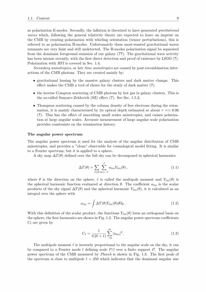
The angular power spectrum is used for the analysis of the angular distribution of CMBanisotropies, and provides a ”clean“ observable for cosmological model fitting. It is similarto a Fourier spectrum, but it is applied to a sphere.
A sky map ∆T (θ) defined over the full sky can be decomposed in spherical harmonics
∆T (θ) =∑l≥0
∑m=−`
a`mY`m(θ) , (1.1)
where θ is the direction on the sphere, ` is called the multipole moment and Y`m(θ) isthe spherical harmonic function evaluated at direction θ. The coefficient a`m is the scalarproducts of the sky signal ∆T (θ) and the spherical harmonic Y`m(θ), it is calculated as anintegral over the sphere with
a`m =∫
∆T (θ)Y`m(θ)dΩθ . (1.2)
With this definition of the scalar product, the functions Y`m(θ) form an orthogonal basis onthe sphere, the first harmonics are shown in Fig. 1.2. The angular power spectrum coefficientsC` are given by
C` = 1`(2`+ 1)
m∑−m|a`m|2 . (1.3)
The multipole moment ` is inversely proportional to the angular scale on the sky, it canbe compared to a Fourier mode l defining scale P/l over a finite support P . The angularpower spectrum of the CMB measured by Planck is shown in Fig. 1.3. The first peak ofthe spectrum is close to multipole ` = 250 which indicates that the dominant angular size
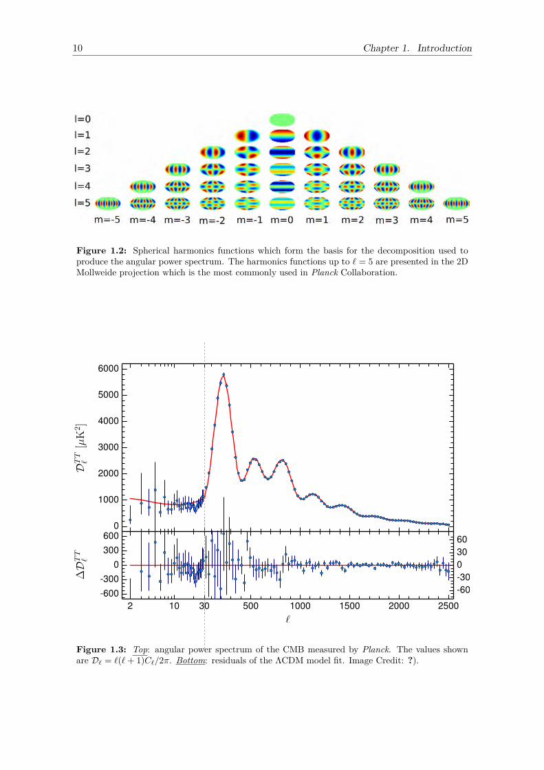
10 Chapter 1. Introduction
Figure 1.2: Spherical harmonics functions which form the basis for the decomposition used toproduce the angular power spectrum. The harmonics functions up to ` = 5 are presented in the 2DMollweide projection which is the most commonly used in Planck Collaboration.
Figure 1.3: Top: angular power spectrum of the CMB measured by Planck. The values shownare D` = `(`+ 1)C`/2π. Bottom: residuals of the ΛCDM model fit. Image Credit: ?).
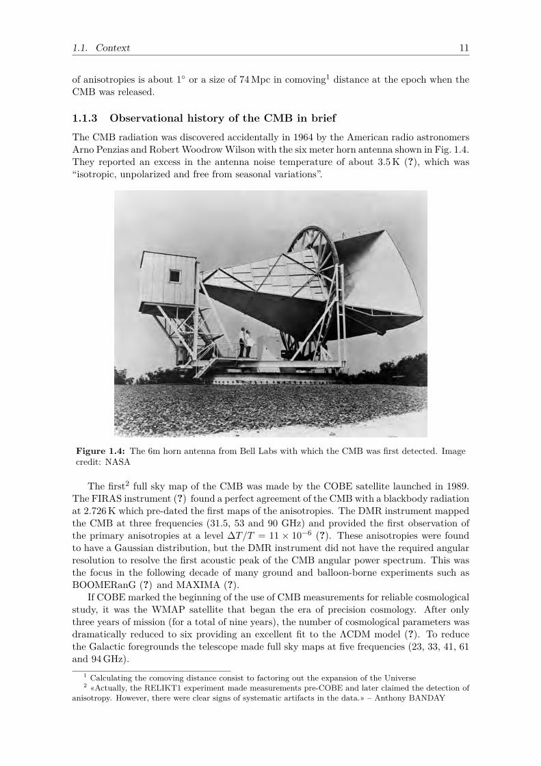
1.1. Context 11
of anisotropies is about 1 or a size of 74 Mpc in comoving1 distance at the epoch when theCMB was released.
1.1.3 Observational history of the CMB in brief
The CMB radiation was discovered accidentally in 1964 by the American radio astronomersArno Penzias and Robert WoodrowWilson with the six meter horn antenna shown in Fig. 1.4.They reported an excess in the antenna noise temperature of about 3.5 K (?), which was“isotropic, unpolarized and free from seasonal variations”.
Figure 1.4: The 6m horn antenna from Bell Labs with which the CMB was first detected. Imagecredit: NASA
The first2 full sky map of the CMB was made by the COBE satellite launched in 1989.The FIRAS instrument (?) found a perfect agreement of the CMB with a blackbody radiationat 2.726 K which pre-dated the first maps of the anisotropies. The DMR instrument mappedthe CMB at three frequencies (31.5, 53 and 90 GHz) and provided the first observation ofthe primary anisotropies at a level ∆T/T = 11 × 10−6 (?). These anisotropies were foundto have a Gaussian distribution, but the DMR instrument did not have the required angularresolution to resolve the first acoustic peak of the CMB angular power spectrum. This wasthe focus in the following decade of many ground and balloon-borne experiments such asBOOMERanG (?) and MAXIMA (?).
If COBE marked the beginning of the use of CMB measurements for reliable cosmologicalstudy, it was the WMAP satellite that began the era of precision cosmology. After onlythree years of mission (for a total of nine years), the number of cosmological parameters wasdramatically reduced to six providing an excellent fit to the ΛCDM model (?). To reducethe Galactic foregrounds the telescope made full sky maps at five frequencies (23, 33, 41, 61and 94 GHz).
1 Calculating the comoving distance consist to factoring out the expansion of the Universe2 «Actually, the RELIKT1 experiment made measurements pre-COBE and later claimed the detection of
anisotropy. However, there were clear signs of systematic artifacts in the data.» – Anthony BANDAY
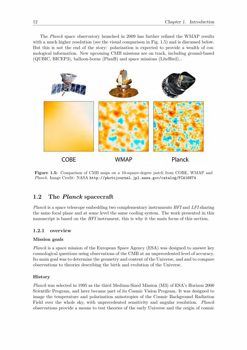
12 Chapter 1. Introduction
The Planck space observatory launched in 2009 has further refined the WMAP resultswith a much higher resolution (see the visual comparison in Fig. 1.5) and is discussed below.But this is not the end of the story: polarization is expected to provide a wealth of cos-mological information. New upcoming CMB missions are on track, including ground-based(QUBIC, BICEP3), balloon-borne (PlanB) and space missions (LiteBird)...
Figure 1.5: Comparison of CMB maps on a 10-square-degree patch from COBE, WMAP andPlanck. Image Credit: NASA http://photojournal.jpl.nasa.gov/catalog/PIA16874
1.2 The Planck spacecraftPlanck is a space telescope embedding two complementary instruments HFI and LFI sharingthe same focal plane and at some level the same cooling system. The work presented in thismanuscript is based on the HFI instrument, this is why it the main focus of this section.
1.2.1 overview
Mission goals
Planck is a space mission of the European Space Agency (ESA) was designed to answer keycosmological questions using observations of the CMB at an unprecedented level of accuracy.Its main goal was to determine the geometry and content of the Universe, and and to compareobservations to theories describing the birth and evolution of the Universe.
History
Planck was selected in 1995 as the third Medium-Sized Mission (M3) of ESA’s Horizon 2000Scientific Program, and later became part of its Cosmic Vision Program. It was designed toimage the temperature and polarization anisotropies of the Cosmic Background RadiationField over the whole sky, with unprecedented sensitivity and angular resolution. Planckobservations provide a means to test theories of the early Universe and the origin of cosmic
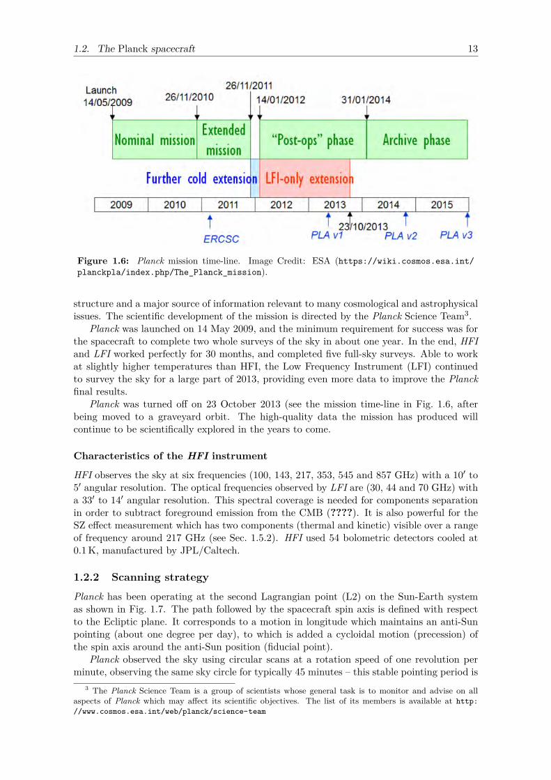
1.2. The Planck spacecraft 13
Figure 1.6: Planck mission time-line. Image Credit: ESA (https://wiki.cosmos.esa.int/planckpla/index.php/The_Planck_mission).
structure and a major source of information relevant to many cosmological and astrophysicalissues. The scientific development of the mission is directed by the Planck Science Team3.
Planck was launched on 14 May 2009, and the minimum requirement for success was forthe spacecraft to complete two whole surveys of the sky in about one year. In the end, HFIand LFI worked perfectly for 30 months, and completed five full-sky surveys. Able to workat slightly higher temperatures than HFI, the Low Frequency Instrument (LFI) continuedto survey the sky for a large part of 2013, providing even more data to improve the Planckfinal results.
Planck was turned off on 23 October 2013 (see the mission time-line in Fig. 1.6, afterbeing moved to a graveyard orbit. The high-quality data the mission has produced willcontinue to be scientifically explored in the years to come.
Characteristics of the HFI instrument
HFI observes the sky at six frequencies (100, 143, 217, 353, 545 and 857 GHz) with a 10′ to5′ angular resolution. The optical frequencies observed by LFI are (30, 44 and 70 GHz) witha 33′ to 14′ angular resolution. This spectral coverage is needed for components separationin order to subtract foreground emission from the CMB (????). It is also powerful for theSZ effect measurement which has two components (thermal and kinetic) visible over a rangeof frequency around 217 GHz (see Sec. 1.5.2). HFI used 54 bolometric detectors cooled at0.1 K, manufactured by JPL/Caltech.
1.2.2 Scanning strategy
Planck has been operating at the second Lagrangian point (L2) on the Sun-Earth systemas shown in Fig. 1.7. The path followed by the spacecraft spin axis is defined with respectto the Ecliptic plane. It corresponds to a motion in longitude which maintains an anti-Sunpointing (about one degree per day), to which is added a cycloidal motion (precession) ofthe spin axis around the anti-Sun position (fiducial point).
Planck observed the sky using circular scans at a rotation speed of one revolution perminute, observing the same sky circle for typically 45 minutes – this stable pointing period is
3 The Planck Science Team is a group of scientists whose general task is to monitor and advise on allaspects of Planck which may affect its scientific objectives. The list of its members is available at http://www.cosmos.esa.int/web/planck/science-team
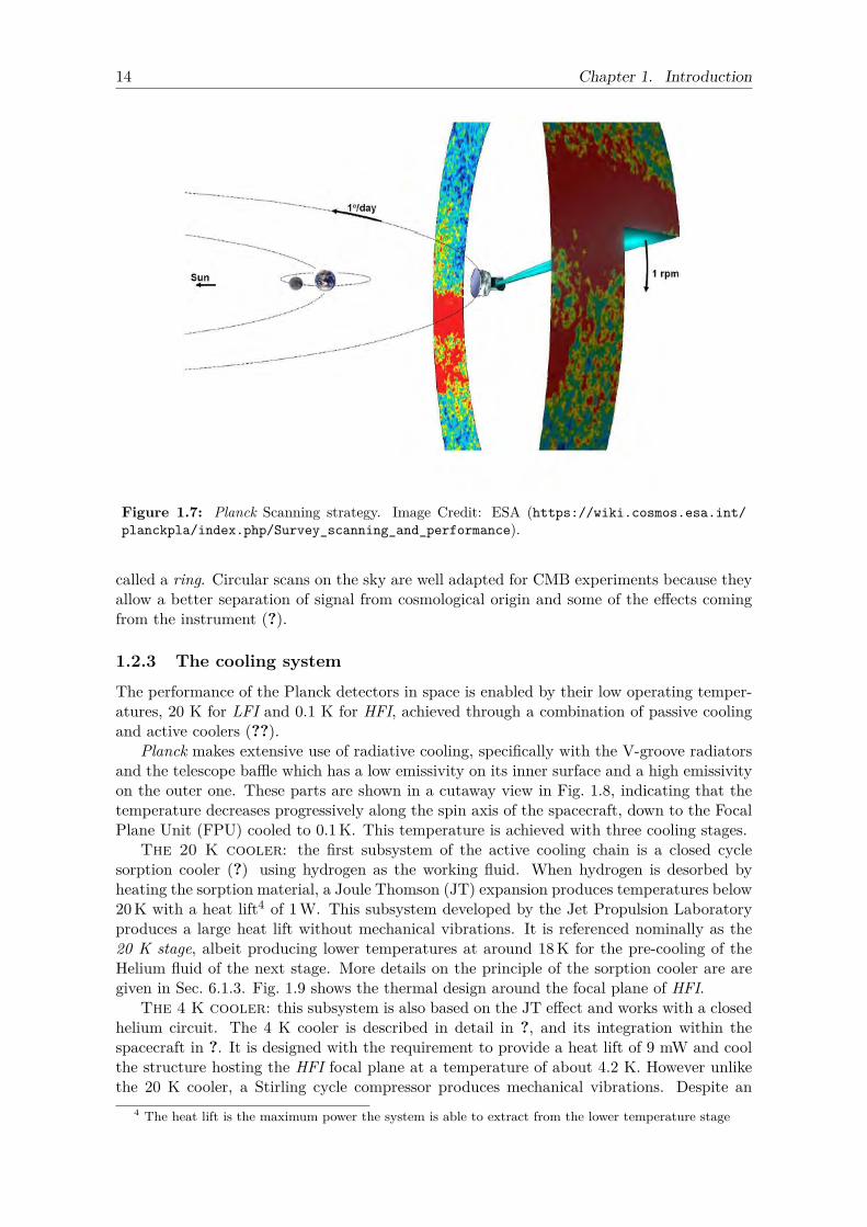
14 Chapter 1. Introduction
Figure 1.7: Planck Scanning strategy. Image Credit: ESA (https://wiki.cosmos.esa.int/planckpla/index.php/Survey_scanning_and_performance).
called a ring. Circular scans on the sky are well adapted for CMB experiments because theyallow a better separation of signal from cosmological origin and some of the effects comingfrom the instrument (?).
1.2.3 The cooling system
The performance of the Planck detectors in space is enabled by their low operating temper-atures, 20 K for LFI and 0.1 K for HFI, achieved through a combination of passive coolingand active coolers (??).
Planck makes extensive use of radiative cooling, specifically with the V-groove radiatorsand the telescope baffle which has a low emissivity on its inner surface and a high emissivityon the outer one. These parts are shown in a cutaway view in Fig. 1.8, indicating that thetemperature decreases progressively along the spin axis of the spacecraft, down to the FocalPlane Unit (FPU) cooled to 0.1 K. This temperature is achieved with three cooling stages.
The 20 K cooler: the first subsystem of the active cooling chain is a closed cyclesorption cooler (?) using hydrogen as the working fluid. When hydrogen is desorbed byheating the sorption material, a Joule Thomson (JT) expansion produces temperatures below20 K with a heat lift4 of 1 W. This subsystem developed by the Jet Propulsion Laboratoryproduces a large heat lift without mechanical vibrations. It is referenced nominally as the20 K stage, albeit producing lower temperatures at around 18 K for the pre-cooling of theHelium fluid of the next stage. More details on the principle of the sorption cooler are aregiven in Sec. 6.1.3. Fig. 1.9 shows the thermal design around the focal plane of HFI.
The 4 K cooler: this subsystem is also based on the JT effect and works with a closedhelium circuit. The 4 K cooler is described in detail in ?, and its integration within thespacecraft in ?. It is designed with the requirement to provide a heat lift of 9 mW and coolthe structure hosting the HFI focal plane at a temperature of about 4.2 K. However unlikethe 20 K cooler, a Stirling cycle compressor produces mechanical vibrations. Despite an
4 The heat lift is the maximum power the system is able to extract from the lower temperature stage
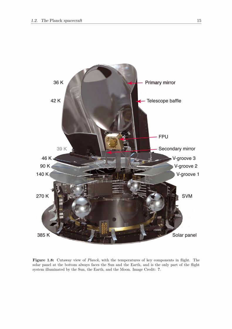
1.2. The Planck spacecraft 15
Planck Collaboration: Planck early results. II.
Solar panel
SVM
V-groove 1V-groove 2
V-groove 3
Telescope baffle
Primary mirror
FPU
Secondary mirror
385 K
270 K
140 K90 K46 K
42 K
36 K
Fig. 1. Cutaway view of Planck, with the tem-peratures of key components in flight. The solarpanel at the bottom always faces the Sun andthe Earth, and is the only part of the flight sys-tem illuminated by the Sun, the Earth, and theMoon. Temperature decreases steadily towardsthe telescope end, due to low-conductivity me-chanical connections and aggressive use of ra-diative cooling. The focal plane detectors areactively cooled to 20 K and 0.1 K.
Fig. 2. Sorption cooler system. The system isfully redundant. One of the compressor assem-blies, mounted on one of the warm radiatorpanels, which faces cold space, is highlightedin orange. Heat pipes run horizontally connect-ing the radiators on three sides of the servicevehicle octagon. The second compressor as-sembly is the black box on the right. A tube-in-tube heat exchanger carries high pressurehydrogen gas from the compressor assemblyto the focal plane assembly and low pressurehydrogen back to the compressor, with heat-exchanging attachments to each of the threeV-grooves. Colours indicate temperature, fromwarm (red, orange, purple) to cold (blue).
A2, page 3 of 31
Figure 1.8: Cutaway view of Planck, with the temperatures of key components in flight. Thesolar panel at the bottom always faces the Sun and the Earth, and is the only part of the flightsystem illuminated by the Sun, the Earth, and the Moon. Image Credit: ?.
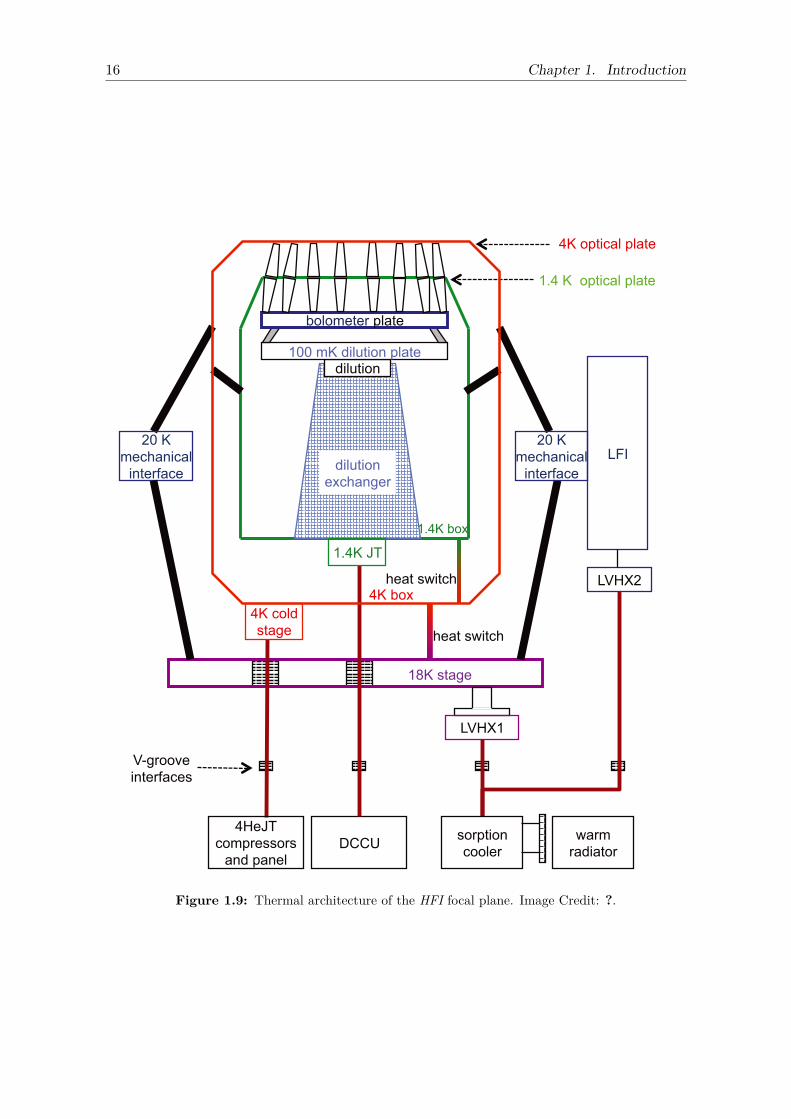
16 Chapter 1. Introduction
Planck Collaboration: Planck early results. II.
DCCU
dilution
100 mK dilution plate
bolometer plate
4K box
1.4K box
dilution
exchanger
LFI
LVHX2
1.4K JT
LVHX1
heat switch
heat switch
4K optical plate
1.4 K optical plate
20 K
mechanical
interface
20 K
mechanical
interface
4HeJT
compressors
and panel
sorption
cooler
warm
radiator
18K stage
V-groove
interfaces
4K cold
stage
Fig. 5. Schematic of the HFI FPU. The designations “20 K”, “18 K”,“4 K”, “1.4 K”, and “100 mK” are nominal. Actual operating tempera-tures are given in Sect. 4.
The flight sorption cooler electronics and software weredeveloped by the Laboratoire de Physique Subatomique et deCosmologie (LPSC) in Grenoble. These electronics and theircontrolling software provide for the basic sequential operation ofthe compressor beds, temperature stabilization of the cold end,and monitoring of cooler performance parameters. In addition,they automatically detect failures and adapt operations accord-ingly. Operational parameters can be adjusted in flight to max-imise the lifetime and performance of the sorption coolers.
The total input power to the sorption cooler at end of life(maximum average power) is 470 W. Another 110 W is availableto operate the sorption cooler electronics.
2.3.2. 4He-JT cooler
Figure 5 shows schematically the thermal interfaces of theHFI cooling system. The compressors of the 4He-JT cooler aremounted in opposition (Lamarre et al. 2010) to cancel to firstorder momentum transfer to the spacecraft. Force transducersbetween the two compressors provide an error signal processedby the drive electronics servo system that controls the profile ofthe piston motions to minimise the first seven harmonics of theperiodic vibration injected into the spacecraft.
The 4 K cold head is a small reservoir of liquid helium in asintered material, located after the expansion of the gas throughthe JT orifice. This provides an important bu!er with high heatcapacity between the JT orifice and the rest of the HFI. It is at-tached to the bottom of the 4 K box of the HFI FPU, as can beseen in Fig. 5. It provides cooling for the 4 K shield and alsopre-cooling for the gas in the dilution cooler pipes described inthe next section.
The cooling power and thermal properties of the 4He-JTcooler, measured by the RAL team at subsystem level and then
Table 2. Requirements and characteristics of the 4He-JT cooler.
Working fluid . . . . . . . . . . . . . . . . . . . . . . . . 4HeliumHeat lift at 17.5 K pre-cool temperature
Maximum . . . . . . . . . . . . . . . . . . . . . . . . . . . 19.2 mWRequired . . . . . . . . . . . . . . . . . . . . . . . . . . . 13.3 mW
Pre-cool requirementsThird V-groove . . . . . . . . . . . . . . . . . . . . . !54 KSorption cooler LVHX1 . . . . . . . . . . . . 17.5–19 K
Nominal operating temperature . . . . . . . . . 4.5 KMass
Compressors, pipes, cold stage . . . . . . 27.7 kgElectronics and current regulator . . . . . . 8.6 kg
Power into current regulator . . . . . . . . . . . . !120 W
in the system thermal vacuum tests, are summarised in the fol-lowing relationships, which depend linearly on the adjustableparameters in the vicinity of the flight operating point:
HLmax = 15.9 mW + 6.8("S " 3.45 mm)" 1.1(Tpc " 17.3 K) + 0.6(Pfill " 4.5 bar); (1)
Heatload = 10.6 mW + 0.5(Tpc " 17.3 K)+ 0.065(Tvg3 " 45 K) + Heaters; (2)
TJT 4 K = 4.4 K " 0.035(HLmax " Heatload). (3)
Here HLmax is the maximum heat lift, Tpc is the pre-cooling tem-perature, Tvg3 is the temperature of V-groove 3, "S is the strokehalf amplitude of the compressors, and Pfill is the helium fillingpressure.
The heat load on the 4 K box was predicted using the ther-mal model and verified on the flight model during the CSL ther-mal balance/thermal vacuum test. Performance in flight was un-changed (Sect. 4.3).
The stroke amplitude, and to some degree the sorption coolerprecool temperature, are adjustable in flight. The interface withthe sorption cooler, including the warm radiator temperature,is the most critical interface of the HFI cryogenic chain. The4He-JT cooler heat load increases and its heat lift decreases asthe sorption cooler precool temperature increases (see Fig. 6).The 4He-JT cooling power margin depends strongly on this tem-perature, itself driven mostly by the temperature of the warm ra-diator. Warm radiator temperatures of 272 K (±10 K, Sect. 2.3.1)lead to sorption cooler temperatures between 16.5 K and 17.5 K(Bersanelli et al. 2010). It can be seen from Fig. 6 that at a 20 Kprecool temperature even the largest possible stroke amplitudeleaves no margin.
The two mechanical compressors produce microvibrationsand also induce electromagnetic interference, potentially a!ect-ing the science signals of bolometers. The risks associated withthese e!ects were taken into account early in the design of theHFI by phase-locking the sample frequency of the data to a har-monic of the compressor frequency.
2.3.3. Dilution cooler
The dilution cooler operates on an open circuit using a largequantity of 4He and 3He stored in four high pressure tanks. Themajor components of the system are shown in Fig. 4, includinga JT expansion valve producing cooling power for the “1.4 Kstage” of the FPU and pre-cooling for the dilution cooler. Thegas from the tanks (300 bar at the start of the mission) is re-duced to 19 bar through two pressure regulators, and the flowthrough the dilution circuits is regulated by a set of discrete re-strictions chosen by telecommand. The flow rates for di!erent
A2, page 7 of 31
Figure 1.9: Thermal architecture of the HFI focal plane. Image Credit: ?.
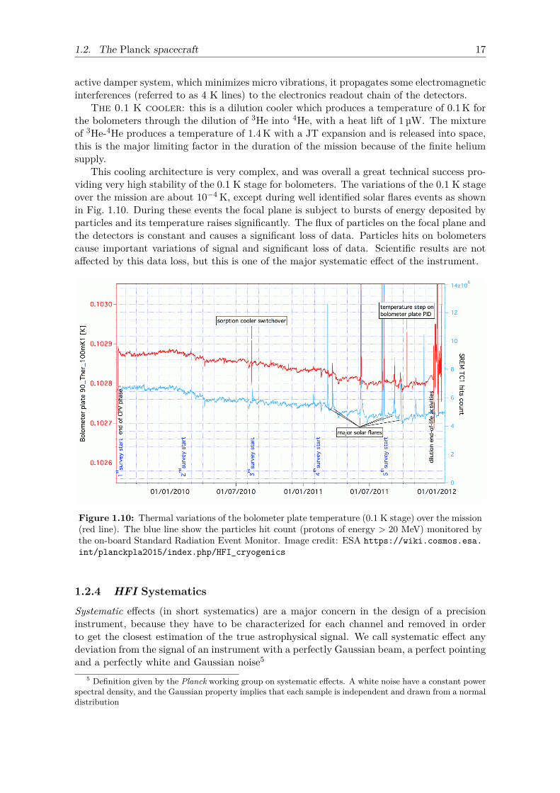
1.2. The Planck spacecraft 17
active damper system, which minimizes micro vibrations, it propagates some electromagneticinterferences (referred to as 4 K lines) to the electronics readout chain of the detectors.
The 0.1 K cooler: this is a dilution cooler which produces a temperature of 0.1 K forthe bolometers through the dilution of 3He into 4He, with a heat lift of 1 µW. The mixtureof 3He-4He produces a temperature of 1.4 K with a JT expansion and is released into space,this is the major limiting factor in the duration of the mission because of the finite heliumsupply.
This cooling architecture is very complex, and was overall a great technical success pro-viding very high stability of the 0.1 K stage for bolometers. The variations of the 0.1 K stageover the mission are about 10−4 K, except during well identified solar flares events as shownin Fig. 1.10. During these events the focal plane is subject to bursts of energy deposited byparticles and its temperature raises significantly. The flux of particles on the focal plane andthe detectors is constant and causes a significant loss of data. Particles hits on bolometerscause important variations of signal and significant loss of data. Scientific results are notaffected by this data loss, but this is one of the major systematic effect of the instrument.
Figure 1.10: Thermal variations of the bolometer plate temperature (0.1 K stage) over the mission(red line). The blue line show the particles hit count (protons of energy > 20 MeV) monitored bythe on-board Standard Radiation Event Monitor. Image credit: ESA https://wiki.cosmos.esa.int/planckpla2015/index.php/HFI_cryogenics
1.2.4 HFI Systematics
Systematic effects (in short systematics) are a major concern in the design of a precisioninstrument, because they have to be characterized for each channel and removed in orderto get the closest estimation of the true astrophysical signal. We call systematic effect anydeviation from the signal of an instrument with a perfectly Gaussian beam, a perfect pointingand a perfectly white and Gaussian noise5
5 Definition given by the Planck working group on systematic effects. A white noise have a constant powerspectral density, and the Gaussian property implies that each sample is independent and drawn from a normaldistribution
18 Chapter 1. Introduction
Major sources of systematics
Beams: these describe the angular response of the optical system to a point source on thesky. In HFI there are several definitions:
• the scanning beam is defined as the beam measured from the response to a point sourceof the full optical and electronic system. This is measured using planet crossings (?).In practice it is strongly degenerate with the time transfer function and both have tobe determined simultaneously. More details are given in Sec. 2.1.2. It is not possible todeconvolve HFI sky maps from the angular response function using this object becausethe computing resources involved are to high, but the scanning beam is the objectrelevant to map analysis at small angular scales and flux calculation;
• the effective beam at the map level is the overall angular response to the sky in amap pixel, which results from the combined effect of the instrumental response, thescanning strategy and the data processing. It is the kind of object which is relevantto deconvolve the average effect of the scanning beam over the CMB angular powerspectrum.
time transfer function: this is the temporal response of the electronic readout chainto an optical power excitation of the bolometer. In HFI a Low Frequency Excess Response(LFER) has been detected during the ground calibration campaigns (?), and proved to beextremely challenging to characterize in-flight. This is a critical issue because the calibrationof HFI detectors relies on the orbital dipole which is seen at 16 mHz resulting from Planckspinning frequency of 1 rpm, in a frequency range where there are no other simple calibrationsources. This complex issue is caused by a mixture of the thermal behavior of the detectors,and the bolometer AC biasing. Chap. 2 is dedicated to the LFER issue and covers in detailsthe time transfer function and how the HFI bolometers works.
Glitches: these are features in the electronic readout response caused by particlesenergy deposited on the highly sensitive HFI detectors. The optical absorber part of thedetector is a metallized grid which offers in theory a small cross-section to cosmic rays.However a combination of the thermal architecture of the detectors (?) and a period of lowsolar activity cycle caused a much higher rate of glitches than expected with around oneevent per second (?). Hopefully they can be removed efficiently and have a minimal impacton HFI data. As a side effect, glitches result in specific excitations of the electronics readoutchain of the detectors, and for this reason they provide a valuable probe of the time transferfunction. This topic is covered in Chap. 3.
Analog to Digital Converter nonlinearity: the ADC is a critical componentwhich digitizes the analog signal at the end of the analog electronics readout chain, beforesending samples to the Digital Processing Unit (DPU) as detailed in the next section. How-ever a combination of factors including a low signal dynamic and acquisition at the locationof the major nonlinear feature of the ADC scale caused apparent gain variations in time ofscience data signal. These gain variations at a level of 1-2% have been a serious concernfor photometric calibration (?). The characterization and correction of ADC nonlinearity iscentral to this thesis work and is covered specifically in part II.
4 K lines: the 4 K lines are a set of parasitic sinusoids produced by the 4 K stage coolerat well identified frequencies. In practice they appear at four distinct frequencies in thescience data and can be removed easily, with the xception of resonant rings acquired when thespacecraft spin frequency fspin is a multiple of the 4 K lines fundamental frequency f4K. Whenworking on ADC nonlinearity I found that their subtle interaction with this component wasa major concern for ADC nonlinearity correction, so they had to be characterized accuratelyfor inclusion in the correction. This topic is covered in Chap. 6.
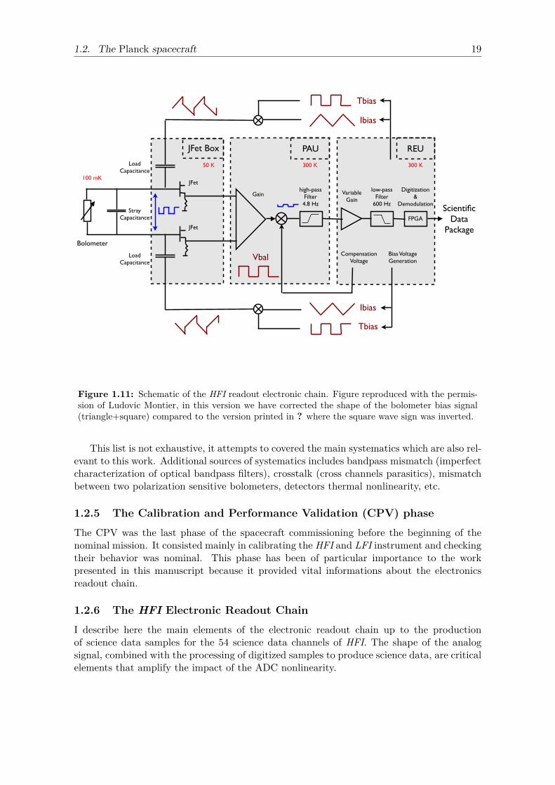
1.2. The Planck spacecraft 19
JFet
JFet
JFet Box PAU REU
Bolometer
Vbal
Tbias
high-pass Filter4.8 Hz
low-pass Filter
600 Hz
Gain VariableGain
Tbias
Ibias
Ibias
100 mK
50 K 300 K 300 K
StrayCapacitance
LoadCapacitance
Digitization &
Demodulation
LoadCapacitance
Scientific Data
Package
Bias Voltage Generation
Compensation Voltage
FPGA
Figure 1.11: Schematic of the HFI readout electronic chain. Figure reproduced with the permis-sion of Ludovic Montier, in this version we have corrected the shape of the bolometer bias signal(triangle+square) compared to the version printed in ? where the square wave sign was inverted.
This list is not exhaustive, it attempts to covered the main systematics which are also rel-evant to this work. Additional sources of systematics includes bandpass mismatch (imperfectcharacterization of optical bandpass filters), crosstalk (cross channels parasitics), mismatchbetween two polarization sensitive bolometers, detectors thermal nonlinearity, etc.
1.2.5 The Calibration and Performance Validation (CPV) phase
The CPV was the last phase of the spacecraft commissioning before the beginning of thenominal mission. It consisted mainly in calibrating the HFI and LFI instrument and checkingtheir behavior was nominal. This phase has been of particular importance to the workpresented in this manuscript because it provided vital informations about the electronicsreadout chain.
1.2.6 The HFI Electronic Readout Chain
I describe here the main elements of the electronic readout chain up to the productionof science data samples for the 54 science data channels of HFI. The shape of the analogsignal, combined with the processing of digitized samples to produce science data, are criticalelements that amplify the impact of the ADC nonlinearity.
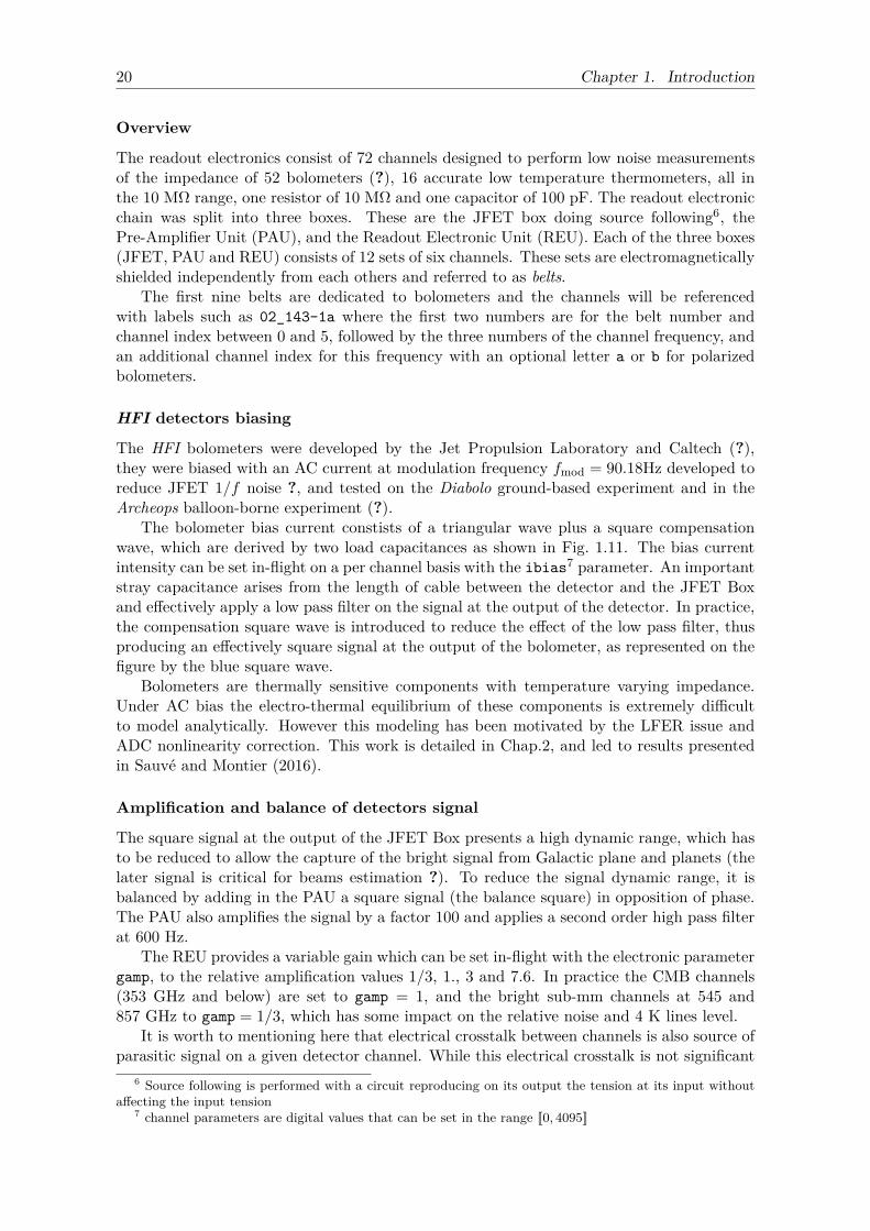
20 Chapter 1. Introduction
Overview
The readout electronics consist of 72 channels designed to perform low noise measurementsof the impedance of 52 bolometers (?), 16 accurate low temperature thermometers, all inthe 10 MΩ range, one resistor of 10 MΩ and one capacitor of 100 pF. The readout electronicchain was split into three boxes. These are the JFET box doing source following6, thePre-Amplifier Unit (PAU), and the Readout Electronic Unit (REU). Each of the three boxes(JFET, PAU and REU) consists of 12 sets of six channels. These sets are electromagneticallyshielded independently from each others and referred to as belts.
The first nine belts are dedicated to bolometers and the channels will be referencedwith labels such as 02_143-1a where the first two numbers are for the belt number andchannel index between 0 and 5, followed by the three numbers of the channel frequency, andan additional channel index for this frequency with an optional letter a or b for polarizedbolometers.
HFI detectors biasing
The HFI bolometers were developed by the Jet Propulsion Laboratory and Caltech (?),they were biased with an AC current at modulation frequency fmod = 90.18Hz developed toreduce JFET 1/f noise ?, and tested on the Diabolo ground-based experiment and in theArcheops balloon-borne experiment (?).
The bolometer bias current constists of a triangular wave plus a square compensationwave, which are derived by two load capacitances as shown in Fig. 1.11. The bias currentintensity can be set in-flight on a per channel basis with the ibias7 parameter. An importantstray capacitance arises from the length of cable between the detector and the JFET Boxand effectively apply a low pass filter on the signal at the output of the detector. In practice,the compensation square wave is introduced to reduce the effect of the low pass filter, thusproducing an effectively square signal at the output of the bolometer, as represented on thefigure by the blue square wave.
Bolometers are thermally sensitive components with temperature varying impedance.Under AC bias the electro-thermal equilibrium of these components is extremely difficultto model analytically. However this modeling has been motivated by the LFER issue andADC nonlinearity correction. This work is detailed in Chap.2, and led to results presentedin Sauvé and Montier (2016).
Amplification and balance of detectors signal
The square signal at the output of the JFET Box presents a high dynamic range, which hasto be reduced to allow the capture of the bright signal from Galactic plane and planets (thelater signal is critical for beams estimation ?). To reduce the signal dynamic range, it isbalanced by adding in the PAU a square signal (the balance square) in opposition of phase.The PAU also amplifies the signal by a factor 100 and applies a second order high pass filterat 600 Hz.
The REU provides a variable gain which can be set in-flight with the electronic parametergamp, to the relative amplification values 1/3, 1., 3 and 7.6. In practice the CMB channels(353 GHz and below) are set to gamp = 1, and the bright sub-mm channels at 545 and857 GHz to gamp = 1/3, which has some impact on the relative noise and 4 K lines level.
It is worth to mentioning here that electrical crosstalk between channels is also source ofparasitic signal on a given detector channel. While this electrical crosstalk is not significant
6 Source following is performed with a circuit reproducing on its output the tension at its input withoutaffecting the input tension
7 channel parameters are digital values that can be set in the range J0, 4095K
1.2. The Planck spacecraft 21
for science data, its amplitude is of order of the balanced signal and as a consequence rendersan analytical modeling of the balanced signal shape nearly impossible.
Digitization by the ADC : the fast samples
Figure 1.12: Functional view of in-flight signal processing. (a) Parasitic wave originating fromthe 4K stage mechanical cooler leaks into the signal through the electronic readout chain. (b) Thedigitization by the ADC introduce the nonlinear effect. (c) The signal summation in the DPUcauses loss of information.
The analog signal, mixed with the parasitic 4 K lines is sampled at a rate of 80fmod =7215Hz, as shown on the functional view in Fig. 1.12. This yields the digital signal (b)counting 80 samples per modulation period. This signal is called fast samples and cannotbe sent to Earth, because of the limited bandwidth for all the 72 high data rate channelsof the HFI instrument. However every 101 seconds, and for each detector, a period of 80fast samples is captured before summation by the Data Processing Unit (DPU) for furtherdata analysis. These fast samples periods have been a gold mine for ADC nonlinearitycharacterization and correction. A clear distinction will be made hereafter between the fastsamples and the science data samples.
The digitization is the step where the ADC nonlinearity effect is introduced, while thebalancing sets the analog signal location exactly at the center of the ADC scale, at the preciselocation of the biggest defect8 of the component. As a consequence, the nonlinearity of theADC has a maximum impact, as detailed further in Chap. 5.
Signal summation
The last step to be considered in the signal processing is the half period summation (see (c)in Fig.1.12), which operates as a low pass filter for reducing electronic noise. Each sciencedata sample is defined as the sum of the 40 fast samples of its corresponding half period,yielding the science data signal sampled at frequency facq = 2fmod.
However, the signal summation leads to a critical loss of information because of:
• Loss of ADC code value: the summation mixes the nonlinear codes9 at the outputof the ADC;
• Loss of 4K lines real signal: the spectral distribution of 4K harmonics extendsto much higher frequencies than fmod, and the summed modulated signal has only 4
8 The exact nature of this defect due to the discrete nature of an ADC output is detailed in Sec. 4.29 A code is the integer value in the range J0, 65535K resulting from the conversion of the analog input
signal by the ADC.
22 Chapter 1. Introduction
visible harmonics at 20Hz, 40Hz, 60Hz, 80Hz resulting from the folding of manyhigher frequency harmonics. As a consequence it is not possible to estimate the analog4K signal directly from the science data.
Because of the DPU summation, it is clear that the knowledge of the ADC nonlinearityalone is not sufficient to correct for its effect on the science data. A model describing thebolometer response to the sky signal along with 4 K lines is necessary to reconstruct thesignal as seen by the ADC. This model is described in Chap. 5.
Compression
The on-board DPU applies a tunable quantization step q on science data to reduce further-more the volume of data. The value of q is set to about half the white noise RMS of thechannel, so that this step increases the total noise of the channel by about 1% (see Sec. 5.2.3in ?). Every 254 science data samples the quantization step window is offset, ensuring astochastic distribution of sample values.
This step is considered to have a negligible impact on the systematics effects discussedin this work and will not be discussed hereafter.
1.3 Data processing
1.3.1 overview
The HFI data processing pipeline is composed of four levels split as follows10:
• Level 1: (L1) consists of receiving the telemetry and ancillary data files and ingestingthem into the Data Processing Center (DPC) data base, handled by the DMC proprietarysoftware which is hosted by the magique3 cluster at IAP.
• Level 2: (L2) is where the data are processed from timelines into maps;
• Level 3: (L3) is where the data in the form of frequency maps are converted tocatalogues and full-sky astrophysical component maps;
• Level S: (LS) is the common HFI/LFI simulation software.
In practice, most of the work presented below belong to L2 where the systematics effect fromthe instrument are corrected for.
Time ordered data
Raw science data is stored in the DMC database (see Appendix G). More than two yearsof HFI science data for the 72 channels is available in the form of continuous Time OrderedInput (TOI) files that can be accessed by sample index, corresponding to 72∗25×109 sciencedata samples.
The TOI data can be accessed by their so-called ring index. A ring is the stable pointingperiod of about 40 minutes duration when the spacecraft continuously scans the same skycircle as described in Sec. 1.2.2. Between each ring the spacecraft changes its pointingorientation and during this period of time, typically a few minutes, the pointing is known tobe unstable and therefore the science data is flagged as unusable. The five full sky surveys ofHFI represent about 5000 rings per survey for a total of 27008 rings (including calibrationphases at the beginning/end of the mission).
10 See https://wiki.cosmos.esa.int/planckpla2015/index.php/The_HFI_DPC
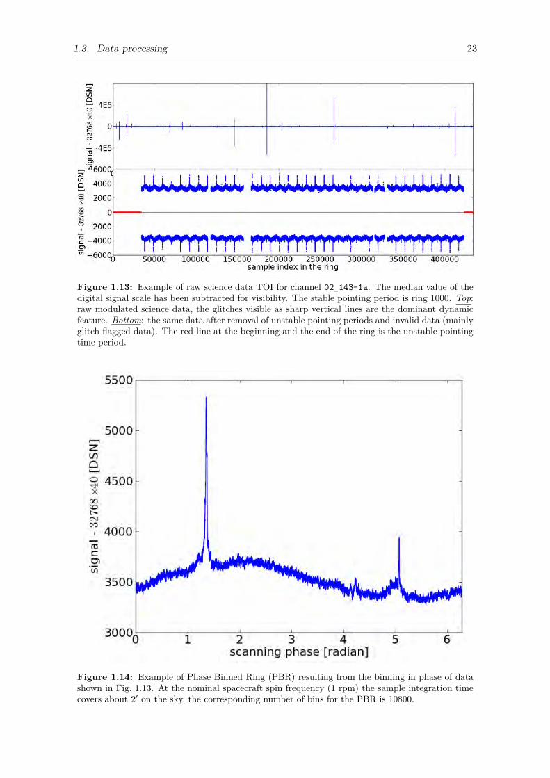
1.3. Data processing 23
Figure 1.13: Example of raw science data TOI for channel 02_143-1a. The median value of thedigital signal scale has been subtracted for visibility. The stable pointing period is ring 1000. Top:raw modulated science data, the glitches visible as sharp vertical lines are the dominant dynamicfeature. Bottom: the same data after removal of unstable pointing periods and invalid data (mainlyglitch flagged data). The red line at the beginning and the end of the ring is the unstable pointingtime period.
Figure 1.14: Example of Phase Binned Ring (PBR) resulting from the binning in phase of datashown in Fig. 1.13. At the nominal spacecraft spin frequency (1 rpm) the sample integration timecovers about 2′ on the sky, the corresponding number of bins for the PBR is 10800.
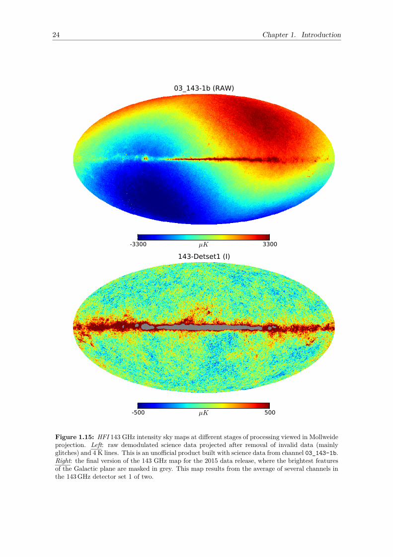
24 Chapter 1. Introduction
03_143-1b (RAW)
-3300 3300µK
143-Detset1 (I)
-500 500µK
Figure 1.15: HFI 143 GHz intensity sky maps at different stages of processing viewed in Mollweideprojection. Left: raw demodulated science data projected after removal of invalid data (mainlyglitches) and 4 K lines. This is an unofficial product built with science data from channel 03_143-1b.Right: the final version of the 143 GHz map for the 2015 data release, where the brightest featuresof the Galactic plane are masked in grey. This map results from the average of several channels inthe 143 GHz detector set 1 of two.
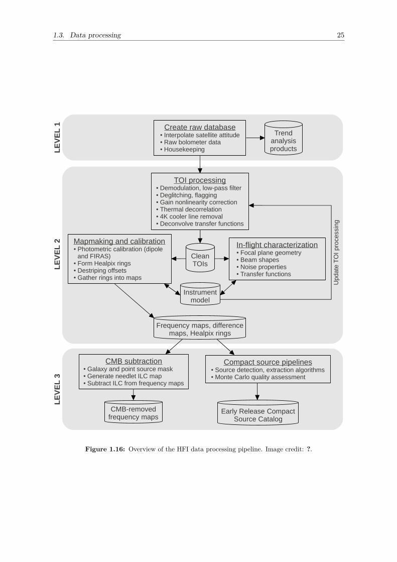
1.3. Data processing 25
Figure 1.16: Overview of the HFI data processing pipeline. Image credit: ?.
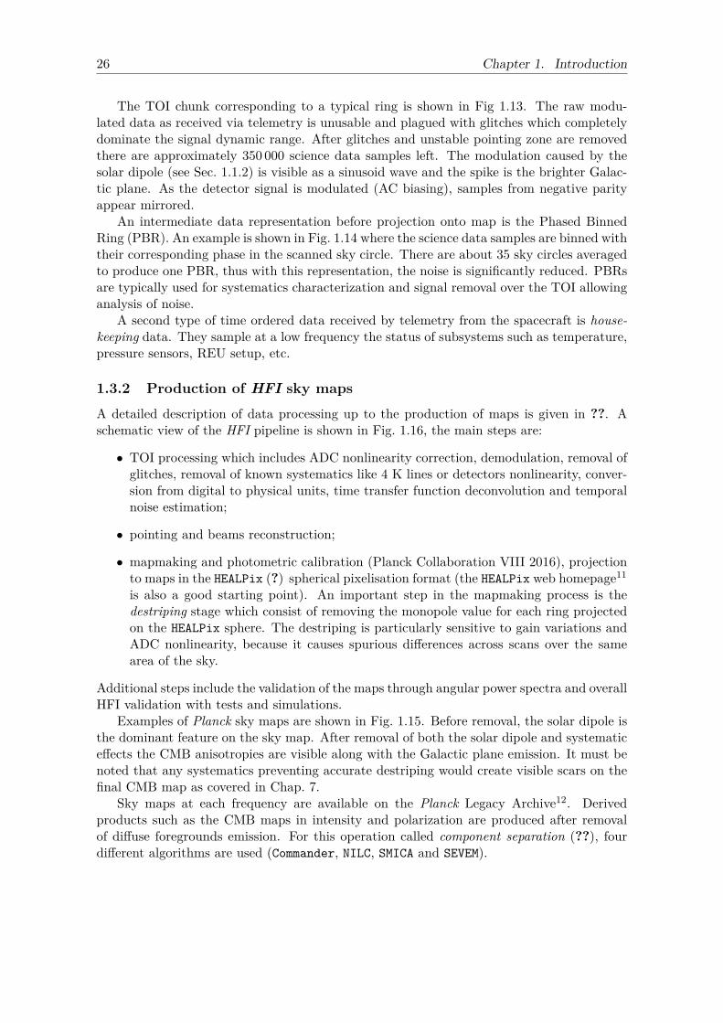
26 Chapter 1. Introduction
The TOI chunk corresponding to a typical ring is shown in Fig 1.13. The raw modu-lated data as received via telemetry is unusable and plagued with glitches which completelydominate the signal dynamic range. After glitches and unstable pointing zone are removedthere are approximately 350 000 science data samples left. The modulation caused by thesolar dipole (see Sec. 1.1.2) is visible as a sinusoid wave and the spike is the brighter Galac-tic plane. As the detector signal is modulated (AC biasing), samples from negative parityappear mirrored.
An intermediate data representation before projection onto map is the Phased BinnedRing (PBR). An example is shown in Fig. 1.14 where the science data samples are binned withtheir corresponding phase in the scanned sky circle. There are about 35 sky circles averagedto produce one PBR, thus with this representation, the noise is significantly reduced. PBRsare typically used for systematics characterization and signal removal over the TOI allowinganalysis of noise.
A second type of time ordered data received by telemetry from the spacecraft is house-keeping data. They sample at a low frequency the status of subsystems such as temperature,pressure sensors, REU setup, etc.
1.3.2 Production of HFI sky maps
A detailed description of data processing up to the production of maps is given in ??. Aschematic view of the HFI pipeline is shown in Fig. 1.16, the main steps are:
• TOI processing which includes ADC nonlinearity correction, demodulation, removal ofglitches, removal of known systematics like 4 K lines or detectors nonlinearity, conver-sion from digital to physical units, time transfer function deconvolution and temporalnoise estimation;
• pointing and beams reconstruction;
• mapmaking and photometric calibration (Planck Collaboration VIII 2016), projectionto maps in the HEALPix (?) spherical pixelisation format (the HEALPix web homepage11
is also a good starting point). An important step in the mapmaking process is thedestriping stage which consist of removing the monopole value for each ring projectedon the HEALPix sphere. The destriping is particularly sensitive to gain variations andADC nonlinearity, because it causes spurious differences across scans over the samearea of the sky.
Additional steps include the validation of the maps through angular power spectra and overallHFI validation with tests and simulations.
Examples of Planck sky maps are shown in Fig. 1.15. Before removal, the solar dipole isthe dominant feature on the sky map. After removal of both the solar dipole and systematiceffects the CMB anisotropies are visible along with the Galactic plane emission. It must benoted that any systematics preventing accurate destriping would create visible scars on thefinal CMB map as covered in Chap. 7.
Sky maps at each frequency are available on the Planck Legacy Archive12. Derivedproducts such as the CMB maps in intensity and polarization are produced after removalof diffuse foregrounds emission. For this operation called component separation (??), fourdifferent algorithms are used (Commander, NILC, SMICA and SEVEM).
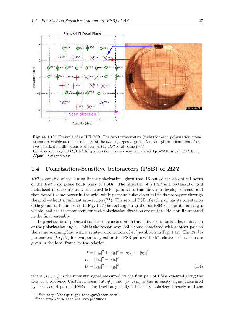
1.4. Polarization-Sensitive bolometers (PSB) of HFI 27
Scan direction
Figure 1.17: Example of an HFI PSB. The two thermometers (right) for each polarization orien-tation are visible at the extremities of the two superposed grids. An example of orientation of thetwo polarization directions is shown on the HFI focal plane (left).Image credit: Left: ESA/PLA https://wiki.cosmos.esa.int/planckpla2015 Right: ESA http://public.planck.fr
1.4 Polarization-Sensitive bolometers (PSB) of HFIHFI is capable of measuring linear polarization, given that 16 out of the 36 optical hornsof the HFI focal plane holds pairs of PSBs. The absorber of a PSB is a rectangular gridmetallized in one direction. Electrical fields parallel to this direction develop currents andthen deposit some power in the grid, while perpendicular electrical fields propagate throughthe grid without significant interaction (??). The second PSB of each pair has its orientationorthogonal to the first one. In Fig. 1.17 the rectangular grid of an PSB without its housing isvisible, and the thermometers for each polarization direction are on the side, non-illuminatedin the final assembly.
In practice linear polarization has to be measured in three directions for full determinationof the polarization angle. This is the reason why PSBs come associated with another pair onthe same scanning line with a relative orientation of 45 as shown in Fig. 1.17. The Stokesparameters (I,Q, U) for two perfectly calibrated PSB pairs with 45 relative orientation aregiven in the local frame by the relation
I = |s1a|2 + |s1b|2 = |s2a|2 + |s2b|2
Q = |s1a|2 − |s1b|2
U = |s2a|2 − |s2b|2 , (1.4)
where (s1a, s1b) is the intensity signal measured by the first pair of PSBs oriented along theaxis of a reference Cartesian basis (−→x ,−→y ), and (s2a, s2b) is the intensity signal measuredby the second pair of PSBs. The fraction p of light intensity polarized linearly and the
11 See: http://healpix.jpl.nasa.gov/index.shtml12 See http://pla.esac.esa.int/pla/#home
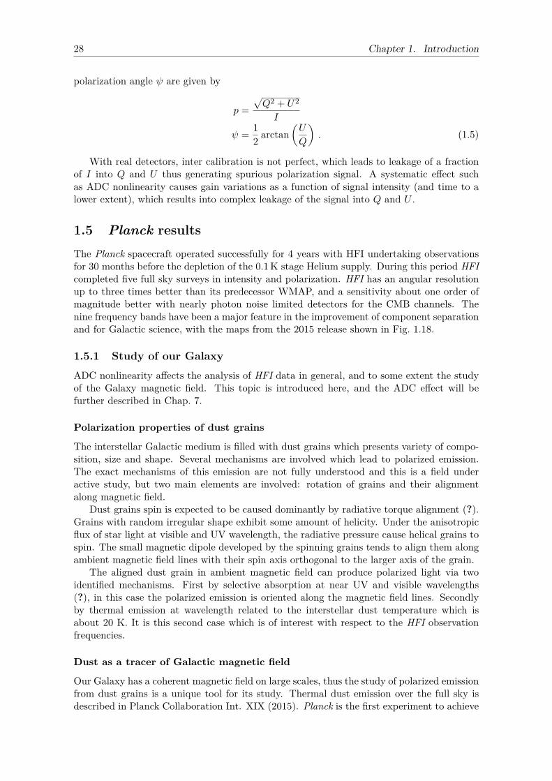
28 Chapter 1. Introduction
polarization angle ψ are given by
p =√Q2 + U2
I
ψ = 12 arctan
(U
Q
). (1.5)
With real detectors, inter calibration is not perfect, which leads to leakage of a fractionof I into Q and U thus generating spurious polarization signal. A systematic effect suchas ADC nonlinearity causes gain variations as a function of signal intensity (and time to alower extent), which results into complex leakage of the signal into Q and U .
1.5 Planck resultsThe Planck spacecraft operated successfully for 4 years with HFI undertaking observationsfor 30 months before the depletion of the 0.1 K stage Helium supply. During this period HFIcompleted five full sky surveys in intensity and polarization. HFI has an angular resolutionup to three times better than its predecessor WMAP, and a sensitivity about one order ofmagnitude better with nearly photon noise limited detectors for the CMB channels. Thenine frequency bands have been a major feature in the improvement of component separationand for Galactic science, with the maps from the 2015 release shown in Fig. 1.18.
1.5.1 Study of our Galaxy
ADC nonlinearity affects the analysis of HFI data in general, and to some extent the studyof the Galaxy magnetic field. This topic is introduced here, and the ADC effect will befurther described in Chap. 7.
Polarization properties of dust grains
The interstellar Galactic medium is filled with dust grains which presents variety of compo-sition, size and shape. Several mechanisms are involved which lead to polarized emission.The exact mechanisms of this emission are not fully understood and this is a field underactive study, but two main elements are involved: rotation of grains and their alignmentalong magnetic field.
Dust grains spin is expected to be caused dominantly by radiative torque alignment (?).Grains with random irregular shape exhibit some amount of helicity. Under the anisotropicflux of star light at visible and UV wavelength, the radiative pressure cause helical grains tospin. The small magnetic dipole developed by the spinning grains tends to align them alongambient magnetic field lines with their spin axis orthogonal to the larger axis of the grain.
The aligned dust grain in ambient magnetic field can produce polarized light via twoidentified mechanisms. First by selective absorption at near UV and visible wavelengths(?), in this case the polarized emission is oriented along the magnetic field lines. Secondlyby thermal emission at wavelength related to the interstellar dust temperature which isabout 20 K. It is this second case which is of interest with respect to the HFI observationfrequencies.
Dust as a tracer of Galactic magnetic field
Our Galaxy has a coherent magnetic field on large scales, thus the study of polarized emissionfrom dust grains is a unique tool for its study. Thermal dust emission over the full sky isdescribed in Planck Collaboration Int. XIX (2015). Planck is the first experiment to achieve
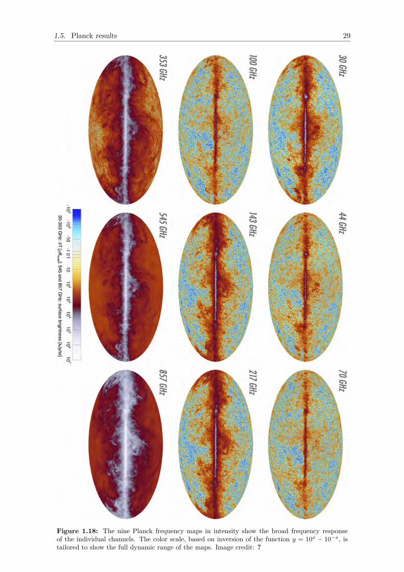
1.5. Planck results 29
Figure 1.18: The nine Planck frequency maps in intensity show the broad frequency responseof the individual channels. The color scale, based on inversion of the function y = 10x − 10−x, istailored to show the full dynamic range of the maps. Image credit: ?
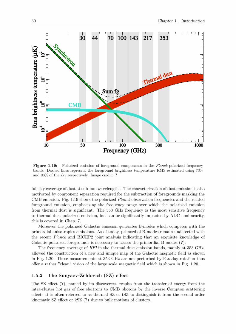
30 Chapter 1. Introduction
Figure 1.19: Polarized emission of foreground components in the Planck polarized frequencybands. Dashed lines represent the foreground brightness temperature RMS estimated using 73%and 93% of the sky respectively. Image credit: ?
full sky coverage of dust at sub-mm wavelengths. The characterization of dust emission is alsomotivated by component separation required for the subtraction of foregrounds masking theCMB emission. Fig. 1.19 shows the polarized Planck observation frequencies and the relatedforeground emission, emphasizing the frequency range over which the polarized emissionfrom thermal dust is significant. The 353 GHz frequency is the most sensitive frequencyto thermal dust polarized emission, but can be significantly impacted by ADC nonlinearity,this is covered in Chap. 7.
Moreover the polarized Galactic emission generates B-modes which competes with theprimordial anisotropies emissions. As of today, primordial B-modes remain undetected withthe recent Planck and BICEP2 joint analysis indicating that an exquisite knowledge ofGalactic polarized foregrounds is necessary to access the primordial B-modes (?).
The frequency coverage of HFI in the thermal dust emission bands, mainly at 353 GHz,allowed the construction of a new and unique map of the Galactic magnetic field as shownin Fig. 1.20. These measurements at 353 GHz are not perturbed by Faraday rotation thusoffer a rather ”clean“ vision of the large scale magnetic field which is shown in Fig. 1.20.
1.5.2 The Sunyaev-Zeldovich (SZ) effect
The SZ effect (?), named by its discoverers, results from the transfer of energy from theintra-cluster hot gas of free electrons to CMB photons by the inverse Compton scatteringeffect. It is often referred to as thermal SZ or tSZ to distinguish it from the second orderkinematic SZ effect or kSZ (?) due to bulk motions of clusters.
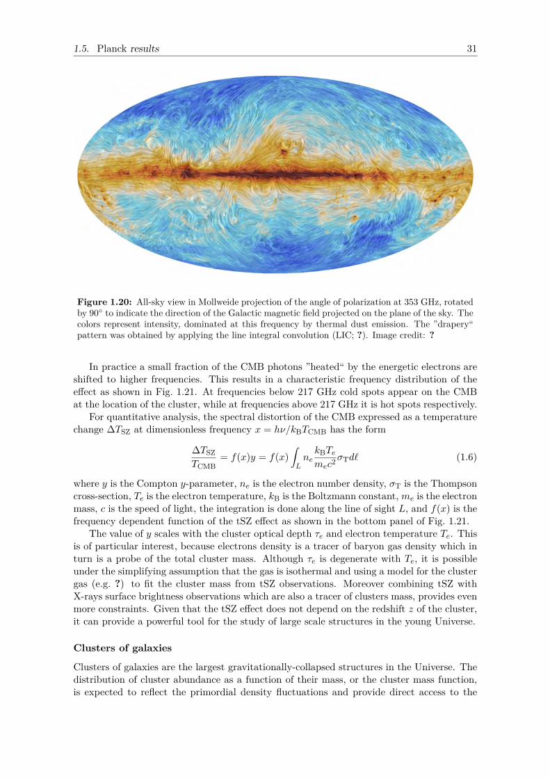
1.5. Planck results 31
Figure 1.20: All-sky view in Mollweide projection of the angle of polarization at 353 GHz, rotatedby 90 to indicate the direction of the Galactic magnetic field projected on the plane of the sky. Thecolors represent intensity, dominated at this frequency by thermal dust emission. The ”drapery“pattern was obtained by applying the line integral convolution (LIC; ?). Image credit: ?
In practice a small fraction of the CMB photons ”heated“ by the energetic electrons areshifted to higher frequencies. This results in a characteristic frequency distribution of theeffect as shown in Fig. 1.21. At frequencies below 217 GHz cold spots appear on the CMBat the location of the cluster, while at frequencies above 217 GHz it is hot spots respectively.
For quantitative analysis, the spectral distortion of the CMB expressed as a temperaturechange ∆TSZ at dimensionless frequency x = hν/kBTCMB has the form
∆TSZTCMB
= f(x)y = f(x)∫LnekBTemec2σTd` (1.6)
where y is the Compton y-parameter, ne is the electron number density, σT is the Thompsoncross-section, Te is the electron temperature, kB is the Boltzmann constant,me is the electronmass, c is the speed of light, the integration is done along the line of sight L, and f(x) is thefrequency dependent function of the tSZ effect as shown in the bottom panel of Fig. 1.21.
The value of y scales with the cluster optical depth τe and electron temperature Te. Thisis of particular interest, because electrons density is a tracer of baryon gas density which inturn is a probe of the total cluster mass. Although τe is degenerate with Te, it is possibleunder the simplifying assumption that the gas is isothermal and using a model for the clustergas (e.g. ?) to fit the cluster mass from tSZ observations. Moreover combining tSZ withX-rays surface brightness observations which are also a tracer of clusters mass, provides evenmore constraints. Given that the tSZ effect does not depend on the redshift z of the cluster,it can provide a powerful tool for the study of large scale structures in the young Universe.
Clusters of galaxies
Clusters of galaxies are the largest gravitationally-collapsed structures in the Universe. Thedistribution of cluster abundance as a function of their mass, or the cluster mass function,is expected to reflect the primordial density fluctuations and provide direct access to the
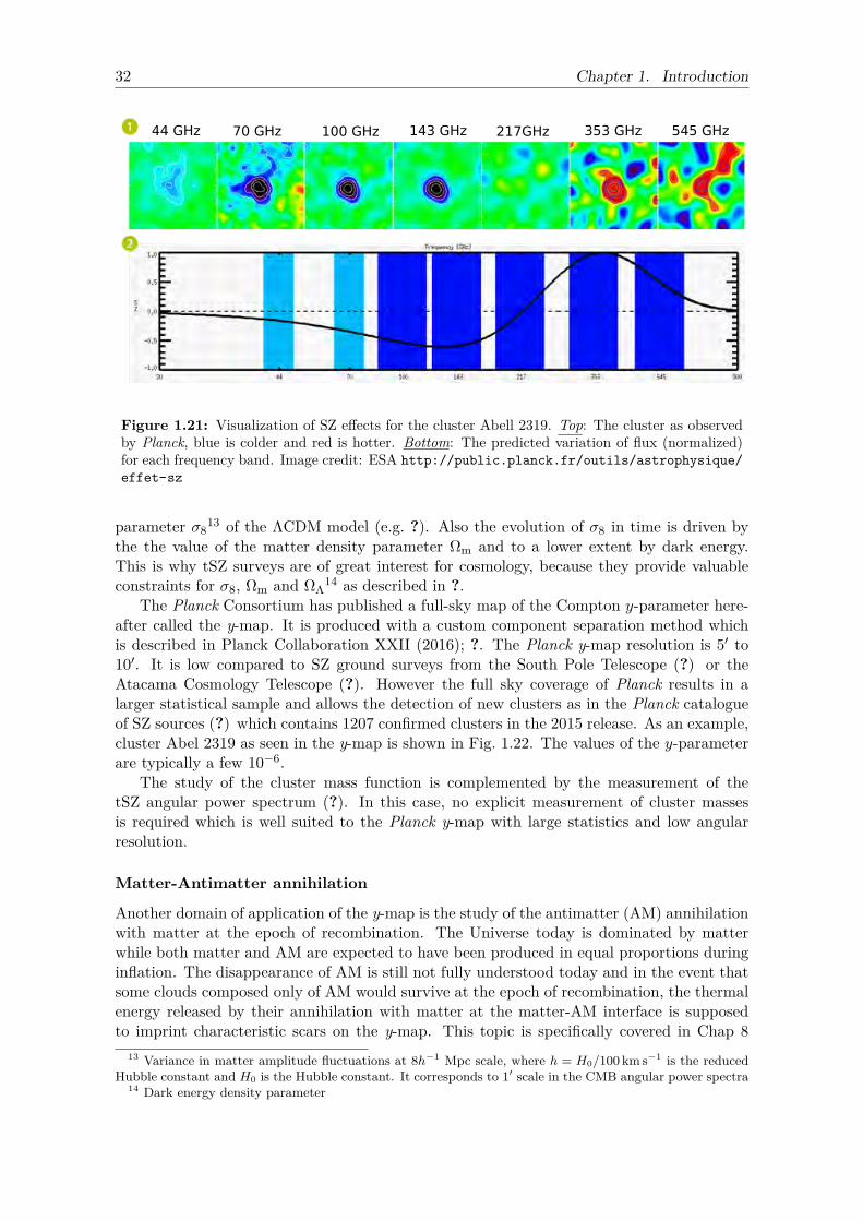
32 Chapter 1. Introduction
44 GHz 70 GHz 100 GHz 143 GHz 217GHz 353 GHz 545 GHz
Figure 1.21: Visualization of SZ effects for the cluster Abell 2319. Top: The cluster as observedby Planck, blue is colder and red is hotter. Bottom: The predicted variation of flux (normalized)for each frequency band. Image credit: ESA http://public.planck.fr/outils/astrophysique/effet-sz
parameter σ813 of the ΛCDM model (e.g. ?). Also the evolution of σ8 in time is driven by
the the value of the matter density parameter Ωm and to a lower extent by dark energy.This is why tSZ surveys are of great interest for cosmology, because they provide valuableconstraints for σ8, Ωm and ΩΛ
14 as described in ?.The Planck Consortium has published a full-sky map of the Compton y-parameter here-
after called the y-map. It is produced with a custom component separation method whichis described in Planck Collaboration XXII (2016); ?. The Planck y-map resolution is 5′ to10′. It is low compared to SZ ground surveys from the South Pole Telescope (?) or theAtacama Cosmology Telescope (?). However the full sky coverage of Planck results in alarger statistical sample and allows the detection of new clusters as in the Planck catalogueof SZ sources (?) which contains 1207 confirmed clusters in the 2015 release. As an example,cluster Abel 2319 as seen in the y-map is shown in Fig. 1.22. The values of the y-parameterare typically a few 10−6.
The study of the cluster mass function is complemented by the measurement of thetSZ angular power spectrum (?). In this case, no explicit measurement of cluster massesis required which is well suited to the Planck y-map with large statistics and low angularresolution.
Matter-Antimatter annihilation
Another domain of application of the y-map is the study of the antimatter (AM) annihilationwith matter at the epoch of recombination. The Universe today is dominated by matterwhile both matter and AM are expected to have been produced in equal proportions duringinflation. The disappearance of AM is still not fully understood today and in the event thatsome clouds composed only of AM would survive at the epoch of recombination, the thermalenergy released by their annihilation with matter at the matter-AM interface is supposedto imprint characteristic scars on the y-map. This topic is specifically covered in Chap 8
13 Variance in matter amplitude fluctuations at 8h−1 Mpc scale, where h = H0/100 km s−1 is the reducedHubble constant and H0 is the Hubble constant. It corresponds to 1′ scale in the CMB angular power spectra
14 Dark energy density parameter
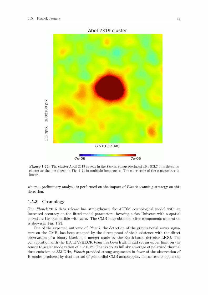
1.5. Planck results 33
Figure 1.22: The cluster Abell 2319 as seen in the Planck y-map produced with NILC, it is the samecluster as the one shown in Fig. 1.21 in multiple frequencies. The color scale of the y-parameter islinear.
where a preliminary analysis is performed on the impact of Planck scanning strategy on thisdetection.
1.5.3 Cosmology
The Planck 2015 data release has strengthened the ΛCDM cosmological model with anincreased accuracy on the fitted model parameters, favoring a flat Universe with a spatialcurvature ΩK compatible with zero. The CMB map obtained after components separationis shown in Fig. 1.23.
One of the expected outcome of Planck, the detection of the gravitational waves signa-ture on the CMB, has been scooped by the direct proof of their existence with the directobservation of a binary black hole merger made by the Earth-based detector LIGO. Thecollaboration with the BICEP2/KECK team has been fruitful and set an upper limit on thetensor to scalar mode ration of r < 0.12. Thanks to its full sky coverage of polarized thermaldust emission at 353 GHz, Planck provided strong arguments in favor of the observation ofB-modes produced by dust instead of primordial CMB anisotropies. These results opens the
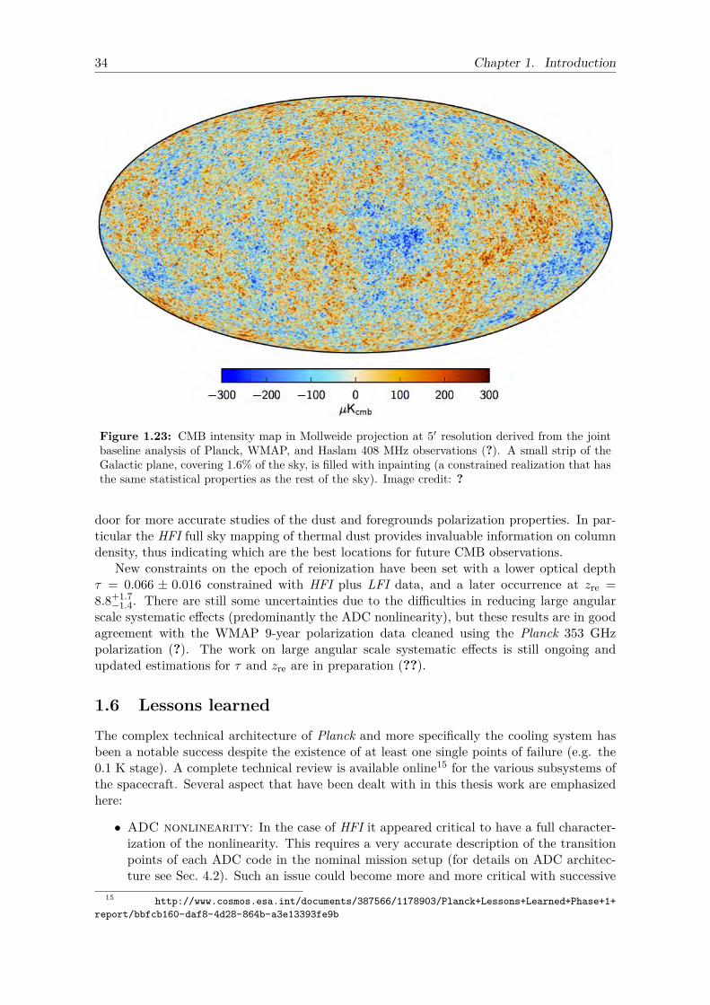
34 Chapter 1. Introduction
Figure 1.23: CMB intensity map in Mollweide projection at 5′ resolution derived from the jointbaseline analysis of Planck, WMAP, and Haslam 408 MHz observations (?). A small strip of theGalactic plane, covering 1.6% of the sky, is filled with inpainting (a constrained realization that hasthe same statistical properties as the rest of the sky). Image credit: ?
door for more accurate studies of the dust and foregrounds polarization properties. In par-ticular the HFI full sky mapping of thermal dust provides invaluable information on columndensity, thus indicating which are the best locations for future CMB observations.
New constraints on the epoch of reionization have been set with a lower optical depthτ = 0.066 ± 0.016 constrained with HFI plus LFI data, and a later occurrence at zre =8.8+1.7−1.4. There are still some uncertainties due to the difficulties in reducing large angular
scale systematic effects (predominantly the ADC nonlinearity), but these results are in goodagreement with the WMAP 9-year polarization data cleaned using the Planck 353 GHzpolarization (?). The work on large angular scale systematic effects is still ongoing andupdated estimations for τ and zre are in preparation (??).
1.6 Lessons learnedThe complex technical architecture of Planck and more specifically the cooling system hasbeen a notable success despite the existence of at least one single points of failure (e.g. the0.1 K stage). A complete technical review is available online15 for the various subsystems ofthe spacecraft. Several aspect that have been dealt with in this thesis work are emphasizedhere:
• ADC nonlinearity: In the case of HFI it appeared critical to have a full character-ization of the nonlinearity. This requires a very accurate description of the transitionpoints of each ADC code in the nominal mission setup (for details on ADC architec-ture see Sec. 4.2). Such an issue could become more and more critical with successive
15 http://www.cosmos.esa.int/documents/387566/1178903/Planck+Lessons+Learned+Phase+1+report/bbfcb160-daf8-4d28-864b-a3e13393fe9b
1.6. Lessons learned 35
generations of instruments and increasing sensitivity. Moreover, the dynamic of theacquired signal was covering a voltage range corresponding to only ≈ 10 codes. Thisrange should be widened significantly to lower the negative impact of unavoidablelocalized defects. Some relevant options are provided in Sec. 4.9.
• Oversampling and summation: In HFI, the fast samples summation is in theory avery good option for improving the SNR of science data. However in practice, in thepresence of any nonlinear systematic effect on the summed signal (such as the ADCbut not limited to it), this destroys vital information for correction of the effect. Henceoversampling should be either replaced by analog integration or ADC nonlinearityshould be corrected for in-flight before summation. These options are discussed furtherin Sec. 4.9.
• 4 K cooler EMI: the electronic vibration damping system of the HFI 4 K stagemechanical compressor worked perfectly, but EMI shielding of this kind of system hasto be strengthened in future mission. Some replacement solutions are promising likeadiabatic demagnetization refrigeration (ADR). The synchronization of the compressorwith DPU acquisition revealed to be a very good idea for removing the spurious signalpropagated on science data. However the EMI leaks (designed farther as 4 K lines)in conjunction with ADC nonlinearity plus fast samples summation produce nonlineareffects that are extremely difficult to deal with. They remain one of the dominantsource of residuals at large angular scale limiting the accuracy of scientific results for` < 10 and generating spurious signals around ` = 1800. Furthermore some shorttimescale variations as generated by the sorption cooler bed switching also producesresiduals that are difficult to deal with. This is remain an issue that can be improvedfor HFI ADC nonlinearity correction as presented in Sec. 6.5.
• cosmic ray susceptibility: One of the surprises in the Planck mission was thehigher than expected rate of glitches seen by HFI detectors. This is partly due to thecoincidence between the spacecraft launch and a solar activity minima, and also to thehigh susceptibility of the detectors which is due to the silicon die part (?). The longglitches generated by hits on the silicon die have a slow thermal relaxation which, ifnot appropriately removed, produce non-Gaussian noise in the science data. Hencefuture experiments with detectors sensitive to thermal relaxation such as TransitionEdge Sensor (TES) arrays should improve heat transport to the housing.
• thermal response of bolometers: Under AC biasing, bolometers have a signifi-cantly different time response than under DC biasing. Albeit behaving like an orderone a low pass filter at first order they exhibit an enhanced response at low frequencywhich is characteristic of AC biasing. This behavior is problematic in the HFI casebecause the photometric calibration relies on the orbital dipole being visible at the verylow frequency of 16 mHz. An analytical model has been developed for AC biasing ofbolometers, as presented in Chap. 2 that can be used to produce valuable constraintsfor the low frequency part of the time transfer function.

37
Part I
Readout Response

39
Chapter 2
time transfer function analyticalmodel
“Oh dear! Oh dear! I shall be toolate!”
White Rabbit
The time transfer function of the HFI readout electronics is a critical component of thescience data processing, and one of the major known source of systematic effects. Hencea very high calibration precision is required. In ? that will be referenced hereafter as thepre-launch paper, the target was set to an accuracy level below 0.2% within the [10 mHz,70 Hz] range. However ground calibration, albeit useful for modeling the time transferfunction, is not sufficient to reach this level of accuracy in-flight where the optical loadand bias parameters of the detectors are significantly different to the setup used duringthe ground calibration campaigns. Since the spacecraft launch, the time transfer functionis approximated with an empirical model using a sum of low pass filters to describe thethermal response of the detectors. This approach presents a major issue with the calibrationbecause the empirical model is not constraining enough. It happens that the work on ADCnonlinearity correction needs also an accurate knowledge of the time transfer function (SeeChap. 5) and reveals a new and unexploited constraint for its characterization. For thesereasons a work has been done to produce an analytical model of the time transfer functionin frequency domain. This chapter presents this work which resulted in an article (Sauvéand Montier 2016) published in Experimental Astronomy, and called hereafter the AC paper(provided in Appendix A).
First the time transfer function definition and characterization within HFI is detailed inSec. 2.1. Then the content of the AC paper is discussed in Sec. 2.2, and a direct applicationto in-flight data is presented in Sec. 2.3. Finally some perspectives are provided for anevolution of the thermal model of the simple bolometer model heat dissipation in Sec. 2.4 tomeet the HFI accuracy goal.
2.1 Context
2.1.1 Definition of the time transfer function
In HFI the time transfer function, also called temporal transfer function, describes the read-out electronic response for demodulated science data to an input optical excitation. It is acomplex function of frequency describing the response in amplitude and phase shift of aninput signal.
The readout electronic response described by the time transfer function can be decom-posed in two functional subsystems which are:
40 Chapter 2. time transfer function analytical model
• the thermal response: it is the detector time response to the signal of the incomingsky power;
• the electronic response: it includes the readout electronics filtering (bandpassfilter) and the DPU digital processing to produce science data samples.
This model is described in details in Sec. 2 of ?. Following the nomenclature of thispaper, the time transfer function can be written
TF (ω) = F (ω)︸ ︷︷ ︸thermal
H ′(ω)︸ ︷︷ ︸electronic
, (2.1)
where F (ω) is the thermal response and H ′(ω) is the electronic response1.The sensitive part in this decomposition is the presence of a stray capacitance due to the
length of the cables between the bolometer and the Pre-Amplifier Unit (PAU, see Sec. 1.2.6).It is included in H ′(ω) in ? but in practice it participates significantly to the electro-thermalcoupling of the detector and should be described within F (ω) as detailed in the AC paper.
2.1.2 Characterization
While the electronic part of the time transfer function has been very well characterized on-ground and rely on well known electronic components, the thermal part is more complexbecause of the AC biasing of bolometers which is not theoretically as well known as DCbiasing. Hence the characterization of the time transfer function described hereafter focusesin practice on the thermal response.
Thermal response model
Under DC bias the time response of bolometers to an optical excitation can be representedby a first order low pass filter (?) . This theory has been extended to AC biasing with asquare current that mimics the DC biasing, as described in Sec. 4 of the pre-launch paper.In practice the response in AC biasing is significantly different, and furthermore impactedby the stray capacitance. These aspects are taken into account and solved for in the ACpaper.
In the case of HFI, the thermal part F (ω) is based on an empirical model using a sumof first order low pass filters reading
F (ω) =7∑i=1
ai1 + jωτi
. (2.2)
Calibration of the HFI thermal response
The main issue with the time transfer function is the estimation of the (ai, τi) parametersof F (ω), given the strong accuracy requirements of HFI. Moreover a Low Frequency ExcessResponse (LFER) has been identified during the ground calibration campaigns, and esti-mated at about 1% level in amplitude in the pre-launch paper. The LFER is particularlyrelevant with the CMB channels channels which are calibrated with the dipole appearing at16 mHz, but for such low frequencies there is no easy way to make calibration in-flight andthe ground calibration data revealed insufficient.
In 2015 the (ai, τi) parameters are estimated from heterogeneous sources (see Sec. 3.4 in?). The shortest time constant parameters are estimated with planets crossings, while the
1 The values of the electronic parameters for H ′(ω) are provided in the Planck explanatory supplement,see https://wiki.cosmos.esa.int/planckpla2015/index.php/HFI_time_response_model
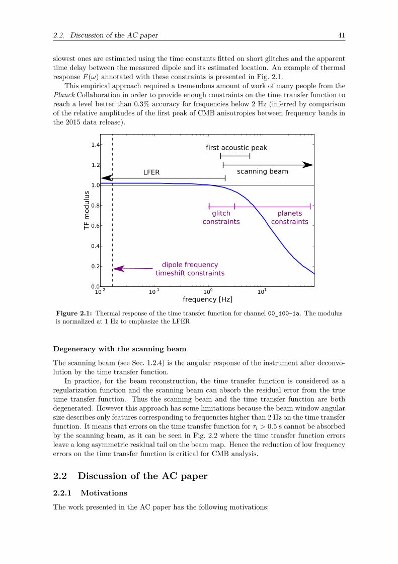
2.2. Discussion of the AC paper 41
slowest ones are estimated using the time constants fitted on short glitches and the apparenttime delay between the measured dipole and its estimated location. An example of thermalresponse F (ω) annotated with these constraints is presented in Fig. 2.1.
This empirical approach required a tremendous amount of work of many people from thePlanck Collaboration in order to provide enough constraints on the time transfer function toreach a level better than 0.3% accuracy for frequencies below 2 Hz (inferred by comparisonof the relative amplitudes of the first peak of CMB anisotropies between frequency bands inthe 2015 data release).
LFER
glitch constraints
dipole frequencytimeshift constraints
planetsconstraints
Figure 2.1: Thermal response of the time transfer function for channel 00_100-1a. The modulusis normalized at 1 Hz to emphasize the LFER.
Degeneracy with the scanning beam
The scanning beam (see Sec. 1.2.4) is the angular response of the instrument after deconvo-lution by the time transfer function.
In practice, for the beam reconstruction, the time transfer function is considered as aregularization function and the scanning beam can absorb the residual error from the truetime transfer function. Thus the scanning beam and the time transfer function are bothdegenerated. However this approach has some limitations because the beam window angularsize describes only features corresponding to frequencies higher than 2 Hz on the time transferfunction. It means that errors on the time transfer function for τi > 0.5 s cannot be absorbedby the scanning beam, as it can be seen in Fig. 2.2 where the time transfer function errorsleave a long asymmetric residual tail on the beam map. Hence the reduction of low frequencyerrors on the time transfer function is critical for CMB analysis.
2.2 Discussion of the AC paper
2.2.1 Motivations
The work presented in the AC paper has the following motivations:
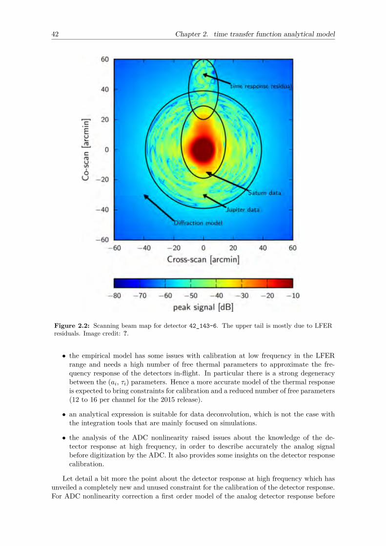
42 Chapter 2. time transfer function analytical modelPlanck Collaboration: Planck 2015 results. VII. HFI TOI and beams
Figure 12. Scanning beam map for detector 143-6 with a roughillustration of the regions that are handled with a di↵erent dataselection or binning.
frequency-band dependence of the e↵ective size of the planetarydisc (Planck Collaboration XXXIV 2015). Because of Saturn’ssmall size relative to the HFI beams, for ` < 4000 the symmet-ric part of Saturn’s shape dominates the window function. Thereis a small variation with HFI band in the apparent mean sizeof Saturn due to the di↵erent ring system temperatures, rangingfrom 9.0025 at 100 GHz to 10.002 at 857 GHz. Because this varia-tion introduces a bias of less than 2105 in B2
` for ` 4000, weignore it and use a correction derived for a mean 9.005 Saturn discfor all bands.
The two e↵ective-beam codes handle temperature-to-polarization leakage in slightly di↵erent ways. The dominantleakage comes from di↵erences in the scanning beams of thepolarization-sensitive detectors (See Sect. 4.7). The Quickbeamcode mimics the data model of the mapmaking code and assumesthat every polarization-sensitive detector at a given frequencyhas the same beam shape, and thus produces a single e↵ectivebeam window function. Temperature-to-polarization leakage ishandled later as a set of parameters in the likelihood of the angu-lar power spectra. The FEBeCoP code produces e↵ective beamwindow functions for the polarized power spectra that accountfor di↵erences in the main beam. However, these are computedas the average power leakage of a given sky signal from temper-ature to polarization. Hence, these polarized window functionsare not strictly instrumental parameters, since they rely on anassumed fiducial temperature angular power spectrum.
4.3. Beam error budget
As in the 2013 release, the beam error budget is based on aneigenmode decomposition of the scatter in simulated planet ob-servations. A reconstruction bias is estimated from the ensembleaverage of the simulations. We generate 100 simulations for eachplanet observation that include pointing uncertainty, cosmic rayglitches, and the measured noise spectrum. Simulated glitchesare injected into the timeline with the correct energy spectrumand rate (Planck Collaboration X 2014) and are detected andremoved using the deglitch algorithm. Noise realizations are de-rived as shown in Sect. 5.3.1. Pointing uncertainty is simulatedby randomizing the pointing by 1.005 rms in each direction.
The improved signal-to-noise ratio compared to 2013 leadsto smaller error bars; for instance, at ` = 1000 the uncertaintieson B2
` are now (2.2, 0.84, 0.81)104 for 100, 143, and 217 GHzfrequency-averaged maps respectively, reduced from the previ-ous uncertainties of (61, 23, 20) 104.
A “Reduced Instrument Model” (RIMO; see Appendix A)containing the e↵ective B(`) for temperature and polarization de-tector sets, for auto- and cross-spectra at 100 to 217 GHz, is in-cluded in the release, for a sky fraction of 100 %. Another RIMOis provided for a sky fraction of 75 %. They both contain the firstfive beam error eigenmodes and their covariance matrix, for themultipole ranges [0, `max] with `max = 2000, 3000, 3000 at 100,143, and 217 GHz respectively (instead of 2500, 3000, 4000 pre-viously). These new ranges bracket more closely the ones ex-pected to be used in the likelihood analyses, and ensure a betterdetermination of the leading modes on the customized ranges.
As described in Appendix A7 of Planck Collaboration XV(2014), these beam window function uncertainty eigenmodes areused to build the C(`) covariance matrix used in the high-` an-gular power spectrum likelihood analysis. It was found that thebeam errors are negligible compared to the other sources of un-certainty and have no noticeable impact on the values or associ-ated errors of the cosmological parameters.
4.4. Consistency of beam reconstruction
To evaluate the accuracy and consistency of the beam recon-struction method, we have compared beams reconstructed usingMars for the main beam part instead of Saturn, and using datafrom Year 1 or Year 2 only. We compared the window functionsobtained with these new beams to the reference ones; new MonteCarlo simulations were created to evaluate the corresponding er-ror bars, and the results are shown in Figs. 14 and 15. Note thatthe e↵ective beam window functions shown in these figures arenot exactly weighted for the scan strategy, rather we plot them inthe raster scan limit, where B2
` is defined as the sum over m theB2`m. The eigenmodes were evaluated for these di↵erent data sets
allowing us to compare them with the reference beam using a 2
analysis. The discrepancy between each data set and the refer-ence beam is fitted using Ndof=5 eigenmodes using `max =1200,2000, and 2500, for the 100, 143, and 217 GHz channels, respec-tively. The 2 is then defined as:
2 =
NdofX
i=1
(ci/i)2 (5)
where ci is the fit coecient for eigenvector i, with eigenvaluei. For each data set, the p-value to exceed this 2 value for a 2
distribution with Ndof degrees of freedom is indicated in Table 4.A high p-value indicates that the given data set is consistent
11
Figure 2.2: Scanning beam map for detector 42_143-6. The upper tail is mostly due to LFERresiduals. Image credit: ?.
• the empirical model has some issues with calibration at low frequency in the LFERrange and needs a high number of free thermal parameters to approximate the fre-quency response of the detectors in-flight. In particular there is a strong degeneracybetween the (ai, τi) parameters. Hence a more accurate model of the thermal responseis expected to bring constraints for calibration and a reduced number of free parameters(12 to 16 per channel for the 2015 release).
• an analytical expression is suitable for data deconvolution, which is not the case withthe integration tools that are mainly focused on simulations.
• the analysis of the ADC nonlinearity raised issues about the knowledge of the de-tector response at high frequency, in order to describe accurately the analog signalbefore digitization by the ADC. It also provides some insights on the detector responsecalibration.
Let detail a bit more the point about the detector response at high frequency which hasunveiled a completely new and unused constraint for the calibration of the detector response.For ADC nonlinearity correction a first order model of the analog detector response before
2.2. Discussion of the AC paper 43
digitization is needed. The detector response to the sky signal can be modeled at first order,at modulation level, using what is called the raw gain within Planck Collaboration, it isdetailed in the AC paper and in Sec. 5.2. It was called the steady state gain in the AC paperfor the general audience because it reflects more its nature. The interesting point about theraw gain is that it results from the electro-thermal equilibrium of the detector. Moreoverthis is an observable easy to measure from in-flight data. Expected outputs from the rawgain analysis are:
• a analytical model which can improve this parameter for the ADC nonlinearity correc-tion;
• strong constraints for the calibration of the thermal response F (ω).
2.2.2 AC paper content
The main issue when building an analytical expression for AC biased bolometers comesfrom the product between differentials terms in coupled differential equations defining theelectrical equilibrium in Eq 2.1 of AC paper and the thermal equilibrium in Eq. 2.2 of theAC paper. Steady state and optical excitation signals are considered separately, and thecoupled differential equations are linearised for each case. Then the products of differentialterms can be managed by using a custom splitting of the discrete frequency support for theconsidered signals. Finally the analytical expression of the time transfer function can beconstructed with classic matrix based linear algebra.
The validation of the time transfer function analytical expression is compared to theoutput of the simulation tool SEB. The former is calculated in frequency domain and thelater integrates the differential equations using finite differences.
A specific analysis is made for the detector response to slow optical signal variation. Theanalytical expression allows us to infer quantitative error estimation for the first order modelof the detector response (using the raw gain). Hence the empirical approach used for ADCnonlinearity correction can be compared to the analytical model.
The analytical expression describes the signal at the output of the detector bias circuit,it is then reformulated to include the DPU integration which produce the HFI science data.This integrated version can be compared to the single low pass filter approximation used inthe case of DC biasing.
In the Appendix B of the AC paper, the analytical expression is extended with a secondheat capacity on the thermal path to the heat sink (and potentially to more components).This case is more realistic as confirmed by the glitch analysis (see Chap. 3).
2.2.3 Constraints for the LFER model
Instead of reformulating the conclusions of the AC paper here, their interpretations arereformulated below in the context of the LFER and ADC nonlinearity issues.
The integrated version of the time response of the simple bolometer model (Fig. 9 of theAC paper) differs significantly from the empirical model used to describe the LFER. Whilethe later uses a sum F (ω) of first order low pass filters to fit the thermal response of thedetector, it is clear that fitting the former with low pass filters will result in spurious longtime constants. This result by itself demonstrates that LFER in the sense of the pre-launchpaper is a natural behavior of AC biased bolometers within HFI readout. Hence a modelwith a correct description of the thermal dissipation within the detector is expected to beconstraining for the time transfer function.
Moreover, the expression for the raw gain (expressed as G in Sec. 5.4 of the AC paper),shows that it results from an interpolation of the thermal response at optical frequency ω = 0.
44 Chapter 2. time transfer function analytical model
As a consequence it is a constraint for the low frequency part of the time transfer function(albeit having a high frequency description). However it is model dependent, meaningthat it is also a tool for model tuning. This constraint at low frequency is important becauseit is exactly the part of the time transfer function which is the most difficult to calibratein-flight.
2.3 Test of the analytical model against HFI dataThis section describes a simple check of the performances of the analytical model presentedin the AC paper. It is used to fit the raw gain, and the empirical time transfer functionmodel used for the HFI 2015 data release.
2.3.1 Fit setups
Three setups are considered with the data of channel 00_100-1a which are:
• setup 1: the one thermal component model is used to fit the raw gain only. Theraw gain has been estimated with the best available ADC nonlinearity correction (INLversion GP41);
• setup 2: the two thermal components model (described in the appendix of the ACpaper) is used to fit the raw gain and the time transfer function of the 2015 datarelease. In order to have equivalent weights for both data sources, 80 data samples areused for the time transfer function in a logarithmic frequency range between 0.1 Hzand fmod × 0.95. The raw gain error per sample is inferred from the symmetry errorbetween both parities (see Sec. 5.2.3) with a value of 1.7×10⁻³ relative to the peak. Forthe time transfer function error, it was used the 0.3% error estimation inferred fromthe cross channels consistency as described in ?, and the analytical model residualsare calculated relative to the 2015 time transfer function modulus of each data samplefrequency.
• setup 3: the two thermal component model is used to fit the time transfer functiononly, with the same frequency range and number of points as for the setup 2.
There are 3 free parameters with one thermal component and five with two thermal com-ponents. For thermal parameters, starting from the nominal values C0 and Gs0 used in SEB(from in-flight and ground calibration), two free parameters are scaling factors f1C appliedon the bolometer heat capacity C0, and f1G on the thermal conductance parameter Gs0 ofthe thermal link from which the heat flows out of the bolometer. For the two thermal com-ponents cases two more scaling parameters (f2C , f2G) are used to set the thermal parametersof the second thermal component with C02 = f2C × C0 and Gs02 = f2G × Gs0 respectively.Additionally a static gain parameter absorbs inaccuracy in the gain of the electronic read-out chain, this parameter converges to 0.954 and is consistent with in-flight measurementserrors. The fit performed withmpfit2 converges in 5 to 25 iterations with a stopping criteriaof 10−3 relative χ2 variation, the quantitative fit results for the three setup are presented inTab. 2.1. All other parameters as reported in Tab. 1 and Tab. 2 of the AC paper comingfrom on-ground and in-flight measurement and are left untouched.
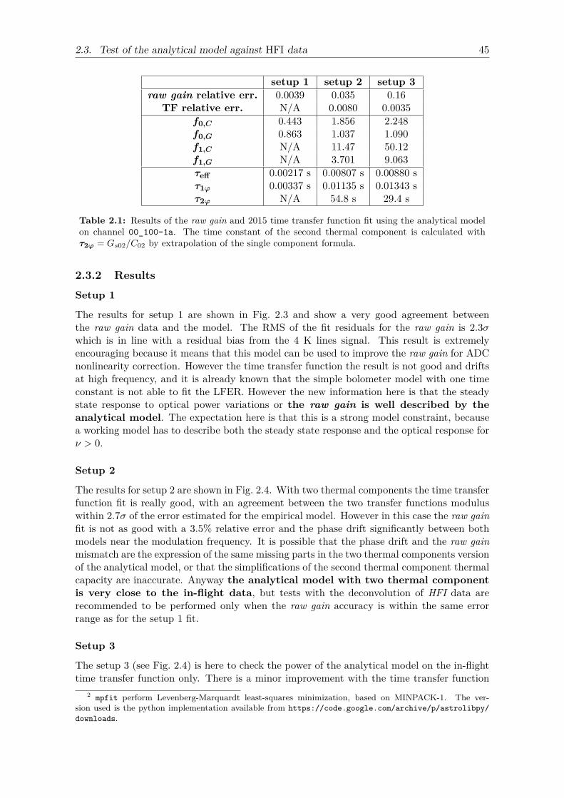
2.3. Test of the analytical model against HFI data 45
setup 1 setup 2 setup 3raw gain relative err. 0.0039 0.035 0.16
TF relative err. N/A 0.0080 0.0035f0,C 0.443 1.856 2.248f0,G 0.863 1.037 1.090f1,C N/A 11.47 50.12f1,G N/A 3.701 9.063τeff 0.00217 s 0.00807 s 0.00880 sτ1ϕ 0.00337 s 0.01135 s 0.01343 sτ2ϕ N/A 54.8 s 29.4 s
Table 2.1: Results of the raw gain and 2015 time transfer function fit using the analytical modelon channel 00_100-1a. The time constant of the second thermal component is calculated withτ2ϕ = Gs02/C02 by extrapolation of the single component formula.
2.3.2 Results
Setup 1
The results for setup 1 are shown in Fig. 2.3 and show a very good agreement betweenthe raw gain data and the model. The RMS of the fit residuals for the raw gain is 2.3σwhich is in line with a residual bias from the 4 K lines signal. This result is extremelyencouraging because it means that this model can be used to improve the raw gain for ADCnonlinearity correction. However the time transfer function the result is not good and driftsat high frequency, and it is already known that the simple bolometer model with one timeconstant is not able to fit the LFER. However the new information here is that the steadystate response to optical power variations or the raw gain is well described by theanalytical model. The expectation here is that this is a strong model constraint, becausea working model has to describe both the steady state response and the optical response forν > 0.
Setup 2
The results for setup 2 are shown in Fig. 2.4. With two thermal components the time transferfunction fit is really good, with an agreement between the two transfer functions moduluswithin 2.7σ of the error estimated for the empirical model. However in this case the raw gainfit is not as good with a 3.5% relative error and the phase drift significantly between bothmodels near the modulation frequency. It is possible that the phase drift and the raw gainmismatch are the expression of the same missing parts in the two thermal components versionof the analytical model, or that the simplifications of the second thermal component thermalcapacity are inaccurate. Anyway the analytical model with two thermal componentis very close to the in-flight data, but tests with the deconvolution of HFI data arerecommended to be performed only when the raw gain accuracy is within the same errorrange as for the setup 1 fit.
Setup 3
The setup 3 (see Fig. 2.4) is here to check the power of the analytical model on the in-flighttime transfer function only. There is a minor improvement with the time transfer function
2 mpfit perform Levenberg-Marquardt least-squares minimization, based on MINPACK-1. The ver-sion used is the python implementation available from https://code.google.com/archive/p/astrolibpy/downloads.
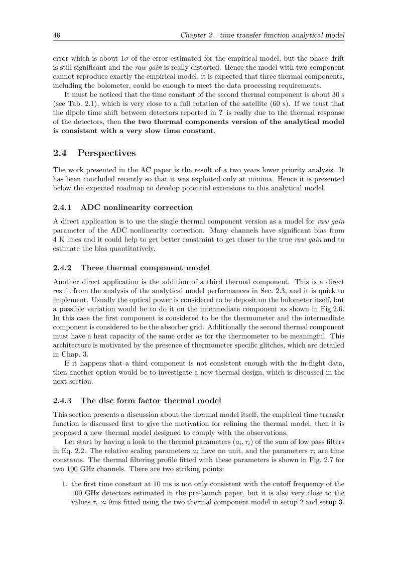
46 Chapter 2. time transfer function analytical model
error which is about 1σ of the error estimated for the empirical model, but the phase driftis still significant and the raw gain is really distorted. Hence the model with two componentcannot reproduce exactly the empirical model, it is expected that three thermal components,including the bolometer, could be enough to meet the data processing requirements.
It must be noticed that the time constant of the second thermal component is about 30 s(see Tab. 2.1), which is very close to a full rotation of the satellite (60 s). If we trust thatthe dipole time shift between detectors reported in ? is really due to the thermal responseof the detectors, then the two thermal components version of the analytical modelis consistent with a very slow time constant.
2.4 PerspectivesThe work presented in the AC paper is the result of a two years lower priority analysis. Ithas been concluded recently so that it was exploited only at minima. Hence it is presentedbelow the expected roadmap to develop potential extensions to this analytical model.
2.4.1 ADC nonlinearity correction
A direct application is to use the single thermal component version as a model for raw gainparameter of the ADC nonlinearity correction. Many channels have significant bias from4 K lines and it could help to get better constraint to get closer to the true raw gain and toestimate the bias quantitatively.
2.4.2 Three thermal component model
Another direct application is the addition of a third thermal component. This is a directresult from the analysis of the analytical model performances in Sec. 2.3, and it is quick toimplement. Usually the optical power is considered to be deposit on the bolometer itself, buta possible variation would be to do it on the intermediate component as shown in Fig.2.6.In this case the first component is considered to be the thermometer and the intermediatecomponent is considered to be the absorber grid. Additionally the second thermal componentmust have a heat capacity of the same order as for the thermometer to be meaningful. Thisarchitecture is motivated by the presence of thermometer specific glitches, which are detailedin Chap. 3.
If it happens that a third component is not consistent enough with the in-flight data,then another option would be to investigate a new thermal design, which is discussed in thenext section.
2.4.3 The disc form factor thermal model
This section presents a discussion about the thermal model itself, the empirical time transferfunction is discussed first to give the motivation for refining the thermal model, then it isproposed a new thermal model designed to comply with the observations.
Let start by having a look to the thermal parameters (ai, τi) of the sum of low pass filtersin Eq. 2.2. The relative scaling parameters ai have no unit, and the parameters τi are timeconstants. The thermal filtering profile fitted with these parameters is shown in Fig. 2.7 fortwo 100 GHz channels. There are two striking points:
1. the first time constant at 10 ms is not only consistent with the cutoff frequency of the100 GHz detectors estimated in the pre-launch paper, but it is also very close to thevalues τe ≈ 9ms fitted using the two thermal component model in setup 2 and setup 3.
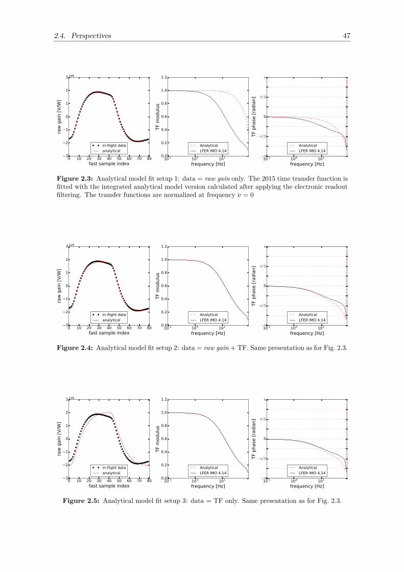
2.4. Perspectives 47
0 10 20 30 40 50 60 70 80
fast sample index
3
2
1
0
1
2
3
raw
gain
[V
/W]
1e9
in-flight data
analytical
10-1 100 101
frequency [Hz]
0.0
0.2
0.4
0.6
0.8
1.0
1.2
TF
modulu
s
Analytical
LFER IMO 4.14
10-1 100 101
frequency [Hz]
−π
−π/2
0
π/2
π
TF
phase
[ra
dia
n]
Analytical
LFER IMO 4.14
Figure 2.3: Analytical model fit setup 1: data = raw gain only. The 2015 time transfer function isfitted with the integrated analytical model version calculated after applying the electronic readoutfiltering. The transfer functions are normalized at frequency ν = 0
0 10 20 30 40 50 60 70 80
fast sample index
3
2
1
0
1
2
3
raw
gain
[V
/W]
1e9
in-flight data
analytical
10-1 100 101
frequency [Hz]
0.0
0.2
0.4
0.6
0.8
1.0
1.2
TF
modulu
s
Analytical
LFER IMO 4.14
10-1 100 101
frequency [Hz]
−π
−π/2
0
π/2
π
TF
phase
[ra
dia
n]
Analytical
LFER IMO 4.14
Figure 2.4: Analytical model fit setup 2: data = raw gain + TF. Same presentation as for Fig. 2.3.
0 10 20 30 40 50 60 70 80
fast sample index
3
2
1
0
1
2
3
raw
gain
[V
/W]
1e9
in-flight data
analytical
10-1 100 101
frequency [Hz]
0.0
0.2
0.4
0.6
0.8
1.0
1.2
TF
modulu
s
Analytical
LFER IMO 4.14
10-1 100 101
frequency [Hz]
−π
−π/2
0
π/2
π
TF
phase
[ra
dia
n]
Analytical
LFER IMO 4.14
Figure 2.5: Analytical model fit setup 3: data = TF only. Same presentation as for Fig. 2.3.
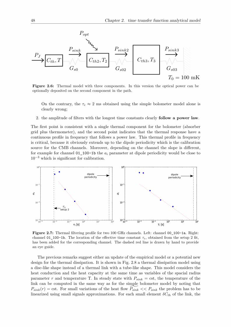
48 Chapter 2. time transfer function analytical model
Figure 2.6: Thermal model with three components. In this version the optical power can beoptionally deposited on the second component in the path.
On the contrary, the τe ≈ 2 ms obtained using the simple bolometer model alone isclearly wrong;
2. the amplitude of filters with the longest time constants clearly follow a power law.
The first point is consistent with a single thermal component for the bolometer (absorbergrid plus thermometer), and the second point indicates that the thermal response have acontinuous profile in frequency that follows a power law. This thermal profile in frequencyis critical, because it obviously extends up to the dipole periodicity which is the calibrationsource for the CMB channels. Moreover, depending on the channel the slope is different,for example for channel 01_100-1b the ai parameter at dipole periodicity would be close to10−3 which is significant for calibration.
setup 2
Figure 2.7: Thermal filtering profile for two 100 GHz channels. Left: channel 00_100-1a. Right:channel 01_100-1b. The location of the effective time constant τe, obtained from the setup 2 fit,has been added for the corresponding channel. The dashed red line is drawn by hand to providean eye guide.
The previous remarks suggest either an update of the empirical model or a potential newdesign for the thermal dissipation. It is shown in Fig. 2.8 a thermal dissipation model usinga disc-like shape instead of a thermal link with a tube-like shape. This model considers theheat conduction and the heat capacity at the same time as variables of the spacial radiusparameter r and temperature T. In steady state with Psink = cst, the temperature of thelink can be computed in the same way as for the simple bolometer model by noting thatPsink(r) = cst. For small variations of the heat flow Psink << Psink the problem has to belinearized using small signals approximations. For each small element δCth of the link, the
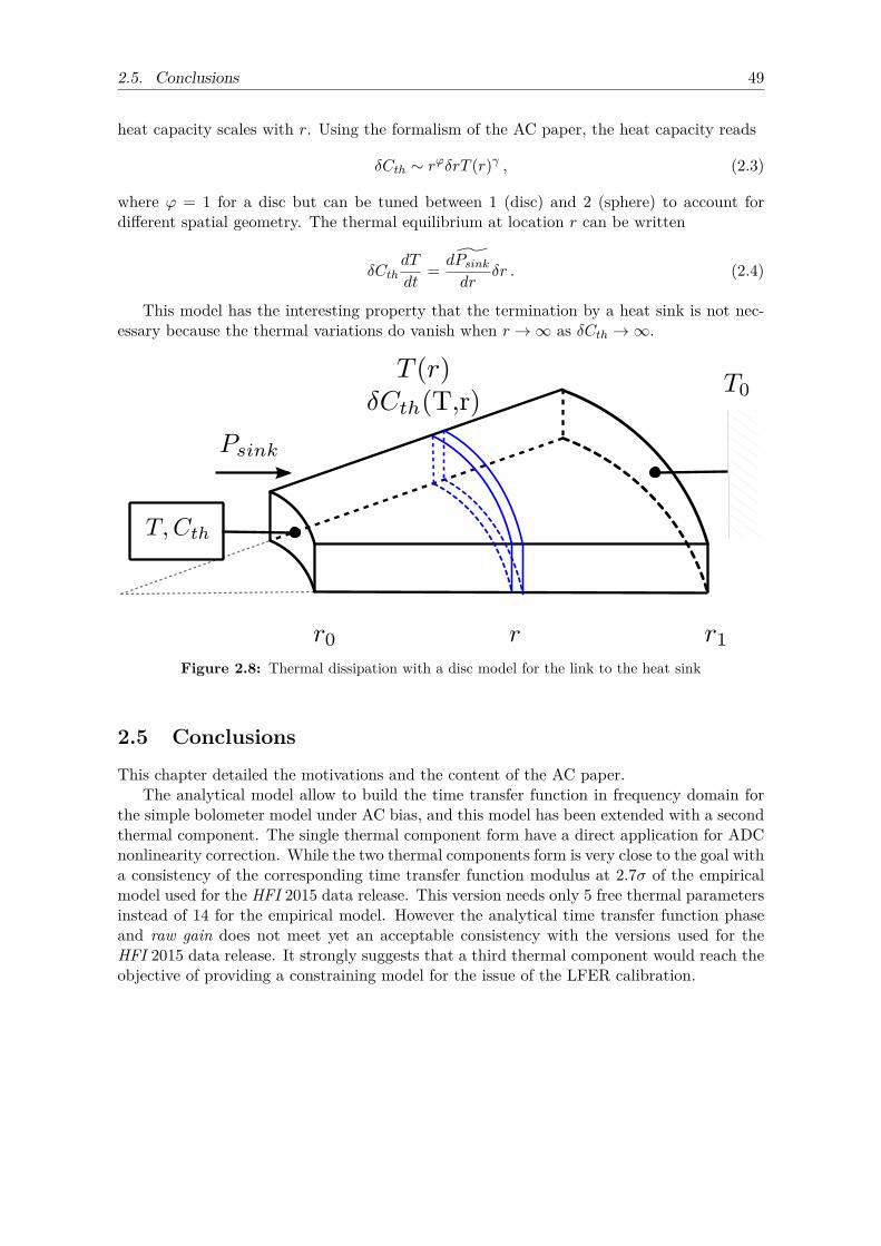
2.5. Conclusions 49
heat capacity scales with r. Using the formalism of the AC paper, the heat capacity reads
δCth ∼ rϕδrT (r)γ , (2.3)
where ϕ = 1 for a disc but can be tuned between 1 (disc) and 2 (sphere) to account fordifferent spatial geometry. The thermal equilibrium at location r can be written
δCthdT
dt= dPsink
drδr . (2.4)
This model has the interesting property that the termination by a heat sink is not nec-essary because the thermal variations do vanish when r →∞ as δCth →∞.
Figure 2.8: Thermal dissipation with a disc model for the link to the heat sink
2.5 ConclusionsThis chapter detailed the motivations and the content of the AC paper.
The analytical model allow to build the time transfer function in frequency domain forthe simple bolometer model under AC bias, and this model has been extended with a secondthermal component. The single thermal component form have a direct application for ADCnonlinearity correction. While the two thermal components form is very close to the goal witha consistency of the corresponding time transfer function modulus at 2.7σ of the empiricalmodel used for the HFI 2015 data release. This version needs only 5 free thermal parametersinstead of 14 for the empirical model. However the analytical time transfer function phaseand raw gain does not meet yet an acceptable consistency with the versions used for theHFI 2015 data release. It strongly suggests that a third thermal component would reach theobjective of providing a constraining model for the issue of the LFER calibration.


51
Chapter 3
Glitches exploitation
Susceptibility to cosmic rays energy deposit is inherent to high sensitivity bolometers andthe energy they deposit on the various part of the detector produce glitches on the measuredsignal. In practice this is a nuisance leading to non-Gaussian noise and loss of data. Howeverthese pretty unwanted residuals for some can become gold for others. In the case of glitchestheir high statistics and the stationarity in their characteristics is a great tool providingimportant constraints for time transfer function characterization and calibration. Usuallyglitches are phase-shifted to be compared to the time transfer function (e.g. see Fig. 10 in?). Below the contrary will be discussed, i.e. how the glitches can be used to produce thetime transfer function.
Sec. 3.1 introduces the topic of glitches, from their origin to their characterization, andhow they are related to the time transfer function. Then in Sec. 3.2, I present a methodto build glitch templates homogeneous with the time transfer function. Finally in Sec. 3.3direct applications of the glitch templates are shown.
The work presented below has been used to validate the empirical time transfer functionLFER model (see Sec. 2 in ?) and provided contents for two other papers which are: ?, andits companion paper ?.
3.1 IntroductionGlitches origin
Cosmic rays deposit energy on the 0.1 K stage detectors which is visible on the acquireddata as glitches. The spacecraft operates at the second Lagrangian point where the dominantpopulation of particles reaching the detectors is protons of energy > 39 MeV (?). The typicalrate of glitches on a detector is about one event per second, with various characteristicsdepending on the physical location of the energy deposit.
Glitches follow closely the rate of particles measured by the Standard Radiation EventMonitor (SREM, see ?). In the HFI instrument, the glitch rate is unexpectedly high becauseof the high sensitivity design of the detectors. Furthermore, it happened that the beginningof the Planck mission corresponded to the minimum of the 11-years cycle of solar activity,as shown in Fig. 3.1. As a consequence, the proton rate from Galactic sources which ismodulated by the solar activity (?) was at its maximum.
Characterization of the glitch families
The location of energy deposit produces glitches with different shapes, which can be classifiedwith the time constants of the relaxation visible after the event. Two examples are shown inFig. 3.2: one short glitch and one long glitch in the sense of the amount of time necessaryfor the relaxation after the transient event.
The classification of glitches into families is critical, because some events have a longrelaxation time leaving low frequency noise on science data. Hence individual events needs
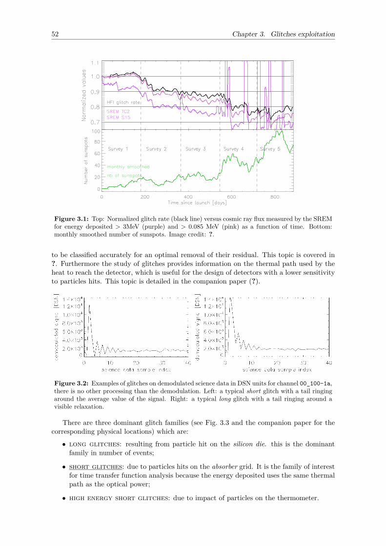
52 Chapter 3. Glitches exploitation
Planck Collaboration: Planck 2013 results. X.
10
010
1
10-4 10-3 10-2 10-1
k [arcmin-1]
Rin
g no
ise
P(k)
(arb
itrar
y un
its) 143-2a
10
010
1
10-4 10-3 10-2 10-1
k [arcmin-1]
Rin
g no
ise
P(k)
(arb
itrar
y un
its) 143-5
Fig. 16. Estimation of the power spectra of noise residuals after averaging data on rings for the 143-2a bolometer (left) and the 143-5 bolometer(right). Power spectra are averaged over 10 000 rings and are computed after removing the input simulated signal from the simulated data andusing the estimated flags. The dot-dashed curve is the result without subtraction of long glitch tails, while the solid curve is with subtraction asdone for the real data, and the dashed curve is for the same simulations but without glitches. Residual glitches are significantly reduced aftertemplate subtraction.
Fig. 17. Mean rate of the three categories of glitches, i.e., long, short,and slow. These rates are computed using all 52 bolometers for long andshort glitches, and the 16 PSB-a bolometers for slow glitches.
above 10 in six months (right panel of Fig. 19). Clearly, all thebolometer glitch distributions exhibit Poisson behaviour. Theseparticular data are from Survey 3 when the glitch rate was rela-tively constant and events above 10 were selected to avoid anycontamination by false events, solar flares, and pile-up. We can-not check multiple simultaneous events because we cannot dis-tinguish between a pile-up of multiple events and a single moreenergetic event. Still, the glitch data are compatible with purerandom events that are not correlated in time and this is consis-tent with the cause of events being individual hits by Galacticcosmic ray particles.
We also studied the coincidence of events between bolome-ters. We found that the largest fraction of coincidences,around 99%, are between PSB-a and PSB-b detector pairs in thesame module (see below). The remaining roughly 1% of coinci-dences are particle shower events that e↵ect a large fraction ofthe detectors in the focal plane in di↵erent modules (the showerevents will be discussed in Sect. 5.7).
Fig. 18. Top: normalized glitch rate (black line), cosmic ray flux mea-sured by the SREM for deposited energy E > 3 MeV (purple), and E >0.085 MeV (pink), as a function of time. Bottom: monthly smoothednumber of sunspots.
5.3. Interaction with the grid/thermistors
There is clear evidence that the short events result from cosmicrays hitting the grid or the thermistor. Indeed, these events havea fast rise time and have a fast decay, and the transfer functionbuilt from the short glitch template (see Catalano et al. 2014, fora comparison) is in good agreement with the HFI optical transferfunction (Planck Collaboration VII 2014), so the energy must bedeposited in the environment close to the thermistor. Figure 20shows the cumulative counts, i.e., the number of events N(>E)with an amplitude higher than a given value E per hour, for shortglitches, after converting the maximum amplitude of each glitchto units of energy (keV) for one reference bolometer (100-1b).The energy calibration for the other bolometers has been scaledso that the cumulative distributions match the one for the refer-ence bolometer at energies of about 10 keV. For this conversionwe use the measured heat capacity of the NTD crystal plus gridsystem (see Holmes et al. 2008), since we assume that the energyof the events is deposited in this system. The relative fitting ofthe energy is necessary for the comparison between bolometers
A10, page 13 of 23
Figure 3.1: Top: Normalized glitch rate (black line) versus cosmic ray flux measured by the SREMfor energy deposited > 3MeV (purple) and > 0.085 MeV (pink) as a function of time. Bottom:monthly smoothed number of sunspots. Image credit: ?.
to be classified accurately for an optimal removal of their residual. This topic is covered in?. Furthermore the study of glitches provides information on the thermal path used by theheat to reach the detector, which is useful for the design of detectors with a lower sensitivityto particles hits. This topic is detailed in the companion paper (?).
Figure 3.2: Examples of glitches on demodulated science data in DSN units for channel 00_100-1a,there is no other processing than the demodulation. Left: a typical short glitch with a tail ringingaround the average value of the signal. Right: a typical long glitch with a tail ringing around avisible relaxation.
There are three dominant glitch families (see Fig. 3.3 and the companion paper for thecorresponding physical locations) which are:
• long glitches: resulting from particle hit on the silicon die. this is the dominantfamily in number of events;
• short glitches: due to particles hits on the absorber grid. It is the family of interestfor time transfer function analysis because the energy deposited uses the same thermalpath as the optical power;
• high energy short glitches: due to impact of particles on the thermometer.
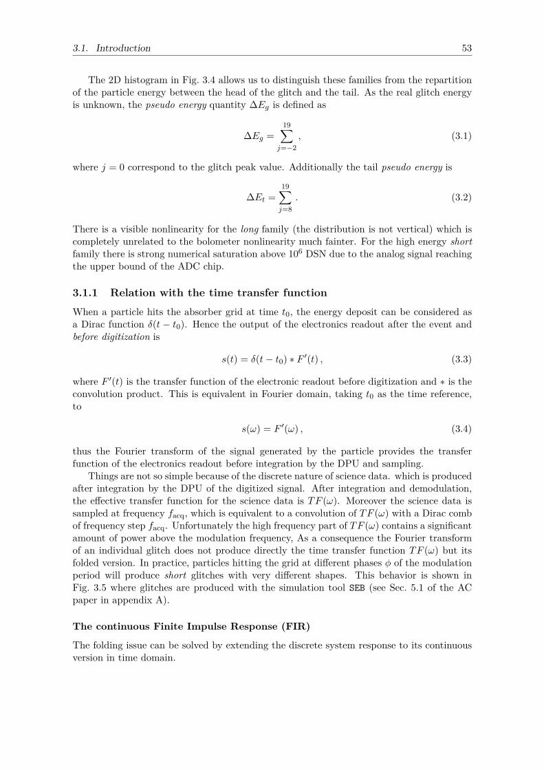
3.1. Introduction 53
The 2D histogram in Fig. 3.4 allows us to distinguish these families from the repartitionof the particle energy between the head of the glitch and the tail. As the real glitch energyis unknown, the pseudo energy quantity ∆Eg is defined as
∆Eg =19∑
j=−2, (3.1)
where j = 0 correspond to the glitch peak value. Additionally the tail pseudo energy is
∆Et =19∑j=8
. (3.2)
There is a visible nonlinearity for the long family (the distribution is not vertical) which iscompletely unrelated to the bolometer nonlinearity much fainter. For the high energy shortfamily there is strong numerical saturation above 106 DSN due to the analog signal reachingthe upper bound of the ADC chip.
3.1.1 Relation with the time transfer function
When a particle hits the absorber grid at time t0, the energy deposit can be considered asa Dirac function δ(t − t0). Hence the output of the electronics readout after the event andbefore digitization is
s(t) = δ(t− t0) ∗ F ′(t) , (3.3)
where F ′(t) is the transfer function of the electronic readout before digitization and ∗ is theconvolution product. This is equivalent in Fourier domain, taking t0 as the time reference,to
s(ω) = F ′(ω) , (3.4)
thus the Fourier transform of the signal generated by the particle provides the transferfunction of the electronics readout before integration by the DPU and sampling.
Things are not so simple because of the discrete nature of science data. which is producedafter integration by the DPU of the digitized signal. After integration and demodulation,the effective transfer function for the science data is TF (ω). Moreover the science data issampled at frequency facq, which is equivalent to a convolution of TF (ω) with a Dirac combof frequency step facq. Unfortunately the high frequency part of TF (ω) contains a significantamount of power above the modulation frequency, As a consequence the Fourier transformof an individual glitch does not produce directly the time transfer function TF (ω) but itsfolded version. In practice, particles hitting the grid at different phases φ of the modulationperiod will produce short glitches with very different shapes. This behavior is shown inFig. 3.5 where glitches are produced with the simulation tool SEB (see Sec. 5.1 of the ACpaper in appendix A).
The continuous Finite Impulse Response (FIR)
The folding issue can be solved by extending the discrete system response to its continuousversion in time domain.
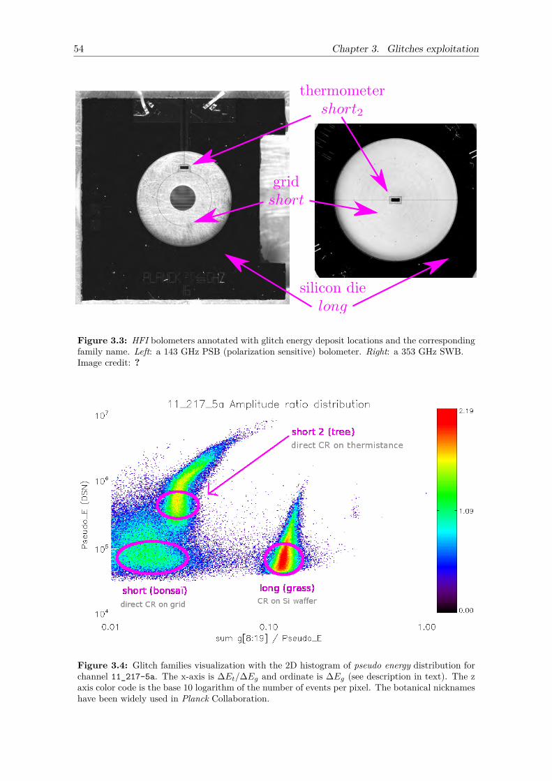
54 Chapter 3. Glitches exploitation
Figure 3.3: HFI bolometers annotated with glitch energy deposit locations and the correspondingfamily name. Left: a 143 GHz PSB (polarization sensitive) bolometer. Right: a 353 GHz SWB.Image credit: ?
Figure 3.4: Glitch families visualization with the 2D histogram of pseudo energy distribution forchannel 11_217-5a. The x-axis is ∆Et/∆Eg and ordinate is ∆Eg (see description in text). The zaxis color code is the base 10 logarithm of the number of events per pixel. The botanical nicknameshave been widely used in Planck Collaboration.
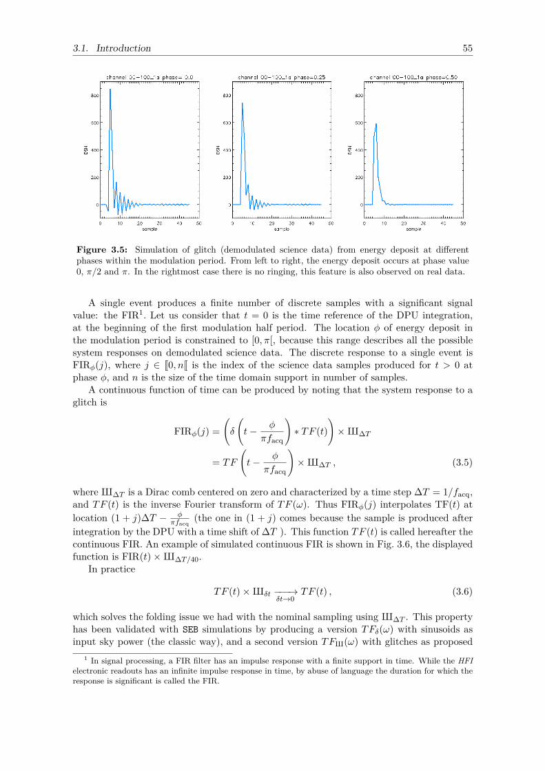
3.1. Introduction 55
Figure 3.5: Simulation of glitch (demodulated science data) from energy deposit at differentphases within the modulation period. From left to right, the energy deposit occurs at phase value0, π/2 and π. In the rightmost case there is no ringing, this feature is also observed on real data.
A single event produces a finite number of discrete samples with a significant signalvalue: the FIR1. Let us consider that t = 0 is the time reference of the DPU integration,at the beginning of the first modulation half period. The location φ of energy deposit inthe modulation period is constrained to [0, π[, because this range describes all the possiblesystem responses on demodulated science data. The discrete response to a single event isFIRφ(j), where j ∈ J0, nJ is the index of the science data samples produced for t > 0 atphase φ, and n is the size of the time domain support in number of samples.
A continuous function of time can be produced by noting that the system response to aglitch is
FIRφ(j) =(δ
(t− φ
πfacq
)∗ TF (t)
)×X∆T
= TF
(t− φ
πfacq
)×X∆T , (3.5)
where X∆T is a Dirac comb centered on zero and characterized by a time step ∆T = 1/facq,and TF (t) is the inverse Fourier transform of TF (ω). Thus FIRφ(j) interpolates TF(t) atlocation (1 + j)∆T − φ
πfacq(the one in (1 + j) comes because the sample is produced after
integration by the DPU with a time shift of ∆T ). This function TF (t) is called hereafter thecontinuous FIR. An example of simulated continuous FIR is shown in Fig. 3.6, the displayedfunction is FIR(t)×X∆T/40.
In practice
TF (t)×Xδt −−−→δt→0
TF (t) , (3.6)
which solves the folding issue we had with the nominal sampling using X∆T . This propertyhas been validated with SEB simulations by producing a version TFδ(ω) with sinusoids asinput sky power (the classic way), and a second version TFX(ω) with glitches as proposed
1 In signal processing, a FIR filter has an impulse response with a finite support in time. While the HFIelectronic readouts has an infinite impulse response in time, by abuse of language the duration for which theresponse is significant is called the FIR.
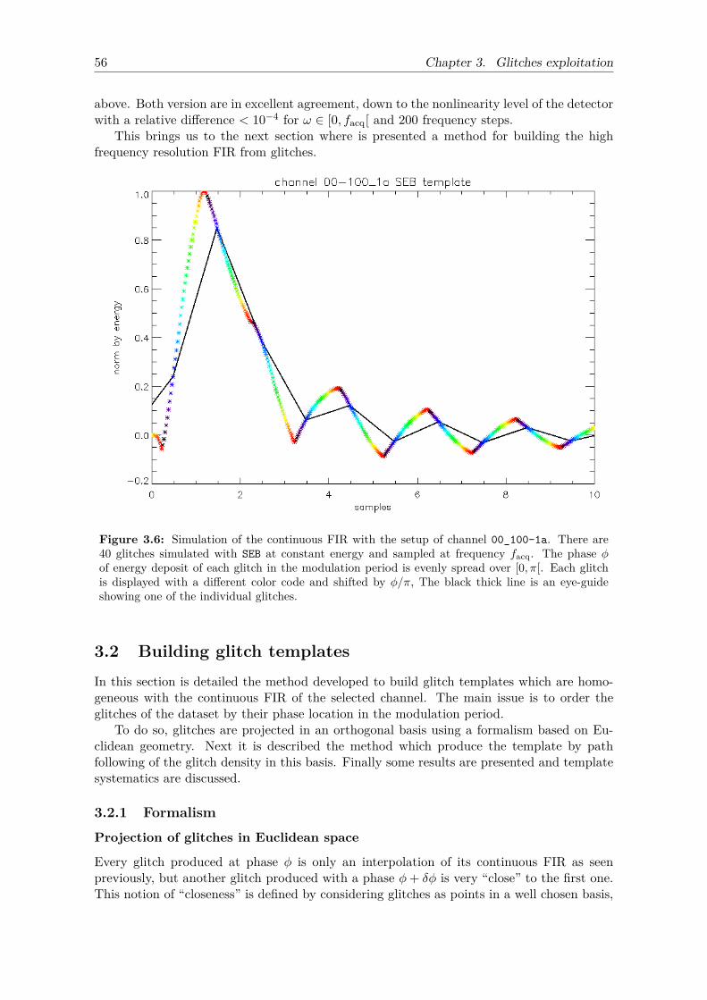
56 Chapter 3. Glitches exploitation
above. Both version are in excellent agreement, down to the nonlinearity level of the detectorwith a relative difference < 10−4 for ω ∈ [0, facq[ and 200 frequency steps.
This brings us to the next section where is presented a method for building the highfrequency resolution FIR from glitches.
Figure 3.6: Simulation of the continuous FIR with the setup of channel 00_100-1a. There are40 glitches simulated with SEB at constant energy and sampled at frequency facq. The phase φof energy deposit of each glitch in the modulation period is evenly spread over [0, π[. Each glitchis displayed with a different color code and shifted by φ/π, The black thick line is an eye-guideshowing one of the individual glitches.
3.2 Building glitch templatesIn this section is detailed the method developed to build glitch templates which are homo-geneous with the continuous FIR of the selected channel. The main issue is to order theglitches of the dataset by their phase location in the modulation period.
To do so, glitches are projected in an orthogonal basis using a formalism based on Eu-clidean geometry. Next it is described the method which produce the template by pathfollowing of the glitch density in this basis. Finally some results are presented and templatesystematics are discussed.
3.2.1 Formalism
Projection of glitches in Euclidean space
Every glitch produced at phase φ is only an interpolation of its continuous FIR as seenpreviously, but another glitch produced with a phase φ+ δφ is very “close” to the first one.This notion of “closeness” is defined by considering glitches as points in a well chosen basis,
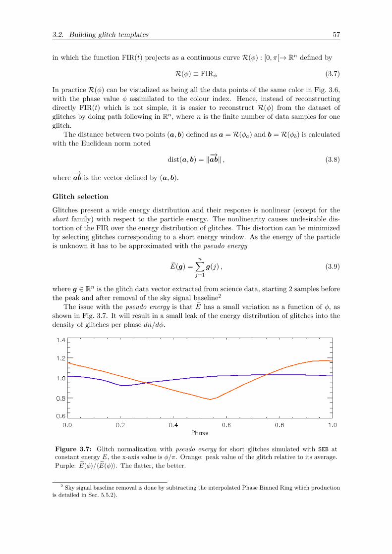
3.2. Building glitch templates 57
in which the function FIR(t) projects as a continuous curve R(φ) : [0, π[→ Rn defined by
R(φ) ≡ FIRφ (3.7)
In practice R(φ) can be visualized as being all the data points of the same color in Fig. 3.6,with the phase value φ assimilated to the colour index. Hence, instead of reconstructingdirectly FIR(t) which is not simple, it is easier to reconstruct R(φ) from the dataset ofglitches by doing path following in Rn, where n is the finite number of data samples for oneglitch.
The distance between two points (a, b) defined as a = R(φa) and b = R(φb) is calculatedwith the Euclidean norm noted
dist(a, b) = ‖−→ab‖ , (3.8)
where −→ab is the vector defined by (a, b).
Glitch selection
Glitches present a wide energy distribution and their response is nonlinear (except for theshort family) with respect to the particle energy. The nonlinearity causes undesirable dis-tortion of the FIR over the energy distribution of glitches. This distortion can be minimizedby selecting glitches corresponding to a short energy window. As the energy of the particleis unknown it has to be approximated with the pseudo energy
E(g) =n∑j=1g(j) , (3.9)
where g ∈ Rn is the glitch data vector extracted from science data, starting 2 samples beforethe peak and after removal of the sky signal baseline2
The issue with the pseudo energy is that E has a small variation as a function of φ, asshown in Fig. 3.7. It will result in a small leak of the energy distribution of glitches into thedensity of glitches per phase dn/dφ.
Figure 3.7: Glitch normalization with pseudo energy for short glitches simulated with SEB atconstant energy E, the x-axis value is φ/π. Orange: peak value of the glitch relative to its average.Purple: E(φ)/〈E(φ)〉. The flatter, the better.
2 Sky signal baseline removal is done by subtracting the interpolated Phase Binned Ring which productionis detailed in Sec. 5.5.2).
58 Chapter 3. Glitches exploitation
Glitch normalization
Because of the wide energy distribution of glitches, even after selection of a small energywindow, the dataset of glitches in Rn does not form a compact curve. Instead it is rather aribbon-like surface parametrized with (φ,E), where E is the real amount of energy depositedby the particle.
The pseudo energy normalization cannot be used here, because it will boost the noise toomuch. Instead, the normalization by peak can be used for the purpose of building a compactcurve in Rn. Let us consider a dataset of glitches gi , i ∈ J1,mK. For a given glitch
gi = E ×R(φi) , (3.10)
where φi is the unknown phase location in the modulation period where the particle depositedenergy.
In practice glitch are extracted from data after peak detection and the peak is alwayslocated at index 2 of the vector gi. The glitch peak value is gi(2) = E×FIR((2+φi/2π)/facq)The normalized glitch expression is
gi = R(φi)FIR ((2 + φi/2π)/facq)
= T (φi) , (3.11)
where T (φ) is the glitch template corresponding to the peak-normalized version of R(φ).The normalized dataset gi achieves the goal of providing a compact parametric function
of φ, even if the template produced by path following within the normalized dataset will haveto be renormalized with pseudo energy.
Noise radius
The noise of the data samples of one glitch gi is σi = σ/max(|gi|), where σ is the TOI noisewhich is considered as white and stationary in time. In Rn the noise has a χ2 distributioncentred on the true location of the glitch T (φi). Half of the noise distribution is containedin a n-sphere of radius rσ. The value of rσ is called the noise radius and is calculated withthe median of a χ2 distribution. When considering a dataset gi the normalization is donewith the median of glitch amplitude, thus the noise radius of the dataset is
rσ = σ√n− 2/3
median(max(|gi|)). (3.12)
Using the median instead of the mean is necessary with a dataset subject to outliers.In practice the noisy dataset is called the glitch cloud and its distribution is the convo-
lution product of the glitch template T (φ) and the χ2 distribution of the noise. It has atube-like shape in Rn. Hence, it is important to consider a short energy window for glitchselection to have homogeneous noise properties over the dataset gi.
Visualization of the glitch cloud
As the cloud of glitches is in Rn it has to be projected in 2 dimensions for visualization. Forthis purpose a projection axis
(go,−→ex)is defined by choosing an origin go and a direction
represented by the unit vector −→ex. The x-axis value x for a glitch g is defined as the distancebetween its orthogonal projection g⊥ on the axis to the origin, and the y-axis value y is
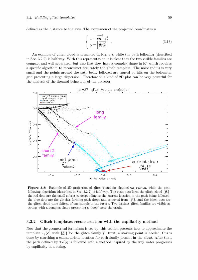
3.2. Building glitch templates 59
defined as the distance to the axis. The expression of the projected coordinates isx =−−→og⊥.−→ex
y =∥∥∥∥−−→g⊥i gi∥∥∥∥ , (3.13)
An example of glitch cloud is presented in Fig. 3.8, while the path following (describedin Sec. 3.2.2) is half way. With this representation it is clear that the two visible families arecompact and well separated, but also that they have a complex shape in Rn which requiresa specific algorithm to reconstruct accurately the glitch template. The noise radius is verysmall and the points around the path being followed are caused by hits on the bolometergrid presenting a large dispersion. Therefore this kind of 2D plot can be very powerful forthe analysis of the thermal behaviour of the detector.
short 2family
longfamily
Figure 3.8: Example of 2D projection of glitch cloud for channel 02_143-2a, while the pathfollowing algorithm (described in Sec. 3.2.2) is half way. The cyan dots form the glitch cloud gi,the red dots are the small subset corresponding to the current location in the path being followed,the blue dots are the glitches forming path drops and removed from gi, and the black dots arethe glitch cloud time-shifted of one sample in the future. Two distinct glitch families are visible asstrings with a complex shape presenting a “loop” near the origin.
3.2.2 Glitch templates reconstruction with the capillarity method
Now that the geometrical formalism is set up, this section presents how to approximate thetemplate Tf (φ) with gi for the glitch family f . First, a starting point is needed, this isdone by searching a characteristic location for each family present in the cloud. After that,the path defined by Tf (φ) is followed with a method inspired by the way water progressesby capillarity in a string.
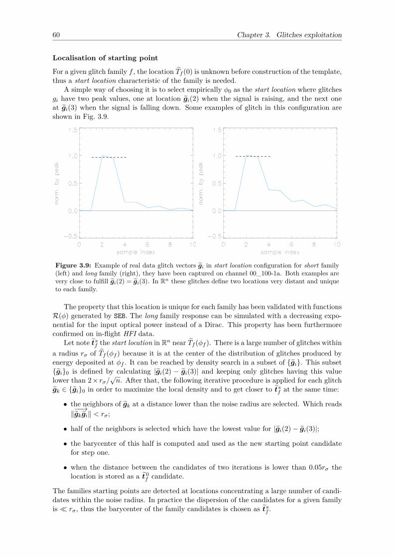
60 Chapter 3. Glitches exploitation
Localisation of starting point
For a given glitch family f , the location Tf (0) is unknown before construction of the template,thus a start location characteristic of the family is needed.
A simple way of choosing it is to select empirically φ0 as the start location where glitchesgi have two peak values, one at location gi(2) when the signal is raising, and the next oneat gi(3) when the signal is falling down. Some examples of glitch in this configuration areshown in Fig. 3.9.
Figure 3.9: Example of real data glitch vectors gi in start location configuration for short family(left) and long family (right), they have been captured on channel 00_100-1a. Both examples arevery close to fulfill gi(2) = gi(3). In Rn these glitches define two locations very distant and uniqueto each family.
The property that this location is unique for each family has been validated with functionsR(φ) generated by SEB. The long family response can be simulated with a decreasing expo-nential for the input optical power instead of a Dirac. This property has been furthermoreconfirmed on in-flight HFI data.
Let note t sf the start location in Rn near Tf (φf ). There is a large number of glitches within
a radius rσ of Tf (φf ) because it is at the center of the distribution of glitches produced byenergy deposited at φf . It can be reached by density search in a subset of gi. This subsetgi0 is defined by calculating |gi(2) − gi(3)| and keeping only glitches having this valuelower than 2× rσ/
√n. After that, the following iterative procedure is applied for each glitch
gk ∈ gi0 in order to maximize the local density and to get closer to t sf at the same time:
• the neighbors of gk at a distance lower than the noise radius are selected. Which reads‖−−→gkgi‖ < rσ;
• half of the neighbors is selected which have the lowest value for |gi(2)− gi(3)|;
• the barycenter of this half is computed and used as the new starting point candidatefor step one.
• when the distance between the candidates of two iterations is lower than 0.05rσ thelocation is stored as a t 0
f candidate.
The families starting points are detected at locations concentrating a large number of candi-dates within the noise radius. In practice the dispersion of the candidates for a given familyis rσ, thus the barycenter of the family candidates is chosen as t s
f .
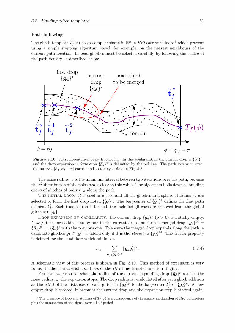
3.2. Building glitch templates 61
Path following
The glitch template Tf (φ) has a complex shape in Rn in HFI case with loops3 which preventusing a simple stepping algorithm based, for example, on the nearest neighbours of thecurrent path location. Instead glitches must be selected carefully by following the centre ofthe path density as described below.
Figure 3.10: 2D representation of path following. In this configuration the current drop is gd1
and the drop expansion in formation gd2 is delimited by the red line. The path extension overthe interval [φf , φf + π[ correspond to the cyan dots in Fig. 3.8.
The noise radius rσ is the minimum interval between two iterations over the path, becausethe χ2 distribution of the noise peaks close to this value. The algorithm boils down to buildingdrops of glitches of radius rσ along the path.
The initial drop: t sf is used as a seed and all the glitches in a sphere of radius rσ are
selected to form the first drop noted gd1. The barycenter of gd1 defines the first pathelement t 1
f . Each time a drop is formed, the included glitches are removed from the globalglitch set gi.
Drop expansion by capillarity: the current drop gdp (p > 0) is initially empty.New glitches are added one by one to the current drop and form a merged drop gdM =gdp−1∪gdp with the previous one. To ensure the merged drop expands along the path, acandidate glitches gk ∈ gi is added only if it is the closest to gdM. The closest propertyis defined for the candidate which minimizes
Dk =∑
gq∈gdM
‖−−→gkgq‖2 . (3.14)
A schematic view of this process is shown in Fig. 3.10. This method of expansion is veryrobust to the characteristic stiffness of the HFI time transfer function ringing.
End of expansion: when the radius of the current expanding drop gdp reaches thenoise radius rσ, the expansion stops. The drop radius is recalculated after each glitch additionas the RMS of the distances of each glitch in gdp to the barycenter t pf of gdp. A newempty drop is created, it becomes the current drop and the expansion step is started again.
3 The presence of loop and stiffness of Tf (φ) is a consequence of the square modulation of HFI bolometersplus the summation of the signal over a half period
62 Chapter 3. Glitches exploitation
Termination: the path is complete when the (virtual) end point t ef is reached by the
connection drop gdc, it is detected for ‖−−→t cf t
ef ‖ < 1.5rσ. The end point is calculated from
t sf by applying a time shift of one sample, which correspond to a shift of the vector t sf onthe left (in practice vectors are calculated with a size of n + 1 to have content for the lastvalue after the shift). The last drop gdc+1 is formed as for gd1, but in this case theremaining glitches are shared among the connection drop gdc and the final drop gdc+1.This sharing is realized by comparing the glitches distance to t cf and t c+1
f .The output of the algorithm is the path t s
f , t1f , ..., t
c+1f , t ef , containing approximations
of the glitch template T (φ) at discrete locations for φ monotonously increasing.
3.2.3 Estimation of the continuous FIR
Reconstruction of the continuous FIR
Two operations are needed to produce the time domain glitch template: a phasing of thepoints forming the path, and the renormalization with the pseudo energy.
The phase of each point of the path is unknown but it can be estimated with the glitchstatistic because the distribution of particles is supposed to be random uniform over thevalues taken by φ. Each drop gdp contains np glitches and covers a phase range ∆φp =πnp/nf , where nf = ∑
j np is the number of glitches of the family f . The first (virtual) pointdefines the location φ = 0. The barycenters of all drops are placed at the center of theircorresponding phase interval, thus the phase location φp of a given point of the path t jf is
φp =∑k<p
∆φk + ∆φp2 . (3.15)
The time domain FIR of the family f is produced after renormalization of Tf with thepseudo energy calculated for each phase. Its expression is
FIR(j∆T + φp) =t pf (j)E(t pf )
, (3.16)
with j ∈ J0, nJ and E is calculated with Eq. 3.9.Some examples of functions Tf (t) are shown in Fig. 3.11 after reconstruction of the
continuous FIR for each glitch family of the channel 00_100-1a. The zoom plot on the rightcolumn show the variety of shape for the slow component of the continuous FIR, a very slowrelaxation can be seen for the long family (hence the name).
Bias and uncertainties
The pseudo-E normalization is a major source of error on the continuous FIR reconstructedfrom glitches. As it bias the selection by energy, the glitch density per phase drifts from arandom uniform distribution. Let note εE the standard deviation of E(φ)/〈E(φ)〉 As theglitch distribution scales with ≈ 1/E2 (see Sec. 2.4 of the glitch paper), for εE 1 therelative error on E is ≈ 2εE . In practice εE is about 3%, this will introduce an error on thephase of about 6%. It can in theory be significantly reduced by applying a correction factorcalculated from simulations.
The noise spread signal by convolving R(φ) with the χ2 distribution. This effect canbe considered to be insignificant for high Signal over Noise Ratio (SNR), obtained by glitchenergy selection. With a high SNR, rσ is smaller and the number of drops becomes greaterthan 40, which corresponds to the fast samples acquisition frequency. Generally 40 drops
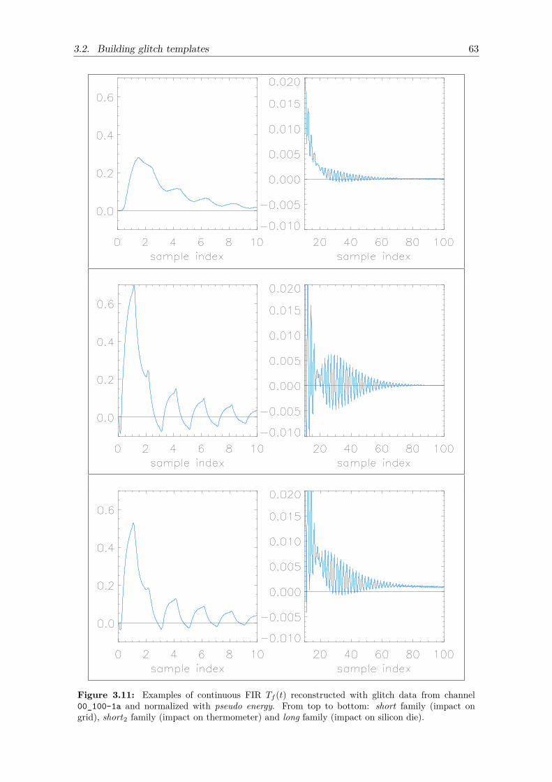
3.2. Building glitch templates 63
Figure 3.11: Examples of continuous FIR Tf (t) reconstructed with glitch data from channel00_100-1a and normalized with pseudo energy. From top to bottom: short family (impact ongrid), short2 family (impact on thermometer) and long family (impact on silicon die).
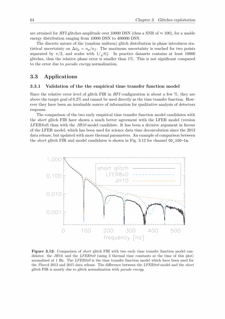
64 Chapter 3. Glitches exploitation
are attained for HFI glitches amplitude over 10000 DSN (thus a SNR of ≈ 100), for a usableenergy distribution ranging from 10000 DSN to 400000 DSN.
The discrete nature of the (random uniform) glitch distribution in phase introduces sta-tistical uncertainty on ∆φp = np/nf . The maximum uncertainty is reached for two pointsseparated by π/2, and scales with 1/√nf . In practice datasets contains at least 10000glitches, thus the relative phase error is smaller than 1%. This is not significant comparedto the error due to pseudo energy normalization.
3.3 Applications
3.3.1 Validation of the the empirical time transfer function model
Since the relative error level of glitch FIR in HFI configuration is about a few %, they areabove the target goal of 0.2% and cannot be used directly as the time transfer function. How-ever they have been an invaluable source of information for qualitative analysis of detectorsresponse.
The comparison of the two early empirical time transfer function model candidates withthe short glitch FIR have shown a much better agreement with the LFER model (versionLFER8v0) than with the JH10 model candidate. It has been a decisive argument in favourof the LFER model, which has been used for science data time deconvolution since the 2013data release, but updated with more thermal parameters. An example of comparison betweenthe short glitch FIR and model candidates is shown in Fig. 3.12 for channel 00_100-1a.
Figure 3.12: Comparison of short glitch FIR with two early time transfer function model can-didates: the JH10, and the LFER8v0 (using 3 thermal time constants at the time of this plot)normalized at 1 Hz. The LFER8v0 is the time transfer function model which have been used forthe Planck 2013 and 2015 data release. The difference between the LFER8v0 model and the shortglitch FIR is mostly due to glitch normalization with pseudo energy.
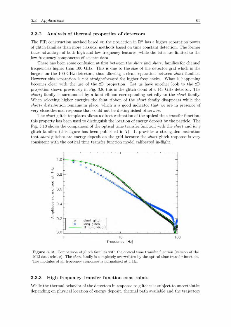
3.3. Applications 65
3.3.2 Analysis of thermal properties of detectors
The FIR construction method based on the projection in Rn has a higher separation powerof glitch families than more classical methods based on time constant detection. The formertakes advantage of both high and low frequency features, while the later are limited to thelow frequency components of science data.
There has been some confusion at first between the short and short2 families for channelfrequencies higher than 100 GHz. This is due to the size of the detector grid which is thelargest on the 100 GHz detectors, thus allowing a clear separation between short families.However this separation is not straightforward for higher frequencies. What is happeningbecomes clear with the use of the 2D projection. Let us have another look to the 2Dprojection shown previously in Fig. 3.8, this is the glitch cloud of a 143 GHz detector. Theshort2 family is surrounded by a faint ribbon corresponding actually to the short family.When selecting higher energies the faint ribbon of the short family disappears while theshort2 distribution remains in place, which is a good indicator that we are in presence ofvery close thermal response that could not be distinguished otherwise.
The short glitch templates allows a direct estimation of the optical time transfer function,this property has been used to distinguish the location of energy deposit by the particle. TheFig. 3.13 shows the comparison of the optical time transfer function with the short and longglitch families (this figure has been published in ?). It provides a strong demonstrationthat short glitches are energy deposit on the grid because the short glitch response is veryconsistent with the optical time transfer function model calibrated in-flight.A. Catalano et al.: Impact of particles on the Planck HFI detectors
Fig. 12. Comparison of the HFI optical transfer function (PlanckCollaboration IV 2011; green line), short-glitch template (black stars),and long-glitch template (blue stars).
found in the comparison between the HFI bolometer electronicstime-response measured on-sky signal (Planck Collaboration IV2011) and the transfer function built from the short-glitch tem-plate (see Fig. 12). The agreement between the transfer func-tion derived from optical measurements (solid green) and shortglitches (black stars) is good, considering that the template isconstructed independently of any model. We can conclude thatthe HFI short glitches are produced by direct interaction ofparticles with one of the absorber grids (or directly with theNTD thermistor for a small subset of them).
6.2. Long glitches
By contrast, the long-glitch template (blue stars in Fig. 12) is notconsistent with the optical transfer function, indicating a di!er-ent physical origin for these glitches.
Two hypotheses have been put forward to explain the manylong glitches seen in HFI flight data: (1) the NTD thermometer issensitive to a change in temperature of other (larger) elements; or(2) long glitches are caused by indirect interaction between CRsand bolometers. From the ground-based tests we determined thatit is not possible to generate enough delta-electrons to reproducethe energy distribution of HFI in-flight long glitches (Fig. 4).On the other hand, we have shown that the NTD thermometeris sensitive to temperature changes of the silicon die. All theground-based tests have confirmed this hypothesis. In addition,the HFI ground-based calibration data show a rate of events com-patible with the CR flux at sea level over the silicon die surface.Starting from these considerations, we developed a toy modelof the impact of CRs with the silicon die in orbit at L2 that canexplain the long-glitch spectrum seen by the Planck HFI duringflight observations. The details of this model are presented inPlanck Collaboration X (2014). These results agree with the re-sults published by the SPIRE collaboration: small co-occurringglitches that are seen simultaneously on many detectors in agiven array in the SPIRE detector timelines, are believed to bedue to ionizing hits on the silicon substrate that supports all thedetectors in an array (Horeau et al. 2012).
The physical interpretation of long glitches can be foundin the shape of the long glitches that we have isolated duringthe ground-based tests. With the improved temporal resolutionmade possible by the faster DC-based REU readout electronicsand sampling, we can clearly see (Fig. 9) the dual time-constantresponse that results from heat transfer between the silicon die
Fig. 13. Raw signal analysis of the silicon die tests: unperturbed rawsignal (black curve). Di!erence between a raw signal with a glitch oc-curred in the center of the half period and the template (blue and redcurves).
and the NTD thermometers. We identify two possible hypothe-ses to explain the heat propagation from the silicon die to theNTD thermometer:
Ionization and thermal diffusion: According to this hypothesis,the faster time-constant is given by ionization within the silicondie. The ionization signal is obtained by the collection of theelectron-hole pairs created by interaction of ! particles in the sil-icon crystal via the gold pad. The long tail can still be explainedby the heat di!usion between the silicon die and the NTD ther-mometers. Using the bolometer parameters, we can determinethe equivalent bias step amplitude needed to produce a glitch ofabout 4 keV (the typical energy absorbed in the bolometer froma hit in the silicon die). We obtain "Ib = 0.2 nA, which is of thesame order as the working bias current. If present, an e!ect asstrong as this should be evident through inspection of the rawTOI signals. In fact, before su#cient time has elapsed for heatdi!usion within the bolometer, a collected charge must show apeak in the raw signal with a decay-time constant determinedonly by the RC time-constant of the individual detector read-out circuitry. The sign of this peak should not change with thechanging polarity of the detector bias current. Therefore, this ef-fect should be easily distinguished from a thermal glitch. The re-sults of this analysis are presented in Fig. 13: in black we show atemplate of the typical unperturbed raw signal set during the test.The red and the blue curves represent the di!erence between araw signal with a glitch (in the center of the half periods) and thetemplate. There is no evidence of ionization in the raw signals;all the glitches can be fully explained by pure thermal events(i.e., hot and/or cold phonons).
Ballistic phonon propagation and thermal diffusion:According to this hypothesis, the faster time-constant, whichcorresponds to the typical time-constant of the bolometers asmeasured with optical sources in ground- and flight-calibrationtesting, can be explained by ballistic phonon heat conduction:6in our case, ballistic phonons can propagate unhindered from thesilicon die and up the grid legs, depending on the geometricalcoupling fixed by the size and the number of the legs. The finale!ect is equivalent to a particle absorbed directly in the grid.
6 Ballistic conduction is the unimpeded flow of energy that carriescharges over large distances within a material.
A88, page 9 of 11
Figure 3.13: Comparison of glitch families with the optical time transfer function (version of the2013 data release). The short family is completely overwritten by the optical time transfer function.The modulus of all frequency responses is normalized at 1 Hz.
3.3.3 High frequency transfer function constraints
While the thermal behavior of the detectors in response to glitches is subject to uncertaintiesdepending on physical location of energy deposit, thermal path available and the trajectory
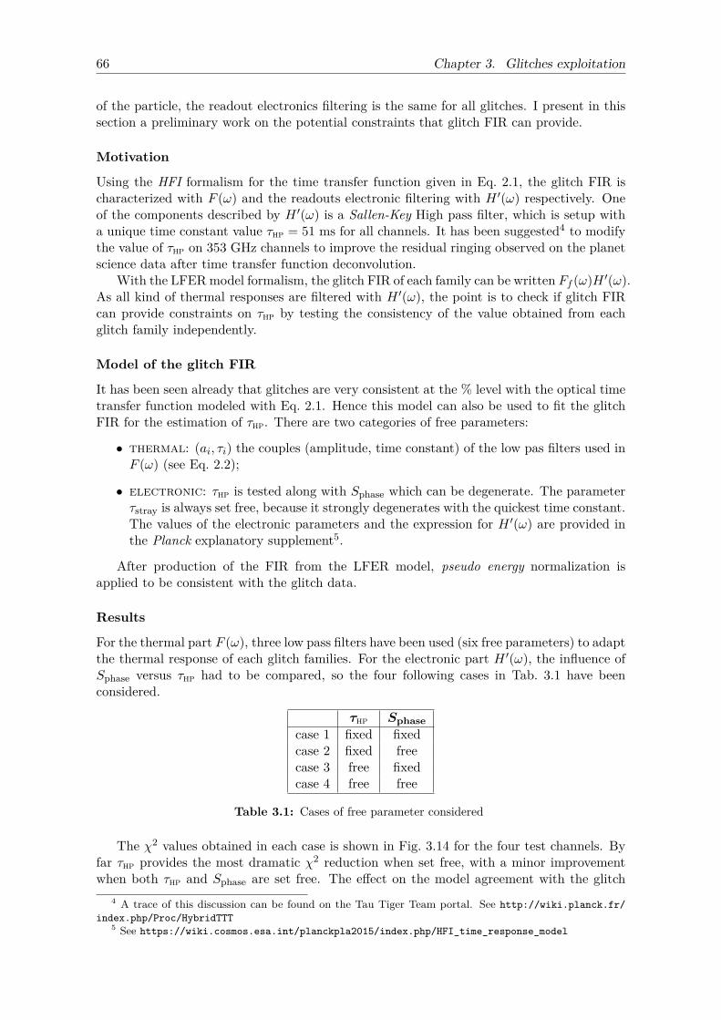
66 Chapter 3. Glitches exploitation
of the particle, the readout electronics filtering is the same for all glitches. I present in thissection a preliminary work on the potential constraints that glitch FIR can provide.
Motivation
Using the HFI formalism for the time transfer function given in Eq. 2.1, the glitch FIR ischaracterized with F (ω) and the readouts electronic filtering with H ′(ω) respectively. Oneof the components described by H ′(ω) is a Sallen-Key High pass filter, which is setup witha unique time constant value τhp = 51 ms for all channels. It has been suggested4 to modifythe value of τhp on 353 GHz channels to improve the residual ringing observed on the planetscience data after time transfer function deconvolution.
With the LFERmodel formalism, the glitch FIR of each family can be written Ff (ω)H ′(ω).As all kind of thermal responses are filtered with H ′(ω), the point is to check if glitch FIRcan provide constraints on τhp by testing the consistency of the value obtained from eachglitch family independently.
Model of the glitch FIR
It has been seen already that glitches are very consistent at the % level with the optical timetransfer function modeled with Eq. 2.1. Hence this model can also be used to fit the glitchFIR for the estimation of τhp. There are two categories of free parameters:
• thermal: (ai, τi) the couples (amplitude, time constant) of the low pas filters used inF (ω) (see Eq. 2.2);
• electronic: τhp is tested along with Sphase which can be degenerate. The parameterτstray is always set free, because it strongly degenerates with the quickest time constant.The values of the electronic parameters and the expression for H ′(ω) are provided inthe Planck explanatory supplement5.
After production of the FIR from the LFER model, pseudo energy normalization isapplied to be consistent with the glitch data.
Results
For the thermal part F (ω), three low pass filters have been used (six free parameters) to adaptthe thermal response of each glitch families. For the electronic part H ′(ω), the influence ofSphase versus τhp had to be compared, so the four following cases in Tab. 3.1 have beenconsidered.
τhp Sphasecase 1 fixed fixedcase 2 fixed freecase 3 free fixedcase 4 free free
Table 3.1: Cases of free parameter considered
The χ2 values obtained in each case is shown in Fig. 3.14 for the four test channels. Byfar τhp provides the most dramatic χ2 reduction when set free, with a minor improvementwhen both τhp and Sphase are set free. The effect on the model agreement with the glitch
4 A trace of this discussion can be found on the Tau Tiger Team portal. See http://wiki.planck.fr/index.php/Proc/HybridTTT
5 See https://wiki.cosmos.esa.int/planckpla2015/index.php/HFI_time_response_model
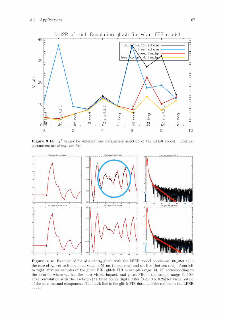
3.3. Applications 67
Figure 3.14: χ2 values for different free parameters selection of the LFER model. Thermalparameters are always set free.
Figure 3.15: Example of fits of a short2 glitch with the LFER model on channel 05_353-1, inthe case of τhp set to its nominal value of 51 ms (upper row) and set free (bottom row). From leftto right: first six samples of the glitch FIR, glitch FIR in sample range [14, 26] corresponding tothe location where τhp has the most visible impact, and glitch FIR in the sample range [0, 100]after convolution with the Archeops (?) three points digital filter [0.25, 0.5, 0.25] for visualizationof the slow thermal component. The black line is the glitch FIR data, and the red line is the LFERmodel.
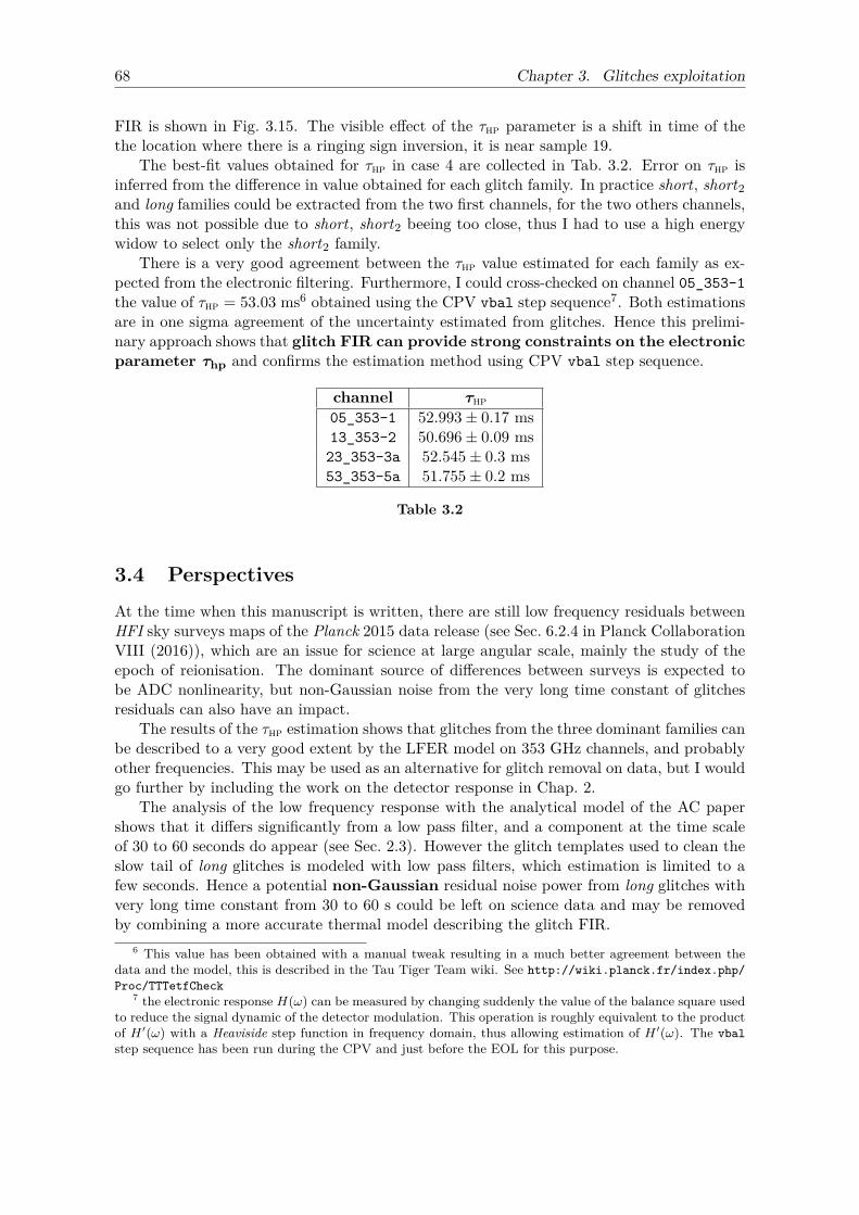
68 Chapter 3. Glitches exploitation
FIR is shown in Fig. 3.15. The visible effect of the τhp parameter is a shift in time of thethe location where there is a ringing sign inversion, it is near sample 19.
The best-fit values obtained for τhp in case 4 are collected in Tab. 3.2. Error on τhp isinferred from the difference in value obtained for each glitch family. In practice short, short2and long families could be extracted from the two first channels, for the two others channels,this was not possible due to short, short2 beeing too close, thus I had to use a high energywidow to select only the short2 family.
There is a very good agreement between the τhp value estimated for each family as ex-pected from the electronic filtering. Furthermore, I could cross-checked on channel 05_353-1the value of τhp = 53.03 ms6 obtained using the CPV vbal step sequence7. Both estimationsare in one sigma agreement of the uncertainty estimated from glitches. Hence this prelimi-nary approach shows that glitch FIR can provide strong constraints on the electronicparameter τhp and confirms the estimation method using CPV vbal step sequence.
channel τhp05_353-1 52.993± 0.17 ms13_353-2 50.696± 0.09 ms23_353-3a 52.545± 0.3 ms53_353-5a 51.755± 0.2 ms
Table 3.2
3.4 PerspectivesAt the time when this manuscript is written, there are still low frequency residuals betweenHFI sky surveys maps of the Planck 2015 data release (see Sec. 6.2.4 in Planck CollaborationVIII (2016)), which are an issue for science at large angular scale, mainly the study of theepoch of reionisation. The dominant source of differences between surveys is expected tobe ADC nonlinearity, but non-Gaussian noise from the very long time constant of glitchesresiduals can also have an impact.
The results of the τhp estimation shows that glitches from the three dominant families canbe described to a very good extent by the LFER model on 353 GHz channels, and probablyother frequencies. This may be used as an alternative for glitch removal on data, but I wouldgo further by including the work on the detector response in Chap. 2.
The analysis of the low frequency response with the analytical model of the AC papershows that it differs significantly from a low pass filter, and a component at the time scaleof 30 to 60 seconds do appear (see Sec. 2.3). However the glitch templates used to clean theslow tail of long glitches is modeled with low pass filters, which estimation is limited to afew seconds. Hence a potential non-Gaussian residual noise power from long glitches withvery long time constant from 30 to 60 s could be left on science data and may be removedby combining a more accurate thermal model describing the glitch FIR.
6 This value has been obtained with a manual tweak resulting in a much better agreement between thedata and the model, this is described in the Tau Tiger Team wiki. See http://wiki.planck.fr/index.php/Proc/TTTetfCheck
7 the electronic response H(ω) can be measured by changing suddenly the value of the balance square usedto reduce the signal dynamic of the detector modulation. This operation is roughly equivalent to the productof H ′(ω) with a Heaviside step function in frequency domain, thus allowing estimation of H ′(ω). The vbalstep sequence has been run during the CPV and just before the EOL for this purpose.

3.5. Conclusions 69
3.5 ConclusionsGlitches have been considered in this chapter as a powerful tool for analysis and estimationof the readout electronics time transfer function and detectors thermal response.
A method has been described for reconstruction of the continuous time domain FIRcorresponding to each glitch family. The glitch FIR built with this generic purpose methodfor the 100 GHz channels been found to be in agreement with the optical time transferfunction estimated from in-flight data at percent level. Finally it has been shown that glitchFIR can provide accurate estimation for the electronics parameter τhp (but not limited to),and that the LFER model allow to describe with a good accuracy the different glitch families.

71
Part II
ADC characterization andcorrection

73
The ADC is a key component in the data acquisition chain of any instrument. It isthe component which converts the analog signal from detectors into discrete numerical datasamples. A perfect ADC would produce only quantization noise (see 4.2.2) on signal, but areal one also introduces nonlinearity, which is neglectable for most applications. The require-ments for the CMB anisotropies study in HFI are very high (∆T/T < 10−5). Unfortunatelyseveral elements in the design of the electronics readout chain have enhanced the effect ofADC nonlinearity. It resulted in apparent gain variations in time estimated to be greaterthan 1% of the solar dipole which have not been detected during on-ground validation cam-paigns. This is what has been called the ADC issue and-revealed an extremely challengingand time consuming problem. Furthermore the on-ground characterization of the chips hasbeen insufficient, whereas for building a correction a very accurate characterization mustbe performed on chips of an already flying instrument. There are of course no dedicatedon-board tools for this purpose, and the data acquisition chain is complex, thus the task isnot easy.
Chap. 4 places the historical context leading to the ADC issue, and describes the char-acterization of ADC chip nonlinearity. After setting these basis it details the final in-flightcharacterization used for the 2013 and 2015 data releases. Next, the correction of sciencedata is detailed in Chap. 5. For this purpose a simplified model of the electronics readoutchain is developed. To assess the validity of the correction, specific ADC nonlinearity ob-servables are studied, and the science data correction validated with simulations. Finallyin Chap. 6 the effect of the 4 K stage mechanical cooler is taken into account. It’s impacton ADC nonlinearity is characterized and the parasitic signal it generates is added to thecorrection model.
I have presented the content of the following chapters at the poster session 9914 of theSPIE Astronomical + instrumentation 2016 conference. The corresponding proceeding (?)is a synthesis of this work and is available in Appendix B. The first characterizations of theADC nonlinearity correction on HFI sky maps have been published in ?. The 2015 versionof the correction taking into account the 4 K lines is detailed in ?.

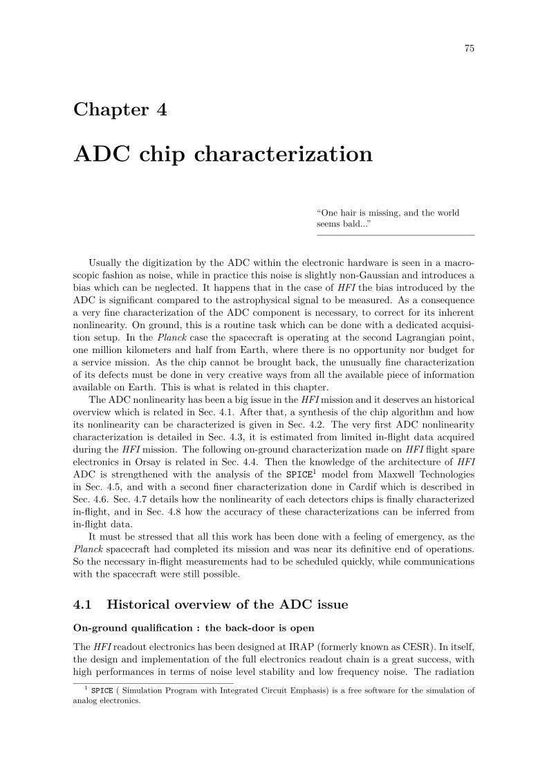
75
Chapter 4
ADC chip characterization
“One hair is missing, and the worldseems bald...”
Usually the digitization by the ADC within the electronic hardware is seen in a macro-scopic fashion as noise, while in practice this noise is slightly non-Gaussian and introduces abias which can be neglected. It happens that in the case of HFI the bias introduced by theADC is significant compared to the astrophysical signal to be measured. As a consequencea very fine characterization of the ADC component is necessary, to correct for its inherentnonlinearity. On ground, this is a routine task which can be done with a dedicated acquisi-tion setup. In the Planck case the spacecraft is operating at the second Lagrangian point,one million kilometers and half from Earth, where there is no opportunity nor budget fora service mission. As the chip cannot be brought back, the unusually fine characterizationof its defects must be done in very creative ways from all the available piece of informationavailable on Earth. This is what is related in this chapter.
The ADC nonlinearity has been a big issue in the HFImission and it deserves an historicaloverview which is related in Sec. 4.1. After that, a synthesis of the chip algorithm and howits nonlinearity can be characterized is given in Sec. 4.2. The very first ADC nonlinearitycharacterization is detailed in Sec. 4.3, it is estimated from limited in-flight data acquiredduring the HFI mission. The following on-ground characterization made on HFI flight spareelectronics in Orsay is related in Sec. 4.4. Then the knowledge of the architecture of HFIADC is strengthened with the analysis of the SPICE1 model from Maxwell Technologiesin Sec. 4.5, and with a second finer characterization done in Cardif which is described inSec. 4.6. Sec. 4.7 details how the nonlinearity of each detectors chips is finally characterizedin-flight, and in Sec. 4.8 how the accuracy of these characterizations can be inferred fromin-flight data.
It must be stressed that all this work has been done with a feeling of emergency, as thePlanck spacecraft had completed its mission and was near its definitive end of operations.So the necessary in-flight measurements had to be scheduled quickly, while communicationswith the spacecraft were still possible.
4.1 Historical overview of the ADC issueOn-ground qualification : the back-door is open
The HFI readout electronics has been designed at IRAP (formerly known as CESR). In itself,the design and implementation of the full electronics readout chain is a great success, withhigh performances in terms of noise level stability and low frequency noise. The radiation
1 SPICE ( Simulation Program with Integrated Circuit Emphasis) is a free software for the simulation ofanalog electronics.
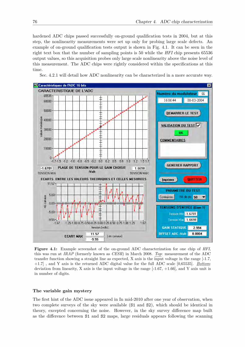
76 Chapter 4. ADC chip characterization
hardened ADC chips passed successfully on-ground qualification tests in 2004, but at thisstep, the nonlinearity measurements were set up only for probing large scale defects. Anexample of on-ground qualification tests output is shown in Fig. 4.1. It can be seen in theright text box that the number of sampling points is 50 while the HFI chip presents 65536output values, so this acquisition probes only large scale nonlinearity above the noise level ofthis measurement. The ADC chips were rightly considered within the specifications at thistime.
Sec. 4.2.1 will detail how ADC nonlinearity can be characterized in a more accurate way.
Figure 4.1: Example screenshot of the on-ground ADC characterization for one chip of HFI,this was run at IRAP (formerly known as CESR) in March 2008. Top: measurement of the ADCtransfer function showing a straight line as expected, X axis is the input voltage in the range [-1.7,+1.7] , and Y axis is the returned ADC digital value for the full ADC scale [0,65535]. Bottom:deviation from linearity, X axis is the input voltage in the range [-1.67, +1.66], and Y axis unit isin number of digits.
The variable gain mystery
The first hint of the ADC issue appeared in In mid-2010 after one year of observation, whentwo complete surveys of the sky were available (S1 and S2), which should be identical intheory, excepted concerning the noise. However, in the sky survey difference map builtas the difference between S1 and S2 maps, large residuals appears following the scanning
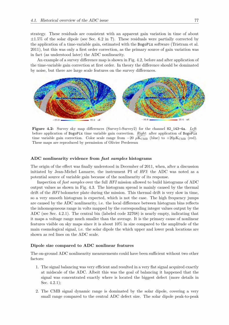
4.1. Historical overview of the ADC issue 77
strategy. These residuals are consistent with an apparent gain variation in time of about±1.5% of the solar dipole (see Sec. 6.2 in ?). These residuals were partially corrected bythe application of a time-variable gain, estimated with the BogoPix software (Tristram et al.2011), but this was only a first order correction, as the primary source of gain variation wasin fact (as understood later) the ADC nonlinearity.
An example of a survey difference map is shown in Fig. 4.2, before and after application ofthe time-variable gain correction at first order. In theory the difference should be dominatedby noise, but there are large scale features on the survey differences.
Figure 4.2: Survey sky map differences (Survey1-Survey2) for the channel 82_143-4a. Left:before application of BogoPix time variable gain correction. Right: after application of BogoPixtime variable gain correction. Color scale range from −20 µKCMB (blue) to +20µKCMB (red).These maps are reproduced by permission of Olivier Perdereau
ADC nonlinearity evidence from fast samples histograms
The origin of the effect was finally understood in December of 2011, when, after a discussioninitiated by Jean-Michel Lamarre, the instrument PI of HFI: the ADC was noted as apotential source of variable gain because of the nonlinearity of its response.
Inspection of fast samples over the full HFI mission allowed to build histograms of ADCoutput values as shown in Fig. 4.3. The histogram spread is mainly caused by the thermaldrift of the HFI bolometer plate during the mission. This thermal drift is very slow in time,so a very smooth histogram is expected, which is not the case. The high frequency jumpsare caused by the ADC nonlinearity, i.e. the local difference between histogram bins reflectsthe inhomogeneous range in volts mapped by the corresponding integer values output by theADC (see Sec. 4.2.1). The central bin (labeled code 32768) is nearly empty, indicating thatit maps a voltage range much smaller than the average. It is the primary cause of nonlinearfeatures visible on sky maps since it is about 10% in size compared to the amplitude of themain cosmological signal, i.e. the solar dipole the which upper and lower peak locations areshown as red lines on the ADC scale.
Dipole size compared to ADC nonlinear features
The on-ground ADC nonlinearity measurements could have been sufficient without two otherfactors:
1. The signal balancing was very efficient and resulted in a very flat signal acquired exactlyat midscale of the ADC. Albeit this was the goal of balancing it happened that thesignal was concentrated exactly where is located the biggest defect (more details inSec. 4.2.1);
2. The CMB signal dynamic range is dominated by the solar dipole, covering a verysmall range compared to the central ADC defect size. The solar dipole peak-to-peak
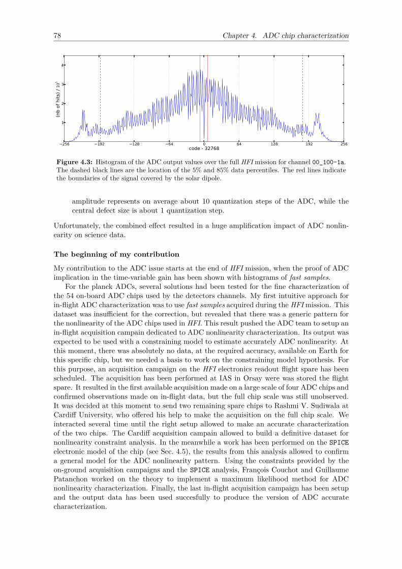
78 Chapter 4. ADC chip characterization
256 192 128 64 0 64 128 192 256code - 32768
1
2
3
4
(nb o
f hit
s) /
105
Figure 4.3: Histogram of the ADC output values over the full HFI mission for channel 00_100-1a.The dashed black lines are the location of the 5% and 85% data percentiles. The red lines indicatethe boundaries of the signal covered by the solar dipole.
amplitude represents on average about 10 quantization steps of the ADC, while thecentral defect size is about 1 quantization step.
Unfortunately, the combined effect resulted in a huge amplification impact of ADC nonlin-earity on science data.
The beginning of my contribution
My contribution to the ADC issue starts at the end of HFI mission, when the proof of ADCimplication in the time-variable gain has been shown with histograms of fast samples.
For the planck ADCs, several solutions had been tested for the fine characterization ofthe 54 on-board ADC chips used by the detectors channels. My first intuitive approach forin-flight ADC characterization was to use fast samples acquired during the HFImission. Thisdataset was insufficient for the correction, but revealed that there was a generic pattern forthe nonlinearity of the ADC chips used in HFI. This result pushed the ADC team to setup anin-flight acquisition campain dedicated to ADC nonlinearity characterization. Its output wasexpected to be used with a constraining model to estimate accurately ADC nonlinearity. Atthis moment, there was absolutely no data, at the required accuracy, available on Earth forthis specific chip, but we needed a basis to work on the constraining model hypothesis. Forthis purpose, an acquisition campaign on the HFI electronics readout flight spare has beenscheduled. The acquisition has been performed at IAS in Orsay were was stored the flightspare. It resulted in the first available acquisition made on a large scale of four ADC chips andconfirmed observations made on in-flight data, but the full chip scale was still unobserved.It was decided at this moment to send two remaining spare chips to Rashmi V. Sudiwala atCardiff University, who offered his help to make the acquisition on the full chip scale. Weinteracted several time until the right setup allowed to make an accurate characterizationof the two chips. The Cardiff acquisition campain allowed to build a definitive dataset fornonlinearity constraint analysis. In the meanwhile a work has been performed on the SPICEelectronic model of the chip (see Sec. 4.5), the results from this analysis allowed to confirma general model for the ADC nonlinearity pattern. Using the constraints provided by theon-ground acquisition campaigns and the SPICE analysis, François Couchot and GuillaumePatanchon worked on the theory to implement a maximum likelihood method for ADCnonlinearity characterization. Finally, the last in-flight acquisition campaign has been setupand the output data has been used succesfully to produce the version of ADC accuratecharacterization.
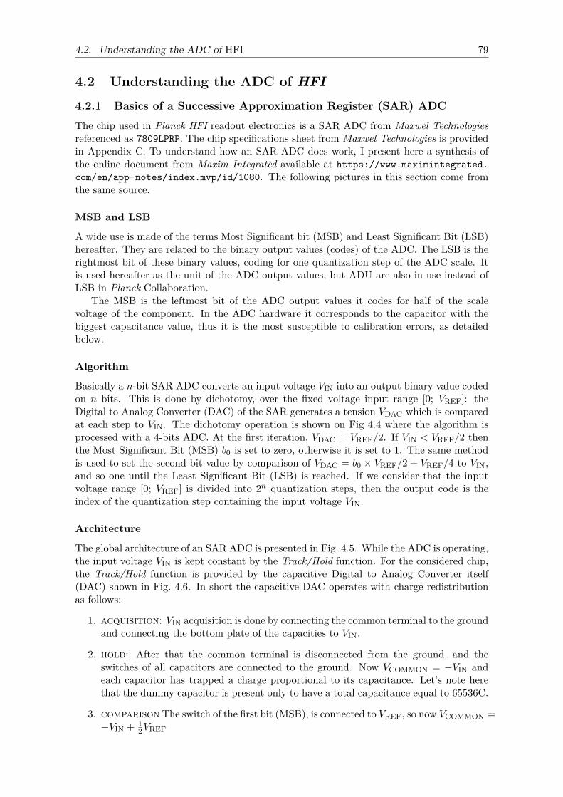
4.2. Understanding the ADC of HFI 79
4.2 Understanding the ADC of HFI4.2.1 Basics of a Successive Approximation Register (SAR) ADC
The chip used in Planck HFI readout electronics is a SAR ADC from Maxwel Technologiesreferenced as 7809LPRP. The chip specifications sheet from Maxwel Technologies is providedin Appendix C. To understand how an SAR ADC does work, I present here a synthesis ofthe online document from Maxim Integrated available at https://www.maximintegrated.com/en/app-notes/index.mvp/id/1080. The following pictures in this section come fromthe same source.
MSB and LSB
A wide use is made of the terms Most Significant bit (MSB) and Least Significant Bit (LSB)hereafter. They are related to the binary output values (codes) of the ADC. The LSB is therightmost bit of these binary values, coding for one quantization step of the ADC scale. Itis used hereafter as the unit of the ADC output values, but ADU are also in use instead ofLSB in Planck Collaboration.
The MSB is the leftmost bit of the ADC output values it codes for half of the scalevoltage of the component. In the ADC hardware it corresponds to the capacitor with thebiggest capacitance value, thus it is the most susceptible to calibration errors, as detailedbelow.
Algorithm
Basically a n-bit SAR ADC converts an input voltage VIN into an output binary value codedon n bits. This is done by dichotomy, over the fixed voltage input range [0; VREF]: theDigital to Analog Converter (DAC) of the SAR generates a tension VDAC which is comparedat each step to VIN. The dichotomy operation is shown on Fig 4.4 where the algorithm isprocessed with a 4-bits ADC. At the first iteration, VDAC = VREF/2. If VIN < VREF/2 thenthe Most Significant Bit (MSB) b0 is set to zero, otherwise it is set to 1. The same methodis used to set the second bit value by comparison of VDAC = b0 × VREF/2 + VREF/4 to VIN,and so one until the Least Significant Bit (LSB) is reached. If we consider that the inputvoltage range [0; VREF] is divided into 2n quantization steps, then the output code is theindex of the quantization step containing the input voltage VIN.
Architecture
The global architecture of an SAR ADC is presented in Fig. 4.5. While the ADC is operating,the input voltage VIN is kept constant by the Track/Hold function. For the considered chip,the Track/Hold function is provided by the capacitive Digital to Analog Converter itself(DAC) shown in Fig. 4.6. In short the capacitive DAC operates with charge redistributionas follows:
1. acquisition: VIN acquisition is done by connecting the common terminal to the groundand connecting the bottom plate of the capacities to VIN.
2. hold: After that the common terminal is disconnected from the ground, and theswitches of all capacitors are connected to the ground. Now VCOMMON = −VIN andeach capacitor has trapped a charge proportional to its capacitance. Let’s note herethat the dummy capacitor is present only to have a total capacitance equal to 65536C.
3. comparison The switch of the first bit (MSB), is connected to VREF, so now VCOMMON =−VIN + 1
2VREF
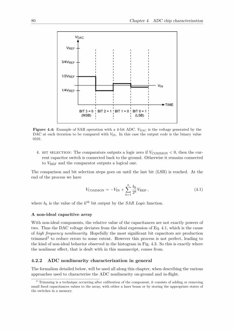
80 Chapter 4. ADC chip characterization
Figure 4.4: Example of SAR operation with a 4-bit ADC. VDAC is the voltage generated by theDAC at each iteration to be compared with VIN. In this case the output code is the binary value0101.
4. bit selection: The comparators outputs a logic zero if VCOMMON < 0, then the cur-rent capacitor switch is connected back to the ground. Otherwise it remains connectedto VREF and the comparator outputs a logical one.
The comparison and bit selection steps goes on until the last bit (LSB) is reached. At theend of the process we have
VCOMMON = −VIN +n∑k=1
bk2kVREF , (4.1)
where bk is the value of the kth bit output by the SAR Logic function.
A non-ideal capacitive array
With non-ideal components, the relative value of the capacitances are not exactly powers oftwo. Thus the DAC voltage deviates from the ideal expression of Eq. 4.1, which is the causeof high frequency nonlinearity. Hopefully the most significant bit capacitors are productiontrimmed2 to reduce errors to some extent. However this process is not perfect, leading tothe kind of non-ideal behavior observed in the histogram in Fig. 4.3. So this is exactly wherethe nonlinear effect, that is dealt with in this manuscript, comes from.
4.2.2 ADC nonlinearity characterization in general
The formalism detailed below, will be used all along this chapter, when describing the variousapproaches used to characterize the ADC nonlinearity on-ground and in-flight.
2 Trimming is a technique occurring after calibration of the component, it consists of adding or removingsmall fixed capacitances values to the array, with either a laser beam or by storing the appropriate states ofthe switches in a memory.
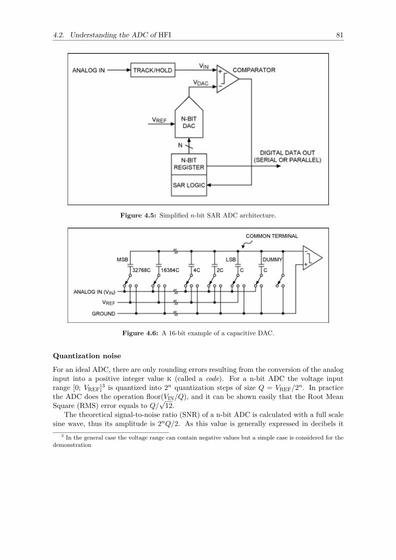
4.2. Understanding the ADC of HFI 81
Figure 4.5: Simplified n-bit SAR ADC architecture.
Figure 4.6: A 16-bit example of a capacitive DAC.
Quantization noise
For an ideal ADC, there are only rounding errors resulting from the conversion of the analoginput into a positive integer value k (called a code). For a n-bit ADC the voltage inputrange [0; VREF]3 is quantized into 2n quantization steps of size Q = VREF/2n. In practicethe ADC does the operation floor(VIN/Q), and it can be shown easily that the Root MeanSquare (RMS) error equals to Q/
√12.
The theoretical signal-to-noise ratio (SNR) of a n-bit ADC is calculated with a full scalesine wave, thus its amplitude is 2nQ/2. As this value is generally expressed in decibels it
3 In the general case the voltage range can contain negative values but a simple case is considered for thedemonstration
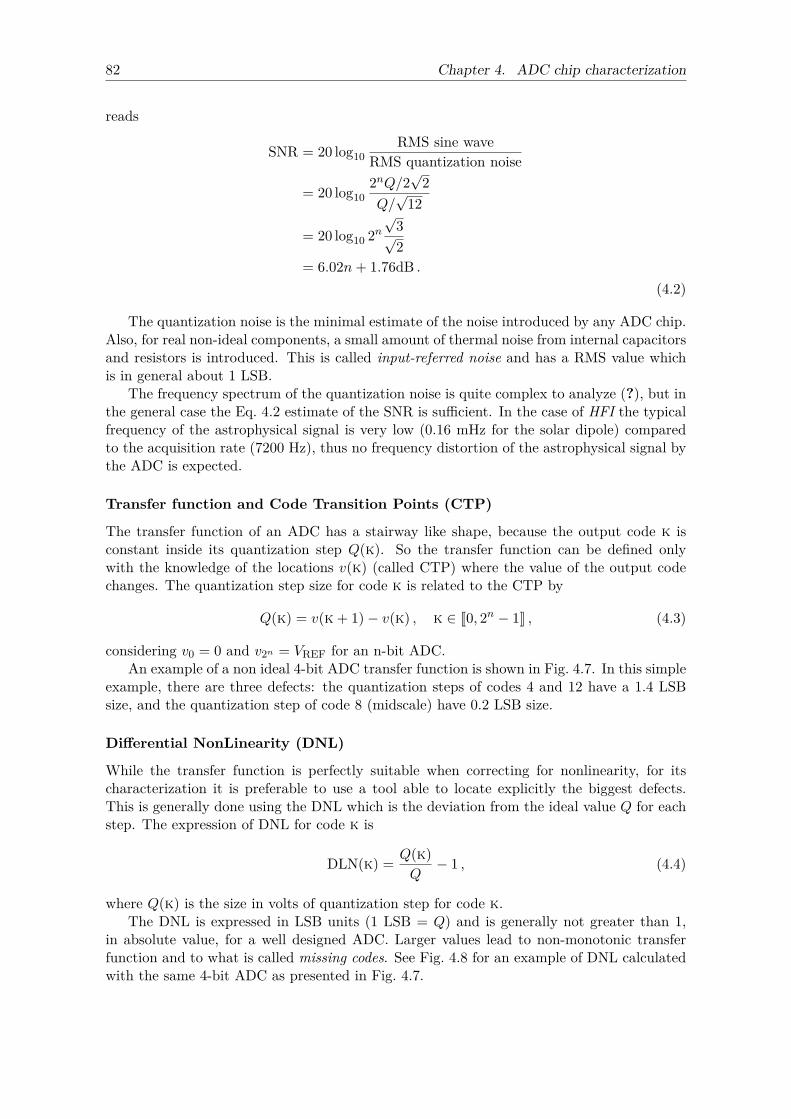
82 Chapter 4. ADC chip characterization
reads
SNR = 20 log10RMS sine wave
RMS quantization noise
= 20 log102nQ/2
√2
Q/√
12
= 20 log10 2n√
3√2
= 6.02n+ 1.76dB .(4.2)
The quantization noise is the minimal estimate of the noise introduced by any ADC chip.Also, for real non-ideal components, a small amount of thermal noise from internal capacitorsand resistors is introduced. This is called input-referred noise and has a RMS value whichis in general about 1 LSB.
The frequency spectrum of the quantization noise is quite complex to analyze (?), but inthe general case the Eq. 4.2 estimate of the SNR is sufficient. In the case of HFI the typicalfrequency of the astrophysical signal is very low (0.16 mHz for the solar dipole) comparedto the acquisition rate (7200 Hz), thus no frequency distortion of the astrophysical signal bythe ADC is expected.
Transfer function and Code Transition Points (CTP)
The transfer function of an ADC has a stairway like shape, because the output code k isconstant inside its quantization step Q(k). So the transfer function can be defined onlywith the knowledge of the locations v(k) (called CTP) where the value of the output codechanges. The quantization step size for code k is related to the CTP by
Q(k) = v(k + 1)− v(k) , k ∈ J0, 2n − 1K , (4.3)
considering v0 = 0 and v2n = VREF for an n-bit ADC.An example of a non ideal 4-bit ADC transfer function is shown in Fig. 4.7. In this simple
example, there are three defects: the quantization steps of codes 4 and 12 have a 1.4 LSBsize, and the quantization step of code 8 (midscale) have 0.2 LSB size.
Differential NonLinearity (DNL)
While the transfer function is perfectly suitable when correcting for nonlinearity, for itscharacterization it is preferable to use a tool able to locate explicitly the biggest defects.This is generally done using the DNL which is the deviation from the ideal value Q for eachstep. The expression of DNL for code k is
DLN(k) = Q(k)Q− 1 , (4.4)
where Q(k) is the size in volts of quantization step for code k.The DNL is expressed in LSB units (1 LSB = Q) and is generally not greater than 1,
in absolute value, for a well designed ADC. Larger values lead to non-monotonic transferfunction and to what is called missing codes. See Fig. 4.8 for an example of DNL calculatedwith the same 4-bit ADC as presented in Fig. 4.7.
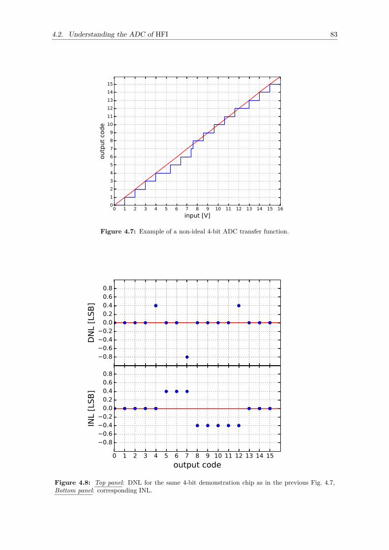
4.2. Understanding the ADC of HFI 83
0 1 2 3 4 5 6 7 8 9 10 11 12 13 14 15 16
input [V]
0
1
2
3
4
5
6
7
8
9
10
11
12
13
14
15
outp
ut
code
Figure 4.7: Example of a non-ideal 4-bit ADC transfer function.
0.80.60.40.20.00.20.40.60.8
DN
L [L
SB
]
0 1 2 3 4 5 6 7 8 9 10 11 12 13 14 15
output code
0.80.60.40.20.00.20.40.60.8
INL
[LSB
]
Figure 4.8: Top panel: DNL for the same 4-bit demonstration chip as in the previous Fig. 4.7,Bottom panel: corresponding INL.
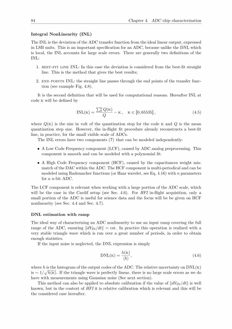
84 Chapter 4. ADC chip characterization
Integral NonLinearity (INL)
The INL is the deviation of the ADC transfer function from the ideal linear output, expressedin LSB units. This is an important specification for an ADC, because unlike the DNL whichis local, the INL accounts for large scale errors. There are generally two definitions of theINL:
1. best-fit line INL: In this case the deviation is considered from the best-fit straightline. This is the method that gives the best results;
2. end points INL: the straight line passes through the end points of the transfer func-tion (see example Fig. 4.8).
It is the second definition that will be used for computational reasons. Hereafter INL atcode k will be defined by
INL(k) =∑k
0 Q(k)Q
− k , k ∈ J0, 65535K , (4.5)
where Q(k) is the size in volt of the quantization step for the code k and Q is the meanquantization step size. However, the in-flight fit procedure already reconstructs a best-fitline, in practice, for the small visible scale of ADCs.
The INL errors have two components (?) that can be modeled independently:
• A Low Code Frequency component (LCF), caused by ADC analog preprocessing. Thiscomponent is smooth and can be modeled with a polynomial fit.
• A High Code Frequency component (HCF), caused by the capacitances weight mis-match of the DAC within the ADC. The HCF component is multi-periodical and can bemodeled using Rademacher functions (or Haar wavelet, see Eq. 4.16) with n parametersfor a n-bit ADC.
The LCF component is relevant when working with a large portion of the ADC scale, whichwill be the case in the Cardif setup (see Sec. 4.6). For HFI in-flight acquisition, only asmall portion of the ADC is useful for science data and the focus will be be given on HCFnonlinearity (see Sec. 4.4 and Sec. 4.7).
DNL estimation with ramp
The ideal way of characterizing an ADC nonlinearity to use an input ramp covering the fullrange of the ADC, ensuring ‖dVIN/dt‖ = cst. In practice this operation is realized with avery stable triangle wave which is run over a great number of periods, in order to obtainenough statistics.
If the input noise is neglected, the DNL expression is simply
DNL(k) = h(k)〈h〉
, (4.6)
where h is the histogram of the output codes of the ADC. The relative uncertainty on DNL(k)is ∼ 1/
√h(k). If the triangle wave is perfectly linear, there is no large scale errors as we do
have with measurements using Gaussian noise (See next section).This method can also be applied to absolute calibration if the value of ‖dVIN/dt‖ is well
known, but in the context of HFI it is relative calibration which is relevant and this will bethe considered case hereafter.
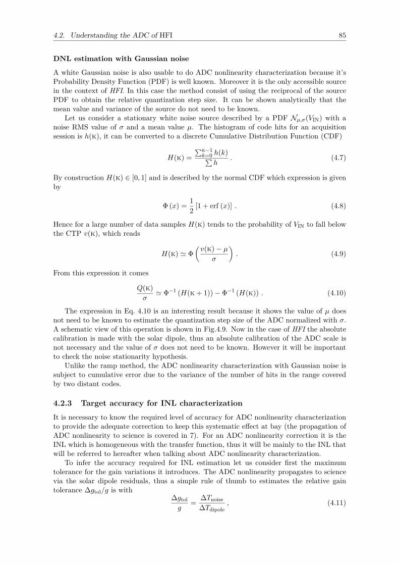
4.2. Understanding the ADC of HFI 85
DNL estimation with Gaussian noise
A white Gaussian noise is also usable to do ADC nonlinearity characterization because it’sProbability Density Function (PDF) is well known. Moreover it is the only accessible sourcein the context of HFI. In this case the method consist of using the reciprocal of the sourcePDF to obtain the relative quantization step size. It can be shown analytically that themean value and variance of the source do not need to be known.
Let us consider a stationary white noise source described by a PDF Nµ,σ(VIN) with anoise RMS value of σ and a mean value µ. The histogram of code hits for an acquisitionsession is h(k), it can be converted to a discrete Cumulative Distribution Function (CDF)
H(k) =∑k−1k=0 h(k)∑
h. (4.7)
By construction H(k) ∈ [0, 1] and is described by the normal CDF which expression is givenby
Φ (x) = 12 [1 + erf (x)] . (4.8)
Hence for a large number of data samples H(k) tends to the probability of VIN to fall belowthe CTP v(k), which reads
H(k) ' Φ(v(k)− µ
σ
). (4.9)
From this expression it comes
Q(k)σ' Φ−1 (H(k + 1))− Φ−1 (H(k)) . (4.10)
The expression in Eq. 4.10 is an interesting result because it shows the value of µ doesnot need to be known to estimate the quantization step size of the ADC normalized with σ.A schematic view of this operation is shown in Fig.4.9. Now in the case of HFI the absolutecalibration is made with the solar dipole, thus an absolute calibration of the ADC scale isnot necessary and the value of σ does not need to be known. However it will be importantto check the noise stationarity hypothesis.
Unlike the ramp method, the ADC nonlinearity characterization with Gaussian noise issubject to cumulative error due to the variance of the number of hits in the range coveredby two distant codes.
4.2.3 Target accuracy for INL characterization
It is necessary to know the required level of accuracy for ADC nonlinearity characterizationto provide the adequate correction to keep this systematic effect at bay (the propagation ofADC nonlinearity to science is covered in 7). For an ADC nonlinearity correction it is theINL which is homogeneous with the transfer function, thus it will be mainly to the INL thatwill be referred to hereafter when talking about ADC nonlinearity characterization.
To infer the accuracy required for INL estimation let us consider first the maximumtolerance for the gain variations it introduces. The ADC nonlinearity propagates to sciencevia the solar dipole residuals, thus a simple rule of thumb to estimates the relative gaintolerance ∆gtol/g is with
∆gtolg
= ∆Tnoise∆Tdipole
, (4.11)
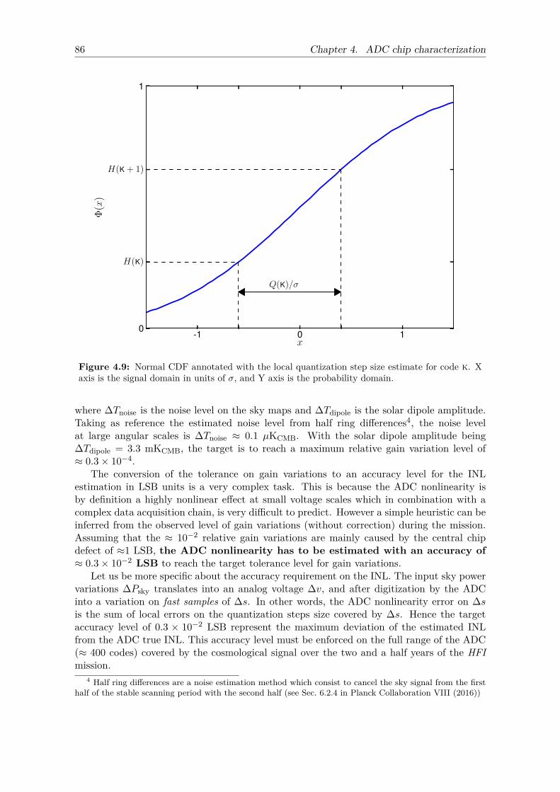
86 Chapter 4. ADC chip characterization
-1 0 1x
0
H(K)
H(K + 1)
1Φ
(x)
Q(K)/σ
Figure 4.9: Normal CDF annotated with the local quantization step size estimate for code k. Xaxis is the signal domain in units of σ, and Y axis is the probability domain.
where ∆Tnoise is the noise level on the sky maps and ∆Tdipole is the solar dipole amplitude.Taking as reference the estimated noise level from half ring differences4, the noise levelat large angular scales is ∆Tnoise ≈ 0.1 µKCMB. With the solar dipole amplitude being∆Tdipole = 3.3 mKCMB, the target is to reach a maximum relative gain variation level of≈ 0.3× 10⁻⁴.
The conversion of the tolerance on gain variations to an accuracy level for the INLestimation in LSB units is a very complex task. This is because the ADC nonlinearity isby definition a highly nonlinear effect at small voltage scales which in combination with acomplex data acquisition chain, is very difficult to predict. However a simple heuristic can beinferred from the observed level of gain variations (without correction) during the mission.Assuming that the ≈ 10−2 relative gain variations are mainly caused by the central chipdefect of ≈1 LSB, the ADC nonlinearity has to be estimated with an accuracy of≈ 0.3× 10⁻² LSB to reach the target tolerance level for gain variations.
Let us be more specific about the accuracy requirement on the INL. The input sky powervariations ∆Psky translates into an analog voltage ∆v, and after digitization by the ADCinto a variation on fast samples of ∆s. In other words, the ADC nonlinearity error on ∆sis the sum of local errors on the quantization steps size covered by ∆s. Hence the targetaccuracy level of 0.3 × 10⁻² LSB represent the maximum deviation of the estimated INLfrom the ADC true INL. This accuracy level must be enforced on the full range of the ADC(≈ 400 codes) covered by the cosmological signal over the two and a half years of the HFImission.
4 Half ring differences are a noise estimation method which consist to cancel the sky signal from the firsthalf of the stable scanning period with the second half (see Sec. 6.2.4 in Planck Collaboration VIII (2016))
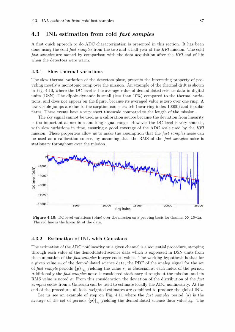
4.3. INL estimation from cold fast samples 87
4.3 INL estimation from cold fast samplesA first quick approch to do ADC characterization is presented in this section. It has beendone using the cold fast samples from the two and a half year of the HFI mission. The coldfast samples are named by comparison with the data acquisition after the HFI end of lifewhen the detectors were warm.
4.3.1 Slow thermal variations
The slow thermal variation of the detectors plate, presents the interesting property of pro-viding mostly a monotonic ramp over the mission. An example of the thermal drift is shownin Fig. 4.10, where the DC level is the average value of demodulated science data in digitalunits (DSN). The dipole dynamic is small (less than 10%) compared to the thermal varia-tions, and does not appear on the figure, because its averaged value is zero over one ring. Afew visible jumps are due to the sorption cooler switch (near ring index 10000) and to solarflares. These events have a very short timescale compared to the length of the mission.
The sky signal cannot be used as a calibration source because the deviation from linearityis too important at medium and long signal range. However the DC level is very smooth,with slow variations in time, ensuring a good coverage of the ADC scale used by the HFImission. These properties allow us to make the assumption that the fast samples noise canbe used as a calibration source, by assuming that the RMS of the fast samples noise isstationary throughout over the mission.
Figure 4.10: DC level variations (blue) over the mission on a per ring basis for channel 00_10-1a.The red line is the linear fit of the data.
4.3.2 Estimation of INL with Gaussians
The estimation of the ADC nonlinearity on a given channel is a sequential procedure, steppingthrough each value of the demodulated science data which is expressed in DSN units fromthe summation of the fast samples integer codes values. The working hypothesis is that fora given value sd of the demodulated science data, the PDF of the analog signal for the setof fast sample periods p|sd yielding the value sd is Gaussian at each index of the period.Additionally the fast samples noise is considered stationary throughout the mission, and itsRMS value is noted σ. From this consideration the deviation of the distribution of the fastsamples codes from a Gaussian can be used to estimate locally the ADC nonlinearity. At theend of the procedure, all local weighted estimates are combined to produce the global INL.
Let us see an example of step on Fig. 4.11 where the fast samples period (a) is theaverage of the set of periods p|sd yielding the demodulated science data value sd. The
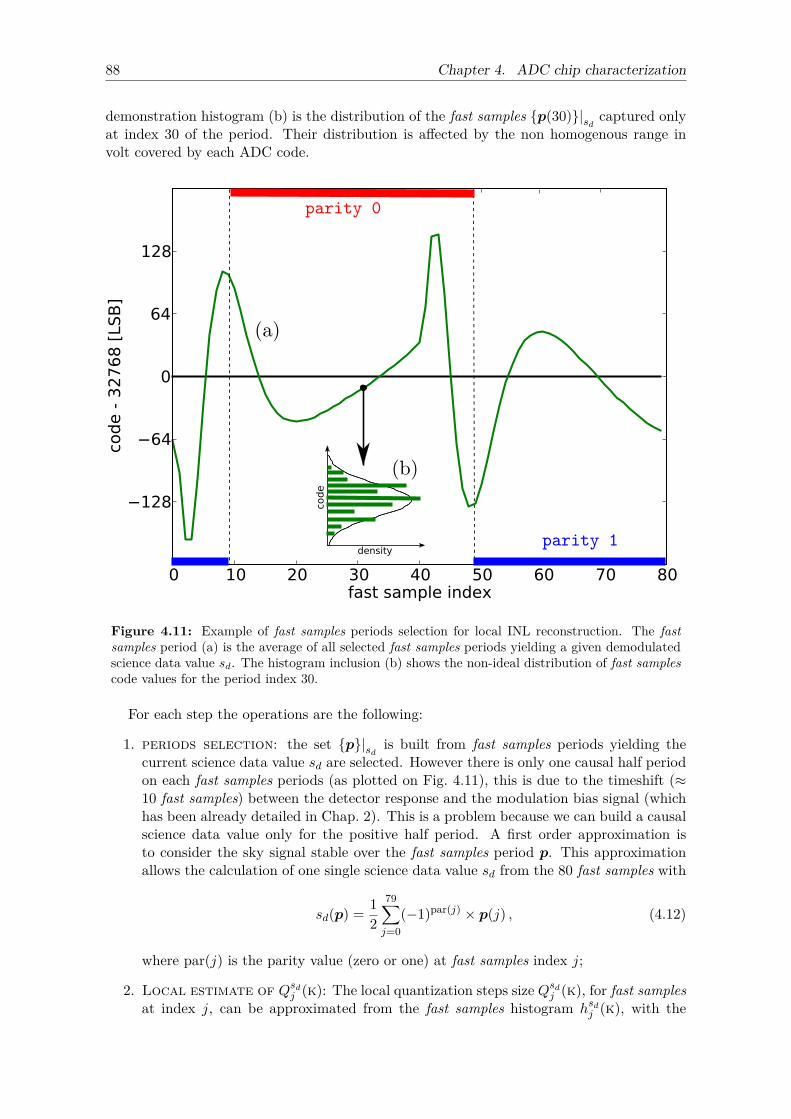
88 Chapter 4. ADC chip characterization
demonstration histogram (b) is the distribution of the fast samples p(30)|sd captured onlyat index 30 of the period. Their distribution is affected by the non homogenous range involt covered by each ADC code.
Figure 4.11: Example of fast samples periods selection for local INL reconstruction. The fastsamples period (a) is the average of all selected fast samples periods yielding a given demodulatedscience data value sd. The histogram inclusion (b) shows the non-ideal distribution of fast samplescode values for the period index 30.
For each step the operations are the following:
1. periods selection: the set p|sd is built from fast samples periods yielding thecurrent science data value sd are selected. However there is only one causal half periodon each fast samples periods (as plotted on Fig. 4.11), this is due to the timeshift (≈10 fast samples) between the detector response and the modulation bias signal (whichhas been already detailed in Chap. 2). This is a problem because we can build a causalscience data value only for the positive half period. A first order approximation isto consider the sky signal stable over the fast samples period p. This approximationallows the calculation of one single science data value sd from the 80 fast samples with
sd(p) = 12
79∑j=0
(−1)par(j) × p(j) , (4.12)
where par(j) is the parity value (zero or one) at fast samples index j;
2. Local estimate of Qsdj (k): The local quantization steps size Qsdj (k), for fast samplesat index j, can be approximated from the fast samples histogram hsdj (k), with the
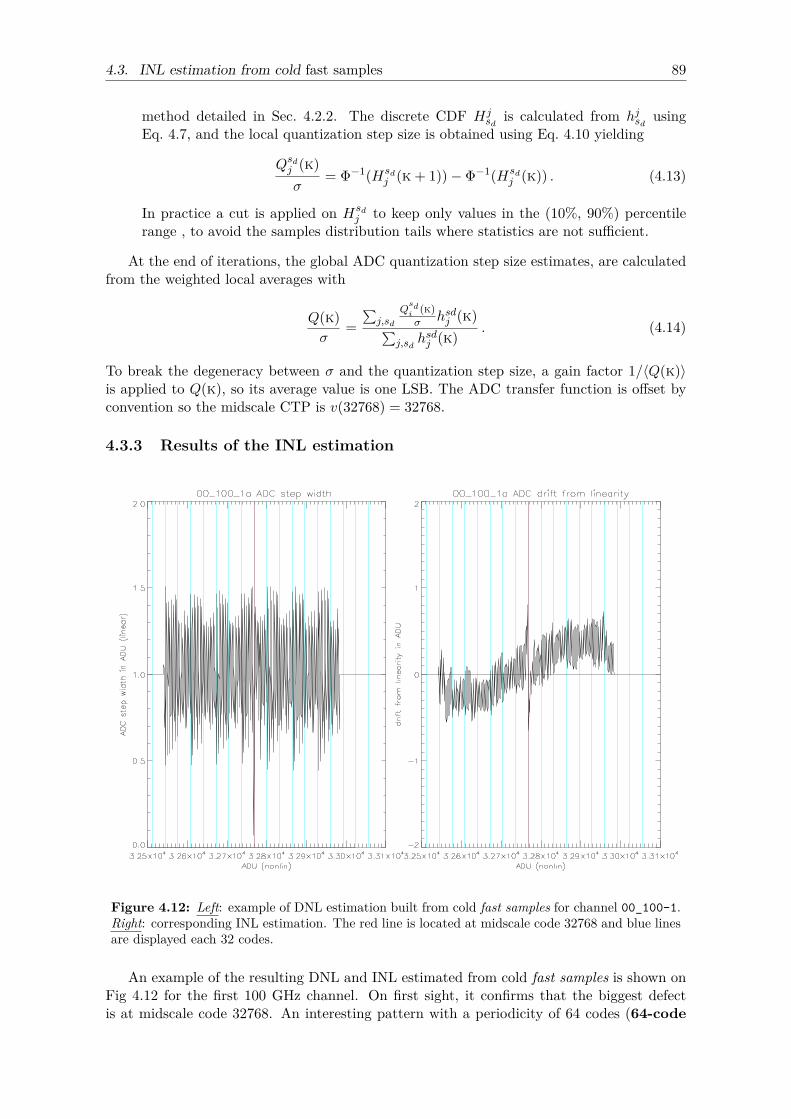
4.3. INL estimation from cold fast samples 89
method detailed in Sec. 4.2.2. The discrete CDF Hjsd
is calculated from hjsd usingEq. 4.7, and the local quantization step size is obtained using Eq. 4.10 yielding
Qsdj (k)σ
= Φ−1(Hsdj (k + 1))− Φ−1(Hsd
j (k)) . (4.13)
In practice a cut is applied on Hsdj to keep only values in the (10%, 90%) percentile
range , to avoid the samples distribution tails where statistics are not sufficient.
At the end of iterations, the global ADC quantization step size estimates, are calculatedfrom the weighted local averages with
Q(k)σ
=∑j,sd
Qsdi (k)σ hsdj (k)∑
j,sdhsdj (k)
. (4.14)
To break the degeneracy between σ and the quantization step size, a gain factor 1/〈Q(k)〉is applied to Q(k), so its average value is one LSB. The ADC transfer function is offset byconvention so the midscale CTP is v(32768) = 32768.
4.3.3 Results of the INL estimation
Figure 4.12: Left: example of DNL estimation built from cold fast samples for channel 00_100-1.Right: corresponding INL estimation. The red line is located at midscale code 32768 and blue linesare displayed each 32 codes.
An example of the resulting DNL and INL estimated from cold fast samples is shown onFig 4.12 for the first 100 GHz channel. On first sight, it confirms that the biggest defectis at midscale code 32768. An interesting pattern with a periodicity of 64 codes (64-code
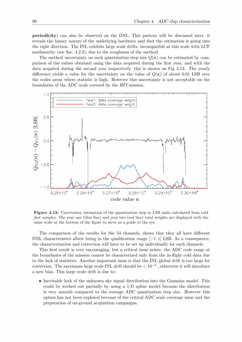
90 Chapter 4. ADC chip characterization
periodicity) can also be observed on the DNL. This pattern will be discussed later, itreveals the binary nature of the underlying hardware and that the estimation is going intothe right direction. The INL exhibits large scale drifts, incompatible at this scale with LCFnonlinearity (see Sec. 4.2.2), due to the roughness of the method.
The method uncertainty on each quantization step size Q(k) can be estimated by com-parison of the values obtained using the data acquired during the first year, and with thedata acquired during the second year respectively, this is shown on Fig 4.13. The yearlydifference yields a value for the uncertainty on the value of Q(k) of about 0.01 LSB overthe codes areas where statistic is high. However this uncertainty is not acceptable on theboundaries of the ADC scale covered by the HFI mission.
Figure 4.13: Uncertainty estimation of the quantization step in LSB units calculated from coldfast samples. The year one (blue line) and year two (red line) total weights are displayed with thesame scale at the bottom of the figure to serve as a guide to the eye.
The comparison of the results for the 54 channels, shows that they all have differentDNL characteristics albeit being in the qualification range [−1, 1] LSB. As a consequence,the characterization and correction will have to be set up individually for each channels.
This first result is very encouraging, but a critical issue arises: the ADC code range atthe boundaries of the mission cannot be characterized only from the in-flight cold data dueto the lack of statistics. Another important issue is that the INL global drift is too large forcorrection. The maximum large scale INL drift should be < 10−4 , otherwise it will introducea new bias. This large scale drift is due to:
• Inevitable leak of the unknown sky signal distribution into the Gaussian model. Thiscould be worked out partially by using a 1-D spline model because the distributionis very smooth compared to the average ADC quantization step size. However thisoption has not been explored because of the critical ADC scale coverage issue and thepreparation of on-ground acquisition campaigns;
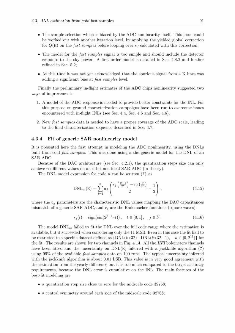
4.3. INL estimation from cold fast samples 91
• The sample selection which is biased by the ADC nonlinearity itself. This issue couldbe worked out with another iteration level, by applying the yielded global correctionfor Q(k) on the fast samples before looping over sd calculated with this correction;
• The model for the fast samples signal is too simple and should include the detectorresponse to the sky power. A first order model is detailed in Sec. 4.8.2 and furtherrefined in Sec. 5.2;
• At this time it was not yet acknowledged that the spurious signal from 4 K lines wasadding a significant bias at fast samples level.
Finally the preliminary in-flight estimates of the ADC chips nonlinearity suggested twoways of improvement:
1. A model of the ADC response is needed to provide better constraints for the INL. Forthis purpose on-ground characterization campaigns have been run to overcome issuesencountered with in-flight INLs (see Sec. 4.4, Sec. 4.5 and Sec. 4.6).
2. New fast samples data is needed to have a proper coverage of the ADC scale, leadingto the final characterization sequence described in Sec. 4.7.
4.3.4 Fit of generic SAR nonlinearity model
It is presented here the first attempt in modeling the ADC nonlinearity, using the DNLsbuilt from cold fast samples. This was done using a the generic model for the DNL of anSAR ADC.
Because of the DAC architecture (see Sec. 4.2.1), the quantization steps size can onlyachieve n different values on an n-bit non-ideal SAR ADC (in theory).
The DNL model expression for code k can be written (?) as
DNLm(k) =n∑j=1
aj
rj(
k+12n)− rj
( k2n)
2 − 12
, (4.15)
where the aj parameters are the characteristic DNL values mapping the DAC capacitancesmismatch of a generic SAR ADC, and rj are the Rademacher functions (square waves)
rj(t) = sign(sin(2j+1πt)) , t ∈ [0, 1] ; j ∈ N . (4.16)
The model DNLm failed to fit the DNL over the full code range where the estimation isavailable, but it succeeded when considering only the 11 MSB. Even in this case the fit had tobe restricted to a specific dataset defined as DNL(k∗32)+DNL(k∗32−1), k ∈ K0, 211J forthe fit. The results are shown for two channels in Fig. 4.14. All the HFI bolometers channelshave been fitted and the uncertainty on DNL(k) inferred with a jackknife algorithm (?)using 99% of the available fast samples data on 100 runs. The typical uncertainty inferredwith the jackknife algorithm is about 0.01 LSB. This value is in very good agreement withthe estimation from the yearly difference but it is too much compared to the target accuracyrequirements, because the DNL error is cumulative on the INL. The main features of thebest-fit modeling are:
• a quantization step size close to zero for the midscale code 32768;
• a central symmetry around each side of the midscale code 32768;
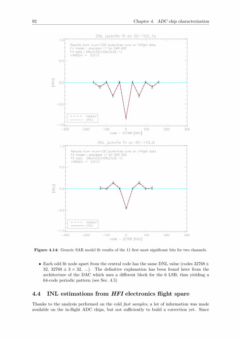
92 Chapter 4. ADC chip characterization
Figure 4.14: Generic SAR model fit results of the 11 first most significant bits for two channels.
• Each odd fit node apart from the central code has the same DNL value (codes 32768±32, 32768 ± 3 × 32, ...). The definitive explanation has been found later from thearchitecture of the DAC which uses a different block for the 6 LSB, thus yielding a64-code periodic pattern (see Sec. 4.5)
4.4 INL estimations from HFI electronics flight spareThanks to the analysis performed on the cold fast samples, a lot of information was madeavailable on the in-flight ADC chips, but not sufficiently to build a correction yet. Since
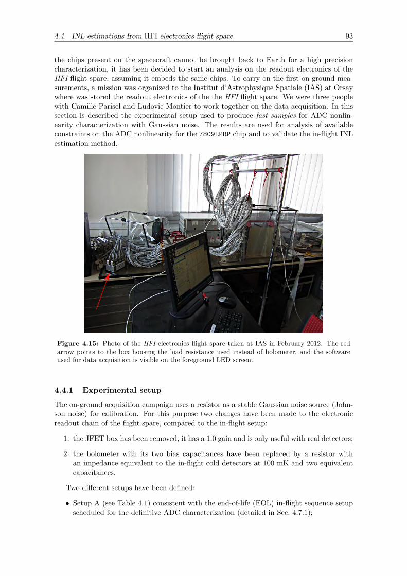
4.4. INL estimations from HFI electronics flight spare 93
the chips present on the spacecraft cannot be brought back to Earth for a high precisioncharacterization, it has been decided to start an analysis on the readout electronics of theHFI flight spare, assuming it embeds the same chips. To carry on the first on-ground mea-surements, a mission was organized to the Institut d’Astrophysique Spatiale (IAS) at Orsaywhere was stored the readout electronics of the the HFI flight spare. We were three peoplewith Camille Parisel and Ludovic Montier to work together on the data acquisition. In thissection is described the experimental setup used to produce fast samples for ADC nonlin-earity characterization with Gaussian noise. The results are used for analysis of availableconstraints on the ADC nonlinearity for the 7809LPRP chip and to validate the in-flight INLestimation method.
Figure 4.15: Photo of the HFI electronics flight spare taken at IAS in February 2012. The redarrow points to the box housing the load resistance used instead of bolometer, and the softwareused for data acquisition is visible on the foreground LED screen.
4.4.1 Experimental setup
The on-ground acquisition campaign uses a resistor as a stable Gaussian noise source (John-son noise) for calibration. For this purpose two changes have been made to the electronicreadout chain of the flight spare, compared to the in-flight setup:
1. the JFET box has been removed, it has a 1.0 gain and is only useful with real detectors;
2. the bolometer with its two bias capacitances have been replaced by a resistor withan impedance equivalent to the in-flight cold detectors at 100 mK and two equivalentcapacitances.
Two different setups have been defined:
• Setup A (see Table 4.1) consistent with the end-of-life (EOL) in-flight sequence setupscheduled for the definitive ADC characterization (detailed in Sec. 4.7.1);
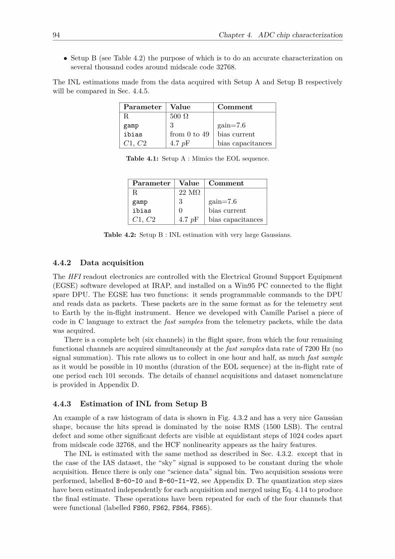
94 Chapter 4. ADC chip characterization
• Setup B (see Table 4.2) the purpose of which is to do an accurate characterization onseveral thousand codes around midscale code 32768.
The INL estimations made from the data acquired with Setup A and Setup B respectivelywill be compared in Sec. 4.4.5.
Parameter Value CommentR 500 Ωgamp 3 gain=7.6ibias from 0 to 49 bias currentC1, C2 4.7 pF bias capacitances
Table 4.1: Setup A : Mimics the EOL sequence.
Parameter Value CommentR 22 MΩgamp 3 gain=7.6ibias 0 bias currentC1, C2 4.7 pF bias capacitances
Table 4.2: Setup B : INL estimation with very large Gaussians.
4.4.2 Data acquisition
The HFI readout electronics are controlled with the Electrical Ground Support Equipment(EGSE) software developed at IRAP, and installed on a Win95 PC connected to the flightspare DPU. The EGSE has two functions: it sends programmable commands to the DPUand reads data as packets. These packets are in the same format as for the telemetry sentto Earth by the in-flight instrument. Hence we developed with Camille Parisel a piece ofcode in C language to extract the fast samples from the telemetry packets, while the datawas acquired.
There is a complete belt (six channels) in the flight spare, from which the four remainingfunctional channels are acquired simultaneously at the fast samples data rate of 7200 Hz (nosignal summation). This rate allows us to collect in one hour and half, as much fast sampleas it would be possible in 10 months (duration of the EOL sequence) at the in-flight rate ofone period each 101 seconds. The details of channel acquisitions and dataset nomenclatureis provided in Appendix D.
4.4.3 Estimation of INL from Setup B
An example of a raw histogram of data is shown in Fig. 4.3.2 and has a very nice Gaussianshape, because the hits spread is dominated by the noise RMS (1500 LSB). The centraldefect and some other significant defects are visible at equidistant steps of 1024 codes apartfrom midscale code 32768, and the HCF nonlinearity appears as the hairy features.
The INL is estimated with the same method as described in Sec. 4.3.2. except that inthe case of the IAS dataset, the “sky” signal is supposed to be constant during the wholeacquisition. Hence there is only one “science data” signal bin. Two acquisition sessions wereperformed, labelled B-60-I0 and B-60-I1-V2, see Appendix D. The quantization step sizeshave been estimated independently for each acquisition and merged using Eq. 4.14 to producethe final estimate. These operations have been repeated for each of the four channels thatwere functional (labelled FS60, FS62, FS64, FS65).
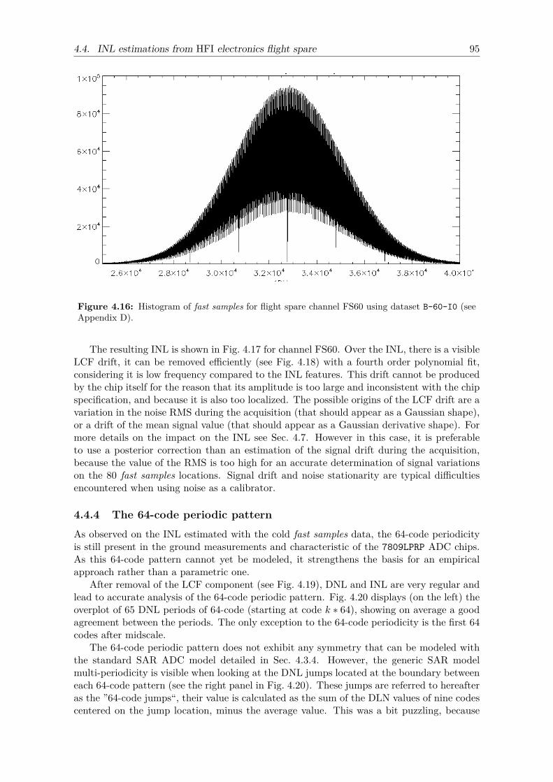
4.4. INL estimations from HFI electronics flight spare 95
with and built using
the dataset value at index j of raw periods.
For inflight setup, the 50 bias steps statistics are summed using the 50 independent weightings. On
large scale it results in a wider error as the correlation on non overlapping dataset is weak.
The following plot show the distribution of the measured ADC values in the whole dataset B-60-I0.
Definition of INL
The integral nonlinearity can only be defined in the area covered by significant statistics and is
defined by abuse of language as:
with being the real ADC quantisation
width in volts for code j, and being the 1st and last code of the area with significant statistics.
The low frequency noise induced by the individual errors on ADC step width is removed with a
polynomial fit of degree 4 or 5.
Illustations
For each channel measured, 5 illustration are provided
• Top: The INL cumulative error fit with the polynomial fit in red
• Middle left: DNL plot in the range [32768-400, 32768+400]
• Middle right: INL plot in the range [32768-400, 32768+400] after polynomial fit correction
• Bottom left: overplot of consecutive range of 64 DNL values showing the peridic shape of
DNL.
Illustration 1: ground calibration histogram for 1st acquisition
dataset on FS60 Figure 4.16: Histogram of fast samples for flight spare channel FS60 using dataset B-60-I0 (seeAppendix D).
The resulting INL is shown in Fig. 4.17 for channel FS60. Over the INL, there is a visibleLCF drift, it can be removed efficiently (see Fig. 4.18) with a fourth order polynomial fit,considering it is low frequency compared to the INL features. This drift cannot be producedby the chip itself for the reason that its amplitude is too large and inconsistent with the chipspecification, and because it is also too localized. The possible origins of the LCF drift are avariation in the noise RMS during the acquisition (that should appear as a Gaussian shape),or a drift of the mean signal value (that should appear as a Gaussian derivative shape). Formore details on the impact on the INL see Sec. 4.7. However in this case, it is preferableto use a posterior correction than an estimation of the signal drift during the acquisition,because the value of the RMS is too high for an accurate determination of signal variationson the 80 fast samples locations. Signal drift and noise stationarity are typical difficultiesencountered when using noise as a calibrator.
4.4.4 The 64-code periodic pattern
As observed on the INL estimated with the cold fast samples data, the 64-code periodicityis still present in the ground measurements and characteristic of the 7809LPRP ADC chips.As this 64-code pattern cannot yet be modeled, it strengthens the basis for an empiricalapproach rather than a parametric one.
After removal of the LCF component (see Fig. 4.19), DNL and INL are very regular andlead to accurate analysis of the 64-code periodic pattern. Fig. 4.20 displays (on the left) theoverplot of 65 DNL periods of 64-code (starting at code k ∗ 64), showing on average a goodagreement between the periods. The only exception to the 64-code periodicity is the first 64codes after midscale.
The 64-code periodic pattern does not exhibit any symmetry that can be modeled withthe standard SAR ADC model detailed in Sec. 4.3.4. However, the generic SAR modelmulti-periodicity is visible when looking at the DNL jumps located at the boundary betweeneach 64-code pattern (see the right panel in Fig. 4.20). These jumps are referred to hereafteras the ”64-code jumps“, their value is calculated as the sum of the DLN values of nine codescentered on the jump location, minus the average value. This was a bit puzzling, because
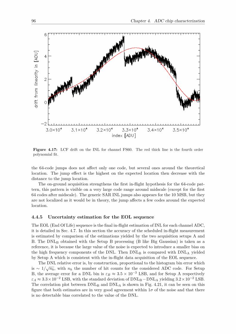
96 Chapter 4. ADC chip characterization
• Bottom right: measure of INL jumps at location modulo 64. The computed value is the
difference between the integral of the 9 local DNL values centered the location and its mean
value.
Results
Channel FS60
data is from ground calibration B-60-I0 dataset merged with B-60-I1-V2, the two runs lasted one
night and then it is the best defined channel.
Illustration 2: cumulative error fit on FS60Figure 4.17: LCF drift on the INL for channel FS60. The red thick line is the fourth orderpolynomial fit.
the 64-code jumps does not affect only one code, but several ones around the theoreticallocation. The jump effect is the highest on the expected location then decrease with thedistance to the jump location.
The on-ground acquisition strengthens the first in-flight hypothesis for the 64-code pat-tern, this pattern is visible on a very large code range around midscale (except for the first64 codes after midscale). The generic SAR INL jumps also appears for the 10 MSB, but theyare not localized as it would be in theory, the jump affects a few codes around the expectedlocation.
4.4.5 Uncertainty estimation for the EOL sequence
The EOL (End Of Life) sequence is the final in-flight estimation of INL for each channel ADC,it is detailed in Sec. 4.7. In this section the accuracy of the scheduled in-flight measurementis estimated by comparison of the estimations yielded by the two acquisition setups A andB. The DNLB obtained with the Setup B processing (B like Big Gaussian) is taken as areference, it is because the large value of the noise is expected to introduce a smaller bias onthe high frequency components of the DNL. Then DNLB is compared with DNLA yieldedby Setup A which is consistent with the in-flight data acquisition of the EOL sequence.
The DNL relative error is, by construction, proportional to the histogram bin error whichis ∼ 1/√nh, with nh the number of hit counts for the considered ADC code. For SetupB, the average error for a DNL bin is εB ≈ 3.5 × 10⁻³ LSB, and for Setup A respectivelyεA ≈ 3.3×10⁻² LSB, with the standard deviation of DNLB−DNLA yielding 3.2×10⁻² LSB.The correlation plot between DNLB and DNLA is shown in Fig. 4.21, it can be seen on thisfigure that both estimates are in very good agreement within 1σ of the noise and that thereis no detectable bias correlated to the value of the DNL.
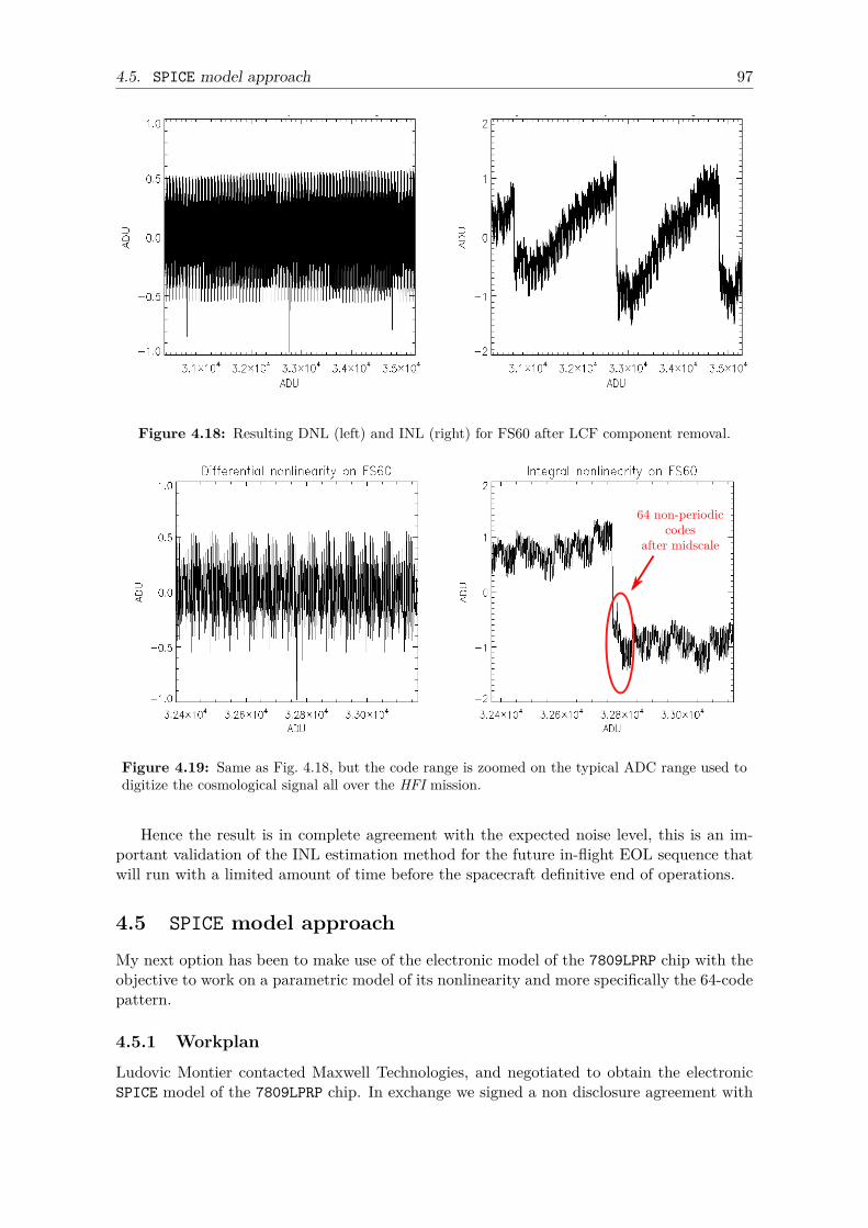
4.5. SPICE model approach 97
Illustration 3: left: large scale DNL on FS6, right: large scale INL on FS60
Illustration 4: left: DNL zoom on FS60, right: INL zoom on FS60
Illustration 5: left: periodic shape of DNL on FS60, right: INL jumps on FS60 for the 10 most significant bits
Figure 4.18: Resulting DNL (left) and INL (right) for FS60 after LCF component removal.
Figure 4.19: Same as Fig. 4.18, but the code range is zoomed on the typical ADC range used todigitize the cosmological signal all over the HFI mission.
Hence the result is in complete agreement with the expected noise level, this is an im-portant validation of the INL estimation method for the future in-flight EOL sequence thatwill run with a limited amount of time before the spacecraft definitive end of operations.
4.5 SPICE model approachMy next option has been to make use of the electronic model of the 7809LPRP chip with theobjective to work on a parametric model of its nonlinearity and more specifically the 64-codepattern.
4.5.1 Workplan
Ludovic Montier contacted Maxwell Technologies, and negotiated to obtain the electronicSPICE model of the 7809LPRP chip. In exchange we signed a non disclosure agreement with
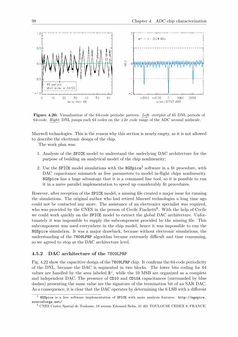
98 Chapter 4. ADC chip characterization
Illustration 3: left: large scale DNL on FS6, right: large scale INL on FS60
Illustration 4: left: DNL zoom on FS60, right: INL zoom on FS60
Illustration 5: left: periodic shape of DNL on FS60, right: INL jumps on FS60 for the 10 most significant bits
Figure 4.20: Visualization of the 64-code periodic pattern. Left: overplot of 65 DNL periods of64-code. Right: DNL jumps each 64 codes on the ±2σ code range of the ADC around midscale.
Maxwell technologies. This is the reason why this section is nearly empty, as it is not allowedto describe the electronic design of the chip.
The work plan was:
1. Analysis of the SPICE model to understand the underlying DAC architecture for thepurpose of building an analytical model of the chip nonlinearity;
2. Use the SPICE model simulations with the NGSpice5 software in a fit procedure, withDAC capacitance mismatch as free parameters to model in-flight chips nonlinearity.NGSpice has a huge advantage that it is a command line tool, so it is possible to runit in a naive parallel implementation to speed up considerably fit procedures.
However, after reception of the SPICE model, a missing file created a major issue for runningthe simulations. The original author who had retired Maxwel technologies a long time agocould not be contacted any more. The assistance of an electronics specialist was required,who was provided by the CNES in the person of Cecile Fiachetti6. With the help of Cecilewe could work quickly on the SPICE model to extract the global DAC architecture. Unfor-tunately it was impossible to supply the subcomponent provided by the missing file. Thissubcomponent was used everywhere in the chip model, hence it was impossible to run theNGSpice simulation. It was a major drawback, because without electronic simulations, theunderstanding of the 7809LPRP algorithm became extremely difficult and time consuming,so we agreed to stop at the DAC architecture level.
4.5.2 DAC architecture of the 7809LPRP
Fig. 4.22 show the capacitive design of the 7809LPRP chip. It confirms the 64-code periodicityof the DNL, because the DAC is segmented in two blocks. The lower bits coding for 64values are handled by the area labeled B’, while the 10 MSB are organized as a completeand independent DAC. The presence of CD10 and CD10A capacitances (surrounded by bluedashes) presenting the same value are the signature of the termination bit of an SAR DAC.As a consequence, it is clear that the DAC operates by determining the 6 LSB with a different
5 NGSpice is a free software implementation of SPICE with more analysis features. http://ngspice.sourceforge.net/
6 CNES Centre Spatial de Toulouse, 18 avenue Edouard Belin, 31 401 TOULOUSE CEDEX 9, FRANCE.
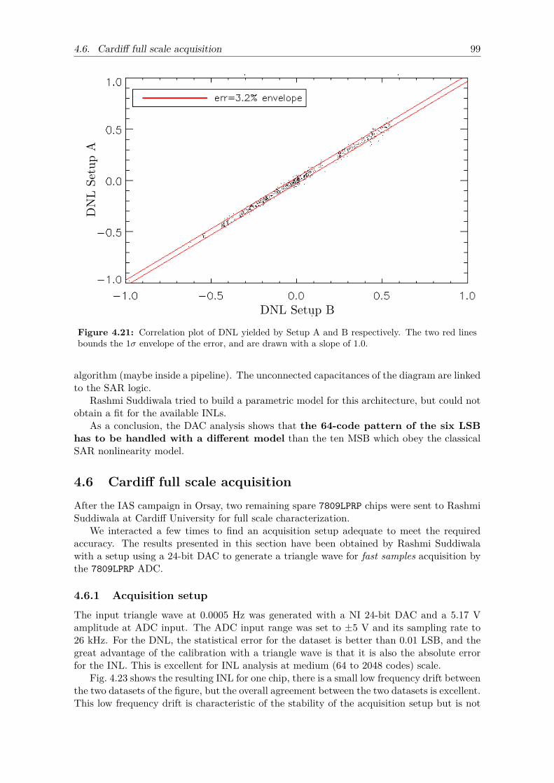
4.6. Cardiff full scale acquisition 99
Figure 4.21: Correlation plot of DNL yielded by Setup A and B respectively. The two red linesbounds the 1σ envelope of the error, and are drawn with a slope of 1.0.
algorithm (maybe inside a pipeline). The unconnected capacitances of the diagram are linkedto the SAR logic.
Rashmi Suddiwala tried to build a parametric model for this architecture, but could notobtain a fit for the available INLs.
As a conclusion, the DAC analysis shows that the 64-code pattern of the six LSBhas to be handled with a different model than the ten MSB which obey the classicalSAR nonlinearity model.
4.6 Cardiff full scale acquisitionAfter the IAS campaign in Orsay, two remaining spare 7809LPRP chips were sent to RashmiSuddiwala at Cardiff University for full scale characterization.
We interacted a few times to find an acquisition setup adequate to meet the requiredaccuracy. The results presented in this section have been obtained by Rashmi Suddiwalawith a setup using a 24-bit DAC to generate a triangle wave for fast samples acquisition bythe 7809LPRP ADC.
4.6.1 Acquisition setup
The input triangle wave at 0.0005 Hz was generated with a NI 24-bit DAC and a 5.17 Vamplitude at ADC input. The ADC input range was set to ±5 V and its sampling rate to26 kHz. For the DNL, the statistical error for the dataset is better than 0.01 LSB, and thegreat advantage of the calibration with a triangle wave is that it is also the absolute errorfor the INL. This is excellent for INL analysis at medium (64 to 2048 codes) scale.
Fig. 4.23 shows the resulting INL for one chip, there is a small low frequency drift betweenthe two datasets of the figure, but the overall agreement between the two datasets is excellent.This low frequency drift is characteristic of the stability of the acquisition setup but is not
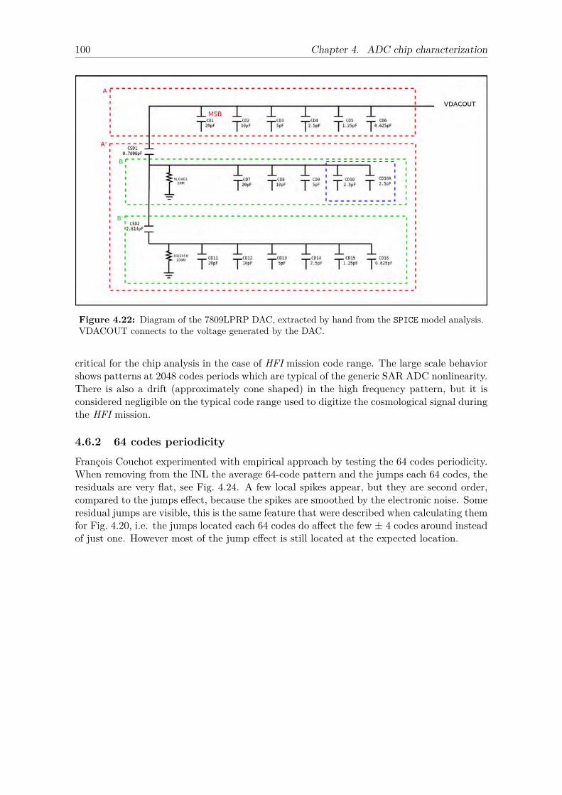
100 Chapter 4. ADC chip characterization
Figure 4.22: Diagram of the 7809LPRP DAC, extracted by hand from the SPICE model analysis.VDACOUT connects to the voltage generated by the DAC.
critical for the chip analysis in the case of HFI mission code range. The large scale behaviorshows patterns at 2048 codes periods which are typical of the generic SAR ADC nonlinearity.There is also a drift (approximately cone shaped) in the high frequency pattern, but it isconsidered negligible on the typical code range used to digitize the cosmological signal duringthe HFI mission.
4.6.2 64 codes periodicity
François Couchot experimented with empirical approach by testing the 64 codes periodicity.When removing from the INL the average 64-code pattern and the jumps each 64 codes, theresiduals are very flat, see Fig. 4.24. A few local spikes appear, but they are second order,compared to the jumps effect, because the spikes are smoothed by the electronic noise. Someresidual jumps are visible, this is the same feature that were described when calculating themfor Fig. 4.20, i.e. the jumps located each 64 codes do affect the few ± 4 codes around insteadof just one. However most of the jump effect is still located at the expected location.
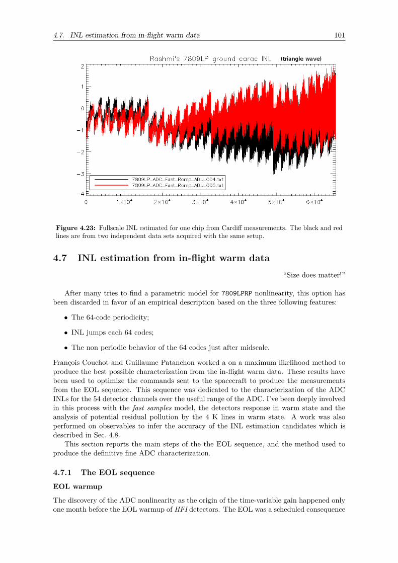
4.7. INL estimation from in-flight warm data 101
Figure 4.23: Fullscale INL estimated for one chip from Cardiff measurements. The black and redlines are from two independent data sets acquired with the same setup.
4.7 INL estimation from in-flight warm data“Size does matter!”
After many tries to find a parametric model for 7809LPRP nonlinearity, this option hasbeen discarded in favor of an empirical description based on the three following features:
• The 64-code periodicity;
• INL jumps each 64 codes;
• The non periodic behavior of the 64 codes just after midscale.
François Couchot and Guillaume Patanchon worked a on a maximum likelihood method toproduce the best possible characterization from the in-flight warm data. These results havebeen used to optimize the commands sent to the spacecraft to produce the measurementsfrom the EOL sequence. This sequence was dedicated to the characterization of the ADCINLs for the 54 detector channels over the useful range of the ADC. I’ve been deeply involvedin this process with the fast samples model, the detectors response in warm state and theanalysis of potential residual pollution by the 4 K lines in warm state. A work was alsoperformed on observables to infer the accuracy of the INL estimation candidates which isdescribed in Sec. 4.8.
This section reports the main steps of the the EOL sequence, and the method used toproduce the definitive fine ADC characterization.
4.7.1 The EOL sequence
EOL warmup
The discovery of the ADC nonlinearity as the origin of the time-variable gain happened onlyone month before the EOL warmup of HFI detectors. The EOL was a scheduled consequence
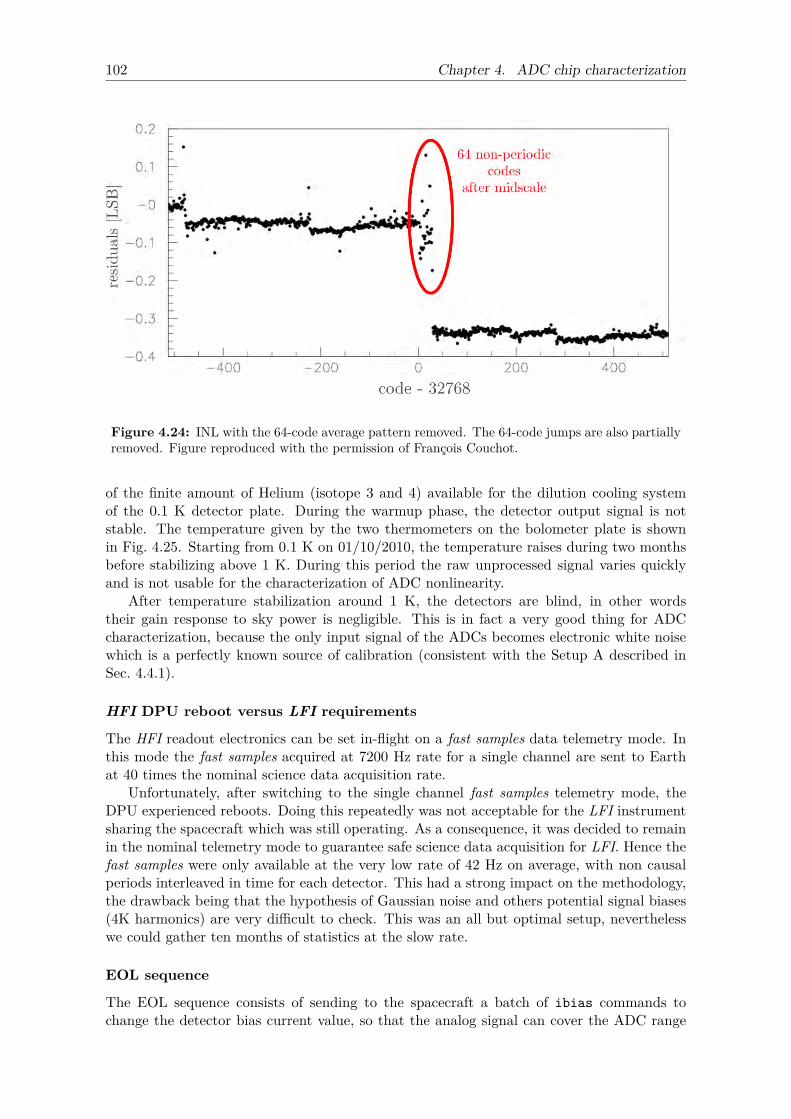
102 Chapter 4. ADC chip characterization
Figure 4.24: INL with the 64-code average pattern removed. The 64-code jumps are also partiallyremoved. Figure reproduced with the permission of François Couchot.
of the finite amount of Helium (isotope 3 and 4) available for the dilution cooling systemof the 0.1 K detector plate. During the warmup phase, the detector output signal is notstable. The temperature given by the two thermometers on the bolometer plate is shownin Fig. 4.25. Starting from 0.1 K on 01/10/2010, the temperature raises during two monthsbefore stabilizing above 1 K. During this period the raw unprocessed signal varies quicklyand is not usable for the characterization of ADC nonlinearity.
After temperature stabilization around 1 K, the detectors are blind, in other wordstheir gain response to sky power is negligible. This is in fact a very good thing for ADCcharacterization, because the only input signal of the ADCs becomes electronic white noisewhich is a perfectly known source of calibration (consistent with the Setup A described inSec. 4.4.1).
HFI DPU reboot versus LFI requirements
The HFI readout electronics can be set in-flight on a fast samples data telemetry mode. Inthis mode the fast samples acquired at 7200 Hz rate for a single channel are sent to Earthat 40 times the nominal science data acquisition rate.
Unfortunately, after switching to the single channel fast samples telemetry mode, theDPU experienced reboots. Doing this repeatedly was not acceptable for the LFI instrumentsharing the spacecraft which was still operating. As a consequence, it was decided to remainin the nominal telemetry mode to guarantee safe science data acquisition for LFI. Hence thefast samples were only available at the very low rate of 42 Hz on average, with non causalperiods interleaved in time for each detector. This had a strong impact on the methodology,the drawback being that the hypothesis of Gaussian noise and others potential signal biases(4K harmonics) are very difficult to check. This was an all but optimal setup, neverthelesswe could gather ten months of statistics at the slow rate.
EOL sequence
The EOL sequence consists of sending to the spacecraft a batch of ibias commands tochange the detector bias current value, so that the analog signal can cover the ADC range
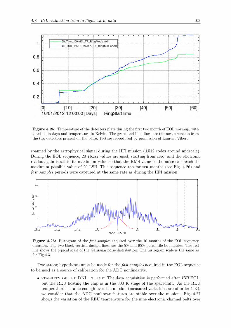
4.7. INL estimation from in-flight warm data 103
Figure 4.25: Temperature of the detectors plate during the first two month of EOL warmup, withx-axis is in days and temperature in Kelvin. The green and blue lines are the measurements fromthe two detectors present on the plate. Picture reproduced by permission of Laurent Vibert
spanned by the astrophysical signal during the HFI mission (±512 codes around midscale).During the EOL sequence, 20 ibias values are used, starting from zero, and the electronicreadout gain is set to its maximum value so that the RMS value of the noise can reach themaximum possible value of 20 LSB. This sequence ran for ten months (see Fig. 4.26) andfast samples periods were captured at the same rate as during the HFI mission.
256 192 128 64 0 64 128 192 256code - 32768
1
2
3
4
(nb o
f hit
s) /
105
Figure 4.26: Histogram of the fast samples acquired over the 10 months of the EOL sequenceduration. The two black vertical dashed lines are the 5% and 95% percentile boundaries. The redline shows the typical scale of the Gaussian noise distribution. The histogram scale is the same asfor Fig.4.3.
Two strong hypotheses must be made for the fast samples acquired in the EOL sequenceto be used as a source of calibration for the ADC nonlinearity:
• stability of the DNL in time: The data acquisition is performed after HFI EOL,but the REU hosting the chip is in the 300 K stage of the spacecraft. As the REUtemperature is stable enough over the mission (measured variations are of order 1 K),we consider that the ADC nonlinear features are stable over the mission. Fig. 4.27shows the variation of the REU temperature for the nine electronic channel belts over
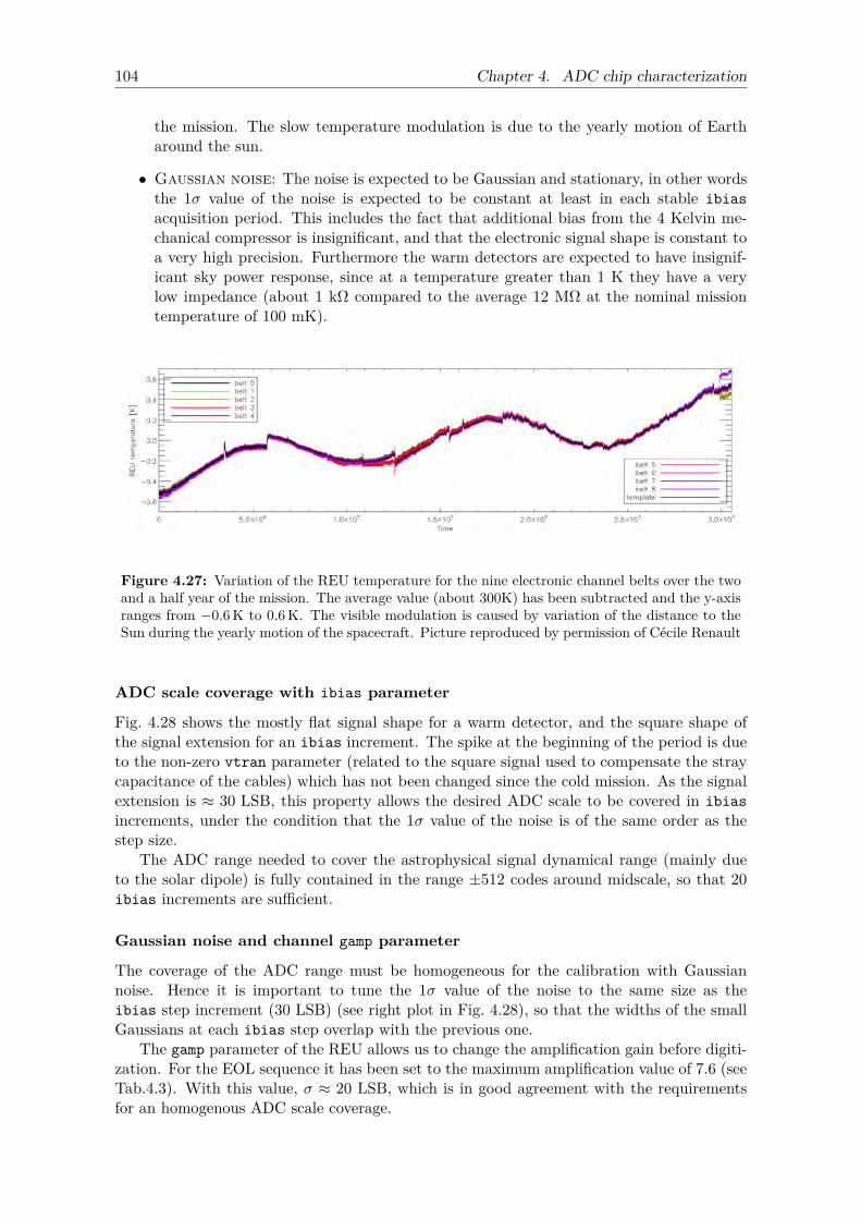
104 Chapter 4. ADC chip characterization
the mission. The slow temperature modulation is due to the yearly motion of Eartharound the sun.
• Gaussian noise: The noise is expected to be Gaussian and stationary, in other wordsthe 1σ value of the noise is expected to be constant at least in each stable ibiasacquisition period. This includes the fact that additional bias from the 4 Kelvin me-chanical compressor is insignificant, and that the electronic signal shape is constant toa very high precision. Furthermore the warm detectors are expected to have insignif-icant sky power response, since at a temperature greater than 1 K they have a verylow impedance (about 1 kΩ compared to the average 12 MΩ at the nominal missiontemperature of 100 mK).
Figure 4.27: Variation of the REU temperature for the nine electronic channel belts over the twoand a half year of the mission. The average value (about 300K) has been subtracted and the y-axisranges from −0.6 K to 0.6 K. The visible modulation is caused by variation of the distance to theSun during the yearly motion of the spacecraft. Picture reproduced by permission of Cécile Renault
ADC scale coverage with ibias parameter
Fig. 4.28 shows the mostly flat signal shape for a warm detector, and the square shape ofthe signal extension for an ibias increment. The spike at the beginning of the period is dueto the non-zero vtran parameter (related to the square signal used to compensate the straycapacitance of the cables) which has not been changed since the cold mission. As the signalextension is ≈ 30 LSB, this property allows the desired ADC scale to be covered in ibiasincrements, under the condition that the 1σ value of the noise is of the same order as thestep size.
The ADC range needed to cover the astrophysical signal dynamical range (mainly dueto the solar dipole) is fully contained in the range ±512 codes around midscale, so that 20ibias increments are sufficient.
Gaussian noise and channel gamp parameter
The coverage of the ADC range must be homogeneous for the calibration with Gaussiannoise. Hence it is important to tune the 1σ value of the noise to the same size as theibias step increment (30 LSB) (see right plot in Fig. 4.28), so that the widths of the smallGaussians at each ibias step overlap with the previous one.
The gamp parameter of the REU allows us to change the amplification gain before digiti-zation. For the EOL sequence it has been set to the maximum amplification value of 7.6 (seeTab.4.3). With this value, σ ≈ 20 LSB, which is in good agreement with the requirementsfor an homogenous ADC scale coverage.
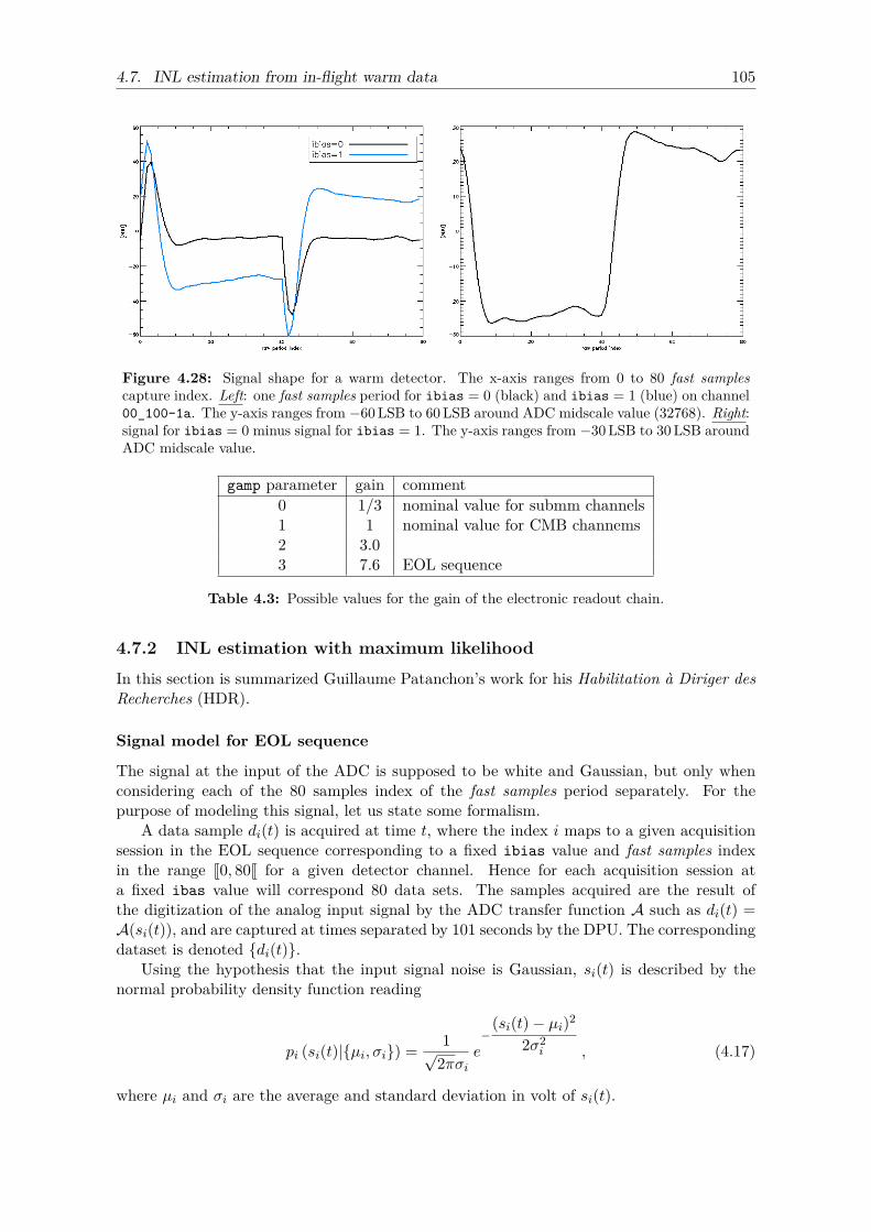
4.7. INL estimation from in-flight warm data 105
Figure 4.28: Signal shape for a warm detector. The x-axis ranges from 0 to 80 fast samplescapture index. Left: one fast samples period for ibias = 0 (black) and ibias = 1 (blue) on channel00_100-1a. The y-axis ranges from −60 LSB to 60 LSB around ADC midscale value (32768). Right:signal for ibias = 0 minus signal for ibias = 1. The y-axis ranges from −30 LSB to 30 LSB aroundADC midscale value.
gamp parameter gain comment0 1/3 nominal value for submm channels1 1 nominal value for CMB channems2 3.03 7.6 EOL sequence
Table 4.3: Possible values for the gain of the electronic readout chain.
4.7.2 INL estimation with maximum likelihood
In this section is summarized Guillaume Patanchon’s work for his Habilitation à Diriger desRecherches (HDR).
Signal model for EOL sequence
The signal at the input of the ADC is supposed to be white and Gaussian, but only whenconsidering each of the 80 samples index of the fast samples period separately. For thepurpose of modeling this signal, let us state some formalism.
A data sample di(t) is acquired at time t, where the index i maps to a given acquisitionsession in the EOL sequence corresponding to a fixed ibias value and fast samples indexin the range J0, 80J for a given detector channel. Hence for each acquisition session ata fixed ibas value will correspond 80 data sets. The samples acquired are the result ofthe digitization of the analog input signal by the ADC transfer function A such as di(t) =A(si(t)), and are captured at times separated by 101 seconds by the DPU. The correspondingdataset is denoted di(t).
Using the hypothesis that the input signal noise is Gaussian, si(t) is described by thenormal probability density function reading
pi (si(t)|µi, σi) = 1√2πσi
e−
(si(t)− µi)2
2σ2i , (4.17)
where µi and σi are the average and standard deviation in volt of si(t).
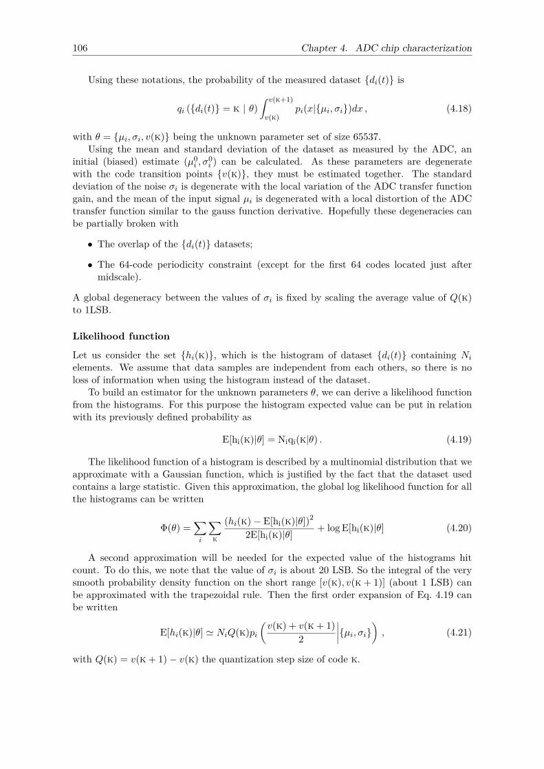
106 Chapter 4. ADC chip characterization
Using these notations, the probability of the measured dataset di(t) is
qi (di(t) = k | θ)∫ v(k+1)
v(k)pi(x|µi, σi)dx , (4.18)
with θ = µi, σi, v(k) being the unknown parameter set of size 65537.Using the mean and standard deviation of the dataset as measured by the ADC, an
initial (biased) estimate (µ0i , σ
0i ) can be calculated. As these parameters are degenerate
with the code transition points v(k), they must be estimated together. The standarddeviation of the noise σi is degenerate with the local variation of the ADC transfer functiongain, and the mean of the input signal µi is degenerated with a local distortion of the ADCtransfer function similar to the gauss function derivative. Hopefully these degeneracies canbe partially broken with
• The overlap of the di(t) datasets;
• The 64-code periodicity constraint (except for the first 64 codes located just aftermidscale).
A global degeneracy between the values of σi is fixed by scaling the average value of Q(k)to 1LSB.
Likelihood function
Let us consider the set hi(k), which is the histogram of dataset di(t) containing Ni
elements. We assume that data samples are independent from each others, so there is noloss of information when using the histogram instead of the dataset.
To build an estimator for the unknown parameters θ, we can derive a likelihood functionfrom the histograms. For this purpose the histogram expected value can be put in relationwith its previously defined probability as
E[hi(k)|θ] = Niqi(k|θ) . (4.19)
The likelihood function of a histogram is described by a multinomial distribution that weapproximate with a Gaussian function, which is justified by the fact that the dataset usedcontains a large statistic. Given this approximation, the global log likelihood function for allthe histograms can be written
Φ(θ) =∑i
∑k
(hi(k)− E[hi(k)|θ])2
2E[hi(k)|θ] + log E[hi(k)|θ] (4.20)
A second approximation will be needed for the expected value of the histograms hitcount. To do this, we note that the value of σi is about 20 LSB. So the integral of the verysmooth probability density function on the short range [v(k), v(k + 1)] (about 1 LSB) canbe approximated with the trapezoidal rule. Then the first order expansion of Eq. 4.19 canbe written
E[hi(k)|θ] ' NiQ(k)pi(v(k) + v(k + 1)
2
∣∣∣∣µi, σi) , (4.21)
with Q(k) = v(k + 1)− v(k) the quantization step size of code k.
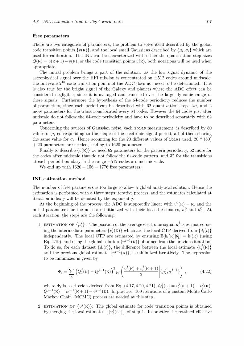
4.7. INL estimation from in-flight warm data 107
Free parameters
There are two categories of parameters, the problem to solve itself described by the globalcode transition points v(k), and the local small Gaussians described by µi, σi which areused for calibration. The INL can be characterized with either the quantization step sizesQ(k) = v(k+1)−v(k), or the code transition points v(k), both notations will be used whenappropriate.
The initial problem brings a part of the solution: as the low signal dynamic of theastrophysical signal over the HFI mission is concentrated on ±512 codes around midscale,the full scale 216 code transition points of the ADC does not need to be determined. Thisis also true for the bright signal of the Galaxy and planets where the ADC effect can beconsidered negligible, since it is averaged and canceled over the large dynamic range ofthese signals. Furthermore the hypothesis of the 64-code periodicity reduces the numberof parameters, since each period can be described with 62 quantization step size, and 2more parameters for the transitions located every 64 codes. However the 64 codes just aftermidscale do not follow the 64-code periodicity and have to be described separately with 62parameters.
Concerning the sources of Gaussian noise, each ibias measurement, is described by 80values of µi corresponding to the shape of the electronic signal period, all of them sharingthe same value for σi. Hence acounting for the 20 different values of ibias used, 20 * (80)+ 20 parameters are needed, leading to 1620 parameters.
Finally to describe v(k) we need 62 parameters for the pattern periodicity, 62 more forthe codes after midscale that do not follow the 64-code pattern, and 32 for the transitionsat each period boundary in the range ±512 codes around midscale.
We end up with 1620 + 156 = 1776 free parameters.
INL estimation method
The number of free parameters is too large to allow a global analytical solution. Hence theestimation is performed with a three steps iterative process, and the estimates calculated atiteration index j will be denoted by the exponent j.
At the beginning of the process, the ADC is supposedly linear with v0(k) = k, and theinitial parameters for the noise are initialized with their biased estimates, σ0
i and µ0i . At
each iteration, the steps are the following:
1. estimation of µji : The position of the average electronic signal µji is estimated us-ing the intermediate parameters vji (k) which are the local CTP derived from di(t)independently. The local CTP are estimated by ensuring E[hi(k)|θj
i ] = hi(k) (usingEq. 4.19), and using the global solution vj−1(k) obtained from the previous iteration.To do so, for each dataset di(t), the difference between the local estimate vji (k)and the previous global estimate vj−1(k), is minimized iteratively. The expressionto be minimized is given by
Φi =∑
k
(Qji (k)−Qj−1(k)
)2pi
(vji (k) + vji (k + 1)
2
∣∣∣∣∣µji , σj−1i
), (4.22)
where Φi is a criterion derived from Eq. (4.17, 4.20, 4.21), Qji (k) = vji (k + 1) − vji (k),Qj−1(k) = vj−1(k + 1)− vj−1(k). In practice, 100 iterations of a custom Monte CarloMarkov Chain (MCMC) process are needed at this step.
2. estimation of vj(k): The global estimate for code transition points is obtainedby merging the local estimates vji (k) of step 1. In practice the retained effective
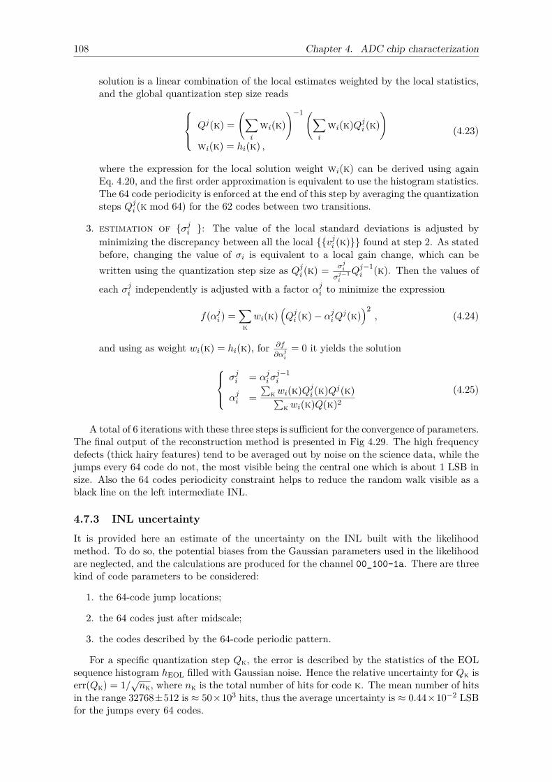
108 Chapter 4. ADC chip characterization
solution is a linear combination of the local estimates weighted by the local statistics,and the global quantization step size reads Qj(k) =
(∑i
wi(k))−1(∑
i
wi(k)Qji (k))
wi(k) = hi(k) ,(4.23)
where the expression for the local solution weight wi(k) can be derived using againEq. 4.20, and the first order approximation is equivalent to use the histogram statistics.The 64 code periodicity is enforced at the end of this step by averaging the quantizationsteps Qji (k mod 64) for the 62 codes between two transitions.
3. estimation of σji : The value of the local standard deviations is adjusted byminimizing the discrepancy between all the local vji (k) found at step 2. As statedbefore, changing the value of σi is equivalent to a local gain change, which can bewritten using the quantization step size as Qji (k) = σji
σj−1i
Qj−1i (k). Then the values of
each σji independently is adjusted with a factor αji to minimize the expression
f(αji ) =∑
kwi(k)
(Qji (k)− αjiQj(k)
)2, (4.24)
and using as weight wi(k) = hi(k), for ∂f
∂αji= 0 it yields the solution
σji = αjiσ
j−1i
αji =∑
kwi(k)Qji (k)Qj(k)∑kwi(k)Q(k)2
(4.25)
A total of 6 iterations with these three steps is sufficient for the convergence of parameters.The final output of the reconstruction method is presented in Fig 4.29. The high frequencydefects (thick hairy features) tend to be averaged out by noise on the science data, while thejumps every 64 code do not, the most visible being the central one which is about 1 LSB insize. Also the 64 codes periodicity constraint helps to reduce the random walk visible as ablack line on the left intermediate INL.
4.7.3 INL uncertainty
It is provided here an estimate of the uncertainty on the INL built with the likelihoodmethod. To do so, the potential biases from the Gaussian parameters used in the likelihoodare neglected, and the calculations are produced for the channel 00_100-1a. There are threekind of code parameters to be considered:
1. the 64-code jump locations;
2. the 64 codes just after midscale;
3. the codes described by the 64-code periodic pattern.
For a specific quantization step Qk, the error is described by the statistics of the EOLsequence histogram hEOL filled with Gaussian noise. Hence the relative uncertainty for Qk iserr(Qk) = 1/√nk, where nk is the total number of hits for code k. The mean number of hitsin the range 32768±512 is ≈ 50×103 hits, thus the average uncertainty is ≈ 0.44×10⁻² LSBfor the jumps every 64 codes.
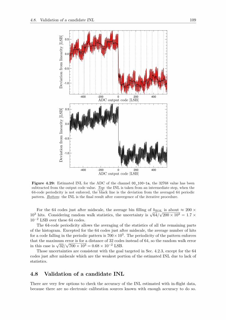
4.8. Validation of a candidate INL 109
-400 -200 0 200 400
-1.0
-0.5
0.0
0.5
-400 -200 0 200 400
-1.0
-0.5
0.0
0.5
Figure 4.29: Estimated INL for the ADC of the channel 00_100-1a, the 32768 value has beensubtracted from the output code value. Top: the INL is taken from an intermediate step, when the64-code periodicity is not enforced, the black line is the deviation from the averaged 64 periodicpattern. Bottom: the INL is the final result after convergence of the iterative procedure.
For the 64 codes just after midscale, the average bin filling of hEOL is about ≈ 200 ×103 hits. Considering random walk statistics, the uncertainty is
√64/√
200× 103 = 1.7 ×10⁻² LSB over these 64 codes.
The 64-code periodicity allows the averaging of the statistics of all the remaining partsof the histogram. Excepted for the 64 codes just after midscale, the average number of hitsfor a code falling in the periodic pattern is 700×103. The periodicity of the pattern enforcesthat the maximum error is for a distance of 32 codes instead of 64, so the random walk errorin this case is
√32/√
700× 103 = 0.68× 10⁻² LSB.Those uncertainties are consistent with the goal targeted in Sec. 4.2.3, except for the 64
codes just after midscale which are the weakest portion of the estimated INL due to lack ofstatistics.
4.8 Validation of a candidate INLThere are very few options to check the accuracy of the INL estimated with in-flight data,because there are no electronic calibration sources known with enough accuracy to do so.
110 Chapter 4. ADC chip characterization
The naive way is to estimate ADC residuals on the maps projection of science data aftercorrection (as detailed in Sec. 5.5, but some quick estimators have also been developed whichare presented below.
This section presents an histogram based method to estimate qualitatively the accuracyof a candidate INL. A second quantitative method is detailed, it is based on the calibrationwith the shape of the detector response (the raw gain), and result from the analysis of thefast samples acquired during the mission (cold fast samples).
4.8.1 The smooth histogram method
This method is based on the expected smoothness of the fast samples histogram over thefull mission. If considering a perfect ADC, the bins are filled with Gaussian noise (RMS≈ 4 LSB) and the average value vary slowly, dominated by the thermal fluctuations of thebolometer plate (≈ 100 LSB for a given fast samples period index). Hence a correction ofthe histogram, using the estimated ADC nonlinearity, would yield a smooth histogram as itwould be the case with a perfect ADC.
To check the smoothness hypothesis let us consider h(k) the histogram of fast samplescodes values over the HFI mission. If the averaged analog input signal 〈s〉 is constant overh(k) and its adjacent bins, then the bin content is proportional to the quantization step sizeh(k) ∼ 〈s〉Q(k). Hence the order zero ADC corrected histogram is
h0(k) = h(k)Q(k) . (4.26)
The resulting h0 histogram is shown in Fig. 4.30 for the channel 00_100_1a, which isknown to have a very low bias coming from other systematics such as 4 K lines. Aftercorrection, the result is impressive compared to the original version (see Fig. 4.26). Thehigh frequency features have nearly disappeared. The few remaining spikes are due to localvariations in the 64-code periodicity and are expected to be negligible after averaging bythe noise of the analog signal (aka noise dithering). It can be seen in the high frequencyresiduals that the 64 codes after midscale look much better corrected (albeit with a noiselevel consistent with the statistics), this is expected because these codes have an ”individual“estimate and do not follow the 64-code pattern. The remaining negative spike at midscale isa bit more problematic, it is not compensated by a positive spike on an adjacent code, hencethis may be a residual bias from the likelihood method.
Finally the comparison between h0 from the cold mission data, and from the EOL se-quence respectively yields two important pieces of information:
• The ADC nonlinearity has not changed significantly over more than 3 years durationof the mission plus EOL sequence;
• The residual high frequency features are consistent between both datasets, this is anexcellent crosscheck of the correction efficiency with uncorrelated data.
4.8.2 The raw gain method
This second method is based on the stability of the detector response also designed as the rawgain (this has been covered in details in Chap. 2). The hypothesis is that the raw gain can beused as a calibration source to estimate the efficiency of ADC nonlinearity corrections. As aconsequence the consistency of the raw gain calculated at different moments in the missionlifetime should be a tracer for ADC nonlinearity residuals.
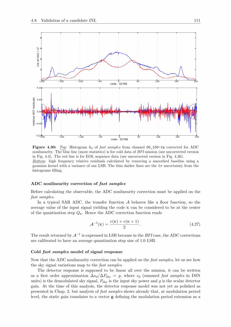
4.8. Validation of a candidate INL 111
256 192 128 64 0 64 128 192 256code - 32768
1
2
3
4(n
b o
f hit
s) /
105
256 192 128 64 0 64 128 192 256code - 32768
0.10
0.05
0.00
0.05
0.10
rela
tive H
CF
resi
duals
Figure 4.30: Top: Histogram h0 of fast samples from channel 00_100-1a corrected for ADCnonlinearity. The blue line (more statistics) is for cold data of HFI mission (see uncorrected versionin Fig. 4.3). The red line is for EOL sequence data (see uncorrected version in Fig. 4.26).Bottom: high frequency relative residuals calculated by removing a smoothed baseline using agaussian kernel with a variance of one LSB. The thin darker lines are the 1σ uncertainty from thehistograms filling.
ADC nonlinearity correction of fast samples
Before calculating the observable, the ADC nonlinearity correction must be applied on thefast samples.
In a typical SAR ADC, the transfer function A behaves like a floor function, so theaverage value of the input signal yielding the code k can be considered to be at the centerof the quantization step Qk. Hence the ADC correction function reads
A−1(k) = v(k) + v(k + 1)2 . (4.27)
The result returned by A−1 is expressed in LSB because in the HFI case, the ADC correctionsare calibrated to have an average quantization step size of 1.0 LSB.
Cold fast samples model of signal response
Now that the ADC nonlinearity correction can be applied on the fast samples, let us see howthe sky signal variations map to the fast samples.
The detector response is supposed to be linear all over the mission, it can be writtenas a first order approximation ∆sd/∆Psky = g, where sd (summed fast samples in DSNunits) is the demodulated sky signal, Psky is the input sky power and g is the scalar detectorgain. At the time of this analysis, the detector response model was not yet as polished aspresented in Chap. 2, but analysis of fast samples shows already that, at modulation periodlevel, the static gain translates to a vector g defining the modulation period extension as a
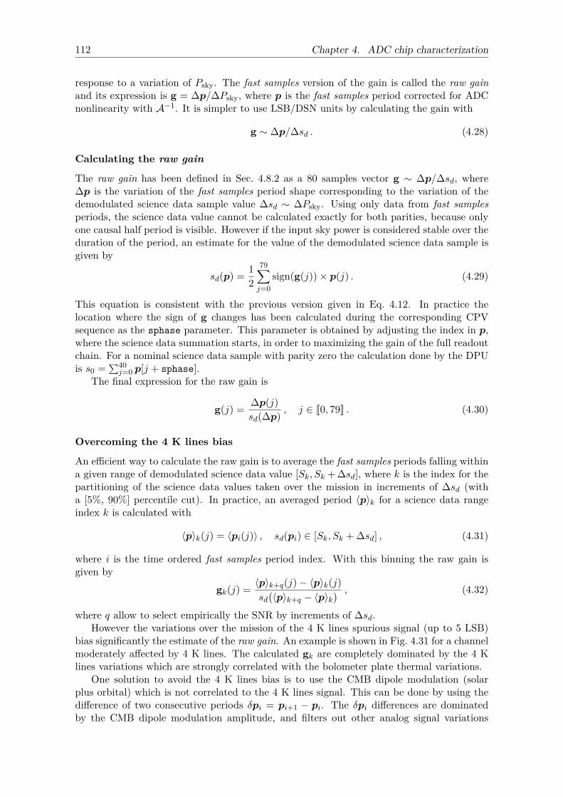
112 Chapter 4. ADC chip characterization
response to a variation of Psky. The fast samples version of the gain is called the raw gainand its expression is g = ∆p/∆Psky, where p is the fast samples period corrected for ADCnonlinearity with A−1. It is simpler to use LSB/DSN units by calculating the gain with
g ∼ ∆p/∆sd . (4.28)
Calculating the raw gain
The raw gain has been defined in Sec. 4.8.2 as a 80 samples vector g ∼ ∆p/∆sd, where∆p is the variation of the fast samples period shape corresponding to the variation of thedemodulated science data sample value ∆sd ∼ ∆Psky. Using only data from fast samplesperiods, the science data value cannot be calculated exactly for both parities, because onlyone causal half period is visible. However if the input sky power is considered stable over theduration of the period, an estimate for the value of the demodulated science data sample isgiven by
sd(p) = 12
79∑j=0
sign(g(j))× p(j) . (4.29)
This equation is consistent with the previous version given in Eq. 4.12. In practice thelocation where the sign of g changes has been calculated during the corresponding CPVsequence as the sphase parameter. This parameter is obtained by adjusting the index in p,where the science data summation starts, in order to maximizing the gain of the full readoutchain. For a nominal science data sample with parity zero the calculation done by the DPUis s0 = ∑40
j=0 p[j + sphase].The final expression for the raw gain is
g(j) = ∆p(j)sd(∆p) , j ∈ J0, 79K . (4.30)
Overcoming the 4 K lines bias
An efficient way to calculate the raw gain is to average the fast samples periods falling withina given range of demodulated science data value [Sk, Sk + ∆sd], where k is the index for thepartitioning of the science data values taken over the mission in increments of ∆sd (witha [5%, 90%] percentile cut). In practice, an averaged period 〈p〉k for a science data rangeindex k is calculated with
〈p〉k(j) = 〈pi(j)〉 , sd(pi) ∈ [Sk, Sk + ∆sd] , (4.31)
where i is the time ordered fast samples period index. With this binning the raw gain isgiven by
gk(j) = 〈p〉k+q(j)− 〈p〉k(j)sd(〈p〉k+q − 〈p〉k
) , (4.32)
where q allow to select empirically the SNR by increments of ∆sd.However the variations over the mission of the 4 K lines spurious signal (up to 5 LSB)
bias significantly the estimate of the raw gain. An example is shown in Fig. 4.31 for a channelmoderately affected by 4 K lines. The calculated gk are completely dominated by the 4 Klines variations which are strongly correlated with the bolometer plate thermal variations.
One solution to avoid the 4 K lines bias is to use the CMB dipole modulation (solarplus orbital) which is not correlated to the 4 K lines signal. This can be done by using thedifference of two consecutive periods δpi = pi+1 − pi. The δpi differences are dominatedby the CMB dipole modulation amplitude, and filters out other analog signal variations
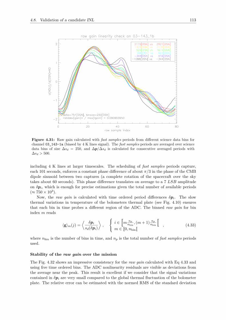
4.8. Validation of a candidate INL 113
Figure 4.31: Raw gain calculated with fast samples periods from different science data bins forchannel 03_143-1a (biased by 4 K lines signal). The fast samples periods are averaged over sciencedata bins of size ∆sd = 250, and ∆p/∆sd is calculated for consecutive averaged periods with∆sd > 500.
including 4 K lines at larger timescales. The scheduling of fast samples periods capture,each 101 seconds, enforces a constant phase difference of about π/3 in the phase of the CMBdipole sinusoid between two captures (a complete rotation of the spacecraft over the skytakes about 60 seconds). This phase difference translates on average to a 7 LSB amplitudeon δpi, which is enough for precise estimations given the total number of available periods(≈ 750× 103).
Now, the raw gain is calculated with time ordered period differences δpi. The slowthermal variations in temperature of the bolometers thermal plate (see Fig. 4.10) ensuresthat each bin in time probes a different region of the ADC. The binned raw gain for binindex m reads
〈g〉m(j) =⟨
δpisd(δpi)
⟩,
i ∈rm
npnbin
, (m+ 1) npnbin
r
m ∈ J0, nbinJ, (4.33)
where nbin is the number of bins in time, and np is the total number of fast samples periodsused.
Stability of the raw gain over the mission
The Fig. 4.32 shows an impressive consistency for the raw gain calculated with Eq 4.33 andusing five time ordered bins. The ADC nonlinearity residuals are visible as deviations fromthe average near the peak. This result is excellent if we consider that the signal variationscontained in δpi are very small compared to the global thermal fluctuation of the bolometerplate. The relative error can be estimated with the normed RMS of the standard deviation
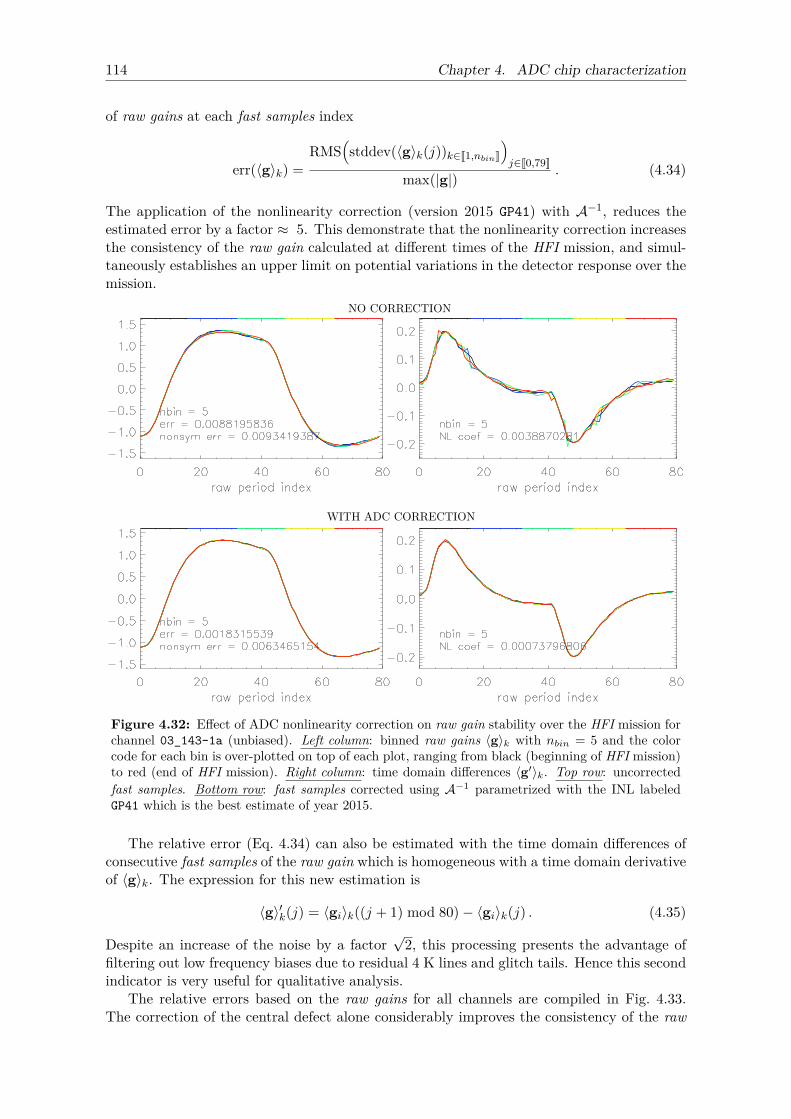
114 Chapter 4. ADC chip characterization
of raw gains at each fast samples index
err(〈g〉k) =RMS
(stddev(〈g〉k(j))k∈J1,nbinK
)j∈J0,79K
max(|g|) . (4.34)
The application of the nonlinearity correction (version 2015 GP41) with A−1, reduces theestimated error by a factor ≈ 5. This demonstrate that the nonlinearity correction increasesthe consistency of the raw gain calculated at different times of the HFI mission, and simul-taneously establishes an upper limit on potential variations in the detector response over themission.
Figure 4.32: Effect of ADC nonlinearity correction on raw gain stability over the HFI mission forchannel 03_143-1a (unbiased). Left column: binned raw gains 〈g〉k with nbin = 5 and the colorcode for each bin is over-plotted on top of each plot, ranging from black (beginning of HFI mission)to red (end of HFI mission). Right column: time domain differences 〈g′〉k. Top row: uncorrectedfast samples. Bottom row: fast samples corrected using A−1 parametrized with the INL labeledGP41 which is the best estimate of year 2015.
The relative error (Eq. 4.34) can also be estimated with the time domain differences ofconsecutive fast samples of the raw gain which is homogeneous with a time domain derivativeof 〈g〉k. The expression for this new estimation is
〈g〉′k(j) = 〈gi〉k((j + 1) mod 80)− 〈gi〉k(j) . (4.35)
Despite an increase of the noise by a factor√
2, this processing presents the advantage offiltering out low frequency biases due to residual 4 K lines and glitch tails. Hence this secondindicator is very useful for qualitative analysis.
The relative errors based on the raw gains for all channels are compiled in Fig. 4.33.The correction of the central defect alone considerably improves the consistency of the raw
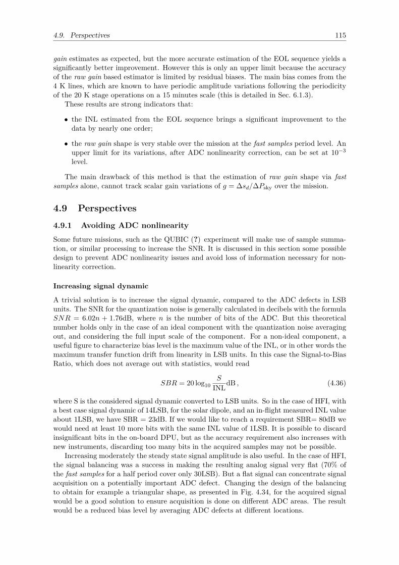
4.9. Perspectives 115
gain estimates as expected, but the more accurate estimation of the EOL sequence yields asignificantly better improvement. However this is only an upper limit because the accuracyof the raw gain based estimator is limited by residual biases. The main bias comes from the4 K lines, which are known to have periodic amplitude variations following the periodicityof the 20 K stage operations on a 15 minutes scale (this is detailed in Sec. 6.1.3).
These results are strong indicators that:
• the INL estimated from the EOL sequence brings a significant improvement to thedata by nearly one order;
• the raw gain shape is very stable over the mission at the fast samples period level. Anupper limit for its variations, after ADC nonlinearity correction, can be set at 10−3
level.
The main drawback of this method is that the estimation of raw gain shape via fastsamples alone, cannot track scalar gain variations of g = ∆sd/∆Psky over the mission.
4.9 Perspectives
4.9.1 Avoiding ADC nonlinearity
Some future missions, such as the QUBIC (?) experiment will make use of sample summa-tion, or similar processing to increase the SNR. It is discussed in this section some possibledesign to prevent ADC nonlinearity issues and avoid loss of information necessary for non-linearity correction.
Increasing signal dynamic
A trivial solution is to increase the signal dynamic, compared to the ADC defects in LSBunits. The SNR for the quantization noise is generally calculated in decibels with the formulaSNR = 6.02n + 1.76dB, where n is the number of bits of the ADC. But this theoreticalnumber holds only in the case of an ideal component with the quantization noise averagingout, and considering the full input scale of the component. For a non-ideal component, auseful figure to characterize bias level is the maximum value of the INL, or in other words themaximum transfer function drift from linearity in LSB units. In this case the Signal-to-BiasRatio, which does not average out with statistics, would read
SBR = 20 log10S
INLdB , (4.36)
where S is the considered signal dynamic converted to LSB units. So in the case of HFI, witha best case signal dynamic of 14LSB, for the solar dipole, and an in-flight measured INL valueabout 1LSB, we have SBR = 23dB. If we would like to reach a requirement SBR= 80dB wewould need at least 10 more bits with the same INL value of 1LSB. It is possible to discardinsignificant bits in the on-board DPU, but as the accuracy requirement also increases withnew instruments, discarding too many bits in the acquired samples may not be possible.
Increasing moderately the steady state signal amplitude is also useful. In the case of HFI,the signal balancing was a success in making the resulting analog signal very flat (70% ofthe fast samples for a half period cover only 30LSB). But a flat signal can concentrate signalacquisition on a potentially important ADC defect. Changing the design of the balancingto obtain for example a triangular shape, as presented in Fig. 4.34, for the acquired signalwould be a good solution to ensure acquisition is done on different ADC areas. The resultwould be a reduced bias level by averaging ADC defects at different locations.
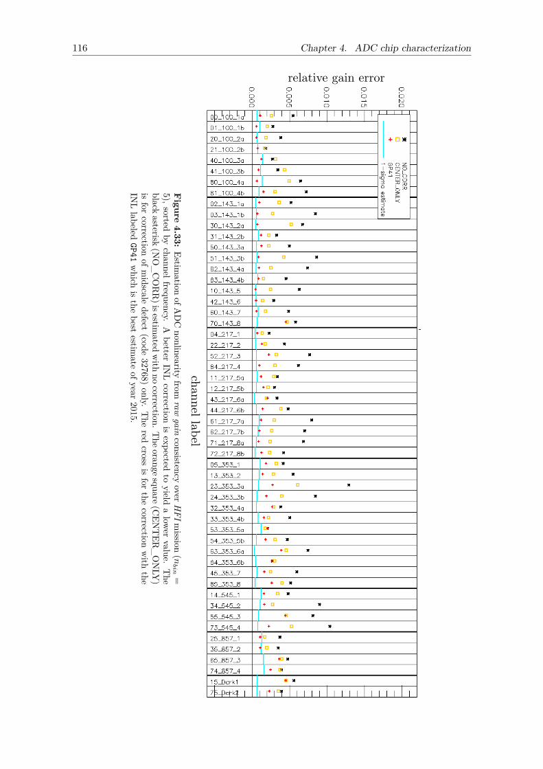
116 Chapter 4. ADC chip characterization
Figure
4.33:Estim
ationofA
DC
nonlinearityfrom
rawgain
consistencyoverH
FImission
(nbin
=5),sorted
bychannelfrequency.
Abetter
INL
correctionis
expectedto
yieldalower
value.The
blackasterisk
(NO_CORR)isestim
atedwith
nocorrection.T
heorangesquare(CEN
TER
_ONLY
)is
forcorrection
ofmidscale
defect(code
32768)only.
The
redcross
isfor
thecorrection
with
theIN
Llabeled
GP41which
isthe
bestestim
ateofyear
2015.
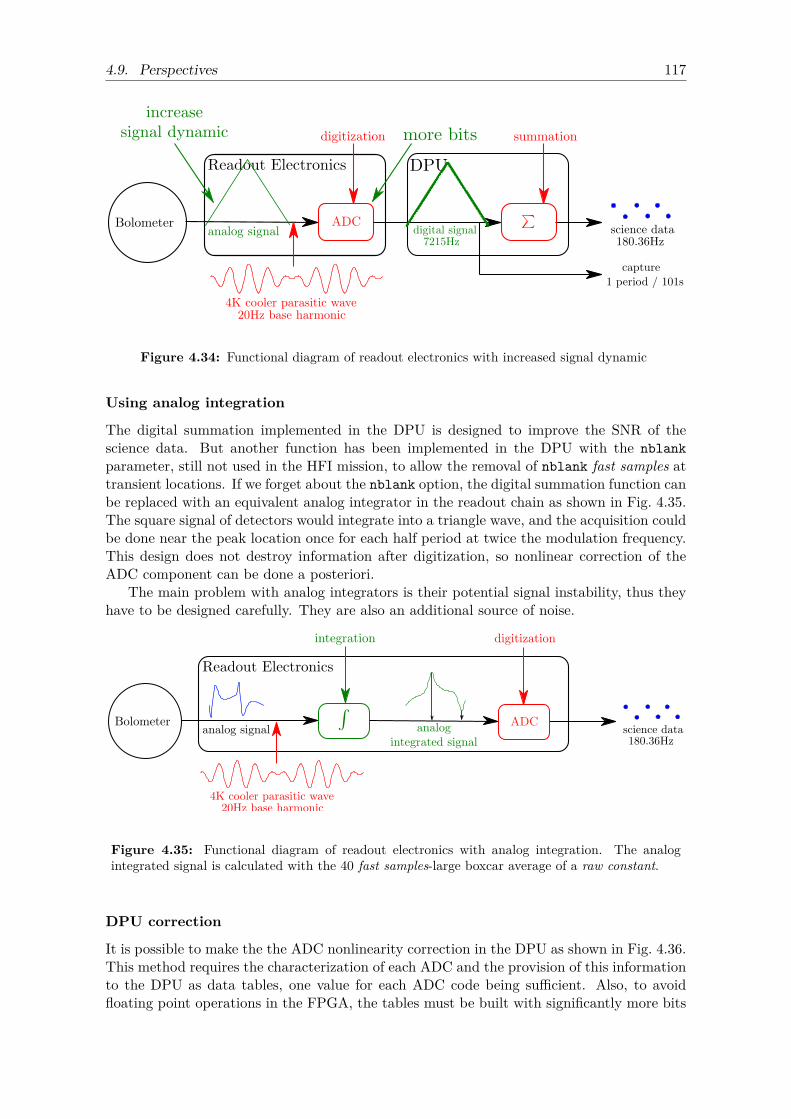
4.9. Perspectives 117
Figure 4.34: Functional diagram of readout electronics with increased signal dynamic
Using analog integration
The digital summation implemented in the DPU is designed to improve the SNR of thescience data. But another function has been implemented in the DPU with the nblankparameter, still not used in the HFI mission, to allow the removal of nblank fast samples attransient locations. If we forget about the nblank option, the digital summation function canbe replaced with an equivalent analog integrator in the readout chain as shown in Fig. 4.35.The square signal of detectors would integrate into a triangle wave, and the acquisition couldbe done near the peak location once for each half period at twice the modulation frequency.This design does not destroy information after digitization, so nonlinear correction of theADC component can be done a posteriori.
The main problem with analog integrators is their potential signal instability, thus theyhave to be designed carefully. They are also an additional source of noise.
Figure 4.35: Functional diagram of readout electronics with analog integration. The analogintegrated signal is calculated with the 40 fast samples-large boxcar average of a raw constant.
DPU correction
It is possible to make the the ADC nonlinearity correction in the DPU as shown in Fig. 4.36.This method requires the characterization of each ADC and the provision of this informationto the DPU as data tables, one value for each ADC code being sufficient. Also, to avoidfloating point operations in the FPGA, the tables must be built with significantly more bits
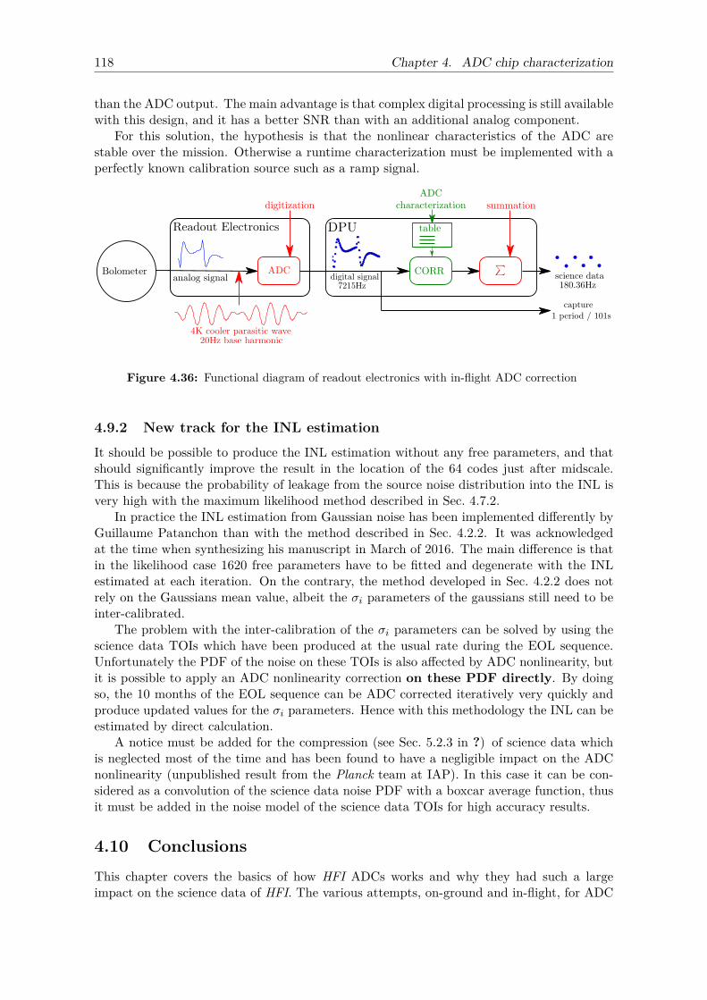
118 Chapter 4. ADC chip characterization
than the ADC output. The main advantage is that complex digital processing is still availablewith this design, and it has a better SNR than with an additional analog component.
For this solution, the hypothesis is that the nonlinear characteristics of the ADC arestable over the mission. Otherwise a runtime characterization must be implemented with aperfectly known calibration source such as a ramp signal.
Figure 4.36: Functional diagram of readout electronics with in-flight ADC correction
4.9.2 New track for the INL estimation
It should be possible to produce the INL estimation without any free parameters, and thatshould significantly improve the result in the location of the 64 codes just after midscale.This is because the probability of leakage from the source noise distribution into the INL isvery high with the maximum likelihood method described in Sec. 4.7.2.
In practice the INL estimation from Gaussian noise has been implemented differently byGuillaume Patanchon than with the method described in Sec. 4.2.2. It was acknowledgedat the time when synthesizing his manuscript in March of 2016. The main difference is thatin the likelihood case 1620 free parameters have to be fitted and degenerate with the INLestimated at each iteration. On the contrary, the method developed in Sec. 4.2.2 does notrely on the Gaussians mean value, albeit the σi parameters of the gaussians still need to beinter-calibrated.
The problem with the inter-calibration of the σi parameters can be solved by using thescience data TOIs which have been produced at the usual rate during the EOL sequence.Unfortunately the PDF of the noise on these TOIs is also affected by ADC nonlinearity, butit is possible to apply an ADC nonlinearity correction on these PDF directly. By doingso, the 10 months of the EOL sequence can be ADC corrected iteratively very quickly andproduce updated values for the σi parameters. Hence with this methodology the INL can beestimated by direct calculation.
A notice must be added for the compression (see Sec. 5.2.3 in ?) of science data whichis neglected most of the time and has been found to have a negligible impact on the ADCnonlinearity (unpublished result from the Planck team at IAP). In this case it can be con-sidered as a convolution of the science data noise PDF with a boxcar average function, thusit must be added in the noise model of the science data TOIs for high accuracy results.
4.10 ConclusionsThis chapter covers the basics of how HFI ADCs works and why they had such a largeimpact on the science data of HFI. The various attempts, on-ground and in-flight, for ADC

4.10. Conclusions 119
characterization and modeling have been described. It led to the final and accurate char-acterization of ADC INLs using a likelihood method on the data acquired during the EOLsequence. Finally it has been shown how the limited dataset of the cold fast samples providesinsights on the accuracy of the estimated INLs.
The in-flight characterization of ADC nonlinearity, despite many difficulties, was a suc-cess. It allowed the measurement of INLs for the 54 detectors channels with an absoluteaccuracy close to the target (≈ 0.3× 10⁻²LSB). The probabilities to get such a good resultwere low and it required the effort of many peoples within the Planck/HFI consortium overseveral years.
During the analysis of fast samples, the basis of a first order signal model for the detectorresponse at modulation level has been developed with the concept of raw gain, this will bedetailed in the next chapter. The stability of the raw gain shape throughout the missionhas been estimated to be better than ≈ 10−3 on most channels where the 4 K lines level ismoderate.

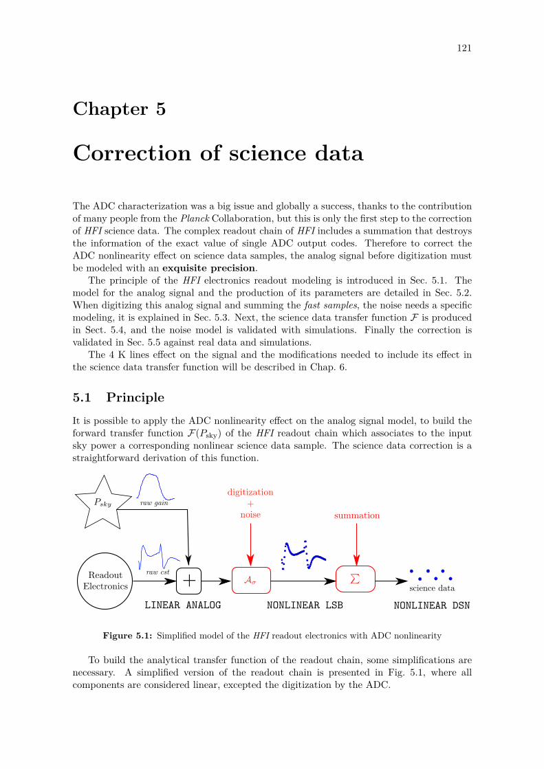
121
Chapter 5
Correction of science data
The ADC characterization was a big issue and globally a success, thanks to the contributionof many people from the Planck Collaboration, but this is only the first step to the correctionof HFI science data. The complex readout chain of HFI includes a summation that destroysthe information of the exact value of single ADC output codes. Therefore to correct theADC nonlinearity effect on science data samples, the analog signal before digitization mustbe modeled with an exquisite precision.
The principle of the HFI electronics readout modeling is introduced in Sec. 5.1. Themodel for the analog signal and the production of its parameters are detailed in Sec. 5.2.When digitizing this analog signal and summing the fast samples, the noise needs a specificmodeling, it is explained in Sec. 5.3. Next, the science data transfer function F is producedin Sect. 5.4, and the noise model is validated with simulations. Finally the correction isvalidated in Sec. 5.5 against real data and simulations.
The 4 K lines effect on the signal and the modifications needed to include its effect inthe science data transfer function will be described in Chap. 6.
5.1 PrincipleIt is possible to apply the ADC nonlinearity effect on the analog signal model, to build theforward transfer function F(Psky) of the HFI readout chain which associates to the inputsky power a corresponding nonlinear science data sample. The science data correction is astraightforward derivation of this function.
Figure 5.1: Simplified model of the HFI readout electronics with ADC nonlinearity
To build the analytical transfer function of the readout chain, some simplifications arenecessary. A simplified version of the readout chain is presented in Fig. 5.1, where allcomponents are considered linear, excepted the digitization by the ADC.
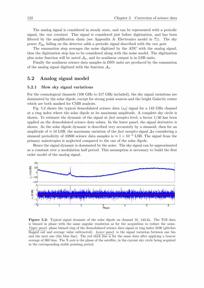
122 Chapter 5. Correction of science data
The analog signal is considered in steady state, and can be represented with a periodicsignal, the raw constant. This signal is considered just before digitization, and has beenfiltered by the amplification chain (see Appendix A: Electronics model in ?)). The skypower Psky falling on the detector adds a periodic signal described with the raw gain.
The summation step averages the noise digitized by the ADC with the analog signal,thus the digitization step has to be considered along with the noise model. The digitizationplus noise function will be noted Aσ, and its nonlinear output is in LSB units.
Finally the nonlinear science data samples in DSN units are produced by the summationof the analog signal digitized with the function Aσ.
5.2 Analog signal model
5.2.1 Slow sky signal variations
For the cosmological channels (100 GHz to 217 GHz included), the sky signal variations aredominated by the solar dipole, except for strong point sources and the bright Galactic centerwhich are both masked for CMB analysis.
Fig. 5.2 shows the typical demodulated science data (sd) signal for a 143 GHz channelat a ring index where the solar dipole at its maximum amplitude. A complete sky circle isshown. To estimate the dynamic of the signal at fast samples level, a factor 1/40 has beenapplied on the demodulated science data values. In the lower panel, the signal derivative isshown. As the solar dipole dynamic is described very accurately by a sinusoid, then for anamplitude of ≈ 10 LSB, the maximum variation of the fast samples signal ∆s considering asinusoid periodicity of 10800 science data samples is ≈ 1 × 10⁻³ LSB. The signal from theprimary anisotropies is neglected compared to the one of the solar dipole.
Hence the signal dynamic is dominated by the noise. The sky signal can be approximatedas a constant over a modulation half period. This assumption is necessary to build the firstorder model of the analog signal.
Figure 5.2: Typical signal dynamic of the solar dipole on channel 10_143-2a. The TOI datais binned in phase with the same angular resolution as for the acquisition to reduce the noise.Upper panel: phase binned ring of the demodulated science data signal at ring index 3100 (glitchesflagged out and average value subtracted). Lower panel: is the signal variation between one binand the next one (the blue line). The red thick line is for the same data after applying a boxcaraverage of 300 bins. The X axis is the phase of the satellite, in the current sky circle being acquiredin the corresponding stable pointing period.
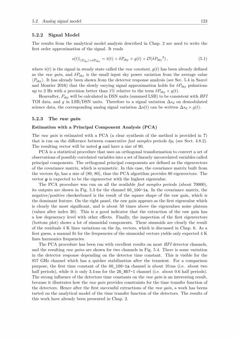
5.2. Analog signal model 123
5.2.2 Signal Model
The results from the analytical model analysis described in Chap. 2 are used to write thefirst order approximation of the signal. It reads
s(t)|〈Psky〉+δPsky= s(t) + δPsky × g(t) +O(δPsky
2) , (5.1)
where s(t) is the signal in steady state called the raw constant, g(t) has been already definedas the raw gain, and δPsky is the small input sky power variation from the average value〈Psky〉. It has already been shown from the detector response analysis (see Sec. 5.4 in Sauvéand Montier 2016) that the slowly varying signal approximation holds for δPsky pulsationsup to 2 Hz with a precision better than 1% relative to the term δPsky × g(t).
Heareafter, Psky will be calculated in DSN units (summed LSB) to be consistent with HFITOI data, and g in LSB/DSN units. Therefore to a signal variation ∆sd on demodulatedscience data, the corresponding analog signal variation ∆s(t) can be written ∆sd × g(t).
5.2.3 The raw gainEstimation with a Principal Component Analysis (PCA)
The raw gain is estimated with a PCA (a clear synthesis of the method is provided in ?)that is run on the difference between consecutive fast samples periods δpi (see Sect. 4.8.2).The resulting vector will be noted g and have a size of 80.
PCA is a statistical procedure that uses an orthogonal transformation to convert a set ofobservations of possibly correlated variables into a set of linearly uncorrelated variables calledprincipal components. The orthogonal principal components are defined as the eigenvectorsof the covariance matrix, which is symmetric. In this case, the covariance matrix built fromthe vectors δpi has a size of (80, 80), thus the PCA algorithm provides 80 eigenvectors. Thevector g is expected to be the eigenvector with the highest eigenvalue.
The PCA procedure was run on all the available fast samples periods (about 70000),its outputs are shown in Fig. 5.3 for the channel 00_100-1a. In the covariance matrix, thenegative/positive checkerboard is the result of the square shape of the raw gain, which isthe dominant feature. On the right panel, the raw gain appears as the first eigenvalue whichis clearly the most significant, and is about 50 times above the eigenvalues noise plateau(values after index 30). This is a good indicator that the extraction of the raw gain hasa low degeneracy level with other effects. Finally, the inspection of the first eigenvectors(bottom plot) shows a lot of sinusoidal components. These sinusoids are clearly the resultof the residuals 4 K lines variations on the δpi vectors, which is discussed in Chap. 6. As afirst guess, a manual fit for the frequencies of the sinusoidal vectors yields only expected 4 Klines harmonics frequencies.
The PCA procedure has been run with excellent results on most HFI detector channels,and the resulting raw gains are shown for two channels in Fig. 5.4. There is some variationin the detector response depending on the detector time constant. This is visible for the857 GHz channel which has a quicker stabilization after the transient. For a comparisonpurpose, the first time constant of the 00_100-1a channel is about 10 ms (i.e. about twohalf periods), while it is only 3.4 ms for the 25_857-1 channel (i.e. about 0.6 half periods).The strong influence of the detectors time constants on the raw gain is an interesting result,because it illustrates how the raw gain provides constraints for the time transfer function ofthe detectors. Hence after the first successful extractions of the raw gain, a work has beenstarted on the analytical model of the time transfer function of the detectors. The results ofthis work have already been presented in Chap. 2.
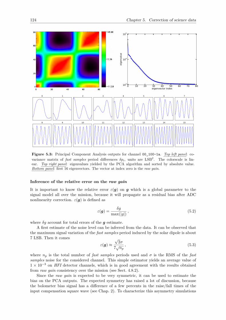
124 Chapter 5. Correction of science data
0 10 20 30 40 50 60 70 80eigenvector index
103
104
105
eig
envalu
e
0 1 2 3 4 5 6 7
8 9 10 11 12 13 14 15
Figure 5.3: Principal Component Analysis outputs for channel 00_100-1a. Top left panel: co-variance matrix of fast samples period differences δpi, units are LSB2. The colorscale is lin-ear. Top right panel: eigenvalues yielded by the PCA algorithm and sorted by absolute value.Bottom panel: first 16 eigenvectors. The vector at index zero is the raw gain.
Inference of the relative error on the raw gain
It is important to know the relative error ε(g) on g which is a global parameter to thesignal model all over the mission, because it will propagate as a residual bias after ADCnonlinearity correction. ε(g) is defined as
ε(g) = δg
max(|g|) , (5.2)
where δg account for total errors of the g estimate.A first estimate of the noise level can be inferred from the data. It can be observed that
the maximum signal variation of the fast samples period induced by the solar dipole is about7 LSB. Then it comes
ε(g) ≈√
2σ7√np
, (5.3)
where np is the total number of fast samples periods used and σ is the RMS of the fastsamples noise for the considered channel. This simple estimator yields an average value of1 × 10−3 on HFI detector channels, which is in good agreement with the results obtainedfrom raw gain consistency over the mission (see Sect. 4.8.2).
Since the raw gain is expected to be very symmetric, it can be used to estimate thebias on the PCA outputs. The expected symmetry has raised a lot of discussion, becausethe bolometer bias signal has a difference of a few percents in the raise/fall times of theinput compensation square wave (see Chap. 2). To characterize this asymmetry simulations
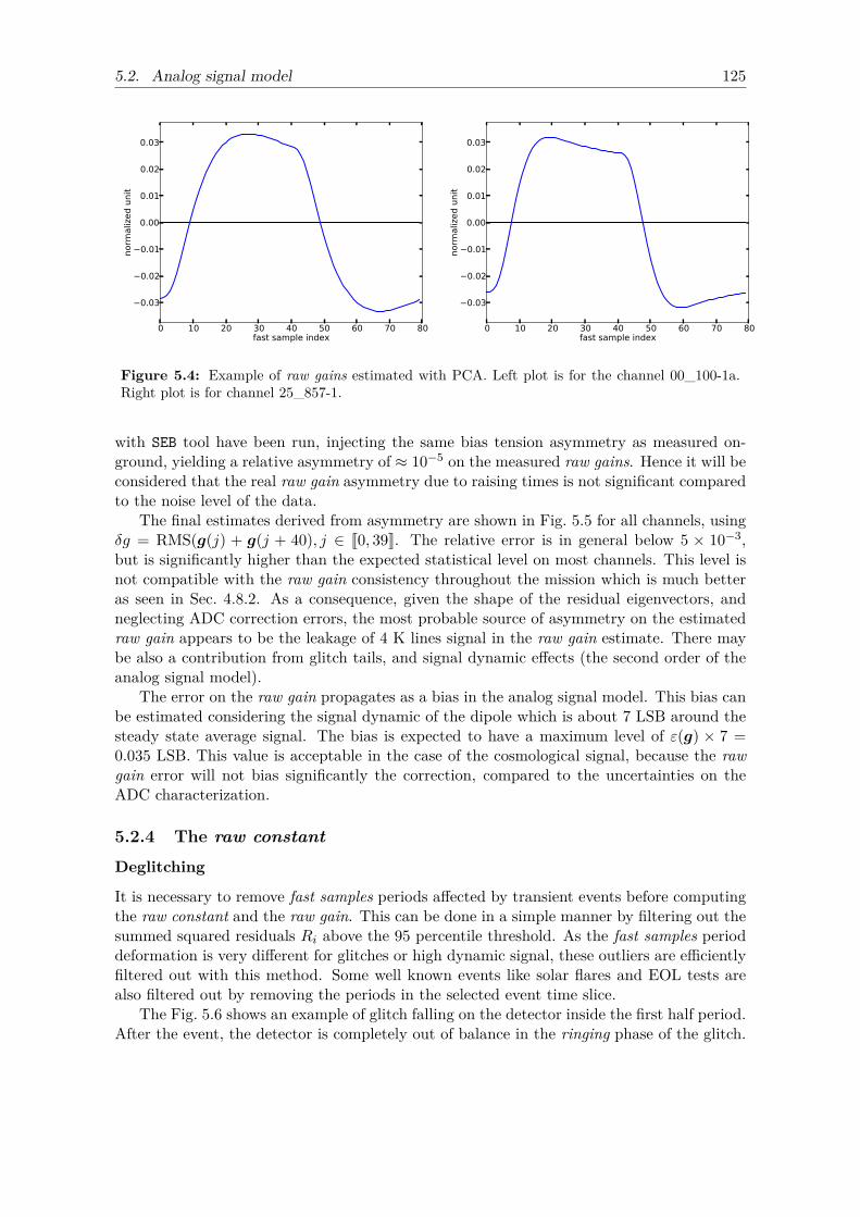
5.2. Analog signal model 125
0 10 20 30 40 50 60 70 80fast sample index
0.03
0.02
0.01
0.00
0.01
0.02
0.03
norm
aliz
ed u
nit
0 10 20 30 40 50 60 70 80fast sample index
0.03
0.02
0.01
0.00
0.01
0.02
0.03
norm
aliz
ed u
nit
Figure 5.4: Example of raw gains estimated with PCA. Left plot is for the channel 00_100-1a.Right plot is for channel 25_857-1.
with SEB tool have been run, injecting the same bias tension asymmetry as measured on-ground, yielding a relative asymmetry of ≈ 10−5 on the measured raw gains. Hence it will beconsidered that the real raw gain asymmetry due to raising times is not significant comparedto the noise level of the data.
The final estimates derived from asymmetry are shown in Fig. 5.5 for all channels, usingδg = RMS(g(j) + g(j + 40), j ∈ J0, 39K. The relative error is in general below 5 × 10⁻³,but is significantly higher than the expected statistical level on most channels. This level isnot compatible with the raw gain consistency throughout the mission which is much betteras seen in Sec. 4.8.2. As a consequence, given the shape of the residual eigenvectors, andneglecting ADC correction errors, the most probable source of asymmetry on the estimatedraw gain appears to be the leakage of 4 K lines signal in the raw gain estimate. There maybe also a contribution from glitch tails, and signal dynamic effects (the second order of theanalog signal model).
The error on the raw gain propagates as a bias in the analog signal model. This bias canbe estimated considering the signal dynamic of the dipole which is about 7 LSB around thesteady state average signal. The bias is expected to have a maximum level of ε(g) × 7 =0.035 LSB. This value is acceptable in the case of the cosmological signal, because the rawgain error will not bias significantly the correction, compared to the uncertainties on theADC characterization.
5.2.4 The raw constantDeglitching
It is necessary to remove fast samples periods affected by transient events before computingthe raw constant and the raw gain. This can be done in a simple manner by filtering out thesummed squared residuals Ri above the 95 percentile threshold. As the fast samples perioddeformation is very different for glitches or high dynamic signal, these outliers are efficientlyfiltered out with this method. Some well known events like solar flares and EOL tests arealso filtered out by removing the periods in the selected event time slice.
The Fig. 5.6 shows an example of glitch falling on the detector inside the first half period.After the event, the detector is completely out of balance in the ringing phase of the glitch.
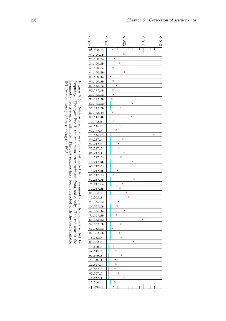
126 Chapter 5. Correction of science data
Figure
5.5:Relative
errorof
rawgains
estimated
fromasym
metry,
with
channelssorted
byfrequency.
The
cyanline
isthe
minim
umerror
estimate
fromnoise
only.The
redstar
isthe
asymmetry
relativeerror
estimate.
The
fastsam
pleshave
beencorrected
with
thebest
availableIN
L(version
GP41)before
runningthe
PCA.
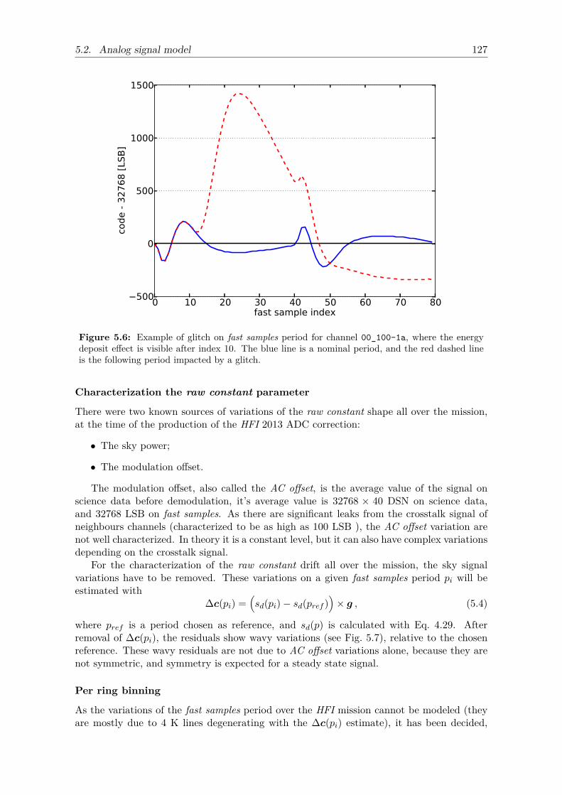
5.2. Analog signal model 127
0 10 20 30 40 50 60 70 80fast sample index
500
0
500
1000
1500
code -
32768 [
LSB
]
Figure 5.6: Example of glitch on fast samples period for channel 00_100-1a, where the energydeposit effect is visible after index 10. The blue line is a nominal period, and the red dashed lineis the following period impacted by a glitch.
Characterization the raw constant parameter
There were two known sources of variations of the raw constant shape all over the mission,at the time of the production of the HFI 2013 ADC correction:
• The sky power;
• The modulation offset.
The modulation offset, also called the AC offset, is the average value of the signal onscience data before demodulation, it’s average value is 32768 × 40 DSN on science data,and 32768 LSB on fast samples. As there are significant leaks from the crosstalk signal ofneighbours channels (characterized to be as high as 100 LSB ), the AC offset variation arenot well characterized. In theory it is a constant level, but it can also have complex variationsdepending on the crosstalk signal.
For the characterization of the raw constant drift all over the mission, the sky signalvariations have to be removed. These variations on a given fast samples period pi will beestimated with
∆c(pi) =(sd(pi)− sd(pref )
)× g , (5.4)
where pref is a period chosen as reference, and sd(p) is calculated with Eq. 4.29. Afterremoval of ∆c(pi), the residuals show wavy variations (see Fig. 5.7), relative to the chosenreference. These wavy residuals are not due to AC offset variations alone, because they arenot symmetric, and symmetry is expected for a steady state signal.
Per ring binning
As the variations of the fast samples period over the HFI mission cannot be modeled (theyare mostly due to 4 K lines degenerating with the ∆c(pi) estimate), it has been decided,
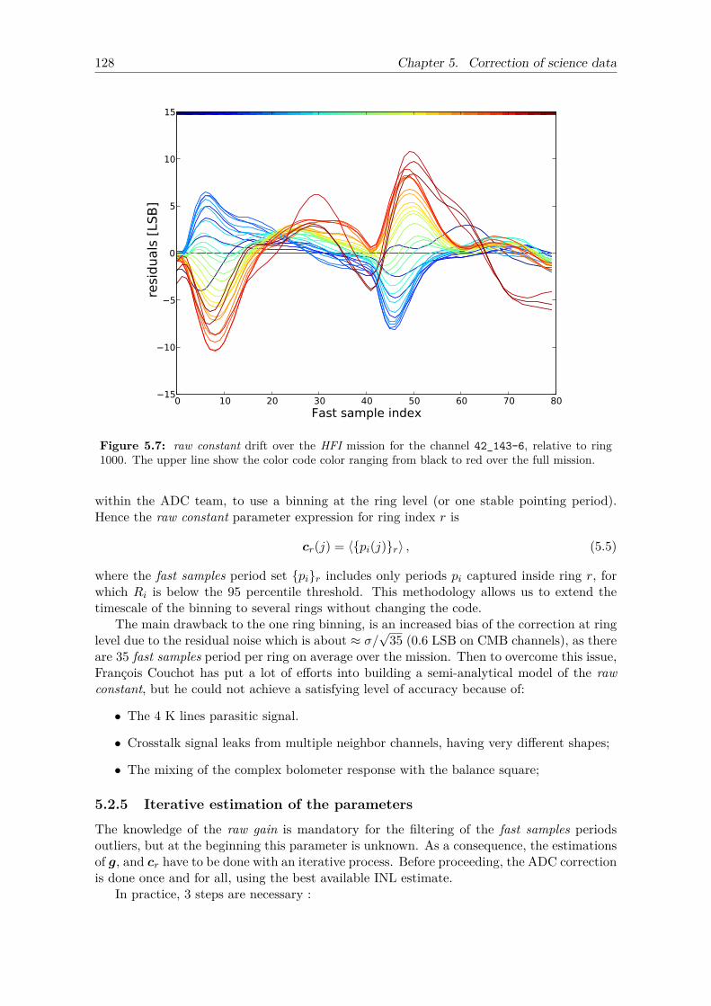
128 Chapter 5. Correction of science data
resi
duals
[LS
B]
Figure 5.7: raw constant drift over the HFI mission for the channel 42_143-6, relative to ring1000. The upper line show the color code color ranging from black to red over the full mission.
within the ADC team, to use a binning at the ring level (or one stable pointing period).Hence the raw constant parameter expression for ring index r is
cr(j) = 〈pi(j)r〉 , (5.5)
where the fast samples period set pir includes only periods pi captured inside ring r, forwhich Ri is below the 95 percentile threshold. This methodology allows us to extend thetimescale of the binning to several rings without changing the code.
The main drawback to the one ring binning, is an increased bias of the correction at ringlevel due to the residual noise which is about ≈ σ/
√35 (0.6 LSB on CMB channels), as there
are 35 fast samples period per ring on average over the mission. Then to overcome this issue,François Couchot has put a lot of efforts into building a semi-analytical model of the rawconstant, but he could not achieve a satisfying level of accuracy because of:
• The 4 K lines parasitic signal.
• Crosstalk signal leaks from multiple neighbor channels, having very different shapes;
• The mixing of the complex bolometer response with the balance square;
5.2.5 Iterative estimation of the parameters
The knowledge of the raw gain is mandatory for the filtering of the fast samples periodsoutliers, but at the beginning this parameter is unknown. As a consequence, the estimationsof g, and cr have to be done with an iterative process. Before proceeding, the ADC correctionis done once and for all, using the best available INL estimate.
In practice, 3 steps are necessary :
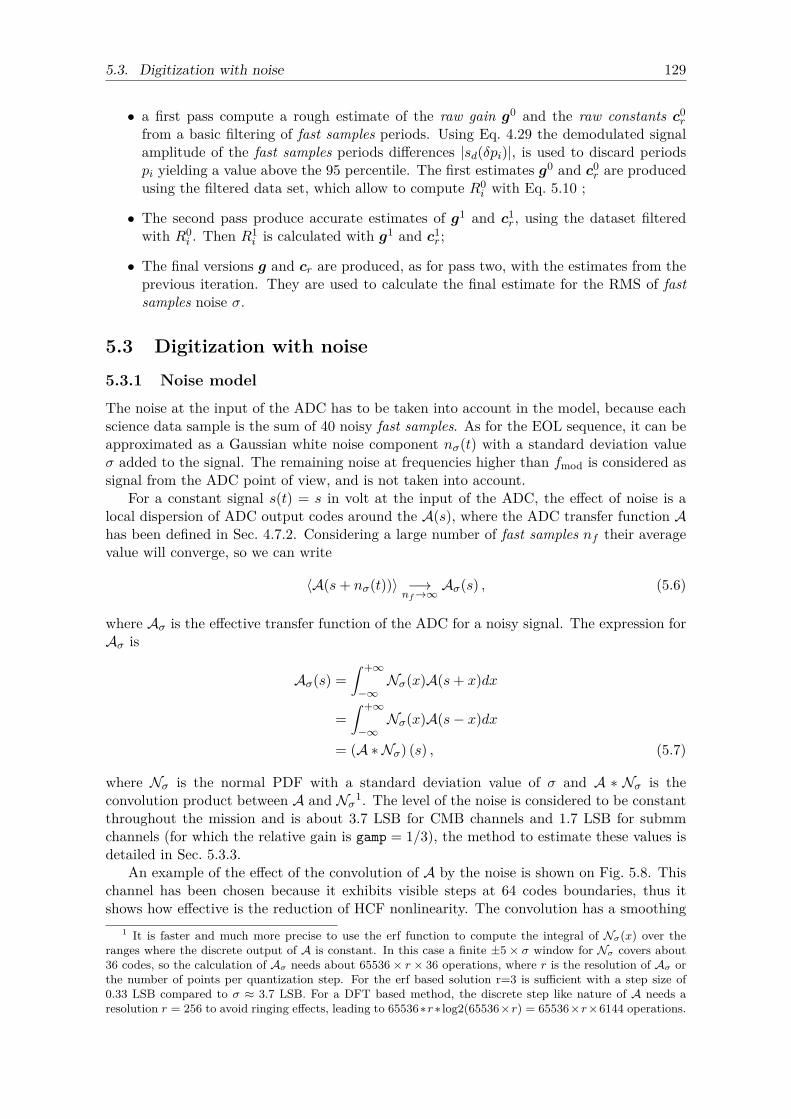
5.3. Digitization with noise 129
• a first pass compute a rough estimate of the raw gain g0 and the raw constants c0r
from a basic filtering of fast samples periods. Using Eq. 4.29 the demodulated signalamplitude of the fast samples periods differences |sd(δpi)|, is used to discard periodspi yielding a value above the 95 percentile. The first estimates g0 and c0
r are producedusing the filtered data set, which allow to compute R0
i with Eq. 5.10 ;
• The second pass produce accurate estimates of g1 and c1r , using the dataset filtered
with R0i . Then R1
i is calculated with g1 and c1r ;
• The final versions g and cr are produced, as for pass two, with the estimates from theprevious iteration. They are used to calculate the final estimate for the RMS of fastsamples noise σ.
5.3 Digitization with noise
5.3.1 Noise model
The noise at the input of the ADC has to be taken into account in the model, because eachscience data sample is the sum of 40 noisy fast samples. As for the EOL sequence, it can beapproximated as a Gaussian white noise component nσ(t) with a standard deviation valueσ added to the signal. The remaining noise at frequencies higher than fmod is considered assignal from the ADC point of view, and is not taken into account.
For a constant signal s(t) = s in volt at the input of the ADC, the effect of noise is alocal dispersion of ADC output codes around the A(s), where the ADC transfer function Ahas been defined in Sec. 4.7.2. Considering a large number of fast samples nf their averagevalue will converge, so we can write
〈A(s+ nσ(t))〉 −→nf→∞
Aσ(s) , (5.6)
where Aσ is the effective transfer function of the ADC for a noisy signal. The expression forAσ is
Aσ(s) =∫ +∞
−∞Nσ(x)A(s+ x)dx
=∫ +∞
−∞Nσ(x)A(s− x)dx
= (A ∗ Nσ) (s) , (5.7)
where Nσ is the normal PDF with a standard deviation value of σ and A ∗ Nσ is theconvolution product between A and Nσ1. The level of the noise is considered to be constantthroughout the mission and is about 3.7 LSB for CMB channels and 1.7 LSB for submmchannels (for which the relative gain is gamp = 1/3), the method to estimate these values isdetailed in Sec. 5.3.3.
An example of the effect of the convolution of A by the noise is shown on Fig. 5.8. Thischannel has been chosen because it exhibits visible steps at 64 codes boundaries, thus itshows how effective is the reduction of HCF nonlinearity. The convolution has a smoothing
1 It is faster and much more precise to use the erf function to compute the integral of Nσ(x) over theranges where the discrete output of A is constant. In this case a finite ±5 × σ window for Nσ covers about36 codes, so the calculation of Aσ needs about 65536× r × 36 operations, where r is the resolution of Aσ orthe number of points per quantization step. For the erf based solution r=3 is sufficient with a step size of0.33 LSB compared to σ ≈ 3.7 LSB. For a DFT based method, the discrete step like nature of A needs aresolution r = 256 to avoid ringing effects, leading to 65536∗r∗ log2(65536×r) = 65536×r×6144 operations.
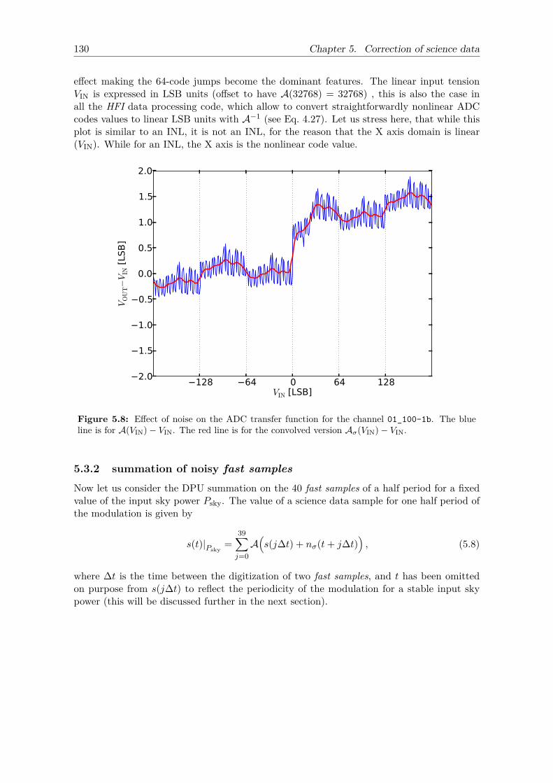
130 Chapter 5. Correction of science data
effect making the 64-code jumps become the dominant features. The linear input tensionVIN is expressed in LSB units (offset to have A(32768) = 32768) , this is also the case inall the HFI data processing code, which allow to convert straightforwardly nonlinear ADCcodes values to linear LSB units with A−1 (see Eq. 4.27). Let us stress here, that while thisplot is similar to an INL, it is not an INL, for the reason that the X axis domain is linear(VIN). While for an INL, the X axis is the nonlinear code value.
128 64 0 64 128VIN [LSB]
2.0
1.5
1.0
0.5
0.0
0.5
1.0
1.5
2.0
VO
UT−V
IN [
LSB
]
Figure 5.8: Effect of noise on the ADC transfer function for the channel 01_100-1b. The blueline is for A(VIN)− VIN. The red line is for the convolved version Aσ(VIN)− VIN.
5.3.2 summation of noisy fast samplesNow let us consider the DPU summation on the 40 fast samples of a half period for a fixedvalue of the input sky power Psky. The value of a science data sample for one half period ofthe modulation is given by
s(t)|Psky=
39∑j=0A(s(j∆t) + nσ(t+ j∆t)
), (5.8)
where ∆t is the time between the digitization of two fast samples, and t has been omittedon purpose from s(j∆t) to reflect the periodicity of the modulation for a stable input skypower (this will be discussed further in the next section).
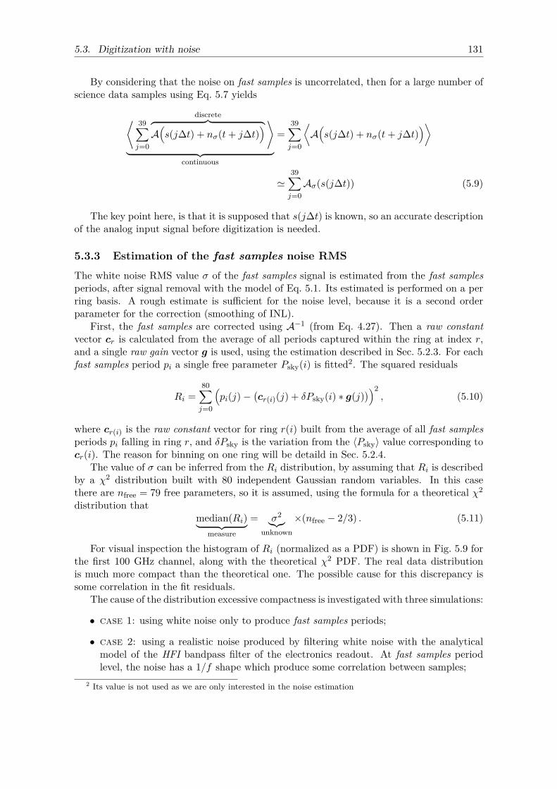
5.3. Digitization with noise 131
By considering that the noise on fast samples is uncorrelated, then for a large number ofscience data samples using Eq. 5.7 yields
⟨ 39∑j=0
discrete︷ ︸︸ ︷A(s(j∆t) + nσ(t+ j∆t)
)⟩︸ ︷︷ ︸
continuous
=39∑j=0
⟨A(s(j∆t) + nσ(t+ j∆t)
)⟩
'39∑j=0Aσ(s(j∆t)) (5.9)
The key point here, is that it is supposed that s(j∆t) is known, so an accurate descriptionof the analog input signal before digitization is needed.
5.3.3 Estimation of the fast samples noise RMS
The white noise RMS value σ of the fast samples signal is estimated from the fast samplesperiods, after signal removal with the model of Eq. 5.1. Its estimated is performed on a perring basis. A rough estimate is sufficient for the noise level, because it is a second orderparameter for the correction (smoothing of INL).
First, the fast samples are corrected using A−1 (from Eq. 4.27). Then a raw constantvector cr is calculated from the average of all periods captured within the ring at index r,and a single raw gain vector g is used, using the estimation described in Sec. 5.2.3. For eachfast samples period pi a single free parameter Psky(i) is fitted2. The squared residuals
Ri =80∑j=0
(pi(j)−
(cr(i)(j) + δPsky(i) ∗ g(j)
))2, (5.10)
where cr(i) is the raw constant vector for ring r(i) built from the average of all fast samplesperiods pi falling in ring r, and δPsky is the variation from the 〈Psky〉 value corresponding tocr(i). The reason for binning on one ring will be detaild in Sec. 5.2.4.
The value of σ can be inferred from the Ri distribution, by assuming that Ri is describedby a χ2 distribution built with 80 independent Gaussian random variables. In this casethere are nfree = 79 free parameters, so it is assumed, using the formula for a theoretical χ2
distribution thatmedian(Ri)︸ ︷︷ ︸
measure
= σ2︸︷︷︸unknown
×(nfree − 2/3) . (5.11)
For visual inspection the histogram of Ri (normalized as a PDF) is shown in Fig. 5.9 forthe first 100 GHz channel, along with the theoretical χ2 PDF. The real data distributionis much more compact than the theoretical one. The possible cause for this discrepancy issome correlation in the fit residuals.
The cause of the distribution excessive compactness is investigated with three simulations:
• case 1: using white noise only to produce fast samples periods;
• case 2: using a realistic noise produced by filtering white noise with the analyticalmodel of the HFI bandpass filter of the electronics readout. At fast samples periodlevel, the noise has a 1/f shape which produce some correlation between samples;
2 Its value is not used as we are only interested in the noise estimation
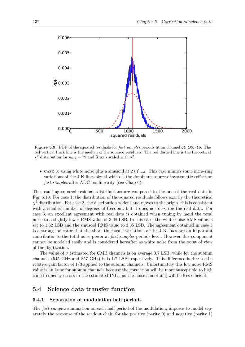
132 Chapter 5. Correction of science data
0 500 1000 1500 2000squared residuals
0.000
0.001
0.002
0.003
0.004
0.005
0.006
PD
F
Figure 5.9: PDF of the squared residuals for fast samples periods fit on channel 01_100-1b. Thered vertical thick line is the median of the squared residuals. The red dashed line is the theoreticalχ2 distribution for nfree = 79 and X axis scaled with σ2.
• case 3: using white noise plus a sinusoid at 2∗fmod. This case mimics some intra-ringvariations of the 4 K lines signal which is the dominant source of systematics effect onfast samples after ADC nonlinearity (see Chap 6).
The resulting squared residuals distributions are compared to the one of the real data inFig. 5.10. For case 1, the distribution of the squared residuals follows exactly the theoreticalχ2 distribution. For case 2, the distribution widens and moves to the origin, this is consistentwith a smaller number of degrees of freedom, but it does not describe the real data. Forcase 3, an excellent agreement with real data is obtained when tuning by hand the totalnoise to a slightly lower RMS value of 3.68 LSB. In this case, the white noise RMS value isset to 1.52 LSB and the sinusoid RMS value to 3.35 LSB. The agreement obtained in case 3is a strong indicator that the short time scale variations of the 4 K lines are an importantcontributor to the total noise power at fast samples periods level. However this componentcannot be modeled easily and is considered hereafter as white noise from the point of viewof the digitization.
The value of σ estimated for CMB channels is on average 3.7 LSB, while for the submmchannels (545 GHz and 857 GHz) it is 1.7 LSB respectively. This difference is due to therelative gain factor of 1/3 applied to the submm channels. Unfortunately this low noise RMSvalue is an issue for submm channels because the correction will be more susceptible to highcode frequency errors in the estimated INLs, as the noise smoothing will be less efficient.
5.4 Science data transfer function
5.4.1 Separation of modulation half periods
The fast samples summation on each half period of the modulation, imposes to model sep-arately the response of the readout chain for the positive (parity 0) and negative (parity 1)
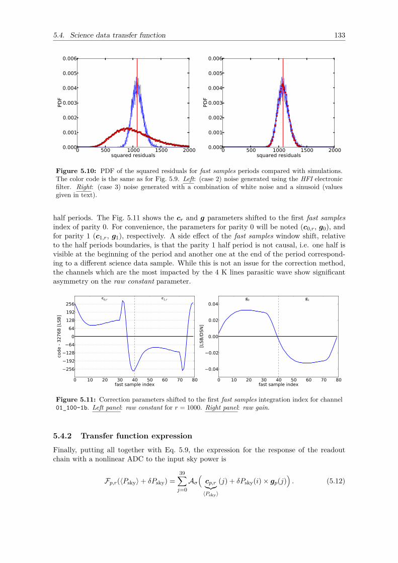
5.4. Science data transfer function 133
0 500 1000 1500 2000squared residuals
0.000
0.001
0.002
0.003
0.004
0.005
0.006PD
F
0 500 1000 1500 2000squared residuals
0.000
0.001
0.002
0.003
0.004
0.005
0.006
PD
F
Figure 5.10: PDF of the squared residuals for fast samples periods compared with simulations.The color code is the same as for Fig. 5.9. Left: (case 2) noise generated using the HFI electronicfilter. Right: (case 3) noise generated with a combination of white noise and a sinusoid (valuesgiven in text).
half periods. The Fig. 5.11 shows the cr and g parameters shifted to the first fast samplesindex of parity 0. For convenience, the parameters for parity 0 will be noted (c0,r, g0), andfor parity 1 (c1,r, g1), respectively. A side effect of the fast samples window shift, relativeto the half periods boundaries, is that the parity 1 half period is not causal, i.e. one half isvisible at the beginning of the period and another one at the end of the period correspond-ing to a different science data sample. While this is not an issue for the correction method,the channels which are the most impacted by the 4 K lines parasitic wave show significantasymmetry on the raw constant parameter.
Figure 5.11: Correction parameters shifted to the first fast samples integration index for channel01_100-1b. Left panel: raw constant for r = 1000. Right panel: raw gain.
5.4.2 Transfer function expression
Finally, putting all together with Eq. 5.9, the expression for the response of the readoutchain with a nonlinear ADC to the input sky power is
Fp,r(〈Psky〉+ δPsky) =39∑j=0Aσ(cp,r︸︷︷︸〈Psky〉
(j) + δPsky(i)× gp(j)). (5.12)
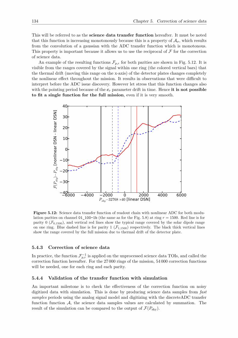
134 Chapter 5. Correction of science data
This will be referred to as the science data transfer function hereafter. It must be notedthat this function is increasing monotonously because this is a property of Aσ, which resultsfrom the convolution of a gaussian with the ADC transfer function which is monotonous.This property is important because it allows us to use the reciprocal of F for the correctionof science data.
An example of the resulting functions Fp,r for both parities are shown in Fig. 5.12. It isvisible from the ranges covered by the signal within one ring (the colored vertical bars) thatthe thermal drift (moving this range on the x-axis) of the detector plates changes completelythe nonlinear effect throughout the mission. It results in observations that were difficult tointerpret before the ADC issue discovery. However let stress that this function changes alsowith the pointing period because of the cr parameter drift in time. Hence it is not possibleto fit a single function for the full mission, even if it is very smooth.
6000 4000 2000 0 2000 4000 6000Psky−32768×40 [linear DSN]
40
30
20
10
0
10
20
30
40
F(P
sky)−Psky
[nonlin
ear
DSN
- lin
ear
DSN
]
Figure 5.12: Science data transfer function of readout chain with nonlinear ADC for both modu-lation parities on channel 01_100-1b (the same as for the Fig. 5.8) at ring r = 1500. Red line is forparity 0 (F0,1500), and vertical red lines show the typical range covered by the solar dipole rangeon one ring. Blue dashed line is for parity 1 (F1,1500) respectively. The black thick vertical linesshow the range covered by the full mission due to thermal drift of the detector plate.
5.4.3 Correction of science data
In practice, the function F−1p,r is applied on the unprocessed science data TOIs, and called the
correction function hereafter. For the 27 000 rings of the mission, 54 000 correction functionswill be needed, one for each ring and each parity.
5.4.4 Validation of the transfer function with simulation
An important milestone is to check the effectiveness of the correction function on noisydigitized data with simulation. This is done by producing science data samples from fastsamples periods using the analog signal model and digitizing with the discreteADC transferfunction function A, the science data samples values are calculated by summation. Theresult of the simulation can be compared to the output of F(Psky).
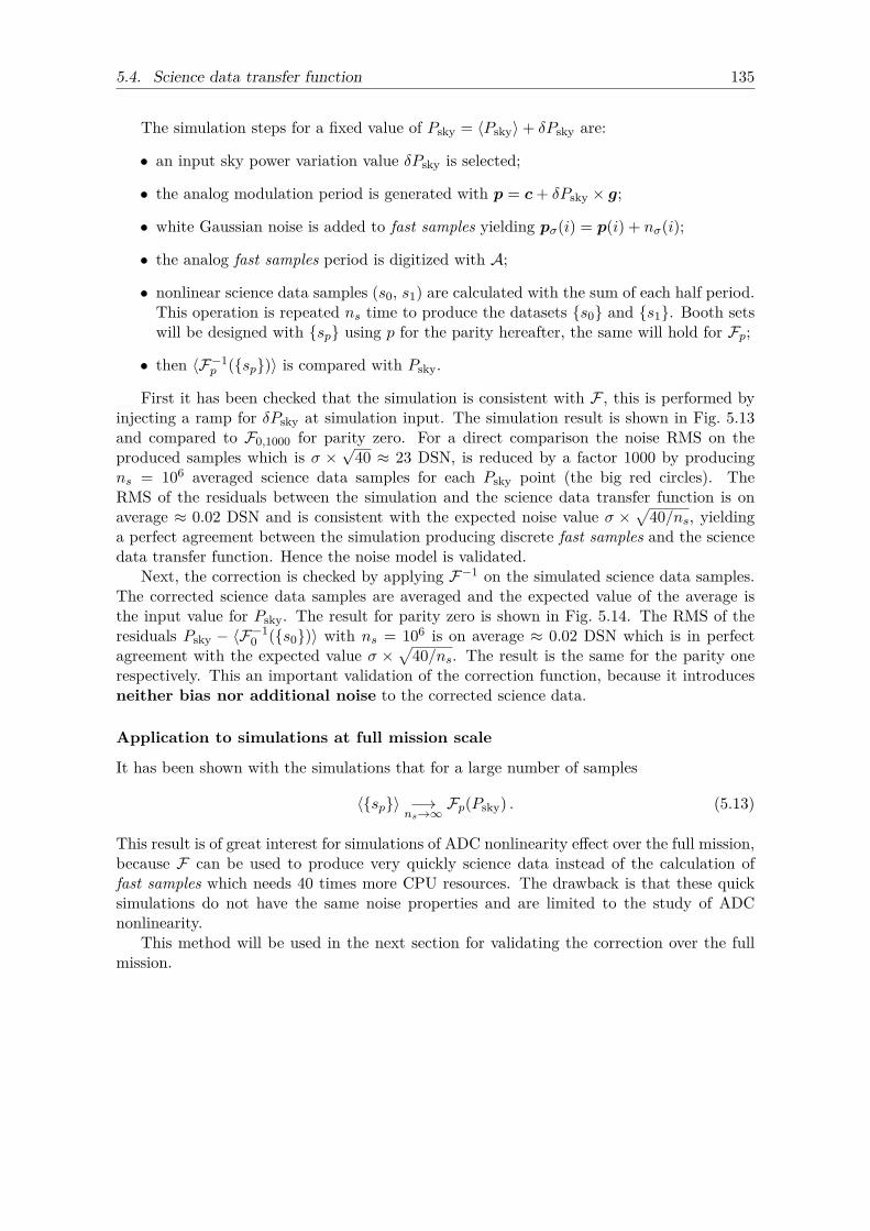
5.4. Science data transfer function 135
The simulation steps for a fixed value of Psky = 〈Psky〉+ δPsky are:
• an input sky power variation value δPsky is selected;
• the analog modulation period is generated with p = c+ δPsky × g;
• white Gaussian noise is added to fast samples yielding pσ(i) = p(i) + nσ(i);
• the analog fast samples period is digitized with A;
• nonlinear science data samples (s0, s1) are calculated with the sum of each half period.This operation is repeated ns time to produce the datasets s0 and s1. Booth setswill be designed with sp using p for the parity hereafter, the same will hold for Fp;
• then 〈F−1p (sp)〉 is compared with Psky.
First it has been checked that the simulation is consistent with F , this is performed byinjecting a ramp for δPsky at simulation input. The simulation result is shown in Fig. 5.13and compared to F0,1000 for parity zero. For a direct comparison the noise RMS on theproduced samples which is σ ×
√40 ≈ 23 DSN, is reduced by a factor 1000 by producing
ns = 106 averaged science data samples for each Psky point (the big red circles). TheRMS of the residuals between the simulation and the science data transfer function is onaverage ≈ 0.02 DSN and is consistent with the expected noise value σ ×
√40/ns, yielding
a perfect agreement between the simulation producing discrete fast samples and the sciencedata transfer function. Hence the noise model is validated.
Next, the correction is checked by applying F−1 on the simulated science data samples.The corrected science data samples are averaged and the expected value of the average isthe input value for Psky. The result for parity zero is shown in Fig. 5.14. The RMS of theresiduals Psky − 〈F−1
0 (s0)〉 with ns = 106 is on average ≈ 0.02 DSN which is in perfectagreement with the expected value σ ×
√40/ns. The result is the same for the parity one
respectively. This an important validation of the correction function, because it introducesneither bias nor additional noise to the corrected science data.
Application to simulations at full mission scale
It has been shown with the simulations that for a large number of samples
〈sp〉 −→ns→∞
Fp(Psky) . (5.13)
This result is of great interest for simulations of ADC nonlinearity effect over the full mission,because F can be used to produce very quickly science data instead of the calculation offast samples which needs 40 times more CPU resources. The drawback is that these quicksimulations do not have the same noise properties and are limited to the study of ADCnonlinearity.
This method will be used in the next section for validating the correction over the fullmission.
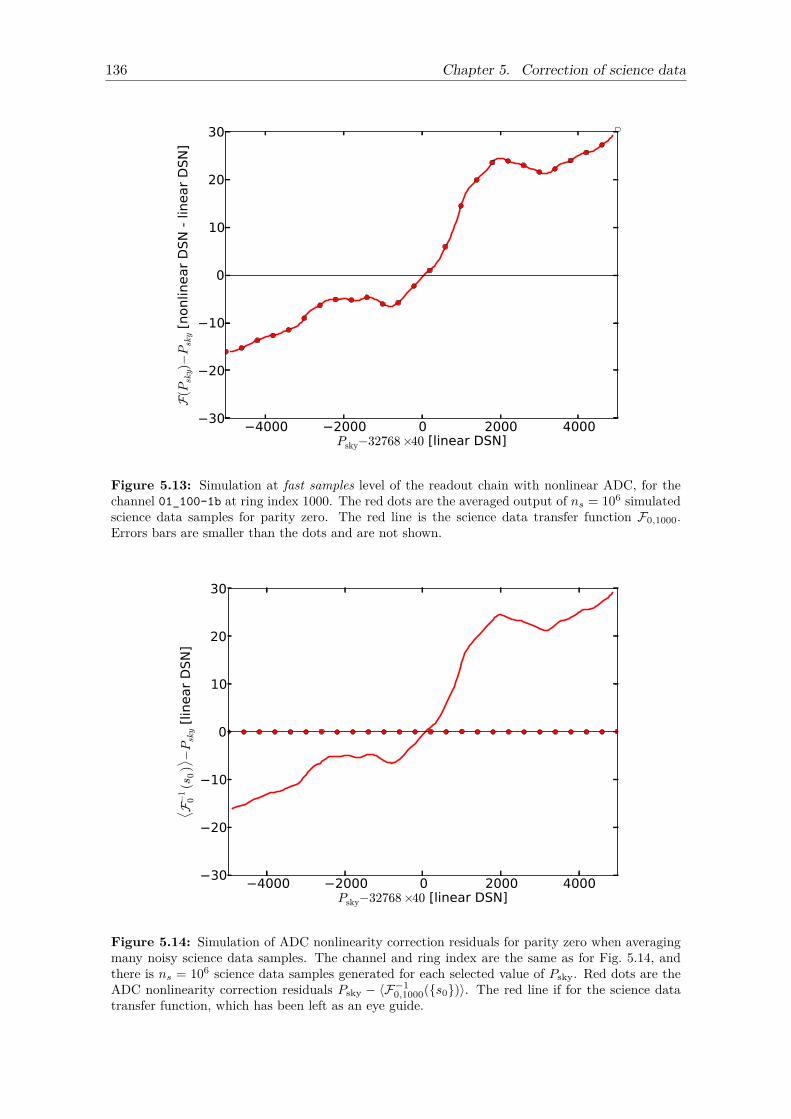
136 Chapter 5. Correction of science data
4000 2000 0 2000 4000Psky−32768×40 [linear DSN]
30
20
10
0
10
20
30
F(P
sky)−Psky
[nonlin
ear
DSN
- lin
ear
DSN
]
Figure 5.13: Simulation at fast samples level of the readout chain with nonlinear ADC, for thechannel 01_100-1b at ring index 1000. The red dots are the averaged output of ns = 106 simulatedscience data samples for parity zero. The red line is the science data transfer function F0,1000.Errors bars are smaller than the dots and are not shown.
4000 2000 0 2000 4000Psky−32768×40 [linear DSN]
30
20
10
0
10
20
30
⟨ F−1 0(s
0)⟩ −P
sky
[lin
ear
DSN
]
Figure 5.14: Simulation of ADC nonlinearity correction residuals for parity zero when averagingmany noisy science data samples. The channel and ring index are the same as for Fig. 5.14, andthere is ns = 106 science data samples generated for each selected value of Psky. Red dots are theADC nonlinearity correction residuals Psky − 〈F−1
0,1000(s0)〉. The red line if for the science datatransfer function, which has been left as an eye guide.
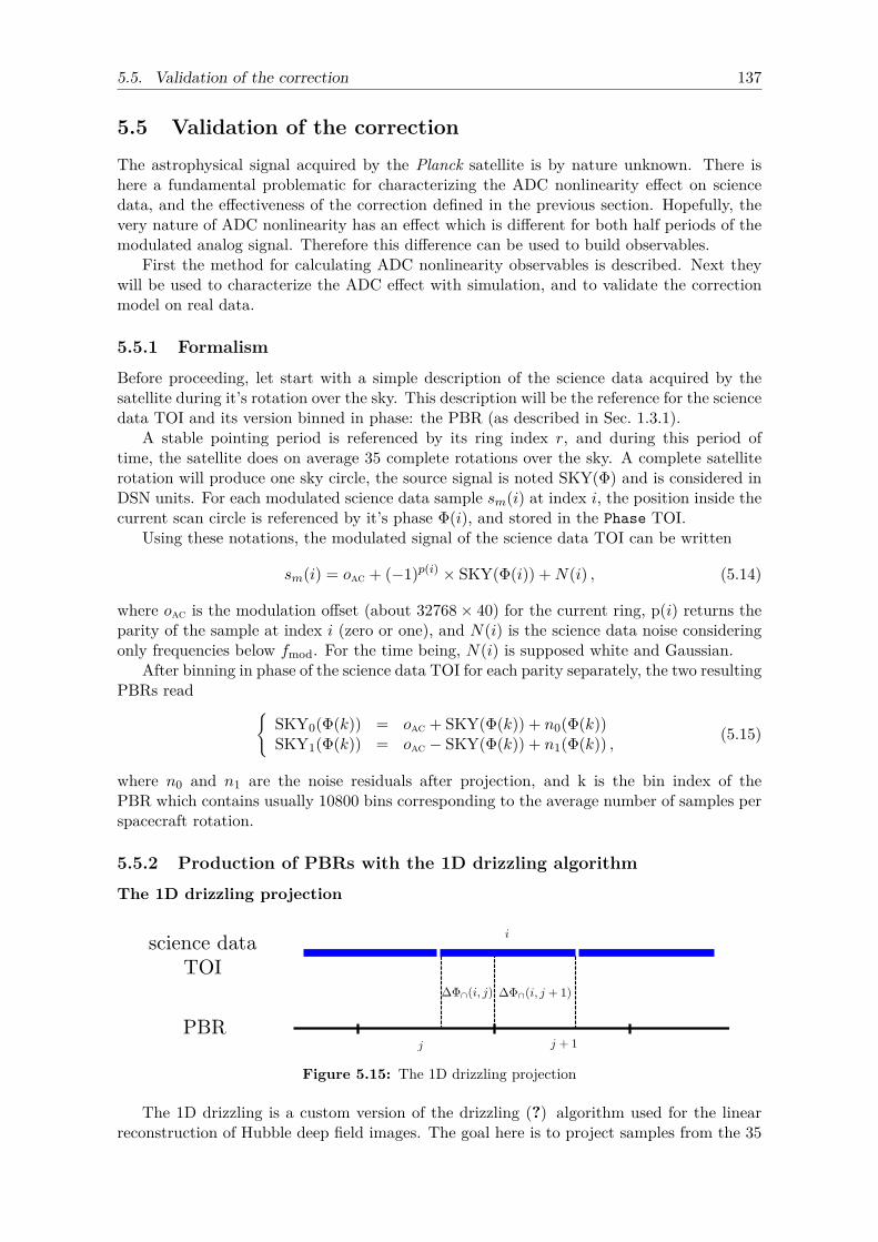
5.5. Validation of the correction 137
5.5 Validation of the correctionThe astrophysical signal acquired by the Planck satellite is by nature unknown. There ishere a fundamental problematic for characterizing the ADC nonlinearity effect on sciencedata, and the effectiveness of the correction defined in the previous section. Hopefully, thevery nature of ADC nonlinearity has an effect which is different for both half periods of themodulated analog signal. Therefore this difference can be used to build observables.
First the method for calculating ADC nonlinearity observables is described. Next theywill be used to characterize the ADC effect with simulation, and to validate the correctionmodel on real data.
5.5.1 Formalism
Before proceeding, let start with a simple description of the science data acquired by thesatellite during it’s rotation over the sky. This description will be the reference for the sciencedata TOI and its version binned in phase: the PBR (as described in Sec. 1.3.1).
A stable pointing period is referenced by its ring index r, and during this period oftime, the satellite does on average 35 complete rotations over the sky. A complete satelliterotation will produce one sky circle, the source signal is noted SKY(Φ) and is considered inDSN units. For each modulated science data sample sm(i) at index i, the position inside thecurrent scan circle is referenced by it’s phase Φ(i), and stored in the Phase TOI.
Using these notations, the modulated signal of the science data TOI can be written
sm(i) = oac + (−1)p(i) × SKY(Φ(i)) +N(i) , (5.14)
where oac is the modulation offset (about 32768× 40) for the current ring, p(i) returns theparity of the sample at index i (zero or one), and N(i) is the science data noise consideringonly frequencies below fmod. For the time being, N(i) is supposed white and Gaussian.
After binning in phase of the science data TOI for each parity separately, the two resultingPBRs read
SKY0(Φ(k)) = oac + SKY(Φ(k)) + n0(Φ(k))SKY1(Φ(k)) = oac − SKY(Φ(k)) + n1(Φ(k)) , (5.15)
where n0 and n1 are the noise residuals after projection, and k is the bin index of thePBR which contains usually 10800 bins corresponding to the average number of samples perspacecraft rotation.
5.5.2 Production of PBRs with the 1D drizzling algorithm
The 1D drizzling projection
Figure 5.15: The 1D drizzling projection
The 1D drizzling is a custom version of the drizzling (?) algorithm used for the linearreconstruction of Hubble deep field images. The goal here is to project samples from the 35
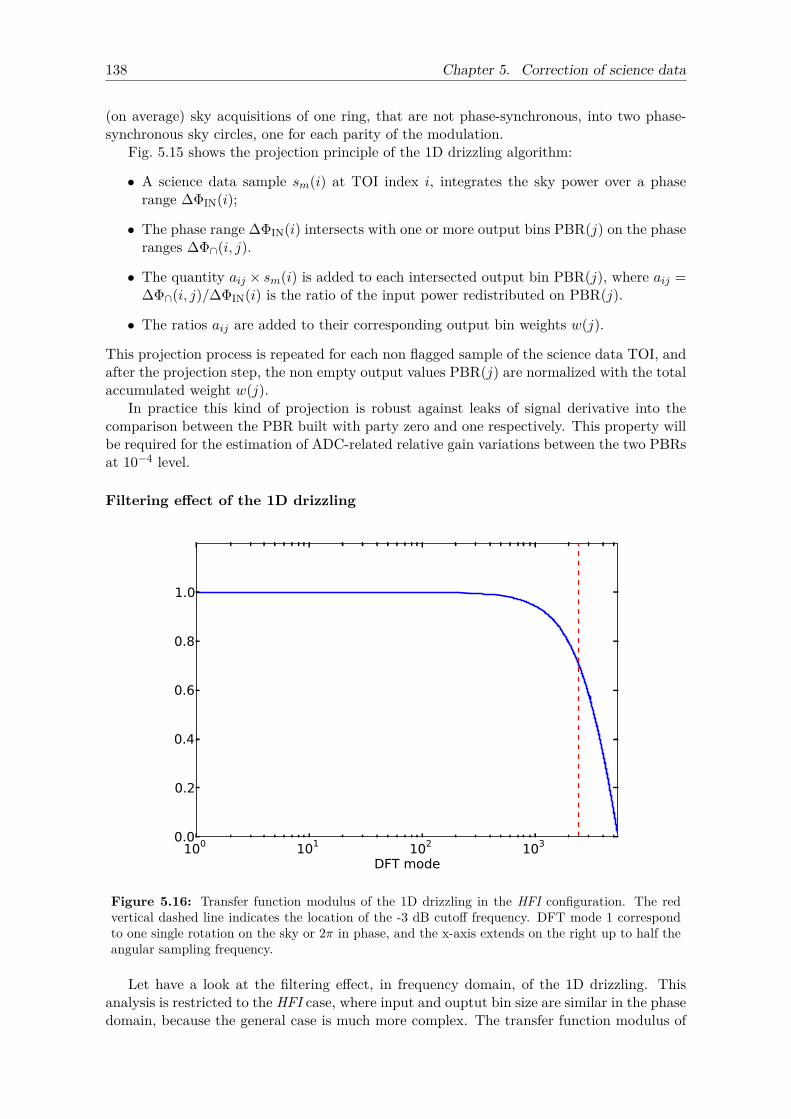
138 Chapter 5. Correction of science data
(on average) sky acquisitions of one ring, that are not phase-synchronous, into two phase-synchronous sky circles, one for each parity of the modulation.
Fig. 5.15 shows the projection principle of the 1D drizzling algorithm:
• A science data sample sm(i) at TOI index i, integrates the sky power over a phaserange ∆ΦIN(i);
• The phase range ∆ΦIN(i) intersects with one or more output bins PBR(j) on the phaseranges ∆Φ∩(i, j).
• The quantity aij × sm(i) is added to each intersected output bin PBR(j), where aij =∆Φ∩(i, j)/∆ΦIN(i) is the ratio of the input power redistributed on PBR(j).
• The ratios aij are added to their corresponding output bin weights w(j).
This projection process is repeated for each non flagged sample of the science data TOI, andafter the projection step, the non empty output values PBR(j) are normalized with the totalaccumulated weight w(j).
In practice this kind of projection is robust against leaks of signal derivative into thecomparison between the PBR built with party zero and one respectively. This property willbe required for the estimation of ADC-related relative gain variations between the two PBRsat 10−4 level.
Filtering effect of the 1D drizzling
100 101 102 103
DFT mode
0.0
0.2
0.4
0.6
0.8
1.0
Figure 5.16: Transfer function modulus of the 1D drizzling in the HFI configuration. The redvertical dashed line indicates the location of the -3 dB cutoff frequency. DFT mode 1 correspondto one single rotation on the sky or 2π in phase, and the x-axis extends on the right up to half theangular sampling frequency.
Let have a look at the filtering effect, in frequency domain, of the 1D drizzling. Thisanalysis is restricted to the HFI case, where input and ouptut bin size are similar in the phasedomain, because the general case is much more complex. The transfer function modulus of
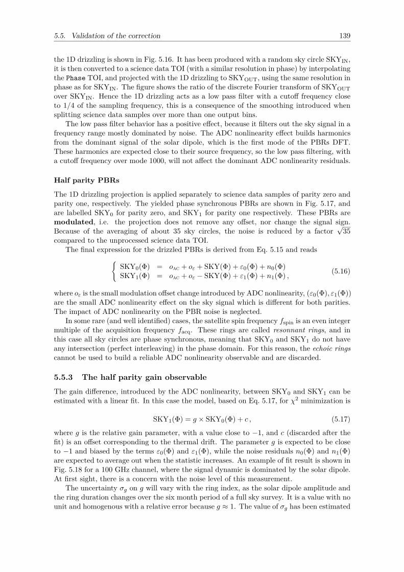
5.5. Validation of the correction 139
the 1D drizzling is shown in Fig. 5.16. It has been produced with a random sky circle SKYIN,it is then converted to a science data TOI (with a similar resolution in phase) by interpolatingthe Phase TOI, and projected with the 1D drizzling to SKYOUT, using the same resolution inphase as for SKYIN. The figure shows the ratio of the discrete Fourier transform of SKYOUTover SKYIN. Hence the 1D drizzling acts as a low pass filter with a cutoff frequency closeto 1/4 of the sampling frequency, this is a consequence of the smoothing introduced whensplitting science data samples over more than one output bins.
The low pass filter behavior has a positive effect, because it filters out the sky signal in afrequency range mostly dominated by noise. The ADC nonlinearity effect builds harmonicsfrom the dominant signal of the solar dipole, which is the first mode of the PBRs DFT.These harmonics are expected close to their source frequency, so the low pass filtering, witha cutoff frequency over mode 1000, will not affect the dominant ADC nonlinearity residuals.
Half parity PBRs
The 1D drizzling projection is applied separately to science data samples of parity zero andparity one, respectively. The yielded phase synchronous PBRs are shown in Fig. 5.17, andare labelled SKY0 for parity zero, and SKY1 for parity one respectively. These PBRs aremodulated, i.e. the projection does not remove any offset, nor change the signal sign.Because of the averaging of about 35 sky circles, the noise is reduced by a factor
√35
compared to the unprocessed science data TOI.The final expression for the drizzled PBRs is derived from Eq. 5.15 and reads
SKY0(Φ) = oac + oε + SKY(Φ) + ε0(Φ) + n0(Φ)SKY1(Φ) = oac + oε − SKY(Φ) + ε1(Φ) + n1(Φ) , (5.16)
where oε is the small modulation offset change introduced by ADC nonlinearity, (ε0(Φ), ε1(Φ))are the small ADC nonlinearity effect on the sky signal which is different for both parities.The impact of ADC nonlinearity on the PBR noise is neglected.
In some rare (and well identified) cases, the satellite spin frequency fspin is an even integermultiple of the acquisition frequency facq. These rings are called resonnant rings, and inthis case all sky circles are phase synchronous, meaning that SKY0 and SKY1 do not haveany intersection (perfect interleaving) in the phase domain. For this reason, the echoic ringscannot be used to build a reliable ADC nonlinearity observable and are discarded.
5.5.3 The half parity gain observable
The gain difference, introduced by the ADC nonlinearity, between SKY0 and SKY1 can beestimated with a linear fit. In this case the model, based on Eq. 5.17, for χ2 minimization is
SKY1(Φ) = g × SKY0(Φ) + c , (5.17)
where g is the relative gain parameter, with a value close to −1, and c (discarded after thefit) is an offset corresponding to the thermal drift. The parameter g is expected to be closeto −1 and biased by the terms ε0(Φ) and ε1(Φ), while the noise residuals n0(Φ) and n1(Φ)are expected to average out when the statistic increases. An example of fit result is shown inFig. 5.18 for a 100 GHz channel, where the signal dynamic is dominated by the solar dipole.At first sight, there is a concern with the noise level of this measurement.
The uncertainty σg on g will vary with the ring index, as the solar dipole amplitude andthe ring duration changes over the six month period of a full sky survey. It is a value with nounit and homogenous with a relative error because g ≈ 1. The value of σg has been estimated
140 Chapter 5. Correction of science data
Figure 5.17: Example of modulated PBRs produced with the 1D drizzling projection. The redline is for SKY0, and the blue line is for SKY1.
with a Monte Carlo method using the PBR of the sky signal, which yields an average valueof 〈σg(r)〉 ≈ 2× 10⁻³.
The result after processing the full mission is shown in Fig. 5.19. Before correction, theobserved gain discrepancy between the signal acquired from different parities is at 1% level.To improve the SNR of the half parity gain observable, PBRs are averaged over 128 ringbefore calculating g, the uncertainty on the observable is reduced down to ≈ 1.7× 10⁻⁴.
After application of the correction function F−1r,p on science data, the reduction of gain
discrepancy between SKY0 and SKY1 is dramatic! This result has been extremely encour-aging for the exploration of the analog model based methodology. Because in this case, thecorrection of science data, does only count on parameters estimated from other sources ofdata. i.e. this reduction of the half parity gain observable is a strong validation of the wholeelectronic readout chain model.
The observables for most channels are shown in Fig. 5.20 for the very first production runof the ADC nonlinearity correction. There is a significant reduction in the observable for thefirst channels, while for higher frequencies, the correction inputs yet needs to be improvedor produced. Another point to be mentioned is the lack of 4 K lines handling in this version,which is the main reason why the observables are worse or poorly reduced on some channels.
5.5.4 The half parity sum observable
This second observable is built by calculating the standard deviation of the sum SKY0 +SKY1. Considering the expression of Eq. 5.16, the sum builds the value 2(oac +oε)+ε0(Φ)+ε1(Φ) + n0(Φ) + n1(Φ). As for the half parity gain observable, averaging the PBRs beforecomputing the observable will average out the terms n0 and n1.
The result of the processing is shown in Fig. 5.21. It has the main advantage that theexpected noise level is pretty much constant over the mission, however it is more difficultto read in terms of gain variations. This is the reason why the half parity gain observablehas been preferred to this one, but as it is used in the simulations (see below) this result is
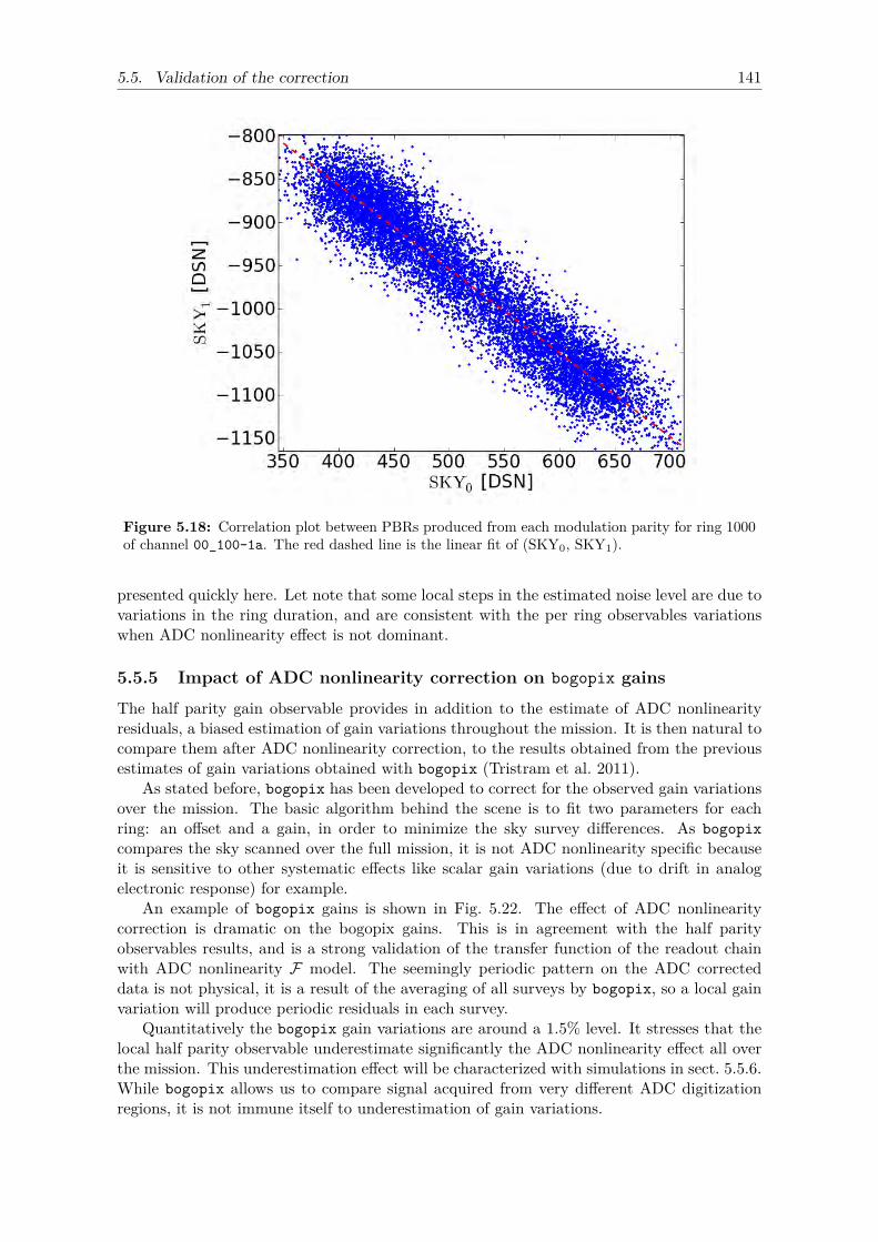
5.5. Validation of the correction 141
Figure 5.18: Correlation plot between PBRs produced from each modulation parity for ring 1000of channel 00_100-1a. The red dashed line is the linear fit of (SKY0, SKY1).
presented quickly here. Let note that some local steps in the estimated noise level are due tovariations in the ring duration, and are consistent with the per ring observables variationswhen ADC nonlinearity effect is not dominant.
5.5.5 Impact of ADC nonlinearity correction on bogopix gains
The half parity gain observable provides in addition to the estimate of ADC nonlinearityresiduals, a biased estimation of gain variations throughout the mission. It is then natural tocompare them after ADC nonlinearity correction, to the results obtained from the previousestimates of gain variations obtained with bogopix (Tristram et al. 2011).
As stated before, bogopix has been developed to correct for the observed gain variationsover the mission. The basic algorithm behind the scene is to fit two parameters for eachring: an offset and a gain, in order to minimize the sky survey differences. As bogopixcompares the sky scanned over the full mission, it is not ADC nonlinearity specific becauseit is sensitive to other systematic effects like scalar gain variations (due to drift in analogelectronic response) for example.
An example of bogopix gains is shown in Fig. 5.22. The effect of ADC nonlinearitycorrection is dramatic on the bogopix gains. This is in agreement with the half parityobservables results, and is a strong validation of the transfer function of the readout chainwith ADC nonlinearity F model. The seemingly periodic pattern on the ADC correcteddata is not physical, it is a result of the averaging of all surveys by bogopix, so a local gainvariation will produce periodic residuals in each survey.
Quantitatively the bogopix gain variations are around a 1.5% level. It stresses that thelocal half parity observable underestimate significantly the ADC nonlinearity effect all overthe mission. This underestimation effect will be characterized with simulations in sect. 5.5.6.While bogopix allows us to compare signal acquired from very different ADC digitizationregions, it is not immune itself to underestimation of gain variations.
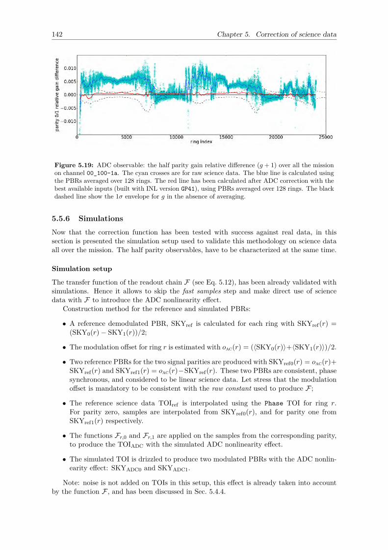
142 Chapter 5. Correction of science data
Figure 5.19: ADC observable: the half parity gain relative difference (g + 1) over all the missionon channel 00_100-1a. The cyan crosses are for raw science data. The blue line is calculated usingthe PBRs averaged over 128 rings. The red line has been calculated after ADC correction with thebest available inputs (built with INL version GP41), using PBRs averaged over 128 rings. The blackdashed line show the 1σ envelope for g in the absence of averaging.
5.5.6 Simulations
Now that the correction function has been tested with success against real data, in thissection is presented the simulation setup used to validate this methodology on science dataall over the mission. The half parity observables, have to be characterized at the same time.
Simulation setup
The transfer function of the readout chain F (see Eq. 5.12), has been already validated withsimulations. Hence it allows to skip the fast samples step and make direct use of sciencedata with F to introduce the ADC nonlinearity effect.
Construction method for the reference and simulated PBRs:
• A reference demodulated PBR, SKYref is calculated for each ring with SKYref(r) =(SKY0(r)− SKY1(r))/2;
• The modulation offset for ring r is estimated with oac(r) = (〈SKY0(r)〉+〈SKY1(r)〉)/2.
• Two reference PBRs for the two signal parities are produced with SKYref0(r) = oac(r)+SKYref(r) and SKYref1(r) = oac(r)−SKYref(r). These two PBRs are consistent, phasesynchronous, and considered to be linear science data. Let stress that the modulationoffset is mandatory to be consistent with the raw constant used to produce F ;
• The reference science data TOIref is interpolated using the Phase TOI for ring r.For parity zero, samples are interpolated from SKYref0(r), and for parity one fromSKYref1(r) respectively.
• The functions Fr,0 and Fr,1 are applied on the samples from the corresponding parity,to produce the TOIADC with the simulated ADC nonlinearity effect.
• The simulated TOI is drizzled to produce two modulated PBRs with the ADC nonlin-earity effect: SKYADC0 and SKYADC1.
Note: noise is not added on TOIs in this setup, this effect is already taken into accountby the function F , and has been discussed in Sec. 5.4.4.
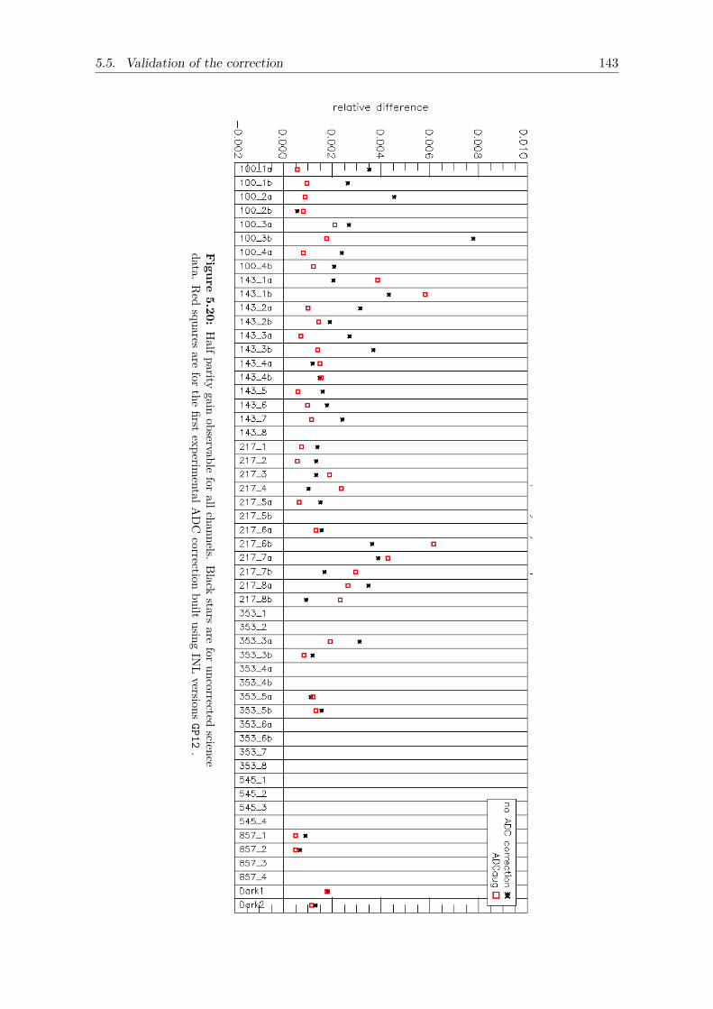
5.5. Validation of the correction 143
Figure
5.20:Halfparity
gainobservable
forallchannels.
Blackstars
arefor
uncorrectedscience
data.Red
squaresare
forthe
firstexperim
entalADC
correctionbuilt
usingIN
Lversions
GP12.
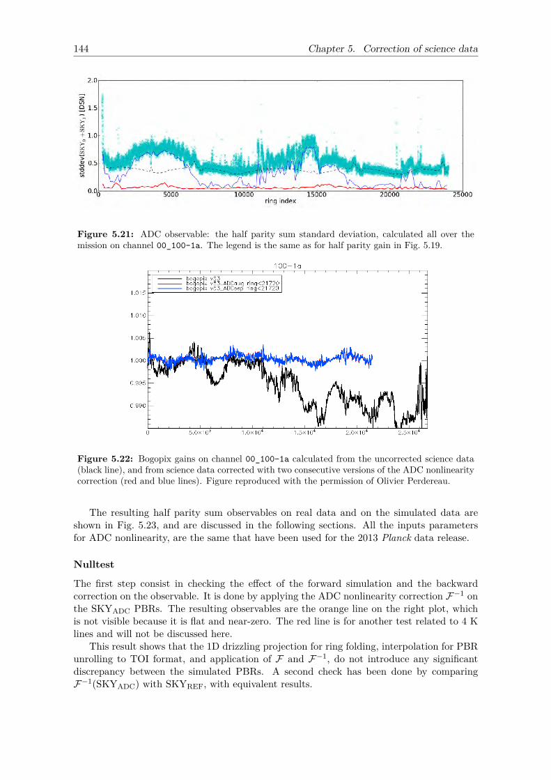
144 Chapter 5. Correction of science data
Figure 5.21: ADC observable: the half parity sum standard deviation, calculated all over themission on channel 00_100-1a. The legend is the same as for half parity gain in Fig. 5.19.
Figure 5.22: Bogopix gains on channel 00_100-1a calculated from the uncorrected science data(black line), and from science data corrected with two consecutive versions of the ADC nonlinearitycorrection (red and blue lines). Figure reproduced with the permission of Olivier Perdereau.
The resulting half parity sum observables on real data and on the simulated data areshown in Fig. 5.23, and are discussed in the following sections. All the inputs parametersfor ADC nonlinearity, are the same that have been used for the 2013 Planck data release.
Nulltest
The first step consist in checking the effect of the forward simulation and the backwardcorrection on the observable. It is done by applying the ADC nonlinearity correction F−1 onthe SKYADC PBRs. The resulting observables are the orange line on the right plot, whichis not visible because it is flat and near-zero. The red line is for another test related to 4 Klines and will not be discussed here.
This result shows that the 1D drizzling projection for ring folding, interpolation for PBRunrolling to TOI format, and application of F and F−1, do not introduce any significantdiscrepancy between the simulated PBRs. A second check has been done by comparingF−1(SKYADC) with SKYREF, with equivalent results.
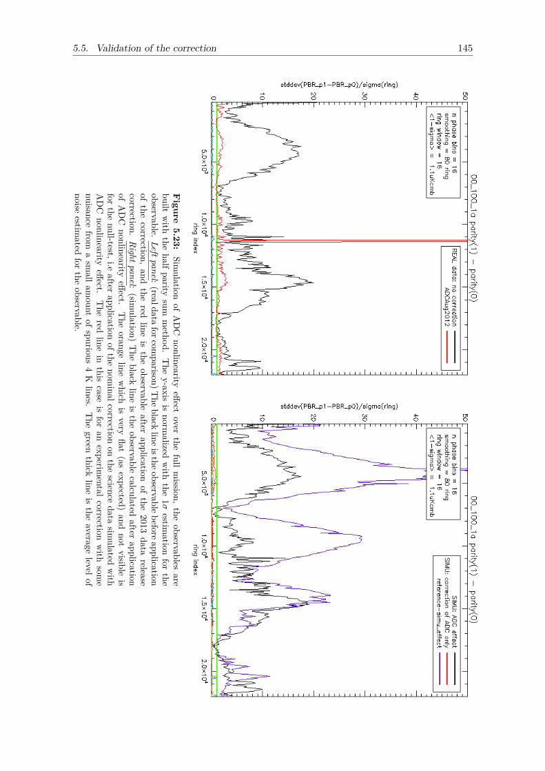
5.5. Validation of the correction 145
Figure
5.23:Sim
ulationof
ADC
nonlinearityeffect
overthe
fullmission,
theobservables
arebuilt
with
thehalfparity
summethod.
The
y-axisis
normalized
with
the1σ
estimation
forthe
observable.Left
panel:(realdataforcom
parison)Theblack
lineistheobservablebeforeapplicationof
thecorrection,
andthe
redline
isthe
observableafter
applicationof
the2013
datarelease
correction.Right
panel:(sim
ulation)The
blackline
isthe
observablecalculated
afterapplication
ofADC
nonlinearityeffect.
The
orangeline
which
isvery
flat(as
expected)and
notvisible
isfor
thenull-test,i.e
afterapplication
ofthenom
inalcorrectionon
thescience
datasim
ulatedwith
ADC
nonlinearityeffect.
The
redline
inthis
caseis
foran
experimental
correctionwith
some
nuisancefrom
asm
allamount
ofspurious4K
lines.The
greenthick
lineis
theaverage
levelofnoise
estimated
forthe
observable.
146 Chapter 5. Correction of science data
ADC nonlinearity effect validation
The second step is the validation of the ADC nonlinearity effect introduced with F . In thiscase the comparison of the observables yielded by the simulated SKYADC (black line on theright) and the raw uncorrected SKY (black line on the left), are in very good agreement.The main difference is the absence of TOI noise in the simulation.
All channels where the 4 K lines level is low, yield a similar result. Hence this testvalidates the first order model of ADC nonlinearity.
Half parity observable characterization
How much of the ADC nonlinearity residuals are we estimating with the half parity observ-ables? To answer this question, the difference between the reference PBR and the one withADC nonlinearity effect has been calculated with d0 = stddev(SKYref0 − SKYADC0), andd1 = stddev(SKYref1−SKYADC1). In Fig. 5.23 The purple line is the RMS of d0 and d1, it ishomogeneous with the half parity sum observable. The observed discrepancy is significantlyhigher by a factor two or three than the observables inferred with parity zero and one.
This result is similar on all the four channels on which the simulation setup has beenrun. It can be explained by the high level of symmetry of the signal around the ADC centraldefect. Hence the half parity observables measure only half of the real deformation effect.
This has some important consequences, it means that the ADC nonlinearity bends thesky measured from both parities in a similar way. As a consequence, one has to be cautiouswhen taking the average of many detectors as a reference, because the ADC nonlinearityeffect is not expected to average out, as it would be for noise.
In practice this very point has not been thoroughly characterized, but raised again in2015, when the peoples remaining active in the Planck Collaboration have been facing thedifficulty of measuring reionisation τ biased significantly by large angular scale ADC nonlin-earity residuals. To work this issue, the sky maps from all the detectors of a single frequencyare averaged to build a reference for the purpose of removing ADC nonlinearity residuals(and others effects).
Frequency domain
The ADC nonlinearity effect in frequency domain is estimated by averaging on the firstsurvey (S1) the DFT modulus of the ADC nonlinearity residuals R0 = SKYref0−SKYADC0
and R1 = SKYref1 − SKYADC1. Fig. 5.24 shows the quantity(< |DFT(R0)| >S1 + <
|DFT(R1)| >S1)/2. The DFT mode index in the sky phase domain has been converted to
a time domain frequency with a 1/60 factor, accounting for the 60 seconds average durationof the PBR.
The ADC nonlinearity residuals from the simulation have globally a 1/f slope in thefrequency domain, with a steeper fall on the first modes of the CMB channels which isconsistent with the main source of signal dynamic on these channels (the solar dipole).
This is an important information, because the ADC nonlinearity effect will impact mainlyat large angular scale on the sky. The important scientific objectives that are impacted are:
• The study of the epoch of reionization, and the calculation of τ ;
• Gravitational waves detection: this is potentially a major issue because it is one of theprimary objectives of the Planck mission;
• The low frequency spectrum part of the thermal SZ effect.
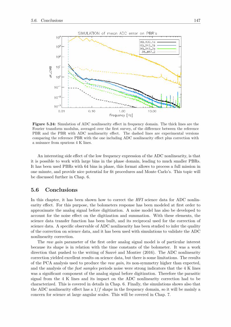
5.6. Conclusions 147
Figure 5.24: Simulation of ADC nonlinearity effect in frequency domain. The thick lines are theFourier transform modulus, averaged over the first survey, of the difference between the referencePBR and the PBR with ADC nonlinearity effect. The dashed lines are experimental versionscomparing the reference PBR with the one including ADC nonlinearity effect plus correction witha nuisance from spurious 4 K lines.
An interesting side effect of the low frequency expression of the ADC nonlinearity, is thatit is possible to work with large bins in the phase domain, leading to much smaller PBRs.It has been used PBRs with 64 bins in phase, this format allows to process a full mission inone minute, and provide nice potential for fit procedures and Monte Carlo’s. This topic willbe discussed further in Chap. 6.
5.6 ConclusionsIn this chapter, it has been shown how to correct the HFI science data for ADC nonlin-earity effect. For this purpose, the bolometers response has been modeled at first order toapproximate the analog signal before digitization. A noise model has also be developed toaccount for the noise effect on the digitization and summation. With these elements, thescience data transfer function has been built, and its reciprocal used for the correction ofscience data. A specific observable of ADC nonlinearity has been studied to infer the qualityof the correction on science data, and it has been used with simulations to validate the ADCnonlinearity correction.
The raw gain parameter of the first order analog signal model is of particular interestbecause its shape is in relation with the time constants of the bolometer. It was a workdirection that pushed to the writing of Sauvé and Montier (2016). The ADC nonlinearitycorrection yielded excellent results on science data, but there is some limitations. The resultsof the PCA analysis used to produce the raw gain, its non-symmetry higher than expected,and the analysis of the fast samples periods noise were strong indicators that the 4 K lineswas a significant component of the analog signal before digitization. Therefore the parasiticsignal from the 4 K lines and its impact on the ADC nonlinearity correction had to becharacterized. This is covered in details in Chap. 6. Finally, the simulations shows also thatthe ADC nonlinearity effect has a 1/f shape in the frequency domain, so it will be mainly aconcern for science at large angular scales. This will be covered in Chap. 7.

149
Chapter 6
4 K lines
After validating the efficiency of the first ADC nonlinearity corrections, enthusiasm has beenquickly cooled by the understanding of the complexity introduced by the 4 K lines, leakedon the detector channels by the 4K stage mechanical cooler. There has been a lots of hintsof this problematic already, ranging from the residuals eigenvectors seen in the PCA outputsof the raw gain estimation, to the raw constant variability over the mission and, last butnot least, their omnipresence on the science data. Their impact on the ADC nonlinearitycorrection has been definitively acted after the observation that the correction was failingmostly on channels with a high level of 4 K lines.
This parasitic signal adds periodic waves over the analog signal before digitization. It is aproblem because its periodicity extends over several fast samples periods, making the analogsignal drift significantly from the model described in Chap. 5. Hence this has to be taken intoaccount in the analog signal model to build an accurate version of the science data transferfunction. However, the summation of fast samples in the DPU, destroys not only informationby mixing nonlinear ADC codes, but also folds in frequency the numerous harmonics of 4 Klines with frequency higher than the modulation frequency. The summation is again a majorissue making the estimation of the unfolded 4 K lines harmonics very challenging. Thatestimation effectively required much more work than for the steps leading to the initial ADCnonlinearity correction.
Sec. 6.1 introduces the topic by the characterization of the 4 K lines from science dataTOIs to the fast samples level. Then the modification of the analog signal model and thenew expression for the science data transfer function is described in Sec. 6.2, and the theimpact of 4 K lines on the science data transfer function is characterized with simulations.The first estimation of the unfolded 4 K lines harmonics is detailed in Sec. 6.3. It has beendone with a method based on Lagrange multipliers, this estimation has been used for thePlanck 2013 data release. However this method presents some limitations that prevents thecorrection to reach an accuracy level better than ≈ 10−3 of the solar dipole amplitude. Toovercome these limitations a work was started on a new estimation method (see Sect. 6.4)based on a Monte Carlo Markov Chain algorithm. This work has been merged with a similarwork from Guillaume Patanchon, to produce an updated model and new unfolded 4 K linesharmonics estimations, allowing to reach an accuracy level close to ≈ 10−4 of the solar dipoleamplitude.
The correction parameters given in Sec. 6.3 and including the 4 K lines in the analogsignal model are the ones that have been used for the ADC nonlinearity correction of thePlanck 2015 data release.
6.1 Characterization of 4 K lines
6.1.1 Origin
The source of 4 K lines is well known and identified as the 4K cooler mechanical compressorsof the cryogenic chain of the Planck spacecraft. The 4K cooler system is based on the Joule
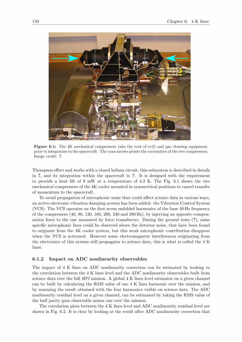
150 Chapter 6. 4 K lines
Figure 6.1: The 4K mechanical compressors (aka the root of evil) and gas cleaning equipment,prior to integration to the spacecraft. The cyan arrows points the extremities of the two compressors.Image credit: ?.
Thompson effect and works with a closed helium circuit, this subsystem is described in detailsin ?, and its integration within the spacecraft in ?. It is designed with the requirementto provide a heat lift of 9 mW at a temperature of 4.2 K. The Fig. 6.1 shows the twomechanical compressors of the 4K cooler mounted in symmetrical positions to cancel transferof momentum to the spacecraft.
To avoid propagation of microphonic noise that could affect science data in various ways,an active electronic vibration damping system has been added: the Vibration Control System(VCS). The VCS operates on the first seven unfolded harmonics of the base 40 Hz frequencyof the compressors (40, 80, 120, 160, 200, 240 and 280 Hz), by injecting an opposite compen-sation force to the one measured by force transducers. During the ground tests (?), somespecific microphonic lines could be observed above the detector noise, that have been foundto originate from the 4K cooler system, but this weak microphonic contribution disappearwhen the VCS is activated. However some electromagnetic interferences originating fromthe electronics of this system still propagates to science data, this is what is called the 4 Klines.
6.1.2 Impact on ADC nonlinearity observables
The impact of 4 K lines on ADC nonlinearity correction can be estimated by looking tothe correlation between the 4 K lines level and the ADC nonlinearity observables built fromscience data over the full HFI mission. A global 4 K lines level estimator on a given channelcan be built by calculating the RMS value of one 4 K lines harmonic over the mission, andby summing the result obtained with the four harmonics visible on science data. The ADCnonlinearity residual level on a given channel, can be estimated by taking the RMS value ofthe half parity gain observable minus one over the mission.
The correlation plots between the 4 K lines level and ADC nonlinearity residual level areshown in Fig. 6.2. It is clear by looking at the result after ADC nonlinearity correction that
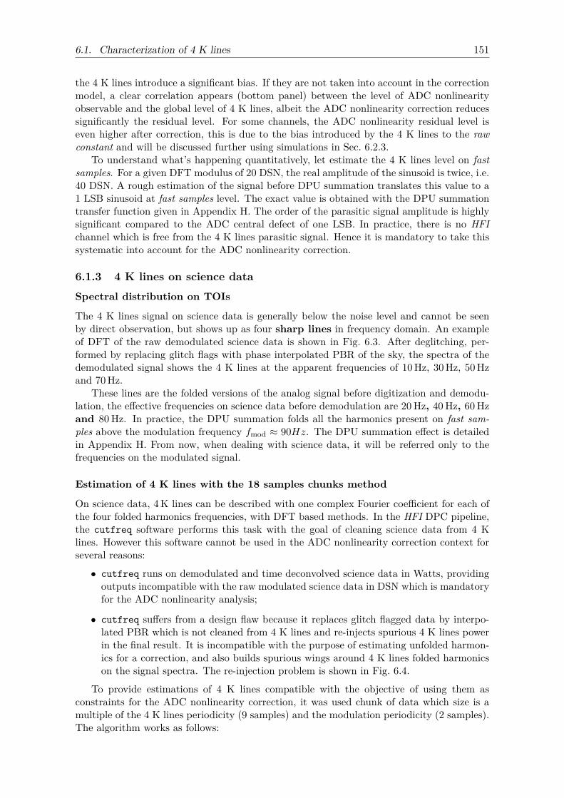
6.1. Characterization of 4 K lines 151
the 4 K lines introduce a significant bias. If they are not taken into account in the correctionmodel, a clear correlation appears (bottom panel) between the level of ADC nonlinearityobservable and the global level of 4 K lines, albeit the ADC nonlinearity correction reducessignificantly the residual level. For some channels, the ADC nonlinearity residual level iseven higher after correction, this is due to the bias introduced by the 4 K lines to the rawconstant and will be discussed further using simulations in Sec. 6.2.3.
To understand what’s happening quantitatively, let estimate the 4 K lines level on fastsamples. For a given DFT modulus of 20 DSN, the real amplitude of the sinusoid is twice, i.e.40 DSN. A rough estimation of the signal before DPU summation translates this value to a1 LSB sinusoid at fast samples level. The exact value is obtained with the DPU summationtransfer function given in Appendix H. The order of the parasitic signal amplitude is highlysignificant compared to the ADC central defect of one LSB. In practice, there is no HFIchannel which is free from the 4 K lines parasitic signal. Hence it is mandatory to take thissystematic into account for the ADC nonlinearity correction.
6.1.3 4 K lines on science data
Spectral distribution on TOIs
The 4 K lines signal on science data is generally below the noise level and cannot be seenby direct observation, but shows up as four sharp lines in frequency domain. An exampleof DFT of the raw demodulated science data is shown in Fig. 6.3. After deglitching, per-formed by replacing glitch flags with phase interpolated PBR of the sky, the spectra of thedemodulated signal shows the 4 K lines at the apparent frequencies of 10 Hz, 30 Hz, 50 Hzand 70 Hz.
These lines are the folded versions of the analog signal before digitization and demodu-lation, the effective frequencies on science data before demodulation are 20 Hz, 40 Hz, 60 Hzand 80 Hz. In practice, the DPU summation folds all the harmonics present on fast sam-ples above the modulation frequency fmod ≈ 90Hz. The DPU summation effect is detailedin Appendix H. From now, when dealing with science data, it will be referred only to thefrequencies on the modulated signal.
Estimation of 4 K lines with the 18 samples chunks method
On science data, 4K lines can be described with one complex Fourier coefficient for each ofthe four folded harmonics frequencies, with DFT based methods. In the HFI DPC pipeline,the cutfreq software performs this task with the goal of cleaning science data from 4 Klines. However this software cannot be used in the ADC nonlinearity correction context forseveral reasons:
• cutfreq runs on demodulated and time deconvolved science data in Watts, providingoutputs incompatible with the raw modulated science data in DSN which is mandatoryfor the ADC nonlinearity analysis;
• cutfreq suffers from a design flaw because it replaces glitch flagged data by interpo-lated PBR which is not cleaned from 4 K lines and re-injects spurious 4 K lines powerin the final result. It is incompatible with the purpose of estimating unfolded harmon-ics for a correction, and also builds spurious wings around 4 K lines folded harmonicson the signal spectra. The re-injection problem is shown in Fig. 6.4.
To provide estimations of 4 K lines compatible with the objective of using them asconstraints for the ADC nonlinearity correction, it was used chunk of data which size is amultiple of the 4 K lines periodicity (9 samples) and the modulation periodicity (2 samples).The algorithm works as follows:
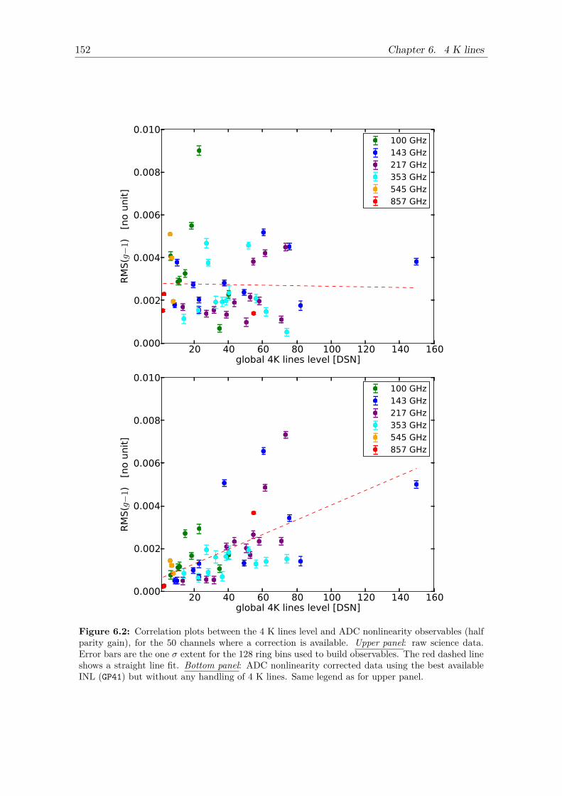
152 Chapter 6. 4 K lines
20 40 60 80 100 120 140 160global 4K lines level [DSN]
0.000
0.002
0.004
0.006
0.008
0.010R
MS(g−
1)
[no u
nit
]
100 GHz143 GHz217 GHz353 GHz545 GHz857 GHz
20 40 60 80 100 120 140 160global 4K lines level [DSN]
0.000
0.002
0.004
0.006
0.008
0.010
RM
S(g−
1)
[no u
nit
]
100 GHz143 GHz217 GHz353 GHz545 GHz857 GHz
Figure 6.2: Correlation plots between the 4 K lines level and ADC nonlinearity observables (halfparity gain), for the 50 channels where a correction is available. Upper panel: raw science data.Error bars are the one σ extent for the 128 ring bins used to build observables. The red dashed lineshows a straight line fit. Bottom panel: ADC nonlinearity corrected data using the best availableINL (GP41) but without any handling of 4 K lines. Same legend as for upper panel.
6.1. Characterization of 4 K lines 153
Figure 6.3: 4 K lines on science data TOI spectra for ring 10000 on channel 02_143-1a. Theblue line is the DFT of raw demodulated science data. The red line is the DFT of deglitcheddemodulated science data.
• TOI mapping to chunks: the science data TOI is mapped to 18 samples using theTOI index modulo 18. The TOI index zero is the reference as the first sample of thefist chunk;
• chunks flagging: all chunks containing at least one invalid sample are discarded(glitch, unstable pointing flag). In addition to the invalid data filtering, chunks withbright signal are also discarded to avoid leaks of signal derivative in the estimation;the brightness of one sample is determined if the corresponding PBR location is twicelarger than the standard deviation of the PBR.
• calculation of global period: all valid chunks of 18 samples are averaged toproduce one single chunk containing two 4 K lines periods plus the modulation signal;
• estimation of folded harmonics: a DFT is run on the global period to get 18complex Fourier coefficients. The 4 K lines Fourier coefficients are in increasing fre-quency order at indices (2, 4, 6, 8). Using 18 samples provides in addition four Fouriercoefficients used as bias estimators at indices (1, 3, 5, 7), where nothing is expectedbut noise.
An example of the resulting DFT coefficients is shown in Fig. 6.5. The folded 20 Hz line istypically the strongest as it can be seen in the time domain period on which it correspondto the dominant sinusoidal shape.
This methods averages out the dipole signal, leading to a direct measurement of 4 Klines folded harmonics. In practice, the bias estimators values are consistent with the noiselevel of about 0.2 DSN all over the mission. Simulations built from a reference PBR andinterpolated science data TOIs plus noise, injected 4 K lines, and using real data glitch flags,gave results consistent with the expected noise level. This validates the estimation method.
The ADC nonlinearity effect could be a concern for the estimated 4 K lines coefficient.In practice it is not the case because its effect is only about 1% of the folded harmonicsamplitude. This level is completely insignificant compared to the noise level of the estimation.It is also a second order term in the context of the ADC nonlinearity correction.
Drift over the mission
Using the previous estimation, the Fig. 6.6 show the variation in amplitude and phase ofthe 4 K lines folded harmonics throughout mission for one typical channel. Their amplitude
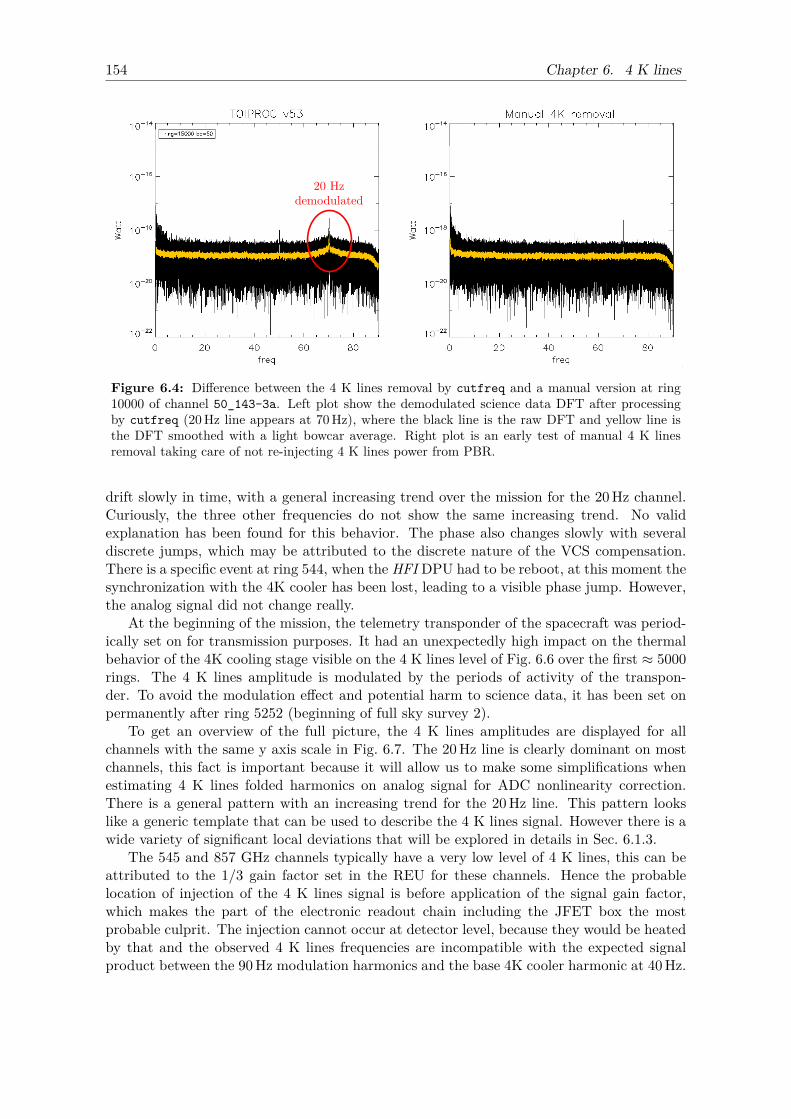
154 Chapter 6. 4 K lines
Figure 6.4: Difference between the 4 K lines removal by cutfreq and a manual version at ring10000 of channel 50_143-3a. Left plot show the demodulated science data DFT after processingby cutfreq (20 Hz line appears at 70 Hz), where the black line is the raw DFT and yellow line isthe DFT smoothed with a light bowcar average. Right plot is an early test of manual 4 K linesremoval taking care of not re-injecting 4 K lines power from PBR.
drift slowly in time, with a general increasing trend over the mission for the 20 Hz channel.Curiously, the three other frequencies do not show the same increasing trend. No validexplanation has been found for this behavior. The phase also changes slowly with severaldiscrete jumps, which may be attributed to the discrete nature of the VCS compensation.There is a specific event at ring 544, when the HFI DPU had to be reboot, at this moment thesynchronization with the 4K cooler has been lost, leading to a visible phase jump. However,the analog signal did not change really.
At the beginning of the mission, the telemetry transponder of the spacecraft was period-ically set on for transmission purposes. It had an unexpectedly high impact on the thermalbehavior of the 4K cooling stage visible on the 4 K lines level of Fig. 6.6 over the first ≈ 5000rings. The 4 K lines amplitude is modulated by the periods of activity of the transpon-der. To avoid the modulation effect and potential harm to science data, it has been set onpermanently after ring 5252 (beginning of full sky survey 2).
To get an overview of the full picture, the 4 K lines amplitudes are displayed for allchannels with the same y axis scale in Fig. 6.7. The 20 Hz line is clearly dominant on mostchannels, this fact is important because it will allow us to make some simplifications whenestimating 4 K lines folded harmonics on analog signal for ADC nonlinearity correction.There is a general pattern with an increasing trend for the 20 Hz line. This pattern lookslike a generic template that can be used to describe the 4 K lines signal. However there is awide variety of significant local deviations that will be explored in details in Sec. 6.1.3.
The 545 and 857 GHz channels typically have a very low level of 4 K lines, this can beattributed to the 1/3 gain factor set in the REU for these channels. Hence the probablelocation of injection of the 4 K lines signal is before application of the signal gain factor,which makes the part of the electronic readout chain including the JFET box the mostprobable culprit. The injection cannot occur at detector level, because they would be heatedby that and the observed 4 K lines frequencies are incompatible with the expected signalproduct between the 90 Hz modulation harmonics and the base 4K cooler harmonic at 40 Hz.
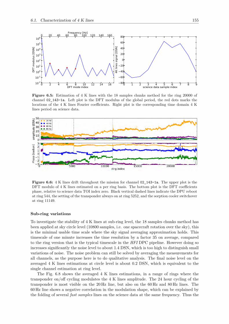
6.1. Characterization of 4 K lines 155
0 2 4 6 8 10 12 14 16DFT mode index
10-2
10-1
100
101
102
103
104
105
106
DFT
modulu
s [D
SN
]0 20 40 60 80 100 120 140 160
Frequency [Hz]
0 1 2 3 4 5 6 7 8 9science data sample index
80
60
40
20
0
20
40
60
80
4K
lin
es
signal [D
SN
]
Figure 6.5: Estimation of 4 K lines with the 18 samples chunks method for the ring 20000 ofchannel 02_143-1a. Left plot is the DFT modulus of the global period, the red dots marks thelocations of the 4 K lines Fourier coefficients. Right plot is the corresponding time domain 4 Klines period on science data.
Figure 6.6: 4 K lines drift throughout the mission for channel 02_143-1a. The upper plot is theDFT modulo of 4 K lines estimated on a per ring basis. The bottom plot is the DFT coefficientsphase, relative to science data TOI index zero. Black vertical dashed lines indicate the DPU rebootat ring 544, the setting of the transponder always on at ring 5252, and the sorption cooler switchoverat ring 11149.
Sub-ring variations
To investigate the stability of 4 K lines at sub-ring level, the 18 samples chunks method hasbeen applied at sky circle level (10800 samples, i.e. one spacecraft rotation over the sky), thisis the minimal usable time scale where the sky signal averaging approximation holds. Thistimescale of one minute increases the time resolution by a factor 35 on average, comparedto the ring version that is the typical timescale in the HFI DPC pipeline. However doing soincreases significantly the noise level to about 1.4 DSN, which is too high to distinguish smallvariations of noise. The noise problem can still be solved by averaging the measurements forall channels, as the purpose here is to do qualitative analysis. The final noise level on theaveraged 4 K lines estimations at circle level is about 0.2 DSN, which is equivalent to thesingle channel estimation at ring level.
The Fig. 6.8 shows the averaged 4 K lines estimations, in a range of rings where thetransponder on/off cycling modulates the 4 K lines amplitude. The 24 hour cycling of thetransponder is most visible on the 20 Hz line, but also on the 60 Hz and 80 Hz lines. The60 Hz line shows a negative correlation in the modulation shape, which can be explained bythe folding of several fast samples lines on the science data at the same frequency. Thus the
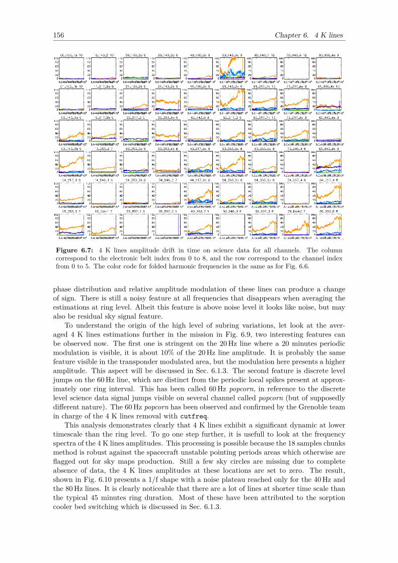
156 Chapter 6. 4 K lines
Figure 6.7: 4 K lines amplitude drift in time on science data for all channels. The columncorrespond to the electronic belt index from 0 to 8, and the row correspond to the channel indexfrom 0 to 5. The color code for folded harmonic frequencies is the same as for Fig. 6.6.
phase distribution and relative amplitude modulation of these lines can produce a changeof sign. There is still a noisy feature at all frequencies that disappears when averaging theestimations at ring level. Albeit this feature is above noise level it looks like noise, but mayalso be residual sky signal feature.
To understand the origin of the high level of subring variations, let look at the aver-aged 4 K lines estimations further in the mission in Fig. 6.9, two interesting features canbe observed now. The first one is stringent on the 20 Hz line where a 20 minutes periodicmodulation is visible, it is about 10% of the 20 Hz line amplitude. It is probably the samefeature visible in the transponder modulated area, but the modulation here presents a higheramplitude. This aspect will be discussed in Sec. 6.1.3. The second feature is discrete leveljumps on the 60 Hz line, which are distinct from the periodic local spikes present at approx-imately one ring interval. This has been called 60 Hz popcorn, in reference to the discretelevel science data signal jumps visible on several channel called popcorn (but of supposedlydifferent nature). The 60 Hz popcorn has been observed and confirmed by the Grenoble teamin charge of the 4 K lines removal with cutfreq.
This analysis demonstrates clearly that 4 K lines exhibit a significant dynamic at lowertimescale than the ring level. To go one step further, it is usefull to look at the frequencyspectra of the 4 K lines amplitudes. This processing is possible because the 18 samples chunksmethod is robust against the spacecraft unstable pointing periods areas which otherwise areflagged out for sky maps production. Still a few sky circles are missing due to completeabsence of data, the 4 K lines amplitudes at these locations are set to zero. The result,shown in Fig. 6.10 presents a 1/f shape with a noise plateau reached only for the 40 Hz andthe 80 Hz lines. It is clearly noticeable that there are a lot of lines at shorter time scale thanthe typical 45 minutes ring duration. Most of these have been attributed to the sorptioncooler bed switching which is discussed in Sec. 6.1.3.
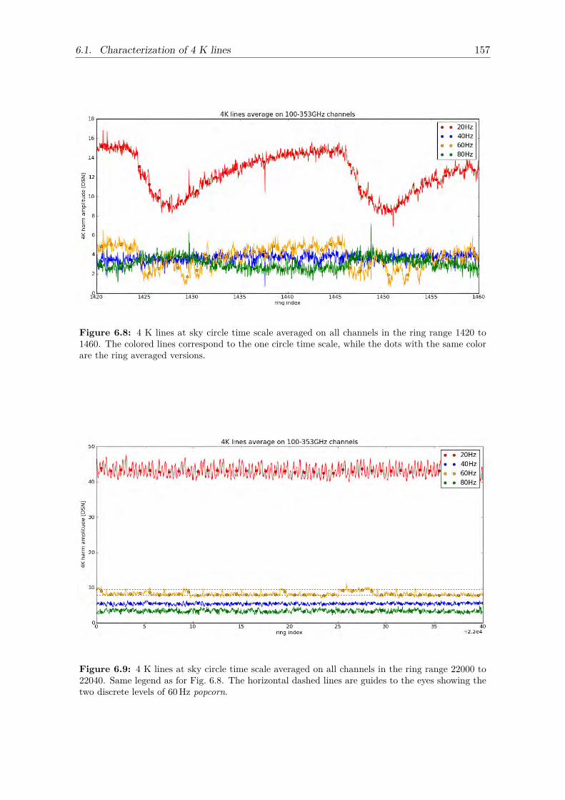
6.1. Characterization of 4 K lines 157
Figure 6.8: 4 K lines at sky circle time scale averaged on all channels in the ring range 1420 to1460. The colored lines correspond to the one circle time scale, while the dots with the same colorare the ring averaged versions.
Figure 6.9: 4 K lines at sky circle time scale averaged on all channels in the ring range 22000 to22040. Same legend as for Fig. 6.8. The horizontal dashed lines are guides to the eyes showing thetwo discrete levels of 60 Hz popcorn.
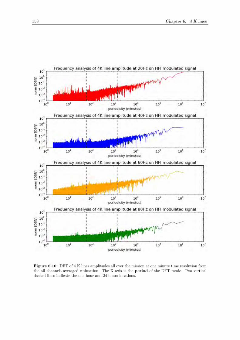
158 Chapter 6. 4 K lines
Figure 6.10: DFT of 4 K lines amplitudes all over the mission at one minute time resolution fromthe all channels averaged estimation. The X axis is the period of the DFT mode. Two verticaldashed lines indicate the one hour and 24 hours locations.
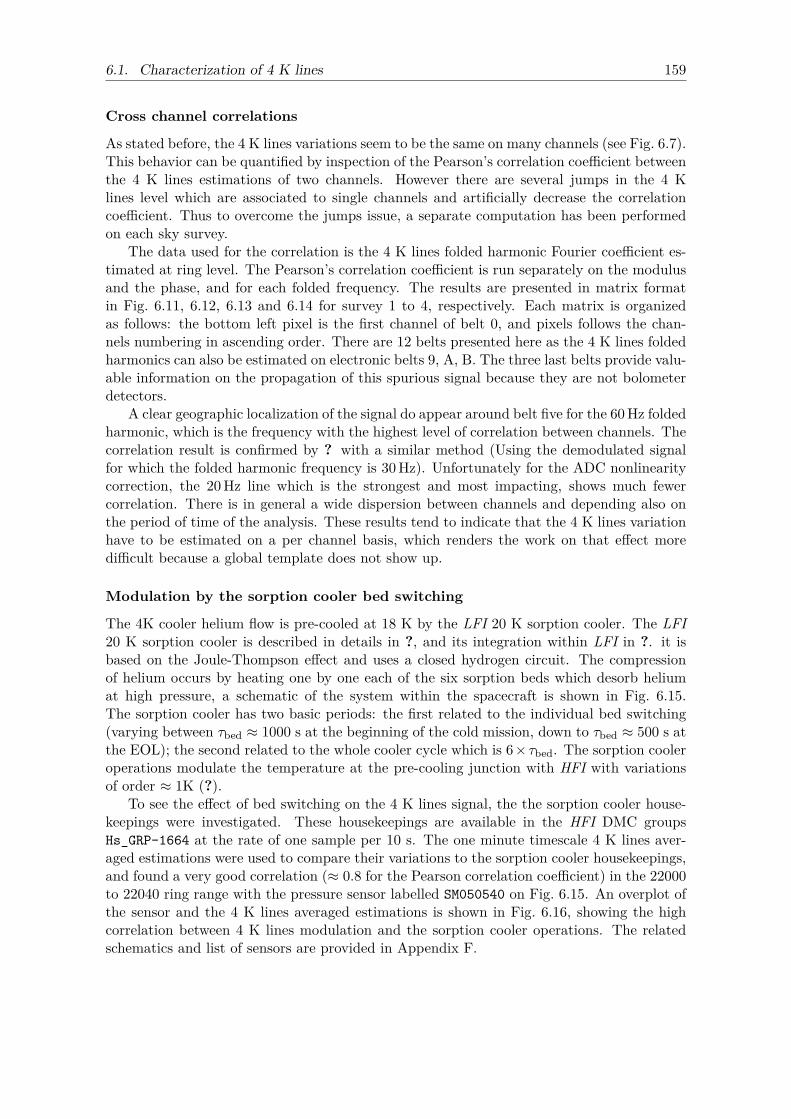
6.1. Characterization of 4 K lines 159
Cross channel correlations
As stated before, the 4 K lines variations seem to be the same on many channels (see Fig. 6.7).This behavior can be quantified by inspection of the Pearson’s correlation coefficient betweenthe 4 K lines estimations of two channels. However there are several jumps in the 4 Klines level which are associated to single channels and artificially decrease the correlationcoefficient. Thus to overcome the jumps issue, a separate computation has been performedon each sky survey.
The data used for the correlation is the 4 K lines folded harmonic Fourier coefficient es-timated at ring level. The Pearson’s correlation coefficient is run separately on the modulusand the phase, and for each folded frequency. The results are presented in matrix formatin Fig. 6.11, 6.12, 6.13 and 6.14 for survey 1 to 4, respectively. Each matrix is organizedas follows: the bottom left pixel is the first channel of belt 0, and pixels follows the chan-nels numbering in ascending order. There are 12 belts presented here as the 4 K lines foldedharmonics can also be estimated on electronic belts 9, A, B. The three last belts provide valu-able information on the propagation of this spurious signal because they are not bolometerdetectors.
A clear geographic localization of the signal do appear around belt five for the 60 Hz foldedharmonic, which is the frequency with the highest level of correlation between channels. Thecorrelation result is confirmed by ? with a similar method (Using the demodulated signalfor which the folded harmonic frequency is 30 Hz). Unfortunately for the ADC nonlinearitycorrection, the 20 Hz line which is the strongest and most impacting, shows much fewercorrelation. There is in general a wide dispersion between channels and depending also onthe period of time of the analysis. These results tend to indicate that the 4 K lines variationhave to be estimated on a per channel basis, which renders the work on that effect moredifficult because a global template does not show up.
Modulation by the sorption cooler bed switching
The 4K cooler helium flow is pre-cooled at 18 K by the LFI 20 K sorption cooler. The LFI20 K sorption cooler is described in details in ?, and its integration within LFI in ?. it isbased on the Joule-Thompson effect and uses a closed hydrogen circuit. The compressionof helium occurs by heating one by one each of the six sorption beds which desorb heliumat high pressure, a schematic of the system within the spacecraft is shown in Fig. 6.15.The sorption cooler has two basic periods: the first related to the individual bed switching(varying between τbed ≈ 1000 s at the beginning of the cold mission, down to τbed ≈ 500 s atthe EOL); the second related to the whole cooler cycle which is 6× τbed. The sorption cooleroperations modulate the temperature at the pre-cooling junction with HFI with variationsof order ≈ 1K (?).
To see the effect of bed switching on the 4 K lines signal, the the sorption cooler house-keepings were investigated. These housekeepings are available in the HFI DMC groupsHs_GRP-1664 at the rate of one sample per 10 s. The one minute timescale 4 K lines aver-aged estimations were used to compare their variations to the sorption cooler housekeepings,and found a very good correlation (≈ 0.8 for the Pearson correlation coefficient) in the 22000to 22040 ring range with the pressure sensor labelled SM050540 on Fig. 6.15. An overplot ofthe sensor and the 4 K lines averaged estimations is shown in Fig. 6.16, showing the highcorrelation between 4 K lines modulation and the sorption cooler operations. The relatedschematics and list of sensors are provided in Appendix F.
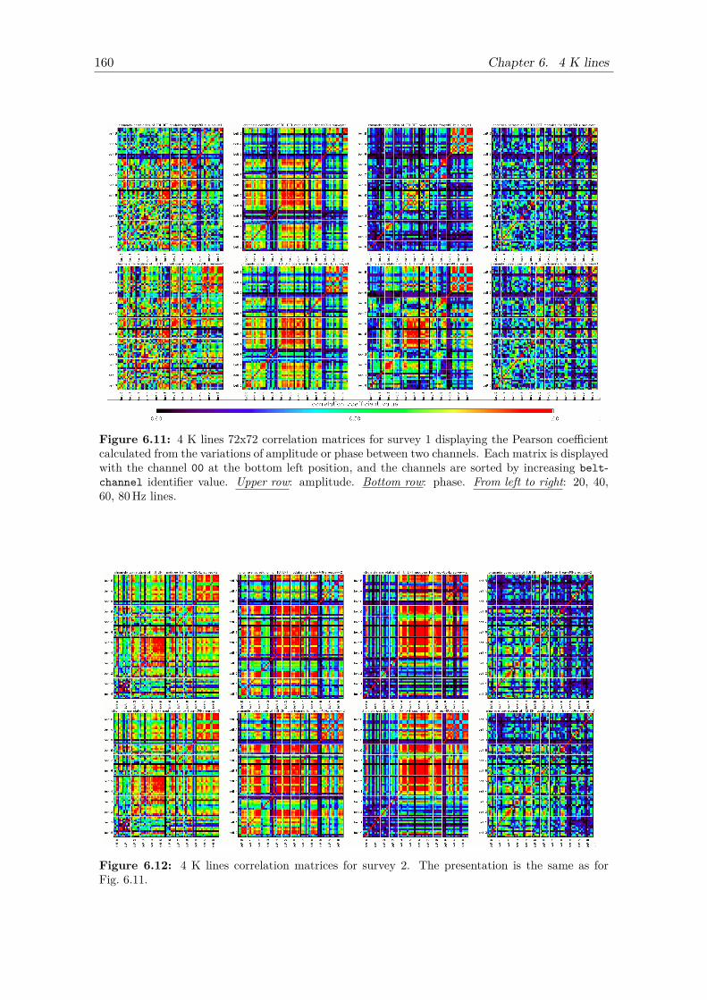
160 Chapter 6. 4 K lines
Figure 6.11: 4 K lines 72x72 correlation matrices for survey 1 displaying the Pearson coefficientcalculated from the variations of amplitude or phase between two channels. Each matrix is displayedwith the channel 00 at the bottom left position, and the channels are sorted by increasing belt-channel identifier value. Upper row: amplitude. Bottom row: phase. From left to right: 20, 40,60, 80 Hz lines.
Figure 6.12: 4 K lines correlation matrices for survey 2. The presentation is the same as forFig. 6.11.
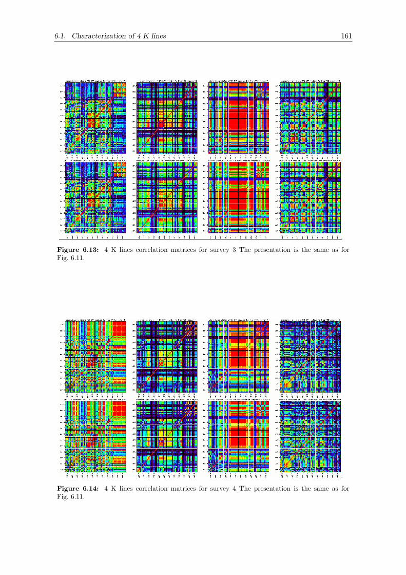
6.1. Characterization of 4 K lines 161
Figure 6.13: 4 K lines correlation matrices for survey 3 The presentation is the same as forFig. 6.11.
Figure 6.14: 4 K lines correlation matrices for survey 4 The presentation is the same as forFig. 6.11.
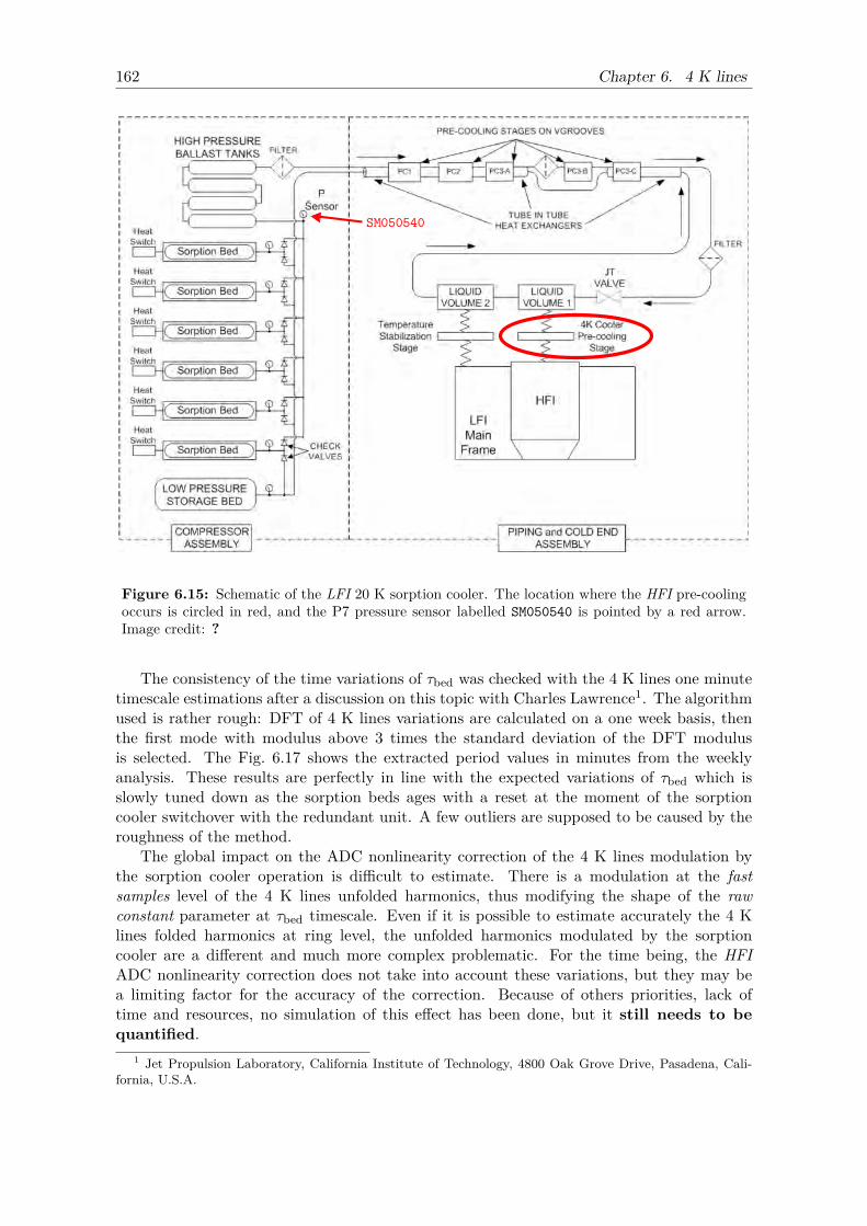
162 Chapter 6. 4 K lines
Figure 6.15: Schematic of the LFI 20 K sorption cooler. The location where the HFI pre-coolingoccurs is circled in red, and the P7 pressure sensor labelled SM050540 is pointed by a red arrow.Image credit: ?
The consistency of the time variations of τbed was checked with the 4 K lines one minutetimescale estimations after a discussion on this topic with Charles Lawrence1. The algorithmused is rather rough: DFT of 4 K lines variations are calculated on a one week basis, thenthe first mode with modulus above 3 times the standard deviation of the DFT modulusis selected. The Fig. 6.17 shows the extracted period values in minutes from the weeklyanalysis. These results are perfectly in line with the expected variations of τbed which isslowly tuned down as the sorption beds ages with a reset at the moment of the sorptioncooler switchover with the redundant unit. A few outliers are supposed to be caused by theroughness of the method.
The global impact on the ADC nonlinearity correction of the 4 K lines modulation bythe sorption cooler operation is difficult to estimate. There is a modulation at the fastsamples level of the 4 K lines unfolded harmonics, thus modifying the shape of the rawconstant parameter at τbed timescale. Even if it is possible to estimate accurately the 4 Klines folded harmonics at ring level, the unfolded harmonics modulated by the sorptioncooler are a different and much more complex problematic. For the time being, the HFIADC nonlinearity correction does not take into account these variations, but they may bea limiting factor for the accuracy of the correction. Because of others priorities, lack oftime and resources, no simulation of this effect has been done, but it still needs to bequantified.
1 Jet Propulsion Laboratory, California Institute of Technology, 4800 Oak Grove Drive, Pasadena, Cali-fornia, U.S.A.
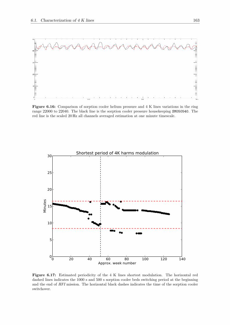
6.1. Characterization of 4 K lines 163
Figure 6.16: Comparison of sorption cooler helium pressure and 4 K lines variations in the ringrange 22000 to 22040. The black line is the sorption cooler pressure housekeeping SM050540. Thered line is the scaled 20 Hz all channels averaged estimation at one minute timescale.
Figure 6.17: Estimated periodicity of the 4 K lines shortest modulation. The horizontal reddashed lines indicates the 1000 s and 500 s sorption cooler beds switching period at the beginningand the end of HFI mission. The horizontal black dashes indicates the time of the sorption coolerswitchover.
164 Chapter 6. 4 K lines
Sequence Begin EndCPV 1 2009/07/03 22:00:00 2009/07/04 23:59:59CPV 2 2009/07/12 00:00:00 2009/07/12 23:59:59
Table 6.1: dates of the fast samples CPV sequences
6.1.4 4 K lines on fast samplesThe 4 K lines window problematic
For the ADC nonlinearity correction, the knowledge of the full period for the unfolded 4 Klines is necessary. Its inclusion in the signal model will be detailed in Sec. 6.2, but there isa big issue preventing to access the full period all over the mission.
The 4K cooler system is phase-synced with the DPU such as the base 40 Hz frequency ofthe two compressors reads f4K = 4fmod/9. This design choice makes the 4 K lines removalon science data easier. However the fast samples period capture occurs every 101 seconds(see Sec. 1.2.6), which is in practice every 18288 science data samples. The problem comesfrom the fact that 18288 = 127 × 18 × 8, is a multiple of 18. As a consequence, the fastsamples period is phase locked to the same exact window viewing only 2/9 of the unfolded4 K lines period. Hence the signal estimation of the full 4 K lines period cannot be madefrom direct observation: end of the may-have-been-short story!
It has been debated before the mission if the period capture would be always the samewindow or not. May the phase locking have been be relaxed there would have been someother issues:• the 4 K lines signal mixes with sky power, it would have impacted the estimation ofthe raw gain;
• the one minute time scale variability (see Sec. 6.1.3) of 4 K lines would have renderedthe reconstruction of the full period from the non causal chunks of 2/9 of the full periodvery difficult.
The CPV fast samples sequences
In the CPV phase, three dedicated sequences have been run in the fast samples telemetrymode, already described in Sec. 4.7.1. These sequences ran much more smoothly that thoseexecuted at EOL, and the two first, labelled CPV 1 and CPV 2, yielded data usable forthe unfolded 4 K lines analysis. The great advantage of these sequences is that they pro-vide several minutes of contiguous fast samples acquisition, which allows us to make directestimation of 4 K lines with DFT based methods.
The CPV 1 sequence provided on average 1 minute of contiguous data per channel, andthe CPV 2 sequence had better stability providing on average 5 minutes of data per channel.The date of the acquisition of both sequences is given in Tab. 6.1. An example of signal fromthe second Dark bolometer is shown in Fig. 6.18, the signal dynamic is high because at thismoment the compensation square is not optimized. After removal of the average modulationperiod the unfolded 4 K lines signal shows up, and a glitch is visible after index 2400. Usingthis dark bolometer channel has the visual advantage that the modulation signal is constantbecause of the absence of sky power, thus making easier to check the unfolded 4 K linessignal by eye.
Estimation of unfolded 4 K lines harmonics : the forrest
The CPV 1 & 2 sequences are a treasure, because they have been the only opportunity inall the HFI mission to have an accurate estimation of the unfolded 4 K lines, but they also
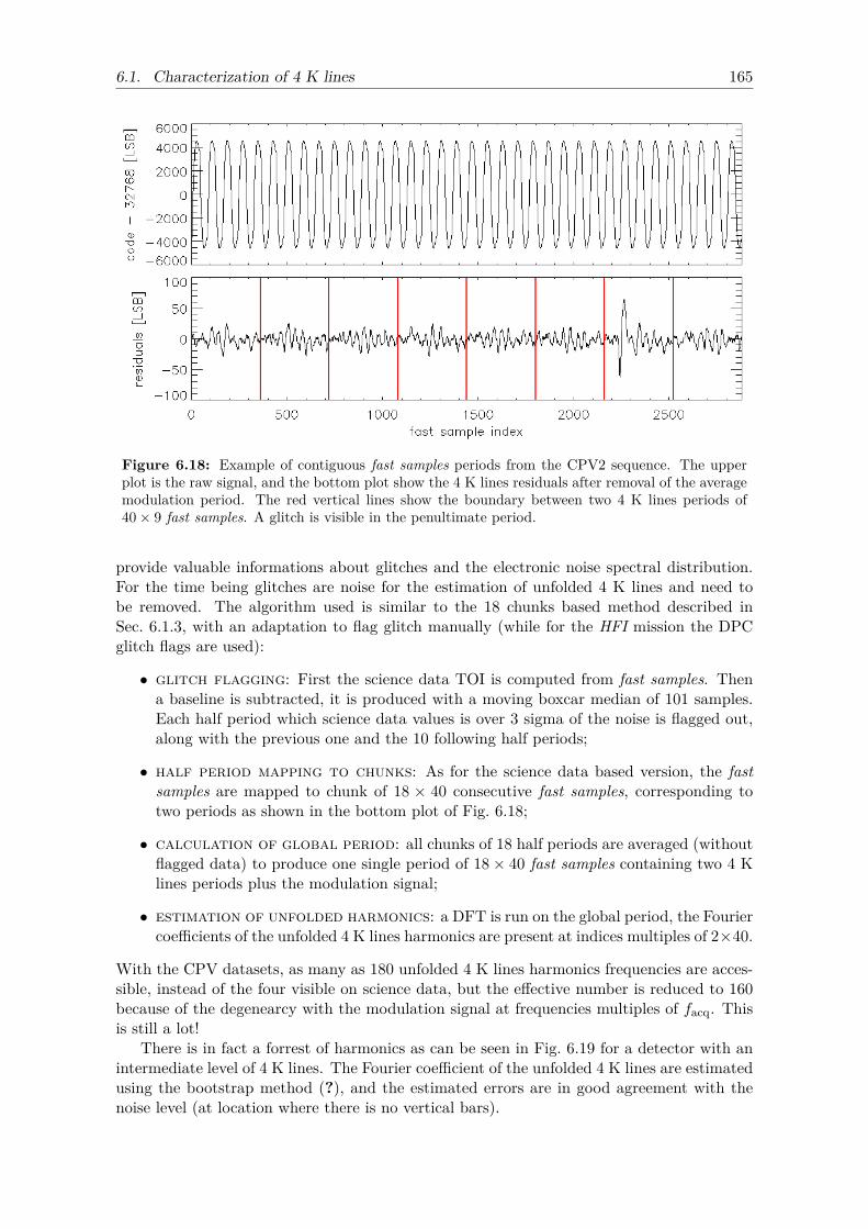
6.1. Characterization of 4 K lines 165
Figure 6.18: Example of contiguous fast samples periods from the CPV2 sequence. The upperplot is the raw signal, and the bottom plot show the 4 K lines residuals after removal of the averagemodulation period. The red vertical lines show the boundary between two 4 K lines periods of40× 9 fast samples. A glitch is visible in the penultimate period.
provide valuable informations about glitches and the electronic noise spectral distribution.For the time being glitches are noise for the estimation of unfolded 4 K lines and need tobe removed. The algorithm used is similar to the 18 chunks based method described inSec. 6.1.3, with an adaptation to flag glitch manually (while for the HFI mission the DPCglitch flags are used):
• glitch flagging: First the science data TOI is computed from fast samples. Thena baseline is subtracted, it is produced with a moving boxcar median of 101 samples.Each half period which science data values is over 3 sigma of the noise is flagged out,along with the previous one and the 10 following half periods;
• half period mapping to chunks: As for the science data based version, the fastsamples are mapped to chunk of 18 × 40 consecutive fast samples, corresponding totwo periods as shown in the bottom plot of Fig. 6.18;
• calculation of global period: all chunks of 18 half periods are averaged (withoutflagged data) to produce one single period of 18× 40 fast samples containing two 4 Klines periods plus the modulation signal;
• estimation of unfolded harmonics: a DFT is run on the global period, the Fouriercoefficients of the unfolded 4 K lines harmonics are present at indices multiples of 2×40.
With the CPV datasets, as many as 180 unfolded 4 K lines harmonics frequencies are acces-sible, instead of the four visible on science data, but the effective number is reduced to 160because of the degenearcy with the modulation signal at frequencies multiples of facq. Thisis still a lot!
There is in fact a forrest of harmonics as can be seen in Fig. 6.19 for a detector with anintermediate level of 4 K lines. The Fourier coefficient of the unfolded 4 K lines are estimatedusing the bootstrap method (?), and the estimated errors are in good agreement with thenoise level (at location where there is no vertical bars).
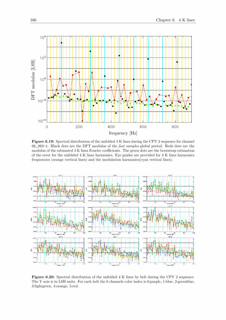
166 Chapter 6. 4 K lines
Figure 6.19: Spectral distribution of the unfolded 4 K lines during the CPV 2 sequence for channel05_353-1. Black dots are the DFT modulus of the fast samples global period. Reds dots are themodulus of the estimated 4 K lines Fourier coefficients. The green dots are the bootstrap estimationof the error for the unfolded 4 K lines harmonics. Eye guides are provided for 4 K lines harmonicsfrequencies (orange vertical lines) and the modulation harmonics(cyan vertical lines).
Figure 6.20: Spectral distribution of the unfolded 4 K lines by belt during the CPV 2 sequence.The Y axis is in LSB units. For each belt the 6 channels color index is 0:purple, 1:blue, 2:greenblue,3:lightgreen, 4:orange, 5:red.
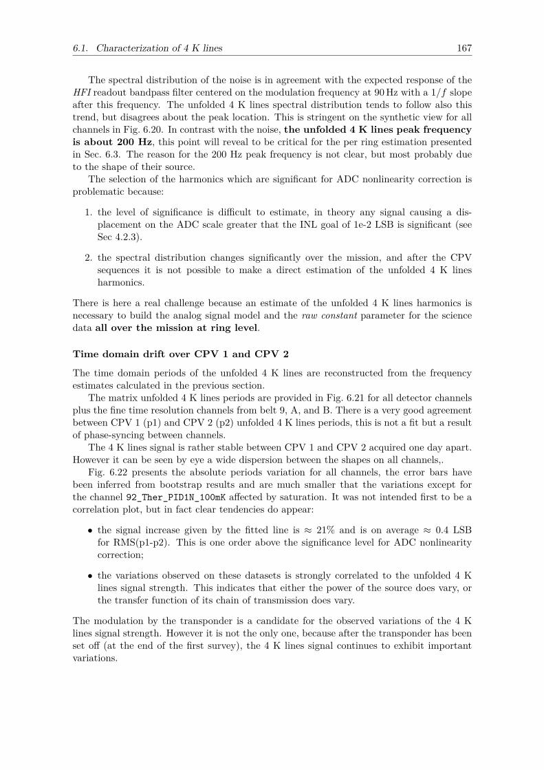
6.1. Characterization of 4 K lines 167
The spectral distribution of the noise is in agreement with the expected response of theHFI readout bandpass filter centered on the modulation frequency at 90 Hz with a 1/f slopeafter this frequency. The unfolded 4 K lines spectral distribution tends to follow also thistrend, but disagrees about the peak location. This is stringent on the synthetic view for allchannels in Fig. 6.20. In contrast with the noise, the unfolded 4 K lines peak frequencyis about 200 Hz, this point will reveal to be critical for the per ring estimation presentedin Sec. 6.3. The reason for the 200 Hz peak frequency is not clear, but most probably dueto the shape of their source.
The selection of the harmonics which are significant for ADC nonlinearity correction isproblematic because:
1. the level of significance is difficult to estimate, in theory any signal causing a dis-placement on the ADC scale greater that the INL goal of 1e-2 LSB is significant (seeSec 4.2.3).
2. the spectral distribution changes significantly over the mission, and after the CPVsequences it is not possible to make a direct estimation of the unfolded 4 K linesharmonics.
There is here a real challenge because an estimate of the unfolded 4 K lines harmonics isnecessary to build the analog signal model and the raw constant parameter for the sciencedata all over the mission at ring level.
Time domain drift over CPV 1 and CPV 2
The time domain periods of the unfolded 4 K lines are reconstructed from the frequencyestimates calculated in the previous section.
The matrix unfolded 4 K lines periods are provided in Fig. 6.21 for all detector channelsplus the fine time resolution channels from belt 9, A, and B. There is a very good agreementbetween CPV 1 (p1) and CPV 2 (p2) unfolded 4 K lines periods, this is not a fit but a resultof phase-syncing between channels.
The 4 K lines signal is rather stable between CPV 1 and CPV 2 acquired one day apart.However it can be seen by eye a wide dispersion between the shapes on all channels,.
Fig. 6.22 presents the absolute periods variation for all channels, the error bars havebeen inferred from bootstrap results and are much smaller that the variations except forthe channel 92_Ther_PID1N_100mK affected by saturation. It was not intended first to be acorrelation plot, but in fact clear tendencies do appear:
• the signal increase given by the fitted line is ≈ 21% and is on average ≈ 0.4 LSBfor RMS(p1-p2). This is one order above the significance level for ADC nonlinearitycorrection;
• the variations observed on these datasets is strongly correlated to the unfolded 4 Klines signal strength. This indicates that either the power of the source does vary, orthe transfer function of its chain of transmission does vary.
The modulation by the transponder is a candidate for the observed variations of the 4 Klines signal strength. However it is not the only one, because after the transponder has beenset off (at the end of the first survey), the 4 K lines signal continues to exhibit importantvariations.
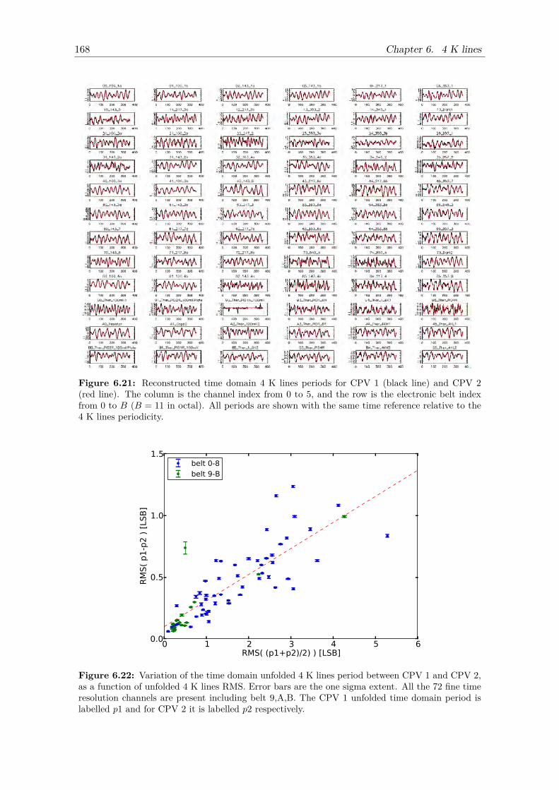
168 Chapter 6. 4 K lines
Figure 6.21: Reconstructed time domain 4 K lines periods for CPV 1 (black line) and CPV 2(red line). The column is the channel index from 0 to 5, and the row is the electronic belt indexfrom 0 to B (B = 11 in octal). All periods are shown with the same time reference relative to the4 K lines periodicity.
0 1 2 3 4 5 6RMS( (p1+p2)/2) ) [LSB]
0.0
0.5
1.0
1.5
RM
S(
p1
-p2
) [
LSB
]
belt 0-8belt 9-B
Figure 6.22: Variation of the time domain unfolded 4 K lines period between CPV 1 and CPV 2,as a function of unfolded 4 K lines RMS. Error bars are the one sigma extent. All the 72 fine timeresolution channels are present including belt 9,A,B. The CPV 1 unfolded time domain period islabelled p1 and for CPV 2 it is labelled p2 respectively.
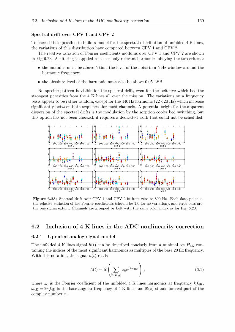
6.2. Inclusion of 4 K lines in the ADC nonlinearity correction 169
Spectral drift over CPV 1 and CPV 2
To check if it is possible to build a model for the spectral distribution of unfolded 4 K lines,the variations of this distribution have compared between CPV 1 and CPV 2.
The relative variation of Fourier coefficients modulus over CPV 1 and CPV 2 are shownin Fig 6.23. A filtering is applied to select only relevant harmonics obeying the two criteria:
• the modulus must be above 5 time the level of the noise in a 5 Hz window around theharmonic frequency;
• the absolute level of the harmonic must also be above 0.05 LSB.
No specific pattern is visible for the spectral drift, even for the belt five which has thestrongest parasitics from the 4 K lines all over the mission. The variations on a frequencybasis appear to be rather random, except for the 440 Hz harmonic (22×20 Hz) which increasesignificantly between both sequences for most channels. A potential origin for the apparentdispersion of the spectral drifts is the modulation by the sorption cooler bed switching, butthis option has not been checked, it requires a dedicated work that could not be scheduled.
0 100 200 300 400 500 600 700belt 0
0
1
2
3
0 100 200 300 400 500 600 700belt 1
0
1
2
3
0 100 200 300 400 500 600 700belt 2
0
1
2
3
0 100 200 300 400 500 600 700belt 3
0
1
2
3
0 100 200 300 400 500 600 700belt 4
0
1
2
3
0 100 200 300 400 500 600 700belt 5
0
1
2
3
0 100 200 300 400 500 600 700belt 6
0
1
2
3
0 100 200 300 400 500 600 700belt 7
0
1
2
3
0 100 200 300 400 500 600 700belt 8
0
1
2
3
Figure 6.23: Spectral drift over CPV 1 and CPV 2 in from zero to 800 Hz. Each data point isthe relative variation of the Fourier coefficients (should be 1.0 for no variation), and error bars arethe one sigma extent. Channels are grouped by belt with the same color index as for Fig. 6.20.
6.2 Inclusion of 4 K lines in the ADC nonlinearity correction
6.2.1 Updated analog signal model
The unfolded 4 K lines signal h(t) can be described concisely from a minimal set H4K con-taining the indices of the most significant harmonics as multiples of the base 20 Hz frequency.With this notation, the signal h(t) reads
h(t) = <
∑k∈H4K
zkejkω4Kt
, (6.1)
where zk is the Fourier coefficient of the unfolded 4 K lines harmonics at frequency kf4K,ω4K = 2πf4K is the base angular frequency of 4 K lines and <(z) stands for real part of thecomplex number z.
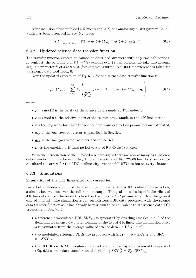
170 Chapter 6. 4 K lines
After inclusion of the unfolded 4 K lines signal h(t), the analog signal s(t) given in Eq. 5.1which has been described in Sec. 5.2, reads
s(t)|Psky+δPsky= s(t) + h(t) + δPsky × g(t) +O(δPsky
2) . (6.2)
6.2.2 Updated science data transfer function
The transfer function expression cannot be described any more with only two half periods.In contrast, the periodicity of s(t) + h(t) extends over 18 half periods. To take into accounth(t), a new vector h of size 9× 40 fast samples is introduced, its time reference is taken forthe science data TOI index 0.
Now the updated expression of Eq. 5.12 for the science data transfer function is
Fp,k,r(Psky) =39∑j=0Aσ
cp,r︸︷︷︸〈Psky〉
(j) + hr(k × 40 + j) + δPsky × gp
, (6.3)
where:
• p = i mod 2 is the parity of the science data sample at TOI index i;
• k = i mod 9 is the relative index of the science data sample in the 4 K lines period;
• r is the ring index for which the science data transfer function parameters are estimated;
• cr,p is the raw constant vector as described in Sec. 5.4;
• gr,p is the raw gain vector as described in Sec. 5.4;
• hr is the unfolded 4 K lines period vector of 9× 40 fast samples.
With the introduction of the unfolded 4 K lines signal there are now as many as 18 sciencedata transfer functions for each ring. In practice a total of 18× 27 000 functions needs to becalculated to correct for the ADC nonlinearity over the full HFI mission on every channel.
6.2.3 Simulations
Simulation of the 4 K lines effect on correction
For a better understanding of the effect of 4 K lines on the ADC nonlinearity correction,a simulation was run over the full mission range. The goal is to distinguish the effect of4 K lines alone from the bias introduced on the raw constant parameter which is the generalcase of interest. The simulation is run on noiseless PBR data processed with the sciencedata transfer function as it has already been shown to be equivalent to the science data TOIprocessing in Sec. 5.4.4.
• a reference demodulated PBR SKYref is generated by drizzling (see Sec. 5.5.2) of thedemodulated science data after cleaning of the folded 4 K lines. The modulation offseto is estimated from the average value of science data (in DSN units);
• two modulated reference PBRs are produced with SKY0 = o + SKYref and SKY1 =o− SKYref ;
• the 18 PBRs with ADC nonlinearity effect are produced by application of the updated(Eq. 6.3) science data transfer function yielding SKY4K
p,k = Fp,k (SKYp);
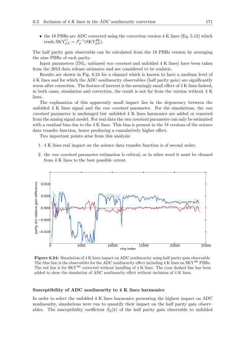
6.2. Inclusion of 4 K lines in the ADC nonlinearity correction 171
• the 18 PBRs are ADC corrected using the correction version 4 K lines (Eq. 5.12) whichreads SKYC
p,k = F−1p (SKY4K
p,k).
The half parity gain observable can be calculated from the 18 PBRs version by averagingthe nine PBRs of each parity.
Input parameters (INL, unbiased raw constant and unfolded 4 K lines) have been takenfrom the 2013 data release estimates and are considered to be realistic.
Results are shown in Fig. 6.24 for a channel which is known to have a medium level of4 K lines and for which the ADC nonlinearity observables (half parity gain) are significantlyworse after correction. The feature of interest is the seemingly small effect of 4 K lines Indeed,in both cases, simulation and correction, the result is not far from the version without 4 Klines.
The explanation of this apparently small impact lies in the degeneracy between theunfolded 4 K lines signal and the raw constant parameter. For the simulations, the rawconstant parameter is unchanged but unfolded 4 K lines harmonics are added or removedfrom the analog signal model. For real data the raw constant parameter can only be estimatedwith a residual bias due to the 4 K lines. This bias is present in the 18 versions of the sciencedata transfer function, hence producing a cumulatively higher effect.
Two important points arise from this analysis:
1. 4 K lines real impact on the science data transfer function is of second order;
2. the raw constant parameter estimation is critical, or in other word it must be cleanedfrom 4 K lines to the best possible extent.
0 5000 10000 15000 20000 25000ring index
0.010
0.005
0.000
0.005
0.010
pari
ty 0
/1 r
ela
tive g
ain
diffe
rence
Figure 6.24: Simulation of 4 K lines impact on ADC nonlinearity using half parity gain observable.The blue line is the observables for the ADC nonlinearity effect including 4 K lines on SKY4K PBRs.The red line is for SKY4K corrected without handling of 4 K lines. The cyan dashed line has beenadded to show the simulation of ADC nonlinearity effect without inclusion of 4 K lines.
Susceptibility of ADC nonlinearity to 4 K lines harmonics
In order to select the unfolded 4 K lines harmonics presenting the highest impact on ADCnonlinearity, simulations were run to quantify their impact on the half parity gain observ-ables. The susceptibility coefficient Sg(k) of the half parity gain observable to unfolded
172 Chapter 6. 4 K lines
harmonic k is defined from the observables over the full mission as follow
Sg(k)|<(zk) = δRMS(g(r)− 1)<(δzk)
Sg(k)|=(zk) = δRMS(g(r)− 1)=(δzk)
, (6.4)
where g(r) is the half parity gain for ring r as defined in Eq. 5.18. The harmonic susceptibilitycoefficient Sg(k) is taken as the quadratic mean of real and imaginary versions.
The results for all channels are shown in Fig. 6.25. It can be noted that the susceptibilityspectra shows a peak for the harmonics around the multiples of facq on most channels. Thisis expected as frequencies close to harmonics of fmod tends to be in synchronization with themodulation, thus degenerate more strongly with the raw constant parameter.
The unfolded 4 K lines harmonics at 160 Hz and 200 Hz are of particular interestfor three reasons: first the ADC nonlinearity is on more susceptible to these frequency onmost channels (see orange dots in Fig. 6.25), next they are among the strongest of the CPVsequences for most channels, and finally they also fold at 20 Hz which is the strongest lineon science data for most channels. Hence they will be included into the restricted set H4Kof harmonics estimated for science data correction.
6.3 Estimation of parameters for 2013 data releaseTo produce the parameters for the updated version of the science data transfer function,the 4 K lines signal must be estimated on a per ring basis along with the raw constantparameter. There were two main issues: the first one is that both 4 K lines and the rawconstant signals are degenerate because of the 2/9 window visibility of the captured fastsamples period (described in Sec. 6.1.4). The second one is the destruction of the unfolded4 K lines harmonics forrest by the DPU summation.
In this section, it is detailed how the degeneracy can be broken between the 4 K linessignal and the fast samples period. Additional constraints from the CPV are needed for thissolution. Finally the estimates of the unfolded 4 K lines harmonics are calculated with aconstrained fit using the Lagrange multipliers method. The constraints for this fit comesfrom the folded 4 K lines on science data.
The parameters produced with the method described below have been the ones used tocorrect for the ADC nonlinearity of the Planck 2013 data relase.
6.3.1 Breaking degeneracy with the half parity sumAs a consequence of the fast samples capture window detailed in Sec. 6.1.4, there is a strongdegeneracy between the unfolded 4 K lines signal and the average modulation shape akathe raw constant. This problem has to be handled in order to provide constraints for theestimation of unfolded 4 K lines.
Hopefully it is possible to take advantage of the symmetry of the raw constant to breakthis degeneracy, because the fast samples period is exactly one modulation period in length.Let write first the raw constant from its Fourier coefficients
c(i) =n∑
k=−nmke
j2πki/80 , i ∈ J0, 79K . (6.5)
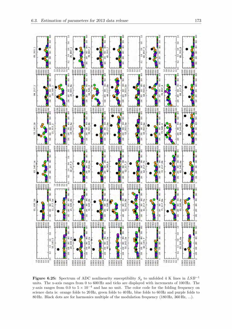
6.3. Estimation of parameters for 2013 data release 173
Figure 6.25: Spectrum of ADC nonlinearity susceptibility Sg to unfolded 4 K lines in LSB−1
units. The x-axis ranges from 0 to 600 Hz and ticks are displayed with increments of 100 Hz. They-axis ranges from 0.0 to 5 × 10⁻⁴ and has no unit. The color code for the folding frequency onscience data is: orange folds to 20 Hz, green folds to 40 Hz, blue folds to 60 Hz and purple folds to80 Hz. Black dots are for harmonics multiple of the modulation frequency (180 Hz, 360 Hz, ...).
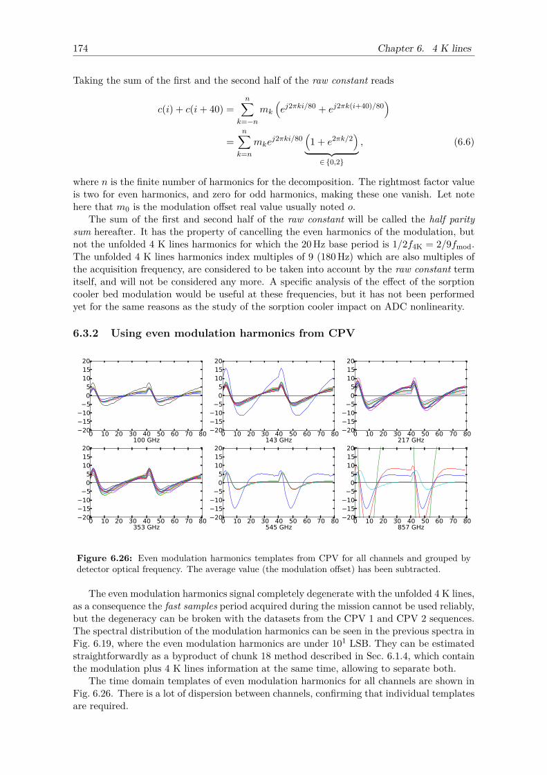
174 Chapter 6. 4 K lines
Taking the sum of the first and the second half of the raw constant reads
c(i) + c(i+ 40) =n∑
k=−nmk
(ej2πki/80 + ej2πk(i+40)/80
)
=n∑
k=nmke
j2πki/80(1 + e2πk/2
)︸ ︷︷ ︸∈0,2
, (6.6)
where n is the finite number of harmonics for the decomposition. The rightmost factor valueis two for even harmonics, and zero for odd harmonics, making these one vanish. Let notehere that m0 is the modulation offset real value usually noted o.
The sum of the first and second half of the raw constant will be called the half paritysum hereafter. It has the property of cancelling the even harmonics of the modulation, butnot the unfolded 4 K lines harmonics for which the 20 Hz base period is 1/2f4K = 2/9fmod.The unfolded 4 K lines harmonics index multiples of 9 (180 Hz) which are also multiples ofthe acquisition frequency, are considered to be taken into account by the raw constant termitself, and will not be considered any more. A specific analysis of the effect of the sorptioncooler bed modulation would be useful at these frequencies, but it has not been performedyet for the same reasons as the study of the sorption cooler impact on ADC nonlinearity.
6.3.2 Using even modulation harmonics from CPV
0 10 20 30 40 50 60 70 80100 GHz
201510
505
101520
0 10 20 30 40 50 60 70 80143 GHz
201510
505
101520
0 10 20 30 40 50 60 70 80217 GHz
201510
505
101520
0 10 20 30 40 50 60 70 80353 GHz
201510
505
101520
0 10 20 30 40 50 60 70 80545 GHz
201510
505
101520
0 10 20 30 40 50 60 70 80857 GHz
201510
505
101520
Figure 6.26: Even modulation harmonics templates from CPV for all channels and grouped bydetector optical frequency. The average value (the modulation offset) has been subtracted.
The even modulation harmonics signal completely degenerate with the unfolded 4 K lines,as a consequence the fast samples period acquired during the mission cannot be used reliably,but the degeneracy can be broken with the datasets from the CPV 1 and CPV 2 sequences.The spectral distribution of the modulation harmonics can be seen in the previous spectra inFig. 6.19, where the even modulation harmonics are under 101 LSB. They can be estimatedstraightforwardly as a byproduct of chunk 18 method described in Sec. 6.1.4, which containthe modulation plus 4 K lines information at the same time, allowing to separate both.
The time domain templates of even modulation harmonics for all channels are shown inFig. 6.26. There is a lot of dispersion between channels, confirming that individual templatesare required.
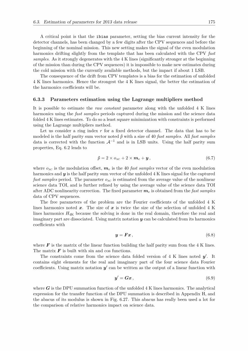
6.3. Estimation of parameters for 2013 data release 175
A critical point is that the ibias parameter, setting the bias current intensity for thedetector channels, has been changed by a few digits after the CPV sequences and before thebeginning of the nominal mission. This new setting makes the signal of the even modulationharmonics drifting slightly from the template that has been calculated with the CPV fastsamples. As it strongly degenerates with the 4 K lines (significantly stronger at the beginningof the mission than during the CPV sequences) it is impossible to make new estimates duringthe cold mission with the currently available methods, but the impact if about 1 LSB.
The consequence of the drift from CPV templates is a bias for the estimation of unfolded4 K lines harmonics. Hence the strongest the 4 K lines signal, the better the estimation ofthe harmonics coefficients will be.
6.3.3 Parameters estimation using the Lagrange multipliers method
It is possible to estimate the raw constant parameter along with the unfolded 4 K linesharmonics using the fast samples periods captured during the mission and the science datafolded 4 K lines estimates. To do so a least square minimization with constraints is performedusing the Lagrange multipliers method.
Let us consider a ring index r for a fixed detector channel. The data that has to bemodeled is the half parity sum vector noted p with a size of 40 fast samples. All fast samplesdata is corrected with the function A−1 and is in LSB units. Using the half parity sumproperties, Eq. 6.2 leads to
p = 2× oac + 2×me + y , (6.7)
where oac is the modulation offset, me is the 40 fast samples vector of the even modulationharmonics and y is the half parity sum vector of the unfolded 4 K lines signal for the capturedfast samples period. The parameter oac is estimated from the average value of the nonlinearscience data TOI, and is further refined by using the average value of the science data TOIafter ADC nonlinearity correction. The fixed parameterme is obtained from the fast samplesdata of CPV sequences.
The free parameters of the problem are the Fourier coefficients of the unfolded 4 Klines harmonics noted x. The size of x is twice the size of the selection of unfolded 4 Klines harmonics H4K because the solving is done in the real domain, therefore the real andimaginary part are dissociated. Using matrix notation y can be calculated from its harmonicscoefficients with
y = Fx , (6.8)
where F is the matrix of the linear function building the half parity sum from the 4 K lines.The matrix F is built with sin and cos functions.
The constraints come from the science data folded version of 4 K lines noted y′. Itcontains eight elements for the real and imaginary part of the four science data Fouriercoefficients. Using matrix notation y′ can be written as the output of a linear function with
y′ = Gx , (6.9)
whereG is the DPU summation function of the unfolded 4 K lines harmonics. The analyticalexpression for the transfer function of the DPU summation is described in Appendix H, andthe abacus of its modulus is shown in Fig. 6.27. This abacus has really been used a lot forthe comparison of relative harmonics impact on science data.
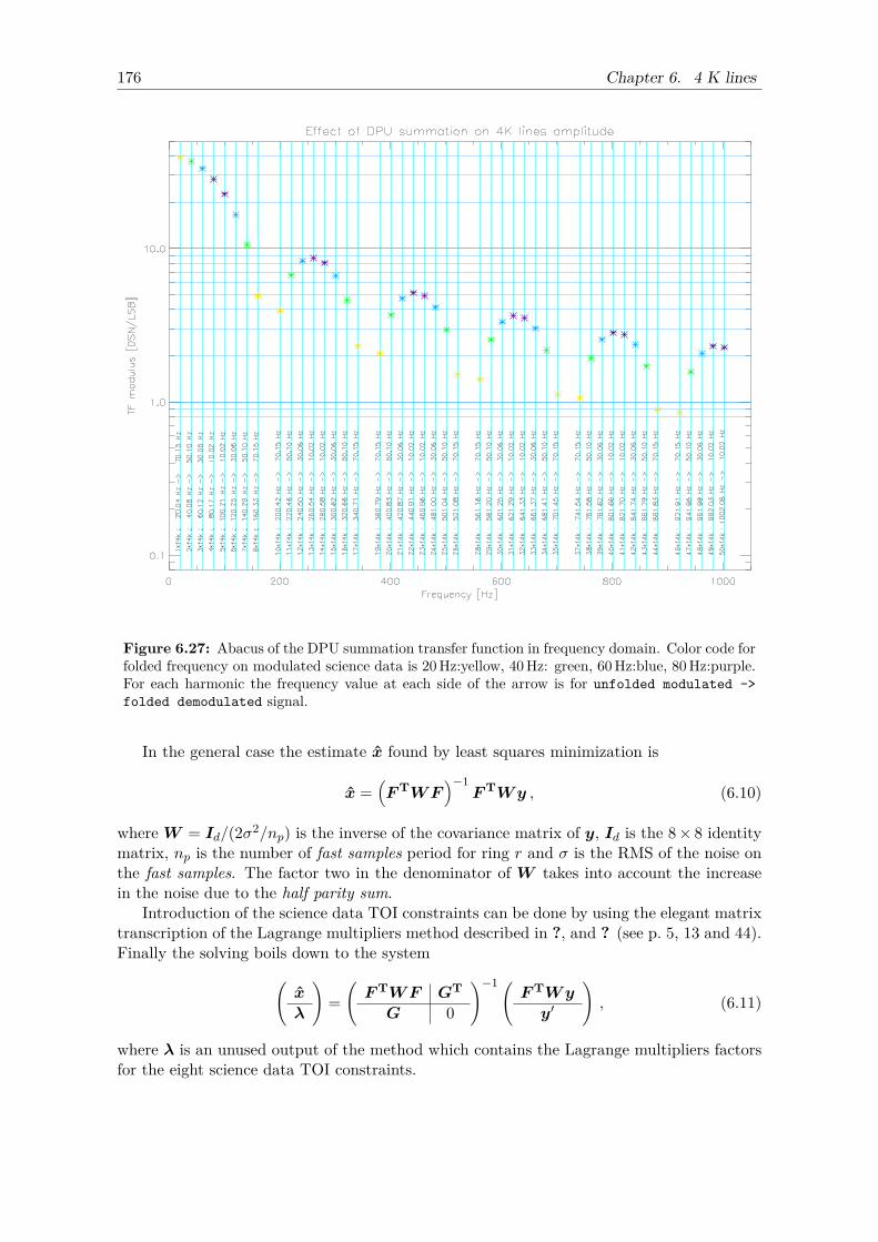
176 Chapter 6. 4 K lines
Figure 6.27: Abacus of the DPU summation transfer function in frequency domain. Color code forfolded frequency on modulated science data is 20 Hz:yellow, 40 Hz: green, 60 Hz:blue, 80 Hz:purple.For each harmonic the frequency value at each side of the arrow is for unfolded modulated ->folded demodulated signal.
In the general case the estimate x found by least squares minimization is
x =(FTWF
)−1FTWy , (6.10)
whereW = Id/(2σ2/np) is the inverse of the covariance matrix of y, Id is the 8× 8 identitymatrix, np is the number of fast samples period for ring r and σ is the RMS of the noise onthe fast samples. The factor two in the denominator of W takes into account the increasein the noise due to the half parity sum.
Introduction of the science data TOI constraints can be done by using the elegant matrixtranscription of the Lagrange multipliers method described in ?, and ? (see p. 5, 13 and 44).Finally the solving boils down to the system(
x
λ
)=(FTWF GT
G 0
)−1(FTWy
y′
), (6.11)
where λ is an unused output of the method which contains the Lagrange multipliers factorsfor the eight science data TOI constraints.
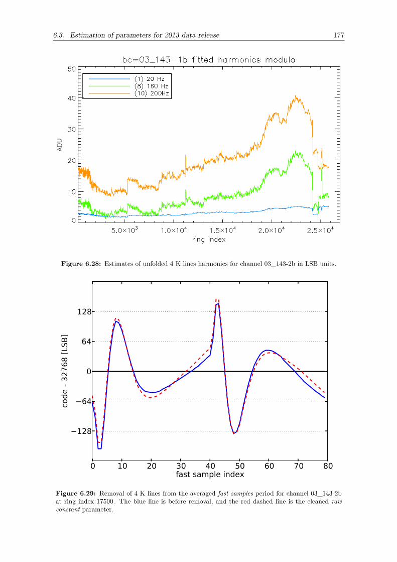
6.3. Estimation of parameters for 2013 data release 177
Figure 6.28: Estimates of unfolded 4 K lines harmonics for channel 03_143-2b in LSB units.
0 10 20 30 40 50 60 70 80fast sample index
128
64
0
64
128
code -
32
76
8 [
LSB
]
Figure 6.29: Removal of 4 K lines from the averaged fast samples period for channel 03_143-2bat ring index 17500. The blue line is before removal, and the red dashed line is the cleaned rawconstant parameter.
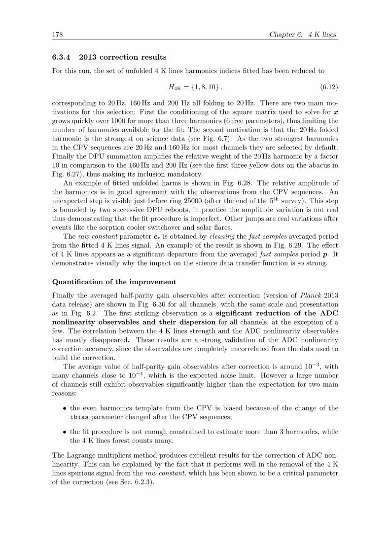
178 Chapter 6. 4 K lines
6.3.4 2013 correction results
For this run, the set of unfolded 4 K lines harmonics indices fitted has been reduced to
H4K = 1, 8, 10 , (6.12)
corresponding to 20 Hz, 160 Hz and 200 Hz all folding to 20 Hz. There are two main mo-tivations for this selection: First the conditioning of the square matrix used to solve for xgrows quickly over 1000 for more than three harmonics (6 free parameters), thus limiting thenumber of harmonics available for the fit; The second motivation is that the 20 Hz foldedharmonic is the strongest on science data (see Fig. 6.7). As the two strongest harmonicsin the CPV sequences are 20 Hz and 160 Hz for most channels they are selected by default.Finally the DPU summation amplifies the relative weight of the 20 Hz harmonic by a factor10 in comparison to the 160 Hz and 200 Hz (see the first three yellow dots on the abacus inFig. 6.27), thus making its inclusion mandatory.
An example of fitted unfolded harms is shown in Fig. 6.28. The relative amplitude ofthe harmonics is in good agreement with the observations from the CPV sequences. Anunexpected step is visible just before ring 25000 (after the end of the 5th survey). This stepis bounded by two successive DPU reboots, in practice the amplitude variation is not realthus demonstrating that the fit procedure is imperfect. Other jumps are real variations afterevents like the sorption cooler switchover and solar flares.
The raw constant parameter cr is obtained by cleaning the fast samples averaged periodfrom the fitted 4 K lines signal. An example of the result is shown in Fig. 6.29. The effectof 4 K lines appears as a significant departure from the averaged fast samples period p. Itdemonstrates visually why the impact on the science data transfer function is so strong.
Quantification of the improvement
Finally the averaged half-parity gain observables after correction (version of Planck 2013data release) are shown in Fig. 6.30 for all channels, with the same scale and presentationas in Fig. 6.2. The first striking observation is a significant reduction of the ADCnonlinearity observables and their dispersion for all channels, at the exception of afew. The correlation between the 4 K lines strength and the ADC nonlinearity observableshas mostly disappeared. These results are a strong validation of the ADC nonlinearitycorrection accuracy, since the observables are completely uncorrelated from the data used tobuild the correction.
The average value of half-parity gain observables after correction is around 10−3, withmany channels close to 10−4, which is the expected noise limit. However a large numberof channels still exhibit observables significantly higher than the expectation for two mainreasons:
• the even harmonics template from the CPV is biased because of the change of theibias parameter changed after the CPV sequences;
• the fit procedure is not enough constrained to estimate more than 3 harmonics, whilethe 4 K lines forest counts many.
The Lagrange multipliers method produces excellent results for the correction of ADC non-linearity. This can be explained by the fact that it performs well in the removal of the 4 Klines spurious signal from the raw constant, which has been shown to be a critical parameterof the correction (see Sec. 6.2.3).
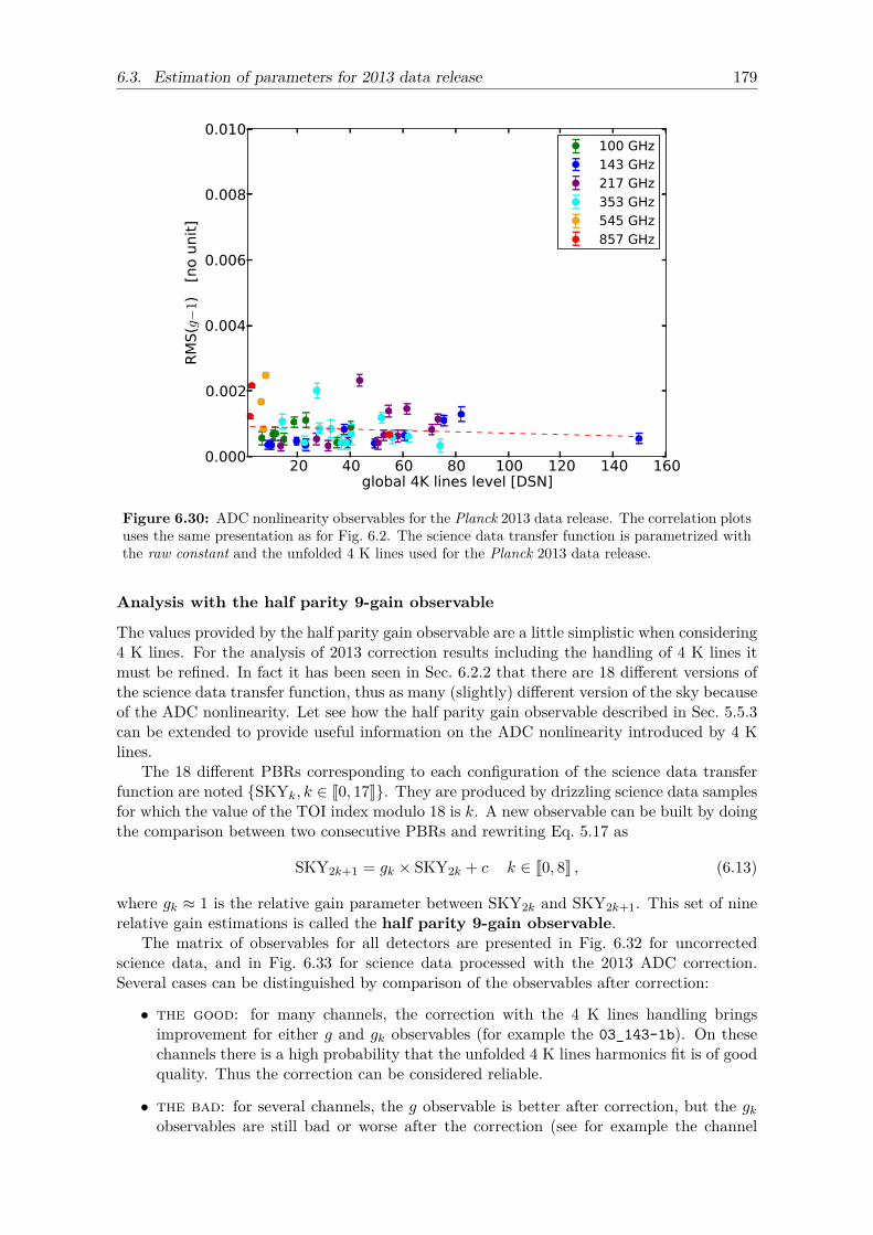
6.3. Estimation of parameters for 2013 data release 179
20 40 60 80 100 120 140 160global 4K lines level [DSN]
0.000
0.002
0.004
0.006
0.008
0.010
RM
S(g−
1)
[no u
nit
]
100 GHz143 GHz217 GHz353 GHz545 GHz857 GHz
Figure 6.30: ADC nonlinearity observables for the Planck 2013 data release. The correlation plotsuses the same presentation as for Fig. 6.2. The science data transfer function is parametrized withthe raw constant and the unfolded 4 K lines used for the Planck 2013 data release.
Analysis with the half parity 9-gain observable
The values provided by the half parity gain observable are a little simplistic when considering4 K lines. For the analysis of 2013 correction results including the handling of 4 K lines itmust be refined. In fact it has been seen in Sec. 6.2.2 that there are 18 different versions ofthe science data transfer function, thus as many (slightly) different version of the sky becauseof the ADC nonlinearity. Let see how the half parity gain observable described in Sec. 5.5.3can be extended to provide useful information on the ADC nonlinearity introduced by 4 Klines.
The 18 different PBRs corresponding to each configuration of the science data transferfunction are noted SKYk, k ∈ J0, 17K. They are produced by drizzling science data samplesfor which the value of the TOI index modulo 18 is k. A new observable can be built by doingthe comparison between two consecutive PBRs and rewriting Eq. 5.17 as
SKY2k+1 = gk × SKY2k + c k ∈ J0, 8K , (6.13)
where gk ≈ 1 is the relative gain parameter between SKY2k and SKY2k+1. This set of ninerelative gain estimations is called the half parity 9-gain observable.
The matrix of observables for all detectors are presented in Fig. 6.32 for uncorrectedscience data, and in Fig. 6.33 for science data processed with the 2013 ADC correction.Several cases can be distinguished by comparison of the observables after correction:
• the good: for many channels, the correction with the 4 K lines handling bringsimprovement for either g and gk observables (for example the 03_143-1b). On thesechannels there is a high probability that the unfolded 4 K lines harmonics fit is of goodquality. Thus the correction can be considered reliable.
• the bad: for several channels, the g observable is better after correction, but the gkobservables are still bad or worse after the correction (see for example the channel
180 Chapter 6. 4 K lines
50_143-3a). In this case, it is probable that the raw constant parameter estimatedfrom the fitted unfolded 4 K lines harmonics is not biased too much. However theharmonics estimates are most probably too far from the reality, as seen with the highdispersion of the gk observables.
• the ugly: a few channels are worse after correction for both observables kind, thisis the case for several 545 GHz and 857 GHz channels, the worst case is the channel25_857-1. The reason has been found in 2015 when working on the new correction. Itcomes from the even harmonic template me which changed dramatically between theCPV sequences and the HFI mission.
It is highly instructive to have a look at the 9-gain observables correlation plots withthe 4 K lines level. The evolution is shown between the science data before and after ADCnonlinearity correction of 2013 in Fig. 6.31. After ADC nonlinearity correction of 2013, thecorrelation with 4 K lines level is still there, albeit it has disappeared for the half parity gainobservable. While the observables values are more compact and the effect is lowered by thecorrection, it is probably mostly due to the first order impact of the INL and mostly clearedraw constant. This is clearly a demonstrating that 4 K lines effect is not completely handled.A lot of effort will be put in this direction for the next version of the correction, becausethese residuals indicates clearly that 4 K lines are a limiting factor for the correction. Theimpact on science at large angular scale will be discussed in the next chapter.
6.4 Alternative parameters estimation for 2015 correctionThe excellent results of the 2013 ADC nonlinearity correction on science data and the analysisof detector response are strongly in favor of the signal model used to produce the science datatransfer function. However the ADC nonlinearity residuals estimated with the observablesstill introduce a bias at ≈ 10−3 level relative to the solar dipole amplitude. This is yet oneorder of magnitude above the target value of 10−4 (as stated in Sec. 4.2.3 for science atlarge angular scales. Starting from the hypothesis that the signal model is valid, this sectionpresents the work leading to a new set of parameters for an improved ADC nonlinearitycorrection. A new constraint will be introduced when fitting the parameters by the inclusionof the ADC nonlinearity observables on science data.
First a characterization of the model parameters is performed with a Metropolis Hastings2 (MH) algorithm which is a Markov Chain Monte Carlo (MCMC) method. A comparisonwith similar work performed by Guillaume Patanchon resulted in a significant simplificationby considering the stability of the raw constant parameter throughout the mission. Then itwill be detailed how the new set of parameters is produced by merging these studies whichgave excellent results on science data.
6.4.1 Characterization of science data transfer function parameters
This section describes the characterization of the unfolded 4 K lines parameter x. Theunfolded 4 K lines harmonics most probable parameter values are estimated with a MetropolisHastings algorithm.
Setup of the MH algorithm
Basically the purpose of the Metropolis Hastingsalgorithm (e.g. see ?) is to approximate theprobability distribution H(x) of the parameter x. In this case x is the unfolded 4 K lines
2 See: https://en.wikipedia.org/wiki/Metropolis-Hastings_algorithm
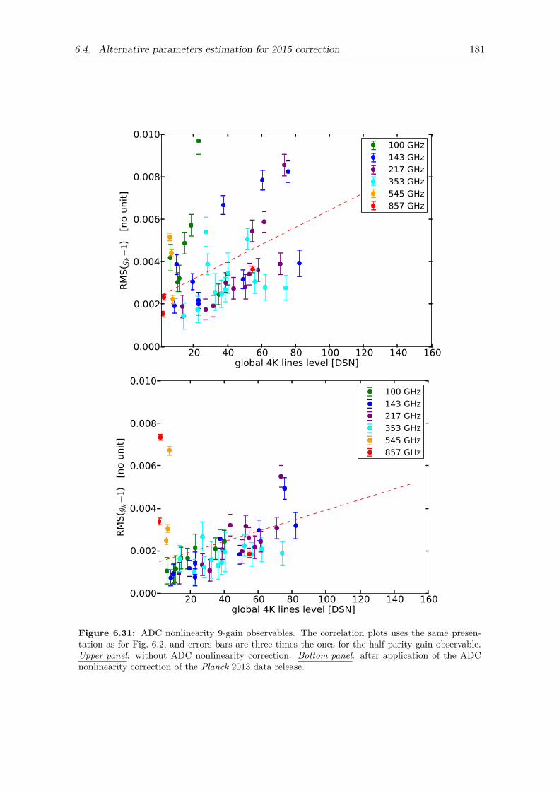
6.4. Alternative parameters estimation for 2015 correction 181
20 40 60 80 100 120 140 160global 4K lines level [DSN]
0.000
0.002
0.004
0.006
0.008
0.010R
MS(gk−
1)
[no u
nit
]
100 GHz143 GHz217 GHz353 GHz545 GHz857 GHz
20 40 60 80 100 120 140 160global 4K lines level [DSN]
0.000
0.002
0.004
0.006
0.008
0.010
RM
S(gk−
1)
[no u
nit
]
100 GHz143 GHz217 GHz353 GHz545 GHz857 GHz
Figure 6.31: ADC nonlinearity 9-gain observables. The correlation plots uses the same presen-tation as for Fig. 6.2, and errors bars are three times the ones for the half parity gain observable.Upper panel: without ADC nonlinearity correction. Bottom panel: after application of the ADCnonlinearity correction of the Planck 2013 data release.
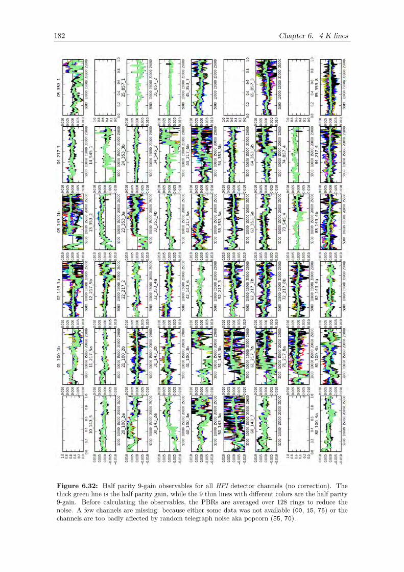
182 Chapter 6. 4 K lines
Figure 6.32: Half parity 9-gain observables for all HFI detector channels (no correction). Thethick green line is the half parity gain, while the 9 thin lines with different colors are the half parity9-gain. Before calculating the observables, the PBRs are averaged over 128 rings to reduce thenoise. A few channels are missing: because either some data was not available (00, 15, 75) or thechannels are too badly affected by random telegraph noise aka popcorn (55, 70).
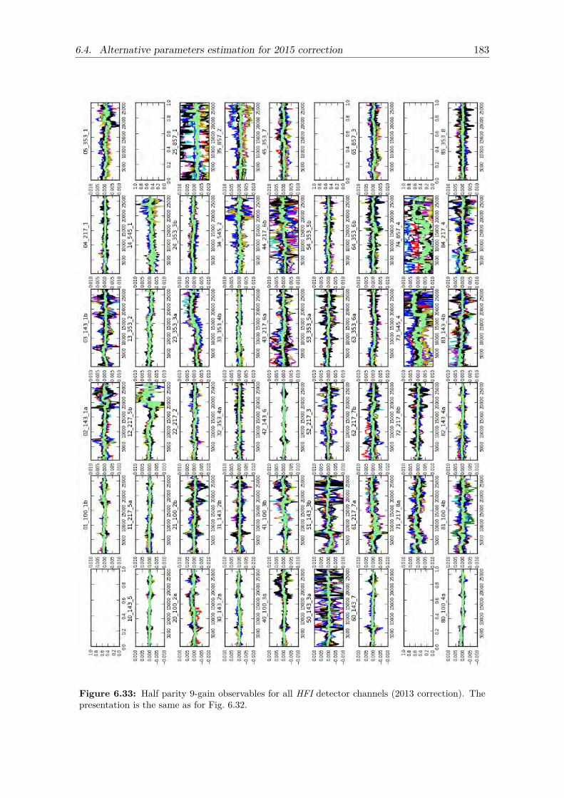
6.4. Alternative parameters estimation for 2015 correction 183
Figure 6.33: Half parity 9-gain observables for all HFI detector channels (2013 correction). Thepresentation is the same as for Fig. 6.32.
184 Chapter 6. 4 K lines
harmonic parameters as defined in Sec. 6.3.3, and the distribution H(x) is considered for agiven ring index.
The algorithm requires a likelihood function f(x) proportional toH(x) to build the targetdistribution. This likelihood function can be built by using the half parity sum residuals,and the two kind of half parity gain observables for which the expected value is 1. Puttingall three data elements together, the error function at ring index r is
R(x)|r =39∑j=0
(p(j)− (2× o+ 2×me))2
2σ2︸ ︷︷ ︸fast samples
+ (g − 1)2
σ2g
+9∑
k=0
(gk − 1)2
3σ2g︸ ︷︷ ︸
science data
, (6.14)
where σ2g is the variance of the half parity gain observable g, and gk is the the half parity
9-gain. The value of σg as a function of r has been estimated with a Monte Carlo method,for an example see Fig. 5.19 in Sec. 5.5.3. The likelihood function is defined as
f(x) = e−R(x) , (6.15)
with the assumption that f(x) ∝ H(x).The target PDF H(x) for x ∈ Ω is built by random exploration with an iterative proce-
dure that will explore preferably the locations of maximum likelihood. An initial value x0 isdrawn from the subset Ωfold which contains all the possible values for x folding to the 4 Klines science data Fourier coefficients y′. In other words x is a solution of Eq. 6.9. The stepsfor generating a Markov chain transition xi → xi+1 are:
1. Candidate generation: a candidate xi+1 is drawn from Ωfold with the PDF g(xi+1|xi)which is described in Sec. 6.4.1.
2. acceptance ratio: the candidate xi+1 is checked against the acceptance ratio α =H(xi+1)/H(xi). As f is proportional to H, the acceptance ratio is calculated withα = f(xi+1)/f(xi);
3. acceptation or rejection: if α ≥ 1, the new candidate is more likely than x and isautomatically accepted. Otherwise it is only accepted if α > u, where u is drawn fromU(0, 1) the uniform distribution on (0, 1). In case of rejection the algorithm returns toCandidate generation.
4. add to chain: if xi+1 is accepted, it is added to the chain and a new candidate isgenerated.
In theory the distribution of the elements of the chain converges toward H(x).If the candidate generation is done carefully the chain transition xi → xi+1 is reversible
by satisfying the condition
H(xi+1)g(xi|xi+1) = H(xi)g(xi+1|xi) . (6.16)
However it cannot be strictly true when enforcing the constraint of folded 4 K lines harmonicsin Eq. 6.9. This is due to the degeneracy between x and the estimations made from sciencedata (the folded harmonics y′ and the modulation offset o). In practice the analysis of theMCMCs in the next section shows that this degeneracy is very low and the condition inEq. 6.16 will be considered to be fulfilled.
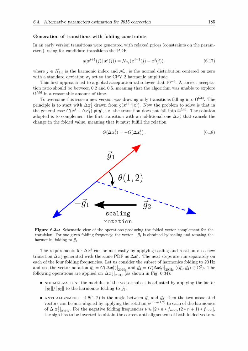
6.4. Alternative parameters estimation for 2015 correction 185
Generation of transitions with folding constraints
In an early version transitions were generated with relaxed priors (constraints on the param-eters), using for candidate transitions the PDF
g(xi+1(j) |xi(j)) = Nσj (xi+1(j)− xi(j)) , (6.17)
where j ∈ H4K is the harmonic index and Nσj is the normal distribution centered on zerowith a standard deviation σj set to the CPV 2 harmonic amplitude.
This first approach led to a global acceptation ratio lower that 10−3. A correct accepta-tion ratio should be between 0.2 and 0.5, meaning that the algorithm was unable to exploreΩfold in a reasonable amount of time.
To overcome this issue a new version was drawing only transitions falling into Ωfold. Theprinciple is to start with ∆xi1 drawn from g(xi+1|xi). Now the problem to solve is that inthe general case G(xi + ∆xi1) 6= y′, i.e. the transition does not fall into Ωfold. The solutionadopted is to complement the first transition with an additional one ∆xic that cancels thechange in the folded value, meaning that it must fulfill the relation
G(∆xic) = −G(∆xi1) . (6.18)
Figure 6.34: Schematic view of the operations producing the folded vector complement for thetransition. For one given folding frequency, the vector −~g1 is obtained by scaling and rotating theharmonics folding to ~g2.
The requirements for ∆xic can be met easily by applying scaling and rotation on a newtransition ∆xi2 generated with the same PDF as ∆xi1. The next steps are run separately oneach of the four folding frequencies. Let us consider the subset of harmonics folding to 20 Hzand use the vector notation ~g1 = G(∆xi1)
∣∣20 Hz and ~g2 = G(∆xi2)
∣∣20 Hz ((~g1, ~g2) ∈ C2). The
following operations are applied on ∆xi2∣∣20Hz (as shown in Fig. 6.34):
• normalization: the modulus of the vector subset is adjusted by applying the factor‖~g1‖/‖~g2‖ to the harmonics folding to ~g2;
• anti-alignment: if θ(1, 2) is the angle between ~g1 and ~g2, then the two associatedvectors can be anti-aligned by applying the rotation ejπ−θ(1,2) to each of the harmonicsof ∆ xi2
∣∣20 Hz. For the negative folding frequencies ν ∈ [2 ∗ n ∗ fmod, (2 ∗ n+ 1) ∗ fmod],
the sign has to be inverted to obtain the correct anti-alignement of both folded vectors.
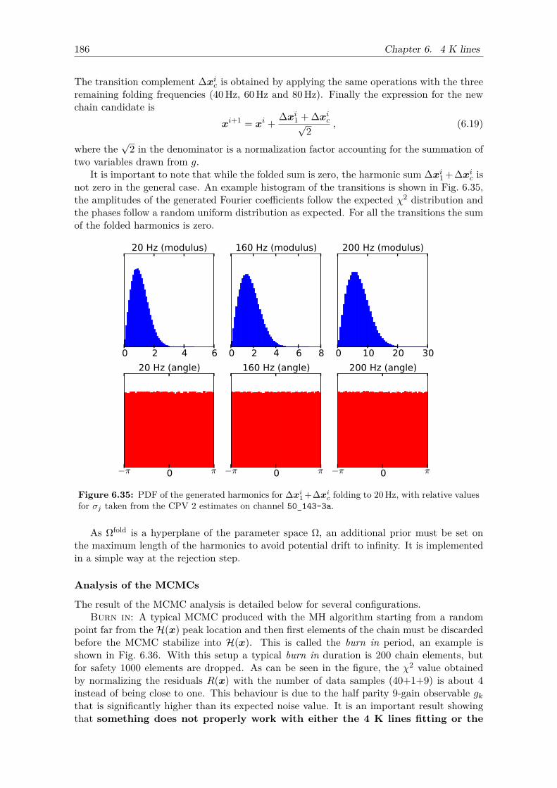
186 Chapter 6. 4 K lines
The transition complement ∆xic is obtained by applying the same operations with the threeremaining folding frequencies (40 Hz, 60 Hz and 80 Hz). Finally the expression for the newchain candidate is
xi+1 = xi + ∆xi1 + ∆xic√2
, (6.19)
where the√
2 in the denominator is a normalization factor accounting for the summation oftwo variables drawn from g.
It is important to note that while the folded sum is zero, the harmonic sum ∆xi1 +∆xic isnot zero in the general case. An example histogram of the transitions is shown in Fig. 6.35,the amplitudes of the generated Fourier coefficients follow the expected χ2 distribution andthe phases follow a random uniform distribution as expected. For all the transitions the sumof the folded harmonics is zero.
0 2 4 6
20 Hz (modulus)
−π 0 π
20 Hz (angle)
0 2 4 6 8
160 Hz (modulus)
−π 0 π
160 Hz (angle)
0 10 20 30
200 Hz (modulus)
−π 0 π
200 Hz (angle)
Figure 6.35: PDF of the generated harmonics for ∆xi1 +∆xic folding to 20 Hz, with relative valuesfor σj taken from the CPV 2 estimates on channel 50_143-3a.
As Ωfold is a hyperplane of the parameter space Ω, an additional prior must be set onthe maximum length of the harmonics to avoid potential drift to infinity. It is implementedin a simple way at the rejection step.
Analysis of the MCMCs
The result of the MCMC analysis is detailed below for several configurations.Burn in: A typical MCMC produced with the MH algorithm starting from a random
point far from the H(x) peak location and then first elements of the chain must be discardedbefore the MCMC stabilize into H(x). This is called the burn in period, an example isshown in Fig. 6.36. With this setup a typical burn in duration is 200 chain elements, butfor safety 1000 elements are dropped. As can be seen in the figure, the χ2 value obtainedby normalizing the residuals R(x) with the number of data samples (40+1+9) is about 4instead of being close to one. This behaviour is due to the half parity 9-gain observable gkthat is significantly higher than its expected noise value. It is an important result showingthat something does not properly work with either the 4 K lines fitting or the
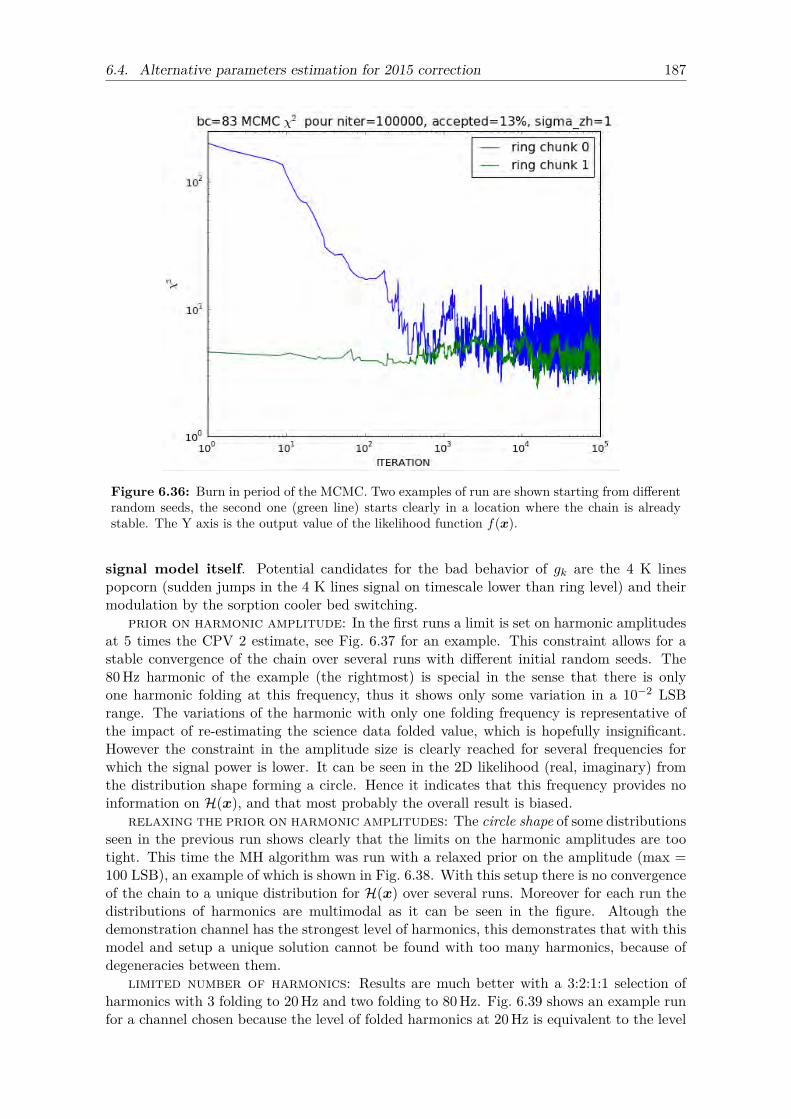
6.4. Alternative parameters estimation for 2015 correction 187
Figure 6.36: Burn in period of the MCMC. Two examples of run are shown starting from differentrandom seeds, the second one (green line) starts clearly in a location where the chain is alreadystable. The Y axis is the output value of the likelihood function f(x).
signal model itself. Potential candidates for the bad behavior of gk are the 4 K linespopcorn (sudden jumps in the 4 K lines signal on timescale lower than ring level) and theirmodulation by the sorption cooler bed switching.
prior on harmonic amplitude: In the first runs a limit is set on harmonic amplitudesat 5 times the CPV 2 estimate, see Fig. 6.37 for an example. This constraint allows for astable convergence of the chain over several runs with different initial random seeds. The80 Hz harmonic of the example (the rightmost) is special in the sense that there is onlyone harmonic folding at this frequency, thus it shows only some variation in a 10−2 LSBrange. The variations of the harmonic with only one folding frequency is representative ofthe impact of re-estimating the science data folded value, which is hopefully insignificant.However the constraint in the amplitude size is clearly reached for several frequencies forwhich the signal power is lower. It can be seen in the 2D likelihood (real, imaginary) fromthe distribution shape forming a circle. Hence it indicates that this frequency provides noinformation on H(x), and that most probably the overall result is biased.
relaxing the prior on harmonic amplitudes: The circle shape of some distributionsseen in the previous run shows clearly that the limits on the harmonic amplitudes are tootight. This time the MH algorithm was run with a relaxed prior on the amplitude (max =100 LSB), an example of which is shown in Fig. 6.38. With this setup there is no convergenceof the chain to a unique distribution for H(x) over several runs. Moreover for each run thedistributions of harmonics are multimodal as it can be seen in the figure. Altough thedemonstration channel has the strongest level of harmonics, this demonstrates that with thismodel and setup a unique solution cannot be found with too many harmonics, because ofdegeneracies between them.
limited number of harmonics: Results are much better with a 3:2:1:1 selection ofharmonics with 3 folding to 20 Hz and two folding to 80 Hz. Fig. 6.39 shows an example runfor a channel chosen because the level of folded harmonics at 20 Hz is equivalent to the level
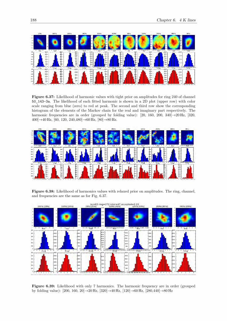
188 Chapter 6. 4 K lines
Figure 6.37: Likelihood of harmonic values with tight prior on amplitudes for ring 240 of channel50_143-3a. The likelihood of each fitted harmonic is shown in a 2D plot (upper row) with colorscale ranging from blue (zero) to red at peak. The second and third row show the correspondinghistogram of the elements of the Markov chain for the real and imaginary part respectively. Theharmonic frequencies are in order (grouped by folding value): [20, 160, 200, 340]→20 Hz, [320,400]→40 Hz, [60, 120, 240,480]→60 Hz, [80]→80 Hz.
Figure 6.38: Likelihood of harmonics values with relaxed prior on amplitudes. The ring, channel,and frequencies are the same as for Fig. 6.37.
Figure 6.39: Likelihood with only 7 harmonics. The harmonic frequency are in order (groupedby folding value): [200, 160, 20]→20 Hz, [320]→40 Hz, [120]→60 Hz, [280,440]→80 Hz
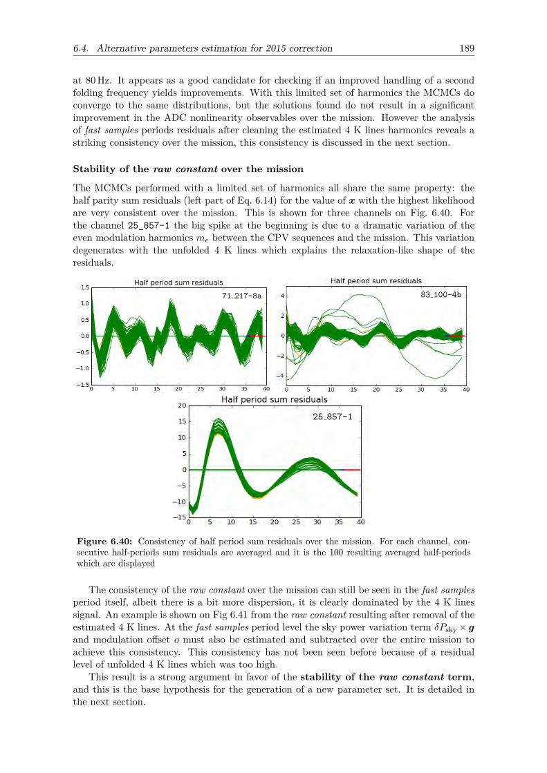
6.4. Alternative parameters estimation for 2015 correction 189
at 80 Hz. It appears as a good candidate for checking if an improved handling of a secondfolding frequency yields improvements. With this limited set of harmonics the MCMCs doconverge to the same distributions, but the solutions found do not result in a significantimprovement in the ADC nonlinearity observables over the mission. However the analysisof fast samples periods residuals after cleaning the estimated 4 K lines harmonics reveals astriking consistency over the mission, this consistency is discussed in the next section.
Stability of the raw constant over the mission
The MCMCs performed with a limited set of harmonics all share the same property: thehalf parity sum residuals (left part of Eq. 6.14) for the value of x with the highest likelihoodare very consistent over the mission. This is shown for three channels on Fig. 6.40. Forthe channel 25_857-1 the big spike at the beginning is due to a dramatic variation of theeven modulation harmonics me between the CPV sequences and the mission. This variationdegenerates with the unfolded 4 K lines which explains the relaxation-like shape of theresiduals.
Figure 6.40: Consistency of half period sum residuals over the mission. For each channel, con-secutive half-periods sum residuals are averaged and it is the 100 resulting averaged half-periodswhich are displayed
The consistency of the raw constant over the mission can still be seen in the fast samplesperiod itself, albeit there is a bit more dispersion, it is clearly dominated by the 4 K linessignal. An example is shown on Fig 6.41 from the raw constant resulting after removal of theestimated 4 K lines. At the fast samples period level the sky power variation term δPsky× gand modulation offset o must also be estimated and subtracted over the entire mission toachieve this consistency. This consistency has not been seen before because of a residuallevel of unfolded 4 K lines which was too high.
This result is a strong argument in favor of the stability of the raw constant term,and this is the base hypothesis for the generation of a new parameter set. It is detailed inthe next section.
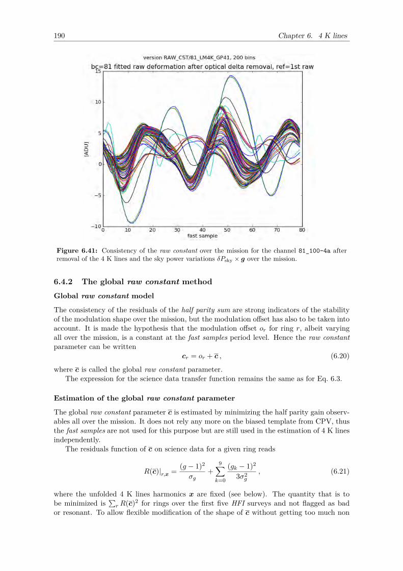
190 Chapter 6. 4 K lines
Figure 6.41: Consistency of the raw constant over the mission for the channel 81_100-4a afterremoval of the 4 K lines and the sky power variations δPsky × g over the mission.
6.4.2 The global raw constant method
Global raw constant model
The consistency of the residuals of the half parity sum are strong indicators of the stabilityof the modulation shape over the mission, but the modulation offset has also to be taken intoaccount. It is made the hypothesis that the modulation offset or for ring r, albeit varyingall over the mission, is a constant at the fast samples period level. Hence the raw constantparameter can be written
cr = or + c , (6.20)
where c is called the global raw constant parameter.The expression for the science data transfer function remains the same as for Eq. 6.3.
Estimation of the global raw constant parameter
The global raw constant parameter c is estimated by minimizing the half parity gain observ-ables all over the mission. It does not rely any more on the biased template from CPV, thusthe fast samples are not used for this purpose but are still used in the estimation of 4 K linesindependently.
The residuals function of c on science data for a given ring reads
R(c)|r,x = (g − 1)2
σg+
9∑k=0
(gk − 1)2
3σ2g
, (6.21)
where the unfolded 4 K lines harmonics x are fixed (see below). The quantity that is tobe minimized is ∑r R(c)2 for rings over the first five HFI surveys and not flagged as bador resonant. To allow flexible modification of the shape of c without getting too much non
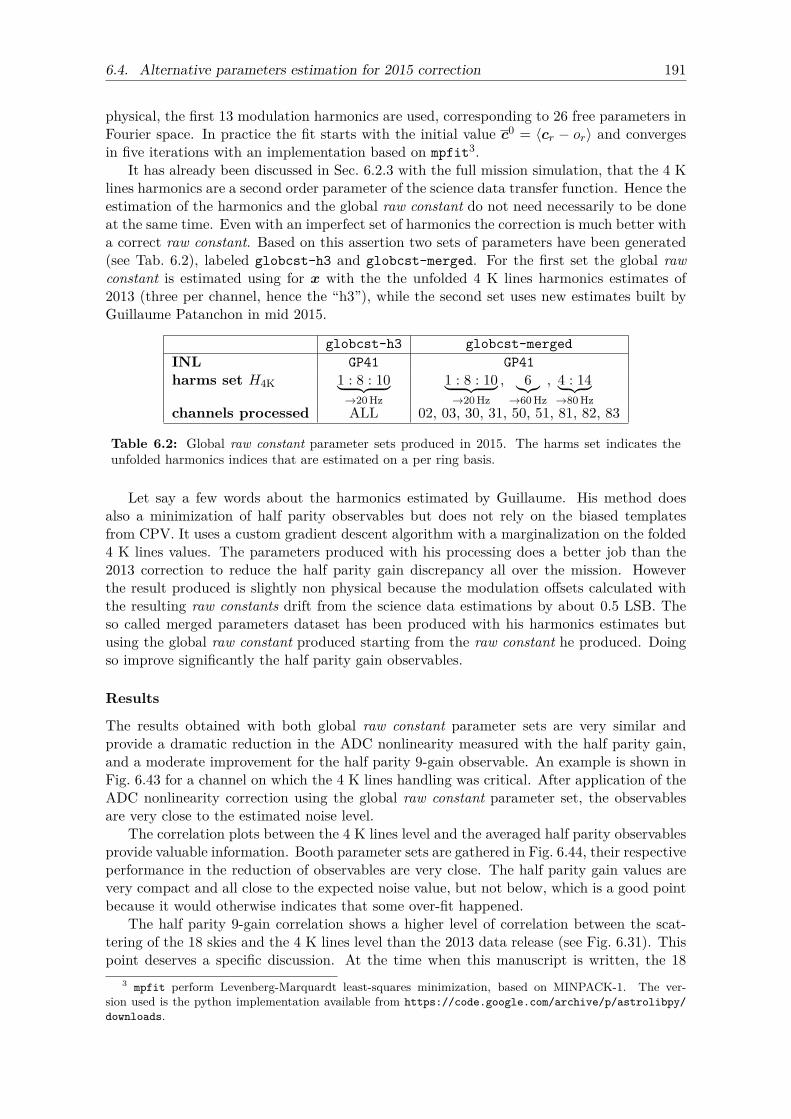
6.4. Alternative parameters estimation for 2015 correction 191
physical, the first 13 modulation harmonics are used, corresponding to 26 free parameters inFourier space. In practice the fit starts with the initial value c0 = 〈cr − or〉 and convergesin five iterations with an implementation based on mpfit3.
It has already been discussed in Sec. 6.2.3 with the full mission simulation, that the 4 Klines harmonics are a second order parameter of the science data transfer function. Hence theestimation of the harmonics and the global raw constant do not need necessarily to be doneat the same time. Even with an imperfect set of harmonics the correction is much better witha correct raw constant. Based on this assertion two sets of parameters have been generated(see Tab. 6.2), labeled globcst-h3 and globcst-merged. For the first set the global rawconstant is estimated using for x with the the unfolded 4 K lines harmonics estimates of2013 (three per channel, hence the “h3”), while the second set uses new estimates built byGuillaume Patanchon in mid 2015.
globcst-h3 globcst-mergedINL GP41 GP41harms set H4K 1 : 8 : 10︸ ︷︷ ︸
→20 Hz
1 : 8 : 10︸ ︷︷ ︸→20 Hz
, 6︸︷︷︸→60 Hz
, 4 : 14︸ ︷︷ ︸→80 Hz
channels processed ALL 02, 03, 30, 31, 50, 51, 81, 82, 83
Table 6.2: Global raw constant parameter sets produced in 2015. The harms set indicates theunfolded harmonics indices that are estimated on a per ring basis.
Let say a few words about the harmonics estimated by Guillaume. His method doesalso a minimization of half parity observables but does not rely on the biased templatesfrom CPV. It uses a custom gradient descent algorithm with a marginalization on the folded4 K lines values. The parameters produced with his processing does a better job than the2013 correction to reduce the half parity gain discrepancy all over the mission. Howeverthe result produced is slightly non physical because the modulation offsets calculated withthe resulting raw constants drift from the science data estimations by about 0.5 LSB. Theso called merged parameters dataset has been produced with his harmonics estimates butusing the global raw constant produced starting from the raw constant he produced. Doingso improve significantly the half parity gain observables.
Results
The results obtained with both global raw constant parameter sets are very similar andprovide a dramatic reduction in the ADC nonlinearity measured with the half parity gain,and a moderate improvement for the half parity 9-gain observable. An example is shown inFig. 6.43 for a channel on which the 4 K lines handling was critical. After application of theADC nonlinearity correction using the global raw constant parameter set, the observablesare very close to the estimated noise level.
The correlation plots between the 4 K lines level and the averaged half parity observablesprovide valuable information. Booth parameter sets are gathered in Fig. 6.44, their respectiveperformance in the reduction of observables are very close. The half parity gain values arevery compact and all close to the expected noise value, but not below, which is a good pointbecause it would otherwise indicates that some over-fit happened.
The half parity 9-gain correlation shows a higher level of correlation between the scat-tering of the 18 skies and the 4 K lines level than the 2013 data release (see Fig. 6.31). Thispoint deserves a specific discussion. At the time when this manuscript is written, the 18
3 mpfit perform Levenberg-Marquardt least-squares minimization, based on MINPACK-1. The ver-sion used is the python implementation available from https://code.google.com/archive/p/astrolibpy/downloads.
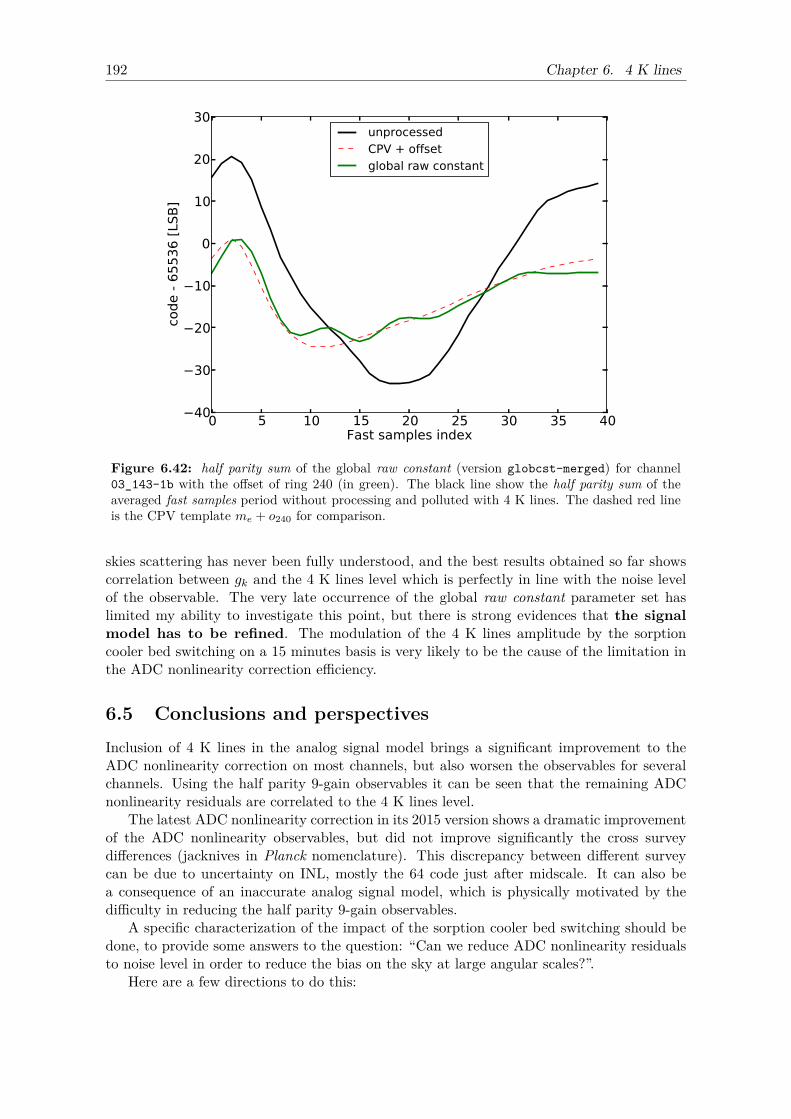
192 Chapter 6. 4 K lines
0 5 10 15 20 25 30 35 40Fast samples index
40
30
20
10
0
10
20
30
code -
65536 [
LSB
]
unprocessedCPV + offsetglobal raw constant
Figure 6.42: half parity sum of the global raw constant (version globcst-merged) for channel03_143-1b with the offset of ring 240 (in green). The black line show the half parity sum of theaveraged fast samples period without processing and polluted with 4 K lines. The dashed red lineis the CPV template me + o240 for comparison.
skies scattering has never been fully understood, and the best results obtained so far showscorrelation between gk and the 4 K lines level which is perfectly in line with the noise levelof the observable. The very late occurrence of the global raw constant parameter set haslimited my ability to investigate this point, but there is strong evidences that the signalmodel has to be refined. The modulation of the 4 K lines amplitude by the sorptioncooler bed switching on a 15 minutes basis is very likely to be the cause of the limitation inthe ADC nonlinearity correction efficiency.
6.5 Conclusions and perspectivesInclusion of 4 K lines in the analog signal model brings a significant improvement to theADC nonlinearity correction on most channels, but also worsen the observables for severalchannels. Using the half parity 9-gain observables it can be seen that the remaining ADCnonlinearity residuals are correlated to the 4 K lines level.
The latest ADC nonlinearity correction in its 2015 version shows a dramatic improvementof the ADC nonlinearity observables, but did not improve significantly the cross surveydifferences (jacknives in Planck nomenclature). This discrepancy between different surveycan be due to uncertainty on INL, mostly the 64 code just after midscale. It can also bea consequence of an inaccurate analog signal model, which is physically motivated by thedifficulty in reducing the half parity 9-gain observables.
A specific characterization of the impact of the sorption cooler bed switching should bedone, to provide some answers to the question: “Can we reduce ADC nonlinearity residualsto noise level in order to reduce the bias on the sky at large angular scales?”.
Here are a few directions to do this:
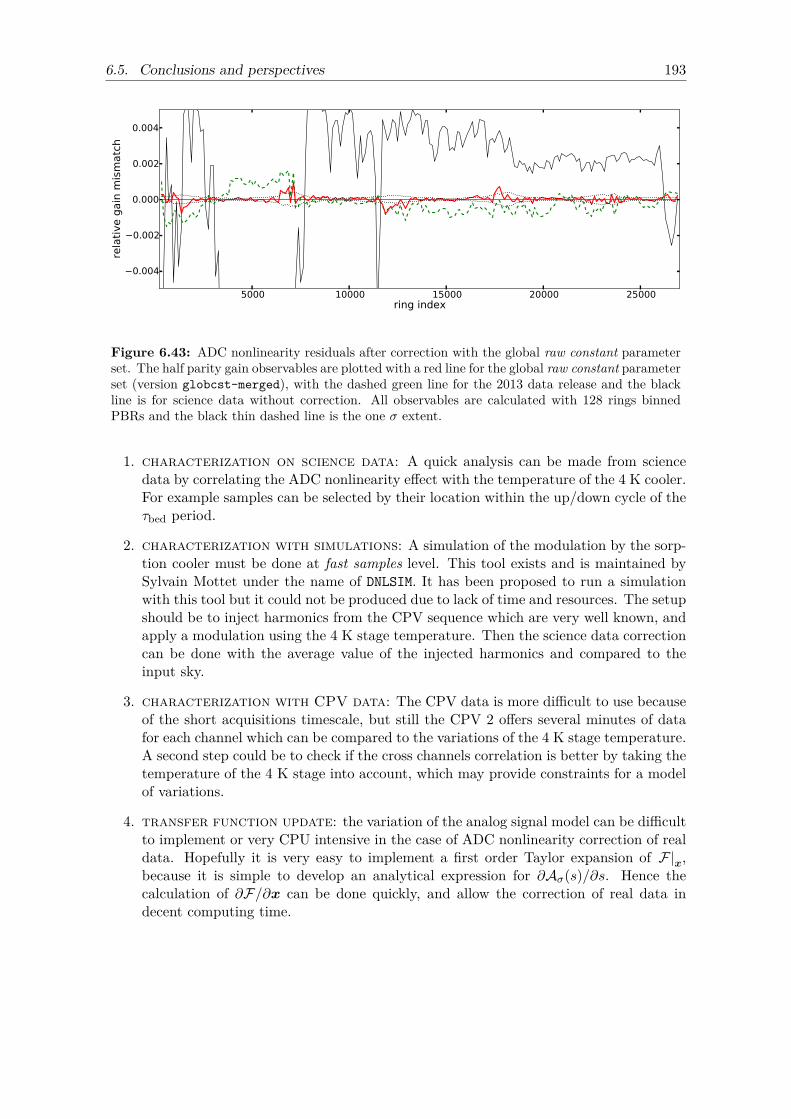
6.5. Conclusions and perspectives 193
5000 10000 15000 20000 25000ring index
0.004
0.002
0.000
0.002
0.004re
lati
ve g
ain
mis
matc
h
Figure 6.43: ADC nonlinearity residuals after correction with the global raw constant parameterset. The half parity gain observables are plotted with a red line for the global raw constant parameterset (version globcst-merged), with the dashed green line for the 2013 data release and the blackline is for science data without correction. All observables are calculated with 128 rings binnedPBRs and the black thin dashed line is the one σ extent.
1. characterization on science data: A quick analysis can be made from sciencedata by correlating the ADC nonlinearity effect with the temperature of the 4 K cooler.For example samples can be selected by their location within the up/down cycle of theτbed period.
2. characterization with simulations: A simulation of the modulation by the sorp-tion cooler must be done at fast samples level. This tool exists and is maintained bySylvain Mottet under the name of DNLSIM. It has been proposed to run a simulationwith this tool but it could not be produced due to lack of time and resources. The setupshould be to inject harmonics from the CPV sequence which are very well known, andapply a modulation using the 4 K stage temperature. Then the science data correctioncan be done with the average value of the injected harmonics and compared to theinput sky.
3. characterization with CPV data: The CPV data is more difficult to use becauseof the short acquisitions timescale, but still the CPV 2 offers several minutes of datafor each channel which can be compared to the variations of the 4 K stage temperature.A second step could be to check if the cross channels correlation is better by taking thetemperature of the 4 K stage into account, which may provide constraints for a modelof variations.
4. transfer function update: the variation of the analog signal model can be difficultto implement or very CPU intensive in the case of ADC nonlinearity correction of realdata. Hopefully it is very easy to implement a first order Taylor expansion of F|x,because it is simple to develop an analytical expression for ∂Aσ(s)/∂s. Hence thecalculation of ∂F/∂x can be done quickly, and allow the correction of real data indecent computing time.
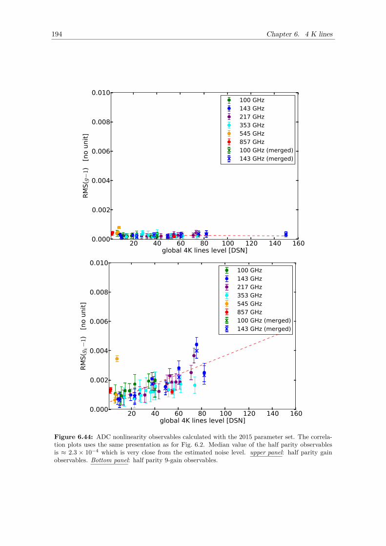
194 Chapter 6. 4 K lines
20 40 60 80 100 120 140 160global 4K lines level [DSN]
0.000
0.002
0.004
0.006
0.008
0.010R
MS(g−
1)
[no u
nit
]
100 GHz143 GHz217 GHz353 GHz545 GHz857 GHz100 GHz (merged)143 GHz (merged)
20 40 60 80 100 120 140 160global 4K lines level [DSN]
0.000
0.002
0.004
0.006
0.008
0.010
RM
S(gk−
1)
[no u
nit
]
100 GHz143 GHz217 GHz353 GHz545 GHz857 GHz100 GHz (merged)143 GHz (merged)
Figure 6.44: ADC nonlinearity observables calculated with the 2015 parameter set. The correla-tion plots uses the same presentation as for Fig. 6.2. Median value of the half parity observablesis ≈ 2.3 × 10⁻⁴ which is very close from the estimated noise level. upper panel: half parity gainobservables. Bottom panel: half parity 9-gain observables.

195
Part III
Propagation of systematics onscience

197
Chapter 7
Propagation of ADC nonlinearityto science
This chapter describes how the ADC nonlinearity systematic affects the scientific analysisof HFI data. It focuses mainly the thermal dust polarized emission and the CMB powerspectrum. As stated before, an important issue is the absence of calibration sources thatcan be used to assess this effect on HFI science data at the required precision level, whichis about 10−4 of the solar dipole amplitude. Nevertheless it is possible to infer reliableestimations of the effect with simulations using the model developed in Chap. 5. This modelwas implemented in the end-to-end simulations (see Sec. 5.4 in ?), but different approachesare discussed below. To complement these simulations with observables from real data, themethodology based on the half parity observables described in Sec. 5.5.3. will be extendedto full sky maps produced with a single parity of the modulation.
In Sec. 7.1 a simulation is used to study the impact of ADC nonlinearity on Galacticpolarization at 353 GHz. Next, in Sec. 7.2 the half parity based methodology is used to inferhow ADC nonlinearity residuals affect the CMB angular power spectra.
Some parts of the work presented below have been included in several sections of (?).
7.1 ADC impact on Galactic polarizationThe simulation described below has been performed to infer quantitative estimation of theimpact of the ADC on polarization angle at 353 GHz. This was for the paper on polarizedthermal emission from Galactic dust (Planck Collaboration Int. XIX 2015).
7.1.1 Simulation
(I,Q, U) maps of polarization Stokes parameters were produced without ADC nonlinear-ity correction by the DPC. The principle of the simulation was to produce maps of ADCnonlinearity residuals (∆Iadc,∆Qadc,∆Uadc) that could be used to infer ADC effect onpolarization fraction and polarization angle.
The functional diagram of the simulation is shown in Fig. 7.1. As the ADC nonlinearityeffect change with time, the simulation must be performed at the relevant TOI level. Forthis purpose the Desire1 simulation software was used to produce the reference TOIrefscience data TOIs of the simulation. The Planck sky model used for the Full Focal Planeversion 6 simulations (FFP6) was used as the input of Desire. The ADC nonlinearity effectwas applied using the function F in Eq. 5.12 to produce TOIadc. As stated in Sec. 1.4,a minimum of three detectors with different orientations are needed to produce the Stokesparameters, therefore the four detectors of the HFI 353 GHz detector set 1 (referred to asDetset-1= 23_353-3a, 24_353-3b, 53_353-5a, 54_353-5b ) were used. Next, the two
1 Desire is a tool developed at IRAP and written in C++ dedicated to the simulation of HFI TOIs andhousekeepings over the full mission
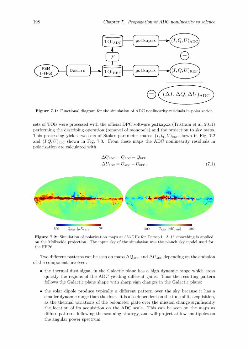
198 Chapter 7. Propagation of ADC nonlinearity to science
PSM(FFP6)
Figure 7.1: Functional diagram for the simulation of ADC nonlinearity residuals in polarization
sets of TOIs were processed with the official DPC software polkapix (Tristram et al. 2011)performing the destriping operation (removal of monopole) and the projection to sky maps.This processing yields two sets of Stokes parameter maps: (I,Q, U)ref shown in Fig. 7.2and (I,Q,U)adc shown in Fig. 7.3. From these maps the ADC nonlinearity residuals inpolarization are calculated with
∆Qadc = Qadc −Qref
∆Uadc = Uadc − Uref . (7.1)
Figure 7.2: Simulation of polarization maps at 353 GHz for Detset-1. A 1 smoothing is appliedon the Mollweide projection. The input sky of the simulation was the planck sky model used forthe FFP6.
Two different patterns can be seen on maps ∆Qadc and ∆Uadc depending on the emissionof the component involved:
• the thermal dust signal in the Galactic plane has a high dynamic range which crossquickly the regions of the ADC yielding different gains. Thus the resulting patternfollows the Galactic plane shape with sharp sign changes in the Galactic plane;
• the solar dipole produce typically a different pattern over the sky because it has asmaller dynamic range than the dust. It is also dependent on the time of its acquisition,as the thermal variations of the bolometer plate over the mission change significantlythe location of its acquisition on the ADC scale. This can be seen on the maps asdiffuse patterns following the scanning strategy, and will project at low multipoles onthe angular power spectrum.
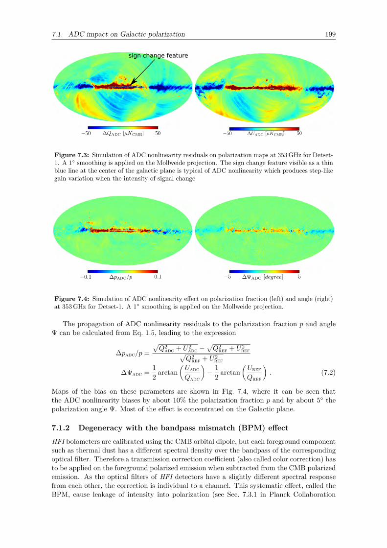
7.1. ADC impact on Galactic polarization 199
sign change feature
Figure 7.3: Simulation of ADC nonlinearity residuals on polarization maps at 353 GHz for Detset-1. A 1 smoothing is applied on the Mollweide projection. The sign change feature visible as a thinblue line at the center of the galactic plane is typical of ADC nonlinearity which produces step-likegain variation when the intensity of signal change
Figure 7.4: Simulation of ADC nonlinearity effect on polarization fraction (left) and angle (right)at 353 GHz for Detset-1. A 1 smoothing is applied on the Mollweide projection.
The propagation of ADC nonlinearity residuals to the polarization fraction p and angleΨ can be calculated from Eq. 1.5, leading to the expression
∆padc/p =√Q2
adc + U2adc −
√Q2
ref + U2ref√
Q2ref + U2
ref
∆Ψadc = 12 arctan
(UadcQadc
)− 1
2 arctan(UrefQref
). (7.2)
Maps of the bias on these parameters are shown in Fig. 7.4, where it can be seen thatthe ADC nonlinearity biases by about 10% the polarization fraction p and by about 5 thepolarization angle Ψ. Most of the effect is concentrated on the Galactic plane.
7.1.2 Degeneracy with the bandpass mismatch (BPM) effect
HFI bolometers are calibrated using the CMB orbital dipole, but each foreground componentsuch as thermal dust has a different spectral density over the bandpass of the correspondingoptical filter. Therefore a transmission correction coefficient (also called color correction) hasto be applied on the foreground polarized emission when subtracted from the CMB polarizedemission. As the optical filters of HFI detectors have a slightly different spectral responsefrom each other, the correction is individual to a channel. This systematic effect, called theBPM, cause leakage of intensity into polarization (see Sec. 7.3.1 in Planck Collaboration
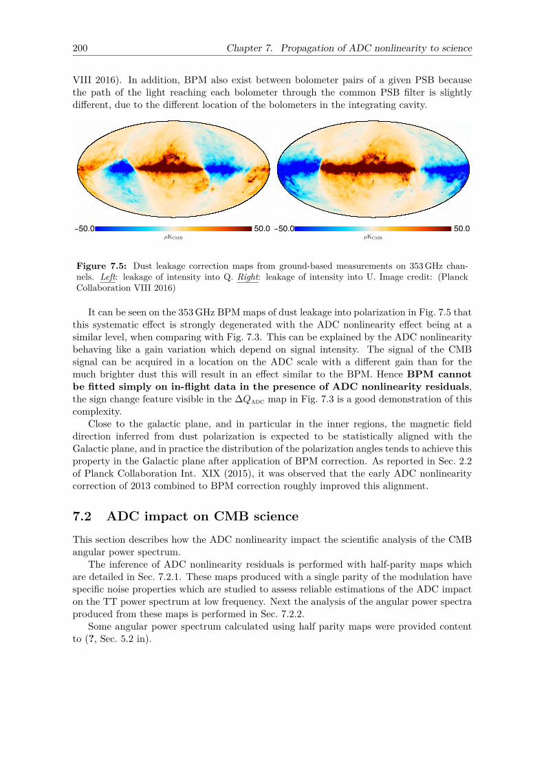
200 Chapter 7. Propagation of ADC nonlinearity to science
VIII 2016). In addition, BPM also exist between bolometer pairs of a given PSB becausethe path of the light reaching each bolometer through the common PSB filter is slightlydifferent, due to the different location of the bolometers in the integrating cavity.
Figure 7.5: Dust leakage correction maps from ground-based measurements on 353 GHz chan-nels. Left: leakage of intensity into Q. Right: leakage of intensity into U. Image credit: (PlanckCollaboration VIII 2016)
It can be seen on the 353 GHz BPM maps of dust leakage into polarization in Fig. 7.5 thatthis systematic effect is strongly degenerated with the ADC nonlinearity effect being at asimilar level, when comparing with Fig. 7.3. This can be explained by the ADC nonlinearitybehaving like a gain variation which depend on signal intensity. The signal of the CMBsignal can be acquired in a location on the ADC scale with a different gain than for themuch brighter dust this will result in an effect similar to the BPM. Hence BPM cannotbe fitted simply on in-flight data in the presence of ADC nonlinearity residuals,the sign change feature visible in the ∆Qadc map in Fig. 7.3 is a good demonstration of thiscomplexity.
Close to the galactic plane, and in particular in the inner regions, the magnetic fielddirection inferred from dust polarization is expected to be statistically aligned with theGalactic plane, and in practice the distribution of the polarization angles tends to achieve thisproperty in the Galactic plane after application of BPM correction. As reported in Sec. 2.2of Planck Collaboration Int. XIX (2015), it was observed that the early ADC nonlinearitycorrection of 2013 combined to BPM correction roughly improved this alignment.
7.2 ADC impact on CMB scienceThis section describes how the ADC nonlinearity impact the scientific analysis of the CMBangular power spectrum.
The inference of ADC nonlinearity residuals is performed with half-parity maps whichare detailed in Sec. 7.2.1. These maps produced with a single parity of the modulation havespecific noise properties which are studied to assess reliable estimations of the ADC impacton the TT power spectrum at low frequency. Next the analysis of the angular power spectraproduced from these maps is performed in Sec. 7.2.2.
Some angular power spectrum calculated using half parity maps were provided contentto (?, Sec. 5.2 in).
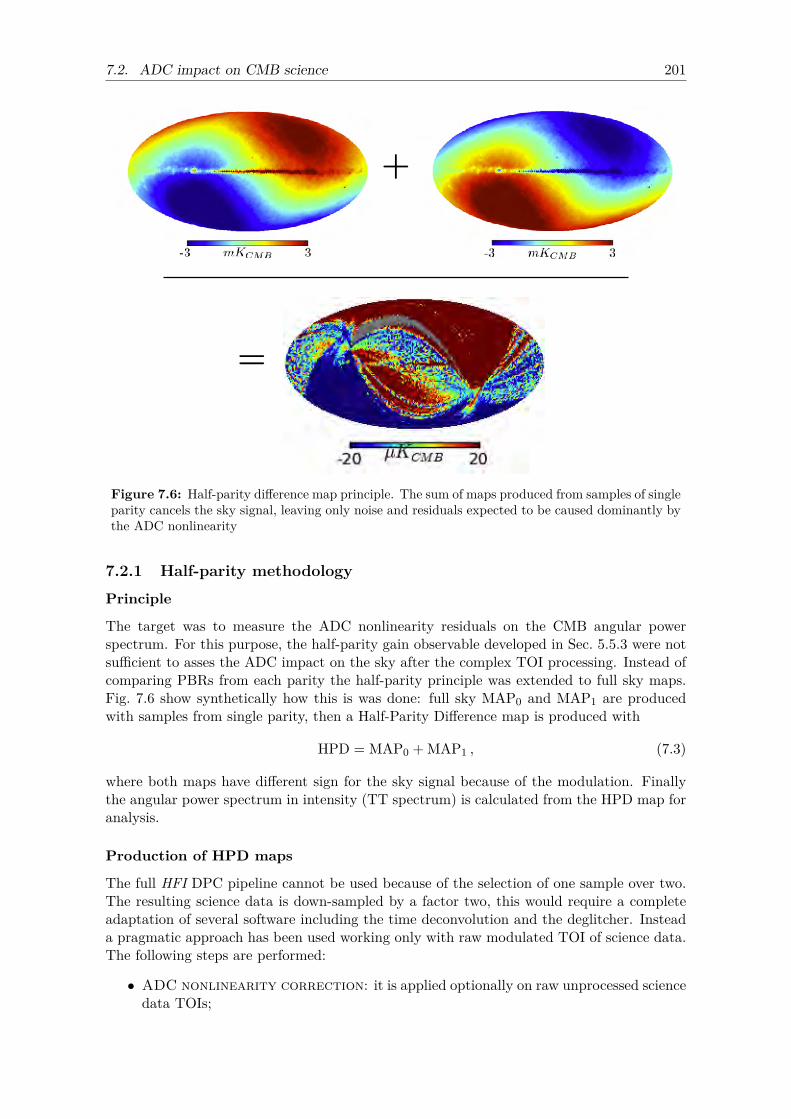
7.2. ADC impact on CMB science 201
+
=
Figure 7.6: Half-parity difference map principle. The sum of maps produced from samples of singleparity cancels the sky signal, leaving only noise and residuals expected to be caused dominantly bythe ADC nonlinearity
7.2.1 Half-parity methodology
Principle
The target was to measure the ADC nonlinearity residuals on the CMB angular powerspectrum. For this purpose, the half-parity gain observable developed in Sec. 5.5.3 were notsufficient to asses the ADC impact on the sky after the complex TOI processing. Instead ofcomparing PBRs from each parity the half-parity principle was extended to full sky maps.Fig. 7.6 show synthetically how this is was done: full sky MAP0 and MAP1 are producedwith samples from single parity, then a Half-Parity Difference map is produced with
HPD = MAP0 + MAP1 , (7.3)
where both maps have different sign for the sky signal because of the modulation. Finallythe angular power spectrum in intensity (TT spectrum) is calculated from the HPD map foranalysis.
Production of HPD maps
The full HFI DPC pipeline cannot be used because of the selection of one sample over two.The resulting science data is down-sampled by a factor two, this would require a completeadaptation of several software including the time deconvolution and the deglitcher. Insteada pragmatic approach has been used working only with raw modulated TOI of science data.The following steps are performed:
• ADC nonlinearity correction: it is applied optionally on raw unprocessed sciencedata TOIs;
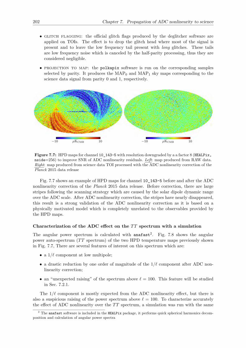
202 Chapter 7. Propagation of ADC nonlinearity to science
• glitch flagging: the official glitch flags produced by the deglitcher software areapplied on TOIs. The effect is to drop the glitch head where most of the signal ispresent and to leave the low frequency tail present with long glitches. These tailsare low frequency noise which is canceled by the half-parity processing, thus they areconsidered negligible.
• projection to map: the polkapix software is run on the corresponding samplesselected by parity. It produces the MAP0 and MAP1 sky maps corresponding to thescience data signal from parity 0 and 1, respectively.
Figure 7.7: HPDmaps for channel 10_143-5 with resolution downgraded by a a factor 8 (HEALPix,nside=256) to improve SNR of ADC nonlinearity residuals. Left: map produced from RAW data.Right: map produced from science data TOI processed with the ADC nonlinearity correction of thePlanck 2015 data release
Fig. 7.7 shows an example of HPD maps for channel 10_143-5 before and after the ADCnonlinearity correction of the Planck 2015 data release. Before correction, there are largestripes following the scanning strategy which are caused by the solar dipole dynamic rangeover the ADC scale. After ADC nonlinearity correction, the stripes have nearly disappeared,this result is a strong validation of the ADC nonlinearity correction as it is based on aphysically motivated model which is completely unrelated to the observables provided bythe HPD maps.
Characterization of the ADC effect on the TT spectrum with a simulation
The angular power spectrum is calculated with anafast2. Fig. 7.8 shows the angularpower auto-spectrum (TT spectrum) of the two HPD temperature maps previously shownin Fig. 7.7, There are several features of interest on this spectrum which are:
• a 1/` component at low multipole;
• a drastic reduction by one order of magnitude of the 1/` component after ADC non-linearity correction;
• an “unexpected raising” of the spectrum above ` = 100. This feature will be studiedin Sec. 7.2.1.
The 1/` component is mostly expected from the ADC nonlinearity effect, but there isalso a suspicious raising of the power spectrum above ` = 100. To characterize accuratelythe effect of ADC nonlinearity over the TT spectrum, a simulation was run with the same
2 The anafast software is included in the HEALPix package, it performs quick spherical harmonics decom-position and calculation of angular power spectra
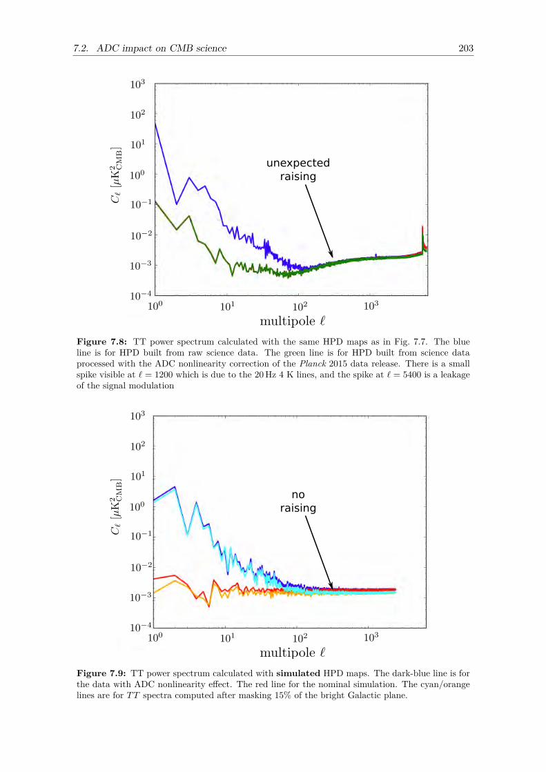
7.2. ADC impact on CMB science 203
unexpectedraising
Figure 7.8: TT power spectrum calculated with the same HPD maps as in Fig. 7.7. The blueline is for HPD built from raw science data. The green line is for HPD built from science dataprocessed with the ADC nonlinearity correction of the Planck 2015 data release. There is a smallspike visible at ` = 1200 which is due to the 20 Hz 4 K lines, and the spike at ` = 5400 is a leakageof the signal modulation
noraising
Figure 7.9: TT power spectrum calculated with simulated HPD maps. The dark-blue line is forthe data with ADC nonlinearity effect. The red line for the nominal simulation. The cyan/orangelines are for TT spectra computed after masking 15% of the bright Galactic plane.
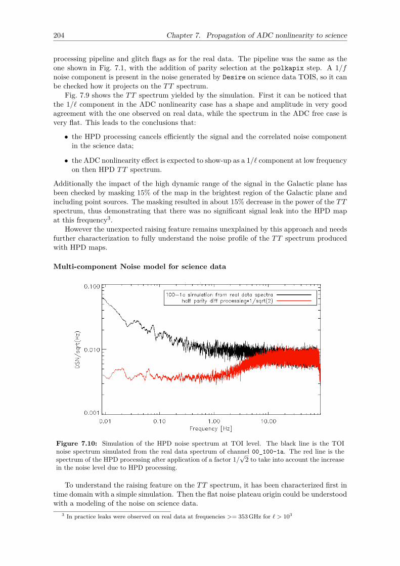
204 Chapter 7. Propagation of ADC nonlinearity to science
processing pipeline and glitch flags as for the real data. The pipeline was the same as theone shown in Fig. 7.1, with the addition of parity selection at the polkapix step. A 1/fnoise component is present in the noise generated by Desire on science data TOIS, so it canbe checked how it projects on the TT spectrum.
Fig. 7.9 shows the TT spectrum yielded by the simulation. First it can be noticed thatthe 1/` component in the ADC nonlinearity case has a shape and amplitude in very goodagreement with the one observed on real data, while the spectrum in the ADC free case isvery flat. This leads to the conclusions that:
• the HPD processing cancels efficiently the signal and the correlated noise componentin the science data;
• the ADC nonlinearity effect is expected to show-up as a 1/` component at low frequencyon then HPD TT spectrum.
Additionally the impact of the high dynamic range of the signal in the Galactic plane hasbeen checked by masking 15% of the map in the brightest region of the Galactic plane andincluding point sources. The masking resulted in about 15% decrease in the power of the TTspectrum, thus demonstrating that there was no significant signal leak into the HPD mapat this frequency3.
However the unexpected raising feature remains unexplained by this approach and needsfurther characterization to fully understand the noise profile of the TT spectrum producedwith HPD maps.
Multi-component Noise model for science data
Figure 7.10: Simulation of the HPD noise spectrum at TOI level. The black line is the TOInoise spectrum simulated from the real data spectrum of channel 00_100-1a. The red line is thespectrum of the HPD processing after application of a factor 1/
√2 to take into account the increase
in the noise level due to HPD processing.
To understand the raising feature on the TT spectrum, it has been characterized first intime domain with a simple simulation. Then the flat noise plateau origin could be understoodwith a modeling of the noise on science data.
3 In practice leaks were observed on real data at frequencies >= 353 GHz for ` > 103
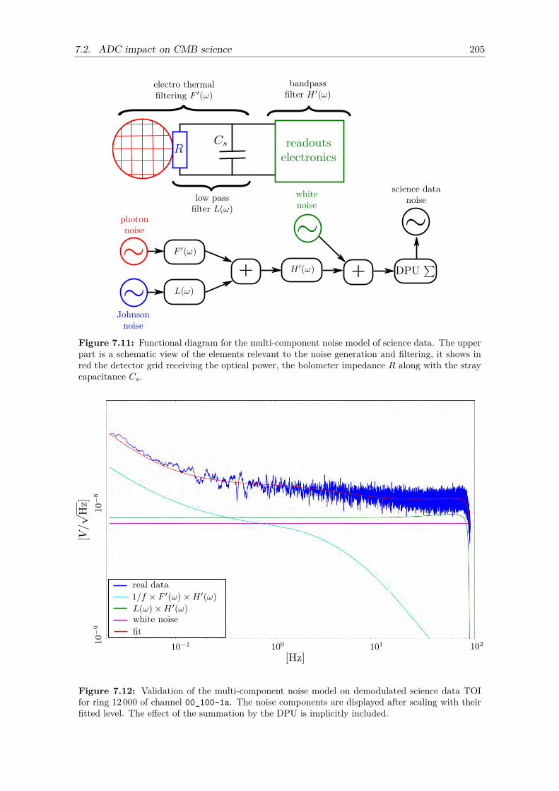
7.2. ADC impact on CMB science 205
Figure 7.11: Functional diagram for the multi-component noise model of science data. The upperpart is a schematic view of the elements relevant to the noise generation and filtering, it shows inred the detector grid receiving the optical power, the bolometer impedance R along with the straycapacitance Cs.
Figure 7.12: Validation of the multi-component noise model on demodulated science data TOIfor ring 12 000 of channel 00_100-1a. The noise components are displayed after scaling with theirfitted level. The effect of the summation by the DPU is implicitly included.
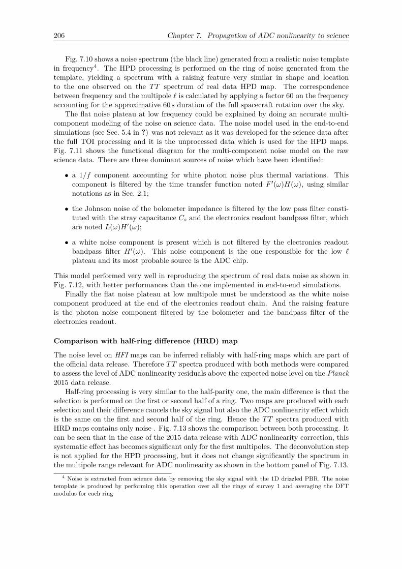
206 Chapter 7. Propagation of ADC nonlinearity to science
Fig. 7.10 shows a noise spectrum (the black line) generated from a realistic noise templatein frequency4. The HPD processing is performed on the ring of noise generated from thetemplate, yielding a spectrum with a raising feature very similar in shape and locationto the one observed on the TT spectrum of real data HPD map. The correspondencebetween frequency and the multipole ` is calculated by applying a factor 60 on the frequencyaccounting for the approximative 60 s duration of the full spacecraft rotation over the sky.
The flat noise plateau at low frequency could be explained by doing an accurate multi-component modeling of the noise on science data. The noise model used in the end-to-endsimulations (see Sec. 5.4 in ?) was not relevant as it was developed for the science data afterthe full TOI processing and it is the unprocessed data which is used for the HPD maps.Fig. 7.11 shows the functional diagram for the multi-component noise model on the rawscience data. There are three dominant sources of noise which have been identified:
• a 1/f component accounting for white photon noise plus thermal variations. Thiscomponent is filtered by the time transfer function noted F ′(ω)H(ω), using similarnotations as in Sec. 2.1;
• the Johnson noise of the bolometer impedance is filtered by the low pass filter consti-tuted with the stray capacitance Cs and the electronics readout bandpass filter, whichare noted L(ω)H ′(ω);
• a white noise component is present which is not filtered by the electronics readoutbandpass filter H ′(ω). This noise component is the one responsible for the low `plateau and its most probable source is the ADC chip.
This model performed very well in reproducing the spectrum of real data noise as shown inFig. 7.12, with better performances than the one implemented in end-to-end simulations.
Finally the flat noise plateau at low multipole must be understood as the white noisecomponent produced at the end of the electronics readout chain. And the raising featureis the photon noise component filtered by the bolometer and the bandpass filter of theelectronics readout.
Comparison with half-ring difference (HRD) map
The noise level on HFI maps can be inferred reliably with half-ring maps which are part ofthe official data release. Therefore TT spectra produced with both methods were comparedto assess the level of ADC nonlinearity residuals above the expected noise level on the Planck2015 data release.
Half-ring processing is very similar to the half-parity one, the main difference is that theselection is performed on the first or second half of a ring. Two maps are produced with eachselection and their difference cancels the sky signal but also the ADC nonlinearity effect whichis the same on the first and second half of the ring. Hence the TT spectra produced withHRD maps contains only noise . Fig. 7.13 shows the comparison between both processing. Itcan be seen that in the case of the 2015 data release with ADC nonlinearity correction, thissystematic effect has becomes significant only for the first multipoles. The deconvolution stepis not applied for the HPD processing, but it does not change significantly the spectrum inthe multipole range relevant for ADC nonlinearity as shown in the bottom panel of Fig. 7.13.
4 Noise is extracted from science data by removing the sky signal with the 1D drizzled PBR. The noisetemplate is produced by performing this operation over all the rings of survey 1 and averaging the DFTmodulus for each ring
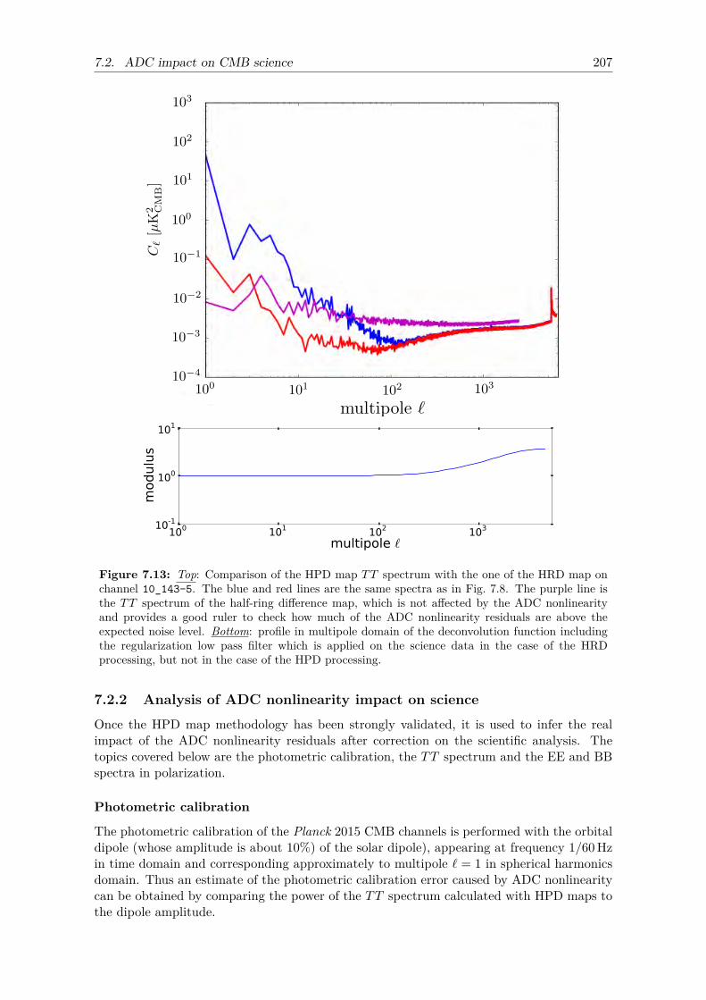
7.2. ADC impact on CMB science 207
100 101 102 103
multipole `
10-1
100
101
modulu
s
Figure 7.13: Top: Comparison of the HPD map TT spectrum with the one of the HRD map onchannel 10_143-5. The blue and red lines are the same spectra as in Fig. 7.8. The purple line isthe TT spectrum of the half-ring difference map, which is not affected by the ADC nonlinearityand provides a good ruler to check how much of the ADC nonlinearity residuals are above theexpected noise level. Bottom: profile in multipole domain of the deconvolution function includingthe regularization low pass filter which is applied on the science data in the case of the HRDprocessing, but not in the case of the HPD processing.
7.2.2 Analysis of ADC nonlinearity impact on science
Once the HPD map methodology has been strongly validated, it is used to infer the realimpact of the ADC nonlinearity residuals after correction on the scientific analysis. Thetopics covered below are the photometric calibration, the TT spectrum and the EE and BBspectra in polarization.
Photometric calibration
The photometric calibration of the Planck 2015 CMB channels is performed with the orbitaldipole (whose amplitude is about 10%) of the solar dipole), appearing at frequency 1/60 Hzin time domain and corresponding approximately to multipole ` = 1 in spherical harmonicsdomain. Thus an estimate of the photometric calibration error caused by ADC nonlinearitycan be obtained by comparing the power of the TT spectrum calculated with HPD maps tothe dipole amplitude.
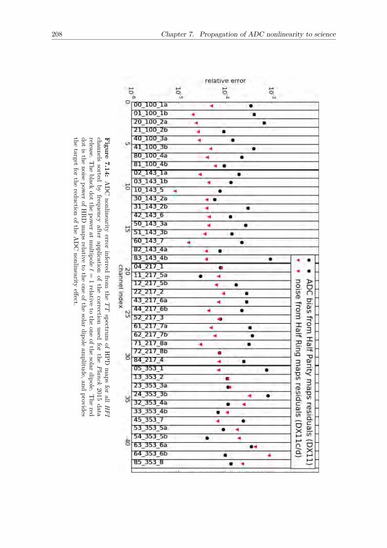
208 Chapter 7. Propagation of ADC nonlinearity to science
Figure
7.14:ADC
nonlinearityerror
inferredfrom
theTT
spectrumofH
PDmaps
forallH
FIchannels
sortedby
frequencyafter
applicationof
thecorrection
usedfor
thePlanck
2015data
release.The
blackdotthe
poweratmultipole
`=1relative
tothe
oneofthe
solardipole.The
reddotisthe
noisepowerofH
RD
mapsrelative
tothe
oneofthe
solardipoleam
plitude,andprovides
thetarget
forthe
reductionofthe
ADC
nonlinearityeffect.
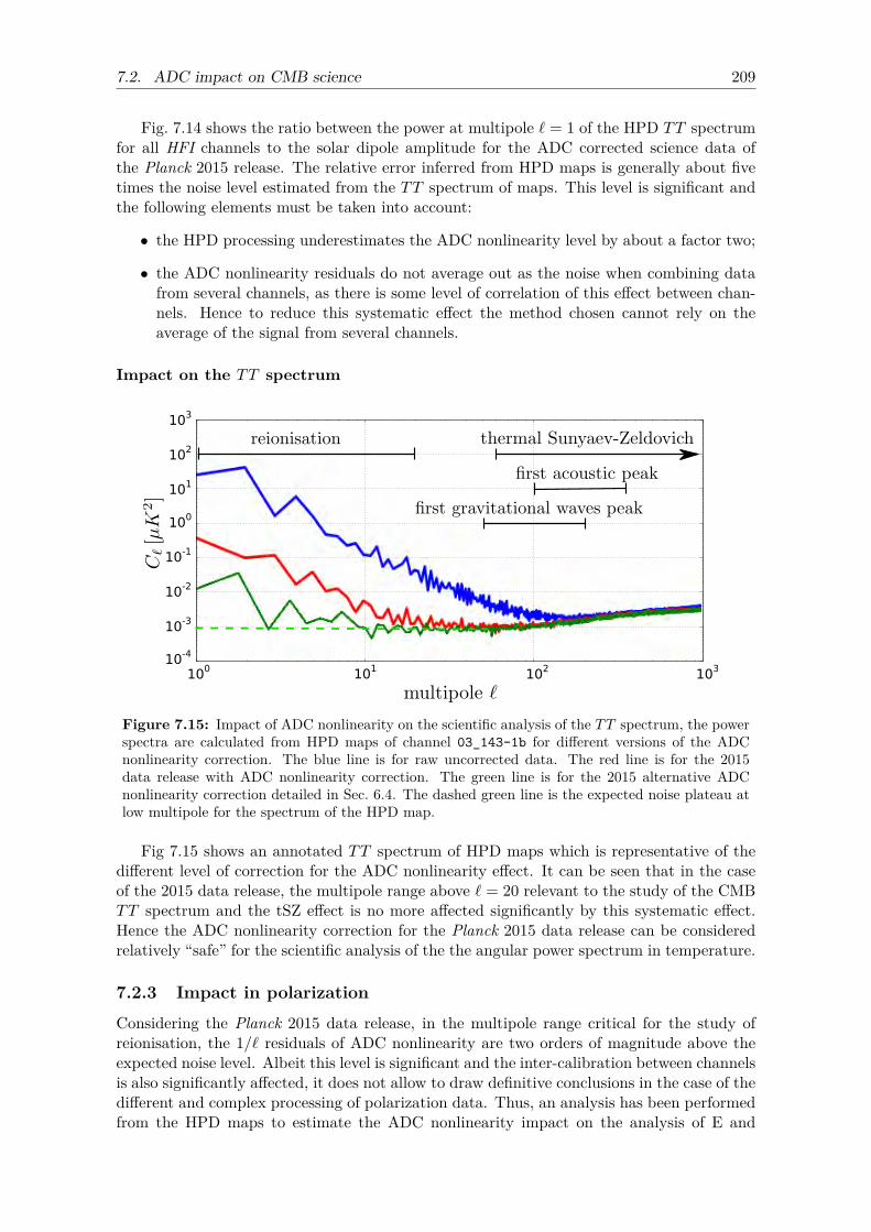
7.2. ADC impact on CMB science 209
Fig. 7.14 shows the ratio between the power at multipole ` = 1 of the HPD TT spectrumfor all HFI channels to the solar dipole amplitude for the ADC corrected science data ofthe Planck 2015 release. The relative error inferred from HPD maps is generally about fivetimes the noise level estimated from the TT spectrum of maps. This level is significant andthe following elements must be taken into account:
• the HPD processing underestimates the ADC nonlinearity level by about a factor two;
• the ADC nonlinearity residuals do not average out as the noise when combining datafrom several channels, as there is some level of correlation of this effect between chan-nels. Hence to reduce this systematic effect the method chosen cannot rely on theaverage of the signal from several channels.
Impact on the TT spectrum
100 101 102 103
3
10-4
10-3
10-2
10-1
100
101
102
10
Figure 7.15: Impact of ADC nonlinearity on the scientific analysis of the TT spectrum, the powerspectra are calculated from HPD maps of channel 03_143-1b for different versions of the ADCnonlinearity correction. The blue line is for raw uncorrected data. The red line is for the 2015data release with ADC nonlinearity correction. The green line is for the 2015 alternative ADCnonlinearity correction detailed in Sec. 6.4. The dashed green line is the expected noise plateau atlow multipole for the spectrum of the HPD map.
Fig 7.15 shows an annotated TT spectrum of HPD maps which is representative of thedifferent level of correction for the ADC nonlinearity effect. It can be seen that in the caseof the 2015 data release, the multipole range above ` = 20 relevant to the study of the CMBTT spectrum and the tSZ effect is no more affected significantly by this systematic effect.Hence the ADC nonlinearity correction for the Planck 2015 data release can be consideredrelatively “safe” for the scientific analysis of the the angular power spectrum in temperature.
7.2.3 Impact in polarization
Considering the Planck 2015 data release, in the multipole range critical for the study ofreionisation, the 1/` residuals of ADC nonlinearity are two orders of magnitude above theexpected noise level. Albeit this level is significant and the inter-calibration between channelsis also significantly affected, it does not allow to draw definitive conclusions in the case of thedifferent and complex processing of polarization data. Thus, an analysis has been performedfrom the HPD maps to estimate the ADC nonlinearity impact on the analysis of E and
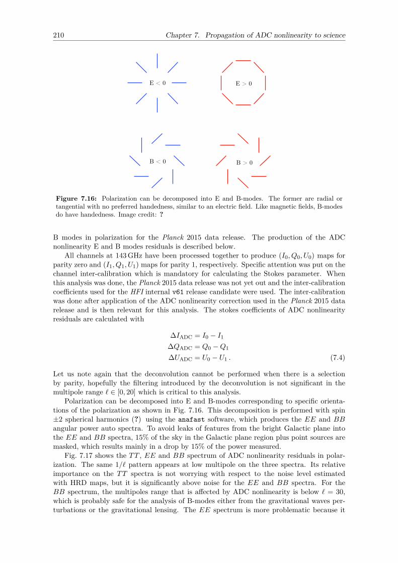
210 Chapter 7. Propagation of ADC nonlinearity to science
Figure 7.16: Polarization can be decomposed into E and B-modes. The former are radial ortangential with no preferred handedness, similar to an electric field. Like magnetic fields, B-modesdo have handedness. Image credit: ?
B modes in polarization for the Planck 2015 data release. The production of the ADCnonlinearity E and B modes residuals is described below.
All channels at 143 GHz have been processed together to produce (I0, Q0, U0) maps forparity zero and (I1, Q1, U1) maps for parity 1, respectively. Specific attention was put on thechannel inter-calibration which is mandatory for calculating the Stokes parameter. Whenthis analysis was done, the Planck 2015 data release was not yet out and the inter-calibrationcoefficients used for the HFI internal v61 release candidate were used. The inter-calibrationwas done after application of the ADC nonlinearity correction used in the Planck 2015 datarelease and is then relevant for this analysis. The stokes coefficients of ADC nonlinearityresiduals are calculated with
∆IADC = I0 − I1
∆QADC = Q0 −Q1
∆UADC = U0 − U1 . (7.4)
Let us note again that the deconvolution cannot be performed when there is a selectionby parity, hopefully the filtering introduced by the deconvolution is not significant in themultipole range ` ∈ [0, 20] which is critical to this analysis.
Polarization can be decomposed into E and B-modes corresponding to specific orienta-tions of the polarization as shown in Fig. 7.16. This decomposition is performed with spin±2 spherical harmonics (?) using the anafast software, which produces the EE and BBangular power auto spectra. To avoid leaks of features from the bright Galactic plane intothe EE and BB spectra, 15% of the sky in the Galactic plane region plus point sources aremasked, which results mainly in a drop by 15% of the power measured.
Fig. 7.17 shows the TT , EE and BB spectrum of ADC nonlinearity residuals in polar-ization. The same 1/` pattern appears at low multipole on the three spectra. Its relativeimportance on the TT spectra is not worrying with respect to the noise level estimatedwith HRD maps, but it is significantly above noise for the EE and BB spectra. For theBB spectrum, the multipoles range that is affected by ADC nonlinearity is below ` = 30,which is probably safe for the analysis of B-modes either from the gravitational waves per-turbations or the gravitational lensing. The EE spectrum is more problematic because it
7.3. Conclusions 211
is the ` ∈ [2, 20] multipole range which is relevant to the analysis of the reionization andthis part of the spectrum is clearly biased by residuals of the ADC nonlinearity effect. Thisdemonstrates clearly that a better handling of the ADC nonlinearity effect is required. Thealternative ADC nonlinearity correction studied in 2015 is a good candidate, but it did notreduce as expected the differences between survey acquired one year apart, therefore it hasnot been used in the 2016 likelihood for constraining reionisation.
7.3 ConclusionsIt has been studied how ADC nonlinearity affects quantitatively the Galactic polarizationof the thermal dust at 353 GHz. This effect produces a bias at the level of about 10% ofthe polarization fraction p and about 5 on the polarization angle Ψ. As this is an estimatefor the effect before ADC nonlinearity correction, it is expected that the residual bias in thecase of the Planck 2015 data release is much less important. However it was observed thatthe ADC nonlinearity effect degenerate with the bandpass mismatch leakage effect, thus agreat attention should be taken when performing fit-like procedure of bandpass mismatch.
The impact of ADC nonlinearity on the scientific analysis based on the TT spectrumof the Planck 2015 data release was performed with the half-parity maps methodology forwhich the noise spectrum has been studied with care. It results from this analysis thatthe ADC nonlinearity leaves residuals with a 1/` shape in the low multipole ` ∈ [1, 20]range which can affect the photometric calibration at a level below 10−3 of the solar dipoleamplitude for the Planck 2015 data release. The same methodology has been applied to theEE and BB spectrum in polarization for the whole set of available 143 GHz channels withsimilar residuals. While the BB spectrum analysis is not significantly impacted by ADCnonlinearity, this effect is more problematic on the EE spectrum for the study of the epochof reionization with residuals that are more than one order of magnitude above the noise atthe lowest multipoles. While the ADC nonlinearity has been significantly reduced for thePlanck 2015 data release, it is still expected to affect the determination of the optical depthparameter τ of the reionization for this data release.
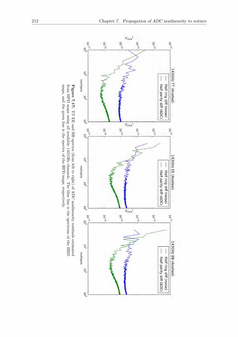
212 Chapter 7. Propagation of ADC nonlinearity to science
Figure
7.17:TT
EEand
BBspectra
(fromleftto
right)ofADC
nonlinearityresidualsestim
atedfrom
HPD
maps
usingallavailable
143GH
zchannels.
The
blueline
isthe
spectrumofthe
HRD
maps,and
thegreen
lineis
thespectra
oftheHPD
maps,respectively.
213
Chapter 8
Preliminary study for the detectionof primordial matter-antimatterannihilation with Planck data
In the modern view of the Universe, laboratory physics and astrophysical observations indi-cate that baryons are dominant over anti-baryons. Three main cases can be considered toexplain the baryon asymmetry. In the first one, “initial conditions” before the inflation leadsto the observed asymmetry. The second one, which is the favored hypothesis today, relies onan asymmetry in the physics of baryons and anti-baryons favoring slightly the former. Thelast one considers a zero baryon charge at large scales with local fluctuations throughout theUniverse, allowing some anti-matter domains to exist. In this chapter, it is the later thatis considered, i.e. if some antimatter (AM) domains survived at the epoch of recombina-tion, their annihilation at the interface with matter would have produced a characteristicsignature on the Planck map of thermal Sunyaev-Zeldovich effect (tSZ-map). Therefore theunprecedented precision of the y parameter at full sky coverage in this map can be used toconstrain further the AM domains hypothesis. It will be shown that the Planck scanningstrategy is a limiting factor to the detection of the annihilation signature, and the impact ofthe leakage of the scanning strategy in the tSZ-map will be studied.
In Sec. 8.1 is discussed how the Planck tSZ-map can be used to perform the detectionof the energy released by matter-AM annihilation at the epoch of recombination. Then inSec. 8.2 the leakage of the Planck scanning strategy in the tSZ-map is studied.
This analysis has been used for the quantitative estimation of scanning strategy system-atics on the tSZ-map published in Sec. 4.1 of Planck Collaboration XXII (2016).
8.1 Introduction
8.1.1 Context
Gamma-ray observations in the 100 MeV domain (e.g. Nolan et al. 2012; von Ballmoos 2014)have virtually excluded the existence of substantial amounts of close-by baryonic antimatter,constraining its fraction to a few times 105 to 109 in structures as large as galaxy clusters. Asa consequence, a universal matter-antimatter symmetric Universe seems to be incompatiblewith theory (e.g. Cohen et al. 1998) on the grounds of existing MeV data (Weidenspointnerand Varendorff 2001). The observed dominance of matter today is supposed to originatefrom a Charge Parity (CP) violation during the baryogenesis in the early Universe (e.g.Cohen and Kaplan 1987), leading to a slight excess in favor of baryons. Since this epoch,most of the anti-baryons have annihilated with baryons generating cascades of secondaryparticles and gamma photons. However in a CP invariant Universe, the baryon charge couldhave been distributed non-homogeneously throughout the Universe and some local domainsof matter and AM could exist. In the later case, if the AM domains (called Anti-Baryonic
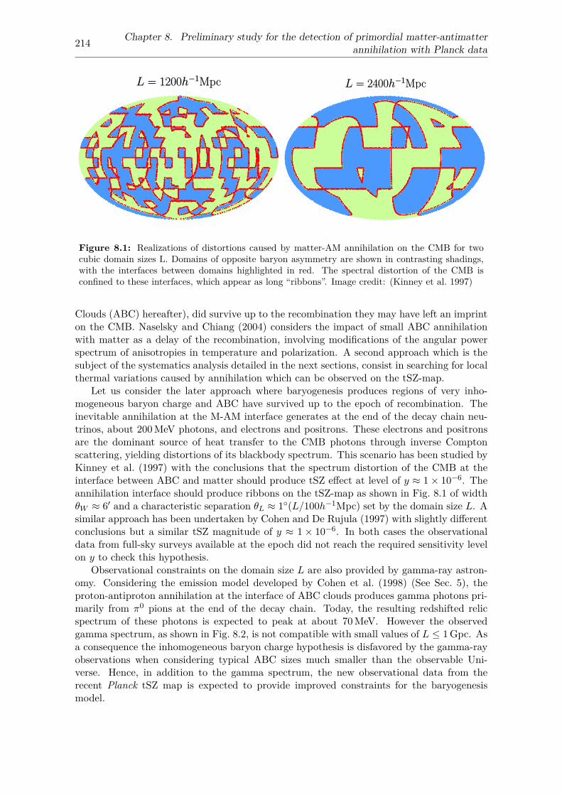
214 Chapter 8. Preliminary study for the detection of primordial matter-antimatterannihilation with Planck data
Figure 8.1: Realizations of distortions caused by matter-AM annihilation on the CMB for twocubic domain sizes L. Domains of opposite baryon asymmetry are shown in contrasting shadings,with the interfaces between domains highlighted in red. The spectral distortion of the CMB isconfined to these interfaces, which appear as long “ribbons”. Image credit: (Kinney et al. 1997)
Clouds (ABC) hereafter), did survive up to the recombination they may have left an imprinton the CMB. Naselsky and Chiang (2004) considers the impact of small ABC annihilationwith matter as a delay of the recombination, involving modifications of the angular powerspectrum of anisotropies in temperature and polarization. A second approach which is thesubject of the systematics analysis detailed in the next sections, consist in searching for localthermal variations caused by annihilation which can be observed on the tSZ-map.
Let us consider the later approach where baryogenesis produces regions of very inho-mogeneous baryon charge and ABC have survived up to the epoch of recombination. Theinevitable annihilation at the M-AM interface generates at the end of the decay chain neu-trinos, about 200 MeV photons, and electrons and positrons. These electrons and positronsare the dominant source of heat transfer to the CMB photons through inverse Comptonscattering, yielding distortions of its blackbody spectrum. This scenario has been studied byKinney et al. (1997) with the conclusions that the spectrum distortion of the CMB at theinterface between ABC and matter should produce tSZ effect at level of y ≈ 1× 10⁻⁶. Theannihilation interface should produce ribbons on the tSZ-map as shown in Fig. 8.1 of widthθW ≈ 6′ and a characteristic separation θL ≈ 1(L/100h−1Mpc) set by the domain size L. Asimilar approach has been undertaken by Cohen and De Rujula (1997) with slightly differentconclusions but a similar tSZ magnitude of y ≈ 1× 10⁻⁶. In both cases the observationaldata from full-sky surveys available at the epoch did not reach the required sensitivity levelon y to check this hypothesis.
Observational constraints on the domain size L are also provided by gamma-ray astron-omy. Considering the emission model developed by Cohen et al. (1998) (See Sec. 5), theproton-antiproton annihilation at the interface of ABC clouds produces gamma photons pri-marily from π0 pions at the end of the decay chain. Today, the resulting redshifted relicspectrum of these photons is expected to peak at about 70 MeV. However the observedgamma spectrum, as shown in Fig. 8.2, is not compatible with small values of L ≤ 1 Gpc. Asa consequence the inhomogeneous baryon charge hypothesis is disfavored by the gamma-rayobservations when considering typical ABC sizes much smaller than the observable Uni-verse. Hence, in addition to the gamma spectrum, the new observational data from therecent Planck tSZ map is expected to provide improved constraints for the baryogenesismodel.
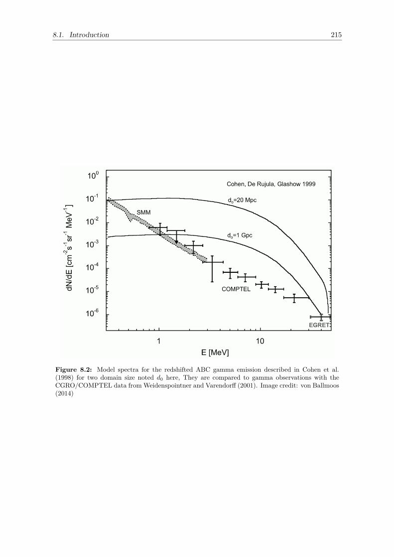
8.1. Introduction 215
Figure 8.2: Model spectra for the redshifted ABC gamma emission described in Cohen et al.(1998) for two domain size noted d0 here, They are compared to gamma observations with theCGRO/COMPTEL data from Weidenspointner and Varendorff (2001). Image credit: von Ballmoos(2014)
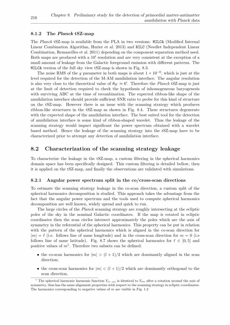
216 Chapter 8. Preliminary study for the detection of primordial matter-antimatterannihilation with Planck data
8.1.2 The Planck tSZ-map
The Planck tSZ-map is available from the PLA in two versions: MILCA (Modified InternalLinear Combination Algorithm, Hurier et al. 2013) and NILC (Needlet Independent LinearCombination, Remazeilles et al. 2011) depending on the component separation method used.Both maps are produced with a 10′ resolution and are very consistent at the exception of asmall amount of leakage from the Galactic foreground emission with different patterns. TheMILCA version of the full sky view tSZ-map is shown in Fig. 8.3.
The noise RMS of the y parameter in both maps is about 1× 10⁻⁶, which is just at thelevel required for the detection of the M-AM annihilation interface. The angular resolutionis also very close to the theoretical value of θW ≈ 6′. Therefore the Planck tSZ-map is justat the limit of detection required to check the hypothesis of inhomogeneous baryogenesiswith surviving ABC at the time of recombination. The expected ribbon-like shape of theannihilation interface should provide sufficient SNR ratio to probe for this kind of structureon the tSZ-map. However there is an issue with the scanning strategy which producesribbon-like structures in the tSZ-map as shown in Fig. 8.4. These structures degeneratewith the expected shape of the annihilation interface. The best suited tool for the detectionof annihilation interface is some kind of ribbon-shaped wavelet. Thus the leakage of thescanning strategy would impact significant the power spectrum obtained with a waveletbased method. Hence the leakage of the scanning strategy into the tSZ-map have to becharacterized prior to attempt any detection of annihilation interface.
8.2 Characterization of the scanning strategy leakageTo characterize the leakage in the tSZ-map, a custom filtering in the spherical harmonicsdomain space has been specifically designed. This custom filtering is detailed bellow, thenit is applied on the tSZ-map, and finally the observations are validated with simulations.
8.2.1 Angular power spectrum split in the co/cross-scan directions
To estimate the scanning strategy leakage in the co-scan direction, a custom split of thespherical harmonics decomposition is studied. This approach takes the advantage from thefact that the angular power spectrum and the tools used to compute spherical harmonicsdecomposition are well known, widely spread and quick to run.
The large circles of the Planck scanning strategy are roughly intersecting at the eclipticpoles of the sky in the nominal Galactic coordinates. If the map is rotated in eclipticcoordinates then the scan circles intersect approximately the poles which are the axis ofsymmetry in the referential of the spherical harmonics. This property can be put in relationwith the pattern of the spherical harmonics which is aligned in the co-scan direction for|m| = ` (i.e. follows line of same longitude) and in the cross-scan direction for m = 0 (i.efollows line of same latitude). Fig. 8.7 shows the spherical harmonics for ` ∈ [0, 5] andpositive values of m1. Therefore two subsets can be defined:
• the co-scan harmonics for |m| > (l + 1)/2 which are dominantly aligned in the scandirection;
• the cross-scan harmonics for |m| < (l + 1)/2 which are dominantly orthogonal to thescan direction.
1 The spherical harmonic harmonic function Y`(−m) is identical to Y`m after a rotation around the axis ofsymmetry, thus has the same alignment properties with respect to the scanning strategy in ecliptic coordinates.The harmonics corresponding to negative values of m are visible in Fig. 1.2
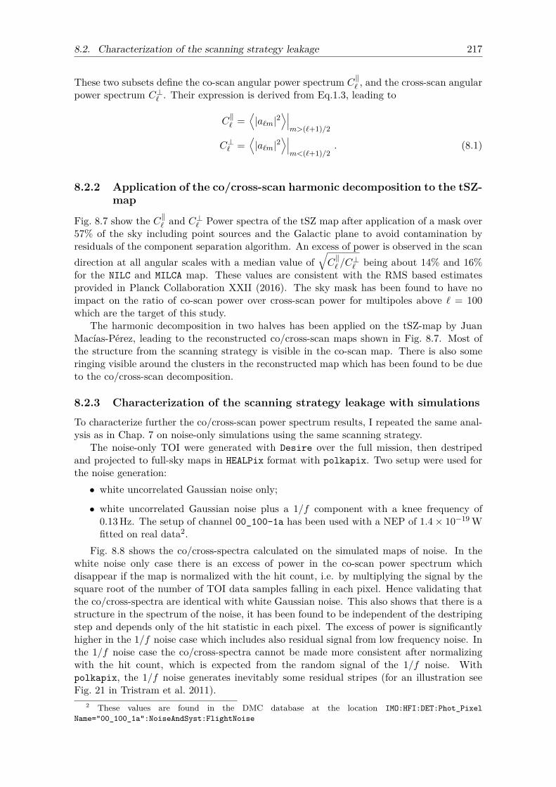
8.2. Characterization of the scanning strategy leakage 217
These two subsets define the co-scan angular power spectrum C‖` , and the cross-scan angular
power spectrum C⊥` . Their expression is derived from Eq.1.3, leading to
C‖` =
⟨|a`m|2
⟩∣∣∣m>(`+1)/2
C⊥` =⟨|a`m|2
⟩∣∣∣m<(`+1)/2
. (8.1)
8.2.2 Application of the co/cross-scan harmonic decomposition to the tSZ-map
Fig. 8.7 show the C‖` and C⊥` Power spectra of the tSZ map after application of a mask over57% of the sky including point sources and the Galactic plane to avoid contamination byresiduals of the component separation algorithm. An excess of power is observed in the scandirection at all angular scales with a median value of
√C‖` /C
⊥` being about 14% and 16%
for the NILC and MILCA map. These values are consistent with the RMS based estimatesprovided in Planck Collaboration XXII (2016). The sky mask has been found to have noimpact on the ratio of co-scan power over cross-scan power for multipoles above ` = 100which are the target of this study.
The harmonic decomposition in two halves has been applied on the tSZ-map by JuanMacías-Pérez, leading to the reconstructed co/cross-scan maps shown in Fig. 8.7. Most ofthe structure from the scanning strategy is visible in the co-scan map. There is also someringing visible around the clusters in the reconstructed map which has been found to be dueto the co/cross-scan decomposition.
8.2.3 Characterization of the scanning strategy leakage with simulations
To characterize further the co/cross-scan power spectrum results, I repeated the same anal-ysis as in Chap. 7 on noise-only simulations using the same scanning strategy.
The noise-only TOI were generated with Desire over the full mission, then destripedand projected to full-sky maps in HEALPix format with polkapix. Two setup were used forthe noise generation:• white uncorrelated Gaussian noise only;
• white uncorrelated Gaussian noise plus a 1/f component with a knee frequency of0.13 Hz. The setup of channel 00_100-1a has been used with a NEP of 1.4× 10⁻¹⁹ Wfitted on real data2.
Fig. 8.8 shows the co/cross-spectra calculated on the simulated maps of noise. In thewhite noise only case there is an excess of power in the co-scan power spectrum whichdisappear if the map is normalized with the hit count, i.e. by multiplying the signal by thesquare root of the number of TOI data samples falling in each pixel. Hence validating thatthe co/cross-spectra are identical with white Gaussian noise. This also shows that there is astructure in the spectrum of the noise, it has been found to be independent of the destripingstep and depends only of the hit statistic in each pixel. The excess of power is significantlyhigher in the 1/f noise case which includes also residual signal from low frequency noise. Inthe 1/f noise case the co/cross-spectra cannot be made more consistent after normalizingwith the hit count, which is expected from the random signal of the 1/f noise. Withpolkapix, the 1/f noise generates inevitably some residual stripes (for an illustration seeFig. 21 in Tristram et al. 2011).
2 These values are found in the DMC database at the location IMO:HFI:DET:Phot_PixelName="00_100_1a":NoiseAndSyst:FlightNoise
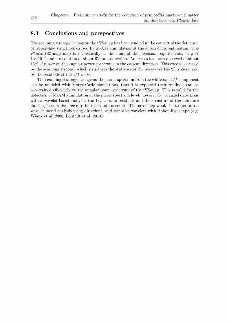
218 Chapter 8. Preliminary study for the detection of primordial matter-antimatterannihilation with Planck data
8.3 Conclusions and perspectivesThe scanning strategy leakage in the tSZ-map has been studied in the context of the detectionof ribbon-like structures caused by M-AM annihilation at the epoch of recombination. ThePlanck tSZ-map map is theoretically at the limit of the precision requirements, of y ≈1× 10⁻⁶ and a resolution of about 6′, for a detection. An excess has been observed of about15% of power on the angular power spectrums in the co-scan direction. This excess is causedby the scanning strategy which structures the statistics of the noise over the 2D sphere, andby the residuals of the 1/f noise.
The scanning strategy leakage on the power spectrum from the white and 1/f componentcan be modeled with Monte-Carlo simulations, thus it is expected their residuals can beconstrained efficiently on the angular power spectrum of the tSZ-map. This is valid for thedetection of M-AM annihilation at the power spectrum level, however for localized detectionswith a wavelet-based analysis, the 1/f co-scan residuals and the structure of the noise arelimiting factors that have to be taken into account. The next step would be to perform awavelet based analysis using directional and steerable wavelets with ribbon-like shape (e.g.Wiaux et al. 2008; Leistedt et al. 2013).
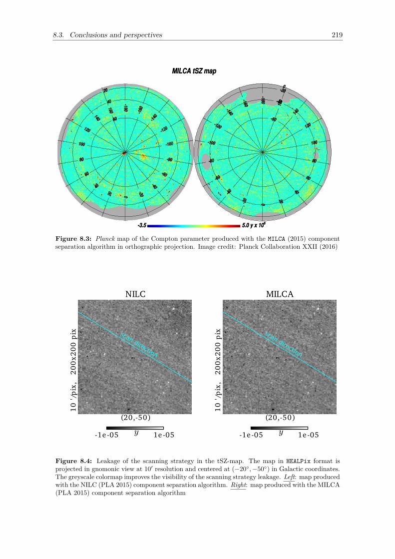
8.3. Conclusions and perspectives 219
Figure 8.3: Planck map of the Compton parameter produced with the MILCA (2015) componentseparation algorithm in orthographic projection. Image credit: Planck Collaboration XXII (2016)
10
'/p
ix,
20
0x2
00
pix
(20,-50)
NILC
-1e -05 1e-05y
scan direction
10
'/p
ix,
20
0x2
00
pix
(20,-50)
MILCA
-1e-05 1e-05y
scan direction
Figure 8.4: Leakage of the scanning strategy in the tSZ-map. The map in HEALPix format isprojected in gnomonic view at 10′ resolution and centered at (−20,−50) in Galactic coordinates.The greyscale colormap improves the visibility of the scanning strategy leakage. Left: map producedwith the NILC (PLA 2015) component separation algorithm. Right: map produced with the MILCA(PLA 2015) component separation algorithm
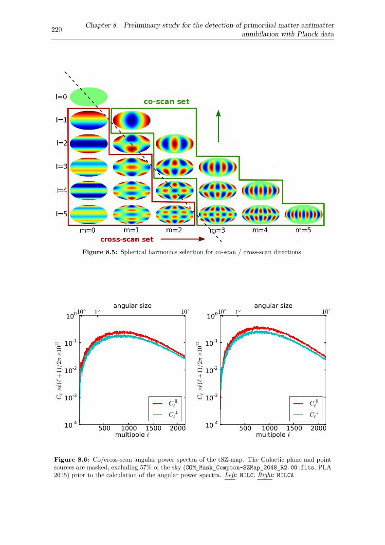
220 Chapter 8. Preliminary study for the detection of primordial matter-antimatterannihilation with Planck data
Figure 8.5: Spherical harmonics selection for co-scan / cross-scan directions
500 1000 1500 2000multipole `
10-4
10-3
10-2
10-1
100
C`×
(`+
1)/2π×1
012
C`
C`
10° 1° 10angular size
500 1000 1500 2000multipole `
10-4
10-3
10-2
10-1
100
C`×
(`+
1)/2π×1
012
C`
C`
10° 1° 10angular size
Figure 8.6: Co/cross-scan angular power spectra of the tSZ-map. The Galactic plane and pointsources are masked, excluding 57% of the sky (COM_Mask_Compton-SZMap_2048_R2.00.fits, PLA2015) prior to the calculation of the angular power spectra. Left: NILC. Right: MILCA
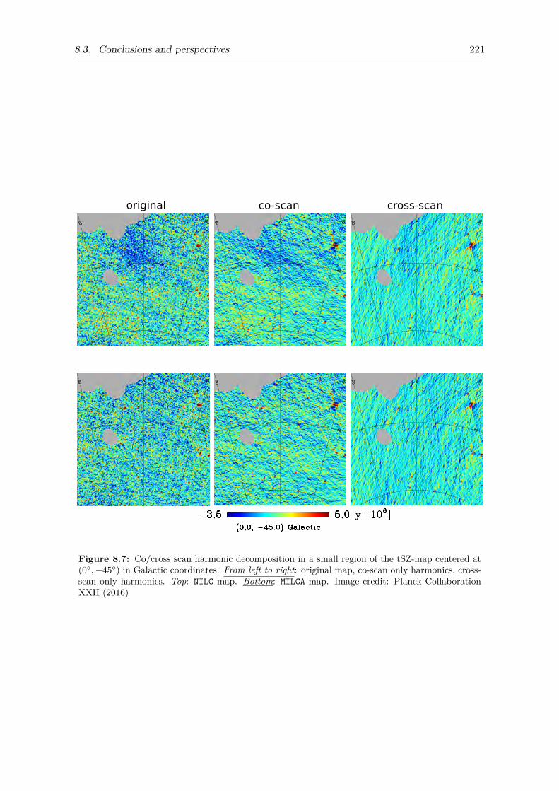
8.3. Conclusions and perspectives 221
original co-scan cross-scan
Figure 8.7: Co/cross scan harmonic decomposition in a small region of the tSZ-map centered at(0,−45) in Galactic coordinates. From left to right: original map, co-scan only harmonics, cross-scan only harmonics. Top: NILC map. Bottom: MILCA map. Image credit: Planck CollaborationXXII (2016)
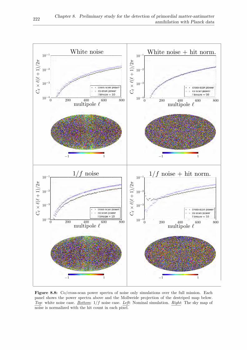
222 Chapter 8. Preliminary study for the detection of primordial matter-antimatterannihilation with Planck data
Figure 8.8: Co/cross-scan power spectra of noise only simulations over the full mission. Eachpanel shows the power spectra above and the Mollweide projection of the destriped map below.Top: white noise case. Bottom: 1/f noise case. Left: Nominal simulation. Right: The sky map ofnoise is normalized with the hit count in each pixel.
223
Conclusions et perspectives
Ce travail de thèse a commencé dans le contexte de la fin de mission du satellite Planck, aumoment où l’implication de l’ADC dans les variations de gains observées venait juste d’êtredécouverte. Il restait moins d’un an avant la décommission de Planck et la perte définitive despossibilités de communication avec la chaîne de lecture de l’électronique de bord qui étaitnécessaire pour collecter les données vitales pour la correction des effets de non-linéaritéde l’ADC. Cela a été le commencement d’un long parcours, où était impliqué le travailavec une large collaboration constituée de personnes de nombreuses origines. Ce qui a menénon seulement à l’acquisition de nombreuses connaissances dans les domaines scientifiqueset techniques nécessaires pour la compréhension d’un télescope spatial très complexe, maisaussi à de très riches interactions humaines et une aventure personnelle unique. Passonsmaintenant aux conclusions de ce travail.
La première partie est dédiée à la caractérisation et à la modélisation de la fonctionde transfert temporelle des détecteur bolométriques d’HFI. Avec comme motivation, à l’ori-gine, l’excès observé dans la réponse temporelle à basse fréquence des détecteurs. Cet excès,observé durant les campagnes d’étalonnage au sol, a été particulièrement compliqué à éta-lonner précisément une fois en vol. Ceci parce que les constantes de temps impliquées sontparticulièrement longues, de l’ordre de 50 ms à une minute. Au sein de la Tau Tiger Teaml’approche empirique qui a été adoptée pour construire le modèle labellisé LFER de la fonc-tion de transfert temporelle pouvait reproduire la réponse temporelle des détecteurs maisne fournissait pas de contraintes à basse fréquence. La problématique principale était quela réponse temporelle des bolomètres alimentés en courant modulé était approximée avecla théorie développée pour l’alimentation avec un courant continu, celle-ci ne décrivait pasassez précisément la réponse observée pour pouvoir atteindre le niveau de précision de l’ordrede 10−3 requis pour HFI. Et donc, pour fournir des contraintes sur la fonction de transferttemporelle, un modèle analytique de la réponse temporelle des bolomètres polarisés avec uncourant carré a été développé à partir du modèle simple de bolomètre. Les résultats ont étépubliés dans Sauvé and Montier (2016). Il est apparu que l’approche classique par passagedans le domaine de Fourier n’était pas utilisable dans le cas de la version linéarisée des équa-tions différentielles qui décrivent l’équilibre électro-thermal des bolomètres. Il a donc falludévelopper une méthode basée sur une décomposition spécifique des signaux en fréquencepour pouvoir calculer une solution matricielle avec l’algèbre linéaire. Le modèle analytiqueobtenu a été validé en le comparant à une simulation réalisée avec le logiciel SEB qui réalisel’intégration des équation différentielle décrivant le système avec la méthode de Runge-Kuttaà l’ordre 4. L’accord obtenu entre le modèle analytique et la simulation était de l’ordre de10−3 pour un détecteur à 100 GHz. Il a été montré cependant que la version de base dumodèle analytique avec un seul composant thermique n’était pas suffisante pour reproduirecorrectement l’estimation de la fonction de transfert temporelle faite avec le modèle LFER.Un second composant thermique a été ajouté au modèle analytique. Avec seulement 5 para-mètres thermiques libres, il a pu reproduire la fonction de transfert temporelle utilisée pourla déconvolution des données du catalogue Planck 2015, avec un accord à 2.7σ de l’estimationsur son incertitude. Cette nouvelle version était très proche de l’objectif et décrivait correc-tement la constante de temps principale du détecteur autour de ≈ 10 ms, avec une secondeconstante de temps autour de ≈ 50 s. La réponse temporelle spécifique aux bolomètres en ré-gime alternatif imposait au modèle LFER l’utilisation de plus de cinq composant thermiques,
224 Chapter 8. Preliminary study for the detection of primordial matter-antimatterannihilation with Planck data
alors que dans le cas du modèle analytique, deux composants arrivent à un résultat qui estpratiquement équivalent. Ces très bon résultats fournissent plusieurs pistes d’applicationsdirectes à ce modèle, en commençant par de nouvelles contraintes sur la reproduction descomposantes basse fréquence de la réponse temporelle des détecteurs de l’instrument HFI.Ce qui nécessite cependant un travail complémentaire pour adapter la procédure d’estima-tion de la fonction de réponse angulaire de l’optique. Le modèle analytique peut égalementreproduire le raw gain qui est un nouvel observable inexploité de la fonction de transferttemporelle. Cette propriété est particulièrement intéressante pour améliorer la correction dela non-linéarité des ADC, car cela fourni un modèle du raw gain qui est un paramètre critiquede cette correction.
Une approche complémentaire à la modélisation analytique a été l’utilisation des glitchqui sont la réponse des détecteurs liée au dépôt d’énergie d’une particule qui les traverse.Habituellement les glitch sont une nuisance qui cause des pertes de données, mais ils peuventégalement être utilisés pour contribuer à la validation d’une fonction de transfert temporellecandidate. Dans le cas présenté ici, ce raisonnement a été poussé plus loin. Une méthode,basée sur la géométrie Euclidienne, a été développée pour reconstruire directement la réponseimpulsionnelle des détecteurs avec les glitch. La problématique principale était la présence deplusieurs familles de glitch correspondant aux différentes parties du bolomètre où se faisais ledépôt d’énergie. La méthode a été adaptée pour séparer efficacement les familles dominantes.Il a été observé que la la réponse impulsionnelle de la famille de glitch labellisée short étaitcelle qui reproduisait le mieux la fonction de transfert temporelle estimée avec le modèleLFER. A ce moment le modèle LFER était en compétition avec un autre modèle nomméJH10. Ce résultat a donc été un argument discriminant en faveur du modèle LFER qui aété utilisé depuis pour la déconvolution temporelle des données scientifiques ayant servi àproduire les catalogues Planck 2013 et 2015. Plus tard la méthode de reconstruction danssa version définitive a permit de reproduire la fonction de transfert temporelle estimée avecle modèle LFER avec une précision de 1%. Et donc, bien que la réponse impulsionnelle desglitch soit un outil très puissant pour l’analyse de la réponse thermique des bolomètres, elleest limitée par des biais comme la proximité de plusieurs familles de glitch short et par ladifficulté de normalisation par l’énergie des particules. Cependant il a été démontré que leparamètre τhp correspondant au filtrage par l’électronique de lecture des détecteurs était biencontraint par la réponse impulsionnelle des glitch, mais cela dépend du modèle qui est utilisépour reproduire la réponse thermique des bolomètres. Dans ce cas la présence de plusieursfamilles de glitch correspondant à des réponses thermiques différentes aidait à améliorer cettecontrainte. Une extension possible de ce travail consisterait à utiliser le modèle analytiqueprésenté ci-dessus pour reproduire la réponse thermique, ce qui fournirait de bien meilleurescontraintes sur le filtrage effectué par l’électronique de lecture des détecteurs. De plus lebruit non-gaussien généré par les queues des familles de glitch avec une relaxation très lente(labellisés glitch long) pourrait être enlevé plus efficacement avec une combinaison du modèleanalytique utilisé pour reproduire ces glitches.
Dans la seconde partie de ce travail, les effets de la non linéarité introduite par l’ADC surles données scientifiques sont caractérisés et corrigés. Cet effet systématique s’est d’abordmanifesté sous forme de variations apparentes du gain au cours du temps de l’ordre de1.5%, et s’est révélé particulièrement difficile à gérer. La première urgence était de faireune caractérisation précise des composant pour les 52 canaux bolométriques de HFI avantle décommissionnemment du satellite. Deux campagnes d’acquisition ont été menées au solavec des composants de rechange, ceci en vue de collecter les informations nécessaires à laconstitution d’un modèle paramétrique des défauts de l’ADC utilisé dans HFI. En parallèle,Maxwell Technologies a fourni le modèle SPICE du composant. L’absence d’un fichier aempêché l’utilisation du modèle pour lancer des simulations afin de reproduire les défautsdes composants à bord du satellite, mais son étude a fourni de précieuses informations sur
8.3. Conclusions and perspectives 225
l’architecture du composant. Les données fournies par les deux campagnes d’acquisition au solont montré la présence d’un motif pseudo-périodique sur 64 codes consécutifs de l’ADC quia été corroboré par l’étude du modèle SPICE. Le modèle paramétrique a donc été abandonnéau profit d’une approche empirique basée sur ce qui a été nommé le motif à 64 codes avecen supplément une estimations des sauts qui apparaissent entre deux motifs. Il faut notercependant que les 64 codes juste après la mi-échelle de l’ADC n’obéissent pas au motif et leursdéfauts doivent être estimés séparément. Toutes ces informations ont été prises en comptepour configurer ce qui a été appelé la séquence EOL et qui a consisté à étalonner les défautsdes composants du satellite avec le bruit Gaussien des fast samples. Puis l’estimation de cesdéfauts a été menée à bien avec une méthode de maximisation de vraisemblance. Finalementla précision obtenue a été d’environ ≈ 3×10⁻³ sur la taille relative des pas de quantificationdes ADC obéissant au motif à 64 codes, très près de l’objectif qui était de ≈ 1 × 10⁻³.Cependant les 64 codes juste après la mi-échelle ne bénéficient pas de la statistique utilisableavec le motif et sont un facteur limitant pour la correction de l’effet de non-linéarité del’ADC. Ceci pourrait être facile à améliorer, en l’absence d’autres sources de biais comme leslignes 4K, car on pourrait mieux contraindre ces 64 codes en se servant des résidus de l’effetde non-linéarité de l’ADC sur les données scientifiques. Une autre possibilité pour mieuxcontraindre ces 64 codes serait d’utiliser les données scientifiques acquises pendant les 10mois de la séquence EOL, durant lesquels HFI n’étant plus à 0.1 K, à mesuré uniquement dubruit qui a été insuffisamment exploité.
L’estimation précise des défauts des ADC en vol était un vrai défi, mais cette informationseule ne permettait pas d’effectuer la correction de l’effet de non-linéarité sur les données,à cause de la sommation des fast samples effectuée dans le DPU pour produire les donnéesscientifiques. Cette étape détruit l’information critique sur la valeur exacte des codes del’ADC qui est la seule utilisable avec les données de caractérisation du composant. En consé-quence la valeur de ces codes devait être estimée en devinant quel était le signal analogiquequi avait servi à les produire. Ce qui nécessitait une modélisation très précise de la réponsede la chaîne de l’électronique de lecture à la puissance optique reçue par le bolomètre. Ce mo-dèle combiné avec l’estimation précise des défauts de l’ADC a permit de produire la fonctionde correction pour les données scientifiques. La validation de cette correction nécessitait uneestimation du niveau des résidus de l’effet de non-linéarité de l’ADC sur les données scien-tifiques. Des observables spécifiques ont été développés en comparant les échantillons desdonnées scientifiques acquis avec la première demi-période de la modulation avec ceux de laseconde demi-période, respectivement. Ceux-ci sont qualifié d’observables par demi-parité etsont sensibles uniquement à l’effet de non-linéarité de l’ADC car c’est la seule source connuede différence, hormis le bruit, entre les ciels scannés par chacune des deux demi-périodesde la modulation. En les utilisant il a été observé que la première version de la correctionréduisait de façon significative les variations de gain dues à l’ADC qui pouvaient descendreà 0.1% pour certains canaux. En complément, des simulations de l’effet de non-linéarité del’ADC étaient en très bon accord avec les observations sur les données scientifiques, ce quivalidait le modèle de correction et la méthodologie basée sur les observables par demi-parité.Cependant il a été trouvé que cette correction était limitée par une source de signal parasitedont l’origine était le compresseur mécanique de l’étage à 4 K, signal qui a été surnommélignes 4K. Ce signal nécessitait une caractérisation spécifique afin de l’inclure dans le modèlede correction.
Les lignes 4K apparaissent sur les données scientifiques sous la forme de 4 lignes très finesdans le domaine des fréquences, mais en réalité il y a une ”forêt“ de lignes sur le signal desfast samples avant la sommation par le DPU qui produit les échantillons des données scien-tifiques. Une fois de plus l’étape de la sommation détruit des informations vitales en repliantles harmoniques au dessus de la fréquence de modulation. L’inclusion des lignes 4K dans lemodèle de signal analogique nécessite la connaissance de sa forme dans le domaine temporel
226 Chapter 8. Preliminary study for the detection of primordial matter-antimatterannihilation with Planck data
dont la périodicité s’étend sur neuf demi périodes de la modulation. Mais ces données étaientinaccessibles pendant la mission. Ce qui a eu pour conséquence que le signal périodique deslignes 4K pouvait seulement être estimé à partir des observables qui sont les quatre versionsrepliées des lignes 4K visibles sur les données scientifiques et la période des fast samples cap-turée toutes les 101 secondes. L’analyse des séquences continues de fast samples capturéespendant la dernière phase de commissionnage (CPV) du satellite n’a pas montré de corré-lation significative entre les canaux qui pouvait être utilisée pour modéliser l’évolution deslignes 4K durant la mission. Pour cette raison, la solution de repli a été l’estimation des troisharmoniques dominantes sur les fast samples en utilisant les observables disponibles. Cettesolution a nécessité le calcul pour chaque période où le pointage est stable de 18 fonctions decorrections, une pour chaque configuration des échantillons de données scientifiques relativeaux lignes 4K et à la modulation. Ce qui a amélioré de façon significative la correction desdonnées scientifiques en abaissant le niveau des variations de gain autour de 10−3 pour lamajorité des canaux. Mais ce n’était pas encore suffisant pour atteindre l’objectif de 10−4.Une nouvelle solution a été développée à partir d’une analyse MCMC de l’espace des so-lutions pour les lignes 4K en incluant les observables par demi-parité dans la fonction devraisemblance. Ce qui a montré que le modèle de signal analogique pouvait être simplifiéen utilisant un signal de modulation (i.e la raw constant) identique sur toute la mission. Enpartant de cette constatation il était possible d’estimer une seule raw constant en minimisantles observables par demi-parité sur toute la mission. Ce qui, combiné avec une estimationdes lignes 4K sur les fast samples fournie par Guillaume Patanchon, a permit de réduireles variations de gain à un niveau proche de 10−4. Cependant les différences annuelles entreles cartes du ciel prises à un an d’intervalle n’ont pas montré d’amélioration significative encomparaison de la solution précédente. Pour cette raison une approche empirique (SRoll)est utilisée depuis 2016 pour réduire les variations observées entre les cartes du ciel vues pardes canaux différents. Une des raisons possibles pour l’absence d’amélioration sur les diffé-rences annuelles est une variation réelle du gain de l’électronique de lecture des détecteurs.Il est également envisagé que la procédure d’estimation des défauts de l’ADC capture unefraction de la distribution du bruit qui a servi à les estimer, et une approche différente pourcette estimation a été proposée. Il reste également à caractériser l’impact de la modulationsignificative des lignes 4K induite par les opérations de l’étage à 20 K qui ont une périodicitétypique de 15 min.
Dans la troisième partie de ce travail, l’impact des effets systématique sur l’analyse scien-tifique des cartes HFI est étudié. Dans le cadre de la préparation du papier (Planck Colla-boration Int. XIX 2015), la propagation de l’effet de non linéarité de l’ADC sur l’emissionpolarisée de la poussière Galactique a été étudié avec une simulation. Le modèle de signalanalogique et la caractérisation de l’ADC décris précédemment dans la seconde partie de cetravail ont été utilisés pour produire la simulation. Il a été déterminé que le biais introduitsur la fraction de lumière polarisée est de l’ordre de 10% et que celui sur l’angle de polarisa-tion est de l’ordre de 5 dans le plan Galactique, de plus les résidus de l’effet de non linéaritéde l’ADC sur les cartes de paramètres de Stokes dégénèrent fortement avec l’incertitude surla correction de couleur (bandpass mismatch). Une étude similaire nécessite d’être refaitesur les cartes du catalogue Planck 2015, et une attention particulière doit être portée dansle cas de l’incertitude sur la correction de couleur à cause de la dégénérescence avec l’effetde l’ADC. Ensuite, dans le cadre de l’analyse du spectre de puissance angulaire du CMB,les résidus causés par la non linéarité de l’ADC été inférés à partir des données scientifiquesde HFI. Pour cela une méthodologie basée sur des cartes par demi-parité a été développéeet validée avec des simulations. La somme des deux cartes de demi-parité contenant princi-palement du bruit et ces résidus, elle permet l’analyse des résidus de l’ADC sur le spectrede puissance angulaire. Il a été ensuite observé que ces résidus se manifestent par un excèsde puissance en 1/` à bas multipôles pour ` ∈ [1, 20], et que la correction utilisée pour le
8.3. Conclusions and perspectives 227
catalogue de données Planck 2015 est suffisante pour ne pas biaiser l’analyse du spectre depuissance angulaire en température du CMB pour ` > 20. Cependant le biais résiduel sur lemultipôle ` = 1 est de l’ordre de cinq fois le niveau de bruit attendu, et il est donc significatifpour l’étalonnage photométrique des détecteurs. Dans le cas de la polarisation, l’analyse descartes par demi-parité à 143 GHz a montré que le résidus en 1/` est problématique pourl’analyse du spectre EE sur lequel il apparait un ordre de magnitude au dessus du bruit.Il apparait donc qu’il est nécessaire d’améliorer la correction de l’effet de non-linéarité del’ADC pour l’étude de l’époque de la réionisation.
Finalement une étude préliminaire a été menée dans le cadre de la détection de l’an-nihilation de domaines résiduels d’antimatière à l’époque de la recombinaison. En théorie,l’interface d’annihilation entre les domaines de matière et d’antimatière laisse une signaturesur la carte d’effet tSZ de Planck à un niveau d’environ y ≈ 1× 10⁻⁶ sous forme de rubansayant une largeur angulaire d’environ 6′. Cet effet est à la limite de détection sur la carted’effet tSZ dont le RMS du bruit est d’environ 1× 10⁻⁶ et la résolution de 10′. Il se trouveque la stratégie de balayage de Planck créé des fuites sur cette carte qui dégénèrent avecla signature recherchée. L’étude de ces fuites a été réalisée avec une partition choisie de labase des harmoniques sphériques qui sélectionne les harmoniques sphériques orientés majo-ritairement dans la direction du balayage et dans celle qui est orthogonale. Il a été ensuitemesuré un excès médian de signal de 14% (16%) via le spectre de puissance angulaire dansla direction du balayage pour la carte produite avec l’algorithme NILC (MILCA) à toutes leséchelles angulaires. La stratégie de balayage donne une structure en 2 dimensions au bruitsur la sphère dont l’impact sur le spectre de puissance angulaire a été caractérisé avec dessimulations. Cette structure dois donc être prise en compte lors d’une recherche de signatured’annihilation à la limite du seuil de détection. Cette recherche peut être faite avec des onde-lettes par exemple mais une détection sera plus significative dans des direction orthogonalesà la stratégie de balayage.
Au moment ou ce manuscrit est rédigé, il y a encore des résidus à grande échelle angulaire,sur les différences entre les cartes du ciel construites avec des balayages effectués à un and’intervalle (voir la Sec. 6.2.4 dans Planck Collaboration VIII 2016). Ces résidus concernentle catalogue Planck 2015 et sont problématiques pour l’analyse scientifique à grande échelleangulaire, principalement l’étude de l’époque de la réionisation. L’ADC est toujours pointécomme la source dominante de ces différences, et l’analyse des lignes 4K indique que leurmodulation par les opérations de l’étage à 20 K est potentiellement le facteur limitant dont ilfaut pousser l’analyse. En ce qui concerne l’étalonnage de la fonction de transfert temporelle àbasse fréquence , le modèle analytique qui a été développé dans ce but est supposé l’améliorersignificativement, mais nécessite encore du travail pour atteindre son objectif. La leçon àretenir sur le compresseur mécanique, c’est que l’isolation contre les interférences électro-magnétiques doit être réalisée avec autant de soins que pour les vibrations mécaniques.Une autre leçon à retenir pour éviter un autre ”problème d’ADC“ c’est que ces composantsdoivent être caractérisés au sol de façon très précise et systématique avec une méthode detype rampe. L’étape de la sommation est également problématique et une solution simplepour éviter des conséquences néfastes est d’appliquer la correction d’ADC en vol avant cettesommation. Malgrés tout, il ne faut pas oublier que Planck a été une mission couronnéede succès, et que ce n’est pas la dernière des missions cosmologiques. Plusieurs nouvellesmissions sont prévues pour analyser plus précisément la multitude d’informations que recèlela polarisation du CMB et sont très attendues comme LiteBIRD.

229
Conclusions and perspectives
This thesis work started in the context of the end of mission of the Planck spacecraft, whenthe implication of the ADC in the gain variation observed on HFI science data was just beingdiscovered. There was less than one year left before the decommissioning of Planck and thedefinitive loss of communication capabilities with the on-board electronics readout neededto get the precious elements for the correction of the ADC nonlinearity effect. This was thestart of a long run, and this process involved the work with a large international collaborationof people from many different origin. It led not only to the gathering of a vast amount ofknowledge in the various scientific and technical aspects involved in understanding a complexspace telescope, but also to rich human interactions and a unique personal adventure. Letus now conclude this new drop poured in the ocean of knowledge.
The first part of this work is dedicated to the characterization and the modeling of thetime transfer function of HFI bolometric detectors. It has been motivated at the originby the challenging excess response of the detectors at low frequency. This excess observedon-ground during the calibration campaigns has been extremely difficult to calibrate in-flight because the involved ”apparent“ time constants were very long, from 50 ms up to oneminute scale. The empirical approach used within the Tau Tiger Team to build the so-calledLFER version of the time transfer function for the deconvolution of science data could fitthe detector temporal response but did not provide constraints at low frequency. The mainissue was that the bolometers temporal response under AC biasing was approximated withDC biasing theory which is not accurate enough for the (≈ 10−3) relative level requiredby HFI. Hence to provide strong constraints for the time transfer function, an analyticalmodeling of the bolometers temporal response under AC biasing was developed from thesimple bolometer model, and the results published in Sauvé and Montier (2016). It appearedthat the classical signal processing approach in Fourier domain to the linearised differentialequations describing the electro-thermal equilibrium of bolometers was not usable in the caseof AC biasing. Therefore a specific method was developed with a custom decomposition ofthe signals in frequency domain, and the problem could be solved with matrix-based linearalgebra. The analytical model built with this method has been validated by comparison witha simulation computed with the SEB software doing Runge-Kutta order 4 integration of thedifferential equations describing the system. The relative agreement between the analyticalmodel and the simulation was about 10−3 for a 100 GHz detector. It was shown that asingle thermal component is not enough to describe accurately the time transfer functionestimated in-flight with the empirical model. The analytical model was extended with asecond component which was capable to fit the in-flight time transfer function estimationwith a much better agreement. Using only 5 free thermal parameters the fit was within 2.7σof the estimated error for the empirical model used in the Planck 2015 data release. Thisnew version was very close to the goal and described accurately the detector dominant timeconstant at ≈ 10 ms with the addition of a very long time constant component at ≈ 50 s.The specific temporal response of bolometers under AC biasing could be approximated bythe empirical LFER model with more than five thermal components, while the analyticalmodel could achieve a similar result with only two thermal components. These excellentresults provide several direct applications to this model, starting with new constraints forfitting the LFER component of the HFI detectors, but it requires probably to add a thirdthermal component and also some work with the beams estimation pipeline. The analytical
230 Chapter 8. Preliminary study for the detection of primordial matter-antimatterannihilation with Planck data
model has also the ability to fit the raw gain observable of detectors which is a completelynew and unused constraint for the time transfer function. It can also be used to improvethe ADC nonlinearity correction by providing a model of the raw gain which is a criticalparameter to this correction.
A complementary approach to the analytical modeling of the bolometer response wasto use the glitches caused by cosmic rays energy deposit on the detectors. Glitches areusually a nuisance which cause loss of data, but they can also be used to check the validityof an existing estimation of the time transfer function. In the case presented here the ideawas pushed further. A method based on Euclidean geometry was developed to reconstructdirectly the impulse response of the detectors from glitches. The main problematic was withthe existence of several glitch families corresponding to different physical locations of theenergy deposit. Therefore the reconstruction method was adapted to separate efficiently thedominant families. It was found that the so-called short family produced the impulse responsewith the best agreement compared to the LFER model estimation of the in-flight timetransfer function. At this moment two time transfer function models were in competition,the other one being the so-called JH10. This result has been a strong argument in favorof the LFER model which has eventually been adopted for the time deconvolution of HFIscience data in the 2013 and 2015 data releases. Later, using the definitive version of theimpulse response reconstruction method, the time transfer function estimation from shortglitches was found to be in agreement within a 1% level of the in-flight time transfer functionfitted against the LFER model. Albeit being a powerful tool for the analysis of the thermalresponse of the bolometers, the impulse responses reconstructed with glitches are limitedby systematic effects such as closeness between several short families and normalization bythe energy of the particles. However it has been shown that the τhp electronics readoutfiltering parameter is well constrained, but it depends on the model used to fit the thermalresponse of the bolometer. In this case the presence of several glitch families corresponding todifferent thermal responses helps to provide better constraints. A possible extension of thiswork would be to use the analytical model developed previously in conjunction with impulseresponses from glitches. The analytical model is more constraining for the thermal responseof the bolometers, thus it would help to provide much better constraints on the electronicsreadout filtering. Additionally the non-Gaussian noise generated at some extent by theglitch families with slow thermal relaxation (the so-called long family) could be removedmore efficiently with a combination of the analytical model fitted against them.
In the second part of this work, the ADC nonlinearity effect on science data is char-acterized and corrected for. This systematic effect could be observed as gain variations intime of science data at about 1.5% level and revealed to be extremely challenging to dealwith. The first urgency was to make an accurate characterization of the ADC chip for allthe 52 bolometers channels of HFI before the spacecraft decommissionning. Two acquisitionground campaigns were run with spare ADC chips to collect information that could be usedto build a parametric model for the defects of the ADC used in HFI. In addition, MaxwellTechnologies provided us with the SPICE model of the ADC chip. Albeit a missing file in themodel prevented to run simulations for testing fits of in-flight components defects, it providedcritical information on the architecture of the component. The data collected with both on-ground campaigns exhibited a pseudo-periodic pattern over 64 consecutive ADC codes whichwas confirmed by the SPICE model analysis. Therefore it was decided to drop the parametricmodel in favor of an empirical approach based on the so-called 64-code pattern plus somespecific estimations at the jump location between two regions of the ADC obeying the pat-tern. At the notable exception of the 64 codes just after midscale of the ADC which werefound to have a different pattern and their defects had to be estimated separately. All theseinformations were taken into account to tune the so-called EOL sequence which consisted inthe acquisition of the Gaussian noise of fast samples to calibrate ADC defects on-board for
8.3. Conclusions and perspectives 231
the 10 remaining monthes. This data was used to estimate the quantization step size of everyADC codes in the range covered by the signal during the mission by the mean of a maximumlikelihood method. The final estimation of ADC nonlinearity achieved a relative accuracyof about ≈ 3× 10⁻³ on the quantization steps size for the 64-code pattern, very close to thetarget requirement of ≈ 1× 10⁻³. However the 64 codes after midscale that cannot benefitfrom the 64-code pattern are a limiting factor to the overall result attainable with the finalADC nonlinearity correction. This issue, in the absence of other sources of bias such as the4 K lines, would be easy to work because these 64 codes could be constrained by using ADCnonlinearity residuals on the science data. Another possibility to better constrain these 64codes would be to use the science data acquired during the 10 monthes of the EOL sequence,when HFI above 0.1 K measured only noise which has been insufficiently exploited.
The accurate characterization of the ADC in-flight was a great challenge, but this infor-mation alone could not be used to correct for ADC nonlinearity on science data because ofthe summation in the DPU of the fast samples to produce science data. This step destroysthe critical information of exact ADC codes values that are the only data relevant to thein-flight ADC defects estimation. As a consequence these codes values had to be estimatedby guessing which was the analog signal producing them. It required an accurate modeling ofthe electronics readout chain response to the sky power at the input of the bolometer. Thismodel combined to the accurate estimation of ADC defects was used to produce the correc-tion for science data. The validation of this correction required an estimation of the level ofADC nonlinearity residuals on science data. For this purpose ADC nonlinearity observablewere developed by comparing the signal from both modulation parities which are acquiredin different regions of the ADC. These so-called half parity observables were very specificto the ADC nonlinearity effect because the ADC is the only known source of discrepancy,excepted for the noise, between the skies scanned with each parity. Using them it was foundthat the first version of the correction reduced significantly the initial gain variations downto a level of about 0.1% for some channels. Further simulations of the ADC nonlinearityeffect were in very good agreement with the observation on science data, thus validating thecorrection model and the half parity observables methodology. However this correction wasfound to be limited by a source of spurious signal originating from the 4 K stage mechanicalcooler and this signal was called the 4 K lines. Hence it required a specific characterizationto be included in the correction model.
The 4 K lines appear on science data as four sharp lines in the frequency domain, but inpractice there is a forest of harmonics on the fast samples signal before the summation bythe DPU producing science data samples. Once again the summation step destroys criticalinformation by folding the harmonics above the modulation frequency. The inclusion of thissignal in the analog signal model requires the knowledge of its time domain shape whichextends over nine half periods of the modulation. The main problem is that only contiguousacquisition of fast samples on a given channel can provide the full knowledge of the 4 K linesperiod, but this data is not available during the mission. As a consequence the 4 K linesperiod can only be estimated from the available observables which are the science data foldedversions and one fast samples period captured each 101 seconds. The analysis of the twocontiguous fast samples acquisition sequences captured during the CPV, showed no signifi-cant correlations between channels that could be used to model the 4 K lines throughout themission. Hence a fall-back solution was to estimate the three dominant 4 K lines on the fastsamples with the available observables. This solution required to calculate for every stablepointing period 18 correction functions for each configuration of the science data samplesrelative to the 4 K lines and the modulation. It provided a significant improvement to thecorrection of science data, bringing down the residual gain variations level on most channelsbelow 10−3. This was not sufficient to reach the target requirement for gain variations of10−4. A new solution was developed starting with a MCMC analysis of the solution space for
232 Chapter 8. Preliminary study for the detection of primordial matter-antimatterannihilation with Planck data
4 K lines and including half parity gain observables in the likelihood function. It was shownthat the analog signal model could be simplified by using the same modulation shape (akathe raw constant) throughout the whole mission. With this consideration it was possible tofit a single raw constant by minimizing the half parity observables over the mission. Com-bined with an estimation of the 4 K lines provided by Guillaume Patanchon it was possibleto correct the gain variations down to a level close to 10−4. However the yearly difference offull-sky surveys scanned one year apart showed no significant improvement over the previouscorrection, and for this reason an empirical approach (SRoll) is used since 2016 to reducethe differences between sky maps from different detector channels. One possible reason forthe absence of improvement on the yearly differences is real gain variations of the electronicsreadout chain. It is also possible that the likelihood method used to estimate ADC defectsleaks the noise distribution in the estimates, and a different method for this estimation hasbeen suggested. It also remains to characterize the impact of the significant modulation ofthe 4 K lines by the 20 K stage sorption cooler operations which has a typical time constantof 15 minute.
In the third part of this work, the impact of systematic effects on the scientific analysis ofHFI maps is studied. For the (Planck Collaboration Int. XIX 2015) paper, the propagationof ADC nonlinearity to the polarized emission of the Galactic thermal dust has been studiedwith a simulation. The analog signal model and the ADC characterization described in thesecond part of this work have been used to produce the simulation. It has been estimated thatthe bias on the polarized light fraction was about 10% and the one on the polarization anglewas about 5 in the Galactic plane. It has also been seen that the ADC nonlinearity residualsin the maps of Stokes parameters degenerate strongly with the bandpass mismatch (BPM)leakage. A similar study should be performed on the maps of the Planck 2015 data releaseand a special care should be taken in the case of BPM leakage because of the degeneracy.Next, in the case of the analysis of the angular power spectrum of the CMB, the residualsfrom the ADC nonlinearity effect were inferred from the HFI science data. For this purposea method based on half-parity maps has been developed and validated with simulations.The sum of the two half-parity maps contains mainly noise and ADC nonlinearity residuals,allowing the analysis of ADC nonlinearity residuals on the angular power spectrum. It wasobserved that these residuals introduce an excess of power with a 1/` shape at low multipolefor ` ∈ [1, 20]. Thus with the correction used for the Planck 2015 data release, the ADCnonlinearity residuals are not expected to bias significantly the TT spectrum of the CMBfor ` > 20. However the residual bias at multipole ` = 1 has been estimated to be aboutfive time the expected noise level, therefore it is significant for the photometric calibrationof detectors. In the case of polarization, the analysis of half-parity maps at 143 GHz showedthat the 1/` residual is problematic for the analysis of the EE spectrum on which it appearsone order of magnitude above the expected noise level. Hence it is necessary to improve theADC nonlinearity correction for studying the reionization epoch.
Finally a preliminary study was performed for the detection of the annihilation betweensurviving domains of antimatter at the recombination epoch. In theory, the annihilationinterface between matter and antimatter domains leaves an imprint on the Planck tSZ mapat a level of about y ≈ 1× 10⁻⁶ visible as ribbons with an angular width of about 6′.This effect is at the detection limit on the Planck tSZ map whose RMS of noise is about1× 10−6 with a 10′ resolution. It happens that the Planck scanning strategy leakage intothis map is degenerate with the expected annihilation signature. The study of this leakagewas performed with a specifically taylored partition of the spherical harmonics which selectsthose dominantly oriented in the co-scan and the cross-scan directions. It was measured amedian excess of signal of 14% (16%) in the co-scan direction of the angular power spectrumfor the map produced with the NILC (MILCA) algorithm. The scanning strategy gives a 2dimension structure to the noise on the sphere whose impact on the angular power spectrum
8.3. Conclusions and perspectives 233
has been characterized with simulations. This structure has to be taken into account whenlooking for the signature of annihilation at the limit of the detection level. The search for asignature may be performed with a wavelet based analysis, but a detection would be moresignificant in the cross-scan direction.
At the time when this manuscript is written, there are still large angular scale residualsin the difference of HFI sky surveys maps scanned one year apart (see Sec. 6.2.4 in PlanckCollaboration VIII 2016). These residuals found in the Planck 2015 data release are supposedto be mainly due to ADC nonlinearity. This is yet an issue for science at large angular scale,mainly the study of the epoch of reionisation. The analysis of 4 K lines indicates that theirmodulation by the 20 K stage cooler operation is potentially the sticky point that need to befurther explored. For the time transfer function calibration at low frequency, the analyticalmodel developed for this purpose is expected to improve this aspect significantly, but requiressome work to achieve this objective. The lesson to be learned about the 4 K mechanicalcompressor is that EMC interferences must be shielded with as much care as for mechanicalvibrations. Another lesson to be learned to avoid a new ”ADC nonlinearity issue“ is thatADC chips should always be accurately characterized on-ground with a ramp-like method.The summation step is also problematic and an easy fix to avoid worst case issues is toapply the ADC nonlinearity correction in-flight before the summation. Finally Planck wasa great and successful mission, but this is not the last of the cosmological missions. Severalnew experiments are much awaited and will analyse more precisely the information that theCMB polarization holds such as LiteBIRD.

235
Appendix A
Building the analytical response infrequency domain of AC biasedbolometers
This article was published in Experimental Astronomy (Sauvé and Montier 2016)
Experimental Astronomy manuscript No.(will be inserted by the editor)
Building the analytical response in frequency domainof AC biased bolometers
Application to Planck/HFI
Alexandre Sauve · Ludovic Montier
the date of receipt and acceptance should be inserted later
PlanckAbstract Context: Bolometers are high sensitivity detector commonly used inInfrared astronomy. The HFI instrument of the Planck satellite makes extensiveuse of them, but after the satellite launch two electronic related problems revealedcritical. First an unexpected excess response of detectors at low optical excitationfrequency for ν < 1 Hz, and secondly the Analog To digital Converter (ADC)component had been insufficiently characterized on-ground. These two problemsrequire an exquisite knowledge of detector response. However bolometers havehighly nonlinear characteristics, coming from their electrical and thermal couplingmaking them very difficult to modelize.
Goal: We present a method to build the analytical transfer function in fre-quency domain which describe the voltage response of an Alternative Current (AC)biased bolometer to optical excitation, based on the standard bolometer model.This model is built using the setup of the Planck/HFI instrument and offers themajor improvement of being based on a physical model rather than the currentlyin use had-hoc model based on Direct Current (DC) bolometer theory.
Method: The analytical transfer function expression will be presented in ma-trix form. For this purpose, we build linearized versions of the bolometer electrothermal equilibrium. And a custom description of signals in frequency is used tosolve the problem with linear algebra. The model performances is validated usingtime domain simulations.
Results: The provided expression is suitable for calibration and data process-ing. It can also be used to provide constraints for fitting optical transfer functionusing real data from steady state electronic response and optical response. The
A. SauveIRAP (CNRS)9, avenue du Colonel Roche - BP 44346 - 31028 Toulouse Cedex 4 - FRANCETel : +33 5 61 55 66 66Fax : +33 5 61 55 86 92E-mail: [email protected]
L. MontierIRAP (CNRS)E-mail: [email protected]
2 Alexandre Sauve, Ludovic Montier
accurate description of electronic response can also be used to improve the ADCnonlinearity correction for quickly varying optical signals.
Keywords Planck, HFI, bolometer, method, analytical model, transfer function
Contents
1 Introduction . . . . . . . . . . . . . . . . . . . . . . . . . . . . . . . . . . . . . . . . . 22 Bolometer model . . . . . . . . . . . . . . . . . . . . . . . . . . . . . . . . . . . . . . 33 Linearizing differential equations . . . . . . . . . . . . . . . . . . . . . . . . . . . . . 54 Solving in frequency domain . . . . . . . . . . . . . . . . . . . . . . . . . . . . . . . 95 Results . . . . . . . . . . . . . . . . . . . . . . . . . . . . . . . . . . . . . . . . . . . 136 Conclusions . . . . . . . . . . . . . . . . . . . . . . . . . . . . . . . . . . . . . . . . 19A Integrated transfer function . . . . . . . . . . . . . . . . . . . . . . . . . . . . . . . . 20B Adding a thermal component . . . . . . . . . . . . . . . . . . . . . . . . . . . . . . . 23C Simulation setup . . . . . . . . . . . . . . . . . . . . . . . . . . . . . . . . . . . . . . 25D Numerical results . . . . . . . . . . . . . . . . . . . . . . . . . . . . . . . . . . . . . . 26
1 Introduction
Bolometers are high sensitivity thermal detectors commonly used in astronomyin the domain of infrared to sub-millimeter wavelengths. They are basically semiconductor thermometers, connected to a heat sink, which impedance vary withtemperature. AC biased bolometers have been extensively used for the last tenyears in balloon borne and space experiments as in the Planck satellite, mainly fortheir good performances in regard to low frequency 1/f noise. However AC biasedbolometers detectors are still described based on DC theory by Holmes et al.(2008). Some work has been done by Catalano et al. (2010) for optimizing theAC biasing of bolometers in the case of the Planck/HFI instrument, but withoutdescribing the shape of the electronic response.
The Planck experiment (Tauber et al., 2010), designed to observe the Cos-mic Microwave Backgroud (CMB), reached an unprecedented sensitivity with ∆T
T
better than 10−5 for the CMB anisotropies observation. With respect to this objec-tive, two problems related to electronics have revealed as critical after the satellitelaunch: the low frequency excess response (LFER) and Analog to Digital Converter(ADC) nonlinearity.
First the detectors response to optical excitation exhibited an excess responseat low frequencies for ν < 1Hz (Planck Collaboration et al., 2015). The mainculprit for this excess is intermediate components in the thermal path to the heatsink operating at 100 mK. These components produce also specific response toenergy deposit from particles (Catalano et al., 2014). The thermal model havebeen extended with a chain of order 1 low pass filters to build an ad-hoc transferfunction model Planck Collaboration (2014) which described well the detectorresponse at first order. However the last version of the model needs to fit up toseven thermal components (Planck Collaboration et al., 2015).
The second in flight issue is the ADC nonlinearity which has been insufficientlycharacterized on ground. This systematic effect becomes very difficult to correctin the Planck/HFI case, because signal is averaged onboard over 40 samples of themodulation half period, before being sent to the ground. A very good knowledge
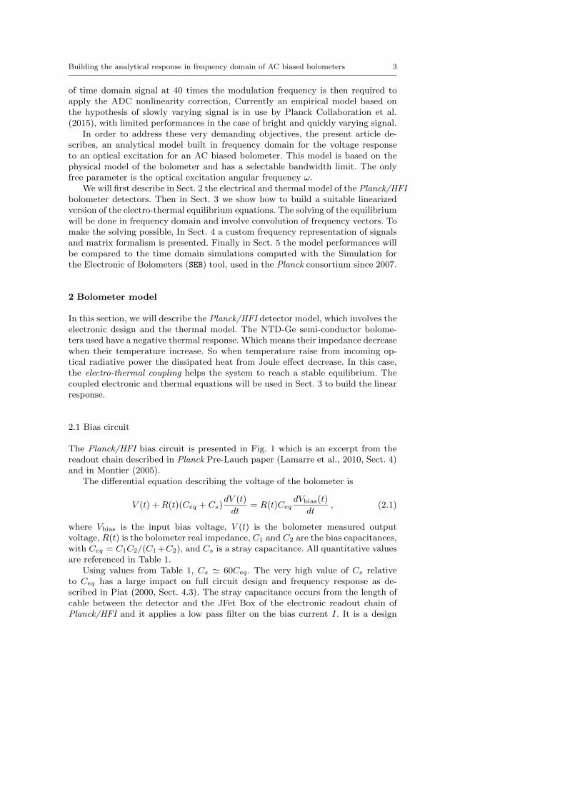
Building the analytical response in frequency domain of AC biased bolometers 3
of time domain signal at 40 times the modulation frequency is then required toapply the ADC nonlinearity correction, Currently an empirical model based onthe hypothesis of slowly varying signal is in use by Planck Collaboration et al.(2015), with limited performances in the case of bright and quickly varying signal.
In order to address these very demanding objectives, the present article de-scribes, an analytical model built in frequency domain for the voltage responseto an optical excitation for an AC biased bolometer. This model is based on thephysical model of the bolometer and has a selectable bandwidth limit. The onlyfree parameter is the optical excitation angular frequency ω.
We will first describe in Sect. 2 the electrical and thermal model of the Planck/HFIbolometer detectors. Then in Sect. 3 we show how to build a suitable linearizedversion of the electro-thermal equilibrium equations. The solving of the equilibriumwill be done in frequency domain and involve convolution of frequency vectors. Tomake the solving possible, In Sect. 4 a custom frequency representation of signalsand matrix formalism is presented. Finally in Sect. 5 the model performances willbe compared to the time domain simulations computed with the Simulation forthe Electronic of Bolometers (SEB) tool, used in the Planck consortium since 2007.
2 Bolometer model
In this section, we will describe the Planck/HFI detector model, which involves theelectronic design and the thermal model. The NTD-Ge semi-conductor bolome-ters used have a negative thermal response. Which means their impedance decreasewhen their temperature increase. So when temperature raise from incoming op-tical radiative power the dissipated heat from Joule effect decrease. In this case,the electro-thermal coupling helps the system to reach a stable equilibrium. Thecoupled electronic and thermal equations will be used in Sect. 3 to build the linearresponse.
2.1 Bias circuit
The Planck/HFI bias circuit is presented in Fig. 1 which is an excerpt from thereadout chain described in Planck Pre-Lauch paper (Lamarre et al., 2010, Sect. 4)and in Montier (2005).
The differential equation describing the voltage of the bolometer is
V (t) +R(t)(Ceq + Cs)dV (t)
dt= R(t)Ceq
dVbias(t)
dt, (2.1)
where Vbias is the input bias voltage, V (t) is the bolometer measured outputvoltage, R(t) is the bolometer real impedance, C1 and C2 are the bias capacitances,with Ceq = C1C2/(C1+C2), and Cs is a stray capacitance. All quantitative valuesare referenced in Table 1.
Using values from Table 1, Cs ' 60Ceq. The very high value of Cs relativeto Ceq has a large impact on full circuit design and frequency response as de-scribed in Piat (2000, Sect. 4.3). The stray capacitance occurs from the length ofcable between the detector and the JFet Box of the electronic readout chain ofPlanck/HFI and it applies a low pass filter on the bias current I. It is a design
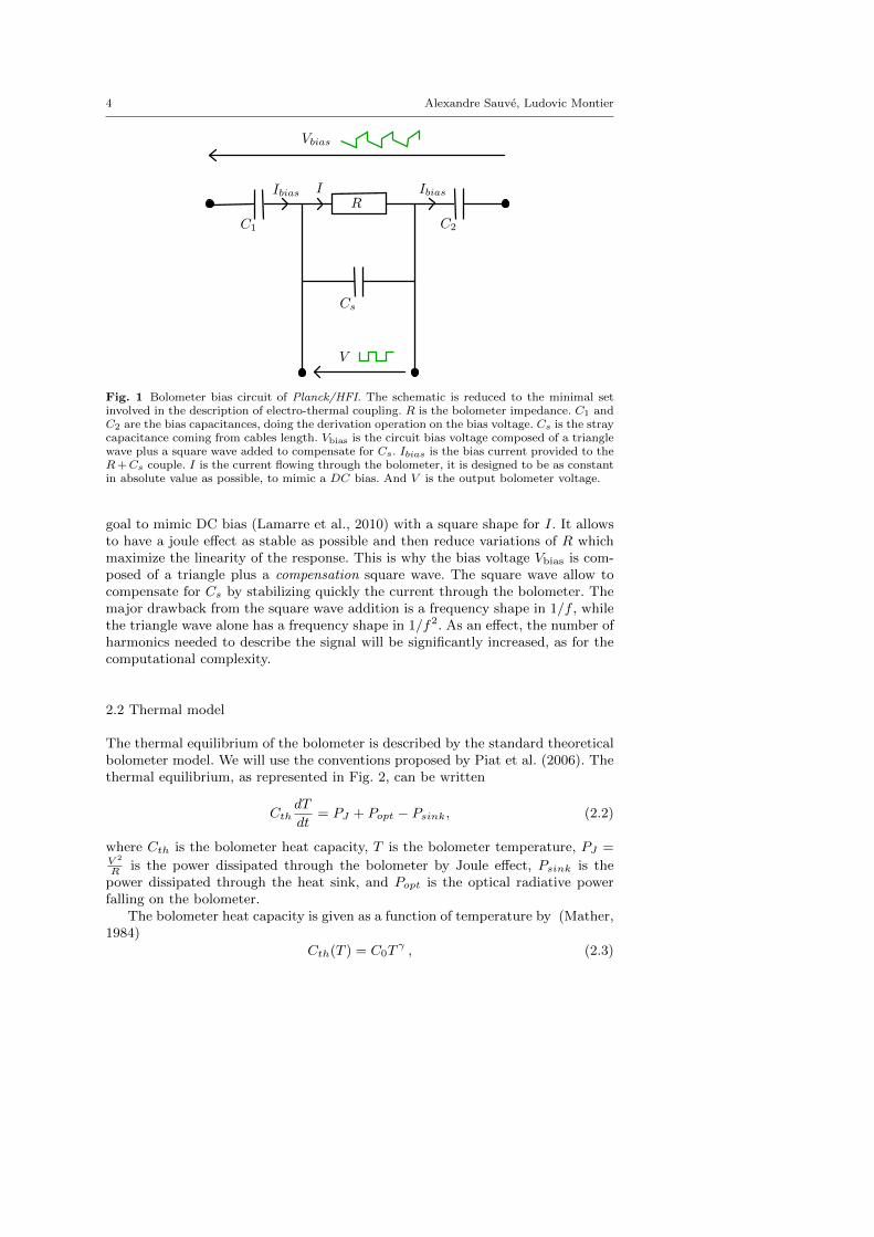
4 Alexandre Sauve, Ludovic Montier
Fig. 1 Bolometer bias circuit of Planck/HFI. The schematic is reduced to the minimal setinvolved in the description of electro-thermal coupling. R is the bolometer impedance. C1 andC2 are the bias capacitances, doing the derivation operation on the bias voltage. Cs is the straycapacitance coming from cables length. Vbias is the circuit bias voltage composed of a trianglewave plus a square wave added to compensate for Cs. Ibias is the bias current provided to theR+Cs couple. I is the current flowing through the bolometer, it is designed to be as constantin absolute value as possible, to mimic a DC bias. And V is the output bolometer voltage.
goal to mimic DC bias (Lamarre et al., 2010) with a square shape for I. It allowsto have a joule effect as stable as possible and then reduce variations of R whichmaximize the linearity of the response. This is why the bias voltage Vbias is com-posed of a triangle plus a compensation square wave. The square wave allow tocompensate for Cs by stabilizing quickly the current through the bolometer. Themajor drawback from the square wave addition is a frequency shape in 1/f , whilethe triangle wave alone has a frequency shape in 1/f2. As an effect, the number ofharmonics needed to describe the signal will be significantly increased, as for thecomputational complexity.
2.2 Thermal model
The thermal equilibrium of the bolometer is described by the standard theoreticalbolometer model. We will use the conventions proposed by Piat et al. (2006). Thethermal equilibrium, as represented in Fig. 2, can be written
CthdT
dt= PJ + Popt − Psink, (2.2)
where Cth is the bolometer heat capacity, T is the bolometer temperature, PJ =V 2
R is the power dissipated through the bolometer by Joule effect, Psink is thepower dissipated through the heat sink, and Popt is the optical radiative powerfalling on the bolometer.
The bolometer heat capacity is given as a function of temperature by (Mather,1984)
Cth(T ) = C0Tγ , (2.3)
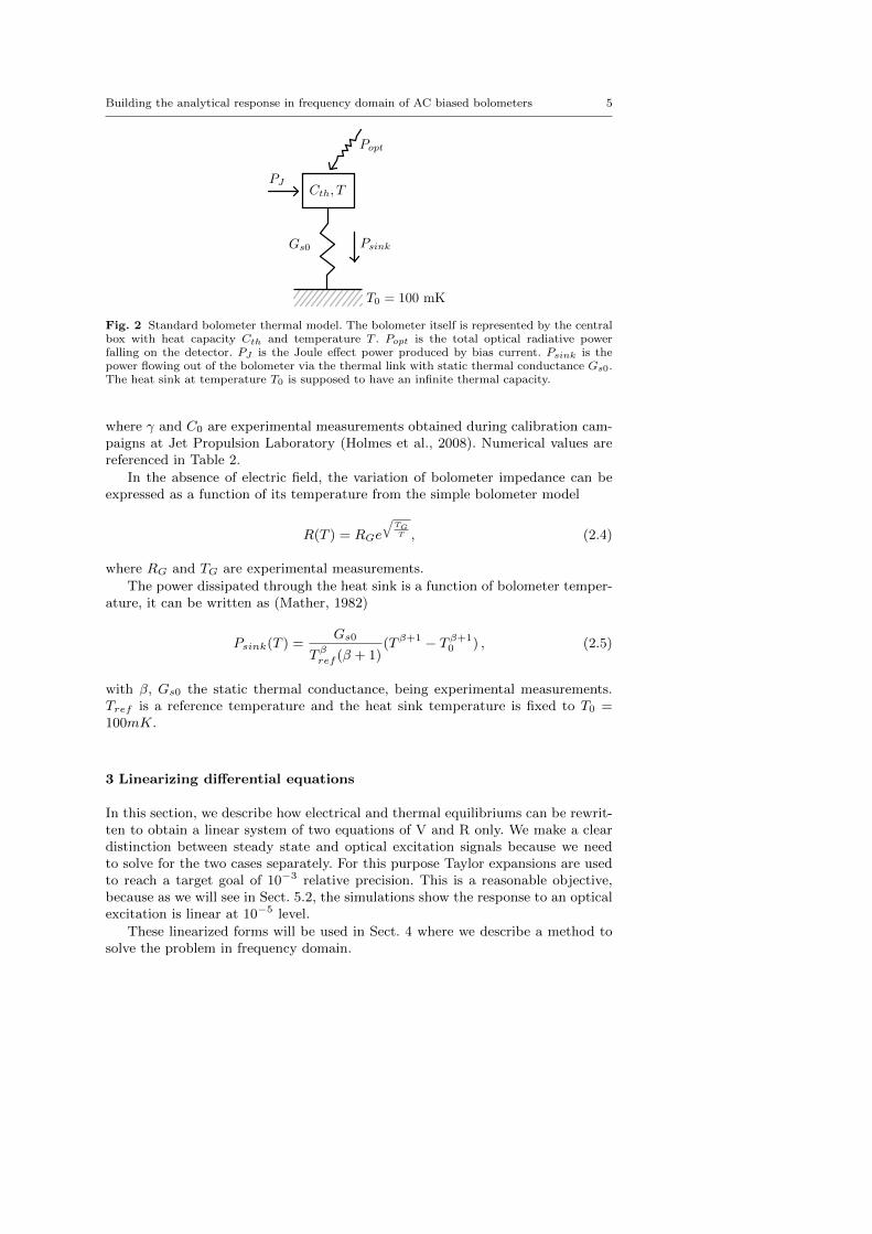
Building the analytical response in frequency domain of AC biased bolometers 5
Fig. 2 Standard bolometer thermal model. The bolometer itself is represented by the centralbox with heat capacity Cth and temperature T . Popt is the total optical radiative powerfalling on the detector. PJ is the Joule effect power produced by bias current. Psink is thepower flowing out of the bolometer via the thermal link with static thermal conductance Gs0.The heat sink at temperature T0 is supposed to have an infinite thermal capacity.
where γ and C0 are experimental measurements obtained during calibration cam-paigns at Jet Propulsion Laboratory (Holmes et al., 2008). Numerical values arereferenced in Table 2.
In the absence of electric field, the variation of bolometer impedance can beexpressed as a function of its temperature from the simple bolometer model
R(T ) = RGe
√TGT , (2.4)
where RG and TG are experimental measurements.
The power dissipated through the heat sink is a function of bolometer temper-ature, it can be written as (Mather, 1982)
Psink(T ) =Gs0
Tβref (β + 1)(Tβ+1 − Tβ+1
0 ) , (2.5)
with β, Gs0 the static thermal conductance, being experimental measurements.Tref is a reference temperature and the heat sink temperature is fixed to T0 =100mK.
3 Linearizing differential equations
In this section, we describe how electrical and thermal equilibriums can be rewrit-ten to obtain a linear system of two equations of V and R only. We make a cleardistinction between steady state and optical excitation signals because we needto solve for the two cases separately. For this purpose Taylor expansions are usedto reach a target goal of 10−3 relative precision. This is a reasonable objective,because as we will see in Sect. 5.2, the simulations show the response to an opticalexcitation is linear at 10−5 level.
These linearized forms will be used in Sect. 4 where we describe a method tosolve the problem in frequency domain.
6 Alexandre Sauve, Ludovic Montier
3.1 Signals decomposition
Let start by making a clear distinction between signals in steady state, and theones generated by optical excitation. We make the hypothesis that the incomingoptical radiative power is the sum of a constant bacground 〈Popt〉 and a small
monofrequency optical excitation term Popt.
The bolometer response to Popt is linear to a good approximation, so we makethe hypothesis that we can write its voltage as
V (t) = 〈V 〉+ V (t) + V (t) +O(V 2) , (3.1)
using the notations
– 〈V 〉 for the average value of V (in this case 〈V 〉 = 0)– V for the steady state modulation harmonics– V for the harmonics appearing in response to Popt
The second order terms in O(V 2) can be neglected, see Sect. 5.1 for quantitativevalues.
The same hypothesis and notations will be applied to T (t), R(t), Cth(t),Psink(t) and PJ(t). These notations allow to distinguish easily the order of the
terms in the equations as we do have in practice the generic relation 〈T 〉 T T .Numerical values will be detaild in Sect. 5.1. Consequently, from now, all termscontaining a product of two optical excitation component like V R will be consid-ered as negligible, and nonlinear.
3.2 Electrical equilibrium
The electrical equilibrium is already a function of V and R. Using previouslydefined notations, we separate the steady state terms from the optical excitationterms. Then Eq. (2.1) reads
V + (〈R〉+R)(Ceq + Cs)V = (〈R〉+R)CeqVbias , (3.2)
and
V + (Ceq + Cs)(
(〈R〉+R)˙V + RV
)= RCeqVbias +O(RV ) . (3.3)
3.3 Thermal equilibrium
The thermal equilibrium Eq. (2.2) is a function of T , V and R. In this section, werewrite its terms as linearized versions of V and R only. To do so we first expressT as a function of R.
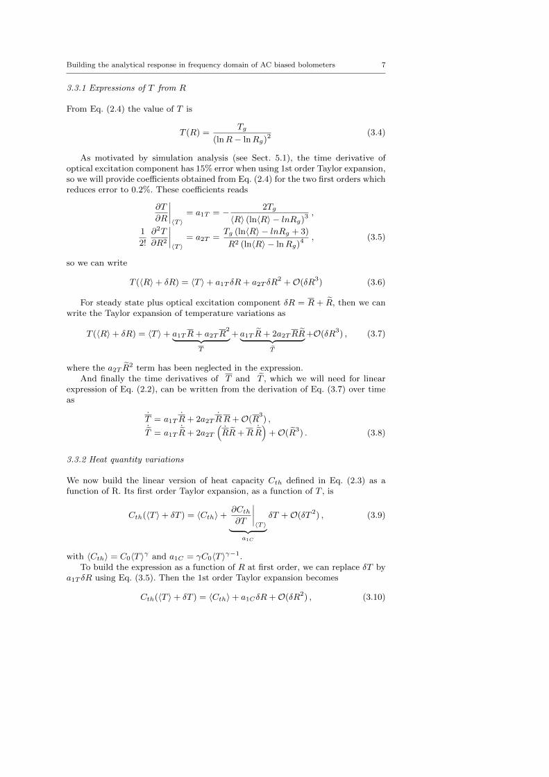
Building the analytical response in frequency domain of AC biased bolometers 7
3.3.1 Expressions of T from R
From Eq. (2.4) the value of T is
T (R) =Tg
(lnR− lnRg)2(3.4)
As motivated by simulation analysis (see Sect. 5.1), the time derivative ofoptical excitation component has 15% error when using 1st order Taylor expansion,so we will provide coefficients obtained from Eq. (2.4) for the two first orders whichreduces error to 0.2%. These coefficients reads
∂T
∂R
∣∣∣∣〈T 〉
= a1T = − 2Tg
〈R〉 (ln〈R〉 − lnRg)3,
1
2!
∂2T
∂R2
∣∣∣∣〈T 〉
= a2T =Tg (ln〈R〉 − lnRg + 3)
R2 (ln〈R〉 − lnRg)4, (3.5)
so we can write
T (〈R〉+ δR) = 〈T 〉+ a1T δR+ a2T δR2 +O(δR3) (3.6)
For steady state plus optical excitation component δR = R + R, then we canwrite the Taylor expansion of temperature variations as
T (〈R〉+ δR) = 〈T 〉+ a1TR+ a2TR2
︸ ︷︷ ︸T
+ a1T R+ 2a2TRR︸ ︷︷ ︸T
+O(δR3) , (3.7)
where the a2T R2 term has been neglected in the expression.
And finally the time derivatives of T and T , which we will need for linearexpression of Eq. (2.2), can be written from the derivation of Eq. (3.7) over timeas
T = a1T R+ 2a2T R R+O(R3) ,
˙T = a1T
˙R+ 2a2T
(RR+R
˙R)
+O(R3) . (3.8)
3.3.2 Heat quantity variations
We now build the linear version of heat capacity Cth defined in Eq. (2.3) as afunction of R. Its first order Taylor expansion, as a function of T , is
Cth(〈T 〉+ δT ) = 〈Cth〉+∂Cth∂T
∣∣∣∣〈T 〉︸ ︷︷ ︸
a1C
δT +O(δT 2) , (3.9)
with 〈Cth〉 = C0〈T 〉γ and a1C = γC0〈T 〉γ−1.To build the expression as a function of R at first order, we can replace δT by
a1T δR using Eq. (3.5). Then the 1st order Taylor expansion becomes
Cth(〈T 〉+ δT ) = 〈Cth〉+ a1CδR+O(δR2) , (3.10)
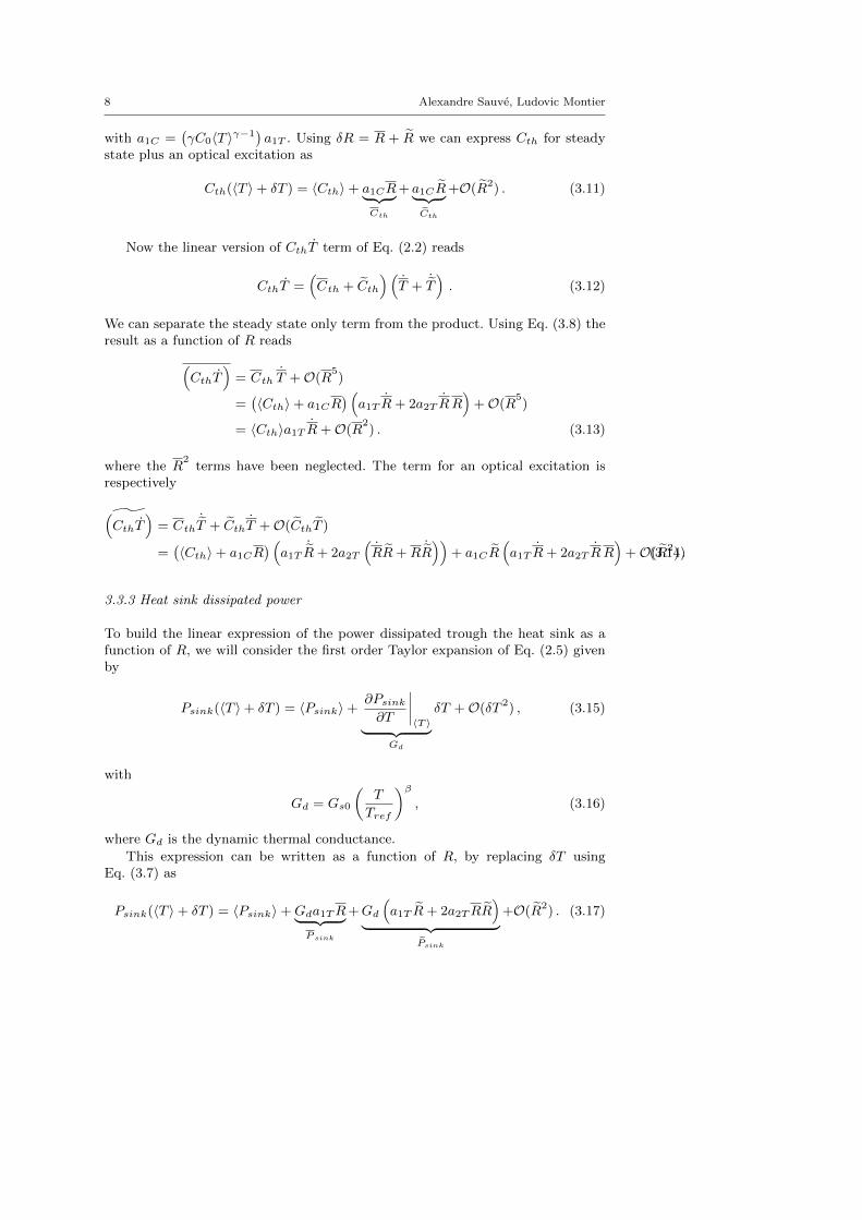
8 Alexandre Sauve, Ludovic Montier
with a1C =(γC0〈T 〉γ−1
)a1T . Using δR = R + R we can express Cth for steady
state plus an optical excitation as
Cth(〈T 〉+ δT ) = 〈Cth〉+ a1CR︸ ︷︷ ︸Cth
+ a1CR︸ ︷︷ ︸Cth
+O(R2) . (3.11)
Now the linear version of CthT term of Eq. (2.2) reads
CthT =(Cth + Cth
)(T +
˙T). (3.12)
We can separate the steady state only term from the product. Using Eq. (3.8) theresult as a function of R reads
(CthT
)= Cth T +O(R
5)
=(〈Cth〉+ a1CR
) (a1T R+ 2a2T R R
)+O(R
5)
= 〈Cth〉a1T R+O(R2) . (3.13)
where the R2
terms have been neglected. The term for an optical excitation isrespectively
˜(CthT
)= Cth
˙T + CthT +O(CthT )
=(〈Cth〉+ a1CR
) (a1T
˙R+ 2a2T
(RR+R
˙R))
+ a1CR(a1T R+ 2a2T R R
)+O(R2) .(3.14)
3.3.3 Heat sink dissipated power
To build the linear expression of the power dissipated trough the heat sink as afunction of R, we will consider the first order Taylor expansion of Eq. (2.5) givenby
Psink(〈T 〉+ δT ) = 〈Psink〉+∂Psink∂T
∣∣∣∣〈T 〉︸ ︷︷ ︸
Gd
δT +O(δT 2) , (3.15)
with
Gd = Gs0
(T
Tref
)β, (3.16)
where Gd is the dynamic thermal conductance.
This expression can be written as a function of R, by replacing δT usingEq. (3.7) as
Psink(〈T 〉+ δT ) = 〈Psink〉+Gda1TR︸ ︷︷ ︸P sink
+Gd
(a1T R+ 2a2TRR
)
︸ ︷︷ ︸Psink
+O(R2) . (3.17)
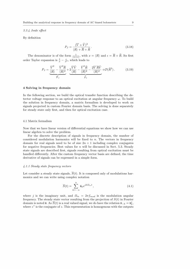
Building the analytical response in frequency domain of AC biased bolometers 9
3.3.4 Joule effect
By definition
PJ =(V + V )2
〈R〉+R+ R. (3.18)
The denominator is of the form 1(x+ε) , with x = 〈R〉 and ε = R + R. Its first
order Taylor expansion is 1x − ε
x2 , which leads to
PJ =V
2
〈R〉 −V
2R
〈R〉2︸ ︷︷ ︸PJ
+ 2V V
〈R〉 −V
2R
〈R〉2 −2V RV
〈R〉2︸ ︷︷ ︸PJ
+O(R2) . (3.19)
4 Solving in frequency domain
In the following section, we build the optical transfer function describing the de-tector voltage response to an optical excitation at angular frequency ω. To buildthe solution in frequency domain, a matrix formalism is developed to work onsignals projected in custom Fourier domain basis. The solving is done separatelyfor steady state only first, and then for optical excitation case.
4.1 Matrix formalism
Now that we have linear version of differential equations we show how we can uselinear algebra to solve the problem.
For the discrete description of signals in frequency domain, the number ofconsidered modulation harmonics will be fixed to n. The vectors in frequencydomain for real signals need to be of size 2n + 1 including complex conjugatesfor negative frequencies. Best values for n will be discussed in Sect. 5.3. Steadystate signals are described first, signals resulting from optical excitation must behandled differently. After the custom frequency vector basis are defined, the timederivative of signals can be expressed in a simple form.
4.1.1 Steady state frequency vectors
Let consider a steady state signals, S(t). It is composed only of modulations har-monics and we can write using complex notation
S(t) =
n∑
k=−nske
jkΩmt , (4.1)
where j is the imaginary unit, and Ωm = 2πfmod is the modulation angularfrequency. The steady state vector resulting from the projection of S(t) in Fourierdomain is noted s. As S(t) is a real valued signal, we do have the relation s−k = s∗k,where z∗ is the conjugate of z. This representation is homogenous with the outputs
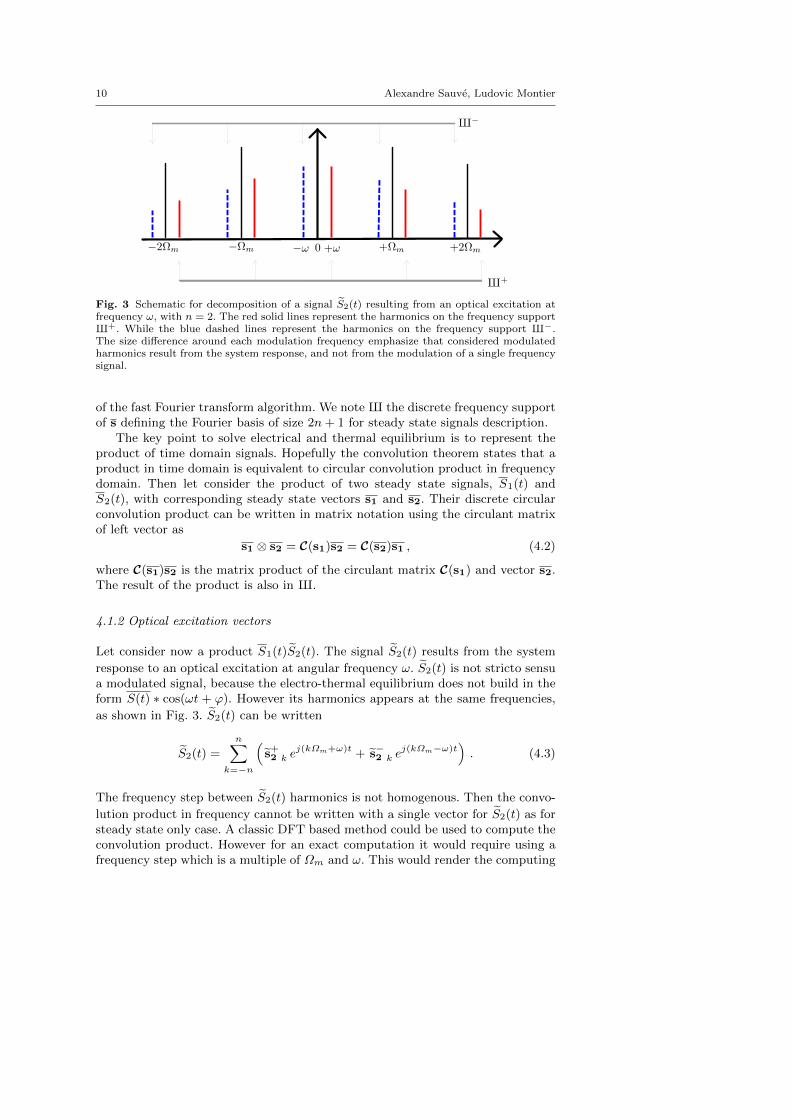
10 Alexandre Sauve, Ludovic Montier
Fig. 3 Schematic for decomposition of a signal S2(t) resulting from an optical excitation atfrequency ω, with n = 2. The red solid lines represent the harmonics on the frequency supportX+. While the blue dashed lines represent the harmonics on the frequency support X−.The size difference around each modulation frequency emphasize that considered modulatedharmonics result from the system response, and not from the modulation of a single frequencysignal.
of the fast Fourier transform algorithm. We note X the discrete frequency supportof s defining the Fourier basis of size 2n+ 1 for steady state signals description.
The key point to solve electrical and thermal equilibrium is to represent theproduct of time domain signals. Hopefully the convolution theorem states that aproduct in time domain is equivalent to circular convolution product in frequencydomain. Then let consider the product of two steady state signals, S1(t) andS2(t), with corresponding steady state vectors s1 and s2. Their discrete circularconvolution product can be written in matrix notation using the circulant matrixof left vector as
s1 ⊗ s2 = C(s1)s2 = C(s2)s1 , (4.2)
where C(s1)s2 is the matrix product of the circulant matrix C(s1) and vector s2.The result of the product is also in X.
4.1.2 Optical excitation vectors
Let consider now a product S1(t)S2(t). The signal S2(t) results from the system
response to an optical excitation at angular frequency ω. S2(t) is not stricto sensua modulated signal, because the electro-thermal equilibrium does not build in theform S(t) ∗ cos(ωt + ϕ). However its harmonics appears at the same frequencies,
as shown in Fig. 3. S2(t) can be written
S2(t) =
n∑
k=−n
(s+2 k e
j(kΩm+ω)t + s−2 k ej(kΩm−ω)t
). (4.3)
The frequency step between S2(t) harmonics is not homogenous. Then the convo-
lution product in frequency cannot be written with a single vector for S2(t) as forsteady state only case. A classic DFT based method could be used to compute theconvolution product. However for an exact computation it would require using afrequency step which is a multiple of Ωm and ω. This would render the computing
Building the analytical response in frequency domain of AC biased bolometers 11
extremely CPU intensive, or infeasible. Because the solving step would involveinversion of huge matrix which is an O(n3) operation. So we have to use anothersolution and split the problem in two.
From the coeficients defined in Eq. 4.3, we can write S2(t) = S+2 (t) + S−2 (t).
The product S1(t)S2(t) can be written in frequency domain as
S1(ν)⊗ S2(ν) = S1(ν)⊗ S+2 (ν) + S1(ν)⊗ S−2 (ν) . (4.4)
All terms in the right part of the equation have a frequency step of Ωm. Thefrequency support for S+
2 and S−2 are noted X+ = JkΩm+ωK and X− = JkΩm−ωK with k ∈ J−n · · ·nK.
With this partitioning in frequency, the convolution product can be computedin the same way as for steady state, but separately for s+2 and s−2 . Consideringthat s1⊗ s+2 builds only terms at frequencies pΩm + (qΩm +ω) = (p+ q)Ωm +ω,with p ∈ J−n · · ·nK, and q ∈ J−n · · ·nK. Then it comes
s1 ⊗ s+2 ∈X+ . (4.5)
Respectivelys1 ⊗ s−2 ∈X− . (4.6)
As a consequence, the terms in X+ and X− have to be manipulated separately,when working in frequency domain.
As S(t) is a real valued signal, we do have by construction s+2 k = s−2∗−k .
From this consideration the computing of solutions is needed only for s+2 vectors,as the s−2 version can be built from it.
4.1.3 Time derivative of vectors
The time domain derivative of a signal can be written from its DFT vector, con-sidering that d
dtejkΩmt = jkΩme
jkΩmt. Then the time derivative operation canbe represented using a complex square diagonal matrix of size 2n+ 1, and can bewritten
d
dts = Ds , (4.7)
with
D =
−jnΩm 0 0
0. . . 0
0 0 jnΩm
. (4.8)
Time domain derivatives for optical excitation vectors s+ and s− respectively,are defined with matrix D+ and D− respectively. Their diagonal elements arej(kΩm + ω) and j(kΩm − ω) respectively, for k ∈ J−n · · ·nK.
4.1.4 indexing of vectors
The 2n+ 1 vector elements are referenced by their harmonic index varying mono-tonically from −n to n. The harmonic index 0 will be considered to be at centerof vector. In practice many DFT implementations store negative elements at theend of the matrix. This is completely equivalent for the expressions presented inthis article.
12 Alexandre Sauve, Ludovic Montier
4.2 Steady state solving
The steady state is characterized by V and R, their values must be computed firstas they are needed for solving the optical excitation expression. For steady state,the electrical equilibrium Eq. (3.2) reads in matrix form
v = (Id + (Cs + Ceq)C(〈R〉+ r)D)−1 CeqC(〈R〉+ r)DVbias . (4.9)
where Id is the identity matrix.Impedance variations R are of order 10−3 of 〈R〉 (see Sect. 5.1). So the electrical
equilibrium behave at first order as a static impedance circuit and the vector vcan be computed directly from Eq. 4.9 by setting r to zero. The value of 〈R〉 issupposed to be known. This is for real life detectors a parameter generally obtainedby direct measurement.
The value of the vector r is obtained from thermal equilibrium Eq. (2.2). Withsteady state notations thermal equilibrium reads
(CthT
)= 〈PJ〉+ PJ − 〈Psink〉 − P sink . (4.10)
Using expressions defined in Eq. (3.13), (3.17) and (3.19) the matrix form is
r =
(〈Cth〉a1TD +
C(C(v)v)
〈R〉2 +Gda1T Id
)−1 (C(v)v
〈R〉 − 〈Psink〉+ 〈Popt〉),
(4.11)where the value of Psink(〈T 〉) is obtained using Eq. (2.5) and (3.4). Let’s stresshere that adding a scalar value like 〈Popt〉 to a steady state vector is equivalent toadding the value to the harmonic index 0 of the vector.
Once the vector r is computed, it can be used to update the value of v byusing Eq. (4.9). This will improve the precision of v by an order.
A second iteration for r is not usefull because the value used for Cth T in thefinal version of Eq. (3.13) cancels second order terms in R
2. So it would not bring
better precision.
4.3 Optical excitation solving
Electrical equilibrium equation 4.12 reads in matrix form
r+ = E+v+
r− = E−v− ,(4.12)
with
E+ = E1(Id + (Ceq + Cs)〈R〉D+
)
E− = E1(Id + (Ceq + Cs)〈R〉D−
)
E1 = CeqC(DVbias)− (Ceq + Cs)C(Dv))−1 .
(4.13)
The thermal equilibrium Eq. (2.2) reads using optical excitation notations
˜(CthT
)= PJ − Psink + Popt . (4.14)
Building the analytical response in frequency domain of AC biased bolometers 13
Which can be written in matrix form using Eq. (3.14), (3.19), (3.17) and (4.12).From this expression the analytical transfer function appears in the form of two2n+ 1 square matrices noted F+ and F− in
v+ =[(
C1 + C2D+ − J2 + S)
E+ − J1
]−1
︸ ︷︷ ︸F+
p+
v− =[(
C1 + C2D− − J2 + S)
E− − J1
]−1
︸ ︷︷ ︸F−
p−,(4.15)
with
C1 = C [(2〈Cth〉a2T + a1Ca1T )Id + 2a1Ca2TC(〈R〉+ r)Dr + 2a1Ca2TC(Dr)r]C2 = C [〈Cth〉a1T + (2〈Cth〉a2T + a1Ca1T )Id + 2a1Ca2TC(r) r]J1 = 2
〈R〉C(v)− 2〈R〉2C(v)r
J2 = − 1〈R〉2C(C(v)v)
S = GdC (a1T + 2a2T r)
(4.16)
And where p+ and p− describe the, real valued, optical excitation signal at angularfrequency ω. Considering Popt(t) = zejωt + z∗e−jωt, then p+ will only have onenonzero coefficient at modulation harmonic index 0 with value z, respectively p−
will only have one nonzero coefficient at the same index with value z∗. C1, C2are heat quantity variation matrices. J1, J2 are Joule effect matrices. And S isheat sink dissipated power matrix. The expression is built in a way to make clearlyvisible which matrices depends on ω (with a + or − sign as exponent) from theones that can be computed once and for all.
5 Results
In this section we will present the simulation tool used to build the time domainsignal response to optical excitation. Then transfer function results will be vali-dated from the simulation results. And finally we will discuss the transfer functionshape in the data processing low sampling frequency case.
5.1 Simulation setup
The tool used to build realistic simulations conform to Planck/HFI readout signalis the Simulation for Electronic and Bolometers (SEB) which has been developedat IRAP. It is an IDL implementation of the electrical and thermal differentialequations of the bolometer with the bias circuit presented in Sect. 2.1. The nu-merical integration is performed using finite differences with Runge Kuta order4 method with 10000 points per modulation period. Simulations have been com-puted with the setup of the 1st 100GHz channel of Planck/HFI (00 100-1a) withthe numerical values presented in Table 1 and Table 2 of Appendix C. Simulation
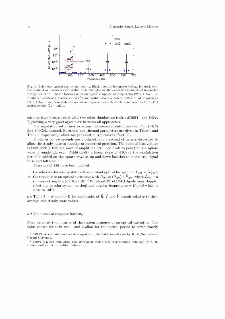
14 Alexandre Sauve, Ludovic Montier
Fig. 4 Bolometer optical excitation linearity. Black lines are bolometer voltage for run1, onlythe modulation harmonics are visible. Blue triangles are the excitation residuals of bolometer
voltage for run2 - run1. Optical excitation signal V appear at frequencies (2k + 1)Ωm ± ω.
Nonlinear excitation harmonics O(V 2) are visible about 5 orders bellow V at frequencies
(2k + 1)Ωm ± 2ω. A modulation nonlinear response is visible at the same level as for O(V 2)at frequencies (2k + 1)Ωm.
outputs have been checked with two other simulations tools : SIMHFI1 and SHDet2, yielding a very good agreement between all approaches.
The simulation setup uses experimental measurements from the Planck/HFIfirst 100GHz channel. Electrical and thermal parameters are given in Table 1 andTable 2 respectively which are provided in Appendices (Sect. C).
Timelines of two seconds are produced, and 1 second of data is discarded toallow the steady state to stabilize at numerical precision. The nominal bias voltageis built with a triangle wave of amplitude vtri (not peak to peak) plus a squarewave of amplitude vsqu. Additionally a linear slope of 4.9% of the modulationperiod is added on the square wave at up and down location to mimic real signalraise and fall time.
Two runs of SEB have been defined :
1. the reference for steady state with a constant optical background Popt = 〈Popt〉;2. the response to an optical excitation with Popt = 〈Popt〉+ Popt, where Popt is a
sin wave of amplitude 9, 6593.10−18W (about 3% of CMB dipole from Dopplereffect due to solar system motion) and angular frequency ω = Ωm/18 which isclose to 10Hz;
see Table 3 in Appendix D for amplitudes of R, T and V signals relative to theiraverage and steady state values.
5.2 Validation of response linearity
First we check the linearity of the system response to an optical excitation. Thevalue chosen for ω in run 1 and 2 allow for the optical period to cover exactly
1 SIMHFI is a simulation tool developed with the LabView software by R. V. Sudiwala atCardiff University
2 SHDet is a fast simulation tool developed with the C programming language by S. R.Hildebrandt at Jet Propulsion Laboratory
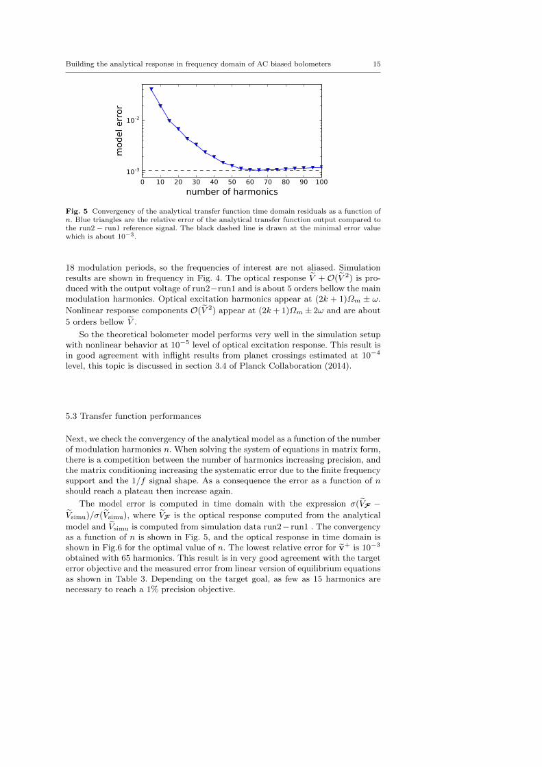
Building the analytical response in frequency domain of AC biased bolometers 15
Fig. 5 Convergency of the analytical transfer function time domain residuals as a function ofn. Blue triangles are the relative error of the analytical transfer function output compared tothe run2 − run1 reference signal. The black dashed line is drawn at the minimal error valuewhich is about 10−3.
18 modulation periods, so the frequencies of interest are not aliased. Simulationresults are shown in frequency in Fig. 4. The optical response V +O(V 2) is pro-duced with the output voltage of run2−run1 and is about 5 orders bellow the mainmodulation harmonics. Optical excitation harmonics appear at (2k + 1)Ωm ± ω.
Nonlinear response components O(V 2) appear at (2k+ 1)Ωm ± 2ω and are about
5 orders bellow V .
So the theoretical bolometer model performs very well in the simulation setupwith nonlinear behavior at 10−5 level of optical excitation response. This result isin good agreement with inflight results from planet crossings estimated at 10−4
level, this topic is discussed in section 3.4 of Planck Collaboration (2014).
5.3 Transfer function performances
Next, we check the convergency of the analytical model as a function of the numberof modulation harmonics n. When solving the system of equations in matrix form,there is a competition between the number of harmonics increasing precision, andthe matrix conditioning increasing the systematic error due to the finite frequencysupport and the 1/f signal shape. As a consequence the error as a function of nshould reach a plateau then increase again.
The model error is computed in time domain with the expression σ(VF −Vsimu)/σ(Vsimu), where VF is the optical response computed from the analytical
model and Vsimu is computed from simulation data run2− run1 . The convergencyas a function of n is shown in Fig. 5, and the optical response in time domain isshown in Fig.6 for the optimal value of n. The lowest relative error for v+ is 10−3
obtained with 65 harmonics. This result is in very good agreement with the targeterror objective and the measured error from linear version of equilibrium equationsas shown in Table 3. Depending on the target goal, as few as 15 harmonics arenecessary to reach a 1% precision objective.
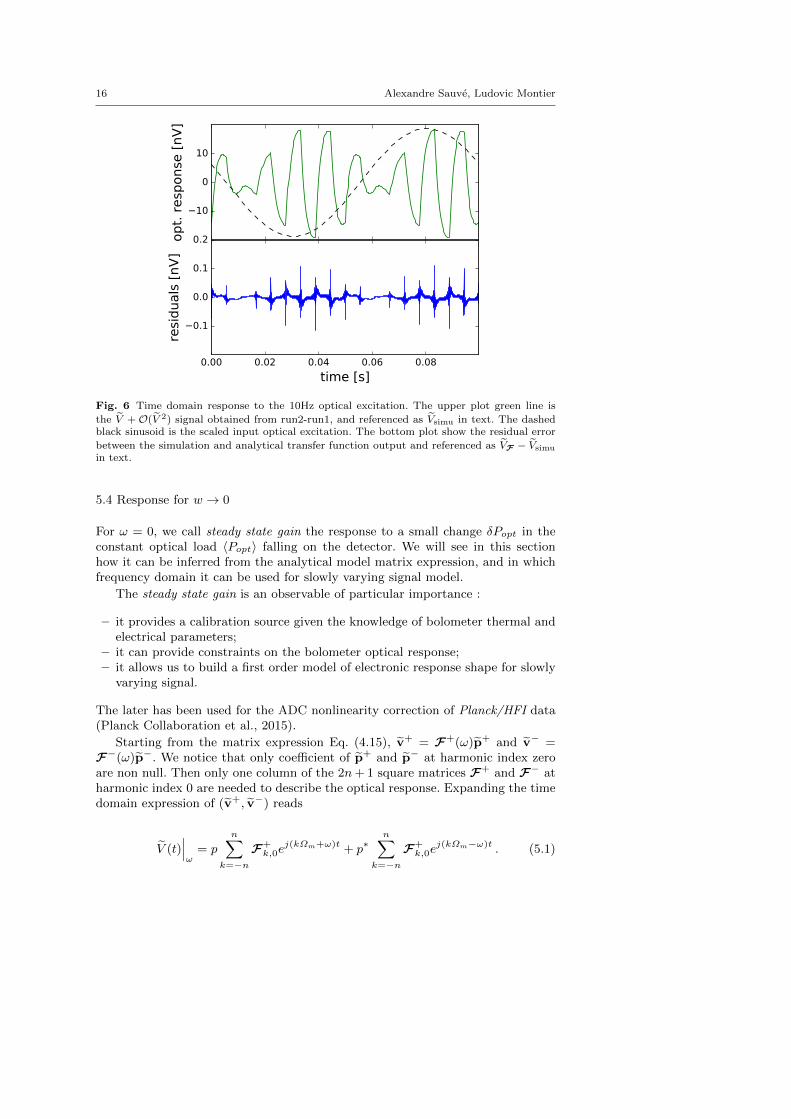
16 Alexandre Sauve, Ludovic Montier
Fig. 6 Time domain response to the 10Hz optical excitation. The upper plot green line is
the V + O(V 2) signal obtained from run2-run1, and referenced as Vsimu in text. The dashedblack sinusoid is the scaled input optical excitation. The bottom plot show the residual error
between the simulation and analytical transfer function output and referenced as VF − Vsimu
in text.
5.4 Response for w → 0
For ω = 0, we call steady state gain the response to a small change δPopt in theconstant optical load 〈Popt〉 falling on the detector. We will see in this sectionhow it can be inferred from the analytical model matrix expression, and in whichfrequency domain it can be used for slowly varying signal model.
The steady state gain is an observable of particular importance :
– it provides a calibration source given the knowledge of bolometer thermal andelectrical parameters;
– it can provide constraints on the bolometer optical response;– it allows us to build a first order model of electronic response shape for slowly
varying signal.
The later has been used for the ADC nonlinearity correction of Planck/HFI data(Planck Collaboration et al., 2015).
Starting from the matrix expression Eq. (4.15), v+ = F+(ω)p+ and v− =F−(ω)p−. We notice that only coefficient of p+ and p− at harmonic index zeroare non null. Then only one column of the 2n+ 1 square matrices F+ and F− atharmonic index 0 are needed to describe the optical response. Expanding the timedomain expression of (v+, v−) reads
V (t)∣∣∣ω
= p
n∑
k=−nF+k,0e
j(kΩm+ω)t + p∗n∑
k=−nF+k,0e
j(kΩm−ω)t . (5.1)
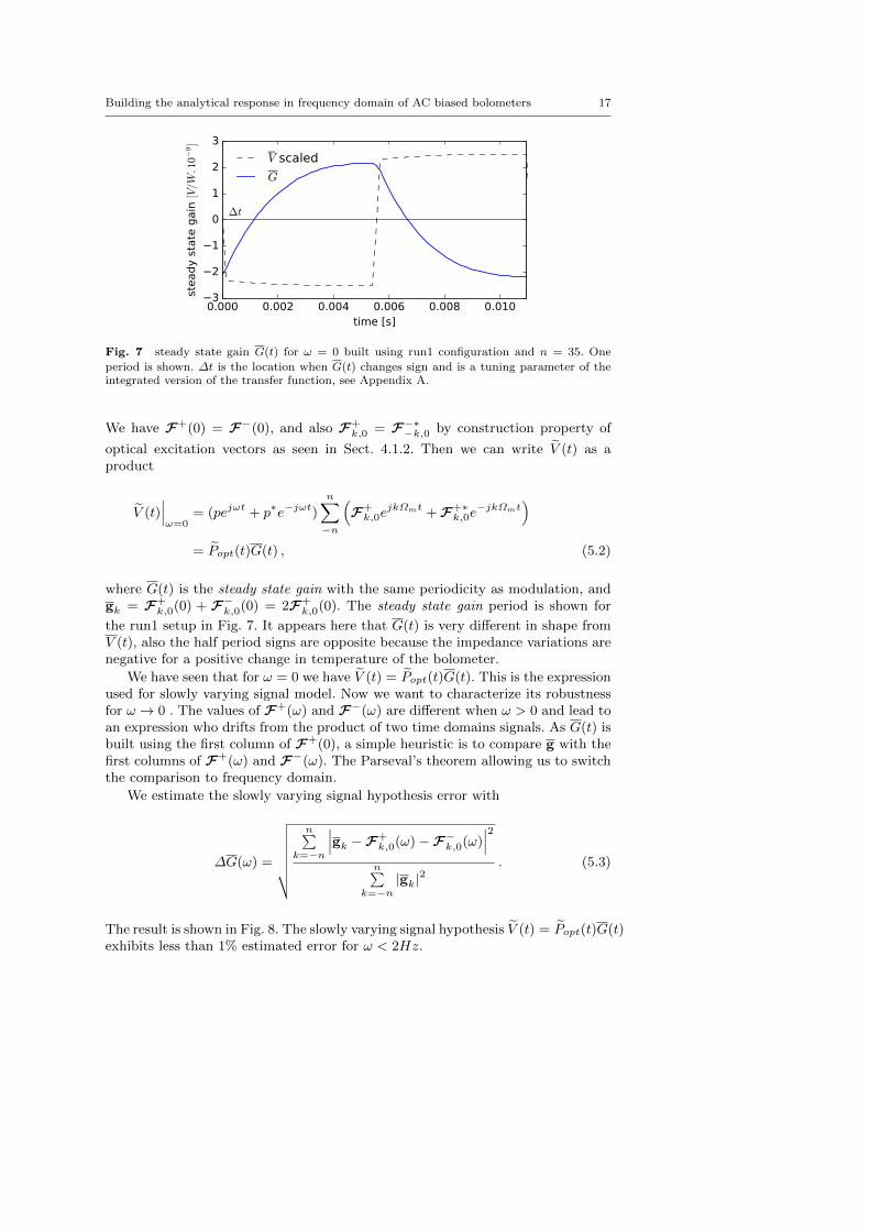
Building the analytical response in frequency domain of AC biased bolometers 17
Fig. 7 steady state gain G(t) for ω = 0 built using run1 configuration and n = 35. One
period is shown. ∆t is the location when G(t) changes sign and is a tuning parameter of theintegrated version of the transfer function, see Appendix A.
We have F+(0) = F−(0), and also F+k,0 = F−∗−k,0 by construction property of
optical excitation vectors as seen in Sect. 4.1.2. Then we can write V (t) as aproduct
V (t)∣∣∣ω=0
= (pejωt + p∗e−jωt)n∑
−n
(F+k,0e
jkΩmt +F+∗k,0e−jkΩmt
)
= Popt(t)G(t) , (5.2)
where G(t) is the steady state gain with the same periodicity as modulation, andgk = F+
k,0(0) + F−k,0(0) = 2F+k,0(0). The steady state gain period is shown for
the run1 setup in Fig. 7. It appears here that G(t) is very different in shape fromV (t), also the half period signs are opposite because the impedance variations arenegative for a positive change in temperature of the bolometer.
We have seen that for ω = 0 we have V (t) = Popt(t)G(t). This is the expressionused for slowly varying signal model. Now we want to characterize its robustnessfor ω → 0 . The values of F+(ω) and F−(ω) are different when ω > 0 and lead toan expression who drifts from the product of two time domains signals. As G(t) isbuilt using the first column of F+(0), a simple heuristic is to compare g with thefirst columns of F+(ω) and F−(ω). The Parseval’s theorem allowing us to switchthe comparison to frequency domain.
We estimate the slowly varying signal hypothesis error with
∆G(ω) =
√√√√√√√
n∑k=−n
∣∣∣gk −F+k,0(ω)−F−k,0(ω)
∣∣∣2
n∑k=−n
|gk|2. (5.3)
The result is shown in Fig. 8. The slowly varying signal hypothesis V (t) = Popt(t)G(t)exhibits less than 1% estimated error for ω < 2Hz.
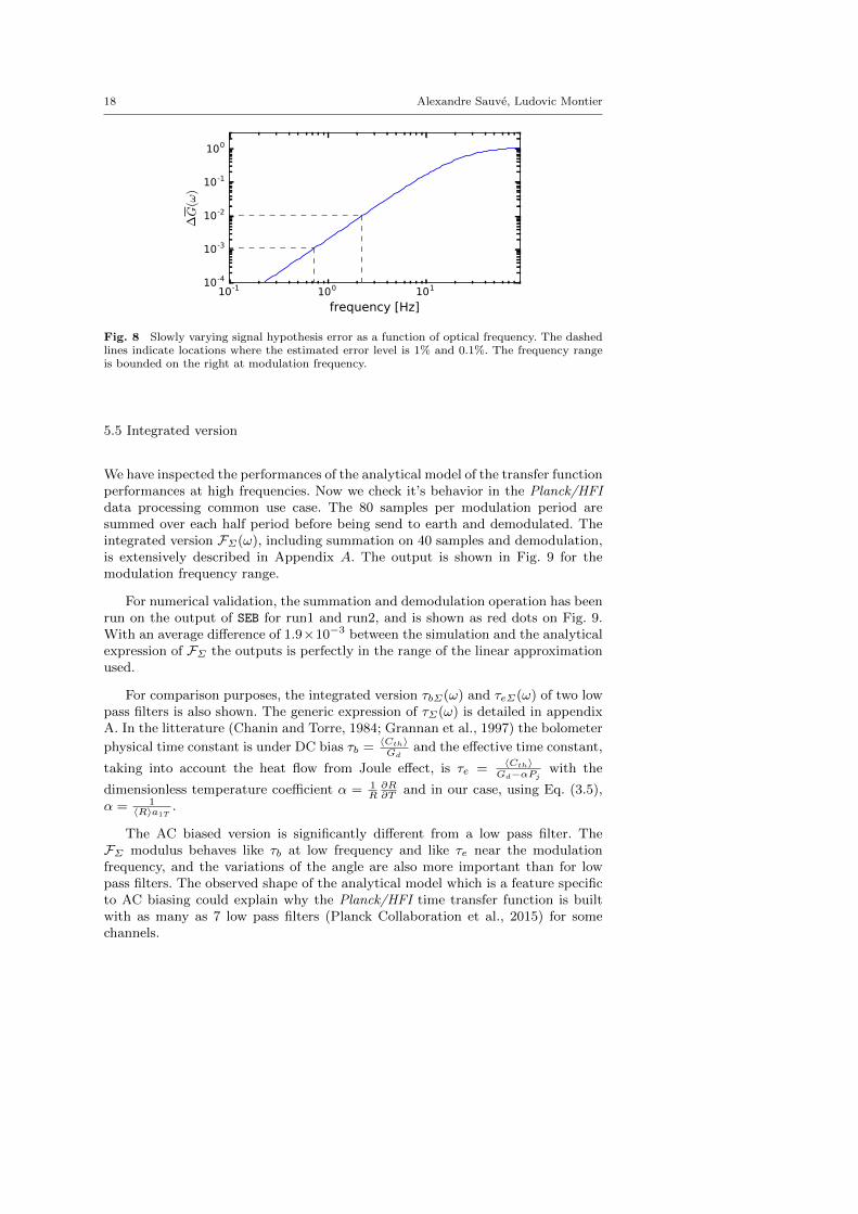
18 Alexandre Sauve, Ludovic Montier
10-1 100 101
frequency [Hz]
10-4
10-3
10-2
10-1
100
∆G(ω)
Fig. 8 Slowly varying signal hypothesis error as a function of optical frequency. The dashedlines indicate locations where the estimated error level is 1% and 0.1%. The frequency rangeis bounded on the right at modulation frequency.
5.5 Integrated version
We have inspected the performances of the analytical model of the transfer functionperformances at high frequencies. Now we check it’s behavior in the Planck/HFIdata processing common use case. The 80 samples per modulation period aresummed over each half period before being send to earth and demodulated. Theintegrated version FΣ(ω), including summation on 40 samples and demodulation,is extensively described in Appendix A. The output is shown in Fig. 9 for themodulation frequency range.
For numerical validation, the summation and demodulation operation has beenrun on the output of SEB for run1 and run2, and is shown as red dots on Fig. 9.With an average difference of 1.9×10⁻³ between the simulation and the analyticalexpression of FΣ the outputs is perfectly in the range of the linear approximationused.
For comparison purposes, the integrated version τbΣ(ω) and τeΣ(ω) of two lowpass filters is also shown. The generic expression of τΣ(ω) is detailed in appendixA. In the litterature (Chanin and Torre, 1984; Grannan et al., 1997) the bolometer
physical time constant is under DC bias τb = 〈Cth〉Gd
and the effective time constant,
taking into account the heat flow from Joule effect, is τe = 〈Cth〉Gd−αPj with the
dimensionless temperature coefficient α = 1R∂R∂T and in our case, using Eq. (3.5),
α = 1〈R〉a1T
.
The AC biased version is significantly different from a low pass filter. TheFΣ modulus behaves like τb at low frequency and like τe near the modulationfrequency, and the variations of the angle are also more important than for lowpass filters. The observed shape of the analytical model which is a feature specificto AC biasing could explain why the Planck/HFI time transfer function is builtwith as many as 7 low pass filters (Planck Collaboration et al., 2015) for somechannels.
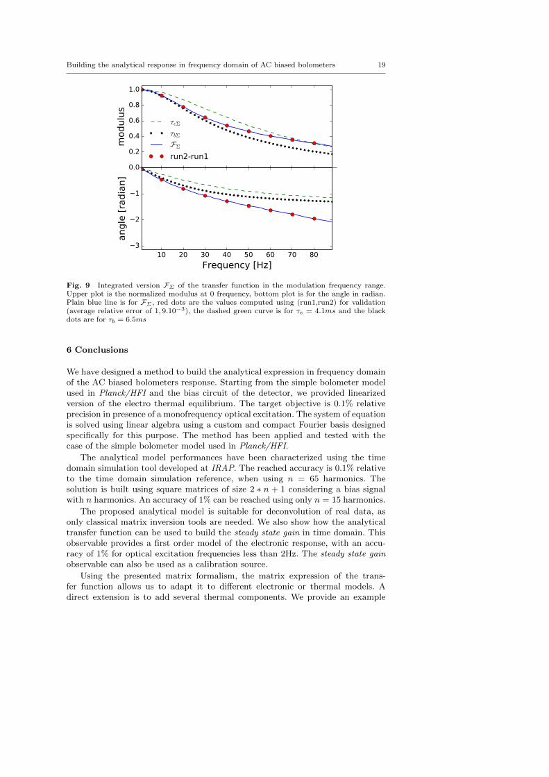
Building the analytical response in frequency domain of AC biased bolometers 19
Fig. 9 Integrated version FΣ of the transfer function in the modulation frequency range.Upper plot is the normalized modulus at 0 frequency, bottom plot is for the angle in radian.Plain blue line is for FΣ , red dots are the values computed using (run1,run2) for validation(average relative error of 1, 9.10−3), the dashed green curve is for τe = 4.1ms and the blackdots are for τb = 6.5ms
6 Conclusions
We have designed a method to build the analytical expression in frequency domainof the AC biased bolometers response. Starting from the simple bolometer modelused in Planck/HFI and the bias circuit of the detector, we provided linearizedversion of the electro thermal equilibrium. The target objective is 0.1% relativeprecision in presence of a monofrequency optical excitation. The system of equationis solved using linear algebra using a custom and compact Fourier basis designedspecifically for this purpose. The method has been applied and tested with thecase of the simple bolometer model used in Planck/HFI.
The analytical model performances have been characterized using the timedomain simulation tool developed at IRAP. The reached accuracy is 0.1% relativeto the time domain simulation reference, when using n = 65 harmonics. Thesolution is built using square matrices of size 2 ∗ n + 1 considering a bias signalwith n harmonics. An accuracy of 1% can be reached using only n = 15 harmonics.
The proposed analytical model is suitable for deconvolution of real data, asonly classical matrix inversion tools are needed. We also show how the analyticaltransfer function can be used to build the steady state gain in time domain. Thisobservable provides a first order model of the electronic response, with an accu-racy of 1% for optical excitation frequencies less than 2Hz. The steady state gainobservable can also be used as a calibration source.
Using the presented matrix formalism, the matrix expression of the trans-fer function allows us to adapt it to different electronic or thermal models. Adirect extension is to add several thermal components. We provide an example

20 Alexandre Sauve, Ludovic Montier
with one thermal component. While the Planck/HFI low frequency components oftime transfer function still need some improvement when writing this article. Thegeneric form of the proposed model is designed as a tool which can be used to getbetter constraints through the measured optical response and the completely newaddition of the steady state gain. Finally, the analytical transfer function modelallow to build a signal model with high resolution in time domain. This propertyis needed to build an improved ADC nonlinearity correction for Planck/HFI, seeSauve et al. (2016) (SPIE proceeding in preparation).
Appendices
A Integrated transfer function
This appendix describes the integration/downsampling of the electronic signal asdone by the onboard Data Processing Unit of Planck/HFI. The correspondingintegrated version of the transfer function FΣ(ω) will be built from the matrixformalism described in this paper. The filtering applied by the readout amplifi-cation chain and the rejection filter is described in the Planck/HFI timeresponsepaper by Planck Collaboration (2014) and will not be considered here.
The data sent to earth at rate 2fmod = 180.3737 Hz is the sum of N =40 samples per modulation half period. And the real onboard data acquisitionfrequency is 2fmod ∗N = 7214.948 Hz before the Data Processing Unit make thesummation. We will start by applying the summation process to a sinusoidal wavedescribed by
s(t) = ejωt , (A.1)
where t has the same origin as the filtered optical signal.
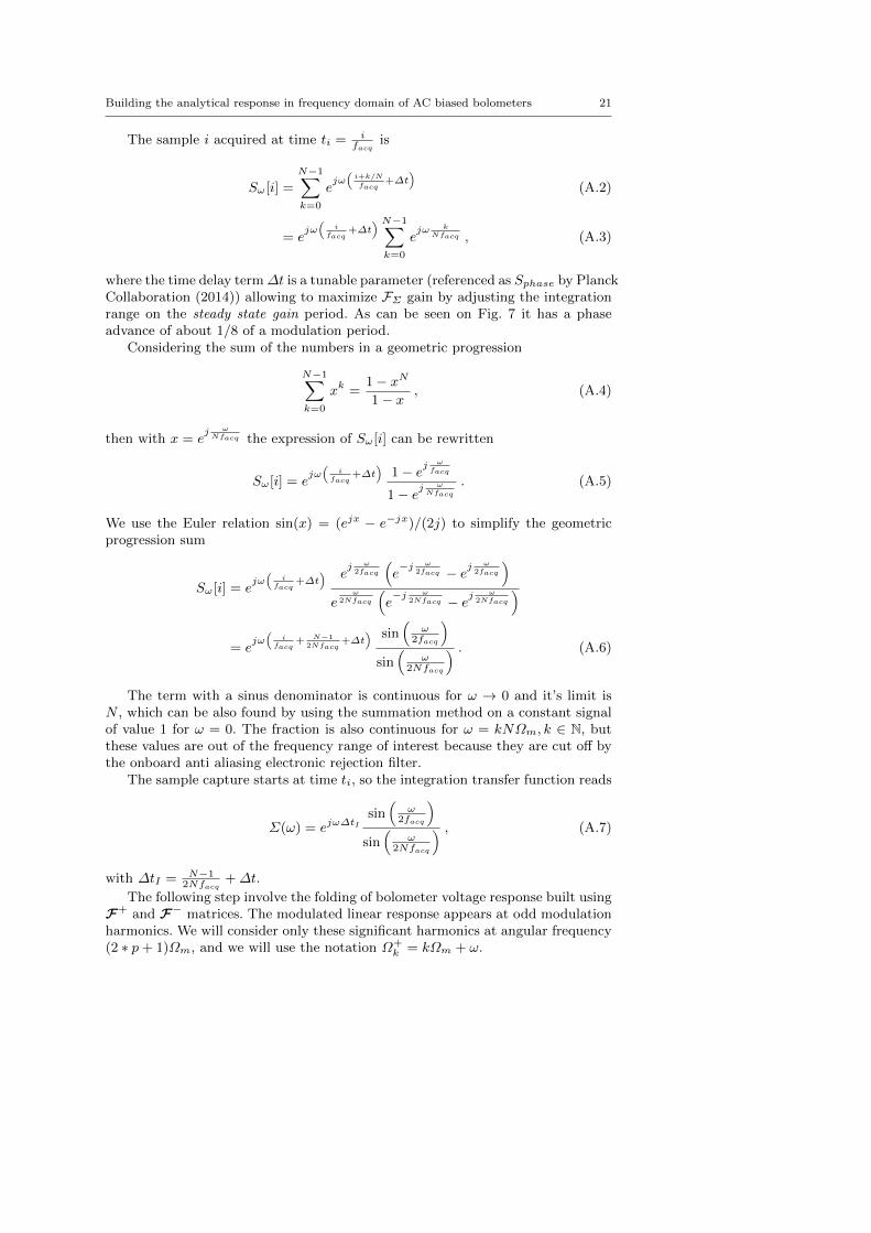
Building the analytical response in frequency domain of AC biased bolometers 21
The sample i acquired at time ti = ifacq
is
Sω[i] =
N−1∑
k=0
ejω(i+k/N
facq+∆t
)
(A.2)
= ejω(
ifacq
+∆t) N−1∑
k=0
ejω k
Nfacq , (A.3)
where the time delay term∆t is a tunable parameter (referenced as Sphase by PlanckCollaboration (2014)) allowing to maximize FΣ gain by adjusting the integrationrange on the steady state gain period. As can be seen on Fig. 7 it has a phaseadvance of about 1/8 of a modulation period.
Considering the sum of the numbers in a geometric progression
N−1∑
k=0
xk =1− xN1− x , (A.4)
then with x = ej ωNfacq the expression of Sω[i] can be rewritten
Sω[i] = ejω(
ifacq
+∆t)
1− ejω
facq
1− ejω
Nfacq
. (A.5)
We use the Euler relation sin(x) = (ejx − e−jx)/(2j) to simplify the geometricprogression sum
Sω[i] = ejω(
ifacq
+∆t) e
j ω2facq
(e−j ω
2facq − ejω
2facq
)
eω
2Nfacq
(e−j ω
2Nfacq − ejω
2Nfacq
)
= ejω(
ifacq
+ N−12Nfacq
+∆t) sin
(ω
2facq
)
sin(
ω2Nfacq
) . (A.6)
The term with a sinus denominator is continuous for ω → 0 and it’s limit isN , which can be also found by using the summation method on a constant signalof value 1 for ω = 0. The fraction is also continuous for ω = kNΩm, k ∈ N, butthese values are out of the frequency range of interest because they are cut off bythe onboard anti aliasing electronic rejection filter.
The sample capture starts at time ti, so the integration transfer function reads
Σ(ω) = ejω∆tIsin(
ω2facq
)
sin(
ω2Nfacq
) , (A.7)
with ∆tI = N−12Nfacq
+∆t.
The following step involve the folding of bolometer voltage response built usingF+ and F− matrices. The modulated linear response appears at odd modulationharmonics. We will consider only these significant harmonics at angular frequency(2 ∗ p+ 1)Ωm, and we will use the notation Ω+
k = kΩm + ω.

22 Alexandre Sauve, Ludovic Montier
Let consider the complex optical excitation power on the bolometer
P (t) = ejωt . (A.8)
then, using the matrix formalism developped in Sect. 4.1 only one vector is neededto represent it with p+ = [1, 0 · · · ]. And the complex output voltage is
V (t) =
p≤n−12∑
p≥−n+12
k=2p+1
F+k,0e
jΩ+k t . (A.9)
The acquisition of summed samples at time ti for odd modulation harmonics folds
the signals so zejΩ+k ti = z∗ej(Ωm−ω)ti . The folded version of output voltage at
facq sampling frequency is
V (ti) =
p≤n−12∑
p≥−n+12
k=2p+1
F+∗k,0Σ
∗(Ω+k )ej(Ωm−ω)ti . (A.10)
The signal is demodulated by applying a e−jΩmt factor and taking the conjugateof the result to get a positive frequency, so we have
Vd(ti) =
p≤n−12∑
p≥−n+12
k=2p+1
F+k,0Σ(Ω+
k )ejωti . (A.11)
The signal described with this expression integrates N samples from time tiand has a time offset of ∆tI appearing in Eq. (A.7) compared to input signal. Thetime offset can be corrected to obtain the final causal version of the integratedtransfer function
FΣ(ω) =
p≤n−12∑
p≥−n+12
k=2p+1
F+k,0Σ(Ω+
k )e−jω∆tI . (A.12)
The bolometer under DC current bias behaves as an order 1 low pass filterwhich can be written
T (w) =1
1 + jωτ, (A.13)
where τ is the time constant of the filter. For comparison purposes we can applythe sampling summation process on T (w). There is no demodulation in this caseand we have τΣ(ω) = Σ(ω)T (ω)e−jω∆tI . As there is no modulated harmonics thetime offset ∆tI cancels with the one in Σ(ω) so we have
τΣ(ω) = T (ω)sin(
ω2facq
)
sin(
ω2Nfacq
) . (A.14)
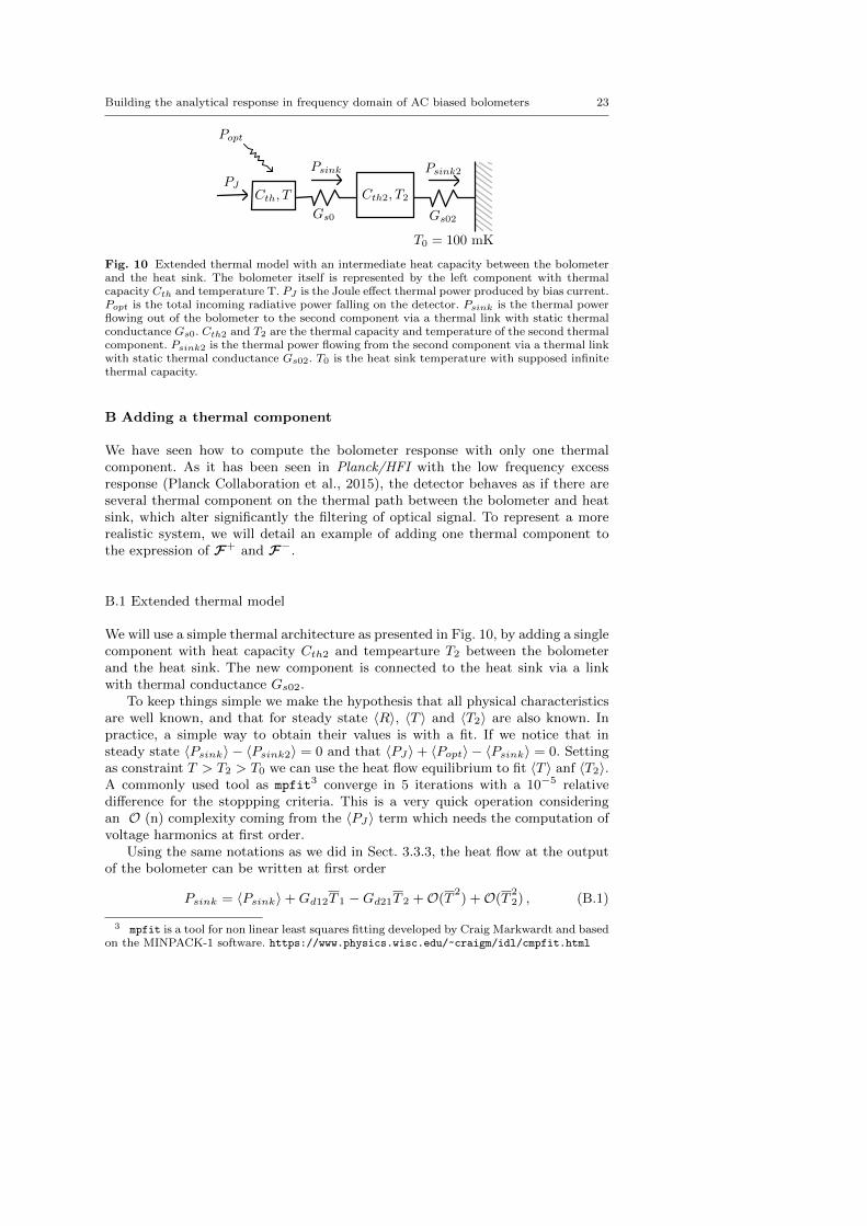
Building the analytical response in frequency domain of AC biased bolometers 23
Fig. 10 Extended thermal model with an intermediate heat capacity between the bolometerand the heat sink. The bolometer itself is represented by the left component with thermalcapacity Cth and temperature T. PJ is the Joule effect thermal power produced by bias current.Popt is the total incoming radiative power falling on the detector. Psink is the thermal powerflowing out of the bolometer to the second component via a thermal link with static thermalconductance Gs0. Cth2 and T2 are the thermal capacity and temperature of the second thermalcomponent. Psink2 is the thermal power flowing from the second component via a thermal linkwith static thermal conductance Gs02. T0 is the heat sink temperature with supposed infinitethermal capacity.
B Adding a thermal component
We have seen how to compute the bolometer response with only one thermalcomponent. As it has been seen in Planck/HFI with the low frequency excessresponse (Planck Collaboration et al., 2015), the detector behaves as if there areseveral thermal component on the thermal path between the bolometer and heatsink, which alter significantly the filtering of optical signal. To represent a morerealistic system, we will detail an example of adding one thermal component tothe expression of F+ and F−.
B.1 Extended thermal model
We will use a simple thermal architecture as presented in Fig. 10, by adding a singlecomponent with heat capacity Cth2 and tempearture T2 between the bolometerand the heat sink. The new component is connected to the heat sink via a linkwith thermal conductance Gs02.
To keep things simple we make the hypothesis that all physical characteristicsare well known, and that for steady state 〈R〉, 〈T 〉 and 〈T2〉 are also known. Inpractice, a simple way to obtain their values is with a fit. If we notice that insteady state 〈Psink〉 − 〈Psink2〉 = 0 and that 〈PJ〉+ 〈Popt〉 − 〈Psink〉 = 0. Settingas constraint T > T2 > T0 we can use the heat flow equilibrium to fit 〈T 〉 anf 〈T2〉.A commonly used tool as mpfit3 converge in 5 iterations with a 10−5 relativedifference for the stoppping criteria. This is a very quick operation consideringan O (n) complexity coming from the 〈PJ〉 term which needs the computation ofvoltage harmonics at first order.
Using the same notations as we did in Sect. 3.3.3, the heat flow at the outputof the bolometer can be written at first order
Psink = 〈Psink〉+Gd12T 1 −Gd21T 2 +O(T2) +O(T
22) , (B.1)
3 mpfit is a tool for non linear least squares fitting developed by Craig Markwardt and basedon the MINPACK-1 software. https://www.physics.wisc.edu/~craigm/idl/cmpfit.html
24 Alexandre Sauve, Ludovic Montier
with
Gd12 = ∂Psink∂T
∣∣T=〈T 〉 = Gs01
Tβref〈T 〉β
Gd21 = − ∂Psink∂T2
∣∣∣T2=〈T2〉
= Gs01Tβref〈T2〉β .
(B.2)
The second thermal component on the thermal path can be characterized atfirst order by
Cth2 = C02Tγ2
2 = 〈Cth2〉+O(T 2)
Psink2 = 〈Psink〉+Gd2T 2 +O(T22) ,
(B.3)
with
Gd2 =∂Psink2∂T2
=Gs02〈T2〉β2
Tβ2
ref
, (B.4)
where 〈Cth2〉,Gs02 and β2 are free parameters. We neglect 〈Cth2〉 variations forthe following developments.
And the thermal equilibrium for the second component reads at first order
Cth2T2 = Psink − Psink2〈Cth2〉T 2 = Gd12T − (Gd21 +Gd2)T 2 +O(T ) . (B.5)
B.2 Extended steady state
The first iteration for v is the same as in Sect. 4.2 because we only need to know〈R〉.
With the second component, its steady state temperature vector t2 is neededfor the thermal equilibrium of the bolometer. t2 can be expressed from r using thethermal equilibrium Eq. (B.5), then it comes
t2 = X2r
X2 = [〈Cth2〉D + (Gd21 +Gd2)Id]−1Gd12a1T , (B.6)
where t2 is the intermediate steady state vector for T 2.
And finally the expression of r can be written from the single thermal compo-nent version Eq. (4.11) by updating the Psink term
r =
[〈Cth〉a1TD +
C(C(v).dot(v))
〈R〉2 +Gd12a1T Id −Gd21X2
]−1 [C(v)v
〈R〉 − 〈Psink〉+ 〈Popt〉],
(B.7)
Once r is obtained, a second iteration can be done as in Sect. 4.2 to get v witha better precision.
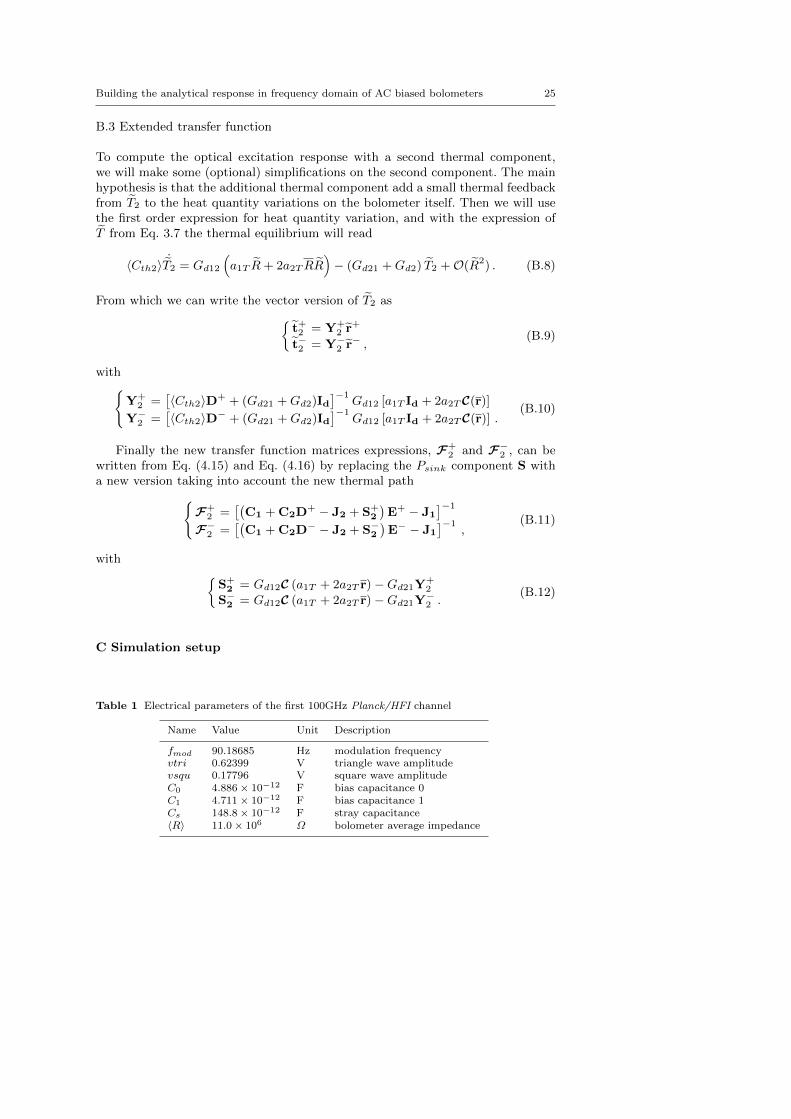
Building the analytical response in frequency domain of AC biased bolometers 25
B.3 Extended transfer function
To compute the optical excitation response with a second thermal component,we will make some (optional) simplifications on the second component. The mainhypothesis is that the additional thermal component add a small thermal feedbackfrom T2 to the heat quantity variations on the bolometer itself. Then we will usethe first order expression for heat quantity variation, and with the expression ofT from Eq. 3.7 the thermal equilibrium will read
〈Cth2〉 ˙T2 = Gd12
(a1T R+ 2a2TRR
)− (Gd21 +Gd2) T2 +O(R2) . (B.8)
From which we can write the vector version of T2 as
t+2 = Y+
2 r+
t−2 = Y−2 r− ,(B.9)
with
Y+2 =
[〈Cth2〉D+ + (Gd21 +Gd2)Id
]−1Gd12 [a1T Id + 2a2TC(r)]
Y−2 =[〈Cth2〉D− + (Gd21 +Gd2)Id
]−1Gd12 [a1T Id + 2a2TC(r)] .
(B.10)
Finally the new transfer function matrices expressions, F+2 and F−2 , can be
written from Eq. (4.15) and Eq. (4.16) by replacing the Psink component S witha new version taking into account the new thermal path
F+
2 =[(
C1 + C2D+ − J2 + S+2
)E+ − J1
]−1
F−2 =[(
C1 + C2D− − J2 + S−2)E− − J1
]−1,
(B.11)
with
S+2 = Gd12C (a1T + 2a2T r)−Gd21Y+
2
S−2 = Gd12C (a1T + 2a2T r)−Gd21Y−2 .(B.12)
C Simulation setup
Table 1 Electrical parameters of the first 100GHz Planck/HFI channel
Name Value Unit Description
fmod 90.18685 Hz modulation frequencyvtri 0.62399 V triangle wave amplitudevsqu 0.17796 V square wave amplitudeC0 4.886× 10⁻¹² F bias capacitance 0C1 4.711× 10⁻¹² F bias capacitance 1Cs 148.8× 10⁻¹² F stray capacitance〈R〉 11.0× 10⁶ Ω bolometer average impedance
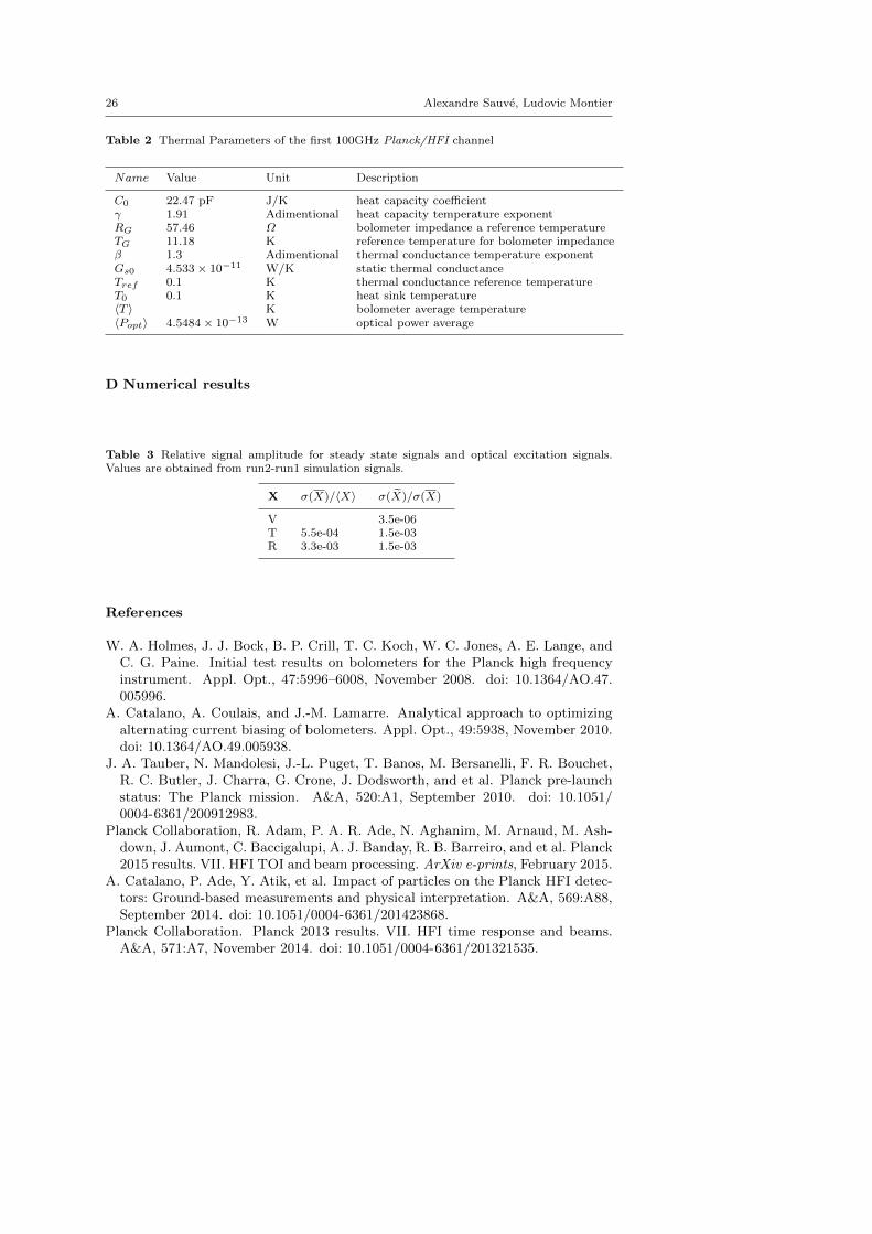
26 Alexandre Sauve, Ludovic Montier
Table 2 Thermal Parameters of the first 100GHz Planck/HFI channel
Name Value Unit Description
C0 22.47 pF J/K heat capacity coefficientγ 1.91 Adimentional heat capacity temperature exponentRG 57.46 Ω bolometer impedance a reference temperatureTG 11.18 K reference temperature for bolometer impedanceβ 1.3 Adimentional thermal conductance temperature exponentGs0 4.533× 10⁻¹¹ W/K static thermal conductanceTref 0.1 K thermal conductance reference temperatureT0 0.1 K heat sink temperature〈T 〉 K bolometer average temperature〈Popt〉 4.5484× 10⁻¹³ W optical power average
D Numerical results
Table 3 Relative signal amplitude for steady state signals and optical excitation signals.Values are obtained from run2-run1 simulation signals.
X σ(X)/〈X〉 σ(X)/σ(X)
V 3.5e-06T 5.5e-04 1.5e-03R 3.3e-03 1.5e-03
References
W. A. Holmes, J. J. Bock, B. P. Crill, T. C. Koch, W. C. Jones, A. E. Lange, andC. G. Paine. Initial test results on bolometers for the Planck high frequencyinstrument. Appl. Opt., 47:5996–6008, November 2008. doi: 10.1364/AO.47.005996.
A. Catalano, A. Coulais, and J.-M. Lamarre. Analytical approach to optimizingalternating current biasing of bolometers. Appl. Opt., 49:5938, November 2010.doi: 10.1364/AO.49.005938.
J. A. Tauber, N. Mandolesi, J.-L. Puget, T. Banos, M. Bersanelli, F. R. Bouchet,R. C. Butler, J. Charra, G. Crone, J. Dodsworth, and et al. Planck pre-launchstatus: The Planck mission. A&A, 520:A1, September 2010. doi: 10.1051/0004-6361/200912983.
Planck Collaboration, R. Adam, P. A. R. Ade, N. Aghanim, M. Arnaud, M. Ash-down, J. Aumont, C. Baccigalupi, A. J. Banday, R. B. Barreiro, and et al. Planck2015 results. VII. HFI TOI and beam processing. ArXiv e-prints, February 2015.
A. Catalano, P. Ade, Y. Atik, et al. Impact of particles on the Planck HFI detec-tors: Ground-based measurements and physical interpretation. A&A, 569:A88,September 2014. doi: 10.1051/0004-6361/201423868.
Planck Collaboration. Planck 2013 results. VII. HFI time response and beams.A&A, 571:A7, November 2014. doi: 10.1051/0004-6361/201321535.
Building the analytical response in frequency domain of AC biased bolometers 27
J.-M. Lamarre, J.-L. Puget, P. A. R. Ade, et al. Planck pre-launch status: The HFIinstrument, from specification to actual performance. A&A, 520:A9, September2010. doi: 10.1051/0004-6361/200912975.
Ludovic Montier. Planck : De l’etalonnage de l’instrument a l’etude des poussieresgalactiques et intergalactiques. Theses, Universite Toulouse III, Paul Sabatier -Toulouse, September 2005.
Michel Piat. Contributions a la definition des besoins scientifiques et des solutionsinstrumentales du projet Planck-HFI. Theses, Universite Paris Sud - Paris XI,October 2000. URL https://tel.archives-ouvertes.fr/tel-00004038.
Michel Piat, Jean-Pierre Torre, Eric Breelle, Alain Coulais, Adam Woodcraft,Warren Holmes, and Rashmi Sudiwala. Modeling of planck-high frequencyinstrument bolometers using non-linear effects in the thermometers. NuclearInstruments and Methods in Physics Research Section A: Accelerators, Spec-trometers, Detectors and Associated Equipment, 559(2):588 – 590, 2006. ISSN0168-9002. doi: http://dx.doi.org/10.1016/j.nima.2005.12.076. URL http://
www.sciencedirect.com/science/article/pii/S0168900205025027. Proceed-ings of the 11th International Workshop on Low Temperature DetectorsLTD-1111th International Workshop on Low Temperature Detectors.
John C. Mather. Bolometers: ultimate sensitivity, optimization, and amplifiercoupling. Appl. Opt., 23(4):584–588, Feb 1984. doi: 10.1364/AO.23.000584.URL http://ao.osa.org/abstract.cfm?URI=ao-23-4-584.
John C. Mather. Bolometer noise: nonequilibrium theory. Appl. Opt., 21(6):1125–1129, Mar 1982. doi: 10.1364/AO.21.001125. URL http://ao.osa.org/
abstract.cfm?URI=ao-21-6-1125.G. Chanin and J. P. Torre. Electrothermal model for ideal semiconductor bolome-
ters. J. Opt. Soc. Am. A, 1(4):412–419, Apr 1984. doi: 10.1364/JOSAA.1.000412. URL http://josaa.osa.org/abstract.cfm?URI=josaa-1-4-412.
S. M. Grannan, P. L. Richards, and M. K. Hase. Numerical optimization of bolo-metric infrared detectors including optical loading, amplifier noise, and elec-trical nonlinearities. International Journal of Infrared and Millimeter Waves,18(2):319–340, 1997. ISSN 1572-9559. doi: 10.1007/BF02677923. URL http:
//dx.doi.org/10.1007/BF02677923.A. Sauve, Couchot F., Patanchon G., and Montier L. Inflight characterization
and correction of the planck hfi analog to digital converter nonlinearity. InSPIE Astronomical Telescopes + Instrumentation (AS16), volume 9914-119 ofProc. SPIE, 2016.

263
Appendix B
SPIE Astronomical Telescope +Instrumentation proceeding
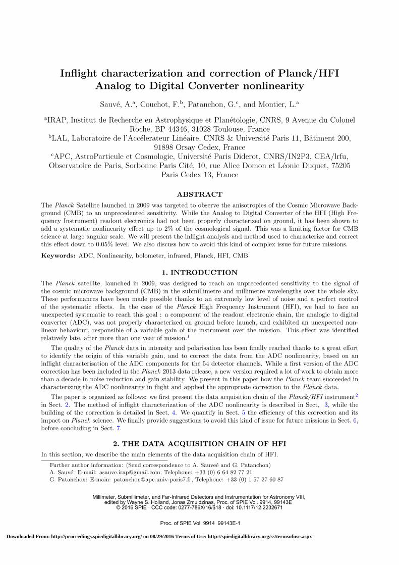
Inflight characterization and correction of Planck/HFIAnalog to Digital Converter nonlinearity
Sauve, A.a, Couchot, F.b, Patanchon, G.c, and Montier, L.a
aIRAP, Institut de Recherche en Astrophysique et Planetologie, CNRS, 9 Avenue du ColonelRoche, BP 44346, 31028 Toulouse, France
bLAL, Laboratoire de l’Accelerateur Lineaire, CNRS & Universite Paris 11, Batiment 200,91898 Orsay Cedex, France
cAPC, AstroParticule et Cosmologie, Universite Paris Diderot, CNRS/IN2P3, CEA/lrfu,Observatoire de Paris, Sorbonne Paris Cite, 10, rue Alice Domon et Leonie Duquet, 75205
Paris Cedex 13, France
ABSTRACT
The Planck Satellite launched in 2009 was targeted to observe the anisotropies of the Cosmic Microwave Back-ground (CMB) to an unprecedented sensitivity. While the Analog to Digital Converter of the HFI (High Fre-quency Instrument) readout electronics had not been properly characterized on ground, it has been shown toadd a systematic nonlinearity effect up to 2% of the cosmological signal. This was a limiting factor for CMBscience at large angular scale. We will present the inflight analysis and method used to characterize and correctthis effect down to 0.05% level. We also discuss how to avoid this kind of complex issue for future missions.
Keywords: ADC, Nonlinearity, bolometer, infrared, Planck, HFI, CMB
1. INTRODUCTION
The Planck satellite, launched in 2009, was designed to reach an unprecedented sensitivity to the signal ofthe cosmic microwave background (CMB) in the submillimetre and millimetre wavelengths over the whole sky.These performances have been made possible thanks to an extremely low level of noise and a perfect controlof the systematic effects. In the case of the Planck High Frequency Instrument (HFI), we had to face anunexpected systematic to reach this goal : a component of the readout electronic chain, the analogic to digitalconverter (ADC), was not properly characterized on ground before launch, and exhibited an unexpected non-linear behaviour, responsible of a variable gain of the instrument over the mission. This effect was identifiedrelatively late, after more than one year of mission.1
The quality of the Planck data in intensity and polarisation has been finally reached thanks to a great effortto identify the origin of this variable gain, and to correct the data from the ADC nonlinearity, based on aninflight characterisation of the ADC components for the 54 detector channels. While a first version of the ADCcorrection has been included in the Planck 2013 data release, a new version required a lot of work to obtain morethan a decade in noise reduction and gain stability. We present in this paper how the Planck team succeeded incharacterizing the ADC nonlinearity in flight and applied the appropriate correction to the Planck data.
The paper is organized as follows: we first present the data acquisition chain of the Planck/HFI instrument2
in Sect. 2. The method of inflight characterization of the ADC nonlinearity is described in Sect, 3, while thebuilding of the correction is detailed in Sect. 4. We quantify in Sect. 5 the efficiency of this correction and itsimpact on Planck science. We finally provide suggestions to avoid this kind of issue for future missions in Sect. 6,before concluding in Sect. 7.
2. THE DATA ACQUISITION CHAIN OF HFI
In this section, we describe the main elements of the data acquisition chain of HFI.
Further author information: (Send correspondence to A. Sauvee and G. Patanchon)A. Sauve: E-mail: [email protected], Telephone: +33 (0) 6 64 82 77 21G. Patanchon: E-main: [email protected], Telephone: +33 (0) 1 57 27 60 87
Millimeter, Submillimeter, and Far-Infrared Detectors and Instrumentation for Astronomy VIII, edited by Wayne S. Holland, Jonas Zmuidzinas, Proc. of SPIE Vol. 9914, 99143E
© 2016 SPIE · CCC code: 0277-786X/16/$18 · doi: 10.1117/12.2232671
Proc. of SPIE Vol. 9914 99143E-1
Downloaded From: http://proceedings.spiedigitallibrary.org/ on 08/29/2016 Terms of Use: http://spiedigitallibrary.org/ss/termsofuse.aspx
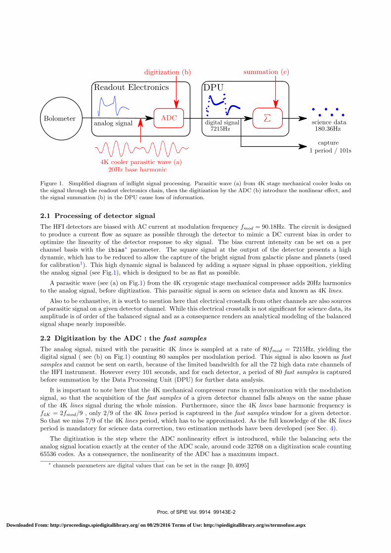
Figure 1. Simplified diagram of inflight signal processing. Parasitic wave (a) from 4K stage mechanical cooler leaks onthe signal through the readout electronics chain, then the digitization by the ADC (b) introduce the nonlinear effect, andthe signal summation (b) in the DPU cause loss of information.
2.1 Processing of detector signal
The HFI detectors are biased with AC current at modulation frequency fmod = 90.18Hz. The circuit is designedto produce a current flow as square as possible through the detector to mimic a DC current bias in order tooptimize the linearity of the detector response to sky signal. The bias current intensity can be set on a perchannel basis with the ibias∗ parameter. The square signal at the output of the detector presents a highdynamic, which has to be reduced to allow the capture of the bright signal from galactic plane and planets (usedfor calibration1). This high dynamic signal is balanced by adding a square signal in phase opposition, yieldingthe analog signal (see Fig.1), which is designed to be as flat as possible.
A parasitic wave (see (a) on Fig.1) from the 4K cryogenic stage mechanical compressor adds 20Hz harmonicsto the analog signal, before digitization. This parasitic signal is seen on science data and known as 4K lines.
Also to be exhaustive, it is worth to mention here that electrical crosstalk from other channels are also sourcesof parasitic signal on a given detector channel. While this electrical crosstalk is not significant for science data, itsamplitude is of order of the balanced signal and as a consequence renders an analytical modeling of the balancedsignal shape nearly impossible.
2.2 Digitization by the ADC : the fast samples
The analog signal, mixed with the parasitic 4K lines is sampled at a rate of 80fmod = 7215Hz, yielding thedigital signal ( see (b) on Fig.1) counting 80 samples per modulation period. This signal is also known as fastsamples and cannot be sent on earth, because of the limited bandwidth for all the 72 high data rate channels ofthe HFI instrument. However every 101 seconds, and for each detector, a period of 80 fast samples is capturedbefore summation by the Data Processing Unit (DPU) for further data analysis.
It is important to note here that the 4K mechanical compressor runs in synchronization with the modulationsignal, so that the acquisition of the fast samples of a given detector channel falls always on the same phaseof the 4K lines signal during the whole mission. Furthermore, since the 4K lines base harmonic frequency isf4K = 2fmod/9 , only 2/9 of the 4K lines period is captureed in the fast samples window for a given detector.So that we miss 7/9 of the 4K lines period, which has to be approximated. As the full knowledge of the 4K linesperiod is mandatory for science data correction, two estimation methods have been developed (see Sec. 4).
The digitization is the step where the ADC nonlinearity effect is introduced, while the balancing sets theanalog signal location exactly at the center of the ADC scale, around code 32768 on a digitization scale counting65536 codes. As a consequence, the nonlinearity of the ADC has a maximum impact.
∗ channels parameters are digital values that can be set in the range J0, 4095K
Proc. of SPIE Vol. 9914 99143E-2
Downloaded From: http://proceedings.spiedigitallibrary.org/ on 08/29/2016 Terms of Use: http://spiedigitallibrary.org/ss/termsofuse.aspx
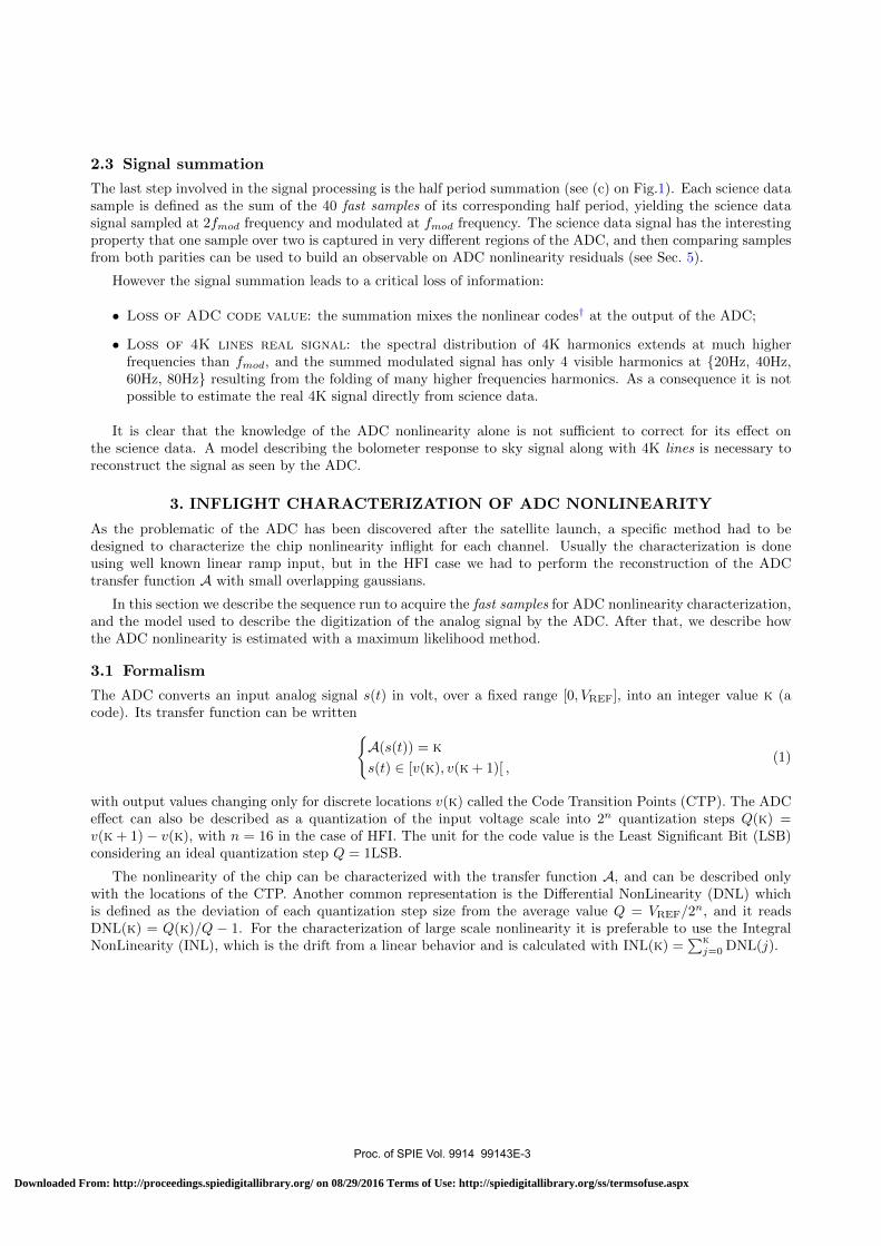
2.3 Signal summation
The last step involved in the signal processing is the half period summation (see (c) on Fig.1). Each science datasample is defined as the sum of the 40 fast samples of its corresponding half period, yielding the science datasignal sampled at 2fmod frequency and modulated at fmod frequency. The science data signal has the interestingproperty that one sample over two is captured in very different regions of the ADC, and then comparing samplesfrom both parities can be used to build an observable on ADC nonlinearity residuals (see Sec. 5).
However the signal summation leads to a critical loss of information:
• Loss of ADC code value: the summation mixes the nonlinear codes† at the output of the ADC;
• Loss of 4K lines real signal: the spectral distribution of 4K harmonics extends at much higherfrequencies than fmod, and the summed modulated signal has only 4 visible harmonics at 20Hz, 40Hz,60Hz, 80Hz resulting from the folding of many higher frequencies harmonics. As a consequence it is notpossible to estimate the real 4K signal directly from science data.
It is clear that the knowledge of the ADC nonlinearity alone is not sufficient to correct for its effect onthe science data. A model describing the bolometer response to sky signal along with 4K lines is necessary toreconstruct the signal as seen by the ADC.
3. INFLIGHT CHARACTERIZATION OF ADC NONLINEARITY
As the problematic of the ADC has been discovered after the satellite launch, a specific method had to bedesigned to characterize the chip nonlinearity inflight for each channel. Usually the characterization is doneusing well known linear ramp input, but in the HFI case we had to perform the reconstruction of the ADCtransfer function A with small overlapping gaussians.
In this section we describe the sequence run to acquire the fast samples for ADC nonlinearity characterization,and the model used to describe the digitization of the analog signal by the ADC. After that, we describe howthe ADC nonlinearity is estimated with a maximum likelihood method.
3.1 Formalism
The ADC converts an input analog signal s(t) in volt, over a fixed range [0, VREF], into an integer value k (acode). Its transfer function can be written
A(s(t)) = k
s(t) ∈ [v(k), v(k + 1)[ ,(1)
with output values changing only for discrete locations v(k) called the Code Transition Points (CTP). The ADCeffect can also be described as a quantization of the input voltage scale into 2n quantization steps Q(k) =v(k + 1)− v(k), with n = 16 in the case of HFI. The unit for the code value is the Least Significant Bit (LSB)considering an ideal quantization step Q = 1LSB.
The nonlinearity of the chip can be characterized with the transfer function A, and can be described onlywith the locations of the CTP. Another common representation is the Differential NonLinearity (DNL) whichis defined as the deviation of each quantization step size from the average value Q = VREF/2
n, and it readsDNL(k) = Q(k)/Q − 1. For the characterization of large scale nonlinearity it is preferable to use the IntegralNonLinearity (INL), which is the drift from a linear behavior and is calculated with INL(k) =
∑kj=0 DNL(j).
Proc. of SPIE Vol. 9914 99143E-3
Downloaded From: http://proceedings.spiedigitallibrary.org/ on 08/29/2016 Terms of Use: http://spiedigitallibrary.org/ss/termsofuse.aspx
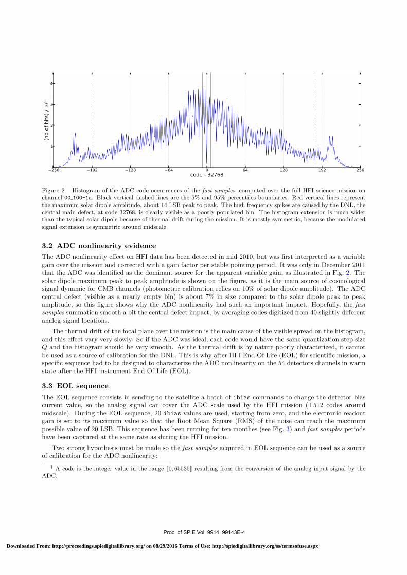
256 192 128 64 0 64 128 192 256code - 32768
1
2
3
4
(nb o
f hit
s) /
105
Figure 2. Histogram of the ADC code occurrences of the fast samples, computed over the full HFI science mission onchannel 00 100-1a. Black vertical dashed lines are the 5% and 95% percentiles boundaries. Red vertical lines representthe maximum solar dipole amplitude, about 14 LSB peak to peak. The high frequency spikes are caused by the DNL, thecentral main defect, at code 32768, is clearly visible as a poorly populated bin. The histogram extension is much widerthan the typical solar dipole because of thermal drift during the mission. It is mostly symmetric, because the modulatedsignal extension is symmetric around midscale.
3.2 ADC nonlinearity evidence
The ADC nonlinearity effect on HFI data has been detected in mid 2010, but was first interpreted as a variablegain over the mission and corrected with a gain factor per stable pointing period. It was only in December 2011that the ADC was identified as the dominant source for the apparent variable gain, as illustrated in Fig. 2. Thesolar dipole maximum peak to peak amplitude is shown on the figure, as it is the main source of cosmologicalsignal dynamic for CMB channels (photometric calibration relies on 10% of solar dipole amplitude). The ADCcentral defect (visible as a nearly empty bin) is about 7% in size compared to the solar dipole peak to peakamplitude, so this figure shows why the ADC nonlinearity had such an important impact. Hopefully, the fastsamples summation smooth a bit the central defect impact, by averaging codes digitized from 40 slightly differentanalog signal locations.
The thermal drift of the focal plane over the mission is the main cause of the visible spread on the histogram,and this effect vary very slowly. So if the ADC was ideal, each code would have the same quantization step sizeQ and the histogram should be very smooth. As the thermal drift is by nature poorly characterized, it cannotbe used as a source of calibration for the DNL. This is why after HFI End Of Life (EOL) for scientific mission, aspecific sequence had to be designed to characterize the ADC nonlinearity on the 54 detectors channels in warmstate after the HFI instrument End Of Life (EOL).
3.3 EOL sequence
The EOL sequence consists in sending to the satellite a batch of ibias commands to change the detector biascurrent value, so the analog signal can cover the ADC scale used by the HFI mission (±512 codes aroundmidscale). During the EOL sequence, 20 ibias values are used, starting from zero, and the electronic readoutgain is set to its maximum value so that the Root Mean Square (RMS) of the noise can reach the maximumpossible value of 20 LSB. This sequence has been running for ten monthes (see Fig. 3) and fast samples periodshave been captured at the same rate as during the HFI mission.
Two strong hypothesis must be made so the fast samples acquired in EOL sequence can be used as a sourceof calibration for the ADC nonlinearity:
† A code is the integer value in the range J0, 65535K resulting from the conversion of the analog input signal by theADC.
Proc. of SPIE Vol. 9914 99143E-4
Downloaded From: http://proceedings.spiedigitallibrary.org/ on 08/29/2016 Terms of Use: http://spiedigitallibrary.org/ss/termsofuse.aspx
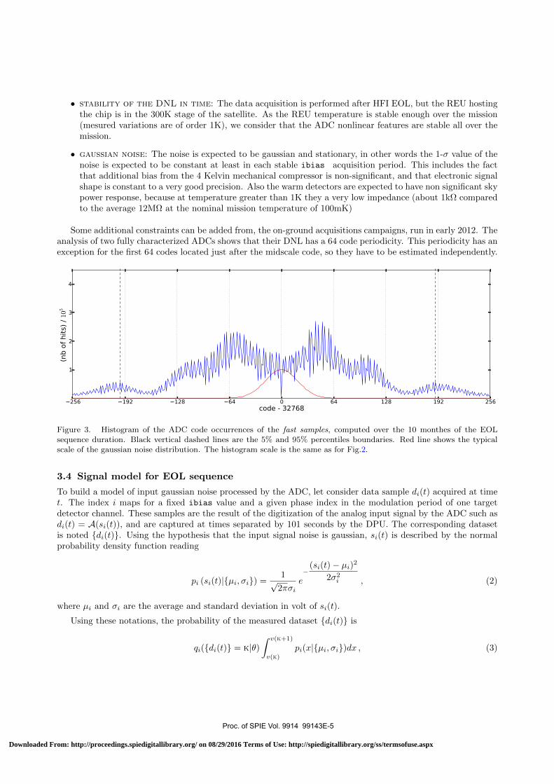
• stability of the DNL in time: The data acquisition is performed after HFI EOL, but the REU hostingthe chip is in the 300K stage of the satellite. As the REU temperature is stable enough over the mission(mesured variations are of order 1K), we consider that the ADC nonlinear features are stable all over themission.
• gaussian noise: The noise is expected to be gaussian and stationary, in other words the 1-σ value of thenoise is expected to be constant at least in each stable ibias acquisition period. This includes the factthat additional bias from the 4 Kelvin mechanical compressor is non-significant, and that electronic signalshape is constant to a very good precision. Also the warm detectors are expected to have non significant skypower response, because at temperature greater than 1K they a very low impedance (about 1kΩ comparedto the average 12MΩ at the nominal mission temperature of 100mK)
Some additional constraints can be added from, the on-ground acquisitions campaigns, run in early 2012. Theanalysis of two fully characterized ADCs shows that their DNL has a 64 code periodicity. This periodicity has anexception for the first 64 codes located just after the midscale code, so they have to be estimated independently.
256 192 128 64 0 64 128 192 256code - 32768
1
2
3
4
(nb o
f hit
s) /
105
Figure 3. Histogram of the ADC code occurrences of the fast samples, computed over the 10 monthes of the EOLsequence duration. Black vertical dashed lines are the 5% and 95% percentiles boundaries. Red line shows the typicalscale of the gaussian noise distribution. The histogram scale is the same as for Fig.2.
3.4 Signal model for EOL sequence
To build a model of input gaussian noise processed by the ADC, let consider data sample di(t) acquired at timet. The index i maps for a fixed ibias value and a given phase index in the modulation period of one targetdetector channel. These samples are the result of the digitization of the analog input signal by the ADC such asdi(t) = A(si(t)), and are captured at times separated by 101 seconds by the DPU. The corresponding datasetis noted di(t). Using the hypothesis that the input signal noise is gaussian, si(t) is described by the normalprobability density function reading
pi (si(t)|µi, σi) =1√
2πσie−
(si(t)− µi)2
2σ2i , (2)
where µi and σi are the average and standard deviation in volt of si(t).
Using these notations, the probability of the measured dataset di(t) is
qi(di(t) = k|θ)∫ v(k+1)
v(k)
pi(x|µi, σi)dx , (3)
Proc. of SPIE Vol. 9914 99143E-5
Downloaded From: http://proceedings.spiedigitallibrary.org/ on 08/29/2016 Terms of Use: http://spiedigitallibrary.org/ss/termsofuse.aspx
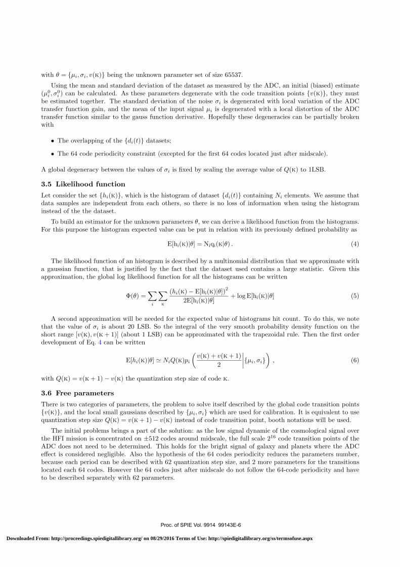
with θ = µi, σi, v(k) being the unknown parameter set of size 65537.
Using the mean and standard deviation of the dataset as measured by the ADC, an initial (biased) estimate(µ0i , σ
0i ) can be calculated. As these parameters degenerate with the code transition points v(k), they must
be estimated together. The standard deviation of the noise σi is degenerated with local variation of the ADCtransfer function gain, and the mean of the input signal µi is degenerated with a local distortion of the ADCtransfer function similar to the gauss function derivative. Hopefully these degeneracies can be partially brokenwith
• The overlapping of the di(t) datasets;
• The 64 code periodicity constraint (excepted for the first 64 codes located just after midscale).
A global degeneracy between the values of σi is fixed by scaling the average value of Q(k) to 1LSB.
3.5 Likelihood function
Let consider the set hi(k), which is the histogram of dataset di(t) containing Ni elements. We assume thatdata samples are independent from each others, so there is no loss of information when using the histograminstead of the the dataset.
To build an estimator for the unknown parameters θ, we can derive a likelihood function from the histograms.For this purpose the histogram expected value can be put in relation with its previously defined probability as
E[hi(k)|θ] = Niqi(k|θ) . (4)
The likelihood function of an histogram is described by a multinomial distribution that we approximate witha gaussian function, that is justified by the fact that the dataset used contains a large statistic. Given thisapproximation, the global log likelihood function for all the histograms can be written
Φ(θ) =∑i
∑k
(hi(k)− E[hi(k)|θ])2
2E[hi(k)|θ]+ log E[hi(k)|θ] (5)
A second approximation will be needed for the expected value of histograms hit count. To do this, we notethat the value of σi is about 20 LSB. So the integral of the very smooth probability density function on theshort range [v(k), v(k + 1)] (about 1 LSB) can be approximated with the trapezoidal rule. Then the first orderdevelopment of Eq. 4 can be written
E[hi(k)|θ] ' NiQ(k)pi
(v(k) + v(k + 1)
2
∣∣∣∣µi, σi) , (6)
with Q(k) = v(k + 1)− v(k) the quantization step size of code k.
3.6 Free parameters
There is two categories of parameters, the problem to solve itself described by the global code transition pointsv(k), and the local small gaussians described by µi, σi which are used for calibration. It is equivalent to usequantization step size Q(k) = v(k + 1)− v(k) instead of code transition point, booth notations will be used.
The initial problems brings a part of the solution: as the low signal dynamic of the cosmological signal overthe HFI mission is concentrated on ±512 codes around midscale, the full scale 216 code transition points of theADC does not need to be determined. This holds for the bright signal of galaxy and planets where the ADCeffect is considered negligible. Also the hypothesis of the 64 codes periodicity reduces the parameters number,because each period can be described with 62 quantization step size, and 2 more parameters for the transitionslocated each 64 codes. However the 64 codes just after midscale do not follow the 64-code periodicity and haveto be described separately with 62 parameters.
Proc. of SPIE Vol. 9914 99143E-6
Downloaded From: http://proceedings.spiedigitallibrary.org/ on 08/29/2016 Terms of Use: http://spiedigitallibrary.org/ss/termsofuse.aspx
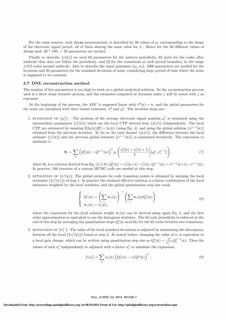
For the noise sources, each ibias measurements, is described by 80 values of µi corresponding to the shapeof the electronic signal period, all of them sharing the same value for σi. Hence for the 20 different values ofibias used, 20 * (80) + 20 parameters are needed.
Finally to describe v(k) we need 62 parameters for the pattern periodicity, 62 more for the codes aftermidscale that does not follow the periodicity, and 32 for the transitions at each period boundary in the range±512 codes around midscale. Also to describe the input gaussians µi, σi, 1600 parameters are needed for thelocations and 20 parameters for the standard deviation of noise, considering large period of time where the noiseis supposed to be constant.
3.7 DNL reconstruction method
The number of free parameters is too high to work on a global analytical solution. So the reconstruction processused is a three steps iterative process, and the estimates computed at iteration index j will be noted with j asexponent.
At the beginning of the process, the ADC is supposed linear with v0(k) = k, and the initial parameters forthe noise are initialized with their biased estimates, σ0
i and µ0i . The iteration steps are:
1. estimation of µji : The position of the average electronic signal position µji is estimated using the
intermediate parameters vji (k) which are the local CTP derived from di(t) independently. The local
CTP are estimated by ensuring E[hi(k)|θji ] = hi(k) (using Eq. 4), and using the global solution vj−1(k)obtained from the previous iteration. To do so, for each dataset di(t), the difference between the localestimate vji (k) and the previous global estimate vj−1(k), is minimized iteratively. The expression tominimize is
Φi =∑k
(Qji (k)−Qj−1(k)
)2pi
(vji (k) + vji (k + 1)
2
∣∣∣∣∣µji , σj−1i
), (7)
where Φi is a criterion derived from Eq. (2, 5, 6), Qji (k) = vji (k+1)−vji (k), Qj−1(k) = vj−1(k+1)−vj−1(k).In practice, 100 iteration of a custom MCMC code are needed at this step.
2. estimation of vj(k): The global estimate for code transition points is obtained by merging the localestimates vji (k) of step 1. In practice the retained effective solution is a linear combination of the localestimates weighted by the local statistics, and the global quantization step size reads Qj(k) =
(∑i
wi(k)
)−1(∑i
wi(k)Qji (k)
)wi(k) = hi(k) ,
(8)
where the expression for the local solution weight wi(k) can be derived using again Eq. 5, and the firstorder approximation is equivalent to use the histogram statistics. The 64 code periodicity is enforced at theend of this step by averaging the quantization steps Qji (k mod 64) for the 62 codes between two transitions.
3. estimation of σji : The value of the local standard deviations is adjusted by minimizing the discrepancy
between all the local vji (k) found at step 2. As stated before, changing the value of σi is equivalent to
a local gain change, which can be written using quantization step size as Qji (k) =σji
σj−1i
Qj−1i (k). Then the
values of each σji independently is adjusted with a factor αji to minimize the expression
f(αji ) =∑k
wi(k)(Qji (k)− αjiQ
j(k))2
, (9)
Proc. of SPIE Vol. 9914 99143E-7
Downloaded From: http://proceedings.spiedigitallibrary.org/ on 08/29/2016 Terms of Use: http://spiedigitallibrary.org/ss/termsofuse.aspx
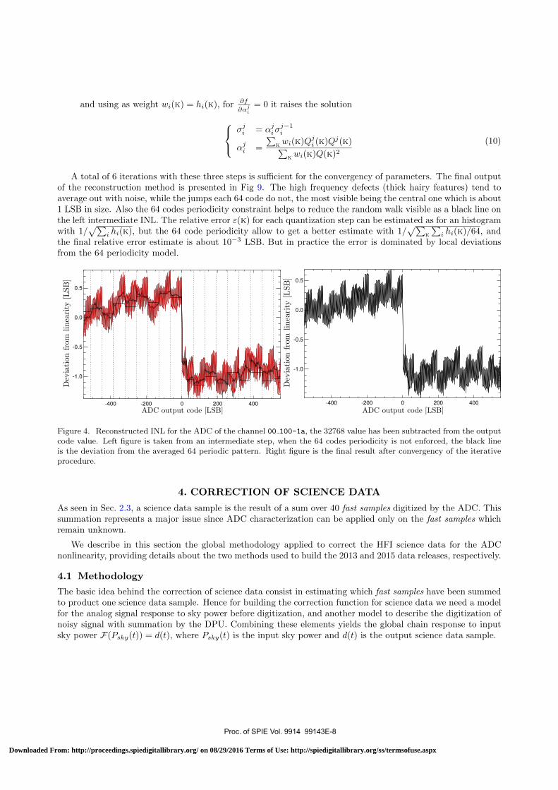
and using as weight wi(k) = hi(k), for ∂f
∂αji
= 0 it raises the solution
σji = αjiσ
j−1i
αji =
∑k wi(k)Qji (k)Qj(k)∑
k wi(k)Q(k)2(10)
A total of 6 iterations with these three steps is sufficient for the convergency of parameters. The final outputof the reconstruction method is presented in Fig 9. The high frequency defects (thick hairy features) tend toaverage out with noise, while the jumps each 64 code do not, the most visible being the central one which is about1 LSB in size. Also the 64 codes periodicity constraint helps to reduce the random walk visible as a black line onthe left intermediate INL. The relative error ε(k) for each quantization step can be estimated as for an histogramwith 1/
√∑i hi(k), but the 64 code periodicity allow to get a better estimate with 1/
√∑k
∑i hi(k)/64, and
the final relative error estimate is about 10−3 LSB. But in practice the error is dominated by local deviationsfrom the 64 periodicity model.
-400 -200 0 200 400
-1.0
-0.5
0.0
0.5
-400 -200 0 200 400
-1.0
-0.5
0.0
0.5
Figure 4. Reconstructed INL for the ADC of the channel 00 100-1a, the 32768 value has been subtracted from the outputcode value. Left figure is taken from an intermediate step, when the 64 codes periodicity is not enforced, the black lineis the deviation from the averaged 64 periodic pattern. Right figure is the final result after convergency of the iterativeprocedure.
4. CORRECTION OF SCIENCE DATA
As seen in Sec. 2.3, a science data sample is the result of a sum over 40 fast samples digitized by the ADC. Thissummation represents a major issue since ADC characterization can be applied only on the fast samples whichremain unknown.
We describe in this section the global methodology applied to correct the HFI science data for the ADCnonlinearity, providing details about the two methods used to build the 2013 and 2015 data releases, respectively.
4.1 Methodology
The basic idea behind the correction of science data consist in estimating which fast samples have been summedto product one science data sample. Hence for building the correction function for science data we need a modelfor the analog signal response to sky power before digitization, and another model to describe the digitization ofnoisy signal with summation by the DPU. Combining these elements yields the global chain response to inputsky power F(Psky(t)) = d(t), where Psky(t) is the input sky power and d(t) is the output science data sample.
Proc. of SPIE Vol. 9914 99143E-8
Downloaded From: http://proceedings.spiedigitallibrary.org/ on 08/29/2016 Terms of Use: http://spiedigitallibrary.org/ss/termsofuse.aspx
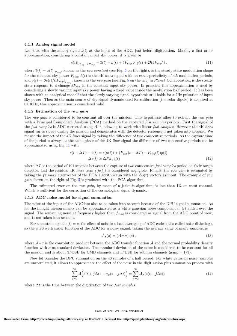
4.1.1 Analog signal model
Let start with the analog signal s(t) at the input of the ADC, just before digitization. Making a first orderapproximation, considering a constant input sky power, it is given by
s(t)|Psky+δPsky= s(t) + h(t) + δPsky × g(t) +O(δPsky
2) , (11)
where s(t) = s(t)|Psky, known as the raw constant (see Fig. 5 on the right), is the steady state modulation shape
for the constant sky power Psky, h(t) is the 4K lines signal with an exact periodicity of 4.5 modulation periods,and g(t) = ∂s(t)/∂Psky|Psky
, known as the raw gain (see Fig. 5 on the left) in Planck Collaboration, is the steady
state response to a change δPsky in the constant input sky power. In practice, this approximation is used byconsidering a slowly varying input sky power having a fixed value inside the modulation half period. It has beenshown with an analytical model3 that the slowly varying signal hypothesis still holds for a 2Hz pulsation of inputsky power. Then as the main source of sky signal dynamic used for calibration (the solar dipole) is acquired at0.016Hz, this approximation is considered valid.
4.1.2 Estimation of the raw gain
The raw gain is considered to be constant all over the mission. This hypothesis allow to extract the raw gainwith a Principal Component Analysis (PCA) method on the captured fast samples periods. First the signal ofthe fast samples is ADC corrected using A−1, allowing to work with linear fast samples. However the 4K linessignal varies slowly during the mission and degenerates with the detector response if not taken into account. Wereduce the impact of the 4K lines signal by taking the difference of two consecutive periods. As the capture timeof the period is always at the same phase of the 4K lines signal the difference of two consecutive periods can beapproximated using Eq. 11 with
s(t+ ∆T )− s(t) = ε(h(t)) + (Psky(t+ ∆T )− Psky(t))g(t)
∆s(t) ' ∆Pskyg(t) (12)
where ∆T is the period of 101 seconds between the capture of two consecutive fast samples period on their targetdetector, and the residual 4K lines term ε(h(t)) is considered negligible. Finally, the raw gain is estimated bytaking the primary eigenvector of the PCA algorithm run with the ∆s(t) vectors as input. The example of rawgain shown on the right of Fig. 5 is produced with the PCA algorithm.
The estimated error on the raw gain, by mean of a jacknife algorithm, is less than 1% on most channel.Which is sufficient for the correction of the cosmological signal dynamic.
4.1.3 ADC noise model for signal summation
The noise at the input of the ADC has also to be taken into account because of the DPU signal summation. Asfor the inflight measurements can be approximated as a white gaussian noise component nσ(t) added over thesignal. The remaining noise at frequency higher than fmod is considered as signal from the ADC point of view,and is not taken into account.
For a constant signal s(t) = s, the effect of noise is a local averaging of ADC codes (also called noise dithering),so the effective transfer function of the ADC for a noisy signal, taking the average value of many samples, is
Aσ(s) = (A ∗ σ) (s) , (13)
where A∗σ is the convolution product between the ADC transfer function A and the normal probability densityfunction with σ as standard deviation. The standard deviation of the noise is considered to be constant for allthe mission and is about 3.7LSB for CMB channels and 1.7LSB for submm channels (gamp = 1/3).
Now let consider the DPU summation on the 40 samples of a half period. For white gaussian noise, samplesare uncorrelated, it allows to approximate the effect of the noise in the digitization plus summation process with
39∑j=0
A(s(t+ j∆t) + nσ(t+ j∆t)
)'
39∑j=0
Aσ(s(t+ j∆t)) (14)
where ∆t is the time between the digitization of two fast samples.
Proc. of SPIE Vol. 9914 99143E-9
Downloaded From: http://proceedings.spiedigitallibrary.org/ on 08/29/2016 Terms of Use: http://spiedigitallibrary.org/ss/termsofuse.aspx
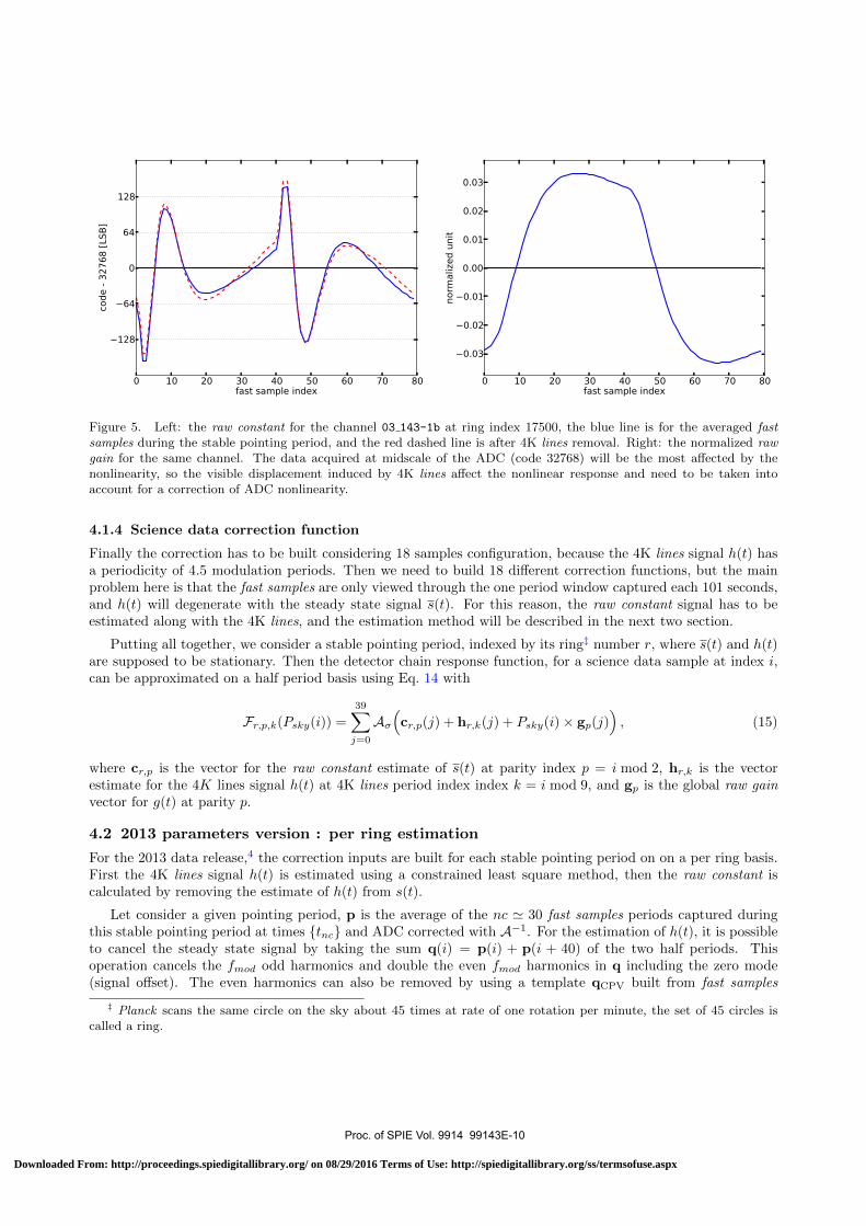
0 10 20 30 40 50 60 70 80fast sample index
128
64
0
64
128
code -
32768 [
LSB
]
0 10 20 30 40 50 60 70 80fast sample index
0.03
0.02
0.01
0.00
0.01
0.02
0.03
norm
aliz
ed u
nit
Figure 5. Left: the raw constant for the channel 03 143-1b at ring index 17500, the blue line is for the averaged fastsamples during the stable pointing period, and the red dashed line is after 4K lines removal. Right: the normalized rawgain for the same channel. The data acquired at midscale of the ADC (code 32768) will be the most affected by thenonlinearity, so the visible displacement induced by 4K lines affect the nonlinear response and need to be taken intoaccount for a correction of ADC nonlinearity.
4.1.4 Science data correction function
Finally the correction has to be built considering 18 samples configuration, because the 4K lines signal h(t) hasa periodicity of 4.5 modulation periods. Then we need to build 18 different correction functions, but the mainproblem here is that the fast samples are only viewed through the one period window captured each 101 seconds,and h(t) will degenerate with the steady state signal s(t). For this reason, the raw constant signal has to beestimated along with the 4K lines, and the estimation method will be described in the next two section.
Putting all together, we consider a stable pointing period, indexed by its ring‡ number r, where s(t) and h(t)are supposed to be stationary. Then the detector chain response function, for a science data sample at index i,can be approximated on a half period basis using Eq. 14 with
Fr,p,k(Psky(i)) =39∑j=0
Aσ(cr,p(j) + hr,k(j) + Psky(i)× gp(j)
), (15)
where cr,p is the vector for the raw constant estimate of s(t) at parity index p = i mod 2, hr,k is the vectorestimate for the 4K lines signal h(t) at 4K lines period index index k = i mod 9, and gp is the global raw gainvector for g(t) at parity p.
4.2 2013 parameters version : per ring estimation
For the 2013 data release,4 the correction inputs are built for each stable pointing period on on a per ring basis.First the 4K lines signal h(t) is estimated using a constrained least square method, then the raw constant iscalculated by removing the estimate of h(t) from s(t).
Let consider a given pointing period, p is the average of the nc ' 30 fast samples periods captured duringthis stable pointing period at times tnc and ADC corrected with A−1. For the estimation of h(t), it is possibleto cancel the steady state signal by taking the sum q(i) = p(i) + p(i + 40) of the two half periods. Thisoperation cancels the fmod odd harmonics and double the even fmod harmonics in q including the zero mode(signal offset). The even harmonics can also be removed by using a template qCPV built from fast samples
‡ Planck scans the same circle on the sky about 45 times at rate of one rotation per minute, the set of 45 circles iscalled a ring.
Proc. of SPIE Vol. 9914 99143E-10
Downloaded From: http://proceedings.spiedigitallibrary.org/ on 08/29/2016 Terms of Use: http://spiedigitallibrary.org/ss/termsofuse.aspx
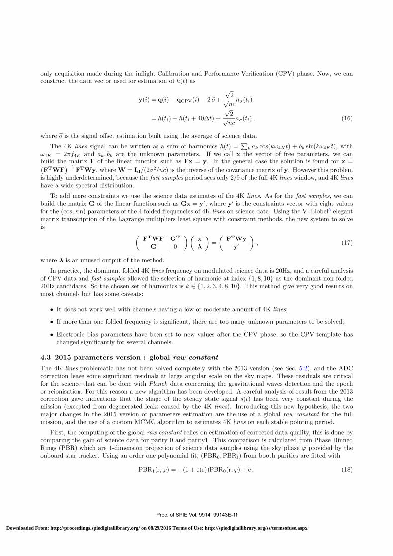
only acquisition made during the inflight Calibration and Performance Verification (CPV) phase. Now, we canconstruct the data vector used for estimation of h(t) as
y(i) = q(i)− qCPV(i)− 2 o+
√2√ncnσ(ti)
= h(ti) + h(ti + 40∆t) +
√2√ncnσ(ti) , (16)
where o is the signal offset estimation built using the average of science data.
The 4K lines signal can be written as a sum of harmonics h(t) =∑k ak cos(kω4Kt) + bk sin(kω4Kt), with
ω4K = 2πf4K and ak, bk are the unknown parameters. If we call x the vector of free parameters, we canbuild the matrix F of the linear function such as Fx = y. In the general case the solution is found for x =(FTWF
)−1FTWy, where W = Id/(2σ
2/nc) is the inverse of the covariance matrix of y. However this problemis highly underdetermined, because the fast samples period sees only 2/9 of the full 4K lines window, and 4K lineshave a wide spectral distribution.
To add more constraints we use the science data estimates of the 4K lines. As for the fast samples, we canbuild the matrix G of the linear function such as Gx = y′, where y′ is the constraints vector with eight valuesfor the (cos, sin) parameters of the 4 folded frequencies of 4K lines on science data. Using the V. Blobel5 elegantmatrix transcription of the Lagrange multipliers least square with constraint methods, the new system to solveis (
FTWF GT
G 0
)(xλ
)=
(FTWy
y′
), (17)
where λ is an unused output of the method.
In practice, the dominant folded 4K lines frequency on modulated science data is 20Hz, and a careful analysisof CPV data and fast samples allowed the selection of harmonic at index 1, 8, 10 as the dominant non folded20Hz candidates. So the chosen set of harmonics is k ∈ 1, 2, 3, 4, 8, 10. This method give very good results onmost channels but has some caveats:
• It does not work well with channels having a low or moderate amount of 4K lines;
• If more than one folded frequency is significant, there are too many unknown parameters to be solved;
• Electronic bias parameters have been set to new values after the CPV phase, so the CPV template haschanged significantly for several channels.
4.3 2015 parameters version : global raw constant
The 4K lines problematic has not been solved completely with the 2013 version (see Sec. 5.2), and the ADCcorrection leave some significant residuals at large angular scale on the sky maps. These residuals are criticalfor the science that can be done with Planck data concerning the gravitational waves detection and the epochor reionisation. For this reason a new algorithm has been developed. A careful analysis of result from the 2013correction gave indications that the shape of the steady state signal s(t) has been very constant during themission (excepted from degenerated leaks caused by the 4K lines). Introducing this new hypothesis, the twomajor changes in the 2015 version of parameters estimation are the use of a global raw constant for the fullmission, and the use of a custom MCMC algorithm to estimates 4K lines on each stable pointing period.
First, the computing of the global raw constant relies on estimation of corrected data quality, this is done bycomparing the gain of science data for parity 0 and parity1. This comparison is calculated from Phase BinnedRings (PBR) which are 1-dimension projection of science data samples using the sky phase ϕ provided by theonboard star tracker. Using an order one polynomial fit, (PBR0,PBR1) from booth parities are fitted with
PBR1(r, ϕ) = −(1 + ε(r))PBR0(r, ϕ) + c , (18)
Proc. of SPIE Vol. 9914 99143E-11
Downloaded From: http://proceedings.spiedigitallibrary.org/ on 08/29/2016 Terms of Use: http://spiedigitallibrary.org/ss/termsofuse.aspx
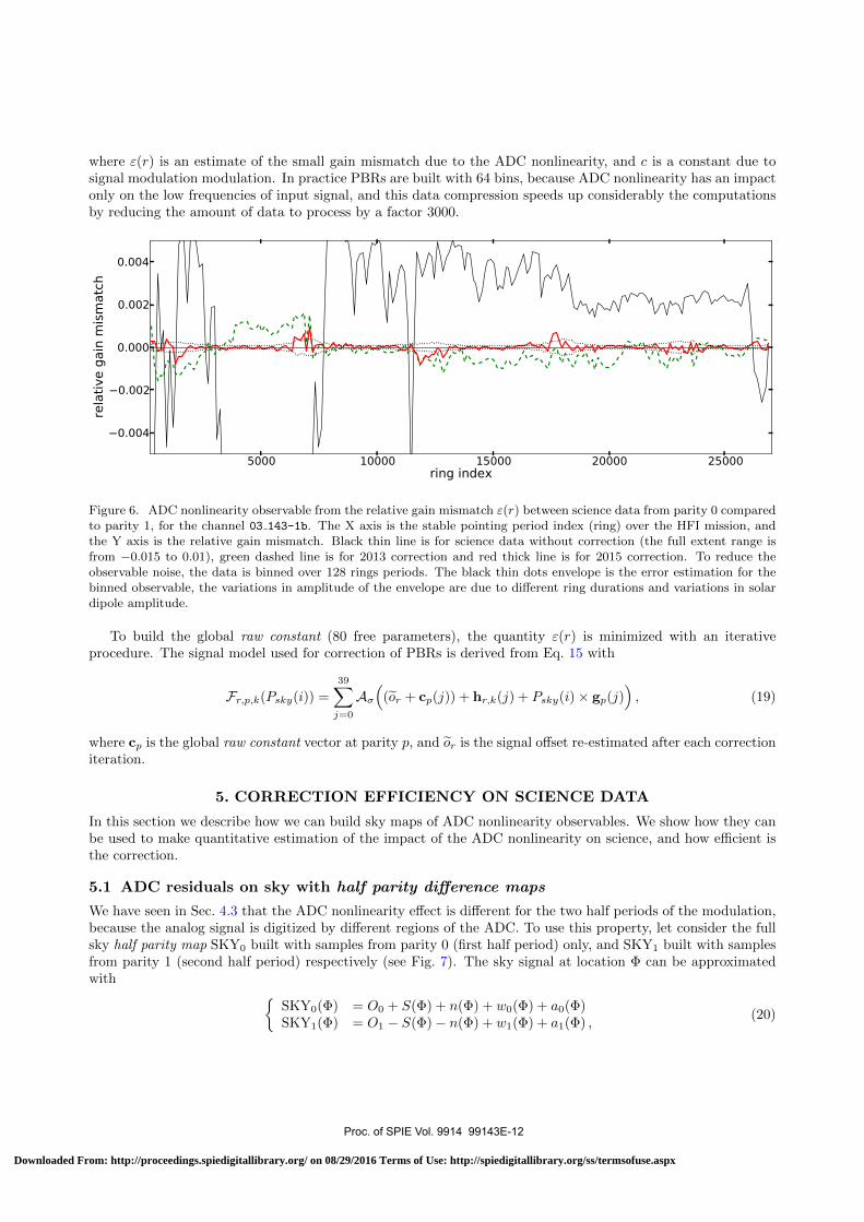
where ε(r) is an estimate of the small gain mismatch due to the ADC nonlinearity, and c is a constant due tosignal modulation modulation. In practice PBRs are built with 64 bins, because ADC nonlinearity has an impactonly on the low frequencies of input signal, and this data compression speeds up considerably the computationsby reducing the amount of data to process by a factor 3000.
5000 10000 15000 20000 25000ring index
0.004
0.002
0.000
0.002
0.004
rela
tive g
ain
mis
matc
h
Figure 6. ADC nonlinearity observable from the relative gain mismatch ε(r) between science data from parity 0 comparedto parity 1, for the channel 03 143-1b. The X axis is the stable pointing period index (ring) over the HFI mission, andthe Y axis is the relative gain mismatch. Black thin line is for science data without correction (the full extent range isfrom −0.015 to 0.01), green dashed line is for 2013 correction and red thick line is for 2015 correction. To reduce theobservable noise, the data is binned over 128 rings periods. The black thin dots envelope is the error estimation for thebinned observable, the variations in amplitude of the envelope are due to different ring durations and variations in solardipole amplitude.
To build the global raw constant (80 free parameters), the quantity ε(r) is minimized with an iterativeprocedure. The signal model used for correction of PBRs is derived from Eq. 15 with
Fr,p,k(Psky(i)) =39∑j=0
Aσ(
(or + cp(j)) + hr,k(j) + Psky(i)× gp(j)), (19)
where cp is the global raw constant vector at parity p, and or is the signal offset re-estimated after each correctioniteration.
5. CORRECTION EFFICIENCY ON SCIENCE DATA
In this section we describe how we can build sky maps of ADC nonlinearity observables. We show how they canbe used to make quantitative estimation of the impact of the ADC nonlinearity on science, and how efficient isthe correction.
5.1 ADC residuals on sky with half parity difference maps
We have seen in Sec. 4.3 that the ADC nonlinearity effect is different for the two half periods of the modulation,because the analog signal is digitized by different regions of the ADC. To use this property, let consider the fullsky half parity map SKY0 built with samples from parity 0 (first half period) only, and SKY1 built with samplesfrom parity 1 (second half period) respectively (see Fig. 7). The sky signal at location Φ can be approximatedwith
SKY0(Φ) = O0 + S(Φ) + n(Φ) + w0(Φ) + a0(Φ)SKY1(Φ) = O1 − S(Φ)− n(Φ) + w1(Φ) + a1(Φ) ,
(20)
Proc. of SPIE Vol. 9914 99143E-12
Downloaded From: http://proceedings.spiedigitallibrary.org/ on 08/29/2016 Terms of Use: http://spiedigitallibrary.org/ss/termsofuse.aspx
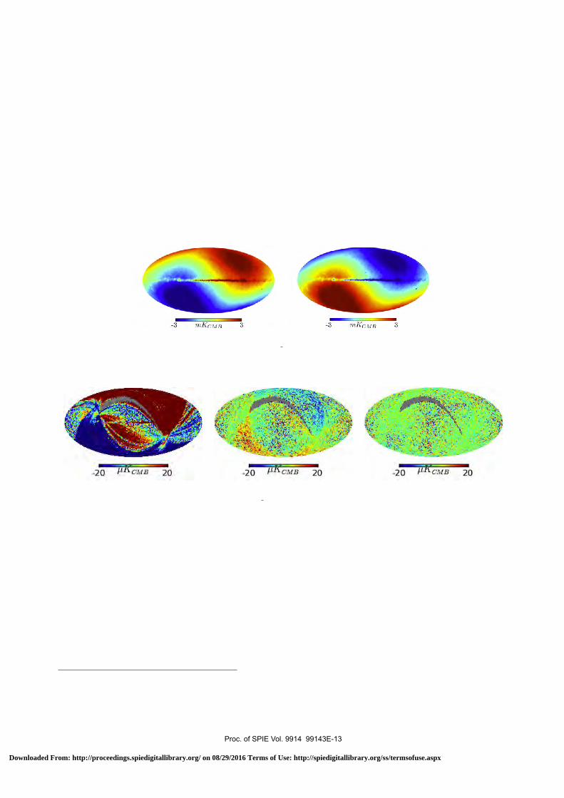
mKcwts 3
/--°411166"..-v-3 mKcms
-20 iii 20 20 P cMa 20 -20 iT C 20
where (O 0 , O 1 ) are global map offsets, S is the sky signal, n is the 1/f modulated detector noise coming fromboth sky signal and temperature variations, w is a white uncorrelated noise component and ( a 0 , a 1 ) is the ADCnonlinear effect for parity 0 and 1 respectively. Hence the expected result of the sum SKY 0 + SKY 1 after offsetremoval is called a half parity difference map capturing mainly white noise and ADC nonlinearity residuals, andfiltering out common low frequency modes from S and n.
In practice, half parity maps (see Fig. 7) are built in the Healpix 6 format from raw science data using theofficial map projector ( polkapix 7 ), with nominal data flags used to exclude data affected by cosmic rays and badrings and select samples from the chosen parity. Results are shown on Fig. 8 for a 143GHz detector. The halfparity difference maps of the uncorrected data is mainly dominated by large scales features following the Planckscanning strategy, due to the ADC nonlinear response to the solar dipole signal. Once corrected, the large scalesfeatures globally disappear, leaving small scales fluctuations compatible with noise. These results are consistentwith ADC nonlinearity simulations. 4
Figure 7. Half parity maps before correction for channel 03 143-1b at Healpix resolution nside=32. Left: parity 0 map(SKY 0 ). Right: parity 1 map (SKY 1 ). The solar dipole has not been removed to show the dominant signal dynamicinteracting with the ADC.
Figure 8. Half parity difference maps for channel 03 143-1b at healpix resolution nside=32. From left to right: noADC correction, 2013 and 2015 correction. The maps are built with data from survey1 (first 6 month of mission), this iswhy the map is not fully covered (grey region).
5.2 Impact of ADC nonlinearity on science
The impact of ADC residuals, on cosmological signal is estimated by the angular power spectrum of half paritydifference maps obtained with anafast § using a 15% sky mask excluding the bright galactic plane and pointsources. The specific processing of the half parity difference maps is not fully consistent with the official pipelineused to perform time deconvolution of the time ordered data. However the effect of the deconvolution on theangular power spectrum can be approximated by applying a factor f (`) = 1/|τ (`/60)| 2 on the power spectrum,where τ (ν ) is the time transfer function, in frequency domain, of the electronic readout chain, and `/60 approx-imates the multipole frequency of the angular sky features in time domaine (It takes 60 seconds for the satelliteto accomplish a complete rotation over the sky).
An example TT spectrum built with the half parity difference maps is shown in Fig. 9 for the same 143GHzchannel as in Fig. 8. The residuals due to ADC nonlinearity can be seen as an additive component in 1 /` 2 at low
§ Anafast is a tool provided with the Healpix software.
Proc. of SPIE Vol. 9914 99143E-13
Downloaded From: http://proceedings.spiedigitallibrary.org/ on 08/29/2016 Terms of Use: http://spiedigitallibrary.org/ss/termsofuse.aspx
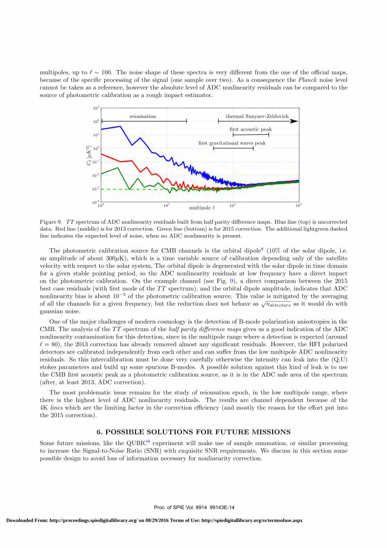
multipoles, up to ` ∼ 100. The noise shape of these spectra is very different from the one of the official maps,because of the specific processing of the signal (one sample over two). As a consequence the Planck noise levelcannot be taken as a reference, however the absolute level of ADC nonlinearity residuals can be compared to thesource of photometric calibration as a rough impact estimator.
100 101 102 10310-4
10-3
10-2
10-1
100
101
102
103
Figure 9. TT spectrum of ADC nonlinearity residuals built from half parity difference maps. Blue line (top) is uncorrecteddata. Red line (middle) is for 2013 correction. Green line (bottom) is for 2015 correction. The additional lightgreen dashedline indicates the expected level of noise, when no ADC nonlinearity is present.
The photometric calibration source for CMB channels is the orbital dipole8 (10% of the solar dipole, i.e.an amplitude of about 300µK), which is a time variable source of calibration depending only of the satellitevelocity with respect to the solar system, The orbital dipole is degenerated with the solar dipole in time domainfor a given stable pointing period, so the ADC nonlinearity residuals at low frequency have a direct impacton the photometric calibration. On the example channel (see Fig. 9), a direct comparizon between the 2015best case residuals (with first mode of the TT spectrum), and the orbital dipole amplitude, indicates that ADCnonlinearity bias is about 10−3 of the photometric calibration source. This value is mitigated by the averagingof all the channels for a given frequency, but the reduction does not behave as
√ndetectors as it would do with
gaussian noise.
One of the major challenges of modern cosmology is the detection of B-mode polarization anisotropies in theCMB. The analysis of the TT spectrum of the half parity difference maps gives us a good indication of the ADCnonlinearity contamination for this detection, since in the multipole range where a detection is expected (around` = 80), the 2013 correction has already removed almost any significant residuals. However, the HFI polarizeddetectors are calibrated independently from each other and can suffer from the low multipole ADC nonlinearityresiduals. So this intercalibration must be done very carefully otherwise the intensity can leak into the (Q,U)stokes parameters and build up some spurious B-modes. A possible solution against this kind of leak is to usethe CMB first acoustic peak as a photometric calibration source, as it is in the ADC safe area of the spectrum(after, at least 2013, ADC correction).
The most problematic issue remains for the study of reionsation epoch, in the low multipole range, wherethere is the highest level of ADC nonlinearity residuals. The results are channel dependent because of the4K lines which are the limiting factor in the correction efficiency (and mostly the reason for the effort put intothe 2015 correction).
6. POSSIBLE SOLUTIONS FOR FUTURE MISSIONS
Some future missions, like the QUBIC9 experiment will make use of sample summation, or similar processingto increase the Signal-to-Noise Ratio (SNR) with exquisite SNR requirements. We discuss in this section somepossible design to avoid loss of information necessary for nonlinearity correction.
Proc. of SPIE Vol. 9914 99143E-14
Downloaded From: http://proceedings.spiedigitallibrary.org/ on 08/29/2016 Terms of Use: http://spiedigitallibrary.org/ss/termsofuse.aspx
6.1 Increasing signal dynamic
A trivial solution is to increase the signal dynamic, compared to the ADC defects in LSB units. The Signal-to-Noise Ratio (SNR) for the quantization noise is generally calculated in decibels with the formula SNR =6.02n + 1.76dB, where n is the number of bits of the ADC. But this theoretical number holds only in thecase of an ideal component with the quantization noise averaging out, and considering the full input scale ofthe component. For a non-ideal component, a useful figure to characterize bias level is the maximum value ofthe INL, or in other words the maximum transfer function drift from linearity in LSB units. In this case theSignal-to-Bias Ratio, which does not average out with statistics, would read
SBR = 20 log10
S
INLdB , (21)
where S is the considered signal dynamic converted in LSB units. So in the case of HFI, with a best case signaldynamic of 14LSB, for the solar dipole, and an inflight measured INL value about 1LSB, we have SBR = 23dB.If we would like to reach a requirement SBR= 80dB we would need at least 10 more bits with the same INLvalue of 1LSB. It is possible to discard non significant bits in the onboard DPU, but as the accuracy requirementalso increase with new instruments, discarding too much bits in the acquired samples may not be possible.
Increasing moderately the steady state signal amplitude is also useful. In the case of HFI, the signal balancingwas a success into making the resulting analog signal very flat (70% of the fast samples for a half period cover only30LSB). But a flat signal can concentrate signal acquisition on a potentially important ADC defect. Changing thedesign of the balancing to obtain for example a triangular shape for the acquired signal would be a good solutionto ensure acquisition is done on different ADC areas, the result would be a reduced bias level by averaging effect.
6.2 Using analog summation
The digital summation implemented in the DPU (label (c) on Fig. 1) is designed to improve the SNR of thescience data. But another function has been implemented in the DPU with the nblank parameter, still notused in the HFI mission, to allow the removal of nblank fast samples at transient locations. If we forget aboutthe nblank option, the digital summation function can be replaced with an equivalent analog integrator in thereadout chain. The square signal of detectors would integrate into a triangle wave, and the acquisition could bedone near the peak location once for each half period at twice the modulation frequency. This design does notdestroy information after digitization, so nonlinear correction of the ADC component can be done a posteriori.
The main problem with analog integrators is their potential signal instability, so they have to be designedcarefully. They also bring some additional noise as each analog component do.
6.3 DPU correction
It is possible to make the the ADC nonlinearity correction in the DPU. This method require to characterize eachADC and to provide this information to the DPU as data tables, one value for each ADC code being sufficient.Also, to avoid floating point operations in the FPGA, the tables must be built with significantly more bits thanthe ADC output. The main advantage is that complex digital processing is still available with this design, andit has a better SNR than with additional analog component.
For this solution, the hypothesis is that the nonlinear characteristics of the ADC are stable over the mission.Otherwise a runtime characterization must be implemented with a perfectly known calibration source like a rampsignal.
7. CONCLUSIONS
We have described how the Planck/HFI instrument is affected by the nonlinearity of the Analog to Digital Con-verter (ADC) component of the readout electronics. While this nonlinearity had not been properly characterisedbefore launch, its impact on science data has been enhanced by a combination of circumstances: the small dy-namic of the cosmological signal ; the location of the balanced signal at mid-scale of the entire ADC range, i.e.,exactly on top of the strongest defect of the ADC ; and the summation of the digitizsed signal on the first andsecond modulation periods to produce the science signal, and destroying the knowledge of the full modulatedsignal. To handle this problematic and build an appropriate correction function, two steps have been necessary:
Proc. of SPIE Vol. 9914 99143E-15
Downloaded From: http://proceedings.spiedigitallibrary.org/ on 08/29/2016 Terms of Use: http://spiedigitallibrary.org/ss/termsofuse.aspx
• The ADC chips nonlinearity had to be characterized inflight for each of the 54 detector channels. Thiswas done with a specific EOL sequence on the last ten months of the mission to acquire statistics onthe component range relevant for the mission cosmological signal acquisition. Then we have developed alikelihood method to reconstruct each ADC transfer function with a precision of about 10−3 LSB on alarge code range.
• To correct science data for ADC nonlinearity, a model of the analog signal before digitization by the ADChad to be developed. This model allow us to revert the signal summation operation of the DPU, so thatthe ADC characterization can be used with this model to build the global science data correction.
In order to estimate the ADC correction efficiency on the final maps, we have also developed a specific methodconsisting in building two sets of all-sky maps containing only samples from the first or second half period ofthe modulation, respectively. The difference of these two sets of maps allows us to remove all low frequencysignals and to conserve only ADC nonlinearity residuals plus white noise. The analysis of the temperature(TT) power spectrum built from half parity difference maps is very powerful to characterize the impact of ADCnonlinearity in the angular frequency domain. The ADC residuals impact significantly the TT spectrum inthe first 100 multipoles when no correction is applied. This range is reduced to the first 30 multipoles withthe correction included in the 2013 data release, and to the first 10 multipoles with the 2015 correction. Theremaining residuals level on CMB channels is about 0.05% of the solar dipole in time domain, and 0.1% ofthe main photometric calibration source (the orbital dipole) on the TT spectrum. This level seems safe whenanalysing the CMB TT spectrum, but remains a possible issue when considering polarisation signals, especiallyfor B-mode or reionisaiton analyses performed at low multipoles.
Finally we have presented how such a large impact from the nonlinearity of the ADC component can beavoided, and inflight ADC correction using tables built from ground calibration seems to be the most promisingsolution.
ACKNOWLEDGMENTS
The work presented in this paper has been realized inside the Planck team responsible of the data processing.
The development of Planck has been supported by: ESA; CNES and CNRS/INSU-IN2P3-INP (France);ASI, CNR, and INAF (Italy); NASA and DoE (USA); STFC and UKSA (UK); CSIC, MICINN and JA(Spain); Tekes, AoF and CSC (Finland); DLR and MPG (Germany); CSA (Canada); DTU Space (Denmark);SER/SSO (Switzerland); RCN (Norway); SFI (Ireland); FCT/MCTES (Portugal); and PRACE (EU). A de-scription of the Planck Collaboration and a list of its members, including the technical or scientific activitiesin which they have been involved, can be found at http://www.rssd.esa.int/index.php?project=PLANCK&
page=PlanckCollaboration.
REFERENCES
[1] Planck Collaboration, Adam, R., Ade, P. A. R., Aghanim, N., Arnaud, M., Ashdown, M., Aumont, J.,Baccigalupi, C., Banday, A. J., Barreiro, R. B., et al., “Planck 2015 results. VII. HFI TOI and beamprocessing,” ArXiv e-prints (Feb. 2015).
[2] Lamarre, J.-M., Puget, J.-L., Ade, P. A. R., et al., “Planck pre-launch status: The HFI instrument, fromspecification to actual performance,” A&A 520, A9 (Sept. 2010).
[3] Sauve, A. and Montier, L., “Building the analytical response in frequency domain of AC biased bolometersApplication to Planck/HFI,” ArXiv e-prints (May 2016).
[4] Planck Collaboration, Ade, P. A. R., Aghanim, N., Armitage-Caplan, C., Arnaud, M., Ashdown, M., Atrio-Barandela, F., Aumont, J., Baccigalupi, C., Banday, A. J., et al., “Planck 2013 results. VI. High FrequencyInstrument data processing,” A&A 571, A6 (Nov. 2014).
[5] Blobel, V. and Kleinwort, C., “A New Method for the High-Precision Alignment of Track Detectors,” ArXivHigh Energy Physics - Experiment e-prints (Aug. 2002).
Proc. of SPIE Vol. 9914 99143E-16
Downloaded From: http://proceedings.spiedigitallibrary.org/ on 08/29/2016 Terms of Use: http://spiedigitallibrary.org/ss/termsofuse.aspx

[6] Gorski, K. M., Hivon, E., Banday, A. J., Wandelt, B. D., Hansen, F. K., Reinecke, M., and Bartelmann, M.,“HEALPix: A Framework for High-Resolution Discretization and Fast Analysis of Data Distributed on theSphere,” ApJ 622, 759–771 (Apr. 2005).
[7] Tristram, M., Filliard, C., Perdereau, O., Plaszczynski, S., Stompor, R., and Touze, F., “Iterative destripingand photometric calibration for Planck-HFI, polarized, multi-detector map-making,” A&A 534, A88 (Oct.2011).
[8] Planck Collaboration, Adam, R., Ade, P. A. R., Aghanim, N., Arnaud, M., Ashdown, M., Aumont, J.,Baccigalupi, C., Banday, A. J., Barreiro, R. B., et al., “Planck 2015 results. VIII. High Frequency Instrumentdata processing: Calibration and maps,” ArXiv e-prints (Feb. 2015).
[9] Qubic Collaboration, Battistelli, E., Bau, A., Bennett, D., Berge, L., Bernard, J.-P., de Bernardis, P., Bordier,G., Bounab, A., Breelle, E., et al., “QUBIC: The QU bolometric interferometer for cosmology,” AstroparticlePhysics 34, 705–716 (Apr. 2011).
Proc. of SPIE Vol. 9914 99143E-17
Downloaded From: http://proceedings.spiedigitallibrary.org/ on 08/29/2016 Terms of Use: http://spiedigitallibrary.org/ss/termsofuse.aspx

281
Appendix C
HFI ADC chip specificationsdesign sheet

77880099 LLPPRRPPAAnnaalloogg-ttoo-DDiiggiittaall CCoonnvveerrtteerr
ww
w.s
pace
elec
tron
ics.
com
Space Electronics Analog-to-Digital ConverterSpace Electronics' 7809LPRP is a radiation-hardened, high speed 16-bit analog-to-digital converter
features up to 100 kilorad (Si) total dose tolerance dependent upon orbit. The device is radiation-hardened
at the microcircuit level using SEi's RAD-PAK® packaging technology and is latchup protected by
Space Electronics' Latchup Protection Technology (LPT™). The device is a 24 pin, 16-bit sampling
analog-to-digital converter that uses state-of-the-art CMOS structures. The 7809LPRP contains a 16-bit
capacitor based SAR A/D with S/H, reference, clock, interface for microprocessor use, and serial output
drivers. It is specified at a 100 kHz sampling rate, and guaranteed over the full temperature range.
Laser-trimmed scaling resistors provide various input ranges including ±10V and 0 to 5 V, while the
innovative design allows operation from a single +5 V supply, with power dissipation of under 132 mW.
In addition, the 7809LPRP is available with packaging and screening up to Class S.
16-bit organization24 pin RAD-PAK® flat package100 kHz min sampling rate±10 V and 0 V to 5 V input rangeAdvanced CMOS technologyDNL: 16-bits "No Missing Codes"86dB min SINAD with 20 kHz inputSingle +5 V supply operationUtilizes internal or external referenceSerial outputPower dissipation: 132 mW max
LPT™ OperationLatchup Protection Technology (LPT™) auto-
matically detects an increase in the supply
current of the 7809LPRP converter due to a
single event effect and internally cycles the
power to the converter off, then on, which
restores the steady state operation of the device.
The LPTTM circuitry consists of two power
switch and current sensor blocks, an LPTTM
controller block, a BIT cur- rent load block,
and an active input protection block.
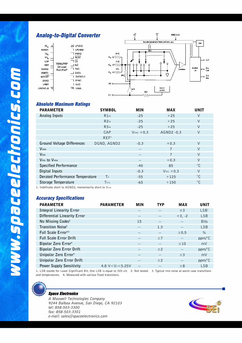
ww
w.s
pace
elec
tron
ics.
com
Space EElectronicsA Maxwell Technologies Company9244 Balboa Avenue, San Diego, CA 92103 tel: 858-503-3300 fax: 858-503-3301e-mail: [email protected]
Accuracy SpecificationsPARAMETER PARAMETER MIN TYP MAX UNIT Integral Linearity Error -- -- ±3 LSB1
Differential Linearity Error -- -- +3, -2 LSBNo Missing Codes2 15 -- -- BitsTransition Noise3 -- 1.3 -- LSBFull Scale Error4,5 -- -- ±0.5 %Full Scale Error Drift -- ±7 -- ppm/°CBipolar Zero Error4 -- -- ±10 mVBipolar Zero Error Drift -- ±2 -- ppm/°CUnipolar Zero Error4 -- -- ±3 mVUnipolar Zero Error Drift -- ±2 -- ppm/°CPower Supply Sensitivity 4.8 V<VS<5.25V -- -- ±8 LSB
1. LSB stands for Least Significant Bit. One LSB is equal to 305 uV. 2. Not tested. 3. Typical rms noise at worst case transitionsand temperatures. 4. Measured with various fixed transistors.
Analog-to-Digital Converter
Absolute Maximum RatingsPARAMETER SYMBOL MIN MAX UNIT Analog Inputs R1IN -25 +25 V
R2IN -25 +25 VR3IN -25 +25 VCAP VANA +0.3 AGND2 -0.3 VREF1
Ground Voltage Differences DGND, AGND2 -0.3 +0.3 VVANA -- 7 VVDIG -- 7 VVDIG to VANA -- +0.3 VSpecified Performance -40 85 °CDigital Inputs -0.3 VDIG +0.3 VDerated Performance Temperature TA -55 +125 °CStorage Temperature TSTG -65 +150 °C
1. Indefinate short to AGND2, momentarily short to VANA

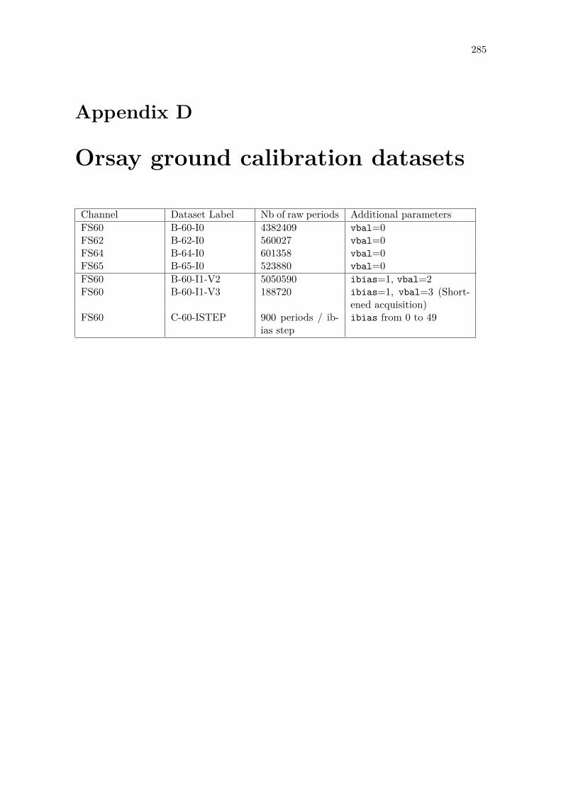
285
Appendix D
Orsay ground calibration datasets
Channel Dataset Label Nb of raw periods Additional parametersFS60 B-60-I0 4382409 vbal=0FS62 B-62-I0 560027 vbal=0FS64 B-64-I0 601358 vbal=0FS65 B-65-I0 523880 vbal=0FS60 B-60-I1-V2 5050590 ibias=1, vbal=2FS60 B-60-I1-V3 188720 ibias=1, vbal=3 (Short-
ened acquisition)FS60 C-60-ISTEP 900 periods / ib-
ias stepibias from 0 to 49


287
Appendix E
Schematics of the Cardif setup
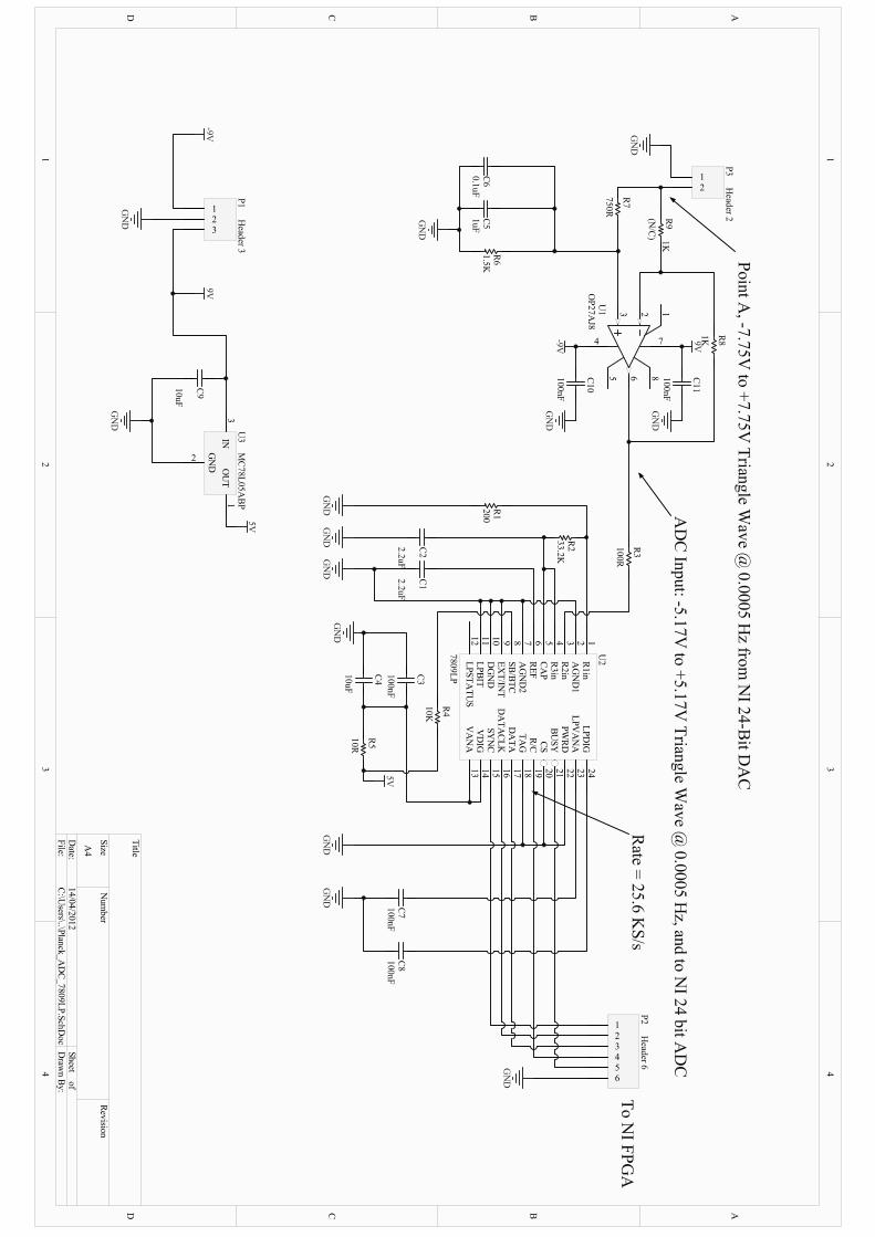
1 1
2 2
3 3
4 4
DD
CC
BB
AA
Title
Num
ber
Revis
ion
Siz
e
A4
Date
:14/0
4/2
012
Sheet o
f
File
:C
:\Users
\..\Pla
nck
_A
DC
_7809L
P.S
chD
oc
Dra
wn B
y:
GN
D
2.2
uF
C1
2.2
uF
C2
GN
DG
ND
R1
200
R2
33.2
K
R3
100R
GN
DG
ND
R4
10K
R5
10R
5V
10uF
C4
100nF
C3
GN
D
1
2
3
P1
Header 3
1
2
3
4
5
6
P2
Header 6
1
2
P3
Header 2G
ND
GN
D
GN
D
9V
R6
1.5
K
R7
750R
C5
1uF
C6
0.1
uF
GN
D
Poin
t A, -7
.75V
to +
7.7
5V
Tria
ngle
Wave @
0.0
005 H
z fro
m N
I 24-B
it DA
C
AD
C In
put: -5
.17V
to +
5.1
7V
Tria
ngle
Wave @
0.0
005 H
z, a
nd to
NI 2
4 b
it AD
C
85
23
4
6
7
1
U1
OP
27A
J8
100nF
C7
100nF
C8
R8
1K
IN3
2
OU
T1
GN
D
U3
MC
78L
05A
BP
5V
10uF
C9
GN
D
-9V
1K
R9
(N/C
)
9V
-9V
R1in
1
AG
ND
12
R2in
3
R3in
4
CA
P5
RE
F6
AG
ND
27
SB
/BT
C8
EX
T/IN
T9
DG
ND
10
LP
BIT
11
LP
ST
AT
US
12
VA
NA
13
VD
IG14
SY
NC
15
DA
TA
CL
K16
DA
TA
17
TA
G18
R/C
19
CS
20
BU
SY
21
PW
RD
22
LP
VA
NA
23
LP
DIG
24
U2
7809L
P
100nF
C10
100nF
C11
GN
D
GN
D
Rate
= 2
5.6
KS
/sT
o N
I FP
GA

289
Appendix F
Sorption cooler schematic andsensors
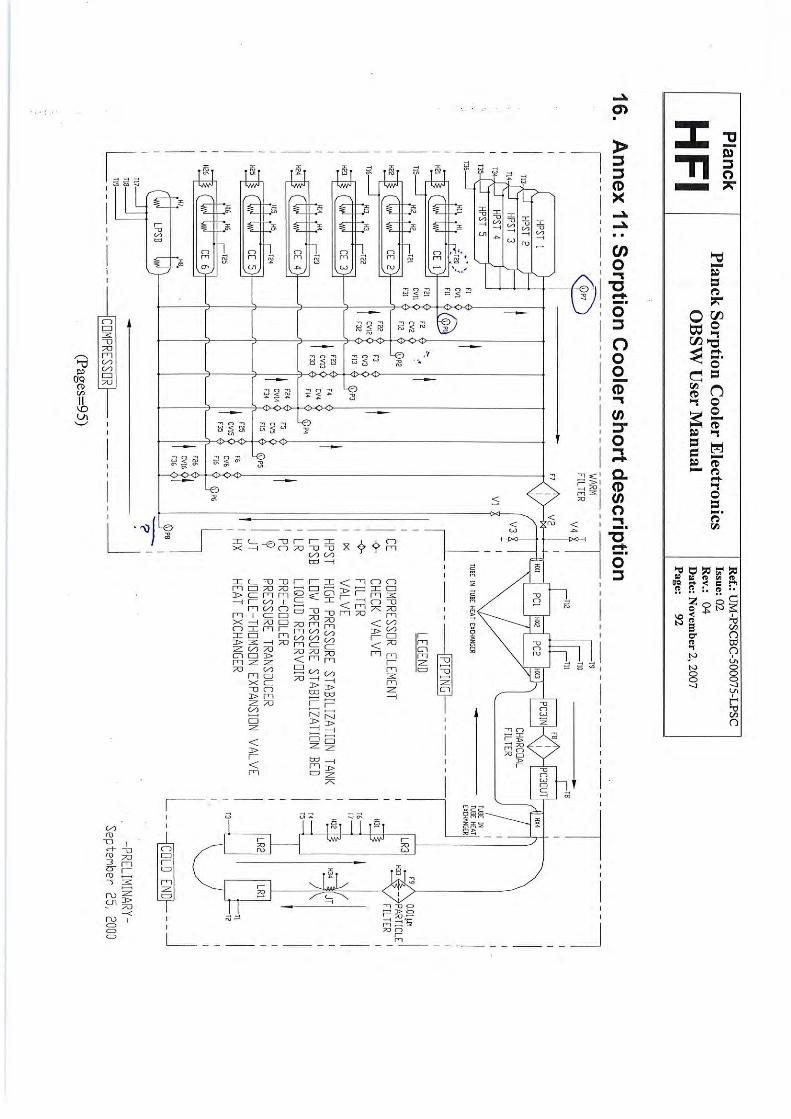
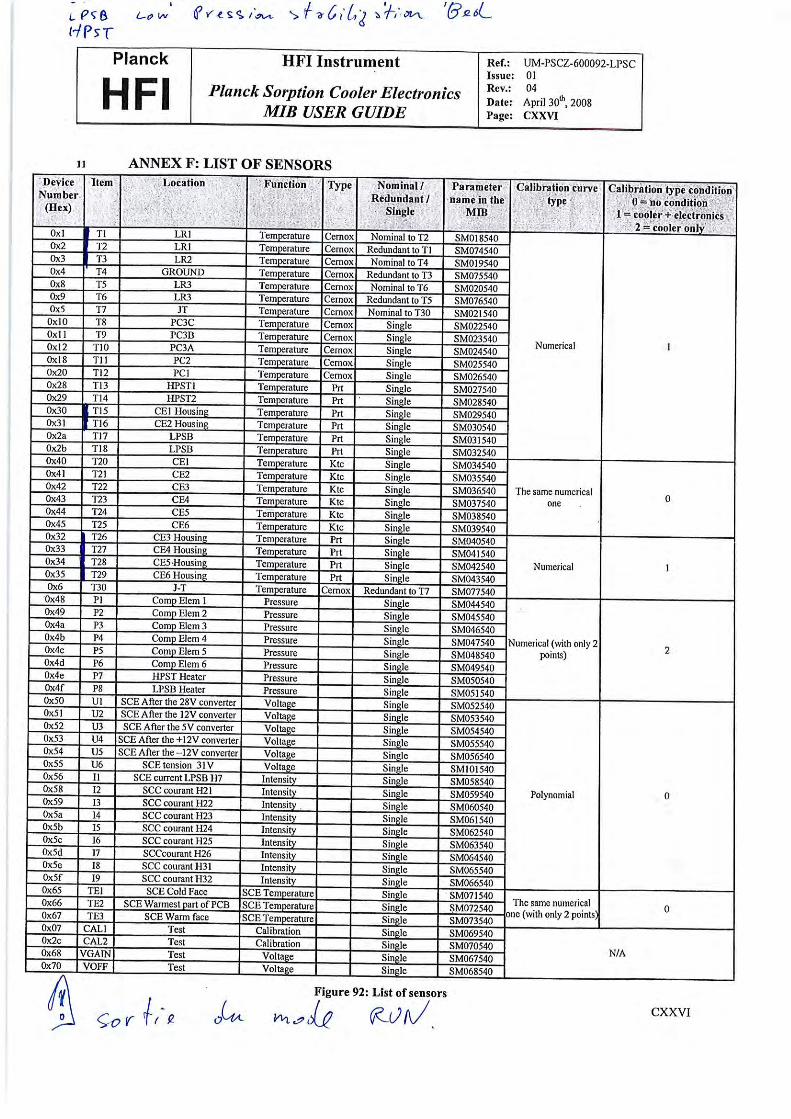

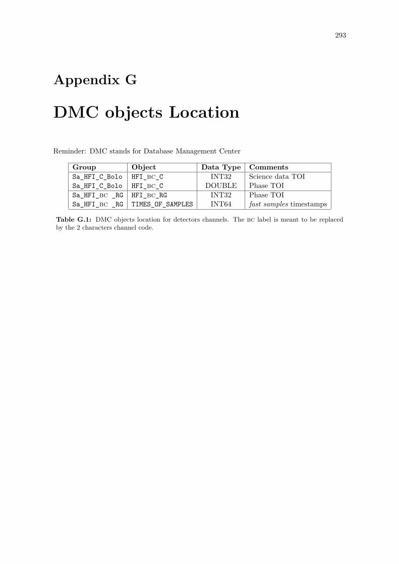
293
Appendix G
DMC objects Location
Reminder: DMC stands for Database Management Center
Group Object Data Type CommentsSa_HFI_C_Bolo HFI_bc_C INT32 Science data TOISa_HFI_C_Bolo HFI_bc_C DOUBLE Phase TOISa_HFI_bc _RG HFI_bc_RG INT32 Phase TOISa_HFI_bc _RG TIMES_OF_SAMPLES INT64 fast samples timestamps
Table G.1: DMC objects location for detectors channels. The bc label is meant to be replacedby the 2 characters channel code.

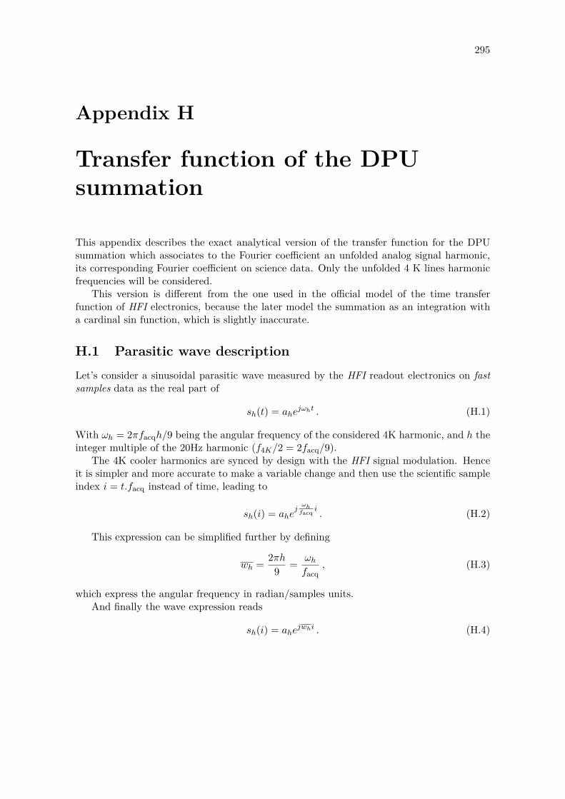
295
Appendix H
Transfer function of the DPUsummation
This appendix describes the exact analytical version of the transfer function for the DPUsummation which associates to the Fourier coefficient an unfolded analog signal harmonic,its corresponding Fourier coefficient on science data. Only the unfolded 4 K lines harmonicfrequencies will be considered.
This version is different from the one used in the official model of the time transferfunction of HFI electronics, because the later model the summation as an integration witha cardinal sin function, which is slightly inaccurate.
H.1 Parasitic wave descriptionLet’s consider a sinusoidal parasitic wave measured by the HFI readout electronics on fastsamples data as the real part of
sh(t) = ahejωht . (H.1)
With ωh = 2πfacqh/9 being the angular frequency of the considered 4K harmonic, and h theinteger multiple of the 20Hz harmonic (f4K/2 = 2facq/9).
The 4K cooler harmonics are synced by design with the HFI signal modulation. Henceit is simpler and more accurate to make a variable change and then use the scientific sampleindex i = t.facq instead of time, leading to
sh(i) = ahejωhfacq
i. (H.2)
This expression can be simplified further by defining
wh = 2πh9 = ωh
facq, (H.3)
which express the angular frequency in radian/samples units.And finally the wave expression reads
sh(i) = ahejwhi . (H.4)
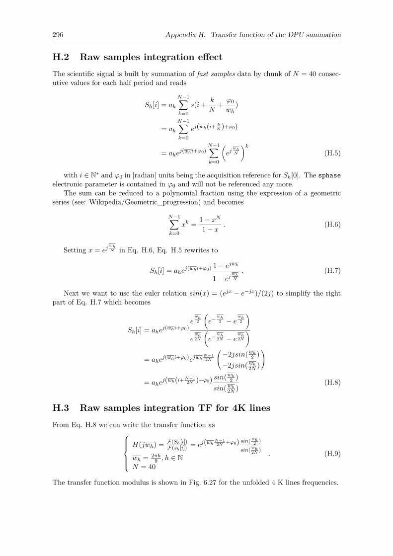
296 Appendix H. Transfer function of the DPU summation
H.2 Raw samples integration effectThe scientific signal is built by summation of fast samples data by chunk of N = 40 consec-utive values for each half period and reads
Sh[i] = ah
N−1∑k=0
s(i+ k
N+ ϕ0wh
)
= ah
N−1∑k=0
ej(wh(i+kN )+ϕ0)
= ahej(whi+ϕ0)
N−1∑k=0
(ej
whN
)k(H.5)
with i ∈ N∗ and ϕ0 in [radian] units being the acquisition reference for Sh[0]. The sphaseelectronic parameter is contained in ϕ0 and will not be referenced any more.
The sum can be reduced to a polynomial fraction using the expression of a geometricseries (see: Wikipedia/Geometric_progression) and becomes
N−1∑k=0
xk = 1− xN1− x . (H.6)
Setting x = ejwhN in Eq. H.6, Eq. H.5 rewrites to
Sh[i] = ahej(whi+ϕ0) 1− ejwh
1− ejwhN
. (H.7)
Next we want to use the euler relation sin(x) = (ejx − e−jx)/(2j) to simplify the rightpart of Eq. H.7 which becomes
Sh[i] = ahej(whi+ϕ0)
ewh2
(e−
wh2 − e
wh2
)ewh2N
(e−
wh2N − e
wh2N
)= ahe
j(whi+ϕ0)ejwhN−12N
(−2jsin(wh2 )−2jsin(wh2N )
)
= ahej(wh(i+N−1
2N )+ϕ0) sin(wh2 )sin(wh2N )
(H.8)
H.3 Raw samples integration TF for 4K linesFrom Eq. H.8 we can write the transfer function as
H(jwh) = F(Sh[i])F(sh[i]) = ej(wh
N−12N +ϕ0) sin(wh2 )
sin(wh2N )wh = 2πh
9 , h ∈ NN = 40
. (H.9)
The transfer function modulus is shown in Fig. 6.27 for the unfolded 4 K lines frequencies.

H.3. Raw samples integration TF for 4K lines 297
The poles of this function are located at multiples of acquisition frequency when h9N ∈ N.
Theses frequencies are however not considered, since the result of the integration is knownto be zero.
The zeros are also located at multiples of acquisition frequency when h9 ∈ N , and are
not relevant for 4K lines characterization since theses harmonics are fully described by theraw constant.

299
Bibliography
B. P. Abbott, R. Abbott, T. D. Abbott, M. R. Abernathy, F. Acernese, K. Ackley, C. Adams,T. Adams, P. Addesso, R. X. Adhikari, and et al. Observation of Gravitational Wavesfrom a Binary Black Hole Merger. Physical Review Letters, 116(6):061102, Feb. 2016. doi:10.1103/PhysRevLett.116.061102.
H. Abdi and L. J. Williams. Principal component analysis. 2(4):433–459, 2010. doi: 10.1002/wics.101.
W. R. Bennett. Spectra of quantized signals. Bell Systems Technical Journal, 27(3):446–472, July 1948. URL http://www.alcatel-lucent.com/bstj/vol27-1948/articles/bstj27-3-446.pdf.
A. Benoît, P. Ade, A. Amblard, R. Ansari, E. Aubourg, J. Bartlett, J.-P. Bernard, R. S.Bhatia, A. Blanchard, J. J. Bock, A. Boscaleri, F. R. Bouchet, A. Bourrachot, P. Ca-mus, F. Couchot, P. de Bernardis, J. Delabrouille, F.-X. Désert, O. Doré, M. Douspis,L. Dumoulin, X. Dupac, P. Filliatre, K. Ganga, F. Gannaway, B. Gautier, M. Giard,Y. Giraud-Héraud, R. Gispert, L. Guglielmi, J.-C. Hamilton, S. Hanany, S. Henrot-Versillé, V. V. Hristov, J. Kaplan, G. Lagache, J.-M. Lamarre, A. E. Lange, K. Madet,B. Maffei, D. Marrone, S. Masi, J. A. Murphy, F. Naraghi, F. Nati, G. Perrin, M. Piat,J.-L. Puget, D. Santos, R. V. Sudiwala, J.-C. Vanel, D. Vibert, E. Wakui, and D. Yvon.Archeops: a high resolution, large sky coverage balloon experiment for mapping cosmicmicrowave background anisotropies. Astroparticle Physics, 17:101–124, May 2002. doi:10.1016/S0927-6505(01)00141-4.
M. Bersanelli, N. Mandolesi, R. C. Butler, A. Mennella, F. Villa, B. Aja, E. Artal,E. Artina, C. Baccigalupi, M. Balasini, G. Baldan, A. Banday, P. Bastia, P. Battaglia,T. Bernardino, E. Blackhurst, L. Boschini, C. Burigana, G. Cafagna, B. Cappellini, F. Cav-aliere, F. Colombo, G. Crone, F. Cuttaia, O. D’Arcangelo, L. Danese, R. D. Davies, R. J.Davis, L. de Angelis, G. C. de Gasperis, L. de La Fuente, A. de Rosa, G. de Zotti, M. C.Falvella, F. Ferrari, R. Ferretti, L. Figini, S. Fogliani, C. Franceschet, E. Franceschi,T. Gaier, S. Garavaglia, F. Gomez, K. Gorski, A. Gregorio, P. Guzzi, J. M. Herreros,S. R. Hildebrandt, R. Hoyland, N. Hughes, M. Janssen, P. Jukkala, D. Kettle, V. H.Kilpiä, M. Laaninen, P. M. Lapolla, C. R. Lawrence, D. Lawson, J. P. Leahy, R. Leonardi,P. Leutenegger, S. Levin, P. B. Lilje, S. R. Lowe, P. M. Lubin, D. Maino, M. Malaspina,M. Maris, J. Marti-Canales, E. Martinez-Gonzalez, A. Mediavilla, P. Meinhold, M. Mic-colis, G. Morgante, P. Natoli, R. Nesti, L. Pagan, C. Paine, B. Partridge, J. P. Pascual,F. Pasian, D. Pearson, M. Pecora, F. Perrotta, P. Platania, M. Pospieszalski, T. Pouta-nen, M. Prina, R. Rebolo, N. Roddis, J. A. Rubiño-Martin, M. J. Salmon, M. Sandri,M. Seiffert, R. Silvestri, A. Simonetto, P. Sjoman, G. F. Smoot, C. Sozzi, L. Stringhetti,E. Taddei, J. Tauber, L. Terenzi, M. Tomasi, J. Tuovinen, L. Valenziano, J. Varis, N. Vit-torio, L. A. Wade, A. Wilkinson, F. Winder, A. Zacchei, and A. Zonca. Planck pre-launchstatus: Design and description of the Low Frequency Instrument. A&A, 520:A4, Sept.2010. doi: 10.1051/0004-6361/200912853.
300 BIBLIOGRAPHY
P. Bhandari, M. Prina, R. C. Bowman, C. Paine, D. Pearson, and A. Nash. Sorption coolersusing a continuous cycle to produce 20 K for the Planck flight mission. Cryogenics, 44:395–401, June 2004. doi: 10.1016/j.cryogenics.2004.02.022.
BICEP2/Keck Array and Planck Collaborations. Joint Analysis of BICEP2/Keck Array andPlanck Data. Phys. Rev. Lett., 114(10):101301, Mar. 2015. doi: 10.1103/PhysRevLett.114.101301.
V. Blobel. Least Square Methods. 2003. URL http://graduierten-kurse.physi.uni-heidelberg.de/WiSe2003/lectures/blobel/export/lsqu/master.pdf.
V. Blobel and C. Kleinwort. A New Method for the High-Precision Alignment of TrackDetectors. ArXiv High Energy Physics - Experiment e-prints, Aug. 2002.
P. Bobik, G. Boella, M. J. Boschini, C. Consolandi, S. D. Torre, M. Gervasi, D. Grandi,K. Kudela, S. Pensotti, P. G. Rancoita, and M. Tacconi. Systematic investigation ofsolar modulation of galactic protons for solar cycle 23 using a monte carlo approach withparticle drift effects and latitudinal dependence. The Astrophysical Journal, 745(2):132,2012. URL http://stacks.iop.org/0004-637X/745/i=2/a=132.
B. Cabral and L. C. Leedom. Imaging vectors using line integral deconvolution. In SpecialInterest Group on GRAPHics and Interactive Techniques Proceedings., Special InterestGroup on GRAPHics and Interactive Techniques Proceedings., pages 263–270, 1993.
J. E. Carlstrom, G. P. Holder, and E. D. Reese. Cosmology with the Sunyaev-Zel’dovichEffect. ARA&A, 40:643–680, 2002. doi: 10.1146/annurev.astro.40.060401.093803.
J. E. Carlstrom, P. A. R. Ade, K. A. Aird, B. A. Benson, L. E. Bleem, S. Busetti, C. L.Chang, E. Chauvin, H.-M. Cho, T. M. Crawford, A. T. Crites, et al. The 10 Meter SouthPole Telescope. PASP, 123:568–581, May 2011. doi: 10.1086/659879.
A. Catalano, P. Ade, Y. Atik, A. Benoit, E. Bréele, J. J. Bock, P. Camus, M. Chabot,M. Charra, B. P. Crill, N. Coron, A. Coulais, F.-X. Désert, L. Fauvet, Y. Giraud-Héraud,O. Guillaudin, W. Holmes, W. C. Jones, J.-M. Lamarre, J. Macías-Pérez, M. Martinez,A. Miniussi, A. Monfardini, F. Pajot, G. Patanchon, A. Pelissier, M. Piat, J.-L. Puget,C. Renault, C. Rosset, D. Santos, A. Sauvé, L. D. Spencer, and R. Sudiwala. Impact ofparticles on the Planck HFI detectors: Ground-based measurements and physical inter-pretation. A&A, 569:A88, Sept. 2014. doi: 10.1051/0004-6361/201423868.
S. Chib and E. Greenberg. Understanding the metropolis-hastings algorithm. The AmericanStatistician, 49(4):327–335, 1995. ISSN 00031305. URL http://www.jstor.org/stable/2684568.
A. G. Cohen and A. De Rujula. Scars on the CBR? ArXiv Astrophysics e-prints, Sept. 1997.
A. G. Cohen and D. B. Kaplan. Thermodynamic generation of the baryon asymmetry.Physics Letters B, 199(2):251 – 258, 1987. ISSN 0370-2693. doi: http://dx.doi.org/10.1016/0370-2693(87)91369-4. URL http://www.sciencedirect.com/science/article/pii/0370269387913694.
A. G. Cohen, A. De Rújula, and S. L. Glashow. A Matter-Antimatter Universe? ApJ, 495:539–549, Mar. 1998. doi: 10.1086/305328.
P. Coppi. How do we know antimatter is absent? In this SLAC Summer In-stitute, available at http: // www-conf. slac. stanford. edu/ ssi/ 2004/ lec_ notes/Coppi/ default. htm , 2004.
BIBLIOGRAPHY 301
B. P. Crill, P. A. R. Ade, D. R. Artusa, R. S. Bhatia, J. J. Bock, A. Boscaleri, P. Car-doni, S. E. Church, K. Coble, P. de Bernardis, G. de Troia, P. Farese, K. M. Ganga,M. Giacometti, C. V. Haynes, E. Hivon, V. V. Hristov, A. Iacoangeli, W. C. Jones, A. E.Lange, L. Martinis, S. Masi, P. V. Mason, P. D. Mauskopf, L. Miglio, T. Montroy, C. B.Netterfield, C. G. Paine, E. Pascale, F. Piacentini, G. Polenta, F. Pongetti, G. Romeo,J. E. Ruhl, F. Scaramuzzi, D. Sforna, and A. D. Turner. BOOMERANG: A Balloon-borne Millimeter-Wave Telescope and Total Power Receiver for Mapping Anisotropy inthe Cosmic Microwave Background. ApJS, 148:527–541, Oct. 2003. doi: 10.1086/376894.
P. de Bernardis, P. A. R. Ade, J. J. Bock, J. R. Bond, J. Borrill, A. Boscaleri, K. Coble,B. P. Crill, G. De Gasperis, G. De Troia, P. C. Farese, P. G. Ferreira, K. Ganga, M. Gi-acometti, E. Hivon, V. V. Hristov, A. Iacoangeli, A. H. Jaffe, A. E. Lange, L. Martinis,S. Masi, P. Mason, P. D. Mauskopf, A. Melchiorri, L. Miglio, T. Montroy, C. B. Netter-field, E. Pascale, F. Piacentini, D. Pogosyan, F. Pongetti, S. Prunet, S. Rao, G. Romeo,J. E. Ruhl, F. Scaramuzzi, D. Sforna, and N. Vittorio. Detection of anisotropy in theCosmic Microwave Background at horizon and sub-horizon scales with the BOOMERanGexperiment. ArXiv Astrophysics e-prints, Nov. 2000.
J. Delabrouille, K. M. Gorski, and E. Hivon. Circular scans for cosmic microwave backgroundanisotropy observation and analysis. MNRAS, 298:445–450, Aug. 1998. doi: 10.1046/j.1365-8711.1998.01646.x.
B. Efron. Bootstrap methods: Another look at the jackknife. Ann. Statist., 7(1):1–26, 01 1979. doi: 10.1214/aos/1176344552. URL http://dx.doi.org/10.1214/aos/1176344552.
A. Fruchter and R. N. Hook. Novel image reconstruction method applied to deep Hubblespace telescope images. In A. G. Tescher, editor, Applications of Digital Image ProcessingXX, volume 3164 of Proc. SPIE, pages 120–125, Oct. 1997.
S. Gaertner, A. Benoît, M. Piat, M. Giard, J. M. Lamarre, R. Pons, and G. Serra. A NewReadout Electronic for the Planck Surveyor Bolometric Instrument. In A. Wilson, editor,The Far Infrared and Submillimetre Universe., volume 401 of ESA Special Publication,page 369, Aug. 1997.
K. M. Górski, E. Hivon, A. J. Banday, B. D. Wandelt, F. K. Hansen, M. Reinecke, andM. Bartelmann. HEALPix: A Framework for High-Resolution Discretization and FastAnalysis of Data Distributed on the Sphere. ApJ, 622:759–771, Apr. 2005. doi: 10.1086/427976.
L. Grego, J. E. Carlstrom, E. D. Reese, G. P. Holder, W. L. Holzapfel, M. K. Joy, J. J.Mohr, and S. Patel. Galaxy Cluster Gas Mass Fractions from Sunyaev-Zeldovich EffectMeasurements: Constraints on ΩM . ApJ, 552:2–14, May 2001. doi: 10.1086/320443.
A. H. Guth. Inflationary universe: A possible solution to the horizon and flatness problems.Phys. Rev. D, 23:347–356, Jan. 1981. doi: 10.1103/PhysRevD.23.347. URL http://link.aps.org/doi/10.1103/PhysRevD.23.347.
S. Hanany, P. Ade, A. Balbi, J. Bock, J. Borrill, A. Boscaleri, P. de Bernardis, P. G. Ferreira,V. V. Hristov, A. H. Jaffe, A. E. Lange, A. T. Lee, P. D. Mauskopf, C. B. Netterfield,S. Oh, E. Pascale, B. Rabii, P. L. Richards, G. F. Smoot, R. Stompor, C. D. Winant,and J. H. P. Wu. MAXIMA-1: A Measurement of the Cosmic Microwave BackgroundAnisotropy on Angular Scales of 10 arcminutes to 5 degrees. ApJ, 545:L5–L9, Dec. 2000.doi: 10.1086/317322.
302 BIBLIOGRAPHY
C. G. T. Haslam, C. J. Salter, H. Stoffel, and W. E. Wilson. A 408 MHz all-sky continuumsurvey. II - The atlas of contour maps. A&AS, 47:1, Jan. 1982.
W. A. Holmes, J. J. Bock, B. P. Crill, T. C. Koch, W. C. Jones, A. E. Lange, and C. G. Paine.Initial test results on bolometers for the Planck high frequency instrument. Appl. Opt.,47:5996–6008, Nov. 2008. doi: 10.1364/AO.47.005996.
G. Hurier et al. MILCA, a modified internal linear combination algorithm to extract as-trophysical emissions from multifrequency sky maps. A&A, 558:A118, Oct. 2013. doi:10.1051/0004-6361/201321891.
W. H. Kinney, E. W. Kolb, and M. S. Turner. Ribbons on the Cosmic Background RadiationSky: A Powerful Test of a Baryon Symmetric Universe. Physical Review Letters, 79:2620–2623, Oct. 1997. doi: 10.1103/PhysRevLett.79.2620.
E. Komatsu and U. Seljak. The Sunyaev-Zel’dovich angular power spectrum as a probe ofcosmological parameters. MNRAS, 336:1256–1270, Nov. 2002. doi: 10.1046/j.1365-8711.2002.05889.x.
L. M. Krauss, S. Dodelson, and S. Meyer. Primordial Gravitational Waves and Cosmology.Science, 328:989, May 2010. doi: 10.1126/science.1179541.
J. Lamarre, J. Puget, F. Bouchet, P. Ade, A. Benoit, J. Bernard, J. Bock, P. D.Bernardis, J. Charra, F. Couchot, J. Delabrouille, G. Efstathiou, M. Giard, G. Guyot,A. Lange, B. Maffei, A. Murphy, F. Pajot, M. Piat, I. Ristorcelli, D. Santos, R. Sudi-wala, J. Sygnet, J. Torre, V. Yurchenko, and D. Yvon. The planck high frequencyinstrument, a third generation CMB experiment, and a full sky submillimeter sur-vey. New Astronomy Reviews, 47(11 - 12):1017 – 1024, 2003. ISSN 1387-6473. doi:http://dx.doi.org/10.1016/j.newar.2003.09.006. URL http://www.sciencedirect.com/science/article/pii/S1387647303002239. Proceedings of the Workshop on The Cos-mic Microwave Background Radiation and its Polarization.
J. Lamarre, J. Puget, P. A. R. Ade, F. Bouchet, G. Guyot, A. E. Lange, F. Pajot, A. Arondel,K. Benabed, J. Beney, A. Benoît, J. Bernard, R. Bhatia, Y. Blanc, J. J. Bock, E. Bréelle,T. W. Bradshaw, P. Camus, A. Catalano, J. Charra, M. Charra, S. E. Church, F. Cou-chot, A. Coulais, B. P. Crill, M. R. Crook, K. Dassas, P. de Bernardis, J. Delabrouille,P. de Marcillac, J. Delouis, F. Désert, C. Dumesnil, X. Dupac, G. Efstathiou, P. Eng,C. Evesque, J. Fourmond, K. Ganga, M. Giard, R. Gispert, L. Guglielmi, J. Haissinski,S. Henrot-Versillé, E. Hivon, W. A. Holmes, W. C. Jones, T. C. Koch, H. Lagardère,P. Lami, J. Landé, B. Leriche, C. Leroy, Y. Longval, J. F. Macías-Pérez, T. Maciaszek,B. Maffei, B. Mansoux, C. Marty, S. Masi, C. Mercier, M. Miville-Deschênes, A. Moneti,L. Montier, J. A. Murphy, J. Narbonne, M. Nexon, C. G. Paine, J. Pahn, O. Perdereau,F. Piacentini, M. Piat, S. Plaszczynski, E. Pointecouteau, R. Pons, N. Ponthieu, S. Prunet,D. Rambaud, G. Recouvreur, C. Renault, I. Ristorcelli, C. Rosset, D. Santos, G. Savini,G. Serra, P. Stassi, R. V. Sudiwala, J. Sygnet, J. A. Tauber, J. Torre, M. Tristram,L. Vibert, A. Woodcraft, V. Yurchenko, and D. Yvon. Planck pre-launch status: TheHFI instrument, from specification to actual performance. A&A, 520:A9, Sept. 2010. doi:10.1051/0004-6361/200912975.
A. Lazarian. Tracing magnetic fields with aligned grains. J. Quant. Spec. Radiat. Transf.,106:225–256, July 2007. doi: 10.1016/j.jqsrt.2007.01.038.
B. Leistedt, J. D. McEwen, P. Vandergheynst, and Y. Wiaux. S2LET: A code to performfast wavelet analysis on the sphere. A&A, 558:A128, Oct. 2013. doi: 10.1051/0004-6361/201220729.
BIBLIOGRAPHY 303
J. F. Macías-Pérez, G. Lagache, B. Maffei, K. Ganga, A. Bourrachot, P. Ade, A. Amblard,R. Ansari, E. Aubourg, J. Aumont, S. Bargot, J. Bartlett, A. Benoît, J.-P. Bernard,R. Bhatia, A. Blanchard, J. J. Bock, A. Boscaleri, F. R. Bouchet, P. Camus, J.-F. Car-doso, F. Couchot, P. de Bernardis, J. Delabrouille, F.-X. Désert, O. Doré, M. Douspis,L. Dumoulin, X. Dupac, P. Filliatre, P. Fosalba, F. Gannaway, B. Gautier, M. Giard,Y. Giraud-Héraud, R. Gispert, L. Guglielmi, J.-C. Hamilton, S. Hanany, S. Henrot-Versillé, V. Hristov, J. Kaplan, J.-M. Lamarre, A. E. Lange, K. Madet, C. Magneville,D. P. Marrone, S. Masi, F. Mayet, J. A. Murphy, F. Naraghi, F. Nati, G. Patanchon,O. Perdereau, G. Perrin, S. Plaszczynski, M. Piat, N. Ponthieu, S. Prunet, J.-L. Puget,C. Renault, C. Rosset, D. Santos, A. Starobinsky, I. Strukov, R. V. Sudiwala, R. Teyssier,M. Tristram, C. Tucker, J.-C. Vanel, D. Vibert, E. Wakui, and D. Yvon. Archeops in-flightperformance, data processing, and map making. A&A, 467:1313–1344, June 2007. doi:10.1051/0004-6361:20065258.
J. C. Mather. Bolometer noise: nonequilibrium theory. Appl. Opt., 21(6):1125–1129,Mar. 1982. doi: 10.1364/AO.21.001125. URL http://ao.osa.org/abstract.cfm?URI=ao-21-6-1125.
J. C. Mather, E. S. Cheng, D. A. Cottingham, R. E. Eplee, Jr., D. J. Fixsen, T. Hewagama,R. B. Isaacman, K. A. Jensen, S. S. Meyer, P. D. Noerdlinger, S. M. Read, L. P. Rosen,R. A. Shafer, E. L. Wright, C. L. Bennett, N. W. Boggess, M. G. Hauser, T. Kelsall, S. H.Moseley, Jr., R. F. Silverberg, G. F. Smoot, R. Weiss, and D. T. Wilkinson. Measurementof the cosmic microwave background spectrum by the COBE FIRAS instrument. ApJ,420:439–444, Jan. 1994. doi: 10.1086/173574.
L. Michaeli, P. Michalko, and J. Šaliga. Unified adc nonlinearity error model for sar adc.Measurement, 41(2):198–204, 2008. doi: 10.1016/j.measurement.2006.10.004.
A. Mohammadzadeh, H. Evans, P. Nieminen, E. Daly, P. Vuilleumier, P. Buhler, C. Eggel,W. Hajdas, N. Schlumpf, A. Zehnder, J. Schneider, and R. Fear. The esa standard radiationenvironment monitor program first results from PROBA-I and INTEGRAL. IEEE Trans-actions on Nuclear Science, 50:2272–2277, Dec. 2003. doi: 10.1109/TNS.2003.821796.
P. D. Naselsky and L.-Y. Chiang. Antimatter from cosmological baryogenesis and theanisotropies and polarization of CMB radiation. Phys. Rev. D, 69(12):123518, June 2004.doi: 10.1103/PhysRevD.69.123518.
P. L. Nolan, A. A. Abdo, M. Ackermann, M. Ajello, A. Allafort, E. Antolini, W. B. Atwood,M. Axelsson, L. Baldini, J. Ballet, and et al. Fermi Large Area Telescope Second SourceCatalog. ApJS, 199:31, Apr. 2012. doi: 10.1088/0067-0049/199/2/31.
F. Pajot, P. A. R. Ade, J. Beney, E. Bréelle, D. Broszkiewicz, P. Camus, C. Carabétian,A. Catalano, A. Chardin, M. Charra, J. Charra, R. Cizeron, F. Couchot, A. Coulais,B. P. Crill, K. Dassas, J. Daubin, P. de Bernardis, P. de Marcillac, J. Delouis, F. Désert,P. Duret, P. Eng, C. Evesque, J. Fourmond, S. François, M. Giard, Y. Giraud-Héraud,L. Guglielmi, G. Guyot, J. Haissinski, S. Henrot-Versillé, V. Hervier, W. Holmes, W. C.Jones, J. Lamarre, P. Lami, A. E. Lange, M. Lefebvre, B. Leriche, C. Leroy, J. Macias-Perez, T. Maciaszek, B. Maffei, A. Mahendran, B. Mansoux, C. Marty, S. Masi, C. Mercier,M. Miville-Deschenes, L. Montier, C. Nicolas, F. Noviello, O. Perdereau, F. Piacentini,M. Piat, S. Plaszczynski, E. Pointecouteau, R. Pons, N. Ponthieu, J. Puget, D. Rambaud,C. Renault, J. Renault, C. Rioux, I. Ristorcelli, C. Rosset, G. Savini, R. Sudiwala, J. Torre,M. Tristram, D. Vallée, M. Veneziani, and D. Yvon. Planck pre-launch status: HFI groundcalibration. A&A, 520:A10, Sept. 2010. doi: 10.1051/0004-6361/200913203.
304 BIBLIOGRAPHY
A. A. Penzias and R. W. Wilson. A Measurement of Excess Antenna Temperature at 4080Mc/s. ApJ, 142:419–421, July 1965. doi: 10.1086/148307.
Planck HFI Core Team. Planck early results. VI. The High Frequency Instrument dataprocessing. A&A, 536:A6, 2011. doi: 10.1051/0004-6361/201116462.
Planck Collaboration II. Planck early results. II. The thermal performance of Planck. A&A,536:A2, 2011. doi: 10.1051/0004-6361/201116486.
Planck Collaboration VI. Planck 2013 results. VI. High Frequency Instrument data process-ing. A&A, 571:A6, 2014. doi: 10.1051/0004-6361/201321570.
Planck Collaboration VII. Planck 2013 results. VII. HFI time response and beams. A&A,571:A7, 2014. doi: 10.1051/0004-6361/201321535.
Planck Collaboration VIII. Planck 2013 results. VIII. HFI photometric calibration andmapmaking. A&A, 571:A8, 2014. doi: 10.1051/0004-6361/201321538.
Planck Collaboration X. Planck 2013 results. X. HFI energetic particle effects: characteriza-tion, removal, and simulation. A&A, 571:A10, 2014. doi: 10.1051/0004-6361/201321577.
Planck Collaboration XII. Planck 2013 results. XII. Diffuse component separation. A&A,571:A12, 2014. doi: 10.1051/0004-6361/201321580.
Planck Collaboration XX. Planck 2013 results. XX. Cosmology from Sunyaev-Zeldovichcluster counts. A&A, 571:A20, 2014. doi: 10.1051/0004-6361/201321521.
Planck Collaboration I. Planck 2015 results. I. Overview of products and results. A&A, inpress, 2016.
Planck Collaboration VII. Planck 2015 results. VII. High Frequency Instrument data pro-cessing: Time-ordered information and beam processing. A&A, in press, 2016.
Planck Collaboration VIII. Planck 2015 results. VIII. High Frequency Instrument dataprocessing: Calibration and maps. A&A, in press, 2016.
Planck Collaboration IX. Planck 2015 results. IX. Diffuse component separation: CMBmaps. A&A, in press, 2016.
Planck Collaboration X. Planck 2015 results. X. Diffuse component separation: Foregroundmaps. A&A, in press, 2016.
Planck Collaboration XIII. Planck 2015 results. XIII. Cosmological parameters. A&A, inpress, 2016.
Planck Collaboration XV. Planck 2015 results. XV. Gravitational lensing. A&A, in press,2016.
Planck Collaboration XXII. Planck 2015 results. XXII. A map of the thermal Sunyaev-Zeldovich effect. A&A, in press, 2016.
Planck Collaboration XXIV. Planck 2015 results. XXIV. Cosmology from Sunyaev-Zeldovichcluster counts. A&A, in press, 2016.
Planck Collaboration XXVII. Planck 2015 results. XXVII. The Second Planck Catalogue ofSunyaev-Zeldovich Sources. A&A, in press, 2016.
BIBLIOGRAPHY 305
Planck Collaboration Int. XIX. Planck intermediate results. XIX. An overview of the polar-ized thermal emission from Galactic dust. A&A, 576:A104, 2015. doi: 10.1051/0004-6361/201424082.
Planck Collaboration Int. XXXVIII. Planck intermediate results. XXXVIII. E- and B-modesof dust polarization from the magnetized filamentary structure of the interstellar medium.A&A, 586:A141, 2016. doi: 10.1051/0004-6361/201526506.
Planck Collaboration Int. XLVI. Planck intermediate results. XLVI. Reduction of large-scalesystematic effects in HFI polarization maps and estimation of the reionization opticaldepth. A&A, submitted, 2016.
Planck Collaboration Int. XLVII. Planck intermediate results. XLVII. Constraints on reion-ization history. A&A, submitted, 2016.
Qubic Collaboration, E. Battistelli, A. Baú, D. Bennett, L. Bergé, J.-P. Bernard, P. deBernardis, G. Bordier, A. Bounab, É. Bréelle, et al. QUBIC: The QU bolomet-ric interferometer for cosmology. Astroparticle Physics, 34:705–716, Apr. 2011. doi:10.1016/j.astropartphys.2011.01.012.
M. Remazeilles et al. Cmb and sz effect separation with constrained internal linear combi-nations. Monthly Notices of the Royal Astronomical Society, 410(4):2481–2487, 2011. doi:10.1111/j.1365-2966.2010.17624.x. URL http://mnras.oxfordjournals.org/content/410/4/2481.abstract.
A. Sauvé and L. Montier. Building the analytical response in frequency domain of ac biasedbolometers. Experimental Astronomy, pages 1–26, 2016. ISSN 1572-9508. doi: 10.1007/s10686-016-9514-1. URL http://dx.doi.org/10.1007/s10686-016-9514-1.
A. Sauvé, F. Couchot, G. Patanchon, and L. Montier. Inflight characterization and correctionof planck/hfi analog to digital converter nonlinearity. volume 9914, pages 99143E–99143E–17, 2016. doi: 10.1117/12.2232671. URL http://dx.doi.org/10.1117/12.2232671.
S. Scull, B. Jones, T. Bradshaw, A. Orlowksa, and C. Jewell. Design and Development ofa 4K Mechanical Cooler, pages 513–519. Springer US, Boston, MA, 2002. ISBN 978-0-306-47090-5. doi: 10.1007/0-306-47090-X_61. URL http://dx.doi.org/10.1007/0-306-47090-X_61.
G. F. Smoot, C. L. Bennett, A. Kogut, E. L. Wright, J. Aymon, N. W. Boggess, E. S. Cheng,G. de Amici, S. Gulkis, M. G. Hauser, G. Hinshaw, P. D. Jackson, M. Janssen, E. Kaita,T. Kelsall, P. Keegstra, C. Lineweaver, K. Loewenstein, P. Lubin, J. Mather, S. S. Meyer,S. H. Moseley, T. Murdock, L. Rokke, R. F. Silverberg, L. Tenorio, R. Weiss, and D. T.Wilkinson. Structure in the COBE differential microwave radiometer first-year maps. ApJ,396:L1–L5, Sept. 1992. doi: 10.1086/186504.
D. N. Spergel, R. Bean, O. Doré, M. R. Nolta, C. L. Bennett, J. Dunkley, G. Hinshaw,N. Jarosik, E. Komatsu, L. Page, H. V. Peiris, L. Verde, M. Halpern, R. S. Hill, A. Kogut,M. Limon, S. S. Meyer, N. Odegard, G. S. Tucker, J. L. Weiland, E. Wollack, and E. L.Wright. Three-Year Wilkinson Microwave Anisotropy Probe (WMAP) Observations: Im-plications for Cosmology. ApJS, 170:377–408, June 2007. doi: 10.1086/513700.
R. A. Sunyaev and I. B. Zeldovich. Microwave background radiation as a probe of thecontemporary structure and history of the universe. ARA&A, 18:537–560, 1980a. doi:10.1146/annurev.aa.18.090180.002541.
306 BIBLIOGRAPHY
R. A. Sunyaev and I. B. Zeldovich. The velocity of clusters of galaxies relative to themicrowave background - The possibility of its measurement. MNRAS, 190:413–420, Feb.1980b. doi: 10.1093/mnras/190.3.413.
J. A. Tauber, H. U. Norgaard-Nielsen, P. A. R. Ade, J. Amiri Parian, T. Banos, M. Bersanelli,C. Burigana, A. Chamballu, D. de Chambure, P. R. Christensen, O. Corre, A. Cozzani,B. Crill, G. Crone, O. D’Arcangelo, R. Daddato, D. Doyle, D. Dubruel, G. Forma, R. Hills,K. Huffenberger, A. H. Jaffe, N. Jessen, P. Kletzkine, J. M. Lamarre, J. P. Leahy, Y. Long-val, P. de Maagt, B. Maffei, N. Mandolesi, J. Martí-Canales, A. Martín-Polegre, P. Martin,L. Mendes, J. A. Murphy, P. Nielsen, F. Noviello, M. Paquay, T. Peacocke, N. Ponthieu,K. Pontoppidan, I. Ristorcelli, J. Riti, L. Rolo, C. Rosset, M. Sandri, G. Savini, R. Sudi-wala, M. Tristram, L. Valenziano, M. van der Vorst, K. van’t Klooster, F. Villa, andV. Yurchenko. Planck pre-launch status: The optical system. A&A, 520:A2, Sept. 2010.doi: 10.1051/0004-6361/200912911.
R. J. Thornton, P. A. R. Ade, S. Aiola, F. E. Angile, M. Amiri, J. A. Beall, D. T. Becker,H. Cho, S. K. Choi, P. Corlies, K. P. Coughlin, R. Datta, et al. The Atacama CosmologyTelescope: The polarization-sensitive ACTPol instrument. ArXiv e-prints, May 2016.
M. Tristram, C. Filliard, O. Perdereau, S. Plaszczynski, R. Stompor, and F. Touze. Iterativedestriping and photometric calibration for Planck-HFI, polarized, multi-detector map-making. A&A, 534:A88, Oct. 2011. doi: 10.1051/0004-6361/201116871.
J. W. Tukey. Bias and confidence in not-quite large samples (abstract). The Annals of Math-ematical Statistics, 29(2):614–614, June 1958. ISSN 0003-4851. doi: http://dx.doi.org/10.1214/aoms/1177706647. URL http://projecteuclid.org/euclid.aoms/1177706647.
P. von Ballmoos. Antimatter in the universe: constraints from gamma-ray astronomy. Hyper-fine Interactions, 228(1):91–100, 2014. ISSN 1572-9540. doi: 10.1007/s10751-014-1024-9.URL http://dx.doi.org/10.1007/s10751-014-1024-9.
G. Weidenspointner and M. Varendorff. The Universe in Gamma Rays, pages 339–366. Springer Berlin Heidelberg, 2001. ISBN 978-3-642-08745-5. doi: 10.1007/978-3-662-04593-0. URL http://dx.doi.org/10.1007/978-3-662-04593-0.
Y. Wiaux, J. D. McEwen, P. Vandergheynst, and O. Blanc. Exact reconstruction withdirectional wavelets on the sphere. MNRAS, 388:770–788, Aug. 2008. doi: 10.1111/j.1365-2966.2008.13448.x.
H. Yan and A. Lazarian. Polarization of Absorption Lines as a Diagnostics of Circumstellar,Interstellar, and Intergalactic Magnetic Fields: Fine-Structure Atoms. ApJ, 653:1292–1313, Dec. 2006. doi: 10.1086/508704.
M. Zaldarriaga and U. c. v. Seljak. All-sky analysis of polarization in the microwave back-ground. Phys. Rev. D, 55:1830–1840, Feb 1997. doi: 10.1103/PhysRevD.55.1830. URLhttp://link.aps.org/doi/10.1103/PhysRevD.55.1830.

v
RésuméUniversité Paul Sabatier
Sciences de l’Univers de l’Environnement et de l’Espace
Docteur en philosophie
Caractérisation des effets systématiques de l’instrument Planck/HFI,propagation et impact sur les données scientifiques
par Alexandre Sauvé
Planck est un satellite de l’ESA lancé en 2009, il représente la troisième génération d’ob-servatoires spatiaux dans l’ère de la cosmologie de précision. Sa mission était de cartographierle fond diffus cosmologique (CMB) avec une extrême précision (∆T/T < 10−5). Le niveaude précision requis nécessite un niveau de contrôle extrêmement élevé des effets systéma-tiques introduits par les instruments embarqués. Il se trouve qu’une combinaison inattendued’éléments a conduit à une amplification de l’impact des effets de non linéarité introduitspar le composant de numérisation des données scientifiques de l’instrument HFI, conduisantà l’introduction d’un des effets systématiques les plus difficiles à maîtriser. Ce manuscritprésente le travail qui a conduit à la caractérisation et à la correction de cette non-linéarité.
Tout d’abord la modélisation de la réponse thermique complexe des détecteurs bolo-métriques sous intensité modulée est présentée. Puis la caractérisation de la réponse desdétecteurs et de l’électronique de lecture est réalisée via l’utilisation du signal produit parl’impact des particules cosmiques sur les détecteurs. Dans un deuxième temps, les étapesmenant à la caractérisation de précision des composants de numérisation sont détaillée. Pourpouvoir corriger l’effet de non-linéarité sur les données scientifiques, la chaîne complète del’électronique de lecture est modélisée en prenant en compte la réponse des détecteurs sousintensité modulée et les effets non-linéaires du composant de numérisation avec le bruit. Enplus de cela, il a fallu tenir compte du signal parasite complexe généré par le compresseur del’étage de refroidissement cryogénique à 4 K, son inclusion dans la correction est détaillée.Ceci a mené à une correction qui a réduit l’impact de cet effet d’un ordre de grandeur sur lecatalogue des données Planck de 2015. Finalement une étude est menée pour mesurer l’im-pact de cet effet de non-linéarité sur l’analyse scientifique de la Galaxie en polarisation et surla cosmologie à travers le spectre de puissance angulaire du CMB. Une étude préliminaireest menée pour la détection de l’annihilation de nuages d’antimatière survivant à l’époquede la recombinaison en utilisant la carte d’effet Sunyaev-Zeldovich de Planck, et commentcette détection est affectée par la stratégie de scan de Planck.