PHYSICAL REVIEW E 89, 062907 (2014)

Empirical Fokker-Planck-based test of stationarity for time series

Cahit Erkal1 and Aydin A. Cecen2

1Department of Chemistry and Physics, The University of Tennessee at Martin, Martin, Tennessee 38238, USA2Department of Economics, Central Michigan University, Mt. Pleasant, Michigan 48859, USA

(Received 16 August 2013; revised manuscript received 18 February 2014; published 10 June 2014)

We propose a test of stationarity based on the drift coefficients of the Langevin type and the associatedFokker-Planck equations. The test relies on the estimation of the drift coefficients of the underlying probabilitydensities and posits that a time series is nonstationary if the estimated drift term is a nonlinear function of therandom variable of the observed time series and the Markov property holds. We provide ample empirical evidencethat demonstrates that well- known stationary systems give rise to linear estimates of the drift coefficients, whereasnonstationary time series exhibit nonlinear estimates of the drift term. This does not, indeed, imply that a nonlineardrift term in the Fokker-Planck equation of a dynamic stochastic process causes nonstationarity.

DOI: 10.1103/PhysRevE.89.062907 PACS number(s): 05.45.−a

I. INTRODUCTION

Stationarity in time series analysis is one of the assumedproperties, which almost all statistical hypothesis testing andtime series models rely on. Put simply, the strong form ofstationarity requires that joint probability density function(PDF) is time independent (for a textbook definition, see, forinstance, Brockwell and Davis [1]). A milder version of thiscondition is often used in practice: a weakly stationary processis usually the underlying data generating process that gives riseto the time series under investigation has time invariant firstand second moments, that is, the mean and the variance areconstant.

Generally speaking, there are two kinds of stationaritytests, parametric and nonparametric. The parametric tests arepreferred by researchers who work in the time domain, suchas the economists, who usually make certain assumptionsabout the nature of their data. On the other hand, users ofthe nonparametric tests assume less about the nature of theirdata, such as engineers, and treat the system as a “black box.”Another important distinction between the two tests is thatin parametric tests the data is assumed to be drawn from anormally distributed population while no such assumption isnecessary in nonparametric tests. However, the advantage ofrobustness and wide applicability of the nonparametric test isoffset by its lower power (efficiency); a larger sample size isrequired to match the statistical power of a parametric test toproduce the same confidence level.

In the econometrics literature, unit root tests are widelyused to identify nonstationarity. In time series modeling, thepresence of a unit root induces nonstationarity and vitiatesthe power of drawing meaningful inferences and hypothesistesting on data. A linear stochastic process is said to have aunit root if the characteristic equation of the process has a rootof one. Briefly, a unit-root process produces runaway solutionsand nonstationarity can severely distort parameter estimation.In regression analysis this may result in spurious regression [2]because the standard assumptions of asymptotic analysis arenot satisfied. For example, the usual “t ratio” may no longerfollow a t distribution, which adversely affects hypothesistesting. Dickey-Fuller [3], augmented Dickey-Fuller, andPhillips-Perron tests [4] are among the most commonly usedparametric unit-root tests in the econometrics literature. These

tests, for the most part, rely on specific time-series models andare shown to have low power, especially in the cases of nearunit-root samples and small samples. Furthermore, they areheavily model dependent; therefore, special assumptions mustbe satisfied before making meaningful inferences from theirresults. There have also been some attempts in the physicsliterature to address the stationarity question based on theunderlying dynamics of the process rather than on parametricmodels (see, for example, Manuca and Savit [5]). Here wepropose a new approach that has its roots in statistical physics.The unique nature of this test is that it is nonparametric andits validity is rooted in stochastic treatment of systems withrandom perturbations.

The main thrust of this paper is to show that the empiricalestimation of the drift coefficients for various time seriesyields nonlinear functions for nonstationary data, whereas theestimates of the drift coefficients of stationary times seriesare always linear functions of the random variable of interest.In Sec. II, we present a review of the Fokker-Planck and theassociated Langevin-type equations along with the estimationmethods of the drift and diffusion coefficient. In Sec. III, wepresent a brief discussion of stationarity. Section IV containsour methodology and a description of Markov processes. InSec. V, we provide empirical evidence in support of usingthe drift coefficient as a nonparametric test for nonstationarity,which also includes the results from a nonlinear regressionanalysis and the parameter estimates. We used the nonlinearregression package of Mathematica to estimate the parametersand the associated test statistics. This package minimizes theχ2 merit function and includes such options as Levenberg-Marquardt, gradient, Newton, and quasi-Newton methods toaccomplish this.

II. STOCHASTIC BEHAVIOR, THE FOKKER-PLANCKEQUATION, AND DRIFT AND DIFFUSION COEFFICIENTS

In the context of dynamical systems, random perturbationscan induce stochastic behavior. For example, in the caseof Brownian motion, stochasticity is due to the aggregatebehavior of a large number of constituents (molecules). Inheart-rate variability studies, the feedback mechanism of theheart and the interaction of the sympathetic and parasympa-thetic nervous system gives rise to stochasticity. In financial

1539-3755/2014/89(6)/062907(8) 062907-1 ©2014 American Physical Society

CAHIT ERKAL AND AYDIN A. CECEN PHYSICAL REVIEW E 89, 062907 (2014)

and foreign exchange markets, sensitivity to small fluctuationscan drive the price changes into the realm of unpredictabilityinsofar as the presumed neoclassical view that markets areinformationally efficient holds [6]. What is common in theseexamples is that the evolution of the underlying PDF isgoverned by a master equation, the Fokker-Planck equation,and the stochasticity can induce unpredictability even thoughthe underlying dynamics may be partially deterministic innature.

The origins of the studies on continuous stochastic systemscan be traced back to the explanation of the Brownianmotion, continuous movement of particles suspended in afluid, which historically provided the proof of the existenceof the molecules. Einstein and Langevin have written ground-breaking papers in explaining the Brownian motion in theirown ways by driving a formula for the root mean square ofthe displacement of these particles and showed that it wasproportional to time of observation. The Langevin approachuses Newton’s second law with a viscous resistance termand an irregular complementary force (for Langevin’s owndescription, see Ref. [7] for a translation of the original paper)to represent the stochastic effects that originates from thesurrounding fluid and drive a Brownian particle on its path.The Langevin equation describes the dynamics of a Markoviansystem (a condition that the dynamics of the process dependsonly on the present state and not on its past history) and isgiven by

dx(t)

dt= D(1)(x,t) +

√D(2)(x,t)f (t), (1)

where x(t) is the time series and f (t) is a random force withzero mean and obeys the Gaussian statistics. The force isfurthermore δ-correlated, i.e., 〈f (t)f (to)〉 = 2δ(t − to). Thecoefficients D(1)(x) and D(2)(x) are, respectively, drift anddiffusion coefficients. A complete characterization of thestochastic properties of the variable x(t) requires an evaluationof the joint probability distribution P (x,t). In general, thenth-order coefficient D(n)(x,t) can be defined through theKramer-Moyal (KM) expansion of the distribution functionP (x,t) of the time series x(t),

∂P (x,t)

∂t=

∞∑n=1

(− ∂

∂x

)n

[D(n)(x,t)P (x,t)]. (2)

For a system with vanishing coefficients for n � 3 (seePawula’s theorem), KM expansion reduces to

∂P (x,t)

∂t=

[− ∂

∂xD(1)(x,t) + ∂2

∂x2D(2)(x,t)

]P (x,t), (3)

which is the Fokker-Planck (FP) equation (also known asKolmogorov equation) associated with Eq. (1).

Since the Langevin equation by itself cannot yield gen-eralized solutions, it has been common practice (as will beoutlined below) to use empirical estimation of the condi-tional probability functions to approximate the diffusion anddrift coefficients. These coefficients quantify the degree ofstochasticity (diffusion coefficient) and of determinism (driftcoefficient) in the process. Siegert et al. [8] showed thatdata sets of stochastic systems describable by a Langevinequation can be analyzed empirically to reveal deterministic

laws and measures of stochasticity by extracting the drift anddiffusion coefficients from a noisy data set. An application toestimate the drift and diffusion coefficients for a time serieshas been introduced by Gradisek et al. [9] and Siegert et al.[8]. According to this method, drift and diffusion coefficientsD(1)(x,t),D(2)(x,t) are computed directly from the data usingthe moments M (k) of the conditional probability distributionP (x ′,t ′ |x,t) via Kramer-Moyal expansion,

D(k)(x,t) = 1

k!lim

�t→0M (k), (4)

M (k) = 1

�t

∫dx ′(x ′ − x)kP (x ′,t + �t |x,t). (5)

In recent years, the FP equation has been applied totime series data in social and physical sciences with aneye toward estimating the relative strength of the stochasticand deterministic components of the underlying dynamicalsystems. Friedrich and Peinke [10] presented the first empiricalapplication of the FP equation using velocity increments inturbulent-free jet data of two different length scales. Theyshow that the conditional probability distribution of the twovelocity increments obtained from a flow experiment obeys aFP equation. In another article, Friedrich et al. [11] investigatea general data-driven method to generate model equations forcomplex systems. Lind et al. [12] applied the FP equationmethod to climatology data to determine whether or notthe NAO (North Atlantic oscillation index) is an effectiveindicator for global climate change. Examples of applyingthe FP framework to finance and economics include empiricalstudies of Nawroth and Peinke [13], Karth and Peinke [14],and Friedrich et al. [15], whereby the probability densitiesfor financial data (exchange rate log returns) are estimated atdifferent time scales using the FP equation.

Yet we must mention here that the methodologies used inestimating the coefficients are not without pitfalls. It is oftenthe case that empirical data contain noise and the estimationsare distorted by the existing noise and by finite samplingrates (see, for example, Sura and Barsugli [16], Ragwitzand Kantz [17], and Gottschall and Peinke [18] for finitesize effects; Nawroth et al. [19] for an improved estimationwith optimization; Kleinhans and Friedrich [20] for maximumlikelihood estimation; Patanarapeelert et al. [21] for colorednoise; Siefert et al. [22] and Bottcher et al. [23] for handlingdynamical noise; and Kleinhans et al. [24] for measurementnoise and Markovian properties).

In particular, heart-rate variability analysis (HRV) usingnonlinear dynamics as the theoretical framework bears manysimilarities with a much broader class of phenomena thatexhibit stochasticity (see Ivanov et al. [25], Cecen and Erkal[26], Baillie et al. [27] for a comprehensive analysis andthe references therein). Stock market prices, climatology,turbulence, concentration fluctuations in chemical reactions,seismic recordings, and internet traffic all exhibit complexstructures that comprise both stochastic and deterministicinfluences. What is common in all these processes is that thereis, at least in theory, a certain degree of determinism that is ofthe first principles origin and is nonlinearly coupled, to varyingdegrees, with random influences that can be external, internal,or dynamical in their nature. Ghasami et al. [28] apply FP

062907-2

EMPIRICAL FOKKER-PLANCK-BASED TEST OF . . . PHYSICAL REVIEW E 89, 062907 (2014)

methodology to cardiac interbeat intervals and determine theMarkov time scale [a duration in time after which time seriescan be considered as a Markovian process (memoriless)].Furthermore, they compute the drift and diffusion coefficientsand find that congestive heart failure (CHF) patients andhealthy subjects have significantly distinct values (see alsoRef. [29]). A stochastic model for HRV is suggested byKuusela and Kuusela et al. [30,31] using a Langevin-typestochastic difference equation and the accompanying diffusionand drifts coefficients were determined using time-series data.They argue that this equation can readily describe the dynamicsof the heart-rate fluctuations in time scales from minutes tohours. They further discuss an algorithm that can be utilized toextract D(1)(x,t) and D(2)(x,t) from the data. Moreover, theyfind that the drift function D(1)(x,t) for healthy subjects hasdifferent analytic characteristics than that of the CHF patients(i.e., there is the absence of stable and unstable centers inCHF data), which can be used as discriminating statistics todistinguish healthy subjects from those with CHF [32].

III. RANDOM WALK, DIFFERENCING,AND STATIONARITY

A random-walk process without a drift can be written as

xt = xt−1 + ut , (6)

where ut is an independent and identically distributed (iid)random variable that has a zero mean and a constant varianceσ 2. It is well known that the random walk is nonstationarybecause its variance is time dependent. However, if Eq. (6) iswritten as

xt − xt−1 = �xt = ut , (7)

one can see that the new first-differenced series �xt isstationary and has short-memory because the random variableut is assumed to be an iid process, hence stationary. Intime-series analysis, {xt } is called an integrated process oforder 1 is denoted as xt ∼ I (1). Therefore, an I (1) process,which is by definition nonstationary, needs to be differencedonce to obtain a stationary series. Similarly, if a processis I(2), then second differencing is required to generate astationary realization. A random walk process is thereforean I (1) process, and needs to be differenced once to makeit stationary. Using the lag operator L, such that Lxt = xt−1,one can write an autoregressive time series of the most generalform,

(1 − L)dxt = ut , (8)

where ut is an I (0) short memory process, d is the long memoryparameter, which is related to the Hurst coefficient H by therelation d = H − 1/2. When d = 0 (or H = 2), the processunder study is I (0): it is stationary and has a short memory.When d = 1, this yields the first-differenced random walkprocess, which is stationary. Consequently, the series {xt } inEq. (8) is said to be a fractionally integrated process of orderd, or simply I (d). It is also known that if −1/2 < d < 1/2,the process is stationary.

In order to gain insight into the dynamics of stationaryversus nonstationary processes, we begin with the standard

Langevin equation expressed in differential form,

dx(t) = D(1)[x(t)]dt +√

D(2)[x(t)]dW (t), (9)

where W (t) is a scalar standard Brownian motion or standardWiener process. Using the Euler-Maruyama scheme andD(1)(x,t) = μx and D(2)(x,t) = σ 2, the discretized form ofthis equation is given by

xj = xj−1 + μxj−1�t + σ [W (τj ) − W (τj−1)], (10)

where Ws − Wt is normally distributed with mean zero andvariance s − t or equivalently, Ws − Wt ∼ √

s − tN (0,1),where N (0,1) denotes a normally distributed random variablewith zero mean and unit variance, μ is the mean reversion rate,�t is the time step, and σ is the volatility. One can generate arandom walk path using this equation where Wj is a discretizedBrownian path, which can be simulated with a random numbergenerator. An interesting observation regarding the behaviorof Eq. (10) is that for μ = −1, the process generates a timeseries that erratically tries to revert back to zero mean [forexample, Ornstein-Uhlenberg process for which D(1)(x) = −x

and D(2)(x) = 2]. In other words, the stability is achieved dueto competition between the drift term, which tries to drift thesystem toward an equilibrium, and the diffusion term, whichcauses the system to erratically wander around an equilibrium.This is a very typical process in many physical systems withrestoring force dynamics. On the other hand, a nonlineardrift coefficient causes the system to wander away from theequilibrium, which is identified as a nonstationary state in thetime-series literature.

IV. MARKOV PROCESSES AND THE METHODOLOGYTO ESTIMATE THE DRIFT COEFFICIENT

Following Friedrich et al. [11,33] and Kuusela [30,31],for a Markov process, the drift and diffusion coefficients canbe estimated as the first and the second moments of theconditional probability distributions Pk(x ′,t + τ |x,t), whichare empirically accessible through the binning process asdescribed below; here k denotes the bin number. The first order(also called 1-point or transition PDF) probability distribution,Pk(x ′,t + τ |x,t), represents the conditional probability offinding the path of the dynamical system at a phase-spaceposition x ′(t + τ ), given that it is currently at x(t). To estimatethe drift coefficient, first the data range is divided into M

bins. Then, for a given observation xi , the future value xi+τ

is placed in the associated bin. By going through all the data(xi,i : 1,N ), all the bins are populated. As a result, each binhas a distribution mean and variance, which are related to thedrift and the diffusion coefficients at the midpoint of the binsuch that

D(1)(x,t) = 1

τ(μx − x), (11)

D(2)(x,t) = 1

τσ 2

x , (12)

where μx is the mean and σ 2 is the variance of the binpopulated with x values consistent with |x − xmiddle| � �x

and �x is the half width of the bin. For sufficiently largedata sets these bins yield normal distributions. We have

062907-3

CAHIT ERKAL AND AYDIN A. CECEN PHYSICAL REVIEW E 89, 062907 (2014)

experimented with bin sizes between 60 and 150, and decidedto use 100 due to efficiency of the algorithm for estimatingthe drift and diffusion coefficients and 60 for Markov propertycomputations. Higher bin sizes result in poorer statistic dueto underpopulated bins; therefore, a normal distribution cannot be assumed. Furthermore, bin sizes comparable to theuncertainties in the time series measurements would producegreater random errors and spurious results.

It is well known that a complete characterization of astochastic system requires a determination of the N -pointjoint PDF, P (xN,tN , . . . ; x1,t1; xo,to), where N is the lengthof the data. A further simplification in constructing the PDF isusually sought by checking the Markov property of the data.The Markov property is defined as the requirement that onlythe current conditional probability density P (xi,ti |xi−1,ti−1)is needed to determine the next conditional probability densityP (xi+1,ti+1|xi,ti). In time series analysis, the Markov propertymeans that the probability of an event xi at time ti cannot beimproved further with knowledge of earlier event xi−2 andbeyond. In simple terms, a time series that is Markovian isforgetful of its past, which allows the conditional multivariatejoint PDF to be constructed out of small interval transitionprobabilities,

P (xi,ti ,xi−1,ti−1; . . . ; x1,t1|xo,to)

=i∏

m=1

P (xm,tm|xm−1,tm−1)P (xo,to). (13)

The Markov property can be tested for a given data set usingthe Chapman-Kolmogorov (CK) equation with three-pointconditional PDF,

P (xj ,tj |xi,ti) =∫

P (xk,tk|xi,ti)P (xj ,tj |xk,tk)dxk. (14)

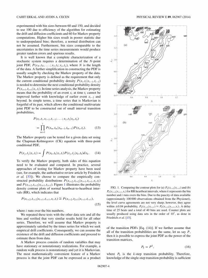
To verify the Markov property, both sides of this equationneed to be evaluated and compared. In practice, severalapproaches of testing for Markov property have been used(see, for example, the authoritative review article by Friedrichet al. [33]). We choose to compare the empirically con-structed probability distributions P (xi+2,ti+2|xi+1,ti+1,xi,ti)and P (xi+2,ti+2|xi+1,ti+1). Figure 1 illustrates the probabilitydensity contour plots of normal heartbeat-to-heartbeat inter-vals (RR), which indicates that

P (xi+2,ti+2|xi+1,ti+1,xi,ti) ∼= P (xi+2,t2+1|xi+1,ti+1),

(15)

where i runs over the bin numbers.We repeated these tests with the other data sets and all the

bins and verified that very similar results hold for all otherseries. Therefore, we will assume that Markov property isapproximately satisfied by the times series for which we seekempirical drift coefficients. Consequently, we can assume theexistence of the drift and diffusion coefficients and proceed toestimate them from data.

A Markov process consists of random variables that mayhave stationary or nonstationary realizations. For example, arandom walk process is nonstationary and yet it is Markovian.The most mathematically convenient feature of a Markovprocess is that the joint PDF can be expressed as a product

0.03

0.03

0.03

0.030.03

0.03

0.03 0.03 0.03 0.03

0.030.03

0.06

0.06

0.06 0.06

0.06

0.06

0.060.06

0.06

0.09

0.09

0.090.09

0.09

0.13

0.13

0.13

0.13

0.13

0.130.13

0.16

0.16

0.16

0.16

0.16

0.16

0.160.19

0.19

0.19

0.23

0.23

0.26

0.26

0.26

0.29

0.290.33

0.03

0.03

0.03

0.030.03

0.03

0.03 0.03 0.03 0.03

0.030.03

0.06

0.06

0.06 0.06

0.06

0.06

0.060.06

0.06

0.09

0.09

0.090.09

0.09

0.13

0.13

0.13

0.13

0.13

0.130.13

0.16

0.16

0.16

0.16

0.16

0.16

0.160.19

0.19

0.19

0.23

0.23

0.26

0.26

0.26

0.29

0.290.33

0.6 0.8 1.0 1.20.4

0.6

0.8

1.0

1.2

1.4

Xi

X i1

0.03

0.03

0.03 0.03 0.03

0.03 0.03

0.07

0.070.070.07

0.11

0.11

0.110.11

0.15

0.15

0.15

0.15

0.15

0.15

0.19

0.19

0.19

0.19

0.19

0.19 0.190.19

0.22

0.22

0.22

0.22

0.22

0.260.26

0.260.26 0.26

0.3

0.3

0.3

0.3

0.34

0.34

0.340.38

0.38

0.6 0.8 1.0 1.20.4

0.6

0.8

1.0

1.2

1.4

Xi

X i1

(a)

(b)

FIG. 1. Comparing the contour plots for (a) Pk(xi+2|xi+1) and (b)Pk(xi+2|xi+1,xi) for RR heartbeat intervals, where k represents the binnumber and i runs overs the bins. Due to the paucity of data available(approximately 100 000 observations obtained from the Physionet),the level curve agreements are not very sharp; however, they agreewithin ±0.04 probability, Pk(xi+2|xi+1) ≈ Pk(xi+2|xi+1,xi). A delaytime of 25 beats and a total of 40 bins are used. Counter plots areusually produced using data sets in the order of 107, as done inFriedrich et al. [15].

of the transition PDFs [Eq. (14)]. If we further assume thatall of the transition probabilities are the same, let us say P ,then it is possible to express the joint PDF as the power of thetransition matrices,

Pk = P k, (16)

where Pk is the k-step transition probability. Therefore,knowledge of the single-step transition probability is sufficient

062907-4

EMPIRICAL FOKKER-PLANCK-BASED TEST OF . . . PHYSICAL REVIEW E 89, 062907 (2014)

0 20000 40000 60000 80000 100000

0.5

1.0

1.5

2.0

beats

RR

0.4 0.6 0.8 1.0 1.2 1.40.5

0.4

0.3

0.2

0.1

0.0

0.1

0.2

x

Dx

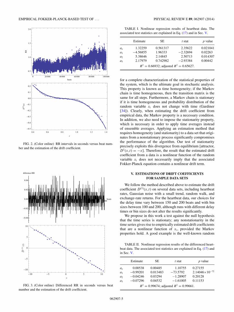
FIG. 2. (Color online) RR intervals in seconds versus beat num-ber and the estimation of the drift coefficient.

200 400 600 800 1000beats

0.04

0.02

5

10

10 5

0.00

0.02

0.04

diference RR

0 5 10

0

5

10

x

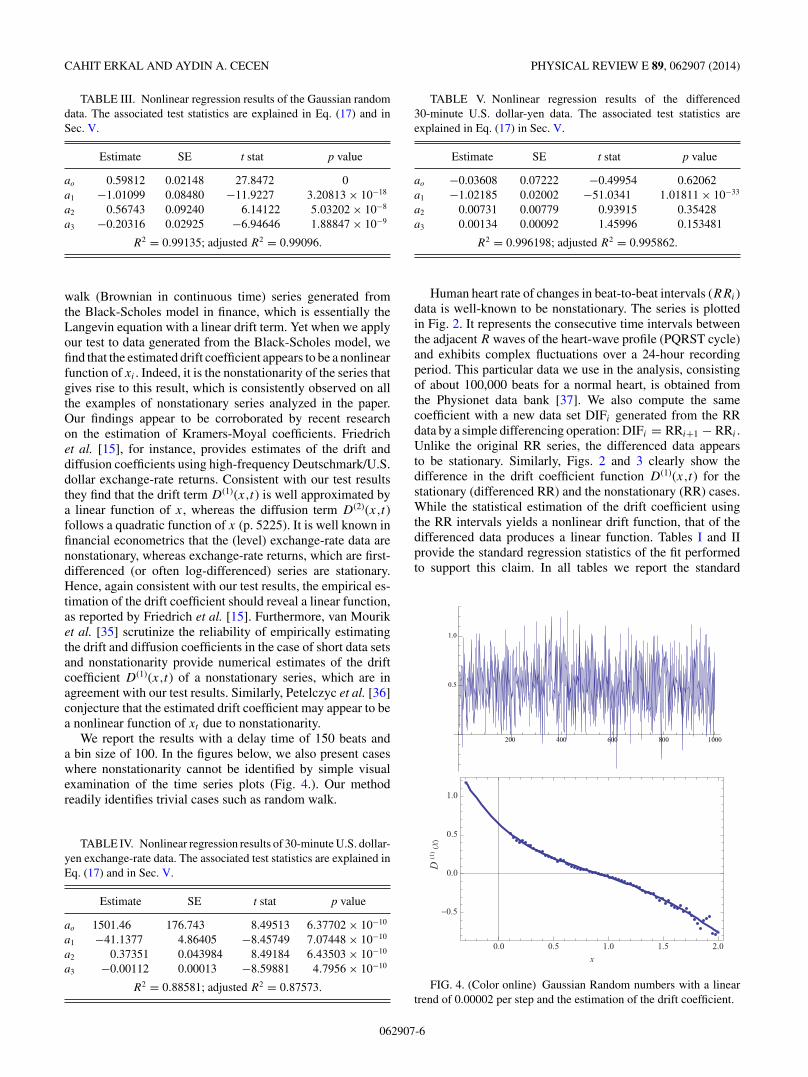
FIG. 3. (Color online) Differenced RR in seconds versus beatnumber and the estimation of the drift coefficient.

TABLE I. Nonlinear regression results of heartbeat data. Theassociated test statistics are explained in Eq. (17) and in Sec. V.

Estimate SE t stat p value

ao 1.32259 0.561317 2.35622 0.021041a1 −4.56855 1.96333 −2.32694 0.02263a2 5.38646 2.14845 2.50713 0.014307a3 2.17979 0.742982 −2.93384 0.00442

R2 = 0.66932; adjusted R2 = 0.65627.

for a complete characterization of the statistical properties ofthe system, which is the ultimate goal in stochastic analysis.This property is known as time homogeneity; if the Markovchain is time homogeneous, then the transition matrix is thesame for all steps. Furthermore, a Markov chain is stationaryif it is time homogeneous and probability distribution of therandom variable xi does not change with time (Gardiner[34]). Clearly, when estimating the drift coefficient fromempirical data, the Markov property is a necessary condition.In addition, we also need to impose the stationarity property,which is necessary in order to apply time averages insteadof ensemble averages. Applying an estimation method thatrequires homogeneity (and stationarity) to a data set that origi-nates from a nonstationary process significantly compromisesthe performance of the algorithm. Our test of stationarityprecisely exploits this divergence from equilibrium [attractor,D1(x,t) = −x]. Therefore, the result that the estimated driftcoefficient from a data is a nonlinear function of the randomvariable xi does not necessarily imply that the associatedFokker-Planck equation contains a nonlinear drift term.

V. ESTIMATIONS OF DRIFT COEFFICIENTSFOR SAMPLE DATA SETS

We follow the method described above to estimate the driftcoefficient D(1)(x,t) on several data sets, including heartbeatrates, Gaussian noise with a small trend, random walk, andexchange-rate returns. For the heartbeat data, our choices forthe delay time vary between 150 and 200 beats and with binsizes between 100 and 200, although runs with different delaytimes or bin sizes do not alter the results significantly.

We propose in this work a test against the null hypothesisthat the time series is stationary; any nonstationarity in thetime series gives rise to empirically estimated drift coefficientsthat are a nonlinear function of xi , provided the Markovproperties hold. A good example is the well-known random

TABLE II. Nonlinear regression results of the differenced heart-beat data. The associated test statistics are explained in Eq. (17) andin Sec. V.

Estimate SE t stat p value

ao 0.00538 0.00485 1.10755 0.27155a1 −0.99201 0.013483 −73.5792 2.14046×10−72

a2 −0.04246 0.03294 −1.28907 0.20128a3 −0.07296 0.04532 −1.61005 0.11153

R2 = 0.99674; adjusted R2 = 0.99661.

062907-5

CAHIT ERKAL AND AYDIN A. CECEN PHYSICAL REVIEW E 89, 062907 (2014)

TABLE III. Nonlinear regression results of the Gaussian randomdata. The associated test statistics are explained in Eq. (17) and inSec. V.

Estimate SE t stat p value

ao 0.59812 0.02148 27.8472 0a1 −1.01099 0.08480 −11.9227 3.20813 × 10−18

a2 0.56743 0.09240 6.14122 5.03202 × 10−8

a3 −0.20316 0.02925 −6.94646 1.88847 × 10−9

R2 = 0.99135; adjusted R2 = 0.99096.

walk (Brownian in continuous time) series generated fromthe Black-Scholes model in finance, which is essentially theLangevin equation with a linear drift term. Yet when we applyour test to data generated from the Black-Scholes model, wefind that the estimated drift coefficient appears to be a nonlinearfunction of xi . Indeed, it is the nonstationarity of the series thatgives rise to this result, which is consistently observed on allthe examples of nonstationary series analyzed in the paper.Our findings appear to be corroborated by recent researchon the estimation of Kramers-Moyal coefficients. Friedrichet al. [15], for instance, provides estimates of the drift anddiffusion coefficients using high-frequency Deutschmark/U.S.dollar exchange-rate returns. Consistent with our test resultsthey find that the drift term D(1)(x,t) is well approximated bya linear function of x, whereas the diffusion term D(2)(x,t)follows a quadratic function of x (p. 5225). It is well known infinancial econometrics that the (level) exchange-rate data arenonstationary, whereas exchange-rate returns, which are first-differenced (or often log-differenced) series are stationary.Hence, again consistent with our test results, the empirical es-timation of the drift coefficient should reveal a linear function,as reported by Friedrich et al. [15]. Furthermore, van Mouriket al. [35] scrutinize the reliability of empirically estimatingthe drift and diffusion coefficients in the case of short data setsand nonstationarity provide numerical estimates of the driftcoefficient D(1)(x,t) of a nonstationary series, which are inagreement with our test results. Similarly, Petelczyc et al. [36]conjecture that the estimated drift coefficient may appear to bea nonlinear function of xt due to nonstationarity.

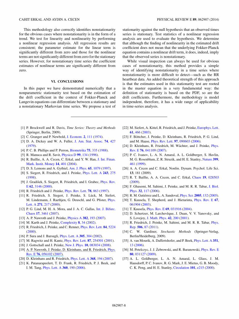
We report the results with a delay time of 150 beats anda bin size of 100. In the figures below, we also present caseswhere nonstationarity cannot be identified by simple visualexamination of the time series plots (Fig. 4.). Our methodreadily identifies trivial cases such as random walk.

TABLE IV. Nonlinear regression results of 30-minute U.S. dollar-yen exchange-rate data. The associated test statistics are explained inEq. (17) and in Sec. V.

Estimate SE t stat p value

ao 1501.46 176.743 8.49513 6.37702 × 10−10

a1 −41.1377 4.86405 −8.45749 7.07448 × 10−10

a2 0.37351 0.043984 8.49184 6.43503 × 10−10

a3 −0.00112 0.00013 −8.59881 4.7956 × 10−10

R2 = 0.88581; adjusted R2 = 0.87573.

TABLE V. Nonlinear regression results of the differenced30-minute U.S. dollar-yen data. The associated test statistics areexplained in Eq. (17) in Sec. V.

Estimate SE t stat p value

ao −0.03608 0.07222 −0.49954 0.62062a1 −1.02185 0.02002 −51.0341 1.01811 × 10−33

a2 0.00731 0.00779 0.93915 0.35428a3 0.00134 0.00092 1.45996 0.153481

R2 = 0.996198; adjusted R2 = 0.995862.

Human heart rate of changes in beat-to-beat intervals (RRi)data is well-known to be nonstationary. The series is plottedin Fig. 2. It represents the consecutive time intervals betweenthe adjacent R waves of the heart-wave profile (PQRST cycle)and exhibits complex fluctuations over a 24-hour recordingperiod. This particular data we use in the analysis, consistingof about 100,000 beats for a normal heart, is obtained fromthe Physionet data bank [37]. We also compute the samecoefficient with a new data set DIFi generated from the RRdata by a simple differencing operation: DIFi = RRi+1 − RRi .Unlike the original RR series, the differenced data appearsto be stationary. Similarly, Figs. 2 and 3 clearly show thedifference in the drift coefficient function D(1)(x,t) for thestationary (differenced RR) and the nonstationary (RR) cases.While the statistical estimation of the drift coefficient usingthe RR intervals yields a nonlinear drift function, that of thedifferenced data produces a linear function. Tables I and IIprovide the standard regression statistics of the fit performedto support this claim. In all tables we report the standard

200 400 600 800 1000

0.5

1.0

0.0 0.5 1.0 1.5 2.0

0.0

0.5

1.0

x

−0.5

FIG. 4. (Color online) Gaussian Random numbers with a lineartrend of 0.00002 per step and the estimation of the drift coefficient.

062907-6

EMPIRICAL FOKKER-PLANCK-BASED TEST OF . . . PHYSICAL REVIEW E 89, 062907 (2014)

0 1000 2000 3000 400060

80

100

120

140

Days

Yen

Dollar

80 90 100 110 120 130 140

0

10

20

x

−10

−20

FIG. 5. (Color online) 30-minute U.S. dollar-yen exchange ratesand the estimation of the drift coefficient.

regression estimation results for an equation of the form

D(1)(x) = ao + a1x + a2x2 + a3x

3 + et , (17)

where ao, a1, and a3 are coefficients to be estimated and et isan iid random variable (innovations).

Tables I–V report the estimated regression coefficients (es-timate), their standard errors (SE), the t statistics (t stat) that areused to test the null hypothesis that each estimated coefficientis zero. P values show the level at which each estimatedcoefficients are statistically significantly different from zero.R2 is the coefficient of determination, which measures thegoodness-of-fit of the overall regression. Adjusted R2 is theR2 adjusted for the degrees of the freedom of the regressionequation.

We also obtain very similar results with a Gaussian randomdata set, which is strongly stationary. We expand this analysisto other cases: logistic map, trend-added logistic map (notreported in the paper), trend-added Gaussian random innovates(Fig. 4), and dollar-yen exchange rate (Figs. 5 and 6). A sampleof a random-walk path and its estimated drift coefficientare provided in Fig. 7. The random-walk path is obtainedfrom Eq. (10), which is a solution to Langevin equation byintegration using stochastic calculus. In comparing Eqs. (9)and (10), we can easily see that the drift coefficient of theunderlying model is a linear function of x: D(1)(x,t) = μxj−1

and yet as the figure shows clearly, the generated time seriesis nonstationary and the estimated drift is nonlinear. Clearly,as explained in Sec. III, the first differenced random-walk datagives rise to a stationary series, which has a linear estimateddrift coefficient.

0 1000 2000 3000 4000

2

0

2

4

6

8

10

beat number

RR

0 5

−5

−5

0

5

x

FIG. 6. (Color online) The 30-minute U.S. dollar-yen exchangerate differences and the estimation of the drift coefficient.

0 1000 2000 3000 4000

0

50

100

i

x

0 20 40 60 80 100

5

0

5

10

15

x

Dx

FIG. 7. (Color online) A random walk series and the estimateddrift coefficient.

062907-7

CAHIT ERKAL AND AYDIN A. CECEN PHYSICAL REVIEW E 89, 062907 (2014)

This methodology also correctly identifies nonstationarityfor the obvious cases where nonstationarity is in the form of atrend. We test for linearity and nonlinearity by performinga nonlinear regression analysis. All regression results areconsistent; the parameter estimate for the linear term issignificantly different from zero and those for the nonlinearterms are not significantly different from zero for the stationaryseries. However, for nonstationary time series the coefficientestimates of nonlinear terms are significantly different fromzero.

VI. CONCLUSIONS

In this paper we have demonstrated numerically that anonparametric stationarity test based on the estimation ofthe drift coefficient in the context of Fokker-Planck andLangevin equations can differentiate between a stationary anda nonstationary Markovian time series. We propose a test of

stationarity against the null hypothesis that an observed timesseries is stationary. Test statistics of a nonlinear regressionanalysis are used to evaluate the hypothesis. We determinethat although the finding of nonlinearity in the estimated driftcoefficient does not mean that the underlying Fokker-Planckequation contains a nonlinear drift term, it does, indeed, implythat the observed series is nonstationary.

While visual inspection can always be used for obviouscases of nonstationarity, this method provides a simpleway of identifying nonstationarity in a time series wherenonstationarity is more difficult to detect—such as the RRheartbeat data. An added theoretical strength of this approachis that the estimates used in this stationarity test are rootedin the master equation in a very fundamental way: thedefinition of stationarity is based on the PDF, so are thedrift coefficients. Furthermore, the methodology is modelindependent, therefore, it has a wide range of applicabilityin time-series analysis.

[1] P. Brockwell and R. Davis, Time Series: Theory and Methods(Springer, Berlin, 2009).

[2] C. Granger and P. Newbold, J. Econom. 2, 111 (1974).[3] D. A. Dickey and W. A. Fuller, J. Am. Stat. Assoc. 74, 427

(1979).[4] P. C. B. Phillips and P. Perron, Biometrika 75, 335 (1988).[5] R. Manuca and R. Savit, Physica D 99, 134 (1996).[6] R. Baillie, A. A. Cecen, C. Erkal, and Y. W. Han, J. Int. Finan.

Mark. Instit. Money 14, 401 (2004).[7] D. S. Lemons and A. Gythiel, Am. J. Phys. 65, 1079 (1997).[8] S. Siegert, R. Friedrich, and J. Peinke, Phys. Lett. A 243, 275

(1998).[9] J. Gradisek, S. Siegert, R. Friedrich, and I. Grabec, Phys. Rev.

E 62, 3146 (2000).[10] R. Friedrich and J. Peinke, Phys. Rev. Lett. 78, 863 (1997).[11] R. Friedrich, S. Siegert, J. Peinke, S. Luck, M. Siefert,

M. Lindemann, J. Raethjen, G. Deuschl, and G. Pfister, Phys.Lett. A 271, 217 (2000).

[12] P. G. Lind, M. H. A. Mora, and J. A. C. Gallas, Int. J. Bifurc.Chaos 17, 3461 (2007).

[13] A. P. Nawroth and J. Peinke, Physics A 382, 193 (2007).[14] M. Karth and J. Peinke, Complexity 8, 34 (2002).[15] R. Friedrich, J. Peinke, and C. Renner, Phys. Rev. Lett. 84, 5224

(2000).[16] P. Sura and J. Barsugli, Phys. Lett. A 305, 304 (2002).[17] M. Ragwitz and H. Kantz, Phys. Rev. Lett. 87, 254501 (2001).[18] J. Gottschall and J. Peinke, New J. Phys. 10, 083034 (2008).[19] A. P. Nawroth, J. Peinke, D. Kleinhans, and R. Friedrich, Phys.

Rev. E 76, 056102 (2007).[20] D. Kleinhans and R. Friedrich, Phys. Lett. A 368, 194 (2007).[21] K. Patanarapeelert, T. D. Frank, R. Friedrich, P. J. Beek, and

I. M. Tang, Phys. Lett. A 360, 190 (2006).

[22] M. Siefert, A. Kittel, R. Friedrich, and J. Peinke, Europhys. Lett.61, 466 (2003).

[23] F. Bottcher, J. Peinke, D. Kleinhans, R. Friedrich, P. G. Lind,and M. Haase, Phys. Rev. Lett. 97, 090603 (2006).

[24] D. Kleinhans, R. Friedrich, M. Wachter, and J. Peinke, Phys.Rev. E 76, 041109 (2007).

[25] P. C. Ivanov, L. A. N. Amaral, A. L. Goldberger, S. Havlin,M. G. Rosenblum, Z. R. Struzik, and H. E. Stanley, Nature 399,461 (1999).

[26] A. A. Cecen and C. Erkal, Nonlin. Dynam. Psychol. Life Sci.13, 181 (2009).

[27] R. T. Baillie, A. A. Cecen, and C. Erkal, Chaos 19, 028503(2009).

[28] F. Ghasemi, M. Sahimi, J. Peinke, and M. R. R. Tabar, J. Biol.Phys. 32, 117 (2006).

[29] R. M. Gutierrez and L. A. Sandoval, Phys. Scr. 2005, 132 (2005).[30] T. Kuusela, T. Shepherd, and J. Hietarinta, Phys. Rev. E 67,

061904 (2003).[31] T. Kuusela, Phys. Rev. E 69, 031916 (2004).[32] D. Schertzer, M. Larcheveque, J. Duan, V. V. Yanovsky, and

S. Lovejoy, J. Math. Phys. 42, 200 (2001).[33] R. Friedrich, J. Peinke, M. Sahimi, and M. R. R. Tabar, Phys.

Rep. 506, 87 (2011).[34] C. W. Gardiner, Stochastic Methods (Springer-Verlag,

Berlin/Heidelberg, 2009).[35] A. van Mourik, A. Daffertshofer, and P. Beek, Phys. Lett. A 351,

13 (2006).[36] M. Petelczyc, J. J. Zebrowski, and R. Baranowski, Phys. Rev. E

80, 031127 (2009).[37] A. L. Goldberger, L. A. N. Amaral, L. Glass, J. M.

Hausdorff, P. C. Ivanov, R. G. Mark, J. E. Mietus, G. B. Moody,C. K. Peng, and H. E. Stanley, Circulation 101, e215 (2000).

062907-8