A&A 571, A22 (2014)DOI: 10.1051/0004-6361/201321569c© ESO 2014

Astronomy&

AstrophysicsPlanck 2013 results Special feature

Planck 2013 results. XXII. Constraints on inflationPlanck Collaboration: P. A. R. Ade90, N. Aghanim62, C. Armitage-Caplan96, M. Arnaud75, M. Ashdown72,6, F. Atrio-Barandela19, J. Aumont62,

C. Baccigalupi89, A. J. Banday99,10, R. B. Barreiro69, J. G. Bartlett1,70, N. Bartolo35, E. Battaner100, K. Benabed63,98, A. Benoît60,A. Benoit-Lévy26,63,98, J.-P. Bernard99,10, M. Bersanelli38,53, P. Bielewicz99,10,89, J. Bobin75, J. J. Bock70,11, A. Bonaldi71, J. R. Bond9, J. Borrill14,93,

F. R. Bouchet63,98, M. Bridges72,6,66, M. Bucher1 ,?, C. Burigana52,36, R. C. Butler52, E. Calabrese96, J.-F. Cardoso76,1,63, A. Catalano77,74,A. Challinor66,72,12, A. Chamballu75,16,62, H. C. Chiang30,7, L.-Y. Chiang65, P. R. Christensen85,41, S. Church95, D. L. Clements58, S. Colombi63,98,

L. P. L. Colombo25,70, F. Couchot73, A. Coulais74, B. P. Crill70,86, A. Curto6,69, F. Cuttaia52, L. Danese89, R. D. Davies71, R. J. Davis71,P. de Bernardis37, A. de Rosa52, G. de Zotti48,89, J. Delabrouille1, J.-M. Delouis63,98, F.-X. Désert56, C. Dickinson71, J. M. Diego69, H. Dole62,61,

S. Donzelli53, O. Doré70,11, M. Douspis62, J. Dunkley96, X. Dupac44, G. Efstathiou66, T. A. Enßlin81, H. K. Eriksen67, F. Finelli52,54 ,?,O. Forni99,10, M. Frailis50, E. Franceschi52, S. Galeotta50, K. Ganga1, C. Gauthier1,80, M. Giard99,10, G. Giardino45, Y. Giraud-Héraud1,

J. González-Nuevo69,89, K. M. Górski70,101, S. Gratton72,66, A. Gregorio39,50, A. Gruppuso52, J. Hamann97, F. K. Hansen67, D. Hanson82,70,9,D. Harrison66,72, S. Henrot-Versillé73, C. Hernández-Monteagudo13,81, D. Herranz69, S. R. Hildebrandt11, E. Hivon63,98, M. Hobson6,

W. A. Holmes70, A. Hornstrup17, W. Hovest81, K. M. Huffenberger28, A. H. Jaffe58, T. R. Jaffe99,10, W. C. Jones30, M. Juvela29, E. Keihänen29,R. Keskitalo23,14, T. S. Kisner79, R. Kneissl43,8, J. Knoche81, L. Knox32, M. Kunz18,62,3, H. Kurki-Suonio29,47, G. Lagache62, A. Lähteenmäki2,47,

J.-M. Lamarre74, A. Lasenby6,72, R. J. Laureijs45, C. R. Lawrence70, S. Leach89, J. P. Leahy71, R. Leonardi44, J. Lesgourgues97,88, A. Lewis27,M. Liguori35, P. B. Lilje67, M. Linden-Vørnle17, M. López-Caniego69, P. M. Lubin33, J. F. Macías-Pérez77, B. Maffei71, D. Maino38,53,

N. Mandolesi52,5,36, M. Maris50, D. J. Marshall75, P. G. Martin9, E. Martínez-González69, S. Masi37, M. Massardi51, S. Matarrese35, F. Matthai81,P. Mazzotta40, P. R. Meinhold33, A. Melchiorri37,55, L. Mendes44, A. Mennella38,53, M. Migliaccio66,72, S. Mitra57,70, M.-A. Miville-Deschênes62,9,A. Moneti63, L. Montier99,10, G. Morgante52, D. Mortlock58, A. Moss91, D. Munshi90, J. A. Murphy84, P. Naselsky85,41, F. Nati37, P. Natoli36,4,52,

C. B. Netterfield21, H. U. Nørgaard-Nielsen17, F. Noviello71, D. Novikov58, I. Novikov85, I. J. O’Dwyer70, S. Osborne95, C. A. Oxborrow17,F. Paci89, L. Pagano37,55, F. Pajot62, R. Paladini59, S. Pandolfi40, D. Paoletti52,54, B. Partridge46, F. Pasian50, G. Patanchon1, H. V. Peiris26,

O. Perdereau73, L. Perotto77, F. Perrotta89, F. Piacentini37, M. Piat1, E. Pierpaoli25, D. Pietrobon70, S. Plaszczynski73, E. Pointecouteau99,10,G. Polenta4,49, N. Ponthieu62,56, L. Popa64, T. Poutanen47,29,2, G. W. Pratt75, G. Prézeau11,70, S. Prunet63,98, J.-L. Puget62, J. P. Rachen22,81,

R. Rebolo68,15,42, M. Reinecke81, M. Remazeilles71,62,1, C. Renault77, S. Ricciardi52, T. Riller81, I. Ristorcelli99,10, G. Rocha70,11, C. Rosset1,G. Roudier1,74,70, M. Rowan-Robinson58, J. A. Rubiño-Martín68,42, B. Rusholme59, M. Sandri52, D. Santos77, M. Savelainen29,47, G. Savini87,

D. Scott24, M. D. Seiffert70,11, E. P. S. Shellard12, L. D. Spencer90, J.-L. Starck75, V. Stolyarov6,72,94, R. Stompor1, R. Sudiwala90, R. Sunyaev81,92,F. Sureau75, D. Sutton66,72, A.-S. Suur-Uski29,47, J.-F. Sygnet63, J. A. Tauber45, D. Tavagnacco50,39, L. Terenzi52, L. Toffolatti20,69, M. Tomasi53,

J. Tréguer-Goudineau1, M. Tristram73, M. Tucci18,73, J. Tuovinen83, L. Valenziano52, J. Valiviita47,29,67, B. Van Tent78, J. Varis83, P. Vielva69,F. Villa52, N. Vittorio40, L. A. Wade70, B. D. Wandelt63,98,34, M. White31, A. Wilkinson71, D. Yvon16, A. Zacchei50, J. P. Zibin24, and A. Zonca33

(Affiliations can be found after the references)

Received 25 March 2013 / Accepted 28 January 2014

ABSTRACT

We analyse the implications of the Planck data for cosmic inflation. The Planck nominal mission temperature anisotropy measurements, combinedwith the WMAP large-angle polarization, constrain the scalar spectral index to be ns = 0.9603 ± 0.0073, ruling out exact scale invariance atover 5σ. Planck establishes an upper bound on the tensor-to-scalar ratio of r < 0.11 (95% CL). The Planck data thus shrink the space of allowedstandard inflationary models, preferring potentials with V ′′ < 0. Exponential potential models, the simplest hybrid inflationary models, andmonomial potential models of degree n ≥ 2 do not provide a good fit to the data. Planck does not find statistically significant running of thescalar spectral index, obtaining dns/dln k = −0.0134 ± 0.0090. We verify these conclusions through a numerical analysis, which makes no slow-roll approximation, and carry out a Bayesian parameter estimation and model-selection analysis for a number of inflationary models includingmonomial, natural, and hilltop potentials. For each model, we present the Planck constraints on the parameters of the potential and exploreseveral possibilities for the post-inflationary entropy generation epoch, thus obtaining nontrivial data-driven constraints. We also present a directreconstruction of the observable range of the inflaton potential. Unless a quartic term is allowed in the potential, we find results consistent withsecond-order slow-roll predictions. We also investigate whether the primordial power spectrum contains any features. We find that models with aparameterized oscillatory feature improve the fit by ∆χ2

eff≈ 10; however, Bayesian evidence does not prefer these models. We constrain several

single-field inflation models with generalized Lagrangians by combining power spectrum data with Planck bounds on fNL. Planck constrains withunprecedented accuracy the amplitude and possible correlation (with the adiabatic mode) of non-decaying isocurvature fluctuations. The fractionalprimordial contributions of cold dark matter (CDM) isocurvature modes of the types expected in the curvaton and axion scenarios have upperbounds of 0.25% and 3.9% (95% CL), respectively. In models with arbitrarily correlated CDM or neutrino isocurvature modes, an anticorrelatedisocurvature component can improve the χ2

effby approximately 4 as a result of slightly lowering the theoretical prediction for the ` <∼ 40 multipoles

relative to the higher multipoles. Nonetheless, the data are consistent with adiabatic initial conditions.

Key words. cosmic background radiation – inflation – early Universe

? Corresponding authors: M. Bucher, e-mail: bucher@apc.univ-paris7.fr; F. Finelli, e-mail: finelli@iasfbo.inaf.it

Article published by EDP Sciences A22, page 1 of 42

A&A 571, A22 (2014)

1. Introduction

This paper, one of a set associated with the 2013 releaseof data from the Planck1 mission (Planck Collaboration I–XXXI 2014), describes the implications of the Planck mea-surement of cosmic microwave background (CMB) anisotropiesfor cosmic inflation. In this first release only the Planck tem-perature data resulting from the nominal mission are used,which includes 2.6 full surveys of the sky. The interpreta-tion of the CMB polarization as seen by Planck will be pre-sented in a later series of publications. This paper exploitsthe data presented in Planck Collaboration II (2014), PlanckCollaboration XII (2014), Planck Collaboration XV (2014), andPlanck Collaboration XVII (2014). Other closely related pa-pers discuss the estimates of cosmological parameters in PlanckCollaboration XVI (2014) and investigations of non-Gaussianityin Planck Collaboration XXIV (2014).

In the early 1980s inflationary cosmology, which postu-lates an epoch of nearly exponential expansion, was proposedin order to resolve a number of puzzles of standard big bangcosmology such as the entropy, flatness, horizon, smoothness,and monopole problems (Brout et al. 1978; Starobinsky 1980;Kazanas 1980; Sato 1981; Guth 1981; Linde 1982; Albrecht &Steinhardt 1982; Linde 1983). During inflation, cosmologicalfluctuations resulting from quantum fluctuations are generatedand can be calculated using the semiclassical theory of quantumfields in curved spacetime (Mukhanov & Chibisov 1981, 1982;Hawking 1982; Guth & Pi 1982; Starobinsky 1982; Bardeenet al. 1983; Mukhanov 1985).

Cosmological observations prior to Planck are consistentwith the simplest models of inflation within the slow-rollparadigm. Recent observations of the CMB anisotropies (Storyet al. 2013; Bennett et al. 2013; Hinshaw et al. 2013; Hou et al.2014; Das et al. 2014) and of large-scale structure (Beutler et al.2011; Padmanabhan et al. 2012; Anderson et al. 2012) indicatethat our Universe is very close to spatially flat and has primordialdensity fluctuations that are nearly Gaussian and adiabatic andare described by a nearly scale-invariant power spectrum. Pre-Planck CMB observations also established that the amplitudeof primordial gravitational waves, with a nearly scale-invariantspectrum (Starobinsky 1979; Rubakov et al. 1982; Fabbri &Pollock 1983), is at most small.

Most of the results in this paper are based on the two-point statistics of the CMB as measured by Planck, exploitingthe data presented in Planck Collaboration XV (2014), PlanckCollaboration XVI (2014), and Planck Collaboration XVII(2014). The Planck results testing the Gaussianity of the pri-mordial CMB component are described in the companion papersPlanck Collaboration XXIII (2014), Planck Collaboration XXIV(2014), and Planck Collaboration XXV (2014). Planck findsvalues for the non-Gaussian fNL parameter of the CMBbispectrum consistent with the Gaussian hypothesis (PlanckCollaboration XXIV 2014). This result has important implica-tions for inflation. The simplest slow-roll inflationary modelspredict a level of fNL of the same order as the slow-roll parame-ters and therefore too small to be detected by Planck.

The paper is organized as follows. Section 2 reviews infla-tionary theory, emphasizing in particular those aspects used later

1 Planck (http://www.esa.int/Planck) is a project of theEuropean Space Agency (ESA) with instruments provided by two sci-entific consortia funded by ESA member states (in particular the leadcountries France and Italy), with contributions from NASA (USA) andtelescope reflectors provided by a collaboration between ESA and a sci-entific consortium led and funded by Denmark.

in the paper. In Sect. 3 the statistical methodology and the Plancklikelihood as well as the likelihoods from the other astrophysicaldata sets used here are described. Section 4 presents constraintson slow-roll inflation and studies their robustness under gener-alizations of the minimal assumptions of our baseline cosmo-logical model. In Sect. 5 Bayesian model comparison of severalinflationary models is carried out taking into account the uncer-tainty from the end of inflation to the beginning of the radia-tion dominated era. Section 6 reconstructs the inflationary po-tential over the range corresponding to the scales observable inthe CMB. In Sect. 7 a penalized likelihood reconstruction ofthe primordial perturbation spectrum is performed. Section 8reports on a parametric search for oscillations and features inthe primordial scalar power spectrum. Section 9 examines con-straints on non-canonical single-field models of inflation includ-ing the fNL measurements from Planck Collaboration XXIV(2014). In Sect. 10 constraints on isocurvature modes are estab-lished, thus testing the hypothesis that initial conditions weresolely adiabatic. We summarize our conclusions in Sect. 11.Appendix A is dedicated to the constraints on slow-roll infla-tion derived by sampling the Hubble flow functions (HFF) inthe analytic expressions for the scalar and tensor power spectra.Definitions of the most relevant symbols used in this paper canbe found in Tables 1 and 2.

2. Lightning review of inflation

Before describing cosmic inflation, which was developed inthe early 1980s, it is useful to review the state of theoryprior to its introduction. Lifshitz (1946; see also Lifshitz &Khalatnikov 1963) first wrote down and solved the equations forthe evolution of linearized perturbations about a homogeneousand isotropic Friedmann-Lemaître-Robertson-Walker spacetimewithin the framework of general relativity. The general frame-work adopted was based on two assumptions:

(i) The cosmological perturbations can be described by asingle-component fluid, at very early times.

(ii) The initial cosmological perturbations were statistically ho-mogeneous and isotropic, and Gaussian.

These are the simplest–but by no means unique–assumptionsfor defining a stochastic process for the initial conditions.Assumption (i), where only a single adiabatic mode is excited, isjust the simplest possibility. In Sect. 10 we shall describe isocur-vature perturbations, where other available modes are excited,and report on the constraints established by Planck. Assumption(ii) is a priori more questionable given the understanding at thetime. An appeal can be made to the fact that any physics at weakcoupling could explain (ii), but at the time these assumptionswere somewhat ad hoc.

Even with the strong assumptions (i) and (ii), comparisonswith observations cannot be made without further restrictionson the functional form of the primordial power spectrum oflarge-scale spatial curvature inhomogeneities R, PR(k) ∝ kns−1,where ns is the (scalar) spectral index. The notion of a scale-invariant (i.e., ns = 1) primordial power spectrum was intro-duced by Harrison (1970), Zeldovich (1972), and Peebles &Yu (1970) to address this problem. These authors showed thata scale-invariant power law was consistent with the crude con-straints on large- and small-scale perturbations available at thetime. However, other than its mathematical simplicity, no com-pelling theoretical explanation for this Ansatz was put forth.An important current question, addressed in Sect. 4, is whetherns = 1 (i.e., exact scale invariance) is consistent with the data, or

A22, page 2 of 42

Planck Collaboration: Planck 2013 results. XXII.

Table 1. Cosmological parameter definitions.

Parameter DefinitionΩb . . . . . . . . . . . Baryon fraction today (compared to critical density)Ωc . . . . . . . . . . . . Cold dark matter fraction today (compared to critical density)h . . . . . . . . . . . . . Current expansion rate (as fraction of 100 km s−1 Mpc−1)θMC . . . . . . . . . . . Approximation to the angular size of sound horizon at last scatteringτ . . . . . . . . . . . . . Thomson scattering optical depth of reionized intergalactic mediumNeff . . . . . . . . . . . Effective number of massive and massless neutrinosΣmν . . . . . . . . . . Sum of neutrino massesYP . . . . . . . . . . . . Fraction of baryonic mass in primordial heliumΩK . . . . . . . . . . . Spatial curvature parameterwde . . . . . . . . . . . Dark energy equation of state parameter (i.e., p/ρ) (assumed constant)R . . . . . . . . . . . . Curvature perturbationI . . . . . . . . . . . . Isocurvature perturbationPX = k3|Xk |

2/2π2 . Power spectrum of XAX . . . . . . . . . . . X power spectrum amplitude (at k∗ = 0.05 Mpc−1)ns . . . . . . . . . . . . Scalar spectrum spectral index (at k∗ = 0.05 Mpc−1, unless otherwise stated)dns/dln k . . . . . . . Running of scalar spectral index (at k∗ = 0.05 Mpc−1, unless otherwise stated)d2ns/dln k2 . . . . . . Running of running of scalar spectral index (at k∗ = 0.05 Mpc−1)r . . . . . . . . . . . . . Tensor-to-scalar power ratio (at k∗ = 0.05 Mpc−1, unless otherwise stated)nt . . . . . . . . . . . . Tensor spectrum spectral index (at k∗ = 0.05 Mpc−1)dnt/dln k . . . . . . . Running of tensor spectral index (at k∗ = 0.05 Mpc−1)

Table 2. Conventions and definitions for inflation physics.

Parameter Definitionφ . . . . . . . . . . . . . . . . InflatonV(φ) . . . . . . . . . . . . . Inflaton potentiala . . . . . . . . . . . . . . . . Scale factort . . . . . . . . . . . . . . . . Cosmic (proper) timeδX . . . . . . . . . . . . . . Fluctuation of XX = dX/dt . . . . . . . . . Derivative with respect to proper timeX′ = dX/dη . . . . . . . . Derivative with respect to conformal timeXφ = ∂X/∂φ . . . . . . . . Partial derivative with respect to φMpl . . . . . . . . . . . . . . Reduced Planck mass (=2.435 × 1018 GeV)Q . . . . . . . . . . . . . . . Scalar perturbation variableh+,× . . . . . . . . . . . . . . Gravitational wave amplitude of (+,×)-polarization componentX∗ . . . . . . . . . . . . . . . X evaluated at Hubble exit during inflation of mode with wavenumber k∗Xe . . . . . . . . . . . . . . . X evaluated at end of inflationεV = M2

plV2φ/2V2 . . . . . First slow-roll parameter for V(φ)

ηV = M2plVφφ/V . . . . . Second slow-roll parameter for V(φ)

ξ2V = M4

plVφVφφφ/V2 . . Third slow-roll parameter for V(φ)$3

V = M6plV

2φVφφφφ/V3 . Fourth slow-roll parameter for V(φ)

ε1 = −H/H2 . . . . . . . First Hubble hierarchy parameterεn+1 = εn/Hεn . . . . . . . (n + 1)th Hubble hierarchy parameter (where n ≥ 1)N(t) =

∫ tet

dt H . . . . . . Number of e-folds to end of inflationδσ . . . . . . . . . . . . . . Curvature field perturbationδs . . . . . . . . . . . . . . . Isocurvature field perturbation

whether there is convincing evidence for small deviations fromexact scale invariance. Although the inflationary potential can betuned to obtain ns = 1, inflationary models generically predictdeviations from ns = 1, usually on the red side (i.e., ns < 1).

2.1. Cosmic inflation

Inflation was developed in a series of papers by Brout et al.(1978), Starobinsky (1980), Kazanas (1980), Sato (1981), Guth(1981), Linde (1982, 1983), and Albrecht & Steinhardt (1982).By generating an equation of state with a significant negativepressure (i.e., w = p/ρ ≈ −1) before the radiation epoch,

inflation solves a number of cosmological conundrums (themonopole, horizon, smoothness, and entropy problems), whichhad plagued all cosmological models extrapolating a matter-radiation equation of state all the way back to the singularity.Such an equation of state (p ≈ −ρ) and the resulting nearly ex-ponential expansion are obtained from a scalar field, the inflaton,with a canonical kinetic term (i.e., 1

2 (∂φ)2), slowly rolling in theframework of Einstein gravity.

The homogeneous evolution of the inflaton field φ is gov-erned by the equation of motion

φ + 3Hφ + Vφ = 0, (1)

A22, page 3 of 42

A&A 571, A22 (2014)

and the Friedmann equation

H2 =1

3Mpl2

(12φ2 + V(φ)

). (2)

Here H = a/a is the Hubble parameter, the subscript φ de-notes the derivative with respect to φ, Mpl = (8πG)−1/2 is thereduced Planck mass, and V is the potential. (We use units wherec = ~ = 1.) The evolution during the stage of quasi-exponentialexpansion, when the scalar field rolls slowly down the potential,can be approximated by neglecting the second time derivative inEq. (1) and the kinetic energy term in Eq. (2), so that

3Hφ ≈ −Vφ, (3)

H2 ≈V(φ)3Mpl

2 · (4)

Necessary conditions for the slow-roll described above areεV 1 and |ηV | 1, where the slow-roll parameters εV and ηVare defined as

εV =M2

plV2φ

2V2 , (5)

ηV =M2

plVφφ

V· (6)

The analogous hierarchy of HFF slow-roll parameters measuresinstead the deviation from an exact exponential expansion. Thishierarchy is defined as ε1 = −H/H2, εi+1 ≡ εi/(Hεi), with i ≥ 1.By using Eqs. (3) and (4), we have that ε1 ≈ εV , ε2 ≈ −2ηV +4εV .

2.2. Quantum generation of fluctuations

Without quantum fluctuations, inflationary theory would fail.Classically, any initial spatial curvature or gradients in the scalarfield, as well as any inhomogeneities in other fields, wouldrapidly decay away during the quasi-exponential expansion. Theresulting universe would be too homogeneous and isotropiccompared with observations. Quantum fluctuations must existin order to satisfy the uncertainty relations that follow from thecanonical commutation relations of quantum field theory. Thequantum fluctuations in the inflaton and in the transverse andtraceless parts of the metric are amplified by the nearly exponen-tial expansion yielding the scalar and tensor primordial powerspectra, respectively.

Many essentially equivalent approaches to quantizing thelinearized cosmological fluctuations can be found in the origi-nal literature (see, e.g., Mukhanov & Chibisov 1981; Hawking1982; Guth & Pi 1982; Starobinsky 1982; Bardeen et al. 1983).A simple formalism, which we shall follow here, was intro-duced by Mukhanov (1988), Mukhanov et al. (1992), and Sasaki(1986). In this approach a gauge-invariant inflaton fluctuation Qis constructed and canonically quantized. This gauge-invariantvariable Q is the inflaton fluctuation δφ(t, x) in the uniformcurvature gauge. The mode function of the inflaton fluctua-tions δφ(t, x) obeys the evolution equation

(aδφk)′′ +(k2 −

z′′

z

)(aδφk) = 0, (7)

where z = aφ/H. The gauge-invariant field fluctuation is directlyrelated to the comoving curvature perturbation2

R = −Hδφ

φ· (8)

2 Another important quantity is the curvature perturbation on uniformdensity hypersurfaces ζ (in the Newtonian gauge, ζ = −ψ − Hδρ/ρ,

Analogously, gravitational waves are described by the two polar-ization states (+,×) of the transverse traceless parts of the metricfluctuations and are amplified by the expansion of the universeas well (Grishchuk 1975). The evolution equation for their modefunction is

(ah+,×k )′′ +

(k2 −

a′′

a

)(ah+,×

k ) = 0. (9)

Early discussions of the generation of gravitational wavesduring inflation include Starobinsky (1979), Rubakov et al.(1982), Fabbri & Pollock (1983), Abbott & Wise (1984), andStarobinsky (1985a).

Because the primordial perturbations are small, of or-der 10−5, the linearized Eqs. (7) and (9) provide an accuratedescription for the generation and subsequent evolution of thecosmological perturbations during inflation. In this paper weuse two approaches for solving for the cosmological perturba-tions. Firstly, we use an approximate treatment based on theslow-roll approximation described below. Secondly, we use analmost exact approach based on numerical integration of the or-dinary differential Eqs. (7) and (9) for each value of the comov-ing wavenumber k. For fixed k the evolution may be dividedinto three epochs: (i) sub-Hubble evolution; (ii) Hubble cross-ing evolution; and (iii) super-Hubble evolution. During (i) thewavelength is much smaller than the Hubble length, and themode oscillates as it would in a non-expanding universe (i.e.,Minkowski space). Therefore we can proceed with quantizationas we would in Minkowski space. We quantize by singling outthe positive frequency solution, as in the Bunch-Davies vacuum(Bunch & Davies 1978). This epoch is the oscillating regime inthe WKB approximation. In epoch (iii), by contrast, there aretwo solutions, a growing and a decaying mode, and the evolu-tion becomes independent of k. We care only about the grow-ing mode. On scales much larger than the Hubble radius (i.e.,k aH), both curvature and tensor fluctuations admit solu-tions constant in time3. All the interesting, or nontrivial, evolu-tion takes place between epochs (i) and (iii) – that is, during (ii),a few e-folds before and after Hubble crossing, and this is theinterval where the numerical integration is most useful since theasymptotic expansions are not valid in this transition region. Twonumerical codes are used in this paper, ModeCode (Adams et al.2001; Peiris et al. 2003; Mortonson et al. 2009; Easther & Peiris2012), and the inflation module of Lesgourgues & Valkenburg(2007) as implemented in CLASS (Lesgourgues 2011; Blas et al.2011)4.

It is convenient to expand the power spectra of curvature andtensor perturbations on super-Hubble scales as

PR(k) = As

(kk∗

)ns − 1 + 12 dns/dln k ln(k/k∗) + 1

6 d2ns/dln k2(ln(k/k∗))2+...

, (10)

Pt(k) = At

(kk∗

)nt+12 dnt/dln k ln(k/k∗)+...

, (11)

where ψ is the generalized gravitational potential), which is related tothe perturbed spatial curvature according to (3)R = −4∇2ζ/a2. On largescales ζ ≈ R.3 On large scales, the curvature fluctuation is constant in time whennon-adiabatic pressure terms are negligible. This condition is typicallyviolated in multi-field inflationary models.4 http://zuserver2.star.ucl.ac.uk/~hiranya/ModeCode/,http://class-code.net

A22, page 4 of 42

Planck Collaboration: Planck 2013 results. XXII.

where As (At) is the scalar (tensor) amplitude and ns (nt),dns/dln k (dnt/dln k) and d2ns/dln k2 are the scalar (tensor) spec-tral index, the running of the scalar (tensor) spectral index,and the running of the running of the scalar spectral index,respectively.

The parameters of the scalar and tensor power spectra maybe calculated approximately in the framework of the slow-rollapproximation by evaluating the following equations at the valueof the inflation field φ∗ where the mode k∗ = a∗H∗ crosses theHubble radius for the first time. (For a nice review of the slow-roll approximation, see for example Liddle & Lyth 1993.) Thenumber of e-folds before the end of inflation, N∗, at which thepivot scale k∗ exits from the Hubble radius, is

N∗ =

∫ te

t∗dt H ≈

1M2

pl

∫ φe

φ∗

dφVVφ, (12)

where the equality holds in the slow-roll approximation, andsubscript e denotes the end of inflation.

The coefficients of Eqs. (10) and (11) at their respective lead-ing orders in the slow-roll parameters are given by

As ≈V

24π2M4plεV

, (13)

At ≈2V

3π2M4pl

, (14)

ns − 1 ≈ 2ηV − 6εV , (15)nt ≈ −2εV , (16)dns/dln k ≈ +16εVηV − 24ε2

V − 2ξ2V , (17)

dnt/dln k ≈ +4εVηV − 8ε2V , (18)

d2ns/dln k2 ≈ −192ε3V + 192ε2

VηV − 32εVη2V

−24εVξ2V + 2ηVξ

2V + 2$3

V , (19)

where the slow-roll parameters εV and ηV are defined in Eqs. (5)and (6), and the higher order parameters are defined as

ξ2V =

M4plVφVφφφ

V2 (20)

and

$3V =

M6plV

2φVφφφφ

V3 · (21)

In single-field inflation with a standard kinetic term, as discussedhere, the tensor spectrum shape is not independent from the otherparameters. The slow-roll paradigm implies a tensor-to-scalarratio at the pivot scale of

r =Pt(k∗)PR(k∗)

≈ 16εV ≈ −8nt, (22)

referred to as the consistency relation. This consistency relationis also useful to help understand how r is connected to the evo-lution of the inflaton:

∆φ

Mpl≈

1√

8

∫ N

0dN√

r. (23)

The above relation, called the Lyth bound (Lyth 1997), impliesthat an inflaton variation of the order of the Planck mass isneeded to produce r & 0.01. Such a threshold is useful to clas-sify large- and small-field inflationary models with respect to theLyth bound.

2.3. Ending inflation and the epoch of entropy generation

The greatest uncertainty in calculating the perturbation spectrumpredicted from a particular inflationary potential arises in estab-lishing the correspondence between the comoving wavenumbertoday and the inflaton energy density when the mode of thatwavenumber crossed the Hubble radius during inflation (Kinney& Riotto 2006). This correspondence depends both on the infla-tionary model and on the cosmological evolution from the endof inflation to the present.

After the slow-roll stage, φ becomes as important as the cos-mological damping term 3Hφ. Inflation ends gradually as theinflaton picks up kinetic energy so that w is no longer slightlyabove −1, but rather far from that value. We may arbitrarilydeem that inflation ends when w = −1/3 (the value dividingthe cases of an expanding and a contracting comoving Hubbleradius), or, equivalently, at εV ≈ 1, after which the epoch ofentropy generation starts. Because of couplings to other fields,the energy initially in the form of scalar field vacuum energyis transferred to the other fields by perturbative decay (reheat-ing), possibly preceded by a non-perturbative stage (preheating).There is considerable uncertainty about the mechanisms of en-tropy generation, or thermalization, which subsequently lead toa standard w = 1/3 equation of state for radiation.

On the other hand, if we want to identify some k∗ today withthe value of the inflaton field at the time this scale left the Hubbleradius, Eq. (12) needs to be matched to an expression that quan-tifies how much k∗ has shrunk relative to the size of the Hubbleradius between the end of inflation and the time when that modere-enters the Hubble radius. This quantity depends both on theinflationary potential and the details of the entropy generationprocess and is given by

N∗ ≈ 67 − ln(

k∗a0H0

)+

14

ln

V∗M4

pl

+14

ln(

V∗ρend

)+

1 − 3wint

12(1 + wint)ln

(ρth

ρend

)−

112

ln(gth),

(24)

where ρend is the energy density at the end of inflation, ρth isan energy scale by which the universe has thermalized, a0H0 isthe present Hubble radius, V∗ is the potential energy when k∗left the Hubble radius during inflation, wint characterizes the ef-fective equation of state between the end of inflation and theenergy scale specified by ρth, and gth is the number of effectivebosonic degrees of freedom at the energy scale ρth. In predictingthe primordial power spectra at observable scales for a specificinflaton potential, this uncertainty in the reheating history of theuniverse becomes relevant and can be taken into account by al-lowing N∗ to vary over a range of values. Note that wint is notintended to provide a detailed model for entropy generation, butrather to parameterize the uncertainty regarding the expansionrate of the universe during this intermediate era. Nevertheless,constraints on wint provide observational limits on the uncertainphysics during this period.

The first two terms of Eq. (24) are model independent,with the second term being roughly 5 for k∗ = 0.05 Mpc−1.If thermalization occurs rapidly, or if the reheating stage isclose to radiation-like, the magnitude of the second to last termin Eq. (24) is less than roughly unity. The magnitude of theln(gth)/12 term is negligible, giving a shift of only 0.58 for theextreme value gth = 103. For most reasonable inflation models,the fourth term is O(1) and the third term is approximately −10,motivating the commonly assumed range 50 < N∗ < 60.Nonetheless, more extreme values at both ends are in principle

A22, page 5 of 42

A&A 571, A22 (2014)

possible (Liddle & Leach 2003). In the figures of Sect. 4 we willmark the range 50 < N∗ < 60 as a general guide.

2.4. Perturbations from cosmic inflation at higher order

To calculate the quantum fluctuations generated during cosmicinflation, a linearized quantum field theory in a time-dependentbackground can be used. The leading order is the two-point cor-relation function

〈R(k1) R(k2)〉 = (2π)3 2π2

k3 PR(k) δ(3)(k1 + k2), (25)

but the inflaton self-interactions and the nonlinearity of Einsteingravity give small higher-order corrections, of which the next-to-leading order is the three point function

〈R(k1) R(k2) R(k3)〉 = (2π)3BR(k1, k2, k3)δ(3)(k1 + k2 + k3), (26)

which is in general non-zero.For single-field inflation with a standard kinetic term in a

smooth potential (with initial fluctuations in the Bunch-Daviesvacuum), the non-Gaussian contribution to the curvature per-turbation during inflation is O(εV , ηV ) (Acquaviva et al. 2003;Maldacena 2003), i.e., at an undetectable level smaller than othergeneral relativistic contributions, such as the cross-correlationbetween the integrated Sachs-Wolfe effect and weak gravita-tional lensing of the CMB. For a general scalar field Lagrangian,the non-Gaussian contribution can be large enough to be ac-cessible to Planck with fNL of order c−2

s (Chen et al. 2007),where cs is the sound speed of inflaton fluctuations (see Sect. 9).Other higher order kinetic and spatial derivative terms contributeto larger non-Gaussianities. For a review of non-Gaussianitygenerated during inflation, see, for example, Bartolo et al.(2004a) and Chen (2010) as well as the companion paper PlanckCollaboration XXIV (2014).

2.5. Multi-field models of cosmic inflation

Inflation as described so far assumes a single scalar field thatdrives and terminates the quasi-exponential expansion and alsogenerates the large-scale curvature perturbations. When thereis more than one field with an effective mass smaller than H,isocurvature perturbations are also generated during inflationby the same mechanism of amplification due to the stretchingof the spacetime geometry (Axenides et al. 1983; Linde 1985).Cosmological perturbations in models with an M-component in-flaton φi can be analysed by considering perturbations paralleland perpendicular to the classical trajectory, as treated for exam-ple in Gordon et al. (2001). The definition of curvature perturba-tion generalizing Eq. (8) to the multi-field case is

R = −H∑M

i=1 φiQi

σ2 , (27)

where Qi is the gauge-invariant field fluctuation associatedwith φi and σ2 ≡

∑Mi=1 φ

2i . The above formula for the curvature

perturbation can also be obtained through the δN formalism, i.e.,R =

∑Mi=1(∂N/∂φi)Qi, where the number of e-folds to the end

of inflation N is generalized to the multi-field case (Starobinsky1985b; Sasaki & Stewart 1996). The M−1 normal directions areconnected to M − 1 isocurvature perturbations δsi j according to

δsi j =φiQ j − φ jQi

σ· (28)

If the trajectory of the average field is curved in field space, thenduring inflation both curvature and isocurvature fluctuations aregenerated with non-vanishing correlations (Langlois 1999).

Isocurvature perturbations can be converted into curvatureperturbations on large scales, but the opposite does not hold(Mollerach 1990). If such isocurvature perturbations are nottotally converted into curvature perturbations, they can haveobservable effects on CMB anisotropies and on structure forma-tion. In Sect. 10, we present the Planck constraints on a com-bination of curvature and isocurvature initial conditions and theimplications for important two-field scenarios, such as the cur-vaton (Lyth & Wands 2002) and axion (Lyth 1990) models.

Isocurvature perturbations may lead to a higher level of non-Gaussianity compared to a single inflaton with a standard kineticterm (Groot Nibbelink & van Tent 2000). There is no reason toexpect the inflaton to be a single-component field. The scalarsector of the Standard Model, as well as its extensions, containsmore than one scalar field.

3. Methodology

3.1. Cosmological model and parameters

The parameters of the models to be estimated in this paper fallinto three categories: (i) parameters describing the initial pertur-bations, i.e., characterizing the particular inflationary scenario inquestion; (ii) parameters determining cosmological evolution atlate times (z . 104); and (iii) parameters that quantify our uncer-tainty about the instrument and foreground contributions to theangular power spectrum. These will be described in Sect. 3.2.1.

Unless specified otherwise, we assume that the late time cos-mology is the standard flat six-parameter ΛCDM model whoseenergy content consists of photons, baryons, cold dark matter,neutrinos (assuming Neff = 3.046 effective species, one of whichis taken to be massive, with a mass of mν = 0.06 eV), and a cos-mological constant. The primordial helium fraction, YP, is setas a function of Ωbh2 and Neff according to the big bang nucle-osynthesis consistency condition (Ichikawa & Takahashi 2006;Hamann et al. 2008b), and we fix the CMB mean temperatureto T0 = 2.7255 K (Fixsen 2009). Reionization is modelled tooccur instantaneously at a redshift zre, and the optical depth τ iscalculated as a function of zre. This model can be characterizedby four free cosmological parameters: Ωbh2,Ωch2, θMC, and τ,defined in Table 1, in addition to the parameters describing theinitial perturbations.

3.2. Data

The primary CMB data used for this paper consist of the PlanckCMB temperature likelihood supplemented by the WilkinsonMicrowave Anisotropy Probe (WMAP) large-scale polarizationlikelihood (henceforth Planck+WP), as described in Sect. 3.2.1.The large-angle E-mode polarization spectrum is important forconstraining reionization because it breaks the degeneracy in thetemperature data between the primordial power spectrum ampli-tude and the optical depth to reionization. In the analysis con-straining cosmic inflation, we restrict ourselves to combiningthe Planck temperature data with various combinations of thefollowing additional data sets: the Planck lensing power spec-trum, other CMB data extending the Planck data to higher `, andBAO data. For the higher-resolution CMB data we use measure-ments from the Atacama Cosmology Telescope (ACT) and theSouth Pole Telescope (SPT). These complementary data sets areamong the most useful to break degeneracies in parameters. Theconsequences of including other data sets such as Supernovae

A22, page 6 of 42

Planck Collaboration: Planck 2013 results. XXII.

Type Ia (SN Ia) or the local measurement of the Hubble con-stant H0 on some of the cosmological models discussed here canbe found in the compilation of cosmological parameters for nu-merous models included in the on-line Planck Legacy archive5.Combining Planck+WP with various SN Ia data compilations(Conley et al. 2011; Suzuki et al. 2012) or with a direct mea-surement of H0 (Riess et al. 2011) does not significantly alterthe conclusions for the simplest slow-roll inflationary modelspresented below. The approach adopted here is the same as inthe parameters paper Planck Collaboration XVI (2014).

3.2.1. Planck CMB temperature data

The Planck CMB likelihood is based on a hybrid approach,which combines a Gaussian likelihood approximation de-rived from temperature pseudo cross-spectra at high multipoles(Hamimeche & Lewis 2008), with a pixel-based temperatureand polarization likelihood at low multipoles. We summarize thelikelihood here. For a detailed description the reader is referredto Planck Collaboration XV (2014).

The small-scale Planck temperature likelihood is basedon pseudo cross-spectra between pairs of maps at 100, 143,and 217 GHz, masked to retain 49%, 31%, and 31% ofthe sky, respectively. This results in angular auto- and cross-correlation power spectra covering multipole ranges of 50 ≤` ≤ 1200 at 100 GHz, 50 ≤ ` ≤ 2000 at 143 GHz, and500 ≤ ` ≤ 2500 at 217 GHz as well as for the 143 ×217 GHz cross-spectrum. In addition to instrumental uncer-tainties, mitigated here by using only cross-spectra among dif-ferent detectors, small-scale foreground and CMB secondaryanisotropies need to be accounted for. The foreground modelused in the Planck high-` likelihood is described in detail inPlanck Collaboration XV (2014) and Planck Collaboration XVI(2014), and includes contributions to the cross-frequencypower spectra from unresolved radio point sources, the cos-mic infrared background (CIB), and the thermal and kineticSunyaev-Zeldovich effects. There are eleven adjustable nuisanceparameters: (APS

100, APS143, A

PS217, r

PS143×217, ACIB

143 , ACIB217 , r

CIB143×217, γ

CIB,AtSZ

143, AkSZ, ξtSZ−CIB). In addition, the calibration parameters for

the 100 and 217 GHz channels, c100 and c217, relative tothe 143 GHz channel, and the dominant beam uncertainty eigen-mode amplitude B1

1 are left free in the analysis, with other beamuncertainties marginalized analytically. The Planck high-` like-lihood therefore includes 14 nuisance parameters6.

The low-` Planck likelihood combines the Planck tem-perature data with the large scale 9-year WMAP polarizationdata for this release. The procedure introduced in Page et al.(2007) separates the temperature and polarization likelihood un-der the assumption of negligible noise in the temperature map.The temperature likelihood uses Gibbs sampling (Eriksen et al.2007), mapping out the distribution of the ` < 50 CMB tem-perature multipoles from a foreground-cleaned combination ofthe 30−353 GHz maps (Planck Collaboration XII 2014). Thepolarization likelihood is pixel-based using the WMAP 9-yearpolarization maps at 33, 41, and 61 GHz and includes the

5 Available at: http://www.sciops.esa.int/index.php?project=planck&page=Planck_Legacy_Archive6 After the Planck March 2013 release, a minor error was found in theordering of the beam transfer functions applied to the 217 × 217 cross-spectra in the Planck high-` likelihood. An extensive analysis of the cor-responding revised Planck high-` likelihood showed that this error has anegligible impact on cosmological parameters and is absorbed by smallshifts in the foreground parameters. See Planck Collaboration XVI(2014) for more details.

temperature-polarization cross-correlation (Page et al. 2007). Itsangular range is ` ≤ 23 for T E, EE, and BB.

3.2.2. Planck lensing data

The primary CMB anisotropies are distorted by the gravitationalpotential induced by intervening matter. Such lensing, whichbroadens and smooths out the acoustic oscillations, is taken intoaccount as a correction to the observed temperature power spec-trum. The lensing power spectrum can also be recovered by mea-suring higher-order correlation functions.

Some of our analysis includes the Planck lensing likelihood,derived in Planck Collaboration XVII (2014), which measuresthe non-Gaussian trispectrum of the CMB and is proportionalto the power spectrum of the lensing potential. As describedin Planck Collaboration XVII (2014), this potential is recon-structed using quadratic estimators (Okamoto & Hu 2003),and its power spectrum is used to estimate the lensing deflec-tion power spectrum. The spectrum is estimated from the 143and 217 GHz maps, using multipoles in the range 40 < ` < 400.The theoretical predictions for the lensing potential power spec-trum are calculated at linear order.

3.2.3. ACT and SPT temperature data

We include data from ACT and SPT to extend the multipolerange of our CMB likelihood. ACT measures the power spectraand cross spectrum of the 148 and 218 GHz channels (Das et al.2014), and covers angular scales 500 < ` < 10 000 at 148 GHzand 1500 < ` < 10 000 at 218 GHz. We use these data in therange ` > 1000 in combination with Planck. SPT measures thepower spectrum for angular scales 2000 < ` < 10 000 at 95,150, and 220 GHz (Reichardt et al. 2012). The spectrum atlarger scales is also measured at 150 GHz (Story et al. 2013),but we do not include this data in our analysis. To model theforegrounds for ACT and SPT we follow a similar approachto the likelihood described in Dunkley et al. (2013), extendingthe model used for the Planck high-` likelihood. Additional nui-sance parameters are included to model the Poisson source am-plitude, the residual Galactic dust contribution, and the inter-frequency calibration parameters. More details are provided inPlanck Collaboration XV (2014) and Planck Collaboration XVI(2014).

3.2.4. BAO data

The BAO (Baryon Acoustic Oscillation) angular scale serves asa standard ruler and allows us to map out the expansion his-tory of the Universe after last scattering. The BAO scale, ex-tracted from galaxy redshift surveys, provides a constraint on thelate-time geometry and breaks degeneracies with other cosmo-logical parameters. Galaxy surveys constrain the ratio DV (z)/rs,where DV (z) is the spherically averaged distance scale to the ef-fective survey redshift z and rs is the sound horizon (Mehta et al.2012).

In this analysis we consider a combination of the mea-surements by the 6dFGRS (Beutler et al. 2011, z = 0.106),SDSS-II (Padmanabhan et al. 2012, z = 0.35), and BOSSCMASS (Anderson et al. 2012, z = 0.57) surveys, assumingno correlation between the three data points. This likelihood isdescribed further in Planck Collaboration XVI (2014).

A22, page 7 of 42

A&A 571, A22 (2014)

3.3. Parameter estimation

Given a model M with free parameters x ≡ x1, · · · , xk and alikelihood function of the data L(data|x), the (posterior) proba-bility density P as a function of the parameters can be expressedas

P(x|data,M) ∝ L(data|x) · P(x|M), (29)

where P(x|M) represents the data-independent prior probabil-ity density. Unless specified otherwise, we choose wide top-hatprior distributions for all cosmological parameters.

We construct the posterior parameter probabilities using theMarkov Chain Monte Carlo (MCMC) sampler as implementedin the CosmoMC(Lewis & Bridle 2002) or MontePython (Audrenet al. 2012) packages. In some cases, when the calculation of theBayesian evidence (see below) is desired or when the likelihoodfunction deviates strongly from a multivariate Gaussian, we usethe nested sampling algorithm provided by the MultiNest add-on module (Feroz & Hobson 2008; Feroz et al. 2009) instead ofthe Metropolis-Hastings algorithm.

Joint two-dimensional and one-dimensional posterior dis-tributions are obtained by marginalization. Numerical valuesand constraints on parameters are quoted in terms of themean and 68% central Bayesian interval of the respective one-dimensional marginalized posterior distribution.

3.4. Model selection

Two approaches to model selection are commonly used in statis-tics. The first approach examines the logarithm of the likelihoodratio, or effective χ2,

∆χ2eff ≡ 2 [lnLmax(M1) − lnLmax(M2)] , (30)

between models M1 and M2, corrected for the fact that mod-els with more parameters provide a better fit due to fitting awaynoise, even when the more complicated model is not correct.Various information criteria have been proposed based on thisidea (Akaike 1974; Schwarz 1978); see also Liddle (2007).These quantities have the advantage of being independent ofprior choice and fairly easy to calculate. The second approach isBayesian (Cox 1946; Jeffreys 1998; Jaynes & Bretthorst 2003),and is based on evaluating ratios of the model averaged likeli-hood, or Bayesian evidence, defined by

Ei =

∫dk x P(x|Mi)L(data|x). (31)

Evidence ratios, also known as Bayes factors, B12 ≡ E1/E2, arenaturally interpreted as betting odds between models7. Nestedsampling algorithms allow rapid numerical evaluation of E. Inthis paper we will consider both the effective χ2 and the Bayesianevidence8.7 Note that since the average is performed over the entire support of theprior probability density, the evidence depends strongly on the proba-bility range for the adjustable parameters. Whereas in parametric infer-ence, the exact extent of the prior ranges often becomes irrelevant aslong as they are “wide enough” (i.e., containing the bulk of the high-likelihood region in parameter space), the value of the evidence willgenerally depend on precisely how wide the prior range was chosen.8 After the submission of the first version of this paper, uncertaintiesarising from the minimization algorithm in the best fit cosmologicalparameters and the best fit likelihood were studied. The uncertaintiesfound were O(10−1) and therefore do not alter our conclusions. Thevalues for ∆χ2 reported have not been updated.

4. Constraints on slow-roll inflationary models

In this section we describe constraints on slow-roll inflation us-ing Planck+WP data in combination with the likelihoods de-scribed in Sects. 3.2.2–3.2.4. First we concentrate on charac-terizing the primordial power spectrum using Planck and otherdata. We start by showing that the empirical pre-inflationaryHarrison-Zeldovich (HZ) spectrum with ns = 1 does not fit thePlanck measurements. We further examine whether generalizingthe cosmological model, for example by allowing the number ofneutrino species to vary, allowing the helium fraction to vary, oradmitting a non-standard reionization scenario could reconcilethe data with ns = 1. We conclude that ns , 1 is robust.

We then investigate the Planck constraints on slow-roll infla-tion, allowing a tilt for the spectral index and the presence of ten-sor modes, and discuss the implications for the simplest standardinflationary models. In this section the question is studied us-ing the slow-roll approximation, but later sections move beyondthe slow-roll approximation. We show that compared to previousexperiments, Planck significantly narrows the space of allowedinflationary models. Next we consider evidence for a runningof ns and constrain it to be small, although we find a preferencefor negative running at modest statistical significance. Finally,we comment on the implications for inflation of the Planck con-straints on possible deviations from spatial flatness.

4.1. Ruling out exact scale invariance

The simplest Ansatz for characterizing the statistical proper-ties of the primordial cosmological perturbations is the so-calledHZ model proposed by Harrison (1970), Zeldovich (1972), andPeebles & Yu (1970). These authors pointed out that a powerspectrum with exact scale invariance for the Newtonian grav-itation potential fitted the data available at the time, but with-out giving any theoretical justification for this form of thespectrum. Under exact scale invariance, which would consti-tute an unexplained new symmetry, the primordial perturbationsin the Newtonian gravitational potential look statistically thesame whether they are magnified or demagnified. In this sim-ple model, vector and tensor perturbations are absent and thespectrum of curvature perturbations is characterized by a singleparameter, the amplitude As. Inflation, on the other hand, generi-cally breaks this rescaling symmetry. Although under inflationscale invariance still holds approximately, inflation must end.Therefore as different scales are imprinted, the physical condi-tions must evolve.

Although a detection of a violation of scale invariance wouldnot definitively prove that inflation is responsible for the gener-ation of the primordial perturbations, ruling out the HZ modelwould confirm the expectation of small deviations from scale in-variance, almost always on the red side, which are generic to allinflationary models without fine tuning. We examine in detailthe viability of the HZ model using statistics to compare to themore general model where the spectral index is allowed to vary,as motivated by slow-roll inflation.

When the cosmological model with ns = 1 is compared witha model in which ns is allowed to vary, we find that allowing ns todeviate from one decreases the best fit effective χ2 by 27.9 withrespect to the HZ model. Thus the significance of the findingthat ns , 1 is in excess of 5σ. The parameters and maximumlikelihood of this comparison are reported in Table 3.

One might wonder whether ns = 1 could be reconciledwith the data by relaxing some of the assumptions of the un-derlying cosmological model. Of particular interest is explor-ing those parameters almost degenerate with the spectral index

A22, page 8 of 42

Planck Collaboration: Planck 2013 results. XXII.

Table 3. Constraints on cosmological parameters and best fit −2∆ln(L) with respect to the standard ΛCDM model, using Planck+WP data, testingthe significance of the deviation from the HZ model.

HZ HZ + YP HZ + Neff ΛCDM

105Ωbh2 2296 ± 24 2296 ± 23 2285 ± 23 2205 ± 28104Ωch2 1088 ± 13 1158 ± 20 1298 ± 43 1199 ± 27100 θMC 1.04292 ± 0.00054 1.04439 ± 0.00063 1.04052 ± 0.00067 1.04131 ± 0.00063τ 0.125+0.016

−0.014 0.109+0.013−0.014 0.105+0.014

−0.013 0.089+0.012−0.014

ln(1010As

)3.133+0.032

−0.028 3.137+0.027−0.028 3.143+0.027

−0.026 3.089+0.024−0.027

ns – – – 0.9603 ± 0.0073Neff – – 3.98 ± 0.19 –YP – 0.3194 ± 0.013 – –−2∆ln(Lmax) 27.9 2.2 2.8 0

such as the effective number of neutrino species Neff and theprimordial helium fraction YP, which both alter the dampingtail of the temperature spectrum (Trotta & Hansen 2004; Houet al. 2013), somewhat mimicking a spectral tilt. Assuming aHarrison-Zeldovich spectrum and allowing Neff or YP to float,and thus deviate from their standard values, gives almost as gooda fit to Planck+WP data as the ΛCDM model with a varyingspectral index, with ∆χ2

eff= 2.8 and 2.2, respectively. However,

as shown in Table 3, the HZ, HZ+Neff , and HZ+YP models re-quire significantly higher baryon densities and reionization opti-cal depths compared to ΛCDM. In the HZ+YP model, one ob-tains a helium fraction of YP = 0.3194 ± 0.013. This valueis incompatible both with direct measurements of the primor-dial helium abundance (Aver et al. 2012) and with standardbig bang nucleosynthesis (Hamann et al. 2008b). (For compar-ison, we note that the value YP = 0.2477 was obtained as bestfit for the ΛCDM model.) The HZ+Neff model, on the otherhand, would imply the presence of ∆Neff ≈ 1 new effectiveneutrino species beyond the three known species. When BAOmeasurements are included in the likelihood, ∆χ2

effincreases to

39.2 (HZ), 4.6 (HZ+YP), and 8.0 (HZ+Neff), respectively, for thethree models. The significance of this detection is also discussedin Planck Collaboration XVI (2014).

4.2. Constraining inflationary models using the slow-rollapproximation

We now consider all inflationary models that can be describedby the primordial power spectrum parameters consisting of thescalar amplitude, As, the spectral index, ns, and the tensor-to-scalar ratio r, all defined at the pivot scale k∗. We assume that thespectral index is independent of the wavenumber k. Negligiblerunning of the spectral index is expected if the slow-roll condi-tion is satisfied and higher order corrections in the slow-roll ap-proximations can be neglected. In the next subsection we relaxthis assumption.

Sampling the power spectrum parameters As, ns, and r isnot the only method for constraining slow-roll inflation. Anotherpossibility is to sample the Hubble flow functions in the analyticexpressions for the scalar and tensor power spectra (Stewart &Lyth 1993; Gong & Stewart 2001; Leach et al. 2002). In theAppendix, we compare the slow-roll inflationary predictions bysampling the HFF with Planck data and show that the resultsobtained in this way agree with those derived by sampling thepower spectrum parameters. This confirms similar studies basedon previous data (Hamann et al. 2008c; Finelli et al. 2010).

The spectral index estimated from Planck+WP data is

ns = 0.9603 ± 0.0073. (32)

This tight bound on ns is crucial for constraining inflation. ThePlanck constraint on r depends slightly on the pivot scales; weadopt k∗ = 0.002 Mpc−1 to quote our results, with r0.002 < 0.12at 95% CL. This bound improves on the most recent results, in-cluding the WMAP 9-year constraint of r < 0.38 (Hinshaw et al.2013), the WMAP 7-year + ACT limit of r < 0.28 (Sievers et al.2013), and the WMAP 7-year + SPT limit of r < 0.18 (Storyet al. 2013). The new bound from Planck is consistent with thetheoretical limit from temperature anisotropies alone (Knox &Turner 1994). When a possible tensor component is included, thespectral index from Planck+WP does not significantly change,with ns = 0.9624 ± 0.0075.

The Planck constraint on r corresponds to an upper boundon the energy scale of inflation

V∗ =3π2As

2r M4

pl = (1.94 × 1016 GeV)4 r∗0.12

(33)

at 95% CL. This is equivalent to an upper bound on the Hubbleparameter during inflation of H∗/Mpl < 3.7 × 10−5. In terms ofslow-roll parameters, Planck+WP constraints imply εV < 0.008at 95% CL, and ηV = −0.010+0.005

−0.011.The Planck results on ns and r are robust to the addition of

external data sets (see Table 4). When the high-` CMB ACT +SPT data are added, we obtain ns = 0.9600 ± 0.0071 andr0.002 < 0.11 at 95% CL. Including the Planck lensing likeli-hood we obtain ns = 0.9653 ± 0.0069 and r0.002 < 0.13, andadding BAO data gives ns = 0.9643 ± 0.0059 and r0.002 < 0.12.

The above bounds are robust to small changes in the polar-ization likelihood at low multipoles. To test this robustness, in-stead of using the WMAP polarization likelihood, we impose aGaussian prior τ = 0.07± 0.013 to take into account small shiftsdue to uncertainties in residual foreground contamination or in-strument systematic effects in the evaluation of τ, as performedin Appendix B of Planck Collaboration XVI (2014). We find atmost a reduction of 8% for the upper bound on r.

It is useful to plot the inflationary potentials in the ns-r planeusing the first two slow-roll parameters evaluated at the pivotscale k∗ = 0.002 Mpc−1 (Dodelson et al. 1997). Given our ig-norance of the details of the epoch of entropy generation, weassume that the number of e-folds N∗ to the end of inflation liesin the interval [50, 60]. This uncertainty is plotted for those po-tentials predicting an exit from inflation without changing thepotential.

Figure 1 shows the Planck constraints in the ns-r plane andindicates the predictions of a number of representative inflation-ary potentials (see Lyth & Riotto 1999, for a review of particlephysics models of inflation). The sensitivity of Planck data tohigh multipoles removes the degeneracy between ns and r found

A22, page 9 of 42

A&A 571, A22 (2014)

Table 4. Constraints on the primordial perturbation parameters in the ΛCDM+tensor model from Planck combined with other data sets.

Model Parameter Planck+WP Planck+WP+lensing Planck+WP+high-` Planck+WP+BAO

ΛCDM + tensor ns 0.9624 ± 0.0075 0.9653 ± 0.0069 0.9600 ± 0.0071 0.9643 + 0.0059r0.002 <0.12 <0.13 <0.11 <0.12

−2∆lnLmax 0 0 0 −0.31

Notes. The constraints for r are given at the pivot scale k∗ = 0.002 Mpc−1.

Fig. 1. Marginalized joint 68% and 95% CL regions for ns and r0.002 from Planck in combination with other data sets compared to the theoreticalpredictions of selected inflationary models.

using the WMAP data. Planck data favour models with a con-cave potential. As shown in Fig. 1, most of the joint 95% al-lowed region lies below the convex potential limit, and concavemodels with a red tilt in the range [0.945–0.98] are allowed byPlanck at 95% CL. In the following we consider the status ofseveral illustrative and commonly discussed inflationary poten-tials in light of the Planck observations.

Power law potential and chaotic inflation

The simplest class of inflationary models is characterized by asingle monomial potential of the form

V(φ) = λM4pl

(φ

Mpl

)n

· (34)

This class of potentials includes the simplest chaotic models, inwhich inflation starts from large values for the inflaton, φ > Mpl.Inflation ends when slow-roll is no longer valid, and we as-sume this to occur at εV = 1. According to Eqs. (5), (6),and (15), this class of potentials predicts to lowest order in slow-roll parameters ns − 1 ≈ −n(n + 2)M2

pl/φ2∗, r ≈ 8n2M2

pl/φ2∗,

φ2∗ ≈ nM2

pl(4N∗ + n)/2. The λφ4 model lies well outside the

joint 99.7% CL region in the ns-r plane. This result confirmsprevious findings from, for example, Hinshaw et al. (2013), inwhich this model lies outside the 95% CL for the WMAP 9-yeardata and is further excluded by CMB data at smaller scales.

The model with a quadratic potential, n = 2 (Linde 1983),often considered the simplest example for inflation, now liesoutside the joint 95% CL for the Planck+WP+high-` data forN∗ . 60 e-folds, as shown in Fig. 1.

A linear potential with n = 1 (McAllister et al. 2010),motivated by axion monodromy, has ηV = 0 and lies withinthe 95% CL region. Inflation with n = 2/3 (Silverstein &Westphal 2008), however, also motivated by axion monodromy,now lies on the boundary of the joint 95% CL region. More per-missive entropy generation priors allowing N∗ < 50 could rec-oncile this model with the Planck data.

Exponential potential and power law inflation

Inflation with an exponential potential

V(φ) = Λ4 exp(−λ

φ

Mpl

)(35)

A22, page 10 of 42

Planck Collaboration: Planck 2013 results. XXII.

is called power law inflation (Lucchin & Matarrese 1985), be-cause the exact solution for the scale factor is given by a(t) ∝t2/λ2

. This model is incomplete since inflation would not endwithout an additional mechanism to stop it. Under the assump-tion that such a mechanism exists and leaves predictions forcosmological perturbations unmodified, this class of modelspredicts r = −8(ns − 1) and now lies outside the joint 99.7%CL contour.

Inverse power law potential

Intermediate inflationary models (Barrow 1990; Muslimov1990) with inverse power law potentials

V(φ) = Λ4(φ

Mpl

)−β(36)

lead to inflation with a(t) ∝ exp(At f ), with A > 0 and 0 < f < 1,where f = 4/(4 + β) and β > 0. In intermediate inflation there isno natural end to inflation, but if the exit mechanism leaves theinflationary predictions for the cosmological perturbations un-modified, this class of models predicts ns − 1 ≈ −β(β − 2)/φ2

∗

and r ≈ −8β(ns − 1)/(β − 2) at lowest order in the slow-roll ap-proximation (Barrow & Liddle 1993)9. Intermediate inflationarymodels lie outside the joint 95% CL contour for any β.

Hilltop models

In another interesting class of potentials, the inflaton rolls awayfrom an unstable equilibrium as in the first new inflationary mod-els (Albrecht & Steinhardt 1982; Linde 1982). We consider

V(φ) ≈ Λ4(1 −

φp

µp + ...

), (37)

where the ellipsis indicates higher order terms that are negli-gible during inflation but ensure positiveness of the potentiallater on. An exponent of p = 2 is allowed only as a largefield inflationary model, predicting ns − 1 ≈ −4M2

pl/µ2 + 3r/8

and r ≈ 32φ2∗M

2pl/µ

4. This potential leads to predictions in agree-ment with Planck+WP+BAO joint 95% CL contours for superPlanckian values of µ, i.e., µ & 9 Mpl.

Models with p ≥ 3 predict ns − 1 ≈ −(2/N)(p − 1)/(p − 2)when r 1. The hilltop potential with p = 3 lies outside thejoint 95% CL region for Planck+WP+BAO data. The case withp = 4 is also in tension with Planck+WP+BAO, but allowedwithin the joint 95% CL region for N∗ & 50 when r 1.For larger values of r these models provide a better fit to thePlanck+WP+BAO data. The p = 4 hilltop model – without ex-tra terms denoted by the ellipsis in Eq. (37) – is displayed inFig. 1 in the standard range 50 < N∗ < 60 at different values of µ(this model approximates the linear potential for large µ/Mpl).

A simple symmetry breaking potential

The symmetry breaking potential (Olive 1990)

V(φ) = Λ4(1 −

φ2

µ2

)2

(38)

9 See Starobinsky (2005) for the inflationary model producing an ex-actly scale-invariant power spectrum with r , 0 beyond the slow-rollapproximation.

can be considered as a self-consistent completion of the hilltopmodel with p = 2 (although it has a different limiting large-field branch for non-zero r). This potential leads to predictionsin agreement with Planck + WP + BAO joint 95% CL contoursfor super Planckian values of µ (i.e. µ & 13 Mpl).

Natural inflation

Another interesting class of potentials is natural inflation (Freeseet al. 1990; Adams et al. 1993), initially motivated by its ori-gin in symmetry breaking in an attempt to naturally give rise tothe extremely flat potentials required for inflationary cosmology.In natural inflation the effective one-dimensional potential takesthe form

V(φ) = Λ4[1 + cos

(φ

f

)], (39)

where f is a scale which determines the slope of the potential(see also Binétruy & Gaillard 1986, for an earlier motivation ofa cosine potential for the inflaton in the context of superstringtheory). Depending on the value of f , the model falls into thelarge field ( f & 1.5 Mpl) or small field ( f . 1.5 Mpl) categories.Therefore, ns ≈ 1−M2

pl/ f 2 holds for small f ,while ns ≈ 1−2/N,r ≈ 8/N holds for large f , approximating the m2φ2 potential inthe latter case (with N∗ ≈ (2 f 2/M2

pl) ln[sin(φe/ f )/ sin(φ∗/ f )]).This model agrees with Planck+WP data for f & 5 Mpl.

Hybrid inflation

In hybrid inflationary models a second field, χ, coupled to theinflaton, undergoes symmetry breaking. The simplest exampleof this class is

V(φ, χ) = Λ4(1 −

χ2

µ2

)2

+ U(φ) +g2

2φ2χ2. (40)

Over most of their parameter space, these models behave effec-tively as single-field models for the inflaton φ. The second field χis close to the origin during the slow-roll regime for φ, and in-flation ends either by breakdown of slow roll for the inflaton atεφ ≈ M2

pl(dU/dφ)2/(Λ4 + U(φ))2 ≈ 1 or by the waterfall transi-tion of χ. The simplest models with

U(φ) =m2

2φ2 (41)

are disfavoured for most of the parameter space (Cortês & Liddle2009). Models with m2φ2/2 ∼ Λ4 are disfavoured due to ahigh tensor-to-scalar ratio, and models with U(φ) Λ4 predicta spectral index ns > 1, also disfavoured by the Planck data.

We discuss hybrid inflationary models predicting ns < 1 sep-arately. As an example, the spontaneously broken SUSY model(Dvali et al. 1994)

U(φ) = αhΛ4 ln(φ

µ

)(42)

predicts ns − 1 ≈ −(1 + 3αh/2)/N∗ and r ≈ 8αh/N∗. For αh 1and N∗ ≈ 50, ns ≈ 0.98 is disfavoured by Planck+WP+BAOdata at more than 95% CL. However, more permissive entropygeneration priors allowing N∗ < 50 or a non-negligible αh givemodels consistent with the Planck data.

A22, page 11 of 42

A&A 571, A22 (2014)

R2 inflation

Inflationary models can also be accommodated within extendedtheories of gravity. These theories can be analysed either in theoriginal (Jordan) frame or in the conformally-related Einsteinframe with a Klein-Gordon scalar field. Due to the invariance ofcurvature and tensor perturbation power spectra with respect tothis conformal transformation, we can use the same methodol-ogy described earlier.

The first inflationary model proposed was of this type andwas based on higher order gravitational terms in the action(Starobinsky 1980)

S =

∫d4x√−g

M2pl

2

(R +

R2

6M2

), (43)

with the motivation to include semi-classical quantum effects.The predictions for R2 inflation were first studied in Mukhanov& Chibisov (1981) and Starobinsky (1983), and can be summa-rized as ns−1 ≈ −8(4N∗+9)/(4N∗+3)2 and r ≈ 192/(4N∗+3)2.Since r is suppressed by another 1/N∗ with respect to the scalartilt, this model predicts a tiny amount of gravitational waves.This model predicts ns = 0.963 for N∗ = 55 and is fully consis-tent with the Planck constraints.

Non-minimally coupled inflaton

A non-minimal coupling of the inflaton to gravity with the action

S =

∫d4x√−g

M2pl + ξφ2

2R −

12gµν∂µφ∂νφ −

λ

4

(φ2 − φ2

0

)2(44)

leads to several interesting consequences, such as a lowering ofthe tensor-to-scalar ratio.

The case of a massless self-interacting inflaton (φ0 = 0)agrees with the Planck+WP data for ξ , 0. Within therange 50 < N∗ < 60, this model is within the Planck+WPjoint 95% CL region for ξ > 0.0019, improving on previousbounds (Tsujikawa & Gumjudpai 2004; Okada et al. 2010).

The amplitude of scalar perturbations is proportional to λ/ξ2

for ξ 1, and therefore the problem of tiny values for the infla-ton self-coupling λ can be alleviated (Spokoiny 1984; Lucchinet al. 1986; Salopek et al. 1989; Fakir & Unruh 1990). Theregime φ0 Mpl is allowed and φ could be the Standard ModelHiggs as proposed in Bezrukov & Shaposhnikov (2008) at treelevel (see Barvinsky et al. 2008; Bezrukov & Shaposhnikov2009, for the inclusion of loop corrections). The Higgs case withξ 1 has the same predictions as the R2 model in terms of nsand r as a function of N∗. The entropy generation mechanism inthe Higgs case can be more efficient than in the R2 case andtherefore predicts a slightly larger ns (Bezrukov & Gorbunov2012). This model is fully consistent with the Planck constraints.

The case with ξ < 0 and |ξ|φ20/M

2pl ∼ 1 was also recently

emphasized in Linde et al. (2011). With the symmetry breakingpotential in Eq. (44), the large field case with φ > φ0 is dis-favoured by Planck data, whereas the small field case φ < φ0 isin agreement with the data.

4.3. Running spectral index

We have shown that the single parameter Harrison-Zeldovichspectrum does not fit the data and that at least the first two termsAs and ns in the expansion of the primordial power spectrum inpowers of ln(k) given in Eq. (10) are needed. Here we consider

0.945 0.960 0.975 0.990Primordial tilt (ns)

−0.0

6−0

.03

0.00

0.03

Run

ning

spec

tral

inde

x(d

n s/d

lnk

) Planck+WP+BAO: ΛCDM + dns/d ln k

Planck+WP+BAO: ΛCDM + dns/d ln k + r

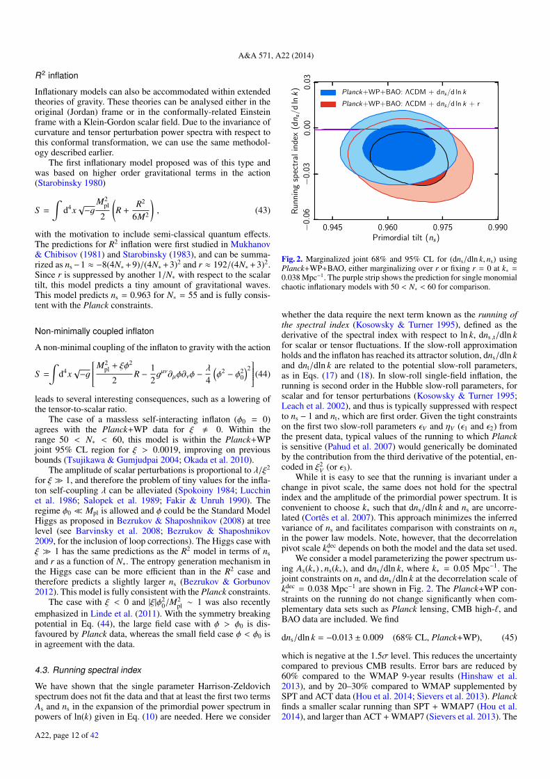
Fig. 2. Marginalized joint 68% and 95% CL for (dns/dln k, ns) usingPlanck+WP+BAO, either marginalizing over r or fixing r = 0 at k∗ =0.038 Mpc−1. The purple strip shows the prediction for single monomialchaotic inflationary models with 50 < N∗ < 60 for comparison.

whether the data require the next term known as the running ofthe spectral index (Kosowsky & Turner 1995), defined as thederivative of the spectral index with respect to ln k, dns ,t/dln kfor scalar or tensor fluctuations. If the slow-roll approximationholds and the inflaton has reached its attractor solution, dns/dln kand dnt/dln k are related to the potential slow-roll parameters,as in Eqs. (17) and (18). In slow-roll single-field inflation, therunning is second order in the Hubble slow-roll parameters, forscalar and for tensor perturbations (Kosowsky & Turner 1995;Leach et al. 2002), and thus is typically suppressed with respectto ns − 1 and nt, which are first order. Given the tight constraintson the first two slow-roll parameters εV and ηV (ε1 and ε2) fromthe present data, typical values of the running to which Planckis sensitive (Pahud et al. 2007) would generically be dominatedby the contribution from the third derivative of the potential, en-coded in ξ2

V (or ε3).While it is easy to see that the running is invariant under a

change in pivot scale, the same does not hold for the spectralindex and the amplitude of the primordial power spectrum. It isconvenient to choose k∗ such that dns/dln k and ns are uncorre-lated (Cortês et al. 2007). This approach minimizes the inferredvariance of ns and facilitates comparison with constraints on nsin the power law models. Note, however, that the decorrelationpivot scale kdec

∗ depends on both the model and the data set used.We consider a model parameterizing the power spectrum us-

ing As(k∗) , ns(k∗), and dns/dln k, where k∗ = 0.05 Mpc−1. Thejoint constraints on ns and dns/dln k at the decorrelation scale ofkdec∗ = 0.038 Mpc−1 are shown in Fig. 2. The Planck+WP con-

straints on the running do not change significantly when com-plementary data sets such as Planck lensing, CMB high-`, andBAO data are included. We find

dns/dln k = −0.013 ± 0.009 (68% CL, Planck+WP), (45)

which is negative at the 1.5σ level. This reduces the uncertaintycompared to previous CMB results. Error bars are reduced by60% compared to the WMAP 9-year results (Hinshaw et al.2013), and by 20–30% compared to WMAP supplemented bySPT and ACT data (Hou et al. 2014; Sievers et al. 2013). Planckfinds a smaller scalar running than SPT + WMAP7 (Hou et al.2014), and larger than ACT + WMAP7 (Sievers et al. 2013). The

A22, page 12 of 42

Planck Collaboration: Planck 2013 results. XXII.

Table 5. Constraints on the primordial perturbation parameters for ΛCDM + dns/dln k, ΛCDM + dns/dln k+r, and ΛCDM + dns/dln k+d2ns/dln k2

models from Planck combined with other data sets.

Model Parameter Planck+WP Planck+WP+lensing Planck+WP+high-` Planck+WP+BAO

ΛCDM + dns/dln k

ns 0.9561 ± 0.0080 0.9615 ± 0.0072 0.9548 ± 0.0073 0.9596 ± 0.0063dns/dln k −0.0134 ± 0.0090 −0.0094 ± 0.0085 −0.0149 ± 0.0085 −0.0130 ± 0.0090−2∆lnLmax –1.50 –0.77 –2.95 –1.45

+ d2ns/dln k2

ns 0.9514+0.087−0.090 0.9573+0.077

−0.079 0.9476+0.086−0.088 0.9568+0.068

−0.063

ΛCDM + dns/dln k dns/dln k 0.001+0.016−0.014 0.006+0.015

−0.014 0.001+0.013−0.014 0.000+0.016

−0.013

d2ns/dln k2 0.020+0.016−0.015 0.019+0.018

−0.014 0.022+0.016−0.013 0.017+0.016

−0.014

−2∆lnLmax –2.65 –2.14 –5.42 –2.40

ΛCDM + r + dns/dln k

ns 0.9583 ± 0.0081 0.9633 ± 0.0072 0.9570 ± 0.0075 0.9607 ± 0.0063r <0.25 <0.26 <0.23 <0.25

dns/dln k −0.021 ± 0.012 −0.017 ± 0.012 −0.022+0.011−0.010 −0.021+0.012

−0.010

−2∆lnLmax –1.53 –0.26 –3.25 –1.5

Notes. Constraints on the spectral index and its dependence on the wavelength are given at the pivot scale of k∗ = 0.05 Mpc−1.

−0.03 0.00 0.03 0.06Running spectral index (dns/d ln k)

−0.0

40.

000.

040.

08

Run

ning

ofru

nnin

gsp

ectr

alin

dex

(d2n s/d

2ln

k)

Planck+WP+BAO:ΛCDM + dns/d ln k+ d2ns/d2 ln k

Fig. 3. Marginalized joint 68% and 95% CL regions for (d2ns/dln k2,dns/dln k) using Planck+WP+BAO.

best fit likelihood improves by only ∆χ2eff≈ 1.5 (3 when high-`

data are included) with respect to the minimal case in which ns isscale independent, indicating that the deviation from scale inde-pendence is not very significant. The constraint for the spectralindex in this case is 0.9630 ± 0.0065 at 68% CL at the decor-relation pivot scale k∗ = 0.038 Mpc−1. This result implies thatthe third derivative of the potential is small, i.e., |ξ2

V | ∼ 0.007,but compatible with zero at 95% CL, for inflation at low energy(i.e., with εV ≈ 0).

We also test the possibility that the running depends on thewavelength so that d2ns/dln k2 is nonzero. With Planck+WPdata, we find d2ns/dln k2 = 0.020+0.016

−0.015. This result is stable withrespect to the addition of complementary data sets, as can beseen from Table 5 and Fig. 3. When d2ns/dln k2 is allowed inthe fit, we find a value for the running dns/dln k consistent withzero.

Finally we allow a non-zero primordial gravitational wavespectrum together with the running. The tensor spectral in-dex and its running are set by the slow-roll consistency re-lations to second order, with nt = −r(2 − r/8 − ns)/8 anddnt/dln k = r(r/8 + ns − 1)/8. Planck measures the running to

0.94 0.96 0.98 1.00Primordial tilt (ns)

0.0

0.1

0.2

0.3

0.4

Ten

sor-

to-s

cala

rra

tio

(r)

Planck+WP+BAO: ΛCDM + r

Planck+WP+BAO: ΛCDM + r + (dns/d ln k)

Fig. 4. Marginalized joint 68% and 95% CL regions for (r , ns), usingPlanck+WP+BAO with and without a running spectral index.

be dns/dln k = −0.016 ± 0.010 when tensors are included (seeTable 5 and Fig. 4). The constraints on the tensor-to-scalar ra-tio are relaxed compared to the case with no running, due to ananti-correlation between r and dns/dln k, as shown in Fig. 4 forPlanck+WP+BAO.

Varying both tensors and running, Planck+WP implicationsfor slow-roll parameters are εV < 0.015 at 95% CL, ηV =−0.014+0.015

−0.011, and |ξ2V | = 0.009 ± 0.006.

In summary, the Planck data prefer a negative running forthe scalar spectral index of order dns/dln k ≈ −0.015, but atonly the 1.5σ significance level. This is for Planck alone andin combination with other astrophysical data sets. Weak statisti-cal evidence for negative values of dns/dln k has been claimed inseveral previous investigations with the WMAP data and smallerscale CMB data (e.g., Spergel et al. 2003; Peiris et al. 2003;Dunkley et al. 2011; Hinshaw et al. 2013; Hou et al. 2014).

If primordial, negative values for dns/dln k of order 10−2

would be interesting for the physics of inflation. The runningof the scalar spectral index is a key prediction for inflation-ary models. It is strictly zero for power law inflation, whose fitto Planck was shown to be quite poor in the previous section.

A22, page 13 of 42

A&A 571, A22 (2014)

Chaotic monomial models with V(φ) ∝ φn predict dns/dln k ≈−8(n+2)/(4N +n)2 ≈ (ns−1)2, and the same order of magnitude(10−3) is quite typical for many slow-roll inflationary models,such as natural inflation (Adams et al. 1993) or hilltop inflation(Boubekeur & Lyth 2005). It was pointed out that a large neg-ative running of dns/dln k . −10−2 would make it difficult tosupport the N∗ ≈ 50 e-foldings required from inflation (Easther& Peiris 2006), but this holds only without nonzero deriva-tives higher than the third order in the inflationary potential.Designing inflationary models that predict a negative runningof O(10−2) with an acceptable ns and number of e-folds is notimpossible, as the case with modulated oscillations in the infla-tionary potential demonstrates (Kobayashi & Takahashi 2011).This occurs, for instance, in the axion monodromy model whenthe instanton contribution is taken into account (McAllister et al.2010), giving the potential

V(φ) = µ3φ + Λ4 cos(φ

f

)· (46)

4.4. Open inflation

Most models of inflation predict a nearly flat spatial geometrywith small deviations from perfect spatial flatness of |ΩK | ∼

10−5. Curvature fluctuations may be regarded as local fluctua-tions in the spatial curvature, and even in models of inflationwhere the perturbations are calculated about a spatially flat back-ground, the spatial curvature on the largest scales accessible toobservation now are subject to fluctuations from perfect spa-tial flatness (i.e., ΩK = 0). This prediction for this fluctuationis calculated by simply extrapolating the power law spectrumto the largest scale accessible today, so that ΩK as probed bythe CMB roughly represents the local curvature fluctuation av-eraged over our (causal) horizon volume. Although it has some-times been claimed that spatial flatness is a firm prediction ofinflation, it was realized early on that spatial flatness is not aninexorable consequence of inflation and large amounts of spa-tial curvature (i.e., large compared to the above prediction) canbe introduced in a precise way while retaining all the advan-tages of inflation (Gott 1982; Gott & Statler 1984) through bub-ble nucleation by false vacuum decay (Coleman & De Luccia1980). This proposal gained credence when it was shown howto calculate the perturbations in this model around and beyondthe curvature scale (Bucher et al. 1995; Bucher & Turok 1995;Yamamoto et al. 1995; Tanaka & Sasaki 1994). See also Ratra& Peebles (1995, 1994) and Lyth & Stewart (1990). For morerefined later calculations see for example Garriga et al. (1998,1999), Gratton & Turok (1999), and references therein. For pre-dictions of the tensor perturbations see for example Bucher &Cohn (1997), Sasaki et al. (1997), and Hertog & Turok (2000).

An interesting proposal using singular instantons and notrequiring a false vacuum may be found in Hawking & Turok(1998), and for calculations of the resulting perturbation spectrasee Hertog & Turok (2000) and Gratton et al. (2000). Models ofthis sort have been studied more recently in the context of thestring landscape. (See, for example, Vilenkin 2007, for a nicereview.) Although some proposals for universes with positivecurvature within the framework of inflation have been put forth(Gratton et al. 2002), it is much harder to obtain a closed uni-verse with a spatial geometry of positive spatial curvature (i.e.,ΩK < 0) (Linde 2003).

Theoretically, it is of interest to measure ΩK to an accuracyof approximately 10−4 or slightly better to test the prediction ofsimple flat inflation for this observable. A statistically signifi-cant positive value would suggest that open inflation, perhaps

−0.075 −0.050 −0.025 0.000

Running spectral index (dns/d ln k)

0.0

0.3

0.6

0.9

1.2

Ten

sor-

to-S

cala

rR

atio

(r)

−0

.24

−0

.16

−0

.08

0.0

0

ΩK

Fig. 5. Joint posterior for tensors and running of the scalar spectral in-dex marginalizing over other parameters. The contours are set at 68%and 95%. The red contours apply for Planck+WP+high-` data. Thecolour of the scattered points indicates the distribution of ΩK . The bluecontours apply when BAO data is also included. (ΩK is then found tobe well constrained close to zero.) The dashed vertical line shows theno-running solution.

in the context of the landscape, was at play. A statistically sig-nificant negative value could pose difficulties for the inflation-ary paradigm. For a recent discussion of these questions, see forexample Freivogel et al. (2006), Kleban & Schillo (2012), andGuth & Nomura (2012).

In order to see how much spatial curvature is allowed,we consider a rather general model including the parame-ters r, ns, and dns/dln k as well as ΩK . We find that ΩK =−0.058+0.046

−0.026 with Planck+WP, and ΩK = −0.004 ± 0.0036 withPlanck+WP+BAO. More details can be found by consultingthe parameter tables available online10. Figure 5 shows r anddns/dln k for this family of models. We conclude that any possi-ble spatial curvature is small in magnitude even within this gen-eral model and that the spatial curvature scale is constrained tolie far beyond the horizon today. Open models predict a tensorspectrum enhanced at small wavenumber k <∼ 1, where k = 1corresponds to the curvature scale, but our constraint on ΩK andcosmic variance imply that this aspect is likely unobservable.

4.5. Relaxing the assumption of the late-time cosmologicalconcordance model

The joint constraints on ns and r shown in Fig. 1 are one of thecentral results of this paper. However, they are derived assum-ing the standard ΛCDM cosmology at late times (i.e., z . 104).It is therefore natural to ask how robust our conclusions are tochanges of the late time cosmological model. We discuss twoclasses of models: firstly, changes to the ΛCDM energy con-tent; and secondly, a more general reionization model. These ex-tensions can lead to degeneracies of the additional parameterswith ns or r11.

10 Available at: http://www.sciops.esa.int/index.php?project=planck&page=Planck_Legacy_Archive11 We considered a further generalization, which also causes the jointconstraints on ns and r to change slightly. We allowed the am-plitude of the lensing contribution to the temperature power spec-trum AL to vary as a free parameter. In this case we find the follow-ing Planck+WP+BAO constraints: ns = 0.972 ± 0.006, AL = 1.24+0.10

−0.11,r < 0.15 at 95% CL.

A22, page 14 of 42

Planck Collaboration: Planck 2013 results. XXII.

0.94 0.96 0.98 1.00 1.02Primordial tilt (ns)

0.0

0.1

0.2

0.3

Ten

sor-

to-s

cala

rra

tio

(r)

Planck+WP+BAO: ΛCDM + r

Planck+WP+BAO: ΛCDM + r + Neff

Planck+WP+BAO: ΛCDM + r + Yp

0.94 0.96 0.98 1.00Primordial tilt (ns)

0.00

0.08

0.16

0.24

Ten

sor-

to-s

cala

rra

tio

(r)

Planck+WP+BAO: ΛCDM + r

Planck+WP+BAO: ΛCDM + r + w

Planck+WP+BAO: ΛCDM + r +∑

mν

Fig. 6. Marginalized joint 68% and 95% CL regions forPlanck+WP+BAO data for ΛCDM + r + Neff and ΛCDM + r +YP (top); and ΛCDM + r +

∑mν and ΛCDM + r + w (bottom). Shown

for comparison are the corresponding contours for the ΛCDM +r model.

4.5.1. Extensions to the energy content

We consider the ΛCDM + r + Neff , ΛCDM + r + YP, ΛCDM +r +

∑mν, and ΛCDM + r + w extensions of the standard model.

This selection is motivated by the impact on the CMB dampingtail of the first two and the effect on the Sachs-Wolfe plateauat low multipoles for the latter two. The resulting contours areshown in Fig. 6. While the lower limit on ns is stable under allextensions considered here, the models that alter the high-` partof the spectrum permit significantly bluer spectral tilts, and ac-cordingly also lead to a weaker bound on the tensor-to-scalarratio. By allowing Neff to float, we obtain ns = 0.9764 ± 0.0106and r0.002 < 0.15 at 95% CL12. For ΛCDM + r + YP we ob-tain ns = 0.9810 ± 0.0111 and r0.002 < 0.18 at 95% CL. Themodels modifying the large-scale part of the power spectrum,

12 Selected non-standard values for Neff deserve further investigation.For the additional fractional contribution motivated by a Goldstone bo-son ∆Neff = 0.39 (Weinberg 2013), we obtain ns = 0.9726 ± 0.0057and r0.002 < 0.14 at 95% CL for Planck+WP+BAO+high-`. For anadditional species of neutrinos, we obtain ns = 0.9947 ± 0.0056 andr0.002 < 0.17 at 95% CL for Planck+WP+BAO+high-`.

on the other hand, do not lead to a notable degradation of con-straints on either ns or r (ns = 0.9648 ± 0.0061 and r0.002 < 0.13at 95% CL for ΛCDM + r +

∑mν, and ns = 0.9601 ± 0.0070

and r0.002 < 0.11 at 95% CL for ΛCDM+r+w).

4.5.2. General reionization scenario

In the standard rapid reionization scenario typically used inCMB analysis, the Universe is assumed to be completely trans-parent after recombination, but the ionization fraction increasesfrom zero to one over a duration ∆z ≈ 1 at a certain redshift zreion,which is the only unknown parameter of the reionization model.This model is obviously simplistic, but for CMB analysis itworks quite well because the CMB has little sensitivity to the de-tails of how the ionization fraction changes from 0 to 1. In thissection we study to what extent allowing more general reion-ization scenarios may alter some of the conclusions concern-ing the constraints on ns and r as well as on τ. As discussed inMortonson & Hu (2008a,b), CMB anisotropies constrain reion-ization almost entirely by using the shape of the large-scale EEpower spectrum, and the power is redistributed from larger tosmaller scales for reionization processes which take place dur-ing a non-negligible redshift interval, since they start at an earlierepoch.

We use the method developed by Mortonson & Hu (2008a)to describe and constrain the reionization history. A completeprincipal component basis serves to describe the effect of reion-ization on the large-scale E-mode polarization power spectrum.Following Mortonson & Hu (2008a) we bin the ionization his-tory xe(zi) using 95 equal width bins with ∆z = 0.25 rangingfrom zmin = 6 to zmax = 30. For the redshifts z < zmin we assumevalues for xe which take into account first (and possibly second)helium ionization and complete hydrogen ionization (xe = 1.16for z < 3 and xe = 1.08 for 3 < z < 6). For z > 30 we fixxe = 2×10−4 as the value of xe expected before reionization (andafter primordial recombination). Any reionization history can beparameterized as a free function of redshift by decomposing theionization fraction as xe(z) = xf

e(z)+∑µ mµS µ(z), where the prin-

cipal components, S µ(z), are the eigenfunctions of the Fishermatrix computed by taking the derivatives of the EE polariza-tion power spectrum with respect to xe(z) and xf

e(z) is a fiducialionization fraction. Following Mortonson & Hu (2008a) we con-sider here the first five eigenfunctions, S µ(z) with µ = 1, ..., 5,which will be varied with the other cosmological parameters.

In Fig. 7 we plot the 68% and 95% CL regions for nsand r. The constraint on the tensor-to-scalar ratio is not signifi-cantly affected by this additional marginalization, increasing tor0.002 < 0.13 at 95% CL. The scalar spectral index is increasedto ns = 0.9650 ± 0.0080, compared with ns = 0.9603 ± 0.0073obtained with the rapid reionization scheme. This is the sametrend as noted in Pandolfi et al. (2010) using WMAP data, butthe effect is less significant due to the improved measurementof the temperature spectrum by Planck. The larger freedomin the reionization history increases the width of the posterioron the derived optical depth, which is still partially degeneratewith the scalar spectral index of primordial perturbations. Thens = 1 model is still excluded at high significance; however, wefind ∆χ2

eff= 12.5 compared to the ΛCDM model.

5. Inflationary model comparison

In Sect. 4.2 several representative families of parameterizedmodels for the inflationary potential were analysed within the

A22, page 15 of 42

A&A 571, A22 (2014)

0.94 0.96 0.98 1.00Primordial tilt (ns)

0.00

0.08

0.16

0.24

Ten

sor-

to-s

cala

rra

tio

(r)

Planck+WP: ΛCDM + r

Planck+WP: ΛCDM + r + General Reionization

Fig. 7. Marginalized joint 68% and 95% CL regions for Planck+WP data for ΛCDM + r for instantaneous and general reionization.

slow-roll approximation in the neighbourhood of the pivotscale k∗. Approximate constraints were applied to reject modelsfor which there is no plausible scenario for entropy generation.In this section we revisit some of the parametric models definedin Sect. 4.2. Here, however, the modes for the first order per-turbations, as described in Sect. 2.2, are integrated numerically.Thus there is no slow-roll approximation, and the issue of theexistence of a plausible scenario for entropy generation is exam-ined more carefully. We perform a statistical model comparisonbetween the competing parameterized potentials, both within theframework of Bayesian model comparison and in terms of therelative likelihoods of the best fit models from each parameter-ized family.

As noted in Sect. 2.3, considerable uncertainty surroundswhat occurred during the epoch of entropy generation, partic-ularly with respect to the energy scale at which entropy genera-tion ends and the average equation of state between that epochand the end of inflation. For this reason, we explore a number ofscenarios for this intermediate era during which entropy gener-ation takes place. The models compared in this section includeinflation with power law potentials, defined in Eq. (34), with sev-eral representative values for n; natural inflation, in Eq. (39); andhilltop inflation, with p = 4 and λ = 4Λ4/µ4 in Eq. (37).

The free parameters in these inflationary potentials may varyover several orders of magnitude corresponding to unknownscales in high energy particle physics. Consequently a logarith-mic prior is a sensible choice for these parameters. However,there is no theoretical guidance on how to truncate these modelpriors. We therefore adopt broad priors initially and then trun-cate them as follows in order to compare all the models on anequal footing.

The strongest constraint on the inflationary parameter spacecomes from the amplitude of the primordial power spectrum.This is a free parameter in most models, and successful structureformation in a universe dominated by cold dark matter has longbeen known to require primordial fluctuations with R ≈ 10−5,or As ≈ 10−10 (see e.g., Zeldovich 1972; Linde 1990). We cantherefore immediately reject models for which As is far from thisvalue, so regions of parameter space which do not yield 10−11 ≤

As ≤ 10−7 are a priori excluded. This range is generous relativeto estimates of As prior to Planck (e.g., Komatsu et al. 2011),

but the results do not depend strongly on the range chosen. Thiseffectively truncates the logarithmic priors on the model param-eters, leaving a parameter subspace compatible with basic struc-ture formation requirements.

For the single parameter models this requirement defines therange of λ in Eq. (34). However, for generic multi-parametermodels, an As-based cut may select a nontrival region of param-eter space, as happens for the two cases considered here (see e.g.,Fig. 1 in Easther & Peiris 2012). Without the As-based cut in theprior, the parameter volume for both natural and hilltop inflationwould be rectangular, and the corresponding Bayesian evidencevalues computed for these models would be lowered.

As discussed in Sect. 2.3, specifying an inflationary potentialdoes not enable us to predict the late time CMB angular powerspectra. The subsequent expansion history and details of theepoch of entropy generation are required to relate the value of theinflaton field at Hubble radius crossing to comoving wavenum-bers in today’s Universe, through Eq. (24). Physically, the funda-mental parameter that sets the observable perturbation spectrumis the value of the field φ∗ at which the pivot mode leaves theHubble radius. It can be rescaled by a shift φ∗ → φ∗ + φ0, andthe range over which φ changes during inflation varies greatlybetween models. Consequently we treat the remaining numberof e-folds, N∗, after the pivot scale leaves the Hubble radius as afree parameter with a wide uniform prior, since this quantity hasa consistent interpretation across models. The pivot scale used tocompute N∗ is k∗ = 0.05 Mpc−1. However, given our ignoranceconcerning the epoch of entropy generation, a multitude of en-tropy generation scenarios for each inflationary potential can oc-cur. Some possibilities are as follows, with parameters referringto Eq. (24).

1. Instantaneous entropy generation scenario.At the end of inflation, all the energy in the inflaton field isinstantaneously converted into radiation.

2. Restrictive entropy generation scenario (narrow rangefor wint).ρ1/4

th = 109 GeV, and wint ∈ [−1/3, 1/3].3. Permissive entropy generation scenario (wide range

for wint).ρ1/4

th = 103 GeV, and wint ∈ [−1/3, 1].

The equations of state with wint in the range [1/3, 1] appear lessplausible, but models with these values have been put forward(Pallis 2006), so this possibility cannot be completely excluded.Moreover the wint parameterization captures a variety of scenar-ios in which the post-inflationary Universe is thermalized, butnot radiation dominated, including phases of coherent oscilla-tions (Martin & Ringeval 2010; Easther et al. 2011), resonance(Traschen & Brandenberger 1990; Kofman et al. 1994, 1997;Allahverdi et al. 2010), kination (Spokoiny 1993; Chung et al.2007), secondary or thermal inflation (Lyth & Stewart 1996),moduli domination (Banks et al. 1994; de Carlos et al. 1993),primordial black hole domination (Anantua et al. 2009), or afrustrated cosmic string network (Burgess et al. 2005), all ofwhich lead to an expansion rate differing from that of a radia-tion dominated universe.

At the other extreme, the decision to exclude wint < −1/3,as done here, is not completely justifiable. We cannot, for ex-ample, rule out a first order phase transition at a lower energyscale that would drive wint below −1/3, but here we neglect thispossibility. Our analysis does not preclude a secondary periodof inflation, but does require that the average expansion duringthe post-inflationary regime parameterized by wint should not beinflationary. This caveat should be kept in mind.

A22, page 16 of 42

Planck Collaboration: Planck 2013 results. XXII.

Table 6. Model priors.

Model Priorsn = 2/3 −13 < log10(λ) < −7n = 1 −13 < log10(λ) < −7n = 2 −13.5 < log10(m2) < −8n = 4 −16 < log10(λ) < −10

Natural −5 < log10(Λ) < 00 < log10( f ) < 2.5

Hilltop −8 < log10(Λ) < −1p = 4 −17 < log10(λ) < −10

ΛCDM 0.9 < ns < 1.023.0 < ln

[1010As

]< 3.2

Matching PriorN∗ 20 ≤ N∗ ≤ 90

For some of the parameterized models, tighter constraintscan, in principle, be placed on wint. It has been argued (see e.g.,Liddle & Leach 2003) that for the λφ4 potential, the uncertaintiesconcerning entropy generation contribute almost no uncertaintyin the determination of φ∗. This is because according to the virialtheorem, a field sloshing about φ = 0 in a quartic potential hasthe same average w, namely w = 1/3, as the radiation equationof state. More generally, for a potential of the form φn aroundthe minimum, wvir = 〈w〉 = (n − 2)/(n + 2) (Turner 1983); there-fore, one may argue that wint should be restricted to the inter-val whose endpoints are 1/3 and wvir. This approach was takenby Martin & Ringeval (2010) in obtaining Bayesian constraintson the reheating temperature for monomial potentials from theCMB. However this scenario requires a carefully tuned poten-tial that has approximately a φn shape, both at large field valuesand near the origin far below the inflationary scale. Typically,potentials for which V(φ) ∼ φn at large field values can havevery different shapes near the origin. Thus, following Easther &Peiris (2012), in this paper we explore a broader range of wint forthese models (including the cases above as subsets) in order toobtain data-driven constraints on wint.

In this paper we focus on the three representative scenar-ios itemized above, referred to hereafter as scenarios (1), (2),and (3). Our algorithm draws a value of N∗ and then given thevalue of ρth, computes wint, which is a derived parameter. Modelsfor which wint lies outside the specified range of each scenariounder consideration are excluded.

The full set of priors for the inflationary physics is given inTable 6. Dimensionful quantities are expressed in units with re-duced Planck mass Mpl set to unity.

Due to the nontrivial likelihood surfaces and the large dimen-sionality of the parameter spaces explored in this section, we useModeCode coupled to MultiNest v3.013 to map out the param-eter space. In addition to the standard nested sampling (NS) al-gorithm, MultiNest v3.0 enables nested importance sampling(NIS), resulting in substantial speed gains14 and significant en-hancements in the accuracy of the Bayesian evidence computa-tion compared to NS alone for the same computational setup.

13 Made available ahead of public release to the Planck Collaborationby Farhan Feroz and Mike Hobson (Feroz et al. 2013).14 We have carried out extensive tests of NIS versus NS, and chosenthe following settings for the computations presented here: NIS on,constant efficiency mode on, 300 live points, tolerance and efficiencyparameters set to 0.5 and 0.02, respectively.

5.1. Results

Table 7 presents model comparison results for the ensembleof parameterized potential families described above. We reportthe Bayesian evidence (model averaged likelihood) ratio, whichprovides a self-consistent framework for calculating the bettingodds between models (see Sect. 3.4). The uncertainty in theselogarithmic evidence values is approximately 0.2. We also re-port the ∆χ2

effvalues computed from the 2 lnLmax values found

by the sampler.The monomial models have a single parameter potential, and

the natural and hilltop inflation models have two parameterseach. All entropy generation scenarios except case (1) contributeone additional parameter to the inflationary sector. The evidenceratios and ∆χ2

effvalues are presented with respect to the ΛCDM

cosmological model.None of the inflationary models tested here fit the data as

well as the ΛCDM model. This mostly reflects that there isno evidence in the data for r different from zero. Furthermore,the priors listed in Table 6 for the ΛCDM primordial sectorare purely phenomenological, roughly corresponding to rangessomewhat broader than WMAP constraints. Narrowing themaround the best fit model arbitrarily increases the evidence in itsfavour. Instead it is instructive to compare the relative evidencefor the inflationary models presented.

Table 7 shows that the λφ4 model is decisively ruled outby Planck, confirming previous analyses by the WMAP team(Peiris et al. 2003; Spergel et al. 2007; Dunkley et al. 2009;Komatsu et al. 2011) based on the model track plotted on thens-r plane. Recent model selection analyses (Martin et al. 2011;Easther & Peiris 2012) with WMAP 7-year data found that themodel was already disfavoured by odds of about 400:1 against.With Planck, the odds against this model are at least 500 000:1compared to ΛCDM for a broad range of entropy generationscenarios. The same conclusion is confirmed by the extremelypoor ∆χ2

effvalues for the model. Given the strength of our re-

sults, in the flexible setting of the permissive entropy generationscenario, it is possible not just to rule out models where the po-tential is of the quartic form in the full range from the origin tothe inflationary scales, but also a general class where the poten-tial is of the n = 4 form in the φ-range where the cosmologicalperturbations are generated, but exhibits a different shape nearthe origin.

Two other large field models, the quadratic potential andnatural inflation, are somewhat disfavoured by the Planck data,especially when broader entropy generation scenarios are con-sidered. Compared with the ΛCDM model, these models aredisfavoured by ∆χ2

eff∼ 5–6 depending on the entropy generation

scenario. This reflects the analysis of Sect. 4, where the over-lap of the model predictions and the data constraints on the ns-rplane is seen to be mostly outside the joint 68% CL contour.However, from the Bayesian evidence point of view, it is tooearly to declare these models incompatible with the data. Tomake this judgement, it is more prudent to compare these mod-els to the n = 1 case, which has the best evidence with respectto ΛCDM, rather than to ΛCDM itself, which provides our ref-erence point for the evidence calculation, but has arbitrary priorranges. In their simplest forms – instantaneous entropy genera-tion – the n = 2 and natural inflation models are only disfavouredby odds of about 1–12:1 against, which does not rise to a highlevel of significance15.

15 In comparison, odds of 150:1 are considered highly significant inthis context.

A22, page 17 of 42

A&A 571, A22 (2014)

Table 7. Inflationary model comparison results.

Model Instantaneous Restrictive Permissiveentropy generation entropy generation entropy generation

ln[E/E′] ∆χ2eff

ln[E/E′] ∆χ2eff

ln[E/E′] ∆χ2eff

n = 4 −14.9 25.9 −18.8 27.2 −13.2 17.4n = 2 −4.7 5.4 −7.3 6.3 −6.2 5.0n = 1 −4.1 3.3 −5.4 2.8 −4.9 2.1n = 2/3 −4.7 5.1 −5.2 3.1 −5.2 2.3Natural −6.6 5.2 −8.9 5.5 −8.2 5.0Hilltop −7.1 6.1 −9.1 7.1 −6.6 2.4ΛCDM −4940.7 9808.4 ... ... ... ...

Notes. For each model and set of assumptions concerning entropy generation [(1), (2), (3)], the natural logarithm of the Bayesian evidence ratioas well as ∆χ2

efffor the best fit model in each category are indicated, relative to the ΛCDM concordance model (denoted by subscript “0”). lnE0

and −2 lnL′ are given for the reference model.

0.948 0.952 0.956ns

0.22

0.24

0.26

0.28

r

n=4

0.955 0.960 0.965 0.970ns

0.10

50.

120

0.13

50.

150

r

n=2

0.960 0.965 0.970 0.975 0.980ns

0.06

0.07

0.08

0.09

0.10

r

n=1

0.960 0.965 0.970 0.975 0.980ns

0.04

80.

056

0.06

40.

072

0.08

0

r

n=2/3

0.955 0.960 0.965 0.970ns

0.10

0.12

0.14

0.16

0.18

r

Natural

0.930 0.936 0.942 0.948 0.954ns

−16

−12

−8−4

log 1

0(r

)

Hilltop

Fig. 8. Constraints on ns vs. r at k∗ = 0.002 Mpc−1 for the inflationary models considered (i.e., power law potentials with n = 2/3, 1, 2, and 4,natural inflation, and hilltop inflation), showing joint 68% and 95% CL. Blue and grey distributions correspond to the restrictive and permissiveentropy generation scenarios, respectively. The instantaneous entropy generation case corresponds to the thin (red) contours in the natural andhilltop panels; for the single parameter models, this case corresponds to the lowest-r extremity of the restrictive case. The difference between thenatural inflation region in Fig. 1 and the natural inflation constraints shown here is due to the strong projection effect described in the text.

The models most compatible with the Planck data in the setconsidered here are the two interesting axion monodromy poten-tials, n = 1 (McAllister et al. 2010) and n = 2/3 (Silverstein& Westphal 2008), which are motivated by inflationary modelbuilding in the context of string theory. The p = 4 hilltop modelpresents an interesting case. This model was previously foundto be compatible with WMAP 7-year data, performing almostas well as the monodromy potentials (Easther & Peiris 2012).However it exhibits significant tension with the Planck data, bothin terms of evidence ratios and the maximum likelihood. Theonly exception is the entropy generation scenario (3) which hasodds of greater than 1000:1 against compared to ΛCDM, and yetthe maximum likelihood is not significantly different from then = 1 case. This indicates that while the extra freedom allowedby the least restrictive entropy generation scenario improves thebest fit, this prior is not very predictive of the data. However,the result seems counterintuitive and merits further comment;we will consider this question further at the end of this sectionwhen parameter estimation results are discussed.

We now turn to parameter constraints. Figure 8 presentsmarginalized joint constraints from Planck+WP alone on thederived parameters ns,0.002 and r0.002. Figure 9 shows the corre-sponding joint constraints on ns,0.002 and wint, again a derived pa-rameter. Figure 10 shows joint constraints on wint and the poten-tial parameter log10(λ) (log10(Λ) in the case of natural inflation).It is instructive to consider the three sets of figures together.The restrictive and permissive entropy generation scenarios areshown on all panels; the instantaneous entropy generation caseis shown for the two parameter models, natural inflation and hill-top, in Fig. 8 – for the monomial potentials this case correspondsto the lowest-r extremity of the restrictive case constraints, andto wint = 1/3 in the other two figures.

The quartic potential conflicts with the data because it pre-dicts a high tensor-to-scalar ratio. Hence the model maximizesits likelihood by pushing towards the lower-r, bluer-ns limitsof its parameter space, which corresponds to increasing wint asmuch as allowed by the entropy generation prior. The contoursterminate at the lowest-r limit when each entropy generation

A22, page 18 of 42

Planck Collaboration: Planck 2013 results. XXII.

0.948 0.952 0.956ns

0.0

0.4

0.8

win

t

n=4

0.955 0.960 0.965 0.970ns

0.0

0.4

0.8

win

t

n=2

0.960 0.965 0.970 0.975 0.980ns

0.0

0.4

0.8

win

t

n=1

0.965 0.970 0.975 0.980ns

−0.2

0.0

0.2

0.4

win

t

n=2/3

0.960 0.966 0.972 0.978ns

0.0

0.4

0.8

win

t

Natural

0.930 0.936 0.942 0.948 0.954ns

0.00

0.25

0.50

0.75

1.00

win

t

Hilltop

Fig. 9. Constraints on ns vs. wint at k∗ = 0.002 Mpc−1 for the inflationary models considered, as in Fig. 8. The instantaneous entropy generationcase (1) corresponds to wint = 1/3.

−13.05 −12.90 −12.75 −12.60log10(λ)

0.0

0.4

0.8

win

t

n=4

−10.5 −10.4 −10.3 −10.2log10(m2)

0.0

0.4

0.8

win

t

n=2

−9.8 −9.7 −9.6 −9.5 −9.4 −9.3log10(λ)

0.0

0.4

0.8

win

t

n=1

−9.6 −9.5 −9.4 −9.3log10(λ)

−0.2

0.0

0.2

0.4

win

t

n=2/3

−2.1 −1.8 −1.5 −1.2log10(Λ)

0.0

0.4

0.8

win

t

Natural

−13.00−12.75−12.50−12.25log10(λ)

0.00

0.25

0.50

0.75

1.00

win

t

Hilltop

Fig. 10. Constraints on log10(λ) vs. wint for the inflationary models considered, as in Figs. 8 and 9.

case hits its wint prior upper limit (i.e., wint = 1/3 and wint = 1for restrictive and permissive entropy generation, respectively).For each case, the lower limit on wint, corresponding to thereddest-ns extremity of the confidence contours, is data-driven.The quadratic potential encounters the same difficulty but at aless extreme level.

The two axion monodromy potentials are compatible with awide range of entropy generation scenarios. The instantaneousentropy generation scenario is compatible with the data for bothmodels. For restrictive entropy generation in the n = 1 model,we obtain a data-driven upper limit on wint, which just touchesthe wint = 1/3 case at the 95% CL. At the lower limit, the wintposterior is truncated by the prior, as for the n = 2/3 case. For

the latter, there is a data-driven upper limit on wint which is con-trolled by the upper limit on ns. For permissive entropy gener-ation, the upper and lower limits on wint for both models aredata-driven, corresponding to the upper and lower limits on ns,respectively.

The constraints on natural inflation require some interpreta-tion. The relationship between the empirical ns and r parametersand the potential parameters for natural inflation is discussed indetail by Savage et al. (2006) and Mortonson et al. (2011) alongwith parameter constraints derived from WMAP 3-year (Spergelet al. 2007) and WMAP 7-year (Larson et al. 2011), respectively.In this model, there is a degeneracy between f and Λ in thelimit where these parameters are large so that natural inflation

A22, page 19 of 42

A&A 571, A22 (2014)

resembles the quadratic model. The priors are chosen to excludemost of this region. The priors on log10( f ) and log10(Λ) still al-low a region of nearly degenerate models that contribute to aridge seen in the natural inflation panel of Fig. 8. These mod-els closely match the values of ns and r seen in the quadraticpotential constraints. The marginalized constraints on ns and rdepend strongly on the prior on log10( f ) due to the projection ofa large number of degenerate models onto this ridge. Thereforethe apparent preference for this region of parameter space overmodels with lower values of r is largely due to this effect and isnot driven by the data. This highly nonlinear mapping betweenthe logarithmic priors on the potential parameters and the powerlaw parameters (which are derived parameters in this analysis)leads to a strong projection effect, which accounts for the differ-ence in visual appearance between these contours and the regionlabelled natural inflation in Fig. 1.

Generally, for fixed N∗, decreasing Λ and f reduces both nsand r. Thus natural inflation models can have lower values of rthan the quadratic potential without increasing ns and N∗. Thisfeature means that the potential parameters for this model arerelatively uncorrelated with wint, in contrast with the other mod-els considered here, as illustrated in the Fig. 10. Neverthelesswe obtain data-driven bounds on wint in the permissive entropygeneration case as well as a lower bound in the restrictive en-tropy generation case. Both bounds overlap with the instanta-neous generation limit.

The upper panel of Fig. 11 shows our lower limit of f &10.0 Mpl (95% CL), compared with the WMAP7 limit f &5.0 Mpl (95% CL) reported by Mortonson et al. (2011). Indeed,the Planck limit is in agreement with the Planck prediction pre-sented in that work. There is a hint of an upper limit on f aswell, driven by the fact that this corresponds to the quadratic in-flation limit, which is in tension with the data. However this isonly a 1σ effect.

The p = 4 hilltop model has two distinct branches: a small-field scenario, where r . 0.001 and ns < 0.95; and a large-field limit in which V(φ) ∼ φ (Adshead et al. 2011). Physically,the small-field limit is consistent with the Lyth bound, and wecan select it by fixing log10(Λ) < −2.5 in the prior. We observethat the data select out this small field branch, which requiresexplanation given that we know that the n = 1 model (the limitof the large field branch) is perfectly compatible with the data. Infact, this can be tested by restricting the log10(Λ) prior by handto the large-field branch. The hilltop model constitutes a difficultsampling problem, as is apparent from Fig. 4 in Easther & Peiris(2012). An examination of the progress of the nested sampler forthe case of the full hilltop prior reveals the reason for the small-field branch being selected out. In this case, the posterior for thelarge-field branch is extremely thin compared to the model priorin this regime – much thinner than the posterior for the small-field branch in comparison to its respective prior. Therefore thisregion occupies very little probability mass, and is dropped inpreference to the more predictive small-field branch. This highlikelihood but extremely thin ridge is also responsible for thecounterintuitive result reported in the model selection analysis,where the model was found to have a good ∆χ2

effwith respect to

ΛCDM, and yet be highly disfavoured by the Bayesian evidence.In summary, confirming the results of Sect. 4, this model is inagreement with the data in the limit where it overlaps the linearn = 1 model. But since this region of high likelihood occupies avery small fraction of the prior, this model is heavily penalizedby the Bayesian evidence for failing to predict the data over mostof its prior space.

−2.00 −1.75 −1.50 −1.25 −1.00log10(Λ)

0.5

1.0

1.5

2.0

2.5

log 1

0(f

)

Natural

−8 −6 −4 −2log10(Λ)

−12.

8−1

2.6−1

2.4−1

2.2−1

2.0

log 1

0(λ

)

Hilltop

Fig. 11. Potential parameters for natural inflation and hilltop inflation,as in Figs. 8–10. On the natural inflation panel, instantaneous entropygeneration corresponds to a thin diagonal along the top edge of entropygeneration case (3).

6. Observable window of inflation

Section 4.2 presented an analysis of several representative in-flationary potentials within the framework of the slow-roll ap-proximation and their compatibility with the Planck data. Theresults are summarized in Fig. 1. In that case the full potential isconsidered in order to identify a plausible range for the locationof φ∗ on the potential V(φ). This requires a complete story. Inother words, the potential must be specified starting above thepoint where the largest observable scales first exited the Hubbleradius, and extending to the minimum of the potential.

In this section we explore another approach. We adopt thepoint of view that we are interested in reconstructing the in-flationary potential only over the observable range – that is,the interval of φ corresponding to the scales observable todayin the CMB. We constrain the potential over the range wherethese scales exited the Hubble radius during inflation as well asa few e-folds before and after. The cosmological perturbationsare not imprinted instantaneously at the moment of Hubble ra-dius crossing, but rather gradually over a few e-folds. We expandaround φ∗, taking the view that a plausible extension of the po-tential outside this observable range is always possible, so that

A22, page 20 of 42

Planck Collaboration: Planck 2013 results. XXII.

one has precisely the number of e-folds of inflation needed for φ∗to correspond to k∗ today.

The argument is that one can always end inflation abruptlyby imposing a sharp waterfall feature where needed, or prolonginflation by inserting a sufficiently long plateau into the potentialby hand, for example, for models with a large tilt. A foreseeableobjection to this approach is that the extensions of the potentialrequired outside the observable window may render the poten-tial unnatural. This possibility should be kept in mind, althoughnaturalness is an elusive and uncomfortably subjective concept.The analysis in this section does not rely on the slow-roll approx-imation. Instead each k mode is integrated exactly by numericalintegration, as described in Sect. 2.2, under the assumption of acanonical kinetic term.

Two complementary approaches to reconstruct the potentialhave been explored in the literature. The first approach, followedin this paper, expands the potential V(φ) directly in powers of(φ − φ∗). In this case the numerical integration of the slow-rollsolution must start sufficiently early so that any initial transienthas had a chance to decay, and one is in the attractor solu-tion when the dynamics of the largest observable modes in theUniverse today start to have an interesting evolution. This is theapproach followed, e.g., by Lesgourgues & Valkenburg (2007)and Mortonson et al. (2011) using publicly available codes16.

A second approach expands H(φ) as a Taylor series in(φ − φ∗). As discussed in Sect. 2.2, this has the advantage thatH(φ) determines both the potential V(φ) and the solution φ(t),so the issue of having to start sufficiently early in order to al-low the initial transient to decay is avoided. This method wasused, for example, in Kinney (2002), Kinney et al. (2006); Peiris& Easther (2006a,b, 2008), and Easther & Peiris (2006) usinganalytic and semi-analytic approximations, and in Lesgourgueset al. (2008), Powell & Kinney (2007), Hamann et al. (2008c),and Norena et al. (2012) using a fully numerical approach.

These approaches could lead to results that differ from thosein Sect. 4.2. Firstly, if the running of the index is large, the slow-roll approximation taken to second order is not necessarily accu-rate for all models allowed by the data. The relation between thespectral parameters (ln As, ns, dns/dln k, r) and the underlyinginflationary potential V(φ) is therefore uncertain. Secondly, forspectra with a large running, there is no guarantee that an infla-tionary model giving such a spectrum exists. All allowed mod-els have r 1, so these models are consistent with εV (k∗) 1at the pivot scale. However, towards the edge of the observablerange, the potential may become incompatible with εV (k) < 1(i.e., with the requirement of inflationary expansion). These pos-sible pitfalls are avoided using the methods in this section, sincethe data have been fit directly by the candidate V(φ) or H(φ),computed numerically without any slow roll assumptions overthe entire observable range.

We define a class of models over the observable range basedon the expectation that the potential should be smooth. V(φ)is approximated by a Taylor expansion up to order n, and weexplore the cases n = 2, 3, and 4. For each V(φ), we inte-grate over inflationary fluctuations using the inflation moduleimplemented in CLASS17 (Lesgourgues 2011; Blas et al. 2011)as described in Lesgourgues & Valkenburg (2007). Potentialsare rejected for which the attractor solution cannot be reachedwhen the largest observable scales cross the Hubble radius. The

16 http://wwwlapp.in2p3.fr/valkenbu/inflationH/, http://zuserver2.star.ucl.ac.uk/~hiranya/ModeCode/17 http://class-code.net

0.00 0.01 0.02εV

−0.0

6−0

.04−0

.02

0.0

00

.02

0.0

40

.06

0.0

8

η V

Slow-roll

n=4

n=3

n=2

−0.06 −0.04 −0.02 0.00 0.02

ξ2V

Fig. 12. Posterior distribution for the first three slow-roll potential pa-rameters using Planck+WP data. In the n = 2−4 cases, the inflaton po-tential is expanded to nth order, and the spectrum is obtained by fittingthe numerically computed power spectrum to the data, with no slow-roll approximation and no assumption about the extrapolation of thepotential outside the observable window.

Table 8. Numerical reconstruction of potential parameters, compared toresults with the slow-roll approximation, when tensors and running areincluded (Planck+WP 95% CL, with k∗ = 0.05 Mpc−1).

From V(φ) Fromn 2 3 4 slow-rollεV <0.0078 <0.015 <0.021 <0.015

ηV −0.011+0.018−0.015 −0.016+0.028

−0.025 0.022+0.052−0.047 −0.014+0.030

−0.022

ξ2V – 0.011+0.012

−0.011 −0.015+0.031−0.032 0.009+0.011

−0.011

$3V – – 0.016+0.018

−0.019 –

∆χ2eff

0 −0.7 −3.7 −0.9

Notes. The effective χ2 value is given relative to the model with aquadratic potential.

parameters sampled are the potential and its derivatives at thepivot scale when k∗ crosses the Hubble radius during inflation.

To avoid parameter degeneracies, we impose uniform pri-ors on εV , ηV , ξ

2V , and $3

V at the pivot field value φ∗. The advan-tage of uniform priors on these parameters is that – to the extentthat the slow-roll conditions are satisfied – these coefficients re-late linearly to observable quantities such as ns, r, dns/dln k, andd2ns/dln k2. Figure 12 and Table 8 show the posterior probabilityfor these coefficients, and Fig. 13 shows the posterior probabil-ity for the Taylor series coefficients Vi. In Fig. 14, we show theobservable range of the best fitting inflaton potentials (for a sam-ple extracted randomly from the converged Markov chains). Theedges of the observable range correspond to Hubble crossing forthe minimum and maximum values of k used in the Boltzmanncode. We stress here that the Planck data suggest a flat potentialwhen the lowest order slow-roll primordial spectra are consid-ered, as analysed in Sect. 4.2. However, when the restrictions tolowest order in the slow-roll approximation are relaxed, the in-flaton potential can differ markedly from a plateau-like potential,as the green curves in Fig. 14 show.

A22, page 21 of 42

A&A 571, A22 (2014)

−2.0

−1.5

−1.0

−0.5

0.0

101

1V

1

n = 4

n = 3

n = 2

0

1

2

3

4

101

1V

2

0.0 0.5 1.0 1.5 2.0 2.5

1011V0

−20

0

20

40

60

101

1V

3

−2 −1 0

1011V1

0 1 2 3 4

1011V2

Fig. 13. Posterior distribution for the Taylor expansion coefficients, Vi,of the inflaton potential. The potential is expanded to nth order, assum-ing a flat prior on εV , ηV , ξ2

V , and$3V . The coefficients Vi are expressed in

natural units (where√

8πMpl = 1). The contours show only half of theallowed regions for potential parameters: the other half is symmetric,with opposite signs for V1 and V3.

−1.2 −1.0 −0.8 −0.6 −0.4 −0.2 0.0 0.2

(φ− φ∗)10−14

10−13

10−12

10−11

10−10

10−9

V

n = 4

n = 3

n = 2

Fig. 14. Observable range of the best fitting inflaton potentials,when V(φ) is Taylor expanded to nth order around the pivot value φ∗,in natural units (where

√8πMpl = 1), assuming a flat prior on εV , ηV ,

ξ2V , and $3

V , and using Planck+WP data. Potentials obtained under thetransformation (φ− φ∗)→ (φ∗ − φ) leave the same observable signatureand are also allowed. The sparsity of potentials with a small V0 = V(φ∗)is explained by the flat prior on εV rather than on ln(V0). In fact, V0 isunbounded from below.

When fitting V(φ) for each model in parameter space, wecompute (ns, dns/dln k, d2ns/dln k2, and r) at the pivot scale a pos-teriori directly from the numerical primordial spectra. The re-sults are shown in Table 9 and can be compared to those ofTable 5 in Sect. 4. We can also use the results of Sect. 4 for theΛCDM + r + dns/dln k model to infer the potential parameters(εV , ηV , and ξ2

V ) using the second-order slow-roll expressions,and compare different approaches in the space of potential pa-rameters (see Fig. 12 and the last column in Table 8).

The model with a quadratic potential in the observable win-dow (n = 2) leads to bounds on εV , ηV , ns, and r very close tothe ΛCDM + r case. This is not a surprise since such potentials

Table 9. Scalar amplitude, tilt, running, running of the running, andtensor-to-scalar ratio inferred from a numerical reconstruction of theinflaton potential (Planck+WP 95% CL, with k∗ = 0.05 Mpc−1).

From V(φ)n 2 3 4

ln[1010As] 3.087+0.050−0.050 3.115+0.066

−0.063 3.130+0.071−0.066

ns 0.961+0.015−0.015 0.958+0.017

−0.016 0.954+0.018−0.018

100 dns/dln k −0.05+0.13−0.14 −2.2+2.2

−2.3 −0.61+3.1−3.1

100 d2ns/dln k2 −0.01+0.73−0.75 −0.3+1.0

−1.2 6.3+8.6−7.8

r <0.12 <0.22 <0.35

cannot give values of ns and r compatible with the data and atthe same time a large running. A significant dns/dln k can begenerated only in the presence of a large ξ3

V (i.e., with a signifi-cant V ′′′). Since quadratic potentials produce little running, theyare faithfully described by the slow-roll approximation.

The model with a cubic term (n = 3) has the freedom to gen-erate a large running, dns/dln k. Indeed one can check that theresults for the n = 3 model are close to those of the ΛCDM +r +dns/dln k model presented in Sect. 4. The agreement betweenthese two models remains very good, despite the fact that in thepresence of a large running, the slow-roll approximation can be-come inaccurate. The running in a potential with n = 3 is notexactly scale invariant; this is not captured by the ΛCDM +r + dns/dln k parameterization.

The n = 4 model has even more freedom, allowing a consid-erable running of the running d2ns/dln k2 (to the extent that infla-tion holds during the observable e-folds). In that case, the spec-trum is better fitted when the two parameters r and d2ns/dln k2

are non-zero. In Fig. 14, we see that most n = 4 potentials havea long and steep tail for φ < φ∗, with a kink around φ∗ − 0.4 (innatural units). This shape generates a significant running on thelargest observable scales, while preserving a smaller running onsmaller scales. With such a feature in the scalar primordial spec-trum at large scales combined with a non-zero contribution fromtensor fluctuations, the best fit model for n = 4 has a tempera-ture spectrum very close to that of the minimal ΛCDM modelfor ` > 40, but not for smaller multipoles. The amplitude of theSachs-Wolfe plateau is smaller. This allows the large-scale datapoints from Planck to be fitted slightly better. However, the caser = dns/dln k = 0 still lies at the edge of the 95% CL, and theminimum effective χ2 of this model is smaller than in the n = 2case by only 3.7.

A comparison of the n = 3 and n = 4 results clearly showsthat the process of expanding the inflaton potential to variousorders and fitting it to the data does not converge (at least notby n = 4). Given the 1–2σ preference of Planck data for anonzero running and running of the running, we find that amodel-independent reconstruction of the inflaton potential is notpossible under the assumptions of this section. In other words,as long as we assume that V(φ) can be described during and afterobservable inflation by a polynomial of order 2 or 3, we can putstrong bounds on εV and ηV . But if we introduce more deriva-tives to describe the observable part of the potential and allowcomplete freedom to extrapolate V(φ) outside this region, theconstraints can be easily evaded.

7. Primordial power spectrum reconstruction

In this section we report on a search for features in the primor-dial power spectrum. In the basic six parameter model studied

A22, page 22 of 42

Planck Collaboration: Planck 2013 results. XXII.

in the companion Planck paper Planck Collaboration XVI(2014), the primordial power spectrum PR(k), which in-cludes only the adiabatic mode, is modelled using the powerlaw PR(k) = As (k/k∗)ns−1, for which the best fit values areAs = 2.20 × 10−9 and ns = 0.9603 for a pivot scale k∗ =0.05 Mpc−1. An extension of this parameterization is also con-sidered allowing for a running of the spectral index (dns/dln k =−0.013± 0.009). But in all cases considered it was assumed thatthe power spectrum is smooth and without bumps, sharp fea-tures, or wiggles. In this section we investigate whether any sta-tistically significant evidence for features is present in the datawhen these assumptions are relaxed. Allowing an arbitrary func-tion for the input power spectrum is not an option because inthis case the recovered primordial power spectrum is dominatedby small-scale noise. Instead we consider here a penalized like-lihood approach where a preference for smooth power spectrais imposed. Section 8 of this paper pursues a complementary ap-proach where several parametric models for wiggles and featuresare explored to see whether a statistically significantly better fitcan be obtained.

An extensive literature exists on how to search for featuresin the power spectrum using a wide range of methods. The fol-lowing papers and the references therein provide a samplingof the literature on non-parametric reconstruction: Richardson-Lucy deconvolution (Lucy 1974; Richardson 1972; Hamannet al. 2010; Shafieloo & Souradeep 2004, 2008), deconvolu-tion (Tocchini-Valentini et al. 2005, 2006; Ichiki & Nagata2009; Nagata & Yokoyama 2008, 2009), smoothing splines(Verde & Peiris 2008; Peiris & Verde 2010; Sealfon et al. 2005;Gauthier & Bucher 2012), linear interpolation (Hannestad 2004;Bridle et al. 2003), and Bayesian model selection (Bridges et al.2009; Vázquez et al. 2012). The approach pursued here followsTocchini-Valentini et al. (2006) and Gauthier & Bucher (2012)most closely. More technical details and extensive tests validat-ing the method can be found in the latter reference.

Let P0(k) = As(k/k∗)ns − 1 be the best fit power spectrum ofthe six parameter model. We define a general Ansatz for thepower spectrum in terms of a fractional variation, f (k), relativeto this fiducial model, so that

PR(k) = P0(k)[1 + f (k)

]. (47)

Any features are then described in terms of f (k).In this analysis we use the Planck+WP likelihood supple-

mented by the following roughness penalty or prior, which isadded to −2 lnL:

f TR(λ, α) f = λ

∫dκ

(∂2 f (κ)∂κ2

)2

+ α

∫ κmin

−∞

dκ f 2(κ) + α

∫ +∞

κmax

dκ f 2(κ),(48)

where κ = ln(k/Mpc−1) and κmin and κmax delimit the scalesprobed by the data. The first regularization term penalizes anydeviation from a straight line of the function f (κ). The secondand third terms drive the f (κ) to zero where there are effectivelyno constraints from the data. The value of λ controls the smooth-ness of the reconstruction, but the precise value of α is less im-portant. It must be large enough to force f (k) towards zero whenκ < κmin and κ > κmax but not so large as to render the matricesill-conditioned. We use α = 104.

We represent f (k) using a cubic B-spline on a grid of pointsin k-space uniformly spaced in κ with step size ∆κ = 0.025and extended from κ = −12.5 to κ = −0.3 giving us a total

of 485 knots so that f = fi485i=1 . The density of grid points is

sufficiently large so that artefacts near the scale of the knot spac-ing are suppressed for the values of λ used here. Given the largenumber of dimensions, it is not practical to explore the likeli-hood using MCMC methods. However, for the power spectrumparameters, the predicted C`s are related by a linear transfor-mation given fixed cosmological parameters, allowing us (forfixed cosmological and nuisance parameters) to find the maxi-mum likelihood solution using the Newton-Raphson method18.We define

M(Θ) = minfi∈[−1,1]

−2 lnL(Θ, f ) + f TR(λ, α) f

, (49)

where the vectorΘ represents the cosmological parameters unre-lated to the power spectrum and the foreground nuisance param-eters. We first minimize over fi using Newton-Raphson iterationand then in an outer loop minimize over Θ using the downhillsimplex algorithm. To carry out this procedure, the Planck like-lihood code was modified to compute the gradient and Hessianof the likelihood with respect to the C`s.

The cosmological Boltzmann solver CAMB was modified toaccept the vector of primordial power spectrum knots f . By de-fault CAMB calculates the C`s for a subset of ` and interpolates toobtain the full multipole power spectrum. Instead we calculatethe C`s at each ` explicitly.

The boundaries κmin and κmax defining where f (κ) is allowedto differ from zero are chosen to match the range of ` con-strained by the high-` likelihood. The likelihood includes C`sbetween ` = 50 and ` = 2500, which roughly corresponds tok ∈ [0.003, 0.2] Mpc−1. The low-` likelihood covers ` = 2 to` = 49, which roughly corresponds to k ∈ [10−4, 0.003] Mpc−1.In this range of `, cosmic variance is large, making featuredetection difficult. Calculating the gradient and Hessian of apixel-based low-` likelihood is computationally time consum-ing. We therefore use the low-` likelihood only to constrain thecosmological parameters. We choose kmin = 0.005 Mpc−1 andkmax = 0.3 Mpc−1. Within this k range, variations in the C`s dueto the fi are too small to affect the overall likelihood through thelow-` likelihood. We observed that the difference in the low-`likelihood between the reconstructed f (k) and f (k) = 0 is small(<1%) compared to the difference in the high-` likelihood.

The cosmological parameters τ and As are almost completelydegenerate for the temperature anisotropy except at very low `,so we fix τ to its best fit value for the fiducial model. The likeli-hood contains additional nuisance parameters that model fore-ground components and beam shapes, as discussed in PlanckCollaboration XV (2014). Many of the nuisance parameters, itcan be argued, are unlikely to introduce spurious small-scalestructure because they represent foreground models with a powerlaw and thus smooth angular power spectrum. However somenuisance parameters, in particular those describing beam un-certainties, could conceivably introduce artefacts into the re-construction. Unfortunately, converging to the correct maximumlikelihood reconstruction with all the beam shape parameters in-cluded is prohibitively time consuming. Therefore we fix thenuisance parameters to their fiducial best fit values, leaving amore detailed examination of this issue to future work.

We found that simultaneously allowing extra degrees of free-dom for small-scale structure and variations in the cosmologi-cal parameters changes the best fit fiducial model – that is, As

18 Since the Planck likelihood uses a quadratic approximation, the max-imum likelihood solution can be found by solving a linear system. TheNewton-Raphson method, however, is needed for other CMB likeli-hoods which include terms beyond quadratic order.

A22, page 23 of 42

A&A 571, A22 (2014)

and ns – so that the variations with respect to the fiducial modelno longer visibly gave the best straight line fit. Therefore we al-low As and ns to vary, so that the fiducial model is indeed the beststraight line fit through the plotted data points. Detailed investi-gation showed that neither the priors, nor low-`, nor high-` dataplay a significant role in determining the best fit fiducial model.This effect is small and within the error bars for As and ns estab-lished assuming the fiducial model. To summarize, we maximizethe likelihood with respect to the control points fi and the threecosmological parameters h, Ωch2, and Ωbh2. We then update thefiducial model (As and ns) at each iteration by finding the best fitpower law through the current best fit reconstruction.

Once the maximum likelihood solution has been found, thesecond derivatives about this solution are readily calculated byextracting the relevant matrices for most of the components, andestimating the remaining components using finite differences.The second derivative matrix is used to estimate the error onthe reconstructed fi and the three cosmological parameters h,Ωch2, and Ωbh2. Monte Carlo simulations of a fiducial data setwith a simplified CMB likelihood including some of the non-Gaussianities19 suggest that this approximation of the error isaccurate for λ >∼ 103.

Figure 15 summarizes our results, showing the esti-mated f (k) in bins and the corresponding 1σ and 2σ errors.Errors in k are also shown to represent the minimum recon-structible width evaluated at the middle of each bin. This is theminimum width that a Gaussian feature must have to be recon-structed with a small enough bias such that the mean reconstruc-tion differs by less than 10% rms. The minimum reconstructiblewidth is closely related to the correlation length, so that the er-rors between adjacent bins are weakly correlated and the totalnumber of bins represents roughly the effective number of inde-pendent degrees of freedom.

While the plots with a significant roughness penalty – thatis, with λ = 106 and λ = 105 – do not show any statisticallysignificant evidence for features standing out above the noiseof the reconstruction, for a smaller roughness penalty – that is,for λ = 104 and λ = 103 – a nominally statistically significantfeature is clearly visible around k ≈ 0.13 Mpc−1. We do not un-derstand the origin of this feature, which may be primordial ormay arise as a foreground or other systematic error in the high-`portion of the likelihood. It should be noted that most of the ro-bustness tests described in the likelihood paper assume smoothpower spectra. The maximum excursions are locally at 3.2σand 3.9σ for λ = 104 and λ = 103, respectively. In each ofthese two cases we correct for the look elsewhere effect by cal-culating the probability that one of the plotted error bars deviatesby the same number of or more standard deviations. This calcu-lation is carried out using the covariance matrix of the plottederror bars. We obtain p = 1.74% and p = 0.21%, which cor-responds to 2.4σ and 3.1σ, respectively. Additional simulationswere carried out to validate the method by generating mock dataaccording to the fiducial model and measuring the errors of thereconstruction obtained. These investigations confirm the errormodel. These tests were carried out both with and without testfeatures. It can be argued that foregrounds are unlikely to explainthe observed feature because all the foreground models involvesmooth power law templates, whereas this feature is localized inmultipole number. It is important to assess by means of a more

19 The simplified likelihood −2 lnLtoy =∑`max`= 2(2` + 1)

(Cobs`

C` + N`−

lnCobs`

C` + N`− 1

)assumes full sky coverage and isotropic instrument noise.

extensive set of simulations whether the statistical significanceassigned to this result is accurate.

We investigate which CMB angular multipoles correspond tothis apparent feature. Figure 16 shows the C` residual from thereconstructed power spectrum with the best fit power law powerspectrum subtracted together with the data for each of the fre-quency map correlation combinations used in the CamSpec like-lihood. We observe a smooth dip around ` ≈ 1800, which is sig-nificant compared to the error bars, in particular for the 217 GHzmap. To determine whether this dip is in fact responsible forlarge deviation in the reconstruction, we take the λ = 103

best fit reconstruction and set f (k) = 0 everywhere exceptfor 0.1 Mpc−1 < k < 0.15 Mpc−1 – the region where the largedeviation is located – and calculate the corresponding C` spec-trum. Figure 17 plots the C` residuals of this test feature, whichshow a large dip at around ` ≈ 1800, thus demonstrating that thedip in the C` residual of the data centred at ` ≈ 1800 is respon-sible for the large excursions in the primordial power spectrumreconstructions.

Note added: the broad dip around ` = 1800 in the temper-ature power spectrum, seen in the 217 GHz channel, has beenshown to result from residuals that were strongest in the firstsurvey. In work done after submission of this paper, this featurewas shown to be associated with imperfectly subtracted elec-tromagnetic interference generated by the drive electronics ofthe 4 K cooler and picked up by the detector read-out electron-ics. In a recent study, more aggressive measures were appliedto remove 4 K contaminated data. When this censured data waspropagated all the way to the maps and the power spectrum, theamplitude of the feature was lowered to below the noise for thefirst survey. A more complete account and analysis will appearin the next round of Planck cosmology papers.

8. Parametric searches for primordial powerspectrum features

In this section we continue to investigate deviations of the pri-mordial power spectrum from a smooth, featureless function, inthis case by testing a set of theoretically motivated models.

8.1. Models and priors

We consider three models describing features in the primordialpower spectrum: adding a global oscillation, a localized oscilla-tion, or a cutoff to the large-scale power spectrum.

8.1.1. Wiggles model

Due to the exponential growth of the scale factor during infla-tion, a periodically recurring event in proper time which affectsthe amplitude of curvature perturbations would produce featuresthat are periodic in ln k. This occurs, for instance, for non Bunch-Davies initial conditions (Easther et al. 2001; Danielsson 2002;Martin & Brandenberger 2003; Bozza et al. 2003), or, e.g., inthe axion monodromy model (Silverstein & Westphal 2008), asa consequence of instanton induced corrections to the potential(Flauger et al. 2010). In these scenarios the primordial spec-trum has an oscillation superimposed on an underlying smoothspectrum.

Here we consider the following parameterization of the pri-mordial spectrum (referred to as the wiggles model):

PR(k) = P0(k)

1 + αw sin[ω ln

(kk∗

)+ ϕ

], (50)

A22, page 24 of 42

Planck Collaboration: Planck 2013 results. XXII.

10−2 10−1

k [Mpc−1]

−0.1

5−0

.05

0.05

0.15

f(k

)λ = 103

10−2 10−1

k [Mpc−1]

−0.0

50.

000.

050.

10

f(k

)

λ = 104

10−2 10−1

k [Mpc−1]

−0.0

3−0

.01

0.01

0.03

f(k

)

λ = 105

10−2 10−1

k [Mpc−1]

−0.0

2−0

.01

0.00

0.01

0.02

f(k

)

λ = 106

103 104 105 106

λ

0.65

50.

675

0.69

50.

715

h

103 104 105 106

λ

0.10

90.

114

0.12

00.

125

Ωch

2

103 104 105 106

λ

2.02

2.10

2.19

2.27

100×

Ωbh

2

Fig. 15. Planck primordial power spectrum feature search results. Top four panels: the reconstructed power spectrum at four values for the smooth-ing parameter λ. The red curves indicate the maximum likelihood configuration for the fractional deviation f (k) of the power spectrum relativeto a power law fiducial model (with As = 2.20 × 10−9 and ns = 0.9603) for the penalized likelihood. The error bars have a width correspondingto the minimum reconstructible width (the minimum width for a Gaussian feature so that the mean square deviation of the expectation value ofthe reconstruction differs by less than 10%) and a vertical extent showing the 1σ and 2σ limits for the fractional deviation averaged over thebox. The grey hashed regions at the far left and right show where the fixing prior (i.e., α) sets f (k) = 0. The inner grey regions show wherethe reconstruction bias is so great that the minimum reconstructible width is undefined. Mock features in this region produce reverberations overthe entire interval. With λ = 103 and λ = 104, we find statistically significant fluctuations around k ∼ 0.1 Mpc−1. Lower panels: the 1σ error barsfor three combinations of cosmological parameters at the four values of λ. The maximum likelihood value for the fiducial model is indicated bythe dashed line for comparison.

A22, page 25 of 42

A&A 571, A22 (2014)

0 500 1000 1500 2000 2500`

−100

−50

050

100

∆D`

[µK

2]

100 GHz

0 500 1000 1500 2000 2500`

−100

−50

050

100

∆D`

[µK

2]

143 GHz

0 500 1000 1500 2000 2500`

−100

−50

050

100

∆D`

[µK

2]

217 GHz

0 500 1000 1500 2000 2500`

−100

−50

050

100

∆D`

[µK

2]

143 x 217 GHz

Fig. 16. CMB multipole spectrum residuals for best fit primordial power spectrum reconstruction with smoothing parameter λ = 103. The panelsshow the C` spectrum residuals (compared to the best fit power law fiducial model represented by the horizontal straight dashed line) for thefour auto- and cross-spectra included in the high-` likelihood. Here D` = `(` + 1)C`/(2π). The data points have been binned with ∆` = 31 andforegrounds subtracted according to the best fit foreground parameters. The solid black line shows the CMB spectrum residual for the maximumlikelihood primordial power spectrum reconstruction with λ = 103.

0.02 0.04 0.06 0.08 0.10 0.12 0.14 0.16

k [Mpc−1]

−0.1

0.0

0.1

f(k

)

500 1000 1500 2000 2500`

−15−5

515

∆D`

[µK

2]

Fig. 17. CMB multipole spectrum residual for the primordial powerspectrum test feature. The test feature (top) is set to the anomalouslylarge deviation of the primordial power spectrum reconstruction forλ = 103 in the interval 0.1 Mpc−1 < k < 0.15 Mpc−1, and is zero else-where. Bottom: the angular spectrum corresponding to this feature. Weobserve a large dip at ` ≈ 1800.

with amplitude αw, frequency ω, and phase ϕ to quantify thesuperimposed oscillations. The underlying smooth spectrum hasthe standard power law form

P0(k) = As

(kk∗

)ns−1

· (51)

Table 10. Prior ranges imposed for the wiggles, step inflation, and cut-off model parameters.

Model Parameter Prior range

Wigglesαw [0, 0.2]ω [0.5, 100]ϕ [0, 2π]

Step inflationAf [0, 0.2]ln

(ηf/Mpc

)[0, 12]

ln xd [–1, 5]

Cutoffln

(kc/Mpc−1

)[–12, –4]

λc [0, 15]

The prior ranges for the wiggles model parameters are given inTable 10. The obvious prior for the phase ϕ is uniform over theinterval (0, 2π). We also choose a uniform prior on αw (a loga-rithmic prior on αw introduces considerable dependence of theresulting marginalized posteriors on the lower limit and does notcontain the smooth spectrum as a limiting case). The sensitivityto primordial wiggles is limited at high frequencies by the widthof the transfer function (Hamann et al. 2008a) and at low fre-quencies by the requirement of at least one full oscillation in theobservable part of the power spectrum. Since Planck data aresensitive to wavenumbers over a range of roughly four ordersof magnitude, this condition implies ω & 0.5. Here we restrictthe analysis to ω < 100 and assume a uniform prior. Larger

A22, page 26 of 42

Planck Collaboration: Planck 2013 results. XXII.

values of the frequency are theoretically possible, e.g., in axionmonodromy models (Flauger et al. 2010), but the amplitude ofthe oscillations in the C`s will be suppressed with respect to theprimordial one. A comprehensive search for higher frequencyoscillations is currently underway.

8.1.2. Step inflation model

If the slow roll of inflation is briefly interrupted, for instance by aphase transition (Starobinsky 1992; Hunt & Sarkar 2004), a burstof resonant particle production (Chung et al. 2000), or a stepin the inflaton potential (Adams et al. 2001), or if the speed ofsound changes suddenly (Achúcarro et al. 2011), a localized os-cillatory feature is superimposed on the scalar primordial powerspectrum. We adopt the approximate parameterization for such afeature from a step in the potential, introduced by Adshead et al.(2012), with

PR(k) = exp[lnP0(k) +

Af

3

√ηf/Gpc

kηf/xd

sinh(kηf/xd)W ′(kηf)

],

(52)

where

W ′(x) =

(−3 +

9x2

)cos 2x +

(15 −

9x2

)sin 2x

2x· (53)

As in the wiggles model, we choose a uniform prior on the am-plitude parameter Af (see Table 10). The parameter ηf deter-mines both the frequency of the feature and its location, whichis required to lie in the observable range. The damping envelopeof the feature is set by the ratio ηf/xd. We impose uniform priorson the logarithms of ηf and xd.

8.1.3. Cutoff model

A number of models have been suggested to explain the ap-parent lack of power in the quadrupole and octupole of theWMAP temperature power spectrum. Typically in these mod-els, the onset of a slow-roll phase coincides with the time whenthe largest observable scales exited the Hubble radius during in-flation. This naturally suppresses the primordial power spectrumat large scales (see, e.g., Sinha & Souradeep 2006). We con-sider a phenomenological parameterization of a cutoff proposedin Contaldi et al. (2003), given by

PR(k) = P0(k)

1 − exp− (

kkc

)λc · (54)

We apply uniform priors on λc, which determines the steepnessof the cutoff, and on the logarithm of the cutoff scale kc.

8.2. Method

To achieve the necessary numerical precision for models withfeatures in the primordial spectra, we modify the standard set-tings of the CAMB numerical code in order to calculate C` ateach ` rather than interpolating and refine the grid in wavenum-ber for the numerical integration. These changes significantlyslow down the computation. In the models considered here, thelikelihood function has characteristics that make sampling dif-ficult, such as extended plateaus and multiple isolated maxima,which render the Metropolis-Hastings algorithm inefficient. Wetherefore use the nested sampling algorithm implemented in the

Table 11. Improvement in fit and logarithm of the Bayes factor B0Xwith respect to power law ΛCDM and best fit parameter values for thewiggles, step inflation, and cutoff models (the larger ln B0X , the greaterthe preference for a featureless power law spectrum).

Model −2∆lnLmax ln B0X Parameter Best fit value

Wiggles −9.0 1.5αw 0.0294ω 28.90ϕ 0.075 · 2π

Step inflation −11.7 0.3Af 0.102ln

(ηf/Mpc

)8.214

ln xd 4.47

Cutoff −2.9 0.3 ln(kc/Mpc−1

)−8.493

λc 0.474

MultiNest add-on (Feroz & Hobson 2008; Feroz et al. 2009)to CosmoMC (Lewis & Bridle 2002), which can also calculate theBayesian evidence and the likelihood profiles.

The signatures of the feature models considered here areunique and cannot be mimicked by varying other parameters,which lead to smooth variations of the power spectrum (with theexception of highly tuned very low frequency oscillations thatcan change the acoustic peak structure). We thus restrict our-selves to varying only the parameters describing the features andkeep all remaining cosmological and nuisance parameters fixedto their ΛCDM best fit values20.

8.3. Results

For all three models we find that including these additional fea-tures improves the quality of the fit with respect to a pure powerlaw spectrum. For the Planck+WP data, we show the best fit pri-mordial curvature power spectra and temperature angular powerspectrum residuals in Fig. 18, and report the best fit parametervalues in Table 11. Since in all three cases the likelihood func-tions do not tend to zero in all directions of the respective param-eter spaces, the Bayesian quantities (i.e., posterior distributionsand Bayes factors) depend strongly on the choice of prior. Forthis reason, we also quote two prior-independent quantities, theeffective χ2 (i.e., −2∆lnLmax = 2 lnLmax − 2 lnLΛCDM

max ) and theprofile −2∆lnLmax as a function of selected model parametersplotted alongside the marginalized posteriors in Fig. 19, whichillustrates the unconventional shape of the likelihood functions.

For the wiggles model, oscillations around the first acous-tic peak and in the 700 < ` < 900 range improve the fit to thedata, whereas for the best fit step inflation model the spectrumbetween the Sachs-Wolfe plateau and the first acoustic peak isfit better. Quantitatively, the cutoff model improves the fit onlymodestly, with ∆χ2

eff≈ 3, but both the wiggles and step inflation

models lead to a larger improvement, with ∆χ2eff≈ 10, at the cost

of three new parameters. Already for pre-Planck data, improve-ments of ∆χ2

eff≈ 10 have been reported in related analyses (e.g.,

Peiris et al. 2003; Martin & Ringeval 2004; Elgarøy et al. 2003;Covi et al. 2006; Meerburg et al. 2012; Benetti et al. 2013; Peiriset al. 2013). Note that in the step inflation model, the best fit doesnot coincide with the maximum of the marginalized posterior

20 An a posteriori maximization of the likelihood in a narrow parameterrange around the best fit feature model parameters, including a variationof all remaining cosmological and nuisance parameters, shows that thechange in the best fit χ2

effis merely O(1) and hence does not affect our

conclusions.

A22, page 27 of 42

A&A 571, A22 (2014)2

3

0.0001 0.001 0.01 0.1

10

9 PR(

k)

k [Mpc-1]

-400

-200

0200

400

600

10 50

∆ D

ℓ [µK

]

ℓ1000 2000 -1

50

-100

-50

0 5

0 1

00

150

200

1000 2000 -150

-100

-50

0 5

0 1

00

150

200

-150

-100

-50

050

100

150

200

50 100 150 200 250 300 350 400 450

∆ D

ℓ [µK

]

ℓ

Fig. 18. Top: best fit primordial spectrum of curvature perturbations forthe power law (black), wiggles (red), step inflation (green), and cutoff(blue) models. Centre: residuals of the temperature angular power spec-trum. Note that the scale of the vertical axis changes at ` = 50. Bottom:zoom of region around the first acoustic peak.

probability, indicating that some degree of fine tuning is neces-sary to reach the maximum of the likelihood. The maximum ofthe marginalized posterior at ln

(ηf/Mpc

)≈ 7.2 actually repro-

duces the feature at ` ≈ 20−40 found previously in WMAP data(Peiris et al. 2003). The secondary peak at ln

(ηf/Mpc

)≈ 4 cor-

responds to a feature at multipoles ` ≈ 1800, where the analysisof Sect. 7 found a feature. However the model does not accountfor this feature well, yielding an improvement of only ∆χ2

eff≈ 3.

-12

-10

-8-6

-4-2

0 2

0 10 20 30 40 50 60 70 80 90 100

-2∆

lnL m

ax

ω

-12

-10

-8-6

-4-2

0 2

0 10 20 30 40 50 60 70 80 90 100

-2∆

lnL m

ax

ω

-12

-10

-8-6

-4-2

0 2

0 2 4 6 8 10 12

-2∆

lnL m

ax

ln(ηf/Mpc)

-12

-10

-8-6

-4-2

0 2

0 2 4 6 8 10 12

-2∆

lnL m

ax

ln(ηf/Mpc)

-12

-10

-8-6

-4-2

0 2

-12 -11 -10 -9 -8 -7 -6 -5 -4

-2∆

lnL m

ax

ln(kc/Mpc-1)

-12

-10

-8-6

-4-2

0 2

-12 -11 -10 -9 -8 -7 -6 -5 -4

-2∆

lnL m

ax

ln(kc/Mpc-1)

Fig. 19. Marginalized posterior probability (red) and profile −2∆lnLmax(black) for selected parameters of the wiggles (top), step inflation (mid-dle), and cutoff model (bottom).

Whether or not these findings can be considered statisti-cally significant or arise simply from overfitting noisy data isnot a trivial question (see, for instance, the discussion in Bennettet al. 2011). From a frequentist statistics point of view, an an-swer would require the rather involved procedure of repeatingthe analysis on a large set of simulations. In designing the teststatistic, special care would need to be taken in making sure totake into account the look elsewhere effect (i.e., the fact that aparticular observed anomaly may be very unlikely, whereas theprobability of observing some anomaly may be much larger).

A22, page 28 of 42

Planck Collaboration: Planck 2013 results. XXII.

From a Bayesian statistics point of view, it is the Bayesian ev-idence that can tell us how probable the extended models are,compared to the baseline power law primordial power spectrum.

For the models and the choice of prior probabilities consid-ered here, the Bayesian evidence in fact favours, albeit weakly,the simple power law spectrum over the more complex mod-els. The reason is that the Bayesian evidence punishes a lack ofpredictivity in these models. Most of the parameter space vol-ume is not compatible with the data. A good match to observa-tions is obtained within only a small subregion. Nonetheless, theobserved features remain interesting since if they are real, theywill also leave traces in other observabless, most notably, in theE-mode polarization spectrum, where the signatures of featuresin the primordial spectrum are actually less washed out than inthe temperature spectrum (Mortonson et al. 2009). The forth-coming Planck polarization data will prove very useful in thisregard. Additionally, since strong deviations from power law be-haviour typically indicate nonlinear physics, these models gener-ically also predict a non-Gaussian signal potentially observablein the bispectrum (Planck Collaboration XXIV 2014). However,the best fit wiggles and step inflation models have oscillationswith a frequency too high to be accessible to bispectrum analy-sis at present.

9. Combined analysis with Planck fNL constraintsfor single field inflation

In the previous sections we have analysed inflationary modelswith a canonical kinetic term. This led to the tensor-to-scalarconsistency condition requiring nt = −r/8. It is interesting toconsider more general classes of inflationary models charac-terized by a non-standard kinetic term (Garriga & Mukhanov1999) or more general higher-derivative operators (Kobayashiet al. 2010). An interesting subclass of these models are thosein which the Lagrangian is a general function of the scalar in-flaton field and its first derivative: L = P(φ, X), where X =−gµν∂µφ∂νφ/2. A more general extension is provided by the so-called effective field theory of inflation (Cheung et al. 2008),which has a richer phenomenology.

We restrict our analysis to the first class of models (Garriga& Mukhanov 1999; Chen et al. 2007), which includes k-inflationmodels (Armendáriz-Picón et al. 1999; Garriga & Mukhanov1999), and Dirac-Born-Infield (DBI) models introduced in thecontext of brane inflation (Silverstein & Tong 2004; Alishahihaet al. 2004). In this class of models inflation can take place witha steep potential or can be driven by the kinetic term. One ofthe main features of inflationary models with a non-standardkinetic term is that the inflaton fluctuations can propagate at asound speed cs < 1. As shown in previous analyses (e.g., Peiriset al. 2007; Powell et al. 2009; Lorenz et al. 2008; Agarwal& Bean 2009) there are strong degeneracies between the pa-rameters determining the observable power spectra. Constraintson primordial non-Gaussianity can help breaking this degen-eracy, and we show how Planck’s combined measurement ofthe power spectrum and the nonlinearity parameter fNL (PlanckCollaboration XXIV 2014) improves constraints on this class ofmodels.

In models with a non-standard kinetic term the sound speedof the inflaton is given by c2

s = P,X/(P,X + 2XP,XX) (Garriga& Mukhanov 1999), so that in the canonical models, whereP(φ, X) = V(φ) − X, one finds cs = 1, while in general anon-trivial cs < 1 corresponds to deviations from this standardcase. Therefore, in these models, new parameters, such as thesound speed and its running, appear in the expressions for the

inflationary observables. For the running of the sound speed it isuseful to define an additional slow-roll parameter

s ≡cs

csH· (55)

For values of the slow-roll parameters much less than unity,the leading order scalar power spectrum is modified (Garriga &Mukhanov 1999) to

As ≈1

8π2M2pl

H2

csε1, (56)

which is evaluated at kcs = aH. The scalar spectral index gets anadditional contribution from the running of the sound speed,

ns − 1 = −2ε1 − ε2 − s. (57)

The gravitational sector remains unaltered by the non-trivial in-flaton sound speed, retaining the same form as for the stan-dard slow-roll models. Therefore the usual consistency relationis modified to r ≈ −8ntcs with nt = −2ε1 as usual (Garriga &Mukhanov 1999). The more accurate relation employed in thisanalysis is

r = 16ε1c(1+ε1)/(1−ε1)s . (58)

This accounts for the difference in freeze-out between the scalarand tensor perturbations (Peiris et al. 2007; Powell et al. 2009;Lorenz et al. 2008; Agarwal & Bean 2009) taking place atkcs = aH for the scalar fluctuations, and at k = aH for the tensormodes.

Limiting ourselves to the predictions at lowest order inthe slow-roll parameters, there are clearly degeneracies be-tween the parameters (As, cs, ε1, ε2, s), which make the con-straints on the inflationary power spectra observables less strin-gent in terms of these microscopic parameters. However, formodels where the inflaton field has a non-standard kinetic termwith cs 1, a high level of primordial non-Gaussianity of thescalar perturbations is generated (see, e.g., Chen et al. 2007).In these models primordial non-Gaussianity is produced by thehigher-derivative interaction terms that arise when expandingthe kinetic part of the Lagrangian, P(φ, X). The amplitude ofthe non-Gaussianity, defined by the nonlinearity parameter fNL,receives two dominant contributions, arising from the inflatoninteraction terms (δφ)3 and δφ(∇δφ)2. Each of them producesnon-Gaussianity shapes similar to the so-called equilateral type(Babich et al. 2004), i.e., a signal that peaks for equilateral tri-angles k1 = k2 = k3. However, they are sufficiently distinctthat the total signal can be very different from the equilateralone (Senatore et al. 2010). The nonlinearity parameter of thesecond interaction term is fNL = (85/324)(1 − c−2

s ), while theother is determined by a second independent amplitude (Chenet al. 2007; Senatore et al. 2010). Constraints on the primor-dial non-Gaussianity, presented in the companion paper PlanckCollaboration XXIV (2014), thus allow us to construct a lowerlimit for the sound speed cs. This helps reduce degeneracies inthe parameter space of inflationary models with non-standard ki-netic terms. In particular, without the limits on the sound speedcoming from the constraints on primordial non-Gaussianity, itis not possible to derive an upper limit on the parameter ε1, be-cause the relation between the tensor-to-scalar ratio and ε1 alsoinvolves the sound speed (see, e.g., Eq. (58)).

In this paper, we consider three cases. One is a general anal-ysis as described above, where we focus on the simplest case ofa constant speed of sound with s = 0. From the Planck limits

A22, page 29 of 42

A&A 571, A22 (2014)

0.00 0.02 0.04 0.06 0.08ε1

−0.0

8−0

.04

0.00

0.04

ε 2

Planck+WP: cs = 1

Planck+WP: cs from NG

Fig. 20. Marginalized joint 68% and 95% CL for (ε1 , ε2) forPlanck+WP data comparing the canonical Lagrangian case with cs = 1to the case of varying cs with a uniform prior 0.02 < cs < 1 derivedfrom the Planck non-Gaussianity measurements.

on primordial non-Gaussianity in general single field models ofinflation (Planck Collaboration XXIV 2014), the most conserva-tive constraint on the sound speed is

cs ≥ 0.02 (95% CL). (59)

In this large parameter space, we assume a uniform prior 0.02 ≤cs ≤ 1 in Eq. (58) within the HFF formalism described inthe Appendix. We show the joint constraints on ε1 and ε2 inFig. 20. By including the 95% CL constraint on cs from Eq. (59),Planck+WP constrain ε1 < 0.053. Such constraints can be com-pared with the restricted case of cs = 1, also shown in Fig. 20,with ε1 < 0.008 at 95% CL.

The other two cases analysed correspond to specific modelswhere the inflaton has a non-standard kinetic term. The degener-acy between the different slow-roll parameters is broken becausethese models specifically predict that s = 0, or s ∝ ε2. As anexample, we first consider the case where the action takes theDirac-Born-Infield (DBI) form

P(φ, X) = − f (φ)−1√

1 − 2 f (φ)X + f (φ)−1 − V(φ) . (60)

Here V(φ) is the potential and f (φ) is the warp factor deter-mined by the geometry of the extra dimensions. For DBI modelsa stronger bound on cs is derived (Planck Collaboration XXIV2014): cs > 0.07 at 95% CL. With the uniform prior 0.07 < cs <1 and s = 0, Planck + WP constrain ε1 < 0.042 at 95% CL.

An important case is f (φ) ≈ λ/φ4 (for details, see Silverstein& Tong (2004), Alishahiha et al. (2004), Chen et al. (2007), andreferences therein). There are two possibilities. First, in ultravio-let (UV) DBI models, the inflaton field moves under a quadraticpotential V(φ) ≈ m2φ2/2 from the UV side of the warped spaceto the infrared side, with m Mpl/

√λ. It is known that this

case is already at odds with observations if theoretical internalconsistency of the model and constraints on power spectra andprimordial non-Gaussianity are taken into account (Baumann &McAllister 2007; Lidsey & Huston 2007; Bean et al. 2007, 2008;Peiris et al. 2007). It is therefore interesting to look at the othercase, namely infrared DBI models (Chen 2005b,a) where the in-flaton field moves from the IR to the UV side, and the inflatonpotential is

V(φ) = V0 −12βH2φ2, (61)

with a wide range of values allowed for β in principle,0.1 < β < 109 (Bean et al. 2008). Here we focus on a minimal

version of the IR DBI models where string effects are neglected,so that the usual field theory computation of the primordialcurvature perturbation holds. For IR DBI models accountingfor such effects and a more involved treatment of the dynam-ics, see Chen (2005a,c), and Bean et al. (2008). In this mini-mal IR DBI model, one finds (Chen 2005c; Chen et al. 2007)cs ≈ (βN∗/3)−1, ns − 1 = −4/N∗, and dns/dln k = −4/N2

∗ (inthis model one can verify that s ≈ 1/N∗ ≈ ε2/3). Here primor-dial non-Gaussianity of the equilateral type is generated with anamplitude f DBI

NL = −(35/108) [(β2 N2∗/9) − 1].

If we consider 60 ≤ N∗ ≤ 90, then the predicted spectralindex lies within the range 0.93 ≤ ns ≤ 0.96, which is con-sistent with the Planck measurement of the spectral index atthe 3σ level, for N∗ ≥ 60. The constraints on non-Gaussianitygive f DBI

NL = 11 ± 69 at 68% CL (Planck Collaboration XXIV2014). Combining these constraints with the power spectrumconstraints, marginalizing over 60 ≤ N∗ ≤ 90, we obtain

β ≤ 0.7 (95% CL). (62)

This strongly limits the allowed parameter space of thesemodels.

As a final example, we consider a class of power-law k-inflation models characterized by the Lagrangian(Armendáriz-Picón et al. 1999)

P(φ, X) =49

4 − 3γγ2

1φ2 (−X + X2). (63)

In this case, for small values of γ one finds: c2s ≈ γ/8, PR =

2H2/(3γcs8π2M2pl)(k/k0)−3γ, ns − 1 = −3γ. The sound speed

is a constant (s = 0), with constant γ. The primordial non-Gaussianity in this model has an amplitude f equil

NL = −170/(81γ).Therefore, all the inflationary observables depend essentially ona single parameter γ. Imposing a prior of 0 < γ < 2/3 from thenon-Gaussianity constraint f equil

NL = −42± 75 at 68% CL (PlanckCollaboration XXIV 2014), we obtain γ ≥ 0.05 at 95% CL.At the same time, our measurement of the spectral index con-strains 0.01 ≤ γ ≤ 0.02 at 95% CL. This class of k-inflationmodels is therefore excluded by the combined constraints on pri-mordial non-Gaussianity and the power spectrum.

10. Isocurvature modes

10.1. Theoretical background

In this section we explore the constraints imposed by Planckon scenarios where the primordial cosmological perturbationswere not entirely adiabatic. These scenarios also include isocur-vature modes, possibly correlated among themselves as well aswith the adiabatic mode. The adiabatic mode is characterized bythe property that at very early times the universe obeyed a com-mon, spatially uniform equation of state and all components ini-tially shared a common velocity field. For the adiabatic mode thedensity perturbations in the various components (i.e., baryons,CDM, photons, and neutrinos) are locked together. Here baryonsinclude their accompanying leptons, assumed tightly coupled tomaintain charge neutrality.

Isocurvature modes arise from spatial variations in the equa-tion of state or from relative velocities between the compo-nents. To analyse how the CMB perturbations were imprinted,it is most convenient to define isocurvature modes at a suffi-ciently late time, such that the relevant components, accord-ing to our present best understanding, consisted of baryons,photons, CDM, and neutrinos. Under this hypothesis, in addi-tion to the adiabatic mode there are four possible non-decaying

A22, page 30 of 42

Planck Collaboration: Planck 2013 results. XXII.

isocurvature modes: the baryon, CDM, and neutrino densityisocurvature modes, and the neutrino velocity isocurvature mode(see, e.g., Bucher et al. 2000, for a discussion and furtherreferences).

The impact of isocurvature modes on the CMB was firststudied in detail by Peebles & Yu (1970) and Efstathiou & Bond(1986, 1987), who contemplated the possibility that isocur-vature perturbations rather than adiabatic perturbations werethe sole source of cosmological perturbations. Linde (1985),Polarski & Starobinsky (1994), Linde & Mukhanov (1997), andGarcía-Bellido & Wands (1996) pointed out various scenarios inwhich isocurvature perturbations could be generated within thecontext of inflation. Bucher et al. (2000) carried out a systematicstudy of isocurvature modes from a phenomenological perspec-tive, pointing out the relevance of two additional modes: the neu-trino density and velocity modes. Lyth & Wands (2002), Moroi& Takahashi (2001), and Bartolo & Liddle (2002) studied aninteresting so-called curvaton scenario, in which adiabatic fluc-tuations from inflation contribute negligibly, but quantum fluctu-ations in a transverse direction modulate the density of decayingparticles, leading to isocurvature perturbations correlated withthe adiabatic mode.

Several authors have studied the constraints on isocurva-ture modes imposed by previous microwave background exper-iments, including Stompor et al. (1996), Langlois & Riazuelo(2000), Amendola et al. (2002), Peiris et al. (2003), Valiviita &Muhonen (2003), Bucher et al. (2004), Moodley et al. (2004),Beltran et al. (2004), Kurki-Suonio et al. (2005), Dunkley et al.(2005), Bean et al. (2006), Trotta (2007), Keskitalo et al. (2007),and Komatsu et al. (2009). A more complete set of referencesmay be found in Valiviita et al. (2012).

Before proceeding we must define precisely how to char-acterize these isocurvature modes on super-Hubble scales dur-ing the epoch after entropy generation, during which we assumethat the stress-energy content of the universe can be modelled asa multi-component fluid composed of baryons, CDM particles,photons, and neutrinos. If we assume that the evolution of theuniverse during this epoch was adiabatic (used here in the senseof thermodynamically reversible), then the entropy per unit co-moving volume is conserved and serves as a useful referencewith respect to which the abundances of the other componentscan be expressed.

The baryon isocurvature mode may be expressed in termsof fractional fluctuations in the baryon-to-entropy ratio, whichis conserved on super-Hubble scales during this epoch. TheCDM and neutrino density isocurvature (NDI) modes may bedefined analogously. The neutrino velocity isocurvature (NVI)mode refers to fluctuations in the neutrino velocity relative tothe average bulk velocity of the cosmic fluid. For the CMB, thebaryon and CDM isocurvature modes yield almost identical an-gular spectra because the deficit of one is balanced by an ex-cess of the other, so we do not consider them separately here.In this way the primordial isocurvature modes may be definedas dimensionless stochastic variables ICDI, INDI, INVI, like thevariable R describing the adiabatic mode21. In this basis, theCDI mode can be seen as an effective isocurvature mode, en-coding both CDM and baryon isocurvature fluctuations throughIeffective

CDI = ICDI + (Ωb/Ωc)IBI (Gordon & Lewis 2003).

21 The symbolS is sometimes used in the literature to denote the isocur-vature modes, also known as entropy perturbations. To prevent confu-sion we avoid this terminology because isocurvature modes are unre-lated to any notion of thermodynamic entropy.

Within this framework, Gaussian fluctuations for the mostgeneral cosmological perturbation are described by a 4 × 4 pos-itive definite matrix-valued power spectrum of the form

PPP(k) =

PR R(k) PR ICDI (k) PR INDI (k) PR INVI (k)PICDIR(k) PICDIICDI (k) PICDIINDI (k) PICDIINVI (k)PINDIR(k) PINDIICDI (k) PINDIINDI (k) PINDIINVI (k)PINVIR(k) PINVIICDI (k) PINVIINDI (k) PINVIINVI (k)

. (64)

Following the conventions used in CAMB (Lewis & Bridle 2002;Lewis 2011) and CLASS (Lesgourgues 2011; Blas et al. 2011),the primordial isocurvature modes are normalized as follows inthe synchronous gauge: for the CDI mode, PII(k) is the primor-dial power spectrum of the density contrast δρCDM/ρCDM; for theNDI mode it is that of δρν/ρν; and for the NVI mode, that of theneutrino velocity vν times 4/322.

If isocurvature modes are present, the most plausiblemechanism for exciting them involves inflation with a multi-component inflaton field. To have an interesting spectrum onthe large scales probed by the CMB, isocurvature modes requirelong-range correlations. Inflation with a multi-component infla-ton provides a well motivated scenario for establishing such cor-relations. Inflation with a single-component scalar field can ex-cite only the adiabatic mode. In models of inflation with light(compared to the Hubble expansion rate) transverse directions,the scalar field along these transverse directions becomes disor-dered in a way described by an approximately scale-invariantspectrum. If the inflaton has M light components, there are(M − 1) potential isocurvature modes during inflation. Whetheror not the fluctuations along these transverse directions are sub-sequently transformed into the late-time isocurvature modes de-scribed above depends on the details of what happens after infla-tion, as described more formally below.

As explained for example in Langlois (1999), Gordon et al.(2001), Groot Nibbelink & van Tent (2000, 2002), and Byrnes& Wands (2006), for inflationary models where the inflaton fol-lows a curved trajectory, correlations are generically establishedbetween the isocurvature and curvature degrees of freedom. Tolowest order in the slow-roll approximation, this leads to a situa-tion where the adiabatic perturbation is the sum of several com-ponents each of differing spectral index.

The post-inflationary evolution determines how the isocur-vature fluctuations generated during inflation transmute into thethree specific isocurvature modes studied here. Little is knownabout the details of what happens during the epoch of entropygeneration, but to linear order we may express how the fieldsRinf(i.e., the curvature perturbation at the end of inflation) and thetransverse components of the inflaton field σ1, . . . , σM−1 (i.e.,the components orthogonal to the slow-roll direction) transforminto curvature perturbations and late-time isocurvature modesat the end of the epoch of entropy generation as the lineartransformation(RoutIa

)=

(1 ΣA0 MaA

) (RinfσA

), (65)

where a = BI, CDI, NDI, NVI, while A = 1, . . . , (M − 1) labelsthe transverse components of the N component inflaton field.Physically, the fluctuations along the transverse directions mod-ulate particle production during the epoch of entropy generation.

The neutrino density isocurvature can be excited in much thesame way as the CDM and baryon isocurvature mode because at

22 In other words, of the neutrino perturbation dipole, Fν1 = 4θv/(3k) inthe notation of Ma & Bertschinger (1995).

A22, page 31 of 42

A&A 571, A22 (2014)

least within the standard electroweak model, in which there areno leptonic flavour changing processes, Le, Lµ, and Lτ are sepa-rately conserved. Known non-perturbative processes such as thesphaleron can trade lepton and baryon asymmetries with eachother and alter flavour asymmetries, but they cannot erase suchasymmetries altogether. Plausible models generating the neu-trino density mode are therefore possible (Bucher et al. 2000;Gordon & Malik 2004), but as for the neutrino velocity isocurva-ture mode, to date no plausible generation mechanism has beenput forth.

This extension of the adiabatic ΛCDM model to non-adiabatic initial conditions represents an important test ofinflation. Single-field inflation can produce only adiabatic per-turbations, since exciting isocurvature perturbations requires ad-ditional degrees of freedom during inflation. Therefore a de-tection of primordial isocurvature perturbations would point tomore complicated models of inflation.

10.2. Adiabatic with one isocurvature mode and free spectralindices

In this paper we investigate three of the four possible isocur-vature modes of the ΛCDM scenario, since the baryon andCDM isocurvature perturbations are indistinguishable in theCMB angular power spectra. The CDM, neutrino density, andneutrino velocity isocurvature perturbations lead to differentpower spectra for CMB anisotropies, as shown in Fig. 21. Welimit ourselves to studying one isocurvature mode at a time, inthe presence of a curvature perturbation. More general combi-nations with two or three isocurvature modes may be contem-plated, but without the Planck high frequency polarization like-lihood, it is difficult to constrain such scenarios, so we postponea discussion of this case to the next release.

Theoretically, one expects the power spectra of the isocur-vature modes and their correlations to exhibit near but not nec-essarily exact scale invariance. As a general test of adiabaticity,it is nevertheless interesting to compare a more general modelto the Planck data, assuming that the adiabatic, isocurvature,and cross-correlation spectra obey power laws with free spectralindices. Blue values of the spectral indices are particularly in-teresting from the point of view of testing adiabaticity, becausethe acoustic peaks arising from two of the isocurvature modesare out of phase with the adiabatic peaks by roughly π/2 nearthe first acoustic peak. This is not true for the neutrino velocityisocurvature mode however.

In the literature, models with one isocurvature as well asthe adiabatic mode (possibly correlated) are often parameter-ized by specifying the 2 × 2 correlation matrix at a certain pivotscale k0 wth componentsPRR,PRI,PII along with their respec-tive spectral indices nRR, nRI, nII (e.g., Amendola et al. 2002;Beltran et al. 2004). We do not follow this approach because inthe absence of a statistically significant detection, the posteriordistributions for the spectral indices are difficult to interpret andsensitive to how the prior is chosen. We instead adopt a parame-terization where Pab is specified at two scales k = k1 and k = k2and interpolated geometrically according to23

Pab(k) = exp[(

ln(k) − ln(k2)ln(k1) − ln(k2)

)ln(P(1)

ab )

+

(ln(k) − ln(k1)ln(k2) − ln(k1)

)ln(P(2)

ab )], (66)

23 Although the models spanned by the one-scale and two-scale param-eterizations are the same, the priors for these parameterizations are re-lated by a non-constant Jacobian and therefore do not coincide.

101 102 103

`

10−1

100

101

102

103

104

`(`

+1)·C

TT/

(2π

)[µ

K2]

Adiabatic

CDI

NDI

NVI

100 200 300 400 500 600 700 800 900 1000

`

100

101

102

103

104

`(`

+1)·C

TT/(

2π)[µ

K2]

Adiabatic

CDI

NDI

NVI

Fig. 21. CTT anisotropy shapes for the three isocurvature modes. Top:the shapes of the CDM isocurvature mode, neutrino density isocurva-ture mode, and neutrino velocity isocurvature mode are shown togetherwith the adiabatic mode. The modes have the same amplitude parame-ters (PRR for the adiabatic mode and PII for each isocurvature mode).Bottom: the narrower multipole range illustrates the relative phases ofthe acoustic oscillations for these modes.

where a, b = I,R and I = ICDI, INDI, or INVI. We setk1 = 2 × 10−3 Mpc−1 and k2 = 0.1 Mpc−1, so that [k1, k2] spansmost of the range in k constrained by Planck data. A uniformprior for the components P(1)

RR, P(1)II, P(1)RI, P(2)RR, P(2)II, P(2)RI

is as-sumed, where auto-correlation amplitudes P(1)

RR, P(1)II, P(2)RR, P(2)II

are positive, although the cross-correlation amplitudes P(1)RI, P(2)RI

may take both signs subject to the constraints

(P(1)RI

)2 < P(1)RRP

(1)II, (P(2)

RI)2 < P(2)

RRP

(2)II

(67)

to ensure positive definiteness. For the logarithm of the off-diagonal elements in Eq. (66) to be real, we must haveP

(1)RI,P(2)RI

> 0. This Ansatz can be trivially modified to admitthe case P(1)

RI,P(2)RI

< 0 by inserting appropriate minus signs, butthis parameterization does not allow the case where the sign ofthe correlation changes. In practice we deal with this by assum-ing a uniform prior not on P(2)

RI, but on its absolute value, and

then we impose P(2)RI

= sign(P(1)RI

) × |P(2)RI|. The constraints in

Eq. (67) ensure that det (Pab(k)) is positive definite within theinterval [k1, k2], but generically positive definiteness is violatedsufficiently far outside this interval, either for very small or very

A22, page 32 of 42

Planck Collaboration: Planck 2013 results. XXII.

Table 12. Isocurvature mode constraints from Planck+WP data.

Model βiso(klow) βiso(kmid) βiso(khigh) α(2,2500)RR

α(2,2500)II

α(2,2500)RI

∆n −2∆lnLmax

General model:CDM isocurvature 0.075 0.39 0.60 [0.98:1.07] 0.039 [–0.093:0.014] 4 –4.6ND isocurvature 0.27 0.27 0.32 [0.99:1.09] 0.093 [–0.18:0] 4 –4.2NV isocurvature 0.18 0.14 0.17 [0.96:1.05] 0.068 [–0.090:0.026] 4 –2.5

Special CDM isocurvature cases:Uncorrelated, nII = 1 (“axion”) 0.036 0.039 0.040 [0.98:1] 0.016 – 1 0Fully correlated, nII = nRR (“curvaton”) 0.0025 0.0025 0.0025 [0.97:1] 0.0011 [0:0.028] 1 0Fully anti-correlated, nII = nRR 0.0087 0.0087 0.0087 [1:1.06] 0.0046 [–0.067:0] 1 –1.3

Notes. For each model, we report the 95% CL upper bound on the fractional primordial contribution of isocurvature modes at three comovingwavenumbers (klow = 0.002 Mpc−1, kmid = 0.05 Mpc−1, and khigh = 0.10 Mpc−1), and the 95% CL bounds on the fractional contribution αRR,αII, and αRI to the total CMB temperature anisotropy in the range 2 ≤ ` ≤ 2500. We also report −2∆lnLmax for the best fitting model in eachcase, relative to the best fit 6-parameter ΛCDM model, with the number of additional parameters ∆n. In the Gaussian approximation, −2∆lnLmaxcorresponds to ∆χ2. The general models have six parameters that specify the primordial correlation matrix at two scales k1 and k2, thus allowingall spectral indices to vary (so, four parameters more than the pure adiabatic model).

1.9 2.3 2.7 3.1

109P(1)RR

1.7

2.1

2.5

2.9

109P(2

)RR

0.0 0.4 0.8 1.2

109P(1)II

0

1

2

3

4

109P(2

)II

NVI

NDI

CDI

1.9 2.3 2.7 3.1

109P(1)RR

0.0

0.4

0.8

1.2

109P(1

)II

1.7 2.1 2.5 2.9

109P(2)RR

0

1

2

3

4

109P(2

)II

0.0 0.4 0.8 1.2

109P(1)II

−1.5

−1.0

−0.5

0.0

0.5

109P(1

)RI

0 1 2 3 4

109P(2)II

0.0

0.2

0.4

0.6

199|P

(2)

RI|

Fig. 22. Two dimensional distributions for power in isocurvature modesusing Planck+WP data.

large k. Where this happens we reduce the magnitude of PRI sothat there is either total correlation or anti-correlation. The kinksthus introduced lie outside the range [k1, k2]. Within this range,the spectral indices nRR, nRI, nII are scale-independent. Finally,our sign conventions are such that positive values for P(1,2)

RIcor-

respond to a positive contribution of the cross-correlation term tothe Sachs-Wolfe component of the total temperature spectrum.

When the constraining power of the data is weak, a crucialquestion is to what extent the posterior distribution results fromthe data rather than from the prior distribution. The parameter-ization above is not the only one that could have been adopted,and other possible priors are typically related by a non-constantJacobian. For each model, we indicate the log-likelihood for thebest fit model, in order to allow model comparison.

The Planck+WP results for the three isocurvature modes us-ing this two-scale parameterization are shown in Fig. 22 andincluded in the summary Table 12. The power spectra PRR(k),

PRI(k), and PII(k) are normalized according to the primordialvalues of the fields R(x) and I(x) defined above. It is interestingto consider how much isocurvature power is allowed expressedas a fraction of the power in three bands spanning the CMB tem-perature spectrum observed by Planck. To this end, we definethe following derived quantities

αRR(`min, `max) =(∆T )2

RR(`min, `max)

(∆T )2tot(`min, `max)

, (68)

αII(`min, `max) =(∆T )2

II(`min, `max)

(∆T )2tot(`min, `max)

, (69)

αRI(`min, `max) =(∆T )2

RI(`min, `max)

(∆T )2tot(`min, `max)

, (70)

where

(∆T )2X(`min, `max) =

`max∑`=`min

(2` + 1)CTTX,` . (71)

The 95% confidence limits from the one-dimensional posteriordistributions for these fractional contributions in the full range(`min, `max) = (2, 2500) are shown in Table 12. The range of al-lowed values for αRR(2, 2500) is a measure of the adiabaticity offluctuations in the CMB. The posterior distributions of the frac-tions αII, αRI in three multipole ranges are shown in Fig. 23.We also report the primordial isocurvature fraction, defined as

βiso(k) =PII(k)

PRR(k) + PII(k)(72)

at three values of k. Table 12 also shows the effective χ2 =−2 lnLmax for all models, compared to the minimal six-parameter ΛCDM model. In Fig. 24 we show the ratio of temper-ature spectra for the best fit mixed model to the adiabatic model.

The results for αRR(2, 2500) show that the nonadiabatic con-tribution to the temperature variance can be as large as 7% (9%,5%) in the CDI (NDI, NVI) model (at 95% CL). These resultsare driven by the fact that on large scales, for ` ≤ 40, the Planckdata points on average have a slightly smaller amplitude thanthe best fitting ΛCDM model. Hence the data prefer a signifi-cant amount of anticorrelated isocurvature modes, leading to a

A22, page 33 of 42

A&A 571, A22 (2014)

0.0 0.1 0.2 0.3 0.4 0.5αII(2, 20)

−1.5 −1.0 −0.5 0.0αRI(2, 20)

NVI

NDI

CDI

0.00 0.02 0.04 0.06αII(21, 200)

−0.15 −0.10 −0.05 0.00 0.05αRI(21, 200)

0.0 0.1 0.2 0.3 0.4 0.5αII(201, 2500)

−0.8 −0.6 −0.4 −0.2 0.0αRI(201, 2500)

Fig. 23. Fractional contribution of isocurvature modes to thepower spectrum. We show the distributions αII(2, 20), αRI(2, 20),αII(21, 200), αRI(21, 200), αII(201, 2500), and αRI(201, 2500), de-fined in Eq. (70), for the CDI, NDI, and NVI modes as constrainedby the Planck+WP data.

101 102 103

0.90

0.93

0.96

0.99

1.02

CT

Tis

o`

/CT

Ta

d`

CDI

NDI

NVI

10 20 30 40 50 60 70`

0

400

800

1200

1600

D`

[µK

2]

CDI

NDI

NVI

ΛCDM

Fig. 24. Temperature spectrum of best fit models with a mixture of adi-abatic and isocurvature modes. Top: spectrum of the best fit mixedmodels relative to that of the pure adiabatic model. Bottom: zoom ofthe Sachs-Wolfe plateau of the best fit temperature spectrum D` =[`(` + 1)/2π]CTT

` for each of the three cases plus the pure adiabaticmodel, shown together with Planck low-` data points.

reduction of amplitude of the Sachs-Wolfe plateau and to a de-crease of the effective χ2 by up to 4.624. This situation explains

24 For the three general models, the posterior distribution is actuallymultimodal. Here we are referring to models contributing to the mainpeak in the posterior, with the highest maximum likelihood. There isanother peak with a smaller maximum likelihood, appearing in Fig. 23as a small bump for positive values of the cross-correlation amplitude.In this paper, we do not carry out a separate investigation for modelscontributing to this secondary peak.

the rather loose bounds on the derived parameter αII(2, 20), asshown in Fig. 23.

A comparison of P(1)II

and P(2)II

shows that best fitting modelshave an isocurvature spectral index nII close to 1.7 for CDI, 1.1for NDI, and 1.0 for NVI modes.

For CDI and NDI, the amplitude of acoustic peaks quicklydecreases with increasing `, so that the constraints are entirelydriven by small `s. Since the same value of the primordial am-plitude P(1)

IIleads to different plateau amplitudes for the two

isocurvature models (see Fig. 21), the bounds on P(1)II

and P(1)RI

are consistently stronger for CDI than for NDI. For NVI, theacoustic peak amplitude is larger than the plateau amplitude. InNVI models, the data cannot allow for a too large amplitude ofcorrelated isocurvature modes at small `, because the total spec-trum would be distorted at larger `. This possibility is stronglydisfavoured by the data, which are consistent with the peak loca-tion predicted by a pure adiabatic model. Hence in the NVI casewe obtain slightly stronger bounds and a smaller reduction of theeffective χ2.

The fact that the data prefer models with a significant con-tribution from CDI or NDI modes should be interpreted withcare. The detection of a shift in the phase of acoustic oscilla-tions would bring unambigous evidence in favour of isocurva-ture modes. With Planck data, we are not in this situation. Theevidence is driven by a small deficit of amplitude in the Sachs-Wolfe plateau, which could have several different possible ex-planations (such as a deficit in the large-scale primordial powerspectrum, as already seen in the previous sections). However,multi-field inflationary scenarios can produce the mixture of cur-vature and isocurvature fluctuations which we have found to pro-vide a good fit to the Planck data.

10.3. Special cases

The six-parameter models of the previous subsection includ-ing one isocurvature mode and the adiabatic mode make no as-sumptions about the spectral indices of each mode or the degreeof correlation between the isocurvature mode and the adiabaticmode. This leads to a large number of additional degrees of free-dom. There are both theoretical and phenomenological motiva-tions for choosing special values for some of the parameters,leading to special cases with just one more degree of freedomwith respect to the adiabatic case. The results are reported inTable 12, for uncorrelated perturbations with nII = 1, and fullycorrelated or anti-correlated perturbations with nII = nRR. In thegeneral case, anti-correlated isocurvature perturbations slightlyimprove the fit to the Planck data. We consider below the im-plications of our results for two important cases: the axion andcurvaton scenarios.

10.3.1. Constraints on axion isocurvature

The axion field was proposed to solve the strong CP problemand constitutes a well-motivated dark matter candidate. (Seefor example Preskill et al. 1983; Turner 1990; Peccei 2008;Sikivie 2008; Raffelt 2008; Kim & Carosi 2010.) The axion isthe pseudo-Goldstone boson of the broken Peccei-Quinn (PQ)symmetry. Under certain assumptions, the axion field may in-duce significant isocurvature perturbations (Turner et al. 1983;Axenides et al. 1983; Steinhardt & Turner 1983; Linde 1984,1985, 1991; Seckel & Turner 1985; Kofman 1986; Lyth 1990,1992; Linde & Lyth 1990; Turner & Wilczek 1991). If inflation

A22, page 34 of 42

Planck Collaboration: Planck 2013 results. XXII.

takes place after PQ symmetry breaking, the quantum fluctua-tions of the inflaton are responsible for primordial curvature per-turbations, while those of the axion field generate primordial en-tropy perturbations. After the QCD transition, when one of thevacua becomes preferred giving the axion field a mass, the ax-ions behave as cold dark matter. This way of producing axionicdark matter is called the misalignment angle mechanism. In sucha scenario, the CMB anisotropy may include significant powerfrom CDM isocurvature fluctuations. In that case, the fractionβiso ≡ PII/(PRR + PII) of CDM isocurvature modes is relatedto the energy scale of inflation, Hinf , through (Lyth 1990; Beltranet al. 2007; Bae et al. 2008; Hamann et al. 2009)

Hinf =0.96 × 107 GeV

Ra

(βiso

0.04

)1/2 (Ωah2

0.120

)1/2 (fa

1011 GeV

)0.408

(73)

where Ωah2 is the relic axion density, Ra the fraction of CDMconsisting of axions, and fa the PQ symmetry breaking scale.In this model, CDM isocurvature perturbations should be totallyuncorrelated with adiabatic perturbations and have a spectral in-dex nII very close to one since in the first-order slow-roll ap-proximation the index reads (1 − 2εV ). Since the sensitivity ofthe data to nII is very limited (Beltran et al. 2007), we assumefor simplicity that nII = 1.

Within the general parametrization presented in Eq. (66), wecan select the axion case by imposing P(1,2)

RI= 0, as well as the

condition

P(2)II

= P(1)II, (74)

corresponding to nII = 1. We therefore have three independentparameters, P(1)

RR, P(2)RR, and P(1)

II, and we sample these parame-

ters with uniform prior distributions. The fraction βiso(k∗) withk∗ = 0.05 Mpc−1 is then a derived parameter. Since the data con-strain βiso 1, the relation between βiso andP(1)

IIis nearly linear,

so the primordial isocurvature fraction is sampled with a close touniform prior.

Constraints on this model are shown in Table 12. We find

βiso < 0.039 (95% CL,Planck+WP), (75)

at the scale kmid = 0.05 Mpc−1, with a best fit value of zero.Hence there is no evidence for axion generated isocurvature per-turbations. This limit significantly improves the previous CMBbounds. At the scale k = 0.002 Mpc−1, our result reads βiso <0.036, to be compared to βiso < 0.15 for WMAP 9-year alone,or βiso < 0.061 for WMAP+ACT+SPT at 95% CL (Hinshawet al. 2013). This bound can be used to exclude regions of pa-rameter space composed of fa, Ra, and the energy scale of in-flation, but cannot be used to obtain a model-independent boundon fa. However, if we assume (i) that the PQ symmetry is brokenduring inflation; (ii) that it is not restored by the quantum fluc-tuations of the inflaton (which imposes Hinf/(2π) < fa), nor bythermal fluctuations in case of a very efficient reheating stage;and (iii) that all the CDM consists of axions produced by themisalignment angle, then we can derive an upper bound on theenergy scale of inflation as

Hinf ≤ 0.87 × 107 GeV(

fa1011 GeV

)0.408

(95% CL). (76)

10.3.2. Constraints on the curvaton scenario

In the simplest one-field inflationary models curvature pertur-bations arise from quantum fluctuations in the inflaton field,but this is not the only way to generate curvature perturbations.Isocurvature perturbations may seed curvature perturbations out-side the Hubble radius (Polarski & Starobinsky 1994; Langlois1999; Gordon et al. 2001), so it is possible that a significant com-ponent of the observed adiabatic mode could be strongly corre-lated with an isocurvature mode. This happens for instance inthe curvaton scenario (Mollerach 1990; Enqvist & Sloth 2002;Moroi & Takahashi 2001; Lyth & Wands 2002; Lyth et al. 2003;Gordon & Lewis 2003). The curvaton is an extra light scalar fieldacquiring a spectrum of fluctuations on cosmological scales dur-ing inflation. Depending on its density evolution and decay his-tory, this field could be responsible for part of the observed adia-batic perturbations, or all of them, or for a mixture of correlatedadiabatic and isocurvature perturbations.

We focus here on the simplest viable version of this sce-nario in which the curvaton decays into CDM particles whilecontributing a non-negligible fraction

rD =3ρcurvaton

3ρcurvaton + 4ρradiation(77)

to the total energy density of the universe. If the curvaton dom-inates at decay time (rD = 1), its primordial fluctuations seedcurvature perturbations equivalent to a pure adiabatic mode. IfrD < 1, curvaton fluctuations are only partially converted intoadiabatic perturbations, while CDM particles carry CDI pertur-bations, which are fully correlated with the adiabatic perturba-tions since they share a common origin. We recall that with ourconventions, “fully correlated” means that the cross-correlationterm contributes constructively to the Sachs-Wolfe componentof the total temperature spectrum. Some authors define the cor-relation with the opposite sign and call this case “fully anti-correlated” (e.g., Komatsu et al. 2011; Hinshaw et al. 2013). Inthis model, the CDI fraction is related to rD by (Gordon & Lewis2003)

ICDI

R=

3(1 − rD)rD

· (78)

In our notation this is equivalent to

βiso =9(1 − rD)2

r2D + 9(1 − rD)2

· (79)

Within the general parametrization presented in Eq. (66), we cansatisfy this case by imposing

P(1)RI√

P(1)RRP

(1)II

=P

(2)RI√

P(2)RRP

(2)II

= 1, (80)

together with the condition

P(2)II

=P

(1)IIP

(2)RR

P(1)RR

, (81)

corresponding to nII = nRR. As in the axion case, this results inthree independent parameters P(1,2)

RRand P(1)

II, which we sample

with uniform priors. The constraints for this model are shown inTable 12. The best fit model is still the pure adiabatic case, andthe upper bound

βiso < 0.0025 (95% CL,Planck+WP) (82)

A22, page 35 of 42

A&A 571, A22 (2014)

is scale independent, since the adiabatic and isocurvature tiltsare assumed to be equal. This is a significant improvement overthe WMAP 9-year bounds, βiso < 0.012 for WMAP alone, orβiso < 0.0076 for WMAP+ACT+SPT at 95% CL (Hinshaw et al.2013). We conclude that in this scenario, the curvaton shoulddecay when it dominates the energy density of the universe, withrD > 0.983.

The nonlinearity parameter in the curvaton model studiedhere is (Bartolo et al. 2004c,b)

f localNL =

54rD−

53−

5rD

6, (83)

assuming a quadratic potential for the curvaton field (Sasakiet al. 2006). In the pure adiabatic case (rD = 1) this leads tof localNL = −5/4. The constraint 0.98 < rD < 1 then corresponds

to −1.25 < f localNL < −1.21. Taking into account the Planck result

f localNL = 2.7 ± 5.8 (Planck Collaboration XXIV 2014), we con-

clude that the Planck data are consistent with the scenario wherethe curvaton decays into CDM when it dominates the energydensity of the universe, and its fluctuations are almost entirelyconverted into adiabatic ones.

11. Conclusions

This paper establishes the status of cosmic inflation in the con-text of the first release of the Planck cosmological results, whichincludes the temperature data from the first 2.6 sky surveys.CMB polarization as measured by Planck will be the subjectof a future release. We find that standard slow-roll single-fieldinflation is compatible with the Planck data. This result is con-firmed by other papers of this series. Planck in combinationwith WMAP 9-year large angular scale polarization (WP) yieldsΩK = −0.006± 0.018 at 95% CL by combining temperature andlensing information (Planck Collaboration XVI 2014; PlanckCollaboration XVII 2014). The bispectral non-Gaussianity pa-rameter fNL measured by Planck is consistent with zero (PlanckCollaboration XXIV 2014). These results are compatible withzero spatial curvature and a small value of fNL, as predicted inthe simplest slow-roll inflationary models.

A key Planck result is the measurement of the scalar per-turbation spectral index. Planck+WP data give ns = 0.9603 ±0.0073 (and ns = 0.9629 ± 0.0057 when combined with BAO).This result disfavours the Harrison-Zeldovich (HZ) ns = 1 modelat more than 5σ. Even in extended cosmological models, the HZspectrum cannot be reconciled with the data. Allowing a generalreionization scenario yields ∆χ2

eff= 12.5 with respect to ΛCDM

for Planck+WP data. When the primordial helium abundance orthe effective number of neutrino species are allowed to vary, thebest fit of the HZ model to a combination of Planck+WP andBAO data is still worse by ∆χ2

eff= 4.6 and 8.0, respectively.

We find no evidence for Planck data preferring a generaliza-tion of a simple power law spectrum to include a running of thespectral index (dns/dln k = −0.0134 ± 0.0090) or a running ofthe running (d2ns/dln k2 = 0.020+0.016

+0.015 with Planck+WP). In amodel admitting tensor fluctuations, the 95% CL bound on thetensor-to-scalar ratio is r0.002 < 0.12 (< 0.11) using Planck+WP(plus high-` CMB data). This bound on r implies an upper limitfor the inflation energy scale of 1.9 × 1016 GeV, or equivalently,for the Hubble parameter H∗ < 3.7 × 10−5 Mpl, at 95% CL.

The degeneracy between ns and r, which plagued previousCMB measurements, is now removed by the Planck precisionin the determination of the highest acoustic peaks. Inflaton po-tentials with a concave shape are favoured and occupy most of

the 95% confidence region allowed by Planck+WP in the ns-rplane. Models with an exponential potential, a monomial poten-tial with a power larger than two, or hybrid models driven bya quadratic term are disfavoured at more than 95% confidence.The quadratic large-field model, in the past often cited as thesimplest inflationary model, now lies at the edge of the 95%CL contours allowed by Planck+WP+high-` CMB data.

A Bayesian parameter estimation and model comparisonanalysis of a representative sample of single-field slow-roll mod-els shows that Planck is able to discriminate between these mod-els with results that are robust even when a broad set of en-tropy generation scenarios are allowed. In addition to confirmingthe exclusion of the φ4 potential, the Bayesian evidence com-puted from the Planck data provides significant odds (logarithmsof the Bayes factor of about −5 or lower relative to ΛCDM)against large-field models compatible with previous cosmologi-cal data, such as the φ2 potential, and two-parameter potentialssuch as natural inflation and the hilltop potential. As presentedin Sect. 5, Planck establishes strong constraints on the param-eter values of specific inflationary scenarios. For example, thescale parameter of the natural inflation potential is constrainedto be log( f /Mpl) & 1.1 (95% CL), improving upon the WMAP7-year limit on f by a factor of two. The Planck data limit thepossibilities for the unexplored physics between the end of in-flation and the beginning of the radiation dominated era. Data-driven constraints are obtained on wint, the effective equation ofstate in the post-inflationary era. Particularly for the disfavouredmodels listed above, their parameters are pushed to unnaturalvalues (wint & 1/3) in order to become more compatible withthe data.

Using an essentially exact numerical calculation of the pre-dicted primordial spectrum, we reconstruct the observable win-dow of the inflaton potential, expanding the potential as a Taylorseries up to a fixed order. For an observable potential describedby a polynomial of order three, the reconstruction agrees wellwith the slow-roll predictions. If a quartic term is allowed, theresult deviates from the slow-roll prediction because the Planckdata favour a slightly smaller amplitude for the Sachs-Wolfeplateau relative to the ` > 40 part of the power spectrum thanthe best fitting minimal ΛCDM model with a power law primor-dial spectrum. A potential with a fourth-order polynomial canfit this feature, thus reducing the effective χ2

effby approximately

four.A penalized likelihood reconstruction of the primordial

power spectrum shows hints of structure at modest statisticalsignificance. However, recent work after submission suggeststhat this feature can be explained by electromagnetic interfer-ence. Parameterized models producing superimposed oscilla-tions (possibly motivated by deviations from the Bunch-Daviesvacuum state, axion monodromy, or a sharp step in the infla-ton potential) improve the χ2

effby roughly 10, where three extra

parameters have been added. However, a Bayesian model com-parison analysis does not strongly favour the model with oscilla-tions over the standard featureless power spectrum. With Planckpolarization data, a more conclusive result on superimposed os-cillations is expected.

We combine power spectrum constraints with those on thenonlinearity parameter fNL (Planck Collaboration XXIV 2014)to constrain single-field inflation with generalized Lagrangians,in which non-Gaussianities are larger than those predictedby the simplest slow-roll inflationary models. We show howthe limits on the inflation sound speed derived in PlanckCollaboration XXIV (2014) are crucial to constrain slow-rollparameters for generalized Lagrangians. We also show how

A22, page 36 of 42

Planck Collaboration: Planck 2013 results. XXII.

particular examples of DBI Inflation and k-inflation can be con-strained by this combination of Planck data.

We test the hypothesis that the primordial cosmologicalperturbations were exclusively adiabatic. We analyse all nonsin-gular (i.e., nondecaying) isocurvature modes arbitrarily corre-lated to the adiabatic mode, using a parameterization where theisocurvature contributions are specified at two scales. The oscil-latory pattern in the Planck temperature spectrum is compatiblewith purely adiabatic perturbations, and therefore constrainsany isocurvature contribution to be small at those multipoles.As a consequence, axion and curvaton scenarios, in which theCDM isocurvature mode is uncorrelated or fully correlated withthe adiabatic mode, are not favoured by Planck. The upperbounds on the isocurvature fraction at k = 0.05 Mpc−1 are 0.039for the axion, and 0.0025 for the curvaton, at 95% CL. Howevergeneral models with an arbitrarily correlated mixture of adia-batic and (CDM or neutrino) isocurvature modes have the free-dom to lower the Sachs-Wolfe plateau relative to the high-`spectrum, and reduce the effective χ2

effby more than four.

The simplest inflationary models have passed an exact-ing test with the Planck data. The full mission data includingPlanck’s polarization measurements will help answer furtherfundamental questions, helping to probe nonsmooth power spec-tra and the energy scale of inflation as well as extensions to morecomplex models.

Acknowledgements. The development of Planck has been supported by:ESA; CNES and CNRS/INSU-IN2P3-INP (France); ASI, CNR, and INAF(Italy); NASA and DoE (USA); STFC and UKSA (UK); CSIC, MICINN,JA and RES (Spain); Tekes, AoF and CSC (Finland); DLR and MPG(Germany); CSA (Canada); DTU Space (Denmark); SER/SSO (Switzerland);RCN (Norway); SFI (Ireland); FCT/MCTES (Portugal); and PRACE (EU).A description of the Planck Collaboration and a list of its members,including the technical or scientific activities in which they have beeninvolved, can be found at http://www.sciops.esa.int/index.php?project=planck&page=Planck_Collaboration. We gratefully acknowl-edge CINECA (http://www.cineca.it/) under the agreement LFI/CINECAand IN2P3 Computer Center (http://cc.in2p3.fr) for providing a signifi-cant amount of the computing resources and services needed for this work.

Appendix A: Sampling the Hubble flow functions

In this Appendix we briefly review how to constrain slow-rollinflation by sampling the Hubble flow functions (HFFs) anddiscuss how well the results agree with those derived by sam-pling directly the parameters ln As, ns, r, and dns/dln k. Thismethod fully exploits an analytic perturbative expansion in termsof the HFFs for the primordial spectra of cosmological fluctu-ations during slow-roll inflation (Stewart & Lyth 1993; Gong& Stewart 2001; Leach et al. 2002), which self-consistently ex-tends to highest order the first terms presented in Eqs. (13)–(19).Since z′′/z in Eq. (7) and a′′/a in Eq. (9) can be rewritten exactlyin terms of the Hubble flow functions, the HFF hierarchy, ratherthan the potential hierarchy, is best suited for this purpose. Theslow-roll analytic power spectra have been calculated up to sec-ond order using the Green’s function method (Gong & Stewart2001; Leach et al. 2002). Other approximations are available inthe literature, including WKB (Martin & Schwarz 2003), theuniform approximation (Habib et al. 2002), or the method ofcomparison equations (Casadio et al. 2006).

The dependence of the amplitudes in Eqs. (13) and (14) interms of HFF is given by

AX = AX 0ebX 0 , (A.1)

−1 0 1 2ε3

0.00

00.

008

0.01

60.

024

ε 1

0.000 0.025 0.050 0.075 0.100ε2

0.00

0.01

0.02

0.03

ε 1

Planck+WP: HFF GFM

Planck+WP: ε3 = 0

0.000 0.025 0.050 0.075 0.100ε2

0.0

1.5

3.0

ε 3

Fig. A.1. Planck constraints on the HFFs (ε1, ε2, ε3) assuming eitherε3 = 0 and the first-order slow-roll approximation for the computa-tion of the primordial spectra, or ε3 , 0 and the second-order slow-rollapproximation (HFF GFM).

where X = s, t, and bs0 , bt0 are

bs0 = − 2 (C + 1) ε1 −Cε2 +(−2C + π2

2 − 7)ε2

1

+(π2

8 − 1)ε2

2 +(−X2 − 3X + 7π2

12 − 7 + ∆s0

)ε1ε2 (A.2)

+(− 1

2 X2 + π2

24 + ∆s0

)ε2ε3,

bt0 = − 2 (C + 1) ε1 +(−2C + π2

2 − 7)ε2

1

+(−C2 − 2C + π2

12 − 2 + ∆t0

)ε1ε2, (A.3)

with C ≡ ln 2 + γE − 2 ≈ −0.7296 (γE is the Euler-Mascheroniconstant). At second order the coefficients of the expansion de-pend on the particular approximation scheme: X = C and ∆s0 =∆t0 = 0 apply for the Green’s function method (GFM; Gong& Stewart 2001; Leach et al. 2002), and X = D = 1/3 − ln 3,

A22, page 37 of 42

A&A 571, A22 (2014)

−1 0 1 2ε3

0.00

0.01

0.02

ε 1

0.000 0.025 0.050 0.075 0.100ε2

0.00

0.01

0.02

0.03

ε 1

Planck+WP: HFF MCE

Planck+WP: HFF GFM

0.000 0.025 0.050 0.075 0.100ε2

02

ε 3

Fig. A.2. Comparison of the Planck constraints on the HFFs (ε1, ε2, ε3)using the GFM and the MCE.

∆s0 = (D − C)(D + ln 2) − 1/18, ∆t0 = 2D(D − C) − 1/9 applyfor the method of comparison equations (MCE; Casadio et al.2006). As predicted by the consistency relation, Ah 0 = 16ε1AR ′.

The full perturbative expressions up to second order in HFFfor the spectral indices and the running of the indices are

ns − 1 = −2ε1 − ε2 − 2ε21 − (2 C + 3) ε1 ε2 −Cε2ε3, (A.4)

dns/dln k = −2ε1ε2 − ε2ε3, (A.5)nt = −2ε1 − 2ε2

1 − 2 (C + 1) ε1 ε2, (A.6)dnt/dln k = −2ε1ε2. (A.7)

We now constrain these parameters using the Planck+WP data.If we restrict ourselves to first order, we obtain ε1 < 0.0074at 95% CL and ε2 = 0.030+0.010

−0.009 at 68% CL. At second orderwith GFM, we obtain ε1 < 0.013 at 95% CL, ε2 = 0.043+0.013

−0.014,

and ε3 = 0.36+0.19−0.22 at 68% CL. The comparison of results at

0.945 0.960 0.975Primordial tilt (ns )

0.00

0.15

0.30

0.45

r

Planck+WP: r + dns/d ln k

Planck+WP: HFF GFM

0.945 0.960 0.975Primordial tilt (ns )

−0.0

40.

000.

04

dn

s/

dln

k

−0.06 −0.04 −0.02 0.00Running spectral index (dns/dlnk)

0.00

0.15

0.30

r

Fig. A.3. Planck constraints on the spectral parameters ns, dns/dln k,and r. We compare constraints computed with the second-order slow-roll approximation, starting from flat priors on the HFF parame-ters at the pivot scale (ε1, ε2, ε3), with those obtained directly fromns , dns/dln k, and r. In the latter case we enforce the second-order con-sistency conditions for the tensor-to-scalar ratio and for the running ofthe tensor spectral index.

first and second order is shown in Fig. A.1. Different approxima-tion schemes lead to small differences, as Fig. A.2 shows for theGFM versus the MCE. Figure A.3 shows the agreement betweenthe physical parameters reconstructed from the HFF method andthose directly sampled as in Sect. 4.3.

ReferencesAbbott, L., & Wise, M. B. 1984, Nucl. Phys. B, 244, 541Achúcarro, A., Gong, J.-O., Hardeman, S., Palma, G. A., & Patil, S. P. 2011,

JCAP, 1101, 030

A22, page 38 of 42

Planck Collaboration: Planck 2013 results. XXII.

Acquaviva, V., Bartolo, N., Matarrese, S., & Riotto, A. 2003, Nucl. Phys. B, 667,119

Adams, F. C., Bond, J. R., Freese, K., Frieman, J. A., & Olinto, A. V. 1993, Phys.Rev. D, 47, 426

Adams, J., Cresswell, B., & Easther, R. 2001, Phys. Rev. D, 64, 123514Adshead, P., Easther, R., Pritchard, J., & Loeb, A. 2011, JCAP, 1102, 021Adshead, P., Dvorkin, C., Hu, W., & Lim, E. A. 2012, Phys. Rev. D, 85, 3531Agarwal, N., & Bean, R. 2009, Phys. Rev. D, 79, 023503Akaike, H. 1974, IEEE Trans. Automat. Cont., 19, 716Albrecht, A., & Steinhardt, P. J. 1982, Phys. Rev. Lett., 48, 1220Alishahiha, M., Silverstein, E., & Tong, D. 2004, Phys. Rev. D, 70, 123505Allahverdi, R., Brandenberger, R., Cyr-Racine, F.-Y., & Mazumdar, A. 2010,

Ann. Rev. Nucl. Part. Sci., 60, 27Amendola, L., Gordon, C., Wands, D., & Sasaki, M. 2002, Phys. Rev. Lett., 88,

211302Anantua, R., Easther, R., & Giblin, J. T. 2009, Phys. Rev. Lett., 103, 111303Anderson, L., Aubourg, E., Bailey, S., et al. 2012, MNRAS, 427, 3435Armendáriz-Picón, C., Damour, T., & Mukhanov, V. 1999, Phys. Lett. B, 458,

209Audren, B., Lesgourgues, J., Benabed, K., & Prunet, S. 2012, JCAP, 1302, 001Aver, E., Olive, K. A., & Skillman, E. D. 2012, JCAP, 1204, 004Axenides, M., Brandenberger, R. H., & Turner, M. S. 1983, Phys. Lett. B, 126,

178Babich, D., Creminelli, P., & Zaldarriaga, M. 2004, JCAP, 8, 9Bae, K. J., Huh, J.-H., & Kim, J. E. 2008, JCAP, 0809, 005Banks, T., Kaplan, D. B., & Nelson, A. E. 1994, Phys. Rev. D, 49, 779Bardeen, J. M., Steinhardt, P. J., & Turner, M. S. 1983, Phys. Rev. D, 28, 679Barrow, J. D. 1990, Phys. Lett. B, 235, 40Barrow, J. D., & Liddle, A. R. 1993, Phys. Rev. D, 47, 5219Bartolo, N., & Liddle, A. R. 2002, Phys.Rev. D, 65, 121301Bartolo, N., Komatsu, E., Matarrese, S., & Riotto, A. 2004a, Phys. Rept., 402,

103Bartolo, N., Matarrese, S., & Riotto, A. 2004b, Phys. Rev. Lett., 93, 231301Bartolo, N., Matarrese, S., & Riotto, A. 2004c, Phys. Rev. D, 69, 043503Barvinsky, A. O., Kamenshchik, A. Y., & Starobinsky, A. A. 2008, JCAP, 0811,

021Baumann, D., & McAllister, L. 2007, Phys. Rev. D, 75, 123508Bean, R., Dunkley, J., & Pierpaoli, E. 2006, Phys. Rev. D, 74, 063503Bean, R., Shandera, S. E., Tye, S.-H. H., & Xu, J. 2007, JCAP, 5, 4Bean, R., Chen, X., Peiris, H., & Xu, J. 2008, Phys. Rev. D, 77, 023527Beltran, M., García-Bellido, J., Lesgourgues, J., & Riazuelo, A. 2004, Phys. Rev.

D, 70, 103530Beltran, M., García-Bellido, J., & Lesgourgues, J. 2007, Phys. Rev. D, 75,

103507Benetti, M., Pandolfi, S., Lattanzi, M., Martinelli, M., & Melchiorri, A. 2013,

Phys. Rev. D, 87, 023519Bennett, C., Hill, R., Hinshaw, G., et al. 2011, ApJS, 192, 17Bennett, C., Larson, D., Weiland, J., et al. 2013, ApJS, 208, 20Beutler, F., Blake, C., Colless, M., et al. 2011, MNRAS, 416, 3017Bezrukov, F., & Gorbunov, D. 2012, Phys. Lett. B, 713, 365Bezrukov, F., & Shaposhnikov, M. 2008, Phys. Lett. B, 659, 703Bezrukov, F., & Shaposhnikov, M. 2009, J. High Energy Phys., 07, 089Binétruy, P., & Gaillard, M. K. 1986, Phys. Rev. D, 34, 3069Blas, D., Lesgourgues, J., & Tram, T. 2011, JCAP, 1107, 034Boubekeur, L., & Lyth, D. 2005, JCAP, 0507, 010Bozza, V., Giovannini, M., & Veneziano, G. 2003, JCAP, 0305, 001Bridges, M., Feroz, F., Hobson, M. P., & Lasenby, A. N. 2009, MNRAS, 400,

1075Bridle, S., Lewis, A., Weller, J., & Efstathiou, G. 2003, MNRAS, 342,

L72Brout, R., Englert, F., & Gunzig, E. 1978, Ann. Phys., 115, 78Bucher, M., & Cohn, J. 1997, Phys. Rev. D, 55, 7461Bucher, M., & Turok, N. 1995, Phys. Rev. D, 52, 5538Bucher, M., Goldhaber, A. S., & Turok, N. 1995, Phys. Rev. D, 52, 3314Bucher, M., Moodley, K., & Turok, N. 2000, Phys. Rev. D, 62, 083508Bucher, M., Dunkley, J., Ferreira, P., Moodley, K., & Skordis, C. 2004, Phys.

Rev. Lett., 93, 081301Bunch, T., & Davies, P. 1978, Proc. Roy. Soc. London A, 360, 117Burgess, C., Easther, R., Mazumdar, A., Mota, D. F., & Multamaki, T. 2005, J.

High Energy Phys., 0505, 067Byrnes, C. T., & Wands, D. 2006, Phys. Rev. D, 74, 043529Casadio, R., Finelli, F., Kamenshchik, A., Luzzi, M., & Venturi, G. 2006, JCAP,

0604, 011Chen, X. 2005a, J. High Energy Phys., 8, 45Chen, X. 2005b, Phys. Rev. D, 71, 063506Chen, X. 2005c, Phys. Rev. D, 72, 123518Chen, X. 2010, Adv. Astron., id.638979Chen, X., Huang, M.-X., Kachru, S., & Shiu, G. 2007, JCAP, 1, 2

Cheung, C., Creminelli, P., Fitzpatrick, A. L., Kaplan, J., & Senatore, L. 2008, J.High Energy Phys., 0803, 014

Chung, D. J., Kolb, E. W., Riotto, A., & Tkachev, I. I. 2000, Phys. Rev. D, 62,043508

Chung, D. J., Everett, L. L., & Matchev, K. T. 2007, Phys. Rev. D, 76, 103530Coleman, S. R., & De Luccia, F. 1980, Phys. Rev. D, 21, 3305Conley, A., Guy, J., Sullivan, M., et al. 2011, ApJS, 192, 1Contaldi, C. R., Peloso, M., Kofman, L., & Linde, A. D. 2003, JCAP, 0307, 002Cortês, M., & Liddle, A. R. 2009, Phys. Rev. D, 80, 083524Cortês, M., Liddle, A. R., & Mukherjee, P. 2007, Phys. Rev. D, 75, 083520Covi, L., Hamann, J., Melchiorri, A., Slosar, A., & Sorbera, I. 2006, Phys. Rev.

D, 74, 083509Cox, R. T. 1946, Am. J. Phys., 14, 1Danielsson, U. H. 2002, Phys. Rev. D, 66, 023511Das, S., Louis, T., Nolta, M. R., et al. 2014, JCAP, 04, 014de Carlos, B., Casas, J. A., Quevedo, F., & Roulet, E. 1993, Phys. Lett. B, 318,

447Dodelson, S., Kinney, W. H., & Kolb, E. W. 1997, Phys. Rev. D, 56, 3207Dunkley, J., Bucher, M., Ferreira, P., Moodley, K., & Skordis, C. 2005, Phys.

Rev. Lett., 95, 261303Dunkley, J., Komatsu, E., Nolta, M. R., et al. 2009, ApJS, 180, 306Dunkley, J., Hlozek, R., Sievers, J., et al. 2011, ApJ, 739, 52Dunkley, J., Calabrese, E., Sievers, J., et al. 2013, JCAP, 7, 25Dvali, G. R., Shafi, Q., & Schaefer, R. K. 1994, Phys. Rev. Lett., 73, 1886Easther, R., & Peiris, H. 2006, JCAP, 0609, 010Easther, R., & Peiris, H. V. 2012, Phys. Rev. D, 85, 103533Easther, R., Greene, B. R., Kinney, W. H., & Shiu, G. 2001, Phys. Rev. D, 64,

103502Easther, R., Flauger, R., & Gilmore, J. B. 2011, JCAP, 1104, 027Efstathiou, G., & Bond, J. R. 1986, MNRAS, 218, 103Efstathiou, G., & Bond, J. R. 1987, MNRAS, 227, 33Elgarøy, Ø., Hannestad, S., & Haugbølle, T. 2003, JCAP, 0309, 008Enqvist, K., & Sloth, M. S. 2002, Nucl. Phys. B, 626, 395Eriksen, H. K., Huey, G., Saha, R., et al. 2007, ApJ, 656, 641Fabbri, R., & Pollock, M. 1983, Phys. Lett. B, 125, 445Fakir, R., & Unruh, W. 1990, Phys. Rev. D, 41, 1783Feroz, F., & Hobson, M. 2008, MNRAS, 384, 449Feroz, F., Hobson, M., & Bridges, M. 2009, MNRAS, 398, 1601Feroz, F., Hobson, M. P., Cameron, E., & Pettitt, A. N. 2013

[arXiv:1306.2144]Finelli, F., Hamann, J., Leach, S. M., & Lesgourgues, J. 2010, JCAP, 1004, 011Fixsen, D. 2009, ApJ, 707, 916Flauger, R., McAllister, L., Pajer, E., Westphal, A., & Xu, G. 2010, JCAP, 1006,

009Freese, K., Frieman, J. A., & Olinto, A. V. 1990, Phys. Rev. Lett., 65, 3233Freivogel, B., Kleban, M., Rodríguez Martínez, M., & Susskind, L. 2006, J. High

Energy Phys., 0603, 039García-Bellido, J., & Wands, D. 1996, Phys. Rev. D, 53, 5437Garriga, J., & Mukhanov, V. F. 1999, Phys. Lett. B, 458, 219Garriga, J., Montes, X., Sasaki, M., & Tanaka, T. 1998, Nucl. Phys. B, 513, 343Garriga, J., Montes, X., Sasaki, M., & Tanaka, T. 1999, Nucl. Phys. B, 551, 317Gauthier, C., & Bucher, M. 2012, JCAP, 1210, 050Gong, J.-O., & Stewart, E. D. 2001, Phys. Lett. B, 510, 1Gordon, C., & Lewis, A. 2003, Phys. Rev. D, 67, 123513Gordon, C., & Malik, K. A. 2004, Phys. Rev. D, 69, 063508Gordon, C., Wands, D., Bassett, B. A., & Maartens, R. 2001, Phys. Rev. D, 63,

023506Gott, J. 1982, Nature, 295, 304Gott, J., & Statler, T. 1984, Phys. Lett. B, 136, 157Gratton, S., & Turok, N. 1999, Phys. Rev. D, 60, 123507Gratton, S., Hertog, T., & Turok, N. 2000, Phys. Rev. D, 62, 063501Gratton, S., Lewis, A., & Turok, N. 2002, Phys. Rev. D, 65, 043513Grishchuk, L. 1975, Sov. Phys. JETP, 40, 409Groot Nibbelink, S., & van Tent, B. 2000, unpublished

[arXiv:hep-ph/0011325]Groot Nibbelink, S., & van Tent, B. 2002, Class. Quant. Grav., 19, 613Guth, A. H. 1981, Phys. Rev. D, 23, 347Guth, A. H., & Nomura, Y. 2012, Phys. Rev. D, 86, 023534Guth, A. H., & Pi, S. 1982, Phys. Rev. Lett., 49, 1110Habib, S., Heitmann, K., Jungman, G., & Molina-Paris, C. 2002, Phys. Rev.

Lett., 89, 281301Hamann, J., Hannestad, S., Sloth, M. S., & Wong, Y. Y. Y. 2008a, JCAP, 0809,

015Hamann, J., Lesgourgues, J., & Mangano, G. 2008b, JCAP, 0803, 004Hamann, J., Lesgourgues, J., & Valkenburg, W. 2008c, JCAP, 0804, 016Hamann, J., Hannestad, S., Raffelt, G. G., & Wong, Y. Y. Y. 2009, JCAP, 0906,

022Hamann, J., Shafieloo, A., & Souradeep, T. 2010, JCAP, 1004, 010

A22, page 39 of 42

A&A 571, A22 (2014)

Hamimeche, S., & Lewis, A. 2008, Phys. Rev. D, 77, 103013Hannestad, S. 2004, JCAP, 0404, 002Harrison, E. R. 1970, Phys. Rev. D, 1, 2726Hawking, S. 1982, Phys. Lett. B, 115, 295Hawking, S., & Turok, N. 1998, Phys. Lett. B, 425, 25Hertog, T., & Turok, N. 2000, Phys. Rev. D, 62, 083514Hinshaw, G., Larson, D., Komatsu, E., et al. 2013, ApJS, 208, 19Hou, Z., Keisler, R., Knox, L., Millea, M., & Reichardt, C. 2013, Phys. Rev. D,

87, 083008Hou, Z., Reichardt, C., Story, K., et al. 2014, ApJ, 782, 74Hunt, P., & Sarkar, S. 2004, Phys. Rev. D, 70, 103518Ichikawa, K., & Takahashi, T. 2006, Phys. Rev. D, 73, 063528Ichiki, K., & Nagata, R. 2009, Phys. Rev. D, 80, 083002Jaynes, E. T., & Bretthorst, G. L. 2003, Probability Theory, Cambridge,

UK: Probability Theory, eds. E. T. Jaynes & G. L. Bretthorst (CambridgeUniversity Press)

Jeffreys, H. 1998, Theory of Probability, 3rd edn. (Oxford University Press)Kazanas, D. 1980, ApJ, 241, L59Keskitalo, R., Kurki-Suonio, H., Muhonen, V., & Valiviita, J. 2007, JCAP, 0709,

008Kim, J. E., & Carosi, G. 2010, Rev. Mod. Phys., 82, 557Kinney, W. H. 2002, Phys. Rev. D, 66, 083508Kinney, W. H., & Riotto, A. 2006, JCAP, 3, 11Kinney, W. H., Kolb, E. W., Melchiorri, A., & Riotto, A. 2006, Phys. Rev. D, 74,

023502Kleban, M., & Schillo, M. 2012, JCAP, 1206, 029Knox, L., & Turner, M. S. 1994, Phys. Rev. Lett., 73, 3347Kobayashi, T., & Takahashi, F. 2011, JCAP, 1101, 026Kobayashi, T., Yamaguchi, M., & Yokoyama, J. 2010, Phys. Rev. Lett., 105,

231302Kofman, L. 1986, Phys. Lett. B, 173, 400Kofman, L., Linde, A. D., & Starobinsky, A. A. 1994, Phys. Rev. Lett., 73, 3195Kofman, L., Linde, A. D., & Starobinsky, A. A. 1997, Phys. Rev. D, 56, 3258Komatsu, E., Dunkley, J., Nolta, M. R., et al. 2009, ApJS, 180, 330Komatsu, E., Smith, K. M., Dunkley, J., et al. 2011, ApJS, 192, 18Kosowsky, A., & Turner, M. S. 1995, Phys. Rev. D, 52, 1739Kurki-Suonio, H., Muhonen, V., & Valiviita, J. 2005, Phys. Rev. D, 71, 063005Langlois, D. 1999, Phys. Rev. D, 59, 123512Langlois, D., & Riazuelo, A. 2000, Phys. Rev. D, 62, 043504Larson, D., Dunkley, J., Hinshaw, G., et al. 2011, ApJS, 192, 16Leach, S. M., Liddle, A. R., Martin, J., & Schwarz, D. J. 2002, Phys. Rev. D, 66,

023515Lesgourgues, J. 2011 [arXiv:1104.2932]Lesgourgues, J., & Valkenburg, W. 2007, Phys. Rev. D, 75, 123519Lesgourgues, J., Starobinsky, A. A., & Valkenburg, W. 2008, JCAP, 0801, 010Lewis, A. 2011, http://cosmologist.info/notes/CAMB.pdfLewis, A., & Bridle, S. 2002, Phys. Rev. D, 66, 103511Liddle, A. R. 2007, MNRAS, 377, L74Liddle, A. R., & Lyth, D. H. 1993, Phys. Rept., 231, 1Liddle, A. R., & Leach, S. M. 2003, Phys. Rev. D, 68, 103503Lidsey, J. E., & Huston, I. 2007, JCAP, 7, 2Lifshitz, E. 1946, J. Phys. (USSR), 10, 116Lifshitz, E., & Khalatnikov, I. 1963, Adv. Phys., 12, 185Linde, A., Noorbala, M., & Westphal, A. 2011, JCAP, 1103, 013Linde, A. D. 1982, Phys. Lett. B, 108, 389Linde, A. D. 1983, Phys. Lett. B,129, 177Linde, A. D. 1984, JETP Lett., 40, 1333Linde, A. D. 1985, Phys. Lett. B, 158, 375Linde, A. D. 1990, Particle physics and inflationary cosmology (Harwood)Linde, A. D. 1991, Phys. Lett. B, 259, 38Linde, A. D. 2003, JCAP, 0305, 002Linde, A. D., & Lyth, D. H. 1990, Phys. Lett. B, 246, 353Linde, A. D., & Mukhanov, V. F. 1997, Phys. Rev. D, 56, 535Lorenz, L., Martin, J., & Ringeval, C. 2008, Phys. Rev. D, 78, 083513Lucchin, F., & Matarrese, S. 1985, Phys. Rev. D, 32, 1316Lucchin, F., Matarrese, S., & Pollock, M. 1986, Phys. Lett. B, 167, 163Lucy, L. B. 1974, AJ, 79, 745Lyth, D. 1992, Phys. Rev. D, 45, 3394Lyth, D. H. 1990, Phys. Lett. B, 236, 408Lyth, D. H. 1997, Phys. Rev. Lett., 78, 1861Lyth, D. H., & Riotto, A. 1999, Phys. Rept., 314, 1Lyth, D. H., & Stewart, E. D. 1990, Phys. Lett. B, 252, 336Lyth, D. H., & Stewart, E. D. 1996, Phys. Rev. D, 53, 1784Lyth, D. H., Ungarelli, C., & Wands, D. 2003, Phys. Rev. D, 67, 023503Lyth, D. H., & Wands, D. 2002, Phys. Lett. B, 524, 5Ma, C.-P., & Bertschinger, E. 1995, ApJ, 455, 7Maldacena, J. 2003, J. High Energy Phys., 5, 13Martin, J., & Brandenberger, R. 2003, Phys. Rev. D, 68, 063513

Martin, J., & Ringeval, C. 2004, Phys. Rev. D, 69, 083515Martin, J., & Ringeval, C. 2010, Phys. Rev. D, 82, 023511Martin, J., & Schwarz, D. J. 2003, Phys. Rev. D, 67, 083512Martin, J., Ringeval, C., & Trotta, R. 2011, Phys. Rev. D, 83, 063524McAllister, L., Silverstein, E., & Westphal, A. 2010, Phys. Rev. D, 82, 046003Meerburg, P. D., Wijers, R. A. M. J., & van der Schaar, J. P. 2012, MNRAS, 421,

369Mehta, K. T., Cuesta, A. J., Xu, X., Eisenstein, D. J., & Padmanabhan, N. 2012,

MNRAS, 427, 2168Mollerach, S. 1990, Phys. Rev. D, 42, 313Moodley, K., Bucher, M., Dunkley, J., Ferreira, P., & Skordis, C. 2004, Phys.

Rev. D, 70, 103520Moroi, T., & Takahashi, T. 2001, Phys. Lett. B, 522, 215Mortonson, M. J., & Hu, W. 2008a, ApJ, 672, 737Mortonson, M. J., & Hu, W. 2008b, ApJ, 686, L53Mortonson, M. J., Dvorkin, C., Peiris, H. V., & Hu, W. 2009, Phys. Rev. D, 79,

103519Mortonson, M. J., Peiris, H. V., & Easther, R. 2011, Phys. Rev. D, 83, 043505Mukhanov, V. F. 1985, JETP Lett., 41, 493Mukhanov, V. F. 1988, Sov. Phys. JETP, 67, 1297Mukhanov, V. F., & Chibisov, G. 1981, JETP Lett., 33, 532Mukhanov, V. F., & Chibisov, G. 1982, Sov. Phys. JETP, 56, 258Mukhanov, V. F., Feldman, H., & Brandenberger, R. H. 1992, Phys. Rept., 215,

203Muslimov, A. 1990, Class. Quant. Grav., 7, 231Nagata, R., & Yokoyama, J. 2008, Phys. Rev. D, 78, 123002Nagata, R., & Yokoyama, J. 2009, Phys. Rev. D, 79, 043010Norena, J., Wagner, C., Verde, L., Peiris, H. V., & Easther, R. 2012, Phys. Rev.

D, 86, 023505Okada, N., Rehman, M. U., & Shafi, Q. 2010, Phys. Rev. D, 82, 043502Okamoto, T., & Hu, W. 2003, Phys. Rev. D, 67, 083002Olive, K. A. 1990, Phys. Rept., 190, 307Padmanabhan, N., Xu, X., Eisenstein, D. J., et al. 2012, MNRAS, 427, 2132Page, L., Hinshaw, G., Komatsu, E., et al. 2007, ApJS, 170, 335Pahud, C., Liddle, A. R., Mukherjee, P., & Parkinson, D. 2007, MNRAS, 381,

489Pallis, C. 2006, Nucl. Phys. B, 751, 129Pandolfi, S., Giusarma, E., Kolb, E. W., et al. 2010, Phys. Rev. D, 82, 123527Peccei, R. 2008, Lect. Notes Phys., 741, 3Peebles, P. J. E., & Yu, J. T. 1970, ApJ, 162, 815Peiris, H., & Easther, R. 2006a, JCAP, 0607, 002Peiris, H., & Easther, R. 2006b, JCAP, 0610, 017Peiris, H., Baumann, D., Friedman, B., & Cooray, A. 2007, Phys. Rev. D, 76,

103517Peiris, H., Easther, R., & Flauger, R. 2013, JCAP, 09, 018Peiris, H. V., & Easther, R. 2008, JCAP, 0807, 024Peiris, H. V., & Verde, L. 2010, Phys. Rev. D, 81, 021302Peiris, H. V., Komatsu, E., Verde, L., et al. 2003, ApJS, 148, 213Planck Collaboration I. 2014, A&A, 571, A1Planck Collaboration II. 2014, A&A, 571, A2Planck Collaboration III. 2014, A&A, 571, A3Planck Collaboration IV. 2014, A&A, 571, A4Planck Collaboration V. 2014, A&A, 571, A5Planck Collaboration VI. 2014, A&A, 571, A6Planck Collaboration VII. 2014, A&A, 571, A7Planck Collaboration VIII. 2014, A&A, 571, A8Planck Collaboration IX. 2014, A&A, 571, A9Planck Collaboration X. 2014, A&A, 571, A10Planck Collaboration XI. 2014, A&A, 571, A11Planck Collaboration XII. 2014, A&A, 571, A12Planck Collaboration XIII. 2014, A&A, 571, A13Planck Collaboration XIV. 2014, A&A, 571, A14Planck Collaboration XV. 2014, A&A, 571, A15Planck Collaboration XVI. 2014, A&A, 571, A16Planck Collaboration XVII. 2014, A&A, 571, A17Planck Collaboration XVIII. 2014, A&A, 571, A18Planck Collaboration XIX. 2014, A&A, 571, A19Planck Collaboration XX. 2014, A&A, 571, A20Planck Collaboration XXI. 2014, A&A, 571, A21Planck Collaboration XXII. 2014, A&A, 571, A22Planck Collaboration XXIII. 2014, A&A, 571, A23Planck Collaboration XXIV. 2014, A&A, 571, A24Planck Collaboration XXV. 2014, A&A, 571, A25Planck Collaboration XXVI. 2014, A&A, 571, A26Planck Collaboration XXVII. 2014, A&A, 571, A27Planck Collaboration XXVIII. 2014, A&A, 571, A28Planck Collaboration XXIX. 2014, A&A, 571, A29Planck Collaboration XXX. 2014, A&A, 571, A30

A22, page 40 of 42

Planck Collaboration: Planck 2013 results. XXII.

Planck Collaboration XXXI. 2014, A&A, 571, A31Polarski, D., & Starobinsky, A. A. 1994, Phys. Rev. D, 50, 6123Powell, B. A., & Kinney, W. H. 2007, JCAP, 0708, 006Powell, B. A., Tzirakis, K., & Kinney, W. H. 2009, JCAP, 4, 19Preskill, J., Wise, M. B., & Wilczek, F. 1983, Phys. Lett. B, 120, 127Raffelt, G. G. 2008, Lect. Notes Phys., 741, 51Ratra, B., & Peebles, P. 1994, ApJ, 432, L5Ratra, B., & Peebles, P. 1995, Phys. Rev. D, 52, 1837Reichardt, C., Shaw, L., Zahn, O., et al. 2012, ApJ, 755, 70Richardson, W. H. 1972, J. Opt. Soc. Am., 62, 55Riess, A. G., Macri, L., Casertano, S., et al. 2011, ApJ, 730, 119Rubakov, V., Sazhin, M., & Veryaskin, A. 1982, Phys. Lett. B, 115, 189Salopek, D., Bond, J., & Bardeen, J. M. 1989, Phys. Rev. D, 40, 1753Sasaki, M. 1986, Prog. Theor. Phys., 76, 1036Sasaki, M., & Stewart, E. D. 1996, Prog. Theor. Phys., 95, 71Sasaki, M., Tanaka, T., & Yakushige, Y. 1997, Phys. Rev. D, 56, 616Sasaki, M., Valiviita, J., & Wands, D. 2006, Phys. Rev. D, 74, 103003Sato, K. 1981, MNRAS, 195, 467Savage, C., Freese, K., & Kinney, W. H. 2006, Phys. Rev. D, 74, 123511Schwarz, G. 1978, Ann. Stat., 6, 461Sealfon, C., Verde, L., & Jimenez, R. 2005, Phys. Rev. D, 72, 103520Seckel, D., & Turner, M. S. 1985, Phys. Rev. D, 32, 3178Senatore, L., Smith, K. M., & Zaldarriaga, M. 2010, JCAP, 1, 28Shafieloo, A., & Souradeep, T. 2004, Phys. Rev. D, 70, 043523Shafieloo, A., & Souradeep, T. 2008, Phys. Rev. D, 78, 023511Sievers, J. L., Hlozek, R. A., Nolta, M. R., et al. 2013, JCAP, 10, 060Sikivie, P. 2008, Lect. Notes Phys., 741, 19Silverstein, E., & Tong, D. 2004, Phys. Rev. D, 70, 103505Silverstein, E., & Westphal, A. 2008, Phys. Rev. D, 78, 106003Sinha, R., & Souradeep, T. 2006, Phys. Rev. D, 74, 043518Spergel, D. N., Verde, L., Peiris, H. V., et al. 2003, ApJS, 148, 175Spergel, D. N., Bean, R., Doré, O., et al. 2007, ApJS, 170, 377Spokoiny, B. 1984, Phys. Lett. B, 147, 39Spokoiny, B. 1993, Phys. Lett. B, 315, 40Starobinsky, A. A. 1979, JETP Lett., 30, 682Starobinsky, A. A. 1980, Phys. Lett. B, 91, 99Starobinsky, A. A. 1982, Phys. Lett. B, 117, 175Starobinsky, A. A. 1983, Sov. Astron. Lett., 9, 302Starobinsky, A. A. 1985a, Sov. Astron. Lett., 11, 133Starobinsky, A. A. 1985b, JETP Lett., 42, 152Starobinsky, A. A. 1992, JETP Lett., 55, 489Starobinsky, A. A. 2005, JETP Lett., 82, 169Steinhardt, P. J., & Turner, M. S. 1983, Phys. Lett. B, 129, 51Stewart, E. D., & Lyth, D. H. 1993, Phys. Lett. B, 302, 171Stompor, R., Banday, A. J., & Gorski, K. M. 1996, ApJ, 463, 8Story, K., Reichardt, C., Hou, Z., et al. 2013, ApJ, 779, 86Suzuki, N., Rubin, D., Lidman, C., et al. 2012, ApJ, 746, 85Tanaka, T., & Sasaki, M. 1994, Phys. Rev. D, 50, 6444Tocchini-Valentini, D., Douspis, M., & Silk, J. 2005, MNRAS, 359, 31Tocchini-Valentini, D., Hoffman, Y., & Silk, J. 2006, MNRAS, 367,

1095Traschen, J. H., & Brandenberger, R. H. 1990, Phys. Rev. D, 42, 2491Trotta, R. 2007, MNRAS, 375, L26Trotta, R., & Hansen, S. H. 2004, Phys. Rev. D, 69, 023509Tsujikawa, S., & Gumjudpai, B. 2004, Phys. Rev. D, 69, 123523Turner, M. S. 1983, Phys. Rev. D, 28, 1243Turner, M. S. 1990, Phys. Rept., 197, 67Turner, M. S., & Wilczek, F. 1991, Phys. Rev. Lett., 66, 5Turner, M. S., Wilczek, F., & Zee, A. 1983, Phys. Lett. B, 125, 35Valiviita, J., & Muhonen, V. 2003, Phys. Rev. Lett., 91, 131302Valiviita, J., Savelainen, M., Talvitie, M., Kurki-Suonio, H., & Rusak, S. 2012,

ApJ, 753, 151Vázquez, J. A., Bridges, M., Hobson, M., & Lasenby, A. 2012, JCAP, 06, 006Verde, L., & Peiris, H. V. 2008, JCAP, 0807, 009Vilenkin, A. 2007, J. Phys. A, 40, 6777Weinberg, S. 2013, Phys. Rev. Lett., 110, 241301Yamamoto, K., Sasaki, M., & Tanaka, T. 1995, ApJ, 455, 412Zeldovich, Y. 1972, MNRAS, 160, 1

1 APC, AstroParticule et Cosmologie, Université Paris Diderot,CNRS/IN2P3, CEA/lrfu, Observatoire de Paris, Sorbonne ParisCité, 10 rue Alice Domon et Léonie Duquet, 75205 Paris Cedex 13,France

2 Aalto University Metsähovi Radio Observatory, Metsähovintie 114,02540 Kylmälä, Finland

3 African Institute for Mathematical Sciences, 6-8 Melrose Road,Muizenberg, 7701 Cape Town, South Africa

4 Agenzia Spaziale Italiana Science Data Center, via del Politecnicosnc, 00133 Roma, Italy

5 Agenzia Spaziale Italiana, Viale Liegi 26, 00198 Roma, Italy6 Astrophysics Group, Cavendish Laboratory, University of

Cambridge, J J Thomson Avenue, Cambridge CB3 0HE, UK7 Astrophysics & Cosmology Research Unit, School of Mathematics,

Statistics & Computer Science, University of KwaZulu-Natal,Westville Campus, Private Bag X54001, 4000 Durban, SouthAfrica

8 Atacama Large Millimeter/submillimeter Array, ALMA SantiagoCentral Offices, Alonso de Cordova 3107, Vitacura, Casilla763 0355 Santiago, Chile

9 CITA, University of Toronto, 60 St. George St., Toronto,ON M5S 3H8, Canada

10 CNRS, IRAP, 9 Av. colonel Roche, BP 44346, 31028 ToulouseCedex 4, France

11 California Institute of Technology, Pasadena, California, USA12 Centre for Theoretical Cosmology, DAMTP, University of

Cambridge, Wilberforce Road, Cambridge CB3 0WA, UK13 Centro de Estudios de Física del Cosmos de Aragón (CEFCA),

Plaza San Juan, 1, planta 2, 44001 Teruel, Spain14 Computational Cosmology Center, Lawrence Berkeley National

Laboratory, Berkeley, California, USA15 Consejo Superior de Investigaciones Científicas (CSIC), 28006

Madrid, Spain16 DSM/Irfu/SPP, CEA-Saclay, 91191 Gif-sur-Yvette Cedex, France17 DTU Space, National Space Institute, Technical University of

Denmark, Elektrovej 327, 2800 Kgs. Lyngby, Denmark18 Département de Physique Théorique, Université de Genève, 24 quai

E. Ansermet, 1211 Genève 4, Switzerland19 Departamento de Física Fundamental, Facultad de Ciencias,

Universidad de Salamanca, 37008 Salamanca, Spain20 Departamento de Física, Universidad de Oviedo, Avda. Calvo Sotelo

s/n, 33007 Oviedo, Spain21 Department of Astronomy and Astrophysics, University of Toronto,

50 Saint George Street, Toronto, Ontario, Canada22 Department of Astrophysics/IMAPP, Radboud University

Nijmegen, PO Box 9010, 6500 GL Nijmegen, The Netherlands23 Department of Electrical Engineering and Computer Sciences,

University of California, Berkeley, California, USA24 Department of Physics & Astronomy, University of British

Columbia, 6224 Agricultural Road, Vancouver, British Columbia,Canada

25 Department of Physics and Astronomy, Dana and David DornsifeCollege of Letter, Arts and Sciences, University of SouthernCalifornia, Los Angeles, CA 90089, USA

26 Department of Physics and Astronomy, University College London,London WC1E 6BT, UK

27 Department of Physics and Astronomy, University of Sussex,Brighton BN1 9QH, UK

28 Department of Physics, Florida State University, Keen PhysicsBuilding, 77 Chieftan Way, Tallahassee, Florida, USA

29 Department of Physics, Gustaf Hällströmin katu 2a, University ofHelsinki, Helsinki, Finland

30 Department of Physics, Princeton University, Princeton, New Jersey,USA

31 Department of Physics, University of California, Berkeley,California, USA

32 Department of Physics, University of California, One ShieldsAvenue, Davis, California, USA

33 Department of Physics, University of California, Santa Barbara,California, USA

34 Department of Physics, University of Illinois at Urbana-Champaign,1110 West Green Street, Urbana, Illinois, USA

35 Dipartimento di Fisica e Astronomia G. Galilei, Università degliStudi di Padova, via Marzolo 8, 35131 Padova, Italy

36 Dipartimento di Fisica e Scienze della Terra, Università di Ferrara,via Saragat 1, 44122 Ferrara, Italy

A22, page 41 of 42

A&A 571, A22 (2014)

37 Dipartimento di Fisica, Università La Sapienza, P.le A. Moro 2,00185 Roma, Italy

38 Dipartimento di Fisica, Università degli Studi di Milano, via Celoria,16, 20133 Milano, Italy

39 Dipartimento di Fisica, Università degli Studi di Trieste, via A.Valerio 2, 34127 Trieste, Italy

40 Dipartimento di Fisica, Università di Roma Tor Vergata, via dellaRicerca Scientifica, 1, 00133 Roma, Italy

41 Discovery Center, Niels Bohr Institute, Blegdamsvej 17, 2100Copenhagen, Denmark

42 Dpto. Astrofísica, Universidad de La Laguna (ULL), 38206La Laguna, Tenerife, Spain

43 European Southern Observatory, ESO Vitacura, Alonso de Cordova3107, Vitacura, Casilla 19001 Santiago, Chile

44 European Space Agency, ESAC, Planck Science Office, Caminobajo del Castillo, s/n, Urbanización Villafranca del Castillo,Villanueva de la Cañada, 28692 Madrid, Spain

45 European Space Agency, ESTEC, Keplerlaan 1, 2201AZ Noordwijk, The Netherlands

46 Haverford College Astronomy Department, 370 Lancaster Avenue,Haverford, Pennsylvania, USA

47 Helsinki Institute of Physics, Gustaf Hällströmin katu 2, Universityof Helsinki, 00014 Helsinki, Finland

48 INAF – Osservatorio Astronomico di Padova, Vicolodell’Osservatorio 5, 35122 Padova, Italy

49 INAF – Osservatorio Astronomico di Roma, via di Frascati 33,00040 Monte Porzio Catone, Italy

50 INAF – Osservatorio Astronomico di Trieste, via G.B. Tiepolo 11,34131 Trieste, Italy

51 INAF Istituto di Radioastronomia, via P. Gobetti 101, 40129Bologna, Italy

52 INAF/IASF Bologna, via Gobetti 101, 40129 Bologna, Italy53 INAF/IASF Milano, via E. Bassini 15, 20133 Milano, Italy54 INFN, Sezione di Bologna, via Irnerio 46, 40126 Bologna, Italy55 INFN, Sezione di Roma 1, Università di Roma Sapienza, P.le Aldo

Moro 2, 00185 Roma, Italy56 IPAG: Institut de Planétologie et d’Astrophysique de Grenoble,

Université Joseph Fourier, Grenoble 1/CNRS-INSU, UMR 5274,38041 Grenoble, France

57 IUCAA, Post Bag 4, Ganeshkhind, Pune University Campus,411 007 Pune, India

58 Imperial College London, Astrophysics group, Blackett Laboratory,Prince Consort Road, London, SW7 2AZ, UK

59 Infrared Processing and Analysis Center, California Institute ofTechnology, Pasadena, CA 91125, USA

60 Institut Néel, CNRS, Université Joseph Fourier Grenoble I, 25 ruedes Martyrs, 38042 Grenoble, France

61 Institut Universitaire de France, 103 bd Saint-Michel, 75005 Paris,France

62 Institut d’Astrophysique Spatiale, CNRS (UMR 8617) UniversitéParis-Sud 11, Bâtiment 121, 91405 Orsay, France

63 Institut d’Astrophysique de Paris, CNRS (UMR 7095), 98bis boule-vard Arago, 75014 Paris, France

64 Institute for Space Sciences, Bucharest-Magurale, Romania65 Institute of Astronomy and Astrophysics, Academia Sinica, 10617

Taipei, Taiwan66 Institute of Astronomy, University of Cambridge, Madingley Road,

Cambridge CB3 0HA, UK67 Institute of Theoretical Astrophysics, University of Oslo, Blindern,

0315 Oslo, Norway68 Instituto de Astrofísica de Canarias, C/Vía Láctea s/n, 38200

La Laguna, Tenerife, Spain69 Instituto de Física de Cantabria (CSIC-Universidad de Cantabria),

Avda. de los Castros s/n, Santander, Spain

70 Jet Propulsion Laboratory, California Institute of Technology, 4800Oak Grove Drive, Pasadena, California, USA

71 Jodrell Bank Centre for Astrophysics, Alan Turing Building, Schoolof Physics and Astronomy, The University of Manchester, OxfordRoad, Manchester, M13 9PL, UK

72 Kavli Institute for Cosmology Cambridge, Madingley Road,Cambridge, CB3 0HA, UK

73 LAL, Université Paris-Sud, CNRS/IN2P3, Orsay, France74 LERMA, CNRS, Observatoire de Paris, 61 avenue de

l’Observatoire, 75014 Paris, France75 Laboratoire AIM, IRFU/Service d’Astrophysique – CEA/DSM –

CNRS – Université Paris Diderot, Bât. 709, CEA-Saclay, 91191Gif-sur-Yvette Cedex, France

76 Laboratoire Traitement et Communication de l’Information, CNRS(UMR 5141) and Télécom ParisTech, 46 rue Barrault, 75634 ParisCedex 13, France

77 Laboratoire de Physique Subatomique et de Cosmologie, UniversitéJoseph Fourier Grenoble I, CNRS/IN2P3, Institut NationalPolytechnique de Grenoble, 53 rue des Martyrs, 38026 GrenobleCedex, France

78 Laboratoire de Physique Théorique, Université Paris-Sud 11 &CNRS, Bâtiment 210, 91405 Orsay, France

79 Lawrence Berkeley National Laboratory, Berkeley, California, USA80 Leung Center for Cosmology and Particle Astrophysics, National

Taiwan University, 10617 Taipei, Taiwan81 Max-Planck-Institut für Astrophysik, Karl-Schwarzschild-Str. 1,

85741 Garching, Germany82 McGill Physics, Ernest Rutherford Physics Building, McGill

University, 3600 rue University, Montréal, QC, H3A 2T8, Canada83 MilliLab, VTT Technical Research Centre of Finland, Tietotie 3,

02044 Espoo, Finland84 National University of Ireland, Department of Experimental

Physics, Maynooth, Co. Kildare, Ireland85 Niels Bohr Institute, Blegdamsvej 17, 2100 Copenhagen, Denmark86 Observational Cosmology, Mail Stop 367-17, California Institute of

Technology, Pasadena CA 91125, USA87 Optical Science Laboratory, University College London, Gower

Street, London, UK88 SB-ITP-LPPC, EPFL, 1015 Lausanne, Switzerland89 SISSA, Astrophysics Sector, via Bonomea 265, 34136 Trieste, Italy90 School of Physics and Astronomy, Cardiff University, Queens

Buildings, The Parade, Cardiff, CF24 3AA, UK91 School of Physics and Astronomy, University of Nottingham,

Nottingham NG7 2RD, UK92 Space Research Institute (IKI), Russian Academy of Sciences,

Profsoyuznaya Str, 84/32, 117997 Moscow, Russia93 Space Sciences Laboratory, University of California, Berkeley,

California, USA94 Special Astrophysical Observatory, Russian Academy of Sciences,

Nizhnij Arkhyz, Zelenchukskiy region, 369167 Karachai-Cherkessian Republic, Russia

95 Stanford University, Dept of Physics, Varian Physics Bldg, 382 viaPueblo Mall, Stanford, California, USA

96 Sub-Department of Astrophysics, University of Oxford, KebleRoad, Oxford OX1 3RH, UK

97 Theory Division, PH-TH, CERN, 1211 Geneva 23, Switzerland98 UPMC Univ Paris 06, UMR7095, 98bis boulevard Arago, 75014

Paris, France99 Université de Toulouse, UPS-OMP, IRAP, 31028 Toulouse Cedex 4,

France100 University of Granada, Departamento de Física Teórica y del

Cosmos, Facultad de Ciencias, 18071 Granada, Spain101 Warsaw University Observatory, Aleje Ujazdowskie 4, 00-478

Warszawa, Poland

A22, page 42 of 42