European inflation expectations dynamics

European inflation expectations dynamics

J�rg D�pke(Deutsche Bundesbank)

Jonas Dovern(Kiel Institute for World Economics (IfW))

Ulrich Fritsche(German Institute for Economic Research (DIW))

Jirka Slacalek(German Institute for Economic Research (DIW))

Discussion PaperSeries 1: Economic StudiesNo 37/2005

Discussion Papers represent the authors’ personal opinions and do not necessarily reflect the views of theDeutsche Bundesbank or its staff.

Editorial Board: Heinz Herrmann

Thilo Liebig

Karl-Heinz Tödter

Deutsche Bundesbank, Wilhelm-Epstein-Strasse 14, 60431 Frankfurt am Main,

Postfach 10 06 02, 60006 Frankfurt am Main

Tel +49 69 9566-1

Telex within Germany 41227, telex from abroad 414431, fax +49 69 5601071

Please address all orders in writing to: Deutsche Bundesbank,

Press and Public Relations Division, at the above address or via fax +49 69 9566-3077

Reproduction permitted only if source is stated.

ISBN 3–86558–093–9

Abstract:

This paper investigates the relevance of the sticky information model of Mankiw and Reis (2002) and Carroll (2003) for four major European economies (France, Germany, Italy and the United Kingdom). As opposed to the benchmark rational expectation models, households in the sticky information environment update their expectations sporadically rather than instantaneously owing to the costs of acquiring and processing information. We estimate two alternative parametrizations of the sticky information model which differ in the stationarity assumptions about the underlying series. Using survey data on households’ and experts’ inflation expectations, we find that the model adequately captures the dynamics of household inflation expectations. Both parametrizations imply comparable speeds of information updating for the European households as was previously found in the US, on average roughly once a year.

Keywords: Inflation, expectations, sticky information, inflation persistence

JEL-Classification: E 31

Non Technical Summary

The idea of sticky information has been proposed recently (see e.g. Mankiw and Reis

(2002, 2003) and Carroll (2003)) to better understand real effects of nominal shocks.

This line of argumentation states that agents update their information about future

economic developments sporadically rather than instantaneously, due to the costs of

acquiring and processing information. Furthermore, it is argued that models based on

the assumption of sticky information may be useful to account e.g. for considerable

inflation persistence and recessionary disinflations which have been frequently observed

in the data.

This paper investigates the relevance of one model of sticky information the

“epidemiology of expectations” model of inflation dynamics introduced by Carroll

(2003) for four major European economies. The model also serves as an underpinning

for other sticky information models, e.g. the sticky information Phillips-curve of

Mankiw and Reis (2002). The basic intuition underlying the epidemiology model is as

follows: Suppose a number of well-informed agents, experts or professional business

cycle forecasters, collect the relevant information on future inflation in every period and

make rational inflation forecasts. These forecasts are published in newspapers.

Households, however, find it costly to read the newspapers all the time and to stay

completely up-to-date. Under such circumstances only a fraction of households follows

the latest inflation stories in the newspapers and update their expectations, while the

remaining households stick to their forecasts from the previous period. In the aggregate,

inflation expectations respond, thus, sluggishly to news about inflation. As a

consequence, nominal shocks have real effects.

Using survey data on household and expert inflation expectations from Germany,

France, Italy and the UK for the period from 1989 to 2003 we estimate and test the

Carroll (2003) model of slow diffusion of information. Generally, we find that the

model adequately captures the dynamics of household inflation expectations. We

document that the qualitative and quantitative findings previously reported for the US

generalize to major European countries. According to the econometric results, most

European households adjust rather sluggishly to new information; they update their

information on average once a year. Interestingly, it turns out that the households are

forward-looking in the sense that they use information processed by experts rather than

just rely on past information.

The findings appear to be robust to a number of parameterizations of the model we

consider. In particular, unlike previous studies, we estimate the model for two

alternative parameterisations. One parameterization assumes the underlying time series

are stationary; the other parameterisation allows the time series to be integrated of

order one, i.e. takes into account that macro-economic time series after an exogenous

shock does not return to the pre-shock level. Both parameterisations imply comparable

speeds of information updating for the European households as was previously found in

the US, on average once a year. Our results indicate that the models of sticky

information are promising candidates for a better understanding for European inflation

expectation dynamics.

Nicht technische Zusammenfassung

Um reale Effekte nominaler Schocks besser verstehen zu können sind jüngst Modelle

vorgeschlagen worden, die auf der Annahme verzögerter Informationsverarbeitung

basieren (sog. „Sticky Information“-Ansätze, vgl. Mankiw and Reis (2002, 2003) und

Carroll (2003)). In diesen Modellen passen Haushalte ihre Erwartungen über die

zukünftige Inflation nur sporadisch und nicht kontinuierlich an, zum Beispiel, weil

Kosten der Informationsbeschaffung und -verarbeitung existieren. Befürworter solcher

Modelle argumentieren zudem, dass solche Ansätze in Übereinstimmung mit wichtigen

makroökonomischen stilisierten Fakten stehen, wie etwa der hohen Persistenz der

Inflationsrate und den in der Regel konjunkturdämpfenden Wirkungen von

Disinflationen.

Das vorliegende Papier untersucht die Relevanz des von Carroll (2003) entwickelten

„epidemiologischen“ Modells, einer langsamen Diffusion von Informationen von

professionellen Prognostikern zu privaten Haushalten. Dieses Modell wurde auch

vorgeschlagen, um anderen Modellen, die auf dem „Sticky Information“ Ansatz

beruhen, etwa der „Sticky Information“ Phillipskurve von Mankiw und Reis (2002),

eine bessere theoretische Grundlange zu geben.

Der grundlegende Gedanke des Modells kann wie folgt erläutert werden. Angenommen,

gut informierte Experten und professionelle Konjunkturbeobachter sammeln zu jedem

Zeitpunkt relevante Informationen und erstellen daraus rationale Vorhersagen der

zukünftigen Inflationsrate. Diese wird in Zeitungen veröffentlicht. Jedoch lesen nicht

alle Haushalte zu jedem Zeitpunkt die Artikel über die Inflation, z.B. weil die

Informationsbeschaffung Kosten verursacht. Unter diesen Umständen ist immer nur ein

Teil der Haushalte über die aktuelle Inflationsentwicklung informiert und passt seine

Erwartungen entsprechend an. Der andere Teil bleibt bei seinen Erwartungen aus der

Vorperiode. Im Aggregate passen sich die Inflationserwartungen der Haushalte somit

nur verzögert an und nominelle Schocks können reale Wirkungen entfalten.

Wir schätzen und testen das Modell von Caroll (2003) unter Verwendung von

Befragungsdaten zu den Erwartungen professioneller Konjunkturprognostiker und

Haushalten für den Zeitraum von 1989 bis 2003 für Deutschland, Frankreich, Italien

und das Vereinigte Königreich. Unsere Ergebnisse zeigen, dass die Dynamik der

Inflationserwartungen der Haushalte durch dieses Modell in den genannten Ländern

alles in allem gut erfasst wird. Insbesondere entsprechen die Ergebnisse jenen, die von

vorhergehenden Studien für die USA mit dem gleichen Ansatz ermittelt wurden.

Danach passen sich die Haushalte recht langsam an das Vorliegen neuer Informationen

an. Im Durchschnitt erfolgt eine Anpassung etwa einmal im Jahr, ein Wert, der auch für

die USA ermittelt wurde. Die Haushalte verhalten sich insofern vorausschauend, als sie

sich bei der Bildung ihrer Erwartungen stärker an den Vorhersagen der Experten

orientieren als an den vergangenen Werten der Inflationsrate.

Die Ergebnisse erweisen sich als robust gegenüber einer Veränderung der

Schätzmethoden. So wird das „Sticky Information“ Modell in zwei Varianten geschätzt.

Zum einen wird angenommen, dass die Zeitreihen stationär sind. Zum anderen trägt das

Papier auch der Möglichkeit Rechnung, dass die Zeitreihen sich nach einem exogenen

Schock nicht zu ihrem ursprünglichen Niveau zurück entwickeln, also einem so

genannten integrierten Prozess folgen. Die Schätzungen nach beiden Varianten führen

zu recht ähnlichen Ergebnissen. Alles in allem schließen wir aus den empirischen

Resultaten, dass die Modelle auf Basis des „Sticky Information“ Ansatzes einen Beitrag

zum Verständnis der Dynamik der europäischen Inflationserwartungen leisten können.

Contents

1. Introduction .............................................................................................................. 1

2 The epidemiology of household inflation expectations................................................. 3

3. Expectations data.......................................................................................................... 4

4. Empirical results ........................................................................................................... 5

4.1 Persistence of inflation and inflation expectations ................................................. 5 4.2 The stationary case: Carroll (2003) model ............................................................. 8 4.3 The nonstationary case: Carroll (2003) model in vector error correction form ... 15

5. Conclusions ................................................................................................................ 18

References ...................................................................................................................... 19

Appendix I: Inflation Expectation Data.......................................................................... 20

Expert forecasts .......................................................................................................... 20 Household forecasts.................................................................................................... 20 Extracting household inflation expectations from the qualitative survey data........... 20

Appendix II: Detailed results of the epidemiology regressions ..................................... 24

The stationary case ..................................................................................................... 24 The non-stationary case .............................................................................................. 33

Lists of Tables and Figures

Table 1: Unit root tests, 1989 IV to 2004 II ..................................................................... 7 Table 2: Test for Granger non-causality of expert’s and household’s expectations, 1989

IV to 2004 II ............................................................................................................. 9 Table 3: Baseline Regressions – epidemiology model, 1989 IV to 2004 II................... 11 Table 4: Baseline regressions – epidemiology model, SUR Estimation, 1989 IV to 2004

II ............................................................................................................................. 13Table 5: Testing cross-equation restrictions................................................................... 14 Table 6: Baseline regressions – epidemiology model, VECM Estimation, 1989 IV to

2004 II .................................................................................................................... 16 Table A.1: Comparison of RMSEs of alternative inflation expectations ....................... 21 Table A.2a: Epidemiology regressions: Germany, stationary equation-by-equation

estimation ............................................................................................................... 25 Table A.2b: Epidemiology regressions: France, stationary equation-by-equation

estimation ............................................................................................................... 26 Table A.2c: Epidemiology regressions: Italy, stationary equation-by-equation estimation

................................................................................................................................ 27 Table A.2d: Epidemiology regressions: United Kingdom, stationary equation-by-

equation estimation................................................................................................. 28 Table A.3a: Epidemiology regressions: Germany, stationary SUR estimation ............. 29 Table A.3b: Epidemiology regressions: France, stationary SUR estimation ................. 30 Table A.3c: Epidemiology regressions: Italy, stationary SUR estimation..................... 31 Table A.3d: Epidemiology regressions: United Kingdom, stationary SUR estimation . 32 Table A.4: Tests for cointegration between household and expert expectations ........... 33 Table A.5: Epidemiology regressions: VECM estimation ............................................. 34 Table A.5, cont.: Epidemiology regressions: VECM estimation ................................... 35

Figure 1: Household and expert expectations and actual inflation................................... 6 Figure A.1: Pentachotomous survey............................................................................... 21 Figure A.2: Comparison of alternative inflation expectations ....................................... 23

1

European inflation expectations dynamics*

1. Introduction

In order to gain a better understanding of the real effects of nominal shocks, the

idea of sticky information was proposed recently (see, for example, Mankiw and Reis

(2002, 2003) and Carroll (2003)). Its advocates argue that the assumption that agents

update their information sporadically rather than instantaneously resolves several

puzzles in the output-inflation dynamics that many of its competitors still struggle with.

For example, sticky information models are able to account for considerable inflation

persistence and substantial sacrifice ratios (recessionary disinflations) typically

observed in the data.

Microeconomic foundations for the sticky information paradigm were elaborated

in Carroll’s (2003) work on the “epidemiological model of expectations.” The author

argues that US survey data on inflation expectations are consistent with a model in

which, for each period, only a fraction of households adopts inflation forecasts of

rational experts. The remaining households find it costly to update their information and

continue using their past expectations rather than forming fully rational predictions. In a

related work Sims (2003, 2005), Branch (2004) and others provide alternative

* Corresponding author: Jörg Döpke, Deutsche Bundesbank, Economics department, Wilhelm-Epstein-Strasse 14 Frankfurt, Germany. Phone: +49 69 9666 3051; Fax: +49 69 9566 4317; e-mail: [email protected] (corresponding author), Ulrich Fritsche, German Institute for Economic Research, Königin-Luise-Strasse 5, D-14195 Berlin, Germany. Phone: +49 30 8978 9315; Fax: +49 30 8978 9102; e-mail: [email protected], Jonas Dovern, Kiel Institute for World Economics, Düsternbrooker Weg 120, D-24105 Kiel, Germany; e-mail: [email protected]; Jirka Slacalek, German Institute for Economic Research, Königin-Luise-Strasse 5, D-14195 Berlin, Germany. Phone: +49 30 8978 9235; Fax: +49 30 8978 9102; e-mail: [email protected]. The second author worked on the paper while staying in the Department of Macro Analysis, DIW Berlin. We thank Christopher Carroll, Christina Gerberding, Heinz Herrmann and Christian Schumacher for helpful comments on an earlier draft of this paper. We are grateful to seminar audiences at Ecomod 2005, Missouri Economics Conference, Society for Computational Economics Meetings in Washington, DC, Universite de Paris I and XI and Templin seminar for valuable feedback. We also thank Cèdric Viguiè for providing us with disaggregated survey response data from European Commission’s Harmonized Business and Consumer Surveys and Christina Gerberding for her data on inflation and GDP expectations. The usual disclaimer applies. The views presented in this paper are the authors’, and do not necessarily reflect those of the DIW Berlin or the Deutsche Bundesbank.

2

justifications for models in which agents do not instantaneously incorporate all available

information as implied by most standard modern macro models.

While the sticky information approach seems to be useful for understanding the

US data, corresponding evidence for European countries is still lacking.1 This paper

attempts to fill this gap by investigating inflation expectation data from four major EU

economies (France, Germany, Italy and the UK). We believe it is particularly interesting

to compare the results since the institutional settings in Europe and the US differ

substantially in at least two ways. First, the monetary policy set-up and recent

experience of inflation in various EMU countries, US and the UK are quite varied. For

example, whereas Germany, under the Bundesbank regime, has always had moderate

and stable inflation rates, Italy faced considerably higher inflation in the early 1990s and

has witnessed pronounced declines in price level increases over the past decade in the

run-up to and since the introduction of the euro. In addition, the fact that central banks

have different communication strategies might affect how information spreads across

households. Second, both the size and structure of the “forecasting industry” are

dissimilar. (In the US it is dominated by private forecasters, while in Europe public

forecasters play a more prominent role.) These factors may, in principle, affect how

much the sticky information model is relevant for European countries as well as the

implied speed of adjustment of households’ expectations.

Interestingly, findings of our research in general confirm the usefulness of the

sticky information model for the description of inflation dynamics in European

countries. We find that households’ inflation expectations adjust sluggishly to the more

precise predictions of professional forecasters. The speed of this adjustment varies little

across the four countries we investigate and is in line with that in the US: a typical

household updates its inflation expectations roughly once a year. This estimate is

remarkably robust across the estimation methods and various stochastic properties of

the data. Finally, similarly to the US, European households are not backward-looking:

they tend to update their expectation from experts’ rational forecasts rather than actual

past inflation rates.

1 The only papers on testing the sticky information model on international data of which

we are aware are Khan and Zhu (2002) and Handjiyska (2004).

3

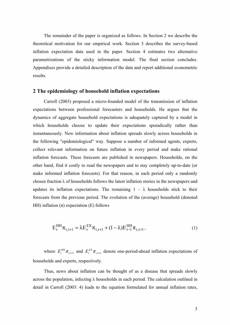
The remainder of the paper is organized as follows. In Section 2 we describe the

theoretical motivation for our empirical work. Section 3 describes the survey-based

inflation expectation data used in the paper. Section 4 estimates two alternative

parametrizations of the sticky information model. The final section concludes.

Appendixes provide a detailed description of the data and report additional econometric

results.

2 The epidemiology of household inflation expectations

Carroll (2003) proposed a micro-founded model of the transmission of inflation

expectations between professional forecasters and households. He argues that the

dynamics of aggregate household expectations is adequately captured by a model in

which households choose to update their expectations sporadically rather than

instantaneously. New information about inflation spreads slowly across households in

the following "epidemiological" way. Suppose a number of informed agents, experts,

collect relevant information on future inflation in every period and make rational

inflation forecasts. These forecasts are published in newspapers. Households, on the

other hand, find it costly to read the newspapers and to stay completely up-to-date (or

make informed inflation forecasts). For that reason, in each period only a randomly

chosen fraction of households follows the latest inflation stories in the newspapers and

updates its inflation expectations. The remaining 1 – households stick to their

forecasts from the previous period. The evolution of the (average) household (denoted

HH) inflation ( ) expectation (E) follows

1t,tHH

1t1t,tEXt1t,t

HHt E)1(EE +−++ πλ−+πλ=π , (1)

where 1, +tt

HH

tE π and 1, +tt

EX

tE π denote one-period-ahead inflation expectations of

households and experts, respectively.

Thus, news about inflation can be thought of as a disease that spreads slowly

across the population, infecting households in each period. The calculation outlined in

detail in Carroll (2003: 4) leads to the equation formulated for annual inflation rates,

4

which are typically reported in surveys of inflation expectations. Carroll (2003: 7)

derives:

3t,1tHH

1t4t,tEXt4t,t

HHt E)1(EE +−−++ πλ−+πλ=π (2)

Equation (2) holds if (i) inflation follows a random walk process or (ii)

4t,tHH

1t3t,1tHH

1t EE +−+−− π≈π . Both of these assumptions are likely to be satisfied in our

dataset. As discussed below, the underlying CPI inflation process in the core European

economies has, indeed, been very persistent recently, warranting the random walk

approximation. Second, given the high persistence of the inflation process, there is not

much difference between households expectations as at time t-1 of inflation rates at t+3

and t+4, which, in turn, implies that condition (ii) is also likely to be met.

3. Expectations data

To test the model of the information diffusion, two kinds of inflation expectation

data are needed: inflation forecasts of households and professional forecasters. The

forecasts of households were obtained from the European Commission’s (EC) consumer

survey and those of professional forecasters from Consensus Economics, a London-

based macroeconomic survey firm.

Household expectations were constructed using the EC survey’s question 6, which

asks how, by comparison with the last 12 months, the respondents expect that consumer

prices will develop in the next 12 months.2 Unfortunately, the answers are qualitative

rather than quantitative (unlike, for example, question 12 concerning expected inflation

in the US Michigan Survey of Consumer Sentiment). This means that the respondents

are asked about the direction of the expected movement of consumer prices

(increase/fall), not about the exact quantitative value of this movement. Consequently,

2 The exact wording of question 6 of the Consumer Survey of the Joint Harmonised EU Programme of Business and Consumer Surveys is “By comparison with the past 12 months, how do you expect that consumer prices will develop in the next 12 months?” For more information on the survey, see the Commission’s webpage, http://europa.eu.int/comm/economy_finance/indicators/businessandconsumersurveys_en.htm.

5

care needs to be taken when transforming these data into quantitative measures of

households expectations, required to test equation (2). We follow much of the existing

literature (including Gerberding (2001), Mankiw et al (2003) and Nielsen (2003)) in

adopting the Carlson and Parkin (1975) method, explained in detail in Appendix I.

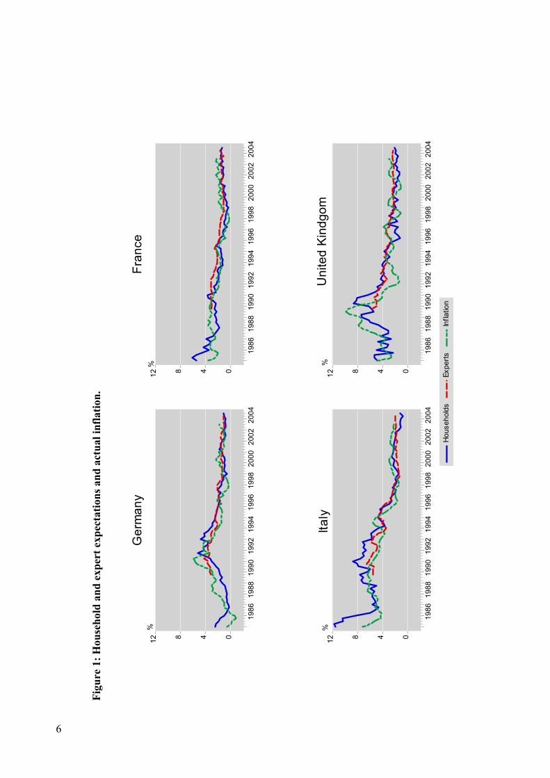
Figure 1. compares experts’ and households’ inflation expectations with actual

inflation rates. Apparently, both expert’s and household’s predictions are roughly in line

with actual inflation. However, sometimes there are even rather persistent differences

between expectations and actual inflation. More importantly, household’s and expert’s

expectations differ considerably in certain time periods. Thus, a closer examination of

the dynamic interaction of both variables is warranted.

4. Empirical results

The choice of the appropriate empirical strategy to estimate equation (2) depends

on the time series properties of the underlying expectations. If the series are stationary,

model (2) can be estimated directly using OLS (as in Carroll (2003)). If they are non-

stationary (I(1)) and cointegrated, the model should be transformed into vector error-

correction (VEC) form. Below, we first discuss the degree of persistence in the inflation

rates at hand. In a second step, we present estimates for both the stationary and the

integrated case.

4.1 Persistence of inflation and inflation expectations

Before estimating equation (1) we test for stationarity of our inflation and

inflation expectation series. Table 1 presents the results of augmented Dickey-Fuller

tests together with estimates of the largest autoregressive roots, calculated following

Stock (1991).3

3 Qualitatively similar results hold for the Elliott, Rothenberg and Stock (1996), DF-GLS test.

Fig

ure

1:

Hou

seh

old

an

d e

xp

ert

exp

ecta

tion

s an

d a

ctu

al

infl

ati

on

.

048

12

19

86

19

88

19

90

19

92

19

94

19

96

19

98

20

00

20

02

20

04

Ge

rma

ny

048

12

19

86

19

88

19

90

19

92

19

94

19

96

19

98

20

00

20

02

20

04

Ho

us

eh

old

sEx

pert

sIn

fla

tio

n

Fra

nce

048

12

19

86

19

88

19

90

19

92

19

94

19

96

19

98

20

00

20

02

20

04

Ita

ly

048

12

19

86

19

88

19

90

19

92

19

94

19

96

19

98

20

00

20

02

20

04

Un

ite

d K

ind

go

m

%%

%%

6

7

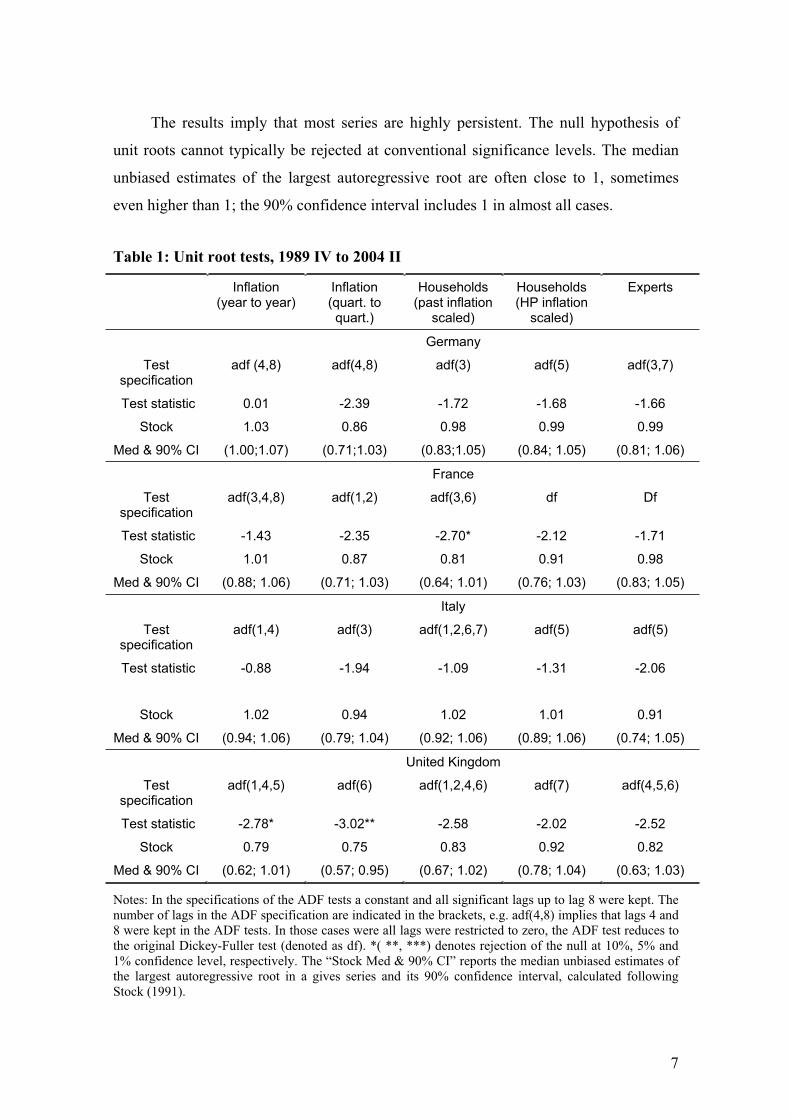
The results imply that most series are highly persistent. The null hypothesis of

unit roots cannot typically be rejected at conventional significance levels. The median

unbiased estimates of the largest autoregressive root are often close to 1, sometimes

even higher than 1; the 90% confidence interval includes 1 in almost all cases.

Table 1: Unit root tests, 1989 IV to 2004 II

Inflation(year to year)

Inflation(quart. to quart.)

Households (past inflation

scaled)

Households (HP inflation

scaled)

Experts

Germany

Testspecification

adf (4,8) adf(4,8) adf(3) adf(5) adf(3,7)

Test statistic 0.01 -2.39 -1.72 -1.68 -1.66

Stock

Med & 90% CI

1.03

(1.00;1.07)

0.86

(0.71;1.03)

0.98

(0.83;1.05)

0.99

(0.84; 1.05)

0.99

(0.81; 1.06)

France

Testspecification

adf(3,4,8) adf(1,2) adf(3,6) df Df

Test statistic -1.43 -2.35 -2.70* -2.12 -1.71

Stock

Med & 90% CI

1.01

(0.88; 1.06)

0.87

(0.71; 1.03)

0.81

(0.64; 1.01)

0.91

(0.76; 1.03)

0.98

(0.83; 1.05)

Italy

Testspecification

adf(1,4) adf(3) adf(1,2,6,7) adf(5) adf(5)

Test statistic -0.88 -1.94 -1.09 -1.31 -2.06

Stock

Med & 90% CI

1.02

(0.94; 1.06)

0.94

(0.79; 1.04)

1.02

(0.92; 1.06)

1.01

(0.89; 1.06)

0.91

(0.74; 1.05)

United Kingdom

Testspecification

adf(1,4,5) adf(6) adf(1,2,4,6) adf(7) adf(4,5,6)

Test statistic -2.78* -3.02** -2.58 -2.02 -2.52

Stock

Med & 90% CI

0.79

(0.62; 1.01)

0.75

(0.57; 0.95)

0.83

(0.67; 1.02)

0.92

(0.78; 1.04)

0.82

(0.63; 1.03)

Notes: In the specifications of the ADF tests a constant and all significant lags up to lag 8 were kept. The number of lags in the ADF specification are indicated in the brackets, e.g. adf(4,8) implies that lags 4 and 8 were kept in the ADF tests. In those cases were all lags were restricted to zero, the ADF test reduces to the original Dickey-Fuller test (denoted as df). *( **, ***) denotes rejection of the null at 10%, 5% and 1% confidence level, respectively. The “Stock Med & 90% CI” reports the median unbiased estimates of the largest autoregressive root in a gives series and its 90% confidence interval, calculated following Stock (1991).

8

While there exists a relatively large literature on persistence properties of inflation

in and outside the US (see, for example, Cogley and Sargent (2002), its discussion by

Stock, and Piger and Levin (2003)), the empirical results on the persistence of inflation

and its stability are often inconclusive. Although the above results indicate the possible

existence of a unit root in most series considered, a potential criticism of the results

shown in Table 1 is that our sample is too short to allow reliable inferences. The fact

that we areunable to reject the null may well result from the notoriously low power of

the unit root tests under such circumstances, rather than the existence of the unit root.

Since the main focus of this paper is not on providing a definitive answer on the

order of integration of inflation (or inflation expectations), we now move on to

estimating our theoretical model and investigate how sensitive its implications are in

respect of whether we assume stationary or non-stationary environments. Because the

tests do not clearly determine the stationarity properties in the relatively short sample

we have, we will first estimate the Carroll model in the stationary environment. We will

then consider how the results are affected if the nonstationary (VECM) set-up is

adopted.

4.2 The stationary case: Carroll (2003) model

We will first estimate and test the epidemiological model under the assumption

that the underlying expectations series are stationary (I(0)). Before estimating

equation (2), we will examine some preliminary evidence on the relationship between

expert and household expectations. Given the interest in the interaction between the

expectations of both professional forecasters and households, a natural starting point is

to ask, (i) which of the two groups forecasts, on average, better and (ii) what is the

causality between the two expectations.

Relationship between Expert and Household Expectations

First, evidence reported in Appendix I (Table A.1) implies that the expert

expectations are substantially more precise than the household expectations. The root

mean squared errors of the expert forecasts are between 15% to 35% lower in Germany,

9

Italy and the UK than for household expectations. The two expectations are comparably

precise in France. This does not, of course, come as a surprise since the households may

know the experts’ forecasts when forming their own expectations. According to the

epidemiology model, at least some of the households update their own expectations by

following the experts.

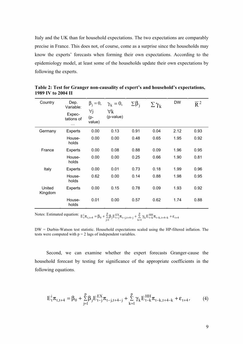
Table 2: Test for Granger non-causality of expert’s and household’s expectations,

1989 IV to 2004 II

Country Dep. Variable:

Expec-tations of

…

j

,0j

∀

=β

(p-value)

k

,0k

∀=γ

(p-value)

β j γkDW 2R

Germany Experts 0.00 0.13 0.91 0.04 2.12 0.93

House-holds

0.00 0.00 0.48 0.65 1.95 0.92

France Experts 0.00 0.08 0.88 0.09 1.96 0.95

House-holds

0.00 0.00 0.25 0.66 1.90 0.81

Italy Experts 0.00 0.01 0.73 0.18 1.99 0.96

House-holds

0.62 0.00 0.14 0.88 1.98 0.95

UnitedKingdom

Experts 0.00 0.15 0.78 0.09 1.93 0.92

House-holds

0.01 0.00 0.57 0.62 1.74 0.88

Notes: Estimated equation: 4t

p

1kk4t,kt

HHktk

p

1jj4t,jt

EXjtj04t,t

it EEE +

=−+−−

=−+−−+ ε+πγ+πβ+β=π

DW = Durbin-Watson test statistic. Household expectations scaled using the HP-filtered inflation. The tests were computed with p = 2 lags of independent variables.

Second, we can examine whether the expert forecasts Granger-cause the

household forecast by testing for significance of the appropriate coefficients in the

following equations.

4t

p

1kk4t,kt

HHktk

p

1jj4t,jt

EXjtj04t,t

it EEE +

=−+−−

=−+−−+ ε+πγ+πβ+β=π , (4)

10

where the regressions are run with both expert and household expectations on the right-

hand side, { }HH,Exi∈ . This is done in Table 2. Columns 3 and 4 indicate that lags of

expert expectations are typically significant predictors of household expectations.

Household expectations, on the other hand, tend not to Granger-cause the experts. Thus,

in all countries, except for Italy we conclude that the direction of causality goes from

experts toward households. This is also documented in columns 5 and 6, which display

the sum of coefficients on past expectations. The sum of coefficients on expert

expectations ( β j ) in household equations is bigger than the sum of household

coefficients ( γ k ) in expert equations (in all countries except for Italy).

Equation-by-Equation Estimation

Having found supportive preliminary evidence for the epidemiological model of

expectations formation, let us now turn to direct estimation of and inference about the

speed of information updating, . Table 3 summarizes the estimation results of the

following regressions

4t3t,1tHH

1t24t,tEXt104t,t

HHt EEE ++−−++ ε+πλ+πλ+λ=π (5)

in unrestricted and restricted forms.4

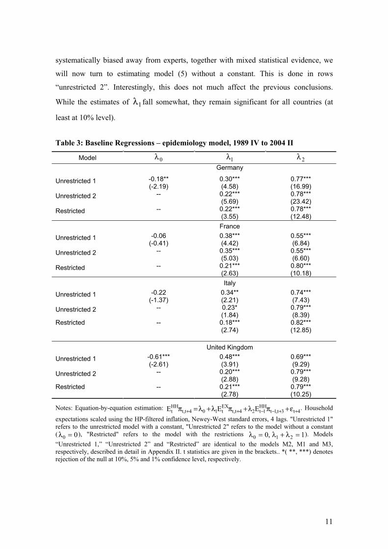
Rows 1 and 2 report coefficients and t statistics of 20 ,..., λλ freely estimated in

the unrestricted model (5). Three findings emerge: First, the constant 0λ is insignificant

for France and Italy, while significant for the UK and Germany. Second, the coefficient

1λ that identifies the speed of updating of household expectations is highly significant

for all countries. Third, 1λ and 2λ roughly add up to 1, as predicted by the Carroll

model. Given that it makes little sense a priori to assume that regression (5) should be

estimated with a constant, since that effectively implies that household expectations are

4 Detailed results are shown in Appendix II, Tables A.2a-d.

11

systematically biased away from experts, together with mixed statistical evidence, we

will now turn to estimating model (5) without a constant. This is done in rows

“unrestricted 2”. Interestingly, this does not much affect the previous conclusions.

While the estimates of 1λ fall somewhat, they remain significant for all countries (at

least at 10% level).

Table 3: Baseline Regressions – epidemiology model, 1989 IV to 2004 II

Model 0λ 1λ 2λGermany

Unrestricted 1 -0.18**(-2.19)

0.30***(4.58)

0.77***(16.99)

Unrestricted 2 -- 0.22*** (5.69)

0.78***(23.42)

Restricted -- 0.22*** (3.55)

0.78***(12.48)

France

Unrestricted 1 -0.06(-0.41)

0.38***(4.42)

0.55***(6.84)

Unrestricted 2 -- 0.35*** (5.03)

0.55***(6.60)

Restricted -- 0.21*** (2.63)

0.80***(10.18)

Italy


0.34**(2.21)

0.74***(7.43)

Unrestricted 2 -- 0.23* (1.84)

0.79***(8.39)

Restricted -- 0.18*** (2.74)

0.82***(12.85)

United Kingdom

Unrestricted 1 -0.61*** (-2.61)

0.48***(3.91)

0.69***(9.29)

Unrestricted 2 -- 0.20*** (2.88)

0.79***(9.28)

Restricted -- 0.21*** (2.78)

0.79***(10.25)

Notes: Equation-by-equation estimation: 4t3t,1t

HH1t24t,t

EXt104t,t

HHt EEE ++−−++ ε+πλ+πλ+λ=π . Household

expectations scaled using the HP-filtered inflation, Newey-West standard errors, 4 lags. "Unrestricted 1" refers to the unrestricted model with a constant, "Unrestricted 2" refers to the model without a constant ( 00 =λ ), "Restricted" refers to the model with the restrictions 1,0 210 =λ+λ=λ ). Models

“Unrestricted 1,” “Unrestricted 2” and “Restricted” are identical to the models M2, M1 and M3, respectively, described in detail in Appendix II. t statistics are given in the brackets.. *( **, ***) denotes rejection of the null at 10%, 5% and 1% confidence level, respectively.

12

In addition, as documented in Table A.2 in Appendix II (line M1) the adding up

restriction 121 =λ+λ is easily met for three countries (except for France). It is then

not surprising that imposing this restriction explicitly in the regressions, as is done in

lines labelled “restricted”, results in little additional change in 1λ .

Interestingly, there is little heterogeneity in estimated 1λ coefficients across

countries with all estimates lying closely around 0.2. This is only slightly less than 1λ =

0.27 estimated by Carroll (2003) and postulated by Mankiw and Reis (2002) for the

US.5 Our baseline estimates in Table 3 therefore imply that the European households

update inflation expectations from experts roughly once in 15 months, only slightly less

frequently than the US households, who do so on average once a year.

Detailed estimation results and specification checks are relegated to Appendix II.

Tables A.2a-d show a number of additional interesting results. In particular, it may be

asked whether the consumers really update inflation expectations from experts’

forecasts or, rather, from past inflation. This can be investigated by adding past inflation

among the regressors in equation (4) and testing for its significance (see equation (A.1)

in Appendix II). It turns out that this term is not statistically significant in any model

considered. This is again in line with Carroll’s findings for the US: households are

forward-looking rather than backward-looking (adaptive) in that they learn from rational

experts rather than simply adopting actual past inflation rates.

Seemingly Unrelated Regression (SUR) Estimation

An obvious advantage of our set-up with four countries is that variants of the

above equation (4) can be estimated as a system using seemingly unrelated regressions

(SUR). This will improve the efficiency of the estimates if the equation-by-equation

residuals are cross-correlated. Since this seems to be the case the cross-correlation

between residuals in our dataset is up to 0.3 we now turn to estimate the parameters

with SUR. In addition to obtaining potentially more efficient estimates, this also makes

5 Carroll’s (2003) sample, 1981:3-2002:1, is slightly different from ours. Re-estimating the model with the US data and our sample range gives = 0.22.

13

it possible to test cross-equation restrictions and answer questions such as “Does the

speed of information updating vary across countries?”

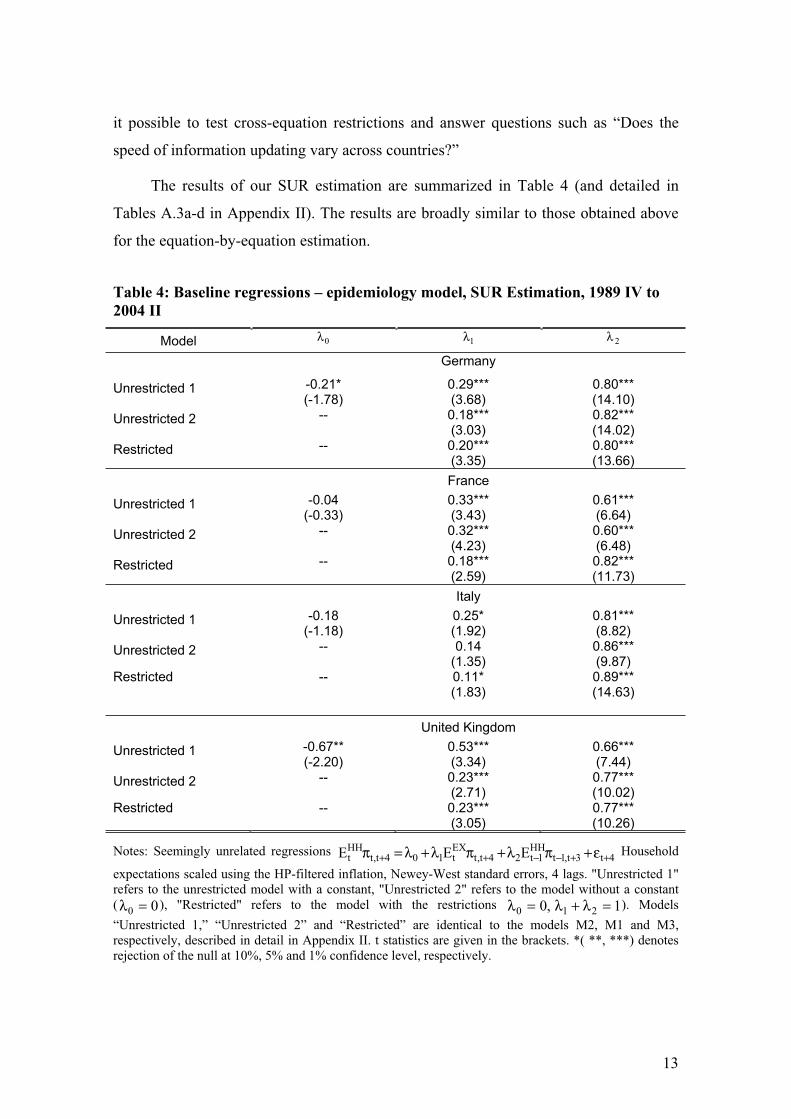
The results of our SUR estimation are summarized in Table 4 (and detailed in

Tables A.3a-d in Appendix II). The results are broadly similar to those obtained above

for the equation-by-equation estimation.

Table 4: Baseline regressions – epidemiology model, SUR Estimation, 1989 IV to

2004 II

Model 0λ 1λ 2λ

Germany

Unrestricted 1 -0.21*(-1.78)

0.29***(3.68)

0.80***(14.10)

Unrestricted 2 -- 0.18*** (3.03)

0.82***(14.02)

Restricted -- 0.20*** (3.35)

0.80***(13.66)

France


0.33***(3.43)

0.61***(6.64)

Unrestricted 2 -- 0.32*** (4.23)

0.60***(6.48)

Restricted -- 0.18*** (2.59)

0.82***(11.73)

Italy


0.25*(1.92)

0.81***(8.82)

Unrestricted 2 -- 0.14 (1.35)

0.86***(9.87)

Restricted -- 0.11* (1.83)

0.89***(14.63)

United Kingdom

Unrestricted 1 -0.67**(-2.20)

0.53***(3.34)

0.66***(7.44)

Unrestricted 2 -- 0.23*** (2.71)

0.77***(10.02)

Restricted -- 0.23*** (3.05)

0.77***(10.26)

Notes: Seemingly unrelated regressions 4t3t,1t

HH1t24t,t

EXt104t,t

HHt EEE ++−−++ ε+πλ+πλ+λ=π Household

expectations scaled using the HP-filtered inflation, Newey-West standard errors, 4 lags. "Unrestricted 1" refers to the unrestricted model with a constant, "Unrestricted 2" refers to the model without a constant ( 00 =λ ), "Restricted" refers to the model with the restrictions 1,0 210 =λ+λ=λ ). Models

“Unrestricted 1,” “Unrestricted 2” and “Restricted” are identical to the models M2, M1 and M3, respectively, described in detail in Appendix II. t statistics are given in the brackets. *( **, ***) denotes rejection of the null at 10%, 5% and 1% confidence level, respectively.

14

The three main findings remain to hold: (i) the constant 0λ is typically

insignificant (again, except for the UK), (ii) the speed of updating 1λ is significant (for

every country at least at 10% confidence level) and finally (iii), the adding-up restriction

121 =λ+λ holds (again expect for France).

Compared to the above results there is a bit more heterogeneity in the 1λ

coefficients across countries: they lie between 0.11 for Italy and 0.23 for the UK. These

imply that Italian households update inflation expectations on average roughly once in

two years (27 months), whereas the British ones do so about once a year (13 months).

The results reported in Appendix II furthermore confirm the findings from the equation-

by-equation set-up on the insensitivity of household expectations with respect to past

inflation.

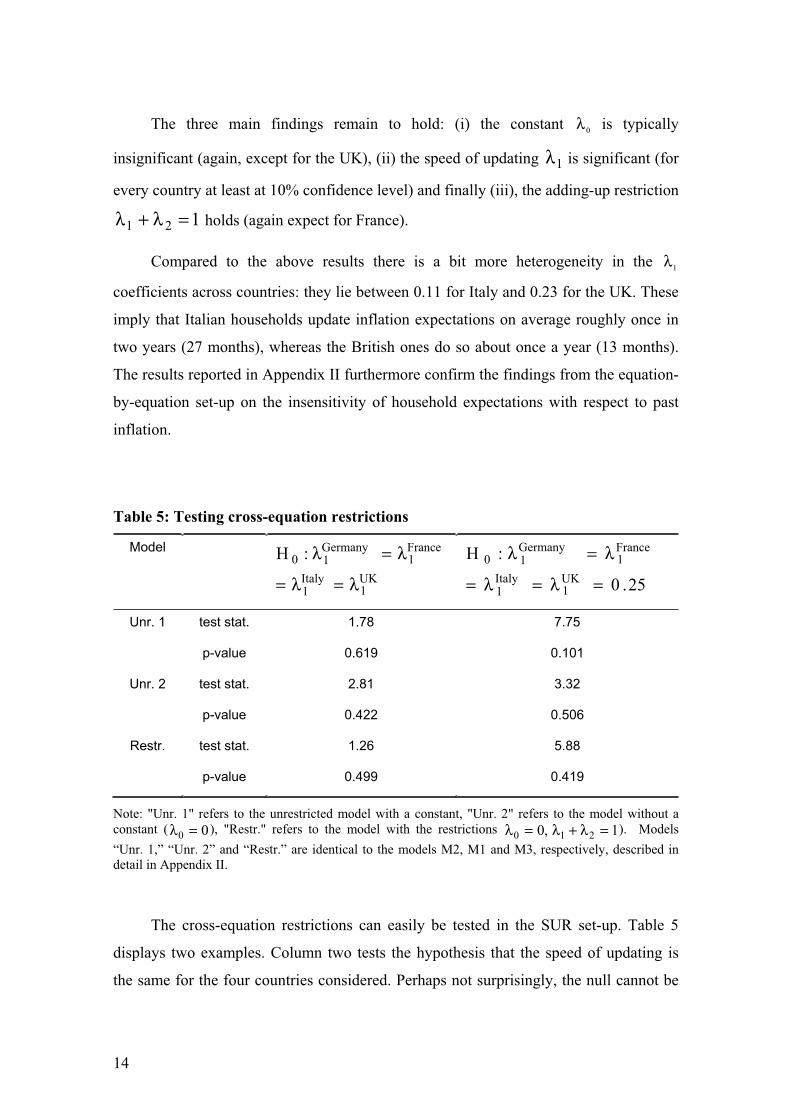
Table 5: Testing cross-equation restrictions

Model

UK1

Italy1

France1

Germany10 :H

λ=λ=

λ=λ

25.0

:H

UK1

Italy1

France1

Germany10

=λ=λ=

λ=λ

Unr. 1 test stat.

p-value

1.78

0.619

7.75

0.101

Unr. 2 test stat.

p-value

2.81

0.422

3.32

0.506

Restr. test stat.

p-value

1.26

0.499

5.88

0.419

Note: "Unr. 1" refers to the unrestricted model with a constant, "Unr. 2" refers to the model without a constant ( 00 =λ ), "Restr." refers to the model with the restrictions 1,0 210 =λ+λ=λ ). Models

“Unr. 1,” “Unr. 2” and “Restr.” are identical to the models M2, M1 and M3, respectively, described in detail in Appendix II.

The cross-equation restrictions can easily be tested in the SUR set-up. Table 5

displays two examples. Column two tests the hypothesis that the speed of updating is

the same for the four countries considered. Perhaps not surprisingly, the null cannot be

15

rejected. Similarly, the hypothesis that the European households update information on

inflation on average once a year, at the same frequency as in the US, seems to hold in

our dataset.

Our findings confirm that the epidemiology model of information diffusion

performs similarly well, quantitatively as well as quantitatively, for the core European

countries as it does for the US. The expert inflation expectations are typically more

precise than the household expectations. Econometric tests indicate that the Carroll

model is adequate along several dimensions (for example, the speed of updating is

positive and statistically significant, the summing-up restriction holds fairly well and

household inflation expectations are not sensitive with respect to the past inflation).

While several models imply that European households update a bit more slowly than

US households, on average once in 15 months compared with once a year, these

differences are not pronounced enough to be statistically significant. Finally, there is

strong evidence that, as suggested by the epidemiology model, European households

update information from the professional forecasters rather than the past inflation rate.6

4.3 The nonstationary case: Carroll (2003) model in vector error correction form

Having estimated the epidemiology model in a stationary framework, let us now

examine how the implications change when we assume that the expectation series are

I(1) instead. Suppose we collect the two series in vector )'E,E(x 4t,t

EX

t3t,1t

HH

1tt ++−− ππ= . If the

two series are cointegrated with cointegrating vector )'1( 1α−=α , the system has the

following vector error correction (VEC) representation

tt1tt x)L(x'x ε+∆β+αλ=∆ − , (6)

6 Consideration might be given to the possibility that households update their expectations by referring

directly to other publicly available information, such as foreign prices. However, in the epidemiology framework this information is already captured and processed by professional forecasters. Moreover, obtaining such information is presumably much more costly than simply referring to the published professional forecasts.

16

where )',( ExHH λλ=λ denotes the vector of loading coefficient and (L) is a

matrix lag polynomial. Similarly to the stationary model (2), λ determines the speed of

adjustment to the (long-run) equilibrium. In particular, we are interested in HH, which

corresponds to the speed of adjustment observed for the households. Furthermore, note

that the theoretical derivation of the “epidemiology model” predicts a cointegrating

vector = (1 –1)’. This is due to the fact that, in the long-run, households completely

adapt to the professional forecasts.

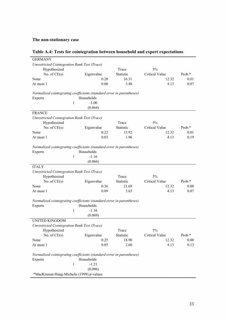
Before estimating the VEC representation (6) and its ‘ α -restricted’ counterpart

some preliminary specification tests need to be done. First, we test whether there exists

a valid cointegrating relationship between the expert and (lagged) household

expectations. In addition, we check whether the theoretical restriction on α is supported

by the data. Detailed results of the Johansen cointegration tests are reported in

Table A.4 in Appendix II. They show that, for all four countries, the two series are

cointegrated. Furthermore, the values for 1α are close to –1 ( a value predicted by the

model) and range from –1.21 for the UK to –1.00 for Germany. In fact, we can formally

conclude that α ’ is not significantly different from (1 –1) as implied by the model,

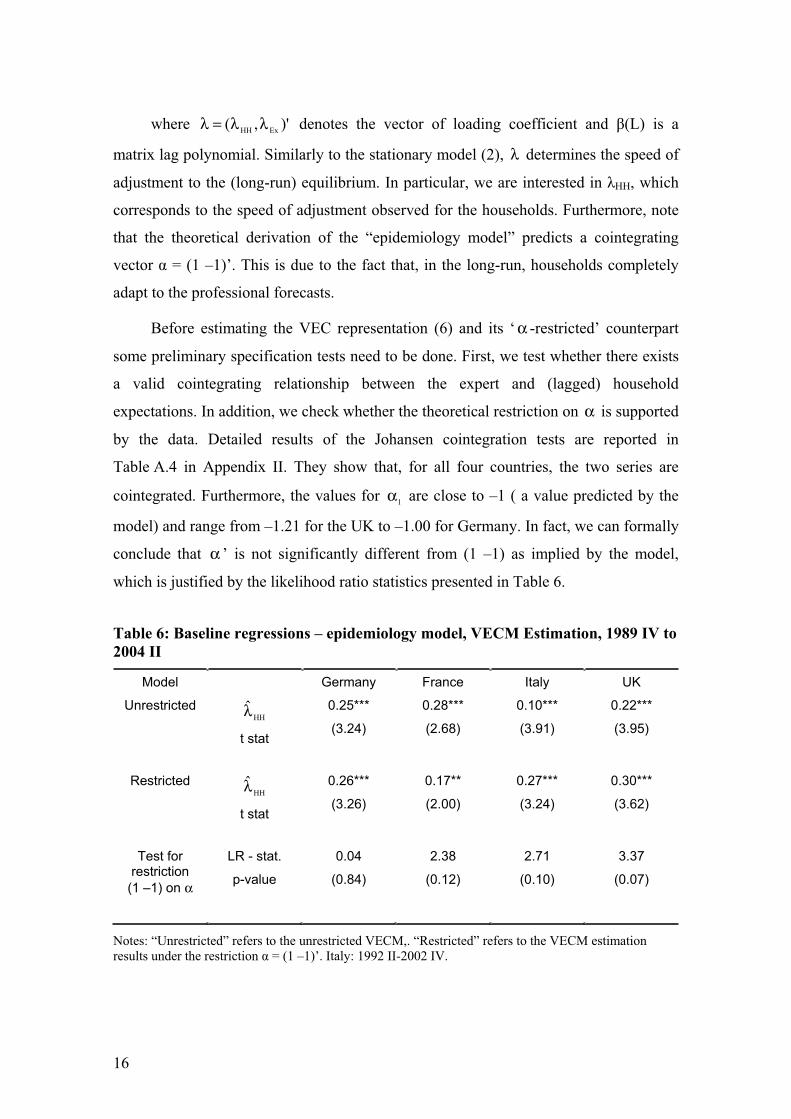
which is justified by the likelihood ratio statistics presented in Table 6.

Table 6: Baseline regressions – epidemiology model, VECM Estimation, 1989 IV to

2004 II

Model Germany France Italy UK

Unrestricted HHλ̂

t stat

0.25***

(3.24)

0.28***

(2.68)

0.10***

(3.91)

0.22***

(3.95)

Restricted HHλ̂

t stat

0.26***

(3.26)

0.17**

(2.00)

0.27***

(3.24)

0.30***

(3.62)

Test for restriction

(1 –1) on α

LR - stat.

p-value

0.04

(0.84)

2.38

(0.12)

2.71

(0.10)

3.37

(0.07)

Notes: “Unrestricted” refers to the unrestricted VECM,. “Restricted” refers to the VECM estimation results under the restriction = (1 –1)’. Italy: 1992 II-2002 IV.

17

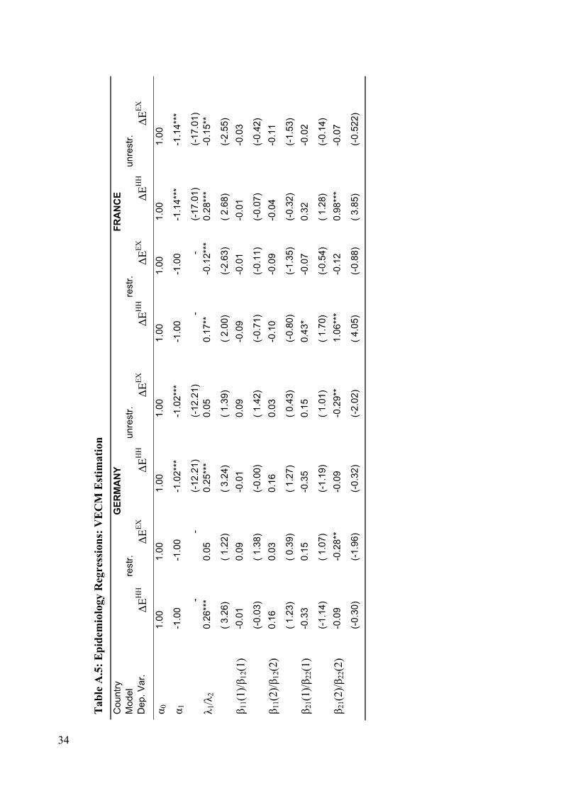
The VEC estimations are summarized in Table 7 (and detailed results are

presented in Appendix II, Table A.5). The estimated speed of adjustment of the

households, HH, is remarkably close tothat in the previous section obtained under the

assumption of stationarity.7 All estimates are significant and lie in the neighbourhood of

0.25 – with the exception of Italy for the unrestricted model (0.10) and France for the

restricted VECM (0.17). Hence, we again find a huge degree of homogeneity among the

four countries with French households updating their inflation expectations on average

once every 18 months, British households updating their views on average once every

ten months, and the frequencies of Italian and German households lying closely below

the British one.

Another point which supports the results of the ‘stationary case’ is the way in

which deviations from the long-term equilibrium are corrected. Owing to the fact that,

except for France, the loading coefficients, Ex, in the experts’ expectation equations are

not significantly different from zero, we can conclude that the entire correction process

is made via the household expectations. This confirms the earlier finding that expert

forecasts Granger-cause the households’ expectations, whereas household forecasts do

not tend to Granger-cause the forecasts of experts.

With these findings, we show that the epidemiology model of Carroll can be

easily extended to the ‘non-stationary world’. The derived VEC epidemiology model of

information diffusion performs similarly well to the stationary model. This result is

especially useful for the analysis of European countries since it is a well-known fact that

their inflation rates are more persistent than the US inflation rate. Thus, even though it

is difficult to draw clear conclusions about the stationarity properties of the series with

the short sample size at hand,8 our VEC representation might be preferable once more

data are available.

7 In a way, this is perhaps not so surprising given that if there is not much autocorrelation in

tx∆ the VEC model (6) is a simple transformation of the restricted stationary model (5)

(with 00 =λ and 121 =λ+λ ).

8 This indeterminacy is ex-post ‘justified’ by the similarities between the results from the Carroll model and the results of the VECMs.

18

5. Conclusions

Inflation expectations are crucial determinants of future inflation dynamics. The

model estimated here attempts to analyze how these expectations are formed and how

information is transmitted from professional forecasters to households. Our estimates of

the speed of information updating have important implications for the persistence of

inflation and inflation expectations. We document that the qualitative and quantitative

findings previously reported for the US generalize to major European countries. Most

European households adjust rather sluggishly to new information; they update their

information on average once a year. Interestingly, it turns out that the households are

forward-looking in the sense that they use information processed by experts rather than

just past information. These findings are robust to a number of estimation methods

(suited for data with various stochastic properties) we consider.

We think of this paper as the beginning of a larger research project that can

continue through a number of avenues. The survey data could possibly be used to

directly estimate the sticky-information Phillips curve in addition to its epidemiological

micro-foundations. Alternatively, it would be possible, in the spirit of Mankiw et al

(2003), to analyze the micro-data on inflation expectations rather than just their mean

values. Finally, the epidemiology model could, in principle, be estimated for additional

countries, using cross-sectional dependence among countries to alleviate problems

related to short samples.

19

References

Batchelor, R. and A. Orr (1988), Inflation expectations revisited, Economica, 55, pp. 17–31.

Branch, W. A. (2004), The Theory of rationally heterogeneous expectations: evidence from survey data on inflation expectations, Economic Journal,114, pp. 592-621.

Carlson, J. and M. Parkin (1975), Inflation expectations, Economica, 42, 123–137.

Carroll, C.D. (2003), Macroeconomic expectations of households and professional forecasters. Quarterly Journal of Economics 118, pp. 269-298.

Cogley, T. and Sargent T. (2002), Evolving oost World War II US inflation dynamics, NBER Macroeconomics Annual.

Gerberding, C. (2001), The information content of survey data on expected price developments for monetary policy. Deutsche Bundesbank Discussion Paper No.

9.

Handjiyska, B. (2004), Adjustment of household inflation expectations in five OECD countries, mimeo, Johns Hopkins University.

Khan, H. and Z. Zhu (2002), Estimates of the sticky information Phillips Curve for the United States, Canada, and the United Kingdom. Bank of Canada Woking Paper No. 2002-19. Ottawa.

Mankiw, N. G. and R. Reis (2002), Sticky information versus sticky prices: a proposal to replace the New Keynesian Phillips curve. Quarterly Journal of Economics

117, pp. 1295-1328.

Mankiw, N. G. and R. Reis (2003), Sticky information: a model of monetary nonneutrality and structural slumps. In. Aghion, P. (ed.), Knowledge, information, and expectation in modern macroeconomics, pp. 64-86.

Mankiw, N. G., R. Reis and J. Wolfers (2003), Disagreement on inflation expectations. In: NBER Macroeconomics Annual 18 (2003), pp. 209-248.

Nielsen, H. (2003), Essays on expectations. Aachen 2003.

Piger, J. and A. Levin (2003), Is inflation persistence intrinsic in industrial economies?, Federal Reserve Bank of St. Louis working paper.

Sims, C. (2003), Implications of rational inattention, Journal of Monetary Economics,50(3), pp. 665-690.

Sims, C. (2005), Rational inattention: A research agenda. Deutsche Bundesbank Discussion Paper, forthcoming.

Stock, J. (1991), Confidence intervals for the largest autoregressive root in macroeconomic time series, Journal of Monetary Economics 28(3), pp. 445-60.

20

Appendix I: Inflation Expectation Data

Expert forecasts

The data on professional forecasts were obtained from Consensus Economics, a

private macroeconomic survey firm (http://www.consensuseconomics.com/). The survey of

experts of private and public institutions in major industrial countries has been collected

monthly since 1989. Once every quarter the questionnaire contains a question on

forecasts over the next six quarters. The consensus forecast, used in the paper as a

measure of expert expectations, is the mean of about 20 to 30 forecasts of local experts

from major banks or research institutes in each country.

Household forecasts

Our measures of household inflation forecasts are based on disaggregated answers

to question 6 from European Commission’s Harmonised Business and Consumer

Surveys. The sample size of the survey is about 2,000 households in Germany, Italy and

the UK, and roughly 3,300 households in France. The data are available monthly since

1985 to the present.

Extracting household inflation expectations from the qualitative survey data

To obtain quantitative expectations data from the balance statistics, a rescaling of

the data is warranted. The standard method, the “probability method,” follows Carlson

and Parkin (1975) and its extensions (see, for example, Gerberding (2001), Mankiw et

al (2003) and Nielsen (2003)). The observed data are from the pentachotomous survey.

Consequently, they classify the responses into five subgroups:

Consumer prices will

- Increase more rapidly

- Increase at the same rate

- Increase at a slower rate

- Stay about the same

- Fall.

21

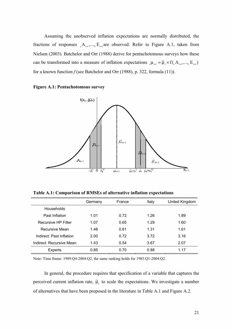
Assuming the unobserved inflation expectations are normally distributed, the

fractions of responses 1tt1tt E,...,A ++ are observed. Refer to Figure A.1, taken from

Nielsen (2003). Batchelor and Orr (1988) derive for pentachotomous surveys how these

can be transformed into a measure of inflation expectations )E,...,A(f~1tt1ttt1tt +++ ×µ=µ

for a known function f (see Batchelor and Orr (1988), p. 322, formula (11)).

Figure A.1: Pentachotomous survey

Table A.1: Comparison of RMSEs of alternative inflation expectations

Germany France Italy United Kingdom

Households

Past Inflation 1.01 0.72 1.26 1.89

Recursive HP Filter 1.07 0.65 1.29 1.60

Recursive Mean 1.48 0.61 1.31 1.61

Indirect: Past Inflation 2.00 0.72 3.72 3.16

Indirect: Recursive Mean 1.43 0.54 3.67 2.07

Experts 0.85 0.70 0.88 1.17

Note: Time frame: 1989:Q4-2004:Q2, the same ranking holds for 1985:Q1-2004:Q2.

In general, the procedure requires that specification of a variable that captures the

perceived current inflation rate, t~µ to scale the expectations. We investigate a number

of alternatives that have been proposed in the literature in Table A.1 and Figure A.2.

22

The Table (and Figure) compare(s) the household expectations constructed using

the following five normalizations for t~µ : (i) past inflation (over the last year, lagged by

one quarter), (ii) inflation trend extracted using the recursive HP filter, (iii) recursive

mean of past inflation calculated from the beginning of the sample till the current

period, (iv) indirect method, normalized with past inflation and, finally, (v) indirect

method, normalized with recursive mean.

The recursive HP filter was calculated using the following quasi-real-time

procedure to minimize the well-known end-of-sample problems. For each period, t, we

first forecast the underlying inflation process for the next 12 quarters with an ARMA

model, selected with the Akaike criterion (maximum number of 4 lags on both AR and

MA terms). We then apply the filter on this artificially extended series (with the HP

filter with the usual penalty parameter 1600HP =λ ). Finally, we set t~µ equal to the value

of the HP filtered inflation as of time t.

An alternative to the above method, proposed by Nielsen (2003), is to make use of

the Survey’s question 5 on the current perceived inflation (“How do you think that

consumer prices have developed over the last 12 months?”). Unfortunately, this does

not solve the problem, since the answers are again only qualitative. Consequently, this

still requires specifying t~µ , just at an earlier stage. This is investigated in rows four and

five of Table A.1.

The Table documents a number of facts. First, the two normalizations of

household inflation expectations that typically perform best in terms of minimizing the

mean squared errors are (i) and (ii): past inflation and recursive HP filter. This holds for

all countries, except for France, where all normalizations imply comparable RMSEs.

Second, the indirect methods (iv) and (v) often imply inflation expectations very

different from the actual inflation. This is particularly true in Italy, but also in Germany

and the United Kingdom. Third, experts’ expectations tend to be substantially more

precise than household expectations (irrespective of the normalization). More precisely,

the RMSEs of expert expectations are between 15% to 35% lower in Germany, Italy

and the UK than for household expectations. The two expectations are comparably

precise in France.

23

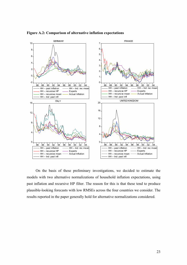
Figure A.2: Comparison of alternative inflation expectations

-2

0

2

4

6

8

10

86 88 90 92 94 96 98 00 02 04

HH -- past inflation

HH -- recursive HP

HH -- recursive mean

HH -- Ind: past infl

HH -- Ind: rec mean

Experts

Actual Inflation

0

1

2

3

4

5

6

7

86 88 90 92 94 96 98 00 02 04


HH -- recursive HP



HH -- Ind: rec mean

Experts

Actual Inflation

0

4

8

12

16

86 88 90 92 94 96 98 00 02 04


HH -- recursive HP



HH -- Ind: rec mean

Experts

Actual Inflation

0

4

8

12

16

20

86 88 90 92 94 96 98 00 02 04


HH -- recursive HP



HH -- Ind: rec mean

Experts

Actual Inflation

GERMANY FRANCE

ITALY UNITED KINGDOM

On the basis of these preliminary investigations, we decided to estimate the

models with two alternative normalizations of household inflation expectations, using

past inflation and recursive HP filter. The reason for this is that these tend to produce

plausible-looking forecasts with low RMSEs across the four countries we consider. The

results reported in the paper generally hold for alternative normalizations considered.

24

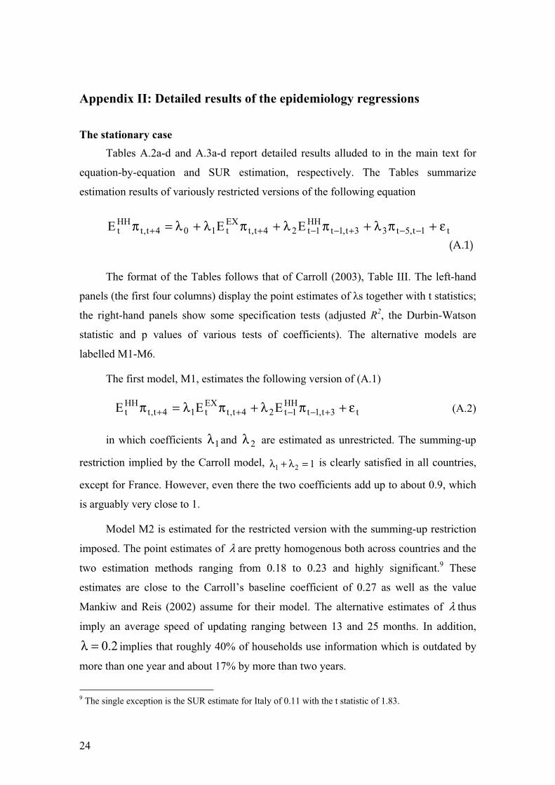
Appendix II: Detailed results of the epidemiology regressions

The stationary case

Tables A.2a-d and A.3a-d report detailed results alluded to in the main text for

equation-by-equation and SUR estimation, respectively. The Tables summarize

estimation results of variously restricted versions of the following equation

t1t,5t33t,1tHH

1t24t,tEXt104t,t

HHt EEE ε+πλ+πλ+πλ+λ=π −−+−−++

(A.1)

The format of the Tables follows that of Carroll (2003), Table III. The left-hand

panels (the first four columns) display the point estimates of s together with t statistics;

the right-hand panels show some specification tests (adjusted R2, the Durbin-Watson

statistic and p values of various tests of coefficients). The alternative models are

labelled M1-M6.

The first model, M1, estimates the following version of (A.1)

t3t,1tHH

1t24t,tEXt14t,t

HHt EEE ε+πλ+πλ=π +−−++ (A.2)

in which coefficients 1λ and 2λ are estimated as unrestricted. The summing-up

restriction implied by the Carroll model, 121 =λ+λ is clearly satisfied in all countries,

except for France. However, even there the two coefficients add up to about 0.9, which

is arguably very close to 1.

Model M2 is estimated for the restricted version with the summing-up restriction

imposed. The point estimates of λ are pretty homogenous both across countries and the

two estimation methods ranging from 0.18 to 0.23 and highly significant.9 These

estimates are close to the Carroll’s baseline coefficient of 0.27 as well as the value

Mankiw and Reis (2002) assume for their model. The alternative estimates of λ thus

imply an average speed of updating ranging between 13 and 25 months. In addition,

2.0=λ implies that roughly 40% of households use information which is outdated by

more than one year and about 17% by more than two years.

9 The single exception is the SUR estimate for Italy of 0.11 with the t statistic of 1.83.

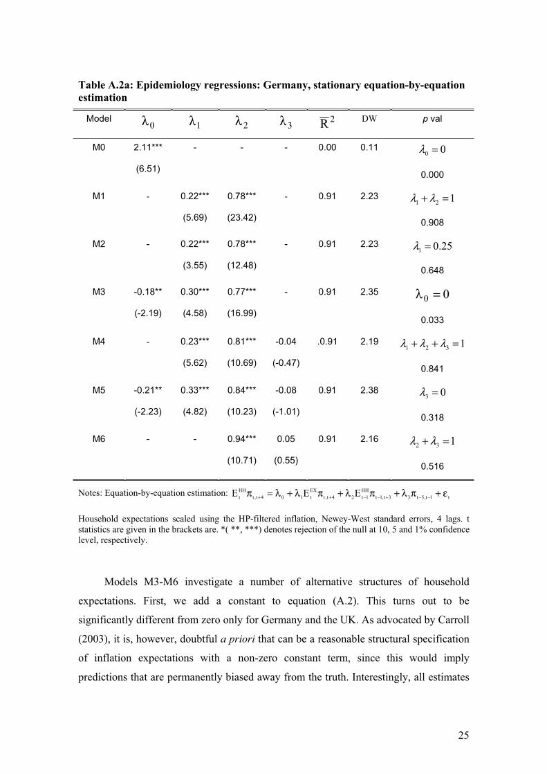
25

Table A.2a: Epidemiology regressions: Germany, stationary equation-by-equation

estimation

Model0λ 1λ 2λ 3λ 2R DW p val

M0 2.11***

(6.51)

- - - 0.00 0.11 00 =λ

0.000

M1 - 0.22***

(5.69)

0.78***

(23.42)

- 0.91 2.23 121 =+ λλ

0.908

M2 - 0.22***

(3.55)

0.78***

(12.48)

- 0.91 2.23 25.01 =λ

0.648

M3 -0.18**

(-2.19)

0.30***

(4.58)

0.77***

(16.99)

- 0.91 2.35 00 =λ

0.033

M4 - 0.23***

(5.62)

0.81***

(10.69)

-0.04

(-0.47)

.0.91 2.19 1321 =++ λλλ

0.841

M5 -0.21**

(-2.23)

0.33***

(4.82)

0.84***

(10.23)

-0.08

(-1.01)

0.91 2.38 03 =λ

0.318

M6 - - 0.94***

(10.71)

0.05

(0.55)

0.91 2.16 132 =+ λλ

0.516

Notes: Equation-by-equation estimation: t1t,5t33t,1t

HH

1t24t,t

EX

t104t,t

HH

t EEE ε+πλ+πλ+πλ+λ=π −−+−−++

Household expectations scaled using the HP-filtered inflation, Newey-West standard errors, 4 lags. t statistics are given in the brackets are. *( **, ***) denotes rejection of the null at 10, 5 and 1% confidence level, respectively.

Models M3-M6 investigate a number of alternative structures of household

expectations. First, we add a constant to equation (A.2). This turns out to be

significantly different from zero only for Germany and the UK. As advocated by Carroll

(2003), it is, however, doubtful a priori that can be a reasonable structural specification

of inflation expectations with a non-zero constant term, since this would imply

predictions that are permanently biased away from the truth. Interestingly, all estimates

26

of model M3, however, give us negative values for the constant term 0λ . One reason for

that may be, as is apparent from Figure 1, that, over our estimation sample, actual

inflation rates were actually falling. In such an environment, some households may have

extrapolated this falling trend into the future, which is reflected in the negative values of

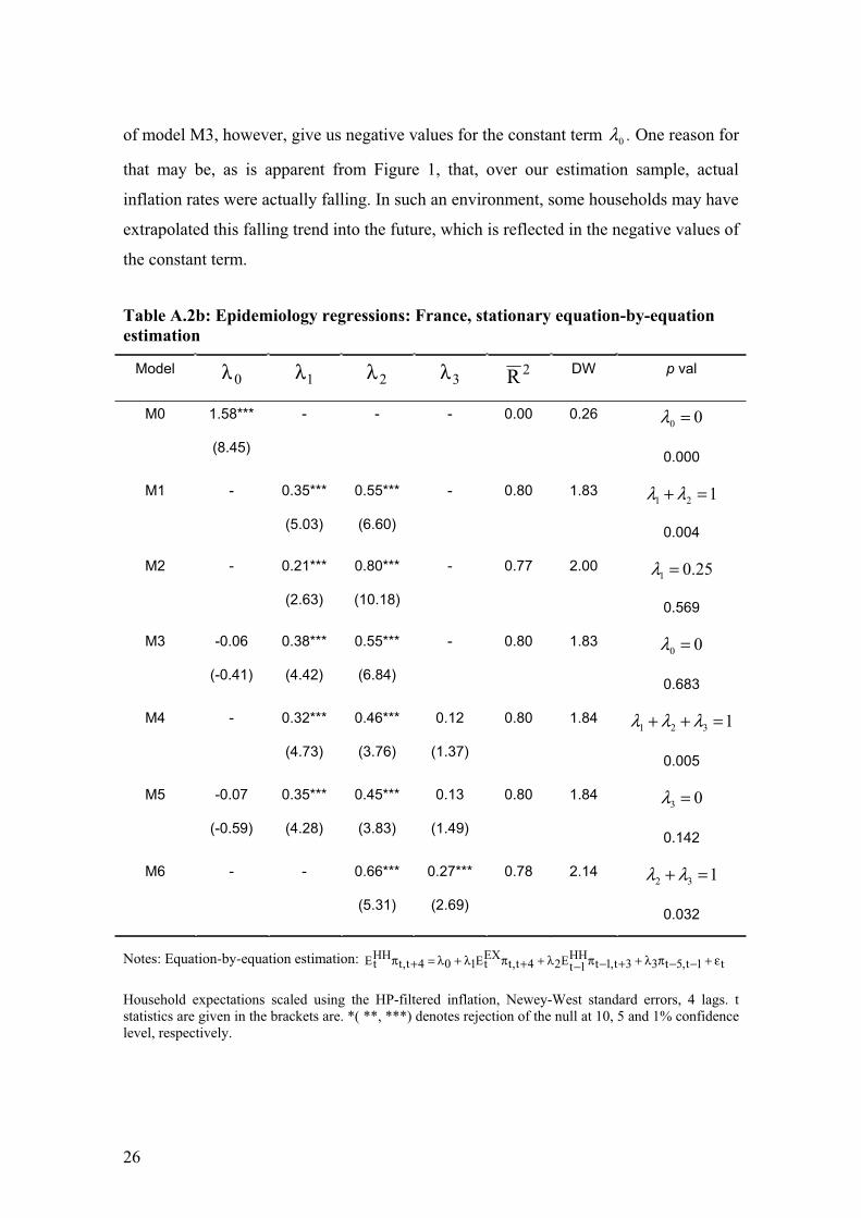
the constant term.

Table A.2b: Epidemiology regressions: France, stationary equation-by-equation

estimation


M0 1.58***

(8.45)

- - - 0.00 0.26 00 =λ

0.000

M1 - 0.35***

(5.03)

0.55***

(6.60)

- 0.80 1.83 121 =+ λλ

0.004

M2 - 0.21***

(2.63)

0.80***

(10.18)

- 0.77 2.00 25.01 =λ

0.569

M3 -0.06

(-0.41)

0.38***

(4.42)

0.55***

(6.84)

- 0.80 1.83 00 =λ

0.683

M4 - 0.32***

(4.73)

0.46***

(3.76)

0.12

(1.37)

0.80 1.84 1321 =++ λλλ

0.005

M5 -0.07

(-0.59)

0.35***

(4.28)

0.45***

(3.83)

0.13

(1.49)

0.80 1.84 03 =λ

0.142

M6 - - 0.66***

(5.31)

0.27***

(2.69)

0.78 2.14 132 =+ λλ

0.032

Notes: Equation-by-equation estimation: t1t,5t33t,1tHH

1tE24t,tEXtE104t,t

HHtE ε+−−πλ++−π−λ++πλ+λ=+π

Household expectations scaled using the HP-filtered inflation, Newey-West standard errors, 4 lags. t statistics are given in the brackets are. *( **, ***) denotes rejection of the null at 10, 5 and 1% confidence level, respectively.

27

Table A.2c: Epidemiology regressions: Italy, stationary equation-by-equation

estimation


M0 3.74***

(5.98)

- - - 0.00 0.05 00 =λ

0.000

M1 - 0.23*

(1.84)

0.79***

(8.39)

- 0.95 1.79 121 =+ λλ

0.679

M2 - 0.18***

(2.74)

0.82***

(12.85)

- 0.95 1.84 25.01 =λ

0.251

M3 -0.22

(-1.37)

0.34**

(2.21)

0.74***

(7.43)

- 0.95 1.79 00 =λ

0.176

M4 - 0.37***

(2.72)

0.80***

(9.74)

-0.14

(-1.44)

0.95 1.87 1321 =++ λλλ

0.446

M5 -0.15

(-0.72)

0.40***

(2.67)

0.76***

(6.82)

-0.10

(-0.72)

0.95 1.84 03 =λ

0.477

M6 - - 0.96***

(15.20)

0.02

(0.28)

0.92 1.96 132 =+ λλ

0.190


1tE24t,tEXtE104t,t


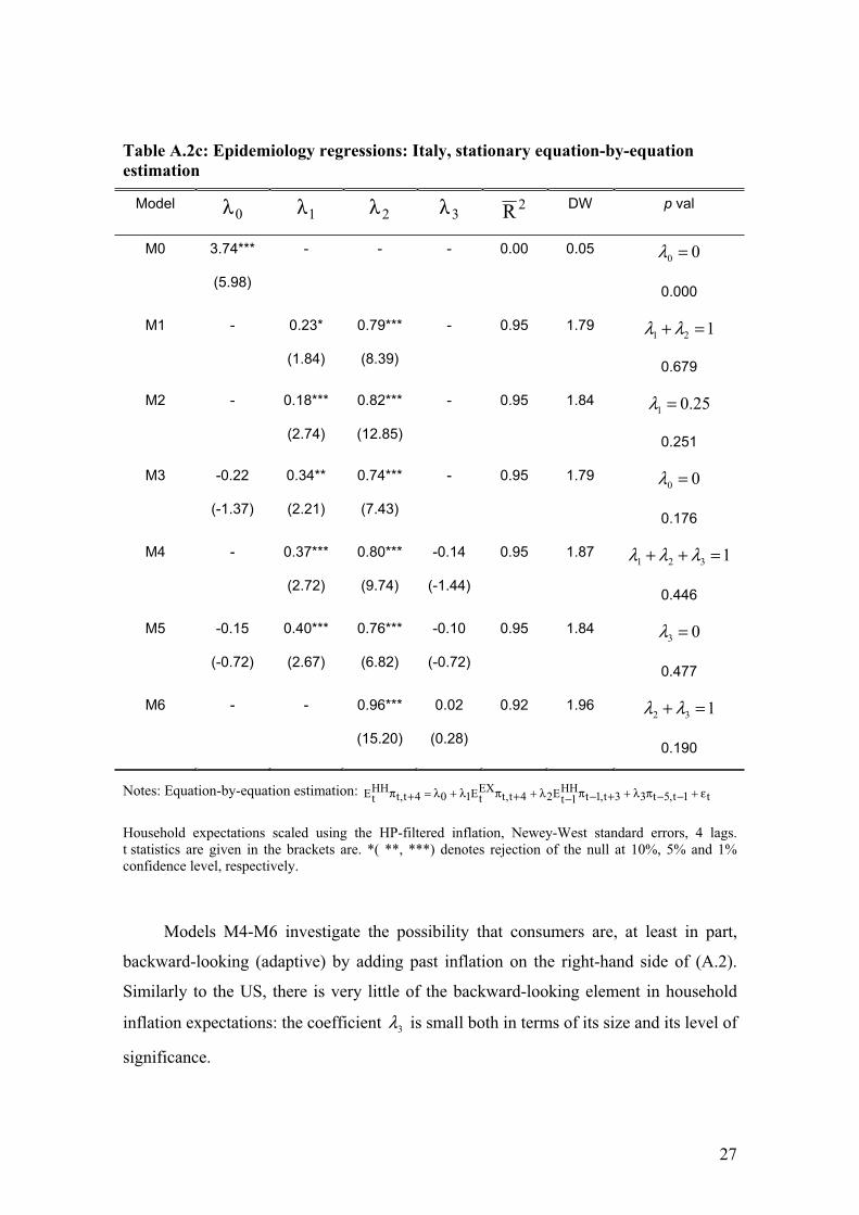
Household expectations scaled using the HP-filtered inflation, Newey-West standard errors, 4 lags. t statistics are given in the brackets are. *( **, ***) denotes rejection of the null at 10%, 5% and 1% confidence level, respectively.

Models M4-M6 investigate the possibility that consumers are, at least in part,

backward-looking (adaptive) by adding past inflation on the right-hand side of (A.2).

Similarly to the US, there is very little of the backward-looking element in household

inflation expectations: the coefficient 3λ is small both in terms of its size and its level of

significance.

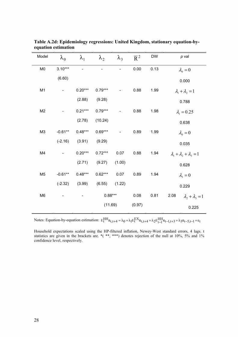
28

Table A.2d: Epidemiology regressions: United Kingdom, stationary equation-by-

equation estimation


M0 3.10***

(6.60)

- - - 0.00 0.13 00 =λ

0.000

M1 - 0.20***

(2.88)

0.79***

(9.28)

- 0.88 1.99 121 =+ λλ

0.788

M2 - 0.21***

(2.78)

0.79***

(10.24)

- 0.88 1.98 25.01 =λ

0.638

M3 -0.61**

(-2.16)

0.48***

(3.91)

0.69***

(9.29)

- 0.89 1.99 00 =λ

0.035

M4 - 0.20***

(2.71)

0.72***

(9.27)

0.07

(1.00)

0.88 1.94 1321 =++ λλλ

0.628

M5 -0.61**

(-2.32)

0.48***

(3.99)

0.62***

(6.55)

0.07

(1.22)

0.89 1.94 03 =λ

0.229

M6 - - 0.88***

(11.69)

0.08

(0.97)

0.81 2.08 132 =+ λλ

0.225


1tE24t,tEXtE104t,t



29

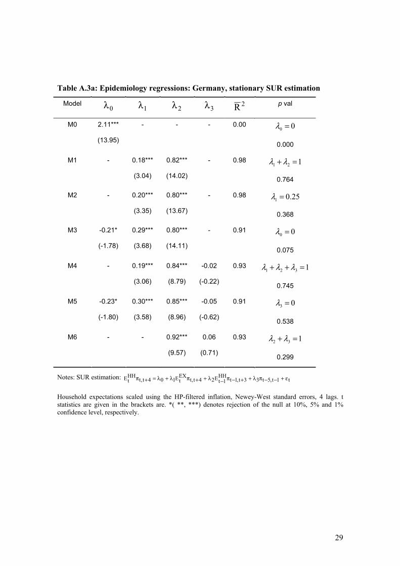
Table A.3a: Epidemiology regressions: Germany, stationary SUR estimation

Model0λ 1λ 2λ 3λ 2R p val

M0 2.11***

(13.95)

- - - 0.00 00 =λ

0.000

M1 - 0.18***

(3.04)

0.82***

(14.02)

- 0.98 121 =+ λλ

0.764

M2 - 0.20***

(3.35)

0.80***

(13.67)

- 0.98 25.01 =λ

0.368

M3 -0.21*

(-1.78)

0.29***

(3.68)

0.80***

(14.11)

- 0.91 00 =λ

0.075

M4 - 0.19***

(3.06)

0.84***

(8.79)

-0.02

(-0.22)

0.93 1321 =++ λλλ

0.745

M5 -0.23*

(-1.80)

0.30***

(3.58)

0.85***

(8.96)

-0.05

(-0.62)

0.91 03 =λ

0.538

M6 - - 0.92***

(9.57)

0.06

(0.71)

0.93 132 =+ λλ

0.299

Notes: SUR estimation: t1t,5t33t,1tHH

1tE24t,tEXtE104t,t



30

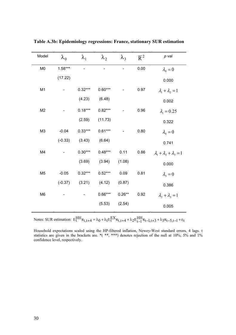
Table A.3b: Epidemiology regressions: France, stationary SUR estimation


M0 1.58***

(17.22)

- - - 0.00 00 =λ

0.000

M1 - 0.32***

(4.23)

0.60***

(6.48)

- 0.97 121 =+ λλ

0.002

M2 - 0.18***

(2.59)

0.82***

(11.73)

- 0.96 25.01 =λ

0.322

M3 -0.04

(-0.33)

0.33***

(3.43)

0.61***

(6.64)

- 0.80 00 =λ

0.741

M4 - 0.30***

(3.69)

0.48***

(3.94)

0.11

(1.08)

0.86 1321 =++ λλλ

0.000

M5 -0.05

(-0.37)

0.32***

(3.21)

0.52***

(4.12)

0.09

(0.87)

0.81 03 =λ

0.386

M6 - - 0.66***

(5.53)

0.26**

(2.54)

0.92 132 =+ λλ

0.005

Notes: SUR estimation: t1t,5t33t,1tHH

1tE24t,tEXtE104t,t



31

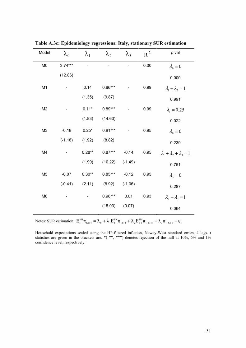
Table A.3c: Epidemiology regressions: Italy, stationary SUR estimation


M0 3.74***

(12.86)

- - - 0.00 00 =λ

0.000

M1 - 0.14

(1.35)

0.86***

(9.87)

- 0.99 121 =+ λλ

0.991

M2 - 0.11*

(1.83)

0.89***

(14.63)

- 0.99 25.01 =λ

0.022

M3 -0.18

(-1.18)

0.25*

(1.92)

0.81***

(8.82)

- 0.95 00 =λ

0.239

M4 - 0.28**

(1.99)

0.87***

(10.22)

-0.14

(-1.49)

0.95 1321 =++ λλλ

0.751

M5 -0.07

(-0.41)

0.30**

(2.11)

0.85***

(8.92)

-0.12

(-1.06)

0.95 03 =λ

0.287

M6 - - 0.96***

(15.03)

0.01

(0.07)

0.93 132 =+ λλ

0.064

Notes: SUR estimation: t1t,5t33t,1t

HH

1t24t,t

EX

t104t,t

HH



32

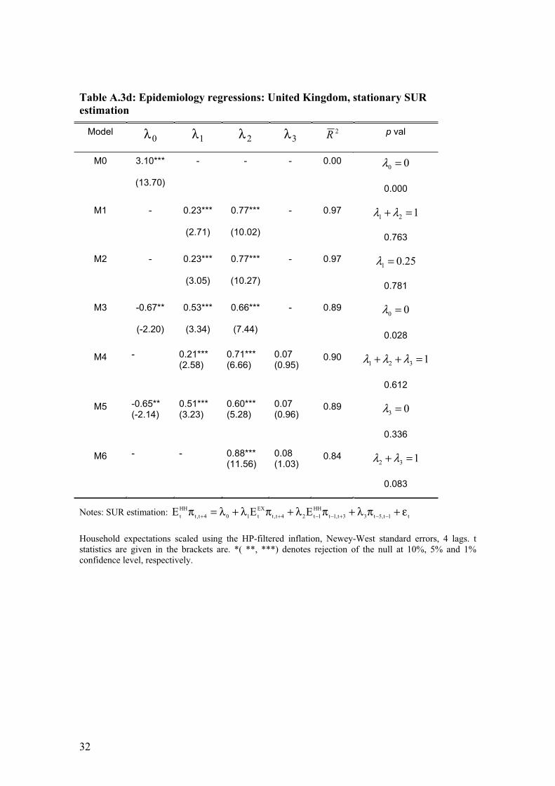
Table A.3d: Epidemiology regressions: United Kingdom, stationary SUR

estimation


M0 3.10***

(13.70)

- - - 0.00 00 =λ

0.000

M1 - 0.23***

(2.71)

0.77***

(10.02)

- 0.97 121 =+ λλ

0.763

M2 - 0.23***

(3.05)

0.77***

(10.27)

- 0.97 25.01 =λ

0.781

M3 -0.67**

(-2.20)

0.53***

(3.34)

0.66***

(7.44)

- 0.89 00 =λ

0.028

M4 - 0.21*** (2.58)

0.71***(6.66)

0.07(0.95)

0.90 1321 =++ λλλ

0.612

M5 -0.65**(-2.14)

0.51***(3.23)

0.60***(5.28)

0.07(0.96)

0.89 03 =λ

0.336

M6 - - 0.88*** (11.56)

0.08(1.03)

0.84 132 =+ λλ

0.083

Notes: SUR estimation: t1t,5t33t,1t

HH

1t24t,t

EX

t104t,t

HH



33

The non-stationary case

Table A.4: Tests for cointegration between household and expert expectations

GERMANY

Unrestricted Cointegration Rank Test (Trace)

Hypothesized Trace 5% No. of CE(s) Eigenvalue Statistic Critical Value Prob.*

None 0.20 16.31 12.32 0.01 At most 1 0.06 3.48 4.13 0.07 Normalized cointegrating coefficients (standard error in parentheses)

Experts Households 1 -1.00

(0.064)

FRANCE Unrestricted Cointegration Rank Test (Trace)




(0.066)

ITALY Unrestricted Cointegration Rank Test (Trace)




(0.069)

UNITED KINGDOM Unrestricted Cointegration Rank Test (Trace)




(0.096)

*MacKinnon-Haug-Michelis (1999) p-values

Tab

le A

.5:

Ep

idem

iolo

gy R

egre

ssio

ns:

VE

CM

Est

imati

on

Countr

y

GE

RM

AN

Y

FR

AN

CE

Mo

de

l re

str

. u

nre

str

. re

str

. u

nre

str

.

Dep. V

ar.

E

HH

EE

XE

HH

EE

XE

HH

EE

XE

HH

EE

X

01

.00

1

.00

1

.00

1

.00

1

.00

1

.00

1

.00

1

.00

1-1

.00

-1

.00

-1

.02

***

-1.0

2**

* -1

.00

-1

.00

-1

.14

***

-1.1

4**

*

- -

(-12

.21

) (-

12

.21

) -

- (-

17

.01

) (-

17

.01

)

1/2

0.2

6**

* 0

.05

0

.25

***

0.0

5

0.1

7**

-0

.12

***

0.2

8**

* -0

.15

**

( 3

.26

) (

1.2

2)

( 3

.24

) (

1.3

9)

( 2

.00

) (-

2.6

3)

( 2

.68

) (-

2.5

5)

11(1

)/12

(1)

-0.0

1

0.0

9

-0.0

1

0.0

9

-0.0

9

-0.0

1

-0.0

1

-0.0

3

(-0

.03

) (

1.3

8)

(-0

.00

) (

1.4

2)

(-0

.71

) (-

0.1

1)

(-0

.07

) (-

0.4

2)

11(2

)/12

(2)

0.1

6

0.0

3

0.1

6

0.0

3

-0.1

0

-0.0

9

-0.0

4

-0.1

1

( 1

.23

) (

0.3

9)

( 1

.27

) (

0.4

3)

(-0

.80

) (-

1.3

5)

(-0

.32

) (-

1.5

3)

21(1

)/22

(1)

-0.3

3

0.1

5

-0.3

5

0.1

5

0.4

3*

-0.0

7

0.3

2

-0.0

2

(-1

.14

) (

1.0

7)

(-1

.19

) (

1.0

1)

( 1

.70

) (-

0.5

4)

( 1

.28

) (-

0.1

4)

21(2

)/22

(2)

-0.0

9

-0.2

8**

-0

.09

-0

.29

**

1.0

6**

* -0

.12

0

.98

***

-0.0

7

(-0

.30

) (-

1.9

6)

(-0

.32

) (-

2.0

2)

( 4

.05

) (-

0.8

8)

( 3

.85

) (-

0.5

22

)

34

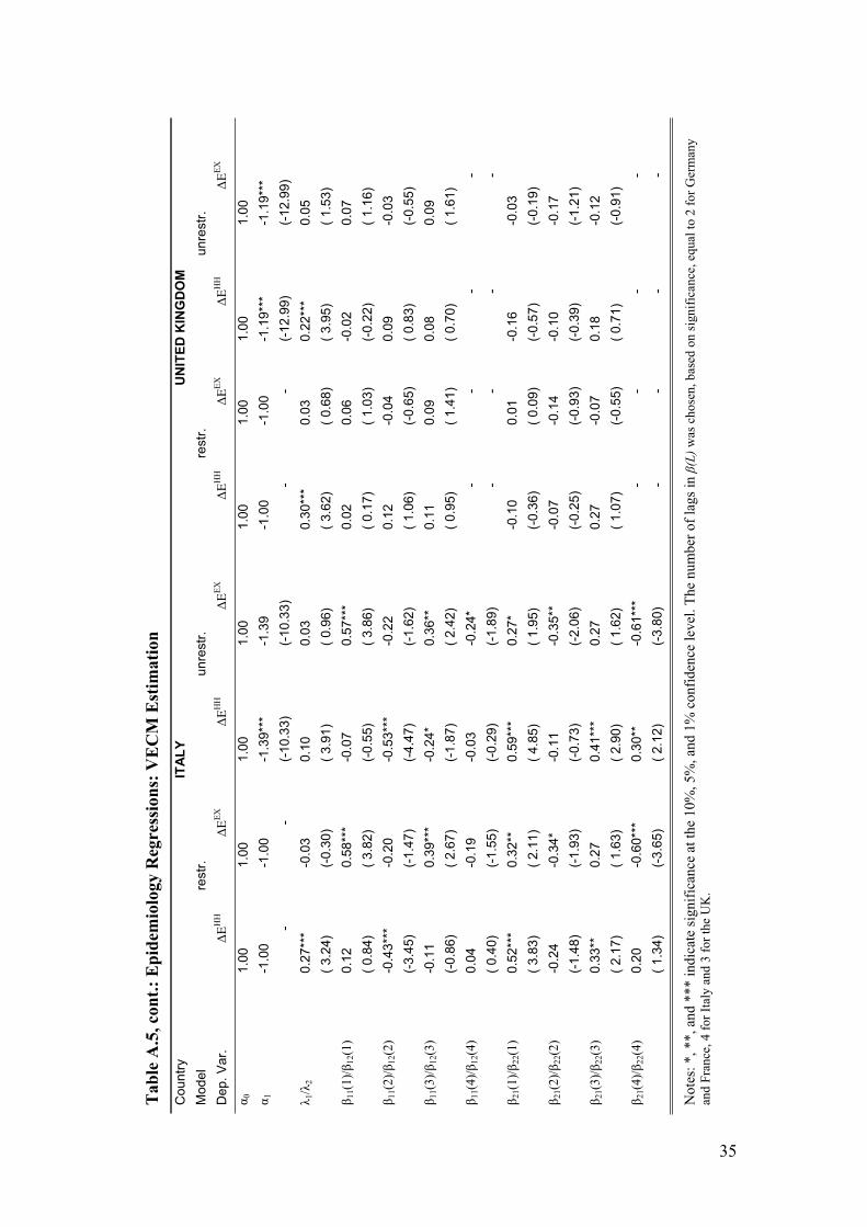
Tab

le A

.5, co

nt.

: E

pid

emio

logy R

egre

ssio

ns:

VE

CM

Est

imati

on

Countr

y

ITA

LY

U

NIT

ED

KIN

GD

OM

Model

restr

. unre

str

. re

str

. u

nre

str

.

Dep.

Var.

E

HH

EE

XE

HH

EE

XE

HH

EE

XE

HH

EE

X

01.0

0

1.0

0

1.0

0

1.0

0

1.0

0

1.0

0

1.0

0

1.0

0

1-1

.00

-1.0

0

-1.3

9**

* -1

.39

-1.0

0

-1.0

0

-1.1

9**

* -1

.19**

*

- -

(-10.3

3)

(-10.3

3)

- -

(-12.9

9)

(-12.9

9)

1/2

0.2

7**

* -0

.03

0.1

0

0.0

3

0.3

0**

* 0.0

3

0.2

2**

* 0.0

5

( 3.2

4)

(-0.3

0)

( 3.9

1)

( 0.9

6)

( 3.6

2)

( 0.6

8)

( 3.9

5)

( 1.5

3)

11(1

)/12

(1)

0.1

2

0.5

8**

* -0

.07

0.5

7**

* 0.0

2

0.0

6

-0.0

2

0.0

7

( 0.8

4)

( 3.8

2)

(-0.5

5)

( 3.8

6)

( 0.1

7)

( 1.0

3)

(-0.2

2)

( 1.1

6)

11(2

)/12

(2)

-0.4

3**

* -0

.20

-0.5

3**

* -0

.22

0.1

2

-0.0

4

0.0

9

-0.0

3

(-3.4

5)

(-1.4

7)

(-4.4

7)

(-1.6

2)

( 1.0

6)

(-0.6

5)

( 0.8

3)

(-0.5

5)

11(3

)/12

(3)

-0.1

1

0.3

9**

* -0

.24*

0.3

6**

0.1

1

0.0

9

0.0

8

0.0

9

(-

0.8

6)

( 2.6

7)

(-1.8

7)

( 2.4

2)

( 0.9

5)

( 1.4

1)

( 0.7

0)

( 1.6

1)

11(4

)/12

(4)

0.0

4

-0.1

9

-0.0

3

-0.2

4*

- -

- -

( 0.4

0)

(-1.5

5)

(-0.2

9)

(-1.8

9)

- -

- -

21(1

)/22

(1)

0.5

2**

* 0.3

2**

0.5

9**

* 0.2

7*

-0.1

0

0.0

1

-0.1

6

-0.0

3

( 3.8

3)

( 2.1

1)

( 4.8

5)

( 1.9

5)

(-0.3

6)

( 0.0

9)

(-0.5

7)

(-0.1

9)

21(2

)/22

(2)

-0.2

4

-0.3

4*

-0.1

1

-0.3

5**

-0

.07

-0.1

4

-0.1

0

-0.1

7

(-1.4

8)

(-1.9

3)

(-0.7

3)

(-2.0

6)

(-0.2

5)

(-0.9

3)

(-0.3

9)

(-1.2

1)

21(3

)/22

(3)

0.3

3**

0.2

7

0.4

1**

* 0.2

7

0.2

7

-0.0

7

0.1

8

-0.1

2

( 2.1

7)

( 1.6

3)

( 2.9

0)

( 1.6

2)

( 1.0

7)

(-0.5

5)

( 0.7

1)

(-0.9

1)

21(4

)/22

(4)

0.2

0

-0.6

0**

* 0.3

0**

-0

.61**

* -

- -

-

(

1.3

4)

(-3.6

5)

( 2.1

2)

(-3.8

0)

- -

- -

Not

es: *

, **,

and

***

ind

icat

e si

gnif

ican

ce a

t th

e 10

%, 5

%, a

nd 1

% c

onfi

denc

e le

vel.

The

num

ber

of l

ags

in

(L)

was

cho

sen,

bas

ed o

n si

gnif

ican

ce, e

qual

to 2

for

Ger

man

y an

d F

ranc

e, 4

for

Ita

ly a

nd 3

for

the

UK

.

35

36

The following Discussion Papers have been published since 2004:

Series 1: Economic Studies

1 2004 Foreign Bank Entry into Emerging Economies:

An Empirical Assessment of the Determinants

and Risks Predicated on German FDI Data Torsten Wezel

2 2004 Does Co-Financing by Multilateral Development

Banks Increase “Risky” Direct Investment in

Emerging Markets? –

Evidence for German Banking FDI Torsten Wezel

3 2004 Policy Instrument Choice and Non-Coordinated Giovanni Lombardo

Monetary Policy in Interdependent Economies Alan Sutherland

4 2004 Inflation Targeting Rules and Welfare

in an Asymmetric Currency Area Giovanni Lombardo

5 2004 FDI versus cross-border financial services: Claudia M. Buch

The globalisation of German banks Alexander Lipponer

6 2004 Clustering or competition? The foreign Claudia M. Buch

investment behaviour of German banks Alexander Lipponer

7 2004 PPP: a Disaggregated View Christoph Fischer

8 2004 A rental-equivalence index for owner-occupied Claudia Kurz

housing in West Germany 1985 to 1998 Johannes Hoffmann

9 2004 The Inventory Cycle of the German Economy Thomas A. Knetsch

10 2004 Evaluating the German Inventory Cycle

Using Data from the Ifo Business Survey Thomas A. Knetsch

11 2004 Real-time data and business cycle analysis

in Germany Jörg Döpke

37

12 2004 Business Cycle Transmission from the US

to Germany – a Structural Factor Approach Sandra Eickmeier

13 2004 Consumption Smoothing Across States and Time: George M.

International Insurance vs. Foreign Loans von Furstenberg

14 2004 Real-Time Estimation of the Output Gap

in Japan and its Usefulness for

Inflation Forecasting and Policymaking Koichiro Kamada

15 2004 Welfare Implications of the Design of a

Currency Union in Case of Member Countries

of Different Sizes and Output Persistence Rainer Frey

16 2004 On the decision to go public: Ekkehart Boehmer

Evidence from privately-held firms Alexander Ljungqvist

17 2004 Who do you trust while bubbles grow and blow?

A comparative analysis of the explanatory power

of accounting and patent information for the Fred Ramb

market values of German firms Markus Reitzig

18 2004 The Economic Impact of Venture Capital Astrid Romain, Bruno

van Pottelsberghe

19 2004 The Determinants of Venture Capital: Astrid Romain, Bruno

Additional Evidence van Pottelsberghe

20 2004 Financial constraints for investors and the

speed of adaption: Are innovators special? Ulf von Kalckreuth

21 2004 How effective are automatic stabilisers?

Theory and results for Germany and other Michael Scharnagl

OECD countries Karl-Heinz Tödter

38

22 2004 Asset Prices in Taylor Rules: Specification, Pierre L. Siklos

Estimation, and Policy Implications for the Thomas Werner

ECB Martin T. Bohl

23 2004 Financial Liberalization and Business

Cycles: The Experience of Countries in Lúcio Vinhas

the Baltics and Central Eastern Europe de Souza

24 2004 Towards a Joint Characterization of

Monetary Policy and the Dynamics of

the Term Structure of Interest Rates Ralf Fendel

25 2004 How the Bundesbank really conducted Christina Gerberding

monetary policy: An analysis based on Andreas Worms

real-time data Franz Seitz

26 2004 Real-time Data for Norway: T. Bernhardsen, Ø. Eitrheim,

Challenges for Monetary Policy A.S. Jore, Ø. Røisland

27 2004 Do Consumer Confidence Indexes Help

Forecast Consumer Spending in Real Time? Dean Croushore

28 2004 The use of real time information in Maritta Paloviita

Phillips curve relationships for the euro area David Mayes

29 2004 The reliability of Canadian output Jean-Philippe Cayen

gap estimates Simon van Norden

30 2004 Forecast quality and simple instrument rules - Heinz Glück

a real-time data approach Stefan P. Schleicher

31 2004 Measurement errors in GDP and Peter Kugler

forward-looking monetary policy: Thomas J. Jordan

The Swiss case Carlos Lenz

Marcel R. Savioz

39

32 2004 Estimating Equilibrium Real Interest Rates Todd E. Clark

in Real Time Sharon Kozicki

33 2004 Interest rate reaction functions for the euro area

Evidence from panel data analysis Karsten Ruth

34 2004 The Contribution of Rapid Financial

Development to Asymmetric Growth of

Manufacturing Industries: George M.

Common Claims vs. Evidence for Poland von Furstenberg

35 2004 Fiscal rules and monetary policy in a dynamic

stochastic general equilibrium model Jana Kremer

36 2004 Inflation and core money growth in the Manfred J.M. Neumann

euro area Claus Greiber

37 2004 Taylor rules for the euro area: the issue Dieter Gerdesmeier

of real-time data Barbara Roffia

38 2004 What do deficits tell us about debt?

Empirical evidence on creative accounting Jürgen von Hagen

with fiscal rules in the EU Guntram B. Wolff

39 2004 Optimal lender of last resort policy Falko Fecht

in different financial systems Marcel Tyrell

40 2004 Expected budget deficits and interest rate swap Kirsten Heppke-Falk

spreads - Evidence for France, Germany and Italy Felix Hüfner

41 2004 Testing for business cycle asymmetries

based on autoregressions with a

Markov-switching intercept Malte Knüppel

1 2005 Financial constraints and capacity adjustment

in the United Kingdom – Evidence from a Ulf von Kalckreuth

large panel of survey data Emma Murphy

40

2 2005 Common stationary and non-stationary

factors in the euro area analyzed in a

large-scale factor model Sandra Eickmeier

3 2005 Financial intermediaries, markets, F. Fecht, K. Huang,

and growth A. Martin

4 2005 The New Keynesian Phillips Curve

in Europe: does it fit or does it fail? Peter Tillmann

5 2005 Taxes and the financial structure Fred Ramb

of German inward FDI A. J. Weichenrieder

6 2005 International diversification at home Fang Cai

and abroad Francis E. Warnock

7 2005 Multinational enterprises, international trade,

and productivity growth: Firm-level evidence Wolfgang Keller

from the United States Steven R. Yeaple

8 2005 Location choice and employment S. O. Becker,

decisions: a comparison of German K. Ekholm, R. Jäckle,

and Swedish multinationals M.-A. Muendler

9 2005 Business cycles and FDI: Claudia M. Buch

evidence from German sectoral data Alexander Lipponer

10 2005 Multinational firms, exclusivity, Ping Lin

and the degree of backward linkages Kamal Saggi

11 2005 Firm-level evidence on international Robin Brooks

stock market comovement Marco Del Negro

12 2005 The determinants of intra-firm trade: in search Peter Egger

for export-import magnification effects Michael Pfaffermayr

41

13 2005 Foreign direct investment, spillovers and

absorptive capacity: evidence from quantile Sourafel Girma

regressions Holger Görg

14 2005 Learning on the quick and cheap: gains James R. Markusen

from trade through imported expertise Thomas F. Rutherford

15 2005 Discriminatory auctions with seller discretion:

evidence from German treasury auctions Jörg Rocholl

16 2005 Consumption, wealth and business cycles: B. Hamburg,

why is Germany different? M. Hoffmann, J. Keller

17 2005 Tax incentives and the location of FDI: Thiess Buettner

evidence from a panel of German multinationals Martin Ruf

18 2005 Monetary Disequilibria and the Dieter Nautz

Euro/Dollar Exchange Rate Karsten Ruth

19 2005 Berechnung trendbereinigter Indikatoren für

Deutschland mit Hilfe von Filterverfahren Stefan Stamfort

20 2005 How synchronized are central and east

European economies with the euro area? Sandra Eickmeier

Evidence from a structural factor model Jörg Breitung

21 2005 Asymptotic distribution of linear unbiased J.-R. Kurz-Kim

estimators in the presence of heavy-tailed S.T. Rachev

stochastic regressors and residuals G. Samorodnitsky

22 2005 The Role of Contracting Schemes for the

Welfare Costs of Nominal Rigidities over

the Business Cycle Matthias Pastian

23 2005 The cross-sectional dynamics of German J. Döpke, M. Funke

business cycles: a bird’s eye view S. Holly, S. Weber

42

24 2005 Forecasting German GDP using alternative Christian Schumacher

factor models based on large datasets

25 2005 Time-dependent or state-dependent price

setting? – micro-evidence from German

metal-working industries – Harald Stahl

26 2005 Money demand and macroeconomic Claus Greiber

uncertainty Wolfgang Lemke

27 2005 In search of distress risk J. Y. Campbell,

J. Hilscher, J. Szilagyi

28 2005 Recursive robust estimation and control Lars Peter Hansen

without commitment Thomas J. Sargent

29 2005 Asset pricing implications of Pareto optimality N. R. Kocherlakota

with private information Luigi Pistaferri

30 2005 Ultra high frequency volatility estimation Y. Aït-Sahalia,

with dependent microstructure noise P. A. Mykland, L. Zhang

31 2005 Umstellung der deutschen VGR auf Vorjahres-

preisbasis – Konzept und Konsequenzen für die

aktuelle Wirtschaftsanalyse sowie die ökono-

metrische Modellierung Karl-Heinz Tödter

32 2005 Determinants of current account developments

in the central and east European EU member

states – consequences for the enlargement of Sabine Herrmann

the euro erea Axel Jochem

33 2005 An estimated DSGE model for the German

economy within the euro area Ernest Pytlarczyk

34 2005 Rational inattention: a research agenda Christopher A. Sims

43

35 2005 Monetary policy with model uncertainty: Lars E.O. Svensson

distribution forecast targeting Noah Williams

36 2005 Comparing the value revelance of R&D report- Fred Ramb

ing in Germany: standard and selection effects Markus Reitzig

37 2005 European inflation expectations dynamics J. Döpke, J. Dovern

U. Fritsche, J. Slacalek

44

Series 2: Banking and Financial Studies

1 2004 Forecasting Credit Portfolio Risk A. Hamerle,

T. Liebig, H. Scheule

2 2004 Systematic Risk in Recovery Rates –

An Empirical Analysis of US Corporate Klaus Düllmann

Credit Exposures Monika Trapp

3 2004 Does capital regulation matter for bank Frank Heid

behaviour? Evidence for German savings Daniel Porath

banks Stéphanie Stolz

4 2004 German bank lending during F. Heid, T. Nestmann,

emerging market crises: B. Weder di Mauro,

A bank level analysis N. von Westernhagen

5 2004 How will Basel II affect bank lending to T. Liebig, D. Porath,

emerging markets? An analysis based on B. Weder di Mauro,

German bank level data M. Wedow

6 2004 Estimating probabilities of default for

German savings banks and credit cooperatives Daniel Porath

1 2005 Measurement matters – Input price proxies

and bank efficiency in Germany Michael Koetter

2 2005 The supervisor’s portfolio: the market price

risk of German banks from 2001 to 2003 – Christoph Memmel

Analysis and models for risk aggregation Carsten Wehn

3 2005 Do banks diversify loan portfolios? Andreas Kamp

A tentative answer based on individual Andreas Pfingsten

bank loan portfolios Daniel Porath

4 2005 Banks, markets, and efficiency F. Fecht, A. Martin

45

5 2005 The forecast ability of risk-neutral densities Ben Craig

of foreign exchange Joachim Keller

6 2005 Cyclical implications of minimum capital

requirements Frank Heid

7 2005 Banks’ regulatory capital buffer and the

business cycle: evidence for German Stéphanie Stolz

savings and cooperative banks Michael Wedow

8 2005 German bank lending to industrial and non-

industrial countries: driven by fundamentals

or different treatment? Thorsten Nestmann

9 2005 Accounting for distress in bank mergers M. Koetter, J. Bos, F. Heid

C. Kool, J. Kolari, D. Porath

10 2005 The eurosystem money market auctions: Nikolaus Bartzsch

a banking perspective Ben Craig, Falko Fecht

11 2005 Financial integration and systemic Falko Fecht

risk Hans Peter Grüner

Visiting researcher at the Deutsche Bundesbank

The Deutsche Bundesbank in Frankfurt is looking for a visiting researcher. Visitors should

prepare a research project during their stay at the Bundesbank. Candidates must hold a

Ph D and be engaged in the field of either macroeconomics and monetary economics,

financial markets or international economics. Proposed research projects should be from

these fields. The visiting term will be from 3 to 6 months. Salary is commensurate with

experience.

Applicants are requested to send a CV, copies of recent papers, letters of reference and a

proposal for a research project to:

Deutsche Bundesbank

Personalabteilung

Wilhelm-Epstein-Str. 14

D - 60431 Frankfurt

GERMANY

46

European inflation expectations dynamics

Documents

Transcript of European inflation expectations dynamics