Delays of Inflation Stabilizations

(Published in Economics & Politics 12(3), 275-295)

Francisco José Veiga*

Núcleo de Investigação em Políticas Económicas (NIPE)

Universidade do Minho

Abstract:

In some new political economic models, delays of stabilizations result from

coordination problems caused by collective choice-making mechanisms. Although

several previous studies have tested the effects of political instability and fragmentation

on seignorage, deficits, or inflation, no direct tests of the influence of these factors on

the delays of stabilizations have previously been undertaken. This paper reports the

results of such tests. The degree of fragmentation of the political system and the level of

inflation are identified as important determinants of the timing of inflation

stabilizations.

Francisco José Veiga

Escola de Economia e Gestão

Universidade do Minho

4710-057 Braga - Portugal

1

A. INTRODUCTION

One intriguing fact that is common to many chronic inflation countries is that

they have followed potentially unsustainable policies for extended periods of time.

These policies include large budget deficits that lead to rapidly growing debt to GDP

ratios and hyperinflation. Although these policies are recognized as suboptimal from a

social standpoint, the necessary (and welfare-improving) stabilizations are often delayed

or not fully implemented. Many economists explain these suboptimal policies by

accusing politicians of myopia or irrational behavior. Others argue that countries lack

the expertise necessary to carry out the reforms, hope that things will get better by

themselves, or wait for a larger crisis that would force them to act.

Needless to say, these explanations are not very convincing. A new political

economic literature has developed formal models that try to explain the adoption of

suboptimal policies by rational and forward looking agents who do the best they can in

the game being played.1 These models depart from the assumption of a social planner

choosing policies according to a social welfare function, and assume, instead, that

policy choices tend to be the result of negotiations between contending interest groups

with conflicting interests. Then, deviations from optimality are explained by

coordination problems caused by the mechanisms of making collective choices.

These models also have testable implications. Many of them focus on the

influence of political factors on the timing of stabilizations: fragmentation or

polarization of the political system; political instability; type of regime; political

orientation of the government; and time in office. Others are related to economic

factors: intensity of the crisis (level of inflation) or the amount of foreign reserves

available. Although previous studies have tested the effects of political instability and

2

fragmentation on seignorage, budget deficits, debt, or inflation, no direct tests of the

influence of these factors on the timing of stabilizations have been undertaken.

In this paper, I employ a probit model to empirically investigate the influence of

political and economic variables on the probability of starting a stabilization program.

Since higher probabilities of reform in any given time interval will be associated with

shorter delays in the implementation of reform after the onset of high inflation, the

analysis also helps to explain the existence of delays in the adoption of stabilization

plans. The empirical results of this investigation are compared with the testable

implications of the theoretical models, so that we can discriminate among them.

The paper is organized as follows. Section B presents a description of the recent

theories of delayed stabilization and reform. The empirical analysis is described in

section C, and the conclusions of this paper are presented in section D.

B. DELAYED STABILIZATION

There are essentially three alternative ways of explaining delays of stabilizations

or reforms. The first simply assumes myopia or irrationality of policymakers. This

approach is theoretically unappealing and empirically vacuous – it offers no

constructive explanation of the phenomenon. The second, based on an optimal control

framework, assumes that delays are the rational and deliberate choice of a policymaker

maximizing a social welfare function. In these models, delay is optimal if the costs of

living under inflation are smaller than the costs of implementing a successful

stabilization program. Finally, political models of conflict assume that policy choices

result from negotiations between contending interest groups, and explain deviations

from optimality (delays) by coordination problems caused by the mechanisms of

3

making collective choices. Examples of the last two types of models are discussed

further below.

Although most of this literature deals with stabilization as a reduction in the

budget deficit or the ratio of public debt to GDP (fiscal stabilization), their conclusions

are also applicable to inflation stabilization, which is the main focus of this paper.

Furthermore, in most of the countries suffering from chronic inflation, large budget

deficits lead to ever-growing debt to GDP ratios and hyperinflation (through

monetization), meaning that an inflation stabilization program can only succeed if it is

accompanied by fiscal stabilization (see: Veiga, 1999). Thus, this literature produces

several testable implications that can be applied to inflation stabilization episodes.

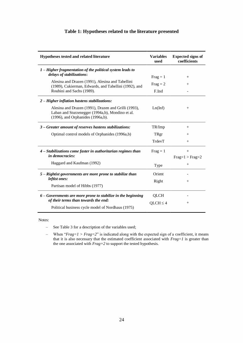
These implications are presented below and summarized in Table 1.

1) Higher fragmentation of the political system leads to delays of stabilizations

Alesina and Drazen (1991) present a model in which delays of fiscal

stabilization result from the failure of rival interest groups to agree on a deficit reduction

program. This stalemate leads to a “war of attrition” in which agreement on a

stabilization program is only reached when one of the groups concedes, that is, accepts

paying a higher proportion of the taxes in order to eliminate the deficit. In this model,

one important factor leading to delays is the degree of political polarization among

interest groups.

Cukierman, Edwards and Tabellini (1992) present a political model of tax

reforms in which strategic considerations may induce the current government to leave

an inefficient tax system to its successors (in the presence of political instability and

polarization). This will limit their availability of funds and, therefore, decrease spending

on areas that are not favored by the incumbent policymaker. Thus, tax reform is delayed

4

when the incumbent faces small probability of reelection and high polarization. Their

empirical results show that after controlling for a set of structural variables countries

with more unstable political systems tend to rely more on seignorage.2

Since contending interest groups tend to be represented by political parties, the

multitude of parties represented in the parliaments of fragmented party systems are

associated with a high degree of political polarization and instability of these systems3,

which in the models discussed above would lead to greater delays of stabilizations.

2) Higher inflation hastens stabilizations

Drazen and Grilli (1993) extend the model of Alesina and Drazen (1991)

emphasizing the possible benefits of economic crises. As higher costs of delay hasten

stabilizations (by revealing the loser faster) an exogenous shock that aggravates the

economic conditions may be welfare improving if the welfare costs of the shock are

more than compensated for by the benefits of earlier stabilization. Since higher inflation

results in higher costs of delaying stabilization, one should observe stabilizations

starting faster as inflation gets higher (assuming no efforts by the government to reduce

the costs of inflation through indexation or other means).4

3) Level of foreign reserves

Orphanides (1996a,b) examines delay and abandonment of a stabilization

program as optimal decisions by a policymaker. He argues that it may be better to delay

the program if more favorable initial conditions are expected: either the adjustment may

become less painful, or political support may increase when the costs of inflation are

fully recognized by the public. An empirical implication is that a more severe inflation

is likely to induce a reform effort sooner (the testable hypothesis discussed above).

5

Further, in the Orphanides models, if a prospective reform is to be accomplished via the

management of the exchange rate, the level of foreign reserves (subject to stochastic

shocks) will be a critical factor. This offers the empirical prediction that low levels of

foreign reserves will result in delayed or abandoned stabilization programs.

4) Stabilization comes faster in authoritarian regimes than in democracies

Haggard and Kaufman (1992) argue that the security of governments and their

independence from the short-run distributive political pressures has great effects on the

level and variability of inflation over the long run. Furthermore, governments in less

fragmented political systems, such as authoritarian regimes, are less exposed to those

political pressures and need not waste time building consensus for reform. Thus,

stabilization programs should be easier to implement in authoritarian regimes.

5) Rightist governments are more prone to stabilize than leftist ones

This hypothesis is related to the partisan model of Hibbs (1977), that suggests

that rightist parties care more about inflation that leftist parties do.

6) Governments are more prone to stabilize in the beginning of their terms

According to the opportunistic political business cycle of Nordhaus (1975)5

governments tend to implement the toughest measures in the beginning of their terms,

hoping short-term hardships will be largely forgotten by the time of the next election.

C. EMPIRICAL EVIDENCE

The empirical analysis consists of using a duration model to test the hypotheses

related to the models discussed in the previous section. Probit and proportional hazards

6

specifications will be estimated for a panel of 10 countries and 27 inflation stabilization

programs in order to determine which variables cause delays in the adoption of

stabilization plans.

1) The Data

Before estimating the probit and proportional hazards specifications, two major

empirical issues had to be solved. The first was to determine when inflation was “high”,

that is, when a stabilization program was clearly necessary. High inflation was defined

as twice the average inflation rate of the last 10 years (inflation much higher than usual)

or greater than or equal to 100% (a high level by most standards). Other definitions of

high inflation will be used in the sensitivity analysis. The second issue was to determine

when a stabilization program had been undertaken. Since the governments that

implemented most of these programs usually publicized them extensively, it is not

difficult to identify their starting dates. The approach followed here was to collect

information on the starting dates of all of the important stabilizations undertaken in

countries suffering from chronic inflation. These major stabilizations have been

previously identified in a considerable number of articles on inflation stabilization.6

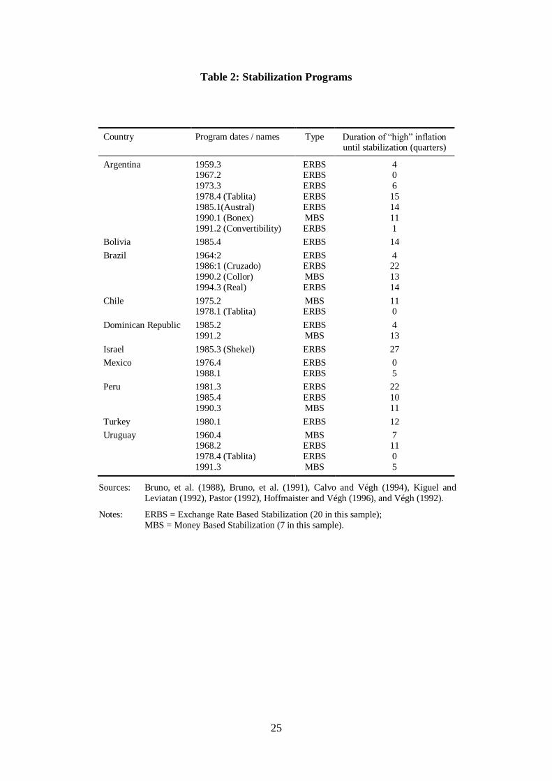
The list of stabilization plans analyzed in this article is shown in Table 2. The

second column indicates the quarter in which the plans were implemented and the third

column indicates whether the stabilization was exchange rate based or money based.

The last column indicates the number of consecutive quarters of high inflation that

preceded the start of a stabilization plan. Those stabilizations that were implemented

when inflation was not high according to my definition have duration of high inflation

of zero quarters.

7

For each country, quarterly data was collected from the first quarter of 1957

(first quarter for which quarterly data is available) until the fourth quarter of 1996. A

description of the variables used in this paper and their sources is presented in Table 3.

Quarterly data are not always available for some of the countries studied, but annual

data usually are. In order to make possible the inclusion of these data in the data set,

straight-line interpolation was used to generate quarterly data.7 The variables for which

interpolation was used are real GDP growth and Fiscal Balance as a percentage of the

GDP. Even after interpolating annual data for these variables there are still a few

missing values. Observations for which there are missing values have been excluded

from the probit estimations.

2) Probit model

In order to determine which factors influence the timing of an inflation

stabilization program, I use a binary probit model to estimate the effect of a set of

political and economic variables on the probability of starting a stabilization program in

a given quarter, when inflation is high. Observations in the data set include only those

quarters occurring between the onset of high inflation and the adoption of a subsequent

reform plan.

An individual inflation spell contains all the consecutive quarters in which

inflation was high according to my definition, until a stabilization plan started or

inflation ceased to be high. For each quarter and each inflation spell the dependent

variable (STAB) takes the value of one if a stabilization plan was implemented in that

quarter, and zero if it was implemented after that quarter. If no stabilization is

implemented, STAB takes the value of zero for all the observations in that inflation

spell.

8

I start by assuming that the unobserved hazard rate, the conditional probability

that a stabilization program is implemented at time t given that it has not been

implemented before, depends only on the explanatory variables. It does not change

autonomously over time and any variation must be due to the independent variables.

The main explanatory variables used were the following:

- Frag=1 and Frag=2: dummies for the fragmentation of the political

system;8

- F.Ind: fragmentation index;

- Ln(Inf): log of growth in CPI since the same quarter of the previous year;

- TR/Imp: total foreign reserves as a percentage of imports;

- Type: dummy for type of regime (authoritarian or democracy);

- Orient: partisan (left-right) orientation of the government;9

- Right: dummy for right or center right government;

- QLCH: number of quarters since last change in government or election;

- QLCH4: dummy for change in government or election in the last four

quarters;

I also consider two variables that were not identified directly in the theoretical

discussion, but which might affect the timing of a stabilization. These variables are:

- FB/GDP: Fiscal Balance as a percentage of GDP;

- GDP: real GDP growth since same quarter of previous year.

Table 1 shows the hypotheses to which these variables are related and the expected

signs of the coefficients, and Table 3 presents a more complete description of the

variables and respective sources. All economic variables were lagged because the start

of a stabilization program could affect their contemporaneous values.

9

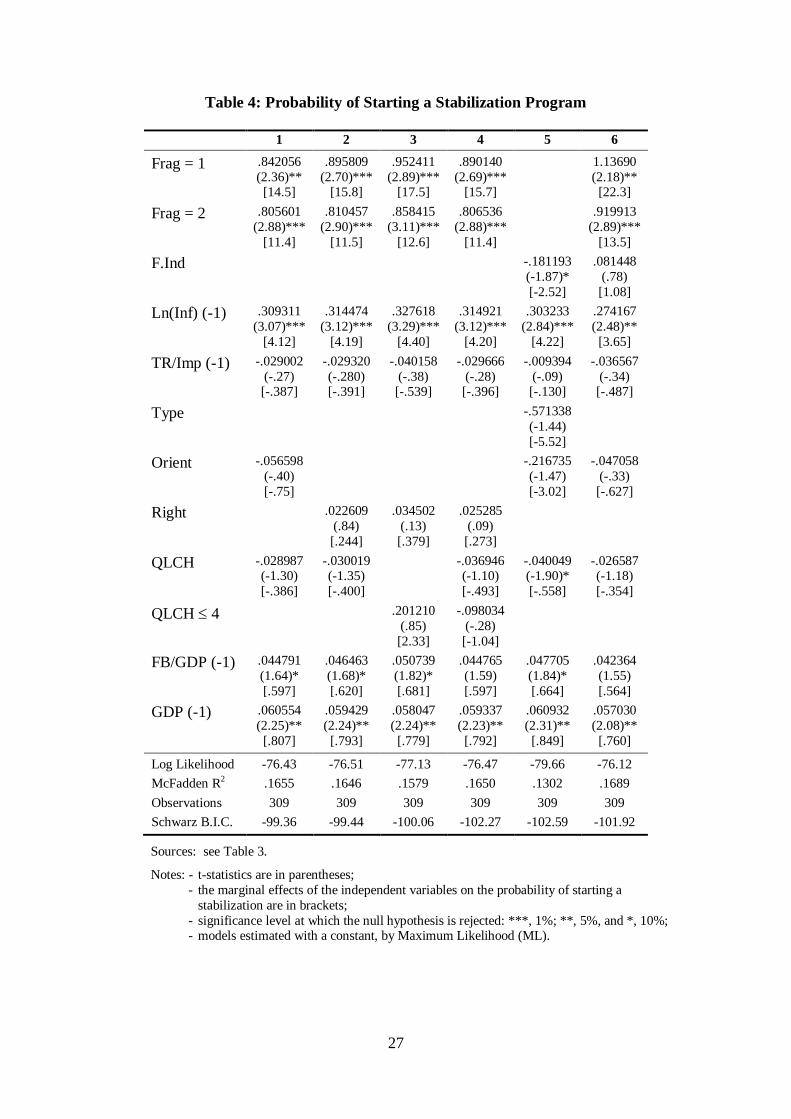
Table 4 shows the results of the probit estimations. Since probit coefficients are

not very intuitive, the marginal effects of the independent variables on the dependent

variable, STAB, are also reported. The latter give the effects of one-unit changes in the

regressors on the probability of starting a stabilization program (expressed in percentage

points) evaluated at the mean of the data. For dummy variables, they correspond to the

effect in that probability when the dummy changes from 0 to 1. T-statistics for the null

of no effect and the significance levels at which the null hypotheses are rejected are also

reported.

Results support my first testable hypothesis that higher fragmentation decreases

the probability of starting a stabilization program (that is, leads to delays).10

Frag=1 and

Frag=2 are always statistically significant and the estimated coefficients have the

expected signs. Furthermore, the estimated coefficient of Frag=1 is always greater than

that of Frag=2, as expected. This indicates that authoritarian regimes that did not allow

political parties tend to stabilize faster, providing some support for the fourth

hypothesis. The other measure of fragmentation, F.Ind11

, is used in column 5. Its

coefficient has the expected sign and is marginally significant (10% significance level),

providing some evidence that the proliferation of parties in the parliament leads to

delays of stabilizations. A one-unit increase in the index decreases the probability of

starting a stabilization by 2.52 percentage points. In column 6, Frag=1 and Frag=2

were included along with F.Ind. Results are very similar to those of column 1 for the

two dummy variables but F.Ind is not statistically significant and has the wrong sign.

Thus, when the two measures of fragmentation are used at the same time, the dummy

variables based on Frag seem to work better that F.Ind.

10

The first lag of the natural logarithm of inflation, Ln(Inf(-1)), is always

statistically significant and has a positive coefficient, as expected, supporting the second

testable hypothesis that stabilization comes faster as inflation gets higher.

TR/Imp(-1) has a positive coefficient, as expected, but is never statistically

significant, providing no support for Orphanides (1996a,b) hypothesis that the decision

on starting or postponing a stabilization depends upon the available level of reserves.

Although the ratio of total reserves to imports may not be a perfect indicator of the

amount of reserves available, it gives an idea of the capacity of one nation to keep

financing its imports. Furthermore, it is one of the best proxies available that can be

compared across countries of different sizes.

Type12

has the wrong sign and is not statistically significant, which goes against

the hypothesis that authoritarian regimes in general tend to stabilize faster. Thus, it

seems that the hypothesis that authoritarian regimes tend to stabilize faster than

democracies is not supported in general (for all authoritarian regimes). But, as

mentioned above, authoritarian regimes that did not allow political parties do seem to

stabilize faster, providing support for a restricted version of the hypothesis.13

Orient (orientation of the government) has the expected sign but is never

statistically significant, providing no support for the fifth testable hypotheses that

governments leaning more towards the right tend to stabilize faster. A dummy variable,

Right, that takes the value of one when Orient is equal to one or two (right or center

right governments) was also used. Again, no support was found for the above-

mentioned hypothesis.

QLCH (quarters since last change in government or election) also has the

expected sign but is only marginally significant in the estimation of column 5.

Therefore, I find little or no support for the hypothesis that governments tend to

11

stabilize early in their terms. I also introduced a dummy variable that takes the value of

one if a change in government or election occurred in the last 4 quarters, QLCH4, in

order to test whether stabilizations tended to be implemented in the first year after

assuming power. Again, no support was found for my last testable hypothesis.

As for the control variables, FB/GDP(-1) has the expected sign but is only

marginally significant in four of the six estimations. GDP(-1) also has the expected sign

and is always statistically significant at the 5% level.

It should be noted that the estimations of Table 4, as well as those of Tables 5

and 6, do not include country dummies because no evidence of country fixed effects

was found when these were accounted for. The country dummies were never

statistically significant individually or jointly, and nothing substantive changes when

they are included.14

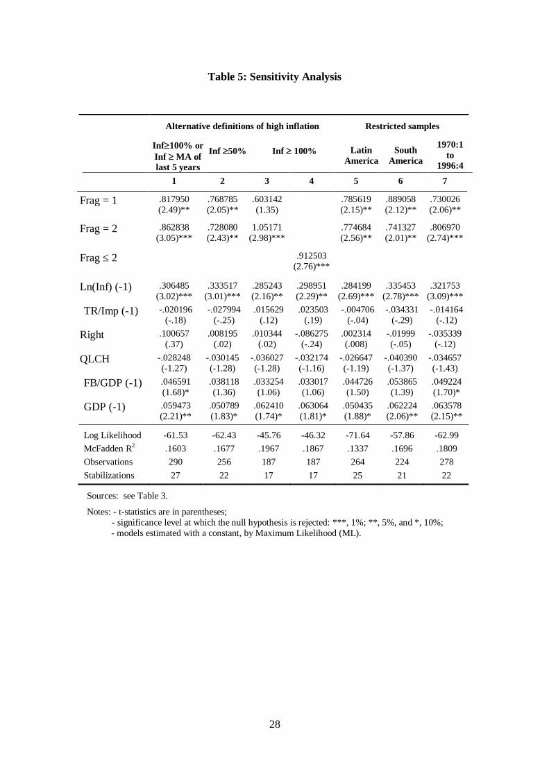
Table 5 presents the results of a sensitivity analysis in which several variants of

the model of column 2 of Table 4 are estimated. First, alternative definitions of high

inflation were used: over twice the average inflation rate of the last five years or greater

than 100% (column 1); or, simply, above 50% (column 2) or 100% (columns 3 and 4).

Second, Israel and Turkey were excluded from the sample, so that one could verify if

conclusions held when only Latin American countries were included (column 5). Third,

Mexico and the Dominican Republic were excluded, so that only South American

countries would remain (column 6). And, fourth, all observations before 1970 were

excluded (column 7). Since most of the problems with chronic inflation started or

became more severe in the 1970s, leading to the implementation of stabilization

programs in several countries, I check whether results are affected by not considering

the earlier stabilizations.

12

Results for most of the tested hypothesis changed little. Although Frag=1 is not

statistically significant in column 3 (Inf100%), it is shown in column 4 that higher

fragmentation still increases delays: the new dummy variable, Frag2, that takes the

value of one when Frag is equal to 1 or 2, is highly significant. Inflation remains highly

significant in most estimations, providing support for the hypothesis that higher

inflation hastens stabilizations. The major difference is that the evidence for the

hypothesis that stabilizations come faster in authoritarian regimes is reduced: the

coefficient on Frag=1 is not significant in the third column and it is smaller than the

one associated with Frag=2 in columns 1 and 7.

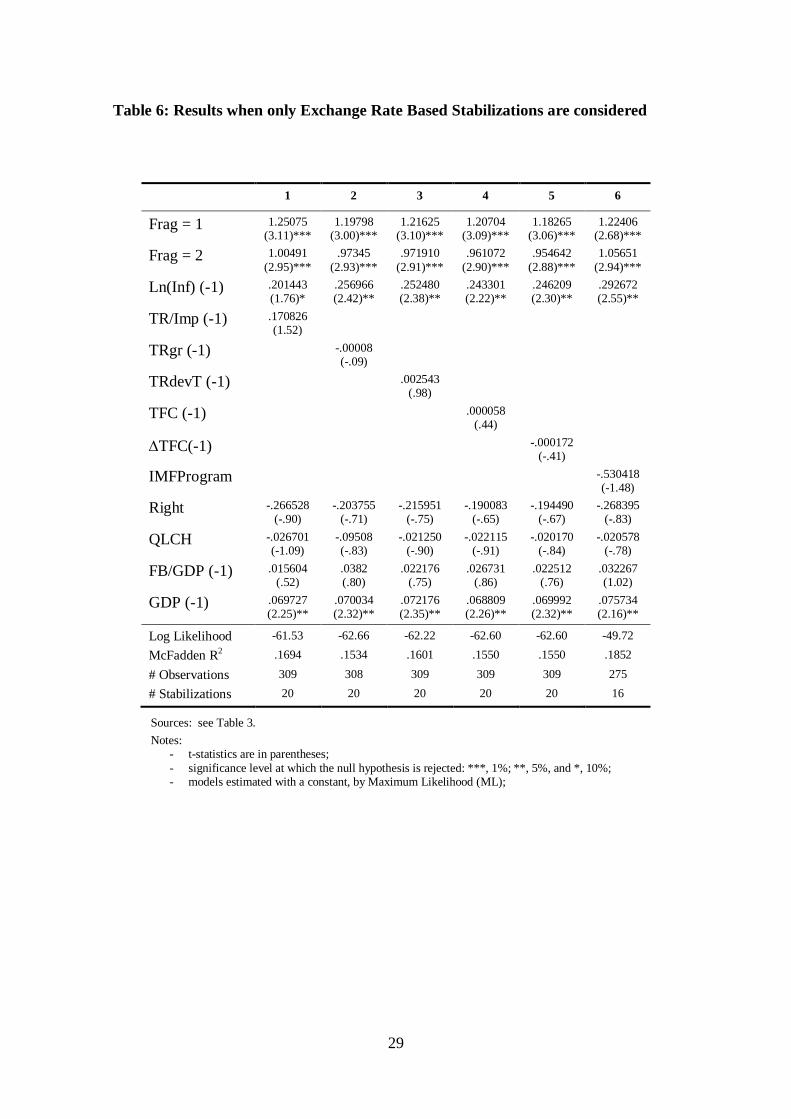
Table 6 shows the results when only Exchange Rate Based Stabilizations are

considered. First, Orphanides (1996a,b) models are tested using three different proxies

for the availability of reserves: total reserves as a percentage of imports (column 1),

change in total reserves since the same quarter of the previous year (column 2), and

percentage deviation from trend15

of total reserves (column 3). None of these variables

is statistically significant. Second, the influence of IMF credit is taken into account by

looking at quarterly data of Total Fund Credit and Loans Outstanding (TFC) and at the

occurrence of IMF arrangements with the countries included in the sample. Columns 4

and 5 show that the lag of the level and of the change in Total Fund Credit do not affect

the probability of starting a stabilization (results are the same for other lags and moving

averages of TFC). Concluding an arrangement with the IMF in the year of the

observation does not have a significant effect either (column 6). The same applies for

IMF arrangements in previous years.

These results seem to indicate that the availability of foreign exchange reserves

and IMF credit or arrangements are not important for the decision to start a stabilization

program. Nevertheless, we should not completely discard that possibility. First, the

13

expected level of reserves, on which we have no data, may be more important than the

actual level of reserves. Second, Casella and Eichengreen (1996) argue that both the

timing of the decision to provide aid and of the actual transfer of funds matter. Since the

only information we have is the year in which an arrangement was agreed upon, we

cannot appropriately test whether the actual provision of foreign aid affects the timing

of stabilization programs.

I also performed a considerable number of robustness tests and sensitivity

analyses not reported here.16

First, quarterly growth in CPI was used instead of growth

in CPI since the same quarter of the previous year. Second, growth in money since the

same quarter of the previous year was used instead of growth in the CPI. Third, current

account balance as a percentage of GDP, growth in exports, and growth in imports were

added to the list of explanatory variables, either one at a time or all at the same time.

Fourth, because results could be sensitive to interpolation methods, I reestimated the

model using only observations for which quarterly data was available, or using only

annual data. Finally, as any definition of high inflation is necessarily arbitrary, I also

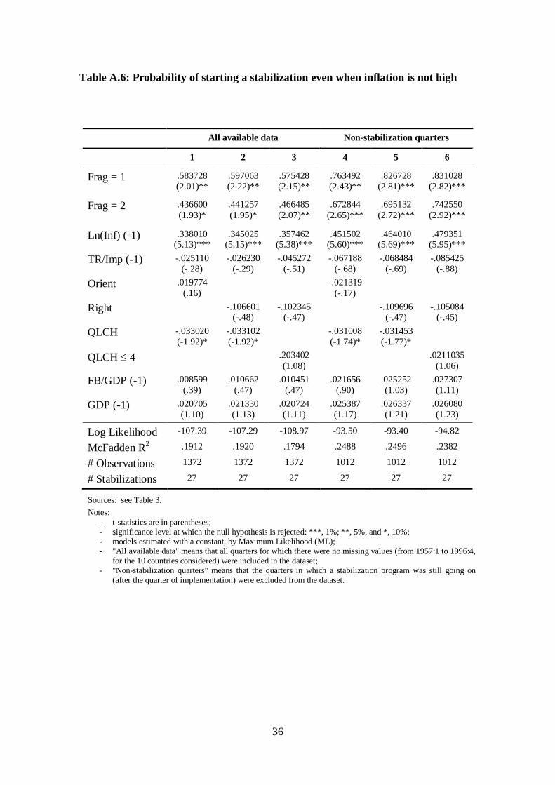
estimated the results using all observations available or all non-stabilization quarters

(those in which a stabilization was not already under way), instead of using just the high

inflation quarters. The conclusions of the analysis are unchanged in these alternative

estimations.

3) Probit with time dummies

In the estimations described above I assumed that the probability of starting a

stabilization plan in a given quarter did not change autonomously over time, meaning

that any variation had to be due to changes in the explanatory variables. A simple way

to allow that probability to change over time, even when the independent variables are

14

held constant, is to create a set of dummy variables accounting for the passage of time

and include them in the probit model.17

Since the duration of high inflation before a

stabilization was never longer than seven years (the longest one was of 27 quarters),

seven year dummies reflecting the duration of high inflation before stabilization were

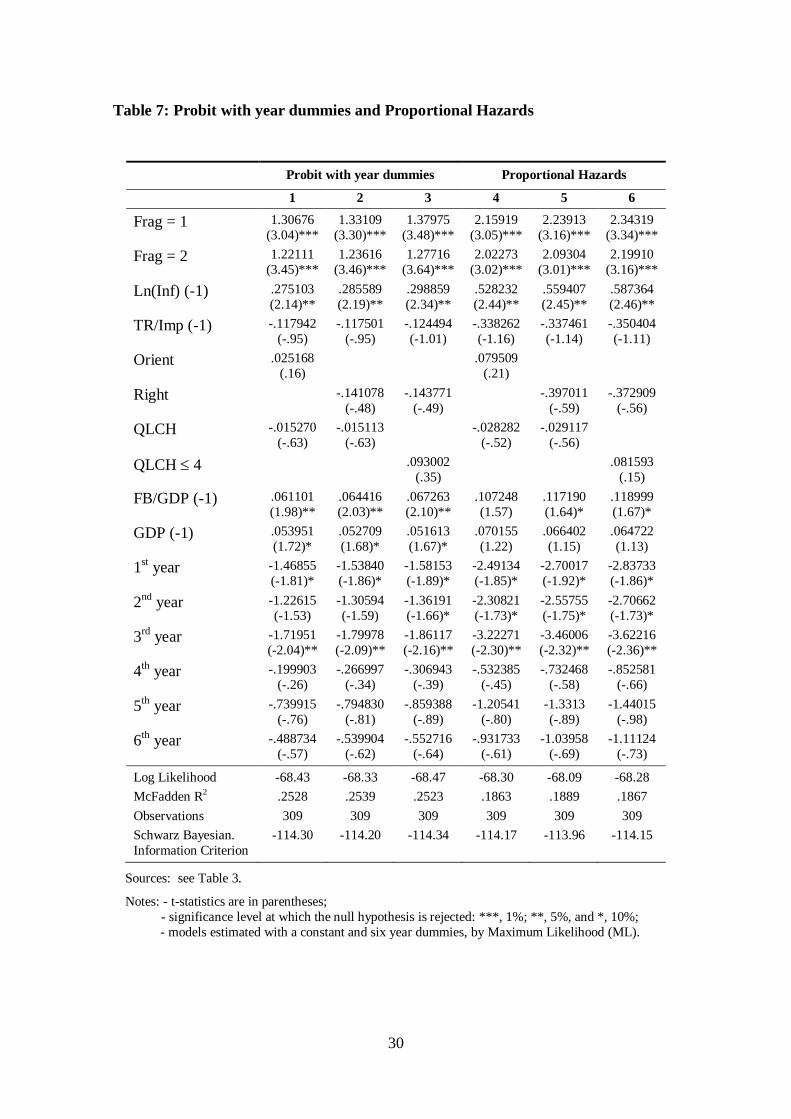
created and six were included in the list of independent variables.18

Results are shown in columns 1 to 3 of Table 7, which should be compared with

columns 1 to 3 of Table 4. Frag=1 and Frag=2 are now highly significant and their

estimated coefficients are larger than before. Ln(Inf(-1)) remains significant, but at a

lower level. Orient, Right, QLCH, QLCH4, and TR/Imp(-1) are not significant.

FB/GDP(-1) is only marginally significant and GDP(-1) is always significant at the 5%

level. Finally, the time dummies for the first and third years are always significant,

meaning that the passage of time does affect the hazard rate. In short, the introduction of

year dummies in the regressions reinforced the support for the hypothesis that higher

fragmentation reduces the probability of starting a stabilization program (increases

delays) and did not change considerably the support found for the other testable

hypotheses.

4) Proportional hazards model19

Although the life of a stabilization plan is a continuous-time process, available

data is discrete, meaning that the best that can be done is to work with data grouped into

time intervals. For the countries involved, the smallest time interval for which it was

possible to gather data for most of the variables used was one quarter. Then, the strategy

followed was to assume an underlying continuous-time model and estimate its

parameters by methods that take into account the discrete character of the data. Our first

approach was to estimate a probit model.

15

While a probit model has the advantage of being easily estimated by most of the

statistical software packages available, it might not be the most correct model to apply

in the present case. Estimated coefficients are not necessarily the discrete-time

equivalent of the underlying continuous-time model and the coefficient vector is not

invariant to the length of the time intervals, meaning that the choice of the time interval

(quarters in the present case) may affect estimated coefficients.

Prentice and Gloeckler (1978) developed a grouped data (discrete-time) version

of the proportional hazards model that does not suffer from the problems of the probit

model noted above. This model is expressed as follows:

(1) P xit t it 1 exp exp ' ,

where Pit is the probability that plan i is implemented at time t, t is an unspecified

function of time, xit is a vector of time-dependent variables (covariates), and is a

vector of parameters which is unknown. In this model, the discrete-time estimated

coefficients are also estimates of the underlying continuous-time model and the

coefficient vector is invariant to the length of the time interval. Thus, the two problems

of the probit model referred to above are avoided by the proportional hazards

specification.

Using the proportional hazards model, I have re-estimated the regressions of

columns 1 to 3 of Table 4. Results, shown in columns 4 to 6 of Table 7, are very similar

to those of the probit model. Therefore, the conclusions regarding the support for the

testable hypotheses remain the same.

D. CONCLUSIONS

The empirical results of this article show that some political variables are

important determinants of the timing of stabilizations. Probit and proportional hazards

16

estimations over a panel of 10 countries and 27 stabilization attempts clearly support the

hypothesis that higher fragmentation of the political system generally leads to delays of

stabilizations. Since higher fragmentation of the political system tends to lead to higher

polarization and political instability, these results are consistent with the “war of

attrition” model of Alesina and Drazen (1991) and with the findings of Cukierman,

Edwards, and Tabellini (1992) regarding the effect of political instability on inflation.

Higher inflation seems to hasten stabilizations, as suggested by the “benefits of

crises” model of Drazen and Grilli (1993) and by the distributional conflict and optimal

control models. There is also some support for the hypothesis that authoritarian regimes

hasten stabilizations, but evidence is found only for those cases in which political

parties are not allowed. Little or no evidence was found of opportunistic business cycles

or partisan effects.

Finally, empirical results do not seem to support the hypothesis of Orphanides

(1996a,b) that the decision of starting or delaying a stabilization program is essentially

based on the available amount of foreign reserves. Nevertheless, we cannot completely

discard that hypotheses because expected reserves, for which there is no data, may be a

more important variable than actual reserves. Furthermore, there is weak evidence that

an IMF arrangement now or in the future increases delays, which seems to be consistent

with Orphanides (1996a,b) argument that the expectation of foreign aid increases

delays.

In sum, it seems that the structure of the political system may help explain why

suboptimal (inflationary) policies are kept for long periods of time and the necessary

corrective actions are not taken. Countries whose electoral systems are highly

proportional tend to have a higher number of parties represented in parliament,

generally leading to higher political polarization and instability. Then, conflicts of

17

interests between political parties make the approval of new legislation harder and

stabilization programs are often delayed until a serious crisis sets in.

* Financial was provided by Programa PRAXIS XXI - Portugal (Reference: BD/3525/94) and CEEG –

Universidade do Minho. The author wishes to thank Henry Chappell, John McDermott, McKinley

Blackburn, Janice Breuer, George Krause, Peter Bernholz, participants at the conference of the European

Public Choice Society of April 1999 in Lisbon, and two anonymous referees for very helpful comments.

1 For surveys on this literature, see: Alesina (1994), Drazen (1996), Rodrik (1993), and Rodrik (1996).

2 Alesina and Tabellini (1989) present a model along the same lines. Similar evidence regarding the

effects of political instability is found by Edwards and Tabellini (1991), and Roubini (1991).

3 Mainwaring and Scully (1995, pp. 28-33) argue that the most polarized political systems in Latin

America are also the most fragmented. Roubini and Sachs (1989) showed for industrial countries that the

degree of fragmentation of the political system is directly related to the public debt, given the difficulty of

parties to agree on fiscal stabilization in more fragmented party systems. Here, I will test the related

hypothesis that higher fragmentation leads to greater delays of inflation stabilization programs.

4 This hypothesis is also consistent with the optimal control models of Orphanides (1996a,b) and with the

class conflict models of Laban and Sturzenegger (1994a,b) and Mondino, et al. (1996), that stress the

importance of capital flight in the process of increasing inflation. We should note that at very high levels

of inflation, currency substitution might be even more important. As Bernholz (1995) points out, the

public tends to restrict its use of the inflating money during hyperinflations or advanced inflations. As

they substitute the national currency by the foreign one(s), the real stock of money shrinks, decreasing the

base for the inflation tax. High inflation will also decrease the revenue from normal taxes because of the

time lags between the assessment, payment and expenditure of tax revenues (Olivera-Tanzi effect). In

such a situation, a stabilization is the last effort of the government to prevent losing its tax power

completely. Since currency substitution is usually illegal, it is impossible for me to get data on it for all

the countries studied and evaluate its effect on the timing of stabilizations. See Bernholz (1996) for an

empirical study for which data on currency substitution was available - the Soviet hyperinflation of 1922-

1924.

5 On political business cycle and partisan theories, see: Alesina (1994).

18

6 See Bruno, et al. (1988), Bruno, et al. (1991), Calvo and Végh (1994), Kiguel and Leviatan (1992),

Pastor (1992), Hoffmaister and Végh (1996), and Végh (1992).

7 For some countries, only annual data is available on some variables and, sometimes, there is no data at

all for earlier decades. I used straight-line interpolation to generate quarterly data and I also interpolated

the series assuming that these were AR1 (auto-regressive or order 1) or RW1 (random walk of order 1).

Although these interpolation techniques may not be the most correct ones, especially for GDP, results

were not driven by the way annual data was interpolated. Results using straight-line interpolation or the

other interpolation techniques are very similar to those obtained when one works only with the available

quarterly data or when annual data is used instead of quarterly data. An appendix containing some of

these results is available from the author upon request.

8 Three dummy variables based on Frag were created: Frag=1, Frag=2, and Frag>2. The 4 degrees of

fragmentation used by Roubini and Sachs (1989) would correspond to the values 2 to 5 of Frag. To

account for dictatorships, one more degree of fragmentation was considered (“1- No parties allowed or

exclusive one-party systems”). Since there were no stabilizations being implemented when Frag was

equal to 4 or 5, it was not possible to create dummy variables for these cases and include them in the set

of regressors, because they would totally predict the value of the dependent variable (STAB=0). Thus,

only three dummies were created and the first two were included in the set of explanatory variables.

9 According to the partisan business cycle of Hibbs (1977), leftist governments are more prone to inflation

than rightist governments. The classification used for this variable follows Haggard and Kaufman (1992).

10 The fact that 3 out of 4 stabilization programs implemented when inflation was not high according to

my definition (Argentina, 1967.2; Chile, 1978.1; and Uruguay, 1978.4) resulted from decisions of

authoritarian regimes that did not allow political parties also seems to support the hypothesis that higher

fragmentation increases delays. Furthermore, in the fourth case, Mexico 1987.4, there was a dominant

party in power, the PRI, that always got an overall majority in the Mexican Parliament (actually, Mexico

was most of the time the least fragmented of the democratic regimes).

11 F.Ind is the Laakso and Taegepera (1979) measure of the effective number of parties in Parliament with

parties being weighted according to their size. The greater the index, the greater are the effective number

of parties and fragmentation. According to Maiwaring and Scully (1995, pp. 31) polarization or the

“ideological distance tends to widen as the effective number of parties increases.”

19

12 This variable was not included in the estimations of columns 1 to 4 because when Frag=1 takes the

value of one Type is also equal to one, resulting in high correlation of these variables, 66.89%, which

could lead to problems of multicolinearity.

13 One direct way of testing whether “strong” dictators tend to stabilize faster than “weak” dictators or not

would be to create a dummy variable representing the latter and include it in the estimation of column

one, so that its coefficient could be compared to that of Frag=1. Unfortunately, that is not possible

because in this sample there is not a single case in which a “weak” dictator implements an inflation

stabilization program. Thus, a dummy variable representing “weak” dictators would totally predict the

value of the dependent variable (STAB=0).

14 An Appendix containing these results is available from the author upon request.

15 The deviations from trend were obtained using the Hodrick-Prescott decomposition method.

16 An Appendix with these results is available from the author upon request.

17 See Allison (1982) for an example with a Logit model. He also compares the results of two Logit

models, with one assuming that the hazard rate does not change autonomously over time, and the other

relaxing that constraint by adding year dummies to the list of regressors.

18 Since the data set is composed of quarterly data, the inclusion of quarterly dummies reflecting the

duration of high inflation before stabilization would be ideal, but that was not possible because for many

quarters there were no stabilizations being implemented. This means that the dummies for these quarters

would completely predict the value of the dependent variable (STAB=0). Thus, I decided to create yearly

dummies instead. Since the longest period of high inflation was of 27 quarters, corresponding to almost 7

years, only seven dummies were created (6 for the first six years of high inflation before a stabilization,

and a 7th for all the remaining years). The creation of additional year dummies was not possible because

these would totally predict the value of the dependent variable.

19 For a description of the proportional hazards model, see: Prentice and Gloeckler (1978), Allison (1982),

and Jenkins (1995).

20

E. REFERENCES

Alesina, Alberto, 1994, Political Models of Macroeconomic Policy and Fiscal Reforms,

in: Haggard, Stephan and Steven B. Webb, eds., Voting for Reform, World

Bank, (Oxford University Press, New York, NY), 37-60.

Alesina, Alberto and Allan Drazen, 1991, Why are Stabilizations Delayed? American

Economic Review 81(5), 1170-1188.

Alesina, Alberto and Guido Tabellini, 1989, External Debt, Capital Flight and Political

Risk. Journal of International Economics 27(3/4), 199-220.

Allison, P.D., 1982, Discrete-Time Methods for the Analysis of Event Histories. In

Leinhardt, S. (Ed.), Sociological Methodology. (Jossey-Bass Publishers, San

Francisco, CA), 61-97.

Banks, Arthur, ed., Political Handbook of the World (McGraw-Hill, New York, NY)

various issues.

Bernholz, Peter, 1995, Necessary and Sufficient Conditions to End Hyperinflations. In

Siklos, Pierre L., ed., Great Inflations of the 20th

Century: Theories, Policies and

Evidence (Edward Elgar, Aldershot, UK), 257-287.

Bernholz, Peter, 1996, Currency Substitution during Hyperinflation in the Soviet Union

1922-1924. The Journal of European Economic History 25(2), 297-323.

Bruno, Michael, et al., eds., 1988, Inflation Stabilization: The Experience of Israel,

Argentina, Brazil, Bolivia, and Mexico (MIT Press, Cambridge, MA).

Bruno, Michael, et al., eds., (1991), Lessons of Economic Stabilization and its Aftermath

(MIT Press, Cambridge, MA).

Calvo, Guillermo A. and Carlos A. Végh, 1994, Inflation Stabilization and Nominal

Anchors. Contemporary Economic Policy 12, 35-45.

21

Casella, Alessandra and Barry Eichengreen (1996), Can Foreign Aid Accelerate

Stabilization? Economic Journal 106, 605-619.

Cukierman, Alex, Sebastian Edwards, and Guido Tabellini, 1992, Seignioriage and

Political Instability. American Economic Review 82(3), 537-555.

Drazen, Allan, 1996, The Political Economy of Delayed Reform. The Journal of Policy

Reform, 1(1), 25-46.

Drazen, Allan and Vittorio Grilli, 1993, The Benefit of Crises for Economic reforms.

American Economic Review 83(3), 598-607.

Dornbush, Rudiger and Sebastian Edwards, eds., 1991, The Macroeconomics of

Populism in Latin America (The University of Chicago Press, Chicago, IL).

Edwards, Sebastian and Guido Tabellini, 1991, Explaining Fiscal Policy and Inflation in

Developing Countries. Journal of International Money and Finance 10,

Supplement, S16-S48.

Gorvin, Ian, ed., 1989, Elections Since 1945: A Worldwide Reference Compendium (St.

James Press, Chicago, IL).

Haggard, Stephan and Robert R. Kaufman, 1992, The Political Economy and

Stabilization in Middle-Income Countries, in: Haggard, Stephan and Robert R.

Kaufman, eds., The Politics of Economic Adjustment (Princeton University

Press, Princeton, NJ), 270-315.

Hibbs, D., 1977, Political Parties and Macroeconomic Policy. American Political

Science Review 71, 1467-1487.

Hoffmaister, Alexander W. and Carlos A. Végh, 1996, Disinflation and the Recession-

Now-Versus-Recession-Later Hypothesis: Evidence from Uruguay. IMF Staff

Papers 43(2), 355-394.

22

Jenkins, Stephen P., 1995, Easy Estimation for Discrete-Time Duration Models. Oxford

Bulletin of Economics and Statistics 57(1), 129-139.

Kiguel, Miguel, and Nissan Leviatan, 1992, The Business Cycle Associated with

Exchange Rate-Based Stabilizations. The World Bank Economic Review 6(2),

279-305.

Knight, Malcom and Juliio A. Santaella, 1997, Economic Determinants of IMF

financial arrangements. Journal of Development Economics 54, 405-436.

Laakso, Markku and Rein Taegepera, 1979, The Effective Number of Parties: A

Measure with Application to Western Europe. Comparative Political Studies

12(1), 3-27.

Laban, Raul and Federico Sturzenegger, 1994a, Distributional Conflict, Financial

Adaptation and Delayed Stabilization. Economics and Politics 6(3), 257-276.

Laban, Raul and Federico Sturzenegger, 1994b, Fiscal Conservatism as a Response to

the Debt Crisis. Journal of Development Economics 45(2), 305-324.

Mainwaring, Scott and Timothy R. Scully, eds., 1995, Building Democratic Institutions:

Party Systems in Latin America (Stanford University Press, Stanford, CA).

McDonald, Ronald H. and J. Mark Ruhl, 1989, Party Politics and Elections in Latin

America (Westview Press, Boulder, CO).

Mondino, Guillermo, Federico Sturzenegger, and Mariano Tommasi, 1996, Recurrent

High Inflation and Stabilization: A Dynamic Game. International Economic

Review 37(4), 981-996.

Nordhaus, W., 1975, The Political Business Cycle. Review of Economic Studies 42,

169-190.

Orphanides, Athanasios, 1996a, Optimal Reform Postponement. Economics Letters 52,

299-307.

23

Orphanides, Athanasios, 1996b, The Timing of Stabilizations. Journal of Economics

Dynamics & Control 20(1-3), 257-279.

Pastor Jr., Manuel, 1992, Inflation Stabilization & Debt: Macroeconomic experiments in

Peru and Bolivia (Westview Press, Boulder, CO).

Prentice, Ross, and L. A. Gloeckler, 1978, Regression Analysis of Grouped Survival

Data with Application to Breast Cancer Data. Biometrics 34, 57-67.

Rodrik, Dani, 1993, The Positive Economics of Delayed Reform. American Economic

Review 83, 356-361.

Rodrik, Dani, 1996, Understanding Economic Policy Reform. Journal of Economic

Literature 34, 9-41.

Roubini, Nouriel, 1991, Economic and Political Determinants of Budget Deficits in

Developing Countries. Journal of International Money and Finance 10,

Supplement, S49-S72.

Roubini, Nouriel and Jeffrey Sachs, 1989, Political and Economic Determinants of

Budget Deficits in the Industrial democracies. European Economic Review 33,

903-938.

Végh, Carlos A., 1992, Stopping High Inflation: An Analytical Overview. IMF Staff

Papers 39(3), 626-695.

Veiga, Francisco José, 1998, Inflation Stabilization. Ph.D. Dissertation, University of

South Carolina, Columbia, SC.

Veiga, Francisco José, 1999, What Causes the Failure of Inflation Stabilization Plans?

Journal of International Money and Finance 18(2), 169-194.

World Europa Yearbook (Europa, London, UK) several issues.

24

Table 1: Hypotheses related to the literature presented

Hypotheses tested and related literature Variables

used

Expected signs of

coefficients

1 – Higher fragmentation of the political system leads to

delays of stabilizations:

Alesina and Drazen (1991), Alesina and Tabellini

(1989), Cukierman, Edwards, and Tabellini (1992), and

Roubini and Sachs (1989).

Frag = 1

Frag = 2

F.Ind

+

+

-

2 – Higher inflation hastens stabilizations:

Alesina and Drazen (1991), Drazen and Grilli (1993),

Laban and Sturzenegger (1994a,b), Mondino et al. (1996), and Orphanides (1996a,b).

Ln(Inf)

+

3 – Greater amount of reserves hastens stabilizations:

Optimal control models of Orphanides (1996a,b)

TR/Imp

TRgr

TrdevT

+

+

+

4 – Stabilizations come faster in authoritarian regimes than

in democracies:

Haggard and Kaufman (1992)

Frag = 1

Type

+

Frag=1 > Frag=2

+

5 – Rightist governments are more prone to stabilize than

leftist ones:

Partisan model of Hibbs (1977)

Orient

Right

-

+

6 – Governments are more prone to stabilize in the beginning

of their terms than towards the end:

Political business cycle model of Nordhaus (1975)

QLCH

QLCH 4

-

+

Notes:

– See Table 3 for a description of the variables used;

– When “Frag=1 > Frag=2” is indicated along with the expected sign of a coefficient, it means

that it is also necessary that the estimated coefficient associated with Frag=1 is greater than

the one associated with Frag=2 to support the tested hypothesis.

25

Table 2: Stabilization Programs

Country Program dates / names Type Duration of “high” inflation until stabilization (quarters)

Argentina 1959.3 ERBS 4 1967.2 ERBS 0

1973.3 ERBS 6

1978.4 (Tablita) ERBS 15

1985.1(Austral) ERBS 14

1990.1 (Bonex) MBS 11

1991.2 (Convertibility) ERBS 1

Bolivia 1985.4 ERBS 14

Brazil 1964:2 ERBS 4 1986:1 (Cruzado) ERBS 22

1990.2 (Collor) MBS 13

1994.3 (Real) ERBS 14

Chile 1975.2 MBS 11 1978.1 (Tablita) ERBS 0

Dominican Republic 1985.2 ERBS 4

1991.2 MBS 13

Israel 1985.3 (Shekel) ERBS 27

Mexico 1976.4 ERBS 0

1988.1 ERBS 5

Peru 1981.3 ERBS 22

1985.4 ERBS 10

1990.3 MBS 11

Turkey 1980.1 ERBS 12

Uruguay 1960.4 MBS 7 1968.2 ERBS 11

1978.4 (Tablita) ERBS 0

1991.3 MBS 5

Sources: Bruno, et al. (1988), Bruno, et al. (1991), Calvo and Végh (1994), Kiguel and

Leviatan (1992), Pastor (1992), Hoffmaister and Végh (1996), and Végh (1992).

Notes: ERBS = Exchange Rate Based Stabilization (20 in this sample);

MBS = Money Based Stabilization (7 in this sample).

26

Table 3: Description of the Variables Used and Respective Sources

Political variables:

Frag - Degree of fragmentation of the political system: 1 no parties allowed or exclusive one-party systems;

2 one-party majority parliamentary government; or presidential government, with the

same party in control of the parliament (with an overall majority);

>2 More fragmented political systems.

F.Ind - Fragmentation Index of the distribution of seats in the lower house of the parliament:

F Indpi

.

1

2, where pi = percentage of seats of party i.

Type - Type of political system: 1 = m military dictatorship or authoritarian government backed by the military;

0 = d democracy.

Orient - Political orientation of the government: 1 conservative, antilabor or antileft government;

2 center-right government or coalition of center-right and center-left parties;

3 center-left government;

4 socialist or populist government.

Right – Right, center right, or coalition of center-right and center-left parties government: 1 (Orient=1 or Orient=2);

0 (Orient=3 or Orient=4).

QLCH - Quarters since last change in government or election

Economic variables:

Ln(Inf) – Natural log of Growth of CPI since the same quarter of the previous year

TR/Imp - Total Reserves as a Percentage of Imports

TRgr – Growth in Total Reserves since the same quarter of the previous year

TrdevT – Percentage deviation from Trend (Hodrick-Prescott) of Total Reserves

IMFProgram = 1 if there was an IMF arrangement in the same year, and zero otherwise

TFC - Total IMF credit and loans outstanding

FB/GDP - Fiscal Balance (Government Budget Balance) as a Percentage of GDP

GDP - Growth of Real GDP since the same quarter of the previous year

Sources:

- Political variables: Arthur Banks, ed., Political Handbook of the World, several issues; Dornbusch

and Edwards (1991); Gorvin (1989); Haggard and Kaufman (1992); McDonald and Ruhl

(1989); Mainwaring and Scully (1995);World Europa Yearbook, Europa, several issues. For

tables containing the data on the political variables see: Veiga (1998).

- Economic variables: International Financial Statistics - IMF. Quarterly data on Real GDP was also

obtained from IBGE (Brazil), INEGI (Mexico), and Végh (1992), for Chile (1977:1 to 1979:4)

and Uruguay (1978:1 to 1983:4). Data on IMFProgram is based on Table 3 of Knight and

Santaella (1997), for the period 1973-91, and on information available in the IMF web page for

the following years (1992-96).

27

Table 4: Probability of Starting a Stabilization Program

1 2 3 4 5 6

Frag = 1 .842056

(2.36)** [14.5]

.895809

(2.70)*** [15.8]

.952411

(2.89)*** [17.5]

.890140

(2.69)*** [15.7]

1.13690

(2.18)** [22.3]

Frag = 2 .805601

(2.88)***

[11.4]

.810457

(2.90)***

[11.5]

.858415

(3.11)***

[12.6]

.806536

(2.88)***

[11.4]

.919913

(2.89)***

[13.5]

F.Ind -.181193

(-1.87)*

[-2.52]

.081448

(.78)

[1.08]

Ln(Inf) (-1) .309311

(3.07)***

[4.12]

.314474

(3.12)***

[4.19]

.327618

(3.29)***

[4.40]

.314921

(3.12)***

[4.20]

.303233

(2.84)***

[4.22]

.274167

(2.48)**

[3.65]

TR/Imp (-1) -.029002

(-.27) [-.387]

-.029320

(-.280) [-.391]

-.040158

(-.38) [-.539]

-.029666

(-.28) [-.396]

-.009394

(-.09) [-.130]

-.036567

(-.34) [-.487]

Type -.571338

(-1.44)

[-5.52]

Orient -.056598

(-.40)

[-.75]

-.216735

(-1.47)

[-3.02]

-.047058

(-.33)

[-.627]

Right .022609

(.84)

[.244]

.034502

(.13)

[.379]

.025285

(.09)

[.273]

QLCH -.028987 (-1.30)

[-.386]

-.030019 (-1.35)

[-.400]

-.036946 (-1.10)

[-.493]

-.040049 (-1.90)*

[-.558]

-.026587 (-1.18)

[-.354]

QLCH 4 .201210

(.85)

[2.33]

-.098034

(-.28)

[-1.04]

FB/GDP (-1) .044791

(1.64)*

[.597]

.046463

(1.68)*

[.620]

.050739

(1.82)*

[.681]

.044765

(1.59)

[.597]

.047705

(1.84)*

[.664]

.042364

(1.55)

[.564]

GDP (-1) .060554

(2.25)**

[.807]

.059429

(2.24)**

[.793]

.058047

(2.24)**

[.779]

.059337

(2.23)**

[.792]

.060932

(2.31)**

[.849]

.057030

(2.08)**

[.760]

Log Likelihood -76.43 -76.51 -77.13 -76.47 -79.66 -76.12

McFadden R2 .1655 .1646 .1579 .1650 .1302 .1689

Observations 309 309 309 309 309 309

Schwarz B.I.C. -99.36 -99.44 -100.06 -102.27 -102.59 -101.92

Sources: see Table 3.

Notes: - t-statistics are in parentheses;

- the marginal effects of the independent variables on the probability of starting a

stabilization are in brackets;

- significance level at which the null hypothesis is rejected: ***, 1%; **, 5%, and *, 10%; - models estimated with a constant, by Maximum Likelihood (ML).

28

Table 5: Sensitivity Analysis

Alternative definitions of high inflation Restricted samples

Inf100% or

Inf MA of

last 5 years

Inf 50% Inf 100% Latin

America

South

America

1970:1

to

1996:4

1 2 3 4 5 6 7

Frag = 1 .817950

(2.49)**

.768785

(2.05)**

.603142

(1.35)

.785619

(2.15)**

.889058

(2.12)**

.730026

(2.06)**

Frag = 2 .862838

(3.05)***

.728080

(2.43)**

1.05171

(2.98)***

.774684

(2.56)**

.741327

(2.01)**

.806970

(2.74)***

Frag 2 .912503

(2.76)***

Ln(Inf) (-1) .306485

(3.02)***

.333517

(3.01)***

.285243

(2.16)**

.298951

(2.29)**

.284199

(2.69)***

.335453

(2.78)***

.321753

(3.09)***

TR/Imp (-1) -.020196

(-.18)

-.027994

(-.25)

.015629

(.12)

.023503

(.19)

-.004706

(-.04)

-.034331

(-.29)

-.014164

(-.12)

Right .100657

(.37)

.008195

(.02)

.010344

(.02)

-.086275

(-.24)

.002314

(.008)

-.01999

(-.05)

-.035339

(-.12)

QLCH -.028248

(-1.27)

-.030145

(-1.28)

-.036027

(-1.28)

-.032174

(-1.16)

-.026647

(-1.19)

-.040390

(-1.37)

-.034657

(-1.43)

FB/GDP (-1) .046591

(1.68)*

.038118

(1.36)

.033254

(1.06)

.033017

(1.06)

.044726

(1.50)

.053865

(1.39)

.049224

(1.70)*

GDP (-1) .059473

(2.21)**

.050789

(1.83)*

.062410

(1.74)*

.063064

(1.81)*

.050435

(1.88)*

.062224

(2.06)**

.063578

(2.15)**

Log Likelihood -61.53 -62.43 -45.76 -46.32 -71.64 -57.86 -62.99

McFadden R2 .1603 .1677 .1967 .1867 .1337 .1696 .1809

Observations 290 256 187 187 264 224 278

Stabilizations 27 22 17 17 25 21 22

Sources: see Table 3.

Notes: - t-statistics are in parentheses;

- significance level at which the null hypothesis is rejected: ***, 1%; **, 5%, and *, 10%;

- models estimated with a constant, by Maximum Likelihood (ML).

29

Table 6: Results when only Exchange Rate Based Stabilizations are considered

1 2 3 4 5 6

Frag = 1 1.25075 (3.11)***

1.19798 (3.00)***

1.21625 (3.10)***

1.20704 (3.09)***

1.18265 (3.06)***

1.22406 (2.68)***

Frag = 2 1.00491

(2.95)***

.97345

(2.93)***

.971910

(2.91)***

.961072

(2.90)***

.954642

(2.88)***

1.05651

(2.94)***

Ln(Inf) (-1) .201443

(1.76)* .256966 (2.42)**

.252480 (2.38)**

.243301 (2.22)**

.246209 (2.30)**

.292672 (2.55)**

TR/Imp (-1) .170826

(1.52)

TRgr (-1) -.00008

(-.09)

TRdevT (-1) .002543

(.98)

TFC (-1) .000058

(.44)

TFC(-1) -.000172

(-.41)

IMFProgram -.530418

(-1.48)

Right -.266528

(-.90) -.203755

(-.71) -.215951

(-.75) -.190083

(-.65) -.194490

(-.67) -.268395

(-.83)

QLCH -.026701

(-1.09) -.09508 (-.83)

-.021250 (-.90)

-.022115 (-.91)

-.020170 (-.84)

-.020578 (-.78)

FB/GDP (-1) .015604

(.52) .0382 (.80)

.022176 (.75)

.026731 (.86)

.022512 (.76)

.032267 (1.02)

GDP (-1) .069727

(2.25)** .070034 (2.32)**

.072176 (2.35)**

.068809 (2.26)**

.069992 (2.32)**

.075734 (2.16)**

Log Likelihood -61.53 -62.66 -62.22 -62.60 -62.60 -49.72

McFadden R2 .1694 .1534 .1601 .1550 .1550 .1852

# Observations 309 308 309 309 309 275

# Stabilizations 20 20 20 20 20 16

Sources: see Table 3.

Notes: - t-statistics are in parentheses;

- significance level at which the null hypothesis is rejected: ***, 1%; **, 5%, and *, 10%; - models estimated with a constant, by Maximum Likelihood (ML);

30

Table 7: Probit with year dummies and Proportional Hazards

Probit with year dummies Proportional Hazards

1 2 3 4 5 6

Frag = 1 1.30676

(3.04)***

1.33109

(3.30)***

1.37975

(3.48)***

2.15919

(3.05)***

2.23913

(3.16)***

2.34319

(3.34)***

Frag = 2 1.22111

(3.45)***

1.23616

(3.46)***

1.27716

(3.64)***

2.02273

(3.02)***

2.09304

(3.01)***

2.19910

(3.16)***

Ln(Inf) (-1) .275103

(2.14)**

.285589

(2.19)**

.298859

(2.34)**

.528232

(2.44)**

.559407

(2.45)**

.587364

(2.46)**

TR/Imp (-1) -.117942

(-.95)

-.117501

(-.95)

-.124494

(-1.01)

-.338262

(-1.16)

-.337461

(-1.14)

-.350404

(-1.11)

Orient .025168

(.16)

.079509

(.21)

Right -.141078

(-.48)

-.143771

(-.49)

-.397011

(-.59)

-.372909

(-.56)

QLCH -.015270

(-.63)

-.015113

(-.63)

-.028282

(-.52)

-.029117

(-.56)

QLCH 4 .093002

(.35)

.081593

(.15)

FB/GDP (-1) .061101

(1.98)**

.064416

(2.03)**

.067263

(2.10)**

.107248

(1.57)

.117190

(1.64)*

.118999

(1.67)*

GDP (-1) .053951

(1.72)*

.052709

(1.68)*

.051613

(1.67)*

.070155

(1.22)

.066402

(1.15)

.064722

(1.13)

1st year -1.46855

(-1.81)*

-1.53840

(-1.86)*

-1.58153

(-1.89)*

-2.49134

(-1.85)*

-2.70017

(-1.92)*

-2.83733

(-1.86)*

2nd

year -1.22615

(-1.53)

-1.30594

(-1.59)

-1.36191

(-1.66)*

-2.30821

(-1.73)*

-2.55755

(-1.75)*

-2.70662

(-1.73)*

3rd

year -1.71951

(-2.04)**

-1.79978

(-2.09)**

-1.86117

(-2.16)**

-3.22271

(-2.30)**

-3.46006

(-2.32)**

-3.62216

(-2.36)**

4th year -.199903

(-.26)

-.266997

(-.34)

-.306943

(-.39)

-.532385

(-.45)

-.732468

(-.58)

-.852581

(-.66)

5th year -.739915

(-.76)

-.794830

(-.81)

-.859388

(-.89)

-1.20541

(-.80)

-1.3313

(-.89)

-1.44015

(-.98)

6th year -.488734

(-.57)

-.539904

(-.62)

-.552716

(-.64)

-.931733

(-.61)

-1.03958

(-.69)

-1.11124

(-.73)

Log Likelihood -68.43 -68.33 -68.47 -68.30 -68.09 -68.28

McFadden R2 .2528 .2539 .2523 .1863 .1889 .1867

Observations 309 309 309 309 309 309

Schwarz Bayesian.

Information Criterion

-114.30 -114.20 -114.34 -114.17 -113.96 -114.15

Sources: see Table 3.

Notes: - t-statistics are in parentheses;

- significance level at which the null hypothesis is rejected: ***, 1%; **, 5%, and *, 10%;

- models estimated with a constant and six year dummies, by Maximum Likelihood (ML).

31

F. APPENDIX

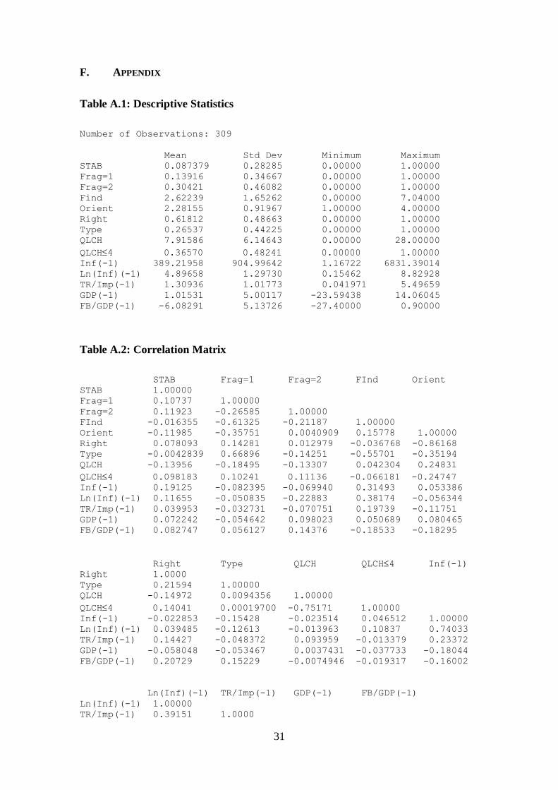
Table A.1: Descriptive Statistics

Number of Observations: 309

Mean Std Dev Minimum Maximum

STAB 0.087379 0.28285 0.00000 1.00000

Frag=1 0.13916 0.34667 0.00000 1.00000

Frag=2 0.30421 0.46082 0.00000 1.00000

Find 2.62239 1.65262 0.00000 7.04000

Orient 2.28155 0.91967 1.00000 4.00000

Right 0.61812 0.48663 0.00000 1.00000

Type 0.26537 0.44225 0.00000 1.00000

QLCH 7.91586 6.14643 0.00000 28.00000

QLCH4 0.36570 0.48241 0.00000 1.00000 Inf(-1) 389.21958 904.99642 1.16722 6831.39014

Ln(Inf)(-1) 4.89658 1.29730 0.15462 8.82928

TR/Imp(-1) 1.30936 1.01773 0.041971 5.49659

GDP(-1) 1.01531 5.00117 -23.59438 14.06045

FB/GDP(-1) -6.08291 5.13726 -27.40000 0.90000

Table A.2: Correlation Matrix

STAB Frag=1 Frag=2 FInd Orient

STAB 1.00000

Frag=1 0.10737 1.00000

Frag=2 0.11923 -0.26585 1.00000

FInd -0.016355 -0.61325 -0.21187 1.00000

Orient -0.11985 -0.35751 0.0040909 0.15778 1.00000

Right 0.078093 0.14281 0.012979 -0.036768 -0.86168

Type -0.0042839 0.66896 -0.14251 -0.55701 -0.35194

QLCH -0.13956 -0.18495 -0.13307 0.042304 0.24831

QLCH4 0.098183 0.10241 0.11136 -0.066181 -0.24747 Inf(-1) 0.19125 -0.082395 -0.069940 0.31493 0.053386

Ln(Inf)(-1) 0.11655 -0.050835 -0.22883 0.38174 -0.056344

TR/Imp(-1) 0.039953 -0.032731 -0.070751 0.19739 -0.11751

GDP(-1) 0.072242 -0.054642 0.098023 0.050689 0.080465

FB/GDP(-1) 0.082747 0.056127 0.14376 -0.18533 -0.18295

Right Type QLCH QLCH4 Inf(-1) Right 1.0000

Type 0.21594 1.00000

QLCH -0.14972 0.0094356 1.00000

QLCH4 0.14041 0.00019700 -0.75171 1.00000 Inf(-1) -0.022853 -0.15428 -0.023514 0.046512 1.00000

Ln(Inf)(-1) 0.039485 -0.12613 -0.013963 0.10837 0.74033

TR/Imp(-1) 0.14427 -0.048372 0.093959 -0.013379 0.23372

GDP(-1) -0.058048 -0.053467 0.0037431 -0.037733 -0.18044

FB/GDP(-1) 0.20729 0.15229 -0.0074946 -0.019317 -0.16002

Ln(Inf)(-1) TR/Imp(-1) GDP(-1) FB/GDP(-1)

Ln(Inf)(-1) 1.00000

TR/Imp(-1) 0.39151 1.0000

32

GDP(-1) -0.30059 0.019179 1.00000

FB/GDP(-1) -0.29274 -0.064023 0.042285 1.00000

33

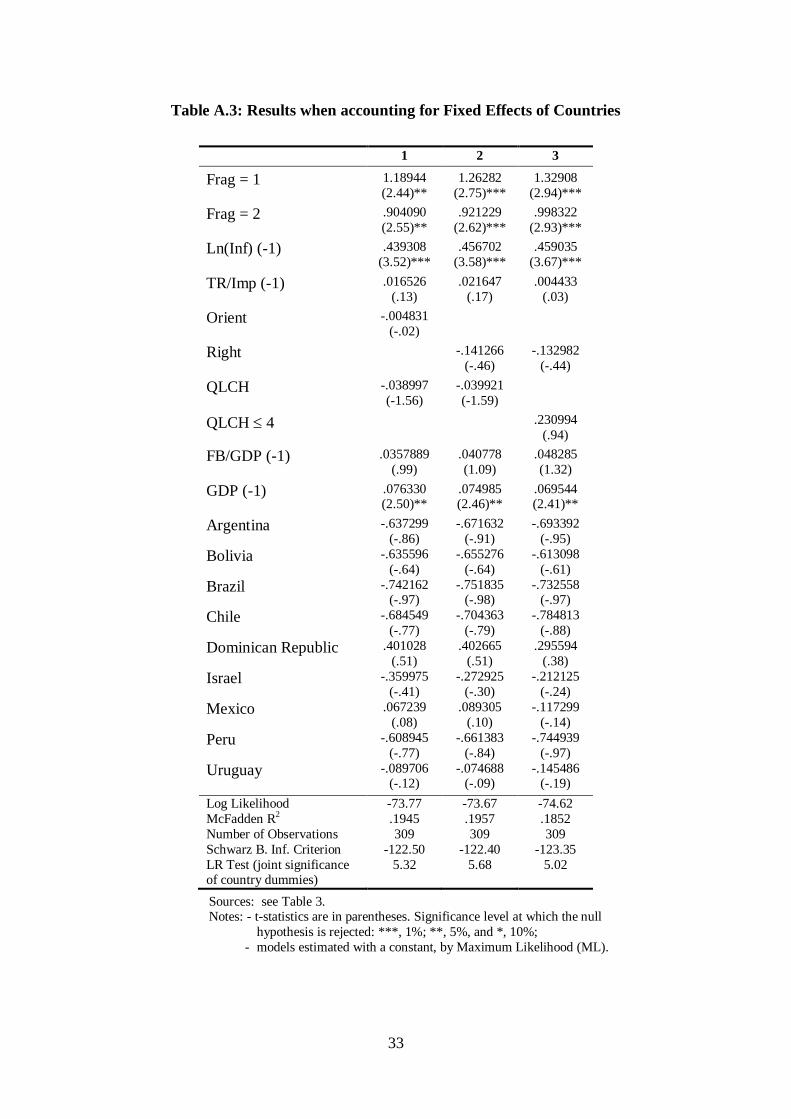
Table A.3: Results when accounting for Fixed Effects of Countries

1 2 3

Frag = 1 1.18944

(2.44)**

1.26282

(2.75)***

1.32908

(2.94)***

Frag = 2 .904090

(2.55)**

.921229

(2.62)***

.998322

(2.93)***

Ln(Inf) (-1) .439308

(3.52)***

.456702

(3.58)***

.459035

(3.67)***

TR/Imp (-1) .016526

(.13)

.021647

(.17)

.004433

(.03)

Orient -.004831

(-.02)

Right -.141266

(-.46)

-.132982

(-.44)

QLCH -.038997

(-1.56)

-.039921

(-1.59)

QLCH 4 .230994

(.94)

FB/GDP (-1) .0357889

(.99)

.040778

(1.09)

.048285

(1.32)

GDP (-1) .076330 (2.50)**

.074985 (2.46)**

.069544 (2.41)**

Argentina -.637299

(-.86)

-.671632

(-.91)

-.693392

(-.95)

Bolivia -.635596

(-.64)

-.655276

(-.64)

-.613098

(-.61)

Brazil -.742162 (-.97)

-.751835 (-.98)

-.732558 (-.97)

Chile -.684549

(-.77)

-.704363

(-.79)

-.784813

(-.88)

Dominican Republic .401028

(.51)

.402665

(.51)

.295594

(.38)

Israel -.359975

(-.41)

-.272925

(-.30)

-.212125

(-.24)

Mexico .067239

(.08)

.089305

(.10)

-.117299

(-.14)

Peru -.608945

(-.77)

-.661383

(-.84)

-.744939

(-.97)

Uruguay -.089706 (-.12)

-.074688 (-.09)

-.145486 (-.19)

Log Likelihood -73.77 -73.67 -74.62

McFadden R2 .1945 .1957 .1852

Number of Observations 309 309 309

Schwarz B. Inf. Criterion -122.50 -122.40 -123.35

LR Test (joint significance of country dummies)

5.32 5.68 5.02

Sources: see Table 3. Notes: - t-statistics are in parentheses. Significance level at which the null

hypothesis is rejected: ***, 1%; **, 5%, and *, 10%;

- models estimated with a constant, by Maximum Likelihood (ML).

34

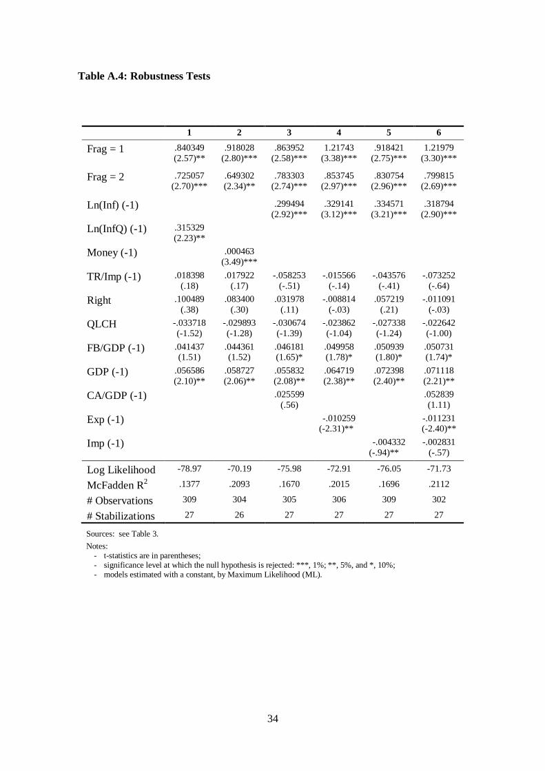
Table A.4: Robustness Tests

1 2 3 4 5 6

Frag = 1 .840349

(2.57)**

.918028

(2.80)***

.863952

(2.58)***

1.21743

(3.38)***

.918421

(2.75)***

1.21979

(3.30)***

Frag = 2 .725057

(2.70)***

.649302

(2.34)**

.783303

(2.74)***

.853745

(2.97)***

.830754

(2.96)***

.799815

(2.69)***

Ln(Inf) (-1) .299494

(2.92)***

.329141

(3.12)***

.334571

(3.21)***

.318794

(2.90)***

Ln(InfQ) (-1) .315329

(2.23)**

Money (-1) .000463

(3.49)***

TR/Imp (-1) .018398

(.18)

.017922

(.17)

-.058253

(-.51)

-.015566

(-.14)

-.043576

(-.41)

-.073252

(-.64)

Right .100489

(.38)

.083400

(.30)

.031978

(.11)

-.008814

(-.03)

.057219

(.21)

-.011091

(-.03)

QLCH -.033718

(-1.52)

-.029893

(-1.28)

-.030674

(-1.39)

-.023862

(-1.04)

-.027338

(-1.24)

-.022642

(-1.00)

FB/GDP (-1) .041437 (1.51)

.044361 (1.52)

.046181 (1.65)*

.049958 (1.78)*

.050939 (1.80)*

.050731 (1.74)*

GDP (-1) .056586

(2.10)**

.058727

(2.06)**

.055832

(2.08)**

.064719

(2.38)**

.072398

(2.40)**

.071118

(2.21)**

CA/GDP (-1) .025599

(.56)

.052839

(1.11)

Exp (-1) -.010259 (-2.31)**

-.011231 (-2.40)**

Imp (-1) -.004332

(-.94)**

-.002831

(-.57)

Log Likelihood -78.97 -70.19 -75.98 -72.91 -76.05 -71.73

McFadden R2 .1377 .2093 .1670 .2015 .1696 .2112

# Observations 309 304 305 306 309 302

# Stabilizations 27 26 27 27 27 27

Sources: see Table 3.

Notes: - t-statistics are in parentheses; - significance level at which the null hypothesis is rejected: ***, 1%; **, 5%, and *, 10%; - models estimated with a constant, by Maximum Likelihood (ML).

35

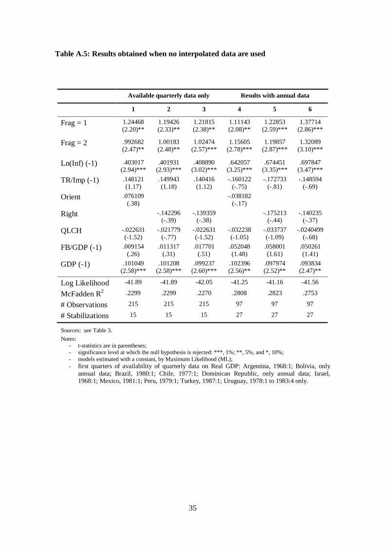
Table A.5: Results obtained when no interpolated data are used

Available quarterly data only Results with annual data

1 2 3 4 5 6

Frag = 1 1.24468

(2.20)**

1.19426

(2.33)**

1.21815

(2.38)**

1.11143

(2.08)**

1.22853

(2.59)***

1.37714

(2.86)***

Frag = 2 .992682

(2.47)**

1.00183

(2.48)**

1.02474

(2.57)***

1.15605

(2.78)***

1.19857

(2.87)***

1.32089

(3.10)***

Ln(Inf) (-1) .403017

(2.94)*** .401931

(2.93)*** .408890

(3.02)*** .642057

(3.25)*** .674451

(3.35)*** .697847

(3.47)***

TR/Imp (-1) .148121

(1.17)

.149943

(1.18)

.140416

(1.12)

-.160122

(-.75)

-.172733

(-.81)

-.148594

(-.69)

Orient .076109

(.38)

-.038182

(-.17)

Right -.142296 (-.39)

-.139359 (-.38)

-.175213 (-.44)

-.140235 (-.37)

QLCH -.022631

(-1.52)

-.021779

(-.77)

-.022631

(-1.52)

-.032238

(-1.05)

-.033737

(-1.09)

-.0240499

(-.68)

FB/GDP (-1) .009154

(.26)

.011317

(.31)

.017701

(.51)

.052048

(1.48)

.058001

(1.61)

.050261

(1.41)

GDP (-1) .101049

(2.58)***

.101208

(2.58)***

.099237

(2.60)***

.102396

(2.56)**

.097974

(2.52)**

.093834

(2.47)**

Log Likelihood -41.89 -41.89 -42.05 -41.25 -41.16 -41.56

McFadden R2 .2299 .2299 .2270 .2808 .2823 .2753

# Observations 215 215 215 97 97 97

# Stabilizations 15 15 15 27 27 27

Sources: see Table 3.

Notes: - t-statistics are in parentheses; - significance level at which the null hypothesis is rejected: ***, 1%; **, 5%, and *, 10%;

- models estimated with a constant, by Maximum Likelihood (ML);

- first quarters of availability of quarterly data on Real GDP: Argentina, 1968:1; Bolivia, only

annual data; Brazil, 1980:1; Chile, 1977:1; Dominican Republic, only annual data; Israel, 1968:1; Mexico, 1981:1; Peru, 1979:1; Turkey, 1987:1; Uruguay, 1978:1 to 1983:4 only.

36

Table A.6: Probability of starting a stabilization even when inflation is not high

All available data Non-stabilization quarters

1 2 3 4 5 6

Frag = 1 .583728

(2.01)**

.597063

(2.22)**

.575428

(2.15)**

.763492

(2.43)**

.826728

(2.81)***

.831028

(2.82)***

Frag = 2 .436600

(1.93)*

.441257

(1.95)*

.466485

(2.07)**

.672844

(2.65)***

.695132

(2.72)***

.742550

(2.92)***

Ln(Inf) (-1) .338010

(5.13)*** .345025

(5.15)*** .357462

(5.38)*** .451502

(5.60)*** .464010

(5.69)*** .479351

(5.95)***

TR/Imp (-1) -.025110

(-.28)

-.026230

(-.29)

-.045272

(-.51)

-.067188

(-.68)

-.068484

(-.69)

-.085425

(-.88)

Orient .019774

(.16)

-.021319

(-.17)

Right -.106601 (-.48)

-.102345 (-.47)

-.109696 (-.47)

-.105084 (-.45)

QLCH -.033020

(-1.92)*

-.033102

(-1.92)*

-.031008

(-1.74)*

-.031453

(-1.77)*

QLCH 4 .203402

(1.08)

.0211035

(1.06)

FB/GDP (-1) .008599

(.39)

.010662

(.47)

.010451

(.47)

.021656

(.90)

.025252

(1.03)

.027307

(1.11)

GDP (-1) .020705

(1.10)

.021330

(1.13)

.020724

(1.11)

.025387

(1.17)

.026337

(1.21)

.026080

(1.23)

Log Likelihood -107.39 -107.29 -108.97 -93.50 -93.40 -94.82

McFadden R2 .1912 .1920 .1794 .2488 .2496 .2382

# Observations 1372 1372 1372 1012 1012 1012

# Stabilizations 27 27 27 27 27 27

Sources: see Table 3.

Notes:

- t-statistics are in parentheses; - significance level at which the null hypothesis is rejected: ***, 1%; **, 5%, and *, 10%; - models estimated with a constant, by Maximum Likelihood (ML); - "All available data" means that all quarters for which there were no missing values (from 1957:1 to 1996:4,

for the 10 countries considered) were included in the dataset; - "Non-stabilization quarters" means that the quarters in which a stabilization program was still going on

(after the quarter of implementation) were excluded from the dataset.