arX

iv:0

906.

4108

v2 [

astr

o-ph

.CO

] 3

Nov

200

9Accepted for Publication in the Astrophysical Journal

Preprint typeset using LATEX style emulateapj v. 08/22/09

COSMOLOGICAL CONSTRAINTS FROM GRAVITATIONAL LENS TIME DELAYS

Dan Coe and Leonidas A. Moustakas

Jet Propulsion Laboratory, California Institute of Technology, 4800 Oak Grove Dr, MS 169-327, Pasadena, CA 91109Accepted for Publication in the Astrophysical Journal

ABSTRACT

Future large ensembles of time delay lenses have the potential to provide interesting cosmologicalconstraints complementary to those of other methods. In a flat universe with constant w includinga Planck prior, LSST time delay measurements for ∼ 4, 000 lenses should constrain the local Hubbleconstant h to ∼ 0.007 (∼ 1%), Ωde to ∼ 0.005, and w to ∼ 0.026 (all 1-σ precisions). Similar constraintscould be obtained by a dedicated gravitational lens observatory (OMEGA) which would obtain precisetime delay and mass model measurements for ∼ 100 well-studied lenses. We compare these constraints(as well as those for a more general cosmology) to the “optimistic Stage IV” constraints expected fromweak lensing, supernovae, baryon acoustic oscillations, and cluster counts, as calculated by the DarkEnergy Task Force. Time delays yield a modest constraint on a time-varying w(z), with the bestconstraint on w(z) at the “pivot redshift” of z ≈ 0.31. Our Fisher matrix calculation is providedto allow time delay constraints to be easily compared to and combined with constraints from otherexperiments. We also show how cosmological constraining power varies as a function of numbers oflenses, lens model uncertainty, time delay precision, redshift precision, and the ratio of four-image totwo-image lenses.Subject headings: cosmological parameters – dark matter — distance scale — galaxies: halos —

gravitational lensing — quasars: general

1. INTRODUCTION

The HST Key Project relied on 40 Cepheids to con-strain Hubble’s constant H0 to 11% (Freedman et al.2001). The first convincing measurements of the ac-celerating expansion rate of the universe (suggestingthe existence of dark energy) by Riess et al. (1998) andPerlmutter et al. (1999) required 50 and 60 supernovae,respectively. So far, time delays have only been reliablymeasured for ∼ 16 gravitational lenses, thanks to dedi-cated lens monitoring from campaigns such as COSMO-GRAIL (Eigenbrod et al. 2005). Yet recent analyses of10–16 time delay lenses already claim to match or surpassthe Key Project’s 11% precision on H0 (Saha et al. 2006;Oguri 2007; Coles 2008). Future surveys promise to yieldhundreds or even thousands of lenses with well-measuredtime delays, which will enable us to obtain much tighterconstraints on H0 as well as constraints on other cosmo-logical parameters.

To date, most efforts have focused on studies of indi-vidual time delay lenses. In theory, one might be ableto control all systematics and constrain H0 unambigu-ously given a single “golden lens”. Such a lens wouldhave a sufficiently simple and well-measured geometry.The closest to a golden lens may be B1608+656. InSuyu et al. (2009b), the authors claim all systematicshave been controlled to 5%. A new estimate for H0 basedon this lens is forthcoming (Suyu et al. 2009a).

Historically, analyses of individual lenses have yieldedvarying answers for H0 (see the Appendix of Jackson2007 for a recent review). This can be attributed totwo factors, both of which, it appears, are now beingovercome.

The first factor is simple intrinsic variation in lensproperties (especially mass slope) and environment (lens-ing contributions from neighboring galaxies). Consider

the following estimate from a simple empirical argument.If statistical uncertainties on H0 decrease as 1/

√N (as-

suming systematics can be controlled), and the currentuncertainty from 16 lenses is ∼ 10%, then the uncer-tainty on a single lens might be ∼ 40%. Thus, assumingh = 0.7 (where H0 = 100h km s−1 Mpc−1), individuallenses may be expected to yield a wide range of h = 0.42– 0.98 (1-σ). (We will revisit these assumptions in thiswork.)

The second factor in the wide range of reported H0

values is that different analyses have assumed differentmass profiles to model the lenses, including isothermal,de Vaucouleurs, and mass follows light. There is sub-stantial weight of evidence that galaxy lenses are roughlyisothermal on average, at least within approximately thescale radius (e.g., Koopmans et al. 2006). Theoreticalwork supports this idea, showing that a wide range ofplausible luminous plus dark matter profiles all combineto yield roughly an isothermal profile at the Einstein ra-dius, though the slope may deviate from isothermal be-yond that radius (van de Ven et al. 2009).

In recent years we have witnessed a steady in-crease in the number of strong lenses discovered bysearches such as CLASS (Myers et al. 2003), SLACS(Bolton et al. 2006), SL2S (Cabanac et al. 2007), SQLS(Inada et al. 2008), HAGGLeS (Marshall et al. 2009b),and searches of AEGIS (Moustakas et al. 2007) andCOSMOS (Faure et al. 2008). Based on this ex-perience, we can expect that future surveys suchas Pan-STARRS1 (Kaiser 2004), LSST2 (Ivezic et al.

1 The Panoramic Survey Telescope & Rapid Response System,http://pan-starrs.ifa.hawaii.edu

2 The Large Synoptic Survey Telescope, http://www.lsst.org

2

2008), JDEM / IDECS3, and SKA4 (Lazio 2008) willyield an explosion in the number of strong lensesknown (e.g., Koopmans et al. 2004; Fassnacht et al.2004; Marshall et al. 2005). Prospects for using theselenses to constrain the nature of dark matter overthe course of the next decade were presented inMoustakas et al. (2009), Koopmans et al. (2009a), andMarshall et al. (2009a).

It is reasonable to expect that time delays will bereliably measured for large numbers of these lenses,whether through repeated observations in surveys (Pan-STARRS and LSST), auxiliary monitoring, and/orthrough tailored specific missions such as OMEGA(Moustakas et al. 2008). Increased sample size, improvedlens model constraints, and higher precision redshifts andtime delay measurements will all improve constraints onH0 and other cosmological parameters, as we present be-low.

A more precise measurement of H0 will yield tighterconstraints on both the dark energy equation of stateparameter (w) and the flatness of our universe (Ωk),independently of the results of future dark energy sur-veys (Blake et al. 2004; Hu 2005; Albrecht et al. 2006;Olling 2007). To this end, the SHOES Program (Su-pernovae and H0 for the Equation of State) has ob-tained new observations of supernovae and Cepheid vari-ables with reduced systematics. Recently, Riess et al.(2009) published a redetermination of H0 = 74.2 ±3.6km s−1 Mpc−1, or 5% uncertainty including bothstatistical and systematic errors. Their H0 determi-nation plus WMAP 5-year data alone constrain w =−1.12± 0.12 (assuming constant w).

Riess et al. (2009) also make the following importantpoint that bears repeating. The seemingly tight con-straints on H0 derived from CMB + BAO + SN exper-iments are in fact predictions or inferences of H0 giventhose data and a cosmological model. They are no substi-tute for direct measurement of H0 such as that presentedin their work or the HST Key Project.

Olling (2007) reviews several methods with the poten-tial to directly constrain H0. Water masers, for exam-ple, hold much promise (Braatz et al. 2008; Braatz 2009).Time delays and water masers both yield direct geomet-ric measurements of the universe to the redshifts of theobserved sources (z ∼ 2 or greater for time delay lenses),bypassing all distance ladders.

Time delays do not simply constrain H0. To first order,each time delay is proportional to the angular diameterdistance to the lensed object and thus inversely propor-tional to H0. An additional factor involves a ratio of twoother distances – from observer to lens and from lensto source. All three of these distances have a complex(though weaker) dependence on the other cosmologicalparameters (Ωm, Ωde, Ωk, w0, wa) which contribute to theexpansion history of the universe.

Most time delay analyses ignore this weaker depen-dence on (Ωm, Ωde, Ωk, w0, wa), in effect assuming theseparameters are known perfectly. In this paper we showhow relaxing this “perfect prior” increases the uncertain-ties on H0. As dark energy surveys endeavor to place con-straints on w and the flatness of our universe Ωk, we must

3 The Joint Dark Energy Mission, http://jdem.gsfc.nasa.gov4 The Square Kilometer Array, http://www.skatelescope.org

study how time delays can contribute to these constraintswithout assuming the very parameters we would like toconstrain. In this work we also study the ability of largetime delay ensembles to constrain (Ωm, Ωde, Ωk, w0, wa).

The idea to use time delay lenses to measure H0 wasfirst proposed by Refsdal (1964). Strong gravitationallenses are elegant geometric consequences of how lighttravels through the universe while grazing massive galax-ies. When the line of sight alignment is very close, lighttakes multiple paths around the curved space of the lens.These paths form multiple images, and the light takesa different amount of time to travel each path. Lightpassing closer to the lens is deflected by a larger angle(increasing its path length) and experiences a greater rel-ativistic time dilation, further delaying its arrival. If thesource flares up, or otherwise varies in intensity (e.g.,if it is an active galactic nucleus, or AGN), we can ob-serve these “time delays” between or among the images.These time delays are functions of the angular diameterdistances between the source, lens, and observer, as wellas the properties of the lens itself.

The ability of time delays to constrain other cosmolog-ical parameters has also been explored. Lewis & Ibata(2002) explored various combinations of (Ωm, ΩΛ) in aflat universe and various (w0, wa) for fixed (Ωm, Ωde).Most notably, they calculated constraints on (h, w) fromensembles of lenses assuming constant w and (Ωm, ΩΛ)= (0.3, 0.7), finding that h and w would not be stronglyconstrained. We show that the addition of a Planckprior improves these constraints considerably. Linder(2004) investigated constraints on the dark energy pa-rameters (w0, wa) from various methods, touting thecomplimentarity of strong lensing to that of other meth-ods. However, they concede that the unique positivecorrelation in strong lensing (w0, wa) constraints evapo-rates when including degeneracies other cosmological pa-rameters. Mortsell & Sunesson (2006) and Dobke et al.(2009) examined the constraints that large ensemblesof lenses might place on H0 and ΩΛ = 1 − Ωm (as-suming a flat universe). Below we present the firstfull treatment of the cosmological constraints expectedon (h, Ωm, Ωde, Ωk, w0, wa) from ensembles of time delaylenses including various priors.

Lens statistics from well-controlled searches forstrongly-lensed sources have also been used to constraincosmology (e.g., Chae 2007; Oguri et al. 2008). If timedelays can be obtained for the lenses in such a sample,the lens statistics and time delays might combine to yieldtighter cosmological constraints. This potential is not ex-plored in this work.

Cosmological constraints can also be obtained fromsymmetric strong lenses for which velocity disper-sions have been measured (e.g., Paczynski & Gorski1981; Futamase & Hamaya 1999; Yamamoto et al. 2001;Lee & Ng 2007). Assuming an isothermal model, themeasured velocity dispersion determines the Einstein ra-dius solely as a function of cosmology (given redshiftsmeasured to the lens and source). Yamamoto et al.(2001) studied the future potential for this method toconstrain cosmology using a Fisher matrix analysis.

The reader is invited to skip ahead to our results in§5, where cosmological constraints expected from timedelays (according to our calculations) are compared tothose expected from other methods (weak lensing, super-

3

novae, baryon acoustic oscillations, and cluster counts).Table 2 summarizes the assumed priors including a guideto specific sections and figures.

The remainder of our paper is organized as follows. In§2 we provide the time delay equations and discuss howcosmology is derived from observed time delays. We de-fine the quantity TC(h, Ωm, Ωde, Ωk, w0, wa; zL, zS) whichtime delays are capable of constraining. In §3 we estimatethe constraints on TC expected from future experiments.(A more detailed analysis of lensing simulations is pre-sented in a companion paper Coe & Moustakas 2009a,hereafter Paper I.) In §4 we illustrate the dependence ofTC on cosmological parameters (h, Ωm, Ωde, w0, wa). In§5, as highlighted above, we give projections for timedelay constraints on (h, Ωde, Ωk, w0, wa) and compare toother methods. Systematic biases are discussed in §6 andtheir impact on our ability to constrain cosmology is an-alyzed in another companion paper (Coe & Moustakas2009c, hereafter Paper III). Finally we present our con-clusions in §7.

We assume all constraints to be centered on the concor-dance cosmology h = 0.7, Ωm = 0.3, Ωde = 0.7, Ωk = 0,w0 = −1, and wa = 0, where H0 = 100h km s−1 Mpc−1.

2. COSMOLOGICAL CONSTRAINTS FROM TIME DELAYS

2.1. Time Delay Equations

A galaxy at redshift zL strongly lenses a backgroundgalaxy at redshift zS to produce multiple images. Eithertwo or four images are typically produced.5 We referto these cases as “doubles” and “quads”, respectively.The lensing effect delays each image in reaching ourtelescope by a different amount of time, given by

∆τ =(1 + zL)

cD

[

12 |θ − β|2 − φ

]

(1)

(e.g., Blandford & Narayan 1986) with terms definedbelow. The factors in the time delay equation can begrouped into a product of two terms:

∆τ = TCTL. (2)

The first factor,

TC ≡ (1 + zL)

cD, (3)

is a function of cosmology and the lens and sourceredshifts, zL and zS . The second factor,

TL ≡[

12 |θ − β|2 − φ

]

, (4)

is a function of the projected lens potential φ, the sourcegalaxy’s position on the sky β, and the image positionsθ.

We concentrate on the cosmological dependence of TC .The factor

D ≡ DLDS

DLS

(5)

5 An additional central demagnified image is also produced byevery lens with a central mass profile shallower than isothermal.Such images are rarely bright enough to be detected, thus we ignorethem throughout this work.

is a ratio of the angular-diameter distances from ob-server to lens DL = DA(0, zL), observer to sourceDS = DA(0, zS), and lens to source DLS = DA(zL, zS).Angular-diameter distances are calculated as follows(Fukugita et al. 1992, filled beam approximation; seealso Hogg 1999):

DA(z1, z2) =c

H0

EA(z1, z2)

1 + z2, (6)

EA =sinn

[

√

|Ωk|E⋆A

]

√

|Ωk|, (7)

where sinn(u) = sin(u), u, or sinh(u) for an open, flat,or closed universe respectively (Ωk < 0, Ωk = 0, orΩk > 0). The curvature is given by Ωk ≡ 1− (Ωm +ΩΛ),while

E⋆A(z1, z2) =

∫ z2

z1

dz′

E(z′). (8)

The normalized Hubble parameter E(z) can have dif-ferent expressions depending on the cosmology assumed:

E(z)≡ H(z)

H0(9)

=√

Ωm(1 + z)3 + Ωk(1 + z)2 + ΩΛ

=√

Ωm(1 + z)3 + Ωk(1 + z)2 + Ωde(1 + z)3(1+w)

=

√

· · · + Ωde(1 + z)3(1+w0+wa) exp

(−3waz

1 + z

)

.

Here we have progressed from a universe with a cosmo-logical constant ΩΛ to one with dark energy with anequation of state p = wρ. In the last line, the last termhas been rewritten in terms of an evolving dark energyequation of state

w =w0 + wa(1 − a) (10)

=w0 + wa

(

z

1 + z

)

, (11)

a common parametrization first introduced byChevallier & Polarski (2001) and Linder (2003). Theuniverse scale factor a = (1 + z)−1.

We next define the dimensionless ratio

E ≡ ELES

ELS

(12)

with factors defined similarly to those above for DA:EL = EA(0, zL), ES = EA(0, zS), ELS = EA(zL, zS).We find that many factors cancel, and TC simplifies to:

TC =E(Ωm, Ωde, Ωk, w0, wa)

H0. (13)

We see here clearly that time delays (∆τ = TCTL) scale

4

inversely with H0. There is also a complex though weakerdependence on the other cosmological parameters as em-bedded in E .

2.2. Deriving Cosmology from Time Delays

Given observed time delays ∆τ and assuming a lensmodel (and thus TL), one can obtain measures of TC .These measures will have some scatter due to both ob-servational uncertainties and deviations of the lens fromthe assumed model.

Recent studies suggest that galaxy lenses, on average,have roughly isothermal profiles within the Einsteinradius (see §1). Deviations from this simple descriptioninclude variation in lens slope, external shear, masssheets, and substructure. Oguri (2007) parametrizedthe deviations as the “reduced time delay”, the ratioof the observed time delay to that expected due to anisothermal potential in a given lens:

Ξ ≡ ∆τ

∆τiso. (14)

In our notation, these observed deviations are due todeviations in the lens model:

ΞL ≡ TLTL,iso

. (15)

By assuming an isothermal model (TL = TL,iso), thesedeviations get absorbed into the derived cosmology:

ΞC ≡ TCTC,true

, (16)

where TC,true is the true cosmology. For example, a lenswhich is steeper than isothermal yields ΞL > 1; thuswhen assuming an isothermal model (ΞL = 1), we deriveΞC > 1 (since Ξ = ΞCΞL). In traditional analyses as-suming fixed E , ΞC > 1 would simply yield a low h. Thisapproximation is adequate for small samples of lensesbut not for the large samples to come in the near future(§5.4.1).

Similarly, observational uncertainties affecting ∆τ areabsorbed into the derived cosmology. In this paper, westudy how observational and intrinsic (lens model) un-certainties combine to yield scatter in the observed ∆τ .We will assume these measurements yield TC with thecorrect mean but a simple Gaussian scatter and explorehow this propagates to Gaussian uncertainties on cosmo-logical parameters.

In practice we do not expect ΞL and measurementsof ∆τ to have Gaussian scatter, but these serve as use-ful approximations. The true expected P (Ξ) from timedelay measurements and methods for handling these dis-tributions are studied in Oguri (2007) and Paper I.

3. CONSTRAINTS ON TC FROM FUTURE EXPERIMENTS

3.1. Extrapolating from Current Empirical Results

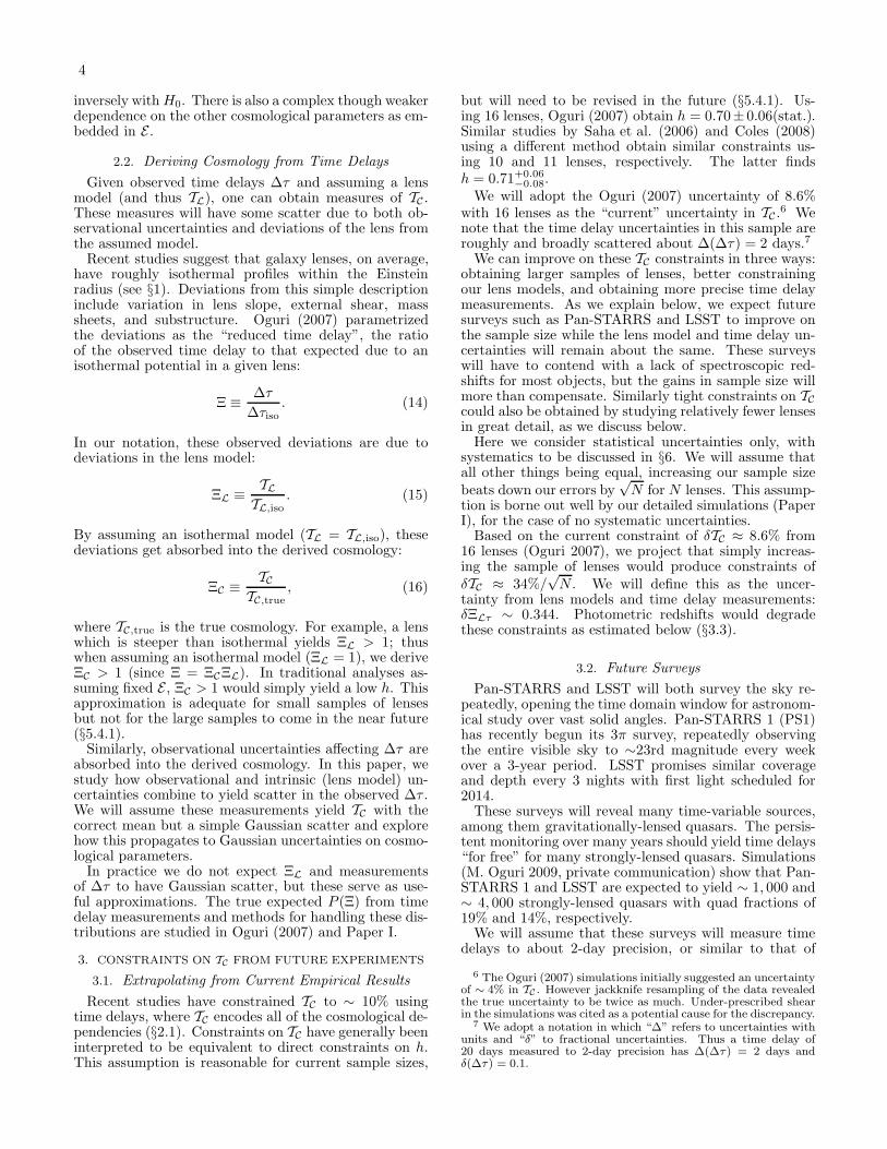
Recent studies have constrained TC to ∼ 10% usingtime delays, where TC encodes all of the cosmological de-pendencies (§2.1). Constraints on TC have generally beeninterpreted to be equivalent to direct constraints on h.This assumption is reasonable for current sample sizes,

but will need to be revised in the future (§5.4.1). Us-ing 16 lenses, Oguri (2007) obtain h = 0.70± 0.06(stat.).Similar studies by Saha et al. (2006) and Coles (2008)using a different method obtain similar constraints us-ing 10 and 11 lenses, respectively. The latter findsh = 0.71+0.06

−0.08.We will adopt the Oguri (2007) uncertainty of 8.6%

with 16 lenses as the “current” uncertainty in TC .6 Wenote that the time delay uncertainties in this sample areroughly and broadly scattered about ∆(∆τ) = 2 days.7

We can improve on these TC constraints in three ways:obtaining larger samples of lenses, better constrainingour lens models, and obtaining more precise time delaymeasurements. As we explain below, we expect futuresurveys such as Pan-STARRS and LSST to improve onthe sample size while the lens model and time delay un-certainties will remain about the same. These surveyswill have to contend with a lack of spectroscopic red-shifts for most objects, but the gains in sample size willmore than compensate. Similarly tight constraints on TCcould also be obtained by studying relatively fewer lensesin great detail, as we discuss below.

Here we consider statistical uncertainties only, withsystematics to be discussed in §6. We will assume thatall other things being equal, increasing our sample sizebeats down our errors by

√N for N lenses. This assump-

tion is borne out well by our detailed simulations (PaperI), for the case of no systematic uncertainties.

Based on the current constraint of δTC ≈ 8.6% from16 lenses (Oguri 2007), we project that simply increas-ing the sample of lenses would produce constraints ofδTC ≈ 34%/

√N . We will define this as the uncer-

tainty from lens models and time delay measurements:δΞLτ ∼ 0.344. Photometric redshifts would degradethese constraints as estimated below (§3.3).

3.2. Future Surveys

Pan-STARRS and LSST will both survey the sky re-peatedly, opening the time domain window for astronom-ical study over vast solid angles. Pan-STARRS 1 (PS1)has recently begun its 3π survey, repeatedly observingthe entire visible sky to ∼23rd magnitude every weekover a 3-year period. LSST promises similar coverageand depth every 3 nights with first light scheduled for2014.

These surveys will reveal many time-variable sources,among them gravitationally-lensed quasars. The persis-tent monitoring over many years should yield time delays“for free” for many strongly-lensed quasars. Simulations(M. Oguri 2009, private communication) show that Pan-STARRS 1 and LSST are expected to yield ∼ 1, 000 and∼ 4, 000 strongly-lensed quasars with quad fractions of19% and 14%, respectively.

We will assume that these surveys will measure timedelays to about 2-day precision, or similar to that of

6 The Oguri (2007) simulations initially suggested an uncertaintyof ∼ 4% in TC . However jackknife resampling of the data revealedthe true uncertainty to be twice as much. Under-prescribed shearin the simulations was cited as a potential cause for the discrepancy.

7 We adopt a notation in which “∆” refers to uncertainties withunits and “δ” to fractional uncertainties. Thus a time delay of20 days measured to 2-day precision has ∆(∆τ) = 2 days andδ(∆τ) = 0.1.

5

0 1 2 3 4 5redshift

0.0

0.2

0.4

0.6

0.8

1.0

Rela

tive n

um

ber

lenses

sources

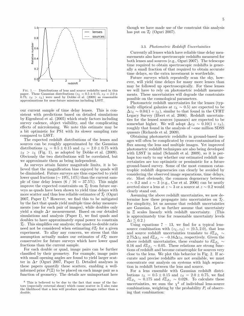
Fig. 1.— Distributions of lens and source redshifts used in thispaper. These Gaussian distributions (zL = 0.5 ± 0.15, zS = 2.0 ±0.75; zS > zL) were used by Dobke et al. (2009) as reasonableapproximations for near-future missions including LSST.

our current sample of time delay lenses. This is con-sistent with predictions based on detailed simulationsby Eigenbrod et al. (2005) which study factors includingsurvey cadence, object visibility, and the complicatingeffects of microlensing. We note this estimate may bea bit optimistic for PS1 with its slower sampling ratecompared to LSST.

The expected redshift distributions of the lenses andsources can be roughly approximated by the Gaussiandistributions zL = 0.5 ± 0.15 and zS = 2.0 ± 0.75 withzS > zL (Fig. 1), as adopted by Dobke et al. (2009).Obviously the two distributions will be correlated, butwe approximate them as being independent.

As surveys attain fainter magnitude limits, it is be-lieved that the magnification bias enjoyed by quads willbe diminished. Future surveys are thus expected to yieldlower quad fractions (∼ 19%, 14%) than the current sam-ple of time delay lenses (6 / 16 = 37.5%). This mightimprove the expected constraints on TC from future sur-veys as quads have been shown to yield time delays withmore scatter and thus less reliable estimates of TC (Oguri2007, Paper I).8 However, we find this to be mitigatedby the fact that quads yield multiple time delay measure-ments (one for each pair of images), while doubles onlyyield a single ∆τ measurement. Based on our detailedsimulations and analysis (Paper I), we find quads anddoubles to have approximately equal power to constrainTC . This simplifies our analysis; the quad-to-double rationeed not be considered when estimating δTC for a givenexperiment. To allay any concern, we stress that thisassumption actually makes our estimates of δTC moreconservative for future surveys which have lower quadfractions than the current sample.

For each double or quad, image pairs can be furtherclassified by their geometry. For example, image pairswith small opening angles are found to yield larger scat-ter in ∆τ (Oguri 2007, Paper I). Detailed analyses inthese papers quantify these scatters, enabling a well-informed prior P (Ξ) to be placed on each image pair as afunction of geometry. The details are unimportant here

8 This is believed to be due to the fact that some of the fac-tors (especially external shear) which cause scatter in Ξ also raisethe likelihood that a lens will produce quad images rather than adouble.

though we have made use of the constraint this analysishas put on TC (Oguri 2007).

3.3. Photometric Redshift Uncertainties

Currently all lenses which have reliable time delay mea-surements also have spectroscopic redshifts measured forboth lenses and sources (e.g., Oguri 2007). The telescopetime required to obtain spectroscopic redshifts is gener-ally a small fraction of that required to obtain accuratetime delays, so the extra investment is worthwhile.

Future surveys which repeatedly scan the sky, how-ever, will yield time delays for many more lenses thanmay be followed up spectroscopically. For these lenseswe will have to rely on photometric redshift measure-ments. These uncertainties will degrade the constraintspossible on the cosmological parameters.

Photometric redshift uncertainties for the lenses (typ-ically elliptical galaxies at zL ∼ 0.5) are expected to be∆zL ∼ 0.04(1 + zL), similar to that found in the CFHTLegacy Survey (Ilbert et al. 2006). Redshift uncertain-ties for the lensed sources (quasars) are expected to besomewhat higher. We will adopt ∆zS ∼ 0.10(1 + zS),roughly that found in the analysis of ∼one million SDSSquasars (Richards et al. 2009).

Obtaining photometric redshifts in ground-based im-ages will often be complicated by cross-contamination offlux among the lens and multiple images. Yet improvedphotometric redshift techniques are also being developedwith LSST in mind (Schmidt et al. 2009), so it is per-haps too early to say whether our estimated redshift un-certainties are too optimistic or pessimistic for a futureground-based survey. Some of the most common catas-trophic redshift degeneracies can clearly be avoided byconsidering the observed image separations, time delays,etc. Most obviously, the common degeneracy betweenz ∼ 0.2 and z ∼ 3 (e.g., Coe et al. 2006) can be neatlyaverted since a lens at z ∼ 3 or a source at z ∼ 0.2 wouldclearly stand out.

Assuming the above redshift uncertainties, we now de-termine how these propagate into uncertainties on TC .For simplicity, let us assume that redshift uncertaintiesare Gaussian. Let us further assume that uncertaintyin Ξ scales linearly with redshift uncertainty. (Thisis approximately true for reasonable uncertainty levels∆z . 0.2.)

Using equations 7 – 13, we find for a typical lens-source combination with (zL, zS) = (0.5, 2.0), that lensand source redshift uncertainties translate to δΞZL

∼2.75∆zL and δΞZS

∼ −0.16∆zS, respectively. Given theabove redshift uncertainties, these evaluate to δΞZL

∼0.16 and δΞZS

∼ 0.05. These relations are strong func-tions of redshift and become catastrophic for sources veryclose to the lens. We plot this behavior in Fig. 2. If ac-curate and precise redshifts are not available, we mustconcentrate our analysis on systems with high separa-tion in redshift between the lens and source.

For a lens ensemble with Gaussian redshift distri-butions zL = 0.5 ± 0.15 and zS = 2.0 ± 0.75, we findδΞZL

∼ 0.175 and δΞZS∼ 0.028. To calculate these

uncertainties, we sum the χ2 of individual lens-sourcecombinations, weighting by the probability Pi of observ-ing that combination:

6

1

σ2=

∑

i

Pi

σ2i

. (17)

Note that this sum naturally assigns more weight to moreconfident measurements.

Assuming the lens and source redshift uncertaintiescan be added in quadrature,

δΞ2Z = δΞ2

ZL+ δΞ2

ZS, (18)

we find δΞZ ∼ 0.177.Of course, these are just estimates for large ensembles.

In practice, redshift probability distributions P (z) forindividual galaxies will be properly folded into the P (TC)determinations. Biased redshifts would yield biased TC ,the effects of which we study in Paper III.

3.4. Projected Constraints from Large Surveys

We now calculate the total uncertainty δTC expectedfor large surveys with photometric redshifts. The com-bined lens model and time delay uncertainties are δΞLτ ∼0.344, based on extrapolation of the current empiricalOguri (2007) finding (§3.1). We estimate uncertain-ties of δΞZ ∼ 0.177 due to redshift uncertainties of∆zL ∼ 0.04(1 + zL) and ∆zS ∼ 0.10(1 + zS) for thelenses and sources, respectively (§3.3).

The simplest estimate of the total uncertainty is toadd these uncertainties in quadrature:

δΞ2 = δΞ2Lτ + δΞ2

Z . (19)

This yields δΞ ∼ 0.387.To be more precise, all of the uncertainties should be

added in quadrature for each lens individually beforecombining them according to Eq. 17. Repeating the anal-ysis in this way, we find δΞ ∼ 0.402.

Thus we expect large surveys with photometric uncer-tainties given above to yield δTC ∼ 40%/

√N . We project

δTC ∼ 1.3% for PS1 (1,000 lenses) and δTC ∼ 0.64% forLSST (4,000 lenses).

Table 1 summarizes the progress we can expect to makein “Stages” corresponding to those defined by the DarkEnergy Task Force (DETF; Albrecht et al. 2006, 2009):“Stage I” = current, “II” = ongoing, “III” = currentlyproposed, “IV” = large new mission. Again, we stressthese are estimates of statistical uncertainties only. Largesurveys are compared to dedicated monitoring and de-tailed analysis of a smaller sample of lenses.

We might have made our analysis more sophisticatedstill, calculating δΞLτ , δΞZL

, and δΞZSindividually for

each lens-source combination in our ensemble. Lensesand sources at higher redshift, for example, will bebrighter and higher magnification cases on average, al-tering their δΞLτ somewhat. The approximations madein our above analysis should suffice for our purposes here.

3.5. Quality vs. Quantity

Thus far we have assumed that detailed observationsand analysis would not be performed on the lenses. Thealternative is to study fewer lenses in more detail, reduc-ing the uncertainties for each lens. In practice, we expect

both strategies to be pursued and the combined power ofboth analyses to place the tightest possible constraintson TC .

Moustakas et al. (2008) have designed a mission con-cept that would be dedicated to monitoring a sample offour-image lenses, with the primary goal of constrain-ing fundamental properties of dark matter. This space-based Observatory for Multi-Epoch Gravitational LensAstrophysics (OMEGA) would monitor 100 time delaylenses to achieve precise and accurate . 0.1 day timedelay measurements. Supporting measurements wouldaim to reduce the model uncertainty of each lens to 5%(δΞL = 0.05) and thus constrain TC to 5% with each lens,as claimed recently for B1608+656 (Suyu et al. 2009a).These supporting measurements, including velocity dis-persion in the lens and characterization of the group envi-ronment (see discussion in §6.2), would be carried out ei-ther with OMEGA itself or though coordinated efforts byground-based telescopes and JWST. Spectroscopic red-shifts would also be obtained for the 100 lens galaxiesand lensed quasars.

Lenses targeted by OMEGA will be quads, enablingmeasurements of time delay ratios among the imagepairs. This would provide constraints on the dark mattersubstructure mass function (Keeton & Moustakas 2009;Keeton 2009, Moustakas et al., in preparation).

Given lens models accurate to 5% for 100 galaxies, wemight expect OMEGA to yield δTC ∼ 5%/

√100 = 0.5%.

The time delays would be measured with sufficient pre-cision so as not to contribute significantly to the totaluncertainty in δTC . The multiple time delay measure-ments per lens (quad) also help reduce this contribution.Based on the expected time delay distribution for a sam-ple of quads (Paper I), we estimate that ∆(∆τ) = 0.1-day uncertainties would inflate the TC uncertainty onlyto ∼ 0.515%.

If both LSST and OMEGA obtain their measure-ments of TC free of significant systematics, their com-bined power could further reduce the uncertainty toδTC ∼ 0.4%.

4. DEPENDENCE OF TC ON COSMOLOGY

We expect LSST time delay lenses to constrain TC to∼ 0.64%. In this section we begin to explore how this“Stage IV” constraint translates to constraints on cos-mological parameters. We study the dependence of TCon (h, Ωm, Ωde, Ωk, w0, wa) for several cosmologies as out-lined in Table 2.

4.1. Flat universe with a cosmological constant (h,ΩΛ = 1 − Ωm)

First, we add a single free parameter ΩΛ (in additionto h) in considering a flat universe with a cosmologicalconstant (w = −1). Given δTC = 0.64% from an ensem-ble with all lenses at zL = 0.5 and all sources at zS = 2.0,we would obtain confidence contours shown in Fig. 4.

The shape of these curves shifts somewhat as a functionof zL and zS . Given an ensemble of lenses and sourceswith Gaussian redshift distributions zL = 0.5± 0.15 andzS = 2.0±0.75 as discussed above, we begin to break the(h, ΩΛ) degeneracy (Table 5). Assuming a flat universe,Stage IV time delays could provide independent evidencefor ΩΛ > 0. Whether this remains interesting by StageIV remains to be seen. The constraints on h are certainly

7

0.2 0.4 0.6 0.8 1.0zL

0.5

1.0

1.5

2.0

2.5

3.0

3.5

z S

zL0.15

0.2

0.30.40.5

12

0.125

0.150

0.175

0.200

0.225

0.250

0.275

0.300

0.325

ZL

0.2 0.4 0.6 0.8 1.0zL

0.5

1.0

1.5

2.0

2.5

3.0

3.5

z S

zL

0.025

0.05

0.10.2

0.3

0.51 2 0.00

0.04

0.08

0.12

0.16

0.20

0.24

0.28

0.32

ZS

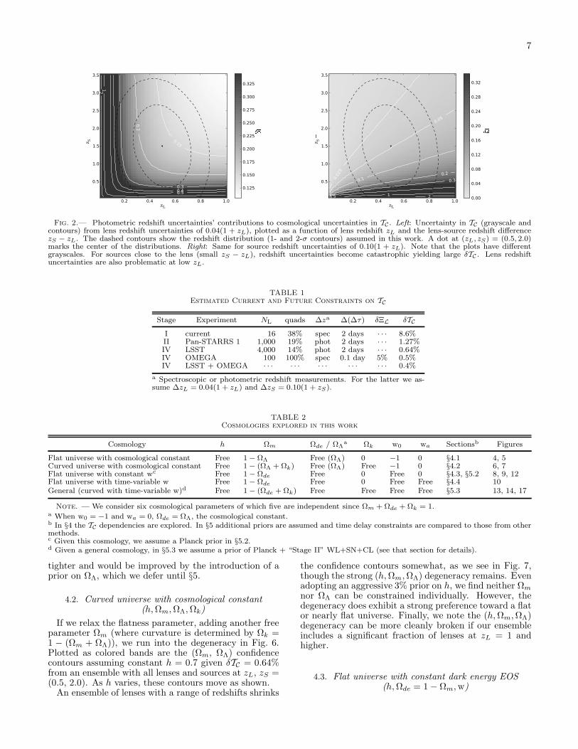
Fig. 2.— Photometric redshift uncertainties’ contributions to cosmological uncertainties in TC . Left: Uncertainty in TC (grayscale andcontours) from lens redshift uncertainties of 0.04(1 + zL), plotted as a function of lens redshift zL and the lens-source redshift differencezS − zL. The dashed contours show the redshift distribution (1- and 2-σ contours) assumed in this work. A dot at (zL, zS) = (0.5, 2.0)marks the center of the distributions. Right: Same for source redshift uncertainties of 0.10(1 + zL). Note that the plots have differentgrayscales. For sources close to the lens (small zS − zL), redshift uncertainties become catastrophic yielding large δTC . Lens redshiftuncertainties are also problematic at low zL.

TABLE 1

Estimated Current and Future Constraints on TC

Stage Experiment NL quads ∆za ∆(∆τ) δΞL δTC

I current 16 38% spec 2 days · · · 8.6%II Pan-STARRS 1 1,000 19% phot 2 days · · · 1.27%IV LSST 4,000 14% phot 2 days · · · 0.64%IV OMEGA 100 100% spec 0.1 day 5% 0.5%IV LSST + OMEGA · · · · · · · · · · · · · · · 0.4%

a Spectroscopic or photometric redshift measurements. For the latter we as-sume ∆zL = 0.04(1 + zL) and ∆zS = 0.10(1 + zS).

TABLE 2

Cosmologies explored in this work

Cosmology h Ωm Ωde / ΩΛa Ωk w0 wa Sectionsb Figures

Flat universe with cosmological constant Free 1 − ΩΛ Free (ΩΛ) 0 −1 0 §4.1 4, 5Curved universe with cosmological constant Free 1 − (ΩΛ + Ωk) Free (ΩΛ) Free −1 0 §4.2 6, 7Flat universe with constant wc Free 1 − Ωde Free 0 Free 0 §4.3, §5.2 8, 9, 12Flat universe with time-variable w Free 1 − Ωde Free 0 Free Free §4.4 10General (curved with time-variable w)d Free 1 − (Ωde + Ωk) Free Free Free Free §5.3 13, 14, 17

Note. — We consider six cosmological parameters of which five are independent since Ωm + Ωde + Ωk = 1.a When w0 = −1 and wa = 0, Ωde = ΩΛ, the cosmological constant.b In §4 the TC dependencies are explored. In §5 additional priors are assumed and time delay constraints are compared to those from othermethods.c Given this cosmology, we assume a Planck prior in §5.2.d Given a general cosmology, in §5.3 we assume a prior of Planck + “Stage II” WL+SN+CL (see that section for details).

tighter and would be improved by the introduction of aprior on ΩΛ, which we defer until §5.

4.2. Curved universe with cosmological constant(h, Ωm, ΩΛ, Ωk)

If we relax the flatness parameter, adding another freeparameter Ωm (where curvature is determined by Ωk =1 − (Ωm + ΩΛ)), we run into the degeneracy in Fig. 6.Plotted as colored bands are the (Ωm, ΩΛ) confidencecontours assuming constant h = 0.7 given δTC = 0.64%from an ensemble with all lenses and sources at zL, zS =(0.5, 2.0). As h varies, these contours move as shown.

An ensemble of lenses with a range of redshifts shrinks

the confidence contours somewhat, as we see in Fig. 7,though the strong (h, Ωm, ΩΛ) degeneracy remains. Evenadopting an aggressive 3% prior on h, we find neither Ωm

nor ΩΛ can be constrained individually. However, thedegeneracy does exhibit a strong preference toward a flator nearly flat universe. Finally, we note the (h, Ωm, ΩΛ)degeneracy can be more cleanly broken if our ensembleincludes a significant fraction of lenses at zL = 1 andhigher.

4.3. Flat universe with constant dark energy EOS(h, Ωde = 1 − Ωm, w)

8

1 10 100 1000 10000# lenses

0.0050.0060.0070.0080.009

0.01

0.02

0.03

0.040.050.060.070.080.09

0.1

0.2

0.3

0.4

TC

current

PS1

LSST

OMEGA

Current (spec-z)Future "quantity" (phot-z)Future "quality" (spec-z+)

Fig. 3.— Constraints on δTC as a function of ensemble size andobservational uncertainties. The current ensemble has time delaysmeasured to roughly ∆(∆τ) = 2 day precision and spectroscopicredshifts measured for all lenses and sources. Future large surveys(“quantity”) should have similar time delay precisions but pho-tometric redshifts measured for lenses (∆zL = 0.04(1 + zL)) andsources (∆zS = 0.10(1 + zS)). A dedicated campaign (“quality”)could in principle obtain tight lens model constraints (δΞL = 5%)with high-precision time delays (∆(∆τ) = 0.1 day) and spectro-scopic redshifts.

0.62 0.64 0.66 0.68 0.70 0.72 0.74h

0.0

0.2

0.4

0.6

0.8

1.0

0.92

0.94

0.94

0.96

0.98

1.00

1.02

1.041.06

1.08

1.10

1.12

1.0

0.8

0.6

0.4

0.2

0.0

m

Fig. 4.— Confidence contours (1- and 2-σ colored bands) for(h, ΩΛ = 1 − Ωm) given “Stage IV” δTC = 0.64% obtained froman ensemble with all lenses and sources at zL, zS = (0.5, 2.0).Here we assume a flat universe with a cosmological constant (w =−1). Also plotted are contours of constant ΞC ≡ TC/TC,true, whereTC,true ≈ 0.99 for the input redshifts and cosmology. The inputcosmology (h, Ωm, ΩΛ) = (0.7, 0.3, 0.7) is marked with dotted linesand a white dot.

Current cosmological constraints are consistent with aflat universe with a cosmological constant (as exploredin §4.1). As a first perturbation to this model, it is com-mon to explore constraints on w 6= −1 while maintainingconstant w in a flat universe. This cosmology has threefree parameters (h, Ωde, w) with Ωm = 1 − Ωde.

Given enough data and appropriate priors, time delaylenses could place strong constraints on the dark energyequation of state parameter w (see §5.2). Figs. 8 and 9explore the dependence of TC on (w, Ωde) assuming a flatuniverse and constant w.

4.4. Flat universe with time-variable dark energy EOS(h, Ωde = 1 − Ωm, w0, wa)

0.62 0.64 0.66 0.68 0.70 0.72 0.74h

0.0

0.2

0.4

0.6

0.8

1.0

1.0

0.8

0.6

0.4

0.2

0.0

mzl = 0.65zs = 2.75zl = 0.5zs = 2.0zl = 0.35zs = 1.25ensemble

Fig. 5.— Confidence contours (1- and 2-σ colored bands) for (h,ΩΛ = 1 − Ωm) given δTC = 0.64% and assuming a flat universewith a cosmological constant (w = −1). Each of the three faintercurves corresponds to all lenses and sources at the same pair ofredshifts: zL, zS = (0.65, 2.75), (0.5, 2.0), (0.35, 1.25), as marked.Next we consider an ensemble of lenses and sources with Gaussianredshift distributions: zL, zS = (0.5±0.15, 2.0±0.75). These yieldthe tighter constraints (marked “ensemble”). The input cosmology(h, Ωm,ΩΛ) = (0.7, 0.3, 0.7) is marked with a white dot.

0.0 0.2 0.4 0.6 0.8 1.0m

0.0

0.2

0.4

0.6

0.8

1.0

FLAT

0.640.65

0.6

6

0.6

7

0.6

8

0.6

9

h =

0.7

0.7

1

0.7

2

0.7

30.7

4

Fig. 6.— Confidence contours (1- and 2-σ colored bands) for(Ωm,ΩΛ) given δTC = 0.64% obtained from an ensemble with alllenses and sources at zL, zS = (0.5, 2.0). The colored bands shiftin (Ωm,ΩΛ) space as h varies. A cosmological constant (w = −1)is assumed. The input cosmology (h, Ωm, ΩΛ) = (0.7, 0.3, 0.7) ismarked with a white dot. Flat cosmologies lie along the dottedline, and this line’s intersection with the colored bands explainsthe strange shape of the colored bands in the previous plot.

The most interesting constraints we can hope to placeon dark energy are to verify or falsify the following: w =−1 (cosmological constant) and wa = 0 (constant w). InFig. 10 we explore the dependence of TC on (w0, wa) (seeEq. 10). The colored bands are the constraints we couldobtain given perfect knowledge of (h, Ωm, Ωde). The solidlines on the left show the curves’ migration as a functionof h. On the right, we also explore dependence on Ωde

for a flat universe (Ωm + Ωde = 1).

5. COSMOLOGICAL CONSTRAINTS FROM FUTUREEXPERIMENTS

We now consider the full parameter space(h, Ωm, Ωde, Ωk, w0, wa) and derive the constraintsthat may be placed on these parameters given con-straints on TC along with various priors. Stage IV timedelay constraints are compared to those expected fromother experiments as estimated by the Dark Energy

9

0.0 0.2 0.4 0.6 0.8 1.0 m

0.0

0.2

0.4

0.6

0.8

1.0

FLAT

ensemble, h = 0.7

fixed (zl, zs), h = 0.7

ensemble, h = 0.7 3%

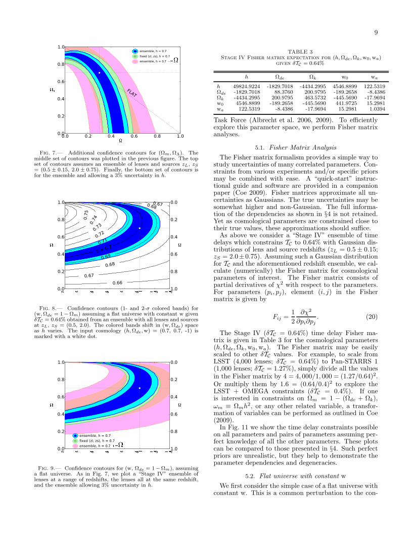
Fig. 7.— Additional confidence contours for (Ωm, ΩΛ). Themiddle set of contours was plotted in the previous figure. The topset of contours assumes an ensemble of lenses and sources zL, zS

= (0.5 ± 0.15, 2.0 ± 0.75). Finally, the bottom set of contours isfor the ensemble and allowing a 3% uncertainty in h.

1.5 1.4 1.3 1.2 1.1 1.0 0.9 0.8w0.0

0.2

0.4

0.6

0.8

1.0

de

0.66

0.67

0.67

0.68

0.68

0.69h = 0.70.71

0.720.7

30.740

.75

1.0

0.8

0.6

0.4

0.2

0.0

m

Fig. 8.— Confidence contours (1- and 2-σ colored bands) for(w, Ωde = 1−Ωm) assuming a flat universe with constant w givenδTC = 0.64% obtained from an ensemble with all lenses and sourcesat zL, zS = (0.5, 2.0). The colored bands shift in (w, Ωde) spaceas h varies. The input cosmology (h, Ωde, w) = (0.7, 0.7, -1) ismarked with a white dot.

1.5 1.4 1.3 1.2 1.1 1.0 0.9 0.8w0.0

0.2

0.4

0.6

0.8

1.0

de

ensemble, h = 0.7

fixed (zl, zs), h = 0.7

ensemble, h = 0.7 3%1.0

0.8

0.6

0.4

0.2

0.0

m

Fig. 9.— Confidence contours for (w, Ωde = 1−Ωm), assuminga flat universe. As in Fig. 7, we plot a “Stage IV” ensemble oflenses at a range of redshifts, the lenses all at the same redshift,and the ensemble allowing 3% uncertainty in h.

TABLE 3

Stage IV Fisher matrix expectation for (h, Ωde,Ωk, w0,wa)given δTC = 0.64%

h Ωde Ωk w0 wa

h 49824.9224 -1829.7018 -4434.2995 4546.8899 122.5319Ωde -1829.7018 88.3760 200.9795 -189.2658 -8.4386Ωk -4434.2995 200.9795 463.5732 -445.5690 -17.9694w0 4546.8899 -189.2658 -445.5690 441.9725 15.2981wa 122.5319 -8.4386 -17.9694 15.2981 1.0394

Task Force (Albrecht et al. 2006, 2009). To efficientlyexplore this parameter space, we perform Fisher matrixanalyses.

5.1. Fisher Matrix Analysis

The Fisher matrix formalism provides a simple way tostudy uncertainties of many correlated parameters. Con-straints from various experiments and/or specific priorsmay be combined with ease. A “quick-start” instruc-tional guide and software are provided in a companionpaper (Coe 2009). Fisher matrices approximate all un-certainties as Gaussians. The true uncertainties may besomewhat higher and non-Gaussian. The full informa-tion of the dependencies as shown in §4 is not retained.Yet as cosmological parameters are constrained close totheir true values, these approximations should suffice.

As above we consider a “Stage IV” ensemble of timedelays which constrains TC to 0.64% with Gaussian dis-tributions of lens and source redshifts (zL = 0.5 ± 0.15;zS = 2.0±0.75). Assuming such a Gaussian distributionfor TC and the aforementioned redshift ensemble, we cal-culate (numerically) the Fisher matrix for cosmologicalparameters of interest. The Fisher matrix consists ofpartial derivatives of χ2 with respect to the parameters.For parameters (pi, pj), element (i, j) in the Fishermatrix is given by

Fij =1

2

∂χ2

∂pi∂pj

. (20)

The Stage IV (δTC = 0.64%) time delay Fisher ma-trix is given in Table 3 for the cosmological parameters(h, Ωde, Ωk, w0, wa). The Fisher matrix may be easilyscaled to other δTC values. For example, to scale fromLSST (4,000 lenses; δTC = 0.64%) to Pan-STARRS 1(1,000 lenses; δTC = 1.27%), simply divide all the valuesin the Fisher matrix by 4 = 4, 000/1, 000 = (1.27/0.64)2.Or multiply them by 1.6 = (0.64/0.4)2 to explore theLSST + OMEGA constraints (δTC = 0.4%). If oneis interested in constraints on Ωm = 1 − (Ωde + Ωk),ωm ≡ Ωmh2, or any other related variable, a transfor-mation of variables can be performed as outlined in Coe(2009).

In Fig. 11 we show the time delay constraints possibleon all parameters and pairs of parameters assuming per-fect knowledge of all the other parameters. These plotscan be compared to those presented in §4. Such perfectpriors are unrealistic, but they help to demonstrate theparameter dependencies and degeneracies.

5.2. Flat universe with constant w

We first consider the simple case of a flat universe withconstant w. This is a common perturbation to the con-

10

1.4 1.2 1.0 0.8 0.6w03

2

1

0

1

2

3

wa

0.6

60.67

0.68

0.69

h = 0.7

0.71

0.72

0.73

0.74

0.75

0.75

0.76

0.760.770.78

1.4 1.2 1.0 0.8 0.6w03

2

1

0

1

2

3

wa

0.20.3

de= 0.4

0.5

0.60.7

0.8 0.9 1.0

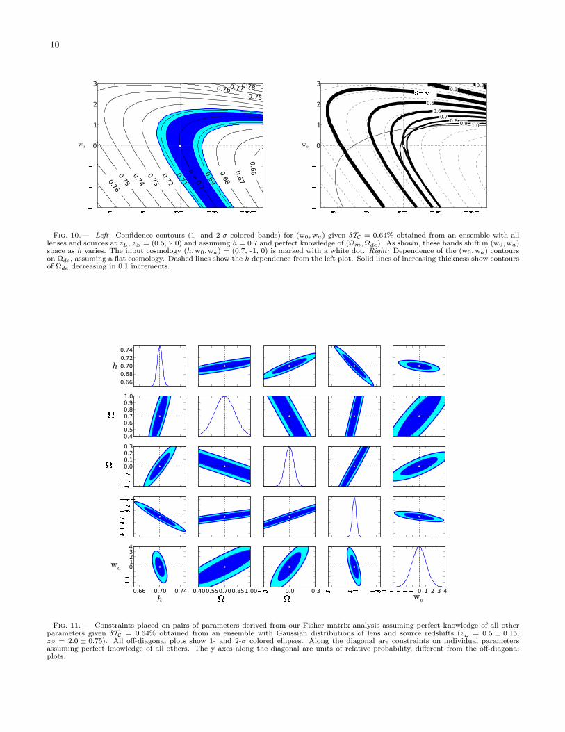
Fig. 10.— Left : Confidence contours (1- and 2-σ colored bands) for (w0,wa) given δTC = 0.64% obtained from an ensemble with alllenses and sources at zL, zS = (0.5, 2.0) and assuming h = 0.7 and perfect knowledge of (Ωm,Ωde). As shown, these bands shift in (w0,wa)space as h varies. The input cosmology (h, w0,wa) = (0.7, -1, 0) is marked with a white dot. Right: Dependence of the (w0,wa) contourson Ωde, assuming a flat cosmology. Dashed lines show the h dependence from the left plot. Solid lines of increasing thickness show contoursof Ωde decreasing in 0.1 increments.

0.660.680.700.720.74

h

0.40.50.60.70.80.91.0

de

0.30.20.10.00.10.20.3

k

1.61.41.21.00.80.60.4w0

0.66 0.70 0.74

h

432101234

wa

0.400.550.700.851.00

de

0.3 0.0 0.3

k

1.6 1.0 0.4w0 4 3 2 1 0 1 2 3 4wa

Fig. 11.— Constraints placed on pairs of parameters derived from our Fisher matrix analysis assuming perfect knowledge of all otherparameters given δTC = 0.64% obtained from an ensemble with Gaussian distributions of lens and source redshifts (zL = 0.5 ± 0.15;zS = 2.0 ± 0.75). All off-diagonal plots show 1- and 2-σ colored ellipses. Along the diagonal are constraints on individual parametersassuming perfect knowledge of all others. The y axes along the diagonal are units of relative probability, different from the off-diagonalplots.

11

cordance cosmology. The goal is to detect deviation fromw = −1, equivalent to the cosmological constant Λ. This3-parameter cosmology (h, Ωde, w, with Ωm = 1 − Ωde)was explored above in §4.3.

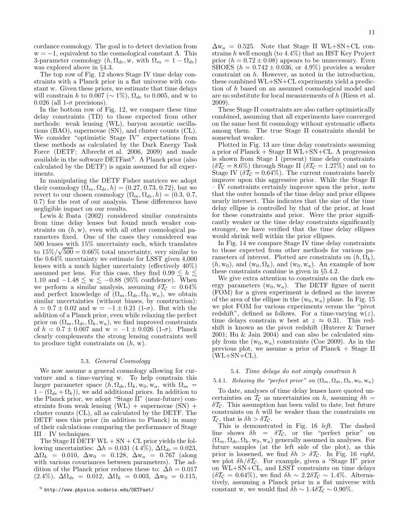
The top row of Fig. 12 shows Stage IV time delay con-straints with a Planck prior in a flat universe with con-stant w. Given these priors, we estimate that time delayswill constrain h to 0.007 (∼ 1%), Ωde to 0.005, and w to0.026 (all 1-σ precisions).

In the bottom row of Fig. 12, we compare these timedelay constraints (TD) to those expected from othermethods: weak lensing (WL), baryon acoustic oscilla-tions (BAO), supernovae (SN), and cluster counts (CL).We consider “optimistic Stage IV” expectations fromthese methods as calculated by the Dark Energy TaskForce (DETF; Albrecht et al. 2006, 2009) and madeavailable in the software DETFast9. A Planck prior (alsocalculated by the DETF) is again assumed for all exper-iments.

In manipulating the DETF Fisher matrices we adopttheir cosmology (Ωm, Ωde, h) = (0.27, 0.73, 0.72), but werevert to our chosen cosmology (Ωm, Ωde, h) = (0.3, 0.7,0.7) for the rest of our analysis. These differences havenegligible impact on our results.

Lewis & Ibata (2002) considered similar constraintsfrom time delay lenses but found much weaker con-straints on (h, w), even with all other cosmological pa-rameters fixed. One of the cases they considered was500 lenses with 15% uncertainty each, which translatesto 15%/

√500 = 0.66% total uncertainty, very similar to

the 0.64% uncertainty we estimate for LSST given 4,000lenses with a much higher uncertainty (effectively 40%)assumed per lens. For this case, they find 0.99 . h .1.10 and −1.48 . w . −0.88 (95% confidence). Whenwe perform a similar analysis, assuming δTC = 0.64%and perfect knowledge of (Ωm, Ωde, Ωk, wa), we obtainsimilar uncertainties (without biases, by construction):h = 0.7 ± 0.02 and w = −1 ± 0.21 (1-σ). But with theaddition of a Planck prior, even while relaxing the perfectprior on (Ωm, Ωde, Ωk, wa), we find improved constraintsof h = 0.7 ± 0.007 and w = −1 ± 0.026 (1-σ). Planckclearly complements the strong lensing constraints wellto produce tight constraints on (h, w).

5.3. General Cosmology

We now assume a general cosmology allowing for cur-vature and a time-varying w. To help constrain thislarger parameter space (h, Ωde, Ωk, w0, wa, with Ωm =1− (Ωde +Ωk)), we add additional priors. In addition tothe Planck prior, we adopt “Stage II” (near-future) con-straints from weak lensing (WL) + supernovae (SN) +cluster counts (CL), all as calculated by the DETF. TheDETF uses this prior (in addition to Planck) in manyof their calculations comparing the performance of StageIII – IV techniques.

The Stage II DETF WL + SN + CL prior yields the fol-lowing uncertainties: ∆h = 0.031 (4.4%), ∆Ωde = 0.023,∆Ωk = 0.010, ∆w0 = 0.128, ∆wa = 0.767 (alongwith various covariances between parameters). The ad-dition of the Planck prior reduces these to: ∆h = 0.017(2.4%), ∆Ωde = 0.012, ∆Ωk = 0.003, ∆w0 = 0.115,

9 http://www.physics.ucdavis.edu/DETFast/

∆wa = 0.525. Note that Stage II WL+SN+CL con-strains h well enough (to 4.4%) that an HST Key Projectprior (h = 0.72 ± 0.08) appears to be unnecessary. EvenSHOES (h = 0.742 ± 0.036, or 4.9%) provides a weakerconstraint on h. However, as noted in the introduction,these combined WL+SN+CL experiments yield a predic-tion of h based on an assumed cosmological model andare no substitute for local measurements of h (Riess et al.2009).

These Stage II constraints are also rather optimisticallycombined, assuming that all experiments have convergedon the same best fit cosmology without systematic offsetsamong them. The true Stage II constraints should besomewhat weaker.

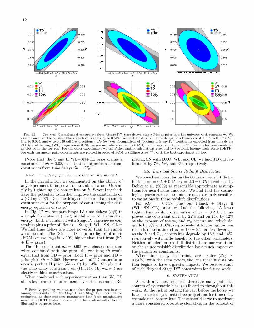
Plotted in Fig. 13 are time delay constraints assuminga prior of Planck + Stage II WL+SN+CL. A progressionis shown from Stage I (present) time delay constraints(δTC = 8.6%) through Stage II (δTC = 1.27%) and on toStage IV (δTC = 0.64%). The current constraints barelyimprove upon this aggressive prior. While the Stage II– IV constraints certainly improve upon the prior, notethat the outer bounds of the time delay and prior ellipsesnearly intersect. This indicates that the size of the timedelay ellipse is controlled by that of the prior, at leastfor these constraints and prior. Were the prior signifi-cantly weaker or the time delay constraints significantlystronger, we have verified that the time delay ellipseswould shrink well within the prior ellipses.

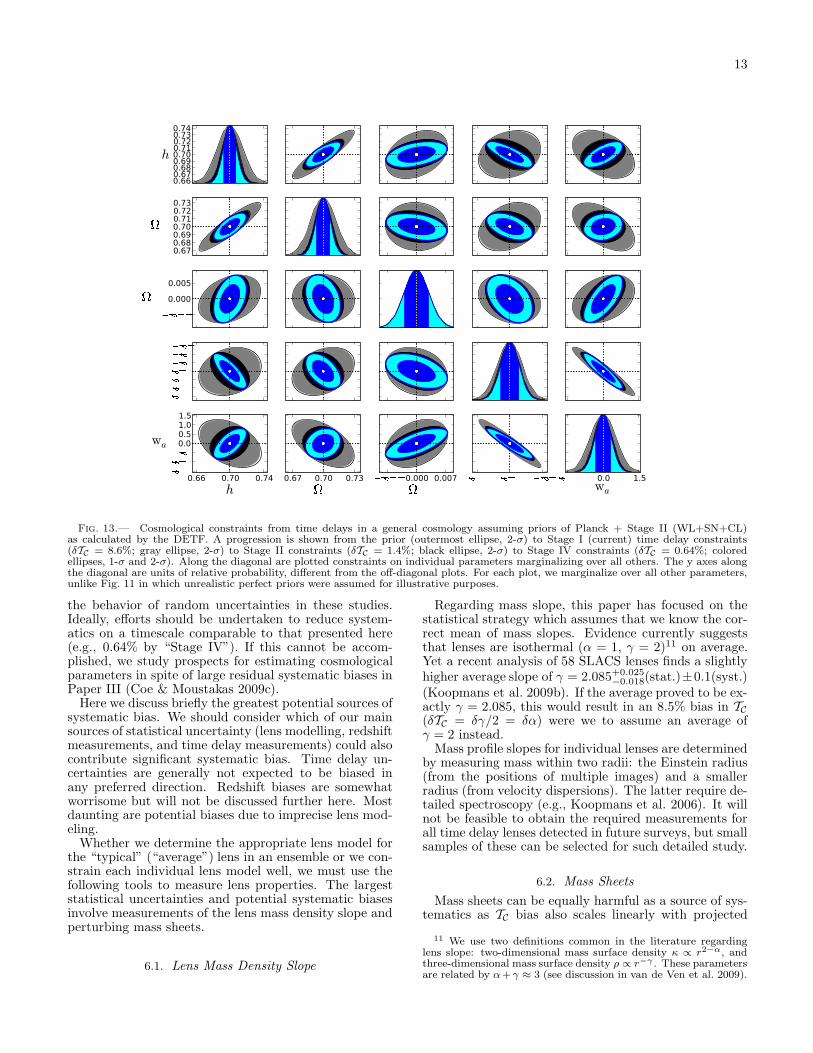
In Fig. 14 we compare Stage IV time delay constraintsto those expected from other methods for various pa-rameters of interest. Plotted are constraints on (h, Ωk),(h, w0), and (w0, Ωk), and (w0, wa). An example of howthese constraints combine is given in §5.4.2.

We give extra attention to constraints on the dark en-ergy parameters (w0, wa). The DETF figure of merit(FOM) for a given experiment is defined as the inverseof the area of the ellipse in the (w0, wa) plane. In Fig. 15we plot FOM for various experiments versus the “pivotredshift”, defined as follows. For a time-varying w(z),time delays constrain w best at z ≈ 0.31. This red-shift is known as the pivot redshift (Huterer & Turner2001; Hu & Jain 2004) and can also be calculated sim-ply from the (w0, wa) constraints (Coe 2009). As in theprevious plot, we assume a prior of Planck + Stage II(WL+SN+CL).

5.4. Time delays do not simply constrain h

5.4.1. Relaxing the “perfect prior” on (Ωm, Ωde, Ωk, w0, wa)

To date, analyses of time delay lenses have quoted un-certainties on TC as uncertainties on h, assuming δh =δTC . This assumption has been valid to date, but futureconstraints on h will be weaker than the constraints onTC , that is δh > δTC .

This is demonstrated in Fig. 16 left. The dashedline shows δh = δTC , or the “perfect prior” on(Ωm, Ωde, Ωk, w0, wa) generally assumed in analyses. Forfuture samples (at the left side of the plot), as thisprior is loosened, we find δh > δTC . In Fig. 16 right,we plot δh/δTC. For example, given a “Stage II” prioron WL+SN+CL, and LSST constraints on time delays(δTC = 0.64%), we find δh ∼ 2.2δTC ∼ 1.4%. Alterna-tively, assuming a Planck prior in a flat universe withconstant w, we would find δh ∼ 1.4δTC ∼ 0.90%.

12

0.6850.690.695 0.7 0.7050.710.715h

0.690

0.695

0.700

0.705

0.710

de

priorTD

0.310

0.305

0.300

0.295

0.290

m

0.685 0.69 0.695 0.7 0.705 0.71 0.715h

1.06

1.04

1.02

1.00

0.98

0.96

0.94w priorTD

1.06 1.04 1.02 1.000.98 0.96 0.94w

0.690

0.695

0.700

0.705

0.710

de

priorTD

0.310

0.305

0.300

0.295

0.290

m

0.67 0.68 0.69 0.7 0.71 0.72 0.73h

0.68

0.69

0.70

0.71

0.72

de

priorBAOTDSNCLWL

0.32

0.31

0.30

0.29

0.28

m

0.67 0.68 0.69 0.7 0.71 0.72 0.73h

1.05

1.00

0.95w

priorBAOCLTDSNWL

1.05 1.00 0.95w

0.68

0.69

0.70

0.71

0.72

!de

priorBAOTDCLSNWL

0.32

0.31

0.30

0.29

0.28

!m

Fig. 12.— Top row: Cosmological constraints from “Stage IV” time delays plus a Planck prior in a flat universe with constant w. Weassume an ensemble of time delays which constrains TC to 0.64% (see text for details). Time delays plus Planck constrain h to 0.007 (1%),Ωde to 0.005, and w to 0.026 (all 1-σ precisions). Bottom row: Comparison of “optimistic Stage IV” constraints expected from time delays(TD), weak lensing (WL), supernovae (SN), baryon acoustic oscillations (BAO), and cluster counts (CL). The time delay constraints areas plotted in the top row. For the other experiments we use Fisher matrix calculations provided by the Dark Energy Task Force (DETF).For each parameter pair, experiments are plotted in order of FOM ∝ (Ellipse Area)−1, with the best experiment on top.

(Note that the Stage II WL+SN+CL prior claims aconstraint of δh = 0.03, such that it outperforms currentconstraints from time delays δh = δTC .)

5.4.2. Time delays provide more than constraints on h

In the introduction we commented on the ability ofany experiment to improve constraints on w and Ωk sim-ply by tightening the constraints on h. Several methodshave the potential to further improve the constraints onh (Olling 2007). Do time delays offer more than a simpleconstraint on h for the purposes of constraining the darkenergy equation of state?

In Fig. 17 we compare Stage IV time delays (left) toa simple h constraint (right) in ability to constrain darkenergy. Each is combined with Stage IV supernovae con-straints plus a prior of Planck + Stage II WL+SN+CL.10

We find time delays are more powerful than the simpleh constraint. The (SN + TD + prior) figure of merit(FOM) on (w0, wa) is ∼ 19% higher than that from (SN+ H + prior).

The “H” constraint δh = 0.009 was chosen such thatwhen combined with the prior, the resulting δh wouldequal that from TD + prior. Both H + prior and TD +prior yield δh = 0.008. However we find TD outperformseven a perfect H prior (δh ∼ 0) by 13%. Simply put,the time delay constraints on (Ωm, Ωde, Ωk, w0, wa) areclearly making contributions.

When combined with experiments other than SN, TDoffers less marked improvements over H constraints. Re-

10 Strictly speaking we have not taken the proper care in com-bining constraints from the Stage II and Stage IV supernova ex-periments, as their nuisance parameters have been marginalizedover in the DETF Fisher matrices. But this analysis will suffice forillustrative purposes here.

placing SN with BAO, WL, and CL, we find TD outper-forms H by 7%, 5%, and 3%, respectively.

5.5. Lens and Source Redshift Distribution

We have been considering the Gaussian redshift distri-butions zL = 0.5 ± 0.15, zS = 2.0 ± 0.75 introduced byDobke et al. (2009) as reasonable approximate assump-tions for near-future missions. We find that the cosmo-logical parameter constraints are not extremely sensitiveto variations in these redshift distributions.

For δTC = 0.64% plus our Planck + Stage II(WL+SN+CL) prior, we find the following. A lowertighter lens redshift distribution of zL = 0.2 ± 0.1 im-proves the constraint on h by 22% and on Ωde by 12%at the expense of the w0 and wa constraints, which de-grade by 8% and 10%, respectively. A higher tighter lensredshift distribution of zL = 1.0 ± 0.1 has less leverage,as the h and Ωde constraints degrade by 15% and 14%,respectively with little benefit to the other parameters.Neither broader lens redshift distributions nor variationson the source redshift distribution have much impact onthe parameter constraints.

When time delay constraints are tighter (δTC <0.64%), with the same priors, the lens redshift distribu-tion begins to have a greater impact. We reserve studyof such “beyond Stage IV” constraints for future work.

6. SYSTEMATICS

As with any measurement, there are many potentialsources of systematic bias, as alluded to throughout thiswork. At the risk of putting the cart before the horse, wehave presented systematic-free projections for time delaycosmological constraints. These should serve to motivatea more considered look at systematics, in the context of

13

0.660.670.680.690.700.710.720.730.74

h

0.670.680.690.700.710.720.73

"de

#0.005

0.000

0.005

"k

#1.3#1.2#1.1#1.0#0.9#0.8#0.7w0

0.66 0.70 0.74

h

#1.5#1.0#0.50.00.51.01.5

wa

0.67 0.70 0.73

"de

#0.0070.000 0.007

"k

#1.3 #1.0 #0.7w0#1.5 0.0 1.5wa

Fig. 13.— Cosmological constraints from time delays in a general cosmology assuming priors of Planck + Stage II (WL+SN+CL)as calculated by the DETF. A progression is shown from the prior (outermost ellipse, 2-σ) to Stage I (current) time delay constraints(δTC = 8.6%; gray ellipse, 2-σ) to Stage II constraints (δTC = 1.4%; black ellipse, 2-σ) to Stage IV constraints (δTC = 0.64%; coloredellipses, 1-σ and 2-σ). Along the diagonal are plotted constraints on individual parameters marginalizing over all others. The y axes alongthe diagonal are units of relative probability, different from the off-diagonal plots. For each plot, we marginalize over all other parameters,unlike Fig. 11 in which unrealistic perfect priors were assumed for illustrative purposes.

the behavior of random uncertainties in these studies.Ideally, efforts should be undertaken to reduce system-atics on a timescale comparable to that presented here(e.g., 0.64% by “Stage IV”). If this cannot be accom-plished, we study prospects for estimating cosmologicalparameters in spite of large residual systematic biases inPaper III (Coe & Moustakas 2009c).

Here we discuss briefly the greatest potential sources ofsystematic bias. We should consider which of our mainsources of statistical uncertainty (lens modelling, redshiftmeasurements, and time delay measurements) could alsocontribute significant systematic bias. Time delay un-certainties are generally not expected to be biased inany preferred direction. Redshift biases are somewhatworrisome but will not be discussed further here. Mostdaunting are potential biases due to imprecise lens mod-eling.

Whether we determine the appropriate lens model forthe “typical” (“average”) lens in an ensemble or we con-strain each individual lens model well, we must use thefollowing tools to measure lens properties. The largeststatistical uncertainties and potential systematic biasesinvolve measurements of the lens mass density slope andperturbing mass sheets.

6.1. Lens Mass Density Slope

Regarding mass slope, this paper has focused on thestatistical strategy which assumes that we know the cor-rect mean of mass slopes. Evidence currently suggeststhat lenses are isothermal (α = 1, γ = 2)11 on average.Yet a recent analysis of 58 SLACS lenses finds a slightlyhigher average slope of γ = 2.085+0.025

−0.018(stat.)±0.1(syst.)(Koopmans et al. 2009b). If the average proved to be ex-actly γ = 2.085, this would result in an 8.5% bias in TC(δTC = δγ/2 = δα) were we to assume an average ofγ = 2 instead.

Mass profile slopes for individual lenses are determinedby measuring mass within two radii: the Einstein radius(from the positions of multiple images) and a smallerradius (from velocity dispersions). The latter require de-tailed spectroscopy (e.g., Koopmans et al. 2006). It willnot be feasible to obtain the required measurements forall time delay lenses detected in future surveys, but smallsamples of these can be selected for such detailed study.

6.2. Mass Sheets

Mass sheets can be equally harmful as a source of sys-tematics as TC bias also scales linearly with projected

11 We use two definitions common in the literature regardinglens slope: two-dimensional mass surface density κ ∝ r2−α, andthree-dimensional mass surface density ρ ∝ r−γ . These parametersare related by α+ γ ≈ 3 (see discussion in van de Ven et al. 2009).

14

0.64 0.66 0.68 0.70 0.72 0.74h

$0.005

0.000

0.005

%k

priorTDCLSNWLBAO

0.64 0.66 0.68 0.70 0.72 0.74h

&1.3

&1.2

&1.1

&1.0

&0.9

&0.8

&0.7w0

priorSNCLTDBAOWL

'1.4 '1.3 '1.2 '1.1 '1.0 '0.9 '0.8 '0.7w0

'0.005

0.000

0.005

(k

priorTDCLSNWLBAO

)1.3 )1.2 )1.1 )1.0 )0.9 )0.8 )0.7w0

)1.0

)0.5

0.0

0.5

1.0

wa

priorTDCLSNBAOWL

Fig. 14.— Comparisons of “Stage IV” constraints possible from time delays (TD), weak lensing (WL), supernovae (SN), baryon acousticoscillations (BAO), and cluster counts (CL) in a general cosmology (allowing for curvature and a time-variable w). For TD, we assume anensemble which constrains TC to 0.64% (see text for details). For the rest we use “optimistic Stage IV” expectations calculated from Fishermatrices provided by the Dark Energy Task Force (DETF). A prior of Planck + Stage II (WL+SN+CL) is assumed for all five experimentsand is plotted in gray. For each parameter pair, experiments are plotted in order of FOM ∝ (Ellipse Area)−1, with the best experiment ontop.

0.25 0.30 0.35 0.40 0.45 0.50Pivot Redshift

1

2

3

4

56789

10

FOM

CL

WL

SN BAO

TD

Fig. 15.— Dark energy figure of merit (FOM ∝

((w0, wa) Ellipse Area)−1, normalized relative to the prior) versuspivot redshift for various “optimistic Stage IV” experiments witha prior of Planck + Stage II (WL+SN+CL) The pivot redshift isthe redshift at which w(z) is best constrained.

mass density, δTC ∼ κ. Mass sheets can result fromboth mass within the lens group environment and massalong the line of sight (over- or under-densities) all theway from source to observer. The former is the domi-nant effect. Simulations (Dalal & Watson 2005) suggest

that group members contribute κenv = 0.03 ± 0.6 dex(i.e., log10(κenv) = log10(0.03) ± 0.6) for a 1-σ upperbound of κenv = 0.12, or 12% bias on TC . Mass alongthe line of sight is generally lower and more nearly fluc-tuates about the cosmic average but should also be ac-counted for. Hilbert et al. (2007) measured mass alongthe lines of sight to strong lenses in the Millennium sim-ulation. For sources at zS = 2, the central 68% span−0.0355 < κlos < 0.0475 (Paper I).

Efforts are made to measure κenv for individuallenses via spectroscopic (and photometric) studies (e.g.,Momcheva et al. 2006; Auger 2008) and simulationswhich estimate the effects of nearby neighbors (e.g.,Keeton & Zabludoff 2004; Dalal & Watson 2005). Simi-lar studies also attempt to identify groups along the lineof sight and estimate their mass sheet contributions (e.g.,Fassnacht et al. 2006).

The alternative is a statistical approach. Measure-ments of κenv or κlos would not be required for individuallenses if we had knowledge of the distributions P (κenv)and P (κlos) for strong lenses. These distributions couldbe obtained from simulations, and one could attemptto correct for the expected bias for lenses to reside inhigh density regions (Dalal & Watson 2005; Oguri et al.2005). However, one might wonder whether these dis-

15

0.005 0.01 0.02 0.05 0.1*TC

0.005

0.01

0.02

0.05

0.1

+h=(

,h)/h

PlanckPlanck + FlatPlanck + w constPlanck + Flat + w constStage IIStage II + w constStage II + Planck"perfect prior"

PS1 currentLSST

OMEG

A

LS+OM

0.005 0.01 0.02 0.05 0.1-TC

1

2

3

4

56789

10

.h/

.TC PlanckPlanck + FlatPlanck + w constPlanck + Flat + w constStage IIStage II + w constStage II + Planck"perfect prior"

PS1 currentLSST

OMEG

A

LS+OM

Fig. 16.— Demonstration that δh > δTC for future ensembles. Left: Constraints on h versus constraints on TC for various priors. Alongthe top horizontal axis we plot experiments with corresponding δTC : current constraints (8.6%), Pan-STARRS 1 (1.27%), LSST (0.64%),OMEGA (0.5%), and LSST + OMEGA (0.4%). The priors are different combinations of the following: Planck, a flat universe, constant w,and a “Stage II” prior from (WL+SN+CL). This Stage II prior constrains Ωk to 0.01, so the additional prior of flatness helps it little here.The bottom line is the “perfect prior”, perfect knowledge of (Ωde, Ωm, Ωk,w0,wa) as is generally assumed, for which δTC = δh. Right:Relative constraints on h compared to the perfect prior. For example, given the Stage II prior, we find δh ∼ 2.2δTC .

/1.3 /1.2 /1.1 /1.0 /0.9 /0.8 /0.7w0

/1.0

/0.5

0.0

0.5

1.0

wa

priorTDSNtot

01.3 01.2 01.1 01.0 00.9 00.8 00.7w0

01.0

00.5

0.0

0.5

1.0

wa

priorHSNtot

Fig. 17.— Left : Combined constraints on (w0, wa) from Stage IV time delays (TD) and supernovae (SN). A prior of Planck + Stage II(WL+SN+CL) is assumed. The TD + prior constraint yields δh = 0.008 (not shown). Right : Similar plot combining Stage IV SN with aδh = 0.009 constraint on Hubble’s constant (that which also yields δh = 0.008 when combined with the prior). Time delays yield a 19%

improvement in figure of merit (FOM ∝ ((w0,wa) Ellipse Area)−1), versus the constraint on h alone. SN + TD shows the most dramaticsuch improvement vs. SN + H. Replacing SN with the other experiments (BAO, WL, CL) we find lesser improvements vs. H of 7%, 5%,and 3%, respectively.

tributions and corrections would prove accurate to thepercent level. Any errors would yield residual systemat-ics in our estimation of TC .

To aid such a statistical approach, lenses in obviousgroups can be excluded from the analysis leaving onlythose systems with low κenv. Such low mass systemswould introduce smaller biases, though a detailed explo-ration of this approach will await future work.

7. CONCLUSIONS

We have presented the first analysis of the potential ofgravitational lens time delays to constrain a broad rangeof cosmological parameters. The cosmological constrain-ing power δTC was calculated for Pan-STARRS 1, LSST,and OMEGA based on expected numbers of lenses (in-cluding the quad-to-double ratio) as well as the expecteduncertainties in lens models, photometric redshifts, andtime delays. Our Fisher matrix results are provided toallow time delay constraints to be easily combined withand compared to constraints from other methods.

We concentrate on “Stage IV” constraints from LSST.

In a flat universe with constant w including a Planckprior, LSST time delay measurements for ∼ 4, 000 lensesshould constrain h to ∼ 0.007 (∼ 1%), Ωde to ∼ 0.005,and w to ∼ 0.026 (all 1-σ precisions). We comparethese results as well as those for a general cosmology toother “optimistic Stage IV” constraints expected fromweak lensing, supernovae, baryon acoustic oscillations,and cluster counts, as calculated by the Dark EnergyTask Force (DETF).

Combined with appropriate priors (those adopted bythe DETF), time delays provide modest constraints on atime-varying w(z) that complement the constraints ex-pected from other methods. Time delays constrain wbest at z ≈ 0.31, the “pivot redshift” for this method.

We find that LSST and OMEGA represent about aneven trade in “quantity versus quality” in terms of con-straining cosmology with time delays. LSST could yieldδTC ∼ 0.64% by measuring time delays for 4,000 lenses,while OMEGA could yield δTC ∼ 0.5% by obtaininghigh-precision time delay measurements and lens model

16

constraints for 100 lenses with spectroscopic redshifts.The combined statistical power of these two missionscould further improve the cosmological constraints toδTC ∼ 0.4%.

We acknowledge useful conversations with Phil Mar-shall, Matt Auger, Chuck Keeton, Chris Kochanek, BenDobke, Chris Fassnacht, Lloyd Knox, Jason Dick, An-

dreas Albrecht, Tony Tyson, and Jason Rhodes. Weare grateful to the DETF for releasing Fisher matri-ces detailing their estimates of cosmological constraintsfrom various experiments. We thank the referee for use-ful comments which led us to significantly improve themanuscript. This work was carried out at Jet PropulsionLaboratory, California Institute of Technology, under acontract with NASA.

REFERENCES

Albrecht, A., Amendola, L., Bernstein, G., Clowe, D., Eisenstein,D., Guzzo, L., Hirata, C., Huterer, D., et al. 2009, ArXive-prints [ADS]

Albrecht, A., Bernstein, G., Cahn, R., Freedman, W. L., Hewitt,J., Hu, W., Huth, J., Kamionkowski, M., et al. 2006, ArXivAstrophysics e-prints [ADS]

Auger, M. W. 2008, MNRAS, 383, L40 [ADS]Blake, C. A., Abdalla, F. B., Bridle, S. L., & Rawlings, S. 2004,

New Astronomy Review, 48, 1063 [ADS]Blandford, R. & Narayan, R. 1986, ApJ, 310, 568 [ADS]Bolton, A. S., Burles, S., Koopmans, L. V. E., Treu, T., &

Moustakas, L. A. 2006, ApJ, 638, 703 [ADS]Braatz, J. 2009, Astronomy, 2010, 23 [ADS]Braatz, J. A., Reid, M. J., Greenhill, L. J., Condon, J. J., Lo,

K. Y., Henkel, C., Gugliucci, N. E., & Hao, L. 2008, inAstronomical Society of the Pacific Conference Series, Vol. 395,Frontiers of Astrophysics: A Celebration of NRAO’s 50thAnniversary, ed. A. H. Bridle, J. J. Condon, & G. C. Hunt,103–+ [ADS]

Cabanac, R. A., Alard, C., Dantel-Fort, M., Fort, B., Gavazzi, R.,Gomez, P., Kneib, J. P., Le Fevre, O., et al. 2007, A&A, 461,813 [ADS]

Chae, K.-H. 2007, ApJ, 658, L71 [ADS]Chevallier, M. & Polarski, D. 2001, International Journal of

Modern Physics D, 10, 213 [ADS]Coe, D. 2009, ArXiv e-prints [ADS]Coe, D., Benıtez, N., Sanchez, S. F., Jee, M., Bouwens, R., &

Ford, H. 2006, AJ, 132, 926 [ADS]Coe, D. A. & Moustakas, L. A. 2009a, in prep. (Paper I)—. 2009c, in prep. (Paper III)Coles, J. 2008, ApJ, 679, 17 [ADS]Dalal, N. & Watson, C. R. 2005, in 25 Years After the Discovery:

Some Current Topics on Lensed QSOs, ed. L. J. Goicoechea[ADS]

Dobke, B. M., King, L. J., Fassnacht, C. D., & Auger, M. W.2009, MNRAS, 397, 311 [ADS]

Eigenbrod, A., Courbin, F., Vuissoz, C., Meylan, G., Saha, P., &Dye, S. 2005, A&A, 436, 25 [ADS]

Fassnacht, C. D., Gal, R. R., Lubin, L. M., McKean, J. P.,Squires, G. K., & Readhead, A. C. S. 2006, ApJ, 642, 30 [ADS]

Fassnacht, C. D., Marshall, P. J., Baltz, A. E., Blandford, R. D.,Schechter, P. L., & Tyson, J. A. 2004, in Bulletin of theAmerican Astronomical Society, Vol. 36, Bulletin of theAmerican Astronomical Society, 1531–+ [ADS]

Faure, C., Kneib, J.-P., Covone, G., Tasca, L., Leauthaud, A.,Capak, P., Jahnke, K., Smolcic, V., et al. 2008, ApJS, 176, 19[ADS]

Freedman, W. L., Madore, B. F., Gibson, B. K., Ferrarese, L.,Kelson, D. D., Sakai, S., Mould, J. R., Kennicutt, Jr., R. C.,et al. 2001, ApJ, 553, 47 [ADS]

Fukugita, M., Futamase, T., Kasai, M., & Turner, E. L. 1992,ApJ, 393, 3 [ADS]

Futamase, T. & Hamaya, T. 1999, Progress of TheoreticalPhysics, 102, 1037 [ADS]

Hilbert, S., White, S. D. M., Hartlap, J., & Schneider, P. 2007,MNRAS, 382, 121 [ADS]

Hogg, D. W. 1999, ArXiv Astrophysics e-prints [ADS]Hu, W. 2005, in Astronomical Society of the Pacific Conference

Series, Vol. 339, Observing Dark Energy, ed. S. C. Wolff &T. R. Lauer, 215–+ [ADS]

Hu, W. & Jain, B. 2004, Phys. Rev. D, 70, 043009 [ADS]Huterer, D. & Turner, M. S. 2001, Phys. Rev. D, 64, 123527

[ADS]

Ilbert, O., Arnouts, S., McCracken, H. J., Bolzonella, M., Bertin,E., Le Fevre, O., Mellier, Y., Zamorani, G., et al. 2006, A&A,457, 841 [ADS]

Inada, N., Oguri, M., Becker, R. H., Shin, M.-S., Richards, G. T.,Hennawi, J. F., White, R. L., Pindor, B., et al. 2008, AJ, 135,496 [ADS]

Ivezic, Z., Tyson, J. A., Allsman, R., Andrew, J., Angel, R., & forthe LSST Collaboration. 2008, ArXiv e-prints [ADS]

Jackson, N. 2007, Living Reviews in Relativity, 10, 4 [ADS]Kaiser, N. 2004, in Presented at the Society of Photo-Optical

Instrumentation Engineers (SPIE) Conference, Vol. 5489,Society of Photo-Optical Instrumentation Engineers (SPIE)Conference Series, ed. J. M. Oschmann, Jr., 11–22 [ADS]

Keeton, C. R. 2009, ArXiv e-prints [ADS]Keeton, C. R. & Moustakas, L. A. 2009, ApJ, 699, 1720 [ADS]Keeton, C. R. & Zabludoff, A. I. 2004, ApJ, 612, 660 [ADS]Koopmans, L. V. E., Auger, M., Barnabe, M., Bolton, A.,

Bradac, M., Ciotti, L., Congdon, A., Czoske, O., et al. 2009a,ArXiv e-prints [ADS]

Koopmans, L. V. E., Bolton, A., Treu, T., Czoske, O., Auger,M. W., Barnabe, M., Vegetti, S., Gavazzi, R., et al. 2009b,ApJ, 703, L51 [ADS]

Koopmans, L. V. E., Browne, I. W. A., & Jackson, N. J. 2004,New Astronomy Review, 48, 1085 [ADS]

Koopmans, L. V. E., Treu, T., Bolton, A. S., Burles, S., &Moustakas, L. A. 2006, ApJ, 649, 599 [ADS]

Lazio, J. 2008, in American Institute of Physics ConferenceSeries, Vol. 1035, The Evolution of Galaxies Through theNeutral Hydrogen Window, ed. R. Minchin & E. Momjian,303–309 [ADS]

Lee, S. & Ng, K.-W. 2007, Phys. Rev. D, 76, 043518 [ADS]Lewis, G. F. & Ibata, R. A. 2002, MNRAS, 337, 26 [ADS]Linder, E. V. 2003, Physical Review Letters, 90, 091301 [ADS]—. 2004, Phys. Rev. D, 70, 043534 [ADS]Marshall, P., Blandford, R., & Sako, M. 2005, New Astronomy

Review, 49, 387 [ADS]Marshall, P. J., Auger, M., Bartlett, J. G., Bradac, M., Cooray,

A., Dalal, N., Dobler, G., Fassnacht, C. D., et al. 2009a, ArXive-prints [ADS]

Marshall, P. J., Hogg, D. W., Moustakas, L. A., Fassnacht, C. D.,Bradac, M., Schrabback, T., & Blandford, R. D. 2009b, ApJ,694, 924 [ADS]

Momcheva, I., Williams, K., Keeton, C., & Zabludoff, A. 2006,ApJ, 641, 169 [ADS]

Mortsell, E. & Sunesson, C. 2006, Journal of Cosmology andAstro-Particle Physics, 1, 12 [ADS]

Moustakas, L. A., Abazajian, K., Benson, A., Bolton, A. S.,Bullock, J. S., Chen, J., Cheng, E., Coe, D., et al. 2009, ArXive-prints [ADS]

Moustakas, L. A., Bolton, A. J., Booth, J. T., Bullock, J. S.,Cheng, E., Coe, D., Fassnacht, C. D., Gorjian, V., et al. 2008,in Society of Photo-Optical Instrumentation Engineers (SPIE)Conference Series, Vol. 7010, Society of Photo-OpticalInstrumentation Engineers (SPIE) Conference Series [ADS]

Moustakas, L. A., Marshall, P., Newman, J. A., Coil, A. L.,Cooper, M. C., Davis, M., Fassnacht, C. D., Guhathakurta, P.,et al. 2007, ApJ, 660, L31 [ADS]

Myers, S. T., Jackson, N. J., Browne, I. W. A., de Bruyn, A. G.,Pearson, T. J., Readhead, A. C. S., Wilkinson, P. N., Biggs,A. D., et al. 2003, MNRAS, 341, 1 [ADS]

Oguri, M. 2007, ApJ, 660, 1 [ADS]

17

Oguri, M., Inada, N., Strauss, M. A., Kochanek, C. S., Richards,G. T., Schneider, D. P., Becker, R. H., Fukugita, M., et al.2008, AJ, 135, 512 [ADS]

Oguri, M., Keeton, C. R., & Dalal, N. 2005, MNRAS, 364, 1451[ADS]

Olling, R. P. 2007, MNRAS, 378, 1385 [ADS]Paczynski, B. & Gorski, K. 1981, ApJ, 248, L101 [ADS]Perlmutter, S., Aldering, G., Goldhaber, G., Knop, R. A.,

Nugent, P., Castro, P. G., Deustua, S., Fabbro, S., et al. 1999,ApJ, 517, 565 [ADS]

Refsdal, S. 1964, MNRAS, 128, 307 [ADS]Richards, G. T., Myers, A. D., Gray, A. G., Riegel, R. N., Nichol,

R. C., Brunner, R. J., Szalay, A. S., Schneider, D. P., et al.2009, ApJS, 180, 67 [ADS]

Riess, A. G., Filippenko, A. V., Challis, P., Clocchiatti, A.,Diercks, A., Garnavich, P. M., Gilliland, R. L., Hogan, C. J.,et al. 1998, AJ, 116, 1009 [ADS]

Riess, A. G., Macri, L., Casertano, S., Sosey, M., Lampeitl, H.,Ferguson, H. C., Filippenko, A. V., Jha, S. W., et al. 2009,ApJ, 699, 539 [ADS]

Saha, P., Coles, J., Maccio, A. V., & Williams, L. L. R. 2006,ApJ, 650, L17 [ADS]

Schmidt, S., Newman, J., Tyson, J., Connolly, A., Wittman, D.,Matthews, D., Margoniner, V., Choi, A., et al. 2009, in Bulletinof the American Astronomical Society, Vol. 41, Bulletin of theAmerican Astronomical Society, 368–+ [ADS]

Suyu, S. H., Marshall, P. J., Auger, M. W., Hilbert, S.,Blandford, R. D., Koopmans, L. V. E., Fassnacht, C. D., &Treu, T. 2009a, ArXiv e-prints [ADS]

Suyu, S. H., Marshall, P. J., Blandford, R. D., Fassnacht, C. D.,Koopmans, L. V. E., McKean, J. P., & Treu, T. 2009b, ApJ,691, 277 [ADS]

van de Ven, G., Mandelbaum, R., & Keeton, C. R. 2009,MNRAS, 398, 607 [ADS]

Yamamoto, K., Kadoya, Y., Murata, T., & Futamase, T. 2001,Progress of Theoretical Physics, 106, 917 [ADS]