arX

iv:1

105.

6226

v3 [

astr

o-ph

.CO

] 1

Aug

201

1

Constraints on cosmological models from strong gravitational

lensing systems

Shuo Cao1, Yu Pan1,2, Marek Biesiada3, Wlodzimierz Godlowski4 and Zong-Hong Zhu1

1 Department of Astronomy, Beijing Normal University, Beijing 100875, China;

zhuzh@bnu.edu.cn2 College Mathematics and Physics, Chongqing Universe of Posts and Telecommunications,

Chongqing 400065, China3 Department of Astrophysics and Cosmology, Institute of Physics, University of Silesia,

Uniwersytecka 4, 40-007 Katowice, Poland4 Institute of Physics, Opole University, Oleska 48, 45-052 Opole, Poland

ABSTRACT

Strong lensing has developed into an important astrophysical tool for probing

both cosmology and galaxies (their structure, formation, and evolution). Using

the gravitational lensing theory and cluster mass distribution model, we try to

collect a relatively complete observational data concerning the Hubble constant

independent ratio between two angular diameter distances Dds/Ds from various

large systematic gravitational lens surveys and lensing by galaxy clusters com-

bined with X-ray observations, and check the possibility to use it in the future as

complementary to other cosmological probes. On one hand, strongly gravitation-

ally lensed quasar-galaxy systems create such a new opportunity by combining

stellar kinematics (central velocity dispersion measurements) with lensing geom-

etry (Einstein radius determination from position of images). We apply such a

method to a combined gravitational lens data set including 70 data points from

Sloan Lens ACS (SLACS) and Lens Structure and Dynamics survey (LSD). On

the other hand, a new sample of 10 lensing galaxy clusters with redshifts ranging

from 0.1 to 0.6 carefully selected from strong gravitational lensing systems with

both X-ray satellite observations and optical giant luminous arcs, is also used

to constrain three dark energy models (ΛCDM, constant w and CPL) under a

flat universe assumption. For the full sample (n = 80) and the restricted sample

(n = 46) including 36 two-image lenses and 10 strong lensing arcs, we obtain

relatively good fitting values of basic cosmological parameters, which generally

agree with the results already known in the literature. This results encourages

further development of this method and its use on larger samples obtained in the

future.

– 2 –

Subject headings: Gravitational lensing: strong - (Cosmology:) cosmological pa-

rameters - (Cosmology:) dark energy

1. Introduction

Pioneering observations of type Ia supernovae (SN Ia) (Riess et al. 1998; Perlmutter et al.

1999) have demonstrated that our present universe is passing through an accelerated phase

of expansion preceded by a period of deceleration. A new type of matter with negative

pressure known as dark energy, has come up to explain the present phase of acceleration.

The simplest candidate of dark energy, the cosmological constant (Λ), is consistent with var-

ious observations such as more precise supernova data (Riess et al. 2004; Davis et al. 2007;

Kowalski et al. 2008), the CMB observations (Spergel et al. 2007; Komatsu et al. 2009), the

light elements abundance from Big Bang Nucleosynthesis (Burles et al. 2001), the baryon

acoustic oscillations (BAO) detected in SDSS sky survey (Eisenstein et al. 2005), radio galax-

ies (Daly et al. 2009), and gamma-ray bursts (Amati et al. 2008). However, various other

models were proposed as candidates of dark energy, such as the typical dynamical scalar

field called quintessence (Caldwell et al. 1998), phantom corrections (Caldwell 2002), a joint

quintom scenario (Feng et al. 2005) or Chaplygin gas (Kamenshchik et al. 2001; Zhu 2004;

Biesiada, Godlowski & Szydlowski 2005; Zhang &Zhu 2006), to mention just a few out of a

long list. On the other hand there are still many other ways to understand the accelerat-

ing universe, such as Modified Friedmann Equation (Freese & Lewis 2002; Zhu et al. 2004)

and Dvali-Gabadadze-Porrati(DGP) mechanism (Dvali et al. 2000). But until now none of

these models was demonstrated superior over the other. Besides, while updating the current

estimates of cosmological model parameters, one should try to use new probes. Strongly

gravitationally lensed systems belong to this category. They can provide the information

on two angular diameter distances, Dds and Ds. One is the distance to the source and the

other is that between the defector and the source. Since angular diameter distance depends

on cosmological geometry, we can use their ratios to constrain cosmological models.

The discovery of strong gravitational lensing in Q0957+561 (Walsh et al. 1979) opened

up an interesting possibility to use strong lens systems in the study of cosmology and as-

trophysics. Up to now, strong lensing has developed into an important astrophysical tool

for probing both cosmology (Zhu 2000a,b; Chae 2003; Chae et al. 2004; Mitchell et al. 2005;

Zhu & Mauro 2008a; Zhu et al. 2008b) and galaxies (their structure, formation, and evolu-

tion) (Zhu & Wu 1997; Mao & Schneider 1998; Jin et al. 2000; Keeton 2001; Kochanek & White

2001; Ofek et al. 2003; Treu et al. 2006a). Now several hundreds of strong lens systems pro-

– 3 –

duced by massive galaxies have been discovered, but only ∼ 90 galactic-scale strong lenses

with known redshift of the lens and the source and measured image separation can form

well-defined samples useful for statistical analyses. These well-defined strong lenses are

particularly useful not only for constraining the statistical properties of galaxies such as

stellar velocity dispersions or galaxy evolution (Chae & Mao 2003; Ofek et al. 2003), but

also for constraining cosmological parameters such as the present-day matter density Ωm,

dark energy density Ωx and its equation of state w (Chae 2003; Mitchell et al. 2005). For

example, the Cosmic Lens All-Sky Survey (CLASS) statistical data, which consists of 8958

radio sources out of which 13 sources are multiply imaged (Browne et al. 2003; Chae 2003)

was first extensively used by Chae (2003), who found Ωm ≈ 0.3 assuming a flat cosmology

and non-evolving galaxy populations. Mitchell et al. (2005) reused this CLASS statistical

sample based on the velocity dispersion function (VDF) of early-type galaxies derived from

the SDSS Data Release 1 (DR1; Stoughton et al. (2002)). Zhu & Mauro (2008a) reana-

lyzed 10 CLASS multiply-imaged sources whose image-splittings are known to be caused by

single early-type galaxies to check the validity of the DGP model with radio-selected grav-

itational lensing statistics. More recently, the distribution of gravitationally-lensed image

separations observed in the Cosmic Lens All-Sky Survey (CLASS), the PMN-NVSS Extra-

galactic Lens Survey (PANELS), the Sloan Digital Sky Survey (SDSS) and other surveys

was used by Cao & Zhu (2011a), who found w < −0.52 assuming a flat cosmology and

adopting semi-analytical modeling of galaxy formation. The idea of using strongly gravita-

tionally lensed systems, in particular measurements of their Einstein radii combined with

spectroscopic data, for measuring cosmological parameters including the cosmic equation of

state was discussed in Biesiada (2006) and also in a more recent papers (Grillo et al. 2008;

Biesiada, Piorkowska & Malec 2010; Biesiada, Malec & Piorkowska 2011).

On the other hand, galaxy clusters, as the largest dynamical structures in the universe,

are also widely used both in cosmology and astrophysics. Firstly, their mass distributions

at different redshifts can be described by the Press-Schechter function (Press & Schechter

1974), which reflects the linear growth rate of density perturbations and therefore can pro-

vide constraints on cosmological parameters such as the matter and dark energy densities

(Borgani et al. 1999). Secondly, combining the Sunyaev-Zel’dovich effect (Sunyaev & Zeldovich

1972) with observations of clusters’ X-ray luminosity, one is able to measure or estimate the

Hubble constant and other cosmological parameters in given cosmological model (Reese et al.

2002; Schmidt et al. 2004; Jones et al. 2005; Bonamente et al. 2006; Zhu & Fujimoto 2004).

Relevant discussions on the corrections to the Sunyaev-Zeldovich effect for galaxy clusters

can be found in Itoh et al. (1998); Nozawa et al. (1998, 2006). More importantly, giant arcs

generated by the galaxy cluster are perfect indicators of its surface mass density, while the

mass distribution of the cluster’s mass halo can be modelled from X-ra

– 4 –

temperature, which may provide certain observable (Sereno 2002; Sereno & Longo 2004).

Recently, Yu & Zhu (2010) collected a new sample with such data from an online database

BAX and various literature, which led to some interesting results compared with those ob-

tained by (Sereno & Longo 2004).

In this paper, we try to collect a relatively complete observational data concerning the

Hubble constant independent ratio between two angular diameter distances Dds/Ds from

various large systematic gravitational lens surveys and galaxy cluster data. This paper is

organized as follows. In Section 2, we briefly describe the methodology for both strong grav-

itationally lensed systems: galactic lenses and galaxy clusters. Then, in Section 3 we present

the Dds/Ds data from various large systematic gravitational lens surveys and lensing galaxy

clusters with X-ray observations and optical giant luminous arcs. We further introduce three

popular cosmological models tested in Section 4. Finally, we show the results of constraining

cosmological parameters using MCMC method and conclude in Section 5.

2. The Method

Gravitational lensing is one of the successful predictions of General Relativity. Strong

gravitational lensing occurs whenever the source, the lens and the observer are so well

aligned that the observer-source direction lies inside the so-called Einstein ring of the lens.

Paczynski & Gorski (1981) tried to use lensing images as indicators to estimate cluster mass

and constrain cosmological constant.

In a cosmological context the source is usually a quasar with a galaxy acting as the lens.

Strong lensing reveals itself as multiple images of the source, and the image separations in

the system depend on angular diameter distances to the lens and to the source, which in

turn are determined by background cosmology. Since the discovery of the first gravitational

lens the number of strongly lensed systems increased to a hundred (in the CASTLES data

base) and is steadily increasing following new surveys like the Sloan Lens ACS (SLACS)

survey (Newton et al. 2011). This opens a possibility to constraining the cosmological model

provided that we have good knowledge of the lens model.

Now, the idea is that the formula for the Einstein radius in a SIS lens (or its SIE

equivalent),

θE = 4πDA(z, zs)

DA(0, zs)

σ2SIS

c2, (1)

depends on the cosmological model through the ratio of (angular diameter) distances between

lens and source and between observer and lens. Under flat Friedman-Walker metric, the

– 5 –

angular diameter distance reads

DA(z;p) =c

H0(1 + z)

∫ z

0

dz′

E(z′; p). (2)

where H0 is the Hubble constant and E(z;p) is a dimensionless expansion rate dependent

on redshift z and cosmological model parameters p. If the Einstein radius θE from image

astrometry and stellar velocity dispersion σSIS (or central velocity dispersion σ0) from spec-

troscopy can be determined, this method can be used to constrain cosmological parameters.

The advantage of this method is that it is independent of the Hubble constant value and is

not affected by dust absorption or source evolutions. However, It depends on the measure-

ments of σ0 and lens modelling (e.g. singular isothermal sphere (SIS) or singular isothermal

ellipsoid (SIE) assumption). Hopefully, spectroscopic data for central parts of lens galaxies

became available from the Lens Structure and Dynamics (LSD) survey and the more re-

cent SLACS survey etc, which make it possible to assess the central velocity dispersions σ0

(Treu et al. 2006a,b; Grillo et al. 2008). Meanwhile, the SIS (or SIE) model is still a useful

assumption in gravitational lensing studies and should be accurate enough as first-order ap-

proximations to the mean properties of galaxies relevant to statistical lensing. For example,

Koopmans et al. (2009) found that inside one effective radius massive elliptical galaxies are

kinematically indistinguishable from an isothermal ellipsoid. In the previous works, such an

isothermal mass profile has also been widely used for analyses of statistical lensing (Kochanek

1996; King et al. 1997; Fassnacht & Cohen 1998; Rusin & Kochanek 2005; Koopmans et al.

2006, 2009; Treu et al. 2006a,b).

In the method we use, the cosmological model enters not through a distance measure

directly, but rather through a distance ratio

Dth(zd, zs;p) =Dds

Ds

=

∫ zszd[dz′/E(z′;p)]

∫ zs0[dz′/E(z′;p)]

(3)

and respective observable counterpart reads

Dobs =c2θE4πσ2

0

(4)

Moreover, strong lensing by clusters with galaxies acting as sources can produces giant

arcs around galaxy clusters, which can also be used to constrain clusters’ projected mass and

cosmological parameters (Lynds & Petrosian 1986; Breimer & Sanders 1992; Sereno & Longo

2004). When a galaxy cluster is relaxed enough, the hydrostatic isothermal spherical sym-

metric β-model (Cavaliere & Fusco-Femiano 1976) can be used to describe the intracluster

medium(ICM) density profile: ne(r) = ne0 (1 + r2/r2c )−3βX/2

, where ne0 is the central electron

– 6 –

density, βX and rc denote the slope and the core radius, respectively. Assuming that whole

gas volume is isothermal (with the temperature TX), the gravity of relaxed cluster and its

gas pressure should balance each other according to the hydrostatic equilibrium condition.

With the approximation of spherical symmetry, the cluster mass profile can be given by

M(r) = 3kBTXβX

Gµmp

r3

r2c+r2, where kB, mp and µ = 0.6 are, respectively, the Boltzmann constant,

the proton mass, and the mean molecular weight (Rosati et al. 2002). A theoretical surface

density can be derived as

Σth =3

2Gµmp

kBTXβX

θc

1

Dd. (5)

Combining this with the critical surface mass density for lensing arcs (Schneider et al. 1992)

Σobs =c2

4πG

Ds

DdDds

√

θ2tθ2c

+ 1, (6)

a Hubble constant independent ratio can be obtained

Dobs =Dds

Ds

∣

∣

∣

obs=

µmpc2

6π

1

kBTXβX

√

θt2 + θc2. (7)

The X-ray data fitting results may provide us the above mentioned relevant parameters

such as TX , βX , and θc. The position of tangential critical curve θt is usually deemed to

be equal to the observational arc position θarc. In this paper we assume that the deflecting

angle has a slight difference with the arc radius angle, θt = ǫθarc, with the correction factor

ǫ = (1/√1.2)± 0.04 (Ono et al. 1999).

We stress here that the observational distance ratio D has both advantage and disad-

vantage. The positive side is that the Hubble constant H0 gets cancelled, hence it does not

introduce any uncertainty to the results. The disadvantage is that the power of estimating

Ωm is relatively poor (Biesiada, Piorkowska & Malec 2010). Therefore we only attempt to

fit Ωm in the case of a ΛCDM model (where it is the only free parameter in flat cosmology).

Then for both cases above (Eq. [4] and Eq. [7]), we can fit theoretical models to observational

data by minimizing the χ2 function

χ2(p) =∑

i

(Dthi (p)−Dobs

i )2

σ2D,i

. (8)

where the sum is over the sample and σ2D,i denotes the variance of Dobs

i .

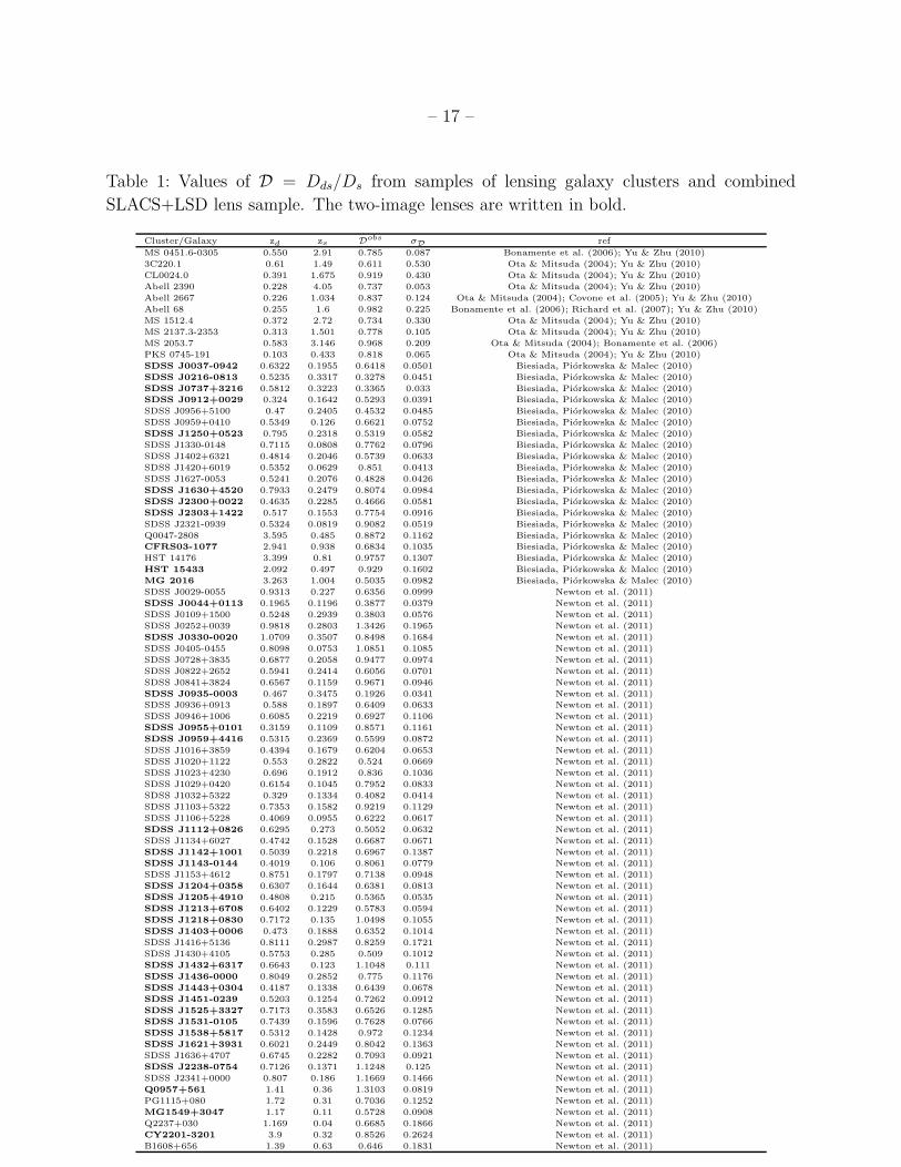
3. Sample used

For the Einstein ring data, we first use a combined sample of 70 strong lensing systems

with good spectroscopic measurements of central dispersions from the SLACS and LSD sur-

– 7 –

veys (Biesiada, Piorkowska & Malec 2010; Newton et al. 2011). Original data concerning the

sample can be found in (Koopmans & Treu 2002, 2003; Treu & Koopmans 2004; Treu et al.

2006a)(see for details). In our sample of 70 lenses some have 2 images and some have 4. There

are some general arguments in favor of SIS model, but strictly speaking SIS lens should have

only 2 images (Biesiada, Piorkowska & Malec 2010; Biesiada, Malec & Piorkowska 2011), so

one can try to use only 2 image systems out of the full sample. Therefore we selected a

subsample of n = 36 lenses, which is summarized in Table 1 where the names of lenses in

the restricted sample are given in bold.

As for the strong lensing arcs, redshifts and temperatures of the galaxy clusters are

always searched out directly from online databases, such as CDS (The Strasbourg astronom-

ical Data Center) or NED (NASA/IPAC Extragalactic Database). Yu & Zhu (2010) have

chosen a new database established especially for X-ray galaxy clusters – BAX, which pro-

vides detailed information including β and θc. They also used the fitting results of Chandra,

ROSAT, ASCA satellites and VIMOS-IFU survey (Ota & Mitsuda 2004; Bonamente et al.

2006; Covone et al. 2005; Richard et al. 2007). The final statistical sample satisfy the fol-

lowing well-defined selection criteria. Firstly, the distance between the lens and the source

should be always smaller than that between the arc source and the observer, Dds/Ds < 1,

which rules out half of selected lensing arcs. Secondly, the arcs whose positions are too far

from characteristic radius (θarc > 3θc) should also be discarded (Yu & Zhu 2010). At last

Yu & Zhu (2010) obtained a sample of 10 giant arcs with all necessary parameters listed in

Table 1.

Now the observational Dds/Ds data containing 80 data points for cosmological fitting

are summarized in Table 1, with errors calculated with error propagation equation. We also

list a restricted sample containing 46 data points, which consists 36 two-image lenses and 10

strong lensing arcs.

4. Cosmological models tested

All cosmological models we will consider in this paper are currently viable candidates

to explain the observed acceleration. Given the current status of cosmological observations,

there is no strong reason to go beyond the simple, standard cosmological model with zero

curvature and cosmological constant Λ (except for the conceptual problems arising when

one attempts to reconcile its observed value with some estimate derived from fundamental

arguments (Weinberg 1989)). However, it is still interesting to investigate alternative models.

And we hope that future observations of more accurate Dds/Ds data could allow to better

discriminate various competing candidates. In the MCMC simulations we assume for each

– 8 –

class of models the best fit values of parameters found in the present work, and vary them

within their 2σ uncertainties. We assume spatial flatness of the Universe throughout the

paper, since it is strongly supported by independent and precise experiments e.g. a combined

5-yr Wilkinson Microwave Anisotropy Probe (WMAP5), baryon acoustic oscillations (BAO)

and supernova data analysis gives Ωtot = 1.0050+0.0060−0.0061 (Hinshaw et al. 2009). Moreover, the

Ωm = 0.27 prior is used except in the ΛCDM model where the fit is attempted.

For comparison we also performed fits to the newly released Union2 SNe Ia data (n=557

supernovae) from the Supernova Cosmology project covering a redshift range 0.015 ≤ z ≤ 1.4

(Amanullah et al. 2010). In the calculation of the likelihood from SNe Ia, we marginalize

over the nuisance parameter (Di Pietro & Claeskens 2003)

χ2SNe = A− B2

C+ ln

(

C

2π

)

, (9)

where A =∑557

i (µdata − µth)2/σ2i , B =

∑557i (µdata − µth)/σ2

i , C =∑557

i 1/σ2i , and the

distance modulus is µ = 5 log(dL/Mpc)+25, with the 1σ uncertainty σi from the observations

of SNe Ia; and the luminosity distance dL as a function of redshift z

dL = (1 + z)

∫ z

0

cdz′

H0E(z′). (10)

4.1. The standard cosmological model (ΛCDM)

We start our analysis by first setting out the predictions for the current standard cosmo-

logical model. In the simplest scenario, the dark energy is simply a cosmological constant,

Λ, i.e. a component with constant equation of state w = p/ρ = −1. If flatness of the FRW

metric is assumed, the Hubble parameter according to the Friedmann equation is

E2(z) = Ωm(1 + z)3 + ΩΛ, (11)

where Ωm and ΩΛ parameterize the density of matter and cosmological constant, respectively.

Moreover, in the zero-curvature case (Ω = Ωm+ΩΛ = 1), this model has only one independent

parameter: p = Ωm.

4.2. Dark energy with constant equation of state (wCDM)

Allowing for a deviation from the simple w = −1 case, the accelerated expansion is

obtained when w < −1/3. In a zero-curvature universe, the Hubble parameter for this

– 9 –

generic dark energy component with density Ωx then becomes

E2(z) = Ωm(1 + z)3 + Ωx(1 + z)3(1+w). (12)

Obviously, when flatness and Ωm = 0.27 are assumed, it is a one-parameter model with the

model parameter: p = w.

4.3. Dark energy with variable equation of state (CPL)

If the equation of state of dark energy is allowed to vary with time, one has to choose

a suitable functional form for w(z), which in general involves certain parametrization. Now,

we consider the commonly used CPL model (Chevalier & Polarski 2001; Linder 2003), in

which the equation of state of dark energy is parameterized as w(z) = w0 + waz

1+z, where

w0 and wa are constants. The corresponding E(z) can be expressed as

E2(z) = Ωm(1 + z)3 + (1− Ωm)(1 + z)3(1+w0+wa) exp

(

−3waz

1 + z

)

. (13)

There are two independent model parameters in this model: p = w0, wa.

5. Results and conclusions

Performing fits of different cosmological scenarios on the full n = 80 sample as well as

the restricted n = 46 sample, we obtain the results displayed in Table 2.

For the full n = 80 sample, first, in ΛCDM model where Ωm is the only free param-

eter we fail to make a reliable fit on the sample considered, which is in agreement with

that of Biesiada, Piorkowska & Malec (2010). The reason is the functional dependence of

the distance on Ωm, which makes the restrictive power of the distance ratio poor for this

parameter. Second, one can see that the w coefficient obtained from the full strong lens-

ing sample agrees with the respective value derived from the WMAP5 results presented in

(Hinshaw et al. 2009) including combined WMAP5, BAO and SNe Ia analysis. Note that

this is also consistent with the ΛCDM model (w = −1). Third, concerning the evolving

equation of state in the CPL parametrization, confidence regions in the (w0,wa) plane are

shown in Fig. 3, which show that fits for w0 and wa are improved comparing with those of

Biesiada, Piorkowska & Malec (2010). For comparison we also plot the likelihood contours

with the Union2 SNe Ia compilation (Amanullah et al. 2010). It can be seen that the con-

cordance ΛCDM model while consistent with SNIa data (at 1σ level) is inconsistent with

– 10 –

0 0.04 0.08 0.12 0.16 0.20

0.1

0.2

0.3

0.4

0.5

0.6

0.7

0.8

0.9

1

Ωm

Pro

babi

lity

0 0.05 0.1 0.15 0.2 0.25 0.30

0.2

0.4

0.6

0.8

1

Ωm

Pro

babi

lity

Fig. 1.— The probability distribution of ΛCDM model from 80 full Dds/Ds data and 46

restricted Dds/Ds data.

−2 −1.8 −1.6 −1.4 −1.2 −1 −0.8 −0.6 −0.40

0.1

0.2

0.3

0.4

0.5

0.6

0.7

0.8

0.9

1

w

Pro

babi

lity

−4 −3.5 −3 −2.5 −2 −1.5 −1 −0.50

0.1

0.2

0.3

0.4

0.5

0.6

0.7

0.8

0.9

1

w

Pro

babi

lity

Fig. 2.— The probability distribution of wCDM model from 80 full Dds/Ds data and 46

restricted Dds/Ds data.

– 11 –

the strong lensing systems method applied here, which is most probably due to the fact that

the theoretical quantity Dds/Ds was the ratio of two integrals differing only by the limits of

integration (Biesiada, Piorkowska & Malec 2010).

Working on the restricted n = 46 sample (containing 36 two-image lenses and 10 strong

lensing arcs), despite the sample size has decreased dramatically, we find that it allows to

obtain improved fits on w0 and wa in CPL parametrization. Even though confidence regions

get larger in Fig. 3, the result turns out to agree with SNIa fits — almost the whole 2σ

confidence region from the Union2 data set lies within the 2σ from lenses. However, fits

on Ωm in ΛCDM model are contradictory to the standard knowledge (see Fig. 1) and the

best fit for the w parameter in quintessence scenario is higher than inferred from SNIa or

WMAP5 (see Fig. 2). One should also note, that a systematic shift downwards in the

(w0,wa) plane persists. Such a shift in best-fitting parameters inferred from supernovae

(standard candles, sensitive to luminosity distance) and BAO (standard rulers, sensitive

to angular diameter distance) has already been noticed and discussed in Linder & Roberts

(2008); Biesiada, Piorkowska & Malec (2010). Our result suggests the need for taking a

closer look at the compatibility of results derived by using angular diameter distances and

luminosity distances, respectively. Recent discussions on the ideas of testing the Etherington

reciprocity relation between these two distances can be found in (Bassett & Kunz 2004;

Uzan et al. 2004; Holanda, Lima & Ribeiro 2010; Cao & Zhu 2011b).

In conclusion our results demonstrate that the method extensively investigated in Biesiada

(2006); Grillo et al. (2008); Biesiada, Piorkowska & Malec (2010); Yu & Zhu (2010) on sim-

ulated and observational data can practically be used to constrain cosmological models.

Moreover, good quality measurements of the relevant observational qualities such as the ve-

locity dispersion and Einstein radius turn out to be crucial. Finally, two important effects,

neglected here, should be mentioned. One is that both the Einstein rings and X-ray obser-

vations of our new lensing sample come from different surveys or satellites (SLACS, LSD

and SBAS and Chandra, ROSAT and ASCA, respectively), the differences in detectors and

observing strategies may cause systematical errors which are hard to estimate. The other

is the influence of line-of-sight mass contamination, with the significant effect of large-scale

structure on strong lensing (Bar-Kana 1996; Keeton et al. 1997). More recent results on

this issue can be found in (Dalal et al. 2005; Momcheva et al. 2006). A straightforward so-

lution based on Poissonian statistics suggests that a sample size of order of a few hundred

lenses might reduce the line-of-sight ’noise’ contamination down to a few percent (Kubo et al.

2010). However, our Dds/Ds data set is really small, and its range of redshift is also limited.

Fortunately, with the ongoing of various systematic gravitational surveys and more giant

arc survey projects carried out by the International X-ray Observatory (IXO) (White et al.

2010), extended Roentgen Survey with an Imaging Telescope Array (eRosita) (Predehl et al.

– 12 –

2010) and the Wide Field X-ray Telescope (WFXT) (Murray & WFXT Team 2010) being

under way (Gladders et al. 2003; Hennawi et al. 2008), the sample of strong lenses is growing

rapidly, which may ease the problem of line-of-sight contamination. Future observations will

definitely enlarge our set and make the method applied in this paper more powerful.

Acknowledgments

This work was supported by the National Natural Science Foundation of China under the

Distinguished Young Scholar Grant 10825313 and Grant 11073005, the Ministry of Science

and Technology national basic science Program (Project 973) under Grant No.2007CB815401,

the Fundamental Research Funds for the Central Universities and Scientific Research Foun-

dation of Beijing Normal University, and the Polish Ministry of Science Grant No. N N203

390034.

REFERENCES

Adelman-McCarthy, J., et al. 2007, ApJS, 172, 634

Adelman-McCarthy, J., et al. 2008, ApJS, 175, 297

Allam, S. S., et al. 2004, AJ, 127, 1883

Allam, S. S., et al. 2007, ApJ, 662, L51

Amanullah, R., et al. 2010, ApJ, 716, 712 [arXiv:1004.1711]

Amati, L., et al. 2008, MNRAS, 391, 577

Bar-Kana, R. 1996, ApJ, 468, 17

Bassett, B. A., & Kunz, M. 2004, PRD, 69, 101305

Biesiada, M.,Godlowski, W., & Szydlowski, M. 2005, ApJ, 622, 28

Biesiada, M. 2006, PRD, 73, 023006

Biesiada, M., Piorkowska, A., & Malec, B. 2010, MNRAS, 406, 1055

Biesiada, M., Malec, B., & Piorkowska, A. 2011, RAA, in print

Bonamente et al. 2006, ApJ, 647, 25

– 13 –

Borgani, S., Rosati, P., Tozzi, P., & Norman, C. 1999, ApJ, 517, 40

Breimer, T. G., & Sanders, R. H. 1992, MNRAS, 257, 97

Browne, I. W. A., et al. 2003, MNRAS, 341, 13

Burles, S., Nollett, K. M., & Turner, M. S. 2001, ApJL, 552, L1

Caldwell, R. R., Dave, R., & Steinhardt, P. J. 1998, PRL, 80, 1582

Caldwell, R. R. 2002, PLB, 545, 23

Cao, S., & Zhu, Z.-H. 2011, China Series G, in press, arXiv:1102.2750

Cao, S., & Zhu, Z.-H. 2011, A&A, in press, arXiv:1105.6182

Cavaliere, A., & Fusco-Femiano, R. 1976, A&A, 49, 137

Chae, K.-H. 2003, MNRAS, 346, 746

Chae, K.-H., & Mao, S. D. 2003, ApJ, 599, L61

Chae, K.-H., Chen, G., Ratra, B., & Lee, D.-W. 2004, ApJ, 607, L71

Chevalier, M., & Polarski, D. 2001, IJMPD, 10, 213

Covone, G., et al. 2005, Submitted to A&A [arXiv:0511332]

Dalal, N., Hennavi, J. F., & Bode, P. 2005, ApJ, 622, 99

Daly, R. A., et al. 2009, ApJ, 691, 1058

Davis, T. M. et al. 2007, ApJ, 666, 716

Di Pietro, E., & Claeskens, J. F. 2003, MNRAS, 341, 1299

Dvali, G., Gabadadze, G., & Porrati, M. 2000, PLB, 485, 208

Eisenstein, D. J., et al. 2005, ApJ, 633, 560

Fassnacht, & Cohen, 1998, MNRAS, submitted

Feng, B., Wang, X., & Zhang, X. 2005, PLB, 607, 35

Freese, K., & Lewis, M. 2002, PLB, 540, 1

Gladders, M. D., et al. 2003, ApJ, 593, 48

– 14 –

Grillo, C., Lombardi, M., & Bertin, G. 2008, A&A, 477, 397

Hennawi, J. F., et al. 2008, AJ, 135, 664

Hinshaw, G., et al. 2009, ApJS, 180, 225

Holanda, R. F. L., Lima, J. A. S., & Ribeiro, M. B., 2010, ApJ, 722, L233

Itoh, N., Kohyama, Y., & Nozawa, S. 1998, ApJ, 502, 7

Jin, K.-J., Zhang, Y.-Z., & Zhu, Z.-H. 2000, PLA, 264,335

Jones, M. E., et al. 2005, MNRAS, 357, 518

Kamenshchik, A., Moschella, U., & Pasquier, V. 2001, PLB, 511, 265

Keeton, C. R., Kochanek, C. S., & Seljak, U. 1997, ApJ, 482, 604

Keeton, C. R. 2001, ApJ, 561, 46

King, L. J., et al. 1997, MNRAS, 289, 450

Kochanek, C. S. 1996, ApJ, 466, 638

Kochanek, C. S., & White, M. 2001, ApJ, 559, 531

Komatsu, E., et al. [WMAP Collaboration], 2009, AJS, 180, 330

Koopmans, L. V. E., & Treu, T. 2002, ApJ, 568, L5

Koopmans, L. V. E., & Treu, T. 2003, ApJ, 583, 606

Koopmans, L. V. E., et al. 2006, ApJ, 649, 599

Koopmans, L. V. E., et al. 2009, ApJ, 703, L51

Kowalski, M., et al. 2008, ApJ, 686, 749

Kubo, J. M., et al. 2010, accepted by ApJL, arXiv:1010.3037v2

Linder, E. V. 2003, PRD, 68, 083503

Linder, E. V., & Roberts, G. 2008, J. Cosmol. Astropart. Phys., 0806, 004

Lynds, R., & Petrosian, V. 1986, AAS, 18, 1014

Mao, S. D., & Schneider, P. 1998, MNRAS, 295, 587

– 15 –

Mitchell, J. L., Keeton, C. R., Frieman, J. A., & Sheth, R. K. 2005, ApJ, 622, 81

Momcheva, I., Williams, K., Keeton, C. R., & Zabludoff, A. 2006, ApJ, 641, 169

Murray, S. S., & WFXT Team. 2010, AAS, 41, 520

Newton, E., et al. 2011, accepted by ApJ, arXiv:1104.2608

Nozawa, S., Itoh, N., & Kohyama, Y. 1998, ApJ, 508, 17

Nozawa, S., Itoh, N., Suda, Y., & Ohhata, Y. 2006, Nuovo Cimento, 121 B, 487

Ofek, E. O., Rix, H.-W., & Maoz, D. 2003, MNRAS, 343, 639

Ono, T., Masai, K., & Sasaki, S. 1999, PASJ, 51, 91

Ota, N., & Mitsuda, K. 2004, A&A, 428, 757

Paczynski, B., & Gorski, K. 1981, ApJL, 248, L101

Perlmutter, S., et al. 1999, ApJ, 517, 565

Predehl, P. et al. 2010, arXiv:1001.2502

Press, W. H., & Schechter, P. 1974, ApJ, 187, 425

Reese, E. D., et al. 2002, ApJ, 581, 53

Richard, J., et al. 2007, ApJ, 662, 781; Abell 68

Riess, A. G., et al. 1998, AJ, 116, 1009

Riess, A. G., et al. 2004, ApJ, 607, 665

Rosati, P., Borgani, S., & Norman, C. 2002, ARA&A, 40, 539

Rusin, D., & Kochanek, C. S. 2005, ApJ, 623, 666

Schmidt, R. W., Allen, S. W., & Fabian, A. C. 2004, MNRAS, 352, 1413

Schneider, P., Ehlers, J., & Falco, E. E. 1992, Gravitational Lenses

Sereno, M. 2002, A&A, 393, 757

Sereno, M., & Longo, G. 2004, MNRAS, 354, 1255

Sheth, R. K., et al. 2003, ApJ, 594, 225

– 16 –

Spergel, D. N. et al. 2007, ApJS, 170, 377

Stoughton, C., et al. 2002, AJ, 123, 485

Sunyaev, R. A., & Zeldovich, Y. B. 1972, Comments on Astrophysics and Space Physics, 4,

173

Treu, T., & Koopmans, L. V. E. 2004, ApJ, 611, 739

Treu, T., et al. 2006a, ApJ, 640, 662

Treu, T., et al. 2006b, ApJ, 650, 1219

Uzan, J. P., Aghanim, N., & Mellier, Y. 2004, PRD, 70, 083533

Walsh, D., Carswell, R. F., & Weymann, R. J. 1979, Nature, 279, 381

Weinberg, S. 1989, Rev. Mod. Phys., 61, 1

White, N. E., et al. 2010, arXiv:1001.2843

Yu, H., & Zhu, Z.-H., submitted to RAA, arXiv:1011.6060

Zhang, H., & Zhu, Z.-H. 2006, PRD, 73, 043518

Zhu, Z.-H., & Wu, X.-P. 1997, A&A, 324, 483

Zhu, Z.-H. 2000, MPLA, 15, 1023

Zhu, Z.-H. 2000, IJMPD, 9, 591

Zhu, Z.-H. 2004, A&A, 423, 421

Zhu, Z.-H., & Fujimoto, M. 2004, ApJ, 602, 12

Zhu, Z.-H., Fujimoto, M., & He, X. 2004, ApJ, 603, 365

Zhu, Z.-H., & Mauro, S. 2008, A&A, 487, 831

Zhu, Z.-H., et al. 2008, A&A, 483, 15

This preprint was prepared with the AAS LATEX macros v5.2.

– 17 –

Table 1: Values of D = Dds/Ds from samples of lensing galaxy clusters and combined

SLACS+LSD lens sample. The two-image lenses are written in bold.

Cluster/Galaxy zd zs Dobs σD ref

MS 0451.6-0305 0.550 2.91 0.785 0.087 Bonamente et al. (2006); Yu & Zhu (2010)

3C220.1 0.61 1.49 0.611 0.530 Ota & Mitsuda (2004); Yu & Zhu (2010)

CL0024.0 0.391 1.675 0.919 0.430 Ota & Mitsuda (2004); Yu & Zhu (2010)

Abell 2390 0.228 4.05 0.737 0.053 Ota & Mitsuda (2004); Yu & Zhu (2010)

Abell 2667 0.226 1.034 0.837 0.124 Ota & Mitsuda (2004); Covone et al. (2005); Yu & Zhu (2010)

Abell 68 0.255 1.6 0.982 0.225 Bonamente et al. (2006); Richard et al. (2007); Yu & Zhu (2010)

MS 1512.4 0.372 2.72 0.734 0.330 Ota & Mitsuda (2004); Yu & Zhu (2010)

MS 2137.3-2353 0.313 1.501 0.778 0.105 Ota & Mitsuda (2004); Yu & Zhu (2010)

MS 2053.7 0.583 3.146 0.968 0.209 Ota & Mitsuda (2004); Bonamente et al. (2006)

PKS 0745-191 0.103 0.433 0.818 0.065 Ota & Mitsuda (2004); Yu & Zhu (2010)

SDSS J0037-0942 0.6322 0.1955 0.6418 0.0501 Biesiada, Piorkowska & Malec (2010)

SDSS J0216-0813 0.5235 0.3317 0.3278 0.0451 Biesiada, Piorkowska & Malec (2010)

SDSS J0737+3216 0.5812 0.3223 0.3365 0.033 Biesiada, Piorkowska & Malec (2010)

SDSS J0912+0029 0.324 0.1642 0.5293 0.0391 Biesiada, Piorkowska & Malec (2010)

SDSS J0956+5100 0.47 0.2405 0.4532 0.0485 Biesiada, Piorkowska & Malec (2010)

SDSS J0959+0410 0.5349 0.126 0.6621 0.0752 Biesiada, Piorkowska & Malec (2010)

SDSS J1250+0523 0.795 0.2318 0.5319 0.0582 Biesiada, Piorkowska & Malec (2010)

SDSS J1330-0148 0.7115 0.0808 0.7762 0.0796 Biesiada, Piorkowska & Malec (2010)

SDSS J1402+6321 0.4814 0.2046 0.5739 0.0633 Biesiada, Piorkowska & Malec (2010)

SDSS J1420+6019 0.5352 0.0629 0.851 0.0413 Biesiada, Piorkowska & Malec (2010)

SDSS J1627-0053 0.5241 0.2076 0.4828 0.0426 Biesiada, Piorkowska & Malec (2010)

SDSS J1630+4520 0.7933 0.2479 0.8074 0.0984 Biesiada, Piorkowska & Malec (2010)

SDSS J2300+0022 0.4635 0.2285 0.4666 0.0581 Biesiada, Piorkowska & Malec (2010)

SDSS J2303+1422 0.517 0.1553 0.7754 0.0916 Biesiada, Piorkowska & Malec (2010)

SDSS J2321-0939 0.5324 0.0819 0.9082 0.0519 Biesiada, Piorkowska & Malec (2010)

Q0047-2808 3.595 0.485 0.8872 0.1162 Biesiada, Piorkowska & Malec (2010)

CFRS03-1077 2.941 0.938 0.6834 0.1035 Biesiada, Piorkowska & Malec (2010)

HST 14176 3.399 0.81 0.9757 0.1307 Biesiada, Piorkowska & Malec (2010)

HST 15433 2.092 0.497 0.929 0.1602 Biesiada, Piorkowska & Malec (2010)

MG 2016 3.263 1.004 0.5035 0.0982 Biesiada, Piorkowska & Malec (2010)

SDSS J0029-0055 0.9313 0.227 0.6356 0.0999 Newton et al. (2011)

SDSS J0044+0113 0.1965 0.1196 0.3877 0.0379 Newton et al. (2011)

SDSS J0109+1500 0.5248 0.2939 0.3803 0.0576 Newton et al. (2011)

SDSS J0252+0039 0.9818 0.2803 1.3426 0.1965 Newton et al. (2011)

SDSS J0330-0020 1.0709 0.3507 0.8498 0.1684 Newton et al. (2011)

SDSS J0405-0455 0.8098 0.0753 1.0851 0.1085 Newton et al. (2011)

SDSS J0728+3835 0.6877 0.2058 0.9477 0.0974 Newton et al. (2011)

SDSS J0822+2652 0.5941 0.2414 0.6056 0.0701 Newton et al. (2011)

SDSS J0841+3824 0.6567 0.1159 0.9671 0.0946 Newton et al. (2011)

SDSS J0935-0003 0.467 0.3475 0.1926 0.0341 Newton et al. (2011)

SDSS J0936+0913 0.588 0.1897 0.6409 0.0633 Newton et al. (2011)

SDSS J0946+1006 0.6085 0.2219 0.6927 0.1106 Newton et al. (2011)

SDSS J0955+0101 0.3159 0.1109 0.8571 0.1161 Newton et al. (2011)

SDSS J0959+4416 0.5315 0.2369 0.5599 0.0872 Newton et al. (2011)

SDSS J1016+3859 0.4394 0.1679 0.6204 0.0653 Newton et al. (2011)

SDSS J1020+1122 0.553 0.2822 0.524 0.0669 Newton et al. (2011)

SDSS J1023+4230 0.696 0.1912 0.836 0.1036 Newton et al. (2011)

SDSS J1029+0420 0.6154 0.1045 0.7952 0.0833 Newton et al. (2011)

SDSS J1032+5322 0.329 0.1334 0.4082 0.0414 Newton et al. (2011)

SDSS J1103+5322 0.7353 0.1582 0.9219 0.1129 Newton et al. (2011)

SDSS J1106+5228 0.4069 0.0955 0.6222 0.0617 Newton et al. (2011)

SDSS J1112+0826 0.6295 0.273 0.5052 0.0632 Newton et al. (2011)

SDSS J1134+6027 0.4742 0.1528 0.6687 0.0671 Newton et al. (2011)

SDSS J1142+1001 0.5039 0.2218 0.6967 0.1387 Newton et al. (2011)

SDSS J1143-0144 0.4019 0.106 0.8061 0.0779 Newton et al. (2011)

SDSS J1153+4612 0.8751 0.1797 0.7138 0.0948 Newton et al. (2011)

SDSS J1204+0358 0.6307 0.1644 0.6381 0.0813 Newton et al. (2011)

SDSS J1205+4910 0.4808 0.215 0.5365 0.0535 Newton et al. (2011)

SDSS J1213+6708 0.6402 0.1229 0.5783 0.0594 Newton et al. (2011)

SDSS J1218+0830 0.7172 0.135 1.0498 0.1055 Newton et al. (2011)

SDSS J1403+0006 0.473 0.1888 0.6352 0.1014 Newton et al. (2011)

SDSS J1416+5136 0.8111 0.2987 0.8259 0.1721 Newton et al. (2011)

SDSS J1430+4105 0.5753 0.285 0.509 0.1012 Newton et al. (2011)

SDSS J1432+6317 0.6643 0.123 1.1048 0.111 Newton et al. (2011)

SDSS J1436-0000 0.8049 0.2852 0.775 0.1176 Newton et al. (2011)

SDSS J1443+0304 0.4187 0.1338 0.6439 0.0678 Newton et al. (2011)

SDSS J1451-0239 0.5203 0.1254 0.7262 0.0912 Newton et al. (2011)

SDSS J1525+3327 0.7173 0.3583 0.6526 0.1285 Newton et al. (2011)

SDSS J1531-0105 0.7439 0.1596 0.7628 0.0766 Newton et al. (2011)

SDSS J1538+5817 0.5312 0.1428 0.972 0.1234 Newton et al. (2011)

SDSS J1621+3931 0.6021 0.2449 0.8042 0.1363 Newton et al. (2011)

SDSS J1636+4707 0.6745 0.2282 0.7093 0.0921 Newton et al. (2011)

SDSS J2238-0754 0.7126 0.1371 1.1248 0.125 Newton et al. (2011)

SDSS J2341+0000 0.807 0.186 1.1669 0.1466 Newton et al. (2011)

Q0957+561 1.41 0.36 1.3103 0.0819 Newton et al. (2011)

PG1115+080 1.72 0.31 0.7036 0.1252 Newton et al. (2011)

MG1549+3047 1.17 0.11 0.5728 0.0908 Newton et al. (2011)

Q2237+030 1.169 0.04 0.6685 0.1866 Newton et al. (2011)

CY2201-3201 3.9 0.32 0.8526 0.2624 Newton et al. (2011)

B1608+656 1.39 0.63 0.646 0.1831 Newton et al. (2011)

– 18 –

Table 2: Fits to different cosmological models from 80 full Dds/Ds data and 46 restricted

Dds/Ds data. Fixed value of Ωm = 0.27 is assumed except ΛCDM.

Cosmological model Best-fitting parameters (n = 80) Best-fitting parameters (n = 46)

ΛCDM Ωm = 0.045+0.039−0.025 Ωm = 0.046+0.054

−0.026

wCDM w = −1.07+0.19−0.17 w = −1.40+0.31

−0.49

CPL w0 = 1.50± 1.25 w0 = −0.24± 2.42

wa = −11.86± 6.64 w0 = −6.35± 9.75

−2−1.5−1−0.5 0 0.5 1 1.5 2 2.5 3 3.5 4−24−22−20−18−16−14−12−10−8−6−4−2

024

w0

wa

80 Dds

/Ds

SNIa Union2

−5 −4 −3 −2 −1 0 1 2 3 4 5−25

−20

−15

−10

−5

0

5

10

w0

wa

47 Dds

/Ds

SNIa Union2

Fig. 3.— The 68.3 and 95.8 % confidence regions for CPL parametrization in the (w0,wa)

plane obtained from 80 full Dds/Ds data, 46 restricted Dds/Ds data, and 557 Union2 SNe

Ia data. The crosses represent the best-fit points and a star corresponding to ΛCDM model

is also added for reference.