Abell 611:II. X-ray and strong lensing analyses

arX

iv:1

002.

1625

v2 [

astr

o-ph

.CO

] 25

Mar

201

1Astronomy & Astrophysicsmanuscript no. 14120 c© ESO 2011March 28, 2011

Abell 611II. X-ray and strong lensing analyses

A. Donnarumma1,2,3, S. Ettori2,3, M. Meneghetti2,3, R. Gavazzi4,5, B. Fort4,5, L. Moscardini1,3,A. Romano6,7, L. Fu8,10, F. Giordano7, M. Radovich8,9, R. Maoli6, R. Scaramella7 and J. Richard11

1 Dipartimento di Astronomia, Universita di Bologna, via Ranzani 1, 40127 Bologna, Italy2 INAF-Osservatorio Astronomico di Bologna, via Ranzani 1, 40127 Bologna, Italy3 INFN, Sezione di Bologna, viale Berti Pichat 6/2, 40127 Bologna, Italy4 Institut d’Astrophysique de Paris, CNRS UMR 7095, 98bis Bd Arago, 75014 Paris, France5 UPMC Universite Paris 06, UMR 7095, 75014 Paris, France6 Dipartimento di Fisica, Universita La Sapienza, PiazzaleA.Moro 00185 Roma, Italy7 INAF-Osservatorio Astronomico di Roma, via Frascati 33, 00044 Monte Porzio Catone (Roma), Italy8 INAF-Osservatorio Astronomico di Napoli, via Moiariello 16, 80131 Napoli, Italy9 INAF-Osservatorio Astronomico di Padova, vicolo dell’Osservatorio 5, 35122 Padova, Italy

10 Key Lab for Astrophysics, Shanghai Normal University, 100 Guilin Road, 200234, Shanghai, China11 Department of Physics, Institute for Computational Cosmology, Durham University, South Road, Durham DH1 3LE, United

Kingdom

Accepted on October 17, 2010

ABSTRACT

We present the results of our analyses of the X-ray emission and of the strong lensing systems in the galaxy cluster Abell 611[z = 0.288]. This cluster is an optimal candidate for a comparison of the mass reconstructions obtained through X-ray and lensingtechniques, because of its very relaxed dynamical appearance and its exceptional strong lensing system. We infer the X-ray mass es-timate deriving the density and temperature profile of the intra–cluster medium within the radius r≃700 kpc through a non-parametricapproach, taking advantage of the high spatial resolution of a Chandraobservation. Assuming that the cluster is in hydrostatic equi-librium and adopting a matter density profile, we can recoverthe total mass distribution of Abell 611 via the X-ray data. Moreover,we derive the total projected mass in the central regions of Abell 611 performing a parametric analysis of its strong lensing featuresthrough the publicly available analysis softwareLenstool. As a final step we compare the results obtained with both methods. Wederive a good agreement between the X-ray and strong lensingtotal mass estimates in the central regions where the stronglensingconstraints are present (i.e. within the radius r≃100 kpc), while a marginal disagreement is found between thetwo mass estimateswhen extrapolating the strong lensing results in the outer spatial range. We suggest that in this case the X-ray/strong lensing massdisagreement can be explained by an incorrect estimate of the relative contributions of the baryonic component and of the dark matter,caused by the intrinsic degeneracy between the different mass components in the strong lensing analysis. We discuss the effect ofsome possible systematic errors that influence both mass estimates. We find a slight dependence of the measurements of theX-raytemperatures (and therefore of the X-ray total masses) on the background adopted in the spectral analysis, with total deviations on thevalue of M200 of the order of the 1σ statistical error. The strong lensing mass results are instead sensitive to the parameterisation of thegalactic halo mass in the central regions, in particular to the modelling of the Brightest Cluster Galaxy (BCG) baryoniccomponent,which induces a significant scatter in the strong lensing mass results.

Key words. Gravitational lensing: strong – X-ray: Galaxies: clusters– Galaxies: clusters: general – Galaxies: clusters: individual(A611) .

1. Introduction

Testing the accuracy of the several approaches used to estimatethe mass of galaxy clusters is necessary to assess the reliabilityof methods involving clusters as cosmological probes. For exam-ple, the comparison of the cluster baryon fractions fb to the cos-mic baryon fraction can provide a direct constraint on the meanmass density of the Universe,ΩM (Ettori et al. 2009; Allen et al.2008; Ettori et al. 2003), while the evolution of the clustermassfunction can tightly constrainΩΛ and the dark energy equation-of-state parameterw (Vikhlinin et al. 2009).Cluster mass profiles can be probed through several indepen-dent techniques, relying on different physical mechanisms and

Send offprint requests to: A. Donnarumma – e-mail: [email protected]

requiring different assumptions. The comparison of results ob-tained with different methods and the (dis)agreement betweenthem provide a useful check, and can give additional insightson the inner structure of clusters. For example, cluster massescan be estimated through the projected phase-space distributionand velocity dispersion of cluster galaxies (Biviano & Poggianti2009; Diaferio et al. 2005); the dynamical studies, however, areaffected by the strong degeneracy between the mass density pro-file and the velocity dispersion anisotropy profile, and thusre-quire strong assumptions on the form of the velocity dispersiontensor.Measurements of the Sunyaev-Zel’dovich effect (hereafter SZE;Sunyaev & Zel’dovich 1972) towards galaxy clusters yield a di-rect measurement of the pressure distribution of the cluster gas:the total gravitational mass can thus be determined combining

1

http://arxiv.org/abs/1002.1625v2

A. Donnarumma et al.: X-ray and strong lensing analyses of Abell 611

Fig. 1:[Left panel]F606WACS/HSTimage of the cluster Abell 611 (see Table 3 for the observation summary). The X-ray isophotesderived from theChandraimage (shown in the middle panel) are overlaid in white. The green cross indicates the X-ray centroid.[Middle panel] The ChandraX-ray image of Abell 611 in the energy range [0.25-7.0] keV. The image was smoothed with a 3pixel FWHM Gaussian filter, and is not exposure-corrected. The contours derived from theHST image (shown in the left panel)are overlaid in white to facilitate the comparison between the images. Here again the green cross marks the X-ray centroid. [Rightpanel]Pseudo-colour composite image of Abell 611, obtained combiningr andg−SLOAN images, taken with the Large BinocularCamera mounted at LBT. The three panels are WCS-aligned; thesize of the field of view is≃ [1.6× 1.8] arcmin.

this information with the intra–cluster medium (hereafterICM)temperature, estimated for example through the X-ray spectralanalysis (Grego et al. 2001). Because it is independent of thecluster redshift, the SZE can be an extremely powerful tool to in-vestigate the mass of high–redshift clusters (Hincks et al.2009),but accurate measurements of the SZE are still a challenge be-cause of intrinsic limitations and systematic biases (faint signalextending over a large angular size and subject to several sourcesof contamination).So far, the analysis of the cluster X-ray emission and of the grav-itational lensing effect are among the most promising techniquesto estimate galaxy cluster masses.The X-ray mass estimate is less biased compared with lensing-derived masses by projection effects, because the X-ray emissionis traced by the square of the gas density (Gavazzi 2005; Wu2000). However, X-ray measurements of cluster masses implythe assumption of hydrostatic equilibrium of the ICM with thedark matter potential and of spherical symmetry of the clustermass distribution. Hence the total mass profile can be inferredfrom the radial profiles of gas temperature and density.On the other hand, the gravitational lensing effect allows for thedetermination of the projected surface mass density of the lens,regardless of its dynamical state or the nature of the interveningmatter. This effect is determined by all massive structures alongthe line of sight, so lensing mass measurements are subject toforeground and background contaminations. Moreover, the lens-ing effect is sensitive to features of the mass distribution such asits ellipticity and asymmetry and to the presence of substructures(Meneghetti et al. 2007a).The combination of X-ray and lensing results could verify andstrengthen the findings on the cluster physics and masses (seefor example Allen 1998; Ettori & Lombardi 2003; Bradac et al.2008); but so far several works in literature claimed a signifi-cant disagreement between strong lensing and X-ray mass es-timates, (Wu & Fang 1996; Smail et al. 1997; Ota et al. 2004;Voigt & Fabian 2006; Gitti et al. 2007; Halkola et al. 2008)which would prevent any joint analysis. Many convincing ex-

planations, even if not conclusive, have been suggested.It is therefore clear that a comparison between independentmassestimates for galaxy clusters can provide a vital check of the as-sumptions adopted in the cluster analysis, and will possibly giveus additional insights into the underlying physics of theseob-jects. In particular, the comparison between lensing and X-raymass in galaxy clusters is also directly related to the cosmo-logical parameters, since their ratio depends on the cosmicden-sity parameter,ΩM, and the cosmological constant,ΩΛ, for theirdifferent dependence on the angular diameter distances, whichare smaller in anΩΛ dominated universe, as pointed out by Wu(2000).Targets for a comparative analysis should be relaxed, unper-turbed objects to avoid biases deriving from the incorrect as-sumption of hydrostatic equilibrium (X-ray analysis) or fromthe contamination of secondary mass clumps or unresolved sub-structures (lensing analysis).An ideal candidate for this kind of analysis is Abell 611. It is arich, cool-core cluster atz = 0.288 (Struble & Rood 1999); itsX-ray emission peak is well centred on the Brightest ClusterGalaxy (hereafter BCG; see left and central panels of Fig. 1),and the X-ray isophotes appear quite regular, with a low de-gree of ellipticity. These characteristics are generally consideredgood indicators of a relaxed dynamical state. Relaxed objects arequite rare at this redshift, so a detailed study of the properties ofAbell 611 is even more appealing.In this work we will focus on the comparison between the X-rayand strong lensing mass estimates. A weak lensing analysisof large field of view data, obtained with the Large BinocularCamera (LBC) mounted at the Large Binocular Telescope(LBT), is presented in Romano et al. (2010) (hereafter PaperI). Here we present new X-ray and strong lensing mass esti-mates, based on a non-parametric reconstruction of gas den-sity and temperature profiles obtained through the analysisofa Chandraobservation, and on a strong lensing reconstructionrespectively, which was performed with theLenstoolanalysissoftware (Kneib et al. 1996; Jullo et al. 2007).

2


Table 1: Observation summary of theChandraexposure used forthe X-ray analysis.

Obs.ID Start Time Total Net PIExpos. [ks] Expos.[ks] name

3194 2001-11-03 18:43:58 36.6 30.9 Allen

This paper is organised as follows. In Sect. 2 we will intro-duce our X-ray analysis, focusing on the data reduction andon the method applied to recover the total and gas mass pro-files, and discuss some possible systematic errors associatedwith the X-ray analysis. The strong lensing analysis is presentedin Sect. 3, where we will briefly discuss our main findings. Wewill compare the X-ray and strong lensing results in Sect. 4:a comparison with previous analyses can be found in Sect. 5.Finally, we will summarise our results and draw our conclusionsin Sect. 6.Throughout this work we will assume a flatΛCDM cosmol-ogy: the matter density parameter will have the valueΩm=0.3,the cosmological constant density parameterΩΛ=0.7, and theHubble constant will beH0 = 70 km s−1Mpc−1. At the clusterredshift and for the assumed cosmological parameters, 1 arcsecis equivalent to 4.329 kpc. Unless otherwise stated, all uncertain-ties are referred to a 68% confidence level.

2. X-ray analysis

2.1. X-ray data reduction

The X-ray analysis of Abell 611 returns several indicators ofa relaxed dynamical state, such as the absence of substruc-tures in the X-ray emission (which appears isotropic over ellip-tical isophotes), a well-defined cool-core, and a smooth surfacebrightness profile. The X-ray emission is centred on the BCG:the distance between the X-ray centroid and the BCG centre is≃ 1 arcsec (the uncertainty on this measure is comparable tothe smoothing scale applied to the X-ray image to determine thecentroid, i.e. 3 pixels≃ 1.5 arcsec). Moreover, Abell 611 ap-pears to be a radio–quiet cluster, because the Giant MetrewaveRadio Telescope (GMRT) Radio Halo Survey (Venturi et al.2007, 2008, see Sect. 5) failed to detect any extended radioemission associated with this cluster. Since giant radio halos arethe most relevant examples of non-thermal activity in galaxyclusters (Brunetti et al. 2009), the absence of a radio halo sup-ports the hypothesis of thermal pressure support, connected tothe hydrostatic equilibrium assumption required in the X-rayanalysis.This cluster can therefore be considered an ideal candidatetohighlight any issue with the current analysis techniques: it full-fills the assumptions of thermal pressure support and of spher-ical symmetry, so it is unlikely that potential biases in there-sults are related to the limiting assumptions underlying the X-rayanalysis. We performed our X-ray analysis on the onlyChandradata set available, retrieved from the public archive (see Table 1for observation log). We reduced the data using theCIAO dataanalysis package – version 4.0 – and the calibration databaseCALDB 3.5.01. We will summarise here briefly the reduction

1 See the CIAO analysis guides for the data reduction:cxc.harvard.edu/ciao/guides/ .

procedure.The Chandraobservation was tele-metered in very faint modeand was performed through both back-illuminated (BI) andfront-illuminated (FI) chips. The cluster centre was imagedin the S3 BI chip. The level-1 event files were reprocessedto apply the appropriate gain maps and calibration productsand to reduce the ACIS quiescent background2. We used theacis process events tool to check for cosmic-ray back-ground events and to correct for eventual spatial gain varia-tions caused by charge transfer inefficiency to re-compute theevent grades. We applied the standard event selection, includingonly the events flagged with grades 0, 2, 3, 4, and filtered for theGood Time Intervals associated with the observation. The brightpoint sources were masked out, and a geometrical correctionforthe masked areas was applied; the point sources were identifiedusing the scriptvtpdetect, and the result was then checkedthrough visual inspection.A careful screening of the background light curve is neces-sary for a correct background subtraction (Markevitch et al.2003), to discard contaminating flare events, which could havea non-negligible influence on the inferred cluster spectralprop-erties. We extracted the background light curve, applying atimebinning of about 1 ks, in the energy range [2.5–7] keV, which isthe most effective band to individuate common flares for S3 chip.We applied the scriptlc clean to include only the time periodswithin a factor 1.2 of the mean quiescent rate. We compared theS3 background light curve with the light curve extracted in theS1 chip using the energy range [2.5–6] keV, to check for faint,long flares, which were not identified. The S3 background lightcurve was examined using theChIPSfacilities to identify andexclude further flaring events. The net exposure time after thelight curve screening is about 31 ks (see Table 1).

2.2. X-ray analysis

In order to derive a reliable cluster mass estimate through theX-ray analysis, a primary issue is to avoid any bias in the tem-perature estimate, because cluster masses derived by assuminghydrostatic equilibrium are dependent on the temperature pro-file, as demonstrated by Rasia et al. (2006). For this purpose, acorrect background modelling is crucial. The X-ray backgroundis often estimated through the blank-sky background data setsprovided by the ACIS calibration team. The blank-sky observa-tions are reduced similarly to the source data sets to be compati-ble with the cluster event files; the former are then re-normalisedby comparing the blank-sky count rate in a given energy range(generallykT > 8.0 keV, since in this band theChandraeffec-tive area is negligible) with the local background count rate. Oneof the advantages of this modus operandi is that the derived ARFand RESPONSE matrices will be consistent both for the sourceand the background spectrum. However, the background in theX-ray soft band can vary both in time and in space, so it is impor-tant to verify whether the background derived by the blank-skydatasets is consistent with the “real” one.For this purpose, we extracted a spectrum from theChandraob-servation in a region where the cluster emission is negligible:we compared the former to a spectrum derived in the same re-gion of the blank-field data set. We tried to fit the residuals inthe [0.4–3] keV band with a MEKAL model, without an absorp-tion component and broadening the normalisation fitting rangeto negative values. This comparison shows some differences be-

2 For a complete discussion on this topic, seecxc.harvard.edu/cal/Acis/Cal prods/vfbkgrnd/index.html .

3


tween the two spectra. For this reason, we decided to proceedinthe spectral fitting utilising both a local background estimate anda blank-sky estimate. The effect of the background choice in themass estimate results will be discussed in Sect. 2.5.

2.3. Spectral fitting

The spectra were extracted on concentric annuli centred on theX-ray surface brightness centroid, each one containing at least2500 net source counts, to infer an estimate of the ICM metallic-ity. We selected six annuli with adequate S/N ratio, up toRspec=

2.9 arcmin. We used theCIAO specextract tool to extractthe source and background spectra and to construct ancillary-response and response matrices. The spectra were fitted in the0.6 − 7.0 keV range except for the last two annuli, in which,due to the higher background level, we restricted the analysis tothe range 0.6− 5.0 keV. We performed the spectral analysis us-ing theXSPECsoftware package (Arnaud 1996). We adoptedan optically-thin plasma emission model (themekal model;Mewe et al. 1985; Kaastra & Mewe 1993) with an absorptioncomponent (the Tubingen–Boulder modeltbabs; Wilms et al.2000).We fixed the Galactic absorption to the value inferred from radioHI maps in Dickey & Lockman (1990), i.e. 4.99×1020 cm−2. Thefree parameters in the spectral fitting model are the temperature,the metallicity and the normalisation of the thermal spectrum.The metal abundance profile presents a central peak with a quitescattered trend (see the right panel of Fig. 2). The metallicityprofile is not directly involved in the X-ray mass reconstruction:but we still verified whether a bias in its measurement can influ-ence the derived mass estimate. The results of this check will bepresented in Sect. 2.5.

2.4. X-ray mass profile

The gas temperature and density profiles are recovered withoutany parameterisation of the ICM properties, but relying on theassumptions of spherical symmetry and hydrostatic equilibriumand on the choice of a model for the total mass.The method that was applied is briefly resumed in the follow-ing; the reader can refer to Ettori, De Grandi, & Molendi (2002);Morandi, Ettori, & Moscardini (2007); Morandi & Ettori (2007)for full details.In this section, the subscript “ring” will indicate a projectedquantity measured in concentric rings (equivalently, spectralbins), whereas the subscript “shell” will point to a deprojectedquantity measured in volume shells. The projected gas temper-atureTring, metal abundanceZring and the normalisationKring ofthe model for each annulus are derived through the spectral anal-ysis. In particular, the normalisation of the thermal spectrum pro-vides an estimate for the emission integralEI =

∫

nenpdV ≃0.82

∫

n2e dV.

To deproject the former quantities, we need to derive the inter-section of each volume shell with the spectral annuli, whichcanbe calculated through an upper triangular matrixV, whose lastpivot represents the outermost annulus if we assume sphericalsymmetry (Kriss, Cioffi, & Canizares 1983; Buote 2000).To calculate the deprojected density profile, we combined thespectral information and the cluster X-ray surface brightness(SB) profile, composed by 15 bins with 1000 counts each. TheSB provides an estimate of the volume-counts emissivityFbin ∝

n2e,binT

1/2bin /D

2L, whereDL is the luminosity distance of the cluster.

By comparing this observed profile with the values predictedby

a thermal plasma model, with temperature and metallicity equalto the measured spectral quantities and taking into accounttheabsorption effect, we can solve for the electron density and ob-tain a gas density profile better resolved than a “spectral–only”one (see the top panel of Fig. 2).The total gravitating mass was then constrained as follows:theobserved deprojected temperature profile in volume shellsTshellwas obtained through

ǫTshell = (VT)−1#(LringTring), (1)

whereǫ = (VT )−1#Lring; (2)

here the symbol # indicates a matrix product,V is the volumematrix andLring is the cluster luminosity measured in concentricrings. We compare it to the predicted temperature profileTmodel,obtained by inverting the equation of hydrostatic equilibrium be-tween the dark matter and the intracluster plasma, i.e.:

−GµmpneMtot,model(< r)

r2=

d(ne× kTmodel)dr

, (3)

wherene is the deprojected electron density. Our best-fit massmodel was determined by comparing the observed temperatureprofile Tobs with the predicted profileTmodel, which depends onthe mass model parameters: accordingly we minimised the quan-tity:

χ2 =∑

rings

(

Tobs− Tmodel

σobs

)2

, (4)

where theTmodel profile was rebinned to match the observedtemperature profile. In the bottom panel of Fig. 2 we show theprojected temperature profile as determined through the spectralanalysis, the deprojected best-fit profile and the deprojected pro-file, rebinned to the spectral intervals.We assumed the NFW profile as the total mass functional; thisprofile can be expressed as:

ρ(r) =ρs

(r/rs) (1+ r/rs)2, (5)

whereρs is the characteristic density andrs is the scale radius.We will describe the NFW profile through the scale radius andthe concentration parameterc200; the former can be defined as

c ≡R200

rs, (6)

whereR200 is the radius within which the mean matter densityof the halo is 200 times the critical density of the Universe.Assuming a mass model, the best-fitting values of its parame-ters are determined by minimising the quantity defined in Eq.4.The NFW profile parameters were optimised in the ranges 0.56c2006 20 and 10 kpc6 rs6 976 kpc, where the scale radius up-per limit is the outer radius of the surface brightness profile. Thegas and total mass profiles are shown in Fig. 3; the inferred massmodel parameters are listed in Table 2. The confidence levelsforthe NFW parameters are shown in the right panel of Fig. 3.

2.5. Systematic effects in the X-ray mass profile

In this section we will briefly assess if our X-ray mass estimateof Abell 611 can be affected by some analysis choices.The choice of the X-ray background estimate, as discussed inSect. 2.2, could have a non-negligible impact on the derived

4


Fig. 2: [Top left panel]Deprojected gas density profile. The red circles indicate the values determined by the normalisation of thethermal spectra, while diamonds represent the values obtained combining both spectral and surface brightness measurements: thedashed line shows the best-fit profile.[Bottom left panel]ICM temperature profile. The figure shows the projected temperaturevalues, directly inferred from the spectral analysis (red filled circles) and the deprojected values, which were rebinned to the samebinning of the spectral profile (diamonds). The dashed line shows the deprojected best-fit profile.[Right panel]The projected (blackempty diamonds) and deprojected (red filled circles) metallicity profile for Abell 611 inferred from the X-ray analysis.The dottedline represents the mean metallicity valueZ = (0.45± 0.1) Z⊙, as determined through the fit of the spectrum extracted in the areawith radiusR= 2.9 arcmin, i.e. the cluster area covered by our spectral analysis. The grey region indicates the 1σ confidence level.

Table 2: Best-fit values for the total mass parameters obtained through the X-ray analysis.

Results of the X-ray analysis of Abell 611

rs c200 M200 χ2red[d.o.f.]

[kpc] [1014M⊙]

(1) Blank-sky background 350.3± 79.6 5.18± 0.84 9.32± 1.39 0.81 [4](2) Local background 420.0± 99.5 4.67± 0.80 11.11± 2.06 0.46 [4](3) Fixed metallicity 367.2± 98.6 5.13± 0.87 10.61± 1.96 0.33 [4]

Notes. (1) the blank-sky dataset is adopted to estimate the X-ray background;(2) the X-ray background is derived from peripheral regionsof the source observation;(3) the background is estimated locally fixing the gas metallicity to Z = 0.3 Z⊙.The columns indicate the best-fit values obtained for the NFWprofile parameters (the scale radiusrs and the concentrationc200), the estimate ofthe total mass withinR200 (here listed asM200) and the reducedχ2, referred to a fit with four degrees of freedom.

temperature profile, and consequently on the total mass mea-surement. Moreover, we verified whether considering the ICMmetallicity as a free parameter in the spectral analysis canim-pact the X-ray mass estimate of Abell 611, since (as shown inFig. 2) its inferred metallicity profile is quite irregular.We thusre-ran the spectral analysis by fixing the metallicityZ to the typ-ical value of 0.3Z⊙ (see e.g. Balestra et al. 2007); we then de-rived a new X-ray mass estimate adopting the spectral profilesobtained under the assumption of a constant metallicity.Therefore we derived the mass of Abell 611 through the X-rayanalysis:

1. by estimating the X-ray background through the spectra ex-tracted from the blank-sky dataset (opportunely reprocessedand re-normalised to be consistent with the source observa-tions) in the same image regions used for the source spectra(case 1);

2. by estimating the X-ray background from peripheral regionsof the S3 chip in the source dataset (case 2);

3. as in the previous case, but by fixing the metallicityZ to thevalue 0.3Z⊙ (case 3).

The NFW parameters derived from the X-ray analysis in thethree aforementioned cases are listed in Table 2.The results obtained in the first two cases mutually agree within

5


50 100 250 800Radius [kpc]

1011

1012

1013

1014

1015M

/MO •

Mgas M total

200 300 400 500rs [kpc]

3

4

5

6

7

c 200

Fig. 3: [Left panel] Mass profiles for Abell 611 as determined through the X-ray analysis. The black solid line and the red dashedline indicate the total mass and the gas mass profile, respectively. [Right panel]Confidence levels determined through the X-rayanalysis for the NFW profile parametersrs andc200. The red circle indicates the best-fit values, while the contours represent the1σ, 2σ, and 3σ confidence levels.

0 200 400 600 800Radius [kpc]

4

5

6

7

8

9

Tga

s[keV

]

Blank-skyLocal bkg

Fig. 4: Comparison between the temperature profile determinedby estimating the X-ray background through the blank-skydataset (red dashed line) or using a local background component(black solid line).

the 1σ range, even if the temperature profile derived in the lattercase is systematically higher (see Fig. 4). Moreover, the best-fitparameters obtained in the third case (i.e. fixing the metallicityto 0.3Z⊙: see case 3 in Table 2) agree with the values obtainedby including the metallicity as a free parameter in the fitting: thechoice of estimating or fixing the metallicity in the spectral anal-ysis has a negligible impact on the derived cluster mass.

3. Strong lensing analysis

3.1. Imaging data

Our strong lensing analysis of Abell 611 benefits from thehigh-resolution imaging data obtained with the Hubble Space

Table 3: Observation summary of theACS/HST image used forthe strong lensing analysis.

Data-set ID J8D102010Start Time 002-12-03 21:07:28Exposure [ks] 2.16Instrument ACS/WFCFilter F606WProposal ID 9270PI Allen

Telescope (HST), which allowed an unambiguous identifica-tion of several lensed systems. Abell 611 was observed withthe Advanced Camera for Surveys (ACS) mounted onHST.We retrieved theACSassociation data of Abell 611 from theMultimission Archive at STScI (MAST)3; the details of theHSTobservation of Abell 611 are summarised in Table 3.TheHSTarchival data for Abell 611 are already processed fol-lowing theACSpipeline and combined using themultidrizzlesoftware (Koekemoer et al. 2002), with a final pixel scale of 0.05arcsec; consequently no additional basic data reduction isneces-sary. But we used the softwaresSExtractor(Bertin & Arnouts1996),Scamp(Bertin 2006) andSwarp4 (Bertin et al. 2002), de-veloped at the TERAPIX data reduction centre to derive the ob-ject catalogue for the Abell 611HST imaging data, re-computean astrometric solution and finally resample the image to de-rive a more accurate astrometric matching and to equalise thebackground level. The WCS coordinates reported in the presentwork are given with regard to theHSTdata and refer to the as-trometric solution that we re-derived. Abell 611 was also ob-served during the Science Demonstration Time for the BlueChannel of the Large Binocular Camera (LBC), mounted at theLarge Binocular Telescope (LBT) (located at the Mt. Graham

3 The url of the MAST is archive.stsci.edu.4 The softwareSExtractor, ScampandSwarpcan be found at the url:

astromatic.iap.fr/software/sextractor, astromatic.iap.fr/software/scampand astromatic.iap.fr/software/swarp, respectively.

6


International Observatory, Arizona), in good seeing conditions(FWHM of the seeing disc∼ 0.6 arcsec). The observationswere made with theg-SLOAN andr filters; the total exposuretimes of the two coadded images are 3.6 ks and 0.9 ks, respec-tively. The LBT data were reduced according to the data re-duction pipeline developed at the INAF/OAR centre5; the as-trometric solution was derived with the ASTROMC software(Radovich et al. 2008). The final plate scale of the LBC imagesis 0.225 arcsec/pixel. Further details on the LBC/LBT data andon their reduction can be found in Paper I and in Giallongo et al.(2008); a comparison with the weak lensing mass estimate ob-tained in Paper I is presented in Sect. 5. The pseudo-colour im-age of Abell 611, obtained by combining the two LBT observa-tions, is shown in Fig. 1. We relied on theg-SLOAN andr LBTobservations both to verify whether the candidate conjugated im-ages have similar colours, as it should be because of the intrinsicsurface brightness conservation in gravitational lensing, and toselect the cluster galaxies, in order to account for their mass inthe lens modelling (see§ 3.5).

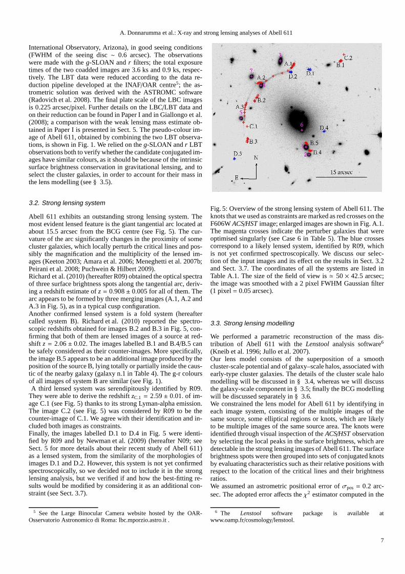
3.2. Strong lensing system

Abell 611 exhibits an outstanding strong lensing system. Themost evident lensed feature is the giant tangential arc located atabout 15.5 arcsec from the BCG centre (see Fig. 5). The cur-vature of the arc significantly changes in the proximity of somecluster galaxies, which locally perturb the critical linesand pos-sibly the magnification and the multiplicity of the lensed im-ages (Keeton 2003; Amara et al. 2006; Meneghetti et al. 2007b;Peirani et al. 2008; Puchwein & Hilbert 2009).Richard et al. (2010) (hereafter R09) obtained the optical spectraof three surface brightness spots along the tangential arc,deriv-ing a redshift estimate ofz= 0.908± 0.005 for all of them. Thearc appears to be formed by three merging images (A.1, A.2 andA.3 in Fig. 5), as in a typical cusp configuration.Another confirmed lensed system is a fold system (hereaftercalled system B). Richard et al. (2010) reported the spectro-scopic redshifts obtained for images B.2 and B.3 in Fig. 5, con-firming that both of them are lensed images of a source at red-shift z = 2.06± 0.02. The images labelled B.1 and B.4/B.5 canbe safely considered as their counter-images. More specifically,the image B.5 appears to be an additional image produced by theposition of the source B, lying totally or partially inside the caus-tic of the nearby galaxy (galaxy n.1 in Table 4). The g-r coloursof all images of system B are similar (see Fig. 1).A third lensed system was serendipitously identified by R09.

They were able to derive the redshiftzC.1 = 2.59± 0.01. of im-age C.1 (see Fig. 5) thanks to its strong Lyman-alpha emission.The image C.2 (see Fig. 5) was considered by R09 to be thecounter-image of C.1. We agree with their identification andin-cluded both images as constraints.Finally, the images labelled D.1 to D.4 in Fig. 5 were identi-fied by R09 and by Newman et al. (2009) (hereafter N09; seeSect. 5 for more details about their recent study of Abell 611)as a lensed system, from the similarity of the morphologies ofimages D.1 and D.2. However, this system is not yet confirmedspectroscopically, so we decided not to include it in the stronglensing analysis, but we verified if and how the best-fitting re-sults would be modified by considering it as an additional con-straint (see Sect. 3.7).

5 See the Large Binocular Camera website hosted by the OAR-Osservatorio Astronomico di Roma: lbc.mporzio.astro.it .

Fig. 5: Overview of the strong lensing system of Abell 611. Theknots that we used as constraints are marked as red crosses ontheF606WACS/HSTimage; enlarged images are shown in Fig. A.1.The magenta crosses indicate the perturber galaxies that wereoptimised singularly (see Case 6 in Table 5). The blue crossescorrespond to a likely lensed system, identified by R09, whichis not yet confirmed spectroscopically. We discuss our selec-tion of the input images and its effect on the results in Sect. 3.2and Sect. 3.7. The coordinates of all the systems are listed inTable A.1. The size of the field of view is≃ 50× 42.5 arcsec;the image was smoothed with a 2 pixel FWHM Gaussian filter(1 pixel= 0.05 arcsec).

3.3. Strong lensing modelling

We performed a parametric reconstruction of the mass dis-tribution of Abell 611 with theLenstool analysis software6

(Kneib et al. 1996; Jullo et al. 2007).Our lens model consists of the superposition of a smoothcluster-scale potential and of galaxy–scale halos, associated withearly-type cluster galaxies. The details of the cluster scale halomodelling will be discussed in§ 3.4, whereas we will discussthe galaxy-scale component in§ 3.5; finally the BCG modellingwill be discussed separately in§ 3.6.We constrained the lens model for Abell 611 by identifying ineach image system, consisting of the multiple images of thesame source, some elliptical regions or knots, which are likelyto be multiple images of the same source area. The knots wereidentified through visual inspection of theACS/HSTobservationby selecting the local peaks in the surface brightness, which aredetectable in the strong lensing images of Abell 611. The surfacebrightness spots were then grouped into sets of conjugated knotsby evaluating characteristics such as their relative positions withrespect to the location of the critical lines and their brightnessratios.We assumed an astrometric positional error ofσpos = 0.2 arc-sec. The adopted error affects theχ2 estimator computed in the

6 The Lenstool software package is available atwww.oamp.fr/cosmology/lenstool.

7


source plane byLenstool:

χ2Si=

ni∑

j=1

x jS− < x j

S >

µ−1j σpos

2

, (7)

wherex jS is the position of the source corresponding to the ob-

served imagej, < x jS > the barycenter of theni source positions

(corresponding to theni conjugated images or knots of the imagesystemi), andµ j the magnification for the lensed imagej; thefinal χ2 is then obtained by combining the individualχ2

Sicom-

puted for each image system.Between the several optimisation methods available inLenstoolwe adopted the Bayesian optimisation method, with a con-vergence speed parameter equal to 0.4; this method, althoughslower than the other optimisation options, is less sensitive tolocal minima in the parameter space.

3.4. Cluster–scale component

We modelled the cluster scale component assuming an ellipticalNFW profile as mass functional. The initial values for thecentre, ellipticity e and position angleθ of the cluster halowere inferred from the BCG luminosity profile. The centrewas allowed to vary±5 arsec, while the ellipticity and theposition angle were optimised in the ranges 0.01 6 e 6 0.4 and100.0 deg6 θDM 6 140.0 deg, respectively. The optimisationrange of the cluster position angle is asymmetric in order totake into account the orientation of the X-ray isophotes. Theoptimisation ranges for the NFW profile parameters werec200 ∈ [0.5− 14.0] andrs ∈ [50.0− 800.0] kpc.

3.5. Galaxy–scale components

3.5.1. Selection of cluster galaxies

Several authors demonstrated that the inclusion of galaxy-scalehalos in the lens modelling (in particular the galaxies whoseprojected position is within the region probed by strong lensing)is necessary to account for their effect on the lensing crosssection and on the appearance of the lensed images that fallclose to the perturbers (Natarajan et al. 2007; Amara et al.2006; Meneghetti et al. 2003; Keeton 2003; Bradac et al. 2002).Although gravitational lensing is sensitive to all massivestruc-tures distributed along the line of sight, the main galacticmassbudget is constituted of the massive early-type cluster galaxies;we will thus consider only this galactic population in our lensmodelling.The cluster members were selected through the characteristiccluster red-sequence, which allows us to identify the redearly-type galaxies (Bell et al. 2004) and which is clearlydetected in the colour-magnitude diagram (see Fig. 6). Wewill assume in the modelling that all the red-sequence galaxiesbelong to the cluster, and thus lie at its same redshift. Thediagram was derived by extracting the object catalogues fromthe two LBT observations, using theSExtractor software insingle and dual-image mode.Even if the total exposure time of the red image is 0.9 ks, whichis one fourth of theg-Sloan observation exposure time, theformer filter allows an easier deblending of the redder clustergalaxies from the bluer lensed features. For this reason we usedthe r filter image for the detection of the sources in the dual-image mode. Moreover, even if the higher spatial resolution

0

0.5

1

1.5

2

2.5

3

18 19 20 21 22 23

mag

G -

mag

R

magR

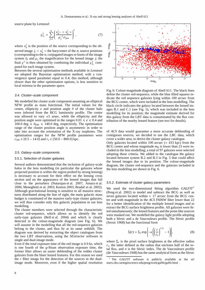
Fig. 6: Colour-magnitude diagram of Abell 611. The black linesdefine the cluster red-sequence, while the blue filled squares in-dicate the red sequence galaxies lying within 100 arcsec fromthe BCG centre, which were included in the lens modelling. Theblack circle indicates the galaxy located between the lensed im-ages B.1 and C.1 (see Fig. 5), which was included in the lensmodelling for its position; the magnitude estimate derivedforthis galaxy from the LBT data is contaminated by the flux con-tribution of the nearby lensed feature (see text for details).

of ACS data would guarantee a more accurate deblending ofcontiguous sources, we decided to use the LBC data, whichcover a wider area, to derive the cluster galaxy catalogue.Only galaxies located within 100 arcsec (≃ 433 kpc) from theBCG centre and whose magnitudemR is lower than 23 were in-cluded in the lens modelling; a total of 97 galaxies were selectedadopting these criteria. We added to the catalogue the galaxylocated between system B.2 and B.3 in Fig. 5 that could affectthe lensed images due to its position. The colour-magnitudediagram, the cluster red-sequence and the galaxies included inthe lens modelling are shown in Fig. 6.

3.5.2. Estimate of cluster galaxy parameters

We used the two-dimensional fitting algorithmGALFIT7

(Peng et al. 2002) to model and subtract the BCG as well asseven galaxies located within≃ 17 arcsec from the BCG cen-tre and with magnitude in theACSF606W filter lower than 22for a better identification of the multiple lensed images andtoextract the BCG surface brightness profile. All galaxies were fit-ted simultaneously; the lensed features and the point-likesourceswere masked out. We modelled the galaxy light profile adoptingboth a Sersic and a de Vaucouleurs profile. The Sersic profile(Sersic 1968) has the functional form

Σ(r) = Σe exp

−κ

(

rre

)1/n

− 1

, (8)

whereΣe is the pixel surface brightness at the effective radiusre, the latter defined as the radius that encloses half of the to-tal flux, andn is the Sersic index. The de Vaucouleurs profile(de Vaucouleurs 1948) has the same analytical form as the Sersic

7 The GALFIT software is publicly available at the urlusers.obs.carnegiescience.edu/peng/work/galfit/galfit.html .

8


Table 4: Best-fit parameters obtained by modelling the galaxy luminosity with the Sersic profile (Sersic 1968).

Best-fitting Sersic profile parameters

ID xc yc Axis re Position Sersic m606W

deg(J2000) deg(J2000) ratio [kpc] Angle index

BCG 120.23678 36.056572 0.70± 0.01 38.54± 0.27 132.5± 0.1 3.0± 0.1 17.0± 0.11 120.23598 36.054391 0.83± 0.01 1.48± 0.01 112.8± 0.1 2.3± 0.1 20.7± 0.12 120.2357 36.053776 0.92± 0.01 1.02± 0.01 13.1± 0.1 2.9± 0.1 21.6± 0.13 120.23855 36.061407 0.50± 0.01 3.85± 0.04 78.7± 0.2 2.6± 0.1 20.7± 0.14 120.24051 36.059402 0.67± 0.01 3.28± 0.07 80.6± 0.5 4.7± 0.1 20.8± 0.15 120.24255 36.056744 0.84± 0.01 1.35± 0.02 128.4± 1.4 4.6± 0.1 21.4± 0.16 120.23639 36.055754 0.90± 0.01 0.64± 0.01 131.6± 4.0 2.3± 0.1 22.0± 0.17 120.24148 36.060146 0.79± 0.01 2.32± 0.04 61.7± 0.9 5.1± 0.1 21.1± 0.1

Notes.The algorithmGALFIT is used. The fit was performed using theACSF606W filter image. We list here the galaxy ID (the galaxy numberingis the same used in Fig. 5), the centroid coordinates, the axis ratio, the effective radiusre, the positional angle, the Sersic indexn and the galaxyintegrated magnitude, computed in the ST magnitude system.Here we report the 68% statistical errors as determined fromGALFIT. The errorswere rounded to the closest value greater than zero.

profile, but the index has the fixed value of 4.The galaxy models were convolved with theHSTPSF image cre-ated using the TinyTim software8 (Krist 1993). The reducedχ2

of the best-fitting models obtained adopting either the Sersic orthe de Vaucouleurs profile are similar,χ2

S = 3.8 andχ2dV = 3.9,

respectively. However, the galaxy-subtracted image derived fit-ting the galaxy light profile with a de Vaucouleurs model showslarger residuals in the central area for some of the fitted galaxies,in particular for the galaxy labelled 1 in Table 4. For this reasonwe chose a Sersic profile to model and subtract from theHSTim-age the galaxies located within≃ 17 arcsec from the BCG centre.The best–fitting parameters for the galaxy profiles are listed inTable 4; the corresponding galaxies are indicated in Fig. 5 withthe same numbering sequence as in Table 4. Snapshots of thegalaxy-subtractedHST image are shown in Fig. A.1.

3.5.3. Mass profiles of cluster galaxies

In order to reduce the number of parameters to an adequatenumber we need to relate the total mass of cluster galaxiesto an observable quantity; we will thus assume a scaling rela-tion that links the mass of a galaxy to its luminosity. We willalso assume that the morphological parameters of the underly-ing galaxy halo match the values inferred from the galaxy lu-minosity; this is a reasonable assumption because of the tightcorrelation between light and mass profile in early-type galax-ies (see e.g. Gavazzi et al. 2007; Koopmans et al. 2006). For thisreason, the galaxy centroid, ellipticity and position angle werefixed to the values obtained from the analysis performed withSExtractorof ther filter LBC images. However, the parametersderived from the LBC data for some of the galaxies close to thelensed images or to the BCG appear to be incorrect, because ofan inefficient de-blending for the lower spatial resolution of LBCimages. In these cases we adopted the parameters (namely cen-troid coordinates, position angle, major/minor axis length andmagnitude) estimated throughSExtractorfrom theHSTF606Wimage.We parameterised the mass of cluster galaxies with thedual pseudo isothermal elliptical mass distribution (hereafterdPIE, Kassiola & Kovner 1993; Kneib et al. 1996), following

8 The TinyTim software is available at the urlwww.stsci.edu/software/tinytim/tinytim.html .

Jullo et al. (2007); Brainerd et al. (1996) and several otherau-thors. The dPIE profile is given by

ρ(r) =ρ0

(1+ r2/r2core)(1+ r2/r2

cut). (9)

The dPIE cut radius can be roughly considered as the half massradius9. The two-dimensional surface mass density distributionis obtained by integrating Eq. 9 (see also Limousin et al. 2005):

Σ(R) =σ2

0rcut

2G(rcut− rcore)

1√

r2core+ R2

−1

√

r2cut + R2

, (10)

whereσ0 is a characteristic central velocity dispersion, whichcannot be simply related to the measured velocity dispersion(Elıasdottir et al. 2007).The free parameters in the dPIE model are thus the core radiusrcore, the truncation radiusrcut, and the characteristic velocitydispersionσ0. For elliptical galaxies, the Faber-Jackson relation(hereafter FJ, Faber & Jackson 1976) predicts that the central ve-locity dispersionσ0 is proportional to the galaxy luminosityLfollowing the scaling relation

σ0 = σ⋆0

( LL⋆

)1/4

, (11)

whereL⋆ is a given arbitrary galaxy luminosity andσ⋆0 is its cor-responding dPIE velocity dispersion; our reference magnitude ism⋆r = 18.0. We will assume the following scaling relations forthe characteristic radii of the dPIE profile:

rcore= r⋆core(L/L⋆)1/2 ,

rcut = r⋆cut(L/L⋆)α ; (12)

here againr⋆core andr⋆cut are the dPIE scale parameters for aL⋆

galaxy. The exponent of the scaling relation forrcut determineshow the mass scales with respect to the light distribution. Ifα = 0.5 the mass-to-light ratio (ML) of the galaxy is constantand independent of its luminosity, as usually assumed in strongand weak lensing analyses (Richard et al. 2007; Hoekstra et al.

9 The cut radius corresponds to the 3-D half mass radius for a nullcore radius (Elıasdottir et al. 2007).

9


2004). Assumingα = 0.8 one obtains that the mass-to-light ra-tio scales with luminosity according toML ∝ L0.3 (Halkola et al.2006; Natarajan & Kneib 1997). In this paper we will assumeα = 0.5, but in§ 3.7 we will compare the results obtained underthis assumption with those obtained by assumingα = 0.8. Wedid not test alternative scaling relations for the cluster galaxycore radius, since we did not identify any reliable constraint onthe galaxy inner mass distribution.The galaxy parameters optimised in the lens modelling are thecentral velocity dispersion and the truncation radius, whereas theother dPIE parameters (ellipticity, position and orientation of thehalo) were tied to the values inferred from the analysis of thegalaxy light profile.The normalisation for the core radius scaling was set tor⋆core=0.035 arcsec≃ 0.15 kpc, while for the velocity dispersionnormalisationσ⋆0 we adopted the uniform prior [120.0–200.0]km s−1. Following the relation between luminosity and velocitydispersion found by Bernardi et al. (2003), our reference mag-nitude corresponds to a velocity dispersion≃ 170 km s−1 foran early-type galaxy. The priorσ⋆0 ∈ [120.0 − 200.0] km s−1

adopts a conservative upper limit; the lower limit was decreasedto 120.0 km s−1 to take into account the recent findings ofNatarajan et al. (2009) about the difference in the dPIE veloc-ity dispersion between cluster galaxies in the core or in theouterregions.The truncation radius normalisation determines the steepness ofthe galaxy mass profile. A common and reasonable approach isto fix it to a likely value (see R09 and Limousin et al. 2009),since usually the strong lensing system does not provide enoughconstraints on the mass distribution of the small scale per-turbers. However, the mass distribution of early-type galaxies inhigh–density environment is likely to be truncated compared tofield galaxies with an equivalent luminosity (Halkola et al.2007;Limousin et al. 2007; Natarajan et al. 2002). For this reason, thetruncation of cluster galaxy halos could be different from onecase to another.Thanks to the peculiar lensing system of Abell 611, an estimateof the truncation radius normalisation will be derived in one ded-icated tests (see Sect. 3.7). The perturbing galaxy labelled 1 inFig. 5 was optimised singularly, since the strong constraints onits Einstein radius provided by the conjugate systems B.4/B.5enable a reliable estimate of its mass distribution. Because how-ever neither R09 or Newman et al. (2009) unlinked this galaxyfrom the cluster member catalogue, we ran a test to verify if andhow this single perturber can affect the global test results.

3.6. Modelling of the BCG

The BCG itself was included in the lens modelling as a dPIEhalo. However, although the BCG was parameterised with thesame mass functional as the cluster members, its mass modelrefers only to itsbaryonic content, while for cluster galaxieswhat is actually modelled is thetotal mass. As pointed out in thework of Miralda-Escude (1995) (see also Limousin et al. 2008;Dubinski 1998; Mellier et al. 1993), the dark matter halo of theBCG is indistinguishable from the cluster halo in the lens mod-elling.For this reason a direct comparison of the measured central ve-locity dispersion of the BCG to the fittedσ0,dPIE would lead toincorrect conclusions: the former is determined by the combinedcontribution of the dark and baryonic matter, while the latter is afitting parameter referred to as a “stellar-only” BCG component.The dPIE mass parameters - characteristic central velocitydis-

persionσ0,dPIE and truncation radiusrcut- were optimised for theBCG in the ranges [100.0-350.0] km s−1 and [8.0-31.0] arcsec(≃ [34.6− 134.2] kpc), respectively: these ranges take into ac-count the results obtained through a strong lensing analysis byR09 and by N09, to allow a comparison with their results (see§ 5).The degeneracy between the central baryonic mass budget andthe dark matter content with regard to the strong lensing resultsis currently well established. It is still to be discussed whetherthe choice of the BCG mass profile can impact the derived clus-ter mass parameters. To assess this point, we ran a dedicatedtestadopting the Sersic profile to parametrise the BCG mass. TheSersic mass profile has the same functional form as Eq. 8, butthe parameterΣe refers to the mass density at the effective radiusre.For the modelling of the BCG we adopted the morphologicalparameters derived from the two-dimensional fitting of the BCGluminosity profile obtained withGalfit, listed in Table 4. We op-timised the Sersic index within±10% of the best-fitting value,to take into account the measurement errors. After some prelim-inary tests, we chose as lower limit to theΣe optimisation rangethe value of 2× 108M⊙kpc−2 to derive a total mass for the BCGsimilar to the mass derived when modelling the BCG as a dPIEprofile, for a safer comparison between the results obtainedinboth cases (see the total projected mass maps and the surfacemass density profiles shown in Fig.7).

1e+07

1e+08

1e+09

1e+10

1e+11

0.1 1 10 100

Sur

face

mas

s de

nsity

Σ

[M⊙

/kpc

2 ]

R [kpc]

BCG=dPIEBCG=Sersic

1e+11

1e+12

0.1 1 10 100

Sur

face

mas

s de

nsity

Σ

[M⊙

/kpc

2 ]

R [kpc]

NFW halo - BCG=dPIENFW halo - BCG=Sersic

Fig. 7: [Top Panels]Comparison between the projected massmaps obtained when modelling the BCG with a dPIE profile (leftpanel, case 1 in Table 5) or with a Sersic profile (right panel, case7 in Table 5). See Table 5 and the text for further details.[BottomPanels]Comparison between the surface mass density profilesfor the BCG halo[left panel] and the NFW cluster scale halo[right panel] derived when modelling the BCG with a dPIE pro-file (red solid line, case 1) or with a Sersic profile (green dashedline, case 7).

10


Table 5: Median values for the total mass parameters, obtained with the strong lensing analysis.

Results of the strong lensing analysis of Abell 611

Case xc yc e PA r⋆ c200 M200 σ0 χ2red[d.o. f .] rmsi

[arcsec] [arcsec] [deg] [kpc] [1014M⊙] [km s−1] [arcsec]

1

Cluster -0.6±0.2 0.9±0.2 0.25±0.01 132.8±0.2 214.3±23.6 6.78+0.81−0.37 4.68±0.31 1300.5±15.7 0.6 [61] 0.33

BCG (0.0) (0.0) 85.5+4.0−67.8 310.9+22.2

−40.0

Perturber 1 (2.33) (-7.85) 22.1+6.1−10.5 176.3+9.4

−6.8

Ref. Galaxy 37.1+6.4−14.0 179.1+15.9

−11.9

2

Cluster -0.6±0.1 0.9±0.2 0.25±0.01 132.8±0.2 228.0+16.6−20.8 6.43+0.56

−0.32 4.87±0.27 1307.2±16.4 0.6 [62] 0.37

BCG (0.0) (0.0) 91.1+8.4−55.0 324.7+4.3

−33.1

Perturber 1 (2.33) (-7.85) 23.1+4.4−10.7 178.2±6.5

Ref. Galaxy (43.3) 187.1+1.5−16.7

3

Cluster -0.6±0.1 0.9±0.2 0.25±0.01 132.9±0.2 218.3+22.7−16.9 6.63+0.67

−0.32 4.68+0.33−0.18 1297.4±15.0 0.6 [62] 0.32

BCG (0.0) (0.0) 96.2+13.2−43.4 311.5+14.3

−36.8

Perturber 1 (2.33) (-7.85) 23.8+1.1−14.3 176.0±6.5

Ref. Galaxy (43.3) 175.9±11.8

4

Cluster -0.3±0.1 0.4±0.1 0.21±0.01 132.9±0.2 158.6+8.8−5.3 8.75+0.19

−0.42 4.01±0.13 1303.7±7.0 0.9 [63] 0.50

BCG (0.0) (0.0) 96.0+2.1−52.3 132.8+47.1

−2.2

Perturber 1 (2.33) (-7.85)

Ref. Galaxy 48.7+0.6−4.8 198.6+0.2

−2.3

5

Cluster -0.4±0.1 0.9±0.2 0.23±0.01 132.8±0.2 192.0±18.7 7.40±0.60 4.40±0.22 1295.4±11.5 1.0 [74] 0.31

BCG (0.0) (0.0) 99.4+7.0−48.4 263.0±35.6

Perturber 1 (2.33) (-7.85) 12.0+7.6−1.9 180.4+1.3

−14.0

Ref. Galaxy (43.3) 190.5+5.6−9.7

Redshift estimate of the candidate system D

zD.1 zD.2 zD.3 zD.4

2.07±0.04 2.32±0.26 2.43±0.39 2.09±0.05

6

Cluster -0.5±0.2 0.8±0.2 0.25±0.01 133.2±0.4 211.8+30.2−11.1 6.81+0.69

−0.41 4.59+0.34−0.16 1294.1±13.9 0.7 [52] 0.20

BCG (0.0) (0.0) 95.6+24.1−28.9 297.2+30.4

−46.8

Perturber 1 (2.33) (-7.85) 19.4+16.8−4.5 186.4+15.7

−10.2

Perturber 2 (3.14) (-10.05) 15.9+5.5−8.3 108.2+33.6

−22.4

Perturber 3 (-5.15) (17.42) 11.4+8.8−2.1 125.4+25.5

−16.2

Perturber 4 (-10.88) (10.22) 16.2+17.7−0.8 103.5+14.5

−7.7

Perturber 5 (-16.79) (0.60) 14.6+12.5−1.8 80.9+21.7

−10.8

Perturber 6 (1.13) (-2.78) 14.8+10.4−3.9 153.8+10.1

−64.0

Ref. Galaxy (43.3) 149.6±17.9

7

Cluster -0.8±0.1 1.0±0.2 0.20±0.01 132.8±0.3 286.9+24.9−11.4 5.59+0.18

−0.31 6.32+0.51−0.23 1392.1±19.0 1.1 [61] 0.44

BCGSersic (0.0) (0.0) Σe=2.08+0.12−0.01 [108M⊙/kpc2] Sersic indexn=2.87+0.26

−0.01

Perturber 1 (2.33) (-7.85) 21.8+1.6−16.5 176.08.1

−6.0

Ref. Galaxy 36.5+9.1−10.8 161.7+11.3

−20.9

Notes. The results are derived assuming an elliptical NFW profile for the cluster-scale lens component and an elliptical dPIE for the galaxy scalehalos. We report only the values that were optimised in the strong lensing fit; additionally, the coordinates of the cluster galaxies are listed in roundbrackets for the sake of clarity, but they were not optimised. The columns list the coordinates of the halo centroid (expressed in arcseconds withrespect to the BCG centre: at the cluster redshift and for theassumed cosmology, 1 arcsec=4.329 kpc), the potential ellipticity (here expressedase = (a2 − b2)/(a2 + b2)), the halo position angle, the scale radius r⋆ (that indicates the scale radiusrs for the cluster-scale NFW halo and thetruncation radiusrcut for the galaxy-scale dPIE halos), the concentration parameter c200, the total massM200, the characteristic velocity dispersionσ0 for the NFW or the dPIE profiles, expressed in km s−1, the reducedχ2 (the number of degrees of freedom is enclosed within square brackets)and the root-mean-square computed in the image plane (rmsi). The uncertainties represent the 68% statistical errors,derived assuming a Gaussianprobability distribution. If the upper and lower errors aresignificantly asymmetric we report both of them. For a description of the cases listedhere, see Pag. 12.

3.7. Strong lensing results

We present in this section the results of the parametric analysisof the strong lensing system in Abell 611. In order to assess the

effect of the galaxy parameterisation on the best-fitting resultsfor the cluster-scale halo we performed several tests, changingthe manner of including the cluster galaxies.

11


5

6

7

8

9c 2

00Case 1

5

6

7

8

9

c 200

Case 2

5

6

7

8

9

c 200

Case 3

5

6

7

8

9

c 200

Case 4

5

6

7

8

9

140 180 220 260 300 340

c 200

rs [kpc]

Case 5

160 200 240 280 320 360

5

6

7

8

9

c 200

rs [kpc]

Case 6

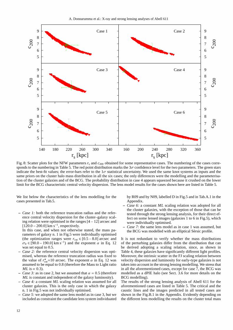
Fig. 8: Scatter plots for the NFW parametersrs andc200 obtained for some representative cases. The numbering of the cases corre-sponds to the numbering in Table 5. The red point distribution marks the 3σ confidence level for the two parameters. The green starsindicate the best-fit values; the error-bars refer to the 1σ statistical uncertainty. We used the same knot systems as inputs and thesame priors on the cluster halo mass distribution in all the six cases; the only differences were the modelling and the parameterisa-tion of the cluster galaxies and of the BCG. The probability distribution in case 4 appears squeezed because it crushed onthe lowerlimit for the BCG characteristic central velocity dispersion. The lens model results for the cases shown here are listedin Table 5.

We list below the characteristics of the lens modelling for thecases presented in Tab.5.

– Case 1:both the reference truncation radius and the refer-ence central velocity dispersion for the cluster–galaxy scal-ing relation were optimised in the ranges [4 – 12] arcsec and[120.0 – 200.0] km s−1, respectively.In this case, and when not otherwise stated, the mass pa-rameters of galaxy n. 1 in Fig.5 were individually optimised(the optimization ranges werercut ∈ [0.5 – 8.0] arcsec andσ0 ∈ [90.0 – 190.0] km s−1) and the exponentα in Eq. 12was set equal to 0.5.

– Case 2:the reference central velocity dispersion was opti-mised, whereas the reference truncation radius was fixed tothe value ofr⋆cut=10 arcsec. The exponentα in Eq. 12 wasassumed to be equal to 0.8 (therefore the Mass to Light ratioML is ∝ 0.3).

– Case 3:as in case 2, but we assumed thatα = 0.5 (thereforeML is constant and independent of the galaxy luminosity).

– Case 4:a constantML scaling relation was assumed for allcluster galaxies. This is the only case in which the galaxyn. 1 in Fig.5 was not individually optimised.

– Case 5:we adopted the same lens model as in case 3, but weincluded as constraint the candidate lens system individuated

by R09 and by N09, labelled D in Fig.5 and in Tab.A.1 in theAppendix.

– Case 6:a constantML scaling relation was adopted for allthe cluster galaxies, with the exception of those that can betested through the strong lensing analysis, for their direct ef-fect on some lensed images (galaxies 1 to 6 in Fig.5), whichwere individually optimised.

– Case 7:the same lens model as in case 1 was assumed, butthe BCG was modelled with an elliptical Sersic profile.

It is not redundant to verify whether the mass distributionsof the perturbing galaxies differ from the distribution that canbe derived adopting a scaling relation, since, as shown inTable 4, these galaxies have significantly different light profiles.Moreover, the intrinsic scatter in the FJ scaling relation betweenvelocity dispersion and luminosity for early-type galaxies is nottaken into account in the strong lensing modelling. We stress thatin all the aforementioned cases, except for case 7, the BCG wasmodelled as a dPIE halo (see Sect. 3.6 for more details on theBCG modelling).The results of the strong lensing analysis of Abell 611 for theaforementioned cases are listed in Table 5. The critical andthecaustic lines and the images predicted in all tested cases areshown in the Fig.B.1 in the Appendix. Evidently depending onthe different lens modelling the results on the cluster total mass

12


can change by up to 15%, so the parameterisation of the per-turber galaxies and of the BCG has a non-negligible impact onthe strong lensing results; the degeneracy between clusterandgalaxy mass parameters is shown in Fig.8. In particular, a strongdegeneracy is found between the fiducial BCG central velocitydispersion and the cluster concentration/total mass (see the toppanels in Fig.9).It is remarkable that the resulting NFW cluster parameters de-pend not only on the BCG baryonic mass, but also on the BCGmass profile. In case 1 and in case 7 we show the results obtainedby modelling the BCG with a dPIE or with a Sersic profile, re-spectively; the corresponding projected mass maps and surfacemass density profiles are shown in Fig. 7. The BCG mass de-rived in both cases is similar, but the inferred cluster parametersare significantly different. In particular, the cluster total mass islarger and the NFW concentration parameter lower when mod-elling the BCG with a Sersic profile. This result can be explainedby considering that, in this case, the surface mass density ofthe best-fitting Sersic profile in the BCG central region is largercompared with the best-fitting dPIE profile (see the bottom leftpanel in Fig. 7). The inferred concentration for the clusterscalehalo in the latter case will thus be higher because of the degen-eracy between the cluster halo and the BCG mass with respectto the lens total mass, which is the quantity constrained by thegravitational lensing.However, the estimates of thetotal mass in the central regions(where the strong lensing constraints are found) derived inthedifferent cases mutually agree, (see the discussion in Sect. 4);themodelling of the galactic component appears to have a negligibleimpact on the total mass results in the central region. Conversely,the differences among several of the test cases arise when thecluster mass is extrapolated outside the region that is accessiblethrough the strong lensing analysis.This is another evidence that the modelling of the BCG stellarmass can directly affect the cluster total mass results: in order toobtain reliable mass estimates through a parametric stronglens-ing analysis, it is crucial to break the degeneracy between thedifferent lens components.Despite the difference in the best-fitting results, all models returnprobability regions in the parameter space that are marginallyconsistent with each other. As previously found for the X-rayanalysis, the strong lensing results appears relatively stableagainst possible systematic errors, which in this case are mainlyconstituted by modelling uncertainties.As stated before, the perturber galaxy n.1 (see Fig. 5) was in-dividually optimised in all the tests that we ran, except in case4, due to the tight constraint on its mass distribution provided bythe conjugated images B.4 and B.5. We found a mild degeneracybetween the mass of this galaxy, the mass of the stellar contentof the BCG, and the concentration of the NFW halo, as expectedgiven the proximity of this perturber to the BCG (see the bottompanels in Fig. 9).Moreover, in case 6 we optimised singularly the galaxies whosemass distribution can be constrained through the strong lens-ing effect alone. As it is evident from Fig. 10, optimising inwide ranges the dPIE parameters for these perturber galaxiesreturns, as expected, large uncertainties in the mass parameters.However, for some perturbers the parameters inferred through anindividual optimisation appear to be incongruous with those pre-dicted assuming the parameter scaling derived from the Faber-Jackson relation. It is reasonable to question whether neglectingthe scatter associated to the galaxy parameter scaling relationsin the strong lensing analysis could bias the inferred results.It seems likely that in most cases this bias, if any, can be safely

Fig. 9: Scatter plots of cluster–halo parameters (c200 and Mtot)versus parameters of the modelling of either the BCG or the per-turber galaxy n.1 (hereafter P1, see text for details). Hereweshow the posterior probability distributions obtained in arep-resentative case (case 1 in Tab.5). The plotted parameters are:1. the NFW concentration parameterc200 versus the BCG fidu-cial central velocity dispersionσ0,BCG [top left panel]; 2. thecluster halo massMtot versusσ0,BCG [top right panel]; 3. theNFW concentration parameterc200 versus the fiducial centralvelocity dispersionσ0,P1 of the galaxy P1 [bottom left panel];4. the cluster halo massMtot versusσ0,P1 [bottom right panel].The contours show the 68%, 95% and 99% confidence levels.The colour code refers to the value of theχ2 estimator.

negligible, as it is obvious by comparing case 1 to case 6.Nonetheless, in the presence of galaxies that strongly affect thestrong lensing features, the biasing effect on the final resultscould be more significant (again, this is the case of the perturbergalaxy labelled n.1 in this work, as can be seen by comparingcase 1 to case 4).Regarding the strong lensing systems, all our models pre-dict that the tangential arc (system A) originates by the largedeformation of a single source located on a “naked cusp”,i.e. a tangential caustic extending outside the radial caustic(Kormann et al. 1994; Bartelmann & Loeb 1998; Rusin & Ma2001). Naked cusps are a quite rare caustic configuration whichmainly occurrs in highly elliptical lens systems whose sur-face density is only moderately above the critical surface den-sity required for the production of multiple images (“marginallenses”, Blandford & Kochanek 1987; Bartelmann 2000), withafew naked cusps detected so far (Lewis et al. 2002; Oguri et al.2008). Sources placed within the exposed tangential causticform only three magnified images on the same side of the lens:this explains why the tangential arc in Abell 611 has no counter-image.The position and the shape of the observed images are well re-produced by all our models, as is obvious from the low scat-ter both in the image and in the source plane resulting from thebest-fit models: all tests returned low values of the reducedχ2

(χ2red ≤ 1) and of the image plane root-mean-square (rmsi ≤ 0.5

13


60

80

100

120

140

160

180

200

220

5 10 15 20 25 30 35 40

σ 0 [km/s]

rcut [kpc]

Case 4Case 6

1

2

3

4

5

61

256

43

Fig. 10: Median values of the dPIE truncation radiusrcut vs thecharacteristic dPIE central velocity dispersionσ0 for the galax-ies that perturb the strong lensing system of Abell 611. The redtriangles show the results obtained linking the galaxy parame-ters to the same scaling relation in the lens modelling (Case4 inTable 5), while the blue stars represent the results obtained op-timising the galaxies individually (Case 6 in Table 5). The greydashed lines show the iso-density contours. The error bars in-dicate the 1σ uncertainty, while the cyan boxes indicate the 3σconfidence region for the results which refer to Case 4.

arcsec) (see also the fitting results for a representative case - Case1 - listed in Tab.6).In particular, the lens models of cases 4 and 7 (see Tab.5) predicta central image for the system B in a position almost coinci-dent with a radial-oriented feature lying close to the centre ofthe BCG (see Fig.11 and the predicted central image in Fig.B.1;this central image was also indentified and interpreted by N09).However, since the detection of this feature is not certain,we didnot include it as an additional constraint.Regarding the third system C, our identification of the positiveparity counter-image, which follows R09, appears reliableow-ing to the very low scatter resulting for this system. Our modelspredict three additional counter-images: two of them should belocated close to the BCG and to the galaxy n.1, and are pre-dicted to be demagnified with respect to the identified image,sothey are likely not detectable. A negative parity counter-imageis predicted at about 2-3 arcsec (depending on the different lensmodels) above the observed one. In that area there are no evi-dent counter-images, but a faint one, identified with SExtractor(S/N≃ 3.9), whose position could be marginally compatible withthe location of the predicted image. The flux ratio derived whenmodelling the BCG as a dPIE halo does not match the observedone well, while the images predicted when modelling the BCGwith a Sersic profile follow the observed flux ratio more closely(see Fig. 12), because of the difference in the inferred mass forthe galactic perturbers. This evidence would seem to favourthemodelling of the BCG with a Sersic profile over the dPIE profile:but we aim to highlight that other explanations could be possibleto the observed mismatch in the flux ratios for the images of thethird system. For example, the effect of unresolved substructuresalong the line of sight would cause the dimming of the negative-parity image in cusp systems (Keeton 2003) (see also Oguri etal.2008). Another explanation could be the misidentification of the

Fig. 11:ACS/HSTsnapshot of a radial-oriented feature, likely acentral counter-image corresponding to System B; the BCG isvisible [subtracted] in the left [right] panel.

Fig. 12: Comparison between theACS/HSTF606W observation[left panel], smoothed with a 3 FWHM pixel Gaussian filter fora better visualisation of the faint lensed image C.1 (markedwitha white circle), and the reconstructed image systems predictedfrom the lens models in case 1 ([middle panel]: in this casethe BCG was modelled as a dPIE potential) and case 7 ([rightpanel]: the BCG was parametrised with a Sersic profile - seeTable 5). The white circles in the middle and right panels markthe centre of the predicted counter-images. The black circle inthe left panel indicates a candidate counter-image of C.1, inden-tified with SExtractor. The three images are WCS-aligned; theflux scale of the second and the third panel is the same.

counter-image C.2, which would cause its predicted magnifica-tion to be incorrect.The candidate system D looks plausible considering the lowscatter in the observed and predicted positions. The redshiftestimates of the four knot systems are marginally consistent.However, the results of the cluster mass parameters are not sig-nificantly changed by including this system.

4. Comparison between X-ray and strong lensingresults

We will compare here the results obtained with the stronglensing and the X-ray analyses for the galaxy cluster Abell 611.The left panel in Fig. 13 shows the probability distributions ofthe NFW profile parameters obtained with both analyses, whilethe right panel compares the corresponding projected mass

14


1

2

3

4

5

6

7

8

9

10

11

12

100 200 300 400 500 600 700 800 900

c 200

rs [kpc]

X−RAY

SL−dPIE

SL−Sérsic

WL−Ro09

WL−N09

SL−N09

SL−R09

3e+14

1e+14

5e+13

2e+13

1e+13

Mto

t,2D [M

⊙]

X−raySL−dPIE

SL−SérsicX−ray−S09

SL−R09

0.6

1

1.4

500 250 100 50

MX

−ra

y/M

SL

R [kpc]

SL X−ray

SL−dPIE

SL−Sérsic

Fig. 13:[Left panel]Comparison of the NFW parameter probability distribution obtained with our X-ray and strong lensing analyses.The X-ray and the strong lensing contours show the 3-σ confidence level (the strong lensing results were marginalised over the otherfit parameters). The X-ray contours were obtained deriving the X-ray background from the blank-sky data-set, while the stronglensing result refers to case 1 and to case 7 in Table 5. For an easier comparison we overplotted some previous recent results. Weshow in the plot the results obtained through a strong lensing analysis by Richard et al. (2010) (label SL-R09), through aweak and astrong lensing analysis by Newman et al. (2009) (labels WL-N09 and SL-N09, respectively) and in Paper I through a weak lensinganalysis (label WL-Ro09; the results shown here were obtained by adopting a spherical NFW profile; the shear catalogue inthis casewas derived through the shapelet decomposition technique). The bars show the 1-σ errors.[Top right panel]Projected 2-D massprofiles obtained with the X-ray (red solid line) and with thestrong lensing analyses when modelling the BCG as a dPIE (greendashed line) or a Sersic halo (blue dashed line). The vertical lines mark the spatial range of the strong lensing (black dotted line)and X-ray (red solid line) constraints. The X-ray [strong lensing] profile was derived by measuring the enclosed mass in cylinderscentred on the X-ray emission centroid [BCG]. The distance between the X-ray centroid and the BCG centre is≃ 1 ± 1.5 arcsec.The mass map derived from the strong lensing analysis was extrapolated up to a radius of 200 arcsec from the mass measurementsobtained in the central regions. The statistical errors on the strong lensing profiles were determined computing the standard deviationfrom 300 mass map realizations. As a comparison, we report the estimates of the projected total mass within 250 kpc obtained byRichard et al. 2010 through a strong lensing analysis (labelSL-R09, marked with a filled black circle) and through an X-ray analysisby Sanderson et al. 2009a (label X-ray-S09, marked with a filled orange square).[Bottom right panel]Ratios between the X-rayand the strong lensing projected mass estimates; the stronglensing estimates were obtained by modelling the BCG through a dPIE(red solid line) or a Sersic (blue dotted line) profile.

profiles. For the strong lensing analysis we show the 3σ region,marginalised over the other fit parameters, derived in case 1andin case 7 of Table 5. The best-fit values for the NFW profileparameters and for the corresponding mass are listed in Table 7.To unfold this issue, higher resolution observations of theSunyaev-Zel’dovich effect measurements towards this clusterwould play a crucial role, because they would allow us with theX-ray data to estimate the projected axis ratio along the line ofsight. Obviously the best-fit values for the scale radius andtheconcentration parameter derived with the X-ray and the stronglensing analyses are consistent within a 2− σ range; however,the results derived from the strong lensing analysis in case7better agree with the X-ray estimates. In particular, the stronglensing mass estimates for Abell 611 are lower than the massderived through our X-ray analysis which is lower by up to afactor of two.This result is somehow surprising, since so far the discrepan-

cies found between strong lensing and X-ray mass estimateshave the opposite trend, with the smaller X-ray masses (seee.g. Richard et al. 2009; Peng et al. 2009; Gitti et al. 2007;Medezinski et al. 2007). However, the mass estimates forAbell 611 derived in three representative cases agree very wellin the region where the strong lensing constraints are found(approximatelyR≤ 100 kpc), as is obvious from the right panelof Fig. 13. On the other hand, the strong lensing mass is smaller

than the X-ray one when extrapolating the mass profile in thecluster peripheral regions.This result confirms that strong lensing provides a robustestimate of thetotal mass of the cluster (DM plus baryoniccomponent) in the central region; it moreover suggests thatthedisagreement between the X-ray and the strong lensing massescan be related to the incorrect estimate of the total baryonicmass budget (for example, the reader can compare the resultsobtained in case 4 and in case 1 in Table 5) or of its radialprofile, because the resulting cluster mass distribution will beincorrectly steepened (with a higher concentration parameterand a smaller scale radius) to account for the missing baryonicmass component.While this possible source of systematic errors in the stronglensing mass estimate was already observed in other studies, thedependence of the derived cluster total mass on the assumedBCG mass profile is a new evidence in the strong lensing analy-sis of real galaxy clusters, which was already observed throughthe analysis of simulated galaxy clusters by Meneghetti et al.(2010). A similar but less significant effect is related to thescaling of theML relation, which is assumed to derive thecluster galaxy masses, as is evident by comparing case 2 andcase 3 in Table 5.Another explanation of the X-ray/strong lensing mass mismatchfor Abell 611 could be an oblate-like cluster geometry: as

15


Table 6: Fitting results of the source–plane optimisation.

Goodness of fitSystem χ2 rmss[′′] rmsi [′′]

A.1 1.73 0.067 0.30A.2 5.56 0.082 0.92A.3 2.98 0.085 0.40A.4 0.23 0.024 0.09A.5 0.15 0.014 0.28A.6 1.27 0.050 0.12A.7 2.88 0.066 0.38A.8 0.98 0.051 0.16B.1 2.80 0.109 0.29B.2 2.44 0.100 0.29B.3 2.37 0.092 0.19B.4 2.23 0.088 0.22B.5 2.56 0.083 0.19C.1 0.58 0.052 0.10Total χ2 [d.o.f] rmss[′′] rmsi [′′]

28.76 [61] 0.079 0.33

Notes.We show here the goodness-of-fit indicators for a representativecase (case 1 in Table 5). The columns list the knots system ID,the totalχ2 for the system, the root-mean-square computed in the sourceplane(rmss), and in the image plane (rmsi). The last row reports the totalχ2

estimator, referring to a model with 61 degrees of freedom.

Table 7: Comparison of the mass results obtained with the X-rayand the strong lensing analyses.

Comparison between X-ray and Strong Lensing Resultsrs c200 M200

[kpc] [1014M⊙]

X-ray - [Blank sky] 350.3± 79.6 5.18± 0.84 9.3± 1.4Strong lensing -[case 1] 214.3+22.2

−24.3 6.78+0.81−0.37 4.7± 0.3

Strong lensing -[case 7] 286.9+24.9−11.4 5.59+0.18

−0.31 6.3± 0.4

demonstrated in Gavazzi (2005) (see also Morandi et al. 2010b;Corless et al. 2009; Morandi et al. 2010a; Meneghetti et al.2010), the orientation of the halo along the plane of the skywould cause the lensing mass to under-estimate the true one.On the contrary, the X-ray derived masses are the most stableagainst possible projection effects because of the cluster as-phericity (see again Gavazzi 2005).

5. Comparison with previous studies

A combined analysis of X-ray data and of Sunyaev-Zel’dovicheffect measurements was performed by De Filippis et al. (2005)to recover the three-dimensional potential distribution for asample of 25 massive clusters. They estimated that the elonga-tion of Abell 611 along the line of sight iselos ≃ 1.05± 0.37,while its maximum axial ratio is≃ 1.19± 0.27, so neither anoblate nor a prolate orientation of Abell 611 can be excluded.Morandi, Ettori, & Moscardini (2007) and Morandi & Ettori(2007) analysedChandraX-ray data for a sample of 24 X-rayluminous clusters to derive the scaling relations between theirX-ray properties and the Sunyaev-Zel’dovich effect measure-

ments (in Morandi et al. 2007) and the profiles and the scalingproperties of their gas entropy (in Morandi & Ettori 2007). Theyanalysed the sameChandraobservation of Abell 611 as we (seeTable 1 for more details on theChandradataset) by adopting atechnique similar to the method followed here. Their estimate ofthe total mass of Abell 611 isM500 = (5.18± 2.15)× 1014M⊙ atthe radiusR500 = (1.1± 0.2) Mpc which agrees very well withour X-ray result ofM500 = (6.77± 0.84)× 1014M⊙ at the radiusR500 = (1.2± 0.1) Mpc.A very recent re-analysis of theChandra data forAbell 611 is presented in Sanderson et al. (2009a) (seealso Sanderson & Ponman 2010; Sanderson et al. 2009b). Themass estimate for Abell 611 atR500 = (1.3±0.1) Mpc derived intheir work isM500 = (9.23± 2.8)× 1014M⊙, which again agreeswell with our results.An analysis of the weak gravitational lensing effect induced bythis cluster was performed by Dahle (2006) through observa-tions in theI andV bands obtained with the University of HawaiiTelescope and the Nordic Optical Telescope. Assuming an NFWprofile to model the radial density distribution and a concentra-tion parameter as predicted by Bullock et al. (2001), they ob-tained a mass value ofM180 = (5.21±3.47)×1014M⊙ within R180.The same data were reanalysed by Pedersen & Dahle (2007),who derived an estimate ofM500 = (3.83± 2.89)× 1014M⊙.A very recent study of the weak lensing effect in Abell 611 ispresented in Paper I. This work takes advantage of the imagingdata obtained through the Large Binocular Camera (LBC)mounted at the Large Binocular Telescope (LBT), which werepresented in Sect. 3. Their weak lensing analysis benefits bythe wide field of view of the LBC (≃ 23 arcmin× 25 arcmin)and two different methods of extracting the shear signal, thewell known KSB approach (Kaiser, Squires, & Broadhurst1995) and the shapelet decomposition technique, proposedmore recently by Refregier (2003); Refregier & Bacon (2003)and Massey & Refregier (2005). Their model-indepent es-timates of the total projected mass within a radius of≃ 1.5 Mpc are Mprojec,WL,1 = (7.7 ± 3.3) × 1014M⊙ andMprojec,WL,2 = (8.4±3.8)×1014M⊙ when adopting the KSB or theshapelet method, respectively. These results agree very well withour X-ray mass estimate, i.e.Mprojec,X−ray = [9.8±1.4]×1014M⊙at the radius R≃ 1.5 Mpc, while our strong lensing massestimate is lower (see the discussion in the previous section andthe right panel of Fig. 13).They also derived a model-dependent estimate by assumingthat the total mass profile of the cluster can be parameterisedthrough the NFW profile. The best-fitting results were a totalcluster mass ofM200 = 5.6+4.7

−2.7[5.9+2.2−1.7] × 1014 M⊙, at the

radiusR200 = 1.54+0.34−0.31 [1.57+0.18

−0.17] Mpc, and a concentrationparameter ofc200 = 3.13+4.67

−1.74[2.95+1.80−1.05] when adopting the KSB

[Shapelets] approach.For an easier comparison, the best-fitting values of the cluster-scale NFW profile derived in the former case are overplotted inFig. 13. These results seems to agree better with our X-ray massresults as regards the strong lensing estimates.Recently, Richard et al. (2010) (R09) published the resultsof astrong lensing analysis performed on a subsample of 10 massiveclusters extracted from the Local Cluster Substructure Survey(LoCuSS), which included Abell 611.Another study dedicated to the analysis of the matter distributionin Abell 611 was recently performed by Newman et al. (2009)(N09). They reconstructed the cluster mass distribution bycom-bining weak and strong lensing analyses and dynamical data,taking advantage of Subaru,HST, and Keck data, respectively.

16


The strong lensing parametric analyses of both R09 and N09were performed with the softwareLenstool. We overplottedtheir results for an NFW profile fit in Fig. 13.Richard et al. (2010) considered as constraints to the lensoptimisation both the confirmed (labelled A, B, and C in ournotation) and the candidate (labelled D) systems (as in the case5 in Table 5), but including only one set of conjugated knots forthe tangential arc (system A in our notation). Their resultsareconsistent with our strong lensing findings, which are obtainedmodelling the BCG as a dPIE halo within the 3σ confidencerange, while a larger mismatch is found with our X-ray resultsand with the strong lensing results in case 7. The discussionin§ 4 could likely also be applied to a comparison between thestrong lensing results of R09 and the X-ray and weak lensingmass estimates of Abell 611.Regarding the results obtained by N09 through the fit of aNFW profile to the strong lensing data, their best-fitting valuesshow an even higher discrepancy with our mass results: forexample, they derive a concentration parameter significantlyhigher than the concentration derived from both our X-ray andour strong lensing analyses. An extensive comparison of ourresults with the findings of R09 and N09 is beyond the aims ofthis comparative section. One of the differences in the stronglensing modelling that could have an impact on the final resultsis the number of adopted constraints, because N09 includedonly the brightest knots of the systems A, B, and D in theirstrong lensing analysis. It could be that using as input all or mostof the constraints that can be derived from the morphology ofthe lensed images in Abell 611 could decrease the discrepancybetween their results and ours. Indeed, it is apparent that theirresults follow the degeneracies expected in the strong lensingparameter estimates between the cluster halo parameters andthe central stellar component, which can be reduced by forcingthe best-fitting lens model to reproduce realistic reconstructionsof the observed lensed images. Moreover, it is interesting thatthe SL best-fit parameters reported in N09 agree better withthe results we obtained by linking all the perturber clustergalaxies to the same relation (case 4 in Table 5). This evidencereinforces our conclusions about the significant impact that themodelling of the galactic component can have in the stronglensing analysis of Abell 611, and it could suggest that adoptingthe same scaling relation for the cluster galaxies in this casecould be inadequate.The weak lensing results of N09, instead, agree within the 3σerrors with both our strong lensing and X-ray mass estimates.

6. Conclusions and discussion

We presented new mass estimates for the relaxed clusterAbell 611, derived through the analysis of the cluster X-rayemission and of its exceptional strong lensing system. We per-formed a non-parametric reconstruction of the gas density andtemperature profile through the onlyChandraobservation avail-able to date. The cluster total mass was then estimated adoptingthe NFW profile as mass functional, under the assumptions ofspherical symmetry and of hydrostatic equilibrium.Our X-ray estimates of the cluster total mass areM200 = 9.32±1.39× 1014 M⊙ andM200 = 11.11± 2.06× 1014 M⊙ when deriv-ing the X-ray background through the blank-field observationsor through the source dataset, respectively, thus demonstratingthe effect of the X-ray background treatment on the cluster massestimate. The inclusion of the metallicity as free parameter inthe spectral fitting was found to have a negligible impact on thecluster mass results.

We reconstructed the projected mass distribution in the centralregion of Abell 611 through a parametric analysis of its remark-able strong lensing system, using the publicly available softwareLenstool. We used as constraints to the lens optimisation a de-tailed system of conjugated lensed images, indentifying 14setsof knots in three different lensed systems. We adopted an ellip-tical NFW profile to parametrise the smooth cluster halo; more-over we added the small-scale perturbers constituted by theclus-ter galaxies by adopting a scaling relation that links theirtotalmass to their luminosity. We ran several tests to verify if andhow the strong lensing cluster mass estimate is dependent onthemodelling of the galactic component, in particular on the distri-bution of the BCG baryonic mass component.We found that the extrapolated strong lensing mass for Abell611is

– moderately sensitive to the mass modelling of the galaxy-scale perturbers that determine the peculiar characteristics ofthe strong lensing system in Abell 611; indeed, we obtainedthat the different cluster galaxy parametrisations can inducea scatter of up to 10% on the total mass estimate (whenextrapolating the SL mass up toR200) with respect to themean value (comparing Cases 1 to 6 in Table 5);

– more significantly affected by the inferred BCG baryonicmass budget (because of the degeneracy between the clusterhalo mass and the BCG baryonic mass) and by the assumedmass profile for the BCG baryonic halo. The deviation of theextrapolated total mass with respect to the mean value canbe as high as 40% when adopting different mass profiles forthe BCG stellar mass distribution (comparing cases 1 to 7 inTable 5).

For example, from the strong lensing analysis we derived forAbell 611 the mass estimates ofM200,dPIE = 4.68 ± 0.31 ×1014 M⊙, when modelling the BCG with a dPIE model, andM200,Sersic= 6.32+0.51

−0.23× 1014 M⊙, when assuming the Sersic pro-file as the BCG mass functional. The baryonic BCG mass in-ferred in both cases is similar, and both estimates are dependenton the optimisation limits imposed to the BCG mass parameters.Our X-ray and strong lensing mass estimates agree well in thecentral regions, where the total projected mass can actually beconstrained through the strong lensing analysis, while we finda significant difference between the X-ray mass and the extrap-olated SL mass in the cluster outer region. This result suggeststhat the observed mismatch between the X-ray and the stronglensing mass could be caused by the incorrect estimate of theBCG stellar mass content or of the total mass of cluster galaxiesin the central regions, because gravitational lensing alone cannotseparate the mass of the different lens components.However, even with these caveats in the interpretation of the re-sults, the X-ray and strong lensing mass estimates for Abell611in the most opportune cases are consistent within the 3σ errorrange. These findings support the hypothesis that taking into ac-count the possible sources of errors and deepening our knowl-edge of the current limitations of the X-ray and strong lensinganalyses, both techniques return robust results. Their reliabil-ity can be increased even more by extending the detailed anal-ysis of possible systematic biases affecting the mass estimatesto other appropriate objects, i.e. massive, relaxed galaxyclusterslike Abell 611.

Acknowledgements

These results are based on observations made with theNASA/ESA Hubble Space telescope, with the Chandra X-ray

17


Observatory and with the Large Binocular Telescope. We thankthe anonymous referee for carefully reading the article, and foruseful comments and suggestions that improved the presenta-tion of our results. We thank Jean Paul Kneib and theLenstooldevelopers for making their lensing software public. AD ac-knowledges the support of European Association for Researchin Astronomy (MEST-CT-2004-504604 Marie Curie - EARAEST fellowship). AD, SE and MM acknowledge the financialcontribution from contracts ASI-INAF I/023/05/0, I/088/06/0and I/016/07/0. LF and MR acknowledge the support of theEuropean Commission Programme 6-th framework, Marie CurieTraining and Research Network “DUEL”, contract numberMRTN-CT-2006-036133. LF is partly supported by the ChineseNational Science Foundation Nos. 10878003 & 10778725, 973Program No. 2007CB 815402, Shanghai Science Foundationsand Leading Academic Discipline Project of Shanghai NormalUniversity (DZL805).

ReferencesAllen, S. W. 1998, MNRAS, 296, 392Allen, S. W., Rapetti, D. A., Schmidt, R. W., et al. 2008, MNRAS, 383, 879Amara, A., Metcalf, R. B., Cox, T. J., & Ostriker, J. P. 2006, MNRAS, 367, 1367Arnaud, K. A. 1996, in Astronomical Society of the Pacific Conference Series,

Vol. 101, Astronomical Data Analysis Software and Systems V, ed. G. H.Jacoby & J. Barnes, 17–+

Balestra, I., Tozzi, P., Ettori, S., et al. 2007, A&A, 462, 429Bartelmann, M. 2000, A&A, 357, 51Bartelmann, M. & Loeb, A. 1998, ApJ, 503, 48Bell, E. F., Wolf, C., Meisenheimer, K., et al. 2004, ApJ, 608, 752Bernardi, M., Sheth, R. K., Annis, J., et al. 2003, AJ, 125, 1849Bertin, E. 2006, in Astronomical Society of the Pacific Conference Series, Vol.

351, Astronomical Data Analysis Software and Systems XV, ed. C. Gabriel,C. Arviset, D. Ponz, & S. Enrique, 112–+

Bertin, E. & Arnouts, S. 1996, A&A Supp., 117, 393Bertin, E., Mellier, Y., Radovich, M., et al. 2002, in Astronomical Society of the

Pacific Conference Series, Vol. 281, Astronomical Data Analysis Softwareand Systems XI, ed. D. A. Bohlender, D. Durand, & T. H. Handley, 228–+

Biviano, A. & Poggianti, B. M. 2009, A&A, 501, 419Blandford, R. D. & Kochanek, C. S. 1987, ApJ, 321, 658Bradac, M., Schneider, P., Steinmetz, M., et al. 2002, A&A,388, 373Bradac, M., Schrabback, T., Erben, T., et al. 2008, ApJ, 681, 187Brainerd, T. G., Blandford, R. D., & Smail, I. 1996, ApJ, 466,623Brunetti, G., Cassano, R., Dolag, K., & Setti, G. 2009, A&A, 507, 661Bullock, J. S., Kolatt, T. S., Sigad, Y., et al. 2001, MNRAS, 321, 559Buote, D. A. 2000, ApJ, 539, 172Corless, V. L., King, L. J., & Clowe, D. 2009, MNRAS, 393, 1235Dahle, H. 2006, ApJ, 653, 954De Filippis, E., Sereno, M., Bautz, M. W., & Longo, G. 2005, ApJ, 625, 108de Vaucouleurs, G. 1948, Annales d’Astrophysique, 11, 247Diaferio, A., Geller, M. J., & Rines, K. J. 2005, ApJ, 628, L97Dickey, J. M. & Lockman, F. J. 1990, ARA&A, 28, 215Dubinski, J. 1998, ApJ, 502, 141Elıasdottir, A., Limousin, M., Richard, J., et al. 2007, ArXiv e-prints, astro-

ph/07105636Ettori, S., De Grandi, S., & Molendi, S. 2002, A&A, 391, 841Ettori, S. & Lombardi, M. 2003, A&A, 398, L5Ettori, S., Morandi, A., Tozzi, P., et al. 2009, A&A, 501, 61Ettori, S., Tozzi, P., & Rosati, P. 2003, A&A, 398, 879Faber, S. M. & Jackson, R. E. 1976, ApJ, 204, 668Gavazzi, R. 2005, A&A, 443, 793Gavazzi, R., Treu, T., Rhodes, J. D., et al. 2007, ApJ, 667, 176Giallongo, E., Ragazzoni, R., Grazian, A., et al. 2008, A&A,482, 349Gitti, M., Piffaretti, R., & Schindler, S. 2007, A&A, 472, 383Grego, L., Carlstrom, J. E., Reese, E. D., et al. 2001, ApJ, 552, 2Halkola, A., Hildebrandt, H., Schrabback, T., et al. 2008, A&A, 481, 65Halkola, A., Seitz, S., & Pannella, M. 2006, MNRAS, 372, 1425Halkola, A., Seitz, S., & Pannella, M. 2007, ApJ, 656, 739Hincks, A. D., Acquaviva, V., Ade, P., et al. 2009, ArXiv e-prints, astro-

ph/09070461Hoekstra, H., Yee, H. K. C., & Gladders, M. D. 2004, ApJ, 606, 67Jullo, E., Kneib, J.-P., Limousin, M., et al. 2007, New Journal of Physics, 9, 447Kaastra, J. S. & Mewe, R. 1993, A&A Supp., 97, 443Kaiser, N., Squires, G., & Broadhurst, T. 1995, ApJ, 449, 460

Kassiola, A. & Kovner, I. 1993, ApJ, 417, 450Keeton, C. R. 2003, ApJ, 584, 664Kneib, J.-P., Ellis, R. S., Smail, I., Couch, W. J., & Sharples, R. M. 1996, ApJ,

471, 643Koekemoer, A. M., Fruchter, A. S., Hook, R. N., & Hack, W. 2002, in The 2002

HST Calibration Workshop : Hubble after the Installation ofthe ACS and theNICMOS Cooling System, ed. S. Arribas, A. Koekemoer, & B. Whitmore,337–+

Koopmans, L. V. E., Treu, T., Bolton, A. S., Burles, S., & Moustakas, L. A. 2006,ApJ, 649, 599

Kormann, R., Schneider, P., & Bartelmann, M. 1994, A&A, 284,285Kriss, G. A., Cioffi, D. F., & Canizares, C. R. 1983, ApJ, 272, 439Krist, J. 1993, in Astronomical Society of the Pacific Conference Series, Vol. 52,

Astronomical Data Analysis Software and Systems II, ed. R. J. Hanisch,R. J. V. Brissenden, & J. Barnes, 536–+

Lewis, G. F., Carilli, C., Papadopoulos, P., & Ivison, R. J. 2002, MNRAS, 330,L15

Limousin, M., Jullo, E., Richard, J., et al. 2009, ArXiv e-prints, astro-ph/09064118

Limousin, M., Kneib, J. P., Bardeau, S., et al. 2007, A&A, 461, 881Limousin, M., Kneib, J.-P., & Natarajan, P. 2005, MNRAS, 356, 309Limousin, M., Richard, J., Kneib, J., et al. 2008, A&A, 489, 23Markevitch, M., Bautz, M. W., Biller, B., et al. 2003, ApJ, 583, 70Massey, R. & Refregier, A. 2005, MNRAS, 363, 197Medezinski, E., Broadhurst, T., Umetsu, K., et al. 2007, ApJ, 663, 717Mellier, Y., Fort, B., & Kneib, J. 1993, ApJ, 407, 33Meneghetti, M., Argazzi, R., Pace, F., et al. 2007a, A&A, 461, 25Meneghetti, M., Bartelmann, M., Jenkins, A., & Frenk, C. 2007b, MNRAS, 381,

171Meneghetti, M., Bartelmann, M., & Moscardini, L. 2003, MNRAS, 346, 67Meneghetti, M., Rasia, E., Merten, J., et al. 2010, A&A, 514,A93+Mewe, R., Gronenschild, E. H. B. M., & van den Oord, G. H. J. 1985, A&A

Supp., 62, 197Miralda-Escude, J. 1995, ApJ, 438, 514Morandi, A. & Ettori, S. 2007, MNRAS, 708Morandi, A., Ettori, S., & Moscardini, L. 2007, MNRAS, 379, 518Morandi, A., Pedersen, K., & Limousin, M. 2010a, ArXiv e-prints, as-

troph/10011656Morandi, A., Pedersen, K., & Limousin, M. 2010b, ApJ, 713, 491Natarajan, P., De Lucia, G., & Springel, V. 2007, MNRAS, 376,180Natarajan, P., Kneib, J., Smail, I., et al. 2009, ApJ, 693, 970Natarajan, P. & Kneib, J.-P. 1997, MNRAS, 287, 833Natarajan, P., Kneib, J.-P., & Smail, I. 2002, ApJ, 580, L11Newman, A. B., Treu, T., Ellis, R. S., et al. 2009, ApJ, 706, 1078Oguri, M., Ofek, E. O., Inada, N., et al. 2008, ApJ, 676, L1Ota, N., Pointecouteau, E., Hattori, M., & Mitsuda, K. 2004,ApJ, 601, 120Pedersen, K. & Dahle, H. 2007, ApJ, 667, 26Peirani, S., Alard, C., Pichon, C., Gavazzi, R., & Aubert, D.2008, MNRAS, 390,

945Peng, C. Y., Ho, L. C., Impey, C. D., & Rix, H.-W. 2002, AJ, 124,266Peng, E., Andersson, K., Bautz, M. W., & Garmire, G. P. 2009, ApJ, 701, 1283Puchwein, E. & Hilbert, S. 2009, MNRAS, 398, 1298Radovich, M., Puddu, E., Romano, A., Grado, A., & Getman, F. 2008, A&A,

487, 55Rasia, E., Ettori, S., Moscardini, L., et al. 2006, MNRAS, 369, 2013Refregier, A. 2003, MNRAS, 338, 35Refregier, A. & Bacon, D. 2003, MNRAS, 338, 48Richard, J., Kneib, J., Jullo, E., et al. 2007, ApJ, 662, 781Richard, J., Kneib, J., Limousin, M., Edge, A., & Jullo, E. 2009, MNRAS,

L365+Richard, J., Smith, G. P., Kneib, J., et al. 2010, MNRAS, 404,325Romano, A., Fu, L., Giordano, F., et al. 2010, A&A, 514, A88+Rusin, D. & Ma, C.-P. 2001, ApJ, 549, L33Sanderson, A. J. R., Edge, A. C., & Smith, G. P. 2009a, MNRAS, 398, 1698Sanderson, A. J. R., O’Sullivan, E., & Ponman, T. J. 2009b, MNRAS, 395, 764Sanderson, A. J. R. & Ponman, T. J. 2010, MNRAS, 402, 65Sersic, J. L. 1968, Atlas de galaxias australes (Sersic, J. L.)Smail, I., Ellis, R. S., Dressler, A., et al. 1997, ApJ, 479, 70Struble, M. F. & Rood, H. J. 1999, ApJS, 125, 35Sunyaev, R. A. & Zel’dovich, Y. B. 1972, Comments on Astrophysics and Space

Physics, 4, 173Venturi, T., Giacintucci, S., Brunetti, G., et al. 2007, A&A, 463, 937Venturi, T., Giacintucci, S., Dallacasa, D., et al. 2008, A&A, 484, 327Vikhlinin, A., Burenin, R. A., Ebeling, H., et al. 2009, ApJ,692, 1033Voigt, L. M. & Fabian, A. C. 2006, MNRAS, 368, 518Wilms, J., Allen, A., & McCray, R. 2000, ApJ, 542, 914Wu, X.-P. 2000, MNRAS, 316, 299Wu, X.-P. & Fang, L.-Z. 1996, ApJ, 467, L45+

18


Appendix A: Multiple–image systems

We list in this appendix the coordinates of the input multiple image systems that we used to constrain the lens model for Abell 611.The position of the knots for the image systems corresponding to source A and B are shown in Fig. A.1.

Table A.1: Coordinates of the multiple images used as constraints in the lens model optimisation.

Multiple image systems

System AA.1 A.2 A.31 120.2372 36.0611511 120.24078 36.0596181 120.24206 36.0578572 120.23744 36.0608322 120.23927 36.0601782 120.24219 36.0569263 120.23715 36.0611853 120.24087 36.0595673 120.242 36.0579754 120.23727 36.061034 120.24057 36.0596484 120.24214 36.0576055 120.23779 36.0605975 120.23838 36.0604275 120.2423 36.0563966 120.2373 36.0609826 120.24046 36.0596116 120.24217 36.0574347 120.23739 36.0608747 120.23999 36.059797 120.24221 36.057218 120.23716 36.0610858 120.24068 36.0596468 120.24209 36.057782

System BB.1 B.2 B.3 B.4 B.51 120.24114 36.058111 120.24183 36.0550471 120.23566 36.0540891 120.2323 36.0614331 120.236 36.0547332 120.24119 36.0581772 120.2419 36.0551062 120.23566 36.0541322 120.2323836.0614642 120.23598 36.0547723 120.2409 36.0584453 120.24188 36.054833 120.23554 36.0540663 120.2323736.0613543 120.23592 36.0546884 120.24099 36.058424 120.24193 36.0549474 120.23556 36.0541114 120.2324436.0614064 120.2359 36.0546955 120.24083 36.0586125 120.24197 36.0548095 120.23541 36.0540895 120.2324936.0613515 120.23586 36.054602

System CC.1 C.21 120.24193 36.0560631 120.23206 36.061931

System D⋆

D.1 D.2 D.3 D.41 120.23551 36.0607431 120.2376 36.0605011 120.24321 36.0534641 120.2341736.0556492 120.23748 36.0605372 120.2357 36.0607193 120.23549 36.0606653 120.23746 36.060454 120.23561 36.0606774 120.23742 36.0605074 120.24326 36.0534214 120.2340936.055685

Notes.Coordinates are in degrees WCS. The redshifts of the sourcescorresponding to System A, System B and System C arezA = 0.908± 0.005,zB = 2.06± 0.02 andzC = 2.59± 0.01, respectively (Richard et al. 2010).⋆ System D is not yet confirmed spectroscopically: for this reason, we included it as constraint only in one dedicated test.The redshift estimatesfor the knot groups of this system are listed in Table 5.

19


Fig. A.1: Details of the images used as constraints for the lens optimisation corresponding to the sources A and B (see Table A.1 inthe Appendix). The first three panels on the left show the location of the knots selected along the tangential arc, while the last fourpanels on the right show the conjugate knots identified in thequintuplet system. All panels were selected in the galaxy-subtractedimage, obtained through the two-dimensional fitting algorithm GALFIT (Peng et al. 2002). The images were smoothed with a 2pixel FWHM Gaussian filter for a better visualisation.

20


Appendix B: Comparison between predicted image configurati ons

In this appendix we compare the observed strong lensing system of Abell 611 to the lensed images predicted by our best-fit models.The top left panel shows theACS/HSTimage of Abell 611 (filter F606W), in which the galaxies were subtracted through the softwareGalfit. The last seven panels show the images predicted by our best-fitting lens models, corresponding to the cases listed in Table 5.

Fig. B.1: Comparison between the images predicted by our best-fit models and the observed lensed features.[Top left panel]Galaxy-subtractedACS/HST image of Abell 611. The identified (A,B,C) and candidate (D) lensed systems are marked in green, magenta,cyan, and red.[Top middle, top right, middle and bottom panels]The predicted critical (caustic) lines are overlaid in red (blue) on theimages predicted by the best-fit models listed in Table 5. They refer to a source plane at redshiftzA = 0.908. The predicted sourcesare drawn in the last seven panels with the same colour as the corresponding image system in the top left panel. The conjugatedknots used as constraints are shown in Fig. 5, whereas their coordinates are listed in Table A.1. The field dimensions of the panelsare≃ [35.2× 35.1] arcsec; all fields are WCS-aligned. The flux scale is the same in the last seven panels.

21

Abell 611:II. X-ray and strong lensing analyses

Documents

Transcript of Abell 611:II. X-ray and strong lensing analyses