Cosmological parameters from strong gravitational lensing and stellar dynamics in elliptical...

arX

iv:0

711.

0882

v1 [

astr

o-ph

] 6

Nov

200

7Astronomy & Astrophysicsmanuscript no. 7534 c© ESO 2008February 2, 2008

Cosmological parameters from strong gravitational lensing andstellar dynamics in elliptical galaxies

C. Grillo1,2, M. Lombardi1,2, and G. Bertin2

1 European Southern Observatory, Karl-Schwarzschild-Str.2, D-85748, Garching bei Munchen, Germanye-mail:[email protected]

2 Universita degli Studi di Milano, Department of Physics, via Celoria 16, I-20133 Milan, Italy

Received X X, X; accepted Y Y, Y

ABSTRACT

Context. Observations of the cosmic microwave background, light element abundances, large-scale distribution of galaxies, and dis-tant supernovae are the primary tools for determining the cosmological parameters that define the global structure of the Universe.Aims. Here we illustrate how the combination of observations related to strong gravitational lensing and stellar dynamics inellipticalgalaxies offers a simple and promising way to measure the cosmological matter and dark-energy density parameters.Methods. A gravitational lensing estimate of the mass enclosed inside the Einstein circle can be obtained by measuring the Einsteinangle, once the critical density of the system is known. A model-dependent dynamical estimate of this mass can also be obtained bymeasuring the central velocity dispersion of the stellar component. By assuming the well-tested homologous 1/r2 (isothermal) profilefor the total (luminous+dark) density distribution in elliptical galaxies acting as lenses, these two mass measurements can be properlycompared. Thus, a relation between the Einstein angle and the central stellar velocity dispersion is derived, and the cosmologicalmatter and the dark-energy density parameters can be estimated from this.Results. We determined the accuracy of the cosmological parameter estimates by means of simulations that include realistic mea-surement uncertainties on the relevant quantities. Interestingly, the expected constraints on the cosmological parameter plane arecomplementary to those coming from other observational techniques. Then, we applied the method to the recent data sets of theSloanLens ACS(SLACS) and theLenses Structure and Dynamics(LSD) Surveys, and showed that the concordance value between 0.7 and0.8 for the dark-energy density parameter is included in our99% confidence regions.Conclusions. The small number of lenses available to date prevents us fromprecisely determining the cosmological parameters, butit still proves the feasibility of the method. When applied to samples made of hundreds of lenses that are expected to become avail-able from forthcoming deep and wide surveys, this techniquewill be an important alternative tool for measuring the geometry of theUniverse.

Key words. cosmology: theory – cosmology: observations – galaxies: distances and redshifts – galaxies: elliptical and lenticular, cD– gravitational lensing – galaxies: kinematics and dynamics

1. Introduction

The Universe appears to be dominated by dark-energy and darkmatter. Although the physical nature of these dark componentsis still unknown, the standard cosmologicalΛCDM model withonly a few parameters fits most of the current data well: preci-sion measurements of the anisotropies in the cosmic microwavebackground (CMB; Bennett et al. 2003; Spergel et al. 2003,2007), the observed abundances of light elements (Burles etal.2001; Cyburt et al. 2003), the large-scale distribution of galaxies(LSS; Tegmark et al. 2004; Cole et al. 2005), and the luminosity-distance relationship for distant type Ia supernovae (SNIa; Riesset al. 1998, 2004; Perlmutter et al. 1999). In this standard model,the Universe is homogeneous and isotropic on its largest scales,and its geometry appears to be flat (Ω = Ωm + ΩΛ ≈ 1);the total mass-energy density is mainly in the form of dark-energy (ΩΛ ≈ 0.7) and matter (Ωm ≈ 0.3), ordinary and dark.These values of the cosmological parameters imply a fairly re-cent transition from a decelerating to an accelerating univer-sal expansion. TheHubble Space Telescope(HST) Key Projecthas measured the current expansion rate, the Hubble parameter

Send offprint requests to: C. Grillo

H0 = (72± 8) km s−1 Mpc−1 (Freedman et al. 2001). The esti-mates of different cosmological parameters from a single obser-vational method are often correlated (hence “degenerate”)andexhibit significant uncertainties. For instance, from theWMAPthree year data alone, without a prior on the flatness of theUniverse, the best-fit model is characterized byΩm = 0.42,ΩΛ = 0.63, H0 = 55 km s−1 Mpc−1 (Spergel et al. 2007), val-ues that are quite different from the concordance values reportedabove. This suggests that precise measurements of the cosmo-logical parameters can only be obtained by using complemen-tary techniques. In fact, considerable efforts are still being madein order to secure accurate measurements of these parameters (inparticular, see the scientific goals of the forthcomingPLANCKandSNAPmissions).

The deflection of light due to gravitational lensing is sensi-tive to the total matter density of the structures in the Universe,independently of the nature or dynamical state of the deflectingmass. Therefore, strong and weak gravitational lensing providevaluable tools for measuring the distribution of mass. In partic-ular, cosmic shear estimates of the amplitude of the weak lens-ing distorsions of distant sources over a wide range of angularscales (Bartelmann & Schneider 1999) are a very encouraging

http://arXiv.org/abs/0711.0882v1

2 C. Grillo et al.: Cosmological parameters from strong gravitational lensing and stellar dynamics in elliptical galaxies

way to study the large-scale structure of the Universe, and there-fore to probe the parameters that define the relevant cosmolog-ical model (Refregier 2003). Further constraints on the geom-etry of the Universe can also be provided by the abundance oflenses or arcs observed in lens surveys (see Bartelmann & Weiss1994 for a numerical approach; Mitchell et al. 2005 for obser-vational results from the CLASS Survey described by Myers etal. 2003 and Browne et al. 2003) and by strong (Link & Pierce1998; Soucail et al. 2004) or weak (Lombardi & Bertin 1999;Jain & Taylor 2003) lensing mass reconstructions in clustersof galaxies. Isolated strong lens galaxies offer another possi-bility to measure the cosmological parameters (Kochanek 1992,1996; Myungshin et al. 1997), including the Hubble parameter(Refsdal 1964; Koopmans et al. 2003b; Mortsell & Sunesson2006).

The various techniques that have been proposed are limitedby several assumptions. For example, a measurement of the mat-ter density parameter from cosmic shear is degenerate with thatof the normalization of the amplitude of the power spectrum ofmatter perturbations (σ8); moreover, an extremely large numberof high-quality galaxy images and some modeling on the growthof the structure in the Universe are required. For techniquesbased on gravitational lens statistics, the luminosity function,the relation between luminosity and velocity dispersion, and thedensity profile of the lens galaxies play an important role. Theuse of arcs statistics awaits more realistic simulations ofclustersand observations, since different studies have led to contrastingresults (e.g., Bartelmann et al. 1998; Dalal et al. 2004). The esti-mates of the cosmological parameters from cluster mass recon-structions have also two distinct limitations: the presence of pos-sible substructure in the region of multiple image formation (forstrong lensing) and the need for a high density of backgroundgalaxies (for weak lensing).

In this paper we propose a new technique that, starting fromstrong gravitational lensing and stellar dynamics observations inelliptical galaxies, is able to probe the geometry of the Universein a different and effective way. The paper is organized as fol-lows. In Sect. 2, we describe our method to estimate the matterand dark-energy density parameters. Then, in Sect. 3, we deter-mine through simulations the precision attainable in thesemea-surements of the cosmological parameters. Good estimatorsforthe quantities relevant to the problem are identified in Sect. 4.In Sect. 5, we apply our technique to the data collected and justpublished of two surveys of lens galaxies for which stellar dy-namical measurements are available. Finally, in Sect. 6, wesum-marize and discuss the results obtained.

2. The method

It is known that in an axisymmetric lens multiple images canonly form in the vicinity of the so-called Einstein ring, at an an-gle θE from the center of the lens (see Schneider et al. 1992).From the theory of gravitational lensing, the “mass”Mgrl en-closed within the disk defined by the Einstein ring is directly re-lated to the geometry of the configuration, through the definitionof the critical density (Mgrl = Σcrπθ

2E). This “mass”Mgrl is con-

nected to the intrinsic massMgrl of the lens by the distance to thelens (by converting the Einstein angle into an Einstein radius).

A dynamical estimateMdyn of the mass can also be givenby measuring the quantityσ2

0θE, whereσ0 is the central velocitydispersion of the stellar component, usually referred to the diskof radiusRe/8 (Re being the standard optical effective radius);the dynamical mass is then obtained by multiplication by a suit-able factor (Mdyn = ασ

20θE) that is model-dependent (the lens

usually includes a significant dark matter component). Again, inorder to relateMdyn to the intrinsic massMdyn we should convertθE into a radius.

With no need to refer to intrinsic masses (and thus with noneed to know the exact distance to the lens, which would bringin a knowledge of the Hubble constantH0), we thus see that, ifwe identify Mgrl = Mdyn, the combination of a measurementof θE and ofσ0 should be uniquely related, in the standard cos-mological model, to a function of the redshiftszl andzs (of thelens and of the source, respectively) and of the cosmological pa-rametersΩm andΩΛ. Note that, in this context,zl andzs can beconsidered to be measured with negligible errors.

Several studies, based on various dynamical tracers (stars,globular clusters, planetary nebulae, X-ray halos, HI disks andrings), have established that bright elliptical galaxies of the lo-cal universe, as a rule, exhibit approximately flat circularve-locity curves (e.g., Gerhard et al. 2001; Peng et al. 2004), thussuggesting that the structure of these systems should be consid-ered as approximately homologous, with the total density dis-tribution (luminous+dark) close to that of a singular isothermalsphere (SIS;ρ ∝ 1/r2). These detailed dynamical studies referto nearby galaxies and thus the result obtained does not dependon the values of the cosmological parameters. Of course, thisis a zeroth-order description, and different galaxies may exhibitdifferent deviations from this “universal” total density profile.

A number of investigations of galaxies at cosmologically sig-nificant distances address observed properties that resultfromthe combined effects of evolution and of the geometry of theuniverse. The interpretation of these data can thus be obtainedin different ways. For example, in the study of the FundamentalPlane out toz≈ 1 (e.g., see Treu et al. 2002 and other parallel in-vestigations, many of which quoted there), one may assume ap-proximate structural homology and a given cosmological modeland use the data on the observed change in the FundamentalPlane to derive information on the evolution properties of theobserved stellar populations.

Here we recall that, under the assumption of the concor-dance cosmological model (Ωm = 0.3 , ΩΛ = 0.7 , H0 =

70 km s−1 Mpc−1), analyses of strong gravitational lensing alone(e.g., Rusin e al. 2003) or combined measurements of stellardy-namics and gravitational lensing (e.g., Treu & Koopmans 2004;Koopmans et al. 2006) have confirmed the persistence of struc-tural homology, i.e., that little evolution appears to takeplacein the observed total density profile of bright ellipticals,in thesense that they are found to be characterized by approximatelySIS density profiles also at cosmologically significant distances.In Sect. 5 we will show that this conclusion is robust with respectto the choice of the adopted cosmological parameters.

These findings have encouraged us to explore the conse-quences of considering the combined measurements of stellardynamics and gravitational lensing on distant ellipticals, start-ing from the simplifying assumption that homology is indeedstrictly followed by these systems; in particular, we wish to ex-plore whether this assumption, applied to the interpretation ofthe data, may lead to interesting constraints on the values of theparameters that define the geometry of the universe. In otherwords, we wish to check the consequences on the cosmologi-cal parameters of assuming from the very beginning that (1) theespression forMgrl is basically that associated with an SIS, and(2) no significant variation on the “virial coefficient”α is presentfrom galaxy to galaxy.

C. Grillo et al.: Cosmological parameters from strong gravitational lensing and stellar dynamics in elliptical galaxies 3

In practice, we proceed as follows. We note that for an SIS

θE = 4π

(

σSIS

c

)2 Dls

Dos, (1)

whereσSIS is the lens “velocity dispersion”,c is the light speed,Dls and Dos are the lens-source and the observer-source angu-lar diameter distances, respectively. We then bypass the issuesraised by dynamical modeling by recalling thatσ0 turns out to bea good estimate ofσSIS. This latter point, exploited by Kochanek(1993, 1994), was confirmed by Treu et al. (2006), and is nowchecked by us independently, by a test described separatelyinSect. 4.2 on a sample of eight well-studied nearby ellipticals.Therefore we consider the quantity

c2

4πθE

σ20

=Dls

Dos= r(zl , zs;Ωm,ΩΛ) , (2)

as the observable that will be used to produce, by studying astatistically significant sample of lenses, a measurement of ΩmandΩΛ.

Given the weak dependence of the relevant coefficients, suchas α, on the detailed relative distributions of dark and lumi-nous matter in galaxies, the method is expected to be robust.In particular, the entire argument could be easily generalized tonon-axisymmetric lenses by referring to the properties of the so-called singular isothermal ellipsoid (see Kormann et al. 1994).

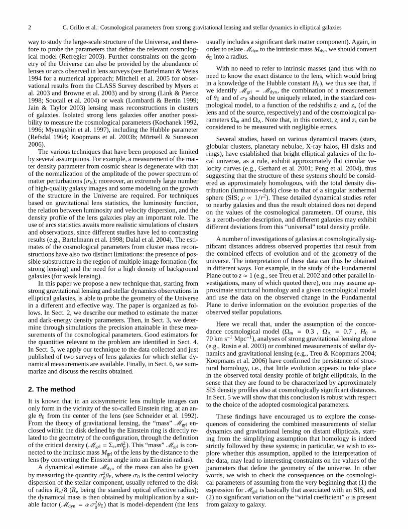
Figure 1 illustrates the distance ratior of Eq. (2) (which doesnot have a simple analytic form) versus the source redshift,as afunction of the lens redshift and of the matter and dark-energydensity parameters. In general, different cosmological modelsgive values ofr which differ more clearly at higher values ofthe source redshift (see the last three panels); in addition, thequantityr is more sensitive to small variations ofΩΛ than ofΩm(compare the second and third panels). As a consequence, wenaturally expect this method to be optimally efficient in measur-ing ΩΛ, provided we have at our disposal a sample of lenses atsufficiently high redshifts.

3. Simulated measurements of the cosmologicalparameters

In order to explore the precision with which the above techniquecan probe the cosmological parameters, we have performed sev-eral simulations. We modelled each lens as a singular isothermalsphere with an external shear component. Because of the knowndegeneracy between external shear and ellipticity (Witt & Mao1997), we remark that our modeling choice is also good at de-scribing simulations with singular isothermal ellipsoid models.As suggested by real lensing systems, we considered the lensredshift uniformly distributed between 0 and 1 and the sourceredshift between 1 and 3.5; the lens velocity dispersion andtheexternal shear values were drawn from uniform distributionsranging from 100 to 350 km s−1 for the first, from 0 to 0.2 inmagnitude and from 0 to 180 in orientation for the second (therole of the external shear component will become relevant inSect. 4.1). We calculated the Einstein angles from Eq. (1) ina(Ωm,ΩΛ) = (0.3, 0.7) cosmology and completed each lensingsystem simulating randomly, inside a square of sideθE and cen-tered on the lens, the position of a source. Only the lenses withtwo images of this source and withθE greater than 0.5′′ wereaccepted for the next analyses. The reason is that we wantedto investigate multiple image systems similar to those observed,

Distance ratio (Ωm = 0.3, ΩΛ = 0.7; zl var.)

0 2 4 6 8 10zs

0.0

0.2

0.4

0.6

0.8

1.0

r =

Dls/D

os

zl increasing

Distance ratio (ΩΛ = 0.7, Ωm var.)

2 4 6 8 10zs

0.0

0.2

0.4

0.6

0.8

1.0

r =

Dls/D

os

Ωm increasing

zl = 0.5

Distance ratio (Ωm = 0.3, ΩΛ var.)

2 4 6 8 10zs

0.0

0.2

0.4

0.6

0.8

1.0

r =

Dls/D

os

ΩΛ increasing

zl = 0.5

Distance ratio (Ωm + ΩΛ = 1)

2 4 6 8 10zs

0.0

0.2

0.4

0.6

0.8

1.0

r =

Dls/D

os

ΩΛ increasing

zl = 0.5

Fig. 1. Dependence of the angular diameter distance ratior =Dls/Dos on the lens redshift (top left), matter density parame-ter (top right), dark-energy density parameter (bottom left), andmatter and dark-energy density parameters in a flat cosmologi-cal model (bottom right). In the first panel, (Ωm,ΩΛ) = (0.3, 0.7)are fixed andzl is varied from 0.1 to 1, with a regular step of0.1. The arrow shows the increasing direction ofzl . In the sec-ond panel,ΩΛ = 0.7 andzl = 0.5 are fixed andΩm is varied from0 to 1, with a regular step of 0.1. The arrow shows the increasingdirection ofΩm. In the third panel,Ωm = 0.3 andzl = 0.5 arefixed andΩΛ is varied from 0 to 1, with a regular step of 0.1. Thearrow shows the increasing direction ofΩΛ. In the fourth panel,Ωm + ΩΛ = 1 andzl = 0.5 are fixed andΩΛ is varied from 0to 1, with a regular step of 0.1. The arrow shows the increasingdirection ofΩΛ.

where the images are far enough from the center of the galaxyacting as a lens to be resolved with the present technology.

We started by examining the dependence of the error es-timates onΩm andΩΛ on the simulated uncertainties on theEinstein angle and on the central velocity dispersion. In orderto do this, we minimized a chi-square (χ2) like estimator withrespect to the two cosmological parameters. This function is de-fined by comparing the “observational” distance ratio calculatedfrom θE andσ0, that is the quantity on the left in Eq. (2), and the“theoretical” distance ratio obtained from the lens and sourceredshifts, that is the quantity on the right in Eq. (2):

χ2(Ωm,ΩΛ) =N

∑

i=1

(

c2

4πθEi

σ20i

− r(zl i , zsi ;Ωm,ΩΛ)

)2

(

c2

4π

)2[

(

1σ2

0i

)2(δθEi )2 +

(

θEi

σ40i

)2(δσ2

0i)2

] . (3)

We included realistic measurement errors on the Einstein angle(δθE) and on the central velocity dispersion (δσ0), consideringnormal distributions with standard deviations equal to 4%,5%,6%, and 7% of the true values. At first, we performed 2000 min-imizations for samples of 100 and 200 lenses, assigning a nom-inal 0% uncertainty to one of the two quantities and varying theerror on the other in the range reported above. Then, we repeated


Parameter distribution (4% err. on θE)

0.0 0.2 0.4 0.6 0.8 1.0Ωm

0.0

0.2

0.4

0.6

0.8

1.0

ΩΛ

N=100

95% 68%

Parameter distribution (4% err. on σ0)

0.0 0.2 0.4 0.6 0.8 1.0Ωm

0.0

0.2

0.4

0.6

0.8

1.0

ΩΛ

N=100

95%68%


0.0 0.2 0.4 0.6 0.8 1.0Ωm

0.0

0.2

0.4

0.6

0.8

1.0

ΩΛ

N=200

95%68%


0.0 0.2 0.4 0.6 0.8 1.0Ωm

0.0

0.2

0.4

0.6

0.8

1.0

ΩΛ

N=200

95%68%


0.0 0.2 0.4 0.6 0.8 1.0Ωm

0.0

0.2

0.4

0.6

0.8

1.0

ΩΛ

N=100

95% 68%


0.0 0.2 0.4 0.6 0.8 1.0Ωm

0.0

0.2

0.4

0.6

0.8

1.0

ΩΛ

N=100

95%95%68%


0.0 0.2 0.4 0.6 0.8 1.0Ωm

0.0

0.2

0.4

0.6

0.8

1.0

ΩΛ

N=200

95%68%


0.0 0.2 0.4 0.6 0.8 1.0Ωm

0.0

0.2

0.4

0.6

0.8

1.0

ΩΛ

N=200

95%68%


0.0 0.2 0.4 0.6 0.8 1.0Ωm

0.0

0.2

0.4

0.6

0.8

1.0

ΩΛ

N=100

95%68%


0.0 0.2 0.4 0.6 0.8 1.0Ωm

0.0

0.2

0.4

0.6

0.8

1.0

ΩΛ

N=100

95%

95%68%


0.0 0.2 0.4 0.6 0.8 1.0Ωm

0.0

0.2

0.4

0.6

0.8

1.0

ΩΛ

N=200

95% 68%


0.0 0.2 0.4 0.6 0.8 1.0Ωm

0.0

0.2

0.4

0.6

0.8

1.0

ΩΛ

N=200

95%68%


0.0 0.2 0.4 0.6 0.8 1.0Ωm

0.0

0.2

0.4

0.6

0.8

1.0

ΩΛ

N=100

95%68%


0.0 0.2 0.4 0.6 0.8 1.0Ωm

0.0

0.2

0.4

0.6

0.8

1.0

ΩΛ

N=100

95%

95%68%


0.0 0.2 0.4 0.6 0.8 1.0Ωm

0.0

0.2

0.4

0.6

0.8

1.0

ΩΛ

N=200

95%68%


0.0 0.2 0.4 0.6 0.8 1.0Ωm

0.0

0.2

0.4

0.6

0.8

1.0

ΩΛ

N=200

95%95%68%

Fig. 2. Estimates of the cosmological parameters. Simulation of 2000 measurements composed of 100 (on the left) and 200 (onthe right) lenses each, with different uncertainties (increasing from the top to the bottom)on the Einstein angle (first and thirdcolumn) and on the central velocity dispersion (second and fourth column). A nominal 0% uncertainty is assigned to the quantitynot mentioned in the panels. Thick bars on the co-ordinate axes and contour levels on the planes represent, respectively, the 95%confidence intervals and the 68% and 95% confidence regions for the cosmological parameters. A cross shows the position ofthetrue parameters: (Ωm,ΩΛ) = (0.3, 0.7).

the analysis just described with the additional hypothesisof a flatcosmological model (Ωm + ΩΛ = 1). Finally, we simulated es-timates of the cosmological parameters, in general and flat cos-mology models, considering 5% errors on both the Einstein an-gle and the central velocity dispersion. This is the precision with

which these quantities can be measured at present by means ofthe best ground and space-based telescopes.

The results for the joint and single probability density func-tions (f ) of the cosmological parameters are summarized byFigs. 2, 3, and 4 and by Tables 1, 2, and 3. As a first good in-dication, the minimumχ2 was found to be asymptotically unbi-


Parameter distributions (4% err. on θE)

0.0 0.2 0.4 0.6 0.8 1.0Parameter values

0.0

0.1

0.2

0.3

f

Ωm ΩΛ

N=100

Parameter distributions (4% err. on σ0)


0.0

0.1

0.2

0.3

f

Ωm ΩΛ

N=100



0.0

0.1

0.2

0.3

f

Ωm ΩΛ

N=200



0.0

0.1

0.2

0.3

f

Ωm ΩΛ

N=200



0.0

0.1

0.2

0.3

f

N=100

Ωm ΩΛ



0.0

0.1

0.2

0.3

f

Ωm ΩΛ

N=100



0.0

0.1

0.2

0.3

f

Ωm ΩΛ

N=200



0.0

0.1

0.2

0.3

f

Ωm ΩΛ

N=200



0.0

0.1

0.2

0.3

f

N=100

Ωm ΩΛ



0.0

0.1

0.2

0.3

f

Ωm ΩΛ

N=100



0.0

0.1

0.2

0.3

f

Ωm ΩΛ

N=200



0.0

0.1

0.2

0.3

f

Ωm ΩΛ

N=200



0.0

0.1

0.2

0.3

f

Ωm ΩΛ

N=100



0.0

0.1

0.2

0.3

f

Ωm ΩΛ

N=100



0.0

0.1

0.2

0.3

f

Ωm ΩΛ

N=200



0.0

0.1

0.2

0.3

f

Ωm ΩΛ

N=200

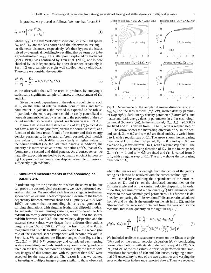
Fig. 3. Estimates of the cosmological parameters in a flat model (Ωm + ΩΛ = 1). Simulation of 2000 measurements composed of100 (on the left) and 200 (on the right) lenses each, with different uncertainties (increasing from the top to the bottom)on theEinstein angle (first and third column) and on the central velocity dispersion (second and fourth column). A nominal 0% uncertaintyis assigned to the quantity not mentioned in the panels. Thick bars on the abscissa axes represent the 95% confidence intervals forthe cosmological parameters. Crosses show the position of the true parameters: (Ωm,ΩΛ) = (0.3, 0.7).

ased, i.e. centered on the original values (Ωm,ΩΛ) = (0.3, 0.7) inthe limit of small uncertainties onθE andσ0. Then, we remarkthat the true values of the cosmological parameters are alwaysinside the regions and intervals at the 95% confidence level,buttheir boundaries are not symmetrical. In fact, in all the three pre-viously mentioned tables these confidence intervals forΩm aremore extended on the high side; in contrast, the intervals for ΩΛ

are generally larger on the low side. Moreover, since the dis-tance ratior depends linearly on the Einstein angle and quadrati-cally on the central velocity dispersion, larger confidenceregionsand intervals are obtained when a fixed uncertainty is consideredon the latter quantity. The assumption about the flatness of theUniverse makes our technique more powerful, allowing a betterestimate of the dark-energy density parameter, as can be seen


Table 1. Intervals at 95% confidence level for the matter and the dark-energy density parameters.

N=100 N=200Err. θE 4% 5% 6% 7% Err.θE 4% 5% 6% 7%Ωm [0.10, 0.52] [0.06, 0.58] [0.01, 0.65] [0.00, 0.73] Ωm [0.16, 0.47] [0.13, 0.51] [0.09, 0.57] [0.05, 0.63]ΩΛ [0.63, 0.74] [0.61, 0.74] [0.58, 0.75] [0.56, 0.75] ΩΛ [0.65, 0.73] [0.63, 0.73] [0.61, 0.73] [0.59, 0.73]

Err.σ0 4% 5% 6% 7% Err.σ0 4% 5% 6% 7%Ωm [0.00, 0.81] [0.00, 0.98] [0.00, 1.19] [0.00, 1.41] Ωm [0.03, 0.63] [0.00, 0.73] [0.00, 0.85] [0.00, 0.97]ΩΛ [0.58, 0.78] [0.54, 0.80] [0.50, 0.80] [0.47, 0.80] ΩΛ [0.60, 0.75] [0.57, 0.75] [0.54, 0.75] [0.50, 0.74]

Notes – These intervals are obtained by excluding from the 2000χ2 minimizations the 50 smallest and the 50 largest values forΩm andΩΛ. Thesimulated measurement uncertainties of the Einstein angle(on the top) and of the central velocity dispersion (on the bottom) range from 4%to 7% (a nominal 0% uncertainty is assigned to one of the two quantities and the error on the other is varied) for samples of 100 (on the left)and 200 (on the right) lenses.

Table 2.Intervals at 95% confidence level for the matter and the dark-energy density parameters in a flat cosmology (Ωm+ΩΛ = 1).

N=100 N=200Err. θE 4% 5% 6% 7% Err.θE 4% 5% 6% 7%Ωm [0.28, 0.34] [0.28, 0.36] [0.28, 0.38] [0.28, 0.40] Ωm [0.29, 0.33] [0.29, 0.34] [0.29, 0.36] [0.30, 0.38]ΩΛ [0.66, 0.72] [0.64, 0.72] [0.62, 0.72] [0.60, 0.72] ΩΛ [0.67, 0.71] [0.66, 0.71] [0.64, 0.71] [0.62, 0.70]

Err.σ0 4% 5% 6% 7% Err.σ0 4% 5% 6% 7%Ωm [0.26, 0.38] [0.26, 0.41] [0.26, 0.44] [0.26, 0.49] Ωm [0.28, 0.36] [0.28, 0.39] [0.28, 0.41] [0.29, 0.45]ΩΛ [0.62, 0.74] [0.59, 0.74] [0.56, 0.74] [0.51, 0.74] ΩΛ [0.64, 0.72] [0.61, 0.72] [0.59, 0.72] [0.55, 0.71]

Notes – These intervals are obtained by excluding from the 2000χ2 minimizations the 50 smallest and the 50 largest values forΩm andΩΛ. Thesimulated measurement uncertainties of the Einstein angle(on the top) and of the central velocity dispersion (on the bottom) range from 4%to 7% (a nominal 0% uncertainty is assigned to one of the two quantities and the error on the other is varied) for samples of 100 (on the left)and 200 (on the right) lenses.

Parameter distribution (5% err. on θE and σ0)

0.0 0.2 0.4 0.6 0.8 1.0Ωm

0.0

0.2

0.4

0.6

0.8

1.0

ΩΛ

N=100

95%

95%68%

Parameter distributions (5% err. on θE and σ0)


0.00

0.02

0.04

0.06

0.08

0.10

0.12

0.14

f

Ωm ΩΛ

N=100

Parameter distribution (5% err. on θE and σ0)

0.0 0.2 0.4 0.6 0.8 1.0Ωm

0.0

0.2

0.4

0.6

0.8

1.0

ΩΛ

N=200

95%68%

Parameter distributions (5% err. on θE and σ0)


0.00

0.02

0.04

0.06

0.08

0.10

0.12

0.14

f

Ωm ΩΛ

N=200

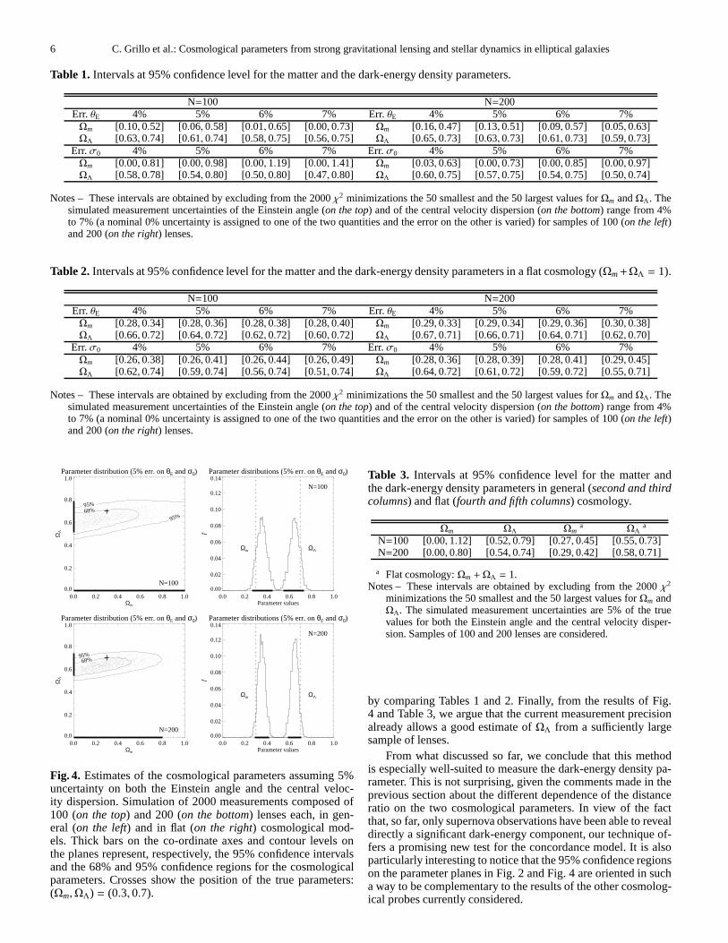
Fig. 4. Estimates of the cosmological parameters assuming 5%uncertainty on both the Einstein angle and the central veloc-ity dispersion. Simulation of 2000 measurements composed of100 (on the top) and 200 (on the bottom) lenses each, in gen-eral (on the left) and in flat (on the right) cosmological mod-els. Thick bars on the co-ordinate axes and contour levels onthe planes represent, respectively, the 95% confidence intervalsand the 68% and 95% confidence regions for the cosmologicalparameters. Crosses show the position of the true parameters:(Ωm,ΩΛ) = (0.3, 0.7).

Table 3. Intervals at 95% confidence level for the matter andthe dark-energy density parameters in general (second and thirdcolumns) and flat (fourth and fifth columns) cosmology.

Ωm ΩΛ Ωma ΩΛ

a

N=100 [0.00, 1.12] [0.52, 0.79] [0.27, 0.45] [0.55, 0.73]N=200 [0.00, 0.80] [0.54, 0.74] [0.29, 0.42] [0.58, 0.71]

a Flat cosmology:Ωm + ΩΛ = 1.Notes – These intervals are obtained by excluding from the 2000 χ2

minimizations the 50 smallest and the 50 largest values forΩm andΩΛ. The simulated measurement uncertainties are 5% of the truevalues for both the Einstein angle and the central velocity disper-sion. Samples of 100 and 200 lenses are considered.

by comparing Tables 1 and 2. Finally, from the results of Fig.4 and Table 3, we argue that the current measurement precisionalready allows a good estimate ofΩΛ from a sufficiently largesample of lenses.

From what discussed so far, we conclude that this methodis especially well-suited to measure the dark-energy density pa-rameter. This is not surprising, given the comments made in theprevious section about the different dependence of the distanceratio on the two cosmological parameters. In view of the factthat, so far, only supernova observations have been able to revealdirectly a significant dark-energy component, our technique of-fers a promising new test for the concordance model. It is alsoparticularly interesting to notice that the 95% confidence regionson the parameter planes in Fig. 2 and Fig. 4 are oriented in sucha way to be complementary to the results of the other cosmolog-ical probes currently considered.


θ1 consistency

100 101 102 103 104 105 106

N

0.8

0.9

1.0

1.1

1.2m

1θ2 consistency

100 101 102 103 104 105 106

N

0.8

0.9

1.0

1.1

1.2

m2

θ1 bias

0 2000 4000 6000 8000 10000N

0.8

0.9

1.0

1.1

1.2

m1

θ2 bias

0 2000 4000 6000 8000 10000N

0.8

0.9

1.0

1.1

1.2m

2

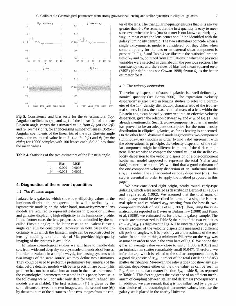
Fig. 5. Consistency and bias tests for theθE estimators.Top:Angular coefficients (m1 and m2) of the linear fits of the trueEinstein angle versus the estimated value fromθ1 (on the left)andθ2 (on the right), for an increasing number of lenses.Bottom:Angular coefficients of the linear fits of the true Einstein angleversus the estimated value fromθ1 (on the left) andθ2 (on theright) for 10000 samples with 100 lenses each. Solid lines showthe mean values.

Table 4.Statistics of the two estimators of the Einstein angle.

Bias MSEθ1 −0.020 0.0008θ2 −0.008 0.0005

4. Diagnostics of the relevant quantities

4.1. The Einstein angle

Isolated lens galaxies which show low ellipticity values intheluminous distribution are expected to be well described by ax-isymmetric models; on the other hand, non-axisymmetric lensmodels are required to represent galaxies in groups or clustersand galaxies displaying high ellipticity in the luminosityprofile.In the former case, the lens properties are embodied by the so-called Einstein angle; in the latter case, an equivalent Einsteinangle can still be considered. However, in both cases the un-certainty with which the Einstein angle can be reconstructed bylensing modeling is on the order of 5%, provided high-qualityimaging of the systems is available.

In future cosmological studies we will have to handle datasets from wide and deep sky surveys made of hundreds of lenses.In order to evaluate in a simple wayθE for lensing systems withtwo images of the same source, we may define two estimators.They could be used to perform a preliminary fast analysis of thedata, before detailed models with better precision are built. (Thisproblem has not been taken into account in the measurements ofthe cosmological parameters presented in this paper, because inthe following we will consider only data for which refined lensmodels are available). The first estimator (θ1) is given by thesemi-distance between the two images, and the second one (θ2)by the semi-sum of the distances of the two images from the cen-

ter of the lens. The triangular inequality ensures thatθ2 is alwaysgreater thanθ1. We remark that the first quantity is easy to mea-sure, even when the lens (mass) center is not known a priori; any-way, in most cases the lens center should be identified with thegalaxy luminosity centroid. The two estimators coincide when asingle axisymmetric model is considered, but they differ whensome ellipticity for the lens or an external shear componentispresent. In Fig. 5 and Table 4 we illustrate the statistical proper-ties ofθ1 andθ2, obtained from simulations in which the physicalvariables were selected as described in the previous section. Theconsistency test and the values of bias and mean squared error(MSE) (for definitions see Cowan 1998) favourθ2 as the betterestimator forθE.

4.2. The velocity dispersion

The velocity dispersion of stars in galaxies is a well-defined dy-namical quantity (see Bertin 2000). The expression “velocitydispersion” is also used in lensing studies to refer to a param-eter of the 1/r2 density distribution characteristic of the isother-mal sphere. In fact, the measured total mass of a lens within theEinstein angle can be easily converted into an effective velocitydispersion, given the relation betweenθE andσSIS of Eq. (1). Asalready mentioned in Sect. 2, a one-component isothermal modelhas proved to be an adequate description for thetotal densitydistribution in elliptical galaxies, as far as lensing is concerned.On the other hand, dynamical modeling requires two-component(luminous+dark) models in order to find valid agreement withthe observations; in principle, the velocity dispersion ofthe stel-lar component might be different from that of the dark compo-nent. Here we wish to compare the central value of the stellarve-locity dispersion to the velocity dispersion of a one-componentisothermal model supposed to represent the total (stellar anddark) matter distribution. We will find that a good estimatorofthe one-component velocity dispersion of an isothermal model(σSIS) is indeed the stellar central velocity dispersion (σ0). Thisstep is essential in order to apply the method proposed in thispaper.

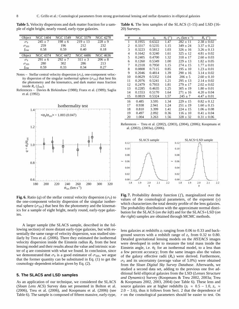
We have considered eight bright, nearly round, early-typegalaxies, which were modeled as described in Bertin et al. (1992)and Saglia et al. (1992). We assumed that the total mass ofeach galaxy could be described in terms of a singular isother-mal sphere and calculatedσSIS starting from the best-fit two-component models of Saglia et al. (1992). Then, using the kine-matical data reported in Davies & Birkinshaw (1988) and Franxet al. (1989), we estimatedσ0 for the same galaxy sample. Theresults are summarized in Table 5; the ratio of the two velocities(q = σ0/σSIS) is displayed in Fig. 6. The uncertainty onσ0 is justthe rms scatter of the velocity dispersions measured at differentslit position angles, so it is probably an underestimate of the realvalue. In addition to this, a minimum 5% error on theσSIS wasassumed in order to obtain the error bars of Fig. 6. We notice thatq has an average value very close to unity (1.003± 0.017) andan intrinsic rms scatter remarkably small (0.047). Therefore, weinfer thatσ0, which is related to the stellar component alone, isa good diagnostic ofσSIS, a tracer of the total (stellar and dark)matter distribution. Moreover, the ratioq does not show any sig-nificant dependence either on theσSIS value, as can be seen inFig. 6, or on the dark matter fractionfDM insideRe, as reportedin Table 5. This fact suggests the existence of an efficient mech-anism of coupling between stellar and dark mass (“conspiracy”).In addition, we also remark thatq is not influenced by a partic-ular choice of the cosmological parameter values, because thegalaxy set is placed in the nearby Universe.


Table 5.Velocity dispersions and dark matter fraction for a sam-ple of eight bright, nearly round, early-type galaxies.

Object NGC 1404 NGC 1549 NGC 3379 NGC 4278σ0 245± 7 198± 6 219± 13 228± 9σSIS 259 196 212 232fDM 0.58 0.59 0.40 0.18

Object NGC 4374 NGC 4472 NGC 4486 NGC 4636σ0 291± 6 292± 7 311± 3 206± 8σSIS 280 302 286 213fDM 0.59 0.33 0.34 0.27

Notes – Stellar central velocity dispersion (σ0), one-component veloc-ity dispersion of the singular isothermal sphere (σSIS) that best fitsthe photometry and the kinematics, and dark matter mass fractioninsideRe ( fDM ).

References – Davies & Birkinshaw (1988); Franx et al. (1989); Sagliaet al. (1992).

Isothermality test

180 200 220 240 260 280 300 320σSIS (km s−1)

0.6

0.8

1.0

1.2

1.4

q =

σ0/σ

SIS

<σ0/σSIS> = 1.003 (0.047)

Fig. 6. Ratio (q) of the stellar central velocity dispersion (σ0) tothe one-component velocity dispersion of the singular isother-mal sphere (σSIS) that best fits the photometry and the kinemat-ics for a sample of eight bright, nearly round, early-type galax-ies.

A larger sample (the SLACS sample, described in the fol-lowing section) of more distant early-type galaxies, but with es-sentially the same range of velocity dispersion, was studied sim-ilarly by Treu et al. (2006). There they estimated the isothermalvelocity dispersion inside the Einstein radiusRE from the bestlensing model and their results about the value and intrinsic scat-ter of q are consistent with what we found. In conclusion, sincewe demonstrated thatσ0 is a good estimator ofσSIS, we arguethat the former quantity can be substituted in Eq. (1) to get thecosmology-dependent relation given by Eq. (2).

5. The SLACS and LSD samples

As an application of our technique, we considered the SLACS(Sloan Lens ACS) Survey data set presented in Bolton et al.(2006), Treu et al. (2006), and Koopmans et al. (2006) (seeTable 6). The sample is composed of fifteen massive, early-type,

Table 6. The lens samples of the SLACS (1-15) and LSD (16-20) Surveys.

# zl zs θE (′′) σ0 (km s−1) Re (′′)1 0.1955 0.6322 1.47 282± 11 2.38± 0.022 0.3317 0.5235 1.15 349± 24 3.37± 0.223 0.3223 0.5812 1.03 326± 16 3.26± 0.134 0.1642 0.3240 1.61 325± 12 4.81± 0.025 0.2405 0.4700 1.32 318± 17 2.60± 0.036 0.1260 0.5349 1.00 229± 13 1.82± 0.057 0.2318 0.7950 1.15 274± 15 1.77± 0.018 0.0808 0.7115 0.85 195± 10 1.23± 0.019 0.2046 0.4814 1.39 290± 16 3.14± 0.0210 0.0629 0.5352 1.04 206± 5 2.60± 0.1011 0.2076 0.5241 1.21 295± 13 2.14± 0.0212 0.2479 0.7933 1.81 279± 17 2.02± 0.0213 0.2285 0.4635 1.25 305± 19 1.80± 0.0114 0.1553 0.5170 1.64 271± 16 4.20± 0.0415 0.0819 0.5324 1.57 245± 7 4.47± 0.01

16 0.485 3.595 1.34 229± 15 0.82± 0.1217 0.938 2.941 1.24 251± 19 1.60± 0.1518 0.810 3.399 1.41 224± 15 1.06± 0.0819 0.497 2.092 0.36 116± 10 0.41± 0.0420 1.004 3.263 1.56 328± 32 0.31± 0.06

References – Treu et al. (2002), (2003), (2004), (2006); Koopmans etal. (2002), (2003a), (2006).

SLACS sample

1.8 1.9 2.0 2.1 2.2γ

0.00

0.02

0.04

0.06

0.08

0.10

0.12

f

SLACS+LSD sample

1.8 1.9 2.0 2.1 2.2γ

0.00

0.02

0.04

0.06

0.08

0.10

0.12

f

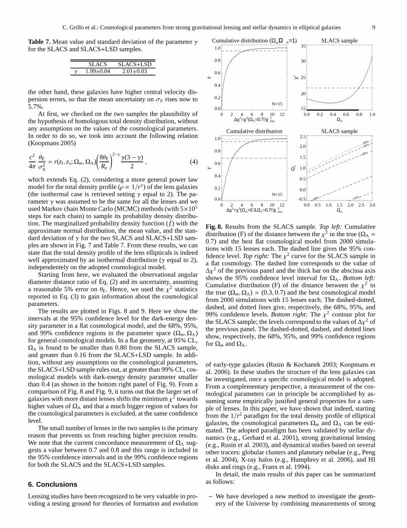
Fig. 7. Probability density function (f ), marginalized over thevalues of the cosmological parameters, of the exponent (γ)which characterizes the total density profile of the lens galaxies.The probability distribution with the approximate normal distri-bution for the SLACS (on the left) and for the SLACS+LSD (onthe right) samples are obtained through MCMC methods.

lens galaxies at redshiftszl ranging from 0.06 to 0.33 and back-ground sources with a redshift range ofzs from 0.32 to 0.80.Detailed gravitational lensing models on theHST/ACS imageswere developed in order to measure the total mass inside theEinstein angle, i.e.θE for an isothermal model, to a less thana few percent accuracy; from the same images also the valuesof the galaxy effective radii (Re) were derived. Furthermore,σ0 and its uncertainty (average value of 5.0%) were obtainedfrom the Sloan Digital Sky Survey Database. Afterwards, westudied a second data set, adding to the previous one five ad-ditional field elliptical galaxies from the LSD (Lenses Structureand Dynamics) Survey (Koopmans & Treu 2002, 2003a; Treu& Koopmans 2002, 2003, 2004) (see Table 6). These lens andsource galaxies are at higher redshifts (zl ≈ 0.5 − 1.0, zs ≈

2.0 − 3.6), thus it follows from Sect. 2 that the dependence ofr on the cosmological parameters should be easier to test. On


Table 7. Mean value and standard deviation of the parameterγ

for the SLACS and SLACS+LSD samples.

SLACS SLACS+LSDγ 1.99±0.04 2.01±0.03

the other hand, these galaxies have higher central velocitydis-persion errors, so that the mean uncertainty onσ0 rises now to5.7%.

At first, we checked on the two samples the plausibility ofthe hypothesis of homologous total density distribution, withoutany assumptions on the values of the cosmological parameters.In order to do so, we took into account the following relation(Koopmans 2005)

c2

4πθE

σ20

= r(zl , zs;Ωm,ΩΛ)

(

8θERe

)2−γγ(3− γ)

2, (4)

which extends Eq. (2), considering a more general power lawmodel for the total density profile (ρ ∝ 1/rγ) of the lens galaxies(the isothermal case is retrieved settingγ equal to 2). The pa-rameterγ was assumed to be the same for all the lenses and weused Markov chain Monte Carlo (MCMC) methods (with 5×105

steps for each chain) to sample its probability density distribu-tion. The marginalized probability density function (f ) with theapproximate normal distribution, the mean value, and the stan-dard deviation ofγ for the two SLACS and SLACS+LSD sam-ples are shown in Fig. 7 and Table 7. From these results, we canstate that the total density profile of the lens ellipticals is indeedwell approximated by an isothermal distribution (γ equal to 2),independentely on the adopted cosmological model.

Starting from here, we evaluated the observational angulardiameter distance ratio of Eq. (2) and its uncertainty, assuminga reasonable 5% error onθE. Hence, we used theχ2 statisticsreported in Eq. (3) to gain information about the cosmologicalparameters.

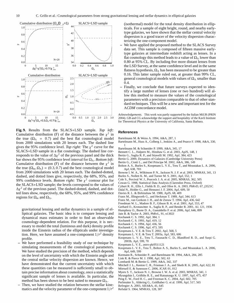
The results are plotted in Figs. 8 and 9. Here we show theintervals at the 95% confidence level for the dark-energy den-sity parameter in a flat cosmological model, and the 68%, 95%,and 99% confidence regions in the parameter space (Ωm,ΩΛ)for general cosmological models. In a flat geometry, at 95% CL,ΩΛ is found to be smaller than 0.80 from the SLACS sample,and greater than 0.16 from the SLACS+LSD sample. In addi-tion, without any assumptions on the cosmological parameters,the SLACS+LSD sample rules out, at greater than 99% CL, cos-mological models with dark-energy density parameter smallerthan 0.4 (as shown in the bottom right panel of Fig. 9). From acomparison of Fig. 8 and Fig. 9, it turns out that the larger set ofgalaxies with more distant lenses shifts the minimumχ2 towardshigher values ofΩΛ and that a much bigger region of values forthe cosmological parameters is excluded, at the same confidencelevel.

The small number of lenses in the two samples is the primaryreason that prevents us from reaching higher precision results.We note that the current concordance measurement ofΩΛ sug-gests a value between 0.7 and 0.8 and this range is included inthe 95% confidence intervals and in the 99% confidence regionsfor both the SLACS and the SLACS+LSD samples.

6. Conclusions

Lensing studies have been recognized to be very valuable in pro-viding a testing ground for theories of formation and evolution

Cumulative distribution (Ωm+ΩΛ=1)

0 2 4 6 8 10 12∆χ2=χ2(ΩΛ=0.7)−χ2

min

0.0

0.2

0.4

0.6

0.8

1.0

F

N=15

SLACS sample

0.0 0.2 0.4 0.6 0.8 1.0ΩΛ

15

20

25

30

35

χ2

Cumulative distribution

0 2 4 6 8 10 12∆χ2=χ2(Ωm=0.3,ΩΛ=0.7)−χ2

min

0.0

0.2

0.4

0.6

0.8

1.0

F

N=15

0.0 0.5 1.0 1.5 2.0 2.5 3.0Ωm

-0.5

0.0

0.5

1.0

1.5

2.0

2.5

ΩΛ

SLACS sample

68%

68%

95%

95%99%

Fig. 8. Results from the SLACS sample.Top left: Cumulativedistribution (F) of the distance between theχ2 in the true (ΩΛ =0.7) and the best flat cosmological model from 2000 simula-tions with 15 lenses each. The dashed line gives the 95% con-fidence level.Top right: Theχ2 curve for the SLACS sample ina flat cosmology. The dashed line corresponds to the value of∆χ2 of the previous panel and the thick bar on the abscissa axisshows the 95% confidence level interval forΩΛ. Bottom left:Cumulative distribution (F) of the distance between theχ2 inthe true (Ωm,ΩΛ) = (0.3, 0.7) and the best cosmological modelfrom 2000 simulations with 15 lenses each. The dashed-dotted,dashed, and dotted lines give, respectively, the 68%, 95%, and99% confidence levels.Bottom right: The χ2 contour plot forthe SLACS sample; the levels correspond to the values of∆χ2 ofthe previous panel. The dashed-dotted, dashed, and dotted linesshow, respectively, the 68%, 95%, and 99% confidence regionsfor Ωm andΩΛ.

of early-type galaxies (Rusin & Kochanek 2003; Koopmans etal. 2006). In these studies the structure of the lens galaxies canbe investigated, once a specific cosmological model is adopted.From a complementary perspective, a measurement of the cos-mological parameters can in principle be accomplished by as-suming some empirically justified general properties for a sam-ple of lenses. In this paper, we have shown that indeed, startingfrom the 1/r2 paradigm for the total density profile of ellipticalgalaxies, the cosmological parametersΩm andΩΛ can be esti-mated. The adopted paradigm has been validated by stellar dy-namics (e.g., Gerhard et al. 2001), strong gravitational lensing(e.g., Rusin et al. 2003), and dynamical studies based on severalother tracers: globular clusters and planetary nebulae (e.g., Penget al. 2004), X-ray halos (e.g., Humphrey et al. 2006), and HIdisks and rings (e.g., Franx et al. 1994).

In detail, the main results of this paper can be summarizedas follows:

– We have developed a new method to investigate the geom-etry of the Universe by combining measurements of strong


Cumulative distribution (Ωm+ΩΛ=1)

0 5 10 15∆χ2=χ2(ΩΛ=0.7)−χ2

min

0.0

0.2

0.4

0.6

0.8

1.0

F

N=20

SLACS+LSD sample

0.0 0.2 0.4 0.6 0.8 1.0ΩΛ

34

36

38

40

42

44

χ2

Cumulative distribution

0 5 10 15∆χ2=χ2(Ωm=0.3,ΩΛ=0.7)−χ2

min

0.0

0.2

0.4

0.6

0.8

1.0

F

N=20

0.0 0.5 1.0 1.5 2.0 2.5 3.0Ωm

-0.5

0.0

0.5

1.0

1.5

2.0

2.5

ΩΛ

SLACS+LSD sample

68%95%

95%99%

99%

Fig. 9. Results from the SLACS+LSD sample. Top left:Cumulative distribution (F) of the distance between theχ2 inthe true (ΩΛ = 0.7) and the best flat cosmological modelfrom 2000 simulations with 20 lenses each. The dashed linegives the 95% confidence level.Top right: Theχ2 curve for theSLACS+LSD sample in a flat cosmology. The dashed line cor-responds to the value of∆χ2 of the previous panel and the thickbar shows the 95% confidence level interval forΩΛ. Bottom left:Cumulative distribution (F) of the distance between theχ2 inthe true (Ωm,ΩΛ) = (0.3, 0.7) and the best cosmological modelfrom 2000 simulations with 20 lenses each. The dashed-dotted,dashed, and dotted lines give, respectively, the 68%, 95%, and99% confidence levels.Bottom right: The χ2 contour plot forthe SLACS+LSD sample; the levels correspond to the values of∆χ2 of the previous panel. The dashed-dotted, dashed, and dot-ted lines show, respectively, the 68%, 95%, and 99% confidenceregions forΩm andΩΛ.

gravitational lensing and stellar dynamics in a sample of el-liptical galaxies. The basic idea is to compare lensing anddynamical mass estimates in order to find an observablecosmology-dependent relation. For this purpose, it is nec-essary to model the total (luminous and dark) density profileinside the Einstein radius of the ellipticals under investiga-tion. Here, we have assumed a one-component 1/r2 densityprofile.

– We have performed a feasibility study of our technique bysimulating measurements of the cosmological parameters.We have studied the precision of the method, which dependson the level of uncertainty with which the Einstein angle andthe central stellar velocity dispersion are known. Hence, wehave demonstrated that the current uncertainty with whichthese quantities can be measured is sufficiently small to ob-tain precise information about cosmology, once a statisticallysignificant sample of lenses is available. In particular, themethod has been shown to be best suited to measureΩΛ.

– Then, we have studied the relation between the stellar kine-matics and the velocity parameter of the one-component 1/r2

(isothermal) model for the total density distribution in ellip-ticals. For a sample of eight bright, round, and nearby early-type galaxies, we have shown that the stellar central velocitydispersion is a good tracer of the velocity dispersion charac-terizing the one-component model.

– We have applied the proposed method to the SLACS Surveydata set. This sample is composed of fifteen massive early-type galaxies at intermediate redshift acting as lenses. Inaflat cosmology this method leads to a value ofΩΛ lower than0.80 at 95% CL. By including five more distant lenses fromthe LSD Survey, at the same confidence level and in the sameflatness hypothesis,ΩΛ has been measured to be greater than0.16. This latter sample ruled out, at greater than 99% CL,general cosmological models with values ofΩΛ smaller than0.4.

– Finally, we conclude that future surveys expected to iden-tify a large number of lenses (one or two hundred) will al-low this method to measure the values of the cosmologicalparameters with a precision comparable to that of other stan-dard techniques. This will be a new and important test for theΛCDM concordance model.

Acknowledgements.This work was partly supported by the Italian MiUR (PRIN2004). GB and CG acknowledge the support and hospitality of the Kavli Institutefor Theoretical Physics at the University of California, Santa Barbara.

References

Bartelmann M. & Weiss A. 1994, A&A, 287, 1Bartelmann M., Huss A., Colberg J., Jenkins A., and Pearce F.1998, A&A, 330,

1Bartelmann M. & Schneider P. 1999, A&A, 345, 17Bennett C. L., Halpern M., Hinshaw G. et al. 2003, ApJS, 148, 1Bertin G., Saglia R. P., and Stiavelli M. 1992, ApJ, 384, 423Bertin G. 2000, Dynamics of Galaxies (Cambridge UniversityPress)Bertin G., Ciotti L., and Del Principe M. 2002, A&A, 386, 149Bolton A. S., Burles S., Koopmans L. V. E., Treu T., and Moustakas L. A. 2006,

ApJ, 638, 703Browne I. W. A., Wilkinson P. N., Jackson N. J. F. et al. 2003, MNRAS, 341, 13Burles S., Nollett K. M., and Turner M. S. 2001, ApJ, 552, 1Cole S., Percival W. J., Peacock J. A. et al. 2005, MNRAS, 362,505Cowan G. 1998, Statistical Data Analysis (Clarendon Press,Oxford)Cyburt R. H., Ellis J., Fields B. D., and Olive K. A. 2003, PhRvD, 67, j3521CDalal N., Holder G., and Hennawi J. F. 2004, ApJ, 609, 50Davies R. L. & Birkinshaw M. 1988, ApJS, 68, 409Franx M., Illingworth G., and Heckman T. 1989, ApJ, 344, 613Franx M., van Gorkom J. H., and de Zeeuw T. 1994, ApJ, 436, 642Freedman W. L., Madore B. F., Gibson B. K. et al. 2001, ApJ, 553, 47Gerhard O., Kronawitter A., Saglia R. P., and Bender R. 2001,AJ, 121, 1936Humphrey O., Buote D. A., Gastaldello F. et al. 2006, ApJ, 646, 899Jain B. & Taylor A. 2003, PhRvL, 91, n1302JKochanek C. S. 1992, ApJ, 384, 1Kochanek C. S. 1993, ApJ, 419, 12Kochanek C. S. 1994, ApJ, 436, 56Kochanek C. S. 1996, ApJ, 473, 595Koopmans L. V. E. & Treu T. 2002, ApJ, 568, 5Koopmans L. V. E. & Treu T. 2003a, ApJ, 583, 606Koopmans L. V. E., Treu T., Fassnacht C. D., Blandford R. D., and Surpi G.

2003b, ApJ, 599, 70Koopmans L. V. E., astro-ph/0511121Koopmans L. V. E., Treu T., Bolton A. S., Burles S., and Moustakas L. A. 2006,

ApJ, 649, 599Kormann R., Schneider P., and Bartelmann M. 1994, A&A, 284, 285Link R. & Pierce M. J. 1998, ApJ, 502, 63Lombardi M. & Bertin G. 1999, A&A, 342, 337Mitchell J. L., Keeton C. R., Frieman J. A., and Sheth R. K. 2005, ApJ, 622, 81Mortsell E. & Sunesson C. 2006, JCAP, 01, 012Myers S. T., Jackson N. J., Browne I. W. A. et al. 2003, MNRAS, 341, 1Myungshin I., Griffiths R. E., and Ratnatunga K. U. 1997, ApJ, 475, 457Peng E. W., Ford H. C., and Freeman K. C. 2004, ApJ, 602, 705Perlmutter S., Aldering G., Goldhaber G. et al. 1999, ApJ, 517, 565Refregier A. 2003, ARA&A, 41, 645Refsdal S. 1964, MNRAS, 128, 307

http://arXiv.org/abs/astro-ph/0511121


Riess A. G., Filippenko A. V., Challis P. et al. 1998, AJ, 116,1009Riess A. G., Strolger L.-G., Tonry J. et al. 2004, ApJ, 607, 665Rusin D., Kochanek C. S., and Keeton C. R. 2003, ApJ, 595, 29Rusin D. & Kochanek C. S. 2005, ApJ, 623, 666Saglia R. P., Bertin G., and Stiavelli M. 1992, ApJ, 384, 433Schneider P., Ehlers J., and Falco E. E. 1992, GravitationalLenses (Springer-

Verlag, New York)Soucail G., Kneib J.-P., and Golse G. 2004, A&A, 417, 33Spergel D. N., Verde L., Peiris H. V. et al. 2003, ApJS, 148, 175Spergel D. N., Bean R., Dore O. et al. 2007, ApJS, 170, 377Tegmark M., Strauss M. A., Blanton M. R. et al. 2004, PhRvD, 69, j3501TTreu T., Stiavelli M., Casertano S., Møller P., and Bertin G.2002, ApJ, 564, 13Treu T. & Koopmans L. V. E. 2002, ApJ, 575, 87Treu T. & Koopmans L. V. E. 2003, MNRAS, 343, 29Treu T. & Koopmans L. V. E. 2004, ApJ, 611, 739Treu T., Koopmans L. V. E., Bolton A. S., Burles S., and Moustakas L. A. 2006,

ApJ, 640, 662Witt H. J. & Mao S. 1997, MNRAS, 291, 211

Cosmological parameters from strong gravitational lensing and stellar dynamics in elliptical...

Documents

Transcript of Cosmological parameters from strong gravitational lensing and stellar dynamics in elliptical...