Weak lensing analysis of SZ-selected clusters of galaxies from ...

arX

iv:1

310.

6744

v2 [

astr

o-ph

.CO

] 3

0 M

ay 2

014

Mon. Not. R. Astron. Soc. 000, 1–42 (2013) Printed 5 June 2018 (MN LATEX style file v2.2)

Weak lensing analysis of SZ-selected clusters of galaxies

from the SPT and Planck surveys

D. Gruen1,2⋆, S. Seitz1,2, F. Brimioulle1,2,3, R. Kosyra1,2, J. Koppenhoefer2,1, C.-

H. Lee2,1, R. Bender1,2, A. Riffeser1,2, T. Eichner1,2, T. Weidinger1,2 and M.

Bierschenk1,2

1University Observatory Munich, Scheinerstrasse 1, 81679 Munich, Germany2Max Planck Institute for Extraterrestrial Physics, Giessenbachstrasse, 85748 Garching, Germany3Observatório Nacional, Rua Gal. José Cristino, 20921-400, Rio de Janeiro, Brazil

ABSTRACT

We present the weak lensing analysis of the Wide-Field Imager SZ Cluster of galaxy(WISCy) sample, a set of 12 clusters of galaxies selected for their Sunyaev-Zel’dovich(SZ) effect. After developing new and improved methods for background selectionand determination of geometric lensing scaling factors from absolute multi-band pho-tometry in cluster fields, we compare the weak lensing mass estimate with publicX-ray and SZ data. We find consistency with hydrostatic X-ray masses with no sig-nificant bias, no mass dependent bias and less than 20% intrinsic scatter and con-strain fgas,500c = 0.128+0.029

−0.023. We independently calibrate the South Pole Telescopesignificance-mass relation and find consistency with previous results. The compari-son of weak lensing mass and Planck Compton parameters, whether extracted self-consistently with a mass-observable relation (MOR) or using X-ray prior informationon cluster size, shows significant discrepancies. The deviations from the MOR stronglycorrelate with cluster mass and redshift. This could be explained either by a signifi-cantly shallower than expected slope of Compton decrement versus mass and a corre-sponding problem in the previous X-ray based mass calibration, or a size or redshiftdependent bias in SZ signal extraction.

Key words: gravitational lensing: weak – galaxies: clusters: general – cosmology:observations

1 INTRODUCTION

As the end product of hierarchical structure formation, clus-ters of galaxies are particularly sensitive to the cosmologicalinterplay of dark matter and dark energy. Studies of individ-ual clusters and, even more so, large surveys have for thisreason been considered a valuable cosmological probe forseveral decades (see Allen et al. 2011 for a recent review).

The framework for cosmological interpretation of clus-ter surveys consists, on the theoretical side, of a halomass function that predicts the dependence of the numberdensity of clusters as a function of mass and redshift oncosmology (e.g. Press & Schechter 1974; Sheth & Tormen1999; Tinker et al. 2008). The observational task consistsin providing an ensemble of clusters detected with a well-determined selection function and measurements of an ob-servable that can be related to their mass.

Most observations that allow a sufficiently high signal-

⋆ E-mail: [email protected] (DG)

to-noise ratio (S/N) detection of sufficiently many clusters todate relate to the minority of cluster matter that is of bary-onic origin (but see Gavazzi & Soucail 2007; Miyazaki et al.2007; Schirmer et al. 2007 for lensing-detected surveys).In particular, use has been made of the density of redgalaxies (e.g. Gladders & Yee 2005, Koester et al. 2007 orRykoff et al. 2014 for observations and Rozo et al. 2010 orMana et al. 2013 for cosmological interpretation) or the hotgas in the intra-cluster medium (ICM) that can be detectedby its X-ray emission (e.g. Piffaretti et al. 2011 for a meta-catalogue and Vikhlinin et al. 2009b or Mantz et al. 2010bfor cosmological interpretation).

Another observable effect is due to the inverse Comp-ton scattering of cosmic microwave background (CMB) pho-tons by the ICM, the Sunyaev & Zel’dovich (1972, hereafterSZ) effect. The scattering distorts the CMB spectrum suchthat below (above) a global null-point frequency of approxi-mately 220 GHz, a decrease (an increase) in microwave fluxdensity is observed in galaxy clusters. The effect at any pointscales with the integrated electron pressure P along the line

c© 2013 RAS

http://arxiv.org/abs/1310.6744v2

2 D. Gruen et al.

of sight, which defines the dimensionless Compton parame-ter y,

y =σT

mec2

∫

P dl , (1)

where σT is the Thomson cross-section and mec2 the restenergy of electrons.

Integration of y over the angular extent of the cluster,Y =

∫

y dΩ, yields a volume integral of electron pressure,

D2AY =

σT

mec2

∫

P dV (2)

with the angular diameter distance DA used to convert ap-parent angles to physical scales. Note that the volume inte-gral of pressure equals the thermal energy and is thereforeexpected to be closely related to cluster mass.

Large surveys of the SZ sky have been and arecurrently being performed by the Planck Satellite (e.g.Planck Collaboration et al. 2013a), the South Pole Tele-scope (SPT; Carlstrom et al. 2011) and the Atacama Cos-mology Telescope (ACT; e.g. Marriage et al. 2011).

1.1 Calibration of the SZ mass-observable relation

As a connection between cosmological models and SZ sur-veys, it is necessary to establish a mass-observable relation(MOR) between SZ observable and cluster mass. As impor-tant as the mean relation is the intrinsic scatter of the MOR(Lima & Hu 2005), since the steepness of the halo mass func-tion causes preferential up-scatter of the (more numerous)less massive haloes. There are a number of ways of achievingthis calibration.

External mass calibration is not strictly required forthe cosmological interpretation of an SZ survey, since largesurveys can determine both cosmological parameters, aparametrized MOR and the intrinsic scatter simultaneously(Hu 2003; Majumdar & Mohr 2004; Lima & Hu 2005) byrequiring that cluster counts as a function of observablebe consistent with the halo mass function of the respec-tive cosmology. The fewer assumptions about the formand evolution of the MOR are made, however, the lesswell-constrained cosmological parameters become in such ascheme.

Previous studies have used astrophysical modelling(e.g. Mroczkowski 2011) or X-ray mass estimates for SZ-selected systems (Planck Collaboration et al. 2011b, 2013b)to constrain the MOR. These approaches require assump-tions about the astrophysical state of clusters, e.g. virial-ization and hydrostatic equilibrium (HSE), and are com-plicated by the variety of evolutionary states clusters arein fact found to be in. One important example of thisis the question of hydrostatic mass bias, i.e. a meanunderestimation of true mass by X-ray analyses basedon HSE (Nagai et al. 2007; Piffaretti & Valdarnini 2008),which has been investigated with controversial results (e.g.Mahdavi et al. 2008; Zhang et al. 2010; Mahdavi et al. 2013;Planck Collaboration et al. 2013c).

Weak lensing (WL) constraints on the MOR are a com-plement to these approaches. A moderate number of accu-rately measured masses greatly reduces the uncertainty ofself-calibration schemes (e.g. Majumdar & Mohr 2004). WL

can measure masses and mass-observable scatters for sam-ples of clusters selected according to the respective surveywith the important advantage that it is sensitive to all mat-ter regardless of its astrophysical state.

In practice, however, WL also faces observational chal-lenges. Biases in WL measurements of the mass due to,for instance, shape measurement bias (e.g. Young et al., inpreparation), cluster orientation (Corless & King 2007) oruncertain determination of source redshifts (Applegate et al.2014) have been explored. Increased uncertainty of ob-served mass due to unrelated projected structures (Hoekstra2001, 2003; Spinelli et al. 2012) or deviations of individ-ual systems from the common assumption of spherical,isolated Navarro, Frenk, & White (1997, hereafter NFW)haloes (Becker & Kravtsov 2011; Gruen et al. 2011) is anissue of similar importance. Despite the need of reducingand quantifying these effects, gravitational lensing remainsthe best candidate for an unbiased mass measurement ofgalaxy clusters to date. For this reason, the WL analysisof SZ selected samples of clusters has been the focus of anumber of recent studies [cf. McInnes et al. 2009 (3 SPTsystems), Marrone et al. 2009, 2012 (a total of 29 systemswith pointed SZ observations at z = 0.15 . . . 0.3, 25 of whichare also detected by Planck), High et al. 2012 (5 SPT sys-tems), AMI Consortium: Hurley-Walker et al. 2012 (6 sys-tems with pointed SZ observations) and Hoekstra et al.2012 (a total of 30 systems with SZ observations, mostlyat z = 0.15, . . . , 0.3, 18 of which are also detected byPlanck Collaboration et al. 2011a in the early data release)].

This work aims to be complementary to the aforemen-tioned studies. Our sample of 12 clusters with an overlap ofonly one is a significant addition in terms of statistics to thepresent list of SZ clusters with WL measurements. We probea wide range of 0.10 < z < 0.69, extending to higher redshiftthan typical previous studies. Seven systems from our sam-ple can be compared to the 2013 Planck release, and this isthe first study to compare the 2013 Planck catalogue andMOR to independent measurements of cluster mass withlensing. Finally, we pay particular attention to the aspectsof shape measurement calibration, background selection andmodelling of neighbouring structures, improving upon meth-ods commonly used to date and reducing potential biasesresulting from the incomplete treatment of these effects.

This paper is structured as follows. Section 2 givesan overview of our sample and the data reduction proce-dure up to photometric catalogues. Section 3 describes ourbackground galaxy selection including an improved methodbased on multi-band photometry without photometric red-shifts. Our methodology for the measurement and interpre-tation of the WL signal is laid out in Section 4. Our use ofSZ data, including the calculation of self-consistent PlanckSZ masses, is detailed in Section 5. Section 6 contains in-dividual analyses for each cluster of the Wide-Field ImagerSZ Cluster of Galaxy (WISCy) sample. The main result ofthis work is presented in Section 7, where we compare ourWL measurements to the SZ observables and X-ray massestimates. We conclude in Section 8.

In this paper we adopt a Λ cold dark matter (ΛCDM)cosmology with H0 = 70 km s−1 Mpc−1 and Ωm = 1 −ΩΛ = 0.3. To accommodate different conventions used in theliterature, we consistently mark published masses with h =H0/(100 km s−1 Mpc−1) or hX = H0/(X km s−1 Mpc−1).

c© 2013 RAS, MNRAS 000, 1–42

Weak lensing analysis of SZ-selected clusters 3

We denote the radii of spheres around the cluster centre withfixed overdensity as r∆m and r∆c, where ∆ is the overdensityfactor of the sphere with respect to the mean matter densityρm or critical density ρc at the cluster redshift. The massinside these spheres is labelled and defined correspondinglyas M∆m = ∆ × 4π

3r3

∆mρm and M∆c = ∆ × 4π3

r3∆cρc. When

comparing masses, we convert according to differences in hbut ignore small differences in Ωm (which would require toassume a density profile to be corrected). All magnitudesquoted in this work are given in the AB system. All mapsand images assume a tangential coordinate system wherenorth is up and east is left.

2 SAMPLE AND DATA

Our sample contains 12 clusters of galaxies. Of these, fiveand seven are detected by SPT and Planck, respectively, ofwhich four and two are in fact discovered by their SZ signalin these surveys.

The set of clusters was selected from four parent sam-ples. We selected four objects (SPT-CL J0551–5709, SPT-CL J0509–5342, SPT-CL J2332–5358, SPT-CL J2355–5056)from the detection-limited sample of 2008 SPT observations(Vanderlinde et al. 2010) based on their visibility in the ob-serving time allocated to us at the 2.2m MPG/ESO tele-scope. By a similar selection, we added two systems (PLCK-ESZ G287.0+32.9, and PLCKESZ G292.5+22.0) from thePlanck early SZ catalog (Planck Collaboration et al. 2011a)and two known strong lensing systems (MACS J0416.1–2403and RXC J2248.7–4431) from the Cluster Lensing And Su-pernova survey with Hubble (CLASH; Postman et al. 2012),for which we expected later SZ detection by Planck atthe time. Note that both of these were recently selectedas Hubble Space Telescope (HST) Frontier Fields.1 Finally,we added all systems detected by Planck in the 2013 cat-alogue (Planck Collaboration et al. 2013a) that were cov-ered serendipitously by the Canada-France-Hawaii Tele-scope Legacy Survey (CFHTLS) in its final public datarelease (PSZ1 G168.02–59.95, PSZ1 G230.73+27.70, PSZ1G099.84+58.45, PSZ1 G099.48+55.62).

The sample spans a wide dynamic range. In terms ofmass it reaches from 1 × 1014M⊙ to several 1015M⊙, interms of redshift from the almost local Universe at z ≈ 0.1close to the limit of feasible ground-based WL at z ≈ 0.7.Table 1 gives an overview of the sample.

2.1 Data reduction and photometry

For eight of the clusters, observations were made with theWide-Field Imager (WFI; Baade et al. 1999) on the 2.2 mMPG/ESO telescope at La Silla. Seeing and photometricdepth is typically best in R band, although in some casesadditional bands can be used for shape measurement ofgalaxies (see Table 1). The raw images are de-biased, flat-fielded and bad pixels are masked in all bands and fringe

1 Observations for MACS J0416.1–2403 have already been per-formed while for RXC J2248.7–4431 they are scheduled for year3 of the survey and contingent on results from the previouslyobserved fields.

patterns are corrected in the I and Z band using the astro-

wise2 framework (Valentijn et al. 2007). Background sub-

traction, final astrometry and co-addition of suitable framesis done with custom scripts using scamp

3 (Bertin 2006) andswarp

4 (Bertin et al. 2002). For fields highly contaminatedwith bright star ghost images, we use the outlier maskingmethod of Gruen et al. (2014, see their Fig. 8 for an exam-ple of an R band stack of SPT-CL J0551–5709) to removeartefacts from the stack.

Observations of the fields in photometric nights to-gether with fields of standard stars are used to fix thephotometric zero-points in R band of all WFI clusters ex-cept PLCKESZ G287.0+32.9 and PLCKESZ G292.5+22.0.Due to the unavailability of standard star observations dur-ing the nights in which the latter two were observed, weuse 2MASS (Cutri et al. 2003) JHK infrared magnitudes ofstars in their field of view and the stellar colours of thePickles (1998) library to fix their R and I zeropoints. Com-parison with V band magnitudes of a single exposure ofPLCKESZ G287.0+32 shows that the R-I colour is recoveredcorrectly by this procedure. The same stellar locus method isalso used to fix the zeropoints of the remaining bands of theWFI fields. This is verified against standard star observa-tions in additional filters in the field of SPT-CL J2248–4431(Gruen et al. 2013, their Section 2). Extinction correctionsof Schlegel et al. (1998) are applied consistently. We notethat for the relatively low galactic latitude fields of PLCK-ESZ G287.0+32.9 and PLCKESZ G292.5+22.0, significantuncertainty (comparing the Galactic extinction models ofSchlegel et al. 1998 and Schlafly & Finkbeiner 2011) andspatial variation of extinction of ≈ 0.15 mag likely causesystematic offsets of our magnitudes in those fields.

For the four clusters in our sample covered bythe CFHTLS, we use photometric redshifts from theBrimioulle et al. (2013) pipeline, re-run on the latest pub-licly available stacks.5 Since no public shape catalogue iscomplete in a region of sufficient diameter around the twoclusters, we process these co-added images with our ownshape pipeline (see Section 4).

The multi-band aperture photometry of the WFI andCanada-France-Hawaii Telescope (CFHT) fields is extractedusing the procedure described in Brimioulle et al. (2013)and Gruen et al. (2013).

3 BACKGROUND SELECTION

The overall lensing signal at a given lens redshift zd scaleswith a factor

Dd(zd)Dds(zs, zd)Ds(zs)

= Dd(zd) × β(zs, zd) , (3)

where D are angular diameter distances. The subscripts dand s denote deflector and source position and ds the dis-tance between the two. Since lens redshifts are known accu-rately in the case of cluster lensing, we have factored out thedependence on source redshift in β(zs, zd), which is zero for

2 http://www.astro-wise.org/3 http://www.astromatic.net/software/scamp4 http://www.astromatic.net/software/swarp5 cf. Erben et al. (2013), http://www.cfhtlens.org/astronomers/data-store

c© 2013 RAS, MNRAS 000, 1–42

4 D. Gruen et al.

# SZ name Assoc. names z RA Dec WFI CFHTLS

1 SPT-CL J0509–5342 ACT-CL J0509–5341 0.4626a 05:09:21 -53:42:18 BVRI -

2 SPT-CL J0551–5709 - 0.4230a 05:51:36 -57:09:22 BRI -

3 SPT-CL J2332–5358 SCSO J233227–535827 0.4020b 23:32:27 -53:58:20 BRI -

4 SPT-CL J2355–5056 - 0.3196c 23:55:49 -50:56:13 BRI -

5 PLCKESZ G287.0+32.9 - 0.3900d 11:50:51 -28:04:09 VRI -

6 PLCKESZ G292.5+22.0 - 0.3000d 12:01:00 -39:51:35 RI -

7 - MACS J0416.1–2403 0.3970e 04:16:09 -24:04:04 BVRI -

8 SPT-CL J2248–4431ACO S 1063

0.3475f 22:48:44 -44:31:48 UBVRIZ -PLCKESZ G349.46-59.94RXC J2248.7–4431

9 PSZ1 G168.02–59.95ACO 329

0.1456g 02:14:41 -04:33:22 - ugrizRXC J0214.6–0433RCC J0214.6–0433

10 PSZ1 G230.73+27.70MaxBCG J135.43706-01.63946

0.2944h 09:01:30 -01:39:18 - ugrizXCC J0901.7-0138

11 PSZ1 G099.84+58.45 SL2S J141447+544703 0.6900i 14:14:47 +54:47:04 - ugriz

12 PSZ1 G099.48+55.62ACO 1925

0.1051j 14:28:26 +56:51:36 - ugrizRXC J1428.4+5652

Table 1. Overview of WISCy sample. The first and second columns give an ID and the name given by the respective SZ survey, bothto be used in the rest of this work. Additional names are shown in the third column. Available photometric bands are shown in the lasttwo columns, marking bands used for shape measurement in bold print. Redshift references: (a) High et al. 2010, (b) Song et al. 2012,(c) Reichardt et al. 2013, (d) Planck Collaboration et al. 2011c, (e) Ebeling et al. 2014, (f) Böhringer et al. 2004, (g) Mirkazemi et al.(in preparation), (h) photometric redshift of Koester et al. (2007), (i) median photometric redshift of 32 visually selected cluster membergalaxies (this work), (j) Struble & Rood 1999, citing Lebedev & Lebedeva 1991.

zs < zd, then rises steeply before it approaches the asymp-totic value at zs → ∞. This fact requires an accurate esti-mation of β for galaxies in the shape catalogue in order toselect a suitable background sample and correctly scale thesignal in the lensing analysis.

Precise photometric source redshifts can, when avail-able, be simply inserted in the above equation to get thescaling of the lensing effect. For the CFHTLS fields andSPT-CL J2248–4431 the photometric information in 5 and 6bands, respectively, allows fitting the redshifted galaxy spec-tral energy distribution (SED) of individual sources over awide wavelength range. In these cases, we therefore use pho-tometric redshifts as provided by Gruen et al. (2013) and are-run of the Brimioulle et al. (2013) pipeline on the latestCFHTLenS data reduction (Erben et al. 2013).

The fewer bands exist, however, the less well determinedany single object’s redshift becomes. Limiting, for the pur-pose of testing this effect, the number of bands used for thetemplate fitting in the case of SPT-CL J2248–4431, the fieldwith the otherwise best wavelength coverage, we verify thatestimates of β are in fact biased when using simply the bestfitted but noisy photometric zs, and in particular when se-lecting by them. We note that this is a natural consequenceof the non-linear propagation of errors from redshifts to ge-ometric scaling factors in equation (3) (cf. Applegate et al.2014 and Section 3.1.6).

3.1 β from Limited Photometric Information

Even when photometric redshifts are not feasible, use of thefull photometric information allows for an optimal back-ground selection. While in some studies magnitude cutsin a single band have been used (cf., e.g., Erben et al.2000; Romano et al. 2010; Israel et al. 2012), the inclusionof additional bands can greatly improve the separabilityof foreground and background objects (see, for instance,High et al. 2012 for a comparison of two-band versus three-band information). We will show that using not only thecolour but also including the apparent magnitude of objectscan be beneficial (see also Fig. 3 and discussion below).

We therefore develop a probabilistic method of calcu-lating the appropriate β factor to use for a galaxy withlimited photometric information in this section. The basisof our method is the position of the galaxy in magnitudespace, which we compare to a deeper reference cataloguewith accurate redshift information. In this way we use notjust the available magnitudes of galaxies in our cluster field,but also the empirical distribution of unavailable magnitudesfor galaxies similar to them, to estimate the geometrical scal-ing of the WL signal. We note that this method shares somecharacteristics with the one described by Lima et al. (2008)and Cunha et al. (2009).

The reference catalogue and basics of the method areexplained in Sections 3.1.1 and 3.1.2. In addition, we correctfor contamination with cluster member galaxies (described

c© 2013 RAS, MNRAS 000, 1–42


Figure 1. Photometric and spectroscopic redshifts of objects inthe ESO-DPS Deep2c field. For the matched 621 objects, theoutlier rate η, scatter σ∆z/(1+z) and bias ∆z/(1 + z) (as definedin Brimioulle et al. 2013, equations 38-40) are excellent down tothe depth of the spectroscopic survey at mR ≈ 24.

in Section 3.1.3) and calculate the optimal minimal β (Sec-tion 3.1.4) above which galaxies should be used as sourcesin a WL analysis.

3.1.1 Reference catalogue

The method used in this work requires a catalogue withmagnitudes and accurate photometric redshifts to whichsources in our cluster fields can be compared. In our case,this catalogue is extracted from stacks of the ESO Deep Pub-lic Survey (ESO-DPS; Erben et al. 2005; Hildebrandt et al.2006). The optical data are taken with the WFI cameraon the MPG/ESO 2.2 m telescope, the primary instru-ment also used in the WISCy sample. We use six pointings(named Deep1a, 1b, 2b, 2c, 3a and 3b in Hildebrandt et al.2006) for which photometric information is complete inthe WFI filters UBVRI and data is available in JK froman additional infrared survey with NTT/SOFI (Olsen et al.2006a,b). These yield approximately 200 000 galaxies atsimilar or significantly better depth than our cluster fields.Photometric redshifts are calculated with the template-fitting algorithm of Bender et al. (2001) as described inBrimioulle et al. (2013). Fig. 1 shows a comparison of photo-metric redshifts of objects in Deep2c to spectroscopic mea-surements from the overlapping VIMOS VLT Deep Survey(Le Fèvre et al. 2005). The quality of photometric redshifts,as a result of wavelength coverage, depth and calibration, isexcellent, a prerequisite for using the catalogue as a refer-ence.

Any selection effects from photometric objects in ourcluster fields into the catalogue of successful shape measure-ments that are potentially redshift dependent must be donesimilarly when selecting objects from the reference field into

Figure 2. Mean value of β = Dds/Ds as a function of R andI magnitude for a hypothetical lens redshift zcl = 0.4 (colouredarea). Note that while regions of high and low mean β are easy toseparate, contamination with objects in the foreground or closeto the cluster redshift is problematic (see the contour lines givingthe combined probabilities for both cases in the field) and willhave to be corrected in the central part of the cluster where suchgalaxies are overabundant relative to the field.

a reference catalogue for the redshifts of lensing sources.While magnitude dependent selection is taken into accountautomatically by the scheme described below, we thereforeapply a size-dependent cut as in the cluster fields (cf. Sec-tion 4.2) to our reference catalogues. This has a small butsignificant effect, particularly for faint galaxies (cf. Fig. 3).

3.1.2 β in Magnitude Space

Given a set of magnitudes m = mi, in our case i =R, I(, B, V ), consider the spherical volume in 2 − 4 dimen-sional magnitude space centred on m with a radius of|∆m| = 0.1 and select a reference sample from that volume.For any fixed cluster redshift, the mean β(m) of the refer-ence sample and, in addition, the fraction of objects fromthe reference sample which are in the foreground (Pfg(m)for z < zcl − 0.06 × (1 + zcl)) or near the cluster redshift(Pcl(m) for |z − zcl| 6 0.06 × (1 + zcl)) can be calculatedand assigned to the objects of interest. For the case of twoavailable bands, this is visualized in Fig. 2.

We note that it is common in WL analyses to use onlycolour information, i.e. the difference of the magnitudes ofa galaxy in different bands (cf. e.g., Medezinski et al. 2010,High et al. 2012 or Okabe et al. 2013 for recent examples).Magnitude cuts are used, too, yet typically in cases whereonly one or two bands are available (cf., e.g., Nakajima et al.2009, Romano et al. 2010 or Okabe et al. 2011). When onlycolours are used, one discards the magnitude offset that cor-responds to a scaling of apparent flux for background se-lection. In contrast, our method includes the complete in-formation. Fig. 3 shows that, depending on the position incolour space, the apparent magnitude does indeed help todiscriminate low and high redshift objects. While for suffi-ciently many bands the colour information might constrainthe source redshift well enough, for few bands and certain re-

c© 2013 RAS, MNRAS 000, 1–42

6 D. Gruen et al.

Figure 3. Mean value of β as a function of R magnitude in binsof R-I colour for fixed B-R = 0.5 at a hypothetical zcl = 0.4. Thehorizontal dashed line indicates a typical level of β below whichobjects add more noise than signal (see equation 11). While for thereddest bin β is determined from the B-R and R-I colours and vir-tually independent of mR, full magnitude information improvesthe background selection in the other colour bins (R-I = 0.0, 0.4).Here, only by including mR we can discriminate objects with lowβ that add excess noise from objects with high β that yield animproved signal, which are both contained in the same colour bin.The solid and dotted lines show results for a reference sample se-lected for our lensing catalogue size cut at 0.5 arcsec FLUX_RADIUS

and for the complete reference sample, respectively, indicatingthat at magnitudes fainter than mR ≈ 24 this is a relevant effect.

gions in colour colour space, therefore, complete magnitudeinformation should be used in order to exploit the full powerof photometric information for background estimation.

3.1.3 Correction for Cluster Members

The treatment presented above would be sufficient if the dis-tribution of galaxies in our fields was similar to the referencefield. However, our fields contain rich clusters of galaxies,and the excess of cluster members, which is also a strongfunction of the separation from the cluster centre, has notbeen considered so far. As has typically also been done inprevious studies, positional information must be used to cor-rect the background sample for a dilution with cluster mem-bers.

Where additional galaxies at the cluster redshift exist,β is overestimated by assuming the distribution of galaxiesin magnitude-redshift space to be equal to an average field,when in fact a larger than usual fraction of galaxies is situ-ated at the cluster redshift with β = 0.6 Estimates of cluster

6 This misestimation of course can only happen in regions ofmagnitude space that are populated with galaxies at the clusterredshift. Due to the presence of non-red cluster members partic-

member density based on counts alone inevitably come withhigh uncertainty and systematic problems due to blending,masked areas and the intrinsic clustering of galaxies, at leastin the case of single clusters.

Our method of determining the cluster member con-tamination is based on decomposing the distribution of βthat we measure in an annulus around the cluster centreinto the known distributions of β for galaxies at the clusterredshift and in fields without excess galaxies at the clusterredshift. The coefficients of both components then give theproportion of excess galaxies at the cluster redshift in thatregion.

In this we make only the following weak assumption,namely that the measured distribution of β(m) of galax-ies at the cluster redshift and in the field is constant overthe image. We can calculate pc(β), the distribution of β ina redshift slice around the cluster, and pf (β), the distribu-tion of β outside the cluster region, by binning the β(m)determined as described above. In the first case, we weighobjects by their probability of being near the cluster red-shift, Pcl(m). In the second case we limit the analysis to thepart of the field sufficiently separated from the cluster coreand use all objects with equal weight. Fig. 4 shows pcl(β)and pf(β) for an exemplary cluster redshift of zcl = 0.4 ascalculated in one of our fields on RI, BRI and BVRI colourinformation. Fortunately, the two distributions are distinctin all these cases, such that a decomposition is possible.

As a function of radius from the cluster centre, we fit aparameter 0 6 fcl(r) 6 1 for the fraction of cluster membergalaxies in our shape catalogue at that separation. This isdone by demanding that

p(β, r) = fcl(r) × pcl(β) + (1 − fcl(r)) × pf(β) , (4)

which can be optimized in terms of fcl(r) using minimumχ2 with Poissonian errors. In practice, we do this in bins of1 arcmin width out to a radius of 6 arcmin. For applicationto individual objects, we linearly interpolate fcl(r) to thegalaxy position.

Results for fcl(r) are shown in Fig. 5. The overall profileof cluster member galaxies is of the order of 50 per cent inthe central region and drops smoothly towards the outskirts.We note that the data are fitted best not by a single powerlaw but by a broken power -aw profile with logarithmic slopenear 0 at small and -2 at large radii. This is consistent withthe expected NFW profile of cluster member number den-sity (cf. Carlberg et al. 1997; Lin et al. 2004; Zenteno et al.2011; Budzynski et al. 2012) rather than a single power law(but cf. Hoekstra et al. 2012, who find a global r−1 depen-dence).

Knowing fcl(r), we can correct the probabilities for agalaxy of belonging to the foreground, the cluster redshiftregion and the background as

(Pfg, Pcl, Pbg) → (P ′fg, P ′

cl, P ′bg) =

(Pfg, Pclbcl, Pbg)1 + (bcl − 1)Pcl

, (5)

where we have defined the cluster member bias bcl as

bcl − 1 = fcl(r) × (1/〈Pcl〉 − 1) , (6)

ularly at larger cluster redshifts and in the deeper data used inWL studies, however, these regions are larger than the commonlyexcised red sequence.

c© 2013 RAS, MNRAS 000, 1–42


Figure 4. Distributions of β determined by magnitude space po-sition for galaxies at a hypothetical lens redshift zcl = 0.4 (solidlines) and field galaxies (dotted lines), in both cases assuming alens redshift zl = 0.4, illustrated using subsets of the BVRI pho-tometry in the field of SPT-CL J0509–5342. When photometry inB, R and I is available, the distributions are well discriminable.Adding V band does not improve the separation much. Limitingthe information to R and I only makes the situation significantlyworse, although the two components are still distinguishable.

with 〈Pcl〉 the fraction of galaxies in the field which lie inthe cluster redshift slice.

The true field population appears reduced to a frac-tion (1 + (bcl − 1)Pcl)−1 due to the excess cluster members.For any galaxy, the probability of actually belonging to thebackground population and with it β therefore decrease bythat same factor,

β → β′ = β × (1 + (bcl − 1)Pcl)−1 . (7)

Note that for galaxies in regions of magnitude space un-likely to be populated with galaxies at the cluster redshift(Pcl ≈ 0), no correction is necessary. Indeed, we find that thechanges to the best-fitting mass when not applying the clus-ter member correction are typically below 5% in our sample.

In the case where β is to be calculated for a secondarylens at a redshift different from the cluster, a small gener-alization to equation (7) must be made. The relevant mu-tually exclusive and collectively exhaustive cases here arePcl, the probability of a galaxy belonging to the main clus-ter redshift slice, and Pfg¬cl and Pbg¬cl, the probabilities fora galaxy to be in the foreground or background of the sec-ondary lens, but now explicitly excluding the cluster redshiftslice in both. These three probabilities transform exactly asin equation (5). However, the initial estimate for β is com-posed of

β = Pclβ(zcl) + Pbg¬clβbg¬cl . (8)

Note that cluster member galaxies could have β(zcl) > 0 ifthe cluster is in the background of the secondary lens, in

Figure 5. Cluster member fraction fcl in the photometric cata-logue as a function of radius for the cluster field without photo-metric redshift information. Colour coding for individual clustersas indicated, with the mean value given by the dotted black line.The richest among these clusters, PLCKESZ G287.0+32.9 (lightgreen), is visually confirmed to contain numerous cluster membergalaxies spread over a large region.

which case equation (7) is no longer correct. Rather then,

β → β′ = β(zcl)P′cl + P ′

bg¬clβbg¬cl

=β(zcl)Pcl(bcl − 1) + β

1 + (bcl − 1)Pcl. (9)

For β(zcl) = 0, this reduces to equation (7).

3.1.4 Optimised β threshold

One can finally make optimised cuts by selecting objectswhose β is above some threshold. A threshold too high wouldremove too many actual background objects and increase theshape noise. A threshold too low would increase the noiseby including objects for which the lensing effect is smallcompared to the intrinsic ellipticity scatter. The optimumcan be found as follows.

Let the density of objects in β space be given by p(β),

such that∫ β(zs→∞)

0p(β) dβ = 1. If we assume a constant

shear γt for objects at a hypothetical β = 1, a constantshape noise of σǫ and a β threshold βmin, then the S/N ofthe measurement will be

S/N =

√

Ngalγt

σ

∫ β(zs→∞)

βminp(β)β dβ

√

∫ β(zs→∞)

βminp(β) dβ

, (10)

where Ngal is the number of galaxies in the sample.A maximum of the S/N can be found at some βmin,opt

c© 2013 RAS, MNRAS 000, 1–42

8 D. Gruen et al.

Figure 6. Both sides of equation (11) plotted against the βthreshold βmin, illustrated for a hypothetical lens redshift zcl =0.4 based on BVRI photometry in the field of SPT-CL J0509–5342. The optimal threshold is in this case βmin,opt ≈ 0.214 asindicated by the dashed vertical line.

where dS/Ndβmin

= 0. This entails

βmin,opt

∫ β(zs→∞)

βmin,opt

p(β)dβ =12

∫ β(zs→∞)

βmin,opt

p(β)βdβ . (11)

The above equation can be solved numerically for any en-semble of galaxies to which β values have been previouslyassigned, as is illustrated in Fig. 6.

3.1.5 Uncertainty in β and Reduced Shear

The observed shear signal is not the gravitational shear γitself, but rather the reduced shear

g =γ

1 − κ. (12)

Note that, unlike γ or convergence κ, this is not linear in β.When a model predicts some value γ1 and κ1 for a hypo-thetical β = 1, the expectation value for a galaxy whose β isdetermined with non-zero uncertainty is (Seitz & Schneider1997, cf. also Applegate et al. 2014)

〈g〉 =〈β〉γ1

1 − 〈β2〉〈β〉

κ1

, (13)

which includes a correction for the non-linear response ofequation (12) to the dispersion of β.

While the β(m) determined above equals 〈β〉 in equa-tion (13), 〈β2〉 can be determined in an equal fashion bytaking the mean of β2 in a magnitude space volume aroundthe position of the source galaxy. Likewise, equation (9) canbe used to correct the estimate for cluster members by sub-stituting β2(zcl) for β(zcl). Compared to the direct applica-tion of equation (12), this correction yields a 1% decrease

in best-fitting mass for our clusters, where the effect is, asexpected, strongest for the most massive systems, for whichthe approximation κ ≪ 1 does not hold.

For the analysis of the two CFHTLS WISCy clusterswith photometric redshifts, we also account for the non-singular probability distribution (cf. Applegate et al. 2014).In this case we approximate the uncertainty by a scatterof photometric redshifts of σ∆z/(1+z) = 0.03 and an outlierrate η = 0.04, as defined and measured against spectro-scopic samples in Brimioulle et al. (2013). From the simu-lated distribution, 〈β〉 and 〈β2〉 are calculated for the indi-vidual galaxy and then used in equation (13).

3.1.6 Comparison to Photometric Redshifts

We finally make a comparison between the β(m) deter-mined by colour-magnitude matching as described aboveand the alternative method of calculating β(zphot) directlyfrom best-fitting photometric redshifts. In particular, we areinterested in how biased 〈β(zphot)〉 becomes when estimatedfrom photometric redshifts in various regimes.

To this end, we use the galaxies from the DPS referencecatalogue with UBVRIJK magnitude information. We gen-erate photometric redshifts for these galaxies, limiting thebands used to either BVRI or UBVRI only. We select ob-jects either by their β(BRI) > 0.22 estimated as describedabove from BRI magnitudes only or by these BVRI or UB-VRI photometric redshifts. In the latter case, we select thebackground by the condition

zs > 1.1 × zl + 0.15 . (14)

The conservative offset of zs − zl > 0.1 × zl + 0.15 is meantto prevent significant scatter of foreground galaxies into thebackground (Brimioulle et al. 2013). In all cases, we com-pare the mean β of the sample selected and estimated withthe respective method to the mean β of the sample basedon the UBVRIJK photometric redshifts. This correspondsto a comparison to the truth under the assumption thatthe latter are accurate redshifts, an approximation justifiedby their excellent quality with respect to the spectroscopiccontrol sample (cf. Fig 1).

Fig. 7 shows these comparisons both in an empty field(solid lines) and in a region heavily populated with clustergalaxies (half of the galaxies at the cluster redshift in excessof the field distribution, i.e. fcl = 0.5, typical for the cen-tral region of our cluster pointings, cf. Fig. 5). We note thefollowing points.

• Photometric redshifts from a limited number of bandsshow little bias, in particular at low to medium cluster red-shifts, in the field. For UBVRI, the bias in 〈β〉 is below 3%up to zcl ≈ 0.35.

• The ability of photometric redshifts with a limited num-ber of bands to yield an unbiased background selection andβ estimate is strongly degraded by the presence of excesscluster members. This is also a strong function of the avail-able bands, as can be seen in the case of BVRI and UBVRIredshifts for zcl ≈ 0.4 and fcl = 0.5: here the BVRI back-ground sample has a ≈ 35% bias in β, while UBVRI is closerto a ≈ 10% bias.

• The β(m) method described in this section is alwaysbiased below the 3% level. The small systematic effect is

c© 2013 RAS, MNRAS 000, 1–42


Figure 7. Bias in estimated mean β for background galaxy sam-ples selected by various methods compared to the β estimatedfrom UBVRIJK photometric redshifts.

caused by our symmetric weighting over the magnitudespace sphere despite the non-uniform magnitude space den-sity of galaxies. Note that the curve of β(BRI) for fcl = 0.5and in the field are identical by definition in this plot dueto our cluster member correction (cf. Section 3.1.3).

These observations are consistent with our data: for sixof our clusters with sufficiently deep WFI multi band pho-tometry (namely SPT-CL J2332–5358, SPT-CL J0551–5709and SPT-CL J2355–5056 with BRI, SPT-CL J0509–5342and MACS J0416.1–2403 with BVRI and SPT-CL J2248–4431 with UBVRIZ), we perform single halo NFW fits onthe same shape catalogue, supplying β with either method.The best-fitting masses measured with these photo-z valuesare, in all cases, significantly lower than the ones we find withβ(m), on average by 30% (cf. also the similar effect notedin Applegate et al. 2014). The difference in ∆Σ profiles isprimarily in the central region, in line with the observationthat the bias of photometric redshift based β is a strongfunction of excess cluster member density. For the photo-metric redshifts calculated with the better spectral coverageand greater depth of the field of SPT-CL J2248–4431, best-fitting masses agree between both methods at the level ofshape noise expected from the different object selection.

3.1.7 Background samples

For the background samples determined as above, we presentsome fundamental metrics in Table 2.

The remaining SPT-CL J2248–4431 WFI data and theCFHT fields have sufficient coverage in five or more bandsfor the determination of photometric redshifts. In thesecases, we select sources by equation (14).

# βmin 〈β〉 z(βmin) z(〈β〉) Ngal,bg

1 0.20 0.40 0.60 0.85 8316

2 0.21 0.42 0.55 0.80 4307

3 0.23 0.46 0.54 0.83 9152

4 0.25 0.51 0.44 0.72 6259

5 0.19 0.38 0.49 0.67 5763

6 0.23 0.46 0.40 0.60 7467

7 0.23 0.46 0.54 0.82 8663

8 - 0.59 - - 8045

9 - 0.77 - - 10639

10 - 0.60 - - 8067

11 - 0.34 - - 2628

12 - 0.83 - - 10053

Table 2. Background sample statistics for WISCy clusters. IDsare taken from Table 1. β is determined as described in Sec-tion 3.1. The threshold βmin is found by means of equation (11).The remaining columns give the mean of β in the selected back-ground, the corresponding source redshifts and the number ofbackground galaxies with successful shape measurements selectedinside the ≈ 30 × 30 arcmin2 WFI pointing. For the five clusterswhere photometric redshifts are used, only 〈β〉 and Ngal,bg of thephoto-z selected background sample are given. For the four CFHTclusters 9-12, source counts are within a WFI pointing centred onthe cluster for direct comparison.

4 WEAK LENSING ANALYSIS

Weak gravitational lensing changes the positions, sizes andshapes of background galaxy images. While the effect on po-sition is indeterminable and changes in size induce changesin the observed surface density of galaxies which dependon the less than fully known intrinsic distribution of galaxysizes and magnitudes, the weak assumption that the orienta-tions of galaxies are intrinsically random allows an unbiasedmeasurement of the mass density field.

One important difficulty is that this requires the accu-rate measurement of pre-seeing galaxy shapes in the pres-ence of a point spread function (PSF) with size of the orderof or exceeding that of small background galaxies and ellip-ticity similar to the gravitational shear signal. This step canbe divided into making a model of the PSF at the galaxyposition in the image and measuring the pre-seeing galaxyshape using this model. The pipeline used in this work per-forms these tasks with the publicly available software psfex

7

(Bertin 2011) and an implementation of the shape measure-ment method of Kaiser et al. (1995, hereafter KSB). It isdescribed also in Gruen et al. (2013), and we only give asummary here, with emphasis on aspects particular to theWISCy sample.

7 http://www.astromatic.net/software/psfex

c© 2013 RAS, MNRAS 000, 1–42

10 D. Gruen et al.

4.1 Model of the Point-Spread Function

From bright but unsaturated stars without significant blend-ing selected in a radius-magnitude diagram, we generate amodel of the PSF using psfex (Bertin 2011). The model as-signs a value to each pixel in a centred vignet image of thestar that is a polynomial of the x and y coordinate in thefield of view.

It is necessary to ensure that the model represents thePSF accurately. The most important metrics for the purposeof WL are residuals in size and shape. Both are based onsecond moments of the PSF profile (cf. Kitching et al. 2013),which we calculate from actual star images and the modelvignets at star positions.

The main requirement for WL is that PSF sizes andshapes are modelled accurately with low statistical uncer-tainty and without spatial coherence in the residuals. Thelatter could cause a systematic signal, since it induces a spa-tially coherent additive and/or multiplicative component onthe measured shear field. We therefore accept a PSF modelonly if the residual between measured stars and the modelat the same position are small. Our qualitative and quanti-tative criteria are as follows:

• no offset of the residual histogram from zero mean forboth size and shape,

• no regions of visibly problematic fit for either size orshape,

• root-mean-squared residual ellipticity below 0.004 inany single component, and

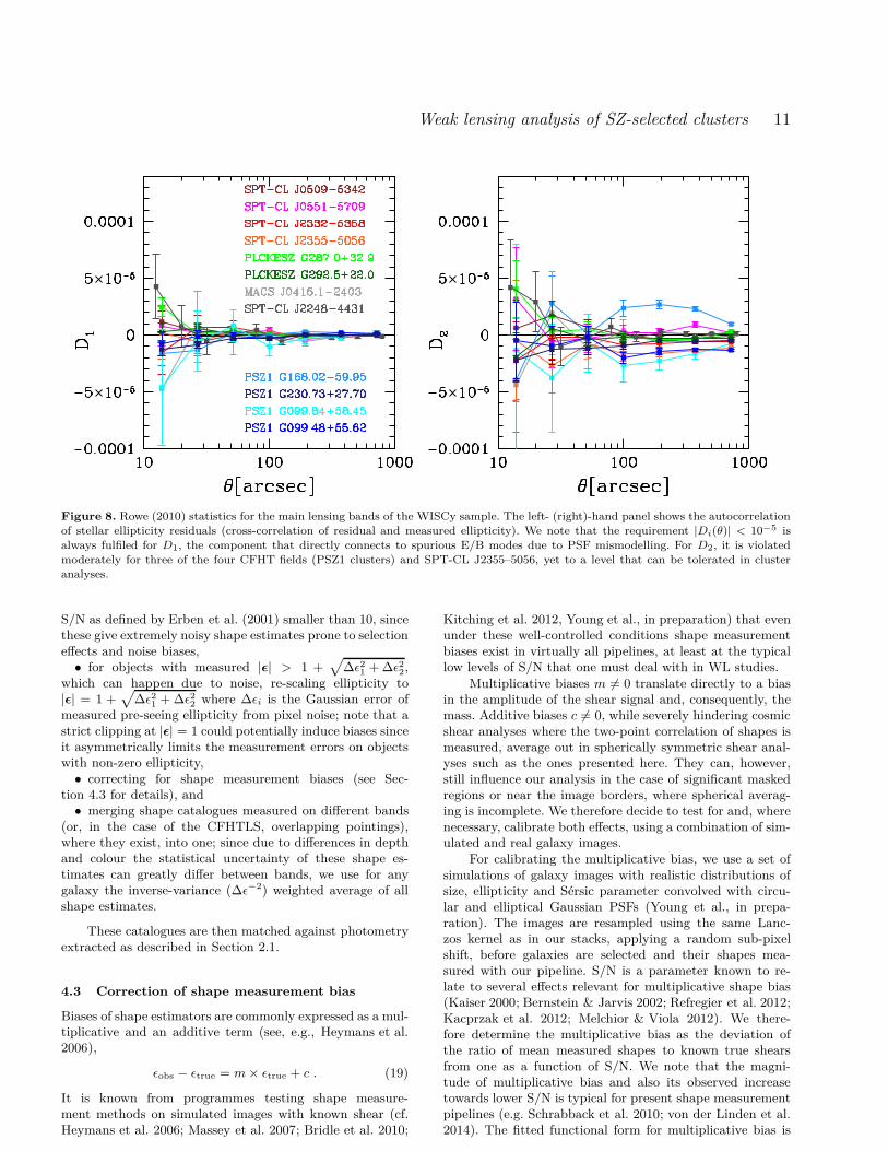
• auto-correlation of ellipticity residuals D1(θ) and cross-correlation of residuals and measured stellar ellipticityD2(θ), i.e. the Rowe (2010) statistics (defined as in theirequations 13 and 14), are consistent with |Di(θ)| < 10−5 ata separation angle of θ > 100 arcsec, the scales relevant toour analysis.

The last criterion is a useful test of having selected the cor-rect polynomial order of PSF interpolation, since it is sensi-tive to both over- and underfitting (Rowe 2010). Fig. 8 showsD1 and D2 for the main lensing band of all our clusters. Ineach frame, we use the lowest order at which the Di statis-tics are either consistent with zero or do not significantlyimprove when increasing the orders further.

For the subsample of eight clusters from the WISCysample imaged with WFI, it is always possible to fulfill thePSF model quality criteria for the R-band stack and in sev-eral cases also in other bands (cf. Table 1 for the list of bandswith successful shape measurement). The negative D2 ofSPT-CL J2355–5056 (cf. Fig. 8) is a minor exception. Sincethis is in principle a sign of overfitting despite the use of apolynomial of only 4th order, we conclude that it is likelya statistical effect and accept the model regardless. In someof the I band frames it is not possible to control D2 to anacceptable level, and we reject these frames for shape mea-surement. For the four clusters imaged by CFHTLS, the cri-teria of root-mean-square (rms) residual and |Di(θ)| < 10−5

prove to be too strict to be fulfilled for the models tested.Modelling the PSF on individual chips while excluding thechip gaps and regions of the field where the PSF model isvisibly problematic, we accept the frames despite a slightlyhigher D2. We note that this higher level of PSF complexity

is typical for the CFHTLS frames (cf. also Brimioulle et al.2013, their section 3.4).

4.2 Shape Measurement

We run an implementation of KSB+ (KSB;Luppino & Kaiser 1997 and Hoekstra et al. 1998) whichuses the psfex PSF model (ksbpsfex). Galaxies areprepared for shape measurement by the following steps:

• unsaturated, reasonably isolated sources with SEx-

tractor flags 6 3 are selected,• postage stamps of 64×64pix size are extracted and

neighbouring objects are masked according to the SExtrac-

tor segmentation map,• the SExtractor photometric background estimate at

the object position is subtracted from the image in orderto compensate for small-scale background variations insuffi-ciently subtracted by the data reduction pipeline,

• bad and masked pixels are interpolated using a GaussLaguerre model of the galaxy (Bernstein & Jarvis 2002), dis-carding objects with more than 20 per cent of postage stamparea or 5 per cent of model flux in bad or masked pixels.

For the actual shape measurement, KSB+ is run on theprepared postage stamp of the galaxy and the sub-pixel res-olution PSF model at the same position. Here we only givea brief summary of this step, referring the reader to theoriginal papers for further details.

KSB measure polarizations

e =1

Q11 + Q22

(

Q11 − Q22

2Q12

)

(15)

defined by second moments calculated inside an aperturewith Gaussian weight,

Qij =

∫

d2θ I(θ) w(|θ|) θi θj , (16)

of the surface brightness distribution of the galaxy I(θ) witha weight function w(|θ|) centred on the galaxy centroid. Ourimplementation allows measuring the galaxy and PSF mo-ments with the identical weight function, scaled with theobserved half-light radius of the galaxy.

In the presence of an elliptical PSF, the linear approx-imation of how observed post-seeing polarization eo reactsto a reduced shear g (cf. Bartelmann & Schneider 2001, p.60) can be expressed as

eo = ei + P smp + P γ

g , (17)

where ei is the intrinsic post-seeing ellipticity of the galaxy,P sm is a 2 × 2 tensor quantifying the response of observedshear to PSF polarization p and P γ is the shear responsivitytensor. We invert (P γ)−1 ≈ 2

trP γ and assume that (P γ)−1ei

is zero on average (because of the random intrinsic orienta-tion of galaxies) to find the ensemble shear estimate

〈g〉 = 〈ǫ〉 =⟨

2trP γ

(

eo − P smp)

⟩

. (18)

We apply some final filtering and corrections to our cat-alogue, namely

• removing objects with any of trP γ < 0.1, half-light ra-dius less than 5% larger than the PSF half-light radius or

c© 2013 RAS, MNRAS 000, 1–42


Figure 8. Rowe (2010) statistics for the main lensing bands of the WISCy sample. The left- (right)-hand panel shows the autocorrelationof stellar ellipticity residuals (cross-correlation of residual and measured ellipticity). We note that the requirement |Di(θ)| < 10−5 isalways fulfiled for D1, the component that directly connects to spurious E/B modes due to PSF mismodelling. For D2, it is violatedmoderately for three of the four CFHT fields (PSZ1 clusters) and SPT-CL J2355–5056, yet to a level that can be tolerated in clusteranalyses.

S/N as defined by Erben et al. (2001) smaller than 10, sincethese give extremely noisy shape estimates prone to selectioneffects and noise biases,

• for objects with measured |ǫ| > 1 +√

∆ǫ21 + ∆ǫ2

2,which can happen due to noise, re-scaling ellipticity to|ǫ| = 1 +

√

∆ǫ21 + ∆ǫ2

2 where ∆ǫi is the Gaussian error ofmeasured pre-seeing ellipticity from pixel noise; note that astrict clipping at |ǫ| = 1 could potentially induce biases sinceit asymmetrically limits the measurement errors on objectswith non-zero ellipticity,

• correcting for shape measurement biases (see Sec-tion 4.3 for details), and

• merging shape catalogues measured on different bands(or, in the case of the CFHTLS, overlapping pointings),where they exist, into one; since due to differences in depthand colour the statistical uncertainty of these shape es-timates can greatly differ between bands, we use for anygalaxy the inverse-variance (∆ǫ−2) weighted average of allshape estimates.

These catalogues are then matched against photometryextracted as described in Section 2.1.

4.3 Correction of shape measurement bias

Biases of shape estimators are commonly expressed as a mul-tiplicative and an additive term (see, e.g., Heymans et al.2006),

ǫobs − ǫtrue = m × ǫtrue + c . (19)

It is known from programmes testing shape measure-ment methods on simulated images with known shear (cf.Heymans et al. 2006; Massey et al. 2007; Bridle et al. 2010;

Kitching et al. 2012, Young et al., in preparation) that evenunder these well-controlled conditions shape measurementbiases exist in virtually all pipelines, at least at the typicallow levels of S/N that one must deal with in WL studies.

Multiplicative biases m 6= 0 translate directly to a biasin the amplitude of the shear signal and, consequently, themass. Additive biases c 6= 0, while severely hindering cosmicshear analyses where the two-point correlation of shapes ismeasured, average out in spherically symmetric shear anal-yses such as the ones presented here. They can, however,still influence our analysis in the case of significant maskedregions or near the image borders, where spherical averag-ing is incomplete. We therefore decide to test for and, wherenecessary, calibrate both effects, using a combination of sim-ulated and real galaxy images.

For calibrating the multiplicative bias, we use a set ofsimulations of galaxy images with realistic distributions ofsize, ellipticity and Sérsic parameter convolved with circu-lar and elliptical Gaussian PSFs (Young et al., in prepa-ration). The images are resampled using the same Lanc-zos kernel as in our stacks, applying a random sub-pixelshift, before galaxies are selected and their shapes mea-sured with our pipeline. S/N is a parameter known to re-late to several effects relevant for multiplicative shape bias(Kaiser 2000; Bernstein & Jarvis 2002; Refregier et al. 2012;Kacprzak et al. 2012; Melchior & Viola 2012). We there-fore determine the multiplicative bias as the deviation ofthe ratio of mean measured shapes to known true shearsfrom one as a function of S/N. We note that the magni-tude of multiplicative bias and also its observed increasetowards lower S/N is typical for present shape measurementpipelines (e.g. Schrabback et al. 2010; von der Linden et al.2014). The fitted functional form for multiplicative bias is

c© 2013 RAS, MNRAS 000, 1–42

12 D. Gruen et al.

shown in Gruen et al. (2013, equation 9) and the corre-sponding correction is applied to our shape catalogues.

No significant additive bias is detected in our simula-tions, yet could potentially be caused in real data by moreintricate observational effects not present in the former. Thefact that the mean ellipticity of galaxies in an unbiasedcatalogue should be zero can be used to empirically cali-brate constant additive biases directly from the data (cf. e.g.,Heymans et al. 2012). In our initial catalogues, we found asignificantly negative ǫ1 component, indicating preferentialorientation of objects along the vertical direction. We tracethis back to a selection effect in the latest public version ofSExtractor.8 Related to buffering with insufficiently largememory settings (Melchior, Bertin, private communication),horizontally elongated objects are preferentially deselected(FLAG=16). An increase of MEMORY_BUFSIZE fixes this andyields shape catalogues without significant additive bias.

4.4 Mass mapping

The WL shear field can be used to estimate the surface massdensity as a function of position. We create such maps for theeight WFI clusters in the WISCy sample. They are shownin the respective subsections of Section 6 and used for thepurpose of illustrating the cluster density fields only.

For the surface density reconstruction we usethe finite field reconstruction technique described inSeitz & Schneider (1996). From the observed galaxy elliptic-ity we estimate the reduced shear using equations 5.4 to 5.7in Seitz & Schneider (1996). We choose a smoothing lengthof 1.5 arcmin for the spatial averaging of the galaxy elliptic-ities (their equation 5.7), accounting for the relatively lowgalaxy density (of order 10 galaxies per square arcminute) ofbackground objects used for the reconstruction. The κ-mapsare obtained on a 100 × 100 grid for the FOV of shear dataof typically 28×28 arcmin2. Spatial resolution is limited bythe required large smoothing length and not by the grid onwhich κ is calculated.

As was pointed out by Schneider & Seitz (1995) andSeitz & Schneider (1995, 1997), as long as one uses sheardata (at one effective redshift) only, the surface density mapscan only be obtained up to the mass sheet degeneracy. Wethus arbitrarily fix this constant such that within the recon-structed field the mean density is κ = 0.01 (accounting forthe fact that the field is not empty but contains a massivecluster with approximately this mean surface density). Ifwe would have chosen this constant differently the contour-pattern of course would not change, but the values would beslightly altered as described by the mass sheet degeneracy.

For the four clusters imaged by the CFHTLS, maskingof the chip border areas is required in our shape catalogue,since the complex and discontinuous behaviour of the stackPSF in this region cannot be controlled well enough. As aresult, two-dimensional density mapping is extremely noisy,and consequently we do not provide density maps for them.

8 Version 2.8.6, cf. http://www.astromatic.net/software/sextractor

4.5 Mass measurement

For the interpretation of the WL signal in each of our clus-ter fields, we follow the scheme described in this section.We follow two different approaches, one ignoring secondarystructures along the line of sight (as is commonly done insimilar WL studies) and one explicitly modelling these. Thefollowing sections detail the components of this procedure.

4.5.1 Density profile

It is supported by a range of observational and simulationstudies that dark matter haloes of clusters of galaxies onaverage follow the profile described first by NFW. We alsoadopt this mass profile, with the three-dimensional densityρ(r) at radius r given as

ρ(r) =ρ0

(r/rs)(1 + r/rs)2. (20)

The profile can be rewritten in terms of two other pa-rameters such as mass M200m and concentration c200m =r200m/rs instead of the central density ρ0 and scale ra-dius rs. Expressions for the projected density and shearof the NFW profile are given by Bartelmann (1996) andWright & Brainerd (2000).

The two parameters of the NFW profile are not in-dependent, but rather connected through a concentration-mass relation. This can be used, for instance, in cases wherethe data are not sufficient for fitting the two parameterssimultaneously. It also allows for proper marginalizationover concentration from the two-dimensional likelihood incases where one is only interested in mass. In our analysis,we assume the concentration-mass relation of Duffy et al.(2008) with a lognormal prior (Bullock et al. 2001) withσlog c = 0.18. Offsets of the assumed concentration-mass re-lation from the truth, which can be due to differences be-tween assumed and true cosmology or imperfect simulationsfrom which the relation is drawn, impact the mass measure-ment, however only mildly (see, for example, the discussionin Hoekstra et al. 2012, their section 4.3).

Unless otherwise noted, we use the brightest clustergalaxy (BCG) position as the centre of the halo (cf. alsoHoekstra et al. 2012 and section 7.5 for a discussion forchoosing the centre for lensing analyses). In order to beless sensitive to miscentring, heavy contamination with clus-ter members, very strong shears and possible deviationsfrom the NFW profile, a central region of 2 arcmin ra-dius around the BCG is not used in our likelihood anal-ysis (see following section). This is in line with previousstudies (cf. Applegate et al. 2014 and Hoekstra et al. 2012,who exclude the central projected 750 and 500 kpc, respec-tively, or Mandelbaum et al. (2010), who propose an aper-ture mass measurement insensitive to surface mass densityinside r200c/5 and discuss, in more detail, the reasons whythis is beneficial for the mass determination). Note, however,that we a posteriori find the measured central shears to beconsistent with the prediction from our fit (cf. Section 7.5).

4.5.2 Likelihood analysis

Assuming Gaussian errors of the shape estimates, the like-lihood of any model can be calculated from the shear cata-logue by means of the χ2 statistics. Given model predictions

c© 2013 RAS, MNRAS 000, 1–42


gi,j for the i component of the shear on background galaxyj (which depend on the masses and concentrations of one ormore haloes in the model and the estimates of β and β2 ofthe background galaxy, cf. Section 3.1), the likelihood L canbe written as

− 2 ln L =∑

i,j

(gi,j − ǫi,j)2

σ2i,j + σ2

int

+ const . (21)

Here ǫi,j is the corresponding shape estimate with uncer-tainty σi,j and the intrinsic dispersion of shapes is σint ≈0.25. The shape measurement uncertainty is calculated bythe ksbpsfex pipeline based on linear error propagation andthen multiplied with an empirically calibrated factor of 1.4to approximate non-linear effects. The latter can be esti-mated by assuming that the observed variance of shape es-timates around the true mean of 0 be equal to the sum ofmeasurement and intrinsic variance, which, unlike the mea-surement error, is constant under different observing condi-tions. In addition, the factor is confirmed by a comparisonof uncertainties measured on CFHT data with our pipelinewith the uncertainties given in the CFHTLenS shape cata-logues (cf. Miller et al. 2013 and Heymans et al. 2012).

Equation (21) readily allows finding maximum-likelihood solutions. Marginalisation over the concentrationparameter can easily be done if a sufficiently large range inconcentration around the concentration prior is probed (cf.Section 4.5.1). By means of the ∆χ2 method (Avni 1976), wecan also determine projected or combined confidence regionsin the parameter space of our model.

4.5.3 Single halo versus multiple halo analysis

Our measurement of masses is done with two different fittingprocedures, which we denote in the following as the singlehalo and multiple halo analysis.

For the single halo analysis, we fit only the central haloof the SZ cluster, placing its centre at the brightest clustergalaxy.

However, no cluster of galaxies is completely isolated inthe field. Rather, both uncorrelated structures along the lineof sight and correlated structures in the vicinity of the clus-ter contain additional matter and therefore cause a lensingsignal of their own.

It is in this important sense that while lensing accu-rately weights the matter along the line of sight (up to themass sheet degeneracy), a mass estimate for a cluster is theresult of our interpretation of the signal. In the same wayas in the case of full knowledge (as it is available only ina high-resolution simulation), the mass we determine there-fore differs by method, yet in the case of lensing with theadditional difficulty of projection.

Several studies in the past have shown that the accu-racy of WL analyses depends on proper modelling of suchprojected structures (see, for example, Dodelson 2004 andMaturi et al. 2005 for minimizing the impact of uncorrelatedstructures, Hoekstra et al. 2011 for the effect of modellingmassive projected structures and Gruen et al. 2011 for theimpact of correlated structures). Projected structures, de-pending on their position, can bias the mass estimate ineither direction, requiring a modelling of the particular con-figuration rather than a global calibration.

For each of the systems considered here, our multiplehalo analysis is therefore done as follows. From known clus-ters and density peaks identified visually and in photomet-ric redshift catalogues we compile a list of candidate haloeswithin the WFI field of view. Details of this procedure aregiven in the respective subsection of Section 6 and Table 5in the appendix.

We determine the redshift of each of the candidatehaloes by three different strategies, depending on the field. Inthe case of PSZ1 G168.02–59.95 and PSZ1 G099.84+58.45,coverage with spectroscopy from SDSS DR 10 (Ahn et al.2014) is used where candidate structure members have beenobserved. In the fields with > 5 bands, the median photo-metric redshift of visually selected cluster members is taken.For the remaining seven WFI fields without accurate pho-tometric redshifts, a different scheme is applied.

In these cases, from a list of visually identified red mem-ber galaxies, we find the median colours with respect to theR-band magnitude. These could be compared to a red galaxytemplate, yet it is known that the SED of red galaxies in-deed changes with redshift and shows significant variabilityeven at fixed redshift (Greisel et al. 2013). We therefore de-termine the mean B-R, V -R and R-I colours of red galaxiesin redshift bins from the DPS catalogues (cf. Section 3.1.1).Fitting a parabola to the squared deviations between thesecolours and the median colour of red member galaxies of thecandidate clusters, we find its minimum χ2 redshift. Exclud-ing the outlier of SPT-CL J0551–5709 (where our estimateof z ≈ 0.30 deviates from the spectroscopic value of 0.423,potentially due to residual star-forming activity in clustermember galaxies), this estimate yields a root-mean-squarederror of σz = 0.02 w.r.t. known redshifts in our WFI clusterfields.

In order to remove the effect of projected structures onthe mass estimate of the central halo, we then determine themaximum-likelihood masses for each of the candidate haloesin a combined fit, assuming a fixed concentration-mass re-lation. As a first-order approximation, in this analysis weassume simple addition of reduced shears due to multiplelenses. Where the best-fitting masses of candidate off-centrehaloes deviate from zero, we subtract the signal of the best-fitting haloes from the shear catalogue, on which we thenperform the same two-parameter likelihood analysis as inSection 4.5.3.

5 SUNYAEV-ZEL’DOVICH CATALOGUES

The comparison of our WL results to the SZ effect of theclusters is performed purely on the basis of publicly availablecatalogues. This section lists the data and our methods ofusing the catalogues.

5.1 South Pole Telescope

The SPT is presently performing multiple surveys of2500 deg2 of the southern sky in three microwavebands, one of its goals being a cosmological analysis ofthe SZ signal of clusters of galaxies (Staniszewski et al.2009; Vanderlinde et al. 2010; Williamson et al. 2011;Reichardt et al. 2013). Five of our clusters have been ob-

c© 2013 RAS, MNRAS 000, 1–42

14 D. Gruen et al.

served in SPT surveys and four of them are indeed SPTdiscovered.

SPT mass estimates are based on the detection signif-icance ζ in the band where it is maximal. In this work, wetake Vanderlinde et al. (2010) as the primary reference formass calibration. They calibrate the mass-significance rela-tion in SPT empirically as

ζ = A ×(

M200m

5 × 1014h−1M⊙

)B

×(

1 + z

1.6

)C

, (22)

with parameters calibrated from simulations as A = 5.62,B = 1.43 and C = 1.40 (Vanderlinde et al. 2010). Here ζ isthe SPT detection significance corrected from the observedsignificance ξ for several noise dependent biases, namely firstthe preferential selection of objects for which intrinsic andmeasurement noise have a positive contribution to the sig-nal and secondly the preferential up-scatter of intrinsicallyless massive objects because of the steepness of the massfunction. These effects are sometimes called the Malmquistand Eddington bias, and are indeed related to the worksby Malmquist (although only widely and with varying def-inition) and Eddington (1913). A third effect particular toSPT is an additional bias on measured significances, causedby the fact that these are measured at the position wherethey are highest (instead of the unknown true position of thecluster). While the first and third effect can be corrected di-rectly, the second requires to assume a mass function, whichin turn depends on cosmology. Where we use ζ in our anal-ysis, we therefore calculate it from the mass estimate pub-lished by the SPT collaboration (Vanderlinde et al. 2010 fortwo of our clusters, Reichardt et al. 2013 for two of the clus-ters where new spectroscopic redshifts had become avail-able in the meantime and Williamson et al. 2011 for SPT-CL J2248–4431, all of which have made corrections for allthree effects), which we insert into equation (22) or (23).

As an alternative calibration based on a very sim-ilar scheme, we also compare to the mass estimates ofReichardt et al. (2013). Using a different mass definition andredshift scaling, Reichardt et al. (2013) and Benson et al.(2013) define the MOR as

ζ = A ×(

M500c

3 × 1014h−1M⊙

)B

×(

E(z)E(0.6)

)C

, (23)

with E(z) =√

Ωm(1 + z)3 + ΩΛ. The parameters are de-termined from survey simulations as A = 6.24 ± 1.87,B = 1.33±0.27 and C = 0.83±0.42 (Reichardt et al. 2013),taking into account modelling uncertainty. Posterior scalingparameters from the combined cosmological analysis includ-ing X-ray cluster measurements and CMB are reported inBenson et al. (2013) as A = 4.91 ± 0.71, B = 1.40 ± 0.15and C = 0.83 ± 0.30 with an intrinsic scatter of ζ at fixedmass corresponding to lognormal σint,log10

= 0.09 ± 0.04.

5.2 Planck

Planck is a mission complementary to SPT in its SZ applica-tions. Unlike SPT, which has imaged a relatively small area,Planck detects an all-sky catalogue of the SZ-brightest ob-jects with sufficient angular extent. However, while the SPTproduces arcminute-resolution images, the Planck SZ anal-yses are complicated by the much lower resolution (above

4 arcmin full width at half-maximum even for the bandswith smallest beam size), which leaves most clusters unre-solved and high redshift clusters hard to detect, and theinhomogeneity of noise over the observed area.

For this reason, Compton parameters Y are providedby Planck Collaboration et al. (2013a) only in the form of atwo-dimensional likelihood grid in terms of Y = Y cyl

5θ500c, in-

tegrated inside a cylindrical volume of 5×θ500c diameter, andthe angular size θs = rs/DA(z), where rs is the scale radiusof the generalized NFW profile (cf. Arnaud et al. 2010) ofthe intracluster gas.9 Due to the large beam size, the Comp-ton parameter can only be confined well if prior informationon θs is available.

5.2.1 De-biasing

As a first step, Compton parameters Y measured near thedetection limit must be (Malmquist) noise-bias corrected. Atthe detection limit, there exists a selection effect based onthe preferential inclusion (exclusion) of objects whose signalscatters up (down) from the fiducial value. Consequently,a majority of objects near the detection limit have a posi-tive noise and intrinsic scatter contribution.10 The resultingmultiplicative bias in

Yobs = bm × Ytrue (24)

can be estimated as (Vikhlinin et al. 2009a)

bm = exp

[

σ × exp(−x2/2σ2)√

π/2erfc(x/√

2σ)

]

, (25)

where

x = − ln[(S/N)0/(S/N)cut] , (26)

σ =√

ln2 ((S/N + 1)/(S/N)) + ln2(10σint,log 10) , (27)

with the nominal S/N according to the MOR at themass of the cluster (S/N)0, the threshold of the catalogue(S/N)cut = 4.5 and the ln-normal scatter of the MORσ. We adopt a value of the lognormal intrinsic scatter ofσint,log 10 ≈ 0.07 (Planck Collaboration et al. 2013a). Asdone by Planck Collaboration et al. (2013a), we simply di-vide the Compton decrement by bm.11

For the seven Planck-detected clusters in the WISCysample, bm ∈ (1.00, 1.10). Note that for a higher σint,log10

as suggested by previous studies (Marrone et al. 2009;Hoekstra et al. 2012; Marrone et al. 2012), bm and with itYtrue and estimated mass for our clusters change signifi-cantly, in particular for the low S/N detections.

9 For a detailed description of the format, please refer tohttp://www.sciops.esa.int/wikiSI/planckpla/index.php?

title=Catalogues&instance=Planck_Public_PLA10 This is true even without the Eddington bias (preferentialup-scatter of less massive haloes due to the steepness of themass function), an effect ignored here for consistency with thePlanck Collaboration et al. (2013a) calibration.11 We consistently work with the natural logarithm here.Planck Collaboration et al. (2013a) appear to use log and ln in-terchangeably in their equation 8 and the following description.

c© 2013 RAS, MNRAS 000, 1–42


Figure 9. Self-consistent mass estimation from Planck likelihoodin θs-Y cyl space. The diagram illustrates how, assuming a pres-sure profile (PP), a mass-observable relation (MOR) and the an-gular diameter distance of the cluster DA(z), θs is a functionof Y cyl (and vice versa). The likelihood for mass need then beevaluated only for consistent tuples of Y cyl and θs.

5.2.2 θs-Y degeneracy

How can the degeneracy between angular size and integratedCompton parameter be broken? In this work we use two dif-ferent schemes of calculating mass estimates from the PlanckSZ signal. For their own calibration, the Planck Collabora-tion uses subsets of clusters with X-ray mass estimates. Fromthese and assumptions about the pressure profile (PP; seebelow) they derive θs, thereby breaking the θs-Y degener-acy. We perform a similar analysis, using X-ray mass esti-mates for our sample from various sources. The resulting SZmass estimates, however, are not made truly independentlyfrom the SZ information, since in fact prior information onthe mass itself is used. In addition, we therefore developa scheme of self-consistent SZ masses, similar to the onesuggested by Planck Collaboration et al. (2013a, their sec-tion 7.2). It is illustrated in Fig. 9.

Likelihoods are given by Planck Collaboration et al.(2013a) in terms of cylindrically integrated Compton pa-rameters Y and angular scale radii θs.12 A value forθ500c corresponding to an external X-ray mass estimatecan be converted to θs by means of the PP con-centration parameter cP,500c=1.1733 (Arnaud et al. 2010;Planck Collaboration et al. 2013a). At the fixed value ofθs, we obtain a confidence interval of Y (see Fig. 10 foran illustration), which can be converted to the spheri-

12 These likelihoods are provided by Planck Collaboration et al.(2013a) for different extraction methods. We will use the MatchedMulti-filter method (MMF3) catalogues of Melin et al. (2006) forconsistency with Planck Collaboration et al. (2013b) in versionR1.11.

cal estimate Y500c and to M500c with the prescriptions ofPlanck Collaboration et al. (2011b, 2013a), namely

Y500c = 0.5567 × Y (28)

(cf. also Arnaud et al. 2010, their section 6.3.1) and

E(z)−2/3 ×(

D2A × Y500c

Mpc2

)

= 10A ×(

M500c × (1 − b)

6 × 1014h−170 M⊙

)B

(29)with E(z) =

√

Ωm(1 + z)3 + ΩΛ and fiducial calibra-tion parameters A = −4.19 ± 0.02, B = 1.79 ±0.08 and b = 0.2+0.1

−0.2 (cf. Planck Collaboration et al.2013b, their equation A.15). We find that the value ofY RX

500c = (2.36 ± 0.20) × 10−4 Mpc−2 determined suchfrom the Planck Collaboration et al. (2013a) likelihoodsfor SPT-CL J2248–4431 is consistent with the valuegiven by Planck Collaboration et al. (2011b) from earlierPlanck data, also using X-ray priors on size, of Y RX

500c =(2.21 ± 0.16) × 10−4 Mpc−2. For PLCKESZ G287.0+32.9and PLCKESZ G292.5+22.0, Planck Collaboration et al.(2011a) give Compton decrements as Y = (6.1 ± 0.6) ×10−3arcmin2 and Y = (3.7 ± 0.6) × 10−3arcmin2. Theseare again consistent with the values we extract of Y =(6.16 ± 0.52) × 10−3 and Y = (3.16 ± 0.52) × 10−3arcmin2,respectively.

The second option we use is to calculate, by way ofequations 28 and 29, for any Y the corresponding

θs = θ500c(M500c(Y ))/cP,500c . (30)

For the PP concentration we again use the fixed value ofcP,500c = 1.1733.

Equation (30) is a criterion of self-consistency, namelythat the analysis result in a mass to which corresponds thevirial radius used in the extraction of the signal. The like-lihood is then evaluated at the combination of Y and θs

matched by equation (30). Thereby we reduce the dimen-sionality of the likelihood analysis by one, applying onlyknowledge about the angular diameter distance to the sys-tem and no mass information external to the Planck SZsignal. An illustration of the method is given in Fig. 10 forone of our clusters.

5.2.3 Mass estimates

We give confidence intervals for the mass estimates basedon the Planck Collaboration et al. (2013a) catalogues in Ta-ble 3, listing three separate uncertainties:

• the statistical uncertainty of Y500c, extracted from thelikelihood as described above,

• the intrinsic scatter of Y500c at fixed mass (and, con-versely, mass at fixed Y500c, which we approximate asσlog Y500c|M500c

= 0.07, and• the systematic uncertainty based on the confidence re-

gions of parameters A, B and b in equation (29), where weassume all deviations from the fiducial values to be uncor-related.

c© 2013 RAS, MNRAS 000, 1–42

16 D. Gruen et al.

SZ name θ500c S/N YRX

500c MSZ,RX500c MSZ,sc

500c

PLCKESZ G287.0+32.9 4.85 17.2 3.43 ± 0.29 17.7+0.8−0.9

+1.7−1.5

+2.7−3.6 18.2+1.0

−0.9+1.7−1.6

+2.8−3.7

PLCKESZ G292.5+22.0 5.00 8.9 1.76 ± 0.29 10.3+0.9−1.0

+1.0−0.9

+1.5−2.1 10.6+1.1

−1.1+1.0−0.9

+1.5−2.1

SPT-CL J2248–4431 4.93 16.7 2.71 ± 0.23 14.5+0.7−0.7

+1.4−1.2

+2.1−2.9 14.8+0.8

−0.8+1.4−1.3

+2.2−3.0

PSZ1 G168.02–59.95 5.97 5.4 1.21 ± 0.33 4.6+0.6−0.8

+0.4−0.4

+0.7−0.9 5.0+0.9

−0.9+0.5−0.4

+0.7−1.0

PSZ1 G230.73+27.70 3.71 5.4 0.69 ± 0.20 6.0+0.9−1.0

+0.6−0.5

+0.9−1.2 6.2+1.2

−1.3+0.6−0.5

+0.9−1.3

PSZ1 G099.84+58.45 2.98 5.9 0.58 ± 0.14 8.6+1.1−1.2

+0.8−0.7

+1.2−1.7 8.3+1.2

−1.3+0.8−0.7

+1.2−1.7

PSZ1 G099.48+55.62 6.27 7.0 1.08 ± 0.23 3.2+0.4−0.4

+0.3−0.3

+0.5−0.7 3.8+0.5

−0.5+0.4−0.3

+0.6−0.8

Table 3. Mass estimates from the Planck Collaboration et al. (2013a) SZ catalogue. MSZ,RX500c is calculated using X-ray mass estimates

for determining the aperture size θ500c. MSZ,sc500c uses the self-consistent mass determination algorithm described herein. All Compton

parameters have been corrected for Malmquist bias by means of equation (25) according to their S/N in the MMF3 catalogue. Masses

are given in units of 1014h−170 M⊙. The Compton parameter integrated inside a sphere of the size of the X-ray r500c , Y

RX500c, is given in

units of 10−3 arcmin2. The MSZ estimates are listed with statistical, intrinsic and systematic uncertainties.

Figure 10. Mass estimation from Planck likelihood in Y cyl-θs

space for SPT-CL J2248–4431. From the tabulated likelihood(Planck Collaboration et al. 2013a) we determine the confidenceinterval in Y using a fixed prior for the scale angle from X-raymeasurements (green line) and using self-consistency with theMOR (blue line). Colour contours indicate the 68, 90 and 99 percent confidence levels for two degrees of freedom.

6 INDIVIDUAL CLUSTER ANALYSIS

This section presents the individual analyses of the WISCysample. The subsections are ordered by cluster ID (cf. Ta-ble 1) and contain information on the following:

(i) Visual appearance. Including a colour image of the cen-tral parts and a map of projected galaxy density,

(ii) Previous work. With a review of published optical,spectroscopic, X-ray, radio and SZ observations and knownneighbouring projected structures,

(iii) Weak lensing analysis. Including shear profile, indi-vidual mass estimates and remarks on particularities of theanalysis, especially in terms of the modelling of nearby struc-tures, and

(iv) Strong lensing. With a review of previous strong lens-

ing analyses and strong lensing candidates discovered in ourcluster fields.

6.1 SPT-CL J0509–5342

6.1.1 Visual Appearance

The centre of SPT-CL J0509–5342 (cf. Fig. 11, top panel,showing a 4×4 arcmin2 region) is marked by a diffuse BCG,embedded in a number of relatively bright foreground starsand neighboured by at least two giant gravitational arcs ofbackground galaxies strongly lensed by the system.

The central panel of Fig. 11 shows the three-dimensionaldensity of galaxies in a 30×30 arcmin map around thecluster, smoothed with a minimum-variance (Epanechnikov)kernel of radius 1 arcmin and corrected for masked area.Galaxies are selected by their photometric redshift within|z − zcl| 6 0.06 × (1 + zcl). Note that the photometric red-shifts used here are very noisy due to the small number ofbands and are therefore provided for illustrative purposesonly. The colour image cutout, as in the respective figuresof all following clusters, corresponds to the red frame in theoverview map (central panel).

6.1.2 Previous Work

Staniszewski et al. (2009) describe the system as one of thefirst clusters discovered in an SZ survey. Its detection signif-icance is quoted by Vanderlinde et al. (2010) as ξ = 6.61σ.Menanteau et al. (2010a) independently discover the SZ sig-nal of the cluster and label it as ACT-CL J0509-5341. Thecluster coincides with the source 1RXS J050921.2-534159from the ROSAT faint source catalogue (Voges et al. 2000).

High et al. (2010) determine a spectroscopic redshift ofthe cluster of z = 0.4626, which we adopt in this analysis.The independent spectroscopy of Menanteau et al. (2010a)yields z = 0.461.

Using griz data from the Blanco Cosmology Survey andMagellan, High et al. (2010) provide an optical richness ofNgal = 41 ± 8, corresponding to their mass estimate ofM200m(Ngal) = (3.3±2.0±1.0)×1014h−1M⊙. Zenteno et al.

c© 2013 RAS, MNRAS 000, 1–42


Figure 11. Colour image (top panel) from VRI frames of the cen-tral 4×4 arcmin region of SPT-CL J0509–5342, corresponding tothe red square in the three-dimensional galaxy density map (cen-tral panel) with overlaid κ contours at κ = 0.05, 0.10, 0.15. Thebottom panel shows shear profile with tangential shear (black),cross-shear (red, dotted) and NFW fit (green boxes), using onlydata > 2 arcmin from the centre (long dashed line).

(2011) fit the luminosity function and the number densityprofile of cluster member galaxies, noting that there is no in-dication that this and the other clusters in their SZ-selectedsample differ in their properties from samples selected byother kinds of observations.

Sifón et al. (2013) use spectroscopic redshifts of 76 clus-ter members to determine a velocity dispersion of (846 ±111)km s−1 and a corresponding dynamical mass estimateof M200c = (5.5 ± 2.1) × 1014h−1

70 M⊙.The SZ mass of the system is estimated by

Vanderlinde et al. (2010) based on the significance-massrelation, yielding M200m = (5.09 ±stat 1.02 ±sys 0.69) ×1014h−1M⊙. The unbiased significance according to equa-tion (22) is ζ = 5.08.

The independent discovery of the cluster by ACT islisted as ACT-CL J0509–5341 (Marriage et al. 2011). TheSZ mass is given by Hasselfield et al. (2013) as M500c =(4.0 ± 0.8) × 1014h−1

70 M⊙.Andersson et al. (2011) present the system in their X-

ray measurements of SPT clusters with Chandra, findingT = 7.0+1.4

−1.1keV, Mg,500 = 5.6+0.2−0.2 × 1013h−1

70.2M⊙ and a cor-responding YX,500c = (4.3 ± 0.8) × 1014h−1

70.2M⊙keV. Usingthe MORs of Vikhlinin et al. (2009a) with mean values cal-ibrated from local clusters under the assumption of HSE,they estimate M500c = (5.43 ± 0.60) × 1014h−1

70.2M⊙ fromYX,500c and M500c = (6.71 ± 1.69) × 1014h−1

70.2M⊙ from thetemperature. In this work, we will adopt the weighted meanvalue M500c = (5.57 ± 0.56) × 1014h−1

70.2M⊙.Andersson et al. (2011) classify SPT-CL J0509–5342 as

a merger at an early stage based on the double-peaked X-raycentre. In contrast, Semler et al. (2012) find the system tohave a moderate cool core.

Reichardt et al. (2013) quote a combined SZ+X-raymass of M500c = (5.36 ± 0.71) × 1014h−1

70 M⊙.McInnes et al. (2009) perform a WL analysis of the sys-

tem as one of the first SZ detected clusters. They calculateKSB shapes on i band and photometric redshifts on g-, r-,i-, and z-band public imaging data from the Blanco Cos-mology Survey. Their mass estimate from an NFW fit isM200m = 3.54+2.07

−1.68h−171 × 1014M⊙.

6.1.3 Weak Lensing Analysis

The κ map (Fig. 11, central panel) contains peaks at thecentre of SPT-CL J0509–5342 and at a secondary locationnear the western edge of the field (B). The latter is thelocation of the candidate strong lensing feature discussed inthe following section and shown in Fig. 12.

A single halo fit, fixing the centre at the BCGand marginalizing over concentration, yields M200m =(8.4+3.4

−2.9) × h−170 1014M⊙ (M500c = (4.7+1.9

−1.7) × h−170 1014M⊙).

The observed shear profile and the confidence interval of theNFW fit are shown in Fig. 11 (bottom panel).

Given the correlated shape noise, this result is incon-sistent with the earlier analysis of McInnes et al. (2009),although without a cross-match to their photometric red-shift catalogue the significance of inconsistency cannot beestimated confidently. We hypothesize that the photomet-ric redshifts calculated by McInnes et al. (2009) on fourbands only, the bluest being the g band, could be a causefor a low bias in their mass estimate (cf. Section 3.1.6 andApplegate et al. 2014). We note that there is additional evi-

c© 2013 RAS, MNRAS 000, 1–42

18 D. Gruen et al.

dence from the strong lensing feature (cf. Section 6.1.4) andthe consistency of our result with all SZ and X-ray basedmeasurements supporting our higher mass estimate.

After subtracting the maximum likelihood signal of sur-rounding structures fitted simultaneously, the resulting massestimate for the central halo is slightly lower at M200m =(6.6+3.1

−2.6) × h−170 1014M⊙ (M500c = (3.8+1.7

−1.5) × h−170 1014M⊙).

Both our mass estimates are in agreement with theSZ masses of Vanderlinde et al. (2010) and Hasselfield et al.(2013), the X-ray masses of Andersson et al. (2011), thecombined SZ+X-ray mass of Reichardt et al. (2013) and thedynamical mass of Andersson et al. (2011).

6.1.4 Strong Lensing

Two giant arcs are visible in Fig. 11 towards the north-eastern direction from the BCG, as previously reported byMenanteau et al. (2010a). At a separation of θ1 = 4.8 arcsecand θ2 = 8.7 arcsec from the BCG they correspond to theEinstein radii of the best-fitting NFW profile at source red-shifts zs,1 = 1.75 and zs,2 = 5.7. For the 68% upper limit ofour NFW fit, the corresponding redshifts are at more plau-sible values of zs,1 = 1.37 and zs,2 = 2.6.

We note that these strong lensing features pose ad-ditional evidence for our mass estimate that significantlyexceeds the previous one by McInnes et al. (2009). AnNFW profile following the concentration-mass relation(Duffy et al. 2008) at their best-fitting mass (their upperlimit), M200m = 3.59 × 1014h−1

70 M⊙ (5.69 × 1014h−170 M⊙),

has a limiting Einstein radius of 4.7 arcsec (7.6 arcsec) forzs → ∞. Likewise, at their best-fitting mass, a high concen-tration of c200m = 8.6 (an outlier from the mean by ≈ 1.5σ)is required to reproduce the outer arc for a hypotheticalsource redshift of zs = 2. Since the BCG is visibly ellip-tical at an axis ratio of A/B = 1.27, a strongly increasedprojected concentration is, however, unlikely.

In addition, the field contains a strangely shaped bluestructure around a red galaxy at the centre of a group inthe west of the main cluster (Fig. 12). At a radius of r ≈4 arcsec and for the 68% upper limit of the group mass ofM200m = 1.8 × 1014M⊙ (although not constrained well dueto its vicinity to the edge of the field) and red sequencecolour redshift (cf. Section 4.5.3) of zl = 0.41, the Einsteinradius for plausible source redshifts is smaller by a factorof at least 1/2. Considering this, the inhomogeneity of thesurface brightness of the feature and its unusual geometry,we conclude that the candidate is more likely to be a pairof interacting galaxies, yet higher resolution imaging wouldbe needed to unambiguously explore its nature.

6.2 SPT-CL J0551–5709


The central part of SPT-CL J0551–5709 (cf. Fig. 13, toppanel, showing a 4 × 4 arcmin2 region) is formed by threegalaxies of similar brightness aligned in almost north-southdirection. Clean imaging of the cluster is impaired by thenearby bright star HR 2072 of magnitude mV ≈ 6 at ap-proximately 6 arcmin separation, and a large area has to bemasked for the purpose of photometry and shape measure-ment.

Figure 12. Colour image of strong lensing candidate in thefield of SPT-CL J0509–5342. The cutout is centred at (α, δ) =(05h07m47.1s, −5348′40.9′′) and 0.5 × 0.5 arcmin2 in size.

6.2.2 Previous Work

The cluster was detected in SZ by SPT (Vanderlinde et al.2010) at a significance of ξ = 6.13σ.

Its spectroscopic redshift is given as z = 0.423(Vanderlinde et al. 2010).

Using griz data from the Blanco Cosmology Survey andMagellan, High et al. (2010) provide an optical richness ofNgal = 54±15, which they relate to a mass of M200m(Ngal) =(5.4 ±stat 3.8 ±sys 1.6) × 1014h−1M⊙.

Vanderlinde et al. (2010) give the SZ mass estimate atM200m = (4.84 ±stat 1.06 ±sys 0.68) × 1014h−1M⊙. The de-biased significance according to equation (22) is ζ = 4.55.

Andersson et al. (2011) present the first X-ray measure-ments SPT-CL J0551–5709 with Chandra. Their analysis isupdated in Reichardt et al. (2013) with deeper data, find-ing T = 4.0+0.6

−0.6keV, Mg,500c = 5.1+0.6−0.6 × 1013h−1

70.2M⊙ and acorresponding YX,500c = (1.9 ± 0.4) × 1014h−1

70.2M⊙keV. Us-ing the MORs of Vikhlinin et al. (2009a) with mean valuescalibrated from local clusters under the assumption of HSE,they convert the X-ray measurements to a mass estimate ofM500c = (3.4 ± 0.4) × 1014h−1

70.2M⊙.Andersson et al. (2011) identify the cluster as a merger

based on its disturbed X-ray morphology. This is consistentwith the analysis of the X-ray surface brightness concentra-tion by Semler et al. (2012), who classify the system as a noncool-core cluster with a relatively large offset of 82 ± 3kpcbetween BCG and X-ray centroid.

Reichardt et al. (2013) quote a combined SZ+X-raymass of M500c = (3.82 ± 0.54) × 1014h−1

70 M⊙.The foreground cluster Abell S 552 (with lowest Abell

richness class, Abell et al. 1989) lies at 5 arcmin separationfrom SPT-CL J0551-5709. High et al. (2010) give its pho-tometric redshift as z = 0.09, the value we adopt in thisanalysis. Our red galaxy method (cf. Section 4.5.3) yields aconsistent value of z = 0.08.


The κ mapping (Fig. 13, central panel) of SPT-CL J0551–5709 is made difficult by the large masked area around thebright star towards the east from the cluster. Nevertheless, adensity peak is identified in the central region of the cluster,its odd shape likely being a result of the masking. The sec-

c© 2013 RAS, MNRAS 000, 1–42


Figure 13. Colour image from BRI frames (top panel), three-dimensional galaxy density and κ contours (central panel) andshear profile (bottom panel) of SPT-CL J0551–5709. See Fig. 11and Section 6.1.1 for details.

ondary κ peak in the south-eastern direction from SPT-CLJ0551–5709 is associated only with a diffuse galaxy over-density at z ≈ 0.2 . . . 0.3 and also noisified by a number ofmoderately bright stars that mask out background galaxiesnear the peak position.


−4.2)×1014h−170 M⊙ (M500c = (6.6+2.6

−2.4)×1014h−170 M⊙).


When including nearby structures in a combined fit andsubtracting their best-fitting NFW signal from the shear cat-alogue, this result is unchanged. The WL mass measurementis consistent with the combined X-ray and SZ estimate ofReichardt et al. (2013) and the SZ mass estimate at the 1σlevel and with the X-ray estimate of Andersson et al. (2011)at ≈ 1.2σ.

For the purpose of our WL analysis, we have set the cen-tre to be the central cluster galaxy, even though the northernone is the most luminous of the central trio, brighter by 0.13magnitudes in R. We test the impact of this and find thatthe best-fit mass at the position of the northern, brightergalaxy is lower by less than 10 per cent of the statisticalerror (less than 4 per cent of the mass), indicating that WLdoes not yield significant information on the true centringof the system, but that our off-BCG centring approach fol-lowing the overall light of the brightest cluster galaxies isreasonable.


We find no compelling evidence for strong lensing featuresin the field of SPT-CL J0551–5709.

6.3 SPT-CL J2332–5358


SPT-CL J2332–5358 (cf. Fig. 14, top panel, showing a4 × 4 arcmin2 region) appears regular with a single domi-nant brightest cluster galaxy (BCG) and no obvious massivestructures in the vicinity. The elongation of the galaxy dis-tribution along the north-south direction is clearly visible,in accordance with the BCG orientation.

6.3.2 Previous Work

SPT-CL J2332–5358 was discovered by SPT(Vanderlinde et al. 2010) at an SZ significance of ξ = 7.3σ.It is also identified as SCSO J233227-535827 after itsoptical detection by the Southern Cosmology Survey(Menanteau et al. 2010b) and associated with 1RXSJ233224.3-535840, a source in the ROSAT bright sourcecatalogue (Voges et al. 1999). Šuhada et al. (2010) inde-pendently discover the cluster in X-ray observations as partof the XMM-Newton Blanco Cosmology Survey, making thesystem one of the first clusters to be detected independentlyboth by X-ray and SZ surveys.

Its redshift was initially estimated photometrically asz = 0.32 (High et al. 2010), but has been determined morerecently spectroscopically to be z = 0.402 (Song et al. 2012).

Using griz data from the Blanco Cosmology Survey

c© 2013 RAS, MNRAS 000, 1–42

20 D. Gruen et al.

Figure 14. Colour image from BRI frames (top panel), three-dimensional galaxy density and κ contours (central panel) andshear profile (bottom panel) of SPT-CL J2332–5358. See Fig. 11and Section 6.1.1 for details.

and Magellan, High et al. (2010) provide an optical rich-ness of Ngal = 42 ± 8, which they translate to a mass ofM200m(Ngal) = (3.5 ± 2.1 ± 1.1) × 1014h−1M⊙ includingstatistical and systematic uncertainty, although using theerroneous redshift z = 0.32.

An SZ mass estimate based on a significance-mass re-lation is given by Vanderlinde et al. (2010) as M200m =(6.21 ±stat 1.15 ±sys 0.94) × 1014h−1M⊙, yet calculated atthe erroneous redshift of z = 0.32 and with the caveat ofpotential blending with a radio point source. The more re-cent measurement of Reichardt et al. (2013) reports a higherM500c = (6.5±0.79)×1014h−1

70 M⊙ at the spectroscopic red-shift, which is the value we will compare to in this work. Thede-biased significance according to equation (23) is ζ = 9.91,which yields M200m = (12.1 ± 1.4) × 1014h−1

70 M⊙ by meansof equation (22).

X-ray imaging of the cluster exists from XMM-Newton,analysed by Šuhada et al. (2010) and Andersson et al.(2011) at the erroneous photometric redshift of z = 0.32.The analysis is repeated by Benson et al. (2013) for the cor-rect redshift. They find a temperature of T = 7.8+1.0

−0.9keV,a gas mass of Mg,500c = 7.6+0.2

−0.3 × 1013h−170.2M⊙ and a cor-

responding YX,500c = (6.1 ± 0.8) × 1014h−170.2M⊙keV. Using

the MORs of Vikhlinin et al. (2009a) with mean values cal-ibrated from local clusters under the assumption of HSE,they convert the X-ray measurements to a mass estimate ofM500c = (6.7 ± 0.5) × 1014h−1

70.2M⊙.Andersson et al. (2011) characterize the cluster as re-

laxed based on its X-ray morphology.The combined SZ+X-ray mass estimate of

Reichardt et al. (2013) is M500c = (6.54 ± 0.82) ×1014h−1

70 M⊙.Greve et al. (2012) describe a candidate strongly lensed

sub-mm galaxy with multiple images at approximately0.5 arcmin separation from the cluster centre with a spec-troscopic redshift of z = 2.7.

The nearby system SCSO J233231.4-540135.8 at θ ≈4 arcmin separation is a cluster of galaxies optically dis-covered by Menanteau et al. (2009), at a photometric red-shift of z = 0.33. Using the relation of Reyes et al. (2008),they calculate mass estimates based on a combination ofBCG luminosity and either richness or total luminosity ofM200m = 4.1×1014h−1

70 M⊙ and M200m = 1.7×1014h−170 M⊙,

respectively.


The κ map (Fig. 14, central panel) shows that the clusteris elongated along the north-south axis, aligned with theBCG ellipticity. An overdensity of galaxies at an estimatedz ≈ 0.24, 18 arcmin from the BCG at the western edge ofthe field, is associated with a clear peak in κ and includedin the multi-halo fit (see below).


−3.5)×1014h−170 M⊙ (M500c = (7.5+1.8

−1.7)×1014h−170 M⊙).


When including nearby structures in a combined fitand subtracting their best-fitting NFW signal from theshear catalogue, a repeated fit of the central halo yields a

c© 2013 RAS, MNRAS 000, 1–42


slightly higher M200m = (15.3+4.2−3.6) × 1014h−1

70 M⊙ (M500c =(7.9+1.8

−1.7) × 1014h−170 M⊙).

Both results are mildly higher than the SPT SZ massestimate of Vanderlinde et al. (2010) at ≈ 1.5σ, yet in goodagreement with the X-ray, SZ and combined mass estimateof Reichardt et al. (2013).


We find several small blue background sources in the south-east and south-west from the BCG. It is unclear from ourdata whether any of these are multiply imaged or correspondto the strongly lensed system discovered by Greve et al.(2012).

6.4 SPT-CL J2355–5056


The central part of SPT-CL J2355–5056 (cf. Fig. 15, upperpanel, showing a 17 × 6 arcmin2 region) features a singlelarge and diffuse BCG. However, the cluster is neighbouredby structures towards the East and est at separations of 3-4 arcmin, which from visual inspection seem to have similarred galaxy colours and thus redshifts. There is no indicationfor the neighbouring structures from the archival ChandraX-ray data, although the field of view is not large enoughfor a conclusive statement.

6.4.2 Previous Work

SPT-CL J2355–5056 is discovered by SPT(Vanderlinde et al. 2010) at a significance of 5.89σ.

Song et al. (2012) and Reichardt et al. (2013) providea spectroscopic redshift of 0.3196, correcting the previousphotometric estimate of 0.35 (High et al. 2010).

Using griz data from the Blanco Cosmology Survey andMagellan, High et al. (2010) provide an optical richness ofNgal = 55 ± 5, on which they base a mass estimate ofM200m(Ngal) = (5.6 ± 3.0 ± 1.7) × 1014h−1M⊙ when as-suming the slightly erroneous redshift of z = 0.35.

An SZ mass estimate is given by Vanderlinde et al.(2010), yet at the erroneous z = 0.35. The more recentmeasurement of Reichardt et al. (2013) reports M500c =(4.07 ± 0.57) × 1014h−1

70 M⊙ at the spectroscopic redshift,which is the value we will compare to in this work. The de-biased significance according to equation (23) is ζ = 5.12,which yields M200m = (7.6 ± 1.0) × 1014h−1

70 M⊙ by meansof equation (22).

Andersson et al. (2011) present the first X-ray measure-ments SPT-CL J2355–5056 with Chandra. Their analysis isupdated in Reichardt et al. (2013) for the corrected redshift,finding T = 5.3+0.9

−0.7keV, Mg,500c = 3.9+0.2−0.1 × 1013h−1

70.2M⊙and a corresponding YX,500c = (2.2±0.4)×1014h−1

70.2M⊙keV.Using the MORs of Vikhlinin et al. (2009a) with mean val-ues calibrated from local clusters under the assumption ofHSE, they convert the X-ray measurements to a mass esti-mate of M500c = (3.8 ± 0.4) × 1014h−1

70.2M⊙.Andersson et al. (2011) report the cluster to be relaxed

based on its X-ray morphology, likely with a cool core.Semler et al. (2012) consistently classify the system as a cool

core cluster, with a relatively small offset of 6.7±2.3kpc be-tween BCG and X-ray centroid.

Reichardt et al. (2013) quote, using the spectroscopicredshift, a combined SZ+X-ray mass of M500c = (4.11 ±0.54) × 1014h−1

70 M⊙.The APM Galaxy Survey (Dalton et al. 1997) lists the

cluster APMCC 936 at (α, δ) = (23h53m21.5s, −5126′57′′),≈ 14 arcmin separated from SPT-CL J2355–5056. They es-timate its redshift at z = 0.118 with a richness of R = 61.6.


The κ map (Fig. 15, central panel) nicely maps the complexstructure of the multiple components in the field of SPT-CLJ2355–5056. Aside the central region, the galaxy peak nearthe south-western corner of the field is associated with a κoverdensity and red galaxy population at z ≈ 0.42, includedas a component in the multi-halo fit (see below).


−3.1) × 1014h−170 M⊙ (M500c = (4.1+1.7

−1.5) × 1014h−170 M⊙).

The observed shear profile and the confidence interval of theNFW fit are shown in Fig. 15 (lower right panel).

When including nearby structures in a combined fitand subtracting their best-fitting NFW signal from theshear catalogue, a repeated fit of the central halo yieldsa significantly lower M200m = (3.8+2.4

−2.0) × 1014h−170 M⊙

(M500c = (2.1+1.4−1.1) × 1014h−1

70 M⊙). In return, significantmass is attributed to the eastern peak ≈ 7 arcmin fromthe BCG (M200m = (4.5+1.7

−1.7) × 1014h−170 M⊙ at z ≈ 0.24)

and a northern and southern component of the westernpeak (M200m = (1.2+1.7

−1.2) × 1014h−170 M⊙ and M200m =

(6.7+3.0−2.1) × 1014h−1

70 M⊙ at redshifts consistent with the cen-tral cluster, respectively).

The single-peak analysis is consistent with the X-ray,SZ and combined result of Reichardt et al. (2013), whilethe WL result with neighbouring structures subtracted is1σ below. The large uncertainty in the WL analysis of thiscomplex system allows for no significant conclusions on theeffect of blending on the SZ analysis. Yet we note that thestructure of the cluster warrants deeper follow-up, since theinterplay of cluster gas and dark matter might be interest-ing.


Apart from inconclusive arc-like features around the BCG,two candidate strong lensing features can be seen towardsthe east. One is a potential arc at a separation of θ ≈20.6 arcsec from the main galaxy of the eastern structure≈ 7 arcmin from the centre of the field (left panel of Fig. 16).The other is composed of a blue symmetric ring with radiusθ ≈ 3.3 arcsec around a red galaxy and a bluish structureblended with two red foreground galaxies close in projec-tion (right panel of Fig. 16). Both features are at unex-pectedly large radii given the likely mass of the lenses, anddeeper follow-up observations at higher resolution would berequired to confirm their strong lensing nature.

c© 2013 RAS, MNRAS 000, 1–42

22 D. Gruen et al.

Figure 15. Colour image from BRI frames of the central 17 × 6 arcmin region (top panel), three-dimensional galaxy density and κcontours (central panel) and shear profile (bottom panel) of SPT-CL J2355–5056. See Fig. 11 and Section 6.1.1 for details.

Figure 16. Colour images of strong lensing candidates in thefield of SPT-CL J2355–5056. Left panel is centred at (α, δ) =(23h56m33.1s, −5057′20′′), right panel is centred at (α, δ) =(23h56m30.4s, −5053′08′′), both are 1 × 1 arcmin2 in size.

6.5 PLCKESZ G287.0+32.9


PLCKESZ G287.0+32.9 features a large number of clus-ter member galaxies, with a clear brightest galaxy in thecentre and numerous gravitational arcs visible near clustermembers at arcminute separations from the core (cf. Sec-tion 6.5.4). Fig. 17 shows a VRI colour image, using thesingle V band frame available.

6.5.2 Previous Work

The cluster was discovered by its SZ signal, detected byPlanck (Planck Collaboration et al. 2011a) at a significanceof 10.62σ.

A redshift estimate is given byPlanck Collaboration et al. (2011c) at z = 0.39, al-though based on X-ray emission lines and therefore not ofoptimal confidence.

The cluster is followed-up with X-ray observations withXMM-Newton. The Planck Collaboration et al. (2011c) find

c© 2013 RAS, MNRAS 000, 1–42


Figure 17. Colour image (top panel), galaxy density weightedwith Pcl (cf. Section 3.1.3) and κ contours (central panel) andshear profile (bottom panel) of PLCKESZ G287.0+32.9. SeeFig. 11 and Section 6.1.1 for details.

from these data a temperature of T = (12.86 ± 0.42)keV,Mg,500c = (2.39 ± 0.03) × 1014h−1

70 M⊙ and a correspond-ing YX,500c = (30.69 ± 0.36) × 1014h−1

70 M⊙keV. From a YX

MOR calibrated with relaxed objects under the assump-tion of HSE (Arnaud et al. 2010), they calculate a mass ofM500c = (15.72 ± 0.27) × 1014h−1

70 M⊙.Bagchi et al. (2011) investigate non-thermal radio emis-

sion from the cluster. They find a double radio relic, whichis an indication of a major merger. Notably, the double relichas a projected separation of over 4 Mpc, the largest foundto date at a redshift as high as z = 0.39 (Bagchi et al. 2011).They characterize the X-ray morphology based on the sameXMM-Newton that is used by Planck Collaboration et al.(2011c) as disturbed, consistent with the merger hypothe-sis. They find the X-ray peak to be separated from the BCGby a large distance of 410 kpc.

From the catalogued SZ likelihood ofPlanck Collaboration et al. (2013a) we calculate massestimates using the X-ray θ500 as a fixed size and theself-consistency method as M500c = 17.7+0.8

−0.9 × 1014 and18.2+0.9

−1.0 × 1014h−170 M⊙, respectively.


The κ map (Fig. 17, central panel) is dominated by thecentral peak, which has symmetric appearance and a centralvalue of κ = 0.22.


−7.6)×1014h−170 M⊙ (M500c = (19.5+3.3

−3.2)×1014h−170 M⊙).


We note that the excess shear at 5 arcmin radius ispotentially due to the added mass from the structure Ain Fig. 17 at that projected separation. Subtracting themaximum likelihood signal of structure A from a com-bined fit, the resulting mass is slightly lower at M200m =(35.4+8.9

−7.1)×1014h−170 M⊙ (M500c = (18.7+3.2

−3.1)×1014h−170 M⊙).

We note that both results are consistent with pre-vious X-ray observations (Planck Collaboration et al.2011c) and the Planck-based SZ mass estimate(Planck Collaboration et al. 2013a; this work).


The central region of PLCKESZ G287.0+32.9 shows severalarc-like features, marked in the enlarged view in Fig. 18.Candidate features can be found over a large region, thetwo most separated ones 2θ ≈ 165 arcsec apart. Even atthe 68% upper limit of the NFW fit and for a hypotheticalsource redshift of zs = 5, the predicted Einstein radius isonly θE ≈ 37 arcsec, although a larger than mean concen-tration can increase this value considerably. It is the mostlikely explanation that the features seen are therefore eithernot actual multiple images or caused by the particular ge-ometry of the system and its subcomponents (e.g. a majormerger as indicated by the radio signature, cf. Bagchi et al.2011). Despite this, the unusual constellation merits follow-up with spectroscopy and higher-quality imaging, since itwould, if confirmed, make PLCKESZ G287.0+32.9 poten-tially the largest strong lens known to date and a can-

c© 2013 RAS, MNRAS 000, 1–42

24 D. Gruen et al.

Figure 18. Colour image of centre of PLCKESZ G287.0+32.9,arc candidates marked with circles. The cutout size is 3 ×3 arcmin2, making this an exceedingly large region for stronglensing features even for a massive cluster.

didate for the largest strong lens in the Universe, withsome tension with ΛCDM (cf. Medezinski et al. 2013, whofind MACS J0717.5+3745 at θE ≈ 55 arcsec for zs ≈ 3and Oguri & Blandford 2009, Waizmann et al. 2012, andRedlich et al. 2012).

6.6 PLCKESZ G292.5+22.0


PLCKESZ G292.5+22.0 has a central region dominated bythe brightest cluster galaxy (cf. Fig 19), with a highly mag-nified strongly gravitationally lensed image of a backgroundgalaxy between it and a bright galaxy towards the southerndirection.

6.6.2 Previous Work

This cluster was discovered by its SZ signal, detectedby Planck Collaboration et al. (2011a) at a significance of6.88σ.

Planck Collaboration et al. (2011c, 2012) provide a red-shift of z = 0.31 using X-ray spectral fitting and of z = 0.29from V -, R- and I -band optical photometry. In this paperwe adopt z = 0.30, noting that spectroscopic confirmationwould benefit the analysis.

The cluster is followed-up with X-ray observations withXMM-Newton. The Planck Collaboration et al. (2011c) findfrom these data a temperature of T = (9.82 ± 0.84)keV,Mg,500c = (1.17 ± 0.04) × 1014h−1

70 M⊙ and a correspond-ing YX,500c = (11.49 ± 1.33) × 1014h−1

70 M⊙keV. From a YX

MOR calibrated with relaxed objects under the assump-tion of HSE (Arnaud et al. 2010), they calculate a mass ofM500c = (9.25 ± 0.60) × 1014h−1

70 M⊙.

Figure 19. Single colour image from RI frames (top panel),galaxy density weighted with Pcl (cf. Section 3.1.3) and κ con-tours (central panel) and shear profile (bottom panel) of PLCK-ESZ G292.5+22.0. See Fig. 11 and Section 6.1.1 for details.

c© 2013 RAS, MNRAS 000, 1–42


The Planck Collaboration et al. (2011c) report the clus-ter to have a disturbed X-ray morphology.


−1.0 × 1014 and10.6+1.1

−1.0 × 1014h−170 M⊙, respectively.


Our κ map of PLCKESZ G292.5+22.0 shows a rather com-plex structure. The central peak is not as strong as a secondstructure towards the north. The latter is approximatelycentred on a diffuse galaxy ∆mR = 0.98 brighter than theBCG of PLCKESZ G292.5+22.0 and at a redshift that isindiscriminable based on the R-I colour.

The shear profile (Fig. 19, bottom panel) has clear signsof this structure, the dip in tangential shear at 5 arcmin andcounter-excess at 7 arcmin indicating that an overdensity ispresent at ≈ 5 arcmin projected separation from the BCG.


−3.0) × 1014h−170 M⊙ (M500c = (3.4+1.7

−1.4) × 1014h−170 M⊙).


The best-fitting mass is reduced considerably whenmodelling multiple nearby structures. We then find M200m =(5.0+3.1

−2.5) × 1014h−170 M⊙ (M500c = (2.7+1.5

−1.3) × 1014h−170 M⊙).

Two structures (D and E) are assigned masses of close toM200m = 1015h−1

70 M⊙ in this combined analysis. Their in-fluence is seen from the tangential shear profile (Fig. 19,bottom panel) as a low outlier around 5 arcmin (and a highoutlier at 7 arcmin) radius, where the BCG-centred over-density is decreased (increased) by matter on the edge of(inside) the respective annulus.

We hypothesize that this vicinity of other massive struc-tures might be the reason for the ≈ 4σ discrepancy betweenour mass estimate and the X-ray and SZ results.


There is one more interesting feature in the field of PLCK-ESZ G292.5+22.0 beside the strongly magnified image ofa background galaxy lensed between the BCG and anotherbright foreground galaxy (see Fig. 19). This other feature isa symmetric ring around a red galaxy (R-I colour of 0.59,redshift not well constrained by this particular colour butconsistent with the cluster redshift) with bluer colour (R-I ≈ 0.3) at a radius of θ ≈ 4 arcsec (see Fig. 20). TheWL analysis shows no significantly massive halo centred atthis position, making it doubtable whether the feature isa star-forming physically associated ring or indeed lensed.However, the lensing strength of the red galaxy could alsobe boosted by the projected dark matter density of the sur-rounding cluster haloes sufficiently to allow for such a largeEinstein radius.

Figure 20. R-I colour image of the candidate galaxy lens inthe field of PLCKESZ G292.5+22.0. The cutout size is 0.5 ×0.5 arcmin2, centred on (α, δ) = (12h01m21.8s, −3951′22′′) (po-sition B in Fig. 19).

6.7 MACS J0416.1–2403


A view of the central part of MACS J0416.1–2403 (cf.Fig 21) reveals its highly elongated shape, with a chainof bright cluster member galaxies along the north-east tosouth-western direction. Several strong lensing features arevisible.

6.7.2 Previous Work

This cluster was discovered in the ROSAT All-Sky surveyas the bright source 1RXS J041609.9-240358 (Voges et al.1999). Postman et al. (2012) estimate its redshift from theChandra X-ray spectrum as z = 0.42 ± 0.02. Ebeling et al.(2014) provide spectroscopy for 65 galaxies in the field ofMACS J0416.1–2403 and determine the cluster redshift asz = 0.397, the value we use in this work.

Sayers et al. (2013) analyse Chandra X-ray data for thecluster and find a mass of M500c = (9.1±2.0)×1014h−1

70 M⊙,assuming a redshift of z = 0.42. They determine this valuefrom the gas mass of Mg,500c = (1.05 ± 0.23) × 1014h−1

70 M⊙with fgas,500c = 0.115 in analogy to Mantz et al. (2010a).

The cluster is covered by the CLASH project(Postman et al. 2012) as part of the high magnification sam-ple. Zitrin et al. (2013) find a highly elongated (≈ 5 : 1)critical area with extraordinarily high density of multipleimages. The system has also been selected as an HST Fron-tier Field.

MACS J0416.1–2403 is not listed in thePlanck Collaboration et al. (2013a) SZ catalogue andtherefore below the 4.5σ detection significance limit in thePlanck SZ map.


Our κ map of MACS J0416.1–2403 (see Fig. 21, centralpanel) shows a strong elongation of the matter density alongthe north-east to south-western direction, in line with thegalaxy density and the strong lensing model of Zitrin et al.(2013). The distribution of galaxies near the cluster redshiftin the overall field shows higher density in the south-western

c© 2013 RAS, MNRAS 000, 1–42

26 D. Gruen et al.

Figure 21. Colour image from BRI frames (top panel), three-dimensional galaxy density and κ contours (central panel) andshear profile (bottom panel) of MACS J0416.1–2403. The latter

includes the prediction of tangential shear (blue triangles) fromthe SL+WL density profile of Zitrin et al. (2013, their Fig. 2).See Fig. 11 and Section 6.1.1 for details.

quadrant, consistent with the numerous small mass peaksdetected in this region. Both observations are in line withthe hypothesis of MACS J0416.1–2403 being located at thecrossing point of two filaments running in a north-south anda north-east to south-west direction.

The centre of MACS J0416.1–2403 is ambiguous, withthe two brightest galaxies differing in magnitude by only0.02. Setting the centre of the system at the midpoint be-tween the two brightest cluster galaxies as proposed byZitrin et al. (2013) yields a best-fitting mass for the singlehalo analysis at M200m = (9.4+2.7

−2.5) × 1014h−170 M⊙ (M500c =

(5.5+1.5−1.4) × 1014h−1

70 M⊙), marginalizing over concentration.The observed shear profile and the confidence interval of theNFW fit are shown in Fig. 21 (bottom panel).

For comparison, we perform a single halo fit fixing thecentre at the marginally brighter north eastern galaxy. Thisyields a consistent mass, yet the shear in the most centralbin, which is excluded from the fit, at this position is sig-nificantly lower, indicating that the BCG is indeed slightlyoff-centred from the mass peak.

Subtraction of the maximum-likelihood profiles ofneighbouring structures determined in a combined fit yieldsa slightly larger best-fitting mass of M200m = (9.8+2.8

−2.5) ×1014h−1

70 M⊙ (M500c = (5.9+1.5−1.5) × 1014h−1

70 M⊙) (updated).Both of these estimates are below the X-ray measure-

ment at ≈ 1.5σ. This is less of a tension since it is to beexpected that both X-ray estimate and spherical WL modelfit are significantly influenced by the disturbed morphologyof the system in the direction of the observed discrepancyand the X-ray analysis uses a slightly higher value for thecluster redshift.


MACS J0416.1–2403 is a known prominent strong lensingsystem, with several of the known multiple images also visi-ble from our data. Thanks to the availability of deeper HSTand Subaru data from the CLASH survey, we can compareour shear measurement with the predicted shear from theZitrin et al. (2013) projected density profile based on a com-bined weak and strong lensing analysis (blue triangles inFig. 21, bottom panel). We find our shear measurements tobe in good agreement with their model. Both our measure-ment and the Zitrin et al. (2013) model exceed the shearin the central region as predicted by the NFW fit (green).Since the latter is drawn with fixed concentration accordingto the Duffy et al. (2008) mass-concentration relation, thisshows that the concentration of MACS J0416.1–2403 is in-deed higher than average. Note that our mass measurement,however, is not based on the fixed concentration profiledrawn here for illustration purposes, but rather marginalizesover concentration with a prior motivated from simulations(Bullock et al. 2001).

6.7.5 Non-Detection in Planck

Since MACS J0416.1–2403 is a large and highly magnifyinggravitational lens, selected as such in the CLASH survey(Zitrin et al. 2013), the question is whether its non-detectionin the Planck SZ catalogue is in line with expectations. We

c© 2013 RAS, MNRAS 000, 1–42


make a rough estimate of detection probability given theresult of the WL analysis here.

MACS J0416.1–2403 is situated 44 away from theGalactic plane, in a region of expected average noise lev-els of the Planck SZ map. At the θ500c corresponding toits best-fitting mass of θ500c ≈ 3 arcmin, the Monte Carloanalysis of Planck Collaboration et al. (2013a, cf. their fig.9) suggests 50% completeness at a Compton parameter ofY500 ≈ 6 × 10−4 arcmin2. This corresponds, in turn, to amass of M500c ≈ 7 × 1014h−1

70 M⊙, above the observed massof the cluster. We therefore conclude there is no tension witheither the Planck calibrations or our WL model, since boththe SZ-detection and non-detection of MACS J0416.1–2403are possible at the mass reconstructed from the shear. Thenon-detection of this relatively high-redshift system, how-ever, is also made even more likely if there is a yet unac-counted for redshift dependence of the Planck SZ MOR (cf.Section 7.4).

6.8 SPT-CL J2248–4431

We refer the reader to the detailed WL analysis of the systemby Gruen et al. (2013). Here, the system is only used as partof the combined analysis and our results are compared to thePlanck results released after this study.

6.8.1 Comparison with SZ data

The de-biased significance for SPT at full depth is calculatedas ζ = 32.8, assuming the mass estimate of Williamson et al.(2011) and equation (22). Note that this is the de-biased sig-nificance at full SPT depth, while in fact Williamson et al.(2011) present the cluster based on less deep SPT observa-tions (and consequently with lower measured significance).

Using the X-ray mass estimate of M500c = (12.6 ±0.2)×1014h−1

70 M⊙ from Planck Collaboration et al. (2011b)as a fixed size prior and, alternatively, the self-consistencymethod, we determine the SZ mass estimate for the sys-tem at M500c = (14.5+0.7

−0.7) × 1014h−170 M⊙ and M500c =

(14.8+0.8−0.8) × 1014h−1

70 M⊙, respectively. We note that thisresult is ≈ 20% higher than the previous estimate basedon the early SZ catalogue in Gruen et al. (2013), due tothe changed MOR which includes a hydrostatic bias of(1 − b) = 0.8. It is still consistent with the previous WLresult. The substructure-subtracted WL result is lower thanthe SZ mass estimate by 1.5σ (1.8σ for the self-consistentmethod), consistent with the hypothesis that the substruc-ture at θ = 3.5 arcmin separation is blended with the maincluster in the Planck SZ signal or that the hydrostatic massbias assumed in the Planck MOR is not correct in the caseof this system.


SPT-CL J2248–4431 is a prominent strong lensing systemwith several known arcs also visible in our data. Our lens-ing mass reconstruction has recently been compared withthe strong lensing model of Monna et al. (2014), two in-dependent CLASH re-analyses of the WFI data, which in-clude magnification and strong lensing in addition to shear(Merten et al. 2014 and Umetsu et al. 2014) and a WL

analysis of Dark Energy Survey science verification data(Melchior et al. 2014), in all cases with consistent mass es-timates.

6.9 PSZ1 G168.02–59.95


The central region of PSZ1 G168.02–59.95 is shown inFig. 22, on a cutout size of 8×8 arcmin due to the smaller dis-tance to the system. One can see the complex and disturbedstructure of the bright central galaxy. The three-dimensionaldensity is difficult to interpret due to the large masked areaaround a number of bright stars.

6.9.2 Previous Work

PSZ1 G168.02–59.95 was first discovered by Abell (1958)and classified at the second-lowest of six richness classes.

Based on a magnitude-redshift relation, Quintana et al.(2000) give a redshift estimate of z = 0.141. The valueadopted here is the spectroscopic z = 0.1456 fromMirkazemi et al. (in preparation), based on four clustermember galaxies.

The cluster is serendipitously discovered by the RASSas RXC J0214.6–0433 (Cruddace et al. 2002). Based on itsX-ray luminosity and temperature in the XMM Cluster Sur-vey, Viana et al. (2012) estimate the probability of detectingthe system by its SZ signal in Planck to be 76 per cent. Thesystem is also part of the CFHT X-ray cluster sample ofMirkazemi et al. (in preparation).

The system is associated with the ROSAT bright X-ray source 1RXS J021439.0-433319 (Voges et al. 1999). Weapply ROSAT band conversion factor, Galactic Hi columndensity correction (Kalberla et al. 2005) and k-correctionfrom tables 2-4 of Böhringer et al. (2004). In this proce-dure, we assume an X-ray temperature TX = 5 keV, as jus-tified by the relative independence of the conversion factorson TX and the large intrinsic scatter of the TX − LX rela-tion (Pratt et al. 2009) that could be used for self-consistentcalibration. The derived X-ray luminosity corresponds to amass of M500c = (2.5 ± 0.2) × 1014h−1

70 M⊙ according tothe Reiprich & Böhringer (2002) LX − M relation, whichwas calibrated using measurements under the assumptionof HSE.


−0.8 × 1014h−170 M⊙

and 5.0+0.9−0.9 × 1014h−1

70 M⊙, respectively.Tovmassian & Moiseev (1967) fail to detect radio emis-

sion from the system at 1410 MHz.


A single halo fit, fixing the centre at the BCG and marginal-izing over concentration, yields M200m = (2.3+1.4

−1.1) ×1014h−1

70 M⊙ (M500c = (1.2+0.7−0.6) × 1014h−1

70 M⊙). The ob-served shear profile and the confidence interval of the NFWfit are shown in Fig. 22 (bottom panel).

Subtraction of the maximum likelihood signal of neigh-bouring structures before re-fitting the central halo yields a

c© 2013 RAS, MNRAS 000, 1–42

28 D. Gruen et al.

Figure 22. Colour image of 8×8 arcmin2 central region from gri

frames (top panel), three-dimensional galaxy density smoothedwith 1.5 arcmin radius Epanechnikov kernel (central panel) andshear profile (bottom panel) of PSZ1 G168.02–59.95. See Fig. 11and Section 6.1.1 for details.

consistent mass M200m = (2.5+1.5−1.2) × 1014h−1

70 M⊙ (M500c =(1.3+0.7

−0.6) × 1014h−170 M⊙).

This result is marginally consistent with the X-ray massestimate (1.5σ lower), yet significantly lower than the PlanckSZ estimate at ≈ 3σ.


Consistent with the relatively low mass and redshift of thesystem, we find no evidence for strong lensing in PSZ1G168.02–59.95.

6.10 PSZ1 G230.73+27.70


Fig. 23 shows the central region of PSZ1 G230.73+27.70. Alarge number of cluster members is visible, although imagingis somewhat obstructed by a bright star in the south of thesystem. We note that in addition the central BCG, there areseveral additional diffuse elliptical galaxies of similar colouroutside this cutout. Two of them (A and B) are included ashalo centres in our multi-halo analysis of the system.

6.10.2 Previous Work

In the Planck catalogue, PSZ1 G230.73+27.70 is associatedwith a system first described in the maxBCG catalog ofclusters at a photometric redshift of z = 0.2944, althoughthe Planck detection is centred on a galaxy with similarcolour 4 arcmin away from the maxBCG centre.

Koester et al. (2007) give the Nr200 richness of themaxBCG system as 60. Rykoff et al. (2012) calculate arichness λ = 70.2 ± 4.7, to which corresponds a mass ofM200m = (6.6 ± 0.5) × 1014h−1

70 M⊙ with an intrinsic scatterof ≈ 30%.

The system is associated with the ROSAT faint X-raysource 1RXS J090134.0-013900 (Voges et al. 2000). We ap-ply ROSAT band conversion factor, Galactic Hi columndensity correction (Kalberla et al. 2005) and k-correctionfrom tables 2-4 of Böhringer et al. (2004). In this proce-dure, we assume an X-ray temperature TX = 5 keV, as jus-tified by the relative independence of the conversion factorson TX and the large intrinsic scatter of the TX − LX rela-tion (Pratt et al. 2009) that could be used for self-consistentcalibration. The derived X-ray luminosity corresponds to amass of M500c = (3.6 ± 0.8) × 1014h−1



−1.0 × 1014h−170 M⊙

and M500c = 6.2+1.2−1.3 × 1014h−1

70 M⊙, respectively.



−3.2) ×

c© 2013 RAS, MNRAS 000, 1–42


Figure 23. Colour image from gri frames (top panel), three-dimensional galaxy density (central panel) and shear profile (bot-tom panel) of PSZ1 G230.73+27.70. See Fig. 11 and Section 6.1.1for details.

1014h−170 M⊙ (M500c = (4.9+1.6

−1.5) × 1014h−170 M⊙). The ob-

served shear profile and the confidence interval of the NFWfit are shown in Fig. 23 (bottom panel).

Subtraction of the maximum-likelihood profiles ofneighbouring structures yields a lower mass of M200m =(6.8+3.2

−2.6) × 1014h−170 M⊙ (M500c = (3.5+1.5

−1.3) × 1014h−170 M⊙).


We find no evidence for strong lensing in the field of PSZ1G230.73+27.70.

6.11 PSZ1 G099.84+58.45


Fig. 24 shows the central region of PSZ1 G099.84+58.45.The giant arc west of the BCG can be seen along with avery large number of cluster member galaxies. The elon-gated pattern towards the north-eastern direction in theredshift density map (central panel) is identified visually,although only barely, as a diffuse filamentary structure ofhigh-redshift galaxies.


The system was first discovered as a strong lens bythe CFHTLS Strong Lensing Legacy Survey (SL2S,Cabanac et al. 2007) as SL2S J141447+544703.

Cabanac et al. (2007) give the photometric redshift ofthe BCG as z = 0.75, while More et al. (2012) find, on thesame data, z = 0.63 ± 0.02. The photometric redshift forthe central galaxy is z = 0.71 in our photometric redshiftcatalogue, from which we also calculate the outlier-clippedmedian photometric redshift of 32 visually selected clustermembers at z = 0.69, which is the value we adopt in ouranalysis.

The system is associated with the ROSAT faint X-raysource 1RXS J141443.2+544652 (Voges et al. 2000), yet notresolved. We apply ROSAT band conversion factor, GalacticHi column density correction (Kalberla et al. 2005) and k-correction in extrapolation of tables 2-4 of Böhringer et al.(2004). In this procedure, we assume an X-ray temperatureTX = 10 keV, as justified by the relative independence ofthe conversion factors on TX and the large intrinsic scatterof the TX−LX relation (Pratt et al. 2009) that could be usedfor self-consistent calibration. The derived X-ray luminositycorresponds to a mass of M500c = (12.5±2.0)×1014h−1

70 M⊙according to the Reiprich & Böhringer (2002) LX − M re-lation, which was calibrated using measurements under theassumption of HSE.


−1.2 × 1014h−170 M⊙

and 8.3+1.2−1.3 × 1014h−1

70 M⊙, respectively.Foëx et al. (2013) follow up the SL2S detections with

WL analyses. Their singular isothermal sphere (SIS) fit tothe object yields σSIS = 969+100

−130km s−1, which we convert to(cf. Gruen et al. 2013, their equations 17 and 18) M200m =(7.1+2.5

−2.5) × 1014h−170 M⊙ (M500c = 3.7+1.3

−1.3 × 1014h−170 M⊙).

A cluster identified by Yoon et al. (2008) at (α, δ) =

c© 2013 RAS, MNRAS 000, 1–42

30 D. Gruen et al.

Figure 24. Colour image from gri frames (top panel), three-dimensional galaxy density (central panel) and shear profile (bot-tom panel) of PSZ1 G099.84+58.45. See Fig. 11 and Section 6.1.1for details.

(14h13m26.3s, 5445′22.0′′) with spectroscopic redshift z =0.08278 lies at ≈ 11.5 arcmin separation from PSZ1G099.84+58.45. The centre of this system appears to bea galaxy brighter by 0.9 magnitudes than the one given byYoon et al. (2008) and at a compatible spectroscopic red-shift of z = 0.0828 at a separation of 1.6 arcmin with co-ordinates (α, δ) = (14h13m27.3s, 5443′46′′). Due to the lowredshift of the system, however, we do not use the positionin our combined lensing analysis.



−10.2) ×1014h−1

70 M⊙ (M500c = (18.1+5.8−5.3) × 1014h−1

70 M⊙). The ob-served shear profile and the confidence interval of the NFWfit are shown in Fig. 24 (bottom panel).

Subtraction of the maximum-likelihood pro-files of neighbouring structures yields a mass ofM200m = (38.3+13.5

−11.7) × 1014h−170 M⊙ (M500c =

(19.6+6.4−5.8) × 1014h−1

70 M⊙), marginally higher than thesingle-halo value. The high sensitivity of the reconstructionof the high redshift system on matter along the line of sightat lower redshift is due to the fact that the geometricalscaling factor of the lensing signal, DdDds

Ds, causes a relative

amplification of the foreground signal.Despite being based on the same observational data and

consistency with the strong lensing feature of the system(see following subsection), our results are in conflict withthe SIS fit of Foëx et al. (2013) at ≈ 3σ significance (theirσSIS = 969+100

−130km s−1 is significantly lower than our σSIS =1540+162

−190km s−1 as fitted out to 10 arcmin).Several effects can in principle contribute to an under-

estimation of the shear around rich, high redshift clusters.The method of determining β in Foëx et al. (2013) is basedon the mean value calculated from the photometric redshiftof all sources fainter than mi′ = 21 (except a colour-removedred sequence at the cluster redshift), and all these sources areused for calculating the shear profile. This is suboptimal forrich, high-redshift systems like PSZ1 G099.84+58.45, wheremost galaxies fainter than this limit are indeed foregroundobjects or (blue) cluster members. We have verified with thehelp of Foëx (private communication) that the difference be-tween our photo-z based β estimated on their backgroundsample and their method of determining β is indeed the pri-mary cause of the discrepancy.

We note that the lensing analysis for this cluster in-cludes data from a CFHT pointing (W3m0m0) with strongly(> 10%) elliptical PSF along the ǫ1 direction. Detailed anal-ysis shows that for this particular field we measure signifi-cant non-zero mean ellipticity for galaxies along the same di-rection, particularly at low S/N, indicating an additive biasbased on selection effects or insufficient correction for thePSF ellipticity. We verify that also in the CFHTLenS cat-alogues, S/N dependent non-zero ǫ1 shear is present in thisfield. At a highly elliptical PSF, such a bias due to sourcedetection and the simplistic modelling of PSF ellipticity inKSB is not unexpected.

We choose to model the additive bias by the samefunctional form used for the multiplicative noise bias inGruen et al. (2013, their equation 9) with A = 0.005, B =

c© 2013 RAS, MNRAS 000, 1–42


0.08 and C = 14. We have verified that removing the point-ing from our analysis or using it without this correction donot significantly alter our results.


The system was originally discovered as a strong lens witha blue giant arc (Cabanac et al. 2007).

We note that for our best-fitting model with fiducialconcentration, the arc redshift would have to be zs = 1.49to give rise to an Einstein radius at the observed arc ra-dius RA = (14 ± 1) arcsec (Cabanac et al. 2007). At thephotometric redshift of the arc of zs ≈ 2.0, the sameEinstein radius would be caused by a lens of M200m =21.6 × 1014h−1

70 M⊙, 1.2σ below our best fit. While spectro-scopic redshifts for lens and source would greatly enhancethe constraining power of the strong lensing feature, this isstill additional evidence for the correctness of our analysis.

6.12 PSZ1 G099.48+55.62


The cluster image of PSZ1 G099.48+55.62 (cf. Fig. 25) isdominated by a BCG with bi-modal core and visibly dis-turbed wings.


PSZ1 G099.48+55.62 was first discovered by Abell (1958)and classified at the third-lowest of six richness classes.

Struble & Rood (1999) quote a spectroscopic redshiftof z = 0.1051, listing as the source the catalog ofLebedev & Lebedeva (1991), which is unavailable to the au-thors of this work.

The system is associated with the ROSAT bright X-ray source 1RXS J142830.5+565146 (Voges et al. 1999). Weapply ROSAT band conversion factor, Galactic Hi columndensity correction (Kalberla et al. 2005) and k-correctionfrom tables 2-4 of Böhringer et al. (2004). In this proce-dure, we assume an X-ray temperature TX = 5 keV, as jus-tified by the relative independence of the conversion factorson TX and the large intrinsic scatter of the TX − LX rela-tion (Pratt et al. 2009) that could be used for self-consistentcalibration. The derived X-ray luminosity corresponds to amass of M500c = (1.2 ± 0.2) × 1014h−1



−0.4 × 1014h−170 M⊙

and 3.8+0.5−0.5 × 1014h−1

70 M⊙, respectively, noting that thisvalue is significantly higher than the X-ray mass estimate.



−0.9) ×

Figure 25. Colour image of 8×8 arcmin2 central region from gri

frames (top panel), three-dimensional galaxy density smoothedwith 2 arcmin radius Epanechnikov kernel (central panel) andshear profile (bottom panel) of PSZ1 G099.48+55.62. See Fig. 11and Section 6.1.1 for details.

c© 2013 RAS, MNRAS 000, 1–42

32 D. Gruen et al.

1014h−170 M⊙ (M500c = (1.0+0.5

−0.4) × 1014h−170 M⊙). The ob-

served shear profile and the confidence interval of the NFWfit are shown in Fig. 25 (bottom panel).

We do not find additional structures in the field of viewthat would warrant a combined fit. The most prominent fea-ture is a very diffuse concentration of high redshift galaxiestowards the south-east of the cluster.

The WL measurement is consistent with our X-ray massestimate. It is, however, below the Planck SZ value with 3σsignificance.


Consistent with the relatively low mass and redshift of thesystem, we find no evidence for strong lensing in PSZ1G099.48+55.62.

7 COMBINED ANALYSIS

In the following, will combinedly analyse our WL mass es-timates and compare them to the X-ray and SZ measure-ments. Table 4 gives an overview of the mass estimates used.

7.1 Comparison of X-ray and weak lensing mass

estimates

We briefly compare the X-ray gas and total mass estimatesfor the WISCy sample with our WL analysis. Our full samplehas the disadvantage that the X-ray mass estimation is farfrom homogeneous. However, the interesting question of amean hydrostatic mass bias can still be addressed, since wehave taken care to only use X-ray mass estimates calibratedunder the assumption of HSE. For the subsample of eightclusters where X-ray gas mass estimates exist, we can makea more homogeneous analysis.

Fig. 26 shows a comparison of the two mass estimates.There is apparent good agreement between WL masses andX-ray based estimates. The most notable exception is thecase of PLCKESZ G292.5+22.0, likely related to its complexstructure (cf. Sec. 6.6).

We are interested in determining the intrinsic scatter,normalization and slope between X-ray mass estimate MX

and WL measurement MWL. To this end, we assume a re-lation of the form

MWL500c = 10A ×

(

MX500c

6 × 1014h−170 M⊙

)B

(31)

with lognormal intrinsic scatter σint,log10. The pivot mass is

chosen such that errors in A and B are uncorrelated. Notethat A = 0 and B = 1 is the case of agreement with hydro-static calibration.

In order to determine confidence limits for the parame-ters, we calculate the likelihood

− 2 ln Li =(log MWL

i − log f(MXi ))2

σ2i,log MWL + (Bσi,log MX )2 + σ2

int,log10

+ ln(σ2i,log MWL + (Bσi,log MX )2 + σ2

int,log10) , (32)

where f(MXi ) is the relation of equation (31). In considera-

tion of Gruen et al. (2011), we increase the WL uncertain-ties by 10% for all following analyses in order to account for

intrinsic variations due to cluster substructure, orientationand projected structures.

For the WL masses based on a single-halo analysis, weget projected single-parameter confidence intervals of A =0.01+0.05

−0.05 , B = 1.06+0.18−0.18 and σint,log10

= 0.00+0.07−0.00. Using the

estimates after subtraction of secondary haloes, we find A =−0.03+0.06

−0.06, B = 1.08+0.19−0.18 and σint,log10

= 0.00+0.09−0.00 . This is

consistent with no hydrostatic bias and regular scaling of X-ray observables with mass and marginally inconsistent withthe assumption of a 20% negative bias of hydrostatic masses(as in the calibration of Planck Collaboration et al. 2013b).

The relation between gas mass and WL estimate of totalmass is consistent with a gas fraction fgas,500c = 0.128+0.029

−0.023 ,in line with the fgas,500c = 0.115 of Allen et al. (2008) andMantz et al. (2010a). For the multi-halo estimates, the fit ismuch more uncertain but still consistent.

7.2 Comparison of SZ signal and mass

In the following, we will compare our WL measurements ofcluster mass to SZ observables, namely the SPT significanceand the Planck Compton parameter inside the θ500c of theX-ray mass measurement. This is meant both as a test ofthe earlier calibrations of the MORs by Vanderlinde et al.(2010) and Planck Collaboration et al. (2013b) and an in-dependent lensing-based determination of the MOR param-eters.

In this, we need to account for uncertainties inboth the WL mass measurement and the SZ signal,together with an intrinsic scatter. While some stud-ies (e.g. Reiprich & Böhringer 2002; Foëx et al. 2013;Planck Collaboration et al. 2013b) have used line fittingtechniques such as the one described in Akritas & Bershady(1996) in the past, this setting favours a Bayesian approachfor unbiased estimation of the MOR parameters (cf. e.g.Kelly 2007). We therefore determine the parameters fromthe likelihood, in analogy to e.g. Hoekstra et al. (2012, theirequations 7-9) and our equation (32), with lognormal uncer-tainties in all parameters,

− 2 ln Li =(log f(MWL

i , zi) − log fi)2

( d log fd log M

σi,log MWL )2 + σ2i,log fi

+ σ2int,log10

+ ln

(

(

d log f

d log Mσi,log MWL

)2

+ σ2i,log fi

+ σ2int,log10

)

, (33)

where fi is the SZ observable of cluster i with intrinsic scat-ter σint,log10

, and f(M, z) is the MOR.Our key results are illustrated in Fig. 27, which we dis-

cuss subsequently. As for the X-ray comparison (see previoussection) we increase the WL uncertainties by 10% for thisprocedure.

7.2.1 South Pole Telescope

For SPT, we assume the MOR of equation (22)(Vanderlinde et al. 2010). A direct comparison of WL esti-mate and SZ mass for the best-fitting parameters A = 5.62and B = 1.43 (Vanderlinde et al. 2010) shows that whilethere is consistency within the errors, all our systems aremeasured with WL to be at a higher mass than predictedwith the SZ MOR, particularly at lower mass (cf. Fig. 27a).

c© 2013 RAS, MNRAS 000, 1–42


cluster MWL,single200m MWL,single

500c MWL,multi200m MWL,multi

500c MX500c MX

gas,500c MSPT200m MPlanck

500c

SPT-CL J0509–5342 8.4+3.4−2.9 4.7+1.9

−1.7 6.6+3.1−2.6 3.8+1.7

−1.5 5.6 ± 0.6C 0.56 ± 0.02 7.3 ± 1.5 -

SPT-CL J0551–5709 11.7+5.1−4.2 6.6+2.6

−2.4 11.7+5.1−4.2 6.6+2.6

−2.4 3.4 ± 0.4C 0.51 ± 0.06 6.9 ± 1.5 -

SPT-CL J2332–5358 14.5+4.0−3.5 7.5+1.8

−1.7 15.3+4.2−3.6 7.9+1.8

−1.7 6.7 ± 0.5X 0.76 ± 0.25 12.1 ± 1.4 -

SPT-CL J2355–5056 8.0+3.7−3.1 4.1+1.7

−1.5 3.8+2.4−2.1 2.1+1.4

−1.1 3.8 ± 0.4C 0.39 ± 0.15 7.6 ± 1.0 -

PLCKESZ G287.0+32.9 37.7+9.5−7.6 19.5+3.3

−3.2 35.4+8.9−7.1 18.7+3.2

−3.1 15.7 ± 0.3X 2.39 ± 0.30 - 17.7+0.8−0.9

PLCKESZ G292.5+22.0 6.8+3.8−3.0 3.4+1.7

−1.4 5.0+3.1−2.5 2.7+1.5

−1.3 9.3 ± 0.6X 1.17 ± 0.04 - 10.3+0.9−1.0

MACS J0416.1–2403 10.0+2.9−2.6 5.9+1.6

−1.5 10.4+3.0−2.6 6.1+1.7

−1.5 9.1 ± 2.0C 1.05 ± 0.23 - -

SPT-CL J2248–4431 31.1+6.3−5.2 13.8+2.8

−2.4 24.7+6.3−6.0 9.9+2.6

−2.4 12.6 ± 0.2X 1.89 ± 0.02 29.0 ± 3.7 14.5+0.7−0.7

PSZ1 G168.02–59.95 2.3+1.4−1.1 1.2+0.7

−0.6 2.5+1.5−1.2 1.3+0.7

−0.6 2.5 ± 0.2R - - 4.6+0.6−0.8

PSZ1 G230.73+27.70 10.0+3.9−3.2 4.9+1.6

−1.5 6.8+3.2−2.6 3.5+1.5

−1.3 3.6 ± 0.8R - - 6.0+0.9−1.0

PSZ1 G099.84+58.45 34.4+11.6−10.2 18.1+5.8

−5.3 38.3+13.5−11.7 19.6+6.4

−5.8 12.5 ± 2.0R - - 8.6+1.1−1.2

PSZ1 G099.48+55.62 1.9+1.2−0.9 1.0+0.5

−0.4 1.9+1.2−0.9 1.0+0.5

−0.4 1.2 ± 0.2R - - 3.2+0.4−0.4

Table 4. Summary of mass estimates for the WISCy sample. The columns give weak lensing (WL) results for single halo and multi haloreconstructions (cf. Sec. 4.5.3) in two definitions of spherical overdensity in units of 1014h−1

70 M⊙. For Planck SZ, we use the estimatesbased on the X-ray size RX (cf. Section 5.2). Details on the X-ray and SZ measurements can be found in the respective part of Section 6.Superscripts C (Chandra), X (XMM-Newton) and R (ROSAT) indicate the instrument used for the X-ray mass and gas mass estimates.Values for SPT-CL J2248–4431 are taken from Gruen et al. (2013) (WL, as in all other cases we use the mass estimate marginalized overthe concentration parameter) and Planck Collaboration et al. (2011b) (X-ray).

(a) (b)

Figure 26. Comparison of X-ray mass estimates determined under the assumption of hydrostatic equilibrium (a) and X-ray gas masses(b) with our weak lensing result (see individual cluster analysis for details). Error bars indicate best-fitting value and confidence regions

of single-halo fit. The solid symbols are best-fitting masses of the central halo in a combined fit to multiple structures in the field of view,to be interpreted with errors of similar size. Colour coding for the individual clusters is as in Fig. 27. Our measurements are consistentwith no mean bias and no mass dependent bias of the HSE mass and a gas fraction fgas,500c = 0.115.

c© 2013 RAS, MNRAS 000, 1–42

34 D. Gruen et al.

(a) (b)

Figure 27. Comparison of SZ and weak lensing (WL) results for the WISCy clusters. Panel (a) shows SPT, panel (b) Planck clusters.The solid line indicates the mass-observable relations of the respective survey given by Vanderlinde et al. (2010) (A = 5.62, B = 1.43)and Planck Collaboration et al. (2013b) (A = −4.19, B = 1.79, b = 0.2, cf. equations 22 and 29). WL single halo fits and statisticaluncertainties are given by the horizontal and vertical error bars. The solid symbols indicate best-fitting WL result after subtractingneighbouring structures, to be interpreted with errors of approximately the same size. Masses are compared to SPT significance ζand Planck Y

RX500c inside a sphere of the r500c radius corresponding to the X-ray mass estimate, where we use shorthand notations

ζ = ζ[(1 + z)/1.6]−C and Y = E(z)−2/3D2AY

RX500cMpc−2. Dashed lines indicate the fit based on our single-halo WL analysis, and dotted

lines the relation after subtracting the signal of neighbouring structures.

This effect is removed when modelling surrounding struc-tures with WL separately (solid squares), which lowers themass estimate for two systems considerably.

For the independent MOR determination (cf. equation22), we fix C = 1.4 (Vanderlinde et al. 2010), since our SPTsample has little leverage on redshift dependence, and deter-mine the remaining parameters A, B and the log10-normalintrinsic scatter σint,log10

from a combined likelihood.

We find parameters A = 5.8+1.8−1.8 and B = 1.15+0.32

−0.22 fromour single halo analysis (Fig. 27a, dashed line). These valuesare in agreement with the calibration of Vanderlinde et al.(2010) (solid line) at the 68% confidence level and we detecta scaling of SPT significance with mass at 3σ significance inthe combiend three-parametric likelihood. When we insteaduse the WL mass estimates made after subtraction of neigh-bouring structures, we find A = 6.8+2.6

−2.0 and B = 1.09+0.33−0.47

(dotted line), also consistent with Vanderlinde et al. (2010).The shallower slope is mostly due to the unusually complexstructure of SPT-CL J2355-5056, which results in a smallmass of the central system in the multi-halo fit.

The intrinsic scatter is consistent with zero at 1σconfidence with best fits σint,log10

= 0 and upper limitsσint,log10

< 0.13 (0.23) for the single-halo (the multiple halo)analysis, respectively. These values are consistent with previ-ous results (Marrone et al. 2009, 2012; Hoekstra et al. 2012;Benson et al. 2013) and in agreement with predictions (e.g.Kay et al. 2012).

An analogous analysis using the MOR definition of

Reichardt et al. (2013) and Benson et al. (2013) yields A =6.0+1.9

−1.8 and B = 1.25+0.36−0.28 at σint,log10

< 0.15 for the single-halo and A = 7.6+3.0

−2.6, B = 1.02+0.62−0.68 at σint,log10

= 0.15+0.18−0.15

for the multi-halo modelling of neighbouring structures. Inboth cases, we fix the slope of the redshift dependence C =0.83 (Reichardt et al. 2013; Benson et al. 2013). We findconsistency with the MOR parameters of Reichardt et al.(2013) and Benson et al. (2013) within 68% confidence.

7.2.2 Planck

We perform a similar analysis for the Planck Y500c, fitting forparameters A and B in equation (29) and the intrinsic scat-ter σint,log10

. This returns A + B log10(1 − b) = −4.09+0.09−0.08 ,

B = 0.76+0.20−0.20 and σint,log10

= 0.14+0.12−0.14 .

The amplitude A is consistent with the value fromPlanck Collaboration et al. (2013b) when assuming no hy-drostatic mass bias. Their baseline hydrostatic bias of b =0.2 (corresponding to A + B log(1 − b) = −4.36 ± 0.02 inPlanck Collaboration et al. 2013b) is disfavoured from ourdata at ≈ 1.2σ significance in three-dimensional parameterspace. Their combination of A, B, b, and σint,log10

is ex-cluded at 3σ significance (p < 0.0028). This is due mostlyto the shallower slope B in our measurement, with theirvalue B = 1.79 excluded at 2.5σ significance in the three-dimensional parameter space. The discrepancy cannot berelieved by allowing a higher intrinsic scatter - even withthe optimal σint,log10

= 0.38 for the Planck A, b and B

c© 2013 RAS, MNRAS 000, 1–42


calibration, the latter is still excluded with high signifi-cance (p < 0.004) relative to our best fit. The maximumlikelihood point with self-similar slope B = 5/3 (cf. e.g.Bonamente et al. 2008) is similarly unlikely in A-B-σint,log10

space (p < 0.01 for the best fit under the B = 5/3 con-straint).

Our multi-halo analysis yields a consistent A +B log10(1 − b) = −4.06+0.10

−0.10, B = 0.72+0.20−0.19 and

σint,log10= 0.19+0.11

−0.12. It is inconsistent with thePlanck Collaboration et al. (2013b) calibration with similarsignificance.

The cautionary remark has to be made that our dis-agreement with Planck Collaboration et al. (2013b) is basedon a relatively small sample. The majority of the objects areat a comparatively low Planck SZ S/N 6 7, where the simpletreatment of Malmquist bias likely does not capture selec-tion biases completely. In addition, even one of the systemswith higher significance, PLCKESZ G292.5+22.0 (see Sec-tion 6.6), is likely to be influenced strongly by neighbouringstructures. It would therefore be of great benefit to increasethe sample size, either with pointed lensing observations ora large area survey.

7.3 Hypothesis tests

For testing the dependence of deviations from the MOR onseveral cluster properties, we use Spearman rank correlationcoefficients, which have been applied previously in compara-ble cluster studies (Lin et al. 2004; Foëx et al. 2012). Afterdetermining the unique ranking of a set of N entities by twoproperties A and B, the Spearman rank correlation coeffi-cient ρ is defined as

ρ = 1 −6∑N

i=1(rA

i − rBi )2

N(N2 − 1), (34)

where rAi = 1, . . . , n and rB

i = 1, . . . , N are the ranks of itemi in the respective property. This definition ensures that themean ρ for unrelated rankings is 0, while ρ = 1 (ρ = −1)corresponds to properties A and B which are a monotoni-cally increasing (decreasing) function of each other. For thesmall sample size used in our work, the probability of ran-dom rankings to exceed some |ρ| can be easily calculated bymeans of calculating all permutations. In the following, wewill always quote the probability of the null hypothesis p.

The Spearman rank coefficient between the MSZ/MWL

ratio and redshift for the five Planck clusters is ρ = −0.93,formally a 99% confidence (p < 0.01) for rejecting the nullhypothesis (for both self-consistent and X-ray size prior SZmass estimates). Indeed, the data suggest that for high red-shift systems, our mass measurement with WL exceeds theexpectations from the Planck SZ signal (and vice versa).We note that this is similar to testing for a connectionbetween MSZ/MWL and angular size (for which we alsofind p < 0.01), since θ500c for our sample is ranked almostinversely as redshift (cf. Table 3). From a comparison ofWL and X-ray mass estimates (cf. Fig 26), it appears thatthe highest redshift system PSZ1 G099.84+58.45 and thesecond-to-lowest redshift system PSZ1 G168.02–59.95 areoutliers in the same direction, although not as strongly. Thisindicates that our particular sample might overestimate theeffect. Yet also a comparison of MSZ/MX rank with redshift

yields evidence for an interdependence (p < 0.01). Interest-ingly, the likelihood analysis of Planck Collaboration et al.(2013b) also shows a redshift dependent tilt (cf. their fig. 7),where at redshifts z > 0.5 the majority of redshift-binnedcounts are below the predictions of any of the models, in-cluding their own best-fit to the SZ data.

For the five SPT clusters, no significant rank correla-tion of mass ratio with redshift is less significant (ρ = 0.7),consistent with no dependence at p > 0.10. We note that forthis sample, the comparatively low dynamic range in red-shift and mass make the ordering very noisy.

We combine mass ratios from Planck and SPT clus-ters into one by taking the arithmetic mean in the case ofSPT-CL J2248–4431. Determining several Spearman rankcoefficients, we find the following.

• Mass ratios are related to the ellipticity of the bright-est cluster galaxy (BCG) with ρ = 0.65 (higher MSZ/MWL

with higher BCG ellipticity with confidence p < 0.05). Thisis in line with the observation of Marrone et al. (2012), al-though we do not make a distinction here between relaxedand unrelaxed systems.

• Mass ratios are not found to be significantly relatedto the magnitude gap between the brightest and second-to-brightest cluster galaxy (p > 0.68). While the magnitudegap is a tracer of assembly history and has significant pre-dictive power for richness at fixed mass (Hearin et al. 2013),we do not find evidence for any impact on SZ measurements.

7.4 Planck redshift dependence

As described in the previous sections, our data shows evi-dence for a redshift-dependent systematic offset of PlanckCompton parameters from their values expected accordingto the WL measurement and the MOR (equation 29). In thissection, we attempt to derive a modified MOR that includesa redshift dependent term.

We assume a MOR of the form

E(z)−2/3 ×(

D2A × Y500c

Mpc2

)

=

10A ×(

M500c

6 × 1014h−170 M⊙

)B

×(

1 + z

1.31

)C

. (35)

The normalization of the redshift term has been chosen suchas to null the effect for the medium redshift clusters, forwhich our analysis above showed good agreement.

The projected 68% confidence interval in each of theparameters according to the likelihood of equation 33 isA = −4.08+0.06

−0.08, B = 0.92+0.20−0.18 with a 1σ indication of a red-

shift dependence of C = −2.1+1.7−2.0. The same analysis with

the multi-halo based estimates of mass yields a result thatis consistent within the errors and in terms of its interpreta-tion. Here we find 68% confidence intervals A = −4.05+0.08

−0.08 ,B = 0.93+0.21

−0.31 , C = −2.4+2.4−2.0. In both cases, the combined

(four-parametric) 68% confidence region allows C = 0.If we assume a fixed slope B = 1.79 and intrinsic

scatter σint,log10= 0.07 from Planck Collaboration et al.

(2013b) and determine only the normalization A and theredshift slope C, we get A = −4.23+0.13

−0.12 , in agreement withthe Planck Collaboration et al. (2013b) parameters and ab = 0.2 hydrostatic bias, and a larger C = −6.9+2.7

−2.7. The two

c© 2013 RAS, MNRAS 000, 1–42

36 D. Gruen et al.

Figure 28. Likelihood of mass slope B versus redshift slopeC when fixing amplitude and intrinsic scatter of Planck SZMOR to their best-fitting values (cf. Section 7.2.2). ThePlanck Collaboration et al. (2013b) value of B = 1.79 ± 0.08(shaded grey region) is excluded with high significance unless inthe case of a large redshift dependence. The physically expectedC = 0 (black line) requires that the mass slope is significantlyshallower.

parameter combined 68% confidence region still includes awide range of values C = −6.9+4.1

−4.1. For the multi-halo massestimates, we find A = 4.15+0.12

−0.13 and C = −7.4+2.6−2.8 (indi-

vidual parameters) and C = −7.4+4.0−4.2 (combined).

Attempts to constrain C are made difficult by the factthat mass and redshift, and therefore B and C, are highlydegenerate in the WISCy sample. The combined 68% con-fidence region of the four parameters allows for a redshiftindependent MOR with C = 0 at the expense of an evenshallower mass slope B. In Fig. 28 we show the likelihood,based on single-halo mass estimates, in B-C space when fix-ing A and σint,log10

to their maximum likelihood values (cf.Section 7.2.2).

Finally, in the four-parametric likelihood of A, B, Cand σint,log10

, a self-similar slope B = 5/3 is only marginallyexcluded compared to the best fit, (p < 0.13) at the expenseof a non-zero C.

We note that in the overlap of the sample ofHoekstra et al. (2012) with the Planck SZ catalogue, all ex-cept one system are at relatively low redshifts around z ≈0.2. The only higher redshift system is MACS J0717.5+3745,a strong lens (Medezinski et al. 2013) at z = 0.548. Forthis cluster, the WL mass measurement by Hoekstra et al.(2012) is 2.5 . . . 3σ above either of their fitted MORs, addingevidence to an unaccounted for redshift dependence of theMOR.

We conclude by noting that the degeneracy betweenmass and redshift slope prohibits a conclusion on the ori-gin of the MOR discrepancy from our WL measurement ofmasses alone.

7.4.1 Comparison with other SZ surveys

A problem with signal extraction or calibration of the PlanckSZ would likely lead to differences with other SZ observa-

tions of the same clusters, and if the hypothesis of a redshiftdependence should hold these differences should in turn bea function of redshift.

Hasselfield et al. (2013) compare SZ mass estimatesof 11 clusters detected and published by both ACTand SPT with good agreement (cf. their fig. 21).Planck Collaboration et al. (2013d) have compared Planckand Arcminute Microkelvin Imager (AMI) measurements of11 clusters, finding significant differences between the twoeven when assuming the same fixed pressure profile (PP)or a profile fitted to the individual objects based on X-rayobservations. Neither of them make a redshift distinction inthese analyses, however.

Following the recent releases of Planck (ThePlanck Collaboration et al. 2013a), ACT (Hasselfield et al.2013) and SPT (Williamson et al. 2011; Reichardt et al.2013) catalogues, we match objects detected both in Planckand either of the other catalogues. Rejecting systems withredshift differences ∆z > 0.03 between the two respec-tive catalogues and ones not successfully extracted withthe Planck MMF3 algorithm, we find 13 matches withHasselfield et al. (2013), 11 with Reichardt et al. (2013)and 19 with Williamson et al. (2011) (3 of which are also inReichardt et al. 2013).

Fig. 29 shows the comparison of SZ based mass esti-mates for these 43 detections. For SPT and ACT, we usethe published values of M500c, while for Planck we applythe self-consistency technique (see Section 5.2) to estimatethe mass. The deviation from mean agreement is significantwith 〈log10 MPlanck/MACT/SPT〉 = 0.10 ± 0.02. The binnedgeometric mean of the mass ratios is consistent with a 20%excess in the Planck estimates (corresponding to the hydro-static bias factor applied there) with no significant indica-tion for redshift dependence. For ACT, we have used theMUPP

500c values based on the Arnaud et al. (2010) PP. Useof the alternative simulation and X-ray based Bode et al.(2012) MOR increases the ACT masses significantly, yetwith no strong trend in redshift.

While this comparison therefore yields no evidence fora redshift dependence in the Planck catalogues that wouldsupport our WL based findings, the number of sometimesstrong outliers indicates that the statistical uncertainties ac-cording to our interpretation of the Planck likelihoods mightnot be appropriate. A significantly larger uncertainty dueto assumptions made during signal extraction, for instance,could reconcile the two strong outliers in our sample (PSZ1G168.02–59.95 and PSZ1 G099.84+58.45) with the WL es-timate and alleviate the tension with the assumption of red-shift independence of the MOR.

7.5 Centring and shear

We briefly test the appropriateness of the NFW profile andour background selection scheme by comparing the tan-gential reduced shear measured in the innermost 2 arcminaround the cluster centre to the model prediction. The latteris derived from the confidence region in mass according toour shear profile fit (that only uses galaxies outside 2 arcminradius) and assuming the Duffy et al. (2008) concentration-mass relation.

Deviations between model and data could be explained,for instance, by incorrect treatment of the abundance of clus-

c© 2013 RAS, MNRAS 000, 1–42


Figure 29. Comparison of Planck self-consistent mass esti-mates with ACT and SPT measurements (Williamson et al. 2011;Hasselfield et al. 2013; Reichardt et al. 2013). The dotted line in-dicates a 20% excess, the black error bars indicate log-mean valuesin redshift bins.

ter members near the centre, offsets of the assumed from thetrue centre (for instance due to multimodality of the densityprofile), a deviation of the central mass profile slope from theNFW prediction or second-order shear bias (cf. Young et al.,in preparation).

Fig. 30 shows the comparison of the model and mea-surement, which are consistent within the errors. The ratioof mean shears between model and data is 1.02 ± 0.10.

8 CONCLUSIONS

We have performed a weak lensing (WL) analysis of twelveclusters of galaxies selected by their Sunyaev-Zel’dovich (SZ)effect.

Among the methods for cluster WL measurements de-veloped and used in the process are a magnitude-based back-ground galaxy selection procedure, along with an accountfor contamination with cluster members and an optimisedbackground cut (Section 3.1).

Several of the systems in our sample are very inter-esting in their own right, among them the HST FrontierField clusters RXC J2248.7–4431 and MACS J0416.1–2403,but also SPT-CL J2355–5056 with its complex structuresof neighbouring haloes and PLCKESZ G287.0+32.9 with avery large strong lensing cross-section as based on a largenumber of candidate strong lensing arcs.

The WL analysis of our cluster sample is consistent withzero mean bias in hydrostatic X-ray masses and no depen-dence of bias on mass. The gas fraction of our clusters isfgas,500c = 0.128+0.029

−0.023 , in line with previous results and ex-pectations.

Our main scientific goal, however, was the comparison

Figure 30. Central (r 6 2 arcmin) reduced tangential shears asmeasured plotted against values according to NFW model fittedoutside that region. The agreement between the two is consis-tent with the claim that the central slope of density profiles is aspredicted by the model and our background selection is correct.

of WL measurements with published SZ significances andCompton parameters according to mass-observable relations(MORs) for the SPT and Planck surveys.

We have found agreement with the SPT calibration,calibrated both from simulations (Vanderlinde et al. 2010;Reichardt et al. 2013) and a combined cosmology fit to X-ray observations and CMB (Benson et al. 2013), both withand without simultaneous modelling of surrounding pro-jected structures.

In our combined sample, we have confirmed a trend ofexcess SZ mass estimate with respect to the WL measure-ment increasing with the projected ellipticity of the BCG,a proxy for projected halo elongation, as noticed before byMarrone et al. (2012).

Finally, our analysis of five Planck SZ-detectedclusters shows significant disagreement with thePlanck Collaboration et al. (2013b) SZ mass-observablerelation as calibrated from X-ray observations. Multipleexplanations appear possible, among them are as follows.

• A shallower mass slope of the MOR – we find a pro-jected 68% confidence interval of B = 0.76+0.20

−0.20, significantlyshallower than the Planck Collaboration et al. (2013b) valueof B = 1.79, which our data disfavours w.r.t. the bestfit at 2.5σ significance in the three-dimensional parameterspace. It appears difficult to find a physical reason for sucha strong deviation from the self-similar B = 5/3. This isthe case even more so as WL analyses of other SZ samples(including the WISCy SPT sample, Marrone et al. 2012 andHoekstra et al. 2012) or X-ray samples (including WISCy)are compatible with the self-similar slope.

• An unaccounted for redshift dependence of the Comp-ton parameter measurement – this could either be unphys-

c© 2013 RAS, MNRAS 000, 1–42

38 D. Gruen et al.

ical and related to the low resolution of the Planck beamcompared to the angular size of moderate to high redshiftclusters, or physical and related to a deviation of the pres-sure profiles of high redshift clusters from the locally de-termined Arnaud et al. (2010) profile. Speaking against thefirst hypothesis is the fact that Planck measurements andSZ observations of higher resolution agree without a strongtrend in redshift (cf. Sec. 7.4.1).

• Noise bias – the simplified treatment of Malmquist bias(cf. equation 25) does not cover the full effect of biased ob-ject selection near the noise limit of the Planck SZ map.What speaks against this explanation is the fact that, in oursample, objects with relatively low SZ S/N ratio (all PSZ1clusters) are found to be outliers in different directions.

• Sample variance – while these findings are of high for-mal significance, even given the small sample, one mustbe careful not to over-interpret the data. For instance, ef-fects of blending with substructure (in the case of PLCK-ESZ G292.5+22.0) and halo orientation (in the casesof PSZ1 G099.48+55.62, PSZ1 G168.02–59.95 and PSZ1G099.84+58.45, with large (small) BCG ellipticity at thelowest (highest) redshifts in our sample, respectively) couldcontribute to the deviations we observe. Blending might bea particularly severe problem in Planck due to the compar-atively large beam size and is investigated in more detailin Kosyra et al. (in preparation). It would cause an effectdifferent from intrinsic scatter, since blending can only addto the observed signal at fixed mass of the central halo.

The first two points especially are intrinsically hard to disen-tangle, since there is a strong correlation of mass and redshiftin our sample and the Planck SZ catalogue in general. Themost likely interpretation of our data, in light of Section 7.4,may be a moderate size/redshift dependent bias that wouldmarginally reconcile our measurements with the self-similarB. Additional lensing measurements of SZ clusters, partic-ularly at high redshift, would be of great value for testingthe underlying assumptions on the pressure profile and themass-observable relations themselves.

ACKNOWLEDGMENTS

The authors thank Bradford Benson, Lindsey Bleem, GaelFoëx, Eduardo Rozo, Jochen Weller and Julia Young forhelpful discussions.

This work was supported by SFB-Transregio 33 ’TheDark Universe’ by the Deutsche Forschungsgemeinschaft(DFG) and the DFG cluster of excellence ’Origin and Struc-ture of the Universe’.

For the ESO Deep Public Survey data used in this work,observations have been carried out using the MPG/ESO2.2m Telescope and the ESO New Technology Telescope(NTT) at the La Silla observatory under Program-ID No.164.O-0561.

This work is based in part on observations obtainedwith MegaPrime/MegaCam, a joint project of CFHTand CEA/IRFU, at the Canada-France-Hawaii Telescope(CFHT) which is operated by the National Research Coun-cil (NRC) of Canada, the Institut National des Sciencesde l’Univers of the Centre National de la Recherche Sci-entifique (CNRS) of France, and the University of Hawaii.This research used the facilities of the Canadian Astronomy

Data Centre operated by the National Research Council ofCanada with the support of the Canadian Space Agency.CFHTLenS data processing was made possible thanks tosignificant computing support from the NSERC ResearchTools and Instruments grant program.

Part of this work has used spectroscopic data fromSDSS-III. Funding for SDSS-III has been provided by theAlfred P. Sloan Foundation, the Participating Institutions,the National Science Foundation, and the U.S. Depart-ment of Energy Office of Science. The SDSS-III website ishttp://www.sdss3.org/.

SDSS-III is managed by the Astrophysical ResearchConsortium for the Participating Institutions of the SDSS-III Collaboration including the University of Arizona, theBrazilian Participation Group, Brookhaven National Lab-oratory, Carnegie Mellon University, University of Florida,the French Participation Group, the German ParticipationGroup, Harvard University, the Instituto de Astrofisica deCanarias, the Michigan State/Notre Dame/JINA Partici-pation Group, Johns Hopkins University, Lawrence Berke-ley National Laboratory, Max Planck Institute for Astro-physics, Max Planck Institute for Extraterrestrial Physics,New Mexico State University, New York University, OhioState University, Pennsylvania State University, Universityof Portsmouth, Princeton University, the Spanish Partic-ipation Group, University of Tokyo, University of Utah,Vanderbilt University, University of Virginia, University ofWashington, and Yale University.

This research has made use of the SIMBAD data base,operated at CDS, Strasbourg, France.

APPENDIX A: SECONDARY COMPONENTS

The following table lists secondary clusters and groups inthe cluster fields that were visually identified from colourimages and redshift-sliced density maps or are listed in theSIMBAD database.

REFERENCES

Abell G. O., 1958, ApJS, 3, 211Abell G. O., Corwin, Jr. H. G., Olowin R. P., 1989, ApJS,70, 1

Ahn C. P. et al., 2014, ApJS, 211, 17Akritas M. G., Bershady M. A., 1996, ApJ, 470, 706Allen S. W., Evrard A. E., Mantz A. B., 2011, ARA&A,49, 409

Allen S. W., Rapetti D. A., Schmidt R. W., Ebeling H.,Morris R. G., Fabian A. C., 2008, Mon. Not. Roy. Astron.Soc., 383, 879

AMI Consortium: Hurley-Walker N. et al., 2012, Mon. Not.Roy. Astron. Soc., 419, 2921

Andersson K. et al., 2011, ApJ, 738, 48Applegate D. E. et al., 2014, Mon. Not. Roy. Astron. Soc.,439, 48

Arnaud M., Pratt G. W., Piffaretti R., Böhringer H., Cros-ton J. H., Pointecouteau E., 2010, A&A, 517, A92

Avni Y., 1976, ApJ, 210, 642Baade D. et al., 1999, The Messenger, 95, 15Bagchi J. et al., 2011, ApJ, 736, L8

c© 2013 RAS, MNRAS 000, 1–42

http://www.sdss3.org/


ID R.A. dec r [arcmin] z M200m[1014h−170 M⊙] external reference

SPT-CL J0509–5342

A 05:09:11 -53:39:29 3.2 0.45b 2.4+2.6−2.0 -1

B 05:07:50 -53:48:30 15.4 0.41b 0+2.3−0.0 -

SPT-CL J0551–5709

A 05:51:33 -57:14:21 5.7 0.09c 0+0.8−0.0 ACO S 552 (Abell et al. 1989)

B 05:51:52 -57:18:15 9.8 0.59b 0+3.2−0.0 -

SPT-CL J2332–5358

A 23:32:36 -54:01:59.5 3.7 0.33a 0+1.0−0

SCSO J233231.4–540135.8(Menanteau et al. 2009)

B 23:33:32 -54:00:53 9.7 0.2b 0+0.8−0.0 -

C 23:32:41 -54:08:20 10.0 0.71b 1.2+4.8−1.2 -

D 23:30:31 -53:51:50 18.4 0.24b 5.0+2.9−1.8 -

SPT-CL J2355–5056

A 23:55:26 -50:53:26 4.0 0.3b 6.7+2.9−2.1 -

B 23:55:10 -50:56:26 6.0 0.3b 1.2+1.7−1.2 -

C 23:56:33 -50:57:12 7.4 0.24b 4.5+1.7−1.7 -

D 23:55:38 -51:08:34 13.0 0.75b 24.3+6.9−12.8 -

E 23:55:57 -51:10:15 14.8 0.11b 0.4+1.2−0.4 APMCC 936 (Dalton et al. 1997)

F 23:54:20 -51:09:10 19.3 0.42b 2.2+4.5−2.2 -

PLCKESZ G287.0+32.9

A 11:50:57 -28:07:38 3.1 0.39b 0.8+2.4−0.8 -

PLCKESZ G292.5+22.0

A 12:01:11 -39:54:44 2.5 0.3b 0+2.9−0.0 -

B 12:01:22 -39:51:22 3.3 0.3b 0+1.0−0.0 -

C 12:01:17 -39:49:02 4.1 0.3b 0.9+2.7−0.9 -

D 12:01:19 -39:46:20 6.6 0.3b 10.0+4.2−4.4 -

E 12:01:35 -40:04:39 13.5 0.43b 7.0+4.0−3.1 -

MACS J0416.1–2403

A 04:16:22 -24:15:16 11.6 0.42b 3.9+2.0−1.9 -

B 04:16:55 -24:16:04 16.4 0.23b 0+0.8−0.0 -

C 04:14:58 -24:12:01 18.1 0.41b 0.6+1.4−0.6 -

PSZ1 G168.02–59.95

A 02:15:12 -04:44:51 13.3 0.2950d 3.0+1.2−1.4 -

B 02:15:28 -04:40:41 13.5 0.3503d 1.8+1.4−1.3 -

Table 5. Sources for redshifts: (a) Menanteau et al. (2009), (b) red galaxy colour method of Section 4.5.3, (c) High et al. (2010), (d)spectroscopic redshift from SDSS, (e) photometric redshift (this work), (f) Koester et al. (2007). Additional notes: (1) this component isclose to an extended X-ray source reported by Andersson et al. (2011).

c© 2013 RAS, MNRAS 000, 1–42

40 D. Gruen et al.

ID R.A. dec r [arcmin] z M200m[1014h−170 M⊙] external reference

PSZ1 G230.73+27.70

A 09:01:45 -01:38:22 3.7 0.2944f 0.0+1.3−0.0

MaxBCG J135.43706–01.63946(Koester et al. 2007)

B 09:01:45 -01:42:36 4.9 0.25e 2.9+2.3−2.9 ZwCl 0859.2-0130 (Zwicky et al. 1961)

C 09:02:22 -01:27:32 17.1 0.2998f 0.0+1.6−0.0

MaxBCG J135.59007–01.46456(Koester et al. 2007)

PSZ1 G099.84+58.45

A 14:14:48 54:55:59 8.9 0.2285d 0.9+1.3−0.9 -

B 14:14:22 54:57:10 10.7 0.1581d 2.6+1.4−1.4 -

C 14:13:07 54:58:36 18.4 0.77e 6.4+7.5−5.7 -

D 14:12:49 54:31:04 23.4 0.69e 1.8+6.2−1.8 -

Table 6. Continued from Table 5.

Bartelmann M., 1996, A&A, 313, 697Bartelmann M., Schneider P., 2001, Physics Reports, 340,291

Becker M. R., Kravtsov A. V., 2011, ApJ, 740, 25Bender R. et al., 2001, in Deep Fields, Cristiani S., RenziniA., Williams R. E., eds., p. 96

Benson B. A. et al., 2013, ApJ, 763, 147Bernstein G. M., Jarvis M., 2002, AJ, 123, 583Bertin E., 2006, in Astronomical Society of the Pacific Con-ference Series, Vol. 351, Astronomical Data Analysis Soft-ware and Systems XV, Gabriel C., Arviset C., Ponz D.,Enrique S., eds., p. 112

Bertin E., 2011, in Astronomical Society of the Pacific Con-ference Series, Vol. 442, Astronomical Data Analysis Soft-ware and Systems XX, Evans I. N., Accomazzi A., MinkD. J., Rots A. H., eds., p. 435

Bertin E., Mellier Y., Radovich M., Missonnier G., DidelonP., Morin B., 2002, in Astronomical Society of the PacificConference Series, Vol. 281, Astronomical Data AnalysisSoftware and Systems XI, Bohlender D. A., Durand D.,Handley T. H., eds., p. 228

Bode P., Ostriker J. P., Cen R., Trac H., 2012, ArXiv e-prints

Böhringer H. et al., 2004, A&A, 425, 367Bonamente M., Joy M., LaRoque S. J., Carlstrom J. E.,Nagai D., Marrone D. P., 2008, ApJ, 675, 106

Bridle S. et al., 2010, Mon. Not. Roy. Astron. Soc., 405,2044

Brimioulle F., Seitz S., Lerchster M., Bender R., SnigulaJ., 2013, Mon. Not. Roy. Astron. Soc., 432, 1046

Budzynski J. M., Koposov S. E., McCarthy I. G., McGeeS. L., Belokurov V., 2012, Mon. Not. Roy. Astron. Soc.,423, 104

Bullock J. S., Kolatt T. S., Sigad Y., Somerville R. S.,Kravtsov A. V., Klypin A. A., Primack J. R., Dekel A.,2001, Mon. Not. Roy. Astron. Soc., 321, 559

Cabanac R. A. et al., 2007, A&A, 461, 813Carlberg R. G. et al., 1997, ApJ, 485, L13Carlstrom J. E. et al., 2011, PASP, 123, 568Corless V. L., King L. J., 2007, Mon. Not. Roy. Astron.

Soc., 380, 149Cruddace R. et al., 2002, ApJS, 140, 239Cunha C. E., Lima M., Oyaizu H., Frieman J., Lin H., 2009,Mon. Not. Roy. Astron. Soc., 396, 2379

Cutri R. M. et al., 2003, 2MASS All Sky Catalog of pointsources.

Dalton G. B., Maddox S. J., Sutherland W. J., EfstathiouG., 1997, Mon. Not. Roy. Astron. Soc., 289, 263

Dodelson S., 2004, Phys. Rev. D, 70, 023008Duffy A. R., Schaye J., Kay S. T., Dalla Vecchia C., 2008,Mon. Not. Roy. Astron. Soc., 390, L64

Ebeling H., Ma C.-J., Barrett E., 2014, ApJS, 211, 21Eddington A. S., 1913, Mon. Not. Roy. Astron. Soc., 73,359

Erben T. et al., 2013, Mon. Not. Roy. Astron. Soc., 433,2545

Erben T. et al., 2005, Astronomische Nachrichten, 326, 432Erben T., Van Waerbeke L., Bertin E., Mellier Y., Schnei-der P., 2001, A&A, 366, 717

Erben T., van Waerbeke L., Mellier Y., Schneider P., Cuil-landre J.-C., Castander F. J., Dantel-Fort M., 2000, A&A,355, 23

Foëx G., Motta V., Limousin M., Verdugo T., More A.,Cabanac R., Gavazzi R., Muñoz R. P., 2013, A&A, 559,A105

Foëx G., Soucail G., Pointecouteau E., Arnaud M.,Limousin M., Pratt G. W., 2012, A&A, 546, A106

Gavazzi R., Soucail G., 2007, A&A, 462, 459Gladders M. D., Yee H. K. C., 2005, ApJS, 157, 1Greisel N., Seitz S., Drory N., Bender R., Saglia R. P.,Snigula J., 2013, ApJ, 768, 117

Greve T. R. et al., 2012, ApJ, 756, 101Gruen D., Bernstein G. M., Lam T. Y., Seitz S., 2011, Mon.Not. Roy. Astron. Soc., 416, 1392

Gruen D. et al., 2013, Mon. Not. Roy. Astron. Soc., 432,1455

Gruen D., Seitz S., Bernstein G. M., 2014, PASP, 126, 158Hasselfield M. et al., 2013, 7, 8Hearin A. P., Zentner A. R., Newman J. A., Berlind A. A.,2013, Mon. Not. Roy. Astron. Soc., 430, 1238

c© 2013 RAS, MNRAS 000, 1–42


Heymans C. et al., 2006, Mon. Not. Roy. Astron. Soc., 368,1323

Heymans C. et al., 2012, Mon. Not. Roy. Astron. Soc., 427,146

High F. W. et al., 2012, ApJ, 758, 68High F. W. et al., 2010, ApJ, 723, 1736Hildebrandt H. et al., 2006, A&A, 452, 1121Hoekstra H., 2001, A&A, 370, 743Hoekstra H., 2003, Mon. Not. Roy. Astron. Soc., 339, 1155Hoekstra H., Franx M., Kuijken K., Squires G., 1998, ApJ,504, 636

Hoekstra H., Hartlap J., Hilbert S., van Uitert E., 2011,Mon. Not. Roy. Astron. Soc., 412, 2095

Hoekstra H., Mahdavi A., Babul A., Bildfell C., 2012, Mon.Not. Roy. Astron. Soc., 427, 1298

Hu W., 2003, Phys. Rev. D, 67, 081304Israel H., Erben T., Reiprich T. H., Vikhlinin A., SarazinC. L., Schneider P., 2012, A&A, 546, A79

Kacprzak T., Zuntz J., Rowe B., Bridle S., Refregier A.,Amara A., Voigt L., Hirsch M., 2012, Mon. Not. Roy. As-tron. Soc., 427, 2711

Kaiser N., 2000, ApJ, 537, 555Kaiser N., Squires G., Broadhurst T., 1995, ApJ, 449, 460Kalberla P. M. W., Burton W. B., Hartmann D., ArnalE. M., Bajaja E., Morras R., Pöppel W. G. L., 2005, A&A,440, 775

Kay S. T., Peel M. W., Short C. J., Thomas P. A., YoungO. E., Battye R. A., Liddle A. R., Pearce F. R., 2012,Mon. Not. Roy. Astron. Soc., 422, 1999

Kelly B. C., 2007, ApJ, 665, 1489Kitching T. D. et al., 2012, Mon. Not. Roy. Astron. Soc.,423, 3163

Kitching T. D. et al., 2013, ApJS, 205, 12Koester B. P. et al., 2007, ApJ, 660, 239Le Fèvre O. et al., 2005, A&A, 439, 845Lebedev V. S., Lebedeva I. A., 1991, Astrofizicheskie Issle-dovaniia Izvestiya Spetsial’noj Astrofizicheskoj Observa-torii, 31, 91

Lima M., Cunha C. E., Oyaizu H., Frieman J., Lin H.,Sheldon E. S., 2008, Mon. Not. Roy. Astron. Soc., 390,118

Lima M., Hu W., 2005, Phys. Rev. D, 72, 043006Lin Y.-T., Mohr J. J., Stanford S. A., 2004, ApJ, 610, 745Luppino G. A., Kaiser N., 1997, ApJ, 475, 20Mahdavi A., Hoekstra H., Babul A., Bildfell C., JeltemaT., Henry J. P., 2013, ApJ, 767, 116

Mahdavi A., Hoekstra H., Babul A., Henry J. P., 2008,Mon. Not. Roy. Astron. Soc., 384, 1567

Majumdar S., Mohr J. J., 2004, ApJ, 613, 41Mana A., Giannantonio T., Weller J., Hoyle B., Hütsi G.,Sartoris B., 2013, Mon. Not. Roy. Astron. Soc., 434, 684

Mandelbaum R., Seljak U., Baldauf T., Smith R. E., 2010,Mon. Not. Roy. Astron. Soc., 405, 2078

Mantz A., Allen S. W., Ebeling H., Rapetti D., Drlica-Wagner A., 2010a, Mon. Not. Roy. Astron. Soc., 406, 1773

Mantz A., Allen S. W., Rapetti D., Ebeling H., 2010b, Mon.Not. Roy. Astron. Soc., 406, 1759

Marriage T. A. et al., 2011, ApJ, 737, 61Marrone D. P. et al., 2012, ApJ, 754, 119Marrone D. P. et al., 2009, ApJ, 701, L114Massey R. et al., 2007, Mon. Not. Roy. Astron. Soc., 376,13

Maturi M., Meneghetti M., Bartelmann M., Dolag K.,Moscardini L., 2005, A&A, 442, 851

McInnes R. N., Menanteau F., Heavens A. F., Hughes J. P.,Jimenez R., Massey R., Simon P., Taylor A., 2009, Mon.Not. Roy. Astron. Soc., 399, L84

Medezinski E., Broadhurst T., Umetsu K., Oguri M.,Rephaeli Y., Benítez N., 2010, Mon. Not. Roy. Astron.Soc., 405, 257

Medezinski E. et al., 2013, ApJ, 777, 43Melchior P. et al., 2014, ArXiv e-printsMelchior P., Viola M., 2012, Mon. Not. Roy. Astron. Soc.,424, 2757

Melin J.-B., Bartlett J. G., Delabrouille J., 2006, A&A,459, 341

Menanteau F. et al., 2010a, ApJ, 723, 1523Menanteau F. et al., 2010b, ApJS, 191, 340Menanteau F. et al., 2009, ApJ, 698, 1221Merten J. et al., 2014, ArXiv e-printsMiller L. et al., 2013, Mon. Not. Roy. Astron. Soc., 429,2858

Miyazaki S., Hamana T., Ellis R. S., Kashikawa N., MasseyR. J., Taylor J., Refregier A., 2007, ApJ, 669, 714

Monna A. et al., 2014, Mon. Not. Roy. Astron. Soc., 438,1417

More A., Cabanac R., More S., Alard C., Limousin M.,Kneib J.-P., Gavazzi R., Motta V., 2012, ApJ, 749, 38

Mroczkowski T., 2011, ApJ, 728, L35Nagai D., Vikhlinin A., Kravtsov A. V., 2007, ApJ, 655, 98Nakajima R., Bernstein G. M., Fadely R., Keeton C. R.,Schrabback T., 2009, ApJ, 697, 1793

Navarro J. F., Frenk C. S., White S. D. M., 1997, ApJ, 490,493

Oguri M., Blandford R. D., 2009, Mon. Not. Roy. Astron.Soc., 392, 930

Okabe N., Bourdin H., Mazzotta P., Maurogordato S.,2011, ApJ, 741, 116

Okabe N., Smith G. P., Umetsu K., Takada M., FutamaseT., 2013, ApJ, 769, L35

Olsen L. F. et al., 2006a, A&A, 452, 119Olsen L. F. et al., 2006b, A&A, 456, 881Pickles A. J., 1998, PASP, 110, 863Piffaretti R., Arnaud M., Pratt G. W., Pointecouteau E.,Melin J.-B., 2011, A&A, 534, A109

Piffaretti R., Valdarnini R., 2008, A&A, 491, 71Planck Collaboration et al., 2013a, ArXiv e-printsPlanck Collaboration et al., 2013b, ArXiv e-printsPlanck Collaboration et al., 2013c, A&A, 550, A129Planck Collaboration et al., 2011a, A&A, 536, A8Planck Collaboration et al., 2011b, A&A, 536, A11Planck Collaboration et al., 2012, A&A, 543, A102Planck Collaboration et al., 2011c, A&A, 536, A9Planck Collaboration et al., 2013d, A&A, 550, A128Postman M. et al., 2012, ApJS, 199, 25Pratt G. W., Croston J. H., Arnaud M., Böhringer H.,2009, A&A, 498, 361

Press W. H., Schechter P., 1974, ApJ, 187, 425Quintana H., Infante L., Fouque P., Carrasco E. R., CuevasH., Hertling G., Nuñez I., 2000, ApJS, 126, 1

Redlich M., Bartelmann M., Waizmann J.-C., Fedeli C.,2012, A&A, 547, A66

Refregier A., Kacprzak T., Amara A., Bridle S., Rowe B.,2012, Mon. Not. Roy. Astron. Soc., 425, 1951

c© 2013 RAS, MNRAS 000, 1–42

42 D. Gruen et al.

Reichardt C. L. et al., 2013, ApJ, 763, 127Reiprich T. H., Böhringer H., 2002, ApJ, 567, 716Reyes R., Mandelbaum R., Hirata C., Bahcall N., SeljakU., 2008, Mon. Not. Roy. Astron. Soc., 390, 1157

Romano A. et al., 2010, A&A, 514, A88Rowe B., 2010, Mon. Not. Roy. Astron. Soc., 404, 350Rozo E. et al., 2010, ApJ, 708, 645Rykoff E. S. et al., 2012, ApJ, 746, 178Rykoff E. S. et al., 2014, ApJ, 785, 104Sayers J. et al., 2013, ApJ, 768, 177Schirmer M., Erben T., Hetterscheidt M., Schneider P.,2007, A&A, 462, 875

Schlafly E. F., Finkbeiner D. P., 2011, ApJ, 737, 103Schlegel D. J., Finkbeiner D. P., Davis M., 1998, ApJ, 500,525

Schneider P., Seitz C., 1995, A&A, 294, 411Schrabback T. et al., 2010, A&A, 516, A63Seitz C., Schneider P., 1995, A&A, 297, 287Seitz C., Schneider P., 1997, A&A, 318, 687Seitz S., Schneider P., 1996, A&A, 305, 383Semler D. R. et al., 2012, ApJ, 761, 183Sheth R. K., Tormen G., 1999, Mon. Not. Roy. Astron.Soc., 308, 119

Sifón C. et al., 2013, ApJ, 772, 25Song J. et al., 2012, ApJ, 761, 22Spinelli P. F., Seitz S., Lerchster M., Brimioulle F.,Finoguenov A., 2012, Mon. Not. Roy. Astron. Soc., 420,1384

Staniszewski Z. et al., 2009, ApJ, 701, 32Struble M. F., Rood H. J., 1999, ApJS, 125, 35Sunyaev R. A., Zel’dovich Y. B., 1972, Comments on As-trophysics and Space Physics, 4, 173

Tinker J., Kravtsov A. V., Klypin A., Abazajian K., War-ren M., Yepes G., Gottlöber S., Holz D. E., 2008, ApJ,688, 709

Tovmassian H. M., Moiseev I. G., 1967, Australian Journalof Physics, 20, 715

Umetsu K. et al., 2014, ArXiv e-printsŠuhada R. et al., 2010, A&A, 514, L3Valentijn E. A. et al., 2007, in Astronomical Society ofthe Pacific Conference Series, Vol. 376, Astronomical DataAnalysis Software and Systems XVI, R. A. Shaw, F. Hill,& D. J. Bell, ed., p. 491

Vanderlinde K. et al., 2010, ApJ, 722, 1180Viana P. T. P. et al., 2012, Mon. Not. Roy. Astron. Soc.,422, 1007

Vikhlinin A. et al., 2009a, ApJ, 692, 1033Vikhlinin A. et al., 2009b, ApJ, 692, 1060Voges W. et al., 1999, A&A, 349, 389Voges W. et al., 2000, 7432, 1von der Linden A. et al., 2014, Mon. Not. Roy. Astron.Soc., 439, 2

Waizmann J.-C., Redlich M., Bartelmann M., 2012, A&A,547, A67

Williamson R. et al., 2011, ApJ, 738, 139Wright C. O., Brainerd T. G., 2000, ApJ, 534, 34Yoon J. H., Schawinski K., Sheen Y.-K., Ree C. H., YiS. K., 2008, ApJS, 176, 414

Zenteno A. et al., 2011, ApJ, 734, 3Zhang Y.-Y. et al., 2010, ApJ, 711, 1033Zitrin A. et al., 2013, ApJ, 762, L30

Zwicky F., Herzog E., Wild P., Karpowicz M., Kowal C. T.,1961, Catalogue of galaxies and of clusters of galaxies, Vol.I

c© 2013 RAS, MNRAS 000, 1–42

Weak lensing analysis of SZ-selected clusters of galaxies from ...

Documents

Transcript of Weak lensing analysis of SZ-selected clusters of galaxies from ...