Precision photometric redshift calibration for galaxy-galaxy weak lensing

University of ZurichZurich Open Repository and Archive

Winterthurerstr. 190

CH-8057 Zurich

http://www.zora.uzh.ch

Year: 2008

Precision photometric redshift calibration for galaxy-galaxyweak lensing

Mandelbaum, R; Seljak, U; Hirata, C M; Bardelli, S; Bolzonella, M; Bongiorno, A;Carollo, M; Contini, T; Cunha, C E; Garilli, B; Iovino, A; Kampczyk, K; Kneib, J P;Knobel, C; Koo, D C; Lamareille, F; Le Fèvre, O; Leborgne, J F; Lilly, S J; Maier, C;Mainieri, V; Mignoli, M; Newman, J A; Oesch, P A; Perez-Montero, E; Ricciardelli,

E; Scodeggio, M; Silverman, J; Tasca, L

Mandelbaum, R; Seljak, U; Hirata, C M; Bardelli, S; Bolzonella, M; Bongiorno, A; Carollo, M; Contini, T; Cunha,C E; Garilli, B; Iovino, A; Kampczyk, K; Kneib, J P; Knobel, C; Koo, D C; Lamareille, F; Le Fèvre, O; Leborgne, JF; Lilly, S J; Maier, C; Mainieri, V; Mignoli, M; Newman, J A; Oesch, P A; Perez-Montero, E; Ricciardelli, E;Scodeggio, M; Silverman, J; Tasca, L (2008). Precision photometric redshift calibration for galaxy-galaxy weaklensing. Monthly Notices of the Royal Astronomical Society, 386(2):781-806.Postprint available at:http://www.zora.uzh.ch

Posted at the Zurich Open Repository and Archive, University of Zurich.http://www.zora.uzh.ch

Originally published at:Monthly Notices of the Royal Astronomical Society 2008, 386(2):781-806.

Mandelbaum, R; Seljak, U; Hirata, C M; Bardelli, S; Bolzonella, M; Bongiorno, A; Carollo, M; Contini, T; Cunha,C E; Garilli, B; Iovino, A; Kampczyk, K; Kneib, J P; Knobel, C; Koo, D C; Lamareille, F; Le Fèvre, O; Leborgne, JF; Lilly, S J; Maier, C; Mainieri, V; Mignoli, M; Newman, J A; Oesch, P A; Perez-Montero, E; Ricciardelli, E;Scodeggio, M; Silverman, J; Tasca, L (2008). Precision photometric redshift calibration for galaxy-galaxy weaklensing. Monthly Notices of the Royal Astronomical Society, 386(2):781-806.Postprint available at:http://www.zora.uzh.ch

Posted at the Zurich Open Repository and Archive, University of Zurich.http://www.zora.uzh.ch

Originally published at:Monthly Notices of the Royal Astronomical Society 2008, 386(2):781-806.

arX

iv:0

709.

1692

v3 [

astr

o-ph

] 2

1 D

ec 2

007

Mon. Not. R. Astron. Soc. 000, 000–000 (0000) Printed 1 February 2008 (MN LATEX style file v2.2)

Precision photometric redshift calibration for

galaxy-galaxy weak lensing⋆

R. Mandelbaum1†, U. Seljak2,3‡, C. M. Hirata4, S. Bardelli5, M. Bolzonella5,

A. Bongiorno5,6, M. Carollo7, T. Contini8, C. E. Cunha9,10, B. Garilli11, A. Iovino12,

P. Kampczyk7, J.-P. Kneib13, C. Knobel7, D. C. Koo14, F. Lamareille8, O. Le Fevre13,

J.-F. Leborgne8, S. J. Lilly7, C. Maier7, V. Mainieri15, M. Mignoli6, J. A. Newman16,

P. A. Oesch7, E. Perez-Montero8, E. Ricciardelli17, M. Scodeggio9, J. Silverman18, L. Tasca131Institute for Advanced Study, Einstein Drive, Princeton NJ 08540, USA2Institute for Theoretical Physics, University of Zurich, Zurich Switzerland3Department of Physics, University of California, Berkeley, CA 94720, USA4Mail Code 130-33, Caltech, Pasadena, CA 91125, USA; 5INAF Osservatorio Astronomico di Bologna, Bologna, Italy6Dipartimento di Astronomia, Universita degli Studi di Bologna, Bologna, Italy7Institute of Astronomy, Department of Physics, ETH Zurich, CH-8093, Switzerland8Laboratoire d’Astrophysique de l’Observatoire Midi-Pyrenees, Toulouse, France9Department of Astronomy and Astrophysics, University of Chicago, Chicago, IL 60637, USA10Kavli Institute for Cosmological Physics, University of Chicago, Chicago, IL 60637, USA11INAF-IASF Milano, Milan, Italy; 12INAF Osservatorio Astronomico di Brera, Milan, Italy; 13Laboratoire d’Astrophysique de Marseille, France14UCO/Lick Observatory and Department of Astronomy and Astrophysics, University of California, Santa Cruz, CA 95064 USA15European Southern Observatory, Garching, Germany; 16Physics and Astronomy Dept., University of Pittsburgh, Pittsburgh, PA, 1526017Dipartimento di Astronomia, Universita di Padova, Padova, Italy18Max Planck Institut fur Extraterrestrische Physik, Garching, Germany

1 February 2008

ABSTRACTAccurate photometric redshifts are among the key requirements for precision weaklensing measurements. Both the large size of the Sloan Digital Sky Survey (SDSS)and the existence of large spectroscopic redshift samples that are flux-limited beyondits depth have made it the optimal data source for developing methods to properlycalibrate photometric redshifts for lensing. Here, we focus on galaxy-galaxy lensingin a survey with spectroscopic lens redshifts, as in the SDSS. We develop statisticsthat quantify the effect of source redshift errors on the lensing calibration and onthe weighting scheme, and show how they can be used in the presence of redshiftfailure and sampling variance. We then demonstrate their use with 2838 source galaxieswith spectroscopy from DEEP2 and zCOSMOS, evaluating several public photometricredshift algorithms, in two cases including a full p(z) for each object, and find lensingcalibration biases as low as < 1% (due to fortuitous cancellation of two types of bias)or as high as 20% for methods in active use (despite the small mean photoz bias ofthese algorithms). Our work demonstrates that lensing-specific statistics must be usedto reliably calibrate the lensing signal, due to asymmetric effects of (frequently non-Gaussian) photoz errors. We also demonstrate that large-scale structure (LSS) canstrongly impact the photoz calibration and its error estimation, due to a correlationbetween the LSS and the photoz errors, and argue that at least two independentdegree-scale spectroscopic samples are needed to suppress its effects. Given the sizeof our spectroscopic sample, we can reduce the galaxy-galaxy lensing calibration errorwell below current SDSS statistical errors.

Key words: gravitational lensing – galaxies: distances and redshifts

⋆ Based in part on observations undertaken at the European Southern Observatory (ESO) Very Large Telescope (VLT) underLarge Program 175.A-0839.

c© 0000 RAS

http://arXiv.org/abs/0709.1692v3

2 Mandelbaum et al.

1 INTRODUCTION

Galaxy-galaxy lensing is the deflection of light from dis-tant source galaxies due to the matter in more nearby lensgalaxies. In the weak regime, gravitational lensing induces0.1–10% level tangential shear distortions of the shapes ofbackground galaxies around foreground galaxies, allowingdirect measurement of the galaxy-matter correlation func-tion around galaxies. Due to the very small signal, typicalmeasurements involve stacking thousands of lens galaxies toget an averaged lensing signal.

Since the initial detections of galaxy-galaxy (g-g) lens-ing (Tyson et al. 1984; Brainerd et al. 1996; Hudson et al.1998; Fischer et al. 2000; Smith et al. 2001; McKay et al.2001), it has been used to address a wide variety of astro-physical questions using data from numerous sources. Theseapplications include (but are not limited to) determiningthe relation between stellar mass, luminosity, and halo massto constrain models of galaxy formation (Hoekstra et al.2005; Heymans et al. 2006a; Mandelbaum et al. 2006c); un-derstanding the relation between halo mass from lensingand bias from galaxy clustering to constrain cosmolog-ical parameters (Sheldon et al. 2004; Seljak et al. 2005);measuring galaxy density profiles (Hoekstra et al. 2004;Mandelbaum et al. 2006b); and understanding the extent oftidal stripping of the matter profiles of cluster satellite galax-ies (Natarajan et al. 2002; Limousin et al. 2007). In the fu-ture, galaxy-galaxy lensing will be used for geometrical teststhat constrain the scale factor a(t) and curvature ΩK ofthe Universe (Jain & Taylor 2003; Bernstein & Jain 2004;Bernstein 2006). As data continue to pour in, and futuresurveys are planned with even greater statistical power, thetime has come to place galaxy-galaxy lensing on a firmerfoundation by addressing systematics to greater precision.

The g-g lensing signal calibration depends onseveral systematics, including the calibration of theshear (Heymans et al. 2006b; Massey et al. 2007)and theoretical uncertainties such as galaxy intrinsicalignments (Agustsson & Brainerd 2006; Altay et al.2006; Heymans et al. 2006c; Mandelbaum et al. 2006b;Faltenbacher et al. 2007), both areas in which there issignificant ongoing work. Here, we focus on the proper cali-bration of the source redshift distribution for galaxy-galaxylensing in the case where all lens redshifts are known.The SDSS has the rather unique capability of offeringspectroscopic redshifts for all lenses, which both removesany calibration bias due to error in lens redshift estimation,and also allows us to compute the signal as a function ofphysical transverse (instead of angular) separation from thelenses, simplifying theoretical interpretation. While severaltheoretical studies have estimated the effects of photozerrors for shear-shear autocorrelations (Huterer et al. 2006;Ma et al. 2006; Abdalla et al. 2007; Bernstein & Ma 2007),we present the first such analysis for galaxy-galaxy lensing,in which we not only offer statistics to use to evaluatethe calibration bias, but also carry out an analysis withattention to practical issues such as sampling variance inthe calibration sample. This work will therefore enablefuture g-g lensing analyses with other datasets to address

† [email protected], Hubble Fellow‡ [email protected]

other scientific questions, and reveal potential issues withspectroscopic calibration of photoz’s that are more generalthan just g-g lensing. We also address the extension of thesetechniques to galaxy-galaxy lensing without lens redshifts,and to cosmic shear, in Appendix A.

Currently, there are two methods used for source red-shift determination in g-g lensing. The first is the use of anaverage redshift distribution for the sources. The primarydifficulty with this method is finding a sample of galaxieswith spectroscopy that has the same selection criteria asthe source galaxies. Weak lensing requires well-determinedshapes for each source, so a lensing source catalog is notpurely flux-limited, and literature estimates of dN/dz forflux-limited samples may not be appropriate (we show inthis paper that for SDSS, the lensing-selected sample is ata higher mean redshift than the corresponding flux-limitedsample at fixed magnitude). The solution is to find a spec-troscopic sample that overlaps the source sample and is atleast as deep, using it to determine the redshift distributionusing only lensing-selected galaxies in the spectroscopic sam-ple. For deeper lensing surveys, no such spectroscopic sam-ple exists. In other cases, it exists but may be quite small,with large uncertainty in dN/dz due to Poisson error and,more significantly, large-scale structure. The second diffi-culty is that without individual redshift estimates for eachsource, there is no way to remove sources that are physically-associated with lenses from the source sample, which canlead to dilution of the lensing signal by non-lensed galaxies(a systematic that is easily controlled) and, more signifi-cantly, signal suppression due to intrinsic alignments [whichcannot yet be easily controlled (Agustsson & Brainerd 2006;Mandelbaum et al. 2006b), and which can cause contamina-tion larger than the size of the statistical errors for smalltransverse separations].

The second method is to use broad-band photometryto measure photometric redshifts (photoz’s) for each sourcegalaxy. Photoz estimation exploits the fact that even withbroad passbands, we can still learn enough about the spec-tral energy distribution to estimate the redshift. While pho-toz estimation that yields accurate values over a wide rangeof redshifts for all galaxy types is difficult, there have beenseveral recent successes in this field (Feldmann et al. 2006;Ilbert et al. 2006). To fully constrain the calibration of theg-g lensing signal, we must understand the full photoz errordistribution as a function of many parameters, particularlythose relevant to galaxy-galaxy lensing, such as brightness,colour, environment, and of course redshift. Since the pho-toz error distributions will depend on a complex interplaybetween the widths and shapes of the filter functions, theset of filters used in the photoz estimates, the photometryerror distributions, and the spectral energy distributions ofthe galaxies themselves, the photoz error distributions willnot be symmetric or Gaussian in general, even if the pho-tometric errors in flux are Gaussian (the magnitude errorsare not in any case, and some photoz methods use magni-tudes instead of fluxes). To be accurate, this photoz errordistribution must be determined with a sample of galaxieswith the same selection criteria (depth, colour, etc.) as thesource sample. This is quite important because, as the pho-tometry gets noisier, the photoz error distribution can notjust broaden, but can also develop asymmetry, tails, andother non-Gaussian properties.

c© 0000 RAS, MNRAS 000, 000–000

Lensing photoz calibration 3

So, as for methods that use a statistical source redshiftdistribution, we once again must find a large spectroscopicsample with the same selection criteria as our source cat-alog. (Some photoz methods also require a training sam-ple with the same selection criteria as the source sample.)The completeness and rate of spectroscopic redshift failureare both potentially important, particularly if the spectro-scopic redshift failures all lie in a specific region of redshiftor colour space. If a photoz method has a significant failurefraction, then we may be forced to eliminate a large frac-tion of the source sample, thus increasing statistical errorsignificantly. Three major advantages of photoz’s for lens-ing are that they (1) allow us to eliminate some fractionof the physically-associated lens-source pairs, thus reducingthe effects of intrinsic alignments, (2) allow us to optimallyweight each galaxy by the expected signal, and (3) allow usto reduce, if not eliminate, “sources” that are in the fore-ground from the sample entirely (a special case of optimalweighting).

We present a method to obtain robust, percent-levelcalibration of the g-g lensing signal using a sample of severalthousand spectroscopic redshifts selected from the sourcesample (i.e., with the same selection criteria). The sourcesof spectroscopy we use to demonstrate this method are theDEEP2 and zCOSMOS surveys (described in section 2). Theuse of two surveys in two areas of the sky carried out withtwo different telescopes is important, because (a) they do nothave the same patterns of redshift failure, and (b) the large-scale structure in the two surveys is not correlated with eachother, so effects of sampling (cosmic) variance are reducedfor the combined sample. In addition, we use space-baseddata for the full COSMOS sample to quantify the efficacyof our star/galaxy separation scheme.

We then use this method to analyze the redshift-related calibration bias of the lensing signal in previousg-g lensing analyses that used our SDSS source catalog(Hirata et al. 2004; Mandelbaum et al. 2005; Seljak et al.2005; Mandelbaum et al. 2006c,b,a; Mandelbaum & Seljak2007). Our calibration bias analysis is quite important, asour statistical error for some applications has dropped below5%, making our systematics requirements more stringent.

More importantly, we take a broad view, testing not justthe redshift determination methods that we have used in thepast, but also several new ones that have been developed inthe past few years, in order to determine which ones aremost useful for lensing. In the process, we determine whichcommon photoz failure modes and error distributions aremost problematic for g-g lensing. The results of our analysiswill be useful not only for SDSS g-g lensing, and the methodwe present is generally useful for future weak lensing analy-ses (and generalizable to scenarios without spectroscopy forlenses and to shear-shear autocorrelations), particularly aslarger, deeper spectroscopic datasets are becoming available.

In section 2, we describe the lensing source catalog andthe spectroscopic redshift samples. Section 3 includes a de-scription of the source redshift determination algorithmsthat we will test in this work. In section 4, we describe ourmethod for determining the source redshift-related calibra-tion bias, including handling complexities such as large-scalestructure. We present the results of our analysis in section 5,and discuss the implications of these results in section 6.

When computing angular diameter distances, we as-sume a flat cosmology with Ωm = 0.27 and ΩΛ = 0.73.

2 DATA

2.1 SDSS

The data used for the lensing source catalog are obtainedfrom the SDSS (York et al. 2000), an ongoing survey to im-age roughly π steradians of the sky, and follow up approxi-mately one million of the detected objects spectroscopically(Eisenstein et al. 2001; Richards et al. 2002; Strauss et al.2002). The imaging is carried out by drift-scanningthe sky in photometric conditions (Hogg et al. 2001;Ivezic et al. 2004), in five bands (ugriz) (Fukugita et al.1996; Smith et al. 2002) using a specially-designed wide-field camera (Gunn et al. 1998). These imaging data areused to create the source catalog that we use in this pa-per. In addition, objects are targeted for spectroscopy us-ing these data (Blanton et al. 2003b) and are observedwith a 640-fiber spectrograph on the same telescope(Gunn et al. 2006). All of these data are processed bycompletely automated pipelines that detect and mea-sure photometric properties of objects, and astrometri-cally calibrate the data (Lupton et al. 2001; Pier et al.2003; Tucker et al. 2006). The SDSS is well underway, andhas had seven major data releases (Stoughton et al. 2002;Abazajian et al. 2003, 2004, 2005; Finkbeiner et al. 2004;Adelman-McCarthy et al. 2006, 2007a,b).

The source sample we describe was originally pre-sented in Mandelbaum et al. (2005), hereinafter M05. Itincludes over 30 million galaxies from the SDSS imag-ing data with r-band model magnitude brighter than21.8. Shape measurements are obtained using the RE-GLENS pipeline, including PSF correction done via re-Gaussianization (Hirata & Seljak 2003) and with selectioncriteria designed to avoid various shear calibration biases. Afull description of this pipeline can be found in M05.

2.2 DEEP2

The DEEP2 Galaxy Redshift Survey (Davis et al. 2003;Madgwick et al. 2003; Coil et al. 2004; Davis et al. 2005)consists of spectroscopic observation of four fields usingthe DEep Imaging Multi-Object Spectrograph (DEIMOS,Faber et al. 2003) on the Keck Telescope. This paper usesdata from field 1, the Extended Groth Strip (EGS), cen-tered at RA 14h17m, Dec. +52 30′ (J2000) and with di-mensions 120′ × 15′ (Davis et al. 2007). Galaxies brighterthan RAB = 24.1 were observed in all four DEEP2 fields,but in the other three fields besides EGS, two colour cutswere made to exclude galaxies with redshifts below z ∼ 0.7.The DEEP2 EGS sample, in contrast, includes objects of allcolours with RAB < 24.1, although colour-selected z < 0.75objects with 21.5 < RAB < 24.1 receive slightly lower selec-tion weight. This is the sample from which a bright subset,r < 21.8, was extracted for this paper. The selection proba-bilities for all objects are well-known, allowing us to accountfor this deweighting directly, though this has little impactfor this study, since only a small fraction of galaxies withuseful SDSS shape measurements are fainter than R = 21.5,

c© 0000 RAS, MNRAS 000, 000–000

4 Mandelbaum et al.

and they have little statistical weight due to their largershape measurement errors. Due to saturation of the CFHTdetectors used for target selection, no galaxies brighter thanRAB ≈ 17.6 were targeted; these galaxies constitute a verysmall fraction of our source sample.

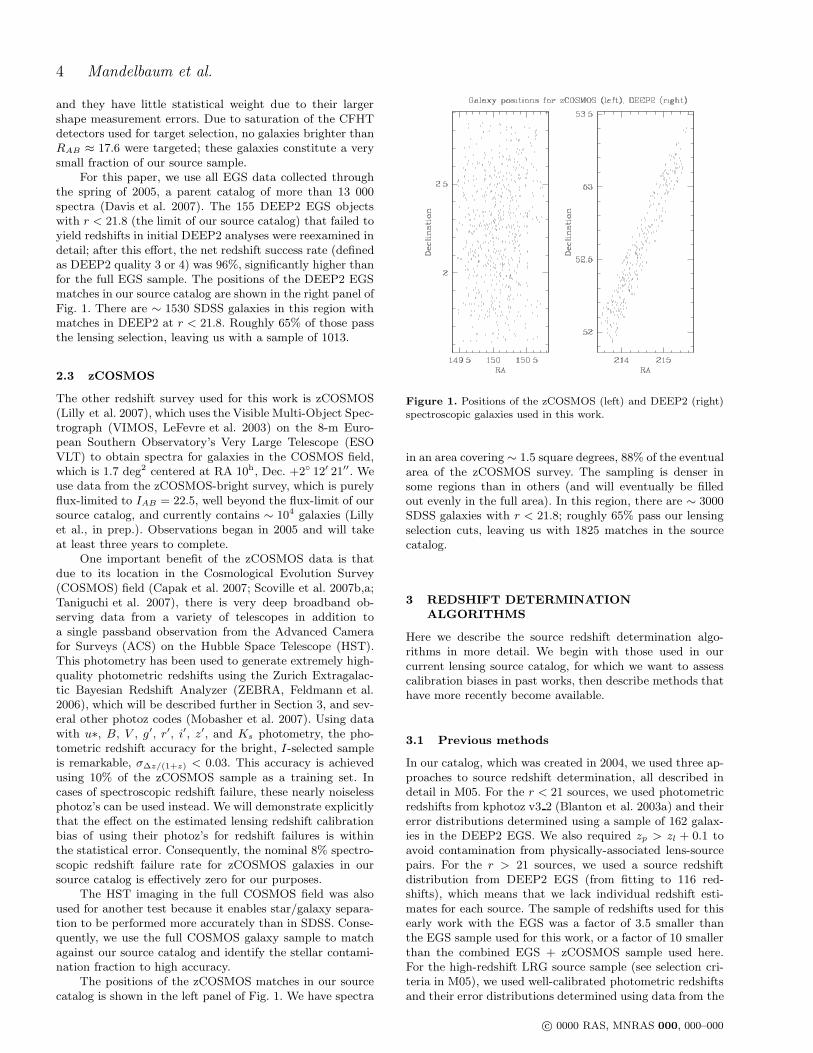
For this paper, we use all EGS data collected throughthe spring of 2005, a parent catalog of more than 13 000spectra (Davis et al. 2007). The 155 DEEP2 EGS objectswith r < 21.8 (the limit of our source catalog) that failed toyield redshifts in initial DEEP2 analyses were reexamined indetail; after this effort, the net redshift success rate (definedas DEEP2 quality 3 or 4) was 96%, significantly higher thanfor the full EGS sample. The positions of the DEEP2 EGSmatches in our source catalog are shown in the right panel ofFig. 1. There are ∼ 1530 SDSS galaxies in this region withmatches in DEEP2 at r < 21.8. Roughly 65% of those passthe lensing selection, leaving us with a sample of 1013.

2.3 zCOSMOS

The other redshift survey used for this work is zCOSMOS(Lilly et al. 2007), which uses the Visible Multi-Object Spec-trograph (VIMOS, LeFevre et al. 2003) on the 8-m Euro-pean Southern Observatory’s Very Large Telescope (ESOVLT) to obtain spectra for galaxies in the COSMOS field,which is 1.7 deg2 centered at RA 10h, Dec. +2 12′ 21′′. Weuse data from the zCOSMOS-bright survey, which is purelyflux-limited to IAB = 22.5, well beyond the flux-limit of oursource catalog, and currently contains ∼ 104 galaxies (Lillyet al., in prep.). Observations began in 2005 and will takeat least three years to complete.

One important benefit of the zCOSMOS data is thatdue to its location in the Cosmological Evolution Survey(COSMOS) field (Capak et al. 2007; Scoville et al. 2007b,a;Taniguchi et al. 2007), there is very deep broadband ob-serving data from a variety of telescopes in addition toa single passband observation from the Advanced Camerafor Surveys (ACS) on the Hubble Space Telescope (HST).This photometry has been used to generate extremely high-quality photometric redshifts using the Zurich Extragalac-tic Bayesian Redshift Analyzer (ZEBRA, Feldmann et al.2006), which will be described further in Section 3, and sev-eral other photoz codes (Mobasher et al. 2007). Using datawith u∗, B, V , g′, r′, i′, z′, and Ks photometry, the pho-tometric redshift accuracy for the bright, I-selected sampleis remarkable, σ∆z/(1+z) < 0.03. This accuracy is achievedusing 10% of the zCOSMOS sample as a training set. Incases of spectroscopic redshift failure, these nearly noiselessphotoz’s can be used instead. We will demonstrate explicitlythat the effect on the estimated lensing redshift calibrationbias of using their photoz’s for redshift failures is withinthe statistical error. Consequently, the nominal 8% spectro-scopic redshift failure rate for zCOSMOS galaxies in oursource catalog is effectively zero for our purposes.

The HST imaging in the full COSMOS field was alsoused for another test because it enables star/galaxy separa-tion to be performed more accurately than in SDSS. Conse-quently, we use the full COSMOS galaxy sample to matchagainst our source catalog and identify the stellar contami-nation fraction to high accuracy.

The positions of the zCOSMOS matches in our sourcecatalog is shown in the left panel of Fig. 1. We have spectra

Figure 1. Positions of the zCOSMOS (left) and DEEP2 (right)spectroscopic galaxies used in this work.

in an area covering ∼ 1.5 square degrees, 88% of the eventualarea of the zCOSMOS survey. The sampling is denser insome regions than in others (and will eventually be filledout evenly in the full area). In this region, there are ∼ 3000SDSS galaxies with r < 21.8; roughly 65% pass our lensingselection cuts, leaving us with 1825 matches in the sourcecatalog.

3 REDSHIFT DETERMINATIONALGORITHMS

Here we describe the source redshift determination algo-rithms in more detail. We begin with those used in ourcurrent lensing source catalog, for which we want to assesscalibration biases in past works, then describe methods thathave more recently become available.

3.1 Previous methods

In our catalog, which was created in 2004, we used three ap-proaches to source redshift determination, all described indetail in M05. For the r < 21 sources, we used photometricredshifts from kphotoz v3 2 (Blanton et al. 2003a) and theirerror distributions determined using a sample of 162 galax-ies in the DEEP2 EGS. We also required zp > zl + 0.1 toavoid contamination from physically-associated lens-sourcepairs. For the r > 21 sources, we used a source redshiftdistribution from DEEP2 EGS (from fitting to 116 red-shifts), which means that we lack individual redshift esti-mates for each source. The sample of redshifts used for thisearly work with the EGS was a factor of 3.5 smaller thanthe EGS sample used for this work, or a factor of 10 smallerthan the combined EGS + zCOSMOS sample used here.For the high-redshift LRG source sample (see selection cri-teria in M05), we used well-calibrated photometric redshiftsand their error distributions determined using data from the

c© 0000 RAS, MNRAS 000, 000–000


2dF-SDSS LRG and Quasar Survey (2SLAQ), as presentedin Padmanabhan et al. (2005).

3.2 New options

There are several relatively new photoz options for SDSSdata, all of which have relatively low failure rates of ∼ 5%.The first is available in the SDSS DR5 (data release 5) sky-server “Photoz” table (Budavari et al. 2000; Csabai et al.2003). The photoz’s for this template method are deter-mined by fitting observed galaxy colours to empirical tem-plates from Coleman et al. (1980) extended using spectralsynthesis models. There is an additional step (not used forall template methods) in which the templates are iterativelyadjusted using a training sample. We have performed ourtests on both the DR5 and DR6 template photoz’s, andfound no significant differences in performance between thetwo.

The second new option is available in the SDSS DR6skyserver in the “Photoz2” table. These photoz’s were com-puted using a neural net (NN) algorithm similar to that ofCollister & Lahav (2004) trained using a training set frommany data sources combined: SDSS spectroscopic samples,2SLAQ, CFRS, CNOC2, DEEP, DEEP2, and GOODS-N.A more complete description of both NN photoz’s in theDR6 database can be found in Oyaizu et al. (2007): the“CC2” photoz’s use colours and concentrations, while the“D1” photoz’s use magnitudes and concentrations. In thetext, we will describe any difference between the DR5 andDR6 results; Oyaizu et al. (2007) recommends against us-ing the DR5 photoz’s for science applications now that theimproved DR6 versions exist.

The third new option we test is the ZEBRA(Feldmann et al. 2006) algorithm, which has already beensuccessfully used with much deeper imaging data in theCOSMOS field. This method involves template-fitting, butalso takes a flux-limited sample of galaxies (without spec-troscopic redshifts) from the data source for which we wantphotoz’s. These data are used to create a Bayesian modifica-tion of the likelihoods based on the N(z) for the full sample(Brodwin et al. 2006) and on its template distribution. Inpractice, this prior helps avoid scatter to low redshifts. Akey question we will address is how this algorithm behaveswith the significantly noisier SDSS photometry. To avoidconfusion, we will refer to the high-quality ZEBRA photoz’sderived using the deep photometry in the COSMOS fieldas “ZEBRA” photoz’s, and the ZEBRA photoz’s using themuch shallower SDSS photometry as “ZEBRA/SDSS” pho-toz’s.

To be specific about the training method, to get the ZE-BRA/SDSS photoz’s, half of a flux-limited sample of SDSSgalaxies with zCOSMOS redshifts are used for template op-timization. This part of the analysis includes fixing the red-shifts of those galaxies to the spectroscopic redshift, findingthe best-fitting template, and optimizing it as described inFeldmann et al. (2006). Then, a sample of 105 SDSS galax-ies (flux-limited to r = 22) without spectra were used toiteratively compute the template-redshift prior.

3.3 Effects of photoz error for lensing

Finally, we clarify the effects of photoz error on the lensingcalibration:

• A positive photoz bias, defined as a nonzero 〈zp − z〉,will lower the signal (because the critical surface density,defined below in Eq. 2, will be underestimated).

• A negative photoz bias will raise the signal.• Photoz scatter will usually lower the signal due to the

shape of the critical surface density near zl. This effect canbe very significant for sources at redshifts below ∼ zl +1.5σ,where σ is the size of the scatter.

The last point is very important for a shallow surveylike SDSS when the lens redshift is above zl ∼ 0.1, becauseof the large number of sources within a few σ of the lensredshift. For a deeper survey such as the Canada-France-Hawaii Telescope Legacy Survey (CFHTLS), with lenses andsources separated by ∆z ∼ 0.5 on average this effect may infact be negligible. The effects of photoz bias are importantnot just in the mean, but as a function of redshift. If lowredshift sources have nonzero photoz bias, and high redshiftsources have nonzero photoz bias in the opposite direction,so that the mean photoz bias for the full sample is zero, theeffect of the opposing photoz biases on lensing calibrationwill not, in general, cancel out since the effect on lensingcalibration tends to be more significant for the sources thatare closer to the lenses.

Catastrophic photoz errors are those that are well be-yond the typical scatter, typically occurring due to somesystematic error, colour-redshift degeneracy, or other prob-lem (and by definition, these photoz’s are not flagged asproblematic by the algorithm, so they can only be identifiedusing a spectroscopic sample with similar selection to thetarget sample). The catastrophic error rate may be impor-tant, depending on the type of catastrophic error. For exam-ple, sending a few percent of the sources to zp = 0 will notlead to calibration bias, it will simply lead to that fractionof the sources not being included because they have zp < zl,causing a percent-level increase in the final error. In short,it is clear that the three metrics often used to quantify theaccuracy of photoz methods – the mean bias, scatter, andcatastrophic failure rate – are not sufficient to quantify theefficacy of a photoz method for lensing. In this paper, we willintroduce a metric that is optimized towards understandingthe effects of photoz’s on galaxy-galaxy lensing calibration,and present results for the photoz mean bias, scatter, andcatastrophic failure rate only as a means of understandingthe results for our lensing-optimized metric. For other sci-ence applications, the optimal metric may be quite differentfrom what we present here.

4 METHODOLOGY

4.1 Theory

Galaxy-galaxy lensing measures the tangential shear distor-tions in the shapes of background galaxies induced by themass distribution around foreground galaxies (for a review,see Bartelmann & Schneider 2001). The result is a measure-ment of the shear-galaxy cross-correlation as a function ofrelative foreground-background separation on the sky. We

c© 0000 RAS, MNRAS 000, 000–000

6 Mandelbaum et al.

will assume that the redshift of the foreground galaxy isknown, so we express the relative separation in terms oftransverse comoving scale R. One can relate the shear distor-tion γt to ∆Σ(R) = Σ(< R)−Σ(R), where Σ(R) is the sur-face mass density at the transverse separation R and Σ(< R)its mean within R, via

γt =∆Σ(R)

Σc. (1)

Here we use the critical mass surface density,

Σc =c2

4πG

DS

(1 + zL)2DLDLS, (2)

where DL and DS are angular diameter distances to the lensand source, DLS is the angular diameter distance betweenthe lens and source, and the factor of (1 + zL)−2 arises dueto our use of comoving coordinates. For a given lens redshift,Σ−1

c rises from zero at zs = zL to an asymptotic value atzs ≫ zL; that asymptotic value is an increasing function oflens redshift.

In this work, we focus on calibration bias in ∆Σ due tobias in Σc arising from source redshift uncertainty.

4.2 Redshift calibration bias determination

Here, we present a method for testing the accuracy of sourceredshift determination that is optimized towards g-g lensing.Formally, we wish to calculate the differential surface density∆Σ using our estimator g∆Σ, which is defined as a weightedsum over lens-source pairs j,

g∆Σ =

P

j wj γ(j)t Σc,j

P

j wj. (3)

To isolate the dependence of calibration on redshift-relatedquantities, we will assume that the estimated tangentialshear, γt, is unbiased. Σc,j (derived from our source red-shift estimator) is the critical surface density estimated fora given lens-source pair j. The weights for each lens-sourcepair are determined using redshift information as well:

wj =1

Σ2c,j(e

2rms + σ2

e)(4)

where erms is the rms ellipticity per component for the sourcesample (shape noise), and σe is the ellipticity measurementerror per component.

We want to relate our estimated g∆Σ to the true ∆Σ. Todo so, we use the relation between the measured shear and∆Σ, Eq. (1). Putting equation 1 into equation 3 (assuming〈γ〉 = γ), we define the redshift calibration bias bz via

bz + 1 =g∆Σ

∆Σ=

P

j wj

“

Σ−1c,j Σc,j

”

P

j wj, (5)

a weighted sum of the ratio of the estimated to the truecritical surface density.

This expression must be computed as a function of lensredshift. In the limit that the sources are at much higherredshift than the lenses, Σc does not depend as strongly onthe source redshift, so (for a given photometric redshift bias)|bz| will be smaller than if the lens redshift is just below thesource redshift. For a lens sample with redshift distribution

p(zl), the average calibration bias 〈bz〉 can be computed asa weighted average over the redshift distribution,

〈bz〉 =

R

dzl p(zl) wl(zl) bz(zl)R

dzl p(zl) wl(zl)(6)

where the redshift-dependent lens weight wl(zl) is definedas the total weight derived from all sources that contributeto the lensing signal for a given lens redshift,

P

j wj .In the ideal case, we would do this calculation with a

large, complete spectroscopic sample drawn at random fromour source sample, sparsely sampled on the sky and thereforelacking features in the redshift distribution due to large-scalestructure. We can then find bz(zl) on a grid of lens redshiftsby forming the sums in equation 5 using all sources withspectra. Finally, we can use the total weight as a function oflens redshift and the lens redshift distribution to estimatethe average redshift bias of the lensing signal.

To get the errors on the bias in this simple scenario, wecan simply bootstrap resample our sample of source galaxieswith spectroscopy. For a sample of Ngal galaxies, bootstrapresampling requires us to make many “new” galaxy samplesconsisting of Ngal galaxies drawn from the original samplewith replacement. Assuming that the observed galaxy red-shifts accurately reflect the underlying redshift distribution,and the redshifts are uncorrelated, the mean best-fit red-shift distribution will reflect the true one, and the errorsin the redshift calibration bias can be determined from thevariance of the calibration biases for each bootstrap resam-pled dataset. Since the bootstrap depends on the assumptionthat the objects we are bootstrapping are independent, thismethod only gives proper errors in the case where LSS isunimportant.

In general, there are several problems that mean weare no longer dealing with the ideal case. The first problemis sampling variance, since most redshift surveys are com-pleted in a well-defined, small region of the sky. The secondis the fact that most redshift surveys suffer from some in-completeness, and that incompleteness may be a function ofapparent magnitude or colour, which means that the loss ofthose redshifts can make the spectroscopic sample no longercomparable to the full source sample. We attempt to amelio-rate these problems by using two sources of spectroscopy ondifferent areas of the sky and with different spectrographsand analysis pipelines, so that the LSS and incompletenesstendencies in each sample are different. Below, we addressthese deviations from the ideal case in more detail.

4.3 Effects of sampling variance

Large-scale structure can be problematic when using surveyson small regions of the sky to determine bias in the lensingsignal due to photometric redshift error. The LSS may em-phasize particular regions of the source redshift distributionthat have unusual features in the photometric redshift er-rors. To avoid this problem, we would like to fit for a redshiftdistribution in a way that accounts properly for uncertain-ties due to sampling variance. There are many approachesto this problem in the literature, such as that demonstratedin Brodwin et al. (2006).

The simplest way around our aforementioned problem,that LSS causes the redshifts to be correlated so that the as-sumption behind the bootstrap is violated, is to bootstrap

c© 0000 RAS, MNRAS 000, 000–000


the bins in the redshift histogram instead. In the limit thatthe bins are significantly wider than the typical sample cor-relation length, the correlations within the bins will be farmore important than the correlations between adjacent bins.Thus, the requirement that the bootstrapped data points beindependent is much closer to being fulfilled. Here, we willuse redshift bins with size ∆z = 0.05, where each bin isconsidered as a pair of points (zi, N(zi)). In a given boot-strapped histogram, some redshift bins (zi, N(zi)) will beincluded multiple times, others not at all, but each time agiven bin is used, it has the same number of galaxies as inthe real data. While this method is simplistic, it has the ad-vantage of not requiring us to understand the details of thesample selection, since the lensing selection is a very non-trivial cut to understand and simulate. The resulting errorson the best-fit N(z) from this bootstrap will include theeffects of both Poisson error (which is non-negligible giventhe size of the samples used) and large-scale structure. Theerrors are valid assuming that there are no correlations be-tween the 150h−1Mpc-wide bins. We discuss this assump-tion, which depends not just on straightforward integrationof the matter power spectrum but also redshift-space dis-tortions, galaxy bias, and magnification bias, further in sec-tion 5.7.

For each bootstrapped histogram with bins centered atzi containing Ni galaxies each, we minimize the function

∆2 =X

i

w(∆)i [Ni − N

(model)i ]2. (7)

via summation over redshift bins i. N(model)i is the number of

galaxies predicted to lie in bin i given the model for dN/dz,i.e.

N(model)i =

Z zi+∆z/2

zi−∆z/2

dN

dzdz. (8)

For each bootstrapped histogram, we also imposed a nor-malization condition on the fit that

R

∞

0dz(dN (model)/dz) =

Ngal (the total number of galaxies in the spectroscopicsample). In the case of Poisson error, the natural choice

for w(∆)i is 1/N

(model)i . However, in the presence of LSS,

which contributes significantly to the variance in each bin,the distribution of values in each bin is, in fact, unknown,so the optimal weighting scheme is unclear. Consequently,we use the simplest possible weighting scheme, w

(∆)i = 1

for all i. We have, however, confirmed that if we do usew

(∆)i = 1/N

(model)i , then the changes in the best-fit redshift

distribution parameters, and the implied changes in redshiftcalibration bias, are well below the 1σ level.

Our 2-parameter model for the redshift distribution is

dN

dz∝

„

z

z∗

«α−1

expˆ

−0.5(z/z∗)2˜

(9)

which has mean redshift

〈z〉 =

√2 z∗Γ [(α + 1)/2]

Γ (α/2). (10)

This choice is based purely on the empirical observation thatit describes the shape of the redshift distribution better thanthe many other functional forms that we tried, and additionof extra parameters did not significantly improve the best-fit∆2. In particular, allowing the power-law inside the expo-nent to vary from 2 (a common choice) did not lead to any

significant change to the best-fit redshift distribution belowz = 0.8, where the vast majority of the galaxies are located.The changes above that redshift are marginally statisticallysignificant, but there are so few sources above that redshiftthat our final results for the redshift bias that we eventuallywant to calculate do not change within the statistical error.

We will present best-fit redshift distributions for zCOS-MOS and DEEP2 EGS separately to demonstrate that theresults are consistent within the errors. We then use bothsamples combined to create an overall redshift distribution.

This distribution is crucial to our scheme to avoid sam-pling variance effects in the determination of the redshiftcalibration bias. To counterbalance regions of source red-shift space that are over- or under-represented in our spec-troscopic sample due to LSS fluctuations, we incorporate anadditional weight into the calculation of the redshift bias inEq. (5). For a galaxy in redshift bin i in our histogram, theLSS weight (wLSS) is the ratio of the number of galaxies pre-dicted to lie in bin i from our best-fit redshift distribution, tothe number actually found in that bin (N

(model)i /Ni). Thus,

those regions in redshift space with too many/few galaxiesdue to LSS or Poisson fluctuations will be down/up-weightedappropriately. We can then get errors on the average red-shift bias 〈bz〉 using the best-fit redshift histograms for eachbootstrap resampled histogram to derive the LSS weights.This procedure incorporates uncertainty in the source red-shift distribution appropriately, since we never need to boot-strap the galaxies themselves.

In an analysis containing many patches of sky, the sizeof the errors can be verified by comparing the redshift biascomputed in each patch of sky. Unfortunately, with only twopatches of sky, this method is not an option for this work.

4.4 Redshift incompleteness and failures

For precision results, we require a high redshift completenessand quality. There are several tests that we can carry out toensure that the sample is of high quality. We consider theredshift failures separately for the DEEP2 and zCOSMOSsamples. In both cases, we will determine the magnitude andcolour distribution of the failures relative to the full sample,to see if a particular region of redshift space is causing theproblems.

For zCOSMOS, there are high-quality photoz’s derivedfrom very deep photometry which we can use in the caseof spectroscopic redshift failure. To control for any effect onthe computed redshift calibration bias, we also check theresults using the zCOSMOS photoz’s for a larger portion ofthe full sample, to ensure that noise in these photoz’s has anegligible effect on the results.

For DEEP2 EGS, we lack redshift estimates for the fail-ures. To place a very conservative bound on the effect offailures on the estimated calibration bias, we estimate theredshift bias with all the failures forced to z = 0, and thento z = 1.5. For both surveys, we will compare the ranges ofcolours and redshifts spanned by the successes and failures,to ensure that our procedures for handling redshift failureare justified.

The next issue is the quality of the non-failed redshifts,which in DEEP2 are assessed by visual inspection and repeatobservations, and in zCOSMOS using the photoz’s as well.For DEEP2, we have used only Q = 3 and Q = 4 redshifts,

c© 0000 RAS, MNRAS 000, 000–000

8 Mandelbaum et al.

which are 96% of our sample, and are estimated to be 95%and 99.5% reliable. For zCOSMOS, the reliabilities for Q =3 and 4 objects (92% of our sample) are > 99%. For thissurvey we also use Q = 2.5, those with slightly lower qualityin principle but with extremely good matches between thespectroscopic and photometric redshift, and Q = 9.5 (single-line redshifts with good matches between the spectroscopicand photometric redshifts, which in this apparent magnitudeand redshift range are usually from Hα), both of which alsoare > 99% reliable as determined from repeat observations.

In the DEEP2 EGS, there are also minor selection ef-fects to control for. The first effect is the fact that no galaxiesbrighter than r ∼ 18.5 were targeted. Galaxies brighter thanthat limit constitute only 4% of the source sample, but wenonetheless include tests of the effect this has on the result.

The other selection effect in DEEP2 EGS occurs atmagnitudes fainter than R = 21.5, where z < 0.75 ob-jects are given slightly lower selection weights than higher-zgalaxies. While the fraction of source galaxies fainter thanthis magnitude is only ∼ 12%, we use their selection prob-abilities psel to properly compensate for this effect. To beexplicit, the total weight for each source is thus a product oflensing weight wj , the LSS weight wLSS, and max(psel)/psel,j

(or 1 for the zCOSMOS galaxies).Finally, we clarify our statement that our method re-

quires the spectroscopic sample used to evaluate photoz’sto be comparable to the source sample. As demonstratedabove, it is possible to use weights to account for well-definedtargeting priorities that might make the spectroscopic sam-ple slightly non-representative of the source catalog. Thus,our statement that we require the spectroscopic sample tobe comparable to the source sample is really a statementthat it must contain all galaxy types (spectral types, magni-tudes, etc.) in the source sample with representation levelsthat are sufficient to overcome the noise. If some reweight-ing is necessary to account for under- or over-representationof a given population, then for our purposes, this is suffi-cient to fulfill our requirements. Thus, one could not usea spectroscopic sample with a strict cutoff two magnitudesbrighter than the flux limit of the source catalog. One coulduse a spectroscopic sample that has a lower redshift successrate for fainter galaxies, as long as that lower success rateis due to statistical error, so that the failures have the sameredshift distribution as the successes, rather than some sys-tematic error (e.g. inability to determine redshifts for anyobject of a particular spectral type above some cutoff red-shift). Reweighting schemes to account for different fractionsof various galaxy populations in the training and photomet-ric samples are being successfull used by the SDSS neuralnet photoz group to predict redshift distributions and pho-toz error distributions in the photometric samples.1

4.5 Direct use of photoz’s

Here, we explain our use of photoz’s directly for Σc estima-tion. One might argue that since we have a spectroscopicsample, we should estimate Σc using a deconvolved photozerror distribution. However, in this paper we test the use ofphotoz’s directly, for several reasons.

1 Lima, Cunha, Oyaizu, Lin, Frieman, 2007, in prep.

First, as we have argued previously, a key advantage ofusing photoz’s is that we can eliminate intrinsically-alignedsources. Once we start eliminating sources from the sampleon the basis of detailed cuts on photoz, colour, or apparentmagnitude, we would have to re-estimate the photoz errordistribution for the sample that passes these cuts and redothe deconvolution procedure. This is computationally expen-sive and potentially difficult to do robustly, if the cuts resultin our photoz error distribution being poorly-determineddue to insufficient spectroscopic galaxies that pass the cutsto properly sample the distribution. We would therefore liketo find a photoz method that can lead to accurate lensingcalibration on its own.

There is, in principle, one simple option that might im-prove the lensing calibration and that can be done withoutfull deconvolution: we can correct each photoz for the meanphotoz bias. To be accurate, this should be done as a func-tion of galaxy colour and magnitude. We will test the resultsof doing so for one of the photoz methods when we presentthe results of our analysis.

The final reason to use photoz’s directly is because thatis the approach taken in many lensing papers to date, andwe would like to test the accuracy of what is currently donein the field to see what improvements need to be made.In section 5.9, we will consider using a full p(z) as a newalternative approach to using the photoz alone.

5 RESULTS: APPLICATION TO SDSSLENSING

5.1 Matching results

There are 1013 and 1825 galaxies in our source catalogwith spectra from DEEP2 EGS and zCOSMOS, respec-tively (including redshift failures). We now characterizethese matches relative to the entire source catalog and com-pared to each other.

Figure 2 shows the redshift histograms for matches be-tween the source catalog and the zCOSMOS and DEEP2samples. The zCOSMOS histogram is shown both with andwithout precision photometric redshifts for the redshift fail-ures, whereas for DEEP2, the failures (4%) were excludedentirely. As shown, there is significant large-scale structurein the redshift histograms, but not correlated between thetwo samples. Visually, the redshift histogram for DEEP2 ap-pears to be at slightly higher redshift on average. We assessthe statistical significance of any differences below.

Figure 3 shows the distribution of apparent r-band mag-nitude p(r) for the zCOSMOS and DEEP2 matches relativeto that of the entire source catalog, pref(r). The apparentmagnitude histogram for zCOSMOS is quite similar to thatfor the full source catalog (within the noise), and the failuresare predominantly at the faint end. The apparent magnitudehistogram for DEEP2 shows the deficit at r < 18.5 (4% ofthe sample) due to targeting constraints.

Of the matches, 151 of those in zCOSMOS (8%) and 38of those in DEEP2 (4%) are redshift failures (where failuresare defined as having redshift success rates below 99%). InFig. 4, we show the distributions of various quantities forthe zCOSMOS and DEEP2 failures as compared with thefull sample. Fig. 3 shows the relation of the failures to the

c© 0000 RAS, MNRAS 000, 000–000


Figure 2. Redshift histogram for the matches between the sourcecatalog and the spectroscopic samples.

Figure 3. Bottom: r-band apparent magnitude histogram for thefull source catalog. Top: Difference between the apparent magni-tude histogram for the zCOSMOS and DEEP2 samples relativeto that for the full source catalog.

general sample as a function of apparent magnitude; the toppart of Fig. 4 shows that the colour distribution for the fail-ures is similar to the colour distribution for the successes.We thus have no reason to believe the failures lie in a partic-ular region of redshift space. The DEEP2 failures lie in the0 < z < 0.75 colour locus, just like the majority of the suc-cesses in this bright subsample of the EGS data. (This is nottrue for deeper redshift samples, such as the other DEEP2fields, where failures typically occur for blue, z > 1.5 galax-ies. The flux and apparent size cuts imposed on our sam-ple essentially remove any such galaxies.) Inspection of the38 DEEP2 spectra suggests that the redshift distribution is

Figure 4. Colour-magnitude scatter plots for redshift successesand failures in zCOSMOS (top) and DEEP2 (middle). Successesare shown as black points and failures as blue hexagons. Thebottom panel shows the zCOSMOS photoz error as a function ofredshift for the redshift successes, including the 68% CL errors as

a function of redshift (red lines).

similar to that for the successes, with failures due to badastrometry, a bad column running through the spectrum, orsimilar failures that do not correlate with redshift. We alsoshow the zCOSMOS photoz error distribution as a functionof redshift in the bottom of Fig. 4 for spectroscopic redshiftsuccesses. The photoz errors for this sample are indeed assmall as, or even smaller than, those presented elsewhere forthese photoz’s (Feldmann et al. 2006). We may view this er-ror as a “systematic floor” to the error, with the increase inerror for the ZEBRA/SDSS photoz’s being ascribed to themuch noisier photometry. We will see that this statisticalerror dominates the error budget.

Next, we present redshift distributions for each surveyseparately, with two purposes: (1) to demonstrate that theyare consistent with being drawn from the same underlyingredshift distribution, and (2) to determine the weights tocompensate for sampling variance as described in section 4.3.

Fig. 5 shows the observed and best-fit redshift his-tograms for zCOSMOS, DEEP2, and both surveys com-bined. Table 1 shows the corresponding best-fit parametersfrom Eq. (9). The weighting to account for the DEEP2 se-lection at R > 21.5 causes a negligible change in the results.By bootstrapping the redshift histogram as described in sec-tion 4.3, we have determined the median predicted numberof galaxies in each bins, and the 68% confidence limits onthat number, as shown on the plot. Because we have imposeda normalization condition on the fit, the errorbars are cor-related between various parts of the histogram. We can seefrom the plot and table 1 that while the DEEP2 sample is atslightly higher redshift on average, the redshift distributionsfrom zCOSMOS and DEEP2 are consistent with each otherwithin the (Poisson plus LSS) errors. While it is difficult tocompare the curves for z > 0.7, where the number of galax-ies has declined sharply, we can compare the total fraction

c© 0000 RAS, MNRAS 000, 000–000

10 Mandelbaum et al.

Table 1. Parameters of fits to redshift distribution from Eq. 9.

Sample z∗ α 〈z〉

zCOSMOS 0.259 ± 0.040 2.58 ± 0.58 0.369 ± 0.018DEEP2 EGS 0.300 ± 0.041 2.35 ± 0.41 0.408 ± 0.025

Both 0.275 ± 0.025 2.42 ± 0.36 0.382 ± 0.012

of the sample with z > 0.7 to show that they are consis-tent: for DEEP2 EGS, this fraction lies between [0.05, 0.12]at the 68% CL; for zCOSMOS, between [0.02, 0.08]. Theselimits were determined using the fraction above z > 0.7for the best-fit N(z) for 200 bootstrap-resampled redshifthistograms, and therefore include both Poisson error andsampling variance. It is clear that any discrepancy betweenthe best-fit zCOSMOS and DEEP2 redshift histograms withrespect to the fraction of the sample above z > 0.7 are notsignificant at the 68% CL.

As shown in the lower left panel of Fig. 5, there is no sys-tematic tendency for the observed and best-fit Ni(z) for thefull sample to deviate from each other, only Poisson and LSSfluctuations, so the form we have chosen for dN/dz is accept-able. (The fluctuations are quite large for z > 1 because the

best-fit N(model)i drops below 1, so discreteness will cause the

ratio of Ni/N(model)i to be either zero or some large number.)

It is important to note that this plot is the unweighted red-shift distribution; inclusion of the lensing weights in Eq. (4)will change the effective source redshift distribution.

5.2 Photoz error distributions

As a way of understanding the trends in our lensing-optimized photoz error statistic bz, we first examine thephotoz error distribution as a function of redshift. Figure 6shows the photoz error as a function of the (true) redshift forthe lensing-selected galaxies from zCOSMOS and DEEP2for the photoz algorithms tested in this work. The galaxiesare divided by apparent magnitude into three samples withr < 20, 20 6 r < 21, and r > 21, and we show the 68% CLerrors determined in bins of size ∆z = 0.05 for each apparentmagnitude bin. For all methods, the error distributions tendto be highly non-Gaussian, often skewed and with significanttails. While the requirement that zp > 0 makes skewness in-evitable at low z even for a well-behaved photoz estimator,the effect persists to such high redshift for all methods thatthis constraint is clearly not the cause. Thus, the 68% confi-dence limits as a function of redshift are more useful than acalculation of the average photoz bias and scatter. Nonethe-less, we do tabulate the mean bias 〈zp − z〉 and the overallscatter σ(zp) in Table 2 for each method, for the full sam-ple and the r < 21 subset (to facilitate comparison betweenkphotoz, used only for r < 21, and the other methods).

For the kphotoz method, there is a clear tendency tofail towards very low redshift, as demonstrated by the peakin p(zp) for zp < 0.05. For lensing, such failures will beflagged as being below the lens redshift for nearly all relevantlens redshifts, thus excluding them from the source sample.Consequently, the only effect of this failure mode is to reducethe number of available sources, not to bias the weak lensingresults. However, it is apparent that this method is as noisyfor r < 21 as the other photoz algorithms are for r < 21.8,

Table 2. Mean properties of the photoz algorithms, for the full

sample and for r < 21 only in parenthesis.

Method Mean bias Scatter

kphotoz (−0.015) (0.14)Template −0.064 (−0.043) 0.16 (0.12)NN/CC2 0.034 (0.013) 0.14 (0.11)NN/D1 0.038 (0.020) 0.13 (0.10)

ZEBRA/SDSS −0.014 (0.012) 0.15 (0.12)

and that the photoz error tends to be positive for z . 0.4and negative above that.

For the template-based database photoz’s, there is aneven stronger failure mode towards zp = 0 than for kphotoz(because the template method goes fainter than the kphotozsample). This failure mode contributes to the significantlynegative 68% CL limits on the photoz error, since the pointssuggest that ignoring these failures leads to a more symmet-ric error distribution. We must quantify the effect this hasin reducing the total weight; even if the bias in the lensingsignal due to the strong failure mode is small, the increasedstatistical error due to loss of sources may be problematic.This failure mode is the cause of the large mean photoz biasin Table 2.

For the neural network algorithm, the plot shows theCC2 (colour- and concentration-based) photoz’s, but thetrends are qualitatively similar for the D1 (magnitude- andconcentration-based) photoz’s. There are entries for bothversions in Table 2. As shown, the method has a reasonablysmall overall scatter and no major failure modes. We cautionthe reader that the same is not true for the NN photoz’s inthe DR5 database, for which there is a significant scatter toredshifts 0.75 < zp < 1 that more than doubles the numberof sources estimated to be in this redshift range. The scat-ter is also larger for the DR5 NN photoz’s. In both the DR5and the DR6 versions, there is a tendency towards positivephotoz bias at low-intermediate redshifts (0 < z < 0.4) thatmay bias the lensing signal low.

Finally, the ZEBRA/SDSS method also lacks a majorcatastrophic failure mode and has reasonably small over-all photoz bias. The redshift histograms derived from thespectroscopic and photometric redshifts agree remarkablywell. As for the NN/CC2 photoz’s, there is a trend towardspositive photoz error at low redshift and negative error athigh redshift. Because of the overall lower number of sourcesabove z & 0.4, and the decreased dependence of Σc on sourceredshift at higher redshift, we have no reason to believe thatthe effects of the different direction of the calibration biasesin the lensing signal will cancel out. We can also conclude,in comparison with the ZEBRA photoz errors in the lowerpanel of Fig. 4 (using the far deeper COSMOS photome-try) for the same exact set of sources, that for the redshiftsand magnitudes dominated by this source sample, statis-tical error due to noisy SDSS photometry dominates oversystematic error in this photoz method.

5.3 Redshift bias

In Figure 7, we show the lensing calibration bias bz(zl) fordifferent source redshift determination methods, using thefull lensing-selected spectroscopic redshift sample. The bot-

c© 0000 RAS, MNRAS 000, 000–000


Figure 5. Top: Rescaled redshift histograms for the matches between the source catalog and the zCOSMOS (left) and DEEP2 (right)sample with best-fit histograms. The black histogram is the observed data, the smooth red curve is the best-fit histogram, the dashedmagenta lines are the ±1σ errors, and the dotted blue line is the best-fit redshift histogram for the other survey. Bottom right: Same asabove, for combined sample, with the dotted blue lines showing the results for each survey separately. Bottom left: ratio of observed tobest-fit N(z) for the combined sample.

tom panel shows the total lensing weight ascribed to thesource sample for that lens redshift, determined via summa-tion over the lensing weights described in Section 4.4. Notethat the r < 21 and LRG samples use photoz’s with therequirement that zp > zl + 0.1, to reduce contamination byphysically-associated sources (for consistency with our pre-vious analyses). However, for the new photoz methods, wehave not imposed any such condition (we will revisit thischoice later).

As shown, the r < 21 sample with photoz’s from kpho-toz has a significant negative calibration bias that increaseswith lens redshift to −35% at zl = 0.35. As for all meth-ods, the bias worsens with lens redshift because, for a givensource with some photoz error, a higher lens redshift leadsto a higher relative error in Σ−1

c . The r > 21 sample (usingdN/dz from DEEP2 EGS) has a small positive bias that

increases to 10% at zl = 0.35. We assess the significance ofthese biases for our previous work in section 5.4. The resultsfor the LRG source sample confirm our assertion in previ-ous works that for zl < 0.3, this sample is essentially free ofredshift bias.

The lack of significant redshift calibration bias for thetemplate photoz code for zl < 0.25 can be explained bythe trends in Fig. 6: the calibration bias due to the slightnegative photoz bias balances out the calibration bias dueto photoz scatter. Even at higher redshift, the redshift cal-ibation bias, while nonzero, is less significant than for theother photoz methods. The neural net and ZEBRA/SDSSphotoz’s, however, have significant negative bias (−30% to−20%, at zl = 0.4), presumably because of the aforemen-tioned tendency to positive photoz bias for zs < 0.4. Thisdifference between the three methods is also the reason why

c© 0000 RAS, MNRAS 000, 000–000


Figure 6. For each photoz method described in the text (in columns labeled according to the method), the top row shows the redshifthistogram determined using the photoz (thin black line) and using the spectroscopic redshift (thick red line). The spectroscopic redshifthistograms are not quite identical for all methods because we exclude photoz failures for each method and because kphotoz was onlyused for those galaxies with r < 21. The lower three panels show photometric redshift errors, for galaxies divided by apparent magnitude:r < 20 in the second row, 20 6 r < 21 in the third row, and r > 21 in the fourth row. The points correspond to individual galaxies inthe source catalog with spectra; the 68% confidence limits on the photoz error are shown as red solid lines. There are also green dashedlines indicating zero error and the lower limit on the error given that the photoz must exceed zero.

the latter two methods have high total weight for the rangeof lens redshift considered here, whereas the template pho-toz code has lower weight (a) because of its scatter to lowphotoz (which eliminates possible sources from the sample)and (b) because it does not tend to scatter sources to higherphotoz, which increases the weight artifically at the expenseof biasing the signal. We emphasize that this higher weightfor the two photoz methods does not mean that the erroron ∆Σ is lower with these methods, because it may be duepurely to the overestimate of Σ−1

c . In section 5.8, we willaddress the effect of using photoz’s on the statistical errorin ∆Σ.

Given that kphotoz has a similarly sized photoz error

(r < 21 only) as the other photoz methods for the full sourcesample (all magnitudes), it is important to understand whythe lensing calibration bias is so much worse for this method.The reason this occurs is that the r < 21 sample is at lowermean redshift. Since those sources are closer on average tothe lens redshift, the same size photoz error translates to alarger error in Σc.

To understand the results, we consider fixed lens red-shift of zl = 0.2, and show the redshift bias as a function oftrue source redshift for each method in Fig. 8 (again, withlensing weight as a function of source redshift as in Sec-tion 4.4). Clearly, all source redshift bins with zs < 0.2 mustgive bz = −1, because the sources are not lensed. Above

c© 0000 RAS, MNRAS 000, 000–000


Figure 7. Redshift bias bz(zl) (top) and weight (bottom, arbi-trary units) for many methods of source redshift determinationas described in the text. To make the plot simpler to read, wehave left off errorbars except for in one case, the ZEBRA/SDSSmethod, which is shown with an errorbar in one direction to indi-

cate the typical size of the uncertainty in bz(zl) for all the meth-ods.

zs = zl = 0.2, the calibration bias is no longer identicallyzero, but may be significantly negative due to scatter inthe estimates of source redshift (near zs = zl, the deriva-tive dΣc/dzs is large so photoz errors are very important).As the source redshift increases, the same photoz error be-comes less important because that derivative decreases, sothe calibration bias approaches zero. The other importantquantity to consider is the weight in each source redshiftbin; if those source redshift bins with significant bias aregiven little weight, then the bias does not matter. If there isno weight for zs < 0.2 that means that none of the galax-ies with true zs < 0.2 have had photoz misestimated tobe above that. This plot makes it clear that part of thereason for the significant bias for the NN, kphotoz and ZE-BRA/SDSS photoz’s is that they give too much weight tozs . 0.3. This is less of a problem for the template photoz’s,so the calibration bias for this method is much less.

Finally, we show the resulting mean calibration biaswhen these results are averaged over a lens redshift dis-tribution using Eq. (6). Errors are determined using theprescription in section 4.3. The lens redshift distribu-tions that we consider are as follows: “sm1”–”sm7” arethe redshift distributions for the seven stellar mass binsfrom Mandelbaum et al. (2006c); “LRG” is the redshiftdistribution for the spectroscopic LRGs, a volume-limitedsample, used for lensing in Mandelbaum et al. (2006b);and “maxBCG” is the redshift distribution of the SDSSmaxBCG clusters (Koester et al. 2007b,a). These nine lensredshift distributions are plotted in figure 9. The stellar masssubsamples correspond roughly to luminosity samples withr-band luminosities of 0.33, 0.53, 0.72, 1.1, 1.8, 3.0, and4.7L∗. The LRGs are red galaxies with typical luminosities

Figure 8. Redshift bias bz(zs) (top) and weight (bottom, ar-bitrary units) for fixed zl = 0.2 with many methods of sourceredshift determination as described in the text. Errorbars are notshown here to make the plot simpler to read.

of a few L∗, and the maxBCG clusters are clusters selectedfrom imaging data with masses & 5 × 1013h−1M⊙.

The average redshift calibration biases 〈bz〉 (defined inEq. 6) for the redshift determination methods given in Fig. 7for these nine lens redshift distributions are shown in Ta-ble 3. As shown, for the stellar mass subsamples, the biasgets more significant at higher stellar mass because of thehigher mean redshift. The maxBCG sample gives similarbias to sm7 because of the similar redshift range, and theLRG sample gives the worst bias because it has the highestmean redshift. The only method for which the trend is dif-ferent is the template photoz code, for which the trend ofbz(zl) changes sign with redshift due to the different trendsof photoz error with redshift.

As shown, the NN/D1 photoz’s give nominally worsecalibration bias than the NN/CC2 photoz’s for lower-redshift lens samples, and the reverse is true at higher red-shift. This trend is consistent with the difference betweenthe two methods in Fig. 7. We also performed the analysiswith the DR5 NN photoz’s, and found the lensing calibrationbias for these lens redshift distributions to be similar to theNN/CC2 calibration biases, well within the 1σ errors. Thisresult suggests that the failure mode to 0.75 < zp < 1 in theDR5 version was not a significant source of lensing calibra-tion bias, and the overall positive photoz bias (present in allNN photoz’s tested in this paper) is the main cause.

Finally, we consider what happens if we correct for themean photoz bias when estimating Σc for each source. Forthe template photoz’s, this correction causes the mean cali-bration bias for sm7 to go from −0.014 to −0.14. This resultmay be puzzling until we consider the effects of photoz biasand scatter separately (section 3.3). We know that photozscatter causes a negative calibation bias, and a negative pho-toz error like this method has causes a positive calibrationbias. When we did not correct for the mean photoz bias,these two effects apparently cancelled out. This cancellation

c© 0000 RAS, MNRAS 000, 000–000


Table 3. Average redshift bias 〈bz〉 for nine lens redshift distributions described in the text.

r < 21 r > 21 LRG template NN/CC2 NN/D1 ZEBRA/SDSSsm1 −0.033 ± 0.008 0.005 ± 0.009 0.004 ± 0.003 0.020 ± 0.003 −0.039 ± 0.007 −0.051 ± 0.007 −0.018 ± 0.006sm2 −0.043 ± 0.009 0.008 ± 0.011 0.005 ± 0.004 0.020 ± 0.004 −0.048 ± 0.008 −0.059 ± 0.008 −0.022 ± 0.007sm3 −0.057 ± 0.011 0.013 ± 0.013 0.006 ± 0.005 0.021 ± 0.004 −0.059 ± 0.008 −0.070 ± 0.008 −0.029 ± 0.007sm4 −0.077 ± 0.012 0.020 ± 0.015 0.007 ± 0.006 0.020 ± 0.005 −0.075 ± 0.009 −0.084 ± 0.009 −0.038 ± 0.008sm5 −0.104 ± 0.014 0.029 ± 0.019 0.010 ± 0.008 0.015 ± 0.005 −0.096 ± 0.009 −0.102 ± 0.009 −0.053 ± 0.008sm6 −0.136 ± 0.016 0.041 ± 0.025 0.014 ± 0.011 0.003 ± 0.007 −0.124 ± 0.011 −0.123 ± 0.011 −0.074 ± 0.010sm7 −0.169 ± 0.018 0.055 ± 0.033 0.022 ± 0.016 −0.014 ± 0.009 −0.155 ± 0.015 −0.146 ± 0.015 −0.099 ± 0.012LRG −0.221 ± 0.022 0.069 ± 0.045 0.038 ± 0.022 −0.037 ± 0.014 −0.195 ± 0.021 −0.171 ± 0.021 −0.131 ± 0.018

maxBCG −0.171 ± 0.018 0.056 ± 0.034 0.023 ± 0.016 −0.015 ± 0.009 −0.158 ± 0.015 −0.147 ± 0.015 −0.101 ± 0.013

Figure 9. Lens redshift distributions for the lens samples de-scribed in the text.

is a non-trivial result that depends on our sample selection.With a different cut on apparent magnitude, for example,it is not clear that the effects would balance as precisely.Now that we have corrected for the effects of mean photozbias, we are left with the suppression of the lensing signaldue to the photoz scatter. For the NN/CC2 and NN/D1photoz’s, the correction for the mean photoz bias decreasescalibration bias from −0.16 and −0.15 to −0.10 and −0.07,respectively, for sm7 (since the positive photoz bias and thescatter change the lensing calibration in the same direction).For ZEBRA/SDSS, the photoz bias was slightly negative,so correcting for it worsens the lensing calibration bias asfor the template photoz’s, but only slightly: from −0.099 to−0.125 for sm7.

From these results, we can conclude that once the effectsof the mean photoz bias are removed, the effects on the lens-ing calibration due to scatter in the photoz’s are the smallestfor the SDSS NN/D1 photoz’s, followed by SDSS NN/CC2,ZEBRA/SDSS, and finally are the largest for the templatephotoz’s. This trend is consistent with the trends in Table 2for the photoz scatter. We therefore have two possible pro-cedures for handling calibration bias in the lensing signal:(1) to correct for the mean photoz bias before computingthe lensing signal, and apply a correction to the lensing sig-nal afterwards to account for residual calibration bias due

Table 4. Average redshift bias 〈bz〉 in previous works using thissource catalog when combining source samples.

Lens sample 〈bz〉sm1 −0.016 ± 0.008sm2 −0.020 ± 0.009sm3 −0.025 ± 0.011sm4 −0.032 ± 0.013sm5 −0.039 ± 0.016sm6 −0.045 ± 0.020sm7 −0.046 ± 0.026LRG +0.021 ± 0.038

to photoz scatter; or (2) to apply a correction to the lensingsignal due to the combined effects of photoz bias and scat-ter at once. In either case, we must depend on the fact thatour calibration subsample has the same sample propertiesas the full source catalog, so that corrections derived usingthis subsample will apply to the full catalog.

5.4 Implications for previous work

Here we determine the implications of Table 3 for previouswork with this lensing source catalog.

First, we consider the results for Mandelbaum et al.(2006c), in which we divided the sample into stellar massand luminosity subsamples with the seven redshift distribu-tions sm1–sm7 shown in Fig. 9. For that work, the signal pre-sented was an average over the signal using the r < 21 andr > 21 source sample with 1/σ2 weighting. To determine theaverage bias on this signal, we use our bootstrap-resampledbz(zl) and w(zl), averaging the bias as a function of redshiftfor each resampling using the weights for these two samples,then find the average over all the resampled datasets. Theaverage biases for sm1–sm7 are shown in Table 4.

We also consider the spectroscopic LRG lensredshift distribution, which was used for lensing inMandelbaum et al. (2006b) and Mandelbaum & Seljak(2007). In that case, we detected a ∼ 15% suppression ofthe lensing signal for the r < 21 source sample relativeto the r > 21 and LRG source samples. Table 3 makes itclear that this suppression was, in fact, real. To accountfor this suppression, we had multiplied the signal and itserror by a factor of 1.18. This is equivalent to multiplyingΣc by 1.18 when computing both the weights (∝ Σ−2

c ) andthe lensing signal. We thus incorporate this factor intothe computation of the bias in Eq. (5) before taking theweighted average with the r > 21 sample. The averagebias once the correction factor is incorporated is shown in

c© 0000 RAS, MNRAS 000, 000–000


Table 4. Because of this suppression of the weight in ther < 21 sample due to the calibration factor, and because ofits already low weight relative to r > 21 for zl > 0.22 (seeFig. 7), the uncertainty on the calibration bias is actuallydominated by the larger r > 21 sample uncertainty, whichis why it is larger than one might naively expect fromcombining the results in Table 3 for r < 21 and r > 21. It isclear that this way of combining the signal for r < 21 andr > 21 is non-optimal from the perspective of constrainingcalibration bias.

No results are shown for the maxBCG lensing samplebecause none of the previous works using this source cataloghave used it.

It is clear from this table that there was statisticallysignificant redshift calibration bias in previous works usingthis source catalog. However, the absolute value of the erroris below the statistical error on the lensing signal in thoseworks, and is smaller than the generous 8% (1σ) systematicerror that was used for those science results. We concludethat there is no cause for concern in using results in our pre-vious work with this catalog without applying a correction.

5.5 Systematics: targeting and redshift failure

In the previous sections, all quoted calibration errors werestatistical. Here, we consider the size of systematic errors.

First, we include the DEEP2 redshift failures in thesample, once putting them all at z = 0 and then all atz = 1.5 (with an LSS weight of 1). We have already shownin section 5.1 that the failures have a similar SDSS magni-tude and colour distribution to the remainder of the sample.This statement is also true in the DEEP2 BRI photometry,placing these galaxies without spectroscopic redshifts in the0 < z < 0.7 colour locus (like those with successful redshiftdetermination). Consequently, placing them all at z = 0 andz = 1.5 gives extremely conservative bounds on the system-atic error due to these redshift failures. Table 5 shows thenew 〈bz〉 and the change in 〈bz〉 compared to table 3 forall methods of source redshift determination, including thecombined r < 21 and r > 21 method used in our previouswork (Sec. 5.4), for four lens redshift distributions: sm1, sm4,sm7, and LRG, which are at progressively higher redshifts.

As shown in Table 5, these extreme assumptions changeour estimated calibration bias at the < 3σ level, in mostcases < 1σ. If we consider that the real effect is likely manyfactors smaller than this (since the failures roughly followthe magnitude and colour distribution of the successes, andtherefore likely the redshift distribution), this systematic isfar below our 1σ uncertainty on the calibration bias, fromwhich we can conclude that systematic effects due to theexcluded DEEP2 redshift failures are negligible.

We next consider the effects of using the zCOSMOSphotoz for their redshift failures. As shown in Fig. 4, the fail-ures have similar colours and magnitudes as the successes, sowe do not anticipate that they will have a significantly dif-ferent photoz error distribution from the successes shown atthe bottom of that figure. To test the effect of using ZEBRAphotoz’s for this 8% of the sample, we randomly replace thephotoz’s for the spectroscopic redshifts in another 8% of thesample that are redshift successes. We then compare theresulting calibration biases 〈bz〉 to the original ones. Theseresults (shown in Table 6) indicate that for all methods of

source redshift distribution determination and lens redshiftdistributions, the use of zCOSMOS photoz’s for the 8% ofthe zCOSMOS sample that lacks redshifts changes the re-sults well below the 1σ statistical error. We conclude thatsystematic error in our results due to redshift failures in ei-ther survey are unimportant, with the caveat that if the red-shift failures are a systematically different population thanthe successes, this test would not uncover any resulting sys-tematic error (however, we have no evidence that this is thecase).

One final systematic is that in DEEP2 EGS, roughly4% of our source catalog at bright magnitudes (r < 18.5)was not targeted. We must assess whether properly includ-ing these galaxies would significantly change the results.However, the small photoz error for bright objects, and thelow mean redshift, makes this unlikely. In the SDSS, onlya subset of these galaxies have spectroscopy, those withr . 17.7 (flux-limited) and fainter ones that are very red.Since including these SDSS spectroscopic redshifts will cre-ate a sample with strange selection (lacking blue galaxies at17.7 . r < 18.5), we instead take the spectroscopic galaxiesfrom zCOSMOS at r < 18.5, choose a random subset to ac-count for the smaller size of the DEEP2 sample, and add theresulting 42 galaxies to the DEEP2 sample. We then refit theredshift histogram for DEEP2, getting new redshift distri-bution parameters z∗ = 0.312 ± 0.048, α = 2.14 ± 0.39, and〈z〉 = 0.400 ± 0.025. We see that the change in mean sourceredshift is well within the errors in Table 1. When comput-ing the mean redshift bias using this augmented sample, wefind that the changes are even smaller than those shown inTable 5. This is not surprising, because in that table wehave taken redshift failures and put them at very extremeredshifts, whereas here we have added a comparable numberof redshifts but with very good photoz’s.

5.6 Agreement between the two surveys

As an additional systematics test, we compare the resultswhen doing the full analysis separately for each survey. Inthis case, we use LSS weights derived using the redshift his-tograms for each survey separately instead of using the com-bined histogram. In Table 7, we show the results for eachsurvey separately, with the bottom section showing the sta-tistical significance of the difference.

The results in this table show apparently significant dis-crepancies between the results with zCOSMOS and withDEEP2 separately. The fact that the statistical significanceof the difference is . 2σ for the last four columns, which usethe full catalog, but > 2σ for the first column (which usesr < 21 only) and . 1σ for the second column (which usesr > 21 only) suggests that we should focus on the r < 21sample to find the source of the discrepancy. We must under-stand this discrepancy in order to assess whether our resultsare biased or our errorbars are significantly underestimatedon the final, combined analysis.

In Fig. 10 we show plots for r < 21 that will shed lighton this discrepancy. The upper left plot shows p(z) for r < 21for both surveys. As shown, the best-fit histograms are verysimilar, but the LSS fluctuations are more pronounced thanfor the full sample. The lower left panel shows the ratio ofthe best-fit number predicted in zCOSMOS to the number inDEEP2 (normalized to the same total numbers of galaxies),

c© 0000 RAS, MNRAS 000, 000–000


Table 5. Change in redshift bias 〈bz〉 for all methods of source redshift determination (including combined methods for r < 21 andr > 21 as in previous work, Sec. 5.4) when putting all DEEP2 failures at z = 0 and z = 1.5 as shown. The number given is the resultingredshift bias, and the number in parenthesis is the fractional change in the bias from Table 3 relative to the statistical error.

r < 21 r > 21 LRG template NN/CC2 ZEBRA/SDSS Previous work

Fail to z = 0sm1 −0.036 (−0.38) −0.017 (−2.4) −0.002 (−2.0) 0.008 (−4.0) −0.062 (−1.9) −0.029 (−1.8) −0.028 (−1.5)sm4 −0.081 (−0.33) −0.003 (−1.5) 0.002 (−0.8) 0.007 (−2.6) −0.094 (−1.6) −0.050 (−1.5) −0.044 (−0.9)sm7 −0.173 (−0.22) 0.032 (−0.7) 0.017 (−0.3) −0.027 (−1.4) −0.166 (−1.0) −0.111 (−1.0) −0.060 (−0.5)LRG −0.224 (−0.14) 0.045 (−0.5) 0.033 (−0.2) −0.050 (−0.9) −0.218 (−0.8) −0.143 (−0.67) 0.005 (−0.4)

Fail to z = 1.5sm1 −0.032 (0.13) 0.009 (0.4) 0.004 (0.00) 0.022 (0.7) −0.046 (0.43) −0.015 (0.50) −0.013 (0.38)sm4 −0.075 (0.17) 0.027 (0.5) 0.008 (0.17) 0.024 (0.8) −0.075 (0.56) −0.034 (0.50) −0.026 (0.46)sm7 −0.166 (0.17) 0.074 (0.6) 0.024 (0.13) −0.005 (1.0) −0.140 (0.73) −0.089 (0.83) −0.033 (0.50)LRG −0.217 (0.18) 0.097 (0.6) 0.042 (0.18) −0.025 (0.9) −0.186 (0.71) −0.118 (0.72) 0.043 (0.58)

Table 6. Change in redshift bias 〈bz〉 for all methods of source redshift determination when replacing 8% of the redshifts for zCOSMOSsuccesses with their photoz’s. The number given is the resulting redshift bias, and the number in parenthesis is the fractional change inthe bias from Table 3 relative to the statistical error.


sm1 −0.033 (0.00) 0.005 (0.00) 0.004 (0.00) 0.019 (−0.33) −0.049 (0.00) −0.018 (0.00) −0.016 (0.00)sm4 −0.078 (−0.08) 0.019 (−0.07) 0.008 (0.17) 0.020 (0.00) −0.080 (0.00) −0.039 (−0.13) −0.032 (0.00)sm7 −0.170 (−0.06) 0.055 (0.00) 0.024 (0.13) −0.013 (0.11) −0.151 (0.00) −0.098 (0.08) −0.046 (0.00)LRG −0.221 (0.00) 0.070 (0.02) 0.041 (0.14) −0.035 (0.14) −0.201 (0.00) −0.130 (0.06) 0.022 (0.03)

with the 68% confidence region shown with dashed lines.This confidence region, including both Poisson and samplingvariance error, was determined as follows: for each survey,200 bootstrap-resampled redshift histograms were created,and used to fit for the dN/dz. We then pair up the 200

best-fit N(model)i from zCOSMOS and from DEEP2 EGS,

and determine the ratio of these values for each survey. The200 ratios are ranked, and the middle 68% are chosen todetermine the 68% confidence region. It is reassuring thatfor all redshifts, this shaded region includes a ratio of 1. Itis apparent that the scarcity of redshifts at z > 0.6 causesthe errorbars on the ratio to become extremely large (welloff the limits of the plot).

The top right panel in Fig. 10 shows bz(zs) for severallens redshifts. As shown, these results are very similar forthe two surveys. The bottom right plot shows the fractionalweight w(zs) for each lens redshift and survey. In principle,the LSS weighting was designed to ensure that these curveswould not have structure due to LSS fluctuations in numberdensity as a function of redshift. We can see (particularly forzl = 0.3) that the curves for each survey are quite differentand have significant LSS fluctuations, so we must under-stand why this is the case. We have ascertained that if weuse bz(zs) from DEEP2 with the weight w(zs) from zCOS-MOS, we recover the same 〈bz〉 as when we use bz(zs) andw(zs) from zCOSMOS, implying that the weight differencescause the discrepancy in 〈bz〉.

To solve this problem, we consider only sources with0.3 6 zs < 0.35. As shown with arrows, for zl = 0.3, theweight in this bin is a factor of ∼ 4 higher in zCOSMOSas in DEEP2. We have confirmed that this bin alone is asignificant reason why the average calibration bias is on av-erage more negative for zCOSMOS as for DEEP2. Thereare 179 and 21 galaxies at r < 21 in this bin in zCOS-MOS and DEEP2 respectively. Using the LSS weights de-rived for each survey separately, we weight zCOSMOS and

DEEP2 by factors of 0.8 and 2.25, giving weighted num-bers of galaxies of 143 and 63. Thus, the weighted ratioN(zCOSMOS)/N(DEEP2) ∼ 2.3, where the expected valueis 1.85 given the total number of galaxies in each survey.This ratio of 2.3 therefore represents a 23% enhancement ofzCOSMOS relative to DEEP2, due to the fact that the LSSweights were derived using all galaxies in each survey, notjust those at r < 21 that we use here. While we can thereforeconclude that LSS weighting may need to be done as a func-tion of apparent magnitude, this 23% enhancement in sourcenumber does not account for a factor of 4 enhancement inthe weights.

Figure 11 shows the photoz distribution p(zp) for kpho-toz for the r < 21 sources in this narrow redshift slice ineach survey. It is important to note that our past analyseshave required zp > zl + 0.1. The photoz distributions forthe zCOSMOS and DEEP2 galaxies in this redshift slice arequite different, with the DEEP2 distribution being skewedto lower photoz, and the zCOSMOS one to higher photoz.Consequently, forty of the 179 zCOSMOS galaxies pass thisphotoz cut (23%), as compared with two of the 29 DEEP2galaxies (7%). In terms of raw numbers, this gives an ad-ditional factor of 23/7 ∼ 3.2 enhancement of the weight inzCOSMOS on top of the previous factor of 1.2. Thus, thetwo factors together give nearly the factor of four enhance-ment in weight that we noticed on Fig. 10 as the source ofthe discrepancy.

Having accounted for the source of the problem, wemust understand why the photoz distributions look so dif-ferent for the two surveys. The bottom panel of Fig. 11gives colour-magnitude information for these r < 21, 0.3 6

zs < 0.35 galaxies in the two surveys. As shown, the DEEP2galaxies are both fainter and bluer on average than those inzCOSMOS at this redshift. This is consistent with the factthat the redshift histograms show a local underdensity inDEEP2 and a significant overdensity in zCOSMOS at this

c© 0000 RAS, MNRAS 000, 000–000


Table 7. Redshift bias 〈bz〉 for each survey separately. The number given is the resulting redshift bias with statistical error. The bottomsection gives the statistical significance on the difference in units of standard deviations.


zCOSMOSsm1 −0.045 ± 0.013 −0.001 ± 0.012 −0.005 ± 0.007 0.020 ± 0.005 −0.051 ± 0.009 −0.021 ± 0.009 −0.026 ± 0.011sm4 −0.101 ± 0.020 0.005 ± 0.024 −0.009 ± 0.014 0.019 ± 0.007 −0.089 ± 0.011 −0.044 ± 0.011 −0.053 ± 0.018sm7 −0.222 ± 0.029 0.013 ± 0.063 −0.016 ± 0.033 −0.026 ± 0.019 −0.179 ± 0.027 −0.109 ± 0.025 −0.097 ± 0.044LRG −0.295 ± 0.034 0.011 ± 0.090 −0.012 ± 0.045 −0.059 ± 0.030 −0.242 ± 0.040 −0.146 ± 0.038 −0.048 ± 0.069

DEEP2 EGSsm1 −0.013 ± 0.006 0.007 ± 0.016 0.013 ± 0.004 0.018 ± 0.004 −0.048 ± 0.010 −0.012 ± 0.007 −0.003 ± 0.010sm4 −0.036 ± 0.009 0.028 ± 0.026 0.025 ± 0.009 0.022 ± 0.006 −0.070 ± 0.012 −0.031 ± 0.009 −0.003 ± 0.018sm7 −0.071 ± 0.017 0.091 ± 0.053 0.062 ± 0.021 0.003 ± 0.013 −0.112 ± 0.022 −0.085 ± 0.018 0.023 ± 0.040LRG −0.075 ± 0.025 0.122 ± 0.072 0.089 ± 0.030 −0.007 ± 0.019 −0.145 ± 0.032 −0.111 ± 0.025 0.113 ± 0.060

Statistical significance of difference (in units of σ)sm1 2.23 0.40 2.23 0.31 0.22 0.79 1.55sm4 2.96 0.65 2.04 0.33 1.17 0.91 1.96sm7 4.49 0.95 1.99 1.26 1.92 0.78 2.02LRG 5.21 0.96 1.87 1.46 1.89 0.77 1.76

Figure 11. Photoz distribution (top) and colour-magnitude in-formation for DEEP2 and zCOSMOS sources with 0.3 6 zs <0.35 (kphotoz). In the bottom panel, we show the g − i colourand r-band magnitude, where the red crosses are DEEP2 and theblack hexagons are zCOSMOS.

redshift. We have found that for this photoz method, thephotoz’s are biased low for blue galaxies, but not red galax-ies. Hence, the different photoz distributions in the top panelof Fig. 11 reflect the different mixes of spectral types anddifferent S/N detections of the galaxies in the two surveysat this source redshift, rather than some more ominous ef-fect such as differences in photometric calibration across theSDSS survey area.

We have confirmed that similar effects are at play inother parts of the source redshift distribution (e.g. 0.6 6

zs < 0.65) that show significant differences in weight be-tween the two surveys in Fig. 10. In short, the cause of thedifferent redshift biases in the two surveys is the interplaybetween large-scale structure and photoz errors, where LSSemphasizes certain spectral types that have different pho-

toz error properties. (Explicit demonstration of how this ef-fect can come about will be shown in Section 5.11, wherewe show photoz error distributions for ZEBRA/SDSS as afunction of colour and magnitude.) Even in the absence ofour zp > zl + 0.1 cut, the mean estimated Σ−1

c would havebeen much higher in zCOSMOS than in DEEP2, giving thesame sign of the discrepancy between the surveys as we havenow (except in that case, both bz(zs) and w(zs) would bedifferent, not just w(zs)). This interplay between photoz’sand LSS is a problem when trying to estimate the bias dueto redshift calibration with a reasonably small subsample ofredshifts (∼ 1000) on a small area of the sky. It is also avoid-able in principle, if we use our sample with spectroscopicredshifts to derive photoz error distributions as a functionof colour and magnitude, which may be used to obtain ac-curate dp/dz for each object.

To confirm these findings, we have boxcar-smoothed theweights ws(zs) shown in Fig. 10 with smoothing lengths of∆zs = 0.1, 0.15, and 0.2 for zl = 0.1, 0.2, and 0.3 (largersmoothing lengths chosen for higher zl because the LSSfluctuations in w(zs) are more significant there). The re-sulting weight functions are reasonably smooth, as shownin Fig. 12, but include some apparent mean offset in theredshift distributions for the two surveys. We find that thediscrepancy between 〈bz〉 for the two surveys is 5%, 15%,and 50% smaller for zl = 0.1, 0.2, and 0.3 respectively thanwhen using the unsmoothed w(zs). Most of the change arisesfrom the DEEP2 mean calibration bias going to lower (morenegative) values, with the zCOSMOS mean calibration biaschanging only slightly. The apparent 5σ discrepancy in Ta-ble 7 for LRG lenses is thus reduced due to this smoothingto a 2.5σ discrepancy, with the remaining discrepancy pre-sumably due to the offset in the weight histograms shown inFig. 12.

We now ask if the LSS fluctuations are the cause ofthe 2σ discrepancy with the other photoz methods. As wewill show later for ZEBRA/SDSS and have confirmed for thetemplate and neural net photoz algorithms (but do not showhere), it is a general tendency of these photoz algorithms tounderestimate the photoz’s for blue galaxies, and slightlyoverestimate them for red galaxies. Consequently the same

c© 0000 RAS, MNRAS 000, 000–000


Figure 10. Results for r < 21 only for each survey separately, as described in more detail in the text of section 5.6. We show the best-fitand observed redshift histograms (upper left); the ratio of the best-fit redshift distributions, with shaded 68% CL region (lower left); andthe lensing calibration bias bz (upper right) and the lensing weight as a function of source redshift (lower right) for three lens redshifts.

effect occurs when the mixes of spectral types are differentin the two surveys, even when we are using another photozalgorithm, and this is evident in w(zs) for each survey. Wetherefore estimate using the same method of boxcar smooth-ing the weight as a function of redshift for each survey thatthe 2σ discrepancies for these methods are really 1σ.

We now address another unusual feature of the cali-bration uncertainties in Table 7: the uncertainties are actu-ally smaller for DEEP2 than for zCOSMOS (only slightlylarger than for the combined sample), despite the fact thatsampling variance is ∼ 20% larger for DEEP2 EGS as forzCOSMOS! This result is also due to the LSS fluctuationsin the weights for both surveys. The DEEP2 mean calibra-tion bias was, as we saw previously, significantly affected bythis problem, and it is also responsible for making the error-bars artificially small (since our method of getting the errorsdoes not allow w(zs) to vary as much as it should in real-ity). So, our worst-case 2.5σ and 1σ calibration differences

for LRG lenses (with kphotoz and with the other photozmethods, respectively) is actually much less significant thanthese numbers suggest, and therefore not a problem.

We must ask whether this effect means that our meanresults are biased or our errorbars are too optimistic whenusing the combined sample of galaxies for the two surveys.However, we are fortunate to be able to combine large sam-ples at completely different points on the sky. The total(sample variance + Poisson) errors when using two uncorre-lated fields with N1 and N2 galaxies are smaller than if wesimply had a single field on the sky with N1 + N2 galaxies(which would be correlated with each other).

A comparison of Fig. 10 with Fig. 8 can help us answerthis question. In Fig. 10, it is clear that the weight as afunction of source redshift w(zs) for zl = 0.2 is not smoothat all due to LSS-photoz error correlation in each survey.The fluctuations are at times ∼ 30% off from the value onemight expect if the curve is smooth. However, in Fig. 8, these

c© 0000 RAS, MNRAS 000, 000–000


Figure 12. Smoothed weight as a function of source redshift forseveral lens redshifts in DEEP2 and zCOSMOS, to minimize theeffects of LSS. This plot is a smoothed version of the lower rightpanel of Fig. 10, with the same line types and colours as in thatplot. The smoothing algorithm is described in the text.

curves for the combined sample are significantly smoother,with fluctuations that are at most 20% for the LRG sources(the smallest and most highly clustered sample) and evenless for the other samples, ∼ 10%. We thus conclude thatthe effect is reduced by a factor of ∼ 3, and is thereforenegligible for the combined sample. To verify this conclu-sion, we have performed the same boxcar smoothing of theweight functions in Fig. 8 with the same smoothing lengthsas for the two survey subsamples, and found that the result-ing redshift calibration biases 〈bz〉 for the combined samplechanged by < 0.5% for sm1–sm5, < 1% for sm6, sm7, LRGs,and maxBCG lenses. These changes are well within the 1σerrors on the calibration bias for these lens samples.

Finally, we notice in the top panel of Fig. 11 that ournaive requirement that zp > zl+0.1 has required us to ignorea significant majority of the galaxies in this redshift slice, allof which are actually lensed. Since zl = 0.3 and the sourcesare all at true redshifts zs > 0.3, we could conceivably usethem all for lensing; using the subset at zp > 0.4 eliminatesa large fraction of these sources. We return to this point insections 5.8 and 5.10.

5.7 Size of errorbars on calibration bias

While we have previously asserted (section 4.3) that corre-lations between the bins in the redshift histograms shouldbe negligible, we now present tests of this assertion, which(if violated) could cause the errorbars to be underestimated.One reason why they might be violated is the existence ofa supercluster that happens to lie partially within two his-togram bins instead of entirely within one. While such alarge LSS fluctuation is unlikely in an area of such smallcomoving volume, we nonetheless present tests of this pos-sibility.

As an example of a candidate supercluster, we find a

large overdensity with 0.34 < z < 0.38 in zCOSMOS. Byplotting the detailed redshift distribution in this region, wesee that there are, in fact, ∼ 3 large overdensities with lineof sight separations of ∼ 80h−1Mpc between them. Clustersthat are separated by such a large separation are unlikelyto be correlated: the correlation function for dark matter atthis separation is 10−3, so the clusters would need to havebias of ∼ 30 to have the correlation probability to becomeappreciable relative to a random distribution. There shouldbe fewer than one cluster with such a high bias in an ob-servable universe. While magnification bias may increase theprobability by a factor of a few (Hui et al. 2007), it does soby invoking the cross-correlation between mass and galaxies,so one loses one power of the bias, which therefore cannotbring the correlations to a level comparable to unity. Thesegalaxy bias and magnification bias effects are difficult tosimulate realistically, so we cannot turn to simulations tosolve this problem.

To test the effects on the errorbars of the best-fit red-shift distribution and on the final calibration bias, we redothe analysis using bins of size ∆z = 0.1, which will then in-clude these structures all in one bin. We find that for zCOS-MOS, this procedure increases the errors on the final resultsby 30%, whereas the size of the errors for DEEP2 and thecombined sample (DEEP2 + zCOSMOS) are essentially un-affected.

As an additional test, we shift the original histogrambins by −0.02 in redshift, so that all three structures fallinto the bin from 0.33 6 z < 0.38. We find that while thebest-fit redshift histogram is unaffected, the errors on it aresignificantly increased (by nearly a factor of 2 in the binsnear this LSS fluctuation, and a smaller factor further awayfrom it). To understand why it has such a large effect, weconsider that it adds an additional number of galaxies ∆Nto the histogram in that one bin. The penalty on the fit ∆2

(Eq. 7) is therefore (∆N)2. When we consider splitting thefluctuation equally into two bins (as we had effectively beendoing before), the excess number of galaxies in each bin is0.5∆N , leading to a ∆2 penalty of 2(0.5∆N)2 = 0.5(∆N)2,half as much as if the entire overdensity is in one bin. Theeffect when fitting to the shifted histogram using both sur-veys together is nearly the same as when fitting zCOSMOSalone, whereas the errors for DEEP2 alone are unaffected(because our contrived bin-shifting did not correlate withany LSS fluctuations in DEEP2).

Given that these structures are likely to be uncorre-lated, our bin-shifting that treated them as correlated leadsto over-estimated errors. On the other hand, our default bin-ning puts one of them into one histogram bin, and left theother two together; we may therefore suppose that our er-rors for zCOSMOS and the combined sample are, in fact,slightly over-estimated (since we effectively treated two ofthe structures as correlated). It is clear that the limitednumber of independent patches makes the error estimatefrom the bootstrap noisy, and while our final results maybe treated as having conservative errorbars, we cannot ex-clude the possibility that they may be a factor of two larger.However, this finding that the zCOSMOS errorbars may beoverestimated may also explain the fact that in the previ-ous section, we found the calibration of the lensing signal inDEEP2 to be constrained more tightly than in zCOSMOSdespite the fact that DEEP2 is smaller.

c© 0000 RAS, MNRAS 000, 000–000


Finally, we note that bootstrapping M data points ≫M times will in general lead to statistical uncertainty in thedetermined errors at the 1/

√M level. For the case where we

bootstrap a redshift histogram with 24 bins to get the best-fit redshift distribution, and use those results to get errorson the lensing signal calibration uncertainty, the errors aretherefore reliable at the ∼ 20% level. This uncertainty is dueto noise, rather than violation of the bootstrap assumptionsas in the rest of this section.

5.8 Purity and completeness

Here we address questions of purity and completeness of thesource sample for each photoz method. We define purity asthe fraction of the total estimated lensing weight that isattributed to sources with spectroscopic redshift above thelens redshift (i.e., that are truly lensed). Low purity wouldbe associated with a strong negative calibration bias. Com-pleteness can be defined by constructing the analogues ofthe lensing weights in Eq. (4), but using the true Σc ratherthan the estimated one. We then define a “true” wj for eachobject, and find the fraction of the total summed “true”weights that is actually used by lensed sources defined us-ing any given photoz method. Low completeness can occurbecause photoz’s are scattered low, so that we assume theyare below the lens redshift.

These two issues, purity and completeness, are two ofthe three factors that determine the statistical error on thelensing signal ∆Σ for a given photoz method as comparedwith the statistical error in the optimal case where all lensand source redshifts are known. The final factor is how mucha photoz method causes the weighting scheme to deviatefrom optimal weighting. We would like to estimate the totalincrease in the error on the lensing signal due to all threefactors combined.

To do so, we consider the lensing signal estimator inthe optimal case where all lenses and sources are known. Inthat case, we have a shear γ, a critical surface density Σc,and weights w = 1/(Σcσγ)2. (These weights are analogousto those defined in Eq. 4, where σγ comes from shape noiseand measurement error added in quadrature.) In this idealcase, the lensing signal is

∆Σ =

P

w(Σcγ)P

w(11)

and its variance is

Ideal var(∆Σ) =

P

w2Σ2cσ

2γ

(P

w)2=

P

w

(P

w)2=

1P

w. (12)

In reality, we have an estimated critical surface densityΣc, an estimated weight w = 1/(Σcσγ)2, and a calibrationbias defined via Eq. (5). We can relate it to the true lensingsignal

∆Σ =

P

w(Σcγ)

(1 + bz)P

w, (13)

so its variance is

Real var(∆Σ) =

P

w2Σ2cσ

2γ

(1 + bz)2(P

w)2=

1

(1 + bz)2(P

w). (14)

We then rearrange the definition of bz as follows:

1 + bz =

P

w(ΣcΣ−1c )

P

w=

P

√ww

P

w. (15)

Inserting this form for 1 + bz into equation 14, we find that

Real var(∆Σ) =

P

w

(P

√ww)2

(16)

Comparing equations 12 and 16, we find that

Ideal var(∆Σ)

Real var(∆Σ)=

(P

√ww)2

(P

w)(P

w). (17)

This ratio has the form of a correlation coefficient betweenthe square roots of the real and ideal weights for each lens-source pair, and therefore is constrained to lie between 0and 1 (not between -1 and 1 as for correlation coefficients ingeneral, since the weights are strictly > 0). It is only equalto one in the case where the estimated weight w is strictlyproportional to the ideal weight w. This is as it should be:the measured (“real”) variance of the lensing signal usinga given photoz method is always greater than or equal tothe ideal variance. This expression encodes all three possibleways the real measurement can be degraded relative to theideal one: via loss of lensed sources, inclusion of sources thatare not lensed, and non-optimal weighting. This statistic istherefore another lensing-optimized metric than can be usedto classify photoz algorithms for g-g lensing purposes.

Fig. 13 shows the purities (bottom left), completenesses(top left), the variance ratio (top right), and the impliedchange in variance due to non-optimal weighting (bottomright) as a function of lens redshift for each method. Wefirst consider the completeness as a function of lens redshiftin the top left panel of Fig. 13. The results for kphotoz verifyour previous findings that the combination of a broad photozerror distribution with our requirement that zp > zl + 0.1causes us to lose a significant fraction of the available lensingweight. The results for the LRG source sample verify ourprevious assertions that the photoz’s for these sources areable to correctly put them all at high redshift, so that wedo not lose essentially any of them. The template photozcompleteness is ∼ 80% on average, which is not surprisinggiven the significant failure mode to zp = 0 that causesus to lose some sources. The neural net photoz’s (CC2 andD1) give the highest completeness of all the photoz methodsconsidered here (except the highly specialized LRG sourcesample), in part due to the positive mean photoz error.

In the lower left panel of Fig. 13, we see the purityas a function of lens redshift. The swiftly declining purityabove zl = 0.2 for kphotoz is the main cause of the largenegative calibration bias for this method for higher redshiftlens samples, and is a result of large photoz error coupledwith a lower mean redshift for r < 21 than the full samplesused for the other photoz methods. The LRG source sam-ple purity is uniformly high, dropping from 1 at zl = 0 toa minimum of 0.96 at zl = 0.35. This result attests to theefficiency of the colour cuts in selecting only high-redshiftsources, and the small size of the photoz error distribution.Of the other photoz methods, the template photoz has thehighest purity; the tendency towards a positive photoz er-ror seen previously for the NN and ZEBRA/SDSS photoz’scause a decline in purity with redshift (though it is also thecause of their relatively high completeness) just as it causesa negative calibration bias in the lensing signal.

The upper right panel of Fig. 13 shows the variancein the ideal case relative to the true variance that resultsfrom using a given photoz method. For kphotoz, this num-

c© 0000 RAS, MNRAS 000, 000–000


Figure 13. Left: Completeness (top) and purity (bottom) as defined in the text as a function of lens redshift. Top right: The resultingratio of ideal to real variance for each method of source redshift determination. Bottom right: the derived change in variance due to thenon-optimal weighting. Redshift determination methods are as follows: solid black = kphotoz (r < 21), dotted red = r > 21 redshiftdistribution, dashed blue = high-redshift LRGs, long-dashed green = template photoz’s, long-short-dashed magenta = NN/CC2 photoz’s,long-short-dashed yellow = NN/D1 photoz’s, and dot-dashed cyan = ZEBRA/SDSS.

ber drops as low as 0.2 for zl > 0.3, implying that the errorsare a factor of

p

1/0.2 ∼ 2.2 larger when using this photozmethod than in the ideal case. ZEBRA/SDSS and the tem-plate photoz’s give similar results for this parameter, from0.85 at zl = 0 to 0.5 at zl = 0.35, implying errors rangingfrom 1.1 to 1.4 times the ideal. The NN photoz’s give slightlybetter results than that, as does using a redshift distribu-tion for r > 21 galaxies. The high-redshift LRGs naturallygive nearly identical errors in reality than in the ideal case,because the sources are at redshifts significantly higher thanthe lenses, so any photoz errors cannot cause a significantdeviation from optimal weighting.

Finally, the lower right panel shows the estimatedchange in variance due to non-optimal weighting, obtainedby taking the variance ratio and dividing out the effects ofimpurity and incompleteness. The results suggest that for

all source samples except the high-redshift LRGs, the non-optimal weighting is non-optimal has a similar effect on theerrors independent of photoz method, increasing them by∼ 7% at worst for this range of lens redshifts.

5.9 Using p(z) distributions

Here we consider the possibility of using a full redshift prob-ability distribution, p(z), for each object, with two differentsources of this distribution. The first is the posterior p(z)from the ZEBRA/SDSS method. For this method, p(z) is de-termined by marginalizing over templates T using the jointredshift-template prior P (z, T ) and the likelihood L(z, T )from the fit χ2:

p(z) ∝X

T

L(z, T )P (z, T ) (18)

c© 0000 RAS, MNRAS 000, 000–000


Table 8. Average calibration bias 〈bz〉 for several lens redshiftdistributions using the full posterior p(z) to get Σc. The errorsare approximately the same on the two columns.

Lenses ZEBRA/SDSS p(z) NN p(z)

sm1 0.013 ± 0.006 −0.001sm2 0.012 ± 0.007 −0.001sm3 0.011 ± 0.007 −0.002sm4 0.009 ± 0.008 −0.002sm5 0.005 ± 0.008 −0.002sm6 −0.002 ± 0.010 −0.003sm7 −0.013 ± 0.014 −0.005LRG −0.032 ± 0.018 −0.007

maxBCG −0.014 ± 0.013 −0.006

The second is a p(z) distribution determined using someof the machinery described in Oyaizu et al. (2007) but inde-pendently of the photoz determination in that paper. Thephotoz-independent estimate of p(z) (Cunha et al. 2007, inprep.) is calculated as follows: the training set comprised of639 915 spectroscopic objects from a variety of surveys isreweighted using the procedures in Oyaizu et al. (2007) andLima et al. (2007), in prep. to match the joint, 5-dimensionalprobability distribution of the source catalog for which wewould like to obtain photoz’s. The five parameters used tocreate this distribution are u − g, g − r, r − i, i − z coloursand the r-band apparent magnitude. The redshift distribu-tion of the weighted training set provides an estimate of thetrue underlying distribution of the photometric sample. Theestimate of p(z) for each galaxy in the photometric sampleis given by the weighted zspec distribution of the 100 nearesttraining set neighbors in colour/magnitude space (the same4-colours and r band-magnitude mentioned above). Finally,to reduce the effects of Poisson noise, large-scale structure,and magnitude errors in the training sample, we adopt a”moving window” smoothing technique. We calculate p(z)in 140 bins in the redshift range 0 < z < 2 with a constantbin width of 0.067. The p(z) derived in this way will be re-ferred to as the NN p(z), where NN in this context refers to“nearest neighbor” rather than “neural net.”

In this section, we recompute bz(zl) and 〈bz〉 for variouslens redshift distributions, but instead of using the photozzp to get Σc(zl, zs = zp), we integrate over the full p(z)(normalized to integrate to unity):

Σ−1c (zl|p(z)) =

Z

∞

0

p(z)Σ−1c (zl, z) dz. (19)

We then compare the results using the two estimates of p(z)to the results using the photoz alone. Figure 14 shows thecalibration bias bz as a function of zl using the photozs di-rectly (as in Fig. 7) and the full estimates of p(z). In Table 8,we show the calibration bias averaged over various lens red-shift distributions (as in Table 3) using the full p(z). Asshown in both the figure and the table, most of the calibra-tion bias is eliminated when using the full p(z) from eithermethod.

The fact that the bias is nearly eliminated by using thefull posterior p(z) is not a trivial result; when integratingover a p(z), there are many effects that will change the Σc

estimation in opposing directions. We have determined thatthe reason the negative calibration bias was nearly elimi-nated is the change in Σc for sources with photoz near the

Figure 14. Lensing calibration bias bz(zl) using photoz’s aloneversus using the full p(z) to compute Σc as described in the text.

lens redshift but slightly above it. When using the photozalone, Σc was on average underestimated due to the way itvaries with source redshift near the lens. Integrating overthe full p(z) raises it to a more reasonable value, which bothincreases the signal calibration and lowers the weight givento these sources.

To understand this result in more detail, we considerFig. 15, which shows the full spectroscopic sample redshiftdistributions from spectroscopy, from the NN/CC2 photoz,and from the summation of the p(z) for each object. Asshown, the use of p(z) gives a mean redshift that is quiteclose to the mean redshift of the full sample, unlike for thephotoz’s which gives a higher mean redshift. There is a slightsuggestion that the p(z) for objects at z ∼ 0.6 is gettingspread to higher redshift, but these objects are such a smallfraction of the sample and the critical surface density is notvarying strongly with source redshift at these high redshifts,so this effect is not very important for lensing calibrationwith zl . 0.35. It is this correction to the mean redshift, incombination with an inclusion of a realistic estimate of thescatter for each object when estimating Σc, that eliminatesthe non-negligible calibration bias when using NN/CC2 pho-toz’s alone.

5.10 Avoiding physically-associated pairs

One benefit of using photoz’s instead of a source red-shift distribution is that it is possible to eliminate somefraction of the “source” galaxies that are physically asso-ciated with the lenses. This is important because of in-trinsic alignments which can suppress the lensing signal(Agustsson & Brainerd 2006; Mandelbaum et al. 2006b).

In the absence of detailed calibration of the photoz er-ror distribution, we can simply require zs > zl + ǫ for someǫ, with the best chance of success if the photoz method doesnot have a mean positive bias 〈zp−z〉 > 0 for all redshifts forwhich there are lenses. Our current method (kphotoz), theneural network photoz’s, and the ZEBRA/SDSS photoz’s

c© 0000 RAS, MNRAS 000, 000–000


Figure 15. Redshift distribution dp/dz for the full calibrationsample using spectroscopic redshifts, NN/CC2 photoz’s, and theNN p(z) for each object.

clearly fail this criterion. Of the methods under considera-tion here, only the SDSS template photoz’s are optimal foravoiding the inclusion of physically-associated sources withthis simple scheme. This is due to their negative photozbias, which may be a liability in some other applicationsand which may cause us to exclude so many sources thatthe statistical error on the signal is strongly degraded.

In the context of our previous work, the plots in sec-tion 5.6 make it quite apparent that our naive zs > zl + 0.1cut, while the best we could do with only 162 spectroscopicredshifts with which to determine the photoz error distri-bution, was causing us to eliminate a significant fraction oftrue, lensed sources from the analysis, without even fulfillingour purpose of excluding nearly all the physically associatedsources.

However, the existence of this analysis will help us fixthis problem for the future. With detailed understanding ofthe photoz error distribution from several thousand sources,we can simply construct a redshift distribution (see sec-tion 5.11) as a function of photoz, source colour and magni-tude. This distribution will tell us p(z|zp, r, colour). We canthen choose to only use sources with

Z

∞

zl

p(z|zp, r, colour) dz > pthres (20)

for some threshold probability pthres. The choice of pthres

will depend on the situation: it should be large forlens samples such as LRGs and clusters in which intrin-sic alignments of satellite ellipticities have been detected(Agustsson & Brainerd 2006; Mandelbaum et al. 2006b;Faltenbacher et al. 2007), and at small transverse separa-tions (. 200kpc) where the effect is similar to or larger thanthe statistical error. In other scenarios, such as at largertransverse separations, we may find that we can afford alower pthres, even zero (because we are only using it to re-move physically-associated sources to avoid intrinsic align-ment contamination, not those with zero shear). A simpler

Table 9. Parameters of fits to redshift distribution from Eq. (9)for all photometric galaxies.

Sample Ngal z∗ α 〈z〉

19 6 r < 20 529 0.157 ± 0.021 4.04 ± 1.03 0.290 ± 0.01520 6 r < 21 1446 0.196 ± 0.031 4.15 ± 1.20 0.363 ± 0.01321 6 r < 22 2996 0.290 ± 0.022 3.08 ± 0.33 0.467 ± 0.017

alternative to this procedure for ZEBRA/SDSS and othersimilar methods that return a full posterior p(z) is to per-form the integral in Eq. 20 using that p(z), provided that itis found to accurately describe the redshift distribution forgalaxies of a given magnitude and colour.

Note that once we have applied such a cut on the sourcesample, the true redshift distribution of those sources ischanged, so we must re-estimate the lensing calibration bias,and if we had chosen to deconvolve the photoz error distri-bution for more accurate estimation of the critical surfacedensity, we would have to redo this procedure. This is onemajor reason we have chosen to estimate the calibration biasusing photoz’s directly.

Fig. 6 suggests that the optimal methods for the pur-pose of excluding physically-associated sources with thismore sophisticated method are the NN and ZEBRA/SDSSmethods, because of the lack of failure modes that will com-plicate this procedure (i.e., because their error distributionsare more compact, and therefore easier to sample fully us-ing a spectroscopic sample of limited size, and because thep(z) will not be multimodal as for the other methods). Thisstatement applies to samples of galaxies reasonably similarto those presented here, but would need to be re-evaluatedfor samples that are much deeper, bluer, and/or at signifi-cantly higher redshift.

5.11 Without lensing selection

Here we show some results for a full flux-limited sample ofredshifts from zCOSMOS and DEEP2. The difference be-tween these and the previous results is that here, we do notimposed the lensing selection cuts. Instead, we have sim-ply required that there be a match in the SDSS reductions(rerun 137) within 1” of the spectrum from zCOSMOS orDEEP2.

For this test, we use 3415 photometric galaxies fromSDSS with r < 22 that have spectra from zCOSMOS (orzCOSMOS photoz’s for the 8% with redshifts with reliabil-ity < 99%), and 1761 from DEEP2. Figure 16 shows theredshift histograms p(z) in magnitude bins one magnitudewide, with best-fit redshift distributions using the functionalform in equation 9. The best-fit parameters are tabulatedin Table 9. For these results, we have again included theDEEP2 selection probabilities; however the selection is soflat for the magnitude range shown here that the effect onthe final results is negligible.

We also use these results to test the effects of lensing se-lection. As an example, we use the ZEBRA/SDSS photoz’sfor this comparison. Figure 17 shows the effects of lensingselection on apparent magnitude, redshift, and photoz his-tograms. Here we require r < 21.8 rather than r < 22 in or-der to compare more readily against our source catalog; thiscut reduces the number of matches in the flux-limited sample

c© 0000 RAS, MNRAS 000, 000–000


Figure 16. Redshift distributions for all photometric galaxieswithout lensing selection.

Figure 17. Magnitude (top), redshift (middle), and ZE-BRA/SDSS photoz (bottom) histograms for the full flux-limitedsample and for the lensing sources. For the magnitude histogram,we have normalized both to the same number of galaxies so thefraction that pass our cuts as a function of magnitude will beapparent. For the redshift and photoz histograms, the histogramsfor both the full and the lensing-selected sample are normalizedto integrate to unity.

by 13%. The magnitude distribution in the flux-limited sam-ple does not rise as sharply as expected at the very faint endbecause of difficulties with star/galaxy separation in SDSS.A previous comparison with HST data (Lupton et al. 2001)found that the default SDSS star/galaxy separation tends toerr on the side of putting more galaxies as stars rather thanvice versa, causing the galaxy counts to flatten for r & 21.5in a way that depends on the seeing (more flattening in worseseeing).

As shown, the lensing selection rate is a strong functionof r-band magnitude, ranging from nearly one around r ∼19 to ∼ 0.3 around the flux limit of 21.8. Nonetheless, theredshift distribution is nearly the same for the full and thelensing-selected sample. This non-trivial result requires someexplanation, since we have already established (a) in the toppanel of Fig. 17 that the flux-limited sample is fainter onaverage than the lensing-selected sample, and (b) in Fig. 16,that fainter samples are on average at higher redshift. Areconcilation of these facts would require that at a givenapparent magnitude, the lensing-selected sample is at higherredshift than the flux-limited sample.

To explain this result, we consider two early-type galax-ies at the same apparent magnitude but different redshiftsz1 and z2 > z1, in the limit that the differences in theirredshifts is small enough that the k-correction connectingthe bandpasses at the two redshifts is negligible. In thatcase, the more distant galaxy is more luminous by a factorof [DL(z2)/DL(z1)]

2 (where DL here is the luminosity dis-tance). For early type galaxies, the physical size of the galaxyis related to luminosity via R ∝ L1.4 (e.g., Bernardi et al.2007), so the more distant galaxy is intrinsically larger thanthe more nearby one by a factor of [DL(z2)/DL(z1)]

2.8. Theangular size of the more distant galaxy relative to the morenearby one is smaller by a factor of DA(z1)/DA(z2) (DA isthe angular diameter distance). We therefore conclude thatbefore convolution with the PSF, the factor due to the in-trinsic luminosity and size difference wins out over the factordue to the decreased angular size, so the more distant galaxyis actually larger. This argument suggests that if one of thegalaxies will be eliminated due to our apparent size cut,it is the one at lower redshift. This counter-intuitive argu-ment (which may explain our finding above, that the lensing-selected redshift distribution is the same as the flux-limitedone despite being brighter on average) is not nearly the fullstory, because (a) in many situations, the k-corrections orluminosity evolution will change the outcome of this result,and (b) not all galaxies are early types following this scalingrelation between luminosity and size, but it appears to bea strong enough effect that it balances out the difference inmean depth between the samples. One must also considerthe effects of the luminosity function, which means that thegalaxies at the same magnitude but higher redshift will befewer in number, so while they are less likely to be elim-inated by an apparent size cut, they will also be rarer tobegin with.

As a test of this unexpected finding, we fit redshift dis-tributions to the lensing-selected galaxies as a function ofapparent magnitude, and compared to the mean redshifts inTable 9. For flux-limited samples, when using 19 6 r < 20,20 6 r < 21, and 21 6 r < 22, we find mean red-shifts of 0.290 ± 0.015, 0.363 ± 0.013, and 0.467 ± 0.017.For the lensing-selected samples with the same cuts on ap-parent magnitude, we find mean redshifts of 0.287 ± 0.015(well within 1σ of the flux-limited sample), 0.372 ± 0.015(0.5σ higher than the flux-limited sample), and 0.484±0.015(0.7σ higher than the flux-limited sample). The results forthe faintest sample are most remarkable, because the flux-limited sample used for the fits is cut at r = 22, whereas thelensing-selected sample is cut at r = 21.8, so its mean mag-nitude is 0.2 magnitudes brighter yet it is at slightly higherredshift. The effect is fortuituously of just the right size that,

c© 0000 RAS, MNRAS 000, 000–000


Table 10. Mean photoz bias and scatter for the ZEBRA/SDSSalgorithm as a function of colour and magnitude for all photo-metric and lensing-selected galaxies.

Flux-limited Lensing-selectedColour Magnitude bias scatter bias scatter

Red r < 19.6 0.038 0.082 0.039 0.085Red 19.6 6 r < 20.4 0.029 0.098 0.035 0.101Red 20.4 6 r < 21.1 0.029 0.118 0.039 0.119Red r > 21.1 0.017 0.126 0.013 0.126Blue r < 20.4 0.004 0.123 0.008 0.110Blue 20.4 6 r < 21.0 −0.034 0.173 −0.025 0.143Blue 21.0 6 r < 21.35 −0.060 0.181 −0.043 0.154Blue r > 21.35 −0.104 0.201 −0.114 0.187

despite the full lensing-selected sample being brighter, theredshift distribution is nearly the same as for the flux-limitedsample.

Next, we present photoz error distributions as a func-tion of colour and magnitude for the full and the lensing-selected sample. We split the sample by colour because ofthe fact that photoz’s are easier to compute for red galaxiesthan for blue ones due to their clearer colour-redshift rela-tion. Our colour separator is redshift-dependent and purelyempirical based on the sample properties, g−i = 0.7+2.67z.The slope was chosen to roughly trace the observed colourof the red ridge, with 40% of the galaxies classified as red.Within each colour, we then split into roughly equal num-bers of galaxies based on magnitude, so the magnitude binsare different for each colour. While we tabulate the meanphotoz bias, 〈zp − z〉 in analogy to earlier in this paper, theplots show p(z − zp) since that can be used in combinationwith p(zp) to reconstruct p(z|r, g − i).

Because it would take a significant amount of space topresent the distributions as a function of photoz, we averagethem over all values of photoz. Table 10 shows the mean biasand scatter as a function of colour and magnitude. Figure 18shows the error distributions as a function of colour andmagnitude, and a Gaussian with the sample mean bias andscatter, to make any non-Gaussianity apparent.

As shown in the table 10, the imposition of lensing selec-tion seems to slightly decrease the scatter for blue galaxies,but has little effect for red galaxies. Figure 18 shows that forred galaxies, the photoz error distributions are slightly non-Gaussian, whereas for blue galaxies they are significantlynon-Gaussian. We also see the same pattern as for kpho-toz, a positive photoz bias for red galaxies and negative forblue ones, and different sizes for the scatter. These trendswill emphasize the correlation we have previously noted be-tween LSS and photoz error. We have not attempted anymore complex functional modeling, e.g. double Gaussians,but future work will use the true distributions (smoothed)rather than the Gaussians.

5.12 Star/galaxy separation results

We also matched our source catalog against a catalog ofobjects from COSMOS with stellarity information. Theirspace-based photometry allows a more reliable star/galaxyclassification than in SDSS. Here we use their stellarityinformation that is determined using both the SextractorCLASS STAR parameter and visual inspection, as follows:

Figure 18. Photoz error distributions for the SDSS/ZEBRAmethod as a function of colour and magnitude for the full flux-limited sample (black, solid) and for the lensing sources (red,dashed). We have also shown the Gaussians with the mean andscatter from Table 10.

• Those with CLASS STAR > 0.8 are automaticallycounted as stars, without visual inspection.

• Those with CLASS STAR < 0.8 are visually inspected,with the decision about star/galaxy classification madebased on the inspection.

Of the 7028 matches between the COSMOS catalog andour source catalog, 67 are identified in COSMOS as stars, or0.95%. This number is constrained to be within [0.74, 1.21]%at the 95% CL assuming Poisson errors. To check whetherthis number is typical compared to the rest of the survey,we compute the mean r-band seeing in the COSMOS areacompared to the entire SDSS survey area, and find that themean seeing in the area that overlaps with COSMOS is 1.20”(PSF FWHM), compared to 1.18” in the rest of the survey.We therefore conclude that this number is fairly typical andmay be applied as a correction to the entire source catalog,provided that the stellar contamination fraction is not anextremely strong function of the PSF FWHM.

To test for this possibility, we have used three SDSSruns that overlap the COSMOS region and have r-bandPSF FWHM ranging from 0.9 to 1.4, a range that includes∼ 85% of the source sample across the SDSS survey area.We then determined the stellar contamination fraction inbins of PSF FWHM after application of all lensing selec-tion criteria. For the four bins with median PSF FWHMof 1.02, 1.14, 1.21, and 1.3”, the stellar contamination frac-tions are 1.04%, 0.92%, 0.79%, and 0.56%. The trend ofdecreasing stellar contamination in poorer seeing is not wellunderstood; however, the mean source number density alsodecreases in poor seeing, so it seems that our cuts may beoverly conservative in regions of poor seeing. This trend,when including Poisson errorbars, is not quite significant atthe 2σ level. However, it is apparent that the stellar con-tamination fraction does not shoot up rapidly in any partof this range of PSF FWHM including nearly all the source

c© 0000 RAS, MNRAS 000, 000–000


Figure 19. Fraction of the weight for our three source samplesthat is attributed to stellar contamination as a function of lensredshift.

sample, so we conclude that our value of 0.95% should applyto the rest of the source catalog.

To properly apply this number to the rest of the sourcesample, we must take into account that the number densityof stars depends on galactic latitude in some complex way.The average 〈1/ sin b〉 for the whole source catalog is 1.40,and for the COSMOS region is 1.43, so we conclude that nocorrection for the variation of stellar density with galacticlatitude is necessary. While this calculation would not workif we included regions where sin b ∼ 0 due to the strong in-crease in stellar number density there, our requirement thatr-band extinction be less than 0.2 magnitudes effectivelyeliminates these regions from the source catalog.

However, we cannot conclude that the fractional con-tamination in the lensing signal is −0.0095, because it de-pends on the weight given to these sources. The total frac-tion of the weight attributed to the stellar contamination asa function of lens redshift is shown in Fig. 19 for the threesource redshift determination methods used in our currentcatalog. As shown, the fraction of the weight attributed tostars is in general larger than the actual stellar contamina-tion fraction. This fraction rises significantly with redshiftfor the r < 21 sample because the stellar contaminationtends to be given relatively high photoz. This is because thestellar contamination is predominantly M stars that mas-querade as red galaxies at the high end of the redshift rangefor this sample. However, as shown in Fig. 7, the r > 21 sam-ple has four times as much weight at these lens redshifts, sothe contamination to the signal is not strongly affected bythis increase in the contamination fraction for the r < 21sample.

6 DISCUSSION

In this paper, we have proposed a method for precision cal-ibration of the source redshift distribution for g-g lensing

with lens spectroscopy using representative subsamples ofthe source catalog with spectroscopy. The key componentsof this method are an estimator for the g-g lensing cali-bration bias (Eq. 5) and for the degradation of the sta-tistical error due to non-optimal weighting (Eq. 17). Thismethod includes techniques for handling complications suchas large-scale structure in the spectroscopic redshift sample,and redshift failure. We then demonstrated its implemen-tation by matching an SDSS lensing catalog used for manyprevious science works against a sample of spectroscopic red-shifts from DEEP2 and zCOSMOS. We have also used thismethod to assess the utility of three more recent photoz al-gorithms that have been proposed for use with SDSS data.In Appendix A we discuss the extension of these techniquesto g-g lensing with lens photoz’s; with redshift distributionsfor the lenses; and to cosmic shear.

Our results in section 5.4 show that the galaxy-galaxylensing calibration bias can be as high as 20–30% for someof the photoz methods, especially for higher lens redshifts.This is despite the fact that for all of the photoz methods,the average redshift bias is well below the scatter. The rea-son for this finding is the nonlinear dependence of the criticalsurface density on the source redshift, which amplifies thephotoz errors in a highly asymmetric way: while an underes-timate of photoz to a value below the lens redshift leads toa rejection of the source galaxy and does not produce lens-ing bias, an overestimate leads to an enhancement of lensingweight and can produce a significant bias. One of the mainlessons of present work is that lensing applications require adedicated photoz calibration, which can give very differentresults from the general photoz calibration tests.

Our analysis demonstrates that the calibration bias inthe lensing signal due to redshift distribution uncertaintyin previous works using the SDSS source catalog used forseveral previous science projects was well within the quotedsystematic error of 8%. Future lensing work using this sourcecatalog will use the results in this paper to obtain a highlyaccurate lensing calibration with a smaller uncertainty thanin our previous work. The decreased systematic error budgetdue to redshift calibration uncertainty, which is now knownto ∼ 2% due to this work, is a timely improvement to SDSSg-g lensing measurements: results coming out in the nextyear will have total statistical error of ∼ 5%, so the reductionin the systematic error is necessary to ensure that it doesnot exceed the statistical error.

For the three new photoz methods tested here, we havemeasured the lensing calibration bias using a statistic bz

(Eq. 5) which is optimized for characterization of photoz’sfor galaxy-galaxy lensing purposes. Another statistic, inEq. 17, can be used to determine how much a photoz methodcauses a deviation from optimal weighting, affecting the sta-tistical error of the measurement. We have also carefullyidentified important aspects of the photoz error distribu-tion. We found that for our source sample, using the SDSStemplate photoz’s (without any corrections for mean photozbias) led to the smallest lensing calibration bias. This re-sult is due to a fortuitous cancellation of lensing calibrationbiases due to photoz bias and scatter, and would not neces-sarily happen with a sample with different selection criteria.While for some applications, the presence of a failure modethat sends sources to zero redshift would be quite problem-atic, it does not cause any bias for lensing (though as we

c© 0000 RAS, MNRAS 000, 000–000


have already shown, it leads to increased statistical error onthe lensing signal). The SDSS neural net photoz’s and theZEBRA/SDSS photoz’s both cause significant lensing cali-bration bias, despite having a reasonable scatter, because ofa significant positive photoz bias for 0 < z < 0.4. This cal-ibration bias can be corrected for after computation of thelensing signal using a calibration factor, since our spectro-scopic sample has the same selection as the full catalog. Ifthe mean photoz bias is corrected for before computing thelensing signal, the SDSS neural net photoz’s lead to smallerlensing calibration bias than the other two new methods,implying that the effects of photoz scatter are smaller forthis method. On some level, once a reliable calibration ofthe photoz’s for lensing is known for a given source sam-ple, the fact that a photoz method causes calibration biasis unimportant: the deterioration of the statistical error dueto the non-optimal weighting, and the inability to properlyremove physically-associated sources, are both more impor-tant. In that sense, the negative photoz bias of the templatephotoz code, which is the cause of its low lensing calibrationbias, may in fact be a liability for its practical use.

We have isolated ways that sampling variance can com-plicate the estimation of redshift calibration bias using asmall subsample of galaxies. Because LSS tends to changethe fractions of blue and red galaxies, which generally havedifferent photoz error distributions, it can bias the estimatedlensing calibration bias 〈bz〉, and can also artificially reducethe error. We have verified that our use of two degree-scaleuncorrelated redshift samples drastically reduces this effect,making it negligible for our analysis.

We have also assessed the level of stellar contamina-tion in our source catalog using COSMOS data, and haveplaced stringent limits on the systematic error due to thiscontamination.

We have tested the use of a full p(z) for estimation ofthe critical surface density, and find that it tends to give su-perior results to the use of the photoz alone, with calibrationbiases consistent with zero for all lens redshift distributionsconsidered in this paper. Because of this success, we advo-cate further work exploring the use of a full p(z) for lensingrather than a single photoz for each object.

We have learned that the details of the photoz bias andscatter as a function of redshift are important. For example,the mean bias for sources with redshift within ∆z ∼ 0.2 ofthe lenses is more important than the overall mean photozbias. In the extension of this formalism to higher redshift,it is important to consider that both the size of the photozerror and the derivative dΣc/dzs determine the redshift cal-ibration bias, so deeper surveys that can ensure a larger sep-aration between the lenses and sources may find smaller red-shift calibration bias even with comparable or larger photozerrors than for the methods demonstrated here. However,these deeper surveys may have a larger systematic uncer-tainty due to spectroscopic redshift failure: our high redshiftsuccess rate meant that we were not very sensitive to thisproblem, but that high success rate was also a product ofthe relatively bright magnitude of the source sample.

For deeper surveys with a higher redshift failure rate,one can imagine two possible scenarios. The first is that thehigher failure rate is due to the lower S/N of the spectra. Inthat case, the failure rate as a function of apparent magni-tude and colour can be quantified, and included as a weight

in the lensing calibration bias calculation. We would assumethat for a given magnitude and colour the redshift distribu-tion is properly being sampled despite redshift failure, so weupweight those in regions of parameter space where failureis more likely. The second case is more pernicious: if there isa region of colour and magnitude space for which essentiallyall the redshifts are failures, then no amount of reweightingwill be able to account for this. Consequently, for properredshift calibration, one would need to either remove thosesources entirely due to the impossibility of calibration, orget external information from some other spectrograph thatis capable of obtaining redshifts for that region of colourspace.

In summary, the results in this work resoundingly ver-ify our claim that the spectroscopic sample used to assessphotoz error for lensing purposes must have the same selec-tion as the source catalog, or selection close enough that itcan be made comparable by a reweighting scheme (see Sec-tion 4.4). The photoz error is a strong function of galaxy typeand apparent magnitude, and the lensing calibration is avery sensitive to details of the photoz error distribution. Wehave also shown that at least two independent degree-scalepatches of the sky must be surveyed in order to suppress thesampling variance effects on photoz calibration (this choicewould have to be re-evaluated for deeper surveys, as wouldour choice of redshift histogram bins ∆z = 0.05). Havingtwo independent spectroscopic surveys, DEEP2 and zCOS-MOS, with nearly 3000 galaxies in total, allowed us to pro-vide photoz calibration of the galaxy-galaxy lensing signalat a percent level, depending on the lens sample. As morespectroscopic redshift surveys become available, it will be-come easier for weak lensing measurements to be carried outwith tight constraints on the redshift calibration bias usingthis method. This is one more important step on the way to-wards galaxy-galaxy lensing becoming a high-precision toolfor addressing questions of astrophysical and cosmologicalimportance. Similar calibration methods must be developedand applied also to other weak lensing applications, mostnotably galaxy-galaxy lensing in the case where lens red-shifts are not known, and shear-shear autocorrelations; wediscuss the steps that would be needed for such a process inAppendix A.

ACKNOWLEDGMENTS

R.M. is supported by NASA through Hubble Fellowshipgrant #HST-HF-01199.02-A awarded by the Space Tele-scope Science Institute, which is operated by the Associ-ation of Universities for Research in Astronomy, Inc., forNASA, under contract NAS 5-26555. U.S. is supported bythe Packard Foundation and NSF CAREER-0132953. Wethank Josh Frieman, Marcos Lima, Huan Lin, Hiro Oyaizu,Nikhil Padmanabhan, and Erin Sheldon for useful discussionabout a variety of topics addressed in this paper.

Funding for the SDSS and SDSS-II has been providedby the Alfred P. Sloan Foundation, the Participating In-stitutions, the National Science Foundation, the U.S. De-partment of Energy, the National Aeronautics and SpaceAdministration, the Japanese Monbukagakusho, the MaxPlanck Society, and the Higher Education Funding Councilfor England. The SDSS Web Site is http://www.sdss.org/.

c© 0000 RAS, MNRAS 000, 000–000

http://www.sdss.org/


The SDSS is managed by the Astrophysical ResearchConsortium for the Participating Institutions. The Partic-ipating Institutions are the American Museum of Natu-ral History, Astrophysical Institute Potsdam, University ofBasel, University of Cambridge, Case Western Reserve Uni-versity, University of Chicago, Drexel University, Fermilab,the Institute for Advanced Study, the Japan ParticipationGroup, Johns Hopkins University, the Joint Institute forNuclear Astrophysics, the Kavli Institute for Particle As-trophysics and Cosmology, the Korean Scientist Group, theChinese Academy of Sciences (LAMOST), Los Alamos Na-tional Laboratory, the Max-Planck-Institute for Astronomy(MPIA), the Max-Planck-Institute for Astrophysics (MPA),New Mexico State University, Ohio State University, Uni-versity of Pittsburgh, University of Portsmouth, PrincetonUniversity, the United States Naval Observatory, and theUniversity of Washington.

Funding for the DEEP2 survey has been provided byNSF grants AST-0071048, AST-0071198, AST-0507428, andAST-0507483.

Some of the data presented herein were obtained at theW. M. Keck Observatory, which is operated as a scientificpartnership among the California Institute of Technology,the University of California and the National Aeronauticsand Space Administration. The Observatory was made pos-sible by the generous financial support of the W. M. KeckFoundation. The DEEP2 team and Keck Observatory ac-knowledge the very significant cultural role and reverencethat the summit of Mauna Kea has always had within theindigenous Hawaiian community and appreciate the oppor-tunity to conduct observations from this mountain.

REFERENCES

Abazajian K. et al. 2003, Astron. J., 126, 2081Abazajian K. et al. 2004, Astron. J., 128, 502Abazajian K. et al. 2005, Astron. J., 129, 1755Abdalla F. B., Amara A., Capak P., Cypriano E. S., LahavO., Rhodes J., 2007, preprint (arXiv:0705.1437)

Adelman-McCarthy J. K. et al. 2006, Astrophys. J. Supp.,162, 38

Adelman-McCarthy J. K. et al. 2007a, Astrophys. J. Supp.,172, 634

Adelman-McCarthy J. K. et al. 2007b, preprint(arXiv:0707.3413)

Agustsson I., Brainerd T. G., 2006, Astrophys. J. Lett.,644, L25

Altay G., Colberg J. M., Croft R. A. C., 2006,Mon. Not. R. Astron. Soc., 370, 1422

Bartelmann M., Schneider P., 2001, Phys. Rep., 340, 291Bernardi M., Hyde J. B., Sheth R. K., Miller C. J., NicholR. C., 2007, Astron. J., 133, 1741

Bernstein G., 2006, Astrophys. J., 637, 598Bernstein G., Jain B., 2004, Astrophys. J., 600, 17Bernstein G., Ma Z., 2007, preprint (arXiv:0712.1562)Blanton M. R. et al. 2003a, Astron. J., 125, 2348Blanton M. R., Lin H., Lupton R. H., Maley F. M., YoungN., Zehavi I., Loveday J., 2003b, Astron. J., 125, 2276

Brainerd T. G., Blandford R. D., Smail I., 1996, Astro-phys. J., 466, 623

Brodwin M., Lilly S. J., Porciani C., McCracken H. J., LeFevre O., Foucaud S., Crampton D., Mellier Y., 2006,Astrophys. J. Supp., 162, 20

Budavari T., Szalay A. S., Connolly A. J., Csabai I., Dick-inson M., 2000, Astron. J., 120, 1588

Capak P. et al. 2007, Astrophys. J. Supp., 172, 99Coil A. L. et al. 2004, Astrophys. J., 609, 525Coleman G. D., Wu C.-C., Weedman D. W., 1980, Astro-phys. J. Supp., 43, 393

Collister A. A., Lahav O., 2004, Pub. Astron. Soc. Pacific,116, 345

Csabai I. et al. 2003, Astron. J., 125, 580Davis M. et al. 2003, in Discoveries and Research Prospectsfrom 6- to 10-Meter-Class Telescopes II. Edited byGuhathakurta, Puragra. Proceedings of the SPIE, Vol-ume 4834, pp. 161-172 (2003).

Davis M., Gerke B. F., Newman J. A., the Deep2 Team,2005, Constraining Dark Energy with the DEEP2 Red-shift Survey

Davis M. et al., Astrophys. J. Lett., 660, L1Eisenstein D. J. et al. 2001, Astron. J., 122, 2267Faber S. M. et al. 2003, in Iye M., Moorwood A. F. M., eds,Instrument Design and Performance for Optical/InfraredGround-based Telescopes, Proceedings of the SPIE, 4841,1657-1669

Faltenbacher A., Li C., Mao S., van den Bosch F. C.,Yang X., Jing Y. P., Pasquali A., Mo H. J., 2007, As-trophys. J. Lett., 662, L71

Feldmann R. et al. 2006, Mon. Not. R. Astron. Soc., 372,565

Finkbeiner D. P. et al. 2004, Astron. J., 128, 2577Fischer P. et al. 2000, Astron. J., 120, 1198Fukugita M., Ichikawa T., Gunn J. E., Doi M., ShimasakuK., Schneider D. P., 1996, Astron. J., 111, 1748

Gunn J. E. et al. 1998, Astron. J., 116, 3040Gunn J. E. et al. 2006, Astron. J., 131, 2332Heymans C. et al. 2006a, Mon. Not. R. Astron. Soc., 371,L60

Heymans C. et al. 2006b, Mon. Not. R. Astron. Soc., 368,1323

Heymans C., White M., Heavens A., Vale C., van WaerbekeL., 2006c, Mon. Not. R. Astron. Soc., 371, 750

Hirata C., Seljak U., 2003, Mon. Not. R. Astron. Soc., 343,459

Hirata C. M. et al. 2004, Mon. Not. R. Astron. Soc., 353,529

Hoekstra H., Hsieh B. C., Yee H. K. C., Lin H., GladdersM. D., 2005, Astrophys. J., 635, 73

Hoekstra H., Yee H. K. C., Gladders M. D., 2004, Astro-phys. J., 606, 67

Hogg D. W., Finkbeiner D. P., Schlegel D. J., Gunn J. E.,2001, Astron. J., 122, 2129

Hudson M. J., Gwyn S. D. J., Dahle H., Kaiser N., 1998,Astrophys. J., 503, 531+

Hui L., Gaztanaga E., Loverde M., 2007, Phys. Rev. D, 76,103502

Huterer D., Takada M., Bernstein G., Jain B., 2006,Mon. Not. R. Astron. Soc., 366, 101

Ilbert O. et al. 2006, Astron. Astrophys., 457, 841Ivezic Z. et al. 2004, Astronomische Nachrichten, 325, 583Jain B., Taylor A., 2003, PRL, 91, 141302Koester B. P. et al. 2007a, Astrophys. J., 660, 239

c© 0000 RAS, MNRAS 000, 000–000


Koester B. P. et al. 2007b, Astrophys. J., 660, 221

LeFevre O. et al. 2003, in Iye M., Moorwood A. F. M., eds,Instrument Design and Performance for Optical/InfraredGround-based Telescopes. Proceedings of the SPIE, Vol-ume 4841, pp. 1670-1681 (2003).

Lilly S. J. et al. 2007, Astrophys. J. Supp., 172, 70

Limousin M., Kneib J. P., Bardeau S., Natarajan P., CzoskeO., Smail I., Ebeling H., Smith G. P., 2007, Astron. As-trophys., 461, 881

Lupton R. H., Gunn J. E., Ivezic Z., Knapp G. R., KentS., Yasuda N., 2001, in ASP Conf. Ser. 238: AstronomicalData Analysis Software and Systems X The SDSS ImagingPipelines. pp 269–+

Ma Z., Hu W., Huterer D., 2006, Astrophys. J., 636, 21

Madgwick D. S. et al. 2003, Astrophys. J., 599, 997

Mandelbaum R. et al. 2005, Mon. Not. R. Astron. Soc.,361, 1287

Mandelbaum R., Hirata C. M., Broderick T., Seljak U.,Brinkmann J., 2006a, Mon. Not. R. Astron. Soc., 370,1008

Mandelbaum R., Seljak U., Cool R. J., Blanton M., HirataC. M., Brinkmann J., 2006b, Mon. Not. R. Astron. Soc.,372, 758

Mandelbaum R., Seljak U., Kauffmann G., Hirata C. M.,Brinkmann J., 2006c, Mon. Not. R. Astron. Soc., 368, 715

Mandelbaum R., Seljak U., 2007, JCAP, 6, 24

Massey R. et al. 2007, Mon. Not. R. Astron. Soc., 376, 13

McKay T. A. et al. 2001, astro-ph/0108013

Mobasher B. et al. 2007, Astrophys. J. Supp., 172, 117

Natarajan P., Kneib J.-P., Smail I., 2002, Astro-phys. J. Lett., 580, L11

Oyaizu H., Lima M., Cunha C. E., Lin H., Frieman J.,Sheldon E. S., 2007, arXiv:0708.00300

Padmanabhan N. et al. 2005, Mon. Not. R. Astron. Soc.,359, 237

Pier J. R., Munn J. A., Hindsley R. B., Hennessy G. S.,Kent S. M., Lupton R. H., Ivezic Z., 2003, Astron. J.,125, 1559

Richards G. T. et al. 2002, Astron. J., 123, 2945

Scoville N. et al. 2007a, Astrophys. J. Supp., 172, 38

Scoville N. et al. 2007b, Astrophys. J. Supp., 172, 1

Seljak U. et al. 2005, Phys. Rev. D, 71, 043511

Sheldon E. S. et al. 2004, Astron. J., 127, 2544

Smith D. R., Bernstein G. M., Fischer P., Jarvis M., 2001,Astrophys. J., 551, 643

Smith J. A. et al. 2002, Astron. J., 123, 2121

Stoughton C. et al. 2002, Astron. J., 123, 485

Strauss M. A. et al. 2002, Astron. J., 124, 1810

Taniguchi Y. et al. 2007, Astrophys. J. Supp., 172, 9

Tucker D. L. et al. 2006, Astronomische Nachrichten, 327,821

Tyson J. A., Valdes F., Jarvis J. F., Mills A. P., 1984,Astrophys. J. Lett., 281, L59

York D. G. et al. 2000, Astron. J., 120, 1579

Zehavi I. et al. 2002, Astrophys. J., 571, 172

Zehavi I. et al. 2005, Astrophys. J., 630, 1

APPENDIX A: EXTENSION TO OTHERLENSING MEASUREMENTS

In this paper we have demonstrated the lensing calibrationusing SDSS g-g lensing data with lens redshifts. Here we dis-cuss the extension of this analysis to other lensing scenarios,particularly

(i) Galaxy-galaxy lensing with lens photoz’s instead ofspectroscopic redshifts;

(ii) Galaxy-galaxy lensing with redshift distributions forboth lenses and sources; and

(iii) Cosmic shear (shear-shear autocorrelations) withphotoz’s or redshift distributions for the source sample.

We discuss the first case on its own, and the second andthird together.

A1 G-g lensing with lens photoz’s

The first case, g-g lensing with photoz’s for the lenses, in-volves the same lensing formalism as for g-g lensing withspectroscopic redshifts. We simply require an additionalspectroscopic calibration sample for the lenses to trace theirphotoz error distribution. However, in addition to the mul-tiplicative calibration bias bz (Eqs. 5 and 6) which will nowinclude contributions from the lens photoz error distribu-tion, the increased variance due to non-optimal weighting(Eq. 17), and the systematic calibration uncertainty to thesampling variance in the calibration sample, there is oneadditional effect to consider.

The conversion to transverse separation R, used to binthe stacked sources for comparison against theoretical pre-dictions, depends on the lens redshift. In our formalism,which uses comoving coordinates, R = θlsDA(zl)(1 + zl),where θls is the angular separation between the lens andsource in radians. When using photoz’s for lenses, we candefine an estimated separation R determined using the lensphotoz. Consequently, the measured lensing signal g∆Σ(R)can be expressed as an integral over the photoz error distri-bution:

g∆Σ(R) =

Z

∞

0

g∆Σ(R)pL(R|R) dR (A1)

where pL(R|R) represents the probability, given the lensphotoz error distribution, that a source at separation R willbe put at estimated separation R. This probability can beobtained trivially from the lens photoz error distribution ex-pressed as pL(zp|z) using the transformation from redshiftto transverse separation and the derivative dR/dz. Even forrelatively simple models for ∆Σ and pL(zp|z) (e.g., power-law and Gaussian, respectively) this integral does not reduceto a simple analytic expression.

Note that this effect is more pernicious in some waysthan a pure calibration error, since the effect depends onthe scale-dependence of the true lensing signal ∆Σ. Thiserror must be treated differently than a pure calibrationerror: rather than changing the computation of the signalby incorporating a calibration factor, this error must be in-corporated at the interpretation step of the analysis, whensome model is used to predict ∆Σ. At that stage, the ad-ditional step of numerically convolving the prediction withpL(R|R) can be included before comparing against the data.

c© 0000 RAS, MNRAS 000, 000–000


The convolution will change the prediction, and also inducesome theoretical uncertainty depending on the statistical +sampling variance uncertainty on pL(R|R). That theoreti-cal uncertainty in the model prediction can be determinedby using pL(R|R) from many realizations of the data to getg∆Σ(R) and fit for the model parameters on each realization.

A2 Redshift distributions for g-g lensing andcosmic shear

The case of galaxy-galaxy lensing with a redshift distribu-tion used for both lenses and sources, and the case of cos-mic shear, are similar in several important aspects. In bothcases, the observed signal is typically expressed as a func-tion of shears as a function of angular separation (angle θ ormultipole ℓ). Most work either does not incorporate redshiftinformation, or uses tomographic cosmic shear in which thephotoz’s are used to separate the source sample into severalbins, with shear-shear autocorrelation functions measured ineach bin (and cross-correlation functions measured betweenbins). The full redshift information (dN/dz, or dN/dz foreach bin) is then incorporated at the interpretation stageof the analysis, when a model for the signal (i.e., ∆Σ(R) incase 2 or the convergence power spectrum in case 3) is trans-formed to the form of the observable to fit for the modelparameters. In general, errors in the redshift distributionscan lead to nontrivial changes in this prediction – not purecalibration bias, but some change with scale dependence.The choice of the wrong redshift distribution therefore leadsto the selection of the wrong model parameters because thetheoretical predictions have been computed in the wrongway. Here we assume that a spectroscopic training sample isbeing used to obtain the proper source redshift distributionin the mean, but we would like to determine the uncertaintyin the model parameters due to Poisson + sampling varianceuncertainty in the source redshift distribution.

In practice, this uncertainty can be trivially included inthe analysis using modifications of the procedures describedfor galaxy-galaxy lensing with lens redshifts. For example,for g-g lensing without lens or source redshift, one can usespectroscopic training samples with the same selection asthe lens and source samples to create redshift histogramsand fit them to some functional form for many bootstrapresamplings of the redshift histogram pairs (zi, Ni). One canthen generate the theoretical prediction for each of the manyrealizations of the best-fit redshift histogram, and fit for themodel parameters on each one to see how much they varydue to the changes in the redshift histogram from realiza-tion to realization. For cosmic shear, this procedure can beadopted using a single spectroscopic calibration sample thatis comparable to the source sample. The Poisson and LSSuncertainty in the redshift histograms will therefore be prop-agated to uncertainties on the model parameters.

c© 0000 RAS, MNRAS 000, 000–000

Precision photometric redshift calibration for galaxy-galaxy weak lensing

Documents

Transcript of Precision photometric redshift calibration for galaxy-galaxy weak lensing