Photometric Observations and Modeling of Asteroid 1620 Geographos

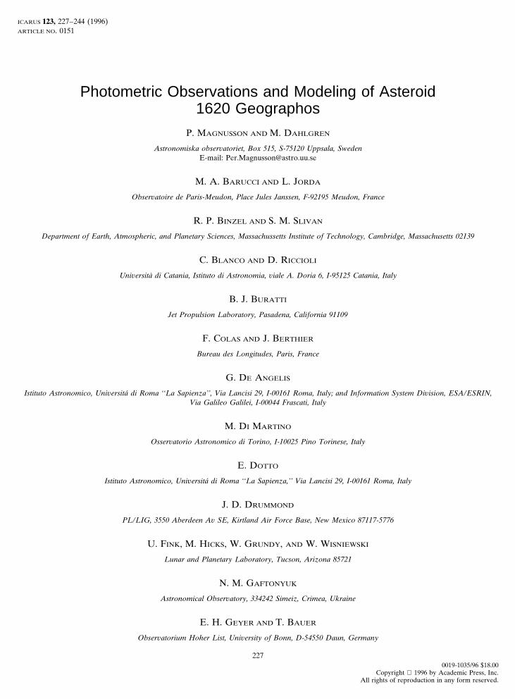
ICARUS 123, 227–244 (1996)ARTICLE NO. 0151

Photometric Observations and Modeling of Asteroid1620 Geographos

P. MAGNUSSON AND M. DAHLGREN

Astronomiska observatoriet, Box 515, S-75120 Uppsala, SwedenE-mail: [email protected]

M. A. BARUCCI AND L. JORDA

Observatoire de Paris-Meudon, Place Jules Janssen, F-92195 Meudon, France

R. P. BINZEL AND S. M. SLIVAN

Department of Earth, Atmospheric, and Planetary Sciences, Massachussetts Institute of Technology, Cambridge, Massachusetts 02139

C. BLANCO AND D. RICCIOLI

Universita di Catania, Istituto di Astronomia, viale A. Doria 6, I-95125 Catania, Italy

B. J. BURATTI

Jet Propulsion Laboratory, Pasadena, California 91109

F. COLAS AND J. BERTHIER

Bureau des Longitudes, Paris, France

G. DE ANGELIS

Istituto Astronomico, Universita di Roma ‘‘La Sapienza’’, Via Lancisi 29, I-00161 Roma, Italy; and Information System Division, ESA/ESRIN,Via Galileo Galilei, I-00044 Frascati, Italy

M. DI MARTINO

Osservatorio Astronomico di Torino, I-10025 Pino Torinese, Italy

E. DOTTO

Istituto Astronomico, Universita di Roma ‘‘La Sapienza,’’ Via Lancisi 29, I-00161 Roma, Italy

J. D. DRUMMOND

PL/LIG, 3550 Aberdeen Av SE, Kirtland Air Force Base, New Mexico 87117-5776

U. FINK, M. HICKS, W. GRUNDY, AND W. WISNIEWSKI

Lunar and Planetary Laboratory, Tucson, Arizona 85721

N. M. GAFTONYUK

Astronomical Observatory, 334242 Simeiz, Crimea, Ukraine

E. H. GEYER AND T. BAUER

Observatorium Hoher List, University of Bonn, D-54550 Daun, Germany

2270019-1035/96 $18.00

Copyright 1996 by Academic Press, Inc.All rights of reproduction in any form reserved.

228 MAGNUSSON ET AL.

M. HOFFMANN

Alter Weg 7, D-54570 Weidenbach, Germany

V. IVANOVA, B. KOMITOV, Z. DONCHEV, AND P. DENCHEV

Bulgarian Academy of Sciences, Department of Astronomy, Sofia, Bulgaria

YU. N. KRUGLY, F. P. VELICHKO, V. G. CHIORNY, D. F. LUPISHKO, AND V. G. SHEVCHENKO

Astronomical Observatory, Sumskaya Str. 35, Kharkiv 310022, Ukraine

T. KWIATKOWSKI AND A. KRYSZCZYNSKA

Astronomical Observatory, Adam Mickiewicz University, ul. S.oneczna 36, PL-60286 Poznan, Poland

J. F. LAHULLA

Observatorio Astronomico, Alfonso XII, 3, E-28014 Madrid, Spain

J. LICANDRO AND O. MENDEZ

Departamento de Astronom’ıa, Instituto de Fısica, Facultad de Ciencias, Tristan Narvaja 1674, 11.200 Montevideo, Uruguay

S. MOTTOLA AND A. ERIKSON

DLR, German Aerospace Research Establishment, Rudower Chausse 5, D-12489 Berlin, Germany

S. J. OSTRO

Jet Propulsion Laboratory, Pasadena, California 91109-8099

P. PRAVEC

Astronomical Institute, Czech Academy of Sciences, CZ-25165 Ondrejov, Czech Republic

W. PYCH

Astronomical Observatory, Warsaw University, Al. Ujazdowskie 4, PL-00-478 Warsaw, Poland

D. J. THOLEN AND R. WHITELEY

Institute of Astronomy, 2680 Woodlawn Drive, Honolulu, Hawaii 96822

W. J. WILD

University of Chicago, Department of Astronomy and Astrophysics, 5640 South Ellis Avenue, Chicago, Illinois 60637

AND

M. WOLF AND L. SAROUNOVA

Astronomical Institute, Charles University, Svedska 8, CZ-15000 Prague, Czech Republic

Received April 24, 1995; revised February 7, 1996

DEDICATED TO THE MEMORY OF DR. WIESLAW Z. WISNIEWSKI

0.00000003 days (5h13m23.975s 6 0.003s). The sense of rotation isretrograde. The ecliptic coordinates of the spin angular velocityPhotometric observations of 1620 Geographos in 1993 andvector are estimated to lp 5 568 6 68 and bp 5 2478 6 481994 are presented and, in combination with previously pub-(equinox J2000.0). The lightcurve amplitudes are well-lished data, are used to derive models of Geographos. Weexplained by an ellipsoidal model with axis ratios a/b 5estimate that the sidereal period of rotation is 0.21763860 6

OBSERVATIONS AND MODELING OF ASTEROID 1620 GEOGRAPHOS 229

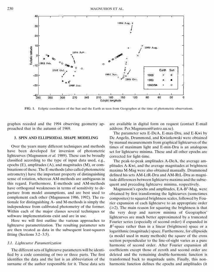
2.58 6 0.16 and b/c 5 1.00 6 0.15. Models that have one or modeling. The illumination and viewing geometry of theboth ends more sharply pointed than the ellipsoid improve the observations are shown graphically in Fig. 1. The observa-fit to the observations. There are no significant indications tions from 1969 by Dunlap (1974) have a quite good distri-of albedo variegation, but non-geometric scattering effects are bution despite the small number of observations. Note thetentatively suggested based on significant rotational color vari- unique geometry at the far left of the diagram for the 1983ation. 1996 Academic Press, Inc.

lightcurve by Weidenschilling et al. (1990). As a check ofthat crucial curve we include in this paper the Eight-ColorAsteroid Survey (ECAS) data for Geographos (Zellner et1. INTRODUCTIONal. 1985) in time-resolved form.

With its orbital period of 507.2 days Geographos makesThe S-type asteroid 1620 Geographos belongs to thepopulation of objects traversing the Earth’s orbital distance almost exactly 18 revolutions in 25 years. Thus, in 1994

Geographos was bound for another close approach withfrom the Sun and occasionally coming very close to us. Assuch it is relatively easily accessible to spacecraft from the Earth, very similar to the one observed by Dunlap in

1969. In fact, Geographos was at the same position in itsEarth. Its orbit offers challenges and opportunities toEarth-based observations and their interpretation. The orbit on a given date in 1994 as it had been 2 (Gregorian)

calendar dates later in 1969. Three lightcurves from thismotion in the sky can be fast, and the viewing geometrychanges dramatically during an apparition. Observations apparition have already been published by Michałowski et

al. (1994).at very large solar phases can be made. All the above isin contrast to main-belt asteroids for which more experi-ence has been gained (see, e.g., the modeling of the Galileo 2. OBSERVATIONSflyby targets by Magnusson et al. 1992 and Binzel et al.1993). Our new observations are available in digital form in

the Asteroid Photometric Catalogue Data Base. TheyThe observations and models presented in this paperare complementary to observations from August 1994 by can be accessed by anonymous ftp at Internet address

ftp.astro.uu.se or at World Wide Web address http://radar (Ostro et al., 1995, 1996) and by the IUE (Festou,private communication). Originally, the observations were www.astro.uu.se/planet/apc.html.

The observation are summarized in Table I. For easyplanned to support the Clementine space mission withground-based observations, but Clementine was unable to reference, previous observations by Dunlap (1974),

Weidenschilling et al. (1990), and Michałowski et al. (1994)complete the asteroidal part of its mission. However, webelieve the experiences gained with Geographos will be are also included in the table. The dates in the first column

refer approximately to the mean time of each lightcurveimportant for the modeling of 433 Eros, also a near-Earthasteroid, which is the 1999 rendezvous target of the (Universal Time). The three subsequent columns (in de-

grees) give the solar phase angle a and the ecliptic coordi-NEAR mission.Our previous knowledge about Geographos is to a large nates (equinox J2000.0) of Geographos as seen from the

Earth.extent based on the observations and analysis carried outby Dunlap (1974). He made extensive photometric and A large number of observers and reducers working at

different observatories were involved in this project, andpolarimetric observations during the 1969 apparition. Oneof the lightcurves Dunlap obtained showed a record maxi- the techniques vary correspondingly. Most observations

were reduced using standard methods (see Harris and Lup-mum amplitude of slightly more than 2 magnitudes. Al-though a solar phase of more than 508 contributed to this, ishko 1989).

Figure 1 shows the illumination and viewing geometriesit indicated that Geographos is an object of extreme elon-gation. Dunlap used laboratory simulations to arrive at a of the photometric observations in 1969, 1983, and 1993/

1994. During our observations from October 1993 to Aprilmodel shape consisting of a cylinder with rounded endshaving a length to width ratio of 2.7. The length was esti- 1994 Geographos was far away and had a relatively modest

apparent motion. In January 1994 the geometry was verymated to 4 km. Dunlap also determined that Geographoshas retrograde rotation. He obtained a spin model with similar to that for Dunlap’s observations in the same month

25 years earlier. By April 1994 the solar phase angle hadthe spin angular velocity vector directed toward ecliptic(J2000.0) coordinates lp 5 218 6 88 and bp 5 2608 6 48, reached 608. During the following months small solar elon-

gations made it difficult to obtain lightcurves of any signifi-and a sidereal period of 0.2176378 6 0.0000004 days. Later,Weidenschilling et al. (1990) obtained one lightcurve of cant length. When observations were resumed in August

1994 Geographos was only 0.0353 AU away and movedGeographos in 1983 as part of their photometric geod-esy program. more than 108 per day. Due to the large parallax the observ-

ing geometry differed significantly from those in the sameA geometrically diverse distribution of observations isessential for a reliable spin vector determination and shape month in 1969. During the following two months Geo-


FIG. 1. Ecliptic coordinates of the Sun and the Earth as seen from Geographos at the time of photometric observations.

graphos receded and the 1994 observing geometry ap- are available in digital form on request (contact E-mailaddress: [email protected]).proached that in the autumn of 1969.

The parameter sets E-DeA, E-max-Dru, and E-Kwi byDe Angelis, Drummond, and Kwiatkowski were obtained3. SPIN AND ELLIPSOIDAL SHAPE MODELINGby manual measurements from graphical lightcurves of the

Over the years many different techniques and methods times of maximum light and E-min-Dru is an analogoushave been developed for inversion of photometric set for lightcurve minima. These and all other epochs arelightcurves (Magnusson et al. 1989). These can be broadly corrected for light-time.classified according to the type of input data used, e.g., The peak-to-peak amplitudes A-DeA, the average am-epochs (E), amplitudes (A), and magnitudes (M), or com- plitudes A-Kwi, and the average magnitudes at brightnessbinations of these. The E-methods (also called photometric maxima M-Mag were also obtained manually. Drummondastrometry) have the important property of distinguishing defined his sets AM-LtR-Dru and AM-RtL-Dru as magni-sense of rotation, whereas AM-methods are ambiguous in tude differences between lightcurve maxima and the subse-this regard. Furthermore, E-methods and AM-methods quent and preceding lightcurve minima, respectively.have orthogonal weaknesses in terms of sensitivity to de- Magnusson’s epochs and amplitudes, EA-B2-Mag, wereparture from model assumptions, and are best used to obtained by first transforming the lightcurves (sometimescomplement each other (Magnusson 1986, 1992). The ra- composites) to squared brightness scales, followed by Fou-tionale for distinguishing A- and M-methods is simply the rier expansion of each lightcurve to an appropriate orderindependence from calibrated photometry of the former. ($2). The main reason for squaring the brightness is thatWithin each of the major classes several techniques or the very deep and narrow minima of Geographos’software implementations exist and are in use. lightcurves are much better approximated by a truncated

Here we will first outline the various approaches to Fourier series (especially of second order) if expanded inlightcurve parametrization. The resulting parameter sets B2-space rather than in a linear (brightness) space or aare then treated as data in the subsequent least-squares logarithmic (magnitude) space. Furthermore, for ellipsoidsfitting (Sections 3.2–3.5). (a model used in many methods) the square of the cross

section perpendicular to the line-of-sight varies as a pure3.1. Lightcurve Parametrization harmonic of second order. After Fourier expansion all

coefficients except those of zeroth and second order areThe different sets of lightcurve parameters will be identi-deleted and the remaining double-harmonic function isfied by a code consisting of two or three parts. The firsttransformed back to magnitude units. Finally, this non-identifies the data and the last is an abbreviation of the

surname of the author responsible for it. These data sets harmonic function defines the epochs and amplitudes (it

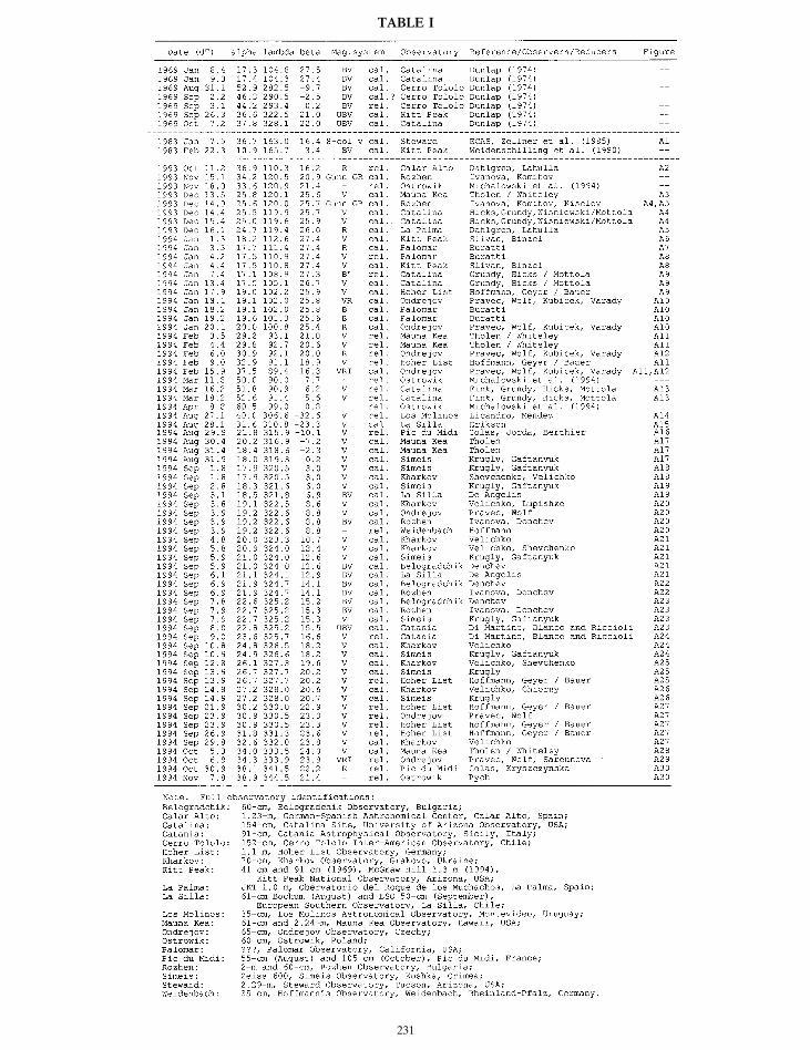
TABLE I

231


could also generate magnitudes). The reason for trans- for some integer nij . Note that the angles fi would havebeen zero if the illumination and viewing geometries hadforming back to magnitudes is to get parameters compati-

ble with the ones measured manually. Since only even remained fixed (constant synodic period). Different meth-ods use different ways of selecting the optimum integersharmonics are included no difference exists between pri-

mary and secondary extrema. nij and different ways of finding the least-squares solutionthat is simultaneously most consistent with (4) for manyPravec’s ‘‘epochs,’’ ‘‘E’’-Pra, remain undefined until the

final solution is found, as explained in the next section, pairs of epochs.An important complication arises for non-zero solarand are therefore not directly available for independent

analysis. phase angles (a ? 0). Empirically (and intuitively?), thevectors ti must be defined to reflect both the direction tothe Earth and the direction to the Sun since we are dealing3.2. Epoch Methodswith sunlight scatter off the asteroid. Some methods define

Epoch methods (also called photometric astrometry) are ti to be along the phase angle bisector, PAB (e.g., Magnus-based on the changing synodic frequency of rotation, which son 1986). Others compute fij values from (3) first withdepends on the motion of the Earth and the asteroid about the Earth direction and then with the solar direction, andthe Sun, and on the spin vector of the asteroid. A vectorial then use the average fij in the least-squares fit (e.g., Taylorpresentation in an inertial frame of reference, due to Wild, 1979). For a numerical investigation of these alternatives,defines for each epoch Ji a unit vector ei in the equatorial see Kwiatkowski (1993).plane of the asteroid by The methods SPA-Dru (Drummond et al. 1988), E-Mag

(Magnusson 1986, Erikson and Magnusson 1993), and W-p ? ei 5 0, Wil (Wild, 1995) are all based on the above principles.

The same applies to the epoch parts of EA-DeA and EA-ti ? ei 5 sin ci , (1)LS-Kwi described in the next two sections.

(ti 3 ei) ? p 5 0, A new method, E-Pra, turns things around a bit (Pravec,in preparation). No fixed epochs Ji are used. Instead, for

where p is a unit vector along the assumed spin angular each spin vector direction (lp , bp) to be tested, anglesvelocity vector, and where the corresponding aspect angle fij are defined as above and the lightcurves are shiftedci is given by accordingly (by explicit or implicit use of the epoch differ-

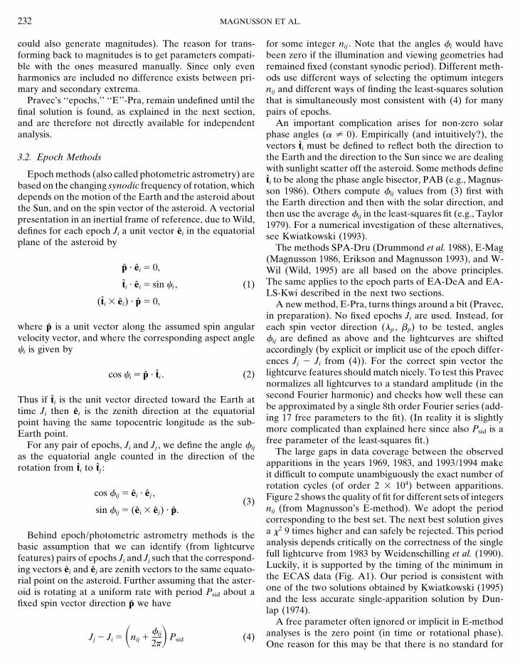
ences Jj 2 Ji from (4)). For the correct spin vector thelightcurve features should match nicely. To test this Praveccos ci 5 p ? ti . (2)normalizes all lightcurves to a standard amplitude (in thesecond Fourier harmonic) and checks how well these canThus if ti is the unit vector directed toward the Earth atbe approximated by a single 8th order Fourier series (add-time Ji then ei is the zenith direction at the equatorialing 17 free parameters to the fit). (In reality it is slightlypoint having the same topocentric longitude as the sub-more complicated than explained here since also Psid is aEarth point.free parameter of the least-squares fit.)For any pair of epochs, Ji and Jj , we define the angle fij The large gaps in data coverage between the observedas the equatorial angle counted in the direction of theapparitions in the years 1969, 1983, and 1993/1994 makerotation from ti to tj : it difficult to compute unambiguously the exact number ofrotation cycles (of order 2 3 104) between apparitions.

cos fij 5 ei ? ej ,(3) Figure 2 shows the quality of fit for different sets of integers

nij (from Magnusson’s E-method). We adopt the periodsin fij 5 (ei 3 ej) ? p.corresponding to the best set. The next best solution givesa x2 9 times higher and can safely be rejected. This periodBehind epoch/photometric astrometry methods is theanalysis depends critically on the correctness of the singlebasic assumption that we can identify (from lightcurvefull lightcurve from 1983 by Weidenschilling et al. (1990).features) pairs of epochs Ji and Jj such that the correspond-Luckily, it is supported by the timing of the minimum ining vectors ei and ej are zenith vectors to the same equato-the ECAS data (Fig. A1). Our period is consistent withrial point on the asteroid. Further assuming that the aster-one of the two solutions obtained by Kwiatkowski (1995)oid is rotating at a uniform rate with period Psid about aand the less accurate single-apparition solution by Dun-fixed spin vector direction p we havelap (1974).

A free parameter often ignored or implicit in E-methodanalyses is the zero point (in time or rotational phase).Jj 2 Ji 5 Snij 1

fij

2fD Psid (4)One reason for this may be that there is no standard for


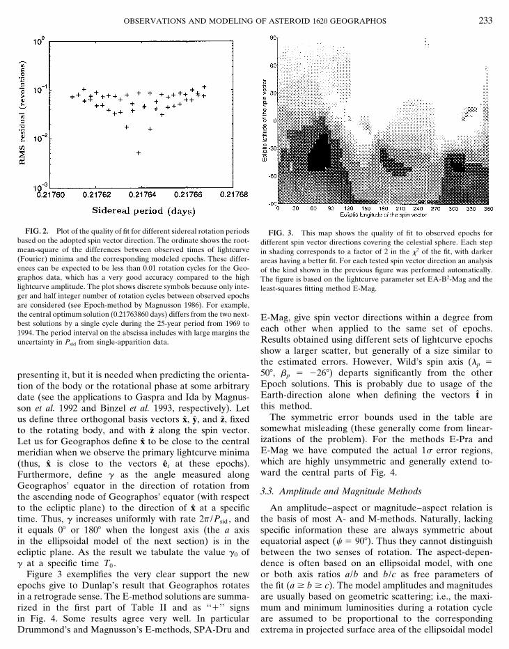
FIG. 2. Plot of the quality of fit for different sidereal rotation periods FIG. 3. This map shows the quality of fit to observed epochs forbased on the adopted spin vector direction. The ordinate shows the root- different spin vector directions covering the celestial sphere. Each stepmean-square of the differences between observed times of lightcurve in shading corresponds to a factor of 2 in the x2 of the fit, with darker(Fourier) minima and the corresponding modeled epochs. These differ- areas having a better fit. For each tested spin vector direction an analysisences can be expected to be less than 0.01 rotation cycles for the Geo- of the kind shown in the previous figure was performed automatically.graphos data, which has a very good accuracy compared to the high The figure is based on the lightcurve parameter set EA-B2-Mag and thelightcurve amplitude. The plot shows discrete symbols because only inte- least-squares fitting method E-Mag.ger and half integer number of rotation cycles between observed epochsare considered (see Epoch-method by Magnusson 1986). For example,the central optimum solution (0.21763860 days) differs from the two next- E-Mag, give spin vector directions within a degree frombest solutions by a single cycle during the 25-year period from 1969 to

each other when applied to the same set of epochs.1994. The period interval on the abscissa includes with large margins theResults obtained using different sets of lightcurve epochsuncertainty in Psid from single-apparition data.show a larger scatter, but generally of a size similar tothe estimated errors. However, Wild’s spin axis (lp 5508, bp 5 2268) departs significantly from the otherpresenting it, but it is needed when predicting the orienta-Epoch solutions. This is probably due to usage of thetion of the body or the rotational phase at some arbitraryEarth-direction alone when defining the vectors t indate (see the applications to Gaspra and Ida by Magnus-this method.son et al. 1992 and Binzel et al. 1993, respectively). Let

The symmetric error bounds used in the table areus define three orthogonal basis vectors x, y, and z, fixedsomewhat misleading (these generally come from linear-to the rotating body, and with z along the spin vector.izations of the problem). For the methods E-Pra andLet us for Geographos define x to be close to the centralE-Mag we have computed the actual 1s error regions,meridian when we observe the primary lightcurve minimawhich are highly unsymmetric and generally extend to-(thus, x is close to the vectors ei at these epochs).ward the central parts of Fig. 4.Furthermore, define c as the angle measured along

Geographos’ equator in the direction of rotation from3.3. Amplitude and Magnitude Methods

the ascending node of Geographos’ equator (with respectto the ecliptic plane) to the direction of x at a specific An amplitude–aspect or magnitude–aspect relation is

the basis of most A- and M-methods. Naturally, lackingtime. Thus, c increases uniformly with rate 2f /Psid , andit equals 08 or 1808 when the longest axis (the a axis specific information these are always symmetric about

equatorial aspect (c 5 908). Thus they cannot distinguishin the ellipsoidal model of the next section) is in theecliptic plane. As the result we tabulate the value c0 of between the two senses of rotation. The aspect-depen-

dence is often based on an ellipsoidal model, with onec at a specific time T0 .Figure 3 exemplifies the very clear support the new or both axis ratios a/b and b/c as free parameters of

the fit (a $ b $ c). The model amplitudes and magnitudesepochs give to Dunlap’s result that Geographos rotatesin a retrograde sense. The E-method solutions are summa- are usually based on geometric scattering; i.e., the maxi-

mum and minimum luminosities during a rotation cyclerized in the first part of Table II and as ‘‘1’’ signsin Fig. 4. Some results agree very well. In particular are assumed to be proportional to the corresponding

extrema in projected surface area of the ellipsoidal modelDrummond’s and Magnusson’s E-methods, SPA-Dru and


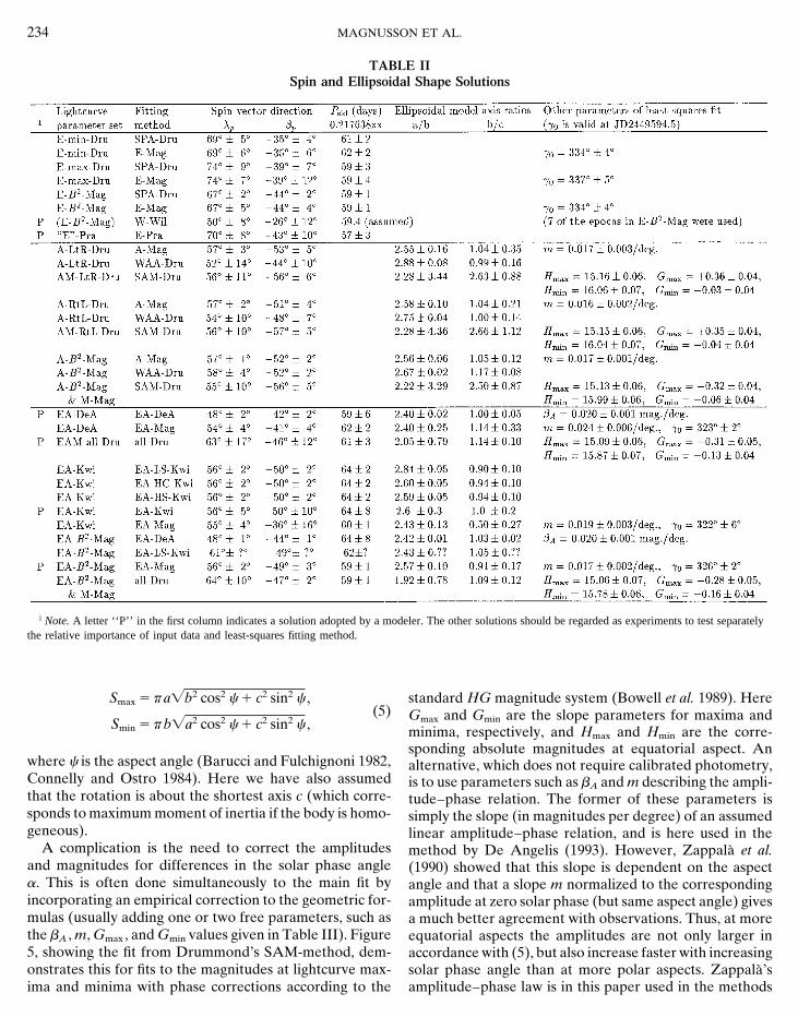
TABLE IISpin and Ellipsoidal Shape Solutions

1 Note. A letter ‘‘P’’ in the first column indicates a solution adopted by a modeler. The other solutions should be regarded as experiments to test separatelythe relative importance of input data and least-squares fitting method.

Smax 5 faÏb2 cos2 c 1 c2 sin2 c ,(5)

standard HG magnitude system (Bowell et al. 1989). HereGmax and Gmin are the slope parameters for maxima and

Smin 5 fbÏa2 cos2 c 1 c2 sin2 c , minima, respectively, and Hmax and Hmin are the corre-sponding absolute magnitudes at equatorial aspect. An

where c is the aspect angle (Barucci and Fulchignoni 1982, alternative, which does not require calibrated photometry,Connelly and Ostro 1984). Here we have also assumed is to use parameters such as bA and m describing the ampli-that the rotation is about the shortest axis c (which corre- tude–phase relation. The former of these parameters issponds to maximum moment of inertia if the body is homo- simply the slope (in magnitudes per degree) of an assumedgeneous). linear amplitude–phase relation, and is here used in the

A complication is the need to correct the amplitudes method by De Angelis (1993). However, Zappala et al.and magnitudes for differences in the solar phase angle (1990) showed that this slope is dependent on the aspecta. This is often done simultaneously to the main fit by angle and that a slope m normalized to the correspondingincorporating an empirical correction to the geometric for- amplitude at zero solar phase (but same aspect angle) givesmulas (usually adding one or two free parameters, such as a much better agreement with observations. Thus, at morethe bA , m, Gmax , and Gmin values given in Table III). Figure equatorial aspects the amplitudes are not only larger in5, showing the fit from Drummond’s SAM-method, dem- accordance with (5), but also increase faster with increasingonstrates this for fits to the magnitudes at lightcurve max- solar phase angle than at more polar aspects. Zappala’s

amplitude–phase law is in this paper used in the methodsima and minima with phase corrections according to the


A-Mag and EA-Mag (see Erikson and Magnusson 1993).For lack of better information we are extending this ampli-tude–phase law far beyond the phase-angle range of about08 to 208 for which it was originally shown to hold (Zap-pala et al. 1990). Although this seems to have worked forGeographos, much more data at large phase angles arerequired to test it properly.

Another item where different methods differ is in thedefinition of the aspect angle c in (5). Going back to (2),we again have a choice of definition of the vector t. Twocommon ones are to point t toward the Earth or along thephase angle bisector.

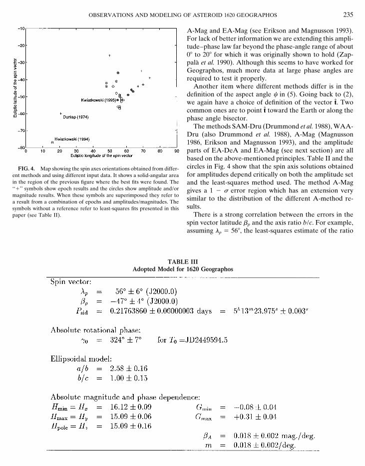
The methods SAM-Dru (Drummond et al. 1988), WAA-Dru (also Drummond et al. 1988), A-Mag (Magnusson1986, Erikson and Magnusson 1993), and the amplitudeparts of EA-DeA and EA-Mag (see next section) are allbased on the above-mentioned principles. Table II and thecircles in Fig. 4 show that the spin axis solutions obtainedFIG. 4. Map showing the spin axes orientations obtained from differ-for amplitudes depend critically on both the amplitude setent methods and using different input data. It shows a solid-angular area

in the region of the previous figure where the best fits were found. The and the least-squares method used. The method A-Mag‘‘1’’ symbols show epoch results and the circles show amplitude and/or gives a 1 2 s error region which has an extension verymagnitude results. When these symbols are superimposed they refer to similar to the distribution of the different A-method re-a result from a combination of epochs and amplitudes/magnitudes. The

sults.symbols without a reference refer to least-squares fits presented in thisThere is a strong correlation between the errors in thepaper (see Table II).

spin vector latitude bp and the axis ratio b/c. For example,assuming lp 5 568, the least-squares estimate of the ratio

TABLE IIIAdopted Model for 1620 Geographos


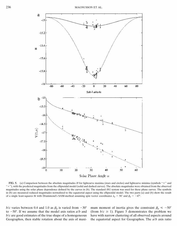
FIG. 5. (a) Comparison between the absolute magnitudes H for lightcurve maxima (stars and circles) and lightcurve minima (symbols ‘‘3’’ and‘‘1’’), with the predicted magnitudes from the ellipsoidal model (solid and dashed curves). The absolute magnitudes were obtained from the observedmagnitudes using the solar phase dependence defined by the curves in (b). The standard HG system was used for these phase curves. The symbolsin (b) are measured reduced magnitudes normalized to the equatorial aspect using the ellipsoidal model. The two parts (a) and (b) show the resultof a single least-squares fit with Drummond’s SAM-method assuming spin vector coordinates lp 5 568 and bp 5 2478.

b/c varies between 0.4 and 1.0 as bp is varied from 2308 mum moment of inertia gives the constraint bp ( 2508(from b/c $ 1). Figure 5 demonstrates the problem weto 2508. If we assume that the model axis ratios a/b and

b/c are good estimates of the true shape of a homogeneous have with narrow clustering of all observed aspects aroundthe equatorial aspect for Geographos. The a/b axis ratioGeographos, then stable rotation about the axis of maxi-


is well-determined by the distance between the curves at analytical formulas may give wrong results (Kwiatkow-ski 1993).the equatorial aspect. The b/c axis ratio, however, is deter-

mined by the rate of convergence of the two curves as The lightcurves of Geographos display different levelsof maxima and minima. Maximal, average, and minimalwe go toward more polar aspects, or by the magnitude

difference between polar and equatorial aspects. The fig- amplitudes are all compared to the modeled amplitudesin the calculations. At present there is no single scatteringure shows that both these are badly constrained for

Geographos, giving relatively ill-constrained b/c ratios. law that could explain fully the asteroid brightness varia-tions in terms of an ellipsoid model shape, which is neces-sarily simplistic. Because of that, and to test the depen-3.4. Combined Methodsdence of the final solution on this part of the algorithm, two

Given the complementary nature of the E-methods andlaws of light scattering are used in calculations: Lommel-

the AM-methods it is natural to combine the two in aSeeliger’s (LS) and Hapke’s laws. The latter is dependent

single least-squares fit (although it is often good first toon five parameters but as they cannot be determined unam-

study the epochs in isolation to narrow down the rangebiguously (and the data for Geographos are insufficient

for Psid and perhaps determine the integers nij in (4)). Thefor constraining them), two sets of Hapke parameters, ob-

methods EA-Kwi (see next section), EA-DeA (De Angelistained for typical C- and S-type asteroids (Helfenstein and

1993), and EA-Mag (Magnusson, in preparation) are basedVeverka 1989) are assumed. We refer to these as HC and

on this principle. The two former methods use a combina-HS, respectively.

tion of amplitude and epoch residuals to compute the x2

The epoch part of the algorithm is very similar to thatof the fit, whereas Magnusson’s method makes the fit in

used by Magnusson (1986) and Drummond et al. (1988),the corresponding Cartesian variables a2 and b2 . These are

except that the model epochs are determined from thesecond order Fourier coefficients of the lightcurves with

numerically modeled lightcurve.absolute rotational phases computed using the fij defined

As shown by fitting methods EA-LS-Kwi, EA-HC-Kwi,in (3). The main advantages of this Cartesian parameteriza-

and EA-HS-Kwi in Table II, all three scattering laws ledtion of the lightcurve are that a2 and b2 are continuous

to the same spin vector and sidereal period. The onlyfunctions of the fitted parameters (epochs have a singular-

difference appears for the shape parameters. The unrealis-ity at zero amplitude) and that the choice of weights is

tic values of the ratio b/c may reflect a departure of Geo-simpler than if epochs and amplitudes are used indepen-

graphos’ shape from the assumed ellipsoid model, or adently.

departure from the assumed scattering law. If the manysystematic effects connected with the scattering law, selec-

3.5. Inversion with More Complex Scattering Lawstion of the data, and the use of the maximal, average, orminimum amplitudes are analyzed (see Kwiatkowski 1995Systematic errors in the derived ellipsoidal models are

likely to arise from the common usage of the geometric for a more detailed discussion) then much larger errorsare estimated (see the solution by Kwiatkowski in Tablescattering law, extended to geometries with non-zero solar

phase angles using various ad hoc empirical corrections. II marked by a ‘‘P’’ in the first column).Less clear is the extent to which also the derived spinvectors will be affected by the simplified treatment of light

3.6. Error Estimation and Adopted Modelscattering. Problems are most likely to appear for Earth-approaching asteroids like Geographos that are observed It is clear from Table II that for many of the solutions

the true error must be much larger than the tabulatedat extremely high phase angles.These problems are avoided entirely by a new method formal error estimates. Part of this is due to unsymmetric

error regions. The remaining part is most likely due toby Kwiatkowski, which is an improvement of the methodby Kwiatkowski (1995). The fit to the amplitudes is done systematic deviations from the assumptions we have made.

Each modeler has adopted a preferred solution, as indi-in a new way. The brightness of a triaxial ellipsoid at ageometry specified by aspect, obliquity, solar phase angle, cated by the letter ‘‘P’’ preceding the first column in Table

II. The last four of these, which correspond to analysesand the rotation phase is obtained by numerical integrationof one of the light scattering laws over the illuminated based on combinations of epoch and amplitude/magnitude

data, were averaged to get our joint adopted direction ofand visible part of the model surface. To get the modellightcurve amplitude, the maximal and minimal brightness the spin vector: lp 5 568 6 68, bp 5 2478 6 48. Here we

have disregarded the formal error estimates and insteadof the model ellipsoid during a full rotation are determined.In the previous version presented by Kwiatkowski (1995) used the standard deviation from the mean as our final

estimates of the errors.the model extrema were assumed to happen at times deter-mined analytically by the classical time shifts by Taylor The other adopted values summarized in Table III were

obtained in similar ways. There is redundancy in these(e.g., Taylor 1979). However, for some geometries such


values since the photometric axis ratios a/b and b/c canbe computed from the absolute magnitudes Hx , Hy , andHz measured along the three basis vectors. Furthermore,the values Gmax 2 Gmin , bA , and m represent three differ-ent ways of parameterizing the amplitude–phase depen-dence. As far as possible, these parameters were ad-justed for consistency with each other, instead of just let-ting each be an average from Table II.

For easy comparison of phase curves from different as-teroids a standard has been suggested in the form of theHG system applied to the reduced magnitudes averagedover the rotation cycle (Bowel et al. 1989). A straightfor-ward application of these rules would give standard G andH parameters for Geographos near the average of thevalues we obtained for lightcurve minima and maxima(Table II). This approach may be reasonable for objectswith small lightcurve amplitudes, but if we want the re-

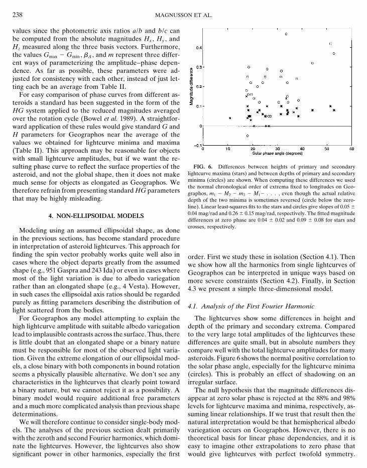
FIG. 6. Differences between heights of primary and secondarysulting phase curve to reflect the surface properties of thelightcurve maxima (stars) and between depths of primary and secondaryasteroid, and not the global shape, then it does not makeminima (circles) are shown. When computing these differences we usedmuch sense for objects as elongated as Geographos. Wethe normal chronological order of extrema fixed to longitudes on Geo-

therefore refrain from presenting standard HG parameters graphos, m1 2 M2 2 m2 2 M12 . . . , even though the actual relativethat may be highly misleading. depth of the two minima is sometimes reversed (circle below the zero-

line). Linear least-squares fits to the stars and circles give slopes of 0.05 6

0.04 mag/rad and 0.26 6 0.15 mag/rad, respectively. The fitted magnitude4. NON-ELLIPSOIDAL MODELSdifferences at zero phase are 0.04 6 0.02 and 0.09 6 0.08 for stars andcrosses, respectively.

Modeling using an assumed ellipsoidal shape, as donein the previous sections, has become standard procedurein interpretation of asteroid lightcurves. This approach forfinding the spin vector probably works quite well also in order. First we study these in isolation (Section 4.1). Thencases where the object departs greatly from the assumed we show how all the harmonics from single lightcurves ofshape (e.g., 951 Gaspra and 243 Ida) or even in cases where Geographos can be interpreted in unique ways based onmost of the light variation is due to albedo variegation more severe constraints (Section 4.2). Finally, in Sectionrather than an elongated shape (e.g., 4 Vesta). However, 4.3 we present a simple three-dimensional model.in such cases the ellipsoidal axis ratios should be regardedpurely as fitting parameters describing the distribution of

4.1. Analysis of the First Fourier Harmoniclight scattered from the bodies.

For Geographos any model attempting to explain the The lightcurves show some differences in height anddepth of the primary and secondary extrema. Comparedhigh lightcurve amplitude with suitable albedo variegation

lead to implausible contrasts across the surface. Thus, there to the very large total amplitudes of the lightcurves thesedifferences are quite small, but in absolute numbers theyis little doubt that an elongated shape or a binary nature

must be responsible for most of the observed light varia- compare well with the total lightcurve amplitudes for manyasteroids. Figure 6 shows the normal positive correlation totion. Given the extreme elongation of our ellipsoidal mod-

els, a close binary with both components in bound rotation the solar phase angle, especially for the lightcurve minima(circles). This is probably an effect of shadowing on anseems a physically plausible alternative. We don’t see any

characteristics in the lightcurves that clearly point toward irregular surface.The null hypothesis that the magnitude differences dis-a binary nature, but we cannot reject it as a possibility. A

binary model would require additional free parameters appear at zero solar phase is rejected at the 88% and 98%levels for lightcurve maxima and minima, respectively, as-and a much more complicated analysis than previous shape

determinations. suming linear relationships. If we trust that result then thenatural interpretation would be that hemispherical albedoWe will therefore continue to consider single-body mod-

els. The analyses of the previous section dealt primarily variegation occurs on Geographos. However, there is notheoretical basis for linear phase dependencies, and it iswith the zeroth and second Fourier harmonics, which domi-

nate the lightcurves. However, the lightcurves also show easy to imagine other extrapolations to zero phase thatwould give lightcurves with perfect twofold symmetry.significant power in other harmonics, especially the first


Thus, in practice we can’t rule out the null hypothesis thatGeographos has a homogeneous surface albedo.

4.2. Two-Dimensional Convex-Profile Inversion

Under certain ideal conditions, one can use convex-pro-file inversion (CPI, Ostro et al. 1988) of a lightcurve toestimate a profile that is a two-dimensional average ofthe asteroid’s shape. That profile is called the mean crosssection, C, and is defined as the average of the envelopeson all the surface contours parallel to the equator. Theideal conditions for estimating C include Condition GEO,that the scattering is uniform and geometric; ConditionEVIG, that the viewing-illumination geometry is equato-rial; and Condition PHASE, that the solar phase angle ais known and non-zero. The logic behind these conditionsis that they collapse the three-dimensional lightcurve inver-sion problem, which cannot be solved uniquely, into a two-dimensional problem that can.

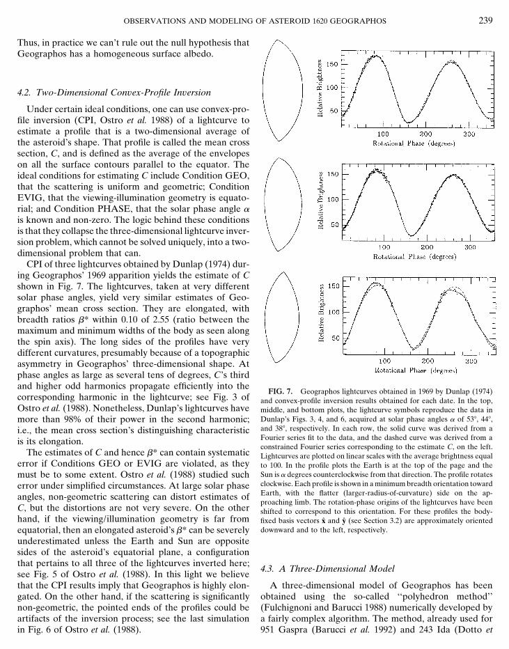
CPI of three lightcurves obtained by Dunlap (1974) dur-ing Geographos’ 1969 apparition yields the estimate of Cshown in Fig. 7. The lightcurves, taken at very differentsolar phase angles, yield very similar estimates of Geo-graphos’ mean cross section. They are elongated, withbreadth ratios b* within 0.10 of 2.55 (ratio between themaximum and minimum widths of the body as seen alongthe spin axis). The long sides of the profiles have verydifferent curvatures, presumably because of a topographicasymmetry in Geographos’ three-dimensional shape. Atphase angles as large as several tens of degrees, C’s thirdand higher odd harmonics propagate efficiently into the

FIG. 7. Geographos lightcurves obtained in 1969 by Dunlap (1974)corresponding harmonic in the lightcurve; see Fig. 3 of and convex-profile inversion results obtained for each date. In the top,Ostro et al. (1988). Nonetheless, Dunlap’s lightcurves have middle, and bottom plots, the lightcurve symbols reproduce the data in

Dunlap’s Figs. 3, 4, and 6, acquired at solar phase angles a of 538, 448,more than 98% of their power in the second harmonic;and 388, respectively. In each row, the solid curve was derived from ai.e., the mean cross section’s distinguishing characteristicFourier series fit to the data, and the dashed curve was derived from ais its elongation.constrained Fourier series corresponding to the estimate C, on the left.

The estimates of C and hence b* can contain systematic Lightcurves are plotted on linear scales with the average brightness equalerror if Conditions GEO or EVIG are violated, as they to 100. In the profile plots the Earth is at the top of the page and the

Sun is a degrees counterclockwise from that direction. The profile rotatesmust be to some extent. Ostro et al. (1988) studied suchclockwise. Each profile is shown in a minimum breadth orientation towarderror under simplified circumstances. At large solar phaseEarth, with the flatter (larger-radius-of-curvature) side on the ap-angles, non-geometric scattering can distort estimates ofproaching limb. The rotation-phase origins of the lightcurves have been

C, but the distortions are not very severe. On the other shifted to correspond to this orientation. For these profiles the body-hand, if the viewing/illumination geometry is far from fixed basis vectors x and y (see Section 3.2) are approximately oriented

downward and to the left, respectively.equatorial, then an elongated asteroid’s b* can be severelyunderestimated unless the Earth and Sun are oppositesides of the asteroid’s equatorial plane, a configurationthat pertains to all three of the lightcurves inverted here;

4.3. A Three-Dimensional Modelsee Fig. 5 of Ostro et al. (1988). In this light we believethat the CPI results imply that Geographos is highly elon- A three-dimensional model of Geographos has been

obtained using the so-called ‘‘polyhedron method’’gated. On the other hand, if the scattering is significantlynon-geometric, the pointed ends of the profiles could be (Fulchignoni and Barucci 1988) numerically developed by

a fairly complex algorithm. The method, already used forartifacts of the inversion process; see the last simulationin Fig. 6 of Ostro et al. (1988). 951 Gaspra (Barucci et al. 1992) and 243 Ida (Dotto et


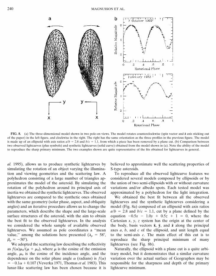
FIG. 8. (a) The three-dimensional model shown in two pole-on views. The model rotates counterclockwise (spin vector and z axis sticking outof the paper) in the left figure, and clockwise in the right. The right has the same orientation as the three profiles in the previous figure. The modelis made up of an ellipsoid with axis ratios a/b 5 2.8 and b/c 5 1.1, from which a piece has been removed by a plane cut. (b) Comparison betweentwo observed lightcurves (plus symbols) and synthetic lightcurves (solid curve) obtained from the model shown in (a). Note the ability of the modelto reproduce the sharp primary minimum. The two examples shown are quite representative of the fits obtained for lightcurves in general.

al. 1995), allows us to produce synthetic lightcurves by believed to approximate well the scattering properties ofS-type asteroids.simulating the rotation of an object varying the illumina-

tion and viewing geometries and the scattering law. A To reproduce all the observed lightcurve features weconsidered several models composed by ellipsoids or bypolyhedron consisting of a large number of triangles ap-

proximates the model of the asteroid. By simulating the the union of two semi-ellipsoids with or without curvaturevariations and/or albedo spots. Each tested model wasrotation of the polyhedron around its principal axis of

inertia we obtained the synthetic lightcurves. The observed approximated by a polyhedron for the light integration.We obtained the best fit between all the observedlightcurves are compared to the synthetic ones obtained

with the same geometry (solar phase, aspect, and obliquity lightcurves and the synthetic lightcurves considering amodel (Fig. 8a) composed of an ellipsoid with axis ratiosangles) and an iterative procedure allows us to change the

parameters, which describe the shape and the large-scale a/b 5 2.8 and b/c 5 1.1, cut by a plane defined by theequation 20.5x 2 1.0y 1 0.5z 1 1 5 0, where thesurface structures of the asteroid, with the aim to obtain

the best fit to the observed lightcurves. In the analysis Cartesian x, y, z system has the origin at the center ofthe body, basis vectors x, y, and z along the principalwe considered the whole sample of available observed

lightcurves. We assumed as pole coordinates a ‘‘mean axes a, b, and c of the ellipsoid, and unit length equalto the semi-axis c. The main effect of this cut is tovalue,’’ among the solutions here presented (lp 5 588,

bp 5 2508). reproduce the sharp principal minimum of manylightcurves (see Fig. 8b).We adopted the scattering law describing the reflectivity

as f (a)e0/(e 1 e0), where e is the cosine of the emission Naturally, the ellipsoid with a plane cut is a quite arbi-trary model, but it demonstrates that a similar curvatureangle, e0 is the cosine of the incidence angle, and the

dependence on the solar phase angle a (radians) is f (a) variation over the actual surface of Geographos may beresponsible for the sharpness and depth of the primary5 20.1a 1 0.107 (Veverka 1971, Thomas et al. 1983). This

lunar-like scattering law has been chosen because it is lightcurve minimum.


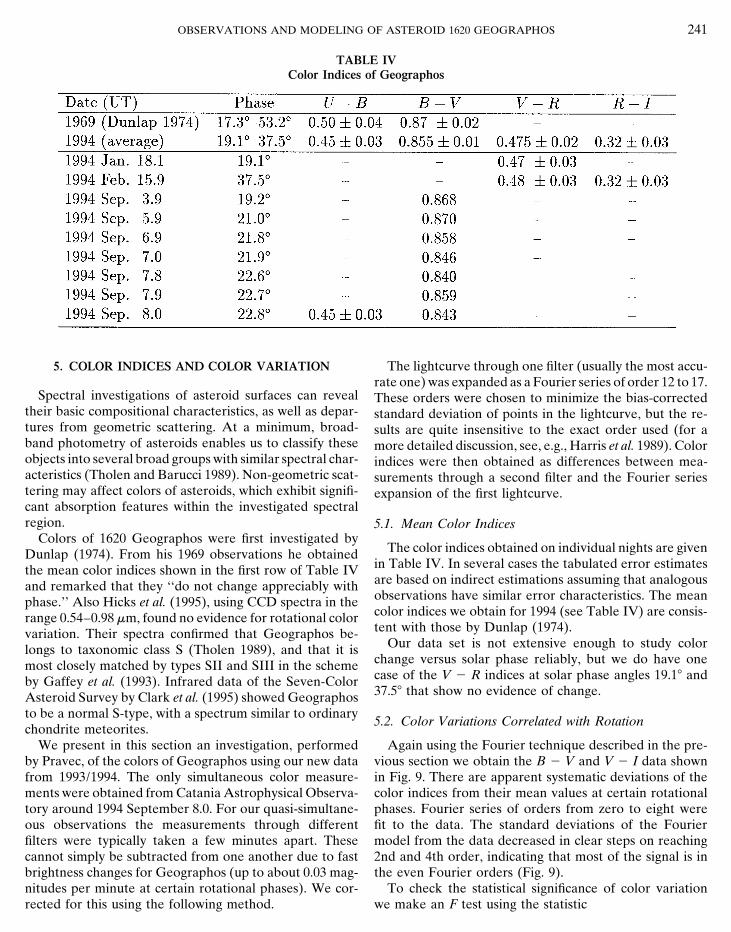
TABLE IVColor Indices of Geographos

5. COLOR INDICES AND COLOR VARIATION The lightcurve through one filter (usually the most accu-rate one) was expanded as a Fourier series of order 12 to 17.

Spectral investigations of asteroid surfaces can reveal These orders were chosen to minimize the bias-correctedtheir basic compositional characteristics, as well as depar- standard deviation of points in the lightcurve, but the re-tures from geometric scattering. At a minimum, broad- sults are quite insensitive to the exact order used (for aband photometry of asteroids enables us to classify these more detailed discussion, see, e.g., Harris et al. 1989). Colorobjects into several broad groups with similar spectral char- indices were then obtained as differences between mea-acteristics (Tholen and Barucci 1989). Non-geometric scat- surements through a second filter and the Fourier seriestering may affect colors of asteroids, which exhibit signifi- expansion of the first lightcurve.cant absorption features within the investigated spectralregion. 5.1. Mean Color Indices

Colors of 1620 Geographos were first investigated byThe color indices obtained on individual nights are givenDunlap (1974). From his 1969 observations he obtained

in Table IV. In several cases the tabulated error estimatesthe mean color indices shown in the first row of Table IVare based on indirect estimations assuming that analogousand remarked that they ‘‘do not change appreciably withobservations have similar error characteristics. The meanphase.’’ Also Hicks et al. (1995), using CCD spectra in thecolor indices we obtain for 1994 (see Table IV) are consis-range 0.54–0.98 em, found no evidence for rotational colortent with those by Dunlap (1974).variation. Their spectra confirmed that Geographos be-

Our data set is not extensive enough to study colorlongs to taxonomic class S (Tholen 1989), and that it ischange versus solar phase reliably, but we do have onemost closely matched by types SII and SIII in the schemecase of the V 2 R indices at solar phase angles 19.18 andby Gaffey et al. (1993). Infrared data of the Seven-Color37.58 that show no evidence of change.Asteroid Survey by Clark et al. (1995) showed Geographos

to be a normal S-type, with a spectrum similar to ordinary5.2. Color Variations Correlated with Rotation

chondrite meteorites.We present in this section an investigation, performed Again using the Fourier technique described in the pre-

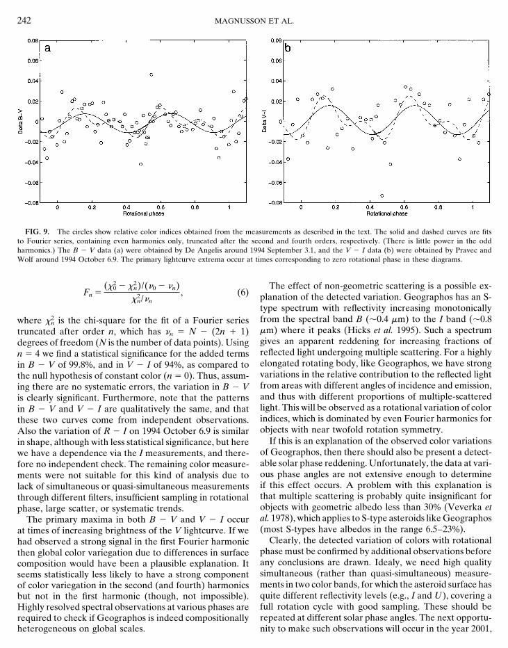
vious section we obtain the B 2 V and V 2 I data shownby Pravec, of the colors of Geographos using our new datafrom 1993/1994. The only simultaneous color measure- in Fig. 9. There are apparent systematic deviations of the

color indices from their mean values at certain rotationalments were obtained from Catania Astrophysical Observa-tory around 1994 September 8.0. For our quasi-simultane- phases. Fourier series of orders from zero to eight were

fit to the data. The standard deviations of the Fourierous observations the measurements through differentfilters were typically taken a few minutes apart. These model from the data decreased in clear steps on reaching

2nd and 4th order, indicating that most of the signal is incannot simply be subtracted from one another due to fastbrightness changes for Geographos (up to about 0.03 mag- the even Fourier orders (Fig. 9).

To check the statistical significance of color variationnitudes per minute at certain rotational phases). We cor-rected for this using the following method. we make an F test using the statistic


FIG. 9. The circles show relative color indices obtained from the measurements as described in the text. The solid and dashed curves are fitsto Fourier series, containing even harmonics only, truncated after the second and fourth orders, respectively. (There is little power in the oddharmonics.) The B 2 V data (a) were obtained by De Angelis around 1994 September 3.1, and the V 2 I data (b) were obtained by Pravec andWolf around 1994 October 6.9. The primary lightcurve extrema occur at times corresponding to zero rotational phase in these diagrams.

The effect of non-geometric scattering is a possible ex-Fn 5

(x20 2 x2

n)/(n0 2 nn)x2

n/nn, (6) planation of the detected variation. Geographos has an S-

type spectrum with reflectivity increasing monotonicallyfrom the spectral band B (p0.4 em) to the I band (p0.8where x2

n is the chi-square for the fit of a Fourier seriesem) where it peaks (Hicks et al. 1995). Such a spectrumtruncated after order n, which has nn 5 N 2 (2n 1 1)gives an apparent reddening for increasing fractions ofdegrees of freedom (N is the number of data points). Usingreflected light undergoing multiple scattering. For a highlyn 5 4 we find a statistical significance for the added termselongated rotating body, like Geographos, we have strongin B 2 V of 99.8%, and in V 2 I of 94%, as compared tovariations in the relative contribution to the reflected lightthe null hypothesis of constant color (n 5 0). Thus, assum-from areas with different angles of incidence and emission,ing there are no systematic errors, the variation in B 2 Vand thus with different proportions of multiple-scatteredis clearly significant. Furthermore, note that the patternslight. This will be observed as a rotational variation of colorin B 2 V and V 2 I are qualitatively the same, and thatindices, which is dominated by even Fourier harmonics forthese two curves come from independent observations.objects with near twofold rotation symmetry.Also the variation of R 2 I on 1994 October 6.9 is similar

If this is an explanation of the observed color variationsin shape, although with less statistical significance, but hereof Geographos, then there should also be present a detect-we have a dependence via the I measurements, and there-able solar phase reddening. Unfortunately, the data at vari-fore no independent check. The remaining color measure-ous phase angles are not extensive enough to determinements were not suitable for this kind of analysis due toif this effect occurs. A problem with this explanation islack of simultaneous or quasi-simultaneous measurementsthat multiple scattering is probably quite insignificant forthrough different filters, insufficient sampling in rotationalobjects with geometric albedo less than 30% (Veverka etphase, large scatter, or systematic trends.al. 1978), which applies to S-type asteroids like GeographosThe primary maxima in both B 2 V and V 2 I occur(most S-types have albedos in the range 6.5–23%).at times of increasing brightness of the V lightcurve. If we

Clearly, the detected variation of colors with rotationalhad observed a strong signal in the first Fourier harmonicphase must be confirmed by additional observations beforethen global color variegation due to differences in surfaceany conclusions are drawn. Idealy, we need high qualitycomposition would have been a plausible explanation. Itsimultaneous (rather than quasi-simultaneous) measure-seems statistically less likely to have a strong componentments in two color bands, for which the asteroid surface hasof color variegation in the second (and fourth) harmonicsquite different reflectivity levels (e.g., I and U), covering abut not in the first harmonic (though, not impossible).full rotation cycle with good sampling. These should beHighly resolved spectral observations at various phases arerepeated at different solar phase angles. The next opportu-required to check if Geographos is indeed compositionally

heterogeneous on global scales. nity to make such observations will occur in the year 2001,


when Geographos will be observable from the northern arbitrary scattering laws and avoiding ad hoc empiricaltreatment of non-zero solar phases.hemisphere in a geometric configuration similar to that in

1994 and be quite bright in February and September It seems reasonable to assume that the mean cross sec-tions of Section 4.2 and the three-dimensional model pre-(V P 14.6 at maximum light).sented in Section 4.3 have captured some aspects of thetrue nature of Geographos. Spin vectors and ellipsoidalmodels, though less informative, have the advantage of6. DISCUSSIONrepresenting well-established parameterizations that lendthemselves to statistical analysis. A big and difficult taskOur results confirm the sense of rotation and elongated

shape inferred by Dunlap (1974). The agreement with ahead of us is to find ways of building on non-ellipsoidalmodeling.Dunlap’s solution for the spin axis is less satisfactory. That

Dunlap actually obtained a solution which well explainsACKNOWLEDGMENTSthe data available at that time is demonstrated by the

similar spin vector direction, lp 5 168 6 108, bp 5Detailed reviews by Drs. B. Zellner and D. Simonelli improved the

2778 6 58, obtained by Kwiatkowski (1994) using datamanuscript in many ways. We are grateful to P. Kubıcek and M. Varady

from 1969 and 1983 (see Fig. 4). Later, with two lightcurves for assistance during observations at Ondrejov Observatory and to E.from the 1993/1994 apparition available Kwiatkowski Roettger and J. Mosher (JPL) for help with observations and reductions.

De Angelis is personally indebted to Jose Alonso, Gaetano Andreoni,(1995) obtained essentially the same spin axis as thoseEmilio Barrios, Edgardo Figueroa Giovannetti, Augusto Macchino, Joseobtained in this paper. Why did not the error estimatesMendez, Angel Otarola, Enrique Schmidt, Arturo Torrejon, and Saulobtained prior to this apparition reflect the true errors?Vidal, and grateful to all the ESO La Silla Staff for the nice, continuous,

How do we know that data from a fourth apparition will and generous support given during his observation run. Ivanova andnot completely contradict our present results and again Komitov are grateful to Dr. Jockers from Max-Planck Institute for Aeron-

omy for the opportunity to use their focal reducer and CCD camera ingive results in a new part of parameter space?November and December 1993 and to Dr. N. Kiselev for his help in theThe errors given in this and previous papers are formalDecember 1993 observations. The observations were supported by theones, and thus good estimates of the true errors only if theBulgarian National Scientific Foundation grant under Contract F-90/1991

assumptions made are valid. Both the assumed ellipsoidal with the Bulgarian Ministry of Education and Science. The Kharkiv groupshape and the assumed solar phase dependencies are obvi- thanks R. A. Mohamed for help during the two observation runs in

September 1995. The Kharkiv team was partially supported by the Rus-ous simplifications. The latter are empirical phase laws forsian Fund of Fundamental Exploration and the ISF Grant U9F 000.amplitudes and magnitudes based mainly on observationsKrugly acknowledges the support from the American Astronomical Soci-of main-belt asteroids, which are limited to solar phaseety. Magnusson was supported by the Swedish National Space Board

angles less than about 308. The validity of these relation- (‘‘Rymdstyrelsen’’) and by the Swedish Natural Science Research Councilships at solar phase angles twice as high is questionable. (‘‘NFR’’). Kwiatkowski and Pych were supported by the Polish Grant

KBN 2 P304 017 06. Fink was supported by a Humboldt fellowship. Fink,In particular, the 1983 lightcurve by Weidenschilling et al.Grundy, and Hicks were supported by NASA Grant NAGW 1549. Pravec(1990) was obtained at a solar phase of 118, whereas Dun-and Wolf were supported in part by a grant within the ESO C&EElap’s data span a range from 178 to 538. Thus, with thatProgramme No. A-02-069. Part of this research was conducted at the Jet

data set the phase difference between 118 and 178 must be Propulsion Laboratory, California Institute of Technology, under contractdetermined from data in the range from 178 to 538 in order with the National Aeronautics and Space Administration (NASA). Part

of the data were taken at the 61’’ Catalina Site telescope of the Universityto utilize the aspect difference between the 1969 and 1983of Arizona Observatories with the CCD system of Dr. Uwe Fink. Weapparitions. Analogous differences in solar phase and as-thank the German–Spanish Astronomical Center, operated by the Max-pect exist between subsets of the 1969 data. In contrast,Planck Institut fur Astronomie (Heidelberg) jointly with the Spanish

for main-belt asteroids the situation is much simplified by National Commission for Astronomy. The Uruguayan group was partlya near constant aspect during apparitions and the relative supported from Proyecto CONICYT-BID #45, Area Fısica. The Jacobus

Kepteyn Telescope is operated on the island of La Palma by the Royalease at which we can convince ourselves that single-appari-Greenwich Observatory in the Spanish Observatorio del Roque de Lostion data are well-fitted to the assumed phase law.Muchachos of the Instituto de Astrofısica de Canarias. T. MichałowskiA prudent approach is to assume only that the lightcurveoffered valuable advice on the manuscript.

amplitude increases monotonically both for increasing so-lar phase (at a fixed aspect) and for aspects approaching REFERENCESequatorial aspect (at a fixed solar phase). For our present

BARUCCI, M. A. AND M. FULCHIGNONI 1982. The dependence of asteroiddata set this assumption alone constrains the allowed pa-lightcurves on the orientation parameters and the shapes of asteroids.rameter space to a region well-represented by the spreadMoon Planets 27, 47–57.of amplitude solutions in Fig. 4. The 1969–1983 data set

BARUCCI, M. A., A. CELLINO, C. DE SANCTIS, M. FULCHIGNONI, K.lack effective constraints based on this principle. LUMME, V. ZAPPALA, AND P. MAGNUSSON 1992. Ground based GaspraThe modeling presented in Section 3.5 definitely points modelling: Comparison with the first Galileo image, Astron. Astrophys.

266, 385–394.to the future, especially for near-Earth objects, by allowing


BINZEL, R. P., S. M. SLIVAN, P. MAGNUSSON, W. Z. WISNIEWSKI, J. DRUM- LANDOLT, A. U. 1992. U BV RI photometric standard stars in the magni-tude range 11.5 , V , 16.0 around the celestial equator. Astron. J.MOND, K. LUMME, M. A. BARUCCI, E. DOTTO, C. ANGELI, D. LAZZARO,104, 340–371.S. MOTTOLA, M. GONANO-BEURER, T. MICHAŁOWSKI, G. DE ANGELIS,

D. J. THOLEN, M. DI MARTINO, M. HOFFMANN, E. H. GEYER, AND F. MAGNUSSON, P. 1986. Distribution of spin axes and senses of rotationVELICHKO 1993. Asteroid 243 Ida: Ground-based photometry and pre- for 20 large asteroids, Icarus 68, 1–39.Galileo physical model. Icarus 105, 310–325. MAGNUSSON, P. 1992. Spin vectors of asteroids: Determination and cos-

BOWELL, E., B. HAPKE, K. LUMME, A. W. HARRIS, D. DOMINGUE, AND mogonic significance. In Observations and Physical Properties of SmallJ. PELTONIEMI 1989. Application of photometric models to asteroids. Solar System Bodies (A. Brahic, J.-C. Gerard, and J. Surdej, Eds.), pp.In Asteroids II (R. P. Binzel, T. Gehrels, and M. S. Matthews, Eds.), 163–180. Universite de Liege.pp. 524–556. Univ. of Arizona Press, Tuscon. MAGNUSSON, P, AND C.-I. LAGERKVIST 1990. Analysis of asteroid

lightcurves. I. Data base and basic reduction. Astron. Astrophys. Suppl.CLARK, B. E., J. F. BELL, F. P. FANALE, AND D. J. O’CONNOR 1995. ResultsSer. 86, 45–51.of the seven color asteroid survey: Infrared spectral observations of

p50-km size S-, K-, and M-type asteroids. Icarus 113, 387–402. MAGNUSSON, P., M. A. BARUCCI, J. D. DRUMMOND, K. LUMME, S. J.OSTRO, J. SURDEJ, R. C. TAYLOR, V. ZAPPALA 1989. DeterminationCONNELLY, R., AND S. J. OSTRO 1984. Ellipsoids and lightcurves. Geome-of pole orientations and shapes of asteroids. In Asteroids II (R. P.triae Dedicata 17, 87–98.Binzel, T. Gehrels, and M. S. Matthews, Eds.), pp. 66–97. UniversityDE ANGELIS, G. 1993. Three asteroid pole determinations. Planet. Spaceof Arizona Press, Tuscon.Sci. 41, 285–290.

MAGNUSSON, P., M. A. BARUCCI, R. P. BINZEL, C. BLANCO, M. DI MAR-DOTTO, E., M. A. BARUCCI, AND M. FULCHIGNONI 1995. Ground basedTINO, J. D. GOLDADER, M. GONANO-BEURER, A. W. HARRIS, T.Ida model: Comparison with the first Galileo image. Planet. Space Sci.MICHAŁOWSKI, S. MOTTOLA, D. J. THOLEN, AND W. Z. WISNIEWSKI 1992.43, 683–689.Asteroid 951 Gaspra: Pre-Galileo physical model. Icarus 97, 124–129.

DRUMMOND, J. D., S. J. WEIDENSCHILLING, C. R. CHAPMAN, AND D. R.MICHAŁOWSKI, T., T. KWIATKOWSKI, W. BORCZYK, AND W. PYCH 1994.DAVIS 1988. Photometric geodesy of main-belt asteroids. II. Analysis

CCD photometry of the asteroid 1620 Geographos. Acta Astron. 44,of lightcurves for poles, periods, and shapes. Icarus 76, 19–77.223–226.

DUNLAP, J. L. 1974. Minor planets and related objects. XV. AsteroidOSTRO, S. J., R. CONNELLY, AND M. DOROGI 1988. Convex-profile inver-

(1620) Geographos, Astron. J. 79, 324–332.sion of asteroid lightcurves: Theory and applications. Icarus 75, 30–63.

ERIKSON, A., AND P. MAGNUSSON 1993. Pole determinations of asteroids.OSTRO, S. J., K. D. ROSEMA, R. S. HUDSON, R. F. JURGENS, J. D. GIORGINI,

Icarus 103, 62–66.R. WINKLER, D. K. YEOMANS, D. CHOATE, R. ROSE, M. A. SLADE,

FULCHIGNONI, M., AND M. A. BARUCCI 1988. Numerical algorithms mod- S. D. HOWARD, AND D. L. MITCHELL 1995. Extreme elongation ofeling asteroids, Bull. Am. Astron. Soc. 20, 866. asteroid 1620 Geographos from radar images. Nature 375, 474–477.

GAFFEY, M. J., J. F. BELL, R. H. BROWN, T. H. BURBINE, J. L. PIATEK, OSTRO, S. J., R. F. JURGENS, K. D. ROSEMA, R. S. HUDSON, J. D. GIORGINI,K. L. REED, AND D. A. CHAKY, 1993. Mineralogical variations within R. WINKLER, D. K. YEOMANS, D. CHOATE, R. ROSE, M. A. SLADE,the S-type asteroid class. Icarus 106, 573–602. S. D. HOWARD, D. J. SCHEERES, AND D. L. MITCHELL 1996. Radar

observations of asteroid 1620 Geographos. Icarus 121, 44–66.HARRIS, A. W., AND D. F. LUPISHKO 1989. Photometric lightcurve obser-vations and reduction techniques. In Asteroids II (R. P. Binzel, T. TAYLOR, R. C. 1979. Pole orientations of asteroids. In Asteroids (T.Gehrels, and M. S. Matthews, Eds.), pp. 39–53. Univ. of Arizona Gehrels, Ed.), pp. 480–493. University of Arizona Press, Tuscon.Press, Tuscon. THOLEN, D. J. 1989. Asteroid taxonomic classifications. In Asteroids

HARRIS, A. W., J. W. YOUNG, E. BOWELL, L. J. MARTIN, R. L. MILLIS, (R. P. Binzel, T. Gehrels, and M. S. Matthews, Eds.), pp. 1139–1150.M. POUTANEN, F. SCALTRITI, V. ZAPPALA, H. J. SCHOBER, H. Univ. of Arizona Press, Tuscon.DEBEHOGNE, AND K. W. ZEIGLER 1989. Photoelectric observations of THOLEN, D. J., AND M. A. BARUCCI 1989. Asteroid taxonomy. In Asteroidsasteroids 3, 24, 60, 261, and 863. Icarus 77, 171–186. (R. P. Binzel, T. Gehrels, M. S. Matthews, Eds.), pp. 298–315. Univ.

of Arizona Press, Tuscon.HELFENSTEIN, P., AND J. VEVERKA 1989. Physical characterization ofasteroid surfaces from photometric analysis. In Asteroids II (R. P. THOMAS, P., J. VEVERKA, D. MORRISON, M. DAVIES, AND T. V. JOHNSON

Binzel, T. Gehrels, and M. S. Matthews, Eds), pp. 557–593. Univ. of 1983. Phoebe: Voyager 2 observations. J. Geophys. Res. 88, 8736–8742.Arizona Press, Tuscon. VEVERKA, J. 1971. The Physical meaning of phase coefficients. In Physical

HICKS, M., W. GRUNDY, U. FINK, S. MOTTOLA, AND G. NEUKUM 1995. Studies of Minor Planets. pp. 79–90. NASA, Washington, DC.Rotationally resolved spectra of 1620 Geographos. Icarus 113, 456–459. VEVERKA, J., J. GOGUEN, S. YOUNG, AND J. ELIOT 1978. Scattering of

KWIATKOWSKI, T. 1993. Analysis of the time-shift effect in asteroid light from particulate surfaces. I. A laboratory assessment of multiplelightcurves. In Abstracts for the conference Asteroids, Comets, Meteors scattering effects. Icarus 34, 406–414.1993, June 14–18, 1993, Belgirate. p. 173. WEIDENSCHILLING, S. J., C. R. CHAPMAN, D. R. DAVIS, R. GREENBERG,

KWIATKOWSKI, T. 1994. Physical model of asteroid 1620 Geographos, a D. H. LEVY, R. P. BINZEL, S. M. VAIL, M. MAGEE, AND D. SPAUTE 1990.Photometric geodesy of main-belt asteroids III. Additional lightcurves.target of the Clementine space mission. In Dynamics and AstrometryIcarus 86, 402–447.of Natural and Artificial Celestial Bodies (K. Kurzynska, F. Barlier,

P. K. Seidelmann, and I. Wytrzyszczak, Eds.), pp. 319–322. Astronomi- WILD, W. J. 1995. Imaging unresolved rotating asteroids, Proc. SPIEcal Observatory, Poznan, Poland. 2622, 16–26.

KWIATKOWSKI, T. 1995. Sidereal period, pole and shape of asteroid 1620 ZELLNER, B., D. J. THOLEN, AND E. F. TEDESCO 1985. The eight-colorGeographos. Astron. Astrophys. 294, 274–277. asteroid survey: Results for 589 minor planets. Icarus 61, 355–416.

LAGERKVIST, C.-I., AND P. MAGNUSSON 1990. Analysis of asteroid ZAPPALA, V., A. CELLINO, A. M. BARUCCI, M. FULCHIGNONI, AND D. F.lightcurves. II. Phase curves in a generalized HG-system. Astron. LUPISHKO 1990. An analysis of the amplitude-phase relationship among

asteroids. Astron. Astrophys. 231, 548–560.Astrophys. Suppl. Ser. 86, 119–165.

Photometric Observations and Modeling of Asteroid 1620 Geographos

Documents

Transcript of Photometric Observations and Modeling of Asteroid 1620 Geographos