arX

iv:a

stro

-ph/

0110

522v

1 2

4 O

ct 2

001

Intracluster Planetary Nebulae in Virgo: Photometric selection, spectroscopic

validation and cluster depth 1

Magda Arnaboldi

Astronomical Observatory of Capodimonte, Via Moiariello 16, I-80131 Naples

magda@na.astro.it

J. Alfonso L. Aguerri

Astronomisches Institut der Universitat Basel, Venusstrasse 7, Binningen, Switzerland

jalfonso@astro.unibas.ch

Nicola R. Napolitano

Astronomical Observatory of Capodimonte, Via Moiariello 16, I-80131 Naples

Dept. of Physics, University ”Federico II”, I-80125 Naples

napolita@na.astro.it

Ortwin Gerhard

Astronomisches Institut der Universitat Basel, Venusstrasse 7, Binningen, Switzerland

gerhard@astro.unibas.ch

Kenneth C. Freeman

RSAA, Mt. Stromlo Observatory, Weston Creek P.O., ACT 2611

kcf@mso.anu.edu.au

John Feldmeier

Case Western Reserve University, 10900 Euclid Avenue, Cleveland, OH 44106-7215

johnf@eor.astr.cwru.edu

Massimo Capaccioli

Astronomical Observatory of Capodimonte, Via Moiariello 16, I-80131 Naples

Dept. of Physics, University “Federico II”, I-80125 Naples

capaccioli@na.astro.it

Rolf P. Kudritzki

– 2 –

Institute for Astronomy, Honolulu, Hawaii 96822 USA

kud@ifa.hawaii.edu

Roberto H. Mendez

Munich University Observatory, Scheinerstr. 1, D-81679 Munich

mendez@usm.uni-muenchen.de

ABSTRACT

We have imaged an empty area of 34 × 34 arcmin2 one and a half degree north of

the Virgo cluster core to survey for intracluster planetary nebula candidates. We have

implemented and tested a fully automatic procedure for the selection of emission line

objects in wide-field images, based on the on-off technique from Ciardullo and Jacoby.

Freeman et al. have spectroscopically confirmed a sample of intracluster planetary

nebulae in one Virgo field. We use the photometric and morphological properties of

this sample to test our selection procedure. In our newly surveyed Virgo field, 75

objects were identified as best candidates for intracluster PNe.

The luminosity function of the spectroscopically confirmed PNe shows a brighter cut-

off than the planetary nebula luminosity function for the inner regions of M87. Such

a brighter cut-off is also observed in the newly surveyed field and indicates a smaller

distance modulus, implying that the front end of the Virgo cluster is closer to us by a

significant amount: 14% closer (2.1 Mpc) than M87 for the spectroscopic field, using

the PN luminosity function distance of 14.9 Mpc to M87, and 19% closer (2.8 Mpc)

than M87 for the newly surveyed field. Independent distance indicators (Tully-Fisher

relation for Virgo spirals and surface brightness fluctuations for Virgo ellipticals) agree

with these findings.

From these two Virgo cluster fields there is no evidence that the surface luminosity

density for the diffuse stellar component in the cluster decreases with radius. The

luminosity surface density of the diffuse stellar population is comparable to that of the

galaxies.

Subject headings: clusters: galaxies, dynamics, planetary nebulae

1This paper is based on observations carried out at the ESO telescopes at La Silla and at the Anglo Australian

Observatory.

– 3 –

1. Introduction

The presence of a diffuse intracluster light filling the regions between galaxies in clusters has

been known for several decades. In his introduction to the study of the galaxy luminosity function in

the Coma cluster in 1951, Zwicky suggested that “... Vast and often very irregular swarms of stars

and other matter exist in the spaces between the conventional spiral, elliptical, and irregular galax-

ies. It is not at all clear how such swarms should be incorporated into any distribution function of

galaxies..” (Zwicky 1951). Early studies of the diffuse light in clusters were based on photographic

techniques (Welch & Sastry 1971; Melnick et al. 1977; Thuan & Kormendy 1977), and were fol-

lowed in the 1990s by CCD observations (Guldheus 1989; Uson et al. 1991; Bernstein et al. 1995;

Vilchez-Gomez et al. 1994). The limitations of photographic photometry and the small CCD fields

used in these works lead to large uncertainties in the results. The best estimates for the contribu-

tion of the diffuse light ranged from 10% to 50% of the total light emitted by cluster galaxies in the

central regions of the clusters. Such studies, which need accurate photometry on large sky areas,

encountered two problems: 1) the typical surface brightness of the intracluster light is less than 1%

of the sky brightness and 2) it is difficult to distinguish between the diffuse light associated with

the halo of the cD galaxy and that associated with the cluster (Bernstein et al. 1995).

A different method for probing intracluster light is through the direct detection of the stars

themselves. In 1977 a search was done for intergalactic supernovae in the Coma cluster (Crane et al. 1977),

but all the supernovae detected were found to be associated with Coma galaxies. In 1981 a super-

nova Type Ia was discovered in the region between M86 and M84 in the Virgo cluster (Smith 1981).

A new approach came from the discovery of intracluster planetary nebulae (ICPNe) in the

Virgo and Fornax clusters. In a radial velocity survey of planetary nebulae (PNe) in NGC

4406 (vsys = −227 kms−1), three objects were found with radial velocities v > 1300 kms−1

(Arnaboldi et al. 1996). Theuns & Warren (1997) found 10 ICPNe candidates in the Fornax clus-

ter and Ferguson et al. (1998) used HST to detect a statistical excess of red stars in a field near

M87 relative to the Hubble Deep Field; for follow-up studies of intracluster light in Virgo see

also Durrell et al. (2001). Further surveys in Virgo (Mendez et al. 1997; Ciardullo et al. 1998;

Feldmeier et al. 1998; Feldmeier 2000) in the [OIII] λ 5007 line resulted in the identification of

more than a hundred ICPNe candidates in the Virgo core region.

The first spectroscopic follow-up (Kudritzki et al. 2000; Freeman et al. 2000) carried out on

subsamples of these catalogues showed that the on-off technique plus the “by-eye” identification

of the PN candidates included some stars which were mis-classified as emission line objects. In

addition, because of the very faint limiting fluxes reached by these surveys, they also detect high

redshift emission-line objects, most probably from Lyα emitters at redshift 3.13 and [OII] emitters

at redshift 0.347.

We have started a survey project which aims at detecting ICPNe in large areas in the Virgo

cluster and tracing their number density profile from the Virgo cluster center. The large CCD

mosaic images used in this project require the implementation of a robust automatic procedure to

– 4 –

reliably select a population of emission line candidates. In this paper we present the survey carried

out in one field at an angular distance of 1.5 deg from the Virgo core (Binggeli et al. 1987), and

discuss in some detail the selection criteria adopted for the identification of ICPNe. A critical step

in this procedure is the validation against a spectroscopically confirmed sample of ICPNe obtained

by Freeeman et al. (2000, 2001 in prep.).

The survey of ICPNe in Virgo associated with the diffuse stellar population is particularly

relevant in the ongoing discussion for the 3D shape of the Virgo cluster. The planetary nebulae

luminosity function (PNLF) has been extensively used as distance indicator for early-type galax-

ies in Virgo and Fornax (Jacoby et al. 1990; McMillan et al. 1993; Mendez et al. 2001). There-

fore the ICPNe luminosity function can be a useful trace of the Virgo cluster structure. Other

distance indicators have advocated a significant depth for the Virgo cluster. The Tully-Fisher

relation (Pierce & Tully 1988; Tonry et al. 1990; Yasuda et al. 1997) supports a distance range

of 12 to 20 Mpc for the Virgo spirals. Surface brightness fluctuations for early-type galaxies

(Neilsen & Tsvetanov 2000; West & Blakeslee 2000) place most of the elliptical galaxies at ∼ ±2

Mpc around M87, but indicate a significant fraction of background and foreground objects. Surveys

of ICPNe covering large areas in the Virgo cluster would detect preferentially those ICPNe at the

closer edge of the Virgo cluster, and therefore trace its extension quite efficiently.

In the following sections, we will review and discuss previous procedures implemented for

the selection of PNe in galaxies and empty fields and test a method for the automatic selection

of a reliable ICPNe catalogue. In Section 2 we present the new observation of a Virgo cluster

field covering 34′ × 34′ and the data reduction of the mosaiced data. In Section 3 we present the

extraction procedure and test its completeness. In Section 4 we discuss the candidate selection

from the extracted catalogue based on their morphology and colors and test them against the

spectroscopic validations. In Section 5 we discussed the properties, the luminosity function and the

inferred luminosity density in the different fields. Conclusions are given in Section 6.

2. Imaging observations and data processing

2.1. Observations

In March 1999 we observed a field in the Virgo cluster 1.5 degrees north of the cluster core

(Binggeli et al. 1987) at coordinates α(J2000) = 12 : 26 : 12.8 and δ(J2000) = +14 : 08 : 02.7; we

will refer to this field as the RCN1 field. This field was selected in a region without bright galaxies,

to target the intracluster population. We used the WFI on the ESO 2.2-m telescope to image this

field through an 80 A wide filter centred at 5023 A, which is the wavelength of the [OIII] λ 5007 A

emission at the redshift of Virgo cluster (the “on-band” filter), plus a broad V band (the “off-band”

filter). The total exposure times were 24000s in the narrow band filter, and 2400s in the V band.

Individual frame exposure times were 3000s for the narrow band filter and 300s for the V broad

band, and were acquired following an elongated rhombi-like dithering pattern in order to remove

– 5 –

the CCD gaps, bad pixels and hot/cold columns, plus optimum flat fielding. Both sets of images

were taken under similar seeing conditions (≈ 1.2′′).

Our new field covers a much larger area than previous observations for the detection of ICPNe in

Virgo fields (Feldmeier et al. 1998; Mendez et al. 1997; Arnaboldi et al. 1996). The whole image

consists of a mosaic of 4× 2 CCD detectors with narrow inter-chip gaps. One pointing of the WFI

covers 34′× 34′. The WFI combines a large field of view with a small pixel size of 0.238′′. The

CCDs have an average read out noise of 4.5 ADU/pixel and a gain of 2.2 e−/ADU. During the

night, several Landolt fields and spectrophotometric standard stars were acquired for the broad

band and narrow band flux calibrations.

2.2. Data reduction

Here we summarise the basic steps for the data reduction: for a detailed treatment of the

mosaic data we refer the reader to Capaccioli et al. (2001). The removal of instrumental signature

(bias subtraction and flat-field corrections) was performed using the tasks in the MSCRED package

in IRAF. The electronic bias level was removed from each CCD by fitting a Chebyshev function to

the overscan region and subtracting it from each column. By averaging 10 bias frames, a master bias

was created and subtracted from the images in order to remove any remaining bias structures. The

dark signal of each CCD detector was also subtracted from the images with the longest exposure

time. Two types of flat-fields were taken: twilight and dome flats. Twilight flats were used for

removing the large scale structure and the dome flats for the residual pixel-to-pixel structure.

Some structures were still present in the sky background at the edges of the field, even after

the twilight flat correction: this was additionally removed using a dark-sky super-flat image. In

CCD mosaiced data, superflats are needed because the optics of the wide field imager diffuse light

in a different way in twilight flats than in dark-sky images. The superflat was constructed as the

median of the un-registered reduced dark-sky science images for each filter independently, with a

3 × σ rejection algorithm. The residual structures in the background of the scientific frames are

corrected when this superflat is used2.

The final images are produced by stacking the dithered set of exposures obtained for each filter.

Each reduced exposure must be corrected for the geometric distortions, registered onto a common

spatial reference, sky-subtracted and transparency-corrected before the final image can be produced.

For further details, see the MSCRED package in IRAF and Capaccioli et al. (2001).

2Because of the large dithering pattern adopted during image acquisition, any diffuse light structures like ripples,

shells or tidal tails as in Calcaneo-Rodan et al. (2000) would be averaged out in the superflat.

– 6 –

2.3. Flux calibrations

The strongest emission of a planetary nebula (PN) is frequently the [OIII] λ5007A line (Dopita et al. 1992).

The integrated flux from the [OIII] line of a PN is usually expressed in a “m(5007)” magnitude

using the definition first introduced by Jacoby (1989):

m(5007) = −2.5 log F5007 − 13.74 (1)

which gives the PN luminosity in equivalent V magnitude3 and F5007 is the total [OIII] λ5007 flux

in erg cm−2 s−1 of each PN. We have adopted a different system for the narrow band and broad

band fluxes. To compare the limiting fluxes in the on-band and off-band, we normalise fluxes to

AB magnitudes, following Theuns & Warren (1997).

The AB magnitude system is normalised to the Vega flux as follows (Oke 1990):

mAB = −2.5(log Fν + 19.436). (2)

The zero points for the narrow and broad band filters in the AB magnitude system were set from

observations of the spectroscopic standard stars LTT 7379 and Hilt600. These two stars were offset

to each CCD of the mosaic, and the errors on the zero points were determined from the RMS of the

zero points from the 8 CCD of the mosaic. Several Landolt fields were observed for the calibration

of the V band image. The zero points for the [OIII] and V band imaging in AB magnitude are

Z[OIII] = 21.08±0.08 and ZV = 23.76±0.08, normalised to one second exposure. The error of 0.08

on the zero point is dominated by a non-uniform illumination of the WFI mosaic (see Capaccioli

et al. 2001 for a detailed discussion of this problem). Airmasses were 1.3 and 1.2 for the reference

[OIII] and the V band exposure4 respectively, and we have adopted the average extinction coef-

ficient for the La Silla observatory of X[OIII] = 0.16 at λ = 5030A and of XV = 0.13 for the V band.

We have computed the relation between the m(5007) and the mAB magnitudes for the narrow

band adopted filter for which

m(5007) = mAB + 2.51; (3)

additional details on this calibration are found in Appendix A. By using the AB magnitude system,

the “on-off” band techniques can be translated to a color selection criterium for an automatically

generated catalogue. Aperture magnitudes are computed in a fixed aperture of 3′′ diameter (see

discussion Sect. 3.1) for all objects, while the Kron magnitudes (mag(auto) in SExtractor) are

computed in an aperture with radius equal to 2.5× the Kron radius (Kron 1980), which scales with

the FWHM of the object luminosity profile. The catalogues extracted in our field provide both

3This definition approximates the apparent V magnitude one would see if all the [OIII] emission were distributed

over the V bandpass.

4The reference [OIII] and V band exposures are those exposures in the dithered set of images which had the lowest

airmass and best seeing.

– 7 –

aperture and Kron magnitudes for the [OIII] and V band images; the correction between aperture

and Kron magnitude is 0.1 in both bands for stellar sources.

3. Extraction of emission line candidates

Because of the strong [OIII] λ5007A emission from PNe, they have so far been easily identified

via the so called “on-off” band technique: if the field of interest is imaged through a narrow band

filter centred at the redshifted [OIII] emission of a PN, and a second image is acquired using an off-

band filter, PNe candidates are usually identified as those point-like objects which are seen in the

on-band image, and not seen in the off-band, when the two images are blinked. This “on-off” band

technique and the “by-eye” identification of suitable candidates were used for PNe identifications in

Virgo and Fornax ellipticals (Jacoby et al. 1990; McMillan et al. 1993; Ciardullo et al. 1998) and

in empty intracluster fields (Mendez et al. 1997; Feldmeier et al. 1998). However, spectroscopic

follow-up of ICPNe candidates from (Feldmeier et al. 1998) has shown some contaminations from

stars (Kudritzki et al. 2000), which may be caused by an off band image which is not “deep”

enough. A more quantitative color selection with an analysis of the limiting magnitudes in each

of the two bands will allow a more detailed analysis of the completeness and contamination of the

survey.

A survey of large fields requires an automatic procedure for the candidate identification: wide

fields and high angular resolution, with image frames of about 64 million pixels, makes the “by-eye”

identification on blinking mosaic images difficult and time consuming. The goal of this Section is

to implement an automatic detection algorithm, identify a series of optimal selection criteria and

apply such a procedure to our newly surveyed RCN1 field. In the next Section, the procedure will

be tested against a spectroscopic confirmed ICPNe sample from Freeman et al. (2000, 2001 in

prep).

The approach by Theuns & Warren (1997) is readily automated for large format CCD images.

They selected IPNe candidates by their color excess in mn −mv color, where mn is the magnitude

of the object in the narrow band filter centred on the line emission, and mv is the V band, both

on in the AB magnitude system5. Their best candidates are those with a significant color excess in

the narrow-band filter, i.e. mn − mv << 0. This approach can be tested against spectroscopically

validated samples.

5Our off-band filter includes the [OIII] line in its band pass, but we can neglect this contribution because it would

be 1.5 magnitudes below our V band detection limit even for the brighter objects

– 8 –

3.1. Automatic candidate detections

We used SExtractor (Bertin & Arnouts 1996) for the photometry in the broad V and narrow

bands. SExtractor identifies and measures fluxes from point-like and extended objects in large

format astronomical images. Here we discuss those parameters in SExtractor that are relevant for

the identification and flux measurements of our objects; for a detailed description of the software

we refer to Bertin & Arnouts (1996).

Given a set of parameters for the source detection, we perform a set of tests to determine

1) the completeness and 2) the fraction of spurious objects. The parameter set for the source

extraction will be the one for which the best compromise will be achieved. We use a catalogue

of simulated objects, homogeneously distributed in our field with a given luminosity function, add

these simulated objects to the narrow band image, and then look for the best parameter set for the

source detection which allows to reach the faintest flux for the modelled objects. The fraction of

spurious detections is derived from a simulated image which includes a realistic background plus

the modelled catalogue6. An optimal parameter set for a source detection with SExtractor is the

one which detects the largest number of real objects and produces the smallest fraction of spurious

detections, in the last magnitude bin. The fraction of spurious detections depends strongly on the

threshold set for source detection and the image noise structure.

The simulated catalogue is computed from a luminosity function (LF) which well reproduces

the PNLF for the sample in M31, see Eq. (5), in the [OIII] AB magnitude interval (22÷26). We tried

detection thresholds between 0.7σ and 1.2σ, where σ is the global background RMS. Table 1 gives

the number of the retrieved sources from the modelled catalogue in magnitude bins and the number

of spurious detections. This number increases rapidly when the detection threshold is lowered, see

Figure 1 for a summary of the different tests. On the other hand, by selecting a higher threshold,

the number of extracted real sources decreases. A compromise value for the detection threshold

on our narrow band image is 0.9σ, because the differential decrease of the number of retrieved

real objects for detection threshold above 0.9σ is always larger than the increase in the number of

spurious detections, as it is evident from Table 1 and Figure 2. For the source extraction in the on

and off-band images, we decided then to use a detection threshold of 1.0σ, to be conservative.

We can compute the limiting magnitude for the catalogue extracted from our narrow band

image as the magnitude for which 50% of the input objects are retrieved; the limiting magnitude is

24.2 with a 1.0σ threshold. The estimated line fluxes for ICPNe in Virgo cluster empty fields are

in the range 25.8 < m(5007) < 27.5 (Feldmeier et al. 1998). This magnitude interval corresponds

to 23.3 < mAB < 25.0 and thus our limiting magnitude allows us to detect the first magnitude

6In this work the optimum parameter set for extracting catalogues was obtained through a complete image

simulation, i.e. background plus modeled catalogue. The background was produced using the interpolated background

image and noise from the background-rms map, both produced by SExtractor as check-images (see SExtractor manual

for additional details). To this background simulated image, we added the modeled catalogue of point-like sources.

– 9 –

interval of the ICPNe luminosity function.

Emission line objects will be extracted from a master catalogue produced as follows:

• detect and measure magnitudes in a fixed aperture7 for all objects in the [OIII] narrow band

image,

• perform aperture photometry in the V band image at the (x,y) positions of the detected [OIII]

sources, with SExtractor in dual image mode (see SExtractor manual for additional details).

The narrow band and V band image are registered before catalogue extraction. The ICPNe can-

didates are identified as those point-like objects with mn − mv << 0 and no detected continuum.

The objects with no detected continuum are those whose measured V mag(aper) values lie below

the 1σ threshold above sky; for our RCN1 V band image this corresponds to 24.75 mag.

4. Catalogues of emission line objects and spectroscopic validation

We extracted a catalogue of objects in the [OIII] image field RCN1 as described in Section 3.1,

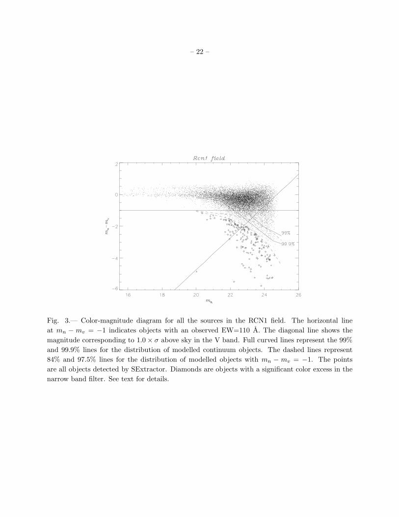
for which we have aperture and Kron magnitudes in [OIII] (mn) and V band (mv). Figure 3 shows

the color magnitude diagram (CMD) for the 18178 objects detected in our field. Most of them are

continuum objects with an average mn −mv color around 0. There is some intrinsic scatter in the

CMD, even with the two filters being so close in wavelength: the sequence of blue and red stars

can be seen in the magnitude interval mn = 16÷22. The scatter in the colors of continuum objects

at fainter magnitudes is caused by two factors: contaminations by line-emitters and background

field galaxies plus errors in the photometry for faint objects. Moreover most faint galaxies are red,

and scatter up in the diagram; we are interested in emission line objects whose color in mn −mv is

negative. ICPNe candidates are not the only emission line objects with this property. This color

criteriom will in principle select at least the following four different kinds of emission line objects:

ICPNe and HII regions in Virgo, [OII] λ = 3726.9 A emitters at z≈ 0.34, Lyα galaxies at z≈ 3.1.

The contamination from [OII] emitters can be greatly reduced by considering only objects with

observed equivalent width (EW) greater than 100 A. Colless et al. (1990), and recently Hammer

et al. (1997) and Hogg et al. (1998) found no [OII] emitters at z=0.35 with rest frame EW greater

than 70 A, which implies an observed EW of 95 A. Following Teplitz et al. (2000), if the emission

line is a negligible contribution to the broad band flux, as it is in this case, the observed equivalenth

width is

EWobs ∼ ∆λnb(100.4∆m

− 1) (4)

7For aperture photometry, we set a radius equal to 1.5′′ = 3σ, where σ = F WHM2.356

. If a detected source is point-like,

a 6σ diameter aperture contains 98.89% of the total flux.

– 10 –

where ∆λnb is the width of the narrow band filter in A. Objects with observed EW= 95A are

those with color mn − mv = −0.91: our emission line candidates will be selected according to the

condition mn − mv = −1.0 corresponding to an observed EW= 110A.

Due to the photometric errors at faint magnitudes, objects with intrinsic mn − mv < −1.0 do

not all fall above the corresponding straight line in the CMD. The scatter at faint magnitudes can

mimic emission line objects from faint continuum sources.

To determine the effects of these photometric errors quantitatively, we modelled a population

of point-like sources with intrinsic colors mn − mv = 0 and -1, and studied their distribution in

the CMD. The continuous lines over plotted in Figure 3 represent the 99% and 99.9% lines for a

distribution of modelled objects with color mn −mv = 0. Thus, above these lines will fall 99% and

99.9% of all continuum objects. The dashed lines in Figure 3 represent the 1×RMS and 2×RMS

lines of the color distribution for objects with mn −mv = −1. If the scatter of these objects in the

CMD plane is Gaussian, then 84% and 97.5% of these objects are located above these lines.

The “on-off” techniques for the identifications of ICPNe requires that there be no detected

emission in the off-band image, which therefore needs to reach to fainter limiting AB magnitude

to avoid contamination of our sample by faint continuum objects. The diagonal line in Figure 3

represents the V magnitude for fluxes corresponding to 1.0× σ above sky in the off-band. Objects

above this diagonal line display some emission in V. Objects whose mv fall below this line are not

detected by SExtractor8 on the off-band RCN1 image, with the selected low-threshold for detection.

Thus ICPNe candidates must be objects located in this region. SExtractor in dual image mode

cannot compute an mv magnitude (either mag(aper) or mag(auto)) for some of the [OIII] detected

sources: these sources will all be considered as emission line candidates.

4.1. Point-like and extended objects

The typical size of a PN is about 0.1−1 pc; therefore at the distance of the Virgo cluster (∼ 15

Mpc) they cannot be resolved on our images. Two methods were used to test whether an object

is extended or point-like: (1) a 2D Gaussian fit and comparison to the PSF and (2) comparison

between mag(auto) and mag(aper) magnitudes from SExtractor (see Section 3.1).

4.1.1. Point-like objects: 2D Gaussian fit

The stellar PSF for our images can be modelled with a two dimensional Gaussian. Twenty

un-saturated stars were selected in the narrow band image and a 2D Gaussian fit was produced

8Their magnitudes are computed from aperture photometry in a 3′′ diameter circular aperture at the positions of

the [OIII] sources.

– 11 –

with the task FITPSF within IRAF. Our emission line candidates are faint, and their fluxes in the

PSF wings looks as background noise; therefore we modeled the light distribution in our selected

emission line candidates using a 2D Gaussian. Those objects with σobject − σPSF >> 0 are most

probably extended objects, while those with σobject − σPSF ∼ 0 are most likely point like objects.

Because our candidates are faint, we need to test whether noise and small changes of the PSF

across the wide field can affect their light distribution in a systematic way. We simulated sources

with σobject = σPSF and [OIII] magnitude in the range from 20 to 25. These simulated objects

were added onto the narrow band image and a 2D Gaussian was fitted in the same way as for the

real objects. The results are shown in Figure 4; the dashed lines over plotted in the upper panel

of Figure 4 show the maximum and minimum value of σobject − σPSF in each mn magnitude bin

of 200 modelled objects. The range in σobject − σPSF is larger for fainter objects, where the noise

affects their 2D light distribution. Based on this simulation, point-like objects are those candidates

whose σobject − σPSF lies between the dashed lines in the upper panel of Figure 4. Those objects

whose σobject−σPSF happen to fall below the dashed-line curve, turned out to be bad pixels or have

cosmic-rays residual in the area influenced by the CCD gaps, where fewer frames were averaged,

and were not plotted. They were rejected in the final catalogue.

4.1.2. Point-like objects: magnitude selections

An independent test on whether a source is extended or not is based on the mag(auto)-

mag(aper) vs. mag(auto) diagrams for the detected sources. In our extraction procedure the

aperture magnitude mag(aper) is computed in a fixed aperture of diameter 1.5′′, equivalent to 3×σ

of the mean seeing measured on the image. The so-called mag(auto) is the same to 0.1 mag as

mag(aper) for point-like objects, while the two magnitudes differ for extended objects.

For the point-like objects modelled in our Monte-Carlo simulations, we studied the distribution

of mag(auto)−mag(aper) as a function of the object magnitude mag(auto). This is shown in the

lower panel of Figure 4. As in the case of the 2D Gaussian fit, for bright point-like objects this

difference is fixed and at faint magnitudes we have a larger spread because of photometric errors.

Point-like objects are those which lie between the dashed lines of Figure 4.

The final set of point-like objects in our extracted catalogue is selected as those which satisfy

both criteria: a 2D Gaussian fit which is consistent with the PSF, and mag(auto)-mag(aper) inside

the distribution for simulated point sources. This is a necessary condition for our selected objects

to be selected as point-like, but it is not sufficient, i.e. high redshift starbursts with a strongly

peaked central luminosity may still get into our sample.

– 12 –

4.2. Spectroscopic confirmation

For spectroscopic validation, we use a sample of spectra obtained with the 2dF fiber spectrom-

eter at the 4 m Anglo Australian Telescope by Freeman et al. (2000; 2001, in prep.). Spectra were

acquired with a spectral resolution R=2000 in the wavelength range 4550 A to 5650 A and a total

integration time of 5 hrs on the 15th of March 1999.

A total of 43 fibers were allocated to the narrow-line emitter candidates selected by Feldmeier

et al. 1998 at coordinate α(J2000) = 12 : 30 : 39 and δ(J2000) = 12 : 38 : 10; we will refer to this

field as the FCJ field. In this field, 15 objects were spectroscopically confirmed as emission line

objects. The best S/N spectra of the ICPNe candidates in the FCJ field are shown in Figure 5.

As a further test on the intrinsic nature of these objects, 23 spectra of ICPNe candidate from

the whole area in Virgo surveyed with the 2dF (see Freeman et al. 2000 for additional details),

were summed: these 23 objects include the 15 from the FCJ field and another 8 from other Virgo

intracluster empty fields. The cumulative spectrum shows the [OIII] doublet very clearly, with

the expected equivalent width ratio EW5007 = 3 × EW4959 for the [OIII] doublet (see Figure 5).

Of the 15 spectroscopically confirmed objects in the FCJ field, 13 are ICPNe and 2 are broad-

lined Lyα emitters. The broad-lined sources were identified as Lyα by Freeman et al. (2000) and

Kudritzki et al. (2000) because of their typical asymmetric line-profile; furthermore in Kudritzki et

al. (2000) no Hβ and [OIII] emissions were detected at the expected redshifted wavelengths, under

the hyphothesis that the strongest emission was [OII] at redshift 0.35.

These observations show that a significant fraction of emission line candidates selected carefully

with the “on-off” band technique are indeed ICPNe. They were used to make the first kinematical

study of the ICPNe population in Virgo. These issues will be discussed by Freeman et al. (2001,

in preparation). Here these objects are used for validation of the automatic selection procedure.

Validation of the selection procedure To compare our photometric selection of emission line

objects with the spectroscopic confirmations, we have applied our selection procedure to the “on-

off” images for the FCJ field. The survey on the FCJ field was carried out with a 44 A narrow

band [OIII] filter, with central wavelength at λc = 5027 A9. Of the 43 emission line candidates in

FCJ selected with the blinking technique and allocated a fiber in the spectroscopic follow-up, we

could detect and measure narrow band magnitudes in the images for 36 of them. The remaining

7 objects were very near to bright objects and were therefore discarded because of likely errors

in the SExtractor photometry. Of these 7 objects, 4 were spectroscopically confirmed (3 ICPNe

+ one Lyα). In the following, we discuss the percentage of spectroscopically confirmed objects in

the sample of 36 objects with allocated fiber which are in common with our selected sample. In

this sample, 11 objects (i.e. 30%) are spectroscopically confirmed as emission line objects; of these

objects 10 are confirmed ICPNe and one is a Lyα candidate.

9The conversion from mAB to m5007 for this filter is m5007 = mAB + 3.04.

– 13 –

In Figure 6 we show the CMD for all sources in this field. Squares indicate those sources in

common with Feldmeier’s catalogue of emission line objects with an allocated fiber, while asterisks

indicate those ICPNe candidates with confirmed spectra; the Lyα is indicated with a full square.

The lines plotted in Figure 6 have the same meaning as in Figure 3. For 16 out of the 36 allocated

fiber, SExtractor could not detect a mv magnitude at the x, y position of the [OIII] detected

emission. All these objects would be selected and are reported on this diagram assuming a mv=2710.

Two out of the 10 confirmed ICPNe were in the region of the frame with bright scattered light

from nearby luminous objects. So their V magnitude appear above the detection limit, because of

scattered background light. The 8 out of the 10 confirmed ICPNe and the Lyα emitter are found

• below the line for detection in the off-filter,

• below the 97.5% line of objects with colour= −111.

• or in the sample with no detected off-band mag(aper), when SExtractor is used in dual image

mode.

The sample selected according to these criteria has a higher spectroscopic confirmation rate, 50%,

compared to the Feldmeier’s sample for the FCJ field, i.e. 30%. The part of the 36 objects which

do not satisfy the above criteria have a much lower spectroscopic confirmation rate: 2/18 = 10%.

These percentages are lower limits because, as Fig 5 shows, they are based on low signal-to-noise

spectra.

We also ran the morphological selection procedure on the spectroscopically confirmed emission

line objects, which are in common with our photometrically selected sample. Eight objects which

showed an unresolved [OIII] λ5007A emission and the additional λ4959A line are point-like sources.

These are the confirmed ICPNe. One object which is spectroscopically confirmed as an emission

line object with a broad asymmetric emission line (see Figure 5) is classified as extended, and it is

probably a Lyα emitter.

Based on the spectroscopically confirmed sample, our selection criteria for Bona Fide ICPNe

candidates are the following: these must be point-like objects lying below the 97.5% line for intrinsic

color mn − mv < −1, and with no detection in the off-band (V) image. This is the population of

objects that we discuss hereafter in the RCN1 field. From Figure 4, we found 75 point-like objects

with those characteristics. These are the ICPNe candidate in our RCN1 field.

10Here we adopted the V magnitude that a star would have if the flux from a [OIII] emission of mAB = 24.5 would

have been seen through a V band filter

11For the FCJ filter, this corresponds to an EW∼ 70A.

– 14 –

5. The Virgo cluster ICPNe

The observations presented in this work allow us to obtain a large statistical sample of IPNe

candidates in the RCN1 field. Using also the data from the FCJ field, we can make a preliminary

study of their distribution on the sky.

5.1. Luminosity function and cluster depth

The PNLF has been used extensively as a distance indicator. Observations in ellipticals, spirals

and irregular galaxies have shown a PNLF truncated at the bright end. The shape of this LF is

given by the semi-empirical fit:

N(M) = c1ec2M [1 − e3(M∗−M)] (5)

where c1 is a positive constant, c2 = 0.307 and the cut-off M∗(5007) = −4.5 (Ciardullo et al. 1989).

The evidence for a bright cut-off comes from the observations of nearby galaxies, and its de-

pendence on the age and metallicity of the stellar population was analysed in some detail by

(Dopita et al. 1992; Mendez et al. 1993). Its overall metallicity dependence seems to be modest

provided that the metallicity differences are no more than about 30%, but see also Mendez et al.

(1993) for an elaborate discussion of the effects of sample size and population age.

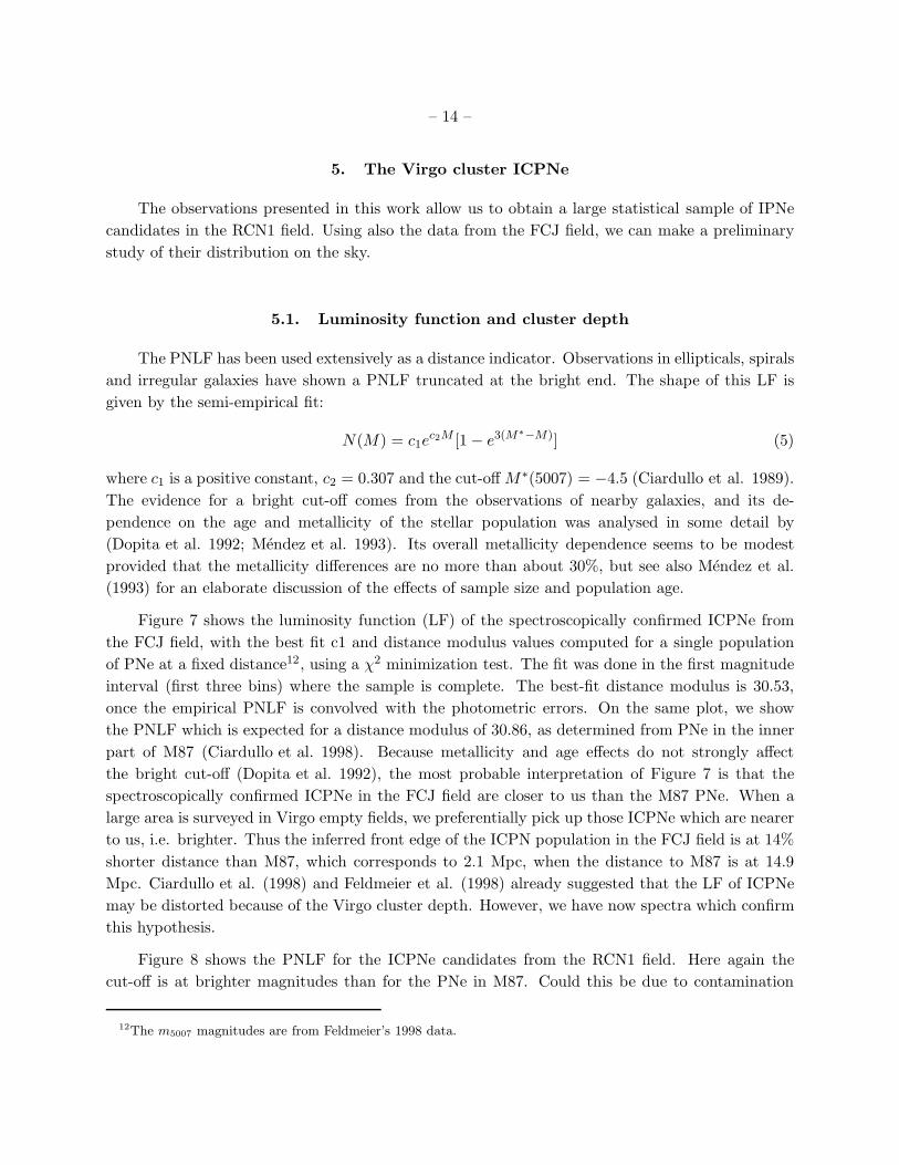
Figure 7 shows the luminosity function (LF) of the spectroscopically confirmed ICPNe from

the FCJ field, with the best fit c1 and distance modulus values computed for a single population

of PNe at a fixed distance12, using a χ2 minimization test. The fit was done in the first magnitude

interval (first three bins) where the sample is complete. The best-fit distance modulus is 30.53,

once the empirical PNLF is convolved with the photometric errors. On the same plot, we show

the PNLF which is expected for a distance modulus of 30.86, as determined from PNe in the inner

part of M87 (Ciardullo et al. 1998). Because metallicity and age effects do not strongly affect

the bright cut-off (Dopita et al. 1992), the most probable interpretation of Figure 7 is that the

spectroscopically confirmed ICPNe in the FCJ field are closer to us than the M87 PNe. When a

large area is surveyed in Virgo empty fields, we preferentially pick up those ICPNe which are nearer

to us, i.e. brighter. Thus the inferred front edge of the ICPN population in the FCJ field is at 14%

shorter distance than M87, which corresponds to 2.1 Mpc, when the distance to M87 is at 14.9

Mpc. Ciardullo et al. (1998) and Feldmeier et al. (1998) already suggested that the LF of ICPNe

may be distorted because of the Virgo cluster depth. However, we have now spectra which confirm

this hypothesis.

Figure 8 shows the PNLF for the ICPNe candidates from the RCN1 field. Here again the

cut-off is at brighter magnitudes than for the PNe in M87. Could this be due to contamination

12The m5007 magnitudes are from Feldmeier’s 1998 data.

– 15 –

by Lyα emitting objects at z ∼ 3.13, which are also picked up by our technique? There is no

well-sampled Lyα LF of such objects available in the literature. We have therefore estimated the

LF of Lyα emitters in our sample from the work of Steidel et al. (2000). These authors showed that

the continuum LFs of Lyα emission selected galaxies and of field Lyman break galaxies (LBGs)

are consistent with being the same, and that there is no evidence for enhanced Lyα emission from

fainter galaxies. The equivalent width (EW) distribution of their spectroscopic sample is consistent

with being a Gaussian centered at zero, such that the fraction of objects with EW> 80A (restframe

EW> 20A) is ≃ 25%. We can thus estimate the narrow band magnitude LF of Lyα emitters in

our on-band filter as follows. We take the LF of field LBGs from Steidel et al. (1999) with the

parameters given in their Fig. 8 except mV∗ = mR

∗ + 0.24 (as LBGs have about 20% fainter flux

density in V than in R; M. Giavalisco, private communication). We then apply the same selection

criteria to those sources as to our ICPNe candidates, that mV = 24.75, and finally convolve with the

EW distribution for the Lyα emission, accepting only those galaxies with an observed EW> 110A

which correspond to our sample selection criteria. The resulting LF, scaled to our larger field and

effective volume, is shown as the full line in Fig. 8.

We have also added the observed data points constructed from the Lyα blank field search done

by Cowie & Hu (1998), as this survey is carried out in a very similar way to our survey for ICPNe

in the Virgo cluster fields. We used their V magnitudes and EWs listed in their Table 1 for those

objects whose V magnitudes are fainter then 24.75, and then converted to our filter AB magnitudes.

Once the resulting LF is scaled to our larger field, the Cowie & Hu (1998) narrow band LF for the

Lyα emitters agrees very well with that computed from Steidel et al. (2000). The comparison of

the candidate ICPNe LF in the RCN1 field with the computed narrow band LF of the field Lyα

emitters from Steidel et al. (2000) and Cowie & Hu (1998) show that the Lyα contribution does not

dominate in the narrow band AB magnitude range 23-24: the fraction of expected contamination

by Lyα emitters with V magnitude fainter of 24.75 in the first magnitude bin is 15%. This is in

agreement (within the errors) with the fraction of Lyα contaminants of 25%, as obtained from the

spectroscopic sample

Therefore most over-luminous bright objects in the RCN1 are likely to be ICPNe, and they are

brighter than those at the cut-off in the M87 PNLF because they too are closer to us than M87.

Once we have convolved the empirical PNLF given by Equation 5 with the photometric error of

our sample, we fit the data point of RCN1 LF and obtain the best fit distance modulus of 30.29

with the following errors +0.2−0.2, which refers to the 90% c.l.. Our estimate of the distance modulus

is slightly biased from the contribution of the [OIII] emission at 4958.9 A which enters in our filter

band pass for radial velocities vrad > 1580 km s−1. We have estimated this systematic contribution

assuming a Gaussian velocity distribution for the ICPNe in Virgo (with vmean = 1100 km s−1 and

σ = 800 km s−1). This gives a maximal brightening of the PNLF of 0.13 mag, assuming that most

ICPNe at the front edge of the cluster have the same velocity dispersion as galaxies in Virgo. If this

systematic brightening is taken into account, the distance modulus to the front edge of the Virgo

cluster is 30.4±0.2 at RCN1, in agreement with the distance modulus derived for the spectroscopic

– 16 –

sample, within the photometric errors. This implies that the front edge population seen in the

RCN1 Virgo field is at 19% shorter distance than M87, i.e. 2.8 Mpc in front of the cluster center.

The Virgo cluster appears to have a significant depth.

Previously, Yasuda et al. (1997) have argued that the distribution of spiral galaxies in Virgo

is best described as an elongated, cigar-like structure with a depth ±4 Mpc from M87. Neilsen

& Tsvetanov (2000) and West & Blakeslee (2000) have used surface brightness fluctuations to

determine the distances to the Virgo ellipticals, and found that most of these are arranged in a

nearly collinear structure extending about ±(2− 3) Mpc from M87. Therefore our result from the

ICPNe population is not entirely surprising.

5.2. Luminosity surface density

From our results we can determine a surface brightness associated with the diffuse population

of evolved stars in the FCJ and the RCN1 fields. Given our tight selection criteria in the photo-

metric analysis and the likely incompleteness of the 2dF detections, this will in both fields be a

lower limit. From stellar evolution theory, it is expected that the luminosity-specific stellar death

rate of a galaxy should be independent of the precise state of the underlying stellar population.

(Renzini & Buzzoni 1986) have shown that this quantity is remarkably independent of both age

and initial mass function: if this is the case, the number density of planetaries per unit bolometric

luminosity should be approximately the same for every galaxy. Here we adopt the luminosity-

specific planetary nebulae density from M31, α1,B = 9.4 × 10−9 PNe L−1B⊙

(Ciardullo et al. 1989)

to infer the amount of light associated with the ICPNe.13 For the spectroscopically confirmed

sample in the FCJ field, the inferred luminosity surface density is 5.2 × 106 LB⊙arcmin−2, corre-

sponding to ≃ 0.28 LB⊙ pc−2 at a distance of ≃ 15 Mpc. For the RCN1 field, we have a sample

of 75 candidates. From the spectroscopic follow-up by Freeman et al. (2000) the contamination by

high redshift objects can still be up to 25%, and the possibility of large-scale structures in the Lyα

emitters implies some uncertainties in a simple statistical subtraction for ICPN measurements. Re-

moving 25% of our sources gives a likely lower limit to the surface luminosity density of the ICPNe

population. Thus we take the number of ICPNe in this field to be 56, which on an area of 31.8×30.1

arcmin2 amounts to a luminosity surface density of 6.2 × 106LB⊙arcmin−2, which corresponds to

≃ 0.33LB⊙pc−2, similar to that for the spectroscopically selected sample. The inferred blue surface

brightness is µB = 28 mB arcsec−2. The inferred luminosity derived assuming all the sample at a

single distance gives the smallest amount of intracluster light: from Feldmeier et al. (1998), if the

ICPN were spherically distributed with a constant density, the amount of starlight could be up to

a factor of three larger.

13The most appropriate value of α1,B for the intracluster light is unknown at this stage, therefore we adopted

the α1,B for the bulge of M31, which is an evolved population similar to those in early-type galaxies. Independent

measurements of α1,B in ellipticals shows a variation up to a factor 5.

– 17 –

The result that the inferred intracluster surface brightnesses for both fields are similar is robust

and very interesting, because the FCJ field is 45′ from the center of the cluster core, while the RCN1

field is 1.5 deg from the center. The azimuthally averaged total luminosity density contributed by

galaxies is given by Binggeli et al. (1987) as a function of distance to the core center. This function

has a large scatter (see Figure 16 (Binggeli et al. 1987)), and implies ∼ 1011 LB⊙ deg−2 at the FCJ

distance (45′) and ∼ 3 · 1010 LB⊙ deg−2 at the RCN1 distance (1.5 deg).

Over the range of radii probed by these two fields, the luminosity surface density of galaxies

in Virgo decreases by a factor of ∼ 3 (Binggeli et al. 1987) while that for the ICPNe population

is nearly constant. The diffuse light contributes from 17% (FCJ) to 43% (RCN1) of the total (i.e.

galaxies + diffuse light) luminosity density in these two fields (recall that these numbers are lower

limits from our data). Because we have no evidence for a radial gradient in the ICPNe luminosity

profile, it is very difficult to estimate the total luminosity for this population at this stage.

6. Conclusions

We have imaged an empty area of 34× 34 arcmin2 in the Virgo cluster in a narrow band filter

centred at the redshifted Virgo [OIII] emission and in the V band. The area surveyed in this work is

the largest probed for ICPNe in one single pointing so far, and it allows us to get a better statistical

sample of ICPNe. We have developed an automatic extraction procedure for ICPNe candidates

using publicly available photometry software (SExtractor). This selection procedure was validated

using a spectroscopic confirmed sample of ICPNe. In our field 75 objects were found which satisfy

the selection criteria for ICPNe, i.e., point-like, no measurable continuum, and equivalent width

EW > 110A after error convolution.

The luminosity functions for both the spectroscopically selected sample and the ICPNe sample

in the new field show a brighter cut-off compared to the M87 PNe. We have evaluated the possible

contribution of Lyα emitting objects at redshift z = 3.13 from Steidel et al. (2000) and found that

these objects contribute mostly at 1-2 magnitudes fainter than the bright cutoff found here, and in

any case only up to 25% of the total sample. The bright cutoff is therefore most probably due to

the three-dimensional depth of the Virgo cluster: our results place it at 14% - 19% shorter distance

than M87. Our selected sample traces preferentially the edge of the cluster near us.

The luminosity surface density in these two fields is about 6 × 106LB⊙ arcmin−2 with both

fields having similar densities. The lack of radial gradient between both fields implies that the total

amount of luminosity in the diffuse component is very sensitive to the outer cut-off, and could be

comparable to the luminosity in galaxies.

The authors wish to thank the referee, Dr. R. Ciardullo, for his insightful comments. Moreover

we would like to thank the ESO 2.2m telescope team for their help and support during the observa-

tions carried out for this project, in particular E. Pompei and H. Jones. We thank F. Valdes for his

– 18 –

help and support in using MSCRED in reducing WFI mosaic data, the OACDF team for support

during astrometry and co-addition, and E. Bertin for his help and suggestions in using SExtractor.

The authors acknowledge the use of NED and the CDS public catalogues. JALA and OG were

supported by the grant 20-56888.99 from the Schweizerischer Nationalfonds. NRN was supported

by the European Social Funds and acknowledges the support from the University Federico II for

travel grants within the program for International Exchange.

A. m(5007) and the AB magnitude system

Absolute flux calibrations for our narrow band imaging (with an interference filter centred

on the [OIII] redshifted wavelength at the Virgo systemic velocity) were performed according to

Jacoby et al. (1987). These calibrations give us the total flux in the [OIII] line in ergs sec−1 cm−2,

which we indicate as F5007. Following Jacoby (1989), the m(5007) magnitudes are defined as:

m(5007) = −2.5 log F5007 − 13.74

The magnitude in the AB system are given by:

mAB = −2.5(log Fν + 19.436)

and we can rewrite mAB as function of m(5007) as follows:

mAB = −2.5 log F5007 − 2.5 log

(

λ2c

∆λeffc

)

− 48.59 = m(5007) − 2.51

where

∆λeff =

∫

dλT (λ),

λc is the filter central wavelength, and T (λ) is the filter bandpass.

– 19 –

REFERENCES

Arnaboldi, M., et al. 1996, ApJ, 472, 145

Bernstein, G.M. et al. 1995, AJ, 110, 1507

Bertin, E. & Arnouts, S. 1996, A&AS 117, 3993

Binggeli, B., Tammann, G.A., Sandage, A. 1987, AJ, 94, 251

Calcaneo-Roldan, C., Moore, B., Bland-Hawthorn, J., Malin, D., Sadler, E.M. 2000, MNRAS, 314,

324

Capaccioli, M., et al. 2001, A&A, submitted

Ciardullo, R., Jacoby, G.H., Ford, H.C., Neill, J.D. 1989, ApJ, 339, 53

Ciardullo, R., Jacoby, G.H., Feldmeier, J.J., Barlett, R. 1998, ApJ, 492, 62

Colless, M., Ellis, R.S., Taylor, K., Hook, R.N. 1990, MNRAS 244, 408

Cowie, L.L., & Hu, E.M. 1998, AJ, 115, 1319

Crane, P., Tammann, G.A., Woltjer, L. 1977, Nature, 265, 124

Dopita, M.A., Jacoby, G.H., Vassiliadis, E. 1992, ApJ, 389, 27

Durrell, P., Ciardullo, R., Feldmeier, J., Jacoby, G.H. 2001, ApJ, submitted

Feldmeier, J.J., Ciardullo, R., Jacoby, G.H. 1998, ApJ, 503, 109

Feldmeier, J.J. 2000, Ph D. Thesis, Penn State University

Ferguson, H., Tanvir, N.R., von Hippel, T. 1998, Nature, 391, 461

Freeman, K.C., et al. 2000, ASP Conf. Series 197, 389

Hammer, F., et al. 1997, ApJ, 481, 49

Hogg, D.W., Cohen, J. G., Blandford, R., Pahre, M. A. 1998, ApJ, 504, 622

Hui, X., Ford, H.C., Ciardullo, R., Jacoby, G.H. 1993, ApJ414, 463

Guldheus, D.H. 1989, ApJ, 340, 661

Kron, R.G. 1980, ApJ343, 305

Kudritzki, R.P., et al. 2000, ApJ536, 19

Jacoby, G.H., Quigley, R.J., & Africano, J.L. 1987, PASP, 99, 672

– 20 –

Fig. 1.— Monte Carlo simulations carried out for a modelled population of point-like objects. Left

panels: the luminosity function adopted for the modelled objects (continuous line) and the recovered

luminosity function (triangles-mag(auto) and diamonds-mag(aper)). Central panels: Percentage of

modelled point-like objects recovered for the different detection thresholds used. The dotted line

at 50% marks the completeness limit. Right panels: Percentage of the modelled point-like objects

(continuous line) and of spurious objects (dashed line) normalised to the total extracted object

catalogue in 0.25 magnitude bins.

– 21 –

Fig. 2.— Ratios of spurious to real detections plotted as a function of limiting magnitude for

different low thresholds.

– 22 –

Fig. 3.— Color-magnitude diagram for all the sources in the RCN1 field. The horizontal line

at mn − mv = −1 indicates objects with an observed EW=110 A. The diagonal line shows the

magnitude corresponding to 1.0 × σ above sky in the V band. Full curved lines represent the 99%

and 99.9% lines for the distribution of modelled continuum objects. The dashed lines represent

84% and 97.5% lines for the distribution of modelled objects with mn − mv = −1. The points

are all objects detected by SExtractor. Diamonds are objects with a significant color excess in the

narrow band filter. See text for details.

– 23 –

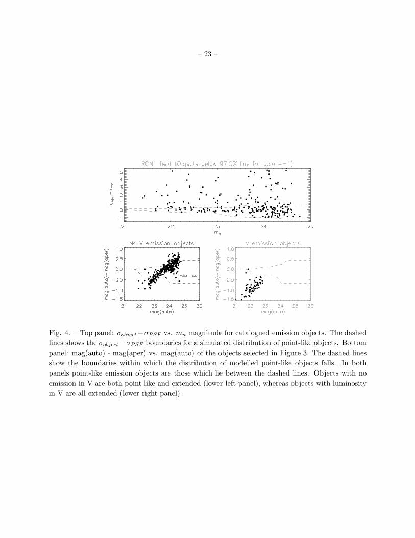
Fig. 4.— Top panel: σobject−σPSF vs. mn magnitude for catalogued emission objects. The dashed

lines shows the σobject−σPSF boundaries for a simulated distribution of point-like objects. Bottom

panel: mag(auto) - mag(aper) vs. mag(auto) of the objects selected in Figure 3. The dashed lines

show the boundaries within which the distribution of modelled point-like objects falls. In both

panels point-like emission objects are those which lie between the dashed lines. Objects with no

emission in V are both point-like and extended (lower left panel), whereas objects with luminosity

in V are all extended (lower right panel).

– 24 –

λ500

7λ5

007

λ495

9

λ500

7

λ495

9λ4

959

Fig. 5.— Top row: spectra of two ICPNe candidate from the AAT 2dF run. The 5007 A line is

visible with S/N > 3 and a second line at 4959 A corresponds to the second emission line of the

[OIII] doublet. Lower left corner: cumulative spectrum of all 23 ICPNe from the 2dF run. Each

spectrum was shifted to zero velocity and normalized by the flux in the 5007 A [OIII] line. The

equivalenth width ratio of the [OIII] 5007A / 4959 A is 3.2 ± 0.1, so the real fraction of ICPNe in

this sample is 0.94 ± 0.03 (Freeman et al. 2000, 2001 in preparation). Lower right corner: the 2dF

spectrum of a likely Lyα emitter. The asymmetric profile of the line is clearly visible.

– 25 –

Fig. 6.— Color magnitude diagrams for the FCJ and the RCN1 fields. Upper panel: CMD for

the FCJ field. The lines have the same meaning as in Figure 3. The diagonal line correspond to

mv = 24.75. which is the 1.0 × σ limiting magnitude in the V band. The over-plotted squares

represent the allocated fibers of Freeman et al. (2000, 2001, in prep.) and the asterisks are the

spectroscopically confirmed ICPNe. The full square represents a spectroscopically confirmed Lyα

emitter located in this field. See text for details . Two spectroscopically confirmed PNe have

off band fluxes near the limiting magnitude because of scattered light from bright emitters in the

field. Fourteen objects in the Feldmeier et al. (1998) catalogue have no computed mag(aper) in

the off-band, assigned by SExtractor in dual image mode: they have been assigned mv = 27.0 (see

text). Lower panel: CMD for the RCN1 field. The ICPNe candidates are indicated with asterisks;

those objects with no computed mag(aper) in the off-band, using SExtractor in dual image mode,

have been assigned mv = 27.0.

– 26 –

Fig. 7.— Luminosity function of the spectroscopically confirmed ICPNe from FCJ field. The

continuous line is the best fit for a distance modulus equal to 30.53. The dashed lines indicates the

same PNLF for the distance modulus 30.86 assigned to M87 using the PNLF within 20 arcmin of

M87.

– 27 –

Fig. 8.— Luminosity function of the ICPNe sample selected in the RCN1 field. The dashed line

shows the PNLF for a distance modulus of 30.29, convolved with the photometric errors. On the

same plot the continuos line shows the expected LF in our narrow filter for the Lyα population in

the field at redshift z= 3.13 from Steidel et al. (2000), see discussion in the text. The faint dotted

line shows the expected contribution from the Lyα emitters with V magnitudes brigther than 24.75.

Full dots indicate the LF in our narrow band filter from Lyα emitters in the blank-field survey by

Cowie & Hu (1998).

– 28 –

Jacoby, G.H. 1989, ApJ, 339, 39

Jacoby, G., Ciardullo, R, Ford, H. 1990, ApJ, 356, 332

McMillan, R., Ciardullo, R., Jacoby, G.H. 1993, ApJ, 416, 62

Melnick, J., White, S.D.M., Hoessel, J. 1977, MNRAS, 180, 207

Mendez, R.H., Kudritzki, R.P., Ciardullo, R., Jacoby, G.H. 1993, A&A , 275, 534

Mendez, R.H. et al. 1997, ApJ, 491, L23

Mendez, R.H., Riffeser, A., Kudritzki, R.P. et al. 2001, ApJ, in press

Neilsen, E.H., Tsvetanov, Z.I. 2000, ApJ, 536, 255

Oke, J.B. 1990, AJ, 99, 1621

Pierce, M., Tully, R.B. 1988, ApJ, 330, 579

Renzini, A., Buzzoni, A. 1986, in Spectral Evolution of Galaxies, ed. C. Chiosi and A. Renzini

(Dordrecht:Reidel), 195

Smith, H.A. 1981, AJ 86, 998

Steidel, C.C., Adelberger, K.L., Giavalisco, M., Dickinson, M., Pettini, M. 1999, ApJ, 519, 1

Steidel, C.C., Adelberger, K.L., Shapley, A.E., Pettini, M., Dickinson, M., Giavalisco, M. 2000,

ApJ, 532, 170

Teplitz, H.I. et al. 2000, ApJ, 542, 18

Theuns, T., Warren, S. 1997, MNRAS, 284, L11

Thuan, T.X., Kormendy, J. 1977, PASP, 89, 466

Tonry, J.L., Ajhar, E.A., Luppino, G.A. 1990, AJ, 100, 1416

Uson, J.M., Boughn, S.P., Kuhn, J.R. 1991, ApJ, 369, 46

Vilchez-Gomez, R. Pello, R., Sanahujia, B. 1994, A&A, 283, 37

Welch, G.A., Sastry, G.N. 1971, ApJ, 169, 13

West, M.J., Blakeslee, J.P. 2000, ApJ, 543, L27

Yasuda, N., Fukugita, M., Okamura, S. 1997, ApJSS, 108, 417

Zwicky, F. 1951, PASP, 63, 61

This preprint was prepared with the AAS LATEX macros v5.0.

– 29 –

Table 1. Number of modelled point-like objects and spurious detections recovered from

simulations.

LOWTHRESHOLD Point-like objects Spurious detections

0.7 σ 680 1001

0.8 σ 567 237

0.9 σ 478 66

1.0 σ 410 30

1.1 σ 362 16

1.2 σ 310 11