
Fitting Isochrones to Open Cluster photometric data: A new global optimization tool
19
arXiv:1003.4230v1 [astro-ph.IM] 22 Mar 2010 Astronomy & Astrophysics manuscript no. monteiro c ESO 2010 March 23, 2010 Fitting Isochrones to Open Cluster photometric data A new global optimization tool H. Monteiro ⋆ , W. S. Dias and T. C. Caetano UNIFEI, DFQ - Instituto de Ciˆ encias Exatas, Universidade Federal de Itajub´ a, Itajub´ a MG, Brazil ABSTRACT We present a new technique to fit color-magnitude diagrams of open clusters based on the Cross-Entropy global optimization al- gorithm. The method uses theoretical isochrones available in the literature and maximizes a weighted likelihood function based on distances measured in the color-magnitude space. The weights are obtained through a non parametric technique that takes into account the star distance to the observed center of the cluster, observed magnitude uncertainties, the stellar density profile of the cluster among others. The parameters determined simultaneously are distance, reddening, age and metallicity. The method takes binary fraction into account and uses a Monte-Carlo approach to obtain uncertainties on the determined parameters for the cluster by running the fitting algorithm many times with a re-sampled data set through a bootstrapping procedure. We present results for 9 well studied open clus- ters, based on 15 distinct data sets, and show that the results are consistent with previous studies. The method is shown to be reliable and free of the subjectivity of most previous visual isochrone fitting techniques. Key words. open clusters and associations: general. 1. Introduction Galactic open clusters are a key class of objects used in a wide range of investigations due to their wide span of ages and dis- tances as well as the precision to which these parameters can be determined through their color-magnitude diagrams (CMD). With the publication of the Hipparcos Catalog (ESA 1997) and its derivatives the Tycho and Tycho2 (Perryman & ESA 1997; Høg et al. 2000) as well as individual efforts using modern ground based instrumentation there has been increased interest in studies involving open clusters in the Galaxy. Individually the results obtained from the study of open clus- ters can provide important constraints for theoretical models of stellar formation and evolution. Comparison of observed CMDs to model isochrones can provide important information on the effect of overshooting VandenBerg & Stetson (2004) and chem- ical abundances Meynet et al. (1993); Kassis et al. (1997). Open clusters can also be used in the study of variable stars, espe- cially Cepheids (Kang et al. (2008); Majaess et al. (2009)), in the search for connections between stellar magnetic fields and their evolution and in the search for extra-terrestrial planets, among many others. Our group has focused efforts in the investigation of open clusters and their use in the understanding of the Galactic spiral structure (Dias & L´ epine (2005); L´ epine et al. (2008)). The re- sults are based on the catalog of open clusters published in Dias et al. (2002) witch is now in version 2.10 and, since 2002, can be accessed on line at http://www.astro.iag.usp.br/∼wilton. The results presented in our catalog are compiled from data published from many authors, using different instruments, tech- niques, calibrations and criteria which results in a heterogeneous sample. However, in Paunzen & Netopil (2006), the authors show that our data has the same statistical significance as the ⋆ E-mail: [email protected] data they use to define the standard parameters of the chosen open clusters when considering the calculated errors. To derive the fundamental parameters of open clusters the main sequence “fitting” in most works up to today has been done mostly with subjective visual fitting. This is mainly due to the fact that the isochrones have no simple parametric form so that a usual least square technique can be applied. The avail- able isochrones in the literature are usually in the form of tabu- lated points for a set of fundamental parameters such as age and metallicity. The traditional “fitting” method utilized is to first de- termine the reddening by adjusting a Zero Age Main Sequence (ZAMS) to the observed color-color diagram (usually ( B − V ) vs. (U − B) of the cluster and then, keeping this value fixed, adjust- ing the distance and age using the observed CMD and tabulated isochrones. Both of these steps are usually performed by eye as mentioned, leading to inevitable subjectivity in the fitting of an isochrone to a given observed CMD. The subjectivity in the determination of the reddening is specially problematic since it affects the subsequent determination of the distance and age of the cluster. It is also important to point out that in some cases the reddening is not determined through the use of U filter photom- etry which can further compromise the results obtained. The lack of homogenization of the data and especially the subjectivity of the methods used to obtain fundamental param- eters of clusters from their CMD indicate the great need for a method that circumvents at least the subjectivity. The subject of automatic fitting and non subjective criteria to choose the best fit was addressed in some papers such the recently published work by Naylor & Jeffries (2006), where the authors propose a maximum likelihood method for fitting two dimensional model distributions to stellar data in a CMD. In this work the authors also discuss the most important attempts at performing isochrone fits using different methods and we refer the reader to their very complete discussion and references therein. The authors also present the main problems involved in this kind of study, as 1
-
Upload
independent -
Category
Documents
-
view
2 -
download
0
Transcript of Fitting Isochrones to Open Cluster photometric data: A new global optimization tool
arX
iv:1
003.
4230
v1 [
astr
o-ph
.IM]
22 M
ar 2
010
Astronomy & Astrophysicsmanuscript no. monteiro c© ESO 2010March 23, 2010
Fitting Isochrones to Open Cluster photometric dataA new global optimization tool
H. Monteiro⋆, W. S. Dias and T. C. Caetano
UNIFEI, DFQ - Instituto de Ciencias Exatas, Universidade Federal de Itajuba, Itajuba MG, Brazil
ABSTRACT
We present a new technique to fit color-magnitude diagrams ofopen clusters based on the Cross-Entropy global optimization al-gorithm. The method uses theoretical isochrones availablein the literature and maximizes a weighted likelihood function based ondistances measured in the color-magnitude space. The weights are obtained through a non parametric technique that takes into accountthe star distance to the observed center of the cluster, observed magnitude uncertainties, the stellar density profile of the cluster amongothers. The parameters determined simultaneously are distance, reddening, age and metallicity. The method takes binary fraction intoaccount and uses a Monte-Carlo approach to obtain uncertainties on the determined parameters for the cluster by runningthe fittingalgorithm many times with a re-sampled data set through a bootstrapping procedure. We present results for 9 well studiedopen clus-ters, based on 15 distinct data sets, and show that the results are consistent with previous studies. The method is shown to be reliableand free of the subjectivity of most previous visual isochrone fitting techniques.
Key words. open clusters and associations: general.
1. Introduction
Galactic open clusters are a key class of objects used in a widerange of investigations due to their wide span of ages and dis-tances as well as the precision to which these parameters canbe determined through their color-magnitude diagrams (CMD).With the publication of the Hipparcos Catalog (ESA 1997) andits derivatives the Tycho and Tycho2 (Perryman & ESA 1997;Høg et al. 2000) as well as individual efforts using modernground based instrumentation there has been increased interestin studies involving open clusters in the Galaxy.
Individually the results obtained from the study of open clus-ters can provide important constraints for theoretical models ofstellar formation and evolution. Comparison of observed CMDsto model isochrones can provide important information on theeffect of overshooting VandenBerg & Stetson (2004) and chem-ical abundances Meynet et al. (1993); Kassis et al. (1997). Openclusters can also be used in the study of variable stars, espe-cially Cepheids (Kang et al. (2008); Majaess et al. (2009)),in thesearch for connections between stellar magnetic fields and theirevolution and in the search for extra-terrestrial planets,amongmany others.
Our group has focused efforts in the investigation of openclusters and their use in the understanding of the Galactic spiralstructure (Dias & Lepine (2005); Lepine et al. (2008)). The re-sults are based on the catalog of open clusters published in Diaset al. (2002) witch is now in version 2.10 and, since 2002, canbe accessed on line at http://www.astro.iag.usp.br/∼wilton.
The results presented in our catalog are compiled from datapublished from many authors, using different instruments, tech-niques, calibrations and criteria which results in a heterogeneoussample. However, in Paunzen & Netopil (2006), the authorsshow that our data has the same statistical significance as the
⋆ E-mail: [email protected]
data they use to define the standard parameters of the chosenopen clusters when considering the calculated errors.
To derive the fundamental parameters of open clusters themain sequence “fitting” in most works up to today has beendone mostly with subjective visual fitting. This is mainly dueto the fact that the isochrones have no simple parametric formso that a usual least square technique can be applied. The avail-able isochrones in the literature are usually in the form of tabu-lated points for a set of fundamental parameters such as age andmetallicity. The traditional “fitting” method utilized is to first de-termine the reddening by adjusting a Zero Age Main Sequence(ZAMS) to the observed color-color diagram (usually (B−V) vs.(U − B) of the cluster and then, keeping this value fixed, adjust-ing the distance and age using the observed CMD and tabulatedisochrones. Both of these steps are usually performed by eyeas mentioned, leading to inevitable subjectivity in the fitting ofan isochrone to a given observed CMD. The subjectivity in thedetermination of the reddening is specially problematic since itaffects the subsequent determination of the distance and age ofthe cluster. It is also important to point out that in some cases thereddening is not determined through the use of U filter photom-etry which can further compromise the results obtained.
The lack of homogenization of the data and especially thesubjectivity of the methods used to obtain fundamental param-eters of clusters from their CMD indicate the great need for amethod that circumvents at least the subjectivity. The subject ofautomatic fitting and non subjective criteria to choose the bestfit was addressed in some papers such the recently publishedwork by Naylor & Jeffries (2006), where the authors propose amaximum likelihood method for fitting two dimensional modeldistributions to stellar data in a CMD. In this work the authorsalso discuss the most important attempts at performing isochronefits using different methods and we refer the reader to their verycomplete discussion and references therein. The authors alsopresent the main problems involved in this kind of study, as
1

H. Monteiro, W. S. Dias and T. C. Caetano: Fitting Isochronesto Open Cluster photometric data
the data precision (see also Narbutis et al. (2007)), the impor-tance of non resolved binaries (see Schlesinger (1975); Fernie& Rosenberg (1961) and in more modern observational studiesMontgomery et al. (1993); von Hippel & Sarajedini (1998)).
In this work we present a new technique to fit models toopen cluster photometric data using a weighted likelihood crite-rion to define the goodness of fit and a global optimization algo-rithm known as Cross-Entropy to find the best fitting isochrone.We have successfully applied the optimization algorithm inthestudy of jet precession in Active Galactic Nuclei (Caproni et al.(2009)) where we demonstrate the robustness of the method. Inthe present work we adapt the method to study open clustersand show that it can find the best parameters and eliminate thesubjectivity (author analysis dependence) of the main sequencefitting process by using well defined control parameters and aweighted likelihood.
In the next section we introduce the optimization techniqueand how it was adapted to the problem of ishocrone fitting. InSec 3. we define the likelihood function used and in Sec. 4 howthe weight function is obtained. In Sec. 5 we demonstrate thevalidity of the method by applying it to synthetic clusters and inSec. 6 we apply the method to the data of 9 clusters carefullychosen. In Sec. 7 we discuss the results and in Sec. 8 we giveour final conclusions.
2. Cross entropy global optimization
2.1. The optimization method
The Cross Entropy technique (CE) was first introduced byRubinstein (1997), with the objective of estimating probabilitiesof rare events in complex stochastic networks, having been mod-ified later by Rubinstein (1999) to deal with continuous multi-extremal and discrete combinatorial optimization problems. Itstheoretical asymptotic convergence has been demonstratedbyMargolin (2005), while Kroese et al. (2006) studied the effi-ciency of the CE method in solving continuous multi-extremaloptimization problems. Some examples of robustness of the CEmethod in several situations are listed in De Boer et al. (2004).The CE procedure uses concepts of importance sampling, whichis a variance reduction technique, but removing the need forapriory knowledge of the reference parameters of the parent dis-tribution. The CE procedure provides a simple adaptive way ofestimating the optimal reference parameters. Basically, the CEmethod involves an iterative procedure where in each iterationthe following is done:
i Random generation of the initial parameter sample, respect-ing pre-defined criteria;
ii Selection of the best candidates based on some mathematicalcriterion;
iii Random generation of updated parameter samples from theprevious best candidates to be evaluated in the next iteration;
iv Optimization process repeats steps (ii) and (iii) until apre-specified stopping criterion is fulfilled.
The CE algorithm is based on a population of solutions in asimilar manner to the well known genetic algorithm and in thissense it is also a type of evolutive algorithm where some fractionof the population is selected in each iteration based on a givenselection criteria. However, a detailed discussion of evolutive al-gorithms and their similarities and comparative performance isbeyond the scope of this work. In the work of De Boer et al.(2004), many standard benchmark optimization problems, such
as the Travelling Salesman, are studied using the CE methodand its efficiency is also discussed. A great advantage of the CEmethod over the genetic algorithm for example is its simplic-ity to code. For problems with many free parameters there is noneed to deal with genes and their definitions, crossing, mutationrates and other details.
Here we have implemented the CE method to find the bestfitting model isochrone to open cluster data as discussed in thefollowing sections.
2.2. Cross entropy isochrone fitting
Let us suppose that we wish to study a set ofNd observationaldata in terms of an analytical model characterized byNp param-etersp1, p2, ..., pNp .
The main goal of the CE continuous multi-extremal opti-mization method is to find a set of parametersp∗i (i = 1, ...,Np)for which the model provides the best description of the data(Rubinstein (1999); Kroese et al. (2006)). It is performed gen-erating randomlyN independent sets of model parametersX =(x1, x2, ..., xN), wherexi = (p1i , p2i , ..., pNpi), and minimizing theobjective functionS (X) used to transmit the quality of the fitduring the run process. If the convergence to the exact solutionis achieved thenS → 0, which meansx→ x∗ = (p∗1, p
∗2, ..., p
∗N).
In order to find the optimal solution from CE optimization,we start by defining the parameter range in which the algorithmwill search for the best candidates:ξmin
i ≤ pi ≤ ξmaxi . Introducing
ξi(0) = (ξmini + ξmax
i )/2 andσi(0) = (ξmaxi − ξmin
i )/2, we cancomputeX(0) from:
Xi j(0) = ξi(0)+ σi(0)Gi, j, (1)
whereGi, j is anNp × N matrix with random numbers generatedfrom a zero-mean normal distribution with standard deviation ofunity.
The next step is to calculateS for each component ofX(0),ordering them from the lowest to the highest value ofS . Thenthe firstNelite set of parameters is selected, i.e. theNelite-sampleswith lower S -values, which will be labeled hereafter as the elitesample arrayXelite.
Having determinedXelite at kth iteration, the mean and stan-dard deviation of the elite sample are calculated,xelite
i (k) andσelite
i (k) respectively, using:
xelitei (k) =
1Nelite
Nelite∑
j=1
Xeliteji , (2)
σelitei (k) =
√
√
√
1(Nelite − 1)
Nelite∑
j=1
[
Xeliteji − xelite
j (k)]2. (3)
In order to prevent convergence to a sub-optimal solutiondue to the intrinsic rapid convergence of the CE method, Kroeseet al. (2006) suggested the implementation of a fixed smoothingscheme forxelite,s
i (k) andσelite,si (k):
xelite,si (k) = α′xelite
i (k) +(
1− α′)
xelitei (k − 1), (4)
σelite,si (k) = αd(k)σelite
i (k) + [1 − αd(k)] σelitei (k − 1), (5)
whereα′ is a smoothing constant parameter (0< α′ < 1) andαd(k) is a dynamic smoothing parameter atkth iteration:
αd(k) = α − α(
1− k−1)q, (6)
2

H. Monteiro, W. S. Dias and T. C. Caetano: Fitting Isochronesto Open Cluster photometric data
with 0 < α < 1 andq being an integer typically between 5 and10 (Kroese et al. (2006)).
As mentioned before, such parametrization prevents the al-gorithm from finding a non-global minimum solution since itguarantees polynomial speed of convergence instead of expo-nential.
The arrayX at kth iteration is determined analogously toequation (1):
Xi j(k) = xelite,si (k) + σelite,s
i (k)Gi, j, (7)
The optimization stops when either the mean value ofσelite,si
is smaller than a pre-defined value or the maximum number ofiterationskmax is reached.
3. Defining the likelihood
To implement an objective function we use a weighted like-lihood function similar to the one proposed by Flannery &Johnson (1982) and Hernandez & David Valls-Gabaud (2008)to fit theoretical isochrones to star cluster data. In the first workthe authors derive what they called the Near Point Estimatorbased on a Maximum Likelihood analysis of cluster data wherethe fitting statistic measures the overall coincidence of modelisochrones and observed data, assuming uniform star distribu-tion along the isochrone. The Near Point Estimator is derived inFlannery & Johnson (1982) and we refer the reader to this workfor the details. The authors show that the probability of a givenmeasurement to be a cluster star related to a given theoreticalisochrone is given byln(Prob) ∝ d2
min, whered2min is the mini-
mum distance from the observed point to the model isochrone,being valid for any number of distinct measurements. In the lat-ter work the authors use a similar method but take the Bayesianapproach to solving the problem by setting a likelihood functionvery similar to the Near Point Estimator of the previous work.Both works relate the probability of a given star of belonging toa given model isochrone to distances in the CMD.
In this work we adopt a similar path to define our likelihoodfunction which will then be maximized by the CE method de-scribed previously. The major difference is that we include aweighting factor, discussed in detail below, in a semi-Bayesianapproach, which defines our prior knowledge based on theobserved data-set. Unlike the work of Flannery & Johnson(1982) we do not assume uniform distribution of stars along theisochrone. To accomplish this we define the isochrone pointsbysampling from an initial mass function (IMF), randomly generat-ing a number of stars in the mass range of the original isochrone.Because we sample from a given IMF, we are also able to di-rectly account for binaries. We have done so assuming a binaryfraction of 100% with companions drawn randomly from thesame IMF as the cluster stars. With these randomly generatedstars we obtain a synthetic cluster which can be compared tothe observed data set through a given metric. Because this pro-cedure populates the CMD in the correct manner through theIMF there is no need to introduce approximations to accountfor weights along the isochrone, therefore a statistic which sumsover the distances in magnitude space of a given observed star tothe generated points will give the observed point probability ofbelonging to that specific model isochrone, which is calculatedby:
P(V, BV,UB|IN)l =∑
m
1σVlσBVlσUBl
× (8)
EXP
−12
(
Vl − IN ,Vm
σVl
)2
×
EXP
−12
(
BVl − IN ,BVm
σBVl
)2
×
EXP
−12
(
UBl − IN ,UBm
σUBl
)2
where IN is a tabulated Isochrone function defined bympoints,Vl is the observed V magnitude,BVl andUBl the colorindexes,σVl is the error on theV magnitude of starl, σBVl andσUBl are the errors on theBV andUB colors of starl.
Because theIN isochrone is a discretely tabulated function,the continuous optimization algorithm described previously wasadapted to find the nearest parameters thus introducing a gridresolution error in the values obtained. The grid used is com-prised of isochrones of ages fromlog(age) = 6.6 to log(age) =10.15 with a step oflog(age) = 0.05. The uncertainty resultingfrom the grid resolution has been incorporated in the final quotederrors.
The weighted likelihood function is then given in the usualmanner by:
L =
Nd∏
l
P(V, BV,UB|IN)l ×Wl (9)
whereWl is the weight for a given star as determined from thedata using the non-parametric technique described in the follow-ing section.
The likelihood above is used to define the objective functionS (X) of the optimization algorithm as follows:
S (X) = −log(L(X)) (10)
whereX is the vector of parameters that define a given isochroneIN and the optimization is then done with respect to N.
4. Determining the weight function
Before determining the weights of each observed star we mustfirst deal with the fact that the data is not free of contaminationfrom stars that do not belong to the cluster itself. The contam-ination is usually from field stars that can be at different dis-tances and have different reddening values than that of the clus-ter. Therefore we must introduce schemes to filter out contami-nating stars as well as to determine which stars are more likelyto belong to the cluster in a way that can be easily reproducedgiven simple and clear parameters.
4.1. Magnitude cut-off
The first step in the decontamination is to inspect the magnitudecut-off of the observations. In many cases the observations areclearly not complete down to the faintest magnitude as can beeasily seen in the histogram of the observedV magnitude. WiththeV magnitude histogram, obtained with a bin size of 0.5, wedetermine in which magnitude it peaks and then reject stars thathave magnitudes higher than this threshold. This proceduretakescare of a good part of the contamination from faint stars, that arein fact intrinsically brighter and further away than the clusteritself and thus show up as faint stars in the CMD. However, thisprocedure is not sufficient to remove contamination from starsthat are within the completeness limit of the observation.
3

H. Monteiro, W. S. Dias and T. C. Caetano: Fitting Isochronesto Open Cluster photometric data
The stars that are within the completeness limit of the ob-servations are usually the main source of contamination in thefainter (lower mass) regions of the CMD where larger magnitudeerrors also contribute to the confusion. Typically when a fieldis very crowded and this contamination type is large, it can beidentified as a triangular region where the stars concentrate withhigh density and no clear clustering around a main sequence.To treat these situations when there is high density of field starsand no detectable clustering around an isochrone main sequencewe introduced a magnitude cut-off that can be defined by theuser. Since the turn-off point and the red giant region of the openclusters are the two most important features that constrainthedetermination of fundamental parameters, this cut-off does notaffect negatively their final value in most situations.
4.2. Cluster density profile
Having eliminated the most obvious types of contamination weproceed to estimating the weight of a given cluster star usingnon-parametric techniques. The main assumption made here isthat cluster stars are concentrated in a limited region in the ob-served field and also in a specific region of the CMD assumingthey formed according to a single isochrone. To determine theregion in the observed field where the cluster stars are locatedwe use the position of the cluster center, usually provided withthe observational data set obtained from the literature. Insomecases where this information is not provided it can be determinedby obtaining a two dimensional histogram of star positions anddetermining the location of the peak, provided sufficient numberof stars.
With the position of each star measured relative to the clus-ter center we obtain their radial distance (measured in pixels).We then use the radial distances to calculate the number of starsat a given radial distance using a histogram. The bin size of thehistogram is calculated withbin = 0.05× MAX(r ), wherer isthe vector of all star radial distances. For a given clusterh binswill determined and the density of stars as a function of radialdistance is then estimated byρ(r h) = Nh/4πr2
h, whereNh is thenumber of stars in thehth bin. Typically the density profile ofa cluster falls off as the radius increases. Integrating this den-sity profile we can define a cluster radius where we find a givenpercentage of the total number of stars in the field. The user de-fined percentage value, which we call star fraction orFstar, isthen used to define two regions, Cluster and Field, using the fol-lowing integral:
∫ Rcluster
0ρ(r)/Nstar dr = Fstar (11)
whereRcluster is the cluster radius for the givenFstar fraction.
4.3. Photometric uncertainty
To determine the weight of each star we also need the photomet-ric errorσphot of the observed data. The error is defined as a per-centage and errors for each star in magnitude and color are cal-culated using this factor. For the color errors we assume that thephotometric errors in each filter are independent of each otherand therefore calculate the error with the usual propagation for-mula. Since few works in the literature include a full study ofthe errors involved in obtaining magnitudes we adopted valuesthat were consistent with the ones obtained by Moitinho (2001),where the author presents error values for stars observed mul-tiple times with the same instrumentation. We also used the re-
sults of the filtering described below to guide the final errorvalueadopted, aiming for the most efficient elimination of contamina-tion.
4.4. Non-parametric weight function
With the Cluster and Field regions as well as the photometricer-rors defined, the weight for each star is then estimated by com-paring the characteristics of the stars in an area around thelth starin the CMD defined by a box with dimensions 3σVl by 3σ(B−V)l .We then calculate the average and standard deviation ofV and(B − V) for the stars that fall within this box and belong to theCluster region defined earlier. The assumption made here is thatthis statistic provides the most likely position for a cluster star inthe CMD region defined by the error box of thelth observed star.This is clearly not the case when there is no detectable concen-tration of cluster stars relative to field stars within the error box.This situation is more likely to happen in clusters with heavyfield contamination and large magnitude errors as in the lowermagnitude regions of the CMD. However, as discussed earlierthe magnitude cut-off can resolve this issue by eliminating thesestars from the sample to be fitted. We then calculate the weightfor thelth star with the expression:
Wl =1
σVlσBVlσUBl
× EXP−(Vl−Vc )2
2σ2Vc ×
EXP−(BVl−BVc )2
2σ2BVc ×
EXP−(UBl−UBc )2
2σ2UBc ×
EXP
−r2l
2( Rcluster
3
)2
(12)
whereVl, BVl andUBl are the observed V magnitude and thecolor indexes of thelth star,Vc, BVc andUBc are the averageV magnitude and the average color indexes of the stars that fallwithin the 3σ error box and belong to the Cluster region as de-fined earlier. Note that according to this procedure stars that falloutside of the Cluster region are automatically givenWl = 0.
In Fig. 1 we show the results of the decontamination andweighting process for the cluster NGC 2477 and data set ofKassis et al. (1997). The black dots in the left graph are theselected stars after decontamination, the open circles arestarsthat fall outside the defined cluster radius (which are then elim-inated from the sample to be fitted) and light dots are stars forwhich no statistic was available due to low numbers. The rightgraph shows open circles with sizes scaled to their weights,withlarger sizes meaning larger weights. It is clear from these graphsthat the decontamination scheme we have adopted is not perfectand in regions where field stars have large densities in the CMDnon-cluster stars are likely to survive the process. However, aswe can see in the right graph, the weighting procedure does agood job of assigning low values to these fields stars. In anycase, as discussed before, we have introduced a magnitude cut-off to eliminate these regions altogether from the fitting processif necessary.
4.5. Implementing the Cross entropy algorithm
In our problemIN is a tabulated function taken from a grid ofmodels calculated by Padova database of stellar evolutionarytracks and isochrones Girardi et al. (2000); Marigo et al. (2008).
4

H. Monteiro, W. S. Dias and T. C. Caetano: Fitting Isochronesto Open Cluster photometric data
Fig. 1.Result of the decontamination (left) and weighting process(right) for the cluster NGC 2477. The black dots in the left graph are the selectedstars after decontamination, the open circles are stars that fall outside the defined cluster radius and light dots are stars for which no statistic wasavailable due to low numbers. The right graph shows open circles with sizes scaled to their weights, with larger sizes meaning larger weights.
The tabulated isochrones are defined by 2 parameters,namely, age and metallicity and to compare to observed data wealso need distance and extinction, which we consider constant.These are the parameters we wish to optimize thus fitting thetabulated isochrone to the observed data. The parameter rangesfor generatingX are pre-defined by the user and should be rep-resentative of the problem being optimized. In general, theCEalgorithm is very forgiving of large parameter spaces, being veryefficient in quickly zoning in on optimal regions. In the isochronefitting done in this work we defined the parameter space as fol-lows:
1. Age: from log(age) = 6.60 to log(age) = 10.15 encompass-ing the full range of theoretical isochrones;
2. distance: from 1 to 10000 parsecs3. E(B − V): from 0.0 to 3.04. Z: fixed (used literature values)
The algorithm has been written to allow the optimization ofthe metallicity as well and work is under way to fully imple-ment this feature. However, since we are mainly concerned withbenchmarking the method and comparing results to the litera-ture values provided by Paunzen & Netopil (2006) we have keptit fixed to values obtained from the literature.
The filtered sample is then fed through the optimization algo-rithm described previously which then minimizes the objectivefunction S thus maximizing the likelihood function to find thebest fitting values for age, distance and reddening for a givenmetallicity.
An important point to be made is that although in the al-gorithm all parameters can be fit simultaneously, we opted totake the usual procedure of determining theE(B − V) parame-ter first, using only the colour-colour diagram and the ZAMS,and then performing the fit for the other parameters in the CMD.However, to ensure that the fit has some liberty in accommodat-ing other possibilities in the second stage of the fitting we allow
E(B − V) to vary in a range of 10% of the value determined inthe first step.
An advantage of this fitting procedure is that it allows fordetermination of parameter errors through Monte-Carlo tech-niques. To accomplish this we perform the fit for each data setNRun times, each time re-sampling from the original data set withreplacement to perform a bootstrap procedure as well as gener-ating new isochrone points from the adopted IMF as describedpreviously. For each run we also replace the stars chosen in thenew bootstrap sample with ones obtained by randomly generat-ing values of (U, B,V)l drawn from a normal distribution cen-tered at the original data value and withσ = σphot. The finaluncertainties in each parameter are obtained by calculating thestandard deviation of theNRun fit values.
5. Validating the method
To validate the method we applied the fitting algorithm to a setof synthetic clusters generated from a predefined isochroneofa given age and metallicity. We set the distance and reddeningand generate a set of stars drawn from a probability distributionobtained from a Salpeter IMF. To make the test more realisticwe also introduce some contaminating field stars, generatedina bigger volume of space and with varying reddening constantsdetermined randomly. It is important to point out that the syn-thetic cluster is not supposed to be a realistic rendition ofa realopen cluster but just a tool to gage the capability of the methodto recover well defined parameters. In this case we know pre-cisely the age and metallicity of the isochrone as well as theIMFthat generated the stars. In real situations the contaminations cancome from many sources and have very different characteris-tics. We did not run exhaustive tests with synthetic clusters anddifferent contamination schemes to determine their effect in theresults. However as the results will show in the following sec-
5
H. Monteiro, W. S. Dias and T. C. Caetano: Fitting Isochronesto Open Cluster photometric data
Table 1.Results for synthetic clusters studied by the fitting method.
Cluster Nstars Contamination (%) 3σphot(%) E(B − V)(mag) Distance (pc) log(Age) (yr)SC 01 432 0% 1.0 0.40± 0.01 2112± 51 8.65± 0.05SC 02 480 20% 1.0 0.40± 0.01 2062± 43 8.71± 0.05SC 03 444 50% 1.0 0.38± 0.01 2073± 30 8.70± 0.07SC 04 65 0% 1.0 0.38± 0.02 2008± 94 8.70± 0.07SC 05 113 20% 1.0 0.40± 0.03 2060± 60 8.75± 0.06SC 06 61 50% 1.0 0.40± 0.02 2102± 58 8.70± 0.07
Notes.Synthetic clusters were generated with parameters log(age)=8.70 yr, distance=2100 pc, E(B-V)=0.40, Z=0.019) andNstars, including thegiven contamination fraction and photometric accuracy of 3σphot.
tions the filtering scheme explained previously does a good jobin rejecting stars with low probability of belonging to the cluster.
5.1. Synthetic cluster
Based on other works published in the literature, we generatedsynthetic clusters with typical numbers of stars, photometric er-rors and contamination. In all tests we were able to recover theparameters used to create the cluster within reasonable errorsconsidering the level of contamination and photometric errors aswell as the number of generated stars. As would be expected,the method is sensitive to the number of observed stars and thephotometric errors, but in all cases gave good values withintheerrors established. In general, as long as the cluster was wellsampled, i.e. had enough member stars, the method convergedwell. Poorly populated clusters should always be treated withcare or be avoided by this type of technique. Even so, we man-aged to fit synthetic clusters with as little as 20 stars with errorsin the order of 25%. The actual accuracy will depend on whatsection of the isochrone is sampled, especially for the age,sincethe presence of red giants usually provide a strong constraint.
The synthetic clusters were generated with the following pa-rameters:
– log(age) = 8.70yr– distance=2100 pc– E(B − V)=0.40– Z=0.019– Number of stars≈ 100 to 1000– Contamination 20% to 50%– Photometric error 3σphot = 1%
The final results obtained for all synthetic clusters using theCE fitting technique are summarized in Table 1. The tunning pa-rameters that gave consistent convergence to the correct answerin all tested cases wereα = 0.6, q = 0, Nelite = 50, a sampleof N = 500 trial solutions per iteration, with a maximum num-ber of 20 iterations. We used the tuning parameter values listedpreviously in all fits in this work.
In Fig. 2 we show plots of the parameter space coverage ofa full run of the optimization algorithm as well as the 2D like-lihood for the fitted parameters for synthetic cluster SC01.It isclear in these plots that the method finds the optimal solutioneven in considerably irregular likelihood space. The errorbarsshown were obtained from the bootstrap procedure. Note thatthesolution obtained from the fitting algorithm (filled circles) areconsistent with the values used to generate the synthetic cluster(open circles). The non-coincidence of the open circle positionsand the likelihood maxima is due to the generation of syntheticclusters with limited number os stars as well as the errors used.The smaller the error and the greater the number of stars thecloser the positions would be.
Fig. 5. Results of the fitting method for one realization of a syntheticcluster with a binary fraction of 0.5. The final fit values obtained werenormalized to the expected (true) values (as defined in sec. 5.1). Thepoints have been slightly shifted in the x axis for clarity.
The generated cluster data as well as the final fittingisochrone is shown for two of the synthetic clusters (SC03 andSC06) in Fig. 3 and Fig. 4.
To quantify the effect of adopting 100% binaries in the fit-ting procedure we generated a synthetic cluster using the sameparameters adopted for the previous tests but now with a binaryfraction of 50%. We then performed fits using different binaryfractions of 0%, 25%, 50%, 75% and 100%. The results areshown in Fig. 5. The main effect observed is the overestima-tion of the distance and reddening for adopted binary fractionsthat are higher than the true value. However, as Fig. 5 shows,in the most extreme case this introduces a systematic error ofabout 10% in the determined distance and reddening and lessthan 1% for the age. Ideally the binary fraction should be deter-mined through other means and then incorporated in the fit per-formed. Adopting a binary fraction of 100% essentialy meansthat the results should be viewed as upper limits for distance andreddening.
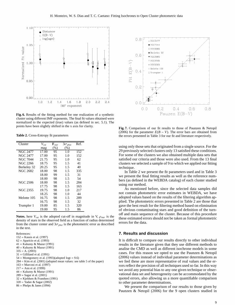
We also probed the effect of using different IMF parametriza-tion. Using a synthetic cluster with no binaries we obtainedfitsusing IMF exponents of 1.0, 1.5, 2.0, 2.1, 2.2 and 2.35. The re-sults are shown in Fig. 6 where it is clear that the IMF variationsdo not affect the final results significantly.
6
H. Monteiro, W. S. Dias and T. C. Caetano: Fitting Isochronesto Open Cluster photometric data
Fig. 2.Parameter space coverage of a full run of the optimization algorithm (left column) as well as the 2D likelihoods (right column) for the fittedparameters for synthetic cluster SC 06. In the right column open circles represent the correct solution and filled circles the final parameter valueobtained from the algorithm.
6. Fitting published data
Having validated the fitting technique with the synthetic clusterswe proceeded to the fitting of real cluster data. We selected asetof well studied clusters based on the work of Paunzen & Netopil(2006) where the authors performed a statistical analysis of thedetermined physical parameters of open clusters publishedin the
literature to characterize the current status of knowledgeand theprecision of open cluster parameters such as age, reddeninganddistance. The authors defined a sample of 72 open clusters withthe most precise known parameters, which they suggest, shouldbe used as standards for future theoretical work.
7
H. Monteiro, W. S. Dias and T. C. Caetano: Fitting Isochronesto Open Cluster photometric data
Fig. 3. Result of the fitting method for the synthetic cluster SC 06 with the ZAMS (thin line) and the fitted isochrone (thick line) where we showthe rejected stars by our filtering method (open circles) as well as stars used in the fit (filled circles)
Fig. 4. Result of the fitting method for the synthetic cluster SC 03 with the ZAMS (thin line) and the fitted isochrone (thick line) where we showthe rejected stars by our filtering method (open circles) as well as stars used in the fit (filled circles)
In our work we pre-selected 29 clusters from the standardsample proposed by Paunzen & Netopil (2006) that had at least5 independent fundamental parameter estimates to be represen-tative of the heterogeneity of the published results. This allowedus to compare our results to others obtained in the literature con-sidering a more representative estimate of the errors in each pa-rameter.
The observational data was obtained through the WEBDAcatalog1 (Mermilliod (1995)) for each cluster. We only selectedclusters with U band photometry as this allowed us to determinethe reddening through the color-color diagram of open clustersas traditionally done (see Phelps & Janes (1994)). We did notuse data sets that had mixed observations from different authors,
1 available at http://obswww.unige.ch/webda
8
H. Monteiro, W. S. Dias and T. C. Caetano: Fitting Isochronesto Open Cluster photometric data
Fig. 6. Results of the fitting method for one realization of a syntheticcluster using different IMF exponents. The final fit values obtained werenormalized to the expected (true) values (as defined in sec. 5.1). Thepoints have been slightly shifted in the x axis for clarity.
Table 2.Cross-Entropy fit parameters
Cluster Vcut Fstar 3σphot Ref.mag (%) (%)
NGC 2477 17.00 95 1.0 152NGC 2477 17.00 95 1.0 152NGC 7044 21.75 95 1.0 62NGC 2266 18.75 95 1.5 41Berkeley 32 20.25 95 1.5 40NGC 2682 18.00 98 1.5 335
18.00 99 1.5 3118.00 98 1.5 54
NGC 2506 18.00 98 1.5 28417.75 98 1.5 163
NGC 2355 19.75 98 1.0 21718.25 98 1.0 44
Melotte 105 16.75 98 1.5 28916.75 98 1.5 32
Trumpler 1 19.00 85 1.5 32019.00 95 1.5 86
Notes.hereVcut is the adopted cut-off in magnitude in V,ρstar is thedensity of stars in the observed field as a function of radius determinedfrom the cluster center and 3σphot is the photometric error as describedin the text.
References:152= Kassis et al. (1997)62= Aparicio et al. (1993)41= Kaluzny & Mazur (1991)40= Kaluzny & Mazur (1991)335= A. (2003)31= Gilliland et al. (1991)54= Montgomery et al. (1993)(adopted logt= 9.6)284= Kim et al. (2001) (adopted mean values: see table 5 of the paper)163= Marconi et al. (1997)217= Ann et al. (1999)44= Kaluzny & Mazur (1991)289= Sagar et al. (2001)32= Kjeldsen & Frandsen (1991)320= Yadav & Sagar (2002)86= Phelps & Janes (1994)
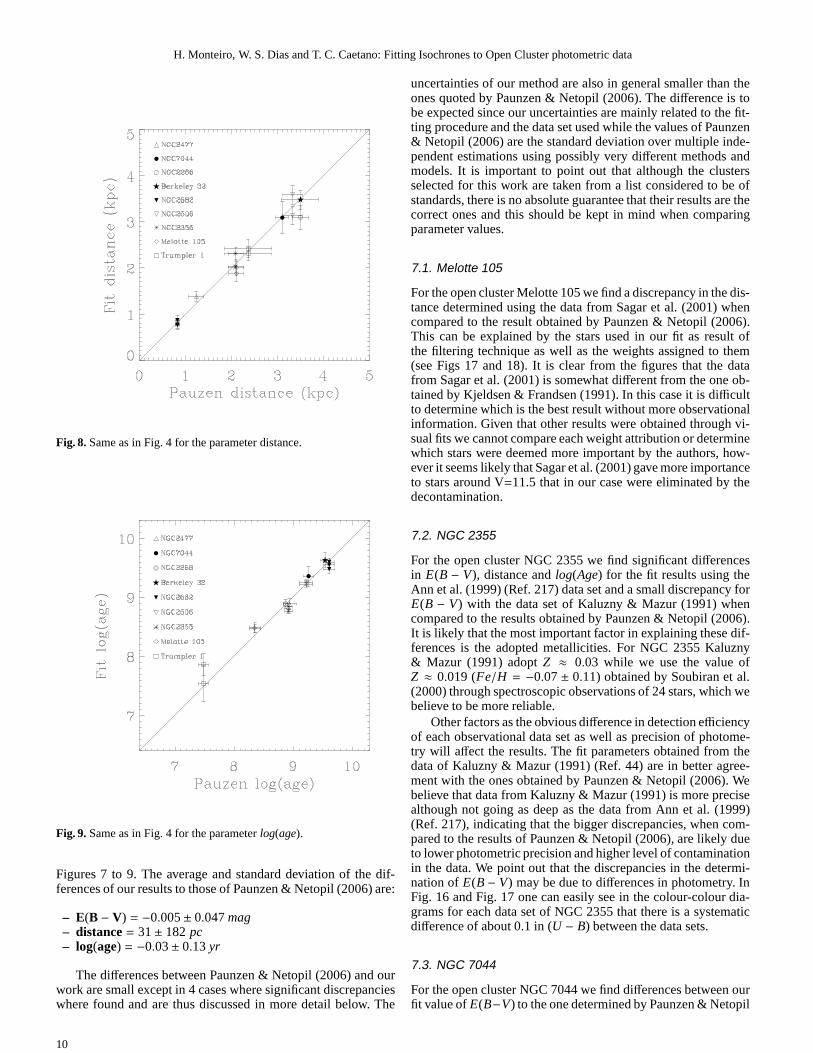
Fig. 7. Comparison of our fit results to those of Paunzen & Netopil(2006) for the parameterE(B − V). The error bars are obtained fromthe errors presented in Table 3 for our fit and literature respectively.
using only those sets that originated from a single source. For the29 previously selected clusters only 13 satisfied these conditions.For some of the clusters we also obtained multiple data sets thatsatisfied our criteria and those were also used. From the 13 finalclusters we selected a sample of 9 to which we applied our fittingtechnique.
In Table 2 we present the fit parameters used and in Table 3we present the final fitting results as well as the reference num-bers (as defined in the WEBDA catalog) of each cluster studiedusing our method.
As mentioned before, since the selected data samples didnot contain photometric error estimates in WEBDA, we haveadopted values based on the results of the filtering algorithm ap-plied. The photometric errors presented in Table 2 are thosethatgave the best result for the filtering method based on eliminationof obvious contaminating stars and good definition of the turn-off and main sequence of the cluster. Because of this procedurethese estimated errors should not be taken as formal photometricerrors for the data.
7. Results and discussion
It is difficult to compare our results directly to other individualresults in the literature given that they use different methods toanalise the CMD as well as different isochrone models in somecases. For this reason we opted to use the Paunzen & Netopil(2006) values instead of individual parameter determinations aswe feel these are more representative of real values and the er-rors reflect the precision of all techniques used so far. In this waywe avoid any potential bias to any one given technique or obser-vational data set and heterogeneity can be accommodated by thequoted errors, also allowing us a more quantifiable comparisonto other parameter determinations.
We present the comparison of our results to those given byPaunzen & Netopil (2006) for the 9 open clusters studied in
9
H. Monteiro, W. S. Dias and T. C. Caetano: Fitting Isochronesto Open Cluster photometric data
Fig. 8.Same as in Fig. 4 for the parameter distance.
Fig. 9.Same as in Fig. 4 for the parameterlog(age).
Figures 7 to 9. The average and standard deviation of the dif-ferences of our results to those of Paunzen & Netopil (2006) are:
– E(B − V) = −0.005± 0.047mag– distance= 31± 182 pc– log(age) = −0.03± 0.13 yr
The differences between Paunzen & Netopil (2006) and ourwork are small except in 4 cases where significant discrepancieswhere found and are thus discussed in more detail below. The
uncertainties of our method are also in general smaller thantheones quoted by Paunzen & Netopil (2006). The difference is tobe expected since our uncertainties are mainly related to the fit-ting procedure and the data set used while the values of Paunzen& Netopil (2006) are the standard deviation over multiple inde-pendent estimations using possibly very different methods andmodels. It is important to point out that although the clustersselected for this work are taken from a list considered to be ofstandards, there is no absolute guarantee that their results are thecorrect ones and this should be kept in mind when comparingparameter values.
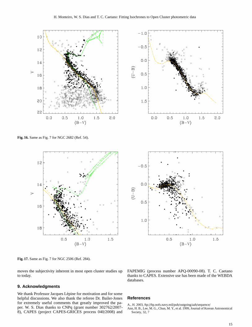
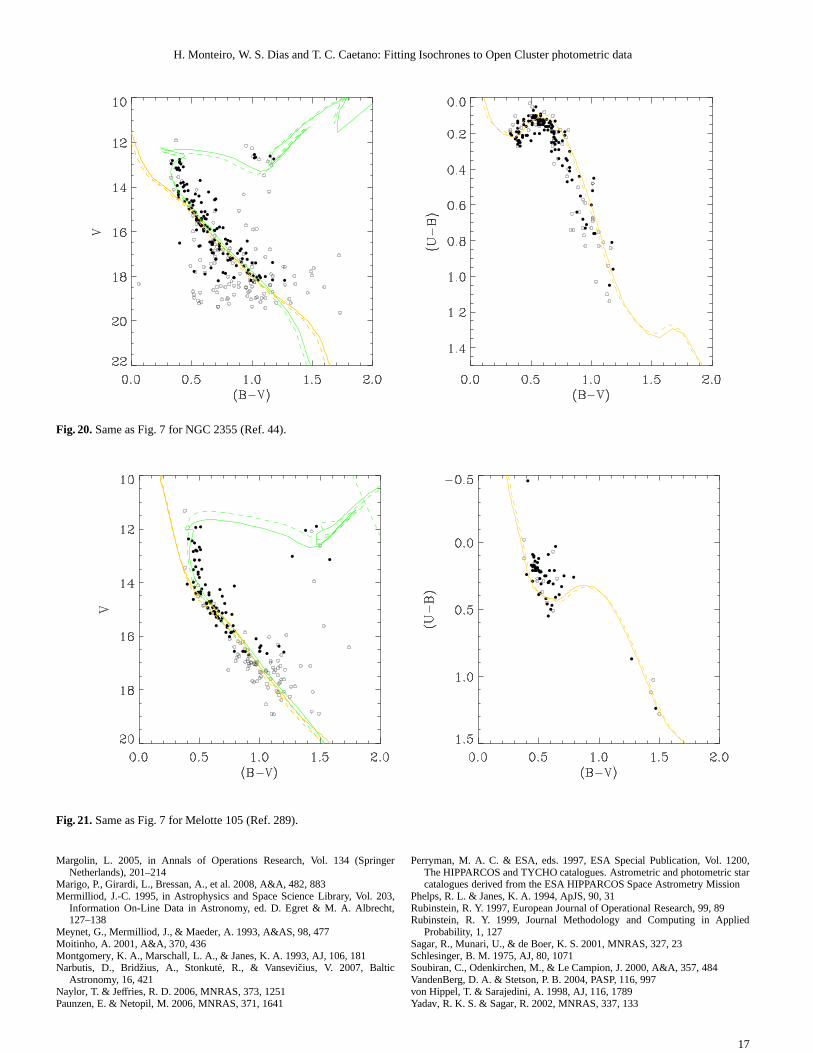
7.1. Melotte 105
For the open cluster Melotte 105 we find a discrepancy in the dis-tance determined using the data from Sagar et al. (2001) whencompared to the result obtained by Paunzen & Netopil (2006).This can be explained by the stars used in our fit as result ofthe filtering technique as well as the weights assigned to them(see Figs 17 and 18). It is clear from the figures that the datafrom Sagar et al. (2001) is somewhat different from the one ob-tained by Kjeldsen & Frandsen (1991). In this case it is difficultto determine which is the best result without more observationalinformation. Given that other results were obtained through vi-sual fits we cannot compare each weight attribution or determinewhich stars were deemed more important by the authors, how-ever it seems likely that Sagar et al. (2001) gave more importanceto stars around V=11.5 that in our case were eliminated by thedecontamination.
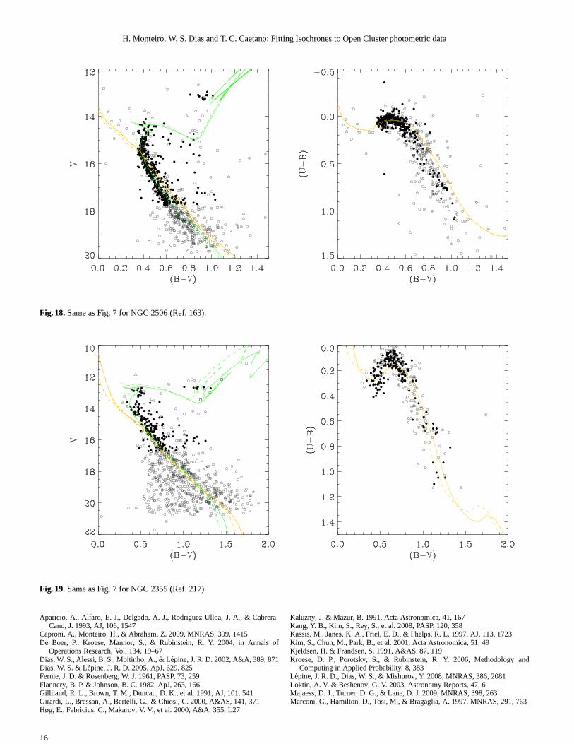
7.2. NGC 2355
For the open cluster NGC 2355 we find significant differencesin E(B − V), distance andlog(Age) for the fit results using theAnn et al. (1999) (Ref. 217) data set and a small discrepancy forE(B − V) with the data set of Kaluzny & Mazur (1991) whencompared to the results obtained by Paunzen & Netopil (2006).It is likely that the most important factor in explaining these dif-ferences is the adopted metallicities. For NGC 2355 Kaluzny& Mazur (1991) adoptZ ≈ 0.03 while we use the value ofZ ≈ 0.019 (Fe/H = −0.07± 0.11) obtained by Soubiran et al.(2000) through spectroscopic observations of 24 stars, which webelieve to be more reliable.
Other factors as the obvious difference in detection efficiencyof each observational data set as well as precision of photome-try will affect the results. The fit parameters obtained from thedata of Kaluzny & Mazur (1991) (Ref. 44) are in better agree-ment with the ones obtained by Paunzen & Netopil (2006). Webelieve that data from Kaluzny & Mazur (1991) is more precisealthough not going as deep as the data from Ann et al. (1999)(Ref. 217), indicating that the bigger discrepancies, whencom-pared to the results of Paunzen & Netopil (2006), are likely dueto lower photometric precision and higher level of contaminationin the data. We point out that the discrepancies in the determi-nation ofE(B − V) may be due to differences in photometry. InFig. 16 and Fig. 17 one can easily see in the colour-colour dia-grams for each data set of NGC 2355 that there is a systematicdifference of about 0.1 in (U − B) between the data sets.
7.3. NGC 7044
For the open cluster NGC 7044 we find differences between ourfit value ofE(B−V) to the one determined by Paunzen & Netopil
10

H. Monteiro, W. S. Dias and T. C. Caetano: Fitting Isochronesto Open Cluster photometric data
Table 3.Basic parameters obtained for the investigated clusters.
Fit LiteratureCluster E(B − V) Distance Log(Age) Z E(B − V) Distance Log(Age) Ref.
(mag) (pc) (yr) (mag) (pc) (yr)NGC 2477 0.29± 0.03 1385± 64 8.90± 0.09 0.019 0.26± 0.08 1227± 166 8.94± 0.11 152NGC 7044 0.55± 0.05 3093± 345 9.35± 0.17 0.019 0.63± 0.06 3097± 145 9.26± 0.08 62NGC 2266 0.17± 0.02 3100± 244 8.90± 0.07 0.008 0.10± 0.01 3490± 180 8.87± 0.04 41Berkeley 32 0.12± 0.04 3483± 186 9.65± 0.13 0.008 0.15± 0.03 3491± 401 9.54± 0.08 40NGC 2682 0.02± 0.01 774± 25 9.55± 0.05 0.019 0.05± 0.02 820± 47 9.61± 0.09 335
0.05± 0.01 758± 26 9.60± 0.06 0.019 0.05± 0.02 820± 47 9.61± 0.09 310.04± 0.01 869± 57 9.50± 0.07 0.019 0.05± 0.02 820± 47 9.61± 0.09 54
NGC 2506 0.03± 0.01 3587± 198 9.20± 0.05 0.008 0.06± 0.04 3315± 219 9.22± 0.11 2840.07± 0.01 3137± 177 9.25± 0.05 0.008 0.06± 0.04 3315± 219 9.22± 0.11 163
NGC 2355 0.25± 0.02 2316± 103 8.80± 0.05 0.008 0.14± 0.06 2086± 163 8.92± 0.07 2170.19± 0.02 2022± 88 8.85± 0.05 0.008 0.14± 0.06 2086± 163 8.92± 0.07 44
Melotte 105 0.47± 0.02 1750± 111 8.40± 0.06 0.019 0.48± 0.05 2094± 159 8.35± 0.09 2890.49± 0.03 2005± 139 8.45± 0.07 0.019 0.48± 0.05 2094± 159 8.35± 0.09 32
Trumpler 1 0.59± 0.05 2419± 185 7.85± 0.19 0.019 0.57± 0.04 2356± 511 7.48± 0.08 3200.53± 0.03 2309± 121 7.55± 0.31 0.019 0.57± 0.04 2356± 511 7.48± 0.08 86
Notes.The numbers, in the last column are the WEBDA reference codes, E(B − V) is the extinction,d the distance to the cluster, log(Age) thelogarithm of the age (in years), Z the adopted metallicity. The literature values are those of Paunzen & Netopil (2006).
(2006) although thelog(Age) and distance values are within theuncertainties. TheE(B−V) value of Paunzen & Netopil (2006) isclearly not adequate for this data set as can be seen in the colour-colour diagram plot of Fig. 8, however our value forE(B−V) aswell aslog(Age) is consistent with the determination of Aparicioet al. (1993) (Ref. 62), the source of the data.
The large spread in the main sequence region is also an im-portant factor as pointed out by Aparicio et al. (1993), wherethey argue that the large spread may be an indication of a largenumber binaries and based on this they estimate a value of 22%for the binary fraction. It is clear from Fig. 8 that our methodof including binaries does a good job in accounting for theirpresence as can be seen also by the agreement in the distancedetermined by the fit.
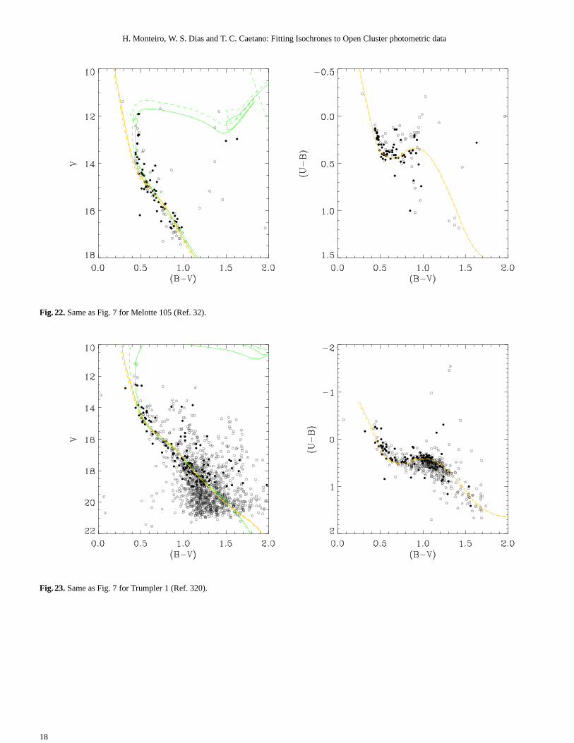
7.4. Trumpler 1
For the open cluster Trumpler 1 the fitted distance agrees withinthe errors to those determined by Paunzen & Netopil (2006) ex-cept for thelog(Age). The age difference, especially for Yadav& Sagar (2002) (Ref. 320), is likely due to the bright stars con-sidered in the fit.
As we can see in Fig. 21 for the data from Yadav & Sagar(2002) (Ref. 320), our filtering technique has removed somebright stars that may belong to the turn-off of the cluster. The re-moval happened because in all cases these were single eventsinthat region of the CMD and thus no statistic could be performed.We have introduced an option to keep these single points if thecase may present itself but did not use it in this cluster as itintro-duced considerable contamination along with the wanted stars inthe tip of the turn-off. It may be the case that in these situationsour errors are underestimated since these stars have low photo-metric errors when compared to the fainter and more numerousstars.
In situations like these other data may resolve the issue ifincorporated in the calculation of the weights. One exampleisthe determination of proper motions for cluster stars, as doneby Loktin & Beshenov (2003) for Trumpler 1, where the authordetermines the proper motion of the cluster from measurementsof 12 stars. However, the author does not provide the individual
data for the stars and therefore it could not be used to assignweights to the observations.
The situation is similar when we examine the results pre-sented in Fig. 21 for the fit of the observational data provided byPhelps & Janes (1994) (Ref. 86). In this case our filtering tech-nique also rejected single points in the CMD in the region of theturn-off. The same considerations made above about the errorsapply in this case.
As a final note we point out that significant differences ex-ist between each data set. The observations of Phelps & Janes(1994) have a limiting magnitude ofV ≈ 21.5 while Yadav &Sagar (2002) have a limiting magnitude ofV ≈ 19.6 yielding1291 and 670 detected stars respectively both with considerablecontamination from field stars. Yadav & Sagar (2002) mentionintheir work that they suspect the data from Phelps & Janes (1994)suffers from calibration problems. All these factors are likelytobe sources of the differences in the results we obtained.
8. Conclusions
As pointed out by Paunzen & Netopil (2006), studying phenom-ena using open cluster physical parameters, is highly dependenton their precision. The authors also show that major discrep-ancies still exist even in well studied clusters. In our workweprovide a new technique for the determination of open clusterphysical parameters that is not dependent on the user and is re-producible within the statistical uncertainties given well definedconditions.
Our method, based on the Cross-Entropy optimization algo-rithm, was tailored to the fitting of theoretical isochronesas theones of Girardi et al. (2000); Marigo et al. (2008) used in thiswork. The procedure is simple and allows for the use of any tab-ulated theoretical isochrones and thus provides also an unbiasedmeans of comparing fits using different theoretical models giventhe same constraints and fitting procedure.
In this work we have concentrated in the validation of themethod limiting ourselves to fitting synthetic clusters andwellstudied open clusters with the tabulated isochrones of Padova.The results show that the method is capable of recovering theoriginal parameters with good accuracy even in cases where weincluded considerable non-uniform field contamination demon-
11
H. Monteiro, W. S. Dias and T. C. Caetano: Fitting Isochronesto Open Cluster photometric data
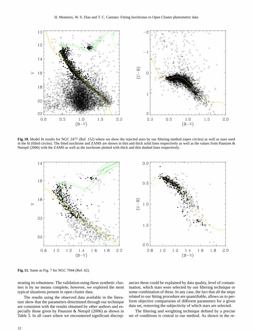
Fig. 10.Model fit results for NGC 2477 (Ref. 152) where we show the rejected stars by our filtering method (open circles) as well as stars usedin the fit (filled circles). The fitted isochrone and ZAMS are shown in thin and thick solid lines respectively as well as the values from Paunzen &Netopil (2006) with the ZAMS as well as the isochrone plottedwith thick and thin dashed lines respectively.
Fig. 11.Same as Fig. 7 for NGC 7044 (Ref. 62).
strating its robustness. The validation using these synthetic clus-ters is by no means complete, however, we explored the mosttypical situations present in open cluster data.
The results using the observed data available in the litera-ture show that the parameters determined through our techniqueare consistent with the results obtained by other authors and es-pecially those given by Paunzen & Netopil (2006) as shown inTable 3. In all cases where we encountered significant discrep-
ancies these could be explained by data quality, level of contam-ination, which stars were selected by our filtering technique orsome combination of these. In any case, the fact that all the stepsrelated to our fitting procedure are quantifiable, allows us to per-form objective comparisons of different parameters for a givendata set, removing the subjectivity of which stars are selected.
The filtering and weighting technique defined by a preciseset of conditions is central to our method. As shown in the re-
12

H. Monteiro, W. S. Dias and T. C. Caetano: Fitting Isochronesto Open Cluster photometric data
Fig. 12.Same as Fig. 7 for NGC 2266 (Ref. 41).
Fig. 13.Same as Fig. 7 for Berkeley 32 (Ref. 40).
sults for Trumpler 1, in cases where the cluster has low sam-pling, i.e. low number of stars, it becomes difficult to determinethe weight for cluster stars. It is likely that better statistical toolsmay improve the efficiency of this step. In general, the filteringtechnique performed well in eliminating most of the contamina-tion and assigning weights in the observed clusters, especially inthe well sampled cases.
The final results show that there is good agreement in gen-eral with the results adopted as standards in the literature, butalso indicates that some issues still remain unresolved. Perhaps
the most important of these issues is related to the metallicity.As mentioned before, we kept the metallicity values fixed in ourfits and attempted to use the ones provided by the observers,except in cases where we believed more reliable values wereavailable. Many of the clusters show results that could be clearlyimproved by changing the metallicity, as for example the caseof NGC 7044. Given the considerations above, it is also impor-tant to point out that the values we used for comparison takenfrom the proposed standard list of Paunzen & Netopil (2006) donot take metallicities into account. The different author deter-
13
H. Monteiro, W. S. Dias and T. C. Caetano: Fitting Isochronesto Open Cluster photometric data
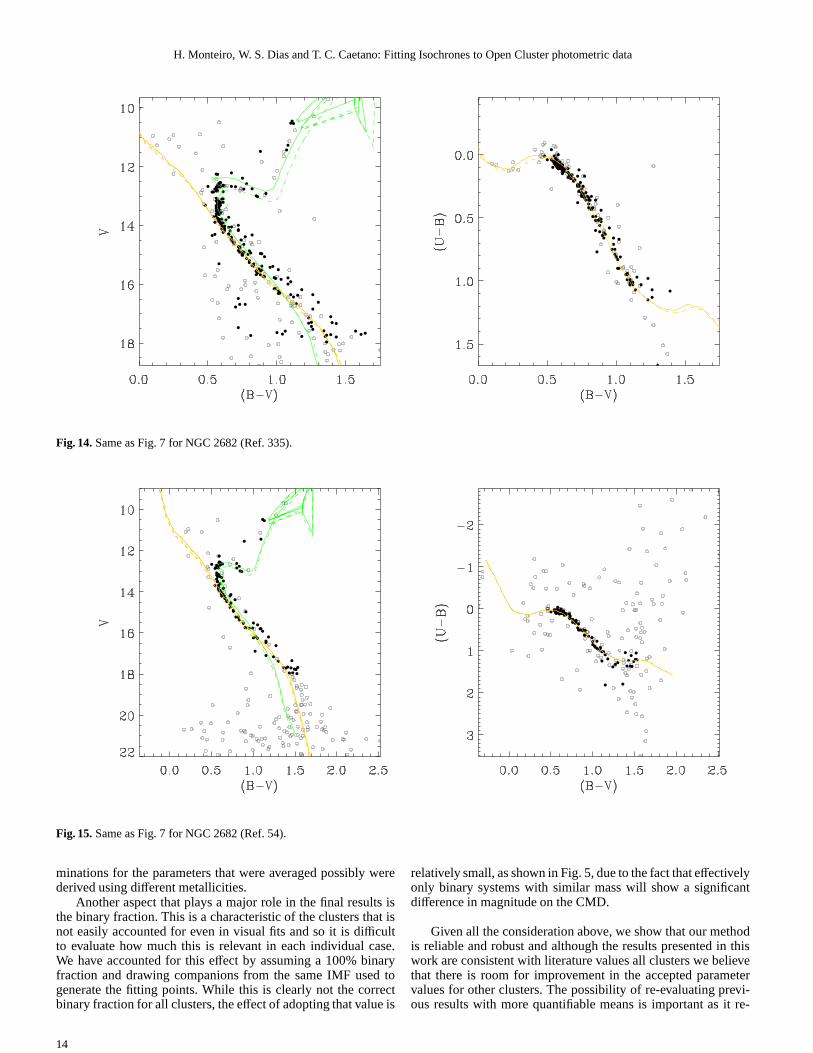
Fig. 14.Same as Fig. 7 for NGC 2682 (Ref. 335).
Fig. 15.Same as Fig. 7 for NGC 2682 (Ref. 54).
minations for the parameters that were averaged possibly werederived using different metallicities.
Another aspect that plays a major role in the final results isthe binary fraction. This is a characteristic of the clusters that isnot easily accounted for even in visual fits and so it is difficultto evaluate how much this is relevant in each individual case.We have accounted for this effect by assuming a 100% binaryfraction and drawing companions from the same IMF used togenerate the fitting points. While this is clearly not the correctbinary fraction for all clusters, the effect of adopting that value is
relatively small, as shown in Fig. 5, due to the fact that effectivelyonly binary systems with similar mass will show a significantdifference in magnitude on the CMD.
Given all the consideration above, we show that our methodis reliable and robust and although the results presented inthiswork are consistent with literature values all clusters we believethat there is room for improvement in the accepted parametervalues for other clusters. The possibility of re-evaluating previ-ous results with more quantifiable means is important as it re-
14
H. Monteiro, W. S. Dias and T. C. Caetano: Fitting Isochronesto Open Cluster photometric data
Fig. 16.Same as Fig. 7 for NGC 2682 (Ref. 54).
Fig. 17.Same as Fig. 7 for NGC 2506 (Ref. 284).
moves the subjectivity inherent in most open cluster studies upto today.
9. Acknowledgments
We thank Professor Jacques Lepine for motivation and for somehelpful discussions. We also thank the referee Dr. Bailer-Jonesfor extremely useful comments that greatly improved the pa-per. W. S. Dias thanks to CNPq (grant number 302762/2007-8), CAPES (project CAPES-GRICES process 040/2008) and
FAPEMIG (process number APQ-00090-08). T. C. Caetanothanks to CAPES. Extensive use has been made of the WEBDAdatabases.
ReferencesA., H. 2003, ftp://ftp.nofs.navy.mil/pub/outgoing/aah/sequence/Ann, H. B., Lee, M. G., Chun, M. Y., et al. 1999, Journal of Korean Astronomical
Society, 32, 7
15
H. Monteiro, W. S. Dias and T. C. Caetano: Fitting Isochronesto Open Cluster photometric data
Fig. 18.Same as Fig. 7 for NGC 2506 (Ref. 163).
Fig. 19.Same as Fig. 7 for NGC 2355 (Ref. 217).
Aparicio, A., Alfaro, E. J., Delgado, A. J., Rodriguez-Ulloa, J. A., & Cabrera-Cano, J. 1993, AJ, 106, 1547
Caproni, A., Monteiro, H., & Abraham, Z. 2009, MNRAS, 399, 1415De Boer, P., Kroese, Mannor, S., & Rubinstein, R. Y. 2004, in Annals of
Operations Research, Vol. 134, 19–67Dias, W. S., Alessi, B. S., Moitinho, A., & Lepine, J. R. D. 2002, A&A, 389, 871Dias, W. S. & Lepine, J. R. D. 2005, ApJ, 629, 825Fernie, J. D. & Rosenberg, W. J. 1961, PASP, 73, 259Flannery, B. P. & Johnson, B. C. 1982, ApJ, 263, 166Gilliland, R. L., Brown, T. M., Duncan, D. K., et al. 1991, AJ,101, 541Girardi, L., Bressan, A., Bertelli, G., & Chiosi, C. 2000, A&AS, 141, 371Høg, E., Fabricius, C., Makarov, V. V., et al. 2000, A&A, 355,L27
Kaluzny, J. & Mazur, B. 1991, Acta Astronomica, 41, 167Kang, Y. B., Kim, S., Rey, S., et al. 2008, PASP, 120, 358Kassis, M., Janes, K. A., Friel, E. D., & Phelps, R. L. 1997, AJ, 113, 1723Kim, S., Chun, M., Park, B., et al. 2001, Acta Astronomica, 51, 49Kjeldsen, H. & Frandsen, S. 1991, A&AS, 87, 119Kroese, D. P., Porotsky, S., & Rubinstein, R. Y. 2006, Methodology and
Computing in Applied Probability, 8, 383Lepine, J. R. D., Dias, W. S., & Mishurov, Y. 2008, MNRAS, 386, 2081Loktin, A. V. & Beshenov, G. V. 2003, Astronomy Reports, 47, 6Majaess, D. J., Turner, D. G., & Lane, D. J. 2009, MNRAS, 398, 263Marconi, G., Hamilton, D., Tosi, M., & Bragaglia, A. 1997, MNRAS, 291, 763
16
H. Monteiro, W. S. Dias and T. C. Caetano: Fitting Isochronesto Open Cluster photometric data
Fig. 20.Same as Fig. 7 for NGC 2355 (Ref. 44).
Fig. 21.Same as Fig. 7 for Melotte 105 (Ref. 289).
Margolin, L. 2005, in Annals of Operations Research, Vol. 134 (SpringerNetherlands), 201–214
Marigo, P., Girardi, L., Bressan, A., et al. 2008, A&A, 482, 883Mermilliod, J.-C. 1995, in Astrophysics and Space Science Library, Vol. 203,
Information On-Line Data in Astronomy, ed. D. Egret & M. A. Albrecht,127–138
Meynet, G., Mermilliod, J., & Maeder, A. 1993, A&AS, 98, 477Moitinho, A. 2001, A&A, 370, 436Montgomery, K. A., Marschall, L. A., & Janes, K. A. 1993, AJ, 106, 181Narbutis, D., Bridzius, A., Stonkute, R., & Vansevicius, V. 2007, Baltic
Astronomy, 16, 421Naylor, T. & Jeffries, R. D. 2006, MNRAS, 373, 1251Paunzen, E. & Netopil, M. 2006, MNRAS, 371, 1641
Perryman, M. A. C. & ESA, eds. 1997, ESA Special Publication,Vol. 1200,The HIPPARCOS and TYCHO catalogues. Astrometric and photometric starcatalogues derived from the ESA HIPPARCOS Space AstrometryMission
Phelps, R. L. & Janes, K. A. 1994, ApJS, 90, 31Rubinstein, R. Y. 1997, European Journal of Operational Research, 99, 89Rubinstein, R. Y. 1999, Journal Methodology and Computing in Applied
Probability, 1, 127Sagar, R., Munari, U., & de Boer, K. S. 2001, MNRAS, 327, 23Schlesinger, B. M. 1975, AJ, 80, 1071Soubiran, C., Odenkirchen, M., & Le Campion, J. 2000, A&A, 357, 484VandenBerg, D. A. & Stetson, P. B. 2004, PASP, 116, 997von Hippel, T. & Sarajedini, A. 1998, AJ, 116, 1789Yadav, R. K. S. & Sagar, R. 2002, MNRAS, 337, 133
17
H. Monteiro, W. S. Dias and T. C. Caetano: Fitting Isochronesto Open Cluster photometric data
Fig. 22.Same as Fig. 7 for Melotte 105 (Ref. 32).
Fig. 23.Same as Fig. 7 for Trumpler 1 (Ref. 320).
18

H. Monteiro, W. S. Dias and T. C. Caetano: Fitting Isochronesto Open Cluster photometric data
Fig. 24.Same as Fig. 7 for Trumpler 1 (Ref. 86).
19