05 Curve Fitting - Spada UNS

05 C

urv

e F

itti

ng 05 Curve Fitting

05 C

urv

e F

itti

ng

Introduction

• Data are often given for discrete values

along a continuum. However, we may

require estimates at points between the

discrete values.

• This Chapter describes techniques to fit

curves to such data to obtain intermediate

estimates.

05 C

urv

e F

itti

ng

• There are two general approaches for curve

fitting that are distinguished from each

other on the basis of the amount of error

associated with the data.

- Regression

- Interpolation

05 C

urv

e F

itti

ng

Regression

• The data exhibit a significant degree of

error, the strategy is to derive a single

curve that represents the general trend of

the data.

• Because any individual data point may be

incorrect, we make no effort to intersect

every point. Rather, the curve is designed to

follow the pattern of the points taken as a

group. One approach of this nature is called

least-squares regression

05 C

urv

e F

itti

ng

Interpolation

• The data are known to be very precise, the

basic approach is to fit a curve or a series of

curves that pass directly through each of the

points.

• Such data usually originate from tables.

Examples are values for the density of water

or for the heat capacity of gases as a

function of temperature.

• The estimation of values between well-

known discrete points is called interpolation

05 C

urv

e F

itti

ng

Three attempts to fit a

“best” curve through

five data points:

(a) least-squares

regression,

(b) linear interpolation,

(c) curvilinear

interpolation.

05 C

urv

e F

itti

ng

5.1. Regressiona. Linear Regression

• The primary objective of this method is to

how least-squares regression can be used to

fit a straight line to measured data.

The mathematical expression for the straightline is,

y = a0 + a1x

05 C

urv

e F

itti

ng

• One strategy for fitting a “best” line through

the data would be to minimize the sum of

the residual errors for all the available data,

as in

05 C

urv

e F

itti

ng

Examples of some criteria

for “best fit” that are

inadequate for regression:

(a) minimizes the sum

of the residuals,

(b) minimizes the sum of

the absolute values of the

residuals, and

(c) minimizes the

maximum error of any

individual point.

05 C

urv

e F

itti

ng

• A strategy that overcomes the shortcomings

of the aforementioned approaches is to

minimize the sum of the squares of the

residuals:

05 C

urv

e F

itti

ng

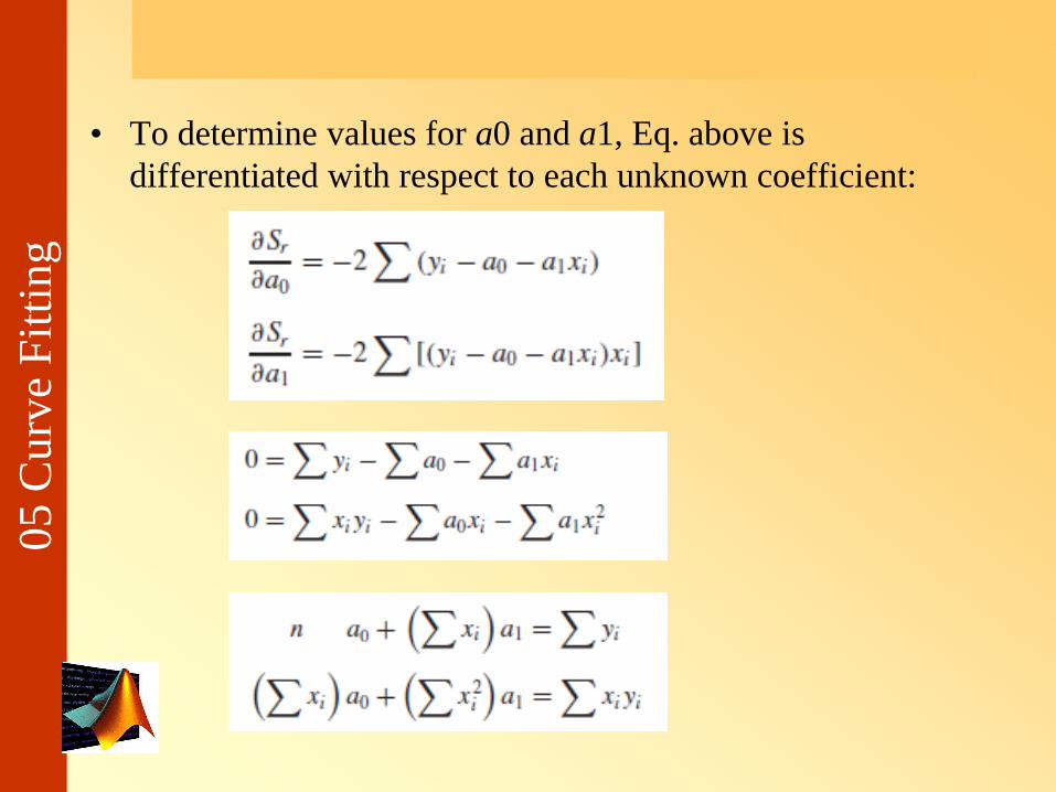
• To determine values for a0 and a1, Eq. above is

differentiated with respect to each unknown coefficient:

05 C

urv

e F

itti

ng

• These are called the normal equations. They

can be solved simultaneously for

05 C

urv

e F

itti

ng

Problem

• Fit a straight line to the values in Table

14.1.

05 C

urv

e F

itti

ng

LINEARIZATION OF NONLINEAR RELATIONSHIPS

• Linear regression provides a powerful

technique for fitting a best line to data.

However, it is predicated on the fact that the

relationship between the dependent and

independent variables is linear.

• This is not always the case, and the first

step in any regression analysis should be to

plot and visually inspect the data to

ascertain whether a linear model applies.

05 C

urv

e F

itti

ng

• In some cases, techniques such as

polynomial regression, which is described

in next sub Chap., are appropriate. For

others, transformations can be used to

express the data in a form that is compatible

with linear regression.

05 C

urv

e F

itti

ng

05 C

urv

e F

itti

ng

b. Regresi Polinomial

05 C

urv

e F

itti

ng

05 C

urv

e F

itti

ng

Regresi dg MatlabFungsi Polyfit

Dalam Matlab, fungsi polyfitmenyelesaikan masalah pencocokan kurva untuk kuadrat terkecil.

Penggunaan fungsi polyfit akan menghasilkan suatu persamaan polinomial yang paling mendekati data.

Jika derajat fungsi polyfit dipilih n = 1, maka akan dihasilkan persamaan garis lurus yaitu regresi linier.

kons = polyfit(x,y,1)

05 C

urv

e F

itti

ng

Soal 1

05 C

urv

e F

itti

ng

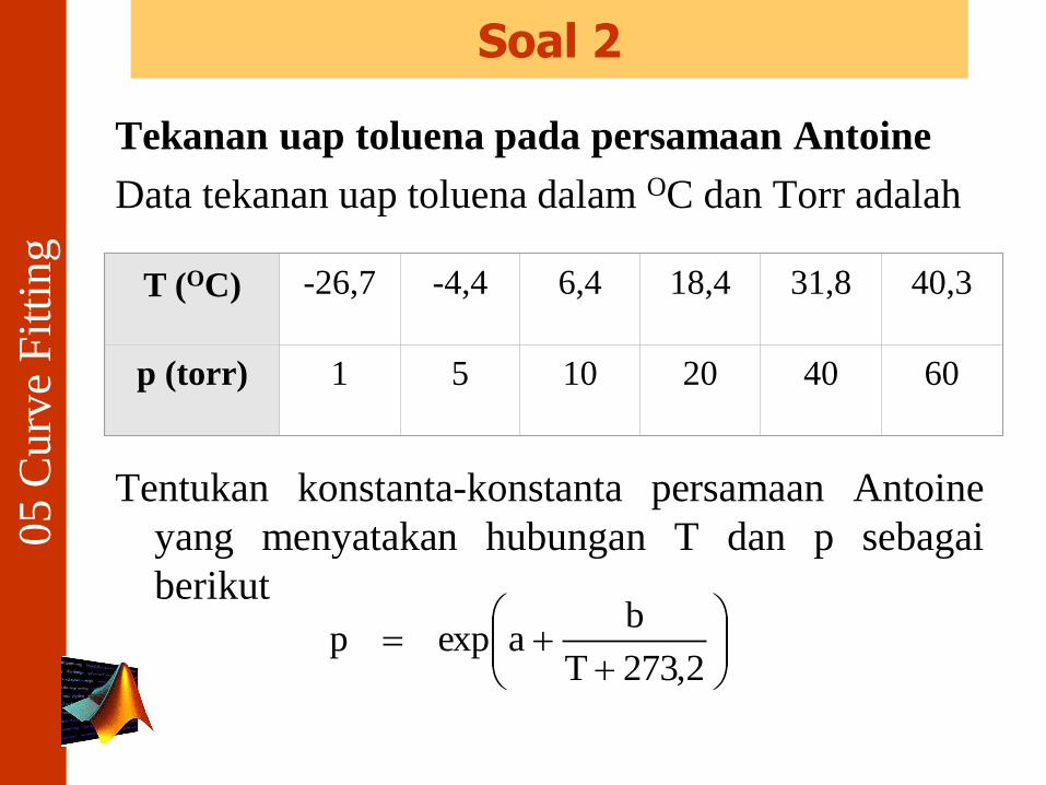
Soal 2

Tekanan uap toluena pada persamaan Antoine

Data tekanan uap toluena dalam OC dan Torr adalah

Tentukan konstanta-konstanta persamaan Antoine

yang menyatakan hubungan T dan p sebagai

berikut

T (OC) -26,7 -4,4 6,4 18,4 31,8 40,3

p (torr) 1 5 10 20 40 60

2,273T

baexpp

05 C

urv

e F

itti

ng

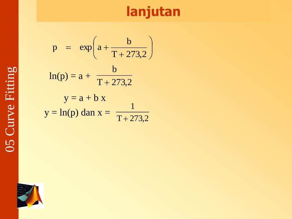
lanjutan

2,273T

baexpp

ln(p) = a +2,273T

b

y = a + b x

y = ln(p) dan x = 2,273T

1

05 C

urv

e F

itti

ng

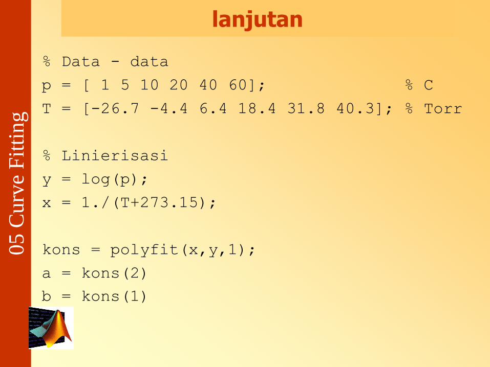
lanjutan

% Data - data

p = [ 1 5 10 20 40 60]; % C

T = [-26.7 -4.4 6.4 18.4 31.8 40.3]; % Torr

% Linierisasi

y = log(p);

x = 1./(T+273.15);

kons = polyfit(x,y,1);

a = kons(2)

b = kons(1)

05 C

urv

e F

itti

ng

Regresi Polinomial

data-data didekati dengan persamaan

polinomial, yaitu :

y = a0+ a

1x + a

2x2 + .... + a

mxm

05 C

urv

e F

itti

ng

lanjutan

Fungsi polyfit dari Matlab dapatdigunakan untuk derajat n = 2, yang disebutpolinomial kuadratis. Hasil fungsipolyfit adalah vektor baris yang berisikoefisien-koefisien polinomial.

Selain fungsi polyfit, Matlab juga mempunyai fungsi polyval untuk mengevaluasi polinomial pada tiap titik yang ingin diketahui nilainya.

05 C

urv

e F

itti

ng

Soal 2Persamaan Fit untuk Data Tekanan Uap Benzena

Data tekanan uap murni benzena pada berbagai temperatur

ditunjukkan pada tabel.Temperatur Tekanan Temperatur Tekanan

(OC) (mmHg) (OC) (mmHg)

-36,7 1 15,4 60

-19,6 5 26,1 100

-11,5 10 42,2 200

-2,6 20 60,6 400

7,6 40 80,1 760

Hubungan tekanan sebagai fungsi temperatur dapat dinyatakan

sebagai persamaan empiris polinomial sederhana sebagai berikut :

P = a0 + a1T + a2T2 + a3T

3 + … + anTn

dengan a0, a1, …, an adalah parameter yang ditentukan dengan regresi

dan n adalah orde polinomial.

05 C

urv

e F

itti

ng

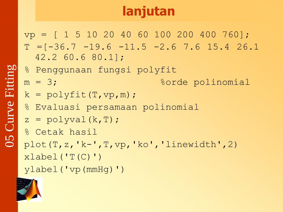
lanjutan

vp = [ 1 5 10 20 40 60 100 200 400 760];

T =[-36.7 -19.6 -11.5 -2.6 7.6 15.4 26.1

42.2 60.6 80.1];

% Penggunaan fungsi polyfit

m = 3; %orde polinomial

k = polyfit(T,vp,m);

% Evaluasi persamaan polinomial

z = polyval(k,55)

05 C

urv

e F

itti

ng

lanjutan

vp = [ 1 5 10 20 40 60 100 200 400 760];

T =[-36.7 -19.6 -11.5 -2.6 7.6 15.4 26.1

42.2 60.6 80.1];

% Penggunaan fungsi polyfit

m = 3; %orde polinomial

k = polyfit(T,vp,m);

% Evaluasi persamaan polinomial

z = polyval(k,T);

% Cetak hasil

plot(T,z,'k-',T,vp,'ko','linewidth',2)

xlabel('T(C)')

ylabel('vp(mmHg)')

05 C

urv

e F

itti

ng

Next meeting

05 C

urv

e F

itti

ng 05 Curve Fitting

05 C

urv

e F

itti

ng

• There are two general approaches for curve

fitting that are distinguished from each

other on the basis of the amount of error

associated with the data.

- Regression

- Interpolation

05 C

urv

e F

itti

ng

6.2. Interpolation

• Interpolation is used to estimate

intermediate values between precise data

points.

05 C

urv

e F

itti

ng

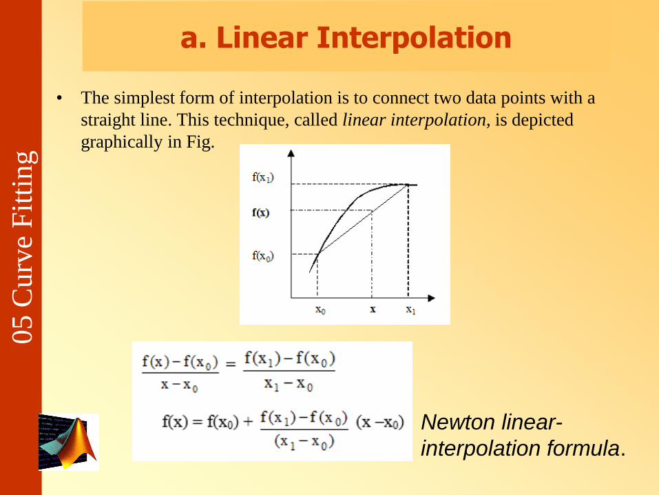
a. Linear Interpolation

• The simplest form of interpolation is to connect two data points with a

straight line. This technique, called linear interpolation, is depicted

graphically in Fig.

Newton linear-

interpolation formula.

05 C

urv

e F

itti

ng

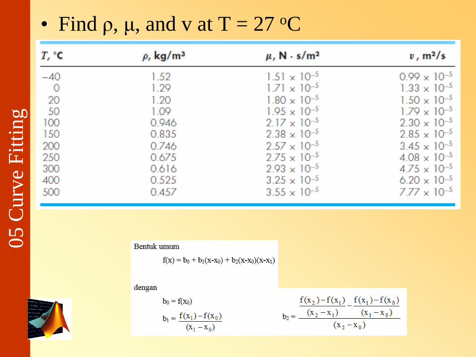
• Find ρ, μ, and v at T = 27 oC

05 C

urv

e F

itti

ng

b. Quadratic Interpolation

• A strategy for improving the estimate is to introduce some

curvature into the line connecting the points. If three data

points are available, this can be accomplished with a

second-order polynomial (also called a quadratic

polynomial or a parabola).

05 C

urv

e F

itti

ng

• Find ρ, μ, and v at T = 27 oC

05 C

urv

e F

itti

ng

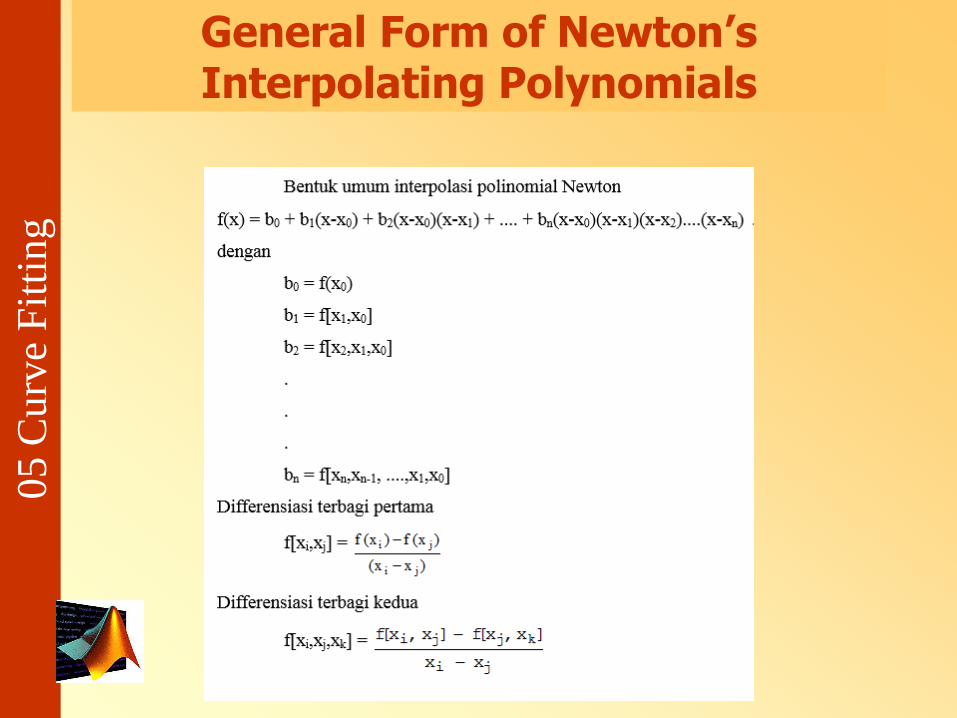
General Form of Newton’s Interpolating Polynomials

05 C

urv

e F

itti

ng

05 C

urv

e F

itti

ng

From data of acetic acid density at 25 OC, find the density of

acetic acid at 65 % !

05 C

urv

e F

itti

ng

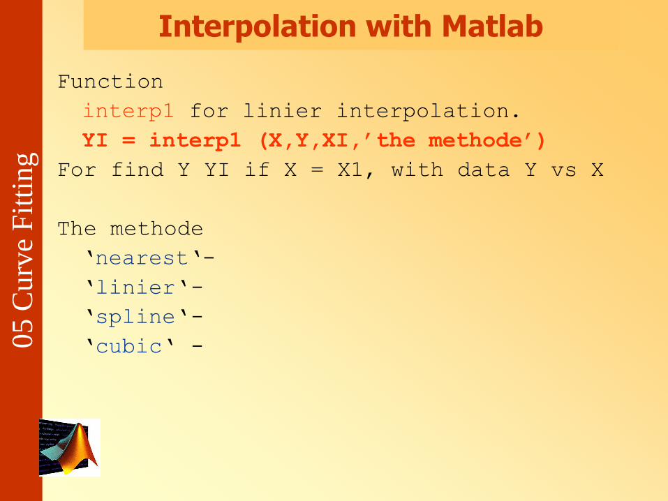
Interpolation with Matlab

Function

interp1 for linier interpolation.

YI = interp1 (X,Y,XI,’the methode’)

For find Y YI if X = X1, with data Y vs X

The methode

‘nearest‘-

‘linier‘-

‘spline‘-

‘cubic‘ -

05 C

urv

e F

itti

ng

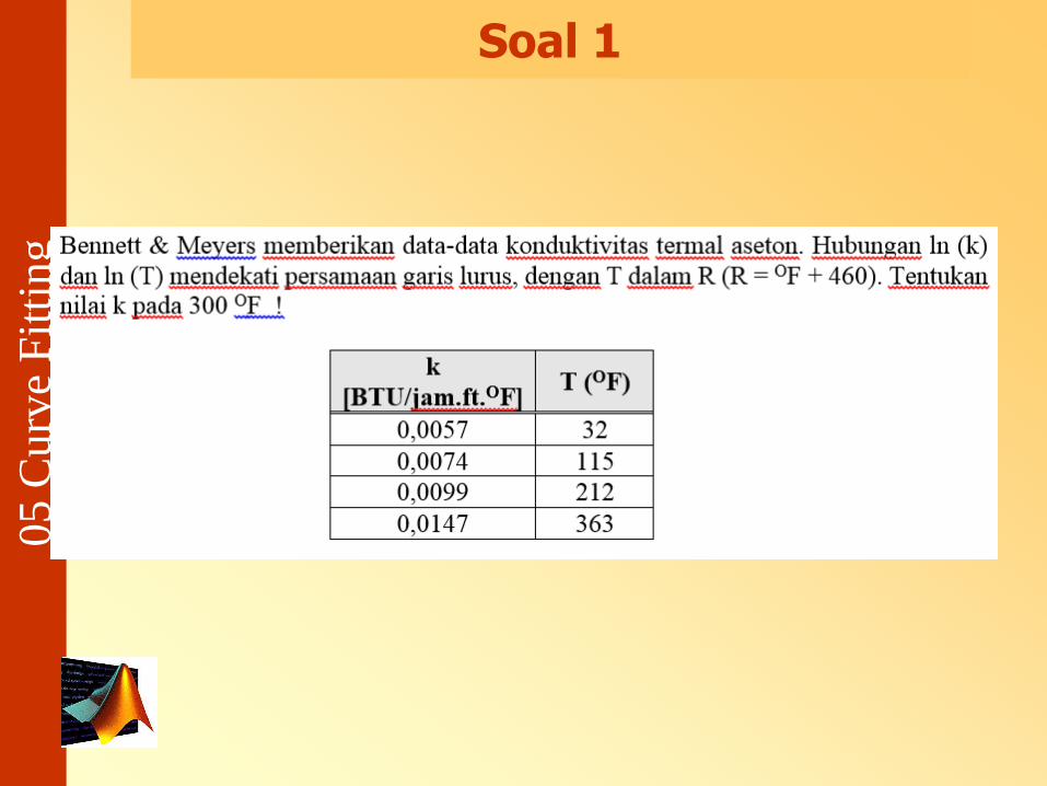
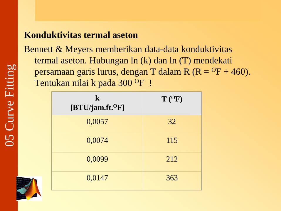
Konduktivitas termal aseton

Bennett & Meyers memberikan data-data konduktivitas

termal aseton. Hubungan ln (k) dan ln (T) mendekati

persamaan garis lurus, dengan T dalam R (R = OF + 460).

Tentukan nilai k pada 300 OF !

k

[BTU/jam.ft.OF]T (OF)

0,0057 32

0,0074 115

0,0099 212

0,0147 363

05 C

urv

e F

itti

ng

lanjutan

k = [0.0057 0.0074 0.0099 0.0147];

T = [32 115 212 363]+460;

% Hubungan k dan T linier

ln_k = log(k);

ln_T = log(T);

% Interpolasi Linier

T300 = log(300+460);

k300 = interp1(ln_T,ln_k,T300,'linier');

% Hasil

k_pd_300 = exp(k300)

05 C

urv

e F

itti

ng

b. Splines Interpolation

• nth-order polynomials were used to interpolate between

(n+1) data points.

• For example, for eight points, we can derive a perfect

seventh-order polynomial. This curve would capture all

the meanderings (at least up to and including seventh

derivatives) suggested by the points.

• However, there are cases where these functions can lead

to erroneous results because of round-off error and

oscillations.

• An alternative approach is to apply lower-order

polynomials in a piecewise fashion to subsets of data

points. Such connecting polynomials are called spline

functions.

05 C

urv

e F

itti

ng

• For example, third-order curves employed to

connect each pair of data points are called cubic

splines.

• These functions can be constructed so that the

connections between adjacent cubic equations are

visually smooth.

05 C

urv

e F

itti

ng

05 C

urv

e F

itti

ng

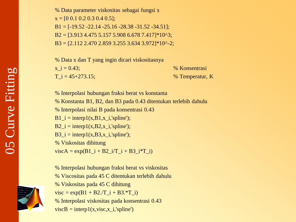
% Data parameter viskositas sebagai fungsi x

x = [0 0.1 0.2 0.3 0.4 0.5];

B1 = [-19.52 -22.14 -25.16 -28.38 -31.52 -34.51];

B2 = [3.913 4.475 5.157 5.908 6.678 7.417]*10^3;

B3 = [2.112 2.470 2.859 3.255 3.634 3.972]*10^-2;

% Data x dan T yang ingin dicari viskositasnya

x_i = 0.43; % Konsentrasi

T_i = 45+273.15; % Temperatur, K

% Interpolasi hubungan fraksi berat vs konstanta

% Konstanta B1, B2, dan B3 pada 0.43 ditentukan terlebih dahulu

% Interpolasi nilai B pada konsentrasi 0.43

B1_i = interp1(x,B1,x_i,'spline');



% Viskositas dihitung

viscA = exp(B1_i + B2_i/T_i + B3_i*T_i)

% Interpolasi hubungan fraksi berat vs viskositas

% Viscositas pada 45 C ditentukan terlebih dahulu

% Viskositas pada 45 C dihitung

visc = exp(B1 + B2./T_i + B3.*T_i)

% Interpolasi viskositas pada konsentrasi 0.43

viscB = interp1(x,visc,x_i,'spline')

05 C

urv

e F

itti

ng

c. Two dimension Interpolation

Interpolasi dua dimensi mempunyai prinsip yang

sama dengan interpolasi satu dimensi. Perbedaanya

adalah interpolasi dua dimensi menginterpolasikan

fungsi dua variabel z = f(x,y).

ZI = interp2 (X,Y,Z,XI,YI) adalah interpolasi untuk

menentukan nilai ZI, dari fungsi Z pada titik XI dan

YI dari matriks X dan Y. Metode yang ditampilkan

pada interpolasi 1 dimensi dapat juga digunakan

pada interpolasi 2 dimensi.

05 C

urv

e F

itti

ng

05 C

urv

e F

itti

ng

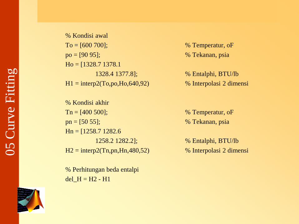
% Kondisi awal

To = [600 700]; % Temperatur, oF

po = [90 95]; % Tekanan, psia

Ho = [1328.7 1378.1

1328.4 1377.8]; % Entalphi, BTU/lb

H1 = interp2(To,po,Ho,640,92) % Interpolasi 2 dimensi

% Kondisi akhir

Tn = [400 500]; % Temperatur, oF

pn = [50 55]; % Tekanan, psia

Hn = [1258.7 1282.6

1258.2 1282.2]; % Entalphi, BTU/lb

H2 = interp2(Tn,pn,Hn,480,52) % Interpolasi 2 dimensi

% Perhitungan beda entalpi

del_H = H2 - H1

05 C

urv

e F

itti

ng

05 Curve Fitting - Spada UNS

Documents

Transcript of 05 Curve Fitting - Spada UNS