A Bayesian Hierarchical Model for Photometric Redshifts

Merrilee Hurn∗, Peter J. Green†, and Fahimah Al-Awadhi‡

March 6, 2007

Abstract

The Sloan Digital Sky Survey (SDSS) is an extremely large astronomical survey conducted with the

intention of mapping more than a quarter of the sky (http://www.sdss.org/ ). Among the data it

is generating are spectroscopic and photometric measurements, both allowing estimation of the redshift

of galaxies. The former is precise but expensive to gather, the latter is far cheaper but correspondingly

gives far less accurate estimates. A recent paper by Csabaiet al. (2003) describes various calibration

techniques aiming to predict spectroscopic redshift from photometric measurements. In this paper, we

investigate what a structured Bayesian approach to the problem can add. In particular, we are interested

in providing uncertainty bounds associated with the underlying redshifts and the classifications of the

galaxies. We find that a quite generic statistical modelling approach, using for the most part standard

model ingredients, can compete with much more specific custom-made and highly-tuned techniques al-

ready available in the astronomical literature.

Keywords: Bayesian Modelling, Calibration, Hierarchical Modelling, Markov Chain Monte Carlo, Pho-

tometric Redshifts

1 Introduction

The Sloan Digital Sky Sky (SDSS) is a huge international collaboration. It describes itself as the most

ambitious astronomical survey ever undertaken (http://www.sdss.org/ ), and eventually it will pro-

vide optical images covering more than a quarter of the sky. It will also provide a 3-dimensional map of

roughly a million galaxies and quasars. The key to producing a 3-dimensional map from 2-dimensional

∗Department of Mathematical Sciences, University of Bath, Bath, BA2 7AY, UK; Email: M.A.Hurn@bath.ac.uk; Tel.: +44

(0)1225 386001†Department of Mathematics, University of Bristol, Bristol, BS8 1TW, UK; Email: P.J.Green@bristol.ac.uk; Tel.: +44 (0)117

928 7967‡Department of Statistics and OR, Kuwait University, Kuwait, 13060; Email: falawadi@kuc01.kuniv.edu.kw; Tel.: +965

4837332

1

images of galaxies lies in measuring theirredshift. The redshift measures how much light emitted from

the galaxy has been shifted in wavelength by the speed at which the galaxy is moving relative to Earth (a

more familiar concept would be that of the Doppler effect changing the apparent pitch of an ambulance’s

siren as it moves towards and then away from an observer). Once the redshift is known, the distance of the

galaxy from Earth can be inferred using standard cosmological theory. The SDSS uses a spectograph to

measure redshift; this technique measures the light the galaxy emits at different wavelengths in the range

3800A(blue) to 9200A(near infrared). By searching the spectra for certain characteristic features, the red-

shift can be measured. Such measurements are known as spectroscopic redshifts; they are believed to be

very accurate but are expensive to collect. As a result there has been much interest in calibrating cheaper

photometric data to predict redshift. Where spectroscopic data are accurate measurements of a whole sec-

tion of the emission spectrum, photometric data are gathered by binning the emissions received in a small

number of wavelength windows; in the case of the SDSS data 5 filter bins are used. As the bins are quite

wide, reasonable signal-to-noise ratios can be achieved with short exposure times, so this form of data is far

cheaper to collect.

A recent paper by Csabaiet al. (2003) provides background to the use of photometric redshifts, and

reviews the main existing approaches to deriving photometric redshifts. These approaches can be categorised

into empirical or template based. Of the former, one approach is nearest neighbour matching where galaxies

are assigned the spectroscopic redshift value of the galaxy whose photometric data most closely resemble

its own (and efficient search techniques are required for this as the number of galaxies involved is huge).

The second main empirical method is multiple regression, regressing the spectroscopic redshift data on

second or third order polynomial functions of the photometric data. The template matching approaches

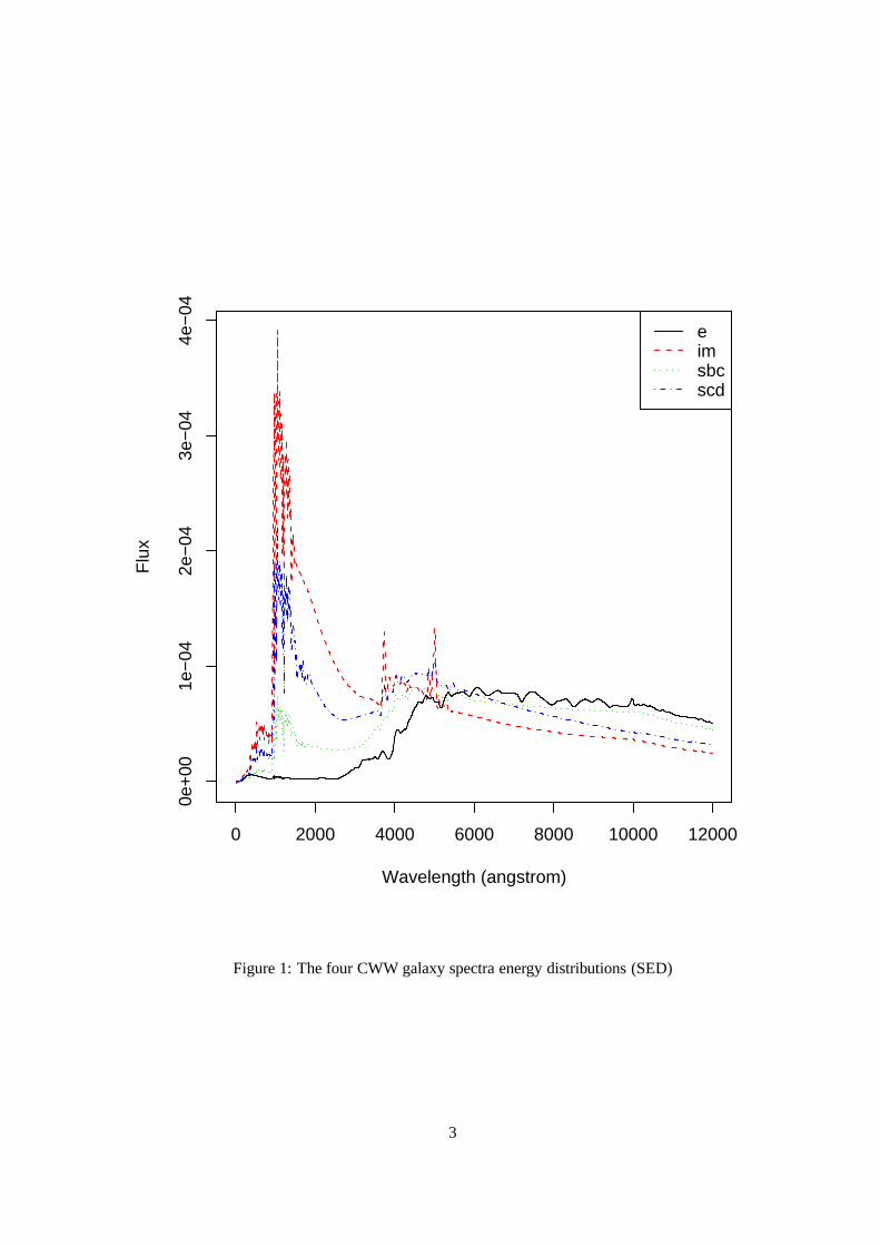
use theoretical “spectral energy distributions” (SEDs) which have been derived to show the shape of the

emissions at rest for various types of galaxies. For example, Figure 1 shows the templates proposed by

Coleman, Wu and Weedman (1980) for galaxies of the four types Elliptical, Irregular, Barred Spirals and

Spirals (E, Im, Sbc, Scd). Photometric redshift and galaxy type are then estimated by a least squares fit of

the data to the observations predicted by these spectra. The paper by Csabaiet al. (2003) also proposes

some iterative techniques for improving the template matching algorithm.

What are we trying to achieve by a Bayesian approach to the problem? One of the drawbacks of the

existing approaches seems to be a lack of both interpretability (in terms of the polynomial regression and

nearest neighbour methods) and uncertainty estimates. A hierarchical Bayesian model will allow us to

capture more of the structure of the application, and to generate estimates of redshift which include uncer-

tainty over galaxy type, brightness, measurement error. A second key motivation is to examine the extent

to which a quite generic statistical modelling approach, using for the most part standard model ingredients,

2

0 2000 4000 6000 8000 10000 12000

0e+

001e

−04

2e−

043e

−04

4e−

04

Wavelength (angstrom)

Flu

x

eimsbcscd

Figure 1: The four CWW galaxy spectra energy distributions (SED)

3

can compete with much more specific custom-made and highly-tuned techniques already available in the

astronomical literature.

In the following section, we set up the structured statistical model we will assume, with particular

emphasis on prior specification, and describe the MCMC computational techniques we use to fit the model

and produce the required predictions. We will begin analysis of the model’s performance in Section 3, with

a small scale calibration problem, selecting a small subset of the data to formulate and evaluate the model

and MCMC algorithm. The priors used at this stage are fairly vague although the form of them, in particular

that for the brightness of the galaxies as a function of redshift, is driven by the application. With the model

and algorithm tuned, in Section 4 we then evaluate the model in the way it might be used in practice, that

is fitting using a large number of galaxies to provide very precise priors for the model parameters when

estimating redshift for additional galaxies with only photometric data.

2 The calibration problem

2.1 Available data

The data we are using in this study come from the Early Data Release of the Sloan Digital Sky Survey. The

larger of the two sets, which we denote MAIN, contains 15477 galaxies, the smaller, denoted LRG, contains

a further 7861 galaxies. This smaller set is composed of galaxies which have been selected as having the

characteristics of elliptical galaxies with high redshifts (the set’s name, Luminous Red Galaxies, indicates

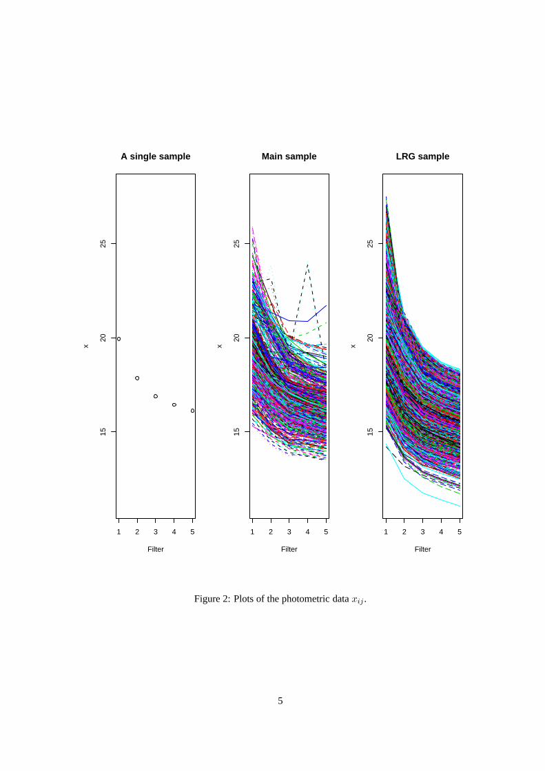
that these are galaxies with a red appearance). The MAIN sample has no such selection process. For each

galaxyi in the data sets we have both the spectroscopic measurement of redshift,yi, and the five photometric

measurements,xi1, . . . , xi5. Figure 2 shows a single set of photometric data, as well as 2000 MAIN and

LRG samples.

2.2 Modelling

Photometric data are recorded on the magnitude scale, with magnitude measured relative to a designated

bright source. The relationship between magnitude and the flux emitted by a galaxy is

M = −2.5 log10(F/F0)

= −2.5 log10 F + C (1)

whereF0 is the flux of the “zero-point” source, andC is a constant (Smith (1995)). The plots in Figure 1

represent the shape of the emitted flux; the actual flux will be a multiple of that template depending on the

brightness of the galaxy. Denote the spectral energy distribution function for thelth galaxy type byφl(λ)

4

1 2 3 4 5

1520

25

A single sample

Filter

x

1 2 3 4 5

1520

25

Main sample

Filter

x

1 2 3 4 5

1520

25

LRG sample

Filter

x

Figure 2: Plots of the photometric dataxij .

5

whereλ is the wavelength. The filter response functionshj(λ) for the five filters are known (see Figure 3).

Then a straightforward physical argument using the definition of redshiftz as the relative stretching of the

wavelength scale due to motion of the source, convolution with the response function, and transformation

using (1), implies that the unscaled response on the magnitude scale when a spectra is shifted by redshiftz

is given by

ψlj(z) = −2.5 log10

∫λhj(λ)φ

(λ

1 + z

)dλ, l = 1, . . . , 4, j = 1, . . . , 5 (2)

These filtered redshifted templates are the key ingredient in our model for the observed photometric data.

Theith astronomical object observed is regarded as a weighted linear combination of the elementary galaxy

typesl, using weightswil, although in practice we generally impose the restriction that each observed object

is of a single pure type so that for eachi,wil = 1 for a singlel. We also need to allow for differences in sensi-

tivity in the different filters, and different underlying brightnesses among the observed objects. These effects

are additive on the magnitude (logarithmic) scale, so the observational model proposed for the photometric

measurements is

xij = aj + bi +4∑l=1

wilψlj(zi) + εij (3)

with εij ∼ N(0, σ2j ), i = 1, . . . , n, j = 1, . . . , 5. (4)

Herezi is the true redshift of theith galaxy,bi is a measure of galaxy brightness, and the{aj} allow for

different filter sensitivities (constrained for identifiability to∑5j=1 aj = 0). The error terms are mutually

independent.

We also propose an observational model for how the spectroscopic redshift measurements arise; we

simply assume independent symmetric Normal measurement errors

yi|zi ∼ N(zi, σ2y). (5)

2.3 Prior specifications

The prior specification for the problem is a combination of quite standard choices assuming independence,

and some more specific models that we find are needed to capture some of the structure required for the

calibration. We suppose

π({zi}, {wil}, {aj}, {bi}, {σ2j }, σ2

y |{yi}, {xij}) ∝ π({yi}|{zi}, σ2y) ×

π({xij}|{aj}, {bi}, {zi}, {wil}, {σ2j }) ×

π({wil}) × π({aj}) ×5∏j=1

π(σ2j ) ×

π(σ2y) × π({bi}|{zi}) × π({zi}). (6)

6

0 2000 4000 6000 8000 10000 12000

0.0

0.1

0.2

0.3

0.4

0.5

0.6

Wavelength (angstrom)

Filt

er r

espo

nse

func

tions

Filter 1Filter 2Filter 3Filter 4Filter 5

Figure 3: The five filter response functions

7

The prior for the galaxy type allocationπ({wil}) is given by

P (wil = 1) = pl, l = 1, . . . , 4, i = 1, . . . , n (7)

where∑4l=1 pl = 1, with the allocation probabilities{pl} given a Dirichlet(1, 1, 1, 1) prior. The filter

sensitivity parameters{aj} are given an improper uniform prior (subject to the identifiability constraint).

The inverse variance parameters are given proper Gamma priors,Γ(5, 5/1000) for σ2y which is expected to

be very small, andΓ(1, 5/100) for theσ2j . Using improper priors here for the variance terms can lead to

problems with variance terms tending to zero, in particularσ2y , with obvious consequences for any MCMC

mixing (Spiegelhalter, Best, Gilks, and Inskip (1996)).

One of the difficulties revealed in earlier experiments using a set of independent standard priors for all

the parameters, was a lack of pooling of information between galaxies with and without recordedyi. One

possible improvement to the model would be to modify the priors on the brightnesses{bi} to depend on the

redshift{zi}. (A possible alternative would be instead to make the type allocation distribution{wil} depend

on brightness, but since we have limited information about the galaxy types, other than that the LRG data set

has been selected to consist generally of type 1, i.e. elliptical, galaxies, we do not pursue this line.) For each

of the five filters, Figure 4 shows a scatter plot for the LRG data ofxij − ψ1j(yi) (the recorded data minus

the filtered type 1 spectra at the observed spectroscopic redshift) againstyi (the spectroscopic redshift). If

the likelihood model forxij is reasonable, on the y-axis we have an indication ofaj + bi + εij, while on

the x-axis assuming that the spectroscopic redshift is quite accurate we have an indication ofzi. There is a

clear relationship, as might be expected by noting that a higher redshift may indicate that a galaxy is further

away and thus less bright. Fitting a regression for each of the five filters gives the following five quadratic

regression curves:

[Filter 1] 9.335535 + 20.626274yi − 25.464682y2i

[Filter 2] 10.96678 + 17.36172yi − 17.87796y2i

[Filter 3] 10.75092 + 17.58528yi − 18.62522y2i

[Filter 4] 10.09591 + 17.26753yi − 17.55181y2i

[Filter 5] 7.918389 + 17.379245yi − 17.346116y2i

Although there are clearly some discrepancies, in particular for filter 1, we suggest the prior

bi|zi ∼ N(α+ βzi + γz2i , σ

2b )

with α, β, γ all having improper priors, and the inverse ofσ2b having anΓ(1, 5/100) prior in common with

the{σ2j }.

8

For the purposes of these calibration experiments, the priorπ({zi}) is taken to be the normalised his-

togram of the combined LRG and MAIN data sets, using 40 equal-sized bins between 0 and 0.8 (see Fig-

ure 5).

2.4 Tuned MCMC moves

Inference from the posterior distribution

π({zi}, {wil}, {aj}, {bi}, {σ2j }, σ2

y , {pl}, α, β, γ, σ2b | {yi}, {xij}) ∝

π({yi}|{zi}, σ2y) ×

π({xij}|{aj}, {bi}, {zi}, {wil}, {σ2j }) ×

π({wil}) × π({aj}) ×5∏j=1

π(σ2j ) ×

π(σ2y) × π({bi}|{zi}) × π({zi}) ×

π({pl}) × π(α) × π(β) × π(γ) × π(σ2b ) (8)

will require Markov chain Monte Carlo (MCMC) methods (Gilks, Richardson and Spiegelhalter (1996)).

Many of the components can be updated using standard single-component Gibbs sampler moves (α, β, γ,

and all of the variance terms:σ2b , σ

2y , {σ2

j }). The constrained parameters{pl} and{aj} can also be updated

using Gibbs moves from their joint conditional distributions; the former is another Dirichlet distribution, the

latter uses the result that if the multivariate normala ∼ N(µ, V ) subject to1′a = 0 (i.e. the sum ofa’s = 0),

then the resulting conditioned distribution can be written asN(Rµ,RV R′), and samples can be generated

by drawingz ∼ N(µ, V ) and premultiplying byR, whereR = I − V 1(1′V 1)−11′.

The standard approach for updating the remaining parameters{bi}, {zi} and{wil} would be single site

proposals, Gibbs for the brightnesses and symmetric Metropolis proposals for the redshifts and galaxy types.

However, as we will demonstrate in the next section, this can lead to mixing problems. Consider Figure 6

which shows the smoothed filter spectra as a function ofz for the five filters, ieψlj(z), j = 1, . . . , 5, j =

1, . . . , 4. Changingz while holding all other variables fixed means a simultaneous shift along the x-axis

for the five graphs. Altering the label{wil} while holding all other variables fixed means a horizontal

jump between curves. In the former case, an acceptable acceptance rate can be maintained by choosing

the spread of the Metropolis proposal to be sufficiently small. However for the label changing, no such

tuning mechanism exists, potentially leading to the chain becoming trapped with the wrong label. If this

happens, the values of the other parameters includingz will evolve to match the data, and results far from

the spectroscopic redshift may result. Ideally the chain should visit all reasonable interpretations of the data

as the goal so as to generate reliable interval estimates ofz.

9

0.0 0.1 0.2 0.3 0.4 0.5 0.6

812

16

Filter 1

Spectroscopic y

x −

psi

(y)

0.0 0.1 0.2 0.3 0.4 0.5 0.6

1012

1416

Filter 2

Spectroscopic y

x −

psi

(y)

0.0 0.1 0.2 0.3 0.4 0.5 0.6

1012

14

Filter 3

Spectroscopic y

x −

psi

(y)

0.0 0.1 0.2 0.3 0.4 0.5 0.6

810

1214

Filter 4

Spectroscopic y

x −

psi

(y)

0.0 0.1 0.2 0.3 0.4 0.5 0.6

68

1012

Filter 5

Spectroscopic y

x −

psi

(y)

Figure 4: Plots for the five filters ofxij − ψ1j(yi) againstyi for the LRG data set

10

Histogram prior for z

Wavelength (angstrom)

Den

sity

0.0 0.2 0.4 0.6 0.8

02

46

8

Figure 5: The histogram of the combined LRG and MAINyi values

11

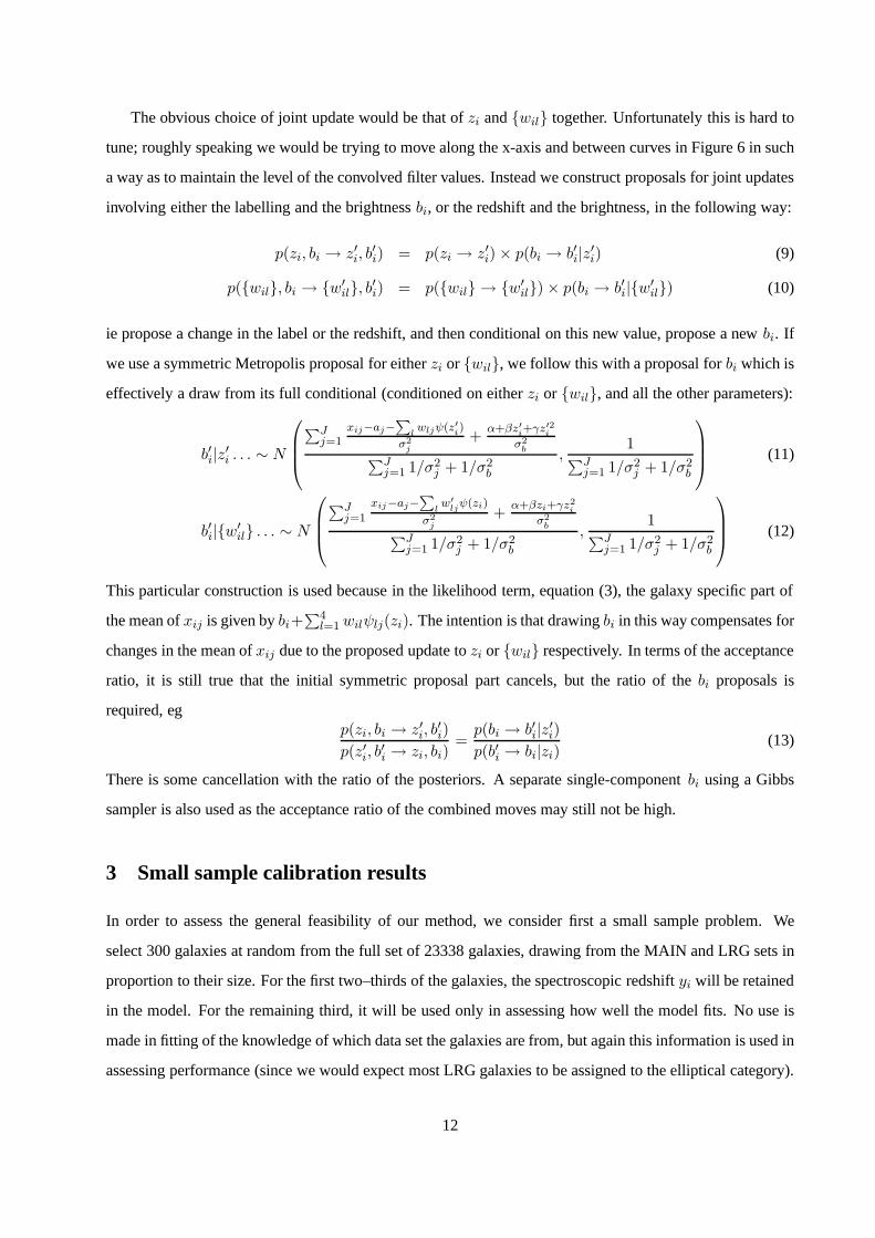
The obvious choice of joint update would be that ofzi and{wil} together. Unfortunately this is hard to

tune; roughly speaking we would be trying to move along the x-axis and between curves in Figure 6 in such

a way as to maintain the level of the convolved filter values. Instead we construct proposals for joint updates

involving either the labelling and the brightnessbi, or the redshift and the brightness, in the following way:

p(zi, bi → z′i, b′i) = p(zi → z′i) × p(bi → b′i|z′i) (9)

p({wil}, bi → {w′il}, b′i) = p({wil} → {w′

il}) × p(bi → b′i|{w′il}) (10)

ie propose a change in the label or the redshift, and then conditional on this new value, propose a newbi. If

we use a symmetric Metropolis proposal for eitherzi or {wil}, we follow this with a proposal forbi which is

effectively a draw from its full conditional (conditioned on eitherzi or {wil}, and all the other parameters):

b′i|z′i . . . ∼ N

∑Jj=1

xij−aj−∑

lwljψ(z′i)

σ2j

+ α+βz′i+γz′2i

σ2b∑J

j=1 1/σ2j + 1/σ2

b

,1∑J

j=1 1/σ2j + 1/σ2

b

(11)

b′i|{w′il} . . . ∼ N

∑Jj=1

xij−aj−∑

lw′

ljψ(zi)

σ2j

+ α+βzi+γz2iσ2

b∑Jj=1 1/σ2

j + 1/σ2b

,1∑J

j=1 1/σ2j + 1/σ2

b

(12)

This particular construction is used because in the likelihood term, equation (3), the galaxy specific part of

the mean ofxij is given bybi+∑4l=1wilψlj(zi). The intention is that drawingbi in this way compensates for

changes in the mean ofxij due to the proposed update tozi or {wil} respectively. In terms of the acceptance

ratio, it is still true that the initial symmetric proposal part cancels, but the ratio of thebi proposals is

required, egp(zi, bi → z′i, b′i)p(z′i, b′i → zi, bi)

=p(bi → b′i|z′i)p(b′i → bi|zi) (13)

There is some cancellation with the ratio of the posteriors. A separate single-componentbi using a Gibbs

sampler is also used as the acceptance ratio of the combined moves may still not be high.

3 Small sample calibration results

In order to assess the general feasibility of our method, we consider first a small sample problem. We

select 300 galaxies at random from the full set of 23338 galaxies, drawing from the MAIN and LRG sets in

proportion to their size. For the first two–thirds of the galaxies, the spectroscopic redshiftyi will be retained

in the model. For the remaining third, it will be used only in assessing how well the model fits. No use is

made in fitting of the knowledge of which data set the galaxies are from, but again this information is used in

assessing performance (since we would expect most LRG galaxies to be assigned to the elliptical category).

12

0.0 0.2 0.4 0.6 0.8

56

78

9

Filter 1

z

Filt

ered

val

ues

0.0 0.2 0.4 0.6 0.8

3.5

4.5

5.5

6.5

Filter 2

z

Filt

ered

val

ues

0.0 0.2 0.4 0.6 0.8

3.5

4.0

4.5

Filter 3

z

Filt

ered

val

ues

0.0 0.2 0.4 0.6 0.8

3.6

4.0

Filter 4

z

Filt

ered

val

ues

0.0 0.2 0.4 0.6 0.8

5.4

5.8

Filter 5

z

Filt

ered

val

ues

Figure 6: The convolved values observed at the five filters as a function of the redshiftz

13

We work with the same measure of success in estimatingzi for the final 100 galaxies used by Csabaiet al.

(2003), the “root mean square error” (RMS)

RMS =

√√√√ 300∑i=201

(yi − zi)2/100 (14)

that is, the root mean square distance between the fitted redshift and the observed spectroscopic redshift.

Figure 7 shows the RMS results over 1000 randomly drawn samples of 300 galaxies. For each sample,

25000 MCMC iterations were run using either single-site updates (Standard) or the jointbi moves described

in the previous section (Tuned). The first 10% of each run is discarded as burn-in. Clearly there is much

variation between samples, but generally, in the cases where the two algorithms do not agree, the Tuned

MCMC moves lead to lower values of the RMS. The average RMS for the Standard case is 0.0455, and for

the Tuned case it is 0.0426 (corresponding medians 0.0442 and 0.0409). Since the model is the same in both

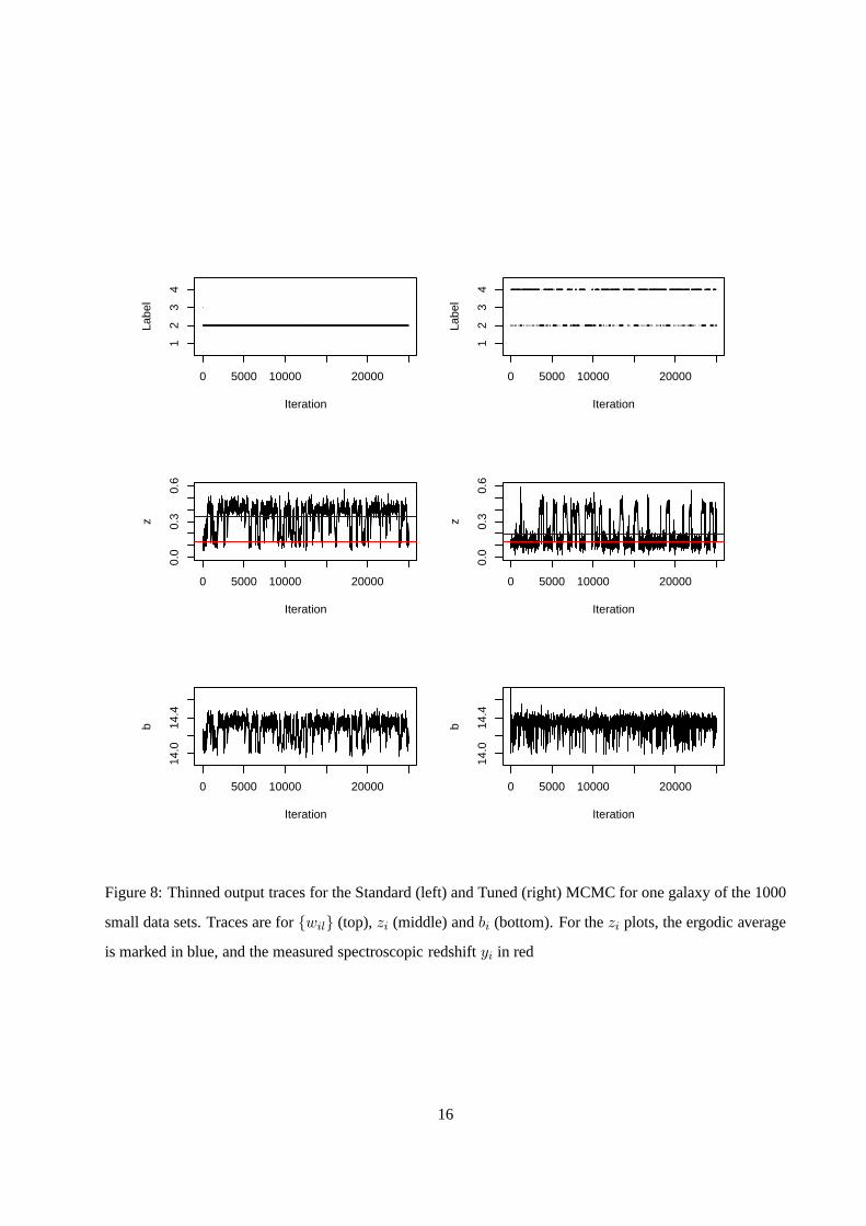
cases, this is a mixing issue. So, what is going on? Figure 8 shows traces, thinned by a factor of 10, of the

25000 iterations for one particular galaxy using the two sampling approaches. For this particular galaxy, the

model supports two potential label-redshift interpretations of the data. The Standard sampler is unable to

move between these two interpretations, while the Tuned move types overcome the problem.

The average RMSs found here are comparable to the results reported in Csabaiet al. (2003) for template

matching methods (although our method also has the benefit of delivering associated uncertainty estimates).

These results are from comparatively small sample sizes, and we would expect to improve on them by using

more than 150 knownyi galaxies to fit 100 unknownyi ones. In particular, there is significant variability in

the fitted values for the regression ofbi on zi, α, β andγ, with some of the worse RMS results displaying

quite distinct values of these parameters. In the next section, we discuss the application of these ideas to

large samples of galaxies.

4 Adding additional galaxies

The SDSS has already generated both spectroscopic and photometric redshift estimates for many thousands

of galaxies. The overall goal of this work is to use these existing data to estimatezi for additional galaxies

without spectroscopic data. We propose the following strategy: The entire data set will be split into a training

set, of size 22338, and a test set of size 1000 galaxies (chosen at random from the LRG and MAIN subsets in

proportion to the size of these sets). The model as described in previous sections will be fitted to the training

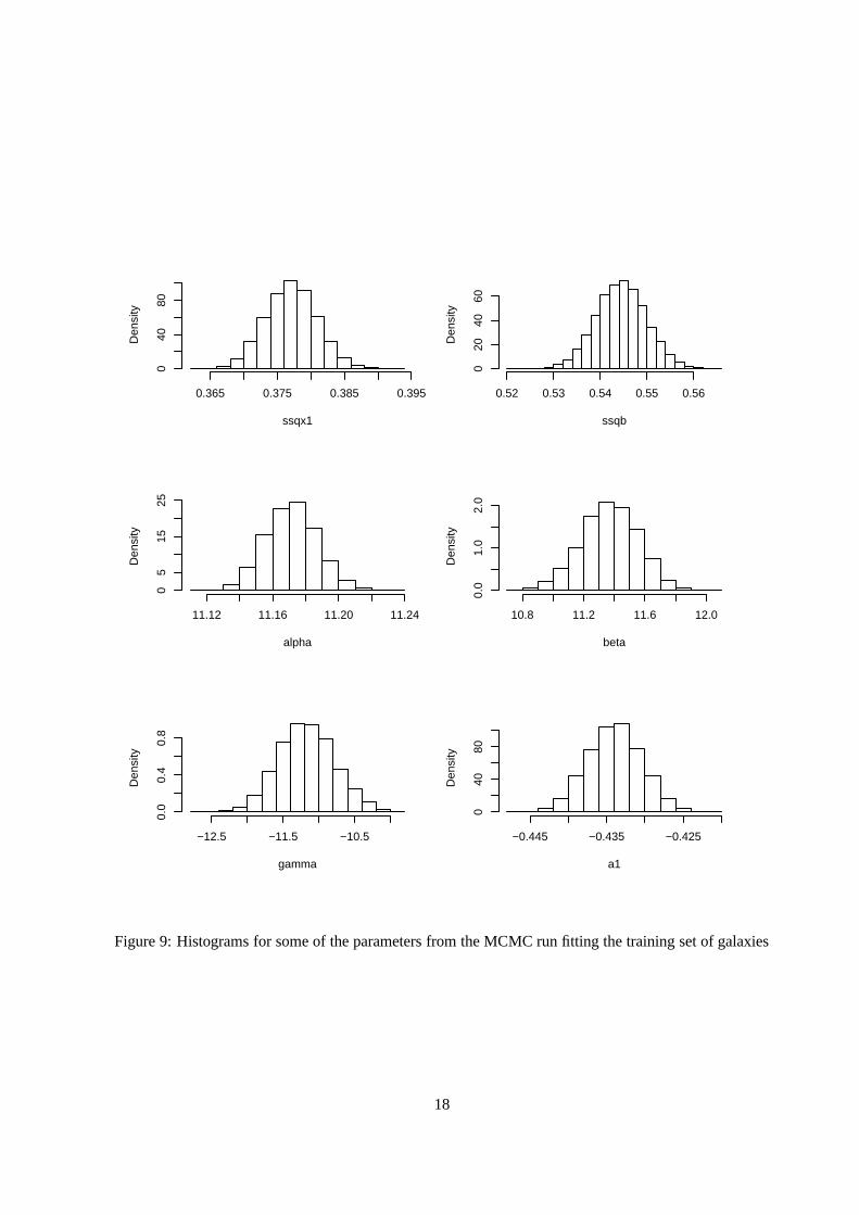
set including spectroscopic measurements for all 22338 galaxies. Histograms of some of the resulting

marginal posterior distributions are shown in Figure 9. The posterior distributions of the model parameters

{aj}, {σ2j }, {pl}, α, β, γ, σ2

b are approximated by parametric models which are then to be used as highly-

14

0.03 0.05 0.07

0.03

0.04

0.05

0.06

0.07

0.08

RMS of the 1000 experiments

Standard MCMC

Tun

ed M

CM

C

Standard Tuned

0.03

0.04

0.05

0.06

0.07

0.08

RMS of the 1000 experiments

Figure 7: The RMS results for the small calibration problem. In the left image, discrepancies of more than

0.001 are marked in red.

15

0 5000 10000 20000

12

34

Iteration

Labe

l

0 5000 10000 20000

12

34

Iteration

Labe

l

0 5000 10000 20000

0.0

0.3

0.6

Iteration

z

0 5000 10000 20000

0.0

0.3

0.6

Iteration

z

0 5000 10000 20000

14.0

14.4

Iteration

b

0 5000 10000 20000

14.0

14.4

Iteration

b

Figure 8: Thinned output traces for the Standard (left) and Tuned (right) MCMC for one galaxy of the 1000

small data sets. Traces are for{wil} (top),zi (middle) andbi (bottom). For thezi plots, the ergodic average

is marked in blue, and the measured spectroscopic redshiftyi in red

16

informative priors in estimating the redshift for the test set of 1000 galaxies; the following distributions are

fitted

σ2j ∼ Γ(λj , tj), j = 1, . . . , 5 (15)

{pl} ∼ Dirichlet(δ1, δ2, δ3, δ4) (16)

α ∼ N(µα, σ2α) (17)

β ∼ N(µβ, σ2β) (18)

γ ∼ N(µγ , σ2γ) (19)

σ2b ∼ Γ(λb, tb) (20)

aj ∼ N(µaj , σ2aj

), j = 1, . . . , 5 (21)

with all model parameters estimated from the posterior marginals of the training set, and where in the case

of the{aj}, the constraint∑aj = 0 will be imposed on top of these distributions.

Figure 10 illustrates a typical fitting of the test sample using 10000 iterations, discarding the first 1000

as burn-in. The RMS of this particular fit is 0.0397. Figure 10 also gives approximate 95% interval es-

timates of the redshift using± 1.96 times the estimated standard deviation. Of the 1000 intervals, 44 do

not cover the spectroscopic redshift; however, as spectroscopic redshift is not exactly equal to true redshift,

this is only a rough indication of whether the nominal coverage is accurate. Also perhaps of some use are

density estimates of the posterior distributions of thezi, Figure 11, which indicate the degree of uncertainty

overz related to the uncertainty of galaxy classification. The skewness of the examples seen suggests that

credible interval estimates computed from the quantiles of the sampledzi might be more appropriate than

the approach used here, although considerably more expensive in computer storage.

5 Discussion

The results obtained using the Bayesian model suggested here produce comparable RMSs to those obtained

in Csabaiet al. (2003) where they use the entire SDSS (LRG and MAIN) samples as training data and

additional sets from other sources as test data. Our results are slightly better than the out–of–sample template

matching they report but slightly worse than the in–sample template matching and empirical methods such

as polynomial regression or nearest neighbour approaches fitted using large numbers of galaxies. For the

out-of-sample galaxies they report results of “0.035 atr∗ < 18 and rising to 0.1 atr∗ < 21” (r∗ is the

third of the photometric measurements, here referred to asxi3, and is generally used as an indicator of

magnitude). Figure 12 plots the cumulative discrepancy betweenyi and the fitted redshift againstr∗ for the

17

ssqx1

Den

sity

0.365 0.375 0.385 0.395

040

80

ssqb

Den

sity

0.52 0.53 0.54 0.55 0.56

020

4060

alpha

Den

sity

11.12 11.16 11.20 11.24

05

1525

beta

Den

sity

10.8 11.2 11.6 12.0

0.0

1.0

2.0

gamma

Den

sity

−12.5 −11.5 −10.5

0.0

0.4

0.8

a1

Den

sity

−0.445 −0.435 −0.425

040

80

Figure 9: Histograms for some of the parameters from the MCMC run fitting the training set of galaxies

18

0.0 0.1 0.2 0.3 0.4 0.5

0.0

0.1

0.2

0.3

0.4

0.5

0.6

Spectroscopic

Fitt

ed

0.0 0.1 0.2 0.3 0.4 0.5

0.0

0.1

0.2

0.3

0.4

0.5

0.6

Spectroscopic

Fitt

ed

Figure 10: Left panel: fitted estimates ofz for the 1000 galaxies in the test sample. Right panel: fitted

estimates± 1.96 estimated standard deviations, with intervals not containing the spectroscopic redshift

marked in red

19

0.0 0.1 0.2 0.3 0.4 0.5

05

1015

Density estimate

z

Den

sity

0.00 0.05 0.10 0.15 0.20 0.25

04

812

Density estimate

z

Den

sity

0.0 0.1 0.2 0.3 0.4 0.5

02

46

8

Density estimate

z

Den

sity

0.0 0.1 0.2 0.3 0.4 0.5

05

1015

Density estimate

z

Den

sity

0.0 0.1 0.2 0.3 0.4

04

812

Density estimate

z

Den

sity

0.00 0.05 0.10 0.15 0.20 0.25

05

1020

Density estimate

z

Den

sity

Figure 11: Density estimates forzi for 6 of the test galaxies, overlaid by thinned MCMC realisations indi-

cating the associated label at each iteration

20

1000 test galaxies. For comparison,r∗ = 18 and a RMS of 0.035 are overlaid. For this set of galaxies, the

majority haver∗ < 20 and so a comparison for allr∗ < 21 is not really appropriate.

The attraction of the approach proposed here is that interval estimates of redshift are generated, along

with galaxy type probabilities. The training set can be expanded as more galaxies with both spectroscopic

and photometric data become available, updating the prior forz and refitting the model parameters. Caveats

are that the “out–of–sample” data used here are a subset of the combined SDSS sample. If data from other

sources are added, it will be important to monitor whether the fitted model changes significantly. In terms

of the existing data, Figure 10 suggests some residual structure to the fitting with more apparent under-

estimation in the mid-range of spectroscopic values. Given the reliance of this method on accuracy in the

spectral energy templates, this may be due to inadequacies in these templates (hence the work on modifying

these in Csabaiet al. (2003) ).

Acknowledgements

We are grateful to Bob Nichol and Andrew Connolly for providing both the data and background information

about the application. F.A-A. was supported in a visit to Bath by the Bath Institute for Complex Systems.

References

[1] G.D. Coleman, C-C. Wu, and D.W. Weedman (1980), “Colors and Magnitudes Predicted for High

Redshift Galaxies”,The Astrophysical Journal Supplement Series, 43, 393–416.

[2] Istvan Csabai, Tamas Budavari, Andrew J. Connolly, Alexander S. Szalay, Zsuzsanna Gyry, Narciso

Benitez, Jim Annis, Jon Brinkmann, Daniel Eisenstein, Masataka Fukugita, Jim Gunn, Stephen Kent,

Robert Lupton, Robert C. Nichol, and Chris Stoughton (2003), “The Application of Photometric Red-

shifts to the SDSS Early Data Release”,The Astronomical Journal, 125, 580–592.

[3] Gilks, W., Richardson, S. and Spiegelhalter, D. (1996),Markov Chain Monte Carlo in Practice. Chap-

man and Hall: London.

[4] Smith, R.C. (1995),Observational Astrophysics. Cambridge University Press: Cambridge.

[5] Spiegelhalter, D. J., Best, N. G., Gilks, W. R. and Inskip, H. (1996), Hepatitis B: a case study in

MCMC methods, Chapter 2 inMarkov Chain Monte Carlo in Practice. Chapman and Hall: London.

(eds Gilks, W., Richardson, S. and Spiegelhalter, D.).

21

12 14 16 18 20

0.00

0.05

0.10

0.15

0.20

0.25

r*

Abs

olut

e er

ror

Figure 12: Absolute error between the fittedzi and the spectroscopic redshift plotted againstxi3, referred to

asr∗, an indicator of magnitude. The overlaid black curve is the cumulative rmse, and the red lines indicate

the cumulative rmse error of 0.035 atr∗ = 18

22