THE ASTRONOMICAL JOURNAL, 122 :1151È1162, 2001 September( 2001. The American Astronomical Society. All rights reserved. Printed in U.S.A.

PHOTOMETRIC REDSHIFTS OF QUASARS1

GORDON T. RICHARDS,2 MICHAEL A. WEINSTEIN,2 DONALD P. SCHNEIDER,2 XIAOHUI FAN,3 MICHAEL A. STRAUSS,4DANIEL E. VANDEN BERK,5 JAMES ANNIS,5 SCOTT BURLES,5,6 EMILY M. LAUBACHER,6,7 DONALD G. YORK,6,8

JOSHUA A. FRIEMAN,5,6 DAVID JOHNSTON,6 RYAN SCRANTON,6 JAMES E. GUNN,4 R. C. NICHOL,9Z‹ ELJKO IVEZIC� ,4TAMA� S BUDAVA� RI,10,11 ISTVA� N CSABAI,10,11 ALEXANDER S. SZALAY,11 ANDREW J. CONNOLLY,12 GYULA P. SZOKOLY,13

NETA A. BAHCALL,4 NARCISO BENI�TEZ,11 J. BRINKMANN,14 ROBERT BRUNNER,15 MASATAKA FUKUGITA,16PATRICK B. HALL,4,17 G. S. HENNESSY,18 G. R. KNAPP,4 PETER Z. KUNSZT,11 D. Q. LAMB,6

JEFFREY A. MUNN,19 HEIDI JO NEWBERG,20 AND CHRIS STOUGHTON5Received 2001 April 3 ; accepted 2001 June 8

ABSTRACTWe demonstrate that the design of the Sloan Digital Sky Survey (SDSS) Ðlter system and the quality

of the SDSS imaging data are sufficient for determining accurate and precise photometric redshifts ofquasars. Using a sample of 2625 quasars, we show that ““ photo-z ÏÏ determination is even possible forz¹ 2.2 despite the lack of a strong continuum break, which robust photo-z techniques normally require.We Ðnd that, using our empirical method on our sample of objects known to be quasars, approximately70% of the photometric redshifts are correct to within *z\ 0.2 ; the fraction of correct photometric red-shifts is even better for z[ 3. The accuracy of quasar photometric redshifts does not appear to be depen-dent upon magnitude to nearly 21st magnitude in i@. Careful calibration of the color-redshift relation to21st magnitude may allow for the discovery of D106 quasar candidates in addition to the 105 quasarsthat the SDSS will conÐrm spectroscopically. We discuss the efficient selection of quasar candidates fromimaging data for use with the photometric redshift technique and the potential scientiÐc uses of a largesample of quasar candidates with photometric redshifts.Key words : galaxies : distances and redshifts È galaxies : photometry È methods : statistical È

quasars : general

ÈÈÈÈÈÈÈÈÈÈÈÈÈÈÈ1 Based on observations obtained with the Sloan Digital Sky Survey.2 Department of Astronomy and Astrophysics, 525 Davey Laboratory,

Pennsylvania State University, University Park, PA 16802.3 Institute for Advanced Study, Einstein Drive, Princeton, NJ 08540.4 Princeton University Observatory, Peyton Hall, Princeton, NJ 08544-

1001.5 Fermi National Accelerator Laboratory, P.O. Box 500, Batavia, IL

60510.6 Department of Astronomy and Astrophysics, University of Chicago,

5640 South Ellis Avenue, Chicago, IL 60637.7 Department of Physics, University of Dayton, Dayton, OH 45469-

2314.8 Enrico Fermi Institute, University of Chicago, 5640 South Ellis

Avenue, Chicago, IL 60637.9 Department of Physics, Carnegie Mellon University, 5000 Forbes

Avenue, Pittsburgh, PA 15232.10 Department of Physics of Complex Systems, Uni-Eo� tvo� s Lora� nd

versity, Pf. 32, H-1518 Budapest, Hungary.11 Department of Physics and Astronomy, Johns Hopkins University,

3400 North Charles Street, Baltimore, MD 21218-2686.12 Department of Physics and Astronomy, University of Pittsburgh,

3941 OÏHara Street, Pittsburgh, PA 15260.13 Astrophysikalisches Institut Potsdam, An der Sternwarte 16,

D-14482 Potsdam, Germany.14 Apache Point Observatory, P.O. Box 59, Sunspot, NM 88349.15 Department of Astronomy, California Institute of Technology, Pasa-

dena, CA 91125.16 Institute for Cosmic Ray Research, University of Tokyo, 5-1-5

Kashiwa, Kashiwa City, Chiba 277-8582, Japan.17 Departamento de y PontiÐcia UniversidadAstronom•� a Astrof•� sica,

de Chile, Casilla 306, Santiago 22, Chile.Cato� lica18 US Naval Observatory, 3450 Massachusetts Avenue, NW, Washing-

ton, DC 20392-5420.19 US Naval Observatory, Flagsta† Station, P.O. Box 1149, Flagsta†,

AZ 86002.20 Department of Physics, Applied Physics, and Astronomy, Rensselaer

Polytechnic Institute, 110 Eighth Street, Troy, NY 12180-3590.

1. INTRODUCTION

““ Astronomical photometry is best considered as low-resolution spectroscopy,ÏÏ said Bessell (1990). With carefullycalibrated CCD imaging data in Ðve broad passbands(u@g@r@i@z@ ; Fukugita et al. 1996) that have sharp edges andlittle overlap, the imaging survey of the Sloan Digital SkySurvey (SDSS; York et al. 2000) is designed to put thisphilosophy into practice. For many applications, theimaging part of the survey can be treated as an RD 4objective-prism survey with wavelength coverage fromD3000 to D10500 Ó.

In recent years, the practice of measuring redshifts ofgalaxies using multiple-band photometry has become bothpopular and powerful (e.g., Brunner et al. 1997 ; Connolly etal. 1999), although the concept has been around for quitesome time (Baum 1962). The popularity of photometric red-shifts is not surprising, given the impressive successes of themethod and the di†erences in exposure times between spec-troscopy and broadband imaging. The e†ectiveness of themethod is primarily the result of discontinuities in the spec-tral energy distribution (SED) of galaxies, such as the 4000

break. A similar feature, namely, the discontinuity causedÓby the onset of the Lya forest, allows one to accuratelyestimate redshifts for z[ 3 quasars and galaxies (the Lyaforest is observable in the optical by z\ 2.2, but it is notuntil z\ 3 that it makes the u@[g@ colors red enough todistinguish from lower redshift quasars).

Although the Lya break allows for accurate redshiftdeterminations from photometry of z[ 3 quasars, theoverall spectrum of quasars is well described by a power-

1151

1152 RICHARDS ET AL. Vol. 122

law continuum, which is invariant under redshift. Thismeans that, for quasars at redshifts too small for the Lyaforest to be observable in the optical from the ground,quasar photometric redshift (““ photo-z ÏÏ) determinationwould be impossible if quasar spectra were purely powerlaws. Despite the fact that quasars also have emission-linefeatures that cause redshift-dependent color changes thatmight be expected to help with low-redshift (z¹ 2.2) quasarphoto-z determinations, the photometric redshift techniquehas hitherto not been e†ective for low-z quasars, because ofthree e†ects : (1) this technique requires precisionphotometryÈerrors in the colors must be smaller than thestructure in the color-redshift relation, which is typicallynot possible (at these redshifts) with photographic material ;(2) Ðlters that overlap signiÐcantly tend to smooth out thefeatures in the color-redshift relation ; and (3) more than twocolors are needed to break the degeneracy (i.e., to dis-tinguish between two or more redshifts that have similarcolors).

Of course, any color selection of quasars is essentially acrude attempt at determining photometric redshifts. Forexample, the selection of quasars as UV-excess pointsources is equivalent to predicting that the objects will turnout to be quasars with z\ 2.2. Similarly, very red outliersfrom the stellar locus that are point sources are quite likelyto be z[ 3 quasars. However, in this work we go one stepfurther and predict speciÐc redshift values for objects, asopposed to predicting broad redshift ranges.

In Richards et al. (2001a, hereafter R01), we showed thatthe colors of quasars in the SDSS photometric system are astrong function of redshift for 0 \ z\ 5. Furthermore, thecolors of quasars at similar redshifts have a relatively smalldispersion. We Ðnd that the existence of signiÐcant struc-ture in the color-redshift relation and the reasonably smallscatter in the SDSS colors at a given redshift allow for thedetermination of photometric redshifts for quasars from theSDSS photometry.

In this paper and in a companion paper et al.(Budava� ri2001), we present the Ðrst large-scale determination ofphotometric redshifts for quasars, at 0 \ z\ 5, using onlyfour colors derived from the Ðve SDSS broadband magni-tudes. This result signals the beginning of practical applica-tions of quasar photometric redshifts that can be used forscientiÐc programs. In this paper, we discuss an empiricalquasar photo-z method that relies upon the structure that ispresent in the empirical quasar color-redshift relation.Photometric redshifts are determined by minimizing the s2between the colors of a new object and the colors of knownquasars as a function of redshift. In et al. (2001),Budava� riwe discuss the application of proven galaxy photo-z tech-niques to quasars. These techniques include other empiricalmethods, such as nearest neighbor searches and polynomialÐtting. In addition, et al. (2001) discuss both aBudava� ristandard spectral template Ðtting procedure and a hybridapproach that allows for the construction of multiple tem-plates. It is our hope that further analysis using the methodpresented herein and the methods presented in etBudava� rial. (2001), or a combination thereof, will result in a methodfor determining photometric redshifts for quasars that rivalsthe usefulness of the galaxy photometric redshifts.

This paper is structured as follows : ° 2 gives a briefdescription of the data used herein. More details can befound in R01, where this data set was deÐned. In ° 3, wedescribe a simple technique for determining quasar photo-

metric redshifts and investigate how we might improve ourphotometric redshift predictions. In ° 4, we discuss somescience that can be done with a sample of ““ quasars ÏÏ withphotometric redshifts. Finally, ° 5 presents our conclusions.

2. THE DATA

The sample studied herein is the same sample analyzed inR01 and includes 2625 quasars. Of these, 801 were pre-viously known quasars from the NASA Extragalactic Data-base (NED) that were matched to objects in the SDSSimaging catalog. A total of 1983 of the 2625 quasars wereindependently discovered or recovered during SDSS spec-troscopic commissioning. The photometry for these 1983quasars was taken from the photometric catalogs of fourscans of the celestial equator that were taken between 1998September 19 and 1999 March 22, which include data““ runs ÏÏ 94, 125, 752, and 756. These are equatorial2¡.5-widescans that were observed and processed as part of the com-missioning phase of the SDSS imaging survey. There is con-siderable (but not complete) overlap between these 1983SDSS commissioning quasars and those used by VandenBerk et al. (2001) in the construction of a composite quasarspectrum using over 2200 SDSS quasar spectra.

The photometry for all previously known quasars in thesample was given in R01. The photometry for the newSDSS quasars is available as part of the SDSS Early DataRelease ; details regarding the new SDSS quasars are givenby Stoughton et al. (2001), including a discussion of theselection algorithm used to target quasars during SDSScommissioning. Quasars were selected primarily as outliersfrom the stellar locus ; the magnitudes have been correctedfor Galactic reddening according to Schlegel, Finkbeiner, &Davis (1998). In addition to ““ normal ÏÏ quasars, the sampleincludes such objects as broad absorption line (BAL)quasars and low-redshift low-luminosity Seyfert galaxies.We note that the inclusion of such objects is likely toproduce results slightly di†erent from those that we wouldobtain with a sample of purely ““ normal ÏÏ quasars.

We emphasize that the quasar target selection algorithmunderwent many changes during the commissioning phaseand that the SDSS quasars that make up the majority of thesample studied herein in no way constitute a homogeneoussample. The Ðnal SDSS quasar target selection algorithm,which di†ers somewhat from the preliminary algorithmdescribed by Stoughton et al. (2001), will be discussed byRichards et al. (2001b) and Newberg et al. (2001). For addi-tional references and more details regarding the entire dataset (not just the SDSS commissioning objects), see R01.

3. PHOTOMETRIC REDSHIFTS FOR QUASARS

The SDSS CCD mosaic imaging camera (Gunn et al.1998) produces accurate (¹0.03 mag) photometry thatmakes it possible to discern structure in the quasar color-redshift relation. As can be seen from Figure 1 (adaptedfrom R01), where we plot the measured colors of 2625quasars (gray points) along with the median color as a func-tion of redshift (solid curve), the color-redshift relation forquasars in the SDSS Ðlter set shows a relatively tight dis-

No. 3, 2001 PHOTOMETRIC REDSHIFTS OF QUASARS 1153

FIG. 1.ÈSDSS colors vs. redshift for 2625 quasars between z\ 0 and z\ 5 (gray points), the median color as a function of redshift (solid curve) and the 1 perror width in the color-redshift relation (dashed curves). (Adapted from R01.)

tribution with a considerable amount of structure.21 Redoutliers are primarily anomalously red quasars (hereafterreferred to as ““ reddened ÏÏ quasars, although is it not clearwhether they are actually reddened or simply redder thanaverage), which will be discussed in ° 3.2. Also note thesharp changes in color due to absorption by the Lya forestas the quasars move to higher redshifts. With the fourcolors derived from the Ðve-band SDSS photometry, it ispossible to break the degeneracy of the color-redshift rela-tion with sufficient accuracy and efficiency that quasars canbe assigned redshifts purely from their colors.

3.1. T he s2 Minimization TechniqueAs a starting point for our photometric redshift investiga-

tion, we begin with one of the simplest methods for deter-mining photometric redshifts given the structure that is seenin Figure 1. First, we construct an empirical color-redshift

ÈÈÈÈÈÈÈÈÈÈÈÈÈÈÈ21 When referring to actual measured values (such as in the Ðgures), the

Ðlter names are designated as, e.g., r* instead of r@, in order to indicate thepreliminary nature of the SDSS photometry presented herein ; however, wewill typically use the r@ convention whenever we are not discussing speciÐcmeasurements. The magnitudes are given as asinh magnitudes (Lupton,Gunn, & Szalay 1999).

relation based on the median colors of quasars as a functionof redshift. The color-redshift relation was formed by deter-mining the median quasar colors in bins with centers at 0.05intervals in redshift, and widths of 0.075 for z¹ 2.15, 0.5 forz[ 2.5, and 0.2 for 2.15 ¹ z¹ 2.5. This relation is based onthe assumption that, in our sample, quasars at a given red-shift have similar colors ; this assumption does not necessar-ily mean that the rest-frame color of all quasars should bethe same (i.e., there is not necessarily a redshift-independentSED). Our empirical color-redshift relation is shown by thesolid curve in Figure 1 ; the colors that encompass 68% ofthe data in each redshift bin, thus deÐning an e†ective 1 perror width in the color-redshift relation, are given by thedashed curves. The median and error vectors for this dataset are also computed in R01 and are given in Table 3 inthat paper. Figure 1 contains quasars that were identiÐedby R01 as a population of reddened quasars, which includesobjects such as BAL quasars ; these anomalously red objectsare removed before computing the median colors as a func-tion of redshift.

Photometric redshifts are then determined by minimizingthe s2 between all four observed colors and the mediancolors as a function of redshift. All colors are corrected forGalactic reddening according to Schlegel et al. (1998). The

1154 RICHARDS ET AL. Vol. 122

s2 (for each redshiftÈindicated by the subscript z) is com-puted as

sz2\ [(u@ [ g@)[ (u@[ g@)

z]2

pu{~g{2 ] p(u{~g{)z2 ] C

gr] C

ri] C

iz, (1)

where (u@[g@) is the measured u@[g@ color of the object,is the color from the median color-redshift relation(u@[g@)

zat a given redshift, is the photometric error in thepu{~g{u@[g@ color, which is given by , and is(p

u{2 ] p

g{2 )1@2 p(u{~g{)zthe 1 p error width of the median color-redshift relation as a

function of redshift. Since the latter term is relatively inde-pendent of redshift (see Fig. 1), we have chosen to use a Ðxedvalue for all redshifts. The terms and are analo-C

gr, C

ri, C

izgous to the term for the u@[g@ colors, but for g@[r@, r@[i@,and i@[z@, respectively. The most probable redshift is givenby the redshift that produces the smallest value of s2. Slight-ly di†erent formulations of s2 may be more appropriatedepending on certain assumptions, such as whether thewidth of the color distribution is independent of redshift orif magnitude errors are correlated.

The Ðrst test of this photometric redshift technique is todetermine whether it can recover the redshifts for theobjects that the input data set comprises. The results of suchan exercise are shown in Figures 2È5, which display theresults for the 2625 quasars from R01. In Figure 2, we plotthe predicted photometric redshift versus the spectroscopicredshift for all of the quasars in our sample : the samequasars that went into making the empirical color-redshiftrelation. We Ðnd that 1834 of 2625 quasars (or 70%) havephotometric redshifts that are correct to within o*z o \ 0.2or better. The rms deviations from the correct values are

and where is the rms for the*all\ 0.676 *0.3\ 0.099, *allwhole sample and is the rms for those objects whose*0.3photometric redshifts are within o*z o \ 0.3 of the spectro-scopic redshift. Considering z[ 3 alone, we see that ourresults are even better than for all redshifts combined.Points marked by plus signs are those quasars that are

FIG. 2.ÈPhotometric redshift vs. spectroscopic redshift for all quasarsin our sample. Points marked with a plus sign are anomalously red quasars(see ° 3.2), and squares indicate extended sources (see ° 3.3).

deemed to be anomalously red ; they are the points inFigure 1 that lie well above the median relation (see R01 fordiscussion). Points marked by squares are extendedsources ; the colors of these objects may be a†ected by thelight from the host galaxy.

Further improvements to our method will come fromunderstanding the distribution of both extended andreddened quasars in addition to investigating inherent red-shift degeneracies, all of which are obvious in Figure 2.Sections 3.2, 3.3, and 3.4 are devoted to discussions of howwe might reduce the fraction of objects with incorrectphotometric redshift estimates. It is also important torealize that all of the objects in our sample are known to bequasars. For actual scientiÐc applications where we knowonly the colors, obviously not all of the objects will bequasars ; this fact must be taken into account in the determi-nation of our efficiency, as we discuss in ° 3.6.

That a solid majority of the quasars have accurate photo-metric redshifts can be seen more clearly in Figure 3, wherewe plot a histogram of the di†erences between the photo-metric redshifts and the spectroscopic redshifts. This histo-gram reveals that the photometric redshift error has arelatively Gaussian core with p D 0.1 that contains D70%of the quasars, and ““ sidelobes ÏÏ at *z\ ^1.5 that containabout 15% of the objects each.

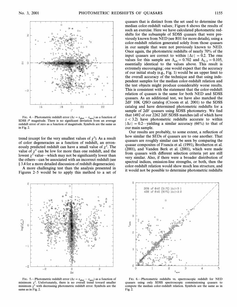
Figure 4 shows *z as a function of the quasar i* magni-tude. That there is no signiÐcant deviation from zero as afunction of magnitude bodes well for using the photometricredshift technique to estimate redshifts for quasars fainterthan the limit of our sample (until the magnitude errorsbecome too large). The potential value of this result forcreating a large sample of faint quasars is discussed in ° 3.6.

Finally, in Figure 5 we plot *z versus the minimum valueof s2 for each quasar. As long as our photometric errors arerelatively small, one would expect the minimum s2 todecrease with increasing photometric redshift accuracy ; ifthis were true, it would provide an estimate of the accuracyof the photometric redshift. Unfortunately, we see no such

FIG. 3.ÈHistogram of photometric redshift errors (*z\ zphot [ zspec)for the data from Fig. 2.

No. 3, 2001 PHOTOMETRIC REDSHIFTS OF QUASARS 1155

FIG. 4.ÈPhotometric redshift error as a function of(*z\ zphot [ zspec)SDSS i* magnitude. There is no signiÐcant deviation from an averageredshift error of zero as a function of magnitude. Symbols are the same asin Fig. 2.

trend (except for the very smallest values of s2). As a resultof color degeneracies as a function of redshift, an erron-eously predicted redshift can have a small value of s2. Thevalue of s2 can be low for more than one redshift, and thelowest s2 valueÈwhich may not be signiÐcantly lower thanthe othersÈcan be associated with an incorrect redshift (see° 3.4 for a more detailed discussion of redshift degeneracies).

A more challenging test than the analysis presented inFigures 2È5 would be to apply this method to a set of

FIG. 5.ÈPhotometric redshift error as a function of(*z\ zphot [ zspec)minimum s2. Unfortunately, there is no overall trend toward smallerminimum s2 with decreasing photometric redshift error. Symbols are thesame as in Fig. 2.

quasars that is distinct from the set used to determine themedian color-redshift values ; Figure 6 shows the results ofsuch an exercise. Here we have calculated photometric red-shifts for the subsample of SDSS quasars that were pre-viously known from NED (see R01 for more details), using acolor-redshift relation generated solely from those quasarsin our sample that were not previously known to NED.Once again, the photometric redshifts of nearly 70% of theinput quasars are correct to within o*z o \ 0.2. The rmsvalues for this sample are and*all\ 0.702 *0.3 \ 0.105,essentially identical to the values above. This result isextremely encouraging ; one would expect that the accuracyof our initial study (e.g., Fig. 1) would be an upper limit tothe overall accuracy of the technique and that using inde-pendent samples for the median color-redshift relation andthe test objects might produce considerably worse results.This is consistent with the statement that the color-redshiftrelation of quasars is the same for both NED and SDSSquasars. As an additional test, we have also matched the2dF 10K QSO catalog (Croom et al. 2001) to the SDSScatalog and have determined photometric redshifts for asample of 2dF quasars using SDSS photometry. We Ðndthat 1492 of our 2262 2dF/SDSS matches (all of which havez\ 3.2) have photometric redshifts accurate to withino*z o \ 0.2Èyielding a similar accuracy (66%) to that ofour main sample.

Our results are probably, to some extent, a reÑection ofhow similar the SEDs of quasars are to one another. Thatquasars are roughly similar can be seen by comparing thequasar composites of Francis et al. (1991), Brotherton et al.(2001), and Vanden Berk et al. (2001), which were madefrom quasars with di†erent selection criteria yet are stillvery similar. Also, if there were a broader distribution ofspectral indices, emission-line strengths, or both, then thecolor-redshift relation would show much less structure, andit would not be possible to determine photometric redshifts

FIG. 6.ÈPhotometric redshifts vs. spectroscopic redshift for NEDquasars using only SDSS spectroscopic commissioning quasars tocompute the median color-redshift relation. Symbols are the same as inFig. 2.

1156 RICHARDS ET AL. Vol. 122

for z\ 2.2 quasars. Francis et al. (1992) found that 75% ofthe variance in quasar spectra can be accounted for by theÐrst three principal components of their composite spec-trum. The Ðrst component represents the quasar emission-line spectrum, whereas the second component includes thepower-law continuum slope and modiÐcations to the emis-sion lines. These two components probably account fornearly all of the structure and the width of the color-redshiftrelation as shown in Figure 1. As a result of these simi-larities, quasar photometric redshifts are possible given suf-Ðciently high quality photometry.

For the sake of comparison, Hatziminaoglou, Mathez, &(2000), using two samples of 51 and 46 quasars withPello�

photometry from six broadband Ðlters, were able to deter-mine photometric redshifts to within o*z o \ 0.1 for 23(45%) and 17 (37%) of their quasars in each sample, respec-tively. Similarly, Wolf et al. (2001) report an accuracy of50% ( o*z o \ 0.1) in their sample of 20 objects using 11intermediate-band and broadband Ðlters. Our accuracy(fraction of objects within o*z o \ 0.2) is competitive with, ifnot considerably better than, these previous results, using asample that is more than 50 times as large. Furthermore, itis signiÐcant that our study uses only four broadbandcolors and that no e†ort beyond routine SDSS operations isneeded to obtain the required measurements.

Thus far, we have applied our algorithm without anypre- or postprocessing of the data in the input sample.However, it is clear that an application of some constraintson the input sample will lead to signiÐcant improvements inour results without introducing any signiÐcant biases. Wenow turn to a discussion of these techniques.

3.2. Reddened QuasarsApproximately 4% of the quasars in our sample are sub-

stantially redder than can be expected from Galactic extinc-tion (R01). Such quasars present a problem for photometricredshift determination, since their colors are signiÐcantlydi†erent from the intrinsic colors of the average quasar atthe same redshift. For example, in Figures 2, 4, 5, and 6 wehave marked quasars that are anomalously red for theirredshift with plus signs ; many of these anomalously redquasars are BAL quasars. As one expects, most of thereddened quasars (92%) have incorrect photometric red-shifts ; moreover, an appreciable fraction (12%) of thequasars with bad photometric redshifts are reddened.

There are a number of ways to deal with reddenedquasars to improve the e†ectiveness of the photo-z algo-rithm. One could attempt to recognize reddened quasars apriori and apply a correction to their colors. However, thisprocess would only work if the red quasars were clearlyidentiÐable and could be corrected with some sort of globalcorrection factor ; such a procedure is unlikely to be verye†ective because of the broad range of reddening that isobserved (the colors of reddened quasars at a given redshiftare consistent with the colors of reddened quasars at nearlyall other redshifts). One could also attempt to recognizereddened quasars before attempting to calculate theirphotometric redshifts and then reject them from consider-ation (as opposed to recognizing them and trying to make acorrection).

Identifying red quasars without knowing their redshiftsmay not be as difficult as it might initially appear. Forexample, the vast majority of z\ 2.2 quasars haveu@[g@¹ 0.6, so a quasar candidate with u@[g@[ 0.6 is

probably either a high-redshift quasar or a reddened low-redshift quasar (if the object is indeed a quasar). Similarapproaches can be tried with outliers in the other colors. Ofcourse, there can be redshift biases inherent in this process :as can be seen in Figure 1, a z\ 1.6 quasar that is reddenedby 0.5 mag stands out more clearly as a red outlier in u@[g@than does a similarly reddened z\ 1.9 quasar, as a result ofthe structure in the quasar color-redshift relation.

We have made a preliminary attempt to reject reddenedquasars and to study the e†ects of their rejection on ourresults. Using only point sources, we have found a series ofcolor cuts (based initially on the u@[z@ colors) that allow forthe identiÐcation of reddened quasars and are roughly inde-pendent of redshift and unbiased against high-z quasars.These color cuts are applied uniformly to the entire datasetÈwithout the knowledge of the actual redshifts of thequasars. We Ðnd that the application of these color cuts toreject reddened quasars improves our (fractional) successrate to roughly 73%. In order to apply this technique withconÐdence in the future, we need more than the 40 quasarswith z[ 4 that are in our current sample. These additionalz[ 4 quasars will determine the empirical scatter in thecolors for the highest redshift quasars, which, in turn, willallow a better separation between real high-z quasars andreddened lower redshift quasars.

3.3. Extended ObjectsExtended sources, which are plotted as squares in the

Ðgures, pose an additional problem. At high redshift (z[ 1),about half of the quasars that are labeled as extended in thesample presented herein are actually classiÐed as pointsources by the latest version of the SDSS image processingsoftware ; such objects should not be a problem in thefuture. However, at low redshift there are low-luminosityobjects (Seyfert galaxies ; see R01) whose colors are likely tobe contaminated by the light from the quasar host galaxyand will appear redder than normal. As with the reddenedquasars discussed above, we must handle such objects prop-erly to obtain the best photometric redshifts. At Ðrst, it maybe wise to simply exclude all extended quasars from ourmedian color-redshift relation and not attempt to determinephotometric redshifts for extended sources. After all, it isclear that these have relatively small redshifts (for quasars),which may be sufficient constraint for most science applica-tions. However, in the future, we would hope to be able todetermine photometric redshifts for these objects as well.

For our present analysis, we have included extendedobjects, which has two e†ects. First, it causes the mediancolors to be slightly redder at low redshift than they wouldotherwise be. Second, this means that some extendedobjects will have quite good photometric redshifts, but thatvery blue point sources at low redshift might have poorerphotometric redshifts than would otherwise be expected.We expect that those extended sources with poor photo-metric redshifts will tend to have large photometric red-shifts, since their redder colors will push them to higherapparent redshifts. A preliminary investigation found thatexcluding extended objects from the median color-redshiftrelation does not, in fact, improve our results for pointsources ; however, more work is needed on the subject.

3.4. Redshift DegeneraciesFrom Figure 2, it is clear that there are some degeneracies

in the color-redshift relation. Such an e†ect is indicated by

No. 3, 2001 PHOTOMETRIC REDSHIFTS OF QUASARS 1157

outliers that are symmetric around the line. Forzspec \ zphotexample, a number of quasars are being assignedzspec D 2photometric redshifts near 0.4 ; similarly, many zspec D 0.4quasars are given photometric redshifts around 2. To someextent, we may be unable to resolve these degeneracies ;however, we have reason to be encouraged that we may beable to determine the correct redshifts for these objects.

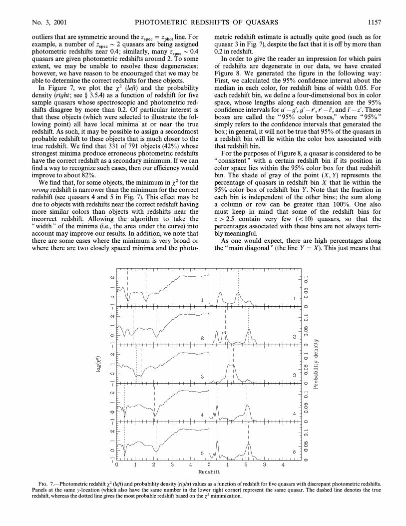
In Figure 7, we plot the s2 (left) and the probabilitydensity (right ; see ° 3.5.4) as a function of redshift for Ðvesample quasars whose spectroscopic and photometric red-shifts disagree by more than 0.2. Of particular interest isthat these objects (which were selected to illustrate the fol-lowing point) all have local minima at or near the trueredshift. As such, it may be possible to assign a secondmostprobable redshift to these objects that is much closer to thetrue redshift. We Ðnd that 331 of 791 objects (42%) whosestrongest minima produce erroneous photometric redshiftshave the correct redshift as a secondary minimum. If we canÐnd a way to recognize such cases, then our efficiency wouldimprove to about 82%.

We Ðnd that, for some objects, the minimum in s2 for thewrong redshift is narrower than the minimum for the correctredshift (see quasars 4 and 5 in Fig. 7). This e†ect may bedue to objects with redshifts near the correct redshift havingmore similar colors than objects with redshifts near theincorrect redshift. Allowing the algorithm to take the““ width ÏÏ of the minima (i.e., the area under the curve) intoaccount may improve our results. In addition, we note thatthere are some cases where the minimum is very broad orwhere there are two closely spaced minima and the photo-

metric redshift estimate is actually quite good (such as forquasar 3 in Fig. 7), despite the fact that it is o† by more than0.2 in redshift.

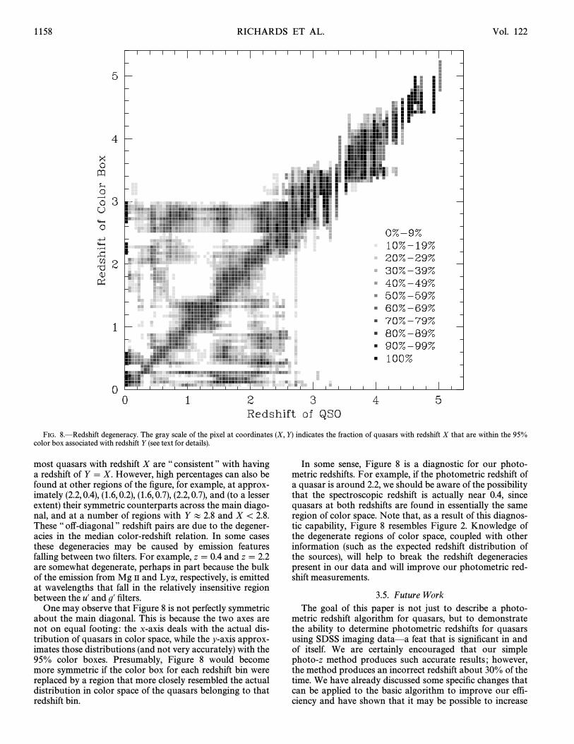
In order to give the reader an impression for which pairsof redshifts are degenerate in our data, we have createdFigure 8. We generated the Ðgure in the following way :First, we calculated the 95% conÐdence interval about themedian in each color, for redshift bins of width 0.05. Foreach redshift bin, we deÐne a four-dimensional box in colorspace, whose lengths along each dimension are the 95%conÐdence intervals for u@[g@, g@[r@, r@[i@, and i@[z@. Theseboxes are called the ““ 95% color boxes,ÏÏ where ““ 95% ÏÏsimply refers to the conÐdence intervals that generated thebox ; in general, it will not be true that 95% of the quasars ina redshift bin will lie within the color box associated withthat redshift bin.

For the purposes of Figure 8, a quasar is considered to be““ consistent ÏÏ with a certain redshift bin if its position incolor space lies within the 95% color box for that redshiftbin. The shade of gray of the point (X, Y ) represents thepercentage of quasars in redshift bin X that lie within the95% color box of redshift bin Y . Note that the fraction ineach bin is independent of the other bins ; the sum alonga column or row can be greater than 100%. One alsomust keep in mind that some of the redshift bins forz[ 2.5 contain very few (\10) quasars, so that thepercentages associated with these bins are not always terri-bly meaningful.

As one would expect, there are high percentages alongthe ““ main diagonal ÏÏ (the line Y \ X). This just means that

FIG. 7.ÈPhotometric redshift s2 (left) and probability density (right) values as a function of redshift for Ðve quasars with discrepant photometric redshifts.Panels at the same y-location (which also have the same number in the lower right corner) represent the same quasar. The dashed line denotes the trueredshift, whereas the dotted line gives the most probable redshift based on the s2 minimization.

1158 RICHARDS ET AL. Vol. 122

FIG. 8.ÈRedshift degeneracy. The gray scale of the pixel at coordinates (X, Y ) indicates the fraction of quasars with redshift X that are within the 95%color box associated with redshift Y (see text for details).

most quasars with redshift X are ““ consistent ÏÏ with havinga redshift of Y \ X. However, high percentages can also befound at other regions of the Ðgure, for example, at approx-imately (2.2, 0.4), (1.6, 0.2), (1.6, 0.7), (2.2, 0.7), and (to a lesserextent) their symmetric counterparts across the main diago-nal, and at a number of regions with Y B 2.8 and X \ 2.8.These ““ o†-diagonal ÏÏ redshift pairs are due to the degener-acies in the median color-redshift relation. In some casesthese degeneracies may be caused by emission featuresfalling between two Ðlters. For example, z\ 0.4 and z\ 2.2are somewhat degenerate, perhaps in part because the bulkof the emission from Mg II and Lya, respectively, is emittedat wavelengths that fall in the relatively insensitive regionbetween the u@ and g@ Ðlters.

One may observe that Figure 8 is not perfectly symmetricabout the main diagonal. This is because the two axes arenot on equal footing : the x-axis deals with the actual dis-tribution of quasars in color space, while the y-axis approx-imates those distributions (and not very accurately) with the95% color boxes. Presumably, Figure 8 would becomemore symmetric if the color box for each redshift bin werereplaced by a region that more closely resembled the actualdistribution in color space of the quasars belonging to thatredshift bin.

In some sense, Figure 8 is a diagnostic for our photo-metric redshifts. For example, if the photometric redshift ofa quasar is around 2.2, we should be aware of the possibilitythat the spectroscopic redshift is actually near 0.4, sincequasars at both redshifts are found in essentially the sameregion of color space. Note that, as a result of this diagnos-tic capability, Figure 8 resembles Figure 2. Knowledge ofthe degenerate regions of color space, coupled with otherinformation (such as the expected redshift distribution ofthe sources), will help to break the redshift degeneraciespresent in our data and will improve our photometric red-shift measurements.

3.5. Future WorkThe goal of this paper is not just to describe a photo-

metric redshift algorithm for quasars, but to demonstratethe ability to determine photometric redshifts for quasarsusing SDSS imaging dataÈa feat that is signiÐcant in andof itself. We are certainly encouraged that our simplephoto-z method produces such accurate results ; however,the method produces an incorrect redshift about 30% of thetime. We have already discussed some speciÐc changes thatcan be applied to the basic algorithm to improve our effi-ciency and have shown that it may be possible to increase

No. 3, 2001 PHOTOMETRIC REDSHIFTS OF QUASARS 1159

our efficiency to nearly 85% accuracy. In the following sec-tions, we introduce some less speciÐc and/or more time-consuming possibilities for improving our accuracy that arebeyond the scope of this paper.

Most importantly, if we are to apply this technique e†ec-tively to do real science, we must also be able to selectquasars efficiently from their colors alone. Our true accu-racy is the efficiency of the quasar color selection algorithm(roughly 70%) multiplied by our photometric redshift accu-racy (roughly 70%), yielding a true accuracy of more like50%. Thus, it is clear that in addition to the need toimprove our photometric redshift accuracy, we must alsoÐnd ways to improve our quasar selection efficiency.

3.5.1. More Data

Clearly, as more SDSS imaging data and spectroscopicredshifts are acquired, we can reÐne our color-redshift rela-tion, which should allow for increased accuracy in deter-mining photometric redshiftsÈparticularly for z[ 2.2,where there are currently very few quasars in each redshiftbin. For real z[ 2.2 quasars, we already do quite well ;however, as we discussed above, additional high-z quasarswill help us to discern between lower redshift quasars thatare reddened and normal high-redshift quasars.

Additional photometric data will allow us to reject moreoutliers when making the color-redshift relation and willhelp us to understand how to recognize these outliersÈwithout knowing their spectroscopic redshifts. We willfurther beneÐt by being able to better determine the widthof the color-redshift relation as a function of redshift andwhether that width is purely due to a range of optical spec-tral indices, or other factors. Better knowledge of the widthof the distribution will, in turn, allow for better understand-ing of what redshifts have color degeneracies. The com-bination of these improvements in our knowledge may helpto improve the accuracy of our photometric redshifts.

3.5.2. More Sophisticated Photo-z Techniques

Since the idea of photometric redshifts has been aroundfor so long (Baum 1962) and since the technique has beensuccessful using the Hubble Deep Fields (see, e.g., Sawicki,Lin, & Yee 1997), there is an extensive body of literaturethat details a number of di†erent techniques from which wemight be able to learn (e.g., Baum 1962 ; Koo 1985 ; Loh &Spillar 1986 ; Connolly et al. 1995 ; Lanzetta, Yahil, &

1996 ; Sawicki et al. 1997 ; Brunner et al.Ferna� ndez-Soto1997 ; Wang, Bahcall, & Turner 1998 ; Connolly et al. 1999 ;

et al. 2000 ; Csabai et al. 2000). As such, in addi-Budava� rition to our simplistic s2 minimization method, we contem-plate the use of other methods that have been tested ongalaxies.

In general, traditional galaxy techniques will be difficultto carry over to quasars. Unlike galaxies, the colors ofquasars do not occupy a relatively Ñat plane in color space,and a given color does not necessarily correspond to aunique redshift. That is, z is not strictly a function of color.As a result, redshift decompositions of the principal com-ponent analysis type (Connolly et al. 1995) are probably notpossible for quasars (at least in terms of determining photo-metric redshifts). For high-redshift quasars, where the colorreddens rapidly as a result of Lya and Lyman limit absorp-tion, the color-redshift relation is more similar to that ofgalaxies, and traditional galaxy techniques may be moreapplicable to quasars.

One might, a priori, think that SED-Ðtting techniqueswould also be difficult for quasars, since the quasar spectralenergy distribution is very close to a power law, unlike theSED for galaxies. However, in et al. (2001) weBudava� rishow that quasar photo-z is indeed possible using SED-Ðtting methods with both a single SED template and a setof four templates. SED-Ðtting techniques can be helpfulwhen attempting to discriminate between di†erent galaxyspectral types. For quasars, while there are clearly di†erenttypes of objects (such as BAL QSOs and BL Lac objects),they are not typically divided into spectral types in the sameway that galaxies are divided into spectral types. This situ-ation is partially due to a relative dearth of uniform quasarspectra, and thus we are hopeful that the situation willchange in the near future and that spectral typing of quasarswill become more common.

In addition, knowing the apparent magnitudes of theobjects is not as useful for quasars as it is for galaxies. Forgalaxies, the redshift is roughly correlated with apparentmagnitude ; more distant galaxies tend to be fainter. While itis also true that more distant quasars tend to be fainter thancloser quasars, the dynamic range of quasar luminosities isso large that any potentially useful correlation is stronglydiluted. However, this does bring up the fact that in usingonly four colors, we are not using all of the informationavailable, and we are certainly free to add the observedbrightness to our equations.

There may be other approaches to be explored that mayimprove our results. One example would be to use aBayesian-type analysis 2000), where we would(Ben•� tezweight our results based on the redshift distribution and/orluminosity function of the quasars in our sample. Such aweighting could help break the degeneracy in cases wheretwo or more photometric redshifts are equally likely. Ourinitial attempts at using the magnitude distribution as aBayesian prior suggest that an improvement of 3.5% mightbe realized by applying this technique.

3.5.3. Infrared Data

Additional improvements may come from adding IRcolors to our analysis ; additional colors will contribute tothe accuracy of the method. 2MASS (Skrutskie et al. 1997)provides IR imaging data for the entire sky and makes anexcellent sample to use for this application. The addition of2MASS quasars (Barkhouse & Hall 2001) to our analysiswould be very interesting ; however, the overlap betweenSDSS and 2MASS in magnitude space is limited to the verybrightest SDSS quasars (typically r@¹ 17.5). Since SDSSwill obtain spectra for all of these objects, this exercise is notas useful as it might otherwise be. Nevertheless, there areapplications for such an analysis, but they are beyond thescope of this paper.

3.5.4. Photometric Redshift Probabilities

In addition to Ðnding more than one probable redshiftfor each object, it would be desirable to give some measureof how conÐdent one can be that the redshift is correct. As apreliminary attempt to assign probabilities to our photo-metric redshifts, we deÐne the quantity to beN exp ([s

z2/2)

an estimate of the probability density as a function of red-shift for each object, where the value of N normalizes theprobability density to unity over the entire redshift range.Examples are given in the right panels of Figure 7, where weshow the probability density functions for the same quasars

1160 RICHARDS ET AL. Vol. 122

as in the left panels. This presentation emphasizes the mostprobable regions of redshift space.

We should also stress that, for some science applications,one will not simply want the most probable redshift. Rather,one might want to know things like ““ what is the probabilitythat this object really has a redshift larger than X? ÏÏ or““ how likely is it that the correct redshift is other than themost probable redshift ? ÏÏ Clearly, the technique presentedhere allows for such applications ; work on this subject is inprogress.

3.6. Toward 1 Million QuasarsMore than 100,000 SDSS quasar candidates brighter

than i@D 19 will eventually have SDSS spectra. Clearly, wecan also determine photometric redshifts for these quasars ;however, doing so has limited value, since these objects willalready have spectroscopic redshifts. The ability to deter-mine photometric redshifts from u@, g@, r@, i@, z@ outside of theSDSS survey area will certainly be of interest, but the truevalue in this method will come from photometric redshiftdetermination of faint objects, for which spectroscopic red-shifts would require large amounts of telescope time.

In theory, we could determine photometric redshifts foras many as 1 million quasars in the SDSS area if we candetermine photometric redshifts for objects as faint asg@\ 21 and if we can select quasar candidates with veryhigh efficiency. We now turn to a discussion of these issues.

3.6.1. Photo-z for Faint Quasars

In principle, we could already determine photometricredshifts for a large sample of faint quasars by using ourexisting data ; however, in practice it would be better toobtain more spectra of fainter quasars in order to calibratethe photometric redshifts at the faint end (i.e., to determinewhether faint quasars have the same intrinsic colors asbright quasars at the same redshift). At least three sources offaint quasar data are possible : (1) the SDSS southernsurvey, where the SDSS will probe to fainter limits than inthe northern survey, (2) matching SDSS photometry tospectroscopically conÐrmed quasars from the 2dF QSORedshift Survey (Croom et al. 2001), and (3) a separate faintquasar follow-up project. To some extent, the need for a testsample of fainter quasars may be moot, since we Ðnd thatthe colors of quasars are not a very strong function of lumi-nosity, as can be seen in Figure 11 of R01, and because oursample already includes relatively faint quasars.

If the photometric redshift technique can be calibratedout to g@\ 21, then we can expect to determine photometricredshifts for as many as 1 million quasars (Fan 1999). Canwe really estimate redshifts to 21st magnitude in the SDSS?It would seem that the answer is yes, especially since Figure4 shows no systematic deviations from zero at fainter mag-nitudes. That is, this technique is getting incorrect redshiftsfor as many quasars at fainter magnitudes as it does at thebright end.

The answer also appears to be yes from the standpoint ofthe photometric limits of the imaging survey. The photo-metric limit of the survey in u@ is approximately 22.3. If weconsider only UV-excess quasars, which have u@[g@¹ 0.8,then this means that we can use this technique to g@\ 21.5(over a magnitude brighter than the survey limit in g@). If wecut our sample at g@\ 21, then our sample should not bea†ected by incompleteness in u@, and the objects will besufficiently bright that the errors in their magnitudes will

not adversely a†ect our results. Furthermore, we note thatthe g@\ 21 limit applies only to low-redshift quasars. Forhigher redshift quasars, where the Lya forest blocks most ofthe light from the quasar in one or more of the SDSS Ðlters,photometric redshifts can be determined for fainter quasars.

3.6.2. Efficient Selection of Quasar Candidates

It is important to mention that Ðnding 1 million quasarsrequires looking at considerably more than 1 million quasarcandidates ; not all SDSS point sources that lie outside ofthe ““ stellar locus ÏÏ are quasars (Richards et al. 2001b). All ofthe objects used in the analysis of this paper are alreadyknown to be quasars. However, in a real photometric red-shift application, we will not know whether all of the objectsin the sample are quasarsÈin fact, we will know that manyare not quasars. If the SDSS selection efficiency were as highfor faint quasars as it is for bright quasars (nearly 70%),then coupled with our 70% accuracy of photometric red-shifts, we would expect that only 50% of our proposed faintquasar sample would actually be quasars with the correctphotometric redshift. Most science applications will requiremore than 50% efficiency/accuracy. We have already dis-cussed how we might increase the fraction of correct photo-zÏs ; we now discuss how to increase the efficiency of quasarselection.

Perhaps the easiest way to increase our selection effi-ciency is to consider only small regions of color space.Without too much difficulty, it should be possible to pickobjects from a restricted range of color space such that thevast majority of objects are quasars. Even a simple UV-excess cut such as u@[g@¹ 0.6 will yield a sample in whichthe majority of point sources are quasars (if they are suffi-ciently faint ; see Fan 1999). Further color-space restrictionscan be used to increase the quasar probability even more(e.g., color cuts to reduce the contamination from whitedwarfsÈwhich have SDSS colors that are considerably dif-ferent than quasarsÏ).

Another approach to increase our efficiency is if non-quasars are found to contaminate only certain regions ofphotometric redshift space. For example, we Ðnd that for asample of 220 white dwarfs, 135 (75%) have photometricredshifts between 1.025 and 1.225. If we were to exclude thisredshift region from our analysis, we would reduce our con-tamination from white dwarfs considerably. If other con-taminants were similarly conÐned in photometric redshiftspace, we might be able to increase our efficiency to a pointwhere the contamination was at an acceptable level. Ofcourse, this method will introduce redshift biases in ouranalysis, but these biases can be corrected on a statisticalbasis.

We might also increase the fraction of real quasars in oursample by looking at the radio properties of the sources.Point objects that are radio sources also have a very highprobability of being quasars. If we were to restrict ourquasar candidate selection to those objects that are alsoFIRST sources, we would improve our quasar selectionefficiency considerably, albeit at the cost of a largereduction in sample size.

Full calibration of the photometric redshift technique willrequire an exploration of most of the color parameter spaceinhabited by quasars, but individual science applicationscan take advantage of smaller regions of color space wherethe quasar fraction is very high. Nevertheless, we are con-Ðdent that quasars can be selected to sufficient efficiency (or

No. 3, 2001 PHOTOMETRIC REDSHIFTS OF QUASARS 1161

that the efficiency can be modeled accurately) and theirphotometric redshifts can be determined to sufficient accu-racy that good science can be done with such samples. Wenow turn to a brief discussion of some of these applications.

4. SCIENCE PROGRAMS WITH SDSS QUASAR

PHOTOMETRIC REDSHIFTS

The SDSS quasar sample will represent a factor of 100increase in the number of quasars from what was recentlythe largest complete survey in the published literature, spe-ciÐcally, the Large Bright Quasar Survey (Morris et al.1991). These 100,000 new SDSS quasars, combined with the25,000 expected from the 2dF QSO survey (Boyle et al.2000 ; Croom et al. 2001), will yield over a factor of 8increase in the number of spectroscopically conÐrmedquasars known today. However, if we can successfully cali-brate photometric redshifts to g@\ 21, we can expect toincrease this number by another factor of 10Èyielding amillion or more quasar candidates with photometric red-shifts in the SDSS area. Although not all of the quasarcandidates will actually be quasars, as we have discussedabove, it should be possible to select subsamples that have arelatively high probability of being quasars.

There are many scientiÐc uses of a such a large statisticalsample of quasar candidates with photometric redshifts.Examples of science that will beneÐt from photometric red-shifts of quasar candidates are quasar-galaxy correlationsand ampliÐcation bias of quasars (e.g., Thomas, Webster, &Drinkwater 1995 ; Norman & Impey 1999), quasar pairsand large-scale structure as traced by quasars (e.g., Mort-lock, Webster, & Francis 1999 ; Croom & Shanks 1996), theluminosity function of faint quasars (e.g., Boyle et al. 2000 ;Koo & Kron 1988), and strong gravitational lensing(Richards et al. 1999 ; Pindor et al. 2000 ; Mortlock &Webster 2000).

Quasar ampliÐcation bias research can beneÐt greatlyfrom photometric redshifts of quasars. Current ampliÐca-tion bias studies are limited by small number statistics, sincethe number of known quasars is actually rather small. Alarger sample of quasars would be a signiÐcant aid to thisresearch. Contamination of the quasar sample (objects thatare not really quasars) merely serves to degrade the ampliÐ-cation bias signal (whether it be a correlation or an anti-correlation with galaxies), making a detection using aphotometric redshift sample even more signiÐcant.

Strong lensing is another area that is likely to beneÐtfrom photometric redshifts. If one were merely attemptingto Ðnd as many gravitationally lensed quasars as possible,then requiring that pairs of objects have similar photo-metric redshifts would increase the efficiency of such search-es. While the imposition of such a selection criterion wouldhinder a statistical analysis to determine it would be a)",very efficient way to Ðnd lenses that could be used to deter-mine H0.Quasar-quasar clustering studies also stand to gain fromsuch a photo-z analysis. Even though the SDSS will conÐrmupward of 105 quasars, quasar-quasar clustering studiesrequire that we take into account the SDSSÏs minimumÐber separation limit and the extent to which spectroscopicplates overlap each other. Photometric redshifts of quasarscan be used to study clustering to fainter limits and higherdensity than the spectroscopic surveyÈwithout the need forcorrections due to spatial selection e†ects. More important-ly, photometric redshifts of quasars will help greatly by

increasing the overall density of objects that can be used inquasars clustering studies ; this is important because of therelative sparseness of bright quasars (as compared withnormal galaxies).

Finally, we discuss the luminosity function of faintquasars. The photometric redshift technique is not veryuseful unless it can be used to fainter limits than the spectro-scopic part of the Sloan survey. The calibration of themethod fainter than i@\ 19 will require an extensive follow-up campaign. Such a calibration sample will be interestingin and of itself. These faint calibration quasars and the even-tual faint photo-z quasars can be used to determine thequasar luminosity function at faint limits, which is of greatinterest in terms of studying the evolution of quasars.

For those programs that are not adversely a†ected bymoderate contamination (i.e., many of the objects really arenot quasars) and errors in the redshifts, large regions ofcolor space can be used to select quasar candidates. In thiscase, the SDSS imaging data can be thought of as anobjective-prism survey. For more sensitive programs,smaller regions of parameter space (e.g., those that are notcontaminated by white dwarfs) can be deÐned that will giveless contamination and more accurate redshifts at the costof biasing the redshift distribution.

In addition to contamination by nonquasars, redshifterrors for real quasars will also need to be accounted for.Although an error in redshift as large as 0.2 may seem largefor those who have experience with photometric redshifts ofgalaxies, for quasars an error of 0.2 is adequate for mostscience applications. For example, an error of 0.2 is suffi-ciently small to allow one to split a photo-z sample into““ high redshift ÏÏ and ““ low redshift.ÏÏ We also emphasize that,to the extent that the photo-z method can be consideredlow-resolution spectroscopy, a redshift error of *z\ 0.2 isreally quite good. For example, at z\ 3 the wavelengtherror of Lya due to an error in redshift of *z\ 0.2 wouldonly be 243 which is smaller than the observed separa-Ó,tion between the Lya and Si IV emission lines.

5. CONCLUSIONS

The color-redshift relation of quasars has considerablestructure as seen through the SDSS Ðlters. This structurecan be used in four dimensions to break the one-dimensional degeneracies between quasar colors and theirredshifts and allows for the determination of photometricredshifts, including low-redshift quasars (z¹ 2.2). While it isclear that the structure induced by the Lya forest allows foraccurate determination of quasar redshifts at large redshift(zº 3.0), to our knowledge this work, together with

et al. (2001), is the Ðrst successful attempt to deter-Budava� rimine photometric redshifts for a large sample of low-redshift quasars using as few as four broadband colors.

We can expect at least 70% of the photometric redshiftsto be accurate to o*z o \ 0.2 for quasars with 0 \ z\ 5,and this fraction is not apparently a function of magnitude(to at least i@\ 20, if not fainter). With a limiting magnitudeof u@\ 22.3, the SDSS should be able to determine photo-metric redshifts for quasars brighter than about g@\ 21.0,which yields of order 1 million quasar candidates over theentire survey area. Photometric redshifts for high-redshiftquasars can be determined to even fainter limits.

We advocate the construction of a large sample of quasarspectra (D1000) fainter than i@\ 19 in order to calibrate thephotometric relation for magnitudes fainter than the limit-

1162 RICHARDS ET AL.

ing magnitude of the main SDSS quasar survey. The con-struction of such a sample may allow for the eventualdetermination of redshifts for a million or more quasar can-didates through the photometric redshift techniquesdescribed herein. This sample will also be useful for study-ing the faint end of the quasar luminosity function.

Although 1 million quasar candidates with photometricredshifts are by no means equivalent to 1 million quasarswith spectroscopic redshifts, there are many scientiÐc topicsthat can be addressed with such a sample. Some science isrelatively insensitive to the quasar selection efficiency andto errors in the redshifts of those objects that are quasars ;other programs will require detailed studies of the selectione†ects and redshift errors in order to take full advantage ofthe sample. With a bit of e†ort, it should be possible tocreate smaller subsamples of the nearly one million quasarcandidates that have both a high probability of being aquasar and an accurate photometric redshift. In any case,we expect that there will be no lack of creative uses for thesample of quasar candidates with photometric redshifts thatthe SDSS will produce.

The Sloan Digital Sky Survey is a joint project of theUniversity of Chicago, Fermilab, the Institute for AdvancedStudy, the Japan Participation Group, Johns Hopkins Uni-

versity, the Max-Planck-Institut Astronomie, the Max-fu� rPlanck-Institut Astrophysik, New Mexico Statefu� rUniversity, Princeton University, the US Naval Observa-tory, and the University of Washington. Apache PointObservatory, site of the SDSS telescopes, is operated by theAstrophysical Research Consortium. Funding for theproject has been provided by the Alfred P. Sloan Founda-tion, the SDSS member institutions, the National Aeronau-tics and Space Administration, the National ScienceFoundation, the US Department of Energy, the JapaneseMonbukagakusho, and the Max Planck Society. The SDSSWeb site is http ://www.sdss.org/. This research has madeuse of the NASA/IPAC Extragalactic Database, which isoperated by the Jet Propulsion Laboratory, CaliforniaInstitute of Technology, under contract with the NationalAeronautics and Space Administration. G. T. R., M. A. W.,and D. P. S. acknowledge support from NSF grant AST99-00703. X. F. was supported in part by NSF grant PHY00-70928 and a Frank and Peggy Taplin Fellowship.M. A. S. was supported in part by NSF grant AST 00-71091.X. F. and M. A. S. further acknowledge support from thePrinceton University Research Board and a Porter O.Jacobus Fellowship. We thank David Weinberg for hiscomments on the manuscript. We also thank an anonymousreferee for a number of constructive suggestions.

REFERENCESBarkhouse, W. A., & Hall, P. B. 2001, AJ, 121, 2843 (erratum 122, 496)Baum, W. A. 1962, in IAU Symp. 15, Problems of Extra-Galactic Research,

ed. G. C. McVittie (New York : Macmillan), 390N. 2000, ApJ, 536, 571Ben•� tez,

Bessell, M. S. 1990, PASP, 102, 1181Boyle, B. J., Shanks, T., Croom, S. M., Smith, R. J., Miller, L., Loaring, N.,

& Heymans, C. 2000, MNRAS, 317, 1014Brotherton, M. S., Tran, H. D., Becker, R. H., Gregg, M. D., Laurent-

Muehleisen, S. A., & White, R. L. 2001, ApJ, 546, 775Brunner, R. J., Connolly, A. J., Szalay, A. S., & Bershady, M. A. 1997, ApJ,

482, L21T., et al. 2001, AJ, 122, 1163Budava� ri,T., Szalay, A. S., Connolly, A. J., Csabai, I., & Dickinson, M.Budava� ri,

2000, AJ, 120, 1588Connolly, A. J., T., Szalay, A. S., Csabai, I., & Brunner, R. J.Budava� ri,

1999, in ASP Conf. Ser. 191, Photometric Redshifts and High RedshiftGalaxies, ed. R. J. Weymann, L. J. Storrie-Lombardi, M. Sawicki, & R.Brunner (San Francisco : ASP), 13

Connolly, A. J., Csabai, I., Szalay, A. S., Koo, D. C., Kron, R. G., & Munn,J. A. 1995, AJ, 110, 2655

Croom, S. M., & Shanks, T. 1996, MNRAS, 281, 893Croom, S. M., Smith, R. J., Boyle, B. J., Shanks, T., Loaring, N. S., Miller,

L., & Lewis, I. J. 2001, MNRAS, 322, L29Csabai, I., Connolly, A. J., Szalay, A. S., & T. 2000, AJ, 119, 69Budava� ri,Fan, X. 1999, AJ, 117, 2528Francis, P. J., Hewett, P. C., Foltz, C. B., & Cha†ee, F. H. 1992, ApJ, 398,

476Francis, P. J., Hewett, P. C., Foltz, C. B., Cha†ee, F. H., Weymann, R. J., &

Morris, S. L. 1991, ApJ, 373, 465Fukugita, M., Ichikawa, T., Gunn, J. E., Doi, M., Shimasaku, K., & Schnei-

der, D. P. 1996, AJ, 111, 1748

Gunn, J. E., et al. 1998, AJ, 116, 3040Hatziminaoglou, E., Mathez, G., & R. 2000, A&A, 359, 9Pello� ,Koo, D. C. 1985, AJ, 90, 418Koo, D. C., & Kron, R. G. 1988, ApJ, 325, 92Lanzetta, K. M., Yahil, A., & A. 1996, Nature, 381, 759Ferna� ndez-Soto,Loh, E. D., & Spillar, E. J. 1986, ApJ, 303, 154Lupton, R. H., Gunn, J. E., & Szalay, A. S. 1999, AJ, 118, 1406Morris, S. L., Weymann, R. J., Anderson, S. F., Hewett, P. C., Foltz, C. B.,

Cha†ee, F. H., Francis, P. J., & MacAlpine, G. M. 1991, AJ, 102, 1627Mortlock, D. J., & Webster, R. L. 2000, MNRAS, 319, 879Mortlock, D. J., Webster, R. L., & Francis, P. J. 1999, MNRAS, 309, 836Newberg, H., et al. 2001, in preparationNorman, D. J., & Impey, C. D. 1999, AJ, 118, 613Pindor, B., et al. 2000, BAAS, 197, No. 13.06Richards, G. T., et al. 1999, BAAS, 194, No. 116.03ÈÈÈ. 2001a, AJ, 121, 2308 (R01)ÈÈÈ. 2001b, in preparationSawicki, M. J., Lin, H., & Yee, H. K. C. 1997, AJ, 113, 1Schlegel, D. J., Finkbeiner, D. P., & Davis, M. 1998, ApJ, 500, 525Skrutskie, M. F., et al. 1997, in The Impact of Large Scale Near-IR Sky

Surveys, ed. F. N. Epchtein, A. Omont, B. Burton, & P. PersiGarzo� n,(Dordrecht : Kluwer), 25

Stoughton, C., et al. 2001, in preparationThomas, P. A., Webster, R. L., & Drinkwater, M. J. 1995, MNRAS, 273,

1069Vanden Berk, D. E., et al. 2001, AJ, submittedWang, Y., Bahcall, N., & Turner, E. L. 1998, AJ, 116, 2081Wolf, C., et al. 2001, A&A, 365, 681York, D. G., et al. 2000, AJ, 120, 1579