
Inferring the photometric and size evolution of galaxies from ...
235
Thèse présentée pour obtenir le grade de docteur de l’Université Pierre et Marie Curie Institut d’Astrophysique de Paris École doctorale Astronomie et Astrophysique d’Île-de-France - ED127 Discipline : Astrophysique Inferring the photometric and size evolution of galaxies from image simulations Inférence de l’évolution photométrique et en taille des galaxies au moyen d’images simulées P ar : S´ ebastien Carassou Sous la co-direction de : Emmanuel Bertin V al ´ erie de Lapparent Damien Le Borgne Membres du jury : Président du jury : Frédéric Daigne Rapporteur : Ignacio Trujillo Rapporteur : Olivier Bienaym ´ e Directrice de thèse : Valérie De Lapparent Examinatrice : Laurence Tresse Date de soutenance : 20 Octobre 2017
-
Upload
khangminh22 -
Category
Documents
-
view
0 -
download
0
Transcript of Inferring the photometric and size evolution of galaxies from ...
Thèse présentée pour obtenir le grade de docteur del’Université Pierre et Marie Curie
Institut d’Astrophysique de ParisÉcole doctorale Astronomie et Astrophysique d’Île-de-France - ED127
Discipline : Astrophysique
Inferring the photometric and size evolutionof galaxies from image simulations
Inférence de l’évolution photométrique et en taille des galaxies aumoyen d’images simulées
Par : Sebastien Carassou
Sous la co-direction de :
Emmanuel Bertin
Valerie de Lapparent
Damien Le Borgne
Membres du jury:
Président du jury : Frédéric DaigneRapporteur : Ignacio TrujilloRapporteur : Olivier BienaymeDirectrice de thèse : Valérie De LapparentExaminatrice : Laurence Tresse
Date de soutenance : 20 Octobre 2017

RemerciementsCelles et ceux qui me connaissent savent que cette thèse représente pour moi l’aboutissement
d’un rêve d’enfant vieux de 13 ans. Et le moins qu’on puisse dire, c’est que ces trois dernièresannées ont été les plus riches, les plus intenses et les plus épanouissantes de toute ma vie. Cettepériode se termine comme elle a commencé: par une succession d’événements aussi improb-ables qu’extraordinaires, qui me mèneront je ne sais où. Et si je pars confiant, c’est que je mesais entouré des meilleurs amis que le multivers puisse générer. Toi qui lis ce message, sacheque croiser ta ligne d’univers a été une chance et un privilège incroyable, que les quelquesmots couchés ici ne suffiront pas à exprimer. Ce qui ne m’empêchera pas d’essayer ! Unimmense merci donc, en vrac : à Charlène L., pour avoir déclenché il y a 3 ans cette séried’événements aussi improbables qu’extraordinaires. Je te dois une reconnaissance éternelle.À mes directeurs, Valérie, Emmanuel et Damien, pour m’avoir toujours soutenu, et pour avoirtoujours su vous rendre disponibles pour répondre à mes questions, même les plus naïves. Pourvotre patience aussi, envers mes nombreuses incompréhensions sur des sujets qui vous parais-saient couler de source. Et pour m’avoir laissé la liberté d’écrire la thèse dont j’avais rêvé.En prenant un peu de recul sur cette période de ma vie, je réalise à quel point vous m’avezchangé1. Au delà du fonctionnement des galaxies, vous m’avez appris à être plus rigoureux,plus autonome, et plus exigeant envers moi même. J’ai beau quitter le monde universitairepour une période indéterminée, ce sont des enseignements que je n’oublierai jamais. À Valérieen particulier, qui pendant ces 3 années a été beaucoup plus qu’une directrice de thèse. Mercid’avoir été une confidente, une amie, toujours ouverte et à l’écoute, même dans les moments lesplus difficiles pour nous deux. Ça compte énormément pour moi. À mes rapporteurs, OlivierBienaymé et Ignacio Trujillo, ainsi qu’aux membres de mon jury, Frédéric Daigne et LaurenceTresse, pour avoir pris le temps d’étudier mon travail en détail. À maman et papa, qui se sonttant sacrifiés pour que je n’aie jamais à me préoccuper d’autres choses que de mes études.Sans votre soutien inconditionnel et permanent dans mes choix de vie, je n’aurais jamais pu yarriver. À Alex, pour ton empathie inspirante et ta sagesse que j’envie beaucoup. Tu es la per-sonne que j’aurais aimé être a ton âge, et je ne peux pas être plus fier de toi. À Cha, pour avoirsu détourner mes yeux du cosmos assez longtemps pour que je me perde dans les tiens. Dansl’immensité de l’espace et l’éternité du temps, c’est une joie pour moi de partager une planèteet une époque avec toi. Aux meilleurs colocs de ce recoin de la Galaxie: Guillaume C., Nico-las M. et Aurélien C. Vous avez minimisé ma souffrance et maximisé mon plaisir. Merci pourvotre grande magnanimité envers mes négligences ménagères, et pour tous nos débats quotidi-ens, qui sont de ceux qui changent des vies, et qui en tout cas ont changé la mienne. À Etienne,pour notre bromance réussie et pour ton infinie patience envers tant de prises ratées et de rushsinterminables. Sans toi, il n’y aurait moins de Sense Of Wonder dans ma vie. Aux savants fousdu bureau 10, pour avoir été les plus géniaux et les plus improbables des compagnons de thèsedont on puisse rêver. Et en particulier:
• À Tilman H. d’être un role model pour nous tous et d’avoir fait de moi un hommemeilleur. Quand je serai grand, je voudrais être comme toi.
• À Federico M. pour le grand voyage au sud, pour les OHPUTAIN et pour les étoiles danstes yeux à la seule mention de “Pizza Popolare”. Tu es et tu resteras le plus italien demes amis.
1En mieux, j’entends.

• À Nicolas C. de continuer d’être l’une des personnes les plus brillantes et les plusdévouées que je connaisse (et je peux me vanter d’en connaître un paquet).
Mais aussi à Nicolas M. pour les combats de NERF et la partie Acknowledgement de ta these.Bureau 10, tu garderas à jamais une place dans mes zygomatiques. Aux merveilleux doctorantsde l’IAP, et en particulier : À Alba V. D., pour les câlins d’encouragement, les discussions surle Dixit et surtout pour CE moment avec la cuillère à soupe. À Caterina U., sans qui la vieà l’IAP sera beaucoup plus triste. À Julia G. d’alimenter les clichés sur les parisiennes. ÀPierre F., Clément R. et Rebekka B., pour toutes les discussions (scientifiques ou non) aussipassionnées que passionnantes. À Siwei, pour les meilleurs falafels chinois au monde. ÀFlorent L., pour ton aide précieuse pendant cette thèse et pour tes casse-têtes statistiques. Auxautres doctorants que j’aurais aimé prendre le temps de connaître plus (Florian, Céline, Gohar,Claire, Tanguy, Corentin, Oscar, Hugo...). À Erwan C., Guilhem L. et Jesse P., pour avoirdonné un sens à mon travail grâce à vos discussions et à vos commentaires. À la famille deCha, pour votre accueil chaleureux, vos incroyables tomates et vos soirées Quiplash. À la teamGato, pour les merveilleux moments (g)astronomiques, et tant d’autres folies. À Mathéo, pourton accueil et ton enthousiasme. À Erwan C. (l’autre), pour tes constants encouragements ettous ces moments intimes dans des endroits exigus2, À Christophe G., Pierre F., Maelle B.,Claire P., Jordan B. et Victor E., pour les parties de loup garou. À la Potûre, pour les soirées,les potins, le lulz et les films. À Pierre Kerner. . . Parce que c’est Pierre Kerner. À Noémie deS. V. et à toute l’équipe de la Méthode Scientifique, pour votre légèreté et pour m’avoir permisde faire mes débuts radiophoniques dans la meilleure émission de science du service public.À Ali E. A. et Mathieu S., pour n’être pas morts à l’intérieur. À Andreas M., pour m’avoirsauvé la vie plusieurs fois quand je galérais sur du code. À Bruce B., Germain O., David L.,Florence P., Renaud J., Arnaud T., Vince H. et Cyril P., pour m’avoir donné l’opportunité departager ma passion au plus grand nombre. À Lucile G., pour m’avoir montré comment vaincrele Kraken et prouvé que la couleur des sentiments, c’est le bleu. À Cécile B., pour l’inventiond’un nouveau genre cinématographique qui fera parler de lui, j’en suis sur. À Nicolas G., dontle potentiel à devenir le prochain Thomas Pesquet n’a d’égal que la portée de ta voix ! À BaurJ. d’avoir été le parfait Jar Jar Binks. À Anaïs G., Nadia B., Alexis M. et Gabriel J., pour toutesles soirées à la coloc et sur les quais de Seine. À toute la team du collectif Conscience, pourtant de tolérance face à mon manque d’implication dans l’association ces dernières années.À Valentine D., en particulier, pour les plus exquis des selflous. À Oza et toute la team ducafé astroparisien, pour les discussions aussi profondes que nos pintes. Je garde un souvenirprécieux des soirées dont je me souviens. À Phil Plait, le Bad Astronomer, pour avoir allumésans le savoir la chandelle de la science dans ma nuit. À Carl Sagan, pour m’avoir si bientransmis ton sens de l’émerveillement et pour avoir donné un sens à ma vie. À André Brahic,passeur de sciences infatigable jusqu’au bout. À Hans Rosling et Jean Christophe Victor, pouravoir retiré mes oeillères sur le monde et m’avoir inspiré à agir pour le rendre meilleur. ÀDavid Grinspoon, Sean Carroll, Gérald Bronner, James Gleick et Geoffrey West (entre autres),qui ont su transformer mes trajets de RER en d’intenses questionnements sur le monde. ÀDouglas Adams, pour la vie, l’univers, et le reste. À Dounia S., pour ta parfaite maîtrise del’art du sarcasme, et pour avoir été la parfaite compagne d’aventure lors des Utopiales. ÀDominique M., le Meier des profs de physique. À Julien D. T., pour ta passion contagieusede l’histoire et nos excursions archéologiques. À Johan M., pour avoir été le best guide of
2Je parle bien entendu d’escape rooms.
3
Baltimore ever. À Maeva R., Nolwenn G. et Marine D., pour ne pas m’avoir oublié après tantd’années. À Yann C. et Yana K., pour votre âme d’enfant et votre bienveillance infinie. ÀRiccardo N., pour les chansons éméchées sur la côte de Spetses. À Johann B. M. et Alexia M.B., pour tous ces moments toujours trop brefs, mais toujours intenses. À Christophe Michel. . .D’exister. À J.P. Goux, d’envoyer du rêve. À Léa J., en souvenir de ta jovialité qui transcendeles continents, de Londres à Melbourne. À Louisa B., pour les réflexions sur l’infini, surl’instant, et sur l’infini dans un instant. À Loki, Colas G. et Cyril P., d’être des artistes aussitalentueux qu’adorables. À Sandra B. pour ta personnalité au delà des tests et pour ton zèleà diffuser les sciences à la Réunion... Même si c’est pas simple. À Tabatha S. et Lucas G.,d’être aussi adorables. À Léa B. et Tania L., pour les cuites et le théâtre (mais pas en mêmetemps). À Margaux P. d’être une Dana Scully en vrai et pour ma première gueule de bois.À Théo D. d’être né en 1984. À Patrick B., Florence P. et Nans B., pour les bons momentsdu festival Imaginascience. Aux membres du Café des Sciences, qui en font plus pour ladiffusion de la culture scientifique que beaucoup de médias traditionnels réunis. À Nanou,pour ta gentillesse infinie et tes questions aléatoires. Guillaume a bien de la chance. À QuentinB. F. de représenter l’incarnation française de Dale Cooper sur le Weird Wide Web. À MaximeL. et Maxime D., pour votre swag de requin et pour nous avoir guidé comme des chefs à traversles meilleurs coins de Nantes. À Jacquie A. et Michel B., pour les moments de procrastinationmalheureusement trop brefs. À Nat et Pilou et pis Lou, et pas seulement pour le jeu de mots.Aux frères Bazz d’être des piles nucléaires à la curiosité sans limite. À Thibault D., pour lesimitations de Vincent Lagaf’ (entre autres). À Emma H. et Alice pour votre positivité et votreénergie communicative au service de LA SCIEEENCE ! À l’imprimante copy1rv, la seuleimprimante de l’IAP qui me comprenne vraiment. Aux abonnés et aux tipeurs, pour votrefidélité (et votre patience !) et pour me permettre de récolter des fruits de ma passion. Et à tousles gens que j’oublie forcément.
4

AbstractCurrent constraints on the luminosity and size evolution of galaxies rely on cata-logs extracted from multi-band surveys. However resulting catalogs are altered byselection effects difficult to model and that can lead to conflicting predictions if nottaken into account properly. In this thesis we have developed a new approach toinfer robust constraints on model parameters. We use an empirical model to gen-erate a set of mock galaxies from physical parameters. These galaxies are passedthrough an image simulator emulating the instrumental characteristics of any sur-vey and extracted in the same way as from observed data for direct comparison.The difference between mock and observed data is minimized via a sampling pro-cess based on adaptive Monte Carlo Markov Chain methods. Using mock datamatching most of the properties of a Canada-France-Hawaii Telescope LegacySurvey Deep (CFHTLS Deep) field, we demonstrate the robustness and internalconsistency of our approach by inferring the size and luminosity functions andtheir evolution parameters for realistic populations of galaxies. We compare ourresults with those obtained from the classical spectral energy distribution (SED)fitting method, and find that our pipeline infers the model parameters using only3 filters and more accurately than SED fitting based on the same observables. Wethen apply our pipeline to a fraction of a real CFHTLS Deep field to constrain thesame set of parameters in a way that is free from systematic biases. Finally, wehighlight the potential of this technique in the context of future surveys and discussits drawbacks.
RésuméLes contraintes actuelles sur l’évolution en luminosité et en taille des galaxiesdépendent de catalogues multi-bandes extraits de relevés d’imagerie. Mais cescatalogues sont altérés par des effets de sélection difficiles à modéliser et pou-vant mener à des résultats contradictoires s’ils ne sont pas bien pris en compte.Dans cette thèse nous avons développé une nouvelle méthode pour inférer descontraintes robustes sur les modèles d’évolution des galaxies. Nous utilisons unmodèle empirique générant une distribution de galaxies synthétiques à partir deparamètres physiques. Ces galaxies passent par un simulateur d’image émulantles propriétés instrumentales de n’importe quel relevé et sont extraites de la mêmefaçon que les données observées pour une comparaison directe. L’écart entre vraieset fausses données est minimisé via un échantillonnage basé sur des chaînes deMarkov adaptatives. A partir de donnée synthétiques émulant les propriétés duCanada-France-Hawaii Telescope Legacy Survey (CFHTLS) Deep, nous démon-trons la cohérence interne de notre méthode en inférant les distributions de tailleet de luminosité et leur évolution de plusieurs populations de galaxies. Nous com-parons nos résultats à ceux obtenus par la méthode classique d’ajustement de ladistribution spectrale d’énergie (SED) et trouvons que notre pipeline infère effi-cacement les paramètres du modèle en utilisant seulement 3 filtres, et ce plus pré-cisément que par ajustement de la SED à partir des mêmes observables. Puis nousutilisons notre pipeline sur une fraction d’un champ du CFHTLS Deep pour con-traindre ces mêmes paramètres. Enfin nous soulignons le potentiel et les limites decette méthode.
6

Contents
I Mining the sky 14
1 The Big Picture 151.1 Cosmological context . . . . . . . . . . . . . . . . . . . . . . . . . . . . . . . 16
1.1.1 Recombination . . . . . . . . . . . . . . . . . . . . . . . . . . . . . . 161.1.2 The Dark Ages . . . . . . . . . . . . . . . . . . . . . . . . . . . . . . 171.1.3 The Epoch of Reionization . . . . . . . . . . . . . . . . . . . . . . . . 171.1.4 The present universe . . . . . . . . . . . . . . . . . . . . . . . . . . . 17
1.2 A century of research . . . . . . . . . . . . . . . . . . . . . . . . . . . . . . . 181.3 What is a galaxy? . . . . . . . . . . . . . . . . . . . . . . . . . . . . . . . . . 22
1.3.1 Bulges and pseudo-bulges . . . . . . . . . . . . . . . . . . . . . . . . 251.3.2 Disks . . . . . . . . . . . . . . . . . . . . . . . . . . . . . . . . . . . 26
1.4 Ingredients of galaxy evolution . . . . . . . . . . . . . . . . . . . . . . . . . . 271.5 Unanswered questions on galaxy evolution . . . . . . . . . . . . . . . . . . . . 29
2 Exploring astronomical surveys 332.1 Galaxy surveys . . . . . . . . . . . . . . . . . . . . . . . . . . . . . . . . . . 34
2.1.1 Survey characteristics . . . . . . . . . . . . . . . . . . . . . . . . . . 342.1.2 Surveying the local universe . . . . . . . . . . . . . . . . . . . . . . . 362.1.3 Surveying the deep universe . . . . . . . . . . . . . . . . . . . . . . . 36
2.2 The luminosity distribution of galaxies and its evolution . . . . . . . . . . . . . 392.3 The size distribution of galaxies and its evolution . . . . . . . . . . . . . . . . 40
2.3.1 Size estimators . . . . . . . . . . . . . . . . . . . . . . . . . . . . . . 402.3.2 The mass-size relation . . . . . . . . . . . . . . . . . . . . . . . . . . 412.3.3 The size evolution of massive early-type galaxies . . . . . . . . . . . . 42
3 From images to catalogs: selection biases in galaxy surveys 453.1 Effects of redshift . . . . . . . . . . . . . . . . . . . . . . . . . . . . . . . . . 46
3.1.1 Cosmological dimming . . . . . . . . . . . . . . . . . . . . . . . . . . 463.1.2 K-correction . . . . . . . . . . . . . . . . . . . . . . . . . . . . . . . 47
3.2 Dust extinction and inclination . . . . . . . . . . . . . . . . . . . . . . . . . . 483.3 Malmquist bias . . . . . . . . . . . . . . . . . . . . . . . . . . . . . . . . . . 493.4 Eddington bias . . . . . . . . . . . . . . . . . . . . . . . . . . . . . . . . . . 503.5 Confusion noise . . . . . . . . . . . . . . . . . . . . . . . . . . . . . . . . . . 52
7

II The forward modeling approach to galaxy evolution 54
4 Modeling the light, shape and sizes of galaxies 554.1 The forward modeling approach . . . . . . . . . . . . . . . . . . . . . . . . . 564.2 Outline of our approach . . . . . . . . . . . . . . . . . . . . . . . . . . . . . . 564.3 Magnitudes and colors . . . . . . . . . . . . . . . . . . . . . . . . . . . . . . 574.4 Light profiles . . . . . . . . . . . . . . . . . . . . . . . . . . . . . . . . . . . 594.5 Dust . . . . . . . . . . . . . . . . . . . . . . . . . . . . . . . . . . . . . . . . 61
4.5.1 Composition, size and evolution . . . . . . . . . . . . . . . . . . . . . 634.5.2 Galactic extinction . . . . . . . . . . . . . . . . . . . . . . . . . . . . 634.5.3 Attenuation curves for local galaxies . . . . . . . . . . . . . . . . . . . 644.5.4 Attenuation curves for high-z galaxies . . . . . . . . . . . . . . . . . . 67
4.6 The Stuff model . . . . . . . . . . . . . . . . . . . . . . . . . . . . . . . . . 68
5 Painting imaginary skies 735.1 Comparison of image simulators . . . . . . . . . . . . . . . . . . . . . . . . . 735.2 The SkyMaker software . . . . . . . . . . . . . . . . . . . . . . . . . . . . . 75
5.2.1 Modeling the Point Spread Function . . . . . . . . . . . . . . . . . . . 755.2.2 Modeling the noise properties . . . . . . . . . . . . . . . . . . . . . . 76
5.3 Extracting sources from images: the SExtractor software . . . . . . . . . . . 78
III Elements of Bayesian indirect inference 80
6 Exploring the parameter space efficiently 816.1 Scientific motivation . . . . . . . . . . . . . . . . . . . . . . . . . . . . . . . 826.2 The Bayesian framework . . . . . . . . . . . . . . . . . . . . . . . . . . . . . 82
6.2.1 The choice of prior . . . . . . . . . . . . . . . . . . . . . . . . . . . . 836.3 Sampling the posterior: Markov Chain Monte Carlo . . . . . . . . . . . . . . . 856.4 Adaptive MCMC . . . . . . . . . . . . . . . . . . . . . . . . . . . . . . . . . 87
6.4.1 The Adaptive Proposal algorithm . . . . . . . . . . . . . . . . . . . . 896.4.2 The Adaptive Metropolis algorithm . . . . . . . . . . . . . . . . . . . 90
6.5 Simulated Annealing . . . . . . . . . . . . . . . . . . . . . . . . . . . . . . . 906.6 Likelihood-free inference . . . . . . . . . . . . . . . . . . . . . . . . . . . . . 916.7 Approximate Bayesian Computation . . . . . . . . . . . . . . . . . . . . . . . 936.8 Parametric Bayesian indirect likelihood . . . . . . . . . . . . . . . . . . . . . 956.9 Our approach for this work . . . . . . . . . . . . . . . . . . . . . . . . . . . . 95
7 Comparing observed and simulated datasets 977.1 Non-parametric distance metrics . . . . . . . . . . . . . . . . . . . . . . . . . 987.2 Binning multidimensional datasets . . . . . . . . . . . . . . . . . . . . . . . . 99
7.2.1 Advantages and caveats of binning . . . . . . . . . . . . . . . . . . . . 997.2.2 Hogg’s rule . . . . . . . . . . . . . . . . . . . . . . . . . . . . . . . . 1007.2.3 Knuth’s rule . . . . . . . . . . . . . . . . . . . . . . . . . . . . . . . . 1017.2.4 Bayesian blocks . . . . . . . . . . . . . . . . . . . . . . . . . . . . . 102
7.3 Comparing observed and simulated binned datasets . . . . . . . . . . . . . . . 1057.3.1 Reducing the dynamic range of the observables . . . . . . . . . . . . . 105
8
7.3.2 Decorrelating the observables . . . . . . . . . . . . . . . . . . . . . . 1057.3.3 Quantifying the similarities between binned datasets . . . . . . . . . . 107
8 Interpreting the results of Bayesian inference 1118.1 Convergence diagnostics . . . . . . . . . . . . . . . . . . . . . . . . . . . . . 112
8.1.1 The trace plot . . . . . . . . . . . . . . . . . . . . . . . . . . . . . . . 1128.1.2 The autocorrelation plot . . . . . . . . . . . . . . . . . . . . . . . . . 1148.1.3 Geweke’s diagnostic . . . . . . . . . . . . . . . . . . . . . . . . . . . 1148.1.4 The Gelman Rubin test . . . . . . . . . . . . . . . . . . . . . . . . . . 116
8.2 The posterior distribution . . . . . . . . . . . . . . . . . . . . . . . . . . . . . 1178.2.1 Credible regions . . . . . . . . . . . . . . . . . . . . . . . . . . . . . 1188.2.2 Constructing credible regions for joint posterior plots . . . . . . . . . . 119
IV Inferring the properties of galaxies 121
9 Testing the pipeline 1239.1 Outline of the tests . . . . . . . . . . . . . . . . . . . . . . . . . . . . . . . . 1249.2 The Canada-France-Hawaii Telescope Legacy Survey . . . . . . . . . . . . . . 1249.3 Providing the input simulated image with realistic galaxy populations . . . . . 1259.4 Configuration of the pipeline . . . . . . . . . . . . . . . . . . . . . . . . . . . 128
9.4.1 Temperature evolution . . . . . . . . . . . . . . . . . . . . . . . . . . 1289.4.2 Prior . . . . . . . . . . . . . . . . . . . . . . . . . . . . . . . . . . . 1299.4.3 Initialization of the chains . . . . . . . . . . . . . . . . . . . . . . . . 1309.4.4 Image simulation configuration . . . . . . . . . . . . . . . . . . . . . 1309.4.5 Source extraction configuration . . . . . . . . . . . . . . . . . . . . . 1309.4.6 Dynamic range compression function configuration . . . . . . . . . . . 1319.4.7 Optimizing the run time: parallelization . . . . . . . . . . . . . . . . . 131
9.5 Tests with one and two galaxy populations . . . . . . . . . . . . . . . . . . . . 1329.5.1 Multi-type configuration: luminosity evolution . . . . . . . . . . . . . 1329.5.2 Fattening ellipticals configuration: size and luminosity evolution . . . . 137
9.6 Comparison with SED fitting . . . . . . . . . . . . . . . . . . . . . . . . . . . 139
10 Improving the pipeline 14510.1 Updating the parallelization strategy . . . . . . . . . . . . . . . . . . . . . . . 14610.2 Simulating more realistic images . . . . . . . . . . . . . . . . . . . . . . . . . 146
10.2.1 Including noise correlation . . . . . . . . . . . . . . . . . . . . . . . . 14610.2.2 Including weight maps . . . . . . . . . . . . . . . . . . . . . . . . . . 15010.2.3 Using the measured PSF on image simulations . . . . . . . . . . . . . 153
10.3 Implementing a more realistic dust treatment . . . . . . . . . . . . . . . . . . 15510.3.1 Adding Galactic extinction to Stuff magnitudes . . . . . . . . . . . . . 15510.3.2 Updating the attenuation curves of Stuff . . . . . . . . . . . . . . . . 158
10.4 Masking the bright stars . . . . . . . . . . . . . . . . . . . . . . . . . . . . . . 15910.5 Improving the sampling scheme . . . . . . . . . . . . . . . . . . . . . . . . . 16010.6 Determining the appropriate binning rule . . . . . . . . . . . . . . . . . . . . . 160
9

10 CONTENTS
11 Towards applying the pipeline to real data 16311.1 Choosing a field to analyze . . . . . . . . . . . . . . . . . . . . . . . . . . . . 16311.2 Test with 3 populations . . . . . . . . . . . . . . . . . . . . . . . . . . . . . . 16411.3 Application to CFHTLS data . . . . . . . . . . . . . . . . . . . . . . . . . . . 171
12 Conclusion and perspectives 177

CONTENTS 11
Introduction
To see a world in a grain of sandAnd a heaven in a wild flower,Hold infinity in the palm of your hand,And eternity in an hour.
William Blake, Auguries of Innocence
A long time ago in a galaxy far, far away
George Lucas, Star Wars
The study of galaxies confronts us to the largest scales imaginable. In order to grasp theprocesses at play in their evolution, astronomers must think in terms of billions of years andof millions of parsecs, which fills students of these beautiful stellar megalopolises with a deepsense of wonder and awe3. In only one century, through the collective effort of thousands ofresearchers using some of the greatest intellectual achievements in human history, we are barelybeginning to develop a quantitative understanding of their evolution. These complex systemshide the details of their history within their structure, and disentangling the pieces of this giantcosmic puzzle requires a lot of time collecting photons from the distant Universe through themechanical eyes of our best telescopes, as well as a lot of computing power to generate largesimulated universes. Although we are currently standing on the threshold of a golden age ofgalaxy research, we are still far from explaining the precise distribution of shapes, colors andsizes of galaxies at various epochs of cosmic history.
Our understanding of galaxy evolution has been mainly shaped by the observation of thelocal and deep Universe by imaging surveys covering large cosmological volumes across theelectromagnetic spectrum. Astronomers extract catalogs listing fluxes, effective sizes andshapes of detected sources from the multi-band images obtained in these surveys. Physicalproperties of different galaxy populations are then derived from these catalogs, and these “ob-served” physical properties are finally compared to the physical properties predicted by mod-els of galaxy evolution. However, performing the comparison of observations and models inthe “physical space” can lead to erroneous predictions, as extracted catalogs face a numberof selection effects and observational biases that preferentially extinguish faint, low surfacebrightness and dusty galaxies below the survey limit, alter observed measurements of flux andsize (hence the derived estimates of their distance) and can add a contribution to the noise ofsurvey images. These selection effects (which are survey-dependent) have various origins, anddepend on the position of the surveyed field on the celestial sphere, on the sensitivity of thesurvey, on the instruments used, on the wavelength range probed, on the atmospheric condi-tions (or lack thereof for space-based instruments), on the properties of dust in galaxies, on thespatial distribution of sources and on their distances.
Current catalogs include basic corrections for the predicted effect of these biases, imple-menting them in an analytical “selection function”. However, as astronomers need ever more
3Although some of them are really good at hiding it...
12 CONTENTS
precise measurements to perform quantitative assessments on the statistical evolution of galaxypopulations, these selection functions represent oversimplifications of their true effect. A de-tailed correction routine for the effects of the selection biases affecting a given survey wouldrequire the complete modeling a posteriori of the full source extraction process, but such mod-eling is out of reach because of their non-linearities of these effects and the complex correla-tions among them.
However, it is relatively easier to simulate realistic galaxy survey images that reproduce thedetailed characteristics of a given survey, such as the exposure time, the filters used, the opticsof the telescope, the properties of the detector, the Point Spread Function, the small-scale andlarge-scale noise properties on the image, the amount of dust extinction by the Milky Way inthe area of the sky reproduced... In fact many realistic image simulators have already beendeveloped for testing the analysis pipeline of current and future galaxy surveys. Provided thatthe synthetic images are realistic enough, if sources are extracted from the simulated images inthe same way as they are on real images, then both resulting catalogs face the same selectioneffects and measurement biases and therefore can be compared directly, in the “observablespace”, in a way that is free from systematic biases. This approach is generally referred to as“forward modeling”. If synthetic and observed data can be compared directly, their discrepancycan be minimized if the right set of input model parameters are used. The set of possibleparameter values form a multidimensional parameter space that needs to be explored efficientlyin order to find the parameters that generate the most realistic distributions of mock data.
During this thesis, we have implemented an approach that couples a forward model to com-pare simulated and observed distributions of galaxy fluxes and radii from a given survey to astatistical inference pipeline to retrieve the sets of input parameters that most closely reproducethe observed data. We have also tested the potential of this technique using mock images witha set of galaxy populations generated by our model as input data. This thesis is divided intofour thematic parts, organized as follows:
Part I summarizes what astronomers can learn from the wealth of data provided by galaxysurveys. Chapter 1 provides a brief review of the cosmological context and the current statusof the field of galaxy evolution, as well as a detailed description of the observed propertiesand supposed formation processes of the main structural components of galaxies. In Chapter2, we list some major galaxy surveys probing the local and deep universe, and summarizewhat their analysis has revealed on the luminosity and size distribution of different galaxypopulations, and the evolution of these quantities over cosmic times. In particular we focus onthe debated question of the size evolution of massive elliptical galaxies, whose estimation isparticularly sensitive to selection effects. In Chapter 3, we address the issue of selection effectsand observational biases affecting the photometric and morphometric catalogs extracted fromgalaxy surveys, and detail some of the efforts that have been made to minimize or correct fortheir effects.
Part II introduces the forward modeling approach for understanding galaxy evolution. InChapter 4, we provide an outline of the main steps of our method. In particular, we describehow the radial light distribution of galaxies and their dust content can be modeled, a well asthe inner workings of the empirical model that we use in this work to test the robustness of ourmethod. In Chapter 5, we provide a detailed description of the image simulation and sourceextraction softwares.
Part III discusses the key notions and methods used for the statistical inference of modelparameters. In Chapter 6, we introduce the general framework in which this inference is per-

CONTENTS 13
formed: the Bayesian probability theory, and more specifically the parametric Bayesian Indi-rect Likelihood (pBIL) framework. We also present the Markov Chain Monte Carlo methodsfor sampling the parameter space, as well as several refinements built upon them that we useto perform this exploration in an efficient way in terms of computing time. Different tech-niques for quantifying the discrepancy between observed and simulated datasets are presentedin Chapter 7. Our approach is based on the comparison of binned observables, that are first pre-processed to reduce their dynamic range and maximize the information content they display inthe multidimensional observable space. In Chapter 8, we review a set of techniques commonlyused to assess whether the Markov chains have sampled the parameter space efficiently andreached the regions that minimize the difference between the synthetic and observed datasets,as well as some tools to visualize and interpret the results of Bayesian inference.
In Part IV, the robustness, accuracy and self-consistency of our pipeline are tested. InChapter 9, we perform early tests in idealized situations by inferring the luminosity and sizedistributions (and evolution with redshift) of two populations of galaxies from a mock image re-producing the characteristics of a Canada-France-Hawaii Telescope Legacy Survey (CFHTLS)Deep field covering one square degree in the sky in two optical bands and one infrared band,and we compare the results of our approach to the results of a more classical (although lesscomputer-intensive) approach, i.e. the use of photometric redshifts based on SED fitting usingthe same set of observables. We then improve the reliability of our pipeline by upgrading therealism of our synthetic images as well as the efficiency of our sampling scheme in Chapter 10.We finally pave the way for an application to real data in Chapter 11 by performing a test ofthe updated pipeline in more realistic conditions, using a mock CFHTLS Deep image with 3galaxy populations approximately reproducing observed number counts, covering ∼0.1 squaredegree in the sky in the same 3 photometric passbands as in previous tests. In Chapter 12,we provide a summary of our results, we discuss potential improvements to our approach anddetail its inherent limitations.

Part I
Mining the sky
14

Chapter 1
The Big Picture
Through our eyes, the universe isperceiving itself. Through our ears, theuniverse is listening to its harmonies. Weare the witnesses through which theuniverse becomes conscious of its glory,of its magnificence.
Alan Watts
Abstract
Galaxies are incredibly complex and fascinating objects. These gravitationallybound structures composed of dark matter, stars, gas, and dust display a remark-able structural diversity, and the story of their formation and evolution is deeplyinterconnected with that of the universe itself. In this chapter, I summarize whatthe last century of research has taught us about the statistical properties of galaxypopulations in their cosmological context and their evolution across cosmic times,and I provide an overview of the challenges that lie ahead in the development of acomplete theory of galaxy evolution.
Contents1.1 Cosmological context . . . . . . . . . . . . . . . . . . . . . . . . . . . . . 16
1.1.1 Recombination . . . . . . . . . . . . . . . . . . . . . . . . . . . . . 16
1.1.2 The Dark Ages . . . . . . . . . . . . . . . . . . . . . . . . . . . . . 17
1.1.3 The Epoch of Reionization . . . . . . . . . . . . . . . . . . . . . . . 17
1.1.4 The present universe . . . . . . . . . . . . . . . . . . . . . . . . . . 17
1.2 A century of research . . . . . . . . . . . . . . . . . . . . . . . . . . . . . 18
1.3 What is a galaxy? . . . . . . . . . . . . . . . . . . . . . . . . . . . . . . . 22
1.3.1 Bulges and pseudo-bulges . . . . . . . . . . . . . . . . . . . . . . . 25
1.3.2 Disks . . . . . . . . . . . . . . . . . . . . . . . . . . . . . . . . . . 26
15

16 CHAPTER 1. THE BIG PICTURE
1.4 Ingredients of galaxy evolution . . . . . . . . . . . . . . . . . . . . . . . . 27
1.5 Unanswered questions on galaxy evolution . . . . . . . . . . . . . . . . . 29
1.1 Cosmological context
Our cosmological framework, the ΛCDM model, or Concordance model (Spergel et al. 2003),sets the scene for the formation and evolution of galaxies. This model describes a homogeneousand isotropic expanding universe (at large scales), whose expansion has been accelerating forthe past 5 billion years due to a mysterious dark energy (the Λ in ΛCDM, Riess et al. 1998;Perlmutter et al. 1999) and whose matter content is largely dominated by an invisible “cold”dark matter (the “CDM” in ΛCDM) interacting with baryonic matter (i.e. gas, stars...) only viagravity. Dark matter is supposed to be cold because it is best described in numerical simulationsas a collection of non-relativistic (i.e. slow moving) particles.
The ΛCDM model has been able to predict the distribution of large-scale structures withstaggering precision (e.g. Tegmark et al. 2004; Samushia et al. 2014) and is now consideredstandard by the majority of the astronomical community. This framework allows us to buildthe most probable chronological history of the cosmos consistent with current observationalconstraints, from the Big Bang to the present universe. This story and its foundations are toldin the following sections.
1.1.1 Recombination
The story of galaxy evolution begins at z ∼ 1100, only 380,000 years after the Big Bang. Up tothat time, the universe was a dense and extremely hot plasma of electrons, photons and atomicnuclei of hydrogen and helium resulting from primordial nucleosynthesis (at t = Big Bang+ 3 min). But at z ∼ 1100, the expanding cosmos was large enough to reach a temperatureof 3000K, lower than the ionization energy of typical atoms. Below that temperature, theuniverse was cold enough so that ions and electrons could combine together to form the firstneutral atoms. This epoch of cosmic history is referred to as cosmological recombination1.
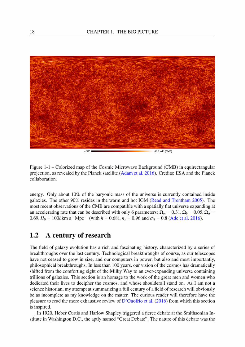
The universe, then opaque, became “suddenly”2 transparent, and photons, finally free fromthe incessant scattering by electrons, decoupled from the baryonic matter and filled the universewith a blackbody radiation we now observe as the Cosmic Microwave Background (CMB)radiation3 (Gamow 1948; Penzias and Wilson 1965). The study of the CMB temperatureanisotropies (of order 10−5K, see Figure 1-1), a relic of this distant past, reveals that at thetime of recombination, the universe was remarkably homogeneous and isotropic. Over thisvast and uniform sea of hydrogen and helium, slightly overdense regions could be seen, result-ing from quantum fluctuations amplified by primordial inflation (e.g. Kolb et al. 1990). Thesetiny overdensities were the seeds from which galaxies and other cosmic structures were grown.
1“Recombination” is a rather odd name when you realize that electrons and atomic nuclei were never actuallycombined before.
2Recombination was fast, but not instantaneous. The universe went from completely ionized to neutral over arange of redshifts ∆z ∼ 200 (Kinney 2003).
3The CMB has since cooled down to its current temperature of 2.7K (Spergel et al. 2003).
CHAPTER 1. THE BIG PICTURE 17
1.1.2 The Dark AgesOver time, due to the expansion and cooling of the universe, the CMB, once a reddish glowof blackbody radiation, ended up emitting most of its energy in the infrared. The universewould then appear completely dark to the human eye, leading to its “Dark Ages”4. No sourceof light had yet been formed and even if they did, their emitted UV radiation would have beenabsorbed by the neutral gas of the intergalactic medium. This period of cosmic history has yetto be revealed by observations, and probing this era would potentially allow to constrain theshape of the matter power spectrum on scales smaller than the CMB fluctuations (Loeb andZaldarriaga 2004). During the vast majority of the Dark Ages, the distribution of atomic gaswas still close to homogeneous, and the growth of the fluctuations of baryonic density likelyremained linear with time. (Furlanetto et al. 2006).
Through gravitational instabilities, regions of high densities collapsed hierarchically, firston small scales and then on large scales. Dark matter structures formed first, because theirgravity was not counteracted by any form of internal pressure. Following the gravitationalpotential wells of dark matter halos, gas clouds began to collapse as they went beyond Jeansmass (∼ 104 M), the mass above which their gravity could overcome gas pressure (Loeb andBarkana 2001).
1.1.3 The Epoch of ReionizationThe dark ages ended a few hundred million years after the Big Bang with the birth of the firstgeneration of luminous objects, such as what are believed to be massive Population III stars,galaxies and quasars, photoionizing the intergalactic medium (IGM) with their emitted UVlight, making it transparent to these wavelengths: this period is known as the Epoch of Reion-ization (EoR, see Figure 1-2). The EoR probably happened in two phases: a slow phase, wherethe UV emitting sources were first isolated in their Strömgren spheres. These bubbles of ion-izing radiation then expanded and overlapped, resulting in a second, much faster reionizationphase (Loeb and Barkana 2001).
The dominant sources and redshift range of the EoR are still ill-constrained. Studies of thelarge-scale polarization of the CMB (Ade et al. 2016) suggest that the EoR might have startedas early as z ∼ 14, and studies of the spectra of high redshift quasars suggest that the universeis fully reionized by z ∼ 6 (Fan et al. 2006). The EoR ended when almost all the atoms of theIGM ended up ionized. The characteristics of this epoch are important to unveil, as the metalenrichment and supernovae shocks created by feedback from the first generation of stars setthe initial conditions for the first galaxies to form (Bromm and Yoshida 2011). This is the goalof the next generation of telescopes, such as the James Webb Space Telescope or the SquareKilometer Array.
1.1.4 The present universeAfter 13.8 billion years of evolution, the present universe is a clumpy mess of galaxies, galaxyclusters and superclusters embedded in a cosmic web of sheets, filaments, and halos of gasand dark matter (cf Figure 1-3), whose dynamics at very large scales is dominated by dark
4The term “Dark Ages” was coined in the cosmological context by Sir Martin Rees, according to Loeb andBarkana (2001).
18 CHAPTER 1. THE BIG PICTURE
Figure 1-1 – Colorized map of the Cosmic Microwave Background (CMB) in equirectangularprojection, as revealed by the Planck satellite (Adam et al. 2016). Credits: ESA and the Planckcollaboration.
energy. Only about 10% of the baryonic mass of the universe is currently contained insidegalaxies. The other 90% resides in the warm and hot IGM (Read and Trentham 2005). Themost recent observations of the CMB are compatible with a spatially flat universe expanding atan accelerating rate that can be described with only 6 parameters: Ωm = 0.31,Ωb = 0.05,ΩΛ =
0.69,H0 = 100hkm s−1Mpc−1 (with h = 0.68), ns = 0.96 and σ8 = 0.8 (Ade et al. 2016).
1.2 A century of researchThe field of galaxy evolution has a rich and fascinating history, characterized by a series ofbreakthroughs over the last century. Technological breakthroughs of course, as our telescopeshave not ceased to grow in size, and our computers in power, but also and most importantly,philosophical breakthroughs. In less than 100 years, our vision of the cosmos has dramaticallyshifted from the comforting sight of the Milky Way to an ever-expanding universe containingtrillions of galaxies. This section is an homage to the work of the great men and women whodedicated their lives to decipher the cosmos, and whose shoulders I stand on. As I am not ascience historian, my attempt at summarizing a full century of a field of research will obviouslybe as incomplete as my knowledge on the matter. The curious reader will therefore have thepleasure to read the more exhaustive review of D’Onofrio et al. (2016) from which this sectionis inspired.
In 1920, Heber Curtis and Harlow Shapley triggered a fierce debate at the Smithsonian In-stitute in Washington D.C., the aptly named “Great Debate”. The nature of this debate was the

CHAPTER 1. THE BIG PICTURE 19
Figure 1-2 – The logarithmic evolution of the universe from z ∼ 1100 to z = 0, according tothe hierarchical scenario of structure formation. From Miralda-Escudé (2003).
Figure 1-3 – The cosmic web at z = 0 from the Millennium-XXL simulation (Angulo et al.2012). The yellow regions are the sites of galaxy formation.

20 CHAPTER 1. THE BIG PICTURE
following question: are the spiral nebulae we see in the sky part of the Galaxy or extragalacticobjects? Shapley was in favor of the “Big Galaxy” hypothesis, and Curtis was in favor of thelatter hypothesis. The discovery of Cepheid stars in M31 by Hubble in 1923, which were usedas a distance measure5, (almost) settled the debate once and for all: the spiral nebulae wereindeed separate "island universes" (Kant 1755), distinct from our own Milky Way. Thanks toVesto Slipher’s measurements of galaxy redshifts, Hubble (1929) discovered an important cor-relation between redshift and distance, in what is now called “Hubble’s law”: galaxies recedefaster from us as their distance increases. This observation provided the first evidence that welive in an expanding universe.
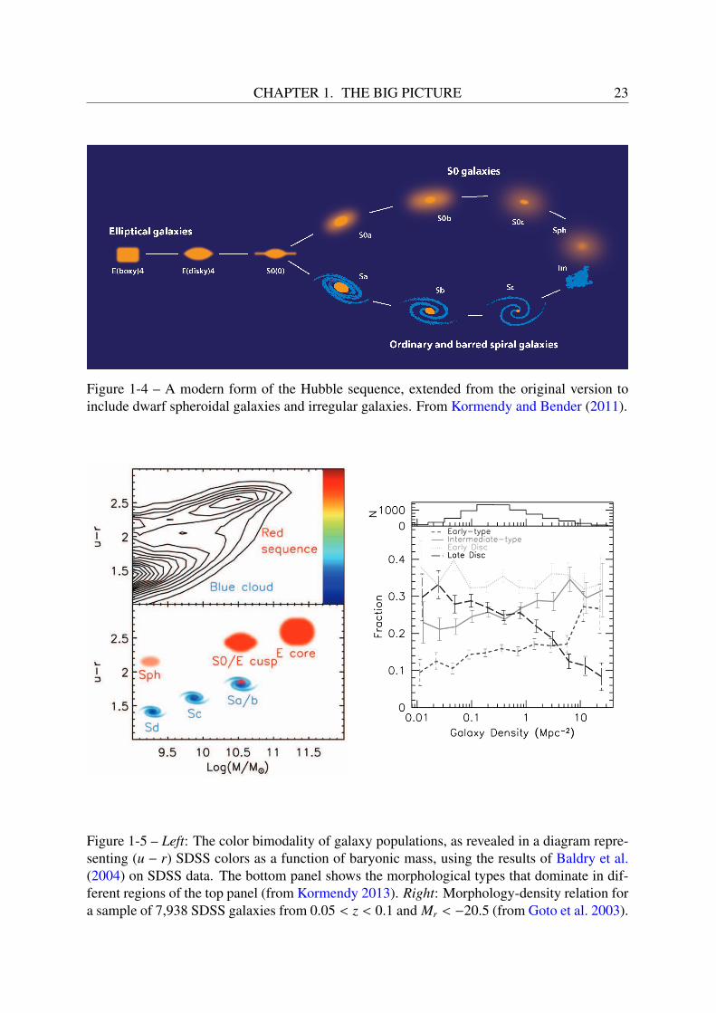
While Friedman, Robertson, Lemaitre and Walker were independently shaping our stan-dard model of modern cosmology by solving Einstein’s equations of general relativity, Hubble(1926, 1936) devised a system of morphological classification of galaxies according to theirvisual appearance. The Hubble sequence, or “tuning fork” diagram, divided galaxies into el-lipticals (E), lenticulars (S0) and spirals (S), and dividing spirals into barred spirals (SB) andnon-barred spirals (S) (cf Figure 1-4). Galaxies that did not fit into this scheme were termed Ir-regulars (Irr) and peculiars (P). The Hubble sequence is now considered simplistic, and severalrefinements and revisions of this classification have been proposed since6 (e.g., Morgan 1958;De Vaucouleurs 1959; Sandage 1961; De Vaucouleurs et al. 1991), but Hubble’s nomenclaturestill holds to this day. Ellipticals and lenticulars are often referred to as “early-types”, whilespirals and irregulars constitute the “late-type” class, as a reference to the early interpretationof the Hubble diagram as an evolutionary sequence. Moreover, galaxies from the left to theright of the spiral sequence are sometimes referred to as “early-type” to “late-type spirals”. Thespectral classification first proposed by Morgan and Mayall (1957) provided a good alternativeto morphological classification, and spectral types appeared to correlate well with morpholog-ical types. Spirals and ellipticals were soon found to exhibit different properties : Holmberg(1958) observed that ellipticals are typically massive and red, and show little star formation,whereas spirals tend to be less massive, bluer and display evidence of ongoing star formation.A first probable causal link between spirals and ellipticals was found by the numerical simula-tions of Toomre and Toomre (1972): elliptical galaxies could be the end-products of mergingspiral galaxies.
Through the study of the velocity dispersion of 8 galaxies of the Coma cluster, Zwicky(1933) remarked that the density of the Coma cluster inferred from its luminous distributionwas 400 times smaller than the value inferred from the velocity dispersion. Zwicky’s "missingmass problem" was later confirmed by Rubin and Ford Jr (1970) thanks to the analysis of therotation curves of spiral galaxies. The nature and properties of this “dark matter” which holdsgalaxies and galaxy clusters together is one of the greatest unsolved mystery of this century.
For a long time, two visions opposed to explain the formation of galaxies, in what wasbasically a “nature vs. nurture” debate of cosmic proportions: the monolithic collapse scenario(Eggen et al. 1962) and the hierarchical scenario (White and Rees 1978; Fall and Efstathiou1980; Blumenthal et al. 1984; White and Frenk 1991; Cole et al. 2000). In the monolithic col-lapse scenario, galaxies come from the gravitational collapse of a cloud of primordial gas in theearly universe, and different galaxy types are born fundamentally different and evolve isolated
5Cepheid stars are variable stars that exhibit a relation between their luminosity and their period of pulsation,as discovered by American astronomer Henrietta Leavitt, which makes them useful as standard candles to measureextragalactic distances.
6For a complete historical review of galaxy morphology classification systems, see Buta (2013).
CHAPTER 1. THE BIG PICTURE 21
from their environment. In the hierarchical scenario, galaxies are gradually assembled throughsuccessive mergers of smaller structures, and the morphological mix depends on individualmerger histories. The model of White and Rees has since become the dominant paradigm forgalaxy formation, thanks to, among other things, the observation of increasing merger rates inthe high redshift universe (e.g., van Dokkum et al. 1999). In this scenario, galaxy formationis a two-stage process: dark matter halos interacting only via gravity first form hierarchicallythough mergers, and galaxies then form by cooling and collapse of baryons in the gravitationalpotential wells of their host dark matter halos (cf Figure 1-8).
The mapping of 2,400 galaxies by the CfA Redshift Survey (Huchra et al. 1983), the firstsystematic survey of this kind, revealed that the spatial distribution of galaxies was far fromrandom: at the scale of several tens of Mpcs, they were lying on the "surfaces of bubble-likestructures" surrounding vast cosmic voids (De Lapparent et al. 1986). The invention of chargecoupled devices (CCDs) marked the beginning of the golden age of extragalactic astronomy inthe mid-1980s. Astronomical surveys such as the Sloan Digital Sky Survey (York et al. 2000),the first fully digital map of the local universe, provided astronomers with an unprecedentedwealth of data that only recently allowed to make reliable, quantitative statements on the distri-bution of different galaxy populations. The morphology of hundreds of thousands of galaxieswas quickly becoming accessible, either by automated classification (e.g. Nair and Abraham2010), by visual classification from citizen scientists around the world (Lintott et al. 2010),or by detailed visual classification from groups of experts on smaller samples (Baillard et al.2011).
Galaxies in the local universe were found to be separated into two robust classes, revealedin their color-magnitude distributions: a “blue cloud” of star-forming late-type galaxies, anda “red sequence” of quiescent ellipticals and lenticulars (e.g. Kauffmann et al. 2003; Baldryet al. 2004, cf Figure 1-5). The morphology of galaxies was also linked to their environment:elliptical galaxies were preferably found in regions of high density, such as the core of clusters,whereas spiral galaxies were the dominant population in regions of low-density (Dressler 1980;Goto et al. 2003, cf Figure 1-5).
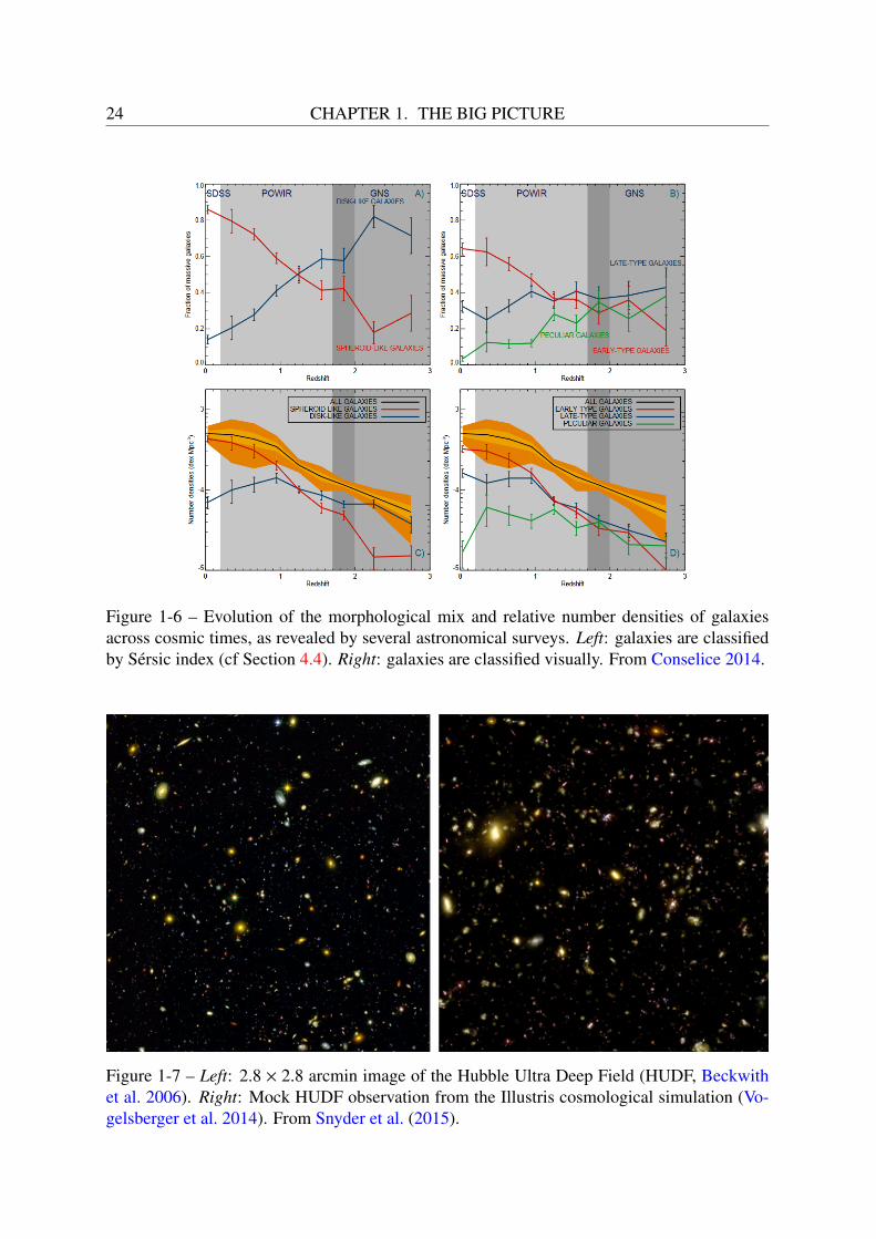
With its Deep Field (Williams et al. 1996) and Ultra Deep field (Beckwith et al. 2006),the Hubble Space Telescope opened a small window on the early universe, and paved the wayfor our understanding of galaxy evolution across cosmic times. The high-redshift universeturned out to be a much more active place than the local universe, with a higher fraction ofirregular and peculiar types (Abraham et al. 1996, cf Figure 1-6). The analysis of a collectionof subsequent deep UV, IR and radio galaxy surveys lead to the observation that the cosmicstar formation rate peaked around z ∼ 2 (an epoch often referred to as the cosmic high noon),with stars forming at a rate of ∼ 10 times higher than what is observed today, and this ratehas been decreasing exponentially ever since (Lilly et al. 1995; Madau et al. 1996; see Madauand Dickinson 2014 for a recent review). Multiwavelengths surveys from ground-based andspace-based instruments over the past two decades shaped our understanding of the evolutionof the cosmos at all scales, with the light, shape and spectrum of millions of galaxies probedacross most of the electromagnetic spectrum. Current and future surveys, such as the DarkEnergy Survey (DES, Collaboration et al. 2005), Euclid (Laureijs et al. 2011), and the LargeSynoptic Survey (LSST, Ivezic et al. 2008) might bring us new insights about galaxy clustering,as well as the nature of dark matter and dark energy. And with the Square Kilometer Array(SKA, Carilli and Rawlings 2004), which is expected to generate 1 exabyte (109 GB) of dataevery day after completion in 2024, radioastronomy is about to enter the “exascale era”, which

22 CHAPTER 1. THE BIG PICTURE
presents new technological challenges for data storage, processing and analysis. Astronomyhas come a long way since Messier’s (1781) catalog of 110 fuzzy objects in the sky.
In parallel with the development of astronomical surveys, cosmological simulations al-lowed us to model the non-linear dynamics of large-scale structures and their interplay withthe small scale physics of galaxy evolution with ever-increasing complexity. Starting from thetiny density fluctuations of the early universe observed in the CMB (now tightly constrainedthanks to the results of the WMAP and Planck satellites), these simulations replayed the historyof the universe, according to our best theoretical models. The numerical simulation method inthe field of galaxy evolution dates back to the first N-body simulations of interacting galaxiesof Holmberg (1941) performed on an analog computer7, and its use has become ubiquitoussince the late 1970’s, with the pioneering simulation of Miyoshi and Kihara (1975) performedon 400 “galaxies” (particles) in an expanding universe8, achieving the prediction of the spatialdistribution of the large-scale structures with remarkable accuracy, and ushering us in the eraof “precision cosmology” (Primack 2005).
For a long time, large-scale cosmological simulations such as the Millenium run (Springelet al. 2005) or the Bolshoi simulation (Klypin et al. 2011) were limited to N-body simula-tions involving only dark matter, and therefore could not trace the evolution of baryonic matter(i.e. gas and stars), due to computational limitations. Only recently does computational power(along with more efficient numerical methods) allow for the complexity of fluid dynamicsto enter the picture, and to simulate statistically significant populations of galaxies. Follow-ing Moore’s law9, cosmological simulations have been doubling in size every ∼ 16.5 months(Springel et al. 2005). The last generation of cosmological hydrodynamic simulations such asIllustris (Vogelsberger et al. 2014), EAGLE (Crain et al. 2015) and Horizon-AGN (Dubois et al.2014) are finally able to simulate cosmological volumes (boxes of hundreds of Mpc in comov-ing size) with enough precision to resolve the internal structure of individual galaxies (of kpcsize). But up to now the differences in numerical implementations of unresolved (“sub-grid”)physical processes make the comparison of the results of these simulations difficult (Scanna-pieco et al. 2012). The direct comparison between cosmological hydrodynamical simulationsand observations has also been seen as a hazardous undertaking, as they trace different physicalphenomena (light for astronomical surveys and mass for simulations). The advent of syntheticobservatories built from the results of simulations, mimicking the effects of telescope resolu-tion and noise, such as, e.g., the work of Snyder et al. (2015) on the Illustris simulation (cfFigure 1-7), might have a role to play to better estimate the reliability of simulations.
With the rise of digital surveys and supercomputers, astronomers have definitely turnedtheir backs on the eyepieces of telescopes and switched to computer screens. The data acquiredis so vast that fascinating discoveries await in our hard drives. We are still learning.
1.3 What is a galaxy?According to the physically-motivated definition of Willman and Strader (2012), galaxies aregravitationally bound collections of stars whose properties cannot be explained by a combina-
7Holmberg’s ingenious experiment involved 37 mass points represented by light bulbs, and the inverse squarebehavior of light was used as an analog of gravity.
8A good historical introduction to the early evolution of cosmological simulations can be found in Suto (2005).9Moore’s law is the empirical assertion that the number of transistors in integrated circuits doubles approxi-
mately every two years (Moore 2006).
CHAPTER 1. THE BIG PICTURE 23
Figure 1-4 – A modern form of the Hubble sequence, extended from the original version toinclude dwarf spheroidal galaxies and irregular galaxies. From Kormendy and Bender (2011).
Figure 1-5 – Left: The color bimodality of galaxy populations, as revealed in a diagram repre-senting (u − r) SDSS colors as a function of baryonic mass, using the results of Baldry et al.(2004) on SDSS data. The bottom panel shows the morphological types that dominate in dif-ferent regions of the top panel (from Kormendy 2013). Right: Morphology-density relation fora sample of 7,938 SDSS galaxies from 0.05 < z < 0.1 and Mr < −20.5 (from Goto et al. 2003).
24 CHAPTER 1. THE BIG PICTURE
Figure 1-6 – Evolution of the morphological mix and relative number densities of galaxiesacross cosmic times, as revealed by several astronomical surveys. Left: galaxies are classifiedby Sérsic index (cf Section 4.4). Right: galaxies are classified visually. From Conselice 2014.
Figure 1-7 – Left: 2.8 × 2.8 arcmin image of the Hubble Ultra Deep Field (HUDF, Beckwithet al. 2006). Right: Mock HUDF observation from the Illustris cosmological simulation (Vo-gelsberger et al. 2014). From Snyder et al. (2015).

CHAPTER 1. THE BIG PICTURE 25
tion of baryons and Newton’s laws of gravity. These structures span a wide range of masses(from ∼ 106 M for the least massive dwarf galaxies to ∼ 1013 M for the most massive giantellipticals) and sizes (from ∼ 102 to ∼ 105 parsecs), and by integrating the number counts de-rived from our deepest images of the universe to date, it is estimated that ∼ 2 × 10¹² galaxiesmore massive than 106 M inhabit the observable universe (up to z ∼ 8), and could theoreticallybe observed using current technology (Conselice et al. 2016).
Most galaxies have two main structural components: a disk and a bulge (or/and pseudo-bulge), each with a distinct formation history and evolution, and with different observationalproperties, as detailed in the following sections. Of course this description is very crude, asmany galaxies display a large variety of intricate structural components, including bars, spiralarms, lenses, nuclear, inner and outer rings, and stellar halos. But in this thesis we will restrictourselves to the description of the bulge and disk. The reader is referred to Buta (2013) andKormendy 2013 for a more detailed description of other galaxy components.
1.3.1 Bulges and pseudo-bulges
Bulges (also referred to as classical bulges or spheroids) consist in densely packed feature-less spheroidal (or mildly triaxial) groups of stars found at the center of spiral and lenticulargalaxies. They can be distinguished from other galaxy components by their rounder smoothisophotes, or by their characteristic radial surface-brightness distribution that creates an ex-cess of light at the center of their host galaxy relative to the inward extrapolation of the outerdisk component (cf Section 4.4) (Gadotti 2012). These structures are kinematically hot, whichmeans that their kinematics is dominated by the random motion of their stars. It is estimatedthat ∼ 1/3 of the stellar mass in the local universe resides in bulges (e.g., Driver et al. 2007;Gadotti 2009), and the stellar populations within bulges display a wide range of ages andmetallicities (e.g., Pérez and Sanchez-Blazquez 2011). They share many properties with ellip-tical galaxies of intermediate luminosity, such as similar color-magnitude relations (Balcellsand Peletier 1993) or metallicity-luminosity relations (e.g., Jablonka et al. 1996). However,defining bulges as merely “smaller ellipticals surrounded by a disk” is oversimplistic, as bothstructures can have different formation histories (Gadotti 2009). Most bulges host a supermas-sive black hole (SMBH) in their center, whose mass correlates with bulge luminosity/stellarmass and velocity dispersion (e.g., Younger et al. 2008; Gültekin et al. 2009). This suggeststhat SMBH and bulge formation are tightly connected. The favored explanation for the growthof classical bulges is via major and minor mergers 10 in the early universe (Aguerri et al. 2001;Robertson et al. 2006), but the coalescence of migrating giant star-forming clumps to the innerregions of galaxies at high redshift also constitutes a viable scenario (e.g., Bournaud et al. 2007;Elmegreen et al. 2009). However, the details of this process, such as the number of mergersinvolved, or the fraction of minor to major mergers are still not well understood.
Classical bulges are to be distinguished from pseudo-bulges, which are are rotationally sup-ported structures (i.e. disk-like) mainly found in Sbc and later-type galaxies. First discoveredby Kormendy (1993), pseudo-bulges have flatter shapes than classical bulges, contain youngerstellar populations and often display boxy or peanut shapes11 when observed close to edge-on.
10A merger event that occurs with a mass ratio between 1:1 and 1:4 is called a major merger. A merger eventthat occurs with a mass ratio between 4:1 and 10:1 is called a minor merger.
11The bulge of the Milky Way is probably a pseudo-bulge, as its peanut shape suggests in near-IR images(Dwek et al. 1995).

26 CHAPTER 1. THE BIG PICTURE
Their birth is thought to be attributed to the secular evolution of disks, namely by transportof angular momentum from bars to the center of galaxies via gravitational instabilities (e.g.,Combes et al. 1990). The properties of pseudo-bulges are reviewed in Kormendy and Kenni-cutt Jr (2004).
To make things even more complex, it has recently been shown that bulges and pseudo-bulges can co-exist within the same galaxy: classical bulges can be found within pseudo-bulges, and pseudo-bulges inside classical bulges are found to be relatively common (e.g.,Gadotti 2009; Nowak et al. 2010, Erwin et al. 2014; Méndez-Abreu et al. 2014). To this date,the very definition of bulges and pseudo-bulges is still a matter of debate, and the communityrelies on various working definitions. Good recent discussions on terminology, respective ob-servational properties and formation processes can be found in Erwin et al. (2014), Fisher andDrory (2016) and Kormendy (2016).
1.3.2 Disks
Disks are rotationally-supported flat structures found in lenticular and spiral galaxies, whoseexponential radial surface brightness distribution defines their characteristic scale radius (cfSection 4.4). Most stellar disks can be decomposed into a thin disk, populated with youngermetal-rich stars and a thick disk, with older metal-poor stars, larger scale heights and longerscale lengths (Burstein 1979; Van der Kruit 1981; Yoachim and Dalcanton 2006). Most ofthe disk stellar mass resides in the thin disk in massive spiral galaxies (Yoachim and Dalcan-ton 2006). Moreover, galaxy disks exhibit a radial gradient of stellar populations, with innerregions hosting older and more metal-rich stars than outer regions (Bell and De Jong 2000).Observations of the 21-cm wavelength line of hydrogen gas have also revealed the existence ofa warped neutral hydrogen (HI) disk, much more extended than the optical stellar disk and mis-aligned to its plane, suggesting different formation scenarios for the two components (Sancisi1976; Rogstad and Shostak 1971). Disks show many correlations between their observed prop-erties: for example brighter and more massive disks tend to be bigger (Shen et al. 2003) andto rotate faster (Tully and Fisher 1977) than less massive ones. At high redshift (z ∼ 2), mostdisks display a characteristic clumpy structure, with large (several kpc in size) massive (107
to 109 M) star-forming clumps, likely formed by gravitational instabilities (e.g., Elmegreenet al. 2005; Bournaud et al. 2007) or by mergers (e.g., Overzier et al. 2008). A theory of diskformation must therefore link these early clumpy galaxies to the exponential disks of the localuniverse.
The birth of galaxy thin disks is well described within the current paradigm of galaxy for-mation (White and Rees 1978; Fall and Efstathiou 1980; Mo et al. 1998; Cole et al. 2000). Inthis paradigm, big dark matter halos form hierarchically through the accretion and merging ofsmaller structures. Neighboring large-scale structures exert a tidal torque on these halos, caus-ing them to spin. Baryonic gas clouds heated by shocks then collapse in the potential wellscreated by the dark matter halos, creating a halo of hot gas, whose internal pressure preventsit from further collapsing. As gas cools thanks to various radiative processes (discussed inKauffmann et al. 1994), pressure decreases and gas clouds start to fall to the center of theirhost dark halo. Assuming conservation of angular momentum during the collapse, this resultsin a rotationally-supported disk, with scale lengths that are in good agreement with observa-tions (e.g., de Jong and Lacey 2000). Recent theoretical development supported by numericalsimulations have since shown that the accretion of cold streams of gas (not heated by shocks)
CHAPTER 1. THE BIG PICTURE 27
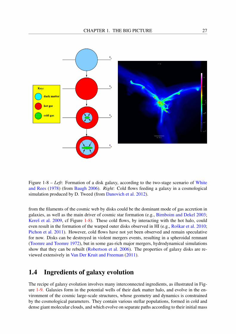
Figure 1-8 – Left: Formation of a disk galaxy, according to the two-stage scenario of Whiteand Rees (1978) (from Baugh 2006). Right: Cold flows feeding a galaxy in a cosmologicalsimulation produced by D. Tweed (from Danovich et al. 2012).
from the filaments of the cosmic web by disks could be the dominant mode of gas accretion ingalaxies, as well as the main driver of cosmic star formation (e.g., Birnboim and Dekel 2003;Kereš et al. 2009, cf Figure 1-8). These cold flows, by interacting with the hot halo, couldeven result in the formation of the warped outer disks observed in HI (e.g., Roškar et al. 2010;Pichon et al. 2011). However, cold flows have not yet been observed and remain speculativefor now. Disks can be destroyed in violent mergers events, resulting in a spheroidal remnant(Toomre and Toomre 1972), but in some gas-rich major mergers, hydrodynamical simulationsshow that they can be rebuilt (Robertson et al. 2006). The properties of galaxy disks are re-viewed extensively in Van Der Kruit and Freeman (2011).
1.4 Ingredients of galaxy evolution
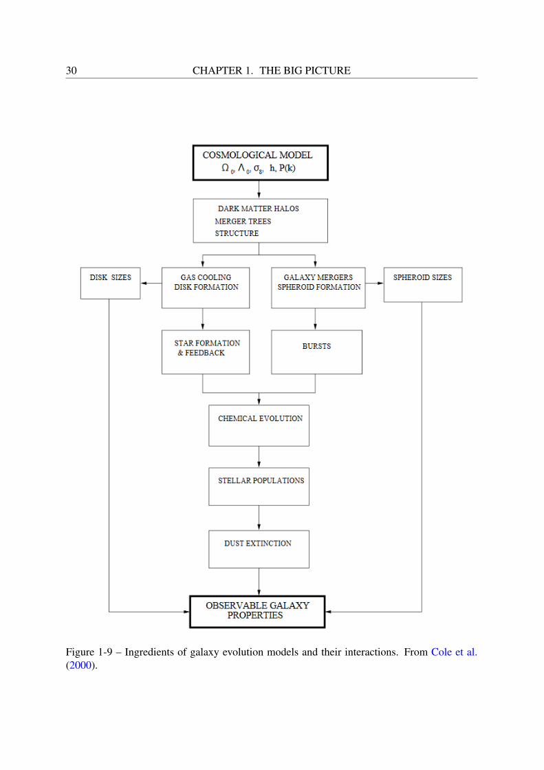
The recipe of galaxy evolution involves many interconnected ingredients, as illustrated in Fig-ure 1-9. Galaxies form in the potential wells of their dark matter halo, and evolve in the en-vironment of the cosmic large-scale structures, whose geometry and dynamics is constrainedby the cosmological parameters. They contain various stellar populations, formed in cold anddense giant molecular clouds, and which evolve on separate paths according to their initial mass
28 CHAPTER 1. THE BIG PICTURE
and metallicity. The most massive stars end in violent explosions known as supernovae, eject-ing vast amounts of gas and heating the local interstellar medium, preventing (or “quenching”)further star formation, a phenomenon known as “supernova feedback” (cf Figure 1-10). Thecycle of life and death of stars enriches the interstellar medium with metals, and the enrichedgas, after a cooling phase, is in turn used to form stars with higher metallicities. The interstellarmedium also contains interstellar dust, mainly grown in dense molecular clouds, which reddensand dims the light of galaxies by absorption and scattering of incident photons out of the lineof sight. In some galaxies, the presence of an active galactic nucleus (AGN) associated to itscentral supermassive black hole can create relativistic jets and winds that clear interstellar gasout and prevent it from cooling, therefore quenching star formation (this is known as “AGNfeedback”, cf Figure 1-10). Galaxies can live isolated lives, developing features associatedwith secular processes, such as bars and spiral arms, or they can interact more or less violentlywith one another via gas-rich (“wet”) mergers, associated with bursts of star formation, or gas-poor (“dry”) mergers with no star formation involved (e.g. Lin et al. 2008). Galaxies movingin a cluster environment can also have their cold gas stripped by the hot intracluster medium,a phenomenon known as “ram pressure stripping”, which can result in a slow decline of starformation rate (a process called “starvation” or “strangulation”).
Understanding how all these elements interact with one another quantitatively to form thedistribution of galaxies we observe in astronomical surveys is a daunting task, notably becausethese complex systems involve physical processes on a remarkably large range of spatial scales,from stellar black holes to the large-scale structures of the cosmic web (cf Table 1.1), with thesmall scales acting on the large scales and inversely. Our current attempt at modeling theprocesses at play in galaxy evolution relies on two main approaches: cosmological simulationsand semi-analytic models.
• Cosmological simulations follow explicitly the evolution of dark matter and gas in thenon-linear regime of a ΛCDM universe. In these simulations, dark matter is modeledas a collection of collisionless massive particles whose dynamics follows the Vlasov-Poisson equations in a box of cosmological (comoving) volume with periodic bound-ary conditions. To reproduce the conditions of the early universe, they use a Gaussianrandom field of density perturbations with a power spectrum constrained by the CMB(e.g., Aghanim et al. 2016) as their initial conditions. These N-body simulations canbe completed with the much more computationally intensive baryonic physics, whichin practices comes down to solving the Euler equations on a collisional ideal fluid12 viaLagrangian or Eulerian methods. In this scheme these simulations are referred to ascosmological hydrodynamical simulations. Sub-grid models that reproduce the effectsof star formation, turbulence, supernovae and AGN feedback on the surrounding gas,supermassive black hole growth, chemistry of heavy elements and dust are unavoidablebecause galaxy evolution span a wide range of scales. These sub-grid models usuallyconsist in a mix of empirical (or ad hoc) rules whose calibration is open to fine tuning tofit the data, as the detailed physics of these processes are not yet well understood. State-of-the-art cosmological hydrodynamical simulations include Illustris (Vogelsberger et al.2014), EAGLE (Crain et al. 2015) and Horizon-AGN (Dubois et al. 2014).
• Semi-analytic models (or SAMs) model small-scale baryonic processes as simplified an-alytical descriptions within the framework of hierarchical structure growth. The physical
12A collisional fluid is a fluid that can be heated and cooled radiatively.

CHAPTER 1. THE BIG PICTURE 29
Table 1.1 – The spatial scales of galaxy evolution
Object Order of magnitude in size [pc]Stellar black hole 10−13 → 10−12
Star 10−13 → 10−5
Supermassive black hole 10−9 → 10−5
Globular cluster 101
Molecular cloud 101 → 102
Galaxy 102 → 105
Galaxy cluster 106 → 107
Large Scale Structures 108 → 109 (comoving)Observable universe 1010 (comoving)
phenomena included in a SAM and the accuracy of their description differ depending onthe models. The first self-consistent semi-analytic model of galaxy evolution of Whiteand Frenk (1991) already included the effects of star formation, stellar populations andfeedback. The main advantage of SAMs over cosmological hydrodynamical simulationsis that they are much less computationally expensive, which allows them to explore thephysical parameter space more easily. They are usually superimposed on N-body sim-ulations, relying on their well-calibrated “merger trees” (recordings of the mass growthhistory of dark matter halos), and using the halo distribution as the sites of galaxy forma-tion. Comparison between the predictions of SAMs and of cosmological hydrodynam-ical simulations show surprising agreement between the two approaches, at least downto the resolution elements of simulations, but these comparisons are usually limited tothe hydrodynamics and cooling of gas (Lu et al. 2011), or to the scale of single galaxies(Stringer et al. 2010). State-of-the-art semi-analytical models include the SAGE modelof Croton et al. (2016), GALACTICUS (Benson 2012) and GALFORM (Lacey et al.2016), among many others.
Recent methodological reviews on cosmological simulations and semi-analytic models canbe found in Baugh (2006) and Somerville and Davé (2015).
1.5 Unanswered questions on galaxy evolutionThe evolution of galaxies in the universe is still an incomplete story. While cosmologicalsimulations have been very successful at predicting the properties of the large-scale structuresof the universe in the ΛCDM paradigm, the modeling of the small-scale baryonic physicsof galaxy evolution is still at its early stage and will require many refinements to be able toreproduce the observed properties of galaxy populations in sky surveys. Besides the billion-dollar questions of the nature of elusive dark matter, that dominates the matter content of theuniverse, and dark energy, which causes the expansion of the universe to accelerate, a lot ofphysical phenomena associated to galaxy evolution are still poorly understood:
• How and when did the first stars and galaxies form? The birth of the first luminousobjects, which constitute the building blocks of present-day galaxies, signed the endof the cosmic “dark ages”, but so far our understanding of these structures has been
30 CHAPTER 1. THE BIG PICTURE
Figure 1-9 – Ingredients of galaxy evolution models and their interactions. From Cole et al.(2000).

CHAPTER 1. THE BIG PICTURE 31
Figure 1-10 – Left: Supernova feedback in NGC 3079 (Credits: NASA and G. Cecil (U. NorthCarolina, Chapel Hill)). Right: AGN feedback in Centaurus A (Credits: ESO / WFI (Optical);MPIfR / ESO / APEX / A.Weiss et al. (Sub-millimeter); NASA / CXC / CfA / R.Kraft et al.(X-ray)).
largely theoretical. Imaging the first galaxies to reveal the complete story of the Epoch ofReionization is the next observational frontier, and the new generation of radiotelescopessuch as LOFAR and SKA should be able to probe this era (Loeb 2010). In this context,what defines a “first galaxy” is currently open to debate (Bromm and Yoshida 2011).
• What is the origin of the Hubble sequence? It all comes down to the question of howgalaxies acquire their mass. At the center of the debate is the relative roles of mergersand secular processes in the buildup of galaxy structure. A complete theory of galaxyformation should be able to explain the whole spectrum of structural properties observedin the cosmic zoo, from pure disks to pure spheroids, and in particular to predict thephysical origin of galaxy bimodality.
• What shuts down star formation in galaxies? This is probably related to the fact that wedo not currently fully understand how stars form. Observations show that only ∼10%of the baryonic mass of the universe is contained within stars or in cold gas (Fukugitaand Peebles 2004). What makes the star formation process so inefficient, and why isthe cosmic star formation rate declining from z ∼ 2? One of the factors to explain thisdecline is the observed decrease of merger rate of galaxies over cosmic time (e.g. Linet al. 2004; Conselice et al. 2008; De Ravel et al. 2009). It is also supposed that a numberof mechanisms prevents the hot interstellar gas from cooling and forming stars, the so-called “feedback” mechanisms. The two favored candidates are supernova feedback atthe low-mass end, and AGN feedback at the high-mass end (as illustrated in Figure 1-10). The small sizes involved in these mechanisms confine them in sub-grid models fornow, and different implementations of feedback in cosmological simulations generate awide scatter in terms of galaxy properties.
• Why did the most massive galaxies formed their stars first and over a shorter time span?Hierarchical models predict that small structures form first, and big structures form last.

32 CHAPTER 1. THE BIG PICTURE
But the most massive elliptical galaxies in the local universe seem to have formed theirstars first and have stopped forming stars first, as attested by their redder colors (De Vau-couleurs 1961) and their higher metallicities (Faber 1973) associated with older stellarpopulations. This “downsizing” (Cowie et al. 1996) of massive galaxies cannot be ex-plained within the current hierarchical framework.
• How do supermassive black holes form? Supermassive black holes, in the form ofquasars, might have a role to play in the reionization of the cosmos (albeit ill-constrainedfor now). Moreover, as we have seen in Section 1.3.1, the formation of galactic bulgesis thought to be associated with the formation of supermassive black holes. But howthese black holes acquire their mass is still unknown. Hypotheses to explain their growthinclude the coalescence of stellar remnants from the first generation of stars (Madau andRees 2001) or the direct collapse of pristine gas clouds (Bromm and Loeb 2003; Hartwiget al. 2016).
A recent review on the current status of the galaxy evolution field detailing these openquestions is available in Silk and Mamon (2012). To conclude, there has been tremendousprogress in the theoretical and observational sides in the last few decades, but we still have along way to go to fully understand how these magnificent structures grow and evolve. This isan exciting time to be alive.

Chapter 2
Exploring astronomical surveys
Physics is really nothing more than asearch for ultimate simplicity, but so farall we have is a kind of elegantmessiness.
Bill Bryson, A Short History of NearlyEverything
Abstract
Astronomical surveys constitute our primary source of information on galaxy for-mation and evolution, by providing us with a panchromatic view of the universethrough different slices of cosmic time. In this chapter1, I review some of the mainexisting spectro-photometric galaxy surveys probing the local and deep universe,and summarize what they indicate about the size and luminosity distribution ofgalaxies, as well as the evolution of these observables with redshift and the biasesinvolved in their estimation.
Contents2.1 Galaxy surveys . . . . . . . . . . . . . . . . . . . . . . . . . . . . . . . . . 34
2.1.1 Survey characteristics . . . . . . . . . . . . . . . . . . . . . . . . . 34
2.1.2 Surveying the local universe . . . . . . . . . . . . . . . . . . . . . . 36
2.1.3 Surveying the deep universe . . . . . . . . . . . . . . . . . . . . . . 36
2.2 The luminosity distribution of galaxies and its evolution . . . . . . . . . . 39
2.3 The size distribution of galaxies and its evolution . . . . . . . . . . . . . . 40
2.3.1 Size estimators . . . . . . . . . . . . . . . . . . . . . . . . . . . . . 40
2.3.2 The mass-size relation . . . . . . . . . . . . . . . . . . . . . . . . . 41
2.3.3 The size evolution of massive early-type galaxies . . . . . . . . . . . 42
1Note: This chapter uses extracts from Carassou et al. (2017) in some of its sections.
33
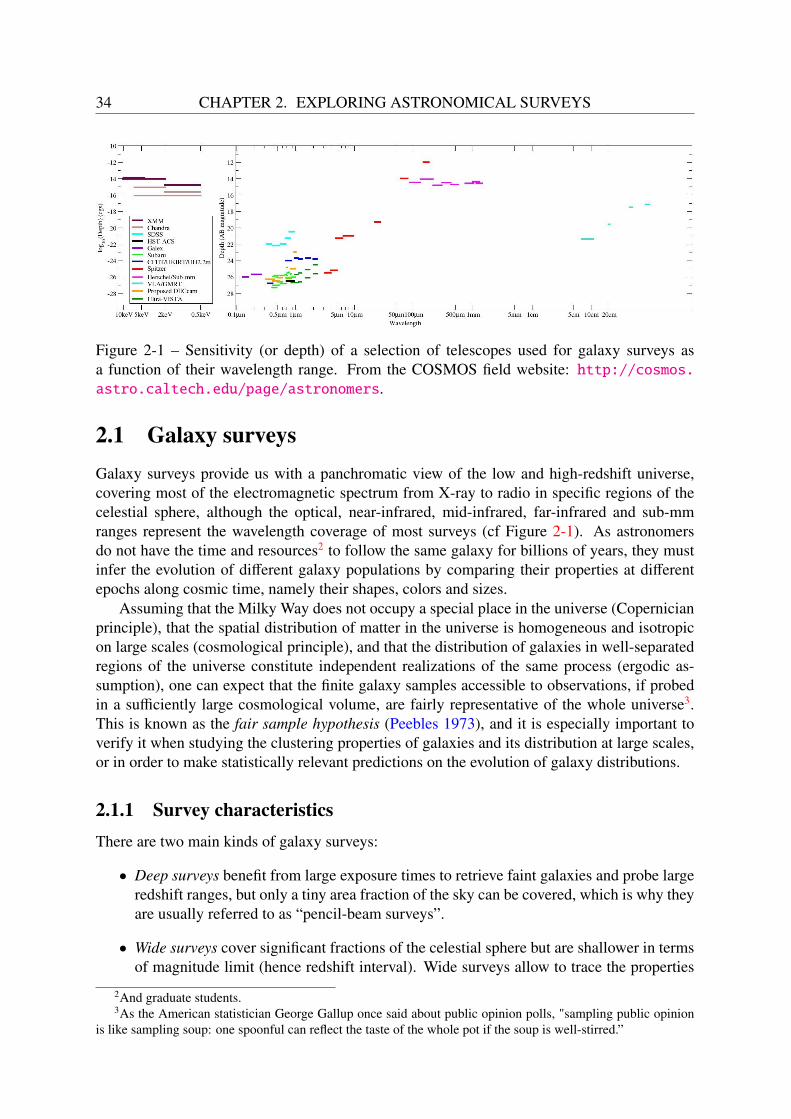
34 CHAPTER 2. EXPLORING ASTRONOMICAL SURVEYS
Figure 2-1 – Sensitivity (or depth) of a selection of telescopes used for galaxy surveys asa function of their wavelength range. From the COSMOS field website: http://cosmos.astro.caltech.edu/page/astronomers.
2.1 Galaxy surveysGalaxy surveys provide us with a panchromatic view of the low and high-redshift universe,covering most of the electromagnetic spectrum from X-ray to radio in specific regions of thecelestial sphere, although the optical, near-infrared, mid-infrared, far-infrared and sub-mmranges represent the wavelength coverage of most surveys (cf Figure 2-1). As astronomersdo not have the time and resources2 to follow the same galaxy for billions of years, they mustinfer the evolution of different galaxy populations by comparing their properties at differentepochs along cosmic time, namely their shapes, colors and sizes.
Assuming that the Milky Way does not occupy a special place in the universe (Copernicianprinciple), that the spatial distribution of matter in the universe is homogeneous and isotropicon large scales (cosmological principle), and that the distribution of galaxies in well-separatedregions of the universe constitute independent realizations of the same process (ergodic as-sumption), one can expect that the finite galaxy samples accessible to observations, if probedin a sufficiently large cosmological volume, are fairly representative of the whole universe3.This is known as the fair sample hypothesis (Peebles 1973), and it is especially important toverify it when studying the clustering properties of galaxies and its distribution at large scales,or in order to make statistically relevant predictions on the evolution of galaxy distributions.
2.1.1 Survey characteristicsThere are two main kinds of galaxy surveys:
• Deep surveys benefit from large exposure times to retrieve faint galaxies and probe largeredshift ranges, but only a tiny area fraction of the sky can be covered, which is why theyare usually referred to as “pencil-beam surveys”.
• Wide surveys cover significant fractions of the celestial sphere but are shallower in termsof magnitude limit (hence redshift interval). Wide surveys allow to trace the properties
2And graduate students.3As the American statistician George Gallup once said about public opinion polls, "sampling public opinion
is like sampling soup: one spoonful can reflect the taste of the whole pot if the soup is well-stirred.”
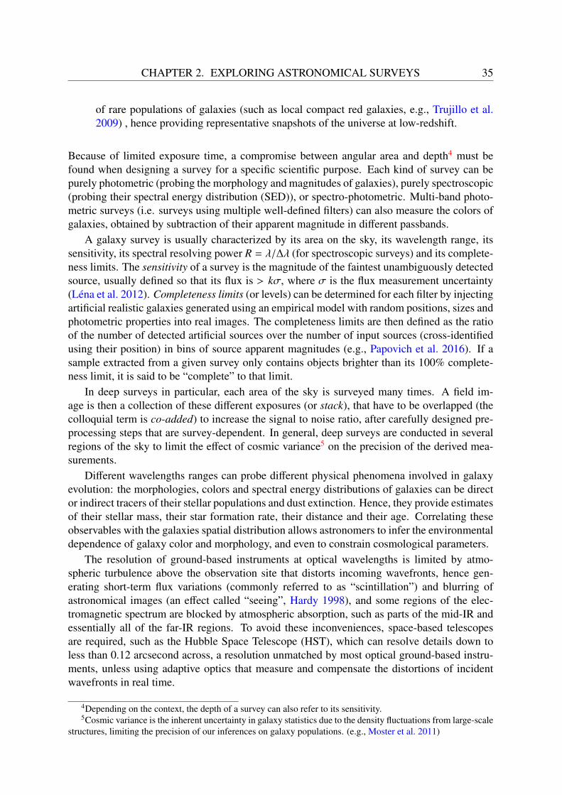
CHAPTER 2. EXPLORING ASTRONOMICAL SURVEYS 35
of rare populations of galaxies (such as local compact red galaxies, e.g., Trujillo et al.2009) , hence providing representative snapshots of the universe at low-redshift.
Because of limited exposure time, a compromise between angular area and depth4 must befound when designing a survey for a specific scientific purpose. Each kind of survey can bepurely photometric (probing the morphology and magnitudes of galaxies), purely spectroscopic(probing their spectral energy distribution (SED)), or spectro-photometric. Multi-band photo-metric surveys (i.e. surveys using multiple well-defined filters) can also measure the colors ofgalaxies, obtained by subtraction of their apparent magnitude in different passbands.
A galaxy survey is usually characterized by its area on the sky, its wavelength range, itssensitivity, its spectral resolving power R = λ/∆λ (for spectroscopic surveys) and its complete-ness limits. The sensitivity of a survey is the magnitude of the faintest unambiguously detectedsource, usually defined so that its flux is > kσ, where σ is the flux measurement uncertainty(Léna et al. 2012). Completeness limits (or levels) can be determined for each filter by injectingartificial realistic galaxies generated using an empirical model with random positions, sizes andphotometric properties into real images. The completeness limits are then defined as the ratioof the number of detected artificial sources over the number of input sources (cross-identifiedusing their position) in bins of source apparent magnitudes (e.g., Papovich et al. 2016). If asample extracted from a given survey only contains objects brighter than its 100% complete-ness limit, it is said to be “complete” to that limit.
In deep surveys in particular, each area of the sky is surveyed many times. A field im-age is then a collection of these different exposures (or stack), that have to be overlapped (thecolloquial term is co-added) to increase the signal to noise ratio, after carefully designed pre-processing steps that are survey-dependent. In general, deep surveys are conducted in severalregions of the sky to limit the effect of cosmic variance5 on the precision of the derived mea-surements.
Different wavelengths ranges can probe different physical phenomena involved in galaxyevolution: the morphologies, colors and spectral energy distributions of galaxies can be director indirect tracers of their stellar populations and dust extinction. Hence, they provide estimatesof their stellar mass, their star formation rate, their distance and their age. Correlating theseobservables with the galaxies spatial distribution allows astronomers to infer the environmentaldependence of galaxy color and morphology, and even to constrain cosmological parameters.
The resolution of ground-based instruments at optical wavelengths is limited by atmo-spheric turbulence above the observation site that distorts incoming wavefronts, hence gen-erating short-term flux variations (commonly referred to as “scintillation”) and blurring ofastronomical images (an effect called “seeing”, Hardy 1998), and some regions of the elec-tromagnetic spectrum are blocked by atmospheric absorption, such as parts of the mid-IR andessentially all of the far-IR regions. To avoid these inconveniences, space-based telescopesare required, such as the Hubble Space Telescope (HST), which can resolve details down toless than 0.12 arcsecond across, a resolution unmatched by most optical ground-based instru-ments, unless using adaptive optics that measure and compensate the distortions of incidentwavefronts in real time.
4Depending on the context, the depth of a survey can also refer to its sensitivity.5Cosmic variance is the inherent uncertainty in galaxy statistics due to the density fluctuations from large-scale
structures, limiting the precision of our inferences on galaxy populations. (e.g., Moster et al. 2011)

36 CHAPTER 2. EXPLORING ASTRONOMICAL SURVEYS
2.1.2 Surveying the local universe
Our best vision of the local universe mainly comes from:
• The Sloan Digital Sky Survey (SDSS, York et al. 2000), an on-going spectro-photometricsurvey that started in 1998, conducted using the 2.5m telescope of the Apache Point ob-servatory in New Mexico. The SDSS covers an area of ∼ 14, 555 deg2 on the sky (over1/3 of the celestial sphere) in five optical bands (ugriz, Fukugita et al. 1996). The lastdata release (DR12, Alam et al. 2015) contains ∼ 4.7 × 10⁸ cataloged objects (detectedin the optical r-band) and more than 1.8 × 10⁶ galaxy spectra. Its main galaxy samplehas a median redshift of z = 0.1. A slice of the 3D distribution of galaxies as revealed bythe SDSS is shown in Figure 2-2.
• The 2-degree Field Galaxy Redshift Survey (2dFGRS, Colless et al. 2001), conductedbetween 1997 and 2002 using the 3.9m Anglo-Australian Telescope, covers ∼ 2000 deg2
(∼5% of the celestial sphere). Its catalog contains the spectra and spectroscopic redshiftsof more than 221,000 galaxies with magnitudes brighter than 19.3 in the optical bJ-band up to a redshift of z ∼ 0.3 (with a median redshift of z = 0.1). A slice of the 3Ddistribution of galaxies as revealed by the 2dFGRS is shown in Figure 2-2.
• The Two Micron All-Sky Survey (2MASS, Jarrett et al. 2000) was conducted between1997 and 2001 using two 1.3m telescopes in the northern and southern hemispheres (theFred Lawrence Whipple Observatory in Arizona and the Cerro Tololo Inter-AmericanObservatory in Chile respectively). Its extended source catalog (the largest all-sky pho-tometric catalog of extended sources so far) contains 1.5 million galaxies observed inthe near-IR JHKs bands, of which 1 million are brighter than Ks = 13.9 mag, the com-pleteness limit of the survey. A subsample of this catalog contains the spectroscopic dataof 44,000 galaxies with a median redshift of z ∼ 0.03, which constitutes the 2MASSRedshift Survey (2MRS, Huchra et al. 2012). Recently, Bilicki et al. (2014) releasedthe 2MASS Photometric Redshift catalog (2MPZ), containing the distance of 940,000galaxies with a median redshift z = 0.07.
• The Wide-field Infrared Survey Explorer (WISE, Wright et al. 2010) is an all-skysurvey conducted in 2010 by NASA’s eponymous space-based instrument in four mid-IR bands (3.4, 4.6, 12, and 22 µm). Benefiting from an uniform sky coverage, it isthe most sensitive mid-IR survey to date. However its poor angular resolution makesits unable to resolve objects beyond the depth already probed by 2MASS. Its publiclyreleased source catalog contains the photometric data of more than 500 million objects(asteroids, planets, stars, nebulae and galaxies) with a signal-to-noise ratio of 5 or higher.
2.1.3 Surveying the deep universe
Here below is a non-exhaustive list of some of the most studied modern deep galaxy surveys,which constitute our main database for the high-redshift universe. A comparison of the relativesize over the sky of those of these surveys that use the Hubble Space Telescope is displayed inFigure 2-3. These surveys include:
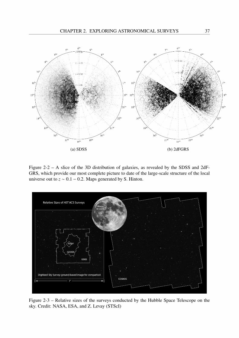
CHAPTER 2. EXPLORING ASTRONOMICAL SURVEYS 37
(a) SDSS (b) 2dFGRS
Figure 2-2 – A slice of the 3D distribution of galaxies, as revealed by the SDSS and 2dF-GRS, which provide our most complete picture to date of the large-scale structure of the localuniverse out to z ∼ 0.1 − 0.2. Maps generated by S. Hinton.
Figure 2-3 – Relative sizes of the surveys conducted by the Hubble Space Telescope on thesky. Credit: NASA, ESA, and Z. Levay (STScI)
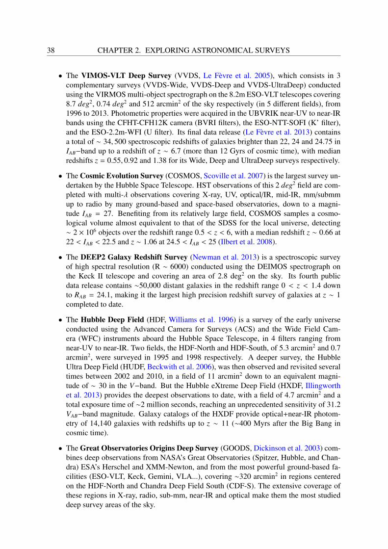
38 CHAPTER 2. EXPLORING ASTRONOMICAL SURVEYS
• The VIMOS-VLT Deep Survey (VVDS, Le Fèvre et al. 2005), which consists in 3complementary surveys (VVDS-Wide, VVDS-Deep and VVDS-UltraDeep) conductedusing the VIRMOS multi-object spectrograph on the 8.2m ESO-VLT telescopes covering8.7 deg2, 0.74 deg2 and 512 arcmin2 of the sky respectively (in 5 different fields), from1996 to 2013. Photometric properties were acquired in the UBVRIK near-UV to near-IRbands using the CFHT-CFH12K camera (BVRI filters), the ESO-NTT-SOFI (K’ filter),and the ESO-2.2m-WFI (U filter). Its final data release (Le Fèvre et al. 2013) containsa total of ∼ 34, 500 spectroscopic redshifts of galaxies brighter than 22, 24 and 24.75 inIAB−band up to a redshift of z ∼ 6.7 (more than 12 Gyrs of cosmic time), with medianredshifts z = 0.55, 0.92 and 1.38 for its Wide, Deep and UltraDeep surveys respectively.
• The Cosmic Evolution Survey (COSMOS, Scoville et al. 2007) is the largest survey un-dertaken by the Hubble Space Telescope. HST observations of this 2 deg2 field are com-pleted with multi-λ observations covering X-ray, UV, optical/IR, mid-IR, mm/submmup to radio by many ground-based and space-based observatories, down to a magni-tude IAB = 27. Benefiting from its relatively large field, COSMOS samples a cosmo-logical volume almost equivalent to that of the SDSS for the local universe, detecting∼ 2 × 10⁶ objects over the redshift range 0.5 < z < 6, with a median redshift z ∼ 0.66 at22 < IAB < 22.5 and z ∼ 1.06 at 24.5 < IAB < 25 (Ilbert et al. 2008).
• The DEEP2 Galaxy Redshift Survey (Newman et al. 2013) is a spectroscopic surveyof high spectral resolution (R ∼ 6000) conducted using the DEIMOS spectrograph onthe Keck II telescope and covering an area of 2.8 deg2 on the sky. Its fourth publicdata release contains ∼50,000 distant galaxies in the redshift range 0 < z < 1.4 downto RAB = 24.1, making it the largest high precision redshift survey of galaxies at z ∼ 1completed to date.
• The Hubble Deep Field (HDF, Williams et al. 1996) is a survey of the early universeconducted using the Advanced Camera for Surveys (ACS) and the Wide Field Cam-era (WFC) instruments aboard the Hubble Space Telescope, in 4 filters ranging fromnear-UV to near-IR. Two fields, the HDF-North and HDF-South, of 5.3 arcmin2 and 0.7arcmin2, were surveyed in 1995 and 1998 respectively. A deeper survey, the HubbleUltra Deep Field (HUDF, Beckwith et al. 2006), was then observed and revisited severaltimes between 2002 and 2010, in a field of 11 arcmin2 down to an equivalent magni-tude of ∼ 30 in the V−band. But the Hubble eXtreme Deep Field (HXDF, Illingworthet al. 2013) provides the deepest observations to date, with a field of 4.7 arcmin2 and atotal exposure time of ∼2 million seconds, reaching an unprecedented sensitivity of 31.2VAB−band magnitude. Galaxy catalogs of the HXDF provide optical+near-IR photom-etry of 14,140 galaxies with redshifts up to z ∼ 11 (∼400 Myrs after the Big Bang incosmic time).
• The Great Observatories Origins Deep Survey (GOODS, Dickinson et al. 2003) com-bines deep observations from NASA’s Great Observatories (Spitzer, Hubble, and Chan-dra) ESA’s Herschel and XMM-Newton, and from the most powerful ground-based fa-cilities (ESO-VLT, Keck, Gemini, VLA...), covering ∼320 arcmin2 in regions centeredon the HDF-North and Chandra Deep Field South (CDF-S). The extensive coverage ofthese regions in X-ray, radio, sub-mm, near-IR and optical make them the most studieddeep survey areas of the sky.
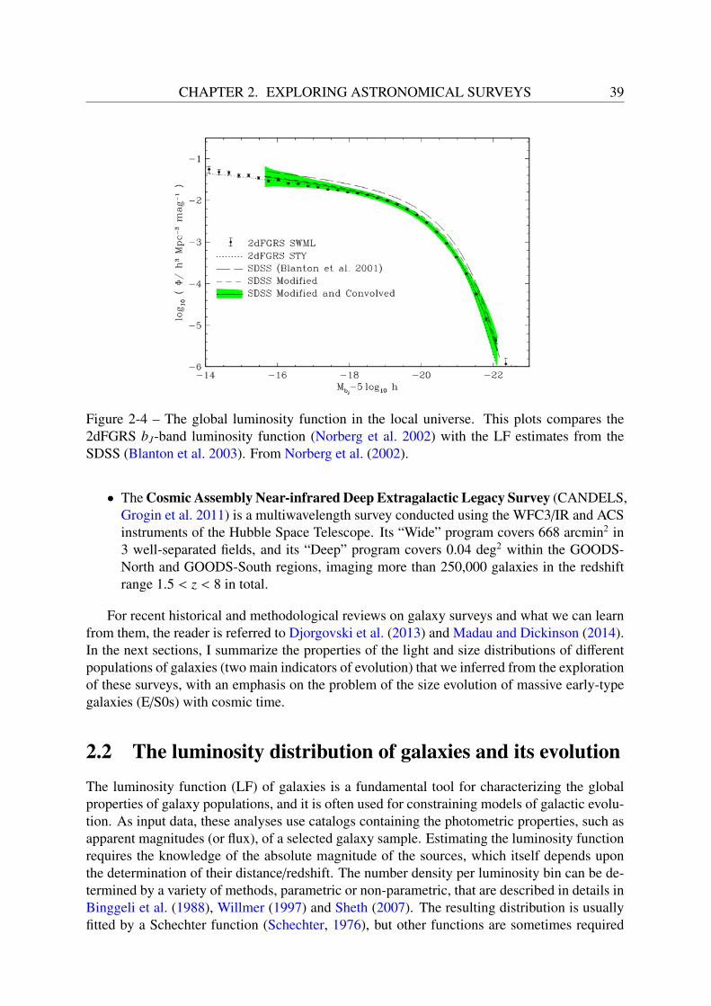
CHAPTER 2. EXPLORING ASTRONOMICAL SURVEYS 39
Figure 2-4 – The global luminosity function in the local universe. This plots compares the2dFGRS bJ-band luminosity function (Norberg et al. 2002) with the LF estimates from theSDSS (Blanton et al. 2003). From Norberg et al. (2002).
• The Cosmic Assembly Near-infrared Deep Extragalactic Legacy Survey (CANDELS,Grogin et al. 2011) is a multiwavelength survey conducted using the WFC3/IR and ACSinstruments of the Hubble Space Telescope. Its “Wide” program covers 668 arcmin2 in3 well-separated fields, and its “Deep” program covers 0.04 deg2 within the GOODS-North and GOODS-South regions, imaging more than 250,000 galaxies in the redshiftrange 1.5 < z < 8 in total.
For recent historical and methodological reviews on galaxy surveys and what we can learnfrom them, the reader is referred to Djorgovski et al. (2013) and Madau and Dickinson (2014).In the next sections, I summarize the properties of the light and size distributions of differentpopulations of galaxies (two main indicators of evolution) that we inferred from the explorationof these surveys, with an emphasis on the problem of the size evolution of massive early-typegalaxies (E/S0s) with cosmic time.
2.2 The luminosity distribution of galaxies and its evolutionThe luminosity function (LF) of galaxies is a fundamental tool for characterizing the globalproperties of galaxy populations, and it is often used for constraining models of galactic evolu-tion. As input data, these analyses use catalogs containing the photometric properties, such asapparent magnitudes (or flux), of a selected galaxy sample. Estimating the luminosity functionrequires the knowledge of the absolute magnitude of the sources, which itself depends uponthe determination of their distance/redshift. The number density per luminosity bin can be de-termined by a variety of methods, parametric or non-parametric, that are described in details inBinggeli et al. (1988), Willmer (1997) and Sheth (2007). The resulting distribution is usuallyfitted by a Schechter function (Schechter, 1976), but other functions are sometimes required

40 CHAPTER 2. EXPLORING ASTRONOMICAL SURVEYS
(e.g., Driver and Phillipps 1996; Blanton et al. 2005). The Schechter function is defined as:
Φ(L)dL = Φ∗( LL∗
)αe−
LL∗
dLL∗
(2.1)
where L is the galaxy luminosity and Φ(L)dL is the number of galaxies with luminosity be-tween L and L+dL per Mpc3. It is characterized by 3 parameters: φ∗ is the normalizationdensity, α represents the faint end slope and L∗ is a characteristic galaxy luminosity. But theSchechter LF is more conveniently expressed in terms of absolute magnitudes. Using the fol-lowing transformation:
M − M∗ = −2.5log10
( LL∗
)(2.2)
one obtains:
Φ(M)dM = 0.4 ln(10)Φ∗100.4(α+1)(M−M∗) exp[−100.4(M−M∗)
]dM (2.3)
where M∗ is a characteristic galaxy absolute magnitude. The global LF at z ∼ 0.1 is nowwell constrained thanks to the analysis of spectroscopic surveys, such as the 2dFGRS (Norberget al. 2002) and the SDSS (Blanton et al. 2003), as illustrated in Figure 2-4. There is also clearevidence that the global LF evolves with redshift, and that the LFs for different populationsof galaxies evolve differently (Lilly et al. 1995, Zucca et al. 2006). The determination of theLF evolution is nevertheless a challenge, as high-z galaxies are faint, and therefore generallyunsuitable for a spectroscopic redshift determination, which would require prohibitive expo-sure times. The current solution to this problem is to use the information contained within thefluxes of these sources in some broad-band filters to derive their distance, an estimate knownas photometric redshift. This procedure has a number of biases in its own right, because theprecision of photometric redshifts relies on the templates and the training set used, that must beassumed as representative of the galaxy populations. These biases are described extensively inMacDonald and Bernstein (2010). In turn, distance uncertainties typically result in an increaseof the estimated number of low and high luminosity galaxies (Sheth 2007).
2.3 The size distribution of galaxies and its evolution
2.3.1 Size estimators
Galaxy sizes can be expressed in terms of angular extent (in arcsec) or in terms of physicalsizes (in kpc). Angular sizes can be converted into physical sizes if the distance of the galaxyis known. A popular size estimator is the half-light radius Re (also called effective radius) ofthe Sersic (1963) surface brightness profile, defined in Section 4.4. Another is the Petrosianradius RP (Petrosian 1976), defined as the radius at which the local surface brightness averagedover an annulus corresponds to 20% of the mean surface brightness within RP, i.e.:∫ βRP
αRPI(r)2πr dr/[π(β2 − α2)R2
P]∫ RP
0I(r)2πr dr/[πR2
P]= 0.2 (2.4)
CHAPTER 2. EXPLORING ASTRONOMICAL SURVEYS 41
where I(r) is the surface brightness profile (usually a Sérsic profile). The SDSS team set α andβ (the extent of the annulus) to 0.8 and 1.25 respectively (Blanton et al. 2001; Shen et al. 2003).
The Petrosian flux FP is defined as the flux observed within a circle of radius kRP (the SDSSteam set k = 2, as suggested by Yasuda et al. (2001) and Shimasaku et al. (2001)):
FP =
∫ kRP
0I(R)2πR dr (2.5)
This allows one to define another size estimator, the Petrosian half light radius, which is theradius that contains half of the Petrosian flux.
2.3.2 The mass-size relation
The size distribution of each galaxy type at given luminosity (or stellar mass) can be welldescribed by a log-normal function of mean Re and of standard deviation σln Re (de Jong andLacey 2000). From a sample of 140,000 local galaxies (0 ≤ z ≤ 0.3) from the SDSS, Shenet al. (2003) showed that galaxy size is correlated with stellar mass: more massive galaxies(early-types as well as late-types) tend to have larger sizes, as seen in Figure 2-5. This so-called mass-size relation (or luminosity-size relation) has been shown to be strongly dependenton galaxy morphology. For early-type galaxies (as defined by their Sérsic index n > 2.56), themass-size relation is best fitted by a single power law:
Re ∝ Ma (2.6)
where M is the stellar mass and a = 0.55 is the best-fit coefficient. For late-type galaxies(n < 2.5), it is best described by a double power law:
Re ∝ Mα
(1 +
MM0
)β−α(2.7)
where M0 = 101.6M is a characteristic mass at which σln Re changes significantly, and α, β arethe fitting coefficients. Late-type galaxies more massive than M0 follow Re ∝ M0.4, and thoseless massive than M0 follow Re ∝ M0.15. Figure 2-5 shows that at fixed stellar mass, early-typegalaxies tend to have smaller sizes than late-type galaxies (except for the most massive ones,i.e. with M > 1011M), and have a steeper mass-size relation.
Whether the mass-size relation depends on galactic environment or not is still a matter ofdebate, with several studies finding no environmental dependence (e.g., Rettura et al. 2010;Maltby et al. 2010; Nair et al. 2010; Huertas-Company et al. 2013; Kelkar et al. 2015; Saraccoet al. 2017), and others concluding that early-type galaxies tend to be larger in average in ahigh density environment, such as galaxy clusters, than in the field (e.g., Papovich et al. 2012;Bassett et al. 2013; Lani et al. 2013; Strazzullo et al. 2013; Delaye et al. 2014; Yoon et al. 2017).Lately, Zhang and Yang (2017) found from a sample of 639,555 galaxies with 0.01 ≤ z ≤ 0.2from the SDSS DR7 (Abazajian et al. 2009) that spiral and elliptical galaxies have larger sizesin low density regions than in high density regions.
6See details in Section 4.4.

42 CHAPTER 2. EXPLORING ASTRONOMICAL SURVEYS
2.3.3 The size evolution of massive early-type galaxies
The size evolution of massive early-type galaxies (ellipticals and lenticulars) is one of thehighly debated topic in the field of galaxy evolution (e.g., Shankar et al. 2012; Delaye 2013).The debate started when Daddi et al. (2005) discovered in the Hubble Ultra Deep field (UDF) apopulation of 7 high-redshift (1.4 . z . 2.5) massive (M > 1011M) E/S0 galaxies much morecompact than their counterparts in the local universe (by a factor ∼ 2 − 3, i.e. Re . 1 kpc).10 more extremely compact galaxies of this type were also found by Trujillo et al. (2006) at1.2 < z < 1.7 in the Munich Near-IR Cluster Survey (MUNICS, Drory et al. 2001), this time4 to 5 times smaller than their equally massive local analogs. The apparent lack of massivecompact elliptical galaxies in the local universe (Trujillo et al. 2009) suggests that the highredshift compact population has evolved and grown into the present-day massive population,in accord to the hierarchical scenario of structure formation. Hypotheses to explain this growthinclude in situ mechanisms, such as AGN activity (e.g., Fan et al. 2008) and SN winds (e.g.,Damjanov et al. 2009) acting to “puff up” galaxies, or ex situ mechanisms, such as dry minormergers (e.g., Ciotti and Van Albada 2001; Khochfar and Silk 2006; Hopkins et al. 2008;Nipoti et al. 2009) and major mergers (e.g., Khochfar and Burkert 2006; Oser et al. 2010).
This size evolution trend has since been confirmed by a variety of independent studies(e.g., Buitrago et al. 2008; Van Dokkum et al. 2008; Van Der Wel et al. 2008; Damjanov et al.2011; Cimatti et al. 2012), as shown in Figure 2-6, and thanks to dynamical mass measure-ments7 (Trujillo et al. 2009, Martinez-Manso et al. 2011; Van de Sande et al. 2011; Newmanet al.), there appears to be a scientific consensus on the compact nature of a population ofhigh redshift galaxies. However, comparing the results of all these studies with one anotherrigorously is a difficult task, because different groups use different datasets, different sampleselection criteria for their galaxy populations, different data analysis methods, and face dif-ferent observational biases. Galaxy populations can be selected by stellar mass, morphology,color, or star formation activity. Cosmological surface brightness dimming for example (seeSection 3.1.1) is known to produce underestimates of galaxy sizes at high redshifts, and stel-lar masses estimates are usually provided by fitting spectral energy distribution templates togalaxy broadband photometric data, and therefore depend on the validity of the templates atthese redshifts. Moreover, the population of compact galaxies found at high redshift might beunrepresentative of the true underlying population due to Malmquist bias (see Section 3.3),as hinted by, e.g., Mancini et al. (2009) and Valentinuzzi et al. (2010). Finally, linking thesehigh-redshift compact galaxies to their local early-type counterparts is prone to the progenitorbias (e.g., Dokkum and Franx 1996; Saglia et al. 2010): by only selecting early-type galaxiesin the high-redshift sample, one rules out the high-redshift late-type galaxies that might evolveinto early-types at low redshift. Therefore early-type galaxies might have undergone a greateramount of transformation that it may seem. The combination of these effects leads to prob-lematic discrepancies between the conclusions of these works: for example, Fan et al. (2010)assert that size evolution of massive early-types occurs rapidly at z & 1 and becomes negligibleat z < 1. Damjanov et al. (2011), however, find a continuous size evolution from z = 2.5 toz = 0, whereas Saracco et al. (2010) find no strong evidence for size growth from z = 2 toz = 0. To be able to circumvent these selection effects and measurement biases in order to infer
7Dynamical mass measurements are obtained via the velocity dispersion of stars within the galaxy, using thevirial theorem: Mdyn = β(n)σ2Re/G, where β(n) depends on the Sérsic index of the galaxy. Cappellari et al. (2006)showed that β = 5 is a good approximation for elliptical galaxies.

CHAPTER 2. EXPLORING ASTRONOMICAL SURVEYS 43
Figure 2-5 – Median mass-size relation in from the 140, 000 galaxies of the SDSS. The size isestimated by the Sérsic half-light radius. From Shen et al. (2003).
robustly the evolution of galaxy structure over cosmic time is the main objective of the workdescribed in this thesis.
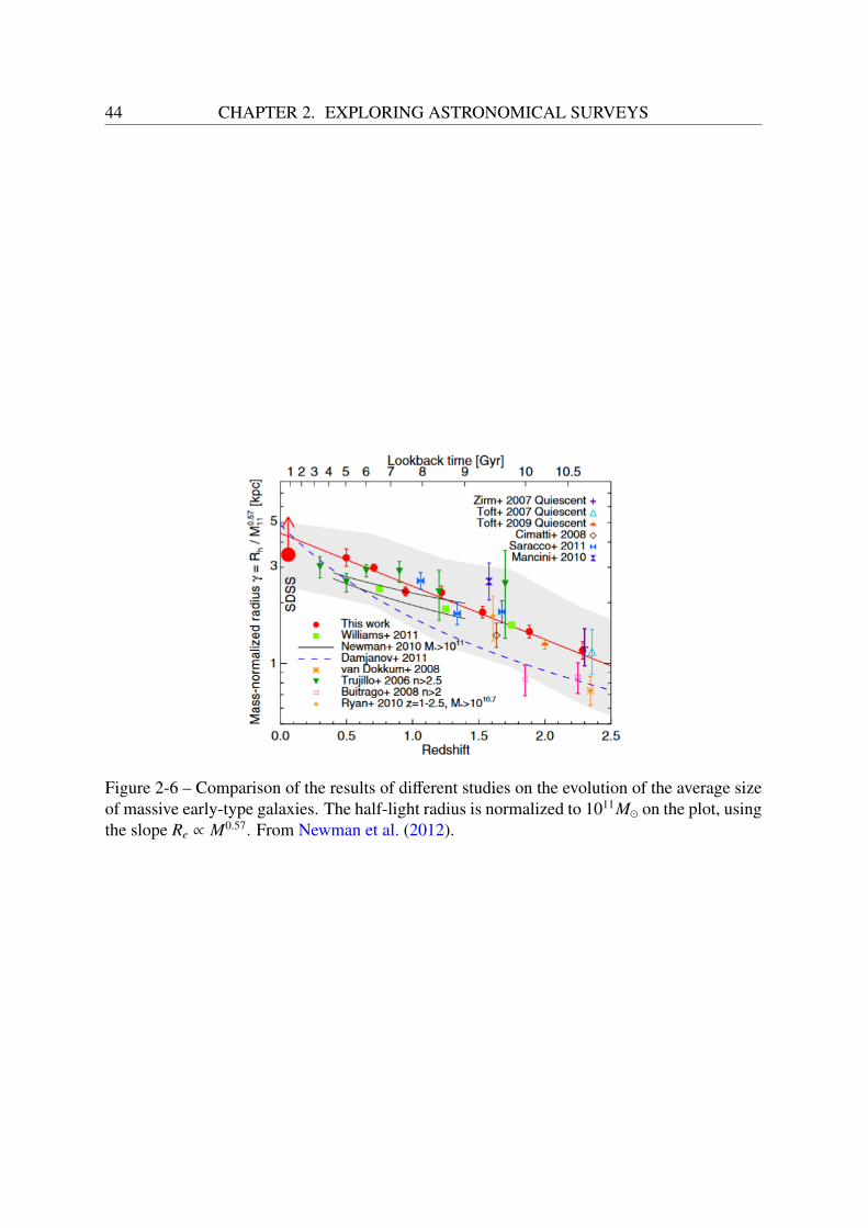
44 CHAPTER 2. EXPLORING ASTRONOMICAL SURVEYS
Figure 2-6 – Comparison of the results of different studies on the evolution of the average sizeof massive early-type galaxies. The half-light radius is normalized to 1011M on the plot, usingthe slope Re ∝ M0.57. From Newman et al. (2012).
Chapter 3
From images to catalogs: selection biasesin galaxy surveys
L’essentiel est invisible pour les yeux
Antoine de Saint-Exupéry, le Petit Prince
Abstract
There’s more to the universe than meets the eye. Because of various selection ef-fects of cosmological, physical and instrumental origins, no source catalog has yetcontained the totality of galaxies in a given cosmological volume. Some of themaffect the number of samples retrieved in a given population, others affect our mea-surements of luminosity, color, surface brightness, and morphological properties.Worse, some of them cannot be corrected for analytically and correlate with eachother in a non-linear way. This inevitably leads to systematic errors in inferringparameters models of galaxy evolution. In this chapter, I review some of the se-lection biases that are affecting most galaxy surveys, and some of the attempts thathave been designed for dealing with them.
Contents3.1 Effects of redshift . . . . . . . . . . . . . . . . . . . . . . . . . . . . . . . 46
3.1.1 Cosmological dimming . . . . . . . . . . . . . . . . . . . . . . . . . 46
3.1.2 K-correction . . . . . . . . . . . . . . . . . . . . . . . . . . . . . . 47
3.2 Dust extinction and inclination . . . . . . . . . . . . . . . . . . . . . . . . 48
3.3 Malmquist bias . . . . . . . . . . . . . . . . . . . . . . . . . . . . . . . . . 49
3.4 Eddington bias . . . . . . . . . . . . . . . . . . . . . . . . . . . . . . . . . 50
3.5 Confusion noise . . . . . . . . . . . . . . . . . . . . . . . . . . . . . . . . 52
45

46CHAPTER 3. FROM IMAGES TO CATALOGS: SELECTION BIASES IN GALAXY
SURVEYS
3.1 Effects of redshift
3.1.1 Cosmological dimming
The bolometric surface brightness (i.e. the surface brightness integrated over all wavelengths)of all cosmologically distant sources is altered by the expansion of the universe. This phe-nomenon was first predicted by Tolman (1930; 1934) and is now referred to in the literature ascosmological surface brightness dimming, or Tolman dimming. It can be theoretically derivedbriefly in the following way1:
Let F be the bolometric flux that an observer receives from a source of intrinsic luminosityL. We define its luminosity distance DL as:
F =L
4πD2L
(3.1)
For a solid angle Ω subtended by the extended source of projected area A, we define its angulardiameter distance DA as:
Ω =A
D2A
(3.2)
Etherington (1933) derived a relation between the angular distance and the luminosity distance,valid for any expanding universe described my a metric theory of gravity, as long as the numberof photons is conserved and photons travel on null geodesics. This relation is termed as thecosmic distance duality relation (CDDR):
DL = (1 + z)2DA (3.3)
The apparent bolometric surface brightness Iobs is defined as the bolometric flux density perunit solid angle:
Iobs =FΩ
=L
4πA1
(1 + z)4 =Ie
(1 + z)4 (3.4)
The surface brightness of the source therefore strongly decreases with increasing redshift. Thisdimming effect is the result of 3 different phenomena:
• In an expanding universe, as light is emitted farther and farther from the observer (interms of proper distances), successive waves of light arrive at the observer with increas-ing delay, reducing de facto the rate of reception of photons by a factor (1+z).
• Each photon is redshifted and therefore loses energy as the universe expands, reducingthe flux density by a factor (1 + z).
• The expansion of the universe also causes angular sizes to increase by a factor (1 + z)in every directions, as the source was closer to the observer when the light was emitted.Therefore the angular surface is increased by a factor (1 + z)2.
1For all the theoretical details, the reader is referred to Chapter 1 of Weinberg (2008)

CHAPTER 3. FROM IMAGES TO CATALOGS: SELECTION BIASES IN GALAXYSURVEYS 47
This unavoidable loss of surface brightness becomes especially apparent at high redshifts:sources are dimmed by a factor 16 at z = 1, and by a factor of more than 625 at z = 4!Tolman dimming therefore gives us a biased view of the early universe, where only the mostcompact objects and the highest surface brightness regions of star formation can be detected(Keel 2007; Calvi et al. 2014). In the latter case, these regions can appear as separate sources,which affects number counts.
3.1.2 K-correctionDue to the expansion of the universe, we do not observe the light from high-redshift sourcesin the same rest-frame that it was emitted. At redshift z, a photon emitted at a frequencyνe will be observed at a frequency νo, where νe = νo(1 + z). When performing broadbandphotometric measurements, the apparent magnitude2 of a source will be “redshifted” from itsabsolute magnitude3. Both quantities can therefore end up in different bands. For example,the flux of the most distant galaxies observed in the Hubble Deep Field (Williams et al. 1996),which sees the universe at UV and optical wavelengths, comes from the far-UV range of theiremission spectrum. Converting the apparent magnitude of a source in band p to its true absolutemagnitude in band q involves a term known as the “K-correction” (Humason et al. 1956; Okeand Sandage 1968; Hogg et al. 2002):
mp = Mq + DM + K(z) (3.5)
where DM is the distance modulus, or the difference (in magnitudes) between the observedbolometric flux of the source and bolometric flux observed at a distance of 10 pc, which isdefined as:
DM = 5 log10(DL
10pc) (3.6)
and K(z) is the K-correction term:
K(z) = −2.5 log10
[(1 + z)
L(νe)L(νo)
](3.7)
where L(νo) and L(νe) are respectively the observed and intrinsic SED of the source.There are two main approaches for determining the K-correction for a given galaxy: the first
approach involves the direct measurement of the galaxy spectrum. But in most cosmologicalsurveys the only information available is the apparent flux in a set of broadband filters, i.e. adiscretized and poorly resolved version of its underlying SED. The galaxy SED can be inferredby fitting the flux measurements to a set of empirical SED templates built from local galaxies,but the reliability of the resulting K-correction will then be limited by the number and widthof the passbands used, as well as by the good match between the data and the fitted template(Westra et al. 2010).
As the determination of the luminosity function of a galaxy sample requires the estimation
2The apparent magnitude of an object in a given photometric passband (in the Vega system) is −2.5 log10(R),where R is the ratio of the observed flux of that source to the observed flux of the Vega star (Hogg, 1999).
3The absolute magnitude of an object is the apparent magnitude that the object would have if it were at adistance of 10 pc (Hogg, 1999).
48CHAPTER 3. FROM IMAGES TO CATALOGS: SELECTION BIASES IN GALAXY
SURVEYS
of the absolute magnitude of the sources (cf Chapter 2.2), poor estimates of the K-correctioncan affect number counts by causing unphysical distortions to the luminosity function (Dalcan-ton 1998; Gabrielli et al. 2006).
3.2 Dust extinction and inclination
Interstellar dust affects the light of galaxies in the optical, as well as in UV and IR bands, asa result of the complex interplay between the distribution of stars and dust clouds, radiativetransfer and interstellar chemistry4. Most of the dust of a “typical” galaxy is located within itsdisk. Bulges, in fact, might contain little to no dust at all5 (Graham and Worley 2008). Due tothe obscuring dust lanes, incoming light from a distant galaxy can be absorbed and scattered outbefore reaching the observer, an effect termed dust extinction or dust attenuation (see details onterminology in Section 4.5). Different morphological types of galaxies are affected differentlyby extinction: spirals are in fact more dimmed than ellipticals and lenticulars (Nagayama et al.2004).
Dust attenuation is also correlated to the angle at which the galaxy is viewed, i.e. itsinclination. The stronger the inclination, the longer the path length of incident photons throughthe disk of the galaxy, and the greater the extinction by the obscuring material. Extinction istherefore minimal when the galaxy is viewed face-on, and maximal when the galaxy is viewededge-on, as illustrated in Figure 3-1. Observations confirm that edge-on galaxies tend to appeardimmer and redder than their face-on counterparts (Holmberg et al. 1975; Burstein et al. 1991;Driver et al. 2007).
As most observed quantities depend on inclination, cuts performed on these quantities canproduce samples that are biased by inclination. For example, magnitude-limited surveys willinevitably miss highly inclined faint dusty galaxies (Masters et al. 2010; Devour and Bell2016). Moreover, photometric quantities of galaxies affected by dust attenuation include opti-cal apparent magnitudes, colors (e.g. Tully et al. 1998; Maller et al. 2009; Masters et al. 2010),and surface brightness profiles (e.g. Byun et al. 1994; de Jong 1996). Because the inner re-gions of disks contain more dust than the outer regions (Boissier et al. 2004; Popescu and Tuffs2005), a radial opacity gradient arises which makes the observed disk scale lengths greater thantheir intrinsic values (Möllenhoff et al. 2006; Graham and Worley 2008, Gadotti et al. 2010).Yip et al. (2011) also showed that inclination effects result in overestimates of the photometricredshifts inferred from the observed magnitudes and colors of highly inclined sources, in orderto match their redder color with empirical templates.
Over the last decades, a lot of work has been done on adjusting for the effects of dustattenuation quantitatively (e.g. Valentijn 1990; De Vaucouleurs et al. 1991; Giovanelli et al.1995; Tully et al. 1998; Graham 2001; Masters et al. 2003; Tuffs et al. 2005; Bailin andHarris 2008; Unterborn and Ryden 2008), but the parameters governing dust attenuation areill-constrained, and no consensus has yet been reached. More details on attempts at modelingthe effects of dust extinction in various studies, including our own approach, are provided inSection 4.5.
4The reader is referred to Section 4.5 for a more detailed introduction on the physical properties of dust andits effect on the light and color of galaxies.
5However the light emitted in the bulge region can be obscured by the dust lanes in the disk when the galaxyis viewed edge-on.

CHAPTER 3. FROM IMAGES TO CATALOGS: SELECTION BIASES IN GALAXYSURVEYS 49
Figure 3-1 – Simulated urz color composite image of a dust attenuated Sbc galaxy at differentinclinations, from face-on (i=0) to edge-on (i=90), generated using the Sunrise radiativetransfer code (Jonsson 2006). As the inclination increases, reddening effects due to dust lanesbecome more and more apparent. Reproduced from Jonsson et al. (2009).
3.3 Malmquist biasIn apparent magnitude-limited surveys, intrinsically brighter sources can be observed at largerdistances (i.e. at higher redshifts) than fainter ones. As a result, the observed mean absolutemagnitude of the sample will be brighter than its intrinsic mean absolute magnitude, as illus-trated in Figure 3-2, and the observed sample will not necessarily be representative of the realunderlying population. This selection effect is referred to as Malmquist bias6 (Malmquist 1920,1922). It was originally discovered for stars spread in Euclidean space, but applies equally togalaxies in an expanding Friedman universe (Teerikorpi 2015). Malmquist bias operates atall magnitudes (Lynden-Bell 1992) and “only” affects the composition of the sample, not thephotometric measurements performed on it. In cosmological studies, not taking it into accountcan lead to a significant overestimate of the average luminosity of standard candles, which inreturn leads to underestimate of their distance, and therefore to an overestimate of the Hubbleconstant (Sandage and Tammann 1975; Tammann 1987).
When the luminosity function of the studied population is a simple Gaussian distribution,an analytical correction correction for Malmquist bias can be derived, which depends on thesquare of the intrinsic dispersion in the absolute magnitude distribution of the sample σM (e.g.,using the notations of Butkevich et al. 2005):
< M >lim= M0 − σ2M
d ln N(mlim)dmlim
(3.8)
where < M >lim is the observed mean absolute magnitude of the magnitude-limited sample,M0 is the intrinsic mean absolute magnitude of the population, and N(mlim) is the total numberof sources whose apparent magnitude is brighter than mlim.
But correcting for this bias happens to be more highly complex in practice. In fact, thelevel of Malmquist bias depends on the shape of the intrinsic luminosity distribution of thepopulation, which is unknown in general, and increases with the width of the intrinsic scatterin the source luminosities. This scatter can be difficult to determine, and must not be confused
6Malmquist bias bias was actually first discovered by Eddington (1914), in a special case where the spatialdensity of sources is homogeneous. Therefore, Malmquist bias is sometimes referred to in the literature as theEddington-Malmquist bias, as suggested by Lynden-Bell (1992). But this terminology is likely to perpetuate theconfusion between the Malmquist bias and the Eddington bias described in Section 3.4 that is already too commonin the astronomical community.
50CHAPTER 3. FROM IMAGES TO CATALOGS: SELECTION BIASES IN GALAXY
SURVEYS
with the observed scatter, which is rendered smaller than the intrinsic scatter by the Malmquistbias (Tammann 1987).
Methods for correction or minimization of the Malmquist bias include the creation ofvolume-limited samples, i.e. the sampling of every galaxies in the survey volume (e.g. Kan-nawadi et al. 2015), the weighting of galaxy properties by the maximum volume over whichthey can be detected (this is called the Vmax method, cf Mo et al. 2010), or the comparisonof realistic mock catalogs that explicitly include magnitude limits to mock catalogs that don’t(e.g. Conley et al. 2010; Saulder et al. 2016). The curious reader is referred to Verter (1993)and Teerikorpi (1997) for historical and methodological reviews of various attempts at imple-menting Malmquist bias corrections.
3.4 Eddington bias
No measuring instrument is perfect. A set of sources with a single luminosity will always bespread out upon observation due to statistical fluctuations in measurement errors. This scattergives rise to the Eddington bias (Eddington 1913, 1940), which distorts number counts in asystematic way. Thus, except for some pathological cases where the distribution is constantor linear, as galaxy number counts are rising steeply with decreasing flux, the number of lowfluxes scattered up by the noise is likely to be greater than the number of large fluxes scattereddown, which leads to a steepening of the slope of the number counts. Moreover, a fractionof the population is likely to be scattered below the detection limit of the survey, and anotherfraction below the detection limit to be scatter up upon observation (Jeffreys 1938). Eddington(1940) proposed a way to estimate analytically the true number counts from the distribution ofobserved values, provided that measurements errors are Gaussian-distributed with a constantwidth σ in magnitude, i.e. if the probability of observing a magnitude m′ for a source of truemagnitude m is:
P(m′,m) =1
(2πσ2)1/2 e−(m−m′)2/2σ2(3.9)
Following the notations of Peterson (1997), let A(m) be the true differential number countper magnitude per unit solid angle. A(m)dm therefore represents the true number of sourcesbetween magnitudes m and m + dm, and Aobs(m)dm the observed number. The true number ofsources brighter than m is then:
N(m) =
∫ m
−∞
A(m)dm (3.10)
and the observed value of Aobs(m′) is the convolution of the true number counts with the mea-surement PDF:
Aobs(m′) =1
(2πσ2)1/2
∫ ∞
−∞
A(m)e−(m−m′)2/2σ2dm (3.11)
Assuming that σ is small and the cumulative number count is a power law:
N(m) = C10κm (3.12)
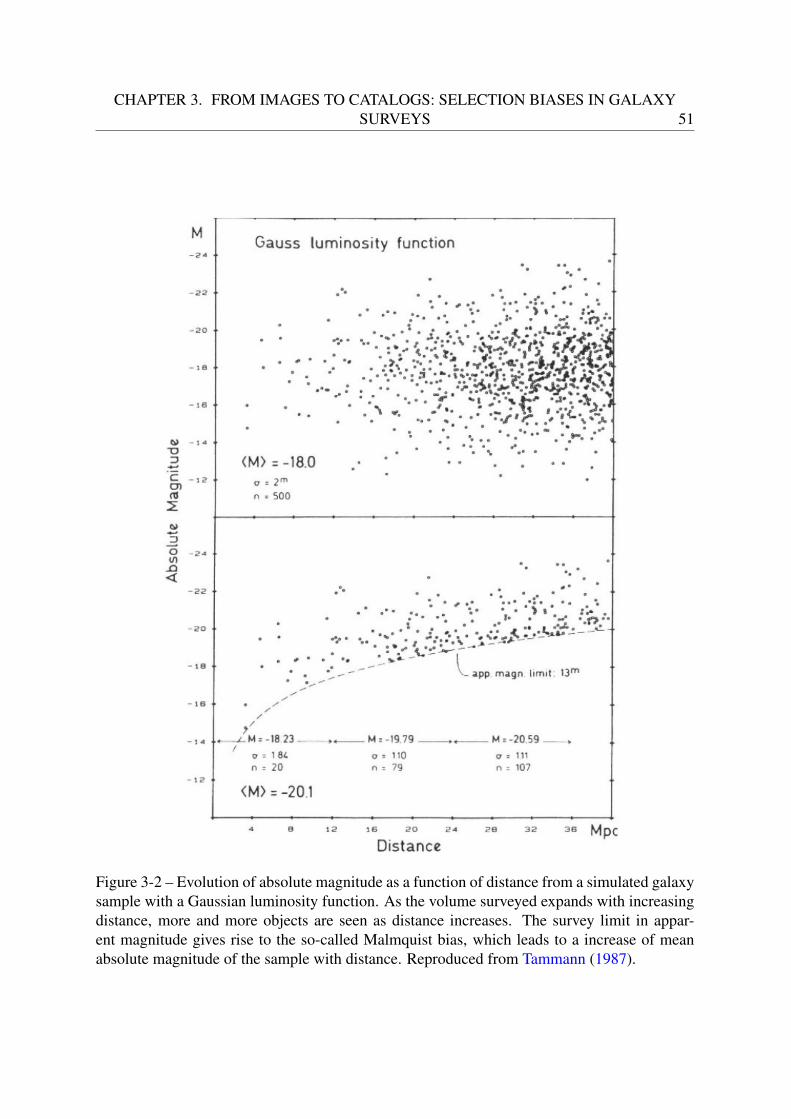
CHAPTER 3. FROM IMAGES TO CATALOGS: SELECTION BIASES IN GALAXYSURVEYS 51
Figure 3-2 – Evolution of absolute magnitude as a function of distance from a simulated galaxysample with a Gaussian luminosity function. As the volume surveyed expands with increasingdistance, more and more objects are seen as distance increases. The survey limit in appar-ent magnitude gives rise to the so-called Malmquist bias, which leads to a increase of meanabsolute magnitude of the sample with distance. Reproduced from Tammann (1987).

52CHAPTER 3. FROM IMAGES TO CATALOGS: SELECTION BIASES IN GALAXY
SURVEYS
Figure 3-3 – Patch of the GOODS-N field (Dickinson et al. 2003) observed at 250, 350 and500 µm (left to right). The green circles indicate the beam FWHM in each band. The field isplagued by source confusion, and the size of the background fluctuations is of the order of thebeam size. Reproduced from Nguyen et al. (2010).
where C and κ are constant, Eddington showed that7:
A(m) = Aobs(m)1 − 1
2
(σκ
log10 e
)2 (3.13)
This correction must be applied at all magnitudes (Baryshev and Teerikorpi 2012). If the mea-surement scatter increases with fainter magnitudes, as it is often the case in galaxy surveys,Equation 3.11 cannot be used anymore, and an analytical correction becomes tricky to de-rive (van der Burg et al. 2010). In this situation, numerical experiments by Teerikorpi (2004)have shown that the steepening of the number counts gets even stronger than the theoreticalprediction of Eddington (1940).
3.5 Confusion noise
The sky background is not empty. It consists of the accumulated light of faint unresolvedsources below the detection limit of the survey, and of extended structures at scales of the orderof the telescope beam8 size (Guiderdoni et al. 1997). Confusion noise (or source confusion)is the corresponding uncertainty in the determination of the background level. These stochas-tic fluctuations of the background generate an uncertainty in the determination of the flux ofresolved faint sources, which must be added to the flux error estimates: σ2
tot = σ2sky + σ2
con f ,where σ2
sky is the classic noise resulting from the combination of Poisson noise and Gaussianread-out noise. Source confusion also increases the positional uncertainty of sources (Hogg2001), boosts the flux of some sources and can lead to spurious detections by the merging ofseveral sources near the detection limit. It cannot be overcome by longer exposure times, andtherefore poses a fundamental limit to the depth of astronomical surveys.
This problem was first mathematically approached by Scheuer (1957) and Condon (1974)
7The full derivation is available in Chapter 10 of Peterson (1997).8The “beam” here refers to an element of resolution in the images. It can be defined as the solid angle of the
1σ radius circle of the Gaussian point spread function (Hogg 2001).

CHAPTER 3. FROM IMAGES TO CATALOGS: SELECTION BIASES IN GALAXYSURVEYS 53
in the context of early radio surveys. In practice, the background sky brightness defines a limitbeyond which individual sources cannot be clearly detected: the confusion limit. Near thislimit, the distinction between faint objects and the background objects is blurred. The confu-sion limit is mainly determined by the beam size (as illustrated in Figure 3-3), the wavelengthand the position on the sky. Using the notations of Dole et al. (2003), the confusion noise (at agiven wavelength) can be defined in the general case as:
σ2con f =
∫f 2(θ, φ)dθdφ
∫ S lim
0S 2 dN
dSdS (3.14)
where f (θ, φ) is the two-dimensional beam profile9, S is the source flux density and dNdS is the
differential number count. The integration includes all sources below the confusion limit, S lim.Moreover, studies by Negrello et al. (2004) and Takeuchi and Ishii (2004) have found that thelevel of source confusion is probably increased by the clustering of unresolved sources. Theconfusion noise can be evaluated by two criteria, described extensively in Dole et al. (2003): the“photometric criterion”, which is related to the quality of the photometry of detected sources,and the “source density criterion”, which is related to the completeness of detected sourcesabove the confusion limit directly linked to the probability to lose sources that are too close toeach other to be separated.
Confusion noise is not a problem in optical surveys, as the confusion limit is generallynot reached, except in very crowded fields such as star clusters. But it can be the dominantnoise contribution in mid and far-infrared, because the sky background is very bright in thesewavelengths. In far-IR especially, the thermal emission of dusty Galactic cirrus clouds stronglycontributes to confusion noise (Low et al. 1984; Gautier et al. 1992; Jeong et al. 2005). And atsub-mm wavelengths, due to the particular shape of the emission spectrum of dust, some high-redshift ultra luminous infrared galaxies (ULIRGs) actually compensate the combined effectsof decrease in flux density with distance and surface brightness dimming, causing a “negativeK-correction” which, coupled to the low instrumental angular resolution, also adds to sourceconfusion (Blain et al. 2002).
There are two main approaches for correcting for the effects of source confusion, whichboth have their advantages and disadvantages (cf Roseboom et al. 2010). One approach in-volves the individual source counterparts identification in other wavelengths (e.g. Pope et al.2005; Ivison et al. 2007). Another estimates statistically the galaxy number counts at faint mag-nitudes via a maximum likelihood fit (assuming a model of number counts, usually a simplepower law) on the pixel intensity distribution (e.g. Patanchon et al. 2009).
9The beam profile can be approximated by a Gaussian profile with the same FWHM as the expected PSF, orby an Airy pattern (Dole et al. 2003).

Part II
The forward modeling approach to galaxyevolution
54

Chapter 4
Modeling the light, shape and sizes ofgalaxies
If you wish to make an apple pie fromscratch, you must first invent theuniverse.
Carl Sagan, Cosmos
What I cannot create, I do notunderstand.
Richard Feynman
Abstract
In this chapter1, I briefly review the tools used by the astronomical communityto model the size, shape, color, brightness, and dust content of galaxies. Thiswill allow me to outline our forward-modeling approach in this thesis and to in-troduce the Stuff empirical model that we are going to use to test the validity ofour method. Stuff generates mock photometric and morphometric catalogs in anarbitrary number of filters, from empirical prescriptions about the light and sizedistributions of various galaxy populations.
Contents4.1 The forward modeling approach . . . . . . . . . . . . . . . . . . . . . . . 56
4.2 Outline of our approach . . . . . . . . . . . . . . . . . . . . . . . . . . . . 56
4.3 Magnitudes and colors . . . . . . . . . . . . . . . . . . . . . . . . . . . . 57
4.4 Light profiles . . . . . . . . . . . . . . . . . . . . . . . . . . . . . . . . . . 59
4.5 Dust . . . . . . . . . . . . . . . . . . . . . . . . . . . . . . . . . . . . . . . 611Note: This chapter uses extracts from Carassou et al. (2017) in some of its sections.
55

56 CHAPTER 4. MODELING THE LIGHT, SHAPE AND SIZES OF GALAXIES
4.5.1 Composition, size and evolution . . . . . . . . . . . . . . . . . . . . 63
4.5.2 Galactic extinction . . . . . . . . . . . . . . . . . . . . . . . . . . . 63
4.5.3 Attenuation curves for local galaxies . . . . . . . . . . . . . . . . . . 64
4.5.4 Attenuation curves for high-z galaxies . . . . . . . . . . . . . . . . . 67
4.6 The Stuff model . . . . . . . . . . . . . . . . . . . . . . . . . . . . . . . . 68
4.1 The forward modeling approachThe traditional approach when comparing the results of models to data is sometimes referredto as backward modeling (e.g., Marzke 1998; Taghizadeh-Popp et al. 2015). In this scheme,physical quantities are derived from the observed data, and are then compared with the phys-ical quantities predicted from simulations, semi-analytical models (SAM), or semi-empiricalmodels. A more reliable technique is the forward modeling approach: a distribution of mod-eled galaxies are passed through a virtual telescope with all the observing process reproduced(filters, exposure time, telescope characteristics, seeing properties, as well as the cosmologicaland instrumental biases described above), and a direct comparison is made between simulatedand observed datasets. The power of this approach comes from the fact that theory and observa-tion are compared in the observational space: ideally, the same systematic errors and selectioneffects affect the simulated and observed data.
The “mock catalogs” approach, as it is sometimes called, is already being used to test theprocessing pipeline of galaxy surveys and characterize their systematics (e.g., Yan et al. 2004;McBride et al. 2009), or to test models of galaxy formation (e.g., Simard and Somerville 2000).Blaizot et al. (2005) were the first to introduce realistic mock telescope images from light conesgenerated by semi-analytical models. Overzier et al. (2013) extended this idea by constructingsynthetic images and catalogs from the Millenium Run cosmological simulation (Springel et al.2005) including detailed models of ground-based and space telescopes. Recently, Bernyk et al.(2016) unveiled the Theoretical Astrophysical Observatory (TAO), an online virtual observa-tory that enables users to generate mock survey images and galaxy catalogs based on selectablecombinations of cosmological simulations or semi-analytical model, as well as stellar popula-tion synthesis models. And Taghizadeh-Popp et al. (2015) used semi-empirical modeling tosimulate Hubble Deep Field (HDF) images, from cutouts of real SDSS galaxies with modifiedsizes and fluxes, and compared them to observed HDF images. Lately, Kacprzak et al. (2017)used a forward model to infer the redshift distribution of a cosmological sample. In this the-sis, we make the case that forward modeling can be used to perform reliable inferences on theevolution of the galaxy luminosity and size functions. I describe our approach in the followingsection.
4.2 Outline of our approachIn order to infer the physical properties of galaxies from observed survey images withouthaving to describe the complex selection effects the latter contain, we propose the followingpipeline. We start from a set of physical input parameters, drawn from the prior distributiondefined for each parameter. These parameters describe the luminosity and size distribution of

CHAPTER 4. MODELING THE LIGHT, SHAPE AND SIZES OF GALAXIES 57
the various populations of modeled galaxies. From this set of parameters, our forward modelgenerates a catalog of galaxies modeled as the sum of their bulge and disk components, eachwith a different profile. The projected light profiles of the galaxies are determined by theirinclination, the relative fraction of light contained within the bulge, and the galaxy redshift aswell as the extinction of the bulge and disk components. The galaxies are randomly drawn fromthe luminosity function of their respective population. The catalog assumes that galaxies areuniformly distributed on a virtual sky that includes the cosmological effects of an expandinguniverse with a cosmological constant. The survey image is simulated in every band coveredby the observed survey, and reproduces all of its characteristics, such as filters transmission,exposure time, point spread function (PSF) model, and background noise model.
Then, a large number of “simulated” images are generated via an iterative process (aMarkov chain) generating new sets of physical parameters at each iteration. Some basic fluxand shape parameters are extracted in the same way from the observed and simulated images:after a pre-processing step (which is identical for observed and simulated data) where observ-ables are decorrelated and their dynamic range reduced, the multidimensional distributionsof simulated observables are directly compared to the observed distributions using a customdistance function on binned data.
The chain moves through the parameter space towards regions of high likelihood, that is,regions that minimize the distance between the modeled and observed datasets. The pathwayof the chain is finally analyzed to reconstruct the multidimensional posterior probability dis-tribution and infer the sets of parameters that most likely reproduce the observed catalogs, aswell as the correlations between these parameters. The main steps of this approach are detailedin the following sections and chapters, and the whole pipeline is sketched in Figure 4-1.
4.3 Magnitudes and colorsWe need to build mock galaxies whose apparent magnitudes and colors closely match currentUV, optical and IR observations. In the AB system2 (Oke and Gunn 19833), the apparentmagnitude of a source in a given band is:
mAB = −2.5 log10
∫fνTνdν∫Tνdν
− 48.6 (4.1)
where fν is the spectral flux density of the source in erg s−1 cm−2 Hz−1 and Tν is the total re-sponse of the system, which is the product of the filter transmission curve by the quantumefficiency of the detector, the response of the telescope (mirror and optics) and the atmospherictransmission, as illustrated in Figure 4-3. Color indices are then derived by subtracting themagnitudes in different bands.
We see from Equation (4.1) that our estimate of the apparent magnitude of a source relieson our knowledge of its spectral energy distribution (SED), which contains all the informationabout the integrated emission and absorption of stars, gas and dust. This requires the use of aset of templates corresponding to every galaxy spectral types, and to every galaxy components
2In the AB photometric system, the zero point is 3631 Jansky for all bands, so a source with a flat spectralenergy distribution ( fν = constant) has the same magnitude in all bands, and all colors = 0.
3Note that there is a sign error in the main formula of this paper.
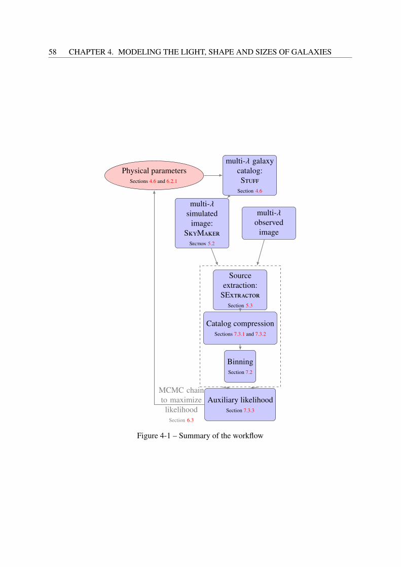
58 CHAPTER 4. MODELING THE LIGHT, SHAPE AND SIZES OF GALAXIES
Physical parametersSections 4.6 and 6.2.1
multi-λ galaxycatalog:Stuff
Section 4.6
multi-λsimulated
image:SkyMaker
Section 5.2
multi-λobserved
image
Sourceextraction:
SExtractorSection 5.3
Catalog compressionSections 7.3.1 and 7.3.2
BinningSection 7.2
Auxiliary likelihoodSection 7.3.3
MCMC chainto maximize
likelihoodSection 6.3
Figure 4-1 – Summary of the workflow

CHAPTER 4. MODELING THE LIGHT, SHAPE AND SIZES OF GALAXIES 59
Figure 4-2 – SED templates of Coleman et al. (1980)
(bulge and disk). SED templates can be derived empirically from observations of local brightgalaxies4, such as the widely used set of Coleman et al. (1980) (illustrated in Figure 4-2)or Kinney et al. (1996), or they can be generated by models via stellar population synthesis(e.g., Fioc and Rocca-Volmerange 1999; Bruzual and Charlot 2003). The reader is referred toWalcher et al. (2011) for a recent review on SED modeling.
4.4 Light profiles
Galaxies display a large variety of sizes and shapes. A good parametrization of their struc-tural and photometric properties is therefore crucial for classification and image simulationpurposes. The light profile of a galaxy, which measures how its intensity varies as a function ofthe distance from its center, has proven a useful tool for that purpose. The most notable earlyattempt5 at providing analytical fits to the radial distribution of stellar light was the work of deVaucouleurs (1948, 1959), who found empirically that the intensity profile of bright ellipticalgalaxies and of the bulges of lenticular and spiral galaxies could be well described by:
I(r) = Ie exp−7.67
( rre
)1/4
− 1 (4.2)
4Empirical templates are computationally advantageous to use, but since they are built on local galaxies, theymight not be representative of the spectra of high-z galaxies.
5An exhaustive historical review of early models to describe the light profile of elliptical galaxies can be foundin Graham (2013).
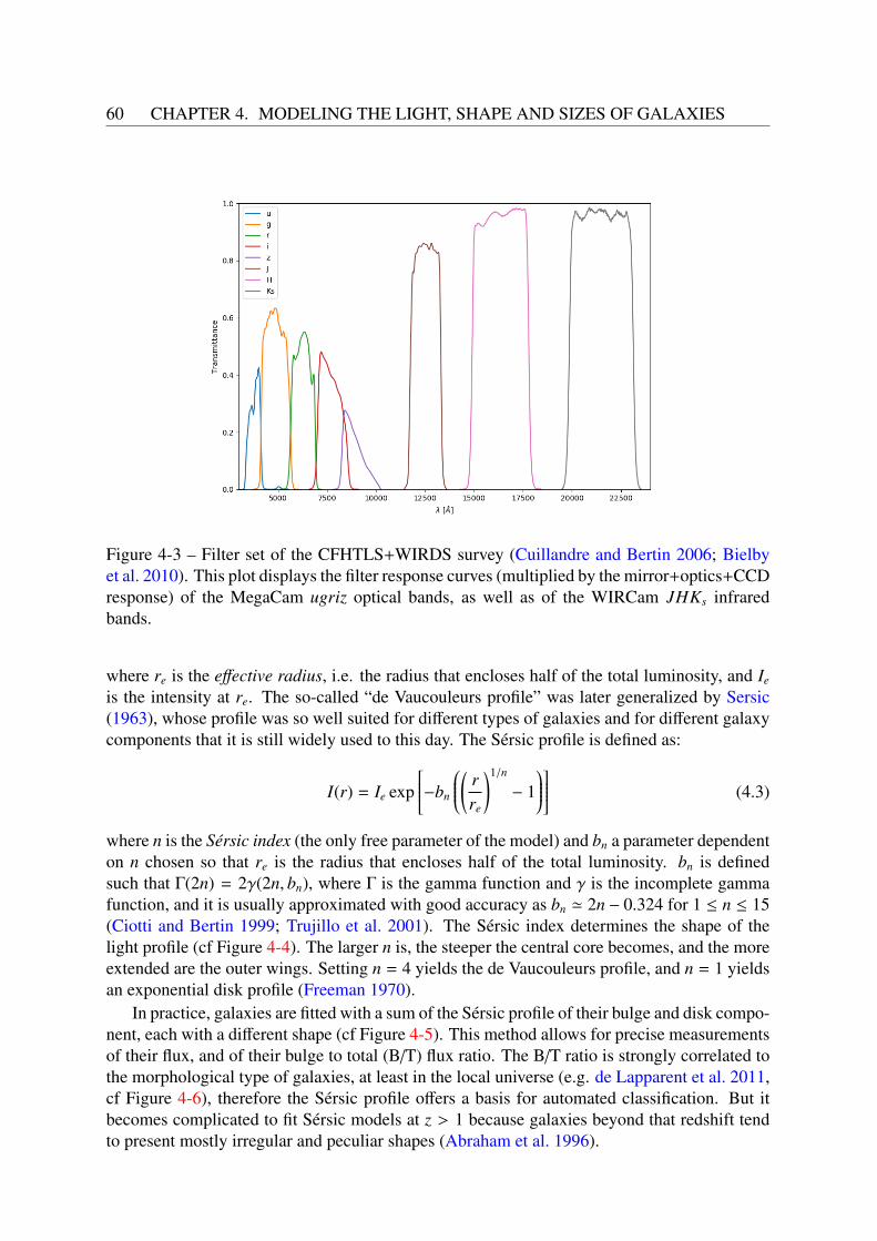
60 CHAPTER 4. MODELING THE LIGHT, SHAPE AND SIZES OF GALAXIES
Figure 4-3 – Filter set of the CFHTLS+WIRDS survey (Cuillandre and Bertin 2006; Bielbyet al. 2010). This plot displays the filter response curves (multiplied by the mirror+optics+CCDresponse) of the MegaCam ugriz optical bands, as well as of the WIRCam JHKs infraredbands.
where re is the effective radius, i.e. the radius that encloses half of the total luminosity, and Ie
is the intensity at re. The so-called “de Vaucouleurs profile” was later generalized by Sersic(1963), whose profile was so well suited for different types of galaxies and for different galaxycomponents that it is still widely used to this day. The Sérsic profile is defined as:
I(r) = Ie exp−bn
( rre
)1/n
− 1 (4.3)
where n is the Sérsic index (the only free parameter of the model) and bn a parameter dependenton n chosen so that re is the radius that encloses half of the total luminosity. bn is definedsuch that Γ(2n) = 2γ(2n, bn), where Γ is the gamma function and γ is the incomplete gammafunction, and it is usually approximated with good accuracy as bn ' 2n − 0.324 for 1 ≤ n ≤ 15(Ciotti and Bertin 1999; Trujillo et al. 2001). The Sérsic index determines the shape of thelight profile (cf Figure 4-4). The larger n is, the steeper the central core becomes, and the moreextended are the outer wings. Setting n = 4 yields the de Vaucouleurs profile, and n = 1 yieldsan exponential disk profile (Freeman 1970).
In practice, galaxies are fitted with a sum of the Sérsic profile of their bulge and disk compo-nent, each with a different shape (cf Figure 4-5). This method allows for precise measurementsof their flux, and of their bulge to total (B/T) flux ratio. The B/T ratio is strongly correlated tothe morphological type of galaxies, at least in the local universe (e.g. de Lapparent et al. 2011,cf Figure 4-6), therefore the Sérsic profile offers a basis for automated classification. But itbecomes complicated to fit Sérsic models at z > 1 because galaxies beyond that redshift tendto present mostly irregular and peculiar shapes (Abraham et al. 1996).

CHAPTER 4. MODELING THE LIGHT, SHAPE AND SIZES OF GALAXIES 61
Figure 4-4 – Sérsic curves for various values of n. n = 4 corresponds to the de Vaucouleurprofile.
For more accurate fits, the one-dimensional structural analysis provided by the Sérsic pro-file can be completed by a two-dimensional analysis including non-axisymmetric structures,such as bars, rings or spiral arms. For example, bars can be modeled as Sérsic profiles, spiralrotation functions can be used to model spiral structure, and ellipsoidal isophotes can be dis-torted using Fourier modes to model the shape of irregular galaxies (Peng et al. 2010). Butfitting all these components at the same time can be computationally prohibitive when apply-ing the fitting routine to a whole survey, due to the high number of free parameters (for eachgalaxy) of the resulting model.
Other popular measurements of galaxy structure include the CAS system (Concentration,Asymetry, Clumpiness, e.g. Conselice 2003), the shapelets decomposition (Refregier 2003)and the Gini/M20 parameters (e.g., Abraham et al. 2003; Lotz et al. 2004). The reader isreferred to Conselice (2014), Graham (2013) and Peng et al. (2010) for historical and method-ological reviews of parametric and non parametric galaxy structure analysis approaches.
4.5 DustInterstellar dust strongly affects the light we receive from galaxies. In fact, photons originat-ing from distant galaxies have to go through their interstellar medium (ISM) and through theISM of the Milky Way before reaching our telescopes. Dust was originally discovered via itsobscuring effect on starlight, an effect termed extinction or reddening, as blue wavelengths aremore dimmed than red wavelengths (Trumpler 1930). It constitutes only a small fraction of thetotal mass of galaxies: in the dust-rich ISM of the Milky Way, its mass represents ∼ 1 % of thetotal HI mass (Draine et al. 2007), and this ratio is supposed to be fairly constant in external

62 CHAPTER 4. MODELING THE LIGHT, SHAPE AND SIZES OF GALAXIES
Figure 4-5 – Sérsic bulge+disk fit performed on a 5′ × 5′ H-band image of NGC 3621 withGALFIT (Peng et al. 2010). From Barth et al. (2008).
Figure 4-6 – Distribution of the B/T ratio attribute as a function of de Vaucouleurs morpho-logical type (De Vaucouleurs et al. 1991) for the 4458 galaxies in the EFIGI catalog (Baillardet al. 2011). This plot reveals a strong correlation of morphological type with B/T, with a largedispersion of B/T for each type. From de Lapparent et al. (2011).

CHAPTER 4. MODELING THE LIGHT, SHAPE AND SIZES OF GALAXIES 63
galaxies6. But the contribution of dust to the observed light emitted by galaxies is crucial tounderstand their evolution, as it shapes their spectra (and therefore their photometry) in vari-ous ways. It also plays a great role in the chemical evolution of galaxies, as the surface of dustgrains constitute the craddle of molecular hydrogen (H2) formation and complex astrochem-istry (e.g. Gould and Salpeter 1963; Cazaux and Spaans 2009). However, as we will see inthis section, the dust evolution cycle in galaxies is still poorly constrained, and this constitutesa significant source of uncertainties in current models of galaxy evolution.
4.5.1 Composition, size and evolution
The physical properties of dust, from its chemical composition to its size distribution, aremostly constrained by the study of interstellar extinction, completed by observations in theinfrared. In fact, dust grains absorb a fraction of the UV emission from young stars and re-emitin IR (Dale et al. 2009).
Interstellar dust is created from the elements ejected from low- and intermediate-mass starsin their asymptotic giant branch (AGB) phase and from type II supernovae (SNe), howeverstardust only account for a small fraction (a few %) of the total interstellar dust mass in galaxies(e.g. Draine and Salpeter 1979; Zhukovska and Henning 2014). Dust grains mainly growby accretion and coagulation in the dense environment of molecular clouds, but can also bedestroyed in the shock waves of SNe explosions, or shattered in collisions with other grains inthe diffuse ISM (e.g. Asano et al. 2013; Aoyama et al. 2017).
The physical properties of dust grains vary significantly across galactic environments,which suggests various possible evolutionary tracks. But overall, its known chemical com-position is a mixture of small grains of polycyclic aromatic hydrocarbons (PAHs), amorphoussilicates and large grains of graphite. PAHs and silicates in particular display strong spectralfeatures in the emission spectrum of dust. Dust grains come with all sizes, with a power lawdistribution for sizes between 0.02 µm and ≥ 0.2 µm (e.g. Weingartner and Draine 2001; Draine2009).
4.5.2 Galactic extinction
The combined effects of light absorption of a point source and scattering of photons out of theline of sight by the ISM of the Milky Way is referred to as Galactic extinction (or interstellarextinction). Given a uniform cloud of dust with an optical depth τext
λ along the line of sight, anobserver would see the original flux of the source F0(λ) reduced to:
F(λ) = F0(λ)10−τextλ (4.4)
The extinction Aλ (expressed in magnitudes) is defined as:
Aλ = −2.5 log10
( F(λ)F0(λ)
)= −2.5 log10(e)τext
λ = 1.086τextλ = m(λ) − m0(λ) (4.5)
6However it is important to note that the dust-to-gas ratio of a galaxy depends on its star formation historybecause it correlates with metallicity (Draine et al. 2007).

64 CHAPTER 4. MODELING THE LIGHT, SHAPE AND SIZES OF GALAXIES
In short, more dust along the line of sight leads to more dimming7. Extinction can also bequantified from the amount of reddening or color excess that the observed source is subjectto. In the Johnson system, the color excess (also called selective extinction) is defined as thedifference between the measured (B-V) color of the source, and its intrinsic color (B−V)0 (i.e.not affected by extinction):
EB−V = (B − V) − (B − V)0 = (B − B0) − (V − V0) = AB − AV (4.6)
where AB is the total extinction in band B (450 nm), and AV is the total extinction in band V (550nm). In practice, galactic extinction is usually probed via the pair method, where a comparisonis performed between the spectra of 2 stars with the same spectral type, one reddened and theother unreddened. The shape of the extinction law (the function describing how extinctionevolves with wavelength) with different environments can be compared by normalizing Aλ byAV . Another widely used normalization uses the quantity k(λ) = Aλ/EB−V . Cardelli et al.(1989) derived an average extinction curve for 0.125 µm ≤ λ ≤ 3.5 µm parametrized by asingle variable RV , which is sometimes referred to in the literature as the CCM relationship:
< Aλ/AV >= a(x) + b(x)/RV (4.7)
where x = 1/λ µm−1, a and b are functions of wavelength and RV is the total-to-selectiveextinction ratio, the slope of the extinction law at V-band, used to link extinction to the colorexcess:
RV =AV
EB−V(4.8)
The value of RV is determined by the environment along the line of sight: a standard value ofRV = 3.1 is observed in the diffuse ISM of the Milky Way (e.g. Schultz and Wiemer 1975), butbigger values (∼ 5.5) are found in dense molecular clouds (e.g. Fitzpatrick 2004). The CCMextinction curves for different values of RV is plotted on Figure 4-7.
To compute Galactic extinction for a given line of sight and a given photometric band, werely on the use of “dust maps”. Schlegel et al. (1998) for example combined IRAS and COBE100 microns data (shown in Figure 4-8) to derive an all-sky map of Galactic reddening, EB−V .This map reveals the complex filamentary structure of the ISM of the Milky Way, even at highgalactic latitudes, a structure known as galactic cirrus. An online service has been developedby NASA/IPAC Infrared Science Archive8 to generate cutouts of this map from a given patchof the sky and return extinction values for most photometric bands.
4.5.3 Attenuation curves for local galaxiesWhen we look at a distant galaxy, we see the integrated emission of all its constituents overits surface. As a result of the relative position between the stars and the dust distributions, afraction of the light is scattered by dust clouds into the line of sight, in addition to the effect ofdust absorption and scattering out of the line of sight. In order to distinguish this phenomenon
7Hopefully we live in a relatively optically thin region of the Milky Way. What would astronomy be like if wewere shrouded by a cloud of interstellar dust? We would only see the closest stars in the optical, and I wouldn’thave a job!
8http://irsa.ipac.caltech.edu/applications/DUST/

CHAPTER 4. MODELING THE LIGHT, SHAPE AND SIZES OF GALAXIES 65
Figure 4-7 – Extinction curves for the Milky Way of Cardelli et al. (1989) for different valuesof RV corresponding to different galactic environments. This plot illustrates how RV controlsthe slope of the extinction curve.
Figure 4-8 – All-sky view of the IRAS+COBE 100 µm imaging data in false colors shown inequirectangular projection, generated by Schlegel et al. (1998). It is used to return the valuesof Galactic dust reddening for a given line of sight.

66 CHAPTER 4. MODELING THE LIGHT, SHAPE AND SIZES OF GALAXIES
from interstellar extinction, we refer to it as dust attenuation, although we will use the sameformalism to describe attenuation and extinction. The difference between the 2 processes isillustrated in Figure 4-9. In practice, the scattering of photons into the line of sight dampensthe effects of reddening compared to the extinction we observe within the Milky Way: anattenuated source appears greyer than an source subject to extinction only.
The shape of the attenuation law for a given galaxy depends on many factors: it is de-termined by the composition and size distribution of dust grain within that galaxy, and bythe geometry of the extended distribution of stars and dust, which can be approximated by asimple screen of dust between the galaxy and observer (e.g. Charlot and Fall 2000) or by aclumpier distribution (e.g. Calzetti 2001). Attenuation also depends on the stellar populationsof the host galaxy: in fact, young stars are strongly attenuated by their birth cloud, while olderstars have cleared their birth cloud and are only attenuated by the diffuse ISM (Calzetti 1997).Some models, like CIGALE (Noll et al. 2009), use a parametric model to fit the attenuationcurve k(λ) empirically via SED fitting. More complex models, like GRASIL (Silva et al. 1998)or MAGPHYS (da Cunha et al. 2008), include a physically motivated treatment of dust with2 components: a distribution of molecular clouds with a characteristic dissipation timescale(∼ 107 years) and a diffuse ISM.
If we want to derive extinction curves for extragalactic sources, we can only use the pairmethod in galaxies that are so close to us that we can resolve individual bright stars. This is thecase for our closest neighbors, hence the most well-known UV extinction curves in the localuniverse besides the Milky Way (MW, Seaton 1979; Fitzpatrick and Massa 1986) are thoseof the Large Magellanic Cloud (LMC, Fitzpatrick and Massa 1986), the Small MagellanicCloud (SMC, Prevot et al. 1984; Bouchet et al. (1985)) and M31 (Bianchi et al. 1996), andeach curve has a distinct shape, as shown in Figure 4-10. In particular, the Magellanic Cloudscurves cannot be fitted by the Galactic extinction laws of Cardelli et al. (1989), which suggestsdifferent dust properties in these galaxies than in the MW.
Some extinction curves present a characteristic bump at 2175 Å. This feature seems to hintthat carbon is a major component of interstellar dust (e.g. Mathis et al. 1977). The bumpcan be observed in the MW curve, and in a lesser way in the LMC curve, but it has not beenfound in the SMC. Many uncertainties surround this feature. Its very presence (or not) in mostextragalactic sources is still under debate: while radiative transfer dust models suggest that the2175 Å feature should be common in star forming galaxies (Conroy 2013), other studies, likeBattisti et al. (2016), do not find any evidence of a significant 2175 Å feature in their sampleof 104 local galaxies from the Galaxy Evolution Explorer and the SDSS. Neither do we knowwhether the presence or not of the bump if an indicator of the spatial distribution of stars anddust, or that of peculiar dust properties.
In the general case, quantifying dust attenuation in external galaxies is a challenge because,unlike stars, there are no dust-free galaxies with the exact same properties to perform a directcomparison of spectra. However, in star-forming galaxies, HII regions heated by young starsproduce some characteristic nebular emission lines, which are good tracers of the ionizing fluxof the host stars, and which can be used to perform an indirect comparison of galaxy spectra.The flux ratio of the (easily detectable) Hα (6563 Å) and Hβ (4861 Å) recombination lines,called the Balmer line ratio (or Balmer decrement), is particularly useful because its valueis set theoretically from quantum physics. Therefore, any departure from the expected valueis attributed to dust attenuation: galaxies with high Balmer line ratios are considered dusty,whereas galaxies with low Balmer line ratios are considered dust-free. This method has been
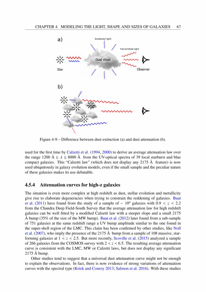
CHAPTER 4. MODELING THE LIGHT, SHAPE AND SIZES OF GALAXIES 67
Figure 4-9 – Difference between dust extinction (a) and dust attenuation (b).
used for the first time by Calzetti et al. (1994, 2000) to derive an average attenuation law overthe range 1200 Å ≤ λ ≤ 8000 Å from the UV-optical spectra of 39 local starburst and bluecompact galaxies. This “Calzetti law” (which does not display any 2175 Å feature) is nowused ubiquitously in galaxy evolution models, even if the small sample and the peculiar natureof these galaxies makes its use debatable.
4.5.4 Attenuation curves for high-z galaxiesThe situation is even more complex at high redshift as dust, stellar evolution and metallicitygive rise to elaborate degeneracies when trying to constrain the reddening of galaxies. Buatet al. (2011) have found from the study of a sample of ∼ 104 galaxies with 0.9 < z < 2.2from the Chandra Deep Field-South Survey that the average attenuation law for high redshiftgalaxies can be well fitted by a modified Calzetti law with a steeper slope and a small 2175Å bump (35% of the size of the MW bump). Buat et al. (2012) later found from a sub-sampleof 751 galaxies at the same redshift range a UV bump amplitude similar to the one found inthe super-shell region of the LMC. This claim has been confirmed by other studies, like Nollet al. (2007), who imply the presence of the 2175 Å bump from a sample of 108 massive, star-forming galaxies at 1 < z < 2.5. But more recently, Scoville et al. (2015) analyzed a sampleof 266 galaxies from the COSMOS survey with 2 < z < 6.5. The resulting average attenuationcurve is consistent with the LMC, MW or Calzetti laws, but does not display any significant2175 Å bump.
Other studies tend to suggest that a universal dust attenuation curve might not be enoughto explain the observations. In fact, there is now evidence of strong variations of attenuationcurves with the spectral type (Kriek and Conroy 2013; Salmon et al. 2016). With these studies

68 CHAPTER 4. MODELING THE LIGHT, SHAPE AND SIZES OF GALAXIES
Figure 4-10 – Comparison of the most well known extinction and attenuation curves from thelocal universe.
in mind, we can safely say that there is no consensus yet reached over an appropriate atten-uation law to choose when simulating the luminous properties of galaxies. To this date, thatchoice is left to the modeler, with the knowledge that this choice can lead to biases in his/herpredictions.
4.6 The Stuff model
For this work, we will generate artificial catalogs with the Stuff package of Bertin (2009)in simulated fields of a given size. Stuff relies on empirical scaling laws applied to a set ofgalaxy “types”, which it uses to draw galaxy samples with photometric properties computedin an arbitrary number of observation passbands. Each galaxy type is defined by its Schechter(1976) luminosity function parameters, its spectral energy distribution (SED), as well as thebulge-to-total luminosity ratio B/T 9 and rest-frame extinction properties of each component ofthe galaxy through a “reference” passband (i.e. the filter where the LF is measured).
The photometry of simulated galaxies is based on the composite SED templates of Colemanet al. (1980) (cf Figure 4-2) extended by Arnouts et al. (1999). Any of the six “E”, “S0”, “Sab”,“Sbc”, “Scd”, and “Irr” SEDs can be assigned to the bulge and disk components separately,for a given galaxy type. The version of Stuff used in this work does not allow the SEDs toevolve with redshift; instead, following Gabasch et al. (2004), galaxy evolution is modeledas a combination of density (Schechter’s φ∗) and luminosity (Schechter’s M∗) evolution with
9In Stuff, B/T=0 corresponds to a bulgeless irregular galaxy, and B/T=1 corresponds to an elliptical galaxy.

CHAPTER 4. MODELING THE LIGHT, SHAPE AND SIZES OF GALAXIES 69
redshift z:M∗(z) = M∗(0) + Me ln(1 + z) (4.9)
φ∗(z) = φ∗(0)(1 + z)φe , (4.10)
where Me and φe are constants. The reference filter will be set to the MegaCam g-band in thepresent thesis. Bulges and elliptical galaxies have a de Vaucouleurs (1953) profile:
µb(r) = Mb + 8.3268(
rrb
) 14
+ 5 log10 rb + 16.6337, (4.11)
where µb(r) is the bulge surface brightness in mag.pc−2, Mb = M−2.5 log10(B/T ) is the absolutemagnitude of the bulge component and M the total absolute magnitude of the galaxy, both in thereference passband. As a projection of the fundamental plane10, the average effective radius〈rb〉 in pc follows an empirical relation we derive from the measurements of Binggeli et al.(1984)):
〈rb〉 =
rknee10−0.3(Mb−Mknee) if Mb < Mknee
rknee10−0.1(Mb−Mknee) otherwise (4.12)
where rknee = 1.58h−1kpc and Mknee = −20.5. The intrinsic flattening q of bulges, defined asthe ratio between the semi minor axis and the semi major axis of the ellipse, follows a normaldistribution with 〈q〉 = 0.65 and σq = 0.18 (Sandage et al., 1970), which we convert to the
apparent aspect-ratio√
q2 sin2 i + cos2 i, where i is the inclination of the galaxy with respect tothe line of sight.
Disks have an exponential profile:
µd(r) = Md + 1.8222(
rrd
)+ 5 log10 rd + 0.8710, (4.13)
where µd(r) is the disk surface brightness in mag.pc−2, Md = M − 2.5 log10(1 − (B/T )) isthe absolute magnitude of the disk in the reference passband, and rd is the effective radius.Semi-analytical models where disks originate from the collapse of the baryonic content ofdark-matter-dominated halos (Dalcanton et al., 1997, Mo et al., 1998) predict useful scalingrelations. Assuming that light traces mass and that there is negligible transport of angularmomentum during collapse, one finds rd ∝ λL−βd , where λ is the dimensionless spin parameterof the halo, Ld = 10−0.4Md the total disk luminosity, and β ' −1/3 (de Jong and Lacey, 2000).The distribution of λ, as seen in N-body simulations, can well be described by a log-normaldistribution (Warren et al., 1992), and is very weakly dependent on cosmological parameters(Steinmetz and Bartelmann, 1995), hence the distribution of rd at a given Md should behave as:
n(rd|Md) ∝1rd
exp
−(ln(rd/r∗d) − 0.4βd(Md − M∗
d))2
2σ2λ
. (4.14)
In de Jong and Lacey (2000), a convincing fit to I-band catalog data of late-type galaxies
10The fundamental plane is a narrow logarithmic plane linking the main observables of elliptical galaxies: theirstellar mass, their size, and their velocity dispersion (Dressler 1987; Djorgovski and Davis 1987).
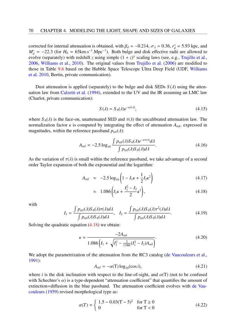
70 CHAPTER 4. MODELING THE LIGHT, SHAPE AND SIZES OF GALAXIES
corrected for internal attenuation is obtained, with βd = −0.214, σλ = 0.36, r∗d = 5.93 kpc, andM∗
d = −22.3 (for H0 = 65km.s−1.Mpc−1). Both bulge and disk effective radii are allowed toevolve (separately) with redshift z using simple (1 + z)γ scaling laws (see, e.g., Trujillo et al.,2006, Williams et al., 2010). The original values from Trujillo et al. (2006) are modified tothose in Table 9.6 based on the Hubble Space Telescope Ultra Deep Field (UDF, Williamset al. 2010, Bertin, private communication).
Dust attenuation is applied (separately) to the bulge and disk SEDs S (λ) using the atten-uation law from Calzetti et al. (1994), extended to the UV and the IR assuming an LMC law(Charlot, private communication):
S (λ) = S 0(λ)e−κτ(λ), (4.15)
where S 0(λ) is the face-on, unattenuated SED and τ(λ) the uncalibrated attenuation law. Thenormalization factor κ is computed by integrating the effect of attenuation Aref , expressed inmagnitudes, within the reference passband pref(λ):
Aref = −2.5 log10
∫pref(λ)S 0(λ)e−κτ(λ)dλ∫
pref(λ)S 0(λ)dλ. (4.16)
As the variation of τ(λ) is small within the reference passband, we take advantage of a secondorder Taylor expansion of both the exponential and the logarithm:
Aref ≈ −2.5 log10
(1 − I1κ +
12
I2κ2)
(4.17)
≈ 1.086(I1κ +
I21 − I2
2κ2
), (4.18)
with
I1 =
∫pref(λ)S 0(λ)τ(λ)dλ∫
pref(λ)S 0(λ)dλ, I2 =
∫pref(λ)S 0(λ)τ2(λ)dλ∫
pref(λ)S 0(λ)dλ. (4.19)
Solving the quadratic equation (4.18) we obtain:
κ ≈−2Aref
1.086(I1 +
√I21 −
21.086 (I2
1 − I2)Aref
) . (4.20)
We adopt the parametrization of the attenuation from the RC3 catalog (de Vaucouleurs et al.,1991):
Aref = −α(T) log10(cos i), (4.21)
where i is the disk inclination with respect to the line-of-sight, and α(T) (not to be confusedwith Schechter’s α) is a type-dependent “attenuation coefficient” that quantifies the amount ofextinction+diffusion in the blue passband. The attenuation coefficient evolves with de Vau-couleurs (1959) revised morphological type as:
α(T ) =
1.5 − 0.03(T − 5)2 for T ≥ 00 for T < 0 (4.22)

CHAPTER 4. MODELING THE LIGHT, SHAPE AND SIZES OF GALAXIES 71
Figure 4-11 – Example of a Stuff output catalog, with 4 galaxies generated in a given photo-metric band. 1 : object type index (200=galaxy, 100=star). 2-3 : galaxy position in pixels (x,y).4 : apparent magnitude. 5 : B/T ratio. 6 : bulge radius (arcsec). 7 : projected bulge axis ratio.8 : bulge position angle (degrees, with respect to x-axis). 9 : disk scale-length (arcsec). 10 :disk aspect ratio (disk inclination). 11 : disk position angle. 12 : redshift. 13 : de Vaucouleurstype.
Stuff applies to SEDs the mean intergalactic attenuation curve at the given redshift follow-ing Madau (1995) and Madau et al. (1996), using the list of Lyman wavelengths and absorptioncoefficients from the Xspec code (Arnaud, 1996). Galaxies are Poisson distributed in 5h−1 Mpcredshift slices from z = 20 to z = 0. For now the model does not include clustering properties,therefore the galaxies positions are uniformly distributed over the field of view. UltimatelyStuff generates a set of mock catalogs (one per filter) to be read by the image simulationsoftware, containing source position, apparent magnitude, B/T , bulge and disk axis ratios andposition angles, and redshift (cf Figure 4-11). We note that for consistency, we kept most ofthe default values applied by Stuff to scaling parameters, although many of them come fromslightly outdated observational constraints dating back to the mid-2000’s (and even earlier).This of course does not affect the conclusions of this work.

72 CHAPTER 4. MODELING THE LIGHT, SHAPE AND SIZES OF GALAXIES
Chapter 5
Painting imaginary skies
We all know that Art is not truth. Art is alie that makes us realize truth at least thetruth that is given us to understand. Theartist must know the manner whereby toconvince others of the truthfulness of hislies.
Pablo Picasso
Abstract
Being able to reproduce realistic images of astronomical surveys and to retrieveaccurate photometric and morphometric catalogs from them is at the heart of themethod we are laying out. In this chapter, I draw up an inventory of currentlyused image simulators, and provide a detailed description of the SkyMaker andSExtractor packages, that we will use for image generation and source extractionrespectively.
Contents5.1 Comparison of image simulators . . . . . . . . . . . . . . . . . . . . . . . 73
5.2 The SkyMaker software . . . . . . . . . . . . . . . . . . . . . . . . . . . . 75
5.2.1 Modeling the Point Spread Function . . . . . . . . . . . . . . . . . . 75
5.2.2 Modeling the noise properties . . . . . . . . . . . . . . . . . . . . . 76
5.3 Extracting sources from images: the SExtractor software . . . . . . . . . 78
5.1 Comparison of image simulatorsSimulations of astronomical images from surveys are an essential component in the develop-ment of any survey. A lot of simulation softwares have been developed to reproduce images
73
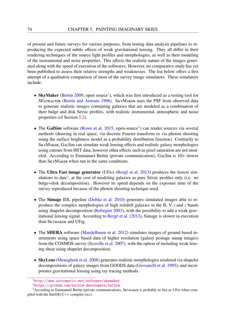
74 CHAPTER 5. PAINTING IMAGINARY SKIES
of present and future surveys for various purposes, from testing data analysis pipelines to re-producing the expected subtle effects of weak gravitational lensing. They all differ in theirrendering techniques of the source light profiles and morphologies, as well as their modelingof the instrumental and noise properties. This affects the realistic nature of the images gener-ated along with the speed of execution of the softwares. However, no comparative study has yetbeen published to assess their relative strengths and weaknesses. The list below offers a firstattempt of a qualitative comparison of most of the survey image simulators. These simulatorsinclude:
• SkyMaker (Bertin 2009, open source1), which was first introduced as a testing tool forSExtractor (Bertin and Arnouts 1996). SkyMaker uses the PSF from observed datato generate realistic images containing galaxies that are modeled as a combination oftheir bulge and disk Sérsic profiles, with realistic instrumental, atmospheric and noiseproperties (cf Section 5.2).
• The GalSim software (Rowe et al. 2015, open-source2) can render sources via severalmethods (drawing in real space, via discrete Fourier transform or via photon shootingusing the surface brightness model as a probability distribution function). Contrarily toSkyMaker, GalSim can simulate weak lensing effects and realistic galaxy morphologiesusing cutouts from HST data, however other effects such as pixel saturation are not mod-eled. According to Emmanuel Bertin (private communication), GalSim is 10× slowerthan SkyMaker when run in the same conditions.
• The Ultra Fast image generator (UFig) (Bergé et al. 2013) produces the fastest sim-ulations to date3, at the cost of modeling galaxies as pure Sérsic profiles only (i.e. nobulge+disk decomposition). However its speed depends on the exposure time of thesurvey reproduced because of the photon shooting technique used.
• The Simage IDL pipeline (Dobke et al. 2010) generates simulated images able to re-produce the complex morphologies of high redshift galaxies in the B, V, i and z bandsusing shapelet decomposition (Refregier 2003), with the possibility to add a weak grav-itational lensing signal. According to Bergé et al. (2013), Simage is slower in executionthan Skymaker and UFig.
• The SHERA software (Mandelbaum et al. 2012) simulates images of ground based in-struments using space based data of higher resolution (galaxy postage stamp images)from the COSMOS survey (Scoville et al. 2007), with the option of including weak lens-ing shear using shapelet decomposition.
• SkyLens (Meneghetti et al. 2008) generates realistic morphologies rendered via shapeletdecompositions of galaxy images from GOODS data (Giovanelli et al. 1995), and incor-porates gravitational lensing using ray tracing methods.
1http://www.astromatic.net/software/skymaker2https://github.com/GalSim-developers/GalSim3According to Emmanuel Bertin (private communication), Skymaker is probably as fast as UFig when com-
piled with the Intel(R) C++ compiler (icc).

CHAPTER 5. PAINTING IMAGINARY SKIES 75
• The Photon Simulator (PhoSim) (Peterson and Jernigan 2013, open source4) reproducesimages of the Large Synoptic Survey Telescope (LSST, Ivezic et al. 2008), but the codecould be extended to other surveys in the future. The virtual photons are collected by thetelescope via Monte Carlo sampling, and galaxies are modeled as bulge+disk Sérsic pro-files. PhoSim is the most realistic simulator to date, as it implements detailed a physicaldescription of atmospheric effects such as dispersion, cloud absorption and molecularscattering. However it is also the slowest simulator in the list.
Considering its ability to produce realistic images in a relatively short time and the accessto the source code for easy bug fixing and updates implementations, we decide to use theSkyMaker software for our goals. In the next section, I describe the inner workings of thecode.
5.2 The SkyMaker softwareSkyMaker can generate simulated images of the universe as if passed through a virtual tele-scope. It therefore has the ability to reproduce the observed data from most astronomicalsurveys with great accuracy (see e.g., Figure 5-1). The user eager to reproduce a given surveycan provide its characteristics, which include the exposure time, the filters used5, the back-ground level, the pupil features such as the diameter of the primary and secondary mirror, andthe detector characteristics (gain, image size, full-well capacity of pixels, zero-point, saturationlevel). These parameters can be found in the technical documentation of the survey reproduced.
The light and shape characteristics of input galaxies are provided in the form of an ASCIIcatalog of sources (one for each band) generated by an empirical model such as Stuff (cfSection 4.6) or EGG (Schreiber et al. 2017). Bulges follow a de Vaucouleurs light profile(Equation (4.11)), and disks an exponential profile (Equation (4.13)). Stars are generated byconvolution of the PSF with the pixel grid. Blooming artifacts at the center of bright stars(creating vertical trails on the images), characteristic of pixel saturation, are also reproduced.In fine, the simulated images in each band are provided in the FITS format.
5.2.1 Modeling the Point Spread FunctionThe PSF is the response of an optical instrument to an impulse. Its good estimation is crucialfor accurate measurements of the photometry and shape of galaxies. The PSF model can begenerated internally by SkyMaker, as a convolution of the instrumental point spread functionwith the atmospheric seeing, tracking errors and optical aberrations. For more realistic renders,the PSF can be extracted from images of stars in observed data, modeled as a two-dimensionalcombination of basis vectors and fitted by χ2 minimization using the PSFEx software of Bertin(2011a), which returns a FITS file. This operation can be carried out in several equally-spacedareas of the field to accurately characterize the PSF variations over the field (cf Figure 5-2).
Beyond ∼ 10 FWHM of the center, the wings of the PSF are dominated by diffusion, addingan “aureole” component to it, as illustrated in Figure 5-3 (Racine 1996). This component, firstdiscovered by de Vaucouleurs (1958) and probably due to micro-ripples on optical surfaces,
4https://bitbucket.org/phosim/phosim_release/wiki/Home5A wide variety of photometric bands can be chosen within the range [0.29, 87.74831] µm (Annunziatella et al.
2013).
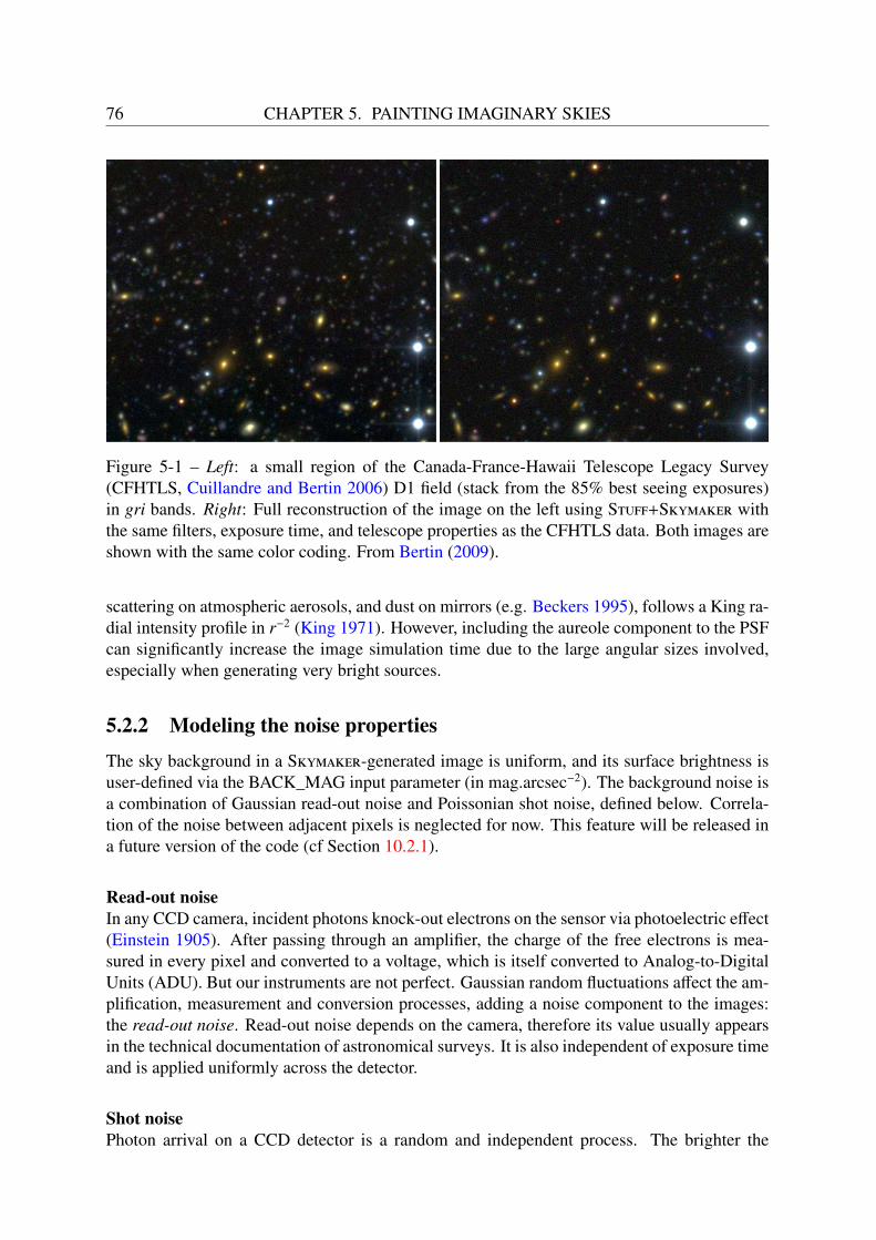
76 CHAPTER 5. PAINTING IMAGINARY SKIES
Figure 5-1 – Left: a small region of the Canada-France-Hawaii Telescope Legacy Survey(CFHTLS, Cuillandre and Bertin 2006) D1 field (stack from the 85% best seeing exposures)in gri bands. Right: Full reconstruction of the image on the left using Stuff+Skymaker withthe same filters, exposure time, and telescope properties as the CFHTLS data. Both images areshown with the same color coding. From Bertin (2009).
scattering on atmospheric aerosols, and dust on mirrors (e.g. Beckers 1995), follows a King ra-dial intensity profile in r−2 (King 1971). However, including the aureole component to the PSFcan significantly increase the image simulation time due to the large angular sizes involved,especially when generating very bright sources.
5.2.2 Modeling the noise properties
The sky background in a Skymaker-generated image is uniform, and its surface brightness isuser-defined via the BACK_MAG input parameter (in mag.arcsec−2). The background noise isa combination of Gaussian read-out noise and Poissonian shot noise, defined below. Correla-tion of the noise between adjacent pixels is neglected for now. This feature will be released ina future version of the code (cf Section 10.2.1).
Read-out noiseIn any CCD camera, incident photons knock-out electrons on the sensor via photoelectric effect(Einstein 1905). After passing through an amplifier, the charge of the free electrons is mea-sured in every pixel and converted to a voltage, which is itself converted to Analog-to-DigitalUnits (ADU). But our instruments are not perfect. Gaussian random fluctuations affect the am-plification, measurement and conversion processes, adding a noise component to the images:the read-out noise. Read-out noise depends on the camera, therefore its value usually appearsin the technical documentation of astronomical surveys. It is also independent of exposure timeand is applied uniformly across the detector.
Shot noisePhoton arrival on a CCD detector is a random and independent process. The brighter the
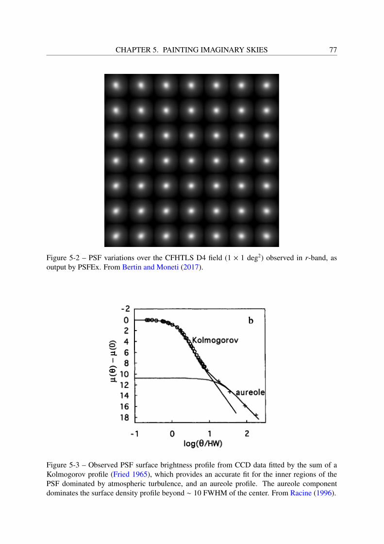
CHAPTER 5. PAINTING IMAGINARY SKIES 77
Figure 5-2 – PSF variations over the CFHTLS D4 field (1 × 1 deg2) observed in r-band, asoutput by PSFEx. From Bertin and Moneti (2017).
Figure 5-3 – Observed PSF surface brightness profile from CCD data fitted by the sum of aKolmogorov profile (Fried 1965), which provides an accurate fit for the inner regions of thePSF dominated by atmospheric turbulence, and an aureole profile. The aureole componentdominates the surface density profile beyond ∼ 10 FWHM of the center. From Racine (1996).

78 CHAPTER 5. PAINTING IMAGINARY SKIES
emitting source, the higher the number of photons per second that reaches the sensor. A givenpixel of the detector will perceive an average flux with some statistical fluctuations followinga Poisson law (Poisson 1837) of parameter p, where p is the number count of the expectedsignal in a given pixel. This added noise component is called shot noise (or photon noise), anddepends on the signal from the sources or the background.
5.3 Extracting sources from images: the SExtractor soft-ware
In order to derive photometric and morphometric catalogs from observed and simulated surveyimages, we use the popular SExtractor package of Bertin and Arnouts (1996). While othersoftwares have been developed for this purpose such as, e.g., DAOPHOT (Stetson 1987) or themore recent Tractor code (Lang et al. 2016), SExtractor’s ability to return accurate photom-etry of galaxies up to very faint magnitudes make it the most widely used source extractor inthe astronomical community (Annunziatella et al. 2013).
In SExtractor, sources are detected in four main steps, as illustrated in Figure 5-4: first,a smooth model of the image background is computed and subtracted. Second, a convolutionmask, acting as matched filter, is applied to the background-subtracted image for improvingthe detection of faint sources. Third, a segmentation algorithm identifies connected regionsof pixels with a surface brightness in the filtered image higher than the detection threshold.Finally, the same segmentation process is repeated at increasing threshold levels to separatepartially blended sources that may share light at the lowest level.
Once a source has been detected, SExtractor performs a series of measurements accordingto a user-defined parameter list. This includes various position, shape, and flux estimates.For this work we rely on FLUX_AUTO photometry (cf Figure 5-5). FLUX_AUTO is basedon Kron’s “first moment” algorithm (Kron, 1980) and gives reasonably robust photometricestimates for all types of galaxies. For object sizes we choose the half-light radius estimationprovided by the FLUX_RADIUS parameter, which is the radius of the aperture that encloseshalf of the FLUX_AUTO source flux. We note that this size estimate includes the convolutionof the galaxy light profile by the PSF. In order to retrieve properties such as color, SExtractoris run in the so-called double image mode, where detection is carried out in one image andmeasurements in another. By repeating source extraction with the same “detection image”, butwith “measurement images” in different filters, we ensure that the photometry is performed inthe exact same object footprints in all filters.
SExtractor flags all issues occurring during the detection and measurements processes inthe output catalogs. These issues are summarized in Table 5.1. Flag indices can add up if thesource extraction encounters more than a problem. In this work, we consider only detectionswith a SExtractor FLAG parameter < 4, which excludes sources that are saturated or trun-cated by the frame boundaries. It is important to stress again again that simulated images mustgo through the same source extraction process as observed images to ensure their comparabil-ity.

CHAPTER 5. PAINTING IMAGINARY SKIES 79
Table 5.1 – SExtractor flags
Flag index Meaning1 The object has neighbors, bright and close enough to significantly bias the photometry,
or bad pixels (more than 10% of the integrated area affected)2 The object was originally blended with another one4 At least one pixel of the object is saturated (or very close to)8 The object is truncates (to close to an image boundary)16 Object’s aperture data are incomplete or corrupted32 Object’s isophotal data are incomplete or corrupted64 A memory overflow occurred during deblending128 A memory overflow occurred during extraction
Figure 5-4 – The four steps of source detection in SExtractor. From a talk given by EmmanuelBertin.
Figure 5-5 – Sources detected by SExtractor in a portion of the CFHTLS D1 field in g-band.The ellipses show the limits of integration for the FLUX_AUTO property of extracted sources.

Part III
Elements of Bayesian indirect inference
80

Chapter 6
Exploring the parameter space efficiently
You have to get lost before you findyourself
John Green, Paper Towns
Abstract
Statistical inference is the process of estimating the properties of a population froma noisy sample of this population (i.e. from observed data). In this chapter1, Iintroduce the Bayesian framework, whose logical coherency and conceptual sim-plicity make it attractive for inference problems. Then I review some techniquesthat I will later use to explore the parameter space efficiently, i.e. in a way thatcan can ensure the fast sampling of the regions of the parameter space that arethe most compatible with observed data. Finally, I explore the Bayesian indirectlikelihood framework, a set of alternatives to traditional Bayesian techniques thathave proven useful when the computation of the probability of the data given themodel is impossible or impractical.
Contents6.1 Scientific motivation . . . . . . . . . . . . . . . . . . . . . . . . . . . . . . 82
6.2 The Bayesian framework . . . . . . . . . . . . . . . . . . . . . . . . . . . 82
6.2.1 The choice of prior . . . . . . . . . . . . . . . . . . . . . . . . . . . 83
6.3 Sampling the posterior: Markov Chain Monte Carlo . . . . . . . . . . . . 85
6.4 Adaptive MCMC . . . . . . . . . . . . . . . . . . . . . . . . . . . . . . . 87
6.4.1 The Adaptive Proposal algorithm . . . . . . . . . . . . . . . . . . . 89
6.4.2 The Adaptive Metropolis algorithm . . . . . . . . . . . . . . . . . . 90
6.5 Simulated Annealing . . . . . . . . . . . . . . . . . . . . . . . . . . . . . 90
6.6 Likelihood-free inference . . . . . . . . . . . . . . . . . . . . . . . . . . . 911Note: This chapter uses extracts from Carassou et al. (2017) in some of its sections.
81

82 CHAPTER 6. EXPLORING THE PARAMETER SPACE EFFICIENTLY
6.7 Approximate Bayesian Computation . . . . . . . . . . . . . . . . . . . . . 93
6.8 Parametric Bayesian indirect likelihood . . . . . . . . . . . . . . . . . . . 95
6.9 Our approach for this work . . . . . . . . . . . . . . . . . . . . . . . . . . 95
6.1 Scientific motivationOur goal in this thesis is to provide the most probable model(s) for the observed properties ofgalaxies. Our Stuff empirical model, described in Section 4.6, generates simulated populationsof galaxies from a set of input parameters describing their luminosity and size distributions.The dynamic range of the values of these parameters defines a multidimensional parameterspace that needs to be explored to find the parameters that reproduce observed data (i.e. pho-tometric catalogs extracted from survey images) with the greatest accuracy. The most naturalframework to explore this parameter space is the Bayesian framework, which I describe in thenext section.
6.2 The Bayesian frameworkWhat is the nature of probability? For more than two centuries, this philosophical questionhas split the field of statistics into two main schools of thought: Bayesianism and frequen-tism, each with a distinct set of tools. For frequentists, probability is seen as the long-runfrequency of occurrence of a random event in a repeated experiment. This interpretation relieson the assumption that if the experiment is reproduced indefinitely, the relative frequencies willconverge to a limit, due to the law of large numbers. Uncertainty here is a measure of variabil-ity, due to errors in measurement. The model parameters are generally (but not always) keptfixed during the repeated experiment, therefore no probability statement can be made on them.Bayesians, however, see probability as a measure of the degree of belief in the occurrence ofan event, which is a broader and more subjective interpretation. The model parameters aretreated as random variables, and we can therefore quantify their probable values by samplingtheir probability distribution function (PDF). This philosophical distinction can create situa-tions where the conclusions of the frequentist and Bayesian approaches to the same problemare contradictory2 (see e.g. the examples provided in VanderPlas 2014). But in real life prob-lems, both methods can be complementary and are often used in concert. Frequentist tools,such as point estimates and maximum likelihood methods for example, are commonly used tosummarize the results of Bayesian inference (Babu 2012).
Bayesian statistics relies on Bayes’ theorem (or rule), which provides a logical frameworkfor updating a prior belief about the world when faced with new objective information.
Theorem 1 (Bayes’ theorem) Given a model about the state of the world with parameters θ,the probability of this model explaining the data is:
P(θ|D) =P(D|θ)P(θ)
P(D)(6.1)
2For simple problems though, the two approaches often yield similar results.

CHAPTER 6. EXPLORING THE PARAMETER SPACE EFFICIENTLY 83
where P(D|θ) is the likelihood (or the likelihood function) of the data, which gives the prob-ability of the data given the model, P(θ) is the prior, or the probability of the model with theparameters θ, and P(D) is the evidence, which acts as a normalization constant and can oftenbe ignored in inference problems.
Bayes’ theorem was first intuited in 1740 by English reverend and amateur mathematicianThomas Bayes (Bayes et al. 1763, published posthumously by Richard Price). It was then laterformalized in its modern mathematical form by Pierre-Simon Laplace (1774)3, who appliedhis “law of inverse probability” to demographics, judicial reforms and celestial mechanics.As Bayes’ theorem usually means the computation of complex integrations, it was largelysupplanted by frequentist methods, easier to compute, and which dominated the statisticallandscape during the first half of the 20th century. But the rise of powerful computers andBayesian computation techniques, such as Markov Chain Monte Carlo (introduced in Section6.3), have rendered the use of Bayesian methods very attractive in many scientific areas. Inastronomy, Bayesian methods became popular only in the early 2000s (Sharma 2017). Thereader is referred to the excellent technical and philosophical introduction to Bayesianism andfrequentism of VanderPlas (2014), and for a more complete treatement of the tools of Bayesianinference, to the book of Wasserman (2013).
6.2.1 The choice of priorThe prior distribution encapsulates our current knowledge about the model parameters, therebysetting initial constraints on the parameter space. Priors can be any probability distribution,which makes their choice a notoriously hard task, especially in high-dimensional problems,where it is almost impossible to have a prior distribution that accurately represents our priorbeliefs about the parameters. In fact, determining the right prior is an intrinsically subjectiveprocess, and this represents the main topic of criticism from frequentists, as the shape of theposterior will be irremediably affected by the shape of the prior.
Priors essentially come in two types: informative and uninformative4. Uninformative pri-ors are often used if no information a priori is known about the model parameter. The term“uninformative” is actually a misnomer, because all priors carry some amount of information.In that case, they are chosen so that their shape minimizes their influence over the posterior. Alarge variety of methods for constructing uninformative priors have been developed, that havebeen mostly cataloged by Yang and Berger (1996).
A simple general rule for choosing uninformative prior distributions is the application ofBernoulli’s (1713) and Laplace’s (1814) “principle of insufficient reason”, which states that ifthere is no reason to believe that a set of outcomes are not equally likely, it is reasonable toassume that they are equally likely. Therefore the simplest uninformative prior is the uniform(or flat) prior, which for multivariate problems is expressed as:
P(θ) =
n∏
i=1
1ui−li
if li ≤ θi ≤ ui ∀i ∈ [1, n]
0 if ∃ i ∈ [1, n] | θi < li or θi > ui
(6.2)
3Fun fact: Laplace also invented the frequentist school of thought.4Alternative terms in the literature for uninformative priors include non-informative priors, reference priors,
vague priors, diffuse priors and objective priors (Lunn et al. 2012).

84 CHAPTER 6. EXPLORING THE PARAMETER SPACE EFFICIENTLY
where θ = θ1, θ2, ..., θn is the parameter values vector, and li and ui are the lower and upperlimit of the support of the prior PDF for parameter i respectively. When using the uniformdistribution as prior, the support of the distribution has to be chosen carefully and with highconfidence, because no one want wants to lose information on a potentially important regionof the parameter space that will never be explored.
Another popular uninformative prior is the Jeffreys prior (Jeffreys 1946; 1961), defined as:
P(θ) =√
det(I(θ)) (6.3)
Where I(θ)) is the n×n Fisher information matrix, i.e. the expected values of the second partialderivatives of the log-likelihood, which measures its curvature:
Ii, j(θ) = −E
[∂2
∂θi∂θ jlog P(D|θ)
](6.4)
The most important property of the Jeffreys prior is that it is invariant by reparametrization ofthe model, i.e. if h is a transformation of the parameter θ so that φ = h(θ), then P(φ) = P(θ).This property, now referred to as Jeffreys invariance, ensures that the prior is independent ofthe parametrization chosen5. Despite the appeal of this property however, the application of theJeffreys prior to multidimensional models is still controversial (Kass and Wasserman 1996). Inpractice, the Jeffreys prior will give more weight to the parameters that create big changes inthe log-likelihood when being subject to small changes (Lunn et al. 2012).
When specific information is known about the parameter, informative priors can be usedto strongly restrict the parameter space. According to the problem, the choice of informativepriors can be based on the posterior distribution from previous published studies, or merely onintuition on the plausible values of the parameters.
Priors with the same parametric form as the posterior are called conjugate priors. Firstformalized by Schlaifer and Raiffa (1961), conjugate priors can be mathematically convenientif no information contradicts their use. For example, when inferring the parameters of a normaldistribution, using a normal prior is advantageous, except if a priori knowledge indicates askewed distribution. An exhaustive catalog of conjugate priors has been made available byFink (1997).
Prior distributions whose integral is infinite are called improper priors. Improper priorsmust be treated with great care, because they can lead to improper posteriors, whose inter-pretation can be awkward. The uniform prior on an infinite interval is a good example of animproper prior.
There is an extensive collection of historical and methodological reviews on the choiceof priors. The reader is especially referred to the works of Jaynes (1968; 1985), Kass andWasserman (1996), and Simpson et al. (2014).
5The uniform prior is not Jeffreys invariant.
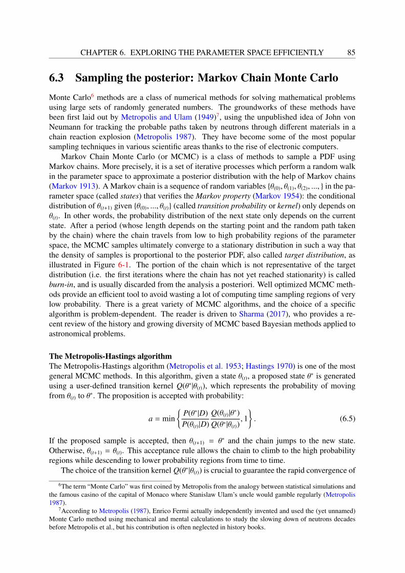
CHAPTER 6. EXPLORING THE PARAMETER SPACE EFFICIENTLY 85
6.3 Sampling the posterior: Markov Chain Monte CarloMonte Carlo6 methods are a class of numerical methods for solving mathematical problemsusing large sets of randomly generated numbers. The groundworks of these methods havebeen first laid out by Metropolis and Ulam (1949)7, using the unpublished idea of John vonNeumann for tracking the probable paths taken by neutrons through different materials in achain reaction explosion (Metropolis 1987). They have become some of the most popularsampling techniques in various scientific areas thanks to the rise of electronic computers.
Markov Chain Monte Carlo (or MCMC) is a class of methods to sample a PDF usingMarkov chains. More precisely, it is a set of iterative processes which perform a random walkin the parameter space to approximate a posterior distribution with the help of Markov chains(Markov 1913). A Markov chain is a sequence of random variables θ(0), θ(1), θ(2), ..., in the pa-rameter space (called states) that verifies the Markov property (Markov 1954): the conditionaldistribution of θ(t+1) given θ(0), ..., θ(t) (called transition probability or kernel) only depends onθ(t). In other words, the probability distribution of the next state only depends on the currentstate. After a period (whose length depends on the starting point and the random path takenby the chain) where the chain travels from low to high probability regions of the parameterspace, the MCMC samples ultimately converge to a stationary distribution in such a way thatthe density of samples is proportional to the posterior PDF, also called target distribution, asillustrated in Figure 6-1. The portion of the chain which is not representative of the targetdistribution (i.e. the first iterations where the chain has not yet reached stationarity) is calledburn-in, and is usually discarded from the analysis a posteriori. Well optimized MCMC meth-ods provide an efficient tool to avoid wasting a lot of computing time sampling regions of verylow probability. There is a great variety of MCMC algorithms, and the choice of a specificalgorithm is problem-dependent. The reader is driven to Sharma (2017), who provides a re-cent review of the history and growing diversity of MCMC based Bayesian methods applied toastronomical problems.
The Metropolis-Hastings algorithmThe Metropolis-Hastings algorithm (Metropolis et al. 1953; Hastings 1970) is one of the mostgeneral MCMC methods. In this algorithm, given a state θ(t), a proposed state θ∗ is generatedusing a user-defined transition kernel Q(θ∗|θ(t)), which represents the probability of movingfrom θ(t) to θ∗. The proposition is accepted with probability:
a = min
P(θ∗|D)P(θ(t)|D)
Q(θ(t)|θ∗)
Q(θ∗|θ(t)), 1
. (6.5)
If the proposed sample is accepted, then θ(t+1) = θ∗ and the chain jumps to the new state.Otherwise, θ(t+1) = θ(t). This acceptance rule allows the chain to climb to the high probabilityregions while descending to lower probability regions from time to time.
The choice of the transition kernel Q(θ∗|θ(t)) is crucial to guarantee the rapid convergence of
6The term “Monte Carlo” was first coined by Metropolis from the analogy between statistical simulations andthe famous casino of the capital of Monaco where Stanislaw Ulam’s uncle would gamble regularly (Metropolis1987).
7According to Metropolis (1987), Enrico Fermi actually independently invented and used the (yet unnamed)Monte Carlo method using mechanical and mental calculations to study the slowing down of neutrons decadesbefore Metropolis et al., but his contribution is often neglected in history books.
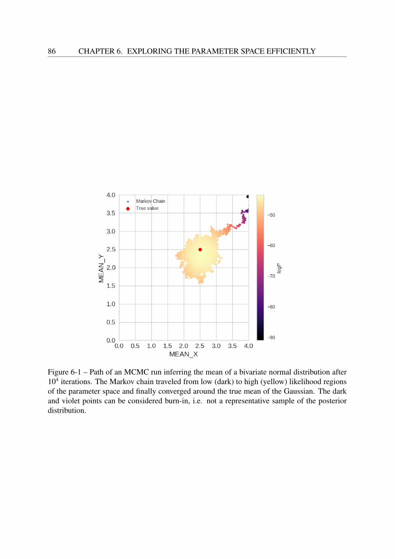
86 CHAPTER 6. EXPLORING THE PARAMETER SPACE EFFICIENTLY
Figure 6-1 – Path of an MCMC run inferring the mean of a bivariate normal distribution after104 iterations. The Markov chain traveled from low (dark) to high (yellow) likelihood regionsof the parameter space and finally converged around the true mean of the Gaussian. The darkand violet points can be considered burn-in, i.e. not a representative sample of the posteriordistribution.

CHAPTER 6. EXPLORING THE PARAMETER SPACE EFFICIENTLY 87
the chain. If the kernel is symmetric, i.e. if it verifies Q(θ∗|θ(t)) = Q(θ(t)|θ∗), then the acceptance
probability reduces to:
a = min
P(θ∗|D)P(θ(t)|D)
, 1. (6.6)
The kernel is usually chosen among distributions that are defined by location and scaleparameters. Popular choices include the multivariate Student’s t distribution tν(0,Σ)8 or themultivariate normal distribution N(0,Σ) centered on the current state and with a covariancematrix Σ (and in the case of the t distribution, with a degree of freedom ν, scalar and positive)which determines the size and orientation of the jumps, so that:
θ∗ = θ(t) + ζ(t+1), (6.7)
where ζ(t+1) follows tν(0,Σ) or N(0,Σ) (Chib and Greenberg 1995). We opt for the latter solu-tion for our problem, due to its intuitive parametrization and computational ease.
6.4 Adaptive MCMCThe shape and size of the proposal distribution have a great influence on the convergence andfast traveling of the Markov chain across the parameter space (Gelman et al. 1994). But howto find the proposal distribution(s) that maximize the efficiency of a given MCMC run?
A good way to assess convergence speed for a given kernel is to monitor the acceptancerate, that is, the fraction of accepted samples over previous iterations. The acceptance rate ismainly influenced by the covariance matrix of the transition kernel Σ. If the jump sizes are toolarge, the acceptance rate is too low, and the chain stays still for a large number of iterations. Ifthe jump sizes are too small, the acceptance rate is very high but the chain needs a high numberof iterations to move from one region of the parameter space to another. These situations areillustrated in Figure 6-2. The desired acceptance rate depends on the target distribution, andthere is no universal criterion for its optimization, but Roberts et al. (1997) proved that for anyd-dimensional target distributions (with d ≥ 5) with independent and identically distributed(i.i.d.) components, optimal performance of the Random Walk Metropolis algorithm is attainedfor an asymptotic acceptance rate of 0.2349. Therefore, the optimal kernel can be found byempirical tuning of its size so that the acceptance rate gets close to 0.234. However, empiricaltuning is difficult and time consuming exercise when dealing with multidimensional problemwith correlations between parameters and a target distribution of unknown shape. To tackle thisissue, a set of methods called adaptive MCMC have been developed, that use past informationabout the chain to automatically tune the kernel. There is a great variety of such methods, andthe reader is referred to Roberts and Rosenthal (2009) for a technical review.
As adaptive methods, by definition, destroy the Markovian nature of the chain, the choiceof an adaptive scheme must ensure correct ergodic properties with respect to the stationarydistribution, in the following sense:
Definition (Ergodicity) A Markov chain θ(0), . . . , θ(t) taking its values in a state space X andwith transition kernel Pγ (where γ is the tuning parameter of the kernel) is said to be ergodic
8When ν→ ∞, the t distribution converges to a normal distribution.9For univariate targets, the optimal asymptotic acceptance rate increases to 0.44 (Roberts et al. 2001).

88 CHAPTER 6. EXPLORING THE PARAMETER SPACE EFFICIENTLY
with respect to a target distribution π if:
limt→∞||Pt
γ(θ, ·) − π(·)||TV = 0, ∀θ ∈ X (6.8)
Where || · ||TV is the total variation distance10.
This means that the Markov chain always converges to the same stationary distribution, regard-less of the starting point.
Definition (Adaptive MCMC) An adaptive MCMC scheme θt,Γt is defined given a family oftransition kernels PΓt, where Γt is the tuning parameter at iteration t (for example, the covari-ance matrix of a multidimensional Gaussian proposal kernel), chosen according to the adaptionscheme (usually from the past history of the chain) and each having the target distribution π astheir stationary distribution.
In order to be suitable, an adaptive MCMC scheme must verify the following conditions:
Definition (Diminishing adaption) limt→∞ Dt = 0 in probability, where
Dt := supθ∈X
||PΓt+1(θ, ·) − PΓt(θ, ·)||TV (6.9)
This means that as t → ∞, the parameters of the proposal distribution must depend less andless on earlier states of the chain, i.e. they must change less as time increases.
Definition (Bounded convergence11) Let Mε(θ, γ) = inft ≥ 1 : ||Ptγ(θ, ·) − π(·)||TV ≤ ε be the
convergence time of kernel Pγ when starting in state θ. An adaptive Markov chain satisfies thebounded convergence criterion if the sequence
Mε(θ(t),Γt)∞t=0 is bounded in probability, ∀ε > 0 (6.10)
This means that the time that transition kernels get close to the target distribution within ε isbounded. In the light of these definitions, Roberts and Rosenthal (2007) proved the followingtheorem:
Theorem 2 For an MCMC algorithm with adaptive proposal distributions, if it satisfies thebounded convergence and diminishing adaptation conditions, then it is ergodic and it willconverge asymptotically to the correct target distribution.
While diminishing adaption can be relatively easy to measure for a given adaption scheme,bounded convergence is harder to prove in practice (Bai 2010). In the following sections, Ireview two adaptive methods that will be used in this study: the Adaptive Proposal algorithmand the Adaptive Metropolis algorithm.
10The total variation distance can be informally defined as the largest possible distance between two probabilitydistributions.
11The Bounded convergence criterion can also be called the Containment condition in the literature.

CHAPTER 6. EXPLORING THE PARAMETER SPACE EFFICIENTLY 89
Figure 6-2 – Traceplots depicting three typical situations that can arise in a standard MCMCchain with the (non-adaptive) Metropolis-Hastings algorithm. The input data is a set of 20points normally distributed with mean 0 and standard deviation 1. The parameter to infer isthe mean µ of the input data distribution. The prior is a normal distribution with mean 0 andstandard deviation 1, and the transition kernel is a normal distribution centered on the currentstate and width σp. In each case the chain starts from µ = 3 and is run for 104 iterations. Thetarget distribution sampled is the same, but the width of the proposal distribution, that is, thejump size, is different for each case. Left panel: The jump size is too small. The burn-in phaseis very long and a much longer chain is needed to sample the target distribution. Central panel:The jump size is optimal, therefore the target distribution is well sampled. Right panel: Thejump size is too big. Hence the chain spends a lot of iterations in the same position, whichmakes the sampling of the target distribution inefficient.
6.4.1 The Adaptive Proposal algorithm
In the Adaptive Proposal (AP) algorithm proposed by Haario et al. (1999), the proposal distri-bution (a Gaussian centered on the current state) is tuned every U iterations from the covariancecomputed on a fixed number H (where H ≥ 2) of previously accepted states. In this situation,the chain learns about the target distribution from its path across the parameter space. The APalgorithm requires three tuning parameters: the update frequency U, the memory parameter H,and an empirical scaling factor cd for d-dimensional problems.
The scaling factor controls the size of the covariance matrix of the transition kernel. Itcan be tuned manually, or based on theoretical justifications. For the latter, Roberts et al.(1997) designed a popular scaling factor, defined as cd = (2.38)2/d. In this case, the proposaldistribution isN(0, cdΣH), where ΣH is the d × d covariance matrix of the proposal distributioncomputed using the subset of accepted states over the last H iterations. The scaling factor ofRoberts et al. optimizes the efficiency of the MCMC process for multivariate Gaussian targetdistributions. Numerical experiments by Haario et al. have shown that the efficiency of theAdaptive Proposal algorithm is more sensible to the choice of scaling factor than to the choiceof update frequency and memory parameter.
The AP algorithm simulates slightly biased samples of the target distribution, and the sta-tionary distribution reached by the algorithm is not strictly ergodic. However, the authors claimthat there is small difference between the simulated distribution and the target distribution forunimodal posteriors.
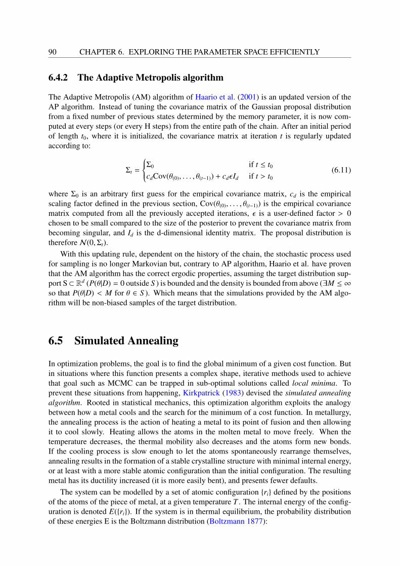
90 CHAPTER 6. EXPLORING THE PARAMETER SPACE EFFICIENTLY
6.4.2 The Adaptive Metropolis algorithm
The Adaptive Metropolis (AM) algorithm of Haario et al. (2001) is an updated version of theAP algorithm. Instead of tuning the covariance matrix of the Gaussian proposal distributionfrom a fixed number of previous states determined by the memory parameter, it is now com-puted at every steps (or every H steps) from the entire path of the chain. After an initial periodof length t0, where it is initialized, the covariance matrix at iteration t is regularly updatedaccording to:
Σt =
Σ0 if t ≤ t0
cdCov(θ(0), . . . , θ(t−1)) + cdεId if t > t0(6.11)
where Σ0 is an arbitrary first guess for the empirical covariance matrix, cd is the empiricalscaling factor defined in the previous section, Cov(θ(0), . . . , θ(t−1)) is the empirical covariancematrix computed from all the previously accepted iterations, ε is a user-defined factor > 0chosen to be small compared to the size of the posterior to prevent the covariance matrix frombecoming singular, and Id is the d-dimensional identity matrix. The proposal distribution istherefore N(0,Σt).
With this updating rule, dependent on the history of the chain, the stochastic process usedfor sampling is no longer Markovian but, contrary to AP algorithm, Haario et al. have proventhat the AM algorithm has the correct ergodic properties, assuming the target distribution sup-port S ⊂ Rd (P(θ|D) = 0 outside S ) is bounded and the density is bounded from above (∃M ≤ ∞so that P(θ|D) < M for θ ∈ S ). Which means that the simulations provided by the AM algo-rithm will be non-biased samples of the target distribution.
6.5 Simulated Annealing
In optimization problems, the goal is to find the global minimum of a given cost function. Butin situations where this function presents a complex shape, iterative methods used to achievethat goal such as MCMC can be trapped in sub-optimal solutions called local minima. Toprevent these situations from happening, Kirkpatrick (1983) devised the simulated annealingalgorithm. Rooted in statistical mechanics, this optimization algorithm exploits the analogybetween how a metal cools and the search for the minimum of a cost function. In metallurgy,the annealing process is the action of heating a metal to its point of fusion and then allowingit to cool slowly. Heating allows the atoms in the molten metal to move freely. When thetemperature decreases, the thermal mobility also decreases and the atoms form new bonds.If the cooling process is slow enough to let the atoms spontaneously rearrange themselves,annealing results in the formation of a stable crystalline structure with minimal internal energy,or at least with a more stable atomic configuration than the initial configuration. The resultingmetal has its ductility increased (it is more easily bent), and presents fewer defaults.
The system can be modelled by a set of atomic configuration ri defined by the positionsof the atoms of the piece of metal, at a given temperature T . The internal energy of the config-uration is denoted E(ri). If the system is in thermal equilibrium, the probability distributionof these energies E is the Boltzmann distribution (Boltzmann 1877):

CHAPTER 6. EXPLORING THE PARAMETER SPACE EFFICIENTLY 91
P(E) ∝ exp[−E(ri)/kBT ] (6.12)
where E(ri) is the internal energy of the configuration and kB is the Boltzmann constant. Inother words, at a given temperature, the system has a low probability of being in a high-energyconfiguration, and a high probability of being in a low-energy configuration.
In the simulated annealing algorithm, the cost function is analogous to the energy of theconfiguration, and kBT is replaced by a notion of effective temperature τ, a variable in the sameunits as the cost function. In this setting, the probability of moving from a state of energy E1
to a state of energy E2 is:
P(E1 → E2) = exp[−(E2 − E1)/τ] (6.13)
At the beginning of the process, the system is "melted" by setting an arbitrarily high initialtemperature τ0. Then, at each step of the iterative process (or every fixed number of steps),the effective temperature is lowered by a user-defined cooling schedule, which depends on theproblem. By decreasing the temperature, the acceptance probability also decreases progres-sively, which means that the system moves less and less often towards "worse" solutions, i.e.towards states with a more energetic configuration a iteration i+1 than at iteration i. At the endof the process, the system should wander around the global minimum of the cost function. Thewhole process is illustrated in Figure 6-3.
Using the formalism introduced in previous sections, when the simulated annealing algo-rithm is used in concert with the Metropolis Hastings algorithm, the acceptance probabilitybecomes:
a =
exp− ln P(θ(t) |D)−ln P(θ∗ |D)τ
if ln P(θ∗|D) − ln P(θ(t)|D) < 01 if lnP(θ∗|D) − ln P(θ(t)|D) ≥ 0
(6.14)
where ln P(θ(t)|D) and ln P(θ∗|D) are respectively the log of the posterior density at the currentand the proposed state. In other words, if a propositio is considered more probable, it is ac-cepted. Otherwise, it is accepted with probability a (defined in Equation (6.14)). To performthe latter operation in practice, a uniformly distributed random number RN is drawn in the in-terval [0, 1]. If RN < a, the jump is accepted. As expected, for τ = 1, the acceptance probabilityis the same as that of the Metropolis-Hastings algorithm in Equation 6.5 for the particular caseof a symmetric proposal distribution.
The simulated annealing algorithm is adaptable to a wide variety of complex optimizationproblems and requires little tuning from the user, merely the initial temperature, the coolingschedule and the frequency at which the temperature is updated.
6.6 Likelihood-free inference
There are multiple cases where the likelihood is intractable or unknown, for mathematical orcomputational reasons, which renders classical Bayesian approaches unfeasible. In our case,it is the selection effects of the modeled galaxy samples (instrumental, calibration, Malmquistand Eddington bias, etc... cf Chapter 3) that is impractical to include in the likelihood. To tackle
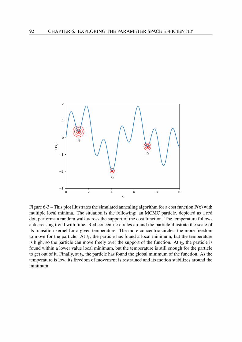
92 CHAPTER 6. EXPLORING THE PARAMETER SPACE EFFICIENTLY
Figure 6-3 – This plot illustrates the simulated annealing algorithm for a cost function P(x) withmultiple local minima. The situation is the following: an MCMC particle, depicted as a reddot, performs a random walk across the support of the cost function. The temperature followsa decreasing trend with time. Red concentric circles around the particle illustrate the scale ofits transition kernel for a given temperature. The more concentric circles, the more freedomto move for the particle. At t1, the particle has found a local minimum, but the temperatureis high, so the particle can move freely over the support of the function. At t2, the particle isfound within a lower value local minimum, but the temperature is still enough for the particleto get out of it. Finally, at t3, the particle has found the global minimum of the function. As thetemperature is low, its freedom of movement is restrained and its motion stabilizes around theminimum.
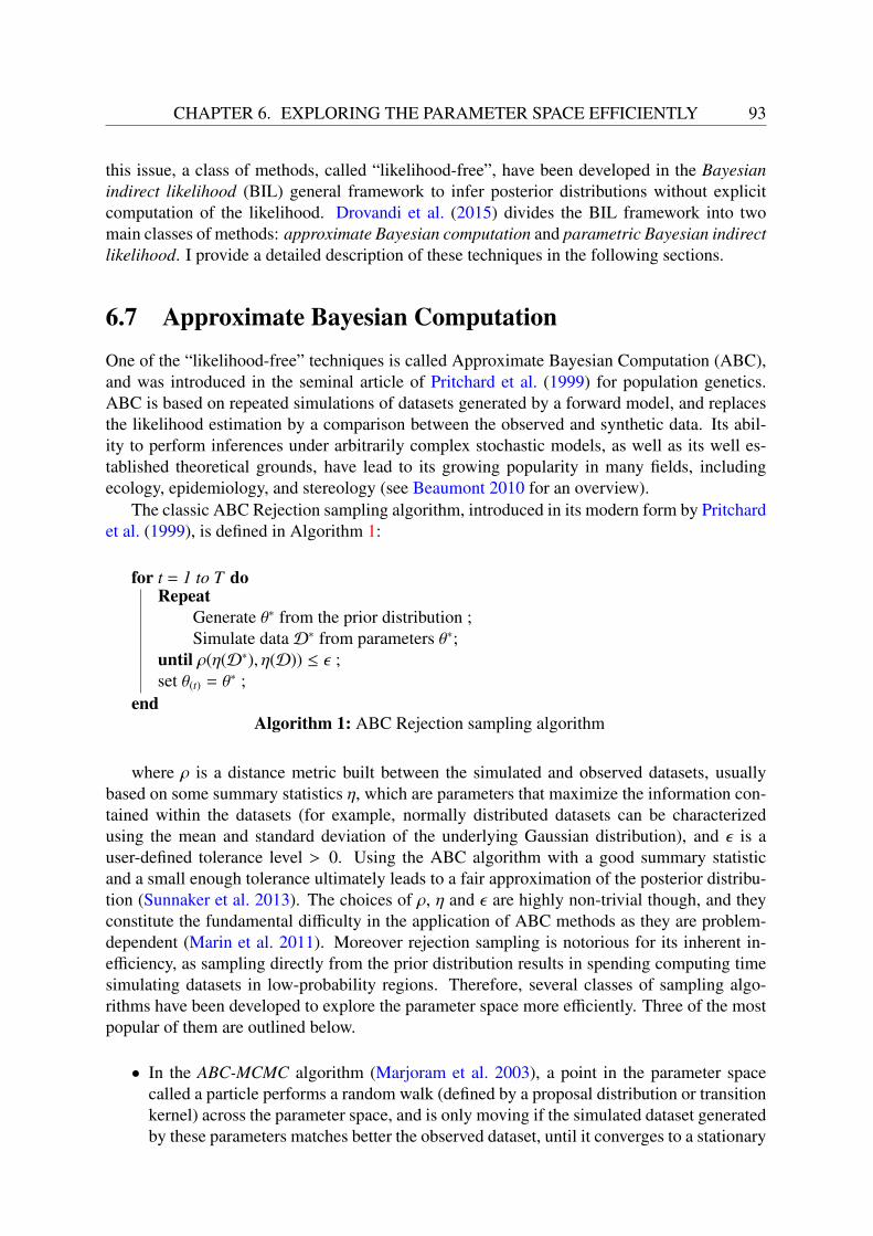
CHAPTER 6. EXPLORING THE PARAMETER SPACE EFFICIENTLY 93
this issue, a class of methods, called “likelihood-free”, have been developed in the Bayesianindirect likelihood (BIL) general framework to infer posterior distributions without explicitcomputation of the likelihood. Drovandi et al. (2015) divides the BIL framework into twomain classes of methods: approximate Bayesian computation and parametric Bayesian indirectlikelihood. I provide a detailed description of these techniques in the following sections.
6.7 Approximate Bayesian ComputationOne of the “likelihood-free” techniques is called Approximate Bayesian Computation (ABC),and was introduced in the seminal article of Pritchard et al. (1999) for population genetics.ABC is based on repeated simulations of datasets generated by a forward model, and replacesthe likelihood estimation by a comparison between the observed and synthetic data. Its abil-ity to perform inferences under arbitrarily complex stochastic models, as well as its well es-tablished theoretical grounds, have lead to its growing popularity in many fields, includingecology, epidemiology, and stereology (see Beaumont 2010 for an overview).
The classic ABC Rejection sampling algorithm, introduced in its modern form by Pritchardet al. (1999), is defined in Algorithm 1:
for t = 1 to T doRepeat
Generate θ∗ from the prior distribution ;Simulate dataD∗ from parameters θ∗;
until ρ(η(D∗), η(D)) ≤ ε ;set θ(t) = θ∗ ;
endAlgorithm 1: ABC Rejection sampling algorithm
where ρ is a distance metric built between the simulated and observed datasets, usuallybased on some summary statistics η, which are parameters that maximize the information con-tained within the datasets (for example, normally distributed datasets can be characterizedusing the mean and standard deviation of the underlying Gaussian distribution), and ε is auser-defined tolerance level > 0. Using the ABC algorithm with a good summary statisticand a small enough tolerance ultimately leads to a fair approximation of the posterior distribu-tion (Sunnaker et al. 2013). The choices of ρ, η and ε are highly non-trivial though, and theyconstitute the fundamental difficulty in the application of ABC methods as they are problem-dependent (Marin et al. 2011). Moreover rejection sampling is notorious for its inherent in-efficiency, as sampling directly from the prior distribution results in spending computing timesimulating datasets in low-probability regions. Therefore, several classes of sampling algo-rithms have been developed to explore the parameter space more efficiently. Three of the mostpopular of them are outlined below.
• In the ABC-MCMC algorithm (Marjoram et al. 2003), a point in the parameter spacecalled a particle performs a random walk (defined by a proposal distribution or transitionkernel) across the parameter space, and is only moving if the simulated dataset generatedby these parameters matches better the observed dataset, until it converges to a stationary

94 CHAPTER 6. EXPLORING THE PARAMETER SPACE EFFICIENTLY
distribution. As in standard MCMC procedures, the efficiency of the algorithm is largelydetermined by the choice of the scale of the kernel.
• In the ABC Sequential Monte Carlo parallel algorithm (ABC-SMC, Toni et al. 2009),samples are drawn from the prior distribution until N particles are accepted, that is, thosewith a distance to the data < ε0. All accepted particles are attributed a statistical weightω0. The weighted particles then constitute an intermediate distribution from which an-other set of samples is drawn and perturbed with a fixed transition kernel, until N parti-cles satisfy the acceptance criterion: ρ < ε1, with ε1 < ε0. They are then weighted withω1
and the process is repeated with a diminished tolerance at each step. After T iterations ofthis process, the particles are sampled from the approximated posterior distribution. Theperformance of ABC-SMC scales as N, where N is the number of particles. Differentvariations of ABC-SMC algorithms have been published, each with a different weightingscheme for particles.
• ABC Population Monte Carlo (ABC-PMC, Beaumont et al. 2008) is similar to ABC-SMC, but differs in its adaptive weighting scheme: its transition kernel is Gaussian andbased on the variance of the accepted particles in the previous iteration. This schemerequires the fewest tuning parameters of the three algorithms discussed here (Turner andVan Zandt 2012). But ABC-PMC is also more computationally costly than ABC-SMC,as its performance scales as N2 (caused by its adaptability).
The reader is referred to Csilléry et al. (2010), Marin et al. (2011), Turner and Van Zandt(2012), Sunnaker et al. (2013), and Gutmann and Corander (2016) for a set of historical, me-thodical, and theoretical reviews of the ABC approach, as well as a complete description of thealgorithms mentioned above.
Application of likelihood-free inference to astrophysics
The application of likelihood-free methods to astrophysics is still rare, as noted by Cameronand Pettitt (2012) in their review. Only lately has the potential of such techniques been consid-ered. Schafer and Freeman (2012) praised the use of likelihood-free inference in the context ofquasar luminosity function estimation. Cameron and Pettitt (2012) explored the morphologicaltransformation of high-redshift galaxies and derived strong constraints on the evolution of themerger rate in the early Universe using an ABC-SMC approach. Weyant et al. (2013) alsoused SMC for the estimation of cosmological parameters from type Ia supernovae samples,and could still provide robust results when the data was contaminated by type IIP supernovae.Robin et al. (2014) constrained the shape and formation period of the thick disk of the MilkyWay using MCMC as their sampling scheme, based on photometric data from the SDSS andthe Two Micron All Sky Survey (2MASS). Finally Hahn et al. (2016) demonstrate the feasi-bility of using ABC to constrain the relationship between galaxies and their dark matter halo.The recent birth of Python packages providing sampling algorithms in an ABC framework,such as astroABC (Jennings and Madigan 2016) and ELFI (Kangasrääsiö et al. 2016), whichimplement SMC methods, and COSMOABC (Ishida et al. 2015) which implements the PMCalgorithm, will probably facilitate the rise of likelihood-free inference techniques in the astro-nomical community.
CHAPTER 6. EXPLORING THE PARAMETER SPACE EFFICIENTLY 95
6.8 Parametric Bayesian indirect likelihoodAnother class of likelihood-free techniques is called parametric Bayesian indirect likelihood(pBIL). First proposed by Reeves and Pettitt (2005) and Gallant and McCulloch (2009), pBILtransforms the intractable likelihood of complex inference problems into a tractable one usingan auxiliary parametric model that describes the simulated datasets generated by the forwardmodel. In this scheme, the resulting auxiliary likelihood function quantifies the discrepancy be-tween the observed and simulated data. It is used in Bayes’ theorem and the parameter space isexplored using a user-defined sampling procedure, in an equivalent way to a classical Bayesiantechnique. While sharing similarities with the previous technique, pBIL is not an ABC methodin the strict sense, as it does not require an appropriate choice of summary statistics and toler-ance level to compare the observed and synthetic datasets. The accuracy of the inference in thepBIL scheme is determined by how well the auxiliary model describes the data (observed andsimlated). The theoretical foundations of this scheme are described extensively in Drovandiet al. (2015).
6.9 Our approach for this workIn this thesis, we will use a pBIL approach to explore the parameter space, whose auxiliarylikelihood and its construction will be described in the next chapter (cf Section 7). We willpreferentially consider flat priors on our parameters, using wide boundaries around commonlyaccepted values in the literature to avoid contamination of our results by previous studies. Wewill rely on an adaptive MCMC sampler for a fast exploration of the parameter space. In thefirst tests of the inference pipeline that we are designing (cf Chapter 9), the sampling processwill be performed using the Adaptive Proposal algorithm of Haario et al. (1999). The pipelinewill be then improved to include the more reliable Adaptive Metropolis algorithm of Haarioet al. (2001) that will be used for further tests and application to real data (cf Chapter 11).To take into account the loss of precision in the inference process generated by the inherentstochasticity of our model (i.e. variations of the auxiliary likelihood values for a given setof input model parameters), a temperature notion from the simulated annealing algorithm ofKirkpatrick (1983) will be superimposed on the Metropolis Hastings acceptance probability,and updated every fixed number of iterations along the MCMC run, in a scheme that will bedetailed in Section 9.4.1.

96 CHAPTER 6. EXPLORING THE PARAMETER SPACE EFFICIENTLY

Chapter 7
Comparing observed and simulateddatasets
Illusions can be pleasant, but therewards of truth are enormously better.
Sean Carroll, The Big Picture
Abstract
Our goal is to find the distributions of apparent luminosity and size of sources ex-tracted from simulated multi-band images generated by our model that maximizethe similarity with the observed distributions. In this chapter, I explore variousdistance metrics that have been designed to compare the discrepancy between twoarbitrary multivariate distributions. We finally choose to bin our datasets, that arefirst preprocessed in order to maximize the efficiency of the binning scheme, and tocompare their discrepancy using a “binned maximum likelihood” approach. In thiscontext, I detail some data-based methods found in the literature to yield optimalbinning schemes for multidimensional datasets.
Contents7.1 Non-parametric distance metrics . . . . . . . . . . . . . . . . . . . . . . . 987.2 Binning multidimensional datasets . . . . . . . . . . . . . . . . . . . . . . 99
7.2.1 Advantages and caveats of binning . . . . . . . . . . . . . . . . . . . 99
7.2.2 Hogg’s rule . . . . . . . . . . . . . . . . . . . . . . . . . . . . . . . 100
7.2.3 Knuth’s rule . . . . . . . . . . . . . . . . . . . . . . . . . . . . . . . 101
7.2.4 Bayesian blocks . . . . . . . . . . . . . . . . . . . . . . . . . . . . 102
7.3 Comparing observed and simulated binned datasets . . . . . . . . . . . . 1057.3.1 Reducing the dynamic range of the observables . . . . . . . . . . . . 105
7.3.2 Decorrelating the observables . . . . . . . . . . . . . . . . . . . . . 105
7.3.3 Quantifying the similarities between binned datasets . . . . . . . . . 107
97

98 CHAPTER 7. COMPARING OBSERVED AND SIMULATED DATASETS
We find ourselves in the following situation: we need to minimize the discrepancy be-tween observed source catalogs from astronomical surveys, and simulated ones generated byour model. Therefore, we need a measure of similarity between our simulated and observeddatasets. In our case, the dimensionality of the observable space is determined by the numberof photometric and size parameters (i.e. the FLUX_AUTO and the FLUX_RADIUS) in everypassbands extracted from the survey images.
Estimating the discrepancy between the observed and simulated binned datasets in a mul-tidimensional space is highly non-trivial, as the choice of a good distance metric is problemdependent (Weber et al. 1998; Aggarwal et al. 2001). Some studies even suggest that the con-cept of “proximity” in a high dimensional space may even be meaningless (Beyer et al. 1999).Distance metrics can be parametric, i.e. relying on assumptions about the shape of the under-lying PDF of the two datasets, or non-parametric, i.e. relying on no such assumptions (Hoskin2012). The distributions of our observables may be multimodal and skewed, however manymetrics rely on the assumption of normality. Others, such as the Kullback-Leibler divergence(Kullback and Leibler 1951) or the Jensen-Shannon distance (Lin 1991), cannot be used with-out estimating an analytical underlying PDF, which can be very computationally expensive ina high-dimensional observable space. Hence the need for a non-parametric distance estimator.
7.1 Non-parametric distance metricsHere is a non-exhaustive list of non-parametric distance metrics found in the literature that canbe used on multivariate data in the Approximate Bayesian Computation framework. A morecomplete review is available in Pardo and Menéndez (2006) and Palombo (2011). However,the literature is astonishingly scarce on guiding the choice of an appropriate distance metricfor a given problem, and no study to quantify their relative power has been performed so far.These metrics include:
• the χ2 test (Chardy et al. 1976) is a simple and widely used way of determining whetherobserved frequencies are significantly different from expected frequencies. The maindrawback of this approach is that χ2 test results are dependent on the binning choice(Aslan and Zech 2002). For example, Kurinsky and Sajina (2014) use the χ2 distance tocompare color-color histograms.
• the Kolmogorov-Smirnov (KS) test (Chakravarti et al. 1967) estimates the maximumabsolute difference between the empirical distribution functions (EDF) of two samples.A generalization of this test for multivariate data has been proposed (Justel et al. 1997).However, as there is no unique way of ordering data points to compute a distance be-tween two EDF, it is not as reliable as the one-dimensional version without the help ofresampling methods such as bootstraping (Babu and Feigelson, 2006).
• the Anderson-Darling (AD) test (Stephens 1974) is a modification of the KS test. Thismethod uses a weight function that gives more weight to the tails of the distributions. Itis therefore considered more sensitive than the KS test, but it also suffers from the sameproblems in the multivariate case.
• the Mahalanobis distance (Mahalanobis 1936) is similar to the Euclidean norm but hasthe advantage of taking into account the correlation structure of multivariate data. The

CHAPTER 7. COMPARING OBSERVED AND SIMULATED DATASETS 99
Mahalanobis statistics, coupled with an univariate KS test, are used by Akeret et al.(2015) to compare photometric parameters for cosmological purposes. However, thisdistance only works for unimodal data distributions.
• the Bhattacharyya distance (Bhattacharyya 1946) is related to the Bhattacharyya coeffi-cient, which measures the quantity of overlap between the two samples. It is consideredmore reliable than the Mahalanobis distance in the sense that its use is not limited tocases where the standard deviations of the distributions are identical.
• the Earth Mover’s distance (EMD) (Rubner et al. 1998) is based on a solution to theTransportation problem. The distributions are represented by a user-defined set of clus-ters called signatures, where each cluster is described by its mean and by the fraction ofthe distribution encapsulated by it. The EMD is defined as the minimum cost of turningone signature into the other, the cost being linked to the distance between the two. Acomputationally fast approximate version of this distance using the Hilbert space-fillingcurve can be found in Bernton et al. (2017).
All these metrics rely on the estimation of the PDF of the datasets. Following the idea ofRobin et al. (2014) and Rybizki and Just (2015), who grouped their data representing stellarphotometry into bins of magnitude and color, we choose to bin our datasets for comparingthem, for reasons I detail in the following section.
7.2 Binning multidimensional datasets
7.2.1 Advantages and caveats of binningHistograms are the oldest and the most widely-used of density estimators. In fact, if normal-ized, they can be considered as piecewise-constant models of the underlying PDF of a givendataset. As our pipeline requires fast comparisons between simulated and observed distribu-tions of observables, binning offers an attractive solution for density estimation, consideringits relative simplicity of implementation and an advantageous computational cost. However,binning comes with some inevitable drawbacks: first, the number of bins increases exponen-tially with the number of dimensions. For a fixed-size dataset, multivariate histograms are alsosparser than their univariate counterparts and display more complex shapes. Also, the choice ofthe size and location of bins can significantly influence the information content of the dataset.If the bins are too big, the histogram will be likely to blend important features of the dataset.And if the bins are too small, the number count in each bin will largely be determined by sta-tistical fluctuations, and most bins will end up empty. The choice of optimal binning is evenless trivial in high-dimensional spaces (Cadez et al. 2002). This class of problems is known as“the curse of dimensionality” (Bellman 1972).
Some data-based binning rules exist to return the optimal size of bins for a given dataset,such as the widely used Scott’s rule (Scott 1979) or the Freedman and Diaconis rule (Freedmanand Diaconis 1981) for univariate datasets. In the following section I explore three rules thathave been developed to tackle multivariate datasets: Hogg’s rule, Knuth’s rule and Bayesianblocks, whose differences on the same dataset is illustrated in Figure 7-2. Finally, alternativesto binning for density estimation are discussed in the conclusion of this thesis.

100 CHAPTER 7. COMPARING OBSERVED AND SIMULATED DATASETS
Figure 7-1 – Dataset consisting of 103 points normally distributed with mean 0 and unit stan-dard deviation binned using Hogg’s rule with a smoothing parameter α = 1.1.
7.2.2 Hogg’s rule
Hogg (2008) proposed a method based on “Jackknife” or “leave one out cross-validation”,where a sub-sample of the dataset is constructed and used to predict the complementary sub-sample. The binning structure for a given number of bins represents a model whose predictivepower is encapsulated within a likelihood function. Bins that are too fine or too coarse havea low predictive power, therefore one can find the optimal number of bins by maximizing thelikelihood.
Hogg starts from assuming that the data is a sample drawn from a PDF that can be approx-imated by a piece-wise constant model f (x) where the number of data points that falls in bini is proportional to the probability in that bin. For M equal bins of volume Vm = ∆x1∆x2 ...∆xD
where ∆xk =max(xk)−min(xk)
M is the width of the bin in dimension k, the probability that a datapoint ends up in bin i is:
p(i) =Nm + α∑M
m=1[Nm + α](7.1)
where Nm is the number of counts in bin m, and α is a "smoothing" parameter of order 1 toprevent zero probabilities in empty bins. The approximate PDF is then:
f (x) =p(i(x))Vi(x)
(7.2)
Hogg’s “Jackknife” log-likelihood for a given number of bins can be defined as the weightedsum of bin probabilities over the bins:
ln L =
M∑m=1
Nm ln(
Nm + α − 1Vm
[∑m′ (Nm′ + α) − 1
]) (7.3)
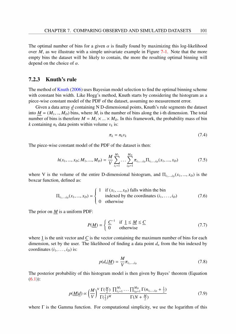
CHAPTER 7. COMPARING OBSERVED AND SIMULATED DATASETS 101
The optimal number of bins for a given α is finally found by maximizing this log-likelihoodover M, as we illustrate with a simple univariate example in Figure 7-1. Note that the moreempty bins the dataset will be likely to contain, the more the resulting optimal binning willdepend on the choice of α.
7.2.3 Knuth’s rule
The method of Knuth (2006) uses Bayesian model selection to find the optimal binning schemewith constant bin width. Like Hogg’s method, Knuth starts by considering the histogram as apiece-wise constant model of the PDF of the dataset, assuming no measurement error.
Given a data array d containing N D-dimensional points, Knuth’s rule segments the datasetinto M = (M1, ..,MD) bins, where Mi is the number of bins along the i-th dimension. The totalnumber of bins is therefore M = M1 × ... × MD. In this framework, the probability mass of bink containing nk data points within volume vk is:
πk = nkvk (7.4)
The piece-wise constant model of the PDF of the dataset is then:
h(x1, ..., xD; M1, ...,MD) =MV
M1∑i1=1
. . .
MD∑iD=1
πi1,...,iDΠi1,...,iD(x1, ..., xD) (7.5)
where V is the volume of the entire D-dimensional histogram, and Πi1,...,iD(x1, ..., xD) is theboxcar function, defined as:
Πi1,...,iD(x1, ..., xD) =
1 if (x1, ..., xD) falls within the bin
indexed by the coordinates (i1, . . . , iD)0 otherwise
(7.6)
The prior on M is a uniform PDF:
P(M) =
C−1 if 1 ≤ M ≤ C0 otherwise (7.7)
where 1 is the unit vector and C is the vector containing the maximum number of bins for eachdimension, set by the user. The likelihood of finding a data point dn from the bin indexed bycoordinates (i1, . . . , iD) is:
p(dn|M) =MVπi1,...,iD (7.8)
The posterior probability of this histogram model is then given by Bayes’ theorem (Equation(6.1)):
p(M|d) ∝(M
V
)N Γ( M2 )
Γ( 12 )M
∏M1i1=1 . . .
∏MDiD=1 Γ(ni1,...,iD + 1
2 )
Γ(N + M2 )
(7.9)
where Γ is the Gamma function. For computational simplicity, we use the logarithm of this
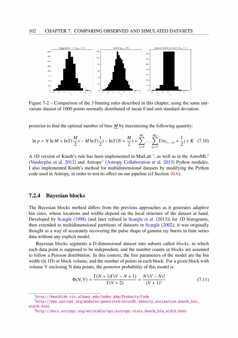
102 CHAPTER 7. COMPARING OBSERVED AND SIMULATED DATASETS
Figure 7-2 – Comparison of the 3 binning rules described in this chapter, using the same uni-variate dataset of 1000 points normally distributed of mean 0 and unit standard deviation.
posterior to find the optimal number of bins M by maximizing the following quantity:
ln p = N ln M + ln Γ(M2
) − M ln Γ(12
) − ln Γ(N +M2
) +
M1∑i1=1
. . .
MD∑iD=1
Γ(ni1,...,iD +12
) + K (7.10)
A 1D version of Knuth’s rule has been implemented in MatLab 1, as well as in the AstroML2
(Vanderplas et al. 2012) and Astropy3 (Astropy Collaboration et al. 2013) Python modules.I also implemented Knuth’s method for multidimensional datasets by modifying the Pythoncode used in Astropy, in order to test its effect on our pipeline (cf Section 10.6).
7.2.4 Bayesian blocks
The Bayesian blocks method differs from the previous approaches as it generates adaptivebin sizes, whose locations and widths depend on the local structure of the dataset at hand.Developed by Scargle (1998) (and later refined in Scargle et al. (2013)) for 1D histograms,then extended to multidimensional partitions of datasets in Scargle (2002), it was originallythought as a way of accurately recovering the pulse shape of gamma ray bursts in time seriesdata without any explicit model.
Bayesian blocks segments a D-dimensional dataset into subsets called blocks, in whicheach data point is supposed to be independent, and the number counts in blocks are assumedto follow a Poisson distribution. In this context, the free parameters of the model are the binwidth (in 1D) or block volume, and the number of points in each block. For a given block withvolume V enclosing N data points, the posterior probability of this model is:
Φ(N,V) =Γ(N + 1)Γ(V − N + 1)
Γ(V + 2)=
N!(V − N)!(V + 1)!
(7.11)
1http://knuthlab.rit.albany.edu/index.php/Products/Code2http://www.astroml.org/modules/generated/astroML.density_estimation.knuth_bin_
width.html3http://docs.astropy.org/en/stable/api/astropy.stats.knuth_bin_width.html
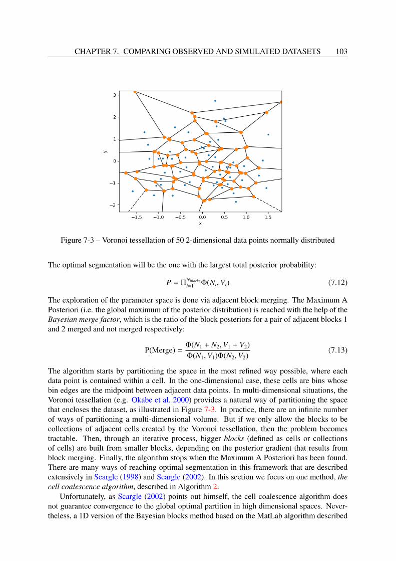
CHAPTER 7. COMPARING OBSERVED AND SIMULATED DATASETS 103
Figure 7-3 – Voronoi tessellation of 50 2-dimensional data points normally distributed
The optimal segmentation will be the one with the largest total posterior probability:
P = ΠNblocksi=1 Φ(Ni,Vi) (7.12)
The exploration of the parameter space is done via adjacent block merging. The Maximum APosteriori (i.e. the global maximum of the posterior distribution) is reached with the help of theBayesian merge factor, which is the ratio of the block posteriors for a pair of adjacent blocks 1and 2 merged and not merged respectively:
P(Merge) =Φ(N1 + N2,V1 + V2)Φ(N1,V1)Φ(N2,V2)
(7.13)
The algorithm starts by partitioning the space in the most refined way possible, where eachdata point is contained within a cell. In the one-dimensional case, these cells are bins whosebin edges are the midpoint between adjacent data points. In multi-dimensional situations, theVoronoi tessellation (e.g. Okabe et al. 2000) provides a natural way of partitioning the spacethat encloses the dataset, as illustrated in Figure 7-3. In practice, there are an infinite numberof ways of partitioning a multi-dimensional volume. But if we only allow the blocks to becollections of adjacent cells created by the Voronoi tessellation, then the problem becomestractable. Then, through an iterative process, bigger blocks (defined as cells or collectionsof cells) are built from smaller blocks, depending on the posterior gradient that results fromblock merging. Finally, the algorithm stops when the Maximum A Posteriori has been found.There are many ways of reaching optimal segmentation in this framework that are describedextensively in Scargle (1998) and Scargle (2002). In this section we focus on one method, thecell coalescence algorithm, described in Algorithm 2.
Unfortunately, as Scargle (2002) points out himself, the cell coalescence algorithm doesnot guarantee convergence to the global optimal partition in high dimensional spaces. Never-theless, a 1D version of the Bayesian blocks method based on the MatLab algorithm described

104 CHAPTER 7. COMPARING OBSERVED AND SIMULATED DATASETS
Perform Voronoi tesselation on the dataset ;Identify each Voronoi cell as a block ;Compute P(Merge) for each pair of adjacent blocks ;while largest P(Merge) ≥ 1 do
Merge the pair with largest P(Merge) and go to (3) ;end
Algorithm 2: Bayesian Blocks: the cell coalescence algorithm
(a) Multi-type case (b) Fattening E case
Figure 7-4 – Histogram of the number of sources extracted per bin for the pre-processed inputdata of the test cases presented in Chapter 9. In the left panel, three observables are considered:the FLUX_AUTO in uiKs. In the right panel, six observables are considered: the FLUX_AUTOin uiKs and the FLUX_RADIUS in uiKs. Using 10 bins per dimension, between the “Multi-type” case and the “Fattening E” case the number of bins increases by a factor 103, and thenumber of empty bins is increased by roughly the same amount. This illustrates the curseof dimensionality we face in this method, and puts computational limits on the number ofobservables we can use.
in Scargle et al. (2013) has been implemented in the AstroML4 (Vanderplas et al. 2012) andAstropy5 (Astropy Collaboration et al. 2013) Python modules.
Despite the appeal of its adaptive nature, we consider the use of the Bayesian blocks methodto be impractical “by construction” for our goal: the difference of geometry (due to the Voronoitesselation) between the two observables datasets partitioned by this method would make thequantification of their discrepancies highly non trivial.
4http://www.astroml.org/modules/generated/astroML.density_estimation.bayesian_blocks.html
5http://docs.astropy.org/en/stable/api/astropy.stats.bayesian_blocks.html
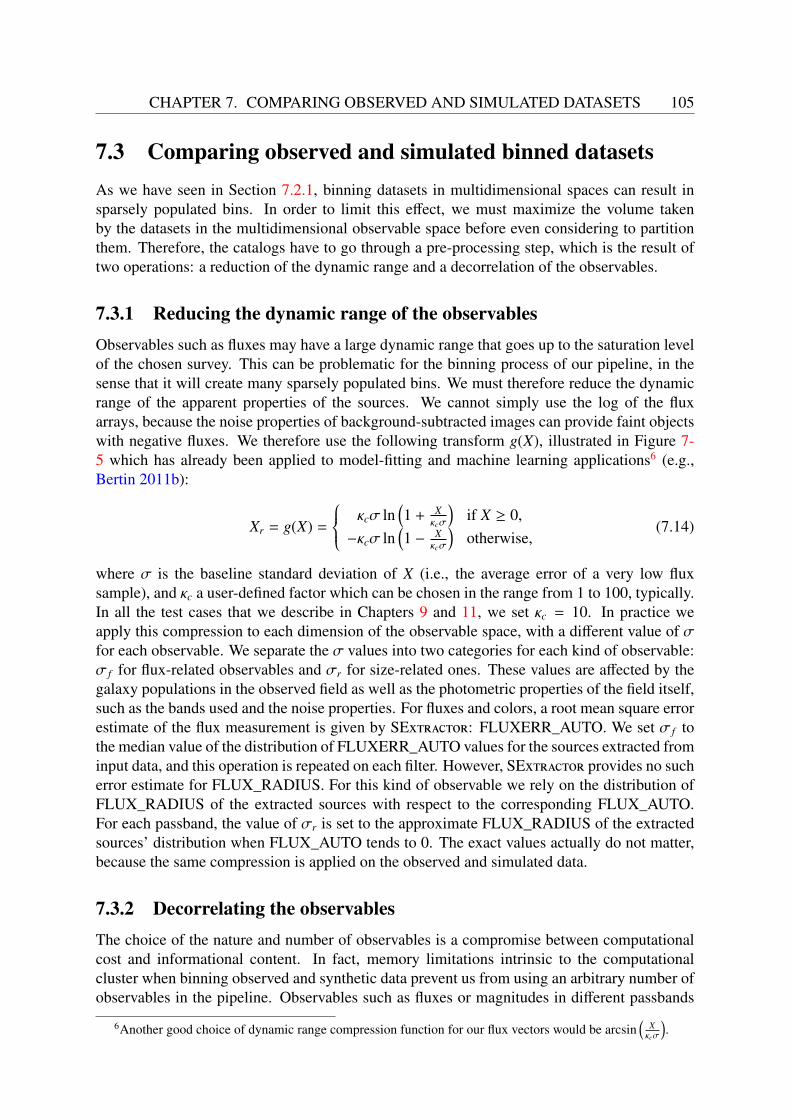
CHAPTER 7. COMPARING OBSERVED AND SIMULATED DATASETS 105
7.3 Comparing observed and simulated binned datasetsAs we have seen in Section 7.2.1, binning datasets in multidimensional spaces can result insparsely populated bins. In order to limit this effect, we must maximize the volume takenby the datasets in the multidimensional observable space before even considering to partitionthem. Therefore, the catalogs have to go through a pre-processing step, which is the result oftwo operations: a reduction of the dynamic range and a decorrelation of the observables.
7.3.1 Reducing the dynamic range of the observablesObservables such as fluxes may have a large dynamic range that goes up to the saturation levelof the chosen survey. This can be problematic for the binning process of our pipeline, in thesense that it will create many sparsely populated bins. We must therefore reduce the dynamicrange of the apparent properties of the sources. We cannot simply use the log of the fluxarrays, because the noise properties of background-subtracted images can provide faint objectswith negative fluxes. We therefore use the following transform g(X), illustrated in Figure 7-5 which has already been applied to model-fitting and machine learning applications6 (e.g.,Bertin 2011b):
Xr = g(X) =
κcσ ln(1 + X
κcσ
)if X ≥ 0,
−κcσ ln(1 − X
κcσ
)otherwise,
(7.14)
where σ is the baseline standard deviation of X (i.e., the average error of a very low fluxsample), and κc a user-defined factor which can be chosen in the range from 1 to 100, typically.In all the test cases that we describe in Chapters 9 and 11, we set κc = 10. In practice weapply this compression to each dimension of the observable space, with a different value of σfor each observable. We separate the σ values into two categories for each kind of observable:σ f for flux-related observables and σr for size-related ones. These values are affected by thegalaxy populations in the observed field as well as the photometric properties of the field itself,such as the bands used and the noise properties. For fluxes and colors, a root mean square errorestimate of the flux measurement is given by SExtractor: FLUXERR_AUTO. We set σ f tothe median value of the distribution of FLUXERR_AUTO values for the sources extracted frominput data, and this operation is repeated on each filter. However, SExtractor provides no sucherror estimate for FLUX_RADIUS. For this kind of observable we rely on the distribution ofFLUX_RADIUS of the extracted sources with respect to the corresponding FLUX_AUTO.For each passband, the value of σr is set to the approximate FLUX_RADIUS of the extractedsources’ distribution when FLUX_AUTO tends to 0. The exact values actually do not matter,because the same compression is applied on the observed and simulated data.
7.3.2 Decorrelating the observablesThe choice of the nature and number of observables is a compromise between computationalcost and informational content. In fact, memory limitations intrinsic to the computationalcluster when binning observed and synthetic data prevent us from using an arbitrary number ofobservables in the pipeline. Observables such as fluxes or magnitudes in different passbands
6Another good choice of dynamic range compression function for our flux vectors would be arcsin(
Xκcσ
).

106 CHAPTER 7. COMPARING OBSERVED AND SIMULATED DATASETS
Figure 7-5 – Dynamic range reduction function g(X) defined in Equation 7.14.
also tend to be strongly correlated with one another, as they originate from the same spectrumof a given galaxy from a given population. These correlations can be high if the passbandsare too narrow, too close to each other, and not covering a large enough wavelength baseline.One must thoughtfully choose the appropriate set of filters a priori in order for the resultingset of observables to be able to disentangle the luminous properties of the different galaxypopulations.
Strong correlations between input vector components can also make binning very ineffi-cient, therefore an important pre-processing step is to decorrelate them. In that regard, we applya linear transformation called principal component analysis whitening, or sphering (Friedman1987, Hyvärinen et al. 2009, Shlens 2014, Kessy et al. 2015) to our reduced matrix of ob-servables Xr of size p × Ns, where p is the number of observables and Ns is the number ofsources. Principal component analysis (PCA) is an algorithm commonly used in the context ofdimensionality reduction. Its goal is to find a set of orthogonal axes in a dataset called princi-pal components that encapsulate most of the variance of the data. This can be performed via asingular values decomposition (SVD) of the covariance matrix of the data:
< XrXTr >= UΛVT , (7.15)
where U and V are orthogonal matrices and Λ the diagonal matrix containing the non-negativesingular values of the covariance matrix, sorted by descending order.
PCA whitening is the combination of two operations: rotation and scaling. First the dataset(previously centered around zero by subtracting the mean in each dimension) is projected alongthe principal components, which removes linear correlations, and then each dimension is scaledso that its variance equals to one. The whitening transform can therefore be summarized by:
Xw = Λ−12 VT (Xr − µ), (7.16)
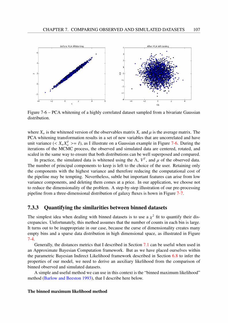
CHAPTER 7. COMPARING OBSERVED AND SIMULATED DATASETS 107
Figure 7-6 – PCA whitening of a highly correlated dataset sampled from a bivariate Gaussiandistribution.
where Xw is the whitened version of the observables matrix Xr and µ is the average matrix. ThePCA whitening transformation results in a set of new variables that are uncorrelated and haveunit variance (< XwXT
w >= I), as I illustrate on a Gaussian example in Figure 7-6. During theiterations of the MCMC process, the observed and simulated data are centered, rotated, andscaled in the same way to ensure that both distributions can be well superposed and compared.
In practice, the simulated data is whitened using the Λ, VT , and µ of the observed data.The number of principal components to keep is left to the choice of the user. Retaining onlythe components with the highest variance and therefore reducing the computational cost ofthe pipeline may be tempting. Nevertheless, subtle but important features can arise from lowvariance components, and deleting them comes at a price. In our application, we choose notto reduce the dimensionality of the problem. A step-by-step illustration of our pre-processingpipeline from a three-dimensional distribution of galaxy fluxes is hown in Figure 7-7.
7.3.3 Quantifying the similarities between binned datasets
The simplest idea when dealing with binned datasets is to use a χ2 fit to quantify their dis-crepancies. Unfortunately, this method assumes that the number of counts in each bin is large.It turns out to be inappropriate in our case, because the curse of dimensionality creates manyempty bins and a sparse data distribution in high dimensional space, as illustrated in Figure7-4.
Generally, the distances metrics that I described in Section 7.1 can be useful when used inan Approximate Bayesian Computation framework. But as we have placed ourselves withinthe parametric Bayesian Indirect Likelihood framework described in Section 6.8 to infer theproperties of our model, we need to derive an auxiliary likelihood from the comparison ofbinned observed and simulated datasets.
A simple and useful method we can use in this context is the “binned maximum likelihood”method (Barlow and Beeston 1993), that I describe here below.
The binned maximum likelihood method
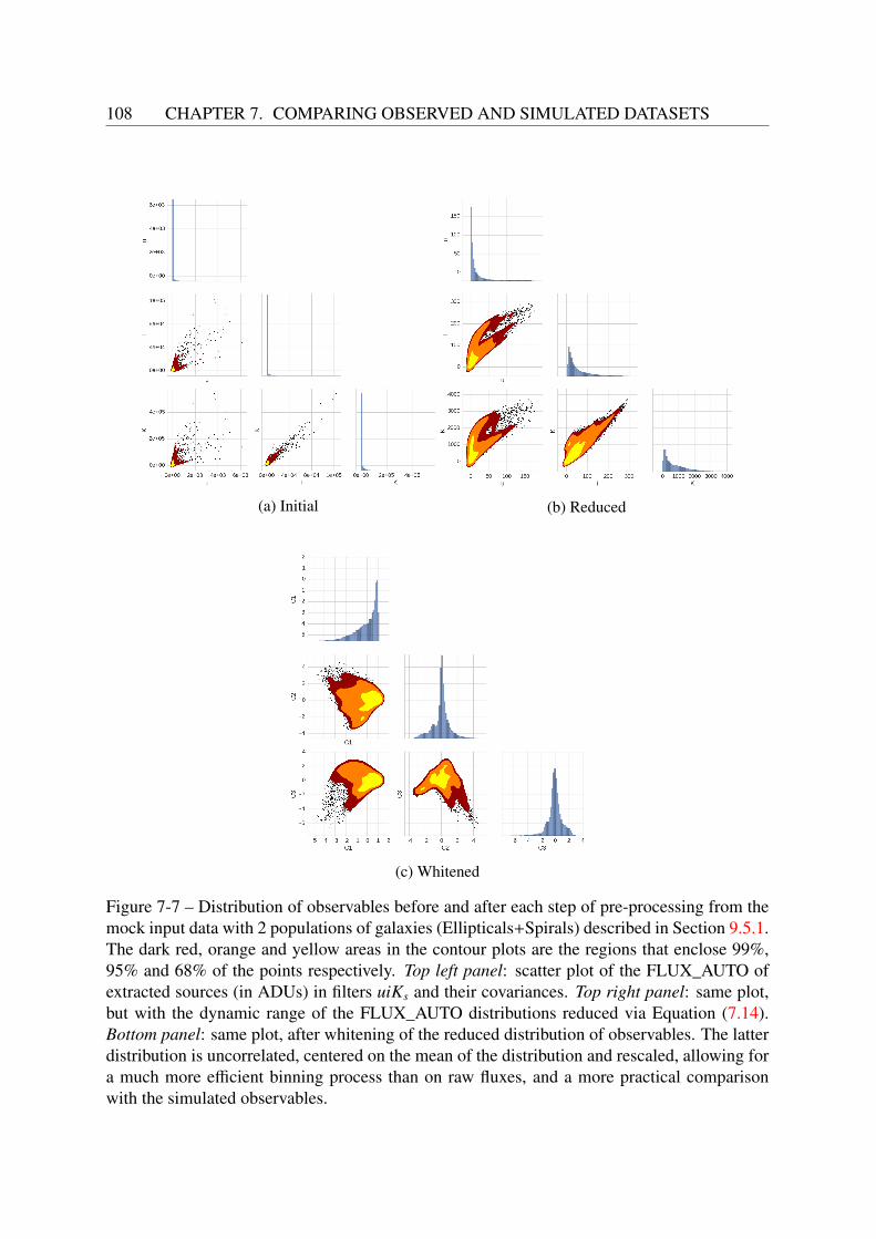
108 CHAPTER 7. COMPARING OBSERVED AND SIMULATED DATASETS
(a) Initial (b) Reduced
(c) Whitened
Figure 7-7 – Distribution of observables before and after each step of pre-processing from themock input data with 2 populations of galaxies (Ellipticals+Spirals) described in Section 9.5.1.The dark red, orange and yellow areas in the contour plots are the regions that enclose 99%,95% and 68% of the points respectively. Top left panel: scatter plot of the FLUX_AUTO ofextracted sources (in ADUs) in filters uiKs and their covariances. Top right panel: same plot,but with the dynamic range of the FLUX_AUTO distributions reduced via Equation (7.14).Bottom panel: same plot, after whitening of the reduced distribution of observables. The latterdistribution is uncorrelated, centered on the mean of the distribution and rescaled, allowing fora much more efficient binning process than on raw fluxes, and a more practical comparisonwith the simulated observables.

CHAPTER 7. COMPARING OBSERVED AND SIMULATED DATASETS 109
If we assume that the number count in each bin i is described by a Poisson distribution, theprobability of oi given the model si is:
li =e−si soi
i
oi!(7.17)
The likelihood function for the histogram is then:
L =
b∏i=1
e−si soii
oi!(7.18)
where b is the total number of bins, si is the number count in bin i for the simulated data, andoi is the number count in bin i for the observed data. Correlations between adjacent bins areneglected here. The log-likelihood is therefore given by:
ln L =
b∑i=1
(−si + oi ln(si) − ln(oi!)) (7.19)
As we want to maximize ln L, ln(oi!) is a constant that can be eliminated, so in fine, we obtain:
ln L =
b∑i=1
(−si + oi ln(si)) (7.20)
An additional correction has to be applied on the log-likelihood, because as the logarithm of si
is used, empty bins cause a problem. In order to avoid singularities, a constant small value ε(that I set to 1) is added to every bin up to the edges of the observables space. This process isdone in both modeled and observed data so that it does not bias our results too much:
ln L =
b∑i=1
(−(si + ε) + (oi + ε) ln(si + ε)) (7.21)
The resulting log-likelihood is then introduced in Bayes’ theorem (Equation (6.1)) at eachiteration of our sampling algorithm.
Equation (7.21) implies that the same binning is applied on synthetic and observed data. Inour pipeline, the binning pattern is only computed once and for the observed data only. Thesame binning is then directly applied to the simulated data to ensure better execution speedand comparability between histograms. Moreover, because the number of counts per bin isdirectly affected by the model parameters that rule the number density of galaxies, such as theφ∗ parameters of the luminosity function, our histograms are not normalized to prevent a lossof information during the comparison process. The fact that the comparison does not extendbeyond the range of the observed data can potentially limit the precision of our approach in away that we have not quantified.
To use the terminology of pBIL, the binning structure and the assumption of a Poissonbehavior of the number counts in each bin represent the auxiliary model that describes thedata. The auxiliary likelihood derived from this structure (Equation 7.20) has been used inprevious studies like e.g. Cash (1979), Bienayme et al. (1987), Adye (1998) or Robin et al.(2014).

110 CHAPTER 7. COMPARING OBSERVED AND SIMULATED DATASETS
Chapter 8
Interpreting the results of Bayesianinference
I may not have gone where I intended togo, but I think I have ended up where Ineeded to be.
Douglas Adams, The Long DarkTea-Time of the Soul
Abstract
The output of an MCMC run is the evolution of the position of each free parameterof the model across iterations. But how can we know whether the MCMC samplesare truly representative of the posterior distribution or not? Can we even know forsure? Is there any objective way to determine the length of the burn-in period?How to know when to stop an MCMC run? In this chapter I review some methodsthat can be used to diagnose the (non-)convergence of a chain. I also discuss somecommon practices to visualize and summarize the resulting posterior distribution.
Contents8.1 Convergence diagnostics . . . . . . . . . . . . . . . . . . . . . . . . . . . 112
8.1.1 The trace plot . . . . . . . . . . . . . . . . . . . . . . . . . . . . . . 112
8.1.2 The autocorrelation plot . . . . . . . . . . . . . . . . . . . . . . . . 114
8.1.3 Geweke’s diagnostic . . . . . . . . . . . . . . . . . . . . . . . . . . 114
8.1.4 The Gelman Rubin test . . . . . . . . . . . . . . . . . . . . . . . . . 116
8.2 The posterior distribution . . . . . . . . . . . . . . . . . . . . . . . . . . . 117
8.2.1 Credible regions . . . . . . . . . . . . . . . . . . . . . . . . . . . . 118
8.2.2 Constructing credible regions for joint posterior plots . . . . . . . . . 119
111
112 CHAPTER 8. INTERPRETING THE RESULTS OF BAYESIAN INFERENCE
8.1 Convergence diagnostics
Diagnosing the behavior of a Markov chain is a famously hard problem, which gets even morechallenging as the number of parameters to infer increases. In fact, it is impossible to knowwith certainty from a finite MCMC sample that a chain has indeed converged to the target dis-tribution (Cowles and Carlin 1996). This is why all the convergence diagnostics that have beendeveloped can only attest failure of convergence. However, they can provide some clues onthe sampling efficiency or the number of iterations after which the starting point of the chain isforgotten. Thus, the use of several diagnostics is recommended to attest convergence with moreconfidence. As many of these diagnostics rely on the comparison of multiple chains, runningmore than 3 chains constitutes a good practice. It is common in the statistical community torun between 3 and 10 chains (Sinharay 2003). In general, the more chains are launched andthe longer they are run, the more precise will be the estimation of the posterior distribution.
In the following sections, I will describe two graphical and two quantitative convergencediagnostics that will be useful for this work. Of course this list is not meant to be exhaustive.The reader is referred to the excellent reviews of Cowles and Carlin (1996), Brooks and Gel-man (1998) and Sinharay (2003) for a more complete overview of these diagnostics and theircaveats.
8.1.1 The trace plot
The simplest of convergence diagnostics is the trace plot (also called the time series plot). It isa plot (or collection of plots) reconstructing the path taken by the Markov chain by displayingthe value of each free parameter of the model at each iteration (cf Figure 8-1). If a singlechain has converged to the target distribution, its trace ends up stabilizing around the mode(s)of the posterior. If the chain periodically jumps from one region of the parameter space tothe other with a stationary behavior in the meantime, it can be an sign of multimodality in theposterior distribution. If multiple chains starting from different regions of the parameter spaceconverge to the same distribution and overlap with each other, it is also a good indication ofconvergence. It can also be useful to determine the burn-in period visually: for each chain,it is the maximum number of iterations necessary for all the parameters to reach a seeminglystationary distribution.
Trace plots can also provide useful visual clues about the mixing behavior of a chain, whichis a good tracer of the efficiency of the exploration of the parameter space. A chain with good(or rapid) mixing will not display any long-term trend in its trace1. On the contrary, a badly(or slowly) mixed chain will take a long time to go from one region of the parameter space tothe other, either because the step size is too low (which results in a trace that displays a wavypattern) or too high (which results in a trace that stays on the same state for many iterations).The worse the mixing, the more samples will be needed to estimate the target distribution withgood accuracy. These situations are illustrated in Figure 8-2. Bad mixing can generally besolved by tuning the width of the proposal distribution, as detailed in Section 6.4.
1It is usually said that an ideal trace should look like a hairy caterpillar.
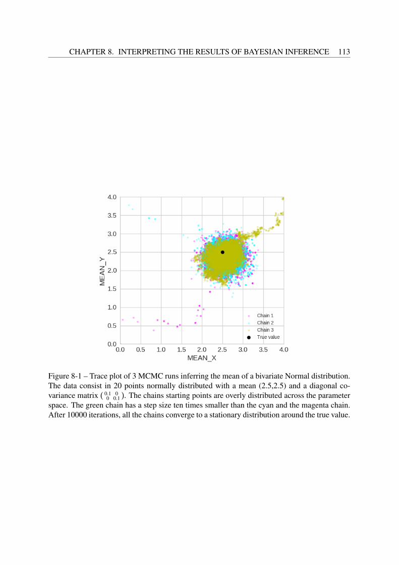
CHAPTER 8. INTERPRETING THE RESULTS OF BAYESIAN INFERENCE 113
Figure 8-1 – Trace plot of 3 MCMC runs inferring the mean of a bivariate Normal distribution.The data consist in 20 points normally distributed with a mean (2.5,2.5) and a diagonal co-variance matrix
( 0.1 00 0.1
). The chains starting points are overly distributed across the parameter
space. The green chain has a step size ten times smaller than the cyan and the magenta chain.After 10000 iterations, all the chains converge to a stationary distribution around the true value.

114 CHAPTER 8. INTERPRETING THE RESULTS OF BAYESIAN INFERENCE
8.1.2 The autocorrelation plotDue to its Markovian nature, each iteration of a Markov chain depends on the previous itera-tion. This introduces a non-zero correlation between distant samples of the same chain. Thecorrelation of a chain of size N with a delayed copy of itself, termed “autocorrelation”, is afunction of delay (or lag), and is assessed graphically via plotting the autocorrelation function(ACF), denoted ρk and defined here below, as a function of lag k:
ρk =
∑N−kt=1 (θ(t) − θ)(θ(t+k) − θ)∑N
t=1(θ(t) − θ)2(8.1)
By construction, the values of ρk are between -1 and 1. At lag 0, the autocorrelation is al-ways 1, which means that the chain is perfectly autocorrelated with itself. The autocorrelationthen generally decreases with increasing lag. This diagnostic should be plotted for each freeparameter of the model.
A perfect Markov chain should yield independent samples of the posterior distribution. Theautocorrelation plot can therefore yield useful information on the mixing rate of the chain: ifthe ACF rapidly drops to zero, this is a sign of good mixing, which means that convergenceto the stationary distribution might be attained quickly. On the contrary, a high degree ofautocorrelation with high values of lag means that on short timescales, the MCMC samples areunrepresentative of the target distribution. This is an indication of slow mixing: the parameterspace is not explored efficiently, and this usually translates into slow convergence. These twosituations are illustrated on Figure 8-2.
One way of decreasing autocorrelation is to thin the sample, by using only the iterationsfrom a certain lag. Thinning the chain to the lag where the autocorrelation function drops tozero will yield independent samples indeed. But this practice is generally a bad idea, becausean unthinned chain always leads to a better estimation of the target distribution than a thinnedchain (Maceachern and Berliner 1994). Therefore thinning should be avoided except whenfacing serious data storage limits. Autocorrelation can also be reduced by tuning the proposaldistribution of the Metropolis Hastings algorithm (Blangiardo and Cameletti 2015).
Finally, it is important to note that a high degree of autocorrelation is NOT a sign of a lackof convergence: in fact, the chain can still display a high degree of autocorrelation after havingconverged to the target distribution. Therefore it is improper to call the autocorrelation plota “convergence diagnostic” (Sinharay 2003). The PyMC Python package (Patil et al. 2010)provides the autocorrelation plot in its default MCMC diagnostics toolbox.
8.1.3 Geweke’s diagnosticGeweke et al. (1992) devised a convergence diagnostic based on a time series analysis of theMarkov chain. Computed for each free parameter of the model, the test divides the chain into2 intervals a and b of user-defined length called windows, one representing the first iterationsand the other the later iterations, and compares the empirical mean computed from differentsegments of the chain using the following statistic, called Z-score:
Z =θa − θb
√Var(θa) + Var(θb)
(8.2)
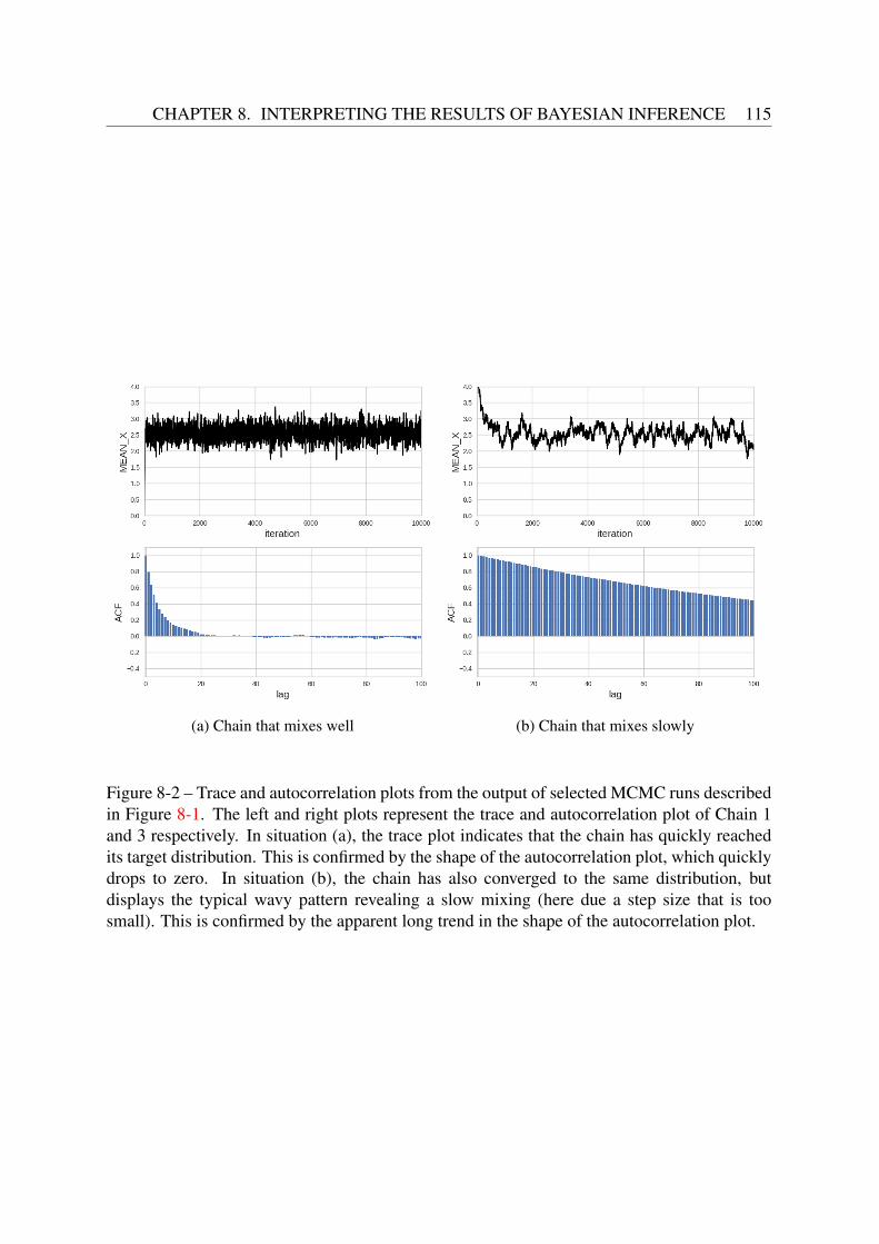
CHAPTER 8. INTERPRETING THE RESULTS OF BAYESIAN INFERENCE 115
(a) Chain that mixes well (b) Chain that mixes slowly
Figure 8-2 – Trace and autocorrelation plots from the output of selected MCMC runs describedin Figure 8-1. The left and right plots represent the trace and autocorrelation plot of Chain 1and 3 respectively. In situation (a), the trace plot indicates that the chain has quickly reachedits target distribution. This is confirmed by the shape of the autocorrelation plot, which quicklydrops to zero. In situation (b), the chain has also converged to the same distribution, butdisplays the typical wavy pattern revealing a slow mixing (here due a step size that is toosmall). This is confirmed by the apparent long trend in the shape of the autocorrelation plot.

116 CHAPTER 8. INTERPRETING THE RESULTS OF BAYESIAN INFERENCE
Figure 8-3 – Results of Geweke’s diagnostic for the MCMC output of Chain 3, in the exam-ple described in Figure 8-1. All the Z-scores computed from the first intervals using morethan 2300 iterations fall within 2σ of zero. This suggests that we can consider the first 2300iterations of the chain as burn-in.
where θa, Var(θa) and θb, Var(θb) are the empirical means and asymptotic spectral variancesof windows a and b respectively, determined by methods of spectral density estimation (alsoknown as Fourier analysis).
If the chain has converged to a stationary distribution, then the two means should be equaland Geweke’s Z-score, by construction, should converge asymptotically to a normal distribu-tion with mean 0 and unit standard deviation N(0, 1). Z-scores that are beyond 2σ of zeroindicate a failure of convergence, which means that more iterations are needed.
A common practice, as first suggested by Geweke et al. (1992), is to compare the mean ofthe first 10% and the last 50% of the chain. One can also use Geweke’s diagnostic to determinethe burn-in period of the chain: the test is performed by comparing various initial windows, andthe last 50% of the chain, as illustrated in Figure 8-3. The burn-in period is then consideredto be the smallest portion of the chain that passes the test for all the free model parameters.Geweke’s diagnostic is implemented in the PyMC Python package (Patil et al. 2010).
8.1.4 The Gelman Rubin test
One of the most popular convergence diagnostics is a test proposed by Gelman and Rubin(1992). Given m chains θ j
(t) ( j = 1, ...,m and m ≥ 3, and typically ∼ 10), each of length n afterdiscarding burn-in (t = 1, ..., n) and with different starting points, the test compares the variancebetween the mean values of the m chains B and the mean of the m within-chain variances W:

CHAPTER 8. INTERPRETING THE RESULTS OF BAYESIAN INFERENCE 117
B =n
m − 1
m∑j=1
(θ j. − θ..)
2 (8.3)
W =1m
m∑j=1
1n − 1
n∑i=1
(θ j(i) − θ
j. )
2
(8.4)
Where θ j. = 1
n
∑nt=1 θ
j(t) is the mean value of chain j, and θ.. = 1
m
∑mj=1 θ
j. is the average value over
the m chains.An overestimate of the true marginal posterior variance is given by the unbiased estimator:
V =n − 1
nW +
1 + mnm
B (8.5)
Finally convergence is estimated using the Potential Scale Reduction Factor (PSRF) R:
R =VW
(8.6)
We consider that convergence has been reached if√
R < 1.1 for all model parameters(Brooks and Gelman 1998). If convergence has not been reached, more iterations are per-formed until the criterion is met. We use the Gelman Rubin diagnostic implemented in thisform in the PyMC package (Patil et al. 2010), to perform our convergence tests.
8.2 The posterior distribution
The goal of Bayesian inference is to reconstruct the shape of the posterior distribution (or sim-ply posterior) of a set of parameters, given some observed data. When multiple parameters areinvolved, the posterior distribution is called the joint posterior distribution. The joint posterior,constructed from the combined samples of all the Markov chains taken after burn-in, can bevisualized to reveal correlations between parameters.
When inferring the posterior distribution of a d-dimensional random variable θ = θ1, . . . , θd,the marginal posterior for parameter θk is found by integrating the joint posterior over all theother parameters:
P(θk|D) =
∫P(θ1, . . . , θd|D)dθ1 . . . dθk−1dθk+1 . . . dθd (8.7)
The posterior distribution can also be summarized by point estimates, by computing themode2 (i.e. the global maximum of the PDF, or the set of local maxima if the posterior has
2The mode can also be called the Maximum A Posteriori (MAP).
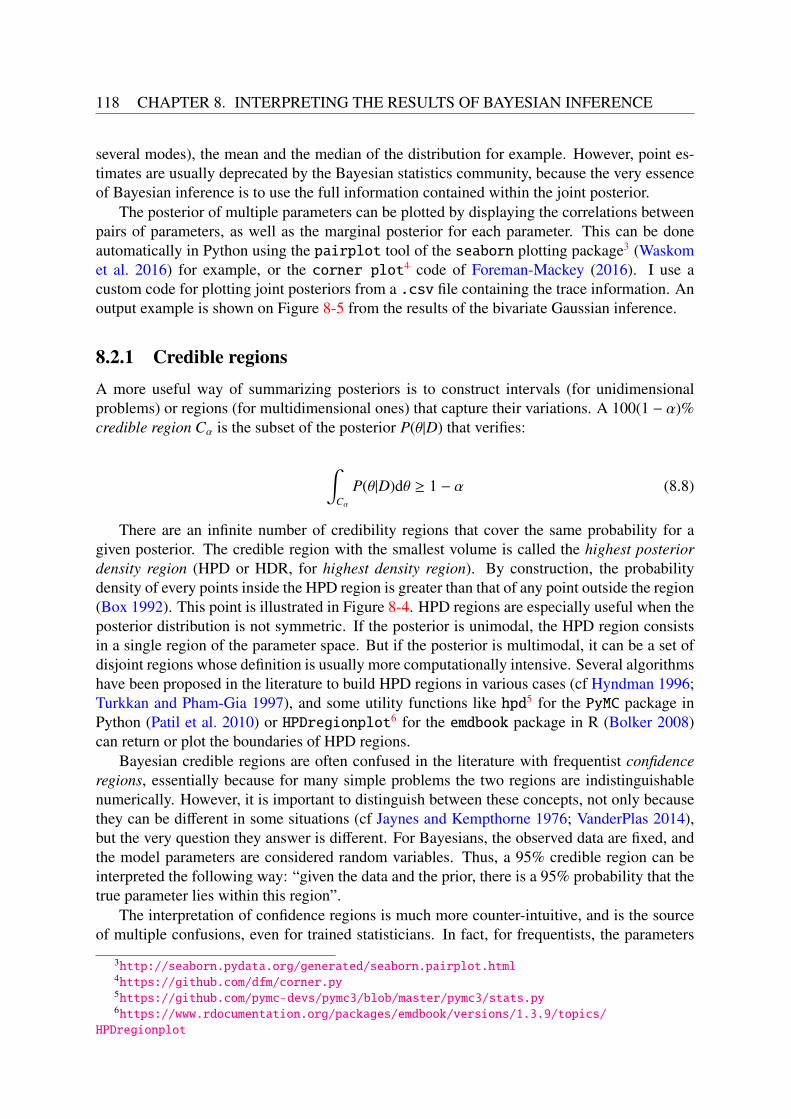
118 CHAPTER 8. INTERPRETING THE RESULTS OF BAYESIAN INFERENCE
several modes), the mean and the median of the distribution for example. However, point es-timates are usually deprecated by the Bayesian statistics community, because the very essenceof Bayesian inference is to use the full information contained within the joint posterior.
The posterior of multiple parameters can be plotted by displaying the correlations betweenpairs of parameters, as well as the marginal posterior for each parameter. This can be doneautomatically in Python using the pairplot tool of the seaborn plotting package3 (Waskomet al. 2016) for example, or the corner plot4 code of Foreman-Mackey (2016). I use acustom code for plotting joint posteriors from a .csv file containing the trace information. Anoutput example is shown on Figure 8-5 from the results of the bivariate Gaussian inference.
8.2.1 Credible regionsA more useful way of summarizing posteriors is to construct intervals (for unidimensionalproblems) or regions (for multidimensional ones) that capture their variations. A 100(1 − α)%credible region Cα is the subset of the posterior P(θ|D) that verifies:
∫Cα
P(θ|D)dθ ≥ 1 − α (8.8)
There are an infinite number of credibility regions that cover the same probability for agiven posterior. The credible region with the smallest volume is called the highest posteriordensity region (HPD or HDR, for highest density region). By construction, the probabilitydensity of every points inside the HPD region is greater than that of any point outside the region(Box 1992). This point is illustrated in Figure 8-4. HPD regions are especially useful when theposterior distribution is not symmetric. If the posterior is unimodal, the HPD region consistsin a single region of the parameter space. But if the posterior is multimodal, it can be a set ofdisjoint regions whose definition is usually more computationally intensive. Several algorithmshave been proposed in the literature to build HPD regions in various cases (cf Hyndman 1996;Turkkan and Pham-Gia 1997), and some utility functions like hpd5 for the PyMC package inPython (Patil et al. 2010) or HPDregionplot6 for the emdbook package in R (Bolker 2008)can return or plot the boundaries of HPD regions.
Bayesian credible regions are often confused in the literature with frequentist confidenceregions, essentially because for many simple problems the two regions are indistinguishablenumerically. However, it is important to distinguish between these concepts, not only becausethey can be different in some situations (cf Jaynes and Kempthorne 1976; VanderPlas 2014),but the very question they answer is different. For Bayesians, the observed data are fixed, andthe model parameters are considered random variables. Thus, a 95% credible region can beinterpreted the following way: “given the data and the prior, there is a 95% probability that thetrue parameter lies within this region”.
The interpretation of confidence regions is much more counter-intuitive, and is the sourceof multiple confusions, even for trained statisticians. In fact, for frequentists, the parameters
3http://seaborn.pydata.org/generated/seaborn.pairplot.html4https://github.com/dfm/corner.py5https://github.com/pymc-devs/pymc3/blob/master/pymc3/stats.py6https://www.rdocumentation.org/packages/emdbook/versions/1.3.9/topics/
HPDregionplot
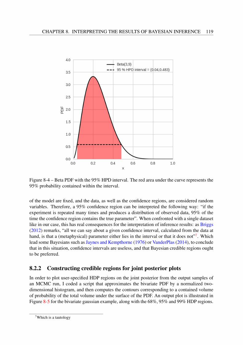
CHAPTER 8. INTERPRETING THE RESULTS OF BAYESIAN INFERENCE 119
Figure 8-4 – Beta PDF with the 95% HPD interval. The red area under the curve represents the95% probability contained within the interval.
of the model are fixed, and the data, as well as the confidence regions, are considered randomvariables. Therefore, a 95% confidence region can be interpreted the following way: “if theexperiment is repeated many times and produces a distribution of observed data, 95% of thetime the confidence region contains the true parameter”. When confronted with a single datasetlike in our case, this has real consequences for the interpretation of inference results: as Briggs(2012) remarks, “all we can say about a given confidence interval, calculated from the data athand, is that a (metaphysical) parameter either lies in the interval or that it does not”7. Whichlead some Bayesians such as Jaynes and Kempthorne (1976) or VanderPlas (2014), to concludethat in this situation, confidence intervals are useless, and that Bayesian credible regions oughtto be preferred.
8.2.2 Constructing credible regions for joint posterior plotsIn order to plot user-specified HDP regions on the joint posterior from the output samples ofan MCMC run, I coded a script that approximates the bivariate PDF by a normalized two-dimensional histogram, and then computes the contours corresponding to a contained volumeof probability of the total volume under the surface of the PDF. An output plot is illustrated inFigure 8-5 for the bivariate gaussian example, along with the 68%, 95% and 99% HDP regions.
7Which is a tautology
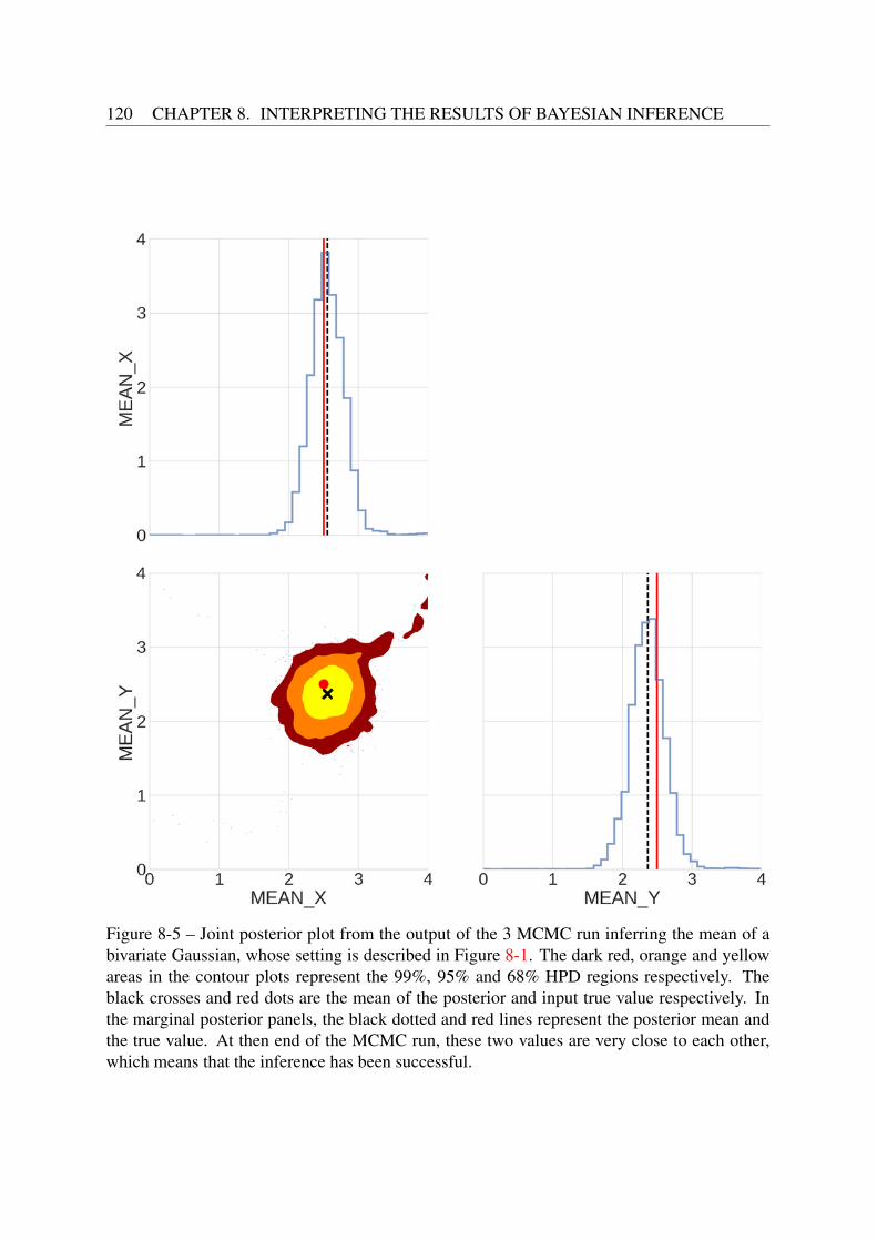
120 CHAPTER 8. INTERPRETING THE RESULTS OF BAYESIAN INFERENCE
Figure 8-5 – Joint posterior plot from the output of the 3 MCMC run inferring the mean of abivariate Gaussian, whose setting is described in Figure 8-1. The dark red, orange and yellowareas in the contour plots represent the 99%, 95% and 68% HPD regions respectively. Theblack crosses and red dots are the mean of the posterior and input true value respectively. Inthe marginal posterior panels, the black dotted and red lines represent the posterior mean andthe true value. At then end of the MCMC run, these two values are very close to each other,which means that the inference has been successful.
Part IV
Inferring the properties of galaxies
121

122

Chapter 9
Testing the pipeline
The universe is computing its owndestiny.
James Gleick, The Information: AHistory, a Theory, a Flood
Abstract
In this chapter1, I use the tools and concepts introduced in previous chapters todesign a pipeline capable of inferring the size and luminosity of galaxy popula-tions in a simplified situation, using simulated images of a Canada-France-HawaiiTelescope Legacy Survey Deep field as input data where all the input parametersof the model and the selection effects are known. The pipeline turns out to be ableto yield robust inferences in all the tests we have run, and even performs betterthan the classical SED fitting approach applied in the same configuration.
Contents9.1 Outline of the tests . . . . . . . . . . . . . . . . . . . . . . . . . . . . . . . 124
9.2 The Canada-France-Hawaii Telescope Legacy Survey . . . . . . . . . . . 124
9.3 Providing the input simulated image with realistic galaxy populations . . 125
9.4 Configuration of the pipeline . . . . . . . . . . . . . . . . . . . . . . . . . 128
9.4.1 Temperature evolution . . . . . . . . . . . . . . . . . . . . . . . . . 128
9.4.2 Prior . . . . . . . . . . . . . . . . . . . . . . . . . . . . . . . . . . 129
9.4.3 Initialization of the chains . . . . . . . . . . . . . . . . . . . . . . . 130
9.4.4 Image simulation configuration . . . . . . . . . . . . . . . . . . . . 130
9.4.5 Source extraction configuration . . . . . . . . . . . . . . . . . . . . 130
9.4.6 Dynamic range compression function configuration . . . . . . . . . . 131
9.4.7 Optimizing the run time: parallelization . . . . . . . . . . . . . . . . 131
1Note: This chapter uses extracts and results from Carassou et al. (2017) in some of its sections.
123
124 CHAPTER 9. TESTING THE PIPELINE
9.5 Tests with one and two galaxy populations . . . . . . . . . . . . . . . . . 132
9.5.1 Multi-type configuration: luminosity evolution . . . . . . . . . . . . 132
9.5.2 Fattening ellipticals configuration: size and luminosity evolution . . . 137
9.6 Comparison with SED fitting . . . . . . . . . . . . . . . . . . . . . . . . . 139
9.1 Outline of the testsWe need to test the potential of our pipeline (outlined in Section 4.2) in realistic conditionsbefore applying it to real data. This involves generating simulated images of a well-calibratedgalaxy survey in several photometric bands, and using them as input data to constrain theluminosity and size properties of multiple galaxy populations generated by Stuff evolvingwith redshift. As we perform these numerical experiments, we must also take into account thelimitations of our computer cluster, as it is difficult to predict a priori the number of iterationsof the MCMC sampler required to infer robustly the input parameters of our model. Thisimplies restricting the number of galaxy populations in these mock input images to limit thedimensionality (and therefore the volume) of the parameter space to explore as well as the timespent in each iteration of the sampler.
We consider two test cases in the following sections: in the first test case (cf Section 9.5.1),the input images contains two types of galaxies, a mix between ellipticals and lenticulars, andlate-type spirals, which undergo both luminosity and size evolution. But we will limit the in-ference to the LF shape and redshift evolution parameters (cf Section 4.6) for both populations,which leads to a total of 10 free parameters to infer. The second test case (cf Section 9.5.2)focuses on a single population of pure bulge ellipticals, but this time the inference is performedon both the LF and the distribution of effective radii (both including the redshift evolutionparameters), which leads to 5 free parameters to infer.
From now on, unless stated otherwise, we adopt the following cosmological parameters: H0
= 100h.km.s−1.Mpc−1 with h = 1, Ωm = 0.3, ΩΛ = 0.7 (Spergel et al. 2003), and magnitudesare given in the AB system.
9.2 The Canada-France-Hawaii Telescope Legacy SurveyOur forward modeling approach can be potentially applied to any astronomical survey repro-ducible by Skymaker. But in order to test the accuracy of our method, we first need to emulatea realistic survey image containing a statistically significant sample of galaxies to infer theproperties of the populations of galaxies spread on it, which are generated with Stuff usingknown input parameters. As input data image, we choose to reproduce a full-sized stack ofthe CFHTLS Deep field (e.g., Cuillandre and Bertin, 2006). The CFHTLS Wide and Deepfields offer carefully calibrated stacks in the optical ugriz bands, with excellent image qualitythanks to the high sensitivity of the MegaCam instrument. Covering 155 deg2 on the sky intotal, the Wide field allows for a detailed study of the large scale distribution of galaxies. Asfor the Deep field, which covers 4 deg2 in total, it benefits from long time exposures (33 to 132hours), which ensure reliable statistical samples of different populations of bright galaxies upto z ∼ 1. Each stack of the CFHTLS Deep field (named D1 to D4 according to their location)

CHAPTER 9. TESTING THE PIPELINE 125
Figure 9-1 – Location of the CFHTLS Deep and Wide fields on the sky. Reproduced fromHudelot et al. (2012).
is a 19,354 × 19,354 pixel image covering 1 deg2 in total, reaching 80% completeness limitsat AB magnitudes of u = 26.3, g = 26.0, r = 25.6, i = 25.4 and z = 23.9. The final publiclyreleased galaxy catalogs (T0007) contain the photometric redshifts of ∼600,000 galaxies downto iAB = 22.5 for the Wide survey, and ∼240,000 galaxies down to iAB = 24 for the Deep survey(Coupon et al. 2009). The locations of the Wide and Deep fields on the sky are illustrated inFigure 9-1. In addition to the observations in optical bands, a fraction of the area of the fourDeep fields have been imaged in the JHKs near-infrared bands by the WIRCam instrument(see Figure 9-2), which represents the WIRCam Deep Survey (WIRDS) (Bielby et al. 2010).
9.3 Providing the input simulated image with realistic galaxypopulations
Astronomical survey images contain various galaxy populations. We need to emulate this sit-uation in order to test the behavior of our pipeline in realistic conditions. To do so, we use asinput data a simulated CFHTLS Deep image containing two types of galaxies: a population ofearly-type galaxies (an average between E and S0) of morphological type T=-5 and a popula-tion of late-type spirals (Sp) of morphological type T=6. We rely on published results to definethese populations. In order to provide Stuff with realistic LF parameters for the simulatedpopulations, we use the results of Faber et al. (2007). Using data from SDSS (York et al. 2000;Blanton et al. 2003), the 2dF Galaxy Redshift Survey (Norberg et al. 2002), COMBO-17 (Wolfet al. 2001; Wolf et al. 2003), and DEEP2 (Davis et al. 2003), Faber et al. (2007) split theirdistribution of galaxies into two populations by color, using the rest-frame MB versus U − Bcolor-magnitude diagram: a blue population and a red population. We associate the red andblue populations with our populations of E/S0 and spirals respectively to derive the evolvingLF parameters for the two simulated populations. The latter are listed in Table 9.1, and apply
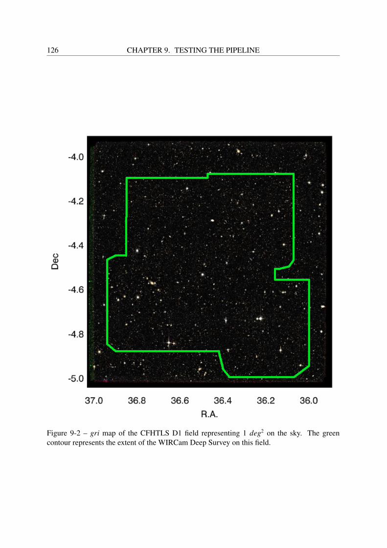
126 CHAPTER 9. TESTING THE PIPELINE
Figure 9-2 – gri map of the CFHTLS D1 field representing 1 deg2 on the sky. The greencontour represents the extent of the WIRCam Deep Survey on this field.
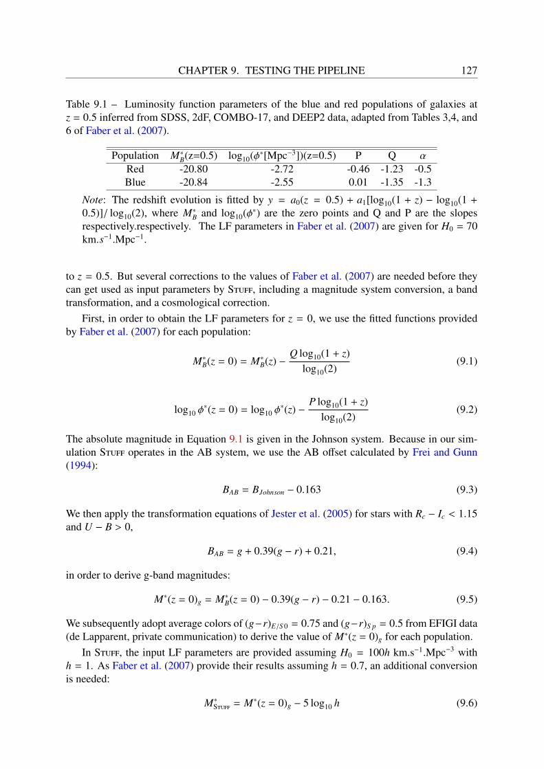
CHAPTER 9. TESTING THE PIPELINE 127
Table 9.1 – Luminosity function parameters of the blue and red populations of galaxies atz = 0.5 inferred from SDSS, 2dF, COMBO-17, and DEEP2 data, adapted from Tables 3,4, and6 of Faber et al. (2007).
Population M∗B(z=0.5) log10(φ∗[Mpc−3])(z=0.5) P Q α
Red -20.80 -2.72 -0.46 -1.23 -0.5Blue -20.84 -2.55 0.01 -1.35 -1.3
Note: The redshift evolution is fitted by y = a0(z = 0.5) + a1[log10(1 + z) − log10(1 +
0.5)]/ log10(2), where M∗B and log10(φ∗) are the zero points and Q and P are the slopes
respectively.respectively. The LF parameters in Faber et al. (2007) are given for H0 = 70km.s−1.Mpc−1.
to z = 0.5. But several corrections to the values of Faber et al. (2007) are needed before theycan get used as input parameters by Stuff, including a magnitude system conversion, a bandtransformation, and a cosmological correction.
First, in order to obtain the LF parameters for z = 0, we use the fitted functions providedby Faber et al. (2007) for each population:
M∗B(z = 0) = M∗
B(z) −Q log10(1 + z)
log10(2)(9.1)
log10 φ∗(z = 0) = log10 φ
∗(z) −P log10(1 + z)
log10(2)(9.2)
The absolute magnitude in Equation 9.1 is given in the Johnson system. Because in our sim-ulation Stuff operates in the AB system, we use the AB offset calculated by Frei and Gunn(1994):
BAB = BJohnson − 0.163 (9.3)
We then apply the transformation equations of Jester et al. (2005) for stars with Rc − Ic < 1.15and U − B > 0,
BAB = g + 0.39(g − r) + 0.21, (9.4)
in order to derive g-band magnitudes:
M∗(z = 0)g = M∗B(z = 0) − 0.39(g − r) − 0.21 − 0.163. (9.5)
We subsequently adopt average colors of (g−r)E/S 0 = 0.75 and (g−r)S p = 0.5 from EFIGI data(de Lapparent, private communication) to derive the value of M∗(z = 0)g for each population.
In Stuff, the input LF parameters are provided assuming H0 = 100h km.s−1.Mpc−3 withh = 1. As Faber et al. (2007) provide their results assuming h = 0.7, an additional conversionis needed:
M∗Stuff = M∗(z = 0)g − 5 log10 h (9.6)
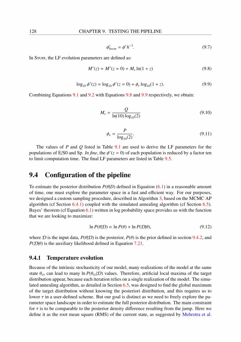
128 CHAPTER 9. TESTING THE PIPELINE
φ∗Stuff = φ∗h−3. (9.7)
In Stuff, the LF evolution parameters are defined as:
M∗(z) = M∗(z = 0) + Me ln(1 + z) (9.8)
log10 φ∗(z) = log10 φ
∗(z = 0) + φe log10(1 + z). (9.9)
Combining Equations 9.1 and 9.2 with Equations 9.8 and 9.9 respectively, we obtain:
Me =Q
ln(10) log10(2)(9.10)
φe =P
log10(2). (9.11)
The values of P and Q listed in Table 9.1 are used to derive the LF parameters for thepopulations of E/S0 and Sp. In fine, the φ∗(z = 0) of each population is reduced by a factor tento limit computation time. The final LF parameters are listed in Table 9.5.
9.4 Configuration of the pipelineTo estimate the posterior distribution P(θ|D) defined in Equation (6.1) in a reasonable amountof time, one must explore the parameter space in a fast and efficient way. For our purposes,we designed a custom sampling procedure, described in Algorithm 3, based on the MCMC APalgorithm (cf Section 6.4.1) coupled with the simulated annealing algorithm (cf Section 6.5).Bayes’ theorem (cf Equation 6.1) written in log probability space provides us with the functionthat we are looking to maximize:
ln P(θ|D) ∝ ln P(θ) + ln P(D|θ), (9.12)
whereD is the input data, P(θ|D) is the posterior, P(θ) is the prior defined in section 9.4.2, andP(D|θ) is the auxiliary likelihood defined in Equation 7.21.
9.4.1 Temperature evolutionBecause of the intrinsic stochasticity of our model, many realizations of the model at the samestate θ(t) can lead to many ln P(θ(t)|D) values. Therefore, artificial local maxima of the targetdistribution appear, because each iteration relies on a single realization of the model. The simu-lated annealing algorithm, as detailed in Section 6.5, was designed to find the global maximumof the target distribution without knowing the posteriori distribution, and this requires us tolower τ in a user-defined scheme. But our goal is distinct as we need to freely explore the pa-rameter space landscape in order to estimate the full posterior distribution. The main constraintfor τ is to be comparable to the posterior density difference resulting from the jump. Here wedefine it as the root mean square (RMS) of the current state, as suggested by Mehrotra et al.
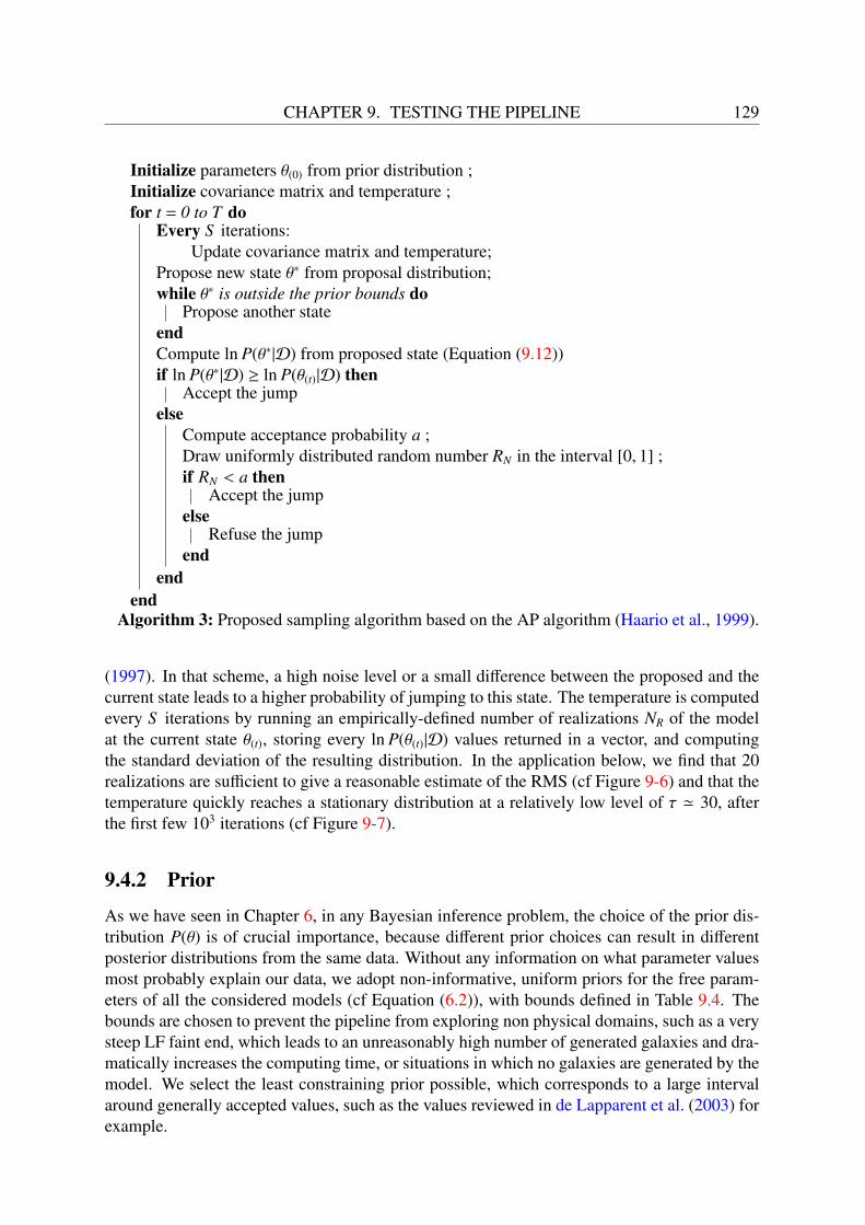
CHAPTER 9. TESTING THE PIPELINE 129
Initialize parameters θ(0) from prior distribution ;Initialize covariance matrix and temperature ;for t = 0 to T do
Every S iterations:Update covariance matrix and temperature;
Propose new state θ∗ from proposal distribution;while θ∗ is outside the prior bounds do
Propose another stateendCompute ln P(θ∗|D) from proposed state (Equation (9.12))if ln P(θ∗|D) ≥ ln P(θ(t)|D) then
Accept the jumpelse
Compute acceptance probability a ;Draw uniformly distributed random number RN in the interval [0, 1] ;if RN < a then
Accept the jumpelse
Refuse the jumpend
endend
Algorithm 3: Proposed sampling algorithm based on the AP algorithm (Haario et al., 1999).
(1997). In that scheme, a high noise level or a small difference between the proposed and thecurrent state leads to a higher probability of jumping to this state. The temperature is computedevery S iterations by running an empirically-defined number of realizations NR of the modelat the current state θ(t), storing every ln P(θ(t)|D) values returned in a vector, and computingthe standard deviation of the resulting distribution. In the application below, we find that 20realizations are sufficient to give a reasonable estimate of the RMS (cf Figure 9-6) and that thetemperature quickly reaches a stationary distribution at a relatively low level of τ ' 30, afterthe first few 103 iterations (cf Figure 9-7).
9.4.2 Prior
As we have seen in Chapter 6, in any Bayesian inference problem, the choice of the prior dis-tribution P(θ) is of crucial importance, because different prior choices can result in differentposterior distributions from the same data. Without any information on what parameter valuesmost probably explain our data, we adopt non-informative, uniform priors for the free param-eters of all the considered models (cf Equation (6.2)), with bounds defined in Table 9.4. Thebounds are chosen to prevent the pipeline from exploring non physical domains, such as a verysteep LF faint end, which leads to an unreasonably high number of generated galaxies and dra-matically increases the computing time, or situations in which no galaxies are generated by themodel. We select the least constraining prior possible, which corresponds to a large intervalaround generally accepted values, such as the values reviewed in de Lapparent et al. (2003) forexample.

130 CHAPTER 9. TESTING THE PIPELINE
9.4.3 Initialization of the chains
The initial state θ(0) of each chain is drawn randomly from the prior distribution. The initial po-sition will only affect the speed of convergence, because the final distribution shall not dependon the initial position, if the chain converges. The initial temperature is then computed fromthis state. As for the proposal distribution, it is initialized so that no direction in the parameterspace is preferred by the sampling algorithm at first. The initial covariance matrix is thereforediagonal, whose non-zero elements are set to:
Cii =ui − li
E∀i ∈ [1,Np], (9.13)
where ui and li are respectively the upper and lower bounds of the prior distribution for param-eter i, Np the number of parameters, and E a value set empirically to 200 in order to ensurereasonable acceptance rates at the beginning of the chain. According to Haario et al. (1999),the adaptive nature of the algorithm implies that the choice of E should not influence the outputof the chain.
9.4.4 Image simulation configuration
We simulate one stack of the Deep field in three bands: MegaCam u and i from the CFHTLS,and the WIRCam Ks, well-separated filters chosen in order to maximize the information on thestellar content of the mock galaxies. In fact, the u−band is appropriate to trace the emissionof young stellar populations, the Ks infrared band is relevant for the emission of old stellarpopulations, and i is an optical band with a mean wavelength at midpoint between the two otherfilters (cf Figure 4-3). In accordance with CFHTLS product conventions, the image exposuretime is normalized to one second and the AB magnitude zero-point is 30. The SkyMakerPSF model for the CFHTLS image is generated within the software. The aureole simulationstep (cf Section 5.2.1) is deactivated to speed up the image generation process. For the samereason, we exclude from the Stuff list all galaxies with apparent magnitudes in the referenceband brighter than 19 or fainter than 30, in order to avoid simulating both very large andvery numerous galaxies. There is no stellar contamination, as Stuff does not yet offer thepossibility to simulate realistic star fields. The overall characteristics of the simulated imagesare summarized in Table 9.2.
9.4.5 Source extraction configuration
SExtractor is configured according to the prescription of the T0007 CFHTLS release doc-umentation (Hudelot et al., 2012). We use it in double image mode, with the i-band imageas the detection image, and the background is estimated and subtracted automatically with a256×256-pixels background mesh size. In order to optimize the detectability of faint extendedsources, detection is performed on the images convolved with a 7×7 pixels Gaussian maskhaving a full width at half maximum (FWHM) of three pixels, that approximates the size ofthe PSF and acts as a matched filter. Finally, the detection threshold is set to 1.2 times the(unfiltered) RMS background noise above the local sky level.
In order for the results concerning faint sources near the detection limit not to depend tooclosely on the details of noise statistics, all negative fluxes and radii are clipped to 0 after
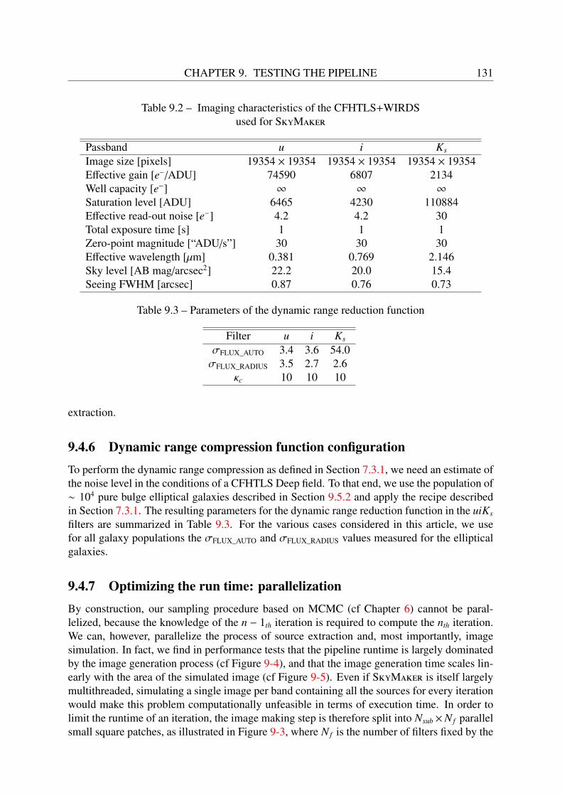
CHAPTER 9. TESTING THE PIPELINE 131
Table 9.2 – Imaging characteristics of the CFHTLS+WIRDSused for SkyMaker
Passband u i Ks
Image size [pixels] 19354 × 19354 19354 × 19354 19354 × 19354Effective gain [e−/ADU] 74590 6807 2134Well capacity [e−] ∞ ∞ ∞
Saturation level [ADU] 6465 4230 110884Effective read-out noise [e−] 4.2 4.2 30Total exposure time [s] 1 1 1Zero-point magnitude [“ADU/s”] 30 30 30Effective wavelength [µm] 0.381 0.769 2.146Sky level [AB mag/arcsec2] 22.2 20.0 15.4Seeing FWHM [arcsec] 0.87 0.76 0.73
Table 9.3 – Parameters of the dynamic range reduction function
Filter u i Ks
σFLUX_AUTO 3.4 3.6 54.0σFLUX_RADIUS 3.5 2.7 2.6
κc 10 10 10
extraction.
9.4.6 Dynamic range compression function configurationTo perform the dynamic range compression as defined in Section 7.3.1, we need an estimate ofthe noise level in the conditions of a CFHTLS Deep field. To that end, we use the population of∼ 104 pure bulge elliptical galaxies described in Section 9.5.2 and apply the recipe describedin Section 7.3.1. The resulting parameters for the dynamic range reduction function in the uiKs
filters are summarized in Table 9.3. For the various cases considered in this article, we usefor all galaxy populations the σFLUX_AUTO and σFLUX_RADIUS values measured for the ellipticalgalaxies.
9.4.7 Optimizing the run time: parallelizationBy construction, our sampling procedure based on MCMC (cf Chapter 6) cannot be paral-lelized, because the knowledge of the n − 1th iteration is required to compute the nth iteration.We can, however, parallelize the process of source extraction and, most importantly, imagesimulation. In fact, we find in performance tests that the pipeline runtime is largely dominatedby the image generation process (cf Figure 9-4), and that the image generation time scales lin-early with the area of the simulated image (cf Figure 9-5). Even if SkyMaker is itself largelymultithreaded, simulating a single image per band containing all the sources for every iterationwould make this problem computationally unfeasible in terms of execution time. In order tolimit the runtime of an iteration, the image making step is therefore split into Nsub ×N f parallelsmall square patches, as illustrated in Figure 9-3, where N f is the number of filters fixed by the

132 CHAPTER 9. TESTING THE PIPELINE
Table 9.4 – Uniform prior bounds for the parameters of the luminosity and size functions, andtheir evolution with redshift.
Parameter φ∗ M∗ α φe Me Mknee rknee γb
lower bound 10−7 -22 -2.5 -3 -2.5 -21 0 -2upper bound 10−2 -17 0 2 0 -19 3 0
Note: All the parameters above are given for H0 = 100 km.s−1.Mpc−3.
observed data and Nsub the user-defined number of patches per band. Both quantities must bechosen so that their product optimizes the resources used by the computing cluster.
We start with N f input catalogs generated from the model, each containing a list of sources’positions in a full-sized square field of size L f , as well as their photometric and size properties.The sources are then filtered according to their spatial coordinates and dispatched to theircorresponding patch. Each patch has a size L f /
√Nsub, where Nsub is a square number. In
practice, the sources are extracted from a box 150 pixels wider than the patch size in order toinclude the objects outside the frame that partially affect the simulated image. All the sourcesof position (x,y) are within a patch of coordinate (i, j) ∈ [0,
√Nsub − 1] × [0,
√Nsub − 1] if
x ∈ [i L f√
Nsub− 150, (i + 1) L f
√Nsub
+ 150], and y ∈ [ j L f√
Nsub− 150, ( j + 1) L f
√Nsub
+ 150].As a result, all the sources are scattered through Nsub catalog files per band. We then use
the HTCondor distributed jobs scheduler (e.g. Thain et al. 2005) on our computing clusterto generate and analyze all the patches at the same time. The flexibility of HTCondor offersmany advantages to a pipeline that requires distributed computing over long periods of time.Thanks to its dynamic framework, jobs can be check pointed and resumed after being migratedif a node of the cluster becomes unavailable, and the scheduler efficiently provides an efficientmatch-making between the required and the available resources. This framework also has itsdrawbacks, in the form of inherent and uncontrollable latencies when jobs input files are sentto the various nodes.
In our case, each job corresponds to a single patch, and the Nsub×N f resulting catalogs serveas input files for the jobs. We found that HTCondor latencies represent between 7% and 50%of the run time of each iteration, as illustrated in Figure 9-4 in the context of the applicationdescribed below (cf Section 9.5).
For each job, the image generation and source extraction procedures are multiprocessed:SkyMaker is first launched simultaneously in every band on the L f /
√Nsub-sized patch and,
when all the images are available, SExtractor is launched in double image mode (cf Section5.3) in order to extract color information of detected galaxies. HTCondor then waits until alljobs are completed. Finally, the catalog files generated from all the patches are merged intoone, so that in fine, a single catalog file per band contains all the extracted sources.
9.5 Tests with one and two galaxy populations
9.5.1 Multi-type configuration: luminosity evolution
The simulated image used as input data contains two populations of galaxies generated byStuff: E/S0 and Sp, whose luminosity function has been defined in Section 9.3. The B/T ratiosin the g adopted reference band are determined using the distribution of B/T in g-band as a

CHAPTER 9. TESTING THE PIPELINE 133
ui
Ku
iK
ui
K
ui
K
ui
K
ui
K
STUFF Catalogs(x,y,M,...)
Patch catalogs(x,y,M,...)
SExtractor catalogs(x,y,FLUX,FLAG)
Skymaker SExtractor
u
i
u
K
u
i
K
...
Detect
32.5 42.1 124.6 012.6 23.1 359.1 378.1 98.3 622.6 2...
Multiproc
CONDOR
Figure 9-3 – Illustration of the parallelization process of our pipeline, described in detail inSection 9.4.7. Stuff generates a catalog, that is, a set of files containing the properties of sim-ulated galaxies, such as inclination, bulge-to-disk ratio, apparent size, and luminosity. Eachfile lists the same galaxies in a different passband. The parallelization process is performedon two levels: first, the Stuff catalogs are split into sub-catalogs according to the positions ofthe sources on the image. These sub-catalogs are sent to the nodes of the computer cluster inall filters at the same time using the HTCondor framework. Each sub-catalog is then used togenerate a multiband image corresponding to a fraction of the total field. This step is multi-processed in order to generate the patches in every band simultaneously. SExtractor is thenlaunched on every patch synchronously, also using multiprocessing. The source detection isdone in one pre-defined band, and the photometry is done in every band. Finally, the SExtrac-tor catalogs generated from all the patches are merged into one large catalog containing thephotometric and size parameters of the extracted sources from the entire field.
Table 9.5 – Characteristics of the galaxy test populations
Population S EDba S EDd φ∗ [h3Mpc−3] M∗ α φe Me B/T T b α(T ) N c
Multi-type: E/S0 E E 0.003 -19.97 -0.5 -1.53 -1.77 0.65 -5 0.0 10447Multi-type: Sp E Scd 1.4e-4 -19.84 -1.3 0.03 -1.95 0.2 6 1.47 28281
Fattening E E E 0.0035 -19.97 -0.5 -1.53 -1.77 1.0 -5 0.0 11353
Notes: The LF parameters are given for H0 = 100 km.s−1.Mpc−3.a The bulge and disk SEDs are Coleman et al. (1980) templates.b de Vaucouleurs (1959) revised morphological type.c Number of sources generated by one realization of Stuff.
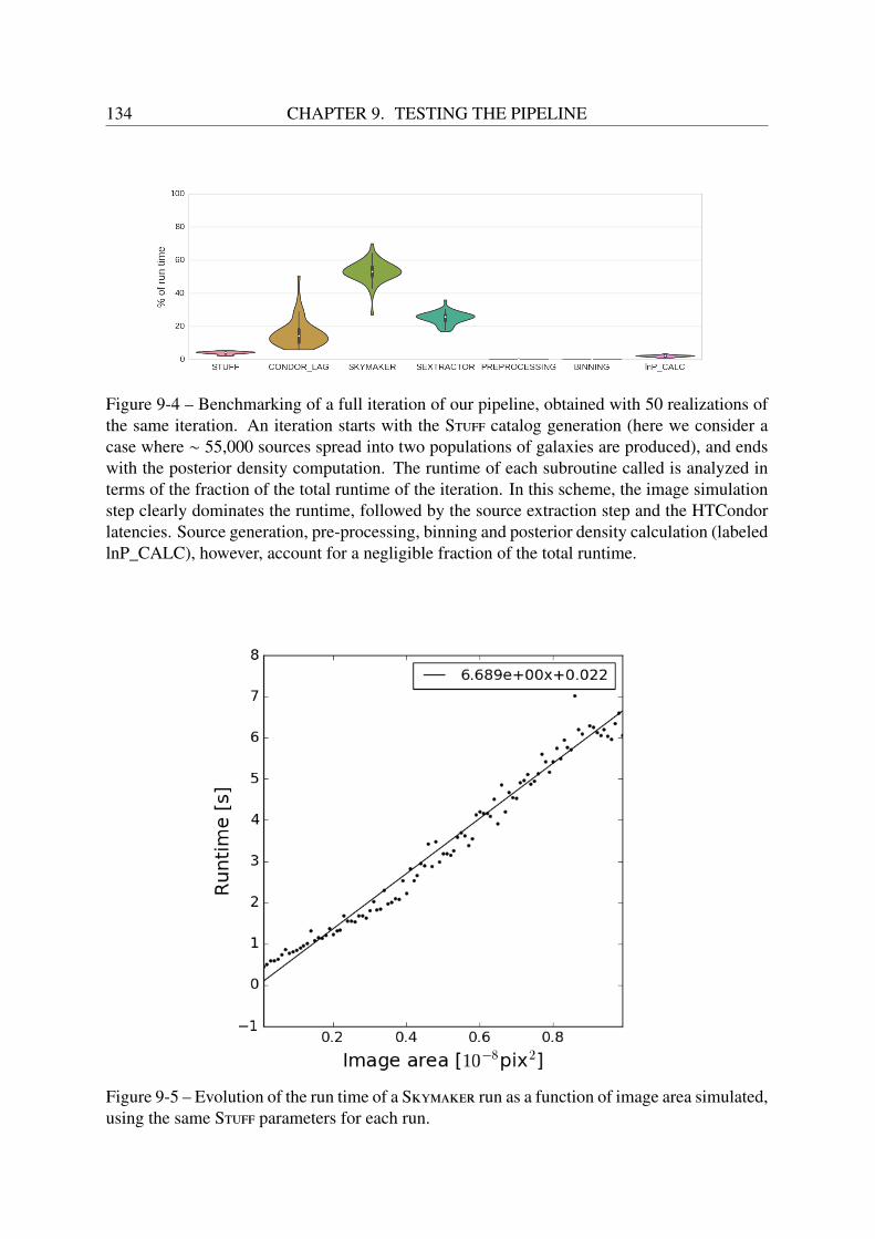
134 CHAPTER 9. TESTING THE PIPELINE
Figure 9-4 – Benchmarking of a full iteration of our pipeline, obtained with 50 realizations ofthe same iteration. An iteration starts with the Stuff catalog generation (here we consider acase where ∼ 55,000 sources spread into two populations of galaxies are produced), and endswith the posterior density computation. The runtime of each subroutine called is analyzed interms of the fraction of the total runtime of the iteration. In this scheme, the image simulationstep clearly dominates the runtime, followed by the source extraction step and the HTCondorlatencies. Source generation, pre-processing, binning and posterior density calculation (labeledlnP_CALC), however, account for a negligible fraction of the total runtime.
Figure 9-5 – Evolution of the run time of a Skymaker run as a function of image area simulated,using the same Stuff parameters for each run.
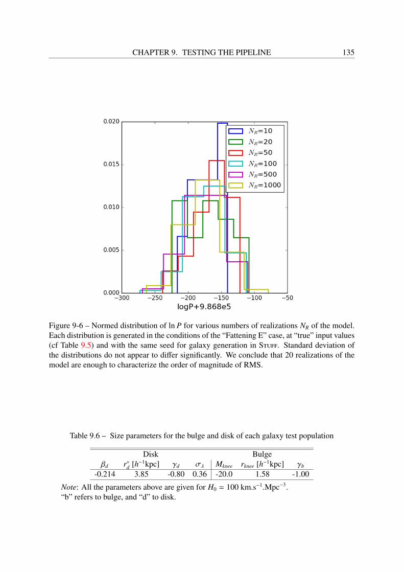
CHAPTER 9. TESTING THE PIPELINE 135
Figure 9-6 – Normed distribution of ln P for various numbers of realizations NR of the model.Each distribution is generated in the conditions of the “Fattening E” case, at “true” input values(cf Table 9.5) and with the same seed for galaxy generation in Stuff. Standard deviation ofthe distributions do not appear to differ significantly. We conclude that 20 realizations of themodel are enough to characterize the order of magnitude of RMS.
Table 9.6 – Size parameters for the bulge and disk of each galaxy test population
Disk Bulgeβd r∗d [h−1kpc] γd σλ Mknee rknee [h−1kpc] γb
-0.214 3.85 -0.80 0.36 -20.0 1.58 -1.00
Note: All the parameters above are given for H0 = 100 km.s−1.Mpc−3.“b” refers to bulge, and “d” to disk.
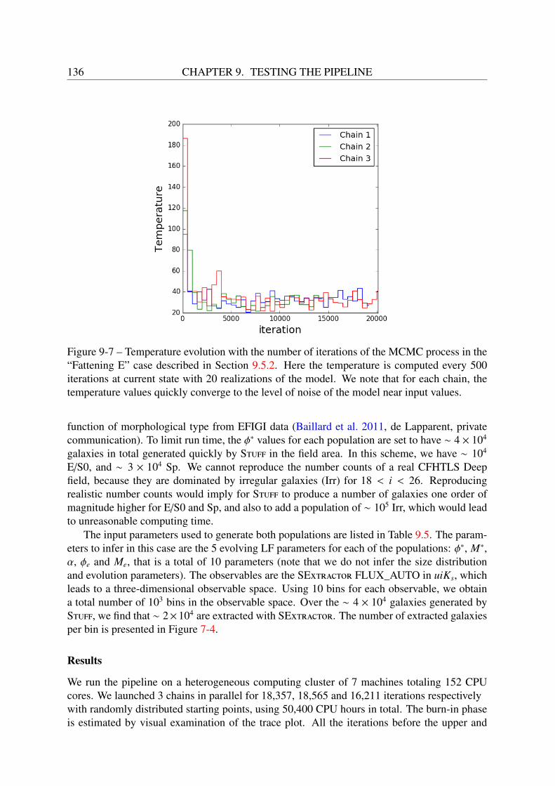
136 CHAPTER 9. TESTING THE PIPELINE
Figure 9-7 – Temperature evolution with the number of iterations of the MCMC process in the“Fattening E” case described in Section 9.5.2. Here the temperature is computed every 500iterations at current state with 20 realizations of the model. We note that for each chain, thetemperature values quickly converge to the level of noise of the model near input values.
function of morphological type from EFIGI data (Baillard et al. 2011, de Lapparent, privatecommunication). To limit run time, the φ∗ values for each population are set to have ∼ 4 × 10⁴
galaxies in total generated quickly by Stuff in the field area. In this scheme, we have ∼ 104
E/S0, and ∼ 3 × 10⁴ Sp. We cannot reproduce the number counts of a real CFHTLS Deepfield, because they are dominated by irregular galaxies (Irr) for 18 < i < 26. Reproducingrealistic number counts would imply for Stuff to produce a number of galaxies one order ofmagnitude higher for E/S0 and Sp, and also to add a population of ∼ 105 Irr, which would leadto unreasonable computing time.
The input parameters used to generate both populations are listed in Table 9.5. The param-eters to infer in this case are the 5 evolving LF parameters for each of the populations: φ∗, M∗,α, φe and Me, that is a total of 10 parameters (note that we do not infer the size distributionand evolution parameters). The observables are the SExtractor FLUX_AUTO in uiKs, whichleads to a three-dimensional observable space. Using 10 bins for each observable, we obtaina total number of 103 bins in the observable space. Over the ∼ 4 × 10⁴ galaxies generated byStuff, we find that ∼ 2×10⁴ are extracted with SExtractor. The number of extracted galaxiesper bin is presented in Figure 7-4.
Results
We run the pipeline on a heterogeneous computing cluster of 7 machines totaling 152 CPUcores. We launched 3 chains in parallel for 18,357, 18,565 and 16,211 iterations respectivelywith randomly distributed starting points, using 50,400 CPU hours in total. The burn-in phaseis estimated by visual examination of the trace plot. All the iterations before the upper and
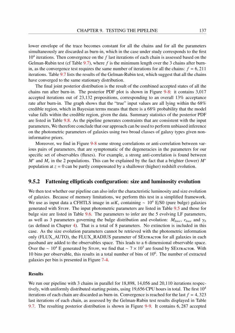
CHAPTER 9. TESTING THE PIPELINE 137
lower envelope of the trace becomes constant for all the chains and for all the parameterssimultaneously are discarded as burn-in, which in the case under study corresponds to the first104 iterations. Then convergence on the f last iterations of each chain is assessed based on theGelman-Rubin test (cf Table 9.7), where f is the minimum length over the 3 chains after burn-in, as the convergence test requires the same number of iterations for all the chains: f = 6, 211iterations. Table 9.7 lists the results of the Gelman-Rubin test, which suggest that all the chainshave converged to the same stationary distribution.
The final joint posterior distribution is the result of the combined accepted states of all thechains run after burn-in. The posterior PDF plot is shown in Figure 9-8: it contains 3,017accepted iterations out of 23,132 propositions, corresponding to an overall 13% acceptancerate after burn-in. The graph shows that the “true” input values are all lying within the 68%credible region, which in Bayesian terms means that there is a 68% probability that the modelvalue falls within the credible region, given the data. Summary statistics of the posterior PDFare listed in Table 9.8. As the pipeline generates constraints that are consistent with the inputparameters, We therefore conclude that our approach can be used to perform unbiased inferenceon the photometric parameters of galaxies using two broad classes of galaxy types given non-informative priors.
Moreover, we find in Figure 9-8 some strong correlations or anti-correlation between var-ious pairs of parameters, that are symptomatic of the degeneracies in the parameters for ourspecific set of observables (fluxes). For example, a strong anti-correlation is found betweenM∗ and Me in the 2 populations. This can be explained by the fact that a brighter (lower) M∗
population at z = 0 can be partly compensated by a shallower (higher) redshift evolution.
9.5.2 Fattening ellipticals configuration: size and luminosity evolution
We then test whether our pipeline can also infer the characteristic luminosity and size evolutionof galaxies. Because of memory limitations, we perform this test in a simplified framework.We use as input data a CFHTLS image in uiKs containing ∼ 104 E/S0 (pure bulge) galaxiesgenerated with Stuff. The input photometric parameters are listed in Table 9.5 and those forbulge size are listed in Table 9.6. The parameters to infer are the 5 evolving LF parameters,as well as 3 parameters governing the bulge distribution and evolution: Mknee, rknee and γb
(as defined in Chapter 4). That is a total of 8 parameters. No extinction is included in thiscase. As the size evolution parameters cannot be retrieved with the photometric informationonly (FLUX_AUTO), the FLUX_RADIUS parameter of SExtractor for all galaxies in eachpassband are added to the observables space. This leads to a 6 dimensional observable space.Over the ∼ 104 E generated by Stuff, we find that ∼ 7 × 10³ are found by SExtractor. With10 bins per observable, this results in a total number of bins of 106. The number of extractedgalaxies per bin is presented in Figure 7-4.
Results
We run our pipeline with 3 chains in parallel for 18,898, 14,056 and 20,110 iterations respec-tively, with uniformly distributed starting points, using 19,656 CPU hours in total. The first 104
iterations of each chain are discarded as burn-in. Convergence is reached for the last f = 4, 323last iterations of each chain, as assessed by the Gelman-Rubin test results displayed in Table9.7. The resulting posterior distribution is shown in Figure 9-9. It contains 6, 287 accepted
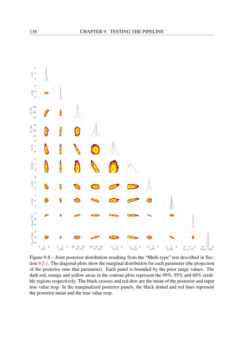
138 CHAPTER 9. TESTING THE PIPELINE
Figure 9-8 – Joint posterior distribution resulting from the “Multi-type” test described in Sec-tion 9.5.1. The diagonal plots show the marginal distribution for each parameter (the projectionof the posterior onto that parameter). Each panel is bounded by the prior range values. Thedark red, orange and yellow areas in the contour plots represent the 99%, 95% and 68% credi-ble regions respectively. The black crosses and red dots are the mean of the posterior and inputtrue value resp. In the marginalized posterior panels, the black dotted and red lines representthe posterior mean and the true value resp.
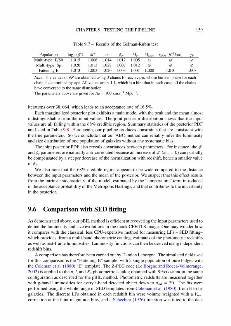
CHAPTER 9. TESTING THE PIPELINE 139
Table 9.7 – Results of the Gelman-Rubin test
Population log10(φ∗) M∗ α φe Me Mknee rknee [h−1kpc] γb
Multi-type: E/S0 1.015 1.006 1.014 1.012 1.005 ∅ ∅ ∅
Multi-type: Sp 1.020 1.013 1.028 1.007 1.012 ∅ ∅ ∅
Fattening E 1.013 1.003 1.020 1.003 1.001 1.008 1.010 1.008
Note: The values of√
R are obtained using 3 chains for each case, whose burn-in phase for eachchain is determined by eye. All values are < 1.1, which is a hint that in each case, all the chainshave converged to the same distribution.The parameters above are given for H0 = 100 km.s−1.Mpc−3.
iterations over 38, 064, which leads to an acceptance rate of 16.5%.Each marginalized posterior plot exhibits a main mode, with the peak and the mean almost
indistinguishable from the input values. The joint posterior distribution shows that the inputvalues are all falling within the 68% credible region. Summary statistics of the posterior PDFare listed in Table 9.8. Here again, our pipeline produces constraints that are consistent withthe true parameters. So we conclude that our ABC method can reliably infer the luminosityand size distribution of one population of galaxies without any systematic bias.
The joint posterior PDF also reveals covariances between parameters. For instance, the φ∗
and φe parameters are naturally anti-correlated because an increase of φ∗ (at z = 0) can partiallybe compensated by a steeper decrease of the normalization with redshift, hence a smaller valueof φe.
We also note that the 68% credible region appears to be wide compared to the distancebetween the input parameters and the mean of the posterior. We suspect that this effect resultsfrom the intrinsic stochasticity of the model, estimated by the “temperature” term introducedin the acceptance probability of the Metropolis Hastings, and that contributes to the uncertaintyin the posterior.
9.6 Comparison with SED fitting
As demonstrated above, our pBIL method is efficient at recovering the input parameters used todefine the luminosity and size evolutions in the mock CFHTLS image. One may wonder howit compares with the classical, less CPU-expensive method for measuring LFs – SED fitting–which provides, from a multi-band photometric catalog, estimates of the photometric redshiftsas well as rest-frame luminosities. Luminosity functions can then be derived using independentredshift bins.
A comparison has therefore been carried out by Damien Leborgne. The simulated field usedfor this comparison is the “Fattening E” sample, with a single population of pure bulges withthe Coleman et al. (1980) “E” template. The Z-PEG code (Le Borgne and Rocca-Volmerange,2002) is applied to the u, i, and Ks photometric catalog obtained with SExtractor in the sameconfiguration as described for the pBIL method. Photometric redshifts are measured togetherwith g-band luminosities for every i-band detected object down to uAB = 30. The fits wereperformed using the whole range of SED templates from Coleman et al. (1980), from E to Irrgalaxies. The discrete LFs obtained in each redshift bin were volume weighted with a Vmax
correction at the faint magnitude bins, and a Schechter (1976) function was fitted to the data
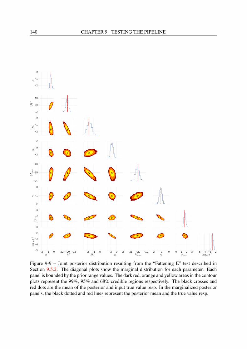
140 CHAPTER 9. TESTING THE PIPELINE
Figure 9-9 – Joint posterior distribution resulting from the “Fattening E” test described inSection 9.5.2. The diagonal plots show the marginal distribution for each parameter. Eachpanel is bounded by the prior range values. The dark red, orange and yellow areas in the contourplots represent the 99%, 95% and 68% credible regions respectively. The black crosses andred dots are the mean of the posterior and input true value resp. In the marginalized posteriorpanels, the black dotted and red lines represent the posterior mean and the true value resp.

CHAPTER 9. TESTING THE PIPELINE 141
Table 9.8 – Summary statistics on the marginalized posterior distributions for the galaxy testpopulations and comparison with the input values.
Population Parameters Input value Mean MAP a 68% interval 95% interval 99% intervallog10(φ∗) -2.52 -2.56 −2.57 [-2.72,-2.40] [-2.85,-2.29] [-2.95,-2.19]
M∗ -19.97 -20.15 −20.12 [-20.54,-19.74] [-20.95,-19.38] [-21.20,-19.08]Multi-type: E/S0 α -0.5 -0.53 −0.54 [-0.68,-0.43] [-0.77,-0.24] [-0.82,-0.06]
φe -1.53 -1.48 −1.37 [-1.82,-1.15] [-2.16,-0.81] [-2.35,-0.49]Me -1.77 -1.66 −1.70 [-1.99,-1.29] [-2.36,-0.96] [-2.46,-0.75]
log10(φ∗) -3.85 -3.93 −3.96 [-4.15,-3.67] [-4.35,-3.54] [-4.53,-3.40]M∗ -19.84 -20.18 −19.81 [-20.68,-19.43] [-21.59,-19.01] [-21.93,-18.84]
Multi-type: Sp α -1.3 -1.30 −1.33 [-1.37,-1.25] [-1.42,-1.17] [-1.44,-1.13]φe 0.03 0.18 0.15 [-0.16,0.47] [-0.34,0.75] [-0.48,0.94]Me -1.95 -1.68 −1.81 [-2.39,-1.29] [-2.49,-0.87] [-2.49,-0.19]
log10(φ∗) -2.46 -2.46 −2.51 [-2.60,-2.31] [-2.75,-2.18] [-2.84,-2.08]M∗ -19.97 -20.04 −20.08 [-20.41,-19.63] [-20.84,-19.23] [-21.15,-19.12]α -0.5 -0.49 −0.51 [-0.62,-0.40] [-0.72,-0.25] [-0.78,-0.13]φe -1.53 -1.49 −1.56 [-1.84,-1.09] [-2.22,-0.74] [-2.41,-0.49]
Fattening E Me -1.77 -1.65 −1.61 [-2.04,-1.29] [-2.35,-0.96] [-2.47,-0.73]Mknee -20.00 -20.10 −19.99 [-20.32,-19.79] [-20.68,-19.58] [-20.90,-19.46]rknee 1.58 1.64 1.56 [1.47,1.77] [1.34,1.97] [1.27,2.09]γb -1.00 -1.03 −1.07 [-1.18,-0.87] [-1.31,-0.71] [-1.50,-0.65]
Notes:The LF parameters are given for H0 = 100 km.s−1.Mpc−3.a Maximum A Posteriori
independently in each redshift bin with a Levenberg-Marquardt algorithm with Φ∗, M∗, and αas free parameters.
Comparison of the evolution with redshift of the LF parameters between the pBIL approach(green dashed line for mean of posterior, and 68% light green shaded region) and the resultsfrom SED fitting (red symbols with error bars) are shown in Figure 9-10. As expected, theyboth roughly follow the trends set by the evolution of the input parameters (blue solid line),with some offsets that can be explained by the fact that SED fitting is done on only threephotometric bands. This is clearly a major limiting factor, albeit partly compensated by thechoice of the SED templates: the input SED and the templates share a common SED (the “E”SED, even if all SEDs from Coleman et al. (1980) are also used for the SED fitting). We believethat this choice is fair because in the pBIL method, the same set of SEDs was also used for datageneration and for the inference of LF parameters.
The significant systematic offset in α from SED fitting compared to the input and pBILcurves in Figure 9-10 shows that the faint-end slope parameters α is poorly estimated, with asignificant systematic offset at z ≥ 0.7. This is caused by the negative input slope (see Table9.5), which yields few faint galaxies in the sample. Moreover, because of numerous catas-trophic outliers in the photometric redshifts (caused by the u,i, Ks-only photometric catalog),there is a mismatch between the true redshift of many faint objects and the redshift bin to whichthey are assigned. This leads to an underestimate of the error bars on the individual points.
For this comparison of the LF parameters between the two approaches, we had to derivethe envelop of the LF parameters as a function of redshift for the trace elements of the MCMCchains within the 68% credible region of the parameters space. Of course, the area appears inFigure 9-10 as much smoother than the individual points derived from SED fitting because thechosen LF model for the inference evolves smoothly with redshift. Still, it is remarkable that

142 CHAPTER 9. TESTING THE PIPELINE
the region is tight and almost centered on the values of the true parameters at all redshifts. Thisis because the various covariances between the five LF parameters of the model tend to narrowdown the shaded areas in these graphs, therefore implying that galaxies at all redshifts in theimages contribute to constrain the parameters of the model in the pBIL approach.
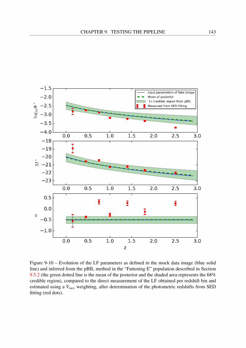
CHAPTER 9. TESTING THE PIPELINE 143
Figure 9-10 – Evolution of the LF parameters as defined in the mock data image (blue solidline) and inferred from the pBIL method in the “Fattening E” population described in Section9.5.2 (the green dotted line is the mean of the posterior and the shaded area represents the 68%credible region), compared to the direct measurement of the LF obtained per redshift bin andestimated using a Vmax weighting, after determination of the photometric redshifts from SEDfitting (red dots).

144 CHAPTER 9. TESTING THE PIPELINE

Chapter 10
Improving the pipeline
We have a method, and that methodhelps us to reach not absolute truth, onlyasymptotic approaches to the truth -never there, just closer and closer,always finding vast new oceans ofundiscovered possibilities. Cleverlydesigned experiments are the key.
Carl Sagan, ’Wonder and Skepticism’,Skeptical Enquirer (Jan-Feb 1995)
Abstract
Due to the high computational cost of running our pipeline over large periods oftime, we need to minimize the time spent on each iteration and ensure that theMarkov chains quickly reach their target distribution before considering applyingit to real observations. We also need to simulate more realistic images by usingthe PSF measured on observed data, by reproducing the small and large-scalesproperties of background noise that arise in observed astronomical survey images,and by improving the dust extinction properties of our model. In this chapter, Iexplore some of the ways we can make the pipeline faster, more reliable and moreefficient, and implement some of them.
Contents10.1 Updating the parallelization strategy . . . . . . . . . . . . . . . . . . . . . 146
10.2 Simulating more realistic images . . . . . . . . . . . . . . . . . . . . . . . 146
10.2.1 Including noise correlation . . . . . . . . . . . . . . . . . . . . . . . 146
10.2.2 Including weight maps . . . . . . . . . . . . . . . . . . . . . . . . . 150
10.2.3 Using the measured PSF on image simulations . . . . . . . . . . . . 153
10.3 Implementing a more realistic dust treatment . . . . . . . . . . . . . . . . 155
10.3.1 Adding Galactic extinction to Stuff magnitudes . . . . . . . . . . . . 155
145
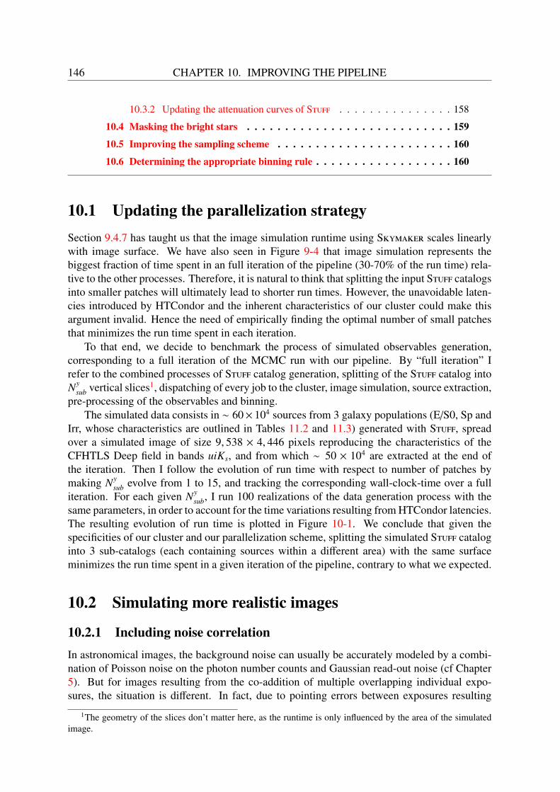
146 CHAPTER 10. IMPROVING THE PIPELINE
10.3.2 Updating the attenuation curves of Stuff . . . . . . . . . . . . . . . 158
10.4 Masking the bright stars . . . . . . . . . . . . . . . . . . . . . . . . . . . 159
10.5 Improving the sampling scheme . . . . . . . . . . . . . . . . . . . . . . . 160
10.6 Determining the appropriate binning rule . . . . . . . . . . . . . . . . . . 160
10.1 Updating the parallelization strategySection 9.4.7 has taught us that the image simulation runtime using Skymaker scales linearlywith image surface. We have also seen in Figure 9-4 that image simulation represents thebiggest fraction of time spent in an full iteration of the pipeline (30-70% of the run time) rela-tive to the other processes. Therefore, it is natural to think that splitting the input Stuff catalogsinto smaller patches will ultimately lead to shorter run times. However, the unavoidable laten-cies introduced by HTCondor and the inherent characteristics of our cluster could make thisargument invalid. Hence the need of empirically finding the optimal number of small patchesthat minimizes the run time spent in each iteration.
To that end, we decide to benchmark the process of simulated observables generation,corresponding to a full iteration of the MCMC run with our pipeline. By “full iteration” Irefer to the combined processes of Stuff catalog generation, splitting of the Stuff catalog intoNy
sub vertical slices1, dispatching of every job to the cluster, image simulation, source extraction,pre-processing of the observables and binning.
The simulated data consists in ∼ 60× 104 sources from 3 galaxy populations (E/S0, Sp andIrr, whose characteristics are outlined in Tables 11.2 and 11.3) generated with Stuff, spreadover a simulated image of size 9, 538 × 4, 446 pixels reproducing the characteristics of theCFHTLS Deep field in bands uiKs, and from which ∼ 50 × 104 are extracted at the end ofthe iteration. Then I follow the evolution of run time with respect to number of patches bymaking Ny
sub evolve from 1 to 15, and tracking the corresponding wall-clock-time over a fulliteration. For each given Ny
sub, I run 100 realizations of the data generation process with thesame parameters, in order to account for the time variations resulting from HTCondor latencies.The resulting evolution of run time is plotted in Figure 10-1. We conclude that given thespecificities of our cluster and our parallelization scheme, splitting the simulated Stuff cataloginto 3 sub-catalogs (each containing sources within a different area) with the same surfaceminimizes the run time spent in a given iteration of the pipeline, contrary to what we expected.
10.2 Simulating more realistic images
10.2.1 Including noise correlationIn astronomical images, the background noise can usually be accurately modeled by a combi-nation of Poisson noise on the photon number counts and Gaussian read-out noise (cf Chapter5). But for images resulting from the co-addition of multiple overlapping individual expo-sures, the situation is different. In fact, due to pointing errors between exposures resulting
1The geometry of the slices don’t matter here, as the runtime is only influenced by the area of the simulatedimage.
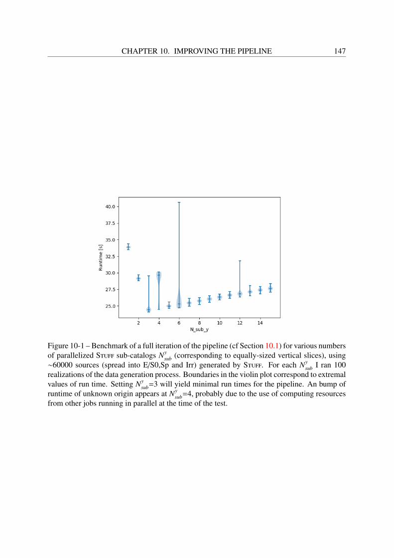
CHAPTER 10. IMPROVING THE PIPELINE 147
Figure 10-1 – Benchmark of a full iteration of the pipeline (cf Section 10.1) for various numbersof parallelized Stuff sub-catalogs Ny
sub (corresponding to equally-sized vertical slices), using∼60000 sources (spread into E/S0,Sp and Irr) generated by Stuff. For each Ny
sub I ran 100realizations of the data generation process. Boundaries in the violin plot correspond to extremalvalues of run time. Setting Ny
sub=3 will yield minimal run times for the pipeline. An bump ofruntime of unknown origin appears at Ny
sub=4, probably due to the use of computing resourcesfrom other jobs running in parallel at the time of the test.
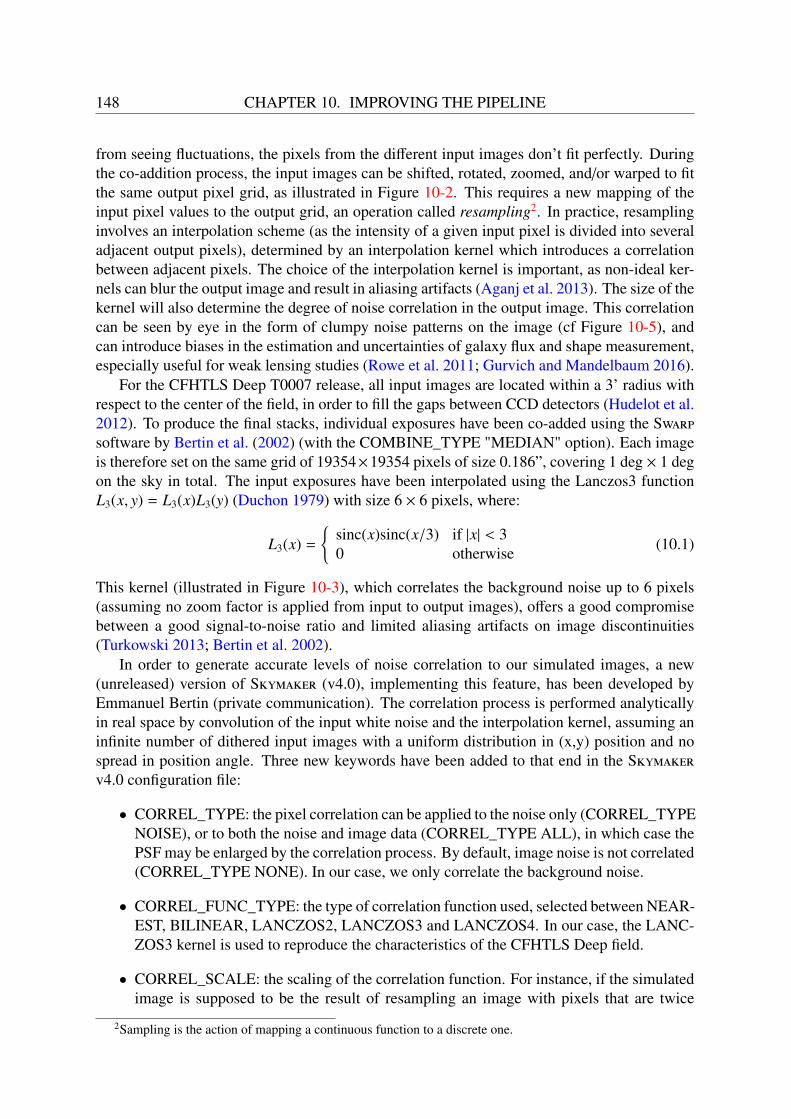
148 CHAPTER 10. IMPROVING THE PIPELINE
from seeing fluctuations, the pixels from the different input images don’t fit perfectly. Duringthe co-addition process, the input images can be shifted, rotated, zoomed, and/or warped to fitthe same output pixel grid, as illustrated in Figure 10-2. This requires a new mapping of theinput pixel values to the output grid, an operation called resampling2. In practice, resamplinginvolves an interpolation scheme (as the intensity of a given input pixel is divided into severaladjacent output pixels), determined by an interpolation kernel which introduces a correlationbetween adjacent pixels. The choice of the interpolation kernel is important, as non-ideal ker-nels can blur the output image and result in aliasing artifacts (Aganj et al. 2013). The size of thekernel will also determine the degree of noise correlation in the output image. This correlationcan be seen by eye in the form of clumpy noise patterns on the image (cf Figure 10-5), andcan introduce biases in the estimation and uncertainties of galaxy flux and shape measurement,especially useful for weak lensing studies (Rowe et al. 2011; Gurvich and Mandelbaum 2016).
For the CFHTLS Deep T0007 release, all input images are located within a 3’ radius withrespect to the center of the field, in order to fill the gaps between CCD detectors (Hudelot et al.2012). To produce the final stacks, individual exposures have been co-added using the Swarpsoftware by Bertin et al. (2002) (with the COMBINE_TYPE "MEDIAN" option). Each imageis therefore set on the same grid of 19354×19354 pixels of size 0.186”, covering 1 deg × 1 degon the sky in total. The input exposures have been interpolated using the Lanczos3 functionL3(x, y) = L3(x)L3(y) (Duchon 1979) with size 6 × 6 pixels, where:
L3(x) =
sinc(x)sinc(x/3) if |x| < 30 otherwise (10.1)
This kernel (illustrated in Figure 10-3), which correlates the background noise up to 6 pixels(assuming no zoom factor is applied from input to output images), offers a good compromisebetween a good signal-to-noise ratio and limited aliasing artifacts on image discontinuities(Turkowski 2013; Bertin et al. 2002).
In order to generate accurate levels of noise correlation to our simulated images, a new(unreleased) version of Skymaker (v4.0), implementing this feature, has been developed byEmmanuel Bertin (private communication). The correlation process is performed analyticallyin real space by convolution of the input white noise and the interpolation kernel, assuming aninfinite number of dithered input images with a uniform distribution in (x,y) position and nospread in position angle. Three new keywords have been added to that end in the Skymakerv4.0 configuration file:
• CORREL_TYPE: the pixel correlation can be applied to the noise only (CORREL_TYPENOISE), or to both the noise and image data (CORREL_TYPE ALL), in which case thePSF may be enlarged by the correlation process. By default, image noise is not correlated(CORREL_TYPE NONE). In our case, we only correlate the background noise.
• CORREL_FUNC_TYPE: the type of correlation function used, selected between NEAR-EST, BILINEAR, LANCZOS2, LANCZOS3 and LANCZOS4. In our case, the LANC-ZOS3 kernel is used to reproduce the characteristics of the CFHTLS Deep field.
• CORREL_SCALE: the scaling of the correlation function. For instance, if the simulatedimage is supposed to be the result of resampling an image with pixels that are twice
2Sampling is the action of mapping a continuous function to a discrete one.
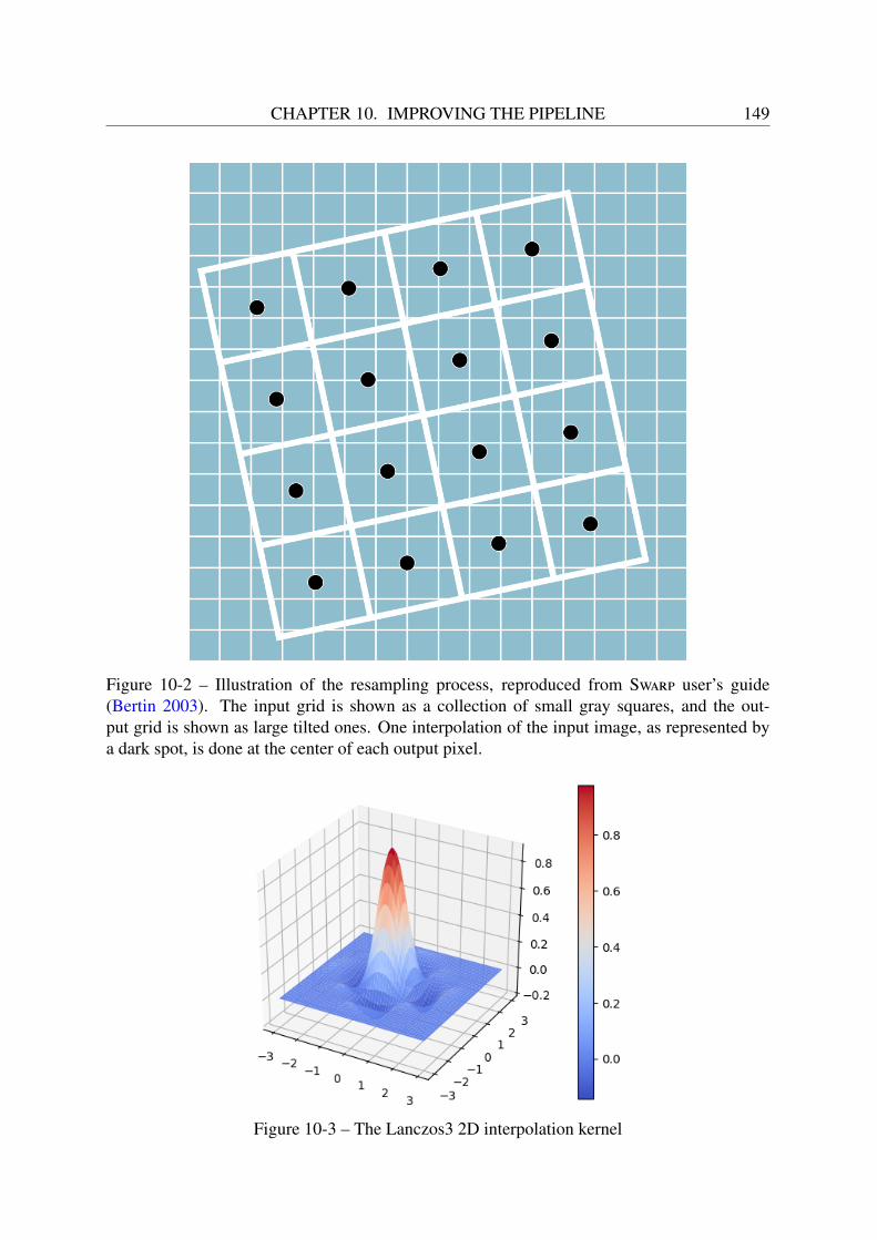
CHAPTER 10. IMPROVING THE PIPELINE 149
Figure 10-2 – Illustration of the resampling process, reproduced from Swarp user’s guide(Bertin 2003). The input grid is shown as a collection of small gray squares, and the out-put grid is shown as large tilted ones. One interpolation of the input image, as represented bya dark spot, is done at the center of each output pixel.
Figure 10-3 – The Lanczos3 2D interpolation kernel

150 CHAPTER 10. IMPROVING THE PIPELINE
Figure 10-4 – Comparison between an observed image in Ks band from the WIRDS survey(left) and a simulated WIRDS image of the same size (370 × 370 pixels), generated by Sky-maker with the correlated noise generation feature (right). Both images display the same in-tensity scaling. The same level of granularity can be seen in the background noise of bothimages.
larger, CORREL_SCALE should be set to 2.0. In CFHTLS stacks, no zoom is appliedon individual exposures, so I set CORREL_SCALE to 1.0 in ugriz. However, in orderto fit WIRDS images obtained with the WIRCAM instrument, whose pixel size is 0.3”(Bielby et al. 2012), to the same pixel grid as CFHTLS Deep images, whose pixel size is0.186”, CORREL_SCALE should be set to 0.3”/0.186”=1.613 in JHKs.
As illustrated in Figure 10-4, the noise correlation introduced on simulated images is vi-sually almost indistinguishable from the noise of real data, when attested by the level of noisegranularity. We also note that this new feature has a negligible cost on the image simulationprocess in terms of computing time and memory usage.
10.2.2 Including weight mapsOver a co-added science image, not all pixels are born equal: some are noisier than others.This can be due to inherent discrepancies of quantum efficiency in the pixel matrix of the CCDsensor, gaps between detectors and vignetting caused by unequal effective exposure time, orother external factors such as satellite tracks, cosmic rays, or saturation trails (Erben et al.2005). The resulting structure of the variable noise level over the co-added image can becomplex, especially when using multidetector (mosaic) cameras creating composite images,such as MegaCam. Hence, a co-added survey image is usually provided with a weight map foreach band, i.e. a FITS image with the same dimensions as the survey image, computed from anormalized flat field and displaying the noise level of each pixel, usually expressed in units of
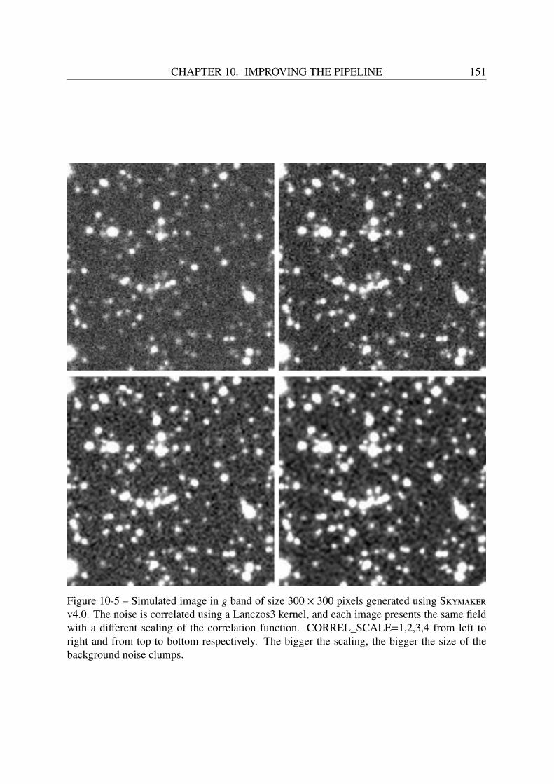
CHAPTER 10. IMPROVING THE PIPELINE 151
Figure 10-5 – Simulated image in g band of size 300 × 300 pixels generated using Skymakerv4.0. The noise is correlated using a Lanczos3 kernel, and each image presents the same fieldwith a different scaling of the correlation function. CORREL_SCALE=1,2,3,4 from left toright and from top to bottom respectively. The bigger the scaling, the bigger the size of thebackground noise clumps.
152 CHAPTER 10. IMPROVING THE PIPELINE
relative inverse noise variance3:
ω j ∝1σ2
j
(10.2)
In such maps, regions of low weight values correspond to regions of high noise level. Bad pix-els and other unreliable regions for scientific analysis are set to 0, which corresponds to infinitevariance of the noise level. Weight maps for co-added images are usually created using theweight maps from all the input images before co-addition, generated with the WeightWatchertool of Bertin (1997). All the input weight images are then co-added by SWarp (Bertin et al.2002). Some examples of the resulting maps for the CFHTLS D1 field are displayed in Figure10-6.
SExtractor uses weight maps when detecting sources and estimating measurement (fluxes,magnitudes...) uncertainties (Bertin 2006). In fact, bad pixels are discarded from the back-ground estimation, and the detection threshold is defined relative to the estimation of the RMSbackground noise. Not including weight maps might therefore result in a lot of spurious de-tections in noisy regions, as illustrated in Figure 10-7. Thus, they have to be included in thesource extraction step of our pipeline.
We can also use weight maps to reproduce the large scale properties of the noise level fromreal data in our simulated images. The version 4.0 of Skymaker (Bertin, private communica-tion) takes weight maps as input files, and returns images with the appropriate variable noiselevel, provided a small calibration step from the user. The result (using an custom weightmap) is illustrated in Figure 10-8. This updated version of Skymaker introduces a new set ofparameters in its configuration file:
• WEIGHT_TYPE, which is type of weight map used (weight, variance or RMS map)
• WEIGHT_IMAGE, which is the filename of the input weight image
• WEIGHT_GAIN, which allows (or not) the modulation of the gain (in e−/ADU) withweights. It is set to Y by default, assuming the changes in noise levels over the imagesare due to local gain changes, which is the most common case (Bertin 2006)
• WEIGHT_FACTOR, a noise scaling factor which corresponds to the background RMSnoise for a weight of 1
The WEIGHT_FACTOR value has to be set in each band so that the background RMS noiselevel output by SExtractor reproduces the one in observed data. To that end, I first set theWEIGHT_FACTOR to 1 in every filter to compare the resulting background RMS noise levelson a simulated and observed CFHTLS D1 field with the same area. The results are outlinedbelow.
3This assumes that input images are background noise limited
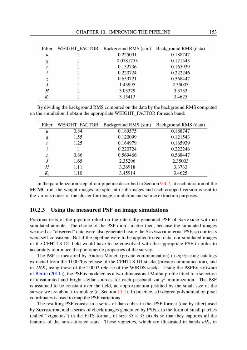
CHAPTER 10. IMPROVING THE PIPELINE 153
Filter WEIGHT_FACTOR Background RMS (sim) Background RMS (data)u 1 0.225091 0.188747g 1 0.0781753 0.121543r 1 0.132736 0.165939i 1 0.220724 0.222246z 1 0.659721 0.568447J 1 1.43995 2.35003H 1 3.03379 3.3733Ks 1 3.15413 3.4625
By dividing the background RMS computed on the data by the background RMS computedon the simulation, I obtain the appropriate WEIGHT_FACTOR for each band:
Filter WEIGHT_FACTOR Background RMS (sim) Background RMS (data)u 0.84 0.189575 0.188747g 1.55 0.120099 0.121543r 1.25 0.164979 0.165939i 1 0.220724 0.222246z 0.86 0.569466 0.568447J 1.65 2.35296 2.35003H 1.11 3.36918 3.3733Ks 1.10 3.45914 3.4625
In the parallelization step of our pipeline described in Section 9.4.7, at each iteration of theMCMC run, the weight images are split into sub-images and each cropped version is sent tothe various nodes of the cluster for image simulation and source extraction purposes.
10.2.3 Using the measured PSF on image simulationsPrevious tests of the pipeline relied on the internally generated PSF of Skymaker with nosimulated aureole. The choice of the PSF didn’t matter then, because the simulated imageswe used as “observed” data were also generated using the Skymaker internal PSF, so our testswere self-consistent. But if the pipeline were to be applied to real data, our simulated imagesof the CFHTLS D1 field would have to be convolved with the appropriate PSF in order toaccurately reproduce the photometric properties of the survey.
The PSF is measured by Andrea Moneti (private communication) in ugriz using catalogsextracted from the T0007bis release of the CFHTLS D1 stacks (private communication), andin JHKs using those of the T0002 release of the WIRDS stacks. Using the PSFEx softwareof Bertin (2011a), the PSF is modeled as a two-dimensional Moffat profile fitted to a selectionof unsaturated and bright stellar sources for each passband via χ2 minimization. The PSFis assumed to be constant over the field, an approximation justified by the small size of thesurvey we are about to simulate (cf Section 11.1). In practice, a 0-degree polynomial on pixelcoordinates is used to map the PSF variations.
The resulting PSF consist in a series of data cubes in the .PSF format (one by filter) usedby Sextractor, and a series of check images generated by PSFex in the form of small patches(called “vignettes”) in the FITS format, of size 35 × 35 pixels so that they captures all thefeatures of the non-saturated stars. These vignettes, which are illustrated in bands uiKs in
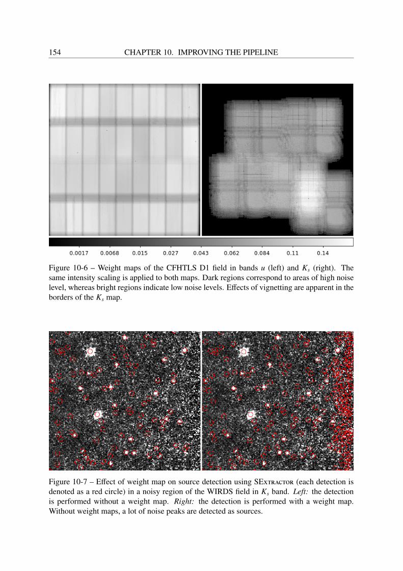
154 CHAPTER 10. IMPROVING THE PIPELINE
Figure 10-6 – Weight maps of the CFHTLS D1 field in bands u (left) and Ks (right). Thesame intensity scaling is applied to both maps. Dark regions correspond to areas of high noiselevel, whereas bright regions indicate low noise levels. Effects of vignetting are apparent in theborders of the Ks map.
Figure 10-7 – Effect of weight map on source detection using SExtractor (each detection isdenoted as a red circle) in a noisy region of the WIRDS field in Ks band. Left: the detectionis performed without a weight map. Right: the detection is performed with a weight map.Without weight maps, a lot of noise peaks are detected as sources.
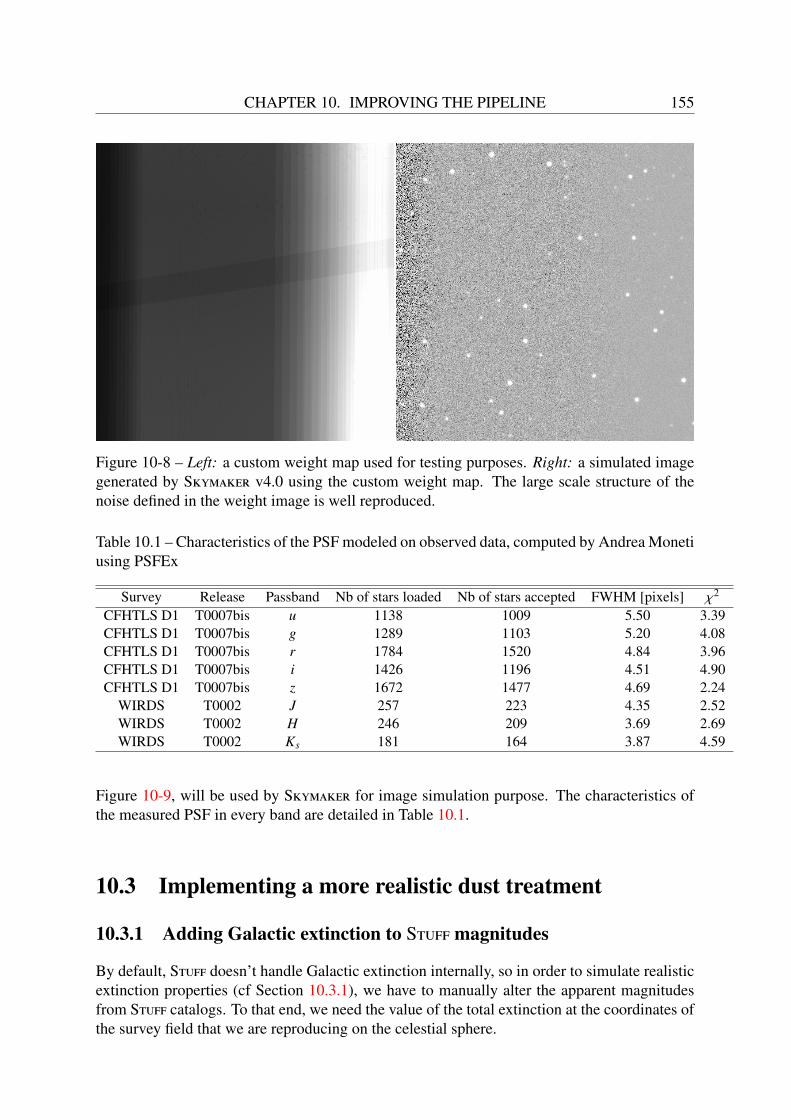
CHAPTER 10. IMPROVING THE PIPELINE 155
Figure 10-8 – Left: a custom weight map used for testing purposes. Right: a simulated imagegenerated by Skymaker v4.0 using the custom weight map. The large scale structure of thenoise defined in the weight image is well reproduced.
Table 10.1 – Characteristics of the PSF modeled on observed data, computed by Andrea Monetiusing PSFEx
Survey Release Passband Nb of stars loaded Nb of stars accepted FWHM [pixels] χ2
CFHTLS D1 T0007bis u 1138 1009 5.50 3.39CFHTLS D1 T0007bis g 1289 1103 5.20 4.08CFHTLS D1 T0007bis r 1784 1520 4.84 3.96CFHTLS D1 T0007bis i 1426 1196 4.51 4.90CFHTLS D1 T0007bis z 1672 1477 4.69 2.24
WIRDS T0002 J 257 223 4.35 2.52WIRDS T0002 H 246 209 3.69 2.69WIRDS T0002 Ks 181 164 3.87 4.59
Figure 10-9, will be used by Skymaker for image simulation purpose. The characteristics ofthe measured PSF in every band are detailed in Table 10.1.
10.3 Implementing a more realistic dust treatment
10.3.1 Adding Galactic extinction to Stuff magnitudes
By default, Stuff doesn’t handle Galactic extinction internally, so in order to simulate realisticextinction properties (cf Section 10.3.1), we have to manually alter the apparent magnitudesfrom Stuff catalogs. To that end, we need the value of the total extinction at the coordinates ofthe survey field that we are reproducing on the celestial sphere.

156 CHAPTER 10. IMPROVING THE PIPELINE
Figure 10-9 – Point spread function measured on CFHTLS D1+WIRDS images in bands uiKs
(from left to right respectively) using PSFEx. The PSF, modeled on a 35 × 35 vignette, willbe considered constant over the field in our future studies. All the images feature the sameintensity scaling.
Using the online tool provided by NASA/IPAC Infrared Science Archive4, we generate acutout of the Galactic dust reddening map of Schlegel et al. (1998), compiled from IRAS andCOBE data that we described in Section 10.3.1. This resulting cutout is a 2 deg2 square image(the smallest area possible to extract) centered on the CFHTLS Deep field, shown on Figure10-10.
We consider that the resulting E(B-V) reddening values have negligible spatial variationsover the field (E(B-V)max−E(B-V)min = 0.01 mag, which is at least 10× lower (depending onthe filter) than the median RMS error for MAG_AUTO estimation with SExtractor). Wetherefore opt for the extinction value computed within a 5 arcmin radius circle at the center ofthe D1 field. This area is represented as a green circle on Figure 10-10. The service providesthe total extinction values of Schlegel et al. (1998), as well as the more recent values estimatedby Schlafly and Finkbeiner (2011) from the analysis of the Sloan Digital Sky Survey. Bothresults assume an extinction to reddening ratio AV/E(B−V) = 3.1, but Schlafly and Finkbeiner(2011) use a different calibration and extinction law. We use the most recent results for ourneeds.
Table 10.2 – Total extinction per band at the center of the CFHTLS D1 field
band u g r i z J H Ks
Aλ 0.113 0.088 0.061 0.045 0.034 0.019 0.012 0.008
Note: the values of extinction in JHKs are those in the UKIRT magnitude system.The extinction values are provided using the extinction law of Schlafly and Finkbeiner (2011)(assuming RV = 3.1).
Using these data, we finally derive the Stuff apparent magnitudes reddened by Galacticextinction mr via:
mr = mStuff + Aλ (10.3)
4http://irsa.ipac.caltech.edu/applications/DUST/

CHAPTER 10. IMPROVING THE PIPELINE 157
Figure 10-10 – Cutout of the Galactic dust E(B-V) reddening map of Schlegel et al. (1998) fromIRAS + COBE 100 µm imaging data centered on the CFHTLS Deep field we want to simulateand covering 2 deg2 on the sky. The field we are simulating represents the inner square onthis image, and is centered on (α, δ)=(36.4926489,-4.486492445) at epoch J2000. The E(B-V)reddening values of Schlafly and Finkbeiner (2011) are 14% smaller than the values of Schlegelet al. (1998).
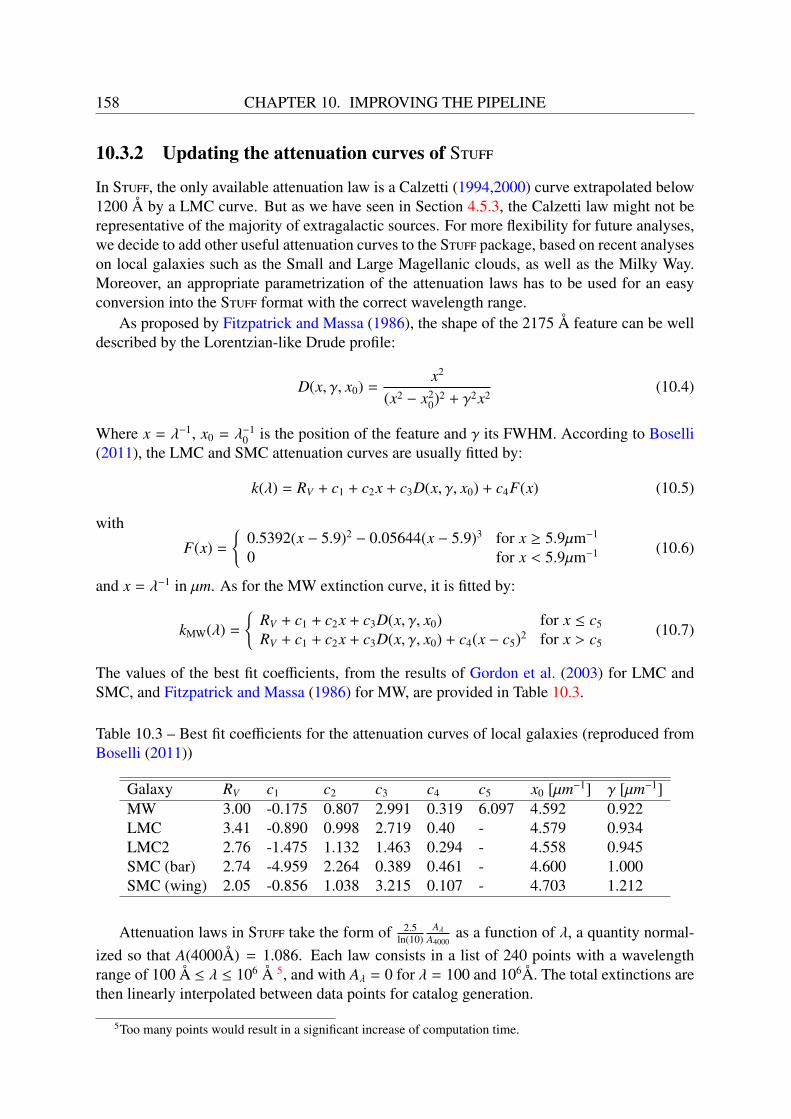
158 CHAPTER 10. IMPROVING THE PIPELINE
10.3.2 Updating the attenuation curves of Stuff
In Stuff, the only available attenuation law is a Calzetti (1994,2000) curve extrapolated below1200 Å by a LMC curve. But as we have seen in Section 4.5.3, the Calzetti law might not berepresentative of the majority of extragalactic sources. For more flexibility for future analyses,we decide to add other useful attenuation curves to the Stuff package, based on recent analyseson local galaxies such as the Small and Large Magellanic clouds, as well as the Milky Way.Moreover, an appropriate parametrization of the attenuation laws has to be used for an easyconversion into the Stuff format with the correct wavelength range.
As proposed by Fitzpatrick and Massa (1986), the shape of the 2175 Å feature can be welldescribed by the Lorentzian-like Drude profile:
D(x, γ, x0) =x2
(x2 − x20)2 + γ2x2
(10.4)
Where x = λ−1, x0 = λ−10 is the position of the feature and γ its FWHM. According to Boselli
(2011), the LMC and SMC attenuation curves are usually fitted by:
k(λ) = RV + c1 + c2x + c3D(x, γ, x0) + c4F(x) (10.5)
with
F(x) =
0.5392(x − 5.9)2 − 0.05644(x − 5.9)3 for x ≥ 5.9µm−1
0 for x < 5.9µm−1 (10.6)
and x = λ−1 in µm. As for the MW extinction curve, it is fitted by:
kMW(λ) =
RV + c1 + c2x + c3D(x, γ, x0) for x ≤ c5
RV + c1 + c2x + c3D(x, γ, x0) + c4(x − c5)2 for x > c5(10.7)
The values of the best fit coefficients, from the results of Gordon et al. (2003) for LMC andSMC, and Fitzpatrick and Massa (1986) for MW, are provided in Table 10.3.
Table 10.3 – Best fit coefficients for the attenuation curves of local galaxies (reproduced fromBoselli (2011))
Galaxy RV c1 c2 c3 c4 c5 x0 [µm−1] γ [µm−1]MW 3.00 -0.175 0.807 2.991 0.319 6.097 4.592 0.922LMC 3.41 -0.890 0.998 2.719 0.40 - 4.579 0.934LMC2 2.76 -1.475 1.132 1.463 0.294 - 4.558 0.945SMC (bar) 2.74 -4.959 2.264 0.389 0.461 - 4.600 1.000SMC (wing) 2.05 -0.856 1.038 3.215 0.107 - 4.703 1.212
Attenuation laws in Stuff take the form of 2.5ln(10)
AλA4000
as a function of λ, a quantity normal-ized so that A(4000Å) = 1.086. Each law consists in a list of 240 points with a wavelengthrange of 100 Å ≤ λ ≤ 106 Å 5, and with Aλ = 0 for λ = 100 and 106Å. The total extinctions arethen linearly interpolated between data points for catalog generation.
5Too many points would result in a significant increase of computation time.

CHAPTER 10. IMPROVING THE PIPELINE 159
Figure 10-11 – Comparison of Stuff default dust attenuation curves before and after the update.The blue curve is a Calzetti (1994, 2000) law extrapolated below 1200 Å by a LMC curve. Theorange curve is the LMC law provided by the best fit of Gordon et al. (2003).
Stuff now uses LMC as its default attenuation curve (cf Figure 10-11). With the new de-fault settings, it generates about 30% less galaxies than before (∼ 15, 000 instead of ∼ 21, 400).
10.4 Masking the bright starsBright stars contaminate the estimated flux of nearby sources, and saturate all the individualexposures, which prevent their removal via co-addition (Coupon et al. 2017). As Stuff doesn’tfeature (yet) the implementation of a realistic stellar field to simulated images, we decide tomask out all regions around the brightest stars, and only use non-contaminated regions forphotometric and morphometric measurements.
The mask files are produced semi-automatically by the IAP TERAPIX team6, who used theUSNO source catalog (Monet et al. 2003) to locate bright stars on the CFHTLS field and drewpolygons whose size depends on the stars’ magnitudes around them. The masks are providedas FITS files (one for the optical bands, and one for the IR bands), where non-masked regionsare assigned a values of 0, and masked regions a value of 1. The shapes of the resulting maskedareas are illustrated in Figure 10-12 on a fraction of the CFHTLS D1 field. Mask files (or flagimages) are recognized by SExtractor via the FLAG_IMAGE keyword in its configurationfile, provided that IMAFLAGS_ISO is present in the parameters file. In this way, sourcesdetected in masked regions are assigned an IMAFLAGS_ISO of 1 in the output catalog (0otherwise). They can therefore be easily ignored in further analyses.
6http://terapix.iap.fr/
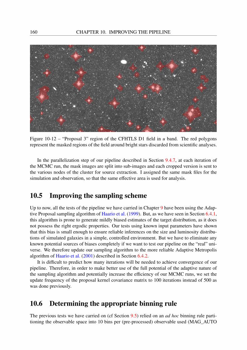
160 CHAPTER 10. IMPROVING THE PIPELINE
Figure 10-12 – “Proposal 3” region of the CFHTLS D1 field in u band. The red polygonsrepresent the masked regions of the field around bright stars discarded from scientific analyses.
In the parallelization step of our pipeline described in Section 9.4.7, at each iteration ofthe MCMC run, the mask images are split into sub-images and each cropped version is sent tothe various nodes of the cluster for source extraction. I assigned the same mask files for thesimulation and observation, so that the same effective area is used for analysis.
10.5 Improving the sampling schemeUp to now, all the tests of the pipeline we have carried in Chapter 9 have been using the Adap-tive Proposal sampling algorithm of Haario et al. (1999). But, as we have seen in Section 6.4.1,this algorithm is prone to generate mildly biased estimates of the target distribution, as it doesnot possess the right ergodic properties. Our tests using known input parameters have shownthat this bias is small enough to ensure reliable inferences on the size and luminosity distribu-tions of simulated galaxies in a simple, controlled environment. But we have to eliminate anyknown potential sources of biases completely if we want to test our pipeline on the “real” uni-verse. We therefore update our sampling algorithm to the more reliable Adaptive Metropolisalgorithm of Haario et al. (2001) described in Section 6.4.2.
It is difficult to predict how many iterations will be needed to achieve convergence of ourpipeline. Therefore, in order to make better use of the full potential of the adaptive nature ofthe sampling algorithm and potentially increase the efficiency of our MCMC runs, we set theupdate frequency of the proposal kernel covariance matrix to 100 iterations instead of 500 aswas done previously.
10.6 Determining the appropriate binning ruleThe previous tests we have carried on (cf Section 9.5) relied on an ad hoc binning rule parti-tioning the observable space into 10 bins per (pre-processed) observable used (MAG_AUTO
CHAPTER 10. IMPROVING THE PIPELINE 161
and/or FLUX_RADIUS in several photometric bands). We have seen in Chapter 7 that lessad hoc binning rules exist to split multidimensional datasets, such as Knuth’s rule or Bayesianblocks. In this section, I explore the consequences of the binning choice on the quality of in-ference, by comparing the use of Knuth’s rule to the use of our previous binning rule during arealistic run of our pipeline.
The tests are performed in the “Multi-type” configuration (cf Section 9.5.1), using a sim-ulated image of size 9358 × 4446 in bands uiKs with a combined distribution of E/S0 and Spgalaxies, reproducing a fraction of the area of the D1 tile of the CFHTLS Deep field, as our“observed” data. From this image, 23,617 sources with a FLAG < 4 (i.e. unsaturated anduncropped) are extracted in total. For each binning rule, 3 chains are launched from randomlyselected starting points for 104 iterations, using the AM + simulated annealing algorithm tosample the parameter space efficiently.
Figure 10-13 plots the number of bins partitioning the observable space as a function ofthe number of galaxies per bin, for each binning rule, applied to the “observed” data. Theplot reveals that Knuth’s rule introduces ∼150× more bins in total than our previous rule, and∼100× more empty bins. When computing the auxiliary likelihood, each empty bin will beartificially filled with 1 source to prevent singularities in log space. Therefore, if Knuth’s ruleis used as our binning rule, we can expect that a lot of unphysical noise will be added to ourdistribution of observables, that will potentially affect the accuracy of the inference processvia a more random evolution of the acceptance probability (defined in Equation 6.14) acrossiterations. This hypothesis is confirmed by the erratic behavior of the temperature evolution(which constitutes a good tracer of the noise level of our model) over 104 iterations when usingKnuth’s rule, as plotted in Figure 10-14, in contrast to the relatively stable behavior of thetemperature when the previous rule is used.
We therefore decide to keep the “10 bins per dimension” binning rule when applying ourpipeline to real data, considering its proven efficiency on previous tests.
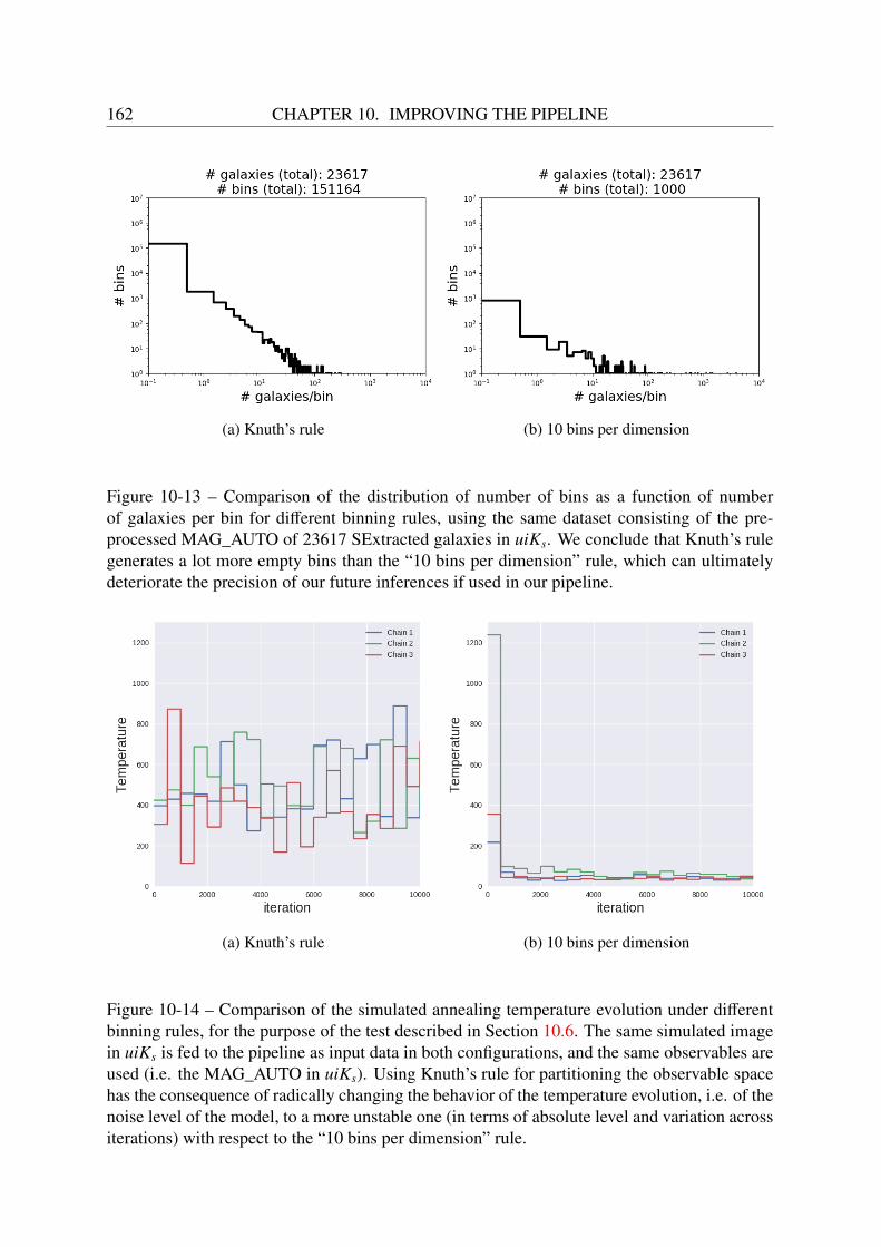
162 CHAPTER 10. IMPROVING THE PIPELINE
(a) Knuth’s rule (b) 10 bins per dimension
Figure 10-13 – Comparison of the distribution of number of bins as a function of numberof galaxies per bin for different binning rules, using the same dataset consisting of the pre-processed MAG_AUTO of 23617 SExtracted galaxies in uiKs. We conclude that Knuth’s rulegenerates a lot more empty bins than the “10 bins per dimension” rule, which can ultimatelydeteriorate the precision of our future inferences if used in our pipeline.
(a) Knuth’s rule (b) 10 bins per dimension
Figure 10-14 – Comparison of the simulated annealing temperature evolution under differentbinning rules, for the purpose of the test described in Section 10.6. The same simulated imagein uiKs is fed to the pipeline as input data in both configurations, and the same observables areused (i.e. the MAG_AUTO in uiKs). Using Knuth’s rule for partitioning the observable spacehas the consequence of radically changing the behavior of the temperature evolution, i.e. of thenoise level of the model, to a more unstable one (in terms of absolute level and variation acrossiterations) with respect to the “10 bins per dimension” rule.
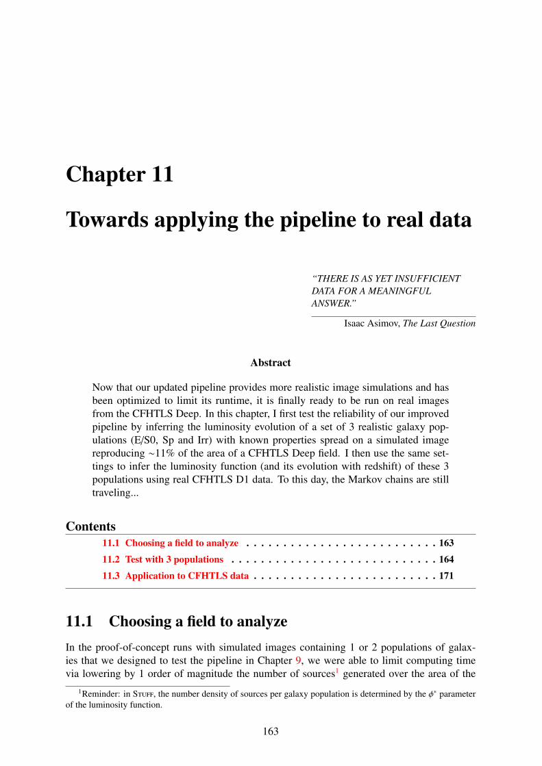
Chapter 11
Towards applying the pipeline to real data
“THERE IS AS YET INSUFFICIENTDATA FOR A MEANINGFULANSWER.”
Isaac Asimov, The Last Question
Abstract
Now that our updated pipeline provides more realistic image simulations and hasbeen optimized to limit its runtime, it is finally ready to be run on real imagesfrom the CFHTLS Deep. In this chapter, I first test the reliability of our improvedpipeline by inferring the luminosity evolution of a set of 3 realistic galaxy pop-ulations (E/S0, Sp and Irr) with known properties spread on a simulated imagereproducing ∼11% of the area of a CFHTLS Deep field. I then use the same set-tings to infer the luminosity function (and its evolution with redshift) of these 3populations using real CFHTLS D1 data. To this day, the Markov chains are stilltraveling...
Contents11.1 Choosing a field to analyze . . . . . . . . . . . . . . . . . . . . . . . . . . 163
11.2 Test with 3 populations . . . . . . . . . . . . . . . . . . . . . . . . . . . . 164
11.3 Application to CFHTLS data . . . . . . . . . . . . . . . . . . . . . . . . . 171
11.1 Choosing a field to analyzeIn the proof-of-concept runs with simulated images containing 1 or 2 populations of galax-ies that we designed to test the pipeline in Chapter 9, we were able to limit computing timevia lowering by 1 order of magnitude the number of sources1 generated over the area of the
1Reminder: in Stuff, the number density of sources per galaxy population is determined by the φ∗ parameterof the luminosity function.
163

164 CHAPTER 11. TOWARDS APPLYING THE PIPELINE TO REAL DATA
CFHTLS D1 simulated field. As we have seen in benchmarking tests (cf Section 9.4.7) andwith the large number of iterations required by the MCMC process (Section 9.5), if we wantto test our pipeline on real data within a reasonable amount of user time (i.e. a few weeks), wecan only afford to simulate a small portion (∼10 %) of the area of the CFHTLS D1 field. Thegiven region of the D1 field will be chosen according to the following criteria:
• It has to maximize the area of the survey fit for analysis by minimizing the number ofvery bright stars contaminating the field (i.e. large masked regions),
• The weight maps of this region must avoid large spatial variations, which are revealingof noisy regions unsuitable for a reliable analysis.
The chosen region that meets these two criteria, dubbed “Proposal 3” and found by explorationof the D1 field using the DS9 visualization tool (Joye 2013), is a 9,538 × 4,446 pixels regioncentered on (α, δ) = (2 : 25 : 56,−4 : 23 : 07) (in the FK5 system2) and covering 11.3 % ofthe surface of the D1 field3. The position and area of the region on the D1 field is illustrated inFigure 11-1, and Figure 11-2 displays a color image of the “Proposal 3” field in the gri bands.Finally, the weight maps corresponding to “Proposal 3” are shown in Figure 11-3.
The last public release of the CFHTLS D1 T0007 stack suffers from an overestimationof the sky background level around bright objects and regions of high number densities dueto insufficient masking of the sources, which makes the sky-subtracted stacks biased in theseregions. Lately, the IAP TERAPIX team has performed a re-stacking of the Deep fields, wherethe background level is estimated including bright object masking with mask files originallydesigned for the staking of WIRDS data. In this “T0007bis” new stack, the sky subtraction istherefore improved, and we use it for this work.
11.2 Test with 3 populationsBefore running our pipeline on CFHTLS Deep data, we need to perform a last test of self-consistency of our updated version of the pipeline in the most realistic way possible consideringour limited resources in terms of computing time. In this test, we use a simulated image of afraction of the CFHTLS D1 field as input data. This image is a mock “proposal 3” field of size9, 538 × 4, 446 pixels (each pixel representing 0.186” on the sky) reproduced in bands uiKs
containing 3 populations of galaxies generated by Stuff, namely E/S0, Sp and Irr.Contrary to previous tests, we want to reproduce the observed number counts by introduc-
ing a realistic population of Irr, which can be done in this situation as we have reduced thesimulated field area. The E/S0 and Sp populations are generated using the LF parameters ofFaber et al. (2007), this time without scaling down the number densities. The LF parameters(and evolution parameters) of the Irr population from EFIGI data (Baillard et al. 2011; de Lap-parent, private communication) were tuned to closely match visually the observed slope of theuiKs number counts in the “proposal 3” field from the CFHTLS D1 T0007bis + WIRDS T0002stacks (described in Section 9.2). The contribution of each population was tracked by cross-identification of input sources and extracted sources using their position on the image. The bestvisual combination of luminosity functions and their evolution per type is shown in 11-4. This
2(xcenter, ycenter)=(9843,11785) in pixel coordinates.3This corresponds to a surface of 42405948 pixels2

CHAPTER 11. TOWARDS APPLYING THE PIPELINE TO REAL DATA 165
Figure 11-1 – Position and area of the “Proposal 3” region on the CFHTLS D1 (T0007bisstacks) field.
Figure 11-2 – gri image of the full “Proposal 3” region of the CFHTLS D1 field (T0007bisstacks).
166 CHAPTER 11. TOWARDS APPLYING THE PIPELINE TO REAL DATA
Figure 11-3 – Left: weight maps of the “Proposal 3” region of the CFHTLS D1 field (T0007bisstacks) in bands u and i (from top to bottom respectively). Right: weight map of the sameregion in band Ks.
configuration allows to generate images with color-magnitude distributions that are at leastcomparable to the observed distributions, although the discrete number of galaxy populationsintroduced by Stuff generates linear features in the distribution due to the fixed SED of eachtype, as displayed in Figure 11-6. The B/T ratios in the g adopted reference band are deter-mined using the distribution of B/T in g-band as a function of morphological type from EFIGI(Baillard et al. 2011) measurements (de Lapparent, private communication). In particular weconsider our Irr population to be bulgeless. The input parameters used to generate the 3 popu-lations are listed in Tables 11.2 and 11.3 for the luminosity and size characteristics respectively.Galactic extinction reddens the apparent magnitude of the modeled galaxy populations follow-ing the method detailed in Section 10.3.1, and using total extinction values Aλ = 0.113, 0.045and 0.008 in bands uiKs respectively, according to the prescriptions of Schlafly and Finkbeiner(2011) (cf Table 10.2). Moreover, we use an LMC law (cf Figure 10-11) as the dust internalattenuation curve.
The synthetic images use a constant PSF of 35×35 pixels modeled by Andrea Moneti fromthe CFHTLS D1 T0007bis data (cf Section 10.2.3), and include correlated background noisedue to resampling (cf Section 10.2.1), using a LANCZOS3 kernel with a correlation scale of1 in u and i bands, and of 1.613 in band Ks. Even though there are no stars in the simulatedimage, this test uses the Terapix bright stars mask files in the source extraction process (cfSection 10-12) to make the test in the exact same conditions as with the real CFHTLS Deepstack (i.e. using the same image area). The weight maps of the “proposal 3” field (cf Figure11-3) are also included in the image simulation and source extraction steps of the pipeline.The imaging characteristics for this test are summarized in Table 11.4, and the input imagegenerated with these settings is shown in gri colors in Figure 11-5.
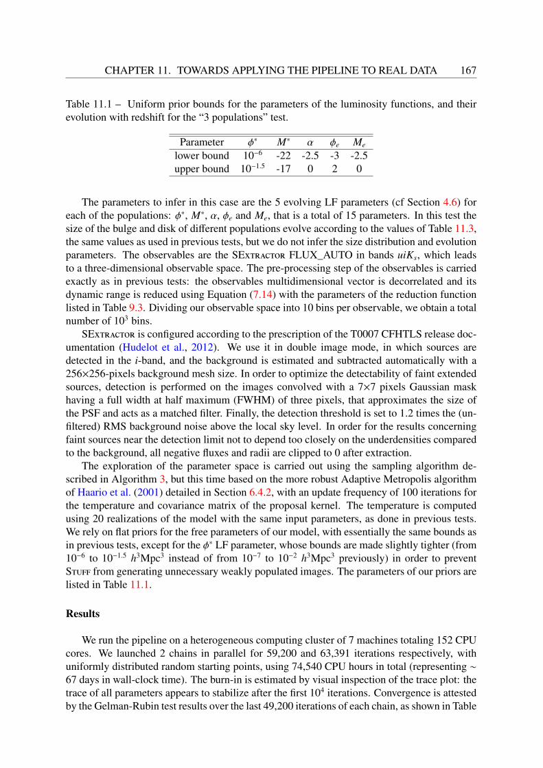
CHAPTER 11. TOWARDS APPLYING THE PIPELINE TO REAL DATA 167
Table 11.1 – Uniform prior bounds for the parameters of the luminosity functions, and theirevolution with redshift for the “3 populations” test.
Parameter φ∗ M∗ α φe Me
lower bound 10−6 -22 -2.5 -3 -2.5upper bound 10−1.5 -17 0 2 0
The parameters to infer in this case are the 5 evolving LF parameters (cf Section 4.6) foreach of the populations: φ∗, M∗, α, φe and Me, that is a total of 15 parameters. In this test thesize of the bulge and disk of different populations evolve according to the values of Table 11.3,the same values as used in previous tests, but we do not infer the size distribution and evolutionparameters. The observables are the SExtractor FLUX_AUTO in bands uiKs, which leadsto a three-dimensional observable space. The pre-processing step of the observables is carriedexactly as in previous tests: the observables multidimensional vector is decorrelated and itsdynamic range is reduced using Equation (7.14) with the parameters of the reduction functionlisted in Table 9.3. Dividing our observable space into 10 bins per observable, we obtain a totalnumber of 103 bins.
SExtractor is configured according to the prescription of the T0007 CFHTLS release doc-umentation (Hudelot et al., 2012). We use it in double image mode, in which sources aredetected in the i-band, and the background is estimated and subtracted automatically with a256×256-pixels background mesh size. In order to optimize the detectability of faint extendedsources, detection is performed on the images convolved with a 7×7 pixels Gaussian maskhaving a full width at half maximum (FWHM) of three pixels, that approximates the size ofthe PSF and acts as a matched filter. Finally, the detection threshold is set to 1.2 times the (un-filtered) RMS background noise above the local sky level. In order for the results concerningfaint sources near the detection limit not to depend too closely on the underdensities comparedto the background, all negative fluxes and radii are clipped to 0 after extraction.
The exploration of the parameter space is carried out using the sampling algorithm de-scribed in Algorithm 3, but this time based on the more robust Adaptive Metropolis algorithmof Haario et al. (2001) detailed in Section 6.4.2, with an update frequency of 100 iterations forthe temperature and covariance matrix of the proposal kernel. The temperature is computedusing 20 realizations of the model with the same input parameters, as done in previous tests.We rely on flat priors for the free parameters of our model, with essentially the same bounds asin previous tests, except for the φ∗ LF parameter, whose bounds are made slightly tighter (from10−6 to 10−1.5 h3Mpc3 instead of from 10−7 to 10−2 h3Mpc3 previously) in order to preventStuff from generating unnecessary weakly populated images. The parameters of our priors arelisted in Table 11.1.
Results
We run the pipeline on a heterogeneous computing cluster of 7 machines totaling 152 CPUcores. We launched 2 chains in parallel for 59,200 and 63,391 iterations respectively, withuniformly distributed random starting points, using 74,540 CPU hours in total (representing ∼67 days in wall-clock time). The burn-in is estimated by visual inspection of the trace plot: thetrace of all parameters appears to stabilize after the first 104 iterations. Convergence is attestedby the Gelman-Rubin test results over the last 49,200 iterations of each chain, as shown in Table

168 CHAPTER 11. TOWARDS APPLYING THE PIPELINE TO REAL DATA
Table 11.2 – Luminosity characteristics of the galaxies in the “3 populations” test.
Population S EDba S EDd φ∗ [h3 Mpc−3] M∗ α φe Me B/T T b α(T ) N c
E/S0 E E 1.0e-2 -19.97 -0.5 -1.53 -1.77 0.65 -5 0.0 1819Sp E Scd 4.2e-3 -19.84 -1.3 0.03 -1.95 0.25 6 1.47 28602Irr E Im 2.0e-4 -19.00 -1.8 1.50 -2.0 0.00 10 0.75 30263
Notes: The LF parameters are given for H0 = 100 km.s−1.Mpc−3.a The bulge and disk SEDs are Coleman et al. (1980) templates.b de Vaucouleurs (1959) revised morphological type.c Number of sources generated by one realization of Stuff.
Table 11.3 – Size parameters for the bulge and disk of each galaxy population in the “3 popu-lations” test.
Disk Bulgeβd r∗d [h−1kpc] γd σλ Mknee rknee [h−1kpc] γb
-0.214 3.85 -0.80 0.36 -20.0 1.58 -1.00
Note: All the parameters above are given for H0 = 100 km.s−1.Mpc−3.“b” refers to bulge, and “d” to disk.
Table 11.4 – Imaging characteristics of the CFHTLS+WIRDS used for SkyMaker in the “3populations” test
Passband u i Ks
Image size [pixels] 9538 × 4446 9538 × 4446 9538 × 4446Effective gain [e−/ADU] 74590 6807 2134Well capacity [e−] ∞ ∞ ∞
Saturation level [ADU] 6465 4230 110884Effective read-out noise [e−] 4.2 4.2 30Total exposure time [s] 1 1 1Zero-point magnitude [“ADU/s”] 30 30 30Effective wavelength [µm] 0.381 0.769 2.146Sky level [AB mag/arcsec2] 22.2 20.0 15.4Seeing FWHM [arcsec] 0.87 0.76 0.73Scale of the correlated noise 1 1 1.613

CHAPTER 11. TOWARDS APPLYING THE PIPELINE TO REAL DATA 169
Figure 11-4 – Number counts in uiKs for the simulated “proposal 3” data with 3 populationsused for tests. In u−band, a second peak in the number counts can be observed at u > 30,probably a result of the interplay between the luminosity evolution and the selection effectsimplemented in Stuff. However, the peak lies beyond the limiting magnitude of the CFHTLSDeep (ulim = 26.3, cf Section 9.2), therefore the sources at these magnitudes do not influencethe distribution of observables retrieved by SExtractor.

170 CHAPTER 11. TOWARDS APPLYING THE PIPELINE TO REAL DATA
Figure 11-5 – Simulated image in bands gri featuring 3 populations of galaxies (E/S0, Sp, Irr)in the area of the “Proposal 3” region of the CFHTLS D1 field, used as observed data for the“3 populations” test described in Section 11.2.
Figure 11-6 – Color-magnitude diagram comparison between the CFHTLS D1 (T0007bisstack) “proposal 3” field and the simulated “proposal 3” field used as data for the “3 popu-lations” test detailed in Section 11.2. The distributions of galaxies occupy roughly the samerange in the diagram, although effects of the discretization of galaxy populations can be ob-served in the simulated case as linear features. The observed color-magnitude distributionappears smoother, as galaxy populations represent a continuum and therefore occupy the color-magnitude space in a more uniform way.
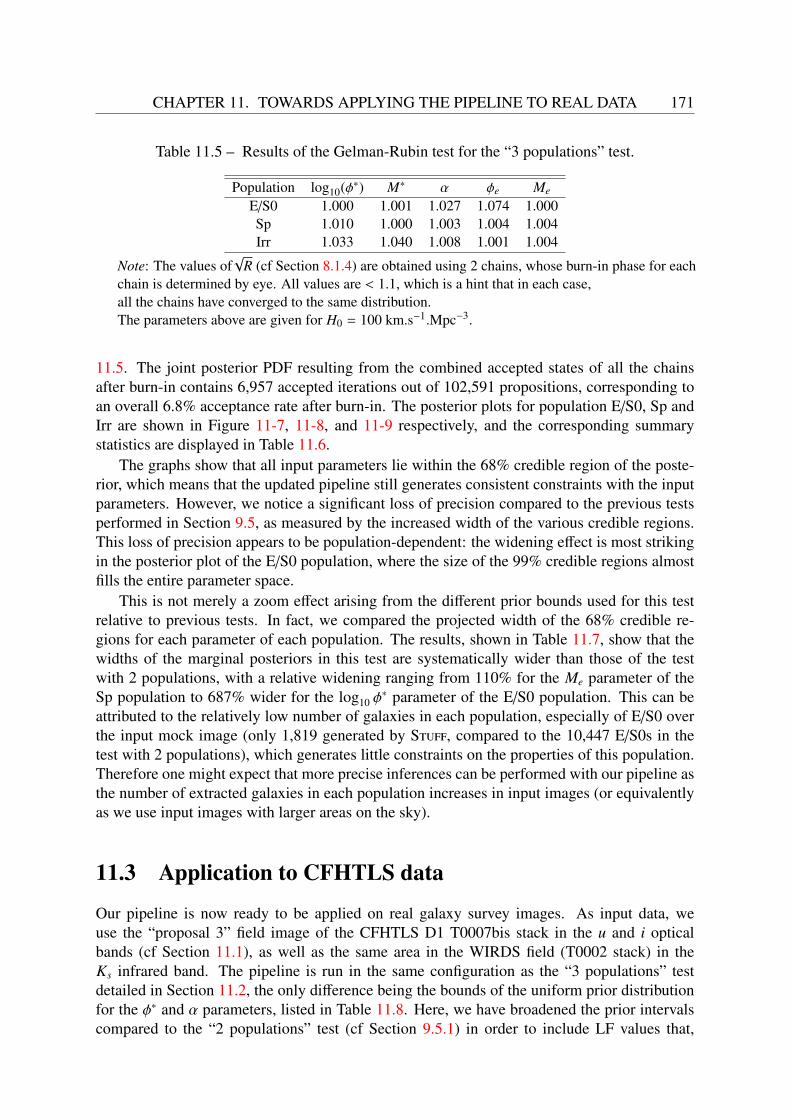
CHAPTER 11. TOWARDS APPLYING THE PIPELINE TO REAL DATA 171
Table 11.5 – Results of the Gelman-Rubin test for the “3 populations” test.
Population log10(φ∗) M∗ α φe Me
E/S0 1.000 1.001 1.027 1.074 1.000Sp 1.010 1.000 1.003 1.004 1.004Irr 1.033 1.040 1.008 1.001 1.004
Note: The values of√
R (cf Section 8.1.4) are obtained using 2 chains, whose burn-in phase for eachchain is determined by eye. All values are < 1.1, which is a hint that in each case,all the chains have converged to the same distribution.The parameters above are given for H0 = 100 km.s−1.Mpc−3.
11.5. The joint posterior PDF resulting from the combined accepted states of all the chainsafter burn-in contains 6,957 accepted iterations out of 102,591 propositions, corresponding toan overall 6.8% acceptance rate after burn-in. The posterior plots for population E/S0, Sp andIrr are shown in Figure 11-7, 11-8, and 11-9 respectively, and the corresponding summarystatistics are displayed in Table 11.6.
The graphs show that all input parameters lie within the 68% credible region of the poste-rior, which means that the updated pipeline still generates consistent constraints with the inputparameters. However, we notice a significant loss of precision compared to the previous testsperformed in Section 9.5, as measured by the increased width of the various credible regions.This loss of precision appears to be population-dependent: the widening effect is most strikingin the posterior plot of the E/S0 population, where the size of the 99% credible regions almostfills the entire parameter space.
This is not merely a zoom effect arising from the different prior bounds used for this testrelative to previous tests. In fact, we compared the projected width of the 68% credible re-gions for each parameter of each population. The results, shown in Table 11.7, show that thewidths of the marginal posteriors in this test are systematically wider than those of the testwith 2 populations, with a relative widening ranging from 110% for the Me parameter of theSp population to 687% wider for the log10 φ
∗ parameter of the E/S0 population. This can beattributed to the relatively low number of galaxies in each population, especially of E/S0 overthe input mock image (only 1,819 generated by Stuff, compared to the 10,447 E/S0s in thetest with 2 populations), which generates little constraints on the properties of this population.Therefore one might expect that more precise inferences can be performed with our pipeline asthe number of extracted galaxies in each population increases in input images (or equivalentlyas we use input images with larger areas on the sky).
11.3 Application to CFHTLS data
Our pipeline is now ready to be applied on real galaxy survey images. As input data, weuse the “proposal 3” field image of the CFHTLS D1 T0007bis stack in the u and i opticalbands (cf Section 11.1), as well as the same area in the WIRDS field (T0002 stack) in theKs infrared band. The pipeline is run in the same configuration as the “3 populations” testdetailed in Section 11.2, the only difference being the bounds of the uniform prior distributionfor the φ∗ and α parameters, listed in Table 11.8. Here, we have broadened the prior intervalscompared to the “2 populations” test (cf Section 9.5.1) in order to include LF values that,

172 CHAPTER 11. TOWARDS APPLYING THE PIPELINE TO REAL DATA
Table 11.6 – Summary statistics on the marginalized posterior distributions for the galaxypopulations in the “3 populations” test and comparison with the input values.
Population Parameters Input value Mean MAP a 68% interval 95% interval 99% intervallog10(φ∗) -2.00 -3.22 -2.33 [-3.95,-1.75] [-5.48,-1.53] [-5.89,-1.53]
M∗ -19.97 -20.11 -20.83 [-21.87,-18.98] [-21.97,-17.48] [-21.97,-17.03]E/S0 α -0.5 -1.10 -1.06 [-1.76,-0.31] [-2.19,-0.01] [-2.36,-0.01]
φe -1.53 -0.60 -0.38 [-2.52,1.32] [-2.92,1.92] [-2.92,1.97]Me -1.77 -1.39 -1.54 [-2.31,-0.81] [-2.49,-0.19] [-2.49,-0.04]
log10(φ∗) -2.38 -2.72 -2.52 [-3.37,-2.00] [-3.97,-1.52] [-4.45,-1.52]M∗ -19.84 -20.51 -20.83 [-21.68,-19.89] [-21.97,-18.70] [-21.97,-17.96]
Sp α -1.3 -1.39 -1.53 [-1.77,-1.19] [-2.05,-0.49] [-2.17,-0.14]φe 0.03 0.31 -0.04 [-0.46,1.18] [-1.07,1.88] [-1.49,1.98]Me -1.95 -1.60 -1.91 [-2.41,-1.19] [-2.49,-0.54] [-2.49,-0.17]
log10(φ∗) -3.70 -3.01 -2.82 [-3.53,-1.97] [-4.47,-1.52] [-5.18,-1.52]M∗ -19 -19.09 -18.87 [-20.33,-17.28] [-21.52,-17.08] [-21.82,-17.03]
Irr α -1.8 -1.44 -1.61 [-2.06,-0.96] [-2.36,-0.31] [-2.41,-0.04]φe 1.5 0.64 1.18 [0.33,1.97] [-1.92,1.97] [-2.92,1.97]Me -2.0 -1.36 -1.69 [-2.41,-0.39] [-2.49,-0.24] [-2.49,-0.06]
Notes: The LF parameters are given for H0 = 100 km.s−1.Mpc−3.a Maximum A Posteriori
Table 11.7 – Comparison of the width of the 68% credible regions between the results of thetest with 2 populations (Section 9.5.1) and those of the test with 3 populations (Section 11.2).
Population Parameter Width of the 68% interval (test 3 pop) Width of the 68% interval (test 2 pop)log10(φ∗) 2.2 0.32
M∗ 2.89 0.8E/S0 α 1.45 0.25
φe 3.84 0.67Me 1.5 0.7
log10(φ∗) 1.37 0.48M∗ 1.79 1.25
Sp α 0.58 0.12φe 1.64 0.63Me 1.22 1.10
log10(φ∗) 1.56 ∅
M∗ 3.05 ∅
Irr α 1.1 ∅
φe 1.64 ∅
Me 2.02 ∅
Notes: The LF parameters are given for H0 = 100 km.s−1.Mpc−3.

CHAPTER 11. TOWARDS APPLYING THE PIPELINE TO REAL DATA 173
Figure 11-7 – Joint posterior distribution for the parameters of the E/S0 population resultingfrom the “3 populations” test. Each panel is bounded by the prior range values. The dark red,orange and yellow areas in the contour plots represent the 99%, 95% and 68% credible regionsrespectively. The black crosses and red dots are the mean of the posterior and input true valueresp. In the marginalized posterior panels, the black dotted and red lines represent the posteriormean and the true value resp.
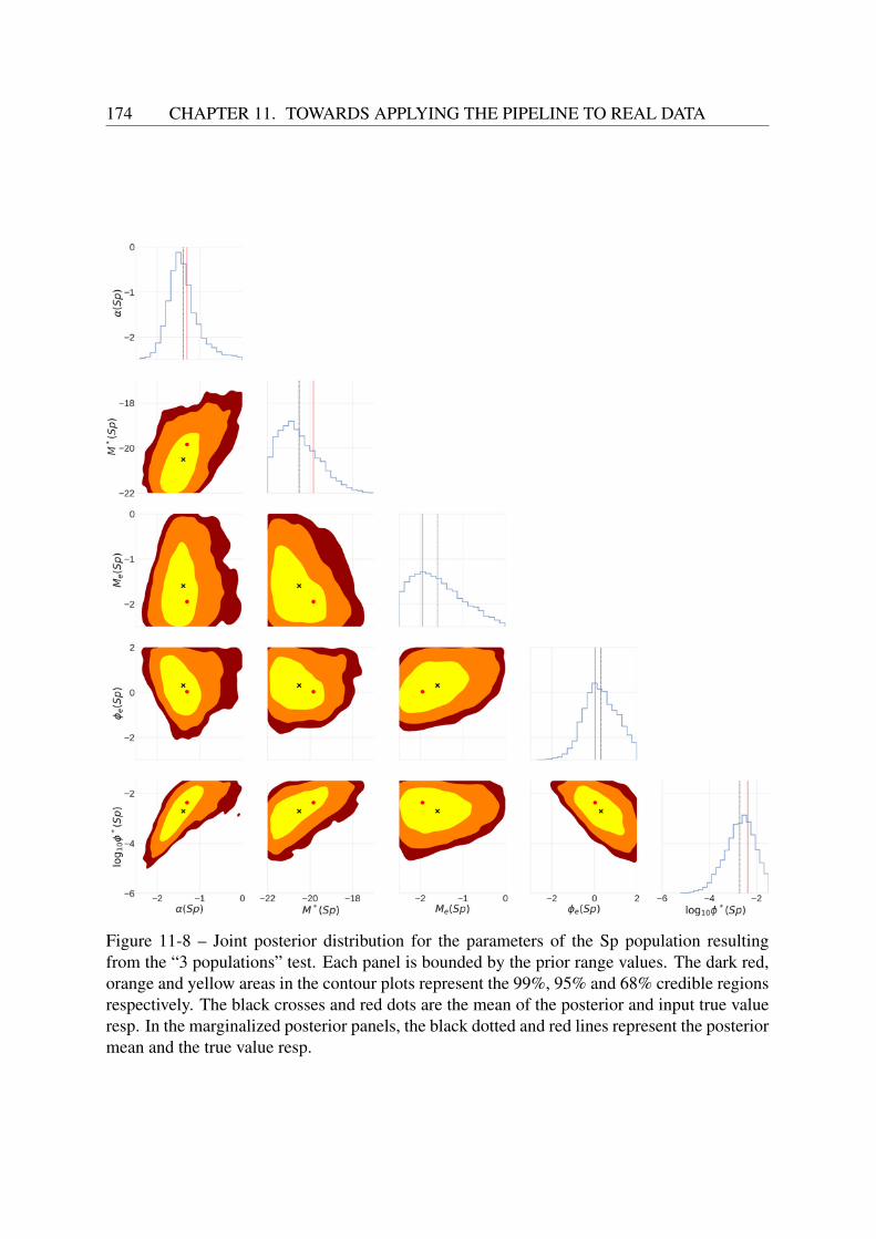
174 CHAPTER 11. TOWARDS APPLYING THE PIPELINE TO REAL DATA
Figure 11-8 – Joint posterior distribution for the parameters of the Sp population resultingfrom the “3 populations” test. Each panel is bounded by the prior range values. The dark red,orange and yellow areas in the contour plots represent the 99%, 95% and 68% credible regionsrespectively. The black crosses and red dots are the mean of the posterior and input true valueresp. In the marginalized posterior panels, the black dotted and red lines represent the posteriormean and the true value resp.
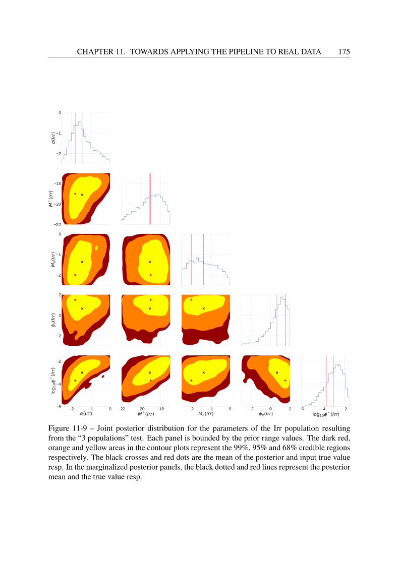
CHAPTER 11. TOWARDS APPLYING THE PIPELINE TO REAL DATA 175
Figure 11-9 – Joint posterior distribution for the parameters of the Irr population resultingfrom the “3 populations” test. Each panel is bounded by the prior range values. The dark red,orange and yellow areas in the contour plots represent the 99%, 95% and 68% credible regionsrespectively. The black crosses and red dots are the mean of the posterior and input true valueresp. In the marginalized posterior panels, the black dotted and red lines represent the posteriormean and the true value resp.
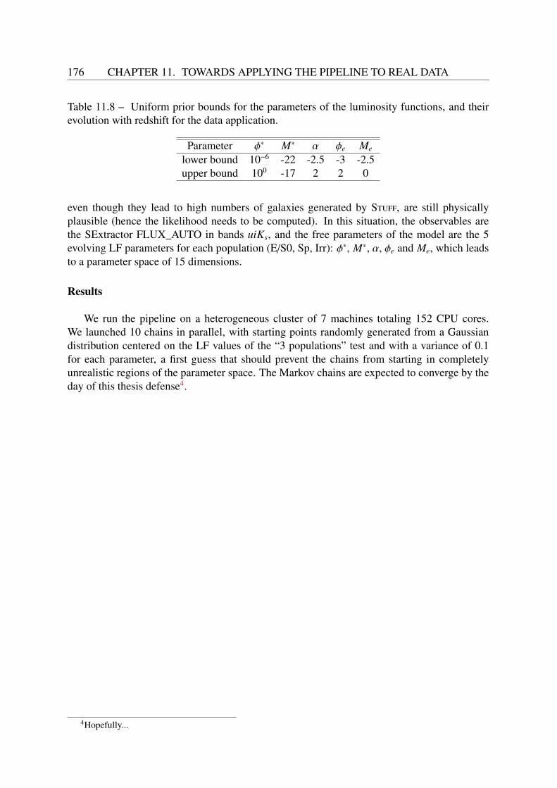
176 CHAPTER 11. TOWARDS APPLYING THE PIPELINE TO REAL DATA
Table 11.8 – Uniform prior bounds for the parameters of the luminosity functions, and theirevolution with redshift for the data application.
Parameter φ∗ M∗ α φe Me
lower bound 10−6 -22 -2.5 -3 -2.5upper bound 100 -17 2 2 0
even though they lead to high numbers of galaxies generated by Stuff, are still physicallyplausible (hence the likelihood needs to be computed). In this situation, the observables arethe SExtractor FLUX_AUTO in bands uiKs, and the free parameters of the model are the 5evolving LF parameters for each population (E/S0, Sp, Irr): φ∗, M∗, α, φe and Me, which leadsto a parameter space of 15 dimensions.
Results
We run the pipeline on a heterogeneous cluster of 7 machines totaling 152 CPU cores.We launched 10 chains in parallel, with starting points randomly generated from a Gaussiandistribution centered on the LF values of the “3 populations” test and with a variance of 0.1for each parameter, a first guess that should prevent the chains from starting in completelyunrealistic regions of the parameter space. The Markov chains are expected to converge by theday of this thesis defense4.
4Hopefully...

Chapter 12
Conclusion and perspectives
In the present thesis, we have laid the basis for a new method to infer robust constraints ongalaxy evolution models. In this method, populations of synthetic galaxies are generated byan empirical model, sampled from luminosity functions for each galaxy type, and determinedby the SEDs of the bulge and disk components and the bulge-to-total ratio. In order to re-produce the selection effects affecting real catalogs, we use an image simulator to reproducerealistic survey images with the appropriate instrumental characteristics. Real and mock im-ages undergo the same source extraction process. After a pre-processing step, the distributionsof extracted observables (fluxes and effective radii) are then compared via a binned maximumlikelihood method, and we minimize their discrepancy using an adaptive MCMC samplingscheme in the parametric Bayesian indirect likelihood framework, designed for an efficientexploration of the parameter space.
This is one of the first attempts in the field of galaxy evolution to make image simulationa central part of the inference process. We have tested the self-consistency of this approachusing a simulated image of a CFHTLS Deep field covering 1 deg2 on the sky in three bands:u and i in the optical, and Ks in the near infrared, generated with the Stuff model containingE/S0 and spiral galaxies with evolving size and luminosity.
Starting from non-informative uniform priors, we found that our pipeline can reliably inferthe input parameters governing the luminosity and size evolution of each of the galaxy pop-ulations in a few 104 iterations, using few and disjointed observables, that is, the photometry(fluxes and radii) of the extracted sources in uiKs. In each test performed, the input parameterslie within the 68% highest posterior density region. We have also compared the results of ourmethod with those of the classical photometric redshifts approach, with measurements fromSED fitting on one of the mock sample, and found that when using the same set of observables(uiKs photometry), our inference pipeline yields more accurate results.
As the validity of our pipeline has been established on mock data, we have applied it to afraction of the area of an observed CFHTLS Deep field covering ∼0.1 deg2 in the sky, in orderto infer the luminosity distributions and their evolution of three galaxy populations (E/S0, Spand Irr). We are now waiting for the results of the inference, but further tests performed onrealistic mock data with the same area containing these three populations suggest that a lossof accuracy in the inference can be expected compared to the results of the first test cases withonly two populations.
The next logical step for this project would use larger areas of the CFHTLS (i.e. the fullD1+W1 fields or the 4 Deep fields) as input data to better constrain the input parameters of
177
178 CHAPTER 12. CONCLUSION AND PERSPECTIVES
the model. Another possible future work could consist in combining these data with severalextragalactic surveys at various depths and with different instrumental setups simultaneously,such as HUDF (Williams et al., 2010) at z ∼ 2, and SDSS (Blanton et al., 2003) at z ∼ 0.1,in order to constrain the evolution of galaxies in a wide range of redshifts. Nevertheless,such application will raise various modeling issues. In particular, real survey images displaya continuum of galaxy populations, and our model only generates a discrete number of galaxypopulations, defined by their bulge and disk SEDs and their B/T ratio. In practice, the numberof modeled populations will be limited by computing time, as more populations lead to morefree parameters to infer, hence to more iterations for the pipeline to find the high probabilityregions. This will certainly require a compromise between the desired accuracy of the modeleduniverse and convergence of the chains within a reasonable computing time.
One issue of concern in the posterior distributions that we derived with our pipeline is il-lustrated by the fact that the 68% shaded region is large compared to the distance between theinput parameters and the mean of the posterior. Two causes of this enlargement are suspected:first, the small number (only ∼ 103 for the E/S0 population in the “3 populations” case) of inputgalaxies spread on input images for tests generates few constrains for the possible parametervalues of their luminosity function. Using surveys with large statistics in the number of charac-teristic population of galaxies is, as always, preferable, and should limit this effect, as attestedby the fact that the populations with the most numerous galaxies in input images (i.e. Sp, Irr)have their parameters better constrained than the populations with less galaxies in all our testruns (i.e. E/S0). We also suspect the “temperature” term, that we use in order to circumventthe stochastic nature of each model realization, to play a role in the size of our posteriors. Inessence, the model’s stochasticity itself (galaxies are randomly drawn from the distributionfunctions) inevitably contributes to the uncertainty in the posterior. We have no quantitativeestimate of this enlargement and we suspect it might be a limiting factor on the precision of theparameter inference. Estimating this enlargement from simulated data would have required usto generate a very large number of realizations for each step of the chain (hence we could haveturned off the “temperature” term). This would, however, be prohibitive in computing time,even in the considered simple tests performed in this thesis.
Moreover, there is room for several technical improvements of our pipeline, in order toguarantee a faster convergence and a more accurate inference:
• As implemented in the present thesis, our method faces the inevitable curse of dimen-sionality. In fact, as we bin each observable over ten intervals, for each observable addedthe hyper-dimensional number of bin increases by one order of magnitude. This limitsour approach to a restricted number of observables in order to prevent memory errors. Inorder to adapt this method to higher numbers of observables, we may have to change ourstrategy and reduce the dimensionality of the problem, either via principal componentanalysis or by binning only projections of the datasets instead of binning the completeobservable space, with the drawback of losing mutual information. More sophisticatedmethods using unsupervised machine learning, such as autoencoders1 trained on largesimulated datasets, could be used to minimize the loss of information induced by thedimensionality reduction.
• Instead of binning the distribution of observables, whose results depend on the bin edges1Autoencoders are neural networks that are trained to learn a representation (or “encoding”) of a dataset for
the purpose of dimensionality reduction.

CHAPTER 12. CONCLUSION AND PERSPECTIVES 179
and bin width, a more reliable method for density estimation for multivariate data is Ker-nel Density Estimation (KDE). KDE transforms the data points into a smooth densityfield, and alleviates the dependence of the results on the bin edges by centering a uni-modal function with mean 0, the kernel, on each data point. In practice, KDE is morecomputationally expensive than binning, and also requires some level of hand tuning, inthe form of the right kernel function and the optimal bandwidth, which in KDE is theanalog of bin width in histograms.
• The mean runtime of an MCMC chain in the context of the test cases described in Chap-ter 9 is approximately two weeks. Up to 50% of this runtime is currently spent in jobscheduling latencies for each iteration (as shown in Figure 9-4). A more integrated ap-proach, based, for example, on Message Passing Interface (MPI) and operating only inmemory might reduce those latencies. The next step would be to increase computationalefficiency by offloading the most time-consuming image rendering and source extractiontasks to graphics processing units (GPUs), especially convolutions and rasterizations.
• We emphasize that on the order of 104 iterations is needed to attain convergence in thetest cases studied. Considering the high computational cost of this approach, one maywonder how to attain faster convergence in realistic frameworks (i.e. when applied tothe full area covered by imaging surveys, deep or shallow). In that regard, Gutmann andCorander (2016), who explored the computational difficulties arising from likelihood-free inference methods, proposed a strategy based on probabilistic modeling of the re-lation between the input parameters and the difference between observed and syntheticdata. This approach would theoretically reduce the number of iterations needed to per-form the inference.
• Instead of using the evolving luminosity functions as input parameters of our empiri-cal model to generate simulated populations of galaxies whose SEDs are fixed, a morephysically-driven approach would make the SEDs of the bulge and disk of the differ-ent populations evolve with redshift via a stellar population synthesis model such asPEGASE.2 (Fioc and Rocca-Volmerange 1999). In this case, the free parameters to con-strain would be the parameters governing the evolution of the stellar mass functions ofeach component (bulge or disk) of each galaxy population with redshift. But such ap-proach would be much more demanding in terms of computing resources than the simpleempirical approach developed in this thesis, as it would lead to an increase in the numberof input parameters to infer.
Finally, more realistic mock astrophysical images would lead to more precise inferences:
• The addition of a likely stellar field to the simulated images would contaminate the sourceextraction process in a realistic way. This could be done via the use of photometriccatalogs from real or simulated stellar surveys (e.g. Gaia Collaboration et al. 2016, Robinet al. 2012).
• The contribution of clustering and environmental effects influence the colors (e.g. Madg-wick et al. 2003, Bamford et al. 2009) and spectral types (Zehavi et al., 2002) of galaxiesas a function of the local density and location within the cosmic web: red and quiescentgalaxies are mostly distributed in regions of high density, such as the centers of clusters,
180 CHAPTER 12. CONCLUSION AND PERSPECTIVES
whereas blue and star forming galaxies are less clustered. Galaxy clustering also has animpact on source blending and confusion. These effects are not implemented in Stuff,and this might bias our results in a way that is difficult to estimate.
• The present application uses as a reference the CFHTLS Deep survey, whose sensitivityis very homogeneous over the field of view. This is, however, not the case for many sur-veys. A more general application of the method would require simulating each individualraw survey exposure, and performing the very same co-addition as with the observed datato generate stacks, hence reproducing all the observational effects affecting the reducedimages, which would require a lot of computing power but could be done for large andshallow surveys such as the Dark Energy Survey (Collaboration et al. 2005).
Because the pipeline in this work makes it possible to constrain not only the galaxy lu-minosity evolution, but also the evolution of galaxy sizes, it opens interesting perspectives foraddressing the current debate on the evolution of galaxy sizes with cosmic time. The contradic-tory results of, for example, Longhetti et al. (2006), Trujillo et al. (2007), Saracco et al. (2010),and Morishita et al. (2014) on the growth of massive early-type galaxies may be plagued withthe varying selection effects in the surveys on which these analyses are based.
The broad features of the technique we detailed in this thesis are model-independent andcan be applied to a variety of problems. In fact, similar forward modeling approaches have beenused recently to infer the distribution of galaxy redshifts in cosmological galaxy samples (e.g.Herbel et al. 2017), or to constrain cosmological parameters directly from image simulationsreproducing the effects of “cosmic shear”, the weak gravitational lensing caused by large scalestructure (e.g. Refregier and Amara 2014, Fenech Conti et al. 2017, Hildebrandt et al. 2017).The forward modeling method, although expensive in terms of computing time, could provideastronomers with promising and reliable results in the context of future large-scale surveyssuch as the Dark Energy Survey (Collaboration et al. 2005) or Euclid (Laureijs et al. 2011).

List of Figures
1-1 Colorized map of the Cosmic Microwave Background (CMB) in equirectangu-lar projection, as revealed by the Planck satellite (Adam et al. 2016). Credits:ESA and the Planck collaboration. . . . . . . . . . . . . . . . . . . . . . . . . 18
1-2 The logarithmic evolution of the universe from z ∼ 1100 to z = 0, according tothe hierarchical scenario of structure formation. From Miralda-Escudé (2003). . 19
1-3 The cosmic web at z = 0 from the Millennium-XXL simulation (Angulo et al.2012). The yellow regions are the sites of galaxy formation. . . . . . . . . . . 19
1-4 A modern form of the Hubble sequence, extended from the original version toinclude dwarf spheroidal galaxies and irregular galaxies. From Kormendy andBender (2011). . . . . . . . . . . . . . . . . . . . . . . . . . . . . . . . . . . 23
1-5 Left: The color bimodality of galaxy populations, as revealed in a diagramrepresenting (u − r) SDSS colors as a function of baryonic mass, using theresults of Baldry et al. (2004) on SDSS data. The bottom panel shows themorphological types that dominate in different regions of the top panel (fromKormendy 2013). Right: Morphology-density relation for a sample of 7,938SDSS galaxies from 0.05 < z < 0.1 and Mr < −20.5 (from Goto et al. 2003). . . 23
1-6 Evolution of the morphological mix and relative number densities of galaxiesacross cosmic times, as revealed by several astronomical surveys. Left: galax-ies are classified by Sérsic index (cf Section 4.4). Right: galaxies are classifiedvisually. From Conselice 2014. . . . . . . . . . . . . . . . . . . . . . . . . . . 24
1-7 Left: 2.8×2.8 arcmin image of the Hubble Ultra Deep Field (HUDF, Beckwithet al. 2006). Right: Mock HUDF observation from the Illustris cosmologicalsimulation (Vogelsberger et al. 2014). From Snyder et al. (2015). . . . . . . . . 24
1-8 Left: Formation of a disk galaxy, according to the two-stage scenario of Whiteand Rees (1978) (from Baugh 2006). Right: Cold flows feeding a galaxy in acosmological simulation produced by D. Tweed (from Danovich et al. 2012). . 27
1-9 Ingredients of galaxy evolution models and their interactions. From Cole et al.(2000). . . . . . . . . . . . . . . . . . . . . . . . . . . . . . . . . . . . . . . . 30
1-10 Left: Supernova feedback in NGC 3079 (Credits: NASA and G. Cecil (U.North Carolina, Chapel Hill)). Right: AGN feedback in Centaurus A (Credits:ESO / WFI (Optical); MPIfR / ESO / APEX / A.Weiss et al. (Sub-millimeter);NASA / CXC / CfA / R.Kraft et al. (X-ray)). . . . . . . . . . . . . . . . . . . . 31
2-1 Sensitivity (or depth) of a selection of telescopes used for galaxy surveys as afunction of their wavelength range. From the COSMOS field website: http://cosmos.astro.caltech.edu/page/astronomers. . . . . . . . . . . . . 34
181

182 LIST OF FIGURES
2-2 A slice of the 3D distribution of galaxies, as revealed by the SDSS and 2dF-GRS, which provide our most complete picture to date of the large-scale struc-ture of the local universe out to z ∼ 0.1 − 0.2. Maps generated by S. Hinton. . . 37
2-3 Relative sizes of the surveys conducted by the Hubble Space Telescope on thesky. Credit: NASA, ESA, and Z. Levay (STScI) . . . . . . . . . . . . . . . . . 37
2-4 The global luminosity function in the local universe. This plots compares the2dFGRS bJ-band luminosity function (Norberg et al. 2002) with the LF esti-mates from the SDSS (Blanton et al. 2003). From Norberg et al. (2002). . . . . 39
2-5 Median mass-size relation in from the 140, 000 galaxies of the SDSS. The sizeis estimated by the Sérsic half-light radius. From Shen et al. (2003). . . . . . . 43
2-6 Comparison of the results of different studies on the evolution of the aver-age size of massive early-type galaxies. The half-light radius is normalized to1011M on the plot, using the slope Re ∝ M0.57. From Newman et al. (2012). . . 44
3-1 Simulated urz color composite image of a dust attenuated Sbc galaxy at differ-ent inclinations, from face-on (i=0) to edge-on (i=90), generated using theSunrise radiative transfer code (Jonsson 2006). As the inclination increases,reddening effects due to dust lanes become more and more apparent. Repro-duced from Jonsson et al. (2009). . . . . . . . . . . . . . . . . . . . . . . . . . 49
3-2 Evolution of absolute magnitude as a function of distance from a simulatedgalaxy sample with a Gaussian luminosity function. As the volume surveyedexpands with increasing distance, more and more objects are seen as distanceincreases. The survey limit in apparent magnitude gives rise to the so-calledMalmquist bias, which leads to a increase of mean absolute magnitude of thesample with distance. Reproduced from Tammann (1987). . . . . . . . . . . . 51
3-3 Patch of the GOODS-N field (Dickinson et al. 2003) observed at 250, 350 and500 µm (left to right). The green circles indicate the beam FWHM in eachband. The field is plagued by source confusion, and the size of the backgroundfluctuations is of the order of the beam size. Reproduced from Nguyen et al.(2010). . . . . . . . . . . . . . . . . . . . . . . . . . . . . . . . . . . . . . . . 52
4-1 Summary of the workflow . . . . . . . . . . . . . . . . . . . . . . . . . . . . 584-2 SED templates of Coleman et al. (1980) . . . . . . . . . . . . . . . . . . . . . 594-3 Filter set of the CFHTLS+WIRDS survey (Cuillandre and Bertin 2006; Bielby
et al. 2010). This plot displays the filter response curves (multiplied by themirror+optics+CCD response) of the MegaCam ugriz optical bands, as well asof the WIRCam JHKs infrared bands. . . . . . . . . . . . . . . . . . . . . . . 60
4-4 Sérsic curves for various values of n. n = 4 corresponds to the de Vaucouleurprofile. . . . . . . . . . . . . . . . . . . . . . . . . . . . . . . . . . . . . . . . 61
4-5 Sérsic bulge+disk fit performed on a 5′ × 5′ H-band image of NGC 3621 withGALFIT (Peng et al. 2010). From Barth et al. (2008). . . . . . . . . . . . . . . 62
4-6 Distribution of the B/T ratio attribute as a function of de Vaucouleurs morpho-logical type (De Vaucouleurs et al. 1991) for the 4458 galaxies in the EFIGIcatalog (Baillard et al. 2011). This plot reveals a strong correlation of morpho-logical type with B/T, with a large dispersion of B/T for each type. From deLapparent et al. (2011). . . . . . . . . . . . . . . . . . . . . . . . . . . . . . . 62

LIST OF FIGURES 183
4-7 Extinction curves for the Milky Way of Cardelli et al. (1989) for different val-ues of RV corresponding to different galactic environments. This plot illustrateshow RV controls the slope of the extinction curve. . . . . . . . . . . . . . . . . 65
4-8 All-sky view of the IRAS+COBE 100 µm imaging data in false colors shownin equirectangular projection, generated by Schlegel et al. (1998). It is used toreturn the values of Galactic dust reddening for a given line of sight. . . . . . . 65
4-9 Difference between dust extinction (a) and dust attenuation (b). . . . . . . . . . 67
4-10 Comparison of the most well known extinction and attenuation curves from thelocal universe. . . . . . . . . . . . . . . . . . . . . . . . . . . . . . . . . . . . 68
4-11 Example of a Stuff output catalog, with 4 galaxies generated in a given pho-tometric band. 1 : object type index (200=galaxy, 100=star). 2-3 : galaxyposition in pixels (x,y). 4 : apparent magnitude. 5 : B/T ratio. 6 : bulge radius(arcsec). 7 : projected bulge axis ratio. 8 : bulge position angle (degrees, withrespect to x-axis). 9 : disk scale-length (arcsec). 10 : disk aspect ratio (diskinclination). 11 : disk position angle. 12 : redshift. 13 : de Vaucouleurs type. . 71
5-1 Left: a small region of the Canada-France-Hawaii Telescope Legacy Survey(CFHTLS, Cuillandre and Bertin 2006) D1 field (stack from the 85% best see-ing exposures) in gri bands. Right: Full reconstruction of the image on theleft using Stuff+Skymaker with the same filters, exposure time, and telescopeproperties as the CFHTLS data. Both images are shown with the same colorcoding. From Bertin (2009). . . . . . . . . . . . . . . . . . . . . . . . . . . . 76
5-2 PSF variations over the CFHTLS D4 field (1 × 1 deg2) observed in r-band, asoutput by PSFEx. From Bertin and Moneti (2017). . . . . . . . . . . . . . . . 77
5-3 Observed PSF surface brightness profile from CCD data fitted by the sum of aKolmogorov profile (Fried 1965), which provides an accurate fit for the innerregions of the PSF dominated by atmospheric turbulence, and an aureole pro-file. The aureole component dominates the surface density profile beyond ∼ 10FWHM of the center. From Racine (1996). . . . . . . . . . . . . . . . . . . . 77
5-4 The four steps of source detection in SExtractor. From a talk given by Em-manuel Bertin. . . . . . . . . . . . . . . . . . . . . . . . . . . . . . . . . . . . 79
5-5 Sources detected by SExtractor in a portion of the CFHTLS D1 field in g-band. The ellipses show the limits of integration for the FLUX_AUTO propertyof extracted sources. . . . . . . . . . . . . . . . . . . . . . . . . . . . . . . . 79
6-1 Path of an MCMC run inferring the mean of a bivariate normal distribution af-ter 104 iterations. The Markov chain traveled from low (dark) to high (yellow)likelihood regions of the parameter space and finally converged around the truemean of the Gaussian. The dark and violet points can be considered burn-in,i.e. not a representative sample of the posterior distribution. . . . . . . . . . . . 86

184 LIST OF FIGURES
6-2 Traceplots depicting three typical situations that can arise in a standard MCMCchain with the (non-adaptive) Metropolis-Hastings algorithm. The input datais a set of 20 points normally distributed with mean 0 and standard deviation 1.The parameter to infer is the mean µ of the input data distribution. The prior isa normal distribution with mean 0 and standard deviation 1, and the transitionkernel is a normal distribution centered on the current state and width σp. Ineach case the chain starts from µ = 3 and is run for 104 iterations. The targetdistribution sampled is the same, but the width of the proposal distribution,that is, the jump size, is different for each case. Left panel: The jump size istoo small. The burn-in phase is very long and a much longer chain is neededto sample the target distribution. Central panel: The jump size is optimal,therefore the target distribution is well sampled. Right panel: The jump size istoo big. Hence the chain spends a lot of iterations in the same position, whichmakes the sampling of the target distribution inefficient. . . . . . . . . . . . . . 89
6-3 This plot illustrates the simulated annealing algorithm for a cost function P(x)with multiple local minima. The situation is the following: an MCMC particle,depicted as a red dot, performs a random walk across the support of the costfunction. The temperature follows a decreasing trend with time. Red concen-tric circles around the particle illustrate the scale of its transition kernel for agiven temperature. The more concentric circles, the more freedom to move forthe particle. At t1, the particle has found a local minimum, but the temperatureis high, so the particle can move freely over the support of the function. At t2,the particle is found within a lower value local minimum, but the temperature isstill enough for the particle to get out of it. Finally, at t3, the particle has foundthe global minimum of the function. As the temperature is low, its freedom ofmovement is restrained and its motion stabilizes around the minimum. . . . . . 92
7-1 Dataset consisting of 103 points normally distributed with mean 0 and unitstandard deviation binned using Hogg’s rule with a smoothing parameter α = 1.1.100
7-2 Comparison of the 3 binning rules described in this chapter, using the same uni-variate dataset of 1000 points normally distributed of mean 0 and unit standarddeviation. . . . . . . . . . . . . . . . . . . . . . . . . . . . . . . . . . . . . . 102
7-3 Voronoi tessellation of 50 2-dimensional data points normally distributed . . . 103
7-4 Histogram of the number of sources extracted per bin for the pre-processedinput data of the test cases presented in Chapter 9. In the left panel, three ob-servables are considered: the FLUX_AUTO in uiKs. In the right panel, six ob-servables are considered: the FLUX_AUTO in uiKs and the FLUX_RADIUSin uiKs. Using 10 bins per dimension, between the “Multi-type” case and the“Fattening E” case the number of bins increases by a factor 103, and the num-ber of empty bins is increased by roughly the same amount. This illustrates thecurse of dimensionality we face in this method, and puts computational limitson the number of observables we can use. . . . . . . . . . . . . . . . . . . . . 104
7-5 Dynamic range reduction function g(X) defined in Equation 7.14. . . . . . . . . 106
7-6 PCA whitening of a highly correlated dataset sampled from a bivariate Gaus-sian distribution. . . . . . . . . . . . . . . . . . . . . . . . . . . . . . . . . . 107
LIST OF FIGURES 185
7-7 Distribution of observables before and after each step of pre-processing fromthe mock input data with 2 populations of galaxies (Ellipticals+Spirals) de-scribed in Section 9.5.1. The dark red, orange and yellow areas in the contourplots are the regions that enclose 99%, 95% and 68% of the points respectively.Top left panel: scatter plot of the FLUX_AUTO of extracted sources (in ADUs)in filters uiKs and their covariances. Top right panel: same plot, but with thedynamic range of the FLUX_AUTO distributions reduced via Equation (7.14).Bottom panel: same plot, after whitening of the reduced distribution of ob-servables. The latter distribution is uncorrelated, centered on the mean of thedistribution and rescaled, allowing for a much more efficient binning processthan on raw fluxes, and a more practical comparison with the simulated ob-servables. . . . . . . . . . . . . . . . . . . . . . . . . . . . . . . . . . . . . . 108
8-1 Trace plot of 3 MCMC runs inferring the mean of a bivariate Normal distribu-tion. The data consist in 20 points normally distributed with a mean (2.5,2.5)and a diagonal covariance matrix ( 0.1 00 0.1 ). The chains starting points areoverly distributed across the parameter space. The green chain has a step sizeten times smaller than the cyan and the magenta chain. After 10000 iterations,all the chains converge to a stationary distribution around the true value. . . . . 113
8-2 Trace and autocorrelation plots from the output of selected MCMC runs de-scribed in Figure 8-1. The left and right plots represent the trace and auto-correlation plot of Chain 1 and 3 respectively. In situation (a), the trace plotindicates that the chain has quickly reached its target distribution. This is con-firmed by the shape of the autocorrelation plot, which quickly drops to zero. Insituation (b), the chain has also converged to the same distribution, but displaysthe typical wavy pattern revealing a slow mixing (here due a step size that istoo small). This is confirmed by the apparent long trend in the shape of theautocorrelation plot. . . . . . . . . . . . . . . . . . . . . . . . . . . . . . . . . 115
8-3 Results of Geweke’s diagnostic for the MCMC output of Chain 3, in the exam-ple described in Figure 8-1. All the Z-scores computed from the first intervalsusing more than 2300 iterations fall within 2σ of zero. This suggests that wecan consider the first 2300 iterations of the chain as burn-in. . . . . . . . . . . 116
8-4 Beta PDF with the 95% HPD interval. The red area under the curve representsthe 95% probability contained within the interval. . . . . . . . . . . . . . . . . 119
8-5 Joint posterior plot from the output of the 3 MCMC run inferring the mean ofa bivariate Gaussian, whose setting is described in Figure 8-1. The dark red,orange and yellow areas in the contour plots represent the 99%, 95% and 68%HPD regions respectively. The black crosses and red dots are the mean of theposterior and input true value respectively. In the marginal posterior panels,the black dotted and red lines represent the posterior mean and the true value.At then end of the MCMC run, these two values are very close to each other,which means that the inference has been successful. . . . . . . . . . . . . . . . 120
9-1 Location of the CFHTLS Deep and Wide fields on the sky. Reproduced fromHudelot et al. (2012). . . . . . . . . . . . . . . . . . . . . . . . . . . . . . . . 125
9-2 gri map of the CFHTLS D1 field representing 1 deg2 on the sky. The greencontour represents the extent of the WIRCam Deep Survey on this field. . . . . 126

186 LIST OF FIGURES
9-3 Illustration of the parallelization process of our pipeline, described in detailin Section 9.4.7. Stuff generates a catalog, that is, a set of files containingthe properties of simulated galaxies, such as inclination, bulge-to-disk ratio,apparent size, and luminosity. Each file lists the same galaxies in a differ-ent passband. The parallelization process is performed on two levels: first,the Stuff catalogs are split into sub-catalogs according to the positions of thesources on the image. These sub-catalogs are sent to the nodes of the com-puter cluster in all filters at the same time using the HTCondor framework.Each sub-catalog is then used to generate a multiband image corresponding toa fraction of the total field. This step is multiprocessed in order to generate thepatches in every band simultaneously. SExtractor is then launched on everypatch synchronously, also using multiprocessing. The source detection is donein one pre-defined band, and the photometry is done in every band. Finally,the SExtractor catalogs generated from all the patches are merged into onelarge catalog containing the photometric and size parameters of the extractedsources from the entire field. . . . . . . . . . . . . . . . . . . . . . . . . . . . 133
9-4 Benchmarking of a full iteration of our pipeline, obtained with 50 realizationsof the same iteration. An iteration starts with the Stuff catalog generation (herewe consider a case where ∼ 55,000 sources spread into two populations ofgalaxies are produced), and ends with the posterior density computation. Theruntime of each subroutine called is analyzed in terms of the fraction of thetotal runtime of the iteration. In this scheme, the image simulation step clearlydominates the runtime, followed by the source extraction step and the HTCon-dor latencies. Source generation, pre-processing, binning and posterior densitycalculation (labeled lnP_CALC), however, account for a negligible fraction ofthe total runtime. . . . . . . . . . . . . . . . . . . . . . . . . . . . . . . . . . 134
9-5 Evolution of the run time of a Skymaker run as a function of image area sim-ulated, using the same Stuff parameters for each run. . . . . . . . . . . . . . . 134
9-6 Normed distribution of ln P for various numbers of realizations NR of the model.Each distribution is generated in the conditions of the “Fattening E” case, at“true” input values (cf Table 9.5) and with the same seed for galaxy genera-tion in Stuff. Standard deviation of the distributions do not appear to differsignificantly. We conclude that 20 realizations of the model are enough tocharacterize the order of magnitude of RMS. . . . . . . . . . . . . . . . . . . . 135
9-7 Temperature evolution with the number of iterations of the MCMC processin the “Fattening E” case described in Section 9.5.2. Here the temperatureis computed every 500 iterations at current state with 20 realizations of themodel. We note that for each chain, the temperature values quickly convergeto the level of noise of the model near input values. . . . . . . . . . . . . . . . 136
LIST OF FIGURES 187
9-8 Joint posterior distribution resulting from the “Multi-type” test described inSection 9.5.1. The diagonal plots show the marginal distribution for each pa-rameter (the projection of the posterior onto that parameter). Each panel isbounded by the prior range values. The dark red, orange and yellow areas inthe contour plots represent the 99%, 95% and 68% credible regions respec-tively. The black crosses and red dots are the mean of the posterior and inputtrue value resp. In the marginalized posterior panels, the black dotted and redlines represent the posterior mean and the true value resp. . . . . . . . . . . . . 138
9-9 Joint posterior distribution resulting from the “Fattening E” test described inSection 9.5.2. The diagonal plots show the marginal distribution for each pa-rameter. Each panel is bounded by the prior range values. The dark red, orangeand yellow areas in the contour plots represent the 99%, 95% and 68% cred-ible regions respectively. The black crosses and red dots are the mean of theposterior and input true value resp. In the marginalized posterior panels, theblack dotted and red lines represent the posterior mean and the true value resp. 140
9-10 Evolution of the LF parameters as defined in the mock data image (blue solidline) and inferred from the pBIL method in the “Fattening E” population de-scribed in Section 9.5.2 (the green dotted line is the mean of the posterior andthe shaded area represents the 68% credible region), compared to the directmeasurement of the LF obtained per redshift bin and estimated using a Vmax
weighting, after determination of the photometric redshifts from SED fitting(red dots). . . . . . . . . . . . . . . . . . . . . . . . . . . . . . . . . . . . . . 143
10-1 Benchmark of a full iteration of the pipeline (cf Section 10.1) for various num-bers of parallelized Stuff sub-catalogs Ny
sub (corresponding to equally-sizedvertical slices), using ∼60000 sources (spread into E/S0,Sp and Irr) generatedby Stuff. For each Ny
sub I ran 100 realizations of the data generation process.Boundaries in the violin plot correspond to extremal values of run time. Set-ting Ny
sub=3 will yield minimal run times for the pipeline. An bump of runtimeof unknown origin appears at Ny
sub=4, probably due to the use of computingresources from other jobs running in parallel at the time of the test. . . . . . . . 147
10-2 Illustration of the resampling process, reproduced from Swarp user’s guide(Bertin 2003). The input grid is shown as a collection of small gray squares,and the output grid is shown as large tilted ones. One interpolation of the inputimage, as represented by a dark spot, is done at the center of each output pixel. 149
10-3 The Lanczos3 2D interpolation kernel . . . . . . . . . . . . . . . . . . . . . . 14910-4 Comparison between an observed image in Ks band from the WIRDS survey
(left) and a simulated WIRDS image of the same size (370 × 370 pixels), gen-erated by Skymaker with the correlated noise generation feature (right). Bothimages display the same intensity scaling. The same level of granularity canbe seen in the background noise of both images. . . . . . . . . . . . . . . . . . 150
10-5 Simulated image in g band of size 300 × 300 pixels generated using Sky-maker v4.0. The noise is correlated using a Lanczos3 kernel, and each im-age presents the same field with a different scaling of the correlation function.CORREL_SCALE=1,2,3,4 from left to right and from top to bottom respec-tively. The bigger the scaling, the bigger the size of the background noise clumps.151

188 LIST OF FIGURES
10-6 Weight maps of the CFHTLS D1 field in bands u (left) and Ks (right). The sameintensity scaling is applied to both maps. Dark regions correspond to areas ofhigh noise level, whereas bright regions indicate low noise levels. Effects ofvignetting are apparent in the borders of the Ks map. . . . . . . . . . . . . . . 154
10-7 Effect of weight map on source detection using SExtractor (each detectionis denoted as a red circle) in a noisy region of the WIRDS field in Ks band.Left: the detection is performed without a weight map. Right: the detection isperformed with a weight map. Without weight maps, a lot of noise peaks aredetected as sources. . . . . . . . . . . . . . . . . . . . . . . . . . . . . . . . . 154
10-8 Left: a custom weight map used for testing purposes. Right: a simulated imagegenerated by Skymaker v4.0 using the custom weight map. The large scalestructure of the noise defined in the weight image is well reproduced. . . . . . . 155
10-9 Point spread function measured on CFHTLS D1+WIRDS images in bandsuiKs (from left to right respectively) using PSFEx. The PSF, modeled on a35 × 35 vignette, will be considered constant over the field in our future stud-ies. All the images feature the same intensity scaling. . . . . . . . . . . . . . . 156
10-10Cutout of the Galactic dust E(B-V) reddening map of Schlegel et al. (1998)from IRAS + COBE 100 µm imaging data centered on the CFHTLS Deep fieldwe want to simulate and covering 2 deg2 on the sky. The field we are simulatingrepresents the inner square on this image, and is centered on (α, δ)=(36.4926489,-4.486492445) at epoch J2000. The E(B-V) reddening values of Schlafly andFinkbeiner (2011) are 14% smaller than the values of Schlegel et al. (1998). . . 157
10-11Comparison of Stuff default dust attenuation curves before and after the up-date. The blue curve is a Calzetti (1994, 2000) law extrapolated below 1200Å by a LMC curve. The orange curve is the LMC law provided by the best fitof Gordon et al. (2003). . . . . . . . . . . . . . . . . . . . . . . . . . . . . . . 159
10-12“Proposal 3” region of the CFHTLS D1 field in u band. The red polygonsrepresent the masked regions of the field around bright stars discarded fromscientific analyses. . . . . . . . . . . . . . . . . . . . . . . . . . . . . . . . . 160
10-13Comparison of the distribution of number of bins as a function of number ofgalaxies per bin for different binning rules, using the same dataset consisting ofthe pre-processed MAG_AUTO of 23617 SExtracted galaxies in uiKs. We con-clude that Knuth’s rule generates a lot more empty bins than the “10 bins perdimension” rule, which can ultimately deteriorate the precision of our futureinferences if used in our pipeline. . . . . . . . . . . . . . . . . . . . . . . . . . 162
10-14Comparison of the simulated annealing temperature evolution under differentbinning rules, for the purpose of the test described in Section 10.6. The samesimulated image in uiKs is fed to the pipeline as input data in both configura-tions, and the same observables are used (i.e. the MAG_AUTO in uiKs). UsingKnuth’s rule for partitioning the observable space has the consequence of radi-cally changing the behavior of the temperature evolution, i.e. of the noise levelof the model, to a more unstable one (in terms of absolute level and variationacross iterations) with respect to the “10 bins per dimension” rule. . . . . . . . 162
11-1 Position and area of the “Proposal 3” region on the CFHTLS D1 (T0007bisstacks) field. . . . . . . . . . . . . . . . . . . . . . . . . . . . . . . . . . . . . 165

LIST OF FIGURES 189
11-2 gri image of the full “Proposal 3” region of the CFHTLS D1 field (T0007bisstacks). . . . . . . . . . . . . . . . . . . . . . . . . . . . . . . . . . . . . . . 165
11-3 Left: weight maps of the “Proposal 3” region of the CFHTLS D1 field (T0007bisstacks) in bands u and i (from top to bottom respectively). Right: weight mapof the same region in band Ks. . . . . . . . . . . . . . . . . . . . . . . . . . . 166
11-4 Number counts in uiKs for the simulated “proposal 3” data with 3 populationsused for tests. In u−band, a second peak in the number counts can be observedat u > 30, probably a result of the interplay between the luminosity evolutionand the selection effects implemented in Stuff. However, the peak lies beyondthe limiting magnitude of the CFHTLS Deep (ulim = 26.3, cf Section 9.2),therefore the sources at these magnitudes do not influence the distribution ofobservables retrieved by SExtractor. . . . . . . . . . . . . . . . . . . . . . . 169
11-5 Simulated image in bands gri featuring 3 populations of galaxies (E/S0, Sp,Irr) in the area of the “Proposal 3” region of the CFHTLS D1 field, used asobserved data for the “3 populations” test described in Section 11.2. . . . . . . 170
11-6 Color-magnitude diagram comparison between the CFHTLS D1 (T0007bisstack) “proposal 3” field and the simulated “proposal 3” field used as data forthe “3 populations” test detailed in Section 11.2. The distributions of galax-ies occupy roughly the same range in the diagram, although effects of thediscretization of galaxy populations can be observed in the simulated case aslinear features. The observed color-magnitude distribution appears smoother,as galaxy populations represent a continuum and therefore occupy the color-magnitude space in a more uniform way. . . . . . . . . . . . . . . . . . . . . . 170
11-7 Joint posterior distribution for the parameters of the E/S0 population resultingfrom the “3 populations” test. Each panel is bounded by the prior range values.The dark red, orange and yellow areas in the contour plots represent the 99%,95% and 68% credible regions respectively. The black crosses and red dotsare the mean of the posterior and input true value resp. In the marginalizedposterior panels, the black dotted and red lines represent the posterior meanand the true value resp. . . . . . . . . . . . . . . . . . . . . . . . . . . . . . . 173
11-8 Joint posterior distribution for the parameters of the Sp population resultingfrom the “3 populations” test. Each panel is bounded by the prior range values.The dark red, orange and yellow areas in the contour plots represent the 99%,95% and 68% credible regions respectively. The black crosses and red dotsare the mean of the posterior and input true value resp. In the marginalizedposterior panels, the black dotted and red lines represent the posterior meanand the true value resp. . . . . . . . . . . . . . . . . . . . . . . . . . . . . . . 174
11-9 Joint posterior distribution for the parameters of the Irr population resultingfrom the “3 populations” test. Each panel is bounded by the prior range values.The dark red, orange and yellow areas in the contour plots represent the 99%,95% and 68% credible regions respectively. The black crosses and red dotsare the mean of the posterior and input true value resp. In the marginalizedposterior panels, the black dotted and red lines represent the posterior meanand the true value resp. . . . . . . . . . . . . . . . . . . . . . . . . . . . . . . 175

190 LIST OF FIGURES

List of Tables
1.1 The spatial scales of galaxy evolution . . . . . . . . . . . . . . . . . . . . . . 29
5.1 SExtractor flags . . . . . . . . . . . . . . . . . . . . . . . . . . . . . . . . . 79
9.1 Luminosity function parameters of the blue and red populations of galaxies atz = 0.5 inferred from SDSS, 2dF, COMBO-17, and DEEP2 data, adapted fromTables 3,4, and 6 of Faber et al. (2007). . . . . . . . . . . . . . . . . . . . . . 127
9.2 Imaging characteristics of the CFHTLS+WIRDS used for SkyMaker . . . . . 1319.3 Parameters of the dynamic range reduction function . . . . . . . . . . . . . . . 1319.4 Uniform prior bounds for the parameters of the luminosity and size functions,
and their evolution with redshift. . . . . . . . . . . . . . . . . . . . . . . . . . 1329.5 Characteristics of the galaxy test populations . . . . . . . . . . . . . . . . . . 1339.6 Size parameters for the bulge and disk of each galaxy test population . . . . . . 1359.7 Results of the Gelman-Rubin test . . . . . . . . . . . . . . . . . . . . . . . . . 1399.8 Summary statistics on the marginalized posterior distributions for the galaxy
test populations and comparison with the input values. . . . . . . . . . . . . . 141
10.1 Characteristics of the PSF modeled on observed data, computed by AndreaMoneti using PSFEx . . . . . . . . . . . . . . . . . . . . . . . . . . . . . . . 155
10.2 Total extinction per band at the center of the CFHTLS D1 field . . . . . . . . . 15610.3 Best fit coefficients for the attenuation curves of local galaxies (reproduced
from Boselli (2011)) . . . . . . . . . . . . . . . . . . . . . . . . . . . . . . . 158
11.1 Uniform prior bounds for the parameters of the luminosity functions, and theirevolution with redshift for the “3 populations” test. . . . . . . . . . . . . . . . 167
11.2 Luminosity characteristics of the galaxies in the “3 populations” test. . . . . . . 16811.3 Size parameters for the bulge and disk of each galaxy population in the “3
populations” test. . . . . . . . . . . . . . . . . . . . . . . . . . . . . . . . . . 16811.4 Imaging characteristics of the CFHTLS+WIRDS used for SkyMaker in the “3
populations” test . . . . . . . . . . . . . . . . . . . . . . . . . . . . . . . . . 16811.5 Results of the Gelman-Rubin test for the “3 populations” test. . . . . . . . . . . 17111.6 Summary statistics on the marginalized posterior distributions for the galaxy
populations in the “3 populations” test and comparison with the input values. . 17211.7 Comparison of the width of the 68% credible regions between the results of the
test with 2 populations (Section 9.5.1) and those of the test with 3 populations(Section 11.2). . . . . . . . . . . . . . . . . . . . . . . . . . . . . . . . . . . 172
191

192 LIST OF TABLES
11.8 Uniform prior bounds for the parameters of the luminosity functions, and theirevolution with redshift for the data application. . . . . . . . . . . . . . . . . . 176

Bibliography
Abazajian, K. N., Adelman-McCarthy, J. K., Agüeros, M. A., Allam, S. S., Prieto, C. A., An,D., Anderson, K. S., Anderson, S. F., Annis, J., Bahcall, N. A., et al. (2009). The seventhdata release of the sloan digital sky survey. The Astrophysical Journal Supplement Series,182(2):543.
Abraham, R., Tanvir, N., Santiago, B., Ellis, R., Glazebrook, K., and Bergh, S. v. d. (1996).Galaxy morphology to i= 25 mag in the hubble deep field. Monthly Notices of the RoyalAstronomical Society, 279(3):L47–L52.
Abraham, R. G., Van Den Bergh, S., and Nair, P. (2003). A new approach to galaxy morphol-ogy. i. analysis of the sloan digital sky survey early data release. The Astrophysical Journal,588(1):218.
Adam, R., Ade, P., Aghanim, N., Akrami, Y., Alves, M., Argüeso, F., Arnaud, M., Arroja, F.,Ashdown, M., Aumont, J., et al. (2016). Planck 2015 results-i. overview of products andscientific results. Astronomy & Astrophysics, 594:A1.
Ade, P. A., Aghanim, N., Arnaud, M., Ashdown, M., Aumont, J., Baccigalupi, C., Banday, A.,Barreiro, R., Bartlett, J., Bartolo, N., et al. (2016). Planck 2015 results-xiii. cosmologicalparameters. Astronomy & Astrophysics, 594:A13.
Adye, T. J. (1998). A Study of J/psi Production at the LEP e+e- Collider; and the Implementa-tion of the DELPHI Slow Controls System. PhD thesis, Lincoln College, Oxford.
Aganj, I., Yeo, B. T., Sabuncu, M. R., and Fischl, B. (2013). On removing interpolation andresampling artifacts in rigid image registration. IEEE Transactions on Image Processing,22(2):816–827.
Aggarwal, C. C., Hinneburg, A., and Keim, D. A. (2001). On the surprising behavior ofdistance metrics in high dimensional spaces. In ICDT, volume 1, pages 420–434. Springer.
Aghanim, N., Arnaud, M., Ashdown, M., Aumont, J., Baccigalupi, C., Banday, A., Barreiro,R., Bartlett, J., Bartolo, N., Battaner, E., et al. (2016). Planck 2015 results-xi. cmb powerspectra, likelihoods, and robustness of parameters. Astronomy & Astrophysics, 594:A11.
Aguerri, J., Balcells, M., and Peletier, R. (2001). Growth of galactic bulges by mergers-i. densesatellites. Astronomy & Astrophysics, 367(2):428–442.
Akeret, J., Refregier, A., Amara, A., Seehars, S., and Hasner, C. (2015). Approximate Bayesiancomputation for forward modeling in cosmology. Journal of Cosmology and AstroparticlePhysics, 2015(08):043–043.
193

194 BIBLIOGRAPHY
Alam, S., Albareti, F. D., Prieto, C. A., Anders, F., Anderson, S. F., Anderton, T., Andrews,B. H., Armengaud, E., Aubourg, É., Bailey, S., et al. (2015). The eleventh and twelfth datareleases of the sloan digital sky survey: final data from sdss-iii. The Astrophysical JournalSupplement Series, 219(1):12.
Angulo, R., Springel, V., White, S., Jenkins, A., Baugh, C., and Frenk, C. (2012). Scalingrelations for galaxy clusters in the millennium-xxl simulation. Monthly Notices of the RoyalAstronomical Society, 426(3):2046–2062.
Annunziatella, M., Mercurio, A., Brescia, M., Cavuoti, S., and Longo, G. (2013). Insidecatalogs: a comparison of source extraction software. Publications of the AstronomicalSociety of the Pacific, 125(923):68.
Aoyama, S., Hou, K.-C., Shimizu, I., Hirashita, H., Todoroki, K., Choi, J.-H., and Nagamine,K. (2017). Galaxy simulation with dust formation and destruction. Monthly Notices of theRoyal Astronomical Society, 466:105–121.
Arnaud, K. A. (1996). XSPEC: The First Ten Years. In Jacoby, G. H. and Barnes, J., editors,Astronomical Data Analysis Software and Systems V, volume 101 of Astronomical Societyof the Pacific Conference Series, page 17.
Arnouts, S., Cristiani, S., Moscardini, L., Matarrese, S., Lucchin, F., Fontana, A., and Gial-longo, E. (1999). Measuring and modelling the redshift evolution of clustering: the HubbleDeep Field North. Monthly Notices of the Royal Astronomical Society, 310:540–556.
Asano, R. S., Takeuchi, T. T., Hirashita, H., and Nozawa, T. (2013). What determines thegrain size distribution in galaxies? Monthly Notices of the Royal Astronomical Society,432:637–652.
Aslan, B. and Zech, G. (2002). A new class of binning free, multivariate goodness-of-fit tests:the energy tests. ArXiv High Energy Physics - Experiment e-prints.
Astropy Collaboration, Robitaille, T. P., Tollerud, E. J., Greenfield, P., Droettboom, M., Bray,E., Aldcroft, T., Davis, M., Ginsburg, A., Price-Whelan, A. M., Kerzendorf, W. E., Con-ley, A., Crighton, N., Barbary, K., Muna, D., Ferguson, H., Grollier, F., Parikh, M. M.,Nair, P. H., Unther, H. M., Deil, C., Woillez, J., Conseil, S., Kramer, R., Turner, J. E. H.,Singer, L., Fox, R., Weaver, B. A., Zabalza, V., Edwards, Z. I., Azalee Bostroem, K., Burke,D. J., Casey, A. R., Crawford, S. M., Dencheva, N., Ely, J., Jenness, T., Labrie, K., Lim,P. L., Pierfederici, F., Pontzen, A., Ptak, A., Refsdal, B., Servillat, M., and Streicher, O.(2013). Astropy: A community Python package for astronomy. Astronomy and Astrophysics,558:A33.
Babu, G. J. (2012). Bayesian and frequentist approaches. In Online Proceedings of the Astro-nomical Data Analysis Conference.
Babu, G. J. and Feigelson, E. D. (2006). Astrostatistics: Goodness-of-Fit and All That! InGabriel, C., Arviset, C., Ponz, D., and Enrique, S., editors, Astronomical Data AnalysisSoftware and Systems XV, volume 351 of Astronomical Society of the Pacific ConferenceSeries, page 127.
BIBLIOGRAPHY 195
Bai, Y. (2010). Convergence of adaptive Markov chain Monte Carlo algorithms. University ofToronto.
Bailin, J. and Harris, W. E. (2008). Inclination-independent galaxy classification. The Astro-physical Journal, 681(1):225.
Baillard, A., Bertin, E., de Lapparent, V., Fouqué, P., Arnouts, S., Mellier, Y., Pelló, R.,Leborgne, J.-F., Prugniel, P., Makarov, D., Makarova, L., McCracken, H. J., Bijaoui, A.,and Tasca, L. (2011). The EFIGI catalogue of 4458 nearby galaxies with detailed morphol-ogy. Astronomy and Astrophysics, 532:A74.
Balcells, M. and Peletier, R. F. (1993). Colors and color gradients in bulges of galaxies. arXivpreprint astro-ph/9311005.
Baldry, I. K., Glazebrook, K., Brinkmann, J., Ivezic, Ž., Lupton, R. H., Nichol, R. C., andSzalay, A. S. (2004). Quantifying the bimodal color-magnitude distribution of galaxies. TheAstrophysical Journal, 600(2):681.
Bamford, S. P., Nichol, R. C., Baldry, I. K., Land, K., Lintott, C. J., Schawinski, K., Slosar,A., Szalay, A. S., Thomas, D., Torki, M., Andreescu, D., Edmondson, E. M., Miller, C. J.,Murray, P., Raddick, M. J., and Vandenberg, J. (2009). Galaxy Zoo: the dependence ofmorphology and colour on environment. Monthly Notices of the Royal Astronomical Society,393:1324–1352.
Barlow, R. and Beeston, C. (1993). Fitting using finite monte carlo samples. Computer PhysicsCommunications, 77(2):219–228.
Barth, A. J., Strigari, L. E., Bentz, M. C., Greene, J. E., and Ho, L. C. (2008). Dynamicalconstraints on the masses of the nuclear star cluster and black hole in the late-type spiralgalaxy ngc 3621. The Astrophysical Journal, 690(1):1031.
Baryshev, Y. and Teerikorpi, P. (2012). Cosmic distances and selection biases. In FundamentalQuestions of Practical Cosmology, pages 47–68. Springer.
Bassett, R., Papovich, C., Lotz, J. M., Bell, E. F., Finkelstein, S. L., Newman, J. A., Tran, K.-V.,Almaini, O., Lani, C., Cooper, M., et al. (2013). Candels observations of the environmentaldependence of the color-mass-morphology relation at z= 1.6. The Astrophysical Journal,770(1):58.
Battisti, A., Calzetti, D., and Chary, R.-R. (2016). Characterizing dust attenuation in localstar-forming galaxies: Uv and optical reddening. The Astrophysical Journal, 818(1):13.
Baugh, C. M. (2006). A primer on hierarchical galaxy formation: the semi-analytical approach.Reports on Progress in Physics, 69(12):3101.
Bayes, T., Price, R., and Canton, J. (1763). An essay towards solving a problem in the doctrineof chances. C. Davis, Printer to the Royal Society of London.
Beaumont, M. A. (2010). Approximate Bayesian Computation in Evolution and Ecology.Annual Review of Ecology, Evolution, and Systematics, 41(1):379–406.

196 BIBLIOGRAPHY
Beaumont, M. A., Cornuet, J.-M., Marin, J.-M., and Robert, C. P. (2008). Adaptive approxi-mate Bayesian computation. ArXiv e-prints.
Beckers, J. (1995). Scientific and engineering frontiers for 8-10 M telescopes. Instrumentationfor large telescopes in the 21st century, page 303. Iye, Masanori and Nishimura, Tetsuo.
Beckwith, S. V., Stiavelli, M., Koekemoer, A. M., Caldwell, J. A., Ferguson, H. C., Hook, R.,Lucas, R. A., Bergeron, L. E., Corbin, M., Jogee, S., et al. (2006). The hubble ultra deepfield. The Astronomical Journal, 132(5):1729.
Bell, E. F. and De Jong, R. S. (2000). The stellar populations of spiral galaxies. MonthlyNotices of the Royal Astronomical Society, 312(3):497–520.
Bellman, R. (1972). Dynamic programming. Princeton University Press.
Benson, A. J. (2012). Galacticus: A semi-analytic model of galaxy formation. New Astronomy,17(2):175–197.
Bergé, J., Gamper, L., Réfrégier, A., and Amara, A. (2013). An ultra fast image generator(ufig) for wide-field astronomy. Astronomy and Computing, 1:23–32.
Bernoulli, J. (1713). Ars conjectandi. Impensis Thurnisiorum, fratrum.
Bernton, E., Jacob, P. E., Gerber, M., and Robert, C. P. (2017). Inference in generative modelsusing the Wasserstein distance. ArXiv e-prints.
Bernyk, M., Croton, D. J., Tonini, C., Hodkinson, L., Hassan, A. H., Garel, T., Duffy, A. R.,Mutch, S. J., Poole, G. B., and Hegarty, S. (2016). The theoretical astrophysical observatory:cloud-based mock galaxy catalogs. The Astrophysical Journal Supplement Series, 223(1):9.
Bertin, E. (1997). Weightwatcher 1.2. User’s manual.
Bertin, E. (2003). Swarp user’s guide.
Bertin, E. (2006). Sextractor user’s manual.
Bertin, E. (2009). SkyMaker: astronomical image simulations made easy. Memorie dellaSocieta Astronomica Italiana, 80:422–.
Bertin, E. (2011a). Automated Morphometry with SExtractor and PSFEx. In Evans, I. N.,Accomazzi, A., Mink, D. J., and Rots, A. H., editors, Astronomical Data Analysis Softwareand Systems XX, volume 442 of Astronomical Society of the Pacific Conference Series, page435.
Bertin, E. (2011b). STIFF: Converting Scientific FITS Images to TIFF. Astrophysics SourceCode Library.
Bertin, E. and Arnouts, S. (1996). Sextractor: Software for source extraction. Astronomy andAstrophysics Supplement Series, 117(2):393–404.

BIBLIOGRAPHY 197
Bertin, E., Mellier, Y., Radovich, M., Missonnier, G., Didelon, P., and Morin, B. (2002). Theterapix pipeline. In Astronomical Data Analysis Software and Systems XI, volume 281, page228.
Bertin, E., Mellier, Y., Radovich, M., Missonnier, G., Didelon, P., and Morin, B. (2002).The TERAPIX Pipeline. In Bohlender, D. A., Durand, D., and Handley, T. H., editors,Astronomical Data Analysis Software and Systems XI, volume 281 of Astronomical Societyof the Pacific Conference Series, page 228.
Bertin, E. and Moneti, A. (2017). Psfex documentation 3.18.2.
Beyer, K., Goldstein, J., Ramakrishnan, R., and Shaft, U. (1999). When is “nearest neighbor”meaningful? In International conference on database theory, pages 217–235. Springer.
Bhattacharyya, A. (1946). On a measure of divergence between two multinomial populations.Sankhya: The Indian Journal of Statistics (1933-1960), 7(4):401–406.
Bianchi, L., Clayton, G. C., Bohlin, R. C., Hutchings, J., and Massey, P. (1996). Ultravi-olet extinction by interstellar dust in external galaxies: M31. The Astrophysical Journal,471(1):203.
Bielby, R., Finoguenov, A., Tanaka, M., McCracken, H., Daddi, E., Hudelot, P., Ilbert, O.,Kneib, J., Le Fevre, O., Mellier, Y., et al. (2010). The wircam deep infrared cluster survey-i.groups and clusters at z ≥ 1.1. Astronomy & Astrophysics, 523:A66.
Bielby, R., Hudelot, P., McCracken, H. J., Ilbert, O., Daddi, E., Le Fèvre, O., Gonzalez-Perez,V., Kneib, J.-P., Marmo, C., Mellier, Y., Salvato, M., Sanders, D. B., and Willott, C. J.(2012). The WIRCam Deep Survey. I. Counts, colours, and mass-functions derived fromnear-infrared imaging in the CFHTLS deep fields. Astronomy and Astrophysics, 545:A23.
Bienayme, O., Robin, A. C., and Creze, M. (1987). The mass density in our Galaxy. Astronomyand Astrophysics (ISSN 0004-6361), vol. 180, no. 1-2, June 1987, p. 94-110., 180:94–110.
Bilicki, M., Peacock, J. A., Jarrett, T. H., Cluver, M. E., and Steward, L. (2014). Mapping thecosmic web with the largest all-sky surveys. Proceedings of the International AstronomicalUnion, 11(S308):143–148.
Binggeli, B., Sandage, A., and Tammann, G. A. (1988). The Luminosity Function of Galaxies.Annual Review of Astronomy and Astrophysics, 26(1):509–560.
Binggeli, B., Sandage, A., and Tarenghi, M. (1984). Studies of the Virgo Cluster. I - Photometryof 109 galaxies near the cluster center to serve as standards. The Astronomical Journal,89:64.
Birnboim, Y. and Dekel, A. (2003). Virial shocks in galactic haloes? Monthly Notices of theRoyal Astronomical Society, 345(1):349–364.
Blain, A. W., Smail, I., Ivison, R., Kneib, J.-P., and Frayer, D. T. (2002). Submillimetergalaxies. Physics Reports, 369(2):111–176.

198 BIBLIOGRAPHY
Blaizot, J., Wadadekar, Y., Guiderdoni, B., Colombi, S. T., Bertin, E., Bouchet, F. R., De-vriendt, J. E. G., and Hatton, S. (2005). MoMaF: the Mock Map Facility. Monthly Noticesof the Royal Astronomical Society, 360:159–175.
Blangiardo, M. and Cameletti, M. (2015). Spatial and Spatio-temporal Bayesian Models withR - INLA.
Blanton, M. R., Dalcanton, J., Eisenstein, D., Loveday, J., Strauss, M. A., SubbaRao, M.,Weinberg, D. H., Anderson Jr, J. E., Annis, J., Bahcall, N. A., et al. (2001). The luminosityfunction of galaxies in sdss commissioning data. The Astronomical Journal, 121(5):2358.
Blanton, M. R., Hogg, D. W., Bahcall, N. A., Brinkmann, J., Britton, M., Connolly, A. J.,Csabai, I., Fukugita, M., Loveday, J., Meiksin, A., Munn, J. A., Nichol, R. C., Okamura, S.,Quinn, T., Schneider, D. P., Shimasaku, K., Strauss, M. A., Tegmark, M., Vogeley, M. S.,and Weinberg, D. H. (2003). The Galaxy Luminosity Function and Luminosity Density atRedshift z = 0.1. The Astrophysical Journal, 592:819–838.
Blanton, M. R., Lupton, R. H., Schlegel, D. J., Strauss, M. A., Brinkmann, J., Fukugita, M., andLoveday, J. (2005). The Properties and Luminosity Function of Extremely Low LuminosityGalaxies. The Astrophysical Journal, 631:208–230.
Blumenthal, G. R., Faber, S., Primack, J. R., and Rees, M. J. (1984). Formation of galaxiesand large scale structure with cold dark matter’.
Boissier, S., Boselli, A., Buat, V., Donas, J., and Milliard, B. (2004). The radial extinctionprofiles of late-type galaxies. Astronomy & Astrophysics, 424(2):465–476.
Bolker, B. M. (2008). Ecological Models and Data in R. Princeton University Press.
Boltzmann, L. (1877). On the relationship between the second fundamental theorem of themechanical theory of heat and probability calculations regarding the conditions for thermalequilibrium. Sitzungberichte der Kaiserlichen Akademie der Wissenschaften, pages 373–435.
Boselli, A. (2011). Dust Extinction, pages 125–142. Wiley-VCH Verlag GmbH and Co. KGaA.
Bouchet, P., Lequeux, J., Maurice, E., Prevot, L., and Prevot-Burnichon, M. L. (1985). Thevisible and infrared extinction law and the gas-to-dust ratio in the Small Magellanic Cloud.Astronomy and Astrophysics, 149:330–336.
Bournaud, F., Elmegreen, B. G., and Elmegreen, D. M. (2007). Rapid formation of exponentialdisks and bulges at high redshift from the dynamical evolution of clump-cluster and chaingalaxies. The Astrophysical Journal, 670(1):237.
Box, G. (1992). Ep, and tiao, gc,". Bayesian Inference in Statistical Analysis.
Briggs, W. M. (2012). It is Time to Stop Teaching Frequentism to Non-statisticians. ArXive-prints.
Bromm, V. and Loeb, A. (2003). Formation of the first supermassive black holes. The Astro-physical Journal, 596(1):34.
BIBLIOGRAPHY 199
Bromm, V. and Yoshida, N. (2011). The first galaxies. Annual Review of Astronomy andAstrophysics, 49:373–407.
Brooks, S. and Gelman, A. (1998). Some issues for monitoring convergence of iterative simu-lations. Computing Science and Statistics, pages 30–36.
Bruzual, G. and Charlot, S. (2003). Stellar population synthesis at the resolution of 2003.Monthly Notices of the Royal Astronomical Society, 344(4):1000–1028.
Buat, V., Giovannoli, E., Heinis, S., Charmandaris, V., Coia, D., Daddi, E., Dickinson, M., El-baz, D., Hwang, H., Morrison, G., et al. (2011). Goods-herschel: evidence of a uv extinctionbump in galaxies at z> 1. Astronomy & Astrophysics, 533:A93.
Buat, V., Noll, S., Burgarella, D., Giovannoli, E., Charmandaris, V., Pannella, M., Hwang,H. S., Elbaz, D., Dickinson, M., Magdis, G., Reddy, N., and Murphy, E. J. (2012). GOODS-Herschel: dust attenuation properties of UV selected high redshift galaxies. Astronomy andAstrophysics, 545:A141.
Buitrago, F., Trujillo, I., Conselice, C. J., Bouwens, R. J., Dickinson, M., and Yan, H. (2008).Size evolution of the most massive galaxies at 1.7< z< 3 from goods nicmos survey imaging.The Astrophysical Journal Letters, 687(2):L61.
Burstein, D. (1979). Structure and origin of s0 galaxies. ii-disk-to-bulge ratios. The Astrophys-ical Journal, 234:435–447.
Burstein, D., Haynes, M. P., and Faber, S. (1991). Dependence of galaxy properties on viewingangle. Nature, 353(6344):515–521.
Buta, R. J. (2013). Galaxy morphology. In Planets, Stars and Stellar Systems, pages 1–89.Springer.
Butkevich, A., Berdyugin, A., and Teerikorpi, P. (2005). Statistical biases in stellar astron-omy: the malmquist bias revisited. Monthly Notices of the Royal Astronomical Society,362(1):321–330.
Byun, Y., Freeman, K., and Kylafis, N. (1994). Diagnostics of dust content in spiral galaxies:Numerical simulations of radiative transfer. The Astrophysical Journal, 432:114–127.
Cadez, I. V., Smyth, P., McLachlan, G. J., and McLaren, C. E. (2002). Maximum Likeli-hood Estimation of Mixture Densities for Binned and Truncated Multivariate Data. MachineLearning, 47(1):7–34.
Calvi, V., Stiavelli, M., Bradley, L., Pizzella, A., and Kim, S. (2014). The effect of sur-face brightness dimming in the selection of high-z galaxies. The Astrophysical Journal,796(2):102.
Calzetti, D. (1997). UV opacity in nearby galaxies and application to distant galaxies. InWaller, W. H., editor, American Institute of Physics Conference Series, volume 408 of Amer-ican Institute of Physics Conference Series, pages 403–412.

200 BIBLIOGRAPHY
Calzetti, D. (2001). The Dust Opacity of Star-forming Galaxies. Publications of the Astronom-ical Society of the Pacific, 113:1449–1485.
Calzetti, D., Armus, L., Bohlin, R. C., Kinney, A. L., Koornneef, J., and Storchi-Bergmann, T.(2000). The dust content and opacity of actively star-forming galaxies. The AstrophysicalJournal, 533(2):682.
Calzetti, D., Kinney, A. L., and Storchi-Bergmann, T. (1994). Dust extinction of the stellarcontinua in starburst galaxies: The ultraviolet and optical extinction law. The AstrophysicalJournal, 429:582–601.
Cameron, E. and Pettitt, A. N. (2012). Approximate Bayesian Computation for astronomicalmodel analysis: a case study in galaxy demographics and morphological transformation athigh redshift. Monthly Notices of the Royal Astronomical Society, 425:44–65.
Cappellari, M., Bacon, R., Bureau, M., Damen, M., Davies, R. L., De Zeeuw, P. T., Emsellem,E., Falcón-Barroso, J., Krajnovic, D., Kuntschner, H., et al. (2006). The sauron project—iv.the mass-to-light ratio, the virial mass estimator and the fundamental plane of elliptical andlenticular galaxies. Monthly Notices of the Royal Astronomical Society, 366(4):1126–1150.
Carassou, S., de Lapparent, V., Bertin, E., and Le Borgne, D. (2017). Inferring the photometricand size evolution of galaxies from image simulations. ArXiv e-prints.
Cardelli, J. A., Clayton, G. C., and Mathis, J. S. (1989). The relationship between infrared,optical, and ultraviolet extinction. The Astrophysical Journal, 345:245–256.
Carilli, C. and Rawlings, S. (2004). Science with the square kilometer array: motivation, keyscience projects, standards and assumptions. arXiv preprint astro-ph/0409274.
Cash, W. (1979). Parameter estimation in astronomy through application of the likelihoodratio. The Astrophysical Journal, 228:939–947.
Cazaux, S. and Spaans, M. (2009). HD and H2 formation in low-metallicity dusty gas cloudsat high redshift. Astronomy and Astrophysics, 496:365–374.
Chakravarti, M., Laha, R. G., and Roy, J. (1967). Handbook of Methods of Applied Statistics,volume I. John Wiley and Sons. pp. 392-394.
Chardy, P., Glemarec, M., and Laurec, A. (1976). Application of inertia methods of BenthicMarine Ecology : Practical implications of the basic options. Estuarine and Coastal MarineScience, 4:179–205.
Charlot, S. and Fall, S. M. (2000). A Simple Model for the Absorption of Starlight by Dust inGalaxies. The Astrophysical Journal, 539:718–731.
Chib, S. and Greenberg, E. (1995). Understanding the metropolis-hastings algorithm. Theamerican statistician, 49(4):327–335.
Cimatti, A., Nipoti, C., and Cassata, P. (2012). Fast evolving size of early-type galaxies at z>
2 and the role of dissipationless (dry) merging. Monthly Notices of the Royal AstronomicalSociety: Letters, 422(1):L62–L66.
BIBLIOGRAPHY 201
Ciotti, L. and Bertin, G. (1999). Analytical properties of the rˆ(1/m) luminosity law. arXivpreprint astro-ph/9911078.
Ciotti, L. and Van Albada, T. S. (2001). The mbh-σc relation as a constraint on the formationof elliptical galaxies. The Astrophysical Journal Letters, 552(1):L13.
Cole, S., Lacey, C. G., Baugh, C. M., and Frenk, C. S. (2000). Hierarchical galaxy formation.Monthly Notices of the Royal Astronomical Society, 319(1):168–204.
Coleman, G. D., Wu, C.-C., and Weedman, D. W. (1980). Colors and magnitudes predicted forhigh redshift galaxies. The Astrophysical Journals, 43:393–416.
Collaboration, D. E. S. et al. (2005). The dark energy survey. arXiv preprint astro-ph/0510346.
Colless, M., Dalton, G., Maddox, S., Sutherland, W., Norberg, P., Cole, S., Bland-Hawthorn,J., Bridges, T., Cannon, R., Collins, C., et al. (2001). The 2df galaxy redshift survey: spectraand redshifts. Monthly Notices of the Royal Astronomical Society, 328(4):1039–1063.
Combes, F., Debbasch, F., Friedli, D., and Pfenniger, D. (1990). Box and peanut shapes gener-ated by stellar bars. Astronomy and Astrophysics, 233:82–95.
Condon, J. (1974). Confusion and flux-density error distributions. The Astrophysical Journal,188:279–286.
Conley, A., Guy, J., Sullivan, M., Regnault, N., Astier, P., Balland, C., Basa, S., Carlberg,R., Fouchez, D., Hardin, D., et al. (2010). Supernova constraints and systematic uncertain-ties from the first three years of the supernova legacy survey. The Astrophysical JournalSupplement Series, 192(1):1.
Conroy, C. (2013). Modeling the Panchromatic Spectral Energy Distributions of Galaxies.Annual Review of Astronomy and Astrophysics, 51:393–455.
Conselice, C. J. (2003). The relationship between stellar light distributions of galaxies andtheir formation histories. The Astrophysical Journal Supplement Series, 147(1):1.
Conselice, C. J. (2014). The Evolution of Galaxy Structure Over Cosmic Time. Annual Reviewof Astronomy and Astrophysics, 52:291–337.
Conselice, C. J., Rajgor, S., and Myers, R. (2008). The structures of distant galaxies–i. galaxystructures and the merger rate to z 3 in the hubble ultra-deep field. Monthly Notices of theRoyal Astronomical Society, 386(2):909–927.
Conselice, C. J., Wilkinson, A., Duncan, K., and Mortlock, A. (2016). The evolution of galaxynumber density at z< 8 and its implications. The Astrophysical Journal, 830(2):83.
Coupon, J., Czakon, N., Bosch, J., Komiyama, Y., Medezinski, E., Miyazaki, S., and Oguri,M. (2017). The bright-star masks for the hsc-ssp survey. arXiv preprint arXiv:1705.00622.
Coupon, J., Ilbert, O., Kilbinger, M., McCracken, H., Mellier, Y., Arnouts, S., Bertin, E.,Hudelot, P., Schultheis, M., Le Fèvre, O., et al. (2009). Photometric redshifts for the cfhtlst0004 deep and wide fields. Astronomy & Astrophysics, 500(3):981–998.
202 BIBLIOGRAPHY
Cowie, L. L., Songaila, A., Hu, E. M., and Cohen, J. (1996). New insight on galaxy for-mation and evolution from keck spectroscopy of the hawaii deep fields. arXiv preprintastro-ph/9606079.
Cowles, M. K. and Carlin, B. P. (1996). Markov Chain Monte Carlo Convergence Diag-nostics: A Comparative Review. Source Journal of the American Statistical Association,91(434):883–904.
Crain, R. A., Schaye, J., Bower, R. G., Furlong, M., Schaller, M., Theuns, T., Dalla Vecchia,C., Frenk, C. S., McCarthy, I. G., Helly, J. C., et al. (2015). The eagle simulations of galaxyformation: calibration of subgrid physics and model variations. Monthly Notices of the RoyalAstronomical Society, 450(2):1937–1961.
Croton, D. J., Stevens, A. R., Tonini, C., Garel, T., Bernyk, M., Bibiano, A., Hodkinson, L.,Mutch, S. J., Poole, G. B., and Shattow, G. M. (2016). Semi-analytic galaxy evolution(sage): Model calibration and basic results. The Astrophysical Journal Supplement Series,222(2):22.
Csilléry, K., Blum, M. G. B., Gaggiotti, O. E., and François, O. (2010). Approximate BayesianComputation (ABC) in practice. Trends in Ecology & Evolution, 25(7):410–418.
Cuillandre, J.-C. and Bertin, E. (2006). CFHT Legacy Survey (CFHTLS) : a rich data set.In Barret, D., Casoli, F., Lagache, G., Lecavelier, A., and Pagani, L., editors, SF2A-2006:Semaine de l’Astrophysique Francaise, page 265.
da Cunha, E., Charlot, S., and Elbaz, D. (2008). A simple model to interpret the ultraviolet,optical and infrared emission from galaxies. Monthly Notices of the Royal AstronomicalSociety, 388:1595–1617.
Daddi, E., Renzini, A., Pirzkal, N., Cimatti, A., Malhotra, S., Stiavelli, M., Xu, C., Pasquali,A., Rhoads, J., Brusa, M., et al. (2005). Passively evolving early-type galaxies at 1.4 < z <2.5 in the hubble ultra deep field. The Astrophysical Journal, 626(2):680.
Dalcanton, J. J. (1998). Systematic Biases in Galaxy Luminosity Functions. The AstrophysicalJournal, 495:251–266.
Dalcanton, J. J., Spergel, D. N., Gunn, J. E., Schmidt, M., and Schneider, D. P. (1997). TheNumber Density of Low-Surface Brightness Galaxies with 23 < mu_0 < 25 V Mag/arcsecˆ2.The Astronomical Journal, 114:635.
Dale, D. A., Cohen, S. A., Johnson, L. C., Schuster, M. D., Calzetti, D., Engelbracht, C. W.,Gil de Paz, A., Kennicutt, R. C., Lee, J. C., Begum, A., Block, M., Dalcanton, J. J., Funes,J. G., Gordon, K. D., Johnson, B. D., Marble, A. R., Sakai, S., Skillman, E. D., van Zee,L., Walter, F., Weisz, D. R., Williams, B., Wu, S.-Y., and Wu, Y. (2009). The Spitzer LocalVolume Legacy: Survey Description and Infrared Photometry. The Astrophysical Journal,703:517–556.
Damjanov, I., Abraham, R. G., Glazebrook, K., McCarthy, P. J., Caris, E., Carlberg, R. G.,Chen, H.-W., Crampton, D., Green, A. W., Jørgensen, I., et al. (2011). Red nuggets athigh redshift: structural evolution of quiescent galaxies over 10 gyr of cosmic history. TheAstrophysical Journal Letters, 739(2):L44.

BIBLIOGRAPHY 203
Damjanov, I., McCarthy, P. J., Abraham, R. G., Glazebrook, K., Yan, H., Mentuch, E.,Le Borgne, D., Savaglio, S., Crampton, D., Murowinski, R., et al. (2009). Red nuggetsat z ∼ 1.5: Compact passive galaxies and the formation of the kormendy relation. TheAstrophysical Journal, 695(1):101.
Danovich, M., Dekel, A., Hahn, O., and Teyssier, R. (2012). Coplanar streams, pancakesand angular-momentum exchange in high-z disc galaxies. Monthly Notices of the RoyalAstronomical Society, 422(2):1732–1749.
Davis, M., Faber, S. M., Newman, J., Phillips, A. C., Ellis, R. S., Steidel, C. C., Conselice,C., Coil, A. L., Finkbeiner, D. P., Koo, D. C., Guhathakurta, P., Weiner, B., Schiavon, R.,Willmer, C., Kaiser, N., Luppino, G. A., Wirth, G., Connolly, A., Eisenhardt, P., Cooper, M.,and Gerke, B. (2003). Science Objectives and Early Results of the DEEP2 Redshift Survey.In Guhathakurta, P., editor, Discoveries and Research Prospects from 6- to 10-Meter-ClassTelescopes II, volume 4834 of Proceedings of SPIE, pages 161–172.
de Jong, R. S. (1996). Near-infrared and optical broadband surface photometry of 86 face-ondisk dominated galaxies. iv. using color profiles to study stellar and dust content of galaxies.arXiv preprint astro-ph/9604010.
de Jong, R. S. and Lacey, C. (2000). The Local Space Density of SB-SDM Galaxies as Func-tion of Their Scale Size, Surface Brightness, and Luminosity. The Astrophysical Journal,545:781–797.
de Laplace, P. (1774). Mémoire sur les suites récurro-récurrentes et sur leurs usages dans lathéorie des hasards. Mém. Acad. Roy. Sci. Paris, 6:353–371.
de Lapparent, V., Baillard, A., and Bertin, E. (2011). The EFIGI catalogue of 4458 nearbygalaxies with morphology. II. Statistical properties along the Hubble sequence. Astronomyand Astrophysics, 532:A75.
de Lapparent, V., Galaz, G., Bardelli, S., and Arnouts, S. (2003). The ESO-Sculptor Sur-vey: Luminosity functions of galaxies per spectral type at redshifts 0.1-0.5. Astronomy andAstrophysics, 404:831–860.
De Lapparent, V., Geller, M. J., and Huchra, J. P. (1986). A slice of the universe. The Astro-physical Journal, 302:L1–L5.
De Ravel, L., Le Fèvre, O., Tresse, L., Bottini, D., Garilli, B., Le Brun, V., Maccagni, D.,Scaramella, R., Scodeggio, M., Vettolani, G., et al. (2009). The vimos vlt deep survey-evolution of the major merger rate since z˜ 1 from spectroscopically confirmed galaxy pairs.Astronomy & Astrophysics, 498(2):379–397.
de Vaucouleurs (1953). The Distribution of Light in Galaxies. Astronomical Society of thePacific Leaflets, Vol. 6, No. 296, p.362, 6:362.
de Vaucouleurs, G. (1948). Recherches sur les Nebuleuses Extragalactiques. Annalesd’Astrophysique, 11:247.
de Vaucouleurs, G. (1958). Photoelectric photometry of the andromeda nebula in the ubvsystem. The Astrophysical Journal, 128:465.

204 BIBLIOGRAPHY
De Vaucouleurs, G. (1959). Classification and morphology of external galaxies. In Astrophysikiv: Sternsysteme/astrophysics iv: Stellar systems, pages 275–310. Springer.
de Vaucouleurs, G. (1959). Classification and Morphology of External Galaxies. Handbuchder Physik, 53:275.
De Vaucouleurs, G. (1959). General physical properties of external galaxies. In AstrophysikIV: Sternsysteme/Astrophysics IV: Stellar Systems, pages 311–372. Springer.
De Vaucouleurs, G. (1961). Integrated colors of bright galaxies in the u, b, v system. TheAstrophysical Journal Supplement Series, 5:233.
de Vaucouleurs, G., de Vaucouleurs, A., Corwin, Jr., H. G., Buta, R. J., Paturel, G., and Fouqué,P. (1991). Third Reference Catalogue of Bright Galaxies. Volume I: Explanations and ref-erences. Volume II: Data for galaxies between 0h and 12h. Volume III: Data for galaxiesbetween 12h and 24h.
De Vaucouleurs, G., De Vaucouleurs, A., Corwin Jr, H., Buta, R., Paturel, G., and Fouqué, P.(1991). Third reference catalogue of bright galaxies. volume i: Explanations and references.volume ii: Data for galaxies between 0h and 12h. volume iii: Data for galaxies between 12hand 24h. 1.
Delaye, L. (2013). Evolution des propriétés structurelles des galaxies de type précoce dansdifférents environnements. PhD thesis, Université Paris-Diderot-Paris VII.
Delaye, L., Huertas-Company, M., Mei, S., Lidman, C., Licitra, R., Newman, A., Raichoor,A., Shankar, F., Barrientos, F., Bernardi, M., et al. (2014). Larger sizes of massive quiescentearly-type galaxies in clusters than in the field at 0.8< z< 1.5. Monthly Notices of the RoyalAstronomical Society, 441(1):203–223.
Devour, B. M. and Bell, E. F. (2016). Global dust attenuation in disc galaxies: strong varia-tion with specific star formation and stellar mass, and the importance of sample selection.Monthly Notices of the Royal Astronomical Society, 459(2):2054–2077.
Dickinson, M., Giavalisco, M., and GOODS Team (2003). The Great Observatories OriginsDeep Survey. In Bender, R. and Renzini, A., editors, The Mass of Galaxies at Low and HighRedshift, page 324.
Djorgovski, S. and Davis, M. (1987). Fundamental properties of elliptical galaxies. The Astro-physical Journal, 313:59–68.
Djorgovski, S. G., Mahabal, A., Drake, A., Graham, M., and Donalek, C. (2013). Sky Surveys,page 223.
Dobke, B. M., Johnston, D. E., Massey, R., High, F. W., Ferry, M., Rhodes, J., and Vanderveld,R. A. (2010). Astronomical image simulation for telescope and survey development. Publi-cations of the Astronomical Society of the Pacific, 122(894):947.
Dokkum, P. G. v. and Franx, M. (1996). The fundamental plane in cl 0024 at z= 0.4: implica-tions for the evolution of the mass-to-light ratio. Monthly Notices of the Royal AstronomicalSociety, 281(3):985–1000.

BIBLIOGRAPHY 205
Dole, H., Lagache, G., and Puget, J.-L. (2003). Predictions for cosmological infrared surveysfrom space with the multiband imaging photometer for sirtf. The Astrophysical Journal,585(2):617.
D’Onofrio, M., Rampazzo, R., and Zaggia, S. (2016). From the Realm of the Nebulae toPopulations of Galaxies. From the Realm of the Nebulae to Populations of Galaxies, 435.
Draine, B. T. (2009). Interstellar Dust Models: Extinction, Absorption and Emission. InBoulanger, F., Joblin, C., Jones, A., and Madden, S., editors, EAS Publications Series, vol-ume 35 of EAS Publications Series, pages 245–268.
Draine, B. T., Dale, D. A., Bendo, G., Gordon, K. D., Smith, J. D. T., Armus, L., Engelbracht,C. W., Helou, G., Kennicutt, Jr., R. C., Li, A., Roussel, H., Walter, F., Calzetti, D., Mous-takas, J., Murphy, E. J., Rieke, G. H., Bot, C., Hollenbach, D. J., Sheth, K., and Teplitz,H. I. (2007). Dust Masses, PAH Abundances, and Starlight Intensities in the SINGS GalaxySample. The Astrophysical Journal, 663:866–894.
Draine, B. T. and Salpeter, E. E. (1979). On the physics of dust grains in hot gas. The Astro-physical Journal, 231:77–94.
Dressler, A. (1980). Galaxy morphology in rich clusters-implications for the formation andevolution of galaxies. The Astrophysical Journal, 236:351–365.
Dressler, A. (1987). Lynden-bell, d., burstein, d., davies, rl. L., Faber SM, Terlevich R. J.,Wegner G.
Driver, S. P. and Phillipps, S. (1996). Is the Luminosity Distribution of Field Galaxies ReallyFlat? The Astrophysical Journal, 469:529.
Driver, S. P., Popescu, C. C., Tuffs, R. J., Liske, J., Graham, A. W., Allen, P. D., and De Propris,R. (2007). The millennium galaxy catalogue: the b-band attenuation of bulge and disclight and the implied cosmic dust and stellar mass densities. Monthly Notices of the RoyalAstronomical Society, 379(3):1022–1036.
Drory, N., Feulner, G., Bender, R., Botzler, C., Hopp, U., Maraston, C., Mendes de Oliveira,C., and Snigula, J. (2001). The munich near-infrared cluster survey–i. field selection, objectextraction and photometry. Monthly Notices of the Royal Astronomical Society, 325(2):550–562.
Drovandi, C. C., Pettitt, A. N., and Lee, A. (2015). Bayesian indirect inference using a para-metric auxiliary model. Statist. Sci., 30(1):72–95.
Dubois, Y., Pichon, C., Welker, C., Le Borgne, D., Devriendt, J., Laigle, C., Codis, S.,Pogosyan, D., Arnouts, S., Benabed, K., et al. (2014). Dancing in the dark: galactic prop-erties trace spin swings along the cosmic web. Monthly Notices of the Royal AstronomicalSociety, pages 1453–1468.
Duchon, C. E. (1979). Lanczos filtering in one and two dimensions. Journal of AppliedMeteorology, 18(8):1016–1022.

206 BIBLIOGRAPHY
Dwek, E., Arendt, R., Hauser, M., Kelsall, T., Lisse, C., Moseley, S., Silverberg, R., Sodroski,T., and Weiland, J. (1995). Morphology, near-infrared luminosity, and mass of the galacticbulge from cobe dirbe observations. The Astrophysical Journal, 445:716–730.
Eddington, A. (1913). On a formula for correcting statistics for the effects of a known error ofobservation. Monthly Notices of the Royal Astronomical Society, 73:359–360.
Eddington, A. (1940). The correction of statistics for accidental error. Monthly Notices of theRoyal Astronomical Society, 100:354.
Eddington, A. S. (1914). Stellar Movements and the Structure of the Universe. Macmillan andCompany, limited.
Eggen, O., Lynden-Bell, D., and Sandage, A. (1962). Evidence from the motions of old starsthat the galaxy collapsed. The Astrophysical Journal, 136:748.
Einstein, A. (1905). On a heuristic point of view concerning the production and transformationof light. Annalen der Physik, pages 1–18.
Elmegreen, B. G., Elmegreen, D. M., Fernandez, M. X., and Lemonias, J. J. (2009). Bulge andclump evolution in hubble ultra deep field clump clusters, chains and spiral galaxies. TheAstrophysical Journal, 692(1):12.
Elmegreen, B. G., Elmegreen, D. M., Vollbach, D. R., Foster, E. R., and Ferguson, T. E. (2005).On the origin of exponential disks at high redshift. The Astrophysical Journal, 634(1):101.
Erben, T., Schirmer, M., Dietrich, J. P., Cordes, O., Haberzettl, L., Hetterscheidt, M., Hilde-brandt, H., Schmithuesen, O., Schneider, P., Simon, P., Deul, E., Hook, R. N., Kaiser, N.,Radovich, M., Benoist, C., Nonino, M., Olsen, L. F., Prandoni, I., Wichmann, R., Zaggia,S., Bomans, D., Dettmar, R. J., and Miralles, J. M. (2005). GaBoDS: The Garching-BonnDeep Survey. IV. Methods for the image reduction of multi-chip cameras demonstrated ondata from the ESO Wide-Field Imager. Astronomische Nachrichten, 326:432–464.
Erwin, P., Saglia, R. P., Fabricius, M., Thomas, J., Nowak, N., Rusli, S., Bender, R., Vega Bel-trán, J. C., and Beckman, J. E. (2014). Composite bulges: the coexistence of classical bulgesand discy pseudo-bulges in s0 and spiral galaxies. Monthly Notices of the Royal Astronomi-cal Society, 446(4):4039–4077.
Etherington, I. (1933). Lx. on the definition of distance in general relativity. The London,Edinburgh, and Dublin Philosophical Magazine and Journal of Science, 15(100):761–773.
Faber, S. (1973). Variations in spectral-energy distributions and absorption-line strengthsamong elliptical galaxies. The Astrophysical Journal, 179:731–754.
Faber, S. M., Willmer, C. N. A., Wolf, C., Koo, D. C., Weiner, B. J., Newman, J. A., Im, M.,Coil, A. L., Conroy, C., Cooper, M. C., Davis, M., Finkbeiner, D. P., Gerke, B. F., Gebhardt,K., Groth, E. J., Guhathakurta, P., Harker, J., Kaiser, N., Kassin, S., Kleinheinrich, M.,Konidaris, N. P., Kron, R. G., Lin, L., Luppino, G., Madgwick, D. S., Meisenheimer, K.,Noeske, K. G., Phillips, A. C., Sarajedini, V. L., Schiavon, R. P., Simard, L., Szalay, A. S.,Vogt, N. P., and Yan, R. (2007). Galaxy Luminosity Functions to z˜1 from DEEP2 and

BIBLIOGRAPHY 207
COMBO-17: Implications for Red Galaxy Formation. The Astrophysical Journal, 665:265–294.
Fall, S. M. and Efstathiou, G. (1980). Formation and rotation of disc galaxies with haloes.Monthly Notices of the Royal Astronomical Society, 193(2):189–206.
Fan, L., Lapi, A., Bressan, A., Bernardi, M., De Zotti, G., and Danese, L. (2010). Cosmicevolution of size and velocity dispersion for early-type galaxies. The Astrophysical Journal,718(2):1460.
Fan, L., Lapi, A., De Zotti, G., and Danese, L. (2008). The dramatic size evolution of ellipticalgalaxies and the quasar feedback. The Astrophysical Journal Letters, 689(2):L101.
Fan, X., Carilli, C., and Keating, B. (2006). Observational constraints on cosmic reionization.Annu. Rev. Astron. Astrophys., 44:415–462.
Fenech Conti, I., Herbonnet, R., Hoekstra, H., Merten, J., Miller, L., and Viola, M. (2017).Calibration of weak-lensing shear in the kilo-degree survey. Monthly Notices of the RoyalAstronomical Society, 467(2):1627–1651.
Fink, D. (1997). A compendium of conjugate priors. See http://www. people. cornell. edu/-pages/df36/CONJINTRnew% 20TEX. pdf, page 46.
Fioc, M. and Rocca-Volmerange, B. (1999). Pegase. 2, a metallicity-consistent spectral evolu-tion model of galaxies: the documentation and the code. arXiv preprint astro-ph/9912179.
Fisher, D. B. and Drory, N. (2016). An observational guide to identifying pseudobulges andclassical bulges in disc galaxies. In Galactic Bulges, pages 41–75. Springer.
Fitzpatrick, E. L. (2004). Interstellar Extinction in the Milky Way Galaxy. In Witt, A. N.,Clayton, G. C., and Draine, B. T., editors, Astrophysics of Dust, volume 309 of AstronomicalSociety of the Pacific Conference Series, page 33.
Fitzpatrick, E. L. and Massa, D. (1986). An analysis on the shapes of ultraviolet extinctioncurves. I - The 2175 A bump. The Astrophysical Journal, 307:286–294.
Foreman-Mackey, D. (2016). corner.py: Scatterplot matrices in python. The Journal of OpenSource Software, 24.
Freedman, D. and Diaconis, P. (1981). On the histogram as a density estimator: L 2 theory.Zeitschrift für Wahrscheinlichkeitstheorie und verwandte Gebiete, 57(4):453–476.
Freeman, K. C. (1970). On the Disks of Spiral and S0 Galaxies. The Astrophysical Journal,160:811.
Frei, Z. and Gunn, J. E. (1994). Generating colors and K corrections from existing catalogdata. Astronomical Journal, 108:1476–1485.
Fried, D. L. (1965). Statistics of a geometric representation of wavefront distortion. JOSA,55(11):1427–1435.
208 BIBLIOGRAPHY
Friedman, J. H. (1987). Exploratory Projection Pursuit. Journal of the American StatisticalAssociation, 82(397):249–266.
Fukugita, M., Ichikawa, T., Gunn, J., Doi, M., Shimasaku, K., and Schneider, D. (1996). Thesloan digital sky survey photometric system. The Astronomical Journal, 111:1748.
Fukugita, M. and Peebles, P. (2004). The cosmic energy inventory. The Astrophysical Journal,616(2):643.
Furlanetto, S. R., Oh, S. P., and Briggs, F. H. (2006). Cosmology at low frequencies: The 21cmtransition and the high-redshift universe. Physics Reports, 433(4):181–301.
Gabasch, A., Bender, R., Seitz, S., Hopp, U., Saglia, R. P., Feulner, G., Snigula, J., Drory, N.,Appenzeller, I., Heidt, J., Mehlert, D., Noll, S., Böhm, A., Jäger, K., Ziegler, B., and Fricke,K. J. (2004). The evolution of the luminosity functions in the FORS Deep Field from low tohigh redshift. I. The blue bands. Astronomy and Astrophysics, 421:41–58.
Gabrielli, A., Labini, F. S., Joyce, M., and Pietronero, L. (2006). Statistical physics for cosmicstructures. Springer Science & Business Media.
Gadotti, D. A. (2009). Structural properties of pseudo-bulges, classical bulges and ellipticalgalaxies: a sloan digital sky survey perspective. Monthly Notices of the Royal AstronomicalSociety, 393(4):1531–1552.
Gadotti, D. A. (2012). Galaxy bulges and elliptical galaxies-lecture notes. arXiv preprintarXiv:1208.2295.
Gadotti, D. A., Baes, M., and Falony, S. (2010). Radiative transfer in disc galaxies–iv. theeffects of dust attenuation on bulge and disc structural parameters. Monthly Notices of theRoyal Astronomical Society, 403(4):2053–2062.
Gaia Collaboration, Brown, A. G. A., Vallenari, A., Prusti, T., de Bruijne, J. H. J., Mignard, F.,Drimmel, R., Babusiaux, C., Bailer-Jones, C. A. L., Bastian, U., and et al. (2016). Gaia DataRelease 1. Summary of the astrometric, photometric, and survey properties. Astronomy andAstrophysics, 595:A2.
Gallant, A. R. and McCulloch, R. E. (2009). On the determination of general scientificmodels with application to asset pricing. Journal of the American Statistical Association,104(485):117–131.
Gamow, G. (1948). The origin of elements and the separation of galaxies. Physical Review,74(4):505.
Gautier, T., Boulanger, F., Perault, M., and Puget, J. (1992). A calculation of confusion noisedue to infrared cirrus. The Astronomical Journal, 103:1313–1324.
Gelman, A., Roberts, G., and Gilks, W. (1994). Efficient metropolis jumping rules". BayesianStatistics, 5.
Gelman, A. and Rubin, D. B. (1992). Inference from Iterative Simulation Using MultipleSequences. Statistical Science, 7(4):457–472.

BIBLIOGRAPHY 209
Geweke, J. et al. (1992). Evaluating the accuracy of sampling-based approaches to the calcu-lation of posterior moments, volume 196. Federal Reserve Bank of Minneapolis, ResearchDepartment Minneapolis, MN, USA.
Giovanelli, R., Haynes, M. P., Salzer, J. J., Wegner, G., da Costa, L. N., and Freudling, W.(1995). Dependence on luminosity of photometric properties of disk galaxies: surfacebrightness, size, and internal extinction. The Astronomical Journal, 110:1059.
Gordon, K. D., Clayton, G. C., Misselt, K. A., Landolt, A. U., and Wolff, M. J. (2003). A Quan-titative Comparison of the Small Magellanic Cloud, Large Magellanic Cloud, and MilkyWay Ultraviolet to Near-Infrared Extinction Curves. The Astrophysical Journal, 594:279–293.
Goto, T., Yamauchi, C., Fujita, Y., Okamura, S., Sekiguchi, M., Smail, I., Bernardi, M., andGomez, P. L. (2003). The morphology—density relation in the sloan digital sky survey.Monthly Notices of the Royal Astronomical Society, 346(2):601–614.
Gould, R. J. and Salpeter, E. E. (1963). The Interstellar Abundance of the Hydrogen Molecule.I. Basic Processes. The Astrophysical Journal, 138:393.
Graham, A. W. (2001). Ak-band central disc surface brightness correlation with scalelengthfor early-type disc galaxies, and the inclination correction. Monthly Notices of the RoyalAstronomical Society, 326(2):543–552.
Graham, A. W. (2013). Elliptical and Disk Galaxy Structure and Modern Scaling Laws,page 91.
Graham, A. W. and Worley, C. C. (2008). Inclination-and dust-corrected galaxy parameters:bulge-to-disc ratios and size–luminosity relations. Monthly Notices of the Royal Astronomi-cal Society, 388(4):1708–1728.
Grogin, N. A., Kocevski, D. D., Faber, S., Ferguson, H. C., Koekemoer, A. M., Riess, A. G.,Acquaviva, V., Alexander, D. M., Almaini, O., Ashby, M. L., et al. (2011). Candels: thecosmic assembly near-infrared deep extragalactic legacy survey. The Astrophysical JournalSupplement Series, 197(2):35.
Guiderdoni, B., Bouchet, F. R., Puget, J.-L., Lagache, G., and Hivon, E. (1997). The opticallydark side of galaxy formation. Nature, 390:257.
Gültekin, K., Richstone, D. O., Gebhardt, K., Lauer, T. R., Tremaine, S., Aller, M. C., Bender,R., Dressler, A., Faber, S., Filippenko, A. V., et al. (2009). The m-σ and ml relations ingalactic bulges, and determinations of their intrinsic scatter. The Astrophysical Journal,698(1):198.
Gurvich, A. and Mandelbaum, R. (2016). The impact of correlated noise on galaxy shapeestimation for weak lensing. Monthly Notices of the Royal Astronomical Society, 457:3522–3534.
Gutmann, M. U. and Corander, J. (2016). Bayesian optimization for likelihood-free inferenceof simulator-based statistical models. Journal of Machine Learning Research, 17(125):1–47.

210 BIBLIOGRAPHY
Haario, H., Saksman, E., and Tamminen, J. (1999). Adaptive proposal distribution for randomwalk metropolis algorithm. Computational Statistics, 14(3):375–395.
Haario, H., Saksman, E., and Tamminen, J. (2001). An adaptive metropolis algorithm.Bernoulli, 7(2):223–242.
Hahn, C., Vakili, M., Walsh, K., Hearin, A. P., Hogg, D. W., and Campbell, D. (2016). Ap-proximate Bayesian Computation in Large Scale Structure: constraining the galaxy-haloconnection. ArXiv e-prints.
Hardy, J. W. (1998). Adaptive optics for astronomical telescopes, volume 16. Oxford Univer-sity Press on Demand.
Hartwig, T., Latif, M. A., Magg, M., Bromm, V., Klessen, R. S., Glover, S. C., Whalen, D. J.,Pellegrini, E. W., and Volonteri, M. (2016). Exploring the nature of the lyman-α emitter cr7.Monthly Notices of the Royal Astronomical Society, 462(2):2184–2202.
Hastings (1970). Monte Carlo sampling methods using Markov chains and their applications.Biometrika, 57(1):97–109.
Herbel, J., Kacprzak, T., Amara, A., Refregier, A., Bruderer, C., and Nicola, A. (2017). Theredshift distribution of cosmological samples: a forward modeling approach. arXiv preprintarXiv:1705.05386.
Hildebrandt, H., Viola, M., Heymans, C., Joudaki, S., Kuijken, K., Blake, C., Erben, T.,Joachimi, B., Klaes, D., Miller, L., et al. (2017). Kids-450: Cosmological parameter con-straints from tomographic weak gravitational lensing. Monthly Notices of the Royal Astro-nomical Society.
Hogg, D. W. (1999). Distance measures in cosmology. ArXiv Astrophysics e-prints.
Hogg, D. W. (2001). Confusion errors in astrometry and counterpart association. The Astro-nomical Journal, 121(2):1207.
Hogg, D. W. (2008). Data analysis recipes: Choosing the binning for a histogram. ArXive-prints.
Hogg, D. W., Baldry, I. K., Blanton, M. R., and Eisenstein, D. J. (2002). The K correction.ArXiv Astrophysics e-prints.
Holmberg, E. (1941). On the clustering tendencies among the nebulae. ii. a study of encountersbetween laboratory models of stellar systems by a new integration procedure. The Astrophys-ical Journal, 94:385.
Holmberg, E. (1958). A photographic photometry of extragalactic nebulae. Meddelanden franLunds Astronomiska Observatorium Serie II, 136:1.
Holmberg, E., Sandage, A., Sandage, M., and Kristian, J. (1975). Galaxies and the universe.Stars and Stellar Systems, 9:123.

BIBLIOGRAPHY 211
Hopkins, P. F., Cox, T. J., Kereš, D., and Hernquist, L. (2008). A cosmological framework forthe co-evolution of quasars, supermassive black holes, and elliptical galaxies. ii. formationof red ellipticals. The Astrophysical Journal Supplement Series, 175(2):390.
Hoskin, T. (2012). Parametric and nonparametric: Demystifying the terms. In Mayo Clinic.
Hubble, E. (1926). No. 324. extra-galactic nebulae. Contributions from the Mount WilsonObservatory/Carnegie Institution of Washington, 324:1–49.
Hubble, E. (1929). A relation between distance and radial velocity among extra-galactic neb-ulae. Proceedings of the National Academy of Sciences, 15(3):168–173.
Hubble, E. P. (1936). The realm of the nebulae, volume 25. Yale University Press.
Huchra, J., Davis, M., Latham, D., and Tonry, J. (1983). A survey of galaxy redshifts. iv-thedata. The Astrophysical Journal Supplement Series, 52:89–119.
Huchra, J. P., Macri, L. M., Masters, K. L., Jarrett, T. H., Berlind, P., Calkins, M., Crook, A. C.,Cutri, R., Erdogdu, P., Falco, E., et al. (2012). The 2mass redshift survey—description anddata release. The Astrophysical Journal Supplement Series, 199(2):26.
Hudelot, P., Goranova, Y., Yannick Mellier, Y., McCracken, H., Magnard, F., Monnerville, M.,Sémah, G., Cuillandre, J.-C., Withington, K., Regnault, N., Betoule, M., Schultheis, M., andAussel, H. (2012). T0007 : The Final CFHTLS Release.
Huertas-Company, M., Shankar, F., Mei, S., Bernardi, M., Aguerri, J. A. L., Meert, A., andVikram, V. (2013). No Evidence for a Dependence of the Mass-Size Relation of Early-typeGalaxies on Environment in the Local Universe. The Astrophysical Journal, 779:29.
Humason, M. L., Mayall, N. U., and Sandage, A. R. (1956). Redshifts and magnitudes ofextragalactic nebulae. The Astronomical Journal, 61:97–162.
Hyndman, R. J. (1996). Computing and graphing highest density regions. The AmericanStatistician, 50(2):120–126.
Hyvärinen, A., Hurri, J., and Hoyer, P. O. (2009). Principal components and whitening. InNatural Image Statistics, pages 93–130.
Ilbert, O., Capak, P., Salvato, M., Aussel, H., McCracken, H., Sanders, D., Scoville, N., Kar-taltepe, J., Arnouts, S., Le Floc’h, E., et al. (2008). Cosmos photometric redshifts with30-bands for 2-deg2. The Astrophysical Journal, 690(2):1236.
Illingworth, G., Magee, D., Oesch, P., Bouwens, R., Labbé, I., Stiavelli, M., Van Dokkum, P.,Franx, M., Trenti, M., Carollo, C., et al. (2013). The hst extreme deep field (xdf): Combiningall acs and wfc3/ir data on the hudf region into the deepest field ever. The AstrophysicalJournal Supplement Series, 209(1):6.
Ishida, E. E. O., Vitenti, S. D. P., Penna-Lima, M., Cisewski, J., de Souza, R. S., Trindade,A. M. M., Cameron, E., and Busti, V. C. (2015). COSMOABC: Likelihood-free inference viaPopulation Monte Carlo Approximate Bayesian Computation. Astronomy and Computing,13:1–11.

212 BIBLIOGRAPHY
Ivezic, Z., Tyson, J., Abel, B., Acosta, E., Allsman, R., AlSayyad, Y., Anderson, S., Andrew,J., Angel, R., Angeli, G., et al. (2008). Lsst: from science drivers to reference design andanticipated data products. arXiv preprint arXiv:0805.2366.
Ivison, R., Greve, T., Dunlop, J., Peacock, J., Egami, E., Smail, I., Ibar, E., Van Kampen,E., Aretxaga, I., Babbedge, T., et al. (2007). The scuba half degree extragalactic survey–iii. identification of radio and mid-infrared counterparts to submillimetre galaxies. MonthlyNotices of the Royal Astronomical Society, 380(1):199–228.
Jablonka, P., Martin, P., and Arimoto, N. (1996). The luminosity-metallicity relation for bulgesof spiral galaxies. arXiv preprint astro-ph/9604132.
Jarrett, T., Chester, T., Cutri, R., Schneider, S., Skrutskie, M., and Huchra, J. (2000). 2massextended source catalog: overview and algorithms. The Astronomical Journal, 119(5):2498.
Jaynes, E. (1985). Highly informative priors.
Jaynes, E. T. (1968). Prior probabilities. IEEE Transactions on systems science and cybernet-ics, 4(3):227–241.
Jaynes, E. T. and Kempthorne, O. (1976). Confidence intervals vs bayesian intervals. InFoundations of probability theory, statistical inference, and statistical theories of science,pages 175–257. Springer.
Jeffreys, H. (1938). The correction of frequencies for a known standard error of observation.Monthly Notices of the Royal Astronomical Society, 98:190.
Jeffreys, H. (1946). An invariant form for the prior probability in estimation problems. InProceedings of the Royal Society of London a: mathematical, physical and engineeringsciences, volume 186, pages 453–461. The Royal Society.
Jeffries, H. (1961). Theory of probability.
Jennings, E. and Madigan, M. (2016). astroABC: An Approximate Bayesian ComputationSequential Monte Carlo sampler for cosmological parameter estimation. ArXiv e-prints.
Jeong, W.-S., Mok Lee, H., Pak, S., Nakagawa, T., Minn Kwon, S., Pearson, C. P., and White,G. J. (2005). Far-infrared detection limits–i. sky confusion due to galactic cirrus. MonthlyNotices of the Royal Astronomical Society, 357(2):535–547.
Jester, S., Schneider, D. P., Richards, G. T., Green, R. F., Schmidt, M., Hall, P. B., Strauss,M. A., Vanden Berk, D. E., Stoughton, C., Gunn, J. E., Brinkmann, J., Kent, S. M., Smith,J. A., Tucker, D. L., and Yanny, B. (2005). The Sloan Digital Sky Survey View of thePalomar-Green Bright Quasar Survey. Astronomical Journal, 130:873–895.
Jonsson, P. (2006). Sunrise: polychromatic dust radiative transfer in arbitrary geometries.Monthly Notices of the Royal Astronomical Society, 372(1):2–20.
Jonsson, P., Groves, B., and Cox, T. J. (2009). High-Resolution Panchromatic Spectral Modelsof Galaxies including Photoionisation and Dust. ArXiv e-prints.
BIBLIOGRAPHY 213
Joye, W. (2013). Saoimage ds9. vers. 6.1. 2. Computer software. Future Directions for Astro-nomical Image Display.
Justel, A., Peña, D., and Zamar, R. (1997). A multivariate Kolmogorov-Smirnov test of good-ness of fit. Statistics & Probability Letters, 35(3):251–259.
Kacprzak, T., Herbel, J., Amara, A., and Réfrégier, A. (2017). Accelerating approximatebayesian computation with quantile regression: Application to cosmological redshift distri-butions. arXiv preprint arXiv:1707.07498.
Kangasrääsiö, A., Lintusaari, J., Skytén, K., Järvenpää, M., Vuollekoski, H., Gutmann, M.,Vehtari, A., Corander, J., and Kaski, S. (2016). Elfi: Engine for likelihood-free inference. InNIPS 2016 Workshop on Advances in Approximate Bayesian Inference.
Kannawadi, A., Mandelbaum, R., and Lackner, C. (2015). The impact of cosmic varianceon simulating weak lensing surveys. Monthly Notices of the Royal Astronomical Society,449:3597–3612.
Kant, I. (1755). Allgemeine Naturgeschichte und Theorie des Himmels.
Kass, R. E. and Wasserman, L. (1996). The selection of prior distributions by formal rules.Journal of the American Statistical Association, 91(435):1343–1370.
Kauffmann, G., Guiderdoni, B., and White, S. (1994). Faint galaxy counts in a hierarchicaluniverse. Monthly Notices of the Royal Astronomical Society, 267(4):981–999.
Kauffmann, G., Heckman, T. M., White, S. D., Charlot, S., Tremonti, C., Peng, E. W., Seibert,M., Brinkmann, J., Nichol, R. C., SubbaRao, M., et al. (2003). The dependence of star for-mation history and internal structure on stellar mass for 105 low-redshift galaxies. MonthlyNotices of the Royal Astronomical Society, 341(1):54–69.
Keel, W. C. (2007). The road to galaxy formation. Springer Science & Business Media.
Kelkar, K., Aragón-Salamanca, A., Gray, M. E., Maltby, D., Vulcani, B., De Lucia, G., Pog-gianti, B. M., and Zaritsky, D. (2015). Galaxy sizes as a function of environment at interme-diate redshift from the eso distant cluster survey. Monthly Notices of the Royal AstronomicalSociety, 450(2):1246–1255.
Kereš, D., Katz, N., Fardal, M., Davé, R., and Weinberg, D. H. (2009). Galaxies in a simulatedλcdm universe–i. cold mode and hot cores. Monthly Notices of the Royal AstronomicalSociety, 395(1):160–179.
Kessy, A., Lewin, A., and Strimmer, K. (2015). Optimal whitening and decorrelation. ArXive-prints.
Khochfar, S. and Burkert, A. (2006). Orbital parameters of merging dark matter halos. Astron-omy & Astrophysics, 445(2):403–412.
Khochfar, S. and Silk, J. (2006). A simple model for the size evolution of elliptical galaxies.The Astrophysical Journal Letters, 648(1):L21.

214 BIBLIOGRAPHY
King, I. R. (1971). The profile of a star image. Publications of the Astronomical Society of thePacific, 83(492):199.
Kinney, A. L., Calzetti, D., Bohlin, R. C., McQuade, K., Storchi-Bergmann, T., and Schmitt,H. R. (1996). Template ultraviolet to near-infrared spectra of star-forming galaxies and theirapplication to k-corrections. The Astrophysical Journal, 467:38.
Kinney, W. H. (2003). Cosmology, inflation and the physics of nothing. Techniques andConcepts of High-Energy Physics XII, pages 189–243.
Kirkpatrick, C. D. Gelatt, M. P. V. (1983). Optimization by simulated annealing. Science,220(4598):671–680.
Klypin, A. A., Trujillo-Gomez, S., and Primack, J. (2011). Dark matter halos in the stan-dard cosmological model: Results from the bolshoi simulation. The Astrophysical Journal,740(2):102.
Knuth, K. H. (2006). Optimal Data-Based Binning for Histograms. ArXiv Physics e-prints.
Kolb, E. W., Salopek, D. S., and Turner, M. S. (1990). Origin of density fluctuations in extendedinflation. Physical Review D, 42(12):3925.
Kormendy, J. (1993). Kinematics of extragalactic bulges: evidence that some bulges are reallydisks. In Galactic Bulges, volume 153, page 209.
Kormendy, J. (2013). Secular evolution in disk galaxies. Secular evolution of galaxies. Cam-bridge University Press, Cambridge, UK, pages 1–159.
Kormendy, J. (2016). Elliptical galaxies and bulges of disc galaxies: Summary of progress andoutstanding issues. In Galactic Bulges, pages 431–477. Springer.
Kormendy, J. and Bender, R. (2011). A revised parallel-sequence morphological classificationof galaxies: structure and formation of s0 and spheroidal galaxies. The Astrophysical JournalSupplement Series, 198(1):2.
Kormendy, J. and Kennicutt Jr, R. C. (2004). Secular evolution and the formation of pseudob-ulges in disk galaxies. Annu. Rev. Astron. Astrophys., 42:603–683.
Kriek, M. and Conroy, C. (2013). The Dust Attenuation Law in Distant Galaxies: Evidencefor Variation with Spectral Type. The Astrophysical Journall, 775:L16.
Kron, R. G. (1980). Photometry of a complete sample of faint galaxies. Astrophysical JournalSupplement Series, 43:305–325.
Kullback, S. and Leibler, R. A. (1951). On Information and Sufficiency. The Annals of Math-ematical Statistics, 22(1):79–86.
Kurinsky, N. and Sajina, A. (2014). Robust Constraint of Luminosity Function Evolutionthrough MCMC Sampling. In Heavens, A., Starck, J.-L., and Krone-Martins, A., editors,Statistical Challenges in 21st Century Cosmology, volume 306 of IAU Symposium, pages295–297.

BIBLIOGRAPHY 215
Lacey, C. G., Baugh, C. M., Frenk, C. S., Benson, A. J., Bower, R. G., Cole, S., Gonzalez-Perez, V., Helly, J. C., Lagos, C. D., and Mitchell, P. D. (2016). A unified multiwave-length model of galaxy formation. Monthly Notices of the Royal Astronomical Society,462(4):3854–3911.
Lang, D., Hogg, D. W., and Mykytyn, D. (2016). The Tractor: Probabilistic astronomicalsource detection and measurement. Astrophysics Source Code Library.
Lani, C., Almaini, O., Hartley, W. G., Mortlock, A., Häußler, B., Chuter, R. W., Simpson, C.,van der Wel, A., Grützbauch, R., Conselice, C. J., et al. (2013). Evidence for a correlationbetween the sizes of quiescent galaxies and local environment to z 2. Monthly Notices ofthe Royal Astronomical Society, 435(1):207–221.
Laplace, P. (1814). Théorie Analytique des Probabilités.
Laureijs, R., Amiaux, J., Arduini, S., Augueres, J.-L., Brinchmann, J., Cole, R., Cropper, M.,Dabin, C., Duvet, L., Ealet, A., et al. (2011). Euclid definition study report. arXiv preprintarXiv:1110.3193.
Le Borgne, D. and Rocca-Volmerange, B. (2002). Photometric redshifts from evolutionarysynthesis with PÉGASE: The code Z-PEG and the z=0 age constraint. Astronomy and As-trophysics, 386:446–455.
Le Fèvre, O., Cassata, P., Cucciati, O., Garilli, B., Ilbert, O., Le Brun, V., Maccagni, D.,Moreau, C., Scodeggio, M., Tresse, L., et al. (2013). The vimos vlt deep survey final datarelease: a spectroscopic sample of 35 016 galaxies and agn out to z˜ 6.7 selected with 17.5≤ iab ≤ 24.75. Astronomy & Astrophysics, 559:A14.
Le Fèvre, O., Vettolani, G., Garilli, B., Tresse, L., Bottini, D., Le Brun, V., Maccagni, D.,Picat, J., Scaramella, R., Scodeggio, M., et al. (2005). The vimos vlt deep survey-first epochvvds-deep survey: 11 564 spectra with 17.5leq i ≤24, and the redshift distribution over 0 ≤z ≤5. Astronomy & Astrophysics, 439(3):845–862.
Léna, P., Rouan, D., Lebrun, F., Mignard, F., and Pelat, D. (2012). Observational astrophysics.Springer Science & Business Media.
Lilly, S. J., Tresse, L., Hammer, F., Crampton, D., and Le Fevre, O. (1995). The Canada-FranceRedshift Survey. VI. Evolution of the Galaxy Luminosity Function to Z approximately 1. TheAstrophysical Journal, 455:108.
Lin, J. (1991). Divergence Measures Based on the Shannon Entropy. IEEE TRANSACTIONSON INFORMATION THEORY, 37(I).
Lin, L., Koo, D. C., Willmer, C. N., Patton, D. R., Conselice, C. J., Yan, R., Coil, A. L., Cooper,M. C., Davis, M., Faber, S., et al. (2004). The deep2 galaxy redshift survey: Evolution ofclose galaxy pairs and major-merger rates up to z˜ 1.2. The Astrophysical Journal Letters,617(1):L9.

216 BIBLIOGRAPHY
Lin, L., Patton, D. R., Koo, D. C., Casteels, K., Conselice, C. J., Faber, S., Lotz, J., Willmer,C. N., Hsieh, B., Chiueh, T., et al. (2008). The redshift evolution of wet, dry, and mixedgalaxy mergers from close galaxy pairs in the deep2 galaxy redshift survey. The Astrophys-ical Journal, 681(1):232.
Lintott, C., Schawinski, K., Bamford, S., Slosar, A., Land, K., Thomas, D., Edmondson, E.,Masters, K., Nichol, R. C., Raddick, M. J., et al. (2010). Galaxy zoo 1: data release ofmorphological classifications for nearly 900 000 galaxies. Monthly Notices of the RoyalAstronomical Society, 410(1):166–178.
Loeb, A. (2010). How did the first stars and galaxies form? Princeton University Press.
Loeb, A. and Barkana, R. (2001). The reionization of the universe by the first stars and quasars.Annual review of astronomy and astrophysics, 39(1):19–66.
Loeb, A. and Zaldarriaga, M. (2004). Measuring the small-scale power spectrum of cosmicdensity fluctuations through 21 cm tomography prior to the epoch of structure formation.Physical Review Letters, 92(21):211301.
Longhetti, M., Saracco, P., Severgnini, P., Della Ceca, R., Mannucci, F., Bender, R., Drory,N., Feulner, G., and Hopp, U. (2006). The kormendy relation of massive elliptical galaxiesat z 1.5: evidence for size evolution. Monthly Notices of the Royal Astronomical Society,374(2):614–626.
Lotz, J. M., Primack, J., and Madau, P. (2004). A new nonparametric approach to galaxymorphological classification. The Astronomical Journal, 128(1):163.
Low, F., Young, E., Beintema, D., Gautier, T., Beichman, C., Aumann, H., Gillett, F., Neuge-bauer, G., Boggess, N., and Emerson, J. (1984). Infrared cirrus-new components of theextended infrared emission. The Astrophysical Journal, 278:L19–L22.
Lu, Y., Kereš, D., Katz, N., Mo, H., Fardal, M., and Weinberg, M. D. (2011). On the algorithmsof radiative cooling in semi-analytic models. Monthly Notices of the Royal AstronomicalSociety, 416(1):660–679.
Lunn, D., Jackson, C., Best, N., Thomas, A., and Spiegelhalter, D. (2012). The BUGS book: Apractical introduction to Bayesian analysis. CRC press.
Lynden-Bell, D. (1992). Eddington-malmquist bias, streaming motions, and the distribution ofgalaxies. In Statistical challenges in modern astronomy, pages 201–216. Springer.
MacDonald, C. J. and Bernstein, G. (2010). Photometric Redshift Biases from Galaxy Evolu-tion. Publications of the Astronomical Society of the Pacific, 122:485–489.
Maceachern, S. N. and Berliner, L. M. (1994). Subsampling the gibbs sampler. The AmericanStatistician, 48(3):188–190.
Madau, P. (1995). Radiative transfer in a clumpy universe: The colors of high-redshift galaxies.The Astrophysical Journal, 441:18.
BIBLIOGRAPHY 217
Madau, P. and Dickinson, M. (2014). Cosmic star-formation history. Annual Review of Astron-omy and Astrophysics, 52:415–486.
Madau, P., Ferguson, H. C., Dickinson, M. E., Giavalisco, M., Steidel, C. C., and Fruchter, A.(1996). High-redshift galaxies in the Hubble Deep Field: colour selection and star formationhistory to z˜4. Monthly Notices of the Royal Astronomical Society, 283:1388–1404.
Madau, P. and Rees, M. J. (2001). Massive black holes as population iii remnants. The Astro-physical Journal Letters, 551(1):L27.
Madgwick, D. S., Hawkins, E., Lahav, O., Maddox, S., Norberg, P., Peacock, J. A., Baldry,I. K., Baugh, C. M., Bland-Hawthorn, J., Bridges, T., Cannon, R., Cole, S., Colless, M.,Collins, C., Couch, W., Dalton, G., De Propris, R., Driver, S. P., Efstathiou, G., Ellis, R. S.,Frenk, C. S., Glazebrook, K., Jackson, C., Lewis, I., Lumsden, S., Peterson, B. A., Suther-land, W., and Taylor, K. (2003). The 2dF Galaxy Redshift Survey: galaxy clustering perspectral type. Monthly Notices of the Royal Astronomical Society, 344:847–856.
Mahalanobis, P. C. (1936). On the generalised distance in statistics. In Proceedings NationalInstitute of Science, India, volume 2, pages 49–55.
Maller, A. H., Berlind, A. A., Blanton, M. R., and Hogg, D. W. (2009). The intrinsic propertiesof sdss galaxies. The Astrophysical Journal, 691(1):394.
Malmquist, G. K. (1920). A study of the stars of spectral type a. Meddelanden fran LundsAstronomiska Observatorium Serie II, 22:3–69.
Malmquist, K. G. (1922). On some relations in stellar statistics. Meddelanden fran LundsAstronomiska Observatorium Serie I, 100:1–52.
Maltby, D. T., Aragón-Salamanca, A., Gray, M. E., Barden, M., Häußler, B., Wolf, C., Peng,C. Y., Jahnke, K., McIntosh, D. H., Böhm, A., et al. (2010). The environmental dependenceof the stellar-mass–size relation in stages galaxies. Monthly Notices of the Royal Astronom-ical Society, 402(1):282–294.
Mancini, C., Matute, I., Cimatti, A., Daddi, E., Dickinson, M., Rodighiero, G., Bolzonella, M.,and Pozzetti, L. (2009). Searching for massive galaxies at z ≥ 3.5 in goods-north. Astronomy& Astrophysics, 500(2):705–723.
Mandelbaum, R., Hirata, C. M., Leauthaud, A., Massey, R. J., and Rhodes, J. (2012). Precisionsimulation of ground-based lensing data using observations from space. Monthly Notices ofthe Royal Astronomical Society, 420(2):1518–1540.
Marin, J.-M., Pudlo, P., Robert, C. P., and Ryder, R. (2011). Approximate Bayesian Computa-tional methods. ArXiv e-prints.
Marjoram, P., Molitor, J., Plagnol, V., and Tavare, S. (2003). Markov chain Monte Carlowithout likelihoods. Proceedings of the National Academy of Sciences of the United Statesof America, 100(26):15324–8.
Markov, A. (1913). Example of statistical research on text of “eugene onegin”, illustratinginterconnection of trials in chain. Izvestiya Akademii Nauk SPb, 6:153–162.
218 BIBLIOGRAPHY
Markov, A. (1954). Theory of algorithms (russian), trudy mat. Istituta imeni VA Steklova, 42.
Martinez-Manso, J., Guzman, R., Barro, G., Cenarro, J., Perez-Gonzalez, P., Sanchez-Blazquez, P., Trujillo, I., Balcells, M., Cardiel, N., Gallego, J., et al. (2011). Velocitydispersions and stellar populations of the most compact and massive early-type galaxiesat redshift ∼ 1. The Astrophysical Journal Letters, 738(2):L22.
Marzke, R. O. (1998). The Galaxy Luminosity Function at Redshift Zero: Constraints onGalaxy Formation. In The Evolving Universe, pages 23–39.
Masters, K. L., Giovanelli, R., and Haynes, M. P. (2003). Internal extinction in spiral galaxiesin the near-infrared. The Astronomical Journal, 126(1):158.
Masters, K. L., Nichol, R., Bamford, S., Mosleh, M., Lintott, C. J., Andreescu, D., Edmondson,E. M., Keel, W. C., Murray, P., Raddick, M. J., Schawinski, K., Slosar, A., Szalay, A. S.,Thomas, D., and Vandenberg, J. (2010). Galaxy zoo: dust in spiral galaxies. Monthly Noticesof the Royal Astronomical Society, 404(2):792–810.
Mathis, J. S., Rumpl, W., and Nordsieck, K. H. (1977). The size distribution of interstellargrains. The Astrophysical Journal, 217:425–433.
McBride, C., Berlind, A., Scoccimarro, R., Wechsler, R., Busha, M., Gardner, J., and van denBosch, F. (2009). Lasdamas mock galaxy catalogs for sdss. In Bulletin of the AmericanAstronomical Society, volume 41, page 253.
Mehrotra, K., Mohan, C. K., and Ranka, S. (1997). Elements of artificial neural networks.MIT Press.
Méndez-Abreu, J., Debattista, V. P., Corsini, E., and Aguerri, J. (2014). Secular-and merger-built bulges in barred galaxies. Astronomy & Astrophysics, 572:A25.
Meneghetti, M., Melchior, P., Grazian, A., De Lucia, G., Dolag, K., Bartelmann, M., Hey-mans, C., Moscardini, L., and Radovich, M. (2008). Realistic simulations of gravitationallensing by galaxy clusters: extracting arc parameters from mock dune images. Astronomy &
Astrophysics, 482(2):403–418.
Messier, C. (1781). Catalogue des nebuleuses & des amas d’etoiles (catalog of nebulae andstar clusters). Connoissance des Temps for 1784, p. 227-267, pages 227–267.
Metropolis, N. (1987). The beginning of the monte carlo method. special issue 15. Los AlamosScience.
Metropolis, N., Rosenbluth, A. W., Rosenbluth, M. N., Teller, A. H., and Teller, E. (1953).Equation of State Calculations by Fast Computing Machines. The Journal of ChemicalPhysics, 21(6):1087.
Metropolis, N. and Ulam, S. (1949). The monte carlo method. Journal of the AmericanStatistical Association, 44(247):335–341.
Miralda-Escudé, J. (2003). The dark age of the universe. Science, 300(5627):1904–1909.

BIBLIOGRAPHY 219
Miyoshi, K. and Kihara, T. (1975). Development of the correlation of galaxies in an expandinguniverse. Publications of the Astronomical Society of Japan, 27:333–346.
Mo, H., Van den Bosch, F., and White, S. (2010). Galaxy formation and evolution. CambridgeUniversity Press.
Mo, H. J., Mao, S., and White, S. D. M. (1998). The formation of galactic discs. MonthlyNotices of the Royal Astronomical Society, 295(2):319–336.
Möllenhoff, C., Popescu, C., and Tuffs, R. (2006). Modelling the spectral energy distribu-tion of galaxies-iv. correcting apparent disk scalelengths and central surface brightnessesfor the effect of dust at optical and near-infrared wavelengths. Astronomy & Astrophysics,456(3):941–952.
Monet, D. G., Levine, S. E., Canzian, B., Ables, H. D., Bird, A. R., Dahn, C. C., Guetter,H. H., Harris, H. C., Henden, A. A., Leggett, S. K., et al. (2003). The usno-b catalog. TheAstronomical Journal, 125(2):984.
Moore, G. E. (2006). Cramming more components onto integrated circuits, reprinted fromelectronics, volume 38, number 8, april 19, 1965, pp. 114 ff. IEEE Solid-State CircuitsSociety Newsletter, 20(3):33–35.
Morgan, W. (1958). A preliminary classification of the forms of galaxies according to theirstellar population. Publications of the Astronomical Society of the Pacific, 70(415):364–391.
Morgan, W. W. and Mayall, N. (1957). A spectral classification of galaxies. Publications ofthe Astronomical Society of the Pacific, 69(409):291–303.
Morishita, T., Ichikawa, T., and Kajisawa, M. (2014). The evolution of galaxy size and mor-phology at z 0.5-3.0 in the goods-n region with hubble space telescope/wfc3 data. TheAstrophysical Journal, 785(1):18.
Moster, B. P., Somerville, R. S., Newman, J. A., and Rix, H.-W. (2011). A cosmic variancecookbook. The Astrophysical Journal, 731(2):113.
Nagayama, T., Woudt, P., Nagashima, C., Nakajima, Y., Kato, D., Kurita, M., Nagata, T.,Nakaya, H., Tamura, M., Sugitani, K., et al. (2004). A deep near-infrared survey aroundthe giant radio galaxy pks 1343–601. Monthly Notices of the Royal Astronomical Society,354(4):980–990.
Nair, P. B. and Abraham, R. G. (2010). A catalog of detailed visual morphological classi-fications for 14,034 galaxies in the sloan digital sky survey. The Astrophysical JournalSupplement Series, 186(2):427.
Nair, P. B., van den Bergh, S., and Abraham, R. G. (2010). The environmental dependence ofthe luminosity–size relation for galaxies. The Astrophysical Journal, 715(1):606.
Negrello, M., Magliocchetti, M., Moscardini, L., De Zotti, G., Granato, G. L., and Silva, L.(2004). Confusion noise at far-infrared to millimetre wavelengths. Monthly Notices of theRoyal Astronomical Society, 352(2):493–500.
220 BIBLIOGRAPHY
Newman, A. B., Ellis, R. S., Bundy, K., and Treu, T. (2012). Can minor merging account for thesize growth of quiescent galaxies? new results from the candels survey. The AstrophysicalJournal, 746(2):162.
Newman, J. A., Cooper, M. C., Davis, M., Faber, S., Coil, A. L., Guhathakurta, P., Koo, D. C.,Phillips, A. C., Conroy, C., Dutton, A. A., et al. (2013). The deep2 galaxy redshift survey:Design, observations, data reduction, and redshifts. The Astrophysical Journal SupplementSeries, 208(1):5.
Nguyen, H., Schulz, B., Levenson, L., Amblard, A., Arumugam, V., Aussel, H., Babbedge, T.,Blain, A., Bock, J., Boselli, A., et al. (2010). Hermes: The spire confusion limit. Astronomy& Astrophysics, 518:L5.
Nipoti, C., Treu, T., Auger, M., and Bolton, A. (2009). Can dry merging explain the sizeevolution of early-type galaxies? The Astrophysical Journal Letters, 706(1):L86.
Noll, S., Burgarella, D., Giovannoli, E., Buat, V., Marcillac, D., and Muñoz-Mateos, J. C.(2009). Analysis of galaxy spectral energy distributions from far-UV to far-IR withCIGALE: studying a SINGS test sample. Astronomy and Astrophysics, 507:1793–1813.
Noll, S., Pierini, D., Pannella, M., and Savaglio, S. (2007). Presence of dust with a UV bumpin massive, star-forming galaxies at 1 < z < 2.5. Astronomy and Astrophysics, 472:455–469.
Norberg, P., Cole, S., Baugh, C. M., Frenk, C. S., Baldry, I., Bland-Hawthorn, J., Bridges, T.,Cannon, R., Colless, M., Collins, C., Couch, W., Cross, N. J. G., Dalton, G., De Propris,R., Driver, S. P., Efstathiou, G., Ellis, R. S., Glazebrook, K., Jackson, C., Lahav, O., Lewis,I., Lumsden, S., Maddox, S., Madgwick, D., Peacock, J. A., Peterson, B. A., Sutherland,W., Taylor, K., and 2DFGRS Team (2002). The 2dF Galaxy Redshift Survey: the bJ-bandgalaxy luminosity function and survey selection function. Monthly Notices of the RoyalAstronomical Society, 336:907–931.
Nowak, N., Thomas, J., Erwin, P., Saglia, R. P., Bender, R., and Davies, R. I. (2010). Do blackhole masses scale with classical bulge luminosities only? the case of the two compositepseudo-bulge galaxies ngc 3368 and ngc 3489. Monthly Notices of the Royal AstronomicalSociety, 403(2):646–672.
Okabe, A., Boots, B., Sugihara, K., and Chiu, S. N. (2000). Spatial Tessellations: Conceptsand Applications of Voronoi Diagrams. New York: Wiley.
Oke, J. and Gunn, J. (1983). Secondary standard stars for absolute spectrophotometry. TheAstrophysical Journal, 266:713–717.
Oke, J. B. and Sandage, A. (1968). Energy distributions, k corrections, and the stebbins-whitford effect for giant elliptical galaxies. The Astrophysical Journal, 154:21.
Oser, L., Ostriker, J. P., Naab, T., Johansson, P. H., and Burkert, A. (2010). The two phases ofgalaxy formation. The Astrophysical Journal, 725(2):2312.
Overzier, R., Lemson, G., Angulo, R. E., Bertin, E., Blaizot, J., Henriques, B. M. B., Marleau,G.-D., and White, S. D. M. (2013). The Millennium Run Observatory: first light. MonthlyNotices of the Royal Astronomical Society, 428:778–803.
BIBLIOGRAPHY 221
Overzier, R. A., Heckman, T. M., Kauffmann, G., Seibert, M., Rich, R. M., Basu-Zych, A.,Lotz, J., Aloisi, A., Charlot, S., Hoopes, C., et al. (2008). Hubble space telescope morpholo-gies of local lyman break galaxy analogs. i. evidence for starbursts triggered by merging.The Astrophysical Journal, 677(1):37.
Palombo, G. (2011). Multivariate Goodness of Fit Procedures for Unbinned Data: An Anno-tated Bibliography. ArXiv e-prints.
Papovich, C., Bassett, R., Lotz, J. M., Van Der Wel, A., Tran, K.-V., Finkelstein, S. L., Bell,E. F., Conselice, C. J., Dekel, A., Dunlop, J., et al. (2012). Candels observations of thestructural properties of cluster galaxies at z= 1.62. The Astrophysical Journal, 750(2):93.
Papovich, C., Shipley, H., Mehrtens, N., Lanham, C., Lacy, M., Ciardullo, R., Finkelstein, S.,Bassett, R., Behroozi, P., Blanc, G., et al. (2016). The spitzer-hetdex exploratory large-areasurvey. The Astrophysical Journal Supplement Series, 224(28):30pp.
Pardo, L. and Menéndez, M. L. (2006). Analysis of Divergence in Loglinear Models WhenExpected Frequencies are Subject to Linear Constraints. Metrika, 64(1):63–76.
Patanchon, G., Ade, P. A., Bock, J. J., Chapin, E. L., Devlin, M. J., Dicker, S. R., Griffin, M.,Gundersen, J. O., Halpern, M., Hargrave, P. C., et al. (2009). Submillimeter number countsfrom statistical analysis of blast maps. The Astrophysical Journal, 707(2):1750.
Patil, A., Huard, D., and Fonnesbeck, C. J. (2010). PyMC: Bayesian Stochastic Modelling inPython. Journal of statistical software, 35(4):1–81.
Peebles, P. (1973). Statistical analysis of catalogs of extragalactic objects. i. theory. TheAstrophysical Journal, 185:413–440.
Peng, C. Y., Ho, L. C., Impey, C. D., and Rix, H.-W. (2010). Detailed Decomposition ofGalaxy Images. II. Beyond Axisymmetric Models. Astronomical Journal, 139:2097–2129.
Penzias, A. A. and Wilson, R. W. (1965). A measurement of excess antenna temperature at4080 mc/s. The Astrophysical Journal, 142:419–421.
Pérez, I. and Sanchez-Blazquez, P. (2011). Study of stellar populations in the bulges of barredgalaxies. Astronomy & Astrophysics, 529:A64.
Perlmutter, S., Aldering, G., Goldhaber, G., Knop, R., Nugent, P., Castro, P., Deustua, S.,Fabbro, S., Goobar, A., Groom, D., et al. (1999). Measurements of ω and λ from 42 high-redshift supernovae. The Astrophysical Journal, 517(2):565.
Peterson, B. M. (1997). An introduction to active galactic nuclei. Cambridge University Press.
Peterson, J. R. and Jernigan, J. G. (2013). phosim: photon simulator. Astrophysics SourceCode Library.
Petrosian, V. (1976). Surface brightness and evolution of galaxies. The Astrophysical Journal,209:L1–L5.
222 BIBLIOGRAPHY
Pichon, C., Pogosyan, D., Kimm, T., Slyz, A., Devriendt, J., and Dubois, Y. (2011). Riggingdark haloes: why is hierarchical galaxy formation consistent with the inside-out build-up ofthin discs? Monthly Notices of the Royal Astronomical Society, 418(4):2493–2507.
Poisson, S. (1837). Research on the probability of judgments in criminal and civil matters.Paris, France: Bachelier.
Pope, A., Borys, C., Scott, D., Conselice, C., Dickinson, M., and Mobasher, B. (2005). Thehubble deep field north scuba super-map-iii. optical and near-infrared properties of submil-limetre galaxies. Monthly Notices of the Royal Astronomical Society, 358(1):149–167.
Popescu, C. C. and Tuffs, R. J. (2005). The effect of dust on the appearance of the outer disks ofspiral galaxies. In American Astronomical Society Meeting Abstracts, volume 37 of Bulletinof the American Astronomical Society, page 1482.
Prevot, M. L., Lequeux, J., Prevot, L., Maurice, E., and Rocca-Volmerange, B. (1984). Thetypical interstellar extinction in the Small Magellanic Cloud. Astronomy and Astrophysics,132:389–392.
Primack, J. R. (2005). Precision cosmology. New Astronomy Reviews, 49(2):25–34.
Pritchard, J. K., Seielstad, M. T., and Perez-Lezaun, A. (1999). Population growth of humanY chromosomes: a study of Y chromosome microsatellites. Molecular biology and . . . .
Racine, R. (1996). The telescope point spread function. Publications of the AstronomicalSociety of the Pacific, 108(726):699.
Read, J. and Trentham, N. (2005). The baryonic mass function of galaxies. PhilosophicalTransactions of the Royal Society of London A: Mathematical, Physical and EngineeringSciences, 363(1837):2693–2710.
Reeves, R. and Pettitt, A. (2005). A theoretical framework for approximate bayesian computa-tion. In Proc. 20th Int. Works. Stat. Mod. Australia., pages 393–396. Francis, A.R., Matawie,K.M., Oshlack, A., Smyth, G.K. (Eds.).
Refregier, A. (2003). Shapelets—i. a method for image analysis. Monthly Notices of the RoyalAstronomical Society, 338(1):35–47.
Refregier, A. and Amara, A. (2014). A way forward for cosmic shear: Monte-carlo controlloops. Physics of the Dark Universe, 3:1–3.
Rettura, A., Rosati, P., Nonino, M., Fosbury, R., Gobat, R., Menci, N., Strazzullo, V., Mei, S.,Demarco, R., and Ford, H. (2010). Formation epochs, star formation histories, and sizes ofmassive early-type galaxies in cluster and field environments at z= 1.2: insights from therest-frame ultraviolet. The Astrophysical Journal, 709(1):512.
Riess, A. G., Filippenko, A. V., Challis, P., Clocchiatti, A., Diercks, A., Garnavich, P. M.,Gilliland, R. L., Hogan, C. J., Jha, S., Kirshner, R. P., et al. (1998). Observational evidencefrom supernovae for an accelerating universe and a cosmological constant. The AstronomicalJournal, 116(3):1009.

BIBLIOGRAPHY 223
Roberts, G. O., Gelman, A., and Gilks, W. R. (1997). Weak convergence and optimal scalingof random walk Metropolis algorithms. The Annals of Applied Probability, 7(1):110–120.
Roberts, G. O. and Rosenthal, J. S. (2007). Coupling and ergodicity of adaptive markov chainmonte carlo algorithms. Journal of applied probability, 44(2):458–475.
Roberts, G. O. and Rosenthal, J. S. (2009). Examples of Adaptive MCMC. Journal of Com-putational and Graphical Statistics, 18(2):349–367.
Roberts, G. O., Rosenthal, J. S., et al. (2001). Optimal scaling for various metropolis-hastingsalgorithms. Statistical science, 16(4):351–367.
Robertson, B., Bullock, J. S., Cox, T. J., Di Matteo, T., Hernquist, L., Springel, V., and Yoshida,N. (2006). A merger-driven scenario for cosmological disk galaxy formation. The Astro-physical Journal, 645(2):986.
Robin, A. C., Luri, X., Reylé, C., Isasi, Y., Grux, E., Blanco-Cuaresma, S., Arenou, F., Babusi-aux, C., Belcheva, M., Drimmel, R., Jordi, C., Krone-Martins, A., Masana, E., Mauduit,J. C., Mignard, F., Mowlavi, N., Rocca-Volmerange, B., Sartoretti, P., Slezak, E., andSozzetti, A. (2012). Gaia Universe model snapshot. A statistical analysis of the expectedcontents of the Gaia catalogue. Astronomy and Astrophysics, 543:A100.
Robin, A. C., Reylé, C., Fliri, J., Czekaj, M., Robert, C. P., and Martins, A. M. M. (2014).Constraining the thick disc formation scenario of the Milky Way. Astronomy & Astrophysics,569:A13–.
Rogstad, D. and Shostak, G. (1971). Aperture synthesis study of neutral hydrogen in the galaxym101: I. observations. Astronomy and Astrophysics, 13:99–107.
Roseboom, I., Oliver, S., Kunz, M., Altieri, B., Amblard, A., Arumugam, V., Auld, R., Aussel,H., Babbedge, T., Béthermin, M., et al. (2010). The herschel multi-tiered extragalacticsurvey: source extraction and cross-identifications in confusion-dominated spire images.Monthly Notices of the Royal Astronomical Society, 409(1):48–65.
Roškar, R., Debattista, V. P., Brooks, A. M., Quinn, T. R., Brook, C. B., Governato, F., Dal-canton, J. J., and Wadsley, J. (2010). Misaligned angular momentum in hydrodynamic cos-mological simulations: warps, outer discs and thick discs. Monthly Notices of the RoyalAstronomical Society, 408(2):783–796.
Rowe, B., Hirata, C., and Rhodes, J. (2011). Optimal Linear Image Combination. The Astro-physical Journal, 741:46.
Rowe, B., Jarvis, M., Mandelbaum, R., Bernstein, G. M., Bosch, J., Simet, M., Meyers, J. E.,Kacprzak, T., Nakajima, R., Zuntz, J., et al. (2015). Galsim: The modular galaxy imagesimulation toolkit. Astronomy and Computing, 10:121–150.
Rubin, V. C. and Ford Jr, W. K. (1970). Rotation of the andromeda nebula from a spectroscopicsurvey of emission regions. The Astrophysical Journal, 159:379.

224 BIBLIOGRAPHY
Rubner, Y., Tomasi, C., and Guibas, L. (1998). A metric for distributions with applicationsto image databases. In Sixth International Conference on Computer Vision (IEEE Cat.No.98CH36271), pages 59–66. Narosa Publishing House.
Rybizki, J. and Just, A. (2015). Towards a fully consistent Milky Way disc model - III. Con-straining the initial mass function. Monthly Notices of the Royal Astronomical Society,447:3880–3891.
Saglia, R., Sánchez-Blázquez, P., Bender, R., Simard, L., Desai, V., Aragón-Salamanca, A.,Milvang-Jensen, B., Halliday, C., Jablonka, P., Noll, S., et al. (2010). The fundamentalplane of ediscs galaxies-the effect of size evolution. Astronomy & Astrophysics, 524:A6.
Salmon, B., Papovich, C., Long, J., Willner, S. P., Finkelstein, S. L., Ferguson, H. C., Dick-inson, M., Duncan, K., Faber, S. M., Hathi, N., Koekemoer, A., Kurczynski, P., Newman,J., Pacifici, C., Pérez-González, P. G., and Pforr, J. (2016). Breaking the Curve with CAN-DELS: A Bayesian Approach to Reveal the Non-Universality of the Dust-Attenuation Lawat High Redshift. The Astrophysical Journal, 827:20.
Samushia, L., Reid, B. A., White, M., Percival, W. J., Cuesta, A. J., Zhao, G.-B., Ross,A. J., Manera, M., Aubourg, É., Beutler, F., et al. (2014). The clustering of galaxies in thesdss-iii baryon oscillation spectroscopic survey: measuring growth rate and geometry withanisotropic clustering. Monthly Notices of the Royal Astronomical Society, 439(4):3504–3519.
Sancisi, R. (1976). Warped hi disks in galaxies. Astronomy and Astrophysics, 53:159.
Sandage, A. (1961). The Hubble atlas of galaxies, volume 618. Carnegie Institution of Wash-ington Washington, DC.
Sandage, A., Freeman, K. C., and Stokes, N. R. (1970). The Intrinsic Flattening of e, so, andSpiral Galaxies as Related to Galaxy Formation and Evolution. The Astrophysical Journal,160:831.
Sandage, A. and Tammann, G. (1975). Steps toward the hubble constant. v-the hubble constantfrom nearby galaxies and the regularity of the local velocity field. The Astrophysical Journal,196:313–328.
Saracco, P., Gargiulo, A., Ciocca, F., and Marchesini, D. (2017). Cluster and field ellipticalgalaxies at z˜ 1.3-the marginal role of the environment and the relevance of the galaxy centralregions. Astronomy & Astrophysics, 597:A122.
Saracco, P., Longhetti, M., and Gargiulo, A. (2010). The number density of superdense early-type galaxies at 1 < z < 2 and the local cluster galaxies. Monthly Notices of the RoyalAstronomical Society, 408:L21–L25.
Saulder, C., Van Kampen, E., Chilingarian, I. V., Mieske, S., and Zeilinger, W. W. (2016). Thematter distribution in the local universe as derived from galaxy groups in sdss dr12 and 2mrs.Astronomy & Astrophysics, 596:A14.
BIBLIOGRAPHY 225
Scannapieco, C. e. a., Wadepuhl, M., Parry, O., Navarro, J., Jenkins, A., Springel, V., Teyssier,R., Carlson, E., Couchman, H., Crain, R., et al. (2012). The aquila comparison project: theeffects of feedback and numerical methods on simulations of galaxy formation. MonthlyNotices of the Royal Astronomical Society, 423(2):1726–1749.
Scargle, J. D. (1998). Studies in Astronomical Time Series Analysis. V. Bayesian Blocks, aNew Method to Analyze Structure in Photon Counting Data. The Astrophysical Journal,504:405–418.
Scargle, J. D. (2002). Bayesian blocks in two or more dimensions: Image segmentation andcluster analysis. In Fry, R. L., editor, Bayesian Inference and Maximum Entropy Methods inScience and Engineering, volume 617 of American Institute of Physics Conference Series,pages 163–173.
Scargle, J. D., Norris, J. P., Jackson, B., and Chiang, J. (2013). Studies in Astronomical TimeSeries Analysis. VI. Bayesian Block Representations. The Astrophysical Journal, 764:167.
Schafer, C. M. and Freeman, P. E. (2012). Likelihood-Free Inference in Cosmology: Potentialfor the Estimation of Luminosity Functions. In Statistical Challenges in Modern AstronomyV, pages 3–19.
Schechter, P. (1976). An analytic expression for the luminosity function for galaxies. TheAstrophysical Journal, 203:297.
Scheuer, P. A. (1957). A statistical method for analysing observations of faint radio stars.In Mathematical Proceedings of the Cambridge Philosophical Society, volume 53, pages764–773. Cambridge University Press.
Schlafly, E. F. and Finkbeiner, D. P. (2011). Measuring reddening with sloan digital sky surveystellar spectra and recalibrating sfd. The Astrophysical Journal, 737(2):103.
Schlaifer, R. and Raiffa, H. (1961). Applied statistical decision theory.
Schlegel, D. J., Finkbeiner, D. P., and Davis, M. (1998). Maps of Dust Infrared Emissionfor Use in Estimation of Reddening and Cosmic Microwave Background Radiation Fore-grounds. The Astrophysical Journal, 500:525–553.
Schreiber, C., Elbaz, D., Pannella, M., Merlin, E., Castellano, M., Fontana, A., Bourne, N.,Boutsia, K., Cullen, F., Dunlop, J., et al. (2017). egg: hatching a mock universe fromempirical prescriptions. Astronomy & Astrophysics, 602:A96.
Schultz, G. V. and Wiemer, W. (1975). Interstellar reddening and IR-excess of O and B stars.Astronomy and Astrophysics, 43:133–139.
Scott, D. W. (1979). On optimal and data-based histograms. Biometrika, 66(3):605–610.
Scoville, N., Aussel, H., Brusa, M., Capak, P., Carollo, C., Elvis, M., Giavalisco, M., Guzzo,L., Hasinger, G., Impey, C., et al. (2007). The cosmic evolution survey (cosmos): overview.The Astrophysical Journal Supplement Series, 172(1):1.

226 BIBLIOGRAPHY
Scoville, N., Faisst, A., Capak, P., Kakazu, Y., Li, G., and Steinhardt, C. (2015). Dust At-tenuation in High Redshift Galaxies: “Diamonds in the Sky”. The Astrophysical Journal,800:108.
Seaton, M. J. (1979). Interstellar extinction in the UV. Monthly Notices of the Royal Astro-nomical Society, 187:73P–76P.
Sersic, J. L. (1963). Influence of the atmospheric and instrumental dispersion on the bright-ness distribution in a galaxy. Boletin de la Asociacion Argentina de Astronomia La PlataArgentina, 6:41.
Shankar, F., Marulli, F., Bernardi, M., Mei, S., Meert, A., and Vikram, V. (2012). Size evolutionof spheroids in a hierarchical universe. Monthly Notices of the Royal Astronomical Society,428(1):109–128.
Sharma, S. (2017). Markov Chain Monte Carlo Methods for Bayesian Data Analysis in As-tronomy. ArXiv e-prints.
Shen, S., Mo, H., White, S. D., Blanton, M. R., Kauffmann, G., Voges, W., Brinkmann, J., andCsabai, I. (2003). The size distribution of galaxies in the sloan digital sky survey. MonthlyNotices of the Royal Astronomical Society, 343(3):978–994.
Sheth, R. K. (2007). On estimating redshift and luminosity distributions in photometric redshiftsurveys. Monthly Notices of the Royal Astronomical Society, 378(2):709–715.
Shimasaku, K., Fukugita, M., Doi, M., Hamabe, M., Ichikawa, T., Okamura, S., Sekiguchi, M.,Yasuda, N., Brinkmann, J., Csabai, I., et al. (2001). Statistical properties of bright galaxiesin the sloan digital sky survey photometric system. The Astronomical Journal, 122(3):1238.
Shlens, J. (2014). A Tutorial on Principal Component Analysis.
Silk, J. and Mamon, G. A. (2012). The current status of galaxy formation. Research in Astron-omy and Astrophysics, 12(8):917.
Silva, L., Granato, G. L., Bressan, A., and Danese, L. (1998). Modeling the Effects of Duston Galactic Spectral Energy Distributions from the Ultraviolet to the Millimeter Band. TheAstrophysical Journal, 509:103–117.
Simard, L. and Somerville, R. (2000). Testing hierarchical galaxy evolution models with theluminosity-size relation of distant field galaxies. In Dynamics of Galaxies: from the EarlyUniverse to the Present, volume 197, page 439.
Simpson, D. P., Rue, H., Martins, T. G., Riebler, A., and Sørbye, S. H. (2014). Penalisingmodel component complexity: A principled, practical approach to constructing priors. ArXive-prints.
Sinharay, S. (2003). Assessing convergence of the markov chain monte carlo algorithms: Areview. ETS Research Report Series, 2003(1).

BIBLIOGRAPHY 227
Snyder, G. F., Torrey, P., Lotz, J. M., Genel, S., McBride, C. K., Vogelsberger, M., Pillepich,A., Nelson, D., Sales, L. V., Sijacki, D., et al. (2015). Galaxy morphology and star forma-tion in the illustris simulation at z= 0. Monthly Notices of the Royal Astronomical Society,454(2):1886–1908.
Somerville, R. S. and Davé, R. (2015). Physical Models of Galaxy Formation in a Cosmologi-cal Framework. Annual Review of Astronomy and Astrophysics, 53:51–113.
Spergel, D. N., Verde, L., Peiris, H. V., Komatsu, E., Nolta, M., Bennett, C., Halpern, M.,Hinshaw, G., Jarosik, N., Kogut, A., et al. (2003). First-year wilkinson microwave anisotropyprobe (wmap) observations: determination of cosmological parameters. The AstrophysicalJournal Supplement Series, 148(1):175.
Springel, V., White, S. D., Jenkins, A., Frenk, C. S., Yoshida, N., Gao, L., Navarro, J., Thacker,R., Croton, D., Helly, J., et al. (2005). Simulations of the formation, evolution and clusteringof galaxies and quasars.
Steinmetz, M. and Bartelmann, M. (1995). On the spin parameter of dark-matter haloes.Monthly Notices of the Royal Astronomical Society, 272:570–578.
Stephens, M. A. (1974). Edf statistics for goodness of fit and some comparisons. Journal ofthe American Statistical Association, 69:p.730–737.
Stetson, P. B. (1987). Daophot: A computer program for crowded-field stellar photometry.Publications of the Astronomical Society of the Pacific, 99(613):191.
Strazzullo, V., Gobat, R., Daddi, E., Onodera, M., Carollo, M., Dickinson, M., Renzini, A.,Arimoto, N., Cimatti, A., Finoguenov, A., et al. (2013). Galaxy evolution in overdense envi-ronments at high redshift: Passive early-type galaxies in a cluster at z 2. The AstrophysicalJournal, 772(2):118.
Stringer, M., Brooks, A., Benson, A., and Governato, F. (2010). Analytic and numerical real-izations of a disc galaxy. Monthly Notices of the Royal Astronomical Society, 407(1):632–644.
Sunnaker, M., Busetto, A. G., Numminen, E., Corander, J., Foll, M., and Dessimoz, C. (2013).Approximate bayesian computation. PLoS Comput Biol, 9(1):1–10.
Suto, Y. (2005). Simulations of large-scale structure in the new millennium. In Symposium-International Astronomical Union, volume 216, pages 105–119. Cambridge UniversityPress.
Taghizadeh-Popp, M., Fall, S. M., White, R. L., and Szalay, A. S. (2015). Simulating DeepHubble Images with Semi-empirical Models of Galaxy Formation. The Astrophysical Jour-nal, 801:14.
Takeuchi, T. T. and Ishii, T. T. (2004). A general formulation of the source confusion statisticsand application to infrared galaxy surveys. The Astrophysical Journal, 604(1):40.
Tammann, G. A. (1987). The cosmic distance scale. In Hewitt, A., Burbidge, G., and Fang,L. Z., editors, Observational Cosmology, volume 124 of IAU Symposium, pages 151–185.

228 BIBLIOGRAPHY
Teerikorpi, P. (1997). Observational selection bias affecting the determination of the extra-galactic distance scale. Annual Review of Astronomy and Astrophysics, 35(1):101–136.
Teerikorpi, P. (2004). Influence of a generalized eddington bias on galaxy counts. Astronomy& Astrophysics, 424(1):73–78.
Teerikorpi, P. (2015). Eddington-Malmquist bias in a cosmological context. Astronomy andAstrophysics, 576:A75.
Tegmark, M., Blanton, M. R., Strauss, M. A., Hoyle, F., Schlegel, D., Scoccimarro, R., Vo-geley, M. S., Weinberg, D. H., Zehavi, I., Berlind, A., et al. (2004). The three-dimensionalpower spectrum of galaxies from the sloan digital sky survey. The Astrophysical Journal,606(2):702.
Thain, D., Tannenbaum, T., and Livny, M. (2005). Distributed computing in practice: thecondor experience. Concurrency - Practice and Experience, 17(2-4):323–356.
Tolman, R. C. (1930). On the estimation of distances in a curved universe with a non-staticline element. Proceedings of the National Academy of Sciences, 16(7):511–520.
Tolman, R. C. (1934). Relativity. Thermodynamics and Cosmology, 235.
Toni, T., Welch, D., Strelkowa, N., Ipsen, A., and Stumpf, M. P. (2009). Approximate Bayesiancomputation scheme for parameter inference and model selection in dynamical systems.Journal of The Royal Society Interface, 6(31).
Toomre, A. and Toomre, J. (1972). Galactic bridges and tails. The Astrophysical Journal,178:623–666.
Trujillo, I., Cenarro, A. J., de Lorenzo-Cáceres, A., Vazdekis, A., Ignacio, G., and Cava, A.(2009). Superdense massive galaxies in the nearby universe. The Astrophysical JournalLetters, 692(2):L118.
Trujillo, I., Conselice, C. J., Bundy, K., Cooper, M., Eisenhardt, P., and Ellis, R. S. (2007).Strong size evolution of the most massive galaxies since z 2. Monthly Notices of the RoyalAstronomical Society, 382(1):109–120.
Trujillo, I., Förster Schreiber, N. M., Rudnick, G., Barden, M., Franx, M., Rix, H.-W., Cald-well, J. A. R., McIntosh, D. H., Toft, S., Häussler, B., Zirm, A., van Dokkum, P. G., Labbé,I., Moorwood, A., Röttgering, H., van der Wel, A., van der Werf, P., and van Starkenburg,L. (2006). The Size Evolution of Galaxies since z˜3: Combining SDSS, GEMS, and FIRES.The Astrophysical Journal, 650:18–41.
Trujillo, I., Graham, A. W., and Caon, N. (2001). On the estimation of galaxy structuralparameters: the Sérsic model. Monthly Notices of the Royal Astronomical Society, 326:869–876.
Trumpler, R. J. (1930). Absorption of Light in the Galactic System. Publications of theAstronomical Society of the Pacific, 42:214.

BIBLIOGRAPHY 229
Tuffs, R. J., Möllenhoff, C., and Popescu, C. C. (2005). Correcting apparent disk scalelengthsfor the effect of dust. In American Astronomical Society Meeting Abstracts, volume 37 ofBulletin of the American Astronomical Society, page 1482.
Tully, R. B. and Fisher, J. R. (1977). A new method of determining distances to galaxies.Astronomy and Astrophysics, 54:661–673.
Tully, R. B., Pierce, M. J., Huang, J.-S., Saunders, W., Verheijen, M. A., and Witchalls, P. L.(1998). Global extinction in spiral galaxies. The Astronomical Journal, 115(6):2264.
Turkkan, N. and Pham-Gia, T. (1997). Algorithm as 308: Highest posterior density credi-ble region and minimum area confidence region: the bivariate case. Journal of the RoyalStatistical Society. Series C (Applied Statistics), 46(1):131–140.
Turkowski, K. (2013). Filters for Common Resampling Tasks. Elsevier.
Turner, B. M. and Van Zandt, T. (2012). A tutorial on approximate Bayesian computation.Journal of Mathematical Psychology, 56(2):69–85.
Unterborn, C. T. and Ryden, B. S. (2008). Inclination-dependent extinction effects in diskgalaxies in the sloan digital sky survey. The Astrophysical Journal, 687(2):976.
Valentijn, E. A. (1990). Opaque spiral galaxies. Nature, 346(6280):153.
Valentinuzzi, T., Fritz, J., Poggianti, B., Cava, A., Bettoni, D., Fasano, G., D’Onofrio, M.,Couch, W., Dressler, A., Moles, M., et al. (2010). Superdense massive galaxies in wingslocal clusters. The Astrophysical Journal, 712(1):226.
Van de Sande, J., Kriek, M., Franx, M., van Dokkum, P. G., Bezanson, R., Whitaker, K. E.,Brammer, G., Labbé, I., Groot, P. J., and Kaper, L. (2011). The stellar velocity dispersion ofa compact massive galaxy at z= 1.80 using x-shooter: confirmation of the evolution in themass-size and mass-dispersion relations. The Astrophysical Journal Letters, 736(1):L9.
van der Burg, R. F. J., Hildebrandt, H., and Erben, T. (2010). The UV galaxy luminosityfunction at z = 3-5 from the CFHT Legacy Survey Deep fields. Astronomy and Astrophysics,523:A74.
Van der Kruit, P. (1981). The thickness of the hydrogen layer and the three-dimensional massdistribution in ngc 891. Astronomy and Astrophysics, 99:298–304.
Van Der Kruit, P. and Freeman, K. (2011). Galaxy disks. Annual Review of Astronomy andAstrophysics, 49:301–371.
Van Der Wel, A., Holden, B. P., Zirm, A. W., Franx, M., Rettura, A., Illingworth, G. D., andFord, H. C. (2008). Recent structural evolution of early-type galaxies: size growth from z=
1 to z= 0. The Astrophysical Journal, 688(1):48.
van Dokkum, P. G., Franx, M., Fabricant, D., Kelson, D. D., and Illingworth, G. D. (1999). Ahigh merger fraction in the rich cluster ms 1054–03 at z= 0.83: Direct evidence for hierar-chical formation of massive galaxies. The Astrophysical Journal Letters, 520(2):L95.

230 BIBLIOGRAPHY
Van Dokkum, P. G., Franx, M., Kriek, M., Holden, B., Illingworth, G. D., Magee, D., Bouwens,R., Marchesini, D., Quadri, R., Rudnick, G., et al. (2008). Confirmation of the remarkablecompactness of massive quiescent galaxies at z˜ 2.3: early-type galaxies did not form in asimple monolithic collapse. The Astrophysical Journal Letters, 677(1):L5.
VanderPlas, J. (2014). Frequentism and Bayesianism: A Python-driven Primer. ArXiv e-prints.
Vanderplas, J., Connolly, A., Ivezic, Ž., and Gray, A. (2012). Introduction to astroml: Machinelearning for astrophysics. In Conference on Intelligent Data Understanding (CIDU), pages47 –54.
Verter, F. (1993). Effect of Malmquist bias on correlation studies with IRAS data base. TheAstrophysical Journal, 402:141–159.
Vogelsberger, M., Genel, S., Springel, V., Torrey, P., Sijacki, D., Xu, D., Snyder, G., Nelson,D., and Hernquist, L. (2014). Introducing the illustris project: simulating the coevolution ofdark and visible matter in the universe. Monthly Notices of the Royal Astronomical Society,pages 1518–1547.
Walcher, J., Groves, B., Budavári, T., and Dale, D. (2011). Fitting the integrated spectralenergy distributions of galaxies. Astrophysics and Space Science, 331(1):1–51.
Warren, M. S., Quinn, P. J., Salmon, J. K., and Zurek, W. H. (1992). Dark halos formed viadissipationless collapse. I - Shapes and alignment of angular momentum. The AstrophysicalJournal, 399:405.
Waskom, M., Botvinnik, O., drewokane, Hobson, P., David, Halchenko, Y., Lukauskas, S.,Cole, J. B., Warmenhoven, J., de Ruiter, J., Hoyer, S., Vanderplas, J., Villalba, S., Kunter,G., Quintero, E., Martin, M., Miles, A., Meyer, K., Augspurger, T., Yarkoni, T., Bachant, P.,Williams, M., Evans, C., Fitzgerald, C., Brian, Wehner, D., Hitz, G., Ziegler, E., Qalieh, A.,and Lee, A. (2016). seaborn: v0.7.1 (june 2016).
Wasserman, L. (2013). All of statistics: a concise course in statistical inference. SpringerScience & Business Media.
Weber, R., Schek, H.-J., and Blott, S. (1998). A quantitative analysis and performance studyfor similarity-search methods in high-dimensional spaces. In VLDB, volume 98, pages 194–205.
Weinberg, S. (2008). Cosmology. Oxford University Press.
Weingartner, J. C. and Draine, B. T. (2001). Dust Grain-Size Distributions and Extinction inthe Milky Way, Large Magellanic Cloud, and Small Magellanic Cloud. The AstrophysicalJournal, 548:296–309.
Westra, E., Geller, M. J., Kurtz, M. J., Fabricant, D. G., and Dell’Antonio, I. (2010). EmpiricalOptical k-Corrections for Redshifts. Publications of the Astronomical Society of the Pacific,122:1258.
BIBLIOGRAPHY 231
Weyant, A., Schafer, C., and Wood-Vasey, W. M. (2013). Likelihood-free Cosmological Infer-ence with Type Ia Supernovae: Approximate Bayesian Computation for a Complete Treat-ment of Uncertainty. The Astrophysical Journal, 764:116.
White, S. D. and Frenk, C. S. (1991). Galaxy formation through hierarchical clustering. TheAstrophysical Journal, 379:52–79.
White, S. D. and Rees, M. J. (1978). Core condensation in heavy halos: a two-stage theoryfor galaxy formation and clustering. Monthly Notices of the Royal Astronomical Society,183(3):341–358.
Williams, R. E., Blacker, B., Dickinson, M., Dixon, W. V. D., Ferguson, H. C., Fruchter, A. S.,Giavalisco, M., Gilliland, R. L., Heyer, I., Katsanis, R., Levay, Z., Lucas, R. A., McElroy,D. B., Petro, L., Postman, M., Adorf, H.-M., and Hook, R. (1996). The Hubble DeepField: Observations, Data Reduction, and Galaxy Photometry. The Astronomical Journal,112:1335.
Williams, R. J., Quadri, R. F., Franx, M., van Dokkum, P., Toft, S., Kriek, M., and Labbé, I.(2010). The Evolving Relations Between Size, Mass, Surface Density, and Star Formationin 3 x 10⁴ Galaxies Since z = 2. The Astrophysical Journal, 713:738–750.
Willman, B. and Strader, J. (2012). “galaxy,” defined. The Astronomical Journal, 144(3):76.
Willmer, C. N. A. (1997). Estimating galaxy luminosity functions. Astronomical Journal,114:898–912.
Wolf, C., Dye, S., Kleinheinrich, M., Meisenheimer, K., Rix, H.-W., and Wisotzki, L. (2001).Deep BVR photometry of the Chandra Deep Field South from the COMBO-17 survey. As-tronomy and Astrophysics, 377:442–449.
Wolf, C., Meisenheimer, K., Rix, H.-W., Borch, A., Dye, S., and Kleinheinrich, M. (2003).The COMBO-17 survey: Evolution of the galaxy luminosity function from 25 000 galaxieswith 0.2< z <1.2. Astronomy and Astrophysics, 401:73–98.
Wright, E. L., Eisenhardt, P. R., Mainzer, A. K., Ressler, M. E., Cutri, R. M., Jarrett, T.,Kirkpatrick, J. D., Padgett, D., McMillan, R. S., Skrutskie, M., et al. (2010). The wide-fieldinfrared survey explorer (wise): mission description and initial on-orbit performance. TheAstronomical Journal, 140(6):1868.
Yan, R., White, M., and Coil, A. L. (2004). Mock catalogs for the deep2 redshift survey. TheAstrophysical Journal, 607(2):739.
Yang, R. and Berger, J. O. (1996). A catalog of noninformative priors. Institute of Statisticsand Decision Sciences, Duke University.
Yasuda, N., Fukugita, M., Narayanan, V. K., Lupton, R. H., Strateva, I., Strauss, M. A., Ivezic,Ž., Kim, R. S., Hogg, D. W., Weinberg, D. H., et al. (2001). Galaxy number counts from thesloan digital sky survey commissioning data. The Astronomical Journal, 122(3):1104.
Yip, C.-W., Szalay, A. S., Carliles, S., and Budavári, T. (2011). Effect of Inclination of Galaxieson Photometric Redshift. The Astrophysical Journal, 730:54.

232 BIBLIOGRAPHY
Yoachim, P. and Dalcanton, J. J. (2006). Structural parameters of thin and thick disks in edge-on disk galaxies. The Astronomical Journal, 131(1):226.
Yoon, Y., Im, M., and Kim, J.-W. (2017). Massive galaxies are larger in dense environments:Environmental dependence of mass–size relation of early-type galaxies. The AstrophysicalJournal, 834(1):73.
York, D. G., Adelman, J., Anderson, Jr., J. E., Anderson, S. F., Annis, J., Bahcall, N. A.,Bakken, J. A., Barkhouser, R., Bastian, S., Berman, E., Boroski, W. N., Bracker, S., Briegel,C., Briggs, J. W., Brinkmann, J., Brunner, R., Burles, S., Carey, L., Carr, M. A., Castander,F. J., Chen, B., Colestock, P. L., Connolly, A. J., Crocker, J. H., Csabai, I., Czarapata,P. C., Davis, J. E., Doi, M., Dombeck, T., Eisenstein, D., Ellman, N., Elms, B. R., Evans,M. L., Fan, X., Federwitz, G. R., Fiscelli, L., Friedman, S., Frieman, J. A., Fukugita, M.,Gillespie, B., Gunn, J. E., Gurbani, V. K., de Haas, E., Haldeman, M., Harris, F. H., Hayes,J., Heckman, T. M., Hennessy, G. S., Hindsley, R. B., Holm, S., Holmgren, D. J., Huang,C.-h., Hull, C., Husby, D., Ichikawa, S.-I., Ichikawa, T., Ivezic, Ž., Kent, S., Kim, R. S. J.,Kinney, E., Klaene, M., Kleinman, A. N., Kleinman, S., Knapp, G. R., Korienek, J., Kron,R. G., Kunszt, P. Z., Lamb, D. Q., Lee, B., Leger, R. F., Limmongkol, S., Lindenmeyer,C., Long, D. C., Loomis, C., Loveday, J., Lucinio, R., Lupton, R. H., MacKinnon, B.,Mannery, E. J., Mantsch, P. M., Margon, B., McGehee, P., McKay, T. A., Meiksin, A.,Merelli, A., Monet, D. G., Munn, J. A., Narayanan, V. K., Nash, T., Neilsen, E., Neswold, R.,Newberg, H. J., Nichol, R. C., Nicinski, T., Nonino, M., Okada, N., Okamura, S., Ostriker,J. P., Owen, R., Pauls, A. G., Peoples, J., Peterson, R. L., Petravick, D., Pier, J. R., Pope,A., Pordes, R., Prosapio, A., Rechenmacher, R., Quinn, T. R., Richards, G. T., Richmond,M. W., Rivetta, C. H., Rockosi, C. M., Ruthmansdorfer, K., Sandford, D., Schlegel, D. J.,Schneider, D. P., Sekiguchi, M., Sergey, G., Shimasaku, K., Siegmund, W. A., Smee, S.,Smith, J. A., Snedden, S., Stone, R., Stoughton, C., Strauss, M. A., Stubbs, C., SubbaRao,M., Szalay, A. S., Szapudi, I., Szokoly, G. P., Thakar, A. R., Tremonti, C., Tucker, D. L.,Uomoto, A., Vanden Berk, D., Vogeley, M. S., Waddell, P., Wang, S.-i., Watanabe, M.,Weinberg, D. H., Yanny, B., Yasuda, N., and SDSS Collaboration (2000). The Sloan DigitalSky Survey: Technical Summary. Astronomical Journal, 120:1579–1587.
Younger, J. D., Hopkins, P. F., Cox, T., and Hernquist, L. (2008). The self-regulated growth ofsupermassive black holes. The Astrophysical Journal, 686(2):815.
Zehavi, I., Blanton, M. R., Frieman, J. A., Weinberg, D. H., Mo, H. J., Strauss, M. A., Ander-son, S. F., Annis, J., Bahcall, N. A., Bernardi, M., Briggs, J. W., Brinkmann, J., Burles, S.,Carey, L., Castander, F. J., Connolly, A. J., Csabai, I., Dalcanton, J. J., Dodelson, S., Doi,M., Eisenstein, D., Evans, M. L., Finkbeiner, D. P., Friedman, S., Fukugita, M., Gunn, J. E.,Hennessy, G. S., Hindsley, R. B., Ivezic, Ž., Kent, S., Knapp, G. R., Kron, R., Kunszt, P.,Lamb, D. Q., Leger, R. F., Long, D. C., Loveday, J., Lupton, R. H., McKay, T., Meiksin, A.,Merrelli, A., Munn, J. A., Narayanan, V., Newcomb, M., Nichol, R. C., Owen, R., Peoples,J., Pope, A., Rockosi, C. M., Schlegel, D., Schneider, D. P., Scoccimarro, R., Sheth, R. K.,Siegmund, W., Smee, S., Snir, Y., Stebbins, A., Stoughton, C., SubbaRao, M., Szalay, A. S.,Szapudi, I., Tegmark, M., Tucker, D. L., Uomoto, A., Vanden Berk, D., Vogeley, M. S.,Waddell, P., Yanny, B., and York, D. G. (2002). Galaxy Clustering in Early Sloan DigitalSky Survey Redshift Data. The Astrophysical Journal, 571:172–190.
BIBLIOGRAPHY 233
Zhang, Y. and Yang, X. (2017). Size distribution of galaxies in sdss dr7. arXiv preprintarXiv:1707.04979.
Zhukovska, S. and Henning, T. (2014). Life Cycle of Dust in the Magellanic Clouds and theMilky Way. ArXiv e-prints.
Zucca, E., Ilbert, O., Bardelli, S., Tresse, L., Zamorani, G., Arnouts, S., Pozzetti, L., Bol-zonella, M., McCracken, H. J., Bottini, D., Garilli, B., Le Brun, V., Le Fèvre, O., Maccagni,D., Picat, J. P., Scaramella, R., Scodeggio, M., Vettolani, G., Zanichelli, A., Adami, C., Arn-aboldi, M., Cappi, A., Charlot, S., Ciliegi, P., Contini, T., Foucaud, S., Franzetti, P., Gavig-naud, I., Guzzo, L., Iovino, A., Marano, B., Marinoni, C., Mazure, A., Meneux, B., Merighi,R., Paltani, S., Pellò, R., Pollo, A., Radovich, M., Bondi, M., Bongiorno, A., Busarello, G.,Cucciati, O., Gregorini, L., Lamareille, F., Mathez, G., Mellier, Y., Merluzzi, P., Ripepi, V.,and Rizzo, D. (2006). The VIMOS VLT Deep Survey. Evolution of the luminosity functionsby galaxy type up to z = 1.5 from first epoch data. Astronomy and Astrophysics, 455:879–890.
Zwicky, F. (1933). The redshift of extragalactic nebulae. Helv. Phys. Acta, 6:110.