Molecular Ecology (2010) 19, 3603–3619 doi: 10.1111/j.1365-294X.2010.04745.x

Inferring landscape effects on gene flow: a new modelselection framework

A. J . SHIRK,* D. O. WALLIN,* S . A. CUSHMAN,† C. G. RICE‡ and K. I . WARHEIT‡

*Huxley College of the Environment, Western Washington University, Bellingham, WA 98225, USA, †Rocky Mountain

Research Station, United States Forest Service, Missoula, MT 59808, USA, ‡Washington Department of Fish and Wildlife,

Olympia, WA 98501, USA

Corresponde

E-mail: ashir

� 2010 Black

Abstract

Populations in fragmented landscapes experience reduced gene flow, lose genetic

diversity over time and ultimately face greater extinction risk. Improving connectivity in

fragmented landscapes is now a major focus of conservation biology. Designing effective

wildlife corridors for this purpose, however, requires an accurate understanding of how

landscapes shape gene flow. The preponderance of landscape resistance models

generated to date, however, is subjectively parameterized based on expert opinion or

proxy measures of gene flow. While the relatively few studies that use genetic data are

more rigorous, frameworks they employ frequently yield models only weakly related to

the observed patterns of genetic isolation. Here, we describe a new framework that uses

expert opinion as a starting point. By systematically varying each model parameter, we

sought to either validate the assumptions of expert opinion, or identify a peak of support

for a new model more highly related to genetic isolation. This approach also accounts for

interactions between variables, allows for nonlinear responses and excludes variables

that reduce model performance. We demonstrate its utility on a population of mountain

goats inhabiting a fragmented landscape in the Cascade Range, Washington.

Keywords: circuit theory, gene flow, isolation by distance, landscape resistance, mountain goat

Received 16 December 2009; revision received 19 May 2010; accepted 19 May 2010

Introduction

Habitat fragmentation can limit the spread of genetic

variation across a landscape (gene flow) and reduce the

local effective population size (Keyghobadi 2007). Small

populations isolated from gene flow lose genetic diver-

sity over time and are therefore susceptible to extinction

by genetic processes, including inbreeding depression

(Crnokrak & Roff 1999), random fixation of deleterious

alleles (Lynch et al. 1995; Lande 1998) and loss of adap-

tive potential (Lande 1995; Swindell & Bouzat 2005).

Improving connectivity in fragmented landscapes, and

therefore the probability of population persistence, is

now a major conservation priority (Crooks & Sanjayan

2006). Designing effective reserve systems and wildlife

corridors for this purpose, however, requires a spatially

nce: Andrew J. Shirk, Tel: 360 753 7694;

k@u.washington.edu

well Publishing Ltd

explicit understanding of how landscapes influence

gene flow.

Despite the importance of genetic connectivity to

the viability of fragmented populations, few studies

employ appropriate empirical data to derive landscape

resistance models. Beier et al. (2008) recently cited 24

studies that produced maps of corridors, linkages or

cost surfaces to guide connectivity conservation deci-

sions. Among these, 15 were based on expert opinion

and literature review alone. The lack of empirical data

to inform these models makes them highly subjective,

given that gene flow is difficult to intuit quantita-

tively, regardless of the modeller’s knowledge of the

species (Wang et al. 2008). While expert knowledge is

important for identifying landscape variables that may

shape gene flow and formulating initial hypotheses,

unvalidated models parameterized entirely by experts

have the potential to misinform connectivity assess-

ments.

3604 A. J . SHIRK ET AL.

Seven of the 24 studies cited in Beier et al. (2008)

assigned landscape resistance to gene flow based on

habitat models or telemetry data. If a species is able to

disperse through poor habitat, however, habitat associa-

tions are not necessarily strong indicators of gene flow.

Telemetry data may also be misleading because explor-

atory movements cannot be distinguished from dis-

persal events that result in survival and reproduction

(Koenig et al. 1996). As a result, relying on these proxy

measures to parameterize landscape resistance models

may also lead to misinformed conclusions and manage-

ment decisions (Horskins et al. 2006).

A more rigorous means to infer landscape effects on

gene flow is to use genetic data to quantify the degree

of genetic isolation between populations or individuals

within the study area (Storfer et al. 2007; Holderegger

& Wagner 2008). Landscape resistance to gene flow

between these populations or individuals can then be

inferred by identifying a spatial model (also known as a

‘resistance surface’) among multiple alternative models

that best accounts for the observed genetic isolation

(reviewed in Spear et al. 2010). Indeed, one of the 24

studies cited in Beier et al. (2008) used genetic data to

relate environmental gradients of slope to gene flow

among bighorn sheep (Ovis canadensis) in southern Cali-

fornia (Epps et al. 2007). Innovative landscape genetics

approaches such as these and others (e.g. Cushman

et al. 2006; Garroway et al. 2008; Perez-Espona et al.

2008; Murphy et al. 2009, 2010; Wang et al. 2009) are

powerful tools that can inform conservation efforts.

Landscape genetic models published to date, how-

ever, are often only weakly related to the genetic isola-

tion observed within the study area. One explanation

may be the limited capacity of previous model selection

frameworks to sample the multidimensional hypothesis

space that can be derived from alternative hypotheses of

several landscape variables thought to govern gene flow.

As it is only practical to test a small subset of this limit-

less space, researchers have made compromises such as

arbitrarily constraining the range of possible resistance

values, not accounting for potential interactions between

variables, and testing only linear relationships between

environmental variables and landscape resistance. These

simplifications, as well as the inability of some frame-

works to exclude variables that do not improve the fit of

the model, reduce the likelihood of identifying a model

strongly related to the observed genetic isolation.

Here, we describe a new model selection framework

that treats the range of resistance values for each vari-

able as a quasi-unconstrained parameter, allows for

interactions among variables, includes nonlinear

responses, is capable of excluding variables that reduce

model fit and bridges the gap between empirical

models and those based on expert opinion alone. Addi-

tionally, this framework incorporates a causal modelling

design that evaluates the support for genetic isolation

by landscape resistance (IBR; Cushman et al. 2006;

McRae 2006) relative to null models of isolation by dis-

tance (Wright 1943) or isolation by barrier (Ricketts

2001). We demonstrate the utility of this framework by

inferring the effect of the Cascade Range, Washington

landscape on the genetic isolation of mountain goats

(Oreamnos americanus).

Methods

Study area

The study area included approximately 36 500 km2 of

the Cascade Range of Washington, extending along a

north–south axis 315 km from Mount Adams to the

Canadian border (Fig. 1). The landscape is mostly

mountainous and covered with montane forests, except

at high elevations, where subalpine parkland, rocky

alpine summits and glaciers predominate (Beckey 1987).

Elevation varies from near sea level to almost 4400 m.

Interstate 90 (I90) crosses the study area on an east–

west axis approximately in the centre of the range. In

addition, three state highways run east–west across the

range (two north and one south of I90), and numerous

other highways and secondary roads intrude towards

the crest from lower elevation valleys.

Sample collection

We obtained 149 genetic samples from the study area

(Fig. 1) by multiple means between 2003 and 2008. The

National Park Service (NPS) contributed nine blood

samples (six from Mount Rainier National Park and

three from the North Cascades National Park) from

chemically immobilized animals. Washington Depart-

ment of Fish and Wildlife (WDFW) also contributed 41

blood samples from chemically immobilized animals.

WDFW contributed an additional 68 tissue samples

donated by legally permitted hunters. We also collected

29 tissue samples by biopsy darting via helicopter or on

foot. Lastly, we obtained one bone marrow and one

muscle sample from carcasses found in the field (cause

of mortality unknown). The 149 genetic samples col-

lected from the Cascade Range represents 6.2% of the

approximately 2400 mountain goats thought to occupy

the study area (C. Rice, WDFW, unpublished). All sam-

ple collection sites were unique except three sites with

two individuals and one site with three individuals

(Fig. 1). In collaboration with the NPS and the United

States Geological Survey (USGS), we collected an addi-

tional 12 tissue and blood samples from the non-native

Olympic Range population, from which approximately

� 2010 Blackwell Publishing Ltd

Fig. 1 Study area. The locations of

genetic samples (black triangles), major

highways (thin black lines), interstate

highways (thick black lines), elevation

and the landscape resistance model

extent (dark grey box) are depicted. The

north Cascade (NOCA), south Cascade

(SOCA) and Olympic peninsula (ONP)

regions are also noted.

INFERRING LANDSCAPE E FFECTS ON GENE FLOW 3605

130 animals were translocated to the Cascade Range in

the 1980s. All procedures were approved by the Animal

Care and Use Committee at Western Washington Uni-

versity and permitted by WDFW and the NPS.

Genotyping

We performed all laboratory procedures at the WDFW

molecular genetics laboratory in Olympia, Washington.

We extracted DNA from tissue, bone marrow or blood

with the commercial DNAeasy� blood and tissue DNA

isolation kit (Qiagen) according to the manufacturer’s

protocol. We eluted DNA from the column with 100 lL

of elution buffer and used polymerase chain reaction

(PCR) to amplify 19 previously characterized polymor-

phic microsatellite markers (Mainguy et al. 2005) in six

separate uni- or multiplex reactions (multiplex Oam-A

[BM121, BM4107, BM6444, TGLA122], Oam-B [OarCP26,

OarHH35, RT27], Oam-C [BM1818, BM4630, RT9,

URB038], Oam-D [BM203, BMC1009, HUJ616, McM527],

Oam-E [BM1225, BM4513, HEL10] and TGLA10). PCR

conditions are provided in Table S1. We visualized

PCR products with an ABI 3730 capillary sequencer

(Applied Biosystems) and sized them using the Gene-

Scan 500-Liz size standard (Applied Biosystems) and

Genemapper 3.7 (Applied Biosystems).

� 2010 Blackwell Publishing Ltd

We used the program MICROCHECKER 2.2.0 (Van

Oosterhout et al. 2004) to screen for genotyping errors,

including allelic dropout, null alleles and stuttering that

might hinder detection of heterozygotes. No evidence

for allelic dropout or stuttering was detected by MI-

CROCHECKER; however, seven loci (BM203, BMC1009,

BM1818, HEL10, BM1225, TGLA10 and HUJ616)

showed significant homozygote excess, indicating the

potential existence of null alleles. Homozygote excess

can also arise because of inbreeding, however. After

accounting for biased null allele estimates owing to

inbreeding (F = 0.10, 0.12 and 0.19 in the north Cascade,

south Cascade and Olympic peninsula subpopulations

identified in the Structure analysis later, respectively)

with Null Allele Estimator 1.3 (Van Oosterhout et al.

2006), the estimated frequency of null alleles was <0.03

for all seven loci. We therefore elected to retain these

loci for further analysis.

Detecting ONP-Cascade admixture because of pasttranslocations

A non-native population of mountain goats was intro-

duced to the Olympic Range from Alaska and British

Columbia in the 1920s. In the 1980s, over 100 goats

were translocated from the Olympic Range to the

3606 A. J . SHIRK ET AL.

Cascade Range to re-establish occupancy in areas

depleted mainly by harvest (Houston et al. 1991).

Although post-release mortality may have been high,

significant admixture between survivors and the native

Cascade population owing to translocation had the

potential to influence our analysis, as the genotypes of

admixed individuals do not solely reflect the Cascade

landscape effects on gene flow. To quantify admixture,

we used Structure 2.2 (Pritchard et al. 2000), which per-

forms Bayesian inference of the most likely number of

populations sampled and assigns individuals to popula-

tions based on minimizing Hardy–Weinberg and link-

age disequilibrium within populations. To infer the

number of populations, the program uses a Markov

chain Monte Carlo (MCMC) simulation to estimate the

posterior probability that the data fit the hypothesis of

K populations, P(X|K). We tested values of K ranging

from 1 to 10 with 10 independent runs per test (admix-

ture model with correlated allele frequencies, a 100 000

step burn-in followed by 106 steps of data collection).

Once we delineated the population structure, we used

the fractional probability (Q) of individuals belonging

to each subpopulation to identify Cascade individuals

strongly admixed with the ONP subpopulation. While

all Cascade genotypes might have some low back-

ground posterior probability of ONP membership, those

with low probability of ONP ancestry are unlikely to

bias results, and their omission reduces sample size for

analyses of the Cascade population. As a balance

between bias and sample size, we required the posterior

probability of ONP population membership to be >0.25

to classify a Cascade genotype as ‘ONP-Cascade

admixed.’ We excluded individuals meeting this crite-

rion from further analysis.

Modelling framework overview

We hypothesized that genetic differentiation within the

study area was a function of isolation by landscape

resistance or isolation-by-resistance (IBR). We a priori

considered four landscape variables to be the most

important resistors of mountain goat gene flow: dis-

tance to escape terrain (Det), roads, landcover type and

elevation (a proxy for climate conditions to which

mountain goats are adapted). We related each of these

variables to landscape resistance with a simple mathe-

matical function characterized by several parameters

(see Model Functions) and used each function to

reclassify appropriate raster data into a resistance sur-

face. Initially, we parameterized these functions based

on expert opinion obtained from the consensus of four

biologists with extensive knowledge of mountain goat

biology and habitat relations. We then evaluated

the relationship of the expert opinion parameterized

resistance surface for each variable to the genetic dif-

ferentiation observed within the study area (see Model

Evaluation). By systematically varying the expert opin-

ion parameter values, we sought to find the univariate

optimal hypothesis (see Univariate Optimization) for

each variable. We then combined resistance surfaces

corresponding to the univariate optimal parameters for

each variable into a multivariate model. We again

evaluated the optimal parameter values, but in the

multivariate context (see Multivariate Optimization).

After identifying a multivariate IBR model most

related to genetic isolation within the study area, we

tested the support for this model in comparison with

the null models of isolation by distance (IBD) and IBB

within a causal modelling framework (see Causal

Modeling).

Model functions

We modelled landscape resistance arising from distance

to escape terrain (Det) by reclassifying a raster repre-

senting Euclidean distance to escape terrain (defined as

slope ‡50� based on a habitat model derived for coastal

mountain goats; Smith 1994) according to the following

function:

R ¼ ðDet=VmaxÞx � Rmax

where R is the resistance for that pixel, x is the response

shape exponent, Rmax is the maximum resistance value

(i.e. resistance ranges from 1 to Rmax) and Vmax is a con-

stant defining the maximum allowed value of the vari-

able. Thus, as the variable increases up to Vmax,

resistance increases towards Rmax. If x = 1, the increase

is linear, and if x < or >1, the increase in resistance is

nonlinear. For Det, we set Vmax = 600 m based on the

observation that 95% of all telemetry observations col-

lected by WDFW from mountain goats within the study

area were within this distance of escape terrain (C. Rice,

WDFW, unpublished). Any pixel >600 m from escape

terrain was assigned a resistance equal to Rmax.

We modelled landscape resistance arising from roads

by reclassifying a raster with four levels (0, 50, 4000

and 28 000 vehicles per day) of annual average daily

traffic volume (AADT) corresponding to typical use of

no road, secondary ⁄ forest service road, highway and

interstate highway within the study area (WSDOT

2006). We related these four levels of road traffic vol-

ume to landscape resistance according to the function:

R ¼ ðAADT=VmaxÞx � Rmax

where x and Rmax represent the response shape expo-

nent and maximum resistance, respectively, and Vmax

� 2010 Blackwell Publishing Ltd

INFERRING LANDSCAPE E FFECTS ON GENE FLOW 3607

is a constant (28 000) representing the vehicle use per

day for the highest traffic volume road category. Thus,

as vehicle traffic on a road increases towards Vmax,

resistance increases towards Rmax at a rate governed

by x.

We obtained landcover data from the Northwest GAP

Analysis Project (NWGAP 2007) and reclassified it into

six broad landcover types. We then ranked these land-

cover types in order of increasing landscape resistance

to mountain goat gene flow based on input from an

expert panel of biologists. We assigned alpine ⁄ rock the

lowest rank, followed by subalpine forest ⁄ parkland, ice,

montane forest, mesic forest ⁄ disturbed and water. We

then generated a resistance surface for landcover

according to the function:

R ¼ ðRank=VmaxÞx � Rmax

where x and Rmax represent the response shape expo-

nent and maximum resistance, respectively, and Vmax is

a constant (6) representing the highest landcover resis-

tance rank. Thus, as the landcover rank increases

towards Vmax, resistance increases towards Rmax at a

rate governed by x.

In addition to the earlier landcover types, some urban

and agricultural areas were present within the study

area. We reasoned that, because these categories are

only present in small patches, and mountain goats

strongly avoid such highly modified human habitats,

gene flow would be directed around rather than

through these areas. Consequently, we assigned these

areas a prohibitively high resistance fixed at 100 000.

We modelled landscape resistance arising from eleva-

tion by reclassifying a digital elevation model of the

study area according to a Gaussian function, which is

appropriate for mountain goats as they are adapted to

an optimal elevation range straddled by suboptimal ele-

vations where lowlands and glaciated summits predom-

inate (Festa-Bianchet & Cote 2008). This function takes

the form:

R ¼ Rmax þ 1� Rmax � e

�ðelevation�EoptÞ2

2�E2SD

where Rmax, Eopt and ESD represent the maximum

resistance, optimal elevation and the standard devia-

tion about the optimal elevation, respectively. Thus, as

elevation increases or decreases away from Eopt, resis-

tance increases to Rmax at a rate governed by ESD

(Fig. S1). We reasoned that mountain goat gene flow

would never traverse the summits of Cascade strato-

volcanoes and therefore assigned this elevation class

(>3300 m) a prohibitively high resistance fixed at

100 000.

� 2010 Blackwell Publishing Ltd

Model evaluation

We constructed a principal components analysis (PCA)-

based genetic data matrix G with n rows x m columns,

where n is the number of individuals in the analysis and

m is the number of alleles present within the population

(m = 97). Each element in the matrix G(i,j) is populated

for individual i by the number of occurrences for the jth

allele. We then computed the eigenvectors of G in R 2.8

(R Development Core Team 2008). Finally, we used the

Ecodist package in R 2.8 (Goslee & Urban 2007) to gen-

erate an n x n pairwise genetic distance matrix (Y) based

on the distance between individuals along the first

eigenvector (Patterson et al. 2006). As a comparison to

PCA-based genetic distance, we also calculated genetic

distance based on the proportion of shared alleles (DPS;

Bowcock et al. 1994) and Rousset’s a (Rousset 2000) in

FSTAT 2.93 (Goudet 1995).

Next, we used Circuitscape 3.0.1 (McRae 2006) to gen-

erate a matrix (X) of pairwise resistance distances

between all genetic sampling locations for each land-

scape resistance surface. Circuitscape uses circuit and

graph theory to quantify current and total resistance

between pairs of points (McRae & Beier 2007). We used

a connection scheme where gene flow was only allowed

between the nearest four cells (i.e. no diagonal connec-

tions because they allow connectivity across linear fea-

tures like highways without additional resistance when

the highway pixels are not aligned north–south or east–

west), and resistance between any two cells was based

on the average of the resistance assigned to both cells.

To achieve a reasonable computing time for each Cir-

cuitscape run (�x � 2hr), we decreased the resolution of

each resistance surface from 30 to 450 m by aggregating

15 · 15 blocks of 30 m pixels into a single pixel based

on the average resistance of all the cells within the

block. We also created landscape distance matrices rep-

resenting the null models of IBD and IBB. We based the

barrier model on the hypothesis that Interstate 90 subdi-

vides the Cascade population into two panmictic sub-

populations (NOCA and SOCA) with no migration.

Specifically, we assigned a pairwise landscape distance

of zero for samples within a subpopulation and a pair-

wise landscape distance of 100 000 (approximating a

complete barrier to migration) for samples between sub-

populations.

To evaluate each model, we used Mantel’s tests

(Mantel 1967) in the R software package Ecodist (Goslee

& Urban 2007) to calculate the correlation between

genetic and landscape distance. We identified the most

supported model as the one with the highest significant

correlation if it also met the additional criteria described

in the Univariate and Multivariate Optimization sec-

tions as follows.

3608 A. J . SHIRK ET AL.

Univariate optimization

First, we determined the correlation between the uni-

variate expert opinion models and genetic distance (i.e.

XDet, XRoad, XLand or XElev � Y). By systematically

increasing or decreasing the function parameters (x or

Rmax for landcover, roads and distance to escape terrain,

or Rmax, Eopt and ESD for elevation) and re-evaluating

the correlation,, we determined whether altering the

expert opinion model parameters improved the correla-

tion with genetic isolation for each variable. We gener-

ated alternative parameter values (favouring the

direction that increases the correlation) until we

observed a unimodal peak of support (i.e. the correla-

tion decreased steadily if the parameter was less than

or greater than the optimal value) for all parameters or

they reached a natural limit (i.e. the optimal parameter

value was zero or infinity).

Given the number of hypotheses tested (25–45 per

variable), it is possible alternative parameter values

were better supported than the expert opinion model

simply by chance. As a unimodal peak of support for a

single alternative hypothesis would be unlikely to arise

randomly, however, we used this as a criterion for

accepting an alternative hypothesis over the expert

opinion model. We also required that the best-sup-

ported hypothesis has a significant positive correlation

with genetic distance after partialling out the effects of

the IBD or IBB null models. With these criteria, we

excluded variables that likely reduce the fit of the IBR

model relative to the null models.

Multivariate optimization

We generated a multivariate model resistance surface

by summing the univariate optimized resistance sur-

faces meeting the criteria for inclusion in the multivari-

ate model. To account for interactions between

variables in the multivariate context, we optimized the

model’s performance by altering parameter values for

each variable. Testing a large factorial of alternative

parameter values for each variable in relation to every

other variable would have required an impractical

number of models to test. Instead, we optimized the

function parameters for one variable while holding

the other variable parameters constant. We re-tested the

same set of parameter combinations performed in the

univariate optimization step; however, in some cases,

we expanded the range of parameter values tested as

needed to reach a unimodal peak of support in the mul-

tivariate context. If optimal parameters changed in the

multivariate context, and this change was still character-

ized by a unimodal peak or natural limit, we held the

new optimal model constant and varied the parameters

of the next variable. We optimized the variables in

order of decreasing correlation from the univariate opti-

mization. If the optimal parameters changed for any of

the variables in the multivariate context, we optimized

each variable again in a second round of optimization.

Causal modelling

Once we identified the most highly supported IBR

model following the univariate and multivariate optimi-

zations, we compared it to the null models of IBD and

IBB within a causal modelling framework (Cushman

et al. 2006; Cushman & Landguth 2010). Specifically, we

established the expectation that the causal model would

retain a significant relationship with genetic isolation

after partialling out the effects of the other competing

models. Conversely, we expected that partialling out

the causal model’s effect would leave no significant

relationship to genetic isolation explained by the com-

peting models. We evaluated these expectations for the

IBR, IBD and IBB models with partial Mantel’s tests

(Smouse et al. 1986) in the R software package Ecodist

(Goslee & Urban 2007).

Results

Genotyping

The 161 genotypes were 97.4% complete. We re-ampli-

fied and genotyped number samples (at all loci) to esti-

mate the error rate, which was <0.6%. Eighteen of the

nineteen loci genotyped were polymorphic. We

excluded the monomorphic locus URB038 from further

analysis. We found no evidence for linkage disequili-

brium (LD) among any of the loci after Bonferroni

correction for multiple comparisons (a = 0.05), but we

observed significant departures from Hardy-Weinberg

equilibrium (HWE) in 13 loci when all samples were

evaluated as a single population. When a population is

structured, however, disequilibrium is predicted by the

Wahlund effect (Wahlund 1928). After dividing the data

into Olympic, Cascade north of I90 and Cascade south

of I90 regions, none of the loci showed significant

departures from HWE after Bonferroni correction for

multiple comparisons.

Population structure and ONP admixture

We found the strongest evidence for three populations

(Fig. S2) based on the criteria proposed by the software

authors; namely the value of K at which P(X|K) asymp-

totes and also meets the expectation that subpopulation

memberships are not uniform across individuals (Prit-

chard et al. 2000). The three subpopulation clusters

� 2010 Blackwell Publishing Ltd

INFERRING LANDSCAPE E FFECTS ON GENE FLOW 3609

(Fig. S2) generally correspond to the Olympic peninsula

(ONP), Cascades north of I90 (NOCA) and Cascades

south of I90 (SOCA). We found no evidence for addi-

tional population substructure within the two Cascade

subpopulations (Fig. S2).

All 12 ONP individuals genotyped had a >95% proba-

bility of belonging to a single ONP cluster. We observed

a generally low but variable degree of admixture

between the Cascade (NOCA and SOCA) and ONP sub-

populations next to past translocation sites (Fig. S3).

Among the 149 Cascade Range genotypes, 14 had a prob-

ability >0.25 of belonging to the ONP population and

were therefore excluded from further analyses (Fig. S3).

To evaluate the potential for the cut-off value to influ-

ence the genetic distances between individuals, we chan-

ged the cut-off value from 0.25 to 0.05. This reduced the

sample size by 29 but did not substantially change

genetic distances between individuals (r = 0.963). We

therefore elected to keep the cut-off threshold at 0.25.

Expert opinion univariate models

The four univariate expert opinion models accounting

for resistance owing to Det, roads, elevation and land-

cover all exhibited high correlations with PCA-based

genetic distance (Fig. 2). The expert opinion hypotheses

for resistance owing to Det and elevation, however,

were not significant after partialling out the effects of

IBD (Table 1).

Univariate optimization

The univariate optimized parameter values differed

from the expert opinion values in all cases (Fig. 2).

With the exception of Det resistance, the univariate opti-

mized alternative hypotheses retained a significant posi-

tive correlation with PCA-based genetic distance after

partialling out the effects either IBD or IBB (Table 1).

Roads, landcover and elevation were therefore retained

in the multivariate optimization, while distance to

escape terrain resistance was excluded. The univariate

optimal parameters for all variables were also character-

ized by a unimodal peak of support or reached a natu-

ral limit (Fig. 2).

Multivariate optimization

We optimized parameter values in multivariate models

in order of decreasing correlation with genetic distance.

Multivariate optimization proceeded in the order of

roads, landcover and elevation resistance one variable

at a time while holding the other variable parameters

constant. Only the multivariate optimal parameter val-

ues for roads and landcover differed from the univari-

� 2010 Blackwell Publishing Ltd

ate optimal parameters (Fig. 3). Because variable

parameters changed in the multivariate analysis, we

performed a second round of optimization in the same

order. In this second round, the optimal parameter val-

ues for roads changed slightly (Fig. 3), while the opti-

mal parameters for landcover and elevation remained

unchanged (Fig. S4). The final estimated resistance for

each landscape variable category is listed in Table 2

and depicted in a study-wide representation in Fig. 4a.

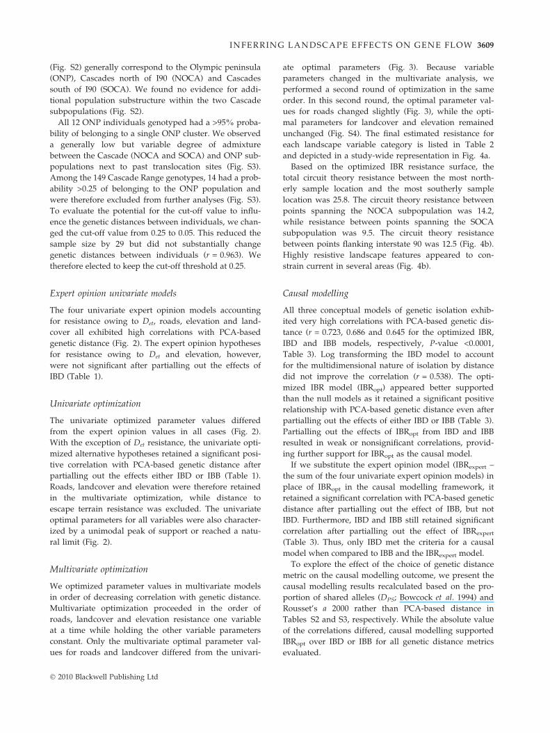
Based on the optimized IBR resistance surface, the

total circuit theory resistance between the most north-

erly sample location and the most southerly sample

location was 25.8. The circuit theory resistance between

points spanning the NOCA subpopulation was 14.2,

while resistance between points spanning the SOCA

subpopulation was 9.5. The circuit theory resistance

between points flanking interstate 90 was 12.5 (Fig. 4b).

Highly resistive landscape features appeared to con-

strain current in several areas (Fig. 4b).

Causal modelling

All three conceptual models of genetic isolation exhib-

ited very high correlations with PCA-based genetic dis-

tance (r = 0.723, 0.686 and 0.645 for the optimized IBR,

IBD and IBB models, respectively, P-value <0.0001,

Table 3). Log transforming the IBD model to account

for the multidimensional nature of isolation by distance

did not improve the correlation (r = 0.538). The opti-

mized IBR model (IBRopt) appeared better supported

than the null models as it retained a significant positive

relationship with PCA-based genetic distance even after

partialling out the effects of either IBD or IBB (Table 3).

Partialling out the effects of IBRopt from IBD and IBB

resulted in weak or nonsignificant correlations, provid-

ing further support for IBRopt as the causal model.

If we substitute the expert opinion model (IBRexpert –

the sum of the four univariate expert opinion models) in

place of IBRopt in the causal modelling framework, it

retained a significant correlation with PCA-based genetic

distance after partialling out the effect of IBB, but not

IBD. Furthermore, IBD and IBB still retained significant

correlation after partialling out the effect of IBRexpert

(Table 3). Thus, only IBD met the criteria for a causal

model when compared to IBB and the IBRexpert model.

To explore the effect of the choice of genetic distance

metric on the causal modelling outcome, we present the

causal modelling results recalculated based on the pro-

portion of shared alleles (DPS; Bowcock et al. 1994) and

Rousset’s a 2000 rather than PCA-based distance in

Tables S2 and S3, respectively. While the absolute value

of the correlations differed, causal modelling supported

IBRopt over IBD or IBB for all genetic distance metrics

evaluated.

(a) (b)

(c) (d)

(e) (f)

Fig. 2 Univariate IBR model optimization. The 3D contours represent the Mantel’s correlation (rM) with genetic isolation (y-axis)

interpolated across the range of parameter values shown. Parameter values governing the response shape (x) and maximum resis-

tance (Rmax) are noted on the x-axis and z-axis, respectively, for various hypotheses relating distance to escape terrain (Det; a), land-

cover (b) and roads (c) to genetic isolation. We also evaluated hypotheses relating elevation to genetic isolation (panel d, e, and f).

Elevation resistance parameters included the elevation standard deviation (ESD; one value shown per plot), optimal elevation (Eopt;

z-axis on each plot), and maximum resistance (Rmax; x-axis on each plot). The x-axis and z-axis labels for all plots represent parame-

ter values we evaluated (i.e. the floor of each plot represents the factorial combination of parameter values). The expert opinion

hypothesis (circle labelled with E) and the univariate optimized alternative hypothesis with the highest correlation (circle labelled

with U) are shown.

3610 A. J . SHIRK ET AL.

� 2010 Blackwell Publishing Ltd

Table 1 Univariate IBR model relationship to genetic isolation

after partialling out the effect of null models

Model Partial r

Monte Carlo

P value

Expert opinion models

G � Det | IBD 0.005 0.4436

G � Det | IBB 0.250 <0.0001

G � Roads | IBD 0.202 <0.0001

G � Roads | IBB 0.391 <0.0001

G � Landcover | IBD 0.124 0.0006

G � Landcover | IBB 0.304 <0.0001

G � Elevation | IBD 0.002 0.4760

G � Elevation | IBB 0.404 <0.0001

Univariate – optimized models

G � Det | IBD 0.039 0.1171

G � Det | IBB 0.363 <0.0001

G � Roads | IBD 0.236 <0.0001

G � Roads | IBB 0.389 <0.0001

G � Landcover | IBD 0.147 <0.0001

G � Landcover | IBB 0.427 <0.0001

G � Elevation | IBD 0.091 0.0050

G � Elevation | IBB 0.420 <0.0001

Partial Mantel’s test correlation with genetic distance (G) for

each expert opinion or univariate optimal model of landscape

resistance after partialling out the effects of the null models of

isolation by distance (IBD) or isolation by barrier (IBB) are

listed. The P values are based on 9999 Monte Carlo

randomizations of the row ⁄ column order.

INFERRING LANDSCAPE E FFECTS ON GENE FLOW 3611

Discussion

Landscapes shape gene flow in a variety of ways. Habi-

tats highly connected by dispersal may give rise to sim-

ple patterns of isolation by distance (e.g. Koopman

et al. 2007), strong barriers may impose a discrete sub-

population structure (e.g. Allentoft et al. 2009), or gradi-

ents of environmental variables influencing dispersal

may yield complex patterns of isolation by resistance

(e.g. Cushman et al. 2006). In this study, we present a

novel analytical framework designed to evaluate the rel-

ative support for isolation by distance, barriers and

multiple alternative landscape resistance hypotheses

with the goal of identifying the model most related to

the observed pattern of genetic isolation. As with all

model selection processes, reducing complex ecological

phenomena to relatively simple models necessarily

involves decisions that balance complexity with practi-

cal realities. These decisions profoundly shape the

framework’s ability to identify a landscape model

strongly related to the process of gene flow.

The multivariate hypothesis space

Two important aspects of a model selection framework

include the number of dimensions comprising the mul-

� 2010 Blackwell Publishing Ltd

tivariate hypothesis space and the density with which

that space is sampled. More dimensions sampled at

higher density permits evaluation of more complex or

more highly optimized landscape resistance models. In

some cases, greater complexity may not be necessary.

For example, Schwartz et al. (2009) identified a land-

scape resistance model related to wolverine gene flow

based on a single variable (spring snow depth) in one

dimension (resistance assigned to low snow depth pix-

els) after sampling the hypothesis space seven times.

Cushman et al. (2006) explored the fit of a more com-

plex model for black bear gene flow in northern Idaho

based on four variables (slope, elevation, landcover and

roads) in a total of four dimensions (each variable var-

ied by the degree of resistance assigned) after sampling

the hypothesis space 108 times. In this study, we con-

sidered mountain goat gene flow to be a function of

several potentially interacting environmental variables

that may exhibit nonlinear relationships with landscape

resistance. We also considered the potential for the

range of resistance values (from 1 to Rmax) to differ

between variables. In total, our hypothesis space con-

tained nine dimensions (Rmax and x for landcover, roads

and Det plus Rmax, Eopt, and ESD for elevation), which

we sampled 310 times (120 times in the univariate opti-

mization and 95 times in each of two multivariate opti-

mization rounds). The added complexity of this

modelling framework appeared warranted, given the

interactions, strongly nonlinear optimal relationships to

genetic isolation, and differences in Rmax between vari-

ables we observed in the multivariate optimized IBR

model. For species that respond in similarly complex

ways to their environment, failure to account for this

complexity in a modelling framework may result in

models that are less informative to connectivity conser-

vation efforts.

A role for expert opinion in landscape genetic models

Although the increased number of dimensions in our

model selection framework likely improved the fit of

the model selected, it also presented a challenge. Land-

scape genetics studies published to date have systemati-

cally sampled the hypothesis space at predefined

intervals. Systematically testing the full factorial of mul-

tiple hypotheses in each of our nine dimensions would

require an impractical number of models to evaluate.

Instead, we specified only a single starting hypothesis

(based on expert opinion), and, through the univariate

and multivariate optimization steps, sampled alterna-

tive hypotheses in the direction favouring improved

model fit. In this way, we greatly reduced the number

of hypotheses tested. Allowing feedback from the

model optimization process to define the hypothesis

(a) (b)

(c) (d)

(e) (f)

Fig. 3 Multivariate IBR model optimization. The 3D contour plot represents the Mantel’s correlation (rM) with genetic isolation (y-

axis) interpolated across the range of parameter values shown. We first optimized road resistance parameters (a), including the

response shape (x) and maximum resistance (Rmax) noted on the x-axis and z-axis, respectively. Next, we optimized landcover resis-

tance parameters (b), including the response shape (x) and maximum resistance (Rmax) noted on the x-axis and z-axis, respectively.

Finally, we optimized elevation resistance parameters (c, d, and e), which included the elevation standard deviation (ESD; one value

shown per plot), optimal elevation (Eopt; z-axis on each plot) and maximum resistance (Rmax; x-axis on each plot). The x-axis and z-

axis labels for all plots represent parameter values we evaluated (i.e. the floor of each plot represents the factorial combination of

parameter values). The univariate optimal parameter values (circled and labelled U) and the multivariate optimized alternative

parameter values with the highest correlation (circled and labelled M1) are shown. Because the parameter values changed in the mul-

tivariate context for one or more variables, we performed a second round of multivariate optimization in the same order. In the sec-

ond round, only the road resistance parameters changed slightly (f; Second round optimal values labelled M2), while the optimal

parameters for landcover and elevation did not change (see Fig. S4).

3612 A. J . SHIRK ET AL.

� 2010 Blackwell Publishing Ltd

Table 2 Landscape resistance values.

Resistance values (per pixel) for the

expert opinion, univariate optimized

and multivariate optimized IBR models

are listed

Variable – Pixel type

Expert

opinion

Univariate

optimized

Multivariate

optimized

Elevation – >3300 m* 100 000 100 000 100 000

Elevation – <3300 m† 1–5 1–5 1–5

Landcover – Urban ⁄ Ag.* 100 000 100 000 100 000

Landcover – Water 50 10 25

Landcover – Mesic ⁄ disturbed forest 16 2 1

Landcover – Montane forest 2 1 1

Landcover – Ice 1 1 1

Landcover – Subalpine 1 1 1

Landcover – Alpine 1 1 1

Roads – Interstate 1000 2500 10 000

Roads – Highway 89 1 80

Roads – Secondary 1 1 1

Det – 0 to 600 + m‡ 1–50 - —

*Urban and agriculture landcover pixels, as well as elevations > 3300 m were considered

impermeable to gene flow and assigned a fixed resistance value (not optimized) of

100 000.†Elevation resistance was one near the optimal elevation and increased according to the

standard deviation of elevation to Rmax at higher and lower elevations.‡Det resistance was one nearest to escape terrain and increased with distance as a

function of x and Rmax up to 600 m. Beyond 600 m, Det resistance was constant at Rmax.

INFERRING LANDSCAPE E FFECTS ON GENE FLOW 3613

space also added tremendous flexibility in finding the

optimal model. Potentially any combination of parame-

ter values could be evaluated with this approach. This

flexibility likely improved our ability to identify a

model strongly related to gene flow, as we did not

anticipate the highly nonlinear responses detected for

all variables, nor the magnitude of resistance owing to

interstate highways. Starting with expert opinion

parameters also allowed us to directly test the assump-

tions of expert opinion, grounding this approach in

classical hypothesis testing and bridging the gap

between empirical studies and those based on expert

knowledge alone.

Univariate and multivariate IBR model optimization

We chose to divide the IBR model optimization process

into two steps. In the first step, univariate optimization

of model parameters provided three important pieces

of information. First, it allowed for a comparison of

models generated from the univariate optimum param-

eter values to null models of isolation by distance or

barrier. With this information, we excluded variables

from the multivariate analysis that were not likely to

improve support for the IBR model relative to the null

models. Second, the univariate optimization provided a

plot of model performance as a function of alternative

parameter values (Fig. 2). We used this to exclude vari-

ables whose univariate optimum model appeared corre-

lated with genetic isolation by chance (i.e. not

characterized by a unimodal peak of support), a con-

� 2010 Blackwell Publishing Ltd

cern given the number of models we tested. Eliminating

variables from the multivariate analysis if their parame-

ters did not meet the earlier criteria also reduced the

dimensionality of the multivariate optimization step.

This, in turn, simplified the task of finding a multivari-

ate optimum set of parameter values while likely

improving the fit of the multivariate model. Third, the

univariate optimization step provided a ranking of each

variable’s importance (based on the strength of their

correlation with genetic isolation). This information

determined the order of the multivariate optimization

step. Optimizing the variable with the greatest univari-

ate correlation first was a practical approach that likely

decreased the number of rounds of optimization

required to reach a stable model compared to an unor-

dered process.

Combining univariate optimized models yielded a

starting point for the multivariate optimization step,

where we sought to account for interactions between

variables and thereby optimize the IBR model in the

multivariate context. In this study, the optimal param-

eters changed for several of the factors during multi-

variate optimization, resulting in a slight increase in

the model’s correlation with genetic isolation. The

slightly higher correlation masks rather large changes

for some model parameters, particularly for roads.

The minor change in correlation for such a large

change in parameter values is a result of the relative

rarity of road pixels in the landscape. Interstate high-

ways represent only a very small proportion of the

total study area, requiring a correspondingly greater

(a) (b)

Fig. 4 (a) Optimized IBR resistance model. The multivariate optimized IBR model is depicted, with the highest resistance in white

and lowest resistance in black. The values represent the sum of resistance owing to roads, landcover and elevation. (b) Circuit theory

current (analogous to gene flow). The predicted current flow after injecting one ampere of current into the most northerly sample

location (point 1) and connecting the most southerly sample location (point 4) to ground is shown (based on the optimized IBR resis-

tance model). Zero current flows through areas where landscape resistance is very high (shown in black). Moderate levels of current

flow through areas where gene flow is relatively unconstrained. In areas where highly resistive features constrain flow, current

increases (approaching white where current is maximum). Because current is constrained by the location where it is injected and the

ground location where it exits, current is also high near points 1 and 4. The total circuit theory resistance between points 1 and 4 is

25.8. Circuit theory resistances for subsets of the study area, including intermediate points (point 2 and 3) flanking interstate 90 are

shown to the right of the current flow map.

3614 A. J . SHIRK ET AL.

resistance assigned to this pixel type to influence the

effective landscape resistance between sampling loca-

tions. Thus, a particular feature’s resistance and rarity

in the landscape interact to shape the overall effect on

the model.

Five important limitations of this model optimization

framework should be noted: (i) In cases where a spe-

cies’ response to one or more environmental variables

is multimodal, exploring the hypothesis space from a

single starting point could potentially identify a local

peak of support for a particular IBR hypothesis rather

than a global peak of support. Particularly in these

instances, the model selected may depend heavily on

the initial starting point. (ii) As we explored the

hypothesis space, we sampled relatively coarse intervals

for each parameter. Consequently, we did not finely

resolve the optimal parameter values. (iii) We evaluated

alternative hypotheses in the multivariate optimization

step one variable at a time while holding other vari-

ables constant. As the combinations tested do not repre-

sent the full factorial of all hypotheses for every

variable, it is possible a more optimal multivariate

hypothesis went untested, or that a different order of

variable optimization could produce a different result.

(iv) It may not be practical to optimize all aspects of the

IBR model (e.g. we assigned fixed ranks to different

landcover types and a fixed resistance to certain habi-

tats thought to be absolute barriers to mountain goat

gene flow). Thus, the optimized parameters of the IBR

model and its performance relative to null models

could be influenced by the value assigned to these un-

optimized components. (v) While optimization clearly

improved the fit of the model to the observed genetic

isolation, the model may be overfit. An overfit model

may provide a spatially explicit prediction of landscape

resistance but fail to offer a robust ecological inference

regarding the actual relationship between landscape

variables and their resistance to gene flow. Exploring

this issue with model cross-validation using indepen-

dent data (as in Braunisch et al. 2010) and simulations

(as in Cushman & Landguth 2010) would be a useful

addition to this framework in future studies.

� 2010 Blackwell Publishing Ltd

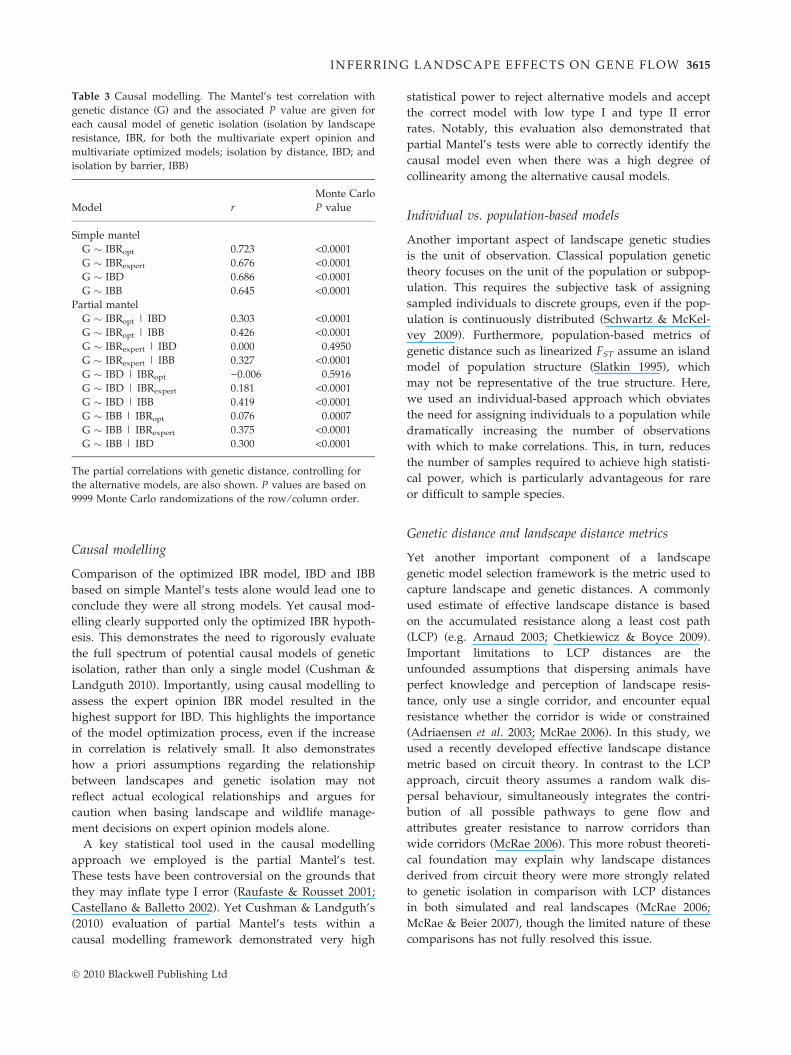
Table 3 Causal modelling. The Mantel’s test correlation with

genetic distance (G) and the associated P value are given for

each causal model of genetic isolation (isolation by landscape

resistance, IBR, for both the multivariate expert opinion and

multivariate optimized models; isolation by distance, IBD; and

isolation by barrier, IBB)

Model r

Monte Carlo

P value

Simple mantel

G � IBRopt 0.723 <0.0001

G � IBRexpert 0.676 <0.0001

G � IBD 0.686 <0.0001

G � IBB 0.645 <0.0001

Partial mantel

G � IBRopt | IBD 0.303 <0.0001

G � IBRopt | IBB 0.426 <0.0001

G � IBRexpert | IBD 0.000 0.4950

G � IBRexpert | IBB 0.327 <0.0001

G � IBD | IBRopt )0.006 0.5916

G � IBD | IBRexpert 0.181 <0.0001

G � IBD | IBB 0.419 <0.0001

G � IBB | IBRopt 0.076 0.0007

G � IBB | IBRexpert 0.375 <0.0001

G � IBB | IBD 0.300 <0.0001

The partial correlations with genetic distance, controlling for

the alternative models, are also shown. P values are based on

9999 Monte Carlo randomizations of the row ⁄ column order.

INFERRING LANDSCAPE E FFECTS ON GENE FLOW 3615

Causal modelling

Comparison of the optimized IBR model, IBD and IBB

based on simple Mantel’s tests alone would lead one to

conclude they were all strong models. Yet causal mod-

elling clearly supported only the optimized IBR hypoth-

esis. This demonstrates the need to rigorously evaluate

the full spectrum of potential causal models of genetic

isolation, rather than only a single model (Cushman &

Landguth 2010). Importantly, using causal modelling to

assess the expert opinion IBR model resulted in the

highest support for IBD. This highlights the importance

of the model optimization process, even if the increase

in correlation is relatively small. It also demonstrates

how a priori assumptions regarding the relationship

between landscapes and genetic isolation may not

reflect actual ecological relationships and argues for

caution when basing landscape and wildlife manage-

ment decisions on expert opinion models alone.

A key statistical tool used in the causal modelling

approach we employed is the partial Mantel’s test.

These tests have been controversial on the grounds that

they may inflate type I error (Raufaste & Rousset 2001;

Castellano & Balletto 2002). Yet Cushman & Landguth’s

(2010) evaluation of partial Mantel’s tests within a

causal modelling framework demonstrated very high

� 2010 Blackwell Publishing Ltd

statistical power to reject alternative models and accept

the correct model with low type I and type II error

rates. Notably, this evaluation also demonstrated that

partial Mantel’s tests were able to correctly identify the

causal model even when there was a high degree of

collinearity among the alternative causal models.

Individual vs. population-based models

Another important aspect of landscape genetic studies

is the unit of observation. Classical population genetic

theory focuses on the unit of the population or subpop-

ulation. This requires the subjective task of assigning

sampled individuals to discrete groups, even if the pop-

ulation is continuously distributed (Schwartz & McKel-

vey 2009). Furthermore, population-based metrics of

genetic distance such as linearized FST assume an island

model of population structure (Slatkin 1995), which

may not be representative of the true structure. Here,

we used an individual-based approach which obviates

the need for assigning individuals to a population while

dramatically increasing the number of observations

with which to make correlations. This, in turn, reduces

the number of samples required to achieve high statisti-

cal power, which is particularly advantageous for rare

or difficult to sample species.

Genetic distance and landscape distance metrics

Yet another important component of a landscape

genetic model selection framework is the metric used to

capture landscape and genetic distances. A commonly

used estimate of effective landscape distance is based

on the accumulated resistance along a least cost path

(LCP) (e.g. Arnaud 2003; Chetkiewicz & Boyce 2009).

Important limitations to LCP distances are the

unfounded assumptions that dispersing animals have

perfect knowledge and perception of landscape resis-

tance, only use a single corridor, and encounter equal

resistance whether the corridor is wide or constrained

(Adriaensen et al. 2003; McRae 2006). In this study, we

used a recently developed effective landscape distance

metric based on circuit theory. In contrast to the LCP

approach, circuit theory assumes a random walk dis-

persal behaviour, simultaneously integrates the contri-

bution of all possible pathways to gene flow and

attributes greater resistance to narrow corridors than

wide corridors (McRae 2006). This more robust theoreti-

cal foundation may explain why landscape distances

derived from circuit theory were more strongly related

to genetic isolation in comparison with LCP distances

in both simulated and real landscapes (McRae 2006;

McRae & Beier 2007), though the limited nature of these

comparisons has not fully resolved this issue.

3616 A. J . SHIRK ET AL.

While the circuit theory distance metric provides the-

oretical advantages, it comes at a cost of greater com-

puter processing requirements. Considering the number

of locations in our sample set and the scale of our study

area, we found a pixel size of 450 m to be the maxi-

mum practical resolution. This may not have been

appropriate to model landscape features that occur at a

finer spatial scale. Escape terrain in particular may

occur in narrow cliff bands that were not captured at

our coarser resolution and may explain why the most

supported model of IBR for this important mountain

goat habitat variable did not outperform the null mod-

els. The latest versions of Circuitscape offer improved

processing efficiency (B. McRae, personal communica-

tion) and continued increases in computer memory use

efficiency as well as processor speed will make this

issue less relevant to future studies.

To quantify genetic distance, we used a metric based

on principal components analysis. A major advantage

of this approach is that alleles that capture the greatest

proportion of the genetic variation within a population

have a correspondingly greater contribution to genetic

distance than common alleles, which capture relatively

little of a population’s genetic variation. In theory, this

makes PCA a more sensitive method to detect genetic

dissimilarity than other methods, such as the propor-

tion of shared alleles (DPS; Bowcock et al. 1994) or

(Rousset’s a 2000) where all alleles contribute equally.

In a limited comparison, we found correlations with

landscape resistance models to be higher overall with

the PCA-based metric, though the causal modelling out-

come was the same regardless of which genetic distance

we used (Figs S3 and S4). While the theoretical advan-

tages of PCA-based genetic distance are compelling, the

statistical basis for its use in landscape genetics and its

performance relative to other metrics requires further

study.

Mountain goat gene flow in the cascade range,Washington

Surprisingly, resistance to gene flow within the study

area did not appear to increase with distance to escape

terrain. While the grain of our analysis may not have

been capable of detecting such an effect (as discussed

previously), there may be other explanations for why

this important habitat variable was not accounted for in

the optimized IBR model. For example, optimizing dis-

persal paths to maximize proximity to escape terrain

may not be possible for individuals dispersing through

unfamiliar habitat. Alternatively, as escape terrain is

abundant within the study area, this important habitat

variable may not be a limiting factor for dispersal and

therefore offer no additional resistance to gene flow.

Elevation appeared to play a modest role in shaping

gene flow within the study area. Cascade Range moun-

tain goats frequently migrate from lower elevation win-

ter habitat to higher elevation summer habitat in late

spring and summer (Rice 2008). During this time,

mountain goats may disperse to new patches of habitat,

potentially resulting in gene flow. Dispersal and migra-

tion to summer habitat is facilitated by the receding

winter snow pack, which presumably decreases the

energetic costs to movement and increases foraging suc-

cess (Festa-Bianchet & Cote 2008). Though mountain

goat habitat use as a function of elevation is variable

throughout the study area, the least resistive elevation

range of the optimized IBR model (from 1000 to

2200 m) generally encompasses both winter and sum-

mer habitat (C. Rice, WDFW, personal communication).

Thus, the lowest elevation resistance aligns with the ele-

vations likely to be used by dispersing mountain goats

when the snow pack recedes. At higher elevations,

increased resistance (up to 5) likely corresponds to

greater snow depth, poorer foraging success and greater

energetic costs. At lower elevations, resistance may

increase because of the generally poor adaptation of this

species to low elevation habitats.

Similar to elevation, landcover also appeared to play

a modest role in shaping gene flow within the study

area. Though mountain goats are commonly considered

alpine habitat specialists, subalpine, montane and mesic

forests offered no additional resistance to gene flow in

the optimized IBR model. This is congruent with the

adaptation of coastal North American mountain goats

to forested environments, where they may spend much

of the winter on steep slopes beneath the canopy (Festa-

Bianchet & Cote 2008). Water was the only optimized

landcover type that appeared to resist mountain goat

gene flow. The resistance attributed to water (25) was

far less than that of crossing a highway (80) or inter-

state (10 000), suggesting at least smaller water bodies

like those found within the study area are not major

impediments to gene flow. Indeed, mountain goats are

capable swimmers and have been observed crossing

major lakes and rivers. In addition to the resistance

owing to water pixels, we apriori assigned a high fixed

resistance prohibiting gene flow through urban and

agriculture pixels. These landcover types are associated

with high human population densities and highly mod-

ified landscapes, both of which are strongly avoided by

mountain goats. Such areas rarely occur within the

study area, minimizing their influence on the IBR

model. In a few instances, however, urban and agricul-

tural areas are configured such that they constrain gene

flow. This is evident in a few locations on Fig. 4B,

where current is increased in narrow corridors of suit-

able dispersal habitat between small towns, and about

� 2010 Blackwell Publishing Ltd

INFERRING LANDSCAPE E FFECTS ON GENE FLOW 3617

50 km south of Mount Baker (Point 1), where agricul-

ture and development likely forces gene flow in a wide

arc to the east.

Together, the influence of elevation gradients and

landcover patterns we inferred based on the optimized

IBR model suggests a clinal population structure only

moderately more resistive to gene flow than IBD (where

the resistance of all pixels is one). In contrast, I90

appears to greatly reduce gene flow and impose a sharp

genetic discontinuity on this otherwise clinal popula-

tion. Major interstates are notorious resistors of gene

flow for many species (Coffin 2007). Its significance to

the genetic structure of this population is supported by

the high resistance assigned to it in the optimized IBR

model and the sharp boundary coinciding with I90 we

detected using Structure (Fig. S3). Despite the small

area, this feature occupies (nearly invisible in Fig. 4), its

resistance is on par with the total resistance spanning

the north or south Cascades. Yet I90 does not appear to

be a complete barrier to gene flow, as we detected

recent admixture between the north and south Cascades

(Fig. S1), and the IBB model (which posits complete

isolation between the north and south) was not sup-

ported by causal modelling. In contrast to interstates,

the resistance attributed to highways within the study

area suggests this road class does not greatly impede

gene flow. Indeed, mountain goats have regularly been

observed crossing these highways. Similarly, mountain

goat gene flow appears to move easily over minor roads

(with no additional resistance based on the optimized

IBR model).

These findings have important consequences for the

conservation of mountain goats in the Cascade Range,

Washington. The population has declined by up to 70%

over the past 50 years, likely because of unsustainable

harvest rates (Rice & Gay 2010). Though harvest has

been dramatically reduced for over two decades, the

population has not shown significant recovery across

most of the range, and large areas of formerly occupied

habitat remain sparsely occupied (C. Rice, WDFW,

unpublished). Recovery and recolonization of habitat

will likely depend heavily on dispersal from the few

remaining large herds. Yet recent landscape changes,

particularly the high resistance values associated with

anthropogenic modifications, suggest greater resistance

to dispersal now than was present in the historic land-

scape. This combination of demographic decline and

reduced gene flow would be predicted to greatly

reduce the local effective population size throughout

the range. As a result, we would expect increased rates

of inbreeding, reduced allelic diversity and concomitant

loss of fitness and adaptive potential over time. The

quantitative and spatially explicit understanding of

landscape resistance gained from the optimized IBR

� 2010 Blackwell Publishing Ltd

model is currently being used to inform habitat connec-

tivity planning in an attempt to improve the population

viability of mountain goats in the Cascade Range,

Washington.

Acknowledgements

We thank Cheryl Dean, WDFW, for DNA isolation and geno-

typing. We also thank the NPS and the USGS for contributing

genetic samples. Funding for this research was provided by

WDFW, the NPS, the USGS, and grants from the WWU Office

of Research and Sponsored Programs, Huxley College of the

Environment, Seattle City Light, the Mountaineers Foundation,

and the Mazamas.

References

Adriaensen F, Chardon JP, De Blust G et al. (2003) The

application of ‘least-cost’ modelling as a functional

landscape model. Landscape and Urban Planning, 64, 233–247.

Allentoft ME, Siegismund HR, Briggs L, Andersen LW (2009)

Microsatellite analysis of the natterjack toad (Bufo calamita)

in Denmark: populations are islands in a fragmented

landscape. Conservation Genetics, 10, 15–28.

Arnaud JF (2003) Metapopulation genetic structure and

migration pathways in the land snail Helix aspersa:

influence of landscape heterogeneity. Landscape Ecology, 18,

333–346.

Beckey FW (1987) Cascade Alpine Guide. Mountaineers, Seattle.

Beier P, Majka DR, Spencer WD (2008) Forks in the road:

choices in procedures for designing wildland linkages.

Conservation Biology, 22, 836–851.

Bowcock AM, Ruizlinares A, Tomfohrde J et al. (1994) High-

resolution of human evolutionary trees with polymorphic

microsatellites. Nature, 368, 455–457.

Braunisch V, Segelbacher G, Hirzel AH (2010) Modelling

functional landscape connectivity from genetic population

structure – a new spatially explicit approach. Molecular

Ecology, 19, 3664–3678.

Castellano S, Balletto E (2002) Is the partial Mantel test

inadequate? Evolution, 56, 1871–1873.

Chetkiewicz CLB, Boyce MS (2009) Use of resource selection

functions to identify conservation corridors. Journal of Applied

Ecology, 46, 1036–1047.

Coffin AW (2007) From roadkill to road ecology: a review of

the ecological effects of roads. Journal of Transport Geography,

15, 396–406.

Crnokrak P, Roff DA (1999) Inbreeding depression in the wild.

Heredity, 83, 260–270.

Crooks KR, Sanjayan MA (2006) Connectivity Conservation.

Cambridge University Press, Cambridge.

Cushman SA, Landguth EL (2010) Spurious correlations and

inference in landscape genetics. Molecular Ecology, 19, 3592–

3602.

Cushman SA, McKelvey KS, Hayden J, Schwartz MK (2006)

Gene flow in complex landscapes: testing multiple hypotheses

with causal modeling. American Naturalist, 168, 486–499.

Epps CW, Wehausen JD, Bleich VC, Torres SG, Brashares JS

(2007) Optimizing dispersal and corridor models using

landscape genetics. Journal of Applied Ecology, 44, 714–724.

3618 A. J . SHIRK ET AL.

Festa-Bianchet M, Cote SD (2008) Mountain Goats: Ecology,

Behavior, and Conservation of an Alpine Ungulate. Island Press,

Washington.

Garroway CJ, Bowman J, Carr D, Wilson PJ (2008) Appli-

cations of graph theory to landscape genetics. Evolutionary

Applications, 1, 620–630.

Goslee SC, Urban DL (2007) The ecodist package for

dissimilarity-based analysis of ecological data. Journal of

Statistical Software, 22, 1–19.

Goudet J (1995) FSTAT (Version 1.2): a computer program to

calculate F-statistics. Journal of Heredity, 86, 485–486.

Holderegger R, Wagner HH (2008) Landscape genetics.

BioScience, 58, 199–207.

Horskins K, Mather PB, Wilson JC (2006) Corridors and

connectivity: when use and function do not equate.

Landscape Ecology, 21, 641–655.

Houston DB, Moorhead BB, Olson RW (1991) Mountain goat

population trends in the Olympic Mountain-Range,

Washington. Northwest Science, 65, 212–216.

Keyghobadi N (2007) The genetic implications of habitat

fragmentation for animals. Canadian Journal of Zoology-Revue

Canadienne De Zoologie, 85, 1049–1064.

Koenig WD, VanVuren D, Hooge PN (1996) Detectability,

philopatry, and the distribution of dispersal distances in

vertebrates. Trends in Ecology & Evolution, 11, 514–517.

Koopman ME, Hayward GD, McDonald DB (2007) High

connectivity and minimal genetic structure among North

American boreal owl (Aegolius funereus) populations,

regardless of habitat matrix. The Auk, 124, 690–704.

Lande R (1995) Mutation and conservation. Conservation

Biology, 9, 782–791.

Lande R (1998) Risk of population extinction from fixation of

deleterious and reverse mutations. Genetica, 103, 21–27.

Lynch M, Conery J, Burger R (1995) Mutation accumulation

and the extinction of small populations. American Naturalist,

146, 489–518.

Mainguy J, Llewellyn AS, Worsley K, Cote SD, Coltman DW

(2005) Characterization of 29 polymorphic artiodactyl

microsatellite markers for the mountain goat (Oreamnos

americanus). Molecular Ecology Notes, 5, 809–811.

Mantel N (1967) The detection of disease clustering and a

generalized regression approach. Cancer Research, 27, 209–

220.

McRae BH (2006) Isolation by resistance. Evolution, 60, 1551–

1561.

McRae BH, Beier P (2007) Circuit theory predicts gene flow in

plant and animal populations. Proceedings of The National

Academy of Sciences of The United States of America, 104,

19885–19890.

Murphy MA, Evans JS, Cushman SA, Storfer A (2009)

Representing genetic variation as continuous surfaces: an

approach for identifying spatial dependency in landscape

genetic studies. Ecography, 31, 685–697.

Murphy MA, Evans JS, Storfer A (2010) Quantifying Bufo

boreas connectivity in Yellowstone National Park with

landscape genetics. Ecology, 91, 252–261.

NWGAP (2007) Northwest GAP Analysis Project. Available

from http://www.gap.uidaho.edu/Northwest/data.htm.

Patterson N, Price AL, Reich D (2006) Population structure and

eigenanalysis. PLoS Genet, 2, 190.

Perez-Espona S, Perez-Barberia FJ, McLeod JE et al. (2008)

Landscape features affect gene flow of Scottish Highland red

deer (Cervus elaphus). Molecular Ecology, 17, 981–996.

Pritchard JK, Stephens M, Donnelly P (2000) Inference of

population structure using multilocus genotype data.

Genetics, 155, 945–959.

Raufaste N, Rousset F (2001) Are partial Mantel tests

adequate? Evolution, 55, 1703–1705.

Rice CG (2008) Seasonal and altitudinal movements of

mountain goats. Journal of Wildlife Management, 72, 1706–

1716.

Rice C, Gay D (2010) Mountain goat harvest in Washington

state: effects on historic and contemporary populations.

Northwest Naturalist, 91, 40–57.

Ricketts TH (2001) The matrix matters: effective isolation in

fragmented landscapes. American Naturalist, 158, 87–99.

Rousset F (2000) Genetic differentiation between individuals.

Journal of Evolutionary Biology, 13, 58–62.

Schwartz MK, McKelvey KS (2009) Why sampling scheme

matters: the effect of sampling scheme on landscape genetic

results. Conservation Genetics, 10, 441–452.

Schwartz MK, Copeland JP, Anderson NJ et al. (2009)

Wolverine gene flow across a narrow climatic niche. Ecology,

90, 3222–3232.

Slatkin M (1995) A measure of population subdivision based

on microsatellite allele frequencies. Genetics, 139, 457–462.

Smith CA (1994) Bi-level analysis of habitat selection by

mountain goats in coastal Alaska. Proceedings of the Biennial

Symposium of the Northern Wild Sheep and Goat Council, 5,

366–379.

Smouse PE, Long JC, Sokal RR (1986) Multiple regression and

correlation extensions of the Mantel test of matrix

correspondence. Systematic Biology, 35, 627–632.

Spear SF, Balkenhol N, Fortin M-J, McRae BH, Scribner K

(2010) Use of resistance surfaces for landscape genetic

studies: considerations for parameterization and analysis.

Molecular Ecology, 19, 3576–3591.

Storfer A, Murphy MA, Evans JS et al. (2007) Putting the

‘landscape’ in landscape genetics. Heredity, 98, 128–142.

Swindell WR, Bouzat JL (2005) Modeling the adaptive potential

of isolated populations: experimental simulations using

Drosophila. Evolution, 59, 2159–2169.

Van Oosterhout C, Hutchinson WF, Wills DPM, Shipley P

(2004) MICRO-CHECKER: software for identifying and

correcting genotyping errors in microsatellite data. Molecular

Ecology Notes, 4, 535–538.

Van Oosterhout C, Weetman D, Hutchinson WF (2006)

Estimation and adjustment of microsatellite null alleles in

nonequilibrium populations. Molecular Ecology Notes, 6, 255–

256.

Wahlund S (1928) Composition of populations from the

perspective of the theory of heredity. Hereditas, 11, 65–105.

Wang YH, Yang KC, Bridgman CL, Lin LK (2008) Habitat

suitability modelling to correlate gene flow with landscape

connectivity. Landscape Ecology, 23, 989–1000.

Wang IJ, Savage WK, Shaffer HB (2009) Landscape genetics

and least-cost path analysis reveal unexpected dispersal

routes in the California tiger salamander (Ambystoma

californiense). Molecular Ecology, 18, 1365–1374.

Wright S (1943) Isolation by distance. Heredity, 28, 114–138.

� 2010 Blackwell Publishing Ltd

INFERRING LANDSCAPE E FFECTS ON GENE FLOW 3619

WSDOT (2006) Washington State Department of Transportation

Annual Traffic Report. Available from http://wsdot.wa.gov.

Andrew Shirk and Samuel Cushman’s research interests

include understanding landscape effects on gene flow and

genitic diversity, population dynamics, habitat modeling, and

population viability analysis. David Wallin’s research interests

include remote sensing applications in ecology, habitat model-

ing, and landscape genetics. Cliff Rice’s research interests

include wildlife biology and conservation, population

dynamics, and habitat modeling. Ken Warheit’s research inter-

ests include population genetics, adaptive genetic variation,

wildlife biology and conservation, and molecular systematics.

Supporting information

Additional supporting information may be found in the online

version of this article.

Table S1 PCR Conditions and multiplex groups

� 2010 Blackwell Publishing Ltd

Table S2 Causal modeling results based on proportion of

shared alleles (DPS) genetic distance

Table S3 Causal modeling results based on Rousset’s a genetic

distance

Fig. S1 A Gaussian function relating elevation to landscape

resistance. This function has three parameters: Rmax (resistance

ranges from 1 to Rmax), Eopt (the optimal elevation where resis-

tance is lowest), and ESD (the standard deviation about the

optimal elevation defining the shape of the response curve).

Fig. S2 Population structure based on Structure.

Fig. S3 Structure population assignments and fractional proba-

bility of subpopulation membership (Q).

Fig. S4 The second round of multivariate IBR model optimiza-

tion for landcover and elevation following the road optimiza-

tion (depicted in Fig. 3) is shown.

Please note: Wiley-Blackwell are not responsible for the content

or functionality of any supporting information supplied by the

authors. Any queries (other than missing material) should be

directed to the corresponding author for the article.