University of Massachusetts Amherst University of Massachusetts Amherst

ScholarWorks@UMass Amherst ScholarWorks@UMass Amherst

Environmental Conservation Faculty Publication Series Environmental Conservation

2018

A landscape index of ecological integrity to inform landscape A landscape index of ecological integrity to inform landscape

conservation conservation

Kevin McGarigal University of Massachusetts Amherst

Brad Compton University of Massachusetts Amherst

Ethan Plunkett University of Massachusetts Amherst

Bill DeLuca University of Massachusetts Amherst

Joanna Grand National Audubon Society

See next page for additional authors Follow this and additional works at: https://scholarworks.umass.edu/nrc_faculty_pubs

Part of the Environmental Monitoring Commons, and the Natural Resources and Conservation

Commons

Recommended Citation Recommended Citation McGarigal, Kevin; Compton, Brad; Plunkett, Ethan; DeLuca, Bill; Grand, Joanna; Ene, Eduard; and Jackson, Scott D., "A landscape index of ecological integrity to inform landscape conservation" (2018). Landscape Ecology. 402. Retrieved from https://scholarworks.umass.edu/nrc_faculty_pubs/402

This Article is brought to you for free and open access by the Environmental Conservation at ScholarWorks@UMass Amherst. It has been accepted for inclusion in Environmental Conservation Faculty Publication Series by an authorized administrator of ScholarWorks@UMass Amherst. For more information, please contact scholarworks@library.umass.edu.

Authors Authors Kevin McGarigal, Brad Compton, Ethan Plunkett, Bill DeLuca, Joanna Grand, Eduard Ene, and Scott D. Jackson

This article is available at ScholarWorks@UMass Amherst: https://scholarworks.umass.edu/nrc_faculty_pubs/402

1Science Division, National Audubon Society, Northampton, MA 01060, USA 2Eco-logica Software Solutions, Waterloo, ON N2T2M7, Canada

A landscape index of ecological integrity to inform landscape conservation

Kevin McGarigala, Bradley W. Comptona, Ethan B. Plunketta, William V. DeLucaa, Joanna

Granda1, Eduard Enea2, and Scott D. Jacksona

aDepartment of Environmental Conservation, University of Massachusetts, Amherst, MA 01003,

USA

Kevin McGarigal (Corresponding author)

email: mcgarigalk@eco.umass.edu

phone: 413-577-0655/fax: 413-545-4358

Bradley W. Compton, bcompton@eco.umass.edu

Ethan B. Plunkett, eplunkett@eco.umass.edu

William V. DeLuca, wdeluca@eco.umass.edu

Joanna Grand, jgrand@audubon.org

Eduard Ene, gispro@gmail.com

Scott D. Jackson, sjackson@umass.edu

Date of the manuscript: May 29, 2018

Manuscript word count (including abstract, text, tables, and captions): 9,899

Abstract

Context. Conservation planning is increasingly using "coarse filters" based on the idea of

conserving "nature's stage". One such approach is based on ecosystems and the concept of

ecological integrity, although myriad ways exist to measure ecological integrity.

Objectives. To describe our ecosystem-based index of ecological integrity (IEI) and its derivative 5

index of ecological impact (ecoImpact), and illustrate their applications for conservation

assessment and planning in the northeastern United States.

Methods. We characterized the biophysical setting of the landscape at the 30 m cell resolution

using a parsimonious suite of settings variables. Based on these settings variables and mapped

ecosystems, we computed a suite of anthropogenic stressor metrics reflecting intactness (i.e., 10

freedom from anthropogenic stressors) and resiliency metrics (i.e., connectivity to similar

neighboring ecological settings), quantile-rescaled them by ecosystem and geographic extent,

and combined them in a weighted linear model to create IEI. We used the change in IEI over

time under a land use scenario to compute ecoImpact.

Results. We illustrated the calculation of IEI and ecoImpact to compare the ecological integrity 15

consequences of a 70-year projection of urban growth to an alternative scenario involving

securing a network of conservation core areas (reserves) from future development.

Conclusions. IEI and ecoImpact offer an effective way to assess ecological integrity across the

landscape and examine the potential ecological consequences of alternative land use and land

cover scenarios to inform conservation decision making. 20

Key words: landscape pattern; landscape metrics; ecological assessment; conservation planning;

landscape conservation design; coarse filter

Introduction

Unrelenting human demand for commodities and services from ecosystems raises questions

of limits and sustainability. Many scientists believe that the earth is facing another mass 25

extinction as a consequence (Pimm et al 1995; Ceballos et al 2015). Indeed, current global

extinction rates for animals and plants are at least 100 times higher than the background rate in

the fossil record (Ceballos et al 2015). A number of factors have been implicated as key drivers

of this global biodiversity crisis, but chief among them is anthropogenic habitat loss and

fragmentation (Sala et al 2000, Pereira et al 2010; Haddad et al 2015, Newbold et al 2015). In 30

response, land use planners and conservationists are seeking better ways to proactively conserve

the most significant natural areas before they are lost or irreversibly degraded, but it is difficult

to prioritize areas that are in the greatest need of protection, or determine which ones provide the

greatest ecological value for the cost of protection. Analyzing a landscape’s

ecological/biodiversity value requires integrating vast amounts of site-specific information over 35

varying spatial scales. Conservation organizations, which collectively spend billions of dollars

each year to protect and connect natural areas (Lerner et al 2007), increasingly need tools to

effectively target conservation.

To meet the growing need for targeting conservation action, a variety of approaches have

been developed for evaluating the human footprint (e.g., Sanderson et al 2002, Theobald 2013, 40

Venter et al 2016) and selecting lands and waters for conservation protection (e.g., Williams et al

2002; Ortega-Huerta and Peterson 2004, Belote et al 2017). Important questions about the

various approaches persist and include the appropriate type or level of diversity on which to

focus (e.g., individual species, biotic communities, ecological systems, or geophysical settings),

the criteria by which areas should be selected, specific protocols for optimizing reserve selection, 45

and the amount of protected area needed to achieve conservation goals. Over time, focus has

shifted from isolated reserves to interconnected reserve networks selected based on landscape

ecology principles (e.g., Soulé & Terborgh 1999; Briers 2002; Cerdeira et al 2005; Beier 2012),

and from single species to multi-species and, more recently, ecosystem- and geophysical-based

approaches that seek to conserve "nature's stage" (e.g., Hunter et al 1988; Noss 1996; Pickett et 50

al. 1992; Anderson and Ferree 2010; Beier et al 2015; Wurtzebach and Schultz 2016). These

approaches emphasize retaining representative ecological and/or geophysical settings instead of

focal species, and as such provide a "coarse filter" (sensu Hunter et al 1988) for biodiversity

conservation. The use of such a coarse filter is touted as being proactive for species conservation

because if ecological settings (which provide the habitat that species depend on) remain intact, 55

most species will also be conserved (e.g., Scott et al. 1993). Moreover, it is assumed that if

ecological settings remain intact, critical ecological and evolutionary processes, such as nutrient

and sediment transport, interspecific interactions, dispersal, gene flow and disturbance regimes,

will also be maintained and provide the necessary environmental stage for climate adaptation to

occur (Beier 2012; Beier et al 2015). This prospect is appealing because biological diversity 60

(with shifting composition) could be conserved under changing environmental conditions with

the same expenditure of funds and commitment of land to conservation and without specific and

detailed knowledge of every species of interest.

While the general concept of focusing on nature's stage is both appealing and intuitive, there

are many different approaches for doing so. One approach has been to focus solely on the 65

geophysical environment without attention to the biota, and identify and prioritize representative,

diverse and connected geophysical settings based on one or more metrics (e.g., Anderson et al

2014; Beier et al 2015). Here the goal is to conserve the abiotic stage and allow the biota to

change and "play out" on this stage over time, especially in response to climate change (Beier

and Brost 2010; Beier 2012). For example, Anderson et al (2014) measured site resiliency using 70

a combination of two metrics: 1) landscape diversity, which refers to the number of

microhabitats and climatic gradients available within a given area based on the variety of

landforms, elevation range, soil diversity, and wetland extent and density, and 2) local

connectedness, which refers to the accessibility of neighboring natural areas. This measure of

site resiliency is agnostic to the distribution of biota and explicit climate change projections, but 75

is somewhat sensitive to the impacts of human development via the fragmentation of natural

areas. This approach has been shown to perform well as a surrogate for species diversity

(Anderson et al 2014).

An alternative approach, but not without its critics (e.g., Brown and Williams 2016), has been

to focus on ecosystems, with attention to both the biotic as well as geophysical environment, and 80

use the concept of ecological integrity to identify and prioritize places of conservation value

(e.g., Tierney et al 2009, Theobald 2013, Wurtzebach and Schultz 2016, Belote et al 2017). Here

the goal is to conserve the "ecological stage" by focusing on places with high ecological integrity

that can sustain the biota and critical ecological processes. Ecological integrity is broadly defined

as "the ability of an ecological system to support and maintain a community of organisms that 85

has species composition, diversity, and functional organization comparable to those of natural

habitats within a region; an ecological system has integrity when its dominant ecological

characteristics (e.g., elements of composition, structure, function, and ecological processes)

occur within their natural ranges of variation and can withstand and recover from most

perturbations imposed by natural environmental dynamics or human disruptions." (Parrish et al. 90

2003, p. 852).

As part of a broader framework for biodiversity conservation in the northeastern United

States that we developed initially under the auspices of the Conservation Assessment and

Prioritization System (CAPS) project (www.umasscaps.org) and expanded for the Designing

Sustainable Landscapes (DSL) project in collaboration with the North Atlantic Landscape 95

Conservation Cooperative (NALCC, McGarigal et al 2017), we developed an ecosystem-based,

landscape ecological approach for quantitatively evaluating the relative ecological integrity, and

thus the biodiversity conservation value of every raster cell over varying extents (e.g., watershed,

ecoregion, state) across the Northeast. Our approach is based on a modified concept of ecological

integrity, which we define as the ability of an area to support native biodiversity and the 100

ecosystem processes necessary to sustain that biodiversity over the long term. Importantly, our

definition emphasizes the maintenance of ecological functions rather than the maintenance of a

particular reference biotic composition and structure, and thus accommodates the modification or

adaptation of systems (in terms of biotic composition and structure) over time to changing

environments (e.g., as driven by climate change) as in the geophysical approach. Moreover, our 105

approach rests on an unproven and perhaps unprovable assumption that an index of ecological

integrity can be measured that reflects the ecological functions necessary to confer ecological

integrity to a site. Our approach assumes that by conserving relatively intact and resilient

ecological settings as measured by an appropriate index, we can conserve most species and

ecological processes. Moreover, by identifying the lands and waters most worthy of protection 110

based on the highest relative ecological integrity, conservation organizations can target their

limited dollars strategically. In this paper, we describe our ecosystem-based assessment of

ecological integrity, which is encapsulated into an index of ecological integrity (IEI), and

illustrate its application for conservation in the northeastern US.

Model Development 115

Our approach is raster-based and can be applied at any spatial resolution over any landscape

extent large enough to capture a sufficiently wide gradient of ecological settings and

anthropogenic land use impacts. Here, we describe the method generically and demonstrate its

application to a 30 m resolution raster over the extent of the 13 northeastern states (VA, WV,

DE, MD, PA, NJ, NY, CT, RI, MA, NH, VT, ME) plus Washington DC (hereafter the 120

Northeast). All modeling was done with custom APL programs (APL+Win 12, APLNow, LLC).

Source code can be obtained from B. Compton. Figure 1 depicts a schematic outline of the

analytical process described in this section.

Ecological settings and ecosystems

Central to our approach is the characterization of the biophysical setting of every cell. For this 125

purpose, we derive a comprehensive but parsimonious suite of continuous "ecological settings"

variables that characterize important abiotic and anthropogenic aspects of the environment

(Table 1). Each settings variable is selected based on a distinct and well-documented influence

on ecological systems. The only biotic attribute that we include is potential dominant life form

(e.g., grassland, shrubland, forest). Otherwise, the ecological settings are agnostic to vegetation 130

composition and structure, as in the geophysical stage approach. The exact list of variables and

their data source can vary among applications depending on data availability and objectives. The

setting variables are used in the calculation of the individual ecological integrity metrics and

(optionally) in the calculation of the composite IEI described below.

We also assign each cell to a discrete ecosystem type, which can be based on any 135

classification scheme that can be mapped (e.g., Appendix B). Ecosystems are used as an

organizational framework for scaling the ecological integrity metrics described below. It is not

necessary to assume discrete ecological systems, since an ecological gradient approach for

scaling the metrics is also feasible (see below), but for ease of interpretation and consistency

with other derived products, we have used discrete ecosystems in all of the conservation 140

applications to date.

Ecological neighborhoods

Ecological neighborhoods (sensu Addicott et al 1987) play an important role in the computation

of the ecological integrity metrics described below, as in other approaches (e.g., Theobold 2013,

Anderson et al 2014), but our particular implementation of neighborhoods are distinctive of our 145

approach. We use non-linear kernels to specify how to weight the ecological neighborhood of a

focal cell; i.e., to determine how much influence a neighboring cell has on the integrity of the

focal cell. We use three different kinds of kernel estimators: 1) standard kernel estimator for the

non-watershed-based metrics, 2) resistant kernel estimator for the connectedness metrics, and 3)

watershed kernel estimator for the watershed-based metrics. 150

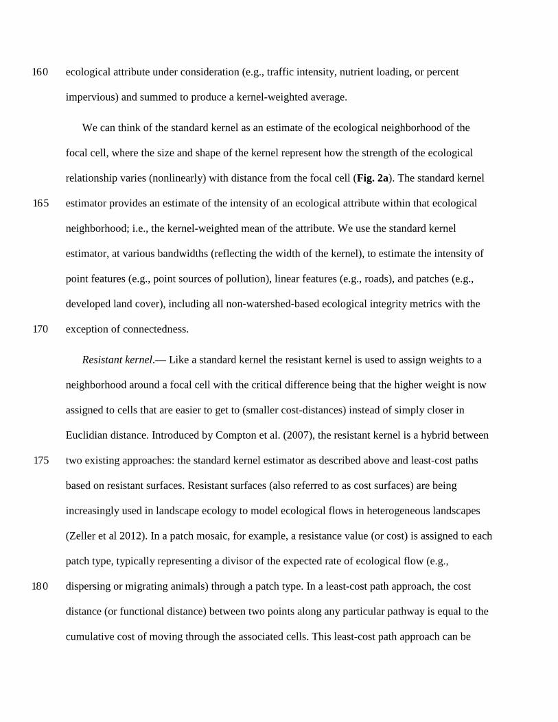
Standard kernel—The standard kernel produces a three-dimensional surface representing an

estimate of the underlying probability distribution (or ecological neighborhood) centered on a

focal cell (Silverman 1986). The standard kernel estimator begins by placing a standard kernel

(e.g., Gaussian kernel) over a focal cell. In the standard Gaussian kernel, the "bandwidth" which

controls the spread of the kernel is equal to one standard deviation and accounts for 39% of the 155

kernel volume. The value of the kernel at each cell represents the weight of the cell, which

decreases monotonically and nonlinearly from the focal cell according to the kernel function as

the distance from the focal cell increases. Typically the kernel is scaled such that the weights

sum to one across all cells. Lastly, the kernel weights are multiplied by the value of the

ecological attribute under consideration (e.g., traffic intensity, nutrient loading, or percent 160

impervious) and summed to produce a kernel-weighted average.

We can think of the standard kernel as an estimate of the ecological neighborhood of the

focal cell, where the size and shape of the kernel represent how the strength of the ecological

relationship varies (nonlinearly) with distance from the focal cell (Fig. 2a). The standard kernel

estimator provides an estimate of the intensity of an ecological attribute within that ecological 165

neighborhood; i.e., the kernel-weighted mean of the attribute. We use the standard kernel

estimator, at various bandwidths (reflecting the width of the kernel), to estimate the intensity of

point features (e.g., point sources of pollution), linear features (e.g., roads), and patches (e.g.,

developed land cover), including all non-watershed-based ecological integrity metrics with the

exception of connectedness. 170

Resistant kernel.— Like a standard kernel the resistant kernel is used to assign weights to a

neighborhood around a focal cell with the critical difference being that the higher weight is now

assigned to cells that are easier to get to (smaller cost-distances) instead of simply closer in

Euclidian distance. Introduced by Compton et al. (2007), the resistant kernel is a hybrid between

two existing approaches: the standard kernel estimator as described above and least-cost paths 175

based on resistant surfaces. Resistant surfaces (also referred to as cost surfaces) are being

increasingly used in landscape ecology to model ecological flows in heterogeneous landscapes

(Zeller et al 2012). In a patch mosaic, for example, a resistance value (or cost) is assigned to each

patch type, typically representing a divisor of the expected rate of ecological flow (e.g.,

dispersing or migrating animals) through a patch type. In a least-cost path approach, the cost 180

distance (or functional distance) between two points along any particular pathway is equal to the

cumulative cost of moving through the associated cells. This least-cost path approach can be

extended to a multidirectional approach that measures the functional distance (or least-cost

distance) from a focal cell to every other cell in the landscape as a means of defining the

accessible ecological neighborhood. These distances can then be converted to weights based on a 185

Gaussian or other function such that higher weight is assigned to closer (in least-cost distance)

cells.

In the resistant kernel algorithm, resistance values can be assigned any number of ways, but

in this application we assign landscape resistance uniquely to each neighboring cell based on its

"ecological distance" to the neighboring cell, where ecological distance is derived from the suite 190

of ecological settings variables. Because resistance of neighboring cells is based on ecological

distance to the focal cell, landscape resistance varies dynamically across the landscape; i.e., there

is a unique landscape resistance surface for each focal cell. For each focal cell, first we calculate

the weighted Euclidean distance between the focal cell and each neighboring cell in settings

space (across all dimensions), where each settings variable is first range rescaled 0-1 and then 195

multiplied by its assigned weight to reflect its importance in determining landscape resistance

(Table 1), as follows:

𝑑𝑛 = ���𝑤𝑖�𝑥𝑓𝑖 − 𝑥𝑛𝑖��2

𝑝

𝑖=1

where dn = Euclidean distance between the nth neighboring cell and the focal cell; i = 1 to p

settings variables (dimensions); wi = weight for the ith settings variable; xif = value of the ith

settings variable (scaled 0-1) at the focal cell; and xni = value of the ith settings variable at the nth 200

neighboring cell. Next, we divide the result above by the maximum possible weighted Euclidean

distance based on the non-anthropogenic (a.k.a. "natural") settings variables. Thus, if the focal

cell and neighboring cell are both undeveloped and have identical values across all natural

settings variables, the weighted Euclidean distance will always equal zero. On the other hand, if

the two cells have maximally different values (i.e., a difference of one for each of the natural 205

settings variables), the weighted Euclidean distance will always equal one. However, if the

neighboring cell is developed, the weighted Euclidean distance can exceed one. Lastly, we

convert weighted Euclidean distance to resistance by multiplying it by a constant and adding one

to ensure that resistance is never less than one. The constant (which interacts with bandwidth)

determines the theoretical maximum resistance between two undeveloped cells (i.e., when their 210

weighted Euclidean distance is one), which we set to be 50 for the connectedness metric and 300

for the aquatic connectedness metrics described below. We selected the constants based on

preliminary analyses in which we subjectively evaluated the behavior of the metric in

discriminating among undeveloped and developed settings. By setting anthropogenic weights to

be relatively high, the resistance (e.g., of a high-traffic expressway or a large dam) can become 215

high enough to cause a neighboring developed cell to act as a complete barrier to spread in the

resistant kernel. Consequently, rivers and other natural features can act as partial barriers to

spread from focal cells with a high ecological distances (e.g., dry oak forests), but the maximum

resistance between natural features is never more than two, while anthropogenic features such as

highways can have higher resistances up to the maximum value determined by the constant. 220

A detailed description of the resistant kernel algorithm is given in Appendix C. Briefly,

using the resistant surface described above, the resistant kernel computes the least cost distance

to each neighboring cell (i.e., cumulative cost of spreading from the focal cell to the neighboring

cell along the least cost path) and transforms these distances into probabilities based on the

specified kernel, such that the probabilities (or weights) sum to one across all cells. The end 225

result is a resistant kernel that depicts the functional ecological neighborhood of the focal cell

(Fig. 2b). In essence, the standard kernel is an estimate of the fundamental ecological

neighborhood and is appropriate when resistance to movement is minimal (e.g., highly vagile

species), while the resistant kernel is an estimate of the realized ecological neighborhood when

resistance to movement is nontrivial. The resistant kernel can also be thought of as representing a 230

process of spread (e.g., dispersal) to or from the focal cell that combines the cost of moving

through a heterogeneous and resistant neighborhood with the typically nonlinear cost of moving

any distance away from the focal cell. In our ecological integrity assessment, we use the resistant

kernel estimator in the terrestrial and aquatic connectedness metrics.

Watershed kernel.—The standard kernel estimator may not be meaningful for aquatic 235

communities where the ecological neighborhood is more likely to be the watershed area above

the focal cell than a symmetrical area around the focal cell. Thus, for the watershed-based

metrics, we use a watershed kernel estimator based on a time-of-flow model (Randhir et al.

2001) as described in detail in Appendix D. Briefly, the time-of-flow model estimates the time

(t) it takes for a drop of water (or water-born materials such as pollutants) to reach the focal cell; 240

it ranges from zero at the focal cell to some upper bound based on the size and characteristics of

the watershed. We rescale t to range 0-1 by dividing t by the maximum observed value of t for

the watershed of the focal cell and then taking the complement. In the resulting kernel, the

weight ranges from 1 (maximum influence) at the focal cell to 0 (no influence) at the cell with

the least influence (i.e., at the furthest edge of the watershed). In essence, kernel weights 245

decrease monotonically as the distance upstream and upslope from the focal cell increases, but

the weights decrease much faster across land than water so that the kernel typically extends

much farther upstream than upslope. The resulting kernel can be viewed as a constrained

watershed in which cells in the stream and closer to the focal cell have higher weight and cells in

the upland and farther from the stream, especially on flat slopes with forest cover, have 250

increasingly less weight (Fig. 2c).

Clearly, this simple time-of-flow model does not capture all the nuances of real landscapes

that influence the actual time it takes for water to travel from any point in the watershed to the

focal cell (e.g., soil characteristics that influence infiltration of precipitation and vegetation

characteristics that influence water loss through evapotranspiration), but it nonetheless provides a 255

much more meaningful way to weight the importance of neighboring cells than either the

standard kernel estimator that does not account for flow or a uniform watershed kernel in which

all cells in the watershed count equally.

Ecological integrity metrics

Our ecological integrity assessment involves computing a suite of metrics that characterize the 260

ecological neighborhood of each focal cell based on one of the kernel estimators described

above. Currently, our suite of metrics measure two important components of ecological integrity:

intactness and resiliency.

Intactness refers to the freedom from human impairment (or anthropogenic stressors) and is

measured using a broad suite of individual stressor metrics (Table 2) such that the greater the 265

level of anthropogenic stress, the lower the estimated intactness. The stressor metrics are

computed for all undeveloped cells, although some metrics apply only to certain ecosystems

(e.g., watershed-based metrics apply only to aquatic and wetland systems). Each stressor metric

measures the magnitude of the anthropogenic stressor within the ecological neighborhood of

each cell and is uniquely scaled to the appropriate units for the metric. For example, the road 270

traffic metric measures the intensity of road traffic (based on the estimated probability of an

animal being hit by a vehicle while crossing a road given the estimated mean traffic rate) in the

neighborhood surrounding the focal cell based on a standard logistic kernel (Fig. 3a). The value

of each metric increases with increasing intensity of the stressor within the ecological

neighborhood of the focal cell. Thus, the raw value of a stressor metric is inversely related to 275

intactness and thus ecological integrity. The value of the metric at any location is generally

independent of the particular ecological setting or ecosystem of the focal cell, as it depends

primarily on the magnitude of the stressor emanating outward from the anthropogenic features of

interest (e.g., roads). Thus, the stressor metrics are all interpretable in their raw-scale form; i.e.,

they do not need to be rescaled by ecological setting or ecosystem (as described below) to be 280

meaningfully interpreted.

Each metric measures a different anthropogenic stressor and is intended to reflect a unique

and well-documented relationship between a human activity and an ecological function.

However, these stressor metrics are not statistically independent, since the same human activity

can have multiple ecological effects. Consequently, these stressor metrics are viewed as a 285

correlated set of metrics that collectively assess the impact of human activities on the intactness

of the ecological setting or ecosystem.

Resiliency refers to the capacity to recover from disturbance and stress; more specifically, the

amount of disturbance and stress a system can absorb and still remain within the same state or

domain of attraction, i.e., resist permanent change in the function of the system (Holling 1973, 290

1996). In other words, as reviewed by Gunderson (2000), resiliency generally deals with the

capacity to maintain characteristic ecological functions in the face of disturbance and stress. In

contrast to intactness, resiliency is both a function of the local ecological setting, since some

settings are naturally more resilient to stressors (e.g., a wetland isolated by resistant landscape

features is less resilient to species loss than a well-connected wetland, because the latter has 295

better opportunities for recolonization of constituent species), and the level of stress, since the

greater the stress the less likely the system will be able to fully recover or maintain ecological

functions. Moreover, the concept of resiliency applies to both the short-term or immediate

capacity to recover from disturbance and the long-term capacity to sustain ecological functions

in the presence of stress. The landscape attributes that confer short-term resiliency may not be 300

the same as those that confer long-term resiliency, as discussed later. Given these considerations,

resiliency is a complex, multi-faceted concept that cannot easily be measured with any single

metric. For the applications presented in this paper we implemented a few different resiliency

metrics (Table 2).

Like the stressor metrics, the resiliency metrics are computed for all undeveloped cells. In 305

contrast to the stressor metrics, the value of each resiliency metric increases with increasing

resiliency, so larger values connote greater integrity. Also in contrast to the stressor metrics, the

value of the resiliency metric at any location is dependent on the particular ecological setting of

the focal cell and its neighborhood. For example, the connectedness metric measures the

functional connectivity of a focal cell to its ecological neighborhood (based on a resistant 310

Gaussian kernel); more specifically, the capacity for organisms to move to and from the focal

cell from neighboring cells with a similar ecological setting as the focal cell (Fig. 3b).

Consequently, connectedness is especially relevant for less vagile organisms where the resistance

of the intervening landscape limits movement to and from the focal cell. Connectedness confers

resiliency to a site since being connected to similar ecological settings should promote recovery 315

of the constituent organisms following a local disturbance.

In contrast to the stressor metrics, the resiliency metrics are not particularly useful in their

raw-scale form because they do not have interpretable units. Instead, they are best interpreted

when rescaled by ecological setting or ecosystem (see below) so that what constitutes high

resiliency for a small patch-forming ecological system such as a wetland need not be the same as 320

for a matrix-forming system such as upland forest. Like the stressor metrics, each resiliency

metric measures resiliency from a different perspective and is intended to reflect a unique and

well-documented relationship between landscape context and ecological function, and resiliency

metrics are correlated, yielding a set of metrics that collectively assess the capacity of a site to

recover from or adapt to disturbance and stress. 325

Index of ecological integrity

The individual stressor and resiliency metrics can be used by themselves, but it is more practical

to combine them into a composite index (IEI) for conservation applications.

Quantile-rescaling.— Each of the raw stressor and resiliency metrics are scaled differently.

Some are bounded 0-1 while others have no upper bound. Moreover, each of the metrics will 330

have a unique empirical distribution for any particular landscape. In order to meaningfully

combine these metrics into a composite index, therefore, it is necessary to rescale the raw metrics

to put them on equal ground. Quantile-rescaling involves transforming the raw metrics into

quantiles, such that the poorest cell gets a 0.01 and the best cell gets a 1. Quantile-rescaling

facilitates the compositing of metrics by putting them all on the same scale with the same 335

uniform distribution regardless of differences in raw units or distribution. Moreover, quantiles

have an intuitive interpretation, because the quantile of a cell expresses the proportion of cells

with a raw value less than or equal to the value of the focal cell. Thus, a 0.9 quantile is a cell that

has a metric value that is greater than 90% of all the cells, and all the cells with >0.9 quantile

values comprise the best 10% within the analysis area. In light of these advantages, it is 340

importance to recognize that quantile scaling means the ecological difference between say 0.5

and 0.6 is not necessarily the same as the ecological difference between say 0.8 and 0.9.

There are two fundamentally different ways to conduct quantile rescaling. In the first

approach, which we refer to as "ecosystem-based rescaling," quantile-rescaling is done by

discrete ecosystems. Ecosystem-based rescaling means that forests are compared to forests, 345

emergent marshes are compared to emergent marshes, and so on. It doesn't make sense to

compare the integrity of an average forest cell to that of an average wetland cell, because

wetlands have been substantially more impacted by human activities such as development than

forests, and they are inherently less-connected to other wetlands. Rescaling by ecosystem means

that all the cells within an ecosystem are ranked against each other in order to determine the cells 350

with the greatest relative integrity for each ecosystem. In the applications of IEI to date (see

below) we have used this form of rescaling. In the second approach, which we refer to as

"gradient-based rescaling," quantile-rescaling is done by comparing focal cells to similar cells

based on multivariate distance in ecological setting space, which does not rely on discrete

ecosystems. Comparative performance of these two alternative rescaling approaches remains an 355

important subject for future research.

Ecological integrity models.—The next step is to combine the quantile-rescaled metrics into

the composite index. However, given the range of metrics (Table 2), it is reasonable to assume

that some metrics are more relevant to some ecological settings or ecosystems than others. For

example, the watershed-based stressor metrics and aquatic connectedness were designed 360

specifically for aquatic and/or wetland communities. Moreover, it is reasonable to assume that

the weights applied to the metrics should vary among ecological settings or ecosystems, since

what stressors matter most, for example, to an emergent marsh may not be the same as for an

upland boreal forest. Consequently, we employ ecosystem-specific ecological integrity models to

weight the component metrics in the composite index (e.g., Appendix F). An ecological 365

integrity model is simply a weighted (by expert teams, Appendix F) linear combination of

metrics designated for each ecosystem, although for parsimony sake we generally designate a

unique model for each ecological formation, which is a group of similar ecosystems (Appendix

B).

Rescaling the final index.—Lastly, we quantile-rescale the final composite index by 370

ecosystem again to ensure the proper quantile interpretation. The final result is a raster that

ranges 0-1. It is important to recognize that quantile-rescaling means that the results are

dependent on the extent of the analysis area, because the quantiles rank cells relative to other

cells within the analysis area (Fig. 4). The best of the Kennebec River watershed, for example, is

not the same as the best of the state of Maine or the entire Northeast. Of course, dependence on 375

landscape extent is true of any algorithm that compares a site to all other sites. Consequently,

quantile-rescaling is done separately for each analysis unit of interest. Ultimately, the choice of

extent for the analysis units is determined by the application objectives, but with consideration of

the mapped heterogeneity. For example, our experience has shown us that when using the DSL

ecosystem map, scaling by ecosystems at extents less than roughly a HUC6-level watershed can 380

produce spurious results owing to the categorical mapping of ecosystems and the limited extent

of some ecosystems. HUCs are a USGS system for hierarchically classifying nested watersheds,

such that a HUC6-level watershed is comprised of two or more HUC8-level sub-watersheds.

Interpreting IEI.—It is critical to recognize the relative nature of IEI; a value of 1 does not

mean that a site has the maximum absolute ecological integrity (i.e., completely unaltered by 385

human activity and perfectly resilient), only that it is the best of that ecological setting or

ecosystem within the geographic extent of that particular analysis unit. In an absolute sense, the

best within any particular geographic extent may still be degraded. Consequently, IEI is only

useful as a comparative assessment tool. In addition, the final IEI has a nicely intuitive

interpretation because the quantile of a cell expresses the proportion of cells with a raw value 390

less than or equal to the value of the focal cell, thus a cell with an IEI of 0.9 is among the best

10% in its ecosystem within its geographic extent.

Index of Ecological Impact

IEI characterizes the integrity of sites relative to other sites in a similar ecological setting or

ecosystem. Thus, it is a static measure of ecological integrity based on a snapshot of the 395

landscape. It can be equally useful to assess the change in ecological integrity over time under a

specific landscape change scenario (see Model Application). For this purpose, we developed the

index of ecological impact (ecoImpact) to measure the change in IEI between the current and

future timesteps relative to the current IEI; i.e., effectively delta IEI times current IEI. A site that

experiences a major loss of IEI has a high predicted ecological impact; i.e., a loss of say 0.5 IEI 400

units reflects a greater relative impact than a loss of 0.2 units. Moreover, the loss of 0.2 units

from a site that has a current IEI of 0.9 is more consequential than the same absolute loss from a

site that has a current IEI of 0.5. Thus, ecoImpact reflects not only the magnitude of IEI loss, but

also where it matters most—sites with high initial integrity.

Delta-rescaling.—The derivation of ecoImpact consists of rescaling the individual raw 405

metrics, but using a different rescaling procedure than we used with IEI, which suffers from what

we call the "Bill Gates" effect when used for scenario comparison. This occurs when the value of

the raw metric is decreased at a high-valued site without changing the quantile. This is analogous

to taking 10 billion dollars away from Bill Gates, yet he remains among the richest 0.1% of

people in the world. Likewise, a small absolute change in a raw metric can, under certain 410

circumstances, result in a large change in its quantile, even though the ecological difference is

trivial. Therefore, the use of quantile-rescaling is not appropriate if we want to be sensitive to the

absolute change in the integrity metrics. To address these issues, we developed delta-rescaling as

an alternative to quantile-rescaling that is more meaningful when comparing landscapes.

Delta-rescaling is rather complicated in detail and thus is presented in full in Appendix G. 415

Briefly, delta-rescaling involves computing the difference in the raw metric from its initial or

baseline value rather than comparing it to the condition of ecologically similar cells or cells of

the same ecosystem. These delta values are rescaled and combined in a weighted linear

combination (as in IEI) and multiplied by the initial or baseline IEI to derive the final index (Fig.

5). The end result is that a cell with maximum initial IEI (1) that is completely degraded (1→0) 420

gets a value of -1, indicating the maximum possible ecological impact. Conversely, a cell that

experiences no change in IEI gets a value of 0, indicating no ecological impact.

It is important to recognize the differences between ecoImpact and IEI. The former measures

the change in IEI relative to the initial or baseline condition. Roughly speaking, ecoImpact

compares each cell to itself—the change in integrity over time—whereas IEI compares each cell 425

to other cells of the same ecological setting or ecosystem within the specified geographic extent.

Also, ecoImpact is weighted by the current IEI of the cell, so that impact is greatest where it

matters most — cells with high initial IEI that lose most or all of their value. Even though the

units of ecoImpact do not have an intuitive interpretation, the absolute value of the index is

meaningful for comparative purposes, and thus it can be summed across all cells in the landscape 430

(or within a user-defined mask) to provide a useful numerical summary of the total ecological

impact of alternative landscape change scenarios.

Model Application

To demonstrate the application of ecoImpact, we quantified the loss of ecological integrity

between 2010-2080 within the northeastern United States under two landscape change scenarios: 435

(a) urban growth without additional land protection, and (b) same amount of urban growth but

with strategic land protection based on a regional landscape conservation design (see

www.naturesnetwork.org). For the first scenario only the existing secured lands representing

~18% of the landscape (and lands otherwise unsuitable for development) were restricted from

future development. For the second scenario, 25% of the highest ecologically-valued lands and 440

waters as well as any lands already secured (representing a total of ~34% of the landscape) or

otherwise unsuitable for development, were protected from future development. For both

scenarios, we simulated urban growth using the SPRAWL model that we developed in

connection with the DSL project mentioned previously (McGarigal et al In review). The

SPRAWL model allocates forecasted demand for new development within subregions 445

(representing counties or census block statistical areas) to local application panes (5 km on a side

in our application) based on their landscape context using a unique matching algorithm, such that

the more historical development that occurred in the matched training windows (i.e., in a similar

landscape context) the higher proportion of the future demand is assigned to the application

pane. Subsequently, the demand in each pane is allocated among transition types (i.e., 450

development classes) and then stochastically allocated to individual cells and patches based on

suitability surfaces derived from logistic regression models unique to that landscape context. We

conducted three replicate 70-year simulations of urban growth under each scenario and computed

the average total impact (sum of ecoImpact across all cells) for each scenario. The total

ecological impact was 8.5% less under the landscape conservation design scenario (Fig. 5). 455

Consequently, even though the conservation design scenario restricted development from an

additional 16% of the highest-valued locations, the reduced impact was only half that amount

because there was still an abundance of moderate- to highly-valued lands that remained

unprotected that suffered impacts from development.

Discussion 460

Coarse-filter ecological assessments are increasingly used by conservation organizations to

evaluate ecological impacts and guide conservation planning, although there appears to be no

consensus yet on a preferred approach (e.g., Andreasen et al 2001, Parrish et al 2003 , Tierney et

al 2009, Beier et al 2015). We developed an approach that has been used in several real-world

applications (see below) that is distinctive in several ways. 465

First, our approach is based predominantly on geophysical settings (i.e., the geophysical

stage) similar to approaches proposed by others (e.g., Anderson and Ferree 2010, Anderson et al

2014, Beier et al 2015), but modified to make limited use of the dominant biotic community as

well. Specifically, we include the dominant potential life form of the vegetation in the broad

suite of ecological settings variables that are used to define the biophysical setting of each cell, 470

which affects ecological similarity and resistance as incorporated into a few of the ecological

integrity metrics. In addition, we use mapped ecosystems to assign models (i.e., weights) for

combining the individual integrity metrics into the composite IEI and ecoImpact indices, which

has at least three advantages. First, it allows the results of the analysis to be easily combined with

other products that adopt the same ecosystem classification. Second, it explicitly recognizes that 475

ecological systems, which represent the co-dependency of the dominant biota and abiotic

environment, are often a conservation target of interest, even while allowing the individual plant

and animal species to vary among sites and over time. Lastly, it allows us to customize

vulnerability to anthropogenic stressors among ecosystems, which can be incorporated directly

into the metric weights that form the integrity models. Note, if distinct ecosystems are not 480

deemed meaningful or reliably mapped, we have an alternative gradient-based approach that can

be used.

Second, our approach embraces the concept of ecological integrity, but defined in a manner

that makes it less subject to the criticisms often leveled against the use of ecological integrity

(Brown and Williams 2016). In particular, our approach does not require the establishment of a 485

reference condition or natural range of variation for each of the metrics as is customary for

definitions of ecological integrity (Parrish et al 2003), which we purport is exceedingly difficult

or even impossible to do in most applications. Instead, we compare each cell to other cells in a

similar ecological setting or ecosystem, or each cell to itself at a different point in time, to derive

an index of relative integrity. Thus, our approach seeks to find the "best" places that are available 490

today or that are likely to be impacted the least (or most depending on the application). In

addition, while most approaches based on ecological integrity are heavily vegetation-centric in

the constituent metrics (e.g., Wurtzebach and Schultz 2016), our approach relies very little on

mapped vegetation patches and instead focuses on the anthropogenic stressors themselves (acting

somewhat independently of the mapped vegetation) in the individual metrics. For example, in 495

contrast to most approaches our approach is agnostic to the current vegetation structural stage on

a site, which we view as a dynamic property of the ecosystem (at least within the bounds of the

dominant life form of the vegetation) and thus not germane to the integrity of the site.

Third, our approach allows us to easily scale the results based on any geographic extent to

facilitate assessments and conservation planning at multiple scales. For example, IEI can be 500

quantile-scaled within watersheds to inform local watershed-based conservation planning, or

within states to inform state agencies with conservation responsibilities, or at even broader scales

to inform regional conservation organizations such as federal agencies and regional land trusts

(Fig. 6).

Fourth, our approach uses a variety of sophisticated kernel estimators to provide an effective 505

assessment of the ecological neighborhood affecting the ecological integrity of a cell (Fig. 2).

The use of ecological neighborhoods is not unique to our approach; for example, Theobold

(2013) used standard kernel density estimators to develop an index of ecological integrity at the

90 m resolution for the entire United States. All of our kernel estimators reflect nonlinear

decreasing ecological influence as distance increases, which is one of the first principles of 510

landscape ecology (Turner et and Gardner 2015). For example, our watershed-based metrics

which evaluate the integrity of aquatic systems use a watershed kernel that honors how terrain

and land cover affect the movement of water and water-born pollutants to a site, which is clearly

more appropriate than treating all locations in the watershed the same. Similarly, our

connectedness metric uses a resistant kernel (Compton et al 2007) to represent how organisms 515

and ecological processes move across the landscape in response to environmental resistance

(Zeller et al 2012). We are unaware of other approaches that adopt these specific kinds of kernel

estimators to evaluate ecological integrity, although our traversability metric (which is a version

of connectedness), is used as a component of The Nature Conservancy's (TNC) terrestrial

resilience (Anderson and Ferree 2010). 520

Limitations.—No approach is without limitations and ours is no exception. Among the many

known limitations, a few are worth noting here. First, like all approaches, our suite of metrics is

incomplete. There are anthropogenic stressors that we recognize as important but have not yet

included due to the lack of reliable and regionally consistent high-resolution data (e.g., toxic

pollutants, hydrological disruptions), and other metrics that adopt an especially crude estimate of 525

the stressor for the same reasons (e.g., non-native invasive plants based solely on land cover

within the ecological neighborhood rather than explicit models of occurrence for each of the

important organisms). Of course, these metrics can be added and/or improved as data and

knowledge become available.

Second, while our approach relies on objective measures of intactness and resiliency, it still 530

has an important subjective component that can be considered either a strength or weakness

(Beazley et al 2010). Specifically, there are a number of model parameters that must be specified

in order to compute the various ecological integrity metrics, including kernel bandwidths,

weights for the ecological settings variables used in the resiliency metrics, and weights for the

metrics used in the ecosystem-specific ecological integrity models to create IEI and ecoImpact. 535

At present these model parameters are assigned by experts in the context of a specific

application, as there is no easy or meaningful way to empirically derive these parameters. While

this allows the assessment to be customized to each application, it comes at the cost of having to

defend the chosen set of model parameters.

Third, our current measurement of resiliency is based on two metrics, similarity and 540

connectedness (and its aquatic counterpart), which reflects a limited perspective on resiliency. In

particular, what may confer short-term resiliency as measured by our two metrics may be

antagonistic to what may confer long-term resiliency in the face of rapid environmental (e.g.,

climate) change. For example, short-term resiliency of a site may be a function of the amount

and accessibility of similar environments in the neighborhood of the focal cell, since having 545

larger and more connected local populations should facilitate population recovery of the

constituent organisms (and thus ecosystem functions) following disturbance—which is the

premise of our two resiliency metrics. However, long-term resiliency of a site may also be a

function of the amount and accessibility of diverse environments in the neighborhood of the

focal cell, since having a diverse assemblage of environments nearby increases the opportunities 550

for different organisms to fill the ecological niche space as the environment (e.g., climate)

changes over time—which is the premise of the metrics used in the geophysical stage approach

proposed by others (e.g., Anderson and Ferree 2010; Beier and Brost 2010; Beier 2012; Beier et

al 2015). Consequently, while still unclear, it is possible that the factors driving short-term

resiliency may differ from those driving long-term resiliency in the face of environmental 555

change. Note, to account for this possibility, in the landscape conservation design applications

referenced below we combined IEI with TNC's terrestrial resilience metric (Anderson and Ferree

2010), which prioritizes sites based on local geophysical diversity and connectivity, to establish

priorities for conservation core areas.

Lastly, despite their increasing use, measures of ecological integrity are exceedingly difficult 560

if not impossible to validate (but see McGarigal et al. 2013, which provides a partial validation

of IEI based on extensive field data on a number of taxa) given the long-term nature of the

predictions, which has been a major source of criticism (Brown and Williams 2016). We sought

to reduce the need for formal validation of IEI by eliminating the need for a reference condition

or natural range of variability and instead using quantile scaling to rate sites relative to each 565

other. Indeed, IEI makes no assumptions about the absolute integrity of site, only that it is

relatively more or less integral than another site. In this regard, each of the constituent metrics

was chosen because of its clear and well-documented relationship with ecological functions that

confer integrity to a site. For example, it is undisputed that increasing the intensity of roads and

road traffic near a site will adversely affect critical ecological processes such as organism 570

dispersal, watershed hydrology, and sedimentation of streams (Forman et al 2003). IEI relies

heavily on this well-established relationship between anthropogenic stressors and ecological

integrity. Although the exact form and magnitude of the relationship is unknown; it may suffice

to know that the relationship is monotonic.

Conservation applications.—Our coarse-filter ecological integrity assessment has been 575

applied to a wide variety of real-world conservation problems. Detailed information about each

of these applications can be found at the DSL project website (McGarigal et al 2017,

www.umass.edu/landeco/research/dsl/dsl.html) or the UMassCAPS website

(www.umasscaps.org).

• Critical Linkages.—Working in partnership with the North Atlantic Aquatic Connectivity 580

Collaborative (NAACC), we have used IEI and the aquatic connectedness metric to

evaluate and prioritize dam removals and road-stream crossing (culvert) upgrades in the

Northeast for their potential to restore aquatic connectivity.

• Wetlands Assessment, Monitoring and Regulation.—Working in partnership with the MA

Department of Environmental Protection (DEP), MA Office of Coastal Zone Management, 585

and U.S. EPA, we have used IEI in a variety of contexts to develop cost-effective tools and

techniques for assessment and monitoring of wetland and aquatic ecosystems in

Massachusetts, including the development and validation of indices of biotic integrity for

selected wetland and aquatic systems. In addition, IEI is being used by DEP in permitting

activities affecting wetlands pursuant to the MA Wetlands Protection Act; specifically, 590

projects occurring in the top 40% of wetlands based on IEI are subject to additional DEP

review.

• BioMap 2.—Working in partnership with the MA Department of Fish & Game’s Natural

Heritage & Endangered Species Program and TNC’s Massachusetts Program, we used IEI

in the development of BioMap2 which serves as a guide for conservation decision making 595

to preserve and restore biodiversity in Massachusetts; specifically, we used IEI to assist in

the identification of forest cores, wetland cores, clusters of vernal pools and undeveloped

landscape blocks with the highest potential for maintaining ecological integrity over time.

• Losing Ground.—Working in partnership with Mass Audubon to prepare the 4th edition of

the Losing Ground publications (DeNormandie and Corcoran 2009), we used IEI and 600

ecoImpact to assess the change in ecological integrity between 1971-2005 in

Massachusetts; specifically, to quantify the indirect impacts of development beyond its

direct footprint.

• South Coast Rail Project.—We used IEI and ecoImpact to assess the potential loss in

ecological integrity of several alternative routes for the proposed South Coast Rail system 605

in southeastern Massachusetts.

• Connect the Connecticut and Nature's Network.—Working with a large partnership of

organizations under the auspices of the North Atlantic Landscape Conservation

Cooperative (NALCC), we used IEI in combination with several other data products to

identify and prioritize a set of terrestrial and aquatic "core areas" as part of a landscape 610

conservation design for the Connecticut River watershed (Connect the Connecticut,

www.connecttheconnecticut.org) and for the entire Northeast (Nature's Network,

www.naturesnetwork.org).

Conclusions.—We suggest that the maintenance of ecological integrity is arguably the ultimate

goal of ecological conservation. However, given the complexity of the ecological integrity 615

concept (Gunderson 2000), the measurement of ecological integrity has remained a daunting

challenge for scientists and conservation practitioners. We presented an index of ecological

integrity (IEI) to evaluate the relative integrity among sites of the same or similar ecosystem that

is derived from readily available spatial data on land use and land cover and that can be applied

at any spatial resolution over any spatial extent (contingent upon data availability), and a 620

corresponding index of ecological impact (ecoImpact) to assess changes in integrity over time.

These two multi-metric indices emphasize the potential intactness (i.e., freedom from

anthropogenic stressors) and resiliency (based on the ecological similarity and connectedness of

the ecological neighborhood) of a site and make use of sophisticated kernels to represent

meaningful ecological neighborhoods for each of the constituent metrics. While not without 625

acknowledged limitations, these metrics have proven useful in several real-world conservation

applications.

Acknowledgements

This work was supported by the United States Fish and Wildlife Service, North Atlantic

Landscape Conservation Cooperative (NALCC), US Geological Survey Northeast Climate 630

Science Center, Massachusetts Executive Office of Environmental Affairs, The Trustees of

Reservations, Massachusetts Department of Environmental Protection, The Nature Conservancy,

US Department of Transportation, and the University of Massachusetts, Amherst. We especially

thank Andrew Milliken and Scott Schwenk of the NALCC for their continued support and close

involvement in several conservation applications involving the DSL project and the use of IEI. 635

Table 1. Weights (determined by expert teams) assigned to ecological settings variables (see

Appendix A for links to detailed descriptions of each variable) in the ecological integrity

assessment. Resistance represents the weights assigned to the settings variables to determine

resistance between the focal cell and each neighboring cell in the resistant kernels and watershed 640

kernels used in the Connectedness and Aquatic connectedness metrics, respectively. Distance

represents the weights to determine ecological distance between the focal cell and each

neighboring cell for Similarity, Connectedness, and Aquatic Connectedness metrics. The settings

variables are arbitrarily grouped into broad classes for organizational purposes.

Resistance Distance

Energy

Incident solar radiation 0.1 1

Growing season degree-days 0.3 1

Minimum winter temperature 0.1 1

Heat Index 35 0.1 1

Stream temperature 0.1 1

Chemical & physical substrate

Water salinity 4 3

Substrate mobility 2 2

CaCO3 content 0.1 1

Soil available water supply 0.05 0.5

Soil depth 0.05 0.5

Soil pH 0.05 0.5

Physical disturbance

Wind exposure 0.1 1

Slope 1 1

Resistance Distance

Moisture & hydrology

Wetness 4 8

Flow gradient 1 2

Flow volume 5 5

Tidal regime 2 2

Vegetation

Dominant life form 3 8

Development

Developed1 1 20

Hard development1 2 1000

Traffic1 40 0

Impervious1 5 0

Terrestrial barriers1 15 0

Aquatic barriers2 100 0

1Setting variable not used in Aquatic Connectedness. 645

2Setting variable used only for Resistance in Aquatic Connectedness.

Table 2. Intactness (a.k.a. stressor) and resiliency metrics included in the ecological integrity

assessment for the northeastern United States (see Appendix E for links to detailed descriptions

of each metric). Note, the final suite of metrics can vary among applications depending on 650

available data. For example, several additional coastal metrics have been developed for the state

of Massachusetts, including salt marsh ditching, coastal structures, beach pedestrians, beach

ORVs, and boating intensity. The metrics are arbitrarily grouped into broad classes for

organizational purposes.

Metric group Metric name Description

Development

and Roads

Habitat loss Intensity of habitat loss caused by all forms of

development in the neighborhood surrounding the focal

cell based on a standard Logistic kernel.

Watershed habitat

loss

Intensity of habitat loss caused by all forms of

development in the watershed above the focal cell based

on a watershed kernel.

Road traffic Intensity of road traffic (based on measured road traffic

rates transformed into an estimated probability of an

animal being hit by a vehicle while crossing the road given

the mean traffic rate) in the neighborhood surrounding the

focal cell based on a standard Logistic kernel.

Mowing &

plowing

Intensity of agriculture (as a surrogate for mowing/plowing

rates) in the neighborhood surrounding the focal cell based

on a standard Logistic kernel.

Metric group Metric name Description

Microclimate

alterations

Magnitude of adverse induced (human-created) edge

effects on the microclimate integrity of patch interiors.

Pollution Watershed road

salt

Intensity of road salt application in the watershed above an

aquatic focal cell based on road class (as a surrogate for

road salt application rates) and a watershed kernel.

Watershed road

sediment

Intensity of sediment production in the watershed above an

aquatic focal cell based on road class (as a surrogate for

road sediment production rates) and a watershed kernel.

Watershed

nutrient

enrichment

Intensity of nutrient loading from non-point sources in the

watershed above an aquatic focal cell based on land use

class (primarily agriculture and residential land uses

associated with fertilizer use, as a surrogate for nutrient

loading rate) and a watershed kernel.

Biotic

Alterations

Domestic

predators

Intensity of development associated with sources of

domestic predators (e.g., cats) in the neighborhood

surrounding the focal cell weighted by development class

(as a surrogate for domestic predator abundance) and a

standard Logistic kernel.

Edge predators Intensity of development associated with sources of edge

mesopredators (e.g., raccoons, skunks, corvids, cowbirds;

i.e., human commensals) in the neighborhood surrounding

Metric group Metric name Description

the focal cell weighted by development class (as a

surrogate for edge predator abundance) and a standard

Logistic kernel.

Non-native

invasive plants

Intensity of development associated with sources of non-

native invasive plants in the neighborhood surrounding the

focal cell weighted by development class (as a surrogate

for non-native invasive plant abundance) and a standard

Logistic kernel.

Non-native

invasive

earthworms

Intensity of development associated with sources of non-

native invasive earthworms in the neighborhood

surrounding the focal cell weighted by development class

(as a surrogate for non-native invasive earthworm

abundance) and a standard Logistic kernel.

Climate Climate stress Magnitude of climate change stress at the focal cell based

on the climate niche of the corresponding ecological

system and the predicted change in climate between 2010-

2080 (i.e., how much is the climate of the focal cell

moving away from the climate niche envelope of the

corresponding ecological system).

Hydrologic

Alterations

Watershed

imperviousness

Intensity of impervious surface (as a surrogate for

hydrological alteration) in the watershed above an aquatic

Metric group Metric name Description

focal cell based on imperviousness and a watershed kernel.

Dam intensity Intensity of dams (as a surrogate for hydrological

alteration) in the watershed above an aquatic focal cell

based on dam size and a watershed kernel.

Sea level rise

inundation

Probability of the focal cell being unable to adapt to

predicted inundation by sea level rise, developed by USGS

Woods Hole (Lentz et al 2015).

Tidal restrictions Magnitude of hydrologic alteration to the focal cell due to

tidal restrictions based on an estimate of the salt marsh loss

ratio above each potential tidal restriction (road-stream and

railroad-stream crossings).

Resiliency Similarity Similarity between the ecological setting of the focal cell

and its ecological neighborhood based on the weighted

multivariate similarity computed across a variety of

ecological settings variables (Table 1) and a standard

Logistic kernel.

Connectedness

(connect)

Connectivity of the focal cell to its ecological

neighborhood based on a resistant kernel (see text and

Appendix C for details).

Aquatic Same as Connectedness except that it is constrained by the

Metric group Metric name Description

connectedness extent of aquatic ecosystems, such that the connectivity

being assessed pertains to flows and disruption of flows

(e.g., culverts and dams) within the aquatic network.

655

Figure 1. Schematic outline of the workflow associated with deriving the index of ecological

integrity (IEI) and the index of ecological impact (ecoImpact) as described in the text.

Figure 2. Kernel estimators to estimate the ecological neighborhood of a focal cell (indicated by

the red cross for each kernel) in an area west of Albany, New York: (a) standard Gaussian kernel 660

around a focal cell in which the weight of the kernel at any cell is indicated by the color gradient

and reflects the bandwidth (spread) of the kernel; (b) resistant Gaussian kernel around a focal

cell in which the weight of the kernel at any cell is indicated by the color gradient and reflects

bandwidth (spread) of the kernel as well as the resistance of the intervening landscape; and (c)

watershed kernel in which the estimated relative time-of-flow from any cell within the watershed 665

of the focal cell to the focal cell is indicated by the color gradient. Image is portrayed with

hillshading.

Figure 3. (a) traffic (stressor) metric and (b) connectedness (resiliency) metric (scaled for the

northeastern United States) for the North Quabbin region of western Massachusetts. See Table 2

for a brief description and Appendix E for a detail description of these two metrics. Note, the 670

color legend is reversed in these two metrics so that the blue end of the gradient represents sites

with greater ecological integrity (i.e., less traffic and greater connectedness in this case). Images

are portrayed with hillshading.

Figure 4. Index of ecological integrity (IEI) scaled by (a) the entire northeastern United States

and (b) by HUC6-level watersheds for an area northwest of State College, Pennsylvania. See the 675

text for a description of IEI and Table 2 and Appendix E for descriptions of the constituent

metrics. Larger values represent greater ecological integrity. Images are portrayed with

hillshading.

Figure 5. Index of ecological impact (ecoImpact) representing the loss of ecological integrity

between 2010-2080 under two landscape change scenarios: (a) urban growth without additional 680

land protection, and (b) same amount of urban growth but with strategic land protection

(delineated polygons) based on a regional landscape conservation design (see

www.naturesnetwork.org), for an area west of Manchester, New Hampshire. ecoImpact ranges

from 0 (no impact) to -1 (maximum impact). The total impact (sum of ecoImpact across all cells,

averaged across three stochastic simulation runs under each scenario) was 8.5% less under the 685

landscape conservation design scenario. Note, the details of these two landscape change

scenarios are not relevant to the demonstration of ecoImpact and thus have been omitted here.

Images are portrayed with hillshading.

Figure 6. Index of ecological integrity (IEI) scaled by the entire northeastern United States (a;

larger values represent greater ecological integrity) and the corresponding Index of ecological 690

impact (ecoImpact) representing the loss of ecological integrity between 2010-2080 under a

baseline urban growth scenario without additional land protection (b, larger negative values

represent greater ecological impact).

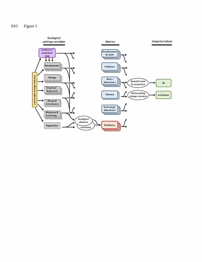
Figure 1 695

Figure 2

700

Figure 3

Figure 4

705

Figure 5

Figure 6 710

References

Addicott JF, Aho JM, Antolin MF, Padilla DK, Richardson JS, Soluk DA (1987) Ecological

neighborhoods: scaling environmental patterns. Oikos 49: 340-346. 715

Anderson M, Clark MG, Sheldon AO (2014) Estimating Climate Resilience for Conservation

across Geophysical Settings. Conservation Biology 28: 959–970.

Anderson M, Ferree C (2010) Conserving the stage: climate change and the geophysical

underpinnings of species diversity. PlOS ONE 5 (e11554) DOI: 10.371/journal/pne.0011554.

Andreasen JK, O’Neill RV, Noss R, Slosser NC (2001) Considerations for the development of a 720

terrestrial index of ecological interity. Ecol Ind 1:21–35.

Beazley KF, Baldwin ED, Reining C (2010) Integrating Expert Judgment into Systematic

Ecoregional Conservation Planning. Pages 235-255 In: Trombulak S., Baldwin R. (eds)

Landscape-scale Conservation Planning. Springer, Dordrecht.

Beier P (2012) Conceptualizing and designing corridors for climate change. Ecological 725

Restoration 30: 312-319.

Beier P, Brost B (2010) Use of land facets to plan for climate change: conserving the arenas, not

the actors. Conservation Biology 24: 701–710.

Beier P, Hunter ML, Anderson M (2015) Special section: conserving nature's stage.

Conservation Biology 29: 613-617. 730

Belote RT, Dietz MS, Jenkins CN, McKinley PS, Irwin GH, Fullman TJ, Leppi JC, and Aplet

GH (2017) Wild, connected, and diverse: building a more resilient system of protected areas.

Ecological Applications 27: 1050-1056.

Briers RA (2002) Incorporating connectivity into reserve selection procedures. Biological

Conservation 103: 77–83. 735

Brown ED, Williams BK (2016) Ecological integrity assessment as a metric of biodiversity: are

we measuring what we say we are? Biodiversity Conservation 25:1011-1035.

Ceballos G, Ehrlich PR, Barnosky AD, Garcia A, Pringle RM, Palmer TM (2015) Accelerated

modern human-induced species losses: entering the sixth mass extinction. Science Advances

1: 1-5. 740

Cerdeira JO, Gaston KJ, Pinto LS (2005) Connectivity in priority area selection for conservation.

Environmental Modeling and Assessment 10: 183–192.

Compton BW, McGarigal K, Cushman SA, Gamble LR (2007) A resistant-kernel model of

connectivity for amphibians that breed in vernal pools. Conservation Biology 21: 788-799.

DeNormandie J, Corcoran C (2009) Losing ground beyond the footprint: patterns of 745

development and their impact on the nature of Massachusetts. Fourth Edition of the Losing

Ground Series, MassAudubon (http://www.massaudubon.org/content/ download/

8601/149722/file/LosingGround_print.pdf).

Forman RTT, Sperling D, Bissonette JA, Clevenger AP, Cutshall CD, Dale VH, Fahrig L,

France R, Goldman CR, Heanue K, Jones JA, Swanson FJ, Turrentine T, Winter TC (2003) 750

Road Ecology; Science and Solutions. Island Press, Covelo, CA. 504 pp.

Gunderson LH (2000) Ecological resilience–in theory and application. Annual Review of

Ecology and Systematics 31: 425–439.

Haddad NM, Brudvig LA, Clobert J, Davies KF, Gonzalez A, Holt RD, Lovejoy TE, Sexton JO,

Austin MP, Collins CD, Cook WM, Damschen EI, Ewers RM, Foster BL, Jenkins CN, King 755

AJ, Laurance WF, Levey DJ, Margules CR, Melbourne BA, Nicholls AO, Orrock JL, Song

D-X, Townshend JR (2015) Habitat fragmentation and its lasting impact on Earth's

ecosystems. Science Advances 1, e1500052.

Holling CS (1973) Resilience and stability of ecological systems. Annual Review of Ecology and

Systematics 4: 1–23. 760

Holling CS (1996) Engineering resilience versus ecological resilience. In P. C. Schulze, editor.

Engineering within ecological constraints. National Academy Press, Washington, D.C., USA.

Hunter Jr ML, Jacobson GL, Webb III T (1988) Paleoecology and the coarse-filter approach to

maintaining biological diversity. Conservation Biology 2: 375–385.

Lentz EE, Stippa SR, Thieler ER, Plant NG, Gesch DB, Horton RM (2015) Evaluating coastal 765

landscape response to sea-level rise in the northeastern United States—Approach and

methods: U.S. Geological Survey Open-File Report 2014–1252, 26 p.

http://dx.doi.org/10.3133/ofr20141252 ISSN 2331–1258 (online).

Lerner J, Mackey J, Casey F (2007) What's in Noah's wallet? Land conservation spending in the

United States. BioScience 57: 419–423. 770

McGarigal, K., Compton, B.W., Plunkett, E.B., Deluca, W.V., and Grand, J. (2017). Designing

sustainable landscapes project: documents and data products. [online] URL:

https://scholarworks.umass.edu/designing_sustainable_landscapes/

McGarigal K, Plunkett EB, Willey L, Compton BW, Deluca WV, and Grand J. 2018. Modelling

urban growth in the northeastern United States: the SPRAWL model and the ecological 775

impacts of urban growth. Ecological Modelling (In press).

McGarigal K, Plunkett EB, Grand J, Compton BW, Portante T, Rolih K, Jackson SD (2013)

Empirically derived indices of biotic integrity for forested wetlands, coastal salt marshes and

wadable freshwaters streams in Massachusetts. Report to Massachusetts Department of

Environmental Protection, September 15, 2013. 249 pp. 780

Newbold T, Hudson LN, Hill SLL, Contu S, Lysenko I, Senior RA, Börger L, Bennett DJ,

Choimes A, Collen B, Day J, De Palma A, Díaz S, Echeverria-Londoño S, Edgar MJ,

Feldman A, Garon M, Harrison MLK, Alhusseini T, Ingram DJ, Itescu Y, Kattge J, Kemp V,

Kirkpatrick L, Kleyer M, Correia DLP, Martin CD, Meiri S, Novosolov M, Pan Y, Phillips

HRP, Purves DW, Robinson A, Simpson J, Tuck SL, Weiher E, White HJ, Ewers RM, Mace 785

GM, Scharlemann JPW, Purvis A (2015) Global effects of land use on local terrestrial

biodiversity. Nature 520: 45–50.

Noss R (1996) Ecosystems as conservation targets. Trends in Ecology and Evolution. 11: 351.

Ortega-Huerta MA, Peterson AT (2004) Modelling spatial patterns of biodiversity for

conservation prioritization in North-eastern Mexico. Diversity and Distribution 10: 39–54. 790

Parrish JD, Braun DP, Unnassch RS (2003) Are we conserving what we say we are? Measuring

ecological integrity within protected areas: BioScience 53: 851−860.

Pereira HM, Leadley PW, Proenca V, Alkemade R, Scharlemann JPW, Fernandez-Manjarres JF,

Araujo MB, Balvanera P, Biggs R, Cheung WWL, Chini L, Cooper HD, Gilman EL,

Guenette S, Hurtt GC, Huntington HP, Mace GM, Oberdorff T, Revenga C, Rodrigues P, 795

Scholes RJ, Sumaila UR, Walpole M (2010) Scenarios for global biodiversity in the 21st

century. Science 330: 1496-1501.

Pickett STA, Parker VT, Fiedler PL (1992) The new paradigm in ecology: implications for

conservation above the species level. Pages 65-88. In: P.L. Fiedler and S.K. Jain, editors.

Conservation biology: theory and practice of nature conservation and management. Chapman 800

and Hall Press. New York. U.S.A..

Pimm SL, Russell GJ, Gittleman JL, Brooks TM (1995) The future of biodiversity. Science 269:

347–350.

Randhir TO, O'Connor R, Penner PR, Goodwin DW (2001) A watershed-based land

prioritization model for water supply protection. Forest Ecology and Management 143: 47-805

56.

Sala OE, Chapin III FC, Armesto JJ, Berlow E, Bloomfield J, Dirzo R, Huber-Sanwald E,

Huenneke LF, Jackson RB, Kinzig A, Leemans R, Lodge DM, Mooney HA, Oesterheld M,

Poff NL, Sykes MT, Walker BH, Walker M, Wall DH (2000) Global biodiversity scenarios

for the year 2100. Science 287: 1770-1774. 810

Sanderson EW, Jaiteh M, Levy MA, Redford KH, Wannebo AV, Woolmer G (2002) The human

footprint and the last of the wild. Bioscience 52: 891–904.

Scott JM, Davis F, Csuti B, Noss R, Butterfield B, Groves C, Anderson H, Caicco S, D’Erchia F,

Edwards Jr. TC, Ulliman J, Wright RG (1993) GAP analysis: a geographic approach to

protection of biological diversity. Wildlife Monographs 123: 1-41. 815

Silverman BW (1986) Density estimation for statistics and data analysis. Chapman & Hall,

London.

Soulé ME, Terborgh J (eds) (1999) Continental Conservation: scientific foundations of regional

reserve networks. Island Press. Washington, D.C., U.S.A..

Theobald DM (2013) A general model to quantify ecological integrity for landscape assessments 820

and US application. Landscape ecology 28: 1859-1874.

Tierney GL, Faber-Langendoen D, Mitchell BR, Shriver WG, Gibbs JP (2009) Monitoring and

evaluating the ecological integrity of forest ecosystems: Frontiers in Ecology and the

Environment 7: 308–316.

Turner MG, Gardner RH (2015) Landscape ecology in theory and practice. Springer-Verlag, 825

New York. 482 pp.

Venter O, Sanderson EW, Magrach A, Allan JR, BeherJ, Jones KR, Possingham HP, Laurance

WF, Wood P, Fekete BM, Levy MA, Watson JEM (2016) Sixteen years of change in the

global terrestrial human footprint and implications for biodiversity conservation. Nature

Communications 7:12558. doi:10.1038/ncomms12558. 830

Williams PH, Margules CR, Hilbert DW (2002) Data requirements and data sources for

biodiversity priority area selection. Journal of Biosciences 27: 327–338.

Wurtzebach Z, Schultz C (2016) Measuring ecological integrity: history, practical applications,

and research opportunities. BioScience 66: 446-457.

Zeller KA, McGarigal K, Whiteley AR (2012) Estimating landscape resistance to movement: a 835

review. Landscape Ecology 27: 777-797.

APPENDICES

A landscape index of ecological integrity: applications in landscape conservation

Kevin McGarigal, Bradley W. Compton, Ethan B. Plunkett, William V. Deluca, Joanna Grand,

Eduard Ene, and Scott D. Jackson

Appendix A. Ecological settings variables. 5

Links to detailed documentation for each of the ecological settings variables (i.e., biophysical

site descriptors used in the calculation of the individual ecological integrity metrics and/or in the

calculation of the final rescaled index of ecological integrity) developed for the northeastern

United States. All settings variables exist as 30 m rasters. Documents include a general

description of the layer, considerations for the use and interpretation of the layer, derivation of 10

the layer, including data sources and algorithm, and metadata for the distributed product. The

settings variables are arbitrarily grouped into broad classes for organizational purposes.

Ecological settings variable Link to detailed documentation

Energy

Incident solar radiation http://jamba.provost.ads.umass.edu/web/lcc/DSL_documentation_sun.pdf

Growing season degree-days http://jamba.provost.ads.umass.edu/web/lcc/DSL_docu

mentation_temperature.pdf Minimum winter temperature

Heat Index 35

Stream temperature http://jamba.provost.ads.umass.edu/web/lcc/DSL_documentation_streamtemp.pdf

Chemical & physical substrate

Water salinity http://jamba.provost.ads.umass.edu/web/lcc/DSL_docu

mentation_salinity.pdf

Substrate mobility http://jamba.provost.ads.umass.edu/web/lcc/DSL_documentation_substrate.pdf

CaCO3 content http://jamba.provost.ads.umass.edu/web/lcc/DSL_documentation_calcium.pdf

Soil available water supply http://jamba.provost.ads.umass.edu/web/lcc/DSL_documentation_soils.pdf Soil depth

Soil pH

Physical disturbance

Wind exposure http://jamba.provost.ads.umass.edu/web/lcc/DSL_documentation_wind.pdf

Slope http://jamba.provost.ads.umass.edu/web/lcc/DSL_documentation_slope.pdf

Moisture & hydrology

Wetness http://jamba.provost.ads.umass.edu/web/lcc/DSL_documentation_wet.pdf

Flow gradient http://jamba.provost.ads.umass.edu/web/lcc/DSL_documentation_gradient.pdf

Flow volume http://jamba.provost.ads.umass.edu/web/lcc/DSL_documentation_volume.pdf

Tidal regime http://jamba.provost.ads.umass.edu/web/lcc/DSL_documentation_tides.pdf

Vegetation

Dominant life form http://jamba.provost.ads.umass.edu/web/lcc/DSL_documentation_structure.pdf

Development

Developed http://jamba.provost.ads.umass.edu/web/lcc/DSL_documentation_development_hard.pdf Hard development

Traffic http://jamba.provost.ads.umass.edu/web/lcc/DSL_documentation_traffic.pdf

Impervious http://jamba.provost.ads.umass.edu/web/lcc/DSL_documentation_impervious.pdf

Terrestrial barriers http://jamba.provost.ads.umass.edu/web/lcc/DSL_documentation_tbarriers.pdf

Aquatic barriers http://jamba.provost.ads.umass.edu/web/lcc/DSL_documentation_abarriers.pdf

Appendix B. Hierarchical classification of formations and ecological systems 15

Hierarchical classification of formations and ecosystems (Anderson et al. 2013, Ferree and

Anderson 2013, Olivero-Sheldon et al. 2014) as used in our coarse-filter ecological integrity

assessment in the northeastern United States. The formations are used for convenience to group

the ecological systems into broader classes for purposes of assigning roughness and runoff

coefficients in the watershed kernels (Appendix D) and weighting the individual integrity 20

metrics in the calculation of the index of ecological integrity (IEI) and the index of ecological

impact (ecoImpact) (Appendix F). See references below for a description of the ecological

systems.

Formation Ecosystem

Alpine Acadian-Appalachian Alpine Tundra

Boreal Upland Forest Acadian Low Elevation Spruce-Fir-Hardwood Forest

Boreal Upland Forest Acadian Sub-boreal Spruce Flat

Boreal Upland Forest Acadian-Appalachian Montane Spruce-Fir-Hardwood Forest

Boreal Upland Forest Central and Southern Appalachian Spruce-Fir Forest

Cliff & Rock Acidic Cliff and Talus

Cliff & Rock Calcareous Cliff and Talus

Cliff & Rock Circumneutral Cliff and Talus

Coastal Scrub-Herb Atlantic Coastal Plain Beach and Dune

Coastal Scrub-Herb Great Lakes Dune and Swale

Coastal Scrub-Herb North Atlantic Coastal Plain Heathland and Grassland

Grassland & Shrubland Acidic Rocky Outcrop

Grassland & Shrubland Appalachian Shale Barrens

Grassland & Shrubland Calcareous Rocky Outcrop

Grassland & Shrubland Central Appalachian Alkaline Glade and Woodland

Formation Ecosystem

Grassland & Shrubland Eastern Serpentine Woodland

Grassland & Shrubland Great Lakes Alvar

Grassland & Shrubland Shrubland & grassland (NLCD 52/71)

Grassland & Shrubland Mafic Glade and Barrens

Grassland & Shrubland Southern Appalachian Grass and Shrub Bald

Grassland & Shrubland Southern Ridge and Valley Calcareous Glade and Woodland

Northeastern Upland Forest Allegheny-Cumberland Dry Oak Forest and Woodland

Northeastern Upland Forest Appalachian (Hemlock)-Northern Hardwood Forest

Northeastern Upland Forest Central and Southern Appalachian Montane Oak Forest

Northeastern Upland Forest Central Appalachian Dry Oak-Pine Forest

Northeastern Upland Forest Central Appalachian Pine-Oak Rocky Woodland

Northeastern Upland Forest Central Atlantic Coastal Plain Maritime Forest

Northeastern Upland Forest Glacial Marine & Lake Mesic Clayplain Forest

Northeastern Upland Forest Laurentian-Acadian Northern Hardwood Forest

Northeastern Upland Forest Laurentian-Acadian Northern Pine-(Oak) Forest

Northeastern Upland Forest Laurentian-Acadian Pine-Hemlock-Hardwood Forest

Northeastern Upland Forest Laurentian-Acadian Red Oak-Northern Hardwood Forest

Northeastern Upland Forest North Atlantic Coastal Plain Hardwood Forest

Northeastern Upland Forest North Atlantic Coastal Plain Maritime Forest

Northeastern Upland Forest North Atlantic Coastal Plain Pitch Pine Barrens

Northeastern Upland Forest North-Central Interior Beech-Maple Forest

Northeastern Upland Forest Northeastern Coastal and Interior Pine-Oak Forest

Northeastern Upland Forest Northeastern Interior Dry-Mesic Oak Forest

Northeastern Upland Forest Northeastern Interior Pine Barrens

Northeastern Upland Forest Piedmont Hardpan Woodland and Forest

Northeastern Upland Forest Pine plantation / Horticultural pines

Northeastern Upland Forest South-Central Interior Mesophytic Forest

Formation Ecosystem

Northeastern Upland Forest Southern and Central Appalachian Cove Forest

Northeastern Upland Forest Southern Appalachian Low Elevation Pine Forest

Northeastern Upland Forest Southern Appalachian Montane Pine Forest and Woodland

Northeastern Upland Forest Southern Appalachian Northern Hardwood Forest

Northeastern Upland Forest Southern Appalachian Oak Forest

Northeastern Upland Forest Southern Atlantic Coastal Plain Mesic Hardwood Forest

Northeastern Upland Forest Southern Atlantic Coastal Plain Upland Longleaf Pine Woodland

Northeastern Upland Forest Southern Piedmont Dry Oak-Pine Forest

Northeastern Upland Forest Southern Piedmont Mesic Forest

Northeastern Upland Forest Southern Ridge and Valley / Cumberland Dry Calcareous Forest

Northeastern Wetland Atlantic Coastal Plain Blackwater/Brownwater Stream Floodplain Forest

Northeastern Wetland Central Appalachian Stream and Riparian

Northeastern Wetland Central Atlantic Coastal Plain Non-riverine Swamp and Wet Hardwood Forest

Northeastern Wetland Central Interior Highlands and Appalachian Sinkhole and Depression Pond

Northeastern Wetland Glacial Marine & Lake Wet Clayplain Forest

Northeastern Wetland High Allegheny Headwater Wetland

Northeastern Wetland Laurentian-Acadian Alkaline Conifer-Hardwood Swamp

Northeastern Wetland Laurentian-Acadian Freshwater Marsh

Northeastern Wetland Laurentian-Acadian Large River Floodplain

Northeastern Wetland Laurentian-Acadian Wet Meadow-Shrub Swamp

Northeastern Wetland North Atlantic Coastal Plain Basin Peat Swamp

Northeastern Wetland North Atlantic Coastal Plain Basin Swamp and Wet Hardwood Forest

Northeastern Wetland North Atlantic Coastal Plain Pitch Pine Lowland

Northeastern Wetland North Atlantic Coastal Plain Stream and River

Formation Ecosystem

Northeastern Wetland North Atlantic Coastal Plain Tidal Swamp

Northeastern Wetland North-Central Appalachian Acidic Swamp

Northeastern Wetland North-Central Appalachian Large River Floodplain

Northeastern Wetland North-Central Interior and Appalachian Rich Swamp

Northeastern Wetland North-Central Interior Large River Floodplain

Northeastern Wetland North-Central Interior Wet Flatwoods

Northeastern Wetland Northern Appalachian-Acadian Conifer-Hardwood Acidic Swamp

Northeastern Wetland Piedmont Upland Depression Swamp

Northeastern Wetland Piedmont-Coastal Plain Freshwater Marsh

Northeastern Wetland Piedmont-Coastal Plain Large River Floodplain

Northeastern Wetland Piedmont-Coastal Plain Shrub Swamp

Northeastern Wetland Ruderal Shrub Swamp

Northeastern Wetland Southern Atlantic Coastal Plain Tidal Wooded Swamp

Northeastern Wetland Southern Piedmont Lake Floodplain Forest

Northeastern Wetland Southern Piedmont Small Floodplain and Riparian Forest

Peatland Acadian Maritime Bog

Peatland Atlantic Coastal Plain Northern Bog

Peatland Atlantic Coastal Plain Peatland Pocosin and Canebrake

Peatland Boreal-Laurentian Bog

Peatland Boreal-Laurentian-Acadian Fen

Peatland North-Central Interior and Appalachian Acidic Peatland

Lentic Great Lakes

Lentic Lentic

Lentic Very Cold Lake

Lentic Cold Lake

Lentic Cold Pond

Lentic Cool Eutrophic Lake

Formation Ecosystem

Lentic Cool Oligo-Mesotrophic Lake

Lentic Cool Eutrophic Pond

Lentic Cool Oligo-Mesotrophic Pond

Lentic Warm Eutrophic Lake

Lentic Warm Oligo-Mesotrophic Lake

Lentic Warm Eutrophic Pond

Lentic Warm Oligo-Mesotrophic Pond

Lentic Small Pond

Lotic Lotic

Stream (headwater/creek) Stream (headwater/creek) cold high

Stream (headwater/creek) Stream (headwater/creek) cold moderate

Stream (headwater/creek) Stream (headwater/creek) cold low

Stream (headwater/creek) Stream (headwater/creek) cool high

Stream (headwater/creek) Stream (headwater/creek) cool moderate

Stream (headwater/creek) Stream (headwater/creek) cool low

Stream (headwater/creek) Stream (headwater/creek) warm high

Stream (headwater/creek) Stream (headwater/creek) warm moderate

Stream (headwater/creek) Stream (headwater/creek) warm low

Stream (small) Stream (small) cold moderate

Stream (small) Stream (small) cold low

Stream (small) Stream (small) cool moderate

Stream (small) Stream (small) cool low

Stream (small) Stream (small) warm moderate

Stream (small) Stream (small) warm low

Stream (medium) Stream (medium) cold

Stream (medium) Stream (medium) cool

Stream (medium) Stream (medium) warm

Stream (large) Stream (large) cool

Formation Ecosystem

Stream (large) Stream (large) warm

Stream (tidal) Freshwater Tidal Riverine

Estuarine Intertidal Estuarine Subtidal Sheltered

Estuarine Intertidal Estuarine Intertidal Aquatic Bed

Estuarine Intertidal Estuarine Intertidal Emergent

Estuarine Intertidal Estuarine Intertidal Forested

Estuarine Intertidal Estuarine Intertidal Reef

Estuarine Intertidal Estuarine Intertidal Rocky Shore

Estuarine Intertidal Estuarine Intertidal Scrub Shrub

Estuarine Intertidal Estuarine Intertidal Unconsolidated Shore

Estuarine Subtidal Estuarine Subtidal Aquatic Bed

Estuarine Subtidal Estuarine Subtidal Unconsolidated Bottom

Marine Intertidal Marine Intertidal Aquatic Bed

Marine Intertidal Marine Intertidal Rocky Shore

Marine Intertidal Marine Intertidal Unconsolidated Shore

Marine Subtidal Marine Subtidal Aquatic Bed

Marine Subtidal Marine Subtidal Unconsolidated Bottom

Agriculture Cultivated crops

Agriculture Pasture/hay

Developed Abandoned train

Developed Active train

Developed Barren land

Developed Culvert/bridge

Developed Dam

Developed Developed- high intensity

Developed Developed- medium intensity

Developed Developed- low intensity

Developed Developed- open space

Formation Ecosystem

Developed Motorway

Developed Primary road

Developed Secondary road

Developed Tertiary road

Developed Local road

Developed Track

References 25

Anderson MG, Clark M, Ferree CE, Jospe A, Olivero-Sheldon A, Weaver KJ (2013) Northeast

Habitat Guides: A companion to the terrestrial and aquatic habitat maps. The Nature

Conservancy, Eastern Conservation Science, Eastern Regional Office. Boston, MA.

http://nature.ly/HabitatGuide.

Ferree C, Anderson MG (2013) A Map of Terrestrial Habitats of the Northeastern United States: 30

Methods and Approach. The Nature Conservancy, Eastern Conservation Science, Eastern

Regional Office. Boston, MA.

Olivero A, Anderson MG (2013) Aquatic Habitat Classification System. The Nature

Conservancy, Eastern Conservation Science, Eastern Regional Office. Boston, MA.

Olivero-Sheldon A, Jospe A, Anderson MG (2014) Northeast lake and pond classification. The 35

Nature Conservancy, Eastern Conservation Science, Eastern Regional Office. Boston, MA.

Appendix C. Detailed description of the resistant kernel algorithm used to define the

ecological neighborhood for the connectedness (resiliency) metric.

The resistant kernel is derived as follows (Fig. C1): 40

Step 1.−The first step is to derive a resistance (or cost) surface for the neighborhood surrounding

a focal cell, and there are two different approaches that can be used to create a resistance surface

for use in a resistant kernel:

1. In the first case, the resistance surface is derived from a single categorical raster (e.g., land

cover types; Fig. C1-A). In this case, we assign a cost to each land cover type. Note, the 45

cost matrix (Fig. C1-B) represents the relative cost of moving through each patch type

from an initial patch type, and it need not be symmetrical. For example, the cost matrix in

figure C1-B is read as follows. The row heading represents the "from" patch type, and the

column heading represents the "to" patch type. Thus, the first row of the matrix is

interpreted as: from a focal cell of patch type A, the cost of moving through a cell of the 50

same patch type (A) is one (the minimum cost); the cost of moving through a cell of patch

type B is two (i.e., two times more costly than moving through a cell of patch type A); the

cost of moving through a cell of patch type C is three (i.e., three times more costly than A),

and so on. The costs are user-defined and can take on any values, as long as the minimum

cost (and the cost of moving through a cell of the same patch type) is one. Thus, the 55

diagonal elements of the matrix are always set to one, but the off-diagonals can take on any

value greater than one. For a focal cell, we generate a resistance (or cost) surface by

assigning the relevant cost to each cell based on the cost matrix (Fig. C1-C). For example,

the focal cell in figure C1-C is of patch type A, so the costs assigned to each cell are based

on the information in the first row of the cost matrix corresponding to "from" patch type A. 60

Note, the resistance surface will change depending on the patch type of the focal cell.

2. In the second case, the resistance surface is derived from one or more continuous rasters

(e.g., representing continuous ecological variables). In this case, we compute the Euclidean

distance in ecological space between the focal cell and each neighboring cell. Note,

Euclidean distance is easily computed for a single continuous variable as the absolute value 65

of the difference between cell values, but this is easily extended to multivariate ecological

distance for two or more variables. In this case, the variables are standardized (e.g., range

rescaled 0-1, z-scores) and (optionally) weighted before computing the Euclidean distance.

Next, we convert the (weighted) Euclidean distance to cost based on a user-specified

transformation function. For example, we might range-rescale Euclidean distance by 70

stretching or shrinking it to fit the desired cost range (e.g., 1-20). Alternatively, we might

apply a nonlinear transformation such as a logistic function or power function. Thus, for a

focal cell, we generate a resistance surface by assigning the transformed Euclidean distance

to each neighboring cell. Note, as in the first case described above, the resistance surface

will change depending the ecological setting of the focal cell. 75

It is important to recognize the dynamic nature of the resistance surface approach described

above, whereby the resistance surface changes depending the land cover type (case 1) or

ecological setting (case 2) of the focal cell and its unique ecological neighborhood. Thus, each

focal cell has a unique resistance surface.

Step 2.−The second step is to assign to the focal cell a "bank account" based on the width of the 80

user-specified standard kernel, and spread outward to adjacent cells iteratively, depleting the

bank account at each step by the minimum cost of spreading to each cell (Fig. C1-D). For

illustrative purposes, suppose that the raster cell size in figure C1-A is 10 m and we wish to

create a resistant Gaussian kernel with a bandwidth h (equal to one standard deviation) of 30 m

(three cells). Further, suppose that we want the Gaussian kernel to extend outward to no more 85

three standard deviations (3h; 90 m or nine cells), since beyond that distance the landscape has

only a trivial influence on the focal cell. Given these parameters, we start with a bank account of

nine, since at the minimum cost of one of moving through a single cell, the kernel will extend

outward nine cells. Starting with a bank account of nine in the focal cell, if we move to an

adjacent cell of patch type F (cost of 10, Fig. C1-B), we reduce the bank account by ten and 90

assign a balance of zero (since negative accounts are not allowed) to that cell. This means that

we use up our entire bank account if we attempt to move through a cell of patch type F and can

spread no further from that cell. On the other hand, if we move to an adjacent cell of patch type

A (cost of one; Fig. C1-B), we reduce the bank account by one and assign a balance of eight to

that cell. For simplicity in this illustration, diagonal paths are treated the same as orthogonal 95

paths; in the model diagonal costs are multiplied by the square root of 2 (=1.4). Note, an artefact

of weighting the diagonal neighbors in this manner and using a cellular automata approach (in

which distance is measured in a zig-zag like manner instead of straight line) is an octagonal

shaped standard kernel. This process is repeated iteratively, spreading outward in turn from each

visited cell, each time finding the least cost of getting to that cell from any of its neighbors, until 100

the balance reaches zero. This produces a "functional proximity" surface representing the

proximity of every cell to the focal cell within a threshold proximity distance. Note the

difference between functional proximity and least-cost path distance. Functional proximity

decreases as you move away from the focal cell, whereas least-cost path distance increases −

they are complementary measures of distance. In addition, note that the proximity surface has 105

embedded within it the least-cost path to each cell.

Step 3.−The last step is to convert the cell values in the proximity surface to weights based on

the specified kernel function. First, transform the proximity values into the number of units from

the focal cell by subtracting the proximity value from the initial bank account, such that in our

example, a proximity value of nine (focal cell) is equal to zero and a proximity value of zero 110

(cells at the periphery of the kernel) is equal to nine. Second, based on the specified kernel

function, compute the probability density for the value derived above. For example, for a

Gaussian kernel, compute the probability density for each value based on a normal distribution

with a mean of zero and standard deviation of three. Third, divide these values by a constant

equal to the sum of the values above for a standard kernel (or resistant kernel in a non-resistant 115

landscape). Note, the constant above ensures that the volume of a standard kernel (or resistant

kernel in a non-resistant landscape) is equal to one. The resulting surface is the resistant kernel

and its volume is always less than or equal to one (Fig. C1-E).

Figure C-1. Illustration of the resistant kernel algorithm as applied to a focal cell (outlined in

bold in the center of the image. (A) categorical land cover map in which each land cover type is 120

represented by a unique letter. (B) matrix of ecological resistance values for each pairwise

combination of land cover types, in which the land cover of the focal cell is given by the row and

the columns represent the resistance values to move from the focal cell land cover type through

each of the other land cover types; note the diagonals are 1 which is the minimum resistance. (C)

the original raster land cover map translated into a resistance surface relative to the land cover of 125

the focal cell derived by applying the corresponding values from the matrix shown in B. (D)

functional proximity distance surface representing the functional distance between each cell and

the focal cell in the center, derived by starting with a "bank account" of 10 units in the focal cell

and spreading outward, discounting the value at each step by the resistance shown in C; the

arrows indicate the "least cost path" spread. (E) the final resistant kernel surface derived by a 130

Gaussian transformation of the surface in D (see text for details).

Appendix D. Description of the watershed kernel used to define the ecological

neighborhood for the watershed-based ecological integrity metrics.

For a given focal aquatic cell, we determine its watershed by identifying all the cells that 135

eventually flow to that cell based on the flow grid derived from the digital elevation model. For

each cell within the watershed of the focal cell, we compute the time-of-flow based on the model

derived by Randhir et al. (2001), but modified slightly for our use, as follows:

If the cell is in a stream channel, use revised Manning’s equation:

SR

LNth 3

249.1

= 140

else, we use the Kinematic Wave equation:

( )( ) 3040

609330..

..SCI

LNt×

×=

Where:

t = time-of-flow

L = cell width (cell size x 1.4 for diagonal flow) 145

N = roughness coefficient (based on land use)

C = runoff coefficient (based on land use)

S = slope

I = rainfall intensity, inches/hour

Rh = hydraulic radius (= cross-sectional area of flow / wetted perimeter) 150

In the “revised” Manning’s equation, 1.49 is k/N, where k is a unit-conversion constant, and N is

the roughness constant for the stream channel. The roughness and runoff coefficients (N and C)

are parameterized uniquely for each land cover type, or ecological formation (groups of related

ecological systems) in our case (Table D1). Rainfall intensity can be estimated for each location

by interpolation of meteorological data or simply assigned the average for the project area (e.g., 155

2 in/h for the Ware River watershed in Massachusetts). Hydraulic radius (Rh) can be

approximated by the stream depth (because the wetted perimeter can be approximated by stream

width), but because streams all have a very short time of flow compared to everything else and

we have no legitimate way of estimating stream depth, we set Rh to a constant of 1 m.

Table D1. Roughness and runoff coefficients used in the watershed kernel based on the model 160

derived by Randhir et al. (2001). Coefficients are given by ecological formation or ecosystem

(see Appendix B) and were based on coefficients used in Randhir et al. (2001), obtained from

the author, and cross-walked to our formations and ecosystems. Ecosystem = n/a pertains to

formations that contain only a single ecosystem. Time-of-flow is used to weight the influence of

each cell in the watershed above a focal cell in the watershed-based stressor metrics. 165

Formation Ecosystem Roughnesss Runoff

Alpine n/a 0.1 0.45

Cliff & Rock All 0.02 0.4

Grassland & Shrubland All 0.1 0.45

Coastal Scrub-Herb All 0.1 0.45

Boreal Upland Forest All 0.6 0.4

Northeastern Upland Forest All 0.6 0.4

Northeastern Wetland All 0.1 0.4

Peatland All 0.1 0.4

Stream (headwater/creek) All 0.02 n/a

Stream (small) All 0.02 n/a

Stream (medium) All 0.02 n/a

Stream (large) All 0.02 n/a

Lentic All 0.02 n/a

Freshwater Tidal Riverine All 0.02 n/a

Estuarine Intertidal All 0.06 0.4

Marine Intertidal All 0.02 0.4

Agriculture Cultivated crops 0.2 0.5

Pasture/hay 0.4 0.45

Developed Abandoned train 0.02 0.6

Active train 0.02 0.6

Culvert/bridge 0.02 0.6

Dam 0.02 0.6

Developed- high intensity 0.02 0.5

Developed- medium intensity 0.04 0.5

Developed- low intensity 0.06 0.5

Developed- open space 0.1 0.3

Local road 0.02 0.6

Motorway 0.02 0.6

Primary road 0.02 0.6

Secondary road 0.02 0.6

Tertiary road 0.02 0.6

Track 0.02 0.6

Barren land 0.08 0.45

Appendix E. Ecological Integrity Metrics

Links to detailed documentation for each of the ecological integrity metrics included in the

ecological integrity assessment for the northeastern United States. All integrity metrics exist as

30 m rasters. Documents include a general description of the metric, considerations for the use 170

and interpretation of the metric, derivation of the metric, including data sources and algorithm,

and metadata for the distributed product. The metrics are arbitrarily grouped into broad classes

for organizational purposes.

Metric group Metric name Link to detailed documentation

Development and Roads

Habitat loss http://jamba.provost.ads.umass.edu/web/lcc/DSL_documentation_habloss.pdf

Watershed habitat loss

http://jamba.provost.ads.umass.edu/web/lcc/DSL_documentation_whabloss.pdf

Road traffic http://jamba.provost.ads.umass.edu/web/lcc/DSL_documentation_road_traffic.pdf

Mowing & plowing

http://jamba.provost.ads.umass.edu/web/lcc/DSL_documentation_mowplow.pdf

Microclimate alterations

http://jamba.provost.ads.umass.edu/web/lcc/DSL_documentation_edges.pdf

Pollution Watershed road salt

http://jamba.provost.ads.umass.edu/web/lcc/DSL_documentation_road_salt.pdf

Watershed road sediment

http://jamba.provost.ads.umass.edu/web/lcc/DSL_documentation_road_sediment.pdf

Watershed nutrient enrichment

http://jamba.provost.ads.umass.edu/web/lcc/DSL_documentation_nutrients.pdf

Biotic Alterations

Domestic predators

http://jamba.provost.ads.umass.edu/web/lcc/DSL_documentation_cats.pdf

Edge predators http://jamba.provost.ads.umass.edu/web/lcc/DSL_documentation_edgepred.pdf

Non-native invasive plants

http://jamba.provost.ads.umass.edu/web/lcc/DSL_documentation_badplants.pdf

Non-native http://jamba.provost.ads.umass.edu/web/lcc/DSL_documen

Metric group Metric name Link to detailed documentation

invasive earthworms

tation_earthworms.pdf

Climate Climate stress http://jamba.provost.ads.umass.edu/web/lcc/DSL_documentation_climate_stress.pdf

Hydrologic Alterations

Watershed imperviousness

http://jamba.provost.ads.umass.edu/web/lcc/DSL_documentation_imperviousness.pdf

Dam intensity http://jamba.provost.ads.umass.edu/web/lcc/DSL_documentation_dams.pdf

Sea level rise inundation

http://jamba.provost.ads.umass.edu/web/lcc/DSL_documentation_searise.pdf

Tidal restrictions http://jamba.provost.ads.umass.edu/web/lcc/DSL_documentation_tidal_restrictions.pdf

Resiliency Similarity http://jamba.provost.ads.umass.edu/web/lcc/DSL_documentation_similarity.pdf

Connectedness http://jamba.provost.ads.umass.edu/web/lcc/DSL_documentation_connect.pdf

Aquatic connectedness

http://jamba.provost.ads.umass.edu/web/lcc/DSL_documentation_aqconnect.pdf

175

Page 22 of 31

Appendix F. Ecological Integrity Models

Relative weights of component metrics (see Appendix E for links to documents describing each metric) in the composite index of

ecological integrity (IEI) and index of ecological impact (ecoImpact) for each ecological formation (groups of similar ecological

systems, Appendix B). Note, the weights reflect the relative importance of each metric to the composite IEI and ecoImpact indices for

each formation and they sum to ~100% for each ecological formation. Note, climate and searise metrics are only used for computing 180

future IEI and ecoImpact. Weights were assigned by expert teams as described below.

Ecological formation ha

blos

s

wha

blos

s

traff

ic

mow

plow

edge

s

salt

sedi

men

t

nutri

ents

cats

edge

pred

badp

lant

s

wor

ms

impe

rv

dam

int

sim

conn

ect

aqco

nnec

t

clim

ate

sear

ise

tidal

re

stric

tions

Alpine 0.0 0.0 5.3 0.0 0.0 0.0 0.0 0.0 0.0 0.0 5.3 0.0 0.0 0.0 7.1 7.1 0.0 25.1 50.0 0.0

Cliff & Rock 6.9 0.0 3.3 0.0 0.0 0.0 0.0 0.0 4.4 3.1 6.5 0.0 0.0 0.0 9.5 10.9 0.0 5.0 50.0 0.0

Grassland & Shrubland

9.0 0.0 4.5 0.0 0.0 0.0 0.0 0.0 2.2 4.5 4.5 2.2 0.0 0.0 6.7 11.2 0.0 5.0 50.0 0.0

Coastal Scrub-Herb

7.4 0.0 4.1 0.0 0.0 0.0 0.0 0.0 3.9 4.5 3.6 0.0 0.0 0.0 10.0 11.3 0.0 4.9 50.0 0.0

Boreal Low Elevation Forest

4.5 0.0 4.5 0.0 2.2 0.0 0.0 0.0 2.2 4.5 4.5 4.5 0.0 0.0 6.7 11.2 0.0 5.0 50.0 0.0

Page 23 of 31

Boreal Montane Forest

3.5 0.0 3.5 0.0 1.7 0.0 0.0 0.0 1.7 3.5 3.5 3.5 0.0 0.0 5.2 8.7 0.0 15.0 50.0 0.0

Northeastern Upland Forest

4.5 0.0 4.5 0.0 2.2 0.0 0.0 0.0 2.2 4.5 4.5 4.5 0.0 0.0 6.7 11.2 0.0 5.0 50.0 0.0

Northeastern Wetland

4.1 4.2 4.1 2.0 0.9 2.0 2.0 2.0 0.0 2.0 2.0 0.9 1.0 0.0 4.1 7.3 1.4 4.5 50.0 4.6

Peatland 4.7 4.7 2.3 2.3 0.0 4.7 2.3 4.7 0.0 2.3 0.0 0.0 2.3 0.0 4.7 9.5 0.0 5.0 50.0 0.0

Stream (headwater/creek)

2.4 4.8 2.4 2.4 2.4 0.0 2.4 2.4 0.0 2.4 0.0 0.0 4.8 7.3 0.0 4.8 7.3 0.0 50.0 4.1

Stream (small) 2.4 4.8 2.4 2.4 2.4 0.0 2.4 2.4 0.0 2.4 0.0 0.0 4.8 7.3 0.0 2.4 9.7 0.0 50.0 4.1

Stream (medium)

2.5 5.1 2.5 2.5 0.0 0.0 2.5 2.5 0.0 2.5 0.0 0.0 5.1 7.7 0.0 2.5 10.3 0.0 50.0 4.1

Stream (large) 2.5 7.7 2.5 2.5 0.0 0.0 2.5 2.5 0.0 2.5 0.0 0.0 5.1 5.1 0.0 2.5 10.3 0.0 50.0 4.1

Lake 2.6 10.6 2.6 2.6 0.0 2.6 2.6 5.2 0.0 2.6 0.0 0.0 2.6 0.0 5.2 5.2 5.2 0.0 50.0 0.0

Pond 2.6 10.6 5.2 2.6 0.0 2.6 2.6 5.2 0.0 2.6 0.0 0.0 2.6 0.0 5.2 7.8 0.0 0.0 50.0 0.0

Freshwater Tidal Riverine

2.5 7.7 2.5 2.5 0.0 0.0 2.5 2.5 0.0 2.5 0.0 0.0 5.1 5.1 0.0 2.5 10.3 0.0 50.0 4.1

Estuarine Intertidal

8.3 0.0 2.4 0.8 0.0 0.0 0.0 0.0 1.6 2.7 0.0 0.0 0.0 0.0 11.4 13.1 0.0 4.5 50.0 4.9

Marine Intertidal

7.2 0.0 0.9 0.0 0.0 0.0 0.0 0.0 2.6 4.2 0.0 0.0 0.0 0.0 14.0 13.2 0.0 4.7 50.0 2.8

Page 24 of 31

We formed the following expert teams for groups of ecological formations to establish weights for the constituent metrics in the

ecological models:

• Forests: The forest expert team met on 14 November 2000 to establish weights for each of the forested ecological formations. 185

The Team consisted of eight professionals and scientists representing the USDA Forest Service, Northeast Experiment

Station, Massachusetts Division of Wildlife, Connecticut College, and the University of Massachusetts, Amherst.

• Wetlands: The wetland expert team met on 13 February 2001 to establish weights for each of the wetland and freshwater

aquatic ecological formations. The Team consisted of seven professionals and scientists representing Massachusetts Division

of Wildlife, University of Rhode Island and University of Massachusetts, Amherst. 190

• Grasslands & Shrublands: The grasslands and shrublands expert team met on 19 December 2000 to establish weights for each

of the non-forested, terrestrial ecological formations (i.e., alpine, cliff and rock, grassland & shrubland, coastal scrub-herb).

The Team consisted of 12 professionals and scientists representing USG Woods Hole Coastal and Marine Science Center,

MassAudubon, Massachusetts Division of Wildlife, Trustees of Reservations, and the University of Massachusetts, Amherst.

• Coastal ecosystems: The coastal expert team met on 12 May 2010 to establish weights for each of the coastal ecological 195

formations. The Team consisted of 15 professionals and scientists representing Massachusetts Division of Wildlife,

Massachusetts Department of Environmental Protection, Massachusetts Coastal Zone Management, and the University of

Massachusetts.

Page 25 of 31

The final metric weights for the forest, wetlands, and grasslands & shrublands teams were arrived at by consensus. For the coastal

team we took a trimmed mean of the independent scores assigned by each participant. Note, the original weights derived from these 200

expert teams have been crosswalked and modified slightly over the years as the ecosystem classification, metrics and approaches

changed.

Page 26 of 31

Appendix G. Index of Ecological Impact.

As described in the text, the index of ecological integrity (IEI) can be computed for any snapshot 205

of a landscape and it reflects the relative intactness and resiliency of a site based on the

conditions existing in that snapshot. Thus, we can compute IEI for the same landscape but at

different points in time under a single land use scenario, or single landscape at the same point in

time but under alternative land use scenarios. Whereas IEI is in effect a static measure of the

ecological integrity of a site at any point in space and time, the index of ecological impact 210

(ecoImpact) essentially measures the change in IEI between the two snapshots of the same

landscape; e.g., current versus future landscape relative to the current IEI. A site that

experiences a major loss of IEI has a high predicted ecological impact of the simulated landscape

changes; a loss of say 0.5 IEI units reflects a greater relative impact than a loss of 0.2 IEI units.

Moreover, the loss of 0.5 units from a site that has a current IEI of 0.9 for example, is much more 215

important than the same absolute loss from a site that has a current IEI of 0.5. Thus, ecoImpact

reflects not only the magnitude of loss of IEI, but also where it matters most — sites with high

initial integrity.

The derivation of ecoImpact consists of rescaling the individual raw metrics, but using a

different rescaling procedure than used with IEI, then combining the metrics into the composite 220

index, and then computing the final index. Each of these steps are described in the following

sections.

Delta-rescaling.—The embedded use of quantile-rescaling in IEI suffers from what we refer

to as the "Bill Gates" effect when used for scenario comparison. The "Bill Gates" effect occurs

when the value of the raw metric is decreased in a cell but it remains the highest valued cell -- 225

the quantile is unchanged. This is analogous to taking millions of dollars away from Bill Gates

Page 27 of 31

and yet he remains the richest man around. Likewise, a small absolute change in a raw metric

can under certain circumstances result in a large change in its quantile, even though the

ecological difference is trivial. Therefore, the use of quantile-rescaling is not appropriate if we

want to be sensitive to any absolute change in the integrity metrics. To address these issues, we 230

developed delta-rescaling as an alternative to quantile-rescaling that is more meaningful when

comparing among scenarios (or timesteps of a single scenario).

Delta-rescaling is rather complicated in detail. Briefly, delta-rescaling involves computing

the difference in the metric from its baseline value at timestep 0. Thus, delta-rescaling does not

involve comparing the condition of a cell to ecologically similar cells of the same ecological 235

system, but rather comparing the condition of a cell to itself under the baseline (e.g., timestep 0)

condition. These delta-rescaled metrics can then be combined in a weighted linear combination

to form a composite delta ecological integrity index, and this composite index can be multiplied

by the ecological integrity index (IEI) of the cell under the baseline scenario to derive an

"impact" index (ecoImpact), as described below. 240

Unfortunately, since the raw metrics are on different scales, we can't simply compute the

delta between the current and future timesteps, as the raw deltas would also be on different

scales. But in order to combine the metrics into a composite index they must be placed on the

same or similar scale. A simple solution would be to range rescale each raw metric so that it

ranges 0-1. However, range rescaling is very sensitive to extreme values and most of the raw 245

metrics have positively or right-skewed distributions containing relatively few very large values.

To address this issue we instead use a rather complicated rescaling procedure, as follows:

Page 27 of 30

1) For each raw stressor

metric at the fullest 250

geographic extent, we

find its 90th quantile

benchmark and apply a

logistic transformation

such that this benchmark 255

ends up with a score of

0.95, as follows:

𝑟𝑟𝑟𝑟𝑟𝑟𝑟𝑟𝑟𝑟𝑟𝑟𝑟𝑟𝑟𝑟.𝑚𝑚𝑟𝑟𝑚𝑚𝑟𝑟𝑚𝑚𝑟𝑟 = �1

𝑟𝑟�−𝑟𝑟𝑟𝑟𝑟𝑟.𝑚𝑚𝑚𝑚𝑚𝑚𝑟𝑟𝑚𝑚𝑚𝑚 𝑠𝑠� � + 1� ∗ 2 − 1

𝑟𝑟 =−𝑏𝑏𝑟𝑟𝑏𝑏𝑟𝑟ℎ𝑚𝑚𝑟𝑟𝑟𝑟𝑚𝑚𝑟𝑟𝑏𝑏�2 1.95� − 1�

The end result is that each rescaled stressor metric ranges from 0~1 (Fig. G1). 260

2) For the aquatic connectedness (aqconnect) metric, we compute the maximum value of

aqconnect (aqcmax) for each cell by running it without the anthropogenic settings variables

(i.e., as if there were no road-stream crossings and dams), find the 95th quantile of aqcmax,

and rescale the metric as follows:

𝑟𝑟𝑟𝑟𝑟𝑟𝑟𝑟𝑟𝑟𝑟𝑟𝑟𝑟𝑟𝑟.𝑟𝑟𝑎𝑎𝑟𝑟𝑎𝑎𝑏𝑏𝑏𝑏𝑟𝑟𝑟𝑟𝑚𝑚 =0.95

𝑎𝑎𝑞𝑞𝑟𝑟𝑏𝑏𝑚𝑚𝑚𝑚𝑟𝑟𝑟𝑟(𝑟𝑟𝑎𝑎𝑟𝑟𝑚𝑚𝑟𝑟𝑎𝑎, 0.95) 265

The end result is that rescaled aqconnect ranges from 0 ~ 1.

Figure G1. Logistic transformation of a raw metric scaled 0-

135 with a 90th quantile of 120 as used in delta-rescaling. The

rescaled metric ranges from 0~1 with a value of 0.95 (red line)

for the 90th quantile.

Page 29 of 31

3) For the connectedness and similarity metrics, which scale naturally from 0~1 (for a highly

similar and connected neighborhood), we keep them in their raw scale form.

After rescaling each of the integrity metrics, we compute the difference (or delta) between 265

the baseline (e.g., timestep 0) value and the alternative (e.g., future landscape) value. These

delta-rescaled metrics have a theoretical range of -1 to 1. A value of -1 indicates the maximum

potential loss of IEI (e.g., a cell with the maximum IEI gets developed), whereas a value of +1

indicates the maximum potential increase in IEI (e.g., a developed cell is restored to the

maximum IEI). These delta-rescaled metrics are combined into a composite index as described 270

next.

Ecological integrity models.—After delta-rescaling, the metrics are all on approximately the

same scale. The next step is to combine the delta-rescaled metrics into a composite index. To do

this we apply the ecological integrity models described in the text for IEI.

Computing the final index.—After combining the delta-rescaled metrics in a weighted linear 275

combination, we multiply the value by the baseline value of IEI (e.g., the value in timestep 0). In

this manner, roughly speaking the index is designed to reflect the percentage change in IEI (as

estimated via delta-rescaling) where it matters most — areas with high initial IEI. For example,

the ecological impact is relatively greater (and thus more important) for a cell with a delta score

of -0.4 and an initial IEI of 1 compared to a cell with the same delta score but an initial IEI of 280

0.5. The final index has a theoretical range of -1 (when a cell with initial IEI=1 gets developed)

to +0.25 (when a cell with initial IEI=0.5 gets restored to the maximum IEI), but in practice it

will rarely approach the upper limit and only infrequently will it even be > 0 (denoting an

improvement in IEI). In addition, because IEI is scaled by ecological setting or ecosystem and

Page 30 of 31

geographic extent, as described in the text for IEI, ecoImpact also varies depending on the 285

geographic extent used to scale IEI for the baseline condition.

Interpreting ecoImpact.—As described above, ecoImpact is a composite index derived from

the individual intactness and resiliency metrics (Table 2 in the main text); it is a synoptic

measure of the predicted local ecological impact of landscape change and represents the

principal result of our coarse-filter assessment of the ecological impact of the forecasted 290

landscape changes. In contrast to IEI, ecoImpact is delta-scaled to reflect the percentage loss of

IEI from cells of high baseline IEI largely independent of their ecological setting or ecosystem,

and is only modestly affect by the geographic extent of the analysis. Briefly, as described in the

previous sections, the individual raw metrics are first delta-rescaled, then combined in a

weighted linear function specific to each ecological setting or ecosystem (e.g., Appendix F), and 295

then multiplied by the baseline IEI to produce the final ecoImpact index for each landscape

comparison. The end result is that a cell with maximum baseline IEI (1) that loses all of its IEI

(1→0) in the alternative landscape (e.g., projected future landscape) gets a value of -1, indicating

the maximum possible ecological impact. Conversely, a cell that experienced no change in IEI

would get would get a value of 0, indicating no ecological impact. Lastly, a cell that experienced 300

a gain in IEI would get a positive value that has an upper limit of 0.25, although in practice

positive values are rare and typically very small.

It is important to recognize the relative nature of ecoImpact and how it differs from IEI.

Whereas IEI is always relative to the ecological system of a cell and the geographic extent of the

scaling, the ecoImpact of a cell is always relative to itself (regardless of ecosystem or landscape 305

extent) under the baseline condition. The ecoImpact of a cell reflects how much the integrity of

the cell (as measured by IEI) decreases as a result of the forecasted landscape changes relative to

Page 31 of 31

the initial or baseline IEI of the cell. Thus, ecoImpact compares a cell to itself — e.g., the change

in integrity over time — whereas IEI compares a cell to other cells of the same ecological setting

or ecosystem within the specified geographic extent. While this interpretation is roughly correct, 310

it is not entirely so. ecoImpact involves multiplying the weighted linear combination of delta-

rescaled metrics by the baseline IEI. Therefore, technically speaking the ecological setting or

ecosystem of the cell and the geographic extent of the analysis have an effect on the final

computed value, but the role of ecosystem membership and geographic extent is relatively minor

compared to IEI. Because of the relative nature of ecoImpact, it can be used as a comparative 315

index to compare one site to another or to compare the same site to itself under different

landscape change scenarios.