ARIZONA LANDSCAPE INTEGRITY AND WILDLIFE ...

ARIZONALANDSCAPEINTEGRITYANDWILDLIFECONNECTIVITYASSESSMENT

JANUARY 2013

Arizona Landscape Integrity

& Wildlife Connectivity Assessment

Prepared by:Ryan M. Perkl, Ph.D.University of Arizona

School of Landscape Architecture & Planning

University of Arizona Research Team:Samuel ChambersBrandon Herman

Garrett Smith

Prepared on:January 1, 2013

Prepared for:AGFD Statewide Connectivity Team:

Pam CavalierJoyce FrancisBill Knowles

Jarrod McFarlinJulie MikolajczykMark Ogonowski

Esther RubinReuben Teran

Kristin Terpening

Chip Young

Full Document Citation:

Perkl, Ryan M. 2013. Arizona Landscape Integrity and Wildlife Connectivity Assessment. The University of Arizona and the Arizona Game and Fish Department. Tucson, AZ.

Funding:This material is based upon work supported by:

The Department of Energy National Energy Technology Laboratory Award Number DE-OE0000422

The Western Governors’ Association Contract Number 30-233-AZ

The Arizona Game and Fish Department Award Number AGFD12-00001454

Disclaimer:

This report was prepared as an account of work sponsored by an agency of the United States Government. Neither the United States Government nor any agency thereof, nor any of their employees, makes any warranty, express or implied, or assumes any legal liability or responsibility for the accuracy, completeness, or usefulness of any information, apparatus, product, or process disclosed, or represents that its use would not infringe privately owned rights. Reference herein to any specific commercial product, process, or service by trade name, trademark, manufacturer, or otherwise does not necessarily constitute or imply its endorsement, recommendation, or favoring by the United States Government or any agency thereof. The views and opinions of authors expressed herein do not necessarily state or reflect those of the United States Government or any agency thereof. Publication of this document shall not be construed as endorsement of the views expressed therein by the Western Governors’ Association or any federal agency.

Acknowledgements:

This work was made possible given the generous support from the Department of Energy National Energy Laboratory through the Western Governors’ Association and the Arizona Game and Fish Department.

It would not have been possible without the contributions from members of the University of Arizona Research Team including: Samuel Chambers, Brandon Herman, and Garrett Smith.

Equally important were contributions made by members of the Arizona Game and Fish Department (AGFD) Statewide Connectivity Team including: Pam Cavalier, Joyce Francis, Bill Knowles, Jarrod McFarlin, Julie Mikolajczyk, Mark Ogonowski, Esther Rubin, Reuben Teran, Kristin Terpening, and Chip Young and additional AGFD internal reviewers. Special thanks are due to Julie Mikolajczyk, the AGFD Connectivity Team Head, for her leadership and contributions throughout this process.

Additional thanks are due to the external peer reviewers including Paul Beier and Gillian Woolmer who provided an early review of this work.

Peer Reviewers:

Paul Beier, Ph.D. Professor, Northern Arizona University

Gillian Woolmer Assistant Director, Wildlife Conservation Society - Canada

Project Context: .......................................................2

Project Overview: .....................................................3

1.0 Introduction: ......................................................4

1.1 Landscape Integrity Modeling Overview: ............4

1.2 Landscape Integrity Modeling Assumptions: ......6

1.2.1 Landscape Impacts: .......................................6

1.2.2 Factor Selection: ............................................6

1.2.3 Factor Scoring: ...............................................7

1.2.4 Edge Effects: ..................................................7

1.3 Landscape Integrity Modeling Methods: ............7

1.4 Factor Selection: .............................................11

1.4.1 Airports: .......................................................12 Model: ...............................................................12

1.4.2 Camping/RV/Recreation: ..............................14 Model: ...............................................................14

1.4.3 Canals/CAP: .................................................16 Model: ...............................................................16

1.4.4 Housing Density: ..........................................18 Model: ...............................................................18

1.4.5 Impaired Waters: ..........................................20 Model: ...............................................................20

1.4.6 Impervious Surface: ......................................22 Model: ...............................................................22

1.4.7 Landcover: ...................................................24 Model: ...............................................................24

1.4.8 Landfills: .......................................................26 Model: ...............................................................26

1.4.9 Military: .........................................................28 Model: ...............................................................28

1.4.10 Mines: ........................................................30 Model: ...............................................................30

1.4.11 Oil/Gas Extraction: ......................................32 Model: ...............................................................32

1.4.12 Pipelines: ....................................................34 Model: ...............................................................34

1.4.13 Point Source Pollution: ...............................36 Model: ...............................................................36

1.4.14 Population Density: .....................................38 Model: ...............................................................38

1.4.15 Railroads: ...................................................40 Model: ...............................................................40

1.4.16 Renewable Energy: .....................................42 Model: ...............................................................42

1.4.17 Roads: .......................................................44 Model: ...............................................................44

1.4.18 Utility Lines: ................................................46 Model: ...............................................................46

1.5 Landscape Integrity Discussion: ......................48

1.6 Landscape Integrity Comparative Analysis: ......51

1.7 Landscape Integrity Conclusions: ....................53

TABLE OF CONTENTS

2.0 Landscape Connectivity Overview: ..................54

2.1 Introduction to Landscape Connectivity Approaches: ................................54

2.2 Review of Available Landscape Connectivity Tools: ...........................................55

2.2.1 Corridor Designer: ........................................55

2.2.2 Linkage Mapper: ..........................................55

2.2.3 Circuitscape: ................................................55

2.2.4 FunConn: .....................................................56

2.2.5 HabMod: ......................................................56

2.2.6 PathMatrix: ...................................................56

2.2.7 Conefor Sensinode: ......................................56

2.2.8 Connectivity Analysis Toolkit (CAT): ...............56

2.3 Landscape Connectivity Modeling Tool Selection: ..................................58

2.4 CAT Landscape Connectivity Modeling Overview: .........................................58

2.5 CAT Landscape Connectivity Modeling: ...........59

2.6 CAT Parameterization and Connectivity Analysis Output: ..............................................60

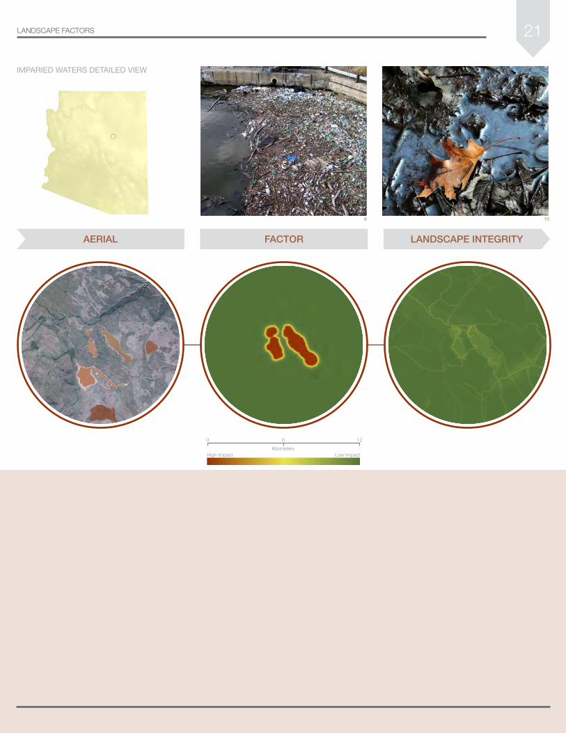
2.7 ICZ Network Delineation: .................................62

2.8 Connectivity Modeling Assumptions: ...............69

2.8.1 General Approach: .......................................69

2.8.2 CAT Modeling: ..............................................69

2.8.3 Connectivity Outputs: ...................................70

2.9 Interpretation and Use of this Document and Data .........................................................71

Appendix 1: (Table 1) Data Summary and Sources ..............72

Appendix 1: (Table 2) Factor Parameterization Summary .....73

Appendix 1: (Table 3) Roads Crosswalk and Hierarchy ........76

Literature Cited: .....................................................78

TABLE OF CONTENTS (continued)

Figure 1: Boolean/discrete Variable Vs. Fuzzy Logic Classification Approach ....9

Figure 2: Fuzzy Logic Membership and Landscape Impact Scoring .....................10

Table 1: Correlation of Peer Data Products ............51

Table 2: Correlation of Survey Respondents ...........52

Table 3: Correlation of Survey Respondents with High Confidence ...............................52

Table 4: Available Connectivity Tools Summary ......57

Map 1: Arizona’s Landscape Integrity ....................49

Map 2: Arizona’s Most Natural Landscape Blocks .....................................50

Map 3: Arizona Connectivity Assessment: CAT Analysis Output ..................................61

Map 4: ICZ’s Top 10% ...........................................63

Map 5: ICZ’s Top 10% & Edited Network ...............64

Map 6: Final ICZ Network by CAT Rank .................66

Map 7: Final ICZ Network & Blocks .......................67

Map 7: Arizona’s ICZs and Landscape Network.....68

Appendix 1: (Table 1) Data Summary and Sources ..............72

Appendix 1: (Table 2) Factor Parameterization Summary .....73

Appendix 1: (Table 3) Roads Crosswalk and Hierarchy ........76

LIST OF FIGURES, TABLES & MAPS

ACRONYM GLOSSARY

ADEQ – Arizona Department of Environmental Quality

ADOT – Arizona Department of Transportation

AGFD – Arizona Game and Fish Department

BLM – Bureau of Land Management

CAP – Central Arizona Project

CAT – Connectivity Analysis Toolkit

DDT – dichlorodiphenyltrichloroethane

EPA – Environmental Protection Agency

FEMA – Federal Emergency Management Agency

ICZs – Important Connectivity Zones

LIWG – Landscape Integrity Work Group (WGA)

NLCD – National Land Cover Dataset

NPMS – National Pipeline Mapping System

RCRA – Resource Conservation and Recovery Act

SCT – Statewide Connectivity Team (AGFD)

SERI – Species of Economic and Recreational Importance

SGCN – Species of Greatest Conservation Need

SHCG – Species and Habitat Conservation Guide

SWAP – State Wildlife Action Plan (Arizona)

SW ReGAP – Southwest Regional Gap Analysis Project

UAiR – The University of Arizona Institutional Repository

USCB – United States Census Bureau

USFS – United States Forest Service

USGS – United States Geological Survey

WGA – Western Governors’ Association

2

Project Context:For many years, the Arizona Game and Fish Department (AGFD) has been engaged in efforts to identify and conserve areas important for wildlife movement and landscape-scale connectivity as part of managing Arizona’s wildlife populations. Local efforts have included working with transportation authorities to build wildlife crossing structures to minimize vehicle collisions with wildlife, as well as working with city and county planners to guide development towards areas that will have the least amount of impact on Arizona’s wildlife. These activities are essential to maintaining the long-term stability of wildlife populations and have been critical in addressing connectivity related issues in numerous locations at more local scales. While the AGFD has developed several statewide datasets in recent years that help inform the identification of crucial habitats, including areas of wildlife conservation potential throughout Arizona, the department acknowledges the need for a systematic large-scale assessment of important landscape connectivity areas for the entire state.

The Species and Habitat Conservation Guide (SHCG) is one of AGFD’s most recent statewide Datasets. The SHCG was developed to meet the requirements of depicting areas of conservation potential for Arizona’s wildlife. As part of Arizona’s State Wildlife Action Plan (SWAP) revision process, the SHCG combined several sub-models, including: 1) a diversity index for Arizona’s Species of Greatest Conservation Need (SGCN), 2) unfragmented habitats, 3) riparian habitats, 4) economically-weighted models for Species of Economic and Recreational Importance (SERI), and 5) sportfish.

Independent of the AGFD’s development of the SHCG, a west-wide effort coordinated by the Western Governors’ Association (WGA) to identify crucial habitats and wildlife corridors across the western United States is also underway. As outlined in the WGA Wildlife Corridor Initiative (WGA 2008), a key part of this west-wide effort has been to identify and develop a series of “Tier 1” datasets important to all western states. These datasets are intended to represent crucial habitats across the west. The sub-models in the AGFD’s SHCG represent the Tier 1 datasets currently completed for Arizona and represent the state’s first deliverables to the WGA. Similar datasets are currently being developed by each of the other 18 western states. When combined, these

data products will represent crucial habitats for individual states and the entire west (Western Governors’ Wildlife Council 2011). The development of one additional Tier 1 dataset for Arizona, a connectivity or linkage assessment, is the primary goal of the effort described in this report. It will result in the identification of Arizona’s Important Connectivity Zones or ICZs. Derivation of this final Tier 1 dataset will complement ongoing AGFD efforts and will satisfy the WGA data requirements.

Based on the AGFD Statewide Connectivity Team (SCT) charter, this work aims to aid in achieving the department’s vision of an interconnected landscape by identifying the crucial connections throughout the Arizonan landscape. Further, this work will support and complement AGFD’s already developed conservation planning tools such as the SHCG, HabiMap™ Arizona, and the Online Environmental Review Tool by providing resource managers and stakeholders with data specific to connectivity conservation and wildlife resource protection early in the planning process.

Additionally, it is envisioned that this statewide assessment will complement existing connectivity efforts including ongoing county-level connectivity assessments and fine-scale modeling work such as the Arizona Missing Linkages and other detailed connectivity assessments. This statewide assessment incorporates both new and existing data from other AGFD efforts and offers a coarse-scale analysis from which to evaluate and unify more localized assessments by providing context on a local area’s broader contribution to statewide connectivity. Additionally, this will aid in the identification of Important Connectivity Zones (ICZs) throughout the state which may be overlooked when focusing on more localized models. Finally, this work also provides a replicable model and framework for future connectivity efforts which will allow for additional iterations of both the landscape integrity and the connectivity model to be revised as new data becomes available.

As a precursor to the development of the statewide connectivity assessment dataset, a statewide landscape integrity dataset was produced. This dataset was the main input for the connectivity model. Both the methodological processes and the derivation of these datasets were developed by the University of Arizona research team who was contracted by the AGFD through DOE/WGA funding.

LANDSCAPE INTEGRITY

Paul Beier

Highlight

Paul Beier

Highlight

Paul Beier

Highlight

3

All inputs, methods, and products were developed through close consultation with the AGFD SCT. The University of Arizona/AGFD partnership is collectively referred to as the “team” throughout the remainder of this report unless otherwise noted.

Project Overview:In order to complete the statewide connectivity assessment, the team first developed a mapped data product depicting Arizona’s landscape integrity. This dataset served as the primary input for the connectivity assessment. Landscape integrity surfaces assess the scope and extent of human alterations to the landscape and can be used for a wide spectrum of management and planning purposes. Modeling Arizona’s landscape integrity was accomplished by adopting and adapting methods currently in use for developing global and downscaled human footprint datasets and naturalness indices. Assessments such as these combine geographic data that inventory the extent of human alteration and infrastructure which is present throughout the landscape. These assessments result in datasets which inventory the landscape’s composition based on gradients ranging from pristine and natural to built and heavily developed. Similar methods have been employed to derive naturalness indices which can be further parameterized to inventory landscape fragmentation and/or the integrity of the landscape.

While modeling landscape integrity by itself is useful, the primary objective of this work was to model and map ICZs for terrestrial ecosystems throughout the state. This resulted in the creation of Arizona’s final Tier 1 dataset (the statewide connectivity assessment) as described by the WGA (WGWC 2011). The connectivity modeling methods utilized here evaluated paths between all possible nodes as represented in a state-wide hexagonal landscape lattice. This illustrated each node’s contribution to landscape connectivity. Nodes which exhibited the greatest flow accumulation across all possible paths where then classified as ICZs. ICZs were then evaluated based on this flow accumulation in order to identify those areas most critical in maintaining connectivity throughout the state as a whole.

While the team believes that the coarse-scale nature of this effort and the prioritization metrics that it generates will be useful in guiding statewide management, it recognizes

some limitations. Namely, ICZs are not to be interpreted as least-cost corridors which are the result of fine-scale modeling between pairs of patches. Rather, ICZs should be viewed as a more general overlay which identifies areas crucial for maintaining flow throughout the entire landscape as opposed to suggesting the discretely bounded path through which that flow will pass. In this way, ICZs could help to prioritize portions of the landscape based on the role they play within the statewide context and suggest where detailed corridor modeling and/or field evaluations may be initiated. More information on how the landscape integrity and connectivity datasets complement other data products, what these datasets can and cannot inform, and how they should be used is detailed in this report and the subsequent AGFD report to the WGA AGFD (Arizona Wildlife Connectivity Assessment: Statewide Analysis in prep).

LANDSCAPE INTEGRITY

Paul Beier

Highlight

Paul Beier

Highlight

Paul Beier

Highlight

Paul Beier

Highlight

Paul Beier

Highlight

Paul Beier

Highlight

4

1.0 Introduction:Common practices for connectivity modeling generally involve assessments of habitat suitability as an indicator for species movement. This contributes to one of the largest assumptions implicit in connectivity modeling – that wildlife choose routes for movement based on the same cues they use to select habitat (Beier et al. 2008). Translated, this means that suitable habitat is utilized as a proxy for high landscape permeability and increased species movement. Approaches currently in use which model connectivity based on the needs of focal species operate with this assumption at the heart of their underlying methods. While this is entirely reasonable and has been utilized to high effect in conservation planning, there are instances when it may be less optimal.

First, for many species, habitat alone can be a poor predictor of species movement. Horskins et al. (2006) reported that corridors with suitable habitat failed to promote gene flow while Haddad and Tewksburry (2005) found that low-quality habitat linkages actually promoted wildlife movement. Second, model parameterization of species’ habitat requirements and associations may be difficult due to incomplete knowledge or data. Third, for habitat generalists, habitat suitability alone is a poor fit for modeling corridors as individuals are likely to be less selective during migration and dispersal than other phases of their life history (Baldwin et al. 2006, Haddad and Tewksbury 2006). Fourth, species-habitat interactions may vary markedly across a species geographic range (Baldwin et al. 2010). This means that habitat proxies will be less consistently linked to species’ movement across large landscapes and may vary greatly in coarse-scale modeling. Fifth, habitat suitability datasets may not include anthropocentric barriers which do not directly impact modeled suitability but may, in fact, impede movement and have substantial impacts on connectivity. Finally, and particularly applicable here, real-world constraints of time and resources may render a focal-species habitat-specific approach impractical or unfeasible.

Given these potential issues, a growing trend is emerging within connectivity conservation to employ coarse-filter approaches which integrate measures of both structural

and functional connectivity (Cook 2002, Baldwin et al. 2010, Panitsa et al. 2011, Theobald et al. 2011, Alagador et al. 2012). Such applications are increasingly adopting the use of landscape integrity datasets, naturalness indices, or variations thereof, as the foundation from which to model connectivity. Employing the use of such data provides for a comprehensive, yet still quantitative, assessment of landscape connectivity which has application across a wide array of ecological systems and spatial scales. Further, such approaches often explicitly integrate measures of anthropocentric influence such as roads, traffic volume, and land use which have direct impacts on wildlife movement but may not be represented in individual species habitat suitability models. Employing such an approach also addresses budgetary and time constraints which may be prohibitive in comprehensive focal-species mapping, as was also the case here.

1.1 Landscape Integrity Modeling Overview:

Landscape integrity can be thought of as a measure of the landscape’s naturalness, or its inverse, the level of human modification. Landscape integrity assessments are closely related to both Ecological Integrity Assessments (EIA) and Index of Biotic Integrity (IBI) methodologies discussed by Harwell et al. (1999) and by Karr and Chu (1998). In each case, a benchmark condition is established from which to base the “standard” or “natural” condition of the landscape being evaluated. Landscapes are further parameterized based on ecological patterns, processes, and an evaluation of how the presence of human activity affects the standard landscape condition. Such approaches have been developed as multi-metric indices designed to evaluate the relative condition of both biotic and abiotic attributes along a gradient. In these approaches, gradients are developed which span from the standard condition on one end to the most degraded condition on the other (Rocchio and Crawford 2011).

Additional measures have been created as methods of inventorying landscape integrity as it relates to human influence. Measures such as human population/housing density (Parks and Harcourt 2002, Theobald 2003), lights at night (WRI 2000), road density (Carroll 2005, Saunders

LANDSCAPE INTEGRITY

5

et al. 2002), and pollutant deposition (Driscoll et al. 2007) all represent anthropocentric variables that may be used as a means of calibrating landscape integrity. In each of these approaches, anthropocentric influences are represented as either indicators or direct causes of landscape degradation (Trombulak et al. 2010).

Sanderson et al. (2002) mapped anthropocentric influence and termed it the “human footprint”. It represented the sum of direct human influence across the lands surface. Signified as a continuum ranging from “natural” to “built”, the human footprint defined human influence via a series of geographic proxies within the larger categorical context of human population density, land transformation, human access, and power infrastructure (Sanderson, et al. 2002). Once identified, human proxies were then scored relative to their impact on natural conditions. The proxies were then weighted to reflect a priori decisions on their relative importance and overall influence in the final human footprint score. Scores were calculated via a heuristic combinatorial model to avoid redundancy. Scores were then normalized to a range of 0 to 100 representing the relative human impact on the landscape (Trombulak et al. 2010). Such methodologies can be adapted and be considered analogous to those employed in landscape integrity modeling.

Additional applications have resulted in fine-scale development of human footprint mapping. Woolmer et al. (2008) applied a down-scaled Sanderson methodology to the Northern Appalachian/Acadian Ecoregion. Their results yielded more detailed information about the nature and extent of human influence and thus landscape integrity within the region. Further, Leu et al. (2008) applied a modified methodology to map the extent and intensity of human influence on the landscape in the western United States. The resulting landscape integrity index was driven by both top-down and bottom-up anthropocentric influences such as avian, dog, and cat predators, invasive plants, human-induced fires, energy production, and habitat fragmentation (Leu et al. 2008).

Recently, researchers have begun merging components of human footprint mapping with landscape naturalness indices as an alternative method intended to substitute

habitat suitability in large-scale connectivity modeling (Cook 2002, Baldwin et al. 2010, Spencer et al. 2010, WHCWG 2010, Panitsa et al. 2011, Theobald et al. 2011, Alagador et al. 2012, and Perkl et al. in prep). After careful evaluation of these methods, the team determined that the utilization of a hybrid human footprint/naturalness indices approach would hold the most promise for developing Arizona’s landscape integrity dataset.

A landscape integrity surface derived in this fashion provides for a logical transition to connectivity mapping. In such an application, the landscape integrity dataset serves as the input surface for the connectivity modeling phase. The team determined this to be a useful methodological approach for several reasons. First, it eases a number of the previously discussed assumptions associated with focal-species based connectivity modeling. Second, calibrating a permeability surface based on widely available anthropocentric data (i.e. impervious surfaces, infrastructure, housing and population density, etc.) integrates fewer species/habitat related assumptions which tend to be lesser known. Third, it allows for anthropocentric barriers to be better accounted for as part of the landscape integrity dataset, which for connectivity modeling purposes, may better incorporate measures of permeability. Fourth, the dataset can be further refined through consultation with orthoimagery, since barriers not implicit in the data can be identified remotely, which can serve as a form of ground-truthing for large areas. Finally, adopting approaches such as this may be helpful in addressing budgetary and time constraints associated with the analysis, as was also the case here.

Even given these benefits however, uncertainty remains in this and all modeling processes. While uncertainty associated with species/habitat related assumptions have been bypassed, they have been replaced by another set of assumptions involving the quantification of landscape impacts. Coupled with the rationale outlined above however, the team concluded that shifting focus in this way may be desirable as landscape impacts may be more easily observed and inferred than would be the case with habitat suitability.

LANDSCAPE INTEGRITY

6 LANDSCAPE INTEGRITY

1.2 Landscape Integrity Modeling Assumptions:

The team acknowledges that in all instances and to the extent possible, a thorough review of available literature, similar modeling efforts, and expert knowledge was incorporated in the process by which methods were developed, factors were chosen, and thresholds, scores, and weights were assigned. Even so, no perfect model exists, thus most modeling efforts are aimed at mitigating the adverse effects of imperfect data, error propagation, factor parameterization, transparency, and adjusting methodologies to find middle ground in balancing assumptions.

Quantitatively predicting the impacts of anthropocentric influence on the landscape is particularly challenging and is most certainly an imperfect science. While best efforts have been made to balance the management needs and timeline of this work with many of the issues previously discussed, the team acknowledges that limitations and modeling assumptions remain. The team recommends that the model factors along with their respective datasets, distance thresholds, impact scores, and model weights be evaluated, reviewed, and updated as new information becomes available. The team is confident however, that this modeling approach and the data products which result will be useful in informing the connectivity needs for wildlife in Arizona.

1.2.1 Landscape Impacts:

The team defines landscape impacts as a generalizable set of negative effects which may be broadly applied to terrestrial, hydrological, and atmospheric systems. Negative effects to these systems may include: 1) the introduction of foreign matter such as pollution, invasive species, particulates, light, and sound; 2) the extraction of landscape constituents such as resources, species, and biomass; and 3) the disruption of landscape flows and processes through landscape fragmentation or other landscape alterations. The team acknowledges that landscape impacts beyond the physical footprints of built systems are largely inferred and may be difficult to quantify in an empirically robust way. Further, the team acknowledges that imperfect knowledge exists in calibrating landscape impacts from anthropocentric sources.

1.2.2 Factor Selection:

The team acknowledges that:

1. Data availability, quality, completeness, statewide coverage, and mitigating uncertainty contributed to factor selection. Landscape integrity, as modeled here, is thus influenced by both the factors selected for analysis and those omitted from the model.

2. In areas where data is lacking no impacts are modeled although the impacts may still exist.

3. Natural processes such as flooding, wildland fires, drought, and others are not captured.

4. Manmade water bodies, unless somehow impaired, are not assumed to negatively affect landscape integrity.

5. Duplication of features is possible. For example, features such as roads are captured by multiple model factors such as roads and impervious surfaces.

6. Features within the modeled factors represent existing conditions to the extent possible; planned or future conditions are not evaluated.

7. Impacts from some modeled factors may be reversible or mitigated over time.

7LANDSCAPE INTEGRITY

1.2.3 Factor Scoring:


•When possible, literature was consulted to aid in theselection of impact scores. When lacking, expert opinion was utilized while attempting to maintain consistency among all factors.

•Assigning scores as part of amodeling processmayoversimplify landscape impacts.

•When applicable, impacts from features within eachfactor diminished with distance.

•When applicable, impacts from features within eachfactor diminished as density decreased within a 1km neighborhood. While this neighborhood size was utilized by others (Theobald et al. 2001 and Theobald et al. 2012), appropriate neighborhood sizes and impact scores are uncertain.

•When applicable, fuzzy logic methodologies wereused to address uncertainties associated with the determination of scores and intermediate distances which are inherent in factor modeling (described in greater detail in section 1.3). Additionally, while fuzzy logic has helped to circumvent the need to assign intermediate distances with discrete scores, it still requires that maximum distance thresholds be applied. While based on expert opinion and available literature when possible, maximum impact distances are also little known, will vary geographically, and may be speculative.

•For large polygon features, landscape impacts areassumed to be homogeneous throughout.

•Impactscoresacrossallfactorsarecompiledadditively,not synergistically.

1.2.4 Edge Effects:


•Nodatawas gathered or evaluatedbeyondArizona’sborder. Edge effects may persist for areas within 3km of Arizona’s border (the maximum impact distance used by any model factor). Such effects would result in slightly higher landscape integrity scores in these areas as impacts from factors beyond the border have not been modeled.

1.3 Landscape Integrity Modeling Methods:

A comprehensive multivariate approach to mapping landscape integrity is the preferred means of inventorying the condition of a landscape. Trombulak et al. (2010) notes that the more variables used to assess the degree and spatial extent of landscape disturbances, the more likely the results will not be biased toward any single variable. As such, a wide array of spatial data were incorporated in the landscape integrity model, including: airports, camping/recreation areas, canals, housing density, impaired waters, impervious surface, land cover, landfills, military operations, mines, oil/gas extraction, pipelines, point source pollution generators, population density, railroads, renewable energy, roads, and utility lines. Individually, each of these factors can serve as a measure of human impacts. Taken together, the cumulative impacts of these factors reduce the naturalness of the landscape and can be utilized to infer landscape integrity. A detailed description of the factors used in this analysis can be found in Section 1.4. Additionally, an accounting of factors considered but not included in the model can be found in Section 1.4.

In modeling landscape integrity, a hybrid approach was developed which incorporated measures of landscape impact related to both proximity and density (when appropriate) of features within the aforementioned factors. The proximity components of the model assumed that landscape impacts were expected to be the greatest at the point of contact with the above features and to diminish with distance. Parameterizing the model in this way ensured that the proximal impact of each individual feature could

8

be calibrated and reflected in the resulting landscape integrity surface. Similarly, the density components of the model assumed that landscape impact was the greatest where there were higher concentrations of these features. Incorporating measures of density ensured that landscape impacts were the greatest where the occurrence of these features was the highest.

The hybrid approach developed here was preferred because scoring landscape impacts based on proximity alone tends to skew modeling impacts in two ways: 1) it can contribute to overestimating the impacts of a single feature in locations where no other like features exist; and 2) it can contribute to underestimating the impacts from many like features in locations where they are numerous and within close proximity to each other. Similarly, parameterizing landscape impacts based on density alone can result in two similar shortcomings: 1) it can contribute to overestimating the impacts of many features in areas of high density; and 2) it can underestimate the impacts from a single feature in areas of low density. Taken together, the hybrid approach developed here mitigates these tendencies by explicitly incorporating both measures of proximity and density. This ensured that the impacts from each feature were represented and that the intensity of those impacts increased where the features were more pervasive.

The proximity and density components for each factor were both parameterized on a 5.0-0.0 floating point scale where high scores were associated with high levels of landscape impact. For the proximity analysis, this resulted in impact scores of 5.0 at or near the physical footprints for each feature within each factor. Scores were parameterized to

decrease to a minimum score of 0.0 once the maximum distance threshold for each factor was achieved. Density was calculated among the features within each factor using a 1 kilometer neighborhood. An impact score of 5.0 was assigned to the highest observed density for each factor and normalized to decrease, as density decreased, to the minimum score of 0.0.

Boolean or discrete proximity impact models typically define distinct distance thresholds to which impact scores are then assigned. Such parameterization however assumes perfect, or at minimum, a high degree of knowledge related to how impacts vary at discretely defined intermediate distances; this however is seldom the case and empirical evidence supporting these distances is typically lacking and/or varies greatly. In order to address the uncertainty inherent in relating landscape impacts with discrete proximity distances, a spatially-explicit fuzzy logic methodology was applied to link impacts related to proximity. This proved to be a valuable advancement in circumventing some of the uncertainty associated with scoring landscape impacts based on little-known or unknown intermediate distance intervals.

The fuzzy logic approach allowed for potential landscape impacts to be calibrated along a continuous gradient which diminished with distance as opposed to distinctly defined intermediate distances. Such approaches have been utilized in expert knowledge-based assessments of agricultural practices (Sattler et al. 2012), risk mapping (Medina et al. 2012), habitat and species distribution modeling (Mouton et al. 2008, Mouton et al. 2009, Fukuda 2009, Amici et al. 2010), and in wildlife dispersion modeling (Pelorosso et al. 2008).

LANDSCAPE INTEGRITY

9

Fuzzy logic methodologies may prove useful in the inclusion of expert knowledge, and therefore, uncertain or undocumented knowledge in the modeling process (Sattler et al. 2012). Such knowledge can then be integrated as a supplement, or in place of, explicit knowledge derived from the literature. Further, such methodological amendments may help to better integrate all forms of available knowledge, ranging from implicit to explicit and quantitative to qualitative, within the modeling process (Sattler et al. 2012). Similarly, Fukuda (2009) points out that such an approach also enables qualitative information to be integrated as part of a quantitative evaluation in ecological applications. Fuzzy logic also addresses the relevant uncertainty and gradients inherent in many ecological variables while enabling non-linear relationships to be expressed (Mouton et al. 2009). Finally, it is believed that fuzzy logic methodologies hold promise in reducing error propagation and information loss, while maintaining or increasing a model’s robustness (Pelorosso et al. 2008).

Fuzzy logic is a science-based approach to modeling inaccuracy or uncertainty in data. Consider the following example: Boolean or discrete variable approaches would require that landscape impact scores be assigned at predefined or known intervals throughout the landscape. In such cases, the modeler would be forced to assign, for example, an impact score of 5 to portions of the landscape within 200 meters of an active mine site, scores of 4 between 200-400m, 3 to 400-600m, and so on to some maximum (figure 1, top). These impact scores, along with their corresponding distances however, may not be known and thus carry with them the potential for error propagation by implying perfect knowledge if they are included in the

model. Further, this uncertainty may also lead analysts to remove such data factors from the analysis entirely because the uncertainty or potential error propagation may be thought to exceed acceptable levels.

In contrast, a fuzzy logic approach circumvents such discrete parameterization by applying a continuum of logical values. This is accomplished by replacing the classical truth-values, such as those above, with degrees of truth which range between 1.0 and 0.0 as part of a fuzzy membership class (Pelorosso et al. 2008). As a result, the factors thought to impact the modeled analysis (landscape integrity in this case) are considered as continuous gradients through which both linear and non-linear functions can be parameterized to describe the relationships between the factors and modeled analysis (Pelorosso et al. 2008). Figure 1 illustrates an example of how Boolean/discrete variable and fuzzy logic approaches differ in impact parameterization.

0.5

0

1.0

1.5

2.0

3.0

3.5

4.0

4.5

Boo

lean

/Dis

cret

e Va

riab

le Im

pac

t S

core

5.0

2.5

900800700600400300200100 500 1000 meters

Distance from mines

0.1

0

0.2

0.3

0.4

0.6

0.7

0.8

0.9

Distance from mines

Fuzz

y m

emb

ersh

ip v

alue

s

1.0

0.5

900 1000 meters800700600400300200100 500

Figure 1: Boolean/discrete Variable vs. Fuzzy Logic Classification Approach

LANDSCAPE INTEGRITY

10

In this application, fuzzy membership scores of 0 represent portions of the landscape where negative impacts are unlikely. Scores that reach or approach 1 are representative of areas where negative impacts are most likely. This translates into a logical and generalizable assumption that can then be applied to model parameterization - that landscape impacts are more likely, and estimated to be higher, the nearer the area to the feature being modeled. Consider the above example once more: fuzzy membership values of 1 are assigned to portions of the landscape nearest a factor being modeled, such as for active mine sites. Fuzzy membership scores diminish across the continuum of potential values to a minimum score of 0 at the maximum distance. These fuzzy membership values are then normalized to their respective landscape impact scores along a floating point continuum which encompasses all scores between 5.0 and 0.0 (figure 2). This allows for fuzzy membership values to be translated and reflected as landscape impact scores

Once fuzzy membership values were assigned, the equation

LIi= ((LIIi-LIImin)×5) (LIImax-LIImin)

was utilized throughout the modeling process to normalize internal impact scores for each factor. LIi represents the total landscape impact score for each factor, while LII represents landscape impact scores internal to the factor sub-model. This ensured consistency across all data factors and resulted in a landscape impact score range of 5.0-0.0. Once each model component was normalized, internal weights were then applied as necessary. This allowed the relative influence of the proximity and density impact scores within each factor to be adjusted. The resulting products were again normalized to maintain consistency across all factors. Once completed, each factor could then be weighted independently in order to adjust the influence of each factor in the final impact model.

LANDSCAPE INTEGRITY

0.1

0

0.2

0.3

0.4

0.6

0.7

0.8

0.9

Distance from mines

Fuzz

y m

emb

ersh

ip v

alue

s

1.0

0.5

900 1000 meters800700600400300200100 500

0.5

0

1.0

1.5

2.0

3.0

3.5

4.0

4.5

Nor

mal

ized

Lan

dsc

ape

Imp

act

Sco

re

5.0

2.5

900800700600400300200100 500 1000 meters

Distance from mines

Figure 2: Fuzzy Logic Membership and Landscape Impact Scoring

11

1.4 Factor Selection:

Factors were initially selected to provide a comprehensive assessment of both built and natural systems throughout the state. Factor selection was further refined based on data availability, statewide data coverage, data reliability, and efforts to sync data temporally. Several factors were included early in the modeling process but were ultimately removed. These included dams, border infrastructure, grazing, invasive species, urban canopy coverage, and wildland fires. These factors were omitted from the final model due to data constraints, lack of reliable statewide data coverage, uncertainties associated with the existing data, complexities of adequately capturing the landscape processes involved, lack of consensus regarding their resulting landscape impacts, and difficulties in addressing differences between both implicit and explicit assumptions related to model parameterization. It is worth pointing out however, that in the case of dams and border infrastructure, impacts may be captured by other model factors such as utility lines, roads, and impervious surfaces.

Spatial data representing each factor was obtained from a combination of authoritative sources but had varying levels of accuracy, attribution, and temporal variability. In all cases,

efforts were made to obtain the most recent and widely applicable dataset which encompassed the statewide extent of this analysis given the constraints of the project timeline. All data sources are provided in the discussion sections of each factor and are summarized in Appendix 1 (Table 1: Data Summary and Sources).

The following sections provide a brief overview of the factors which were included in the landscape integrity model. The overview of each factor is intended to speak generally about how each factor may impact landscape integrity. Each factor overview is then followed by a detailed description which outlines the specifics of how each factor was parameterized within the model. Model parameterization involved applying maximum impact distances which ranged from 0 to 3km, analyzing factor densities within a 1km neighborhood where applicable, and normalizing landscape impact scores which ranged from 5.0 (highest impact) to 0.0 (lowest impact). Scores were applied to both the distance and density components of the model. A summary table which illustrates the model factors analyzed including their proximity distances, landscape impact scores, and model weights is provided in Appendix 1 (Table 2: Factor Parameterization Summary).

LANDSCAPE INTEGRITY

12 LANDSCAPE FACTORS

1.4.1 Airports:

Landscape impacts from airports and their resulting air traffic are likely to vary greatly in both scope and scale. Most studies which evaluate the environmental impacts of airports tend to focus on air and noise pollution and to lesser extents on soil and groundwater pollution. Areas most at risk for contamination within airports are places where materials such as fuel and waste are stored (Nunes et al. 2011). Additionally, aircraft engine emissions have been documented to have an extensive impact on vegetation and ecosystems (Lu and Morrell 2006). Exhaust pollutants are the highest during take-off, ascent, descent, and landing. Given that emissions are greatest when the aircraft is nearest the airport, impacts are expected to be the greatest on the natural habitats surrounding them (Lu and Morrell 2006). Additionally, landscape impacts are also expected from associated support infrastructure such as fencing, roads, structures etc.

The team acknowledges data limitations in attempting to parameterize the landscape impacts of airports when represented as point data. As such, the area of impact associated with large airports may be underrepresented by this model while the impacts from smaller airports may be overestimated. Regarding potential underrepresentation however, other model factors such as roads, impervious surface, and land use capture many of the related infrastructural components associated with airports mitigating these concerns.

Airport data were obtained as TIGER® points from the United States Census Bureau (USCB). The data were joined with flight volume data supplied by the Arizona Department of Transportation (ADOT). Airports were categorized into three classes of varying intensity of use

which were determined by flight volume. The three classes consisted of airports with volume greater than 25,000 taxis annually, less than 25,000 annual taxis, and airports with no available flight volume data. Fuzzy membership was applied to each airport and parameterized to reflect the greatest impact at each point location (impact score = 5.0). Fuzzy membership was then set to decay with distance to a maximum of 1km for airports of large volume, 0.5km for low volume and 200m for airports with no reported volume (impact score = 0.0). Kernel density was also analyzed for all airports using the standard 1km neighborhood size. Landscape impact scores associated with both distance and kernel density were then normalized, summed, and again normalized to a 5.0-0.0 scale for inclusion in the final model.

*DATA SOURCE: ADOT (2005)

Model:

200

Undefined

5–0

Undefined

1

Undefined

1000

Kernel Density

5–0

Kernel Density

1

Kernel Desnsity

1

DISTANCE USED

LI SCORE

INTERNAL WEIGHT

FACTOR WEIGHT

(METERS)

(5.0–1.0)

1000

Class 1

5–0

Class 1

1

Class 1

500

Class 2

5–0

Class 2

1

Class 2

13LANDSCAPE FACTORS

AIRPORTS DETAILED VIEW

AERIAL FACTOR

6 12

Kilometers

0

LANDSCAPE INTEGRITY

21

High Impact Low Impact


1.4.2 Camping/RV/Recreation:

Camping and recreation may represent threats to natural habitats in wilderness areas, national parks, and other natural areas. In wilderness areas, where campers and recreationalists are allowed to travel and camp at will, the impacts can be locally severe and widespread (Cole and Monz 2003). Campsites may have negative impacts on vegetation, trees, wildlife, and soils. In such instances, vegetation can become trampled and even eliminated from the campsite grounds. Additionally, soils can become compacted, eroded, and biologically and/or chemically altered (Leung and Marion 1999). Impacts from campgrounds tend to increase with use intensity and are thus expected to be more extensive at more popular destination zones (Marion and Cole 1996). As use intensity varies greatly among Camping/RV/Recreation areas, landscape impacts are also expected to vary as a result. Others have integrated, or noted the potential for integrating, impacts from recreational activities in the development of human footprint and naturalness indices (Woolmer et al. 2008, Theobald 2010).

*DATA SOURCE: AGFD DIGITIZED (2008)

Model:1

DISTANCE USED

LI SCORE

INTERNAL WEIGHT

FACTOR WEIGHT

(METERS)

1000

Camping/RV/Recreation

3–0


1


The impacts from Camping/RV/recreational areas are particularly applicable in Arizona because large portions of the landscape are intensely utilized by out-of-state recreational vehicles during the winter months. Efforts were undertaken to capture the expanses and impacts of these areas. AGFD staff digitized large, known and heavily utilized portions of the landscape where such activities were observed to occur via orthoimage interpretation. The footprints of these areas were given an intermediate landscape impact score of 3 to account for the temporal/seasonal fluctuations in use and impact intensity. Fuzzy membership was applied to the perimeter of these areas and parameterized to reflect the greatest

impact at the boundary (impact score = 3.0). Applying the intermediate impact score reduced the overall influence of this factor in the final model. This was due in part to the potential subjectivity associated with the digitization of these areas and to address the seasonal fluctuations in use mentioned previously. Fuzzy membership was then set to decay as distance increased to a maximum of 1km (impact score = 0.0). The 1 km distance was adopted by Woolmer et al. (2008) as the zone of impact adjacent to features utilized for recreational purposes. All scores were then normalized to a scale of 3.0-0.0 for inclusion in the final model.

(5.0–1.0)

15LANDSCAPE FACTORS

AERIAL FACTOR

6 12

Kilometers

0

LANDSCAPE INTEGRITY

43


CAMPING/RV/RECREATION DETAILED VIEW


1.4.3 Canals/CAP:

Like other linear infrastructure features, canals can greatly impact local landscapes by contributing to landscape fragmentation, altering surface water flow regimes, and may pose substantial barriers to wildlife movement. Canals are prevalent features within agricultural landscapes throughout Arizona. The Central Arizona Project (CAP) canal also traverses the state to the south bisecting both urban and largely natural landscapes to supply water to numerous agricultural and urban areas. Landscape conditions adjacent to canals vary depending on the presence of fencing, pump stations, siphons, width, and flow rates of the canal and surrounding land uses. The CAP canal for example, contains numerous long sections that are not only fenced, but have been designed with steep embankments and fast-moving currents which have been documented to restrict wildlife movement and pose a mortality risk for wildlife attempting to cross the canal (Tull and Krausman 2001).

Spatial data were obtained through the USCB as TIGER/Lines® and from the CAP. The datasets were merged to produce a comprehensive master dataset which included both smaller agricultural canals and the CAP canal. Due to the extreme differences between canal types, canals were classified into two categories which consisted of the CAP canal and all others. Fuzzy membership was applied to both the CAP canal and all others. The model was parameterized to reflect the greatest impact at the canal itself (impact score = 5.0). Impacts were then set to decay as distance increased to a maximum of 1km for the

CAP canal and 0.5km for all other canals (impact score = 0.0). Kernel Density was calculated for the master canals dataset and normalized with the distance impact scores to 5.0-0.0 scale. A weighted sum of the CAP canal distance impact scores, all other canal distance impact scores, and the kernel density for all canals was then performed. An internal weight of 2 was applied to the CAP canal distance impact scores as to reflect larger landscape impact from the CAP canal over smaller agricultural canals. The resulting product was then normalized to a 5.0-0.0 scale for inclusion in the final model.

*DATA SOURCE: CENSUS TIGER/LINE® (2011), CENTRAL ARIZONA PROJECT (2010)

Model:

DISTANCE USED

LI SCORE

INTERNAL WEIGHT

FACTOR WEIGHT

(METERS)

500

Canals

5–0

Canals

1

Canals

1000

CAP

5–0

CAP

2

CAP

1000

Kernel Density

5–0

Kernel Density

1

Kernel Density

2

(5.0–1.0)

17LANDSCAPE FACTORS

AERIAL FACTOR

6 12

Kilometers

0

LANDSCAPE INTEGRITY

65


CANALS/CAP DETAILED VIEW


1.4.3 Housing Density:

Housing density is a measure of anthropogenic land cover modification (Theobald 2010). Housing and its associated infrastructure represent a transformation from natural to human-modified landscapes and is a direct form of habitat loss (Trombulak et al. 2010). Because of the strong adverse effect on habitats and species that can be associated with housing density, it is oftentimes used as one of the first measures to indicate the intensity of human induced impacts on the natural landscape (Parks and Harcourt 2002). Housing density can be use used to provide missing information pertaining to private land use not found from typical land cover-based analyses. It can also be used to run preliminary forecasts on the effects of land use change on current ecological conditions (Theobald 2010). Together with population density and other factors, housing density can be used to provide an assessment of development intensity.

Housing density spatial data were obtained from the USCB at the census block level. Housing density was calculated for each block, converted to a raster surface, and classified into 6 classes utilizing a ½ standard deviation classification method. This classification method was selected because it yielded the desired degree of heterogeneity amongst the classified blocks. The highest landscape impact score of 5.0 was assigned to census blocks with the highest housing densities (>356 units/km2). A landscape impact score of 4.0 was assigned to blocks classified between 356-291, 3.0 for blocks between 291-226, 2.0 for blocks between 226-162, and 1.0 for blocks between 162-97. A score of 0.0 was assigned to blocks with the lowest housing density (<97 units/km2). Applying these landscape impact scores allowed for direct inclusion in the final model.

Note:

Scores of 0 were assigned to housing densities of <97 because of the spatial uncertainty associated with the distribution of the housing units within large blocks. For example, in a large, sparsely populated block, housing may be clustered,

distributed throughout, or both. If clustered in a small portion of the block, most of the block would exhibit low to no impacts. If distributed throughout, impacts would be expected to be potentially less intense but persistent throughout the entire block. This uncertainty was addressed, in part, by using seemingly high density values to establish the lower class breaks. This ensured that the model did not overestimate impacts in large sparsely populated blocks where the distribution of the population was unknown.

The team acknowledges that this may under-represent landscape impacts in less densely populated areas and that density is a potentially poor measure for capturing sprawling, low density/large lot, forms of housing which may be present in rural areas or urban fringes. In these areas however, it is likely that other model factors capture the presence of these populations given their supporting infrastructure such as roads, impervious surface, land use, etc. Alternatively however, establishing class breaks in this way maintained the ability to calibrate and differentiate landscape impacts in more urbanized areas where housing densities were higher.

*DATA SOURCES: CENSUS TIGER/LINE® / AMERICAN FACTFINDER (2011)

Model:

3

291–226

2

226–162

1

162–97

0

<97

2

LI SCORE

FACTOR WEIGHT

5

>356 units/km2

4

356–291

(5.0–1.0)

19LANDSCAPE FACTORS

AERIAL FACTOR

6 12

Kilometers

0

LANDSCAPE INTEGRITY

87


HOUSING DENSITY DETAILED VIEW


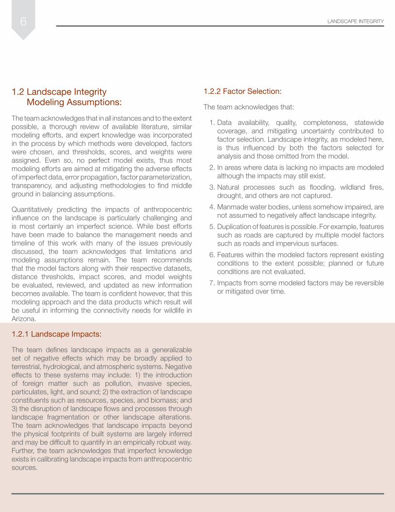
1.4.4 Impaired Waters:

In arid Arizona, despite the artificial nature of lakes and highly modified streams throughout the state, bodies of inland freshwater provide valuable ecosystem services and important habitat for terrestrial and non-terrestrial species alike. They are also important for economic, cultural, aesthetic, scientific, and educational opportunities. Rivers, washes, streams, wetlands, lakes, and reservoirs often become the “receivers” of land-use effluents delivered indirectly by drainage networks or directly by surrounding development (Dudgeon et al. 2006). Additionally, bodies of freshwater can become impaired as a result of pollutants from point sources, non-point sources, diffuse sources, and atmospheric deposition. Pollutants associated with these sources can be toxic to aquatic ecosystems and surrounding lands. In many cases however, pollutants are delivered in such low concentrations that their effects exist but may not be immediately apparent (Soldan 2003).

EPA designated impaired waters spatial data were obtained from the Arizona Department of Environmental Quality (ADEQ) via the University of Arizona Institutional Repository (UAiR). Waters which were classified as being impaired by dichlorodiphenyltrichloroethane (DDT), chlordane, toxaphene, and/or mercury were selected for inclusion in the model. Through consultation with AGFD aquatic habitat specialists, other impairments such as low dissolved oxygen, high/low pH, and turbidity were not considered to have significant impacts on the surrounding

terrestrial landscape and therefore were not included. The footprints of the selected water bodies were classified as having the maximum landscape impact score of 5.0. Fuzzy membership was then applied to these water bodies and was parameterized to reflect the greatest landscape impact score at the shoreline (impact score = 5.0). Impacts were then set to decay to a maximum distance of 0.5km (impact score = 0.0). Having applied the 5.0-0.0 scale range, the factor was then included in the final model.

*DATA SOURCE: ADEQ (2006, 2008)

Model:

1

DISTANCE USED

LI SCORE

INTERNAL WEIGHT

FACTOR WEIGHT

(METERS)

1000


3–0


1


(5.0–1.0)

21LANDSCAPE FACTORS

AERIAL FACTOR

6 12

Kilometers

0

LANDSCAPE INTEGRITY

109


IMPARIED WATERS DETAILED VIEW


1.4.5 Impervious Surface:

Impervious surfaces can prevent the infiltration of water into the soil and may have a negative impact on ecosystem services, natural hydrologic cycles, and aquatic ecosystems. Represented by a wide array of infrastructural systems such as roads, rooftops, sidewalks and pavements of all types, impervious surfaces are an effective proxy for development intensity. Measuring impervious surface area is seen as an important environmental indicator given the effects that anthropogenic practices have on water quality and aquatic habitats (Sutton et al. 2009).

While primarily associated with urbanization or the urban built environment, the impacts from impervious surfaces on habitat quality and ecosystem services can extend well beyond the urban extent. Stormwater runoff carried by impervious surfaces to water bodies has the potential to increase sediment and nutrient loads and can have impacts on surface waters far downstream from the built environment (Wade et al. 2009). Though not generating pollutants directly, impervious surfaces may serve as conduits for: 1) hydrologic changes that degrade waterways, 2) intensive land uses that have the potential to generate pollution, 3) the prevention of soils from performing natural pollutant removal before water percolation, and 4) the transport of pollutants into waterways (Arnold et al. 1996). Additionally, riparian habitats may be lost through increased erosion and siltation that can result from increased volumes of water delivered by impervious stormwater management systems. Given these effects, measures of impervious surface can serve as an important indicator of landscape transformation and as a proxy for potential landscape impacts.

Impervious surface spatial data were obtained from the United States Geological Survey (USGS) via the Seamless Data Server. Raw data reflected values ranging from 0-100 percent impervious surface coverage for each 30m raster cell. A quantile classification method was utilized to create 6 classes reflecting varying levels of impervious surface coverage. Break values consisted of >41% for the most intense class followed by, 41-18%, 18-7%, 7-2%, 2-1% and 0%

coverage as the least intense. These break values provided adequate classification of impervious surfaces throughout the state given variations in road widths, canopy coverage, and the reflectance of various surfaces. Landscape impact scores of 5.0, 4.0, 3.0, 2.0, 1.0, and 0.0 were applied respectively. Applying these landscape impact scores allowed for direct inclusion in the final model.

Model:

*DATA SOURCES: USGS (2006)

3

18–7%

2

7–2%

1

2–1%

0

0%

2

LI SCORE

FACTOR WEIGHT

5

>41%

4

41–18%

(5.0–1.0)

23LANDSCAPE FACTORS

AERIAL FACTOR

6 12

Kilometers

0

LANDSCAPE INTEGRITY

1211


IMPERVIOUS SURFACE DETAILED VIEW


1.4.6 Landcover:

Human induced land conversions of natural habitats to other land use types have had a significant impact on most terrestrial ecosystems (Etter et al. 2011). Saunders et al. (2002) note that within a landscape, human activities often result in a conversion of land from its natural state, the loss of a variety of land cover types, and the fragmentation of the remaining land cover into more isolated elements. Human activities that have an impact on, or produce a change in, natural landscapes include: urban development, agriculture, grazing, natural resource extraction, and mineral extraction (Etter et al. 2011, Theobald et al. 2012). These impacts and changes are usually captured in land cover data (Theobald et al. 2012). According to Trombulak et al. (2010) anthropogenic land cover transformation can contribute to increases in soil erosion and the degradation of freshwater ecosystems while also changing regional and global climates, ecosystem structures and functions, and global carbon and nutrient cycles. Landcover data can be used to identify varying land uses and development intensity, allowing landscape impacts to be inferred.

Landcover spatial data were obtained from the USGS via the Seamless Data Server as the National Land Cover Dataset (NLCD). NLCD classes were reclassified based on the relative naturalness or intensity of the land use associated with each land cover type. Land cover classes of “developed, high intensity” were assigned the maximum landscape impact score of 5.0, followed by “developed, medium intensity” and “cultivated crops” receiving a score of 4.0,

“developed, low intensity” and “pasture/hay” were scored 3.0, and “developed open space was scored 2.0. Scores of 0.0 were applied to all other natural land cover types. Applying these landscape impact scores allowed for direct inclusion in the final model.

Model:

*DATA SOURCES: USGS ReGAP (2007)

4

Cultivated Crops

0

Deciduous Forest

3

Developed, Low

0

Evergreen Forest

3

Pasture/Hay

0

Mixed Forest

0

Grassland/Herbaceous

0

Emergent Herbaceous Woodlands

2

Developed, Open Space

0

Shrub/Scrub

0

Woody Wetlands

3

LI SCORE

FACTOR WEIGHT

5

Developed, High

0

Open Water

4

Developed, Medium

0

Barren Land

(5.0–1.0)

25LANDSCAPE FACTORS

AERIAL FACTOR

6 12

Kilometers

0

LANDSCAPE INTEGRITY

1413


LANDCOVER DETAILED VIEW


1.4.7 Landfills:

Landfills can act as point source polluters with potentially far-reaching negative environmental effects. Landfills also have the potential to release toxic leachates from the refuse itself or through various processes of microbial decomposition (Lisk 1991). Any leachate that is not captured by on-site collection systems or not attenuated by natural processes such as adsorption, ion exchange, and dilution can potentially drift into the surrounding landscapes and infiltrate into both surface and subterranean water supplies (Lisk 1991). Additionally, possible negative effects from landfills may include direct habitat loss, increased heavy vehicle traffic, dispersal of particulate matter, odors, and alterations to both surface and

The team acknowledges that applying a universal impact zone for all landfills is particularly difficult given the wide range and varied impact of the materials being disposed of, differences of the onsite man-agement practices being employed, and the potential variability in on-site factors such as soils, geologic formations, and surface and subsurface hydrology. Additionally, the team acknowledges that due to data limitations, namely the lack of landfill footprint data and attribution indicating size and use, the land-scape impacts of large regional landfills may be underrepresented while smaller sites may be overestimated by this model.

Landfill spatial data were obtained from the ADEQ as point data. Fuzzy membership was applied to each landfill point and parameter-ized to reflect the greatest landscape impact at each point (impact score = 5.0). Impacts were then set to decay until a maximum distance of 1km was reached (impact score = 0.0). Kernel Density was also calculated across all landfills. Impact scores for both distance and density were then normalized, summed, and again normalized to the 5.0-0.0 scale for inclusion in the final model.

*DATA SOURCE: ADEQ (2003)

Model:

1

DISTANCE USED

LI SCORE

INTERNAL WEIGHT

FACTOR WEIGHT

(METERS)

1000

Landfills

5–0

Landfills

1

Landfills

1000

Kernel Density

5–0

Kernel Density

1

Kernel Density

(5.0–1.0)

27LANDSCAPE FACTORS

AERIAL FACTOR

6 12

Kilometers

0

LANDSCAPE INTEGRITY

1615


LANDFILLS DETAILED VIEW


1.4.8 Military:

The physical effects of habitat disturbances due to military activity may vary based on geographic location and species-specific habitat requirements (Krausman et al. 2005). Responses to military activities by wildlife are difficult to quantify as they may vary widely by species, type of military activity, and the spatial and temporal heterogeneity of those activities. Specific landscape impacts from military activities, such as from the use of rockets and dummy bombs for example, may result in greater metallic and energetic material contamination of soils; concentrations of both materials have been documented to exceed background levels on military lands (Bordeleau et al. 2008). Additional impacts may be caused from the presence of pollutants and chemicals, light and noise, soil compaction, and support infrastructure such as impervious surfaces, barriers, and fencing among others.

The team acknowledges that all military lands are not to be considered as posing negative landscape impacts. In Arizona, the Department of Defense is considered to be an important conservation partner by the AGFD and portions of military lands are recognized as highly valuable for a number of species and as refugia for others.

As military activities have widely varying impacts on local landscapes, it is critical that attempts be made to parameterize such variations as to not grossly overestimate or underestimate landscape impacts which may occur if only the boundaries of such instillations were utilized. Within Arizona for example, extremely disturbed and intensely-used portions of military installations are common. The flipside of this however is also true, whereas there are numerous examples of military lands which are largely unaffected by military operations.

In an effort to address this variability, members of the AGFD staff digitized military areas where landscape disturbance was determined to be ongoing and observable from aerial imagery. Such impacts were observed as cleared areas, buildings and structures, and areas with visibly high concentrations of vehicle tracks and other disturbances. Given limitations however, the team acknowledges that historic disturbances may not be captured in this analysis. Additionally locations that were observed to be adequately captured and categorized as “developed” by the NLCD dataset as part of the landcover factor were not included here a second time.

The footprints of these disturbed areas were categorized as having the highest landscape impacts. Fuzzy membership was then applied to the perimeter of each disturbed area and parameterized to reflect the greatest impact at the boundary (impact score = 5). Impacts were then set to diminish as distance increased to a maximum distance of 1km (impact score = 0). Having applied the 5-0 scale, the factor was then included in the final model.


Model:

1

DISTANCE USED

LI SCORE

INTERNAL WEIGHT

FACTOR WEIGHT

(METERS)

1000

Military

5

Military

1

Military

(5.0–1.0)

29LANDSCAPE FACTORS

AERIAL FACTOR

6 12

Kilometers

0

LANDSCAPE INTEGRITY

1817


MILITARY DETAILED VIEW


1.4.10 Mines:

Though mining activities affect relatively small portions of the landscape as a whole, they can have numerous impacts on the local environments in which they are located. Tailings and the erosion of waste rock deposits associated with mines have been documented to release metals, processing chemicals, and other pollutants into adjacent habitats. Such contaminants can become more widely dispersed in aquatic ecosystems when carried by leachates that come in to contact with water bodies (Salomons 1995).

While the physical footprint of mining activities can vary greatly depending on the methods being utilized and the materials being extracted, surface mines tend to impact a larger area on the landscapes surface than sub-surficial mines. Further, surface mining tends to result in negative changes to the landscapes surface which can persist for long periods of time even after production ceases, causing diminished ecological function of such areas and their surrounding landscapes (Krausman et al. 2005). Mines have also been documented to impose significant alterations to groundwater flow regimes (Cragg et al. 1995). Additionally, mining activities tend to be associated with the development of support infrastructure such as roads, railroads, housing, and power plants (Cragg et al. 1995).

The impacts of mines have been incorporated into similar models by Comer and Hak (2012), Woolmer et al. (2008), Copeland (2007) Morgan (2003), and WWF Canada (2003). Impact zones ranged from 500m to 20km. Variations of annual rainfall, surface and sub-surficial hydrology, and underlying geologic formations are all factors which will drastically influence the impacts of mining on the adjacent landscape. Given Arizona’s arid climate and more consolidated geologic conditions, the team determined that the impacts of mining may be overestimated if large impact zones such as some of those from above were applied. Additionally, the team acknowledges that applying a universal impact zone for mining operations is a potential oversimplification given the varying conditions explained above, each of which will have varying influence on landscape impacts. Further, the team acknowledges limitations in the specificity of the dataset incorporated in the model in that a proportion of data-points may represent bore-holes

which may be only a few inches in diameter; such occurrences would be expected to have markedly smaller zones of impact. Taken together, the team determined that a more measured impact zone be applied to this factor in an attempt to mitigate these concerns. The team acknowledges that the impact zones associated with this factor may under or over represent landscape impacts of an individual mine and recommends that additional evaluation be undertaken as new information becomes available.

Mine locations were represented as point data obtained from the Bureau of Mines. Mines were categorized by their type and production status in order to calibrate their relative landscape impact. Mines which were categorized as “producers” and of the type “leach”, “proc plant”, “surface-underground”, or “surface” were considered to have the greatest impact. Non-active mines with past function types which included “leach”, “mineral loc”, “placer”, “proc plant”, “prospect”, “surface-underground”,

*DATA SOURCE: US BUREAU OF MINES (2012)OPEN PIT: SW ReGAP (2007)

Model:

500

Other

5–0

Other

1

Other

1000

Kernel Density

5–0

Kernel Density

1

Kernel Desnsity

3 1

DISTANCE USED

LI SCORE

INTERNAL WEIGHT

FACTOR WEIGHT

(METERS)

1000

Open Pit

5–0

Open Pit

1

Open Pit

1000

Producer

5–0

Producer

1

Producer

Open Pit Producer/Other

(5.0–1.0)

31LANDSCAPE FACTORS

“surface”, “underground”, “underwater”, “well”, or “unknown” were considered to have less impact on the surrounding landscape than active mines.

Fuzzy membership was applied to both of the mine categories and parameterized to reflect the greatest impact at the mine datapoint (impact score = 5.0). Impacts were then set to decay as distance increased to a predetermined maximum distance (impact score = 0.0). A maximum distance of 1km was applied to the mines in the greatest impact category while a smaller zone of influence (0.5km) was applied to the smaller impact category. Kernel density was then calculated for all mines. Scores from the two distance classes and density analysis were then normalized, summed utilizing equal weighting and the resulting product was normalized to the 5.0-0 scale for inclusion in the final model.

Utilizing point data to represent large open pit mines, which are present throughout Arizona, may significantly underrepresent their physical footprints. For this reason, Southwest Regional Gap Analysis Project (SW ReGAP) landcover data was utilized to further identify open pit mines. Cells classified as open pit mines were extracted and reclassified to the maximum impact score of 5.0. Fuzzy membership was then applied to reflect that greatest impact at the mine site (impact score = 5.0). Impacts were then set to decay as distance increased to a maximum distance of 1km (impact score = 0.0). Open pit mines and their resulting zones of impact were treated as a stand-alone factor separate from all other mines. This allowed the team to weight the impacts of open pit mines more heavily than other mining operations in the final model.

AERIAL FACTOR

6 12

Kilometers

0

LANDSCAPE INTEGRITY

2019


MINES DETAILED VIEW


1.4.11 Oil/Gas Extraction:

Oil and natural gas extraction sites can act as point sources of pollution during all stages of their lifecycle (exploration through decommissioning). Additionally, the risk of potential spills or leakage from the site is constant even when appropriately managed (EPA 2008). While less common in Arizona, operations associated with certain types of energy extraction, such as hydraulic fracturing, have the potential for higher levels of landscape impact due to the intensity of operations and the use of large volumes of water withdrawal and injection (EPA 2008). Landscape impacts will vary greatly with the size, type, and geographic location of operations. Further, there may be additional variations in local disturbances from noise and vehicular traffic based on the daily operations associated with each site.

Landscape impacts from oil and gas extraction have been discussed as generalizable expressions of pollutant dispersal and in terms of impacts on specific taxa (Jensen 1991, Bock and Lindzey 1999, Morgan 2003, WWF Canada 2003, Copeland et al. 2007, Leu et al. 2008, Lusk and Kraft 2010, Theobald et al. 2012). Documented effects are highly variable with impact distances ranging from 300 feet to 50km. While the team acknowledges that zones of impact may be variable given the differences in landscape characteristics associated with each site, the impacts of oil and gas extraction are not trivial and are thus included in the model.

Oil and natural gas spatial data were obtained from the USGS. Each data point represented an extraction site. Fuzzy membership was applied and parameterized to reflect the greatest landscape impact at each data point (impact score = 5.0). Impacts were set to diminish with distance to a maximum of 0.5km (impact score = 0.0). Both the distance and kernel density impact scores were normalized to a 5.0-0.0 scale, summed, and again normalized for inclusion in the final model.

*DATA SOURCE: USGS (2004)

Model

1

DISTANCE USED

LI SCORE

INTERNAL WEIGHT

FACTOR WEIGHT

(METERS)

500

Oil/Gas

5–0

Oil/Gas

1

Oil/Gas

1000

Kernel Density

5–0

Kernel Density

1

Kernel Density

(5.0–1.0)

33LANDSCAPE FACTORS

AERIAL FACTOR

6 12

Kilometers

0

LANDSCAPE INTEGRITY

2221


OIL/GAS EXTRACTION DETAILED VIEW


1.4.12 Pipelines:

Landscape impacts from pipelines can include landscape fragmentation, barrier effects, introduction or access for invasive non-native species, disruption of sensitive and natural habitats, and impacts to threatened and endangered species (Nathanson 2000). Landscape impacts from pipelines are expected to vary greatly based on the width of the utility easement, the above- or below-grade nature of the pipeline itself, support access, methods of pumping conveyance, and fencing infrastructure. Even in instances where the pipeline may be constructed underground however, landscape impacts resulting from the initial site disturbance and excavation may continue to persist.

The team acknowledges a general deficiency in documentation which parameterizes the landscape impacts of pipelines beyond their physical footprints. Even so, the team believes that value is added to the model given the landscape disturbance experienced during construction, maintenance of the easement post-construction, and the added potential for negative edge effects and possible dispersion of invasive species into adjacent lands. The team acknowledges that the impacts from pipelines may exceed, or be smaller than, the impact distance modeled here. As the zones of influence may be uncertain, the team recommends that distances be adjusted as additional data becomes available. Attribution on fencing, pipeline diameter, height above ground and whether sections are buried or on the surface would be particularly useful in differentiating landscape impacts; no such attribution was available at the time of this analysis.

Spatial data for pipelines were obtained through both the USCB as TIGER/Line® data and from the National Pipeline Mapping System (NPMS). The data products were merged into a master pipelines dataset. Fuzzy membership was applied to all pipelines and parameterized to reflect the greatest landscape impact at the line itself (impact score = 5.0). Impacts were then set to decay until a maximum distance of 0.5km was reached (impact score = 0.0). Kernel Density was also calculated for all pipelines. Both the landscape impact scores from the proximity and kernel density analysis were normalized, summed, and again normalized to a 5.0-0.0 scale for inclusion in the final model.

*DATA SOURCE: CENSUS TIGER/LINE® (2011), NPMS (2012)

Model

1

DISTANCE USED

LI SCORE

INTERNAL WEIGHT

FACTOR WEIGHT

(METERS)

500

Pipelines

5–0

Pipelines

1

Pipelines

1000

Kernel Density

5–0

Kernel Density

1

Kernel Density

(5.0–1.0)

35LANDSCAPE FACTORS

AERIAL FACTOR

6 12

Kilometers

0

LANDSCAPE INTEGRITY

2221


PIPELINES DETAILED VIEW


1.4.13 Point Source Pollution:

Industrial and commercial facilities which produce or discharge point source pollutants to the air, water, and land can have adverse effects on the environment and surrounding landscapes. Though ecological functions of the natural environment are capable of assimilating some wastes from human and industrial activities, accumulation of pollutants associated with point source polluters can exceed the assimilative capacity of the environment (Kebede et al. 2002). Point source pollution can alter the composition and function of natural plant communities, can lead to the extinction of both aquatic vertebrates and invertebrates, and can cause changes in species composition (Forester and Machlis 1996). Given these impacts, it is assumed that the landscapes surrounding such sites may be adversely affected not only by the byproducts of their operations, but by the additional infrastructure and more intensely

Point source pollution generators vary greatly in size and level of impacts. Given data availability however, the team acknowledges limitations in not being able to differentiate between large and small generators. As such, all point source generators are modeled using the same zone of impact. The team acknowledges that this may over-represent the impacts of small producers which may have only local zones of influence and under-represent the impacts of larger facilities such as power plants. In cases of possible under-representation however, the impacts of these facilities may be captured by other modeled factors such as impervious surface, land cover, transmission lines, and others. The team underscores the additional value added to the model however as point sources are typically associated with commercial and/or industrial land uses, greater land use intensity, and the propensity for greater landscape impacts given the regulated pollutants that they generate. Pollutant generators of this type would not be explicitly incorporated in the model if this factor were excluded.

Point data which represented Resource Conservation and Recovery Act (RCRA) monitored point source pollution generators were obtained from the EPA via the UAiR. Fuzzy membership was applied to each generator and parameterized to reflect the greatest impact at the pollution generator datapoint (impact score = 5.0) Impacts were set to decay as distance increased to a maximum distance of 0.5km (impact score = 0.0). Kernel density was then calculated for all points. The distance and kernel density scores were then summed, and the resulting product was normalized to a 5.0-0.0 scale for inclusion in the final model.

*DATA SOURCE: EPA (2012)

Model

1

DISTANCE USED

LI SCORE

INTERNAL WEIGHT

FACTOR WEIGHT

(METERS)

500

Point Source

5–0

Point Source

1

Point Source

1000

Kernel Density

5–0

Kernel Density

1

Kernel Density

(5.0–1.0)

37LANDSCAPE FACTORS

AERIAL FACTOR

6 12

Kilometers

0

LANDSCAPE INTEGRITY

2423


POINT SOURCE POLLUTION DETAILED VIEW


1.4.14 Population Density:

Human population density is a geographic proxy from which human influence on natural environments can be gauged (Sanderson et al. 2002). Species and ecosystem declines are frequently correlated with a general increase in human habitation. Higher population densities represent a higher anthropogenic influence on natural habitats and typically results in additional demand on the lands resources (Cincotta and Engleman 2000).

In the western United States, as human population density expands into rural and exurban areas, it fundamentally changes natural habitats and ecosystems (Leu et al. 2008). Intensive land use results as roads, power lines, and other habitat altering anthropogenic infrastructure are built in order to support human populations (Leu et al. 2008). Population centers also have landscape impacts beyond their physical footprints. Such impacts include the introduction of recreational activities such as hiking and off-highway vehicle use in nearby areas, the introduction of invasive plant and animal species, and even increased predation by domestic dogs and cats in adjacent landscapes (Leu et al. 2008).

Human population spatial data were obtained through the USCB at the census block level. Population density was calculated for each block, converted to a raster surface, and then classified into 6 classes utilizing a ½ standard deviation method. This classification method was selected because it yielded the desired degree of variability amongst classified blocks throughout the state. Additionally, this classification method ensured that large sparsely populated blocks in rural portions of the state were not overrepresented in the model. The highest landscape impact score of 5.0 was assigned to the most densely populated blocks (>612 people/km2). Impact scores of 4.0 were assigned to blocks between 612-501, 3.0 for blocks between 501-390, 2.0 for blocks between 390-278, and 1.0 for blocks between 278-167. A landscape impact score of 0.0 was assigned to the least densely population blocks (<167 people/km2). Applying these landscape impact scores allowed for direct inclusion in the final model.

Note:

As Theobald (2003) points out, urban densities are typically associated with areas which exceed 386 people/km2. While the above classification scheme is consistent with this characterization, the team acknowledges that assigning the minimum score to areas with 167 or fewer people may appear to be high. This was done because of the spatial uncertainty associated with the distribution of populations within large blocks. In a large, sparsely populated census block for example, it is likely that the population may be clustered leaving most of the block with no impact. The team acknowledges that calibrating the model in this way is best suited for quantifying and differentiating landscape impacts within densely populated areas as opposed to large and sparsely populated blocks. While this provided greater differentiation of landscape impacts in more urbanized areas, it may underrepresent landscape impacts in areas with lower population densities. Impacts associated with populations in these areas however are likely captured by other model factors such as roads, impervious surface, and landcover.

*DATA SOURCES: CENSUS TIGER/LINE® / AMERICAN FACTFINDER (2011)

Model:

3

501–390

2

390–278

1

278–167

0

<167

2

LI SCORE

FACTOR WEIGHT

5

>612 people/km2

4

612–501

(5.0–1.0)

39LANDSCAPE FACTORS

AERIAL FACTOR

6 12

Kilometers

0

LANDSCAPE INTEGRITY

2625


POPULATION DENSITY DETAILED VIEW


1.4.15 Railroads:

As a prevalent component of manmade transportation systems, railroads span vast expanses across virtually every landscape. As with any infrastructural component, railroads can be considered to be a substantial obstacle to the movements of certain wildlife species and a contributor to habitat fragmentation. Railroads have been documented to block and restrict the movement of certain species and populations (Yanes et al. 1995). Barrier effects can be physical and/or behavioral and may vary by species. Effects such as these can be in reaction to the railroad tracks as well as the noise, light, and other pollution generated from the trains themselves (Rodriguez et al. 1997). Railroads have also been noted to be responsible for the direct mortality of wildlife as a result of collisions during attempted crossings (Sanderson et al 2002). Railroad data has been widely integrated into a broad variety of similar landscape analyses including connectivity assessments, landscape integrity inventories, and human footprint analyses (Sanderson et al. 2002, Dougherty and Byers 2008, Leu 2008, Woolmer et al. 2008, Theobald 2010, Theobald et al. 2011).

Railroads spatial data were obtained from the USCB as TIGER/Line® data. Landscape impacts were assumed to be the greatest at the rail bed itself and then decrease with distance (Sanderson et al. 2002, Dougherty and Byers 2008, Leu 2008, Woolmer et al. 2008, Theobald 2010, Theobald et al. 2011). Further, landscape impacts were assumed to be greatest around active lines with increased intensity of use (Woolmer et al. 2008, Theobald 2010). As such, rail lines were first categorized based on their use status, which included the following categories: “abandoned”, “abandoned 1950-1979”, “out of service”, and “in service”. These categories were used to determine which lines were actively in use. Active lines were further refined based on their intensity of use, which included the following categories: “siding”, “spur”, “mainline”, and “unclassified”. Mainlines were determined to have the highest use intensity while all other classes were categorized as being less intensely used. Landscape impact was assumed to be the greatest in areas adjacent to active, intensely used rail lines.

Fuzzy membership was applied to each of the new classes and parameterized to reflect greatest impact at the rail bed (impact score = 5.0). Landscape impacts were then parameterized to diminish with distance to a maximum of 0.5 km (Leu et al. 2008) for active, intensely used lines and 0.25 km for all out of service and unclassified rail segments (impact score = 0.0). The fuzzy logic membership layers were summed across classes and the total values were normalized to a 5-0 scale. Kernel Density was also calculated for all railroads. A weighted sum of both the distance and density values was then performed. Whereas a weight of 2 was assigned to the intensely-used and active mainlines while weights of 1 were applied to all other distance classes and kernel density scores. The resulting product was again normalized to a 5.0-0.0 scale for inclusion in the final model. *DATA SOURCES: ARIZONA DOT (2010)

Model:

250

Out of Service/Undefined

5–0


250


500

In Service (Mainline)

5–0


500


1000

Kernel Density

5–0

Kernel Density

1

Kernel Density

2

DISTANCE USED

LI SCORE

INTERNAL WEIGHT

FACTOR WEIGHT

(METERS)

250

In Service (Siding & Spur)

5–0


250


(5.0–1.0)

41LANDSCAPE FACTORS

AERIAL FACTOR

6 12

Kilometers

0

LANDSCAPE INTEGRITY

2827


RAILROADS DETAILED VIEW


1.4.16 Renewable Energy:

Solar energy production, particularly in desert ecosystems, can cause negative environmental effects including an increased consumption of water for cooling purposes and the disruption of ground and surface water flow patterns. Large-scale systems may also cause the direct destruction of desert habitat for burrowing animals and desert wildlife alike (Abassi and Abassi 2000). Oftentimes, large installations are also fenced, creating an impenetrable barrier to most wildlife species. Additionally, wind farms have been documented to interfere with habitats, cause noise pollution, interfere with bird flight, reduce wind speeds causing stress to ecosystems, warm downwind lakes, and increase soil moisture (Abassi and Abassi 2000). While the pollutant effects associated with renewable energy infrastructure tend to be less than non-renewable forms of energy production, such operations do have the potential to negatively impact landscapes.

While impact distances are not explicitly discussed, Leung and Yang (2012) and Meyerhoff et al. (2010) report residential land use restrictions within 2km and 750m respectively of wind facilities. These restrictions however appear to be linked to public safety concerns and not necessarily attributable to negative landscape impacts. Additionally, due to the relatively recent increase in production-scale renewable energy facilities in Arizona and elsewhere, the team acknowledges a general lack of information available on landscape impacts from such projects. The team acknowledges that more research is needed to better determine the impacts of both solar and wind development on Arizona’s landscape and wildlife populations.

In calibrating impacts for this effort, the team relied on internal knowledge of both wind and solar facilities specific to the state. Wind facilities were determined to have less of an impact on the landscape than large solar facilities, which in Arizona, tend to result in the complete transformation of the landscape within their immediate footprints. The team acknowledges that support infrastructure for renewable energy facilities

is likely captured by other model factors such as roads and transmission lines. This may aid in mitigating concerns of potentially underestimating landscape impacts from these sites.

Renewable energy data were obtained from the AGFD. The footprints of renewable energy projects involving geothermal, wind, and solar energy sites were categorized by their functional status. Only sites listed as “under construction” or “operational” were included in the model. Areas associated with solar sites were determined to have the largest impact and were assigned the maximum score of 5.0; wind sites were assigned a score of 1.0, while geothermal sites were not scored as there are currently no operational or sites under construction within the state. Fuzzy membership was applied to the perimeter of each renewable energy site and parameterized to reflect the greatest impact at the site boundary (impact score = 5.0 and 1.0 respectively). Landscape impact was set to decrease to a maximum distance of 1km for all sites (impact score = 0.0). Scores were then normalized to a 5.0-0.0 and a 1.0-0.0 scale for inclusion in the final model.


Model:

1000

Solar

1–0

Solar

1

Solar

1

DISTANCE USED

LI SCORE

INTERNAL WEIGHT

FACTOR WEIGHT

(METERS)

1000

Wind

5–0

Wind

1

Wind

(5.0–1.0)

43LANDSCAPE FACTORS

AERIAL FACTOR

6 12

Kilometers

0

LANDSCAPE INTEGRITY

3029


RENEWABLE ENERGY DETAILED VIEW


1.4.17 Roads:

Perhaps the most pervasive of humankind’s infrastructure, roads are linear features that probe virtually the entire globe. By virtue of their characteristics, road networks have negative effects on natural habitats along their routes (Forman and Alexander 1998). Roads affect biodiversity through the elimination or alternation of natural habitat, alterations in drainage and stream dynamics, increased erosion, the introduction of edge effects, fragmentation of contiguous ecosystems, disruptions in species movements, and the facilitation of dispersing non-native species (Forman and Alexander 1998). Road avoidance and mortality are two additional negative impacts on wildlife (Forman and Alexander 1998, McRae et al. 2001, Ament et al. 2008). Density, level of use, and location on the landscape are all functions that determine the effects that roads have on the natural environment (McRae et al. 2001). An amplification of the negative effects of roads has been documented with an increase of road size, speed limits, and traffic volumes (Ament et al. 2008).

Given their prevalence in landscapes and their relative ease of data acquisition, roads are among the most widely integrated components of landscape inventories, habitat and connectivity assessments, naturalness indices, and human footprint analyses (Merrill et al. 1999, McRae et al. 2001, Sanderson et al. 2002, Machado 2004, Carrol 2005, Dougherty and Byers 2008, Leu et al. 2008, Woolmer et al. 2008, Carrol et al. 2011, Etter et al. 2011, Theobald et al. 2011).

While road data is very commonly used in landscape integrity and similar analyses, there was not a single authoritative data source depicting the footprints of all roads in Arizona. For this model, a total of 15 roads datasets were used. These datasets came from sources such as: the USCB as TIGER/Line® data, the Bureau of Land Management (BLM), United States Forest Service (USFS), ADOT, AGFD as digitized military roads, and other local jurisdictions. All datasets were merged to create a single, master roads dataset. Issues of redundancy resulting from the same road being represented in two or more non-topologically related datasets

were addressed through processing such features using the integrate tool within ArcGIS. In these instances, a variation tolerance consistent with the maximum resolution of this analysis (30m) was applied. While this was effective in reducing feature redundancy to an acceptable level within the master dataset, time constraints for this work made complete removal of redundancy impractical. The team acknowledges that traffic volume data is lacking from each of these sources and recommends that it be integrated as it becomes available.

Road features were processed to retain corresponding attribute information from their original sources within the master roads dataset. Using these attributes, a crosswalk was performed to provide a consistent road hierarchy within the master roads dataset. Roads which were considered to have the greatest landscape impact included those which were previously categorized as “interstates”, “interstate access ramps”, and “class 1 highways”. The second class consisted of “class 2 highways”, “state routes”, “U.S. highways”, and those simply labeled as “highways”. The third class

*DATA SOURCES: ARIZONA DOT (2007), BLM (2012), CENSUS TIGER/LINE® (2008), USFS (2008)

Model:

1550

Class 3

5–0

Class 3

1

Class 3

820

Class 4

5–0

Class 4

1

Class 4

90

Class 5

5–0

Class 5

1

Class 5

90

Undefined

5–0

Undefined

1

Undefined

1000

Kernel Density

5–0

Kernel Density

1

Kernel Density

3

DISTANCE USED

LI SCORE

INTERNAL WEIGHT

FACTOR WEIGHT

(METERS)

3000

Class 1

5–0

Class 1

1

Class 1

2280

Class 2

5–0

Class 2

1

Class 2

(5.0–1.0)

45LANDSCAPE FACTORS

included “class 3 routes”, those labeled as “suitable for passenger cars”, those with “high degree of user comfort”, “primary paved roads”, and “arterials”. The fourth class included those classified with a “moderate degree of user comfort”; and the fifth included all those classified as “null”, “abandoned”, “other”, “single track”, “unpaved”, “military” (as digitized by AGFD staff), or “national forest”. A summary of this crosswalk is provided in Appendix 1 (Table 3: Roads Crosswalk and Hierarchy).

Fuzzy membership classification was performed at varying distances for the 5 separate road classes within the master roads dataset. Landscape impacts were assumed to be the greatest at each road feature (impact score = 5.0). Landscape impacts were then parameterized to diminish with distance from the road feature to a unique maximum

distance for each road class (impact score = 0.0). A maximum distance of 3km was applied to class 1 roads (Woolmer et al. 2008), followed by an incremental reduction of maximum distances for the remaining classes (2.28km for class 2, 1.55km for class 3, 0.82km for class 4, and 90m for class 5 roads). Kernel density was also analyzed for all road features within the master roads dataset. The resulting distance impact scores from each road class and the kernel density analysis were then normalized, summed, and again normalized to a 5.0-0.0 scale for inclusion in the final model.

AERIAL FACTOR

6 12

Kilometers

0

LANDSCAPE INTEGRITY

3231


ROADS DETAILED VIEW


1.4.18 Utility Lines:

Utility lines are continuous linear features that have greater fragmentation effects in areas where alterations made to the surrounding vegetation are more pronounced. This is primarily linked to the utility easement, or cleared area, which typically accompanies this and similar infrastructure. With the exception of edge-averse species or those with limited motility, the restriction of wildlife movement caused by utility lines may be minimal, especially when compared to less permeable anthropocentric features such as canals and high use roadways (Dobkin 1994). Cleared easements however have been documented to impact landscapes by altering microclimate, promoting the occurrence of edge species, and facilitating the spread of invasive species (Dobkin 1994).

Utility line spatial data were obtained through the USCB as TIGER/Line® data and through the Federal Emergency Management Agency (FEMA). The data were merged into a single comprehensive master dataset. Fuzzy membership was applied to each transmission line feature and parameterized to reflect the greatest landscape impact at the line itself (impact score = 5.0). Landscape impacts were then set to decay to a maximum distance of 0.5km (impact score = 0.0) (Leu et al. 2008, Woolmer et al. 2008). Kernel Density was then calculated for all utility lines and normalized along with the distance scores. Both the distance and kernel density

impact scores were then summed and again normalized to a 5.0-0.0 scale for inclusion in the final model.

*DATA SOURCE: CENSUS TIGER/LINE® (2011)

Model:

1

DISTANCE USED

LI SCORE

INTERNAL WEIGHT

FACTOR WEIGHT

(METERS)

500

Utility Lines

5–0

Utility Lines

1

Utility Lines

1000

Kernel Density

5–0

Kernel Density

1

Kernel Density

(5.0–1.0)

47LANDSCAPE FACTORS

AERIAL FACTOR

6 12

Kilometers

0

LANDSCAPE INTEGRITY

3433


UTILITY LINES DETAILED VIEW

48

1.5 Landscape Integrity Discussion:

The above factors were evaluated and ranked by AGFD members of the team as part of an independent survey; this was done to determine each factor’s weight in the final landscape integrity model. Each team member distributed a total of 100 points across all model factors; assigning more points indicated a higher model weight. Points were assigned with several considerations in mind. First, the impact of the factor on landscape integrity was to be considered. Assigning more points indicated that the factor had a larger impact on landscape integrity relative to the others. Second, data reliability was also taken into consideration. Where the accuracy of the data was in question, assigning fewer points proved to be an effective check ensuring that the factor in question was not a major driver in the final model. Third, the level of certainty associated with how each factor impacted landscape integrity was also considered. In instances where the impacts are well documented or logical, more points may be assigned; alternatively, where uncertainty existed, assigning fewer points ensured that the impacts of this uncertainty would be mitigated by diminishing the factor’s impact in the final model.

Points assigned to each factor were then summed and categorized into three groups. These groups were then used to assign model weights. The factors which received the greatest point totals were parameterized to have the largest impact in the model. These factors received a model weight of 3 and included: landcover (a measure of development intensity and land use) open pit mines, renewable energy sites (such as large solar facilities which result in the complete conversion of the landscape) and roads. Intermediate factors were assigned a weight of 2 and included: canals, housing density, impervious surface, population density, and railroads. All other model factors were assigned to the smallest impact category which received a weight of 1 and included: airports, camping/RV/recreation sites, impaired waters, landfills, military, mines, oil/gas extraction sites, pipelines, point source pollution sites and utility lines.

Upon applying the model weight to each of the above factors, a final weighted sum was performed to identify the cumulative landscape impacts across all factors. The maximum landscape impact score was observed to be 82.11, while the minimum was 0.00. These scores where then normalized to a 0-100 scale using the equation

LI=((LIi-LImin)×100) (LImax-LImin)

where LIi represents the landscape impact score for each cell. The final landscape impact score represents the summation of all negative landscape impacts across all factors; its inverse represents landscape integrity.

Early versions of the landscape integrity model and initial data products were vetted via internal review by AGFD personnel not on the team. Additional model adjustments were made based on external peer review, reviewed literature, expert opinion, and ultimately consensus among members of the team. Several iterations of this review yielded the current model and resulting landscape integrity indices. The final landscape integrity surface for the state of Arizona is depicted in Map 1. The map is symbolized using a standard deviation stretch (n = 2) to provide for greater visual differentiation of the modeled landscape integrity scores.

Upon completion of the landscape integrity dataset, it was utilized by AGFD team members to identify large unfragmented areas of high landscape integrity. Landscape integrity values of 100 were selected and grouped. Regions which were 5,000 hectares or larger were then extracted. These areas represented the largest and most natural areas within the state and are analogous to the “last of the wild” areas identified by others (Sanderson et al. 2002, Woolmer et al. 2008). Arizona’s high integrity blocks are depicted in Map 2. Along with smaller areas of equally high landscape integrity, these areas may be considered for future conservation efforts as they represent relatively untouched natural areas which may be of statewide importance.

LANDSCAPE INTEGRITY

49

HIGH

LOW

LOW

(0)

HIG

H (1

00)

Land

scap

e A

rea%

Landscape Integrity Values 50 100

Miles

0

N

MAP 1: ARIZONA’S LANDSCAPE INTEGRITY

LANDSCAPE INTEGRITY

50

50 100

Miles

0

N

MAP 2: ARIZONA’S MOST NATURAL LANDSCAPE BLOCKS

LANDSCAPE BLOCKS (LI = 100; >5,000 Ha)

MAJOR ROADS

LANDSCAPE INTEGRITY

51

1.6 Landscape Integrity Comparative Analysis:

Four correlation analyses were conducted in order to assess the relative agreement between our modeled landscape integrity surface modeled here and similar data products. The first correlation analysis involved a comparison with a human footprint study undertaken on a global extent by Sanderson et al. (2002). Using data pertaining to population density, land transformation, accessibility and electric power infrastructure, Sanderson et al. scored areas based on their relative human influence.

A second correlation analysis compared a human footprint dataset of the western U.S. developed by Leu et al. (2008). Again similar in concept and data inclusion to Sanderson et al., Leu et al. (2008) first defined and delineated the physical footprints of anthropocentric features, or the physical effect area. Secondly, they quantified the zone of influence associated with these features utilizing a composition of both top-down and bottom-up impact models. The resulting impact zones were termed the ecological effect areas. All components were then compiled to generate a final score depicting an areas human footprint.

The third correlation analysis was conducted using the human modification dataset for the conterminous United States developed by Theobald et al. (2012). Similar to the global human footprint, data pertaining to land cover types, housing density, presence of roads, and the effects of highway traffic were modeled to generate a composite of human modification.

The fourth correlation analysis evaluated the most recent draft of a landscape integrity model prepared by the Western Governors’ Association (WGA) Landscape Integrity Working Group (LIWG) (Comer and Hak, 2012). This working group was tasked with creating a west-wide connectivity model as outlined in the WGA Wildlife Corridor Initiative (WGA, 2008). The LIWG utilized a modified version of the NatureServe Landscape Condition model, originally made available in 2009 (Comer and Hak, 2009). Factors used included more than 20 datasets in categories related to transportation, urban and industrial development, and managed and modified land cover. Site impact scores for each factor were assigned and a distance decay function was added. These were combined and normalized to produce a final composite depicting landscape condition.

To compare the landscape integrity scores derived here with those from the global human footprint, human footprint of the west, human modification, and landscape condition datasets, we evaluated the mean scores (landscape integrity, human influence, human footprint, human modification, and landscape condition) across the entire spatial extent of Arizona. Given the variation in resolution among the five data products, 30m, 1km, 180m, 270m, and 270m respectively, scores were evaluated via the creation of a hexagonal grid (Jenness, 2012) that covered the extent of the state. The resulting hexmap contained 2,956,142 individual hexagons which were 0.1 km2 (10 hectares) in size. Mean scores from each dataset were then calculated for each hexagon and utilized in the correlation analysis.

As the number of unique values exceeded the capabilities of most statistical processing platforms, an SQL expression was developed and utilized within Microsoft Access to process the nearly three million records. The coding was used to perform the correlation analysis between the mean landscape integrity values for each hexagon and the other peer data products. The analysis resulted in a correlation of 0.61 when compared to Sanderson et al. (2002), 0.64 for Leu et al. (2008), 0.75 for Theobald et al. (2012), and 0.62 for Comer and Hak (2012) (Table 1). In each case, the results yielded highly positive correlations. Positive correlation was expected as we evaluated the initial landscape impact scores derived from the model prior to inverting them to represent landscape integrity. This ensured that all five datasets represented the sum of landscape impacts, anthropocentric influence, human modification and/or human footprint.

AGFD LANDSCAPE INTEGRITY CORRELATION

DATASET CORRELATION

Sanderson et al. (2002) 0.61

Leu et al. (2008) 0.64

Theobald et al. (2012) 0.75

Comer and Hak (2012) 0.62

LANDSCAPE INTEGRITY

Table 1: Correlation of Peer Data Products

52

These results indicate that the data product developed here has strong correlation with each of the previously developed datasets. Perfect correlation is not expected given the variation in data resolution, the factors modeled, and the temporal variability of each model. Additionally, perfect correlation would not be desirable as this landscape integrity dataset has been developed to provide a more specific assessment of Arizona’s landscape and thus is expected to vary from other regional assessments. Finally, the resolution of this analysis is the finest grain (30m) of any of the other products, thus differences are expected when compared to more coarse data products. Given these results, the team is confident that the landscape integrity dataset developed here provides the desired mix of consistency among large-scale landscape patterns and variability at finer scales when compared to other peer developed data products.

A fifth correlation comparison was also conducted with survey results from the WGA Landscape Integrity Working Group’s (LIWG) data development efforts. In the survey, biologist respondents from the 19 state wildlife agencies involved in the WGA were asked to score landscape naturalness for a series of random and user-selected plots of land throughout the west. AGFD employees with first-hand knowledge of the individual sites, or the general area in Arizona, were asked to assign naturalness scores which ranged from 100 (completely natural) to 0 (completely unnatural and built). Points were allocated in 10 point increments for each plot via aerial imagery interpretation. Plots consisted of 81 randomly selected sites within the state. AGFD respondents provided information for an additional 59 sites that they selected based on personal knowledge of the area. The mean landscape integrity score from this model was then calculated for each survey plot and compared with the independently derived expert scores. A correlation value of 0.69 was observed for the randomly selected sites. A slightly smaller correlation value of 0.60 was observed for the user-selected sites (Table 2). In each case however, the observed values indicate high correlation between the landscape integrity dataset and the independently derived expert scores.

The correlation analysis was further refined to control for the respondents level of confidence in their survey response. In so doing, only scores from each survey which the respondents coded as having a high level of certainty in their assigned score were extracted. Using only responses with a high level of certainty, we observed a correlation value of 0.69 (previously 0.69) was observed for the preselected sites (n=28) and a correlation value of 0.65 (previously 0.60) was observed for the user-selected sites (n=43) (Table 3). While controlling for a respondent’s confidence in their response had no impact on correlation among randomly selected sites, it was effective in increasing correlation, albeit slight, amongst user-selected sites. These results again indicate a strong match between the landscape integrity scores derived here and those assigned by expert classification as part of a separate analysis; yielding high confidence in the product modeled here.

AGFD AND EXPERT SURVEY SITES

DATASET CORRELATION

Preselected 0.69

User–Selected 0.60

Table 2: Correlation of Survey Respondents

LANDSCAPE INTEGRITY

AGFD AND EXPERT SURVEY HIGH CERTAINTY SITES

DATASET CORRELATION

Preselected 0.69

User–Selected 0.65

Table 3: Correlation of Survey Respondents with High Confidence

53

1.7 Landscape Integrity Conclusions:

Given the factors included, the landscape integrity dataset presented here represents both measures of human influence and landscape naturalness. This was accomplished by including measures of proximity and density in calibrating landscape impacts across a wide array of modeled factors. Additionally, the utilization of fuzzy logic classification methods allowed landscape impacts to be calibrated as gradients which may better capture real-world patterns and conditions.

The results of this process yielded an assessment of Arizona’s landscape which inventoried the extent of human modification. Analyses such as this are particularly useful in conservation planning as they can be utilized to inventory the relative naturalness of a region. Once identified, these natural areas can be integrated within the conservation planning process as they may represent core areas from which to focus management efforts. Such areas have been termed the “last of the wild” by others and have been utilized to prioritize conservation efforts (Sanderson 2002, Woolmer 2008, Baldwin et al. 2010). Additionally, landscape integrity data products can be used as inputs for additional analyses such as the connectivity modeling portion of this work which is discussed in the following sections.

LANDSCAPE INTEGRITY

54 LANDSCAPE CONNECTIVITY

2.0 Landscape Connectivity Overview:

The concept of landscape permeability is central to all connectivity approaches (Compton et al. 2007, McRae and Beier 2007). Permeability surfaces represent the backbone upon which connectivity modeling takes place. Permeability can also be represented as its inverse, resistance. In either case, cells within each surface are scored based on how the overlapping landscape variables they encompass are likely to influence movement. Cells which exhibit high permeability and low resistance will have characteristics which do not impede movement; whereas cells exhibiting low permeability and high resistance will have landscape characteristics that restrict movement to varying degrees. For purposes here, landscape integrity served as a surrogate for permeability. Cells exhibiting high landscape integrity were assumed to be the most permeable and vice versa. Landscape integrity or similar surfaces have been integrated with success in connectivity modeling by Cook (2002), Baldwin et al. (2010), Spencer et al. 2010, WHCWG (2010), Panitsa et al. (2011), Theobald et al. (2011), Alagador et al. (2012) and Perkl et al. (in prep) among others.

Using landscape integrity in connectivity modeling identifies paths of likely wildlife movement which retain high levels of landscape naturalness. These paths are typically comprised of areas which exhibit lower levels of human influence and/or modification. As a result, landscape integrity based connectivity modeling approaches result in the derivation of networks which reflect highly natural conditions with low to no human influence. The team considers the adoption of such an approach to be a hybrid between structural and functional connectivity assessments, applicable to a broad range of taxa and processes as it is not parameterized to focal-species requirements, and to be the most appropriate for modeling at the statewide scale given uncertainties, modeling assumptions, and other project constraints.

The following section provides a brief overview of several connectivity modeling approaches and tools used in similar efforts. Each approach has varying data requirements, objectives, and relies on user-defined model parameterization in different ways. Together, these methods and tools produce a wide range of data and map products for varying applications.

2.1 Introduction to Landscape Connectivity Approaches:

Approaches which utilize least-cost approaches are the most widely used in connectivity modeling to date. Least-cost approaches calculate effective distances which delineate an optimal pathway given the resistance values in a permeability surface (Baldwin et al. 2010). Resistance can be calibrated based on discrete barriers such as roads or as gradients representing reduced permeability as a function of proximity to such features. In a least cost approach, it is assumed that the path with the least cumulative cost is being selected by wildlife traveling from one location to another.

Factorial least-cost approaches integrate a vast number of least-cost paths to illustrate networks of connectivity across large and complex landscapes. Incorporation of graph theory likens the landscape to be considered as a network of habitat nodes connected by a series of alternative least-cost paths (Urban and Keitt 2001, Urban et al. 2009). Landscape networks can be thought of as a topologically related graph in which both nodes and their connections can be evaluated based on their overall importance and contribution to connectivity within the network (Theobald, 2006). Each of these approaches can be parameterized to generate corridors between specified blocks within a given landscape.

Alternative approaches which do not result in the explicit delineation of linkages or corridors, but rather depict the landscape as a connectivity gradient, are also heavily utilized. “Current” maps resulting from circuit-based approaches can be useful in reflecting the predicted probability of movement between two end points. Such an application is particularly useful in the identification of “pinch-points” within the landscape. These represent areas where both movement and resistance are predicted to be high (McRae and Beier 2007, McRae et al. 2008). Resistance kernels are another dispersal approach which calculates expected relative densities of dispersers around each cell of a potential source (Compton et al. 2007). In each of these approaches, continuous surfaces are generated as a conveyance of species movement which are represented as gradients of flow, as opposed to discretely bounded corridors.

55LANDSCAPE CONNECTIVITY

2.2 Review of Available Landscape Connectivity Tools:

As is the case with the methods they employ, each tool encompasses a particular set of assumptions, limitations, benefits, and applications. A brief overview of connectivity modeling tools which the team considered to generate the landscape connectivity dataset and map ICZs is provided here. For additional reference, a comprehensive overview of several connectivity modeling approaches and tools was also recently completed by Rudnick et al. (2012).

2.2.1 Corridor Designer:

Corridor Designer is inarguably the most widely utilized corridor modeling tool to date. Corridor Designer is an ArcGIS toolbox comprised of a number of custom connectivity related tools which were created using Python scripting language. Corridor Designer tools perform four basic tasks: 1) creation of habitat suitability models, 2) identification of potential habitat patches, 3) creation of corridors between pairs of patches, and 4) the creation of topographic slope position rasters. At minimum, Corridor Designer typically requires at least one raster layer identifying habitat quality and/or resistance (Majka et al. 2007). Corridor Designer employs a least-cost path methodology which is then expanded to include a contiguous collection of cells which exhibit the lowest cumulative cost as the path spans across the landscape from the starting point to the end point (Rudnick et al. 2012).

2.2.2 Linkage Mapper:

Linkage Mapper, an ArcGIS toolbox, uses resistance surfaces to map linkages between core habitat areas. Data inputs indicate core habitat and resistance (CS Web, 2012). As with all least-cost approaches, the resistance values applied to raster cells reflect energy costs, difficulty, or risk of mortality (CD Web, 2012). Linkage Mapper delineates cost-weighted linkages by evaluating cell values and calculating resistance scores. This is accomplished through the use of ArcGIS utilities and numerical Python functions which identify neighboring areas of the least-cost pathway. The cells are then normalized, combined, and converted to generate the resulting corridor (CS Web, 2012). Linkage

mapper is specifically designed for regional wildlife habitat connectivity analyses, not fine-scale applications, making it valuable for large-scale planning (LM Web, 2012). Linkage mapper was recently used by the Washington Wildlife Habitat Connectivity Working Group (WHCWG) as part of their statewide connectivity analysis (2010).

2.2.3 Circuitscape:

Circuitscape, a Python program, uses algorithms from electric circuit theory to predict wildlife (and plant) population movements and connectivity based on an input of an ASCII raster layer depicting resistance (CD Web, 2012). Circuit theory complements least-cost path models by considering all possible pathways (CS Web, 2012). Circuitscape represents landscapes as conductive surfaces whereas low resistance is associated with suitable or non-constrained areas and high resistance is linked with less permeable landscapes (Theobald et al. 2006). Circuitscape has the advantage of evaluating connectivity via multiple modes: pairwise, one-to-all, all-to-one, and combinations of each. Pairwise is calculated between all pairs of focal nodes; one-to-all iterates to all nodes; all-to-one grounds one node and leaves others as a current source; additional parameterization allows the user to define the grounds and current sources (Theobald et al. 2006).

Circuitscape also has the advantage of being well suited to projecting gene flow across the matrix (McRae and Beier, 2007). It can therefore be used as a stand-alone platform or in combination with another to evaluate the quality of genetic connectivity and areas of high priority for linkages (Castilho et al. 2011). This applies well to the variance in size and energy-cost across a diverse spectrum of dispersing wildlife (Castilho et al. 2011, Schwartz et al. 2009, Lee-Yaw et al. 2009). Circuitscape is in active use by the Nature Conservancy, the Wildlife Conservation Society, and the Snow Leopard Conservancy (Abood 2012). However, current maps can be difficult to interpret; and in large and unconstrained landcapes, they tend to provide little specification of important pathways as current can be evenly dispersed (Rudnick et al. 2012).

56

2.2.4 FunConn:

FunConn, an ArcGIS toolbox, aims to link species behavior with the physical structure of the landscape in linkage mapping (CD Web, 2012). The tool calculates minimum spanning trees using a graph based approach, applies weight values, calculates node and edge interaction, and finds the shortest paths from each node to all others (Saura and Torné 2009). FunConn uses land cover raster data, a cost raster, and shapefiles to make datasets depicting habitat quality, patches, and a landscape network graph (Theobald et al. 2006). These datasets are then used to derive the linkages, edges, and corridors between all nodes (defined as patches) in the graph. While utilized in past research by a member of this team (Perkl and Baldwin 2010), FunConn has not been updated for use with Arc 9.3 or greater.

2.2.5 HabMod:

HabMod is an ArcGIS tool that produces multivariate habitat prediction rasters through implementing classification and regression, linear, and general additive models. An extra toolbox (ConnMod) applies these concepts to connectivity modeling. The tool has been utilized for mapping connectivity for private land trusts by Ryman (2010) on a regional scale.

2.2.6 PathMatrix:

PathMatrix, an ArcView extension, computes matrices of effective geographic distances among samples using a least-cost path algorithm (CD Web, 2012). It is specifically designed to evaluate the role spatial environmental factors play in influencing the genetic structure of populations (Ray 2005). The tool has been employed in large-scale assessments of wildlife and human populations (Huck et al. 2010, Lawson Handley et al. 2007).

2.2.7 Conefor Sensinode:

Conefor Sensinode identifies and prioritizes critical sites for connectivity and prioritizes these areas based on indices of connectivity and the probability of connectivity (McRae and Shah 2009). Using graph theory, it takes both habitat and distance into account based on the behavior of certain species (Saura and Pascual-Hortal 2007). Node files are used to calculate binary and probabilistic connections which are then used with indices to create maximum landscape attributes which result in a connectivity model (Saura and Pascual-Hortal 2007). Conefor Sensinode does not actually delineate corridors, only the critical “stepping-stones” as a modeled result. It can therefore be valuable in prioritizing protection areas and potential node selection, but is less helpful in delineating connections.

2.2.8 Connectivity Analysis Toolkit (CAT):

The Connectivity Analysis Toolkit (CAT) develops and compares three contrasting centrality metrics based on suitability and permeability (CD Web, 2012). It models the best linkages from source to target, in multitude or singularly. CAT is well suited for large-scale modeling and has been used in modeling gray wolf habitat in the Pacific Northwest and the Northern Rockies (Carrol et al. 2011). It models connectivity using three metrics: shortest-path, current flow, and minimum-cost maximum-flow betweenness as a measure of centrality (Carroll et al. 2011). CAT and these metrics are discussed in greater detail in the following section as the team determined it to be the most appropriate toolset available for meeting the objectives of this work, generating the statewide connectivity dataset, and modeling ICZs. A brief summary of all tools discussed here can be found in Table 4.

LANDSCAPE CONNECTIVITY

57

NAME PLATFORM DESCRIPTION

Corridor Designer ArcGIS Identifies the least-cost path between a single pair of user-defined end points. The least-cost path is then expanded based on habitat criteria to delineate the corresponding corridor.

Linkage Mapper ArcGIS Identifies and maps linkages between core areas. Resistance values are typically determined by cell characteristics, such as land cover or housing density, combined with species-specific landscape resistance models. As animals move away from specific core areas, cost weighted distance analysis produces maps of total movement resistance accumulated.

Circuitscape Stand–alone Uses algorithms from circuit theory to predict patterns of movement, gene flow, and genetic differentiation among populations in heterogeneous landscapes. It uses raster habitat maps as inputs and predicts connectivity and movement patterns as gradients between user-defined points on the landscape.

FunConn ArcGIS (9) Incorporates graph theory and least-cost modeling. Examines connectivity from a functional perspective using structure. Used extensively for species, individuals, or process. No longer supported by current versions of ArcGIS.

HabMod/ConnMod ArcGIS Produces multivariate habitat prediction rasters by implementing classification and regression, linear, and general additive models. An extra toolbox applies these methods to aspects of connectivity.

Path Matrix ArcView (3) Computes matrices of effective geographic distances among samples using a least-cost path algorithm.

Conefor Sensinode Stand–alone Quantifies importance of habitat for management in relation to planning and conservation. Prioritizes areas for connectivity but does not model connectivity itself.

Connectivity Analysis Toolkit (CAT) Stand–alone Develops and compares three contrasting centrality metrics based on input data representing habitat suitability or permeability. Incorporates graph theory through the use of a hexagonal landscape lattice.

Table 4: Available Connectivity Tools Summary


58

2.3 Landscape Connectivity Modeling Tool Selection:

Upon evaluating the data requirements, modeling assumptions, strengths, weaknesses, and sample output map products from the most applicable of the tools listed above, the team determined that utilizing the Connectivity Analysis Toolkit (CAT) developed by Carroll et al. (2011) to be an appropriate match for several reasons. First, CAT has the ability to generate a continuous surface which depicts an accumulation of flow as opposed to discretely bounded corridors. The team believes that this may be a desirable complement to other previously conducted analyses such as Arizona’s Missing Linkages which employed least-cost methods and resulted in the delineation of corridors. Additionally, evaluating connectivity as a continuous surface provides supplementary information for identifying sub-optimal flows which may be overlooked by a single least-cost corridor. This is potentially important because such areas may serve as functional connections in the real-world. Additionally, representing connectivity as a gradient may serve as a better surrogate for modeling flows and patterns found in natural systems.

Second, patch or block selection can be problematic and can influence the results of a connectivity assessment (Perkl et al. in prep). The approach utilized here circumvents the need to provide patches or blocks as an input. Instead, it provides an assessment of potential connections among all nodes represented in a hexagonal landscape lattice found throughout the entire analysis extent, as opposed to connections between only user-defined locations.

Third, an analysis such as this is useful in assessing a node’s connectivity role relative to all other nodes throughout the analysis extent. In so doing, useful context is derived which can help to illuminate just how important one location is for connectivity purposes when compared to others. This also provides a potential metric for prioritization. Additionally, this can provide a useful context for interpreting previously modeled corridors. By evaluating fine-scale corridors within the context of this work, an assessment can be made as to their relative contribution to the connectivity of the whole landscape. All else being equal, this could serve as a useful ranking metric for the modeling and implementation of fine-scale assessments by determining which locations contribute the most to statewide connectivity.

Finally, the creation of a connectivity surface such as this can provide useful context for inventorying both inter- and intra-patch flows should patches or blocks be added later. This may be useful for identifying flows between and within large patches or blocks that may be overlooked by methods which utilize a block edge or centroid when modeling potential connections.

2.4 CAT Landscape Connectivity Modeling Overview:

While CAT outputs vary, those most applicable here yield results which depict flow as a continuous gradient as opposed to a discretely defined path. Utilization of CAT avoids the need to establish the binary patch-matrix classification and circumvents patch pair modeling (Carroll et al. 2011). Graph theory underlies all CAT methodologies whereas a landscape lattice is derived by dividing the analysis extent into hexagons of a user-defined size. CAT treats each hexagon as a node from which connections are modeled between and among all possible combinations. Coupled with measures of centrality, information can be gained which indicates the relative role each node plays in facilitating movement across the graph. Metrics such as this ensure that all possible pairwise combinations between all nodes are considered (Carroll et al. 2011). Given this, computational complexity increases at quadratic or cubic rates as more nodes are added (Ahuja et al. 1993). Only recently have computationally efficient algorithms been developed to the degree necessary to make analysis of large landscapes possible using methods such as this.

CAT employs the usage of least-cost, current flow, and network linkage modeling methods. Employing least-cost is analogous to other methods in that it results in the identification of the single shortest path. Current-flow assesses the probabilistic current across all potential pathways. Network-flow identifies optimal current pathways that could be used, although the sum of the network may be less optimal (Carroll et al. 2011).

Coupled with graph theory through the usage of the landscape lattice and measures of node centrality, CAT creates metrics which are analogous to the shortest-path, current-flow, and network-flow as described above. CAT’s adaptation of the shortest-path analysis results in the derivation of a shortest-path betweenness centrality metric


Paul Beier

Highlight

59

which detects the shortest path between all possible pairs of nodes in the graph. All shortest paths are then analyzed and summed to determine how many times each node was included in a shortest path for the entire graph (Borgatti and Everett 2006).

The current-flow metric within CAT analogize landscapes to conductive surfaces. This results in outputs which illustrate the likelihood that a “random walker” leaving a source will pass through cells within the landscape while moving to the destination (McRae et al. 2008). The current-flow betweenness centrality within CAT disperses random walkers from, and between, all possible node pairs and then sums the results indicating the number of times a random walker encountered each node (Newman 2005). This typically results in a more diffuse landscape network than the shortest-path betweenness centrality metric but may allow for prioritization of redundant linkages (Carroll et al. 2011).

Network-flow is another potential connectivity assessment metric within CAT. Such methods frame connectivity as an optimization solution as opposed to probabilistic movement (Phillips et al. 2008). Minimum-cost maximum-flow betweenness centrality sums the results from all potential node pairs, indicating the node’s contribution to the graph based on the proportion of the min-cost max flow that passes through it (Freeman et al. 1991). CAT utilizes a minimum-cost-maximum-flow analysis which identifies the maximum-flow sets with the lowest total cost to the network (Carroll et al. 2011). In such an application, two cost metrics are required. The first includes the typical landscape resistance costs, such as in the case of modeling a least-cost path. The second includes an additional metric such as an institutional, implementation, or other cost to be used for optimizing the network.

Each of these three metrics were tested within a sub-area of the state and their respective outputs evaluated by the team. The team determined that utilizing the shortest-path betweenness centrality metric would be the most desirable for this assessment for several reasons. First, it yielded the desired mix of specificity being sought by the team for identifying ICZs while still being generalizable enough to infer “next best” solutions. Second, the team believed that the results of this metric may be more easily understood and interpreted by stakeholders spanning a diverse spectrum

of groups and jurisdictions. Third, it was concluded that the resulting products would serve as the best complement to existing analyses throughout the state and that it could be seamlessly integrated with other data products more easily. Finally, it was found to be more computationally efficient when compared to the other CAT methods given the desired scale and resolution of this analysis; although some limitations surfaced upon expanding the analysis to the statewide extent (discussed in section 2.5).

2.5 CAT Landscape Connectivity Modeling:

Three refinements were made to the landscape integrity dataset prior to using it as the input for connectivity modeling. The landscape integrity dataset was constructed using a combination of factors aimed at evaluating the relative naturalness of the landscape. Utilizing a surface such as this implies that as naturalness increases so does landscape permeability. Permeability, however, may be influenced by natural landscape factors as well. Factors such as slope and large expanses of open water may influence the movements of terrestrial species and thus impact landscape permeability. To address this, a fuzzy logic methodology was developed to alter the permeability of water bodies based on a function of their width. Fuzzy membership scores were assigned to the interior of all water bodies starting at the shoreline (1.0) and extended to their center (0.0). Fuzzy membership scores were then inverted and converted to permeability scores. Permeability was set to be the highest at the shoreline and decrease with distance towards the center of each water body. Scores were then normalized across all water bodies in the state. This resulted in permeability being little changed for narrow water bodies but reduced for wider water bodies. Additionally, slope was also considered for refining the permeability surface but was ultimately omitted due to both uncertainties in generalizing its impacts on permeability for the majority of terrestrial species and a lack of consensus by the team.

Second, centrality-based connectivity metrics tend to be sensitive nearer the edge of the analysis extent. As nodes near the analysis extent have fewer neighbors, they are less likely to be utilized in connections modeled between all potential node pairs. This creates an artificial reduction in a nodes importance as it approaches the edge of the analysis extent. Visual interpretation of early runs of the statewide connectivity analysis indicated that edge effects


60

were observed within 50km of the State’s border. In order to address this, the most recent draft of the landscape condition dataset prepared by the WGA (Comer and Hak, 2012) was utilized as a surrogate for landscape integrity beyond the extent of Arizona. As the correlation analysis previously indicated, the WGA dataset was highly correlated to the landscape integrity surface generated here. Given this, the team was confident in using the WGA data as a surrogate beyond Arizona’s border.

The WGA dataset was resampled and normalized to match the resolution and landscape integrity values of the landscape integrity dataset developed here. The WGA dataset was then mosaicked to provide landscape integrity data which extended 50km beyond the extent of the state. While this was effective in addressing the observed edge effects for portions of Arizona bordered by other states, edge effects are expected to persist, and continue to be observed, along Arizona’s southern border with Mexico as this process did not address a lack of data there.

The final refinement involved aggregating the landscape integrity dataset (30m2) into a slightly coarser data product (90m2). This was done because of the computational limits and apparent maximum size limitations of the ASCII file utilized in the CAT modeling process. This is not expected to impact the results of the connectivity assessment however as the resolution of the final CAT outputs are aggregated as part of the modeling process to match the desired resolution of the final data product (1km2 Hexagons). Upon aggregation to the 90m2 cells, landscape integrity scores were inverted. This resulted in the necessary cost surface input for use in the CAT modeling.

2.6 CAT Parameterization and Connectivity Analysis Output:

Within CAT, the “HexMaps” tab was used to produce a shapefile comprised of 1km2 hexagons (100 hectares). This represents the spatial resolution of the connectivity assessment and resulted in the creation of 382,740 hexagons within the analysis extent. Hexagons were attributed from the original ASCII version of the landscape integrity raster (90m2). This served two purposes: first, it yielded the input values from which the subsequent connectivity assessment was run using the CAT “Graphs” tab; and second, it generated the spatial surface upon which the modeled results were joined for spatial display when the analysis was complete.

The “Graphs” tab was then used to create the required multiple edgelist text files. The edgelist is a graph format file. For this process, “Edgelist–Distance” was used. The resulting edgelist was then used as the input for the “Connectivity” tab using “Shortest-Path Betweenness Centrality” as the modeling function. As previously discussed, shortest-path betweenness centrality identifies the shortest paths, analyzed as effective distance, between all pairs of hexagons throughout the graph. The results represent the relative usage of each hexagon given the accumulation of shortest paths between all hexagon pairs. This indicates the number of times each hexagon was used as part of a path. This output, represented as a “.txt” file, was then joined with the original hexagon output for display. The results can be found in Map 3. Areas depicted in green contribute the most to connectivity of the landscape and reflect the highest accumulation of flow throughout the state. Conversely, areas depicted in red were less widely used and contribute less to statewide connectivity.


61

50 100

Miles

0

N

Num

ber

of H

exag

ons

(1 H

ex =

1km

)

LOW

CAT Analysis Values

HIG

H

25,000

0


MAP 3: ARIZONA CONNECTIVITY ASSESSMENT: CAT ANALYSIS OUTPUT

62

2.7 ICZ Network Delineation:

CAT values were then evaluated and ranked based on their statistical uniqueness. After exploring a number of value thresholds, the team determined that selecting the top 10% of CAT values struck the desired balance between being overly selective and too general in the derivation of ICZs. Hexagons which were among the top 10% are represented in green and depicted in Map 4. ICZs represent those hexagons which contributed the most to flows throughout the network and therefor to connectivity throughout the state. Selecting these most critical hexagons resulted in a largely connected, but locally fragmented, network of ICZ’s.

As selecting locations based on threshold values alone did not yield a completely interconnected network throughout the state, additional editing of the ICZ network was needed. As a result, the original CAT output (represented in Map 3) was analyzed for network editing. A series of rules were devised in order to ensure that all hexagons within the top 10% threshold were connected throughout the state. First, wherever a single hexagon belonging to the top 10%, or string of such hexagons, was floating and not connected to the larger network, hexagons outside of the top 10% were manually selected to ensure that a connection was made. Second, anywhere where there was a spur of at least two

hexagons belonging to the top 10% protruding from the network, hexagons outside of the top 10% were manually selected to connect the spur with the larger network. In all cases, the highest CAT value from the neighboring 6 hexagons was chosen for selecting hexagons outside of the top 10% group. This process continued on a hexagon by hexagon basis until the selection rejoined the larger ICZ network. Areas with a single hexagon spur, or areas where the top 10% hexagons were two or more wide, were not expanded unless they met the criteria noted above. This process resulted in a completely interconnected ICZ network which was built around the top 10% hexagon class and expanded to include the next best options. The edited ICZ network is displayed in Map 5.

Also evident in Map 5, editing along the southern border, where edge effects persisted, was more common than in other parts of the state. Along the southern border region, the network was more intensely edited by manually selecting the highest available CAT values. This created a network which consisted of a similar ICZ density to that observed elsewhere in the state. While this process addressed the lack of connections which resulted from edge effects caused by the absence of data in Mexico, it yielded ICZs that were more reliant on expert interpretation of CAT results than data driven thresholds.


63

50 100

Miles

0

N

CAT TOP 10% (ICZ)


Map 4: ICZ’s Top 10%

64

50 100

Miles

0

N

MAP 5: ICZ’S TOP 10% & EDITED NETWORK

Number of Hexagons (1 Hex = 1km²)

40,0000

ICZ’s Top 10%

ICZ Edited Network


65

Once the ICZ network was derived, the network was displayed using the CAT values attributed to each hexagon as part of the original network development. Displayed as 10% quantiles in Map 6, the relative importance to each ICZ network hexagon can be observed. Hexagons displayed in green contribute the greatest degree to statewide flow and connectivity across the landscape. Hexagons depicted in red, while still important, contribute less. Evaluating the ICZ network in this way could provide a metric for future prioritization efforts. Areas of high flow within the network may be considered to be key areas for conservation as they are both highly natural and highly important to statewide connectivity. Coupled with more localized connectivity modeling and conservation efforts along high flow ICZs, these results would illuminate where local efforts would contribute to both local and statewide connectivity.

Map 6 also illustrates the edge effects that were previously mentioned along the southern border of the state. Most of the ICZs in this region were included in the network via editing, as evidenced by the relatively low CAT values when compared to the top 10% hexagons within the state. While hexagons within this region of the network exhibit lower CAT values, they should not be universally interpreted as less important because edge effects in this area are a known limitation of this analysis. While speculative, it is likely that the patterns observed in the edited network would remain consistent, although with increased CAT values, should the analysis extent be expanded further south into Mexico. This was observed in the border regions with other states once the analysis extent was expanded. The team highly recommends that an analysis which explores trans-border connectivity between Arizona and Mexico be conducted in the future.

While not part of the connectivity modeling process employed here, ICZ network interpretation can be useful within the context of the patches or blocks. The blocks of high landscape integrity (LI = 100, >5,000ha) which were previously identified and discussed in section 1.5 were overlaid with the ICZ network as seen in Map 7 and 8. This is useful for several reasons. First, it illustrates the utility of methodologies such as this in providing intra-patch connectivity. Second, it provides context for interpreting which areas throughout the state might benefit the most from an ICZ network like this one. Third, it illustrates what blocks might be considered as critical hubs for connectivity across the entire network. Finally, it provides a draft of what a comprehensive network of conservation areas and ICZs may look like for the state. The focus of such a network would be to prioritize ICZs based on their contribution to connectivity across the entire state, as opposed to localized efforts which may focus only on connections between pairs of patches or blocks. Together with localized efforts, a more comprehensive understanding can be gained as this analysis provides the context for interpreting what role local connections play in contributing to statewide connectivity.


66

50 100

Miles

0

N

Num

ber

of H

exag

ons

(1 H

ex =

1km

2 )

CAT Analysis Values

HIG

H

LOW

20,000

0


MAP 6: FINAL ICZ NETWORK BY CAT RANK

67

50 100

Miles

0

N

40,000Area (km²)

97,5000

Edited Network

Blocks

ICZ’s Top 10%


MAP 7: FINAL ICZ NETWORK & BLOCKS

68

50 100

Miles

0

N

MAP 8: ARIZONA’S ICZs AND LANDSCAPE NETWORK


LANDSCAPE BLOCKS

ICZ NETWORK

69

2.8 Connectivity Modeling Assumptions:

There exists no perfect model, only attempts to capture the infinite complexities found in nature. Given this, the results of this effort are influenced by a lack of perfect knowledge, imperfect data, and a series of additional assumptions related to modeling and how species move through landscapes. In all cases, the impacts of such assumptions must be considered when interpreting and utilizing the results of this and any other work.

2.8.1 General Approach:


•This is a coarse-scale analysis which employed thegeneralizable assumption - natural landscapes are more conducive to wildlife movement than those negatively affected by human development.

•The analysis conducted here utilized a measure ofnaturalness (landscape integrity), rather than habitat suitability, to model connectivity.

•This connectivity assessment was derived from thelandscape integrity dataset. Changes to that surface will result in subsequent alternations to the connectivity assessment.

•The connectivity assessment represents present-dayconnectivity to the extent possible, given data age and availability.

•Thisisnotafocal-speciesapproachbutratherageneralassessment of the landscape at large. It is intended to compliment focal-species modeling, not replace it.

•Ananalysissuchasthisshouldnotbeconsideredasareplacement for more local- and fine-scale assessments. There remain local conservation challenges throughout the state that this analysis cannot address.

2.8.2 CAT Modeling:


•Thisanalysisdoesnotmodelconnectivitybetweenoramong habitat patches or blocks, but rather connectivity across the entire landscape, represented as a landscape lattice which includes hundreds of thousands of nodes.

•The shortest-path betweenness centrality functionutilized within CAT employs least-cost methodologies. Such methodologies assume that species have perfect knowledge of the landscape they are traversing.

•Theoutputsderivedherearenot least-costpathsandshould not be interpreted as least-cost corridors. Rather, the ICZs represented here reflect the accumulation of such paths and not the paths themselves.

•Metrics of centrality, as employed by CAT, are edge-sensitive. This can result in under reporting a node’s connectivity contribution nearer the limits of the analysis extent. In reality, such nodes have neighbors beyond the analysis extent thus their relative contribution may change.

•ThedefaultPython-based,shortest-path,betweennesscentrality function used here employs algorithms that approximate exact solutions. The error tolerance however provides solutions that are highly correlated (>99%) with the exact solutions (Carroll et al. 2011). This allows for a large graph, such as the one analyzed here, to be evaluated whereas it would have previously been computationally infeasible.


70

2.8.3 Connectivity Outputs:


•Theoriginalanalysisoutput(Map3)shouldbereferencedwhen evaluating all ICZs (Maps 4, 5, 6, 7, and 8) and their relative importance. The original analysis output provides the necessary context for interpreting all other results.

•Theconnectivityassessmentusedherewasdevelopedto analyze connectivity within Arizona. This analysis does not model connections between Arizona and adjacent states or Mexico.

•WhiletheanalysisextentwasexpandedbeyondArizona’sborder by 50km to include areas within neighboring states, edge effects remain along the State’s southern border with Mexico.

•BeyondtheoriginalCAToutput,mapproductsdepictedhere utilize a top 10% threshold for extracting ICZ’s of highest importance. While useful, setting thresholds can be highly subjective and thus should be evaluated within the context of specific resource management and conservation objectives and decisions as they arise.

•The ICZs identified here are data driven and expertrefined. A newly developed methodology was employed to expand ICZ’s beyond the data driven threshold. This was necessary in order to create an interconnected and contiguous ICZ network. This process may be adapted to address specific project goals and objectives of future work, as was the case here.

•ICZs are not least-cost paths and are not least-cost

corridors. The results do not represent the discrete boundaries of connectivity areas. Instead, they represent general areas throughout the landscape which contribute the most to connectivity of the whole landscape, they may be used to help identify, in part, areas where more discrete corridor modeling ought to occur.

•Whiletheoutputsdevelopedhereprovideaprioritizationmetric that may be used to identify zones important for connectivity, they reflect only variables modeled here and do not provide an evaluation of other equally valid prioritization metrics such as threats, vulnerability, feasibility, opportunity, etc.

•Thisisascience-basedanalysisthatcanbeusedwithadditional information to support conservation and other planning objectives. This document, and the data generated, should not be assumed to be a stand-alone vision for statewide conservation planning efforts.


71

2.9 Interpretation and Use of this Document and Data

This analysis and document were created to contribute to the AGFD’s Teir 1 datasets as part of the department’s first deliverable to the WGA Wildlife Corridor Initiative. While the Tier 1 connectivity assessment dataset created here was the primary goal of this effort, it would not have been possible without the methods development and landscape integrity modeling which was a necessary first step. Given this, the team believes that the methods developed, employed, and described throughout this report to be of value for future efforts. The team believes that the methods and processes which were used to be as valuable as the data products that were generated. Both the landscape integrity surface and subsequent ICZ derivation are equally useful products that may help inform decision making of many forms in managing the states resources and planning for the future. This report and data are intended to complement ongoing conservation efforts by both the AGFD and the WGA.

This analysis was conducted in order to provide a coarse-scale science-based assessment of landscape integrity and connectivity throughout Arizona. This work is intended to aid in the maintenance, restoration, and conservation of connectivity related resources. In so doing, the ICZ’s identified here should not be interpreted as equivalent to other connectivity related products such as discretely modeled least-cost corridors, but rather as fuzzy zones which serve a critical role in maintaining connectivity throughout the state. The ICZs modeled here are representative of a network comprised primarily of highly natural lands found throughout the state. Additionally, many of the ICZs identified here may be considered as highly important areas for conservation as they are both highly natural and highly important to connectivity throughout the state.

Further, this analysis provides an added dimension of evaluation which can both complement fine-scale analysis and provide context for interpreting the impact of fine-scale linkages at the statewide scale. All ICZs identified here should be considered for complimentary fine-scale analysis in the

future as the conservation and habitat needs of individual species may vary from the conservation priorities identified here. It is envisioned that combining both approaches will result in a more robust and comprehensive landscape network which serves both local and statewide connectivity goals. Such a network would reflect both the importance of its local parts on resident populations as well as the sum of its parts in contributing to larger landscape flows.

Finally, it is envisioned that this work can serve as a bridge for further interpreting much of the great work that has already been conducted in Arizona and serve as a foundation from which future efforts can begin.

Additionally the team believes that this report and data could be used to:

•Inform futurehabitatand landscape integritymodelingmethodologies.

•Aidintheinterpretationofpreviouslydevelopedanalysis,data, and plans.

•Advise non-conservation related planning anddevelopment as a decision making support tool for a wide spectrum of stakeholders and jurisdictions.

•Serve as a benchmark for assessing the potentialimpacts of human population growth and development simulations on statewide connectivity.

•Provide context for deducing the impact that localconnectivity efforts and analysis may have at the state-wide scale.

•Complement and inform land management plans,programs, revisions, and decisions on both private and public lands.

•Aid in land protection and prioritization efforts ofconservation organizations, NGOs, and other local groups.

•Serve as a framework for coordinating conservationefforts and investments across private, state, and federal programs and partners.


72

FACTOR NAME SOURCE DATE TYPE CELLSIZE ORIGINAL PROJECTION

Airports ADOT 2005 Point n/a GCS_North_American_1984 ADOT 2005 Point n/a GCS_North_American_1985

Camping/RV/Rec AGFD Digitized 2008 Polygon n/a GCS_North_American_1983

Canals/CAP 2011 Census TIGER/LINE® 2011 Polyline n/a NAD_1983_HARN_UTM_Zone_12N Central Arizona Project 2010 Polyline n/a GCS_North_American_1983

Housing Density 2011 Census TIGER/LINE® 2011 Polygon n/a GCS_North_American_1983

/American Factfinder

Impaired Waters ADEQ 2006 Polygon n/a GCS_North_American_1983 ADEQ 2008 Polygon n/a GCS_North_American_1983

Impervious Surface USGS 2006 Raster 30 m GCS_North_American_1983

Landcover USGS NLCD 2006 Raster 30 m GCS_North_American_1983

Landfills ADEQ 2003 Polygon n/a GCS_North_American_1983

Military AGFD Digitized 2012 Polygon n/a GCS_North_American_1983

Mines Bureau of Mines 2012 Point n/a NAD_1983_HARN_UTM_Zone_12N USGS ReGAP 2007 Raster 30 m GCS_North_American_1983

Oil/Gas Extraction USGS 2004 Point n/a GCS_WGS_1984

Pipelines 2011 Census TIGER/LINE® 2011 Polyline n/a GCS_North_American_1983 NPMS 2012 Polyline n/a GCS_North_American_1983

Point Source Pollution EPA 2012 Point n/a NAD_1983_HARN_UTM_Zone_12N

Population Density 2011 Census TIGER/LINE® 2011 Polygon n/a GCS_North_American_1983 / American Factfinder

Railroads ADOT 2010 Polyline n/a NAD_1983_StatePlane_Arizona_Central _FIPS_0202_Feet_intl

Renewable Energy AGFD 2012 Polygon n/a GCS_North_American_1983

Roads Arizona State Land Dept 2009 Polyline n/a GCS_North_American_1983 USFS 2008 Polyline n/a GCS_North_American_1983 Arizona DOT 2007 Polyline n/a GCS_North_American_1983 AGFD Digitized 2012 Polyline n/a GCS_North_American_1983 2011 Census TIGER/LINE® 2008 Polyline n/a GCS_North_American_1983 2011 Census TIGER/LINE® 2009 Polyline n/a GCS_North_American_1983 BLM 2012 Polyline n/a GCS_North_American_1983

Utility Lines 2011 Census TIGER/LINE® 2011 Polyline n/a GCS_North_American_1983 FEMA 1993 Polyline n/a GCS_North_American_1983

Appendix 1: (Table 1) Data Summary and Sources

APPENDIX

73

CATEGORIES/LAYERS DISTANCES USED LI SCORE INTERNAL FACTOR LITERATURE DISTANCE(S) USED (meters) WEIGHT WEIGHT CONSULTED/CITED IN LITERATURE

Airports Class 1 1000 0–5 1 1 Nunes et al. (2011) Not Specified (AGFD) Class 2 500 0–5 1 Lu and Morrell (2006) Not Specified Undefined 200 0–5 1 Kernel Density 1000 0–5 1

Camping/RV/Recreation Camping/RV/Recreation 1000 3 1 1 Theobald (2010) Not Specified (AGFD) Woolmer et al. (2008) 1 km

Canals/CAP Canal 500 0–5 1 2 Jones (2012) 200 m (AGFD, CAP 1000 0–5 2 Leu et al. (2008) Not Specified Census 2011 Tigerline) Cook (2002) Not Specified Kernel Density 1000 0–5 1

Housing Density Housing Density 0 - 97.28694 0 N/A 2 Woolmer et al. (2008) 0-5.5 U/km2

(Census 2011 Tigerline) 97.286964 - 162.009455 1 N/A Theobald (2003) 1.2 U/Ha 162.009455 - 226.731947 2 N/A Copeland et al. (2007) 0-0.06 U/Ha 226.731947 - 291.454439 3 N/A 291.454439 - 356.176931 4 N/A > 356.176931 5 N/A

Impaired Waters Impaired Waters 500 0–5 1 1 None Applicable Not Specified (AGFD/EPA) (DDT metabolites, chlordane, toxaphene, Internal AGFD aquatic

DDT, chlordane, toxaphene, mercury) habitat specialists 0.5 km

Impervious Surfaces Impervious Surface 0% 0 N/A 2 Theobald (2010) NA (USGS) 0–2 1 N/A Wade et al. (2009) NA 2–7 2 N/A Brooks (2004) NA 7–18 3 N/A 18–41 4 N/A 41–100% 5 N/A

Landcover Landcover Open Water 0 N/A 3 Carrol (2005) NA (NLCD, MODIS LC)

(USGS) Developed, Open Space 2 N/A Saunders et al. (2002) NA (NLCD, LANDSAT TM)

Developed, Low Intensity 3 N/A Theobald (2010) NA (NLCDr)

Developed, Medium Intensity 4 N/A Theobald (2003) NA (CO GAP)

Developed. HIgh Intensity 5 N/A Barren Land (Rock/Sand/Clay) 0 N/A Deciduous Forest 0 N/A Evergreen Forest 0 N/A Mixed Forest 0 N/A Shrub/Scrub 0 N/A Grassland/Herbaceous 0 N/A Pasture/Hay 3 N/A Cultivated Crops 4 N/A Woody Wetlands 0 N/A Emergent Herbaceous Wetlands 0 N/A

Appendix 1: (Table 2) Factor Parameterization Summary



CATEGORIES/LAYERS CLASSIFICATION VALUES LI SCORE INTERNAL FACTOR LITERATURE DISTANCE(S) USED (U/km2) WEIGHT WEIGHT CONSULTED/CITED IN LITERATURE


CATEGORIES/LAYERS CLASSIFICATION VALUES LI SCORE INTERNAL FACTOR LITERATURE DISTANCE(S) USED (%) WEIGHT WEIGHT CONSULTED/CITED IN LITERATURE

CATEGORIES/LAYERS ORIGINAL VALUES LI SCORE INTERNAL FACTOR LITERATURE DISTANCE(S) USED (NLCD) WEIGHT WEIGHT CONSULTED/CITED IN LITERATURE

APPENDIX

74


Landfills Landfills 1000 0–5 1 1 Leap (2008) Not Specified (AGFD) Leu et al. (2008) Not Specified Kernel Density 1000 0–5 1

MIlitary Military 1000 5 1 3 Bordeleau et al. (2008) Not Specified (AGFD) Krausman et al. (2005) Not Specified

Mines (open pit) Open Pit Mines 1000 5 1 3 Comer & Hak (2012) 500 m (USGS ReGAP) Woolmer et al. (2008) 20.0 km Copeland et al. (2007) Not Specified Morgan (2003) Not Specified WWF Canada (2003) 20.0 km

Mine Sites Producer 1000 0–5 1 1 Comer and Hak (2012) 500 m (Bureau of Mines) Other 500 0–5 1 Woolmer et al. (2008) 20.0 km Copeland et al. (2007) Not Specified Kernel Density 1000 0–5 1 Morgan (2003) Not Specified WWF Canada (2003) 20.0 km

Oil/Gas Extraction Oil/Gas 500 0–5 1 1 Theobald et al. (2012) 1 km (WRP) Kraft (2010) 80 m Kernel Density 1000 0–5 1 Leu et al. (2008) 1 km Copeland et al. (2007) 400 m WWF Canada (2003) 50 km Morgan (2003) Not Specified Bock & Lindzey (1999) 3 miles Jensen (1991) 300 feet

Pipelines Pipelines 500 0–5 1 1 Anderson (2012) Not Specified (AGFD) Copeland et al. (2007) 60 m Kernel Density 1000 0–5 1

Point Source Pollution Point Source Pollution 500 0–5 1 1 Day et al. (2001) 300 ft. (EPA) Korich (2001) Not Specified Kernel Density 1000 0–5 1 Smith et al. (2000) Not Specified Chen et al. (1999) Not Specified Lopes & Bender (1998) Not Specified Rice et al. (1995) 250 ft. Belnap & Harper (1990) Not Specified

Population Density Population Density 0 - 167.503737 0 N/A 2 Etter et al. (2011) 0-35 P/km2 (USGS) 167.503737 - 278.813799 1 N/A Leu et al. (2008) > 1 P/Ha 278.813799 - 390.123861 2 N/A Woolmer et al. (2008) 0-10 P/km2 390.123861 - 501.433923 3 N/A Theobald (2003) 0-386 P/km2 501.433923 - 612.743985 4 N/A Sanderson et al. (2002) 0-10 P/km2 > 612.743985 5 N/A

Appendix 1: (Table 2) Factor Parameterization Summary (continued)







CATEGORIES/LAYERS CLASSIFICATION VALUES LI SCORE INTERNAL FACTOR LITERATURE DISTANCE(S) USED (P/km2) WEIGHT WEIGHT CONSULTED/CITED IN LITERATURE

APPENDIX

75


Railroads Siding 0–5 1 2 Theobald et al. (2011) 1.0 km (Census 2011 Tigerline) In Service 500 Theobald (2010) 1.0 km Out of Service 250 Dougherty et al. (2008) Not Specified Spur 0–5 1 Leu et al. (2008) 0.5 km In Service 500 Woolmer et al. (2008) 3.0 km Out of Service 250 Sanderson et al. (2002) 2.0 km Mainline 0–5 2 In Service 500 Out of Service 250 Undefined 250 Kernel Density 1000 0–5 1

Renewable Energy Renewable Energy Geothermal 3 Leung & Yang (2012) 2 km (AGFD) Permitting 0 0 N/A Mayerhoff et al. (2010) 750 m Kuvlesky et al. (2007) Not Specified Wind Magoha (2002) Not Specified Permitting 0 0 N/A Abassi & Abassi (2000) Not Specified Cancelled 0 0 N/A Construction 1000 0–1 N/A Operational 1000 0–1 N/A Scoping 0 0 N/A Testing 0 0 N/A Solar Permitting 0 0 N/A Cancelled 0 0 N/A Construction 1000 0–5 N/A Operational 1000 0–5 N/A Scoping 0 0 N/A

Roads Class 1 (High Intensity) 3000 0–5 1 3 Theobald et al. (2012, 2011) 1 km (AGFD) Class 2 2280 0–5 1 Theobald (2010) 1 km Class 3 1550 0–5 1 Etter et al. (2011) 20 km Class 4 820 0–5 1 Dougherty & Byers (2008) Not Specified Class 5 (Low Intensity) 90 0–5 1 Leu et al. (2008) 1 km Undefined 90 0–5 1 Woolmer et al. (2008) 3 km Carrol (2005) Not Specified Machado (2004) Not Specified Theobald (2003) 500 m Sanderson et al. (2002) 2 km Saunders et al. (2002) 600 m Mcrae (2001) 1 km

Utility Lines Utility Lines 500 0–5 1 1 Theobald (2010) Not Specified (AGFD, Trombulak et al. (2010) Not Specified Census 2011 Tigerline) Kernel Density 1000 0–5 1 Leu et al. (2008) 500 m Woolmer et al. (2008) 500 m

Appendix 1: (Table 2) Factor Parameterization Summary (continued)



APPENDIX

CATEGORIES/LAYERS ORIGINAL VALUES DISTANCES USED LI SCORE INTERNAL FACTOR LITERATURE DISTANCE(S) USED (meters) WEIGHT WEIGHT CONSULTED/CITED IN LITERATURE

76

ORIGINAL DATASET NAME CLASS UPDATED CROSSWALK CLASS

Trans123 1 1 2 2 3 3 all other values 5

MajorRoadsADOT Interstate 1 State Route 2 U.S. Hwy 2 all other values 5

AllRoadsTIGER Access Ramps 1 Interstates 1 Highways 2 Arterials 3 Streets 4 all other values 5 Primitive Roads 5 Trails_alleys 5

AZ_BLM_Statewide_Routes Railroad 0 Primary_Road_Paved 3 Primary_Road_Unpaved 4 Secondary_Road_Paved 4 all other values 5 OutsideO 5 Reclaiming 5 Single_Track 5 Secondary_Road_Unpav 5 Single Track 5 Single_Track 5 Tertiary_Road_Unpav 5

AZ_BLM_Statewide_Routes_Other_Jurisdictions None 0 Primary 3 Primary_Road_Paved 3 Primary_Road_Unpaved 4 Secondary 4 Secondary_Road_Paved 4 all other values 5 Abandoned Airstrip 5 Not LHFO 5 Other 5 Patrol 5 Reclaiming 5 Secondary_Road_Unpav 5 Single_Track 5 Tertiary 5 Tertiary99 5 Tertiary_Road_Unpav 5

Appendix 1: (Table 3) Roads Crosswalk and Hierarchy

ORIGINAL DATASET NAME CATEGORY UPDATED CROSSWALK CLASS

ORIGINAL DATASET NAME ROUTE TYPE UPDATED CROSSWALK CLASS

ORIGINAL DATASET NAME ROUTE TYPE UPDATED CROSSWALK CLASS

ORIGINAL DATASET NAME ROAD TYPE UPDATED CROSSWALK CLASS

APPENDIX

77

ORIGINAL DATASET NAME OBJECTIVE UPDATED CROSSWALK CLASS

RoadsNatlForests 3 - SUITABLE FOR PASSENGER CARS 3 5 - HIGH DEGREE OF USER COMFORT 3 4 - MODERATE DEGREE OF USER COMFORT 4 all other values 5 1 - BASIC CUSTODIAL CARE (CLOSED) 5 2 - HIGH CLEARANCE VEHICLES 5 C - CONVERT USE 5 D - DECOMMISION 5

Prescott_transRoads 3 - SUITABLE FOR PASSENGER CARS 3 5 - HIGH DEGREE OF USER COMFORT 3 4 - MODERATE DEGREE OF USER COMFORT 4 all other values 5 1 - BASIC CUSTODIAL CARE (CLOSED) 5 2 - HIGH CLEARANCE VEHICLES 5 C - CONVERT USE 5 D - DECOMMISION 5

Tonto_tranRoads No Hierarchy 5

Kaibab_tranRoads No Hierarchy 5

Coronado_tranRoads No Hierarchy 5

Coconino_tranRoads No Hierarchy 5

ApacheSitgreaves_tranRoads No Hierarchy 5

LocalRoadsTIGER No Hierarchy 5

MilitaryRoads No Hierarchy 5

NonADOTRoads No Hierarchy 5

Appendix 1: (Table 3) Roads Crosswalk and Hierarchy (continued)

ORIGINAL DATASET NAME OBJECTIVEt UPDATED CROSSWALK CLASS

ORIGINAL DATASET NAME ORIGINAL ATTRIBUTE CLASS UPDATED CROSSWALK CLASS

APPENDIX

78 LITERATURE CITED

Abbasi, S. A. and N. Abbasi. 2000. The likely adverse environmental impacts of renewable energy sources. Applied Energy 65:121-144.

Abood, J.E. 2012. Washington: room to roam. Nature Conservancy. Accessed May, 2012. Available at: http://www.nature.org/

ourinitiatives/regions/northamerica/unitedstates/washington/washington-room-to-roam.xml

AGFD (Arizona Game and Fish Department) and the University of Arizona. In Prep. Arizona Wildlife Connectivity Assessment: Statewide Analysis. Phoenix, AZ.

Ahuja, R. K., T. L. Magnanti, and J. B. Orlin. 1993. Network flows: theory, algorithms, and applications. Prentice Hall, Englewood Cliffs,

New Jersey.

Alagador, D., M. Trivino, M. Cabeza, M. B. Araujo, J. O. Cerdeira, and R. Bras. 2012. Linking like with like: Optimising connectivity between

environmentally-similar habitats. Landscape Ecology 27:291-30.

Ament, R., A. Clevenger, O. Yu, and A. Hardy. 2008. An assessment of road impacts on wildlife populations in U.S. national parks.

Environmental Management 42:480-496.

Amici, V., F. Geri, and C. Battisti. 2010. An integrated method to create habitat suitability models for fragmented landscapes. Journal for

Nature Conservation 18:215-223.

Arnold, C. L., Jr., and C. J. Gibbons. 1996. Impervious surface coverage: the emergence of a key environmental indicator. Journal

of the American Planning Association 62:p243(216).

Baldwin, R. F., A. J. K. Calhoun, and P. G. deMaynadier. 2006. Conservation planning for amphibian species with complex

habitat requirements: a case study using movements and habitat selection of the Wood Frog Rana sylvatica. Journal of Herpetology 40:442-453.

Baldwin, R. F., R. M. Perkl, S. C. Trombulak, and W. B. Burwell III. 2010. Modeling ecoregional connectivity in S. Trombulak and R Baldwin,

editors. Landscape-scale conservation planning. Springer-Verlag, New York, NY. USA.

Beier, P., D. R. Majka, and W. D. Spencer. 2008. Forks in the road: choices in procedures for designing wildland linkages. Conservation

Biology 22:836-851.

Bock, R. and F. Lindzey. 1999. Progress report, Jack Morrow Hills desert elk study. University of Wyoming Coorpertive Fish and Wildlife

Research Unit, Laramie, WY.

Bordeleau, G., R. Martel, G. Ampleman, and S. Thiboutot. 2008. Environmental impacts of training activities at an air weapons range.

Journal of Environmental Quality 37:308-317.

Borgatti, S. P. and M. G. Everett. 2006. A graph-theoretic perspective on centrality. Social Networks 28:466–484.

Carroll, C. 2005. Carnivore restoration in the northeastern U.S. and southeastern Canada: a regional-scale analysis of habitat and

population viability for wolf, lynx, and marten (Report 2: lynx and marten viability analysis). Wildlands Project Special Paper No. 6. Richmond, VT: Wildlands Project. 46 pp.

Carroll, C., B. H. McRae, and A. Brookes. 2011. Use of linkage mapping and centrality analysis across habitat gradients to conserve

connectivity of gray wolf populations in western North America. Conservation Biology 26:78-87.

Castilho, C. S., L. G. Marins-Sa, R. C. Benedet, and T. O. Freitas. 2011. Landscape genetics of mountain lions (Puma concolor) in southern

Brazil. Mammalian Biology 76:476-483.

CD Web. Corridordesign. Gis tools for connectivity, corridor, or habitat modeling. Flagstaff, AZ. Accessed March 20, 2012. Available at:

http://corridordesign.org/designing_corridors/resources/gis_tools

Cincotta, R. and R. Engelman. 2000. Nature’s place: human population density and the future of biological diversity. Population Action

International. Report.

Cole, D. N. and C. A. Monz. 2003. Impacts of camping on vegetation: response and recovery following acute and chronic

disturbance. Environmental Management 32:693-705.

Literature Cited

79LITERATURE CITED

Comer, P. J. and J. Hak. 2012. Landscape condition in the contermi nous United States. Spatial model summary. in NatureServe, editor.

NatureServe, Boulder, CO.

Comer, P. J and J. Hak. 2009. NatureServe landscape condition model. Technical documentation for NatureServe Vista decision support

software engineering. NatureServe, Boulder, CO.

Compton, B. W., K. M cGarigal, S. A. Cushman, and L. R. Gamble. 2007. A Resistant-kernel model of connectivity for amphibians that

breed in vernal pools. Conservation Biology 21:788-799.

Cook, E. A. 2002. Landscape structure indices for assessing urban ecological networks. Journal of Planning Literature 17:85-168.

Copeland, H. E., J. E. Kiesecker, and J. M. Ward. 2007. Assessing tradeoffs in biodiversity, vulnerability and cost when prioritizing

conservation sites. Journal of Conservation Planning 3:1-16.

Cragg, W., D. Pearson, and J. Cooney. 1995. Ethics, surface mining and the environment. Resources Policy 21:229-235.

CS Web. STARMAP. Functional connectivity model (Funconn). Fort Collins, CO. Colorado State University. Accessed March 20, 2012.

Available at: http://www.nrel.colostate.edu/projects/starmap/funconn_index.htm

Dobkin, D. S. 1994. Conservation and management of neotropical migrant landbirds in the Northern Rockies and Great Plains. Moscow,

Idaho: University of Idaho Press.

Dougherty, M. and E. Byers. 2008. Preliminary Calculation of Landscape Integrity in West Virginia Based on Distance from

Weighted Disturbances. Technical Support and Wildlife Diversity Units, Wildlife Resources Section West Virginia Division of Natural Resources, Elkins, WV.

Driscoll, C. T., Y.-J. Han, C. Y. Chen, D. C. Evers, K. F. Lambert, T. M. Holsen, N. C. Kamman, and R. K. Munson. 2007. Mercury

contamination in forest and freshwater ecosystems in the northeastern United States. BioScience 57:17-28.

Dudgeon, D., A. H. Arthington, M. O. Gessner, Z.-I. Kawabata, D. J. Knowler, C. Lévêque, R. J. Naiman, A.-H. Prieur-Richard, D. Soto,

M. L. J. Stiassny, and C. A. Sullivan. 2006. Freshwater biodiversity: importance, threats, status and conservation challenges. Biological Reviews 81:163-182.

EPA. Environmental Protection Agency. 2008. An assessment of the environmental implications of oil and gas production: a regional case

study. Report.

Etter, A., C. A. McAlpine, L. Seabrook, and K. A. Wilson. 2011. Incorporating temporality and biophysical vulnerability to quantify

the human spatial footprint on ecosystems. Biological Conservation 144:1585-1594.

Forester, D. J., and G. E. Machlis. 1996. Modeling human factors that affect the loss of biodiversity. Conservation Biology 10:1253-1263.

Forman, R. T. T., and L. E. Alexander. 1998. Roads and their major ecological effects. Annual Review of Ecology and Systematics

29:207-231.

Freeman, L. C., S. P. Borgatti, and D. R. White. 1991. Centrality in valued graphs: a measure of betweenness based on network flow.

Social Networks 13:141-154.

Fukuda, S. 2009. Consideration of fuzziness: Is it necessary in modeling fish habitat preference of Japanese medaka (Oryzias latipes)?

Ecological Modeling 220:2877-2884.

Haddad, N. M. and J. J. Tewksbury. 2006. Impacts of corridors on populations and communities. Pages pp. 390-415 in K. R. Crooks,

and M. Sanjayan, editors. Connectivity Conservation. Cambridge University Press, Cambridge, UK.

Haddad, N. M. and J. J. Tewksbury. 2005. Low-quality habitat corridors as movement conduits for two butterfly species. Ecological

Applications 15:250-257.

Handley, L. J. L., A. Manica, J. Goudet, and F. Balloux. 2007. Going the distance: human population genetics in a clinal world. Trends in

Genetics 23:432-439.

80

Harwell, M. A., V. Myers, T. Young, A. Bartuska, N. Gassman, J. H. Gentile, C. C. Harwell, S. Appelbaum, J. Barko, B. Causey, C.

Johnson, A. McLean, R. Smola, P. Templet, and S. Tosini. 1999. A Framework for an ecosystem integrity report card. BioScience 49:543-556.

Horskins, K., P. Mather, and J. Wilson. 2006. Corridors and connectivity: when use and function do not equate. Landscape Ecology

21:641-655.

Huck, M., W. Jedrzejewski, T. Borowik, M. Milosz-Cielma, K. Schmidt, B. Jedrzejewska, S. Nowak, and R. W. Myslajek. 2010. Habitat

suitability, corridors and dispersal barriers for large carnivores in Poland. Acta Theriologica 55:177-192.

Jeness, J. 2012. Repeating shapes for ArcGIS. Accessed May 2012. Available at: http://www.jennessent.com/arcgis/repeat_shapes.htm

Karr, J. R. and E. W. Chu. 1998. Restoring life in running waters: better biological monitoring. Island Press, Washington, D.C.

Kebede, E., D. F. Schreiner, and G. Huluka. 2002. Economic-environmental modeling of point source pollution in Jefferson County,

Alabama, USA. Journal of Environmental Management 65:85-94.

Krausman, P. R., L. K. Harris, S. K. Haas, K. K. G. Koenen, P. Devers, D. Bunting, and M. Barb. 2005. Sonoran pronghorn habitat use on

landscapes disturbed by military activities. Wildlife Society Bulletin 33:16-23.

Lee-Yaw, J. A., A. Davidson, B. H. McRae, and D. M. Green. 2009. Do landscape processes predict phylogeographic patterns in the wood

frog? Molecular Ecology 18:1863-1874.

Leu, M., S. E. Hanser, and S. T. Knick. 2008. The human footprint in the west: A large-scale analysis of anthropogenic impacts. Ecological

Applications 18:1119-1139.

Leung, Y. F. and J. L. Marion. 1999. Characterizing backcountry camping impacts in Great Smoky Mountains National Park, USA.

Journal of Environmental Management 57: 193-203.

Leung, D. Y. C., and Y. Yang. 2012. Wind energy development and its environmental impact: a review. Renewable and Sustainable Energy

Reviews 16:1031-1039.

Lisk, D. J. (1991). Environmental effects of landfills. The Science of the Total Environment 100: 415-468.

LM Web. Linkage-mapper: a GIS tool designed to support regional widlife habitat connectivity analyses. Accessed March 20 2012.

Available at: http://code.google.com/p/linkage-mapper/

Lu, C. and P. Morrell. 2006. Determination and applications of environmental costs at different sized airports: aircraft noise and

engine emissions. Transportation 33:45-61.

Lusk, J. D. and E. A. Kraft. 2010. Hydrogen sulfide monitoring near oil and gas production facilities in southeastern New Mexico and

potential effects of hydrogen sulfide. U.S. Department of the Interior Fish & Wildlife Service Environmental Contaminants Program, Albuquerque, New Mexico. Report.

Machado, A. 2004. An index of naturalness. Journal for Nature Conservation 12:95-110.

Majka, D., J. Jenness, and P. Beier. 2007. CorridorDesigner: ArcGIS tools for designing and evaluating corridors.

Marion, J. L. and D. N. Cole. 1996. Spatial and temporal variation in soil and vegetation impacts on campsites. Ecological Applications

6:520-530.

McRae, B. H., and P. Beier. 2007. Circuit theory predicts gene flow in plant and animal populations. Proceedings of the National Academy

of Sciences of the United States of America 104:19885-19890.

McRae, D. J., L. C. Duchesne, B. Freedman, T. J. Lynham, and S. Woodley. 2001. Comparisons between wildfire and forest harvesting

and their implications in forest management. Environmental Reviews - Ottawa - National Research Council 9:223-260.

McRae, B. H., N. H. Schumaker, R. B. McKane, R. T. Busing, A. M. Solomon, and C. A. Burdick. 2008. A multi-model framework for

simulating wildlife population response to land-use and climate change. Ecological Modelling 219:77-91.

Mcrae, B. H., and V. B. Shah. 2011. Circuitscape user’s guide. The University of California, Santa Barbara.

LITERATURE CITED

81

Medina, D., M. Bevilacqua, L. Cardenas, L. Gonzalo Morales, Y. Rubio- Palis, A. Martinez, V. Behm, J. Moreno, and M. Magris. 2012. Risk

map of malaria transmission in the Caura river basin, Venezuela. Boletin De Malariologia Y Salud Ambiental 51:129-144.

Merrill, T., D. J. Mattson, R. G. Wright, and H. B. Quigley. 1999. Defining landscapes suitable for restoration of grizzly bears Ursus

arctos in Idaho. Biological Conservation 87:231-248.

Meyerhoff, J., V. Hartje, and C. Ohl. 2010. Landscape externalities from onshore wind power. Energy Policy 38:82-92.

Morgan, A. 2003. Biodiversity pressure footprint: the methodology for the nature audit pressure footprint. World Wildlife Fund Canada.

Report

Mouton, A. M., B. De Baets, and P. L. M. Goethals. 2009. Knowledge- based versus data-driven fuzzy habitat suitability models for river

management. Environmental Modelling and Software 24:982-993.

Mouton, A. M., M. Schneider, A. Peter, G. Holzer, R. Mueller, P. L. M. Goethals, and N. De Pauw. 2008. Optimization of a fuzzy physical

habitat model for spawning European grayling (Thymallus thymallus L.) in the Aare river (Thun, Switzerland). Ecological Modelling 215:122-132.

Nathanson, E. 2000. Direct relevance to the natural gas industry of the habitat fragmentation/biodiversity issue resulting from the

construction of new pipelines : topical report. Accessed August 23 2012. Available at: http://gasunie.eldoc.ub.rug.nl/root/2000/2042755/

Newman, M. E. J. 2005. A measure of betweenness centrality based on random walks. Social Networks 29:39-54.

Nunes, L. M., Y. G. Zhu, T. Y. Stigter, J. P. Monteiro, and M. R. Teixeira. 2011. Environmental impacts on soil and groundwater at airports:

origin, contaminants of concern and environmental risks. Journal of Environmental Monitoring 13:3026-3039.

Nunez, T. A. 2011. Connectivity planning to facilitate species movements in response to climate change. Department of Forest

Resources. University of Washington, Seattle, WA.

Panitsa, M., N. Koutsias, I. Tsiripidis, A. Zotos, and P. Dimopoulos. 2011. Species-based versus habitat-based evaluation for

conservation status assessment of habitat types in the East Aegean islands (Greece). Journal for Nature Conservation 19:269-275.

Parks, S. A. and A. H. Harcourt. 2002. Reserve size, local human density, and mammalian xxtinctions in U.S. protected areas.

Conservation Biology 16:800-808.

Pelorosso, R., L. Boccia, and A. Amici. 2008. Simulating Brown hare (Lepus europaeus Pallas) dispersion: a tool for wildlife management

of wide areas. Italian Journal of Animal Science 7:335-350.

Perkl, R. M., R. F. Baldwin, and S.C. Trombulak. In Prep. Landscape network congruence at the ecoregion scale: can we expect corridor

“umbrellas”?

Perkl, R.M and R.F. Baldwin. (2010). Ecoregional connectivity models. Two Countries One Forest Data Warehouse. Accessed May

2012. Available at: http://www.2c1forest.org/atlas/metadata/connectivity_gap1.htm, http://www.2c1forest.org/atlas/metadata/connectivity_LTW.htm, http://www.2c1forest.org/atlas/metadata/connectivity_marten.htm

Phillips, S. J., A. Archer, P. Williams, and G. Midgley. 2008. Optimizing dispersal corridors for the cape proteaceae using network flow.

Ecological Applications 18:1200-1211.

Ray, N. 2005. Pathmatrix: a geographical information system tool to compute effective distances among samples. Molecular Ecology

Notes 5:177-180.

Rocchio, F. J. and R. C. Crawford. 2011. Applying NatureServe’s ecological integrity assessment methodology to Washington’s

ecological systems. Washington State Department of Natural Resources. Report.

Rodríguez, A., G. Crema, and M. Delibes. 1997. Factors affecting crossing of red foxes and wildcats through non-wildlife passages

across a high-speed railway. Ecography 20:287-294.

Rudnick, D.A., S.J. Ryan, P. Beier, S.A. Cushman, F. Dieffenbach, C.W. Epps, L.R. Gerber, J. Hartter, J.S. Jenness, J. Kintsch, A. M.

Merenlender, R.M. Perkl, D.V. Preziosi, and S.C. Trombulak. 2012. The role of landscape connectivity in planning and implementing conservation and restoration priorities. Issues in Ecology 16:1-20

LITERATURE CITED

82

Ryman, G. L. 2010. More than bucks and acres: assessing the value of conserving land. School of the Environment. Duke University,

Durham, NC

Salomons, W. 1995. Environmental impact of metals derived from mining activities: processes, predictions, prevention. Journal of

Geochemical Exploration. 52:5-21.

Sanderson, E. W., M. Jaiteh, M. A. Levy, K. H. Redford, A. V. Wannebo, and G. Woolmer. 2002. The Human Footprint and the Last of the

Wild. BioScience 52:891-904.

Sattler, C., U. Stachow, and G. Berger. 2012. Expert knowledge-based assessment of farming practices for different biotic indicators using

fuzzy logic. Journal of Environmental Management 95:132-143.

Saunders, S. C., M. R. Mislivets, J. Chen, and D. T. Cleland. 2002. Effects of roads on landscape structure within nested ecological units

of the Northern Great Lakes Region, USA. Biological Conservation. 103:209-225.

Saura, S. and L. Pascual-Hortal. 2007. Conefor Sensinode 2.2 user’s tmanual: software for quantifying the importance of habitat patches

for maintaining landscape connectivity through graphs and habitat availability Indices. University of Leida, Leida, Spain.

Saura, S., and J. Torné. 2009. Conefor Sensinode 2.2: a software package for quantifying the importance of habitat patches for

landscape connectivity. Environmental Modelling & Software 24:135-139.

Schwartz, M. K., J. P. Copeland, N. J. Anderson, J. R. Squires, R. M. Inman, K. S. McKelvey, K. L. Pilgrim, L. P. Waits, and S. A. Cushman.

2009. Wolverine gene flow across a narrow climatic niche. Ecology 90:3222-3232.

Soldán, P. 2003. Toxic risk of surface water pollution: six years of experience. Environment International 28:677-682.

Spencer, W.D., P. Beier, K. Penrod, K. Winters, C. Paulman, H. Rustigian-Romsos, J. Strittholt, M. Parisi, and A. Pettler. 2010.

California essential habitat connectivity project: a strategy for conserving a connected California. Report.

Sutton, P. C., S. J. Anderson, B. T. Tuttle, T. Ghosh, and C. D. Elvidge. 2009. Paving the planet: impervious surface as proxy measure of

the human ecological footprint. Progress in Physical Geography 33:510-527.

Theobald, D. M. 2010. Estimating natural landscape changes from 1992 to 2030 in the conterminous U.S. Landscape Ecology 25:999-1011.

Theobald, D. M. 2006. Exploring functional connectivity of landscapes using landscale networks. pp. 416-443 in C. M. Sanjayan, editor.

Connectivity conservation. Cambridge University Press, Cambridge, UK.

Theobald, D. M. 2003. Targeting conservation action through assessment of protection and exurban threats. Conservation Biology

17:1624-1637.

Theobald, D. M., K. R. Crooks, and J. B. Norman. 2011. Assessing effects of land use on landscape connectivity: Loss and

fragmentation of western U.S. forests. Ecological Applications 21:2445-2458.

Theobald, D. M., J. B. Norman, and M. R. Sherburne. 2006. FunConn v1 user’s manual: ArcGIS tools for functional connectivity modeling.

Natural Resources Ecology Lab, Colorado State University, Fort Collins, Colorado.

Theobald, D. M., S. E. Reed, K. Fields, and M. Soule. 2012. Connecting natural landscapes using a landscape permeability model to prioritize

conservation activities in the United States. Conservation Letters 5:123-133.

Trombulak, S. C., R. F. Baldwin, and G. Woolmer. 2010. The human footprint as a conservation planning tool in S.C. Trombulak, and R.F.

Baldwin, editors. Landscape-scale conservation planning. Springer-Verlag, New York, NY. USA.

Tull, J. C. and P. R. Krausman. 2001. Use of a wildlife corridor by desert mule deer. The Southwestern Naturalist. 46:81-86.

Urban, D. and T. Keitt. 2001. Landscape connectivity: a graph-theoretic perspective. Ecology 82:1205-1218.

Urban, D. L., E. S. Minor, E. A. Treml, and R. S. Schick. 2009. Graph models of habitat mosaics. Ecology Letters 12:260-273.

Wade, T. G., J. D. Wickham, N. Zacarelli, and K. H. Ritters. 2009. A multi-scale method of mapping urban influence. Environmental

Modelling and Software 24:1252-1256.

WGA. Western Governors’ Association. June 2008. Wildlife Corridors Initiative. Available at: http://www.westgov.org/component/joomdoc/

doc_download/66-wildlife-corridors.

LITERATURE CITED

83

WGWC. Western Governors’ Wildlife Council. August 2011. White Paper Version II-Western wildlife crucial habitat

assessment tool (CHAT): vision, definitions and guidance for state systems and regional viewer. Available at: http://www.westgov.org/component/joomdoc/doc_download/1560-wgwc-whitepaper-082011-2012-roster.

WHCWG. Washington Wildlife Habitat Connectivity Working Group. 2010. Washington connected landscapes project: statewide

analysis. Washington Departments of Fish and Wildlife, and Transportation, Olympia, WA. Report.

Woolmer, G., S. C. Trombulak, J. C. Ray, P. J. Doran, M. G. Anderson, R. F. Baldwin, A. Morgan, and E. W. Sanderson. 2008. Rescaling the

human footprint: a tool for conservation planning at an ecoregional scale. Landscape and Urban Planning 87:42-53.

WRI. 2000. City lights of the world: based on NOAA-National Geophysi- cal Data Center, stable lights and radiance calibrated lights of the

world. Accessed May 2012. Available at: http://earthtrends.wri.org/pdf_library/maps/4_m_citylights.pdf%3E.

WWF Canada. 2003. The nature audit: setting canada’s conservation agenda for the 21st Century. World Wildlife Fund Canada, Toronto,

Canada. Report.

Yanes, M., J. M. Velasco, and F. Suárez. 1995. Permeability of roads and railways to vertebrates: the importance of culverts. Biological

Conservation 71:217-222.

Photo 1: redlegsfan1 via Flickr, Creative Commons Attribution

Photo 2: Squirrel Flight via Flickr, Creative Commons Attribution

Photo 3: Gord Mckenna via Flickr, Creative Commons Attribution

Photo 4: bill85704 via Flickr, Creative Commons Attribution

Photo 5: Road Warrior via Flickr, Creative Commons Attribution

Photo 6: NazarethCllege via Flickr, Creative Commons Attribution

Photo 7: plasticdollhous via Flickr, Creative Commons Attribution

Photo 8: Daquella manera via Flickr, Creative Commons Attribution

Photo 9: radworld via Flickr, Creative Commons Attribution

Photo 10: Coxsj via Flickr, Creative Commons Attribution

Photo 11: Beige Alert via Flickr, Creative Commons Attribution

Photo 12: Julia Folsom via Flickr, Creative Commons Attribution

Photo 13: lars hammar via Flickr, Creative Commons Attribution

Photo 14: Joe Parks via Flickr, Creative Commons Attribution

Photo 15: 66ismoney via Flickr, Creative Commons Attribution

Photo 16: WI_Department_of_Nat_Resources via Flickr, Creative Commons Attribution

Photo 17: Aic Combat Command via Flickr, Creative Commons Attribution

Photo 18: United States Forces - Iraq via Flickr, Creative Commons Attribution

Photo 19: gvgoebel via Flickr, Creative Commons Attribution

Photo 20: poweron via Flickr, Creative Commons Attribution

Photo 21: L_Gnome via Flickr, Creative Commons Attribution

Photo 22: Source via Flickr, Creative Commons Attribution

Photo 23: bill85704 via Flickr, Creative Commons Attribution

Photo 24: jeffk via Flickr, Creative Commons Attribution

Photo 25: squeaks2569 via Flickr, Creative Commons Attribution

Photo 26: abrunvoll via Flickr, Creative Commons Attribution

Photo 27: gwilmore via Flickr, Creative Commons Attribution

Photo 28: BrotherMagneto via Flickr, Creative Commons Attribution

Photo 29: Watne via Flickr, Creative Commons Attribution

Photo 30: Slideshow Bruce via Flickr, Creative Commons Attribution

Photo 31: Jumanji Solar via Flickr, Creative Commons Attribution

Photo 32: daxoneil via Flickr, Creative Commons Attribution

Photo 33: squeaks2569 via Flickr, Creative Commons Attribution

Photo 34: Kaibab National Forest via Flickr, Creative Commons Attribution

Photo 35: mandiberg via Flickr, Creative Commons Attribution

Photo 36: Jeremy Buckingham via Flickr, Creative Commons Attribution

LITERATURE CITED

ARIZONA LANDSCAPE INTEGRITY AND WILDLIFE ...

Documents

Transcript of ARIZONA LANDSCAPE INTEGRITY AND WILDLIFE ...