A methodology for photometric validation in vehicles visual interactive systems

A.W.C. Fariaa,c,∗, D. Menottib,a,∗, G.L. Pappaa, D.S.D. Laraa, A.A. Araújoa

aUniversidade Federal de Minas Gerais, Computer Science Department,Belo Horizonte-MG, Brazil

bUniversidade Federal de Ouro Preto, Computing Department,Ouro Preto-MG, Brazil

cFIAT Automobile S/A, Electro-Electronic Products Engineering Department,Betim-MG, Brazil

Abstract

This work proposes a methodology for automatically validating the internallighting system of an automobile by assessing the visual quality of each instru-ment in an instrument cluster (IC) (i.e., vehicle gauges, such as speedometer,tachometer, temperature and fuel gauges) based on the user’s perceptions.Although the visual quality assessment of an instrument is a subjective mat-ter, it is also influenced by some of its photometric features, such as the lightintensity distribution. This work presents a methodology for identifying andquantifying non-homogeneous regions in the lighting distribution of these in-struments, starting from a digital image. In order to accomplish this task, aset of 107 digital images of instruments were acquired and preprocessed, iden-tifying a set of instrument regions. These instruments were also evaluatedby common drivers and specialists to identify their non-homogenous regions.Then, for each region, we extracted a set of homogeneity descriptors, andalso proposed a relational descriptor to study the homogeneity influence of aregion in the whole instrument. These descriptors were associated with theresults of the manual labeling, and given to two machine learning algorithms,which were trained to identify a region as being homogeneous or not. Exper-iments showed that the proposed methodology obtained an overall precisionabove 94% for both regions and instrument classifications. Finally, a metic-ulous analysis of the users’ and specialist’s image evaluations is performed.

Key words: image intensity, homogeneity, segmentation, classification,

∗Corresponding author. Fax: +55 31 3559 1692Email addresses: [email protected] (A.W.C. Faria), [email protected]

(D. Menotti), [email protected] (G.L. Pappa), [email protected](D.S.D. Lara), [email protected] (A.A. Araújo)

Preprint submitted to Expert Systems with Applications October 12, 2011

pattern recognition, user’s evaluation.

1. Introduction

Instrument Clusters (IC) have become one of the most complex electronicembedded control systems in modern vehicles (Huang et al., 2008), providingthe user with a diverse range of information varying from driving conditions,messages, and pre-diagnostics to powerful infotainment systems (Castineiraet al., 2009). In order to provide all these data, the numbers of componentsincluded into a single dashboard (or IC) increased considerably.

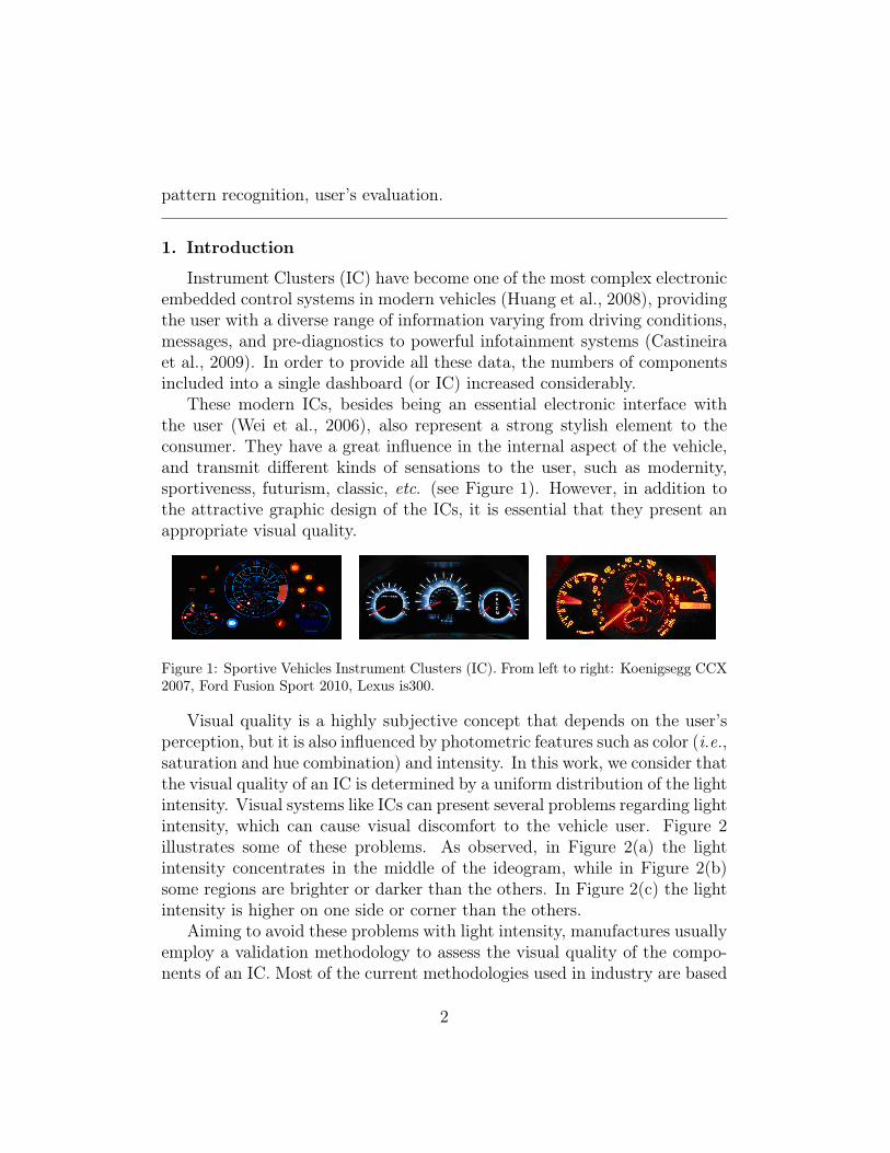
These modern ICs, besides being an essential electronic interface withthe user (Wei et al., 2006), also represent a strong stylish element to theconsumer. They have a great influence in the internal aspect of the vehicle,and transmit different kinds of sensations to the user, such as modernity,sportiveness, futurism, classic, etc. (see Figure 1). However, in addition tothe attractive graphic design of the ICs, it is essential that they present anappropriate visual quality.

Figure 1: Sportive Vehicles Instrument Clusters (IC). From left to right: Koenigsegg CCX2007, Ford Fusion Sport 2010, Lexus is300.

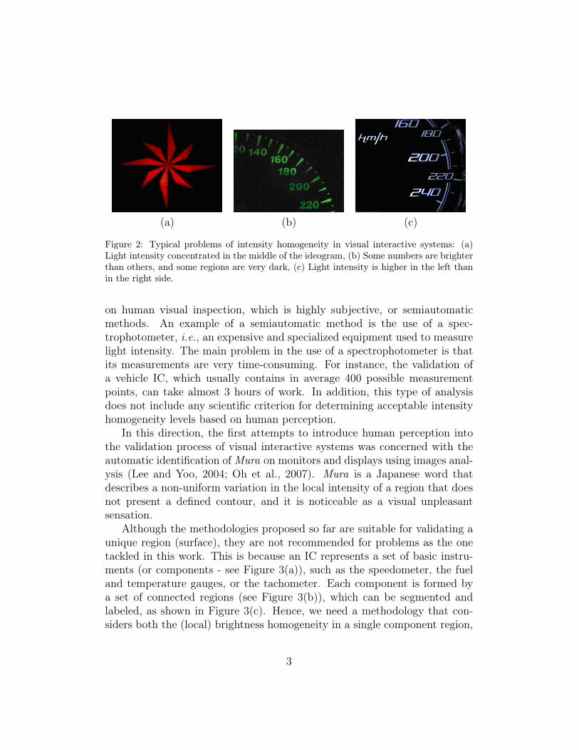
Visual quality is a highly subjective concept that depends on the user’sperception, but it is also influenced by photometric features such as color (i.e.,saturation and hue combination) and intensity. In this work, we consider thatthe visual quality of an IC is determined by a uniform distribution of the lightintensity. Visual systems like ICs can present several problems regarding lightintensity, which can cause visual discomfort to the vehicle user. Figure 2illustrates some of these problems. As observed, in Figure 2(a) the lightintensity concentrates in the middle of the ideogram, while in Figure 2(b)some regions are brighter or darker than the others. In Figure 2(c) the lightintensity is higher on one side or corner than the others.

Aiming to avoid these problems with light intensity, manufactures usuallyemploy a validation methodology to assess the visual quality of the compo-nents of an IC. Most of the current methodologies used in industry are based

2

(a) (b) (c)

Figure 2: Typical problems of intensity homogeneity in visual interactive systems: (a)Light intensity concentrated in the middle of the ideogram, (b) Some numbers are brighterthan others, and some regions are very dark, (c) Light intensity is higher in the left thanin the right side.

on human visual inspection, which is highly subjective, or semiautomaticmethods. An example of a semiautomatic method is the use of a spec-trophotometer, i.e., an expensive and specialized equipment used to measurelight intensity. The main problem in the use of a spectrophotometer is thatits measurements are very time-consuming. For instance, the validation ofa vehicle IC, which usually contains in average 400 possible measurementpoints, can take almost 3 hours of work. In addition, this type of analysisdoes not include any scientific criterion for determining acceptable intensityhomogeneity levels based on human perception.

In this direction, the first attempts to introduce human perception intothe validation process of visual interactive systems was concerned with theautomatic identification of Mura on monitors and displays using images anal-ysis (Lee and Yoo, 2004; Oh et al., 2007). Mura is a Japanese word thatdescribes a non-uniform variation in the local intensity of a region that doesnot present a defined contour, and it is noticeable as a visual unpleasantsensation.

Although the methodologies proposed so far are suitable for validating aunique region (surface), they are not recommended for problems as the onetackled in this work. This is because an IC represents a set of basic instru-ments (or components - see Figure 3(a)), such as the speedometer, the fueland temperature gauges, or the tachometer. Each component is formed bya set of connected regions (see Figure 3(b)), which can be segmented andlabeled, as shown in Figure 3(c). Hence, we need a methodology that con-siders both the (local) brightness homogeneity in a single component region,

3

as well as the impact that each small region has in the global visualizationof the component.

(a)

(b) (c)

Figure 3: An instrument cluster and its parts; (a) A typical Brazilian instrument cluster,(b) A component (i.e., a tachometer), (c) Areas: a labeled tachometer image with morethan 60 connected regions.

In this direction, the main goal of this work is to develop a methodologybased on both digital image analysis and the human visual perception (user’sevaluation) to validate the instruments of an IC. By validate we mean toevaluate if a component presents a good, a critical or a poor visual quality tothe user. Note that this work focuses on a single component of the IC (e.g.,the speedometer) instead of a set of components, i.e., the IC. The latter isleft for future work.

The proposed methodology preprocesses and extracts intensity homo-geneity descriptors from a set of acquired component images. At the sametime, users evaluate the components and identify their non-homogeneousregions. The users perceptions are then combined with the intensity ho-mogeneity descriptors, and later given to two machine learning algorithms,

4

namely artificial neural network (ANN) and support vector machine (SVM).These algorithms learn to identify homogenous and non-homogenous regionsand, given a new component image, validate it as a good, critical or poorvisual quality.

A preliminary version of this work appears in (Faria et al., 2010), wherethe methodology was first introduced. However, in (Faria et al., 2010), asingle dataset obtained from the classification of a specialist was given asinput to two machine learning algorithms. Here, we extend the set of exper-iments so that six different datasets are used. These datasets were createdbased on the opinions of five ordinary drivers regarding the ICs. The analysisperformed by the users is contrasted with the analysis of the specialist, aswell as the results obtained by the machine learning algorithms with thesedatasets. Moreover, an overview of the automotive systems of visual inter-action is given, and some formalisms are introduced to better describe theproposed methodology.

By identifying the non-homogeneous regions of the instruments, we willcontribute in an effective way to the industrial development process of IC,reducing significantly the time of quality analysis.

The remainder of this work is organized as follows. Section 2 introducesbasic concepts regarding lighting systems. Section 3 presents the proposedmethodology. An analysis of the users’ and specialist’s evaluations is per-formed in Section 4. Section 5 presents the experiments performed to val-idate the proposed methodology. Finally, conclusions and future works arepointed out in Section 6.

2. Automotive Systems of Visual Interaction

This section introduces some basic concepts of visual ergonomics neces-sary to understand the users analysis. According to the International Er-gonomics Association (IEA), ergonomics is the scientific discipline that stud-ies the interactions between men and the environment where they live in,and its main objective it to improve men’s welfare and their interaction withthe environment.

In the automotive environment, the visual ergonomics regards the har-mony of the illumination of IC, considering colors, contrast, reflexes, ghostlights, lighting distribution (homogeneity), glare, etc. Its main objectivesare to improve the safety and comfort of the human visual system, avoidingfatigue.

5

As indicated by Walraven and Alferdinick (2001), the visual ergonomics ofaircrafts interaction systems, which is extensible to the automotive industry,comprehends two types of evaluation:

• Cognitive: Studies the efficiency of the information transmission bythe instruments, which should be easily readable, of fast interpretation,and not give margins to double meanings;

• Visual quality of the instrument: Studies the color, intensity andhomogeneity of the luminous distribution of the component.

In this work, we focus on the visual quality of the instrument, study-ing the perception that users have on the illumination homogeneity of thecomponents.

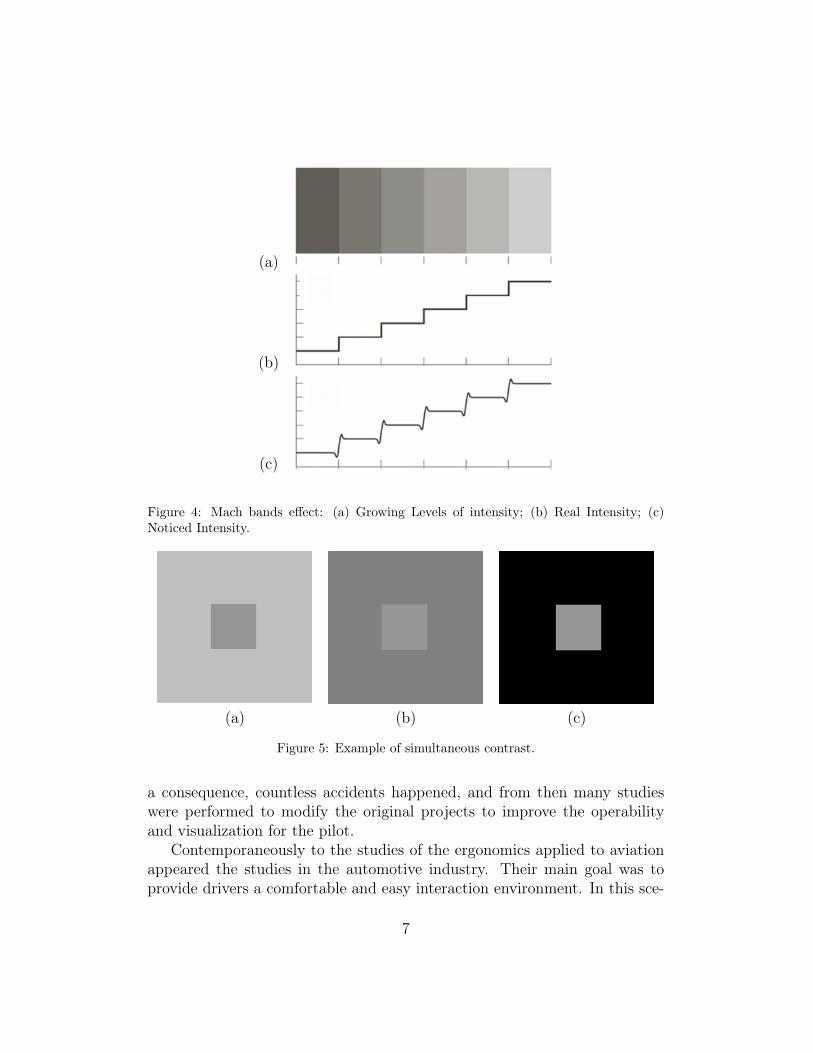
In this context, Gonzalez and Woods (2007) describe two interesting ef-fects in the human perception of the lighting intensity that an object hasin relation to its context. The first effect, exemplified by the Mach1 bands,shows that the perception of the lighting intensity is not only given in func-tion of the object. The human visual system tends to exceed or to reduce theintensity perception as it approximates or stands back from another level ofintensity. For example, in Figure 4(a), although the intensity of each columnis constant, the intensity perception of the transition regions are brighter fordark columns and darker for bright columns. Figures 4(b) and 4(c) highlightthis effect.

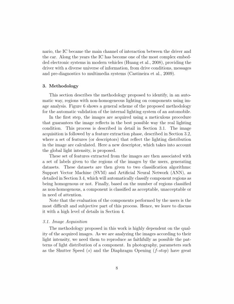
The second effect, called simultaneous contrast, also shows that the per-ception of the intensity is strongly influenced by the background in which theobject is inserted. For instance, in Figure 5, although the central square (ob-ject) has the same intensity in the three images, as soon as the backgroundbecomes darker the human perception tends to notice the object brighter.

Regarding studies considering the ergonomics of automotive interactivesystems, they first appeared right after the Second World War, where severalcomponents (gauges) were added to the aircrafts cockpits. The equipmentswere designed to give valuable information to the pilots, but their interfacedid not allow pilots to make a correct and fast interpretation of their readings.This was mainly because of the lack of good visibility of some instrumentsand the non-standardization of the instruments disposition in the cockpit. As

1Ernst Mach 1838-1916, Austrian physical and philosopher.

6

(a)

(b)

(c)

Figure 4: Mach bands effect: (a) Growing Levels of intensity; (b) Real Intensity; (c)Noticed Intensity.

(a) (b) (c)

Figure 5: Example of simultaneous contrast.

a consequence, countless accidents happened, and from then many studieswere performed to modify the original projects to improve the operabilityand visualization for the pilot.

Contemporaneously to the studies of the ergonomics applied to aviationappeared the studies in the automotive industry. Their main goal was toprovide drivers a comfortable and easy interaction environment. In this sce-

7

nario, the IC became the main channel of interaction between the driver andthe car. Along the years the IC has become one of the most complex embed-ded electronic systems in modern vehicles (Huang et al., 2008), providing thedriver with a diverse universe of information, from drive conditions, messagesand pre-diagnostics to multimedia systems (Castineira et al., 2009).

3. Methodology

This section describes the methodology proposed to identify, in an auto-matic way, regions with non-homogeneous lighting on components using im-age analysis. Figure 6 shows a general scheme of the proposed methodologyfor the automatic validation of the internal lighting system of an automobile.

In the first step, the images are acquired using a meticulous procedurethat guarantees the image reflects in the best possible way the real lightingcondition. This process is described in detail in Section 3.1. The imageacquisition is followed by a feature extraction phase, described in Section 3.2,where a set of features (or descriptors) that reflect the lighting distributionin the image are calculated. Here a new descriptor, which takes into accountthe global light intensity, is proposed.

These set of features extracted from the images are then associated witha set of labels given to the regions of the images by the users, generatingdatasets. These datasets are then given to two classification algorithms:Support Vector Machine (SVM) and Artificial Neural Network (ANN), asdetailed in Section 3.4, which will automatically classify component regions asbeing homogenous or not. Finally, based on the number of regions classifiedas non-homogenous, a component is classified as acceptable, unacceptable orin need of attention.

Note that the evaluation of the components performed by the users is themost difficult and subjective part of this process. Hence, we leave to discussit with a high level of details in Section 4.

3.1. Image AcquisitionThe methodology proposed in this work is highly dependent on the qual-

ity of the acquired images. As we are analyzing the images according to theirlight intensity, we need them to reproduce as faithfully as possible the pat-terns of light distribution of a component. In photography, parameters suchas the Shutter Speed (s) and the Diaphragm Opening (f -stop) have great

8

Figure 6: A diagram of the proposed methodology.

influence in the image exposure (Gimena, 2004). Figure 7 shows the effectsof varying these parameters for image acquisition.

Figure 7: Differences obtained in the images when calibrating the f -stop and shutter speed(s) parameters.

In order to obtain the best parameter values for s and f -stop, we se-lected two IC components of different colors and used a spectrophotometerto measure their “real” light intensities in a set of 52 points, as showed inFigure 8. We chose to use the spectrophotometer due to its very accuratemeasurements. After that, we acquired images for these two IC components

9

using a basic digital camera with six s variations (1/5"; 1/8"; 1/10"; 1/13";1/15", and 1/20"), letting the f -stop fixed to 2.7. We chose a small valuefor f -stop because the depth of field2 (Peterson, 2004) should be as shallowas possible, since we want to focus only on the IC.

The f -stop was fixed because there is a reciprocity law between shutterspeed and diaphragm opening, i.e., s and f -stop hold a direct relation (Gi-mena, 2004).

Figure 8: Points of measurement with the spectrophotometer.

Having the set of acquired images, we selected for each of them the pixelvalues corresponding to each of the 52 points previously measured by thespectrophotometer in the “real” IC component (see Figure 8). The pixelvalues of the image were taken from the V (value/intensity) channel of theHSV color system (Gonzalez and Woods, 2007). We wanted to compare thevalues measured by the spectrophotometer with the ones found in the images.In order to do that, we first normalized both values following the max-minrule (Martinez et al., 2005), i.e.,

2In optics, particularly as it relates to film and photography, the depth of field (DOF)is the portion of a scene that appears acceptably sharp in the image.

10

z =x−min(x)

max(x)−min(x), (1)

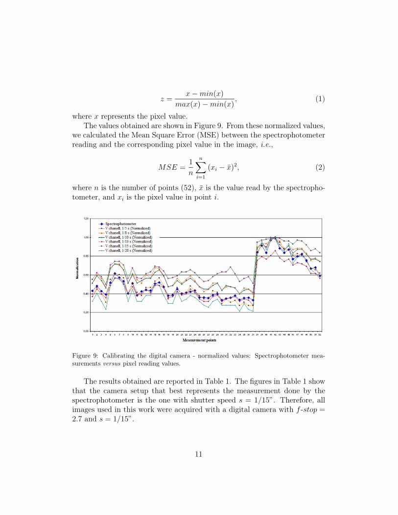
where x represents the pixel value.The values obtained are shown in Figure 9. From these normalized values,

we calculated the Mean Square Error (MSE) between the spectrophotometerreading and the corresponding pixel value in the image, i.e.,

MSE =1

n

n∑i=1

(xi − x̄)2, (2)

where n is the number of points (52), x̄ is the value read by the spectropho-tometer, and xi is the pixel value in point i.

Figure 9: Calibrating the digital camera - normalized values: Spectrophotometer mea-surements versus pixel reading values.

The results obtained are reported in Table 1. The figures in Table 1 showthat the camera setup that best represents the measurement done by thespectrophotometer is the one with shutter speed s = 1/15”. Therefore, allimages used in this work were acquired with a digital camera with f -stop =2.7 and s = 1/15”.

11

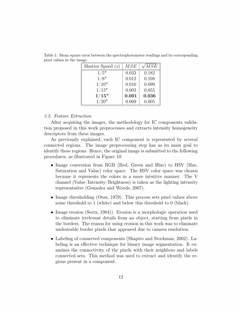
Table 1: Mean square error between the spectrophotometer readings and its correspondingpixel values in the image.

Shutter Speed (s) MSE√MSE

1/5" 0.033 0.1821/8" 0.012 0.1081/10" 0.010 0.0991/13" 0.003 0.0551/15" 0.001 0.0361/20" 0.069 0.005

3.2. Feature ExtractionAfter acquiring the images, the methodology for IC components valida-

tion proposed in this work preprocesses and extracts intensity homogeneitydescriptors from these images.

As previously explained, each IC component is represented by severalconnected regions. The image preprocessing step has as its main goal toidentify these regions. Hence, the original image is submitted to the followingprocedures, as illustrated in Figure 10:

• Image conversion from RGB (Red, Green and Blue) to HSV (Hue,Saturation and Value) color space. The HSV color space was chosenbecause it represents the colors in a more intuitive manner. The Vchannel (Value/Intensity/Brightness) is taken as the lighting intensityrepresentative (Gonzalez and Woods, 2007).

• Image thresholding (Otsu, 1979). This process sets pixel values abovesome threshold to 1 (white) and below this threshold to 0 (black).

• Image erosion (Serra, 1984)). Erosion is a morphologic operation usedto eliminate irrelevant details from an object, starting from pixels inthe borders. The reason for using erosion in this work was to eliminateundesirable border pixels that appeared due to camera resolution.

• Labeling of connected components (Shapiro and Stockman, 2002). La-beling is an effective technique for binary image segmentation. It ex-amines the connectivity of the pixels with their neighbors and labelsconnected sets. This method was used to extract and identify the re-gions present in a component.

12

(a) (b) (c)

(d) (e)

Figure 10: Stages of preprocessing: (a) Original image; (b) V channel from HSV colorspace; (c) Binary image; (d) Image after erosion; (e) Labeled connected components.

3.3. Homogeneity descriptorsAfter identifying the regions of an image, we extract a set of descriptors

that represent the light homogeneity in each region of the component. Ourgoal is to later associate these descriptors with a category defined by theuser. This category says whether the region is homogenous or not accordingto the user’s sensations.

Several metrics have already been proposed in the literature to computethe light homogeneity of a region (Gimena, 2004; Cheng and Sun, 2000). InOh et al. (2007), for example, the authors define the Lighting Uniformitymetric, i.e.,

UL(R) = (rmin/rmax)× 100, (3)

where rmax and rmin represent the maximum and minimum intensity valuesof a region R, respectively. In Gonzalez and Woods (2007) and Borges et al.(2008), the intensity distribution is defined by statistical moments of thelevels of the histogram of a region. Let R be a random variable denotinglevels of the regions and let PR(ri), i = 0, 1, 2, ..., L− 1, be the correspondinghistogram, where L is the number of distinct levels. Then, the nth momentof R is defined as:

13

µn(R) =L−1∑i=0

(ri −m(R))nPR(ri), (4)

where

m(R) =L−1∑i=0

(ri × PR(ri). (5)

where m stands for the average level. From these equations, other statisti-cal moments, namely the 3rd moment (Eq. 6), uniformity (Eq. 7), entropy(Eq. 8), smoothness (Eq. 9), and standard deviation (Eq. 10) can be esti-mated as

µ3(R) =L−1∑i=0

(ri −m(R))3PR(ri), (6)

U(R) =L−1∑i=0

P 3R(ri), (7)

e(R) = −L−1∑i=0

PR(ri)× log2 PR(ri), (8)

SM(R) = 1− 1/(1 + σ2(R)), (9)

andσ(R) =

√µ2(R) =

√σ2(R). (10)

The descriptors presented in Equations 3, 6, 7, 8, 9 and 10 were extractedfrom each of the component regions. Furthermore, we are also interestedin the impact each region has in the global uniformity (GU) of the entirecomponent. Hence, we propose a descriptor that considers both the localregion and global component intensities, named as Relative Descriptor (Fariaet al., 2010) and defined as

RD(R) = (mL(R)/mG)× 100, (11)

where mL(R) and mG stand for the average intensity of a region R andthe average intensity of the whole component (or instrument) in analysis,respectively.

These descriptors were associated with the labels given by the userthrough the process detailed in Section 4, and given to the machine learningalgorithms described in the next section.

14

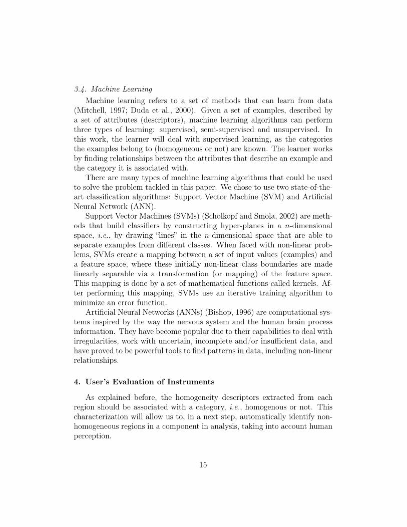
3.4. Machine LearningMachine learning refers to a set of methods that can learn from data

(Mitchell, 1997; Duda et al., 2000). Given a set of examples, described bya set of attributes (descriptors), machine learning algorithms can performthree types of learning: supervised, semi-supervised and unsupervised. Inthis work, the learner will deal with supervised learning, as the categoriesthe examples belong to (homogeneous or not) are known. The learner worksby finding relationships between the attributes that describe an example andthe category it is associated with.

There are many types of machine learning algorithms that could be usedto solve the problem tackled in this paper. We chose to use two state-of-the-art classification algorithms: Support Vector Machine (SVM) and ArtificialNeural Network (ANN).

Support Vector Machines (SVMs) (Scholkopf and Smola, 2002) are meth-ods that build classifiers by constructing hyper-planes in a n-dimensionalspace, i.e., by drawing “lines” in the n-dimensional space that are able toseparate examples from different classes. When faced with non-linear prob-lems, SVMs create a mapping between a set of input values (examples) anda feature space, where these initially non-linear class boundaries are madelinearly separable via a transformation (or mapping) of the feature space.This mapping is done by a set of mathematical functions called kernels. Af-ter performing this mapping, SVMs use an iterative training algorithm tominimize an error function.

Artificial Neural Networks (ANNs) (Bishop, 1996) are computational sys-tems inspired by the way the nervous system and the human brain processinformation. They have become popular due to their capabilities to deal withirregularities, work with uncertain, incomplete and/or insufficient data, andhave proved to be powerful tools to find patterns in data, including non-linearrelationships.

4. User’s Evaluation of Instruments

As explained before, the homogeneity descriptors extracted from eachregion should be associated with a category, i.e., homogenous or not. Thischaracterization will allow us to, in a next step, automatically identify non-homogeneous regions in a component in analysis, taking into account humanperception.

15

(a) (b)

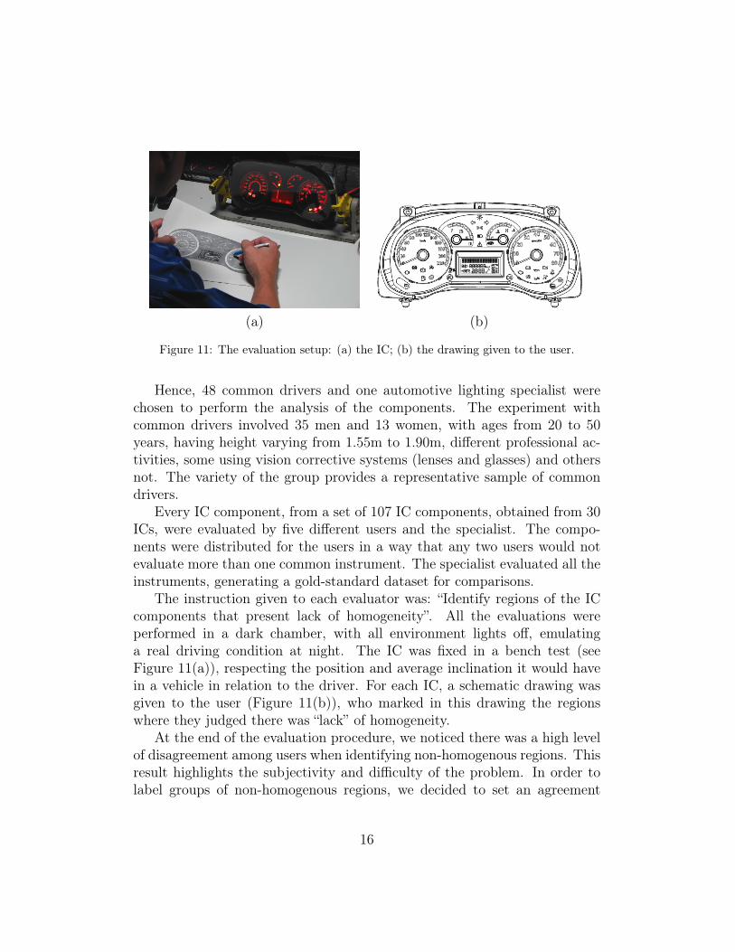
Figure 11: The evaluation setup: (a) the IC; (b) the drawing given to the user.

Hence, 48 common drivers and one automotive lighting specialist werechosen to perform the analysis of the components. The experiment withcommon drivers involved 35 men and 13 women, with ages from 20 to 50years, having height varying from 1.55m to 1.90m, different professional ac-tivities, some using vision corrective systems (lenses and glasses) and othersnot. The variety of the group provides a representative sample of commondrivers.

Every IC component, from a set of 107 IC components, obtained from 30ICs, were evaluated by five different users and the specialist. The compo-nents were distributed for the users in a way that any two users would notevaluate more than one common instrument. The specialist evaluated all theinstruments, generating a gold-standard dataset for comparisons.

The instruction given to each evaluator was: “Identify regions of the ICcomponents that present lack of homogeneity”. All the evaluations wereperformed in a dark chamber, with all environment lights off, emulatinga real driving condition at night. The IC was fixed in a bench test (seeFigure 11(a)), respecting the position and average inclination it would havein a vehicle in relation to the driver. For each IC, a schematic drawing wasgiven to the user (Figure 11(b)), who marked in this drawing the regionswhere they judged there was “lack” of homogeneity.

At the end of the evaluation procedure, we noticed there was a high levelof disagreement among users when identifying non-homogenous regions. Thisresult highlights the subjectivity and difficulty of the problem. In order tolabel groups of non-homogenous regions, we decided to set an agreement

16

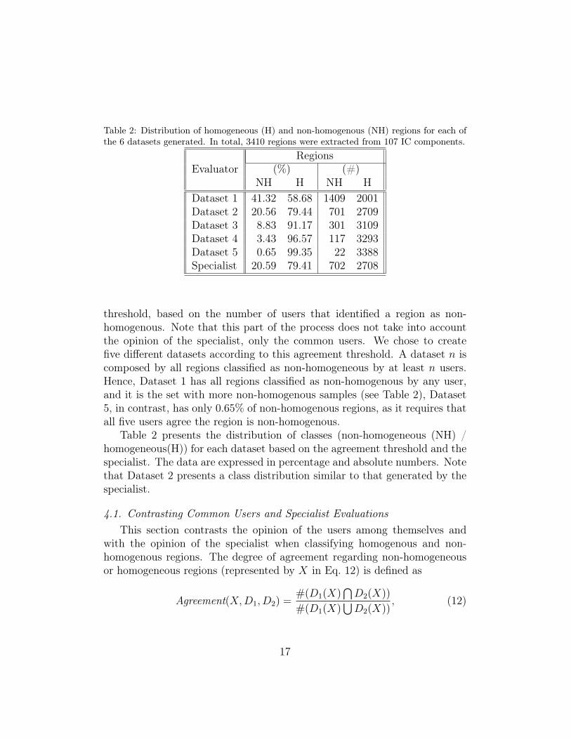
Table 2: Distribution of homogeneous (H) and non-homogenous (NH) regions for each ofthe 6 datasets generated. In total, 3410 regions were extracted from 107 IC components.

EvaluatorRegions

(%) (#)NH H NH H

Dataset 1 41.32 58.68 1409 2001Dataset 2 20.56 79.44 701 2709Dataset 3 8.83 91.17 301 3109Dataset 4 3.43 96.57 117 3293Dataset 5 0.65 99.35 22 3388Specialist 20.59 79.41 702 2708

threshold, based on the number of users that identified a region as non-homogenous. Note that this part of the process does not take into accountthe opinion of the specialist, only the common users. We chose to createfive different datasets according to this agreement threshold. A dataset n iscomposed by all regions classified as non-homogeneous by at least n users.Hence, Dataset 1 has all regions classified as non-homogenous by any user,and it is the set with more non-homogenous samples (see Table 2), Dataset5, in contrast, has only 0.65% of non-homogenous regions, as it requires thatall five users agree the region is non-homogenous.

Table 2 presents the distribution of classes (non-homogeneous (NH) /homogeneous(H)) for each dataset based on the agreement threshold and thespecialist. The data are expressed in percentage and absolute numbers. Notethat Dataset 2 presents a class distribution similar to that generated by thespecialist.

4.1. Contrasting Common Users and Specialist EvaluationsThis section contrasts the opinion of the users among themselves and

with the opinion of the specialist when classifying homogenous and non-homogenous regions. The degree of agreement regarding non-homogeneousor homogeneous regions (represented by X in Eq. 12) is defined as

Agreement(X,D1, D2) =#(D1(X)

⋂D2(X))

#(D1(X)⋃D2(X))

, (12)

17

Table 3: Agreement matrix for non-homogeneous regions.Dataset 1 Dataset 2 Dataset 3 Dataset 4 Dataset 5 Spec.

Dataset 1 1.00 0.50 0.21 0.08 0.02 0.32Dataset 2 0.50 1.00 0.43 0.17 0.03 0.33Dataset 3 0.21 0.43 1.00 0.39 0.07 0.22Dataset 4 0.08 0.17 0.39 1.00 0.19 0.12Dataset 5 0.02 0.03 0.07 0.19 1.00 0.02Specialist 0.32 0.33 0.22 0.12 0.02 1.00

Table 4: Agreement matrix for homogeneous regions.Dataset 1 Dataset 2 Dataset 3 Dataset 4 Dataset 5 Spec.

Dataset 1 1.00 0.74 0.64 0.61 0.59 0.63Dataset 2 0.74 1.00 0.87 0.82 0.80 0.77Dataset 3 0.64 0.87 1.00 0.94 0.92 0.80Dataset 4 0.61 0.82 0.94 1.00 0.97 0.81Dataset 5 0.59 0.80 0.92 0.97 1.00 0.80Specialist 0.63 0.77 0.80 0.81 0.80 1.00

where Dn(X) represents the set of regions of type X (i.e., non-homogeneousor homogeneous) in Dataset n (where n varies from 1 to 6 - datasets gener-ated by 5 agreement thresholds plus the specialist) and #(•) represents thecardinality of dataset •.

Tables 3 and 4 present the degree of agreement among each dataset pair.An agreement of 1 says that all the labels are the same for the two groups(or datasets). As expected, the figures in the tables show that there is ahigher level of agreement for homogeneous labeling than non-homogeneous.This is natural as the images tend to present much more homogenous re-gions (and these ones can be easily identified by the user). Consideringnon-homogeneous regions, the opinions vary a lot according to the userssensitivity to the lightning system (some are more critical and others moretolerant). We also note that the largest number of disagreements occurs inregions close to the global perception threshold between homogeneous andnon-homogeneous, which varied from user to user.

Considering the agreements among the specialist and the five datasetsgenerated by the users’ evaluations, again in the homogeneous regions the

18

agreement indexes are relatively high, reaching 0.81. However, for the non-homogeneous regions, they did not go over 0.33.

4.2. Users Opinions on the Specialist EvaluationIn this work, we assume the knowledge and experience of the specialist

makes it easier for him to identify non-homogenous regions correctly. How-ever, it is important for us to know if the common users agree with thespecialist evaluations. Hence, in order to find out if the specialist evalua-tion really represents the general users’ perception, a new experiment wasperformed, and the users evaluated the classifications made by the specialist.

Each user received a schematic drawing were all the non-homogenousregions identified by the specialist, and that the industry assumes needscorrection, were marked. They were taken to the bench test in a darkroom,and were asked the following question: “How do you evaluate the suggestedcorrections (the specialist’s evaluation)?”. The user had three options, in ascale from 1 to 3:

1. Inadequate: After correcting the suggested regions the instrument wouldnot present a homogeneous illumination;

2. Appropriate: After correcting the suggested regions the instrumentwould present a suitable illumination;

3. Excessive: It is not necessary to correct all regions for the instrumentto present a good illumination.

Each instrument was evaluated by 5 different users and each user evalu-ated 10 instruments on average. In total, 535 evaluations (5 users ×107 ICcomponents) were performed. The graph in Figure 12 summarizes the resultsobtained after evaluation.

Analyzing the graph, we observe that 72% of the specialist’s labeling wereconsidered by 5 out of 5 users as appropriate, while 17% were consideredappropriate by 4 out of 5 users. The remaining 11% are evaluations whereonly one, two or three users found the change appropriate. From the 535evaluations, only 48 were considered as not appropriate by the users, obtainedan acceptance rate of 91% on the specialist labeling.

Figure 13 shows in more detail the opinions of users when they disagreewith the specialist correction. From the 48 labeled evaluations considered asnot appropriate, 73% were classified as excessive, and only 27% as insufficient.It is important to point out that there was no correction considered as notappropriate by all 5 users.

19

Figure 12: Summary graph of the users opinion on the specialist evaluation.

5. Computational Results

Having created the datasets, experiments were performed in two phases.First the regions of the images are classified as homogenous or not by themachine learning algorithms. Then, based on the number of non-homogenousregions, the instruments are classified as acceptable, unacceptable or in needof attention.

Throughout this section, the results obtained by the machine learningalgorithms are presented in the form of confusion matrices. The values inthese matrices are presented in percentage (%) and in absolute value (#).Those express the average and the standard deviation (µ ± σ) of 107 testsperformed through leave-N -out/leave-one-out validation, where N stands forthe number of regions of each instrument when an instrument is left out(i.e., leave-one-out). Note that the high values of standard deviation in theconfusion matrices are due to the great variation in the number of regionsfound in each instrument. For instance, some fuel gauges have 7 regions,while some speedometers have 80 regions.

5.1. Classifying instrument cluster regionsThis section shows the classification of the instrument regions. As pre-

viously mentioned, we worked with ANN and SVM, using MatLab imple-mentations. As we are dealing with non-linear data, the standard Matlab

20

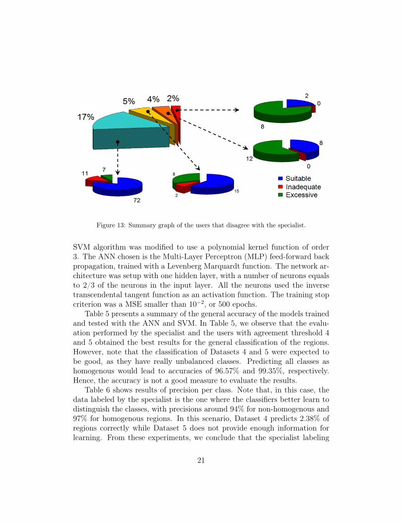
Figure 13: Summary graph of the users that disagree with the specialist.

SVM algorithm was modified to use a polynomial kernel function of order3. The ANN chosen is the Multi-Layer Perceptron (MLP) feed-forward backpropagation, trained with a Levenberg Marquardt function. The network ar-chitecture was setup with one hidden layer, with a number of neurons equalsto 2/3 of the neurons in the input layer. All the neurons used the inversetranscendental tangent function as an activation function. The training stopcriterion was a MSE smaller than 10−2, or 500 epochs.

Table 5 presents a summary of the general accuracy of the models trainedand tested with the ANN and SVM. In Table 5, we observe that the evalu-ation performed by the specialist and the users with agreement threshold 4and 5 obtained the best results for the general classification of the regions.However, note that the classification of Datasets 4 and 5 were expected tobe good, as they have really unbalanced classes. Predicting all classes ashomogenous would lead to accuracies of 96.57% and 99.35%, respectively.Hence, the accuracy is not a good measure to evaluate the results.

Table 6 shows results of precision per class. Note that, in this case, thedata labeled by the specialist is the one where the classifiers better learn todistinguish the classes, with precisions around 94% for non-homogenous and97% for homogenous regions. In this scenario, Dataset 4 predicts 2.38% ofregions correctly while Dataset 5 does not provide enough information forlearning. From these experiments, we conclude that the specialist labeling

21

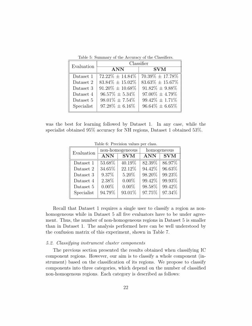
Table 5: Summary of the Accuracy of the Classifiers.

Evaluation ClassifierANN SVM

Dataset 1 72.22% ± 14.84% 70.39% ± 17.78%Dataset 2 83.84% ± 15.02% 83.63% ± 15.67%Dataset 3 91.20% ± 10.68% 91.82% ± 9.88%Dataset 4 96.57% ± 5.34% 97.00% ± 4.79%Dataset 5 98.01% ± 7.54% 99.42% ± 1.71%Specialist 97.28% ± 6.16% 96.64% ± 6.65%

was the best for learning followed by Dataset 1. In any case, while thespecialist obtained 95% accuracy for NH regions, Dataset 1 obtained 53%.

Table 6: Precision values per class.

Evaluation non-homogeneous homogeneousANN SVM ANN SVM

Dataset 1 53.68% 40.19% 82.39% 86.97%Dataset 2 34.65% 22.12% 94.42% 96.63%Dataset 3 9.37% 5.20% 98.20% 99.23%Dataset 4 2.38% 0.00% 99.42% 99.93%Dataset 5 0.00% 0.00% 98.58% 99.42%Specialist 94.79% 93.01% 97.75% 97.34%

Recall that Dataset 1 requires a single user to classify a region as non-homogeneous while in Dataset 5 all five evaluators have to be under agree-ment. Thus, the number of non-homogeneous regions in Dataset 5 is smallerthan in Dataset 1. The analysis performed here can be well understood bythe confusion matrix of this experiment, shown in Table 7.

5.2. Classifying instrument cluster componentsThe previous section presented the results obtained when classifying IC

component regions. However, our aim is to classify a whole component (in-strument) based on the classification of its regions. We propose to classifycomponents into three categories, which depend on the number of classifiednon-homogenous regions. Each category is described as follows:

22

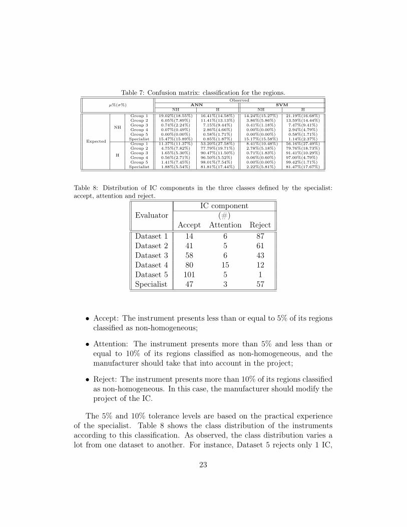
Table 7: Confusion matrix: classification for the regions.

µ%(σ%)Observed

ANN SVMNH H NH H

Expected

NH

Group 1 19.02%(18.55%) 16.41%(14.58%) 14.24%(15.27%) 21.19%(16.68%)Group 2 6.05%(7.89%) 11.41%(13.13%) 3.86%(5.86%) 13.59%(14.44%)Group 3 0.74%(2.24%) 7.15%(9.44%) 0.41%(1.18%) 7.47%(9.41%)Group 4 0.07%(0.49%) 2.86%(4.66%) 0.00%(0.00%) 2.94%(4.79%)Group 5 0.00%(0.00%) 0.58%(1.71%) 0.00%(0.00%) 0.58%(1.71%)Specialist 15.47%(15.89%) 0.85%(1.87%) 15.17%(15.58%) 1.14%(2.37%)

H

Group 1 11.37%(11.37%) 53.20%(27.58%) 8.41%(10.48%) 56.16%(27.49%)Group 2 4.75%(7.82%) 77.79%(19.71%) 2.78%(5.18%) 79.76%(18.73%)Group 3 1.65%(5.30%) 90.47%(11.50%) 0.71%(1.83%) 91.41%(10.29%)Group 4 0.56%(2.71%) 96.50%(5.52%) 0.06%(0.60%) 97.00%(4.79%)Group 5 1.41%(7.45%) 98.01%(7.54%) 0.00%(0.00%) 99.42%(1.71%)Specialist 1.88%(5.54%) 81.81%(17.44%) 2.22%(5.81%) 81.47%(17.67%)

Table 8: Distribution of IC components in the three classes defined by the specialist:accept, attention and reject.

EvaluatorIC component

(#)Accept Attention Reject

Dataset 1 14 6 87Dataset 2 41 5 61Dataset 3 58 6 43Dataset 4 80 15 12Dataset 5 101 5 1Specialist 47 3 57

• Accept: The instrument presents less than or equal to 5% of its regionsclassified as non-homogeneous;

• Attention: The instrument presents more than 5% and less than orequal to 10% of its regions classified as non-homogeneous, and themanufacturer should take that into account in the project;

• Reject: The instrument presents more than 10% of its regions classifiedas non-homogeneous. In this case, the manufacturer should modify theproject of the IC.

The 5% and 10% tolerance levels are based on the practical experienceof the specialist. Table 8 shows the class distribution of the instrumentsaccording to this classification. As observed, the class distribution varies alot from one dataset to another. For instance, Dataset 5 rejects only 1 IC,

23

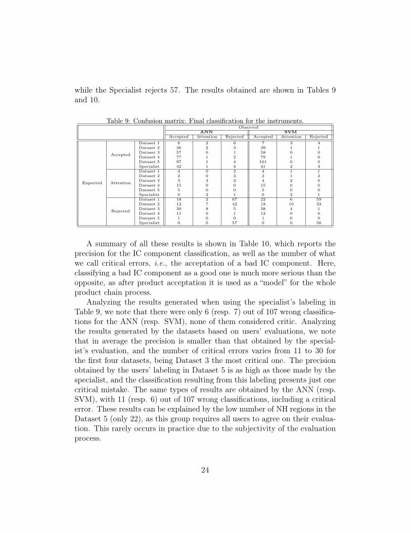
while the Specialist rejects 57. The results obtained are shown in Tables 9and 10.

Table 9: Confusion matrix: Final classification for the instruments.Observed

ANN SVMAccepted Attention Rejected Accepted Attention Rejected

Expected

Accepted

Dataset 1 6 2 6 7 3 4Dataset 2 36 2 3 39 1 1Dataset 3 57 0 1 58 0 0Dataset 4 77 1 2 79 1 0Dataset 5 97 1 4 101 0 0Specialist 42 1 4 41 2 4

Attention


Rejected


A summary of all these results is shown in Table 10, which reports theprecision for the IC component classification, as well as the number of whatwe call critical errors, i.e., the acceptation of a bad IC component. Here,classifying a bad IC component as a good one is much more serious than theopposite, as after product acceptation it is used as a “model” for the wholeproduct chain process.

Analyzing the results generated when using the specialist’s labeling inTable 9, we note that there were only 6 (resp. 7) out of 107 wrong classifica-tions for the ANN (resp. SVM), none of them considered critic. Analyzingthe results generated by the datasets based on users’ evaluations, we notethat in average the precision is smaller than that obtained by the special-ist’s evaluation, and the number of critical errors varies from 11 to 30 forthe first four datasets, being Dataset 3 the most critical one. The precisionobtained by the users’ labeling in Dataset 5 is as high as those made by thespecialist, and the classification resulting from this labeling presents just onecritical mistake. The same types of results are obtained by the ANN (resp.SVM), with 11 (resp. 6) out of 107 wrong classifications, including a criticalerror. These results can be explained by the low number of NH regions in theDataset 5 (only 22), as this group requires all users to agree on their evalua-tion. This rarely occurs in practice due to the subjectivity of the evaluationprocess.

24

Table 10: Summary of the accuracy of the classification of the instrument.

Evaluation ANN SVMPrecision Critical Errors Precision Critical Errors

Dataset 1 71.96% 18 62.62% 22Dataset 2 72.89% 12 68.22% 18Dataset 3 60.75% 30 57.00% 38Dataset 4 72.90% 11 73.82% 12Dataset 5 90.65% 1 94.39% 1Specialist 94.39% 0 92.52% 0

5.3. Visualization of IC Components ClassificationsThis section presents and discusses the classification of four IC compo-

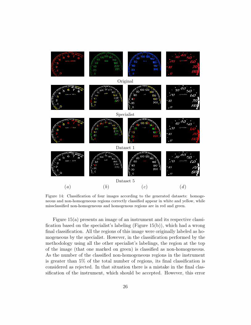
nents images classified by the system. Each column in Figure 14 representsan image. In the first row are the original images, followed by the resultingimages of the classification based on the specialist, Dataset 1 and Dataset5, respectively. For these last images the classification generated by thesystem is represented by colors. The homogeneous and non-homogeneousregions correctly classified appear in white and yellow, respectively. Thenon-homogeneous regions classified as homogeneous (critical errors) are inred, whilst the homogeneous regions classified as non-homogeneous appearin green.

Observing the images in Figure 14, we verify that in Dataset 1 great partof the regions are considered as non-homogeneous. On the other hand, inDataset 5 almost 100% of the regions are accepted as homogeneous. An-alyzing these images, some facts previously verified by the computationalexperiments can be confirmed. The results obtained by the specialist’s label-ing (second line) show very few regions missclassified, which did not impactthe final classification of the instrument (accept or reject). The results ob-tained by Dataset 1 (third line) present a lot of regions erroneously classified,directly contributing to the final missclassification of the instrument. Dataset5 has the problem of highly unbalanced classes, which makes that the fewnon-homogeneous regions are wrongly classified as homogeneous.

As claimed in the last subsection and shown in Table 10, the proposedmethodology achieve promising results by using the specialist for training theclassifiers. In the following, we illustrate an example where the classificationusing the specialist labeling makes a mistake but not a critical one.

25

Original

Specialist

Dataset 1

Dataset 5(a) (b) (c) (d)

Figure 14: Classification of four images according to the generated datasets: homoge-neous and non-homogeneous regions correctly classified appear in white and yellow, whilemissclassified non-homogeneous and homogenous regions are in red and green.

Figure 15(a) presents an image of an instrument and its respective classi-fication based on the specialist’s labeling (Figure 15(b)), which had a wrongfinal classification. All the regions of this image were originally labeled as ho-mogeneous by the specialist. However, in the classification performed by themethodology using all the other specialist’s labelings, the region at the topof the image (that one marked on green) is classified as non-homogeneous.As the number of the classified non-homogeneous regions in the instrumentis greater than 5% of the total number of regions, its final classification isconsidered as rejected. In that situation there is a mistake in the final clas-sification of the instrument, which should be accepted. However, this error

26

is not considered a critical mistake, i.e., accepting a “bad” instrument.

(a) (b)

Figure 15: Instrument regions and theirs respective classifications obtained by the pro-posed methodology.

5.4. Final ConsiderationsThe methodology proposed in this work has proved to be effective in

automatically identifying non-homogeneous regions in a component from aninstrument cluster, used to aid the classification of the complete instrumentas accepted, on need of attention, and rejected. The two classifiers usedin this work (ANN and SVM) obtained similar results for both the users’evaluation and the specialist’s evaluation. An analysis on the number ofdescriptors used in the models learnt showed that SVM uses less descriptorsthan the ANN, achieving equivalent results in terms of precision.

The evaluations were divided in two groups:

1. Labeling with the specialist: Appropriate learning of the algorithms;not so unbalanced distribution of the classes (homogeneous and non-homogeneous) and high precision in the final classification of the instru-ment (accepted versus rejected);

2. Labeling with the users: Deficient learning of the algorithms; quite un-balanced distribution of the classes (biased learning on the homogeneousclass) and final classification of the instrument with critical mistakes (ac-ceptation of “bad” instruments, i.e., instrument with more than 5% ofnon-homogeneous regions).

27

The specialist’s technical evaluation provided a learning for the classifierswhich generates the best precision for both non-homogeneous and homoge-neous classes. Through the users’ evaluations about the specialist’s eval-uation, it was possible to notice that the specialist represents the averageperception of users very well, obtaining an index of acceptance higher than90%.

The proposed methodology presents two main advantages over themethod that uses the spectrophotometer: it is cheap to implement (a spec-trophotometer is much more expensive than a digital camera) and computa-tionally efficient. These two characteristics allow the manufacturer of auto-motive ICs to apply the methodology in several points of his production line,reducing the number of reproofs made in the assembly line due to instrumentswith bad illumination.

6. Conclusions

Studies looking to map, characterize, and understand human perceptionsare as attractive as complex. Human sensations depend on each individualsexperience and acquired knowledge. This work presented a methodology forautomatic validation of Automotive Instrument Cluster using the concept oflight homogeneity in images analysis, computational intelligence, and humanevaluations. To feed the machine learning algorithms (ANN and SVM),aiming at the classification of the region as homogeneous or not, evaluationswere performed by a specialist and ordinary users. The experimental resultsfor classifying both instrument regions and components are above 94%.

The evaluations with the users presented great dispersion among the re-sults. On the other hand, the evaluations accomplished by the specialist pre-sented good consistence and obtained high acceptance indexes by the users,i.e., more than 90%.

As presented in the introduction, the application of this methodology inthe industry will help to raise quality and save precious time in the develop-ment phase of new instruments. The use of this methodology will also aidthe phase of experimental tests in both the assembly line and indicating themanufacturer the points that should be improved in its project.

References

Bishop, C. M., 1996. Neural Networks for Pattern Recognition, 1st Edition.Oxford University Press, USA.

28

Borges, P. V. K., Mayer, J., Izquierdo, E., 2008. Document image processingfor paper side communications. IEEE Transactions on Multimedia 10 (7),1277–1287.

Castineira, F. G., Dieguez, D. C., Castano, F. J. G., 2009. Integration ofnomadic devices with automotive user interfaces. IEEE Transactions onConsumer Electronics 55 (1), 31–34.

Cheng, H. D., Sun, Y., 2000. A hierarchical approach to color image segmen-tation using homogeneity. IEEE Transactions on Image Processing 9 (12),2071–2082.

Duda, R. O., Hart, P. E., Stork, D. G., 2000. Pattern Classification, 2ndEdition. Wiley-Interscience.

Faria, A. W. C., Menotti, D., Lara, D. S. D., Pappa, G. L., Araújo, A. A.,march 2010. A new methodology for photometric validation in vehiclesvisual interactive systems. In: XXIV ACM Symposium On Applied Com-puting, Track: Computational Intelligence and Image Analysis. pp. 1–6.

Gimena, L., 2004. Exposure value in photography. a graphics concept mapproposal. In: International Conference on Concept Mapping. pp. 256–269.

Gonzalez, R. C., Woods, R. E., 2007. Digital Image Processing, 3rd Edition.Prentice Hall.

Huang, Y., Mouzakitis, A., McMurran, R., Dhadyalla, G., Jontes, P., 2008.Design validation testing of vehicle instrument cluster using machine visionand hardware in the loop. In: IEEE International Conference on VehicularElectronics and Safety. pp. 22–24.

Lee, J. Y., Yoo, S. I., 2004. Automatic detection of region-mura defect in tft-lcd. IEICE Transactions on Information and Systems E87-D (10), 2371–2378.

Martinez, J. C., Sanches, D., Prados, B., Pereles, F. G., 2005. Fuzzy ho-mogeneity measures for path-based colour image segmentation. In: 14thIEEE International Conference on Fuzzy Systems. Vol. 5. pp. 218–223.

Mitchell, T., 1997. Machine Learning. McGraw Hill.

29

Oh, J. H., Yun, B. J., Park, K. H., 2007. The defect detection using humanvisual system and wavelet transform in tft-lcd image. In: Frontiers in theConvergence of Bioscience and Information Technologies (FIBIT). pp. 498–503.

Otsu, N., 1979. A threshold selection method from gray level histograms.IEEE Transactions on Systems, Man and Cybernetics 9 (5), 62–66.

Peterson, B., 2004. Understanding Exposure: How to Shoot Great Pho-tographs with a Film or Digital Camera - Revised edition. Amphoto Books.

Scholkopf, B., Smola, A. J., 2002. Learning with Kernels: Support VectorMachines, Regularization, Optimization, and Beyond. The MIT Press.

Serra, J., 1984. Image Analysis and Mathematical Morphology. AcademicPress.

Shapiro, L., Stockman, G., 2002. Computer Vision. Prentice Hall.

Walraven, J., Alferdinick, J. W. A. M., 2001. Visual Ergonomics of Colour-Coded Cockpit Displays: A Generic Approach, 2nd Edition. The ResearchAnd Tecnhology Organization (RTO).

Wei, Z., Xian-Kui, Z., Lei, Z., Rui, Z., Bin, C. Z., 2006. Study on the evalu-ation system of instrument cluster. In: Computer Aided Industrial Designand Conceptual Design. pp. 1–5.

30

A methodology for photometric validation in vehicles visual interactive systems

Documents

Transcript of A methodology for photometric validation in vehicles visual interactive systems