Dynamics of Growth Control in a Marine Yeast Subjected to Perturbation
Upload
khangminh22Category
view
1download
0
Dynamics of Marine vehicles
By S. Hossein MousavizedeganFaculty of Marine TechnologyAmirkabir University of TechnologyNo. 424, Hafez Ave.Tehran, Iran

Dedication
This book is dedicated to my family.

Preface
This is an introduction to the water wave motion. It is included four chapters. The first chapter is on thebasic assumption and the general formulation of the water waves. The second chapter is on the long crestedwave theory. The third chapter is about the finite amplitude waves and the effect of the nonlinearities onthe wave motion. The final chapter is about the real ocean waves.
March 2010 S. Hossein Mousavizadegan
iii
Contents
1 Introduction 11.1 Fundamental assumptions on seawater properties and wave motion . . . . . . . . . . . . . . . 31.2 Boundary value problem of ocean gravity waves . . . . . . . . . . . . . . . . . . . . . . . . . . 4
2 Long-Crested, Linear Wave Theory (LWT) 12.1 Boundary value problem for LWT . . . . . . . . . . . . . . . . . . . . . . . . . . . . . . . . . 12.2 Analytical solution of the LWT BVP . . . . . . . . . . . . . . . . . . . . . . . . . . . . . . . . 32.3 Dispersion relation . . . . . . . . . . . . . . . . . . . . . . . . . . . . . . . . . . . . . . . . . . 52.4 Classification of water waves . . . . . . . . . . . . . . . . . . . . . . . . . . . . . . . . . . . . . 62.5 Characteristics of linear plane progressive wave . . . . . . . . . . . . . . . . . . . . . . . . . . 7
2.5.1 particle motion . . . . . . . . . . . . . . . . . . . . . . . . . . . . . . . . . . . . . . . . 82.5.2 Pressure distribution . . . . . . . . . . . . . . . . . . . . . . . . . . . . . . . . . . . . . 9
2.6 Progressive oblique waves . . . . . . . . . . . . . . . . . . . . . . . . . . . . . . . . . . . . . . 132.7 Superposition of waves . . . . . . . . . . . . . . . . . . . . . . . . . . . . . . . . . . . . . . . . 172.8 Wave reflection and standing wave . . . . . . . . . . . . . . . . . . . . . . . . . . . . . . . . . 192.9 Wave group . . . . . . . . . . . . . . . . . . . . . . . . . . . . . . . . . . . . . . . . . . . . . . 212.10 Wave energy . . . . . . . . . . . . . . . . . . . . . . . . . . . . . . . . . . . . . . . . . . . . . 22
2.10.1 Energy propagation . . . . . . . . . . . . . . . . . . . . . . . . . . . . . . . . . . . . . 242.10.2 Equation of energy conservation . . . . . . . . . . . . . . . . . . . . . . . . . . . . . . 25
3 Finite-amplitude waves 283.1 Stokes Finite-amplitude waves theory . . . . . . . . . . . . . . . . . . . . . . . . . . . . . . . . 28
3.1.1 The first-order waves theory . . . . . . . . . . . . . . . . . . . . . . . . . . . . . . . . . 303.1.2 The second-order waves theory . . . . . . . . . . . . . . . . . . . . . . . . . . . . . . . 31
3.2 Trochoidal wave theory . . . . . . . . . . . . . . . . . . . . . . . . . . . . . . . . . . . . . . . 363.3 Wave transformation . . . . . . . . . . . . . . . . . . . . . . . . . . . . . . . . . . . . . . . . . 37
3.3.1 Wave shoaling . . . . . . . . . . . . . . . . . . . . . . . . . . . . . . . . . . . . . . . . 383.3.2 Wave refraction . . . . . . . . . . . . . . . . . . . . . . . . . . . . . . . . . . . . . . . . 393.3.3 Wave breaking . . . . . . . . . . . . . . . . . . . . . . . . . . . . . . . . . . . . . . . . 403.3.4 Wave diffraction . . . . . . . . . . . . . . . . . . . . . . . . . . . . . . . . . . . . . . . 41
4 Real ocean Waves 454.1 Introduction . . . . . . . . . . . . . . . . . . . . . . . . . . . . . . . . . . . . . . . . . . . . . . 454.2 Statistical and probabilistic definitions . . . . . . . . . . . . . . . . . . . . . . . . . . . . . . . 45
4.2.1 Basic definitions and concept of random process . . . . . . . . . . . . . . . . . . . . . 484.3 Irregular waves . . . . . . . . . . . . . . . . . . . . . . . . . . . . . . . . . . . . . . . . . . . . 49
4.3.1 Wave height definitions . . . . . . . . . . . . . . . . . . . . . . . . . . . . . . . . . . . 504.3.2 Irregular wave periods . . . . . . . . . . . . . . . . . . . . . . . . . . . . . . . . . . . . 524.3.3 Probability distribution of a sea state . . . . . . . . . . . . . . . . . . . . . . . . . . . 52
4.4 Spectral description of Ocean waves . . . . . . . . . . . . . . . . . . . . . . . . . . . . . . . . 584.4.1 Spectral density function . . . . . . . . . . . . . . . . . . . . . . . . . . . . . . . . . . 594.4.2 Spectral properties of ocean waves . . . . . . . . . . . . . . . . . . . . . . . . . . . . . 65
iv
CONTENTS Dynamics of Marine Vehicle
4.4.3 Typical wave energy density spectrum . . . . . . . . . . . . . . . . . . . . . . . . . . . 664.4.4 Directional spectral function . . . . . . . . . . . . . . . . . . . . . . . . . . . . . . . . 71
4.5 Application of wave energy density spectrum . . . . . . . . . . . . . . . . . . . . . . . . . . . 714.5.1 Simulation of wave profile . . . . . . . . . . . . . . . . . . . . . . . . . . . . . . . . . . 714.5.2 Computation of the average heights characteristics . . . . . . . . . . . . . . . . . . . . 744.5.3 Arbitrary wave spectra . . . . . . . . . . . . . . . . . . . . . . . . . . . . . . . . . . . . 744.5.4 Wave period . . . . . . . . . . . . . . . . . . . . . . . . . . . . . . . . . . . . . . . . . 75
v
Chapter 1
Introduction
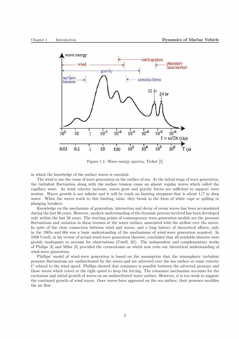
Ocean water is permanently subjected to the external forces of nature that dictate the types of induced wavesin the ocean. We may distinguish five basic types: sound; capillary; gravity; internal; and planetary waves.Sound waves are due to the water compressibility that is very small. The combination of the turbulentfluctuation of the atmospheric pressure and surface tension induce small waves, of almost regular form,with a high frequency. This type of waves are called capillary waves. These waves are usually unstableand attenuate, due to the surface tension, when the wind calms. Gravity waves, acting on water particlesdisplaced from equilibrium at the ocean surface or at an internal geopotential surface surface in a stratifiedfluid, induced gravity waves (surface or internal). There are also vary slow and large scale planetary orRossby waves induced by the variation of the equilibrium potential vorticity, due to changes in depth orlatitude. All of the above wave types can occur together, producing more complicated patterns of oscillations.The frequency range associated with external forces is very wide and ocean surface response occupies anextraordinary broad range of wave lengths and periods, from capillary waves, with period less than a second,through wind-induced waves and swell with period of the order of few second, to tidal oscillations withperiods of the order of several hours and days. The schematic representation of energy contained in thesurface waves is given in Fig. 1.1. The physical mechanisms generating these waves is also listed in Tab.1.1.
Wave types Physical mechanism periods
Capillary waves Surface tension < 10−1 sWind waves Wind shear, gravity < 15 sSwell Wind waves < 30 sTsunami Earthquake 10 min − 2 hTides Gravitational action of the moon and sun, earth rotation 12 − 24 h
Table 1.1: Waves, physical mechanism, and periods, Masse,l [2]
The gravity waves are of the greatest importance for engineering activity in the sea. The influence of wind-induced waves on engineering structures is most sensible and hostile. Marine structures must be designed tosustain the forces and motions induced by these waves. A through understanding of the interaction of waveswith marine structures has now become a vital factor in the safe and economical design of such structures.The calculation procedures needs to established the structural loading and induced motions generally involvethe following steps:
◮ establishing the wave climate in the working area of the marine structure;
◮ estimating the wave conditions for the structure; and
◮ selecting and applying a wave theory to determine the induced motions and hydrodynamic loading
1
Chapter 1 Introduction Dynamics of Marine Vehicle
Figure 1.1: Wave energy spectra, Tichet [5]
in which the knowledge of the surface waves is essential.The wind is one the cause of wave generation on the surface of sea. At the initial stage of wave generation,
the turbulent fluctuation along with the surface tension cause an almost regular waves which called thecapillary wave. As wind velocity increase, waves grow and gravity forces are sufficient to support wavemotion. Waves growth is not infinite and it will be reach an limiting steepness that is about 1/7 in deepwater. When the waves reach to this limiting value, they break in the form of white caps or spilling orplunging breakers.
Knowledge on the mechanism of generation, interaction and decay of ocean waves has been accumulatedduring the last 80 years. However, modern understanding of the dynamic process involved has been developedonly within the last 50 years. The starting points of contemporary wave generation models are the pressurefluctuations and variation in shear stresses at the water surface, associated with the airflow over the waves.In spite of the clear connection between wind and waves, and a long history of theoretical efforts, onlyin the 1965s and 60s was a basic understanding of the mechanisms of wind-wave generation acquired. In1956 Ursell, in his review of actual wind-wave generation theories, concluded that all available theories weregrossly inadequate to account for observations (Ursell, [6]). The independent and complementary worksof Philips [4] and Miles [3] provided the cornerstones on which now rests our theoretical understanding ofwind-wave generation.
Phillips’ model of wind-wave generation is based on the assumption that the atmospheric turbulentpressure fluctuations are undistributed by the waves and are advected over the sea surface at some velocityU related to the wind speed. Phillips showed that resonance is possible between the advected pressure andthose waves which travel at the right speed to keep the forcing. The resonance mechanism accounts for theexcitation and initial growth of waves on an undistributed water surface. However, it is too weak to supportthe continued growth of wind waves. Once waves have appeared on the sea surface, their presence modifiesthe air flow.
2
Chapter 1 Introduction Dynamics of Marine Vehicle
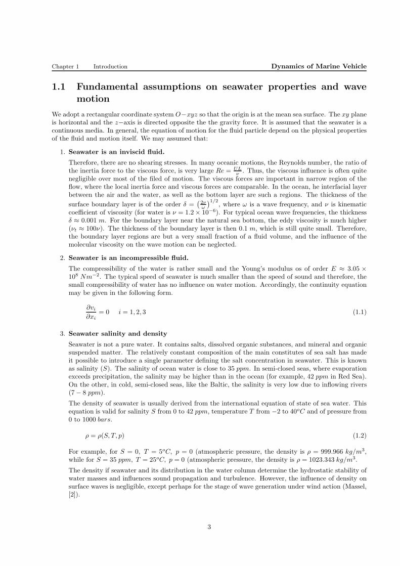
1.1 Fundamental assumptions on seawater properties and wave
motion
We adopt a rectangular coordinate system O−xyz so that the origin is at the mean sea surface. The xy planeis horizontal and the z−axis is directed opposite the the gravity force. It is assumed that the seawater is acontinuous media. In general, the equation of motion for the fluid particle depend on the physical propertiesof the fluid and motion itself. We may assumed that:
1. Seawater is an inviscid fluid.
Therefore, there are no shearing stresses. In many oceanic motions, the Reynolds number, the ratio ofthe inertia force to the viscous force, is very large Re = UL
ν . Thus, the viscous influence is often quitenegligible over most of the filed of motion. The viscous forces are important in narrow region of theflow, where the local inertia force and viscous forces are comparable. In the ocean, he interfacial layerbetween the air and the water, as well as the bottom layer are such a regions. The thickness of the
surface boundary layer is of the order δ =(2νω
)1/2, where ω is a wave frequency, and ν is kinematic
coefficient of viscosity (for water is ν = 1.2× 10⁻⁶). For typical ocean wave frequencies, the thicknessδ ≈ 0.001 m. For the boundary layer near the natural sea bottom, the eddy viscosity is much higher(νt ≈ 100ν). The thickness of the boundary layer is then 0.1 m, which is still quite small. Therefore,the boundary layer regions are but a very small fraction of a fluid volume, and the influence of themolecular viscosity on the wave motion can be neglected.
2. Seawater is an incompressible fluid.
The compressibility of the water is rather small and the Young’s modulus os of order E ≈ 3.05 ×10⁸ Nm−2. The typical speed of seawater is much smaller than the speed of sound and therefore, thesmall compressibility of water has no influence on water motion. Accordingly, the continuity equationmay be given in the following form.
∂vi∂xi
= 0 i = 1, 2, 3 (1.1)
3. Seawater salinity and density
Seawater is not a pure water. It contains salts, dissolved organic substances, and mineral and organicsuspended matter. The relatively constant composition of the main constitutes of sea salt has madeit possible to introduce a single parameter defining the salt concentration in seawater. This is knownas salinity (S). The salinity of ocean water is close to 35 ppm. In semi-closed seas, where evaporationexceeds precipitation, the salinity may be higher than in the ocean (for example, 42 ppm in Red Sea).On the other, in cold, semi-closed seas, like the Baltic, the salinity is very low due to inflowing rivers(7− 8 ppm).
The density of seawater is usually derived from the international equation of state of sea water. Thisequation is valid for salinity S from 0 to 42 ppm, temperature T from −2 to 40oC and of pressure from0 to 1000 bars.
ρ = ρ(S, T, p) (1.2)
For example, for S = 0, T = 5oC, p = 0 (atmospheric pressure, the density is ρ = 999.966 kg/m3,while for S = 35 ppm, T = 25oC, p = 0 (atmospheric pressure, the density is ρ = 1023.343 kg/m3.
The density if seawater and its distribution in the water column determine the hydrostatic stability ofwater masses and influences sound propagation and turbulence. However, the influence of density onsurface waves is negligible, except perhaps for the stage of wave generation under wind action (Massel,[2]).
3
Chapter 1 Introduction Dynamics of Marine Vehicle
4. Motion is irrotational.
This means that the individual elementary particles of the fluid do not rotate. The fluid flow is calledirrotational if ζ = ∇× v = 0. It implies that for an irrotational fluid flow
ωi =1
2eijk
∂vk∂xj
= 0 (1.3)
As indicated above, in many oceanic motions the influence of the viscous terms is quite negligible.In this event, the Lagrangian theorem indicates that if, at some initial instant, the vorticity vanisheseverywhere in the filed of flow, the motion is irrotational. This remain so in the absence of the viscouseffects. The consequence of irrotatinality of the flow indicate that the velocity field can be representedas the gradient of a scalar function called as the velocity potential φ.
vi =∂φ
∂xii = 1, 2, 3 (1.4)
In virtue of the continuity equation (??), the velocity potential function is an harmonic function andobeys the Laplace equation.
∇2φ =∂2φ
∂x2+
∂2φ
∂y2+
∂2φ
∂z2= 0 (1.5)
1.2 Boundary value problem of ocean gravity waves
The water way in a sea region is bounded by:
◮ free surface that is the interface of the air and water. This surface may be defined in form
z = η(x, y, t) (1.6)
that is the elevation of the free surface with respect to the reference frame that is located at the themean sea surface.
◮ sea bottom, It may be defined as
z = −h(x, y, t) (1.7)
◮ other boundaries, There may be possible some other boundaries in the region that is studied, such asa ship or an offshore structure. We defined them as
B(x, y, z, t) = 0 (1.8)
◮ Far filed boundary, we should also consider a far field boundary if the water way is not restricted. Itshould be in a place that there is no disturbance and is not affected by the presence of wind generatedwaves.
4

Chapter 1 Introduction Dynamics of Marine Vehicle
Based on the assumption that is described in the last section and the above boundaries of the fluid flow,we may formulate the gravity ocean waves as follows:
∇2φ = 0 on z < η(x, y, t)
∂φ∂t + P
ρ + 12 |∇φ|2 + gz = c(t) on z < η(x, y, t)
Boundary conditions:
Free Surface
∂η∂t +
∂φ∂x
∂η∂x + ∂φ
∂y∂η∂y = ∂φ
∂z
∂φ∂t + gz + 1
2
[(
∂φ∂x
)2
+
(
∂φ∂y
)2
+
(
∂φ∂z
)2]
= 0
on z = η(x, y, t)
Fluid Bottom boundary{
∂φ∂z + ∂h
∂t + ∂φ∂x
∂h∂x + ∂φ
∂y∂h∂y = 0 on z = −h(x, y, t)
Other Boundaries,
∂B∂t + (∇φ · ∇)B = 0 on B(x, y, z, t) = 0
F =∫
SBpn ds
M =∫
SBp(r− rG)× n ds
on B(x, y, z, t) = 0
Far field boundary ∂φ∂t = 0, ∇φ = 0
(1.9)
Example - 1Fluid in a U-tube has been forced to oscillate sinusoidally due to an oscillating pressure on one leg of thetube, 1.2. Develop the kinematic boundary condition for the free surface in leg A.
Figure 1.2: Oscillating flow in a U-tube, Dean and Dalrymple [1]
5
Chapter 1 Introduction Dynamics of Marine Vehicle
Solution
The equation of the free surface may be written as follows.
F (z, t) = z − η(t) = 0 and η(t) = a cos (ωt)
Where a is the amplitude of the free surface and ω is the frequency. The kinematic Boundary condition is:
DF (z, t)
Dt= 0 → ∂F (z, t)
∂t+V · ∇F (z, t) = 0
∂F (z, t)
∂t= −aω sin (ωt)
V = ui+ vj + wk
u = 0 v = 0
V = wk
V · ∇F (z, t) = w
w = −aω sin (ωt)
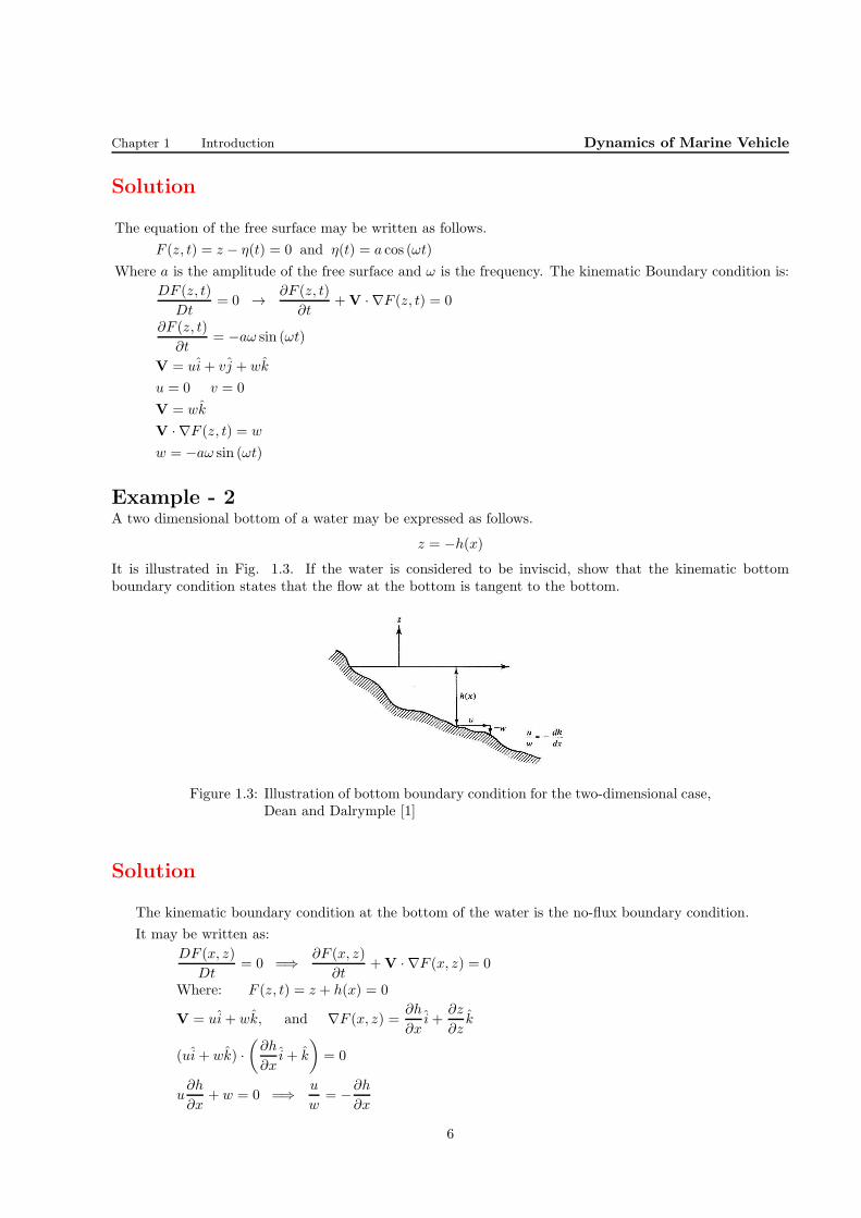
Example - 2A two dimensional bottom of a water may be expressed as follows.
z = −h(x)
It is illustrated in Fig. 1.3. If the water is considered to be inviscid, show that the kinematic bottomboundary condition states that the flow at the bottom is tangent to the bottom.
Figure 1.3: Illustration of bottom boundary condition for the two-dimensional case,Dean and Dalrymple [1]
Solution
The kinematic boundary condition at the bottom of the water is the no-flux boundary condition.
It may be written as:
DF (x, z)
Dt= 0 =⇒ ∂F (x, z)
∂t+V · ∇F (x, z) = 0
Where: F (z, t) = z + h(x) = 0
V = ui+ wk, and ∇F (x, z) =∂h
∂xi+
∂z
∂zk
(ui+ wk) ·(∂h
∂xi+ k
)
= 0
u∂h
∂x+ w = 0 =⇒ u
w= −∂h
∂x
6
Bibliography
[1] Robert G. Dean, Robert A. Dalrymple, Water wave mechanics for engineers and scientists, WorldScientific publishing Co. Pte. Ltd., 2000
[2] Massel, Stanislaw R., Ocean surface waves: Their physics and prediction, World Scientific publishingCo. Pte. Ltd., 1996
[3] Miles, J. W., On the generation of surface waves by shear flows, Jour. Fluid Mech., 3: 185 - 204
[4] Phillips, O. M., On the generation of waves by turbulent wind, Jour. Fluid Mech., 2: 417 - 445 Springer-Verlag, Berlin, pp.445-814, 1960,
[5] Tichet, A. H., Phillips, O. M., Hydrodynamics, Open course, MIT, 2005
[6] Ursell, F., Wave generation by wind, In: Batchelor, G. (Editor) Survey in Mechanics, Cambridge Uni-versity Press, 216 - 249
7
Chapter 2
Long-Crested, Linear Wave Theory(LWT)
We formulated the gravity wave in general form in the previous lecture. The gravity wave is a nonlinearboundary value problem (BVM). In addition, the free surface boundary conditions should be applied toa surface z = η(x, y, t) that is initially unknown. We should make some more assumptions to make theproblem amenable to an analytical solution. The simplest and most fundamental approach is to seek a linearsolution of the problem by taking the wave amplitude A to be very small in compare with the wave lengthλ. It is also assumed that the waves are two dimensional in the xz plane and the bottom of the waterway is a constant flat horizontal surface. The wave theory which results from this additional assumptionsis referred to alternatively as small amplitude wave theory, linear wave theory, sinusoidal wave theory, or asAiry theory. We will explain the linear wave theory (LWT), its properties and the associated problem withit in this lecture.
2.1 Boundary value problem for LWT
The most commonly description for wind-generated surface gravity waves is the linear wave theory (LWT).In addition to the basic assumption for gravity waves have been described already, the following assumptionsare also taken into account:
1. The waves are two dimensional in xz-plane, (long-crested waves in the y-direction);
This assumption reduce a three dimensional problem into a two dimensional problem and we can omitall of the y dependent terms.
2. The slopes of the waves are very small, Aλ << 1;
This assumption simplified the free surface boundary conditions. The nonlinear terms in free surfaceboundary conditions are negligible in comparison with the remaining linear terms. If we also considerthe Taylor series expansion, it can be written that
( )
z=η(x,t)=( )
z=0+ η
∂
∂z
( )
z=0+
1
2η2
∂2
∂z2
( )
z=0+ · · · (2.1)
The first term on the left hand side of (2.1) is linear and the rest are nonlinear. We keep the linearterms and discard the nonlinear terms. Therefore, the free surface boundary conditions are reduce to:
∂η∂t = ∂φ
∂z
∂φ∂t + gη = 0
on z = 0 (2.2)
1
Chapter 2 Long-Crested, Linear Wave Theory (LWT) Dynamics of Marine Vehicle
If we combine theses two conditions, the free surface boundary condition can be given in the followingform.
∂η∂t = ∂φ
∂z
η = − 1g∂φ∂t
=⇒ ∂2φ
∂t2+ g
∂φ
∂z= 0 on z = 0 (2.3)
As a general rule of thumb for wave amplitude to wavelength ratios of(Aλ < 1
14
), we can linearize the
free surface boundary conditions.
3. The fluid bottom boundary is flat, z = −h.
This assumption is also make the bottom boundary condition simple.
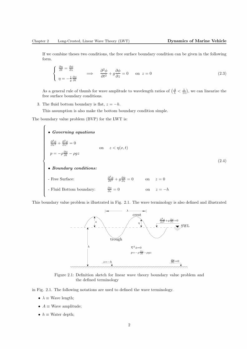
The boundary value problem (BVP) for the LWT is:
• Governing equations
∂2φ∂x2 + ∂2φ
∂z2 = 0
p = −ρ∂φ∂t − ρgz
on z < η(x, t)
• Boundary conditions:
- Free Surface: ∂2φ∂t2 + g ∂φ
∂z = 0 on z = 0
- Fluid Bottom boundary: ∂φ∂z = 0 on z = −h
(2.4)
This boundary value problem is illustrated in Fig. 2.1. The wave terminology is also defined and illustrated
λ
h
A η
∂2φ
∂t2+g ∂φ
∂z=0
∂φ∂z
=0z=−h
crest
trough
∇2φ=0
p=−ρ ∂φ∂t
−ρgz
SWL
Figure 2.1: Definition sketch for linear wave theory boundary value problem andthe defined terminology
in Fig. 2.1. The following notations are used to defined the wave terminology.
• λ ≡ Wave length;
• A ≡ Wave amplitude;
• h ≡ Water depth;
2

Chapter 2 Long-Crested, Linear Wave Theory (LWT) Dynamics of Marine Vehicle
• ω ≡ Wave frequency;
• T ≡ Wave period;
• k ≡ Wave number;
• vp or C ≡ Phase velocity, or celerity
• η(x, t) ≡ Vertical displacement of water surface at point x and time t;
2.2 Analytical solution of the LWT BVP
The Laplace equation is subjected to the free surface and bottom boundary conditions, (2.4). The methodof separation of variables may be applied to find the solution. We may assume that:
φ(x, z, t) = X(x)Z(z)T (t) (2.5)
If we substitute (2.5) in the Laplace equation in (2.4), we obtain
X ′′
X= −Z ′′
Z= −k2 (2.6)
where k2 is a separation constant. The resulting two ordinary differential equations are:
X ′′ + k2X = 0 (2.7)
Z ′′ − k2Z = 0 (2.8)
The solutions of (2.7) and (2.8) are:
X = B cos kx+Dsinkx (2.9)
Z = Eekz +Ge−kz (2.10)
Thus, the solution can be written in the following form.
φ(x, z, t) = (B cos kx+Dsinkx)(Eekz +Ge−kz
)T (t) (2.11)
The function T (t) should be a harmonic function from physical point of view. It may be given in the formof cosωt or sinωt, where ω is defined as the circular frequency and is given by ω = 2π/T = 2πf .
According to Rahman [3], we may distinguish four independent solution for the Laplace equation. Theyare:
φ1 = A1Z(z) coskx cosωt (2.12)
φ2 = A2Z(z) sinkx sinωt (2.13)
φ3 = A3Z(z) sinkx cosωt (2.14)
φ4 = A4Z(z) coskx sinωt (2.15)
Decomposing the solution in this manner helps in the evaluation of the unknown constants. If we considerthe first solution (??), the application of the bottom boundary condition gives:
∂φ1
∂z = 0 on z = −h
φ1 = A1
(Eekz +Ge−kz
)cos kx cosωt
=⇒ Eekh = Ge−kh =⇒ E = Ge2kh (2.16)
Then
φ1 = 2A1Gekh(ek(z+h) +Ge−k(z+h)
2
)
cos kx cosωt
= 2A1Gekh coshk(z + h) cos kx cosωt. (2.17)
3
Chapter 2 Long-Crested, Linear Wave Theory (LWT) Dynamics of Marine Vehicle
The application of the free surface boundary conditions yields:
η1 = − 1g∂φ1
∂t on z = 0
φ1 = 2A1Gekh coshk(z + h) cos kx cosωt.
=⇒ η1 =2ω
gA1Gekh coshkh cos kx sinωt (2.18)
The maximum value of η1 is the wave amplitude A. It will occur when cos kx sinωt = 1. Therefore,
A1Gekh =Ag
2ω coshkh(2.19)
and subsequently
η1 = A cos kx sinωt. (2.20)
This present a system of standing waves of wavelength 2πk and amplitude of A. The velocity potential φ1 is
in the form
φ1 =Ag
ω
coshk(z + h)
coshkhcos kx cosωt. (2.21)
The velocity potential φ1 is a periodic function in x with a wavelength of λ. The wavelength is obtained byλ = 2π
k where k is known as the wave number.We may follow the same procedure to find the constant of other elementary solution for the velocity
potentials given in (2.13), (??) and (??). The final solutions are:
φ1 =Ag
ω
coshk(z + h)
coshkhcos kx cosωt (2.22)
φ2 = −Ag
ω
coshk(z + h)
coshkhsin kx sinωt (2.23)
φ3 =Ag
ω
coshk(z + h)
coshkhsin kx cosωt (2.24)
φ4 = −Ag
ω
coshk(z + h)
coshkhcos kx sinωt (2.25)
Since the Laplace equation is a linear equation, any linear combination of these elementary solution willalso be a solution to the problem. Thus
φ = φ3 + φ4 =Ag
ω
coshk(z + h)
cosh khsin (kx− ωt) (2.26)
This velocity potential is due to a progressive wave traveling in the positive x−direction. The free surfaceelevation can be obtained from the free surface boundary condition.
η = − 1g∂φ∂t on z = 0
φ = Agω
cosh k(z+h)cosh kh sin (kx− ωt)
=⇒ η = A cos (kx− ωt) (2.27)
This solution is periodic in x and t and is called the progressive wave.If an observer moves along with the wave such that his position relative to the wave front remains fixed,
then kx− ωt = constant. The speed of movement of the observer is:
kx− ωt = constant =⇒ dx
dt=
ω
k=
λ
T= vp (2.28)
which is known as the wave phase velocity. It may also be denoted by C and called as wave celerity.The progressive wave traveling in the negative x−direction can be obtained in the similar manner as we
get (??). It can be written that:
φ = φ3 − φ4 =Ag
ω
coshk(z + h)
cosh khsin (kx+ ωt) (2.29)
4

Chapter 2 Long-Crested, Linear Wave Theory (LWT) Dynamics of Marine Vehicle
The associated water elevation is:
η = −A cos (kx+ ωt) (2.30)
Similarly, we can also combined φ1 and φ2 to obtain different forms of the progressive wave.
φ = φ1 − φ2 =Ag
ω
coshk(z + h)
coshkhcos (kx− ωt) (2.31)
η = −A sin (kx− ωt) (2.32)
and
φ = φ1 + φ2 =Ag
ω
coshk(z + h)
coshkhcos (kx+ ωt) (2.33)
η = A sin (kx+ ωt). (2.34)
Velocity potentials (2.31) and (2.32) are identical to (2.26) and (2.27) except for a phase shift.
2.3 Dispersion relation
Substituting (2.26) in the combined form of the free surface boundary equation, we get the dispersion relation.
∂2φ∂t2 + g ∂φ
∂z = 0 on z = 0
φ = Agω
cosh k(z+h)cosh kh sin (kx− ωt)
=⇒ ω2 = gk tanh kh (2.35)
This equation represents the relationship between the wave frequency ω and the wave number k. The sameresult can be obtained for a progressive wave traveling in the negative x−direction. The dispersion relationdescribes the interaction between the inertia force and gravitational forces.
If we take into account that ω = kvp, we can also obtain a relationship between the phase velocity andthe wave number and the depth of the water.
v2p =g
ktanhkh (2.36)
This relation shows the rate of the propagation of gravity waves as a function of water depth h and wavelengthλ. It shows that longer waves are propagating with a higher velocity. The waves of the same length arepropagating faster in water with a higher depth.
The wavelength can be also obtained from the dispersion relation.
λ =gT 2
2πtanh
(2πh
λ
)
(2.37)
The important feature of (2.35) and (2.36) is that the frequency and the phase velocity are functionsof wave number and so of wavelength. The gravity waves of different wavelengths travel at different wavevelocities. Such waves are called dispersive, since the waves would disperse as time goes on with variousgroups of waves such that each group would consists of waves having approximately the same wavelength.
Example - 1A wave with a period T = 10 s is propagated shore-ward over a uniformly sloping shelf from a depthd = 200 m to a depth d = 3 m. Find the wave phase speed (celerities) vp and lengths λ corresponding todepths d = 200 m and d = 3 m.
5
Chapter 2 Long-Crested, Linear Wave Theory (LWT) Dynamics of Marine Vehicle
Solution
It is assumed that the water is deep enough, Therefore:
λ0 =gT 2
2π=
9.806× 10²
2× 3.14= 156.067m
The assumption should be controlled, it means:
tanh2πh
λ= 1 =⇒ tanh
2× π × 200
156.067= 1
or it can be written that:
h
λ≥ 1
2=⇒ 200
156.067= 1.28 ≥ 1
2
thus, it is correct. The wave phase speed is:
vp =λ
T=
156.067
10= 15.61 m/s
If it is assumed that the water is also deep in h = 3 m, the value of the function
tanh2πh
λ= tanh
2× π × 3
156.067= 0.12 ≤ 1
Therefore, the water is not deep for such a wave. The length of the wave at this depth situation should becalculated.
λ =gT 2
2πtanh
2πh
λ
The solution for λ should be obtained by numerical computation. It may be obtained by using the followingMATLAB m-file.
g = 9.806;
T = 10 s;
h = 3 m;
L0 = g*T.^2/2/pi;
Lambda = fzero(@(L) L - g*T^2/2/pi*tanh(2*pi*h/L), L0)
The computation gives:
λ = 53.145 m
and, the wave phase speed is;
vp =λ
T=
53.145
10= 5.31 m/s
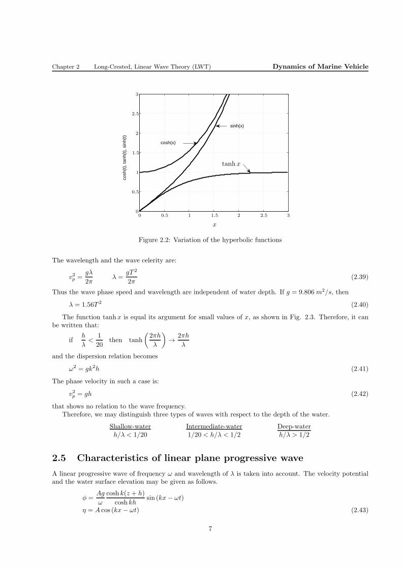
2.4 Classification of water waves
The variation of hyperbolic functions are shown in Fig. 2.2. The argument of tanh−function in dispersionrelation are 2πh
λ . We can write that:
ifh
λ>
1
2then tanh
(2πh
λ
)
→ 1
and the dispersion relation becomes
ω2 = gk (2.38)
6
Chapter 2 Long-Crested, Linear Wave Theory (LWT) Dynamics of Marine Vehicle
cosh
(t),
tanh
(t),
sin
h(t)
sinh(x)
cosh(x)
x
tanhx
00
0.5
0.5
1
1
1.5
1.5
2
2
2.5
2.5
3
3
Figure 2.2: Variation of the hyperbolic functions
The wavelength and the wave celerity are:
v2p =gλ
2πλ =
gT 2
2π(2.39)
Thus the wave phase speed and wavelength are independent of water depth. If g = 9.806 m2/s, then
λ = 1.56T 2 (2.40)
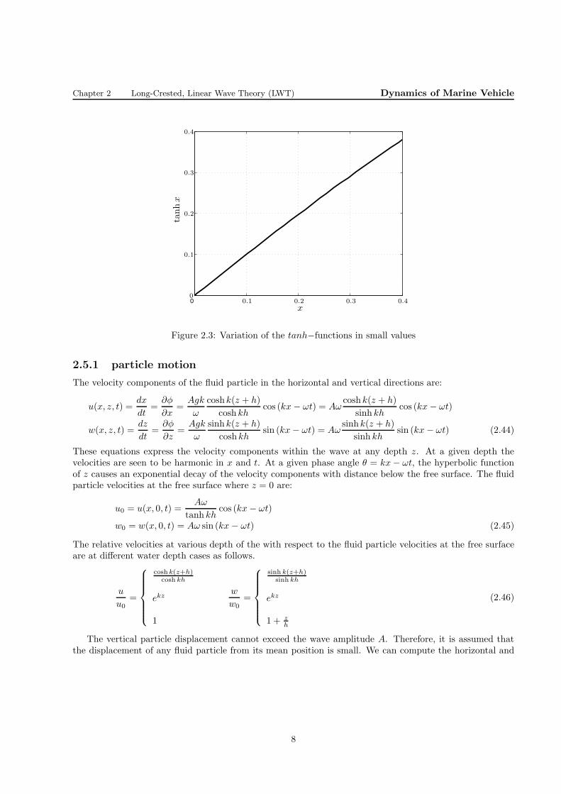
The function tanhx is equal its argument for small values of x, as shown in Fig. 2.3. Therefore, it canbe written that:
ifh
λ<
1
20then tanh
(2πh
λ
)
→ 2πh
λ
and the dispersion relation becomes
ω2 = gk2h (2.41)
The phase velocity in such a case is:
v2p = gh (2.42)
that shows no relation to the wave frequency.Therefore, we may distinguish three types of waves with respect to the depth of the water.
Shallow-water Intermediate-water Deep-waterh/λ < 1/20 1/20 < h/λ < 1/2 h/λ > 1/2
2.5 Characteristics of linear plane progressive wave
A linear progressive wave of frequency ω and wavelength of λ is taken into account. The velocity potentialand the water surface elevation may be given as follows.
φ =Ag
ω
coshk(z + h)
coshkhsin (kx− ωt)
η = A cos (kx− ωt) (2.43)
7
Chapter 2 Long-Crested, Linear Wave Theory (LWT) Dynamics of Marine Vehicle
0 x
tanhx
0
0.1
0.1
0.2
0.2
0.3
0.3
0.4
0.4
Figure 2.3: Variation of the tanh−functions in small values
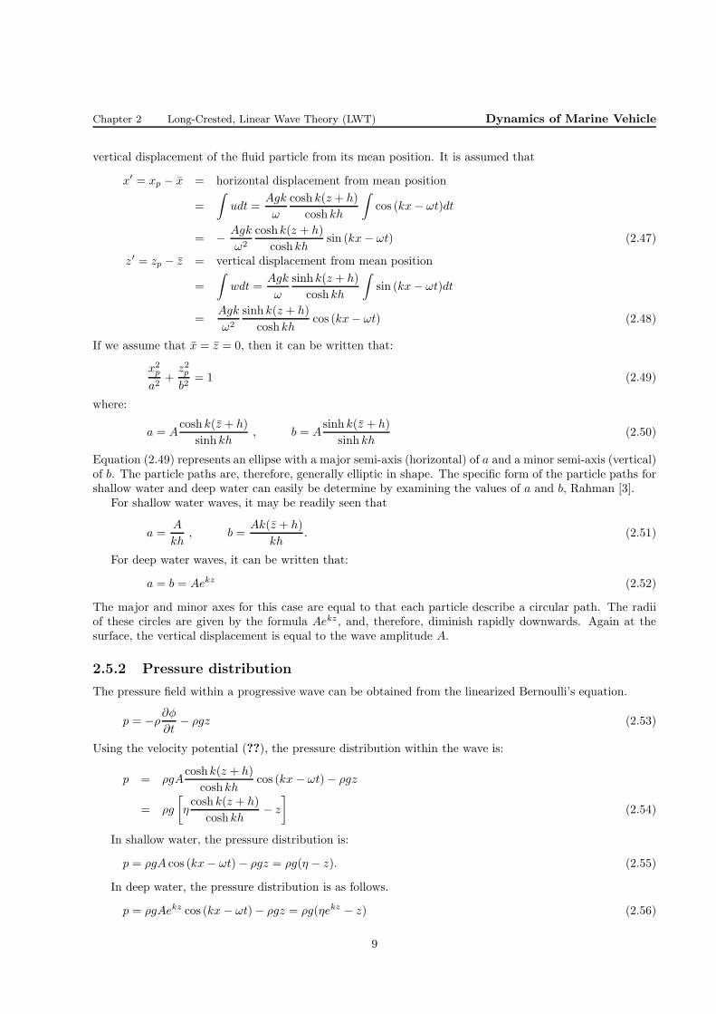
2.5.1 particle motion
The velocity components of the fluid particle in the horizontal and vertical directions are:
u(x, z, t) =dx
dt=
∂φ
∂x=
Agk
ω
coshk(z + h)
coshkhcos (kx− ωt) = Aω
coshk(z + h)
sinh khcos (kx− ωt)
w(x, z, t) =dz
dt=
∂φ
∂z=
Agk
ω
sinhk(z + h)
coshkhsin (kx− ωt) = Aω
sinhk(z + h)
sinh khsin (kx− ωt) (2.44)
These equations express the velocity components within the wave at any depth z. At a given depth thevelocities are seen to be harmonic in x and t. At a given phase angle θ = kx− ωt, the hyperbolic functionof z causes an exponential decay of the velocity components with distance below the free surface. The fluidparticle velocities at the free surface where z = 0 are:
u0 = u(x, 0, t) =Aω
tanh khcos (kx− ωt)
w0 = w(x, 0, t) = Aω sin (kx− ωt) (2.45)
The relative velocities at various depth of the with respect to the fluid particle velocities at the free surfaceare at different water depth cases as follows.
u
u0=
coshk(z+h)cosh kh
ekz
1
w
w0=
sinh k(z+h)sinh kh
ekz
1 + zh
(2.46)
The vertical particle displacement cannot exceed the wave amplitude A. Therefore, it is assumed thatthe displacement of any fluid particle from its mean position is small. We can compute the horizontal and
8
Chapter 2 Long-Crested, Linear Wave Theory (LWT) Dynamics of Marine Vehicle
vertical displacement of the fluid particle from its mean position. It is assumed that
x′ = xp − x = horizontal displacement from mean position
=
∫
udt =Agk
ω
cosh k(z + h)
coshkh
∫
cos (kx− ωt)dt
= − Agk
ω2
coshk(z + h)
coshkhsin (kx− ωt) (2.47)
z′ = zp − z = vertical displacement from mean position
=
∫
wdt =Agk
ω
sinh k(z + h)
coshkh
∫
sin (kx− ωt)dt
=Agk
ω2
sinh k(z + h)
coshkhcos (kx− ωt) (2.48)
If we assume that x = z = 0, then it can be written that:
x2p
a2+
z2pb2
= 1 (2.49)
where:
a = Acosh k(z + h)
sinh kh, b = A
sinh k(z + h)
sinh kh(2.50)
Equation (2.49) represents an ellipse with a major semi-axis (horizontal) of a and a minor semi-axis (vertical)of b. The particle paths are, therefore, generally elliptic in shape. The specific form of the particle paths forshallow water and deep water can easily be determine by examining the values of a and b, Rahman [3].
For shallow water waves, it may be readily seen that
a =A
kh, b =
Ak(z + h)
kh. (2.51)
For deep water waves, it can be written that:
a = b = Aekz (2.52)
The major and minor axes for this case are equal to that each particle describe a circular path. The radiiof these circles are given by the formula Aekz , and, therefore, diminish rapidly downwards. Again at thesurface, the vertical displacement is equal to the wave amplitude A.
2.5.2 Pressure distribution
The pressure field within a progressive wave can be obtained from the linearized Bernoulli’s equation.
p = −ρ∂φ
∂t− ρgz (2.53)
Using the velocity potential (??), the pressure distribution within the wave is:
p = ρgAcoshk(z + h)
coshkhcos (kx− ωt)− ρgz
= ρg
[
ηcosh k(z + h)
coshkh− z
]
(2.54)
In shallow water, the pressure distribution is:
p = ρgA cos (kx− ωt)− ρgz = ρg(η − z). (2.55)
In deep water, the pressure distribution is as follows.
p = ρgAekz cos (kx− ωt)− ρgz = ρg(ηekz − z) (2.56)
9
Chapter 2 Long-Crested, Linear Wave Theory (LWT) Dynamics of Marine Vehicle
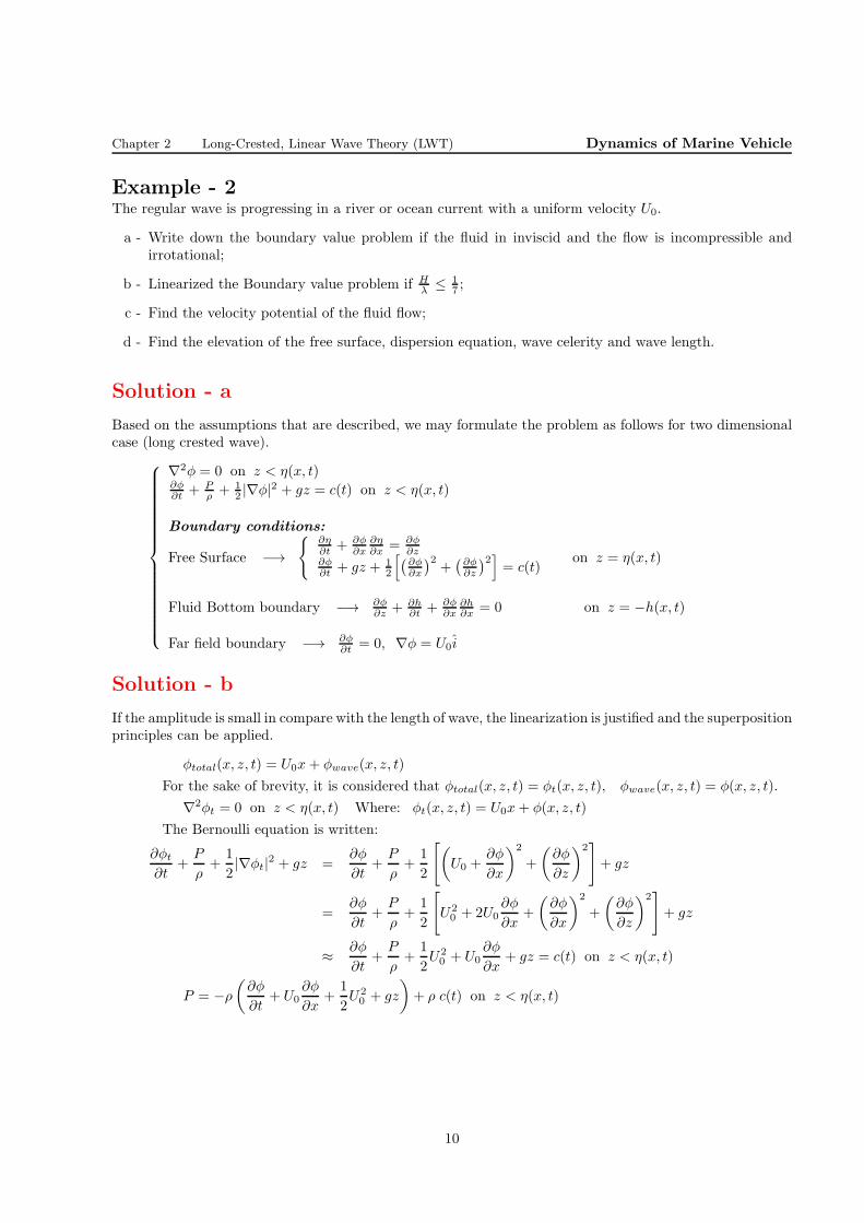
Example - 2The regular wave is progressing in a river or ocean current with a uniform velocity U0.
a - Write down the boundary value problem if the fluid in inviscid and the flow is incompressible andirrotational;
b - Linearized the Boundary value problem if Hλ ≤ 1
7 ;
c - Find the velocity potential of the fluid flow;
d - Find the elevation of the free surface, dispersion equation, wave celerity and wave length.
Solution - a
Based on the assumptions that are described, we may formulate the problem as follows for two dimensionalcase (long crested wave).
∇2φ = 0 on z < η(x, t)∂φ∂t + P
ρ + 12 |∇φ|2 + gz = c(t) on z < η(x, t)
Boundary conditions:
Free Surface −→{
∂η∂t +
∂φ∂x
∂η∂x = ∂φ
∂z∂φ∂t + gz + 1
2
[(∂φ∂x
)2+(∂φ∂z
)2]
= c(t)on z = η(x, t)
Fluid Bottom boundary −→ ∂φ∂z + ∂h
∂t + ∂φ∂x
∂h∂x = 0 on z = −h(x, t)
Far field boundary −→ ∂φ∂t = 0, ∇φ = U0i
Solution - b
If the amplitude is small in compare with the length of wave, the linearization is justified and the superpositionprinciples can be applied.
φtotal(x, z, t) = U0x+ φwave(x, z, t)
For the sake of brevity, it is considered that φtotal(x, z, t) = φt(x, z, t), φwave(x, z, t) = φ(x, z, t).
∇2φt = 0 on z < η(x, t) Where: φt(x, z, t) = U0x+ φ(x, z, t)
The Bernoulli equation is written:
∂φt
∂t+
P
ρ+
1
2|∇φt|2 + gz =
∂φ
∂t+
P
ρ+
1
2
[(
U0 +∂φ
∂x
)2
+
(∂φ
∂z
)2]
+ gz
=∂φ
∂t+
P
ρ+
1
2
[
U20 + 2U0
∂φ
∂x+
(∂φ
∂x
)2
+
(∂φ
∂z
)2]
+ gz
≈ ∂φ
∂t+
P
ρ+
1
2U20 + U0
∂φ
∂x+ gz = c(t) on z < η(x, t)
P = −ρ
(∂φ
∂t+ U0
∂φ
∂x+
1
2U20 + gz
)
+ ρ c(t) on z < η(x, t)
10
Chapter 2 Long-Crested, Linear Wave Theory (LWT) Dynamics of Marine Vehicle
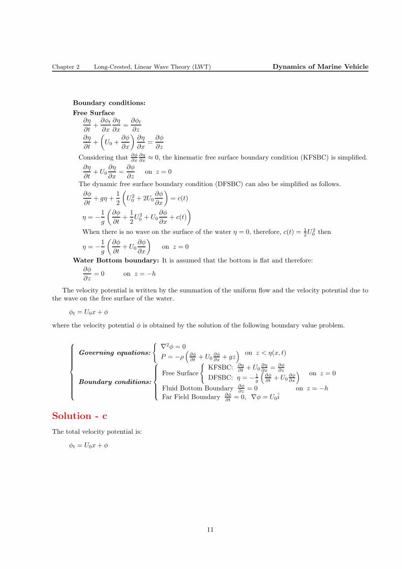
Boundary conditions:
Free Surface∂η
∂t+
∂φt
∂x
∂η
∂x=
∂φt
∂z∂η
∂t+
(
U0 +∂φ
∂x
)∂η
∂x=
∂φ
∂z
Considering that ∂φ∂x
∂η∂x ≈ 0, the kinematic free surface boundary condition (KFSBC) is simplified.
∂η
∂t+ U0
∂η
∂x=
∂φ
∂zon z = 0
The dynamic free surface boundary condition (DFSBC) can also be simplified as follows.
∂φ
∂t+ gη +
1
2
(
U20 + 2U0
∂φ
∂x
)
= c(t)
η = −1
g
(∂φ
∂t+
1
2U20 + U0
∂φ
∂x+ c(t)
)
When there is no wave on the surface of the water η = 0, therefore, c(t) = 12U
20 then
η = −1
g
(∂φ
∂t+ U0
∂φ
∂x
)
on z = 0
Water Bottom boundary: It is assumed that the bottom is flat and therefore:
∂φ
∂z= 0 on z = −h
The velocity potential is written by the summation of the uniform flow and the velocity potential due tothe wave on the free surface of the water.
φt = U0x+ φ
where the velocity potential φ is obtained by the solution of the following boundary value problem.
Governing equations:
{∇2φ = 0
P = −ρ(
∂φ∂t + U0
∂φ∂x + gz
)on z < η(x, t)
Boundary conditions:
Free Surface
{
KFSBC: ∂η∂t + U0
∂η∂x = ∂φ
∂z
DFSBC: η = − 1g
(∂φ∂t + U0
∂φ∂x
) on z = 0
Fluid Bottom Boundary ∂φ∂z = 0 on z = −h
Far Field Boundary ∂φ∂t = 0, ∇φ = U0i
Solution - c
The total velocity potential is:
φt = U0x+ φ
11
Chapter 2 Long-Crested, Linear Wave Theory (LWT) Dynamics of Marine Vehicle
The velocity potential due to the wave is obtained by the solution of the Laplace equation.
∇2φ = 0
The solution for the Laplace equation may be given for a progressive wave after applying
the bottom boundary condition as follows.
φ = A1 cosh k(z + h) sin (kx− ωt)
Considering DFSBC, it may be written that:
η = −1
g(−A1ω + U0A1k) coshkh cos (kx− ωt)
The maximum value of η is the wave amplitude A.
It will occur when cos (kx− ωt) = 1. Therefore,
A = −1
g(−A1ω + U0A1k) coshkh
A1 =Ag
ω − U0k=
Ag
k(vp − U0) coshkh
φ =Ag
k(vp − U0)
coshk(z + h)
coshkhsin (kx− ωt)
Where vp = ωk is the phase velocity of the wave. Therefore,
φt = U0x+Ag
k(vp − U0)
cosh k(z + h)
coshkhsin (kx− ωt)
Solution - d
• The surface elevation:
η = A cos (kx− ωt)
• The dispersion equation:
P = −ρ
(∂φ
∂t+ U0
∂φ
∂x+ gz
)
Since the pressure is constant along the free surface, therefore:
DP
Dt=
∂P
∂t+V · ∇P = 0
∂
∂t
[
−ρ
(∂φ
∂t+ U0
∂φ
∂x+ gη
)]
+
[
(U0 +∂φ
∂x)i+
∂φ
∂zk
]
· ∇[
−ρ
(∂φ
∂t+ U0
∂φ
∂x+ gz
)]
= 0
If the nonlinear terms are omitted, the combined free surface boundary condition is obtained.
∂2φ
∂t2+ 2U0
∂2φ
∂x∂t+ U2
0
∂2φ
∂x2+ g
∂φ
∂z= 0 on z = 0
The dispersion equation is obtained by inserting the wave velocity potential in the combined
free surface boundary condition.
Ag
k(vp − U0)
(−ω2 + 2U0kω − U2
0k2 + gk tanh kh
)sin (kx− ωt) = 0
ω2 − 2U0kω + U20k
2 = gk tanh kh
ω2 − 2U0ω2
vp+ U2
0
ω2
v2p= gk tanh kh
ω2
(
1− U0
vp
)2
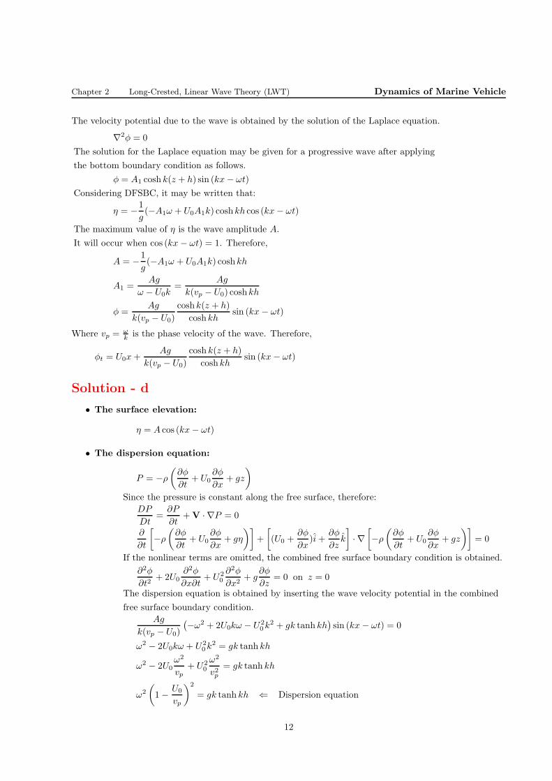
= gk tanh kh ⇐ Dispersion equation
12
Chapter 2 Long-Crested, Linear Wave Theory (LWT) Dynamics of Marine Vehicle
• The phase velocity:
The dispersion equation may be written in the following form.
ω2
v2p(vp − U0)
2= gk tanh kh
k2 (vp − U0)2= gk tanh kh
(vp − U0)2=
g
ktanhkh
vp = U0 +
√g
ktanh kh
• The wave length:
vp =λ
T= U0 +
√g
ktanh kh
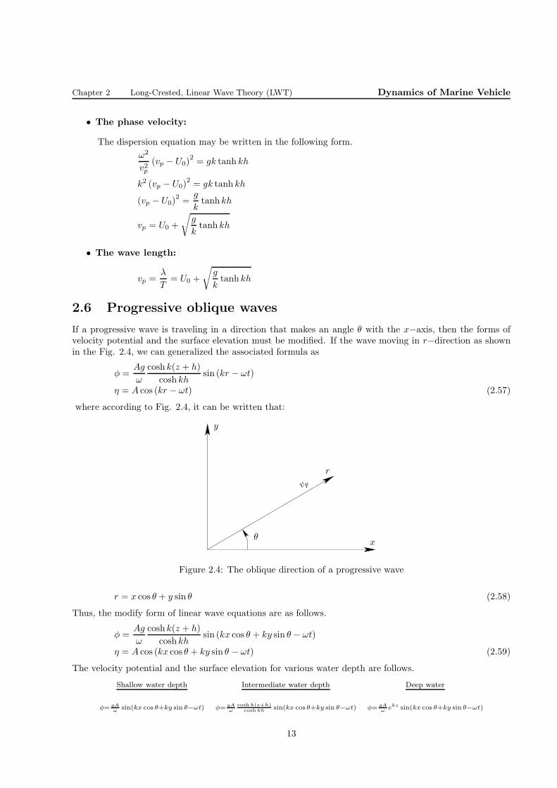
2.6 Progressive oblique waves
If a progressive wave is traveling in a direction that makes an angle θ with the x−axis, then the forms ofvelocity potential and the surface elevation must be modified. If the wave moving in r−direction as shownin the Fig. 2.4, we can generalized the associated formula as
φ =Ag
ω
coshk(z + h)
coshkhsin (kr − ωt)
η = A cos (kr − ωt) (2.57)
where according to Fig. 2.4, it can be written that:
y
x
vp
θ
r
Figure 2.4: The oblique direction of a progressive wave
r = x cos θ + y sin θ (2.58)
Thus, the modify form of linear wave equations are as follows.
φ =Ag
ω
coshk(z + h)
coshkhsin (kx cos θ + ky sin θ − ωt)
η = A cos (kx cos θ + ky sin θ − ωt) (2.59)
The velocity potential and the surface elevation for various water depth are follows.
Shallow water depth Intermediate water depth Deep water
φ= gAω
sin(kx cos θ+ky sin θ−ωt) φ= gAω
cosh k(z+h)cosh kh
sin(kx cos θ+ky sin θ−ωt) φ= gAω
ekz sin(kx cos θ+ky sin θ−ωt)
13
Chapter 2 Long-Crested, Linear Wave Theory (LWT) Dynamics of Marine Vehicle
Example - 3Consider a wave with a period T = 8 s, in a water depth h = 15 m with and a height of H = 5.5 m. Find:
a - the local horizontal and vertical velocities u and w; and
b - the accelerations ax and az;
at an elevation z = −5 m when Θ = (kx− ωt) = π3 .
Solution - a
u = Aωcoshk(z + h)
sinh khcos(kx− ωt)
w = Aωsinh k(z + h)
sinh khsin(kx− ωt)
It is necessary to find, A,ω, k.
A =H
2=
5.5
2= 2.75 m
ω =2π
T=
2× 3.14
8= 0.7854 1/s
λ =gT 2
2πtanh
2πh
λ=
9.806× 82
2× 3.14× tanh
2× π × 15
λ=⇒ λ = 81.767 m
k =2π
λ=
2× 3.14
81.767= 0.0768 1/m
u = Aωcoshk(z + h)
sinh khcosΘ = 2.75× 0.7854× cosh [0.0829× (−5 + 15)]
sinh (0.0829× 15)× cos
π
3= 0.993 m/s
w = Aωsinh k(z + h)
sinh khcosΘ = 2.75× 0.7854× sinh [0.0829× (−5 + 15)]
sinh (0.0829× 15)× sin
π
3= 1.111 m/s
Solution - b
ax =∂u
∂t= Aω2 coshk(z + h)
sinh khsin(kx− ωt)
az =∂w
∂t= −Aω2 sinh k(z + h)
sinhkhcos(kx− ωt)
ax = 2.75× 0.78542 × cosh [0.0829× (−5 + 15)]
sinh (0.0829× 15)× sin
π
3= 1.351 m/s2
w = −2.75× 0.78542 × sinh [0.0829× (−5 + 15)]
sinh (0.0829× 15)× cos
π
3= 0.504 m/s2
Example - 4Consider a wave in a depth h = 12 m with a height of H = 3 m and a period of T = 10 s. The correspondingdeep-water wave height is H0 = 3.13 m. Find:
a - The maximum horizontal and vertical displacement of a water particle from its mean position whenz = 0 and z = −h.
b - The maximum water particle displacement at an elevation z = −7.5 m when the wave is in infinitelydeep water.
c - For the deepwater conditions of above, show that the particle displacements are small relative to thewave height when z = −λ0
2 .
14
Chapter 2 Long-Crested, Linear Wave Theory (LWT) Dynamics of Marine Vehicle
Solution a
A fluid particle is moving in an elliptical path due to the wave motion.
x2p
a2+
z2pb2
= 1
where a is the major semi-axis (horizontal) and b is the minor semi-axis (vertical) of the ellipse.
a = Acosh k(z + h)
sinh kh, b = A
sinh k(z + h)
sinh kh
The parameters a and b are also the maximum horizontal and vertical displacement of a water particle fromits mean position. It should be emphasis that A is the amplitude of wave at z = 0. The amplitude of a wave
at an elevation z in a given depth of h is b = A sinh k(z+h)sinh kh .
It is necessary to find, k.
λ =gT 2
2πtanh
2πh
λ=
9.806× 10²
2× 3.14× tanh
2× π × 12
λ=⇒ λ = 99.703 m
k =2π
λ=
2× 3.14
99.703= 0.063 1/m
The maximum horizontal and vertical displacement of a water particle from its mean position at z = 0.
a =3
2
cosh (0.063× 12)
sinh (0.063× 12)= 2.349 m
b =3
2= 1.5 m
The maximum horizontal and vertical displacement of a water particle from its mean position at z = −d.
a =3
2× 1
sinh (0.063× 12)= 1.807 m
b =3
2= 0
Solution b
A fluid particle is moving in a circular path due to the wave motion in deep water.
x2p + z2p = a2
where a = Aek(z is the radius of the circle. The parameter a is also the amplitude of the wave at an elevationz for the free surface of the water.
λ =gT 2
2π=
9.806× 10²
2× 3.14= 156.073m
k =2π
λ=
2× 3.14
156.073= 0.0403 1/m
a =3.13
2× e[0.0403×(−7.5)] = 1.157 m
15

Chapter 2 Long-Crested, Linear Wave Theory (LWT) Dynamics of Marine Vehicle
Solution c
z = −λ0
2= −156.073
2= −78.036m
a =3.13
2× e[0.0403×(−78.036)] = 0.067 m
a
H=
0.067
3.13= 0.0213 ≈ 0
Characteristics of a linear plane progressive wave
Shallow water depth Intermediate water depth Deep water
h < λ20
λ20 < h < λ
2 h > λ2
φ = gAω sin(kx− ωt) φ = gA
ωcosh k(z+h)
cosh kh sin(kx− ωt) φ = gAω ekz sin(kx− ωt)
η = A cos (kx− ωt) η = A cos (kx− ωt) η = A cos (kx− ωt)
ω2 = k2gh ω2 = gk tanh kh ω2 = gk
u = aωkh cos (kx− ωt) u = Aω cosh k(z+h)
sinh kh cos(kx− ωt) u = Aωekz cos(kx− ωt)
w = Aωkh
(1 + z
h
)sin (kx− ωt) w = Aω sinh k(z+h)
sinh kh sin(kx− ωt) w = Aωekz sin(kx− ωt)
uu0
= 1 uu0
= cosh k(z+h)sinh kh
uuo
= ekz
ww0
= 1 + zh
ww0
= sinhk(z+h)sinh kh
wwo
= ekz
pd = ρgA cos (kx− ωt) pd = ρgA cosh k(z+h)cosh kh cos (kx− ωt) pd = ρgAekz cos (kx− ωt)
pd = ρgη Pd = ρg cosh k(z+h)cosh kh η pd = ρgekzη
pT = ρg(η − z) pT = ρg[cosh k(z+h)
cosh kh η − z]
pT = ρg(ekzη − z
)
xp−xa2 +
zp−zb2 = 1
a = Akh and b = A(1 + z
h ) a = A cosh k(z+h)sinh kh , b = A sinh k(z+h)
sinh kh a = b = Aekz
16

Chapter 2 Long-Crested, Linear Wave Theory (LWT) Dynamics of Marine Vehicle
Example - 5Two pressure sensors are mounted according to Fig. 2.5. The amplitudes of dynamic pressure are 20.4 kN/m2
and 25.6 kN/m2 as recorded on sensors 1 and 2, respectively. What are the wave length, water depth andwave amplitude?
Figure 2.5: The position of the sensors in example 6
Solution
pd = ρgAcoshk(z + h)
cosh khcos (kx− ωt)
Pd1 = ρgAcoshk(−h+ h)
cosh kh= ρgA
1
coshkh=⇒ The dynamic pressure amplitude at the sensor 1
Pd2 = ρgAcoshk(−h+ 7.62 + h)
coshkh= ρgA
cosh 7.62k
coshkh=⇒ The dynamic pressure amplitude at the sensor 2
Pd1
Pd2
=1
cosh 7.62k=⇒ 2.04
2.56=
1
cosh 7.62k=⇒ cosh 7.62k = 1.255 =⇒ k = 0.092
2π
λ= 0.092 =⇒ λ = 68.42 m
Using the dispersion relationship to find the water depth.
ω2 = gk tanh kh(2π
T
)2
= gk tanh kh =⇒ tanh kh =4π2
gkT 2=
4× π2
9.806× 0.092× 82=⇒ kh = 0.836
h =0.836
0.092= 9.086 m
The amplitude of wave is obtained by using the pressure amplitude at a sensor, say the sensor 1.
Pd1 = ρgA1
coshkh=⇒ A =
Pd1 coshkh
ρg=
2.04× 10⁴ × cosh 0.836
992× 9.806= 2.874 m
2.7 Superposition of waves
The boundary value problem associated with the small amplitude plane waves is linear. Therefore, theinfluence of a combination of several waves can be obtained by superposing the effects of individual wavecomponents. The velocity potential of a wave system consist of n regular wave are:
φt = φ1 + φ2 + · · ·+ φn (2.60)
17
Chapter 2 Long-Crested, Linear Wave Theory (LWT) Dynamics of Marine Vehicle
where
φn =Ang
ωn
coshkn(z + h)
coshknhsin (knx± ωnt+ δn). (2.61)
The minus and plus sign is related to the direction of the propagation of the nth wave. The phase differencebetween various waves is denoted by δn and is measured from the origin (kx± ωt).
The free surface elevation can be obtained from
ηt = −1
g
(∂φ
∂t
)
z=0
= −1
g
∂
∂t(φ1 + φ2 + · · ·+ φn)
∣∣∣∣∣z=0
= η1 + η2 + · · ·+ ηn. (2.62)
Therefore, it can be written that:
ηt = ±n∑
i=1
Ai cos(kix± ωit+ δi) (2.63)
The other characteristics of wave can also obtained by the superimpose of the characteristics of individualwave components.
ut =
n∑
i=1
Aiωicoshki(z + h)
sinh kihcos(kix− ωit) (2.64)
wt =n∑
i=1
Aiωisinh ki(z + h)
sinh kihsin(kix− ωit) (2.65)
pt =
n∑
i=1
ρg
[cosh ki(z + h)
coshkihηi − z
]
(2.66)
We may consider such a case that all wave components have the same period and moving in a waterof depth h in the same direction. Hence, the circular frequency and the wave numbers are identical for allwaves components. Under these special condition, the free surface elevation may be expressed as
ηt = r cos(kx− ωt+ λ) (2.67)
where r is such that:
r cosλ =
n∑
i=1
An cos δn
r sinλ =
n∑
i=1
An sin δn.
Hence
r =
(n∑
i=1
An cos δn
)2
+
(n∑
i=1
An sin δn
)2
1/2
λ = tan−1
(∑ni=1 An sin δn
∑ni=1 An cos δn
)
. (2.68)
For the special case in which there are only two wave components that have the same period, we canwrite that:
ηt = A1 cos(kx− ωt+ δ1) +A2 cos(kx− ωt+ δ2)
= cos(kx− ωt)(A1 cos δ1 +A2 cos δ2) + sin(kx− ωt)(A1 sin δ1 +A2 sin δ2)
= cos(kx− ωt)
2∑
i=1
Ai cos δi + sin(kx− ωt)
2∑
i=1
Ai sin δi
= r cos(kx− ωt+ λ)
18
Chapter 2 Long-Crested, Linear Wave Theory (LWT) Dynamics of Marine Vehicle
where
r =√
A21 +A2
2 + 2A1A2 cos (δ1 − δ2)
λ = tan−1
(A1 cos δ1 +A2 cos δ2A1 sin δ1 +A2 sin δ2
)
.
In the case that the two waves are in phase, δ1 = δ2, then
ηt = (A1 +A2)r cos(kx− ωt+ δ1).
If the two components are out of phase, i.e. δ1 = δ2 + π, then
ηt = (A1 −A2)r cos(kx− ωt+ δ1).
For δ1 − δ2 = π/2, then
ηt = A1 cos(kx− ωt+ δ1) +A2 sin(kx− ωt+ δ1).
2.8 Wave reflection and standing wave
If there is a barrier at x = b an the way of waves, the waves will be reflected. The reflection coefficient isdefined as
Kr =amplitude of the reflected wave
amplitude of the incident wave=
Ar
Ai(2.69)
where kr ≤ 1. If the value of kr = 1, then the reflection is perfect. Assume that the incident wave ispropagating in positive x−direction and is reflected by a plane vertical barrier at point x = b. It is assumethat the reflection is perfect. Hence, The velocity potential of the system of waves is
φ =Ag
ω
coshk(z + h)
coshkh[sin (kx− ωt) + sin (kx+ ωt+ δ2)] (2.70)
It is assumed that the barrier is impermeable, the velocity is zero at the barrier. Thus, the boundarycondition is
u = −∂φt
∂x= 0 at x = b (2.71)
The application of this boundary condition yields
cos (kb− ωt)− cos (kb + ωt+ δ2) = 0
Expanding and equating the coefficients of sinωt and cosωt, we obtain{
cos kb = cos (kb+ δ2)sinkb = − sin (kb+ δ2)
=⇒ δ2 = 2nπ − 2kb , n = 0, 1, 2, · · ·
For two progressive waves moving in opposite directions with the same amplitude, the surface elevationis
η = A cos (kx− ωt) +A cos (kx+ ωt+ δ2)
= A cos (kx− ωt) +A cos (kx+ ωt) cos δ2 +A sin (kx+ ωt) sin δ2
= A cos (kx− ωt) +A cos (kx+ ωt) cos (2nπ − 2kb) +A sin (kx+ ωt) sin (2nπ − 2kb)
= A cos (kx− ωt) +A cos (kx+ ωt) cos 2kb−A sin (kx+ ωt) sin 2kb
= A cos kx cosωt+A sin kx sinωt+A cos kx cosωt cos 2kb−A sin kx sinωt cos 2kb
−A sinkx cosωt sin 2kb−A sin kx cosωt sin 2kb.
The final solution can be written in the form,
η = 2A cos (kb − ωt) cos k(x− b) (2.72)
19
Chapter 2 Long-Crested, Linear Wave Theory (LWT) Dynamics of Marine Vehicle
The equation (2.69) is the product of two terms, one independent of x and the other independent of t. Thus,there are certain times when η = 0 for all x and there are also certain x of which η = 0 for all times. Theselater points are called the nodes of the system and are located by the condition
cos k(x− b) = 0 =⇒ x = b +2n+ 1
2π , n = 0, 1, 2, · · · (2.73)
The condition of stationary nodes defines standing waves. The slope of the free surface of the incident andreflected waves are always equal and opposite at x = b.
∂ηt∂x
= 0 , at x = b for all t (2.74)
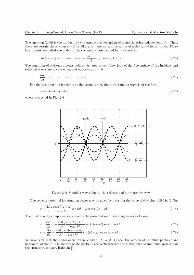
For the case that the barrier is at the origin, b = 0, then the standing wave is in the form
η = 2A cosωt cos kx (2.75)
where is plotted in Fig. 2.6
0
0
node node
t = 0, T, 2T, · · ·
t = T4 ,
3T4 , · · ·
t = T2 ,
3T2 , · · ·
2A
π2k
πk
3π2k
2πk
3πk
5π2k
7π2k
4πk
x
η
Figure 2.6: Standing waves due to the reflection of a progressive wave
The velocity potential for standing waves may be given by inserting the value of δ2 = 2nπ−2kb in (2.70).
φ =2Ag
ω
coshk(z + h)
cosh khsin (kb− ωt) cos (kx− kb) (2.76)
The fluid velocity components are due to the presentation of standing waves as follows.
u =∂φ
∂x= −2Akg
ω
coshk(z + h)
coshkhsin (kb− ωt) sin (kx− kb) (2.77)
w =∂φ
∂z=
2Akg
ω
sinh k(z + h)
coshkhsin (kb− ωt) cos (kx− kb) (2.78)
we have seen that the nodes occur where cos k(x− b) = 0. Hence, the motion of the fluid particles arehorizontal at nodes. The motion of the particles are vertical where the maximum and minimum variation ofthe surface take place, Rahman [3].
20
Chapter 2 Long-Crested, Linear Wave Theory (LWT) Dynamics of Marine Vehicle
2.9 Wave group
Consider two waves of same amplitude, direction and in phase at the origin. The surface elevation can beobtained by summing the effect of each wave.
ηt = A cos (k1x− ω1t) +A cos (k2x− ω2t) (2.79)
It can be rewritten as:
ηt = 2A cos
{1
2[(k1 + k2)x− (ω1 + ω2)t]
}
· cos{1
2[(k1 − k2)x− (ω1 − ω2)t]
}
(2.80)
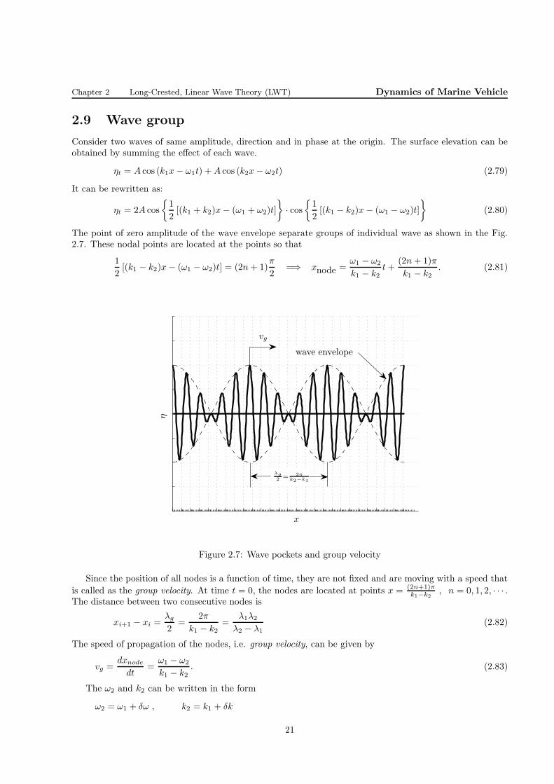
The point of zero amplitude of the wave envelope separate groups of individual wave as shown in the Fig.2.7. These nodal points are located at the points so that
1
2[(k1 − k2)x− (ω1 − ω2)t] = (2n+ 1)
π
2=⇒ xnode =
ω1 − ω2
k1 − k2t+
(2n+ 1)π
k1 − k2. (2.81)
vg
λg2 = 2π
k2−k1
x
η
wave envelope
Figure 2.7: Wave pockets and group velocity
Since the position of all nodes is a function of time, they are not fixed and are moving with a speed that
is called as the group velocity. At time t = 0, the nodes are located at points x = (2n+1)πk1−k2
, n = 0, 1, 2, · · · .The distance between two consecutive nodes is
xi+1 − xi =λg
2=
2π
k1 − k2=
λ1λ2
λ2 − λ1(2.82)
The speed of propagation of the nodes, i.e. group velocity, can be given by
vg =dxnode
dt=
ω1 − ω2
k1 − k2. (2.83)
The ω2 and k2 can be written in the form
ω2 = ω1 + δω , k2 = k1 + δk
21
Chapter 2 Long-Crested, Linear Wave Theory (LWT) Dynamics of Marine Vehicle
then the speed of propagation of the nodes is
vg =δω
δk.
As ω2 and k2 approach to ω1 and k1, it can be written that
vg =dω
dk. (2.84)
We now that ω = vpk and thus the group velocity is
vg =dvpkdk = vp + k
dvpdk
v2p = gk tanh kh
=⇒ vg =vp2
(
1 +2kh
sinh 2kh
)
(2.85)
The asymptotic forms of hyperbolic functions are as follows.
function large kh small kh
sinh kh 12e
kh kh
cosh kh 12e
kh 1
tanh kh 1 kh
Therefore, the group velocity at different water depth condition are:
vg =vp2
(
1 +2kh
sinh 2kh
)
⇐= Intermediate water depth
vg =vp2
⇐= deep water
vg = vp ⇐= shallow water (2.86)
2.10 Wave energy
The total energy of a harmonic wave is the summation of the potential energy and kinetic energy of thewave. The potential energy of the wave may be computed by first finding the total potential energy of thewater in presence of the wave above z = −h, PE1, minus the potential energy of water above z = −h whenthere is no wave on the free surface of the water, PE2.
The potential energy of a column of water of height h+ η with respect to z = −h with the area of dx× 1is:
∆(PE1) = g × height of the center of mass of the water column× the mass of the water column
= g ×(h+ η
2
)
×[
ρ(h+ η)∆x]
= ρg(h+ η)2
2∆x
Thus the average potential energy per unit surface area is
PE1 =ρg
2λT
∫ t+T
t
∫ x+λ
x
(h+ η)2dxdt.
Taking into account that η = A cos (kx− ωt), we can write that
PE1 =ρg
2λT
∫ t+T
t
∫ x+λ
x
[
h+A cos (kx− ωt)]2
dxdt =ρgh2
2+
ρgA2
4
22
Chapter 2 Long-Crested, Linear Wave Theory (LWT) Dynamics of Marine Vehicle
The potential energy without wave on the free surface is:
PE2 =ρg
2λT
∫ t+T
t
∫ x+λ
x
h2dxdt =ρgh2
2
Hence, the average potential energy attributed to the presence of wave of the free surface of the water perunit area is
PE = PE1 − PE2 =ρgA2
4(2.87)
The kinetic energy of the water due to the presence of wave is attributed to the motion of the fluidparticles. The components of the water particle velocity are:
u(x, z, t) =dx
dt=
∂φ
∂x=
Agk
ω
coshk(z + h)
coshkhcos (kx− ωt) = Aω
coshk(z + h)
sinh khcos (kx− ωt)
w(x, z, t) =dz
dt=
∂φ
∂z=
Agk
ω
sinhk(z + h)
coshkhsin (kx− ωt) = Aω
sinhk(z + h)
sinh khsin (kx− ωt). (2.88)
The kinetic energy of a small element of water with the length of δx, height of δz and unit width is:
δ(KE) =1
2(u2 + w2)ρδxδz.
The average of the kinetic energy of the wave per unit surface area is obtained as follows.
KE =ρ
2λT
∫ t+T
t
∫ x+λ
x
(u2 + w2)ρdxdzdt
Using the velocity components given in (2.88), we obtain
KE =ρgA2
4(2.89)
The total average energy of wave per unit surface area is
E = KE +KE =ρgA2
2(2.90)
Example - 6An ocean bottom-mounted pressure sensor measures a reversing pressure as a train of swells propagates pastthe sensor toward the shore. The pressure fluctuations have a 5.5 s period and vary from a maximum of54.3 kN/m2 to a minimum of 41.2 kN/m2.
a - How deep is the pressure sensor (and bottom) below the still water level?
b - Determine the wave height, celerity, group celerity and energy as it passes the sensor.
Solution a
P = −ρ∂φ
∂t− ρgz
φ =gA
ω
coshk(z + h)
coshkhsin(kx− ωt)
∂φ
∂t= −gA
coshk(z + h)
coshkhcos(kx− ωt)
P = ρgAcoshk(z + h)
coshkhcos(kx− ωt)− ρgz
P∣∣∣z=−h
=ρgA
coshkhcos(kx− ωt) + ρgh
{cos(kx− ωt) = 1 =⇒ ρgA
cosh kh + ρgh = 54.3× 10³
cos(kx− ωt) = −1 =⇒ − ρgAcosh kh + ρgh = 41.2× 10³
23

Chapter 2 Long-Crested, Linear Wave Theory (LWT) Dynamics of Marine Vehicle
Summation of these two relationships gives:
2ρgh = 95.5× 103 =⇒ h =95.5× 10³
2× 1000× 9.806= 4.87 m
Solution b
{cos(kx− ωt) = 1 =⇒ ρgA
cosh kh + ρgh = 54.3× 10³
cos(kx− ωt) = −1 =⇒ − ρgAcosh kh + ρgh = 41.2× 10³
Subtracting these two relationships gives:
2ρgA
coshkh= 13.3× 10³
ω2 = gk =⇒ k =4π2
gT 2=
4× π2
9.806× 5.52= 0.133
1
m
2ρgA
coshkh= 13/3× 103 =⇒ H = 2A =
13.3× 10³
1000× 9.806cosh (0.133× 4.87) = 1.651 m
ω2 = gk =⇒ ω2
k2=
g
k=⇒ v2p =
9.806
0.133=⇒ vp = 8.59 m/s
vg =vp2
=8.59
2= 4.295 m/s
E =ρgA2
2=
1000× 9.806× 4.872
2× 10−3 = 23.877 kW
2.10.1 Energy propagation
The trajectories of water particles in small-amplitude water waves are closed and therefore there is notransmission of mass as they propagate across a fluid. However, water waves propagate energy. If weconsider waves generated by a stone impacting on an initially calm water surface. Some portion of thekinetic energy of the stone is transformed into wave energy. As these waves travel to and perhaps break onthe shoreline, it is clear that there has been a propagation of energy away from the generation area. Therate at which the energy is transferred is called the energy flux. It is the rate at which work is being doneby the fluid on one side of a vertical section on the fluid on the other side in linear wave theory.
We may consider a fixed control volume V to the right of a vertical section S , as shown in Fig. 2.8.The force on an element of the surface with height dz and unit width is dF = pdz where p = −ρ∂φ
∂t − ρgz.
x
u
vp S
Figure 2.8: The control volume and a fixed vertical section in a wave
The instantaneous rate at which work is being done by the pressure force per unit width in the direction of
24

Chapter 2 Long-Crested, Linear Wave Theory (LWT) Dynamics of Marine Vehicle
wave propagation is
J =
∫ η
−h
p · udz (2.91)
Using (2.54) and (2.88), we can write that
J =
∫ η
−h
ρg
[
ηcosh k(z + h)
coshkh− z
]
·Aω coshk(z + h)
sinh khcos (kx− ωt)dz. (2.92)
The average energy flux is obtained over a wave period as
J =1
T
∫ t+T
t
∫ η
−h
ρg
[
ηcosh k(z + h)
coshkh− z
]
·Aω coshk(z + h)
sinh khcos (kx− ωt)dz. (2.93)
The final solution for the energy flux after some manipulations according to Dean [2] is
J =
(1
2ρgA2
)
︸ ︷︷ ︸
(ω
k
)
︸ ︷︷ ︸
[1
2
(
1 +2kh
sinh 2kh
)]
(2.94)
= E vp
[1
2
(
1 +2kh
sinh 2kh
)]
︸ ︷︷ ︸
= E vg
J = E · vg (2.95)
It shows that the wave energy is propagating at the speed of group velocity. In other word, we may interpretthat the wave group velocity is the speed of advance of wave energy.
2.10.2 Equation of energy conservation
If we consider a control volume of V that is limited between the control surfaces of 1 and 2, as given in Fig.2.9. The flux of energy can be written that
∆x
x
J1 J2
vp
Figure 2.9: The Flux of energy
(J1 − J2)∆t = ∆E∆x
J2 = (J1 +∂J
∂x
∣∣∣∣∣1
∆x+∂2J
∂x2
∣∣∣∣∣1
∆2x
2+ · · ·
keep the linear term, then
∂E
∂t+
∂J
∂x= 0
According to (2.95), take into account that J = E · vg
25
Chapter 2 Long-Crested, Linear Wave Theory (LWT) Dynamics of Marine Vehicle
∂E
∂t+
∂
∂x
(
vgE)
= 0 (2.96)
26

Bibliography
[1] Rahman, M., Water waves, relating modern theory to advanced engineering applications, Oxford Uni-verisit press, 1994
[2] Dean, R. G. and Dalrymple, R. A., Water wave mechanics for engineers and scientists, World ScientificPublishing Co., 2000
27
Chapter 3
Finite-amplitude waves
The perturbation procedure may be applied to obtained a more close approach to a complete solution forthe waves motion. The free surface conditions prevent a complete solution to the waves motion equations.They are linearized by assuming that the contribution of the higher order terms are negligible. However, inmany engineering applications, the experimental evidence indicates the nonlinear effects are also importantand should be taken into account in computation procedure. More importantly, some of the effect will bemissed if we restrict the computation to the linear influence of the wave effects. For example, the drift forceis a steady force that act on structures in waves. It can be calculated if we consider the nonlinear effect ofthe waves on a structure. The Finite-amplitude waves theory, the trochoidal waves and the transformationof waves are consider in this lecture. We also pointed out the nonlinear effect on the wave motions.
3.1 Stokes Finite-amplitude waves theory
The mathematical formulation describing the wave motion are in the following form.
∂2φ∂x2 + ∂2φ
∂z2 = 0
∂φ∂t + p
ρ + 12
[(∂φ∂x
)2
+(
∂φ∂z
)2]
+ gz = c(t)on z < η(x, t)
Boundary conditions:
Free surface;∂η∂t +
∂φ∂x
∂η∂x = ∂φ
∂z
η = − 1g
{
∂φ∂t + 1
2
[(
∂φ∂x
)2
+
(
∂φ∂z
)2]} on z = η(x, t)
Fluid bottom boundary;∂φ∂z = 0 on z = −h
(3.1)
It is assumed that the waves are long crested and the fluid bottom boundary is a flat horizontal surface. Thefree surface boundary conditions may be expressed in a single form according to Sarpkaya and Isaacson [4]as follows.
∂2φ
∂t2+ g
∂φ
∂z+
[∂
∂t+
1
2
∂φ
∂x
∂
∂x+
1
2
∂φ
∂z
∂
∂z
] [(∂φ
∂x
)2
+
(∂φ
∂z
)2]
= 0 on z = η(x, t) (3.2)
Stokes (1847, 1880) applied the perturbation method to develop a more generalized formulation andcapture the nonlinear effects. It is assumed that the variables describing the flow are expressed as a power
28
Chapter 3 Finite-amplitude waves Dynamics of Marine Vehicle
series of small parameters ε that is called the perturbation parameter.
φ = εφ1 + ε2φ2 + ε3φ3 + · · · (3.3)
η = εη1 + ε2η2 + ε3η3 + · · · (3.4)
Substituting (3.3) into Laplace’s equation and the sea bed boundary condition and collecting the terms oforder ε, ε2, ε3, · · · , we obtain:
∂2φn
∂x2 + ∂2φn
∂z2 = 0
∂φn
∂z = 0 on z = −h
for n = 1, 2, 3, · · · (3.5)
The difficulties arise in taking into account the free surface boundary condition (3.2) that contains nonlinearterms and should be applied to an unknown surface z = η(x, t). We may apply the Taylor series expansionto express the velocity potential about z = 0.
φ[x, η(x)] = φ(x, 0) + η∂φ
∂z
∣∣∣∣z=0
+η2
2!
∂2φ
∂z2
∣∣∣∣z=0
+ · · ·
=(
εφ1 + ε2φ2 + ε3φ3 + · · ·)∣∣∣∣∣z=0
+(
εη1 + ε2η2 + ε3η3 + · · ·) ∂
∂z
(
εφ1 + ε2φ2 + ε3φ3 + · · ·)∣∣∣∣∣z=0
+1
2!
(
εη1 + ε2η2 + ε3η3 + · · ·)2 ∂2
∂z2
(
εφ1 + ε2φ2 + ε3φ3 + · · ·)∣∣∣∣∣z=0
+ · · ·
= εφ1(x, 0) + ε2(
φ2 + η1∂φ1
∂z
)∣∣∣∣∣z=0
+ ε3(
φ3 + η1∂φ2
∂z+ η2
∂φ1
∂z+
1
2η21
∂2φ1
∂z2
)∣∣∣∣∣z=0
+O(ε4)
(3.6)
Similarly, the derivatives of the velocity potential φ can also be expanded by Taylor series about z = 0 asfollows.
∂φ[x, η(x)]
∂x= ε
∂φ1(x, 0)
∂x+ ε2
[∂φ2
∂x+ η1
∂
∂z
(∂φ1
∂x
)]∣∣∣∣∣z=0
+ε3[∂φ3
∂x+ η1
∂
∂z
(∂φ2
∂x
)
+ η2∂
∂z
(∂φ1
∂x
)
+1
2η21
∂2
∂z2
(∂φ1
∂x
)]∣∣∣∣∣z=0
+O(ε4)
∂φ[x, η(x)]
∂z= ε
∂φ1(x, 0)
∂z+ ε2
[∂φ2
∂z+ η1
∂
∂z
(∂φ1
∂z
)]∣∣∣∣∣z=0
+ε3[∂φ3
∂z+ η1
∂
∂z
(∂φ2
∂z
)
+ η2∂
∂z
(∂φ1
∂z
)
+1
2η21
∂2
∂z2
(∂φ1
∂z
)]∣∣∣∣∣z=0
+O(ε4)
∇φ[x, η(x)] = ε∇φ1(x, 0) + ε2(
∇φ2 + η1∂
∂z∇φ1
)∣∣∣∣∣z=0
+ε3(
∇φ3 + η1∂
∂z∇φ2 + η2
∂
∂z∇φ1 +
1
2η21
∂2
∂z2∇φ1
)∣∣∣∣∣z=0
+O(ε4) (3.7)
29
Chapter 3 Finite-amplitude waves Dynamics of Marine Vehicle
Using (3.6) and (3.7), the free surface boundary condition (3.2) may be written in the following form.
ε(
∂2φ1
∂t2 + g ∂φ1
∂z
)
+ ε2
∂2φ2
∂t2 + g ∂φ2
∂z + η1∂∂z
(∂2φ1
∂t2 + g ∂φ1
∂z
)
+ ∂∂t
[ (∂φ1
∂x
)2
+(
∂φ1
∂z
)2]
+
ε3
∂2φ3
∂t2 + g ∂φ3
∂z +
∂2
∂t2
(
η1∂φ2
∂z
)
+ gη1∂∂z
(∂φ2
∂z
)
+ 2 ∂∂t
(∂φ1
∂x∂φ2
∂x + ∂φ1
∂z∂φ2
∂z
)
+
∂2
∂t2
(
η2∂φ1
∂z + 12η
21∂2φ1
∂z2
)
+ g[
η2∂∂z
(∂φ1
∂z
)
+ 12η
21
∂2
∂z2
(∂φ1
∂z
)]
+
12
[∂φ1
∂x∂∂x + ∂φ1
∂z∂∂z
] [(∂φ1
∂x
)2
+(
∂φ1
∂z
)2]
= 0 +O(ε4) on z = 0
(3.8)
3.1.1 The first-order waves theory
If we only take into account the coefficients of ε and equating them, we obtain the first order theory of wavemotion.
∂2φ1
∂x2 + ∂2φ1
∂z2 = 0
p = −ρ(
∂φ1
∂t + gz) in z < 0
Boundary conditions:
Free surface;∂2φ1
∂t2 + g ∂φ1
∂z = 0
η1 = − 1g∂φ1
∂t
at z = 0
Fluid bottom boundary;∂φ1
∂z = 0 at z = −h
(3.9)
The first-order theory was developed in previous lectures. It is referred to as Airy wave theory and thesolution of which is given in the previous lectures. These are:
φℓ = εφ1 =Ag
ω
coshk(z + h)
coshkhsin (kx− ωt)
ηℓ = εη1 = A cos (kx− ωt) (3.10)
30

Chapter 3 Finite-amplitude waves Dynamics of Marine Vehicle
3.1.2 The second-order waves theory
If the coefficients of ε2 are taken into account and equating them, the Stokes second-order waves formulationsare obtained.
∂2φ2
∂x2 + ∂2φ2
∂z2 = 0
p = −ρ
{
∂φ2
∂t + 12
[(∂φ1
∂x
)2
+(
∂φ1
∂z
)2]
+ gz
} in z < 0
Boundary conditions:
Free surface;
∂2φ2
∂t2 + g ∂φ2
∂z + η1∂∂z
(∂2φ1
∂t2 + g ∂φ1
∂z
)
+ ∂∂t
[(∂φ1
∂x
)2
+(
∂φ1
∂z
)2]
= 0
η2 = − 1g
{
∂∂t
(
φ2 + η1∂φ1
∂z
)
+ 12
[(∂φ1
∂x
)2
+(
∂φ1
∂z
)2]}
at z = 0
Fluid bottom boundary;
∂φ2
∂z = 0 at z = −h
(3.11)
The free surface boundary condition may be substituted for φ1 and η1 from (3.10). After doing somemanipulations, we obtain
∂2φ2
∂t2+ g
∂φ2
∂z=
3A2gkω
sinh 2khsin 2(kx− ωt). (3.12)
The equation (3.12) suggest that the solution for the second-order potential should be in the following form.
φ2 = B cosh 2k(z + h) sin 2(kx− ωt) (3.13)
Where B is an arbitrary constant. The argument of cosine hyperbolic has been chosen to be double tocomply with the second-order theory. If we substitute (3.13) in (3.12), it yields
B =3
8
A2ω
sinh4 kh. (3.14)
Hence, the second-order velocity potential is
φq = ε2φ2 =3A2ω
8
cosh 2k(z + h)
sinh4 khsin 2(kx− ωt). (3.15)
If the asymptotic values for the hyperbolic function in deep water and shallow water are taken into account,it can be written that:
limkh→∞
cosh 2k(z + h)
sinh4 kh= lim
kh→∞
8e2k(z+h)
e4kh= 0
limkh<π/10
cosh 2k(z + h)
sinh4 kh=
1
(kh)4
therefore, the second-order velocity potential in deep and shallow water depths are as follows.
φq = 0 ⇐= Deep water
φq =3A2ω
8
1
(kh)4sin 2(kx− ωt) ⇐= Shallow water (3.16)
31
Chapter 3 Finite-amplitude waves Dynamics of Marine Vehicle
The total velocity potentials up to the second-order approximation are:
φ = φℓ + φq =Ag
ω
cosh k(z + h)
coshkhsin (kx− ωt) +
3A2ω
8
cosh 2k(z + h)
sinh4 khsin 2(kx− ωt) +O(ε3)
φ = φℓ + φq =Ag
ωekz sin (kx− ωt) +
3A2ω
8
1
(kh)4sin 2(kx− ωt) +O(ε3) ⇐= Shallow water
φ = φℓ + φq =Ag
ωekz sin (kx− ωt) +O(ε3) ⇐= Deep water (3.17)
The second-order free-surface profile according is:
ηq = −1
g
{
∂
∂t
(
φ2 + η1∂φ1
∂z
)
+1
2
[(∂φ1
∂x
)2
+
(∂φ1
∂z
)2]} ∣∣∣∣∣z=0
= −1
g
{
− 3A2ω2
4
cosh 2kh
sinh4 khcos 2(kx− ωt)−A2gk tanh kh cos 2(kx− ωt)
+1
2
(Agk
ω
)2 [
cos2 (kx− ωt) + tanh2 kh sin2 (kx− ωt)]}
=A2k
4
coshkh
sinh3 kh
(
2 + cosh 2kh)
cos 2(kx− ωt) +A2k
2 sinh 2kh(3.18)
The wave elevation due to the second-order effect has two parts: one oscillatory part and one steady part.The steady part shows that the mean free surface in the presence of waves is different than the steel watersurface.
The total free-surface profile with the second-order approximation is:
η = ηℓ + ηq = A cos (kx− ωt) +A2k
4
coshkh
sinh3 kh
(
2 + cosh 2kh)
cos 2(kx− ωt) +A2k
2 sinh 2kh+O(ε3)(3.19)
A plot of the free surface elevation is shown in Fig. ??. The maximum values for the free surface elevation,i.e. (crest ηc), are happened where kx − ωt = 2nπ , n = 0, 1, 2, · · · . The minimum values free surfaceelevation, i.e. (trough ηt), are occurred where kx− ωt = (2n+ 1)π , n = 0, 1, 2, · · · .
ηc = A+A2k
4
coshkh
sinh3 kh
(
2 + cosh 2kh)
+A2k
2 sinh 2kh
ηt = A− A2k
4
coshkh
sinh3 kh
(
2 + cosh 2kh)
+A2k
2 sinh 2kh
Therefore, the free surface elevation up to second-order approximation shows a steeper crest and a flattertrough in compare with the linearized wave theory. This is also observed in Fig. 3.1, i.e. a steeper crest anda flatter trough. The second-order free surface elevation can be obtained for deep and shallow water wavesby inserting the asymptotic values of the hyperbolic functions.
ηq =A2k
2cos 2(kx− ωt) ⇐= Deep water
ηq =3A2k
4
1
(kh)3cos 2(kx− ωt) +
A2
4h⇐= Shallow water (3.20)
Hence, the total free-surface profile up to second-order approximation are in shallow and deep water asfollows.
η = ηℓ + ηq = A cos (kx− ωt) +3A2k
4
1
(kh)3cos 2(kx− ωt) +
A2
4h+O(ε3) ⇐= Shallow water
η = ηℓ + ηq = A cos (kx− ωt) +A2k
2cos 2(kx− ωt) +O(ε3) ⇐= Deep water (3.21)
32

Chapter 3 Finite-amplitude waves Dynamics of Marine Vehicle
0
kx
ηℓ
ηq
η
η
−A
A
−A2
A2
0
π2
3π2
5π2
7π2π 2π 3π 4π
Figure 3.1: First-order and second-order free surface elevation for waves with kA =0.1 and kh = 1.5
The power series for φ in term of ε is converged if the ratio of the (n+1)th term divided by the nth termmust be less than unity as n goes to infinity. Hence, we must have for the φ series (3.3)
r =
∣∣∣∣
εφ2
φ1
∣∣∣∣=
3
8
kA cosh 2kh
coshkhsinh3kh<< 1. (3.22)
For deep water waves, when kh > π, the asymptotic values of the hyperbolic functions can be substitutedto obtain the relationship for r.
r =
∣∣∣∣
εφ2
φ1
∣∣∣∣=
3
8
kAe2kh
ekhe3kh/8= 3(kA)e−2kh (3.23)
The values of kA is very small and therefore, the values of r should be very small. If we consider the limitingvalue of kh = π and kA = π/7 (for the wave of maximum steepness), we get
r = 3(kA)e−2kh = 3(π
7
)
e−2π = 0.0025.
It shows that the Stokes perturbation solution is valid for second-order term.In shallow water where kh < π/10, the asymptotic form of (3.22) is
r =
∣∣∣∣
εφ2
φ1
∣∣∣∣=
3
8
kA
(kh)3. (3.24)
The constraint for validation of the Stokes perturbation solution for shallow water waves is
r =3
8
kA
(kh)3< 1 =⇒ kA <
8
3(kh)3 =⇒ A
h<
8
3(kh)2 (3.25)
where kh is small.The maximum value for the ratio of A/h is as follows when kh = π/10.
A
h<
8
3(kh)2 =
8
300π2 =⇒ A
h< 0.2632
33

Chapter 3 Finite-amplitude waves Dynamics of Marine Vehicle
Therefore, the maximum wave amplitude is about 26% of the water depth. The wave amplitude of breakingwave in shallow water is almost 40% of the water depth. Hence, the Stokes expansion up to second-order isnot a good approximation for high waves in shallow water. We should consider some other waves theory inshallow water or take into account higher order terms in the Stoke perturbation method.
The dispersion relation remains the same as the first-order wave theory.
ω2 = gk tanh kh (3.26)
The wave phase velocity is obtained with the second-order approximation as follows.
v2p =g
ktanh kh (3.27)
There is no difference for the second-order and first-order wave phase velocity. By the third-order theory,the celerity takes the following form according to Rahman [3].
v2p =g
ktanh kh
[
1 + (kA)25 + 2 cosh 2kh+ 2 cosh2 2kh
8 (sinhkh)4
]
(3.28)
The water particle velocities in the x− and z−directions are obtained by differentiation of total velocitypotential (3.17) with respect to x and z.
u = ∂φ∂x = Agk
ωcosh k(z+h)
cosh kh cos (kx− ωt) + 3A2ωk4
cosh 2k(z+h)sinh4 kh
cos 2(kx− ωt) +O(ε3) Intermediatewater
w = ∂φ∂x = Agk
ωsinh k(z+h)
cosh kh sin (kx− ωt) + 3A2ωk4
sinh 2k(z+h)sinh4 kh
sin 2(kx− ωt) +O(ε3) depth
u = ∂φ∂x = Aωekz cos (kx− ωt) +O(ε3)
Deep water
w = ∂φ∂x = Aωekz sin (kx− ωt) +O(ε3)
(3.29)
The components of water particle trajectory beneath a second-order finite-amplitude wave are as follows.
ξ = −Acoshk(z + h)
sinh khsin (kx− ωt) +
kA2
4
1
sinh2 kh
[
1− 3 cosh2k(z + h)
2 sinh2 kh
]
sin 2(kx− ωt)
+kA2
2
cosh 2k(z + h)
sinh2 khwt (3.30)
ζ = Asinh k(z + h)
sinh khcos (kx− ωt) +
3kA2
8
sinh 2k(z + h)
sinh4 khcos 2(kx− ωt) (3.31)
Where ξ and ζ are the horizontal and vertical displacement of a fluid particle, respectively. The horizontaldisplacement consist of two oscillatory parts and a non-oscillatory part that is a function of time also. Thenon-oscillatory part shows that a fluid particle is moved as time is passing. The components of water particletrajectory beneath a second-order finite-amplitude in deep water are:
ξ = −Aekz sin (kx− ωt) + kA2e2kz wt (3.32)
ζ = Aekz cos (kx− ωt) (3.33)
The vertical motion of a given particle of fluid is strictly periodic but the horizontal motion has a non-periodic term that cause the mass transfer due to the action of the waves motions. This is illustrated in Fig.3.2. This steady motion is called Stokes drift. The total mean flux is as follows in deep water.
q =
∫ 0
−∞
ωkA2e2kzdz =1
2ωA2 =
1
2kA2vp (3.34)
The pressure variation is obtained by using the Bernoulli equation as given in (3.11) which is rewrittenhere.
p = −ρ
{
∂φq
∂t+
1
2
[(∂φℓ
∂x
)2
+
(∂φℓ
∂z
)2]
+ gz
}
(3.35)
34
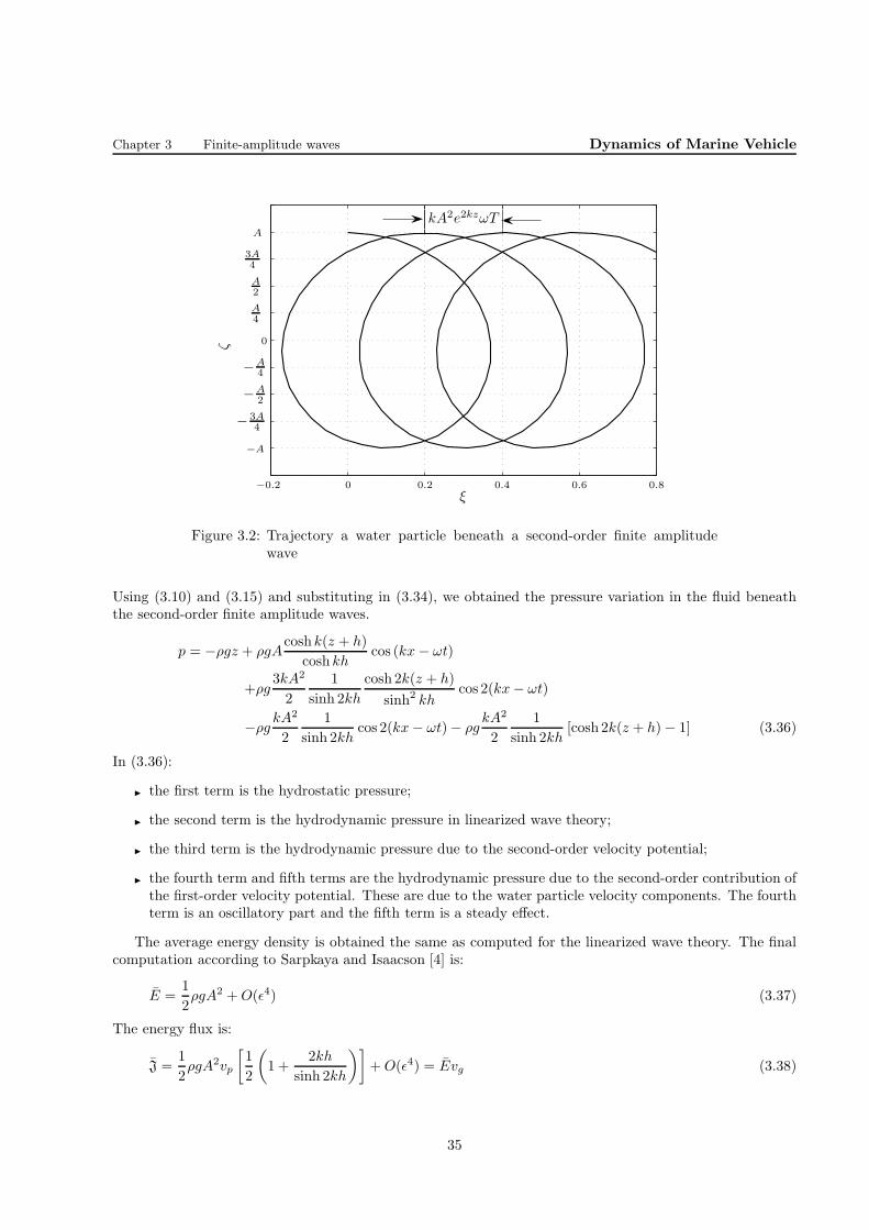
Chapter 3 Finite-amplitude waves Dynamics of Marine Vehicle
−A
A
−A2
A2
−A4
A4
− 3A4
3A4
kA2e2kzωT
ξ
ζ
−0.2 0.2 0.4 0.6 0.8
0
0
Figure 3.2: Trajectory a water particle beneath a second-order finite amplitudewave
Using (3.10) and (3.15) and substituting in (3.34), we obtained the pressure variation in the fluid beneaththe second-order finite amplitude waves.
p = −ρgz + ρgAcoshk(z + h)
coshkhcos (kx− ωt)
+ρg3kA2
2
1
sinh 2kh
cosh 2k(z + h)
sinh2 khcos 2(kx− ωt)
−ρgkA2
2
1
sinh 2khcos 2(kx− ωt)− ρg
kA2
2
1
sinh 2kh[cosh 2k(z + h)− 1] (3.36)
In (3.36):
◮ the first term is the hydrostatic pressure;
◮ the second term is the hydrodynamic pressure in linearized wave theory;
◮ the third term is the hydrodynamic pressure due to the second-order velocity potential;
◮ the fourth term and fifth terms are the hydrodynamic pressure due to the second-order contribution ofthe first-order velocity potential. These are due to the water particle velocity components. The fourthterm is an oscillatory part and the fifth term is a steady effect.
The average energy density is obtained the same as computed for the linearized wave theory. The finalcomputation according to Sarpkaya and Isaacson [4] is:
E =1
2ρgA2 +O(ǫ4) (3.37)
The energy flux is:
J =1
2ρgA2vp
[1
2
(
1 +2kh
sinh 2kh
)]
+O(ǫ4) = Evg (3.38)
35
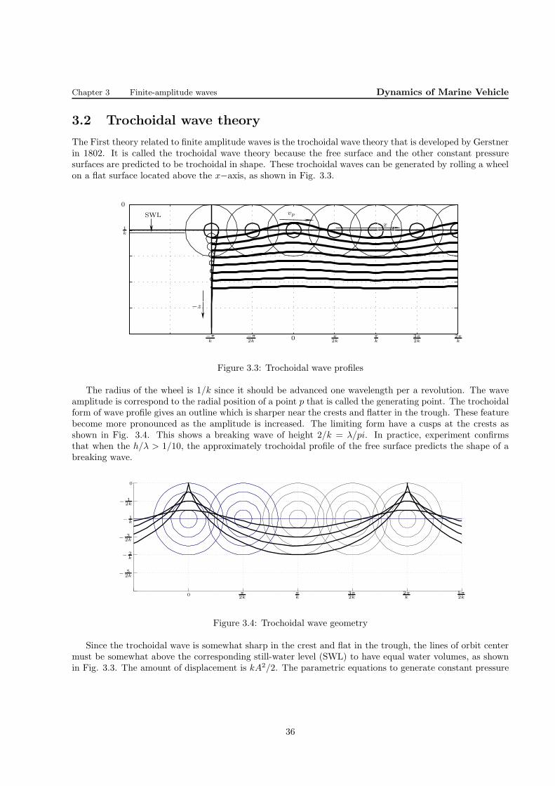
Chapter 3 Finite-amplitude waves Dynamics of Marine Vehicle
3.2 Trochoidal wave theory
The First theory related to finite amplitude waves is the trochoidal wave theory that is developed by Gerstnerin 1802. It is called the trochoidal wave theory because the free surface and the other constant pressuresurfaces are predicted to be trochoidal in shape. These trochoidal waves can be generated by rolling a wheelon a flat surface located above the x−axis, as shown in Fig. 3.3.
SWL
−πk
−π2k
π2k
πk
3π2k
2πk
0
0
x
−z
1k
vp
Figure 3.3: Trochoidal wave profiles
The radius of the wheel is 1/k since it should be advanced one wavelength per a revolution. The waveamplitude is correspond to the radial position of a point p that is called the generating point. The trochoidalform of wave profile gives an outline which is sharper near the crests and flatter in the trough. These featurebecome more pronounced as the amplitude is increased. The limiting form have a cusps at the crests asshown in Fig. 3.4. This shows a breaking wave of height 2/k = λ/pi. In practice, experiment confirmsthat when the h/λ > 1/10, the approximately trochoidal profile of the free surface predicts the shape of abreaking wave.
0
0 π2k
πk
3π2k
2πk
5π2k
−12k
−1k
−32k
−2k
−52k
Figure 3.4: Trochoidal wave geometry
Since the trochoidal wave is somewhat sharp in the crest and flat in the trough, the lines of orbit centermust be somewhat above the corresponding still-water level (SWL) to have equal water volumes, as shownin Fig. 3.3. The amount of displacement is kA2/2. The parametric equations to generate constant pressure
36
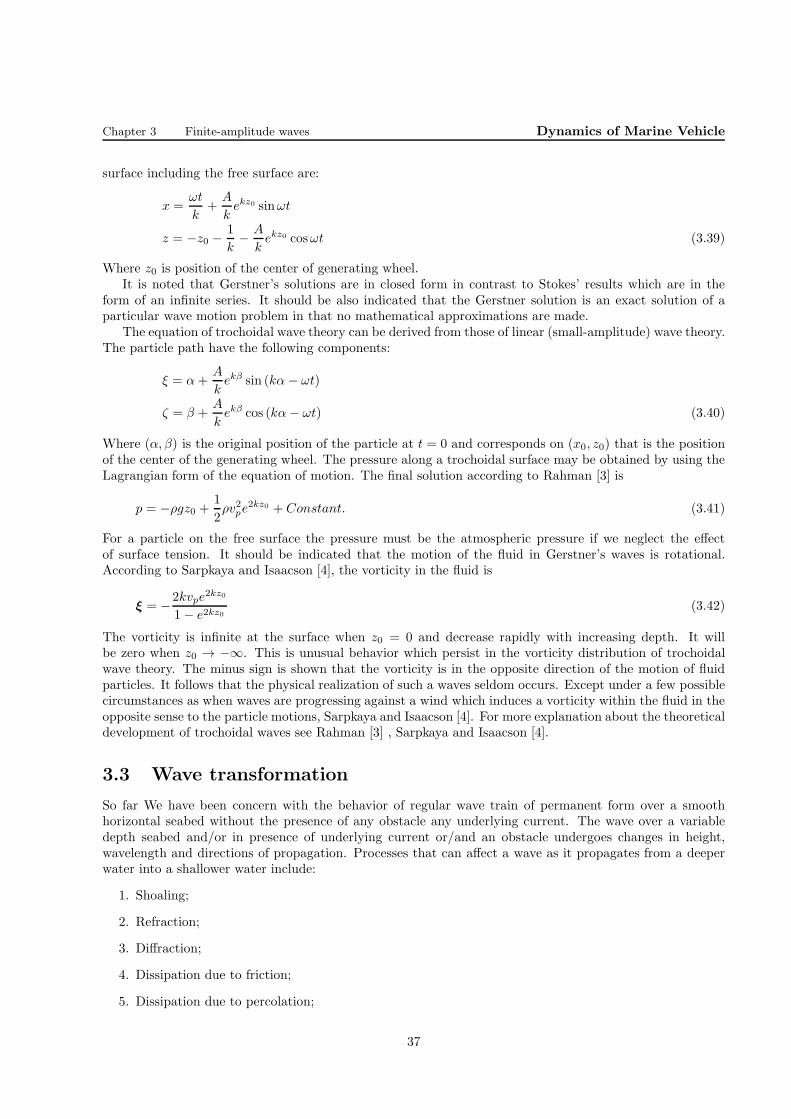
Chapter 3 Finite-amplitude waves Dynamics of Marine Vehicle
surface including the free surface are:
x =ωt
k+
A
kekz0 sinωt
z = −z0 −1
k− A
kekz0 cosωt (3.39)
Where z0 is position of the center of generating wheel.It is noted that Gerstner’s solutions are in closed form in contrast to Stokes’ results which are in the
form of an infinite series. It should be also indicated that the Gerstner solution is an exact solution of aparticular wave motion problem in that no mathematical approximations are made.
The equation of trochoidal wave theory can be derived from those of linear (small-amplitude) wave theory.The particle path have the following components:
ξ = α+A
kekβ sin (kα− ωt)
ζ = β +A
kekβ cos (kα− ωt) (3.40)
Where (α, β) is the original position of the particle at t = 0 and corresponds on (x0, z0) that is the positionof the center of the generating wheel. The pressure along a trochoidal surface may be obtained by using theLagrangian form of the equation of motion. The final solution according to Rahman [3] is
p = −ρgz0 +1
2ρv2pe
2kz0 + Constant. (3.41)
For a particle on the free surface the pressure must be the atmospheric pressure if we neglect the effectof surface tension. It should be indicated that the motion of the fluid in Gerstner’s waves is rotational.According to Sarpkaya and Isaacson [4], the vorticity in the fluid is
ξ = −2kvpe2kz0
1− e2kz0(3.42)
The vorticity is infinite at the surface when z0 = 0 and decrease rapidly with increasing depth. It willbe zero when z0 → −∞. This is unusual behavior which persist in the vorticity distribution of trochoidalwave theory. The minus sign is shown that the vorticity is in the opposite direction of the motion of fluidparticles. It follows that the physical realization of such a waves seldom occurs. Except under a few possiblecircumstances as when waves are progressing against a wind which induces a vorticity within the fluid in theopposite sense to the particle motions, Sarpkaya and Isaacson [4]. For more explanation about the theoreticaldevelopment of trochoidal waves see Rahman [3] , Sarpkaya and Isaacson [4].
3.3 Wave transformation
So far We have been concern with the behavior of regular wave train of permanent form over a smoothhorizontal seabed without the presence of any obstacle any underlying current. The wave over a variabledepth seabed and/or in presence of underlying current or/and an obstacle undergoes changes in height,wavelength and directions of propagation. Processes that can affect a wave as it propagates from a deeperwater into a shallower water include:
1. Shoaling;
2. Refraction;
3. Diffraction;
4. Dissipation due to friction;
5. Dissipation due to percolation;
37
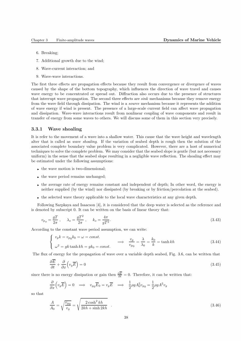
Chapter 3 Finite-amplitude waves Dynamics of Marine Vehicle
6. Breaking;
7. Additional growth due to the wind;
8. Wave-current interaction; and
9. Wave-wave interactions.
The first three effects are propagation effects because they result from convergence or divergence of wavescaused by the shape of the bottom topography, which influences the direction of wave travel and causeswave energy to be concentrated or spread out. Diffraction also occurs due to the presence of structuresthat interrupt wave propagation. The second three effects are sink mechanisms because they remove energyfrom the wave field through dissipation. The wind is a source mechanism because it represents the additionof wave energy if wind is present. The presence of a large-scale current field can affect wave propagationand dissipation. Wave-wave interactions result from nonlinear coupling of wave components and result intransfer of energy from some waves to others. We will discuss some of them in this section very precisely.
3.3.1 Wave shoaling
It is refer to the movement of a wave into a shallow water. This cause that the wave height and wavelengthalter that is called as wave shoaling. If the variation of seabed depth is rough then the solution of theassociated complete boundary value problem is very complicated. However, there are a host of numericaltechniques to solve the complete problem. We may consider that the seabed slope is gentle (but not necessaryuniform) in the sense that the seabed slope resulting in a negligible wave reflection. The shoaling effect maybe estimated under the following assumptions:
◮ the wave motion is two-dimensional;
◮ the wave period remains unchanged;
◮ the average rate of energy remains constant and independent of depth; In other word, the energy isneither supplied (by the wind) nor dissipated (by breaking or by friction/percolation at the seabed).
◮ the selected wave theory applicable to the local wave characteristics at any given depth.
Following Sarpkaya and Isaacson [4], it is considered that the deep water is selected as the reference andis denoted by subscript 0. It can be written on the basis of linear theory that:
vpo =gT
2π, λo =
gT 2
2π, ko =
4π
gT 2. (3.43)
According to the constant wave period assumption, we can write:
vpk = vp0k0 = ω = const.
ω2 = gk tanh kh = gk0 = const.=⇒ vp
vp0=
λ
λ0=
k0k
= tanhkh (3.44)
The flux of energy for the propagation of wave over a variable depth seabed, Fig. 3.6, can be written that
∂E
∂t+
∂
∂x
(
vgE)
= 0 (3.45)
since there is no energy dissipation or gain then ∂E∂t = 0. Therefore, it can be written that:
∂
∂x
(
vgE)
= 0 =⇒ vg0E0 = vgE =⇒ 1
2ρgA2
0vg0 =1
2ρgA2vg
so that
A
A0=
√vg0vg
=
√
2 cosh2 kh
2kh+ sinh 2kh. (3.46)
38
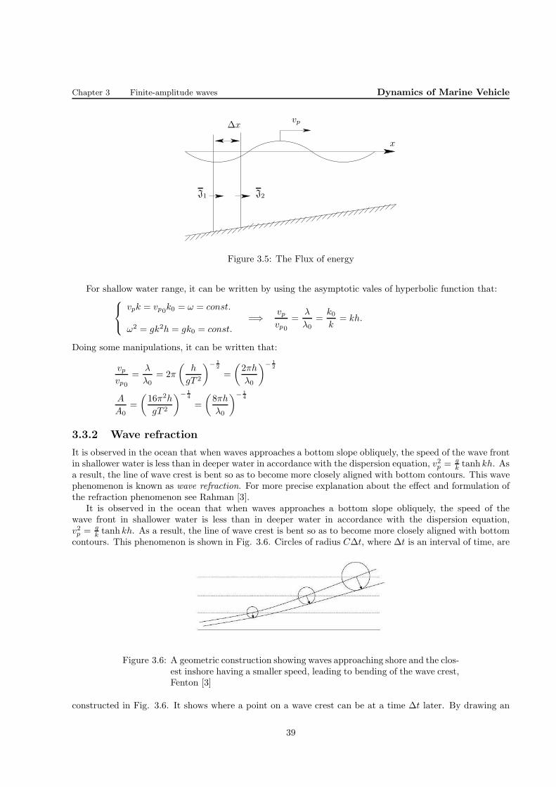
Chapter 3 Finite-amplitude waves Dynamics of Marine Vehicle
∆x
x
J1 J2
vp
Figure 3.5: The Flux of energy
For shallow water range, it can be written by using the asymptotic vales of hyperbolic function that:
vpk = vp0k0 = ω = const.
ω2 = gk2h = gk0 = const.=⇒ vp
vp0=
λ
λ0=
k0k
= kh.
Doing some manipulations, it can be written that:
vpvp0
=λ
λ0= 2π
(h
gT 2
)− 12
=
(2πh
λ0
)− 12
A
A0=
(16π2h
gT 2
)− 14
=
(8πh
λ0
)− 14
3.3.2 Wave refraction
It is observed in the ocean that when waves approaches a bottom slope obliquely, the speed of the wave frontin shallower water is less than in deeper water in accordance with the dispersion equation, v2p = g
k tanh kh. Asa result, the line of wave crest is bent so as to become more closely aligned with bottom contours. This wavephenomenon is known as wave refraction. For more precise explanation about the effect and formulation ofthe refraction phenomenon see Rahman [3].
It is observed in the ocean that when waves approaches a bottom slope obliquely, the speed of thewave front in shallower water is less than in deeper water in accordance with the dispersion equation,v2p = g
k tanh kh. As a result, the line of wave crest is bent so as to become more closely aligned with bottomcontours. This phenomenon is shown in Fig. 3.6. Circles of radius C∆t, where ∆t is an interval of time, are
Figure 3.6: A geometric construction showing waves approaching shore and the clos-est inshore having a smaller speed, leading to bending of the wave crest,Fenton [3]
constructed in Fig. 3.6. It shows where a point on a wave crest can be at a time ∆t later. By drawing an
39

Chapter 3 Finite-amplitude waves Dynamics of Marine Vehicle
envelope to all such circles we have an approximation to the wave crest at the later time, and it is clear thatit has apparently turned towards shallower water. The wave is subject to a continuous refraction which tendsto align the wave front to the depth contours. This phenomenon is illustrated in Fig. 3.7 where all depthcontours evenly spaced and parallel to the shoreline. If a wave crest initially has some angle of approach to
Figure 3.7: Straight shore with all depth contours evenly spaced and parallel to theshoreline, Coastal engineering manual [1]
the shore other than 0o, part of the wave at point A will be in shallower water than another part at point Band because the depth at A, hA, is less than the depth at B, hB, the speed of the wave at A will be slowerthan that at B according to dispersion equation.
CA =g
ωtanh khA <
g
ωtanh khB = CB
The speed differential along the wave crest causes the crest to turn more parallel to shore. The propagationproblem becomes one of plotting the direction of wave approach and calculating its height as the wavepropagates from deep to shallow water. For the case of monochromatic waves, wave period remains constant,as applied in description of shoaling. In the case of an irregular wave train, the transformation process mayaffect waves at each frequency differently; consequently, the peak period of the wave field may shift.
3.3.3 Wave breaking
Waves approaches the coast increase in steepness as water depth decrease. The shoaling coefficient indicatesthat the wave height will approach infinity in very shallow water, which is not realistic. At some depth, awave of given characteristics will become unstable and break, dissipating energy in the form of turbulence.When designing a structure which at times may be inside the surf zone it becomes necessary to be able topredict the location of the breaker line. The surf zone is the region extending from seaward boundary of wavebreaking to the limit of wave uprush. Within the surf zone, wave breaking is the dominant hydrodynamicprocess.
Waves break as they reach a limiting steepness which depends on the nature of the bottom and thecharacteristics of the wave. The limiting steepness is a function of relative depth h/λ and the slope of thebottom m = tanβ. There are three main types of wave breaking that are illustrated in Fig. 3.8.
• Spilling breakers : For very mildly sloping beaches, typically the waves are spilling breakers, and ischaracterized by breaking gradually over a long distance such that many waves occur within the surfzone (defined as that region where the waves are breaking, extending from the beach to the seawardlimit of the breaking). The rate of energy loss is small, permitting a nearly complete reforming of thewaves should they once again progress into deep water, such as when they cross a sand bar. The wave
40
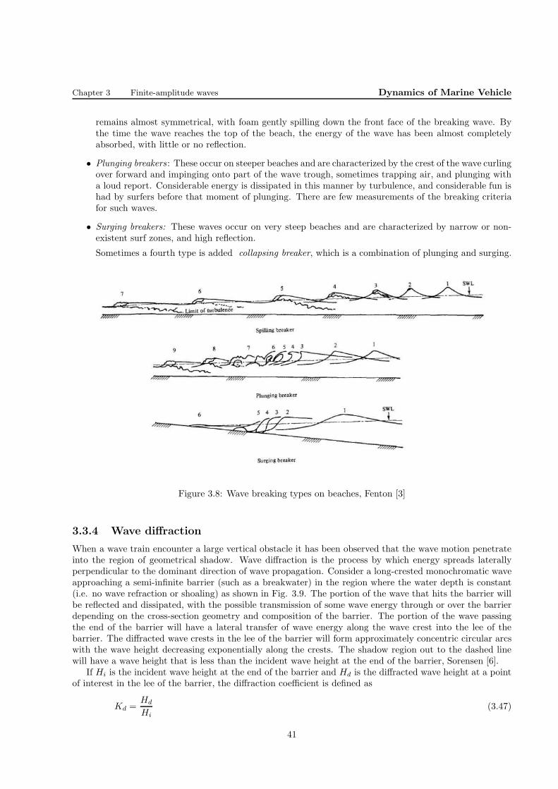
Chapter 3 Finite-amplitude waves Dynamics of Marine Vehicle
remains almost symmetrical, with foam gently spilling down the front face of the breaking wave. Bythe time the wave reaches the top of the beach, the energy of the wave has been almost completelyabsorbed, with little or no reflection.
• Plunging breakers : These occur on steeper beaches and are characterized by the crest of the wave curlingover forward and impinging onto part of the wave trough, sometimes trapping air, and plunging witha loud report. Considerable energy is dissipated in this manner by turbulence, and considerable fun ishad by surfers before that moment of plunging. There are few measurements of the breaking criteriafor such waves.
• Surging breakers: These waves occur on very steep beaches and are characterized by narrow or non-existent surf zones, and high reflection.
Sometimes a fourth type is added collapsing breaker, which is a combination of plunging and surging.
Figure 3.8: Wave breaking types on beaches, Fenton [3]
3.3.4 Wave diffraction
When a wave train encounter a large vertical obstacle it has been observed that the wave motion penetrateinto the region of geometrical shadow. Wave diffraction is the process by which energy spreads laterallyperpendicular to the dominant direction of wave propagation. Consider a long-crested monochromatic waveapproaching a semi-infinite barrier (such as a breakwater) in the region where the water depth is constant(i.e. no wave refraction or shoaling) as shown in Fig. 3.9. The portion of the wave that hits the barrier willbe reflected and dissipated, with the possible transmission of some wave energy through or over the barrierdepending on the cross-section geometry and composition of the barrier. The portion of the wave passingthe end of the barrier will have a lateral transfer of wave energy along the wave crest into the lee of thebarrier. The diffracted wave crests in the lee of the barrier will form approximately concentric circular arcswith the wave height decreasing exponentially along the crests. The shadow region out to the dashed linewill have a wave height that is less than the incident wave height at the end of the barrier, Sorensen [6].
If Hi is the incident wave height at the end of the barrier and Hd is the diffracted wave height at a pointof interest in the lee of the barrier, the diffraction coefficient is defined as
Kd =Hd
Hi(3.47)
41

Chapter 3 Finite-amplitude waves Dynamics of Marine Vehicle
Figure 3.9: Wave diffraction and definition of terms, Sorensen [6]
where Hd is the diffracted wave height at a point in the lee of the barrier and Hi is the incident wave heightat the breakwater tip.The value of the diffraction coefficient Kd depends on the location behind the barrierdefined by r and β, and the incident wave direction θ. It can be write that Kd = f(θ, r
λ , β) where λ is thewave length. Since the wave length is a function of the wave period and water depth, the resulting diffractioncoefficient for each component of the wave spectrum would depend on the incident direction and period ofthat component.
When waves approach a barrier of finite length and wave diffraction occurs at both ends, a wave crestpattern similar to that shown in Fig. 3.10 will develop. It can be constructed by combining the patternsfor semi-infinite barrier diffraction at each end. The wave crests combine along lines like the dashed line toform the higher amplitudes which may be estimated (assuming linear waves) by combining the heights fromthe two separate patterns.
Figure 3.10: Wave diffraction in the lee of a barrier of finite length, Sorensen [6].
42

Chapter 3 Finite-amplitude waves Dynamics of Marine Vehicle
When waves pass through a gap in a barrier, diffraction occurs in the lee of the barrier on both sides ofthe gap. As the waves propagate further and passing the gap of the barrier, the zone affected by diffractiongrows toward the center line of the gap until the two diffraction zones interact, as shown in Fig. 3.11. Theinteraction point is depends on the width of the gap, the wider the gap, the further behind the barrier thisinteraction point occurs. For typical harbor conditions and gap widths greater than about five wavelengths,suggests that the diffraction patterns at each side of the gap opening will be independent of each other. Forsmaller gap widths, an analysis employing the gap geometry must be used.
Figure 3.11: Wave diffraction through a gap, Coastal engineering manual, [1].
The waves approaching a barrier gap will usually not approach in an angle of 90o (in direction normalto the gap). The results for normally incident waves can be used as an approximation for oblique waves byemploying a projected imaginary gap width as shown in Fig. 3.12.
Figure 3.12: Oblique wave incident to a barrier gap, Sorensen [6]
43

Bibliography
[1] Coastal manual engineering, Part II, 2008
[2] Dean, R. G. and Dalrymple, R. A., Water wave mechanics for engineers and scientists, World ScientificPublishing Co., 2000
[3] Fenton, J., Coastal and ocean Engineering, 2013
[4] Rahman, M., Water waves, relating modern theory to advanced engineering applications, Oxford Uni-verisit press, 1994
[5] Sarpkaya, T. and Isaacson, M., Mechanics of wave forces on offshore structures, Van Nostrand ReinholdCompany, 1981
[6] Sorensen, R. M., Basic coastal engineering, Springer, 2006
44

Chapter 4
Real ocean Waves
4.1 Introduction
In practice, ocean waves are not regular but random in the sense that the ocean surface is composed of wavesmoving in different directions and with different amplitudes, frequencies and phases. The wind causes theformation of waves on the free surface of oceans. The variation of the ocean surface is depend on the windspeed. The ocean surface varies from time to time and place to place. The Beaufort number is a means toestimate and report the wind speed and sea state. An individual can derive a Beaufort number and hencea wind speed by observing the ocean surface. Wave traveling out of a distance generating area are calledswells while waves generating locally are known as sea.
Since the ocean waves are random in nature, they should be describes by their statistical properties. Thischapter is started with description of the statistical properties of a random signal x(t) varying continuouslywith time t. Then, these statistical definition are applied to the random wave field. The random signalmay be the free surface elevation η(t) and/or the other wave characteristics and wave effects such as a waveinduced force F (t) on a structure.
4.2 Statistical and probabilistic definitions
The field of statistics deals with the collection, presentation, analysis, and use of data to make decisions, solveproblems, and design products and processes. In simple terms, statistics is the science of data. Statisticalmethods are used to help us describe and understand variability. By variability, it means that successiveobservations of a system or phenomenon do not produce exactly the same result.
Often data are collected over time. In this case, it is usually very helpful to plot the data versus timein a time series plot. Phenomena that might affect the system or process often become more visible ina time-oriented plot and the concept of stability can be better judged. An experiment that can result indifferent outcomes, even though it is repeated in the same manner every time, is called a random experiment.The set of all possible outcomes of a random experiment is called the sample space of the experiment. Thesample space is denoted as S. A sample space is discrete if it consists of a finite or countable infinite set ofoutcomes. A sample space is continuous if it contains an interval (either finite or infinite) of real numbers.An event is a subset of the sample space of a random experiment.
Probability is a number that is assigned to each member of a collection of events from a random experimentthat satisfies the following properties:If S is the sample space and E is any event in a random experiment,
(1) P (S) = 1
(2) 0 ≤ P (E) ≤ 1
(3) For two events E1 and E2 with E1 ∩ E2 = ⊘ P (E1 ∪ E2) = P (E1) + P (E2)
Whenever a sample space consists of N possible outcomes that are equally likely, the probability of eachoutcome is 1
N .
45

Chapter 4 Real ocean Waves Dynamics of Marine Vehicle
Beaufort Description Wind speed Wave height Sea conditions
number km/h kts m/s m ft
0 calm <1 <1 <0.3 0 0 Flat
1 Light air 1.1 − 5.5 1 − 2 0.3 − 1.5 0 − 0.2 0 − 1 Ripples without crests
2 Light breeze 5.6 − 11 3 − 6 1.6 − 3.4 0.2 − 0.5 1 2 Small wavelets.
3 Gentle breeze 12 − 19 7 − 10 3.4 − 5.4 0.5 − 1 2 − 3.5 Large wavelets.
4 Moderate breeze 20 − 28 11 − 15 5.5 − 7.9 1 − 2 3.5 − 6 Small waves with breaking crests.
5 Fresh breeze 29 − 38 16 − 20 8.0 − 10.7 2 − 3 6 − 9 Moderate waves of some length
6 Strong breeze 39 − 49 21 − 26 10.8 − 13.8 3 − 4 9 − 13 Long waves begin to form.
7 High wind 50 − 61 27 − 33 13.9 − 17.1 4 − 5.5 13 − 19 Sea heaps up.
8 Gale, Fresh gale 62 − 74 34 − 40 17.2 − 20.7 5.5 − 7.5 18 − 25 Moderately high waves
9 Strong gale 75 − 88 41 − 47 20.8 − 24.4 7 − 10 23 − 32 High waves
10 Storm 89 − 102 48 − 55 24.5 − 28.4 9 − 12.5 29 − 41 Very high waves
11 Violent storm 103 − 117 56 − 63 28.5 − 32.6 11.5 − 16 37 − 52 Exceptionally high waves.
12 Hurricane-force ≥118 ≥64 ≥32.7 ≥14 ≥46 Huge waves
Table 4.1: The modern Beaufort scale, From Wikipedia, the free encyclopedia [5]
A probability density function p(x) can be used to describe the probability distribution of a continuousrandom variable X . If an interval is likely to contain a value for X, its probability is large and it correspondsto large values for p(x). For a continuous random variable X , a probability density function is a functionsuch that:
(1) p(x) ≥ 0
(2)∫∞
−∞p(x)dx = 1
(3) P (a ≤ X ≤ b) =∫ b
ap(x)dx = area under p(x) from a to b
for any a and b
A probability density function provides a simple description of the probabilities associated with a random
variable. As long as p(x) is non-negative and f(x) =∫∞
−∞p(x)dx = 1, 0 ≤ P (a ≤ X ≤ b) =
∫ b
a p(x)dx ≤ 1so that the probabilities are properly restricted. A probability density function is zero for x values thatcannot occur and it is assumed to be zero wherever it is not specifically defined. If X is a continuous randomvariable, for any x1 and x2
P (x1 ≤ X ≤ x2) = P (x1 < X ≤ x2) = P (x1 ≤ X < x2) = P (x1 < X < x2)
The cumulative distribution function of a continuous random variable X is
P (X ≤ x) =
∫ x
−∞
p(u)du −∞ < x < ∞ (4.1)
The probability density function of a continuous random variable can be determined from the cumulativedistribution function by differentiating. Recall that the fundamental theorem of calculus states that
d
dx
∫ ∞
−∞
p(u)du = p(x)
Then, given P (x),
p(x) =P (x)
dx(4.2)
as long as the derivative exists.
46
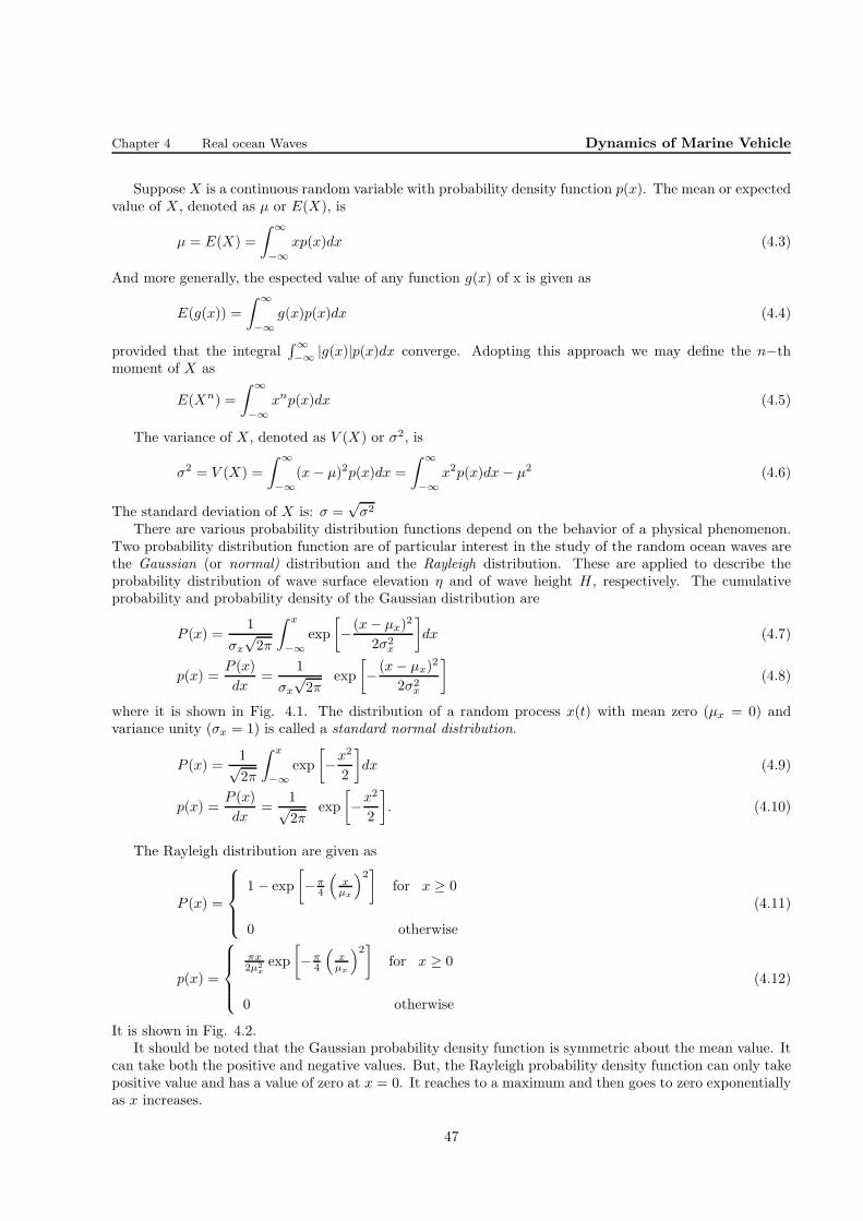
Chapter 4 Real ocean Waves Dynamics of Marine Vehicle
Suppose X is a continuous random variable with probability density function p(x). The mean or expectedvalue of X , denoted as µ or E(X), is
µ = E(X) =
∫ ∞
−∞
xp(x)dx (4.3)
And more generally, the espected value of any function g(x) of x is given as
E(g(x)) =
∫ ∞
−∞
g(x)p(x)dx (4.4)
provided that the integral∫∞
−∞|g(x)|p(x)dx converge. Adopting this approach we may define the n−th
moment of X as
E(Xn) =
∫ ∞
−∞
xnp(x)dx (4.5)
The variance of X , denoted as V (X) or σ2, is
σ2 = V (X) =
∫ ∞
−∞
(x− µ)2p(x)dx =
∫ ∞
−∞
x2p(x)dx − µ2 (4.6)
The standard deviation of X is: σ =√σ2
There are various probability distribution functions depend on the behavior of a physical phenomenon.Two probability distribution function are of particular interest in the study of the random ocean waves arethe Gaussian (or normal) distribution and the Rayleigh distribution. These are applied to describe theprobability distribution of wave surface elevation η and of wave height H , respectively. The cumulativeprobability and probability density of the Gaussian distribution are
P (x) =1
σx
√2π
∫ x
−∞
exp
[
− (x− µx)2
2σ2x
]
dx (4.7)
p(x) =P (x)
dx=
1
σx
√2π
exp
[
− (x− µx)2
2σ2x
]
(4.8)
where it is shown in Fig. 4.1. The distribution of a random process x(t) with mean zero (µx = 0) andvariance unity (σx = 1) is called a standard normal distribution.
P (x) =1√2π
∫ x
−∞
exp
[
−x2
2
]
dx (4.9)
p(x) =P (x)
dx=
1√2π
exp
[
−x2
2
]
. (4.10)
The Rayleigh distribution are given as
P (x) =
1− exp
[
−π4
(xµx
)2]
for x ≥ 0
0 otherwise
(4.11)
p(x) =
πx2µ2
xexp
[
−π4
(xµx
)2]
for x ≥ 0
0 otherwise
(4.12)
It is shown in Fig. 4.2.It should be noted that the Gaussian probability density function is symmetric about the mean value. It
can take both the positive and negative values. But, the Rayleigh probability density function can only takepositive value and has a value of zero at x = 0. It reaches to a maximum and then goes to zero exponentiallyas x increases.
47

Chapter 4 Real ocean Waves Dynamics of Marine Vehicle
Figure 4.1: The Gaussian probability density and cumulative probability distribution
Figure 4.2: The Raleigh probability density and cumulative probability distribution
4.2.1 Basic definitions and concept of random process
Let us begin with an ensemble of k wave records xk(t) taken under identical macroscopic conditions, i.e.:position on the ocean surface, water depth, mean wind velocity, air-sea temperature. Even under identicalconditions, we cannot expect that these wave records will be identical or even closely similar in detail. Thefamily xk(t) represents k realizations of the stochastic process x(t). For a given k, x(t) is a function of time,while when t = t1, xk(t) is a random variable. Stochastic processes may belong to one of three categories:
a - Stationary and ergodic;
b - Stationary; and
c - Non-stationary.
48
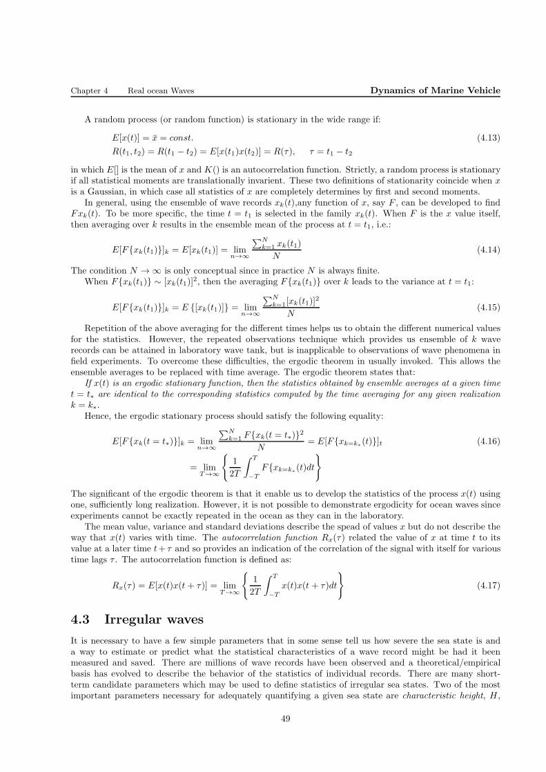
Chapter 4 Real ocean Waves Dynamics of Marine Vehicle
A random process (or random function) is stationary in the wide range if:
E[x(t)] = x = const. (4.13)
R(t1, t2) = R(t1 − t2) = E[x(t1)x(t2)] = R(τ), τ = t1 − t2
in which E[] is the mean of x and K() is an autocorrelation function. Strictly, a random process is stationaryif all statistical moments are translationally invarient. These two definitions of stationarity coincide when xis a Gaussian, in which case all statistics of x are completely determines by first and second moments.
In general, using the ensemble of wave records xk(t),any function of x, say F , can be developed to findFxk(t). To be more specific, the time t = t1 is selected in the family xk(t). When F is the x value itself,then averaging over k results in the ensemble mean of the process at t = t1, i.e.:
E[F{xk(t1)}]k = E[xk(t1)] = limn→∞
∑Nk=1 xk(t1)
N(4.14)
The condition N → ∞ is only conceptual since in practice N is always finite.When F{xk(t1)} ∼ [xk(t1)]
2, then the averaging F{xk(t1)} over k leads to the variance at t = t1:
E[F{xk(t1)}]k = E {[xk(t1)]} = limn→∞
∑Nk=1[xk(t1)]
2
N(4.15)
Repetition of the above averaging for the different times helps us to obtain the different numerical valuesfor the statistics. However, the repeated observations technique which provides us ensemble of k waverecords can be attained in laboratory wave tank, but is inapplicable to observations of wave phenomena infield experiments. To overcome these difficulties, the ergodic theorem in usually invoked. This allows theensemble averages to be replaced with time average. The ergodic theorem states that:
If x(t) is an ergodic stationary function, then the statistics obtained by ensemble averages at a given timet = t∗ are identical to the corresponding statistics computed by the time averaging for any given realizationk = k∗.
Hence, the ergodic stationary process should satisfy the following equality:
E[F{xk(t = t∗)}]k = limn→∞
∑Nk=1 F{xk(t = t∗)}2
N= E[F{xk=k∗
(t)}]t (4.16)
= limT→∞
{
1
2T
∫ T
−T
F{xk=k∗(t)dt
}
The significant of the ergodic theorem is that it enable us to develop the statistics of the process x(t) usingone, sufficiently long realization. However, it is not possible to demonstrate ergodicity for ocean waves sinceexperiments cannot be exactly repeated in the ocean as they can in the laboratory.
The mean value, variance and standard deviations describe the spead of values x but do not describe theway that x(t) varies with time. The autocorrelation function Rx(τ) related the value of x at time t to itsvalue at a later time t+ τ and so provides an indication of the correlation of the signal with itself for varioustime lags τ . The autocorrelation function is defined as:
Rx(τ) = E[x(t)x(t + τ)] = limT→∞
{
1
2T
∫ T
−T
x(t)x(t + τ)dt
}
(4.17)
4.3 Irregular waves
It is necessary to have a few simple parameters that in some sense tell us how severe the sea state is anda way to estimate or predict what the statistical characteristics of a wave record might be had it beenmeasured and saved. There are millions of wave records have been observed and a theoretical/empiricalbasis has evolved to describe the behavior of the statistics of individual records. There are many short-term candidate parameters which may be used to define statistics of irregular sea states. Two of the mostimportant parameters necessary for adequately quantifying a given sea state are characteristic height, H ,
49
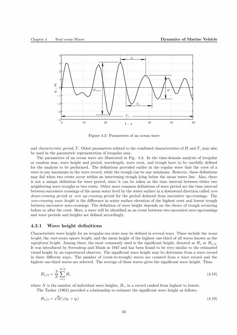
Chapter 4 Real ocean Waves Dynamics of Marine Vehicle
0 10 20 40 50 60
0
1
2
3
4
−1
−2
−3
−4
t , s
η,m
Tc
Tz
HHmax
Tsi
Figure 4.3: Parameters of an ocean wave
and characteristic period, T . Other parameters related to the combined characteristics of H and T , may alsobe used in the parametric representation of irregular seas.
The parameters of an ocean wave are illustrated in Fig. 4.3. In the time-domain analysis of irregularor random seas, wave height and period, wavelength, wave crest, and trough have to be carefully definedfor the analysis to be performed. The definitions provided earlier in the regular wave that the crest of awave is any maximum in the wave record, while the trough can be any minimum. However, these definitionsmay fail when two crests occur within an intervening trough lying below the mean water line. Also, thereis not a unique definition for wave period, since it can be taken as the time interval between either twoneighboring wave troughs or two crests. Other more common definitions of wave period are the time intervalbetween successive crossings of the mean water level by the water surface in a downward direction called zerodown-crossing period or zero up-crossing period for the period deduced from successive up-crossings. Thezero-crossing wave height is the difference in water surface elevation of the highest crest and lowest troughbetween successive zero-crossings. The definition of wave height depends on the choice of trough occurringbefore or after the crest. Here, a wave will be identified as an event between two successive zero-upcrossingsand wave periods and heights are defined accordingly.
4.3.1 Wave height definitions
Characteristic wave height for an irregular sea state may be defined in several ways. These include the meanheight, the root-mean-square height, and the mean height of the highest one-third of all waves known as thesignificant height. Among these, the most commonly used is the significant height, denoted as Hs or H1/3.It was introduced by Sverndrup and Munk in 1947 and has been found to be very similar to the estimatedvisual height by an experienced observer. The significant wave height may be determine from a wave recordin three different ways. The number of (crest-to-trough) waves are counted from a wave record and thehighest one-third waves are selected. The average of these waves gives the significant wave height. Thus:
H1/3 =3
N
N/3∑
i=1
Hi (4.18)
where N is the number of individual wave heights, Hi, in a record ranked from highest to lowest.The Tucker (1963) provided a relationship to estimate the significant wave height as follows.
H1/3 =√2C1(ηc + ηt) (4.19)
50

Chapter 4 Real ocean Waves Dynamics of Marine Vehicle
The notation ηc is the height of the highest crest in a wave record and ηt is and the depth of the lowesttrough. The coefficient C1 is calculated by knowing the the number of zero up-crossing cycles Nz.
C1 = (lnNz)−1/2
[
1 + 0.289 (lnNz)−1 − 0.247 (lnNz)
−2]−1
(4.20)
Similarly, Hp is defined as the average of the first highest pN recorded waves, p = 1/n, where n =10, · · · , 100.
Hp =1
pN
pN∑
i=1
Hi (4.21)
The mean height H is the average wave height over all records,
H = H1 =1
N
N∑
i=1
Hi (4.22)
If there are N waves of heightsH1, H2, · · · , HN , then the root mean square (rms) wave height is calculatedby the formula
Hrms =
√√√√ 1
N
N∑
i=1
H2i (4.23)
The root mean square wave height is always greater than H1 in real ocean.The largest wave height or the most probable maximum wave height is related to the rms wave height by
follows according to Longuet-Higgins (1952).
Hmax =
(√lnN +
0.2886√lnN
)
Hrms (4.24)
Example - 1
A wave height from an ocean wave record are given in the following table. Find the average height, thesignificant height, the average of one-tenth and one-hundred highest wave height and the root mean squarewave height.
Wave height Number of waves of height (1)(1) (2)5 24 253 312 401 4
Solution:
Wave number of percentage Cumulative Cumulative One-third One-tenth One-hundred
height wave of waves number of number of of highest of highest of highest
[ft] height (1) waves wave height waves height waves height waves height
(1) (2) (3) (4) (5) (6) (7)
5 2 2% 2 10 10 10 5
4 25 25% 27 110 110 42
3 31 30% 58 203 131
2 40 39% 98 283
1 4 4% 102 287
100%
51
Chapter 4 Real ocean Waves Dynamics of Marine Vehicle
H = H1 =287
102= 2.81 ft or
H = µH =∑
i
ηip(ηi) =5× 2 + 4× 25 + 3× 30 + 2× 39 + 1× 4
100= 2.82 ft
H1/3 =3
102× 131 ≈ 3.85 ft
H1/10 =10
102× 42 ≈ 4.2 ft
H1/100 =100
102× 5 ≈ 5 ft
Hrms =
√√√√ 1
N
N∑
i=1
H2i =
√
2× 52 + 25× 42 + 31× 32 + 40× 22 + 4× 12
102= 2.96 [ft]
Hmax =
(√lnN +
0.2886√lnN
)
Hrms =
(√ln 102 +
0.2886√ln 102
)
2.96 = 6.76 [ft]
4.3.2 Irregular wave periods
There may be specified two types of average wave periods of a wave record.
1. Average zero-upcrossing wave period which is denoted by Tz; and
2. Average crest period which is denoted by Tc.
They are shown in Fig. 4.3.If we denote the total recording length of time by Ts, we may divide it into Nz equal interval of Tsi. The
average zero-upcrossing wave period over each interval is given by
Tzi =Tsi
Nzi
(4.25)
where Nzi is the number of zero upcrossing in time interval, i. The average zero-upcrossing wave period ofthe record is
Tz =1
Nz
Nz∑
i=1
Tzi (4.26)
Similarly, the average crest period is given for the interval i as
Tci =Tsi
Nci
(4.27)
where Nci is the number of crest to crest in time interval, i. If the number of intervals is denoted by Nc, theaverage wave crest period of the record is as follows.
Tc =1
Nc
Nc∑
i=1
Tci (4.28)
4.3.3 Probability distribution of a sea state
The probability density distribution of free surface elevation of sea η, wave height H and wave period T isintroduced in this section.
52
Chapter 4 Real ocean Waves Dynamics of Marine Vehicle
Probability distribution for the surface elevation
The sea surface elevation distribution is assumed to be Gaussian. It is based on the assumption that thecomponents phases are arbitrary but uniformly distributed in the interval of (π,−π). The Gaussian modelimplies that a symmetry distribution about the still water level that corresponds to zero mean, µη = 0.
p(η) =1
ση
√2π
exp
[
− η2
2σ2x
]
(4.29)
The probability density of water surface elevation is symmetric about the still water level where the proba-bility density is maximum. The probability of having a particular positive elevation is the same as that forthe negative elevation.
The measured data on the water surface elevation have indicated that the Gaussian distribution for ηis appropriate. For waves of appreciable amplitude, however, crest amplitudes are higher than the troughamplitudes and the sea-surface elevation are skewed, Chakrabarti [1]. In such a case, the expected value isdifferent from the still water elevation.
Probability distribution of wave height
The ocean surface is considered to be composed of a large number of sinusoidal waves with different frequen-cies, amplitudes, and phases. When these frequencies are in a narrow frequency band about ω then it is saidthat it is a narrow-band ocean. The surface elevation is obtained by superposing of different waves profiles.
η(t) =
K∑
i=1
Hi
2cos (ωit− εi) (4.30)
where Hi is the amplitude of the ith harmonic wave, ωi is the frequency of the ith harmonic wave, εi is thephase of the ith harmonic wave and K is the number of time harmonic waves. It can be written using thecomplex form as
η(t) = ℜ{
K∑
i=1
Hi
2exp
[
i(ωit− εi)]}
(4.31)
where ℜ is stand for the real part of {.}. It may be rearranged as
η(t) = ℜ{c(t) exp (iωt)} (4.32)
where
c(t) = ℜ{
K∑
i=1
Hi
2exp
{
i[(ωi − ω)t− εi
]}}
(4.33)
is the slowly varying wave group for a narrow-band spectrum. If a combination of the following four sinusoidalwaves is taken into account
η(t) =
4∑
i=1
Hi
2cos (ωit− εi)
Hi = 2 , 2.25 , 2.75 , 3
ωi =π
6,
π
5.5,
π
5,
π
4
ε =π
4,
π
3,
π
2,
2π
3
the plot of the surface elevation is as shown in Fig. 4.4. The wave profile resembles a slowly varying wavegroup.
53

Chapter 4 Real ocean Waves Dynamics of Marine Vehicle
0 60 120 180 240
0
1
2
3
4
5
−1
−2
−3
−4
−5
t, [s]
η,[m
]
Figure 4.4: Surface profile of combination of four sinusoidal waves
It has been theoretically shown by Longuet-Higgins (1952) that the wave amplitude A has a Rayleighdistribution for a narrow-band Gaussian ocean wave whose components are in random phase. According to(4.11) and (4.12), it can be written that
P (A) = 1− exp
[
−π
4
(A
µA
)2]
(4.34)
p(A) =πA
2µ2A
exp
[
−π
4
(A
µA
)2]
(4.35)
Since any single wave is closely sinusoidal for a narrow-band motion, the variance σ2A may be expressed as
the average of integrals taken over each wave. (For a single wave σ2A = A2
i /2.) In this manner, it can beobtained that
Arms =√2σA µA =
√π
2σA (4.36)
Therefore, we can write that:
P (A) = 1− exp
[
−(
A
Arms
)2]
(4.37)
p(A) =4A
A2rms
exp
[
−(
A
Arms
)2]
(4.38)
Usually, wave heights H are employed in describing ocean waves rather than the amplitude A. Assumingthat H = 2A, we can write that:
P (H) = 1− exp
[
−(
H
Hrms
)2]
(4.39)
p(H) =2H
H2rms
exp
[
−(
H
Hrms
)2]
(4.40)
The probability that a wave height is greater (less) than or equal to a design wave height H0 may befound from
P (H > H0) =m
N
P (H ≤ H0) = 1− m
N(4.41)
54
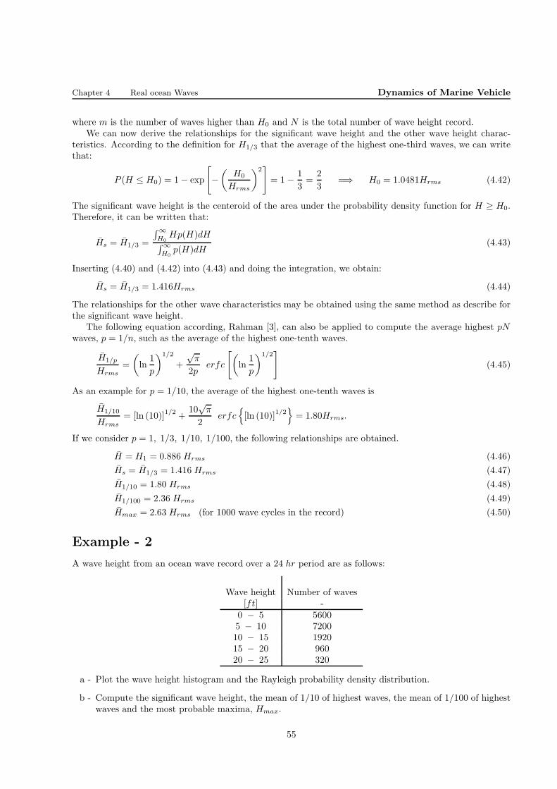
Chapter 4 Real ocean Waves Dynamics of Marine Vehicle
where m is the number of waves higher than H0 and N is the total number of wave height record.We can now derive the relationships for the significant wave height and the other wave height charac-
teristics. According to the definition for H1/3 that the average of the highest one-third waves, we can writethat:
P (H ≤ H0) = 1− exp
[
−(
H0
Hrms
)2]
= 1− 1
3=
2
3=⇒ H0 = 1.0481Hrms (4.42)
The significant wave height is the centeroid of the area under the probability density function for H ≥ H0.Therefore, it can be written that:
Hs = H1/3 =
∫∞
H0Hp(H)dH
∫∞
H0p(H)dH
(4.43)
Inserting (4.40) and (4.42) into (4.43) and doing the integration, we obtain:
Hs = H1/3 = 1.416Hrms (4.44)
The relationships for the other wave characteristics may be obtained using the same method as describe forthe significant wave height.
The following equation according, Rahman [3], can also be applied to compute the average highest pNwaves, p = 1/n, such as the average of the highest one-tenth waves.
H1/p
Hrms=
(
ln1
p
)1/2
+
√π
2perfc
[(
ln1
p
)1/2]
(4.45)
As an example for p = 1/10, the average of the highest one-tenth waves is
H1/10
Hrms= [ln (10)]1/2 +
10√π
2erfc
{
[ln (10)]1/2}
= 1.80Hrms.
If we consider p = 1, 1/3, 1/10, 1/100, the following relationships are obtained.
H = H1 = 0.886 Hrms (4.46)
Hs = H1/3 = 1.416 Hrms (4.47)
H1/10 = 1.80 Hrms (4.48)
H1/100 = 2.36 Hrms (4.49)
Hmax = 2.63 Hrms (for 1000 wave cycles in the record) (4.50)
Example - 2
A wave height from an ocean wave record over a 24 hr period are as follows:
Wave height Number of waves[ft] -
0 − 5 56005 − 10 720010 − 15 192015 − 20 96020 − 25 320
a - Plot the wave height histogram and the Rayleigh probability density distribution.
b - Compute the significant wave height, the mean of 1/10 of highest waves, the mean of 1/100 of highestwaves and the most probable maxima, Hmax.
55
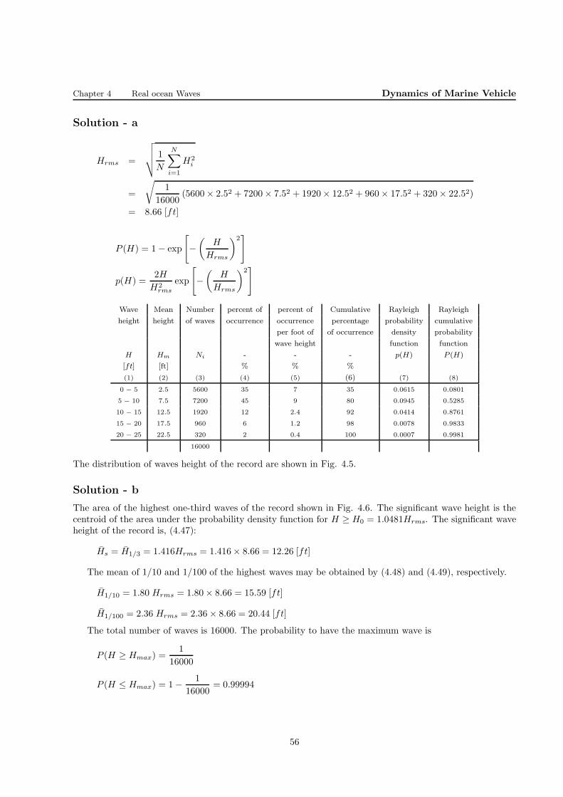
Chapter 4 Real ocean Waves Dynamics of Marine Vehicle
Solution - a
Hrms =
√√√√ 1
N
N∑
i=1
H2i
=
√
1
16000(5600× 2.52 + 7200× 7.52 + 1920× 12.52 + 960× 17.52 + 320× 22.52)
= 8.66 [ft]
P (H) = 1− exp
[
−(
H
Hrms
)2]
p(H) =2H
H2rms
exp
[
−(
H
Hrms
)2]
Wave Mean Number percent of percent of Cumulative Rayleigh Rayleigh
height height of waves occurrence occurrence percentage probability cumulative
per foot of of occurrence density probability
wave height function function
H Hm Ni - - - p(H) P (H)
[ft] [ft] % % %
(1) (2) (3) (4) (5) (6) (7) (8)
0 − 5 2.5 5600 35 7 35 0.0615 0.0801
5 − 10 7.5 7200 45 9 80 0.0945 0.5285
10 − 15 12.5 1920 12 2.4 92 0.0414 0.8761
15 − 20 17.5 960 6 1.2 98 0.0078 0.9833
20 − 25 22.5 320 2 0.4 100 0.0007 0.9981
16000
The distribution of waves height of the record are shown in Fig. 4.5.
Solution - b
The area of the highest one-third waves of the record shown in Fig. 4.6. The significant wave height is thecentroid of the area under the probability density function for H ≥ H0 = 1.0481Hrms. The significant waveheight of the record is, (4.47):
Hs = H1/3 = 1.416Hrms = 1.416× 8.66 = 12.26 [ft]
The mean of 1/10 and 1/100 of the highest waves may be obtained by (4.48) and (4.49), respectively.
H1/10 = 1.80 Hrms = 1.80× 8.66 = 15.59 [ft]
H1/100 = 2.36 Hrms = 2.36× 8.66 = 20.44 [ft]
The total number of waves is 16000. The probability to have the maximum wave is
P (H ≥ Hmax) =1
16000
P (H ≤ Hmax) = 1− 1
16000= 0.99994
56
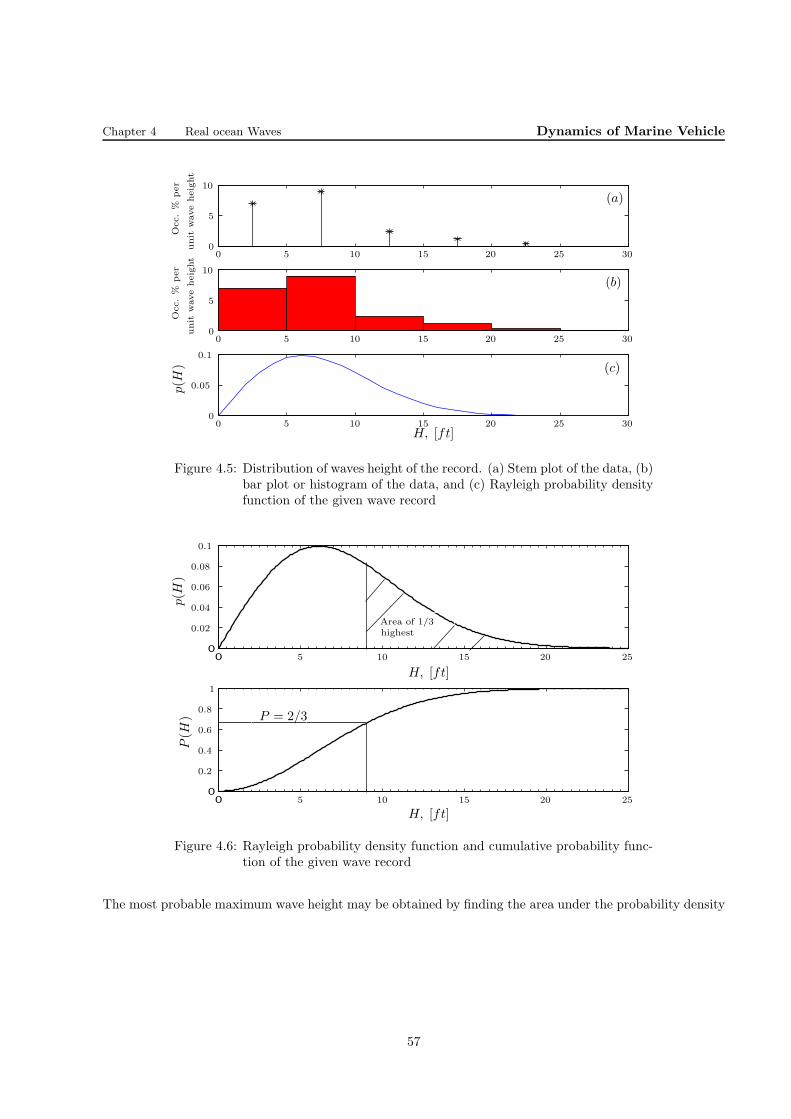
Chapter 4 Real ocean Waves Dynamics of Marine Vehicle
00
00
00
0.05
5
5
5
5
5
10
10
10
10
10
15
15
15
20
20
20
25
25
25
30
30
30
0.1
(a)
(b)
(c)
p(H
)
H, [ft]
Occ.%
per
Occ.%
per
unit
waveheight
unit
waveheight
Figure 4.5: Distribution of waves height of the record. (a) Stem plot of the data, (b)bar plot or histogram of the data, and (c) Rayleigh probability densityfunction of the given wave record
00
00
5
5
10
10
15
15
20
20
25
25
0.02
0.04
0.06
0.08
0.1
0.2
0.4
0.6
0.8
1
P(H
)p(H
)
H, [ft]
H, [ft]
P = 2/3
Area of 1/3highest
Figure 4.6: Rayleigh probability density function and cumulative probability func-tion of the given wave record
The most probable maximum wave height may be obtained by finding the area under the probability density
57

Chapter 4 Real ocean Waves Dynamics of Marine Vehicle
function, p(H).
∫ Hmax
0
2H
H2rms
exp
(
− H2
H2rms
)
dH = 0.99994
Consider that:
u =H2
H2rms
=⇒ du =2H
H2rms
dH
therefore∫ Hmax
0
2H
H2rms
exp
(
− H2
H2rms
)
dH =
∫ H2max/H
2rms
0
exp (−u)du = 0.99994
Hmax = 3.118Hrms = 3.118× 8.66 = 27 ft
It may also be found more easily from the probability distribution P (H) as follows.
1− exp
(
−H2max
H2rms
)
= 0.99994 =⇒ Hmax = 3.118Hrms = 3.118× 8.66 = 27 ft
Probability distribution for the wave period
The probability distribution of wave period is much more difficult to deal with. On the basis of experimentaldata, Bretschneider (1959) has suggested that the wave length may be characterized by a Rayleigh distribu-tion, and consequently in deep water so also the squared of wave period. The distribution of wave period indeep water is thus expressed as:
P (T ) =
1− exp[
−0.675(T/T
)4]
For T ≥ 0
0 otherwise
(4.51)
p(T ) =
2.7(T 3/T 4
)exp
[
−0.675(T/T
)4]
For T ≥ 0
0 otherwise
(4.52)
4.4 Spectral description of Ocean waves
The concept of a spectrum can be attributed to Newton, who discovered that sunlight can be decomposedinto a spectrum of colors from red to violet, based on the principle that white light consists of numerouscomponents of light of various colors (wave length or wave frequency). Energy spectrum means the energydistribution over frequency. Spectral analysis is a technique of decomposing a complex physical phenomenoninto individual components with respect to frequency. Frequency analysis deals mainly with the evaluationof the distribution of wave energy among various frequencies and directions.
The profile of a small amplitude wave traveling at an angle θ with respect to the x axis may be presentedby
η(x, y, t) = A cos[
k(x cos θ + y sin θ)− ωt+ ε]
(4.53)
where ε is a phase shift. If the observation location is selected at x&y = 0 then
η(t) = A cos (ωt− ε) (4.54)
The average wave energy per unit area is:
E =1
2ρgA2 =
1
8ρgH2 (4.55)
58
Chapter 4 Real ocean Waves Dynamics of Marine Vehicle
The variance of the surface elevation of a sinusoidal wave is:
V ar[η(t)] = σ2η = E
[
(η(t)η(t))2]
= E[η(t)2
]=
1
T
∫ T
0
A2 cos2 (ωt− ε)dt =A2
2(4.56)
The simplest and the most natural representation of the confused sea surface would be the linear su-perposition of many time harmonic waves traveling in various directions. A simple illustration of such arepresentation is given in Fig. 4.7. The combination of 13 elementary components, Fig. 4.7-a, are summeda final profile, Fig 4.7-b. The surface profile can be given as:
η(x, y, t) =
N∑
i=1
Ai cos[
ki(x cos θi + y sin θi)− ωit+ εi
]
(4.57)
where the direction θi and εi are in the range of π to π.The plot of 1
2A2 against f , the wave frequency, is given in Fig. 4.7-c. This is called the energy spectrum or
variance diagram. Since the frequency components are discrete, the plot as shown in Fig. 4.7 is line diagram.The variance diagram can be converted to variance desity spectrum by dividing to ∆f , a frequency bandwidth.
S(f)η =12A
2
∆f(4.58)
The value of ∆f depends on signal recording duration, it is considered ∆f = 1 Hz in Fig. 4.8. In reality anirregular wave is composed of infinite number of linear waves with different frequency. When ∆f in (4.58)approaches zero, the variance spectrum becomes a continuous curve, Fig. 4.8.
4.4.1 Spectral density function
For a continuous range of frequencies where −∞ ≤ ωi ≤ ∞, The equation (4.57) can be put in integral formas
η(x, y, t) =
∫ ∞
−∞
∫ π
−π
A(ω, θ) cos[
k(x cos θ + y sin θ)− ωt+ ε(ω, θ)]
dωdθ (4.59)
where A(ω, θ) is called the directional amplitude density function. The plot of A(ω, θ) against f or ω is calledthe continuous directional amplitude spectrum.
If the waves recorded at a certain point say at the origin, x = y = 0 and it is assumed that all the waveshas a single direction, say along the x-axis, then (4.59) may be given in the form
η(t) =
N∑
i=1
Ai cos(ωit− εi
). (4.60)
and for a continuous range of frequency, we can write in integral form as
η(t) =
∫ ∞
−∞
A(ω) cos[ωt− ε(ω)
]dω (4.61)
where A(ω) is called the amplitude density function.The Fourier expansion series play a very important role in the study of spectral analysis. If η(t) is a
piecewise continuous function defined over d ≤ t ≤ d + 2p where 2p is the period of the function η(t), thenit can be written that
η(t) =
∞∑
−∞
cneinπt/p (4.62)
59

Chapter 4 Real ocean Waves Dynamics of Marine Vehicle
1.5
(a)1
1
2
2
3
4
5
6
7
8
9
10
11
12
13
0 0.5
t, s
1.5
(b)
1 2
5
10
0
0 0.5−5
t, s
η,f
t
0.1
0.3
0.7
0.9(c)
1
1 2 3 4 5 6 7 8 9 10 11 12 130
0.2
0.4
0.5
0.6
0.8
f,Hz
1 2A
2,f
t2
Figure 4.7: a.) Spectral components of the surface wave, b.) Surface elevation, c.) Energyspectrum 60
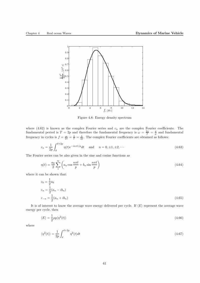
Chapter 4 Real ocean Waves Dynamics of Marine Vehicle
1
2 4 6 8 10 12 1400
0.2
0.4
0.5
0.6
0.8
0.3
0.7
0.9
0.1
f, [Hz]
1 2A
2
∆f,[ft2·s]
Figure 4.8: Energy density spectrum
where (4.62) is known as the complex Fourier series and cn are the complex Fourier coefficients. Thefundamental period is T = 2p and therefore the fundamental frequency is ω = 2π
T = πp and fundamental
frequency in cycles is f = ω2π = 1
T = 12p . The complex Fourier coefficients are obtained as follows:
cn =1
2p
∫ d+2p
d
η(t)e−inπt/pdt and n = 0,±1,±2, · · · (4.63)
The Fourier series can be also given in the sine and cosine functions as
η(t) =a02
∞∑
1
(
an cosnπt
p+ bn sin
nπt
p
)
(4.64)
where it can be shown that:
c0 =1
2a0
cn =1
2(an − ibn)
c−n =1
2(an + ibn) (4.65)
It is of interest to know the average wave energy delivered per cycle. If 〈E〉 represent the average waveenergy per cycle, then
〈E〉 = 1
2ρg〈η2(t)〉 (4.66)
where
〈η2(t)〉 = 1
2p
∫ d+2p
d
η2(t)dt (4.67)
61
Chapter 4 Real ocean Waves Dynamics of Marine Vehicle
is the variance of η(t) over a wave cycle. Using Parseval’s identity, it can be written that
〈η2(t)〉 =a204
+1
2
∞∑
n=1
(a2n + b2n
)
= c20 + 2
∞∑
n=1
cn × c−n
= c20 + 2
∞∑
n=1
∣∣c2n∣∣ . (4.68)
Substituting (4.66) in (4.68), the average wave energy per cycle can be given as
〈E〉 = 1
2ρg
(
c20 + 2∞∑
n=1
∣∣c2n∣∣
)
(4.69)
The foregoing analysis based on the Fourier expansion series should be modified for random waves dueto the fact that there is no finite time period of wave. In fact the period of random waves is infinite. It isassumed that d = −p and the complex Fourier series (4.62) may be given in the form
ηp(t) =
∞∑
−∞
cneinπt/p
cn =1
2p
∫ p
−p
ηp(t)e−inπt/pdt =
1
2p
∫ p
−p
ηp(τ)e−inπτ/pdτ
where ηp(t) is a periodic function of period 2p. Substituting the relationship for complex Fourier coefficientscn into ηp(t)
ηp(t) =
∞∑
−∞
(1
2p
∫ p
−p
ηp(τ)einπτ/pdτ
)
e−inπt/p
=
∞∑
−∞
(1
2π
∫ p
−p
ηp(τ)einπτ/pdτ
)
e−inπt/p
(π
p
)
and defining that
ωn =nπ
p, ωn+1 =
(n+ 1)π
p, and δω = ωn+1 − ωn =
π
p,
we obtain the following equation.
ηp(t) =
∞∑
−∞
[1
2π
∫ p
−p
ηp(τ)e−iωnτdτ
]
eiωnt∆ω
Let p goes to infinity such that the non-periodic limit of ηp(t) becomes η(t). If p → ∞ then ∆ω → 0 and thesummation over the frequency can be replaced by integral for the continuous random wave records or waveelevations.
η(t) =
∫ ∞
−∞
[1
2π
∫ ∞
−∞
η(τ)e−iωτdτ
]
eiωtdω (4.70)
The equation (4.70) is known as the Fourier integral. We may rewrite (4.70) in the following form.
η(t) =1
2π
∫ ∞
−∞
∫ ∞
−∞
η(τ)eiω(t−τ)dτdω
=1
2π
∫ ∞
−∞
∫ ∞
−∞
η(τ)
[
cosω(t− τ) + i sinω(t− τ)
]
dτ dω
62

Chapter 4 Real ocean Waves Dynamics of Marine Vehicle
Taking into account oddness of the sine function and the evenness of the cosine function, we can write that:∫ ∞
−∞
sinω(t− τ)dω = 0
∫ ∞
−∞
cosω(t− τ)dω = 2
∫ ∞
0
cosω(t− τ) dω
Therefore:
η(t) =1
π
∫ ∞
0
∫ ∞
−∞
η(τ) cosω(t− τ)dτdω.
Expanding the cosine function and defining:
a(ω) =
∫ ∞
−∞
η(t) cosωt dt ,
b(ω) =
∫ ∞
−∞
η(t) sinωt dt (4.71)
we can write
η(t) =1
π
∫ ∞
0
[
a(ω) cosωt+ b(ω) sinωt]
dω. (4.72)
The total energy of wave per unit surface area in the wave record is
E =1
2ρg
∫ ∞
−∞
η2(t)dt. (4.73)
Using (4.72), it can be written that
E =1
2ρg
∫ ∞
−∞
η(t).η(t)dt
=1
2ρg
∫ ∞
−∞
η(t)
[1
π
∫ ∞
0
[
a(ω) cosωt+ b(ω) sinωt]
dω
]
dt
=ρg
2π
∫ ∞
0
[
a(ω)
∫ ∞
−∞
η(t) cosωt dt+ b(ω)
∫ ∞
−∞
η(t) sinωt dt
]
dω
Using (4.71), the total wave energy per unit surface area is
E =ρg
2π
∫ ∞
0
[a2(ω) + b2(ω)
]dω (4.74)
which, alternately, is written as
E =ρg
2π
∫ ∞
0
A2(ω)dω (4.75)
whereA2(ω) = a2(ω)+b2(ω). Comparing (4.73) with (4.75), we obtain the Parsavel’s identity for a continuousnon-periodic random wave function η(t).
∫ ∞
−∞
η2(t)dt =1
π
∫ ∞
0
A2(ω)dω (4.76)
This equation really gives rise to the concept of the wave energy spectrum. The amplitude A(ω) has a unitof Length-time and is a continuous function of the frequency ω.
If the wave record is obtained over the time length Ts, the mean square value (variance) of η(t) can begiven as follows.
〈η2(t)〉 = 1
Ts
∫ Ts
0
η2(t)dt (4.77)
63

Chapter 4 Real ocean Waves Dynamics of Marine Vehicle
Therefore, the average wave energy per unit surface area can be given as
〈E〉 = ρg
2
1
Ts
∫ Ts
0
η2(t)dt. (4.78)
Doing some manipulations, we finally obtained the average wave energy in the following form, Rahman [3].
〈E〉 = ρg
2π
∫ ∞
0
A2(ω)
Tsdω (4.79)
The spectral density function is defined as
S(ω) =A2(ω)
πTs(4.80)
where S(ω) has a unit of Length2-time. The total energy is obtained from the area covered by the energydensity curve as a function of frequency.
〈E〉 = 1
2ρg
∫ ∞
0
S(ω)dω (4.81)
There are two methods to compute the spectral density function from an ocean wave records: theautocorrelation method and the fast Fourier transform (FFT) method. However, the procedure of extractingspectra from wave records is an evolving field and is beyond the scope of this lecture. Chackrabarti [1] hasgiven a good account in extracting the wave spectral density function from an ocean wave record.
There are several widely used conventions in the display of energy spectrum. We have illustrated theenergy density spectrum in Fig. 4.9 that is the most popular one, S(ω). The advantage of the energy densityspectrum is that the area under the curve gives the total energy of the wave system. The representation ofthe energy density spectrum could be in a linear scale, a log-log scale or a semilog scale. The wave spectrummay be represented as a function of cyclic frequency f or circular frequency ω. It should be considered that:
S(f) = 2πS(ω) (4.82)
The total energy present in the ocean waves is not distributed equally throughout the range of frequencies;
00
0.3 0.6 0.9 1.2 1.5
5
10
15
20
25
S(ω
)
ω
Figure 4.9: A one-sided energy density spectrum
instead, in every spectrum, the energy is concentrated around a particular frequency (fmax), that correspondsto a certain wind speed. The frequency range is decrease as the wind speed in increases.
It is customary to represent the spectrum as a one-sided spectrum, as shown in Fig. 4.9. The two sidedspectrum covered both positive and negative side of the frequency, ω. The difference between a two-sidedspectrum and a one-sided spectrum as illustrated in Fig. 4.10 is quite important. Note that the two-sided
64

Chapter 4 Real ocean Waves Dynamics of Marine Vehicle
spectrum is symmetric about the origin, covering both negative and positive frequencies to account for allwave energy from −4 to +4. But, it is customary in ocean engineering to present the spectrum as a one-sidedspectrum. This requires that the spectral density ordinates of two-sided spectrum be doubled in value ifonly the positive frequencies are considered.
Figure 4.10: Definition of one- and two-sided wave spectrum
4.4.2 Spectral properties of ocean waves
if it is assumed that the wave train is generated by constant wind blowing over a fitch limited, X surfacearea of ocean with depth h, the frequency spectrum S(ω) of surface wave is a function of
S(ω) = f(ω, ρa, ρw, νa, νw,Υ, g, U∞, fc, t,X, h) (4.83)
where:
- ρa and ρw are the density of air and water,respectively,
- νa and νw are kinematic viscosity of air and water, respectively,
- Υ is the surface tension of water and air interface,
- g is the gravitational acceleration,
- U∞ is the wind speed at the upper limit of the atmospheric,
- fc is the Coriolis parameter,
- t is the duration of wind blowing, and
- ω is the circular frequency.
It is assumed that:
1. Wave motion is irrotational and the influence of molecular viscosity νw can be neglected.
2. Only the gravitational part of the spectrum S(ω) is considered and the influence of surface tension isneglected and frequency ω is restricted to the range
ω << ωΥ =
(4ρwg
3
Υ
)1/4
(4.84)
3. Nonlinear interaction between spectral components are neglected.
65
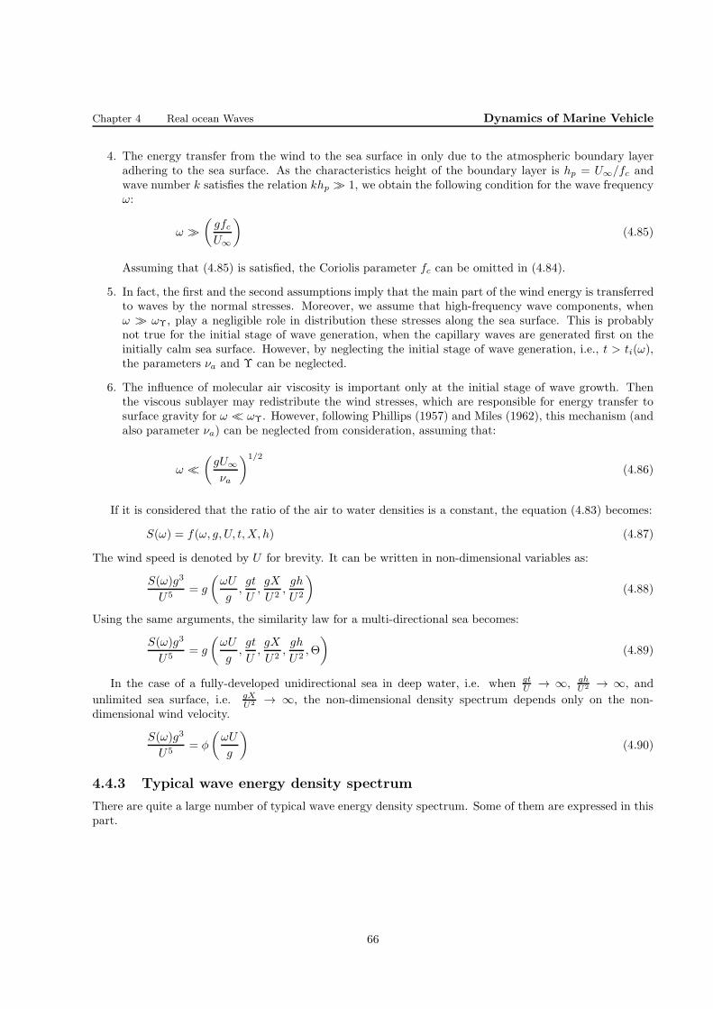
Chapter 4 Real ocean Waves Dynamics of Marine Vehicle
4. The energy transfer from the wind to the sea surface in only due to the atmospheric boundary layeradhering to the sea surface. As the characteristics height of the boundary layer is hp = U∞/fc andwave number k satisfies the relation khp >> 1, we obtain the following condition for the wave frequencyω:
ω >>
(gfcU∞
)
(4.85)
Assuming that (4.85) is satisfied, the Coriolis parameter fc can be omitted in (4.84).
5. In fact, the first and the second assumptions imply that the main part of the wind energy is transferredto waves by the normal stresses. Moreover, we assume that high-frequency wave components, whenω >> ωΥ, play a negligible role in distribution these stresses along the sea surface. This is probablynot true for the initial stage of wave generation, when the capillary waves are generated first on theinitially calm sea surface. However, by neglecting the initial stage of wave generation, i.e., t > ti(ω),the parameters νa and Υ can be neglected.
6. The influence of molecular air viscosity is important only at the initial stage of wave growth. Thenthe viscous sublayer may redistribute the wind stresses, which are responsible for energy transfer tosurface gravity for ω << ωΥ. However, following Phillips (1957) and Miles (1962), this mechanism (andalso parameter νa) can be neglected from consideration, assuming that:
ω <<
(gU∞
νa
)1/2
(4.86)
If it is considered that the ratio of the air to water densities is a constant, the equation (4.83) becomes:
S(ω) = f(ω, g, U, t,X, h) (4.87)
The wind speed is denoted by U for brevity. It can be written in non-dimensional variables as:
S(ω)g3
U5= g
(ωU
g,gt
U,gX
U2,gh
U2
)
(4.88)
Using the same arguments, the similarity law for a multi-directional sea becomes:
S(ω)g3
U5= g
(ωU
g,gt
U,gX
U2,gh
U2,Θ
)
(4.89)
In the case of a fully-developed unidirectional sea in deep water, i.e. when gtU → ∞, gh
U2 → ∞, and
unlimited sea surface, i.e. gXU2 → ∞, the non-dimensional density spectrum depends only on the non-
dimensional wind velocity.
S(ω)g3
U5= φ
(ωU
g
)
(4.90)
4.4.3 Typical wave energy density spectrum
There are quite a large number of typical wave energy density spectrum. Some of them are expressed in thispart.
66
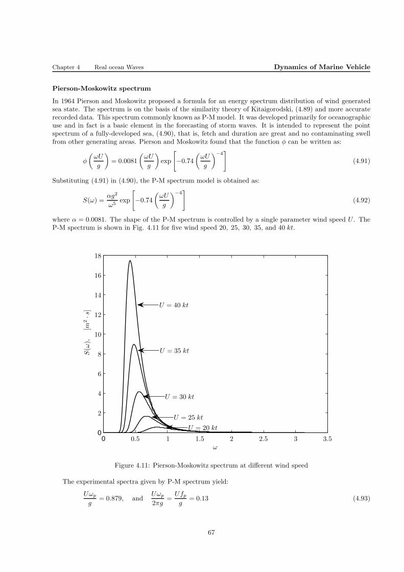
Chapter 4 Real ocean Waves Dynamics of Marine Vehicle
Pierson-Moskowitz spectrum
In 1964 Pierson and Moskowitz proposed a formula for an energy spectrum distribution of wind generatedsea state. The spectrum is on the basis of the similarity theory of Kitaigorodski, (4.89) and more accuraterecorded data. This spectrum commonly known as P-M model. It was developed primarily for oceanographicuse and in fact is a basic element in the forecasting of storm waves. It is intended to represent the pointspectrum of a fully-developed sea, (4.90), that is, fetch and duration are great and no contaminating swellfrom other generating areas. Pierson and Moskowitz found that the function φ can be written as:
φ
(ωU
g
)
= 0.0081
(ωU
g
)
exp
[
−0.74
(ωU
g
)−4]
(4.91)
Substituting (4.91) in (4.90), the P-M spectrum model is obtained as:
S(ω) =αg2
ω5exp
[
−0.74
(ωU
g
)−4]
(4.92)
where α = 0.0081. The shape of the P-M spectrum is controlled by a single parameter wind speed U . TheP-M spectrum is shown in Fig. 4.11 for five wind speed 20, 25, 30, 35, and 40 kt.
00
0.5 1 1.5 2.5 3 3.5
2
2
4
6
8
10
12
14
16
18
S(ω
),[m
2·s]
ω
U = 40 kt
U = 20 kt
U = 25 kt
U = 30 kt
U = 35 kt
Figure 4.11: Pierson-Moskowitz spectrum at different wind speed
The experimental spectra given by P-M spectrum yield:
Uωp
g= 0.879, and
Uωp
2πg=
Ufpg
= 0.13 (4.93)
67

Chapter 4 Real ocean Waves Dynamics of Marine Vehicle
where ωp is the peak frequency where the wave spectral energy reaches its maximum. The peak frequency
ωp is obtained by condition dS(ωdω = 0. Using (4.93) and substituting in (4.92), it is obtained:
S(ω) =αg2
ω5exp
[
−5
4
(ω
ωp
)−4]
(4.94)
The JONSWAP Spectrum
The JONSWAP spectrum extends the P-M spectrumto include fetch-limited seas. This spectrum is basedon an extensive wave measurement program (Joint North Sea Wave project) carried out in 1968 and 1969in North Sea. The JONSWAP spectrum received almost instant recognition and become very well known ininternational literature. According to Hasselmann et. al 1973, the resulting spectral model takes the form:
S(ω) =αg2
ω5exp
[
−5
4
(ω
ωp
)−4]
γδ (4.95)
Where the term γδ is a peak enhancement factor, added to the P-M spectrum, to represent a narrow, morepeaked spectrum which is typical for a growing sea. The notation δ is given in the form:
δ = exp
[
− (ω − ωp)2
2σ20ω
2p
]
(4.96)
Spectrum (4.95) contains five parameters, i.e. α, γ, ωp, and σ0 = σ′0 for ω ≤ ωp and omega > ωp, which
should be know in prior. The γ parameter describes the degree of peakedness and σ0 parameter describesthe width of the peak region. The mean JONSWAP spectrum yields:
γ = 3.3;
σ0 = σ′0 = 0.07 for ω ≤ ωp;
σ = σ′′
0 = 0.09 for ω > ωp;
α = 0.076
(gX
U2
)−0.22
; and
ωp = 7π( g
U
)(gX
U2
)−0.33
The JONSWAP spectrum are illustrated for U = 20 m/s when X = 40, 80, 120, 160 and 200 km in Fig. 4.12.
The JONSWAP spectrum and the P-M spectrum are compared for two different regimes in Fig. 4.13-aand -b when the fetch lengths are X = 25 km and X = 200 km, respectively.
Bretschneider spectrum
Bretschneider derived a spectrum model based on the assumption that the spectrum is narrow-banded andthe individual wave height and wave period follow Rayleigh distribution. This spectrum is given in term ofthe significant wave height and period rather than the wind speed. The Bretschneider wave density spectrummay be written in the following form.
S(ω) = 0.258 H2s
ω4s
ω5exp
[
−1.03
(ω
ωs
)−4]
(4.97)
where Hs is the significant wave height and ωs = 2π/Ts is the significant wave frequency. The notation Ts
is the significant wave period. It is defined as:
Ts = 0.9528Tp (4.98)
68

Chapter 4 Real ocean Waves Dynamics of Marine Vehicle
0.25 0.5 0.75 1.25 1.5 1.75 20
1
1
1
3
4
5
6
7
8
9
10
U = 20 m/s
X = 20 km
160
120
80
40
S(ω
),m
2·s
ω, rad/s
Figure 4.12: The JONSWAP spectrum at various limited fetch length areas
0
0
0.5
0.5
1
1
1.5
1.5
2
2
2.5
2.5
3
3
0
0.4
0.8
1.2
1.6
2
2.4
0
0.02
0.04
0.06
0.08
0.1
0.12
P-M Spectrum
P-M Spectrum
JONSWAP Spectrum
JONSWAP Spectrum
S(ω
),m
2·s
S(ω
),m
2·s
ω, rad/s
ω, rad/s
a
b
Figure 4.13: Comparison of the P-M spectrum with the JONSWAP spectrum: a)X = 25 km, b) X = 200 km
where Tp is the peak period. Taking into account (4.98), the Bretschneider wave density spectrum may alsobe written as function of peak frequency as follows.
S(ω) =5
16H2
s
ω4p
ω5exp
[
−5
4
(ω
ωp
)−4]
(4.99)
The following MATLAB m-file is used to plot the spectrum at different sea stats. clear all;
69
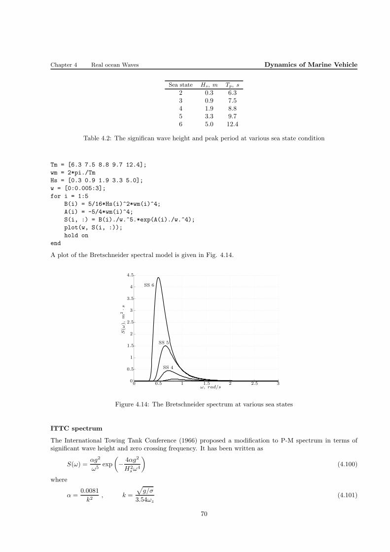
Chapter 4 Real ocean Waves Dynamics of Marine Vehicle
Sea state Hs, m Tp, s
2 0.3 6.33 0.9 7.54 1.9 8.85 3.3 9.76 5.0 12.4
Table 4.2: The significan wave height and peak period at various sea state condition
Tm = [6.3 7.5 8.8 9.7 12.4];
wm = 2*pi./Tm
Hs = [0.3 0.9 1.9 3.3 5.0];
w = [0:0.005:3];
for i = 1:5
B(i) = 5/16*Hs(i)^2*wm(i)^4;
A(i) = -5/4*wm(i)^4;
S(i, :) = B(i)./w.^5.*exp(A(i)./w.^4);
plot(w, S(i, :));
hold on
end
A plot of the Bretschneider spectral model is given in Fig. 4.14.
0 0.5 1 1.5 2 2.5 30
0.5
1
1.5
2
2.5
3
3.5
4
4.5
SS 6
SS 5
SS 4
S(ω
),m
2·s
ω, rad/s
Figure 4.14: The Bretschneider spectrum at various sea states
ITTC spectrum
The International Towing Tank Conference (1966) proposed a modification to P-M spectrum in terms ofsignificant wave height and zero crossing frequency. It has been written as
S(ω) =αg2
ω5exp
(
− 4αg2
H2sω
4
)
(4.100)
where
α =0.0081
k2, k =
√
g/σ
3.54ωz(4.101)
70

Chapter 4 Real ocean Waves Dynamics of Marine Vehicle
in which σ =√m0 = Hs/4 is the standard deviation (r.m.s. value) of the water surface elevation.
4.4.4 Directional spectral function
The most widely used and accepted method of studying wind generated waves is an examination of the spectraat a single point. However, single point measurements are not sufficient to describe the full nature of wind-induced surface waves. Due to the complicated energy transfer from the atmosphere to the sea and due towave-wave interactions the resulting surface waves are multidirectional. Only part of the wave energy alignedwith the wind direction. More specifically, wave energy associated with the frequency ω = ωp is primarilypropagated in the direction of the wind, whereas wave energy associated with lower and higher frequenciesis distributed over a range of directions. Wave multidirectionality is also result of the superposition at agiven point of various wave train, which may be generated by different remote atmospheric forcing systems,Massel [2].
Due to the limitation of the observational methods, knowledge on the directional spectrum is relativelypoor compared to the frequency spectrum. The basic approach is to multiply the frequency spectrum S(ω)by an empirically determined directional spreading function D(Θ;ω, p1, p2, · · · ) to find the directional wavespectrum.
S(ω,Θ) = S(ω)D(Θ;ω, p1, p2, · · · ) (4.102)
Where p1, p2, · · · represent the various parameters associated with the various directional spreading functions.There are four basic form of the directional spreading function: the cosine-power function, the exponentialfunction, the exponential series and the hyperbolic function.
On the basis of a field study with pitch-and-roll buoy, Louguet-Higgins et. al (1961) developed a elabo-rated for of cosine spreading function as follows.
D(Θ, p) =22p−1Γ2(p+ 1)
πΓ(2p+ 1)cos2p (
1
2Θ) (4.103)
Where
p = 100.99(
ω
ωm
)κ
, and κ =
{4.06 for ω < ωm,−2.34 for ω ≥ ωm
(4.104)
A three dimensional form of the JONSWAP spectrum using the spreading function (4.103) is shown in Fig.4.15.
4.5 Application of wave energy density spectrum
The short-term ocean wave are treated as random process. It is also assumed that the statistics of oceanwaves are stationary and ergodic. It indicate that the ensemble average E(η(t1)) at same time t1 of aninfinite number of finite length time series η1(t1), η2(t1), η3(t1), · · · , η∞(t1) is equivalent to the temporalaverage over all times of an infinitely long single time series η1(t1), η1(t2), η1(t3), · · · , η2(t∞). In other word,a realization of η(t), say η1(t), is typical of all other possible realizations.
It is also assumed that the real ocean waves composed of various sinusoidal waves of different amplitudes,frequencies, direction and phases. However, the stationary and ergodic assumptions indicate that sinusoidalcomponents of ocean waves are the same regardless of times and places and differ from one record to anotheronly in the phase orientation and thereby keeping the energy of the wave system constant. In other word,the statistical characteristics of the sea state, that is, the energy spectrum or wave spectrum, will remainthe same. Application of wave energy density spectrum is discussed in this part.
4.5.1 Simulation of wave profile
The average energy per unit area is given for a wave system as
〈E〉 = 1
2ρg〈η2(t)〉 = 1
2ρg
∫ ∞
0
S(ω)dω (4.105)
71
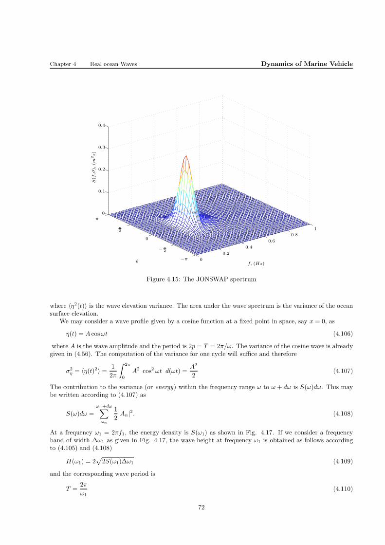
Chapter 4 Real ocean Waves Dynamics of Marine Vehicle
−π
π
−π2
π2
0
0
0
0.1
0.2
0.2
0.3
0.4
0.4
0.6
0.8
1
ϑf, (Hz)
S(f
,ϑ),
(m2s)
Figure 4.15: The JONSWAP spectrum
where 〈η2(t)〉 is the wave elevation variance. The area under the wave spectrum is the variance of the oceansurface elevation.
We may consider a wave profile given by a cosine function at a fixed point in space, say x = 0, as
η(t) = A cosωt (4.106)
where A is the wave amplitude and the period is 2p = T = 2π/ω. The variance of the cosine wave is alreadygiven in (4.56). The computation of the variance for one cycle will suffice and therefore
σ2η = 〈η(t)2〉 = 1
2π
∫ 2π
0
A2 cos2 ωt d(ωt) =A2
2(4.107)
The contribution to the variance (or energy) within the frequency range ω to ω + dω is S(ω)dω. This maybe written according to (4.107) as
S(ω)dω =
ωn+dω∑
ωn
1
2|An|2. (4.108)
At a frequency ω1 = 2πf1, the energy density is S(ω1) as shown in Fig. 4.17. If we consider a frequencyband of width ∆ω1 as given in Fig. 4.17, the wave height at frequency ω1 is obtained as follows accordingto (4.105) and (4.108)
H(ω1) = 2√
2S(ω1)∆ω1 (4.109)
and the corresponding wave period is
T =2π
ω1(4.110)
72
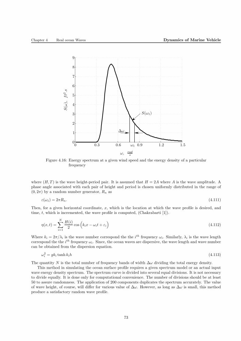
Chapter 4 Real ocean Waves Dynamics of Marine Vehicle
00
1
2
3
4
5
6
7
8
9
0.3 0.6 0.9 1.2 1.5
ω, rads
S(ω
),ft2.s
ω1
S(ω1)
∆ω
Figure 4.16: Energy spectrum at a given wind speed and the energy density of a particularfrequency
where (H,T ) is the wave height-period pair. It is assumed that H = 2A where A is the wave amplitude. Aphase angle associated with each pair of height and period is chosen uniformly distributed in the range of(0, 2π) by a random number generator, Rn as
ε(ω1) = 2πRn. (4.111)
Then, for a given horizontal coordinate, x, which is the location at which the wave profile is desired, andtime, t, which is incremented, the wave profile is computed, (Chakrabarti [1]).
η(x, t) =
N∑
i=1
H(i)
2cos(
kix− ωit+ εi
)
(4.112)
Where ki = 2π/λi is the wave number correspond the the ith frequency ωi. Similarly, λi is the wave lengthcorrespond the the ith frequency ωi. Since, the ocean waves are dispersive, the wave length and wave numbercan be obtained from the dispersion equation.
ω2i = gki tanh kih (4.113)
The quantity N is the total number of frequency bands of width ∆ω dividing the total energy density.This method in simulating the ocean surface profile requires a given spectrum model or an actual input
wave energy density spectrum. The spectrum curve is divided into several equal divisions. It is not necessaryto divide equally. It is done only for computational convenience. The number of divisions should be at least50 to assure randomness. The application of 200 components duplicates the spectrum accurately. The valueof wave height, of course, will differ for various value of ∆ω. However, as long as ∆ω is small, this methodproduce a satisfactory random wave profile.
73

Chapter 4 Real ocean Waves Dynamics of Marine Vehicle
4.5.2 Computation of the average heights characteristics
The area under the wave spectrum is
〈η2(t)〉 =∫ ∞
0
S(ω)dω = m0 (4.114)
and therefore, m0 is the value of the wave elevations squared or√m0 is the root mean square (rms) value
of the irregular ocean surface elevations. Thus, the area under the wave spectrum yields the mean ofdeviation squared. The significant wave amplitude or height or the other averages are multiples of rms, (i.ea const.×√
m0). Such multipliers depend on the probability distribution of ocean wave properties.For a narrow-band Gaussian ocean wave whose components are in random phase, the wave amplitude
and hence the wave height follow a Rayleigh distribution. Since any single wave is closely sinusoidal for anarrow-band motion, the variance of the surface elevation may be expressed as the average of integrals takenover each wave. Therefore according to (4.56), it can be σ2
i = H2i /8. In this manner we can write that
〈η2(t)〉 =∫∞
0 S(ω)dω = m0
〈η2(t)〉 = 1N
∑Ni=1 σ
2i
σ2i =
H2i
8
H2rms =
1N
∑Ni=1 H
2i
=⇒ Hrms = 2√2m0 (4.115)
The probability cumulative distribution function and the probability density function of the wave heightis given in (4.39) and (4.40) for a a narrow-band Gaussian ocean. They may be written in the following formas a function of m0.
P (H) = 1− exp
[
− H2
8m0
]
(4.116)
p(H) =H
4m0exp
[
− H2
8m0
]
(4.117)
For a Rayleigh distribution of wave height, the average wave height, the significant wave height (oraverage of one-third highest waves), the average of one-tenth highest waves and the average of one-hundredhighest waves are:
H = H1 = 0.886 Hrms = 2.506√m0 (4.118)
Hs = H1/3 = 1.416 Hrms = 4.005√m0 (4.119)
H1/10 = 1.80 Hrms = 5.091√m0 (4.120)
H1/100 = 2.36 Hrms = 6.672√m0 (4.121)
4.5.3 Arbitrary wave spectra
The result for the wave distribution is for the special case of a narrow-band spectrum. The probability distri-bution of wave amplitude depends upon one additional parameter ǫ terms the spectral bandwidth parameter.It is defined as
ǫ =
(
1− m22
m0m4
)1/2
(4.122)
where m0 is the area under the wave spectrum and m2 and m4 are the second and fourth spectral moment,respectively. In general the n− th spectral moment is defined as
mn =
∫ ∞
0
ωnS(ω)dω (4.123)
74
Chapter 4 Real ocean Waves Dynamics of Marine Vehicle
hence
m2 =
∫ ∞
0
ω2S(ω)dω and m4 =
∫ ∞
0
ω4S(ω)dω. (4.124)
The spectral bandwidth parameter ǫ takes values between 0 and 1 and for a narrow-band spectrum ǫ → 0.Based on the definition for ǫ, the oceanographers have introduce a correction factor as follows.
CF =(1− ǫ2
)1/2(4.125)
by which the above constant to compute the wave height characteristics or the other wave characteris-tics based on the narrow-band assumption should be multiplied to take into account the broadness of thespectrum.
4.5.4 Wave period
The probability distribution of wave periods for an arbitrary spectrum is complex. The distribution of waveperiod in deep water according to Bretschneider (1969) follows a Rayleigh distribution.
P (T ) =
{
1− exp[
−0.675(TT
)4]
for T ≥ 0
0 otherwise(4.126)
p(T ) =
{2.7T 3
T 4 exp[
−0.675(TT
)4]
for T ≥ 0
0 otherwise(4.127)
Where T is a mean period defined as
T =m0
m1. (4.128)
The more appropriate distribution of the wave period is derived by Longuet-Higgins. It can be found inChakrabarti [1].
The expression for the average zero upcrossing period Tz is given as
Tz =1
Nz= 2π
√m0
m2. (4.129)
The crest-to-crest period Tc is defined as
Tc = 2π
√m2
m4. (4.130)
There are also two other characteristic period often used in statistics. One is the peak period, Tp, definedas the period at which the energy density spectrum peaks. The other one is the significant wave period, Ts,defined as the average of the highest one-third waves in the record.
Ts = 2π
√m0
m1. (4.131)
Taking into account (4.129) and (4.130), the spectral width parameter ǫ may be given as
ǫ =
[
1−(Tc
Tz
)2]1/2
(4.132)
75
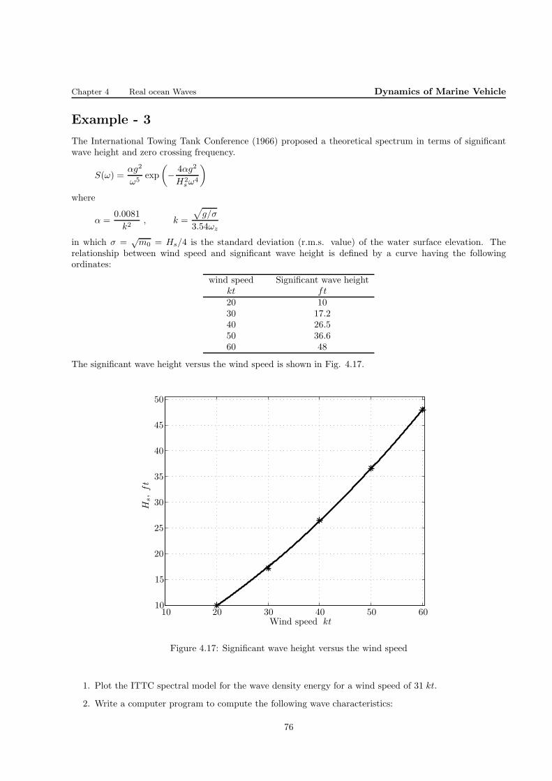
Chapter 4 Real ocean Waves Dynamics of Marine Vehicle
Example - 3
The International Towing Tank Conference (1966) proposed a theoretical spectrum in terms of significantwave height and zero crossing frequency.
S(ω) =αg2
ω5exp
(
− 4αg2
H2sω
4
)
where
α =0.0081
k2, k =
√
g/σ
3.54ωz
in which σ =√m0 = Hs/4 is the standard deviation (r.m.s. value) of the water surface elevation. The
relationship between wind speed and significant wave height is defined by a curve having the followingordinates:
wind speed Significant wave heightkt ft20 1030 17.240 26.550 36.660 48
The significant wave height versus the wind speed is shown in Fig. 4.17.
1010
15
20
20
25
30
30
35
40
40
45
50
50 60Wind speed kt
Hs,ft
Figure 4.17: Significant wave height versus the wind speed
1. Plot the ITTC spectral model for the wave density energy for a wind speed of 31 kt.
2. Write a computer program to compute the following wave characteristics:
76

Chapter 4 Real ocean Waves Dynamics of Marine Vehicle
• the one-tenth of highest H1/10;
• the one-hundred of highest H1/100;
• zero upcrossing average period Tz; and
• the average crest to crest period Tc.
Assumed that the wave height probability distribution is Rayleigh.
3. If the wave height histogram does not follow Rayleigh distribution, find the the significant wave heightHs.
4. Find the most probable largest wave amplitude.
Solution-1
The ITTC spectrum is
S(ω) =αg2
ω5exp
(
− 2αg2
H2sω
4
)
where
α =0.0081
k2, k =
√
g/σ
3.54ωz
in which σ =√m0 = Hs/4 is the standard deviation (r.m.s. value) of the water surface elevation. The
significant wave height for a wind speed of 31 kt is:
Hs = 18.5 ft
It is taken into account that k = 1. The ITTC spectrum for a wind speed of 31 kt is given in Fig. 4.18.
00
10
20
30
40
50
60
0.5 1 1.5 2 2.5 3ω, s−1
S(ω
),ft2.s
Figure 4.18: ITTC wave Energy density spectrum at the wind speed of 31 kt
77

Chapter 4 Real ocean Waves Dynamics of Marine Vehicle
Solution-2
The following MATLAB m.file is written to obtain the solution for the wave height averages and waveperiods.
a = 0.0081; %a = alpha
g = 32.2;
Hs = 18.5;
A = a*g^2;
B = 4*a*g^2/Hs^2;
w = [0.1:0.001:10];
Sw = A./w.^5.*exp(- B./w.^4);
plot(w, Sw)
clear w Sw
Sw = @(w) A./w.^5.*exp(- B./w.^4);
m0 = quad(Sw, 0, 10)
Sw2 = @(w) A./w.^3.*exp(- B./w.^4);
m2 = quad(Sw2, 0, 10)
Sw4 = @(w) A./w.^1.*exp(- B./w.^4);
m4 = quad(Sw4, 0, 10)
H_ave = 2.506*sqrt(m0)
H_s = 4.005*sqrt(m0)
H_110 = 5.091*sqrt(m0)
H_1100 = 6.672*sqrt(m0)
Tz = 2*pi*sqrt(m0/m2)
Tc = 2*pi*sqrt(m2/m4)
e = sqrt(1 - m2^2/m0/m4)
CF = sqrt(1 - e^2)
H_s1 = H_s*CF
The solution are:
m0 = 21.3904 ft2
m2 = 11.8363 ft2.s−2
m4 = 22.9997 ft2.s−4
H = 11.5902 ft
Hs = 18.523 ft
H1/10 = 23.5458 ft
H1/100 = 30.8578 ft
Tz = 8.4466 s
Tc = 4.5074 s
Solution-3
In the case that the wave height probability distribution is not a Rayleigh distribution, the wave significantheight is
ǫ =
(
1− m22
m0m4
)1/2
= 0.8457
CF =(1− ǫ2
)1/2= 0.5336
Hs1 = Hs.CF = 18.523× 0.5336 = 9.8846 ft
78

Chapter 4 Real ocean Waves Dynamics of Marine Vehicle
Solution-4
It is assumed that the number of recorded waves are N = 1000. Therefore,
Hmax = 2.63Hrms = 7.44√m0 = 7.44×
√21.3904 = 34.4 ft
It is when the wave height probability distribution is Rayleigh. Since it is not follow the Rayleigh distributionexactly, the probable maxima is
H∗max = Hmax.CF = 34.4× 0.5336 = 18.36 ft
79
Bibliography
[1] Chakrabarti, S. K., Hydrodynamics of offshre structures, Springer-Verlag Berlin, Heidelberg, 1987
[2] Massel, Stanislaw R., Ocean surface waves: Their physics and prediction, World Scientific publishingCo. Pte. Ltd., 1996
[3] Rahman, M., Water waves, relating modern theory to advanced engineering applications, Oxford Uni-verisit press, 1994
[4] Sarpkaya, T. and Isaacson, M., Mechanics of wave forces on offshore structures, Van Nostrand ReinholdCompany, 1981
[5] Wikipedia, The free encyclopedia,, http:en.wikipedia.org/wiki/Beaufort-scale
80
Copyright © 2022 FDOKUMEN