Low-luminosity Type II supernovae: spectroscopic and photometric evolution

Mon. Not. R. Astron. Soc. 000, 000–000 (0000) Printed 28 December 2013 (MN LATEX style file v2.2)
Photometric Metallicities in Bootes I
J. Hughes,1 G. Wallerstein,2 A. Dotter,3 D. Geisler41Physics Department, Seattle University, Seattle, WA 981222Astronomy Department, University of Washington, Box 351580, Seattle, WA 98195-15803Research School of Astronomy & Astrophysics, Australian National University, Weston, ACT 2611, Australia4Grupo de Astronomıa, Departamento de Astronomıa, Universidad de Concepcion, Casilla 160-C, Concepcion, Chile
Accepted xxx. Received xxx.
ABSTRACTWe present new Stromgren and Washington data sets for the Bootes I dwarf galaxy, andcombine them with the available SDSS photometry. The goal of this project is to refine aground-based, practical, accurate method to determine age and metallicity for individual starsin Bootes I that can be selected in an unbiased imaging survey, without having to take spectra.With few bright upper-red-giant branch stars and distances of about 35 ! 250 kpc, the ultra-faint dwarf galaxies present observational challenges in characterizing their stellar population.Other recent studies have produced spectra and proper motions, making Bootes I an ideal testcase for our photometric methods. We produce photometric metallicities from Stromgren andWashington photometry, for stellar systems with a range of!1.0 > [Fe/H ] > !3.5. Needingto avoid the collapse of the metallicity sensitivity of the Stromgren m1-index on the lower-red-giant branch, we replace the Stromgren v-filter with the broader Washington C-filter tominimize observing time. We construct two indices: m! = (C ! T1)0 ! (T1 ! T2)0, andm!! = (C ! b)0 ! (b ! y)0. We find that CT1by is the most successful filter combination,for individual stars with [Fe/H ] < !2.0, to maintain " 0.2 dex [Fe/H]-resolution over thewhole red-giant branch. The m!!-index would be the best choice for space-based observa-tions because the (C ! y) color is not sufficient to fix metallicity alone in an understudiedsystem. Our photometric metallicites of stars in the central regions of Bootes I confirm thatthat there is a metallicity spread of at least !1.9 > [Fe/H ] > !3.7. The best-fit Dartmouthisochrones give a mean age, for all the Bootes I stars in our data set, of 11.5± 0.4 Gyr. Fromground-based telescopes, we show that the optimal filter combination is CT1by, avoiding thev-filter entirely. We demonstrate that we can break the isochrones’ age-metallicity degeneracywith the CT1by filters, using stars with log g = 2.5 ! 3.0, which have less than a 2 per centchange in their (C ! T1)-colour due to age, over a range of 10-14 Gyr.
Key words: galaxies: dwarf; galaxies: individual – (Bootes I) – Local Group.
1 INTRODUCTION
The Sloan Digital Sky Survey (SDSS) survey (in ugriz bands) hasbeen used to identify! 8 (see Willman & Strader 2012) newMilkyWay satellites (for example, Willman et al. 2005a,b; Belokurovet al. 2006a,b; Zucker et al. 2006a,b; Willman 2010). This paperis the second in a series, describing our ongoing studies of severalof the recently discovered dwarf galaxies surrounding the MilkyWay Galaxy (MWG), using the Apache Point Observatory’s 3.5-mtelescope. We discuss new Stromgren photometry of Bootes I andcompare it with our previously-published Washington photometryand other recent spectroscopic studies, particularly those of Ko-posov et al. (2011) and Gilmore et al. (2013a,b). In this paper wededuce the star formation history of the central region of BootesI from photometry, and determine the most effective and efficientcombination of broad-band and medium band filters to break theage/metallicity degeneracy of populations such as these.
Willman (2010) wrote a review of the search methods, forthese “least luminous galaxies”, which can be as faint as 10!7
times the luminosity of the MWG. Ten years ago, the MWGonly had 11 known dwarf galaxy companions, which was at oddswith cosmological simulations predicting hundreds of low mass(105M") dark matter halos. Where were the “missing satellites”?The apparent mismatch between the number of observed dark mat-ter halos, and those predicited by the !CDM cosmological modelswas partially explained by “simple” models (Willman 2010) of howstellar populations form inside low-mass dark matter halos (Bul-lock, Kravtsov & Weinberg 2000; Benson et al. 2002; Kravtsov,Gnedin & Klypin 2004; Simon & Geha 2007). The first part of theproblem is finding the least luminous galaxies, and the second issueis to determine the most efficient method to study these sparsely-populated systems. A recent review by Belokurov (2013) calls thepre-SDSS dwarf galaxy population “classical” dwarfs.

2 J. Hughes et al.
Willman’s (2010) review of the automated star-count analysisshows how we have increased the completeness of unbiased skysurveys, and also describes the next generation of surveys plannedfor the next decade or so. Detailed descriptions of how the auto-mated searches were carried out can be found in Willman et al.(2002) and Walsh, Willman, & Jerjen (2009, hereafter, WWJ).Once the stellar-overdensities were found, observers have to sep-arate the dSph population from that of the MWG’s halo stars inthe field. The method used by WWJ first selects a range of Girardiisochrones (see Girardi et al. 2005, and references therein), assum-ing that the dSphs have populations which are aged between 8 and14 Gyr, with "1.5 < [Fe/H ] < "2.3. This range of modelswas used to create a colour-magnitude (CM) filter, which was thenmoved to 16 values of the distance modulus, between 16.5 and 24.0.The software then looked for stellar overdensities, above a certaindetection threshold; WWJ describe this in detail, along with howthe data was simulated. Along with dwarf galaxies, the MWG’shalo has tidal debris and unbound star clusters, which can also bepicked up in this method. Following up the detections with photom-etry and spectroscopy is essential to finding which of the detectionsare actual dwarf galaxies. When these SDSS searches were per-formed, Willman (2010) notes that the least luminous galaxies canonly be detected out to about 50 kpc. The CM filter method (WWJ)can locate systems with distances in the range of 20-600 kpc, but itis brightness limited. Koposov et al. (2008) and Belokurov (2013)discuss the SDSS completeness limits, where dwarf satellite of ourgalaxy are complete out to a virial radius of 280 kpc atMV ! "5(using SDSS DR5). For systems such as Segue 1 withMV ! "3,only a few percent of the “virial volume” can be sampled. Thus,part of the problem is the faintness of the “darker” satellites, andpart of it is the automated detection method uses filters which donot separate the sparse dwarf populations from the foreground starsin colour-magnitude diagrams.
Some of these lowest luminosity dSphs (discovered in theSDSS) do not look like the tidal debris of collisions (as discussedin Belokurov 2013), they look like the primordial leftovers fromgalaxy-assembly and Gilmore et al. (2013a) go as far as to identifyBootes I as “surviving example of one of the first bound objects toform in the Universe.”
Early star formation can progress in different ways, depend-ing on the star formation rate, but the pathway should be detectablein spectroscopic surveys (Gilmore et al. 2013a,b). Both papers dis-cuss two star formation channels for these extremely metal-poorsystems. Rapid-star-formation after Pop III core-collapse super-novae can produce carbon rich (CEMP-no) stars. The “long-lived,low star-formation rate” would produce more carbon-normal abun-dances. Gilmore et al. (2013a,b) identify Bootes I as the latter case.However, some authors have identified a few red giant stars in BooI as carbon-rich (Lai et al. 2011; Gilmore et al. 2013b). The 2.5#rhdistance of the radial-velocity-confirmed member, Boo-1137, fromthe center of Bootes I might indicate that a much more massiveoriginal system is being stripped (see Figure 1). The half-light ra-dius of Bootes I is about 240 pc (Gilmore et al. 2013a). At first ex-amination, Bootes I appears to be a normal, if extended, dSph at aGalactocentric distance of about 60 kpc, with e ! 0.2, and"3.7 to(at least)"1.9 in [Fe/H]. Any stellar system/dwarf galaxy found ataround 20 kpc would be contaminated by MWG thick disk and halostars, while those which lie beyond 100 kpc are mostly affected bythe MWG halo stars. However, the Sloan filters do not separate outthe dSph stars from the MWG stars very well on colour-magnitudediagrams (CMDs) or colour-colour plots (Belokurov et al. 2006b;Hughes, Wallerstein & Bossi 2008, hereafter, HWB).
Figure 1. (a) Map of the stars on the Bootes I region. Stars with radial ve-locity measurements and identified as members, from Martin et al. (2007)are shown as filled red triangles. Koposov et al.’s (2011) sample is shown asopen blue circles, and the stars having radial velocities consistent with thedSph are indicated as filled blue circles (74). In addition, the stars with ve-locities 95 < Vr < 108 km/s are encircled by an outer blue ring (55), andthose with a greater dispersion (19), but within the range 85 < Vr < 119km/s are the filled blue squares. The stars with high resolution spectroscopydiscussed by Norris et al. (2009, 2010a,b) and Feltzing et al. (2009) arenumbered as Boo-1137 and Boo-127 as open red stars. The 7 RGB starsstudied by Gilmore et al. (2013b) are indicated by red 5-point-line stars.The small red open circles are the 165 stars from HWB, and show the4.78! 4.78 square-arcminute, APO SPIcam FOV. We also re-observed theoutlying RGB stars in vbyCT1T2(RI). (b) Finding chart for HWB’s dataon a 1024 ! 1024 pixel scale. The black filled circles are proportional toT1-magnitudes, and the open circles around them signify stars statisticallylikely to be Boo I members from color-comparisons. (c) The central fieldco-added image of the same field as (b), with the RGB stars from HWB andthis paper identified.
Koposov et al. (2011) used an “enhanced” data reduction tech-nique to achieve velocity errors of better than 1 km/s with the fiber-fed VLT/FLAMES+GIRAFFE system, around the CaII-triplet(hereafter CaT, 8498, 8542, and 8662A). Koposov et al.’s (2011)interpretation of their data prefers a two-component velocity distri-bution for Bootes I, with 98% confidence. We plot the finding chartfor this survey, our photometric data and Martin et al.’s (2007) sur-vey in Figure 1. Koposov et al. (2011) state that it is less likely thatthere is a one-component Gaussian with a velocity dispersion of4.6+0.8
!0.6 km/s. About 70% of the stars in their data set have a veloc-ity dispersion of 2.4+0.9
!0.7 km/s (the “colder” population) and a “hot-ter” population with a velocity dispersion of 9 km/s. They give analternative explanation that Bootes I could have a one componentvelocity distribution, but that the stars’ velocities are not distributedisotropically; we agree with Koposov et al. (2011) that this model ishard to test without full spatial coverage. From Figure 1, it is clearthat a much deeper survey needs to be made of the whole regionout to at least 3 half-light radii, as Koposov et al. (2011) assert,but that there is likely to be a very low density of “halo” objectsbelonging to Bootes I. The multiple short exposures around CaT,

Photometric Metallicities 3
used for the Koposov et al. (2011) study, can’t resolve metallici-ties below [Fe/H ] ! "2.5. High-resolution spectroscopy of thesestars require about 15 hours observation each with VLT FLAMESand GIRAFFE and FLAMES (Gilmore et al. 2013a,b).
If we have any hope of mapping the full extent of Bootes I andexamining the more distant systems which are likely to be found inthe future, we need a more efficient method to identify age andmetallicity spreads in sparsely populated systems, before select-ing stars for spectroscopy. Martin et al. (2007) found only 30/96stars identified as having the appropriate SDSS colors had BootesI’s radial velocity. SDSS ugriz-filters were not designed for thistask. In this paper, we are using the relatively well-studied Bootes Ito find an efficient photometric method of locating dSph-membersand solving for age and metallicity, with at least the 0.5 dex ac-curacy in [Fe/H ] given by the CaT spectra. Simply stated, ourproblem in studying the stellar populations in the dSphs/UFDs, isthat some have few or no upper-red-giant branch stars. Withoutthese bright stars, we require exposure-times of many thousandsof seconds to achieve acceptable S/N, when observing in blue orUV filters. If we want to survey these objects spectroscopically,we should have an efficient way of identifying interesting stars bycolor, over and above the SDSS photometry. Traditional gravity-sensitive and metallicity-sensitive colours and indices involve theuse of filters which become impractical with red, faint stars onthe subgiant branch (SGB). Which blue filter is best for balancingmetallicity sensitivity with achievable S/N? Our method for com-paring spectroscopic and photometric metallicity measurements isset out in §2, with the observations described in §3. The detailedanalysis is given in §4 and §5.
2 METHOD
How do we characterize the stellar populations of a system withsimilar properties to Bootes I? Studies show (Willman 2010, andreferences therein) that the majority of these dSph and UFDs havevery few red-giant branch (RGB) stars, which are normally the onlystars bright enough for high-resolution spectroscopy.
2.1 Filters
We considered using some combination of the Washington,Stromgren, and SDSS filters, which are available at most obser-vatories (see Figure 2). We began this project in 2007, imagingseveral of the dwarf galaxies using the Washington CT1T2-filters(using R & I instead of T1 and T2 to reduce observing time; see§2.3) in 2007, and the first paper on Bootes I has been published(HWB). The second, and concurrent, part of the imaging projectbegan in early 2008, utilizing the Stromgren vby-filters. All the ob-servations used for the analysis in this paper are given in Table 1,and discussed in detail in §3.
Our method used an evolving choice of filters, and the earlypart of the Stromgren work was described in Hughes &Wallerstein(2011a,b). Strong evidence of a spread in [Fe/H ] came from earlyspectroscopy (Martin et al. 2007), from our Washington observa-tions (HWB), and higher resolution spectroscopy by Norris et al.(2008, 2010a,b); Lai et al. (2011); Gilmore et al. (2013b).
TheWashington system was used to define the Geisler & Sara-jedini (1999, hereafter, GS99) standard giant branches. GS99 showthat compared to Da Costa & Armandroff (1990), using the broad-band V - & I-filters, they can obtain three times the precision in
metallicity determinations, at about a magnitude below the tip ofthe RGB, at aroundMT1
= "2.
2.2 Metallicity Scales
Martin et al. (2007) and HWB found evidence of metallicity spreadin Bootes I, which has been confirmed by higher resolution spec-troscopy (Norris et al. 2008; Ivans 2013 in preparation; Gilmoreet al. 2013a,b). HWB’s estimate of the spread in [Fe/H ] for BootesI was calibrated to GS99’s standard giant branches, and is there-fore tied to the metallicity-scale of globular clusters used in thatpaper. Siegel (2006) notes that Boo I’s stellar population is sim-ilar to that of M92 HWB, and we note that M92 and M15 are re-garded as the most metal poor globular clusters at [Fe/H ] ! "2.3.GS99 discuss the metallicity scales of Zinn (1985); Zinn & West(1984); Carretta & Gratton (1997), and also define a “HDS” scaleof their own, which takes the unweighted means of available high-dispersion spectroscopy (mostly fromRutledge, Hesser & Stetson’s(1997) study of calcium-triplet strengths). In GS99, the most metal-poor globular cluster in their study, M15, has [Fe/H ] = "2.24 onthe HDS scale, [Fe/H ] = "2.15 on the Zinn &West (1984) scale,but -2.02 on the Carretta & Gratton (1997) calibration. Within theuncertainties, this magnitude of disagreement alone could explainthe difference in mean [Fe/H] between the Washington photome-try and the SDSS data (also see discussion in Hughes & Waller-stein 2011a). The Washington filters and the GS99 standard giantbranches are generally designed to return the CaT-matched metal-licity scale of Zinn (1985). GS99 derive nine calibrations based onMT1
and metallicity, and let the user decide which is appropriatefor their cluster/galaxy.
The HWB-average value of [Fe/H ] = "2.1+0.3!0.5 dex
1 wasdetermined from the 7 brightest members of Bootes I in their dataset (detected in the CRI filters), with the smallest photometric un-certainties. Hughes & Wallerstein (2011a) discuss a recent paperby Lai et al. (2011) on Bootes I, which used low resolution spectra,the SDSS bands and other available filters to characterize the stars.Lai et al. (2011) determined [Fe/H], [C/Fe], and [!/Fe] for eachtarget star, utilizing a new version of the SEGUE Stellar ParameterPipeline (SSPP; Lee et al. 2008a,b) named the n-SSPP (the methodfor non-SEGUE data). The Lai et al. (2011) study found the [Fe/H]-range to be about 2.0 " 2.5 dex, and a mean [Fe/H ] = "2.59(with an uncertainty of 0.2 dex in each measurement). HWB, usingWashington photometry alone, find [Fe/H ] = "2.1, and a range> 1.0 dex in the central regions. Martin et al. (2007) studied 30 ob-jects in Bootes I and found the same mean value as HWB with thecalcium triplet (CaT) method. It is known that the CaT-calibrationmay skew to higher [Fe/H]-values at the lower-metallicity end, be-low [Fe/H ] ! "2.0 (Kirby et al. 2008). Koposov et al. (2011)comment that the inner regions of Bootes I do seem to be moremetal-rich at the 2.4" level, than the outer regions (Figure 1a),which our photometry does not cover. Koposov et al. (2011) ex-amined 16 stars from Norris et al. (2010a) and showed that pro-gressing radially outwards from the center of Figure 1a, the inner 8stars have a mean [Fe/H ] = "2.30 ± 0.12 and the outer 8 have[Fe/H ] = "2.78± 0.17.
Frebel, Simon & Kirby (2011), have amassed a high-resolution spectroscopic study of the chemical composition of sev-eral UFDs, and a recent paper by Kirby et al. (2012) discusses how
1 which we normally quote as ±0.4 dex, but the error bars combined withthe calibrations make the metallicity determination slightly asymmetric.
4 J. Hughes et al.
supernovae (SN) enrich/pollute the gas in low-mass dSphs. In thelatter paper, they comment that SN in systems like Bootes I wouldbe more effective at enrichment, on an individual basis, than earlymassive stars were at enriching the MW’s halo because there wasless gas to contaminate. In addition, Kirby et al. (2012) note that astar in a dSph with [Fe/H ] ! "3.0 is sampling the previous gen-eration of massive stars with [Fe/H ] << "3.0. This is a partic-ularly important point when we consider that Norris et al. (2010b)have found that Boo-1137 has [Fe/H ] = "3.7, and this is dis-cussed at length in Gilmore et al. (2013a,b).
2.3 Practical Filter Sets for Studying Nearby Dwarf Galaxies
Hughes & Wallerstein (2011a, a summary of a conference presen-tation) discussed recent papers that explored the optimal colour-pairs to use for age and metallicity studies (e.g. Li & Han 2008;Holtzman et al. 2011). However, much of the rhetoric is theoreticaland involves testing on nearby, densely populated globular clusters.The search for practical colour-pairs also challenges the observerto use filters that can be employed on the same instrument, on thesame night (if possible), to minimize zero-point offsets and seeingdifferences.
Ross et al. (2014) calibrated the Dartmouth isochrones forHST/WFC3 using 5 globular clusters in the metallicity range"2.30 < [Fe/H ] < +0.4. They found that clusters with knowndistances, reddening and ages could have their metallicities deter-mined to! 1.0 dex (overall). Otherwise, non-pre-judged results onthe globulars’ dominant metallicity showed the best colors to be:F336W " F555W (SDSS-u combined with Johnson-V) yieldsthe cluster metallicity to! 0.2 to 0.5 dex (high to low metallicity),F390M "F555W (CaII Cont. combined with Johnson-V) gives! 0.15 to 0.25 dex, and F390W " F555W (Washington-C andJohnson-V) gives ! 0.2 to 0.4 dex. In this paper, we did not testF390M , but (C " y) is equivalent to (C " V ). With the dSphs,the systems are not very well-studied, and we require the best colorfor individual stars, not the whole RGB.
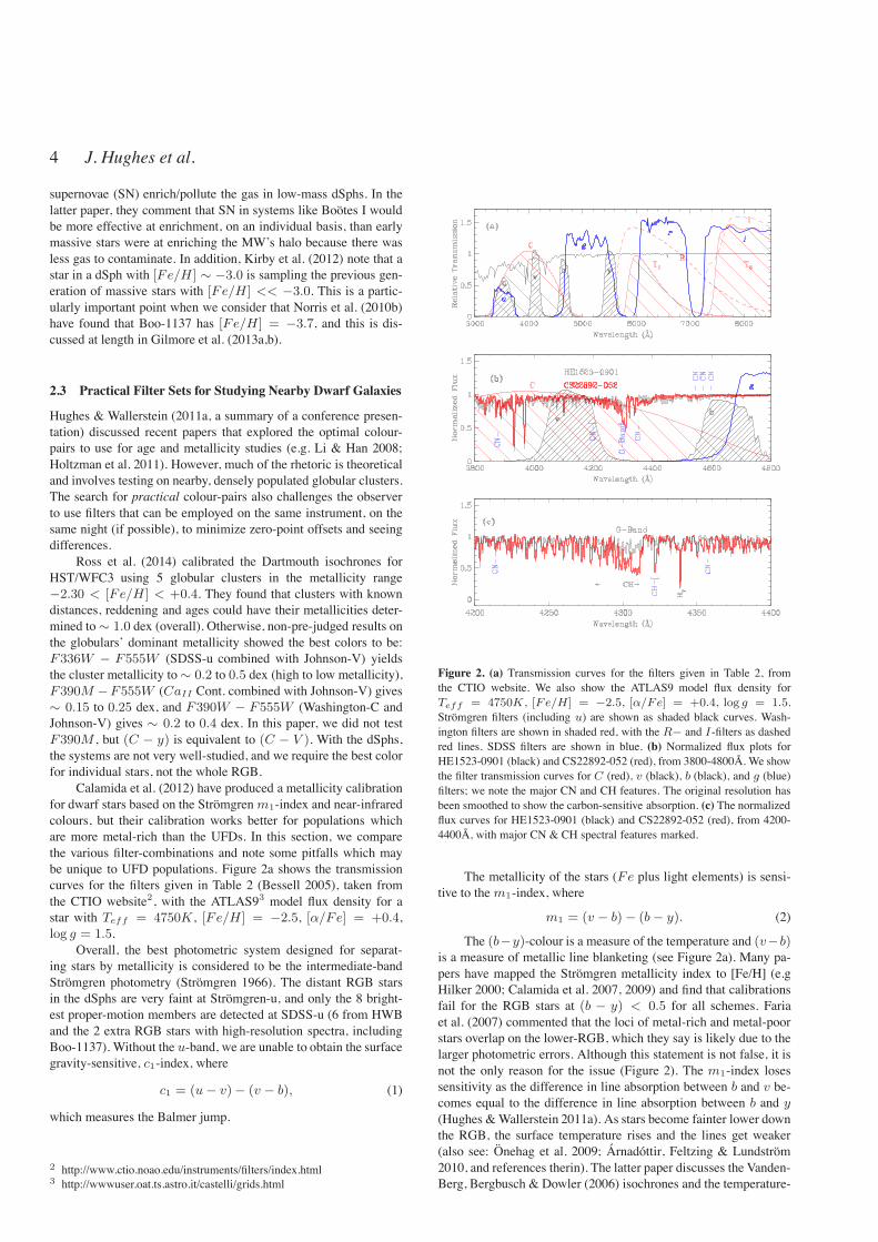
Calamida et al. (2012) have produced a metallicity calibrationfor dwarf stars based on the Stromgrenm1-index and near-infraredcolours, but their calibration works better for populations whichare more metal-rich than the UFDs. In this section, we comparethe various filter-combinations and note some pitfalls which maybe unique to UFD populations. Figure 2a shows the transmissioncurves for the filters given in Table 2 (Bessell 2005), taken fromthe CTIO website2, with the ATLAS93 model flux density for astar with Teff = 4750K, [Fe/H ] = "2.5, [!/Fe] = +0.4,log g = 1.5.
Overall, the best photometric system designed for separat-ing stars by metallicity is considered to be the intermediate-bandStromgren photometry (Stromgren 1966). The distant RGB starsin the dSphs are very faint at Stromgren-u, and only the 8 bright-est proper-motion members are detected at SDSS-u (6 from HWBand the 2 extra RGB stars with high-resolution spectra, includingBoo-1137). Without the u-band, we are unable to obtain the surfacegravity-sensitive, c1-index, where
c1 = (u" v)" (v " b), (1)
which measures the Balmer jump.
2 http://www.ctio.noao.edu/instruments/filters/index.html3 http://wwwuser.oat.ts.astro.it/castelli/grids.html
Figure 2. (a) Transmission curves for the filters given in Table 2, fromthe CTIO website. We also show the ATLAS9 model flux density forTeff = 4750K , [Fe/H] = "2.5, [!/Fe] = +0.4, log g = 1.5.Stromgren filters (including u) are shown as shaded black curves. Wash-ington filters are shown in shaded red, with the R" and I-filters as dashedred lines. SDSS filters are shown in blue. (b) Normalized flux plots forHE1523-0901 (black) and CS22892-052 (red), from 3800-4800A. We showthe filter transmission curves for C (red), v (black), b (black), and g (blue)filters; we note the major CN and CH features. The original resolution hasbeen smoothed to show the carbon-sensitive absorption. (c) The normalizedflux curves for HE1523-0901 (black) and CS22892-052 (red), from 4200-4400A, with major CN & CH spectral features marked.
The metallicity of the stars (Fe plus light elements) is sensi-tive to them1-index, where
m1 = (v " b)" (b" y). (2)
The (b"y)-colour is a measure of the temperature and (v"b)is a measure of metallic line blanketing (see Figure 2a). Many pa-pers have mapped the Stromgren metallicity index to [Fe/H] (e.gHilker 2000; Calamida et al. 2007, 2009) and find that calibrationsfail for the RGB stars at (b " y) < 0.5 for all schemes. Fariaet al. (2007) commented that the loci of metal-rich and metal-poorstars overlap on the lower-RGB, which they say is likely due to thelarger photometric errors. Although this statement is not false, it isnot the only reason for the issue (Figure 2). The m1-index losessensitivity as the difference in line absorption between b and v be-comes equal to the difference in line absorption between b and y(Hughes &Wallerstein 2011a). As stars become fainter lower downthe RGB, the surface temperature rises and the lines get weaker(also see: Onehag et al. 2009; Arnadottir, Feltzing & Lundstrom2010, and references therin). The latter paper discusses the Vanden-Berg, Bergbusch & Dowler (2006) isochrones and the temperature-
Photometric Metallicities 5
colour transformation by Clem et al. (2004), and makes a pointthat their classification scheme can only be used for giants with(b" y)0 ! 0.6.
Also from Figure 2, we can see the advantages that the Wash-ington filters provide over the Stromgren and SDSS filters. Thebroad C-filter includes the metallicity-defining lines contained inthe narrower v-filter and part of the b-filter, and also surface-gravitysensitive Stromgren-u and SDSS-u. Thus, the colour (C " T1)should be sensitive to Teff , [Fe/H ], [!/Fe], and log g (GS99).The Stromgren filters are more effective than Washington bands ina system with a well-populated upper RGB, or if the stellar systemis close enough to have ! 1 per cent photometry below the sub-giant branch (SGB), where the isochrones separate. As discussedin HWB, Geisler (1996) and Geisler, Claria & Minniti (1991), themore-commonly used broadbandR" and I-filters can be convertedlinearly to Washington T1 and T2, but with less observing timeneeded (also see the filter profiles in Figure 2a). The C-filter isbroader than the Johnson B-band, and is more sensitive to line-blanketing. Washington-C is a better filter choice than Johnson-Bor Stromgren-v for determining metallicity in faint, distant galax-ies. Table 2 includes estimates for the total exposure times requiredto reach the MSTO of dSphs with the WFPC3 on HST (also seeRoss et al. 2014).
Summarizing comments by Sneden et al. (2003), metallicityis usually synonymous with [Fe/H], but other elements may beinhomogeneously-variable in dSphs as well as the Milky Way’shalo.
[Fe/H ] = log10(NFe/NH)# " log10(NFe/NH)". (3)
The metallicity is normally taken to be:
Z = Z0(0.694f! + 0.306), (4)
where f! $ [!/Fe], the !-enhancement factor, and Z0 is the“heavy element abundance by mass for the solar mixture with thesame [Fe/H ]” (Kim et al. 2002).
In Figure 2b and 2c, we use 2 metal-poor RGB stars to il-lustrate the sensitivity of the Stromgren, Washington and SDSSfilters to carbon-enhancement. HE 1523-0901 (black line: Frebelet al. 2007) is a r-process-enhanced metal-poor star with [Fe/H ] %"3.0, [C/Fe] = "0.3, log Teff = 4650K, and log g = 1.0. CS22892-052 (red line) is also an r-process rich object (Sneden et al.2003, 2009; Cowan et al. 2011) with [Fe/H ] % "3.0, [C/Fe] %1.0, log Teff = 4800K, log g = 1.5, and [!/Fe] % +0.3.The change in the CH-caused G-band is apparent in Figure 2c, andCN/CH features affect the C (in particular), v", and b-filters, butthe SDSS g-band is relatively clear of contamination, but g is notvery sensitive to metallicity either. The spectra shown in Figure 2were provided by Anna Frebel (private communication).
Carretta et al. (2011) reports a study of globular cluster starswith CN/CH variations. They discuss other ways to constructStromgren-indices, finding a filter combination that will separatethe first and second generations of globular cluster stars. Carrettaet al. (2011) settled on
cy = c1 " (b" y) (5)
#4 = (u" v)" (b" y), (6)
with cy being defined by Yong et al. (2008), and is an indexwhich is sensitive to gravity and N . Both of these indices havelimited use in our study, since they require high precision pho-tometry at the Stromgren-u" and v"bands. Carretta et al. (2011)
point out that m1 and cy have a “complicated,” degenerate depen-dence on metallicity (involving [Fe/H ] and N ), and show that #4is much more effective at estimating the N"abundance, and re-mains CNO-sensitive over a much broader range of stellar tem-peratures, metallicities and surface gravities, since the temperaturedependence is weak. Carretta et al. (2011) are more concerned withseparating the N-poor, Na-poor, O-rich first generation globularpopulation, from the N-rich, Na-rich, O-poor, second generationstars (if present). We note that there is a particular problem whichinvolves the carbon-rich stars in the dSphs, because their coloursalways make a metal-poor star mimic those of a much more metal-rich object.
3 OBSERVATIONS
As in HWB, we observed the same central field (see Table 1) inBootes I (RA = 14h00m06s, Dec = 14.5$ J2000) with theApache Point Observatory’s 3.5-m telescope, using the direct imag-ing SPIcam system. The detector is a backside-illuminated SITeTK2048E 2048 # 2048 pixel CCD with 24 micron pixels, whichwe binned (2 # 2), giving a plate scale of 0.28 arc seconds perpixel, and a field of view (FOV) of 4.78# 4.78 square arcminutes.The HWB data set for Bootes I was taken on 2007 March 19 (witha comparison field in M92 taken on 2007 May 24). We took 21frames in Washington C, and Cousins R and I filters, with exposuretime ranging from 1 seconds to 1000 seconds. The readout noisewas 5.7e- with a gain of 3.4 e-/ADU. The images were flat-fieldedusing dome or night-sky flats, along with with a sequence of zeros.We then processed the frames using the image-processing softwarein IRAF.4
The vby-observations used in this paper are detailed in Ta-ble 1, along with the Washington filter data from HWB (whenthe seeing, and most airmass-values, were noticeably better). TheStromgren data was taken on 2009 January 17-18, 2009 May 1, and2011 April 5. The January 2009 data used the 2# 2 in2 Stromgrenfilter set, which had vignetted the images. The 3-inch square uvbyfilters arrived from the manufacturer (Custom Scientific, Inc., ofPheonix, AZ) after the January 2009 observing run. We comparedthe Bootes I stars observed in January and May 2009 and found thatthere was no appreciable difference in the instrumental magnitudesat the same airmass. The photometric quality of the January datawas better than the May data, but the January 2009 images weretaken with the smaller filters. After some questions about recordedexposure times in the image headers were resolved, more frameswere taken in April, 2011, to ensure stability of the zero-points.We also took some additional images in June, 2012 in C and R,but the seeing was never better than 1.5%% so they are not included.The final weighted mean-magnitude program rejected the latter ob-servations because of poor image quality compared to the earlierframes. In addition to the Bootes I central field chosen in 2007, wealso observed two RGB stars, in separate fields, which had highresolution spectra in the literature: Boo-1137 and Boo-127 (Norriset al. 2010a,b; Frebel, Kirby & Simon 2010; Feltzing et al. 2009).
Table 1 lists the data taken at APO. The images taken on 2007March 19 had sub-arcsecond seeing, and enabled us to make thebest possible master source list for DAOPHOT. For conversion to
4 IRAF is distributed by the National Optical Astronomy Observatory,which is operated by the Association of Universities for Research in As-tronomy (AURA) under cooperative agreement with the National ScienceFoundation.
6 J. Hughes et al.
the standard Washington system, we used the Geisler (1996) Wash-ington standard frames, containing at least 5 stars in each frame, forat least 30 standards per half-night (the APO 3.5-m is scheduled inthat manner). For the Stromgren data, this was more of an issue,since the Stromgren system was calibrated with single stars. To re-duce observing overheads, we used M92 as a cluster standard. Weused the M92 fiducial lines to assist in matching the APO data tothe standard system. To supplement the HWBWashington data, wetookC andR images of the Bootes I central field in 2009 (not I), tomake sure that there was no calibration issue with the earlier data.No problems were detected.
Employing the same data reduction method as HWB, we usedtwo iterations of (DAOPHOT-PHOT-ALLSTAR), with the first it-eration having a detection threshold of 4", and the second pass hada 5" detection limit. We used ! 10 stars in each frame to constructthe point spread functions (PSFs), and assume that it do not varyover the chip. The chip had been found to be very stable and therehas been no evidence that the PSF varies over the image. ALLSTAR(Stetson 1987) was further constrained to only detect objects with aCHI-value < 2.0, and almost all sources had CHI (the DAOPHOTgoodness-of-fit statistic) between 0.5 and 1.5 (to remove cosmicrays and non-stellar, extended objects). We found the aperture cor-rection between the small (4 pixel) aperture used by ALLSTAR inthe Bootes I field, and the larger (10-15 pixel) aperture used forthe standards, by using the best point spread function (PSF) starsin each images. We used the IMMATCH task to match the sourcesin each image, making several datasets in each filter combination.We then put together the final source list as follows: requiring thateach star be detected in at east one image in each filter, and thefinal magnitude and colours were calculated as the weighted (air-mass, FWHM, DAOPHOT uncertainty) mean of each individualdetection.
We later tested the final photometry using the standaloneversion of ALLFRAME (Stetson 1994), and found that the re-sults were consistent with our method. When we used DAOPHOTIII/ALLFRAME, this method produced almost identical results tothose obtained by manually shifting all the images to the samepositions, median-filtering them all and producing a source listfrom that. When we used that master-list to feed into the IRAFversion of ALLSTAR, it produced 166 total detections seen atvbyCT1T2(RI), but the v-band data is noticeably noisier, as ex-pected. Compared to the HWB list, 117 objects were detected, andwe use this group of objects in the comparison to M92. We find thatthere are 34 objects having a v-band uncertainty less than 0.10 dex,which were detected in multiple frames in each band (on more thanone night), and had a lower overall standard-deviation-of-the-meanuncertainty; these objects are listed in Table 3. However, we plotthe full-dataset in Figure 3, to show the uncertainty in magnitudesand colors, for comparison with models in §6.
In order to display how well DAOPHOT (both versions)worked on the central Bootes I field, we used the median-filteredimages in each filter to show the uncertainty for each object againstT1 and V (y). This is the best measure of how well DAOPHOT isworking, and it is correlated with airmass and seeing. The imagesare not crowded, we have a factor of 10 fewer objets than we woulddetect in M92. With the artificial star experiments, the complete-ness of the data set is controlled by the v-band magnitude. Theonly completeness issue involves the 2 bright foreground stars seenin Figure 1c, but the source density is too low for many objects tobe missed. At this point, we are not constructing luminosity func-tions below the MSTO, so completeness is less of a concern thanthe photometric uncertainties for each star. Using M92 as a clus-
ter standard, we reduced the frames using IRAF’s DAOPHOT, with20-30 stars to fit the PSF. We then selected stars on the outer partsof the globular cluster for testing; our photometry yielded matchesto the standard system used for ! 20 randomly selected stars incommon with the Frank Grundahl M92’s data set (private commu-nication, F. Grundahl; Grundahl et al. 2000) of "rms = 0.026 inV (y), "rms = 0.035 in (b " y), and "rms = 0.046 in m1. Ourconfirmation frames from 2011 were only deep enough to detect thebright RGB stars in Bootes I, so those stars have more observationsand hence lower uncertainties in vbyCT1. In Figure 4, we showcolour-magnitude diagrams used for calibration of Boo I to M92(cyan points: Grundahl et al. 2000). The dark blue line is the Dart-mouth isochrone (Dotter et al. 2008) which fits well with a recentstudy by di Cecco et al. (2010), DM = 14.74, [Fe/H ] = "2.32,[!/Fe] = 0.3 and Y = 0.248, and Age= 11 ± 1.5 Gyr. Bootes Iis taken to have E(B " V ) = 0.02 and DM = 19.11, as used inHWB.
We solved for each filter, rather than the Stromgren indices,for each night. The transformation equations on 2009 May 1 are asfollows:
V = yi " 2.187" 0.012(bi " yi)" 0.163X, "rms = 0.007 (7)
b = bi " 2.217 + 0.031(bi " yi) + 0.220X, "rms = 0.017 (8)
v = vi " 2.464" 0.512(vi " bi)" 0.300X, "rms = 0.020 (9)
Here, X denotes the effective airmass and the subscript i indicatesthe instrumental magnitude. The "rms values are the comparisonwith the standards.
HWB’s photometry from 2007 March 19 yielded matches tothe GS99 standard system of "rms = 0.021 in T1, "rms = 0.015in (C " T1), and "rms = 0.017 in (T1 " T2). In T1, the averageuncertainties in the final CMD were "rms = 0.024 at the level ofthe horizontal branch, and "rms = 0.04 at the MSTO. The trans-formation equations are as follows:
T1 = Ri " 0.461 + 0.021(Ci "Ri)" 0.150X, "rms = 0.021(10)
(C " T1) = 1.117(Ci "Ri)" 1.015 " 0.322X, "rms = 0.015(11)
(T1 " T2) = 1.058(Ri " Ii) + 0.460 " 0.046X, "rms = 0.017(12)
Here, X denotes the airmass and the subscript i indicates the instru-mental magnitude.
The final calculated uncertainties for each individual star ineach image were found by taking the uncertainties from photonstatistics, DAOPHOT’s uncertainties, the aperture corrections, andthe standard photometric errors in quadrature. We then took theweighted means of multiple observations, which reduced uncer-tainties internal to the data set. Thus, we achieved better uncer-tainties in for each star by taking the weighted means, with theweighting being dependent on the DAOPHOT uncertainties and theairmass, which was found to be equivalent to the seeing. We con-structed image sets comparing short and long exposures, keepingto similar airmass and seeing between frames, to achieve multi-ple, independent observations of each star and improved the final(standard-deviation-of-the-mean) uncertainty for the objects aboveT1 ! 22 mag. We were able to detect 166 objects in the field inthe vbyCT1T2(RI)-filters. A finding chart for the objects in Ta-ble 3 (117 objects) is given in HWB, and is shown in Figure 1b and

Photometric Metallicities 7
Table 1. APO 3.5-m CCD Frames taken in 2007-2011
Field UT1 Filter "(s) Airmass2 FWHM(%%)3Boo-127 09-01-18 y 300 1.19 1.0Boo-127 09-01-18 b 600 1.17 1.8Boo-127 09-01-18 v 1200 1.14 1.6Boo-1137 09-01-18 y 300 1.10 1.0Boo-1137 09-01-18 b 600 1.09 1.3Boo-1137 09-01-18 v 1200 1.08 0.9Boo Ic4 09-05-01 b 1500 1.25 0.9Boo Ic 09-05-01 y 900 1.33 1.0Boo Ic 09-05-01 y 600 1.87 1.0Boo Ic 09-05-01 b 900 1.65 1.0Boo Ic 09-05-01 b 900 2.06 1.2Boo Ic 09-05-01 v 1200 2.35 1.3Boo Ic 09-05-01 v 2100 1.48 1.0Boo Ic 11-04-05 R 300 1.08 0.9Boo Ic 11-04-05 C 900 1.07 1.3Boo Ic 11-04-05 y 600 1.06 1.1Boo Ic 11-04-05 b 600 1.06 1.1Boo Ic 11-04-05 v 1200 1.05 1.3Boo-1137 11-04-05 R 300 1.08 1.3Boo-1137 11-04-05 C 900 1.09 1.4Boo-1137 11-04-05 y 600 1.11 1.5Boo-1137 11-04-05 b 800 1.13 0.9Boo-1137 11-04-05 v 1200 1.16 1.0Boo-127 11-04-05 R 300 1.22 1.1Boo-127 11-04-05 C 900 1.24 1.5Boo-127 11-04-05 y 600 1.30 1.3Boo-127 11-04-05 b 800 1.34 1.2Boo-127 11-04-05 v 1200 1.40 1.7Boo Ic 07-03-19 R 1 1.07 0.9Boo Ic 07-03-19 R 3 1.07 0.8Boo Ic 07-03-19 R 10 1.06 0.8Boo Ic 07-03-19 R 30 1.06 0.8Boo Ic 07-03-19 R 90 1.06 0.8Boo Ic 07-03-19 R 300 1.06 0.7Boo Ic 07-03-19 R 1000 1.06 0.8Boo Ic 07-03-19 I 1 1.05 0.6Boo Ic 07-03-19 I 3 1.05 0.6Boo Ic 07-03-19 I 10 1.05 0.6Boo Ic 07-03-19 I 30 1.05 0.6Boo Ic 07-03-19 I 90 1.05 0.7Boo Ic 07-03-19 I 300 1.05 0.7Boo Ic 07-03-19 I 1000 1.05 0.8Boo Ic 07-03-19 C 1 1.06 0.7Boo Ic 07-03-19 C 3 1.06 0.9Boo Ic 07-03-19 C 10 1.06 0.8Boo Ic 07-03-19 C 30 1.06 0.7Boo Ic 07-03-19 C 90 1.06 0.8Boo Ic 07-03-19 C 300 1.07 0.7Boo Ic 07-03-19 C 1000 1.07 0.7(1) Year-Month-Day(2) Effective airmass(3) Average seeing(4) Boo Ic:- Bootes I central field, see Figure 1c.
1c here. Also, from Table 3, the 19 brightest stars were detected inthe SDSS survey5, and we include them in Table 4.
An independent, external test on how well we have calibratedthe data is discussed in §6.1, which covers spectral energy distribu-tions (SEDs).
5 accessed through http://www.sdss.org/
4 STATISTICAL REMOVAL OF NON-MEMBERS
The process used by HWB to remove non-dSph stars from our finaldata set was modified from that used on the globular clusters, NGC6388 and $ Cen (Hughes et al. 2007; Hughes & Wallerstein 2000,respectively). Due to observing-time constraints, we did not ob-serve an off-galaxy field, but instead generated artificial field starswith the TRILEGAL code (Girardi et al. 2005), calibrated for theSPIcam FOV and the appropriate magnitude limits. Briefly, we can
8 J. Hughes et al.
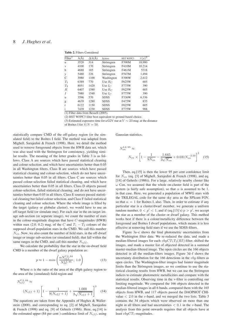
Table 2. Filters Considered
Filter1 #(A) !#(A) System HST WFPC3 "(s)2
u 3520 314 Stromgren F390M 18,980v 4100 170 Stromgren F410M 10,214b 4688 185 Stromgren F461M 5318y 5480 226 Stromgren F547M 1,494C 3980 1100 Washington F390W 2,612T1 6389 770 Use RC F625W 605T2 8051 1420 Use IC F775W 390R 6407 1580 Use RC F625W 605I 7980 1540 Use IC F775W 390u 3596 570 SDSS F336W 6,336g 4639 1280 SDSS F475W 835r 6122 1150 SDSS F625W 605i 7439 1230 SDSS F775W 988(1) Filter data from Bessell (2005).(2) HST WFPC3 filter best equivalent to ground-based choice.(3) Estimated exposures time for a G2V star at V # 23mag. at the distanceof Bootes I for S/N = 50.
statistically compare CMD of the off-galaxy region (or the sim-ulated field) to the Bootes I field. The method was adapted fromMighell, Sarajedini & French (1998). Here, we detail the methodused to remove foreground objects from the HWB data set, whichwas also used with the Stromgren for consistency, yielding simi-lar results. The meaning of the letter grades in Table 3 is as fol-lows. Class A are sources which have passed statistical cleaningand colour-selection, and which have uncertainties better than 0.05in all Washington filters. Class B are sources which have passedstatistical cleaning and colour-selection, which do not have uncer-tainties better than 0.05 in all filters. Class C are sources whichpassed colour-selection failed statistical cleaning, and which haveuncertainties better than 0.05 in all filters. Class D objects passedcolour-selection, failed statistical cleaning, and do not have uncer-tainties better than 0.05 in all filters. Class E sources passed statisti-cal cleaning but failed colour selection, and Class F failed statisticalcleaning and colour selection. Where the whole image is filled bythe target (galaxy or globular cluster), we would have to use anoff-target field (or simulate one). For each star in the on-target im-age sub-section (or separate image), we count the number of starsin the colour-magnitude diagram that have C-magnitudes (HWB)within max (2.0, 0.2) mag. of the C and T1 " T2 colours of thesupposed dwarf-population stars in the CMD. We call this numberNon. Now, we also count the number of field stars, in the off-dwarfimage or image sub-section (or simulated field), that fall within thesame ranges in the CMD, and call this number Noff .
We calculate the probability that the star in the on-dwarf fieldCMD is a member of the dwarf galaxy population as:
p % 1"min
!
!NUL 84off
NLL 95on
, 1.0
"
(13)
Where ! is the ratio of the area of the dSph galaxy region tothe area of the (simulated) field region and
NUL 84off %
(Noff + 1)
#
1"1
9(Noff + 1)+
1.000
3$
Noff + 1
%3
(14)
The equations are taken from the Appendix of Hughes & Waller-stein (2000), and corresponding to eq. [2] of Mighell, Sarajedini& French (1998) and eq. [9] of Gehrels (1986). Here, eq.[14] isthe estimated upper (84 per cent ) confidence limit of Noff , using
Gaussian statistics.
NLL 95on %
Non #&
1"1
9Non"
1.645
3&Non
+ 0.031N!2.50on
'3
(15)
Then, eq.[15] is then the lower 95 per cent confidence limitfor Non (eq. [3] of Mighell, Sarajedini & French (1998), and eq.[14] of Gehrels (1986)). For a large, relatively nearby cluster like$ Cen, we assumed that the whole on-cluster field is part of thesystem (a fairly safe assumption), so that ! is assumed to be 1,in that case. Here, we generated a population of MWG stars withthe TRILEGAL code for the same sky area as the SPIcam FOV,so that ! = 1 for Bootes I, also. Then, in order to estimate if anyparticular star is a cluster/dwarf member, we generate a uniformrandom number, 0 < p% < 1, and if (eq.[13]’s) p > p%, we acceptthe star as a member of the cluster or dwarf galaxy. This methodworks best if there is a colour/metallicity difference between theforeground and Bootes I dwarf populations, which means it is lesseffective at removing field stars if we use the SDSS-filters.
Figure 3a–c shows the final photometric uncertainties fromthe Washington filter data. We re-reduced the data, and made amedian-filtered images for each vbyCT1T2(RI)-filter, shifted theimages, and made a master list of objected detected in a summedmaster-median-filtered image. The open circles are the 166 objectsdetected in all the median-filters images. Figure 3d–f shows theuncertainty distribution for the 166 detections in the vby-filters asopen circles. The Washington-filter images had fainter magnitudelimits than the Stromgren images, so we continue to use the sta-tistical cleaning results from HWB, but we can use the Stromgrenindices to estimate photometric metallicities and compare with thestatistical results. Observing time in the v-filter is controlling ourlimiting magnitude. We compared the 166 objects detected in themedian-filtered images in all 6 bands, compared them with the 165objects from HWB, and 117 objects passed the DAOPHOT CHI-value < 2.0 in the v-band, and we merged the two lists. Table 3contains the 34 objects which were observed on more than onenight in all filters and had uncertainties < 0.1 in the v-band. Theanalysis from this point onwards requires that all objects have atleast vbyCT1-magnitudes.

Photometric Metallicities 9
Table 3. Objects in Bootes I with Washington & Stromgren Photometry
ID1 X2R YR RA DEC Class3 T1 (C " T1) (T1 " T2) V (b" y) m1
Boo-1137 " " 13:58:33.82 14:21:08.5 A 17.08(0.02) 1.69(0.03) 0.61(0.02) 17.65(0.01) 0.62(0.02) 0.09(0.03)Boo-127 " " 14:00:14.57 14:35:52.1 A 17.12(0.02) 1.84(0.03) 0.57(0.02) 17.68(0.004) 0.68(0.02) 0.14(0.03)Boo-117/HWB-8 298.68 891.95 14:00:10.49 14:31:45.6 C 17.20(0.02) 1.82(0.03) 0.61(0.02) 17.79(0.004) 0.61(0.02) 0.16(0.03)Boo-119/HWB-9 330.67 171.27 14:00:09.85 14:28:23.1 A 17.48(0.02) 1.80(0.03) 0.57(0.02) 17.98(0.005) 0.63(0.02) 0.20(0.03)HWB-22 950.94 97.89 13:59:57.85 14:28:02.8 A 19.77(0.02) 1.16(0.04) 0.47(0.02) 20.22(0.01) 0.47(0.02) 0.04(0.04)HWB-24 667.94 272.14 14:00:03.33 14:28:51.6 C 20.10(0.02) 1.06(0.03) 0.50(0.02) 20.48(0.01) 0.42(0.03) 0.04(0.06)HWB-28 564.80 599.22 14:00:05.34 14:30:23.5 A 20.40(0.02) 1.16(0.04) 0.50(0.03) 20.88(0.02) 0.45(0.03) 0.09(0.04)HWB-34 681.50 600.22 14:00:03.08 14:30:23.8 A 20.86(0.02) 1.09(0.04) 0.46(0.02) 21.27(0.02) 0.44(0.04) 0.03(0.06)HWB-3 960.10 499.42 13:59:57.69 14:29:55.6 F 16.01(0.01) 3.47(0.03) 1.65(0.03) 16.91(0.03) 1.27(0.03) -0.03(0.04)HWB-4 54.57 53.07 14:00:15.18 14:27:49.8 F 16.24(0.01) 3.29(0.03) 1.28(0.03) 17.17(0.02) 1.02(0.03) 0.33(0.05)HWB-6 630.81 818.25 14:00:04.07 14:31:25.1 E 16.86(0.01) 1.20(0.03) 0.49(0.02) 17.26(0.02) 0.44(0.03) 0.08(0.05)HWB-11 891.80 840.98 13:59:59.02 14:31:31.5 E 17.71(0.01) 3.26(0.03) 1.10(0.02) 18.67(0.01) 0.97(0.02) 0.46(0.04)HWB-14 540.96 301.43 14:00:05.78 14:28:59.8 E 18.63(0.01) 0.96(0.03) 0.40(0.02) 18.95(0.02) 0.40(0.03) 0.09(0.05)HWB-15 461.31 912.01 14:00:07.35 14:31:51.3 E 18.79(0.01) 3.39(0.03) 1.30(0.02) 19.82(0.02) 1.04(0.03) 0.37(0.06)HWB-16 287.26 389.96 14:00:10.69 14:29:24.6 A 18.92(0.01) 1.37(0.03) 0.52(0.02) 19.39(0.02) 0.52(0.03) 0.07(0.04)HWB-17 72.98 337.39 14:00:14.84 14:29:09.7 F 19.06(0.01) 0.88(0.03) 0.38(0.02) 19.40(0.01) 0.35(0.02) 0.08(0.04)HWB-18 171.21 684.41 14:00:12.95 14:30:47.3 E 19.23(0.01) 2.11(0.03) 0.59(0.02) 19.83(0.01) 0.59(0.02) 0.46(0.04)HWB-19 626.80 6.28 14:00:04.11 14:27:36.9 A 19.33(0.02) 0.87(0.03) 0.38(0.02) 19.59(0.01) 0.36(0.03) 0.07(0.04)HWB-20 329.81 701.76 14:00:09.88 14:30:52.2 E 19.37(0.01) 2.73(0.03) 0.86(0.02) 20.18(0.02) 0.80(0.04) 0.51(0.06)HWB-21 963.85 2.41 13:59:57.59 14:27:35.9 E 19.57(0.01) 3.12(0.06) 0.94(0.02) 20.38(0.02) 0.96(0.03) 0.32(0.09)HWB-26 589.61 886.86 14:00:04.87 14:31:44.3 E 20.30(0.02) 2.78(0.04) 0.88(0.02) 21.13(0.02) 0.77(0.04) 0.59(0.07)HWB-29 510.88 714.46 14:00:06.38 14:30:55.8 A 20.47(0.01) 1.20(0.03) 0.63(0.03) 20.91(0.02) 0.46(0.03) 0.08(0.07)HWB-31 207.93 381.42 14:00:12.23 14:29:22.1 C 20.72(0.01) 0.97(0.03) 0.46(0.03) 21.09(0.02) 0.44(0.03) -0.04(0.04)HWB-32 692.68 332.82 14:00:02.85 14:29:08.7 E 20.77(0.01) 0.76(0.03) 0.36(0.02) 20.99(0.03) 0.32(0.03) 0.03(0.05)HWB-33 848.41 14.94 13:59:59.83 14:27:39.4 E 20.84(0.01) 0.96(0.04) 0.36(0.03) 21.14(0.02) 0.44(0.03) -0.04(0.05)HWB-36 653.27 903.42 14:00:03.64 14:31:49.0 E 20.95(0.02) 1.12(0.04) 0.41(0.03) 21.40(0.03) 0.44(0.04) 0.01(0.06)HWB-37 925.81 867.63 13:59:58.36 14:31:39.0 E 21.06(0.01) 1.80(0.05) 0.59(0.02) 21.60(0.03) 0.52(0.05) 0.31(0.08)HWB-40 789.33 824.54 14:00:01.00 14:31:26.9 A 21.28(0.02) 1.13(0.04) 0.50(0.03) 21.64(0.03) 0.46(0.04) 0.05(0.07)HWB-44 945.51 434.38 13:59:57.97 14:29:37.3 E 21.52(0.02) 1.00(0.04) 0.39(0.03) 21.86(0.04) 0.43(0.05) -0.06(0.08)HWB-45 545.05 475.10 14:00:05.71 14:29:48.6 A 21.54(0.01) 0.21(0.03) 0.57(0.03) 22.03(0.04) 0.34(0.05) -1.02(0.07)HWB-47 673.78 935.68 14:00:03.24 14:31:58.1 A 21.75(0.02) 0.92(0.04) 0.47(0.04) 22.11(0.04) 0.36(0.06) 0.10(0.09)HWB-48 845.80 760.07 13:59:59.91 14:31:08.8 A 21.82(0.02) -0.08(0.04) 0.17(0.05) 21.78(0.03) 0.07(0.05) 0.08(0.06)HWB-50 87.95 538.21 14:00:14.56 14:30:06.1 A 21.92(0.02) 0.86(0.05) 0.40(0.03) 22.28(0.05) 0.38(0.07) 0.02(0.09)HWB-51 661.84 801.67 14:00:03.47 14:31:20.4 A 21.92(0.02) 0.33(0.04) 0.28(0.05) 22.05(0.05) 0.24(0.06) 0.05(0.08)(1) ID from HWB, proper motion-confirmed members listed first.(2) Positions from the Figure 1b.(3) HWB’s object classes:A - If sources passed the statistical cleaning process, had the correct colours and had photometry in all filters with uncertainties less than 0.05.B - Objects passed the cleaning program, but had uncertainties in all filters not less than 0.05.C - Passed the statistical cleaning process, had the correct colours and A-type good photometry, but failed the comparison with the randomly generatedprobability.D - Objects failed the statistical cleaning process (also had the right colours but poor photometry).E - Passed statistical cleaning but failed colour selection (according to HWB).F - These objects failed both statistical cleaning and colour selection, and tended to be well outside the CMD area of a metal-poor dwarf. Usually brightforeground stars.
5 PHOTOMETRICMETALLICITIES
Following on from the discussion in §2, several authors have gen-erated photometric calibrations on the Stromgren [Fe/H]-scale,amongst them, Hilker (2000) and Calamida et al. (2007). In thissection, we select several calibrations from those papers, wherem0
is the dereddened m1-index and [m] is the reddening-free version:
Hilker (2000) :
[Fe/H ]Hil =m0 " 1.277(b " y)0 + 0.331
0.324(b " y)0 " 0.031. (16)
Calamida et al. (2007) :
[Fe/H ]m1=
m0 + 0.309 " 0.521(v " y)00.159(v " y)0 " 0.090
. (17)
Calamida et al. (2007) :
[Fe/H ][m] =[m] + 0.251 " 0.585(v " y)0
0.131(v " y)0 " 0.070. (18)
These methods of calculating photometric metallicities are used forcolumns 2–4 of Table 5.
In Figure 5a and 5b, we show colour-colour plots and [Fe/H]-calibrations for M92 (cyan points). The blue points are the M92RGB stars above the horizontal branch (HB). Having the same typeof cool, metal-poor RGB as the expected dSph population, theseplots illustrate the loss of metallicity resolution on the lower-RGBin the Stromgren system. We used the TRILEGAL code6 to gener-ate a field of artificial stars at the correct galactic latitude, for thesame magnitude limits as our dSph field. Figure 5c and 5d show
6 http://stev.oapd.inaf.it/cgi-bin/trilegal
10 J. Hughes et al.
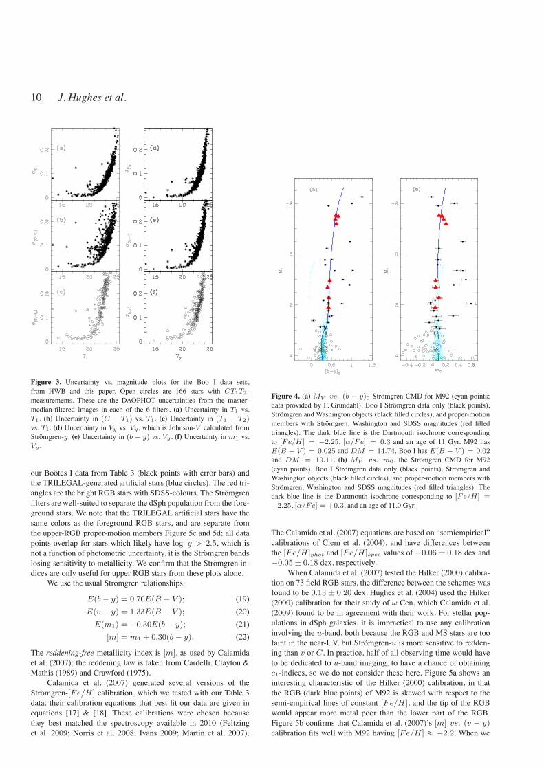
Figure 3. Uncertainty vs. magnitude plots for the Boo I data sets,from HWB and this paper. Open circles are 166 stars with CT1T2-measurements. These are the DAOPHOT uncertainties from the master-median-filtered images in each of the 6 filters. (a) Uncertainty in T1 vs.T1. (b) Uncertainty in (C " T1) vs. T1. (c) Uncertainty in (T1 " T2)vs. T1. (d) Uncertainty in Vy vs. Vy , which is Johnson-V calculated fromStromgren-y. (e) Uncertainty in (b " y) vs. Vy . (f) Uncertainty in m1 vs.Vy .
our Bootes I data from Table 3 (black points with error bars) andthe TRILEGAL-generated artificial stars (blue circles). The red tri-angles are the bright RGB stars with SDSS-colours. The Stromgrenfilters are well-suited to separate the dSph population from the fore-ground stars. We note that the TRILEGAL artificial stars have thesame colors as the foreground RGB stars, and are separate fromthe upper-RGB proper-motion members Figure 5c and 5d; all datapoints overlap for stars which likely have log g > 2.5, which isnot a function of photometric uncertainty, it is the Stromgren bandslosing sensitivity to metallicity. We confirm that the Stromgren in-dices are only useful for upper RGB stars from these plots alone.
We use the usual Stromgren relationships:
E(b" y) = 0.70E(B " V ); (19)E(v " y) = 1.33E(B " V ); (20)E(m1) = "0.30E(b " y); (21)
[m] = m1 + 0.30(b " y). (22)
The reddening-free metallicity index is [m], as used by Calamidaet al. (2007); the reddening law is taken from Cardelli, Clayton &Mathis (1989) and Crawford (1975).
Calamida et al. (2007) generated several versions of theStromgren-[Fe/H ] calibration, which we tested with our Table 3data; their calibration equations that best fit our data are given inequations [17] & [18]. These calibrations were chosen becausethey best matched the spectroscopy available in 2010 (Feltzinget al. 2009; Norris et al. 2008; Ivans 2009; Martin et al. 2007).
Figure 4. (a) MV vs. (b " y)0 Stromgren CMD for M92 (cyan points;data provided by F. Grundahl), Boo I Stromgren data only (black points),Stromgren and Washington objects (black filled circles), and proper-motionmembers with Stromgren, Washington and SDSS magnitudes (red filledtriangles). The dark blue line is the Dartmouth isochrone correspondingto [Fe/H] = "2.25, [!/Fe] = 0.3 and an age of 11 Gyr. M92 hasE(B " V ) = 0.025 and DM = 14.74. Boo I has E(B " V ) = 0.02and DM = 19.11. (b) MV vs. m0, the Stromgren CMD for M92(cyan points), Boo I Stromgren data only (black points), Stromgren andWashington objects (black filled circles), and proper-motion members withStromgren, Washington and SDSS magnitudes (red filled triangles). Thedark blue line is the Dartmouth isochrone corresponding to [Fe/H] ="2.25, [!/Fe] = +0.3, and an age of 11.0 Gyr.
The Calamida et al. (2007) equations are based on “semiempirical”calibrations of Clem et al. (2004), and have differences betweenthe [Fe/H ]phot and [Fe/H ]spec values of "0.06 ± 0.18 dex and"0.05± 0.18 dex, respectively.
When Calamida et al. (2007) tested the Hilker (2000) calibra-tion on 73 field RGB stars, the difference between the schemes wasfound to be 0.13 ± 0.20 dex. Hughes et al. (2004) used the Hilker(2000) calibration for their study of $ Cen, which Calamida et al.(2009) found to be in agreement with their work. For stellar pop-ulations in dSph galaxies, it is impractical to use any calibrationinvolving the u-band, both because the RGB and MS stars are toofaint in the near-UV, but Stromgren-u is more sensitive to redden-ing than v or C. In practice, half of all observing time would haveto be dedicated to u-band imaging, to have a chance of obtainingc1-indices, so we do not consider these here. Figure 5a shows aninteresting characteristic of the Hilker (2000) calibration, in thatthe RGB (dark blue points) of M92 is skewed with respect to thesemi-empirical lines of constant [Fe/H ], and the tip of the RGBwould appear more metal poor than the lower part of the RGB.Figure 5b confirms that Calamida et al. (2007)’s [m] vs. (v " y)calibration fits well with M92 having [Fe/H ] % "2.2. When we

Photometric Metallicities 11
Figure 5. (a) Plot ofm0 = (v" b)0" (b"y)0 vs. (b"y)0 for M92 RGBstars (blue points, F.Grundahl, private communication), and the rest of theglobular cluster’s stars (cyan). The calibration lines of constant [Fe/H] aretaken from Hilker (2000). (b) For the same M92 sample, we show [m] =m1+0.3(b"y), the reddening-free index, plotted against (v"y)0 . Calibra-tion from Calamida et al. (2007). (c)m0 = (v"b)0"(b"y)0 vs. (b"y)0for our sample (from the median filtered images), with the Hilker (2000)calibration. In total, 117 objects were detected in vby filters, shown as blackpoints. The TRILEGAL code was used to generate a sample of foregroundstars, shown as blue filled circles. The RGB proper-motion members areshown as red triangles. (d) [m] = m1 + 0.3(b " y) vs. (v " y)0 for thesame sample of Bootes I stars, with the Calamida et al. (2007) calibration.
apply the calibrations to our data in Table 5, this skewing is ob-served (comparing column 2 to columns 3 & 4). Again, we noticethat the fainter RGB stars have large uncertainties, resulting fromthe loss of sensitivity of them1-index and the increasing photomet-ric uncertainties, particularly at Stromgren-v.
For the Washington filters, we use:
E(C " T1) = 1.966E(B " V ); (23)E(T1 " T2) = 0.692E(B " V ); (24)
MT1= T1 + 0.58E(B " V )" (m"M)V ; (25)
from Geisler, Claria & Minniti (1991) and GS99. HWB used equa-tions (23)–(25) and the GS99 standard giant branches to find the[Fe/H ]-values for the Bootes I RGB stars. Note that GS99 useAV = 3.2E(B " V ); not setting RV = 3.1 does not transforminto an appreciable difference for Bootes I, as E(B " V ) = 0.02.
In Table 6, we show the preliminary results from Hughes &Wallerstein (2011b), where the stellar parameters were estimatedfrom %2 fits to the [!/Fe] = 0.0 to +0.4 Dartmouth isochrones(Dotter et al. 2008). We found that the best fits gave [!/Fe] =+0.3 ± 0.1 dex. The early results presented in Hughes & Waller-stein’s (2011b) conference paper were consistent with the Martinet al. (2007), CaT-based spectroscopy, available at the time. How-ever, the model grid was not fine enough for our goals, and we ranextensive, finer-grid models, based on the Dartmouth isochrones.
We expect that the dSph stars are !-enhanced in the sameway as the MWG halo population (see discussion in Cohen &
Figure 6. CMDs and colour-colour plots using a mixture of SDSS andWashington filters to show the [Fe/H]-sensitivity (HWD). In all diagrams,the red triangles are the 8 RGB stars, known to be proper-motion mem-bers. All isochrones shown are solar-scaled and have an age of 12 Gyr.(a) Mr vs. (g " r)0 with Dartmouth models, !-enhanced to +0.3. (b)MT1
vs. (C"T1)0 with Dartmouth models, also !-enhanced to +0.3. (c)Mr vs. (C " r)0 (d) (r " i)0 vs. (g " r)0 SDSS colour-colour plot,with the Dartmouth isochrones. (e)Washington colours with GS99 standardgiant branches (HWB).
Huang 2009; Norris et al. 2008, and our §5). We use both the !-enhanced and solar-scaled models from the Dartmouth Stellar Evo-lution Database7 (Dotter et al. 2008) to compare with our data.
6 DISCUSSION
From Figure 6b, we see that (C " T1) widens the separation ofthe giant branches of different metallicities, giving a resolution forthe GS99 RGB fiducial lines of ! 0.15 dex. One of us (GW) sug-gested the Washington system, which was developed by Canterna(1976); Geisler (1996) defined CCD standard fields for the system.In HWB, we found that Washington filters spread out the stars atthe MSTO, and we have found that (C " T1) is more effectivethan the SDSS-colours (g " r), as shown in Figure 6a. The SDSS
7 http://stellar.dartmouth.edu/#models/

12 J. Hughes et al.
Table 4. SDSS Magnitudes for Stars in Bootes I Central Field
ID SDSS u g r i z ClassBoo-1137 19.77(03) 18.11(01) 17.37(01) 17.04(01) 16.86(01) Member1Boo-127 20.01(05) 18.16(01) 17.37(01) 17.02(01) 16.85(01) Member1HWB-3 20.10(05) 17.73(01) 16.28(01) 14.77(01) 13.98(01) FHWB-4 20.47(05) 18.00(01) 16.57(00) 15.65(01) 15.16(01) FHWB-6 23.37(74) 22.43(12) 20.96(04) 19.47(02) 18.76(04) EBoo-117/HWB-8 19.98(05) 18.21(01) 17.44(01) 17.10(01) 16.92(01) CBoo-119/HWB-9 20.21(04) 18.43(01) 17.69(01) 17.38(01) 17.21(01) AHWB-11 21.74(20) 19.49(01) 18.05(01) 17.23(01) 16.77(01) EHWB-15 24.46(13) 20.63(03) 19.22(01) 18.18(01) 17.63(02) EHWB-16 21.08(11) 19.70(02) 19.13(01) 18.87(01) 18.72(04) AHWB-18 22.48(36) 20.42(02) 19.54(02) 19.16(02) 19.01(05) EHWB-20 23.47(80) 20.90(03) 19.62(02) 19.03(02) 18.70(04) EHWB-21 24.50(67) 21.22(03) 19.86(02) 19.18(02) 18.77(03) EHWB-22 21.63(11) 20.35(02) 19.85(02) 19.63(02) 19.55(06) AHWB-23 24.11(61) 21.92(06) 20.31(02) 19.00(01) 18.24(02) EHWB-24 21.69(11) 20.74(02) 20.21(02) 20.02(03) 19.99(08) CHWB-26 25.01(12) 21.82(07) 20.59(03) 19.94(03) 19.64(08) EHWB-28 22.51(38) 21.04(04) 20.63(03) 20.42(04) 20.40(15) AHWB-29 22.24(29) 21.00(04) 20.69(03) 20.50(05) 20.27(13) AHWB-31 21.71(19) 21.27(05) 20.87(04) 20.77(06) 20.55(17) CHWB-34 22.67(43) 21.47(05) 21.00(05) 20.81(06) 20.44(15) A(1) Confirmed Boo I members outside central field.
photometry is not sensitive enough to this difference in colours todistinguish Boo I’s level of metallicity spread. The subset of 19 ob-jects with ugriz magnitudes (Table 4) contains most of the brightobjects from HWB and this paper’s Stromgren data set. These arethe objects which have Stromgren and Washington colours fallingin the appropriate ranges which enable us to calculate the photo-metric values of [Fe/H ]. Table 3 contains foreground stars andBootes I members, and intersects with the spectroscopic data setof Martin et al. (2007). We have radial velocities and independentmetallicities for 8 of the objects in Table 3, and Stromgren andWashington [Fe/H ]phot-values for many of them. We added the2 giants outside the central Bootes I field, Boo-1137 and Boo-127,as additional calibrators, because Boo-1137 (Norris et al. 2010b) isvery metal poor, and both have had a number of spectra taken (seeTable 5).
We considered the effect of replacing the g-filter with themuch broader C-band (Hughes & Wallerstein 2011a). As we cansee from Figure 6b and 6c, the colour, (C " r) works well forthe upper RGB (log g < 1.5) in Bootes I, but that the lower-RGBstars (2.5 < log g < 3.0) are not well-separated in this colour.The reasons for this discrepancy are filter-width and transmission,which are shown in Figure 2a and Table 2. While the Sloan r-filterhas a greater overall transmission than the Washington T1-filter, ithas become standard practice to substitute the broadband R-filterfor T1, since it has "&R = 1580A, compared to "&T1
= 770A(Geisler 1996, also see Table 2).
As with the Lai et al. (2011) method, there are merits in com-bining all the available photometry, but we are searching for theminimum useful number of filters that can break the age-metallicitydegeneracy. In Figure 7, we compare the Stromgren and Washing-ton filters, and construct two new indices:
m# = (C " T1)0 " (T1 " T2)0 (26)
and
m## = (C " b)0 " (b" y)0. (27)
Our motivation in defining these indices is to avoid the col-lapse of the metallicity sensitivity of the m1-index on the lower
RGB, and to attempt to replace the v-filter with the broader C-filter (also see Hughes & Wallerstein 2011a). Figure 7h showsm## vs. (C " T1)0, and allows us to use 4 filters, CT1by, whichreduces observing time and keeps ! 0.3 dex [Fe/H]-resolution forstars with "1.5 > Fe/H > "4.0. Figure 7i shows that we coulduse Cby for metallicity estimates "1.5 > Fe/H > "4.0. Thesecolour-colour plots are not sensitive to age on the RGB, recoveringage-resolution at the MSTO. However, reaching the MSTO withCby is much faster than with vby (see Table 2). Figs.7a, b & cshow thatm0 may be preferred for systems with"1.0 > Fe/H >"2.0, but we note that (C " T1) would also be more useful there,with much shorter exposure times.
6.1 SPECTRAL ENERGY DISTRIBUTIONS OFINDIVIDUAL STARS
When crossing the boundaries between photometric systems, wefound it instructive to construct SEDs for our sample, as a indepen-dent and external check, on our photometry, and to make sure allthe magnitudes were on their standard systems (Bessell 2005). Thisprocess enabled us to compare the Dartmouth models and the AT-LAS9 synthetic stars to the real data, and understand better the con-straints placed by the observational uncertainties and the relation-ship between each stars’ temperature and metallicity. Figures 8–15display SEDs for the 8 RGB proper-motion confirmed membersof Bootes I shown with the best-fitting (employing a simple %2 fit)ATLAS9model fluxes, appropriately scaled to pass through the ma-jority of the photometry data points. If there is a wide discrepancybetween the fits to the ATLAS9 models in Washington, Stromgren,and SDSS filters, we show 2 fits. The y-axes are always flux den-sity, log('F" ), in ergs/s/cm, and the x-axes are wavelength in mi-crons. We used the conversions from magnitudes to fluxes from theHST ACS website.8 The Washington system and the Stromgrendata are VEGAmag and the SDSS system is ABmag, and we deter-mined that the 8 RGB stars had the fluxes transformed to the same
8 http://www.stsci.edu/hst/acs/analysis/zeropoints
Photometric Metallicities 13
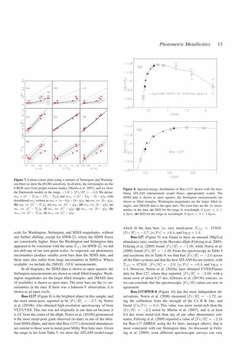
Figure 7. Colour-colour plots using a mixture of Stromgren and Washing-ton filters to show the [Fe/H]-sensitivity. In all plots, the red triangles are the8 RGB stars from proper-motion studies (Martin et al. 2007), and we showthe Dartmouth models in the range, "1.0 > [Fe/H] > "4.0. We define:m# = (C " T1)0 " (T1 " T2)0 andm## = (C " b)0 " (b" y)0, withdereddened-m1 written asm0 = (v"b)0"(b"y)0. (a)m0 vs. (b"y)0.(b)m0 vs. (C " T1)0. (c) m0 vs. (C " y)0. (d) m# vs. (b " y)0. (e)m# vs. (C " T1)0. (f) m# vs. (C " y)0 . (g) m## vs. (b " y)0. (h)m## vs. (C " T1)0. (i)m## vs. (C " y)0 .
scale for Washington, Stromgren, and SDSS magnitudes, withoutany further shifting, except for HWB-22, where the SDSS fluxesare consistently higher. Since the Washington and Stromgren dataappeared to be consistent with the same Teff for HWB-22, we didnot shift any of our zero-point scales. As expected, our photometryuncertainties produce smaller error bars than the SDSS data, andthese stars also suffer from large uncertainties in SDSS-u. Whereavailable, we include the 2MASS, JHK measurements.
In all diagrams, the SDSS data is shown as open squares, theStromgren measurements are shown as small filled triangles, Wash-ington magnitudes are the larger filled triangles, and 2MASS data(if available) is shown as open stars. The error bars are the 1" un-certainties in the data. If there was a Johnson-V observation, it isshown as an open circle.
Boo-1137 (Figure 8) is the brightest object in this sample, andthe most metal-poor, reported to be [Fe/H ] = "3.7, by Norriset al. (2010b), who obtained high-resolution spectroscopy of fromVLT/UVES. This star was not originally in our data set because itis 24% from the center of the dSph. Norris et al. (2010b) pronouncedit the most metal-poor giant observed (to-date) in one of the ultra-faint SDSS dSphs, and show that Boo-1137’s elemental abundancesare similar to those seen in metal-poor Milky Way halo stars. Giventhe range in fits from Table 5, we show the ATLAS9 model-range
Figure 8. Spectral-energy distribution of Boo-1137 shown with the best-fitting ATLAS9 (interpolated) model fluxes, appropriately scaled. TheSDSS data is shown as open squares, the Stromgren measurements areshown as filled triangles, Washington magnitudes are the larger filled tri-angles, and 2MASS data is the open stars. The error bars are the 1$ uncer-tainties in the data. (a) SED for the range in wavelength, 0.1µm < # <2.3µm. (b) SED for the range in wavelength, 0.3µm < # < 1.0µm.
which fit the data best, i.e. very metal-poor, Teff = 4750K,[Fe/H ] = "3.7, [!/Fe] = +0.4, and log g = 1.4.
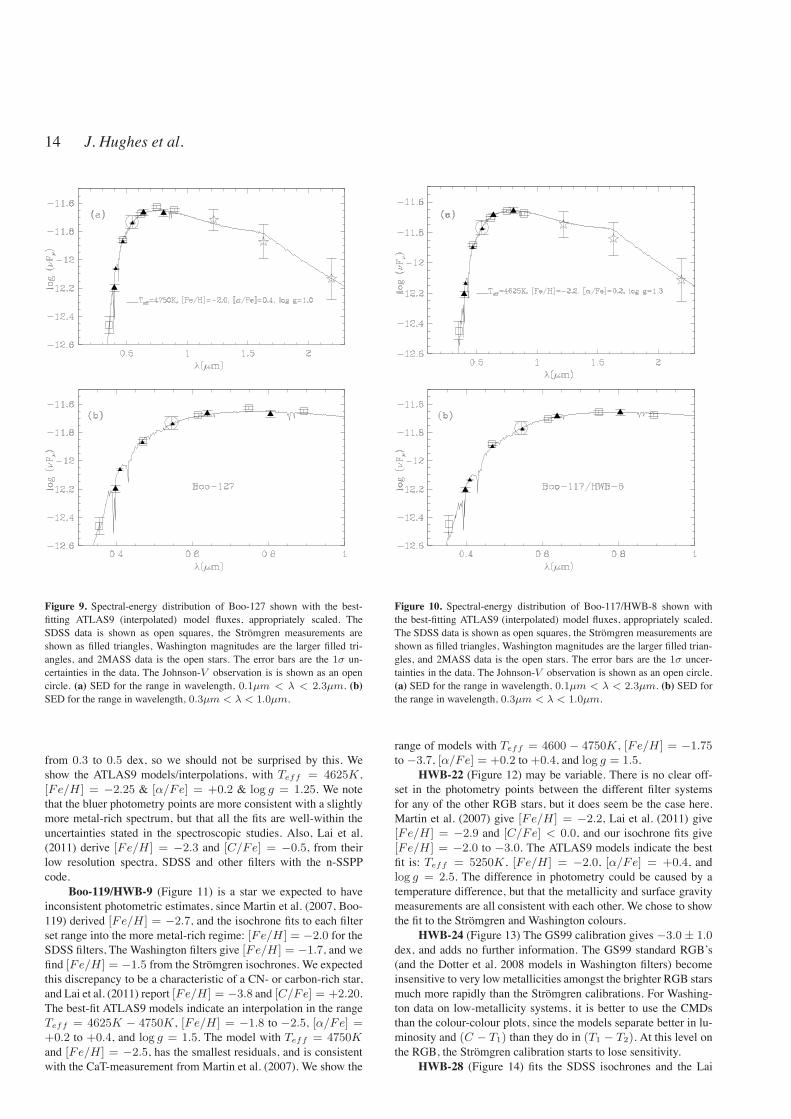
Boo-127 (Figure 9) was found to have an unusual [Mg/Ca]abundance ratio, similar to the Hercules dSph (Feltzing et al. 2009).Feltzing et al. (2009) found [Fe/H ] = "1.98, while Norris et al.(2008) found [Fe/H ] = "1.49. From the spectroscopy in Table 5and isochrone fits in Table 9, we find that [Fe/H ] = "2.0 acrossall the filter-systems and that the best ATLAS9 fits are models, withTeff = 4750K, [Fe/H ] = "2.0, [!/Fe] = +0.4, and log g =1.3. However, Norris et al. (2010a) later obtained UVES/Flamesdata for Boo-127, where they reported, [Fe/H ] = "2.08; with amean error of about 0.27 dex. Gilmore et al. (2013b) concurs, sowe can conclude that the spectroscopic [Fe/H ]-values are now inagreement.
Boo-117/HWB-8 (Figure 10) has the most independent ob-servations. Norris et al. (2008) measured [Fe/H ] = "1.72, us-ing the calibration from the strength of the Ca II K line, andfound [Ca/Fe] ! 0.3. This value was more metal-rich than the[Fe/H ] = "2.2 noted by Martin et al. (2007), and is at least0.4 dex more metal-rich than any of our other photometric esti-mates. Feltzing et al. (2009) reported a value of [Fe/H ] = "2.24for Boo-117 (HIRES; using the Fe lines, amongst others), that ismore consistent with our Stromgren data. As discussed in Feltz-ing et al. (2009), even different spectroscopic surveys can vary
14 J. Hughes et al.
Figure 9. Spectral-energy distribution of Boo-127 shown with the best-fitting ATLAS9 (interpolated) model fluxes, appropriately scaled. TheSDSS data is shown as open squares, the Stromgren measurements areshown as filled triangles, Washington magnitudes are the larger filled tri-angles, and 2MASS data is the open stars. The error bars are the 1$ un-certainties in the data. The Johnson-V observation is is shown as an opencircle. (a) SED for the range in wavelength, 0.1µm < # < 2.3µm. (b)SED for the range in wavelength, 0.3µm < # < 1.0µm.
from 0.3 to 0.5 dex, so we should not be surprised by this. Weshow the ATLAS9 models/interpolations, with Teff = 4625K,[Fe/H ] = "2.25 & [!/Fe] = +0.2 & log g = 1.25. We notethat the bluer photometry points are more consistent with a slightlymore metal-rich spectrum, but that all the fits are well-within theuncertainties stated in the spectroscopic studies. Also, Lai et al.(2011) derive [Fe/H ] = "2.3 and [C/Fe] = "0.5, from theirlow resolution spectra, SDSS and other filters with the n-SSPPcode.
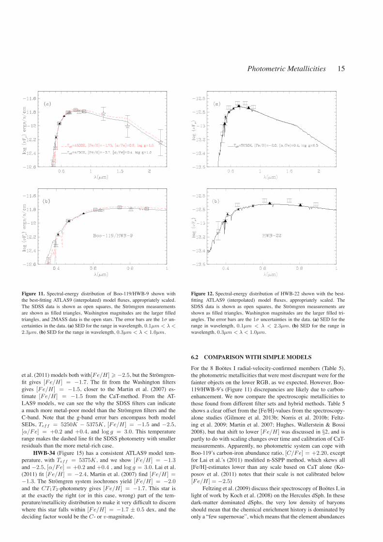
Boo-119/HWB-9 (Figure 11) is a star we expected to haveinconsistent photometric estimates, since Martin et al. (2007, Boo-119) derived [Fe/H ] = "2.7, and the isochrone fits to each filterset range into the more metal-rich regime: [Fe/H ] = "2.0 for theSDSS filters, The Washington filters give [Fe/H ] = "1.7, and wefind [Fe/H ] = "1.5 from the Stromgren isochrones. We expectedthis discrepancy to be a characteristic of a CN- or carbon-rich star,and Lai et al. (2011) report [Fe/H ] = "3.8 and [C/Fe] = +2.20.The best-fit ATLAS9 models indicate an interpolation in the rangeTeff = 4625K " 4750K, [Fe/H ] = "1.8 to "2.5, [!/Fe] =+0.2 to +0.4, and log g = 1.5. The model with Teff = 4750Kand [Fe/H ] = "2.5, has the smallest residuals, and is consistentwith the CaT-measurement from Martin et al. (2007). We show the
Figure 10. Spectral-energy distribution of Boo-117/HWB-8 shown withthe best-fitting ATLAS9 (interpolated) model fluxes, appropriately scaled.The SDSS data is shown as open squares, the Stromgren measurements areshown as filled triangles, Washington magnitudes are the larger filled trian-gles, and 2MASS data is the open stars. The error bars are the 1$ uncer-tainties in the data. The Johnson-V observation is shown as an open circle.(a) SED for the range in wavelength, 0.1µm < # < 2.3µm. (b) SED forthe range in wavelength, 0.3µm < # < 1.0µm.
range of models with Teff = 4600 " 4750K, [Fe/H ] = "1.75to "3.7, [!/Fe] = +0.2 to +0.4, and log g = 1.5.
HWB-22 (Figure 12) may be variable. There is no clear off-set in the photometry points between the different filter systemsfor any of the other RGB stars, but it does seem be the case here.Martin et al. (2007) give [Fe/H ] = "2.2, Lai et al. (2011) give[Fe/H ] = "2.9 and [C/Fe] < 0.0, and our isochrone fits give[Fe/H ] = "2.0 to "3.0. The ATLAS9 models indicate the bestfit is: Teff = 5250K, [Fe/H ] = "2.0, [!/Fe] = +0.4, andlog g = 2.5. The difference in photometry could be caused by atemperature difference, but that the metallicity and surface gravitymeasurements are all consistent with each other. We chose to showthe fit to the Stromgren and Washington colours.
HWB-24 (Figure 13) The GS99 calibration gives "3.0± 1.0dex, and adds no further information. The GS99 standard RGB’s(and the Dotter et al. 2008 models in Washington filters) becomeinsensitive to very low metallicities amongst the brighter RGB starsmuch more rapidly than the Stromgren calibrations. For Washing-ton data on low-metallicity systems, it is better to use the CMDsthan the colour-colour plots, since the models separate better in lu-minosity and (C " T1) than they do in (T1 " T2). At this level onthe RGB, the Stromgren calibration starts to lose sensitivity.
HWB-28 (Figure 14) fits the SDSS isochrones and the Lai
Photometric Metallicities 15
Figure 11. Spectral-energy distribution of Boo-119/HWB-9 shown withthe best-fitting ATLAS9 (interpolated) model fluxes, appropriately scaled.The SDSS data is shown as open squares, the Stromgren measurementsare shown as filled triangles, Washington magnitudes are the larger filledtriangles, and 2MASS data is the open stars. The error bars are the 1$ un-certainties in the data. (a) SED for the range in wavelength, 0.1µm < # <2.3µm. (b) SED for the range in wavelength, 0.3µm < # < 1.0µm.
et al. (2011) models both with[Fe/H ] ! "2.5, but the Stromgren-fit gives [Fe/H ] = "1.7. The fit from the Washington filtersgives [Fe/H ] = "1.5, closer to the Martin et al. (2007) es-timate [Fe/H ] = "1.5 from the CaT-method. From the AT-LAS9 models, we can see the why the SDSS filters can indicatea much more metal-poor model than the Stromgren filters and theC-band. Note that the g-band error bars encompass both modelSEDs, Teff = 5250K " 5375K, [Fe/H ] = "1.5 and "2.5,[!/Fe] = +0.2 and +0.4, and log g = 3.0. This temperaturerange makes the dashed line fit the SDSS photometry with smallerresiduals than the more metal-rich case.
HWB-34 (Figure 15) has a consistent ATLAS9 model tem-perature, with Teff = 5375K, and we show [Fe/H ] = "1.3and "2.5, [!/Fe] = +0.2 and +0.4 , and log g = 3.0. Lai et al.(2011) fit [Fe/H ] = "2.4, Martin et al. (2007) find [Fe/H ] ="1.3. The Stromgren system isochrones yield [Fe/H ] = "2.0and the CT1T2-photometry gives [Fe/H ] = "1.7. This star isat the exactly the right (or in this case, wrong) part of the tem-perature/metallicity distribution to make it very difficult to discernwhere this star falls within [Fe/H ] = "1.7 ± 0.5 dex, and thedeciding factor would be the C- or v-magnitude.
Figure 12. Spectral-energy distribution of HWB-22 shown with the best-fitting ATLAS9 (interpolated) model fluxes, appropriately scaled. TheSDSS data is shown as open squares, the Stromgren measurements areshown as filled triangles, Washington magnitudes are the larger filled tri-angles. The error bars are the 1$ uncertainties in the data. (a) SED for therange in wavelength, 0.1µm < # < 2.3µm. (b) SED for the range inwavelength, 0.3µm < # < 1.0µm.
6.2 COMPARISONWITH SIMPLEMODELS
For the 8 Bootes I radial-velocity-confirmed members (Table 5),the photometric metallicities that were most discrepant were for thefainter objects on the lower RGB, as we expected. However, Boo-119/HWB-9’s (Figure 11) discrepancies are likely due to carbon-enhancement. We now compare the spectroscopic metallicities tothose found from different filter sets and hybrid methods. Table 5shows a clear offset from the [Fe/H]-values from the spectroscopy-alone studies (Gilmore et al. 2013b; Norris et al. 2010b; Feltz-ing et al. 2009; Martin et al. 2007; Hughes, Wallerstein & Bossi2008), but that shift to lower [Fe/H ] was discussed in §2, and ispartly to do with scaling changes over time and calibration of CaT-measurements. Apparently, no photometric system can cope withBoo-119’s carbon-iron abundance ratio, [C/Fe] = +2.20, exceptfor Lai et al.’s (2011) modified n-SSPP method, which skews all[Fe/H]-estimates lower than any scale based on CaT alone (Ko-posov et al. (2011) notes that their scale is not calibrated below[Fe/H ] = "2.5)
Feltzing et al. (2009) discuss their spectroscopy of Bootes I, inlight of work by Koch et al. (2008) on the Hercules dSph. In thesedark-matter dominated dSphs, the very low density of baryonsshould mean that the chemical enrichment history is dominated byonly a “few supernovae”, which means that the element abundances

16 J. Hughes et al.
Figure 13. Spectral-energy distribution of HWB-24 shown with the best-fitting ATLAS9 (interpolated) model fluxes, appropriately scaled. TheSDSS data is shown as open squares, the Stromgren measurements areshown as filled triangles, Washington magnitudes are the larger filled tri-angles. The error bars are the 1$ uncertainties in the data. (a) SED for therange in wavelength, 0.1µm < # < 2.3µm. (b) SED for the range inwavelength, 0.3µm < # < 1.0µm.
of the stellar population might show star-to-star chemical inhomo-geneities, tracing individual SNe II events (Gilmore et al. 2013a,b).In studying the Hercules system, Koch et al. (2008) estimate thatonly 10 SN were needed to give the “atypical abundance ratios”(and more should have contributed). Bootes I is less massive thanHercules, but Feltzing et al. (2009) only report one star, Boo-127,(and possibly Boo-094, also not observed here), has unusual vari-ations in Mg and Ca. Expecting more individuality, Feltzing et al.(2009) conclude that Bootes I is surprisingly well-mixed. Norriset al. (2009) beg to differ, and they take issue with Feltzing et al.’s(2009) [Mg/Ca] value as being too high for one of their sevenBootes I stars, the aforementioned, Boo-127. We agree with Nor-ris’s group, and also Gilmore et al. (2013b).
Norris et al. (2009) obtained high-resolution spectroscopy ofBoo-1137 from VLT/UVES (not included in HWB’s data set be-cause it is 24% from the center of the dSph), pronouncing it themost metal-poor giant observed (to-date) in one of the ultra-faintSDSS dSphs, with [Fe/H ] = "3.7. Norris et al. (2009) findthat Boo-1137’s elemental abundances are similar to those seen inmetal-poor MWG halo stars. They also discuss Bootes I’s SF his-tory, surmising that it most likely underwent an early, short periodof star formation, cleared by SN II which enriched it’s interstellarmedium inhomogeneously. In Boo-1137, Norris et al. (2009) find!-enhancement (compared to Fe) of "[!/Fe] ! 0.2, “relative
Figure 14. Spectral-energy distribution of HWB-28 shown with the best-fitting ATLAS9 (interpolated) model fluxes, appropriately scaled. TheSDSS data is shown as open squares, the Stromgren measurements areshown as filled triangles, Washington magnitudes are the larger filled tri-angles. The error bars are the 1$ uncertainties in the data. (a) SED for therange in wavelength, 0.1µm < # < 2.3µm. (b) SED for the range inwavelength, 0.3µm < # < 1.0µm.
to the mean of the metal-poor halo stars.” Even though the spec-troscopy studies we have mentioned have tried to cover as much ofthe Bootes I dSph as possible (and Boo-1137 is almost two half-light radii from the center), all groups have collected medium reso-lution spectra of less than 30 members, with high-resolution spec-tra of only a handful of stars. As Tolstoy, Hill & Tosi (2009) andGilmore et al. (2013a) say, SNe Ia start to contribute to the chem-ical composition 108 " 109 years after the first stars form. Thereis a wide range in [Fe/H ], but not in the !-elements. So, if themassive stars in Bootes I cleared the interstellar medium quickly,star formation lasted less than 1 Gyr. Can we detect an age spreadthat small?
What kind of metallicity or age spread would we expect to seein Bootes I? Age estimates cannot usually be made for individualRGB stars, but the GS99 standard giant branches do have an age-metallicity degeneracy, compared to the Dartmouth isochrones. Isthe separation of RGB stars with Bootes I’s range in chemical com-position, large enough to differentiate between RGB-isochrones inany colour? Our normal practice is to use the RGB to find the metal-licity and the MSTO to find ages, where the isochrones separate.Brown et al. (2012) and Kirby et al. (2012) studied the metallicitydistributions and star formation histories (SFHs) of several dSphs.Isochrone fits to these populations, as noted by Kirby, have to beperformed at the upper-RGB, the SGB and the MSTO, in order to
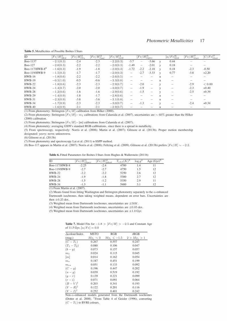
Photometric Metallicities 17
Table 5.Metallicities of Possible Bootes I Stars
ID [Fe/H]1Hil [Fe/H]2m1[Fe/H]3[m] [Fe/H]4GS [Fe/H]5spec [!/Fe]6Gil [Fe/H]7Lai [C/Fe]7Lai
Boo-1137 "2.1(0.3) -2.4 -2.3 "2.2(0.3) -3.7 " -3.66 y 0.44 " "
Boo-127 "2.0(0.3) -2.2 -2.2 "2.0(0.3) -1.49 " -2.01 y 0.18 " "
Boo-117/HWB-88 "1.6(0.3) -1.9 -1.8 "2.0(0.3) -1.72 -2.2 -2.18 y 0.18 -2.3 -0.50Boo-119/HWB-9 "1.5(0.3) -1.7 -1.7 "2.0(0.3) " -2.7 -3.33 y 0.77 -3.8 +2.20HWB-16 "1.8(0.6) -2.2 -2.2 "2.6(0.5) " " " u " " "
HWB-19 "0.5(1.0) -0.5 -0.6 "3.3(0.8) " " " n " " "
HWB-22 "1.8(0.6) -2.3 -2.3 "2.9(0.7) " -2.0 " y " -2.9 < 0.00HWB-24 "1.4(0.7) -2.0 -2.0 "3.0(0.7) " -1.9 " y " -2.3 +0.40HWB-28 "1.2(0.6) -1.6 -1.6 "2.9(0.6) " -1.5 " y " -2.5 +0.39HWB-29 "1.4(0.9) -1.8 -1.7 "2.8(0.6) " " " u " " "
HWB-31 "2.3(0.9) -3.8 -3.6 "3.1(0.8) " " " u " " "
HWB-34 "1.7(0.9) -2.3 -2.3 "3.0(0.7) " -1.3 " y " -2.4 +0.34HWB-40 "1.6(0.9) -2.1 -2.1 "2.9(0.7) " " " u " " "
(1) From photometry: Stromgren-[Fe/H] calibration from Hilker (2000).(2) From photometry: Stromgren-[Fe/H]:–m1 calibrations from Calamida et al. (2007), uncertainties are # 60% greater than the Hilker(2000) calibration.(3) From photometry: Stromgren-[Fe/H]:– [m] calibrations from Calamida et al. (2007).(4) From photometry: averaging GS99’s standard RGB-calibrations, since there is a spread in metallicity.(5) From spectroscopy, respectively: Norris et al. (2008); Martin et al. (2007); Gilmore et al. (2013b). Proper motion membershipdesignated: yes=y; no=n; unknown=u.(6) Gilmore et al. (2013b)(7) From photometry and spectroscopy Lai et al. (2011) n-SSPP method.(8) Boo-117 appears in Martin et al. (2007); Norris et al. (2008); Feltzing et al. (2009). Gilmore et al. (2013b) prefers [Fe/H] # "2.2.
Table 6. Fitted Parameters for Bootes I Stars from Hughes & Wallerstein (2011b)
ID [Fe/H]1Spec [Fe/H]2phot Teff (K)3 log g4 Age (Gyr)5
Boo-117/HWB-8 -2.25 -2.4 4700 1.4 11Boo-119/HWB-9 -2.7 -2.7 4750 1.5 12HWB-22 -2.2 -2.2 5250 2.6 12HWB-24 -1.9 -1.8 5300 2.7 12HWB-28 -1.5 -1.2 5350 2.9 11HWB-34 -1.3 -1.1 5400 3.1 12(1) From Martin et al. (2007).(2) Means found from fitting Washington and Stromgren photometry separately to the !-enhancedDartmouth isochrones, then taking weighted means, dependent on error bars. Uncertainties arethen ±0.25 dex.(3) Weighted mean from Dartmouth isochrones, uncertainties are ±50K .(4) Weighted mean from Dartmouth isochrones, uncertainties are ±0.05 dex.(5) Weighted mean from Dartmouth isochrones, uncertainties are ±1.0 Gyr.
Table 7. Model Fits for "1.8 > [Fe/H] > "2.5 and Constant Ageof 11.5 Gyr, [!/Fe] = 0.0
!colour/Index MSTO RGB rRGB(mag.) MT1
# 3 MT1" "1.5 2 > MT1
> 1(C " T1) 0.267 0.557 0.247(T1 " T2) 0.080 0.106 0.047(b " y) 0.073 0.157 0.057m1 0.024 0.115 0.045[m] 0.014 0.162 0.054m# 0.187 0.451 0.199m## 0.051 0.133 0.092(C " y) 0.196 0.447 0.202(u" g) 0.039 0.519 0.192(g " r) 0.139 0.221 0.099(r " i) 0.071 0.091 0.064(B " V )† 0.203 0.341 0.193(V " R)† 0.122 0.201 0.116(V " I)† 0.252 0.401 0.242Non-!-enhanced models generated from the Dartmouth isochrones(Dotter et al. 2008). †From Table 4 of Geisler (1996), converting(C " T1) to BVRI colours.

18 J. Hughes et al.
Table 8. colour Change/Gyr for Model Fits for Constant [Fe/H] ="1.8, [!/Fe] = 0.0, and Age Range of 10-14 Gyr
!colour/Index MSTO RGB rRGB(mag.) MT1
# 3 MT1" "1.5 2 > MT1
> 1(C " T1) 0.129 0.417 0.016(T1 " T2) 0.040 0.084 0.004(b " y) 0.037 0.109 0.004m1 0.010 0.135 0.000[m] 0.004 0.168 0.001m# 0.090 0.333 0.012m## 0.027 0.111 0.003(C " y) 0.095 0.329 0.012(u" g) 0.008 0.413 0.014(g " r) 0.072 0.170 0.007(r " i) 0.008 0.076 0.003(B " V )† 0.137 0.274 0.084(V " R)† 0.084 0.163 0.053(V " I)† 0.181 0.329 0.123Non-!-enhanced models generated from the Dartmouth isochrones(Dotter et al. 2008). †From Table 4 of Geisler (1996), converting(C " T1) to BVRI colours.
Figure 15. Spectral-energy distribution of HWB-34 shown with the best-fitting ATLAS9 (interpolated) model fluxes, appropriately scaled. TheSDSS data is shown as open squares, the Stromgren measurements areshown as filled triangles, Washington magnitudes are the larger filled tri-angles. The error bars are the 1$ uncertainties in the data. (a) SED for therange in wavelength, 0.1µm < # < 2.3µm. (b) SED for the range inwavelength, 0.3µm < # < 1.0µm.
break the age-metallicity degeneracy. In many dSphs, we do nothave sufficient upper-RGB stars to make this fit (Willman 2010).
To improve the resolution of our grid of Dartmouthisochrones, we ran a simple closed-box chemical evolution mode.We used the Dartmouth (solar-scaled) isochrones to produce pop-ulations of stars with a similar physical size, mass, and metallicityspread to Bootes I, but with ages of 10–14 Gyr over the approx-imate metallicity range "1.0 > Fe/H > "4.0. We obtainedover 50,000 artificial stars (binary fraction of 0.5) with Stromgren,Washington and SDSS magnitudes. We compared model stars withour objects having vbyCT1T2 measurements.
From these model runs, we chose 3 simple cases. Firstly, thereis a single-age (11.5 Gyr) population (1216 stars), with a conser-vative spread in metallicity from [Fe/H ] = "3.5 up to "1.5.We call this Case I. The second population (Case II: 9133) wasdesigned to be enriched in situ, with "4.0 < [Fe/H ] < "1.0.The metallicity distribution terminated after star formation lastingat least 4 Gyr. We added Case III, an alternative long-duration pop-ulation with a few “starbursts,” to determine if we could tell itapart from Case II. In Case III, there are 1374 stars born 12 Gyrago, with "3.5 < [Fe/H ] < "2.5, 6375 stars with "2.5 <[Fe/H ] < "1.75, which are 0.5 Gyr younger, and 1363 stars with"1.75 < [Fe/H ] < "1.0, with SF extending up to 10 Gyr ago,and then terminating. Using the Kolmogorov-Smirnov Test for TwoPopulations, where the null-hypothesis (H0) is that the populationsare the same, we can tell the difference between the age spreads inCases I, II and III, but not the metallicity ranges.
In order to make the models more realistic, we use the pho-tometric uncertainties from Figure 3. From tests, we found that werequired at least 2% photometry at the MSTO to determine if thereare age spreads present, since the isochrones exhibit a change of! 0.06 mag. in (C"T1) for each Gyr in age. There would have tobe much deeper Stromgren photometry for any age spread less than1.5 Gyr to be distinguished. In the Washington system alone, with[Fe/H ] ! "2.0, 2 per cent photometric uncertainty at the MSTOwould reveal an age spread of > 1 Gyr.
We selected models with log g of 1.0-2.0 for the RGB stars,2.0-3.0 for the rising-RGB (rRGB), below the level of the HB,and log g ! 4.0 for the MSTO. We examined the colours in theStromgren, Washington and SDSS systems, at fixed age and fixed-
Photometric Metallicities 19
[Fe/H]. Our goal was to quantify the filter systems sensitivity andbreak the age-metallicity degeneracy as cleanly as possible, avoid-ing the upper-RGB. The results of the artificial star experiments aregiven in Tables 7 and 8, and Figure 16. Figure 16a shows coloursand indices for the stars in all the models with an age of 11.5 Gyr,and examines a range of "2.5 < [Fe/H ] < "1.8. The RGBstars’ range is shown in orange, the rRGB in gold, and the MSTOin violet. Figure 7b takes stars at a constant [Fe/H ] = "1.8. Weknow that the real stars are !-enhanced at the +0.2 to +0.4 dexlevel, (Norris et al. 2010b and Gilmore et al. 2013b; see Table 5)which would make a metal-poor star look more metal rich in thebroad-band colors. In Figure 16b, we let the model stars have afixed metallicity value of [Fe/H ] = "1.8 (more like a real sampleof [Fe/H ] ! "2.0) and let the age vary from 10-14 Gyr.
Even though these models cannot be considered well-calibrated below [Fe/H ] = "2.5, we show the lower end of the[Fe/H ]-range, from "4.0 < [Fe/H ] < "3.0, at a constant ageof 11.5 Gyr, but we hatch the bar-chart to recognize this factor. Ifwe were fortunate to collect so many [Fe/H ]-values of enoughreal stars in dSphs at this low range in [Fe/H ], the stars may be!-enhanced and may not appear so metal-poor broadband colors(CN- or C-enhanced). However, this is the parameter-space wherethe SDSS-colors recover their usefulness. For our sample, that theSDSS-colors are very uncertain here, as the u" and g"magnitudeshave large uncertainties (see Table 4) returned are too low for theMSTO-stars, at the sensitive TO-value of log g. If we had de-tections down to the MSTO stars, they would have a spread in(u " g) ! 3.0. Here, the SDSS filters lack of sensitivity to !-elements lets us recover a star’s metal-poor nature, even if it wasan extreme example, e.g. Boo-119. However, for this color to beeffective, the stars have to be detected at SDSS " u, which takesmore than twice as long as the C-band (see Table 2). For stars justabove the MSTO to the upper-RGB, (C "T1) is most effective forall evolutionary stages in both age and metallicity. The (C " T1)calibration loses is sensitivity below [Fe/H ] ! "2.2 on this scale,which is why we have to supplement it with (b"y). The filter com-bination CT1by, or even Cby, maintains its sensitivity to metallic-ity below [Fe/H ] ! "3.0, as can be seen in Figures 7g–i. Alsonote that the rRGB colours are hardly sensitive to age at all, and canbe used to break the age-metallicity degeneracy. We want to avoidusing Sloan-u or Stromgren-u, and the v-band, as both consume ob-serving time (see Table 2). However, many searches for closer andbrighter extremely metal-poor stars (Spite et al. 2013), this colorcould be vital, but even they use (g " z) to avoid SDSS-u.
From the models, we find that the (C " T1)-colour is best forour sample above theMSTO; the (C"y)-colour is shown to be use-ful (in agreement with Ross et al. 2014),m# is better thanm##, andall these are better than the SDSS colours. However, constructingindices involves 3 or 4 filters, which increases the uncertainty in anparameters derived from a colour-colour or color-index calibration.The method of deriving age and [Fe/H ] will the smallest uncer-tainty is to use a color sensitive to temperature and one sensitiveto chemical composition, but we need to combine the Washingtonand Stromgren filters.
We considered that Bootes I might resemble $ Cen, the coreof a captured dE, with extended enrichment and a long period ofstar formation (Gratton et al. 2011; Hughes et al. 2004). Due toits lack of HI or recent star formation (SF) (Bailin & Ford 2007),we might expect Bootes I to have a simple history, similar to mostglobular clusters (Milone et al. 2012), with a short burst of starformation, terminated by supernovae (SNe) II events, or tidal strip-ping (Fellhauer et al. 2008) removing the ISM. This scenario should
give rise to almost a single-age fit to the CMD, and a very narrow("[Fe/H ] < 0.5) dex metallicity range. Marcolini & D’Ercole(2008) discussed the model of Marcolini et al. (2006) which de-scribes the chemical evolution of dSphs (particularly Draco, but itcan be generalized). Marcolini & D’Ercole (2008) argue that theSNe II ejecta from the star formation event in a Draco-like dSph(actually about “50 instantaneous bursts” over 60 Myr) should beretained, due to the extra mass from the dark matter halo, and be-cause “efficient radiative losses” keep the enriched ISM flowingback to the central regions of the dSph, mixing the gas. Cohen &Huang (2009) obtained high-resolution spectra of 8 stars in Draco,adding to 14 they had observed previously, which had a metallicityrange of "1.5 < [Fe/H ] < "3.0 dex, similar to Bootes I; theirage-metallicity relationship indicated that SF in Draco lasted about5 Gyrs. An age spread even half this large should have been obvi-ous for Bootes I, even with the uncertainties in Figure 3. The mod-eling of Draco’s enrichment history (Marcolini & D’Ercole 2008),showed a star formation process lasting about 2 Gyr, with most ofthe initial Fe-enrichment coming from SNe II, with chemical inho-mogeneities appearing later, caused by SNe Ia “pockets” of mate-rial, with higher [Fe/H ] and lower [!/Fe], which take 2–3 Gyr tomix in with the rest of the gas, the dynamics of which is driven bythe SNe II effects. The discussion of possible star formation histo-ries for this system is also illustrated by Gilmore et al. (2013a).
At the very least, the real Bootes I stars have [!/Fe] =+0.3± 0.1 dex, but this value seems to be unchanging; it is likelythat SF terminated before the onset of SN Ia contamination. Weassume this can be quantified as a colour-shift. When we exam-ined the Dartmouth isochrones, for [!/Fe] = 0.0 and +0.4,in the Stromgren system only the y-filter seemed to be sensitiveto [!/Fe], making stars brighter by 0.046 mag. at 12 Gyr and[Fe/H ] = "2.5. We saw that the model stars with low metal-licities lost sensitivity in the v- and b-filters, making those mag-nitudes insensitive to !-abundances. In the Washington filters, T1
was shifted by -0.057 mag. and (C " T1) by +0.035, with a varia-tion of less than 1 per cent .
Setting [!/Fe] ! +0.4 for Bootes I, we compare our ClassA–C stars’ CT1by-magnitudes with the whole data set of over50,000 artificial stars, and the results are listed in Table 9. Weperformed %2 fits to the stars generated from the [!/Fe] = 0.0Dartmouth isochrones (Dotter et al. 2008), using the colour-shiftsdetermined for the CT1by-filters. With the possible inclusion oftwo blue stragglers (HWB-45 and HWB-51), and HWB-9 beingcarbon-rich (and CN-strong), the average age is 11.5 ± 0.4 Gyr,and the range in metallicity is "1.6 > [Fe/H ] > "3.4, whichwould be shifted to around "1.9 > [Fe/H ] > "3.7 with !-enhancement added back (in agreement with Gilmore et al. 2013b).We note that Boo-1137 does not appear as metal poor as it should,also, likely because the C-filter also loses sensitivity for very metal-poor stars. Our tests of the recovery of the artificial stars where weadded typical photometric uncertainties found that the (C " T1)-colour started to become insensitive when [Fe/H ] < "2.2. Wealso found it necessary to use (b " y) as the temperature-sensitivecolour instead of (T1"T2): otherwise, the temperatures of the realstars became at least 500K too hot compared to the SEDs shown inFigures 8–15. Usingm## and (b " y) or (C " y) did not improvethe fit. (C " y) or (C " T1) alone are not sufficient for individualstars, unlike whole giant branches (Ross et al. 2014).
We conclude that the fewest number of filters we can use forthese old, metal-poor populations, is 4, and those are CT1by. Wepreserve the ! 2 dex range in [Fe/H] from the spectra, but we esti-mate Table 9’s [Fe/H ]-values are, on average, 0.5 dex more metal-

20 J. Hughes et al.
Table 9. Final Model Fits to Bootes I Stars
ID Age(Gyr) [Fe/H] Teff (K) log g±0.5 Gyr ±0.3 dex ±50 K ±0.10 dex
Boo-1137 12.0 -2.6 4775 1.34Boo-127 10.8 -2.2 4743 1.38Boo-117/HWB-8 10.6 -2.0 4684 1.42Boo-119/HWB-9 10.8 -1.8 4705 1.49HWB-16 11.5 -1.6 5022 2.21HWB-19 11.5 -3.4 5292 2.91HWB-22 11.5 -1.9 5184 2.60HWB-24 11.5 -2.4 5314 2.77HWB-28 11.5 -1.6 5288 2.89HWB-29 11.5 -1.6 5298 2.92HWB-31 12.0 -2.5 5422 3.03HWB-34 11.5 -1.7 5365 3.10HWB-40 11.6 -1.6 5411 3.49HWB-45 12.0 -3.0 6919 4.07HWB-47 11.9 -1.7 5574 3.51HWB-48 11.5 -3.5 7022 4.17HWB-50 11.5 -1.8 5709 3.62HWB-51 11.5 -3.5 6948 3.91%2 fits to artificial stars generated from the [!/Fe] = 0.0Dartmouth isochrones (Dotter et al. 2008), using the CT1by-filters. Light cyan rows are confirmed members and the lightgray row is a star that was ruled out by Martin et al. (2007)using its radial velocity.
rich than Lai et al. (2011). Our results are more consistent with theCaT-calibrations, and the other spectroscopic studies (see Gilmoreet al. 2012).
To display the observational uncertainties in derived parame-ters for Table 9, Figure 17 shows the CMDs in Stromgren, Wash-ington, and SDSS filters for the model stars to match the real datashown in Figures 4 & 18. Starting with the black circles for CaseII, with "4.0 < [Fe/H ] < "1.0 and ages, 10–14 Gyr. We thenrestrict the age range to 11-12 Gyr (green circles), and then to11.3-11.7 Gyr (yellow). The green and yellow points have the samemetallicity spread. Figure 17a–c are the models with no photomet-ric scatter, and Figures 17d–f introduce the photometric uncertaintyaccording to Figure 3 to match the Bootes I data (and if we had ob-tained similar SDSS-data instead of just the catalog magnitudes).We are able to detect the slight metallicity range contraction fromthe black points, "4.0 < [Fe/H ] < "1.0, to the green points"3.0 < [Fe/H ] < "1.5 at the SGB in Figure 17e, but not inthe Stromgren filters in Figure 17d, as expected from Figure 16 andTables 7 & 8. The vertical section of the MSTO is likewise able todetect the age contraction from a spread of 1 Gyr to 0.4 Gyr. Weconfirm that the SGB is sensitive to metallicity and not age, and theMSTO is more sensitive to age, except if we had very metal-poorwith better than 1%-photometry in (u" g) at the MSTO. We notethat as the age spread contracts from the green to the yellow pointsfor a few thousand stars in our models, and the RGB depopulates.The model-fits in Table 9 have a smaller value of %2 when we use(b " y) in addition to (C " T1), rather than T1 " T2. We con-clude that only combining CT1by can cover this range in [Fe/H ]and age smoothly, with no break between the RGB and the MSTOstars, unless it is caused by photometric uncertainties. The uncer-tainties in Table 9 metallicities are ±0.2 dex in [Fe/H ] and ±0.3Gyr in age using 4 filters and with 1% photometry.
Figure 18 shows the final CMD with the [!/Fe] ! +0.4Dartmouth isochrones. The Class A–C objects in Bootes I havean age slightly less than 12 Gyr, but a wide [Fe/H]-range, likelyexceeding 2 dex (Norris et al. 2008). It is possible to use the
(C " T1)-colours alone, if the upper-RGB is well-populated and[Fe/H ] > "2.0, to get age and metallicity (Ross et al. 2014).For most dSphs, with few stars on the upper-RGB, the rRGB andMSTO stars are sufficient to break the age-metallicity degeneracy,if you have 2 colours, (C " T1)) & (b " y). Figure 17a showsthat Stromgren colours are not sufficient alone to extract age in-formation from the RGB with normal ! 1 per cent photometry,and that high S/N is necessary at the MSTO to recover age infor-mation. We also note that Figure 18b shows (C " T1) isochronesfor "1.0 > [Fe/H ] > "2.5 maintain good separation for ages10–12 Gyr, only having a pinch-point at the base of the RGB.
7 CONCLUSIONS
We have shown that the most efficient way to evaluate the metal-licity, [!/Fe], and age of old, metal-poor systems is to observe in-dividual stars with the CT1by filters combined with the Dartmouthisochrones. Application to the real Bootes I stars from Table 9 isas follows. If the distance and reddening are known, use the T1-magnitude and the (C " T1)-colour to obtain [Fe/H ], [!/Fe],age, log Teff and log g from a %2-fit to the Dartmouth !-enhancedcourse model-grid, with ages of (10, 12, & 14 Gyr). Primarily, thisfixes [!/Fe] to ±0.2 dex for the star (or to see if !-enhancementappears constant for the system). Then we use another %2-fit modelstars’ T1-magnitudes, (C " T1) and (b " y) colours, to find thebest-fit [Fe/H ], age, log Teff and log g for each star. A recovery-test of this method returns over 90 per cent of the model stars if weadd in 1–5% photometric errors. Noting that spectroscopic surveysdo not always agree with each other (Gilmore et al. 2013a), ourfinal estimates of [Fe/H ] from photometry agree with the spec-troscopy measurements within ! 0.2 dex. If the model stars have[Fe/H ] = "1.0 to "2.0, then T1-magnitudes and (C " T1)-colours are sufficient, and the metallicity of the whole system canbe defined by them#-index. If [Fe/H ] < "2.0, the (b"y)-coloursneed to be added and the metallicity alone can be found fromm##.
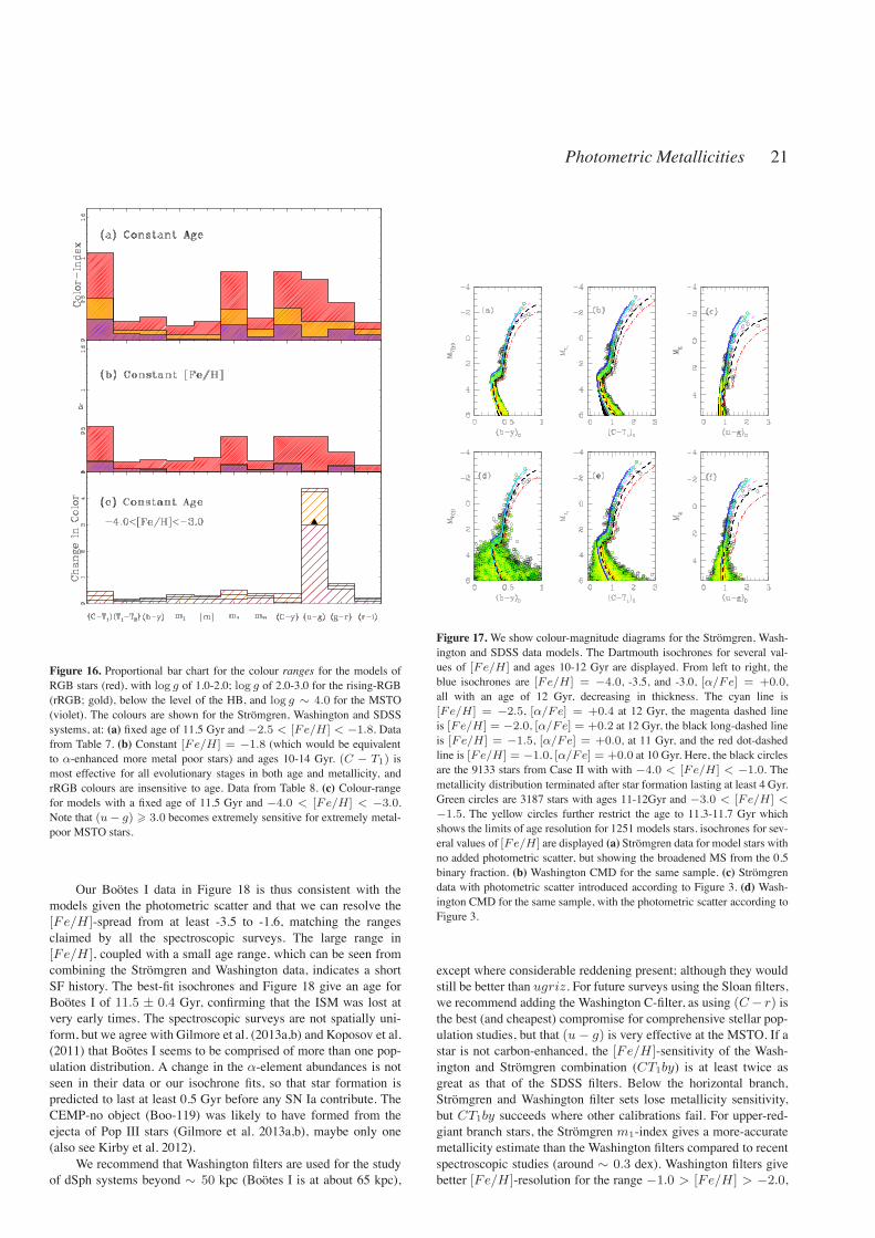
Photometric Metallicities 21
Figure 16. Proportional bar chart for the colour ranges for the models ofRGB stars (red), with log g of 1.0-2.0; log g of 2.0-3.0 for the rising-RGB(rRGB; gold), below the level of the HB, and log g # 4.0 for the MSTO(violet). The colours are shown for the Stromgren, Washington and SDSSsystems, at: (a) fixed age of 11.5 Gyr and "2.5 < [Fe/H] < "1.8. Datafrom Table 7. (b) Constant [Fe/H] = "1.8 (which would be equivalentto !-enhanced more metal poor stars) and ages 10-14 Gyr. (C " T1) ismost effective for all evolutionary stages in both age and metallicity, andrRGB colours are insensitive to age. Data from Table 8. (c) Colour-rangefor models with a fixed age of 11.5 Gyr and "4.0 < [Fe/H] < "3.0.Note that (u" g) ! 3.0 becomes extremely sensitive for extremely metal-poor MSTO stars.
Our Bootes I data in Figure 18 is thus consistent with themodels given the photometric scatter and that we can resolve the[Fe/H ]-spread from at least -3.5 to -1.6, matching the rangesclaimed by all the spectroscopic surveys. The large range in[Fe/H ], coupled with a small age range, which can be seen fromcombining the Stromgren and Washington data, indicates a shortSF history. The best-fit isochrones and Figure 18 give an age forBootes I of 11.5 ± 0.4 Gyr, confirming that the ISM was lost atvery early times. The spectroscopic surveys are not spatially uni-form, but we agree with Gilmore et al. (2013a,b) and Koposov et al.(2011) that Bootes I seems to be comprised of more than one pop-ulation distribution. A change in the !-element abundances is notseen in their data or our isochrone fits, so that star formation ispredicted to last at least 0.5 Gyr before any SN Ia contribute. TheCEMP-no object (Boo-119) was likely to have formed from theejecta of Pop III stars (Gilmore et al. 2013a,b), maybe only one(also see Kirby et al. 2012).
We recommend that Washington filters are used for the studyof dSph systems beyond ! 50 kpc (Bootes I is at about 65 kpc),
Figure 17.We show colour-magnitude diagrams for the Stromgren, Wash-ington and SDSS data models. The Dartmouth isochrones for several val-ues of [Fe/H] and ages 10-12 Gyr are displayed. From left to right, theblue isochrones are [Fe/H] = "4.0, -3.5, and -3.0, [!/Fe] = +0.0,all with an age of 12 Gyr, decreasing in thickness. The cyan line is[Fe/H] = "2.5, [!/Fe] = +0.4 at 12 Gyr, the magenta dashed lineis [Fe/H] = "2.0, [!/Fe] = +0.2 at 12 Gyr, the black long-dashed lineis [Fe/H] = "1.5, [!/Fe] = +0.0, at 11 Gyr, and the red dot-dashedline is [Fe/H] = "1.0, [!/Fe] = +0.0 at 10 Gyr. Here, the black circlesare the 9133 stars from Case II with with "4.0 < [Fe/H] < "1.0. Themetallicity distribution terminated after star formation lasting at least 4 Gyr.Green circles are 3187 stars with ages 11-12Gyr and "3.0 < [Fe/H] <"1.5. The yellow circles further restrict the age to 11.3-11.7 Gyr whichshows the limits of age resolution for 1251 models stars. isochrones for sev-eral values of [Fe/H] are displayed (a) Stromgren data for model stars withno added photometric scatter, but showing the broadened MS from the 0.5binary fraction. (b) Washington CMD for the same sample. (c) Stromgrendata with photometric scatter introduced according to Figure 3. (d) Wash-ington CMD for the same sample, with the photometric scatter according toFigure 3.
except where considerable reddening present; although they wouldstill be better than ugriz. For future surveys using the Sloan filters,we recommend adding the Washington C-filter, as using (C" r) isthe best (and cheapest) compromise for comprehensive stellar pop-ulation studies, but that (u" g) is very effective at the MSTO. If astar is not carbon-enhanced, the [Fe/H ]-sensitivity of the Wash-ington and Stromgren combination (CT1by) is at least twice asgreat as that of the SDSS filters. Below the horizontal branch,Stromgren and Washington filter sets lose metallicity sensitivity,but CT1by succeeds where other calibrations fail. For upper-red-giant branch stars, the Stromgren m1-index gives a more-accuratemetallicity estimate than the Washington filters compared to recentspectroscopic studies (around ! 0.3 dex). Washington filters givebetter [Fe/H ]-resolution for the range "1.0 > [Fe/H ] > "2.0,

22 J. Hughes et al.
Figure 18.We show colour-magnitude diagrams for the Stromgren, Wash-ington and SDSS data on Bootes I objects. The Dartmouth isochronesfor several values of [Fe/H] and ages 10-12 Gyr are displayed. Fromleft to right, the blue isochrones are [Fe/H] = "4.0, -3.5, and -3.0,[!/Fe] = +0.0, all with an age of 12 Gyr, decreasing in thickness. Thecyan line is [Fe/H] = "2.5, [!/Fe] = +0.4 at 12 Gyr, the magentadashed line is [Fe/H] = "2.0, [!/Fe] = +0.2 at 12 Gyr, the black long-dashed line is [Fe/H] = "1.5, [!/Fe] = +0.0, at 11 Gyr, and the reddot-dashed line is [Fe/H] = "1.0, [!/Fe] = +0.0 at 10 Gyr. In all plots,open circles are sources from Table 3 and the large red filled triangles rep-resent the 8 proper motion-confirmed members. We useE(B"V ) = 0.02and DM = 19.11 for Bootes I. (a) The Stromgren CMD with stars fromTable 3. (b) The Washington CMD with stars from Table 3. (c) The SDSSCMD shown with 8 proper-motion members from Table 4.
but for lower values, [Fe/H ] < "2.5, CT1by is the most effectivecombination for these populations.
ACKNOWLEDGMENTS
This paper used observations obtained with the Apache Point Ob-servatory 3.5-meter telescope, which is owned and operated bythe Astrophysical Research Consortium. Hughes wishes to thankthe APO observing staff for their support and late-night instant-messaging and Myra Stone for help with data analysis. We alsoacknowledge financial support from the NSF, and the KennilworthFund of the New York Community Trust. We thank Frank Grun-dahl (for sharing his M92 data), and Myra Stone for help withDAOPHOT III. We are grateful to: Ata Sarajedini, Inese Ivans, Pe-ter Stetson, Jeff Brown, Beth Willman, John Norris, Anna Frebel,Marla Geha, Ricardo Munoz, Kim Venn, and Ryan Leaman foruseful discussions. We made use of the SDSS DR7: Funding forthe Sloan Digital Sky Survey (SDSS) and SDSS-II has been pro-vided by the Alfred P. Sloan Foundation, the Participating Insti-
tutions, the National Science Foundation, the U.S. Department ofEnergy, the National Aeronautics and Space Administration, theJapanese Monbukagakusho, and the Max Planck Society, and theHigher Education Funding Council for England. The SDSS Website is http://www.sdss.org/. The SDSS is managed by the Astro-physical Research Consortium (ARC) for the Participating Insti-tutions. The Participating Institutions are the American Museumof Natural History, Astrophysical Institute Potsdam, University ofBasel, University of Cambridge, Case Western Reserve University,The University of Chicago, Drexel University, Fermilab, the Insti-tute for Advanced Study, the Japan Participation Group, The JohnsHopkins University, the Joint Institute for Nuclear Astrophysics,the Kavli Institute for Particle Astrophysics and Cosmology, theKorean Scientist Group, the Chinese Academy of Sciences (LAM-OST), Los Alamos National Laboratory, the Max-Planck-Institutefor Astronomy (MPIA), the Max-Planck-Institute for Astrophysics(MPA), New Mexico State University, Ohio State University, Uni-versity of Pittsburgh, University of Portsmouth, Princeton Univer-sity, the United States Naval Observatory, and the University ofWashington.
Photometric Metallicities 23
REFERENCES
Arnadottir A. S., Feltzing S., Lundstrom I., 2010, A&A, 521, A40Bailin J., Ford A., 2007, MNRAS, 375, L41Belokurov V., 2013, New Astrononomy Reviews, 57, 100Belokurov V. et al., 2006a, ApJL, 642, L137Belokurov V. et al., 2006b, ApJL, 647, L111Benson A. J., Frenk C. S., Lacey C. G., Baugh C. M., Cole S.,2002, MNRAS, 333, 177Bessell M. S., 2005, AAR&A, 43, 293Brown T. M. et al., 2012, ApJL, 753, L21Bullock J. S., Kravtsov A. V., Weinberg D. H., 2000, ApJ, 539,517Calamida A. et al., 2007, ApJ, 670, 400Calamida A. et al., 2009, ApJ, 706, 1277Calamida A., Monelli M., Milone A. P., Bono G., Pietrinferni A.,Lagioia E. P., 2012, A&A, 544, A152Canterna R., 1976, AJ, 81, 228Cardelli J. A., Clayton G. C., Mathis J. S., 1989, ApJ, 345, 245Carretta E., Bragaglia A., Gratton R., D’Orazi D’Orazi V., Lu-catello S., 2011, A&A, 535, A121Carretta E., Gratton R. G., 1997, A&AS, 121, 95Clem J. L., VandenBerg D. A., Grundahl F., Bell R. A., 2004, AJ,127, 1227Cohen J. G., Huang W., 2009, ApJ, 701, 1053Cowan J. J., Roederer I. U., Sneden C., Lawler J. E., 2011, in RRLyrae Stars, Metal-Poor Stars, and the Galaxy, McWilliam A.,ed., p. 223Crawford D. L., 1975, AJ, 80, 955Da Costa G. S., Armandroff T. E., 1990, AJ, 100, 162di Cecco A. et al., 2010, PASP, 122, 991Dotter A., Chaboyer B., Jevremovic D., Kostov V., Baron E., Fer-guson J. W., 2008, ApJS, 178, 89Faria D., Feltzing S., Lundstrom I., Gilmore G., Wahlgren G. M.,Ardeberg A., Linde P., 2007, A&A, 465, 357Fellhauer M., Wilkinson M. I., Evans N. W., Belokurov V., IrwinM. J., Gilmore G., Zucker D. B., Kleyna J. T., 2008, MNRAS,385, 1095Feltzing S., Eriksson K., Kleyna J., Wilkinson M. I., 2009, A&A,508, L1Frebel A., Christlieb N., Norris J. E., Thom C., Beers T. C., RheeJ., 2007, ApJL, 660, L117Frebel A., Kirby E. N., Simon J. D., 2010, Nature, 464, 72Frebel A., Simon J. D., Kirby E. N., 2011, in Bulletin of the Amer-ican Astronomical Society, Vol. 43, American Astronomical So-ciety Meeting Abstracts #217, p. 147.04Gehrels N., 1986, ApJ, 303, 336Geisler D., 1996, AJ, 111, 480Geisler D., Claria J. J., Minniti D., 1991, AJ, 102, 1836Geisler D., Sarajedini A., 1999, AJ, 117, 308Gilmore G. et al., 2013a, The Messenger, 151, 25Gilmore G., Norris J. E., Monaco L., Yong D., Wyse R. F. G.,Geisler D., 2013b, ApJ, 763, 61Gilmore G. et al., 2012, The Messenger, 147, 25Girardi L., Groenewegen M. A. T., Hatziminaoglou E., da CostaL., 2005, A&A, 436, 895Gratton R. G., Johnson C. I., Lucatello S., D’Orazi D’Orazi V.,Pilachowski C., 2011, A&A, 534, A72Grundahl F., VandenBerg D. A., Bell R. A., Andersen M. I., Stet-son P. B., 2000, AJ, 120, 1884Hilker M., 2000, A&A, 355, 994Holtzman J. A., Anthony-Twarog B., Bond H., Oravetz D., Saha
A., Twarog B., Walker A., 2011, in Bulletin of the AmericanAstronomical Society, Vol. 43, American Astronomical SocietyMeeting Abstracts #217, p. 153.10Hughes J., Wallerstein G., 2000, AJ, 119, 1225Hughes J., Wallerstein G., 2011a, in RR Lyrae Stars, Metal-PoorStars, and the Galaxy, McWilliam A., ed., p. 249Hughes J., Wallerstein G., 2011b, in Astronomical Society of thePacific Conference Series, Vol. 448, 16th Cambridge Workshopon Cool Stars, Stellar Systems, and the Sun, Johns-Krull C.,Browning M. K., West A. A., eds., p. 899Hughes J., Wallerstein G., Bossi A., 2008, AJ, 136, 2321Hughes J., Wallerstein G., Covarrubias R., Hays N., 2007, AJ,134, 229Hughes J., Wallerstein G., van Leeuwen F., Hilker M., 2004, AJ,127, 980Ivans I., 2013 in preparationIvans I. I., 2009, in Bulletin of the American Astronomical Soci-ety, Vol. 41, American Astronomical Society Meeting Abstracts#213, p. 407.16Kim Y.-C., Demarque P., Yi S. K., Alexander D. R., 2002, ApJS,143, 499Kirby E. N., Lanfranchi G. A., Simon J. D., Cohen J. G.,Guhathakurta P., 2012, ApJ, 750, 173Kirby E. N., Simon J. D., Geha M., Guhathakurta P., Frebel A.,2008, ApJL, 685, L43Koch A., McWilliam A., Grebel E. K., Zucker D. B., BelokurovV., 2008, ApJL, 688, L13Koposov S. et al., 2008, ApJ, 686, 279Koposov S. E. et al., 2011, ApJ, 736, 146Kravtsov A. V., Gnedin O. Y., Klypin A. A., 2004, ApJ, 609, 482Lai D. K., Lee Y. S., Bolte M., Lucatello S., Beers T. C., JohnsonJ. A., Sivarani T., Rockosi C. M., 2011, ApJ, 738, 51Lee Y. S. et al., 2008a, AJ, 136, 2022Lee Y. S. et al., 2008b, AJ, 136, 2050Li Z., Han Z., 2008, MNRAS, 385, 1270Marcolini A., D’Ercole A., 2008, in IAU Symposium, Vol. 255,IAU Symposium, Hunt L. K., Madden S. C., Schneider R., eds.,pp. 152–156Marcolini A., D’Ercole A., Brighenti F., Recchi S., 2006, MN-RAS, 371, 643Martin N. F., Ibata R. A., Chapman S. C., Irwin M., Lewis G. F.,2007, MNRAS, 380, 281Mighell K. J., Sarajedini A., French R. S., 1998, AJ, 116, 2395Milone A. P., Piotto G., Bedin L. R., Marino A. F., Momany Y.,Villanova S., 2012, Memorie della Societa Astronomica ItalianaSupplementi, 19, 173Munoz R. R., Carlin J. L., Frinchaboy P. M., Nidever D. L., Ma-jewski S. R., Patterson R. J., 2006, ApJL, 650, L51Norris J. E., Gilmore G., Wyse R. F. G., Wilkinson M. I., Be-lokurov V., Evans N. W., Zucker D. B., 2008, ApJL, 689, L113Norris J. E., Gilmore G., Wyse R. F. G., Wilkinson M. I., Be-lokurov V., Evans N. W., Zucker D. B., 2009, ApJL, 695, L217Norris J. E., Wyse R. F. G., Gilmore G., Yong D., Frebel A.,Wilkinson M. I., Belokurov V., Zucker D. B., 2010a, ApJ, 723,1632Norris J. E., Yong D., Gilmore G., Wyse R. F. G., 2010b, ApJ,711, 350Onehag A., Gustafsson B., Eriksson K., Edvardsson B., 2009,A&A, 498, 527Ross T. L., Holtzman J. A., Anthony-Twarog B. J., Bond H. E.,Twarog B., Saha A., Walker A., 2014, AJ, 147, 4Rutledge G. A., Hesser J. E., Stetson P. B., 1997, PASP, 109, 907
24 J. Hughes et al.
Siegel M. H., 2006, ApJL, 649, L83Simon J. D., Geha M., 2007, ApJ, 670, 313Sneden C. et al., 2003, ApJ, 591, 936Sneden C., Lawler J. E., Cowan J. J., Ivans I. I., Den Hartog E. A.,2009, ApJS, 182, 80Spite M., Caffau E., Bonifacio P., Spite F., Ludwig H.-G., Plez B.,Christlieb N., 2013, A&A, 552, A107Stetson P. B., 1987, PASP, 99, 191Stetson P. B., 1994, PASP, 106, 250Stromgren B., 1966, ARA&A, 4, 433Tolstoy E., Hill V., Tosi M., 2009, ARA&A, 47, 371VandenBerg D. A., Bergbusch P. A., Dowler P. D., 2006, ApJS,162, 375Venn K. A., Hill V. M., 2008, The Messenger, 134, 23Venn K. A., Irwin M., Shetrone M. D., Tout C. A., Hill V., TolstoyE., 2004, AJ, 128, 1177Walsh S. M., Willman B., Jerjen H., 2009, AJ, 137, 450Willman B., 2010, Advances in Astronomy, 2010Willman B. et al., 2005a, AJ, 129, 2692Willman B., Dalcanton J., Ivezic Z., Schneider D. P., York D. G.,2002, AJ, 124, 2600Willman B. et al., 2005b, ApJL, 626, L85Willman B., Strader J., 2012, AJ, 144, 76Yong D., Grundahl F., Johnson J. A., Asplund M., 2008, AJ, 684,1159Zinn R., 1985, ApJ, 293, 424Zinn R., West M. J., 1984, ApJS, 55, 45Zucker D. B. et al., 2006a, ApJL, 650, L41Zucker D. B. et al., 2006b, ApJL, 643, L103
Copyright © 2022 FDOKUMEN