in 1 i(i|-!rN I-1 Eif' M\ i%l # Ä life', li i0^ IS is?' i \j

-"si "ON IK f'il

v_..

.. ;

{7,

I ■v ' ]

\<-' " -..

■•'/ ;' •;,

19990629 128

Springer

my kiaynciK

Marcelo Ang, Jr (Eds,,}'

REPORT DOCUMENTATION PAGE Form Approved OMB No. 0704-0188

Public reporting burden for this collection of information is estimated to average 1 hour per response, including the time for reviewing instructions, searching existing data sources, gathering and maintaining the data needed, and completing and reviewing the collection of information. Send comments regarding this burden estimate or any other aspect of this collection of information, including suggestions for reducing this burden to Washington Headquarters Services, Directorate for Information Operations and Reports, 1215 Jefferson Davis Highway, Suite 1204, Arlington, VA 22202-4302, and to the Office of Management and Budget, Paperwork Reduction Project (0704-0188), Washington, DC 20503.

1. AGENCY USE ONLY (Leave blank) 2. REPORT DATE

1999

3. REPORT TYPE AND DATES COVERED

Conference Proceedings

4. TITLE AND SUBTITLE

2nd International Conference on Recent Advances in Mechatronics: ICRAM 99

6. AUTHOR(S)

Conference Committee

5. FUNDING NUMBERS

F61775-99-WF029

7. PERFORMING ORGANIZATION NAME(S) AND ADDRESS(ES)

Bogazici University Faculty of Engineering, Bebek Instanbul 80815 Turkey

8. PERFORMING ORGANIZATION REPORT NUMBER

N/A

9. SPONSORING/MONITORING AGENCY NAME(S) AND ADDRESS(ES)

EOARD PSC 802 BOX 14 FPO 09499-0200

10. SPONSORING/MONITORING AGENCY REPORT NUMBER

CSP 99-5029

11. SUPPLEMENTARY NOTES

Two different volumes of abstracts.

12a. DISTRIBUTION/AVAILABILITY STATEMENT

Approved for public release; distribution is unlimited.

12b. DISTRIBUTION CODE

A

13. ABSTRACT (Maximum 200 words)

The Final Proceedings for 2nd International Conference on Recent Advances in Mechatronics: ICRAM 99, 24 May 1999 - 26 May 1999

This is an interdisciplinary conference involved with the synergistic integration of mechanical engineering with electronics and intelligent computer control for design and manufacture of products and processes. Topics include: mechatronics design, distributed systems, visjon and sensors, robots and mobile machines, vibration and control, computational intelligence in mechatronics, embedded real-time systems, micro-mechatronics, motion control, hardware/software co-design, and intelligent manufacturing systems

14. SUBJECT TERMS

EOARD, Robotics, MEMs, Space Technology

15. NUMBER OF PAGES

488 and 589 16. PRICE CODE

N/A

17. SECURITY CLASSIFICATION OF REPORT

UNCLASSIFIED

18. SECURITY CLASSIFICATION OF THIS PAGE

UNCLASSIFIED

19, SECURITY CLASSIFICATION OF ABSTRACT

UNCLASSIFIED

20. LIMITATION OF ABSTRACT

UL NSN 7540-01-280-5500 Standard Form 298 (Rev. 2-89)

Prescribed by ANSI Std. 239-18 298-102

RECENT ADVANCES IN

MECHATRONICS

täfFW-oq-/in

Springer Singapore Berlin Heidelberg New York Barcelona Budapest HongKong London Milan Paris Tokyo

RECENT ADVANCES IN

MECHATRONICS

Olcyay Kaynak Sabri Tosunoglu Marcelo Ang, Jr (Eds.)

^B Springer

Prof. Dr. Okyay Kaynak Bogazici University Bebek, 80815 Istanbul Turkey

Prof. Dr. Sabri Tosunoglu Department of Mechanical Engineering Florida International University Miami, Florida 3199 USA

Prof. Dr. Marcelo H. Ang, Jr Department of Mechanical Engineering National University of Singapore Singapore 119260

Library of Congress Cataloging-in-Publication Data

Recent advances in mechatronics—1999 : proceedings of the international conference, Istanbul, Turkey, May 24-26,1999 / Okyay Kaynak, Sabri Tosunoglu, Marcelo Ang, Jr. (eds..)

p. cm. Includes bibliographical references (p. ). ISBN 9814021342

1. Mechatronics—Congresses. I. Kaynak, Okyay. II. Ang, Marcelo, 1959- . III. Tosunoglu, Sabri, 1955- TJ163.12.R43 1999 621—dc2i 99-18308

CIP

ISBN 981-4021-34-2

This work is subject to copyright. All rights are reserved, whether the whole or part of the material is concerned, specifically the rights of translation, reprinting, reuse of illustrations, recitation, broadcasting, reproduction on micro-films or in any other way, and storage in databanks or in any system now known or to be invented. Permission for use must always be obtained from the publisher in writing.

© Springer-Verlag Singapore Pte. Ltd. 1999 Printed in Singapore

The publisher makes no representation, express or implied, with regard to the accuracy of the information contained in this book and cannot accept any legal responsibility or liability for any errors or omissions that may be made.

Typesetting: Camera-ready by Contributors SPIN 10717447 543210

Preface

The word mechatronics was first coined by a senior engineer of a Japanese company; Yaskawa, in 1969, as a combination of "media" of mechanisms and "tronics" of electronics and the company was granted the trademark rights on the word in 1971 [1- 2]. The word soon received broad acceptance in industry and, in order to allow its free use, Yaskawa elected to abandon its rights on the word in 1982 [3]. The word has taken a wider meaning since then and is now widely being used as a technical jargon to describe a philosophy in engineering technology, more than the technology itself. For this wider concept of mechatronics, a number of definitions has been proposed in the literature, differing in the particular characteristics that the definition is intended to emphasize. The most commonly used one emphasizes synergy and is as follows: Mechatronics is the synergistic integration of mechanical engineering with electronics and intelligent computer control in the design and manufacture of products and processes. The embedded intelligence may vary from programmed behaviour to self organization and learning.

The development of mechatronics has gone through three stages. The first stage corresponds to the years around the introduction of the word. During this stage, technologies used in mechatronic systems developed rather independently of each other and individually. With the start of the eighties, a synergistic integration of different technologies started taking place, the notable example being in optoelectronics (i.e. an integration of optics and electronics). The concept of hardware/software co-design also started in these years. The third and the last stage starts with the early nineties. The most notable aspect of this stage is the increased use computational intelligence in mechatronic products and systems. It is due to this development that we can now talk about Machine Intelligence Quotient (MIQ). Another important development in the third stage is the possibility of miniaturization of the components; in the form of microactuators and microsensors (i.e. micromechatronics).

The field of mechatronics is now widely recognized in all parts of world. Various undergraduate and graduate degree programs on mechatronic engineering are being offered at different universities. Journals dedicated to the field of mechatronics are being published, dedicated conferences are being held. One such conference is the one organized in Turkey during August 14-16, 1995, with the tide, "International Conference on Recent Advances in Mechatronics: ICRAM95," under the technical co-operation of ASME (American Society of Mechanical Engineers), IEEE (Institute of Electrical and Electronics Engineers) Industrial Electronics Society, IEEE Robotics and Automation Society, IEEJ (Institute of Electrical Engineers of Japan) , IFAC (International Federation of Automatic Control), IFToMM (Int. Fed. for the Theory of Machines and Mechanisms), JSME (Japanese Society of Mechanical Engineers), RSJ

(Robotics Society of Japan) and SICE (Society of Instr. and Control Engineers of Japan). The conference was highly successful, it had more than 200 participants from 34 different countries. Four years has since then passed and in order to discuss the most recent advances, it has been decided to hold another similar conference during 24-26 May 1999, again in Istanbul, Turkey, under the title 2nd International Conference on Recent Advances in Mechatronics: ICRAM99. It is organized by UNESCO Chair on Mechatronics and Mechatronics Research and Application Center of Bogazici University, Istanbul, co-sponsored by IEEE Industrial Electronics Society and IEEE Robotics and Automation Society, and in technical co-operation with ASME Dynamic and Control Systems Division, ASME Design Engineering Division, RSJ, IEEJ, JSME and SICE. This book contains a selected set of papers prepared for presentation during the conference by leading experts in the field of mechatronics.

The first two chapters of the book consider the recent advances made in one of the most important fields of mechatronics, i.e. robotics. In the third chapter, the use of intelligent techniques in mechatronic products and systems is addressed. The following short chapter contains two papers on mobile robotics. The frontiers in mechatronics in the form of virtual techniques and telecommanding are the subject matter of the fifth chapter. The next three chapters of the book are devoted to applications, such as in motion control, in biomedical engineering and in inspection and fault detection. The last two chapters are on design and analysis of mechatronic systems. The book therefore covers a wide spectrum of mechatronics. We would like to take this opportunity to thank all the authors for their valuable contributions. We are confident that the readers will find the contents of the book interesting and beneficial.

Thanks are also due to Feza Kerestecioglu, Onder Efe and other members of the organization committee who put a lot of time and effort into ICRAM99. Additionally, we wish to thank the following for their contribution to the success of the conference:

UNESCO Bogazici University Foundation European Office of Aerospace Research and Development, Air Force Office of Scientific Research, United States Air Force Research Laboratory European Research Office, United States Army

Okyay Kaynak (Bogazici University, Istanbul, Turkey) Sabri Tosunoglu (Florida International University, Miami, USA)

Marcelo H Ang Jr. (Singapore National University, Singapore) Editors

References 1. Japan Trade Mark Kohhoku, Class 9, Shou 46-32713,46-32714, Jan. 1971. 2. Japan Trade Registration No. 946594, Jan. 1972 3. N. Kyura, The Development of a Controller for Mechatronics Equipment,

IEEE Transactions on Industrial Electronics, (1996), 43 (1), 30-37

Vll

Table of Contents

Preface v

1. ADVANCES IN ROBOTICS

Where Is The Field of Robotics Going? Delbert Tesar, U.S.A 1

Computational Intelligence for Robotic Systems Toshio Fukuda, Naoyuki Kubota, JAPAN 13

Evolving Fuzzy Neural Networks for Adaptive, On-line Intelligent Agents and Systems

Nikola Kasabov, NEW ZEALAND 27

An Agent-Oriented Architecture for Human-Robot Symbiosis in Flexible Manufacturing

K. Kawamura, D. M. Wilkes, R. A. Peters II, W. A. Alford, T. E. Rogers, U.S.A 42

A Survey of the Optimum Quality Index for Some Spatial In-Parallel Manipulators

Yu Zhang, Jaehoon Lee, Joseph Duffy, U.S.A 57

2. CONTROL ISSUES IN ROBOTICS

Control of Flexible Manipulators Using Vision and Modal Feedback Klaus Obergfell, Wayne Book, U.S.A 71

Robust Adaptive Cartesian Control for Free-Joint Robot Manipulators Jin-Ho Shin, Ju-Jang Lee, KOREA 87

Design of Real-Time Robust Adaptive Controller for a Assembling Robot Based-on DSPs(TMS320C40)

Sung-Hyun Han, Man-Hyung Lee, KOREA 102

Adaptive Robust Controller Design and Implementation for Electrically Driven Robots

Chun-YiSu, Yury Stepanenko, Steven Tang, HugangHan, CANADA 115

VUl

Force-Impedance Control: A New Control Strategy of Robotic Manipulators Fernando Almeida, Antonio Lopes, Paulo Abreu, PORTUGAL 126

The Use of Partially Decoupled Uniform Structures and Procedures for the Robust and Adaptive Control of Mechanical Devices

JozsefK. Tar, OkyayM. Kaynak, ImreJ. Rudas, J. F. Bito, HUNGARY 138

3. INTELLIGENT TECHNIQUES IN MECHATRONICS

The Development of Model Free Intelligent Assistance Control of Electrical Wheelchair

Ren C. Luo, Tse Min Chen, Che-Yang Hu, TAIWAN 152

An Investigation of Fuzzy Logic Control of a Complex Mechatronic Device Joseph Fournell, Jon C. Ervin, Sema E. Aiptekin, U.S.A 165

A Computational Intelligence Approach to Sliding Mode Control of Robotic Manipulators

Meliksah Ertugrul, Kemalettin Erbatur, Okyay Kaynak, TURKEY 176

Experimental Comparison of Neural Networks Based Controllers for Industrial Robots

Antonio Visioli, Giovanni Legnani, ITALY 192

Neural Network Architecture of a Direct Drive Robot Adaptive Controller RikoSafaric, Karel Jezernik, Suzana Uran, SLOVENIA 205

Intelligent Robotic Gait Synthesis Using Slope Information Neural Network Jih-Gau Juang, TAIWAN 220

A High Performance Precision Linear Stage using Predictive Control and Genetic Algorithm

Kay-Soon Low, Meng-Teck Keck, SINGAPORE 232

Robot Behavior Evolution based upon the Intelligent Composite Motion Control

Masakazu Suzuki, JAPAN 245

4. MOBILE ROBOTS

Modular Real-Time Control via an Optical Field Bus System for the Four Legged Walking Machine ALDURO

U. Roll, M. Torlo, M. Hiller, GERMANY 259

Performance Issues in Biped Walking Robots Filipe M. Silva, J. A. Tenreiro Machado, PORTUGAL 270

IX

5. VIRTUAL TECHNIQUES AND TELECOMMANDING

From Robot Control to Virtual Reality Based Commanding: The Systems Approach

Eckhard Freund, Juergen Rossmann, GERMANY 282

Haptics for Multi-scale Virtual Prototyping Diego Ruspini, Oussama Khatib, U.S.A 294

Development of a Mechatronic System: A Telesensation System for Training and Teleoperation

Pattaraphol Batsomboon, Sabri Tosunoglu, Daniel W. Repperger, U.S.A 304

Teleoperated Nano Scale Object Manipulation Metin Sitti, Hideki Hashimoto, JAPAN 322

Virtual Manufacturing Oriented Generic Manufacturing Process Model Läszlö Horväth, ImreJ. Rudas, OhyayKaynak, HUNGARY 336

6. MOTION CONTROL

Design of Self-Tuning Controller for Systems with Unknown Time-Delay and Uncertain Parameters

Man Hyung Lee, Kang Sup Yoon, Yu Shin Chang, KOREA 349

Implementation of an Angle Measurement System for an Anti-Sway Crane System

Man Hyung Lee, Keum Sick Hong, Young Kiu Choi, Sang Hwa Chung, Kwang Ryul Baek, Young Jin Yoon, Nam Huh, KOREA 361

Position Control of a Pneumatic Servo Mechanism G. H. Ho, C. L. Teo, SINGAPORE 372

Motion Control of a Tension/Winder System Landoh Garninto, P. M. Bruijn, J. B. Klaassens, Tienan Zhao, Faouzi Grebici, THE NETHERLANDS 387

Robust Accurate Motion Control for Belt-Driven Servomechanism AlesHace, Karel Jezernik, Martin Terbuc, SLOVENIA 399

Application of a Silicon Microvalve to Pilot-operation of Pneumatic Valves Götz Günther, GERMANY 411

X

7. BIOMEDICAL APPLICATIONS

Tactile Controlling and Image Manipulating Apparatus for Computer Simulation of Image Guided Surgery

Chee-Kong Chui, Percy Chen, Yaoping Wang, Marcelo H. Ang Jr, Yiyu Cai, Koon-HouMak, SINGAPORE 423

Static and Dynamic Modeling of the McKibben Artificial Muscle Bertrand Tondu, FRANCE 444

8. INSPECTION AND FAULT DETECTION

Faults Identification of Oil Wells Using neural Networks Bogdan M. Wilamowski, U.S.A 459

Automated Inspection of Steel Structures Cem Ünsalan, Aytül Ereil, TURKEY 468

Fault Detection in Robot Manipulators Using Statistical Tests Feza Kerestecioglu, Bekir Sami Nalbantoglu, TURKEY 481

Robust Fault-Tolerant Control for Robot Manipulators with Actuator Failures: Fault Detection Strategy and Fault Recovery Control

Jin-HoShin, Ju-Jang Lee, KOREA 493

9. DESIGN ISSUES

Information Loss in Analog Digital Conversion Revisited Craig C. Smith, David W. Robinson, David S. Hansen, Bryan F. Bihlmaier,U.S.A 508

Design and Modelling of a Two-Degree-of-Freedom Spherical Actuator with Unlimited Angular Range

B. Dehez, V. Froidmont, D. Grenier, B. Raucent, BELGIUM 522

Self-sensing Magnetic Suspension Using an H-bridge Type Hysteresis Amplifier

Takeshi Mizuno, Yujilshino, JAPAN 536

10. ANALYSIS OF MECHATRONIC SYSTEMS

Chaotic Phenomena and Performance Optimization in the Trajectory Control of Redundant Manipulators

Fernando B. M. Duarte, J. A. Tenreiro Machado, PORTUGAL 548

XI

Stabilization of Nonholonomic Dynamic Systems Based on the Force/Torque Feedback and Its Applications

Tatsuo Narikiyo, Masakazu Katoh, JAPAN 560

A Generic Simulator/Controller for Robot Manipulators Abdelshakour A. Abuzneid, TarekSobh, U.S.A 575

WHERE IS THE FIELD OF ROBOTICS GOING?

Prof. Delbert Tesar The Carol Cockrell Curran Chair in Engineering

The Robotics Research Group The University of Texas at Austin

J.J. Pickle Research Center The University of Texas at Austin MC: R9925, Austin, Texas 78712

Tel: 512-471-3039

ICRAM'99

Abstract. Robotics is now becoming a mature technology with increasing commercial viability. The market has tripled in the last three years in the United States. The opportunity to expand this market ten-fold will depend on a dramatic increase of performance (of several orders of magnitude) while reducing cost. This can only be achieved by using the lessons learned from the personal computer industry and finding the equivalent in robotics. This means standardization at the correct level of granularity (of machine modules) and the creation of a universal operating software system to drive any machine system that can be assembled on demand from these standard modules to meet a customer's requirements. For industrial applications, this will lead to dexterous manufacturing cells of 40 degrees-of-freedom (or more) that are rapidly reconfigurable to do automated warehousing, truck palletizing, food packaging, shoe manufacture, fettling of plastic parts, etc. The age of robotics is just before us. Unfortunately, more than 95% of our robots are imported at this time. The University of Texas is providing key leadership in the required development to create the foundations for a U.S. industry for robotics. This article outlines the basis for this enthusiasm for the technology and briefly outlines activity within UT Austin's Robotics Research Group.

I. PAST EMBODIMENTS OF ROBOTICS? The oldest form of the technology was represented by automata and its first

sophisticated description was given by Leonardo da Vinci (see Fig.l) [1], approximately 500 years ago. This 4 input-4 output device was intended to duplicate the complex motion of a bird's wing, perhaps 200 years before the much simpler single output machines were first being conceptualized. Another exceptional example was provided by J. Vaucanson in 1738 (see Fig. lb), when he produced an automata to play a brief sonata with a flute (with correct fingering and air velocity control) [3,4]. This level of technology was then transferred to complex patterns in textiles resulting in the Jacquard loom with digital inputs in the form of a continuous belt of punched cards in 1801 [5]. It was subsequently embodied in the player pianos developed during the 19th century. One should consider the

* This is an expanded version of a paper in the Discovery magazine published by The University of Texas at Austin, Fall, 1997.

punched cards as the stored "map" of the program to govern the operation of the system. The player piano had one input - and 88 distinct and independent outputs - very similar to a modern automatic screw machine used in manufacturing. Today, the "electronic" map is more likely to be the functional description of the operation of the fuel system in a modern automobile. This map is obtained by carefully operated tests and experiments of the prototype system. Even though the fuel system may be extraordinarily complex, the highly refined map ensures that maximum performance is achieved under a very wide range of sensed conditions. This is the modern equivalent of an intelligent machine except that a majority of the decision making was done in advance and stored for retrieval during operation. Another more recent form of this type of automata is represented by the Sarcos World Anthropomorphic figure developed by Steve Jacobson of the University of Utah (see

a) Leonardo da Vinci's mechanical

wing (-I486)

[2].

b) Vaucanson flute player

(1783) [3].

d) K-9

intelligent dog of

Dr. Who TV series

[7].

e) Popular

Star Wars robotic

pair [8].

Figure 1. Automata and science fiction devices Fig.lc) [6]. This system has a very large number of Degrees-of-Freedom (DOF) driven by a fixed digital memory (usually on a repeating tape). Although visually fascinating, it does not offer significant levels of precision, speed, force (or intelligence) that would be required in future production systems for manufacturing.

The dog, K-9, of the science fiction series, "Dr. Who," is, in fact, increasingly viable today (see Fig.ld) [7]. It had an encyclopedic memory and could rapidly respond to a very wide range of verbal questions. Today, the need for the equivalent system for entertainment purposes as represented by the popular "robots" of Star Wars (see Fig.le) or for companion support for our independent but aging population is obvious. Finally, a wide range of toy robots (see Fig. If) have been produced to respond to the fascination young people have for this technology

Early attempts to develop realistic functional systems are shown in Figure 2. The manual controller (see Fig.2b) is used as a master to provide kinesthetic input to the system and force feedback to the operator of a slave manipulator device (this is called teleoperation where the slave can be remote from the master). In this case, the master is quite human-like in its geometry (as is the slave manipulator). Hardyman [10] was a prototype (see Fig.2a) developed by G.E. to provide force amplification for the human,

a) Hardyman (by G.E., 1968) multiplies human lifting capacity 10 times [10].

b) Argonne derived manual controller byK.Flatau(1981)[26].

c) DLR Articulated Hand (1997) [11]. d) Ohio State's 6 legged Adaptive Suspension Vehicle Ü984H131.

Figure 2. Human like prototypes.

making the combination capable of picking up ten times the load possible by the man alone. Today, this remains a very desirable goal (human augmentation) although the dominant requirement for specialized backdriveable actuators has not yet been met. The hand prototype (see Fig. 2c) by G. Hirzinger involves 12 DOF, 28 sensors, a unique embedded actuator module, and an on-board electronic controller. This prototype, in total, is an exceptional development coming from the field of feinwerktechnik—fine mechanics—a field common to central Europe and recently emerging in the United States as MEMS—Micro-Electro-Mechanical Systems [12].

A topic of broad interest over the past four decades is walking. Two-legged walking prototype systems do exist but they remain far from satisfactory. The six-legged system by Ohio State University [13] was a major effort during the 80's funded by DARPA (see Fig.2d). It did show that six-legged walking (and some running gates) were feasible although expensive and complex.

Another topic that has been proposed for robotics is associated with health care (see Fig.3). Eye surgery is one of those opportunities. Recently JPL, in concert with Dr. Steve Charles, a renowned eye surgeon, has designed, fabricated, and tested a miniature (6" long) manipulator of enough resolution to be useful (see Fig.3a) [14]. Another surgical task which requires high forces and stiffness is the cutting of bone (see Fig.3b) [15]. Carnegie Mellon University researchers have shown that this is feasible using a high quality Adept industrial robot manipulator. This Adept system uses direct drive motors to improve its tracking capability to meet the requirements of this demanding physical task. Finally, Joe Engelberger, the father of American robotics, has developed a system called HelpMate (see Fig. 3c). The initial use of this system is for transport in hospitals. A future

use will be to add two manipulators to the platform to enable it to become the nurse's aide and companion to incapacitated humans [16].

i

Figure 4 illustrates a range of mobile platforms to carry out remote tasks. The platform in Figure 4a represents an underwater system for ocean exploration or for oil field service functions [18]. That in Figure 4b is an emerging concept by the Johnson

a) Robot Assisted Micro Surgery b) Bone milling robot by c) Mobile platform by (RAMS) by JPL [14]. CMU Robotics Institute [15]. HelpMate Robotics, Inc. [16].

Figure 3. Health related technologies.

Space Center robotics division to create an astronaut assistant to augment his capability [19]. The goal is to reduce astronaut EVA by 50%. Finally, to survey unknown planetary surfaces, JPL is sending rovers to Mars and other planets (see Fig 4c) [20]. These devices are miniaturized to reduce weight.

a) Underwater platform for explora- b)Robonaut concept as dual c) JPL rover for deployment on tion and oil field service [18]. of astronaut in space [19]. Mars [20].

Figure 4: Mobile platforms for remote operations. Systems of higher complexity are increasingly becoming feasible. The 17

DOF dual arm system was built by Robotics Research Corporation as a prototype system for a major robot development in the mid 80's' [21]. It represents a very high level of dexterity and motion flexibility and is an exceptional laboratory demonstrator. The dual arm system in Figure 5b is being used to dismantle the Chicago Pile 5 at Argonne near Chicago. This is an example of a future need that faces the U.S. and other industrialized nations; i.e., the dismantlement of most of our nuclear facilities and reactors. The basic requirement is to make it unnecessary for humans to enter a high radiation environment. Finally, Figure 5c shows a concept of a 10 DOF, 50 ft. long

* This device was recently donated to The University of Texas at Austin by Northrup Grumman.

dexterous "crane" manipulator capable of precision placement of building components with minimal human involvement thus dramatically improving worker safety which is a major issue in this industry. One requirement here is a special light weight, high force, and high resolution actuator to drive this large structure.

Robotic Research Corporation's dual Manipulator of 17 DOF,

b) Long reach arm (50 ft.) of 10 DOF For construction industry.

16 DOF Dual arm system for nuclear facilities dismantlement.

Figure 5: Unique prototypes of 10 or more DOF

The market for industrial robots in the U.S. has tripled in the last three years, now exceeding $1 billion per year [22]. General Motors purchases 4,000 robots per year. These systems are extraordinarily smooth with a reliability exceeding 20,000 hours (recall that cars may now be considered to be 3,000-hour machines). One of the most common applications is spot welding (see Fig. 6a) as well as spray painting and some assembly. The most important reality is that the cost to integrate (make it work) a robot into the factory is four times the cost of the robot itself. Also, time of integration makes rapid product model changeovers virtually impossible. In order to make rapid integration feasible, it will be necessary to improve the absolute accuracy of industrial robots from 0.2 inch to 0.01 inch (a factor of 20) and to have computer control directly from the product database. No industrial robot technology is prepared to meet this dominant requirement at this time. Another important application is electronic assembly. The Hirata manipulator (Fig. 6b) uses high accuracy direct drive motors to maintain the level of speed and precision required. This Japanese made manipulator is also used by Adept in the U.S. It is the only U.S. based industrial robot system manufacturer of any magnitude, leaving the enterprise open to the entry of vigorous technology based start-ups.

n. WHAT IS ROBOTICS

The concept of a machine equivalent to humans has always intrigued mankind and is frequently represented in various forms in the literature. It was crystallized for us by Karel Capek who coined the word robot* in the sophisticated tale of the gradual rise of a

*Robota (Czech) was the number of days of work per year the serfs owed the local baron for his protection and governance.

robot society, the reduction of the role of humans, and the eventual genocidal destruction of the robot population to follow by its rebirth in terms of two surviving individuals.

Today, this fascination continues in our science fiction and in game competitions such as the recent contest between Deep Blue (of IBM) and chess master, B. Kasperov. While these manifestations are fascinating, they have very little to do with reality. Think of the exceptional ability of the eye-brain combination to accurately distinguish a face among hundreds, thousands, or millions of similar "shapes" that differ only by small nuances. Consider the exceptional accuracy and fingertip control necessary by a basketball player to shoot a 3-point shot. These human capabilities are obtained through trial and error perceptions and corrections obtained through rigorous training, none of which the technical field of robotics is approaching in its most aggressive development. The Deep Blue - Kasperov chess contest is not representative of these highly integrated multi-sensory, multi- motor responses which are best described as highly coupled nonlinear functions which are always in conflict to result in a refined and delicate balance. They are not simple digital (discrete) alternatives. It is the differencing (conflict resolution) which makes it possible for humans to be trained at an exceptionally high level. In fact, antagonistic control of large forces to provide a refined small force output has long been known to be a difficult technical task. Yet, the motion of the human eye is governed by a number of parallel acting muscles which antagonistically move the eyeball in a slewing mode at high speed and, just before focusing, changes to a high accuracy slow motion to prevent overshoot and jitter. In fact, these systems begin to fail when the antagonistic error exceeds the corrective decision making of the "analog" control system. This is a lesson of greatest importance technically. We know there are measurement limits for many physical phenomena. There will also be similar limits on the control of highly nonlinear-coupled man-made systems. The human/biological system is basically analog (a continuous relationship between input command and output response) while the man-made system is increasingly digital (discrete steps in the input-output relationship). We are on the verge of a revolution in the digital control of machines. Why? Because by the year 2000, there will be available computer technology producing a gigaflop of computational power as a $5000 commodity [25]. This is equivalent to three or more 1980 super computers. Hence, the architectural generality described in [26] and the forecast of a super-robot discussed in [27] now become truly feasible. The fields of computer science, micro-electronics, and materials science are yielding support to this revolution. But the real demand of the technology come in the field which the Japanese have called mechatronics—an intimate combination of mechanical and electrical technologies. The mechanicals must generate the physical embodiment of the

a) Spot

welding in an

automobile assembly

plant [23].

b) Precision

high speed electronics assembly.

[24].

Figure 6. Common applications for industrial robots.

system—in other words, they must create the best possible parametric representation of the system. The electricals, by means of exceptional decision making software, must resolve demand/response conflicts through criteria fusion at several hierarchical levels. In fact, as the speed of digital making increases, the more analog the control response will appear. Today, the field of robotics is moving rapidly to a blending of these fields into a new discipline. Those young people who wish to be leaders will strive to excel in this emerging science of mechatronics.

m. WHAT IS THE FUTURE OF INDUSTRIAL ROBOTICS? The robot industry (and most machines in general) has concentrated on a

monolithic design of manipulators (4 to 7 DOF arms) which are one-off designs in much the same way we built and operated our earliest computers. A massive lesson from computers has been learned from the last two decades on the commercial development of an open architecture for the hardware system (Dell Computers) and a generalized software for the operating system (Microsoft). In other words, these systems are so open that they can be assembled on demand and integrate virtually all technical modifications from a broad range of sources (because of standardization) without disturbing the remainder of the system. The widespread awareness of this standardization encourages investment to organically occur from a variety of sources. This concentration on an open architecture enables a continuous improvement on performance while reducing cost—quite a contrast to the paradigm of most existing production machine technologies.

It now becomes possible to open up the architecture of dexterous machines (robots). Actuators (the muscles) can be produced in a small number of standard sizes to populate a very wide range of systems to meet a diverse set of applications (see Tablel). These standardized actuators will contain sensors, motors, bearings, gear trains, brakes, electronic controller, wiring, communication buses, etc. In other words, a massive amount of technology. It has the same significance to machines as the electronic chip has to computers.

Barrier To Agile Manufacturing (JIGS Block Flow of Information)

Figure 7. Agile manufacturing barriers

(i.e., it becomes one of the standards for investment). Perhaps 7 to 10 actuators in each of five distinct classes would be necessary to populate all the systems required by applications listed in Table 1. Adding links between the actuators makes up the manipulator. All that is necessary to complete the system is an open architecture system controller (now being offered by several suppliers) and a generalized operational software (which is under development at UT Austin) in the same format as offered for computers by Microsoft (the other standard for investment) [28]. Is this feasible? Can commercial entities make money in this manner? Yes, if they expand their markets to applications which are virtually untouched (food, textiles, apparel, agriculture, etc.) which are global in nature, and much larger than those already addressed (automobiles, electronics).

Industrial Automation

Precision light machining Microfabrication Complex assembly/flexible

jnanufacruring/remanufacturing Batch processing Small-scale industrial processes Seam Welding Force fit assembly

Energy Systems

Utility nuclear reactor maintenance Offshore oil and gas exploration Nuclear waste site clean-up Coal production

Military Operations

Battlefield operations All-electric or hybrid vehicles Flight surface control Automatic ammunition loader Logistics operations Explosive ordnance disposal Maintenance and emergency repair

Human Augmenta-

tion

Hazardous duty missions Training and service machines Prosthetics and orthotics Microsurgery

Agriculture Field mapping and harvesting Space Operations

Space Station maintenance Assembly and construction of Planetary surface systems

Table 1: Listing of Robot Applications

To do so, however, requires that a fully integrated technology be established which is not only responsive to market demands but reacts quickly (and at virtually no cost) to product design changes. This is a concept called agile manufacturing (see Fig.7). The high value added functions (drilling, routing, trimming, etc.) usually contain large force disturbances which are contained by a jig (or rigid frame). The jig maintains operational precision but it blocks all the information flow to the central computer and it certainly is not agile. Further, it can easily cost ten times more than the robot. Hence, a science of machines must be developed which makes it possible to eliminate the jig. To do so will require a whole series of new sciences (metrology, criteria fusion, performance norms, etc.) and a generalized decision making software (opportunities of real magnitude for young people to enter the field) [29].

Some of the future applications in industry are shown in Figure 8. Figure 8a illustrates a very common dilemma in the food industry. Many onerous repetitive physical tasks exist that must be performed in high humidity, temperature extremes, chemical fumes, etc. It now becomes possible to build low cost, modular robots that can operate economically anywhere in the world. Further, nominally trained operators can replace failed robot modules (plug-and-play) and to do so from a small collection of spares (i.e., just as we now do for personal computers). The robot actuator module shown in Figure 8b is representative of the modularity required [31]. Figure 8c is a concept of an advanced micro-fab architecture which would make it possible to virtually remove the human from any entry into the clean room space. The inner cylindrical core would be occupied by modular handling robots and elevators, all of which can be repaired by module replacement by other robots (see Fig.8d) [32]. The second inner cylindrical shell would be for storage of all work (wafers) in progress. Beyond that would be a cylindrical shell for dedicated production machines which could be moved to an outer cylindrical shell for major service, repair, or modification.

Finally, it now becomes feasible to address high value added functions such as airframe assembly. Figure 8e is the nose cone of a fighter aircraft. It contains 120 parts with hundreds of rivets now assembled by hand using expensive jigs and fixtures. It is proposed to design a finite number of link and actuator modules to be assembled, on demand, fully calibrated with integrating software to carry out this demanding assembly task. The result would be a precision assembly cell of 40(+) DOF [33]. Some of the manipulators would maintain precision under load of 0.01" (at least ten times better than that available from the best industrial robot today). Some of the manipulators would be

force robots to prevent deformation of the product. Others would be dexterous fixturing devices. The whole would be a completely reprogrammable system whose control inputs would be based on commands derived from the data base of the product~a true representation of agile manufacturing (Fig. 8f).

a)Humans face demanding and repetitive tasks in food production [301,

d) Modular robot concept [32].

b)Standardized actuator as a basis for Plug-and-Play systems [31].

e)Nose cone airframe for an F-18 fighter [331.

^Revolutionary cylindrical micro-fab architecture [32].

f)40 DOF handling cell for pre- cision airframe assembly [33].

Figure 8:Demanding future applications of robotics in industry. These industrial examples all indicate that open architecture (modular) systems of

many degrees of freedom able to satisfy a broad range of applications will be the future of production machines that we need to be working on now. This architectural generality is what we classify as manufacturing cells. IV. CONTINUUM FOR ADVANCED MACHINE OPERATION

The benefits of the massive technology associated with computers can now be expanded by changing the basis for machine control from analog and stability algorithms to criteria based decision making such that task performance, condition based maintenance, and fault tolerance become possible for complex production systems such as 40 DOF precision assembly cells for airframe manufacture. This generic approach would also apply to all intelligent machines such as aircraft, automobiles, harvesting equipment, medical equipment, etc.

Most mechanical systems are based on a control paradigm associated with the criteria of stability and a few ancillary criteria such as overshoot, settling time, and steady state error. Not only are these criteria irrelevant to the critical operation of most high value added production systems, issues such as task performance (precision, force, obstacle avoidance, etc.), condition based maintenance (when should a component be replaced to maintain system performance) and fault tolerance (operation even under a fault) cannot be addressed by this out-dated approach to control. The successful fly-by- wire approach used in fighter aircraft shows that criteria based decision making not only works but that it is essential to generalize the architecture of production systems, make agile manufacturing feasible for high value added operations including advanced manufacturing cells, and to reduce life cycle cost.

Figure 9 describes what is meant by this new continuum of machine operation. Each operational concept (task performance, condition based maintenance, and fault tolerance) is based on a "residual" (or difference) between a predicted model reference

10

Continuum for Advanced Machine Operation

Task Performance

Fault Tolerance

Precision Performance- 4 Structural Accuracy Indices Layers High Value- Decision- FDI, Recovery

Operations Thresholds Archiving

I

Metrology, Model Reference, Sensor Reference, Operational Criteria,

Decision Making, Modularity,

Standardized Interfaced, Mechanical Architecture, Software Architecture,

High Speed System Controllers, Communications Technology

^

(based on a parametric description of how the "as built" machine should perform) with a sensor reference (based on actual parameters measured by distributed sensors within the system). This difference model then can be used by the decision making software to

maximize performance, to identify faults and to recommend the best configuration to mask the fault, or to recommend the replacement of a component which is adversely effecting the system's performance. To obtain these benefits, a massive development of foundation technologies such as metrology, operational criteria, decision making, modularity, communications technology, etc. (see Figure 9) must be undertaken. Little of these foundation technologies now exists or is being developed or taught in our academic institutions. It is also necessary to mention that federal research funding for manufacturing has provided virtually no support for this revolutionary but essential technology. For example, it can be forecast that condition based maintenance will be common to automobiles within this decade. Why not now also vigorously pursue this same technology for production systems and bring excitement back to our manufacturing industry and to the discipline of mechanical engineering.

CONTRIBUTION BY UTS ROBOTICS RESEARCH GROUP The Robotics Research Group at UT Austin has a 40 year history in machine

development, 30 years specifically devoted to robotics. Since 1975, much of this effort has been to establish the general analytical and design infrastructure for an open (modular) architecture of systems with many degrees of freedom which are able to satisfy a broad range of applications for future production machines. This work has coalesced in two principal areas: Standardized Actuators. We have defined five unique classes of actuators and have designed one or more actuators in four of these classes (high precision, high force, low cost, and backdrivable). We are pursuing all essential component technologies (gear trains, sensors, clutches, electronic controllers, communications buses, quick-change mechanical interfaces, etc.) as well as a complete test environment composed of four unique test-beds (endurance, condition based maintenance, control, and metrology) for these actuators. Finally, we are developing a ten sensor environment (torque, position, temperature, current, voltage, etc.) to create an architecture for an intelligent and reconfigurable actuator to maximize performance as well as make fault tolerance and condition based maintenance possible. The overall goal is to create a standardized set of advanced actuators whose production cost can be dramatically reduced by large production runs. This minimal set of actuators would then be available to create a very large population of open architecture machines and manufacturing cells which can be assembled on demand in the same manner that we now employ for personal computers.

Figure 9

V.

11

Generalized Software. Once an open architecture structure for machine systems exists, it becomes necessary to provide a software architecture sufficiently general to operate any machine that can be assembled from these standardized machine modules. Our research program has laid the foundation for this software in an object oriented structure called OSCAR. This software is based on resource allocation by high speed (in less than 5 milli- sec) decision making among 100+ operational criteria (speed, force, precision, deflection, energy, etc.). This software can operate simple 6 DOF robot manipulators or complex 40 DOF manufacturing cells. Its decision versatility allows for a unified control for maximum performance (is there sufficient precision), condition based maintenance (does a module need replacement), and fault tolerance (can a fault be avoided even during operation). Much of this class of technology is being employed in the operation of our nuclear reactors, supercomputers, and even our modern automobiles. It now becomes possible to use this technology in our future production machines and to do so at reduced cost.

Based on this aggressive technical development, the Robotics Research Group is pursuing the following applications at this time:

Plutonium Processing: The operation of multiple robots in a glove box to handle and repackage highly radioactive plutonium. (Fig.5a)

Dismantlement: The operation of 16 DOF dual arm systems to decommission nuclear facilities and nuclear reactors. (Fig. 5b)

Airframe Manufacture: The development of precision manipulators to create versatile assembly cells without the use of expensive jigs and fixtures. (Fig- 8e, f)

Robonaut: The development of control software for the operation of dexterous hands and dual arm systems to assist the astronaut in space. (Fig. 4b)

Shipbuilding: The design and development of low cost, modular portable robots to weld ship structures at a cost/benefit ratio 50 times better than previous systems. (Fig. 8b)

Robot Crane: The design of a 50 to 60 ft. long dexterous crane to assemble standard components of buildings with minimal human involvement, thereby increasing worker safety. (Fig 5c)

Other topics of interest are in the fields of food processing, handling and packaging; textiles; microsurgery; automobile assembly; microelectronics processing; and anti-terrorist operations.

VI. COMMENT This is exciting business. A revolution is at hand. Just the thing to attract the

brightest young minds. It does not have to lead to science fiction to be exciting. The goal is to move away from a simple concept of single purpose machines to those which can be assembled on demand to meet a wide range of applications at reduced costs. These systems will be fully integrated and reconfigurable, maintainable by a nominally trained technician, and repairable by module replacement from a limited number of modules that can be kept on hand at low cost. This architectural generality (standardized actuators and generalized operating software) is what we wish to consider as the basis for manufacturing cells. This approach to standards for Investment is identical to the successful commercial model for personal computers (standardized computer chips and operating systems). Come and join us in this exciting development.

12

REFERENCES 1. Rosheim, M.E., Robot Evolution, The Development of Anthrobotics, John Wiley & Sons, Inc., New York, NY (1994). 2. Rosheim, M.E., Robot Evolution, The Development of Anthrobotics, p19. John Wiley & Sons, Inc., New York, NY

(1994). 3. Doyan, A. and Liaigre, L, Jacques Vaucanson, M6canicien de Gönie, p50. University de Grenoble, Publications de la

Faculty des Lettres et Sciences Humaines, Presses Universitäres de France, Paris, France (1966). 4. Vaucanson, J., "An Account of the Mechanism of an Image," presented to the Gentlemen of the Royal Academy of

Sciences,* (1738) "Le Mecanisme du Fluteur," The Flute Library, First Series No. 5. "Editions Frans Vester, Intro. Lasocki, D., Buren (GLD), The Netherlands: Uitgeverij Frits Knuf (1979), "Vaucanson: Flute Automation." "Delightful Machines page," Online. Internet, 12 June 1997. Available http://www.msen.com/~lemurfraucanson-flute-enalish.htm.

5. . Scott, P.B., The Robotics Revolution, Basil Blackwell Publisher Ltd., New Yort, NY (1985). 6. Jacobson, S. Entertainment Systems. 1996. Online. Internet. 10 June 1997. Available

httD-7/www.sarcos.com/entertainment.html. 7. Morgan, S.M., K-9 intelligent dog of Dr. Who television series. Department of Earth Science, University of Northern Iowa.

1997. Online. Internet. 20 June 1997. Available to://nifro9.earth,uni.edu/Dub/dortor/araphics/jpg/. 8. Asimov, I. and Frenkel, K.A., Robots, Machines in Man's Image, p215. Nightfall, Inc., Crown Publishers, Inc., New York,

NY (1985). 9. Doboz, P., Museum of Ephemeral Cultural Artifacts (MECA). 1997. Online. Internet. 19 June 1997. Available

httpy/www.edaechaos.com/MECA/robots/fiahtina.html. 10. Rosheim, M.E., Robot Evolution, The Department of Anthrobotics, p341. John Wiley & Sons, Inc., New York, NY (1994). 11. DLR Articulated Hand. "Hirzinger Hand." 1996. Online. Internet. 19June1997. Available http^/www.op.dlr.de/FF-DR-

HS/mechatronics/DFG/. 12. Hirzinger, G., "Deutsche Forschungsanstalt fur Luft-und Raumfahrt e.V.", Status Report, Institute of Robotics and

System Dynamics, (1997). 13. Klein, C, Department of Electrical Engineering, The Ohio State University. Online. Internet. 10 June 1997. Available

http^eewww.eno.ohio-state.edu/klein/roboticsO. 14. Volpe, R., "Robot Assisted Microsurgery," Jet Propulsion Laboratory, NASA. 1996. Online. Internet. 10 June 1997.

Available http^/robotics.ipl.nasa.aov/tasks/rams/homepaae.html. 15. Shefman, D., "Bone Cutting Robot," Medical Robotics and Computer Assisted Surgery, Robotics Institute, Carnegie

Mellon University. 1995. Online. Internet. 10 June 1997. Available http://www.cs.cmu.edu/afs/proiect/mrcas/. 16. Engelberger, G., "HelpMate Robot," 1997. Online. Internet. 6 June 1997. Available:

http7/www.helpmaterobotics.com.hmrobot.htm. 17. Englberger, J.F., Robotics in Service, The MIT Press, Cambridge, MA (1989). 18. IFREMER (The French Institute of Research and Exploration of the Sea), "Griffon System Characteristics" 1996. Online.

Internet. 25 June 1997. Available htto://www.ifrerner,fr/boc/enains/oriff uk.htm. 19. Li, L, "EWS: Robotic Astronaut-Robonaut," NASA Johnson Space Center. 1996. Online. Internet. 8 June 1997.

Available htto://tommv.i5C.nasa.qov/~li/Robonaut.htrnl. 20. Weisbin, C.R., "JPL Rover for deployment on Mars." Jet Propulsion Laboratory NASA. 1996. Online. Internet. 10 June

1997. Available http://lmcoradian.ipl.nasa.aov/planefrobs.html. 21. "Development and Demonstration of a Coordinated Control System for Dual-Arm Robots," Rackers, K., Spring 1996. 22. Robot Industries Association paper, 1997. 23. ABB Flexible Automation. 1996. Online. Internet. 10 June 1997. Available http^www.abb.se/robotics/applic.hum. 24. Hirata Industrial Machineries Co., Ltd., "Robot Insertion Cell for Special Odd Shaped PCB Components" Vol. 9:2000

(1991). 25. "Design and Development of a Multi-Channel Robotic Controller," Aalund, M., and Tesar, D., March 1997. 26. "An Applications-Based Assessment of Present and Future Robot Development," Butler, M.S., Robotics Research

Group, The University of Texas at Austin, May 1992. 27. Thirty-Year Forecast The Concept of a Fifth Generation of Robotics—The Super Robot," D. Tesar in Manufacturing

Review, Vol., 2:1, American Society of Mechanical Engineers, March 1989. 28. "A Reusable Operational Software Architecture for Advanced Robotics," Kapoor, C. and Tesar, D., Robotics Research

Group, The University of Texas at Austin, December 1996. 29. "Intelligent Automation," presented by D. Tesar at the ISIC '97 International Symposium on Intelligent Control, IEEE

Conference, Istanbul, Turkey, July 1997. 30. Shultz, D.P. and Shultz, S.E., Psychology in Industry Today, 5» Ed., p86. McMillian Publishers, New York, NY, 1990. 31. "Design of Low Cost Robotic Actuators for a Modular, Reconfigurable Six Degree-of-Freedom Robotic Manipulator," S.

Grupinski, Robotics Research Group, The University of Texas at Austin, May 1997. 32. "Simulation and Animation Software for Robot Manipulators," Tesar, D. and Hooper, R., Robotics Research Group, The

University of Texas at Austin, September 1994. 33. "Cost Analysis, Technology Review and Simulation of a Low-Cost Assembly Cell for Airframe Modules,"

McDonnell/Douglas Project paper by D. Tesar, A. Legoullen and R. Hooper, Robotics Research Group, The University of Texas at Austin, June 1997.

13

Computational Intelligence for Robotic Systems

Toshio FUKUDA1 and Naoyuki KUBOTA2

1 Center for Cooperative Research in Advanced Science and Technology, Dept. of Mechano-Informatics and Systems &

Dept. of Micro System Engineering, Nagoya University, 1 Furo-cho, Chikusa-ku, Nagoya, 464-8603, Japan

e-mail: fukuda@mein.nagoya-u.ac.jp

2 Dept. of Mechanical Engineering, Osaka Institute of Technology, 5-16-1 Omiya, Asahi-ku, Osaka 535-8585, Japan

kubota@med.oit.ac.jp

Abstract: This paper introduces recent topics of computational intelligence. The intelligent capabilities will be required to the various systems to adapt a system to dynamically changing environment. First, we introduce the computational intelligence including evolutionary computing, neural computing, and fuzzy computing. Next, some of the important problems including the system architecture, structured intelligence, emerging system and implementation methods is discussed in this paper from the viewpoint of coevolution.

1. Introduction Recently, intelligence and life itself have been discussed in various fields of brain science, cognitive science, artificial intelligence, soft computing, computational intelligence, and artificial life [1-9]. Furthermore, the intelligent techniques have been applied to knowledge engineering, robotics, manufacturing systems, and others [1-10]. Especially, computational intelligence methods including neural network, fuzzy logic, evolutionary computation, and reinforcement learning are applicable to various systems. Furthermore, the synthesized approach of those techniques can give high intelligence to a system. This paper introduces recent topics of computational intelligence and discusses intelligent robotic systems.

2. (Revolutionary Computation Evolutionary computation (EC) is a field of simulating evolution on a computer [7]. From the historical point of view, the evolutionary optimization methods can be divided into three main categories, genetic algorithm (GA), evolutionary programming (EP), and evolution strategy (ES) [7,8]. These methods are fundamentally iterative generation

14

and alternation processes operating on a set of candidate solutions, which is called a population. All the population evolves toward better candidate solutions by a selection operation and genetic operators of crossover and mutation. The selection decides candidate solutions into the next generation, which limits the search space spanned by the candidate solutions. The crossover and mutation generate new candidate solutions.

Recently, coevolutionary computation (CEC) has been discussed in various fields [17-21]. CEC is generally composed of several species with different types of individuals (candidate solutions), while a standard EC has a single population of individuals. In the CEC, crossover and mutation are performed only in a single species, because a species is used as a group of interbreeding individual, not normally able to interbreed with other groups [16]. In addition, the selection can be performed among individuals in a species and among species. The concept of coevolution is based on the two basic interactions: cooperation and competition. These interactions are generally determined by the benefit and harm between several species.

Figure 1 shows the coexistence of several species in nature. In general, there are various interactions in two or more species. These interactions depends on the influence of a species against the other. To simplify the interaction, we consider two species: A and B. Table 1 shows the interaction between two species, and these terms are referred from biology as suitably as possible [16], except for neutralism. We can first divide the relationship of two species into symbiosis and competition. Furthermore, the symbiosis can be divide into three types: mutualism, commensalism, and parasitism. (1) Mutualism: Both species benefit from the association. (2) Commensalism: One species benefits from the association (+) and the other is

not affected (0). (3) Parasitism: One species (parasite) benefits from the association (+) but the other

(host) is harmed (-). In addition, the competition includes amensalism as a special case. (4) Competition: both species are inhibited. (5) Amensalism: One species is inhibited (-) and the other is not affected (0).

In CEC, these interactions are often discussed on the influences concerning fitness between species. Each fitness value is defined as:

fitnessA(xi) = fA(xi,yi) (1)

fitnessB(yi) = fB(xi,yi) (2)

where an individual xt is included in species A and an individual y, is included in species

B. Thus, each fitness value is evaluated by the combination of xL and y,. In addition, the

fitness of Xj or y, is often evaluated by the several individuals of the other species as a

simple extension. The above fitness functions can be basically defined as two different functions. However, the same fitness function is practically used in both species without different objectives: for example, minimization and maximization, positive

15

Environment

Competition — _, - £ . Cooperat!

X Predator

Prey

Fig.l Coexistence of several species in nature

Table 1 Interaction between two species A and B

Influence of B to A

+ (benefit) 0 - (harm)

Influence of AtoB

+ mutualism commensalism parasitism

0 commensalism neutralism amensalism

.- parasitism amensalism competition

evaluation and negative evaluation, etc. However, because the interaction between two species is much complicated, it is difficult to define a fitness function. In the following, we consider three simple models based on the definition of fitness functions.

2.1. Mutualism Model

In the mutualism model, the fitness function of both species is basically the same.

max fitnessA(yj) = /(*,, yj)

max fitnessB(Xj) = /(*,•,y,-)

(3)

(4)

When the fitness of an individual in one species is increased, that of the other species is also increased. The mutualism model has been applied to complicated optimization problems with many decision variables. Each species separately has individuals of a single decision variable, and a candidate solution is evaluated after binding one individuals from each species. This model is a typical cooperative CEC.

16

2.2. Competition Model

In the competition model, the increase of fitness of an individual in one species results in the decrease of the fitness in the other species.

max fitnessA{x;) = /(x-„y,) i (D)

vaZLXfitnessB{yj) = -f{xi,yJ) J (o)

In this case, the fitness can be regarded as reward or penalty in the evolutionary game theory. The competition model includes several species, and a species can be eliminated by the other species. This competition model has been applied to complicated optimization problems with multimodal functions. In the competition model, a set of candidate solutions is often divided into several subpopulations (species) according to similarity. The divided individuals evolve locally in each species, and a species can be eliminated by the rapid evolution of the other species. This subpopulation model does not strictly correspond to the above fitness functions, but the increase of the fitness of one species obviously causes the decrease of the fitness of the other species.

2.3. Parasitism Model

In the parasitism model, the fitness function can be basically regarded as two different objective functions.

max fitnessA(x,) = /(*,•,yt) ._.

uän fitness B{yj) = f(x„yj) J (8)

This model can be regarded as predator-prey model. One species (predator) tries to maximize the fitness, while the other species (prey) tries to minimize the fitness. This model has often been applied to test-solution problems [17,19]. One species searches for solutions passing the tests. The other species searches for difficult tests against the candidate solutions. In this model, the prey can not be eliminated from the biological point of view, because the predator can not live without prey. However, we should obtain the best solution to pass all difficult tests from the viewpoint of engineering.

2.4. Coding in Coevolutionary Computation

This subsection discusses coevolutionary computation from the viewpoint of coding. In the previous researches [7,8], multiple populations (or island) models have been proposed to avoid premature or local convergence. Figure 2 shows an island model of CEC. In the model, the selection is performed within each species, and individuals are exchanged among species by immigration. Recently, the model is extended into the coevolution of several species that evolve in different time-scale. For example, species A is used for solving an optimization problem, while species B is used for maintaining

17

Species A

x, ■ ■ x ■ - . x„

Species B

X. ■ ■ X: ■ ■ ■ x„

X, ■ ■ X, ■ ■ ■ x„ *l *i x»

Fig.2 Island model of CEC

A candidate solution

xl 1 ' I 1 r " 1

r" •^V-iSv/""^--^^ ^LJ^s—^^^_J^~

Kl

Species A Species B

\x5 \x6 II *7 | -*8 | Species C \Species D

Fig.3 Subsets (species) divided by distributed coding

Species A A candidate solution

xl xi ■xn

Subsets x5 x6

X2 x3 xh xl XS

Species B

Fig.4 Hierarchical coding

best solutions. By using this model, the species A can refer some individuals from the species B suitable to the current environmental conditions when the environment changes. Next, we consider the coevolution between different types of species.

When we deal with a complicated optimization problem, we can often divide a problem into several subproblems. This means that a candidate solution of decision variables is divided into several subsets of partial decision variables. Here we use two basic models: distributed coding and hierarchical coding.

Figure 3 shows a distributed coding with several subsets (species) of partial decision variables. The CEC by the distributed coding does not basically have a set of candidate solutions of decision variables as a whole, but the CEC maintains the best candidate

18

solution formed by the combination of decision variables selected from all species. The fitness value of an individual in each species depends on the combination of decision variables selected from the other species. This distributed coding has been often applied to function optimization problems with many decision variables [7-9].

Figure 4 shows a hierarchical coding composed of a set of candidate solutions and subsets of partial decision variables. A set of candidate solutions searches for the best solution, while the subsets search for the good combination of decision variables and partial decision variables which can improve the candidate solutions. The hierarchical coding has been used in the schema-based search in GAs, and automatically defined function in GPs [7-10,21]. In the GP, each function module is evaluated according to the fitness values of the candidate solutions including the function module.

3. Emerging Synthesis in Computational Intelligence 3.1. Neural Computing and Fuzzy Computing

Artificial neural network and fuzzy logic is based on the mechanism of human brain. The human brain processes information super-quickly like a network. The artificial NN can be trained to recognize patterns and to identify incomplete patterns [2]. The basic attributes of NN are the architecture and the functional properties; neurodynamics. The neurodynamics plays the role of non-linear mapping from input to output. NN is composed of many interconnected neurons with input, output, synaptic strength, and activation. The learning algorithms for adjusting weights of synaptic strength are classified into three types: supervised learning with target responses, unsupervised learning without target responses, and reinforcement learning only with the response of success or failure. In general, a multi-layer NN is trained by a back propagation algorithm based on the error function between the output response and the target response. However, the back propagation algorithm which is known as a gradient method, often misleads to local minima. In addition, the learning capability of the NN depends on the structure of the NN and initial weights of the synaptic strength. Therefore, the optimization of the structure is very important for obtaining the desired target responses.

While NN simulates physiological features of human brain, fuzzy theory simulates psychological features of the human brain. Fuzzy theory provides us the linguistic representation such as 'slow' and 'fast'. Fuzzy theory [5] expresses a degree of truth, which is represented as a grade of a membership function. The fuzzy logic is a powerful tool for non-statistic and ill-defined structure. Fuzzy inference system is based on fuzzy set theory, fuzzy if-then rule, and fuzzy reasoning. The fuzzy reasoning derives conclusions from a set of fuzzy if-then rules. Fuzzy inference system implements mapping from its input space to output space by a number of fuzzy if-then rules. From the view point of calculation in the inference, recently used inference methods are classified into min-max-gravity methods, product-sum-gravity methods, functional fuzzy inference methods, and simplified fuzzy inference methods [5]. In order to tune fuzzy

19

Neuro-Fuzzy Fuzzy-Neuro

«MHMMMMMMMMMMMMM!

Fig.5 Synthesis ofNN, FS, and EC

inference methods, and simplified fuzzy inference methods [5]. In order to tune fuzzy systems, delta rules have been often applied to the functional fuzzy inference methods likeNN.

3.2. Emerging Synthesis of FS, NN, and EC

To realize highly intelligent systems, the emerging synthesis of various techniques is required. Figure 5 shows the synthesis of NN, FS, and EC. Each technique plays the peculiar role in intelligent systems. The main characteristics of NN are to recognize patterns and to classify input, and to adapt themselves to dynamic environments by learning, but the mapping structure of NN is a black box. The resulting NN behavior is difficult to understand. In addition, FS can cope with human knowledge and can perform inference, but FS does not fundamentally include learning mechanisms. Neuro-fuzzy computing has developed for overcoming their disadvantages [5]. In general, the neural network part is used for learning, while the fuzzy logic part is used for representing knowledge. Learning is fundamentally performed as necessary change such as incremental learning, back propagation methods, and delta rules. EC can also tune NN and FS, but the evolution can be defined as resultant or accidental change, not necessary change, since the EC does not consider and estimate the effect of the change. To summarize, an intelligent system can quickly adapt to dynamic environment by NN and FS with the back propagation methods and delta rules, and furthermore, the structure of the intelligent system can globally evolve by EC. The capabilities concerning adaptation and evolution can construct more intelligent systems. As mentioned before, the intelligence arises from the information processing on the linkage of perception, decision making and action.

The concept of coevolution has been applied to various types of design problems and pattern classification problems. The host-parasite model is applied to the learning of NNs and FS [17,19]. The host and parasite species are a set of NNs and a set of learning

20

Raw data

Output (class)

Fig.6 Fuzzy inference system (NN) with GP (GA)

data [17,19]. The parasite selects and provides the learning data difficult for NNs to learn. In the classification problems, the input data are directly used for the classification, or the input data are translated into qualitative information by human operators. This translation is a very difficult task and it takes much effort. Therefore, this task is also introduced into the optimization process of classifier system. Generally, the classifier system is organized as follows;

step 1: preprocessing of input data, step 2: classification by classifier system, and step 3: post-processing of output data.

The preprocessing includes feature extraction and feature selection. To build a well performed classifier, preprocessing is very important, because the the translated information differentiates a class from other classes. By using computational intelligent methods, we can develop the following systems (Fig.6):

(1) GP + NN (FS), (2)GA + NN(FS), (3) GP (GA) + NN (FS) + GP, etc.

In the case (1), the GP plays the role of feature extraction, i.e., the GP translates a set of given raw data into meaningful data for the classifier (NN or FS). In the case (2), the GA plays the role of feature selection, i.e., the GA reduces input dimension to the classifier (NN, or FS). In the case (3), the last GP plays the role of post-processing. In this way, the coevolution (co-optimization) of GP (GA) and FS (NN) can generate high intelligent systems.

4. Computational Intelligence for Robotic Systems 4.1. Structured Intelligence for Robotic Systems

This section describes the architecture of the mobile robot with structured intelligence [12,13]. Figure 7 shows the conceptual figure of a robotic system with structured

21

Sensing Decision Making

Action

_ I •Reactive Motion

•Skilled Motion •Primitive Motion Planning •Motion Planning

Fig.7 Architecture of a robot with structured intelligence

intelligence. Based on the perceptual information from the environment, the robot makes decisions and takes actions from four levels in parallel. To perceive the environment, a sensory network is applied. When a sensor is fired by other sensors, the sensing range and threshold are changed according to timeseries of sensed information. The robot recognizes quantitative information of the environment. Next, the robot perceives its external environment through the interpretation into qualitative information. The action comprises a reactive motion (reflex), skilled motion, primitive motion planning, and motion planning. When the robot recognizes dangerous quantitative information from environment, it makes a reactive motion without exact decision making. In the skilled motion level, the robot recognizes the state of its environment and it selects and takes a fundamental motion such as locomotion, tracing, and running. In different environmental conditions, the robot must generate its suitable motion. If it can simply combine the already acquired skills or motions, the robot can generate its new motion by binding them [12,13]. However, if it can't apply the acquired motions and skills, the robot generates new motions by the motion planning. Thus, a robot has no skill initially, but gradually acquires skills and motions through the interaction with the environment. Next, we describe the control mechanism of a mobile robot based on the sensory network.

4.2. Structured Intelligence for Redundant Manipulators

We have proposed various trajectory planning methods for redundant manipulators by GAs [10,12]. Hierarchical trajectory planning method for intelligent robots is based on the concept of external and internal evaluations [12]. The hierarchical trajectory planning method can easily generate a collision-free trajectory by combining several intermediate configurations of a redundant manipulator. This architecture is also based on the hierarchical coding method in CEC. In addition, the generated trajectory is used for the

22

Primitive i^ Motion ^i^

Recursive Motion Planning

Task dinit. NN VE-GA

dsol. —► Internal

Simulator Evaluations

0*

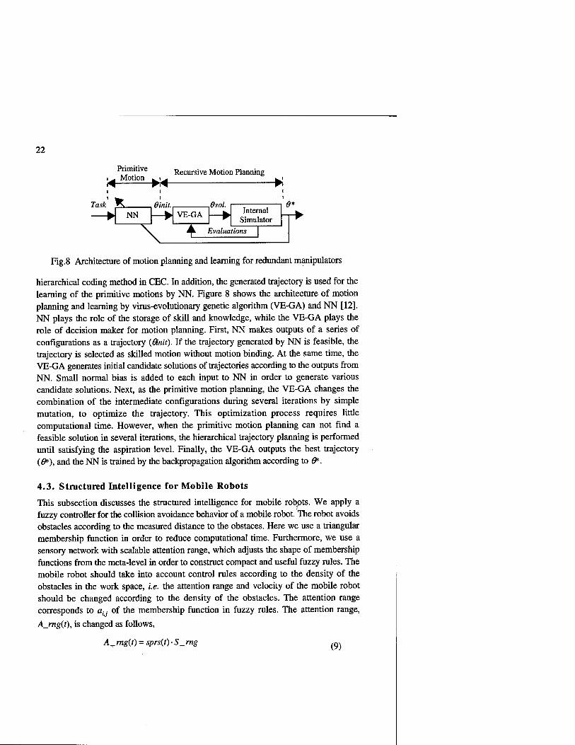
Fig.8 Architecture of motion planning and learning for redundant manipulators

hierarchical coding method in CEC. In addition, the generated trajectory is used for the learning of the primitive motions by NN. Figure 8 shows the architecture of motion planning and learning by virus-evolutionary genetic algorithm (VE-GA) and NN [12]. NN plays the role of the storage of skill and knowledge, while the VE-GA plays the role of decision maker for motion planning. First, NN makes outputs of a series of configurations as a trajectory ((knit). If the trajectory generated by NN is feasible, the trajectory is selected as skilled motion without motion binding. At the same time, the VE-GA generates initial candidate solutions of trajectories according to the outputs from NN. Small normal bias is added to each input to NN in order to generate various candidate solutions. Next, as the primitive motion planning, the VE-GA changes the combination of the intermediate configurations during several iterations by simple mutation, to optimize the trajectory. This optimization process requires little computational time. However, when the primitive motion planning can not find a feasible solution in several iterations, the hierarchical trajectory planning is performed until satisfying the aspiration level. Finally, the VE-GA outputs the best trajectory (#*), and the NN is trained by the backpropagation algorithm according to 0*.

4.3. Structured Intelligence for Mobile Robots

This subsection discusses the structured intelligence for mobile robots. We apply a fuzzy controller for the collision avoidance behavior of a mobile robot. The robot avoids obstacles according to the measured distance to the obstaces. Here we use a triangular membership function in order to reduce computational time. Furthermore, we use a sensory network with scalable attention range, which adjusts the shape of membership functions from the meta-level in order to construct compact and useful fuzzy rules. The mobile robot should take into account control rules according to the density of the obstacles in the work space, i.e. the attention range and velocity of the mobile robot should be changed according to the density of the obstacles. The attention range corresponds to ar) of the membership function in fuzzy rules. The attention range,

A_rag(0, is changed as follows,

A_mg(t) = sprs(t) ■ S_rng (9)

23

y-*-sprs(t) ifaUxi>A_rng(t) sprs(t +1) = \

[ y-sprs(t) otherwise

where sprs(t) is the degree of sparseness of obstacles satisfying 0 < sprsmin<sprs(t) <

1.0 for the perception of the work space, S_rng is the maximal sensing range, and y{0 < y< 1.0) is a perception coefficient. If the sensory network is not used, many fuzzy rules are required to describe the collision avoidance behavior because the sensing range is partitioned by many membership functions. However, the sensory network can dynamically change the meanings of the linguistic labels {'Danger' and 'Safe' in this case) by scaling A_rng(t) in online. Figure 9 shows the meanings of linguistic variables in cases of inputs x, and x2 in the sparse and crowded areas. Even if the input data is

same, there is the big difference of meanings (z, and z2) between the sparse area

(Fig.9.(a)) and crowded area (Fig.9.(b)). Thus, the sensory network can update the meanings of linguistic variables according to the timeseries of sensed information. Furthermore, the sensory network can reduce computational cost because the number of membership functions is relatively small comparing to the fixed linguistic variables. In the simplified fuzzy inference for the collision avoidance, *, is regarded as A_rng(t) if xt

is larger than A_rng(t). We have shown that the fuzzy controllers for the above collision avoidance behaviors can be optimized by genetic algorithm [13].

The mobile robot with structured intelligence basically takes reactive motions in a given work space. Its trajectory is generated as the result of these reactive motions. If the work space is much complicated and has dead ends of street, the mobile robot should generate several intermediate points to the target point and it should trace these intermediate points in order. Therefore, this path planning problem results in a generation problem of intermediate target points. Figure 10 shows a total architecture of the fuzzy-based mobile robot with path planning. The number of the required intermediate points depends on the complexity of a given work space. The aim of the mobile robot is to reach the target point. According to the environmental conditions, the robot acquires fuzzy controller and intermediate points through several trials.

Figure 11 shows a simulation result where the number of obstacles is 9 and the size of the work space is 500x500. The starting and target points are (50,50) and (450, 450), respectively. In the figure, the mobile robot is depicted every 10 discrete time steps. It cannot reach the target point, since it cannot escape from a local area surrounded by obstacles in the center. Figure 12 shows the actual trajectory of the mobile robot traced by reactive motions through the intermediate point generated by the GA for path planning. The location of intermediate point within obstacles is infeasible in standard path planning problems, but the collision check of intermediate points against obstacles is not required, because the proposed method includes the collision avoidance behavior. The mobile robot acquires a collision avoidance behavior through the coevolution of fuzzy controllers and intermediate point in the path planning.

24

XJ

(a) Minimal attention range (= sprsmin-S_rng)

S_rng X:

(b) Maximal attention range (= S_rng)

Fig.9 Membership functions corresponding to linguistic variables of dangerous and safe based on the attention range against measured distance

Sensing Sensory network

(Perception)

External evaluations Perceptual information

Action Fuzzy controller

(Decision making)

Path Planning

SSGA

Rules

On-line learning W

Delta rule

(Adaptation)

Off-line learning

SSGA

(Evolution)

Fitness

Update of learning rate

Fig. 10 Perception, decision making and action for the mobile robot

5. Summary This paper introduced recent topics of computational intelligence including coevolutionary computation, and discussed structured intelligence for robotic systems. First, we showed the motion planning and learning of redundant manipulators based on genetic algorithm and neural network. Next, we showed fuzzy controller optimization

25

Starting point

Target point

Fig. 11 A trajectory of the mobile robot traced by reactive motions.

Starting point ^* 1

£*;

..&'

■#;

Target point

Fig. 12 A trajectory of the mobile robot traced by reactive motions based on an intermediate point

genetic algorithm and neural network. Next, we showed fuzzy controller optimization and path planning of mobile robots based on genetic algorithm and sensory network as a perception mechanism.

In near future, the coevolution of multiple robots, the coevolution of the robot and dynamic environment will be discussed more and more.

26

References

1 SJ.Russell, P.Norvig, "Artificial Intelligence", Prentice-Hall, Inc., 1995. 2 J. A. Anderson, E. Rosenfeld, "Neurocomputing - Foundations of Research", The MIT

Press, 1988. 3 J. M. Zurada, R. J. Marks II, C. J. Robinson, "Computational Intelligence - Imitating

Life", IEEE Press, 1994. 4 M.Palaniswami, Y.Attikiouzel, RJ.Marks II, D.Fogel, and T.Fukuda, "Computational

Intelligence - A Dynamic System Perspective", IEEE Press, 1995. 5 J.-S.R.Jang, C.-T.Sun, E.Mizutani, "Neuro-Fuzzy and Soft Computing", Prentice-Hall,

Inc., 1997. 6 C.G.Langton, "Artificial Life -An Overview", The MIT Press, 1995. 7 D.B.Fogel, "Evolutionary Computation", IEEE Press, 1995. 8 D.E.Goldberg, "Genetic Algorithms in Search, Optimization, and Machine Learning",

Addison Welsey, 1989. 9 J.Koza, "Genetic Programming I and //", The MIT Press, 1992,1994. 10 • T.Fukuda, N.Kubota, and T.Arakawa, "GA Algorithms in Intelligent Robots," in Fuzzy

Evolutionary Computation (edited by W.Pedricz), Kluwer Academic Publishers, pp.81- 105, 1997.

11 R. A. Brooks, "A Robust Layered Control System for a Mobile Robot," IEEE Journal of Robotics and Automation, RA-2-1, 1986, pp.14-23.

12 T.Fukuda and N.Kubota, "Intelligent Robotic System -Adaptation, Learning and Evolution," in Proc. of The Third International Symposium on Artificial Life and Robotics, Oita, Japan, 1998-1, pp.I-40-45.

13 N.Kubota and T.Fukuda "Sensory Network for Mobile Robotic System with Structured Intelligence" Journal of Robotics and Mechatronics, Vol.10, No.4, 1998.

14 J.Maynard Smith, "Evolutionary Genetics", Oxford University Press, 1989. 15 J.J.Bull and W.R.Rice, "Distinguishing Mechanisms for the Evolution of

Cooperation, Journal of Theoretical Biology, Vol.149,1991, pp.63-74. 16 E.Lawrence, "Henderson's Dictionary of Biological Terms, Tenth Edition", Longman

Scientific & Technical, 1989. 17 W.D.Hillis, Co-Evolving Parasites Improve Simulated Evolution as An Optimization

Procedure, Artificial Life II, edited by C.G.Langton, C.Taylor, J.D.Farmer and S.Rasmussen, Addison Wesley, 1991, pp.313-324.

18 P.J.Angeline and J.B.Pollack, "Competitive Environments Evolve Better Solutions for Complex Tasks", Proc. of The Fifth International Conference on Genetic Algorithms, 1993, pp.264-270.

19 J.Paredis, "Coevolutionary Computation", Artificial Life, Vol.2, No.4, 1995, pp.355- 375.

20 HJ.C.Barbosa, "A Coevolutionary Genetic Algorithm for A Game Approach to Structural Optimization", Proc. of The Seventh International Conference on Genetic Algorithms, 1997, pp.545-552.

21 J.R.Koza, "Genetic Evolution and Co-Evolution of Computer Programs", Artificial Life II, edited by C.G.Langton, C.Taylor, J.D.Farmer and S.Rasmussen, Addison Wesley, 1991, pp.603-629.

27

Evolving Fuzzy Neural Networks for Adaptive, On-line Intelligent Agents and Systems

Nikola Kasabov Department of Information Science

University of Otago, P.O Box 56, Dunedin, New Zealand Phone: +64 3 479 8319, fax: +64 3 479 8311

nkasabov@otago.ac.nz

Abstract. This paper discusses and illustrates one paradigm of neuro-fuzzy techniques for building on-line, adaptive intelligent agents and systems. This approach is called evolving connectionist systems (ECOS). ECOS evolve through incremental, on-line learning, both supervised and unsupervised. They can accommodate new input data including new features, new classes, etc. The ECOS framework is presented and illustrated on a particular type of evolving neural networks - evolving fuzzy neural networks. ECOS are orders of magnitude faster than multilayer perceptrons, or fuzzy neural networks and they belong to the new generation of adaptive intelligent systems. ECOS are suitable techniques for building intelligent agents on the WWW, intelligent mobile robots and embedded systems. An ECOS based structure of an intelligent agent is proposed and discussed.

1. Introduction: Adaptive, On-Line, Incremental Learning

The complexity and the dynamics of many real-world problems, particularly in engineering and manufacturing, requires sophisticated methods and tools for building on-line, adaptive decision making and control systems. Such systems should grow as they operate, increase their knowledge, and refine themselves through interaction with the environment [14].

Many developers and practitioners in the area of neural networks (NN) [3], fuzzy systems (FS) [299] and hybrid neuro-fuzzy techniques [10, 13, 18, 20, 21, 23, 29] have enjoyed the power of these now traditional techniques when solving AI problems. Despite of their power, using these techniques for on-line, incremental, life-long learning through adaptation in a changing environment may create difficulties. There are some methods that have already been developed and implemented, such as: ART and Fuzzy ARTMAP [3] for incremental learning; several methods for on-line learning [1, 6, 9, 11, 25]; methods for dynamically changing NN structures during learning process, that include growing and pruning of unnecessary connections and nodes of an NN[7, 12, 24, 26, 27].

The paper continues the list of the techniques from above by introducing a new framework called evolving connectionist systems (ECOS) and a new hybrid model called evolving fuzzy neural network. It discusses their potential for building intelligent agents and intelligent robotic systems.

2. ECOS - Evolving Connectionist and Fuzzy - Connectionist Systems

28

ECOS are systems that evolve in time through interaction with the environment, i.e. an ECOS adjusts its structure with a reference to the environment (fig.l) as explained in [13-18].

Environment

Fig.l. ECOS evolve through interaction with the environment

ECOS are multi-level, multi-modular structures in which many modules have inter- and intra- connections. The evolving connectionist system does not have a clear multi-layer structure. It has a modular open structure. The functioning of the ECOS is based on the following general principles [14 -17]. (1) There are three levels of functionality of an ECOS, defined by :

(a) Genetically specified parameters, such as size of the system, types of inputs, learning rate, forgetting.

(b) Synaptic connection weights (c) Activation of neurons.

(2) Input patterns are presented one by one, in a pattern mode, not necessarily having the same input feature sets. After the presentation of each input vector (example), the ECOS associates this example through a local tuning of units with either an already existing node (called rule or case node), or it creates a new one. In this respect, ECOS are similar to the case-based learning and reasoning systems. An NN module or a neuron is created when needed at any time of the functioning of the whole system.

(3) The ECOS structure evolves in two phases in a hybrid unsupervised- supervised mode of one pass data propagation. In phase one, an input vector x is passed through the representation module and the case (rule) nodes become activated based on the similarity between the input vector and the input connection weights. If there is no node activated above a certain sensitivity threshold (Sthr), a new rule neuron (rn) is connected ('created') and its input weights are set equal to the values of the input vector x; the output weights are set to the desired output vector. In this respect, the ECOS paradigm is similar to ART [3]. Activation either from the winning case neuron (one-out of-n mode), or from all case neurons that have activation values above an activation threshold (Athr) (many-of-n mode) is passed to the next level of neurons. In phase two, if there is no need to create a new node, the output error is found and the output connections are adjusted accordingly in a supervised mode. The input connections are also adjusted but

29

according to similarity between the existing nodes and the input vectors (unsupervised mode).

(4) ECOS have a pruning and aggregation procedure defined. It allows for removing neurons and their corresponding connections that are not actively involved in the functioning of the ECOS (thus making space for new input patterns). Pruning is based on local information kept in the neurons. Each neuron in ECOS keeps a track' of its 'age', its average activation over the whole life span, the global error it contributes to, and the density of the surrounding area of neurons. Through aggregation many neurons are merged together based on their similarity.

(5) The case neurons are spatially and temporarily organized. Each neuron has its relative spatial dimensions in regards to the rest of the neurons based on their reaction to the input patterns. If a new rule node is to be created when an input vector x is presented, then this node will be positioned closest to the neuron that had the highest activation to the input vector x, even though not sufficiently high to accommodate this input vector. Temporal connections between neurons can be established thus reflecting the temporal correlation of input patters.

(6) There are two global modes of learning in ECOS as explained in [13-18]: (a) Active learning mode - learning is performed when a stimulus

(input pattern) is presented and kept active. (b) ECO training mode - learning is performed when no input pattern is

presented at the input of the ECOS. In this case, the process of further elaboration of the connections in ECOS is done in a passive learning phase, when existing connections that store previous input patterns are used as training examples. The connection weights that represent stored input patterns are now used as exemplar input patterns for training other modules in ECOS. This type of learning with the use of 'echo' data is called here ECO training.

There are two types of ECO training [14, 16]: (i) Cascade eco-training: a new NN module is created in an on-

line mode when conceptually new data (e.g., a new class data) is presented. This mode is similar to the one from [3]. The module is trained on the positive examples of this class, plus the negative examples of the following different class data, and on the negative examples of previously stored patterns in previously created modules taken from the connection weights of these modules.

(ii) Sleep eco-training: modules are created with part of the data presented (e.g., positive class examples). Then the modules are trained on the stored data in the other modules' patterns as negative examples (exemplars).

(7) ECOS provide explanation information extracted from the structure of the NN modules. Each case (rule) node can be interpreted as an IF-THEN rule as it is in the FuNN fuzzy neural network [19-20]. As ECOS are connectionist knowledge- based systems, important part of their functionality is inserting and extracting rules.

(8) ECOS are biologically inspired. Some biological motivations are given in [ 18]. (9) The ECOS framework can be applied to different types of NN (different neurons,

activation functions etc.) and FS. One realisation of the ECOS framework is the

30

evolving fuzzy neural network EFuNN and the EFuNN algorithm as given in [18] and in section 4. Before the notion of EFuNNs is presented, the notion of the fuzzy neural networks FuNNs is presented in the next section.

3. Fuzzy Neural Networks FuNNs

Fuzzy neural networks are neural networks that realise a set of fuzzy rules and a fuzzy inference machine in a connectionist way [10, 13, 19, 23, 29]. FuNN is a particular fuzzy neural network introduced in [19] and developed in [21]. FuNN is part of a comprehensive environment called FuzzyCOPE/3 available free on the WWW: http://divcom.otago.ac.nz/infosci/kel/software/FuzzvCOPE3/main.htm

It is a connectionist feed-forward architecture with five layers of neurons and four layers of connections. The first layer of neurons receives the input information. The second layer calculates the fuzzy membership degrees to which the input values belong to predefined fuzzy membership functions, e.g. small, medium, and large. The third layer of neurons represents associations between the input and the output variables, fuzzy rules. The fourth layer calculates the degrees to which output membership functions are matched by the input data, and the fifth layer does defuzzification and calculates exact values for the output variables. A FuNN has features of both a neural network and a fuzzy inference machine. A simple FuNN structure is shown in fig.2. The number of neurons in each of the layers can potentially change during operation through growing or shrinking. The number of connections is also modifiable through learning with forgetting, zeroing, pruning and other operations [19, 21]. The membership functions (MF) used in FuNN to represent fuzzy values are of triangular type, the centres of the triangles being attached as weights to the corresponding connections. The MF can be modified through learning that involves changing the centres and the widths of the triangles.

Rule(case) nodes

Input ^vKX W J>° ► °UtpUt

Fig. 2. A FuNN structure of two inputs (input variables), two fuzzy linguistic terms for each variable (two membership functions). The number of the rule (case) nodes can vary. Two output membership functions are used for the output variable.

Several algorithms for training, rule insertion, rule extraction and adaptation have been developed for FuNN [19, 21]. FuNNs have several advantages when compared with the traditional connectionist systems, or with the traditional fuzzy systems: they are statistical and knowledge engineering tools; they are relatively robust to catastrophic forgetting, i.e. when they are further trained on new data, they keep a reasonable memory of the old data; they interpolate and extrapolate well in regions where data is sparse; they accept both real input data and fuzzy input data represented

31

as singletons (centres of the input membership functions). The above listed features of FuNNs make them universal statistical and knowledge engineering tools. Many applications of FuNNs have been developed and explored so far [19, 21].

4. Evolving Fuzzy Neural Networks EFuNNs

4.1. The EFuNN Principles and Structures

EFuNNs are FuNN structures that evolve according to the ECOS principles. EFuNNs adopt some known techniques from [3,19, 22], but here all nodes in an EFuNN are created/connected during (possibly one-pass) learning. The nodes representing membership functions (MF) (fuzzy label neurons) can be modified during learning. As in FuNN, each input variable is represented here by a group of spatially arranged neurons to represent a fuzzy quantisation of this variable. For example, three neurons can be used to represent "small", "medium" and "large" fuzzy values of the variable. Different MFs can be attached to these neurons (triangular, Gaussian, etc.). New neurons can evolve in this layer if, for a given input vector, the corresponding variable value does not belong to any of the existing MFs to a degree greater than a set threshold. A new fuzzy input neuron, or an input neuron, can be created during the adaptation phase of an EFuNN. An optional short-term memory layer can be used through a feedback connection from the rule (also called, case) node layer (see fig.3). The layer of feedback connections could be used if temporal relationships between input data are to be memorized structurally.

The third layer contains rule (case) nodes that evolve through supervised/unsupervised learning. The rule nodes represent prototypes (exemplars, clusters) of input-output data associations, graphically represented as an association of hyper-spheres from the fuzzy input and fuzzy output spaces. Each rule node r is defined by two vectors of connection weights - Wl(r) and W2(r), the latter being adjusted through supervised learning based on the output error, and the former being adjusted through unsupervised learning based on similarity measure within a local area of the problem space. The fourth layer of neurons represents fuzzy quantization for the output variables, similar to the input fuzzy neurons representation. The fifth layer represents the real values for the output variables.

The evolving process can be based on two assumptions, that either no rule nodes exist prior to learning and all of them are created (generated) during the evolving process, or there is an initial set of rule nodes that are not connected to the input and output nodes and become connected through the learning (evolving) process. The latter case is more biologically plausible. The EFuNN evolving algorithm presented in the next section does not make a difference between these two cases.

Each rule node (e.g., rl) represents an association between a hyper-sphere from the fuzzy input space and a hyper-sphere from the fuzzy output space (see fig.4), the Wl(rj) connection weights representing the co-ordinates of the center of the sphere in the fuzzy input space, and the W2 (rj) - the co-ordinates in the fuzzy output space. The radius of an input hyper-sphere of a rule node is defined as (1- Sthr), where Sthr is the sensitivity threshold parameter defining the minimum activation of a rule node (e.g., rl) to an input vector (e.g., (Xd2,Yd2)) in order for the new input vector to be associated to this rule node.

32

Outputs

Fuzzy input layer

Input layer

Fig.3. An EFuNN architecture with a short term memory and feedback connections

Two pairs of fuzzy input-output data vectors dl=(Xdl,Ydl) and d2=(Xd2,Yd2) will be allocated to the first rule node ri if they fall into the ri input sphere and in the ri output sphere, i.e. the local normalised fuzzy difference between Xdl and Xd2 is smaller than the radius r and the local normalised fuzzy difference between Ydl and Yd2 is smaller than an error threshold Errthr.

The local normalised fuzzy difference between two fuzzy membership vectors dlf and d2f that represent the membership degrees to which two real values dl and d2 data belong to the pre-defined MF are calculated as D(dlf,d2f) = sum(abs(dlf - d2f))/sum(dlf + d2f». For example, if dlf=(0,0,1,0,0,0) and d2f=(0,1,0,0,0,0), than D(dl,d2) = (1+1)/2=1 which is the maximum value for the local normalised fuzzy difference. If data example dl = (Xdl,Ydl), where Xdl and Xd2 are correspondingly the input and the output fuzzy membership degree vectors, and the data example is associated with a rule node rl with a centre r/, than a new data point d2=(Xd2,Yd2), that is within the shaded area as shown in fig.4, will be associated with this rule node too. Through the process of associating (learning) of new data points to a rule node, the centres of this node hyper-spheres adjust in the fuzzy input space depending on a learning rate lrnl and in the fuzzy output space depending on a learning rate lr2, as it is shown in fig.4a on two data points. The adjustment of the center rj1 to its new position ri2 can be represented mathematically by the change in the connection weights of the rule node rl from Wlfa1) and W2(r,') to Wl(r, ) and W2(r!2) as it is presented in the following vector operations:

W2 (r,2) = W2(r,') + lr2. Err(Ydl,Yd2). Alfa1),

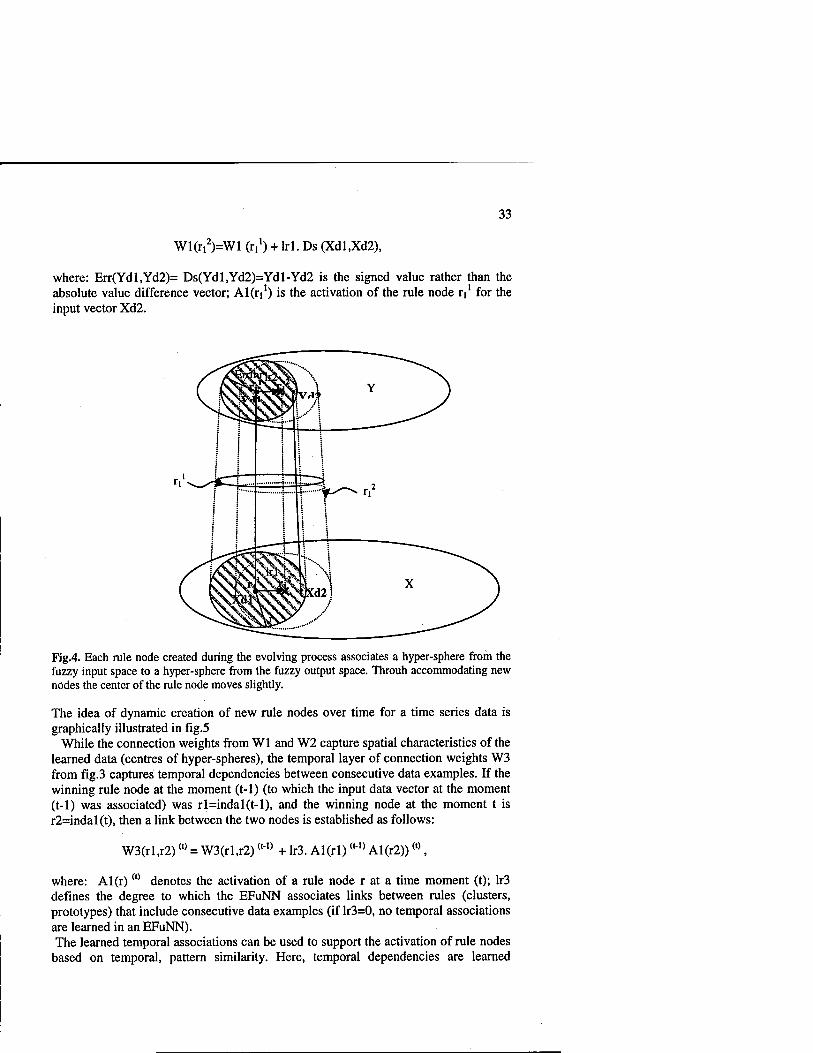
33

Wl(riZ)=Wl (r,1) + lrl. Ds (Xdl,Xd2),

where: Err(Ydl,Yd2)= Ds(Ydl,Yd2)=Ydl-Yd2 is the signed value rather than the absolute value difference vector; Al(ri') is the activation of the rule node ri' for the input vector Xd2.

Fig.4. Each rule node created during the evolving process associates a hyper-sphere from the fuzzy input space to a hyper-sphere from the fuzzy output space. Throuh accommodating new nodes the center of the rule node moves slightly.

The idea of dynamic creation of new rule nodes over time for a time series data is graphically illustrated in fig.5

While the connection weights from Wl and W2 capture spatial characteristics of the learned data (centres of hyper-spheres), the temporal layer of connection weights W3 from fig.3 captures temporal dependencies between consecutive data examples. If the winning rule node at the moment (t-1) (to which the input data vector at the moment (t-1) was associated) was rl=indal(t-l), and the winning node at the moment t is r2=indal(t), then a link between the two nodes is established as follows:

W3(rl,r2)(t) = W3(rl,r2)(M) + lr3. Al(rl)(M) Al(r2)) (0

where: Al(r)(t) denotes the activation of a rule node r at a time moment (t); lr3 defines the degree to which the EFuNN associates links between rules (clusters, prototypes) that include consecutive data examples (if lr3=0, no temporal associations are learned in an EFuNN). The learned temporal associations can be used to support the activation of rule nodes

based on temporal, pattern similarity. Here, temporal dependencies are learned

34

through establishing structural links. These dependencies can be further investigated and enhanced through synaptic analysis (at the synaptic memory level) rather than through neuronal activation analysis (at the behavioural level). The ratio spatial- similarity/temporal-correlation can be balanced for different applications through two parameters Ss and Tc such that the activation of a rule node r for a new data example dnew is defined as the following vector operations:

Al (r) = f ( Ss. D(r, dncw) + Tc.W3(r(1,), r))

where: f is the activation function of the rule node r, D(r, dnew) is the normalised fuzzy difference value and r (tl)is the winning neuron at time moment (t-1).

▲ Output

. Input data over time

Fig.5. The rule nodes in an EFuNN evolve in time depending on the similarity in the input data

Several parameters were introduced so far for the purpose of controlling the functioning of an EFuNN. Some more parameters will be introduced later, that will bring the EFuNN parameters to a comparatively large number. In order to achieve a better control of the functioning of an EFuNN structure, the three-level functional hierarchy is used here as defined in section 2 for the ECOS architecture, namely: genetic level, long-term synaptic level, and short- term activation level.

At the genetic level, all the EFuNN parameters are defined as genes in a chromosome. These are: (a) structural parameters, e.g.: number of inputs, number of MF for each of the inputs, initial type of rule nodes, maximum number of rule nodes, number of MF for the output variables, number of outputs. (b) functional parameters, e.g.: activation functions of the rule nodes and the fuzzy output nodes (in the experiments below saturated linear functions are used); mode of rule node activation ("one-of-n", or "many-of-n", depending on how many activation values of rule nodes are propagated to the next level); learning rates lrl,lr2 and lr3; sensitivity threshold Sthr for the rule layer; error threshold Errthr for the output layer; forgetting rate; various pruning strategies and parameters, as explained in the EFuNN algorithm below.

4.2. The EFuNN algorithm

35

The EFuNN algorithm has been first presented in [18]. A new rule node rn is connected (created) and its input and output connection weights are set The EFuNN algorithm, to evolve EFuNNs from incoming examples, is based on the principles explained in the previous section. It is given below as a procedure of consecutive steps. Vector and matrix operation expressions are used for the sake of simplicity of presentation.

1. Initialise an EFuNN structure with a maximum number of neurons and no (or zero- value) connections. Initial connections may be set through inserting fuzzy rules in the structure. If initially there are no rule (case) nodes connected to the fuzzy input and fuzzy output neurons, then create the first node rn=l to represent the first example dl and set its input Wl(rn) and output W2(rn) connection weight vectors as follows:

<Create a new rule node rn>: Wl(rn)=EX; W2(rn ) = TE, where TE is the fuzzy output vector for the current fuzzy input vector EX.

2. WHILE <there are examples in the input stream> DO

Enter the current example (Xdi.Ydi), EX denoting its fuzzy input vector. If new variables appear in this example, which are absent in the previous examples, create new input and/or output nodes with their corresponding membership functions.

3. Find the normalised fuzzy local distance between the fuzzy input vector EX and the already stored patterns (prototypes, exemplars) in the rule (case) nodes rj=rl,r2,...,rn

D(EX, rj)= sum (abs (EX - Wl(j))/ 2) / sum (WIG))

4. Find the activation Al (rj) of the rule (case) nodes rj, rj=rl :rn. Here radial basis activation function, or a saturated linear one, can be used, i.e.

Al (rj) = radbas (D(EX, rj)), or Al(rj) = satlin (1 - D(EX, rj)). The former may be appropriate for function approximation tasks, while the latter may be preferred for classification tasks. In case of the feedback variant of an EFuNN, the activation is calculated as explained above:

Al (rj) = radbas (Ss. D(EX, rj) - Tc.W3), or Al(j) = satlin (1 - Ss. D(EX, rj) + Tc.W3).

5. Update the pruning parameter values for the rule nodes, e.g. age, average activation as pre-defined in the EFuNN chromosome.

6. Find all case nodes rj with an activation value Al(rj) above a sensitivity threshold Sthr.

7. If there is no such case node, then <Create a new rule node> using the procedure from step 1. ELSE

36

8. Find the rule node indal that has the maximum activation value (e.g., maxal).

9. (a) in case of "one-of-n" EFuNNs, propagate the activation maxal of the rule node indal to the fuzzy output neurons.

A2 = satlin (Al(indal). W2(indal) (b) in case of "many-of-n" mode, the activation values of all rule nodes that are above an activation threshold of Athr are propagated to the next neuronal layer (this case is not discussed in details here; it has been further developed into a new EFuNN architecture called dynamic EFuNN, or DEFuNN).

10. Find the winning fuzzy output neuron indal and its activation maxal. 11. Find the desired winning fuzzy output neuron indtl and its value maxtl. 12. Calculate the fuzzy output error vector: Err=A2 - TE. 13. IF {indal is different from indtl) or (D(A2,TE) > Errthr ) <Create a new rule node> ELSE 14. Update: (a) the input, (b) the output, an (c) the temporal connection vectors (if such exist) of the rule node k=indal as follows: (a) Ds(EX,Wl(k)) =EX-Wl(k); Wl(k)=Wl(k) + lrl.Ds(EX,Wl(k)), where

Irl is the learning rate for the first layer; (b) W2(k) = W2 (k) + lr2. Err. maxal, where Irl is the learning rate for the

second layer; (c) W3(l,k)=W3(l,k)+lr3. Al(k).Al(l)(t,), here 1 is the winning rule neron

at the previous time moment (t-1), and Al(l)(tl) is its activation value kept in the short term memory.

15. Prune rule nodes j and their connections that satisfy the following fuzzy pruning rule to a pre-defined level:

IF (a rule node rj is OLD) AND (average activation Alav(rj) is LOW) and (the density of the neighbouring area of neurons is HIGH or MODERATE (i.e. there are other prototypical nodes that overlap with j in the input-output space; this condition apply only for some strategies of inseting rule nodes as explained in a sub-section below) THEN the probability of pruning node (rj) is HIGH

The above pruning rule is fuzzy and it requires that the fuzzy concepts of OLD, HIGH, etc., are defined in advance (as part of the EFuNN's chromosome). As a partial case, a fixed value can be used, e.g. a node is OLD if it has existed during the evolving of a FuNN from more than 1000 examples. The use of a pruning strategy and the way the values for the pruning parameters are defined depends on the application task.

16. Aggregate rule nodes, if necessary, into a smaller number of nodes (see the explanation in the following subsection).

37

17. END of the while loop and the algorithm

18. Repeat steps 2-17 for a second presentation of the same input data or for an ECO training if needed.

ECOS, and EFuNNs in particular, allow for different learning strategies to be experimented, depending on the type of data available and on the requirements of the learning system. Several of these are introduced and illustrated in [17, 18]. They are:

• Incremental, one-pass learning: Data is propagated only once through the EFuNN. • Incremental, multiple-pass learning: Consecutive passes of data on evolved

EfuNNs, are performed • Using positive examples only • Cascade eco-learning • Sleep eco-training: Different modules evolve quickly to capture the most important

information concerning their specialised functions (e.g., class information). The modules store exemplars of relevant for their functioning examples during the active training mode. After that, the modules begin to exchange exemplars that are stored in their Wl connections as negative examples for other modules to improve their performance.

• Unsupervised and reinforcement learning: Unsupervised learning in ECOS systems is based on the same principles as the supervised learning, but there is no desired output and no calculated output error

• Rule insertion and rule extraction: these algorithms allow for insertion of fuzzy rules in an EFuNN structure at any time of its operation, or extraction of a minimal set of fuzzy rules (aggregated), that is in general much smaller in size than the number of the rule nodes.

4.3. EFuNN Simulators

Figure 6 shows the GUI of an EFuNN simulator. EFuNN simulators and MATLAB functions are available from the WWW site: http://divcom.otago.ac.nz/infosci/kel/software/FuzzvCOPE3/main.htm.

It is possible to set values for the following parameters: sensitivity threshold SThr, error threshold Ethr, learning rates lrl and lr2, number of inputs, number of membership functions, number of outputs, passes of learning.

The simulation and the testing can be done either in an on-line, or in an off-line mode. In an on-line mode after learning each input example, the system is tested on the following input data to locally predict the corresponding output value. After the output value becomes known this example is learned by the system and the next output is predicted, etc. This is illustrated in fig.7 on a waste-water flow data hourly collected (see site http://divcom.otago.ac.nz/infosci/kel/software/datasetsA. The task of the evolved EFuNN is to learn in an-on-line mode and predict the next hour flow volume, which is shown in the figure.

The off-line mode is similar to the way multilayer perceptrons and other neural network types for supervised learning are trained and tested. •

38

fEMMnmm E031

Fw 1 1 l I ' I i W^^^^'^i"

m N 1 Hi |i:^^SSssdf 4 hi »ä^SSWI i Jil I* Liil !i iJ fi&assaw Jsw' A vl\ \\P. ji IP r In HA lUl W lur: W r M flffl VI alft KsM ^v-j-jjÄcaasp1^??»^ ■Sal !fl ? IH niKl / fl 14n " ? W JÜ •'^^»'«Ws^^Psf.ra

Kt I U li'll I I1 ; I 1 MrSHSSMlf; II I1 IM HI Sfi

-II #,-lt A— lU^uLu-JuiJ (um. -I'. fX'.'Q

]cf;i«NSUlv.. JttJQä&j^FM'

Fig.6. The GUI of an EFuNN simulator

5. ECOS and EFuNNs for Adaptive, On-Line, Intelligent Agents and Systems

Agent-based techniques allow the implementing of modular systems that consist of independent software modules. These modules can communicate with each other and with the user by using a standard protocol and they can 'navigate' in a new software environment by searching for relevant data, then process the data and pass the results [28]. Intelligent agents can perform intelligent information processing, such as reasoning with uncertainties and generalisation. Intelligent agents should be able to adapt to a possibly changing environment as they work in an on-line mode. Such adaptation is crucial for mobile robot navigation, or for an adequate decision making on operations with a dynamically changing data.

A general block diagram of the architecture of an ECOS and EFuNN-based adaptive, on-line agent is given in fig. 7. It consists of the following blocks: • Pre-processing (filtering) block for input data (this block checks input data for

consistency; selects appropriate input features and vectors)

39

EFuNN modules that are continuously trained with data in one of the explained in section 4 modes. Rules can be are inserted at any time of the operation of the agent.

A block for decision making/control and communication - this block communicates with other agents and the environment and sends the results produced by the EFuNN modules.

Adaptation block - this block compares the behaviour of the agent with a desired behaviour over regular periods of time. The error is used to adjust/adapt the evolving EFuNN modules in a continuous mode. Genetic algorithms can be applied here or other optimisation procedures [5, 8].

Rule extraction, explanation block - this block extracts rules from the evolved EFuNN modules for explanation purposes

Adaptation

EFuNN modules

InDuts

Decision Making and Control

Outputs

Rule extraction, p.xnlanatinn

Fig.7. A block diagram of an ECOS-based agent for on-line, intelligent decision and control

The above general scheme of an intelligent evolving agent is currently being applied in the Knowledge Engineering Laboratory at the University of Otago to two classes of problems:

• Intelligent agents on the WWW, for the purpose of: learning from data repositories; climate prediction; financial decision making;

• Mobile robot control.

For solving specific problems from the two generic classes of problems, a repository of different connectionist, AI and data processing techniques (including different types of EFuNNs) are organised in a Repository for Intelligent Connectionist Based InformationSystemsRICBIS (http://divcom.otago.ac.nz/infosci/kel/software/RICBIS/. For solving problems from the first class the Voyager environmnet is currently being experimented for building intelligent agents for ditributed processing on the WWW. For the second class of applications both sensory and visual information are enabled to collec and process in an on-line mode with the use of EFuNNs. The experiments deal with speech, image and text input. The evolving agents, as part of the robot's software, evolve in real time for different purposes of recognition of object classes,

40

for navigation in a new environment, and for adaptation to new input features. The experiments are in their initial phase and more results are expected in the near future.

6. Conclusion

This paper discusses the ECOS framework for evolving connectionist systems and for evolving fuzzy neural networks (EFuNNs) and introduces a framework for building on-line, adaptive learning agents and agent-based systems. ECOS have features that address the major requirements for the next generation of intelligent and adaptive information systems, such as fast learning (possibly, one pass learning); continuous on-line incremental learning and adaptation; the possibility of working in a life-long learning mode; storing information and data for a consecutive improvement and rule extraction.

Acknowledgements This research is part of a research programme funded by the New Zealand Foundation for Research Science and Technology, New Zealand, project UOO808.

References

1. Albus, J.S., A new approach to manipulator control: The cerebellar model articulation controller (CMAC), Tarns, of the ASME: Journal of Dynamic Systems, Measurement, and Control, pp.220:227, Sept. (1975)

2. Amari, S. and Kasabov, N. eds (1997) Brain-like computing and intelligent information systems, Springer Verlag

3. Carpenter, G.A., Grossberg, S., Markuzon, N., Reynolds, J.H., Rosen, D.B., FuzzyARTMAP: A neural network architecture for incremental supervised learning of analog multi-dimensional maps, IEEE Transactions of Neural Networks , vol.3, No.5 (1991), 698-713

4. Edelman, G., Neuronal Darwinism: The theory of neuronal group selection, Basic Books (1992)

5. Freeman, J.A.S., Saad, D., On-line learning in radial basis function networks, Neural Computation vol. 9, No.7 (1997)

6. Fritzke, B., A growing neural gas network learns topologies, Advances in Neural Information Processing Systems, vol.7 (1995)

7. Fukuda, T., Komata, Y., and Arakawa, T. "Recurrent Neural Networks with Self- Adaptive GAs for Biped Locomotion Robot", In: Proceedings of the International Conference on Neural Networks ICNN97, IEEE Press (1997)

8. Gaussier, P. and Zrehen, S., A topological neural map for on-line learning: Emergence of obstacle avoidance in a mobile robot, In: From Animals to Animats No.3, (1994) 282-290

9. Hashiyama, T., Furuhashi, T., Uchikawa, Y.(1992) A Decision Making Model Using a Fuzzy Neural Network, in: Proceedings of the 2nd International Conference on Fuzzy Logic & Neural Networks, Iizuka, Japan, 1057-1060.

10. Heskes, T.M., Kappen, B. (1993) On-line learning processes in artificial neural networks, in: Math, foundations of neural networks, Elsevier, Amsterdam, 199- 233

41

11. Ishikawa, M. (1996) "Structural Learning with Forgetting", Neural Networks 9, 501-521.

12. Jang, R. (1993) ANFIS: adaptive network-based fuzzy inference system, IEEE Trans, on Syst.,Man, Cybernetics, 23(3), May-June 1993,665-685

13. Kasabov, N. ECOS: A framework for evolving connectionist systems and the eco learning paradigm, Proc. of ICONIP^, Kitakyushu, Oct. 1998, IOS Press, 1222- 1235

14. Kasabov, N. Evolving connectionist and fuzzy connectionist system for on-line decision making and control, in: Soft Computing in Engineering Design and Manufacturing, Springer Verlag, 1999

15. Kasabov, N. The ECOS Framework and the ECO Learning Method for Evolving Connectionist Systems, Journal of Advanced Computational Intelligence, 2 (6) 1998, 1-8

16. Kasabov, N. Evolving connectionist and fuzzy connectionist systems. IEEE Transactions on Man, Machine and Cybernetics, submitted

17. Kasabov, N. Evolving Fuzzy Neural Networks - Algorithms, Applications and Biological Motivation, in: Yamakawa and Matsumoto (eds), Methodologies for the Conception, design and Application of Soft Computing, World Scientific, 1998, 271-274

18. Kasabov, N.(1996) Foundations of Neural Networks, Fuzzy Systems and Knowledge Engineering, The MIT Press, CA, MA.

19. Kasabov, N., "Adaptable connectionist production systems". Neurocomputing, 13(2-4)95-117(1996).

20. Kasabov, N, Kim J S, Watts, M., Gray, A (1997) FuNN/2- A Fuzzy Neural Network Architecture for Adaptive Learning and Knowledge Acquisition, Information Sciences - Applications, 101(3-4): 155-175 (1997)

21. Kohonen, T. (1990) The Self-Organizing Map. Proceedings of the IEEE, vol.78, N-9, pp. 1464-1497.

22. Lin, C.T. and C.S. G. Lee, Neuro Fuzzy Systems, Prentice Hall (1996). 23. Mozer. M, and P.Smolensky, A technique for trimming the fat from a network

via relevance assessment, in: D.Touretzky (ed) Advances in Neural Information Processing Systems, vol.2, Morgan Kaufmann, 598-605 (1989).

24. Rummery, G.A. and Niranjan, M., On-line Q-learning using connectionist systems, Cambridge University Engineering Department, CUED/F-INENG/TR 166 (1994)

25. Sankar, A. and R.J. Mammone, Growing and Pruning Neural Tree Networks, IEEE Trans. Comput. 42(3) 291-299 (1993).

26. Whitley, D. and Bogart, C, The evolution of connectivity: Pruning neural networks using genetic algorithms. Proc. Int. Joint Conf. Neural Networks, No.l (1990) 17-22.

27. Woldrige, M. and Jennings, N. Intelligent agents: Theory and practice, The Knowledge Engineering review (10) 1995

28. Yamakawa, T., H. Kusanagi, E. Uchino and T.Miki, (1993) "A new Effective Algorithm for Neo Fuzzy Neuron Model", in: Proceedings of Fifth IFSA World Congress, 1017-1020

29. Zadeh, L. 1965. Fuzzy Sets, Information, and Control, vol.8, 338-353.

42

An Agent-Oriented Architecture for Human-Robot Symbiosis in Flexible Manufacturing

K. Kawamura, D. M. Wilkes, R. A. Peters II, W. A. Alford, and T. E. Rogers

Intelligent Robotics Laboratory Vanderbilt University

Department of Electrical and Computer Engineering Nashville, Tennessee 37235 USA

Abstract A software system for human-robot interaction is described. The soft- ware is being designed to control a holonic system for flexible manufacturing. Hu- man-robot symbiosis enables human training of the robot in assembly tasks and fa- cilitates interaction between robot and person on an assembly line. In this paper: holonic systems are defined in the context of manufacturing. A general structure for a holonic manufacturing system that interacts with people is proposed. An agent- based software architecture, the Intelligent Machine Architecture (IMA), is de- scribed. IMA permits concurrent execution of software agents on separate machines in a network while permitting extensive inter-agent communication. Human-robot interaction is enabled by two software agents in the system, a robot agent and a hu- man agent The former encapsulates information about the status of the robot and performs (or controls the agents that perform) action selection. The latter includes information about the person necessary for successful interaction and controls the agents responsible for communication with the person. Human-robot interaction is then controlled by the interaction between the respective agents. A testbed for ex- perimentation with this dual agent model is described.

1 Introduction

Researchers in the Intelligent Robotics Laboratory (IRL) at Vanderbilt University are de- veloping robots that interact closely with human beings for applications both in home and factory. System integration, a problem with any versatile robot, is further complicated if the system is to interact with people. To simplify the implementation of such systems the Intelligent Machine Architecture (IMA) has been developed at the IRL. IMA is an agent- based software architecture that has been designed specifically to facilitate the integration of the many diverse algorithms, sensors, and actuators necessary for intelligent interactive robots. This paper is a description of IMA and a hardware testbed designed for experi- ments in flexible manufacturing.

43

2 Human-Robot Symbiosis in Flexible Manufacturing

Manufacturing has evolved from an enterprise involving labor and individual skill to a process of technology-driven mass production. There is a move recently among a signifi- cant number of companies away from mass production and toward the manufacture of customized products in small batches - which requires flexible manufacturing [1]. In re- sponse, the Holonic Manufacturing System project (HMS) was proposed by researchers in the early 1990s. They were part of a global program called Intelligent Manufacturing Systems (IMS) sponsored, in part, by the U.S. Department of Commerce. The IMS pro- gram was formed to advance a technological and organizational manufacturing agenda to meet the challenges of a global manufacturing environment (www.acims.org). The HMS was one of the four original projects.

Arthur Koestler in his book, The Ghost in the Machine, coined the term, "holon" to describe a basic unit of organization in biological and social systems, which he called "holonic systems" [2]. It reflects the tendency of holons to act autonomously while, nev- ertheless, cooperating as self-organizing hierarchies of sub-systems. A holonic manufac- turing system is, therefore, a manufacturing system autonomous yet cooperative elements.

2.1 Holonic Assembly Robot

An HMS related goal of the IRL has been to use the Intelligent Machine Architecture to develop a prototype assembly robot, called ISAC, for small-batch manufacturing (see http://shogun.vuse.vanderbilt.edu/CIS/IMS). A subsidiary goal has been to integrate peo- ple into the system. A person could assist the robot in higher-level perception tasks, or could provide suggestions for motion planning and coordination. IMA plays a fundamen- tal role in holonic architectures developed at the IRL, for the agents that comprise the ar- chitectures are holons in the sense described above. The ISAC robot, with its dual arms and multifarious sensors, may be adapted to become an assembly holon in an "agile enter- prise" [3]. An agile enterprise is a type of flexible manufacturing in an open, distributed environment

A general architecture for an HMS holon is depicted in Figure 1 [4]. The physical processing layer is the actual hardware performing the manufacturing operation such as assembly. Decision making represents the kernel of the holon and provides two inter- faces: the first for interaction with other holons, and the second for interaction with hu- mans [5]. IMA holons differ from that general architecture in several, significant ways. IMA incorporates a two-level logical structure: 1) a high-level, robot-environment model and 2) a low-level, or primitive, agent-component object model. The logical separation into primitive agents and component objects allows designers of intelligent machine soft- ware to address software engineering issues such as : reuse, extensibility, and manage- ment of complexity. At the highest level of its holarchy, ISAC (whose control software was written with IMA) has two holons, the Robot Agent and the Human Agent (See Figure 2). The Robot Agent monitors the internal status of the robot (positions and velocities of actuators and end effectors, current task, next task, task history, sensory data stream, etc.)

44

and controls all actuation and manipulation. The Human Agent monitors a person in the robot's environment It contains information about the person (identity, location, com- mands given, current interaction status, etc.) and controls the user interface (GUI, speech I/O, gesture recognition, etc.). Together the two agents enable the robot to interact with its environment in an anthropocentric manner.

ad w Inter-holon interface

Decision making

Human interface

J 1 J

Information processing part

k,

Physical control Physical processing part (optional) aft ^ w

Figure 1: General architecture of a holon as described by Christensen, (1994).

IA I IMA Primitive Agent

HardWt Interface

Human Interaction

Software System

Figure 2: Robot and Human IMA Agents in ISAC

3 The Intelligent Machine Architecture

An intelligent machine or robot must exhibit skills that make it useful in a complex dy- namic environment Thus, the development of an intelligent robot involves difficult soft- ware problems. There are several software design issues involved: the choice of comput- ing platform, the degree of modularity to use, the extensibility desired, and the division of

45

labor among programmers. In service robots [6] [7] [8] [9], researchers at the IRL have found software system integration to be a key problem. It was largely to facilitate such integration that the Intelligent Machine Architecture (IMA) was developed.

The implementation of robot skills requires knowledge of many domains. Therefore, the timely development of a robot and its software requires a team effort. The integration of software produced by many programmers increases the complexity of the task If the system will run on a set of distributed processors, the robot gains computational advan- tages of parallelism, scalability, redundancy, and lower cost. However, the software must be written for parallel distributed processing where communication among concurrently executing modules is critical.

3.1 Ideas Behind IMA

The Intelligent Machine Architecture (IMA) is a two-level software architecture for rap- idly integrating the elements of an intelligent machine. The robot-environment level de- scribes the system structure in terms of a group of primitive software agents connected by a set of agent relationships. The concepts used for this agent-based decomposition of the system are inspired by Minsky's The Society of Mind [10] and object-oriented software engineering [11]. The agent-object level, describes each of the primitive agents and agent relationships as a network of software modules called component objects. This separation of the architecture into two levels allows designers of intelligent machine software to ad- dress software engineering issues such as reuse, extensibility, and management of com- plexity, as well as system engineering issues such as parallelism, scalability, reactivity, and robustness. IMA draws on ideas from many modern robot software architectures in- cluding Subsumption Architecture [12], AuRA [13], GLAIR [14], ANA [15], and others. It represents the synthesis of these ideas with those from [16] and [17] into a pattern for the development of software subsystems of intelligent machines that emphasizes integra- tion and software reuse.

3.2 Robot-Environment Model

Rumbaugh [11], defined actors as software agents that have a thread of execution and that use other agents as resources. He defined servers as software agents that provide re- sources for other agents. In that context, the lowest level IMA agents, —primitive agents — are both actors and servers. A primitive agent within IMA has properties that differ- entiate it from what are most typically called "Agents" in the literature. For example, some stipulate that agents must be able to reason, hold explicitly represented beliefs, communicate in formal languages and maximize their own utility [18][19]. Such capa- bilities are not essential for the concept of agent as an abstraction to be useful for the de- velopment of software systems [20] [21]. The primary features of an agent that make it useful are autonomy, proactivity, reactivity, connectivity and resource parsimony.

At the robot-environment level, IMA defines several classes of primitive agents and describes their primary functions in terms of environmental models, the machine itself, or

46

behaviors and tasks developed for the machine (Figure 3). The classifications were in- spired by an earlier agent-based control software system for intelligent service robots [6] and by the work of Minsky [10]. Lim [22] and Suehiro and Kitagaki [23] also developed multi-agent software systems based on ideas from Minsky, but each used a fixed set of relationship types between all agents. Figure 3 shows how IMA agents are grouped into several classes, described below.

Sensor agents abstract sensor hardware and incorporate basic sensory processing and filtering. Actuator agents abstract controlled actuator hardware and incorporate servo control loops. Environment agents link the robot to its surroundings through mechanisms that process sensorydata to maintain a suitable abstraction of the environment. Skill agents encapsulate closed-loop processes that combine sensors and control actuators to achieve a certain sensory-motor goal. Behavior agents are a simplified subset of highly reactive skill agents that are suitable for the implementation of safety reflexes for an intelligent ma- chine. Task agents encapsulate sequencing mechanisms that select skill and environment agents for invocation in specific order.

Primitive agents serve as the scaffolding for everything the intelligent machine knows or does. A primitive agent encapsulates a specific element of the robot, task, or environment, much like the concept of object in object-oriented systems. For example, Figure 3 shows IMA agents built to represent the physical resources of our humanoid robot, as well as behaviors, skills, and tasks. The model of the environment is also devel- oped as a set of agents that engage in a process of anchoring to maintain coherence with the world as experienced by the sensor agents.

Gripper lAgcntfLY

Gripper lAgcntOO

I Environment Agent

CZH> Skill Agent I I Resource Agent ( ) Task Agent

Soft ArmfL')

Soft Arm(R)

1 „ Table

Figure 3 : IMA Overview Example

47

4. The Robot Agent

The cooperation of human and robot could simplify the solutions of complicated manu- facturing problems. Needed is a symbiotic working relationship. This presupposes the interest of the person in the "well-being" of the robot: Is the robot operating properly? Is it achieving its goals? Symbiosis requires the human to assist the robot when the robot needs help, whether the robot asks for help, or whether the human takes the initiative and intervenes.

It is possible, of course, for a human to monitor and control the robot at the primitive agent level. However, useful robot software must be distributed among many primitive agents, and across many computers. Hence direct human control is difficult, even for the most trivial of robot tasks. Such difficulty increases with the task demands on the robot. The harder the task, the more difficult it is for a person to provide direct control.

Another problem is action selection. Assuming the robot has a substantial repertoire of tasks and skills, what should the robot do? It is desired to have the robot perform tasks locally with as little human assistance as possible, but at some point the person may need to tell the robot what to do. Again, the person could control each primitive agent to ac- complish this, but the same objection applies — the approach is too clumsy and incon- venient, especially when the primitive agents are spread among multiple computers. The same argument applies to assisting the robot. Ideally, the person would tell the robot, in general terms, what she wants, and the robot would decide which primitive agents are necessary for the job, or it would decide how to adjust or set up individual primitive agents in response to human assistance.

The solution to the problems of monitoring, action selection, and human assistance is simplified by dividing the logical structure of the robot control software system into two parts. All robot-centric information and tasks are encapsulated within a high-level Robot Agent. All human related information and tasks are encapsulated within a similarly high- level Human Agent. This simplifies the problems by specifying the interaction between person and robot can in terms of the interaction between these two agents.

The robot agent maintains knowledge of the robot status and communicates this to the human. The Robot Agent controls the behavior of the robot according to its internal state. Quasi emotional models can be defined to describe these states. Breazeal [24] de- veloped a system to control facial expressions on a robot head based on an emotional model. Ho [25] proposed an emotional control model based on fuzzy logic. Elliot [26] discussed a "broad, shallow" model of emotion for artificial agents. An advantage of an emotional model is that it summarizes the state of the robot in qualitative terms that can easily be communicated to a person.

The Robot Agent could also use an emotional model to generate expressive behav- iors that make the robot seem more "alive." Cassell, etal. [27] describe a system for gen- erating gestures, facial expressions, and speech intonation for software agents. Robot heads, once mainly used for camera platforms, are now being equipped with expressive hardware such as eyebrows, ears [24], and eyelids [28]. The Robot Agent could also cre- ate graphical representations of the robot with which a human can interact. Koda and Maes [29] claim that such personified interfaces for agents help engage the human user.

48

The Robot Agent has three major parts as shown in Figure 4: the robot status model, me interaction handler, and the primitive agent activator. The robot status model creates a description of the current state of the robot and its constituent primitive agents. The pur- pose of the model is to give the human a simple, qualitative description of the robot's status. Another purpose of the model is to provide internal feedback to modify the be- havior of the robot. The interaction handler cooperates with the human agent to inform the human of the robot's status and to get commands from the human. This subsection interprets human input to determine the human's goals and decides which of the robot's primitive agents are appropriate to achieve those goals. The primitive agent activator controls the primitive agents in the robot. These primitive agents are the tasks and skills that the robot can perform. The activator assigns a numerical value, called the activation level, to each primitive agent (similar to the concepts discussed in Bagchi [30] and Maes, [31]. The activation level for each agent is adjusted by the interaction handler based on the input from the human, and also by feedback from the robot status model. If a primi- tive agent's activation level crosses a threshold, then that agent will become active, and will perform its task.

To Human Agent To Robot Agent

To Primitive Agents To Primitive Agents

Figure 4 : The Robot Agent (left) and the Human Agent (right)..

49

5. The Human Agent

The Human Agent encapsulates all information known about the person within the robot. This is done to define the interaction between person and robot in terms of the interaction between the Human Agent and the Robot Agent in the software control system. The hu- man agent is a high-level agent in IMA that monitors the human workers in the robot's environment The Human Agent acts as both an object and an actor in the environment When a task involves human-robot interaction, the human periodically becomes the object of the robots attention. Moreover, it is generally useful for the robot to know if a human is present, even when the task objective does not directly involve the person. The pres- ence of a human can indicate a need for the robot to modify its behavior for safety and other reasons. A human in the environment also may desire to independently redefine the task of the robot, so the robot's intelligence should allow for this communication. There- fore, The Human Agent is an agent that allows the human the ability to communicate the need for control, while freeing the robot to be autonomous.

5.1. Human Agent Structure

This section describes the Human Agent and its makeup. The Human Agent has three major parts as shown in Figure 4: the human detector, the human identifier, and the hu- man monitor. These agents facilitate a natural interaction between person and robot.

Human Detector This agent allows the robot to detect that people are in its environment. This involves the integration of several primitive agents that are tuned to specific human actions or features. Technologies for detecting people include infrared sensing, vision, and audition. Infrared sensors alert the robot of proximal warm bodies. Face detectors operate on a video image stream to find a combination of skin colors and facial features in a correct configuration Speech recognition algorithms detect the presence of speech in an audio stream. Each of these detection modes is sensitive to a different environmental cue provided by a person. The weakness of one detection mode is strengthened by the support of another sensor de- pending on the circumstances. Together the several detectors reliably detect the presence of a person.

Human Identifier When the presence of a person is detected, the identification ofthat person requires addi- tional processing. Features that can be quantified distincdy are combined to form a fea- ture set. The feature set can be quantified as a vector in a vector space. A set of known individuals can be acquired and stored in the space. Then the identification of a detected person is done by projecting the feature vector onto the space and selecting the closest preset vector. If the distance is too great, the ID agent can determine that the person is unknown to the robot. For example, Fourier descriptors of speech sounds and facial-

50

feature relative-position metrics computed from imagery can be combined into an ID vector.

Human Monitor The robot uses the Human Agent to monitor a person in its vicinity. All information re- garding the person is encapsulated within this agent The Human Monitor is the primitive agent responsible for monitoring a detected person The agent monitors the person's lo- cation and current "intention." Localization and tracking algorithms [32] allow the robot to keep up with the human and update the Current Location feature. "Watching" the hu- man includes tracking visual characteristics of humans, such as hands and faces. Moni- toring also includes detecting changes in position through infrared sensing. In addition to monitoring location and physical properties of the human worker, the Human Agent monitors the human's intention, which is a key concern for the intelligent robot.

The Current Intention feature is updated from the information communicated by the human and is an internal representation of the human's current intention. This includes information such as the person does not want the robot's attention, or the person has re- cently asked the robot to perform a particular task When the Human Agent detects that the person has asked the robot to do something, the command is passed to the Robot Agent

The Human Agent receives input from the person to determine if there is relevant in- formation being conveyed. The most widely used interaction between people is speech, followed by text and simple gestures. The speech recognition engine is used to process the human vocal patterns to determine the words spoken to the robot. Using key words or phrases, the robot can be trained for interaction in certain environments. As importantly, speech recognition also can be sensitive to particular words and phrases to be used as emergency commands. This ability to override or interrupt the robot is essential when machines are working closely with humans.

Another technology that fosters communication is finger point tracking. This is used in a situation where a physical, spatial indicator is used to eliminate ambiguity in textual communication. For example, pointing to a particular object while giving a more general command, "pick that up," can allow clarity when several objects are present. At a higher level, the hand information can be combined with tracking to interpret gestures that con- vey information

6. Demonstration System

The dual-agent, human-robot interaction control software is continually being modified to improve it. This requires experimentation with a working robot. Experimentation in real time uncovers errors and omissions not only in the software but also in design concepts. Simulation of such complex activity is not parsimonious. It is less costly to build the ro- bot, implement the software and test the interaction with different people. Thus, we have

51

developed IS AC-III, a dual arm humanoid robot with active sensors that is controlled by a network of PCs running IMA agents under Windows NT 4.0.

6.1 Testbed

The humanoid robot hardware comprises a pair of 6-degree-of-freedom arms, a multi- fingered, anthropomorphic hand with haptic sensors, a Greifer gripper, two 6-axis force- torque sensors at the arms' wrist joints, an active, stereo, color vision system with pan, tilt, and verge control, digital audio input and output, a chest-mounted CRT for graphical out- put, and an infrared motion detection array (figure 6).

The robot arms are pneumatically actuated by McKibben artificial muscles. These are low-power, lightweight, and naturally compliant - characteristics that make the arms ideal for close contact with people. The arms are controlled by a PC expansion card de- signed at the IRL. The four fingered, anthropomorphic hand was designed at the IRL and is pneumatically actuated (but with pistons, not McKibben muscles). This "PneuHand" is mounted on the right arm, the Greifer, on the left. The fingers of the PneuHand have force-sensing resistors and the palm has an infrared proximity sensor. The camera head is a Directed Perceptics pan/tilt unit on which has been mounted an IRL designed stereo vengeance platform. This platform holds two color CCD cameras and two motor- controlled eyebrows.

6.2 Human-Robot Interaction Demo

To demonstrate the use of the Human Agent and the Robot Agent, and to test the interac- tion between a person and ISAC, a simple interaction was set up. On the request of the person, ISAC reaches out to grasp an object held by the person. Once the object is grasped, the person indicates, through either speech or gesture, into which of two bins the robot should place the object. Figure 5 shows the agents used and their interactions.

52

Primitive Pgert

Hc^-Lovd Ajent

/feentMdionrfiip

Figure 5 : Software agent network for human-robot interaction.

The camera head and arm hardware are controlled by actuator primitive agents, namely CameraHead and RightArm. These primitive agents interface to the robot hard- ware. They accept motion commands from other primitive agents and using an arbitration mechanism compute a final result that is sent to the hardware. They also provide other primitive agents with information on the state of the hardware (e.g., encoder angles).

The SpeechRecognition primitive agent uses a freely available speech recognition engine. It provides parsed text to the Human Agent and the digitized speech sound to the Speakerldentification primitive agent. The TextToSpeech agent accepts text strings from the Robot Agent and generates speech output.

The Speakerldentification primitive agent uses information from SpeechRecogni- tion, in this case the wave data captured from the robot's microphone. The wave data that corresponds to the newly spoken utterance is processed and manipulated in the frequency domain, and compared to mat of known speakers. The success or failure of the identifica- tion procedure, and the name of the speaker (if identified), is sent to the Human Agent.

Human detection is done using color image tracking and a template-based face de- tection algorithm [32][33]. The ColorlmageCapture primitive agent interfaces to a pair of color frame grabbers. These provide 320x240 pixel color images at 15 frames/sec. These images are sent to primitive agents which subscribe for updates, namely the SkinTone- Tracking. FingerPointing, and FaceDetection primitive agents.

The SkinToneTracking primitive agent performs segmentation on the images. The median of the foreground pixels inside a subwindow of the image is computed and its image coordinates are used to compute a desired velocity for the camera head angles.

The FaceDetection primitive agent also uses segmented images to find candidate re- gions to perform its detection algorithm. The algorithm returns the image coordinates of a

53

point between the eyes of the detected face. The SkinToneTracking primitive agent can use these coordinates to reset its tracking subwindow.

The FingerPoint primitive agent locates the best estimate of the location of the tip of a single extended finger. A skin tone segemented image is projected in several directions and compared with a finger-shaped template. The best match is then translated into image coordinates to represent the fingertip and the location and estimate of direction are sent to the Human Agent.

The PneuHand primitive agent controls the hand hardware, setting the pressures in the actuator cylinders and reading the FSR values. In addition, PneuHand also imple- ments a reflexive grasp behavior. When the proximity sensor in the palm detects an ob- ject, the fingers close. This behavior can be activated or deactivated by signals from other agents.

A primitive agent called DiagnosticTask moves the arms and camera head to pre- defined positions to make sure the hardware and actuator primitive agents are working. It sends a signal to PneuHand to open and close the hand and checks the hand sensor input to determine if the actions were successful.. The Robot Agent activates DiagnosticTask when it initializes, and possibly later, if the robot is unoccupied. If the diagnostic tests are successful, DiagnosticTask gives a positive contribution to the Robot Agent's internal model; otherwise, it gives a negative contribution.

An environment primitive agent, Bin, is used to encapsulate the robot's knowledge about the destination bins. It also uses information from the Human Agent to determine which bin the human has indicated. If Bin is unable to determine which bin the human is indicating it will give a negative contribution to the Robot Agent's internal model, caus- ing the Robot Agent to ask the human for assistance.

The HandoffTask primitive agent is activated by the robot agent It sends a com- mand to Softarm to extend the arm toward the human, and sends a command to PneuHand to enter the auto-grip state. When the PneuHand closes on an object, HandoffTask sends a command to Bin to send the location of the correct bin to Softarm. When the bin is reached, HandoffTask sends a command to PneuHand to open. If the task of taking the object and placing it in the bin is not completed within a certain time limit, HandoffTask will HandoffTask will gives a negative contribution to the Robot Agent's internal model; otherwise, it gives a positive contribution.

The Robot Agent activates the task agents and monitors their performance. It also determines the robot's reaction to the human. If no human is present, the Robot Agent has nothing to do, except run the DiagnosticTask from time to time. If a human is present, the Robot Agent will follow the human's instruction. Since the robot can really only perform one useful task, i.e., HandoffTask, it need only understand communication which relates to this task. For example, the robot may act on spoken phrases from the human such as "Here," or "Take this," but not phrases such as "Pickup the wrench."

54

Figure 6 Interaction between ISAC and a person.

The Robot Agent's internal model consists of two variables. These variables repre- sent the robot's degree of success and confusion, respectively. These variables affect the robot's interaction with the human and the actions taken by the robot. DiagnosticTask and HandoffTask contribute to the success variable; when these primitive agents achieve then- goals, they increase the success measure; conversely, when they fail they decrease it. Bin increases the confusion variable when it cannot determine which bin the human is indi- cating. The Robot Agent's interaction handler will also increase the confusion variable when it receives input from the Human Agent which it does not understand. Should the success value drop below a threshold, or the confusion rise above a threshold, then the Robot Agent will ask the human for help.

7 Conclusion

Human-robot interaction can be facilitated with an agent-based software control system. A Robot Agent, which encapsulates robot status and tasks, is programmed to communi- cate with a Human Agent that actively monitors the person with whom the robot is to in- teract. Information and/or commands from the person are processed by the Human Agent and sent to the Robot Agent which determines what, if any, action to perform. The Robot Agent either initiates the appropriate action agents or queries the Human Agent for addi- tional information. In the latter case, the Human Agent constructs a graphical, verbal, or

55

gestund query to present to the person. Some parts of this query, in particular gestures, would be sent back to the Robot Agent for planning and execution. The physical interac- tion between person and robot is the outward manifestation of the interaction between the two software agents. A dual arm humanoid, ISAC-III, and an agent-based software ar- chitecture, IMA have been designed and implemented at the IRL. These comprise a working system (not a simulation) that has permitted researchers to design and test the dual agent model. Successful tests have been performed but much experimentation and development remains to converge on agent designs that are robust and widely useful.

References

1. Biswas, G., K. Kawamura, A. Saad, and M Curtin, "Intelligent and Environmentally Con- scious Manufacturing Systems - State of the Art," International Journal of Environmentally Conscious Design and Manufacturing, Vol. 4, No. 2, pp. 1-10,1995.

2. KoesÜer,A.,A Ghost in the Machine. The Macmillan Company, 1971. 3. Goldman, S.L., R.N. Nagel, and K. Preiss, Agile Competitors and Virtual Organizations. Van

Nostrand Reinhold, 1995. 4. Christensen, X, "Holonic Manufacturing Systems: Initial Architecture and Standards Direc-

tions," In: First European Conference on Holonic Manufacturing Systems, European HMS Consortium, Hannover, Germany, 1994.

5. Bussman, S., "An Agent-Oriented Architecture for Holonic Manufacturing Control," Proc. First Int Workshop on Intelligent Manufacturing Systems, pp. 1-12, Lausanne, Switzerland, 1998.

6. Bagchi, S., and Kawamura, K, '1SAC: A Robotic Aid System for Feeding the Disabled" hi Proceedings of the AAAI Spring Symposium on Physical Interaction and Manipulation. Stan- ford University, 1994.

7. Pack, RT., and Iskarous, M, "The Use of the Soft Arm for Rehabilitation and Prosthetics. In Proceedings ofOieRESNA '94 Annual Conference, 472-475. Nashville, TN, 1994.

8. Kawamura, K., Wilkes, D.M., Pack, T., Bishay, M., and Barile, J., "Humanoids: Future Robots for Home and Factory". In Proceedings of the International Symposium on Humanoid Robots, 53-62. Waseda University, Tokyo, Japan, 1996.

9. Kawamura, K.,. Pack, R, Bishay, M., and Iskarous, M., "Design Philosophy for Service Ro- bots." Robotics and Autonomous Systems, 18:109-116,1996.

10. Minsky, M, The Society of Mind. Simon and Schuster, 1988. 11. Rumbaugh, J., Blaha, M, Premerlani, W., Eddy, F., and Lorensen, W., Object Oriented Analy-

sis and Design, Prentice-Hall, 1991. 12. Brooks, R A, "A Robust Layered Control System for a Mobile Robot," IEEE Journal of Ro-

botics and Automation, Vol. 2, No. 1, March 1986, pp. 14-23,1986. 13. Arkin, R. C, "Integrating Behavioral, Perceptual and World Knowledge in Reactive Naviga-

tion," Robotics and Autonomous Systems, Vol. 6, pp. 105-122,1990. 14. Hexmoor, H.H, Lammens, J.M., and Shapiro, S.C., "An Autonomous Agent Architecture for

Integrating Unconsious and Consious, Reasoned behaviors," In AAAI Spring Symposium: Les- sons Learned from Implemented Software Architectures for Physical Agents, 1995.

15. Maes, P., "Behavior-based Artificial Intelligence", Proceedings of the 2"1 Conference on Adaptive Behavior, MIT Press, 1993.

16. Shaw, M., DeLine, R, Klein, D, Ross, T., Young, D, and Zelesnik, G., "Abstractions for Software Architecture and Tools to Support Them," IEEE Transactions on Software Engi- neering, 1995.

56

17. Sztipanovits, J. Karsai, G., and Franke, H, "MULTIGRAPH: An Architecture for Model- Integrated Computing,"proceedings ICECCS '95, pp 361-368,1995.

18. Wooldridge, M, "Time, Knowledge and Choice." Technical Report, Department of Comput- ing, Manchester Metropolitan University, Manchester, UK, 1994.

19. Rao, AS., "Agentspeak(I): BDI Agents Speak out in a Logical Computable Language," m Walter Van der Velde and John W. Perram, eds., Agents breaking Away: 7* European Work- shop on Modelling Autonomous Agents in a Multi-Agent World, pp 42-71. Springer-Verlag, 1996.

20. Baejis, C, Demazeau, Y., and Alvares, L., "SIGMA: Application of Multi-agent Systems to Cartographic generalization," in Walter Van der Velde and John W. Perram, eds., Agents Breaking Away: 7* European Workshop on Modeling Autonomous Agents in a Multi-Agent World, pp.163-176, Springer-Verlag, 1996.

21. Overgaard, L., Petersen, KG., and Perram, J.W., "Motion planning for an Articulated Robot: A Multi-agent Approach," In John W. Perram and JeanPierre Muller, eds., Distributed Software Agents and Applications: (P European Workshop on Modelling Autonomous Agents in aMulti- Agent World, pp 206-219. Springer-Verlag, 1994.

22. Lim, W., "An Agent-based Approach for Programming Mobile Robots", Proceedings IEEE Conference on Robotics and Automation, pp 3584-3589,1994.

23. Suehiro, T. and Kitagaki, K., "Multi-agent Based Implementation of Robot Skills," Proceed- ings IEEE Conference on Robotics and Automation, pp 2976-2981,1996.

24. Breazeal(Ferrell), C, "Regulating Human-Robot Interaction Using 'Emotions', 'Drives' and Facial Expressions." In Autonomous Agents Workshop: "Agents in Interaction - Acquiring Competence through Imitation," 1998.

25. Ho, K. H L... "A Fuzzy Adaptive Model of Emotion and Personality for an Autonomous Ro- bot" In Proceedings of the International Symposium on Artificial Life and Robotics (AROB'96), pages 150-154, Beppu, Japan, February 1996,1996.

26. Elliot, C, "Research Problems in the Use of a Shallow Artificial Intelligence Model of Person- ality and Emotion." In Proceedings of the Twelfth National Conference on Artificial Intelli- gence, pp 9-15, Seattle, WA. AAAL 1994.

27. Cassell, J., C. Pelachaud, N.I. Badler, M Steedman, B. Achorn, T. Becket, B. Douville, S. Prevost, and M Stone., "Animated Conversation: Rule-based Generation of Facial Expression, Gesture, and Spoken Intonation for Multiple Conversational Agents." In Siggraph '94, 1994.

28. Takanishi, A, S. Hirano, and K. Sato., "Development of an Anthropomorphic Head-eye Sys- tem for a Humanoid Robot Realization of Human-like Head-eye Motion Using Eyelids Ad- justing to Brightness." In IEEE International Conference on Robotics and Automation, pages 1308—1314,1998.

29. Koda, T., and Maes, P., "Agents with Faces: The Effect of Personification." hi: Proceedings of 5th International Workshop on Robot and Human Communication, November 11-14, 1996, Tsukuba, Japan, pp. 189-194.

30. Bagchi, S., Biswas, G., and Kawamura, K, "Interactive Task Planning Under Uncertainty and Goal Changes," Robotics and Autonomous Systems, 18:157-167,1996.

31. Maes, P., "Situated Agents Can Have Goals," J. Robotics and Autonomous System, Vol. 6, No 1, North-Holland, June 1990.

32. Barile, J., M. Bishay, M. Cambron, R. Watson, R. A. Peters U, and K. Kawamura., "Color- based Initialization for HumanTracking with a Trinocular Camera System." In IASTED Inter- national Conference on Robotics and Manufacturing, Cancun, Mexico, 1997.

33. Qiu, B., "Face and Facial Feature Detection in a Complex Scene." M.S. Thesis, Vanderbilt University, 1997.

57

A Survey of the Optimum Quality Index for Some Spatial In-Parallel Manipulators

Yu Zhang, Jaehoon Lee, and Joseph Duffy

Center for Intelligent Machines and Robotics, Department of Mechanical Engineering,

University of Florida, Gainesville, FL 32611 cimar@cimar.me.ufl.edu

Abstract. The quality index is a measure for determining the geometry stability of parallel platform type manipulators. It is defined as a dimensionless ratio which takes a maximum value of 1 at a central configuration that is shown to correspond to the maximum value of either the determinant of the Jacobian matrix for non-redundant parallel manipulators or the square root of the determinant of the product of Jacobian matrix by its transpose for the redundant parallel manipulators. For both cases the Jacobian matrix is none other than the normalized coordinates of the leg lines. It is shown that the quality index can be used as a constructive measure of not only acceptable and optimum design proportions but also an acceptable operating workspace (in the static stability sense). This information is valuable for the practical design and control on both non-redundant and redundant parallel manipulators.

1. Introduction

Parallel manipulators have been the subject of much investigation due to their inherent advantages of load carrying capacity and spatial rigidity compared to serial manipulators. However, the complexity of the kinematics of the parallel manipulators makes it more difficult for a designer to determine a set of kinematic and geometry parameters which will efficiently produce prescribed performances. Indeed, the behavior of parallel manipulators is far less intuitive than that of serial manipulators. The geometrical properties associated with singularities, for example, may be much more difficult to identify directly [1]. Therefore, more systematic analysis and optimization tools are needed in order to make parallel manipulators more accessible to designers. At this time a designer still has little information available to assist him to

(a) choose the relative sizes of the fixed and moving platforms, (b) locate the positions of the centers of the six spherical joints in the base and

the six centers in the moving platform, (c) determine an optimum position which would be an ideal 'center' location of

58

the workspace, (d) determine acceptable ranges of pure translations of the platform parallel to the

x, y, and z axes for which the platform is stable, i.e. not too close to a singularity,

(e) determine acceptable ranges of pure rotations about the x, y, and z axes for which the platform is stable,

(f) determine the ranges of leg displacements. This is why the quality index was proposed.

The quality index was defined initially for a planar 3-3 in-parallel device by the dimensionless ratio [2]

x = ldet/1 Idet/J (1)

where / is the 3x3 Jacobian matrix of the normalized coordinates of the leg lines. Following this it was defined for a 3-3 octahedral in-parallel manipulator [3]. For that case / is the six-by-six matrix of the normalized coordinates of the six leg lines. For these fully symmetrical non-redundant parallel manipulators the quality index takes a maximum value of X = 1 at a central symmetrical configuration that is shown to correspond to the maximum value of the determinant of the six-by-six Jacobian matrix (det / = det /m) of the manipulator. When the manipulator is actuated so that the moving platform departs from its central configuration, the determinant always diminishes, and, as is well known, it becomes zero when a special configuration is reached (The platform then gains one or more uncontrollable freedoms).

The quality index was extended for redundant manipulators in [4] by

det JJ T

(2)

This makes complete sense since by the Cauchy-Binet theorem det//r = A^+Aj+'+A^ has geometrical meaning. Each Aj is simply the

determinant of the 6x6 submatrices of / which is a 6x« matrix. Clearly when n = 6, (2) reduces to (1). It has been shown using the Grassmann-Cayley algebra (White and Whiteley [5]) that, for a general octahedron, when the leg lengths are not normalized, det/ has dimension of (volume)3 and it is directly related to the products of volumes of tetrahedra which form the octahedron. In this way det / and det//T have geometrical meaning.

We mention in passing the work of Cox [6] and Duffy [7]; both of which cover special configurations of planar motion platforms. McAree and Hunt [8] go into considerable detail for the general octahedral manipulator, its special configurations being described in the context of other geometrical properties. Many papers have been published on the optimal design of parallel manipulations (see for example

59

Gosselin and Angeles [9, 10], Zanganeh and Angeles [11]). Zanganeh and Angeles [11] point out that there are problems with quantities

such as condition number due to the inherent inhomogeneity of the columns "of the Jacobian, /. This is precisely why equation (1) was adopted as an index of quality rather than other well-established methods (found in books on theory of matrices and linear algebra) that lead, via norms, or diagonalization and singular values, and so forth, to properties that relate to 'conditioning'. All such methods are implicitly based on the presumption that a column-vector, say, of a six-by-six matrix can be treated as a vector in 9t6. However, the six elements in the column of a typical robot Jacobian are the normalized coordinates of a screw (almost always of zero pitch, i.e. a line); in a metrical coordinate frame three of them are dimensionless and three have dimension [length], such a length being the measure of the moment about a reference point of a unit force. The column is in general made up of two distinct vectors each of them in 9t3. For the legs of the octahedral manipulator there is no possibility of the removal of all the length dimensions from their coordinates; even the adoption of some artificial length unit fails, simply because a moment can never be converted to a pure force.

In this paper we make a comparable study of the quality index between non- redundant parallel manipulators and redundant parallel manipulators. An octahedral manipulator is used first to show the way to get the quality index for non-redundant manipulators. Then, a redundant 4-4 parallel manipulator is analyzed. The analyses yields the following important and simple design criteria:

(i) For an octahedral manipulator the determinant is a maximum when the platform equilateral triangle is half the size of the base triangle and the perpendicular distance between platform and base is equal to the side of the platform triangle,

(ii) For a redundant 4-4 parallel manipulator the quality index for a platform of side a to be a maximum, the base has side \Jla and the perpendicular

distance between the platform and the base is a/i/2. Finally, the implementation of the quality index and the comparison between the

non-redundant octahedral manipulator and the redundant 4-4 parallel manipulator are shown. The results of this paper and those of [2, 3, 4] provide a proper foundation for the design of parallel manipulators based on firm geometric principles.

2. The Quality Index for a Non-redundant Octahedral Manipulator

Fig. 1 illustrates the plan view of a 3-3 non-redundant octahedral manipulator with an equilateral triangular base of side b, and an equilateral triangular moving platform of side a. The moving platform is parallel to the base and has a distance h from it. The six legs AE, AF, BF, BG, CG, and CE have ball-joints at their ends and linear actuators to vary their lengths.

60

Fig. 1 Plan view of a non-redundant 3-3 parallel manipulator

Firstly, it is necessary to determine the Pliicker line coordinates of the six legs of the platform under consideration. The Pliicker coordinates for the line joining the points with coordinates (*„ y„ z,) and (x2, y2, z2) were elegantly expressed by Grassmann by the six 2x2 determinants of the array

vi ?i

x2 ^2 ^:

where the direction ratios of the line are

1 X, , M=

i y, , N=

1 zx

1 x2 i y2 1 Z2

and the moments of the line segment about the three coordinate axes are

>l «1 , 0 =

z, xx

, Ä = xi y\

y2 z2 %2 X2 x2 y2

(3)

(4)

(5)

The (JC, y, z) coordinates of the points A, B, C, E, F and G are determined with the origin of a fixed coordinate frame placed at the center of the base triangle EFG, and then

61

J3a

E -b- -& o I 2 6

B a \ßa ii 6 J

b Jßb_ 0 \2 " 6 , 3

(6)

Counting the 2x2 determinants of the various arrays of the joins of the pairs of points AE, AF, BF, BG, CG, and CE yields the normalized Jacobian matrix of the six lines now all reduced to unit length which can be expressed in the form

det/=— I6

b 2

_b 2

a-b 2 2

a 2 2

i(b-2a) y/3(b-2a) fi(a+b) fi(a-2b) yß(a-2b) V3V&: 6 6 6 6 6 6

h h h h A A

fibh fibh yßbh fibh fibh fibh 6 6 6 3 3 6

bh 2

bh 2

bh 2

0 0 2

fiab sßab sßab Jiab fiab ißab 6 6 6 6 6 6

• (7)

Conveniently, here, the normalization divisor is the same for each leg, namely the leg length, / = AE = AF = BF = BG = CG = C£, and for every leg

/ = \/L2+M2+N2 = . -V-afc+&2+3/i2) N 3^ '

(8)

Expansion of (7) and inclusion of (8) leads to

3fia3b3h3

ldet/1 a2-ab+b2 ., 2 -+A;

(9)

Dividing above and below by h3 yields

IdetJI 3fia3b3

a2-ab+b2

3/i +Ä

(10)

62

Differentiating the denominator with respect to h and equating to zero (to get a minimum or maximum value) yields

*<f2-ab+b2), (11)

which is now substituted in (9) to give the expression for the maximum of IdetJI, namely

ldet/1 21 a3 b 3u3

32((i2-ab+b2)2

Substituting b=ya into (12) and dividing above and below by y yields

27 a3

(12)

Idetil

32 1-I+1 y Y2

(13)

The absolute maximum value of ldet/1^, namely ldet/lmax, is obtained by taking

the derivative of the denominator of (13) with respect to y which yields

TR) "• whence we obtain a further condition, namely

Y = ^ = 2 a

(14)

(15)

This octahedron is, therefore, at maximum quality-index configuration as it is shown in Fig. 2, and the distance from the base to the platform is, from (11), h=a. Now, from (13)

Idet/J = ldet/1 m max

The volume of the octahedron of Fig. 2 is

3^3 3 = —*—a

and when b=2a and h=a,

V = fi-h(a+b)2

12

V = W-a3 = IdetJJ 4 m

(16)

(17)

(18)

Now the interpretation of Idet/J (16) is clear. It is simply the volume of the

particular octahedron with moving platform sides a, base sides 2a, and distance between platform and base a (Fig. 2).

63

Fig. 2 The optimum octahedral manipulator with the highest quality index

Finally, the quality index for this non-redundant octahedral manipulator can be obtained by using (1) and will be implemented later in the paper.

3. The Quality Index for a Redundant 4-4 Parallel Manipulator

A redundant 4-4 in-parallel manipulator, as shown in Fig. 3, has a square platform of side a and a square base of side b connected by eight legs. The moving platform is parallel to the base with a distance h. This manipulator is said to be redundant since all eight legs are actuated.

The coordinates of the points A, B, C, and D in the platform and E, F, G, and H in the base are determined with the origin of a fixed coordinate system placed at the center of the square base, and then

A\ 0 s/2a 2

a -i ■)• M

0

b 2

*). c(o f *

o). '<{* f o (19)

Also counting the 2x2 determinants of the various arrays of the joins of the pairs of points AE, AF, ..., DE yields the normalized Jacobian matrix of the eight lines now all reduced to unit length which can be expressed in the form

64

Fig. 3 Plan view of a redundant 4-4 parallel manipulator

"7

ft ft 2

s[2a-b 2

b 2

b 2

-sßa+b 2

fia-b 2

-Jia+b 2 2

-J2a+b -fia+b 2

b 2

ißa-b 2

yßa-b 2

b 2

b 2

b 2 2

A h h h h h h h

2 bh 2

bh 2

bh 2

bh 2

bh 2

bh 2

bh 2

2 bh 2

bh 2

bh 2

bh 2

bh 2

bh 2

bh 2

Jlab 4

J2ab 4

J2ab 4 4

■fiab

4 fiab

4 yßab

4 Jlab

4

(20)

Here, for convenience, the device is in a symmetrical position so that the normalization divisor is the same for each leg, namely the leg length / = AE = AF = BF = BG = CG = CH = DH = DE, and for every leg

/ = ^L2+M2+7V2 ±(fi2-j2ab+b2+2h2) . (21)

From equation (20), the determinant of the product JJT turns out to be

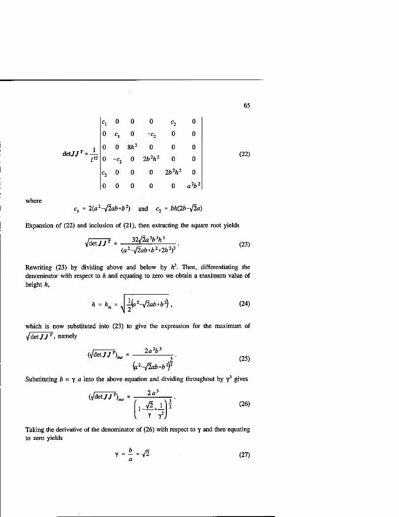
65

,T. 1 det/7' = — I12

c, 0 0

0 cl 0 "C2 0

0 0 8/i2 0 0

0 ~C2 0 2b2h2 0

C2 0 0 0 2b2h2

0 0 0 0 0

0

0

0

0

0

a2b2

(22)

where c, = 2(a2-feab+b2) and c2 = bh(2b-j2a)

Expansion of (22) and inclusion of (21), then extracting the square root yields

VdetTT1 32ißa3b3h-

(a2-fiab+b2+2h2)3 (23)

Rewriting (23) by dividing above and below by A3. Then, differentiating the denominator with respect to h and equating to zero we obtain a maximum value of height h,

h„ = *l(i2-j2ab+b2) , (24)

which is now substituted into (23) to give the expression for the maximum of

2aV

\ZdetJ77-, namely

()/teaj\ (25) (<i2-j2ab+b2)2

Substituting b = y a into the above equation and dividing throughout by y3 gives

(Jtetjj\ 2a2

(l-£+l \ 3

2 y yl)

(26)

Taking the derivative of the denominator of (26) with respect to y and then equating to zero yields

Y = Z - V2 a

(27)

66

Therefore, when b = yßa, and then from (24) h = (yfil2)a, the 4-4 redundant manipulator is at maximum quality index configuration as shown in Fig. 4. Now from (26),

l/det7M/mr=(l/det//r)max=4v^a3,

where Jm denotes the Jacobian matrix for this configuration.

B x

(28)

Fig. 4 The optimum 4-4 redundant manipulator with the highest quality index

It is interesting to compare Fig. 2 and Fig. 4 and note the similarity between these two optimal configurations. Finally, the quality index for this redundant 4-4 manipulator can be obtained by using (2).

4. The Implementation of the Quality Index

The quality index A. = Idet/l/ldet/J for the octahedral manipulator can, from (9)

and (12), be expressed in the form

8ft V m

(29)

67

It is most interesting to note that for the redundant 4-4 parallel manipulator, from

(23) and (25), the quality index X = ^(det JJ T)/(det /m/J) is identical to X for

the octahedron platform expressed in (29). Hence X is a function only of the height ratio 5 = hlhm for both cases and

8 883

(5 ♦ ^)3 (82 + l)3 (30)

A plot of Y vs. 6 is shown in Fig. 5.

x <B

C

o

1.0 -

0.8 -

0.6 -

0.4 -

0.2 -

0.0 -

i : I

\ i ! ;

i \ : i

■ j j j

0 1 2 3 4

Height Ratio 8 = h/hm

Fig. 5 Quality index vs. height ratio 8 = hlhm

Fig. 6 shows the contours of quality index as the platform of the redundant 4-4 parallel manipulator is translated away from the central location parallel to the base when hlhm= 1. The side of the moving platform for the octahedral manipulator is chosen as a = 1 and, from (15), the base side b = 2. The side of the platform for the redundant 4-4 manipulator is chosen as a = 1 and from (27) the base side b = ^2. The contours are labeled with values of constant quality index. When x or y is infinite, y = 0. The contours are close to being concentric circles of various radii, especially for the octahedral case.

Fig. 7 illustrates how the quality index varies as the platform is rotated from its central location about a vertical axis through its center, the legs being adjusted in length to keep the platform in the xy plane. Both two manipulators have the highest quality index X = 1 when 6 = 0, and X = 0 when 0 = ± 90 degrees. The area below

68

the curve of octahedral manipulator is just a little larger than the curve for the redundant case. They have very similar workspaces under these conditions.

-1.5 -1.0 -0.5 0.0 0.5 1.0 1.5 X

(a) 3-3 octahedral manipulator (b) Redundant 4-4 parallel manipulator

Fig. 6 Contours of quality index for translations in the xy plane

-90 -60 -30 0 30 60

Rotation Angle 6

Fig. 7 Variation in quality index for rotation about the z axis

*-ajus/y-a> is

If''-;

-90 -60 -30 0 30 60

Rotation Angle e

Fig. 8 Variation in quality index for rotation about the x and y axes

90

Fig. 8 illustrates the variation of the quality index for rotation about the x and y axes. Rotation about any line in the xy plane passing through the origin are simply linear combination. As the octahedral manipulator is not fully symmetric about x and y axes, its rotations about these two axes are not same. For the 4-4 manipulator, since it is fully symmetric, it has the same curve for the rotation about these two

69

axes. It is interesting to note that for the redundant 4-4 manipulator X * 0 between ±90 degrees as A. = 0 is the case for the octahedral manipulator (see Fig. 8).

Finally it is interesting to compare equation (9) for the octahedron with equation (23) for the 4-4 redundant manipulator. Fig. 9 illustrates the variation JdetJJT with

h for the 4-4 redundant manipulator optimum design a = 1 and b = y/2. This is compared with a size of octahedron using (9) for a = 1 and b = 2, the optimum design and is labeled Idet 7lopt. However, it is most interesting to note that if the moving platform both have the same area then for comparison with \JdetJJT for

the octahedron a = 2/31/4 «1.52, b = 4/31'4 « 3.04 and the curve is labeled Idet f\ which is a more realistic base for comparison.

Fig. 9 Comparison with the octahedral manipulator

5. Conclusion

A quality index, X, see equation (1) for non-redundant parallel manipulators and equation (2) for redundant parallel manipulators, can easily be determined for every in-parallel manipulator at any configuration. It is shown in this paper how the proportion and the configuration that give X = 1 can be obtained for both non- redundant and redundant parallel manipulators. We note that with acceptable A,- values, there is a useful workable range of configurations over which there is the potential for high precision and repeatability.

70

References

1. J. P. Merlet, "Singular Configurations of Parallel Manipulators and Grassmann Geometry," The International Journal of Robotics Research, 8(5), 45-56, 1989.

2. J. Lee, J. Duffy and M. Keler, "The Optimum Quality Index for the Stability of In-Parallel Planar Platform Devices," Proceedings of the ASME 24th Biennial Mechanisms Conference, 96-DETC/MECH-1135, Irvine, Ca., 1996.

3. J. Lee, J. Duffy and K. H. Hunt, "A Practical Quality Index Based on the Octahedral Manipulator," The International Journal of Robotics Research, 17(10), 1081-1090. 1998.

4. Y. Zhang and J. Duffy, "The Optimum Quality Index for a Redundant 4-4 In-Parallel Manipulator," Proceedings ofRoManSy 98: Twelfth CISM-IFToMM Symposium on Theory and Practice of Robots and Manipulators, Paris, July 1998.

5. N. White and W. Whiteley, "The Algebraic Geometry of Stresses in Frameworks," S.I.A.M. Journal of Algebraic and Discrete Methods, 4(4), 481-511, 1983.

6. D. J. Cox, "The Dynamic Modeling and Command Signal Formulation for Parallel Multi- Parameter Robotic Devices," Master Thesis, Mechanical Engineering, University of Florida, 1981.

7. J. Duffy, Statics and Kinematics with Applications to Robotics, Cambridge University Press, April, 1996.

8. K. H. Hunt and P. R. McAree, "The Octahedral Manipulator: Geometry and Mobility," The International Journal of Robotics Research, 17(8), 868-885, 1998.

9. C. Gosselin and J. Angeles, "The Optimum Kinematic Design of a Planar Three-Degree-of- Freedom Parallel Manipulator," ASME Journal of Mechanisms, Transmissions, and Automation in Design, 110(3), 35-41, 1988.

10. C. Gosselin and J. Angeles, "The Optimum Kinematic Design of a Spherical Three- Degree-of-Freedom Parallel Manipulator," ASME Journal of Mechanisms, Transmissions, and Automation in Design, 111(6), 202-207, 1989.

11. K. E. Zanganeh and J. Angeles, "Kinematic Isotropy and the Optimum Design of Parallel Manipulators," The International Journal of Robotics Research, 16(2), 185-197, 1997.

71

Control of Flexible Manipulators Using Vision and Modal Feedback

Klaus Obergfell1 and Wayne Book2

1 Seagate Technology, 7801 Computer Ave. S., Bloomington, MN 55435 klaus_obergfell@notes.seagate.com

2 G.W. Woodruff School of Mechanical Engineering, Georgia Institute of Technology, Atlanta, GA 30332-0405, U.S.A.

wayne.book@me.gatech.edu

Abstract. Literature for end point measurement and control is reviewed. An integrated vision sensor for tip position and an optical deflection sensor are incorporated into the control of a hydraulically actuated, flexible two-link manipulator arm. Analysis and experiments provide a design procedure and performance evaluation. The design procedure is based on successive loop closure and the use of output feedback modified to maintain stability. Point to point positioning performance is improved over alternative controllers.

1 Introduction

Attempts to further increase speed, accuracy, workspace and payload of motion systems ultimately lead to a constraint resulting from elasticity of the materials of construction. Vibration and static deflection impede completion of the intended task. The sources of elasticity are in the drive train, the linkages, and in the supporting structure. A number of approaches to overcome existing constraints have been proposed and attempted with varying degrees of success and many of these methods are reviewed in Book [1]. One of the most appealing approaches from the standpoint of overall capability of the resulting motion system is joint control based on end point position measurement. With such a control functioning ideally, the point of engagement with the task can be positioned with minimal regard for imperfections in the mechanism that attains that position. With such an approach minimal provisions need to be provided in the workspace or on the arm for additional degrees of freedom, fixtures or points on which to brace the arm. Ideally the size of the workspace and the precision within that workspace would be independently achievable. This paper will describe research working toward that ideal and results showing the improvements that end point sensing can achieve when coupled with other sensors of link dynamics.

End point sensing detects the position of the tool in the relevant degrees of freedom without relying on the linkages of the mechanism. This research uses an integrated vision system for tracking of passive fiduciaries (landmarks) at the tool. This system has proven effective and economical. On the other hand, typical joint position sensors can lead to inferences of the tool position which are inaccurate if

72

deflection due to loads, thermal expansion, inaccurate construction or machine placement has occurred. Insuring that these inaccuracies are minimal is an expensive undertaking involving precision machining, massive structures and perhaps even climate control of the machine's environment. Consequences of massive structures are larger actuators, more energy use, greater floor capacity requirements and other effects. The joint position measurement approach unfortunately mixes the energy related machine functions with the information related machine functions so machine components cannot be optimized for either function.

Two groups of problems must be solved if we are to use end point sensors successfully. First, the sensors themselves must meet technical and economic constraints. Secondly, the control algorithms must use the resulting sensor data effectively. Both problems have been addressed in this research for two degrees of positioning freedom. Since the sensors have been discussed in previous publications by Obergfell et al. [2-4], this paper will focus on the control algorithms and the resulting system performance as predicted by analysis and verified by experiments.

With end point sensing, the transducers and the actuators in the same control loop are separated in space. This noncollocation in a distributed elastic system has been shown to produce a nonminimum phase open loop system [5]. In linear systems this simply corresponds to poles or zeros of the transfer function in the right half of the complex plane. Zeros in particular are dependent on where the measurement is made, while the poles are intrinsic with the system dynamics. Our application requires that this nonminimum phase system be controlled with a feedback controller. The right half plane zeros are responsible for unstable branches of the root locus as feedback gains are varied. While equivalent phenomena exist for nonlinear system dynamics, explanations based on linear analysis are sufficient.

At this point an overview of the research presented will be given. Our research is focused on a large but lightweight, two-link arm, electro-hydraulically actuated. It is referred to as RALF (Robotic Arm Large and Flexible) and it is shown in Figure 1(a). The control is composed of nested digital control loops. An inner PD loop uses joint measurements. A second loop is closed around analog optical measurements of link deflection and is critical for stability. The outer loop is closed around fundamentally discrete camera measurements of the position of the tip of the arm. A coordinated strobe light illuminates a retro-reflective fiduciary to enhance the discrimination of the tip and the accuracy of measurement of the moving arm. While the tests are primarily intended to achieve accuracy at the end of the motion, the research also examined the complete time history of the moves.

This paper is organized as follows. A brief review of some of the literature relevant to the problem will follow this introduction. The experimental system will be described next. Extensive work in sensor hardware and software development will be only briefly summarized in that section. The control algorithms, analysis predicting closed-loop performance, and design procedures will then be presented followed by selected experimental results. Experimental results will then be compared to previous work using dimensionless performance metrics. A brief section on conclusions will end the paper.

73

2 Review of Previous Research

This section will focus on control using end point sensors, both direct and indirect, control of nonminimum phase systems and, briefly, the control of flexible arms in general.

Cannon and Schmitz [6] investigated a one-link flexible manipulator operating in the horizontal plane controllers designed by LQG. This work was later extended by Oakley and Cannon [7] and Oakley and Barratt [8] who investigated a two-link manipulator. Schmitz and Ramey [9] also extended the original work and presented a classical control design. A Cartesian controller based on the transposed manipulator Jacobian was investigated by Lee et al. [10]. Using proportional tip position and joint rate control like the previous researchers, they improved stability and performance by adding strain feedback. Obergfell and Book [11] investigated a two-link flexible manipulator with 3m long links that operate in a vertical plane. A quasi-static end- point controller was used. In summary, LQG control is capable of high performance but is very sensitive to modeling errors. Classical control designs trade performance for fewer (adjustable) gains and reduced sensitivity to parameter variation. However, additional sensors may be necessary to achieve good performance.

Other researchers have used indirect measurements of tip position. Wang and Vidyasagar [12] showed that the transfer function using the time-derivative of the reflected tip position is passive when the flexible link is sufficiently rigid and hence easier to control. Extensions of this research were later explored by Alberts and Pota [13] and Rossi et al. [14]. In summary, it is possible to define different transfer functions for flexible manipulators. When a passive transfer function can be obtained, it is possible to achieve good performance and robustness with a simple controller.

Joint controllers utilize position and velocity feedback but improve with strain feedback. Book et al. [15] compared various joint and flexible state feedback configurations. Hastings and Book [16] studied linear LQR control of a single-link flexible manipulator including strain measurements. Yuan et al. [17] implemented a decentralized control utilizing joint position and strain rate on a two-link flexible manipulator. Henrichfreise et al. [18] investigated the control of a two-link, three degrees-of-freedom manipulator with joint and link compliance. Pfeiffer [19] studied position and force control of a three-link, five degrees-of-freedom manipulator with two flexible links.

The objective of tracking control is to make the output follow the input as closely as possible, i.e. make the transfer function one. However, to cancel non-minimum phase zeros to achieve this requires adding unstable poles to the system, thereby making the practical system unstable. Tomizuka [20] suggested zero phase error tracking control for non-minimum phase systems. Several variations of this basic algorithm were developed, for example by Jayasuriya and Tomizuka [21] and by Menq and Xia [22]. In summary, feedforward methods offer good tracking performance for non-minimum phase systems. However, the feedforward control is sensitive to modeling error, which makes the application to multi-link flexible manipulators difficult.

Inverse dynamics methods calculate torques such that the flexible manipulator tip follows a desired trajectory with minimal vibrations and zero overshoot. This method differs from rigid manipulator in that the dynamics cannot be inverted directly because of the non-minimum phase zeros. Bayo et al. [23], Kwon and Book [24] and

74

others have explored this approach. It generally requires a good model and much computational power.

Landmark Tracking System Field of View

RALF's Workspace

(3.96,4.75)m

Figure 1 (a) The experimental manipulator RALF, (b) Shape of manipulator workspace with key features and Landmark Tracking System field of view

3 The Experimental System

A two-link manipulator testbed named RALF (Robotic Arm, Large and Flexible) at the Intelligent Machine Dynamics Laboratory at Georgia Tech is used as an experimental platform for this research. RALF has a high payload to weight ratio given its workspace, but is stiff enough to perform real world applications. Since it operates in a vertical plane, gravity effects are significant. The two main links are 3.05 m long and constructed from aluminum pipe. The lower link has a 141.3 mm O.D. with a wall thickness of 3.4035 mm, the upper link has a 114.3 mm O.D. with a wall thickness of 3.048 mm. The actuation link is constructed from a rectangular aluminum tube. The weights of the links without attachments are 12.18 kg, 8.8 kg, and 4.625 kg. The assembled manipulator structure without actuators and base weights approximately 45 kg, while its payload capacity is approximately 27 kg.

The hydraulic cylinders actuating RALF have a 50.8 mm bore, 25.4 mm rod and 508 mm stroke. Two stage electro-hydraulic servovalves provide fluid from a regulated supply. With mechanical feedback and constant load pressure the flow will be proportional to current driving the first valve stage. The linear hydraulic cylinder velocities are 0.156 m/s for extension and 0.208 m/s for retraction. The maximum linear speed of the link end-points is over 1 m/s. A Temposonics linear transducer measures the displacement of each cylinder and the velocity is calculated from samples of the position. The manipulator geometry and the stroke of the hydraulic actuators define RALF's workspace. Figure 1(b) shows the shape of the workspace with key features.

75

3.1 The Landmark Tracking System for Tip Position Measurement

The LTS (Landmark Tracking System) consists of a machine vision system, optics, strobe illumination, retroreflective landmarks, and landmark tracking software. Here, a single, fixed LTS measures the position of a landmark attached to RALF's tip in part of the manipulator's workspace as illustrated by the square in Figure 1(b). A 163 row by 192 column charge coupled device (CCD) array integrates light from the scene. The resulting digital image in video RAM is accessible from the M68000 CPU communicating with the controller via a serial line. The stationary LTS is mounted on the laboratory wall with a line of sight perpendicular to and 6.1 m from the manipulator's plane of motion. The estimated resolution of the LTS is 1/10* of a pixel or l/loSO* of FOV in row direction of the CCD. Strobe illumination is used to freeze motion with short (less than 10 |J,s) bursts of light. Measurement variations of a fixed target of less than 0.4 mm horizontally and 0.5 mm vertically are experienced. A relative accuracy of about 1.5 mm has been measured. Sampling frequencies above 50 Hz are normally obtained, but this is not guaranteed since a search for the landmark is required, starting at the last known position. The rate could be as low as 7.8 Hz and as fast as 70 Hz.

3.2 Link Deflection Sensing

A Lateral Effect Photo Diode sensor and a lens, mounted to one end of the link, are focused on a light source which is mounted to the other end of the link. The voltage output from the sensor is proportional to the relative motion of the light source and, therefore, proportional to the deflection of the link. The measurement is linear with a regression coefficient of 0.999 and an overall deflection resolution of more than 1.5 mm. The link deflection sensor was originally envisioned as a possible substitute or enhancement for the LTS. The LTS proves to be much more accurate as an overall measurement system, but link deflection proved to be extremely valuable for stabilization of the vibrations anyway. As it is an analog sensor, it can be sampled at the conversion rate of the 12 bit A/D.

4 Feedback Control

The presented control is composed of three nested feedback loops as illustrated in Figure 2. An inner PD loop controls the joint motion of the manipulator. The second loop feeds back the deflection modes of the links thereby improving the stability of the control. A vision based outer loop feeds back direct end-point position measurements in order to reduce end-point position error.

The PD joint control of the innermost loop is based on previous work by [17, 25, 26]. Analog measurements of joint position are sampled and processed by a digital proportional controller. The equivalent of analog joint velocity feedback is provided by the electro-hydraulic servo valves [2].

76

X

-,

1

r.

^ ^

Inverse Jacobian

Tip Compensation

™<

i + ^u^ Flexible

Manipulator

i Inverse

Kinematics

6i. + 1

Joint Control

w

1 + , J * J—w

•II 1 1 1 '

Link Deflection Feedback

Figure 2 End-point position control composed of nested feedback loops

4.1 Link Deflection Feedback

Wang and Vidyasagar [12] have previously shown that a modified output allowed for a simpler end-point control for single link flexible manipulators. A new interpretation of Wang's and Vidyasagar's work would be to view their end-point controller as identical to PD joint control with positive link deflection feedback. This research expands their work to apply to multiple links through a separation of joint control and link deflection feedback. A design procedure based on the root-locus method is outlined to add proportional link deflection feedback to all links of a flexible manipulator. Improvements to the dynamic response of a flexible manipulator are illustrated with the root-locus method. These results can be generalized to any serial link flexible manipulator.

The tip position output used by Cannon and Schmitz [6] and most other researchers is given by

yi(L,t) = 6(t)L + w(L,t) (1)

The reflected tip position output used by Wang and Vidyasagar is given by

y2(L,t) = 6(t)L-w(L,t) (2)

Both outputs are illustrated in Figure 3. Wang and Vidyasagar showed that the transfer function using the time-derivative of the reflected tip position is passive when the flexible link is sufficiently rigid. Therefore, any passive controller with finite gain (e.g. simple PD control) will stabilize the system. This is in contrast to the complicated control structures associated with the tip position output. Extensions of this research were later explored by Alberts and Pota [13] and Rossi et al. [14]. They defined modified outputs, which are linear combinations of rigid body rotation and elastic deflection:

y3(L,t) = 6(t)L-Aw(L,t) (3)

77

The additional degree of freedom provided by X was used to relax the conditions to obtain a passive TF. However, this method was only applied to manipulators with a single flexible link.

Y n

Tip Position"»

w(L,t)

y2(L,t)

X

Figure 3 Definition of tip position and reflected tip position outputs

The control input to a flexible manipulator when modified outputs are used with PD control is given by

U(s) = kp(l + TdsXYd(s)-Y3(s)) (4)

Note that the desired end-point position input is identical to the rigid body tip displacement. Substituting equation (3), therefore, yields

U(s) = kp(l+TdsXL&d(s)-Le(s)+AW(s)) (5)

Equation (5) can also be written as

U(s) = kpi(l+TdsX©d(s)-e(s))+kp2(l+Tds)V(s) (6)

where kpl =Lkp, and kp2 =Akp. This shows that modified outputs with PD

control are equivalent to PD joint control with positive PD link deflection feedback. The effect of link deflection feedback was studied using a mathematical model of

RALF1. In root-locus plots it was observed that positive link deflection feedback improved dynamic response by "pushing" the closed-loop poles into the left half- plane. The opposite behavior was observed for negative link deflection feedback, i.e. the closed-loop poles quickly moved into the right half-plane destabilizing the system. Figure 4(a) shows closed loop pole locations when positive link deflection feedback is applied to both links of RALF simultaneously. Dynamic response of the first and second mode can be improved in a large area of the s-plane. Not shown is that the higher modes are slightly destabilized and even go unstable for very high gains (Several orders of magnitude larger than discussed here). Note that the PD joint control loop had been closed before link deflection feedback was applied.

Non-linear model of structural dynamics (2 assumed modes per link) combined with actuator model based on experimental verification, [2]

78

A root-locus procedure can be used to select link deflection feedback gains for multi-link flexible manipulators. For a two-link manipulator this is illustrated in [2]. The procedure consists of two steps: First, a suitable gain ratio is determined from root-loci plotted for various gain ratios. Second, final gain values are determined from the root-locus for the selected gain ratio. An example of a root-locus for a fixed gain ratio and the gains selected for the experimental evaluation are shown in Figure 4(b).

45

40

35

.«30 < !=25 S |20

15

o >J

S) >> -^

Y> '(i v

*§5

Mt-

S25

E

^x

4 /

/

/ /

s ( (

\ \ \

-40 -35 -30 -25 -20 -15-10-5 0 Real Axis

5 10 -30 -25 -20 -15-10 -5 0 Real Axis

(a) (b)

Figure 4 Root-locus design of proportional link deflection feedback, display of first modes, (a) gain sweep: Kld)=Kld2=0-1500, step size 5, Kldi is swept at constant Kld2, (b) fixed gain ratio KU2/Kidi =1.6, starting point Kldl=0 (x), final gain selection KIdl=16 (+)

4.2 End-Point Position Feedback

Although positive link deflection feedback improved the dynamic response of the manipulator significantly, an end-point position error remained due to static link deflection, kinematical error, and payload uncertainty. These errors are more noticeable on RALF because (1) RALF is operated in the vertical plane, (2) the long- reach structure amplifies small kinematical errors and structural imperfections into large tip position errors, and (3) the complex structure is more difficult to model than simple beams causing larger parameter errors.

This research developed a new end-point position feedback loop to eliminate the remaining tip errors which vary slowly. It is an extension of previous work, [11], which transformed tip errors into joint errors using the inverse manipulator Jacobian and added the resulting joint error to the desired joint command in a quasi-static algorithm. In this paper, the quasi-static control is replaced by an integral compensator to decrease the settling time of the control. A design procedure is developed to determine integral gains using the root-locus method.

The complete end-point position control consists of three feedback loops as illustrated in Figure 2. The multi-loop approach easily facilitates the incorporation of multiple sensors operating at different sampling rates. Joint and link deflection feedback loops operated at 200 Hz during experiments while the end-point position

79

loop ran at 40 Hz. The controller developed is a regulator not a tracking controller. However, it performs well following point-to-point trajectories.

Proportional and integral tip compensators were investigated in this research. Derivative compensators were not considered because the slow update rate of the end- point position sensor would make a difference calculation not very accurate. Closed loop pole locations were investigated numerically using the mathematical model of RALF. Proportional tip compensation was quickly ruled out because it provides only a small gain margin. Figure 5(a) shows the dominant closed-loop pole locations for integral tip compensation. Acceptable pole locations can be achieved for the investigated range of feedback gains but two modes go unstable for higher gains. Note that joint control and link deflection feedback loops were closed before tip feedback was applied. The gain selection procedure follows the two step root-locus design procedure outlined in the previous section. An example of a root-locus for a fixed gain ratio and the gains selected for experimental evaluation are shown in Figure 5(b).

35

30

■§25 < §20 '§> E15

-35 -30 -25 -20 -15 -10 -5 0 5 10 Real Axis

f

X

\

\ \ K 1

1 -40 -30 -20 -10

Real Axis

(a) (b)

Figure 5 Root locus design of integral end-point position compensation, display of first modes, (a) gain sweep: Kj1( Ki2=0-50, step size 1.0, Kn is swept at constant Ki2, (b) fixed gain ratio Ki21 Kix = 1, starting point K(1 = 0 (x), final gain selection Kn = 4 (+)

5 Experimental Results

Manipulator commands for experimental implementation were specified in end-point position coordinates. For joint based control the end-point coordinates are converted to joint coordinates using rigid inverse kinematics. The results presented in this chapter are for a one meter square trajectory at the center of the LTS workspace traversed in clockwise direction. Each side of the square is described by a second order position trajectory. At the corners the manipulator stops for 1.3 seconds in order to allow the observation of transient behavior. Different tip speeds and payloads were investigated in [2], two cases (0.67 m/s tip speed with no payload and 0.77 m/s tip speed with 7.5 kg payload) will be presented in this paper.

80

The improvements provided by positive link deflection feedback are illustrated in Figure 6 and Figure 7. Link deflection feedback dampens oscillations under all test conditions.

link 1 relative deflection [mm] - Joint control

K. h M^fir' \fwJ\

■ ■" w. Y~- f^

w

0 2 4 6 8 10 12 14

link 1 relative deflection [mm] - ink deflection feedback

A Jta ,-ur- w-A s,.,. y- r V V

link 2 relative deflection [mm] - oint control

. .^A-nA^Wv^i,»,...

^0 2 4 6 8 10 12 14

link 2 relative deflection [mm] - Ink deflection feedback

A*-^* r-Afr A^ y" '

6 8 10 12 14 time[s]

2 4 6 8 10 12 14 time[s]

Figure 6 Comparison between joint control with and without link deflection feedback, link deflection for the square trajectory, 0.67 m/s tip speed, no payload

13

6.5

0

-6.5

-13 (

13

6.5

0

-6.5

-13

link 1 relative deflection [mm] - joint control link 2 relative deflection [mm] • Joint control

iA 4

0

-4

-8

L All 1 m J l l s ww w J %i ll/lr M IW V \ m ti>\ If I r r | in 1 1 f¥ F IP '

1 i 0 2 4 6 8 10 12 14

link 1 relative deflection [mm] - fink deflection feedback

0 2 4 6 8 10- 12 14

link 2 relative deflection [mm] - Snk deflection feedback

1 i n 8

4

0

-4

-8

Ii f. i |

L L ■A ~V ̂ - L JH uHW Jlk| ■"-'i/v L»,„ 'V fl s\ f f f • V 1! Wir ii K 1

6 8 10 12 14 time[s]

10 12 14 time[s]

Figure 7 Comparison between joint control with and without link deflection feedback, link deflection for the square trajectory, 0.77 m/s tip speed, 7.5 kg payload

XY-plots of desired and actual tip positions for the square trajectory are shown in Figure 8 for joint control and end-point position control. The improvements made by link deflection feedback are most noticeable in the vertical section between corners 3 and 4, replacing a oscillatory response with a smooth line and settling the tip quickly when the manipulator is commanded to stop. End-point position feedback places the tip response much closer to the desired trajectory, removing static deflection offsets and eliminating the tip error in the corners.

Figure 9 shows total tip position error as a function of time for joint control and end-point position control and two test conditions. End-point position feedback removes the static deflection offset and eliminates steady state error while link deflection feedback dampens oscillations during motion.

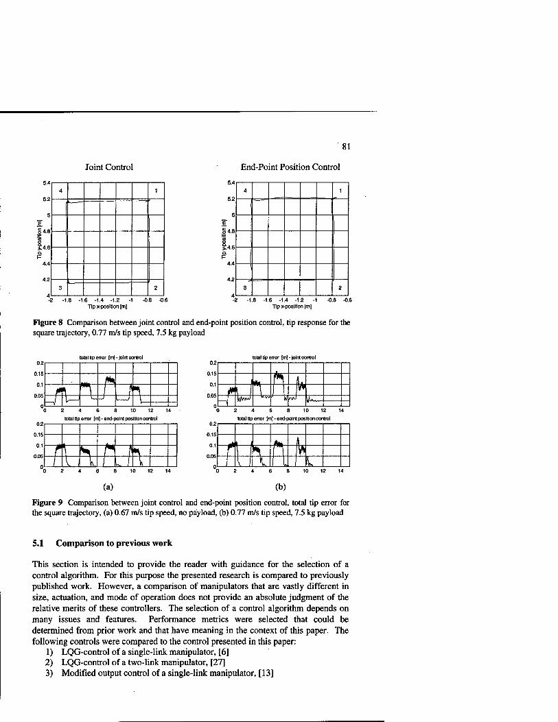
81

Joint Control End-Point Position Control

5.4

5.2

5

o4.8

I g4.6 Q. F

4.4

4.2

4

4 1

~~ " "^

- - — ^^ 3 2

-2 -1.8 -1.6 -1.4 -1.2 -1 -0.8 -0.6 Tip x-position [m]

5.4

5.2

5

§4.8 'S '« S4.6 a. F

4.4

4.2

4

4 1

—3 —-

3 2

-2 -1.8 -1.6 -1.4 -1.2 -1 -0.8 -0.6 Tip x-position [m]

Figure 8 Comparison between joint control and end-point position control, tip response for the square trajectory, 0.77 m/s tip speed, 7.5 kg payload

total tip error [m] - joint control total tip error [m]-Joint control

0.15

0.1

0.05

0

0.15

0.1

t \ fa m r f 1 -f V-> L, j / \

0.15

0.1

_f\jJ ***' w J j; 2 4 6 8 10 12 14

total tip error [m] - end-point position control

0 2 4 6 8 10 12 14

total tip enor [m] - end-point position control

ffl 1 8 10 12 14 6 8 10 12 14

(a) (b)

Figure 9 Comparison between joint control and end-point position control, total tip error for the square trajectory, (a) 0.67 m/s tip speed, no payload, (b) 0.77 m/s tip speed, 7.5 kg payload

5.1 Comparison to previous work

This section is intended to provide the reader with guidance for the selection of a control algorithm. For this purpose the presented research is compared to previously published work. However, a comparison of manipulators that are vastly different in size, actuation, and mode of operation does not provide an absolute judgment of the relative merits of these controllers. The selection of a control algorithm depends on many issues and features. Performance metrics were selected that could be determined from prior work and that have meaning in the context of this paper. The following controls were compared to the control presented in this paper:

1) LQG-control of a single-link manipulator, [6] 2) LQG-control of a two-link manipulator, [27] 3) Modified output control of a single-link manipulator, [13]

82

The following dimensionless performance metrics were used for comparison: 1) The normalized settling time ts is defined as:

*s=*sfnl (7)

where ts is the settling time and fnl is the first, locked, natural frequency of the

system. 2) The normalized steady state error ess, is defined with respect to the total

manipulator length L (the sum of the link lengths), and with respect to the effective

manipulator length Leff (the distance from the first joint to the end-point):

eSStL=^f and ess,E=-^- <8> L Leff

where ess is the steady state end-point position error.

3) The normalized maximum error is also defined with respect to the total manipulator length and with respect to the effective manipulator length:

W^T and W=-^ (9)

L Leff

where emi is the maximum end-point position error. The maximum error depends on the tip speed used. The normalized tip speed is, therefore, defined as:

v. = ^- (10) up f

Jn\

where vtip is the linear tip velocity. The normalized tip speed is not

dimensionless. The performance metrics were computed as follows:

1) [6]: Settling time and steady state error were graphically determined from a tip step response (Figure 11 A) The settling time of the step response was defined as the time it takes the system transients to decay to ±2% of the step size. The steady

state error was defined as the error after approximately 2ts have passed. The locked natural frequency was approximated by the first open-loop zero of the joint transfer function (Figure 5A). The maximum error was not evaluated because trajectory following was not investigated by this publication.

2) [27]: Settling time and steady state error were graphically determined from tip step responses (Figure 9.16) and averaged. The locked natural frequency was approximated by the open-loop zeros (Table 6.2). Maximum errors were determined graphically (Figures 9.12 and 9.13).

3) [13]: Settling time was graphically determined from a step response (Figure 4). Steady state error was not evaluated because a direct end-point position measurement was not provided and the maximum error was not determined because trajectory following was not investigated by this paper.

4) [2]: Settling time and steady state error were determined from a impulse response (Figure 6-41). The settling time of the impulse response was defined as the time it takes the system transients to decay to ±2% of the maximum value of the

impulse response. The maximum error was determined for the square trajectory, three

83

different tip speeds, and no payload (Table 6-15). Performance metrics and dependent quantities are given in Table 1 through Table 3.

',(«) /„i (Hz) *,

Cannon, Schmitz 1.16 0.53 0.615

Oakley 4.18 0.37 1.547

Alberts, Pota 1.17 2.17 2.539

Obergfell 0.63 3.6 2.268

Table 1: Normalized settling time comparison

ess (mm) L(mm) Leff (mm) ess,L ess,E

Cannon, Schmitz 1.9 1000 1000 0.00190 0.00190

Oakley 0.8 1040 830 0.00077 0.00096

Obergfell 1.4 6293 4914 0.00022 0.00028

Table 2: Normalized steady-state error comparison

emax(m

m) v^ (m/s) vtip (mm) ^max.L ^max,£

Oakley

64.3 0.1167 315.0 0.0618 0.0775

41.4(*) 213.9 0.0398(*) 0.0499(*)

28.6 0.0583 157.5 0.0275 0.0333

Obergfell

129.2 0.77 213.9 0.0205 0.0263

107.4 0.67 186.1 0.0171 0.0219

97.8 0.59 163.9 0.0155 0.0199

Table 3: Normalized maximum error comparison, (*) denotes linear interpolation

LQG control positions a single-link flexible manipulator in less than one (natural) period. This time more than doubles when a two-link manipulator is controlled. The time to position a single-link manipulator with modified output control is more than four times longer than when LQG is used. The control presented in this paper is only 47 % slower than LQG for a two-link manipulator. However, this is achieved with a control that is less sensitive to parameter variations and easy to tune. The control presented in this research is able to position the tip of the manipulator with an accuracy that is equivalent to 0.03 % of the manipulator length. The LQG controller is 3.4 times less accurate even though it operates in the horizontal plane. Integral end- point position error compensation enables this high precision. By comparison, the LQG controller use a "rigid" state reference command and does not compute a position error signal. The maximum error for the control presented in this research is approximately two times smaller than for LQG control.

84

6 Conclusions

Direct sensing of the end-point position of a flexible positioning system can provide a feedback signal that allows accurate tip placement even with link deflection, inaccurate construction and uncertain placement of equipment. The desired accuracy was achieved here with a rapid response and robustness to load variations and arm configuration. Successive closure of feedback loops was used. Link deflection and joint position were combined to give a modified output that is similar to the reflected tip position of Wang and Vidyasagar. This provided a modification of the plant dynamics that was the basis of the end-point position feedback. An end-point position feedback loop utilizing the inverse manipulator Jacobian and integral compensation was added to reduce end-point-positioning errors. The design of the control system was carried out principally with the classical techniques of root locus.

Experiments verified the desired characteristics of accuracy, speed and robustness with good path following capabilities for a large two-link manipulator. Link deflection feedback reduced structural vibrations by from 44% to 86% for a variety of tip speeds and payloads. The end-point position feedback loop reduced the average tip position error by from 48% to 85%. Normalized performance metrics were used to compare this work to previous research. The presented control positions the manipulator 3.4 times more accurately than a previously published LQG control. At the same time it is also 47 % slower than the LQG control. However, the speed reduction is traded for insensitivity to parameter variations and ease of implementation. Experiments reported here included moving along a one meter square in a vertical plane. The time history shows the stability with a range of operating conditions and corner stop positioning accuracy of between 2 and 7.8 mm. (less than Vi a pixel), an improvement of between 120% and 164% over no end-point feedback. The path of the end-point shows the ability to follow a straight line path, although a lag results giving significant error in the tracking response that this research did not seek to eliminate, but which might be reduced with feed forward techniques. Other experiments not included in detail have used alternative motions, a wider range of payloads, and have imposed disturbances on the manipulator. These experiments further confirm the success of our approach.

Sensor design is an important part of fielding a successful system. An integrated vision system and a link deflection sensor were briefly described here. Other means of sensing might be more appropriate in a given application, but the control techniques used here should still provide a useful basis for the designer.

In summary, the approach used here is an attractive alternative to sensitive state feedback methods that provides acceptable behavior even if end-point position feedback is disrupted.

This work was supported by the Department of Energy and Sandia National Laboratories under contract #AK-9037.

85

References

[I] W. J. Book, "Controlled Motion in an Elastic World," ASME Journal of Dynamic Systems, Measurement, and Control, vol. 115, pp. 252-261, 1993.

[2] K. Obergfell, "End-Point Position Sensing and Control of Flexible Multi-Link Manipulators," Ph.D. Dissertation, Georgia Institute of Technology, August 1998.

[3] K. Obergfell and W. J. Book, "Vision Sensing for Control of Long-Reach Flexible Manipulators," presented at Japan-U.S.A. Symposium on Flexible Automation, Boston, Massachusetts, USA, 1996.

[4] K. Obergfell and W. J. Book, "End-Point Measurements of Long-Reach Flexible Manipulators," in Symposium on Robot Control 94, vol. 2. Capri, Italy, 1994, pp. 669- 674.

[5] V. A. Spector and H. Flashner, "Modeling and Design Implications of Noncollocated Control in Flexible Systems," ASME Journal of Dynamic Systems, Measurement, and Control, vol. 112, pp. 186-193, 1990.

<[6] R. H. Cannon, Jr. and E. Schmitz, "Initial Experiments on the End-Point Control of a Flexible One-Link Robot," The International Journal of Robotics Research, vol. 3, pp. 62-75,1984.

[7] C. M. Oakley and R. H. Cannon, "Anatomy of an Experimental Two-Link Flexible Manipulator Under End-Point Control," presented at IEEE Conference on Decision and Control, Honolulu, Hawaii, USA, 1990.

[8] C. M. Oakley and C. H. Barratt, "End-Point Controller Design for an Experimental Two- Link Flexible Manipulator Using Convex Optimization," presented at American Control Conference, San Diego, California, USA, 1990.

[9] E. Schmitz and M. Ramey, "Initial Experiments on the End-Point Control of a 2-DOF Long-Reach Elastic Manipulator," in Cooperative Intelligent Robotics in Space II, vol. 1612. Boston, Massachusetts, USA, 1991, pp. 245-256.

[10] H. G. Lee, S. Kawamura, F. Miyazaki, and S. Arimoto, "External Sensory Feedback Control for End-effector of Flexible Multi-Link Manipulators," presented at IEEE International Conference on Robotics and Automation, Cincinnati, Ohio, USA, 1990.

[II] K. Obergfell and W. J. Book, "End-Point Control of a Two-Link Flexible Manipulator Using the Landmark Tracking System," presented at Japan/USA Symposium on Flexible Automation, San Francisco, California, USA, 1992.

[12] D. Wang and M. Vidyasagar, "Passive Control of a Stiff Flexible Link," The International Journal of Robotics Research, vol. 11, pp. 572-578, 1992.

[13] T. E. Alberts and H. R. Pota, "Experiments in Control of Flexible Beam with Modified Outputs," in Controls for Optical Systems, vol. 1696. Orlando, Florida, USA, 1993, pp. 222-230.

[14] M. Rossi, K. Zuo, and D. Wang, "Issues in the Design of Passive Controllers for Flexible Link Robots," presented at IEEE International Conference on Robotics and Automation, San Diego, CA, USA, 1994.

[15] W. J. Book, O. Maizza-Netto, and D. E. Whitney, "Feedback Control of Two Beam, Two Joint Systems with Distributed Flexibility," ASME Journal of Dynamic Systems, Measurement, and Control, vol. 97, pp. 424-431, 1975.

[16] G. G. Hastings and W. J. Book, "Experiments in the Optimal Control of a Flexible Arm," presented at American Control Conference, Boston, MA, USA, 1985.

[17] B. S. Yuan, W. J. Book, and J. D. Huggins, "Control of a Multi-Link Flexible Manipulator with a Decentralized Approach," presented at ll"1 Trinnial IFAC World Congress, Tallinn, (formally) USSR, 1990.

86

[18] H. Henrichfreise, W. Moritz, and H. Siemensmeyer, "Control of a Light, Elastic Manipulator Device," presented at Applied Motion Control Conference, Minneapolis, Minnesota, USA, 1987.

[19] F. G. Pfeiffer, "Path and Force Control of Elastic Manipulators," presented at IEEE Conference on Decision and Control, Honolulu, Hawaii, USA, 1990.

[20] M. Tomizuka, "Zero Phase Error Tracking Algorithm for Digital Control," ASME Journal of Dynamic Systems, Measurement, and Control, vol. 109, pp. 65-68, 1987.

[21] S. Jayasuriya and M. Tomizuka, "Generalized Feedforward Controllers, Perfect Tracking and Zero Phase Error," presented at Japan/USA Symposium on Flexible Automation, San Francisco, 1992.

[22] C.-H. Menq and Z. Xia, "Characterization and Compensation of Discrete-Time Nonminimum-Phase Zeros for Precision Tracking Control," in Robotics Research, vol. DSC. Dallas, Texas, USA: ASME Winter Annual Meeting, 1990, pp. 15-23.

[23] E. Bayo, P. Papadopoulos, J. Stübbe, and M. A. Serna, "Inverse Dynamics and Kinematics of Multi-Link Elastic Robots. An Iterative Frequency Domain Approach.," Internationaljournal of Robotics Research, vol. 8, pp. 49-62, 1989.

[24] D.-S. Kwon and W. J. Book, "A Time-Domain Inverse Dynamic Tracking Control for a Single-Link Flexible Manipulator," ASME Journal of Dynamic Systems, Measurement, and Control, vol. 116, pp. 193-200, 1994.

[25] J. W. Lee, "Dynamic Analysis and Control of Lightweight Manipulators With Flexible Parallel Link Mechanisms," Ph.D. Dissertation, Georgia Institute of Technology, June 1990.

[26] S. H. Lee, "Robust Control of A Flexible Link Robot and Rigid Link Robot: Theory, Simulation, and Experiment," Ph.D. Dissertation, Georgia Institute of Technology, March 1992.

[27] C. M. Oakley, "Experiments in Modelling and End-Point Control of Two-Link Flexible Manipulators," Ph.D. Dissertation, Stanford University, April 1991.

87

Robust Adaptive Cartesian Control for Free-Joint Robot Manipulators

Jin-Ho Shin and Ju-Jang Lee

Department of Electrical Engineering Korea Advanced Institute of Science and Technology (KAIST) 373-1, Kusong-dong, Yusong-gu, Taejon, 305-701, KOREA

TEL: +82-42-869-5432, FAX: +82-42-869-3410 Email: jhshin@i1iad.kaist.ac.kr: jjlee@ee.kaist.ac.kr

Abstract. This paper addresses a robust adaptive Cartesian control for free- joint robot manipulators faced with actuator failures and uncertainties. This scheme is suitable for some joints with failed actuators and brakes as well as passive joints without actuators and brakes. In order to overcome the dynamic singularity problem for a nominal decoupling matrix (input matrix of the controller) used in the presented Cartesian controller, a singularity-free Cartesian path planning is achieved via a computer simulation. The proposed Cartesian space control scheme does not need a priori knowledge of the accurate dynamic parameters and the exact uncertainty bounds. To illustrate the feasibility and robustness of the proposed control scheme, simulation results are shown for a three-link planar robot manipulator with a free-swinging passive joint.

1 Introduction

The control of nonholonomic mechanical systems has attracted growing attention in recent years [1]. In fact, many nonholonomic systems naturally fit into the category of underactuated mechanisms, defined as systems in which the dimension of the configuration space exceeds that of the control input space. There are many nonholonomic underactuated mechanical systems in real world applications.

The advantages of using such underactuated systems reside in the fact that they weigh less, and consume less energy than their fully-actuated counterparts, thus being useful for applications such as space robotics. For hyper-redundant robots, such as snake-like robots or multilegged mobile robots, where large redundancy is available for dexterity and specific task completion, underactuation allows a more compact design and simpler communication schemes. The underactuated robot concept is also useful for the reliability or fault-tolerant design [2], [3], [4] of fully-actuated manipulators working with dangerous materials or in remote or hazardous areas such as space, underwater, nuclear power plants, etc., where the repair or replacement of actuators is a very difficult task.

Usually, a robot manipulator that has fewer numbers of joint actuators than the number of total joints is known as an "underactuated robot manipulator". The underactuated robot manipulator has actuated joints or active joints with their own actuators, and unactuated joints or passive joints without their own actuators at some joints. It is a well-known fact that an articulated underactuated manipulator with passive joints satisfies a second-order nonholonomic constraint which is a non- integrable constraint on acceleration [5], [6], [7]. It is very difficult to directly apply the control methods and mathematical approaches developed so far for nonlinear dynamical systems with first-order nonholonomic constraints without drift to underactuated robot manipulator systems with second-order nonholonomic constraints and a drift term, because of the different dynamical and mathematical characteristics.

The dynamics and control of underactuated robot manipulators have been being studied from the 1990's [5], [6], [7], [8], [9], [10], [11]. The control of underactuated robot manipulators has drawn a great attention in recent years, but the research on it is not so much active yet, as it is much more difficult than that of fully-actuated robot manipulators.

Robots that operate in remote or hazardous environments must be used in a manner that reflects the implications of failure scenarios on system performance [4]. Most of the previous works focused on failures that are modeled as locked joints, either due to a failure directly resulting in an inability to move or due to the application of brakes to prevent unpredictable behaviors [3].

In contrast, the study of free-swinging failures is still in its infancy and presents additional possibilities for usefulness after a failure. The term free-swinging failure refers to a hardware or software fault in a robotic manipulator that causes the loss of torque (or force) on a joint. Examples include a ruptured seal on a hydraulic actuator, the loss of electric power and brakes on an electric actuator, and a mechanical failure in a drive system. After a free-swinging failure, the failed joint moves freely under the influence of external forces and gravity [2], [10].

Even actuators and brakes at passive joints may fail due to hardware or software joint failures, or passive joints may have neither actuators nor brakes originally to achieve lighter weight, a more compact design, smaller energy consumption, etc.. These passive joints are referred to as "free-swinging passive joints" or "free joints" [2], [5], [6], [10], [11]. A robot manipulator with free-swinging passive joints is called as a "free-joint robot manipulator".

Compared to control methods using brakes at passive joints of an underactuated robot manipulator, presently there are not so much results for control schemes of. a free-joint robot manipulator without both actuators and brakes. Tasks of robot manipulators are usually planned in Cartesian space or operational space. Even either actuators and brakes at passive joints may fail, or passive joints may have neither actuators nor brakes originally in the design of robot manipulators. Therefore, it is needed to study a fault-tolerant control of free-joint robot manipulators in Cartesian space without using brakes at passive joints. This topic is a very attractive and hot issue in controlling underactuated robot manipulators.

The previous control methods in Cartesian space or operational space for free-joint robot manipulators assumed the nonsingularity or full-rankness of the control input matrix [5], [6], [9]. However, these previous works did not show the validity of the nonsingularity assumption in the controller and did not perform any singularity

89

analysis. Hence, these papers did not provide any singularity-free path planning and control method avoiding the singularity.

Most of the present existing works on underactuated robot manipulators require an accurate dynamic model in the controller [5], [6], [7], [8]. In other words, these works did not consider uncertain underactuated robot systems subject to modeling errors and disturbances. Bergerman and Xu [9] presented a variable structure control scheme to overcome modeling errors and disturbances. However, one of the drawbacks of this work is that their controller needs an accurate model of the inertial matrix. This is a very restrictive condition in the control of uncertain robot systems.

In this paper, a robust adaptive Cartesian control scheme for free-joint robot manipulators is proposed to overcome failures of actuators and brakes, and uncertainties such as the parametric uncertainty and external disturbances. Then the robot control system has the fault-tolerant property against hard actuator faults presenting zero torques at some failed joints and the robustness property against system uncertainties.

It is assumed that the nominal decoupling matrix used in the controller should be nonsingular. In order to guarantee the availability of the presented control scheme, a singularity-free Cartesian path planning is performed within the nonsingular regions shown in Cartesian space via a computer simulation.

To show the feasibility and robustness of the proposed control scheme, simulation results are presented for a three-link planar robot manipulator with one free joint.

2 Kinematics, Jacobian Matrix and Dynamics of Underactuated Robot Manipulators

The forward kinematic equation is written as pe = f(q) e SRm where pe e 5Rm is the manipulator's end-effector position and orientation vector with respect to the base frame in Cartesian space, q e 9t" is the joint position vector and f{q) e 5Rm is a nonlinear sinusoidal function of the joint variable vector q .

The Jacobian relationship is obtained by pe = {df(q)ldq)q = J(q)q e 5Rm where

J(q) e SRmx" is the Jacobian matrix of a robot manipulator. The Jacobian matrix can

be partitioned as J(q) = (ja(q) Jp(q))e 9TX" where Ja(q) e SR"xr is the active part

of the Jacobian matrix and Jp(q) e W"*r is the passive part ofthat. Here, n(= r + p) is the number of total joints, r is the number of actuated or active joints and/; is the number of unactuated or passive joints.

Using the Lagrangian formulation, the dynamic equation of an n-link rigid underactuated robot manipulator with r -actuated and p -unactuated joints can be described in joint space as

90

( M(q)q + C(q, q)q + G(q) = u + d{t) =

OB +dM)

\ (1)

where q = \q„ qTp) € 5R("=''+'') is the vector of joint variables, #ae9Tis the

position vector of active joints, qp e W is the position vector of passive joints,

Af(qr) e 9TX" is the symmetric positive definite inertial matrix, C(<jr,<j)0e9T

represents the centririigal and Coriolis torques, M(q)-2C(q,q) is a skew-symmetric

matrix, G(q) e 5R" is the vector of gravitational torques, u = (rj* Oj) E 5R" is the

control torque input vector, ra e SRr is the actual control torque vector applied to

active joints, Op e SR' is the zero vector at passive joints, and

d(t) = \dl dTp) e5R"is a norm-bounded external disturbance vector, for which

dae9lr, <f,e9l',and

\\d \\<d , \\d I < d , ||rf(f )ll < d (2) W^aW — **flm» \\ P\\ pm' II ^ •'I! max VA7

where rf,,,, dpm and </„„,. are unknown positive constants.

Equation (1) can be partitioned as

(M.. M ap

\ P" M

(Q.\ (F.

ppj 1p) KFPJ

rTa+da(t)S

Op + dp(t)/ (3)

where both Maa e SRrxr and M e 5R'"</' are symmetric positive definite matrices by

the property of the inertial matrix M, and M = M e 9T and

F(q,q) = (Fj FfJ = C(q,q)q + G{q) . In equation (3) with no disturbances, a second-order nonholonomic constraint [7]

which is a non-integrable constraint on the acceleration is found as follows:

M-q. + M„q,+F=0. eft' (4)

Property 1. There exist positive constants jmax, y,,_, mmax, cmax, gmax, fg and

fe such that \\j(.q)\\<jmax, |>(?,?)h/rfmax|k||, \\M(q)\\ <mmax,

\\C(q,q)\\ * cJH, \\G(q)\\ < gmax, and \\F{q,qi < f, + fM W\-

To obtain a dynamic model in Cartesian space, we begin with the joint space dynamic model (1) and then use kinematic and Jacobian relationships of the manipulator.

Multiplying (1) by JM"', we have

91

Jq + JMl (Cq + G) = JM~ + d(t) = JaM-lara+JM-ld(t) (5)

where the positive definite matrix Mm = Maa - MvMppMpa is called the effective

inertial matrix. Also, Ja is called the effective Jacobian matrix of the robot arm and

defined as, Ja=Ja- J',MpApa e 9T*'. The relationship to map the joint acceleration to the acceleration of the end-effector

is Jq- pe-Jq ■ Substituting the above equation into (5), we obtain the following differential

equation representing a dynamic model in Cartesian space

p. -b(q,q) = Dtt{q)ra + D(q)d(t) e 9T (6)

where Da(q) is the decoupling matrix for the system and is defined by

D„ (?) = Ja U)M-2 (q) e «"". D(q) = J(q)Ml (q) e 9T*" and b(q, q) = J(q, q)q

-J(q)Ml(q)[C(q,q)q + G(q)] €9T Based on Property 1, the following boundedness property for the terms in (6) is

found.

Property 2. By Property 1, there exist positive constants 0^, 6h^, 6^ and 6d such

that \Da{q)\ * 0t.. {KM)] * 0K + 0bi\\q( and \\D(q)\\ < ed.

3 Robust Adaptive Cartesian Control

3.1 Control System Design

In this section, a robust adaptive Cartesian control scheme overcoming the parametric uncertainty and external disturbances is proposed for robot manipulators with free-swinging passive joints. The controller is developed based on the Lyapunov direct method by using the norm-bounded property of uncertainty.

The Cartesian tracking error (e) and the augmented error (s) are denoted by

e = pe- pe £ 9tM and s = e + Ae e 5Rm where pej e 5Rm is a desired trajectory of

the end-effector specified in Cartesian space and A is an mxm positive definite diagonal constant gain matrix.

We now summarize the proposed robust adaptive Cartesian controller:

^a=D!(q{vr-kq,q)) e9T, (7)

92

vr =v + Av e5Rm,

v = p„d-{K + K)e-KKe e$Rm

£=«>, ^«»IKHl4IHl)=(i ikir

e = T fM\>M\m

a -ad eW, <r>0,

(8)

(9)

(10)

(11)

(12)

where D*(q)e9{r*'n is a pseudoinverse matrix of Da(q)(= Ja(q)Mj(q)), and

D„(?) and b(q,q)(= J(q,q)q - J(q)M~ (q)F(q,q)) are the nominal models of

/)„(#) and b(q,q) with the guessed nominal dynamic parameters. The estimation

vector 6 e 9t5 is the estimate of the unknown positive constant vector 6 e 9t5 for

uncertainty bounds. The gain matrices K = KT, R = RT and T = Tr are positive definite diagonal constant matrices. A0|a|) is a positive function to alleviate the

chattering of the control input. For example, ha (||a|) can be defined as follows.

Assumption 1. // is assumed that the number of active joints (/•) is greater than or

equal to the dimension of the Cartesian configuration of the robot's end-effector (m)

controlled in the design of the controller, that is r>m. Then it is selected that

D* = D^(DaD^)~i by the property of a pseudoinverse matrix.

Assumption 2. In'the Cartesian dynamics (6), it is assumed that the decoupling matrix Da(q) is of full rank or nonsingular for a given robot manipulator. In the

controller (7), it is also assumed that a pseudoinverse matrix Da (q) exists for a

robot manipulator during the total control process. In other words, it is assumed that

Da(q) is of full rank or nonsingular for a given underactuated robot manipulator

with the guessed nominal dynamic parameters during the total control process.

Remark 1. The full-rankness of the control input matrix in linear and nonlinear dynamical systems including robot systems is a basic pre-condition to obtain satisfactory control results in most of the works reported. If the full-rankness of the control input matrix Da{q) fails, then some of the degrees of freedom of the overall

system may not be controlled completely. Hence, the motion of joints has to be made within the nonsingular regions satisfying the full-rankness of Da(q).

93

Remark 2. In underactuated robot manipulators, since the singularities of Da(q)

depend on both the kinematic parameters and the dynamic ones of robot manipulators, (unlike the singularities for general industrial robot manipulators with fully-actuated joints), they are called "dynamic singularities". These singularities of

Da(q) are avoided by means of Assumption 2.

Substituting the control law (7)~(9) into the Cartesian dynamics (6), the closed- loop error dynamics for the augmented error 5 becomes

s = -Ks + Av + T] (13)

where the lumped uncertainty term 77 is 77 = (DaD* - Im)vr +(b- DaD*ab) + Dd(t).

The norm-bound of lumped uncertainty 77 is

IMI ^ ||D.# - /„(Ml + (ft - DaD*j\\ + ||Z>|*(0| (14)

Assumption 3. By Property 2, it is assumed that there exist an unknown positive constant *r0 such that

\\DaD«a-Im\\<K6<l. (15)

Property 3. By Property 2, there exist unknown positive constants K1 and K1 such

that

|ft-D.Z>:%*i+*2ll*fl2- (16)

Property 4. By the definition of the control input vr, there exist unknown positive

constants K3 and K4 such that

IHI = ||v + Av| < |v| + ||Av|| < 1^ I + K3\\4 + *M + P. (17)

The initial estimate vector 0(0) is selected as a vector of which all elements have

nonnegative values.

From Assumption 3, Property 3, Property 4 and the norm-bounded property of

disturbances (2), equation (14) is calculated as l?j\\ < xr0|vj + K1 + ir2|q| + 9Admax .

We can obtain a norm-bound for lumped uncertainty as

\4<ex + ^qf+ej{pe\+p)+9M\+ö5\4 (is)

where Gx = 6^,^ + /r,, 02 = K2 , 03=tco, 04= /r0Ar3 and 0S = K0K4 . From

Assumption 3, it is assumed that 0 < 03 = K0 < 1.

Theorem 1. Under Assumptions 1-3, if we apply the control law (7)~(12) to the underactuated robot manipulator system (6), then the Cartesian tracking errors e and e are globally uniformly ultimately bounded (GUUB).

94

Proof: Let us consider a following Lyapunov function candidate,

V = -STRS + ldLgTT-lg = lrp 2 2 2

where 0=0-0 6 91* is the vector of estimation errors, z = (sr 0Tj

(19)

and

P = R 0

o (i-03)r , The time derivative of V along the solution of the system is

V = sTRs + (l-Ö3)0TT-}0 = sTR(-Ks + ^ + T])+{\-93)0TT-x9

<-sTRKs + sTRAv + \\Tj\lRs\\ + (l-03)0Tr-10 (20)

Substituting the control law Av (10) into the above equation (20), we obtain

a V < -sTRKs - p %' „v + |a U + (1 - 03)0 TT'l0

hAa (21)

where a = Rs, aTa = |a| . By substituting the norm-bound of lumped uncertainty

(18) into the above equation (21), and through the effective manipulation, we obtain

v < STRKS - p-j^h)+lw+0M+e4h II+p)+0M\+*5|H

+ (l-0i)9Tr~l0

- a -sTRKs - p(l - 03) " J1 „v + p6.

hAa

\\a\\ a -"

A„ k l-03 l-03

1-0. rlK l+-^=-y+- I-*,»-» ■ i-03

r11, (i-03)y+(i-03)ö7'r-,0

-s' ÄÄs - p(l - 03)Tl3Lf5 + P(l - #3)TTrJi + pa - *,)

+ M a -

hj\a

|2

D^,'"",'^H" a

a hAa

a

KM) + (i-03)0Tr-le (22)

0 where 0; = J^p / = 1,V",5, 0 = (0, 02 03 04 05)' , ^ = (1 ^f |p.J ||e|| \\e\\)T' ,

p = 0>P,||jpeJ|,||4Hj, p = p-p = {0-9)T¥ = 9Tyf, and 0=0. Hence, by

substituting the adaptation law (12) into the above equation (22), we have

V <-sTRKs-(\-93)0Ta0 + w(p,p,\a\) (23)

95

where w(P,P,H = j^kW-MlpO, + P(l-ea)]. Here, the following

relationship holds: 1(0 + 0)Ta(0+0)> 0, and thus 0Ta0 + 0Ta0 >-{0Ta0 -

0 ad) . We now have

V < -sTRKs -1(1 -0sWTo8 +1(1 -e^'off + w{p,p,\\a\)

= -2ZTQz + Hp,pM)Z-±Amin(Q)\\z\\2 + w(p,p,\\a\\) (24)

0 (1-03)J' M'^'AN|) = |(l-ö,)ö,,oö + where z = [sT 0TJ, Q =

w(p,p,\\a\\), and Amiii(.) represents the minimum eigenvalue of its argument. From

(19), V(z) = \zTPz<\xmm(P)\zf where AmJ.) represents the maximum

eigenvalue of its argument. Therefore,

V<-pV + W(p,p,\\a\\) (25)

Amin(0 re ^ = 1—TPT ' and both Ö and /> are positive definite matrices

The differential inequality (25) has the following solution: v(t,z(tj) <

4^"WWr and F(^Z(0)>l(l-^)örr-ö ^^l-^^^fl2, both s(t) and 0(0 are bounded as follows:

M < 2V

\\0\\< 2V

(i-^Mm^r1) (26)

Consequently, since both s(t) and 0{t) are globally uniformly ultimately bounded (GUUB), the stable dynamics s = e + Ae guarantees that the tracking errors e and e are also globally uniformly ultimately bounded. a

Remark 3. // e ->0 and a^O, then the uniformly ultimately boundedness approaches the asymptotic stability. Here, we can find the trade-off between the magnitude of tracking error and the chattering of control input

96

3.2 Singularity-Free Cartesian Path Planning

The assumption for the nonsingular configurations (Assumption 2) mentioned in the previous section should be satisfied to guarantee the availability of the presented controller. Once a robot manipulator is within the singular configurations, Assumption 2 is not guaranteed. Therefore, a path planning avoiding the dynamic singularities is needed.

The nominal decoupling matrix Da(q) with the guessed nominal dynamic parameters is a nonlinear sinusoidal function of the joint position vector. Therefore,

the singularities of Da{q) must be shown in joint space. The set of singular points found in joint space can be obtained as the regions in Cartesian space via the kinematics. Some regions shown in Cartesian space corresponding to those shown in joint space may be or may not be the singular regions as known by the inverse kinematics which is a one-to-many mapping. We call these regions as "semi-singular regions". The terminology of "sem/-singular regions" means that it is doubtful whether those regions are singular or not. On the other hand, it is guaranteed that the nonsingular regions in Cartesian space are always nonsingular in joint space. Therefore, a path of the end-effector avoiding the dynamic singularities should be formed within the regions in Cartesian space into which the nonsingular regions in joint space are transformed by the kinematics. Then, it is guaranteed that the desired path of the end-effector, which is made within the nonsingular regions in Cartesian space, can avoid the singularities.

We now present a path planning procedure avoiding the singularities:

1. Obtain the dynamic singularity regions in joint space such that

\pet\pa(q)Dl(q)\<£d for almost all joint configurations for the given

underactuated manipulator, where ' Det' represents the determinant of a matrix and the criterion sd is a very small positive constant in the neighborhood of zero.

2. Get the semi-singular regions in Cartesian space corresponding to the singular regions in joint space by means of the forward kinematics. And find the singularity-free regions in Cartesian space corresponding to the nonsingular regions in joint space.

3. Make a desired path or trajectory within the nonsingular regions in Cartesian space.

4 Simulation Study

The underactuated robot manipulator simulated is a three-link planar robot arm (n = 3 ) with two active joints (r = 2) and one free (passive) joint ( p = 1) moving on a horizontal plane. The robot's end-effector can control two degrees of freedom (m = 2 ) position in the X-Y plane.

97

The simulated robot manipulator is illustrated in Fig. 1. In this case it is also considered that the third joint (q3) is passive. It is assumed that only two active joints

have actuators. The passive joint has no actuator or brake and is free to swing. Even if the passive joint has an actuator or a brake, in this case it is considered that the brake as well as the actuator cannot perform a normal operation due to a hardware or software fault. It is assumed that there are no frictions for the manipulator's joints in this simulation. It is also assumed that there are no joint limits for the joints and the joint angles can vary from 0 (rad) to 2K (rad).

% Active Joints (Joint 1 & Joint 2)

O Passive Joint (Joint 3)

Fig. 1. A three-link planar robot manipulator with a passive joint:

[q1&q2: active (qa = (?, q2f); q3: passive (qp =q3)].

The real and nominal numerical values of the physical parameters of the simulated robot manipulator are given in Table 1. It is assumed that the lengths of each link are exactly known. The nominal dynamic parameters used in the proposed controller (7)~(12) are set to 70 % of the real dynamic parameter values.

Table 1. Numerical parameter values of the simulated three-link manipulator: KLt,ml,Il,Lcl) = (L2,m2,I2,Lc2) = (L3,m3,I3,Lc3)].

Parameters Values Linkl Link 2 Link 3

Length [JL, (m)] Real Values 0.5 0.5 0.5

Mass Real Values 1 1 1

Nominal Values 0.7 0.7 0.7

Moment of inertia

Ihikgm1)] Real Values 0.1 0.1 0.1

Nominal Values 0.07 0.07 0.07

Center of mass position Real Values 0.25 0.25 0.25

Nominal Values 0.175 0.175 0.175

98

The simulation includes the singularity-free Cartesian trajectory planning and the robust adaptive control tracking the planned trajectory.

In this simulation, a desired path of the end-effector in Cartesian space is a circle. Now, the singularity-free regions are shown by the simulation. In the criterion

equation Z)e*(j&fl(gr)Z)^(0)l < ed shown in the singularity-free path planning, a small

positive criterion constant ed to determine the singularity numerically, is selected as

ed = 10"7 in the simulation. For the underactuated robot manipulator with the robot parameters given in Table

1, the singularity-free regions in joint space and Cartesian space are shown in Fig. 2.

Joint 1 (dcg)

9E^ED Singular regions tlnlidBlherectaitgalarplanes NoosiqgDbr region! : Elsewhere

(a) Singular and nonsingular regions in joint space

-0.5 D 0.5 1

X-coanKnate (m)

$ Sean-singular regions O Nonnngubr regions

(Boundary Hoes do not belong to nondsgnlarregloiu)

(b) Semi-singular and nonsingular regions in Cartesian space

Fig. 2. Singular/semi-singular and nonsingular regions in joint space and Cartesian space for the robot parameters given in Table 1.

As mentioned in the above statements, the Cartesian path of the end-effector here is a circle in the X-Y plane. The specified circle is used as the desired Cartesian path in the following tracking control simulation. The center point of the desired circle is (xe^yeJ = (0.0,0.0). Therefore, the desired circle path x\s + y\t = R\ is used in the

control simulation. The nonsingular region in Cartesian space shown in Fig. 2-(b) is the inside of the circle with the radius of 0.5 (Re = 0.5) in the X-Y plane. In the control of the underactuated robot manipulator, the radius of the used circle can be selected as the value of 0.2 (Re= 0.2). The initial and final positions of the desired trajectory are (*c<(, y^) = (*v, j>v) = (0.2,0.0).

In this control simulation, the singularity-free desired trajectory here is used as that defined in the above trajectory planning simulation. The desired trajectory is the

99

circular motion with a quintic polynomial, with all zero initial and final velocities and accelerations. The used Cartesian task is the circle-tracking task that the robot end- effector circulates one time along the specified circle in the X-Y plane. The total execution time of the circle tracking task is 5.0 (sec).

In the controller, a positive continuous function ABjj|a|j) is chosen as

MMIHMI+- The used constants are as follows: K = diag(100,100), A = diag(50,50),

Ä = diag(2,2), r = diag(0.01,0.01,0.01,0.01,0.01), £ = 0.1, 0(0) = (0 0 0 0 0)r, a = 0.1.

The parameters for the circular motion are as follows: The center point of the circle is (xe^,yeic) = (0.0,0.0). The radius of the circle is Re = 0.2. The initial and final

positions of the desired trajectory are (JC^ , ytu ) = (xe , ye ) = (0.2,0.0).

The actual initial position of the end-effector is the same as the desired initial position.

The control results are shown in Fig. 3-(a) ~ Fig. 3-(d). From the simulation results, it is observed that the proposed control scheme with

the singularity-free path planning is feasible. It is also found that the end-effector of the manipulator with two active joints and one free-swinging passive joint can satisfactorily and successfully accomplish the task in a two-dimensional Cartesian space by driving only two active joints.

0.5 x

2 3 time (sec)

(a) Snapshot of robot motion (b) Position tracking error (e = pe - ped)

100

(c) Joint angles (q)

2 3 time (sec)

(d) Control torque input (ra)

Fig. 3. Control results for end-point control of a SCARA type three-link manipulator with one free joint.

5 Conclusions

In this work, a robust adaptive Cartesian control with fault tolerance of free-joint robot manipulators overcoming actuator failures and uncertainties in robot systems has been studied.

The presented Cartesian space control scheme for robot manipulators with free- swinging passive joints assumes that the joint configurations remain within the nonsingular regions during the total control process. To overcome this dynamic singularity problem for a nominal decoupling matrix, a singularity-free Cartesian path planning has been achieved through a computer simulation.

The proposed controllers are very robust to parametric uncertainty and external disturbances. The proposed control schemes do not need a priori knowledge of the accurate dynamic parameters and the exact uncertainty bounds.

To show the feasibility and robustness of the proposed control scheme, the simulation study has been performed for the horizontal motion of a three-link planar robot manipulator with a free joint. It has been observed that the proposed scheme is valid and robust through simulation results.

A study on nonholonomic underactuated mechatronic systems has many real application fields and will last an emerging topic continually to the future.

101

References

l.Kolmanovsky, I., McClamroch, N. H.: Development of Nonholonomic Control Problems. IEEE Contr. Syst. Mag. 15(6) (1995) 20-36

2. English, J. D., Maciejewski, A. A.: Fault Tolerance for Kinematically Redundant Manipulators Anticipating Free-Swinging Joint Failures. Proc. IEEE Int. Conf. Robot. Automat. (1996) 460-467

3. Ting, Y., Tosunoglu, S., Fernandez, B.: Control Algorithms for Fault-Tolerant Robots. Proc. IEEE Int. Conf. Robot. Automat. (1994) 910-915

4. Visinsky, M. L., Cavallaro, J. R, Walker, I. D.: A Dynamic Fault Tolerance Framework for Remote Robots. IEEE Trans. Robot. Automat. 11(4), (1995) 477-490

5.Arai, H.: Controllability of a 3-DOF Manipulator with a Passive Joint Under a Nonholonomic Constraint. Proc. IEEE Int. Conf. Robot. Automat. (1996) 3707-3713

6. Arai, H.: Position Control of a 3-DOF Manipulator with a Passive Joint Under a Nonholonomic Constraint. Proc. JEEE/RSJInt. Conf. urteil. Robots Syst. (1996)74-80

7. Oriolo, G., Nakamura, Y.: Control of Mechanical Systems with Second-Order Nonholonomic Constraints: Underactuated Manipulators. Proc. IEEE 30th Conf. Decision Contr. (1991)2398-2403

8. Arai, H., Tachi, S.: Position Control of a Manipulator with Passive Joints Using Dynamic Coupling: IEEE Trans. Robot. Automat. 7(4) (1991) 528-534

9. Bergerman, M., Xu, Y.: Robust Joint and Cartesian Control of Underactuated Manipulators. ASMEJ.Dyn. Syst., Measure. Contr. 118(3) (1996) 557-565

10. Shin, J. H., Lee, J. J.: Dynamic Control of Underactuated Manipulators with Free-Swinging Passive Joints in Cartesian Space. Proc. IEEE Int. Comv Robot. Automat. (1997) 3294-3299

11. Suzuki, T., Koinuma, M., Nakamura, Y.: Chaos and Nonlinear Control of a Nonholonomic Free-Joint Manipulator. Proc. IEEE Int. Conf. Robot. Automat. (1996) 2668-2675

12. Lewis, F. L., Abdallah, C. T., Dawson, D. M.: Control of Robot Manipulators. Macmillan Publishing Company (1993)

102

Design of Real-Time Robust Adaptive Controller for a Assembling Robot Based-on DSPs(TMS320C40)

Sung-Hyun Han1, Man- Hyung Lee2

School of Mechanical Engineering, Kyungnam University, Masan, 630-701, Korea. 2TEL: +82-551-249-2590, FAX : +82-551-243-8133, E-mail: shhan@kyungnam.ac.kr

School of Mechanical Engineering and ERC/NET Shape & Die Manufacturing, Pusan National University, Pusan, 609-735, Korea. TEL: +82-51-510-2331, FAX : +82-51-512-9835, E-mail: mahlee@hyowon.cc.pusan.ac.kr

Abstract This paper presents a new approach to the design and real-time implementation of an adaptive controller for robotic manipulator based on digital signal processors. The Texas Instruments DSP(TMS320C40) chips are used in implementing real-time adaptive control algorithms to provide enhanced motion control performance for robotic manipulators. In the proposed scheme, adaptation laws are derived from the direct model reference adaptive control principle based on the improved Lyapunov second method. The proposed adaptive controller consists of an adaptive feed-forward and feedback controller and Pi-type time-varying auxiliary control elements. The proposed control scheme is simple in structure, fast in computation, and suitable for real- time control. Moreover, this scheme does not require any accurate dynamic modeling, nor values of manipulator parameters and payload. Performance of the proposed adaptive controller is illustrated by experimental results for an assembling robot AMI with six joints(made in Samsung Electronics Co., Ltd., Korea) at the joint space and cartesian space.

1 Introduction

Current industrial approaches to the design of robot arm control systems treat each joint of the robot arm as a simple servomechanism. This approach models the varying dynamics of a manipulator inadequately because it neglects the motion and configuration of the whole arm mechanism. The changes in the parameters of the controlled system are significant enough to render conventional feedback control strategies ineffective. This basic control system enables a manipulator to perform simple positioning tasks such as in the pick-and-place operation. However, joint controllers are severely limited in precise tracking of fast trajectories and sustaining desirable dynamic performance for variations of payload and parameter uncertainties [1], [2]. In many servo control applications the linear control scheme proves unsatisfactory, therefore, a need for nonlinear techniques is increasing. Today there are many advanced techniques that are suitable for servo control of a large class of nonlinear systems including robotic manipulators [3]-[6]. Since the pioneering work of Dubowsky and DesForges [3], the interest in adaptive control of robot manipulators has been growing steadily [7]-[l 1]. This growth is largely due to the fact

103

that adaptive control theory is particularly well-suited to robotic manipulators whose dynamic model is highly complex and may contain unknown parameters. However, implementation of these algorithms generally involves intensive numerical computations[12], [13].

Digital signal processors(DSPs) are special purpose microprocessors that are particularly suitable for intensive numerical computations involving sums and products of variables. Digital versions of most advanced control algorithms can be defined as sums and products of measured variables, thus can naturally be implemented by DSPs[14]. Adaptive and optimal multivariable control methods can track system parameter variations. Learning, neural networks, genetic algorithms and fuzzy logic control methodologies are all among the digital controllers implementable by a DSP[15]. In addition, DSPs are as fast in computation as most 32-bit microprocessors and yet at a fraction of their price. These features make them a viable computational tool for digital implementation of advanced controllers. High performance DSPs with increased levels of integration for functional modules have become the dominant solution for digital control systems. Today's DSPs with performance levels ranging from 5 to 40 MIPS are on the market with price tags as low as $3[16]. In order to develop a digital servo controller one must carefully consider the effect of the sample-and-hold operation, the sampling frequency, the computational delay, and that of the quantization error on the stability of a closed- loop system. Moreover, one must also consider the effect of disturbances on the transient variation of the tracking error as well as its steady-state value.

This paper describes a new approach to the design of adaptive control system and real-time implementation using digital signal processors for robotic manipulators to achieve the improvement of speedness, repeating precision, and tracking performance at the joint and cartesian space. This paper is organized as follows : in Section 2, the dynamic model of the robotic manipulator is derived. Section 3 derives adaptive control laws based on the model reference adaptive control theory using the improved Lyapunov second method. Section 4 presents simulation and experimental results obtained for a assembling robot. Finally, Section 5 discusses the findings and draws some conclusions.

2 Dynamic modeling

The dynamic model of a mampulator-plus-payload is derived and the tracking control problem is stated in this section.

Let us consider a nonredundant joint robotic manipulator in which the nx 1 generalized joint torque vector r (t) is related to the nx 1 generalized joint coordinate vector q(t) by the following nonlinear dynamic equation of motion

D(q) q + N(q, q) + G(q) = T(<) (1)

where D(q) is the nxn symmetric positive-definite inertia matrix, N(q,q) is the nx 1 Coriolis and centrifugal torque vector, and G(q) is the nx 1 gravitational loading vector.

Equation (1) describes the manipulator dynamics without any payload. Now, let the nx 1 vector X represent the end-effector position and orientation coordinates in a fixed task-related Cartesian frame of reference. The Cartesian position, velocity, and

104

acceleration vectors of the end-effector are related to the joint variables by X(t) = <D(?) X(t) = J(q) q{t) (2) X(t) = j(q,q)q(t) + J(q)q(t)

where <D(q) is the nx 1 vector representing the foreward kinematics and J(q) = [8 ®(q)/S q] is the nx n Jacobian matrix of the manipulator. Let us now consider payload in the manipulator dynamics. Suppose that the

manipulator end-effector is firmly grasping a payload represented by the point mass AL For the payload to move with acceleration X(t) in the gravity field, the end- effector must apply the nx 1 force vector T(t) given by

T(t)=AL[X(t) + g] (3) where g is the n x 1 gravitational acceleration vector.

The end-effector requires the additional joint torque

Tf(t) = J(q)T T(t) (4)

where superscript T denotes transposition. Hence, the total joint torque vector can be obtained by combining equations (1) and (4) as

J(qf T{t) +D(q) q + N(q, q) + G(q) = r(t) (5)

Substituting equations (2) and (3) into equation (5) yields

ALJ(q)r[J(q)q+j(q,q)q+g]+ D(q)q+ N(q,q) + G(q) = r (t) (6)

Equation (6) shows explicity the effect of payload mass AL on the manipulator dynamics. This equation can be written as

[D(q) + AL J(qf J(q)] q +[N(q, q)

+ALJ(q)rJ(q,q)q]+[G(q)+ALJ(q/g] = r (t) (?)

where the modified inertia matrix [D(q)+ALJ(q)T J(q)] is symmetric and positive- definite. Equation (7) constitutes a nonlinear mathematical model of the manipulator- plus-payload dynamics.

3 Adaptive control scheme

The manipulator control problem is to develop a control scheme which ensures that the joint angle vector q(t) tracks any desired'reference trajectory qr (t), where qr (t) is an nx 1 vector of arbitrary time functions. It is reasonable to assume that these functions are twice differentiable, that is, desired angular velocity qr (t) and angular

acceleration qr(t) exist and are directly available without requiring further

differentiation of qr (t). It is desirable for the manipulator control system to achieve

trajectory tracking irrespective of payload mass AL. The controllers designed by the classical linear control scheme are effective in fine

motion control of the manipulator in the neighborhood of a nominal operating point P0. During the gross motion of the manipulator, operating point P0 and consequently

105

the linearized model parameters vary substantially with time. Thus it is essential to adapt the gains of the feedforward, feedback, and PI controllers to varying operating points and payloads so as to ensure stability and trajectory tracking by the total control laws. The required adaptation laws are developed in this section. Fig. 1 represents the block diagram of adaptive control scheme for robotic manipulator.

T G R E A N J E E R C A I T 0 I R 0 T H

1r

ROBOTIC MANIPULATOR

Fig. 1. Block diagram of the adaptive control scheme for assembling Robotic Manipulator.

Nonlinear dynamic equation (7) can be written as r(0 = D\AL, q, q) q(t) +N'(AL,q, q) q(t)+G'(AL, q, q) q(t) (8)

where D*, N', and G* are nxn matrices whose elements are highly nonlinear functions of AL, q, and q .

In order to cope with changes in operating point, the controller gains are varied with the change of external working condition.

This yields the adaptive control law

T(f) = [PJOqit) + PB(t)q + Pc(t)q,(t)]+[Pv(t)E(t) +Pf(t)E(t) + P,(t) ] (9)

where PA(t), PB(t), Pc(t) are feedforward time-varying adaptive gains, and PP(t) and Pr{t) are the feedback adaptive gains, and P7(<) is a time-varying control signal corresponding to the nominal operating point term, generated by a feedback controller driven by position tracking error E{t).

On applying adaptive control law (9) to nonlinear model (8) as shown in Fig. 1, the error differential equation can be obtained as

D*E(t) + (N' + PV )E(t) + (G' + PP) E(t)

= Pj(.t)+(.D' -PA)qr(t)+(N' -PB)qr(t)+{G' -Pc)qr(t)

Defining the 2nx 1 position-velocity error vector 5{t)=[E{t\E{t)f , equation (10) can be written in the state-space form

(10)

S(f) = 0 z z

S(t) + 0

?,(')+ '3 J

fo <7,(0 +

0 *,(') +

J5 / (ID

where Z, = -[D*]"1 [G* +PF], Z2 = -[D"]A [N' + Pv],

Z3 = [D*]-1 [G* -Pc], Z4 = [DT1 [AT -PB],

Z5 = [D'y1 [G'-PA] and Z6 = -[D*]-1 [Pj]

106

Equation (11) constitutes an adjustable system in the model reference adaptive control frame-work. We shall now define the reference model which embodies the desired performance of the manipulator in terms of the tracking error E(t). The desired performance is that each joint tracking error £,(/) = qn(t) - qt{t) be decoupled from the others and satisfiy a second-order homogeneous differential equation of the form

E,(t) + 2^m,£,<$) + *)E,(f) = 0 0=1, ... , n) (12)

where £, and er, are the damping ratio and the undamped natural frequency.

The desired performance of the control system is embodied in the definition of the stable reference model equation (12) as following vector equation (13).

«5,(0 = [s, -s, SM) 2 J

(13)

where S1=diag(srf) and S7=diag(2%tmj) are constant nxn diagonal matrices,

ör(t) = [Er(t), Er(t)]T is the 2nx 1 vector of desired position and velocity errors, and

the subscript' y' denotes the reference model. Because reference model is stable, equation (13) has Lyapunov function's solution R

defined as following equation

RS+STR = -H (14)

where H is symmetric positive definite matrix, and R is the 2 x 2 symmetric positive definite matrix.

We shall now state the adaptation laws which ensure that, for any reference trajectory qr{t), the state of the adjustable system, S(t) = [E(t),E(t)f approaches 5r{t) = 0 asymptotically. The controller adaptation laws will be derived using the

direct Lyapunov method-based model reference adaptive control technique. The adaptive control problem is to adjust the controller continuously so that, for any qr(t), the system state error 8(t) approaches asymptotically, i.e. S(t) -> Sr(t) as <-»«>.

Let the adaptation error be defined as s = [6r{t) - 5 (t)}, and then from equation (13), the error differential equation (11) can be defined as

s= 0

-Sl -S2j s +

0

Zdt JJI £if\ —O'

/ "l f

+

0 ir +

o ^ f , 9r +

qr J3/

JiJ

0

-z,

(15)

6/

The controller adaptation laws shall be derived by ensuring the stability of error dynamics equation (15). To this end, let us define a scalar positive-definite Lyapunov function as

V = 8TR8 + trace{[ AZ, - Sl f Hx [AZ, - 5, ] }

+ trace{[AZ2-S2]TH2[AZ2-S2]}

+ trace{[ AZ3 ]TH3[ AZ3 ] } + trace{[ AZ4 ]TH4[ AZ4 ] }

+ trace{[ AZ5 ]r Hs[ AZ5 ] } + [ AZ6T H6 AZ6 ]

107

where AZ^Z^Z", AZ2 = Z2-Z2\ AZ3=Z3-Z3*, AZ^-Z,*,

AZt = Z, -Z,*, AZt = Z, -Z* andR is the solution of the Lyapunov equation for the reference model, [ tf,, ..., H6 ] are arbitrary symmetric positive-definite constant nx n matrices, and the matrices [ Hl, ... ,H6] are functions of time which will be specified later. Now, differencing V along error trajectory and simplifying the result, We obtain

V = -6 TH5 + 2Z\ [Q + Hx AZ,] - 2 Z'TH, Z,

+ 2trace{ [Z2 -S2]T [-QET + H2 AZ2 ] - Z2*r//2 AZ2}

+ 2trace{ [Z3 -S3f [-QET + H3 AZ3] - Z?H3 AZ3}

+ 2trace{ Z\ [QqTr + H4 AZ4 ] - ZjH4 AZ4}

+ 2trace{ Z\ [QqTr + H5 AZ5 ] - Z?HS AZ5}

+ 2trace{ Z\ [QqTr + H6 AZ6] - ZjH6 AZ6}

where AZ, = Z, - Z* and H, is given by the Lyapunov equation (14) and

Q = -[R2,R3]5 = [R2,R3]e=R2E + R3E (18)

noting that sm= 0 and S = -s. Now, for the adaptation error f(t) to vanish

asymptotically, i.e., for s (0 - em(t), the function V must be negative-definite in 8. For this purpose, we set

Ö + #! Z, -#, Z' = 0 , -QET+H2 Z2-H2 Z\ = 0,

-ߣr + //3Z3-#3Z3* = 0, ß^+^^-^^O, (19) 2 # +tf5 Z5-tf5 Z5* = 0, 2 # +H6 Z6-H6 Z"6 = 0

From the equation (19), We obtain //.[Z, - Z,*] = -S , H2[Z2 - Z'2) = -QET, H3[Z3 - Z'3] = -QET ,

HA[ZA - Zl] = -Qql,H5[Z5 - Z'5] = -QqT5, H6[Z6 - Z'6] = -QqT

6

In the case of definition of equation (19) and (20), V reduces to

(20)

V = -5 THS + 2Z;TQ-2tr[Z'2TQET]-2tr[Z'/QET ]

+ 2tr[ Z'/QqTr ]+2tr[Z7Q fi ]+2tr[Z7Q q\ ]

(21)

(22)

Now, let us choose Z* , ••• , Z"6 as follows

z; = -E\Q, Z\ = -E\Q, Z\ = -E\Q,

z; = -H; Q q\, z\ = -H\ Q qi, z; = -H; Q $ where H*,—, H*6 are symmetric positive semi-definite constant nx n matrices. Equation (21) simplifies to

V = -S TH8 -2QTH;Q -2(QTQ)ETH'2E- 2{QTQ)ETH\E

-2(SW#k- mTQ)qTrKq, - 2(QTQ)qTrH'6qr

which is a negative definite function of 8 in view of the positive semi-definiteness of Hi, ■■■ ,H"6 • Consequently, the error differential equation (15) is asymptotically stable; implying that e(t) -+em(t) (or S(t) ->-0) as * -►». Thus, from equations (20) and (22) adaptation laws are found to be

108

at

*,=H?[Q£*]+H;-£{Q&T}, Zt=-H?[Qql]-H't±[Qql], (24)

Now, it is assumed that the relative change of the robot model matrices in each sampling interval is much smaller than that of the controller gains. This implies that the robot model parameters D*, N*, and G* can be treated as

unknown and slowly time-varying compared with the controller gains. This assumption is justifiable in practice since the robot model changes noticeably

in the (50 msec) time-scale during rapid motion; whereas the controller gains can change significantly in the (10 msec) time-scale of the sampling interval. Hence there is typically two orders-of-magnitude difference between the controller and the robot time-scales, the adaptive controller continues to perform remarkably well. Thus, from the equation (24), the gains of adaptive control law in equation (9) are

defined as follows:

PÄt) = <*XPaß + PalEmX +aJ0lP«E + PaMqr]Tdt + pa(0) (25)

pAO = b1[pblE+pb2E]lqJ+b2j'0[pblE + pblE][qr]Tdt + pb(0) (26)

W) = c\pclE + pcMqJ +cJ0[pclE + pc2E][qJdt + pe(0) (27)

PJ(O=MpllE]+ÄlS)[ptiEYdt + pt(0) (28)

P,(f) = P\pplE+PpMEf + P>i:[ppiE + pp2E][E]Tdt + Pp(0) (29)

Py (') = v, [PvlE+pJ] [E]T +v2 I'0IP«E+P,ME)Tdt+Pr(0) (30)

where [ppUPvuPcuPb\>Pa\\an& [pp2,pv2,pc2,pbl,pal] are positive and zero/positive scalar adaptation gains, which are chosen by the designer to reflect the relative significance of position and velocity errors E and E.

4 Experiment

Consider the assembling robot with the end-effector grasping a payload of mass AL. The emulation set-up consists of a TMS320 evm DSP board and a 586/133MHz personal computer(PC). The TMS320 evm card is an application development tool which is based on the TI's TMS320C40 floating-point DSP chip with 50ns instruction cycle time. The adaptive control algorithm is loaded into the DSP board, while the manipulator, the drive system, and the command generator is simulated in the host computer in C language. The communication between the PC and the DSP board is done via interrupts. These interrupts are managed by an operating system called Ashell which is an extension of MS-DOS. It is assumed that drive systems are ideal, that is, the actuators are permanent magnet DC motors which provide torques proportional to actuator currents, and that the PWM inverters are able to generate the equivalent of their inputs.

109

Fig. 2. Link coordinates of assembling robot with six-joints.

g. 3. Experimental set-up.

The performance test of the proposed adaptive controller has been performed for the assembling robot at the joint space and cartesian space. At the cartesian space, it has been tested for the peg-in-hole tasks, repeating precision tasks, and trajectory tracking for B-shaped reference trajectory. At the joint space, it has been tested for the trajectory tracking of angular position and velocity for a assembling robot (AMI model) made in Samsung Electronics Company in Korea.

MAIN Host Computer

Position Commander

BUS SERVO CONTROLLER

Joint Controller CTMS320C40)

Control Input

ROBOT SYSTEM

BUS SERVO p INVERTER P

.^^^^v.^^^^^^^^-.•.v.-.-.-.■.-.■.■.v.■.■.■■.■.■.■.■.■.^■.■.■.■.■.■.■.■.■.■.■.!S:

Fig. 4. The block diagram of the interface between the PC, DSP and assembling robot.

110

Fig. 3 represents the experimental set-up equipment. To implement the proposed adaptive controller, we used our own developed TMS320C40 assembler software. Also, the TMS320C40 emulator has been used in experimental set-up. At each joint of a assembling robot, a harmonic drive (with gear reduction ratio of 100 : 1 for joint 1 and 80 : 1 for joint 2) has been used to transfer power from the motor, which has a resolver attached to its shaft for sensing angular velocity with a resolution of 8096 (pulses/rev). Fig. 4 represents the schematic diagram of control system of assembling robot. And Fig. 5 represents the block diagram of the interface between the PC, DSP, and assembling robot.

The performance test in the joint space is performed to evaluate the position and velocity control performance of the four joints under the condition of payload variation, inertia parameter uncertainty, and change of reference trajectory.

HOST COMPUTER (586 PC)

I/O MAP I/O INTERFACE

GLOBAL MEMORY (32Kbyte)

MAIN BOARD |

ML

DATA BUS. ADRESS BUS.

Fig. 5. The schematic diagram control system of assembling robot.

Fig. 6 represents the B-shaped reference trajectory in the cartesian space. Fig. 7 represents the kinematic configuration of peg-in-hole task in the cartesian space. Fig. 8 shows the experimental results of the position and velocity control at the first joint with payload 5kg and the change of reference trajectory. Fig. 9 shows the experimental results for the position and velocity control at the second joint with 5kg

Ill

payload. Fig.'s 10 and 11 show the experimental results for the position and velocity control of the PID controller with 3kg payload. As can be seen from these results, the DSP-based adaptive controller shows extremely good control performance with some external disturbances. It is illustrated that this control scheme shows better control performance than the exiting PID controller, due to small tracking error and fast adaptation for disturbance.

B7 /

05

B4

D3

B2

Fig. 6. The B shaped reference trajectory in Fig. 7. The kinematic configuration for peg- the cartesian space. in-hole task in the cartesian space.

Fig. 12 shows the experimental results of the position and velocity tracking performance at the first joint and second joint with 5 kg payload. Fig. 11 shows the experimental results of the position and velocity tracking performance at second joint with 5 kg payload. The experimental results at the cartesian space are shown in Fig. 12 G13. Fig. 12 represents the experimental results of adaptive controller for the B shaped reference trajectory with 5 kg payload and maximum velocity (2.2 m/s) in the cartesian space. Table. D represents the experimental results for the peg-in hole tasks with 5 kg payload and maximum velocity (2.2 m/s) in the cartesian space. The task was performed repeatedly for eight hours. Form the above experimental results, it is illustrated that the proposed adaptive controller shows very good performance with 5 kg payload and maximum velocity (2.2 m/s).

1OO0 1500 2000 ämo(msec)

\ <5 J

1000 1500 2000 „ _,. Ume(msec)

Fig. 8. (a)-(d) Experimental results for the position and velocity tracking of adaptive controller at the first joint with 5kg payload.

112

Table □. The experimental results cornparison of adaptive controller and PID controller for the peg-in-hole tasks with 5kg payload and maximum velocity (2.2 m/s).

Running time 28800sec ( 8hours) Paylaod : 5 kg Task speed

(Basic of maximum speed (100%)) 80 (%) 100 (%)

Failure percentage (%)

Adaptive control 0.009 (%) 0.015 (%)

PID control 0.018 (%) 0.041 (%)

-200

.ifiBj-F »ncenrajectpry nteckory j y*\

1 i \ /

1 ^"^ 1 1000 1500 2000 <«.> t)me(msec)

500 1000 1500 2000

<b> äme(msec)

0.3

3 0.2 I 0.1 i o "1-0.1 «-0.2

I ]_ J_

„4—j—-i— I

«! 20

10

0

:-io

500

es

1000 1500 2000 ^"^O (c) time(msec)

I ! S

i i ; ; ■ t

500 1000 1500 2000 (<i) tirne(msec)

Fig. 9. (a)-(d) Experimental results for the position and velocity tracking of adaptive controller at the second joint with 5kg payload.

i 1

0.5

0

-0.5

-1.

■

rajecrtory . 3ET L J.

10O0 1500 2000 < a > öme(msec)

500 1000 1500 2000 -I ( c ) Öme(msec)

«-40:

500 1000 1500 2000 < b > tirne(möec)

1500 2000 Ume{ms©c)

Fig. 10. (a)-(d) Experimental results of PID controller for the position and velocity tracking at the first joint with 3kg payload.

113

so

I CM

^3

£

-50(

0.3 0.2 0.1

0 -O.I -0J2 -0.3

1000 1500 2000 < b > öme<rnsec)

■]—\j«M 4-\y/--- -f-

? C* &

500 1000 1500 2000 time(msec)

(c)

-10

-20.

"^h^z%t. 500 1000 1500 2O0O

f.. Öme(msec)

Fig. 11. (a)-(d) Experimental results of PID controller for the position and velocity tracking at the second joint with 3kg payload.

„IA-^^^-A^*^^ _ 1000 1SOO 2000

TlME(ms«:)

Fig. 12. Experimental results of adaptive controller for tracking of R-shaped reference trajectory with 5kg payload.

5 Discussion and conclusions

A new adaptive digital control scheme is described in this paper using DSP (TMS320C40) for robotic manipulators. The adaptation laws are derived from the direct adaptive technique using the improved Lyapunov second method. The simulation and experimental results show that the proposed DSP-adaptive controller is robust to the payload variation, inertia parameter uncertainty, and change of reference trajectory. This adaptive controller has been found to be suitable to the real- time control of robot system. A novel feature of the proposed scheme is the utilization of an adaptive feedforward controller, an adaptive feedback controller, and a PI type time-varying control signal to the nominal operating point which result in improved tracking performance. Another attractive feature of this control scheme is that, to generate the control action, it neither requires a complex mathematical model of the manipulator dynamics nor any knowledge of the manipulator parameters and payload. The control scheme uses only the information contained in the actual and reference trajectories which are directly available. Furthermore, the adaptation laws generate the controller gains by means of simple arithmetic operations. Hence, the calculation

114

control action is extremely simple and fast. These features are suitable for implementation of on-line real-time control for robotic manipulators with a high sampling rate, particularly when all physical parameters of the manipulator cannot be measured accurately and the mass of the payload can vary substantially. The proposed DSP-based adaptive controllers have several advantages over the analog control and the micro-computer based control. This allows instructions and data to be simultaneously fetched for processing. Moreover, most of the DSP instructions, including multiplications, are performed in one instruction cycle. The DSP tremendously increase speed of the controller and reduce computational delay, which allows for fester sampling operation. It is illustrated that DSPs can be used for the implementation of complex digital control algorithms, such as our adaptive control for robot systems.

References

1. R. Ortega and M.W. Spong, "Adaptive Motion Control of Rigid Robots: A Tutorial", Automatica, Vol. 25, pp. 877-888,1989.

2. P. Tomei, "Adaptive PD Controller for Robot Manipulators", IEEE Trans. Robotics and Automation, Vol. 7, No. 4, Aug. 1991.

3. N. Sadegh and R. Horowitz, "An Exponentially Stable Adaptive Control Lav for Robot Manipulators", IEEE Trans. Robotics and Automation, Vol. 9, No. 4, Aug. 1990.

4. P.C.V. Parks, "Lyapunov Redesign of Model Reference Adaptive Control System", IEEE Trans. Auto. Contir, Vol. AC-11, No. 3, pp. 362-267, July 1966.

5. S. Dubowsky, and D.T. DesForges, "The Application of Model Reference Adaptation Control to Robot Manipulators", ASME J. Dyn. Syst., Meas., Contr., Vol. 101, pp. 193-200, 1979.

6. Y.K. Choi, MJ. Chang, and Z. Bien, "An Adaptive Control Scheme for Robot Manipulators", IEEE Trans. Auto. Contr., Vol. 44, No. 4, pp. 1185-1191,1986.

7. Y.M. Yoshhiko, "Model Reference Adaptive Control for Nonlinear System with unknown Degrees", In the proceeding of American Control Conference, pp.2505-2514, Seatle, June 1995.

8. T.C. Hasi, "Adaptive Control Scheme for Robot Manipulators-A Review", In Proceeding of the 1987 EEE Conference on Robotics and Automation, San Fransisco, CA, 1986.

9. D. Koditschek, "Quadratic Lyapunov Functions for Mecanical Systems", Technical Report No. 8703, Yale University, New Haven, CT, 1983.

10. A. Koivo and T. H. Guo, "Adaptive Linear Controller for Robot Manipulators", IEEE Transactions and Automatic Control, Vol. AC-28, pp. 162-171,1983.

11. S. Nicosia and P. Tomee, "Model Reference Adaptive Control Algorithm for Imdustrial Robots", Automatica, Vol. 20, No. 5, pp. 635-644,1984.

12. J.J. Craig, "Adaptive Control of MeduanicalManipulator", Addison-wesley, 1988. 13. H. Berghuis, R.Orbega, and H.Nijmeijer, "A Robust Adaptive Robot controller", IEEE

Trans., Robotics and Automation, Vol. 9, No. 6, pp. 825-830,1993. 14. Z.Ma, J.shen, A.Hug, and K.Nakayama, "Automatic optimum Order Assignment in

Adaptive Filters", international conference on signal Processing Applications & Technology, Boston pp. 629-633, October 1995.

15. T.A. Lasky and T.C. Hsia, "Application of a Digital Signal Processor in Compliant Control of an Industrial Manipulator", Proceedings of American Control Conference, July 1994.

16. K. Michael and P.Issa, "Digital Signal Processor: A Control Element", In Proceedings of American Control Conference, Seatle, pp. 470-474, June 1995.

115

Adaptive Robust Controller Design and Implementation

for Electrically Driven Robots

Chun-Yi Su ', Yury Stepanenko 2, Steven Tang 3 and Hugang Han 4

1 Department of Mechanical Engineering, Concordia University, Canada 2 Department of Mechanical Engineering, University of Victoria, Canada

3 InStep Mobile Communications Inc., Canada 4 Hiroshima Prefectural University, Japan

Abstract. In this paper the issue of controller design and implementation for rigid-link electrically-driven robot manipulators was addressed. The main features of this scheme eliminate the requirement of the joint velocity measurements and the time-derivative of the manipulator regressor matrix, which was generally required in the literature. To illustrate the feasibility of this controller, the developed control algorithm was implemented on a Reis VI5 industrial manipulator. The effectiveness of the proposed control strategies has been confirmed by experiments.

1 Introduction

Recently actuator (DC motor) dynamics have been explicitly included in control schemes of robot manipulators. These dynamics become extremely important during fast robot motion and highly varying loads. However, as demonstrated by Good et cd. [I], the inclusion of actuators in the dynamic equations complicates both the controller structure and its stability analysis. This is because the inclusion of robot actuator dynamics in the robot dynamic equations makes the latter a system of third-order differential equation [4]. The study of controlling the motion of rigid-link electrically-driven manipulators has been described in [1-16]. Research in which controllers are designed with the capability to compensate for uncertainty in the manipulator/actuator system includes work on robust control schemes [6-9], adaptive schemes [10-14], and hybrid schemes [14-17]. It should be mentioned that these controllers usually require velocity measurements, that with the required accuracy can be difficult to realize in practical applications since joint measurements are typically either contaminated with noise or not available at all [19]. An additional observation is that derivation of these robust and adaptive schemes typically requires the calculation of very complex quantities, such as the time-derivative of the manipulator regressor matrix or upper bounds on the derivatives of the embedded controls, which can make implementation of these strategies difficult and computationally expensive. In this paper a new hybrid adaptive/robust control scheme is proposed in an effort to eliminate the two limitations, these being the measurements of velocities and time-derivative of the manipulator regressor matrix. To illustrate the feasibility of this controller, the developed control algorithm was implemented on a Reis V15 industrial manipulator. The effectiveness of

116

the proposed control strategies has been confirmed by experiments. We should mention that a preliminary version for the controller design was reported in [18].

2 Design of the Control Law

2.1 Control Objective: The dynamics for rigid-link electrically-driven manipulators are described by

(D(q) + J)q + B(q,q)q + G(q) = KNI (1)

LJ + RI + Keq = u (2)

where q € R" is the vector of the joint position, I e R" is the vector of the armature currents

and ue R" is the vector of the armature voltages; D(q) is the manipulator mass-matrix,

which is a symmetric positive definite matrix; B(q, q)q represents the centripetal and Coriolis

force; G(q) denotes the gravitational force; J is the actuator inertia matrix; L represents the

actuator inductance matrix; R is the actuator resistance matrix, Ke is the matrix characterizing

the voltage constant of the actuator and KN is the matrix which characterizes the

electromechanical conversion between current and torque. While D(q) , B(q, q)q and G(q)

are nonlinear functions, J, L, R, Ke are positive definite constant diagonal matrices. We attacks the same control objective as in [16] [17], i.e., for any given desired bounded

(3) trajectories qd, qd, qd, and qd , with some or all of the manipulator and actuator

parameters unknown, derive a controller for the actuator voltages u such that the manipulator position vector q(t) tracks qd (t) .

In accordance with the backstepping control strategy described by [20], the design procedure can be described as a two-step process. Firstly, the vector / is regarded as a control variable for subsystem (1) and an embedded control input Id is designed so that the tracking goal may be

achieved. Secondly, u is designed such that / tracks Id. In turn, this allows q(t) to track

qd (r) . In this paper (1) is called the manipulator subsystems and (2) the actuator subsystem.

2.2 Adaptive Control for the Manipulator subsystem

Using the embedded armature current vector Id, the model (1) can be rewritten as

(D(q) + J)q + B(q,q)q + G(q) = KNId +KNT (3)

Where / =I-Id represents a current perturbating to the rigid-link dynamics. The system (3)

can be viewed as a rigid model system with an input disturbance KNI , controlled by KNId. Based on the parameterization technique [15], the nonlinear terms D, B, and G in (1) can be expressed as

(D(q) + J)qd+B(q,qd)qd+G(q) = <f>a(q,Lid,qd)0Ca (4)

117

where the term, 4>a (q, qd, qd) € Rnx<-nxm^ > js the augmented regressor matrix independent of T the dynamic parameters; the term, <Xa is a corresponding augmented inertia parameter vector.

Then, one has

KN®aaa =®aKNaaa =&*,<*<* (5)

where KNg =diag[kN.Im] and aTalc = KN\aa.

We suppose that in the right hand side of (5) only the parameter vector aak is uncertain. The

desired Id is then synthesized by

Id =®a(q,qd,qd)äak-Y2r(w+läi)

2~ w=w+Yq

w = -2yw-2y3q

&ak = ?r(aak,-aOTaz), ^(0)6 ü

z = q wH—q Y Y

(6)

(7)

(8)

(9)

(10)

where q —q — qd is the joint tracking error; a^ is the estimate of aat; T is an arbitrary positive definite constant diagonal matrix; y, K, and (7 are positive constants; w and w

are intermediate vectors; Pr(-, •) is a projection operator, which is constructed as follows. Choose a set

Tl = {äak\\äaki\<0i V/e{l,nxm}} (11)

with 61 some given real numbers. In this case, the project operator on defined by

0 if&aki=eimaada(filz),<Q

-ff(*Jz), if [0imin <aaU <9imm]

Pr(aat,-oOaz) = ' orlä^-Oi^andcr^lz^^O]

orlä^e^ and cr^z),- < 0]

0 ifä^e^anda^l^^O

satisfies i) p(t) e II if p(0) e II; ii) |Pr oj(p, y)\\ < \\y\\;

and iii) (p* - pf Proj(p, y) > (p* - p)T y.

(12)

Remark. It can easily be shown that aak does not involve link velocity measurements, though a & includes the signal q. Therefore, Id only needs link position measurements. This fact will be used later to prove that the controller for the overall system will depend only on the measurements of / and q.

118

2.3 Hybrid Adaptive Control for the Actuator subsystem

We now turn to the development of a voltage input «, which forces / to zero. However, as shown in [17], using the backstepping technique [20], we are required to calculate

Id =(d/dt)(^a(q,qd,qd)äak)-y2nw+4)

where (dfdt) (<&a&ak) = ®a&ak + <*>a<*a* • ^so>tne calculations of derivative Id require measurements of the velocity q. The challenge addressed here is to design the control input u

without involving the computation of «J>a and the measurements of q. In order to do so, we

divide the embedded signals Id as

Id=Ip+Ic (13)

Ip=Y2T{y2q-w) (14)

Ic=®a(4><ld>'4d)äak-Y2ny2+K)q (15)

and simply substitute

ip = Y2ny2q~ vv) = 2y3rw (16)

for Id. The effect of the signal lc will be compensated in the actuator subsystem. We note

that (16) in the relation w = —2yw+y q has been used. So, no velocity q is involved in

(16). Following [17], it is assumed that the electrical parameters KN , L, R , and Ke are all of

uncertain values. However, there exist L0 , R0, and KeQ, all known, such that

||L-L0|<5i; ||/?-Ä0||<52; \\Ke-K4<53 (17)

With the above in mind, the adaptive robust control law, forcing I = 0, is then synthesized by

u = L0Ip +R0Id +Ke0qd -(8i\\ip\\ + 82\\id\\+S3\\qdl)sgn(I) (18)

4""h|M|7| (19)

^^H^lfl (20)

S"3 =773M|/| (21)

Where Id, Ip, and Ip are defined in (6), (14), and (16), dak is given by (9), rj,- (i'= 1,2,3)

are constants which determine the rates of adaptations.

Remark 1. Thanks to the definition of / _, the time derivative of I' does not involve the velocity measurements, which in turn implies no velocity measurements in the controller (18). Thus, the cascade control system only requires the measurements of/ and q.

119

Remark 2. It is clear from (18), the time-derivative of the manipulator regressor matrix or upper bounds on the derivatives of the embedded controls are not involved. Therefore, the difficulty encountered in the literature is removed. •

2.4 Main Result

The following main result is achieved under the above control law.

Theorem: If the robust control voltages u given by (6) and (18) are applied to the manipulator (1-2), then all closed-loop signals are bounded and lim,_>co<jf=0, provided y initially satisfies

yXq >Z\Bd\+nx +2^11+2^1^-1^(0)1 (22)

where Aq is defined in [18]; Avl, Av2, and xv , are defined in [18] while

_Ä* ITRI /*iB;n- A=(3 + S+|K||) and Ar=inf

Proof. See [18].

Remark. The stability result is semi-global since the gain y can be arbitrarily increased to encompass any set of initial conditions to provide for asymptotic link position tracking.

3 Experimental Results

3.1 Description of Reis V15 Robotic System

Fig. 1. Configuration of the Reis RR-V15 robot arm.

120

The proposed control scheme was implemented on a Reis V15 industrial manipulator. The Reis V15 is a six degree of freedom revolute joint manipulator. Each axis of the robot is driven by a permanent magnet DC motor through a harmonic drive gear reducer with a ratio goof 100:1. Monte d on the shaft of each motor is a four channel encoder for position feedback. The Reis V15 manipulator is controlled by a multiprocessor VME bus computer running the VxWorks multiprocessor, multitasking operating system. The control computer is attached to the campus ethernet, thereby enabling user interaction via a Sun work-station running X-windows. A digital drive signal from the VME bus control computer is sent to the Reis I/O card responsible for driving the joint of interest through a pulse width modulated (PWM) servo amplifier card. The trains of pulse from the four channel optical encoder drive counters on the Reis I/O cards to keep track of position. A configuration of the Reis RR-V15 robot arm is shown in Fig. 1. The user can also access to motor current information by reading voltage on each servo amplifier card. A graphical user interface program running on a Sun workstation and displayed on any X-windows terminal allows the system user to monitor and control the operations of the Reis V15 manipulator. Information is exchanged with the VME bus control computer over ethemet. The main interface panel, as shown in Fig. 2, consists of seven iconic buttons, a row of controller buttons and a row of path planner buttons. The row of controller buttons allows the user to set up and select a controller. A selection of path planners is also available through the row of Path Planner buttons.

Fig. 2. Snapshot of X-windows user interface.

121

<D15 = gcos(ql), <&l6=gcos(ql+q2) (23)

* 23 =4 dl, ®u=cos(q2)qdl-sm(q2)q$]

4>2l=0, <^ 22 ='4dl

<&25=0, &l6=gcos(.ql+q2)

The Reis V15 manipulator uses Mavilor MO-800 DC motors to actuate its joints. The dynamics of actuators (2) can be rewritten as

ai, aq, Rli,+L,—*-+Ke,N,-H- = ul, j = l — ,n (24)

j J J dt J J dt J J

where Kj is the voltage constant of the motor; N ,■ is the gear ratio of the jth joint;

K = N j Kmj, Kmj is the torque constant of they'th motor.

The physical parameters of robot arm were identified. The motor constant can be estimated from the motor rating data supplied by the manufacturer. The identified manipulator and actuator parameters are listed in Table 1 and Table 2 respectively.

Table 1. Nominal physical parameters of robotic arms

/,=0.6m /cl= 0.37m Z2= 1.02m lc2 = 0.34m

m,=18.3£g /,=0.892^m2 m2=28.5kg I2=3.29kgm2

Table 2. Nominal parameters for actuators

L, =0.0052Q-J /?, =2Q Kel = 0.21V / rag / s

L2 = 0.0052fl -s R2=2Cl Ke2=0.2WI rag I s

Km=0.28SNm/A /, =7.91xl0"4^m2

^2=0.288A^m/A J2 =1.91x10^ kgm2 .

In order to examine the validity of the proposed method, the manipulator is required to move along the desired trajectories. By using the "path planner" in the X-windows user interface panel, we select a sinusoid as the desired trajectories

qd(t) = csin(wt)

where different values of w are used for testing the algorithm. The adaptive algorithm (18-21) was run at a sample rate of 240 Hz. The initial values of &ak and the projection operator 0,- are list in Table 3. We should mention that the control law (18) involves the discontinuous functions and may result in chattering behavior. The chattering effects can be eliminated by introducing a boundary layer at a sacrificed control accuracy. In this implementation, it was

done by replacing Sgn(7) in (18) by

- Jsgn(7) ifI>S sgn(/)=-L

[lie if I <£

for some small £ > 0. The parameters of the controller are given in Table 4.

122

Table 3. Parameters of &ak and 0,

c^(0) = 14.45 CQ(0) = 3.37 a^(0) = 3.29

c&(0) = 21.30 c&(0) = 27.96 <&(0) = 35.49

0,=25 02=6 03=6

04=3O 05=5O 05=6O

Table 4. Parameters of the controller

7, =170

r=i5/

772=lxlO-2

?r = 10

0=0.5

7?3 = 1x10"

cr = 0.4

7], =1x10"

£ = 0.1

For given desired trajectories, the results of the experiments are shown in Figs. 4-5. Fig. 4 shows the trajectory tracking performance of joint 1. Fig. 5 shows the trajectory tracking performance of joint 2. The results of this experiment indicate the expected tracking performance. Hence, validity of this robust controller is confirmed for the purpose of trajectory tracking in the presence of actuator dynamics. To further examine tracking performance of the proposed algorithm, we increased the values of w in the desired trajectories by adjusting the button of "Sine Wave Path Planner." The results of the tracking are shown in Figs. 6-7. Fig. 6 shows the trajectory tracking performance of joint 1. Fig. 7 shows the trajectory tracking performance of joint 2. We see that the tracking errors have very similar transient patterns as those results shown in Fig. 4-5. Therefore, the proposed control law provided good tracking performance in the experiments, and the desired properties of the proposed control were confirmed by the experimental results.

i 1 1 r ~i r

Fig. 4. Tracking performance of joint 1.

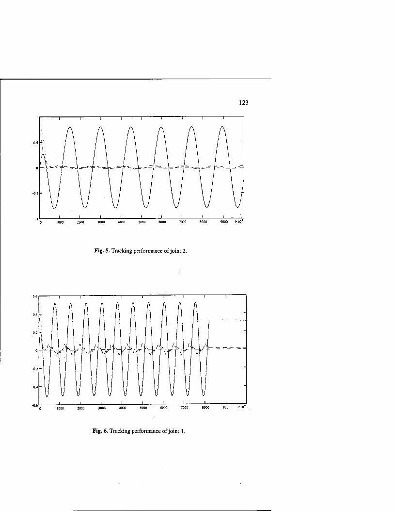
123

0 1000 2000 3000 4000 5000 6000 7000 8000 9000 1-10

Fig. 5. Tracking performance of joint 2.

1000 2000 3000 4000 5000 6000 7000 8000 9000 WO

Fig. 6. Tracking performance of joint 1.

Fig. 7. Tracking performance of joint 2

4 Conclusion

In this work the issue of the controller design and implementation has been addressed for rigid- link electrically-driven robot manipulators. Two major limitations in the literature, these being the measurements of velocities and time-derivative of the manipulator regressor matrix, have been eliminated. Experiments on Reis V15 industrial manipulator were performed, and experimental results verified the correctness of the algorithm.

Acknowledgements

The authors wish to acknowledge the support of the Natural Science and Engineering Research Council of Canada, the Institute for Robotic and Intelligent Systems (IRIS) and Precam Associates Inc.

References

1. Good, M. C, Sweet, L. M., and Strobel, K. L.: Dynamic models for control system design of integrated robot and drive systems. J. Dyn. Syst., Meas., and Control, vol. 107 (1985) 53-59 2. Beekmann, R. W. and Lee, K. Y.: Nonlinear robotic control including drive motor interactions. Proc. of Amer. Control Conf., Atlanta (1988) 1333-1338 3. Taylor, D.: Composite control of direct-drive robots. Proc. of the 28th Cönf. on Decision and Control (1989) 1670-1675 4. Tarn, T. J., Bejczy, A. K., Yun, X. and Li, Z.: Effect of motor dynamics on nonlinear feedback robot arm control. IEEE Trans, on Robotics and Automation, vol. 7 (1991) 114-122

125

5. Su, C.-Y., Leung, T. P. and Stepanenko, Y.: Real-time implementation of regressor based sliding mode control scheme for robot manipulators. IEEE Trans, on Industrial Electronics, vol. 40 (1993) 71-79 6. Dawson, D. ML, Qu, Z. and Carrol, J. J.: Tracking control of rigid-link electrically-driven robot manipulator. International Journal of Control, vol. 56 (1992) 911-1006 7. Mahmoud, M.: Robust control of robot arms including motor dynamics, International Journal of Control, vol. 58 (1993) 853-873 8. Liu, G. and Goldenberg, A. A.: Robust control of robot manipulators incorporating motor dynamics. Proc. of the 1993 IEEE/RSJ Int. Conf. on Intelligent Robots and Systems, Yokohama, Japan (1993) 68-75 9. Su, C.-Y. and Stepanenko, Y.: On the robust control of robot manipulators including actuator dynamics. Journal of Robotic Systems, vol. 13 (1996) 1-10 10. Bridges, M. M„ Dawson, D. M. and Gao, X.: Adaptive control of rigid-link electrically driven robots. Proc. of the IEEE Conf. on Decision and Control (1993) 159-165 11. Ge, S. S. and Postlethwaite, I.: Nonlinear adaptive control of robots including motor dynamics. Proc. of American Control Conference, San Francisco (1993) 1423-1427 12. Ge, S. S. and Postlethwaite, I.: Nonlinear adaptive control of robots including motor dynamics. Journal of Systems and Control Engineering, Proceedings of the IMechE, UK, Vol.208 (1994) 89-99 13. Yuan, J.: Adaptive control of robotic manipulators including motor dynamics. IEEE Trans, on Robotics and Automation, vol. 11 (1995) 612-617 14. Colbaugh, R. and Glass, K.: Adaptive regulation of rigid-link electrically-driven manipulators. Proc. IEEE Int. Conf. on Robotics and Automation (1995) 15. Guenther, R. and Hsu, L.: Variable structure adaptive cascade control of rigid-link electrically-driven robot manipulators. Proc. IEEE Conf. on Decision and Control, San Antonio, Texas (1993) 2137-2142 16. Stepanenko, Y. and Su, C.-Y.: Adaptive motion control of rigid-link electrically-driven robot manipulators. Proc. of IEEE Int. Conf. on Robotics and Automation (1994) 630-635 17. Su, C.-Y. and Stepanenko, Y.: Hybrid adaptive/robust motion control of rigid-link Electrically-driven robot manipulators. IEEE Trans, on Robotics and Automation, vol. 11 (1995)426-432 18. Su, C.-Y. and Stepanenko, Y.: Redesign of hybrid adaptive/robust motion control of rigid- link Electrically-driven robot manipulators. Proc. of IEEE Conf. on Decision and Control, San Diego (1997) 1341-1346 19. Klafterm, Chmielewski, R. T. and Negin, M.: Robotic Engineering: An Integrated Approach. Prentice Hall, Englewood Cliffs, NJ (1989) 20. Krstic, M., Kanellakopoulos, I. and Kokotovic, P.V.: Nonlinear and Adaptive Control Design. John Wiley & Sons. Inc. (1995)

126

Force-Impedance Control: a new control strategy of robotic manipulators

Fernando Almeida', Antonio Lopes', Paulo Abreu'

'IDMEC - Polo FEUP, Faculdade de Engenharia da Universidade do Porto, Rua dos Bragas, 4099 Porto codex, Portugal

{fga, ami, pabreu}@fe.up.pt

Abstract. A novel control strategy of robotic manipulators is presented in this paper: the force-impedance controller. This controller enables two kinds of behaviour: force limited impedance control and position limited force control. The type of behaviour only depends on the chosen manipulator trajectories. Free space error dynamics and post-contact manipulator dynamics may be independently chosen if a new impedance control architecture is used. Simulation results of a force-impedance controlled parallel manipulator, executing tasks that involve end-effector contact with uncertain environments of unknown stiffness, are presented.

1. Introduction

Position control strategies have been successfully used on robotic tasks involving a null or week interaction between the manipulator and its environment. Good examples are provided by spray painting, welding and palletising tasks [1], [2], [3].

On the other hand, although the set of tasks requiring a strong interaction between the manipulator and the environment is very large [1], [4], [5], the use of robots on assembly, polishing, grinding and deburring tasks, as well as on the field of medical surgery [6], is still low due to control difficulties.

The two main approaches to the control of the interaction of the manipulator and its environment are [4], [7]: - Hybrid Force-Position Control [8], [9]; - Impedance Control [1], [4], [10].

Hybrid control is motivated by the task analysis made by Mason [11]: on each direction of the task space, the environment imposes a force or a position constraint. These natural constraints are originated by the task geometry. Only the unconstrained variables may be controlled, their reference values being artificial constraints imposed by the task execution strategy.

Hybrid control enables the tracking of position and force references, the task space being decomposed into force and position controlled directions. As the decomposition is based on an ideal model of the environment, the ever present modelling errors always lead to unwanted movements along the force controlled directions and

127

unwanted forces along position controlled directions. This problem is more acute during the transition between free space and interactive movements, necessitating the use of some kind of controller switching strategy based on contact force information. Unfortunately, the switching process may induce an unstable manipulator behaviour [12], [13], [14], [15].

The impedance control objective is to control neither force nor position but their dynamic relation, the desired impedance, along each direction on the task space. Impedance controllers possess some inherent robustness to environment modelling errors [16], [17], [7]. Nevertheless, as contact forces cannot be directly imposed, they may grow in an uncontrolled manner due to modelling errors of the environment impedance.

Controllers combining the hybrid and the impedance control approaches have been developed, their main objective being a robust behaviour under environment modelling errors [18].

The Hybrid Impedance Controller proposed by Anderson and Spong [19] uses an inner control loop for manipulator dynamics linearization and decoupling. Impedance control substitutes for the position control used on hybrid controllers position subspace. This way, a desired manipulator dynamic behaviour is imposed.

Chiaverini and Sciavicco [16] combine a PD position control loop in parallel with a PI force control loop. The controller achieves the typical robustness of an impedance controller and the ability to follow position and force references of an hybrid controller. Position and force references must be specified for each task space direction. Control action is obtained as the sum of the two parallel loops control actions. Conflicting situations, as an unexpected contact, are naturally solved as force control always rules over position control, due to the integral control action. Unfortunately this may lead to an undesirable manipulator drift, along the contact surface, in the presence of environment modelling errors.

Neither of the above controllers enable the definition, over a force controlled direction, of a free space trajectory up to the contact surface without the use of some sort of force measure based switching strategy.

The novel force-impedance controller presented in this paper behaves itself as an impedance (position) controller up to contact set up. Afterwards, impedance or force control is achieved. This behavioural change is performed without the use of any supervising switching strategy.

Section 2 presents a new impedance controller structure that enables a definition of different free space error dynamics and post-contact impedance. The novel force- impedance controller is developed in section 3. Simulation results of an experimental parallel manipulator under force-impedance control are presented in section 4. Conclusions are drawn in section 5.

128

2. Impedance Control

The control objective of an impedance controller is to impose, along each direction of the task space, a desired dynamic relation between the manipulator end-effector position and the force of interaction with the environment, the desired impedance.

Usually, the desired impedance is chosen linear and of second order, as in a mass- spring-damper system. Higher order impedances have a less well known behaviour and require additional state variables.

In order to fulfil the task requirements, the user chooses a desired end-effector impedance that may be expressed by equation 1,

MJ(x-xd) + BJ(x-xll)+Kd(x-xJ) = -fl. (1)

where Mr/, Brf and K(, are constant, diagonal and positive definite matrices representing the desired inertia, damping, and stiffness system matrices. Vectors x and x, represent the actual and the desired end-effector positions, and f, represents the generalised force the environment exerts upon the end effector.

If the manipulator is able to follow an acceleration reference given by

ir=*rf+Mrf ■[-',+B(,(i(,-i) + K(,(xl/-x)] (2)

it will behave as described by equation 1. So, x,. is the reference for an inner loop acceleration tracking controller, that linearizes and decouples the manipulator nonlinear dynamics.

x-^r X + X +

+ X x. <£)-► K„ -Kg»(g^ M;' -Kg^

Controlled System

*G,„,(.^

B, «

Fig. 1. Block diagram of an impedance controller

Fig. 1 shows a block diagram of an impedance controller. The transfer function matrix GM0) represents the non-ideal behaviour of the inner loop acceleration controller, such as finite bandwidth and incomplete decoupling. At low frequency, up to a maximum meaningful value, the acceleration controller must ensure that G (s)

129

may be taken as the identity matrix, I. Hence, and without loss of generality, the force-impedance controller will be presented for a single dof system.

Under these conditions, and taking all values from Fig. 1 as scalar quantities, the end-effector position on the Laplace domain, X(s), is given by

X(s)=Xd(s)-Gf(syFr(s) (3)

where

Gf(s) = r-^ (4)

represents the desired manipulator admittance. The initial error between x and x(l decays to zero, in free space, according to a

characteristic equation equal to the desired impedance. The desired manipulator dynamics, expressed by equation 1, may also be

implemented using a new, and more general, structure presented in Fig. 2. x&

represents the position changes, relative to the free space trajectory, due to the contact force/,.

In this case,

G'{s)=MS + lB,s+Kf- (5)

This new structure enables the independent definition of free space error dynamics, and post-contact, G/s), manipulator dynamics. In free space, the error between x and x,! decays to zero with a dynamic behaviour given by the following characteristic equation:

Mxs2 + Bxs+Kx=0- (6)

This extra degree of freedom may be used to improve free space error dynamics, without compromising the desired impedance under contact.

Using the conventional structure presented in Fig. 1, a similar behaviour could only be obtained by switching controller gains (impedance). With the new control structure, the need for a supervising switching strategy is avoided.

From equations 5 and 6 it is easily concluded that the impedance controller is stable as long as parameters Mx, Bx, Kx, Mp Bf and Kf are chosen strictly positive. However, it should not be forgotten that the inner acceleration loop finite bandwidth (G„„(i) * I) may lead to instability if the desired manipulator dynamics are chosen too fast.

130

n

+ +

' k/s?U. K ^ r * I 1

V* J - k ' '

i 1 1 x

- 1 " J

1 Bx 4—r ̂ r r +

s L + + r

J r <

f + > ' *4 *A . *A

_i L ' ' ' ' '

^< ß 4 y* ß/ * k '

"/

Fig. 2. New impedance controller structure: free space error dynamics and manipulator impedance may be independently defined

3. The new Force-Impedance Controller

The force-impedance controller presented on this paper combines the robustness properties of an impedance controller with the ability to follow position and force references of an hybrid controller. The proposed controller has two cascaded control loops (see Fig. 4): an impedance controller, as the one presented on the previous section, is implemented as a inner loop controller. An integral force controller is used as an external loop controller.

This force controller acts by modifying the position reference, given by *,,, in order to limit the contact force to a specified maximum value.

For each task space direction the user must specify a, possible time variant, force reference, in addition to the desired position trajectory, impedance, and free space dynamics. The force reference has the meaning of a limiting value to the force the end-effector may apply to the environment.

131

The static force-displacement relation imposed by the force-impedance controller is presented in Fig. 3. Positive force values are obtained with a "pushing" environment and the negative values with a "pulling" one. The contact force saturation behaviour is obtained by the use of limited integrators on the force control loop.

While the manipulator is not interacting with the environment the controller ensures reference position tracking with the specified free space error dynamics. After contact is set up the controller behaviour may be interpreted in two different ways: - as a force limited impedance controller; - as a position limited force controller.

If contact conditions are planed in such a way that the force reference (limit) is not attained, the manipulator is impedance controlled. If environment modelling errors result in excessive force, the contact force is limited to the reference value.

If contact conditions are planed in order to ensure that the force reference is attainable, the manipulator is force controlled. When environment modelling errors result in excessive displacement, manipulator position is limited to its reference value.

This kind of manipulator behaviour ensures a high degree of robustness to environment uncertainty.

Fig. 3. Static force-displacement relation imposed by the force-impedance controller

Fig. 4 shows the force-impedance controller under a contact situation with a purely elastic environment. Its contact surface is positioned at xe and presents a stiffness Kc. In order to allow a choice of integrator gain, KF, that is not dependent on the desired manipulator stiffness, Kf the force error is divided by it. When the force control loop is in action the end-effector position, on the Laplace domain, is described by the next equation,

X(s)=Xd(s)+Gx(sp(s)-Gf(s)Fe(s) (7)

where

u('HFA>)-F.(')]-*f-jr (8)

132

and

G,M = - Mrs2 + Brs+K,

(9)

Force Controller Impedance Controller

M>(X^HKSK^

G, *

Fig. 4. Block diagram of the novel force-impedance controller interacting with an elastic environment of stiffness K

Substituting equations 5, 8 and 9 in equation 7 the following relation results:

yW_AW.v f,uM F M+ P*W Y M

where,

Px{s)=Kfs(Mxs1+Bxs + Kx)(Mfs

2+Bfs+Kf)

(10)

(11)

PF(s)= KFKx(Mfs2 +Bfs + Kf) (12)

PE{s)=KFKxKe(Mfs2+Bfs + Kf) + sKeKf(Mxs

2+BxS + Kx) (13)

Qx (s) = Kfs(Mxs2 + Bxs + Kx )(M / + Bfs + Kf) +

KfKes(Mxs2 + Bxs+Kx) + KxKFKe(Mfs

2+Bfs + Kf)- (14)

If the desired manipulator free space error dynamics is made equal to the desired impedance, then Mx = Mf=Milt Bx = Bf=BiP and Ks = Kf= Kd. Under this assumption the force-impedance controller can be simplified (see Fig. 5) and the manipulator position may be expressed as

133

X(S): (M/+Bds+K,i)s

s(Mds2 + Bds + Kd)+Ki

KF

s+K, •K,

s(Mds2 + Bds + Kd)+Ke

KFKe+sKr

s + KF Ke

s(Mds2 + Bds + Kd)+Kes + KFKe

(15)

If the Routh stability criteria is applied to equation 15, a maximum value of the force control loop integral gain, KF, is obtained as

MdKr Md

(16)

So, KF may be chosen in a manner that is independent of the environment stiffness Ke, increasing the controller robustness to environment modelling uncertainty.

A similar stability analysis for the case when different free space error dynamics and post-contact impedance are desired is still under study.

Impedance Controller

Fig. 5. Force-impedance controller: same free space error dynamics and post-contact impedance

4. Force-Impedance Controller Simulation Results

A simulation of the force-impedance controller, when applied to the control of a 6 dof parallel manipulator, was performed. An experimental set-up is under construction: the Robotic Controlled Impedance Device (RCID). This is a fully parallel mini- manipulator with a Merlet platform architecture [20], [21]. The RCID is coupled to an industrial manipulator: the latter one performs the large amplitude movements

134

while the RCID is only used for the fine and high bandwidth movements needed for force-impedance control.

The simulation program was developed on ACSL (Advanced Continuous Simulation Language) [22] and implements a discrete time version of the controller. Fully dynamic models of the manipulator, actuators, and transducers were included. The simulation also takes into account position, acceleration, and force measurement noises, as well as input and output quantization. The inner loop acceleration controller uses a 1 kHz sampling frequency and achieves a closed loop bandwidth of 400 rad/s. The force-impedance controller runs with a 500 Hz sampling frequency and includes a velocity observer having acceleration and position as input variables.

The two simulation cases that are presented next were chosen in order to enable an easy performance evaluation of the force-impedance controller.

The first case shows the force-impedance controller working as a force limited impedance controller. The task includes an approach to a contact surface, followed by a contact phase and, in the end, a pull back movement. During the contact phase, the end-effector must follow the surface xe, presented in Fig. 6(a), and the contact force must be limited to/,= 100 N. The desired trajectory x(/ was planed without taking into account a 2 mm hump on the contact surface and requires the end-effector to move with a speed of 5 mm s~'.

Simulation results, with impedance matrices Mtl = diag([2Q0 200 200 111]) (Kg; Kg m), Bd = diag([ 1.2xl04 1.2xl04 1.2xl04 40 40 40]) (N s m-'; N m s rad-1), and K, = diag{[ 1.8x10s 1.8x10s 1.8xl05 400 400 400]) (N m-'; N m rad-1), force controller gain KF = AQ s~' on all dof, and force environment stiffness Ke = 2xl06Nnf1, are presented in Fig. 6(b), position tracking error norm, and Fig. 6(c), contact force.

The manipulator tracks xr, up to the contact surface. After impact, impedance is regulated. When the unexpected hump is attained, the contact force grows up quickly and is limited to its reference value. After the hump, and to the end of the contact phase, the controller returns to impedance control. Position tracking is regained when the end-effector goes back into free space.

In the second case the force-impedance controller is used as a position limited force controller, tracking a reference force profile. After a free space approach to the contact surface, the end-effector must track a desired contact force profile and, in the end, do a pull back movement. The desired trajectory x, (Fig. 6(d)) was planned on the basis of an uncertain model of the environment, and requires the end-effector to move with speed of 20 mm s~\

Simulation results, using the same set of parameters as on the previous case, are presented in Fig. 6(e), position tracking error norm, and Fig. 6(f), reference force profile and actual contact force. During the approach phase, the manipulator follows the desired position trajectory up to the contact surface. After impact, a short period of impedance control is observed. When the desired force becomes attainable, force control starts. The desired force profile is followed up to the beginning of the pull out movement. During the pull out phase the controller returns to impedance control, enabling the manipulator to follow the desired free space position trajectory.

135

S 2

Position (x - axis) (mm)

(a)

Position (x - axia) (mm)

(b)

I : :

1 : :

I :

I

l : i '• ;•

i

'- ; i ; . ■■—

| 80-

Position (x - axis) (mm)

(c)

Position (x - axis) (mm)

(d)

Position (x - axis) (mm)

(e)

r^-"" i ■

E \V

\

i 1 0.

0.5 /

! ! 1 i I

^J

1/ ! i h

Position (x - axis) (mm)

(f)

Fig. 6. Simulation results: (a), (b), and (c) - force limited impedance control case; (d), (e), and (f) - position limited force control case. (References are represented by dashed lines)

136

5. Conclusions

The novel force-impedance controller presented on this paper enables the follow up of position and force trajectories, nevertheless achieving the robustness properties inherent to impedance controllers. If the new impedance control structure is used, different free space error dynamics and post-contact dynamics may be used, without the need of a switching strategy.

Force limited impedance control and position limited force control may be implemented with the proposed force-impedance controller. The type of behaviour is only dependent on the chosen trajectories and does not necessitates any other decision mechanism.

The simulation of a force-impedance controlled parallel mini-manipulator, the RCID, shows that good position, impedance, and force tracking is obtained

The robust behaviour of the proposed controller is also enhanced by the fact that its parameters may be fully defined without the knowledge of the environment stiffness.

This research was supported by Ministerio da Ciencia e Tecnologia - FCT, under the project n° PBIC/C/TPR/2552/95.

References

1. Hogan, N.: Impedance Control: an Approach to Manipulation: Part I-III. ASME Journal of Dynamic Systems, Measurement, and Control, Vol. 107 (1985) 1-24

2. Hogan, N.: Stable Execution of Contact Tasks Using Impedance Control. Proc. IEEE International Conference on Robotics and Automation (1987) 1047-1054

3. Mills, J. K., Goldenberg, A. A.: Force and Position Control of Manipulators During Constrained Motion Tasks. IEEE Transactions on Robotics and Automation, Vol. 5, N. 1 (1989)30-46

4. Kazerooni, H., Sheridan, T. B„ Houpt, P. K.: Robust Compliant Motion for Manipulators: Part I-II. IEEE Journal of Robotics and Automation, Vol. 2, N. 2 (1986) 83-105

5. De Schutter, J., Van Brüssel, H.: Compliant Robot Motion: Part I-II. The International Journal of Robotics Research, Vol. 7, N. 4 (1988) 3-33

6. Ho, S. C, Hibberd, R. D., Cobb, J., Davies, B. L.: Force Control for Robotic Surgery. Proc. of the International Conference on Advanced Robotics (1995) 21-31

7. Seraji, H., Colbaugh, R.: Force Tracking in Impedance Control. The International Journal of Robotics Research, Vol. 16, N. 1 (1997) 97-117

8. Raibert, M., Craig, J.: Hybrid Position/Force Control of Manipulators. ASME Journal of Dynamic Systems, Measurement, and Control, Vol. 102 (1981) 126-133

9. Khatib, O.: A Unified Approach for Motion and Force Control of Robot Manipulators: the Operational Space Formulation. IEEE Journal of Robotics and Automation, Vol. 3, N. 1 (1987)43-53

10. Kazerooni, H.: On the Robot Compliant Motion Control. ASME Journal of Dynamic Systems, Measurement, and Control, Vol. Ill (1989)416-425

137

11. Mason, M.: Compliance and Force Control for Computer Controlled Manipulators. IEEE Transactions on Systems, Man and Cybernetics, Vol. 11, N.6 (1981) 418-432

12. Whitney, D. E.: Historical Perspective and State of the Art in Robot Force Control. Proc. of the IEEE International Conference on Robotics and Automation (1985) 262-268

13. Paul, R. P.: Problems and Research Issues Associated with the Hybrid Control of Force and Displacement. Proc. of the IEEE International Conference on Robotics and Automation (1987)1966-1971

14. Eppinger, S. D., Seering, W. P.: Understanding Banwidth Limitations in Robot Force Control. Proc. of the IEEE Int. Conference on Robotics and Automation (1987) 904-909

15. Lu, Z., Goldenberg, A. A.: Implementation of Robust Impedance and Force Control. Journal of Intelligent and Robotic Systems, Vol. 6 (1992) 145-163

16. Chiaverini, S., Sciavicco, L.: The Parallel Approach to Force/Position Control of Robotic Manipulators. IEEE Transactions on Robotics and Automation, Vol. 9, N. 4 (1993) 361-373

17. Lu, Z., Goldenberg, A. A.: Robust Impedance Control and Force Regulation: Theory and Experiments. The International Journal of Robotics Research, Vol. 14, N. 3 (1995) 225-254

18. De Schutter, J., Bruyninckx, H., Zhu, W.-H., Spong, M. W.: Force Control: a bird's eye view. IEEE CSS/RAS International Workshop on Control Problems in Robotics and Automation: Future Directions (1997)

19. Anderson, R. J., Spong, M. W.: Hybrid Impedance Control of Robotic Manipulators. IEEE Journal of Robotics and Automation, Vol. 4, N. 5 (1988) 549-555

20. Merlet, J.-P., Gosselin, C: Nouvelle Architecture pour un Manipulateur Parallele a Six Degres de Liberte. Mech. And Machine Theory, Vol. 26, N. 1 (1991) 77-90

21. Lopes, A. M., Almeida, F. G.: Manipulability Optimization of a Parallel Structure Robotic Manipulator. Proc. of the 2nd Portuguese Conference on Automatic Control (1996) 243-248

22. MGA Software: ACSL Reference Manual, Edition 11.1 (1995)

138

The Use of Partially Decoupled Uniform Structures and Procedures for the Robust and Adaptive Control of

Mechanical Devices

Jozsef K. Tar', Okyay M. Kaynak^, Imre J. Rudas*, J.F. Bit6^

'Bänki Donät Polytechnic, Department of Information Technology, Nepszinhäz utca 8. H-1081 Budapest, Budapest, Hungary

{JKTar, Rudas}@zeus.banki.hu ^Bogazici University, Faculty of Engineering, UNESCO Chair of Mechatronics, Bebek

8085 Istanbul, Turkey Kaynak@boun.edu.tr

^Centre of Robotics and Automation, Bänki Donät Polytechnic, Nepszinhäz utca 8. H-1081 Budapest, Budapest, Hungary

JBito(2)zeus.banki.hu

Abstract: This paper is a brief report on the operation of a novel approach in- vented for the control of approximately and partially known multivariable, non- linear, strongly coupled mechanical systems under dynamic interaction with an unmodeled environment. As the traditional Soft Computing solutions are based on the use of uniform structures fit to solve typical classes of particular problems this method also uses simple uniformized structures and standard procedures but these special structures originate from the general mathematical framework of the Lagrangian Mechanics. In contrast to the application of Artificial Neural Networks or Fuzzy Controllers in which the number and proper parameter-range of the necessary neurons or fuzzy rules and membership functions is unknown in advance, the number of the tunable parameters is given ab ovo by knowing only the degree of freedom of the system to be controlled. This fact simplifies the tuning of the free parameters which process often is called "learning". The operation of the method is illustrated by simulation results developed for 3 degree of freedom a SCARA robot.

1 Introduction

Robots normally are approximately known, non-linear, strongly coupled multivariable mechanical systems the motion of which also is influenced by the dynamic interaction with the work-piece they manipulate. While manipulation of tightly gripped rigid bodies can be modeled simply by the change in the inertial parameters of the robot, other kinds of environmental interactions during technological operations as grinding or polishing, etc. needs more complicated modeling techniques in which the behavior of the processed material also has to be taken into account. All these circumstances

139

could impose a huge burden on the controller within the frames of the traditional "exact" or "analytical" modeling techniques. This makes their real time implementation dubious. Furthermore, they need controllers which are strictly tailored to the particular properties of the robot and the given task as well.

Fault tolerant control of mechanical devices gained considerable attention in the last years e.g. [1]. Even in the case of "rigid body approximation" during the mo- tion normally no satisfactory information is available for real-time system-identifica- tion in the classical "complete and analytical" sense [2]. For tackling such problems typical adaptive or robust methods as Model Reference Adaptive Control or Variable Structure Controllers still offer ample possibilities (e.g. [3]).

As alternative approaches to similar problems the use of modern, highly parallel Soft Computing methods completely abandoning any analytical description of the system's dynamics can be mentioned. In several NP-hard problems of high complexity no "orthodox methods" can be applied, like in scheduling tasks [4]. These methods use simple and uniform architectures not strictly tailored to the particular properties of the task to be solved by them. Instead, they contain a considerable number of free parameters by the appropriate variation or "tuning" of which some adaptivity can be achieved. This process frequently is referred to as "learning".

However, in such problem tackling determination the number of the neces- sary free parameters or elements connected to each other in a uniformized structure may mean a serious problem. For instance, multilayer perceptrons used for non-linear mapping and realized by feed-forward Artificial Neural Networks (ANNs) contain typical sigmoidal activation functions, connection weights and threshold values to be determined "experimentally". In similar way, Fuzzy Controllers (FCs) normally contain typical membership functions having their typical parameters, some fuzzy re- lations describing the approximately and linguistically already known "rules" de- termining the actions to be carried out by the controller. The necessary number of these functions and rules cannot be known in advance.

Another problem typical in such approaches is the fact that in these repre- sentations the appropriate "range" of the parameters to be tuned cannot be known in advance, too. In connection with FCs this fact is frequently referred to as "scaling problem". For ANNs for improperly large thresholds and connection weights the network paralysis can be mentioned in this context.

In connection with learning, normally serious problems arise in the practice. Due to the intricate nature of the non-linear coupling so characteristic to mechanical devices this learning or parameter fitting cannot be realized on the basis of simple cases and appropriate, ab ovo known rules. Typical combination of "stochastic" and "deterministic" learning methods may achieve some optimum between the learning time and the avoidance of local minima which can normally manifest itself in low performances. However, in the case of a very large set of parameters and unknown ranges of tuning these methods can be efficient mainly for static problems in which the optimal parameter setting does not depend on time, neither explicitly, nor in an implicit way.

In case of dynamic control of robots any formulation of the dynamic proper- ties in a static way based on Kolmogorov's famous approximation theory would lead to

140

a huge space for tuning. Though a dynamic representation allowing time-dependent parameters considerably can decrease this space, it still remains too large for real time tuning. Further problem in this context is that in the description of mechanical systems not only well-defined functions occur. Their partial derivatives also are present in the formulae. However, Kolmogorov's theorem does not state that the derivatives of the approximation of a smooth function will well approximate its derivatives, too. This fact also is a dimension-increasing problem in parameter tuning.

The new method described in this paper was invented for addressing the above problems of traditional Soft Computing approaches as well as abandoning the burden of "exact modeling", too. It can be reckoned as a "compromise" between ana- lytical modeling with full system identification and pure Soft Computing-based ap- proaches neglecting any a priory known analytical information on the system other- wise available for mechanical devices as robots. In the sequel the antecedents and ba- sic idea of this approach is described in details.

2 The Basic Idea and Antecedents of the Novel Approach

The idea of using "uniform structures" in elaboration of solutions for wider classes of problems in itself is not a novelty. It forms the essential part of different approaches altogether referred to as "Soft Computing". However, the "origin" of these uniform structures can be traced back to two different traditional sources: typical membership functions (triangular, trapezoidal, etc.) normally can be invented on the basis of simple and plausible considerations in connection with fuzzy controllers. Also, typical "sigmoid", Gaussian bell or periodic functions used in the "neurons" of ANNs can be based on either "illustrative" considerations or on the more exact approximation theorem proved by Kolmogorov in 1957. These are fit to quite broad categories, therefore it cannot be expected to reduce the number of their free parameters on the basis of general considerations.

As an alternative solution seeking uniform structures originating from stricter mathematical model fit to a well defined, "narrower" set of problems can be mentioned. In many cases certain physical systems have well defined symmetries the properties of which can be transparently described by symmetry groups. This leads to the idea of using Group Theory for the introduction of uniform structures.

Application of Group Theory has a long and partly "forgotten" tradition in connection with mechanical systems. In the seventies of the 19th century different "mechanisms" stimulated the interests of famous mathematicians as Darboux or Chebychev. For describing translations and rotations Clifford developed the idea of geometric algebra on the basis of Hamilton's quaternions [5] which later lead to a wide set of the so-called "Clifford Algebras" serving as quite general algebraic tools by the use of which different symmetry-operations can be represented.

The internal symmetry of Symplectic Geometry (e.g. in [6]) lead to the idea of using the elements of the Symplectic Group as the "source" of uniform structures for the control of Mechanical Systems [7, 8]. In spite of its lucid mathematical structure, due to some measurability problems the rich structure of Hamiltonian

141

Mechanics was put aside and the Euler-Lagrange eguations were considered as the source of an appropriate symmetry group [9-11]. The preliminary results achieved are summarized as follows.

As is well known by using the Lagrangian model of a robot arm the equations of motion for a robot of open kinematic chain has the form of the Euler-Lagrange equations

lH(*+Z-^-X^*+-f--a m in which q denotes the generalized coordinates of the robot, Q represents the sum of the effects of the torques/forces exerted by the drives on the appropriate pivots of the joints, the projection of the external and the friction-caused forces on the joint shafts. The symmetric inertia matrix M(q) depends only on the generalized coordinates. The gravitational term V(q) is derived from the partial derivative of the Lagrangian L.

In the traditional Computed Torque control M is built up on the basis of a detailed dynamic robot-model expressed according to the Denavit-Hartenberg Con- ventions. For a rather complicated robot arm construction of M and its necessary de- rivatives is a complicated and time-consuming work. Furthermore, the "fruits" of such calculations are degraded by the presence of the unknown external or environmental interactions so influencing the robot's motion that they cannot easily be taken into account in Q.

For getting rid of such complicated calculations in the antecedents of the present proposition the singular value decomposition of the positive definite symmet- ric inertia matrix

M(q) = 0(q)D(q)0'(q) (2)

leading to the time-derivative

M=ÖDOr + ODÖ7+OD07=GM-MG + ODH07 (3)

was used. In this equation in the case of a three degree of freedom system, the skew- symmetric matrix G and the diagonal matrix H

G = ÖOr, H = (H„,//22,//33) (4)

correspond to the generators of simple Lie groups and they can be built up from sim- ple linearly independent generators and the joint coordinate velocities. In the former approach O was constructed as the product of three independent orthogonal matrices combining only the (1,2), (2,3), (3,1) matrix elements as

cos£12 sin£l2 0 0 = Oa2,(q)0(2'5,(q)0""(q), 0,u> = - sin £,, cos £,, 0

0 0 1

etc. (5)

in which the Lie-parameters of the group were the functions of the generalized coor- dinates of the robot, therefore their partial time-derivatives were expressed by the simple terms

142

£,(q,q) = E^(qk, • (6) s

Similar terms were gained for the elements of the diagonal matrix as

D„(q) = exp(<f„(q)), etc. (7)

It is obvious that with the exception of the potential energy it was possible to construct each term in the Euler-Lagrange equations in a "standardized way" for which the only necessary information regarding the robot dynamics was the degree of freedom of the robot arm.

In the former approach initially a very rough and approximate dynamic model of the robot arm, a constant inertia matrix proportional with the identity transformation and zero partial coordinate derivatives were used. The potential energy term in the model was completely abandoned. In the learning process the g//? parameters were tuned via a simple adaptive version of the Simplex Algorithm with the aim of minimizing the difference between the expected and the measured joint coordinate accelerations. The environmental dynamic interaction unmodeled by the controller was represented by a damped viscous spring attached to the end-effector of the robot at its one end and fixed in the workshop at its other end.

This idea can be reckoned as a rough analogy of the problem of controlling a bowl rolling on the surface of a plane in a gravitational field. In this case small tilting of the plane can keep the bowl on the appropriate trajectory. In a multidimensional space the gjjx parameters of Eq. (6) correspond to the tilting angles and the Euler-La- grange equations together with the variation of these parameters determine the motion of the system.

In the initial phase of learning this rough model yields very bad control results. For keeping the motion of the system convergent conventional "standard" ancillary control loops were applied to the system. One of them was a simple PID/ST type feedback signal the parameters of which were planned in the phase space of the motion. The actual model of the inertia data was used to transform the calculated joint angle accelerations into "generalized forces" (physically torques of forces) for the robot drives. Based on the observation that the change in the joint coordinate accelerations must be linear functions of the changes in the joint torques or forces if the inertia matrix of the robot does not vary too fast a simple regression-analysis-based technique also was added to the other loops whenever the motion of the arm comprised satisfactory information for calculating this term. When no enough information was available for this term it was simply dropped. Since these additional loops are used in the present approach, too, their more detailed description will be given in the next paragraph.

This approach was investigated via simulation from several points of view and it was found to have the advantages as follows: 1) It made it possible to avoid the tedious work of constructing a dynamic model on

the basis of the Denavit-Hartenberg conventions which also needs the precise ki- nematic model of the robot. It was just enough to start the learning from a very approximate initial model;

143

2) It yielded very simple uniformized structures that can easily be constructed if we know at least de degree of freedom of the robot arm;

3) In contrast to the more traditional Soft Computing approaches as ANNs the number and the proper role of each tuned parameter was clearly set and determined from starting the tuning; This number is quite limited in comparison with the possibly required number of neurons in the case of a multi-layer perceptron;

4) The characteristic ranges of the tuned parameters were set almost completely in- dependently from the particular dynamic properties of the robot modeled by this structure; For the ^ values of Eq. (5) describing rotational angles the [0, 2n) interval contains all the different physical possibilities; In similar way, for the £/7

values of Eq. (7) being the arguments of the exponential functions it is trivial that exp(-lO) is a very small positive value while exp(10) is very big, that is in the practice when at least an order of magnitude estimation is available for the dynamic data of the robot this scaling can be regarded practically problem-independent;

5) On the basis of simulation results for considerable joint velocities it was possible to achieve a considerable improvement of the control with respect to the simple linear control case; The method had considerable flexibility for compensating the effect of the external disturbances represented by the viscous spring; On this basis it was stated that the control realized an imperfect and partial "system identification" the use of which is restricted only nearby a given point of the phase space of the system; As the robot leaves this point the "identification" must be refreshed; Normally, in the process of "identification" each component of the control took part with comparable significance.

The above method also had some limitations that can be listed as follows:

1) For slow motion Eq. (6) yields a very slow parameter tuning which is not efficient enough; Also, slow motion means unfavorable conditions for the operation of the regression analysis based ancillary control loop;

2) The mathematical form expressed by Eqs. (2) and (5) contains a strong coupling between the effect of tuning the arguments of the orthogonal and the diagonal ma- trices; Whenever the diagonal matrix remains almost proportional to the unit matrix the effect of tuning the orthogonal matrices remains almost negligible; Also, between the non-diagonals also is a strong coupling;

3) The very preliminary way according to which the regression-analysisrbased term was included or dropped introduced some noise into the system and it was not easy to get rid from these fluctuations by using simple filtering techniques.

In this paper some more simple and "standardized" modification in the original approach is presented. The simulation results reveal that these modifications seem to overcome the above deficiencies.

144

3. The Present Approach

The present approach, like the previous ones, consists of the main idea concerning the tuned parameters and ancillary methods that are applied simultaneously.

3.1 The Tuned Parameters

For decreasing the problem of parameter coupling addressed in paragraph 2) instead of a single positive definite matrix the inertia matrix is approximated as the sum of linear combination of positive definite matrices for each pair of symmetric non-diagonal components as

exp(£12)

cos?*,. -sin^?l2 0 1 0 0 cos#>l2 s'm<pn 0

sin q>n cosq>u 0 0 2 0 - sin ipn cos <pl2 0

0 0 1 0 0 0 0 0 1 (8)

etc. and additional main diagonal components resulting in the final expression

M(q) = 2«p(^)(«l)Mm(^(q)) + M/'1(q)),-..,exp(//.(q))) (9)

In this structure the "undiagonalized" matrices have two non-zero main diagonals which guarantees appropriate sensitivity for the rotation angles. The non-diagonal elements are not coupled to each other as far as the rotations are concerned though some coupling remains between the appropriate £, and (p parameters. Since in the struc- ture given by Eq. (8) there is a constraint between the possible ratio of the diagonal and the non-diagonal elements the additional diagonal matrix helps to modify this relation if needed by increasing the main diagonals even when the off diagonals are very small. It is easy to see that the rotated matrix in Eq. (8) has the form of

(10)

and this means that the main diagonals in this case have the lower limit of 1 in these matrices and the matrix given by Eq. (9) is strictly positive definite. This may help to avoid singularity problems that may be caused by under-estiination of the inertia matrix. It is easy to see that by using the

1 + sin2 <pn -sin^,,cos^12 0

sin q>n cos <pv 1 + cos2 <pa 0

0 0 0

dp Jain ^A%> and 4AA% (11)

parameters for tuning a control more or less similar to the antecedents can be devel- oped. However, this structure contains more independent parameters for tuning than the former one, so it is expected to be more versatile, more simple to tune and more stable than the previous method. It is also clear that with the exception of the potential

145

energy each term in the Euler-Lagrange equations can be expressed by this structure. For a robot of "n" degree of freedom the total number of the tuned functions is nxn, which is a redundant but partially uncoupled representation. The number of the tuned parameters is just nxnxn.

3.2 The Ancillary Control Loops and Methods Applied

3.2.1 A Sim pie Version of PID/ST Control Regarding the ancillary parts of the control the PID/ST addition is operating under the following basis. The desired acceleration for the coordinate error signal is expressed by the terms as

£=-b'£-c'e-kJ£{t')dt' (12)

in which the b', c' and k parameters are not constants. They are tuned according to the rule that the characteristic polynomial of Eq. (12) for a linear system would be

P{a) = {a+A oc+^\ =<X, + (C + KV+ — + cic\a+ — K (13)

of an almost constant pole structure describing a fast relaxation with the time exponent c/2 and a slower relaxation for the integrated error K. It is this latter parameter which is tuned by the rigid rule

c K= —

2 0.1 + tanh 50 \e{f)dt' (14)

expressing the practical rule that a) if the integrated error remains too much increase in the integrating coefficient is necessary, and b) even for zero integrated error some feedback is needed, too, and that c) this coefficient must remain finite, practically of the same order of magnitude like the "fast" poles of the PD controller would be without the integrating term. The method does not mean too much computational effort and adding this loop into the control considerably increases the quality achieved.

3.2.2 A Simple Version of Regression Analysis The application of regression analysis as a second "uniformized" ancillary tool is based on the observation that for a given physical state of the robot the changes in the joint coordinate accelerations are the linear combination of the changes in the generalized force components Q. If the velocity of the robot arm is not too large, for a given time "t" this linear dependence can be extended approximately for the AQ(l)=Q(t)-Q(t-l), AQ(2)=Q(t-l)-Q(t-2), values exerted by the drives of the robot and a similar expression made of the joint coordinate accelerations in the form of

146

t s * s

This is a matrix equation of the formB=CR in which R is a known symmetric matrix. In similar way B also is known. If R can be inverted than the desired correction based on the regression analysis can be estimated as

AQ""' = BR^'Acf*""" (16)

It is worth of noting that Eq. (16) does not require a complete matrix inversion. It needs just the solution of a linear equation Rb = AqA"'f'"" for vector b since the matrix B also is given. For this purpose a simple modification of the "Gram-Schmidt Algorithm" is used which truncates the potential singularities and "masks out" those sub-spaces for which no solution exists.

Since this truncation still may introduce considerable noise into the system, an additional simple smoothing technique also was applied: the set of those part of the exerted momentums and forces which were applied in the six previous steps is com- pleted by the expectation gained from Eq. (16) as the seventh point. For these points as a time-function a linear form AQ(t)=At+const. is fitted and the result of Eq. (16) is replaced by the value calculated from this formula for the latest point. The number of the necessary past points was determined on the basis of simulation investigation for different trajectories over which the system had run with different velocities. This smoothing itself was not found to be satisfactory in eliminating fluctuations charac- teristic to the Regression Analysis. Increasing the number of the past point introduced too much "inertia" by involving too much "partly obsolete" data in the calculation.

For further improvement a different way of taking into account a wider set of the more or less obsolete "past data" was necessary. The solution was found in a "reliability factor" R measuring the "noisiness" of the environment from which the above smoothed data origins. Instead the smoothed value At+const. its weighted ver- sion AQ(t)=Ä(At+const.) was finally used as a contribution from regression analysis. The weight factor R approaches 1 for a "reliable" (that is "not very much fluctuating") environment and it tends to approach zero for very noisy "near past history" the data of which "cannot be taken so seriously". R was determined by the simple formula with constant H and a. It is worth noting that the calculation of the sum oninfinite elements does not require too much computational efforts: only the content of a buffer must be multiplied by a and following this the new contribution can be added to the content of the same buffer.

*(,) = _ £ (17) H + (1 - «)£ <*•( AQ- {t-s)- AQ:1W {t - s))

5=0

These ancillary solutions were found to be optimal by giving sufficient smoothing without considerably increasing the "inertia" of the system.

147

3.2.3 Introduction of Lower Limits in the Velocities in Parameter Tuning For keeping the parameter tuning "speedy enough" even for slow motion the following simple lower limit has been applied only in the arguments of the tuned functions in which the constant C was determined "experimentally".

Uif|<7f|>C *'• $ CsignU) if \q,\<C

(18)

4 Simulation Investigations

For this purpose a 3 DOF SCARA type robot was considered in dynamic interaction with a damped spring of spring- and viscosity constants Spr [N/m] and Vis [N/(mxs)]. For a wide velocity range a simpler and a more intricate trajectory was investigated.

10

5

0

-5

-10

"15-4

Phase Space

•»-...... -V—-— r U-

1 -3 -2 -1 0 1

Figs, la- Id. The phase-trajectories described in terms of the desired and realized motion for four different required velocities for the "simple trajectory case". The "Phase Space" describes the dq/dt—qi graphs given in one diagram for the three different joints inm, rad, and m/s, rad/s units in the horizontal arid vertical axes, respectively.

Typical phase-trajectories are described in Figs, la - Id for the "simple" trajectory with different velocity requirements for the desired and simulated trajectories for the "environmental parameters" Vis=T0 Ns/m, Spr=1000 N/m.

148

-3

-4

4

2

0

-2

-4

100 200 300 400 500

Müdes ■

'"" Amplitudes - Time

1ÖÖ "200" 300 "4ÖÖ 500

500 500

Figs. 2a - 2d The desired and simulated "Amplitudes Time" functions, that is the joint coordinate-time functions pertaining to Figs, la- Id (time in 5 ms units on the horizontal axis, joint coordinates in m and rad units for the linear and the rotary joints, respectively).

The figures well illustrate the initial relaxation of the errors and the efficient adaptivity of the control with the help of the phase-trajectories. The same process also is illustrated in Figs. 2a - 2d by the desired and simulated joint-coordinate-time functions.

For revealing the "background processes" in Figs. 3a - 3d simulation results are described for the "fast motion" along a more complicated or "intricate trajectory" for the same value of the "environmental parameters". In spite of the great imprecision of the initial model the simulated phase-trajectories well approximate the desired ones in both spaces (Figs. 3a-3b). In Figs. 3c-3d the generalized forces are given (full value and the regression contribution, respectively.) It can well be seen that in this case, due to the "intricate" nature of the desired motion satisfactory information was given to the regression analysis for providing reliable and significant contribution.

Fig. 4a displays the joint-coordinate errors versus time for the same motion. It is clear that following a fast "relaxation" phase this error is kept at bay in spite of the considerable velocities, the very rough initial dynamic model and the considerable external interaction. The dynamic coupling between the different joints not completely suppressed by the control can also be revealed.

The "zigzag" in the variation of the estimated inertia is the consequence of the velocity-truncation defined by Eq. (18) and the quick and slight variation of the directly tuned parameters of which three particular ones are plotted in Fig. 4d. This well illustrates the analogy with the task of keeping bowl at a prescribed path via small tilting of the plane on which it is rolling.

149

30 20 10 0

-10 -20 -30

Phase Space

-2 0 2 Joint Generalised

4

2

0

-2

-4

6000

Amplitudes - Time

500

200C

0 -2000

-6000

100 200 300 400 500 ,A(jditiv-6LQe_neraJisfid Forces

100 200 300 400 500

Figs. 3a - 3d. Fast motion along the "intricate" trajectory: the "phase-trajectories", the "amplitude-time functions" (using the same units as in Figs, la-2d), the full amount of the generalized forces, and the contribution of the terms calculated on the basis of regression analysis (in N and Nm units for the linear and the rotary joints, respectively).

5. Conclusions

It was illustrated via simulations that the proposed method combining an improved PID/ST adaptivity with the application of a simple uniform structure containing tun- able parameters adjusted by the Simplex Algorithm and with the ancillary tool of re- gression analysis can co-operate successfully. The synthesis of the individually quite limited methods leads to an efficient control in which the significance of the different components changes according to the task to be executed. The method is based on simple considerations, does not require a priori information on the dynamic model of the robot and its environment. In its philosophy this approach is very similar to the traditional Soft Computing but the structures it uses are better fit to the requirements of Classical Mechanics, therefore considerable reduction in the number of the tuned parameters was achieved in comparison with a general approach. The new method also is free from scaling problems. It can be regarded as a compromise between the traditional Soft Computing and Hard Computing.

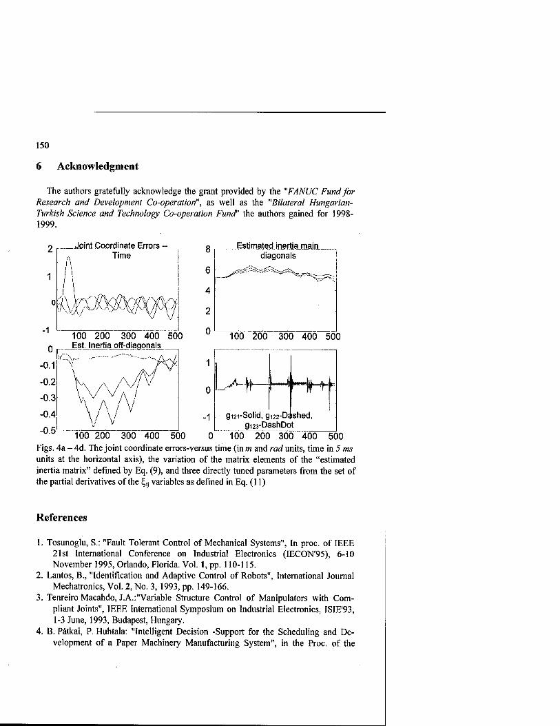
150

6 Acknowledgment

The authors gratefully acknowledge the grant provided by the "FANUC Fund for Research and Development Co-operation", as well as the "Bilateral Hungarian- Turkish Science and Technology Co-operation Fund" the authors gained for 1998- 1999.

.Joint CoordinateJErxors -_ Time

100 200 300 400 500 Q r Est. Inertia off-diagonals

-0.1

-0.2

-0.3

-0.4

-0.5

«Q- 1

0

-1

.„EMm_atedjnMiajnajn_. diagonals

100 200 300 400 500

_^*-)k— r—^ '""TlMh *

gi2i-Solid, gi22-Däshed, gi23-DashDot

100 200 300 400 500 0 100 200 300 400 500 Figs. 4a - 4d. The joint coordinate errors-versus time (in m and rad units, time in 5 ms units at the horizontal axis), the variation of the matrix elements of the "estimated inertia matrix" defined by Eq. (9), and three directly tuned parameters from the set of the partial derivatives of the £,% variables as defined in Eq. (11)

References

1. Tosunoglu, S.: "Fault Tolerant Control of Mechanical Systems", In proc. of IEEE 21st International Conference on Industrial Electronics (IECON'95), 6-10 November 1995, Orlando, Florida. Vol. 1, pp. 110-115.

2. Lantos, B., "Identification and Adaptive Control of Robots", International Journal Mechatronics, Vol. 2, No. 3, 1993, pp. 149-166.

3. Tenreiro Macahdo, J.A.:"Variable Structure Control of Manipulators with Com- pliant Joints", IEEE International Symposium on Industrial Electronics, ISIE'93, 1-3 June, 1993, Budapest, Hungary.

4. B. Pätkai, P. Huhtala: "Intelligent Decision -Support for the Scheduling and De- velopment of a Paper Machinery Manufacturing System", in the Proc. of the

151

"1998 IEEE International Conference on Intelligent Engineering Systems" (INES '98), 17-19 September, Vienna, Austria, pp. 169-174.

5. W.K. Clifford: "Preliminary Sketchs of Biquaternions", Proceedings of the London Mathematical Society, VI.(64/65), pp. 381-395, 1873.

6. V.l. Arnold: "Geometrical Methods of Classical Mechanics", vol. 60 of Graduate Texts in Mathematics, Springer-Verlag, New York, 1978.

7. J.K. Tar, I.J. Rudas, J.F. Bitö- Group Theoretical Approach in Using Canonical Transformations and Symplectic Geometry in the Control of Approximately Modeled Mechanical Systems Interacting with Unmodelled Environment", Robotica, Vol. 15, pp. 163-179, 1997.

8. J.K. Tar, I.J. Rudas, J.F. Bitö, B. Pätkai: "New Prospects in the Adaptive Control of RobotsUnder Unmodeled Environmental Interactions", in the Proc. of the 23 International Conference of the Industrial Electronics Society (IECON'97), New Orleans, Lousiana, USA, 1997, p. 1349 (ISBN 0-7803-3932-0).

9. J.K. Tar, I.J. Rudas, Jos6 A. Tenreiro Machado, Okyay M. Kaynak: „On the Tuning of the Lagrangian Parameters in a Uniform Structure in Adaptive Robot Control", in the Proc. of the 2nd IEEE International Conference on Intelligent Processing Systems (ICIPS'98), Gold Coast, Australia, August 4-7, 1998., pp. 599-602.

10. J.K. Tar, O.M. Kaynak, J.F. Bitö, I.J. Rudas, T. Kegl: "The Use of Uniform Structures in Adaptive Dynamic Control of Robots", in the Proc. of IEEE International Symposium on Industrial Electronics (ISIE'98), Pretoria, South Africa, 7-10 July, 1998, Vol. 1, pp. 137-142.

11. J.K. Tar, K. Kozlowski, I.J. Rudas, J.F. Bitö: "Combined Application of Regression Analysis and Approximate Modeling in an Adaptive Control for Mechanical Devices", in the Proc. of the 5th International Symposium on Methods and Models in Automation and Robotics ~ MMAR'98, 25-29 August 1998, Miedzyzdroje, Poland, pp. 807-812, ISBN 83-87423-81-5.

152

The Development of Model-Free Intelligent Assistance Control of Electrical Wheelchair

Ren C. Luo, Tse Min Chen, and Chi-Yang Hu

Intelligent Automation Laboratory Department of Electrical Engineering, National Chung Cheng University

160 Shang-Shing, Ming-Hsiung, Chia-Yi, Taiwan 621, R.O.C. Email: luo@ia.ee.ccu.edu.tw. tmchen ©ia.ee.ccu.edu.tw. cyhu@ia.ee.ccu.edu.tw Tel: 886-5-2720980 Fax: 886-5-2720729 http://www.ia1ah.ee.ccu.edu.tw

Abstract: Most of the electrical wheelchairs available in the world today are direct control mode, through which many potential accidents may be occurred by unreasonable control in various environmental conditions. This usually caused by the uncertainties of the front caster wheels and the unbalanced friction condition between wheels and floor. In this paper, we first derive a model-free equation to translate human inputs to the differential velocities of the two wheels for electrical wheelchair control. An adaptive predictive controller based on grey theory and fuzzy logic control theory is presented to integrate the electronic compass and dead reckoning measurements to reduce the influence caused by the uncertainties. The algorithm is tested and examined on the wheelchair base "Luoson-1" successfully. We have demonstrated the capability of the system for the increased certainty and safety to operate an electrical wheelchair. We also conduct the comparison between grey theory and extended Kaiman filter used in the heading prediction. The result shows that our algorithm is more efficient and flexible than another.

1. Introduction

Electrical wheelchairs are broadly used on assisting the disabled people as convenient mobile tools for their daily activities. Most of the electrical wheelchairs available in the world today are electrical joystick-controlled styles, through which many potential accidents may be occurred by unreasonable control in various environmental conditions. Beside, these types of wheelchair are unsuitable for more severe impaired users who are handicapped on operating. These severe impaired people usually need someone to push traditional wheelchairs to assist their daily activity. Therefore there is a need to develop an intelligent wheelchair that can autonomously or semi-autonomously to assist the daily activity of disabled people [1- 4].

For this purpose, additional sensors are used to gather the environmental information to perform necessary assistance for the wheelchair. Some of the researches construct the wheelchair by the mobile robot refit, such as VAHM [1] project. A chair is set on the multisensor based mobile platform, and the technologies of sensor fusion and control theory for the robot motion is applied to the wheelchair

153

navigation. A legged wheelchair, another structure, that is able to climb a footstep, is an interesting device [2]. In the future, there may have more applications achieved by such expensive legs mounted on a wheelchair. The SENARIO [3] project develops an intelligent wheelchair that is able to navigate autonomously in an indoor environment by the vision system mounted on top of a chair.

1.1. The Need of Handicapped People

In fact, not all of the handicapped people need the autonomous navigation for their daily activities. The following operating modes are suitable for the different handicapped people with different level of impairment.

Direct Mode: This mode is for the users who can operate electrical wheelchair properly. User can directly control the wheelchair by joystick, microphone, keypad, glove, etc. This mode is especially helpful in the initial stage of the development for testing the mechanism, man-machine interface, and low-level control, etc. Assistant Mode: For general disabled users who can operate an electrical wheelchair but accidents may occur while performing unreasonable command, they may need the assistant mode to control the wheelchair. The cooperation or the shared control of human and computer can achieve this goal [4]. Primitive intelligent control, e.g. collision avoidance, wall following, and docking [5-6] can be applied here. For the consideration of the development in second stage, this mode is also helpful to test the new control modules. Autonomous Mode: For the severely handicapped users, who are unable to operate the classical electrical wheelchair by themselves, the autonomous mode of the intelligent wheelchair may be a good solution to assist their daily activity. Using this autonomous mode, users can interact with the wheelchair through multimedia input interface. The inputs are interpreted by the expert system of intelligent man-machine interface to high-level motion command, e.g. "go to dinning room". Motion planner then generates the behavior/path commands to achieve the goal according to an a- prior map. The low-level motion behavior module executes the command to guide the wheelchair to the goal position. As a result, the user just needs to give high-level command input and mission can be intelligently accomplished. For this purpose, the past experience cumulated by the authors who involve the intelligent autonomous mobile robot can be applied to complete the local intelligence build-up[7-9]. Supervisory Autonomous Mode: While working in a dynamic environment the previously considered autonomous function might not be enough to complete a complex task. One should consider that the patient might have emergency while sitting on the wheelchair. For hospital automation, a supervisory system should be constructed. The supervisory autonomous mode is developed for this purpose. In the case of emergency of the user-wheelchair on multiple user-wheelchairs, the supervisory station will take the authority of the wheelchair, and perform remote control through the local computer network of the hospital. Past researches [1-4,10-11] does not consider this function, but it is necessary if the wheelchair applied in hospital automation. The supervisory mode is also a promising solution to increase the fault tolerance of an automation system [12].

154

Although the higher level of control mode brings a convenient way for the user to control the wheelchair, the wheelchair equipped with multiple sensors is expensive. The autonomous navigation of mobile robot or land vehicle also in research stage. However, we can see that the intelligent assistant control of various vehicles are realized, such as GPS, and will become a basic equipment of the vehicles in the first 21st century. From this point of view we will study the intelligent assistant control in the following paragraphs.

1.2. Primitive Issue of Assistance Control

The level of intelligence is increased as we increase the level of intelligence in control mode. The higher level function is built on top of the lower level. If the low- level controller has a good performance it makes the high-level intelligence become easier to achieve. However, due to the two caster wheels, the dynamics of an electrical wheelchair has its inherent uncertainties. Furthermore, the differential driving of an electrical wheelchair causes large slippage between the wheels and the floor. In other words, the direct control of an electrical wheelchair has its difficulty and may cause unpredicted accidents. When operating an electrical wheelchair, as shown in Fig. 1, the resultant trajectory may have a discrepancy due to the two uncertain casters and slippage.

In this paper, a low-level intelligent assistant for control of an electrical wheelchair is investigated. The objective of the controller is to reduce the influence on discrepancy error caused by the uncertain caster wheels and the slippage between wheels and floor. We first derive a model-free equation to translate human inputs to the differential velocities of the two wheels for electrical wheelchair control. An adaptive predictive controller based on grey [13, 14] and fuzzy logic theories is presented to integrate the electronic compass and dead reckoning measurements to reduce the influence caused by the uncertainties. Experimental results show that it increases the certainty and safety to operate a wheelchair. We also conduct the comparison between grey theory and extended Kaiman filter used in the prediction in the experiments. The result shows that the control method we developed is highly flexible and efficient.

Given VLen=' " Right

i

Desired Trajectory 4. 1 Actual Trajectory

Cester Wheel 'm Caster Wheel

Vlatt

lllllf ■ "Saht

Rear

Fig 1: An illustration for the potential error occurs while direct control a wheelchair to go straight.

155

2. System Configuration

Most of existing electrical wheelchairs are joystick controlled. User can control the wheelchair directly through the joystick. But the user has to pay most of his attention on observing the environmental change and the reaction of the wheelchair.

In many cases, direct control of a wheelchair can cause potential danger to environment and the operator. For this problem, the development of intelligent assistant control is a solution to achieve high safety operation. The basic concept of intelligent assistant control is to make motion decision by integrating the human inputs and the environmental condition from sensory measurements. The intelligent assistant control concept has been applied on advanced manufacturing systems and teleoperating systems [15].

The inherent problem of direct control of an electrical wheelchair is the slippage caused by wheels. Our approach for an intelligent assistant control is to integrate electronic compass and the dead reckoning measurements to estimate and predict the actual wheelchair-heading angle. Since the heading angle and the heading velocity can be obtained by measurement, we can perform low-level velocity control by referring to the sampled human input to reduce the influence from the potential uncertainties.

Fig. 2 illustrates our basic concept of the low-level intelligent assistant control of an electrical wheelchair. The wheelchair is the second-generation electrical wheelchair base named "Luoson-II" in our laboratory. Similar to the general electrical wheelchairs, differential driven by the two DC motors mounted on the two rear wheels. The front two wheels are casters. An electronic compass with measurement rate Hc=5Hz and resolution of 2 degrees is used to obtain the absolute heading angle. Two optical encoders mounted on the axis of the rear wheels are for dead-reckoning and motor feedback control. The rotating velocity of the two rare wheels are controlled by the PID controller with a sampling rate of HE2=2.5K Hz in the feedback loop. The dead reckoning with sampling rate of HEI=100Hz is used to compensate the zero feedback gap caused by low measurement rate of the compass. The joystick sampling rate H} islOHz to receive the user's input command.

In general electronic compass has low sampling rate but usually can get more accurate measurement, and dead reckoning has high sampling rate but usually, the accuracy is lower while in longer travel distance. The two sensors are combined in this intelligent assistant control system to reduce the influence caused by the uncertainty of the caster wheels and the slippage between wheels and floor.

3. Model-Free Control Issue

The steering velocities of electrical wheelchair are decided based on the difference between the right and left rare wheel velocities. To reduce the complexity, we can choose the driving velocity ratio J?v for steering control. The Äv can be derived from the measurement of wheelchair dead reckoning. The average movement Auavg and the changed heading angle AB of a unit time are:

156

Sampling H,

Sampling Hc

Sampling HE1

Joystick

Desired Heading

^^ Sampling H^ ipling

Controller/ ?

Fig 2: Basic concept of the low-level intelligent assistant control of the electrical wheelchair.

Ae = {urig„,-ukft)/Dwheelbasi

(1)

(2)

, where urigkl and ulefi are the movement of right and left wheels in unit time respectively; and the Dwheelbase is the wheel center distance of the wheelbase. The position measurement from dead reckoning is:

x(t + l)= x{t)+Auavg xcos(A0)

y(t + l)= y(t)+Auavg xsin(A0)

The equation (2) can be rewritten by:

Urigh, ~ "left ~ AdxDWheelhase

Then the ratio between left and right wheel movement can be written as:

Urigh, • »left = Urigh, ■ (Urigh, - A0 X D,

The equation (5) must satisfy the condition:

U right * Uleft when Ad = — 2

Wheelbase >

K

(3)

(4)

(5)

(6)

Substitute (6) to (4) we obtain:

157

Debase =bright I'* (7)

Thus,

The velocity ratio Äv between the left and right wheels is:

R ="*»>- ] (9)

v uUft 1-4AB/X

Finally, the rotating velocity v, and vr of left wheel and right wheel can be obtained by multiply eq.(8) with a user input magnitude A of the velocity. In our implementation, we have selected the magnitude from joystick coordinate (Xj, yj) as:

A = fif^) (10)

4. Intelligent Predictive Fuzzy Control

4.1. Prediction of Heading Direction

Prediction of the object position is a common means to speed up the converge rate of the controller. Accurate and fast prediction usually leads to achieve the desired stability of the system rapidly.

Grey theory [13, 14] describes a sequence of time-varying information by a differential equation from the existing information. Different from the existing statistic methods for prediction, Grey theory uses data generation method, such as accumulated generation, to obtain more regular sequence from the existing information. The regular sequence is used to estimate the parameters of the differential equation. The solution of the differential equation is then used to predict the moving trend of the target.

Furthermore, the differential equation can be seen as the dynamics behavior of the system. The Grey theory tries to update the equation parameters from historical feedback information. The Grey prediction has adaptive capability because the dynamics parameters are adjusted as the system operating in different environment,.

For predicting the wheelchair-heading angle, we consider the one-dimension time- varying measurements from the integration of electronic compass and dead reckoning is:

X = [x(l) x(2) - x(n)] (11) , and the accumulated generating operation can be obtained:

Z = [z(l) z(2) ••• z(n)], (12) *

where. z(ifc) =£.*(*)

158

We consider the motion relation of wheelchair-heading angle is represented by a first-order Grey model:

x(t)+ag(t) = b, (13)

where g(t) = (z(t)+z(t-l))/2

The equation (13) is approximated by a first-order ordinary differential equation in Grey theory:

dz{t) dt

+az{t)=b (14)

To estimate the optimal parameters a and b, least square method can be applied by introducing the accumulated generating operation in a time interval. For simplification purposes, the sampled time of past measurement X is taken as a unit. The first term of equation (14) in a discrete system can be written as:

dzit) dt

= z(t+\)-z{t)=x(t+\) (15)

, and the second term Z(t) can be substituted by - (z{t + 1J+ z[t))/2. Equation (14) can then be written as:

x(t + l)= a _I(Z(,+ 1)+Z(,)) + b (16)

Substitute the sequential data X and Z into (16), we get the matrix relation:

Let

r*(2)i ~(z(2hz(l)) 1

40 = ~(z(3hz(2)) 1 a

b

An). ~(z(nhz(n-l)) 1

Y = [ x(2) 4 3) - x(n)J,

(17)

(j> = [a bj, and

S = -|(z(2)+Z(l)) -|(z(3)+Z(2)) ••• -I(Z(M)+Z(„_i))

1 1 ••■ 1

, the equation (17) can be

rewritten as:

Y = i (18)

The optimal estimation <j) can be calculated by least square method:

1 =(BTBYB

TY

b

159

(19)

The estimated parameters are then brought into the response solution of the first- order ordinary differential equation for prediction of the accumulated generating operation:

l(n + l) = 4)4 a

b (20) + —

a

The predicted heading xp of the wheelchair can then be obtained: xp{n + \)=z(n + l)-z(n) (21)

4.2. Motion Control

Fuzzy controller is basically a rule-based operation in "if <condition> then <operaiion>". Compared with the traditional rule-based method, the condition and operation are fuzzy descriptions in fuzzy controller. Thus the measured information is interpreted to fuzzy descriptions through the membership function. The description is as a condition to infer the corespondent operation in fuzzy form. The resultant control signal is calculated from the operation by a defuzzization processing. Fuzzy control emulates human control strategy, and its principle is easy to understand. Therefore the design of necessary rules and membership is inherently intuitive and easy. However, a system using pure fuzzy logic control might result in a worse performance than model based system unless an optimum combination of rule set and membership function can be obtained. For this reason we consider the look-ahead fuzzy control strategy, in which the inputs contain a predicted error and error derivation of time.

To complete the motion control of our system, we consider the combination of the Grey prediction and fuzzy controller. For the look-ahead method, we define two inputs for the fuzzy controller. For simplification, we define the following algebra:

xw(t): the measured heading angle of the wheelchair at time t. xw

+(t): the predicted angle of the wheelchair at t+1 calculated at t. Xj(t): the user's input command in heading direction at time t.

To obtain xw+(t) by Grey prediction theory the accumulated generating operation is

necessary at first: Zw = [zw(t-n + l) zw(f-n + 2) - zw(t)l

where Zw(fc)= j>w(m)-

The optimal estimation of the first order differential equation parameters </>w can be calculated by least square strategy from Equation (17)-(19). Then the heading angle prediction can be obtained through:

160

Zw(t-n + \)-^ a

b V b (22)

To make the rotating velocity ratio for the two wheels we consider two inputs, one is the error value of predicted heading angle and the desired heading distance x/t) from user input:

£(o=*:c)-*,(o (23)

and the other input is the derivation error:

^-teM-*,«)-^-!)-*,*-!)) (24)

The motion decision is then calculated through three general fuzzy logic inference steps, they are fuzzization, rule inference, and defuzzization. The output of fuzzy decision for the wheelchair is the driving velocity ratio /fv, The output of the low-level intelligent assistant are two wheel velocities:

Vuft=^2j + y2j^Rv (25)

VRight=Jx2j+y2

jx(l-Rv)

5. Experimental Results

5.1. Experimental Setup for Wheelchair Base

We have built an wheelchair base is named "Luoson-I" which is a differential driven mobile platform as shown in Fig. 3. The dimension of the air-filled type caster wheel is 8cm x 12cm, and the dimension of the rear wheel is 10cm x 14cm. The wheels are designed for outdoor travel therefore they are larger than general one. However, the large caster wheels can cause larger uncertainty.

Luoson-I is driven by the differential velocity from the two individually controlled rear wheels. The other two front wheels are casters for stability purposes. The maximum driving velocity of Luoson-1 is 200 inch/sec. Currently a color and a mono CCDs camera mounted on it. One Pentium-133 PC is attached and used as a center controller. Through radio LAN it can communicate with other computers or robots. Currently Luoson-1 equips four ultrasonic range sensors, 2 sets of switch bumppers, an electronic compass, and two optical encoders. The following experiments will use the electrical compass for acquiring the absolute heading and the encoders for dead reckoning. The user interface used includes a joystick and a LCD monitor.

5.2. Experiment 1: Motion Response of the Intelligent Assistance Control

In this experiment we examine the function of Luoson-1 to evaluate our low-level intelligent assistant control algorithm in the laboratory shown in Fig. 3. An operator stands on the Luoson-I to operate it around the laboratory. After 3000 cycle, we get

the experimental result of the system response as shown in Fig. 4.

Fig 3: The experimental mobile base "Luoson-I" for intelligent wheelchair.

161

The lowest curve shown in Fig. 4 is the samples of the user's input. The top curve is the wheelchair's heading direction measured by the electronic compass. Basically the heading angle must be positively proportional to the integration of user's input. For demonstration purpose for the effectiveness of the algorithm we calculate the integrated the user's input value as shown in the medium curve of the figure. The result shows the accuracy of the algorithm.

Response of the Intelligent Assistance Controller 6000

5000 -

S 3000 •

■" 2000 •

Heading ——

user's Command -*—

500 1000 1500 2000 2500 3000 3500 Urne

Fig 4: The response of the low-level intelligent assistant control of Luoson-I.

5.3. Experiment 2: Caster Uncertainty and Frictional Influence between wheels and floor

The purpose of this experiment is to demonstrate the intelligent assistant control algorithm capable of dealing with different roughness of the floor or frictional condition. We have conducted four experiments, the first is normal condition the same as previous one and the second is to drive on blacktop road surface in outdoor. The third is to attach plastic tape on half side the left rear wheel to make different friction condition between the two driving wheels. And the fourth is to attach plastic tape on full surface of the wheel to make larger friction difference.

162

Fig 5: Three different experimental conditions for examining the intelligent assistant control algorithm.

In these experiments we set the desired heading to zero with a constant driving velocity. Fig. 6 shows the responses of the four experiments. We can see that the magnitudes of the four results are very close after they redress the influence of the caster wheel uncertainty. In other words, the intelligent assistant control is not influenced by different and unbalanced frictional coefficients.

Response of the Intelligent Assistance Controller

4000

Fig 6: The responses of the low-level intelligent assistant control of Luoson-I driven in various frictional conditions.

5.4. Experiment 3: Comparison of the assistance control using grey theory and Extended Kaiman filter prediction

To demonstrate the reliability and flexibility of our algorithm, we have conducted another strategy that performs heading prediction by extended Kaiman filter [16] instead of the grey theory. Fig. 7 shows the experimental results of system responses by the two methods. We have conducted four experiments for each method. In these experiments, the wheelchair base runs on the indoor floor. Fig. 7(a) shows the results by our method using Grey prediction theory and Fig. 7(b) is by the extended Kaiman filter. The large magnitudes of the first 500 cycles are caused by the random set front caster wheels. It shows that our method has a better converge performance than the extended Kaiman filter method. Table 1 shows a comparison of the two prediction methods. It shows the prediction by Grey theory is more flexible than another.

163

"- —-____ Kaiman Filter Prediction Grey Theory Prediction Dynamic Model a priori definition Adaptive

(no a priori definition) Sensor Model Required No Noise Distribution model Required No Prediction Mode Recursive Non-Recursive Data Sampling Time Constant Constant or Float Sampling Interval Short Unlimited

Table 1. A comparison of the Kaiman prediction and Grey theory prediction.

6. Conclusion

This paper presents an adaptive intelligent assistant controller for electrical wheelchairs. The algorithm is essentially a model free control based on the combination of grey prediction theory and fuzzy logic control. Through the integration with an electronic compass and the dead reckoning, the control strategy is able to overcome the uncertainty and unbalanced factional condition to drive the wheelchair smoothly following user's command. Currently, with the experience of Luoson-I, we are developing a new wheelchair named "Luoson-IT as shown in Fig. 2. Higher level intelligent assistant is under development.

(a) Response of the Grey Theory Based ControBer

-100

(b)

0 200 400 600 800 1000 1200 1400 1800 1800 time

Response of the Extend Kaiman Filer Based Controller

0 200 400 600 800 1000 1200 1400 1S00 1800 2000 time

Fig 7: The responses of the low-level intelligent assistant control of Luoson-I using (a) grey prediction theory and (b) extended Kaiman filter.

164

Reference

1. G. Bourhis & P. Pino, "Mobile Robotics and Mobility Assistance for People with Motor Impairments: Rational Justification for the VAHM Project," IEEE Trans. On Rehabilitation Engineering, Vol. 4, No. 1, pp7-12,1996

2. P. Wellman, V. Krovi, V. Kumar, & W. Harwin, "Design of a Wheelchair with Legs for People with Motor Disabilities," IEEE Trans on Rehabilitation Engineering, Vol. 3, No. 4, pp343-353,1995.

3. N.I. Katevas, N.M. Sgouros, S.G. Tzafestas, G. Papakonstantinous, P. Beattie, J.M. Bishop, P. Tsanaksa, & D. Koutsouris, "The Autonomous Mobile Robot SENARIO: A Sensor-Aided Intelligent Navigation System for Powered Wheelchairs," IEEE Robotics & Automation Magazine, pp60-70,1997

4. Rory A. Cooper, "Intelligent Control of Power Wheelchairs," IEEE Engineering in Medicine and Biology, pp423-431,1995

5. Ren C. Luo and Tse Min Chen, "Multiagent System with Event Driven Control for Autonomous Mobile Robot Navigation," Proceedings of the 1998 IEEE Int'l Conference on Robotics and Automation, pp.964-969, Leuven, Belgium, May, 1998.

6. Tse Min Chen and Ren C. Luo, "Development and Integration of Multiple Behaviors for Autonomous Mobile Robot Navigation," IEEE International Conference on Industrial Electronics, Control, and Instrumentation, Aachen, Germany, 1998..

7. Steven G. Goodridge, Ren C. Luo, and Michael G. Kay, "Multi-Layered Fuzzy Behavior Fusion for Real-time Control of System with Many Sensors," in Proc. of 1994 IEEE Int'l Conf. on Multisensor Fusion and Integration for Intelligent System, pp.272-279.

8. J. A. Jan6t, Ren C. Luo and M. G. Kay, "Autonomous Mobile Robot Global Motion Planning and Geometric Beacon Collection Using Traversability Vectors," IEEE Trans, on Robotics and Automation, vol. 13(1), February 1997, pp. 132-140.

9. Ren C. Luo, Arthur M. D. Shr, Chi-Yang Hu, "Multiagent Based Multisensor Resource Management System," Proceedings of the IEEE/RSJ Int. Conf. On Intelligent Robots and Systems, 1998.

10. J. Yoder, Eric T. Baumgartner, & S. B. Skaar, "Initial Results in the Development of a Guidance System for a Powered Wheelchair," IEEE Trans on Rehabilitation Engineering, Vol. 4, No. 3, ppl43-151,1996.

11. R. D. Jackson, "Robotics and Its Role in Helping Disabled People," Engineering Science and Education Journal, pp267-272,1993.

12. Ren C. Luo and Tse Min Chen, " Remote Supervisory Control of A Sensor Based Mobile Robot Via Internet," Proceedings of the IEEE/RSJ Int. Conf. On Intelligent Robots and Systems, Vol.2, pp.1163-1168,1997.

13. Deng Julong, Grey Forecasting Control, In Grey System, China Ocean Press, 1988. 14. Liu Jitao, Wang Chengfa, Xiao Dasong, and Liu Peigang, "Application of Grey System

Theory to the Forecasting and Control of Air Environment Quality," The Journal of Grey System, Vol.4, pp. 181-192,1992.

15. J. V. Draper, "Teleoperators for advanced manufacturing: Applications and human factors challenges, International Journal of Human Factors in Manufacturing, 5 (1), pp. 53- 85,1995.

16. F. L Lewis, "Optimal Estimation With An Introduction to Stochastic Control Theory," John Wiley&Sons, Inc., Canada, 1986.

165

An Investigation of Fuzzy Logic Control of a Complex Mechatronic Device

Joseph Fournell1, Jon C. Ervin2, Sema E. Alptekin3

1 Intel Mask Operations joseph.foumell@intel.com

2 Apogee Research Group Jervin@ccaccess.net

3 Department of Industrial and Manufacturing Engineering Cal Poly-San Luis Obispo

Salpteki@polymail.calpoly.edu

Abstract The most common uses for fuzzy logic control today are relatively simple applications in various consumer and industrial products. These applications only scratch the surface of the potential for fuzzy logic control in complex mechatronic systems. Smart products and intelligent manufacturing processes are becoming increasingly common and this trend is expected to continue. Fuzzy logic control of these devices shows a great deal of promise in providing flexibility and tolerance when there is conflict or ambiguity in data inputs. In order to demonstrate the utility of fuzzy logic in complex device control, a fuzzy logic fly-by-wire system has been developed for a model airplane. The model airplane is a relatively complex system, with inputs that require rapid processing and action taken in order to maintain flight stability. In addition, payload and power constraints severely limit the size, weight and processing power of the hardware to be carried on board the craft. This challenging set of needs and constraints make the model airplane an ideal platform to investigate the potential of incorporating fuzzy logic in a complex mechatronic device.

1. Introduction

Smart products and intelligent manufacturing processes are becoming increasingly common and complex and this trend is expected to continue. This new field provides fertile ground for the study of trade-offs associated with incorporating intelligence in a complex system including; cost, weight, volume, heat, speed, and accuracy concerns. We believe that fuzzy logic control algorithms can provide advantages in some or all of these areas in a variety of applications.

166

The model airplane is a relatively complex system, with inputs that require rapid processing and action taken in order to maintain flight stability. This challenging set of needs and constraints make the model airplane an ideal platform to investigate the potential of incorporating fuzzy logic in a complex system.

At present, the use of fuzzy logic control techniques are not common in most commercial aircraft. However, there are several advantages to fuzzy logic control systems over the conventional control systems that are now in place. Some of the benefits that would be realized by implementing fuzzy control in this application as well as others include:

• Easier implementation of complex control laws, • Exact and repeatable performance, • Relative insensitivity to the environment, • Partial self-test and diagnostic capability.

A fuzzy logic fly-by-wire control system for a model airplane is being developed to demonstrate the utility of fuzzy logic control in complex device control. A demand has been exhibited for the application of microprocessor control systems in a variety of smart products and intelligent manufacturing processes. Mechatronics can be thought of as the combination of mechanical, electronic, computer, and systems engineering.

In this paper, the first two sections provide a brief description of mechatronics and fly-by- wire technologies. In the third section, the results of a literature search provides background information on the use of fuzzy logic in air vehicle control. Then components of the system are introduced and details of the fuzzy logic controller are provided. The last section presents our conclusions and suggestions for future work.

2. Mechatronics

Mechatronics can be thought of as the combination of mechanical, electronic, computer, and systems engineering. The mechanical components supply the physical action in a system to achieve a desired result. In current technology, the list of mechanical parts can include actuators, drive systems, gears, and so on. For instance, actuators are used in manufacturing systems to move parts on and off a conveyor belt. This allows humans to focus on the value added aspects of the manufacturing process and reduces job injuries that develop by repeating the same processes over and over.

Electronic components are another important aspect of mechatronics. These components use changes in voltage or current to effect or sense changes in a physical system. In current technology, this includes switches, sensors, transistors, microprocessors, microcontrollers, and so on.

A third important aspect of mechatronics is software control. Computer scientists have several tools at their disposal in order to provide decision making for the system. Often the complexity of the system will be an important determinant in the software language used for control purposes. For simple systems, high level languages such as C can be used, but for more

167

complex response systems, a low level language such as assembly may be required. Assembly gives the computer scientist the ability to directly program the transistors, which cannot be done in C. This gives greater control over the system and more efficient use of memory space.

The fourth aspect of mechatronics is systems engineering. Systems engineering develops how all the different components of the mechatronic device will interact. It is generally much more efficient to use concurrent engineering techniques in the development of complex mechatronic devices. By including all design disciplines into the early development of the product, the system engineer is able to avoid design flaws and costly rework.

An analogy of human biology can be made to mechatronics. First, the mechanical system for humans includes muscles, bones blood sinews, etc. The body allows us to perform work and change our immediate environment. Second, the electronic system, for humans, is the nervous system. The nervous system includes our various senses and the wiring (nerve cells) that communicate between these senses t and the brain. This wiring also connects the mechanical system to the brain, allowing the brain to control the mechanical system. However, this is not enough, the knowledge and responses programmed into our brain allow the human to use the input from the senses, make a decision, and execute actions through the body.

Mechatronics works this way too. Input is received from the sensors which change voltages in the electronics of the system. The computer program interprets the changes in these voltages and sends signals through electronic means to the mechanical system. These signals turn on various mechanical components, altering the physical world.

The term "Mechatronics" may be new to most people, but there are several examples of consumer and industrial products that employ the technologies of mechatronics. Products that the average consumer is familiar with range from microwaves to VCR's to dishwashers to cameras. These products, which have their origins as purely mechanical devices, have been vastly improved with the introduction of electronic control and systems thinking.

As for industrial products, mechatronics has made manufacturing faster, more reliable, and with greater quality. Machines, such as lathes, mills, and saws, were all directed by human operators in the past. The operator had to adjust all the settings on the lathe, for instance, in order to cut the proper dimensions. However, it was very hard to maintain tight tolerances. Also, the price of the process was extremely expensive. With the advent of mechatronics, these machines became easier to use and tolerances never before imagined are now being achieved at a reasonable cost.

3. Fly-By-Wire

Fly-By-Wire (FBW) controls have been studied and implemented in various aircraft over the past forty years. Originally, FBW designs had been implemented exclusively in military [1] and experimental aircraft such as the F-16 fighter. More recently, commercial aircraft such as the Airbus A320 [2] and Boeing 777 [3] make extensive use of fiy-by-wire in their respective flight control systems.

Historically, flight control had been achieved through a system of mechanical linkages or steel cables connecting controls in the cockpit to the various flight control surfaces. As airplanes became bigger and faster, hydraulic actuators were introduced into the system to

168

provide mechanical assistance in moving control surfaces. Now with fly-by-wire, control inputs from the pilot are communicated electronically (through electrical/optical wires hence 'fly-by- wire') to hydraulic servos located near the respective control surfaces [3]. Typically, the pilot inputs are first processed in combination with various other flight data in on-board computers to produce the desired flight maneuver. A more complete description of the fly-by-wire airplane is discussed in "Mechatronic Philosophy: A Fly-by-Wire System"[4].

The introduction of a computer in the control process has expanded the design envelope for aircraft manufacturers to include features never before available. By eliminating the steel cables and linkages FBW systems often result in significant weight savings over previous flight controls. In addition, computer enhanced FBW systems have efficient systems checking and maintenance routines and provide the pilot with excellent fault detection and recommended corrective action.

The F-16 fighter plane is designed to be inherently unstable in the pitch axis. This provides superior lift and aerobatic response, but would be uncontrollable for the pilot without fly-by- wire technology. The system is capable of making hundreds of minor adjustments in pitch control every second to prevent a catastrophic pitch excursion from occurring. These adjustments are made by the computer without the pilot even being aware of them throughout the flight mission. The F-l 17a stealth attack aircraft is reported to be unstable about all three rotational axes due to the unusual faceted design required for radar avoidance. The effectiveness of this aircraft would have been severely limited had designers been constrained by aerodynamic stability issues.

In commercial airliners fly-by-wire also means added safety by programming in routines to prevent stalls, over-speeds or uncontrolled flight. There are also features that automatically compensate for an engine failure and add stability in turbulent weather. Backup power supplies and redundant systems are designed into both the A320 and Boeing 777 to reduce the chance of a catastrophic system failure to an extremely low probability.

4. Fuzzy Logic in Air Vehicle Control

A search of the existing literature provides relatively few but important precedents in the use of fuzzy logic in aircraft control applications. An excellent example of this application is provided by Sugeno in the control of an unmanned helicopter[5]. Sugeno's helicopter control system uses the knowledge and techniques of an experienced pilot. The on-board fuzzy controller is installed to achieve intelligent control and can be tele-controlled from the ground by issuing verbal commands. The helicopter is stabilized and performs various maneuvers including landings under autonomous fuzzy control.

Another application of fuzzy flight control is in a jet trainer that NASA has modified to mimic the response of the shuttle spacecraft[6]. Pilot inputs are sent to a processor employing fuzzy logic to determine the control surface deflections that provide the "feel" of the space shuttle in flight. The result is reported to be a very realistic simulation of the actual shuttle flight handling characteristics.

There are now a variety of tools that can be used in the development of fuzzy control systems. In an earlier development of a fuzzy controlled aircraft, Fournell [7] used FIDE while

169

Montgomery and Bekey [8] report on using MATLAB/SIMULINK in the development of their flying robot.

Weise and Biezad [9] provide an excellent description of an RC helicopter control project. Included in their study was a test stand for the helicopter which allowed them to get limited flight data in a laboratory environment.

5. Research Goals

The primary goal of this research is to determine the potential and issues that arise in using fuzzy logic control in providing aircraft stability augmentation. Two specific research objectives that provide a great deal of latitude in exploring these issues have been identified as follows:

• Provide safety augmentation during training for the novice pilot and, • Provide stability for new aircraft designs with inherently unstable flight characteristics.

In the first objective we are attempting to provide "training wheels" for the novice pilot. The fuzzy algorithm prevents the pilot from inducing flight conditions which would prove catastrophic to the model airplane. The fuzzy logic controller prevents stalls, slips, spins, and overspeed conditions. Even tighter constraints are placed on the flight envelope when the aircraft is in landing and take-off modes. The Radio Frequency (RF) transmitter is equipped with the capability to toggle the fuzzy logic controller on and off, whenever the trainee feels ready take complete control of the plane.

One of the main issues in this first objective is to determine how much control should be assumed by the on-board electronics and how much is left to the trainee. The algorithm should not be so constraining as to prevent the trainee from taking emergency measures when required, but it should not be so loose as to allow the plane to slip into uncontrolled flight. Future generations will probably allow the trainee to gradually relax the fuzzy constraints as they become more familiar with handling the aircraft.

The second objective would enable the serious hobbyist to design and fly inherently unstable aircraft. The fuzzy controller, operating much like a fly-by-wire system in a full scale aircraft, would provide stability in all three rotational axes (yaw, pitch, and roll). The stability augmentation would reduce pilot load and would open up a much larger set of design options for the aircraft enthusiast.

6. Development of The Fly-By-Wire Model Airplane

In order to demonstrate the use of fuzzy logic in fly-by-wire, an attempt was made to design and fabricate a physical model of an airplane consisting of mechanical, electronics, software components. A commercially available, conventional model airplane was used to provide the platform for the physical model.

170

The selection of the model airplane to be used in this project was influenced by several critical criteria. Good lift was especially necessary in this case because the plane would be required to carry servo motors, rate gyroscope sensors, battery packs, MiniBoard controllers [10] and various other pieces of hardware. Also, with a large variety of model airplanes the payload area is not designed into the model. Thus, the plane not only had to have good lift qualities, but it also had to have a payload section, located under the center of gravity of the plane, that allowed for extra items. The Tower Trainer 60 model aircraft met both of these needs admirably [ 11].

The control function is provided by the Motorola M68HC11 microcontroller on a MiniBoard. The MiniBoard incorporates two network ports and one RS-232 serial port for ease of program downloading. The M68HC11 has two kilobytes of EEPROM (Electrically Erasable Programmable Read Only Memory) used to store the program. Using EEPROM is an important factor because constant refinements in the control program are necessary to optimize performance. The EEPROM can be erased and reprogrammed in seconds. The M68HC11 also has 256 bytes of RAM (Random Access Memory), useful for stacking information and other RAM variables. On Port A of the microcontroller, there are three input and four output pins. These pins can be used to collect inputs from the receiver, as well as send commands to the servo motors. Although not used in this project, Port E on the microcontroller has 8 pins connected to four Analog/Digital (A/D) converters which allow the user to capture four different sensor inputs at one time.

7. Fuzzy Control Development

In the fly-by-wire system, there are three sections of the program. The first section, called the Fuzzy logic Operations Unit (FOU) provides data acquisition, accepting inputs from the three rate gyros and stick commands from the pilot. The second section of the program is the Fuzzy logic Inference Unit (FIU), which takes the inputs from the first section of the program and executes the fuzzy logic process. The Fuzzy logic Execution Unit (FEU) then acts on the output received from the FIU, controlling the servo motors used to move the flight surfaces. The program repeats the loop by returning to the data acquisition section of the program.

In this current effort we are developing our system in MATLAB [12] using the Fuzzy Logic Toolbox to define the control rules and membership functions. The various fuzzy logic control algorithms are then imported to SIMULINK within the MATLAB environment to simulate the performance of the complete system.

Three single axis rate gyros are used to measure roll, pitch and yaw velocities. The information from these gyros in addition to control commands from the pilot are used as inputs to three separate fuzzy inference systems. In addition, altimeter data is collected and combined with pilot motor control commands providing inputs to a fourth fuzzy system. Each individual fuzzy inference system is programmed into a separate MiniBoard, onboard the aircraft. Output from the Miniboards provide commands to servo motors that move the elevator, aileron, and rudder control surfaces as well as the motor throttle setting. Figure 1 shows a block diagram of the various major components in the simulation environment.

171

The original development of the fuzzy rules and membership functions were driven by interviews with an expert pilot [7]. This data was later supplemented by experience gained through the use the CSM Intelligent Technology flight simulator [13]. This commercially available simulator is specifically designed for RC aircraft training. The simulator receives input from the pilot through the same transmitter that is used to fly the actual model aircraft. The transmitter is connected to the computer through a cable providing a high degree of realism to the simulation.

Flight characteristics of the aircraft can be modified in the simulation program to provide a close match to the actual RC model. Experience gained from this training was invaluable in refining the fuzzy rules and membership functions. The simulator permitted the exploration of the limits of various flight maneuvers without fear of damage to expensive hardware.

Pilot Yaw Input

Yau» Gyro Input Rudder Control Signal

Pilot Roll Input

Rudder Control Subsystem

Pilot Roll Input

Roll Gyro Input MFeron Control Signal

Aileron Control Subsystem

Pilot Pitch Input

Pitch Gyro Input S«vat or Control Signal

Elevator Control Subsysten Airoi»« Control*

Pile« Throttle Input

jOftimwtar Input Throttle Control Signal

Throttle Control Subsysterr

Aircraft Dynamics

Figure 1. Block diagram of aircraft svstem simulation

The refinement of the fuzzy rules and membership functions has continued throughout the life of the project. Figure 2 shows the membership functions for the pilot aileron commands. After an adequate set of fuzzy inference systems had been developed they were included in the SIMULINK model as shown in Figure 1. The SIMULINK model combines all of the fuzzy logic controllers together with sensor and pilot inputs in an attempt to simulate the entire aircraft system. The fidelity of the aircraft dynamics in SIMULINK are not as accurate as that provided by the CSM flight simulator and this discrepancy remains as an area for further refinement.

In the early development of the fuzzy controllers it was assumed that each control surface could be treated independently. In the paper by Sugeno [5] much emphasis is placed on the importance for allowing for coupling between rotational and translational axes. An example of coupling in the RC airplane is seen when the pilot attempts a turn. These effects are described in a simple and understandable way by Conway [14]. When rolling into a left turn the pilot moves the stick to the left which causes the left aileron (Figure 3) to raise and the right aileron to be lowered. This action provides a net increase in lift to the right side of the aircraft, however

172

the down aileron (right) also increases drag on that side of the aircraft causing a yaw rotation in the direction against the turn. This yaw is countered by applying rudder control in the direction of the turn. Conway describes four other undesirable forces that occur in a simple turn that must be compensated through deflection of various control surfaces.

Compensation for coupling is addressed in this project for only the most extreme instances, such as the adverse yaw effect in a rum. This compensation is provided to help prevent uncontrolled flight conditions that would prove difficult for the novice to correct. Yaw rate gyro sensor data is sent to both the yaw controller and to the roll controller to provide input for coupling compensation. Since the goal is not to provide autonomy in flight, but rather provide assistance in maintaining stability it was not necessary to compensate for secondary coupling effects. Figure 4 shows the fuzzy logic control surface for the roll axis. Control surfaces for the various other inputs take a similar form.

mmfmmimmmmm gave | fix»] jfaaiwiI '"£*£«* fF^rf^fT -4 :

1.0-

0.0 127.5 255.0

Figure 2: Membership functions of pilot aileron commands

An altimeter similar to that described by Cousin [ 15] is added to provide data used in take- offs, landings, and to help prevent the novice from allowing the aircraft to wander out of range. The accuracy of this system at +/- 5 meters is not as good as desired but is adequate for this application. A GPS system such as that used by Sugeno [5] would have been more accurate, but would have exceeded budget limitations.

8. Conclusions and Future Research

There are a number of areas for further improvement and extension of this project. Continued refinement of the flight dynamics module in SIMULEMK would provide a means of achieving rapid improvement in the control algorithm. Greater sensitivity in the sensors, particularly in

173

altitude would also enhance the system performance. The recent invention of a "Radar on a chip" [16] by Thomas McEwan has the potential of providing altitude data to within tenths of an inch accuracy. Incorporation of a Global Positioning System as was done by Sugeno would also enhance control capability.

Figure 3. Primary airplane control surfaces

, y,Yi ■■ >Yl I» m ?I ■ ■ ■« ■! M! MIMHUMMIMI

Figure 4: The fuzzy logic control surface for the roll axis

174

A number of fuzzy control development tools are now available to researchers opening new doors for advanced applications. MATLAB provides a great deal of freedom in selecting membership curves, defuzzification method and inference method to name a few. It is reported that there are advantages to using Sugeno style inference in a control problem of the sort being addressed here and this should be investigated in future work. There are many opportunities in the hardware to consolidate boards and functions to make a more compact and efficient unit. This project is still very much a work-in-progress, but it has already proven to be a valuable learning experience in the practical application of fuzzy control in a complex environment.

The Fly-by-Wire model airplane has provided an excellent example of mechatronics device development. It is also an exciting investigation into the value of using a fuzzy logic algorithm in a complex control environment. There seems little doubt that there will be many new and more complex applications for fuzzy logic control in a variety of products in the near future.

References

1. "Have Blue", http://www-scf.usc.edu/~khelm/shaba.html. 2. Burgner, N., "Airbus A320 Family Still Going Strong", Flug Revue Online,

September 1997, http://www.flug-revue.rotor.OTm/FRHeft/FRH9709a.htm. 3. Ranade S. and J. Darden, "The Evolution of Flight Control Systems",

http://fulton.seas.virgima.edu/~shj2n/case/class/boeing777.html. 4. Bradley et al, Mechatronics, Chapman and Hall, 1991. 5. Sugeno, M., "Development of an Intelligent Unmanned Helicopter", presentation at

the World Automation Congress, May 10-14, 1998, Anchorage, Alaska. 6. Swanson, S. R , Fuzzy Control of the Shuttle Training Aircraft, Applications of Fuzzy

Logic Towards High Machine Intelligence Quotient Systems, Prentice Hall, NJ, 1997, pg 387.

7. Fournell, Joseph A., Mechatronic Philosophy: A Fly-by-Wire System, Masters Thesis, Industrial and Manufacturing Engineering Department, Cal Poly San Luis Obispo, June 11,1997.

8. Montgomery J. F. and G. A. Bekey, "Learning fuzzy-neural behaviour-based control through "teaching by showing".

9. Weise T. M. and D. J. Biezad, "Development of a Digital Flight Data Recorder/ Controller System for a Radio Controlled Helicopter", Proceedings of ASEE Conference, Seattle, WA, June 1998.

10. Martin, Fred, "The MiniBoard 2.0 Technical Reference", Media Laboratory, MIT 1994.

11. Tower Hobbies, www.towerhobbies.com. 12. MATLAB, http://www.mathworks.com. 13. CSM 3inl R/C Flight Simulator, Version 9, CSM, England. 14. Conway, C, "The Joy of Soaring", The Soaring Society of America, 1969.

175

15. Cousin, H., "Small Altimeter for Model Rockets", http://sunsite.unc.edu/pub/archives/rec.models.rockets/ELECTRONICS/readme.txt.

16. "Micropower Impulse Radar", http://;asers.llnl.gov/lasers/idp/mir/overview.html.

Partial funding for this project was made available through a grant from the National Aeronautics and Space Administration (NASA).

176

A Computational Intelligence Approach to Sliding Mode Control of Robotic Manipulators

Meliksah Ertugrul!, Kemalettin Erbatur', Okyay Kaynak 2

1TUBITAK Marmara Research Center, Robotics and Automation Group, Turkey {melik, erbatur} @mam. gov.tr

2 UNESCO Chair on Mechatronics, Bogazici University, Turkey kaynak@boun.edu.tr

Abstract. In this paper, computational intelligence methodologies, neural networks and fuzzy logic, are incorporated in sliding mode controllers in order to alleviate the well-known problems met in practical implementations of sliding mode controllers. The proposed approach is almost model-free, requiring a minimal amount of a priori knowledge and robust in the face of parameter changes. Experimental studies carried out on a direct drive arm are presented, indicating that the proposed approach is a good candidate for trajectory control applications.

1. Introduction

In many motion control applications, the system dynamics or parameters may change with time. A powerful control technique for alleviating this problem is the use of Variable Structure System (VSS) theory with Sliding Mode Control (SMC) [1]. The technique is practical to use since only the bounds on the uncertain parameters need to be known [2].

Variable structure systems with a sliding mode were first proposed in early 1950's, but it was not until the seventies that sliding mode control became more popular. It nowadays enjoys a wide variety of application areas. The main reason for this popularity is die attractive properties of SMC, such as good control performance even in the case of nonlinear systems, applicability to MMO systems, availability of design criteria for discrete time systems, etc. The best property of the SMC is its robustness. Loosely speaking, a system with a SMC is insensitive to parameter changes or external disturbances.

The theory of VSS with a sliding mode has been studied intensively by many researchers. A recent comprehensive survey is given in [1]. Motion control, especially in robotics, has been an area that has attracted particular attention and numerous reports have appeared in the literature [4-6], [13-18].

The essential characteristic of VSS is that the feedback signal is discontinuous, switching on one or more manifolds in state space. When die state crosses each discontinuity surface, the structure of the feedback system is altered. All motion in the neighbourhood of the manifold is directed towards the manifold and thus a sliding motion occurs in which the system state repeatedly crosses the switching surface [3].

177

In practical motion control applications, a SMC suffers mainly from two disadvantages. The first one is the high frequency oscillations of the controller output, termed "chattering". The second disadvantage is the difficulty involved in the calculation of what is known as the equivalent control. A thorough knowledge of the plant dynamics is required for this purpose [4]. In literature, some suggestions are made to abate these problems. The most popular technique for the elimination of the chattering is the use of a saturation function [3]. This approach is based on the idea of the equivalence of the high gain systems and the systems with sliding modes [2]. For avoiding the computational burden involved in the calculation of the equivalent control an estimation technique can be used [4]. More recently, the use of "intelligent" techniques based on fuzzy logic, neural networks, evolutionary computing and other techniques adapted from artificial intelligence have also been suggested. These methodologies provide an extensive freedom for control engineers to exploit their understanding of the problem, to deal with problems of vagueness, uncertainty or imprecision, and to learn by experience and therefore are good candidates for alleviating the problems associated with sliding mode controllers above. A good deal of work is reported in the literature in this respect, a few examples of which are cited in the references [7-26]. The main emphasis in these works is on the elimination of the requirement on exact priory knowledge of plant dynamics and on the smoothing of the control input.

SMC design that is based on the selection of a Lyapunov function yields two parts: equivalent control and corrective control [4]. In this paper, a fuzzy-SMC for corrective control term is proposed that directly eliminates the chattering effect. In the approach proposed, in order to minimize the requirement of the system dynamics knowledge in the design of SMC, the equivalent control part is computed by a neural network^ and also alternatively, by fuzzy identifiers.

The paper concludes with the presentation of some experimental results obtained for the control of a direct drive scara type robot.

2. Sliding Mode Control

In the application of Variable Structure System theory to control of nonlinear processes, it is argued that, one only needs to drive the error to a "switching" or "sliding" surface, after which the system is in "sliding mode" and will not be affected by any modelling uncertainties and/or disturbances [1,2].

Intuitively, VSS with a sliding mode is based on the argument that the control of first order systems is much easier, even when they are nonlinear or uncertain, than the control of general n^-order systems [3].

2.1 The System (Plant)

Consider a nonlinear, multi-input multi-output system of the form,

178

*,A) =//(*)+Zty»7 (1) 7=1

where xj '' stands for the kf derivative of xt. Also, the vector U of components u/s

is the control input vector and the state A'is composed of the *,'s and their first (krl) derivatives. Such systems are called square systems since they have as many control inputs as outputs xt to be controlled. The system can be written in a more compact form as

X(t) = F(X)+BU(t) (2)

where,

A4* ...%*... i, ... tf* ... £-*F. U - h ... «. F 0) and assuring X is (wxl), B is an (nxm) input gain matrix.

2.2 Sliding Surface

For the system given in (2), the sliding surface that is represented by S is generally an (mxl) matrix and it is selected [4] as,

S«) = GE(t) = G(Xd(t)-X(t)) = m-Sa(X) (4)

where,

W) = GXd(t), Sa(X) = GX(t) (5)

In above fy(t) and Sa (X) are the time and state dependent parts respectively, Xd

represents the desired (reference) state vector and G is (mxri) slope matrix of the sliding surface. The matrix G is generally selected such mat the sliding surface function becomes,

(d \k'~X

(«)

where, 5,-means the i* element of the S vector, et is the error for xt (et = xt - x{) and ^ is a constant positive design parameter. Therefore, e, goes to zero when 5, equals to zero.

The objective in SMC is to force system states towards the sliding surface. Once the states are on the sliding surface, the system errors converge to zero with an error dynamics dictated by the matrix G.

179

2.3 Sliding Mode Controller Design

The method described in this section is based on the Lyapunov approach. The control should be chosen such that the candidate Lyapunov function satisfies the Lyapunov stability criteria [3]. A Lyapunov function is selected as,

V(S) = ±STS (7)

It can be noted that this function is positive definite. (V(S) = 0 if S = 0 and

V(S) > 0 VS * 0). It is aimed that the derivative of the Lyapunov function is negative definite. This can be maintained if one can assure that

—±-± = -STDsign(S) (8)

where, D is (mxm) positive definite diagonal gain matrix, and sign(S) indicates a signum function applied to each element of S. Taking the derivative of (7), and equating this to (8), one will obtain,

ST^- = -STDsign(S) (9) at

By taking the time derivative of (4) and using the plant dynamics in (2),

dS di dS„ dX rfd>

dt dt dX dt dt K }

is obtained. By putting (10) into (9), the control input signal turns out to be,

U(t) = Ueq(t) + Uc(t) (11)

where Ueq(t) is the equivalent control given by

Ueq{t) = -{GB)-xiGF{X)-^\ (12)

and Uc{f) is the corrective control term given by

Uc(t) = (GB)~1Dsign(S) = Ksign(S) (13)

The controller of (11) exhibits high frequency oscillations in its output, causing a problem known as the chattering phenomena. Chattering is highly undesirable because it may excite the high frequency dynamics of the system. For its elimination, it is suggested to use a saturation [3] or a shifted sigmoid function [14] instead of the sign function. In the latter case, the corrective control term is computed as,

Uc(t) = Kg(S) and g(5>) = _J___1 (14)

l + e '

g(.) is a shifted sigmoid function applied to each element of 5.

180

3. Computational Intelligence and Sliding Mode Control

Computational intelligence is oriented towards the analysis and design of intelligent systems. It is based on fuzzy logic, artificial neural networks, and genetic algorithms and has the attributes of approximation and dispositionality. Fuzzy logic is mainly concerned with imprecision and approximate reasoning, neural networks mainly with learning and curve fitting, and probabilistic reasoning mainly with uncertainty and propagation of belief. Genetic algorithms, on the other hand, are parallel global searching algorithms based on the mechanism of natural selection and genetics [12].

A comparison of their capabilities in different application areas, together with those of control theory and artificial intelligence is presented in [11]. It is seen that the approaches are complementary rather than competitive and there can be much to be gained in using them in a combined manner, rather than exclusively. For example, an integration of fuzzy logic and neuro-computing has become very popular (known as neuro-fuzzy control) with many diverse applications, ranging from chemical process control to consumer goods. The synergy of neural networks and fuzzy reasoning follows naturally. They are the best couple to mimic the structure and the reasoning of human brain. Neural network accomplishes what a person does with data and fuzzy logic realizes what a person does with language. The resulting controller is a nonlinear one, suitable to overcome the difficulties involved in using linear controllers for (naturally) nonlinear systems.

The fusion of computational intelligence methodologies in sliding mode control or, more correctly in variable structure systems, in general has the objective of alleviating the problems met in practical implementations. On the other hand VSS theory can be used in the design of fuzzy controllers in applying rigorous design procedures and establish stability results.

The controller scheme presented in this paper consists of an identifier network for the equivalent control and a corrective control term, which is the output of a fuzzy sliding mode controller. Two alternatives are considered for the computation of the equivalent controller: (i) the use of neural networks (ii) the use of fuzzy identifiers. In the following, the fuzzy-SMC is the corrective control term and the two equivalent control estimation methods are detailed.

Neitfd Network

Fuzzy Mgntifier

Ü,

iiivalentControl

*%iU Fuzzy Logic Controller

eq

SMC Equivalent Control _j_

+ Uc

r Robot

SMC Corrective Control

Fig. 1. The structure of the overall control system

181

3.1 Corrective Control Computation via Fuzzy Logic

In this section, a fuzzy sliding mode controller is constructed for the dynamic system in (2). The Lyapunov function in (7) is employed to construct a rule base to drive system states to the sliding surface described in (6). The derivative of the Lyapunov function as given in the left hand side of (9) must be negative definite for system stability. Considering the individual components in S, (9) will be satisfied if

SiSi<0 V7<m (15)

and states will be driven to the sliding hyperplane and following that hyperplane, they will move to the origin provided that Xj 's in (6) are positive. Therefore, the objective is to find a control structure to ensure (15) when system states deviate from the sliding surface. In the following analysis, the effect of the sign of the applied control on the value of the term S,S,- is considered. In the case of robotic manipulators with dynamics equations including U as a generalized torque vector, the matrix B in (2) is of the form

B = M-' (16)

where M is the inertia matrix of the robot. In the design procedure presented in this paper, the matrix G is constructed as a composition of two matrices:

G = [A /] (17)

Here, / is the identity matrix and A is a diagonal matrix with entries Xj. The numbers kt in (1) are all equal to 2 since the joint position and joint velocity are the two state variables for joint i which is regarded as the i* sub-system in (2). Such a structure defines a sliding surface which can be described by independent sliding lines for the m sub-systems, that is, m joints of the robot.

From (10), using (16) and (17), the following expression forS(S,- is obtained.

S,St = Sfo - S,{GF)t ~ SiM^U; + 5,-r,- (18)

The off-diagonal terms of the matrix M are regarded as disturbance generators and T,- in (18), is introduced as a disturbance term reflecting this coupling effect.

Considering that M~ is a positive definite matrix, (18) indicates the following: If St is positive then the control component U{ should be increased and if St is

negative, Ut should be decreased to decrease 5,5,-. Singleton fuzzification, product inference rale, center average defuzzification and triangular membership functions are used in the construction of the fuzzy controller. The membership functions for 5,- are shown in Fig. 2. The rule base in Table 1 is employed to realize the corrective controller. In that table, a signifies a fuzzified variable of 5,- and the membership centers are used to signify values of the fuzzy variables. The rales employed are of

182

Table 1. The rule base, a

n4s In3s In2s Inls zzs pis Ip2s |p3s |p4s

u n4c n3c n2c nlc zzc pic p2c p3c p4c

the form "If a is CT^ then the corrective control is Y^ ". The entries of the table are output constants of the controller. p4c stands for the biggest positive controller output, pic is the smallest positive output and other entries are defined similarly. Uct, the fuzzy controller for joint i is computed as

Uct = H, (jt\iak (S{) Yk) i £uCTt (5,-)

where H,- is introduced as a scaling and tuning term.

(19)

Ha, Ho Mo, Ho,

i

fa,

tnbcT

Mo

ship

Ho Ma 9

i i t f i f )^ X \ $ n4s n3s n2s nls zzs pis p2s p3s p4s

Fig. 2. Membership functions sliding variable

3.2 Neural computation of the equivalent control

In a practical application of the control law of (12), there will always be difficulties due to the fact that the knowledge of F(X) and B will not be exact. It is shown in the literature that in the face of similar difficulties for the calculation of inverse dynamics, neural networks provide a solution, being able to learn the inverse dynamics quite satisfactorily. This has motivated the authors of this paper to use a NN in the computation of the equivalent control.

The equivalent control has a parallel with the inverse dynamics mat the functional structure of them and the effect on the closed loop control system are similar. A direct approach to show this parallelism is as follows; the system equation given in (2) can be solved for desired control signal as given below,

Xd{t) = F(Xd) + BUd(t) (20)

Since B is not a square matrix, (19) is multiplied with a transformation matrix G,

183

GXd(t) = GF(Xd) + GBUd(t) (21)

If (20) is solved for the desired control, it will be obtained as;

Ud=HGB)-*[GF(Xd)-*f^ (22)

The functional structure of the inverse dynamics is exactly the same as the equivalent control that is given in (12). The only difference is that F(Xd) term in desired control is replaced with F(X) which is the actual value in the equivalent control. It can therefore be concluded that when system is in the sliding mode, the equivalent control is the same as the inverse dynamics.

3.2.1 Neural Network structure to compute the equivalent control The structure of NN is selected as two layer feed-forward network, with one hidden layer and one output layer. The inputs and outputs of the network are dictated by the equivalent control equation. In the computation of the equivalent control, all the desired and actual states are used, as it is obvious from (12). Therefore, the inputs to NN are the desired and the actual states. The number of neurons in the output layer is determined by the number of the actuators of the robot. In other words, it equals to the number of inputs of the robot. The number of neurons in the hidden layer should be selected such that the NN is capable to compute whole span of inverse dynamics. In practice, this can be selected as two times the number of neurons in the input layer. Any errors that may occur due to poor modeling is expected to be compensated by the secondary controller.

Let us consider a two degrees of freedom (DOF) robot manipulator. The states of the robot dynamics can be selected as angular positions and velocities. The number of states will therefore be four and the NN has eight inputs (four for actual states and four for desired states). In accordance with the rule of thumb stated above, the number of neurons in the hidden layer can be selected as sixteen. The structure of NN for this manipulator is presented in Fig. 3.

The inputs (designated as Z) to the net consist of desired and actual states

( Z = \xd )T XTf). The net sum and the output of the hidden layer are designated as Ynet and Yout, respectively. Similarly, The net sum and the output of the output layer are designated as Unet and Ueq, respectively. These values can be computed as,

8 Ynetj = YJWzj>i*Zi j=l..M Youtj =g(Ynetj) (23)

'=l

M=16 Unetj= YtWyj^Youtt j=1..2, Ueqj =g(Unetj) (24)

/=1 where g(.) is an activation function, and selected as a shifted sigmoid function as

defined in (14).

184

Zl «J^Lryi 'i

y

'8 WzM,8 Ynet

Fig. 3. NN structure for a 2 DOF robot to compute the equivalent control ({/„,)

3.2.2 Weight Adaptation of NN for Ueq The weight adaptation is based on a minimization of a cost function that is selected as the difference between the desired and the actual equivalent control;

E = ^i(uegdj-UeqjJ (25)

Gradient descent method (or back propagation) is used for the output layer as,

Where, u is the learning rate and

dE dE dUeq: I . \ ,/ \ ^ -W^T-W^W^^ W -<>*jb P»«j) (27)

The derivative of the shifted sigmoid function is computed as,

*M-^N 4(1-^(^)4(1-^) (28) ax x=Unet L l

Gradient descent for the hidden layer is computed as,

dE Wzu {t + l)= Wzu (t)- u^— = Wzjti (f)+ iiSzj Z, (29)

Where,

tej=\hykWykj)g\Ynetj)Ji5ykWyktJ)(l-Yout!) \k=l ) \k=\ )

185

(30)

In (27), peqj - Ueqj) cannot be calculated, because desired value of the equivalent

control (Ueqj ) is not known. When sliding motion occurs, the corrective control term

becomes zero and the desired value of Ueqj keeps the states on the surface. Any

difference between the desired and applied equivalent control is reflected as a non- zero corrective control. Consequently, the difference can be written as a function of the corrective term. In simple case, for small values of S, a linear relation can be established,

limjueqj -Ueqj)=Ucj (31)

The equation (27) can be rewritten as,

8yj=(Ucj)(l-Ueqj)/2 (32)

3.3 Equivalent Control Computation by Fuzzy Logic Identifier

The second method to estimate the equivalent control via inverse dynamics formulation employs fuzzy identifiers. Dynamics equations of a robot can be represented in the following form

M(q)q + C(q, q)q + g(q) = u (33)

Here M is the cumulative inertia matrix of the manipulator and the motors, C is the matrix for Coriolis and centripetal forces, friction effects, g is the gravity effect, « € Rm is the vector of generalized force or torque inputs and q e Rm is the vector of

joint positions, where m is the number of the degrees of freedom. This equation can be interpreted as m functions of the 3 m variables q\,--,qm,q\,--,qm,q\,--,qm, i.e. the components of q, q and q.

The general structure of the robot is assumed to be known. Therefore, valuable information on the ranges of the inputs can be exploited. This is where the human knowledge enters to the modeling process. In fact, incorporating human knowledge to model structure design is the main reason why fuzzy systems are employed for identification. The inertial, centripetal, Coriolis and gravity effects for each joint modeled separately in this section. The minimum number of rules is tried to be obtained. The on-line tuning algorithm is responsible to compensate for differences in the parameters and the structure by very quickly adjusting fuzzy system parameters. This tuning algorithm is explained in the next section.

The fuzzy systems which will be used in this paper are of the form (34).

186

M ... M

Layer 3

Layer 2

jj&n ra Layer 1

Fig. 4. The three-layer feed-forward neuro-fuzzy architecture

L T.l n*y *(*)=■

f

n^a'exp f. =A

V ai J

2\

n. n^a/exp Xi-X,

K ai J

(34)

This function characterizes a fuzzy system with center average defuzzifier, product inference rule, singleton fuzzifier and Gaussian membership functions. Here L is the number of rules, y' stands for the output constant of rule /, N is the number of input

variables, *,. is the i* input variable, 3c/ is the center of the membership function for

x, for rule /, a\ represents the width and a\ the height of this membership function. Gaussian membership functions are differentiable. This feature is required in the back-propagation algorithm. The function in (34) can be represented with a three- layer feed-forward neural network structure shown in Fig. 4 [23]. In this figure, /i stands for the membership functions described above. Triangles represent gains.

With the motivation that systems of the form (34) are universal approximators [23- 24], [23] develops a back-propagation training algorithm for this class of fuzzy systems as in the following.

For a given input-output pair (xp,d) with xp e R" and d sR, a measure of the modeling error of a fuzzy model h{x) of the form above can be defined by

E = \]t,(xP)-df (35)

187

In order to minimize this error, assuming that all the a\ terms are equal to 1, fuzzy system parameters will be varied according to the back-propagation rules below.

y\k + \) = yl{k)-a^1 dyl

_/ h - d i = y (k)- a z

3c/(*+l) = */(*:)-a-^4 dx-

<s'i(k + l) = cli(k)-a dE

dc\ b oli (k)

(36)

(37)

(38)

Here a is a constant step size. The variable b is defined in Fig. 4 and h stands for the

function h(xp). This scheme is used in the mechanism of fuzzy identifiers [23]. Separate fuzzy identifiers are employed to estimate the equivalent control for each

individual robot joint. In this paper, the corrective control component Uct is used as

the difference h(xp)-d. The method of fuzzy identifiers is also used in [25] and [26] in similar schemes.

4. Robotics Application

In order to study the performance of the proposed controller, extensive implementation studies are carried out on a two degrees of freedom, direct drive, scara type experimental manipulator shown in Fig. 5, that is manufactured by Integrated Motion Corporation [27].

Fig. 5. The experimental DD robot

188

4.1 Robot Dynamics

The model of the experimental manipulator in (33) can be written in the state-space form representation as,

-M-'(C*2+/C) 0

(39)

where,

[*i xlf=h $ = [<1\ 12 Ä ft] and «=*• The equation (39) is in the form of (2), and therefore the proposed methods are

applicable in mis case.

4.2 The Experimental Setup

The control workstation has an open architecture, enabling the modifications of the control algorithm. The latter can be written and complied in C-language in a personal computer equipped with a 80486 CPU. The compiled form of the proposed control algorithm is downloaded to a DSP based servo-controller. A TMS320C30 DSP is used which is a floating point DSP with a 32-bit architecture. Necessary torques to track a desired trajectory are computed by software and written to DACs of the board. The motor driver, functionally, converts the complex variable reluctance motor into a system that behaves like a high torque, low velocity DC motor. It also amplifies the controller output to a level that is capable of driving the direct drive motors. The only available feedback signals are the angular positions which are measured by encoders with 153 600 counts per actuator revolution.

4.3 Experimental Results

Experimental studies are carried out with both equivalent control identification methods, namely, with the use of NN and FL. The results obtained by the use of the NN identifier are presented in Fig. 6. The desired state trajectories used are depicted in Fig. 6a. The angular errors are presented in Fig. 6b. It should be pointed out that the initial position errors are deliberately introduced to see the system behavior (see Fig. 6c) when the system is not on the sliding surface. The states are pushed inside a boundary layer by the fuzzy-SM corrective controller designed to eliminate chattering. The control signals that are applied to the robot are presented in Fig. 6d. The equivalent control signals computed by the NN are smooth. It can be noted that those signals average the applied control signals as expected.

Fig. 7 shows results obtained with the fuzzy identifier functioning as equivalent control estimator. As in the case of NN identifiers, with the fuzzy identifier, the errors are small and control signals are smooth. Fig. 7b indicates good performance of the equivalent control identifier in that the equivalent control signal it is very similar to the totally applied control signal. Due to lack of space only signals for the base are presented. Similar curves are obtained for die elbow joint.

189

1 2

UJ

ü o a > -4

1 2 a) time (sec)

r, i J K ̂ £. /

■a 2. % 0.05

LU c o

o Q.

-0.05

-0.05 0 0.05 0.1 0.15 c) Position Error! (rad)

1 2 b) time (sec)

1 2 d) time (sec)

Fig. 6. The experimental results where the equivalent controls are computed by a NN.

0.01

■o 0.005

1.5 a) time (sec)

1.5 b) time (sec)

Fig. 7. Fuzzy identifiers are employed for the determination of the equivalent control. Signals for the base joint, a) Position error, b) Total control and the equivalent control

190

5. Conclusions

The experimental results presented in this paper indicate that the suggested approach has considerable advantages compared to the classical one and is capable of achieving a good chatter-free trajectory following performance without an exact knowledge of the plant parameters. These characteristics make it a good candidate for motion control applications.

Acknowledgements

The authors would like to acknowledge the support provided by Bogazici University Research Fund within the project no: 97A0202.

References

1. Hung J. Y.: Variable Structure Control: A survey. IEEE Transaction on industrial Electronics. 40-1 (1993) 2-22

2. Utkin, V.l.: Sliding Modes in Control Optimization. Springer-Verlag, (1981) 3. Slotine J. J. and Li W.: Applied Nonlinear Control. Prentice Hall. (1991) 4. Ertugrul M., Kaynak O., Sabanovic A., Ohnishi K.: A Generalized Approach For

Lyapunov Design Of Sliding Mode Controllers For Motion Control Applications. Proc. Of Advanced Motion Control Conference. (1996) 407-412

5. Young K.D.: Variable Structure Control for Robotics and Aerospace Applications. Elsevier-Science Publishers (1993)

6. Denker A., Kaynak O.: Applications of VSC in motion control systems. In: Zinober A.S.I, (ed.): Variable Structure and Lyapunov Control. Springer-Verlag, (1994) 365-382

7. Hunt K. J., Sbarbaro D., Zbikowski R. and Gawthrop P. J.: Neural Networks for Control Systems-A Survey. Automatica. 28-6 (1992) 1083-1112

8. Psaltis D., Sideris A., Yamamura A.A.,: A Multilayered Neural Network controller. IEEE Control System Magazine. 8 (1988) 17-21

9. Guez A., Ahmad Z.: Solution to the inverse problem in robotics by neural networks. Proc. Int. Conference on Neural Networks. (1988) 617-624

10. Narendra K. and Parthasarathy K.: Identification and control of dynamical systems using neural networks. IEEE Trans. Neural Networks. 1-1 (1990) 4-27

11. Fukuda T. and Shimojima K.: Intelligent robotic systems based on soft computing - Adaptation, learning and evolution. In Kaynak et al. (eds): Computational Intelligence- Soft Computing and Fuzzy-Neuro Integration With Applications. Springer-Verlag, (1998) 458-489

12. J.H. Holland: Adaptation in Natural and Artificial Systems. The University of Michigan Press, Ann Arbor, (1975)

13. Erbatur K, Kaynak O, Sabanovic A. and Rudas I.: Fuzzy adaptive sliding mode control of a direct drive robot. Robotics and Autonomous Systems. 19 (1996) 215-227

14. Ertugrul M and Kaynak O.: Neural Computation of the Equivalent control in sliding mode for robot trajectory control Applications. Proc. of the 1998 IEEE Int. Conf. On Robotics and Automation. (1998) 2042-2047

191

15. Jezemik K., Rodic M., Safaric R., Curk B.: Neural Network Sliding Mode Robot Control. Robotica. 15 (1997) 23-30

16. Ge S.S., Lee T. H., and Harris C.J.: Adaptive Neural Network Control of Robotic Manipulators. World Scientific, (1998)

17. Karakasoglu A., and Sundareshan M.K.: A Recurrent Neural Network-Based Adaptive Variable Structure Model-Following Control of Robotic Manipulators. Automatica, Vol. 31 No.10 (1995) 1495-1507

18. Sundareshan M.K., Askew C: Neural Network-assisted Variable Structure Control Scheme for Control of a Flexible Manipulator Arm. Automatica, Vol. 33 No.9 (1997) 1699-1710

19. Sun F., Sun Z., Woo P. Y.: Stable Neural-Network-Based Adaptive control for Sampled- Data Nonlinear Systems. IEEE Trans. On Neural Networks, Vol. 9, No.5, (1998) 956-968

20. Hwang K. S., and Lin C.S.: Smooth trajectory Tracking of Three-Link Robot: A Self- Organizing CMAC Approach. IEEE Trans. On Systems, Man, and Cybernetics-Part B: Cybernetics, Vol.28, No.5, (1998) 680-692

21. Yeh Z.M., Tarng Y.S. and Nian C.Y.: A self-organizing neural fuzzy-logic controller for turning operations. Int. J. Machine Tools and Manufacture, v. 35, no: 10 (1995) 1363-1374

22. Kim H.G., and Oh S.Y.: Locally activated neural networks and stable neural controller- design for nonlinear dynamic-systems. Int. J. Neural Sys. v. 6, no: 1 (1995) 91-106.

23. X. Wang, Adaptive Fuzzy Systems and Control. Prentice Hall, Englewood Cliffs, NJ (1994)

24. Wang X. and Mendel J. M.: Fuzzy basis functions, universal approximation, and orthogonal least squares learning. IEEE Trans. Neural Networks, vol. 3, (1992) 807-814

25. Erbatur, K., Kaynak, O, Rudas I.: An inverse dynamics based robot control method using fuzzy identifiers. Proc. of the Advanced Intelligent Mechatronics Conference. (1997)

26. Erbatur, K., Kaynak, O., Rudas I.: Fuzzy Identifier Based Inverse Dynamics Control for a 3-dof Articulated Manipulator. Proc. of IECON'97. (1997) 1052-1056

27. Integrated Motion Incorporated. Direct Drive Manipulator R&D package User Guide. Berkeley CA. (1992)

192

Experimental Comparison of Neural Networks Based Controllers for Industrial Robots

Antonio Visioli1 and Giovanni Legnani2

1 Dipartimento di Elettronica per 1'Automazione, University of Brescia Via Branze, 38,1-25123 Brescia, Italy

visioli@ing.unibs.it 2 Dipartimento di Ingegneria Meccanica, University of Brescia

Via Branze, 38,1-25123 Brescia, Italy legnani@ing.unibs.it

Abstract. In this paper we present an original experimental comparison between different neural networks based controllers for trajectory tracking of robot manipulators. The different control schemes, in which the neural network has to compensate for dynamics uncertainties, have been tested on an actual two degrees-of-freedom SCARA robot, in order to prove their efficacy in industrial environments. Performances are compared with respect to the trajectory tracking errors after a training phase, and the capability of the controllers to effectively learn the robot dynamics is examined. Moreover, the choice of the neural network parameters and of the training procedure, as well as the overall control scheme design is discussed. Results show good performances achieved in the trajectory tracking in spite of a simple overall controller design procedure.

1 Introduction

Nowadays, a lot of robot manipulators are involved in factory environments in order to increase the productivity of automated cells. High-speed and high-precision trajectory tracking is one of the indispensable capability required for a mechanical manipulator in order to perform different tasks and to handle various complex situations. It is also well-known that an industrial robot is a highly nonlinear and coupled system subjected to structured and unstructured uncertainties. Therefore, many efforts have been provided by researchers in the design of suitable nonlinear control algorithms and many solutions have been proposed. The most famous control algorithm which take into account system nonlinearities is the computed-torque control [1]; namely, each joint of the manipulator is decoupled and linearized, based on the estimated robot dynamics. However, an accurate estimation of the robot model is very difficult to obtain and classical adaptive control schemes [2] seem to be impractical in industrial settings because they cannot guarantee the stability of the system in presence of unstructured uncertainties and they are sensitive to the noise of the environment.

193

For these reasons, in the last decade many researchers have proposed the use of neural networks to compensate for the uncertainties in the estimated model [3-9]. Neural networks are suitable for the control of nonlinear dynamical systems [10,11] because of their capability to approximate arbitrary nonlinear mappings and many robot control schemes have been devised involving them in different forms. Although many theoretical results have been presented, there is a lack of experimental verifications and many problems still have to be addressed in order to provide a detailed frame in the use of neural networks in the industrial context. The aim of this paper is to make a step toward this goal. We present an experimental comparison among different control schemes adopting multi-layer perceptrons neural networks with a back-propagation training algorithm. Specifically, we first discuss the use of neural networks in control schemes where no model of the robot is required [3,4], therefore the neural network has to learn it in order to compute the right torque to apply to each joint, depending on the reference or actual values of joint positions, velocities and accelerations. Then, we consider different schemes in which an approximate model of the system has been estimated and an inverse dynamic control is implemented. In this case, the neural network has to compensate the differences between the estimated model and the real one [5-9]. The capability of the network to improve the tracking performances and to effectively learn the robot model is examined, by evaluating the performance of the controllers in the tracking of trajectories also different from those used in the learning context. Moreover, the significance of the various controller design parameters has been extensively investigated. The paper is organized as follows. In Section 2 the analyzed neural based controllers are presented. In Section 3 the experimental setup is described and in Section 4 results are exposed. A discussion is proposed in Section 5 and some conclusions are drawn in the last section.

2 Trajectory tracking of manipulators using neural networks

As well-known, the dynamic model for a «-joint manipulator can be written as follows:

M(q)q + C(q,q)q + g(q) + f(q) = u (1)

where q is the nxl joint angle vector, u is the nxl input torque vector, M(q) is the nxn inertia matrix, C(q,q) is the nxn matrix representing the centrifugal and Coriolis terms, g(q) is the nxl vector of the gravity terms and /(<7)is the nxl vector of the frictional terms. Grouping some terms, we can rewrite equation (1) as follows:

M(q)q + h(q,q) = u (2)

When an accurate estimation of the model parameters is available, the computed- torque control can be implemented for the trajectory following. In this context, two schemes can be generally implemented. In what we denote as the feedforward computed-torque approach (see Figure 1), a model-based feedforward action is applied to each joint. This is calculated upon the reference values of position, velocity

194

and acceleration, denoted respectively with qd,qd,qd. A PD feedback part is also necessary to cope with the unavoidable uncertainties and disturbances. Differently, we denote as feedback computed-torque control the approach described in Figure 2. In this case, the error dynamics is arbitrary and tends to zero according to the following differential equation:

q+Kvq + Kpq=0 (3) where q = qd-q and Kv and Kp are diagonal matrices with the values of the proportional and derivative constant respectively. It is obvious that the performances of these kind of model-based controllers strongly depend on the accuracy of the model. Since it is often very hard to obtain a sufficiently accurate model, many researchers have proposed to exploit the nonlinear mapping capabilities of neural networks to identify the nonlinear dynamical system and to compensate for any structured and unstructured uncertainty. The most adopted kind of neural network has a single hidden layer with sigmoidal functions whilst a linear function is used in the output layer. It is worth stressing that a convenient choice of the objective function to be minimized in the back-propagation procedure might not be the position tracking error, because this generally implies the knowledge of the Jacobian of the dynamic model of the manipulator, which in practice is not easy to obtain.

Is

-e-

0

Inverse model

K,

Kn

e-

Fig. 1. The feedforward computed-torque control system.

Fig. 2. The feedback computed-torque control system.

195

Miyamoto et al. [3] proposed the feedback error learning structure depicted in Figure 3, in which the neural network provides the feedforward action and no a priori knowledge of the dynamics is required. This scheme presents some drawbacks since, in general, a saturation of the sigmoid functions of the hidden layer occurs and the weights of the output layer oscillate in phase with the desired trajectory of the manipulator. This has also been pointed out by Hamavand and Schwartz [4] who proposed a new strategy where random trajectories are tracked by the manipulator and the collected data are shuffled before using them to train the network. It is clear, however, that this procedure is time consuming since it has to be applied many times to complete the learning phase. Moreover, the application of a torque generated by a non trained neural network is critical for the safety of the mechanical manipulator and the choice of initial weights equal to zero can lead to an unsuccessful learning. For these reasons, a simple way to effectively use this approach could be to collect the data (reference input and applied torque) for a trajectory tracked by means of a PD controller only, and then use these data for a pre-learning of the neural network, in order to provide it with suitable initial weights. Subsequently, during the learning phase, only a selection of the training sample have to be used, as will be explained in the following. A similar approach that does not present these training problems has been proposed by Khemaissia and Morris [5], in which the inputs of the neural network are the actual values of the position and velocity of each joint and the reference value of the acceleration (see Figure 4). It has to be noted that the latter may not be easily measured in practical cases. A different approach developed in the last years relies on a roughly estimated model of the robot in order to implement an inverse dynamic control; neural networks are employed to compensate the uncertainties. Ozaki et al. [6] proposed a control scheme where two neural networks are placed instead of the two matrices h and M. The main problem of this strategy is that, for safety reasons, it necessarily needs a pre-learning phase, which has to be performed on a simulated model of the robot. Furthermore, the use of two neural networks complicates the design of the whole controller since many choices regarding the neural networks themselves (e.g. number of hidden neurons, value of the learning parameters, etc.) are not trivial, as will be discussed in the following. Finally, with this scheme, the neural network has to learn the whole structure of the robotic manipulator so that no advantages appear with respect to the computed-torque based neural controllers. More promising approaches seem to be the ones presented by Ishiguro et al.[7] (see Figure 5) and by Jung and Hsia [8] (see Figures 6,7) where a single neural network is devoted just to compensate for modelling errors. In the first case the neural network supplies an additional torque term and the training signal is obtained from a comparison between the real applied torque and the ones predicted by the model. Differently, in Jung and Hsia systems, the neural network acts directly on the control variable, having the actual (Jung-a scheme) or reference (Jung-b scheme) values of joint positions, velocities and accelerations as inputs. Finally, Jung and Hsia devised the so-called Reference Compensation Technique (RCT) [9] which aims to achieve an ideal computed-torque controlled system, compensating for uncertainties in robot dynamics at the input trajectory level rather than at the joint torque level (Figures 8,9). Two solutions have been proposed; they

196

are shown in Figures 8 and 9. However, the first one, where the output of the neural network completely determines the reference trajectory, resulted to be impractical. In fact, the choice of the initial weights is a very critical issue, because it may lead to an unsafe robot motion at the beginning of the trajectory. It has to be also stressed that these schemes need the system Jacobian calculation. However, an approximation can be easily determined neglecting the system uncertainties [9].

'id \ 1

NN

»/I ft K % *v

\ ) * ' 1

Robot «- -

id ) 1

*VJ [) *" — **i h Kp

J q )

Fig. 3. The feedback-error-learning controller (Miyamoto).

y % NN

% _m «v

\

' i ' '

Robot %

i J -vj u ■■ d. (1 r\ _ Kp

i i q m \ 1

) i

Fig. 4. The Khemaissia and Morris control system.

id

►©-

—$■

-*-ffi—»• Mf«; —i

Fig. 5. The Ishiguro control system.

197

%

*i- -O

Finite differences

NN

M(q) -®- Robot

Hq.k)

q(t) q(t-l) q(t-2)

Fig. 6. The Jung and Hsia control system in which the neural network inputs are the actual values of position, velocity and acceleration (Jung-a scheme).

Fig. 7. The Jung and Hsia control system in which the neural network inputs are the reference values of position, velocity and acceleration (Jung-b scheme).

*</_

1A

JL NN

—©•

e— F»

—-*-®^

■e-

•fJEH—i M(q) «-*

Finite differences 1

Robot

Hm)

Fig. 8. The RTC control system in which the neural network outputs completely determine the reference trajectory (the error signals are used for the backpropagation learning algorithm).

198

1—. 1

X %

NN %

'4d 'i ' ,• a u -v J — "V

— ' M(q) Robot

9 _ -, ~

id. St ,' o

,1 1 - ~~

— i

■> ("1 Mq.k) ^h-

Finite differences

— /• N ~

—►< **

Fig. 9. The RTC control system adopted in the experiments (the error signals are used for the backpropagation learning algorithm).

3 Experimental setup

The most significant control schemes presented in the previous section have been tested on a planar two degrees-of-freedom ICOMATIC03 SCARA robot (see Figure 10) installed in the Applied Mechanics and Robotics Laboratory of the University of Brescia (Italy). Each joint is actuated by a direct current motor with an Harmonic Drive reduction gear. The drives are configured in torque mode. An approximate dynamic model has been evaluated by means of simple experiments. Specifically, some simplifying assumptions have been made for the robot dynamic model. In this framework, various motions for each joint with different constant velocity values have been performed in order to determine the friction function. Then, motions with constant acceleration profiles have been adopted to evaluate the contribution of the inertial terms, and finally the Coriolis and centrifugal terms have been determined.

Fig. 10. The ICOMATIC03 SCARA robot used in the experiments.

199

idi=

M^i^Ästfi" S TW j

f^ ^W^m%\ J If|p£f- i 2 4 %. il?6 '' l

HP — actual torque — estimated totque

Time [s] Time [s]

Fig. 11. Comparison between estimated and actual torque for joint 1 and 2 of the SCARA robot.

Many tests have been performed to verify the accuracy of the obtained model. A typical result is reported in Figure 11, where the estimated and actual torque of each joint are compared for a point-to-point motion of 4s followed by a circular trajectory of 4s. The controller has been assembled using a standard industrial PC Pentium 166MHz and two industrial I/O cards. The control software has been written in ANSI C-language under QNX real-time operating system. The control loop frequency is 1kHz; for all the considered controllers, it includes the calculation of the control variables and of the back-propagation algorithm.

4. Experimental results

A circular trajectory (in the Cartesian space), which covers a large portion of the workspace and significantly involves both the links has been accomplished in 4s with the most significant neural based controllers described in Section 2. Table 1 reports the tracking error of each joint and the error in the end-effector trajectory for the different schemes. According to the ISO standard 9283 the tracking error is defined as the absolute distance between the Tool Center Point and the reference trajectory, regardless of the delay in following it. Results shown in Table 1 are related to the maximum and mean absolute errors obtained after a training performed in batch mode, i.e. the updating of the network weights is executed after the trajectory is completed. Analogous experiments have been performed using the classic on-line training, in which the values of the weights are updated, according to the back- propagation algorithm, at the control frequency. Results are similar for the two training methods, although the batch training seems to be slightly faster to converge for all the analyzed controllers. From the above analysis it also appears that the number of epochs needed for the neural network to converge is quite the same for the different controllers. Specifically, after a few epochs (about ten) the trajectory error is significantly reduced with respect to the classic computed torque and inverse dynamic (whose results are also reported in Table 1) and then only a small improvement is achieved continuing the training (see for example Figures 13 and 14). It has also to be stressed that an excessive number of training epochs have to be avoided, since the

200

network may specialize its learning on the single trajectory more than on the robot dynamics. In practical cases the learning phase can be stopped when no improvements in the tracking errors are noticed. Regarding the Miyamoto controller, the gradient of the back-propagation is calculated taking into account only a few samples (e.g. one over five) in order to avoid the saturation of the sigmoid functions in the hidden layer. The same performances can also be achieved by means of a random choice of the samples to be adopted for the training and, however, the tracking error is only slightly less than the one obtained by utilizing the original Miyamoto scheme where only the output layer of the network works properly. Other general considerations can be done regarding the controller design. The significance of the different number of neurons in the hidden layer has been investigated. For all the controllers, no significant differences in the final tracking error have been obtained in presence of a number of hidden units varying from 4 to 12. Six hidden units have been adopted for the experiments reported in Table 1. Again, the choice of the value of the learning rate parameter r) has been considered. For all the controllers it has been noted that this value cannot be increased too much since it may lead the system to instability. Hence, a good method is to start with a low value and then increasing it until performances do not improve. This can be done easily since for each controller the obtained performances are good and almost the same for a wide range of values of the update rate parameter before the instability region is attained. In our experiments we set the learning rate r) to 0.0001. Finally, also different values of the momentum coefficient a have been experimented. For all the controllers no relevant differences have been noticed varying the value from 0.5 to 0.9. Hence, the classic value of 0.9 has been adopted.

Table 1. Trajectory tracking errors on the two joints rotations (in encoder steps) and on the end-effector position (in millimeters) of the SCARA for the different examined controllers on the circular trajectory. Note that for our robot manipulator one encoder step is equal to 7tl05rad (hence, for example, one encoder step error on both the two joints implies a maximum error on the end-effector of 0.01mm). Character '*' denotes the controllers that do not require a system model and character '#' those that do not generalize the learning.

Controller Joint 1 [step] Joint 2 [step] End-effector [mm] max mean max mean Max mean

Computed torque 18 6.21 13 3.24 0.172 0.039 Inverse dynamic 17 4.53 12 3.33 0.166 0.035 Miyamoto * 11 1.84 8 2.04 0.101 0.019 Khemaissia * 9 2.16 11 2.61 0.101 0.024 Ishiguro 6 1.31 6 1.29 0.075 0.014 Jung-a # 8 1.52 8 1.46 0.087 0.017 Jung-b # 9 2.04 7 1.48 0.098 0.021 RCT 13 2.65 8 2.50 0.103 0.024

201

5 Discussion

From the above results it appears how the performances of all the examined controllers are good and quite similar. The maximum tracking error is in general lower than 0.1mm whilst its mean absolute value is generally lower than 0.02mm and there is a significant improvement with respect to the classic computed-torque and inverse dynamic control (for example, using the Ishiguro controller the mean absolute error is reduced of 60%). Nevertheless, it appears how the schemes that are based on a dynamic model, apart the RCT controller, performs better than the others. Furthermore, there are some differences between the examined controllers under different points of view. To verify the neural network effectiveness in learning the robot model, after a training on the circular trajectory we asked the robot to follow a straight line and we measured the tracking error. The algorithms in which the output of the neural network is not a torque signal (Jung-a, Jung-b) required a further training to achieve good performances. This means that these controllers do not generalize the learning. Figure 12 shows an example of the results of the experiments. Specifically, a long training procedure on the circular trajectory has been stopped every 100 epochs and the performances on the obtained controller have been evaluated on the linear trajectory. On the contrary, it can be seen how a correct learning is accomplished with the Ishiguro scheme, since the mean absolute error tends to decrease as the training goes on. We have also experimented that a further training accomplished directly on the linear trajectory does not improve the performances.

0.06

0.05

0.04

0.03

0.02

0.01

1600 epochs

Fig. 12. Mean absolute errors for the end-effector tracking on a linear trajectory obtained with the Ishiguro and Jung-b schemes every 100 epochs of training on the circular trajectory. The dashed line represents the mean absolute error obtained after a specific training on the linear trajectory performed with the Jung-b controller.

202

It appears also that after many epochs, the training should be stopped since the algorithm tends to specialize on the circular trajectory, more than learning the dynamic model (hence the mean absolute error for the linear trajectory increases after about 1000 epochs). Another difference which results from the experiments regards the capability of the network to cope with a bad tuning of the PD coefficients of the controller. If the PD is significantly detuned (in our case the value of the proportional coefficient was divided by four and the derivative coefficient by two), only the Ishiguro scheme is able to provide about the same performances as those obtained with a good PD tuning (see Figure 13 where a comparative example with the Jung-a scheme is reported). For the other controllers, the neural network is still able to improve the tracking performances with respect to the classic computed torque or inverse dynamic schemes, but a good tuning of the PD part is crucial to achieve the lowest tracking errors. In other words, the Ishiguro control system appears more robust to the PD tuning. On the contrary, it has to be noticed that all the controllers are robust to model uncertainties, that is if the estimated dynamic model is less accurate (different parameters have been increased or decreased of 20%), the only consequence is that the number of epochs in the training phase has to be greater to achieve the same performances as those obtained with a more accurate model. As an example, again the mean absolute errors along the training for the Ishiguro and Jung-a schemes are plotted in Figure 14, comparing the results obtained with two different models, one more accurate than the other. Finally, the influence of the choice of the initial weights of the neural network on the learning has been investigated. Again, the Ishiguro controller appears more robust than the others, since with the initial weights set both to zero and to small random values, the learning procedure converges after the same number of epochs. For the other controllers, the choice of the zero value for the initial weights significantly slows down the learning process and in particular for the computed-torque based controllers, where no model is present, the learning process may also diverge, so that it turns out how this choice has to be generally avoided.

Ishiguro scheme

| •—detuned PD —wetl-tunedPD |

02 ■

0.15.

O.t ■ i

0.05- \

^-..

0-

n*r Jur> j-a scheme

L -J \

—wel-tuned PD -detuned PD |

0.2

0.15

0.1

0.05 ■ \/W**rJV* W\ 3,

VVvvV

0'

number of epochs

Fig. 13. Comparison between the mean absolute errors on a circular trajectory obtained with Ishiguro and Jung-a schemes along a training procedure with a well-tuned and a detuned PD.

203

Ishiguro scheme

0.06

t X

m«v~^,^^.v~-—.,w-%

0.05-

■"-less accurate model

—more accurate model

0.04-

0.03-

0.02'

0.01 ■

§ 0.03

0.02

-loss accurate model -more accurate model

150 200 number of epochs

Fig. 14. Comparison between the mean absolute errors on a circular trajectory obtained with Ishiguro and Jung-a schemes along a training procedure using a less and a more accurate robot model.

6 Conclusions

In this paper we presented a review of different neural network based controllers for trajectory tracking of industrial robot manipulators, as well as original experimental results. Specifically, a neural network has to estimate the whole robot dynamic model or it has to compensate for the modeling error. The different control schemes have been implemented on a low-cost PC-based architecture, which allows a control frequency of 1kHz, and tested on a two degrees-of-freedom SCARA robot. From the obtained results, it appears how in general these kind of controllers are suitable for applications in industrial environments, since they improve the tracking performances achieved with the typical computed-torque control and no particular difficulties are present in the design of the overall controller parameters. No particular differences have been noticed between the batch and the on-line training methods; hence, the former seems to be preferable since it requires a less computational effort. However, there are control schemes that present some advantages with respect to the others. In particular, between the analyzed controllers, it appears how the presence of an estimated model, although approximated, of the robot dynamics allows in general the neural network to reduce the tracking error more effectively. Moreover, when the output of the neural network is directly the torque signal and not the control variable, the robot dynamics is effectively learned, so that the training phase has not to be repeated when the robot task changes. Hence, neural networks based controllers have been proved to be valuable adaptive schemes. In this context, the Ishiguro control scheme appears however superior to the others, also for its robustness to the PD tuning and to the initial weights values choice, so that the overall controller design is greatly simplified with respect to the standard control algorithm.

204

References

1. Siciliano, B., Sciavicco, L.: Modelling and control of robot manipulators. McGraw-Hill (1995).

2. Slotine, J.J., Li, W.: On the adaptive control of robot manipulators. Int. J. of Robotics Research 6(1987) 49-59.

3. Miyamoto, H., Kawato, M., Setoyama, T., Suzuki, R.: Feedback-error-learning neural networks for trajectory control of a robotic manipulator. Neural Networks 1(1988) 251-265

4. Hamavand, Z., Schwartz, H.M.: Trajectory control of robotic manipulators by using a feedback-error-learning neural network. Robotica 13(1995) 449-459

5. Khemaissia, S., Morris, A.S.: Neuro-adaptive control of robotic manipulators. Robotica 11(1993)465-473

6. Ozaki, T., Suzuki, T., Furuhashi T., Okuma, S., Uchikawa, Y.: trajectory control of robotic manipulators using neural networks. IEEE Trans, on Industrial Electronics 38(1991) 195- 202

7. Ishiguro, A., Furuhashi, T, Okuma, S., Uchikawa, Y.: A neural network compensator for uncertainties of robotic manipulators. IEEE Trans, on Industrial Electronics 39(1992) 565- 569

8. Jung, S., Hsia, T.C.: A study of neural network control of robot manipulators. Robotica 14(1996)7-15.

9. Jung, S., Hsia, T.C.: A neural network control technique for robot manipulators. Robotica 13(1995)477-484.

10. Narendra, K.S., Parthasarathy, K.: Identification and control of dynamical systems using neural networks. IEEE Trans, on Neural Networks 1(1990) 4-27.

11. Hunt, K.J., Sbarbaro, D., Zbikowski, R., Gawthrop, P.J.: Neural networks for control systems - a survey. Automatica 6(1992) 1083-1112.

205

Neural Network Architecture of a Direct Drive Robot Adaptive Controller

Riko Safaric, Karel Jezernik and Suzana Uran

Faculty of Electrical Engineering and Computer Science, University of Maribor,

Smetanova 17,2000 Maribor, Slovenia riko.safaric@uni-mb.si

Abstract. The Lyapunov based theoretical development of a direct-drive neural network robot controller is shown in the paper. Derived equations of the adaptive neural network sliding-mode controller were verified on a real industrial direct-drive 3.D.O.F. PUMA mechanism. The new neural network continuous sliding-mode controller was successfully tested for trajectoiy tracking control tasks with respect to two criteria: convergence properties of the proposed control algorithm (high speed cyclic movement) and adaptation capability of the algorithm for sudden changes in the manipulator dynamics (load). An influence of the number of neurons in the hidden layer of the neural network is also tested in the paper.

1 Introduction

High precision and high-speed trajectory tracking direct-drive (DD) robotic manipulators have become increasingly important in the field of flexible automation. However, the derived dynamic mathematical model equations of the DD robot mechanism show its high non-linearity. Therefore structured and/or unstructured uncertainties [9] in case of the DD robot mechanism are even more important than in the geared robot mechanism where influences of the mechanism on the AC-motors are decreased due to the high gear ratios in gear boxes. Adaptive approaches have the ability to compensate for the influence of structured uncertainty, but it is not clear whether they can also reduce the effect of unstructured uncertainty [7], [8]. The same effect has been reported in sliding mode robot control applications [12], [13], [14]. Futhermore, it was reported [12] that sliding mode in motion control exhibits undesired motion imposed by the discontinuity of the control action - so called chattering. Many different ideas were proposed to deal with that problem. One of them is called "the boundary layer method" which uses a continuous function instead of discontinuous one within the boundary layer [12]. The drawback of this method is that there is no systematic method of choosing the continuous function in the analysis of system dynamics within the boundary layer. Another idea is to divide a controller in two parts [4], [15]. One part is the equivalent control or linear state feedback and the other part is the traditional VSS control. The applications of the last mentioned method have the problem of abundant information about controlled plant needed to determine the VSS part. This is solved in [16], where unstructured uncertainties are estimated simply by "Pi-estimator". This method gives good application results and it is used as a comparison method to our newly developed neural network sliding mode-controller. The need of meeting demanding control requirements in increasingly complex dynamical control systems under significant structured and/or unstructured uncertainties makes neural networks attractive because of their ability to learn by experience and generalize the acquired knowledge about system dynamics. Through the learning process, the model uncertainties are eliminated, and thus neural networks (NN) provide the necessary compensation in the robot controller. A number of publications dealing with the topic of the trajectory tracking neural network controllers based on the computed torque method mostly on the level of simulations [1],[2],[3] and [9] etc. have been published in recent years. In sources [1] and [2] they tried to replace the estimated model of the real mechanism with two neural networks. The disadvantage of this method is that it requires generalized

206

learning [2] in addition to specialized learning or a time-consuming convergence of neural network learning [1] if generalized learning is not implemented. In order to speed up the convergence without generalized learning, the source [3] retained the complete compensator based on the computed torque method and added a neural network approximating an unstructured uncertainty, which would not be compensated by the computed torque method itself and would introduce an error into the control system if used with this method. The disadvantage of the method described in the source [3] is that the exact robot model has to be known. In order to diminish the drawbacks of all the mentioned methods, we tried to reach a compromise between the methods of the sources [3] and [1]. Thus we decided to use one neural network because of a higher convergence speed and a robust control scheme (a sliding mode controller) with as little preliminary knowledge on the estimated mechanism model as possible. In our case, only nominal (average) constant values of inertia matrix parameters were used. Both, sliding mode control and neural network control are direct methods for the control of dynamic systems without the need of a mathematical model, in contrast to the conventional control (computed torque method) which is an indirect method with the implementation of the mathematical model. In our method, the sliding mode is used to determine the learning procedure for neural network's weight and thus guarantee a linear input-output behavior of overall motion control system. A basic idea of this method is to eliminate the chattering effect with the equivalent control, which is estimated by using on-line neural network estimator. The reaching condition of sliding mode is assured by the application of the Lyapunov design method. Neither the explicit calculation of the equivalent control nor high gains inside boundary layer are used. The parameters of the control depend on the plant gain matrix and gradients of the sliding mode manifold. For validation of the proposed method a real 3. D.O.F. PUMA DD-robot system is used.

2 Synthesis of the continuous sliding-mode neural-network controller

A known mathematical notation of the robot mechanism dynamics (equation 1) has been transformed into a n-dimensional dynamical system linear with respect to control u (equation 2) [5] because for such transformed system of equations it is possible to use Lyapunov theory to find nonlinear control law:

T = M(d)£ + h(0,9) + G/(0) + F(0) + T„, (1)

where T is a torque vector, M is an inertia matrix, h is a torque vector due to centrifugal, centripetal and Coriollis forces, F is a torque vector due to friction forces, Gt is a torque vector due to gravitational

forces, T„ is a torque vector due to unknown disturbances, and 0,0,0 are the vectors of actual position, speed and acceleration, respectively.

x = f(x,t) + B(x,t).u + d(x,t) (2)

x e R",u e Rm,B(x,t) = B(x,t) + AB(x,t) (3)

where h is the external disturbance, B is the actual input matrix, B is the estimated input matrix, u is the control vector, x is the vector of the mechanism's state space variables, and t is the time. Our aim is to prove the robot system (equation 2) stability for function a(x,t) = 0 (equation 4). It means

that after the transient time determined by the parameters of matrix G the differences between reference and actual state space variables of vectors xr and x are zero and stable for all disturbances. The function

<r(x,r) = 0 would be stable if the Lyapunov function V>0 and first time-derivative of the Lyapunov

time-dependent function V < 0. The chosen Lyapunov function V (equation 5) is always greater than zero for all chosen vectors xr, x and a matrix G. But it was not possible to find the negative first time-

derivative of the Lyapunov function V (equation 6) for all xr, x and the matrix G. If we define:

a = G.(x-xr) (4)

207

where xr is a vector of the reference state space variables and G is the matrix defining the dynamics of the controlled system, we are not able to prove the stability of the robot system (equation 2). But we are able to find conditions for a control law w in which circumstances the robot system will be stable. The procedure is next: The simplest Lyapunov function V has been chosen to define the control u :

V = aT.cr/2>0.

It follows from equation 5:

V = -crT.&.

(5)

(6)

Because V is not lower than zero for all xr, x and G we have defined the negative desired first time- derivative Lyapunov function:

V = -aT.D.<y. (7)

where D is a diagonal matrix with positive diagonal elements. If definition 7 and derivative of the Lyapunov function 6 are made equal, this results in

<jT.(D.a + &) = 0. (8)

The equation 8 is valid if both or at least one of the multiplicators would be zero. Because the term aT is not zero during the transient time the control law can be computed if the following equation is satisfied:

(D.CT + C7) = 0. (9)

If equation 4 is derived and equation 2 is substituted into the derivation, the following is obtained:

& = G.(f + B.u + AB.u + d-xr). (10)

After having substituted equation 10 into the condition for the implementation of the control law 9, we obtain:

u = -(G.By'.[G.(f+AB.u + d-xr) + Dcr]. (11)

Since the expression (/ + AB.u + d) is unknown and unmeasurable, it is approximated [4] with the aid of

the neural network N = [o, ...o, ]T (figure 1) by changing equation 11 after the neural network learning (transient) time [17] in:

u = -(G.B)-'.[G.(N-xr) + Do-]. (12)

Fig. 1: Instead of the classical supervised learning approach the estimated value Da + & is used. Architecture of two-layer NN is also shown.

208

There exists the problem how to learn neural network weights during learning procedure when neural network N is used. Supervised learning [14] is usually used to learn NN weights. But in this case we can not use it because the term (/ + AB.u + d) is unknown or unmeasurable. So, we have developed a so called on-line estimator (figure 1) which estimates the learning signal (ie. difference between target and output of the NN)and is used instead of well-known supervised learning (figure 1).

After having derived equation 4, we get:

& = G.(x-ir) (13)

By inserting the expressions 12 and 13 into the basic equation of the mechanism dynamics 2 we obtain:

& + Da = G.(f + AB.u + d)-G.N = G(Z-N) (14)

whereby we have substituted f + AB.u + d = Z .

By applying the derivation of the Lyapunov function and the equation 14 we now verify the conditions under which our controlled neural network robot system remains stable:

V = <jT<T = aTG.(f + AB.u + d-N)-crT.D.<T<0 (15)

Condition 16 can be expressed by equations 14 and 15. If we want that V < 0 and consequently a -> 0, this condition has to be satisfied when the neural network N approximates the unknown part of the dynamics (f + AB.u + d) [17].

\G.(f + AB.u+d)-G.N)\ = \D.a + 6\<\D.(r\ (16)

A known neuron model 17 and the known back-propagation learning rule 18 [6] have been used for the neural network output layer learning (figure 1).

net, = 2 (wtj .Oj ) + *,.; o, = g(net,) (17) j

g(netl) = l-2/(\+e-""'); AWlJ = -?).dE/dw,J (18)

E = (& + D<T)T

.(CT + DCT)/2 = [G(Z-N)]T.G(Z-N)/2 (19)

Aw,j = -ij.8EI8n,.dn,8wij = -r\.dEIdni.o> = -Tj.dE/80,60, ldn,.o} (20)

= -1J.SE I do,g'(mt, ).0j = -tj-8{[G(Z - N)f.G(Z -N)/2}/ doig\net, ).0j

= 7j.d[(GN)T.G(,Z-N)]/8o,g'(net,).Oj = TJ.8[{GN)T

.G(Z-N)UDa + &)

The learning algorithm in the hidden layer is the same as in the traditional back-propagation learning rule [6].

2.1 Three D.O.F. direct-drive PUMA like robot mechanism model

Figure 2 shows a used real 3. D.O.F. direct-drive mechanism in the laboratory environment. Data on the robot mechanism is shown on WEB site: (http://www.ro.feri.uni-mb.si/proiekti/4 {-}dd Hmere.html). The mathematical model of the direct drive 3 D.O.F. PUMA mechanism is presented in [10].

T = M.6 + h + G/+T„, (21)

where T, h, Gf , and T„ are column vectors of the 3 x 1 dimension, M is a matrix of the 3 x 3

dimension, and 0 = [0l,02,0if is a column vector of the 3 x 1 dimension of all three joint positions.

209

Fig. 2: The direct-drive robot mechanism in the laboratory

Equation 21 has been transformed as follows:

x = f + AB.u + B.u + d (22)

where

Ar = [ö1,ö2,e3,ö,,ö2,Ö3]r; x^AAÄAÄY; (23)

/ =

Ox

-Af-1.[A + G/+F + r„]

0 0 0

0 0 0

0 0

A/"'

0 (24)

where M, h ,Gf and T„ are estimated values of M, h, Gf and T„. The matrix M has nominal or

average parameters. It means that all nine parameters of the matrix M are constant during all robot tasks.

The dimensions of the vector / are 6 x 1, and the dimensions of the matrix B and Aß are 6 x 3. The control law u is described by the following equation:

u = -(G.B)-' .[G.(N -xr) + Da]

where

G = <* 0 0 Kvl 0 0 4 0 0

0 Kr> 0 0 Kv2 0 ; D = 0 *2 0 0 0 *„ 0 0 Kv3 0 0 d,

(25)

(26)

The coefficients of the matrices G and D are selected in such a manner that the most rapid convergence of the neural network learning algorithm is made possible.

Xr ~ \6\r »Ol, > &3r ' 0\, »&2r >&3r] i ir=[0irArArA,A,ArY; (27)

a = G.(x-xr); a = G.{x-xr) (28)

210

The column vector N is of the 6 x 1 dimension and represents the outputs of the neural network o, (i = 1 • • • 6). The dimension of the control column vector u is 3 x 1. The learning procedure for all weights of the neural network output layer is:

AH-y^Ki 0 0](D<r + CT).g'(«er>; (29)

Aw,,.^,, 0 0}(Da + &).g'(.net2).Oj

Aw}J=?][o 0 Kpl}(Da + &).g\net,).oj

AwtJ=rj[Krl 0 0}(Da + &).gXnet4).Oj

AwSJ=40 Krl 0](Da + &).g'(net5).Oj

Aw6J=rj[0 0 Kp,)(Da + &).g'(net6).Oj

where

(30) net, = I (w,j .Oj ) + b,; o, = g(net,) J

where the number of neurons in the hidden layer j = 1 • ■ • 60, the number of neurons in the output layer / = 1---6, the number of inputs of the NN / = l---9 and g'(*) is first derivative of sigmoid function (equation 18). Nine neural network inputs were used: three actual positions, three actual velocities and three differences between desired and actual positions in the joint space. The control scheme of described neural network sliding mode controller is presented in figure 3.

6+[

Fig. 3: Control scheme

211

3 Application results

3.1 The realization of the robot system

The computer system

The computer used in the robot controller consists of (figure 4) the following: 1. A personal computer (PC) used as a host computer for communication with the user. It enables the entry of data and instructions and the storage of user programs and results. All results can be seen as graphs on PC screens, either on-line or off-line. 2.Transputers are connected by high-speed serial links in a multiprocessor transputer network. Transputer Tl is linked to the host system. It communicates directly with the user. Transputer T2 executes interpolation algorithms, transformations of movements and communications with Tl, T3, T4 and T5. The third and fourth transputers (T3 and T4) execute the control algorithm and the protection against excessive speed and position values, and communicate with the joint controller (transputers T6, T7 and T8). The fifth transputer (T5), with the Power PC, is used for mathematically intensive calculations, in this case for neural-network execution and learning. 3. The joint controller (T6, T7, T8) makes it possible to measure the actual position with an incremental

encoder, calculating and filtering the actual velocity and acceleration, together with measurements of the motor currents with A/D converters and D/A conversions of the desired AC-motor currents. It is necessary to filter the actual position and velocity, because this neural-network control scheme uses the precise, actual acceleration, especially in low-speed trajectory tracking of the robot tip's velocity (1 cm/s). As a consequence of using this hardware and software, the system's sampling time is 2 ms. Within this time, the total interpolation in the task space, the position control, the communication between the master and slave computers, and the transformation from the joint space into the task space and vice versa, occurs. In the same time a display of the position, speed, and reference values for each robot axis appears on a PC screen. Figure 4 presents the scheme of the computer control system. A more precise explanation of the robot controller hardware and software can be found in [11].

Host PC T

7 I Slave2

T4 r*

Slavee T7 13

« ransputer 1

r*t i**

:p«

I

iwerbru gel

MiAta M « Slave1 T2

- = Slave3 T3

H SbveS

T6 «_ j r Pt

Ti «nsput« 2 Tr ansp It« 3 «**

wer brie feel

Slave* TS 11

Tr anOTirter 8 ! _ w

| rower onoge i

H

Fig. 4: The computer system

212

The robot mechanism

Dynaserv AC-motors produced by the Yokogawa Company with the maximal torque of 220Nm, 160Nm and 60 Nm and nominal angle velocity of 2 rotations per second are used. The robot's body is made of steel, whereas the connection elements are made of aluminum alloy, welded and tightened to the motors. A wrist or a welding device can be added to the robot's tip. More precise explanation of the robot mechanism is made in [17]. As the robot mechanism should be used for welding or manipulation, several tasks were tested: 1. high-speed robot tip trajectory tracking (over 1 m/sec), position error lower than 2 cm is expected, 2. robot tip point-to-point movement, the expected value of the position error independently of speed is lower than 0.1 mm, 3. robustness to load torque changes.

3.2 Convergence properties of the proposed control algorithm

The following equation has been applied for the purpose of the convergence quality measurements (the sum square error):

SSE„ =£[(*, -X,)2 +(Y* -Y,)2 +(y- -Y,)2] (31)

where n is the number of sampling times in drawing one complete cyclic movement by the robot mechanism's tip (n = 1200 = TC/TS).

Tc = 2.4s is the duration of one complete cycle. Ts = 2ms is the sampling time. Xs, Ys, Z# are

reference trajectories in the i-th sampling time in the task space. XlyYiy Z, are the actual trajectories in the i-th sampling time in the task space. The robot tip position (equation 32) and velocity error or trajectory tracking error (equation 33) in the task space have been used:

EP =[(Jf- -X,)2 HY* -Y.,)2 +(yt -r,)2]"2 (32)

Ey =[{XV<B -Xv,f +(Yv* -Xv,)2 +(Kv,, -JV,)2]"2 (33)

where Xva, Yvj, Zvj! are reference velocities in the i-th sampling time in the task space. Xvf, Kv,, Zvi are the actual velocities in the i-th sampling time in the task space.

High-speed trajectory tracking test

The test trajectory for the high speed cyclic PTP movements are shown in figures 5 to 9. The initial weights of neural network were randomly chosen between -1 and +1

(77 = le-8,</, =20,c/2 = rf3 =30, AT,, =Kp2=Kp3 =100,Kyl=Kyl =KV3 =60). Figure 5 shows the robot tip cyclic reference trajectory in the three dimensional (X-Y-Z) task space. Figure 4 shows the robot tip reference speed and acceleration in the task space. Figure 7 shows the difference between the reference and actual robot tip position and speed in the task space.

Figure 8 shows the convergence speed value SSEP for robot tip movements in the task space. In the last

figure 9 the convergence of some output layer weights (w00, w10 and w2 0) is shown.

It is evident from figures 4 to 8 that convergence is finished after twelve learning cycles, for which the initial weights of the neural network were randomly chosen; the robot tip position error in the task space is less than 2 cm for high speed (lm/sec) cyclic PTP movement.

213

Z(m)

0.6

0.5 H

0.4

0.3

0.25

0.2

0.15

0.1

0.05

O

-0.05

-O.l

-O. I 5

-0.2

0-8

o.e

0.4

0.2

O

-0.2

-0.4

-0.6

-O.S

Y(m)

e C**i/s) e (m)

0.2 0.35 0.3

Fig. 5: Robot tip reference position X(m)

rrt ¥P^MMII

io 20 15 t(s)

Fig. 6: Robot tip ref. velocity and acceleration

25 30

-v (m

\ 0(\ y\ A A n a. (rr

Pi kj "w

\ K \ A k v.. fj l\ '\o3

p : l 1. ( ll IO 20 15

t Cs) Fig. 7: Robot tip position and velocity error

30

214

SSEp

~7

<S

5

■*

3 -

2

1

O

~L X

w

i o is :

Fig. 8: Convergence of the SSEp

l

0.5

O

-O.S

-1

-1 .5

W [ 1 ,0]

»sjß~^j^h^^

lO IS 20 * <S>

Fig. 9: Convergence oftheNN weights

3.3 Adaptation capability for sudden load changes

The test of sudden load changes in stationary position

The test of sudden load changes in stationary position has the same initial conditions as the high-speed trajectory-tracking test. The robot tip position error is shown in figure 10, when sudden load changes occurred (figure 11). The sudden load change was a gravitational torque of 22.5 Nm (approx. 40 per cent of max. torque) on the robot tip. It is shown that the robot tip position error is lower than 0.1 mm for every sudden load change after the transient time. One of the changes in neural network outputs and weights during the test time is shown in figure 12. The convergence of a phase trajectory & - f(cr), when the sudden load change occured is shown in figure 13. The phase trajectory started in the point "start", when the sudden load change occured. In a point A (0.1 s) the NN learning algorithm has started to learn robot dynamic (load) change and has begun to approach to the point "stop" (more than 0.3 s) at the line Da + & as a first order plant with time constant D (a diagonal positive definite matrix) as was desired in equation 14 and figure 1 and equations 26 and 29. In figure 14 the condition 16 is observed. The condition 16 could be rewritten as:

\D.a\-\D.cr + & >0. (34)

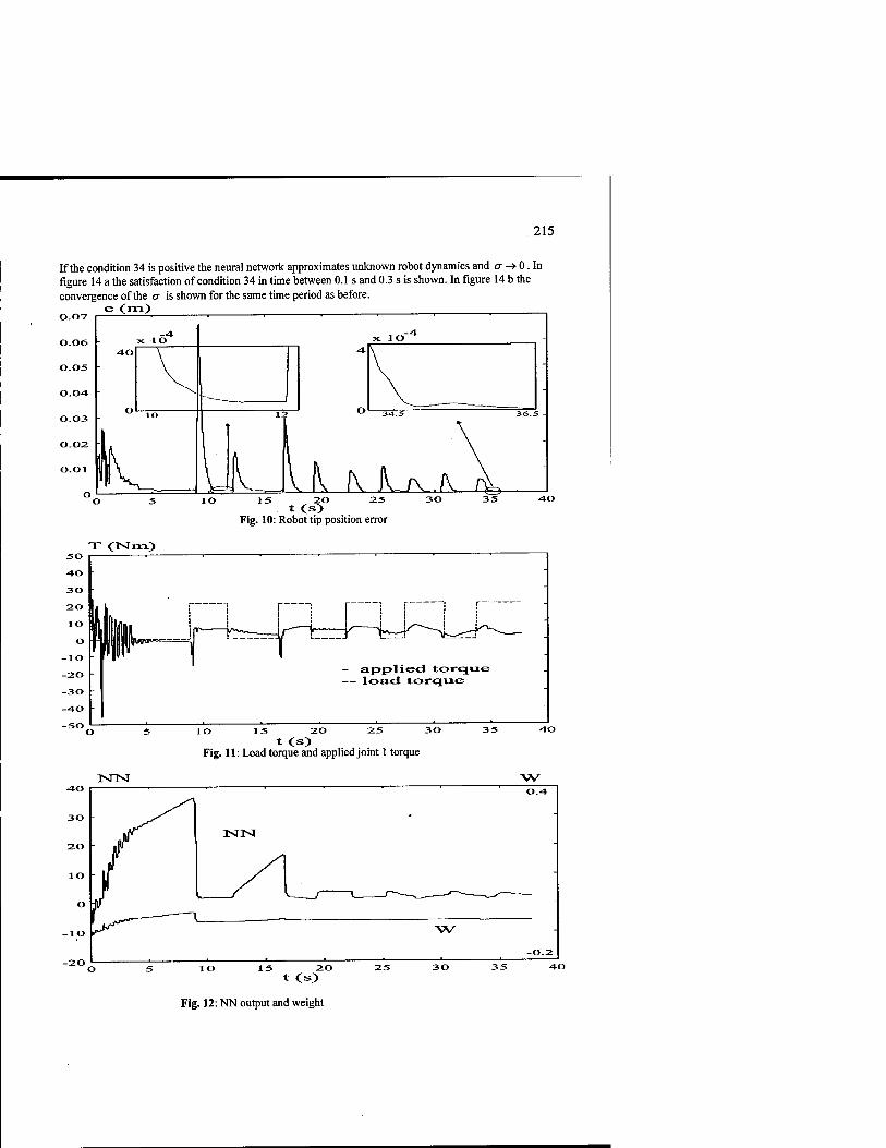
215

If the condition 34 is positive the neural network approximates unknown robot dynamics and a -» 0. In figure 14 a the satisfaction of condition 34 in time between 0.1 s and 0.3 s is shown. In figure 14 b the convergence of the CT is shown for the same time period as before.

e C"^0 _^

lO

T CNm)

TSTTSI

A__ II H IV IV a K \ 1S 20 25

t Cs> Fig. 10: Robot tip position error

15 20 t (S)

Fig. 11: Load torque and applied joint 1 torque

W

30 35 40

Fig. 12: NN output and weight

216

Fig. 13: Phase trajectory during the last of the load changes

Dcr| - IDcr+6-l

0.7

0.7

t(s) Fig. 14: A satisfaction of the convergence condition

0.7

The comparison between CSMC (continuous sliding mode controller) with Pi-estimator and NNSMC (neural network sliding mode controller)

Figure 15 shows robot tip position error when CSMC with Pi-estimator at 1 ms sampling time is used instead of our NNSMC at 2 ms sampling time for the same load changes as in figure 11. We can see that robot tip peak and steady state position error are remarkably smaller in case of NNSMC (figure 16), even if we used CSMC with Pi-estimator at 1 ms sampling time. The advantage of CSMC with Pi-estimator against NNSMC is that it could be simpler to build (it needs less computational time), so it could be executed with 1 ms sampling time with the same computer hardware. The sample time for NNSMC is 2ms. At last, figure 17 shows robot tip position error when well known computed torque method controller (CTMC) is used at the same test as before (sampling time is 2 ms). We can see that this method for the case of 3.D.O.F. DD robot mechanism with almost unknown torque vector due to Coulomb friction F{6) is of no use.

217

e(iTi)

1 Ilk. 1 i J ^ , 1 , , ». O 5 lO 15 20 UX)

Fig. 15: Robot tip position error for CSMC at 1 ms sampling time during load changes

LI Li u LI ^ 8 12 16

Fig. 16: Robot tip position error for NNSCM at 2 ms sampling time during load changes

so eo

Fig. 17: Robot tip position error for CTMC at 2 ms sampling time during load changes

218

3.4 Generalization properties of the control scheme

The generalization properties of the control scheme are defined by the ability of NN to learn how to react to the same or "almost" the same changes in the robot dynamics. The quality of generalization for the changes of the load torque (figure 11) is shown in figure 10. Peak robot tip position error and steady state error are smaller after repeating the same load change. We can see that the sliding-mode neural network controller has the ability to learn how to react to the same load changes. The interesting effect (the convergence of the peak and steady-state robot tip position error) could have two explanations. One of the explanations is that disturbances (sudden load changes) force the weights of NN learning algorithm from local minima to global minima or better local minima. Another explanation is that the neural network, due to high number of neurons in the hidden layer, has the ability to generalize reactions to disturbances. The last explanation can be proved with the next observation. If the number of neurons in the hidden layer is decreased the convergence is slower with higher peak and steady-state robot tip position error and vice versa, if the number of neurons in the hidden layer is increased the convergence is faster with smaller peak and steady-state robot tip position error. Eighty neurons instead of sixty (figure 10) are used for response in figure 16 where lower peak and steady-state robot tip position error could be observed. Figure 18 shows the lowest peak robot tip position errors after the learning time of the NN for the test of the sudden load changes in a stationary position, explained in the start of the section 3.2, when the number of neurons in the hidden layer of the NN changed between 8 and 90 neurons. All tests were made at 2 ms sampling time. When the number of neurons was smaller than 8 the quality of the control system becomes so poor that tests for such a system are not presented in the figure 18. The tests for the number of neurons greater than 90 are also not presented because they were not be done in 2 ms sampling time period due to high computational demands of the algorithm of the neural network. In fact, it was made also simulation tests on the computer model and it was estimated that for the number of neurons more than 90 there is no more substantial improvement of the system behavior.

20 40 60 80 TOO

Fig. 18: The lowest peak robot tip position error e(m) when the number of neurons in the hidden layer of the NN was changed between 8 neurons and 90 neurons at 2 ms sampling time

219

4 Conclusions

This paper presented the theoretical development and up to date the first known implementation of the neural network continuous sliding-mode controller for trajectory tracking and manipulation tasks of the real DD 3.D.O.F. PUMA like robot manipulator. The neural network was used to compensate structured (the inertia matrix) and unstructured (torque due to Coriollis forces, gravitational forces, friction forces ...) uncertainties of the robot manipulator. The adaptive and self-improving capability of the neural network controller to unstructured effects (sudden load changes) was shown. Futhermore, the robot tip position error at sudden load changes was remarkably reduced in comparison with the continuous sliding mode controller with Pi-estimator [16] or with the computed torque method controller. The satisfaction of the neural network learning condition has been shown, when the sudden change of robot dynamics occured. The quality of trajectory tracking and PTP movement control tasks with respect to two criteria: convergence properties of the neural network control algorithm and adaptation capability of the control algorithm to sudden changes in the manipulator dynamics were shown. Several trajectory tracking quality tests were made. By the new control algorithm implemented on the described manipulator mechanism a desired accuracy of the trajectory tracking high-speed movements and PTP movements in a laboratory environment is assured. In future work, the neural network sliding-mode controller will be improved, especially the speed of the convergence by a learning with momentum or/and an adaptation of the learning rate in the neural network learning algorithm.

References

1. R. Safaric, K. Jezernik.: Trajectory Tracking Neural Network Controller for a Robot Mechanism and Lyapunov Theory of Stability. Conference Proceedings IROS'94, Munich (1994)

2. T. Ozaki, T. Suzuki, T. Furuhashi, S. Okuma, Y. Uchikawa.: Trajectory Control of Robotic Manipulator Using Neural Networks. IEEE Transaction on Industrial Electronics, Vol. 38 (1991) 195-202

3. A. Ishiguro, T. Furuhashi, Sh. Okuma, Y. Uchikawa.: A Neural Network Compensator for Uncertainties of Robotics Manipulators. IEEE Transactions on Industrial Electronics, VOL. 39, No. 6 (1992) 555-570

4. H. Morioka, K. Wada, A. Sabanovic, K. Jezernik.: Neural Network Based Chattering Free Sliding Mode Control. Proceedings SICE'95 (1995)

5. A. Sabanovic: Sliding Mode in Robotic Manipulator Control Systems. Electrotechnical review, 60(2-3) (1993) 99- 107

6. A. Cichocki, R. Unbehauen.: Neural Networks for Optimization and Signal Processing. John Wiley and Sons, Chichester - New York- Brisbane

- Toronto - Singapore (1993) 7. J.J.Craig.: Adaptive Control of Mechanical Manipulators. MA: Addison-Wesley (1988). 8. J. E. Slotine and W. Li.: Adaptive manipulator control: A case study. IEEE Trans. Automat. Control. Vol. AC-33,

no. 11 (1988)995-1003 9. S. Khemaissia, A. S. Morris.: Neuro-adaptive control of robotic manipulators. Robotica, vol. 11 (1993)465-473 10. M. Terbuc, M. Rodic, K. Jezernik.: Direktno gnani robotski sistem (Direct Drive Robot System). Zbornik cetrte

Elektrotehniske konference ERK'95, Zvezek B, Slovenska sekcija IEEE, Portoroz, Slovenia (1995) 187-190 11. M. Terbuc, K. Jezernik, K. Gotlih.: Trajectory Control of DD Robot. Proceedings of the IFAC/Workshop Motion

Control, Munich, (1995) 12. J.J. Slotine, S. Shastry.: Tracking Control of Nonlinear Systems Using Sliding Surfaces with Application to Robot

Manipulators. Int. J. Contr. 38, No. 2 (1983) 465-492 13. W. J. Wang, G. H. Wu.: Variable Structure Control Design on Discrete-time Systems - Another viewpoint. Control

theory and Advanced Technology 8, No. 1 (1992) 1-16 14. K. Jezernik: Robust Chattering Free Sliding Mode Control. Int. J. Electronics 80, No 2, (1996) 169-179 15. Z. Fengxi, D. G. Fisher.: Continuous Sliding Mode Control," Int. J. Control 55, No. 2 (1992) 313 - 327 16. B. Curk, K. Jezernik, M. Terbuc: Continuous Sliding Mode Control of DD Robot Mechanism. Conference

ISIE'97, Guimaraes, Portugal (1997) 17. K. Hornik, M. Stinchombe, H. Whiteat.: Multilayer Feedforward Networks are Universal Aproximators. Neural

Networks, Vol. 2 (1989) 359-366

220

Intelligent Robotic Gait Synthesis Using Slope Information Neural Network

Jih-Gau Juang

Institute of Maritime Technology National Taiwan Ocean University

jgjuang@imt.ntou.edu.tw

Abstract A learning scheme is developed to generate walking gaits on different sloping surfaces. This scheme uses three neural networks: a neural network controller, a neural network emulator, and a slope information neural network. The neural network controller is pre-trained by a reference trajectory on horizontal surface. The emulator is pre-trained to identify the robotic dynamics. The slope information neural network provides compensated control signals to the robot on different slope angles by using the control signals on horizontal surface from the pre-trained controller. The training rule is backpropogation algorithm with time delay. The proposed technique can generate gaits on different sloping surfaces by following reference trajectory with desired step length, crossing height and walking speed.

1 Introduction

Walking robot locomotion control includes many topics, such as the design of a control law, dynamics modeling and environment fitness. In most previous studies [l]-[7], the constraints to the environment are under the assumptions on a horizontal flat surface. In this study, a learning scheme which uses a neural network controller, a neural network emulator and a slope information neural network is developed to generate walking gaits on different sloping surfaces.

Since biped locomotion is periodic, robotic walking control can be considered as a recurrent trajectory-tracking problem. Investigation of the biped locomotion can focus on gait synthesis of one walking step. Most of the gait synthesis algorithms require not only the reference pattern as the target data but also the initial conditions, such as link positions or velocities. Because the adequate initial conditions are not always available, these constraints on the needs of the initial conditions have limited the controller's capability of optimization. To overcome this problem, a near-optimal control scheme is developed in our previous study [8], [9]. This technique can generate the walking gait by using partial or inaccurate initial conditions. Further more, most of the biped locomotion studies put emphasis on balance control and walking. The step length and crossing height of a walking gait are not considered. The proposed technique can also generate the walking gait by following a desired step length and crossing clearance, which are not easy to accomplish if the traditional methods are used.

There are four parts in the proposed learning scheme: a neural network controller, a neural network emulator, biped model and a slope information network. The neural

221

network controller is pre-trained by a reference trajectory on horizontal surface. The emulator is pre-trained to identify the robotic dynamics. Since the emulator is a neural network, it can provide necessary error signals to the controller directly. Thus, the whole training architecture can be considered as one multilayered neural network and be trained simultaneously. This makes the walking learning more human like, which means all neural process. The slope information neural network provides compensated control signals to the robot on different slope angles. So that the robot can walk on different sloping surface by using a pre-trained controller (on horizontal surface) with one extra network, the slope information neural network. The control scheme only updates the weights in the slope information neural network. The controller's weights are unchanged in the learning process. Unlike other studies [10], [11], the proposed technique stores different slope angle information in one network only. There is no need to build up a look-up table or database for storing the information of different slope angles. This makes the proposed technique an adaptive and intelligent control scheme.

2 Biped Model and Reference Trajectory

In this study, the walking machine BLR-G1 robot [12] is used as the simulation model. This robot consists of five links, a body, two lower legs and two upper legs, with two hip joints and two knee joints as shown in Fig. 1.

-<>+

Fig. 1. 5-link biped model.

The dynamic equation of motion is:

4(0)9 + £(9)A(9)+Cg(0) = DT,

where 0 = [0!, 02, 93, 64, 05] ,

T = [T„ T2, x3, T4]T,

A(0) = [^02>03,9^]T,

(1)

222

g(9) = [sin9„ sin92, sin93, sin94, sine5]T,

and

A(Q) = {qiJcoS(Qi-ej) + py},

5(0) = {?,sin(e,.-e,)},

C = diag{-A,},

D =

1 0 0 0"

-1 1 0 0

0 -1 1 0

0 0 -1 1

0 0 0 -1

qv, Pij and A, are constants derived by using Lagrange's equation of motion, rf is the torque at /""joint, 9, and 6, are the position and velocity of link /'.

Before training, nominal trajectory is needed. There are several methods to determine the reference trajectory for the walking robot. The Human's walking pattern is most often used. In this study, we use a cycloidal profile [13] for the trajectories of the hip and ankle joints of the swinging leg. The reason we used this profile is that it shows an analog to human's ankle trajectory in normal walking and it is described by a simple function which can be easily changed for different walking patterns.

a In. . ,2n d,, ,2K .., *.(') = -{—'-sm(—»)}, za(0 = -{l-cos(—0},

K n n 2 n ... 1 ... a

*h(0 = Y*aO)+y, 1 rl

\0) = -^ii) + r,+r2--, (2)

where xh, zh and xa, za are the positions of hip and swinging ankle (the model we used has no ankle, so it is the point at lowest end of the lower leg in this study), a is the step length, d is the height of the swinging ankle,«is the total sampling number for a step, / is the sampling index and rt is the length of link z.

Assume the body is always upright. Let a = 40 cm, d = 11 cm and n = 25, the trajectory is shown in Fig. 2. For inclined surface, let a = 30 cm and n = 27. The reference trajectories with different crossing height are shown in Fig. 3, Fig. 4 and Fig. 5.

Fig. 2. Trajectory on level ground. Fig. 3. d = 6 cm on 5° inclined surface.

223

Fig. 4. d = 5 cm on 10° inclined surface. Fig. 5. d- 4 cm on 15° inclined surface.

3 Robot Dynamics Identification

During the past few years, investigation of the approximation capabilities of standard multilayer feedforward neural networks has received broad research interest. There have been many papers related to this problem. Hornik [14]-[16] had shown that standard feedforward networks, with as few as a single hidden layer and an appropriately smooth hidden layer activation function, are capable of arbitrarily accurate approximation to an arbitrary function. Ito [17]-[18] proved that uniform approximation could be approached with a sigmoid function as the hidden layer activation function. Kosmatopoulos et cd. [19] had used this network with the sigmoid function in the identification problem of a robotic manipulator successfully. Here, we use this standard three-layered neural network with the sigmoid function to identify the biped model. The neural network structure is shown in Fig. 6. The neural network emulator is trained to match the robot dynamics.

The robot links' current position (Qu 02,03,94,05), velocity (0,, 02, 03, 04, 05) and torque to each joint (TI, T2, T3, T4) are the inputs of the neural network emulator. The outputs are the links' position and velocity of the next state. A sigmoid function is used as the nonlinear function in the networks. An extra input, which is usually set to +1, is added to provide a constant bias to the weighted sum. Initial weights are random values from +1 to -1.

The patterns we used to train the neural network emulator are from the results of

our previous study [8]. Each stage's link positions 0' and velocities 0 are used as

network's input patterns. Control signals, Tu and next stage's link positions 0_'+1 and

velocities 0<+ are the target patterns. The training rule is the backpropagation algorithm with batch learning process [20], [21]. After training, maximum error is less than 1% of the real target value. Because the workspace of the biped robot is too big and the dynamics is too complex, it is impossible to identify the robot system accurately. Since the emulator is used as an error reference provider only, this inaccurate matching problem can be compensated for during the controller training.

224

Inputs ^\JF^ Outputs

Fig. 6. Three-layered neural network.

4 Gait Synthesis

Human walking trajectory can be modeled as a periodic function if the locomotion is performed on an unchanged surface environment. This character is very important for robotic locomotion control. If we can obtain the first cycle of the walking trajectory properly, we will be able to reduce the difficulties of the robotic walking control. The biped locomotion control will then be simplified to periodic trajectory tracking problem. Thus, gait synthesis of the first walking step becomes an important issue on the locomotion control.

A walking gait is divided into several stages. The training patterns are obtained from the reference trajectory which defines the desired step width, crossing clearance and speed. A neural network controller is used to provide the control signals. The network learns to drive the biped from an initial state S0 to the desired state Sd in k time stages, where

■S,- = (e',0')\ (3)

e'^e'^.e;,^)1, (4)

9 =(0'J,0J,03,04,95) . (5)

The objective of the learning process is to find a set of net weights that minimizes the cost function E, where E is the mean square error of the final states Sk and desired states Sd.

£=4dkf) (6) ek=Sd-Sk. (7)

Our goal in this study is to train a walking gait for which the final position 0*

approaches the mirror image of the initial position 0°, and the velocity after ground

225

impact action of its final velocity 0 approaches the mirror image of the initial

velocity 0 . The meaning of "mirror image" is shown as follows

e*=(0f,e*,e*,e*,e*)T=(0S,eJ,e»,e5,e?)T,

/p{ei:(ef,e*,e*,e*,e*)T}=(0°,0°,e»)0°,e?)T>

(8)

(9)

where Ip{§} is the function of ground impact action [9]. This means the initial position and velocity conditions of the second step are the same as the initial conditions of the first step. Once we reach this step, a conventional position and velocity feedback control technique can be used for further walking control.

4.1 Gait Synthesis Without Slope Information Neural Network

In this section, the slope information neural network is not included in the learning scheme. The learning process for the gait synthesis is illustrated in Fig. 7. There are three parts in this trajectory generation algorithm: neural network controller (NC), biped dynamic model (BM) and neural network emulator (NE). The NC is a three- layered feedforward neural network that is used to generate the control signals T, at each stage with input states $ given. The BM and the NE have been given in the previous section. The ek is back propagated through the NE then the NC at each stage. The real plant can not be used here because the error can not be propagated through it. This is why NE is needed. The error continues to be back propagated through all k stages of the run, and the network's weight change is computed for each stage. Note that the weights in NE never change; NE only passes the error through it. The weight changes from all the stages obtained from the backpropagation algorithm are added together and then added to the original weights at the end of the run. This completes the training for one run.

BTT

To ■Si-2 T„,. B M St.,

N C

TVi

*•

N K 4

ek %±S± U±L

Fig. 7. Learning process for biped locomotion.

4.1.1 Learning process

The locomotion learning is divided into three sections: lift up, cross over and landing. The following training rales are used in each section:

226

1. Set initial state So=(0°, 0° )T, desired state Sj=(Qd, & )T and £culTent=0. 2. Let *"=0. 3. Feedforward £, through neural controller; obtain Tf from network

outputs. 4. Feedforward S, and J, into biped model and neural emulator. 5. Store every neuron's output activation from neural emulator and neural

controller for later use (BTT).

6. Obtain 9 from biped dynamic equations.

7. Calculate S)+,=(0'+1,0,+1 )T, where e'+1 = (f At + Q1 and

e,+,=ie,+V+e'A/+e'. 2" - -

8. Let Z-/+1; check i<k where k is the number of stages in each section, if yes let k=k+\ then go to step 3.

9. Landing section only: check whether swinging leg touches ground or not, i.e., check za>0, if yes go to step 3.

10. Calculate ek= Sd - Sk=( Qd - 0_\ Qd - 0* )T.

11. Let Ep^iaurEeaa«*, Calculate £'current= ~ (|«A | ) ', Check

l^cmrent " ^previous| < *, ^Y^ gO tO END.

12. Back propagates ek through neural emulator then neural controller at all stages.

13. Calculate weights change AJfat each stage. 14. Update weights W=W+AW0+A1Vi+ ... +AWkA in neural controller

only. 15. Go to step 2.

After the last section (landing) training, apply the final position and velocity to the impact action equation. Add the results to the desired trajectory's initial conditions and take the average. Then set the new desired trajectory's initial conditions equal to this averaged value. Start the above training again until the results of impact action of the final conditions reach the current desired trajectory's initial conditions.

4.1.2 Simulation results

The controller's inputs are the links' position 0' and velocity Ö' of the robot's current state. The outputs are the joints' torque T{; they provide four control signals (ti, x2, t3, T4) to the robot's joints which will be used to drive the robot to next state.

The robot links' current position 0', velocity 0 and torque to each joint Tf are the

inputs of the emulator. The outputs are the links' position 0'+1 and velocity 0'+ of the next state. The emulator is trained to match the robot dynamics. Since the emulator is used as an error reference provider only, the inaccurate matching problem

227

can be compensated for during the controller training. We use sigmoid function as the nonlinear function in our networks. Initial weights are random values from +1 to -1.

To test our learning scheme, the results from [8] are used as the reference trajectory with upright body, and the initial positions are changed to 0 degree, -30 degrees, 0 degree, 5 degrees, 30 degrees for 0i, 02,03, Ö4,95, respectively. The desired step length is 36cm, maximum ankle height is 9cm, stage interval is 0.02 seconds, and the total time period of one walking gait is 0.54 seconds. The emulator is pre-trained. The learning scheme is able to generate a real walking gait by following this pattern. Fig. 8 shows a successful training. The trained step length is 37cm, maximum ankle height is 8cm, stage interval is 0.02 seconds, and the total time period of one walking gait is 0.52 seconds. The maximum position error is less than ±1.5 degrees. Now, assume the walking robot is on a 5 degrees inclined surface and the body is always upright. The desired step length is 35cm, maximum ankle height is 8cm, stage interval is 0.02 seconds, and the total time period of one walking gait is 0.5 seconds. Fig. 9 shows a successful training. The first trial takes more runs in each section's training. The number of runs decreases after each trial. As mentioned before, the desired pattern is used as reference trajectory only. The learning scheme will train the controller to follow this given pattern as closely as possible. The actual and the final step length of the above example is 32cm, and the ankle height is 10cm, with the total time period of one walking gait being 0.54 seconds. These values are very close to the desired values.

Fig. 8. Gait after training on level ground. Fig. 9. Gait after training on 5° slope.

4.2 Gait Synthesis With Slope Information Neural Network

In previous section, the controller uses different control parameters for different sloping surface's locomotion control. This requires designer to build up a look-up table or database to store the information. In this section, an extra neural network is used in the learning structure. Slope information is added in the control scheme. A trained walking pattern, which is on horizontal surface, is used as the reference control signals. The compensated control signals are provided by the slope information neural network. Walking gaits on different sloping surface can be

228

obtained by using these fixed reference control signals with the slope information network.

4.2.1 Learning process

The control scheme is shown in Fig. 10. There are four parts in this trajectory generation algorithm: neural network controller (NC), biped dynamic model (BM), neural network emulator (NE), and slope information neural network (SI). The SI is a three-layered feedforward neural network. It has eleven inputs: five link's positions, five link's velocities, and one slope angle information. The ek is back propagated through the NE then the SI at each stage. The error continues to be back propagated through all k stages of the run, and the network's weight change is computed for each stage. Only the weights in the SI are updated. The weights in the NC and the NE are unchanged. This is different to the previous section. The weight changes from all the stages obtained from the backpropagation algorithm are added together and then added to the original weights at the end of the run. This completes the training for one run. By doing this, the slope information will be stored in the SI. Thus, there will be only one set of control data to store.

S*-!

äSM TK>5IT

^.BTT

Slope Angle

AT

Sk

-+ *

Fig. 10. Control scheme with slope information neural network at stage k.

The learning process is similar to Section 4.1.1. Procedure 3,4, 5,12 and 14 are modified as follows:

3. Feedforward reference trajectory AS, through neural controller, AS, and slope angle through slope information network; obtain rand Ar from NC and SI outputs, respectively.

4. Let Ti = T+AT, feedforward Sf and T, into biped model and neural emulator. 5. Store every neuron's output activation from neural emulator and slope

information network for later use (BIT). 12. Back propagates ek through neural emulator then slope information network at

all stages. 14. Update weights W=W+AW<>+AW\+... +AWkA in slope information network

only.

Different slope angles are trained individually with same NC and NE. Each trained SI then provides training patterns for different slope angles. These data are used to train

229

the SI again. The training rule is backpropogation algorithm with batch learning process. The final trained SI stores different slopes' information and provides compensated control signals for different sloping surfaces.

4.2.2 Simulation results

The trained results in Fig. 8 are used as the reference control signals. These reference sequences provide major control signals to the robot. Compensated control signals are generated by the SI with slope angle given. The initial weights are zero in the slope information network. So that the training starts without any compensated signals. Reference trajectories on different sloping surfaces are shown in Fig. 3, Fig. 4 and Fig. 5. The step length is 30 cm. The crossing height is 6 cm in 5-degree slope, 5 cm in 10-degree slope and 4 cm in 15-degree slope. Each walking gait is 0.54 second.

Inclined walking gaits on 5 degrees, 10 degrees and 15 degrees are trained individually. These trained networks provide its results as the new training data. Then the SI is trained to store these angles' information. After training, with the original reference control signals, the SI can provide appropriated compensations to the robot and make it walks on different slope angles. The gaits after training are shown in Fig. 11. The step length is 32 cm in 5-degree slope, 28 cm in 10-degree slope and 30 cm in 15-degree slope. The crossing height is 6 cm in 5-degree slope, 5 cm in 10-degree slope and 4 cm in 15-degree slope. These values are very close to the desired values.

Fig. 11. Gaits after training on 5,10 and 15 degrees inclined surface.

Simulation results show that the proposed goals are achieved. Walking gaits on different sloping surfaces can be obtained by using fixed reference control signals with a slope information network. Giving different slope angles, the SI can generate compensated control sequences and drive the robot along a pre-specified step length and crossing height on different sloping surfaces.

5 Conclusion

230

The multilayered neural network, which derives its powerful capability from the nonlinear activation used by many researchers in robot locomotion control and the efficient backpropagation through time learning rule, has been successfully used in many experimental works. In this paper, we have shown how the layered neural networks with the time-delayed backpropagation learning rule can be applied to the gait synthesis of a walking robot. Giving the desired trajectory of a walking gait, the networks can generate control sequences and drive the robot along this pre-specified pattern on different sloping surfaces. Simulation results show that the presented learning scheme (with or without the SI) can do the gait synthesis intelligently. With the slope information network added, the learning scheme use only one pre-trained data for gait synthesis on different sloping surfaces. The proposed technique stores different slope angle information in one network only. There is no need to build up a look-up table or database for storing the information of different slope angles. This makes the proposed technique an adaptive and intelligent control scheme.

References

1. W. T. Miller and A. L. Kun, "Dynamic Balance of a Biped Walking Robot," Neural Systems for Robotics, ed. by O. Omidvar and P. Smagt, pp. 17-35, Academic Press, 1997.

2. W. T. Miller, P. W. Lathan, and S. M. Scalera, "Bipedal Gait Adaptation for Walking With Dynamic Balance," in Proc. Amer. Control Conf, pp 1603-1608 1991.

3. H. Hemami and B. F. Wyman, "Modeling and Control of Constrained Dynamic System With Application to Biped Locomotion in Frontal Plane," IEEE Trans, on Automatic Control, vol. 24, no. 4, pp. 526-535, 1979.

4. A. A. Frank, "An Approach to The Dynamic Analysis and Synthesis of Biped Locomotion Machines," Med. andBiol. Engineering, vol. 8, pp. 465-476, 1970.

5. J. Furusho and M. Masubuchi, "A Theoretically Motivated Reduced Order Model for the Control of Dynamic Biped Locomotion," Journal of Dynamic Systems, Measurements, and Control, vol. 109, pp. 155-163, June 1987.

6. S. Pannu, H. Kazerooni, G. Becker and A. Packard, "^-Synthesis Control for a Walking Robot," IEEE Control Systems Magazine, vol. 16, no. 1, pp 20-25 February 1996.

7. T. C. W. Wong and Y. S. Hung, "Stabilization of Biped Dynamic Walking Using Gyroscopic Couple," in Proceedings IEEE International Join Symposia on Intelligence and Systems, pp. 102-108, 1996.

8. J-G. Juang and C-S. Lin, "Gait Synthesis of a Biped Robot Using Back- propagation Through Time Algorithm," in Proceedings IEEE International Conference on Neural Networks, vol. 3, pp. 1710-1715, 1996.

9. J-G. Juang, "Intelligent Path Training of a Five-Link Walking Robot," in Proceedings IEEE International Symposium on Intelligent Control pp 1-6 1996. ' M-Y. Cheng and C-S. Lin, "Genetic algorithm for control design of biped locomotion," Journal of Robotic Systems, vol. 14, no. 5, pp. 365-373, 1997.

10

231

11. M-Y. Cheng and C-S. Lin, "Measurement of robustness for biped locomotion using a linearized Poincare map" Robotica, vol. 14, no. 3, pp. 253-259,1996.

12. J. Furusho and M Masubuchi, "Control of a Dynamical Biped Locomotion System for Steady Walking," Journal of Dynamic Systems, Measurement, and Control, vol. 108, pp. 111-118, June 1986.

13. Y. Kurematsu, S. Kitamura and Y. Kondo, "Trajectory Planning and Control of a Biped Locomotive Robot -Simulation and Experiment-," Robotics and Manufacturing, Recent Trends in Research, Education and Applications, M. Jamshidi (ed.), pp. 65-72, ASME Press, 1988.

14. K. Hornik, M. Stinchcombe and H. White, "Universal Approximation of an Unknown Mapping and Its Derivatives Using Multilayer Feedforward Networks," Neural Networks, vol. 3, pp. 551-560,1990.

15. K. Hornik, M. Stinchcombe and H. White, " Multilayer Feedforward Networks are Universal Approximators," Neural Networks, vol. 2, pp. 359-366, 1989.

16. K. Hornik, "Approximation Capabilities of Multilayer Perceptrons," Neural Networks, vol. 4, pp. 251-257, 1991.

17. Y. Ito, "Approximation of Continuous Functions on R6 by Linear Combinations of Shifted Rotations of a Sigmoid Function with and without Scaling," Neural Networks, vol. 5, pp. 105-115, 1992.

18. Y. Ito, "Approximation of Function on a Compact Set by Finite Sums of a Sigmoid Function without Scaling," Neural Networks, vol. 4, pp. 385-394,1991.

19. E. B. Kosmatopoulos, A. K. Chassiakos and M. A. Christodoulou, "Robot Identification using Dynamical Neural Networks," in Proc. IEEE Conference on Decision and Control, pp 2934-2935, December 1991.

20. D. E. Rumelhart, J. L. McClelland, and the PDP Research Group, Parallel Distributed Processing, The MIT Press, 1987.

21. P. J. Werbos, "Backpropagation Through Time: What It Does and How to Do It," Proceedings of the IEEE, vol. 78, no. 10, pp. 1550-1560, October 1990.

232

A High Performance Precision Linear Stage using Predictive Control and Genetic Algorithm

Kay-Soon Low, Meng-Teck Keck

Nanyang Technological University, School of Electrical and Electronic Engineering Blk S2, Nanyang Avenue, Singapore 639798

Email: ekslow@ntu.edu. sg

Abstract. To improve the productivity, vision based leads inspection systems are used in the industry to ensure that the lead form meets the PCB assembly requirement. Such system comprises a camera system and a linear stage. In this paper, we present the motion control system of our prototype leads in- spection system. To achieve high performance, we use a permanent magnet DC linear motor as the actuator for the linear stage. This eliminates the needs of mechanical transmission from the rotary to linear motion. To obtain fast and accurate servo response, a model predictive controller has been developed for the closed loop motion control. The gains of the controller are optimally tuned by using genetic search algorithm. The proposed approach results in a system that has a positioning accuracy of 1 urn and a speed of more than 1 m/s. Some experimental results are presented.

1 Introduction

The advancement of microelectronics has resulted in the continuing increase in the lead counts and tighter lead pitches of the integrated circuit. Consequently, the leads have become inherently more fragile and the lead forms may not meet the PCB as- sembly requirements after the integrated circuits have gone through the various pro- cesses. Thus, vision based leads inspection systems are increasingly used in factory automation for improving the productivity. Besides the computation time required by the vision algorithm, the speed of the motion control system plays a vital role in the overall performance. In most of the present industry systems, the rotary type brush- less DC motors are used as the actuators. To obtain the required linear motion, lead screws or other mechanical means are usually used for the mechanical transmission. Consequently, the achievable maximum speed and acceleration are limited.

In this paper, we discuss the development of the motion control system used in our leads inspection system; whose primary objective is to perform automated leads in- spection efficiently for fine pitch packages such as Quad Flat Packs (QFP) etc. The

233

system uses a permanent magnet DC linear motor. This leads to a system that offers a smooth direct drive linear thrust, as there are no mechanical transmission devices. Consequently, high performance and accurate positioning can be achieved in closed loop.

To obtain a robust and fast closed loop system, we use the model predictive control (MPC) approach to control the linear stage. Within the framework of model predic- tive control, there are various ways to design a predictive controller. For examples, generalised predictive control (GPC), Dynamic Matrix control (DMC), etc. In con- trast to other control methodologies, the MPC employs a strategy known as the re- ceding-horizon approach [1,2]. In this approach, the controller predicts the output of the plant over a time horizon based on the system model and the assumption about future controller output sequences. The sequence of the control signals is calculated such that the tracking error is minimized. This process is repeated for every sample interval to allow regular updating of new information. Consequently, this leads to a system that is robust against modeling errors and disturbances.

In this paper, a controller based on the GPC approach is developed for the linear stage. The GPC approach has been applied successfully in various process control industries [3,4]; and has proven to be an effective and reliable control methodology. Its' application in the process industries include steel casting, glass processing, oil refinery, pulp and paper industries, etc. It has also been investigated in the area of motor control [5,6]. In this paper, we explore its application in the control of the linear stage. To achieve optimal performance, the genetic algorithm (GA) is used to search for a set of well-tuned control parameters. GAs are global, parallel search techniques which emulate natural genetic operations [7,8]. As compared to other optimization techniques such as the traditional gradient-type optimization proce- dures, GA obtains the optima by evolving from generation to generation without the needs of stringent mathematical formulation. Moreover, the GA evaluates multiple points in the search space simultaneously. Consequently, it is capable of searching for a global optimum solution. GA has been used by a number of researchers to find the optimum gains of a PID controller [9,10]. In this paper, we use it to search the optimum gains of the predictive controller. The effectiveness of the proposed ap- proach has been evaluated using our experimental prototype. The results have dem- onstrated that the GA based optimized predictive controller for the linear stage has performed well.

2 The Permanent Magnet Brushless DC Linear Motor

The motor under consideration is a permanent magnet brushless DC linear motor. It has a short moving coil secondary (containing a three-phase winding), that is posi- tioned in the airgap between an U shaped permanent magnet primary. It can be thought as a rotary permanent magnet synchronous motor (PMSM) that is rolled out flat. In brushless DC linear motor, the rotor is rolled out flat to become the magnet

234

track (also known as the magnet way). The stator windings of the PMSM are rolled out flat to become the coil assembly (also known as the slider). Due to the relative masses of these two components, the magnet way is usually stationary and the coil assembly is in motion in most applications. However, reverse arrangement is also possible and is sometimes advantageous.

In our system, we use the ironless type linear motor. It has no iron, or slots for the coils to be wound on. Therefore, the motor has zero cogging. These characteristics result in low bearing friction and high acceleration. Fig. 1 shows the picture of our experimental system. As shown in the picture, the magnet way of the motor is placed upright. The travel length of the magnet way is 0.33m. The slider is attached to a platform that is supported by two low friction linear guides placed at two sides of the magnet way. The winding of the coil assembly has a rated peak current of 7A per phase. The motor has a peak force and continuous force rated at 76N and 38N re- spectively.

Fig. 1. The experimental leads inspection system

235

3 System Setup and Dynamic Model of the Drive

3.1 System Setup

The block diagram of the system setup is depicted in Fig. 2. The motor is driven by a three-phase voltage source PWM inverter. The switching signals of the inverter are generated by the current controllers, which receive reference signals from the outer servo control loop. The output of the servo controller gives the d-axis and q-axis current commands. As the motor has sinusoidal back emfs and its generated force depends only on the q-axis current, the d-axis current reference is set to zero in this application. As a safety precaution, the peak current command of the q-axis current loop has been limited to 6A in the implementation. To facilitate position measure- ment and to provide the commutation logic, a linear optical encoder with a resolu- tion of lfim has been used. The linear encoder is placed at the outer side of the fix- ture as shown in Fig. 1. For the industrial applications, a resolution of 10 |j.m is acceptable. The use of a higher resolution encoder provides us the flexibility to re- configure the system for other developmental work in the future. With the measured motor position and the outputs from the current controllers, the reference signals for the PWM inverter can be generated using an inverse dq transformation. In the sys- tem, the various controllers and functions have been implemented in software using a 32 bit floating-point digital signal processor (TMS320C31). A sampling period of 2ms has been used for the servo control loop.

236

&

ti

666

<£)<C/ig)

mm -► GA optimized

Predictive Controller

I Observer

PI Current Controllers

33

PWM

Inverse dq Transformation

dq Transformation

TMS320c31

Commutation Angle generator

Fig. 2. The overall block diagram of the system

3.2 Dynamic Model of the Drive

Linear Motor

Linear Encoder

To model the linear motor, we define the control input u as the motor q-axis current. Let the output of the drive be the mechanical position d and mechanical speed v. For the inner current control loops, two PI controllers have been used. With properly tuned current controllers, the effect of the d-axis current dynamics on the system output can be neglected. Fig. 3 shows the simplified block diagram of the drive.

Uaad

K

^T{[^»P^»|R^-»FL

r

Isf-R ^|-> + *

K.4

d

Fig. 3. Block diagram of the drive.

237

Define the state variables and the output of the system as,

Z=[d v iq yf, (1)

Y=[d vf. (2)

Then the motor dynamics can be described using the following state space equation,

Z = AZ + Bic.+EFL, (3)

where

Y=CZ , (4)

0 1

0 -D M

L 0

0

EL M

R + Kf L

-Kt

B K„

0 0-^ JL/

K,

10 0 0] E = 0 1 0 0J 0 0 0

M

In the above system, R and L are the motor winding resistance and inductance. D is the viscous frictional coefficient. Mis the mass of the moving coil secondary plus the nominal weight of the camera system. Kf is the force constant. Kb is the back emf constant, and FL is the unknown disturbance, which includes both frictional force and additional loads due to the use of different cameras and mounting brackets.

In this paper, we treat the disturbance as unknown constant load. This assumption is reasonable, as the load will not change once the camera and the supporting bracket are fixed to the system. Thus, (3) & (4) can be expressed using the following discrete time state space model,

AZ(kT + T) = G AZ(kT) + HAi* (kT),

AF(kT) =CAZ(kT) ,

(5)

(6)

where T is the sampling time of the system and

238

G = eAT , H = (jeAÄdA)B, 0

k is the discrete time index and A is the difference operator such that

AZ(kT) = Z(kT) - Z(kT- T),

AiJ(kT) =/J(kT) -z*(kT-T),

AF(kT) = F(kT) - F(kT - T) .

From (5) and (6), we reformulate the system as,

(7)

(8)

(9)

(10)

AZ(kT + T)" F(kT)

G 0 C I

AZ(kT) F(kT-T)

+ H 0

A**(kT) .

Define

X(kT) = ' AZ(kT)" F(kT-T)

(11)

(12)

then (11) can be expressed as

X (kT + T) = GX (kT) + HAiq (kT)

F(kT) = CAT(kT),

(13)

(14)

where

G = G 0 C I

H H

0 10 0 0 10 0 10 0 0 1

With this model of the drive, we can now proceed to design the control system. This will be discussed in the next section.

4 Design of Control System

To develop the motion control algorithm for the drive, we employ the model predic- tive control approach which uses the receding horizon control strategy. In this strat- egy, a sequence of future control signals is calculated by minimizing a cost function defined over a prediction horizon. However, only the first element of the calculated

239

control sequence is used to drive the motor. At the next sampling interval, the con- trol calculation is repeated again based on the new measurements to obtain a new sequence of control signals.

d' K,

V controller gain

sa l/z

current controllers >^-> 3-0 brushless

linear motor drive

observer

controller gain tH encoder ^

Fig. 4. Controller and observer structure

Figure 4 shows the control structure of the system. In the model predictive control approach, the control law of the first element can be written as,

A ^„(kT)=K1[rf (kT) v (kT)f+K2A:(kT) (15)

where Ki and K2 are the controller gains, d , v are the position reference vector

and speed reference vector respectively. X is the estimate of X. Denote A

J(kT + 7'F|kT) as the prediction of d(kT + jT) at time kT, the controller gains

Ki and K2 can be obtained by minimizing the following cost function,

j=i

„A |P Ny A f Nu 2 l\kT+jT)-d(kT+j7\kTi +Z v\kT+jT>-v(kT+fl}kTJ + xfhiq{kT+jT-ft

II J=1 1 /=!

with respect to Aia and subject to the constraint that, (16)

MJkT+jT-T) = 0, VJ>NU. (17)

The parameter Ny in (16) is known as the prediction horizon. It is defined as the interval over which the tracking error is minimized. The control weighting factor X is used to penalize excessive control activity and to ensure a numerically well condi- tioned algorithm. The parameter Nu is called the control horizon. It defines the de- gree of freedom available for optimization.

240

5 Gain Search based on the Genetic Algorithm

Traditionally, the controller gains are determined by solving (16) with a specified set of control parameters, namely the Ny, Nu and X. With the computed gains, the re- sponse can then be simulated. The control parameters are then re-adjusted and the process is repeated again until a satisfying response is obtained. This approach is time consuming and may not yield optimal performance as the effect of the amplifier saturation, system noise etc are not taken into consideration.

In this paper, we use the genetic algorithm (GA) to search for the optimal gains. GA is an adaptive search technique that mimics the process of evolution based on Dar- win's survival-of-the-fittest strategy. The operation of GA is based on the principle emanating from evolution theory [7]. The underlying basis of GA comprises a set of individual elements and a set of biologically inspired operators defined over the population itself. The potential solution is represented by a string, which is also known as the chromosome. Normally, the chromosomes are represented in binary form. However, some researchers have used other representations such as integer and floating point number to suit the needs of their problems [8].

These chromosomes undergo three basic genetic operations: reproduction, crossover and mutation. When a new organism is to be created, two parents are chosen from the current population. Organisms that have high fitness scores are given a higher probability to be chosen as parents. In this paper, parents are chosen with a rank- based mechanism. Thus, the worst performing organisms are always replaced with the new organism that is created through the basic genetic operations, regardless of its fitness score. Unlike some genetic algorithm systems whereby a parent's chance to be selected for reproduction is directly proportional to its fitness, a ranking approach offers a smoother selection probability curve. Consequently, it prevents good organ- isms from completely dominating the evolution too early.

To use the genetic algorithm for optimal gain matrix search, we first encode the control parameters by a set of genes using floating point numbers. The use of float- ing point numbers rather than the binary string eliminated the difficult task of en- coding and decoding the chromosomes. In the encoding, the genes are string to- gether to form a single chromosome. The search then starts with a random initial population. In our formulation, the size of the population is set as 50. Thereafter, the entire generation of the chromosomes can be readily processed in accordance with the three basic genetic operations. For these operations, the crossover probability pc

is set as 0.6 and the mutation probability pm is set as 0.02.

The fitness function to be minimized by the genetic algorithm is defined as,

AT 2 «

Fitness = iwid*(kT)-d(kTJ +w2iv*(kT)-v(kTJ +^[A/(/rr|2 (18) k=0

241

where AT =Tf is the user defined move time set for the linear stage to reach the final position dpk. In (18), Wi , w2 and w3 are the weighting factors. To achieve a smooth motion, the position reference trajectory is formulated as follows,

/(*) =

lpk r

ilT ■, (0<kT<Tf)

lpk (kT>Tf)

(19)

where the parameters a and c determine the slope and the settling time of the posi- tion profile. The corresponding speed reference trajectory is

v (k) = \ d\k) (0<kT<Tf)

(kT>Tf) (20)

With the system model (13)-(14) together with the experimentally identified friction model and system noise, the control law (15), the reference motion trajectory (19)- (20) and the fitness function (18), the genetic algorithm can now proceed its evolu- tionary process to optimize the digital controller. Fig. 5 shows the results of the aver- age fitness and the best fitness over the iterated generations. As shown in the figure, the fitness level is minimized after 1000 generations. No further improvement is found after that.

242

^ Average Fitness

lest Fitness

1000 1200 Generations

1*0 1600 1800

Fig. 5. Average and best fitness values versus generations

6 Experimental Results

To study the effectiveness of the proposed approach, various experiments have been conducted. We first study a full-length move of the system with a 30cm position reference. In this test, the desired motion profile is specified as in (19) and (20) with a move time of one second. The experimental results are demonstrated in Fig. 6-8. Fig. 6 shows the actual position response. The result confirms that the system follows the position reference trajectory accurately. Furthermore, it reaches the desired final position at the one second settling time. The corresponding speed response in Fig. 7 shows that the achievable peak speed reaches 1.127 m/s at half the move time (i.e. 0.5 seconds). We can further increase this peak speed by setting a higher gradient of the reference trajectory. However, this is at the expense of higher control signals. Fig 8 shows the speed versus position profile. In this figure, both the reference and the actual experimental results are shown together for ease of comparison. It is clear that the actual trajectory follows very well with the desired motion profile. Another set of the experimental results is shown in Fig. 9 - 11. In this case, the required move distance is reduced to 2cm and the settling time is set to 0.15 second. Fig. 9 shows the position response. The speed response in Fig 10 shows that the achievable speed is 0.474 m/s while the motor current (Fig 11) remains below the saturation limit of 6A.

243

1.5

0.3

0.25

0.2

0.15

0.1

0 0.5 1 1.5 2

Fig. 6. Position response of 30cm setpoint

0.8

0.6

0.4

0.2

~*\ I Ac Ni. /

tual

/Kr \I \ Reference j \

0 0.05 0.1 0.15 0.2 0.25

Fig. 8. Desired & actual motion profile

0.5

0.45

0.4

0.35

0.3

0.25

0.2

0.15

0.1

0.05

0 0.05 0.1 0.15 0.2 0.25

Fig. 10. Speed response of 2cm setpoint

0.5

0.5

Fig. 7. Speed response of 30cm setpoint

0.02

0.015

0.005

0 0.05 0.1 0.15 0.2 0.25

Fig. 9. Position response of 2cm setpoint

10r

0.05 0.1 0.15 0.2 0.25

Fig. 11. Motor current response of 2cm set- point

244

7 Conclusions

The development of a high precision linear stage using a permanent magnet dc lin- ear motor drive has been presented in this paper. High closed loop performance is achieved by using a predictive controller. The gains of the controller have been op- timally tuned by using the genetic algorithm which minimises a fitness function that reduces both the tracking errors and control signals. An experimental system has been constructed. The linear stage allows our vision system to move rapidly with a positioning accuracy of 1 \im and at a speed of more than 1 m/s. The experimental results have demonstrated that the system performs well.

References

[1] Clarke, D. W.: Advances in Model-based Predictive Control. In: Clarke, D. W (Eds).Advances in Model-Based Predictive Control, Oxford Science Publica- tions, (1994) 3-21

[2] Soeterboek, R.: Predictive Control - A unified approach. Prentice Hall (1992) [3] Jolly, T., Bentsman, J.: Generalized Predictive Control with Dynamic Filtering

for Process Control Applications. Conference record of American Control Conference, San Francisco, California, (1993) 1741-1745

[4] Wang, Q., Chalaye, T. G. G, Gilles, G: An Industrial Application of Predic- tive Control to Glass Process - Working Basin and Feeder. Conference record of IEEE Conference on Control Applications, (1994) 1891-1896

[5] Zhang, L., Norman, H. R., Shepherd, W.: Long-range predictive control of a current regulated PWM for induction motor drives using the synchronous ref- erence frame. IEEE Trans. Control Systems Technology, Vol. 5, (1997) 119- 126

[6] Low, K. S., Chiun, K. Y., Ling, K. V.: Evaluating generalized predictive con- trol for a brushless DC drive. IEEE Trans. Power Electronics., Vol. 13, No. 6, (1998) 1191-1198

[7] Goldberg, D.E.: Genetic Algorithms in Search, Optimization and Machine Learning. Addison-Wesley (1989)

[8] Man, K.F, Tang, K.S., Kwong, S: Genetic Algorithms : Concepts and Appli- cations. IEEE Trans, on Industrial Electronics, Vol. 43, No. 5, (1996) 519-533

[9] B. S. Chen, Y. M. Cheng and C. H. Lee: A genetic approach to mixed H2/Hoc optimal PID control. IEEE Control System Magazine, Vol. 15, No. 5, (1996) 51-60

[10] Wang, P., Kwok, D. P.: Optimal design of PID process controllers based on genetic algorithms. Control Engineering Practice, Vol. 2, No. 4, (1994) 641- 648

245

Robot Behavior Evolution based upon the Intelligent Composite Motion Control

Masakazu Suzuki

Department of Precision Mechanics, Faculty of Engineering, Tokai University 1117 Kitakaname, Hiratsuka, Kanagawa, Japan

suzuki@keyaki. cc .u-tokai .ac.jp

Abstract. The Intelligent Composite Motion Control (ICMC) is a methodology to build up robot systems in which robots can realize complex and dexterous behaviors autonomously and adap- tively by parameter optimization and utilization of empirical knowl- edge only if the motion control for fundamental element motions is given. In this article, first reviewed is the ICMC, mainly as for the Method of Knowledge Array which gives a tool for realiz- ing suboptimal motions for unexperienced situations by use of the empirical knowledge. And the behavior evolution based upon the ICMC is proposed, i.e., it is shown how a robot motions are coor- dinated from the most fundamental motions such as joint rotation, and how they are evolved into complex behaviors such as dexterous ball throwing.

1 Introduction As robots are requested to perform more and more complex and dexterous mo- tions, methodologies for intelligent robot behaviors are vigorously investigated (e.g. [1] ~ [8]). Some of those, however, assume a complex system structure as a precondition or remain too conceptual. Others realize highly autonomous behavior selection method, but most robot behaviors produced are quite simple. These circumstances may be a cause of the large gap between intelligent robots and current practical robots, and the fact seems to delay intelligent robots to be put onto practical use.

The Intelligent Composite Motion Control [10], ICMC, aims for realizing highly intelligent robots that can perform complex and dexterous behaviors autonomously and adäptively only if the motion control for fundamental ele- ment motions is given. In the ICMC a complex robot behavior is regarded as a combination of some simple element motions and dexterous robot behaviors are realized by optimally composing the element motions. Thus the hierarchical structure assumed in the ICMC is simple: all the robot behaviors from joint rota- tions, simple point-to-point (PTP) motions to complicated tasks are regarded as "element motions and composite motions". And a complex robot motion is real- ized as a composite motion by directly and explicitely composing some element motions which are already realized by current practical robots. Therefore the ICMC is applicable to current industrial robots as well as to future much more complicated robot systems in a unified manner. And this noticeable advantage might bridge the gap stated above.

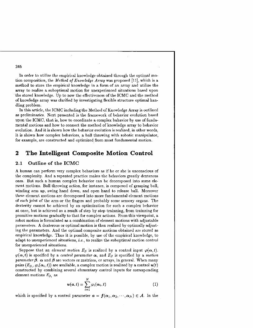
246

In order to utilize the empirical knowledge obtained through the optimal mo- tion composition, the Method of Knowledge Array was proposed [11], which is a method to store the empirical knowledge in a form of an array and utilize the array to realize a suboptimal motion for unexperienced situations based upon the stored knowledge. Up to now the effectiveness of the ICMC and the method of knowledge array was clarified by investigating flexible structure optimal han- dling problem.

In this article, the ICMC including the Method of Knowledge Array is outlined as preliminaries. Next presented is the framework of behavior evolution based upon the ICMC, that is, how to coordinate a complex bahavior by use of funda- mental motions and how to connect the method of knowledge array to behavior evolution. And it is shown how the behavior evolution is realized, in other words, it is shown how complex behaviors, a ball throwing with robotic manipulator, for example, are constructed and optimized from most fundamental motion.

2 The Intelligent Composite Motion Control

2.1 Outline of the ICMC

A human can perform very complex behaviors as if he or she is unconscious of the complexity. And a repeated practice makes the behaviors greatly dexterous ones. But such a human complex behavior can be decomposed into some ele- ment motions. Ball throwing action, for instance, is composed of grasping ball, winding arm up, swing hand down, and open hand to release ball. Moreover these element motions are decomposed into more fundamental element motions of each joint of the arm or the fingers and probably some sensory organs. The dexterity cannot be achieved by an optimization for such a complex behavior at once, but is achieved as a result of step by step trainning, from trainning for promitive motions gradually to that for complex actions. From this viewpoint, a robot motion is formulated as a combination of element motions with adjustable parameters. A dexterous or optimal motion is then realized by optimally adjust- ing the parameters. And the optimal composite motions obtained are stored as empirical knowledge. Thus it is possible, by use of the empirical knowledge, to adapt to unexperienced situations, i.e., to realize the suboptimal motion control for unexperienced situations.

Suppose that an element motion Eß is realized by a control input ip(a,t). (p(a,t) is specified by a control parameter a, and Eß is specified by a motion parameter ß. at and ß are vectors or matrices, or arrays, in general. When many pairs (Eßt, y>,-(a,-, <)) are available, a complex motion is realized by a control u(t) constructed by combining several elementary control inputs for corresponding element motions Eß{ as

N

8 = 1

which is specified by a control parameter a = f(cti,a2, • • •, ctjv) £ A. In the

247

simplest case / is the identity mapping, i.e., a = [c*i a2 ■ ■ ■ <*N]- But as the motions become complex, only a small part of the large number of control parameters can be skillfully determined. The complex motion realized by (1) is refered to as a composite motion composed of Eß{,i = l,2,---,N, and is represented as C7. The composite motion C1 is specified by a motion parameter 7 er.

A dexterous motion is realized, like the case of human, through "practice", or iteration of composite motions, i.e., by modification of the parameter a so that some performance index is minimized. Therefore the optimal motion composi- tion problem is formulated as a parameter optimization problem:

min J-yfa] (2) a,£AycA

where J7 is the performance index that evaluates the optimality (dexterity) of the composite motions. For complex robot motions, the function J7 is unknown in general, the value of J7 is obtained only by a trial, i.e., by actually performing the composite motion corresponding to a. A-, C A represents the constraints on the control parameter a corresponding to the motion parameter 7. When 7 is the desired position/attitude in a PTP motion, for instance, a represents the variation of each joint angle (see subsection 4.2), and then a is restricted by movable range of the joints depending on hardware structure and/or working space.

All the experiences of optimal composition, (7*, ak), k = 1,2, • • •, meaning the control specified by ak was optimal for the motion specified by 7*, are stored as empirical knowledge. And then, in order to seek suboptimal composite motions based upon the past experiences, some manipulation such as interpolation is given to the knowledge data, that is, the basic knowledge obtained for typical situations (scattered in motion parameter space) is generalized into the one for the situation overall (See Figure 1). In this way robots adaptively realize suboptimal composite motions for unexperienced situations by utilizing the past experiences.

2.2 Method of Knowledge Array

The numerical knowledge data obtained through optimal compositions distribute continuously over the space of the motion parameters which express various situations. For the effective utilization of such spatially distributing numerical data, the array [9] is so attractive because spatial data structure is preserved in the array and then the spatial distribution pattern can be utilized.

An array a is represented with its elements, a»1ia...1-<1, *"*: = 1,2, ■■■,h (k = 1,2, • ••,<*) , as

a = {aili2...id} £ R(d I h,h,--- Jd)

where R{d \ h,h, ■ ■ ■ ,Id) is refered to as an array space which is the space composed of all arrays having d suffixes with their maximum values h (k = 1,2, ■■■,d). On account of its general structure, it is expected that the array

248

Control j parameter a

I iff f i* • • Motion parameter / 1 2 3 4 5 ••• Motion index ;'

Figure 1: Suboptimal control parameters from empirical knowledge: • represents the optimal control parameters obtained by optimal composition, o represents suboptimal control parameters estimated from empirical knowledge

will realize intelligent knowledge operations done by human unconciously such as "abstraction" and "broad interpretation" which have been difficult to realize in engineering problems.

Storing the empirical knowledge into an array, a specific motion can be repre- sented by a set of suffixes of the knowledge array, which is refered to as a motion index. The elements of .the knowledge array for unexperienced situations are es- timated so that they conform the empirical knowledge under some smoothness constraint. Once a knowledge array is generated, a suboptimal control parame- ter for an unexperienced motion 7 can be promptly obtained only by accessing the elements of the array corresponding to 7.

Suppose that the control parameter to be optimized is an array a — {a,^,-.,...^}

G A = R(d I h,h,- ■■ ,Id) , and the motion parameter is a vector 7 = {7*} €

r = Re. The domains of jk, T^(jk), are divided into </& sub domains adequately

V(yk) = Vl+Vl + --- + Vi as

■\Jk = 1,2,-...e (3)

where V\ = [7°>72] ,!>{* = (fi^M'] , i* = 2,3, • • ■, h- Then a knowledge array V and an auxiliary knowledge array S are considered.

v = {vi1i3...idjc...hh} eK = A®r , s = {sjlj2...jc} Gr (4)

where JT = R(e \ Ji,J2,---,Je) • The empirical knowledge is accumulated in V, and the reliability of the empirical knowledge is stored in S.

When a control a" = {afli2...id} was optimal for a motion 7" = {7£} ,7£ €

Pfc ,fc=l,2,---,easa result of optimal composition, then the result is stored in V and S. And for every experience of optimal composition for the motion

249

Figure 2: Division of domains of motion parameters for a case e = 2. Divided is a rectangular solid when e = 3, and a hyper-rectangular-solid when e > 4

specified by motion index (j?j$ • ••./"), all the corresponding elements of V and S are updated as

"iii2-'-*dii

CSjnjn...jnVili2...idjn...jnjn + ßüf^...^

< s

(5)

(6)

where weighting parameters satisfy 0<a<l,0</?<l, and then V and S are formed as shown in Figure 3. Basically, (5) calculates the average value of the optimal control parameters obtained in the past experiences, and (6) counts the number of times of the motion optimization with adequate saturation. The updating formulea (5),(6) are the prototype, there may be various modifications.

V_1J2,j1 V_2,j2J1 SJ1J2

Figure 3: Knowledge array and auxiliary knowledge array for a simple case of d=l,Ii = 2le = 2,Ji = 4,J2 = 3.

Now consider that it is required to perform a motion specified by 7" =

{7ft } > 7* ^ T^k >k - 1' 2>""' >e- The contro1 parameter a" is determined by uti- lizing V as follows. If the motion 7" has been optimized in the past («JJ>>»...J» >

250

0), a suboptimal composite motion based upon the past experiences can be re- alized by directly utilizing V, i.e.,

«n = K«a...,<}, "»i»»--»<i.7?i •w (7)

If there is no empirical knowledge for 7" (S,/»JJ...J» = 0), it is impossible to determine a" directly from V. In such a case Vili2...idjn...jnjn are estimated by interpolating the already-obtained elements of V, and determine a" with the estimated values to execute 7".

For a more precise knowledge with respect to the motion in a specific param- eter domain, the corresponding subdomain is devided again into smaller ones, and then the knowledge array becomes a generalized array. To consider some new factors to realize more dexterous or refined motions, increased is the number of suffixes of the knowledge array.

3 Behavior Coordination

3.1 Hierarchical Structure of Composite Motions

The optimal composite motion obtained by optimally composing several element motions on a certain intelligence level is regarded as an element motion on a higher intelligence level (See Figure 4). Starting from low intelligence level, gradually realized are highly intelligent robot motions.

High /

Opfy

cyrEß7 fyz-Eßs

Cy^-Eßg Cy4

Eß{ Ep2 Eßi Eß4 Eß5 Eß6

Figure 4: Hierarchy of composite motions: a composite motion C72 obtained by optimally composing Eß3, Eßi and Eßi is regarded as an element motion Eßt for composite motions on a higher intelligence level

Knowledge arrays produce optimal control parameters from the given motion parameters. As a behavior becomes complex, however, the total control parame- ters to perform a composite motion will be vast. Thus the output of a knowledge

251

arrays for a complex composite motions is not the total control parameters but some intermediate parameters, which specify its component element motions, and are transformed into motion parameters and handed over to the knowledge arrays for the element motions. And finally, the motion parameters indirectly specify the total control parameters through the element motions.

3.2 Behavior Coordinator In order to use knowledge arrays in practical, it is necessary to equip a behavior coordinator, a behavior evaluator and an actuator controller (See Figure 5).

Situation

Composite motion Cy j^

1 ..-Parameter

Behavior Coordinator

Choice elf, \ element \ potions \

4

Performance Criterion Jy

Knowledge array for Cy

Behavior Evaluator

motions

Knowledge arrays for ipa\ component element motions i^P; /

Actuator Controller

Motor Torque r(0

Robot Robot ( Motion

Figure 5: Behavior coordination and utilization of knowledge array

The behavior coordinator plans an appropreate composite motion 7 from a given situation, i.e., chooses several element motions Ei, £2, • • •, EN and a way of motion composition (sequential or parallel), and specifies the control param- eter a to be optimized (including the relation between a and ßi,ß2, ■ • • >/3/v)-

252

Moreover the behavior coordinator has to define performance criterion to eval- uate the resultant composite motion.

The actuator controller generates, in many cases, motor torque from the con- trol parameter given by the knowledge arrays on the lowest intelligence level. The actuator controller is, however, a matter of little concern here, hence ex- pression of the controller is often omitted and it is assumed to be included in the robot. The behavior evaluator evaluates composite motions based upon the performance criterion defined by the behavior coordinator.

Two ways of behavior coordination might be considered: One is coordina- tion by teaching, the other is autonomous coordination by robot itself. In the coordination by teaching, adequate element motions and control parameters to optimize are selected by the robot user or operator. In case of behavior coordi- nation by autonomous learning, various candidate sets of element motions are chosen, and the best one is selected so that simulated composite motion gives a satisfactory behavior result by some optimization technique such as genetic algorithm.

When a situation i.e., an environmental condition, an objective of the behavior and so on, is given, the robot itself thinks what to do, plans the behavior and then controls the necessary motions. The ultimate intelligent robot should be something like this. But at this moment it is quite difficult to realize such high intelligence. If the purpose and outline of the motion process are instructed by a teacher, then the robot autonomously achieves the optimal (i.e., favorable and fitting to the purpose) motion by repeated practice. Such kind of semi- autonomous robots may be valuable, too. This conception will be acceptable to industial applications.

On the other hand, the ultimate intelligent robot should perform autonomous behavior planning by learning without any teacher. When a human performs a complex bahavior, he or she combines element motions in mind to plan a complex motion and checks, by using imagination, whether the composite motion can achieve the purpose or not. It is, as it were, feasibility check by imaginative simulation. A rough mathematical motion model of a robot is usually available. Based on the model, it is possible to roughly simulate pre-planned behaviors and plan a feasible composite motions through some optimization techniques.

4 Behavior Evolution — From Joint Rotations to Dual Arm Cooperation —

4.1 Joint Rotations

Joint rotation is most fundamental. Joint rotations with acceptable accuracy can be realized by model-based control theory, hence learning is not necessary for currently used robots. While, living creatures seem to realize even this kind of primitive motions by repeated training. Therefore in order to realize intelligent motions of future animal-like robots that have mechanisms which are absolutely

253

different from those of current robots, it will be quite significant to realize this fundamental motion by learning.

n 9(a,t) 5 t s>

^ h u

'l h t

T, i , , 6

Figure 6: Torque and control parameters for joint rotation

Figure 6 shows a simple time chart of the joint torque r{t) = ip(pT,t) specified

by pT = [ti t2 t3 <4 T\ r2] , which realizes an element motion: a joint rotation with angle A9. The function of the knowledge array for joint rotation is then to produce the control parameter a = pT from the motion parameter ß = Ä0 (See Figure 7).

fi=Ad Joint Rotation

a=pt Actuator Controller

T{t) Robot

Joint a Rotation At/

Figure 7: Knowledge array for joint rotation: Given motion parameter Ad, the knowledge array produces control parameter pT, which is handed over to actuator controller to generate torque r(t), and the requested joint rotation A6 is realized

The joint rotation realized by a control parameter pT is basically evaluated by the difference between the requested rotation angle 0r and the actual rotation angle A6(pT). The criterion function is then defined as

jA9\pT] = \AeT-Ae(pT)\

Even for the simple torque time chart in Figure 6, the pT that realizes A9T = A9(pT) is not unique. In order to minimize the time or the energy to complete the requested joint rotation, \t4 -tx\ or ft

4 r(t)2dt is added to JAO\PT] witn an

adequate weighting parameter, respectively.

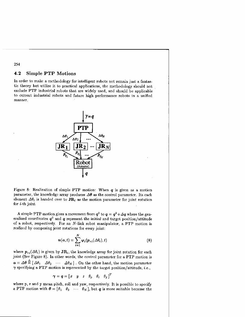
254

4.2 Simple PTP Motions

In order to make a methodology for intelligent robots not remain just a fantas- tic theory but utilize it to practical applications, the methodology should not exclude PTP industrial robots that are widely used, and should be applicable to current industrial robots and future high performance robots in a unified manner.

' 1

PTP A#iy

JRl JR2 •

^1 v

\Afy

• JRJV

Robot (Actuator)

Figure 8: Realization of simple PTP motion: When q is given as a motion parameter, the knowledge array produces A8 as the control parameter. Its each element A0{ is handed over to JRj as the motion parameter for joint rotation for i-th joint

A simple PTP motion gives a movement from q° to q — q°+Aq where the gen- eralized coordinates q° and q represent the initial and target position/attitude of a robot, respectively. For an iV-link robot manipulator, a PTP motion is realized by composing joint rotations for every joint:

N

u(a,t) = J2<Pi(Pri(Mi),t) (8) t=i

where pTi(A6{) is given by JR,-, the knowledge array for joint rotation for each joint (See Figure 8). In other words, the control parameter for a PTP motion is

a = A9 = [AOi A62 ■ ■ ■ AO^] . On the other hand, the motion parameter 7 specifying a PTP motion is represented by the target position/attitude, i.e.,

<y = q=[x y z 6p ör 0yf

where p, r and y mean pitch, roll and yaw, respectively. It is possible to specify a PTP motion with 6 = [6X 02 ••• 9N], but q is more suitable because the

255

operator can straightforwardly understand the motion. Note that q° is usually available by calculating from 0° monitored by internal sensors and hence it does not need to be given as motion parameter though A9 depends on both q° and q. Therefore q° is not explicitely represented.

The purpose of a PTP motion is to realize the requested position/attitude qT, the criterion function to evaluate the motion by A6 is then denned as

Jq[A9] = \\qt - q(A9)\\

4.3 Intelligent PTP Motions

Choosing simple PTP motions as element motions gives a dexterous and/or intelligent motion by optimizing a composite PTP motion. Such an optimal composite PTP motion is refered to as an intelligent PTP motion in the ICMC. It is very significant to investigate the intelligent PTP motions, since the industrial robots today are operated by the PTP control.

Component element motions (Joint rotations)

T(0

Robot

(V).

Figure 9: Realization of intelligent PTP motion

The control parameter for a composite motion, C7, composed of AT-step PTP motion that starts from q°, is expressed by the position/attitude after each step as

a=W q2 ••• QN]

in some cases, or equivalently by the movement at each step as ,2 A„Nl A~k k „fc-1 a^iAq1 Aq2 AqN], Aq* = q"-q"

256

in other cases. The knowledge array for an intelligent PTP motion transfers qi or Aq' to

knowledge arrays for element PTP motions which are sequentially executed. In the latter case, as mentioned in the previous subsection, PTP, calculates the target position/attitude q' by use of q'~x (obtained from monitored 0i_1) and Aq* (received from Intelligent PTP).

There is no formulary form of representing motion parameters 7, because in- telligent PTP motions are used as a wide variety of behaviors. When it was used as the optimal handling motion of flexible structures [10], the intelligent PTP motion was 2-step PTP motion with the control parameter a = [Aq1 Aq2]. In that case, for instance, the motion parameter was 7 = [q° q2] (or 7 = q2

when q° is supposed to be fixed), that is, the position/attitude at initial state and terminal state.

4.4 Dexterous throwing motion

A ball throwing motion is composed of several element motions such as "reach for ball", "grasp ball", "wind up arm", "swing down arm" and "open hand to release ball". If such element motions are learned as intelligent PTP motions, and the knowledge arrays for the motions are available, then a dexterous ball throwing motion, as a single composite motion, is realized by optimally composing the motions.

Given a ball position PB and weight WB and a target position PT where the ball should be thrown, the knowledge array Catch&Throw produces the necessary control parameters and transfers them to component element motions. QR, the position/attitude of arm to reach for the ball, for instance, is given to Reach for Ball and transformed to {qR}, sequence of position/attitude to realize the intelligent PTP motion, and they are handed over to the knowledge array for PTP motions of arm.

4.5 Cooperative Work of Arms and Multi-Legged Walking

Choosing a right-arm motion and a left-arm motion as element motions, a dual arm cooperation is realized by parallel motion composition. Similarly, walking is achieved by optimally composing the motions of every leg (See Figure 11).

5 Concluding Remarks

To seek a method to bridge the large gap between intelligent robots and current practical robots, presented is the framework of behavior evolution based upon the Intelligent Composite Motion Control. It is shown how complex bahaviors are coordinated by use of fundamental motions and how the behavior evolution connects to the method of knowledge array. And as an example of behavior evolution, the process of realization of a ball throwing with robotic manipulator from most fundamental motion, joint rotations. Although a throwing motion

257

Catch&Throw

Reach for Ball

Grasp Ball

Wind up Swing down

Open Hand

FTP motions of Arm

FTP motions of Hand

Arm joint rotations

Component Element Motions

Hand joint rotations

Figure 10: Ball throwing motion composed of three intelligent PTP motions of the arm and two intelligent PTP motions of the hand

was investigated in this article, the procedure used is expected to be applicable to more complicated behaviors in the same manner.

References [1] Bekey.G.A. et.al, 1993, Knowledge-based control of grasping in robot hands using

heuristics from human motor skills, IEEE T. Robotics and Automation, Vol.9, No.6, pp.709-722

[2] Brooks, R. A., 1986, A robust layered control systems for a mobile robot, IEEE J. Robotics and Automation, Vol.2, No.l, pp.14-23

[3] Chakrabarty,S. and Wolter,J., 1997, A structure-oriented approach to assembly sequence planning, IEEE T. Robotics and Automation, Vol.13, No.l, pp.14-29

[4] Connel, J. H. and Mahadevan, S., 1993, Robot Learning, Kluwer, Boston

[5] Dorigo, M. and Colombetti, M., 1998, Robot Shaping - An Experiment in Be- havior Engineering -, The MIT Press, Cambridge

[6] Kang,S.B., and Ikeuchi.K., 1997, Toward automatic robot instruction from per- ception - mapping human grasps to manipulator grasps, IEEE T. Robotics and Automation, Vol.13,No.l,pp.81-95

258

Dual Arm Cooperation

/k* Nfl A« Motion of Left Arm

Motion of Right Arm

Component Element Motions

Walking

m Legl Leg 2

a)

LegN

7TV 7TT 7TV7TT 7TI Component Element Motions

Figure 11: Knowledge arrays for cooperative work of dual arm and N-legged walking

[7] Narendra,K.S. and Venkataraman,S.T., 1995, Adaptation and Learning in Robotics and Automation, Proc. ICRA, pp.1244-1249, Nagoya, Japan

[8] Simmons, R.G., 1994, Structured control for autonomous robots, IEEE T. Robotics and Automation, Vol.10, No.l, pp.34-43

[9] Suzuki,M. and Shimizü, K., 1990, Analysis of distributed systems by array alge- bra, Int. J. Systems Science, Vol.21, No.l, pp.129-155

[10] Suzuki, M., 1995, Optimal handling of flexible structures through Intelligent Com- posite Motion Control, Preprints The 3rd IFAC/IFIP/IFROS Workshop on In- telligent Manufacturing Systems, pp.63-68, Bucharest

[11] Suzuki, M, 1999, Suboptimal Robot Motion for Unexperienced Situations through Intelligent Composite Motion Control - Method of Knowledge Array -, Int. J. Systems Science, Vol.30, No.l, pp.87-94

259

Modular Real-time Control via an Optical Field Bus System for the Four Legged Walking Machine ALDURO

U. Roll, M. Torlo and M. Hiller

Gerhard-Mercator-Universität - GH Duisburg Department of Mechatronics D-47048 Duisburg, Germany

{roll, torlo, hiller}@mechatronik.uni-duisburg.de

Abstract. In the Department of Mechatronics at the University of Duisburg the four legged walking machine ALDURO, with anthropomorphic leg kinematics, has been built as part of the project "Autonomes Laufen" funded by the German Research Council. A powerful real-time computer control system is necessary to control the complex system. Actuators and remote sensors are integrated using a modular, optical field bus system that fullfils the' required real-time criteria.

1 Real-time Capability at Field Bus Level

Computer systems are the intelligent components in contemporary automatic control systems. The communication between these components determines the performance of the system. Not only does the processes have to be considered, but also the capability of communication systems chosen limit the real-time capability. The demands on real-time behaviour increase proportional to the data transmission distance for the actual process. The choice of a field bus system for communication between the control computer and the peripheral systems becomes a most important factor effecting the atainability of real-time operating speeds [8].

During analysis of the real-time capability of a field bus system, the compatibility between each component must be considered. In this case, the technical process determines real-time conditions, and as a consequence the dynamic requirements. Such an automated system is designated as real-time capable if the process can be controlled in accordance with these requirements. The sections "communication" and "target applications" must be considered as a whole. Consequently , the real-time field bus system is required to carry out a number tasks in excess of bidirectional data transmission , for example system diagnosis and failure detection.

260

The tasks of the computer and devices at field level can be defined as follows:

• Status and instantaneous values are supplied by sensors; • Measured data is processed and new output values are obtained from the control

computer; • Process and control data is transmitted to the actuators.

The Real-time capability of applications depends on the architecture of the hard- and software and on computer performance. In this case, the real-time capabality of a process computer is essentially determined by the operating system [6] and the communication equipment (the field bus specified) [7]. For each bus system it is important that the total transfer time (telegram length, telegram duration, calculation time) does not exceed the cycle time for the complete process. Depending on the base computer architecture the operating system employed has a different performance. The operating system manages the allotment of the available hardware components, executes the communication between several processes and/or processors and is responsible for the generation and deletion of process streams. The user can only take access machine hardware functions through interfaces provided by the operating system. This minimizes possible sources of errors. The operating system protects against illegal access or modifications and allows fast reaction times between user applications and the hardware.

2 Field Bus Application in Mobile Hydraulic Systems

In modern mechanical engineering systems, processing the load become more and more complex by the application of modern technologies. In the course of auto- matization, decentralization gains more and more importance. This decentralization is achieved through the application of field bus systems. The characteristics of the field bus system required are dictated by the controlling application (figure 1). An example for this field bus technology is the contoller area network (CAN) field bus system which is widely used in the motor vehicle electronics. The increasing interaction between individual master controllers, sensors and actuators becomes too complex and leads to extensive wiring. The extensive increase in data exchange between electronic components cannot be performed using con- ventional techniques. Furthermore, mechanical systems in cars and mobile machines are increasingly being replaced by electronic ones. An example of one of these electronic components in hybrid design is the development of electro-hydraulic braking and guidance (brake/drive by wire).

261

Common to the point mentioned are the following features of a modular, real-time capable, control concept:

Data integrity, i.e. systems with large hamming distances also guarantee the reliability of data transfer for safety critical applications; A deterministic system with constant time periods is provided to attain the required timing conditions; The complexity of the hydraulic circuits and the electrical connections is reduced, and an improvement in efficiency is achieved; Obtaining improved ergonomics by optimal placement of control components; Lower assembly costs due to optimal component placement; Diagnostic functionality is provided, allowing a higher machine availability and improved maintenance capability; Better extendability and flexibility due to the modular system design.

Fieldbus

Figure 1: Schematic Representation of the Field Bus Principle

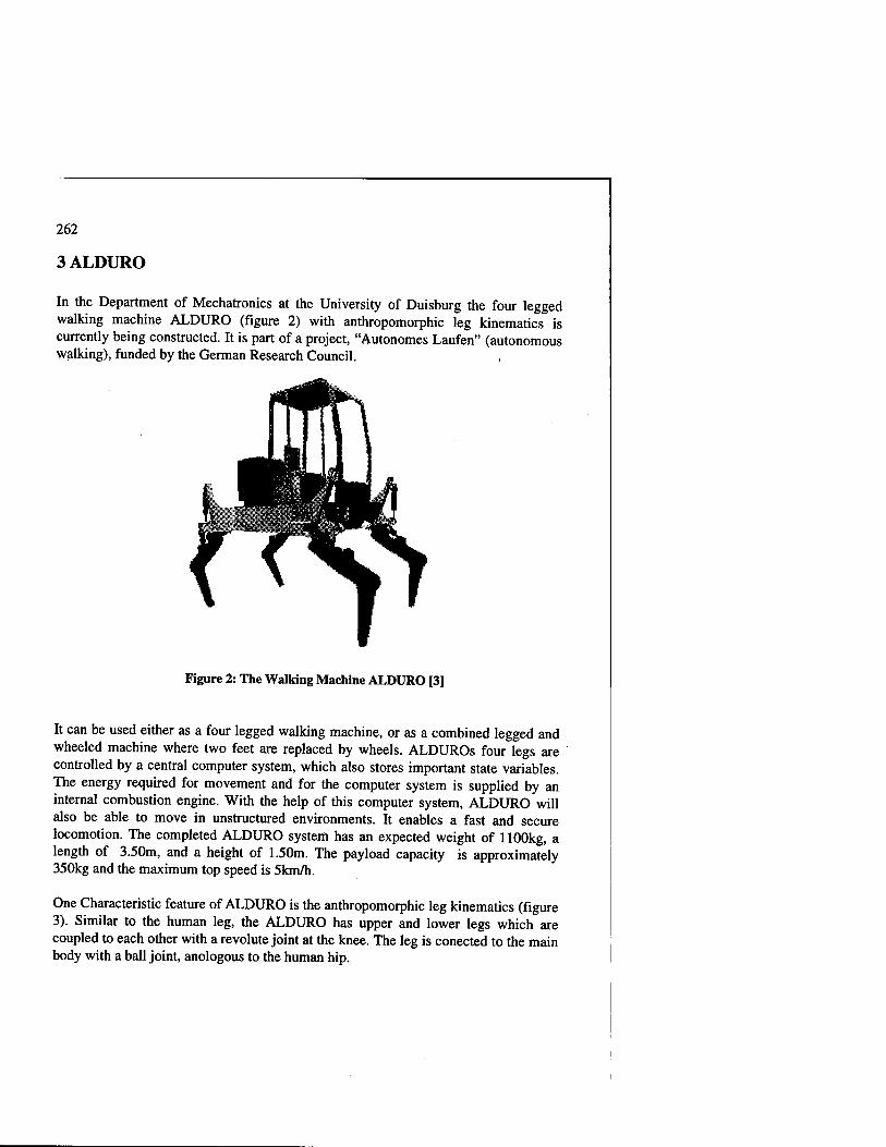
262

3 ALDURO

In the Department of Mechatronics at the University of Duisburg the four legged walking machine ALDURO (figure 2) with anthropomorphic leg kinematics is currently being constructed. It is part of a project, "Autonomes Laufen" (autonomous walking), funded by the German Research Council.

Figure 2: The Walking Machine ALDURO [3]

It can be used either as a four legged walking machine, or as a combined legged and wheeled machine where two feet are replaced by wheels. ALDUROs four legs are controlled by a central computer system, which also stores important state variables. The energy required for movement and for the computer system is supplied by an internal combustion engine. With the help of this computer system, ALDURO will also be able to move in unstructured environments. It enables a fast and secure locomotion. The completed ALDURO system has an expected weight of 1100kg, a length of 3.50m, and a height of 1.50m. The payload capacity is approximately 350kg and the maximum top speed is 5km/h.

One Characteristic feature of ALDURO is the anthropomorphic leg kinematics (figure 3). Similar to the human leg, the ALDURO has upper and lower legs which are coupled to each other with a revolute joint at the knee. The leg is conected to the main body with a ball joint, anologous to the human hip.

263

In contrast to conventional walking machines, that have rather simple kinematics with two or three degrees of freedom per leg, the complex structure of the anthropomorphic leg with four degrees of freedom allows a fexible adaptation of the overall system to the environment.

Figure 3: The Duisburg Anthropomorphic Leg [3]

Four hydraulic linear actuators with integrated potentiometor position measurement sensors are responsible for the drive of each leg. By using position, pressure and force measurements a force coupled position control system is implemented. A man- machine-interface with cartesian control will make it simple for the operator to work with ALDURO. The embedded computer control system is implemented as a real- time system in order to guarantee a sufficiently high safety margin in all imaginable situations, for man and machine. This will guarantee that sudden events, for example

264

slipping, subsidence of the soil, or operator errors are corrected in the shortest possible time.

4 Integration of the Field Bus in the Real-time System

Through use of hydraulic cylinders rather than electric motors, five kinematic loops per leg are created. Because of the special kinematic structure of the leg (figure 4), obtaining an explicit solution for kinematics and dynamics [1] is possible. The forces' in the cylinders during the standing (on three or four legs) phases of walking are determined. A central computer will be used to control ALDURO in the first development stage.

Li - kinematic loops

joint

generalized coordinate

rigid body

rigid body without mass

hydraulic cylinder

Figure 4: The Kinematic Structure of one Leg [1]

To control such a complex system as ALDURO a powerfull computer control system is required in order to process the control data at high enough rates (figure 5). The main component of this computer system is a VMEbus based PowerPC processor board. The real-time operating system used is VxWorks. The integration of all actuators and sensors is carried out using a field bus system, which uses an optical fiber system as the data transmission medium. The interface to the field bus system is

265

via a VME bus based central control board. The control data is retreved by the control computer via the VMEbus backplane. Thus the VMEbus represents the link between process computer and interface modules, and offers the possibility of later expansion by integration of further control processors or interface modules. A seconnd processor board is connected to the bus for the man machine interface. This also allowes connection of force feedback joysticks [4] and visual display of relevant operating states to the operator, without compromising real time system operating speed.

[11 Ringtopology

«All «fill «All «All e m

Figure 5: Integration of the Field Bus in the Real-time System [5]

5 The Implementation of the Real-time Field Bus System

The implementation of the field bus system under VxWorks is realized using a C++ class. It is possible to implement new C++-classes, which can be automatically extended by simple inheritance, by the functionality for excitation of the bus system. On the one hand, the handler class has the possibility to pass acyclically command functions to the bus, on the other hand it is possible to actuate cyclically the states of the sensors and of the actuators. The memory area which corresponds to the states of the sensors and to the actuators is designated as the Input and Output process image.

266

Via the command functions, an assignment of the I/Os of the decentralized peripheral modules can be implemented into a Dual-Ported-RAM (DPRAM). Test and analysis functions can be executed over which the correct function of the central module as well as of the complete bus system can be checked. In this case, the actual communication runs across information channels described in the DPRAM in which the output functions must be stored. By setting the corresponding bit shadow masks in the correct registers, the central module posts the process map or carries out the requested commands. The deterministic read-out and setting of the sensors and of the actuators required a cyclically called handler routine that requests the update of the Input and Output process map at regular intervals. The operating system VxWorks makes different mechanisms available for periodic execution of program functions. In order to achieve the necessary accuracy in the field of microseconds, it is necessary that an interrupt is responsible for a hardware integrated timer event. For this, in addition to further analogous functions, VxWork offers an implementation from the POSIX Standard 1003.1b. An interrupt service routine calls the system clock which is responsible for task scheduling. The routine decrements all the registered virtual timers depending on state to their conditions. At the beginning of the periodic function processing the timer must first be reloaded. After processing the function, it is called again by the timer. These timers are implemented according to the POSIX 1003.1b standard and verify the necessary accuracy. In the microseconds range, a timer event can be implemented exactly. In this case, the number of the interrupt events of the system clock occurring per second can be determined. This interrupt is normally called only 60 times per second. Consequently a timer function can be called with a minimum, according to the POSIX standard, period of 16.67ms, regardless of whether a shorter time interval was adjusted for loading of the timer. Since task scheduling is also controlled by the system clock, the system routine which is responsible for scheduling is also called more often with an increase in the number of timer events per second. The complete system then becomes more broken up. Consequently all processes are interrupted more often, due to more frequent task swapping, this creates too much overhead. In this case, a special feature of the PowerPC based processor board we are using is utilized. The board contains four supplementary timers which are integrated in the interrupt controller, and work independent of the system clock. The cyclical handler routine is implemented using one of these timers. The operating system VxWorks makes no use this particular supplementary timer. The timer is initialzed via the PCI bus. For the initialization the clock speed must be set and the corresponding handler routine must be registered as the interrupt service routine (ISR) for this timer. Subsequently the interrupt can be indicated as beeing unlocked and the period can be specified as a multiple or a part of the clock speed of the timer. The actual updating of the process image is divided into two different phases, which are alternately updated. The ISR must not wait for the result of the requested process image update. All that is required is that a static variable is used to record the status of the update. In the first step a requirement mask is filled with the process image number. The field bus interface module (figure [5]) starts independently with the dispatch of previously determined communication telegrams. After successful processing of all telegrams by the peripheral modules and

267

the deposit of the input data in the DPRAM, the interface module reports this via a ready mask. After this the status of the update is checked. The requirement mask must be reset before a new process image can be requested. Any errors are indicated in the error mask. Examples of this would be damage of the optical fiber cable, or the failure of one of the peripherie modules. Via diagnostic functions, this failure point can be located. Further operation of the peripheral modules is not possible. The interface module runs a continous background check to see whether all peripheral modules are still responding. Through a bit in the error mask, a CPU error in a peripheral module is reported to the interface module. If one of these errors occurs, an error routine is carried out to attempt to correct it, or to shut down the machine in safe manner.

6 Summary and Future Development

Through the great transmission capability of the fiber optic medium it is possible to attain high data transfer rates. With the number of sensors and actuators given, and with a sufficient time margin for other proceses, an update cycle time of a maximum of 2.1ms can be guaranteed. In this time, all sensors and actuators are interrogated and updated. Only considering, the transfer of user data (per leg 102Bytes) in such a way, one receives an effective transfer rate of 1.577Mbits/s. This is to be categoriesed, in the case of todays available field bus systems, to be in the top performance segment. For each leg we have four D/A and twelve A/D converters with a resolution of 12Bit each, and two digital outputs. In spite of given communication volume there is still sufficient bandwidth to integrate further sensors. The sensors of position and other environmental values are given a lower control weighting. For this, the used field bus system has corresponding methods through which the individual update cycles can be subdivided into levels in a priority based manner.

268

Fieldbus

Virtual "Technical Process

Figure 6: The Connection of a Real System over a Field Bus System in a Hardware in the Loop Environment

Due to the conception of the ALDURO to move in a striding movement, extensive simulations have to be caried out, so that error-free operation can be guaranteed. Through the application of a field bus system, the application offers itself to so-called "hardware in the loop" simulations. This simulation, already established in the automotive development area, may enable the safe carrying out to test extreme situations (figure 6). In the case of the ALDURO the complete field bus peripheral equipment can be replaced by a second computer system. This system is coupled directly to the field bus via an easily modified interface board. The second computer system, based on efficient standard PC hardware, imitates the kinematic and dynamic behavior of the ALDURO. Consequently, slipping on the ground or the disturbance of relevant system components can be simulated safely and in a reproducible form. In this case, coupling to the real process hardware occurs simply via the optical fiber system. With the corresponding modifications, technique lets itself use in the mobile hydraulics in same manner.

269

7 Literature

[1] MüLLER, J.: Simulationsmodell zur Kraftberechnung des Schreitfahrwerks ALDURO, Internal Research Report, Department of Mechatronics, Gerhard-Mercator-Universität - GH Duisburg, 1998

[2] CAURIN, G.: Control of walking Robots on Natural Terrain, Dissertation, ETH Zürich, 1994

[3] SCHRöTER, D.: Festigkeitsberechnung am Beispiel eines ALDURO-Beins, Institute Report 98-4, Department of Mechatronics, Gerhard-Mercator-Universität - GH Duis- burg, 1998

[4] TRUNINGER, R.: Eine Mensch-Maschine-Schnittstelle zur Rückführung der Kippstabilität von Arbeitsplattformen, Dissertation, ETH Zürich, 1993

[5] ROLL, U.: Konzeption und Aufbau einer echtzeitfähigen Prozeßsteuerung für das Schreitfahrwerk ALDURO, Internal Report, Department of Mechatronics, Gerhard-Mer- cator-Uni-versität - GH Duisburg, 1998

[6] FEDERHENN, H.: Echtzeitbetriebssysteme in der Steuerungstechnik, Seminar „Steuer- ungstechnik", Fachhochschule Trier, 1997

[7] WENZEL, P.: Echtzeit-Merkmale von Feldbussystemen, Tagungsbeitrag auf der Echtzeit' 97,1997

[8] BORST, W.: Der Feldbus in der Maschinen- und Anlagentechnik, Franzis Verlag, 1992

[9] TORLO, M.: Programmierung eines Embedded Systems auf der Basis des Echtzeit- betriebssystems VxWorks, Diplomarbeit, Fachgebiet Mechatronik, Gerhard-Mercator- Universität - GH Duisburg, 1998

270

Performance Issues in Biped Walking Robots

Filipe M. Silva1 and J.A. Tenreiro Machado2

1 Dept. of Mechanical Engineering University of Aveiro, 3810 Aveiro, Portugal

fsilva@mec.ua.pt 2 Dept. of Electrical Engineering

Polytechnic Institute of Porto (ISEP) Rua de S. Tome, 4200 Porto, Portugal

jtm@dee.isep.ipp.pt

Abstract. This paper presents the dynamic analysis of robotic biped systems. The main goal is to gain insight into the phenomenon of walking and to evaluate its performance. In this study, we propose three methods to quantitatively measure the dynamic efficiency of walking: energy analysis, perturbation analysis and lowpass frequency analysis. In order to accomplish this goal, the prescribed motion of the biped is completely characterised in terms of a set of locomotion variables, namely: step length, hip height, hip ripple, hip offset, foot clearance and link lengths. Based on these variables and their influence, the performance measures are discussed and the results compared with those observed in nature.

1 Introduction

In the last years a growing field of research in biped locomotion culminated in the development of a large variety of prototypes [1-3]. A retrospective analysis of past legged machines, shows that the design methodologies led to the reproduction of structures, functions and principles found in nature. At the same time, we are still in a primitive stage in understanding the motor control principles and the sensory integration subjacent to human walking. These questions have motivated several researchers in the pursuit of efficient walking robots stimulated by the synergy in the biology and robotic areas. Vukobratovic et dl. [4] have proposed models and mechanisms to explain biped locomotion. In another perspective, Raibert and his colleagues [5] built hopping and running legged robots in order to study the major issues with dynamic balance. Bearing this fact in mind, in this article a planar biped is modelled and its performance evaluated according to different viewpoints. The main purposes are threefold: • To characterise the biped motion in terms of a set of locomotion variables. • To search for the optimal locomotion variables that minimise the proposed cost

functions. • To establish the correlation among these locomotion variables and the system's

performance.

271

The remainder of the paper is organised as follows. A short description of the biped model is given in section 2. In section 3 we describe the algorithm used to plan the kinematic trajectories of the biped robot. In section 4 various dynamic performance measures are proposed and discussed mathematically. Based on these indices, several numerical results are presented in section 5 to illustrate the application of the proposed methods. Finally, in section 6 we outline the main conclusions and the perspectives towards future research.

2 Biped Model

Figure 1 shows the planar biped model with the notation used throughout this paper. The proposed model consists of seven links in order to approximate locomotion characteristics similar to those of the lower extremities of the human body (i.e., body, thigh, shank). In the present study, we assume that a complete walking cycle is divided in two phases: • Single-support phase - in which one leg is in contact with the ground and the other

leg swings forward. • Exchange-of-support phase - in which the legs trade role.

In the single support phase, the stance leg is in contact with the ground and carries the weight of the body, while the swing leg moves forward in preparation for the next step. At the exchange of support, the swing leg contacts the ground with zero velocity to avoid impulsive forces due to the impact phenomenon [6]. The impact of the swing leg is assumed to be perfectly inelastic while ensuring that no slippage occurs. At the same time, the feet maintain a flat contact with the ground.

(xu,yn)

Fig. 1. Planar biped model.

Stance Leg

272

Using the Newton-Euler formulation, we derive the dynamic equations for the seven- link biped that describe the behaviour of a complete single step. The redundancies in the exchange of support are used to satisfy the torque continuity between the single- support and the double-support phases. At the time that the swing leg contacts the ground, an adequate reaction force is prescribed allowing a smooth transition of support. In this study, the ratio of the duration period of exchange of support and complete step is constant (10%).

3 Motion Planning and Evaluation

In early studies, the determination of the biped trajectories was made largely on the basis of experience (e.g., recording kinematic data from human locomotion [9,10]). In this work, the motion planning is accomplished by prescribing the cartesian trajectories of the body and the lower extremities of the leg.

3.1 Locomotion Variables

The motion of the biped system is characterised in terms of a set of variables. The step length Ls is the distance travelled by the body in each step. The hip height HH

is defined as the mean height of the hip along the walking cycle. The hip ripple HR

is measured as the peak-to-peak oscillation magnitude at the hip. The hip offset H0

measures the position of the hip in relation to the middle point between two consecutive contacts of the feet on the ground (i.e., H0 = Dl-D2).

Fig. 2. Locomotion variables.

273

The foot clearance Fc represents the maximum elevation of the swing foot above the

ground. Finally, we examine the role of the link lengths considering that \ +12

assumes a constant value equal to 1 meter (Fig. 2).

3.2 The Trajectory Generator

The proposed algorithm accepts the hip and feet's Cartesian trajectories as inputs and, by means of the inverse kinematics, generates the corresponding joint evolution. To improve the smoothness of the motion we impose two restrictions: the body maintains an erect posture and the body forward velocity VF is constant. In dynamic walking, at each footfall, the system may suffer impacts and incurs on additional accelerations that influence the forward velocity. For this reason, we impose a set of conditions on the leg velocities so that the feet are placed on the ground while avoiding the impacts. We denote the moment of exchange of support as time *!, and by t[ and t? the instants just before and after the impact occurs, respectively. For a smooth exchange-of-support, we require that the angular velocities, before and after, to be identical, that is:

ß»fe-)=4,(*i+)- («

The locomotion parameters characterise completely any configuration in which both feet are on the ground. Nevertheless, between two such configurations there is an infinite number of possible trajectories. In order to simplify the problem, we consider that such motions are produced based on sinusoidal functions. The equation of the tip of the swing leg along the *-axis is computed by summing a linear function with a sinusoidal function. This is implemented using the function:

x2i(t) = 2V1 t sin(2^) 2nf

(2)

where/is the step frequency. Moreover, the vertical motion, that allows the foot to be lifted, has the form:

y2l(t) = ^[l-cos(2nft)]. (3)

The trajectory generator synchronises and coordinates the leg behaviour so that the swing limb arrives at the contact point when the upper body is properly centred with respect to the lower limbs. These trajectories are somewhat restrictive when compared with those of humans where we have ballistic-like motions. In this perspective, the sinusoidal trajectories constitute, merely, a first-order approach to more efficient movements.

274

Lowpass Fnquency Analysis

Fig. 3. Block diagram of the performance evaluation.

4 Performance Evaluation

This section covers the implementation of the performance measures used for the dynamic evaluation of the biped system (Fig. 3). In mathematical terms, we shall provide global measures of the overall efficiency in some average sense. The aim is to verify whether a correlation among different view points could be found in walking.

4.1 Energy Analysis

After planning the joint trajectories, we calculate the inverse dynamics in order to map the kinematics into power consumption. The key measure of this analysis is the average mechanical power. It is computed assuming that power regeneration is not available by motors doing negative work, that is, by taking the absolute value of the power. At a given joint j of the leg i, the mechanical power is the product of the motor torque and the angular velocity. The global index is obtained by averaging the mechanical absolute power delivered over a period T:

v: M> dt. (4)

Although minimizing energy appears to be an important consideration, it may occur an instantaneous near-infinite power demand. In such a case, the average value can be small while the peak is physically unrealizable. As an alternative index, the

275

Standard deviation measure is used to evaluate the dispersion around the mean absolute power:

where Pt is the total instantaneous mechanical power. For an actuated system, it should be also necessary to consider the average energy lost in the electric motors. This index can be defined as:

Le=-\Tfrdt. (6)

4.2 Perturbation Analysis

In many practical cases the robotic system is noisy, that is, has internal random disturbing forces. As such, an approach called perturbation analysis was implemented to determine how the biped model adapts to these distortions. The torque vectors are 'corrupted' by additive noise using an uniform distribution with zero mean. As result, the trajectories of the system suffer some distortion and can only approximate the desired ones. By computing the forward dynamics and kinematics, we can determine two scalar indices based on the statistical average of the well-known mean-square error (Fig. 3). We can express the indices in terms of the following equations:

fi-i£#J>'>-«'«tf<*- <7)

1 Ns I 1 |T ~ i=-^Itij)^(^-r^)pt. (8)

where Ns is the total number of steps for averaging purposes, 9[ and Of (r' and

rf) are the ith samples of the real and desired angular (linear) displacements. The perturbation .^analysis is a 'second order' method that measures the system's robustness against variations around the desired trajectory. The stochastic perturbation penalizes the system's smoothness and we shall be concerned with minimizing both |s and £.

4.3 Lowpass Frequency Analysis

In robotics, the electro-mechanical system that regulates the movement (e.g., actuators and drives) is constrained by its bandwidth. Hence, the practical conditions

276

of motor control should also be considered when evaluating the system's performance. In this perspective, the torque variables are expanded in Fourier series and the time domain signals are described by the coefficients of its harmonic terms. Afterwards, these series are filtered through the same lowpass filter. In order to determine the degradation occurred we use, as our figure of merit, the ratio between the energy of the filtered signal EF and the energy of the original signal Es, that is:

Er=^. (9) Es

This method, based on the frequency domain has also been successfully employed. However, it is a less general method, because it requires the a priori knowledge about the nature of the robotic actuators.

5 Simulation Results

In this section, we describe the simulation results obtained using the different performance indices. At this stage, the relative performance indices by itself are not sufficient to address the issues of dynamic stability or control. The main purpose is to determine the implications of the locomotion variables on the cost functions and to compare the results with biological data. The simulations are carried out considering a total system mass and body height of M = 70 Kg and L = 1.8 m, respectively.

Table 1. The robot link lengths and masses.

i /,• (m) nh (Kg) 1 2 3

0.5 0.5 0.3

4.0 7.5 47

5.1 Step Length and Hip Height

In a first case study we analyse (Fig. 4) the performance index with respect to the step length and the hip height. For convenience, the chart portion corresponding to hip heights lower than 0.5 m is not represented. One trajectory that undergoes smooth motion is the body flat trajectory in which the stance leg adjusts itself so that the hip maintains a constant height. The body of the robot is assumed to be moving horizontally with a constant forward velocity VF = 1 ms'1. Furthermore, it is considered that the swing foot stays always on the ground. The system performance is particularly sensitive to the body mass above the hip. Therefore, the link length vs mass values adopted in this study are based on anthropometric data [7-8] (Table 1).

277

As shown in Fig. 4-a, to minimize the average mechanical power Pm the hip height must be about 90% of the body height, with optimal step lengths in the range of 0.3- 0.6 m. Moreover, an important degradation occurs for small step lengths. In Fig. 4-b, we depict the results when evaluating the energy lost Le. The performance surface

presents a similar evolution, but Le is minimized for a slightly higher hip height. At the same time, these results agree with those observed in human locomotion when a subject is allowed to walk without the imposition of a pace frequency constraint.

fm = 480

02 0.4 OS 0.8 1 1.2 1.4 1.6 Step Length (m)

L, = 5.3e4 .

£, = 8.1e4

(a) (b)

0.2 0.4 0.6 08 1 1.2 1.4 1.6 Step Length (m)

Fig. 4. Contour plot: (a) mean mechanical power Pm vs HH and Ls ; (b) mean power lost

Le vs HH and Ls

Now, let us examine the "lowpass frequency analysis" method. For an ideal lowpass filter whose cutoff frequency is fe = 5 Hz, the performance surface Er is illustrated in Fig. 5-a. At this phase, we calculate also the mean square error of x(t)-i(t) (see Fig. 5-b).

0 0,2 0.4 0.6 0.8 1 1.2 1.4 1.6 1.8 Step Length (m)

(«)

s

4

2

0 0.2 0.4 0.6 0.8 1 1.2 1.4 1.6 1.8 Slep Lengtfi (m)

(b)

Fig. 5. Lowpass frequency analysis: (a) energy ratio Er vs Ls ; (b) mean square error £. vs

Ls (Hh = 0.6m).

278

The discontinuity points solely depend on the number of harmonic terms up to fe. In contrast to the other methods above, these results suggest that there is an optimum solution for higher step length values, while the performance remains almost unchanged to hip height variations.

5.2 Hip Ripple

In this sub-section, we consider a hip trajectory with a sinusoidal oscillation, while the foot of the swing leg slides over the ground surface. The contour plot in Fig. 6-a suggests that a small adjustable oscillation at the hip may be advantageous in terms of mechanical power. At the same time, the optimum value remains almost unchanged to hip height variations.

Fig. 6. Contour plot: (a) mean mechanical power Pm vs HH and HR ; (b) mean perturbation

£g vs HH and HR (is = 0.4 m and H0 = Fc = 0 m).

A similar phenomenon can be observed in biological systems as well as in previous studies concerning the kinematic analysis of biped locomotion systems [9]. At the same time, the results obtained with the perturbation index 4 (see Fig. 6-b) indicate the advantage in applying ripple to increase the system's robustness against noise.

5.3 Hip Offset

The desired leg coordination is established by assuring that the swing leg arrives at the contact point when the upper body is properly centred with respect to both feet. However, the experiments carried out indicate the advantage of applying a small offset to the hip. Fig. 7 represents the contour plot of two cost functions in terms of hip offset and hip height.

279

-0.4 -0.2 0 0.2 0.4 Hip Ripple (m)

(a) Hip Offset (m)

Fig. 7. Contour plot: (a) mean mechanical power Pm vs Hu and H0 ; (b) mean perturbation

E,r vs HH and H0 (Ls = 0.4 m and HR=Fc = 0m).

Considering the above plots, two features can be pointed out: • The optimal hip offset from the viewpoint of energy (perturbation) is a small

positive (negative) value. • The optimal hip offset tends to zero as the hip height increases for both indices

Pmand£.

From this simulation, we can observe an opposite behaviour suggesting a compromise in the final result. The benefits of a small hip offset results from the fact that, during walking, the legs move back and forth to provide, simultaneously, propel and balance actions.

5.4 Foot Clearance

Until now, all the experiences considered that the foot stays on the ground without any friction. Next, we analyse the situation in which the foot can be lifted off the ground. Fig. 8-a shows the influence of the foot clearance variable when using the absolute power and the perturbation analysis. In terms of the index Pm, the minimum foot clearance (except when avoiding any accidental contact) is the optimal one. Although less efficient from the Pm perspective, we believe that the foot clearance is responsible for the system's robustness in uneven walking surfaces. We can observe this process in one-year-old infant's first steps knowing that walking will be learned. The results obtained with the perturbation index 4 w& shown in Fig. 8-b. It was confirmed that a zero foot clearance optimise the system's performance, except for a narrow range of higher hip heights. This means that such cost functions may not be appropriated in this circumstances.

280

= 490

005 0.1 0.15 Foot Clearance (m)

0.05 0.1 0.15 Foot Clearance (m)

(a) (*)

Fig. 8. Contour plot: (a) mean mechanical power Pm vs HH and Fc; (b) mean perturbation

£g vs HH and Fc \LS = 0.4 m and HR = H0 = 0 mj.

5.5 Relative link lengths

This sub-section investigates the role of the relative link lengths in the system's performance considering ll + l2 = \m. The minimum mechanical power Pm occurs for link lengths Z, = 0.65 and l2 = 0.35 m. The values of mean power are plotted against link length lx in Fig. 9-a. Moreover, the results indicate that for /j in the range from 0.4 to 0.8 m the performance index remains almost constant. On the other hand, the point of minimum 4 corresponds to a slightly smaller knee-ankle length, whilst the curve values change considerably around the minimum (Fig. 9-b).

2500 •

2000 ■

1500 ■

1000 /

500 J 0

) 0.2 0.4 0.6 Link Length 11 (m)

0.8 1 0 0.1 0.2 0.3 0.4 0.5 0.6 0.7 0.8 0.9 1 Link Length 11 (m)

(a) (b)

Fig. 9. Performance index: (a) mean mechanical power Pm vs link length /,; (fc) mean

perturbation £a vs link length /,.

281

6 Conclusions

In this paper, we have studied several aspects of biped locomotion^ By implementing different motion patterns, we estimated how the robot reacts to a variety of locomotion variables: step length, hip height, hip ripple, hip offset, foot clearance and link lengths. The performance indices used provide a way to evaluate the system's behaviour during normal walking. Moreover, the simulation results could be used to gain insight into the implications of many design and motion planning parameters on the energy efficiency of a bipedal system. Future work will address the refinement of our models to include other phenomena of the gait, such as lateral balance and zero ankle torque. At an higher level, it is essential to explore complementary performance measures (e.g., stability, obstacle avoidance) for the generation of efficient motion strategies.

Acknowledgments

The first author is supported by the Fundacäo para a Ciencia e a Tecnologia under grant PRAXIS XXI/BD/9541/96.

References

1. J-I Yamaguchi, A. Takanishi and I. Kato, "Development of a Biped Walking Robot Adapting to a Horizontally Uneven Surface", Proc. Int. Conf. on Intelligent Robots and Systems, pp. 1156-1163,1994.

2. S. Kajita, K. Tani, "Experimental Study of Biped Dynamic Walking", IEEE Control Systems, pp. 13-19, 1996.

3. K. Hirai, M. Hirose, Y. Haikawa and T. Takenaka, "The Development of Honda Humanoid Robot", Proc. IEEE Int. Conf. on Robotics and Automation, pp. 1321-1326, Leuven, Belgium, 1998.

4. M. Vukobratovic, B. Botovac, D. Surla and D. Stokic, Biped Locomotion: Dynamics, Stability, Control and Applications, Springer-Verlag, 1990.

5. M.H. Raibert, Legged Robots that Balance, The MIT Press, 1986. 6. Y.F. Zheng and H. Hemami, "Impact Effects of Biped Contact with the Environment",

IEEE Trans. Syst. Man Cyber., Vol. 14, n. 3, pp. 437-443,1984. 7. D.A. Winter., Biomechanics and Motor Control of Human Movement, John Wiley &

Sons, 1990. 8. J. Basmajian and C. Luca, Muscles Alive: Their Functions Revealed by

Electromyography, Williams & Wilkins,1978. 9. F. Silva and J.A. Tenreiro Machado, "Kinematic Aspects of Robotic Biped Locomotion

Systems", Proc. IEEE Int. Conf. on Intelligent Robots and Systems, IROS'97, Vol. 1, pp. 266-271, 8-13 Sept., Grenoble, France, 1997.

10. F. Silva and J.A. Tenreiro Machado, "Towards Efficient Biped Robots", Proc. IEEE Int. Conf. on Intelligent Robots and Systems, IROS'98, 13-17 Oct., Victoria, Canada, 1998.

282

From Robot Control to Virtual Reality Based Commanding: The Systems Approach

Eckhard Freund1, Juergen Rossmann1

1 Institute of Robotics Research (IRF), University of Dortmund, Otto-Hahn-Str. D-44227 Dortmund, Germany

{freund.rossmann} @irf.de

Abstract. Today's complex automation systems do not just have to function well, they also have to be intuitively usable and provide suitable interfaces to be integrated into the factory automation control and supervision hierarchy. Practical experiences in the development such automation systems showed that the most successful components developed were those, making the integration and operability a major design issue. As the components are forced to fit into a greater framework, developers have to adhere to standards and to standardized interfaces in order to facilitate integration and test of the final system. Although it was suspected in the beginning that system constraints in the form of architectural design guides imposed on the different parts of the realization might hamper the creativity of the developers, it was found that just the opposite was the case. After a training phase the developers managed to "think globally, but act locally", so that the development, the integration and the tests of different robot control and supervision applications in space and industrial context worked well and efficiently. The paper outlines the key ideas for system structuring and gives application example ranging from control development to virtual reality based user-interface design.

1. Introduction

The development of intelligent and autonomous robotic systems with a high degree of flexibility, good operational capabilities and the potential for efficient integration into an industrial CIM-environment is still a difficult task which requires both, technical and management skills. In the recent years, the transfer of know-how from the area of space robotics to industrial applications has been emphasized at the Institute of Robotics Research because robotic system capabilities for space applications have already reached a considerable standard with regard to system autonomy, safety and local intelligence that is appropriate and ready to be applied to industrial applications.

Nevertheless, the development-strategy for modern robot control software at the IRF had to be changed during the recent years, because it was found that the mere development of different new methodologies and software components was not enough to attract industrial partners at large, who want readily developed „products" rather than methods and components. The need for products implied that the involved methods fit into a framework which is built on standard interfaces where possible and

283

which allows a thorough testing of the components to be delivered. Only the adherence to industrial standards helps to convince industrial partners of the quality of the developed control systems and components. At the first glance this might sound as if the development of new methodologies is hampered by the necessity to adhere to standards, but just the opposite is the case: We found that the new methodologies can more easily be tested the more comprehensive the framework is, in which the method has to prove its applicability. For example a developed simulation system was developed to simulate and visualize a robotic workcell. But as it was equipped with an ethernet- and a ProfiBus fieldbus-interface, there quickly came up the idea to control and supervise autonomously guided vehicles (AGV) and to also visualize their paths and transport tasks. With the open interfaces, there were only minor changes necessary to incorporate a part of the control software from the AGV research group — and today the simulation software can simulate AGVs as well as robotics workcells and „matured" even to a full fledged virtual reality system which is currently being with each new problem that was solved.

Before the examples are given, the system theory which led to the development of the greater framework will shortly be described.

2. The framework for the systems' development

Flexible, future-oriented robot controllers today need to have the capability to incorporate information from different classes of sensors and they should have standardized communication interfaces with other factory-automation components. To ease the robot systems' operation an intuitive graphical user-interface should be provided. Furthermore, implicit programming and action planning methods should allow robot programming on a much higher level of abstraction than today's procedural programming languages.

2.1 The principle of the hierarchical coordinator

Until today, most features of this comprehensive list, have at most been available as „non-integrated components" in different research laboratories. This was also true for the IRF, where research was and is being carried out in the field of the development of intelligent control structures. But about three years ago our focus shifted from the development of different methods — which had already reached a satisfactory standard at that time — to the development of a comprehensive system which incorporates the different features.The first comprehensive system that was fully developed and implemented at the IRF was the CIROS-testbed, a multirobot system well suited to perform service tasks in a space laboratory environment (see chapter 0). The system theory behind this development was based on the „principle of the hierarchical coordinator". As discussed in detail in [5] [6], the hierarchical coordinator provides the system-theoretic framework for the integration of new features like

284

collision-avoidance, coordinated operation, automatic task planning and sensor-based robot control into single and multirobot systems.

Fig. 1 shows the hierarchical architecture emphasizing mainly the control theory behind this approach. The bottom layer describes the state-space equations for the different robots with their actuators, the layer on top of the robots gives the basic structure of the feedback-control methodology that is chosen to control the robots and the top layer shows the basic notation for the hierarchical coordinator. As stated in [5] [6], the hierarchical coordinator approach works best, if the „nonlinear decoupling and control methodology" [5] is used as the feedback-controller because then it fully matches the system theory.

desired values

hierarchical coordinator

nonlinear decoupling and control

/_ wr feE ft(£, i„üi,...£,)

robot

ML vv.ft)

au.)

^Whl wr ML

i,(i) = A,(i,) + 4U1)i,(i)

£,(i,)

*."' HL,(0

C-(ir)

^l==0 1uW iJiT ir(i) = A,(x,) + fi,d,)ji,(i)

£,(£,)

Fig. 1: Structure of a multirobot system using the hierarchical coordinator theory

A very appealing aspect about the „the principle of the hierarchical coordinator" is that this basic system concept for the development of complex control systems can be employed for a wide range of applications. The applications to be presented in this paper range from the design of a flexible assembly workcell including logistic services by autonomously guided vehicles to a multirobot system for autonomous experiment-servicing in a space laboratory module. While implementing the different systems it was found, that the „principle of the hierarchical coordinator" was useful as a basic system theory, but it was also found, that besides this system theory a less generic, more application oriented architectural design guide is needed to make the step from system-theoretic interface specifications to interface-descriptions in hard- and software.

2.2 Space robotics as a motor for the development of intelligent robot control systems

One of the first major space robotics projects the TRF took part in was the ROTEX- (Robot Technology Experiment) project, a joint project between different companies and research institutes in Germany. ROTEX was funded by the German Space Agency DARA. While the ROTEX software was developed concentrating especially on the precise project timing and the quality standards for flight software, research beyond the scope of ROTEX was carried out developing a robot control system

285

suitable to control a multirobot system for space applications. In the CIROS (Control of Intelligent Robots in Space) project, this multirobot control structure was developed and implemented, based on the concept of the hierarchical coordinator [5] [6]. Applying the methodology of the hierarchical coordinator, a robot control system with a significant increase in autonomy and the operational capabilities for space laboratory servicing was designed [3] [7]. The implemented control system IRCS (Intelligent Robot Control System) is well suited to perform service tasks in a space laboratory environment such as the CIROS testbed shown below.

Fig. 2: The CIROS multirobot testbed

The CIROS testbed is equipped with two robots with redundant kinematics. Each robot has 6 revolute axes and both robots are mounted on tracks to enlarge their workspace to cover the whole laboratory.

The layout of the laboratory is similar to that of the Columbus Orbital Facility (COF), the European contribution to Internation space Station (ISS) and can easily be adapted to incorporate the latest experiments.

The redundant two-armed robot configuration with the torque/force-sensors at the robots' wrists permits fully coordinated operation as well as synchronized or independent action of the two robots. Furthermore, the robots are equipped with hand cameras and the whole laboratory can be supervised by a scene camera. A vision system performs the image-processing in order to provide the planning levels with necessary information, i.e. about the exact location of objects to be gripped. The control desk in the foreground contains devices for system control and supervision.

Fig. 3 shows the structure of the CIROS multirobot control IRCS (Intelligent Robot Control System), that contains, superimposed on the level of the individual robot controllers, the additional levels for online-collision-avoidance[ll], multirobot coordination and automatic action planning [4][12].

286

Fig. 3: Structure of the multirobot control system IRCS

The automatic action planning component a task oriented programming interface facilitates the programming of the multirobot system and the cooperation with a virtual reality based man machine interface. The automatic action planning component, the top layer of the IRCS (fig. 3), can interpret action descriptions which are formulated on a high level of abstraction. With the aid of the central world model that contains a mathematical description of the environment, tasks formulated in a „user-friendly" manner like "close drawer 1 in rack 4" or, as shown in fig. 4, „put sample 1 into heater slot 1" are decomposed into so-called elementary actions.

Fig. 4: Automatic action planning for multirobot systems

287

These elementary actions are selected from a predetermined set of actions comprising the activation of endeffectors, locking or unlocking of the gripper exchange system and the path planning functionality for independently working or cooperating robots. During task execution, the robots are supervised by the level of online collision avoidance [11], which actively avoids collision dangers between robots and between robots and their environment.

The description of the functionality of the CIROS multirobot control system gives an idea of the complexity of a system including capabilities for automatic action planning, coordinated operation and online collision avoidance. It might be interesting to mention, that the structure of the IRCS shown in fig. 3 is an application that almost literally realizes the „principle of the hierarchical coordinator". The IRCS was the first multirobot control that realized all features described in the system theory [5] [6].

3. Modern virtual reality based man-machine-interfaces for intuitive operation

When we started to control the robots via VR, we immediately found that the standard teleoperation or "hand-tracking" approach would not work for most applications which contain assembly tasks [2] [9] [10]. The following problems arose: • Time delays between the display of a robot's movement in the VR and its physical

movements are critical for the stability of the process, because, similar to standard teleoperation approaches, the user is still "in a real-time control loop".

• The graphical model has to be very precise. • The measurement of the position and orientation of the data-glove has to be very

precise. • Measures have to be taken to reduce "trembling" of the operators hand. • A versatile sensor-control is necessary to compensate for unwanted tensions when

objects are inserted into tight fittings.

The solution was to enhance the VR-system in the way that while the user is working, the different subtasks that are carried out by him are recognized and task descriptions for the IRCS, the multi-robot control system of the CIROS environment are deduced (chapter 4). These task descriptions are then sent to the action planning component1 of the IRCS (see above). The action planning component can "understand" task descriptions on a high level of abstraction like "open drawer", "insert sample 1 into heater slot 1" etc. and thus is the ideal counterpart for the task deduction component of the VR-system. Using this task deduction mode is almost ideal, because: • The required communication bandwidth is low, because only subtasks like "open

flap", "move part A to location B" or "close drawer" are sent over the communication channel.

• The user is no longer in the "realtime feedback loop". Complete subtasks are recognized and carried out as a whole.

• For assembly tasks, the accuracy of the environment model can be compensated for by automatic sensor-supported strategies.

288

• The accuracy of the data-glove tracking-device is not as important as for the direct tracking mode. The allowable tolerances when the user is gripping an object or inserting a peg into a hole can be adjusted in the VR-software.

• Different users working at different VR-systems can do different tasks that are sent to the planning component of the IRCS, which then can compute an adequate sequence of the tasks to be carried out, depending on the available resources. Thus one robotic system can serve e.g. multiple users in the same virtual environment.

• If the robot control is versatile enough, there is no longer a need to even show a robot in the virtual environment displayed to the user; so the user more and more gets the impression of carrying out a task "himself", which is the highest level of intuitivity that can be achieved.

• If the planning component is versatile enough, it cannot only control the robots, but also other kinds of automated devices.

In general terms, it is one of the key issues of Projective Virtual Reality is splitting the job between the task deduction in the VR and the task "projection" onto the physical automation components by the automatic action planning component. The necessary expertise to conduct an experiment in a space laboratory environment like CIROS is thus shared between the user with the necessary knowledge about the experiment and the robot-control with the necessary "knowledge" about how to control the robots.

4. Task Deduction in the VR-Environment

The task-deduction module relies on messages from inside the VR system. Messages are generated and are sent to the task-deduction module for example when an object was gripped by the user, when an object was released or when the user's dataglove enters a certain region of the environment displayed in the VR.

TasR interpretation and Execution in fho IJsjSts-Ro'K-t Control Svstom

Fig. 5: Cooperation between the petri-nets for task-deduction and the action planning system

289

These messages are interpreted by means of finite-state machines which can be visualized as petri-net structures. These structures determine whether the actions can be combined to a task description for the robotic system. Fig. 5 shows an example of such a petri-net which allows to deduce tasks like "open Flap" or "close Flap" from the actions a user is performing in the VR. Fig. 5 gives a simple example of a task- deduction network which allows to detect whether the user wants to open a flap. As a starting point, the flap shall be closed, so that we have to imagine a mark in the state "Flap closed" in the lower left part of fig. 5. During run-time, the task-deduction component is notified of different events related to user actions in the virtual environment.

For these events, different classes are distinguished, e.g. those related to interactions between the user and the environment by means of the dataglove, events related to user movements and events related to communication between the multi- robot control system and the VR-system. If the user grasps the flap, the corresponding message is evaluated, the "grasp Flap" transition fires, and a state-change in the petri- net is carried out from "Flap Closed" to "Flap is moving" (fig. 5). If the flap is released again, the state changes to "Flap released". For the next transition, the actual angle of the flap's joint has to be evaluated. If, for example, the user opened the flap, the angle is approximately 90 degrees, so that the mark is to be moved to "Flap open". On the way from "Flap released" to "Flap open" in fig. 5, we passed the six-edged "communication-symbol", which indicates, that the task description "open Flap" is to be sent to the action planning component of the robot control system at this time to have the robot perform this task physically. In order to be able to adapt the petri-nets to new types of tasks flexibly, a description language was defined that allows to load into the VR-system the correct set of rules to work on for different applications. As the necessary set of rules is formulated in this description language, the mechanism to work on these rules could be kept generic. No source-code changes in the VR-system are necessary.

5. New Supervision Capabilities

In order to "immerse" into the Virtual Reality, the experimentator wears a head- mounted-display (HMD) and a data-glove. A view into the virtual world, that is presented to the user is shown in fig. 6. The realized system for Projective Virtual Reality introduces new ideas for both intuitive control of the robots and intuitive supervision of the whole workcell. The new ideas related to the commanding and directing of the robots are presented in chapter 7. In this chapter, we will introduce new metaphors as supervision aids. One simple example for its intuitive supervision capabilities has already been given in the left part of fig. 6, where wireframes of the physical robots at their actual positions are shown.

This wireframe representation is shown in "supervision mode", which can be switched on and off by the user through a simple gesture with the dataglove. In supervision mode, not only the wireframes of the physical robots are shown, but also parameters of robot specific sensors, may be visualized to give the user an intuitive insight into the state of the physical robotic system.

290

Fig. 6: Views of the CIROS environment in the Virtual Reality representation

Especially for space applications it is crucial to know how much power the robots' motors consume. The right part of fig. 6 shows, how the motor currents are visualized to the user in the virtual world: red arrow heads as gauges for the current consumption of the different motors travel between the zero position and positive and negative limits thus giving the user an idea how much current is being applied to move the individual axes.

Fig. 7: Visualization of robot sensor information

The left part of fig. 7 shows a close view of a robot which is about to exchange its gripper. By means of the colored arrows at the robot's wrist which change their lengths and pointing directions according to the forces and torques measured by a force/torque sensor at the robot's wrist, the user in the virtual world can e.g. supervise the insertion of the gripper, the release and the mounting of a new gripper. This "variable arrows" metaphor for the visualization of force/torque sensor information is just one example, another type of sensor that can easily be visualized is a distance sensor. In the CIROS testbed, we use a laser distance sensor equipped with a gripper flange, so that any robot can take the sensor and attach it to its wrist like a gripper. As the distance sensor is attached centrically to the robot's gripper flange the current position of the laser spot in world coordinates can easily be calculated by treating the measured distance as a tool offset in z-direction. In the right part of fig. 7 the coordinate frame displayed on the surface of the satellite — the z-axis of the frame points into the satellite-model and is thus not visible — is the "virtual image" for the laser spot of the distance sensor.

291

5.1 Teleoperation and Inspection

Another field where strong metaphors are necessary is the teleoperation and inspection support in Virtual Reality. Teleoperation in space applications mostly means that a specialist at the ground station gets a video image from the robot system flying in space and controls the robot by means of a joystick or a 6D input device (e.g. a space mouse). In order to also support teleoperation and video inspection by Projective Virtual Reality a first approach was to have a virtual camera that can be guided to the desired position. The action planning system then commands an available robot equipped with a hand camera to this location, so that the desired object can be viewed. The deficiency of this idea is, that the user, after having positioned the camera correctly in the virtual world, would have to take off the head-mounted- display he might be using to immerse into the virtual world, to watch the screen with the video image. This is an annoying procedure if applied practically, so that the metaphor of a "TV-View into Reality" was invented.

Fig. 8: Inspection with the help of the "TV-View into Reality" metaphor

Fig. 8 shows this new approach for inspection support. Instead of moving around a virtual camera to position the robot's hand camera, we replaced the virtual camera with a virtual TV and on the TV screen we show the actual video image as a texture. Thus the user does not have to "leave" the virtual world in order to get visual information about the physical environment. All he has to do is to "watch TV." Apart from not having to leave the virtual world, this approach has another advantage over the first one: If the robot's hand cameras have to be turned and tilted to show a desired object, most users have difficulties imagining the current orientation of the camera, when they just look at the video screen. With the "TV-View into Reality"- approach, the user in the VR intuitively knows how the physical cameras are oriented by the orientation of the screen of the virtual TV. Most users that tested both methods preferred the virtual TV.

5.2 Controll of the Japanese ERA Robot by means of Projective Virtual Reality

Besides the realization in the IRF testbed CIROS, all the idea presented before are also currently being implemented for the GETEX project as part of a cooperation

292

between the Japanese and the German Space Agencies. The aim of the GETEX project is to realize the man-machine interface for the Japanese ERA robot (fig. 9), a robot that is attached to the ETS VII satellite which was launched in October 1997. Under contract of the Japanese Space Agency NASDA, a Projective Virtual Reality system was developed building on the experiences gained in the CIROS testbed to fully control the ERA robot in space. First tests with the ground mockup have already been carried out successfully. The fully operable man machine interface will be delivered to NASDA by the end of 1998.

Fig. 9: Views of the Virtual Reality representation of the ETS VII satellite and the ERA robot

The basic ideas of Projective Virtual Reality that have been discussed in this paper could be applied to the Japanese application almost without changes; this new paradigm proved to be very universally applicable.

6. Conclusion

The aim of this paper is, to show how a comprehensive system structure based on a unifying system theory was developed and successfully applied to the development of different modern control systems. Examples showed that the specification of interface- and communication standards pushed forward the development and almost guaranteed the re-usability of developed software components. Starting with the discussion of the CIROS multi robot controller it was illustrated which functionalities are needed and how they can be implemented to ensure optimal cooperation. In addition, it was pointed out how the development of various sub-components are coordinated and how their requirements are defined, such that the necessary subsystem interfaces are suitable. Done properly, this allows the re-use of various components to economically generate a whole family of compatible automation products ranging from scaleable controllers to robot simulators and virtual-reality man machine interfaces. The underlying principles were briefly illustrated and the most important functions were presented; examples of these are the coordinated operation of robots and the collision avoidance. It was also emphasized, that space robotics is considered a motor for the development of advanced terrestrial robotic systems. All the examples presented and the ones that are given here and on our

293

website (www.irf.de) demonstrate that it pays off if during the components' development careful attention is paid to the maintaining of the interface definitions and that does not hamper the scientific aspects of the work, if industrial standards for interfaces and communication protocols are used whenever possible. The described realizations are characterized by high modularity and precise interfaces that guarantee that a desired automation system can be developed piecemeal and can easily and clearly be adopted to new requirements and technologies.

References

1. Ashmore, L.; Lara Ashmore's Home Page: Excellent starting-point for Virtual Reality related topics on the Internet: http://curry.edschool.virginia.edu/~lha5w/vr/.

2. A.K. Bejczy: "Virtual Reality in Telerobotics", Barcelona, Spain, August 1995.

3. E. Freund, J. Roßmann: "Control of Multi-Robot-Systems for Autonomous Space Laboratory Servicing", Proc. of the International Symposium on Artificial Intelligence, Robotics and Automation in Space, i-SAIRAS, Vol. 1, .S. 443-453, Toulouse, France, September 1992.

4. E. Freund, J. Roßmann, K. Hoffmann.:" Automatic Action Planning as a Key Technique for Virtual Reality based Man Machine Interfaces", Proceedings of the Conference on Multisensor Fusion and Integration for Intelligent Systems (MFI'96), Washington D.C., USA, December 1996.

5. Freund, E., „Fast Nonlinear Control with arbitrary Pole-Placement for Industrial Robots", The International Journal ofRobotics Research, Vol. l,No. 1, 1982.

6. Freund, E.; Roßmann, J., „A Generic Hierarchical Control Structure for a Large Class of Automation Problems: Theory and Applications", Proceedings of the International Workshop on Advanced Robotics, Beijing, China, August 1991.

7. Freund, E.; Roßmann, J.: "Intelligent Autonomous Robots for Industrial and Space Applications", Proceedings of the IEEE/RSJ/GI Intelligent Robots and Systems, IROS, München, Deutschland, September 1994.

8. K. Helsel (Editor): "Virtual Reality: Theory, practice and promise", Meckler, London, 1991, ISBN 0-88736-728-3.

9. G. Hirzinger, B. Brunner, K. Landzettel, J. Heindl: "Multisensory shared autonomy and tele-sensor-programming - key issues in the space robot technology experiment ROTEX", IEEE/RSJ Int. Conf. on Intelligent Robots and Systems (IROS), Yokohama, July 1993.

10. A. Kheddar, P. Coiffet, K.Tanie et. al.: "Parallel Multi-Robots Long Distance Teleoperation", Proceedings of the 8th International Conference on Advanced Robotics (ICAR'97), pp. 251-260, Monterey, California, USA, July 1997.

11. Roßmann, J: "Online Collision Avoidance for Multi-Robot-Systems, a new Security Methodology", Proceedings of the 6th Topical Meeting on Robotics and Remote Systems, Monterey, CA, Februar 1995.

12. A. Täte., J. Hendler, M. Drummond: "Readings in Planning", Morgan Kaufman Publishers Inc., 1990.

294

Haptics for Multi-scale Virtual Prototyping

Diego Ruspini and Oussama Khatib

Robotics Laboratory Department of Computer Science,

Stanford University, Stanford, CA 94305-9010, ruspini,khatibCcs.Stanford.edu

Abstract. The design and testing of a new mechanical system currently requires the construction of several costly mechanical prototypes. The time and expense incurred in building each of these prototypes greatly reduces the number of iterations of a design that can be tested as well as the extent of changes that can be made. In this paper we discuss our current work in haptic, force-feedback display. The aim of this work is to allow a designer to physically interact with a virtual prototype permitting the testing of a system while it is still in a computer and easy to modify.

1 Introduction

Today the design and testing of a new mechanical system often requires the con- struction of several costly mechanical prototypes. The cost of these prototypes, both in terms of time and money, greatly reduces the number of iterations of a design that can be tested, as well as the extent of changes that can be made during each iteration. Rather then building a physical prototype, it would be desirable to be able to develop and test a design on a computer where changes can be made rapidly, and early in the design process. To permit this type of test- ing, however, it is essential that the design engineer still be allowed to interact with the prototype in a physically intuitive manner. This is important not only to determine how well the final device will satisfy the needs of the end-user, but also to see how suitable the design is for cost-effective assembly and servicing.

Haptic is a emerging technology that permits this type of "hands-on" inter- action with a virtual environment. A haptic device uses mechanical actuators to physical push a user's hand or fingers to allow someone to touch, manipulate, create or alter objects in a simulated virtual world. In this paper we will dis- cuss our current research in developing haptic technology to permit the intuitive testing of a design as well as the efficient determination of assemblability and servicablity of a mechanical system in a virtual environment.

2 Haptic Display

Haptic systems have been around for a number of years. Early haptic rendering systems modeled surface contacts by generating a repulsive force proportional

295

Fig. 1. A user is haptically interacting with a dynamic virtual environment (left). The sensation of contact is created by applying forces through the haptic device to move the user's finger to the location of the constrained representative object (the proxy). The virtual proxy moves to locally minimize the distance to the user's finger position subject to the constraints in the environment (right)

to the amount of penetration into an obstacle. These penalty based methods, however, behaved poorly when the environment contained thin or overlapping obstacles.

Constraint based methods, first introduced by Zilles et. al [19] defined a con- strained point, or representative object that was prevented from penetrating the surfaces in the environment. We have proposed a similar model [18], the virtual proxy which allows for more robust interaction with graphical virtual en- vironments. In our approach, a finite sized, massless "proxy" substitutes in the virtual environment for the physical finger or probe. The "virtual proxy" can be viewed as if connected to the user's real finger by a stiff spring. As the user moves his/her finger in the workspace of the haptic device he/she may pass into or through one or more of the virtual obstacles. The proxy, however, is stopped by the obstacles and quickly moves to a position that minimizes its distance to the user's finger position subject to the constraints in the environment. The haptic device is used to generate the forces of the virtual spring which appear to the user as the constraint forces caused by contact with a real environment. An example of this motion is shown in Figure 1.

From an algorithmic point of view it can be easily seen that the motion of the proxy is very similar to that of a robot reactively moving towards a goal (the user's finger) under the influence of an artificial potential field [11]. When unobstructed, the proxy moves directly towards the goal. If the proxy encounters an obstacle, direct motion is not possible, but the proxy may still be able to reduce the distance to the goal by moving along one or more of the constraint surfaces. When the proxy is unable to further decrease its distance to the goal, it stops at the local minimum configuration. This analogy also holds for the goal

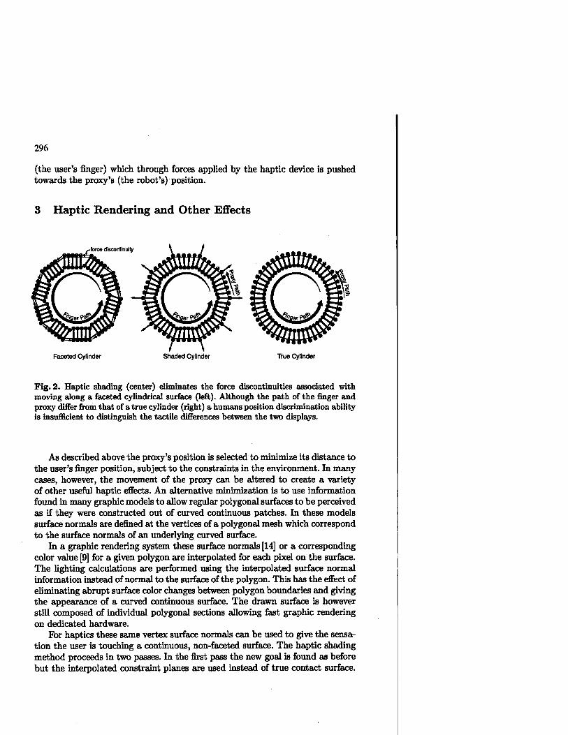
296

(the user's finger) which through forces applied by the haptic device is pushed towards the proxy's (the robot's) position.

3 Haptic Rendering and Other Effects

rforce discontinuity

Faceted Cylinder Shaded Cylinder True Cylinder

Fig. 2. Haptic shading (center) eliminates the force discontinuities associated with moving along a faceted cylindrical surface (left). Although the path of the finger and proxy differ from that of a true cylinder (right) a humans position discrimination ability is insufficient to distinguish the tactile differences between the two displays.

As described above the proxy's position is selected to minimize its distance to the user's finger position, subject to the constraints in the environment. In many cases, however, the movement of the proxy can be altered to create a variety of other useful haptic effects. An alternative minimization is to use information found in many graphic models to allow regular polygonal surfaces to be perceived as if they were constructed out of curved continuous patches. In these models surface normals are defined at the vertices of a polygonal mesh which correspond to the surface normals of an underlying curved surface.

In a graphic rendering system these surface normals [14] or a corresponding color value [9] for a given polygon are interpolated for each pixel on the surface. The lighting calculations are performed using the interpolated surface normal information instead of normal to the surface of the polygon. This has the effect of eliminating abrupt surface color changes between polygon boundaries and giving the appearance of a curved continuous surface. The drawn surface is however still composed of individual polygonal sections allowing fast graphic rendering on dedicated hardware.

For haptics these same vertex surface normals can be used to give the sensa- tion the user is touching a continuous, non-faceted surface. The haptic shading method proceeds in two passes. In the first pass the new goal is found as before but the interpolated constraint planes are used instead of true contact surface.

297

surface normal interpolated normal

^sj/ ccnstraintpsane

^Y ^»sub-goal PflSQl Passl

finger

surface normal interpolated normal

new proxy goal constraint plane

lS-goaf Pass 2

Fig. 3. Two pass haptic shading with specified normals

This new sub-goal can be thought of as the desired goal configuration of the un- derlying curved model. This goal position may, however, violate the constraints of the original polygonal geometry since it may lie above or below the true object surface. In the second pass the update procedure is called again but using the original (non-interpolated) constraint surface, and substituting the goal config- uration generated in the first pass for the user's finger position. This two pass approach has the effect of finding the nearest valid configuration to the minimal configuration as defined by the interpolated surface normals.

An example of this approach is illustrated in Figure 3. After the first pass, using the interpolated surface normal, the goal position lies below the surface of the object. After the second pass a valid proxy goal on the surface of the original obstacle is found. This goal is to the right of the goal position that would have been found if shading were not applied. If no obstacle is encountered, the proxy will move to this configuration and a force pulling the user's finger to right will be applied as would be expected from a object having the surface normal illustrated.

The difference between a haptically shaded surface, a flat surface and the true curved surface is illustrated in Figure 2. In all the figures the difference between the user's position and the position of the proxy are shown as the user's finger follows a circular counter-clockwise path around the object. As seen in Figure 2(a), a strong discontinuity occurs when the proxy reaches each edge of this ten-sided polygonal approximation of a circular obstacle. This results in a force discontinuity which gives the user the impression of crossing over and edge. In Figure 2(b), surface normals have been specified on vertices of the

298

obstacle. The resulting movement of the proxy shows that the resultant force is always perpendicular to the interpolated surface just as in the case of the true circular object illustrated in Figure 2(c). The affect of this minimization is to eliminate the large instantaneous changes in force that normally occur at polygon boundaries resulting in a surface that feels smooth and continuous. The discrimination abilities of humans are insufficient to detect the small positional differences between the polygonal and underlying curved surface.

Haptic textures can also be produced in a similar fashion. As in graphics an image-based texture can be used to modify the local surface normal of a constraint surface [2]. This surface normal defines a local constraint plane which is used in the same way as in shading to produce a intermediate goal in the haptic servo loop. Unlike shading, however, textures are typically used to render higher frequency information and, as such, may require permitting multiple constraint planes to be defined as shown in Figure 4.

Constraint Planes

Fig. 4. An image based texture can be used to introduce local constraint planes to create the sensation of bumps on the virtual surface

Other haptic effects can be created by limiting the movement of the proxy. Static friction can be easily achieved by not permitting the movement of the proxy if the user's finger is in a friction cone below the surface of the object. By restricting the velocity of the proxy to be less then some portion of the force applied by the user, the user can be given the sensation of moving through a viscous liquid. Other effects like surface stiffness or stickiness can also be easily modeled [16].

4 Collision Detection

Because the environment is normally constructed from a large number of primi- tives, a naive test based on checking if each primitive is in the path of the proxy would be prohibitively expensive. Instead a hierarchical bounding representation for the object is constructed to take advantage of the spatial coherence inherent in the environment. The bounding representation, based on spheres, is similar to that first proposed by Quinlan[15]. This hierarchy of bounding spheres is

299

constructed by first covering each polygon with small spheres in a manner simi- lar to scan conversion in computer graphics. These spheres are the leaves of an approximately balanced binary tree. Each node of this tree represents a single sphere that completely contains all the leaves of its descendants.

After covering the object, a divide and conquer strategy is used to build the interior nodes of the tree. This algorithm works in a manner similar to quick-sort. First an axis aligned bounding box that contains all the leaf spheres is found. The leaf spheres are then divided along the plane through the mid- point of the longest axes of the bounding box. Each of the resulting two subsets should be compact and contain approximately an equal number of leaf spheres. The bounding tree is constructed by recursively invoking the algorithm on each subset and then creating a new node with the two sub-trees as children. A cut- away view showing the leaf nodes (yellow) and bounding sphere hierarchy for a typical model is illustrated in Figure 5. Note that a node is not required to fully contain all the descendant internal nodes, only the descendant leaf nodes.

Fig. 5. Bounding Sphere Hierarchy of a cat model

Two heuristics are used to compute the bounding sphere of a given node. The first heuristic finds the smallest bounding sphere that contains the spheres of its two children. The second method directly examines the leaf spheres. The center is taken as the mid-point of the bounding box already computed earlier. The radius is taken to be just large enough to contain all the descendant leaf nodes. The method that generates the sphere with the smallest radius is used

300

for the given node. The first heuristic tends to work better near the leaves of the tree, while the second method produces better results closer to the root. This algorithm has an expected O(nlgn) execution time, where n is the number of leaf spheres. Once constructed the time required to determine which primitives may lie in the proxy's path is only O(lgn).

The sphere hierarchy is used to prune the number of low-level checks that need to be performed but is not used to determine the exact contact point. If the proxy's path intersects one of the leaf nodes of the hierarchy then the primitive attached to that leaf is checked to see if it intersects the path of the proxy. In our system a very fast distance algorithm by Gilbert et. al [7] is used. The algorithm can quickly find the nearest point between two arbitrary bounded convex polyhedron while requiring no pre-processing. The nearest point between two polyhedron is returned as the weighted sum of a set of vertices in the poly- hedron. These weights can be used to interpolate surface normals or texture coordinates when shading or texture effects are required. The low-level distance check runs in linear time with the number of vertices in the two polyhedron. Since the proxy path is a line segment and the number of vertices in a polygon is normally small (3 or 4) this low-level check typically takes 0(1) constant time.

5 Dynamics

Our previous discussion has been limited to the kinematic aspects of the motion of the virtual environment. To create an engaging virtual world, the user must be able to manipulate and dynamically interact with the virtual objects. In general a mechanical system can be described by a configuration space vector q = [qi... qn]T, where n is the number of DOF of the system. The forward dynamics equations of motion of such a system can be used to obtained the configuration space accelerations of the system. These equations have a general from that can be written as:

q = M(q)~l(r-b(q,q)-g(q)), (1)

where M(q) is the mass matrix, b(q,q) the centrifugal and Coriolis forces, g(q) the gravity force vector and T is the vector representing the internal and exter- nal torques applied to the system either through internal actuation or external forces applied by the environment. A simplified set of equations that neglects the centrifugal, Coriolis forces and some dynamic coupling terms is used in our current system. We are in the process of converting the system to make use of an extremely fast variation of Featherstone's articulated body solution [6] to permit the simulation of very complex dynamic models at real-time rates [4].

When a collision occurs, between the proxy and an object(s) in the environ- ment, a force is applied to the user simulating a contact with the surface. In a dynamic environment an equal and opposite force fc is applied at the contact point (s) which may induce accelerations on the virtual system. The correspond- ing joint torque vector is given by

rext = Jc fc, (2)

301

Fig. 6. Haptics permits interaction between a user and a virtual model even if the environment is very small as in the simulation of a micro sensor (left) or large as in a model of a windmill (right).

where Jc is the Jacobian of the contact point c, such that the velocity v of the contact point is given by v = JCG. For a simple PD controller the force applied to the environment can be given by

Jc — «plPpraxy — Pfinger)» (3)

where kp is the positional gain, and pproxy,Pfinger are the current positions of the proxy and finger respectively. Note that this force is in general not sufficient to prevent penetration between the proxy and objects in the environment as this equation does not incorporate the internal constraints of the proxy or other objects. A more complete solution to computing the contact forces for rigid body simulation can be found in [17]. This simplified model, however, is sufficient for simulating the interactions found in most haptic environments. Once the joint space accelerations are known, the equations of motion for the system can be integrated, from a given initial joint space configuration and velocity, to obtain the motion for the entire system over time.

302

6 Applications

The intuitive nature of haptic interaction makes it well suited for a wide range of applications. For instance, haptics can be used to train a surgeon to perform an operation without the cost and difficulties of training on animals or cadavers. In another area a haptic system can be used to allow an animator to specify the movement of a 3D model. The animator can feel the joint limits of the model and feel the penetration constraints imposed by the environment.

One area of application that is of particular interest to mechanical engineer- ing community is virtual prototyping. Virtual prototyping allows a system to be designed and evaluated in a computer without the costs associated with building a physical prototype. By allowing a developer to apply forces and interact with the model in a physically intuitive manner, haptic systems can greatly increase the understanding the design of a mechanical system. In addition, by being un- restricted by the limitations of the physical world, haptic systems can shrink the designer to the microscopic level or allow the user to manipulate large struc- tures with ease. The ability to manipulate and interact with these out of scale environments can greatly increase our ability to understand and work in these multi-scale worlds.

Figure 6 illustrates some of the virtual environments that can be modeled by our system. On the left a micro-mechanical sensor is modeled. The user if free to push on the test mass to see how the system responds to his/her input. The user can also use the probe to check clearances and ensure that the system will behave as expected. The size, mass, and time parameters of the system are scaled to allow intuitive interactions with the model. In Figure 6(right) a large scale structure is depicted. In this case, the size and mass of the system is reduced so that the user can easily interact with an object which would be difficult to interact with in reality. These models illustrate the numerous possibilities for using haptics to interact with virtual systems.

7 Conclusion

The techniques we have described were used to model a variety of virtual mod- els, see Figure 6. As computational power continues to increase the size and complexity of the models that can be simulated will continue to grow. Haptics by allowing a user to interact intuitively with a. model can greatly improve the efficiency in designing and evaluating new systems and designs. We are currently investigating methods to allow more complex systems to be modeled and allow interaction through more complex articulated effectors.

Acknowledgments

The financial support of NASA/JSC (grant NGT 9-6), NSF (grant IRI-9320017), the Boeing Company, and Interval Research Corporation is gratefully acknowl- edged.

303

References

1. D. Baraff, "Fast Contact Force Computation for Nonpenetrating Rigid Bodies," SIGGRAPH 94 Proceedings, (August 1994), pp. 23-34.

2. J., Blinn, "Simulation of Wrikled Surfaces," SIGGRAPH 89 Proceedings, (August 1978), pp. 286-292.

3. P., Buttolo, D. , Kung, B., Hannaford, "Manipulation in Real Virtual and Re- mote Environments," Proc. IEEE Conference on Systems, Man and Cybernetics, (August 1990), pp. 177-185.

4. K. Chang, "Efficient Dynamic Control and Simulation of Robotic Mechanisms," internal report.

5. J. Craig, "Introduction to Robotics Mechanics and Control," Addison-Wesley, 1989.

6. R. Featherstone. Robot Dynamics Algorithms. Kluwer, 1987. 7. E. G., Gilbert, D. W., Johnson, S. S., Keerthi, "A Fast Procedure for Comput-

ing the Distance Between Complex Objects in Three-Dimensional Space," IEEE Journal of Robotics and Automation, Vol. 4, No. 2, April 1988.

8. H. Goldstein, "Classical Mechanics," Addison-Wesley Publishing Company Inc., 1980.

9. H. Gouraud. "Continuous Shading of Curved Surfaces," IEEE Transactions on Computers, C-20(6):pp 623-629, June 1971.

10. T. Kane, Dynamics: Theory and Applications, McGraw-Hill, 1985. 11. O. Khatib, "Real-Time Obstacle Avoidance for Manipulators and Mobile Robot,"

International Journal of Robotics Research, 5(1), pp. 90-98. 12. M. D. R., Minsky, "Computational Haptics: The Sandpaper System for Synthesiz-

ing Texture for a Force-Feedback Display," PhD thesis, MIT, June 1995. 13. H. B., Morgenbesser, "Force Shading for Haptic Shape Perception in Haptic Virtual

Environments." M.Eng. thesis, MIT, September 1995. 14. B. T. Phong, "Illumination for Computer Generated Pictures." Communications

of the ACM, 18(6), pp311-317, June 1975. 15. S. Quinlan, "Efficient Distance Computation between Non-Convex Objects," Int.

Conference on Robotics and Automation, April 1994. 16. D. Ruspini, K. Kolarov and O. Khatib, "The Haptic Display of Complex Graphical

Environments." SIGGRAPH 97 Proceedings, (August 1997), pp. 345-352. 17. D., Ruspini, and O. Khatib, "Collision/Contact Models for the Dynamic Sim-

ulation of Complex Environments," Workshop on the Dynamic Simulation, IEEE/RSJ Int. Conference on Intelligent Robots and Systems, IROS '97, Geno- ble, France, 1997.

18. D., Ruspini, K. Kolarov and O. Khatib, "Graphical and Haptic Manipulation of 3D Objects." First PHANToM User's Group Workshop, September 27-30, 1996.

19. C. Zilles, J. Salisbury, "Constraint-based God-object Method for Haptic Display." ASME Haptic Interfaces for Virtual Environment and Teleoperator Systems 1994, Dynamic Systems and Control 1994, vol. 1, pp. 146-150.

304

Development of a Mechatronic System: A Telesensation System for Training and Teleoperation

Pattaraphol Batsomboon1, Sabri Tosunoglu1, and Daniel W. Repperger2

'Florida International University Department of Mechanical Engineering

10555 West Flagler Street Miami, Honda 33174 USA

tosun@fiu.edu

2Air Force Research Laboratory, AFRL/HECP Human Sensory Feedback Laboratory

Wright Patterson Air Force Base Dayton, Ohio 45433 USA

Abstract A telesensation system is an advanced teleoperator system that provides the operator with sensational feedback. In this context, a telesensation system is a mechatronic system which integrates the use of a Force-Reflecting Manual Controller (FRMC), Graphical User Interface (GUI), and a Virtual Reality (VR) unit. In an attempt to develop this advanced system, a single axis FRMC prototype is constructed. A mathematical model is identified and validated for the FRMC. In addition, a fuzzy logic control scheme is developed and implemented to test system performance. A GUI software package is also developed to integrate several teleoperation unit components including an industrial robot (which represents the remote system), joystick, electric motor (to provide force reflection for the FRMC unit), encoder, force/torque sensor, and a CCD camera. Encouraging experimental test results are obtained and reported.

1. Introduction

As technology advances, machines become more complex and intelligent. For instance, industrial robots nowadays are able to make decisions and work autonomously. This becomes possible due to the intense use of computers to run mechanical systems; hence, we see the frequent use of the term mechatronic systems. Although mechatronic systems attempt to add intelligence to mechanical systems, some applications are inherently more vulnerable to failure, and they still need to be supervised by humans. For instance, in nuclear reactor maintenance, nuclear waste cleanup operations, or in space, even the most intelligent autonomous robot cannot

305

yet perform all the tasks successfully. In order to achieve the goal, humans must be a part of the system.

The concept of "man in the loop" is introduced in the so-called teleoperator system. The purpose of having humans in the system is to guide machines to do the tasks properly since he/she cannot perform these tasks by himself/herself as the environment conditions may be harmful. In some cases, the remote site may be a thousand miles away from the operating station. Therefore, better interface between these two stations is a must to carry out many operations safely and reliably.

2. Teleoperator and Telesensation Systems

Teleoperation is a general term that refers to a human-machine remote control system. The system usually consists of two robot manipulators that are connected in such a way as to allow the human operator control one of the manipulators (the master arm) to generate commands which map to the remote manipulator (the slave arm). A teleoperator system generally consists of a manual controller, control hardware/software, sensory feedback, and a remote manipulator. Teleoperation tasks are distinguished by the continuous interaction between a human operator, teleoperator system, and the environment as illustrated in Fig. 1.

[Environment]

Remote System Human / Machine Interface

MMmMmmMi

Robot/Platform Display

GUI Software Actuators Actuators

Control Software

Sensors Interface Software Sensors '

I Operator

Fig. 1. Information flow in teleoperation systems

The main function of the teleoperator system is to assist the operator to perform and accomplish complex, uncertain tasks in hazardous and less structured environments such as space, nuclear reactors, and underwater operations, with ease, comfort, and fidelity. For instance, robotic technologies have been used to inspect, maintain and service nuclear power plants [1]. As a result, the radiation exposure of workers at the plants has been reduced to the lowest possible level [2]. In a typical teleoperator system, the operator receives feedback information that includes aural, tactile, and force feedback. Although the audio channel may be useful to the operator, the sound is often limited from the system [3].

A more recent goal in the development of teleoperation is called telesensation. Telesensation refers to a remote control system that combines the use of computer vision, computer graphics and virtual reality [4]. The word "telesensation" has also been used in literature to describe a telecommunication system such as teleconferencing where people from different remote locations in the real world are able to hold a meeting or work cooperatively in the same artificial world.

In the field of robotics, the term "telesensation" implies the advanced teleoperator system that provides the operator with sensation feedback by employing

306

the five senses (if possible). As a result, the operator is able to perceive the "feel" of presence at a remote site while he/she is in a safe workstation. The feel of presence can be provided by feedback information such as visual, aural, tactile, and force feedback. A flexible programming environment and better integration of human and computer capabilities highlight the advanced teleoperation technology [5]. The telesensation system as depicted in Fig. 2 integrates the use of an advanced operator interface, virtual reality unit, force-reflecting manual controller, and sensor-based manipulator to provide the feel of presence at the remote site [6]. Thus, with the skilled operator and sophisticated systems, the tasks can be accomplished with the most efficient and effective manner. It is also noted that such a system naturally lends itself for use as an effective tool for training purposes. A telesensation system with realistic visual and sensational feedback provides an inexpensive and safe training tool.

Computer Graphics Interface

Virtual Reality Unit

Sensor-Based Remote System

FR Manual Controller

Fig. 2. Major components of a telesensation system

3. Design and Development of a One-Axis Force-Reflecting Manual Controller Prototype

The 1-Degree-of-Freedom (DOF) Force-Reflecting Manual Controller (FRMC) has been designed and constructed to demonstrate the basic principles of the force- reflecting teleoperation system. The setup of 1-DOF FRMC is shown in Fig. 3. The principle of the control system can be summarized as follows. First, the joystick is used to control the motion of the robot. In this case, a Unimation Puma 760 six-axis industrial robot and its controller Unimation U500 represents the remote system for laboratory experiments. The control software reads in the amount of the joystick movement and computes the data according to the operation parameters such as control modes (position or velocity), scaling values for position, velocity or force reflection, and re-referencing parameters which are input by the user.

Forces experienced by the remote manipulator are received through the Force/Torque (F/T) sensor. The F/T driver receives the signals, processes the data and transmits it to the control software. The control software carries out the calculations such as force feedback scaling, position scaling, etc. Once the calculations are completed, the program sends the data to the controller, Unimation's U500, which

307

accepts high-level commands. The controller then computes the necessary torque needed and passes the signals as low-level command signals to the interface board, BB501. The interface board BB501 on the other end is connected to the amplifier BA20 which is used to amplify the signal and deliver the power to operate the motor. The motor drives the joystick that is attached directly to the motor.

PC-IBM Pentium 1 66 M(*

Control

Software

F/r Sensor

Receive*'

Controller

U500

^

Interface Boad

Fig. 3. Setup of the one-axis testbed

For the setup shown in Fig. 3, the system is able to provide a peak torque of 404 oz-in. With the length of the handgrip of 5 in, the 1-DOF FRMC prototype can produce a maximum force reflection of 5 lb. The update rate of the system is approximately 0.002 sec or 500 Hz. Note that the system is set up in the form of a direct-drive configuration. Therefore, more force reflection can be obtained by implementing a gear set to the system. However, the system will sustain higher friction and/or backlash as a result of using a gear system.

3.1 System Identification

The main purpose of constructing a model is to predict the output of the system. A mathematical model is a useful tool to prevent damages to the system that result from unexpected system response. In addition, it serves as a means to experiment for various control schemes such as PID, fuzzy logic, adaptive, neural and other controllers.

The system identification is the process of estimating a model of a system based on observed input-output data. According to Ljung, a mathematical model can never be used to represent the true description of the system, but rather it can be best regarded as a sufficient description of certain aspects that are of particular interest [7].

The choice of an identification method and the type of a model depend on the nature of the system and the purpose of identification. Parametric system models are usually more preferable than nonparametric models because modern control theory and system design techniques require the state variable description of the system dynamics [8]. As for the choices between discrete and continuous models, it is more practical to estimate the system as a discrete model since digital computers are commonly used to control and store the data in discrete forms. In addition, difference equations are easier to manipulate and identify than differential equations.

308

For a parametric, single-variable, linear, time-invariant discrete system, the input- output relationship can be represented by an nth order linear difference equation:

y(k)+a1y(k-\)*.....+a„y(k-n) = b0u(k)+b1u(k-iy- +bnu(k-n)+e(k) (1)

where y(k) and u(k) are the measured output and input data, respectively. Equation (1) is written as

A(q-l)y(k)=B(q-i)u{k)+e(k) (2)

where

A(q-l)=l + alq-l+.....+a„q-"

B(q-i) = b0+blq-i+ +b„q-"

The transfer function of this system is defined by

«^

Equation (1) is also referred to as the ARX model (AR refers to the autoregressive part A(q"')y(k) and X to the extra input B(q_1)u(k)). The a, and bt terms of the ARX model are estimated using the least squares estimation method. This method is described below [8]. Equation (2) is rewritten as

(4) y(k)=-5>/>(* - 0+XM* - «MO

(=1 i=0

Defining the 2n+l input-output vector x(t) as

x{k) = [-y(^ -1), ,-y(k — n),u(k), ,u[k-n^

the n parameter vector 0as

f=[fli .«»A b,J

Equation (4) becomes

y(k) = xT(k)i + e(k) (5)

This is set up as a system of N equations (for k = 1,..., (N+n)) as

Z=2UL +£ (6)

where

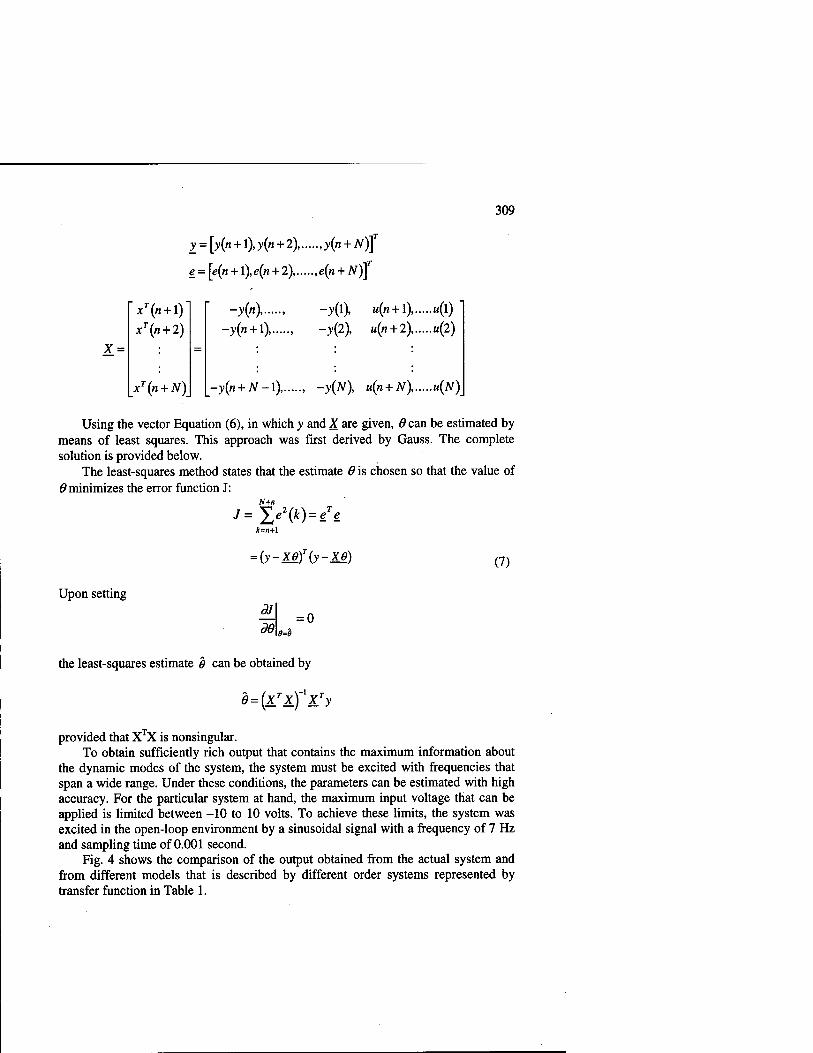
309

X =

y = [y(n + l),y(n + 2), y(n + N)J

e = [e(n + l),e(n + 2), e(n + N)f

T(n + l)l I" -y(n) , -v(l), u(n + l) u(l) T(n + 2) -y{n + l) , -v(2), u(n + 2), «(2)

r(n + N)\ [-y(n+N-l) , -y(JV), u(n + N), u(N)

Using the vector Equation (6), in which v and X are given, 6 can be estimated by means of least squares. This approach was first derived by Gauss. The complete solution is provided below.

The least-squares method states that the estimate 6 is chosen so that the value of 8 minimizes the error function J:

N+n

J= ^e2{k) = eTe

Upon setting

= (y-Mf(y-M)

^ =0

(7)

de 9=9

the least-squares estimate 0 can be obtained by

0 = {xT]C)lXTy

provided that XTX is nonsingular. To obtain sufficiently rich output that contains the maximum information about

the dynamic modes of the system, the system must be excited with frequencies that span a wide range. Under these conditions, the parameters can be estimated with high accuracy. For the particular system at hand, the maximum input voltage that can be applied is limited between -10 to 10 volts. To achieve these limits, the system was excited in the open-loop environment by a sinusoidal signal with a frequency of 7 Hz and sampling time of 0.001 second.

Fig. 4 shows the comparison of the output obtained from the actual system and from different models that is described by different order systems represented by transfer function in Table 1.

310

- Output >-()nU'r: 3 Order:

Fig. 4. Comparison of the actual system response with 2nd-, 3rd-, and 4*-order model outputs

Table 1. Models represented by 2 , 3 , and 4m order systems

Model

2nd-Order

3rd-Order

4th-Order

Transfer Function

G(5) = 0.02965 + 0.042

s2+1.89445 + 0.8950

G(sh 0.01s2 +0.0015 + 0.008

53 + 2.9438s2 + 2.91745 + 0.9736

G(s)= 0.0253353 +0.047352 +0.09375 + 0.01336

54 + 3.366s3 + 4.177752 + 2.23975 + 0.428

As can be seen, the 2nd- and 3rd-order models produce output that match the actual system output fairly well whereas the 4th-order model tails away at the end. Thus, either the 2nd- or 3r -order system can be used as a model for this system. For simplicity, the 2nd-order model is used to represent the 1-DOF FRMC prototype system dynamics. Therefore, the selected model is represented as

G(s)= 0.02965 + 0.042

s2 +1.89445+0.8950 (8)

3.2 Model Validation

To verify the accuracy of the model, the servo loop of the U500 controller was numerically simulated on the computer. Fig. 5 illustrates the U500 servo loop where

KP is Proportional Gain K{ is Integral Gain KD is Derivative Gain

311

Vyis Velocity Feedforward Gain Affis Acceleration Feedforward Gain Fs is Sampling Frequency

PotWon Command

•'AIT F"t

t Fi X

Velocity Feedforward

Po,|tion X VW«*« Ernr , , ♦▼ VWodty

Integral Error

Amplifier ^ Actuator

Position Loop

Fig. 5. Servo loop of U500 controller

The control method of the U500 controller is based on the traditional PID feedback with velocity and acceleration feedforward loops. It uses a dual control loop having an inner velocity loop and an outer position loop. The block diagram was created using the SIMULINK program to represent the servo loop of the U500 controller. Fig. 6, 7, and 8 compare the system response between the model and the actual system of different gains represented in Table 2. The sampling time in this experiment is 0.001 second whereas the amplifier block is modeled as a gain whose value is set to 100.

Table 2. Gains used in system identification process

KP Ki KD

ID1 4 10,000 20,000 ID2 8 30,000 20,000 ID3 10 20,000 40,000

Fig. 6. Comparison of the system response between the model and actual system for the gain set ID1

312

/

400 600

Tim« Im»)

Fig. 7. Comparison of the system response between the model and actual system for the gain set ID2

Fig. 8. Comparison of the system response between the model and actual system output for the gain set ID3

In Fig. 6 and 7, the model does not yield the output that matches exactly with the actual system response. However, it displays similar behavior which is considered as the most important aspect when constructing the model. The discrepancy between the model response and the actual system output can be explained by unmodeled friction and unmodeled high-frequency, low-magnitude system dynamics. Because the FRMC system is direct-drive and has only one degree of freedom, the friction is minimal and omitted in the model [9]. With a better set of gains, ID3, Fig. 8 shows that the model is able to produce the result that closely matches the actual system response. Therefore, it can be concluded that the second-order model obtained in the previous section is sufficiently accurate to represent the actual system to test the performance of various controllers.

3.3 Development of Fuzzy Logic Controller

Fuzzy logic was first introduced by Lotfi Zadeh of the University of California at Berkeley in 1965. Since then, fuzzy logic has become one of the most successful control system schemes. Fuzzy logic provides a bridge in control system design between mathematical approaches (e.g. linear control design) and logic-based approaches (e.g. expert systems). While other approaches require an accurate model to represent the real system, fuzzy design can accommodate the ambiguities of real- world human language and logic. It provides both an intuitive method for describing

313

systems in human terms and automation for the conversion of those system specifications into effective models.

Simplicity, flexibility, and cost effectiveness are among the other benefits of fuzzy logic. Fuzzy logic is capable of handling problems with imprecise data, and it can model nonlinear functions of arbitrary complexity. Not only do the rule-based approach and flexible membership function scheme make fuzzy systems straightforward to create, but they also simplify the design of systems and ensure that the system designer can easily update and maintain the system over time.

The fuzzy controller consists of a set of user-supplied rules of which the inputs and outputs are both fuzzy values. All control rules are used in parallel, and the recommended actions are combined according to the fuzzy control rules, which are weighted by the degree of satisfaction of the antecedent. This implies that the fuzzy controller has the ability to control system in an uncertain or unknown environment. However, one of the fundamental problems of fuzzy control is how to establish the control rules without human expertise and knowledge of the plant [10].

A user-supplied rule consists of IF-THEN statements which provide the output of a system. The rule mechanism is generally of the form:

R"K. IF xi is F/ and x2 is F2' and ... and xn is Fn', THEN y1 = c1

/?w:rF^isF/andx2isF: and ... and x„ is F„k, THEN / = ck

Rm>: IF X! is FT and x2 is F2m and ... and xn is F„\ THEN f = cm

where Ffk) means the //A rule Xi is a real-valued input variable Ff is a fuzzy set specified by membership functions {i/Xj) is a membership function (often defined as triangular functions) n specifies the number of input variables ck is a real-valued constant yk is the system output for this rule.

If there are m rules defined in the rule base, the system output is

y = A- V-c*

w (9)

where wk represents a variable weight assigned to the corresponding constant c A is defined as a scaling and tuning term.

The individual weights are computed as

314

w n

7=7 ' (10)

To apply fuzzy logic to a robotics control system, the position and velocity feedback are used to compare the desired values given by the operator. The resulting errors are then used to compute the input torque of the actuator. This input torque cap be considered as the torque to compensate for these errors. Therefore, the IF-THEN rules are written in the form:

IF e\ is Ej and cej is CE,, THEN y = Cy (11)

where e; is defined as position error cei is defined as velocity error

Ej is the linguistic measure of the fuzzy sets of position error CEj is the linguistic measure of the fuzzy sets of velocity error Cjj is a constant representing the torque to be applied (found in a look-up table)

The membership functions provide the continuity of control inputs rather than the on/off Boolean logic strategy. The weights of Equation (10) are now computed as:

Wj^il (e)-u (e)-C„ (12)

since n = 2 (position and velocity errors). Substituting these weights into Equation (9), we obtain

„ = A±LM_J

M j-1 (13)

where q and v define the size of the look-up table. The fuzzy logic control scheme developed for the 1-DOF FRMC prototype uses the triangular membership functions as shown in Fig. 9.

Ml M2 m3

Fig. 9. Position error (left) and velocity error membership functions (right)

These membership functions represent a total of eighty-one rules (nine linguistic measures for position error and nine linguistic measures for velocity error) with the centers of the fuzzy sets shown in Table 3. Although different spacing between the

315

centers can be done, the centers of the fuzzy sets in this experiment are equally spaced so that they can be changed easily without complicating the program. Note that it is important that a fuzzy set center be located at ne = 0 so that the errors may converge to zero. Otherwise, continuous oscillations of the joint errors will result at about zero or at convergence to a nonzero value at which the system provides no error compensation [11]. Crossover of the non-zero membership functions is limited to one crossover for any point along the error and velocity error axes although different schemes can be used that may be more effective.

Table 3. Centers for the position error and velocity error for the membership functions from Fig. 9

Position error center Value (radians) Velocity error center Value (rps) nel -0.25 ncel -1.5. ne2 -0.1875 nce2 -1.125 ne3 -0.125 nce3 -0.75 ne4 -0.0625 nce4 -0.375 ne5 0.0 nce5 0.0 ne6 0.0625 nce6 0.375 ne7 0.125 nce7 0.75 ne8 0.1875 nce8 1.125 ne9 0.25 nce9 1.5

The membership functions vary from 0 to 1 and can be calculated from Fig.9 with knowledge of the position error and velocity error. The control input (Equation 13) can then be determined utilizing the membership functions and the look-up table of constant input values (Table 4) with q = 9 and v = 9. The model obtained in the previous section is used to simulate the 1-DOF FRMC prototype. Moreover, the constant values in Table 4 represent the values of input voltage that can be provided by the actual actuator of the 1-DOF FRMC. A look-up table has to be generated that, in essence, is a set of gains for the system. According to Cha [12], the performance of a teleoperation system is greatly influenced by the force-reflection gain. If the gain is too small, the performance is poor. If the gain is too large, the system is unstable. To simplify this process, the look-up table is set up as a function of a single base value. The base value is multiplied by the weighting corresponding to the position in the table.

The look-up table coefficients as illustrated in Table 4 are chosen with the aim of sending the position and velocity errors to their respective zero value as shown in Fig. 9 [13]. The location where both the position and velocity have a large negative error receives a large negative torque and vice-versa for the positive end. For the case where there is large positive position error and large negative velocity error, the corresponding table location receives a small input torque due to the correctness of the situation being somewhere in between the two error values. The same applies for the case of large positive velocity error and large negative position error. The values in between these cases are chosen in the same manner so as to produce a continuous table flow towards zero.

316

Fig. 10 and 11 show the actual system response of the 1-DOF FRMC testbed under fuzzy logic controller with various base values.

Table 4. Look-up table representing input voltage of the actuator

nel ne2 ne3 ne4 ne5 ne6 ne7 ne8 ne9 ncel -4.0*b -4.0*b -3.0*b -3.0*b -2.0*b -2.0*b -2.0*b -1.0*b -1.0*b nce2 -4.0*b -4.0*b -3.0*b -3.0*b -2.0*b -2.0*b -1.0*b -1.0*b -1.0*b nce3 -3.0*b -3.0*b -3.0*b -3.0*b -2.0*b -2.0*b -1.0*b -1.0*b -1.0*b nce4 -2.0*b -2.0*b -2.0*b -2.0*b -2.0*b -2.0*b 1.0*b 1.0*b 1.0*b nce5 -2.0*b -1.0*b -1.0*b -1.0*b 0.0 1.0*b 1.0*b 1.0*b 1.0*b nce6 -1.0*b -1.0*b 1.0*b 2.0*b 2.0*b 2.0*b 2.0*b 2.0*b 2.0*b nce7 -1.0*b 1.0*b 2.0*b 1.0*b 2.0*b 2.0*b 3.0*b 3.0*b 3.0*b nce8 1.0*b 1.0*b 2.0*b 2.0*b 2.0*b 2.0*b 3.0*b 4.0*b 4.0*b nce9 1.0*b 1.0*b 2.0*b 2.0*b 2.0*b 2.0*b 3.0*b 4.0*b 4.0*b

b - base value

Time (s)

I—Desired - -b = 0.35 ■ • • b = 0,4 - • b = 0.45 — -b . 0.51

Fig. 10. Actual system response with base values between 0.35 to 0.5

Time (s)

I—Desired - -b = 0.5 b = 0.55 b = 0.61

Fig. 11. Actual system response with base values between 0.5 to 0.6

317

As can be seen from the above figures, different base values produce different system response. Thus, the fuzzy logic controller, as is the case with most controllers, the selection of the system gain is one of the most important factors that determine the performance of the system. In the case of the 1-DOF FRMC, the most appropriate base value is 0.5 for the look-up table represented in Table 4. Note that the results obtained above were in the case that the operator held the joystick with a loose grip.

A soft grip uses lower gains while a firm grip uses higher gains in order to provide a force-reflection sensation. As for the 1-DOF FRMC, the experiments show that for the stable region of the soft grip, the base value is in the range of 0.35-0.55; whereas for the firm grasp, the base value can be as much as 0.8-1.0. If the base value falls below the above values, poor performance results, and higher base value causes the system to be unstable.

4. Development of Graphical User Interface (GUI)

Computer-based simulations and training are very important tools in critical operations where the task needs to be operated without an error. Otherwise, the operator does not have the opportunity to practice and gain expertise in the operation. Creating a realistic simulation assists the operator to learn the process before the actual operation occurs. Thus, the performance of the operator is greatly improved when operating on the actual task. For advanced operations such as hazardous material handling in nuclear reactors and space missions, real-time graphical simulation is considered to be one of the most important tools for an advanced teleoperator system [14].

The goal of the development of an advanced graphical user interface software for a teleoperation system is to provide the operator with various options of operating modes such that the tasks can be achieved with relative ease and fidelity. However, the package should be easy to use and relatively simple to implement for any remote system.

The software package demonstrates that it is capable of accepting multiple inputs from different devices. In this case, it provides connections to video cameras, CCD cameras, force-reflecting manual controller, and virtual reality unit. Unlike many other software packages developed on mainframe workstations, our GUI software operates on a standard PC computer. This allows us to reduce the costs and simplify the entire process considerably.

The graphical user interface is being developed in a C++ environment. Several versions of the interface software have been developed. One of the earlier versions was developed in the Windows environment. This version seemed to be more user- friendly since it facilitated the manipulation of different windows. However, programming in a Windows platform requires much more space and memory than on a DOS platform [15].

Fig. 12 shows the most recent of the interface software, which is being developed on a DOS platform. The software is written using the concept of objected-oriented programming: the same concept applied to the Windows environment [15]. One of the advantages of working on the DOS platform is that the program is developed in terms of modularity. This allows the system designer to easily add or remove any features from the package. Thus, the software can be used for any remote system.

318

us 133

r^H rr^\ rr*! im B^ ia

BUM

ESI B Bs3 BRsa

BEI

fil", , )

POSITION SCALINQ: 5 CONTROL.: POSITION

SCALINQ: 5 FEEDBACK: ON

LOOP:CLOSED

DOF:lCJOJM- 1 F1U-MAM

Fig. 12. DOS-based version of the interface software

5. Virtual Reality Unit

A Virtual Reality (VR) unit is a visual device, similar to a helmet, that enables a person to perceive and interact with a virtual environment as if it were real [16]. In telesensation systems, the VR unit provides the view of the remote site as the operator turns or tilts his/her head which corresponds to a remote system camera. A VR system not only provides the operator with the 3-D view of the remote site, but also sound feedback, voice input and motion tracking [17]. A standard TV monitor is not able to provide the operator with a sense of a 3-D view of the working environment. Thus, the feeling of presence and sensation is reduced which results in poor performance [18]. Hence, a VR unit will be integrated into the telesensation system described in this paper.

One of the major advantages of having a VR unit is that the actual manipulator can be removed from the training loop while the operator is being trained. This training approach can be quite beneficial because the robot cannot be damaged by any mistreatment by an operator, and the operator should feel more comfortable during the training exercise. In addition, training scenarios can be set up easily. These scenarios usually include an emergency situation procedure training. Should the actual emergency occur, the operator would be much better in handling the situation [16]. Also, the cost associated with training personnel reduces significantly since direct hardware usage is significantly reduced.

Vision. VR systems usually include stereo vision. Two types of displays used in lower cost systems are Liquid Crystal Displays (LCD) and CRT. The CRT display areas are usually small with high light output while flat-panel LCD displays have low weight and optional color, but with poor resolution and relatively low light output. Thus, CRTs are more preferable in display design with folded optical paths.

In terms of complexity and realism, VR units have similar objectives of visual image generation to those in aircraft simulation. However, faster scene changes are required in the VR systems as a result of user head movements. VR units must be able

319

to provide effective visual simulation which requires computational complexity in order to eliminate hidden lines and produce effective perspective [19]. In addition, computational speed must be fast enough to provide the operator with acceptable scene update rates. Currently, one of the most powerful and popular work stations is produced by Silicon Graphics.

The image generator produces an output by receiving the signal from the measurement of head movements which are measured optically, acoustically, mechanically or magnetically. One of the most popular systems is the Polhemus Spasyn system. This technique requires only small sensors to be mounted on the head and is insensitive to most interference. However, one of the biggest disadvantages of this system is that the accuracy is affected by metal, and the environments must be mapped extensively.

Audio. An audio system is one of the most important elements in VR units. Spatially distinct sounds are important attributes of a convincing virtual reality. One approach to produce a successful virtual 3-D sound is to apply a mathematical function called Head-Related Transfer Function or HRTF. The HRTF relates to an individual's ear shape, but generalized HRTFs have been successfully created that work for most people. Research has shown that perceptual errors can cause problems, such as sounds behind the head that are perceived as if they were in the front of the head. These types of problems cannot be solved even when generalized HRTFs are used [20].

One of the most efficient VR systems, built at the Armstrong Aerospace Medical Research Laboratory, is called the Visually Coupled Airborne Systems Simulator (VCASS). The system uses miniature CRTs as image resources to produce high- resolution displays. VCASS provides a binocular field of view of 120 degrees horizontal and 60 degrees vertical. It has high bandwidth video amplifiers, programmable analog circuits for pre-distorting the images and many other features. Other proficient VR units have been produced by Honeywell for use in the "Falcon Eye," the F-16 night attack system, the Apache attack helicopter and in other various British research projects.

Extensive teleoperation research projects using the VR technology have been developed at NASA's AMES Research Project [21]; the JPL to control remotely deployed robots [22]; the Automation and Robotics (A&R) Division at the Johnson Space Center (JSC) for telepresence research, robotics and extravehicular activities (EVA) analysis and training [23]; the Advanced Controls Manipulation Laboratory (ACML) at Sandia National Laboratories for waste remediation technologies; the University of Tennessee at Knoxville Mobile-Manipulator Robotics Research (M2R2); and the Oak Ridge National Laboratory (ORNL) Advanced Servo Manipulator (ASM)-based Decontamination and Decommissioning (D&D) [18].

6. Conclusions

A teleoperator system extends the intelligence and capabilities of humans and robots by feeding back visual and force information, whereas a telesensation system attempts to achieve the same goal by providing multi-sensory feedback to the operator in a virtual reality environment, and thus, offers a powerful potential for training purposes as well. In either case, force reflection represents an important component of these

320

Systems. A one-axis force-reflecting manual controller has been constructed and tested in a laboratory environment. This mechatronic system has been integrated into an industrial robot via a computer. A user-friendly graphical software package was developed to integrate system components. System parameters were identified experimentally, and the system performance was tested using PID feedback and fuzzy logic-based controllers.

Acknowledgements

This work is partially funded by the U.S. Air Force, Air Force Materiel Command (Grant No: FY8990-95-00094). The authors gratefully acknowledge this support.

References

1. Tosunoglu, S., and Hamel, W. R.: Robotics Technology Assessment for Decontamination and Dismantle Tasks. Report to the U.S. Department of Energy, Grant No. DE-FG02-86NE37966 (1994)

2. Rochelear, D. N, and Crane, C. D. III.: Development of a Graphical Interface for Robotic Operation in a Hazardous environment. Proceedings of the IEEE International Conference on Systems, Man and Cybernetics, Vol. 2 (1991) 1077- 1081

3. Draper, J. V.: Teleoperators for Advanced Manufacturing: Applications and Human Factors Challenges. The International Journal of Human Factors in Manufacturing, Vol. 5, No. 1 (1995) 53-85

4. Terashima, N.: Telesensation - Distributed Interactive Virtual Reality - Overview and Prospects. MP Transactions A: Computer Science and Technology, No. A- 51(1994)49-59

5. Schenker, P. S., Bejczy, A. K., Kim, W. S., and Lee, S.: Advanced Man-Machine Interface and Control Architecture for Dexterous Teleoperation. Ocean Technologies and Opportunities in the Pacific for the 90's, Vol. 3 (1991) 1506- 1525

6. Batsomboon, P., Tosunoglu S., and Repperger, D. W.: Component Technologies for Virtual Reality-Based Telesensation Systems. The Third ASME Biennial Joint Conference on Engineering Systems Design & Analysis, ASME ESDA'96. Vol. 2. Montpellier, France (1996) 229-236

7. Ljung, L.: System Identification - Theory for the User. Prentice-Hall, Englewood Cliffs, New Jersey (1987)

8. Hsia, T. C: System Identification: Least-Squares Methods. Lexington Books, Massachusetts (1977)

9. Batsomboon, P., Tosunoglu, S., and Repperger, D. W.: System Identification and Experiments on a One-Degree-of-Freedom Force-Reflecting Manual Controller Prototype. 1998 Florida Conference on Recent Advances in Robotics. Florida Institute of Technology, Melbourne, Florida (1998) 139-145

10. Fukumi, J., Kamano, T. Suzuki, T., and Kataoka, Y.: Fuzzy Two-Degree-of- Freedom Speed Control System. Japan/USA Symposium on Flexible Automation, Vol. 1 (1996) 383-386

321

11. Monteverde, V.: Fault Tolerance: Architectures, Capabilities, and Control Strategies for Robotics. Master's Thesis, Florida International University (1997)

12. Cha, D. H., Cho, H. S., and Kim, S.: Design of a Force Reflection Controller for Telerobot Systems using Neural Network and Fuzzy Logic. Journal of Intelligent and Robotic Systems: Theory & Applications, Vol. 16, No. 1 (1996) 1-24

13. Erbatur, K., Kaynak, O., and Rudas, I.: A Study of Fuzzy Schemes for Control of Robotic Manipulators. Proceedings - 1995 IEEE International Conference on Industrial Electronics, Control, and Instrumentation, Part 1 (1995) 63-68

14. De Rossi, V., Batsomboon, P., Tosunoglu, S., and Repperger, D. W.: Interactive Modular Graphical User Interface Development for Telesensation Systems. Computational Cybernetics and Simulation. 1997 JEEE International Conference on Systems, Man, and Cybernetics, IEEE SMC'97, Vol. 2 (1997) 1604-1608

15. Ezzell, B.: Graphics Programming in Turbo C++. Addison-Wesley, Reading, Massachusetts (1990)

16. Miner, N. E., and Stansfield, S. A.: An Interactive Virtual Reality Simulation System for Robot Control and Operator Training. Proceedings of the IEEE International Conference Robotics and Automation, Vol. 2 (1994) 1428-1435

17. Christopher, C, and Stansfield, S.: Interactive Graphical Model Building using Telepresence and Virtual Reality. Proceedings of the IEEE International Conference Robotics and Automation, Vol. 2 (1994) 1436-1439

18. Trivedi, M. M., and Chen, C: Developing Telerobotic Systems Using Virtual Reality Concepts. Proceedings of the IEEE/RSJ International Conference on Intelligent Robots and Systems (1993) 352-359

19. Burdea, G., and Coiffet, P.: Virtual Reality Technology. John Wiley & Sons, Inc., New York (1994)

20. Vince, J.: Virtual Reality Systems, ACM Press, New York (1995) 21. Stark, L.: Telerobotics: Display, Control, and Communication Problems. IEEE

Journal of Robotics and Automation, Vol. 3, No. 2 (1987) 205-214 22. Bejczy, A. K., and Salisbury, J. K.: Kinesthetic Coupling Between Operator and

Remote Manipulator. Proceedings of the ASME International Computer Technology Conference (1980)

23. Read, D. A., Ruta, K. J., and Bell, B. N: Application of Virtual Reality to Space Robotics Operations. ASCE Specialty Conference on Robotics for Challenging Environments Albuquerque (1994) 19-27

322

Teleoperated Nano Scale Object Manipulation

Metin Sitti and Hideki Hashimoto

Institute of Industrial Science, University of Tokyo, Roppongi, 7-22-1, Minato-ku, Tokyo, 106-8558

{sitti,hideki}@vss.iis.u-tokyo.ac.jp

Abstract. In this paper, a teleoperated nano scale object manipulation system is proposed, and requirements of such systems are defined. The system consists of a user interface utilizing visual and haptic displays (macro world), nano-manipulator, controller and sensors (nano world), and teleoperation control and rough to fine imaging and actuation tools (between macro and nano worlds). A home-made Atomic Force Microscope is constructed for nano sensing and manipulation, and a home-made 1-DOF haptic device with Virtual Impedance-based bilateral teleoperation control scheme are utilized. Preliminary experiments consisting of nano scale tactile and force feedback while touching to materials, and 2-D assembly of 2.02 (im size latex particles are realized and results are reported.

1 Introduction

In the field of mechatronics, one of the main directions of research is the miniaturization of robots, machines and devices more and more where this new branch is called as micolnano mechatronics. Recent advances in this field enabled milli-robots inside of nuclear plants, milli-surgical robots for minimal invasive surgery, Scanning Probe Microscopy such as Atomic Force Microscopy (AFM) and Scanning Tunneling Microscopy (STM) where the geometrical, electrical, magnetic, etc. kind of properties of materials can be measured down to atomic scale in 3-D, precision positioning down to 0.01 nm resolution, etc. However, still the total sizes of these robots and machines are limited to millimeter or centimeter sizes, and one of the major reasons is the lack of the manipulation and fabrication technologies for the objects with the sizes less than 10 |xm. Construction of these technologies at the nanometer scale can enable nanoelectromechanical systems (NEMS) which are the new frontier in miniaturization and can have revolutionary implications in science and technology. NEMS will be extremely small and fast, and have applications in biological systems such as manipulating cells or genes for repairing or understanding mechanisms more clearly, computer industry such as high-density disk/memory storage and miniaturization of integrated circuit components, material science such as fabricating man-made ultrastrong and defectless materials, etc.

One of the main challenging matters for nano scale object manipulation is the

323

micro/nano physical and chemical phenomenon which is still not completely understood. Therefore, it is very early for automatic manipulation systems, and teleoperation technology at the initial phase is a promising tool for understanding these uncertainties and improving automatic manipulation strategies using the human intelligence. On the other hand, teleoperation systems have the stages of direct teleoperation, and task-based/supervised teleoperation systems where in the former, an operator directly enters to the control-loop of the nano-manipulator, and in the latter, the operator only sends high-level task commands, and the nano-manipulator realizes the tasks in an autonomous way. The final goal is fully automatic systems which can enable the mass-production of micro/nano robots or machines in the future.

By manipulation we mean using an external force for positioning or assembling objects in 2-D or 3-D, cutting, drilling, twisting, bending, pick-and-place, push and pull kind of tasks. For manipulating nano scale objects different approaches are utilized. They can be classified into two parts as non-contact and contact manipulation systems. At the former, laser trapping (optical tweezers) or electrostatic or magnetic field forces are utilized. Yamomoto et al. [1] can cut DNA using restriction enzymes on a laser trapped bead, and Stroscio et al. [2] utilized electrical force between STM probe tip and surface atoms for manipulating Xe or Ni atoms. As the contact manipulation, AFM probe tip is utilized for positioning particles [3, 4] or other nano objects such as carbon nanotubes [5] on a substrate by contact pushing or pulling operations. In these studies, only two uses teleoperation depending upon our information. Hollis et al. [6] utilized STM probe as the slave-robot and 6DOF fine motion device called Magic Wrist as the master device for feeling atomic scale topography in operator's hand. They tried to feel the topology of gold and graphite, but there were problems of mechanical and electrical noise which deforms the tactile feeling, and no true force-reflecting behaviour. Another group [7] utilizes commercial AFM and haptic device for real-time haptic display, but they do not have any report on teleoperation control problem.

In this paper, a tele-nanomanipulation system utilizing AFM probe tip as a contact-type manipulator, and at the same time as a 3-D topology and force sensor is introduced. A 1-DOF home-made haptic device with Virtual Impedance teleoperation control enables haptic display while a 3-D Virtual Reality computer graphics system shows the nano world to the user. As different from previous works, this paper reports the general requirements of the teleoperated nano manipulation systems, discusses the teleoperation control problem, and presents 2-D task-based teleoperated manipulation of 2.02 |im latex particles.

As the organization of the paper, at first, requirements of the teleoperated nano manipulation systems are defined. Then, the proposed system with macro, nano and macro to nano world components is explained in detail. Next, preliminary experiments and results with future directions are reported.

2 Requirements of Teleoperated Nano Manipulation Systems

Main structure of a directly teleoperated nano manipulation system can be seen in Figure 1. In the macro world, an operator sends commands to the nano manipulator

324

controller while feeling the nano manipulator and object interaction through visual and force displays. Nano world consists of the nano manipulator, controller, sensors and physical environment. Between both worlds, teleoperation controller constitutes the interaction bridge.

Macro World: Visual and Haptic Display

Nano World Teleoperation Controller

Fig. 1. The structure of a directly teleoperated nano manipulation system.

For a reliable teleoperated nano scale object manipulation using the system in Figure 1, following requirements should be held: 1. Nano World:

1.1. Real-time force feedback from the nano world is essential. Because, in ambient conditions, only force feedback can be possible for manipulation control since there is no real-time global 3-D vision sensor in the nano world. In vacuum environments, Scanning Electron Microscope (SEM) can give a global 2-D visual information down to 5-7 nm resolution for only conducting and some specific objects, but it is not real-time at the nano scale, and it is 2- D. Secondly, force feedback is required for controlling the interaction force such that the tool is not broken or object is not flipped away where objects become fragile and easily deformable at the nano scale. Furthermore, force measurement can enable recording of forces during manipulation, and then reliable strategies based on force control can be introduced.

1.2. 3-D visual display of the nano world is required for intuitive manipulation. SPMs can give 3-D topology, electricity, magnetism, etc. images which can be displayed to the operator. However, the imaging sampling time is in the order of seconds or minutes which means on-line imaging is not possible. Moreover, even the sampling time is very fast, since the SPMs are local sensors, and when also SPMs are utilized as the nano manipulator, the on-line imaging of the manipulator-object interaction is impossible physically because there can be one probe at one point at a given time.

1.3. A nanorobot that can manipulate objects between lnm-2jim size in 2-D or 3-D in any environment such as air, liquid or vacuum is required. The gripper size of the nanorobot should be in the order of the object to be manipulated.

325

1.4. Understanding nano forces and nanorobot dynamics is indispensable for reliable manipulation strategies. Therefore, forces and dynamics should be modeled by combining the analytical models with experimental results.

1.5. Nanorobot position controller should have the accuracy at least in the order of 1/10th of the minimum nano object part size to be observed.

Macro World: 2.1. A user friendly human-machine interface with 3-D interactive graphics display

and real-time force feedback enables easy, flexible and safe operation. Macro to Nano (M2N) World: 3.1. A bilateral teleoperation control system is needed for haptic device motion

commands transmission to the nano controller, and nano force feedback commands to the haptic device taking the scaling effect into account. Selection of the proper scaling algorithm is challenging. During the teleoperation control, also bandwidth differences of the haptic device and nano controller should be compensated. Furthermore, the stability and robustness of the teleoperation controller should be checked where the nano robot-object interactions, and nano actuators are mostly nonlinear.

3.2. Micro scale imaging (Optical Microscope down to submicron resolution) and positioning (rough to fine methodology) simplifies reaching to the nano scale gradually through micro scale.

3 Nano World

For satisfying the nano world requirements, from SPMs, AFM probe is selected as the nanorobot and force and topology sensor. Because, it enables 3-D atomic resolution imaging and real-time force feedback for any material in any environment, and can be utilized as a simple contact push and pull manipulator with probe tip sizes down to 10s of nm.

3.1 AFM as the Nano Manipulator and Sensor

Basic structure of a conventional AFM is given in Figure 2. A micro-fabricated Si cantilever/probe with a very sharp tip at the end, and measured stiffness and geometrical properties can be deflected due to the interatomic forces if the probe tip is positioned very close to a material surface in the order of few nm or Angstrom (A°) where a standard nano force-distance relation during the tip-surface approach and retraction is shown in Figure 3. When approaching there is a nonlinear attractive force due to the long range van der Waals forces and sometimes capillary forces, and after a maximum peak (small peak), the tip begins to contact around the interatomic distance, i.e. 1.69 A0. After contact, the cantilever is elastically deformed, and the interatomic force is repulsive and almost linear until to the plastic deformation region.

Using XYZ piezolelectric actuators with the resolution down to 0.01 nm, very precise positioning is possible. The cantilever deflection Az can be measured using a

326

laser beam and a photo detector system down to 0.01 nm resolution, or other methods such as piezoresistance or capacitance measurement, etc. Since the stiffness of the probe kc is known, the normal force on the tip can be computed as F=kc Az assuming at the equilibrium. Controlling the z-motion such that force reaches a reference value in the contact region, the relative motion corresponds to the height at that (x,y) point. Scanning all (x,y) points in a rectangular region, topology data can be held. This method is called contact imaging. However, for the manipulation applications, the nano objects to be manipulated are designed not to be fixed on the substrate, and contact-type of scanning can move the objects. Therefore, during imaging, non- contact AFM imaging is required. As the non-contact imaging type, tapping mode imaging is prefereble where soft samples can be scanned with few deformation, and unstabilities due to the water layer on the surface are reduced. In the tapping mode, the cantilever tip is set to several 10s of nm above the substrate, and it is vibrated externally around its resonance frequency fr by an amplitude equal to its separation distance. Thus, the tip taps to the substrate, and the interatomic forces change the vibration amplitude and frequency. Detecting these changes and controlling the sample/cantilever z-position during scanning, surface topology image is held. Thus, our strategy is imaging in the tapping mode and manipulation in the contact-mode.

Using AFM also lateral factional forces can be measured which is very useful for 2-D push and pull object manipulation where friction plays a major role. Frictional force can be measured by detecting the cantilever torsional bending angle using a four-cell photo detector, and knowing the torsional stiffness of the cantilever. In the experiments, the home-made AFM system as can be seen in Figure 4 is utilized [8]. Piezoresistive cantilevers are used where the deflection is measured through a Wheastone bridge. This kind of cantilevers are advantageous for manipulation applications where laser detection systems limit the mechanical design, and motion capabilities of the probe while these cantilevers do not. However, the deflection resolution is almost ten times worse than laser detection one.

laser beam

interatomic force]

deflection detection 'system (photo detector)

sä cantilever

XYZ Positioner

*'pösftjöji controjter

;*y scanner

Fig. 2. Structure of a normal and lateral force measuring conventional AFM.

327

1.5 •

I 0.5

-0.5-

1 1 1 1 1 r- i

sample surface

\

non-contacVattracOve region

; \^ ct intact point

contact/repulsive ' region \

►

^^^-* separation point > i > ■

-0.6 -0.4 -0.2 0 0.2 0.4 0.6 0.8 Tip-Sample Distance (|i m)

Fig. 3. Interatomic force and distance relation during Si tip and Si surface approach and retraction (experimental).

Fig. 4. Photo of the home-made AFM setup with top-view Optical Microscope.

ushing load

nano object

Fig. 5. Interaction forces during pushing nano objects by AFM probe tip.

328

3.2 Nano Forces

During the manipulation of a nano object using an AFM probe, the interacting forces are shown in Figure 5. All of these forces should be modeled, and the dynamical analysis of the manipulation should be conducted for improving general design rules and strategies. The forces consist of adhesive forces (van der Waals, capillary and electrostatic forces), contact deformation forces, frictional forces, and triboelectrification forces (charge induction on the objects during pushing due to the substrate friction). Modeling of these forces in the spherical particle pushing case is given in [9,10]. From these models, the conditions for a reliable contact pushing of any object are driven as follows: 1. Objects should be precisely movable by contact pushing on the substrate reducing

friction between particle and substrate. 1.1. Depositing lubricant monolayer on the substrate, i.e. for a Au object, Silane

monolayer on a Si substrate, and Polylysine layer on a Mica [4], 1.2. Minimizing the particle-substrate adhesion (friction is function of external

load plus adhesive force at the nano scale [9]): 1.2.1. Selecting proper material types (minimal surface energies), 1.2.2. Reducing the adhesive forces such as capillary force by reducing

the humidity level or coating the tip by teflon, or electrostatic force by grounding the tip and substrate, etc.,

1.3. Proper cantilever selection: 1.3.1. high stiffness (10s of N/m) for pushing stability (applying enough

load for pushing and breaking the adhesion force during separation from the object after manipulation),

1.3.2. hardtip(SiorSi3N4), 1.4. Contact point/angle selection (for applying maximum shearing force such

that the horizontal line passing through the object center in spherical particle case),

1.5. High motion accuracy (for precise positioning during pushing): 1.5.1. closed-loop positioners for reducing hystheresis and drift effects, 1.5.2. reducing environmental noise sources (vibration, thermal

changes, etc.), 1.5.3. selecting low thermal conductivity materials on the mechanical

parts for reducing the thermal drift, 2. Objects should not stick to the tip while retracting the probe after manipulation:

(tip-particle adhesion) < (particle-substrate adhesion) 2.1. small tip radius (few 10s of nm) with hard material: small contact area, 2.2. manipulation in liquid (reduces capillary and electrostatic forces), 2.3. tip or particle coating for reducing adhesion forces (latex particles are

coated with Au for reducing adhesion due to triboelectrification [9]). However, some of conditions have trade-offs. Conditions 1.2 and 2 are

opposite, then a between optimum particle-substrate adhesion should be designed. Secondly, Condition 1.3.1 results in reduction of force measurement sensitivity such

329

that smaller stiffness means higher force resolution. These trade-offs can be solved depending on the priority in a specific application.

3.3 AFM Position Control

Piezoelectric XYZ actuators are utilized for atomic resolution positioning. These actuators have hystheresis and drift problems depending on the motion duration and range, and temperature changes. For imaging, since xy motion consists of scanning with specified range, actuators can be calibrated off-line using laser interferometry, and these calibration data are then can be used for accurate scanning (in the case of commercial AFMs). However, in manipulation tasks, the tip moves on arbitrary points in a given range; thus, open-loop control is almost not reliable. Therefore, the best is to integrate high resolution sensors such as capacitive, strain gauge, LVDT, or optical sensors to motion axes for closed-loop control. In our system, a Physick Instrumente XYZ closed-loop stage with 10 nm resolution LVDT sensors, 0.1% hystheresis error and 100 \im range in all axes is utilized. The transfer function with stage plant dynamics and PID controller is computed as:

XM = S(s) = GAKyS + Kj+KgS2) (i)

*,« ,3 +^+GAKsDyH(0>+GAK0)S+GAKM

where GA is the voltage amplifier gain,/, is the resonance frequency of the stage with {u=2itfn, Q is the quality factor which is related to the damping of the stage, and KlP, Ka, Km are the PID controller gains. Our fine stage has the values of j=450 Hz and Q=20 for the z-axis, and/'=200 Hz and Q=20 for the xy-axes.

4 Macro World: Human-Machine Interface

Overall view of the Virtual Reality user interface for tele-nanomanipulation system which consists of force and visual displays can be seen in Figure 6.

4.1 Visual Display

Real-time and interactive visual feedback from the nano world which gives information about surface roughness, shape, texture, etc. is essential besides of haptic feedback. For this purpose, using Virtual Reality graphics technology, two systems are constructed: Nano Visulator (NV) [11] and Nano Animator/Simulator (NA/S). The former is for presenting the 3-D topology image as a shaded image to the user such that the image can be rotated, zoomed, etc. in an interactive way (Figure 7). The latter combines visualization with nano-physics where the nano forces and dynamics can be simulated in a graphics environment. Thus, connecting with force display, training and feasibility tests can be realized before the experiments, and, during

330

manipulation since there is no real visual feedback, this deficiency can be eliminated by animating the object motions during manipulation using NA/S tool.

Fig. 6. Overall photo of the Virtual Reality user interface.

Fig. 7. An example graphics display of Nano Visulator interface for 0.5 um size latex particles on a Si surface.

331

4.2 Force Display

For feeling the interatomic force normal to the AFM tip (lateral forces are excluded in this study), a 1DOF master device is constructed [8]. The actual to reference position transfer function can be computed as:

Xmr(s) = M(s) =

K.MK^s + K^+K^s2)

s* + b2s3 + (b3 + K^K^ )s2 + K^K^s + K^K^

(2)

where b,=Ktr)pl(2nJL), b2=RIL, b3=KJCJ(JL) with Kt is the torque gain, 77=0.7 is the efficiency of the gear box, p=0.175 mm/round, J=3.81 mNms2 is the inertia of the motor, L=055 mH is the inductance, R=ll Q is the resistance, Ke=0.036 Vlrads1 is the back emf constant, KPA is the power amplifier gain, and K„p, K^, and K^ are the master PID controller gains.

Operator puts his/her hand to the master arm, applies the normal force FJt), moves it with xjt), and meanwhile feels the scaled nano forces by applied motor torque. The arm is admittance type such that there is no power transmission from operator to the master arm.

Fig. 8. Bilateral force feedback control system setup.

5 M2N World: Bilateral Teleoperation Control

In the manipulation mode, during approaching and contacting to the surface or the object, or manipulating the object, the operator controls the x-y-z motion of the cantilever/sample while feeling the normal tip-sample interaction force. Using linear scaling approach, at the steady-state, the ideal response of the bilateral teleoperation system is defined as:

xs -> apxm

where FJt), F/t) are operator and nano forces, and xjt) and x/t) are positions respectively.

In order to realize the ideal responses, the bilateral teleoperation system in Figure 8 is proposed. Virtual Impedance (VI) control approach is utilized to control the impedance between the master and slave arms for realizing the desired force

332

feedback depending on the task. Thus, VI control transfer function term V(s)=l/(Mvs2

+ByS+Kv) generates smooth reference master and slave positions as xm=xjap since it also behaves as a second order low-pass filter. M(s) and S(s) are master and slave overall (plant and control) transfer functions. Kf is the force error feedback gain. At the steady state, x=ap xm, and, in the case of a constant spring dynamics for the tip- nano object interaction, i.e. FJs)=KXJs), the following equality is held for the forces:

Kv * m

F. ~a„KKt

+ a, (3)

For the ideal responses, Kv=0, or Kp»Kv condition should be provided. Furthermore, assuming the operator and nano object-tip interaction dynamics are passive, and providing the ideal responses, the system stability is also held.

6 Experiments

Three main experiments have been realized for testing the feasibility of the teleoperation control by touching to a point on a surface [12], tactile feedback by touching to many points on nano surfaces, and manipulation control by latex particle 2-D assembly experiments. At first, bilateral teleoperation scheme is tested. Touching to a point on a Si surface results in the operator and nano force and position as shown in Figure 9. Parameters of the system are M=0.1 kg, B=2 Nl(mlsec), K=0, a=8xl(f, af=25, Kf=30, ^=5 , K^OJ, and K^O.05. Initial tip-sample position is approximately 100 nm, and z motion steps are around 10-20 nm. As can be seen in the force-time graph, the operator starts to apply force at around 0.6 sec. Then the master device also begins to move until to the contact point. After the contact, ideal response is being held where scaled forces and positions follow similar shapes. The position offset is due to the piezoelectric actuator offset, and the force offset is due to thermal drift at the deflection measurement hardware and noise which limits a.

r\

IJ V ivi %

Fig. 9. Touching vertically to a point on a Si substrate: the master (solid) and scaled slave (dotted) positions (left), the master (solid) and scaled slave (dotted) forces (right) vs. time.

333

Next, a Focused Ion Beam (FIB) fabricated number '3' on Si is felt by the operator by moving in x-y using the mouse cursor. 3-D Nano Visulator view of the surface and scanned points on the sample are shown in Figure 10a and 10b respectively. Depending on the surface height frequency, and x-y motion speed the frequency of felt height increases as in the Figure 10c. If the motion speed is decreased each feature can be felt more precisely. In this experiment, for only feeling the topology information, only position ideal response is held, and force response is not realized.

Fig. 10. (a) (left upper image) FIB fabricated character '3' is shown in 3-D graphics (8 um x 8 fim x 0.1 |im size image), (b) (right upper image) Top-view 2-D image is used for x-y scanning on the surface for feeling the topology feedback, (c) The topology feedback on the operator hand vs. time: actual position (solid line) and measured reference scaled surface height (dotted line).

334

Finally, 2.02 \tm gold coated latex particles are positioned on a Si substrate by pushing on 2-D in ambient conditions with 60% humidity level. In Figure 11, a particle is added to a line of other particles successfully. Coating with gold reduced the triboelectrification forces. Cantilever parameters are k=20 Nlm and 25 nm tip radius. Optical Microscope images are utilized for real-time monitoring with 95 nmlpixel resolution. Modeling of forces and their evaluation with the experimental results are given in [9].

Fig. 11. 2-D positioning of a gold-coated latex particle to a line of other particles by contact pushing where the initial configuration (left) and last one (right) are shown.

7 Conclusion

In this paper, a teleoperated nano manipulation system using home-made AFM as the nano manipulator and sensor is introduced. Regarding to nano physics, requirements for these kind of systems are reported. Besides of 3-D visual feedback in the user interface, a 1DOF haptic device has been constructed for nano scale force sensing and generating motion commands for the AFM. Introducing teleoperation control system with Virtual Impedance approach, nano scale forces or topologies are felt by the operator. Preliminary experiments on teleoperation system and object manipulation show that the system can be utilized for tele-nanomanipulation experiments.

As the future work, the sizes of the manipulated objects will be decreased to few 10s of nanometer, and types of manipulated objects will be increased. Nano carbon tubes which are very important for nanotechnology applications will be pushed and their tribological, adhesive, mechanical, electrical and magnetic properties will be analyzed. Furthermore, biological object manipulation and mechanism understanding experiments will be conducted. On the other hand, by increasing the number of AFM probes it is possible to pick and place nano objects which can be utilized for constructing 3-D nano structures and devices.

335

References

[1] T. Yamomoto et al., "Molecular surgery of DNA using restriction enzymes," Proc. of the France-Japan Workshop from nano to macro science and tech. through microsystems, pg. 38, Nov. 1998.

[2] J. A. Stroscio and D. M. Eigler, "Atomic and molecular manipulation with the scanning tunneling microscope", Science, pp. 1319-1326, Vol. 254, No. 5036, Nov. 1991.

[3] D. M. Schaefer et al., "Fabrication of two-dimensional arrays of nanometric-size clusters with the atomic force microscopy", App. Physics Letters, pp. 1012-1014, VoL 66, No. 8, Feb. 1995.

[4] R. Resch, C. Baur et al, "Manipulation of nano particles using dynamic force microscopy: simulation and experiments", Applied Physics A, VoL 67, No. 3, pp. 265-271, Sept. 1998.

[5] M. R. Falvo, R. M. Taylor II, et aL, "Nanometre-scale rolling and sliding of carbon nanotubes,"Mi/we, VoL 397, pp. 236-238, Jan. 1999.

[6] R. L. Hollis, S. Salcudean, and D. W. Abraham, "Toward a tele-nanorobotic manipulation system with atomic scale force feedback and motion resolution", Proc. of MEMS, pp. 115- 119,1990.

[7] M. Falvo, R. Superfine, S. Washbum et al., "The nanomanipulator: a teleoperator for manipulating materials at the nanometer scale", Proc. of the Int. Symp. on the Sei. and Technology of Atomically Engineered Materials, pp. 579-586, Nov. 1995.

[8] M. Situ and H. Hashimoto, "Tele-nanorobotics using atomic force microscope," Proc. of the IEEEIRSJInt. Conf. on Intelligent Robots and Systems, pp. 1739-1746, Oct. 1998.

[9] M. Sitti and H. Hashimoto, "Two-dimensional fine particle positioning using a piezo- resistive cantilever as a micro/nano-manipulator," IEEE Int. Conf. on Robotics and Automation, May 1999 (to be published).

[10]M. Sitti and H. Hashimoto, "Macro to Nano Tele-manipulation through nanoelectro- mechanical systems," Proc. of the IEEE Ind. Electronics Conf, pp. 98-103 , Germany, Sept. 1998.

[11]S. Horiguchi, M. Sitti, and H. Hashimoto, "Virtual reality user interface for teleoperated nanometer scale object manipulation", Proc. of IEEE Int. Workshop on Robot and Human Communication, pp. 142-147, Sept 1998.

[12]M. Sitti, S.Horiguchi, and H. Hashimoto, "Tele-touch feedback of elastically deformable surfaces at the micro/nano scale: modeling and experiments," Proc. of the IEEE/RSJ Int. Conf on Intelligent Robots and Systems, Korea Oct. 1999 (submitted).

336

Virtual Manufacturing Oriented Generic Manufacturing Process Model

Läszlö Horväth*, Imre J. Rudas^, Okyay Kaynak^

1 Department of Manufacturing Engineering, Bänki Donät Polytechnic, N6pszinhäz u. 8., Budapest H-1081 Hungary

lhorvath@zeus.banki.hu department of Information Technology, Bänki Donät Polytechnic, Nepszinhäz u.

8., Budapest H-1081 Hungary rudas@zeus.banki.hu

^Bogazici University, Bebek, 80815, Istanbul, Turkey

Abstract. This paper describes a contribution to Virtual Manufacturing emphasizing product modeling and analysis using product models. An on going research by the authors is aimed to investigate a modeling method that is appropriate for manufacturability analysis of mechanical parts described by advanced shape modeling. A generic process model is generated for a cluster of manufacturing tasks. Petri net is used as manufacturing process model representation. Feasibility and resource requirements of the manufacturing are revealed by an evaluation procedure of the process model. Firstly the relevant concepts in virtual manufacturing are outlined. Then techniques of evaluation of manufacturability, the applied approach to integration of shape and manufacturing process modeling and the related virtual manufacturing concepts are introduced. The proposed process model is outlined. Next, problems and solutions at evaluating of process model in close connection with design and environmental changes are detailed. Following this, integration of the method into a comprehensive virtual manufacturing concept is explained. Finally, main issues and future research plans are concluded.

1. Introduction

Virtual Manufacturing (VM) is an integrated application of modeling and analysis techniques. In mechatronics both mechanical and electronic units of a product contain

337

parts that should be manufactured using numerical control technology. A wide range of simulation processes is based on sophisticated computer models [7]. Consequently, there is an ever growing importance of research of modeling methods. This paper describes an on going research by the authors for integrating an earlier developed manufacturing process modeling method in the virtual manufacturing technology. A manufacturing process model is generated for a cluster of manufacturing tasks then process entities are created by evaluation of the model on the basis of part, form feature, production environment, production planning and cost information. The method is devoted to process planning for mechanical parts. As the part design or environmental conditions are changed, the manufacturing process can be changed easily. Considered as a virtual manufacturing tool, the proposed modeling method can be used at evaluation of manufacturability. It makes effective integration of conceptual design and conceptual process planning possible. Sophisticated shape models with unified description of topology and geometry as well as concepts of ACIS and STEP modeling are considered as it usual nowadays in advanced CAD/CAM systems [2]. The form feature model driven manufacturing process modeling applies Petri net execution and rule based decision assistance techniques.

The paper emphasizes the model evaluation procedure in the course of which feasibility and resource demands of the manufacturing are revealed. Firstly the relevant concepts in virtual manufacturing are outlined. Then techniques of evaluation of manufacturability, the applied approach to integration of shape and manufacturing process modeling and the related virtual manufacturing concepts are introduced. The process model is outlined. Next, problems and solutions at evaluating of process model in close connection with design and environmental changes are detailed. Following this, integration of the method into a comprehensive virtual manufacturing concept is explained. Finally, main issues and future research plans are concluded.

2. Related Concepts of Virtual Manufacturing

The simulation of capability of parts and part manufacturing processes needs model descriptions that are sophisticated enough to make a reliable prediction with error that is acceptable by the industrially. The term virtual manufacturing is relative new in the application of the virtual world of advanced computing. Really, it covers an integration of computing techniques with the objective of moving the prototype testing and the related product and production development in the largest possible extent from machine shops to computer systems. Widespread application of the simulated reality is anticipated for the future. Conventional design methodology emphasizes detailed design. Whereas virtual manufacturing integrates conceptual design, analysis and manufacturability evaluation techniques [1].

338

It is anticipated for the future that customers will select vendors on the basis of ability to take into account special requirements and to configure new products within short time. Important results of product modeling efforts in the last decade as the STEP (Standard for Exchange of Product Model Data, ISO 10303) stimulated application of virtual techniques in the every day engineering practice [2].

The Laboratory for Computer Aided Engineering Studies at the Bänki Donät Polytechnic constitutes the background of investigation of virtual manufacturing. Industrial versions of typical advanced CAD/CAM and other relevant systems represent recent technology and wide range of proved ideas and methodology. At the development needs of the emerging Hungarian industry has been taken into account. One of the activities in this laboratory is integrated research of advanced modeling and simulation as well as the related computational methods.

Manufacturing Production Factory process process environment modeling modeling modeling

Production

Fig. 1 Modeling in Virtual manufacturing

A virtual manufacturing system for mechanical parts is based on modeling, model simulation and presentation techniques (Fig. 1). Part modeling, shape analysis modeling, assembly and mechanism modeling, manufacturing process modeling, production process modeling and factory environment modeling tools serve simulation as finite element analysis, analysis of mechanisms and simulation of manufacturing and production processes. Computer graphics serve human-computer interaction (HCI) processes. Realistic modeling of object surface (shader) and environment (scene) as well as animation are considered as tools of visual realistic.

339

A lot of different model representations have been implemented in practical CAD/CAM systems. Moreover, different systems produce different quality models on the basis of the same principle. For that reason capability of model representation is one of the main issues when the virtual manufacturing is applied in our globalized world where transfer of models between different modeling systems is an every day practice. In Fig. 2 part modeling is outlined as definition of topological entities, geometric entities, constraints, part attributes and design intent. The modeling system that processes the model may offer one or more of the typical modeling methods that are shown on the right in Fig. 2. Model data translation should handle this situation. For example unified shape model should be decomposed into surfaces and trimming closed line chains if surface modeling without trimmed surfaces is the only modeling method at the application of the model.

Design intent information

Constraints

Part attributes

Relations with other entities in the model of the product

Models that apply part model

data. Cäpatiyij^^'the application systeii

Fig. 2 The problem of different model representation capabilities of different systems

3. The Role of Process Modeling in Virtual Manufacturing

In the last decade early manufacturing process models involved similar description as conventional manufacturing process plans. Engineers make continuous efforts to cut development costs, to shorten product development cycles and to predict performance of a manufacturing process without actual manufacturing and measurements. Computer simulation makes it possible to avoid time and cost consuming iterative prototype manufacturing and test programs. More and more engineering tasks are placed in this manner from the machine shop to the virtual world of advanced computer systems.

340

Manufacturing process model is used by computer procedures that simulate real world conditions and predict the behavior of the process in order to establish an optimal solution for the manufacturing process (Fig. 3). Conditions are presented by description of the manufacturing task and the production environment. Simulations are utilized among others by product design, production planning, configuration of manufacturing resources or handling of machine breakdowns.

One of the main issues is the evaluation of manufacturability [5]. Conceptual stage of product design and production planning are integrated in a concurrent and collaborative engineering procedure. Among others, shape and material concepts are evaluated from the point of view of manufacturing. This is a basis information for step-wise refinement of a design.

Conceptual and detailed design of the product

Conceptual planning of the production

Detailed planning of the production

Handling machine breakdowns

Configuration of manufacturing

resources

Fig. 3 Virtual manufacturing and manufacturing process modeling

4. Process Model and its Evaluation

Authors have developed a manufacturing process model in which generic entities describe all possible manufacturing process variants for a mechanical part [3]. A manufacturing task description is defined using part model information then applied at creation and evaluation of the process model [4]. The resulted generic manufacturing process model carries information for creating all possible process variants. Actual process variant is created by using a more detailed manufacturing task description.

341

Process ns1 Net of setups 2

<s>-

yv

no2

• • •

no3

Process

Net of setups 2

Net of operations 3

6 Net of operations 3 to2

®" • ••

Sequence of NC cycles Sequence of NC cycles

Fig. 4 The manufacturing process model

Availability of machine tools, preferred machining processes, special demands of customers and product designs and other conditions are changed frequently in the every day engineering practice. These changes are handled by using repeated evaluation of the manufacturing process model. Process model entities contain knowledge for their repeated evaluation so that they can be considered as active ones. Using description of actual conditions and this knowledge, the manufacturing process plan can be modified or machineability can be repeatedly analyzed. Fig. 4 summarizes the manufacturing process model. The modeling method was elaborated for mechanical parts that are produced by machining processes. However, other classes of manufacturing processes can be handled using proper model structure. The model consists of a set of process entities. Main groups of these are process, net of setups and operations, and sequence of numerical control (NC) cycles.

In Petri net representation of model entities a transition represents a setup or an operation, a place carries tokens. Petri net is a frequently applied formal method for modeling manufacturing systems [6, 8]. A typical application of Petri net for manufacturing process modeling is described in [7]. This formal modeling approach is used for solving a lot of problems that have characteristics similar to manufacturing process modeling [9].

Special transitions are used for creating branches. An OR split-join pair defines branches to choose from. An AND split-join pair defines branches all of which are to be

342

involved in the actual manufacturing process. The model is evaluated when a single process is to be created or manufacturability analysis is to be conducted. The evaluation is based on the usual execution of the net by firing enabled transitions.

; :£jS&&ft&:- Geometric .r^~r;;i:rv "■. model i&S^^fr&l.v epresentationj

I ^S^^^^

Part modeling

Create manufacturing task

description ü

Select feature operation mode

Select manufacturing process feature class

Create manufacturing process feature

Analyse for manufacturability

Interprete the results

lanufacturability analysis

t t Operations

management

Fig. 5 The evaluation of manufacturability

A transition in the Petri net model feature will fire when the evaluation process makes this possible. This is done by checking of suitability and availability of the process object that represents the transition when the execution of the Petri net arrives at the proper transition. Enabled transitions get an active token then fires. Fail of suitability or availability of the process object makes the transition disabled for firing, the place that precedes the transition gains an inactive token and the execution on the branch halts. If there is not any other branches in the net, the execution of the Petri net will halt. This means that the manufacturing process feature has been proved unsuitable for the manufacturing task.

The above outlined manufacturing process model is developed to involve domain, application and engineer specific (personal practice and experience based) knowledge. The knowledge representation can range from few simple production rules to fuzzy rule sets and these rules are attached to transitions.

343

«1 «2, |x>4*o,6^;^|--'!

I l\ Ä flidK I 'X Inactive branch|

token I

S##^:, . a) " -^!§äPH>'*>-: . . b> :<aii3StaarOi^T^ .—•• r .*■■.** - i r?Tj£2>pr*»#*r:* .v»'^i-i-8(r..-.i*,'<'t.v*.i*ik»/fl#*i ■•< ^?- rf"^v?-i^*ii^«- • ••• >■ *•■-* -'»■<-'* * ''

|ofa4<3 ;, SfoOoj ~^'3 '4 ISi • l\ Inactive ^ *■"_.- -_ ■

H H» < ■ - -

I split

Inactive branchl

split l7 Inactive branchl

raSftW^.-rf:ty;...;?.~;-;: :■■;;;■'j r-»■:-'-■?;-•!

Fig. 6 Handling of branches

One of the problems that are in the center of virtual manufacturing is manufacturability. The objective is to establish expert's report on the manufacturing process without actual manufacturing and measurements. Part object parameters, form feature data and manufacturing engineer's prescriptions are used for creating manufacturing task description. The role of constraints that are defined within and between form features should be emphasized. The manufacturing process feature analysis may cover creation of process model entities, evaluation of process model entities or checking suitability and availability of manufacturing processes. Sometimes a combination of the three modes is applied. Reports are fed back to product modeling. Manufacturing process consists of a sequence of process objects that are represented by the fired transitions is passed to the operations management. Modified part models are undergone to repeated manufacturability analysis. Operations management may ask repeated evaluation of the model because of changes in shop floor conditions or production schedules.

344

A special method has been elaborated for handling OR branches in the Petri net model (Fig. 6). The transition representing the OR split fires when a token is placed at the place that precedes it (Fig. 6/a). Firing results in moving one token to each of the places that follow the transition. However these tokens are inactive ones. The next step of the evaluation procedure is choosing branch. Knowledge is attached to the places that follow the OR split to assist choosing. If there aren't any appropriate knowledge in the above mentioned places, the preferred branch will be chosen. If there isn't any preferred branch, manufacturing process object that represented by the first transition is checked for suitability and availability at each of the branches. The appropriate branch is chosen by changing the status of the token to active (Fig. 6/b). The actual branch has been defined. The inactive token is moved to the place that precedes the appropriate OR join as an active one (Fig. 6/c). Following this, evaluation procedure is done on the branch when the first transition has been enabled for firing by the active token. At the end of the branch all the places that precede the transition of the OR joint will have one active token, so the transition will fire (Fig. 6/d). If the execution on the actual branch halts and the first transition on none of the other branches is enabled, the execution of the Petri net halts. In this case the manufacturing process feature that is represented by the Petri net model is not suitable for the manufacturing task. Some details of checking of manufacturing process objects are shown on Fig. 7. This procedure is the basis of decision on enabled or disabled state of a transition. The transitions t0j and t02 represent operation objects. Among others, a list of processes and sets of rules are stored. In this simple example the process and two rules are attached to each of the process objects. The manufacturing task description is represented by two data, namely the prescribed type of the machine tool and notation on machine tool types that are not available.

In the case 1 horizontal machine centre is prescribed. It is because the machine tool type for the actual setup has been decided. At the same time, horizontal machine centre is not available. These data came from different sources. Pj place has a token so the ts] OR split transition fires. Token moves to P2 and P3 places. The tokens that are mapped as inactive ones remain inactive because both of operation objects failed at checking of manufacturability. In the case 2 checking of the operation that is represented by the transition t02 was successful, the state of the token at the P2 was changed to active so transition toj fires. Operation that is represented by the transition t0j is involved in the manufacturing process until a repeated evaluation of the Petri net changes this situation. A process object is described by its attributes, by its relations to other objects and by appropriate procedures. There are procedures for defining actual values of the attributes. This takes place when the transition that represents the process object fires. Attribute values are refreshed automatically during each repeated evaluation of the Petri net. Interrelations between attributes of a process object and attributes of different process objects are mapped as constraints. In integrated product models constraints connect manufacturing process model with part and other models. Rules can be defined and used for creation of constraints.

process 1 = end milling on vertical milling machine process 2 = end milling on horizontal machining centre

345

RULE1 IF machine tool type = other than vertical milling machine THEN object is not suitable

RULE 2

IF vertical milling machine = not available THEN object is not available

RULE 3

IF machine tool type = other than horizontal machining centre THEN object is not suitable

RULE 4 IF horizontal machining centre = not available THEN object is not available

■■■■■■«»■■■■■■I

Case 1 machine tool type = horizontal machining centre

horizontal machining centre = not available ts. fires

an inactive token is placed at and

01 token at net halts

and t 02 and

disabled

P 3 remain inactive

Case 2 machine tool type = vertical milling machine

vertical milling machine = available ts. fires

an inactive token is placed at

t „, enabled and t 01

token at 02

2 is made active

disabled

and

Fig. 7 Evaluation of a process model entity

346

5. Process Modeling in Virtual Manufacturing

The virtual manufacturing should be based on a model of the manufacturing process that is suitable to answer all questions about real process that would be realized in the shop floor in the course of field tests. First of all, the modeling environment should be integrated in the virtual manufacturing. It is difficult to establish a general description of a virtual manufacturing system, so that inherently integrable manufacturing process modeling method is needed. Authors are working on integration of manufacturing process modeling to CAD/CAM processes [4]. The problem of integration in virtual manufacturing can be considered as an extension of this problem complex.

The proposed manufacturing process model involves all the relevant information about sub-processes, process elements and manufacturing resources. The model can act as an agent that operates according to its environmental conditions and produces output according to the type of application and demand of production engineers. It contains all available relevant knowledge and offers knowledge acquisition functions.

The related virtual manufacturing activities are realized in a concurrent engineering environment. Present day CAD/CAM systems offer comprehensive tool sets and well- organized simultaneous engineering environment for workgroups. A lot of tools are available for virtual manufacturing activities. The manufacturing process model that has been proposed by authors can be considered as an extension to conventional computer aided engineering tools. There are other tools with functionality that overlap the functionality of manufacturing process modeling and model evaluation.

Shape modeling is supported by different manufacturability analysis tools at conceptual and detailed levels. The proposed manufacturing process modeling is considered as a special tool kit that is suitable for creating a process plan or checking process models. Evaluation of the process model is a multi purpose procedure for systematic checking of suitability and availability of process objects independently of existence a process plan. Consequently, this methodology inherently involves simulation functions. It can be connected with proved simulation techniques. An application oriented simulation can be arranged for complex simulation of the system that includes part, fixture, machine tool, cutting tool and manufacturing process models.

Important parts of the system are advanced tools for realistic presentation and visualization of analysis results. Among others stationary or animated presentation of 3D shape models, visualization of realistic surface models as well as transparent presentation of curves and data sets that describe given features are applied.

Distance between computer systems of workgroup members may be few thousand kilometers or longer. There are computer tools that support collaboration of engineering team members [9].

347

6. Summary

In the paper some of issues related to application of manufacturing process modeling in virtual manufacturing are discussed. The authors have focused on application of manufacturing process modeling in virtual manufacturing environments, utilizing the strengths of the proposed manufacturing process modeling method and integration of manufacturing process modeling in a virtual manufacturing environment. The authors proposed application of their earlier developed Petri net based modeling methodology.

The main objective is development of a methodology that is suitable to predict all possible problems in a manufacturing process using computer simulation instead of actual manufacturing and measurements. One of the main issues in virtual manufacturing is evaluation of manufacturability by simulation tools. Flexibility in application, entity based process definition and possibilities of including knowledge in the model give good prospect for the proposed process model. By presenting some details on evaluation of the model, the authors intended to support this fact.

Further research for better understanding of connections and interrelations within virtual manufacturing, and for integration of the proposed manufacturing process modeling method with well-established simulation, virtual reality and visualization methods are the most important future plans of the authors.

7. Acknowledgment

The authors gratefully acknowledge the grant provided by the OTKA Fund for Research of the Hungarian Government. Project number is T 026090. Authors also would like thank Hungarian-Turkish Intergovernmental Science & Technology Cooperation Programme (project number is TR-6/97) for the financial support.

References

1 Robert G. Wilhelm: Virtual manufacturing, Industrial Electriconics, Vol. 42, No. 4, December 1995, pp 4-8.

2 Schild, P. J. and Klemm, W. and Walz and G. J., Ruess, H. J. (1995): Open data Exchange with HP PE/Solid Designer, Hewlett-Packard Journal, October 1995, pp. 35-50

348

3 Läszlö Horväth - Imre J. Rudas: Manufacturing Process Planning Using Object Oriented Petri Nets Supported by Entropy Based Fuzzy Reasoning. Integrated Systems Engineering, PERGAMON, Oxford, 1994, pp. 335-340.

4 Läszlö Horväth, Imre J. Rudas: Procedures for Generating and Evaluation of Generic Manufacturing Process Model Entities, Proceedings of the 1997 IEEE International Conference on Systems, Man and Cybernetics, Computational Cybernetics and Simulation, Volume 1, Orlando, Florida, USA, 1997, pp. 565-570.

5 Laszlo Horvath, Imre J. Rudas: Evaluation of Petri Net Process Model Representation as a Tool of Virtual Manufacturing, Proceedings of the 1998 IEEE International Conference on Systems, Man, and Cybernetics, Information, Intelligence and Systems, IEEE, San Diego, California, USA, 1998, Volume l,pp. 178-183

6 A. A. Desrochers - R. Y. Al-Jaar: Applications of Petri Nets in Manufacturing Systems, IEEE PRESS, New York, 1995

7 Kruth, J. P. - Detand, J: A CAPP System for Non-linear Process Plans, Annals of the CIRP, 1992/1. pp. 489-492

8 Ang, J. S. K. - Conrath, D. W.: An Office Analysis Metodology Using Petri Nets and Playscripts, IEEE Transactions on Systems, Man and Cybernetics, Vol. 28, No. 5, September 1996, pp: 572-582

9 Ferraro, A. M. - Rogers, E. H.: Petri Nets in the Evaluation of Collaborative Systems, Proceedings of the 1997 IEEE International Conference on Systems, Man and Cybernetics, Computational Cybernetics and Simulation, Volume 1, Orlando, Florida, USA, 1997, pp. 3918-3923.

349

Design of Self-Tuning Controller for Systems with Unknown Time-Delay and Uncertain Parameters

Man Hyung Lee1, Kang Sup Yoon2 , and Yu Shin Chang3

1 School of Mechanical Engineering and ERC/Net Shape & Die Manufacturing, P.N.U. 2 Harashima Lab., Institute of Industrial Science, University of Tokyo, 7-22-1, Roppingi,

Minato-ku, Tokyo, 106-8558, Japan yoon@vss.iis.u-tokyo.ac.jp

3 Department of Intelligent and Mechanical Engineering, Pusan National University, Pusan, 609-735, Korea

yschang@hyowon.cc.pusan.ac.kr

Abstract. Generalized Predictive Control(GPC) has been reported as a useful self-tuning control technique for systems with unknown time-delay and parameters, and thus has won popularity among many practicing engineers. Despite its success, GPC does not guarantee its nominal stability. In this paper, GPC is rederived in the frequency domain instead of in the time domain, to guarantee its nominal stability. Derivation of GPC in the frequency domain involves spectral factorization and Diophantine equations. Frequency domain GPC control system is stable because the characteristic polynomials are strictly Schur. A Recursive least square algorithm is used to identify unknown parameters. To observe the effectiveness of the proposed controller, the controller is simulated with a numerical problem that changes in dead-time, order, and parameters.

1 Introduction

GPC[1,2] is known as a useful algorithm for systems with unknown time delay and parameters. Though it cannot guarantee stability, it is known that GPC is easy to understand and implement. Even though there has been research on stability[3,4] most of them were limited to special cases, such as mean level and dead beat. Constrained Receding Horizon Predictive Control (CRHPC) suggested by Clarke et al.[5], using the Lagrange multiplier, can be hardly regarded as a systematic study about stability. But, Stable Generalized Predictive Control(SGPC) suggested by Kouvaritakis et al.[6] makes a system stable at first by using the Bezout identity and then applies GPC to the system, so that it solves the stability problem of GPC, which makes it possible to systematically study the robustness of GPC. In this paper, to guarantee the stability of GPC, the standard GPC control law, which is developed in the time domain, is rederived in the frequency domain. Derivation of GPC in the frequency domain involves spectral factorization and Diophantine equations. After leading out a j-step predictor in the frequency domain, frequency

350

domain GPC, which has the same 2 degree-of-freedom(DOF) as the time domain GPC controller, is induced. Then, to prove that the frequency domain GPC can always ensure nominal stability, the proposed controller is simulated for an unstable non-minimum phase plant. Also, to see the effectiveness of the frequency domain GPC, the frequency domain GPC is compared with the time domain GPC through numerical simulation.

2 Plant Model

The plant is assumed to be described by the following discrete time Controlled Auto- Regressive Integrated Moving Average(CARIMA) model

A^)y{k^B(Z-%)+c(z-^f (1)

where y(k) is plant output, u{k) is control input., z~x is a backward shift operator,

and A is a backward difference operator( A = 1 - z~x). %(k) is assumed to be Gaussian white noise the mean of which is zero and the variance is Qd.

A(z-l)=l + alZ-l+-+anaz-"a,

B(z-l)=b1z-]+- + bnbz-"b,

c(z-1)=c0+c1(z-l)+:. + c„cz-»c.

Eq.( 1) can be rewritten in the following transfer function form

y{k) = w(z-iYu(k) + Wd{z-l\{k) (2)

where

„. B(Z_1

) _, cL'1) A4"1) A4"1) w

Polynomials A(z~]) and B(z~') are not necessarily coprime so long as the plant does not contain any unstable hidden modes. The poles of system(i.e., poles of iv(:-

[) ) can be either stable or unstable. Numerator polynomial ß(z_1) can be a Schur polynomial where zeros exist within a unit circle(|z|=l) in a z-plane or a non-

minimum phase polynomial. Numerator polynomial C(z~l) is assumed to have no zeros on the unit circle in the z-plane.

3 Frequency Domain j-step Predictor

To lead out the GPC law in the frequency domain, a frequency domain j-step predictor is first required. To have a j-step predictor defined in the frequency domain, the Wiener filter formulation given by Grimble[7] is referred to. In time k , given the set of output and control input as

fi = {;K*i),«i(*2);*i£*.*2 ** + ;'-*>,

351

The j-step predictor may be put in the following linear estimator form_

y(k + j\k) = HpJ(z-l)y(k) + zJH0(z-^k). (4)

Then, the j-step ahead predictor which minimizes the estimation error

y(k + j\k) = y(k + j)-y(k + j\k) (5)

under the cost function

J»=E[y2(k + j\k)\Cl\ (6)

is given as

HJZ-1)

where £[•] is the expectation operator, and the denominator polynomial Hd{z~x) is a Schur spectral factor that satisfies the following equation

HdH/=DQdc', (8)

The numerator polynomials //,y(z_1) are computed from the solution H„j (with F.

of the smallest degree) of the following Diophantine equation

AFpJ + HnjHd*z-g' = CQdC*Z-g>+j (9)

where A(z~1) = AA(z~]) and gp are the smallest positive integer that ensures the

above Diophantine equation to be in the power of z~\gp=nc+j. And, superscript

'*' denotes the adjoint of a polynomial (e.g. A*(z~i) = A(z)). And, H0 is

Ha=(\-z-'Hpj)^. (10)

Given that the j-step predictor y(k + j\k) is described by (7)-(10), whether or not cost function (6) can be minimized is proven by the following process. First, from Eq. (1),

><* + ./) = *'4»(*)+*'-£■«*)■ (11) A AA v '

Substituting (4) and (11) into (5), the estimation error becomes

y(k + j\k) = (^(1 - zJHpj) - //0l--'»(*) 1 c

J (12) + —0----'*„,)='«*)

Since estimation has to be unbiased (i.e., E{y(k + j) | k} = 0 ), H0 is the same as (10),

and the estimation error y{k+j\k) can be expressed as

y(k + j\k) = ^(\-z-JHpJ)zJt(k). (13) A

Using a discrete form of Parseval's theorem [8], cost function (6) can be expressed as

2m Jz|=i " A " (14)

A " z

352

where <&„ is power-density spectra of white noise £(£). Variance of £(£) is Qd,

so that the cost function (14) can be described as the following complete square form.

2*Hr|=i[ AHd PJ A j

z,CQdC Ha\ dz_

AHd ~HpJ A z

By using Diophantine equation (9), square term in (15) will be rewritten as

(15)

(16)

(17)

AHd » A Hd

Therefore, cost function (15) can be described as

rP __}_! FpjF Pi dz

2m%\=iHdH*d z'

From cost function (17), the term FpiF* p> IHdH* d is independent of the predictor, so that the above cost function shows minimum cost.

The proposed optimal linear predictor Hpi(z~l) is asymptotically stable since Hd(z~l) is strictly a Schur. Also, the optimal j-step predictor can be written as

y(k + j\k) = HpJ^(k)+^u(k + j) (18)

= HpJd(k) + WAu(k + j) (19)

where d{k) = —^(k) is disturbance. (20) AA

4 Frequency Domain Generalized Predictive Control

In this section, GPC in the frequency domain, which is developed in the time domain is rederived. The frequency domain derivation of GPC law minimizes the following cost function [1]

J1' =E N2 Nu

Je^t + yW + ^Aii^ + y-l) (21)

where A, is the minimum costing horizon, N2 is the maximum costing horizon,

A„ is the control horizon, and X is the scalar control weighting. And, e(k + j\k) is the future predicted tracking error as

e{k + j\k) = r{k + j) -y(k + j\k) (22)

where r(k + j) is the future reference input. The form of time domain GPC controller can be seen through a 2 DOF controller that is composed of a prefilter and a feedback loop controller, so the form of the frequency domain GPC controller is also made to be composed of a 2 DOF controller, and the block diagram for its control system can be described as shown in Fig. 1.

353

% , c JA

d +

Reference Following Controller

E Ar

-U Ki. KM ^

~,&i B ZIA

+.r y, ? ' FW

Feedback Loop Controller

Kon

Köd

-Z

Fig. 1. GPC system in the frequency domain

Therefore, the future control input increment signal from the frequency domain GPC can be defined as

AH(* + j) = Kxr{k + j) - K0y(k + j\k) (23)

where K0=K0„/Kod is the feedback loop controller, and K^=KXnIKxd is the reference following controller. The reference input, r(k), is assumed to be generated by white noise 4(z). Then, r(k) can be described as,

r(k) = Wr(z-l)g{k) (24)

where Wr(z 1) = E(z x)IAr(z

l) is assumed to be asymptotically stable and casual.

The polynomial E(z~l) is assumed to have no zeros on the unit circle in the z-plane. £(t) is assumed to be Gaussian white noise whose mean is zero and variance is Qr.

And, white noise sources 4(t) and £"(/) are assumed to be mutually statistically independent. Under the assumption that the delay-time of a plant is unknown, set Mi = 1, and suppose that Nu = N2 and the future reference input signal r(k + j) is given. Optimal feedback loop controller and optimal reference input following controller, which can minimize the cost function of GPC (21), will respectively be.[7,9]

Kn=^r (25)

Yz

H N,-\,

DrH (26)

Optimal feedback loop controller of (25) can be computed from the solutions G,H (with F of the smallest degree) of the following two coupled Diophantine equations.

DcGz Ss +FA=B Dfz

D*cHz 8s -FB = M'D}Z *e

(27)

(28)

And optimal reference following controller of (26) can be computed from the solutions Y (with Z of the smallest degree) of the following Diophantine equations.

D'JZ-Z- +ZAr = B'Drz-g*-N2+l (29)

where gg and gr are the smallest positive integers that ensure that the above

Diophantine equations are in the power of

354

z"1, gg = max(nb, na + \),gr= max(«6 -1, na +1, nb - N 2 +1).

And Df,Dc,Dr are strictly Schur spectral polynomials, which are

D/ß/=I>»X (30)

DCD*C = MA* + BB* (31)

w2

DrD;=^£Ö,£* . (32) 7=1

Therefore, the optimal control law is

Au(k + j) = JDH r(k + j)-^y(k + j) ■ (33)

In case of using above optimal controller, characteristic polynomial of the closed loop system will be

AKod + BK0„=0 or AH + BG = 0. (34)

On the other hand, eliminating F from two Diophantine equations (27) and (28), it will be

AH + BG = DfDc (35)

where Df and Dc are strictly Schur spectral polynomials. So, the closed loop system is stable. When frequency domain generalized predictive controller is given as (25)~(33), minimization of the cost function(21) will be proved as is the following process. First, cost function (21) can be rewritten in the following form

where <bCje. and OA„AHJ are power-density spectra of the future predicted tracking

error e(k + j\ k) and the future control input increment Au(k + j-l), respectively. Substituting (19) into (23), the future control input increment Au(k + j-l) becomes

Au(k + j -\)= KlSr(k + j -))- H pjK0Sd(k-\) (37)

where S = 1/(1 + WK0) is a sensitivity function.

Future predicted tracking error e(k + j\k) can be described as the following form by substituting (19) and (37) into (22)

e(k + j\k) = (\- K{SW)r(k + j)~ H pj(\- K0SW)d(k) . (38)

Substituting (37) and (38) into (36), the cost function becomes

JG--^{-7^) + T^))d7 (39)

PJ

(39a)

355

j

+ Yd^HPJSK^dd<StHt

pj

j

T2=Yp-K\smw>n<y-K\Sin*

^ . , (39b) + 2_lÄKlS<S>rrS £,

j

where <t>n and Q>dd are power-density spectra of future reference input r(k + j)

and disturbance d(k), respectively.

Let the generalized spectral factors Yj,Yr,Yc be defined as

YfYf=2lHPJ^ddH*pj (40)

yX=Ys>r. (41)

YCYC =WW +Ä . (42)

Then, ^(z-1) and T2(z~]), given in (39), can be described as the following

complete square form

Tx = 1 YrfV'Y Y,W^

K0SYcYf --L— K0SYcYf --i_

(43) , W YfY,W + J7>7—ihh

W*Y W*Y * » W*Y Y*W T2=(K,SYL.Yr -!^)(K,SYcYr -H-h-)' + YrY*r -"Lllh^L . (44)

*c *c *c*c Next, (40) by using (23) and (20), and (41) by using (24), and (42) by using (23), will be rearranged as the following respective

W) = X HriWri ^HpJfT

HpJ (45) J J AA

^•-Z^-Z^r (46)

YX-^4^ (47) A A

Therefore, the generalized spectral factor Yf, Yr, Yc can be defined as

Df D D r'-i--r'-t-r--T (48)

where Dj,Dr and Dc are strictly Schur spectral polynomials, and those are the

same with (30), (31), and (32).

The term K0SYcYj , which appears in (43), can be described as

356

DfDcK0„ K0SYcYf = _ f °" (49)

and using Diophantine equation (27), the term W*Yj I Yc can be described as

W*Yf zB*D, G F

Therefore, the square term in (43), by using (49), (50) and (35), can be separately expressed as stable and unstable terms as shown in

W*Yf . K0SYcYf——L = T,+ +T{ (51)

Yc

MJC —CK F where T,+ = _ °" 5£ is asymptotically stable, and T,~ = is unstable,

AKod+BK0n Dc*z-g*

since Dc is a Schur. The term KxSYcYr, which appears in (44), can be described as

= D,KodKlnDr (KodA + KQ„B)KidAr W

and using Diophantine equation (29), the term W*Yr IY* can be expressed as

W*Y. B'D. YZN

>~1 Zzg'+N>-]

—rL = r = —;—+ ; (53) Yc ArDc Ar Dc

Therefore, the square term in (44), by using (52) and (53), can be separately expressed as stable and unstable terms as shown in

W*Y KlSYcYr-—^ = T2

+-T2- (54) Yc

where T2+ = DcK^i„Dr-YzN^Kid(KodA + K0nB) ^ totica„ stab, and

(KodA + K0„B)KldAr

Zz^N2-\ T-) = j— is unstable, since Dc is a Schur.

A. From (43), (44), (51), and (54), the cost function (39) can be expressed as

JG=^-<\m+ -Tew* -7D*+n 1 j",,„,+ „,-„„,+ „-,* To

'i

, (55) + (T2

+-T2-)(T2+-T2-)*+T2

0} —

n « W YfYfW n , w*Y Y*W where 1» = YfYf -f-£-, T2° =Y^-^^ ■

ICIC *c'c

The terms T^T* (/ = 1, 2) are analytic for |z|<=l, so that, by the residue theorem, the

sum of the residues is zero (i.e., <fr;""7}** —= 0, '=1, 2),

<f r,-*7;+* = -(frrr^^=o(i=l,2). ■Jz|=l Z 3 Z

Therefore, cost function (55) becomes

and

357

•/G=rL4'{r1+7i+*+r,-rr*

2**H (56)

+r2+ r2

+* + 27 57*+7f+r20}—

z

Since TfTf*, T2T2*, T,0, and T2° are independent of the controller transfer

function, the cost function is minimized when T^Tf* and T2T2* are zero (i.e.,

when 7i+ and r2+ are zero).

The optimal feedback loop controller is computed by setting 7i+ to zero( 7j+ =0 ),

The optimal reference input following controller is computing by setting T2 to zero

(7/2+=0),

K=hL = Hfll (58) 1 Kld DrH

When it has optimal controllers like (57) and (58), the minimal cost function is given by

,c. =_L<f I FF' ■ zz' 2igi\=i\DcDc DC.DC

, (59) WJDJ XDrDrAA \dz

DCDC DcDcArAr ] z

A. Self-tuning frequency domain GPC

To expand the above frequency domain GPC controller into an unknown system parameter, a self-tuning control scheme is adopted, which can obtain controller parameters from estimated system parameters. For the parameter estimator, a recursive least-square estimation algorithm with exponential forgetting is used[10],

K(k)=p(k - w(A)[///+*T{k)P(k - nmr1

P(k) = [P(k-\)-K(k)f(k)P(k-\)]/ju (60)

0(k) = 0(k-\)+K(k)\y(k)-<fir(k)0(k-\)]

where e(k)=[a„-,a„aM,-;b,J\

(t>{k)^[-y(k-\),--y(k-na)Mk-W--,u{k-nb)]r .

B. The Computing Procedure of Self-tuning frequency domain GPC

The Computing procedure of self-tuning frequency domain GPC algorithm can be summarized as

CD selecting prediction horizon(Nx ) and control weighting(A)

(2) estimating system parameters a,.• ••.ana.6,,■ ■ •,bnh , using a parameter estimator

358

® solving prediction equation (9), using estimated A(z~l) and B(z~l)

® computing stable spectral factor Df (30), Dc (31), and Dr (32)

© computing Diophantine equations (27), (28), and (29) © determining the optimal controller from (25) and (26) © first control increment is computed by (33), added to a previous control value,

and resulting control value is applied to the plant input ® repeating © ~ ® steps The Proposed frequency domain GPC has a similar design parameter^,Ar2,Ar„ =N2,A ) as the time domain GPC. And, it is a receding horizon controller, which is structured as 2 DOF controller, like the time domain GPC.

5 Simulation

The objective of these simulations is to show that the proposed frequency domain GPC can always guarantee stability of closed loop systems and to show how the proposed self-tuning frequency domain GPC, which changes in delay-time, order, and parameters, compared with a time domain GPC can cope with a plant. First, to compare the stability of a time domain GPC with that of a frequency domain GPC, consider the following unstable non-minimum phase plant

(1 - 4.0023z-1 + 3.4903z-2 )><(*)

= (-0.7621z-1+1.2501z-2)M(/l) ^61)

The prediction horizon(A' ) is chosen to be 10 (i.e., AT, = l,N2 =10). The control

horizon( N„) is also chosen to be 10. The control input weighting^ ) is chosen to

be 0.01, 0.1, 1, 10, and 100. Simulation results of time domain GPC and frequency domain GPC are shown in Fig. 2. In each case, unit step response is expressed by changing a design parameter (i.e., control input weighting into 0.01, 0.1, 1, 10, and 100). Fig. 2 shows that the stability of the time domain GPC depends on a design parameter (especially control input weighting). But, it also indicates that the frequency domain GPC always guarantees stable closed loop systems, regardless of the design parameter. Second, to compare the performance of the proposed frequency domain GPC with that of a time domain GPC regarding the plant, which is changing in delay-time, order, and parameters, consider the plant shown in Table 1 [1]. During the first 10 samples, the control input was fixed at 10 for parameter estimation.

To estimate the system parameters, A(z~x) and £(z-1) are assumed to be the 2nd and 5th degree polynomial, respectively. The prediction horizon is chosen to be 10 (i.e., Nt =l,N2 = 10). The control horizon(Nu ) is also chosen to be 10. The control input weighting( X) is chosen to be 0.01. Simulation results of time domain GPC and frequency domain GPC are shown in Fig. 3. This figure shows that both time domain GPC and frequency domain GPC can produce positive response characteristics.

359

Table 1. Transfer functions of the simulated models

Number Samples Model

1

2

3

4

5

1-100

101-200

201-300

301-400

401-500

l l + 10s + 40r

,-15i

l + 10s + 4tV „-1 -Si

l + lOs 1

1 + lOi 1

10j(l + 2.5i)

(a) Output of time domain GPC.

(b) Output of frequency domain GPC. Fig. 2 Responses of time domain GPC and frequency domain GPC

for non minimum phase plant.

PLANT OUTPUT & REFERENCE INPUT

(a) output of time domain GPC. PLANT OUTPUT 8 REFERENCE INPUT

(b) output of frequency domain GPC. Fig. 3 Responses of time domain GPC and frequency domain GPC

for the plant given in Table 1.

360

6 Conclusion

To guarantee nominal stability of GPC, the standard GPC control law, which is developed in a time domain, is rederived in the frequency domain. By designing GPC in a frequency domain with the proposed method, a stable control system can be made, regardless of a designed parameter. Through simulation of an unstable non- minimum phase plant, the proposed frequency domain GPC has been proven to be always stable, while the stability of time domain GPC depends on a design parameter (especially control input weighting). In terms of performance, the frequency domain GPC can be seen to have almost similar performance as the time domain GPC.

7 Acknowledgement

This work was supported by ERC/Net Shape & Die Manufacturing, and the Research Fund of the POSCO Chair Professor at Pusan National University.

References

1. Clarke, D. W., C. Mohtadi, and P. S. Tuffs, "Generalized Predictive Control -Part I. The Basic Algorithm," Automatica, Vol. 23, pp. 137-148, 1987a.

2. Clarke, D. W., C. Mohtadi, and P. S. Tuffs, "Generalized Predictive Control-Part II. Extensions and Interpretations," Automatica, Vol. 23, pp. 149-160, 1987b.

3. Clarke, D. W., and C. Mohtadi, " Properties of Generalized Predictive Control," Automatica Vol. 25, No. 6, pp. 859-875, 1989.

4. Robinson, B. D. and D. W. Clarke, " Robustness Effects of a Prefilter in Generalized Predictive Control," IEE-Proceedings-D, Vol. 138, No. 1, pp. 2-8, 1991

5. Clarke, D. W., and R. Scattolini," Constrained Receding-Horizon Predictive Control," IEE- Proceedings Part D, Vol. 138, No. 4, pp. 347-354, 1991.

6. Kouvaritakis, B., J. A. Rossitar, and A. O. T. Chang. "Stable Generalized Predictive Control: an Algorithm with guaranteed stability," IEE- Proceedings Part D, Vol 139 No 4 DD 349- 362,1992.

7. Grimble, M. J., "Polynomial Systems Approach to Optimal Linear Filtering and Prediction," International Journal of Control, Vol. 41, No. 6. pp. 1545-1564. 1985.

8. Grimble, M. J. and A. Johnson, Optimal Control and Stochastic Estimation: Theory and Application, Volume 1, 2, John Wiley & Sons, Chichester. London, 1988.

9. Grimble, M. J., Robust Industrial Control - Optimal Design Approach for Polynomial Systems, Prentice Hall, 1994.

10. Astrom, K. J. and B. Wittenmark, Adaptive Control, Addison-Wesley, 1989.

361

Implementation of an Angle Measurement System for an Anti-Sway Crane System

Man Hyung Lee1, Keum Sick Hong1, Young Kiu Choi2, Sang Hwa Chung3, Kwang Ryul Baek3, Young Jin Yoon4, and Nam Huh4

1 School of Mechanical Engineering, Pusan National University and the Center for Intelligent and Integrated Port Management Systems

{kshong, mahlee}@ hyowon.pusan.ac.kr 2Dep't of Electrical Engineering, Pusan National University

ykichoi@hanmail.net 3 School of Computer and Electronics Engineering, Pusan National University

{shchung, krbaek}@ hyowon.pusan.ac.kr 4 Graduate School of Intelligent and Mechanical Engineering, Pusan National University, 30

Changjeon-dong, Kumjeong-ku, Pusan, 609-735, Korea {yoonyj, clown}@hyowon.pusari.ac.kr

Abstract. To implement an angle measurement system for an anti-sway crane system, lasers or camera systems are generally used. In this paper, a camera system is used, and the camera used to measure angle is the Sirrah TC212113, and the infrared beacon is the BMA-1213. The TC212113 is a camera especially developed to measure angles. The measured values are signal- processed to a basic signal result like the moving average, which is the sent to the main controller. But, in a control system, the data needed is the angular velocity. So, the increment of angles is used as the angular velocity data. The angle signal acquired from the system is acceptable, but the angular velocity from these signal contains much noise, which is not suitable for use. Therefore, the Kaiman Filter is used to reduce the noise.

1 Introduction

A potainer crane is a loading equipment that loads and unloads cargo containers to and from container ships and container trucks in a harbor. Nowadays, the amount of cargo is getting grower. To improve productivity, it is very important to load and unload more containers in the given a mount of operation time. When doing a quick feeding of containers during loading and unloading operations, the most serious problem is that it is hard to continue the next operation, because the container suspended at the end of a rope (which is supported by the trolley) is still swaying when the trolley is stopped at a target position. The purpose of this study is to design a control law that provides an almost zero-swaying angle of a container suspended at the end of a rope. This will be accomplished by feeding the velocity control of the horizontal direction of the trolley when the trolley reaches a target position[l],[2]. [Manson, 1977] introduced analytical solutions for the time-optimal control of overhead cranes by using a velocity control motor[7]. [Auering, 1985] extended it by using a torque-direct motor. Papers of [Alsop et al, 1965], f Manson, 1977], and others

362

considered the hoist motion, but, because they didn't take the limit of the velocity into consideration, the obtained time-optimal solutions were not applicable in practice. [Morishita, 1978] proposed dividing the moving range of the trolley into two parts. In the first part, the trolley moves in an arbitrary pattern and memorizes its movements ; in the second part, the trolley is controlled on a "last-in first-out" basis. [Mita and Kanai, 1979] introduced the time-optimal control, which has a notch velocity pattern to achieve acceleration/deceleration in shorter time, as they divided the moving range of the trolley into three parts (the acceleration velocity - the maximum constant velocity - the deceleration velocity) in the case of a constant rope length[8]. On the motion control of a trolley, an important factor in the configuration of the problem is that the control method is either a position control or a torque control. Previous research studied position control(i.e., velocity control motor is used). [Auernig and Troger, 1987] found the time-optimal control rule, which includes torque control and the hoist motion by Pontryagin's maximum principle[12]. [Yasunobu, 1986] tried predictive fuzzy control by fuzzy set theory, [Yamaguchi, 1994] announced an adaptation of error (between the desired swing trajectory and the real swaying angle) feedback to the velocity pattern generator on an overhead crane, and [Okawa et al, 1995]'s paper showed the use of the optical-fiber gyro inclinometer for the feedback of swaying angle and for the velocity pattern control[4],[9]. Recent development of the nonlinear control theory made its adaptation to the crane system. [Fiss et al, 1991] announced the linearization control law via a generalized state space model, and [Boustany and Novel, 1992] proposed an adaptive control of a crane, a control that uses dynamic feedback linearization. For control the swaying of overhead crane which has the constant rope length[3],[5],[6], [Yoon et al, 1989] and [Park et al, 1990] proposed that a damping effect be imposed on the simple pendulum motion by providing feedback to the control input, which is measured by the variation rate of the swaying angle. The two studies also proposed that the partition of the feeding velocity pattern be the maximum velocity feeding control range, the swaying control range, the pre-programmed decelerated range, and the stop-position control range[10],[ll]! [Lim, 1992] and [Lee, 1994] announced the configuration of a fuzzy logic controller for the position control of an overhead crane, and [Hong and Lee, 1995] studied the optimal control of the performance index minimization, which includes the swaying of cargo and the swaying and the acceleration time due to a difference between the velocity of the cargo and the trolley. This paper consists of four sections. In section 1, an introduction, a brief review of previous studies, and the purpose of this paper are presented. The derivation of the dynamics for a container crane and the control law are introduced in section 2. Section 3 presents a sensing system designed for this study, and also the experimental results. Final a conclusion is presented in section 4.

2 Design of Controller

In crane-swaying control, the most remarkable thing is that the number of DOF (degree of freedom) in the system is more than that of the input implementable by the system. That is, to express the position of a container with a constant rope length during horizontal trolley moves, we must know the rotational motion of the container on the trolley (1 DOF, if the rotation is restricted on the plane) and the position of the

363

trolley (1 DOF), but the control input is just input (velocity or torque) on the trolley motor. In general, a crane system has heavy non-linearity, and a potainer crane operated in a harbor needs to have the capability to overcome disturbances such as wind. Shown in Fig. 1, container crane motion will be divided into hoist motion and trolley motion.

Fig. 1. Schematic of a Container Crane

First of all in the swaying motion of a container crane and a crane system, we assume that, (1) the container do a plane motion, that is, the swaying of a crane is generated in the

plane that was perpendicular to the direction of the trolley motion, (2) the elasticity strain of the crane structure is small, so we may disregard it, (3) the damping effect generated in the rolling friction resistance and the drive

mechanism is negligible, and (4) the container is a particle suspended by a rope (i.e., the container has no mass). The container motion equation that satisfies the previous assumptions is

*(0 = »(0 (1)

#'(/) +g*(0 = -«(0 x is the trolley displacement, <p is the swaying angle, g is the acceleration of gravity, and / is the length of the pendulum. This equation is derived from the Lagrange motion equation. We can obtain the following velocity patterns used in this motion equation : a trapezoid velocity pattern (Fig. 2), a step velocity pattern (Fig. 3), and a notch velocity pattern (Fig. 4). The previous velocity pattern provides an exact zero swaying-angle when acceleration and deceleration is over under the ideal condition if (1) the rope length is constant, (2) the initial conditions are exactly zero, (3) external disturbances such as wind do not exist, and (4) the previous second order equation exactly models the swaying motion of a

364

container.

10 12 14

Fig. 2. Speed trajectory for a trapezoidal reference command

1200

1000

800 E E-

400 -

I :). j k I reference / j ' \ '

NyH \ |-\"j •

^- i i i i i 6

time

Fig. 3. Speed trajectory for a step reference command

f

BOO

600

400

200

speed refeitence

speed "txäj ecföry"

O 2 A 6 8 10 time

Fig. 4. Speed trajectory for a notch reference command

365

In the case of the multiple acceleration velocity pattern, the variation of rope length should be considered. But, we did not consider the original time-varying system ; instead, we considered the approximated time-invariant system used by making substitute values according to variations rope length. Therefore, the exact variation of rope length was not considered. However, at least one of the before-mentioned assumptions may always occur in a practical situation. In addition, it is very important to quickly remove the swaying in case of sudden stops while a trolley is being driven. To solve these problems, a control concept should be designed for a desired velocity pattern if the cases are the same as or similar to those mentioned above. Also, the control concept should compensate the actual trolley velocity by providing feedback of the error between the measured swaying angle and the reference angle when a trolley moves in the velocity pattern. So, we made the following control law to solve these problems. We set up the equation by putting the swaying trajectory, which is the

reference of the length of rope (lr= constant: r - reference), into the motion equation of a simple pendulum in a time-invariant system.

*«/ =

" 0 \ " 0 " g 0 Zrf +

1

L lr L lr\ -Lxd , Zrf(0) =

(2)

= Arz,, + BrXj

Where subscript "d" denotes "desired." The reference length of rope may be (1) length( /, ) after completing a rising when the hoist rises(in an accelerating trolley)

or length(/2) after completing a falling when the hoist falls (in a decelerating trolley), or

(2) lme = (2a+bT)/2 when the hoist moves up and down by equation I = a + bt, where T is the damping vibration period. If the trapezoid velocity pattern is used, for example, xd is

*d

a, = V V is ' max _ rmax I 5

'up 2n XL 0 < t < T,

0 T,<t<T2 (3)

'down 2.X \l2

If the step velocity pattern is used, given Fmax, a, xd, lx, /2 are

nn _ r max

2a

To=x± h

T,=T2+TX

T^ 2aT,

366

T5=Tt+Tx

And, we can express the plant as follows.

i(0 = 0 1

--*- 0 /(0

z(0 + 0

1 /(O

m 2(0) = "o" 0 <4>

= (Ar + AA(t))z(t) + (Br + M(t))x(t)

Then, when time tx ->■ 7j or T3, we can know that AA(t), AB(t) ->■ 0.

Now, consider control input x(t) by using the sum of the correction term xc(t) on

the reference input xd(t).

x = xd+xc (5) Where,

xc=K(z-zd) (6)

Subscript "c" denotes "correction term," and K = [£, k2] is the feedback gain. This correction term will correct the real-state vector when theyt (swaying angle and angle velocity) deviate from the reference state vector, and pay attention to take the full state feedback form. Hence, we define the error that the real state deviates from the reference state.

ze(0 = z(0-zrf(0 So, it becomes

ze(t) = (Ar + AA(t))z(t) + (Br + AB(t))(xd(t)+ Kze(t)) -[ArzdU)+ Brxd(t)] = (Ar+KB(t))ze(t) + AA(t)z(t)+ ABO)xd(t)

Hence, when Tx < t < T2 and T3 < t , the real state error equation for the reference state is as follows.

ze(t) = (A/+BrK)ze(t) (9) And, we rewrite it in the form of a differential equation.

*L)&(0 = 0 <10)

(7)

(8)

when k2 = 2£»/, and a2 = (g/lr + kjlr), we can obtain the damping coefficient £

and the frequency a by suitable regulation of the k}, k2.

3 Sensing System

A camera and a beacon are the measurement instruments used in this study. The schematic diagram of a crane system with a camera and a beacon is shown in Fig. 6. The camera system is firmly attached to a trolley and the beacon to the hoist. The camera system receives a infrared rays from the beacon to measure the swaying angle of the trolley. The camera used in this system is a TC212113 made by the SIRRAH company, and the beacon, a BMA-1213-DUR, is composed of infrared LEDs.

367

This system can provide various functions following the user's commands and specifications. The maximum measurement speed of the camera system in a given view is 200 frames per second, with an angular precision rate of 1/10000. The camera system also has a function to calculate the average of the measured values. So, the number of values needed for an average can be decided by the user, as shown in Fig. 5. In this study, the control period of the whole control system is 54msec, so 10 or 11 values are used for an average result. The values measured by the camera are the phi and the theta. The phi value is the swaying angle perpendicular to the moving trolley, and the theta is the swaying angle the direction of which is that of the moving trolley. Both values are measured, but, in the real system, the theta angle, which has the same direction of the trolley, is used. Also, since the angular velocity is needed, the increment of the angle relative to time is used. A basic experiment is carried out to test the system. In Fig. 7, the trolley velocity, position, and the swaying angular velocity are shown. Swaying occurs when the trolley is accelerated and also when the trolley comes to rest. When the trolley comes to rest, small amount of swaying can be observed. In Fig. 8, the measured angle and the calculated angular velocity are shown. The acquired angle signal is satisfactory, but the calculated angular velocity, which will be used to control the system, contains much noise. To reduce the noise, the average method and the FIR filter have generally been used. But, these methods need abundant data for acceptable results, and the average result will also be past results. For effective noise reduction, if the amount of data needed for everaging or the number of taps needed for filtering is increased, it will cause a time delay, which will cause problems in controlling the system. In this paper, for the reduction of noise we have modelled the swaying of the pendulum, as shown in Eq. (11), and used the Kaiman Filter for noise reduction.

x(/) = w(/)

s u(t) ÜD ^(0 + ^(0 = -^

If the Kaiman Filter is used, the control system states can be estimated and, since there is no time delay, effective control can be possible. The system noise characteristics used in the Kaiman filter are acquired by the measured angle and angular velocity when the hoist is fixed so that no swaying occurs. The results from the Kaiman Filter are shown in Fig 9. There is little difference in the angles, but the noise from the angular velocity is reduced.

measure(5ms) 0 1 2 3 4 5 6 7 8 9 10 11

Tttttttttfttt average MM4

result EC4 | f

Fig. 5. Measurement and average results (average of four measured values)

368

o T

^ EH BEACON

Fig. 6. Schematic crane system

Trolley velocity 0.8

0.7

0.6

0.5

| 0.4

0.3

0.2

0.1

0

0.2

0.15

0.1

0.05

0

-0.05

-01

-0 15

-02

Jl I i

-iL-----r-- - * - - -

nJ ( T

1 - -1- ---r-----7------

10 20 30 time (sec)

(a)

Trolley Accel

10 20 30 time (sec)

(c)

40

. .rrrrt . J i i

-- — ■ -i 1- t______

.. _., -r T

40

6

5

4

E3

2

1

0

0.06

0.04

«•0.02

Trolley position

^j § . it i i ■f i i

J • i

j ■ i

j i a

j i i

-0.02

-0.04

10 20 30 time (sec)

(b)

Measured angle

10 20 30 time (sec)

40

Fig. 7. (a) velocity, (b) position, (c) angular velocity, and (d) measured angle of the trolley

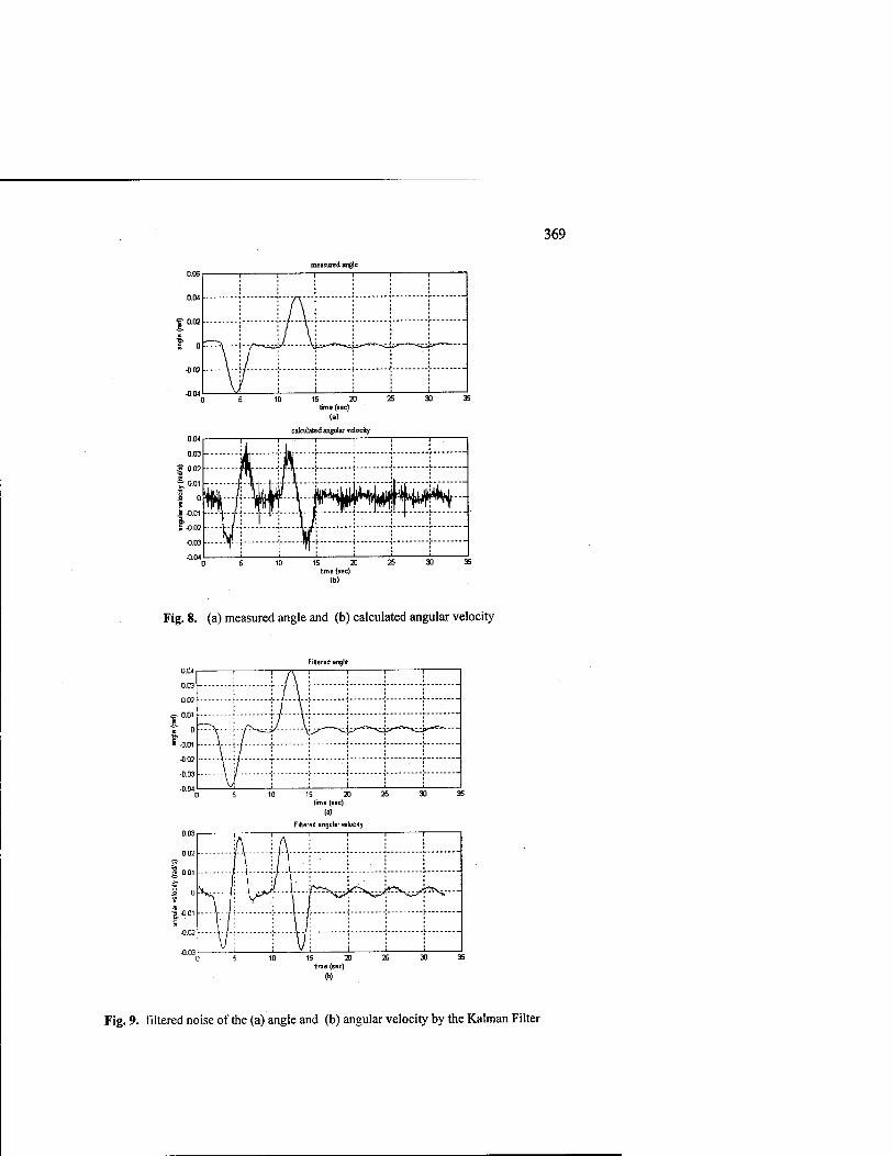
369

measured angle

0.04

? °°2 2.

I 0

-0.02

15 20 time (sec)

(a)

calculated angular Telocity

Fig. 8. (a) measured angle and (b) calculated angular velocity

Filtered angle

15 20 time (sec)

■<»>

Filtered angular velocity

lime (sec)

(b)'

Fig. 9. filtered noise of the (a) angle and (b) angular velocity by the Kaiman Filter

370

4 Conclusion

In this paper, to measure the angular velocity, the dynamics of a crane is derived with some assumptions, and the Kaiman Filter is used with satisfactory results. But, since the calculation of the Kaiman Filter was done in a main controller there is some burden in the control time. If these calculations can be done in a camera system then better results may be achieved.

5 Acknowledgement

This work was supported by the Research Fund of the POSCO Chair Professor at Pusan National University and the Center for Intelligent and Integrated Port Management Systems(assigned by KOSEF, Korea Science and Engineering Foundation) at Dong-A University.

6 References

1. Andrzej M. Trzynadlowski, "The Field Orientation Principle in Control of Induction Motors", Kluwer Academic Publishers, 1994.

2. Paul C. Krause, "Analysis of Electric Machinery", McGraw-Hill, 1986. 3. Boustany, F. and d'Andrea-Novel, B., "Adaptive Control of Noncompletely

Controlled Mechanical Systems Using Dynamic Feedback Linearization and Estimation Design", Int. J. Adaptive Control and Signal Processing. Vol. 6, pp. 589-610, 1992.

4. Hamalainen, J.J., Marttinen, A., Baharova, L., and Virkkunen, J., "Optimal Path Planning for a Trolley Crane: Fast and Smooth Transfer of Load", IEEE Proc- Control Theory Appl., Vol. 142, No. I, pp. 51-57,1995.

5. Hong, K. S., Sohn, S. C, and Lee, M. H, "Sway Control of a Container Crane: Part I and Part II", J. of Control, Automation and System Engineering, 1997.

6. Lee, H.-H, Cho, S.-K, and Cho, J.-S., "A New Anti-Swing Control of Overhead Cranes", Proc. IFAC Int. Workshop, Automation in the Steel Industry: Current Practice and Future Development, ASI'97, Kyungju, Korea, pp. 137-142, 1997.

7. Manson, G. A., Time Optimal Control Methods Arising from the Study of Overhead Cranes, Ph.D Thesis, Univ. of Strathclyde, Glasgow, U. K, 1977.

8. Mita, T., and Kanai, T., "Optimal Control of the Crane System Using the Maximum Speed of the Trolley", Trans. Soc. Instrum. Control Enge. Vol. 15, No. 6, pp. 125-130, 1979.

9. Sakawa, Y. and Shindo, Y., "Optimal Control of Container Cranes", Automatica. Vol. 18, No. 3, pp. 257-266, 1982.

10. B. S. Park, J. S. Yoon, J. S. Lee, "A Study on the Swing Control using Anti- Swing Crane", KACC, Vol. 1, pp. 292-297, 1990.

11. J. S. Yoon, B. S. Park, J. S. Lee, "A Design of Control Algorithms for the Anti- Swing Crane", KACC, Vol. 1, pp. 260-265, 1989.

12. J. W. Auerning and H. Troger, "Time Optimal control of Overhead Cranes with Hoisting of the Load", Automatica, Vol. 23, No. 4, pp. 437-447, 1987.

371

13. H. J. Hong, S. S. Lee, "Optimal Control of Crane-Pendulum System", KSPE, Spring pp. 832-837,1995.

14. J. S. Yoon, B. S. Park, J. S. Lee and H. S. Park, "Controller Design for the Anti- swing Crane. J. of Control", Automation and System Eng., Vol. 1, pp. 229-233, 1994.

372

Position Control of a Pneumatic Servo Mechanism

G.H. Ho1 and C.L. Teo2

Department of Mechanical and Production Engineering, National University of Singapore, Singapore 119260

'engp7581@nus.edu.sg 2mpeteocl@nus.edu.sg

Abstract. In this paper, a simple practical sliding mode controller is implemented for the position control of a rodless pneumatic servomechanism. A mathematical model was first derived and then linearised to give an estimated 3rd order system. To circumvent the need for acceleration or pressure feedback, an internal proportional loop is added to the pneumatic system so that the resulting system can be approximated by a 2nd order system. A sliding mode controller is then designed based on this 2nd order system. The effectiveness of the new scheme is evaluated using an industrial rodless pneumatic cylinder with proportional valve. Our results showed that the controller gives better accuracy over a larger operating range, and is more robust against any changes to the system as compared to a standard PID controller.

1 Introduction

Pneumatics has always presented problems to its controller design due to the compressibility of air, friction and stiction, all being highly non-linear. The usual approach is to linearise the system about a nominal position but such a linearised model is only suitable for a limited range about that point. In addition, the robustness is poor with respect to changes in payload and other parametric variations. In recent years, more sophisticated controllers have been employed in pneumatic control. A PID self-tuning controller is developed in [1]. The pneumatic system is assumed to be 2nd order and the PID parameters are adjusted based on the results of the real-time identification. In [2], a sliding mode controller is used for the position control of the pneumatic actuator. The use of differential pressure feedback is proposed in order to circumvent the need for acceleration feedback. Acceleration feedback is usually needed as the typical model of the pneumatic system is at least 3rd order. It is shown that the sliding mode controller with differential pressure feedback works well and is robust to payload and parametric variations.

In this paper, a simple sliding mode controller for a rodless pneumatic system is proposed. As in [1], the model of the system is assumed to be 2nd order. However, to ensure that this approximation be more accurate, an internal high-gain proportional loop is first added. The effect of adding this loop is that, if the gain is sufficiently

373

high, the resulting system is approximately unity. Since the gain cannot be set to be arbitrarily very high we assume that the resulting system is 2nd order. This proportional loop can be incorporated into the controller and so no external modifications of the system are required. Finally an outer sliding-mode controller is added in order to compensate for the unknown and resulting unmodelled dynamics.

2 Experimental Setup

The servomechanism consists of the following Festo Pneumatics components (Fig.l): • linear actuator with a rodless cylinder, • proportional 5/3 way closed-centered control servo-valve, • linear potentiometer for position feedback

Control of the system was implemented in software using a PC via an AD/DA card.

load

cylinder

WS 5S s_

Potentiometer feedback

Proportional Control valve *F A11" 11L BSP«—□ .Position

GonW&Ber

Fig. 1. Schematic Diagram of the Whole Pneumatic Servo System

3 System Dynamics

As we can see from the block diagram of the overall system in Fig.2, the servo system consists of 6 main parts: the spool valve and its controller, the cylinder, the load, the system controller and the position feedback potentiometer. In order to analyze the whole system, we need to find out the governing equations for each system component, then combine them together to obtain the overall transfer function of the system.

The mathematical equations of all the parts were derived from the flow equations, energy equations and dynamics equations [3]. In the derivation process, we made a number of assumptions in order to simplify the analysis. Furthermore, the spool position controller was assumed to be proportional.

374

O E 1 Spool

Pos it ion Controller

rt.)

m

controller servo valve

cylinder * load

P'h e urhätic'"S'erv b System

linear potentiometer (Jfcf) 4

Fig. 2. Overall System Block Diagram of Festo Pneumatic Servomechanism

3.1 Cylinder/Ram

Taking the control volume of side a (charging) in Fig.3, applying the NSFEE (Non Steady Flow Energy Equation),

1 11 Pa,V„Ta

T 1.K.T,

control volume ä-

Fig. 3. Schematic Diagram of a Simplified Pneumatic Cylinder in action

where

v2 v2 dE Qa-Wa+ma{h+ — + gz)in-ma(h+ — + gz)out= —

*■ i at Qa = rate of heat flow into control volume a

Wa = rate of work done (power generated)

ma = mass flow rate into and out of control volume a h = enthalpy of the fluid v = velocity of the fluid flow z = elevation Et = total internal energy inside the control volume a

We assumed the following conditions: 1. perfect gas 2. fast process (i.e. fast expansion and contraction) 3. good insulation of cylinder wall 4. piston only moves slightly from its initial position 5. cylinder is lying horizontal (i.e. the inlets and outlets of the control volume are

at the same elevation)

375

From assumptions 2 and 3, we assumed the process to be adiabatic, rearranging, NSFEE yields the following:

1 Pa dVtt [ d PaVa Cv

Cn dt dt R C„ 1

RT. dK dt Y dt

Similarly, it can be shown for the control volume on side b (discharging),

1 mh =•

RTh

pdVLJbdPb

dt y dt

To linearise the charging and discharging process for the cylinder, the following assumptions were made:

1. changes about a steady state initial conditions are very small, such that Pa, Va, Pb, Vb do not vary too much from their initial values,

2. Tai = rbi = T{= Ts, Vn = Vbi = Kj (i.e. piston is at the central position initially), Pai= Pbi= Pi, where subscripts i stands for initial, s for supply.

Neglecting products of small quantities, we combine the equations to give

Sma+Smb = 1

RT. 2PiA±.{Sy)+^-±-(8Pa-SPh)

dt Y "t

(1)

3.2 Valve

Applying SFEE (Steady Flow Energy Equation) to an orifice under adiabatic conditions

CJTU-Td) = 2 2

where subscripts u = upstream d = downstream

and since in this case, au » a^, which means Vd » vu, hence

Vd=,JCp(Tu-Td)

Since Cp, (Ta - 7^) are difficult to measure, but not Tu, PA and Pu, therefore we try to find the mass flow equation in terms of these variables only.

For ideal gas,

Tä=Tu\f ru J

7 and^- ( n \

Pd = Pu 'u J \?u J

our mass flow equation becomes

376

m. -°f.\ 2y

Ä(y-i)Vl/»

r+i

= a 1•> / ft

For sonic flow, Cm will be a constant, and that will definitely simplify our analysis a lot. Unfortunately the conditions we had did not allow us to make that kind of assumption, and we had to stick to subsonic flow analysis. And also for actual flow, we will have to include a drag coefficient, Cd, in order to include the effects of fluid drag. Cd is approximately 0.8 for gases. Since the valve orifice in our servo valve is annular, our analysis could be simplified further, and orifice opening area becomes

a = bxv

where xv = valve spool displacement from centre, b = total circumference of annular orifice.

Hence combining with the cylinder (Fig.4), flow equations for our servo valve becomes

Fig. 4. Schematic Diagram of Pneumatic Cylinder with Valve in Action

mn --^mwW mb =Cdbx I 2y

Th \R(r-i) (Pe]

2

Y * e

r+\

vb

where subscripts a and b refers to the side of the piston the valve opening is connected, and e refers to exhaust.

To simplify and linearise these 2 equations, we assumed : 1. Ps, Pe, Ts, Te are all constant, 2. there is no heat transfer between fluid and environment (i.e. adiabatic

process), 3. changes in valve spool position (Axv) is very small, 4. cylinder pressures vary only by very small amounts from Pj.

From Taylor's expansion series of these 2 equations, . . dm dm sn dm sn dm

m-m, = 8m = 8xv+——8P^+^-^8P„ + . _ <?T„ dx„ dP, dP. dT„

= V x, + W pd + W P„ + KS Tu

hence

<J mfl = kXa8 xva + k2a8 Pa + kla8 Ps + *4a<5 Ts

377

8mb = kib8 xvb + k2bS Pe + k3b8 Pb + k^S Tb

From assumption 1, 8PS = £.Pe = <? Ts = 0. For ease of analysis, we also assumed that 8 Ts = 8 Ts = 0. Also, <5 jcva = 8 xvb (since they came from the same spool), hence these 2 equations become

8ma = kXa8xv+k2a8Pi and 8mb =kxb8 xv+k3b8Ph

where

u-^-ciic.

*, = dP~7

dxu

m 2y

m

xv

2 r+i

^p-i

3 ~~d~P T~ 1 + 2r

2 y+l

'r r

= —(l + O)

note that when O -> », we can see that k2i = -kib, i.e.

dP„

m„ m. = -<D^L = -(l + 0>)^i- = -

P P = "*,

This assumption is valid provided PA -> Pa (and hence O -»• oo), which implies that the orifice pressure drop is very small, which is consistent with our assumptions for a linearised analysis. Later on we shall see from the calculations from the valve specifications that the actual pressure drop is quite small.

Since k\„ — kih — k,, k 36 : -k2, mai = mbl = m,, Pai = Pbl = P,

we have from the previous 2 equations 8ma=ki(8xv) + k28Pa and 8mb = kt(8 xv)-k28 Pb

378

hence, summing up, we have

Sma +Ömb =2ki(Sxv) + k2(SPa -ÖPb) (2)

3.3 Valve Spool Position Equation

The spool position xv has to be achieved by some means, and in this case electrically. Hence we had to find equation of spool position as a function of input solenoid voltage. According to the specifications sheet data, the function appears to be somewhere near a 3rd order polynomial. However, in order to simplify the analysis, we assumed that the valve position is proportional to the input voltage about a desired operating point (we chose the mid-point, which is the closed position of the spool, which is at 5V). Hence we assumed that

xv = kvE

where k, = constant valve spool position gain, E = valve solenoid input voltage

(3)

3.4 Load Dynamics

Referring to Fig.5, our governing equation for load in our pneumatic system is simply

, IB A

p. ph

Ü2S

&T^

Fig. 5. Schematic Diagram of Load Dynamics

where m = load, / = fluid viscous friction, F = external forces (gravitational, stiction etc.)

Since we are dealing with air (gas), fluid viscosity is negligible. If our cylinder is only placed horizontally, we can ignore the gravitational forces. Stiction is complex and unpredictable, and in order not to complicate our analysis further, we shall leave it out for the time being (we shall see how well the controllers can control these unmodelled dynamics).

Hence the dynamics equation becomes (Pa-Pb)A = my

and after linearisation,

(SPa-8Pb)A = my

379

(4)

3.5 System Transfer Function

Combining the mass flow equations (1) and (2) for the valve and the cylinder, introducing the Laplace operator s, and including the load dynamics equation (3) and the valve spool position controller equation (4), we have

*4% kAky

f A2^

5y_ SE

Kk6mj

,fe'Ä + l

8y *Aß,2

where £ = mkc

2AiJmk6

wl =

SE s{s2+2£cons + a>2n)

A2

k6m

and kA = RT.k i^i

, *S="

RT.k s*2

IP, , *6 =

V;

2yPt

As we can see from the transfer function, our system seemed to be a 3r order system. A point to take note is that there is an integrator in our model, hence we cannot perform an open loop frequency response test on the system.

From the overall system transfer function equation , we needed the following system parameters

y, R, K, kf, Ts, Ph V„ m, A, xv, m, Pd and Pu

in order to derive the transfer function for this particular setup. The numerical data for this system are :

Specific heat ratio, y Gas constant, R Spool position controller gain, ky, Linear potentiometer f/b gain kf, Supply temperature, T^ Initial chamber pressure, Pf

Chamber volume, V-„ Mass of load, m Piston area, A Maximum mass flow rate, m Maximum spool position, xv

= 1.40 = 287.0 J/kg K = 2.34x1 O^mm/V = 1.0 = 298.0 K = 2.5 x 105 N/m2

= 2.945 x 10-4 m3

= 1.020 kg = 4.9087 xlO^m2

=1.4058xl0-2kg/s = 1.17xl0"3m

380

Upstream pressure, Pu = 4.0 x 105 N/m2

Downstream pressure, Pd = 3.8xl05 N/m2

These values were derived from their respective equations. Take note that all pressures are absolute, not gauge.

Hence by substituting these values into the transfer function, we arrived at the system transfer function in s domain

1100

8E(s) 53+18b2+56b

3.6 Reduced Order System

As we can see from the transfer function, the linearised model is 3rd order. In order to implement the sliding mode controller, either acceleration or pressure feedback [2] would be needed. In our approach, we introduce an internal feedback loop within the servo system [5] itself as in Figure 6.

-»Q-»|K|—► System

^Order)

Fig. 6. Block diagram of the internal loop

We tuned the proportional gain K, forcing the system to behave like a 2nd order overdamped system, but in order not to significantly affect the tracking performance, we used the greatest value of K before the system response overshoots. We obtained the following closed loop transfer function, with #=0.7.

G = 770 c s3+18b2+5615 + 770

770

(s+1.57 +1.37/)(s +1.57 -1.37/)(s +177.96) Closing the loop gave us a closed loop pole at s=-177.96 which decays so much

faster than the other 2 poles such that we could actually neglect its effects and estimate the system with the internal loop with the other 2 poles

770

(s +1.57 +1.37/)(s +1.57 -1.37/)

770

S2+3.13J+4.33

This estimate would give a gain of approximately 100, so we still need to adjust the zero to give us the same unity gain as before, i.e.

381

4.33

s* +3.13^+4.33 All controller designs henceforth were based on this 2nd order estimate.

4 Controller Design

The concept of SMC lies mainly in turning a n* order tracking problem into a 1st

order stabilization problem, in a pre-defined time varying sliding surface called s(t) [4]. Considering a single input dynamic system as a n* order equation in the form of

x'=f(x)+b(x)u where x is the variable,

f(x) is the unknown dynamics u is the control input and b(x) is the input gain

and for the tracking task to be achievable using a finite control u, initial desired state must be such that

xd(0) = x(0) where xj is the desired output

otherwise tracking can only be achieved after a transient. Let the tracking error be

X — X — X j

Defining a time-varying surface by the equation

s{x;t) = {±- + X)n-'x at

where A is a strictly positive constant. for example, a sliding surface of 2nd order would be

s = x+X x which is nothing more than a weighted sum of position error and velocity error.

Given the initial conditions, tracking x = xd is equivalent to that of remaining on the sliding surface s(t) for all t >0, and this condition, i.e. s = 0 represents a linear differential equation with unique solution of 3c = 0. This is effect, replaces the original n* order tracking problem by a 1st order stabilisation problem. Now the problem of keeping sliding surface s at zero can be achieved by choosing the control law M such that outside s(t)

I^<_^|S| 2dt '

where 7 is a strictly positive constant. This sliding condition constrains all system trajectories to point towards the surface s(t), and remain on the surface once on the surface.

The controller design basically consists of 2 steps. Firstly, a feedback control law u is selected in order to verify the sliding condition. Then the control law has to

382

incorporate a discontinuous term to take care of the modelling imprecision and disturbances.

The concept was first applied based on the assumptions of an estimated 2nd order system in our servomechanism.

Considering the servo-system as a 2nd order equation in the form of x = f + bu

1. The dynamics/ which is possibly non linear and time varying, is not exactly known and hence estimated as /, and the estimation error is also assumed to be bounded by some known function F = F(x,x,'x), giving

|/-/|<F 2. The control gain b, which may possibly be time-varying or state-dependant, is

treated as unknown but of known bounds (which themselves may possibly be time-varying or state-dependant):

0<bmin<b<bnax

Since control input enters multiplicatively in the dynamics, we shall choose the estimate b of the control gain as the geometric mean of the bounds as:

b = Vftmin*max

Our 2nd order sliding surface would be in the form of s = x+Xx

The dynamics while in sliding mode can be written as

s = x + fä = x-xd+Xx=f+bu-xd+fä = 0 To achieve s = 0, the best approximation of a continuous control law, ü , would be

. _ - f +'xd -Ax

b Adding a discontinuous term across the surface to take care of the uncertainties due to estimation, our controller becomes

„ _ $ ksgn(*) = (.-f + Xj-Xx)-ksgnjs) b b

+ k ifs>6 where k sgn(s) =

[-k if s < 0

By choosing k to be large enough, we can guarantee that the sliding condition is verified. Substituting control input u back into s, we have

i = (/-4/) + (4-lX*rf -Ä)-4*sgn(5) b b b

In order to satisfy the sliding condition, s2 < -n I s I, we need 2 dt

öD b b

+ — ?]<k b

since \f-f\<F,

383

k>-F + b o (X'J -2ÄX-A x)-f

b

Starting with the mathematical model for the estimated 2nd order system obtained in the previous section,

y _ 4.33

E s2+3Ä3s + 433 y = -(3.Uy + 4.33y) + 4.33E

and comparing with x' = f + bu , we have x = y, w = £, 6 = 4.3268, / =-(3.1308*+ 4.3268x)

In practice, the switching caused by the discontinuous term k sgn(ty leads to chattering, which in most cases are undesirable. This is because it involves high control activity and may excite high frequency dynamics neglected during modelling. To achieve this, the control discontinuity was smoothened out by a boundary layer sandwiching the switching, or sliding surface, by replacing the sgci(s) by satfs/^), where "sat" is the saturation function, while the term ^ defines the width of the boundary layer. The effect of this is essentially the same as assigning a lowpass filter structure to the local dynamics of the sliding plane so as to eliminate chattering.

Hence our controller becomes

u = ■ (-f + Xj -Ax)-ksat(s /$

5 Results

We compare the performances of the proposed sliding mode controller with a standard PID controller. Controllers were implemented on the actual system through software control, with controller parameters were tuned separately. Sampling time was set at 0.5 ms. Comparisons were made between different conditions and a standard condition (4 bars supply pressure (abs), standard load 1.020kg, step input 0V-5V), only varying one parameter each time.

PID. The PID controller values were tuned at the mid-stroke using Ziegler-Nichol's method, with the actual system response. The values used were: Kp =1.76, X/=5.87, Kd =0.132. Figures 7 to 12 shows the various responses as we vary the desired positions, loads and supply pressures.

Sliding Mode. For the sliding mode controller, the control values used were X =10, F =1, 7] =50. Figures 13 to 18 shows the various responses as we vary the desired positions, loads and supply pressures.

384

—™ 8l«p ^— Oulp

*räi 1 II • ff i I Hi I 1,

• \ — Outpul CW Input

:I —Äv^ ■

0 3 0.4 oe 1.2 14 16 1.« 1

0 0 0 0 0 111

Fig.7. Actual System Response with PID Controller with Standard Conditions (4 bars abs, 1.020kg load, 0V-5V step input)

Fig. 10. With Additional 1.5kg Load

02 64 OS

Fig. 11. With 3 bars (abs) Supply Pressure

Fig. 8. With a 0V-3V Step Input

\ SUptipul Output

anhput

\f* ~^-—^

1 h^f-.--i o oi 04 oe oi

Fig. 12. With 5 bars (abs) Supply Pressure

Fig. 9. With a 0V-7V Step Input

385

02 0.4 0.S O« 1 12 1.4 1« II 2

0 0.2 0.4 0.« Öl 1 1.2 14 1,0 1.0 2

Fig. 13. Actual System Response for Sliding Mode Controller with Standard Conditions (4 bars abs, 1.020kg load, OV-5V step input)

„Li

Fig. 16. With Additional 1.5kg Load

0.2 04 08 08 1 12 1.4 1.6 IS 2

0 02 0 4 0 6 0* 1 12 14 18 18 2

Fig. 17. With 3 bars (abs) Supply Pressure

Fig. 14. With a 0V-3V Step Input

0 2 0 4 08 0» 1 12 14 1.6 1.8 2

02 04 06 08 1 12 14 18 18 2

Fig. 18. With 5 bars (abs) Supply Pressure

Fig. 15. With a 0V-7V Step Input

6 Discussions

From the responses of the PID controlled system in Figure 7, we found that stiction is inevitable, and its effects were quite significant. A simple PID is not effective enough

386

to get rid of effects of stiction. We have also seen that, changes in system parameters (e.g. change in supply pressure, change in load) significantly affects the performance of the controller, especially the stick-slip behaviour and the accuracy of the position control.

In comparison, sliding mode not only provides better accuracy it is also more effective in overcoming other non-linear characteristics that were not modeled in our mathematical model. In addition, it is also more robust to any changes in the system's parameters. However, there were slight oscillations during the transient response when the controller reaches the sliding plane and switches about the plane.

7 Conclusions

A simple sliding mode with additional feedback loop controller has been implemented. Our results showed that this non-linear controller gives better accuracy and remains effective over a larger operating range, and is more robust against any parameter variations as compared to the PID controller.

References

[1]M.C. Shih and S.I Tseng, Pneumatic Servo Cylinder Position Control by PID-Self-Tuning Controller, JSME International Journal, Series C, Vol. 37, No.3,1994, pp565-572.

[2]S.R. Pandian, Y. Hayakawa, Y. Kanazawa, Y. Kamoyama and S. Kawamura, Practical Design of a Sliding Mode Controller for Pneumatic Actuators, Transactions of the ASME, Vol. 119, Dec 1997, pp666-674.

[3]D.McCloy and H.R. Martin, The Control of Fluid Power, Longman, 1973 [4] J.E. Slotine and W.P. Li, Applied Nonlinear Control, Prentice-Hall, 1991 [5]K. Hamiti, A Voda-Besancon, and H. Roux-Buisson, Position Control of a Pneumatic

Actuator under the Influence of Stiction, Control Engineering Practice Vol. 4, No. 8, 1996, pp. 1079-1088.

387

MOTION CONTROL of

TENSION/WINDER SYSTEM

Landoh Garninto, P.M. Bruijn, J.B. Klaassens Delft University Of Technology

Department Of Electrical Engineering, Control Laboratory Mekelweg 4, P.O.Box 5031, 2600 GA Delft, The Netherlands

E-mail: L.Garninto@et.tudelft.nl; P.M.Bruijn@et.tudelft.nl; J.B.Klaassens@et.tudelft.nl

Tienan Zhao, Faouzi Grebici OMRON Europe B.V

Zilverenberg 2, 5234 GM 's-Hertogenbosch, The Netherlands E-mail: Tienan_Zhao@eu.omron.com; Faouzi_Grebici@eu.omron.com

ABSTRACT: The tension/winder system is a demonstration model for tape-winding application. It operates with a new OMRON motion controller MC_NEW. The basic idea of the system is to transport a film paper from one winder to the other winder without damaging the film. This can be achieved if the tension control is employed in the system. The whole system is controlled by an OMRON-PLC (programmable logic controller) which manages the communication between the MC and its support components such as AD converter, input digital and output digital (OD).A gain scheduling "PI" control strategy has been proposed and tested. The proposed control method could be employed in tension/winder system with good control performance. The control performance with the gain scheduling is much better than the standard "PI".

1. Introduction

Tension control is required in many industrial continuous process such as web cutting, slicing, printing and tape-winding applications. There are several control methods that can be implemented to control the tension such as Fuzzy logic and PID- controller.

Recently OMRON is developing a new motion controller which is suitable for the continuous motion, synchronization and tape-winding application. Here we call it MC_NEW. MC_NEW was applied to the demonstration model of the tension/winder system to show its capability as tension controller.

Figure 1. Demonstration model of the tension /winder system.

388

Figure 1 presents the demonstration model of the tension/winder system. In the left

side, the MC and its support components —integrated into the PLC— can be seen. The support components include A/D converter, digital input (ID) and digital output (OD). See figure 2.

In the middle of the demonstration model 3 winders and 2 tension rollers are mounted in which the transportation of the film takes place. In the right side, a control panel and displays can be found.

On the control panel, a user can adjust a film speed manually. Based on this speed the film must be transported from one winder to the other. In the same

time the tension in all parts of the film must be constant and called even tension. This is represented by the position of the two tension rollers. In the reality the tension rollers can dance up and down in order to keep its position in the middle. This will be described in more detail in section 2.

Figure 2. OMRON-PLC

2. System Configuration

Film paper

In the system three winders are linked to 3 servo motors through three gearboxes behind them. A reference winder (winder_ref) generates a reference angular speed with a constant radius r. Winder_l and winder_2 rotate with a variation angular speed while their radius (rl and r2) change. There is no sensor employed in the system to measure the radius. Tension roller 1 and tension roller 2 are position sensors which indicates the tension/force in the film paper.

Figure 3 shows a construction of the three winders and two tension rollers belonging to the tension/winder system. Where M is a constant mass of the tension rollers. The slip between them is assumed to be zero, because of the strong friction between film and roller. In order to keep even tension, the position of the tension rollers must be controlled always in the middle of the free space. Therefore the film speed of the three winders must be equal. However their angular speed are

Figure 3. Configuration of the three normally not the same due to their winders and two tension radius differences.

^^^^ Wlnderjef I

Winder-2

Tension Roller 2 fill Tension

Free space

Mg Mg

389

Figure 4 presents a block diagram of the entire system. The system is built up from 3 main components i.e. mechanics, mechanics-electronics and the motion controller (MC). Ui is a reference voltage corresponding to the angular speed of winder_i (i= 1, 2 and ref.). This voltage is utilized to generate a film speed in winder_l (Vi), winder_2 (V2) and winder_ref (Vr) respectively through electric-mechanical components, hi from tension roller 1 is resulted from the difference between Vr and Vi. h2 from tension roller 2 is resulted from the difference between Vr and. Q)i and a^ are respectively the actual angular speed of winder_l and winder_2. are/is the actual angular speed of the reference winder.

hrl hr2

cor

Motion

Controller

(MC)

U

Ur jf

U2

Mechanics-Electrics

Electrics

Setvo driver, servomotor

ol

Electrics ciref

Servo driver, servomotor

Electrics

Servo driver, servo motor

ü2

Mechanics 1

Gearbox, Winder 1

Mechanics

VI

Ö evl

Mechanics R Gearbox, winder ref

Vr

Tension roller 1 hi

Qev2

Mechanics 2

Gearbox, Winder 2

VI

Tension roller 2

h.2

Figure 4. Block diagram of the open-loop tension/winder system

2.1. Mechanics

Mechanics consists of 3 main components i.e. gearbox, winder and tension roller. The Gearbox can be considered as an ideal speed transformer (no backlash) with an input/output ratio of 1:25. 00[ is an angular speed in rps and V, is the film speed (rn/min) for winder_i. In steady state condition, the tension should be equal in all parts of the film. That is represented by a consistent level of roller positions (hj and h2) in mm. Therefore the film speed in all winders (Vt's) should be equal. However the angular speed of the three winders (toi's) in rps (revolution per second) are not necessary to be equal due to their radius differences. Assuming the film is transported from winder_l to winder_2. The relation between speed an and the position h of each tension roller can be seen in equations below.

Tension roller 1: n

hKs)=—{riG)1(s)-ra>r(s)} (1)

390

Tension roller 2: n h1{s) = -^{rar (s) ~ h^i (*)} (2)

(Dl , rl

25

vl

coref

+ hl c 7t

s

Jt

s

►•

h?

) * i

r 25

Vr •

©2

( !

r2 25 v2

Figure 5 shows a block diagram of the mechanical system belonging to the tension/winders system which is based on the equation (1) and (2). rt and r2 can be varied in range of 35 mm to 75 mm.

Figure 5. Model of the Winders/rollers system

2.2. Mechanics-electronics

Mechanics-Electronics (mechatronic) consists of a servo driver and an AC-motor. Figure 6 shows a general construction of the servo driver and the AC-motor.

u id m Ka i- PI —► i/K 1.:: AC-Motor 1—1+

k Speed measurement

i ,

Pulses C V Figure 6. Block diagram of the servo driver/motor

Figure 6 shows a block diagram of the servo driver/motor. "£/" is a reference voltage that can be varied between ±10 Volt. It corresponds to a reference angular speed for the servo motor, id is a current disturbance which occur in the motor. A current "i" is proportional to the torque of the motor. An AC-motor can be modelled as follow (id = 0):

M(s) = (0(s) KT

i(s) Js+f (3)

Where KT is a torque constant, its value is equal to 408 Nmm/A./is a friction inside the motor. J is a moment inertia of the motor which is dependent on the gearbox and the load in the winders. If the above consideration are put into figure 6, the servo driver/motor can be redraw as been described in figure 7.

391

co*=a>

Figure 7. Model of the servo driver/motor

Gain parameters inside the servo driver (Ka, Kp, Ki and Kb) could be adjusted according to an auto tuning program. The auto tuning program is a program to set the gain parameters inside the servo driver automatically. Adjustment of the gain parameter is dependent on a constant load [6]. Using the auto tuning function with maximum and minimum load respectively, following parameters are obtained:

Ka = 15

Äj> = 328 (9)

Ki = 0.075

Kb = 410-* A model of the servo driver/motor Gd(s) can be simplified as a first order system. It

can be written as (fcan be ignored)

G^=ls7W5 (11)

2.3. Motion Controller (MC)

hr(z)

Control Algorithm

«r(z)

Cöntroller-I:

Gc1(z)

mis

Speed control

FC(Z)

Gc2(z) ro2s

ntemol convert«*

Ur[l)

Ul(t)

U2(t)

Figure 8. Model of the MC in open loop

The motion controller (MC) is a multi-axes digital controller. It consist of two parts i.e. a control algorithm and an internal converter. The internal converter is built up for 4 axes which is independent with each other. In this application, only 3 axes are used. It transforms the setting angular speeds (cols, ors and ©2s) from the control algorithm to the reference voltages "U". Inside the control algorithm, a control can be implemented in a BASIC like language to get the performance required for the system.

Figure 8 presents a block diagram of the MC. K is an amplifier of a D/A converter inside the MC. Gc](z) and Gc2(z) are the designed controllers of winder_l and winder_2 respectively to determine the setting speeds of cols and co2s. Fc(s) is a designed speed's profile of ors . The purpose of Fc(z) is to give a limitation for the variation of the reference speed.

392

3. Control Designs

Inside the motion controller, several control methods can be applied. One of the control methods is a gain scheduling controller. The gain scheduling controller is based on the adjustment of gains in the controller automatically. The controllers (Gc](z), Gc2(z)) are designed based on the PI (proportional and integral -controller). First they will be determined and analysed as continuous time-domain. Using Laplace transformation they will be transformed to the s-domain. After that they will be converted to the z-domain. Specifications of the tension/winder system can be found in the table below.

Table 1 . Specification of the tension/winder system. NO. CRITERIA SPECIFICATION 1. The accuracy of "hi" and "A2" within 1 mm 2. The overshoot of "hi" and "h2" ±15 mm (bottom-top) 3. The settling time to reach the target position within 4 second. 4. Maximum film speed Vr 30m/min 5. Maximum angular speed co 75 rps 6. Acceleration/deceleration "b" 50rps2

7. The reference position "hr" 0mm 8. The moment inertia of the ref. winder "7" 7.15-10-3Kgm2

9. The maximum moment inertia of winder_l "Jimax" and winder_2 "J2max"

5.68102Kgm2

10. The minimum moment inertia of winder_l "Jlmin" and winder_2 "J7m!n"

4.810"3Kgm2

11. The minimum radius of winder_l "rim,„" and winder_2 "r2m,n"

35 mm

12. The maximum radius of winder_l "rImwc" and winder_2 "r2max"

75 mm

13. The radius of the reference winder "r" 40 mm

3.1. Speed Profile

cors

or

b/

ff Time

Figure 9. Profile of(0,s

The speed profile is applied only in the reference winder. The goal of the speed's profile is to control the reference film speed "Vr" in order to reach its target velocity with a certain acceleration/ deceleration.

In this application the profile of ors is presented in figure 9. Tf is the settling time of the profile. Using this speed profile, the variation of the speed for every moment is limited by a constant acceleration/

393

deceleration rate "b". The acceleration/deceleration "b" can be set inside the control algorithm.

3.2. Position Control

,Ae1. Gdl(s] ml VI

^H^i Fc(s) Gd[s] mref

.9-

+ e2

Gc2[s] 0>2S U2 Gd2(s)

V2

h2

Figure 10. Closed-loop position control of the tension/winder system

In the previous section the main goal of the position control has been mentioned i.e. to keep a constant position level of the tension rollers. Figure 10 shows a closed-loop position control system, el and e2 are the position errors of tension roller 1 and tension roller 2 respectively against the reference position hr.

Regarding the above figure the transfer function of both tension rollers can be written as Tension roller 1:

GA(s)Gix{s)rJCx , , , Gd(s)Fc(s)rKn Ä,(5)-25* + Gel(S)G,1(*)r1^^(5)

Tension roller 2: Gc2(s)Gd2(s)r2K7t

h2(s) = 25s+Gc2(s)Gd2{s)r2KK h,(s) +

25s+GcX(s)Gdl(s)rxKn

Gd(s)Fc(s)rKn

cor(s)

25s + Gc2 (s)Gd2 (s)r2 Kit cor{s)

(6)

(7)

Gci(s) and Gc2(s) are designed controller in s-domain. In this application they will be based on classical Pi-controller.

3.3. Stability Analysis

There are two possible conditions occurred in the system. 1. Position initialization. In the first time when ß). = 0, the tension rollers must be

put immediately to their reference position hr. Using steady state error, in this situation only Kp is needed.

2. Film movement. In this condition fi). is not zero where the position of the tension rollers are influence by hr and fi} . Using steady state error, in this situation the proportional as well as the integral gain are needed.

394

1. Position initialization.

In this situation the system is only influenced by hr. Using equation (6) and (7), hj(s) and h2(s) can be rewritten as

Tension roller 1: h(s\ = _ £lÜ h fs\ (8) hV ; 25V2 +1.25*+0.16/^ rV ;

Tension roller 2: u (*\ = ! £li u /c\ (9) W 25725

2 + 1.25.+0.16A:p2r2'ZrW

Because the denominator of the above two equation are similar, one equation is enough to represent both tension rollers. In this case the transfer function of the tension rolled is used. Following the ITAE criterion [4], the optimum value of Kpi can be written as follows

K =\U9 f°rJ^ (10) " 10.03 forJ2max

The above equation presents that the optimum value of Kpl lies between 0.03 and 1.19. In this case one KpI is selected which is valid for all condition of the load variation i.e. 0.6. This value is also set for Kp2.

2. Film Movement.

If the Pi-controller are substituted to the equation (6) and (7), the transfer function of h! and h2 can be rewritten as (Fc(s) can be considered as 1). Tension roller 1:

(g^+^1)0.16r1 633(7^+0.05)^ (11)

257/ +1-25/ +{KpXs+Kn)0X6rl r (Js+0.05)(25J/+ 1.25s2+(K^s+Kn)0.16rl)

C°r

Tension roller 2: . (Kp2s+KnW6ri 653(72J+0.05)5 (12) fU fl + fQ

2572?+L25s2 +(Kp2s+Kl2)0.l6r2 (is+0.05)(2572i3 +L25s2 +(Kp2s+Ki2)0.16r2)

The stability analysis of 1^ will be used as representation for both equation. This representation is possible because the two equations present the similarity in their characteristic equation. /; can be varied in range of JJmin to JImax which is dependent on its varied radius rt. When Kpi=0.6, regarding Routh-Hurtwitz stability criterion: for the minimum load, the system is stable when 0<Kn<6.51. For the maximum load, the system is stable when 0<Kn<0.5. For all situation, the system is stable when K» and Ki2 are set in range of 0 and 0.5. Following the above results Gcl(s) and Gc2(s) can written in z-domain as

Tension roller 1: Gcl(z) = Kpl+^ (13) z—1

Tension roller 2: Gc2(z) = K„2+^4 (14) z — 1

395

(15)

Ku and Ki2 can be also written as Kn ~ KnTc

Ki2 = KnTc Tc is a cycle/sampling time occurred in the control algorithm. If Tc is equal to 60

ms, the system is stable when Ku* and Ki2* are set in range of 0 and 8.33.

3.4. Test Results Of Standard PI (Constant Gains)

1.Position Initialization: Figure 11 presents the performance of the tension rollers in the position

initialization where Ku* and Ki2* are adjusted to a constant value. It is clear that in this situation, K,i* and Ki2* should be adjusted to a small value or even to zero in order to get small overshoot.

ion roller 2 — 9fl JH

1

sion roller 1 —\Ju |

U-A A-T; 7^

-?0

i 1 1 i

i 1 Tension roller A

1

r / / „-■*- !

i 1 20

Time (second)

a. b. Figure 11. The performance of the tension roller in the position initialization

with J2maxandJlmin. (a) Kn*=Ki2*=7and(b) Ku*=Ka*=l.

2. Film Movement:

9-

7

I •■ ¥ 3 ^ 1

\ -, o » -3

Z -5 o o "7

•5 "9 o o. -11

-13

I I nsionroll »2 i- " r

■~\ \ -r-S f s?

Tension roller 1

0 1 2 3 4 Tlme(second)

15

10

S. 5

20 30 Time {second]

.1 i . s S \ [lenston roller;; |

A i x.^ \ A /, / { V < < \ ./ —N V'

"\ \ s* \ r \ / \ > •* . _ / \ <\ N M 1 | Tension roller 11

_l—I H~ 1

a. b. Figure 12. TAe performance of the tension roller with, speed=32.06 m/min with

hmax and Jlmin in first movement (a) Ku*=Ki2*=7 and (b) Ku*=Ka*=l.

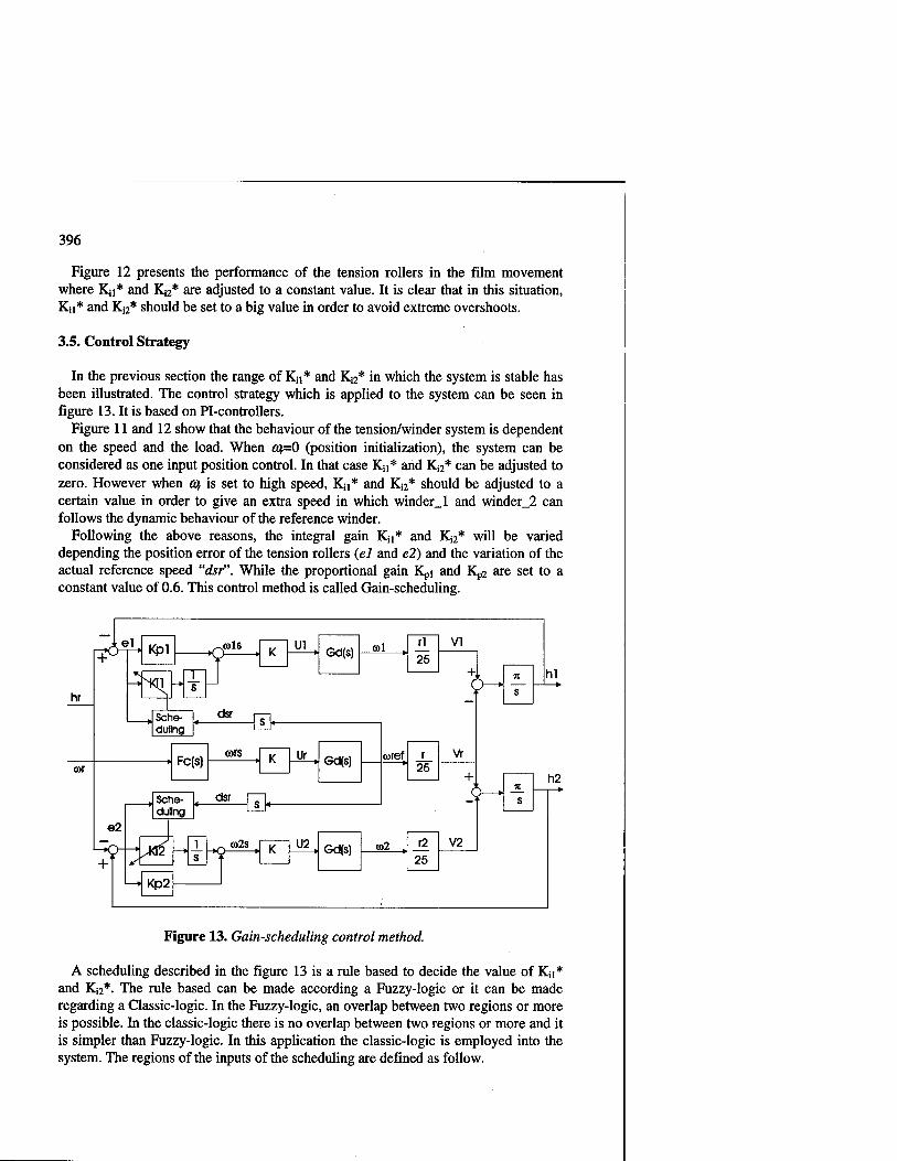
396

Figure 12 presents the performance of the tension rollers in the film movement where Kn* and Ki2* are adjusted to a constant value. It is clear that in this situation, Kii* and K^* should be set to a big value in order to avoid extreme overshoots.

3.5. Control Strategy

In the previous section the range of Kn* and Ki2* in which the system is stable has been illustrated. The control strategy which is applied to the system can be seen in figure 13. It is based on Pi-controllers.

Figure 11 and 12 show that the behaviour of the tension/winder system is dependent on the speed and the load. When oj=0 (position initialization), the system can be considered as one input position control. In that case Kn* and Ki2* can be adjusted to zero. However when a\ is set to high speed, Kn* and Ki2* should be adjusted to a certain value in order to give an extra speed in which winder.. 1 and winder_2 can follows the dynamic behaviour of the reference winder.

Following the above reasons, the integral gain Kn* and Ki2* will be varied depending the position error of the tension rollers {el and e2) and the variation of the actual reference speed "dsr". While the proportional gain Kp] and Kp2 are set to a constant value of 0.6. This control method is called Gain-scheduling.

VI ,—w ̂e1> Kpl „cols K Ul

Gd(s) col , rl

25 + ^ % J «■

•

Vr

K

s

hi —►

hr ^ V

i * s

. Sehe dulln

a» pq, 9 LJLT

, :c(s) cars K Uf . Gd(s) a>ref r

25 car + t

V2

h9

dsr n S

—i—>■

Sehe dulln

1- t_

e2 g

.-" /KT2 -

l s

-K e>2s K U2 » Gd(s) 0)2 , r2

25 > + i L

Kp2-

Figure 13. Gain-scheduling control method.

A scheduling described in the figure 13 is a rule based to decide the value of Kn* and Ki2*. The rule based can be made according a Fuzzy-logic or it can be made regarding a Classic-logic. In the Fuzzy-logic, an overlap between two regions or more is possible. In the classic-logic there is no overlap between two regions or more and it is simpler than Fuzzy-logic. In this application the classic-logic is employed into the system. The regions of the inputs of the scheduling are defined as follow.

397

dsr =

zero, 0<\dsr\<05

small, 05<|fifer|<l

medium, 1 < \dsr\ < 2

big, 2 < \dsr\

zero, 0<\Ep12\<05

Epl2 = ■ small, 05 < \Ep12 < 1

big, 1<\EPIA\

^ = ^=(0,05,1,2,5,8)

Where Eli2 means el or e2. The region of dsr and Ei2 are designed based on the stability criterion and experiments. The above regions show that Kn* and Ki2* are always inside the stability range defined in the section 3.3. Following the above region's definition the rule-base can be developed as been seen in a table below.

Table 2. Rule-base

\dsrHEl.2\ Zero Small Big Zero 0 0.5 1 Small 2 medium 5 Big 8

When the above rule base is applied into the scheduling, the results can be seen in figure 14.

IB

14

— 10-

1 6 I «■

I: f-"

i 1 1

ndon rolle 111

s- s / < , / / / / / /

1 1 Tension TOJU "•1 MU_ •26'

0 1 s 3 4 oeond)

9-

7-

„ 6 E E 3

1: i"7

-13'

i- —i- ^1— "'■'x I tension roller I 1

1\ \ \ V" \ \ /~^ V' \ f > \ ( \ —A 1 Tenmon roller 1

0 12 3 4 T1m*{Mcond)

a. b. Figure 14. The performance of the position of the tension rollers with variation of Kn * and Ki2 * with J2max and 7im,n. (a) in the position initialization and (b)film speed=32.06 m/min.

398

The above two figures show that the performance of the tension rollers when Kn* and Ki2* are varied. In the position initialization the overshoot is within ±6 mm and the accuracy is less than 1 mm. When the speed is bigger than zero, the overshoot is within ±13 mm with the accuracy of 1 mm. Those performances meet the requirements of the specification described in table 1.

4. Conclusion

Concluding from the results found in the previous chapters, the motion controller MC_NEW is capable to control the tension of the tape-winding application using the gain scheduling control method. The tension is presented by the position of the tension rollers. The important part inside MC_NEW is the control algorithm in which several control methods can be applied due to the BASIC like language such as PID- controller, Fuzzy-logic etc. Because MC_NEW is based on the digital controller, thus the cycle/sampling time must be considered too.

References 1. T. Zhao, A. Osseyran, The Benefits Of Integrating Motion Control Into PLC

System, Proceeding of the ICMA'98, Tampere, Finland, September 15-18, 1998. 2. Werner Leonhard, Control Of Electrical Drives, Braunchweigh, October 1984. 3. J.C.A. van der Lubbe, E. Backer, Fuzzy Logic Versus Classical Logic, Delft

University of Technology, Department of Electrical Engineering, Information theory group.

4. Richard C. Dorf, Robert H. Bishop, Modern Control Systems, 7* edition, USA 1995.

5. Tension Control, OMRON Fuzzy Guide Book, Japan 1992. 6. OMRON User's Manual OMNUC U series AC Servo motors/drivers (30 to 750-

W Analog inputs), version 2, 1996. 7. Robert H. Canon, Jr., Dynamics Of Physical Systems, USA 1967. 8. Franklin J. David Powel, Michel Workman, Digital Control Of Dynamic System,

third edition, USA 1998. 9. Priyadarshee D.Mathur, William C. Messner, Controller Development For a

Prototype High-Speed Low-Tension Tape Transport, IEEE Transaction on control system technology, Vol. 6, No 4, July 1998.

10. L. Garninto, Motion Control of Tension/Winder System, Graduation report, TU.Delft, the Netherlands, February 12, 1999.

11. J.P. Den Hartog, Mechanics, first edition, USA 1948. 12. J.J. DAzzo and C.H. Houpis, Linear Control System Analysis & Design

Conventional and Modern, third edition, USA 1988. 13. Y. Dote, Servo Motor And Motion Control Using Digital Signal Processor, New

Jersey, 1990. 14. M. Camras, Magnetic Recording Handbook, New York,1988. 15. J.J.E.Slotine and W.Li, Applied Nonlinear Control, USA, 1991. 16. M.Breen, Enhancing Web Processes with Tension Transducer System, Sensor

Magazine, Augusr 1997, vol. 14, no. 8.

399

Robust Accurate Motion Control for Belt-Driven Servomechanism

Ales' Hace, Karel Jezernik, Martin Terbuc

Faculty of Electrical Engineering and Computer Sciences Institute for Robotics

SI-2000 Maribor, Smetanovaul. 17, Slovenia

{ales.hace, karel.jezernik, martin.terbuc}@uni-mb.si

Abstract. A control algorithm for accurate position tracking task for a servomechanism with inherent linkage flexibility is derived. The control algorithm is obtained by the use of the sliding mode control theory and Lyapunov design. Robustness of the sliding manifold is achieved using continuous control instead of discontinuous bang-bang control action. Thus, the control law performance is chattering free. The proposed position tracking algorithm is applied to the motion controller of a 2DOF Cartesian planar table, which uses belt-driven servomechanisms. The table is used as a laser-cutting machine in an industrial manufacture process. Experimental results are shown.

1 Introduction

Modem mechanical systems such as machine tools are confronted with demands of high productivity and high quality. These demands can be achieved with high-speed, high-accurate motion and positioning. A motion performance depends on electro- and mechanical components, which are used in assembling of drives, as well as a motion controller, which is accompanied to the machine tool. Therefore, machine tools must be equipped by servo-drives, which consist of high-quality AC or DC servomotors, high quality mechanical components (gears, joints, linkages, etc.), which must be assembled in order to ensure that phenomena of backlash, friction, etc., are not relevant, and joining high performance motion controller, which ensures high accuracy of position tracking performance at high speeds. Mechanical components used in the motion transmission chain from the motor shaft to the tool are the most relevant factors for the high static (accurate positioning) and dynamic (high speed) performance. Gears with minimal backlash or spindles with minimal vibrations at high speeds are most common in high performance applications. The use of belts as the motion transmission components introduces low-cost solution and degrades static and dynamic performance of servodrives. In order to attain high performance an advanced control strategy has to be developed.

400

This paper introduces the advanced motion control law derived for a belt-driven servomechanism. The design of this control law requires the preliminary derivation of a linear nominal control model joined by uncertainties of the mechanical parts involved in the motion of the controlled system. The belt-driven servomechanism incorporates many undesired and unfortunately highly relevant nonlinear phenomena of position depended stiction and friction, backlash, and linkage flexibility, which can not be exactly modeled. They can not be incorporated in the control model. Therefore, higher order control model due to the linkage flexibility is adopted, which is perturbed with external disturbances. Thus, the control law has to assure robust stability in spite of parameters variations of the non-rigid mechanical system, torque disturbance rejections, high accuracy in steady state, and rapid dynamic behavior.

The erroneous model and high performance task demands require a robust control law. In recent years, disturbance observer technique [1], [2] or disturbance estimation technique [3] are often used in an advanced motion control of mechanical systems at high performance task demands. The control law [3] has inherent and transparent robust properties against disturbances which perturb nominal model, since it is derived with a powerful sliding mode control (SMC) theory. SMC law based on the variable structure control can be used if the uncertainties in the model structure are bounded with known bounds. However, an SMC law has some disadvantages related to well known chattering in the system due to the discontinuous bang-bang control action. This phenomena is undesirable in the control of mechanical systems, since it causes excessive control action leading to increased wear of the actuators and to excitation of the high order unmodeled dynamics. Consequently, the demanded performance can not be achieved, or even worse - mechanical parts of the servo system can be destroyed. This is a well-known problem and is widely treated in the literature. Slotine and Sastry [4] introduced a boundary layer around the sliding surface and used a continuos control within the boundary layer. SabanoviC [5] proposed continuos SMC Lyapunov design. Elmali and Olgac [6], as well as Jezernik and Curk [3] developed perturbation estimation schemes. Another approach to avoid chattering is proposed by Bartolini and Ferrara [7] introducing second-order SMC. While the basic idea of the chattering-free control law in [6] and [3] is involving the perturbation estimator in the control scheme, in [7] a continuous control law is achieved by passing a bang-bang control action on a derivative of the control action. The variable structure control law design is applied to a control plant, which is extended by additional augmented state variable. Common to the SMC design approaches demonstrated in [6], [3], and [7] is a dynamic control scheme instead static one. As it is suggested in [8], the static SMC is referred to reduced-order sliding mode, and the dynamic SMC is referred to full-order sliding mode. The full-order sliding mode implies that orders of the sliding mode equation and the original system coincide and the sliding motion exists starting from any initial state with the desired dynamics independent of the perturbation [8].

If the continuos SMC design is used [5] combined with [7], the equivalence to the control law presented in [3] could be shown. The system governed by the control law [3] is enforced in the full-order sliding mode. The control law is derived for a rigid mechanical system and it is robust against perturbation, which influences single-mass

401

nominal model. Applying it to the non-rigid servodrive under a high performance task demands, only poor motion performance can be achieved since the perturbation estimator is not able to estimate high order dynamics. Thus, a new control law is derived considering high modes of the non-rigid belt-driven servomechanism, which is represented as a two-mass nominal model perturbed with external disturbances.

In the paper, a new SMC law for accurate position tracking for the belt-driven servomechanism is represented. The control algorithm is applied to the high performance motion controller of planar Cartesian table of a laser-cutting machine. The machine is briefly described in the 2nd section, which also introduces mechanical models of belt-driven axes. The 3rd and the 4* sections represent derivation of SMC algorithms used in motion controller. Experimental results are represented in the 5th

section, which follows with conclusions in the 6th section.

2 Control Object

*"fc»

IRT8

|T805|

Digital I/O «

laser system, autofollowing system,

seivo system, cooling system, nitrogen purge

X axis ILS

laser head

Y axis

Fig. 1. The machine and the controller hardware

The mechanical system under consideration is 2DOF planar XY Cartesian table used as a laser-cutting machine (Fig. 1), where a laser head with a laser beam represents a cutting tool, which is not influenced by environment. Both axes of the machine are driven by electrical DC servomotors with permanent magnets and supplied by a PWM current amplifier. Input in the current amplifier is driven by the reference current information with the voltage signal up to ±10V (reference current). The motor produces the torque necessary for the movement of the single drive. A rotational movement is reduced by the gear placed on the motor shaft. Then, the rotational movement is transmissed to a translational movement by the belt. In the X-axis, it connects gear shaft to the laser head. In the Y-axis, it connects the bridge with the

402

shaft. The laser head that is placed on a bridge represents the dominant load of «12kg in the X-axis. The bridge represents the dominant load of «120kg in the Y-axis.

The original machine construction solution results in low-cost belt-driven motion system. Combined with high loads the torque/force transmission rate from the motor shaft to the machine tool (the laser cutting head) is uncertain. The machine tool motion and positioning are the main control objectives and can be effectively controlled only if position informations of the motor shaft and the laser-cutting head are available simultaneously. Therefore, the position measuring system consists of rotary incremental encoders (RIE), which are placed on the motor shafts, and incremental linear scales (ILS), which are placed on the mechanical construction of the machine. RIEs have a resolution of 8000 p/rev. ILSs have the resolution of lp/um. Position is transmissed from the motor shaft to the load side (tool) by the reduction coefficient of 12 mm/rev in the X-axis and 26.7 mm/rev in the Y-axis.

The mechanical system under consideration are both drives. In order to obtain valid control model, step pulses of reference current were applied to the input into the PWM current amplifier. Current closed-loop has a time constant of approximately lms. The response of servo drives is depicted in Fig. 2. The upper diagrams show the velocity response of the load side (in mm/s), and the lower diagrams introduce "belt- stretch" as the difference in the position measurement between RIE - motor angle position x reduction coefficient - and ILS - tool position (in urn). The amplitude of the reference current is equivalent to the 0.28Nm and 2.48Nm on the motor shaft for X-axis and Y-axis, respectively. Velocity response of the single drive introduces large nonlinear phenomena degrading the dynamic and static behavior. In the transmission mechanism, the belt introduces elasticity, backlash, hysteresis, and additional stiction/friction effects. The complex transmission mechanism and the small DC motor introduce relevant stiction and friction phenomena. This is particularly true for the X axis, while in the Y axis inertia/mass property reduces friction influence. The presence of the static and dynamic friction can be seen as a particular dissipative torque. This kind of nonlinearity introduces a reduction of the dynamic rapidity and the steady-state accuracy. Moreover, it could introduce a possible source of instability in the controlled system (limit cycle).

a)

Fig. 2. Step response of the belt-driven axes: a) X-axis, b) Y-axis

403

The belt-driven servomechanism represents a distributed parameter system. Using a modal analysis, it can be modeled as a two-mass system. Motor inertia (J) and load mass ( M ) coupled with the belt, which is modeled as a spring with the stiffness K, can be dominant properties of the physical model with concentrated parameters. Friction on the motor side and the load side, backlash in the gears are represented as external disturbances, which influence the motor part and the load part. Such a mechanical model of a belt-driven axis is featured by Fig. 3. Since the control objective is to control the tool position (x), the model is transformed on the load side.

<p, T , Td,s!, Fw and Fdm are the motor angle position, the applied torque, and the

disturbance torque, the spring force, and the disturbance force due to the nonlinear friction and unmodeled dynamics on the load side, respectively. L is the reduction coefficient (Z = 9x/cty>). Block scheme derived from the mechanical model is

featured by the block scheme in Fig. 4, where w = L ■ cp - x denotes the belt stretch.

////////

Fig. 3. Mechanical model of a belt-driven axis

■z-o 1/J 1/8 1/S

K K w i 3

Q—- 1 L

1/M X ► 1/S

X 1/S

X

pdii

Fig. 4. Block scheme of the mechanical model

Considering the motion and positioning of the tool (the load side) as the most relevant control objective, the dynamics due to the flexible linkage between the motor shaft and the tool, which influences the transmission of the torque r to the force Fw

is of great importance, since it influences the feasible task dynamics. Let us assume the unit reduction coefficient (1 = 1). Then the control model is depicted by the block

scheme in Fig. 5, where KW=K- (l + JIM) and rf =Tdis'-J/M- Fdis'.

1

dist

■

pdk

J ► 1/J w ► 1/S

W ► 1/S

w K

K >—• MM

X —> 1/S -*+ 1/S X

*{.

3elt-st retch c ynam ics

*w

load-side dynamics

Fig. 5. Block scheme of the control model

404

The control model of single belt-driven mechanism has the control input of applied torque z and consists of two interconnected parts. The first one describes the belt- stretch dynamics and the second one describes load-side dynamics. Both parts are described by the nominal linear second order dynamics and are perturbed by disturbances rf* and Fdisl, respectively. It is worth to notice, that the force Fw, which is necessary for the load-side motion (machine tool motion and positioning) is not directly accessible through the control model input.

3 Full-Order SMC Design

In this paper, the SMC theory combined with Lyapunov design is used in order to derive the robust control law. The aim of the control design with SMC is to reject disturbances, which influence the nominal control model in order to achieve predefined full-order closed-loop dynamics. Let us assume a SISO nonlinear uncertain mechanical system of a single DOF:

i,=*2 (1) z2=Az) + b(z)-{u-d(t))

with measurable state vector z = [zx z2f of position and velocity, scalar control input u{t), and scalar disturbance d(t). The terms f(z) and b(z) correspond to the nonlinear driving term and the nonlinear control gain, respectively . It is evident that the matching condition [9] is satisfied. Complement (1) by an additional first-order dynamic subsystem of state variable z3, as it is suggested by Jezernik [3]:

z3=b-(ü-dlalal(z,u,t)), ' •*

where z3 is referred to acceleration, b is the estimate of b(z), and

dmal(z,u,t) = b'1- (- /(z) + b(z) ■ d(t) + {b- b(z)} u) is the perturbation present in the system, which includes all system uncertainties. The control task is to drive the state vector [zT z3] to the desired value despite this perturbation. For the practical control implementation, the acceleration is not measurable signal. Consequently, it needs to be replaced by the estimate z3, which is obtained simply from the differential

equation of motion z3 =b\-dlolal), where dtotal denotes the estimate of the perturbation. In [3] the perturbation estimator is proposed, which is designed with the SMC theory.

The goal of the SMC design is to find such control input u thus the motion of the control model system is restricted to belong to the sliding mode manifold S

S = {z,z3: (T(Z,Z3,0 = 0}, (3)

where a is a scalar time-variant function

405

a = R(t)-(z,+gT-z), W

R(t) is a continuous function, and gT =[g, g2], g,2 >0 . If the system states are

restricted to the sliding manifold, then the sliding motion is governed by the second order system z3 + g2 ■ z2 + g, • z, = R(t), and does not depend on the disturbance. Deriving the second order motion equation using the algebraic system a = 0 control u should be substituted by the so-called "equivalent control", that is the solution to & = 0 with respect to the control input [10].

The condition under which the system states will move toward and reach the sliding manifold is known as the reaching condition. Choosing the Lyapunov function candidate

V(a) = cx2/2, (5)

a global reaching condition is given by V < 0 when a * 0 or equivalently a ■ & < 0. Various choices of V lead to different rates of change for a and the robust control law can be calculated directly from a. As it is suggested by [5], the robust control law is chosen with the proportional rate

CT = -Z)cr, D>0, (6)

thus obtaining smooth continuos control action. Let us calculate & and substitute i3

by (2):

& = R(t)-gT-z-b-(ü-dlolal). (?)

If the control input is chosen as

« = $-'■ (ß(0 - gT ■ z + D ■ jadt), W

then combining (7) and (8) yields to the system motion projection on the «r-space governed by

& = -D-a + b-dlolal. (')

The system reaches the sliding mode regime if disturbances change slowly (^ma *0), since putting (9) into the Lyapunov function candidate derivative yields to

V = a-ä = -Da2<0. (10)

One can see, that for the perturbed system (1) the continuos control law (6) guarantees attractiveness of the full-order sliding manifold (3). The control law with the control input (8) is feasible, since the state vector z is measurable, the acceleration is substituted with the estimate

z,=R(t)-gT-z, (»)

406

which in the sliding mode motion is the same as the actual one, and the perturbation estimator is of reduced-order

dlotal =t>-]-D- \adt = b~]-D-{fadt-z2}. (12)

4 Position Tracking Control Derivation

The control model of non-rigid uncertain mechanism is depicted in Fig. 5. The model can be described with the perturbed load-side dynamics

M-x = K-w-fdisl, (13)

and the perturbed belt-stretch dynamics

J-w + Kw-w = T-rdJsl. (14)

M, J, K are equivalent mass, inertia, and stiffness, respectively, and

Kw = K-(l + J/M). Applied torque r is the control input, and tf, fdisl are

unknown disturbance torque and disturbance force, respectively, x, x, w, w are measurable signals of the tool position and velocity, equivalent belt-stretch and belt- stretch derivative, respectively.

It's obvious, that the main problems of a control design are disturbances in the model, and slow, poor dumped belt response. Additional constraints are given on the set of measurable signals. Hence, the proposed procedure of the control design consists of two steps: in the first step, a qualitative design of a perturbation controller for a fictitious rigid mechanism is worked out; then the second step involves design of a belt controller, which will assure arbitrary chosen fast and dumped belt response, and control parameters calculation.

4.1 Perturbation Controller

Let us assume that the applied torque in the control model (13), (14) directly influences load mass, i.e. the rigid mechanism dynamics is described by

M-X = T-Td". (15)

The model is uncertain, since it is perturbed by disturbance torque r*'. The

control objective is position tracking i.e. x(t)&xd(t). xd(t) is the time-variant

smooth position trajectory and xd, xd , xd exist, with xd(0) = x(0) xd(0)-x(0),

xd(0) = x(0). The desired dynamics of the closed-loop system is of full order:

e + Kv-e + Kp-e = 0. e = xd -x is the position tracking error and Kv > 0, Kp > 0 are velocity and position gains, respectively.

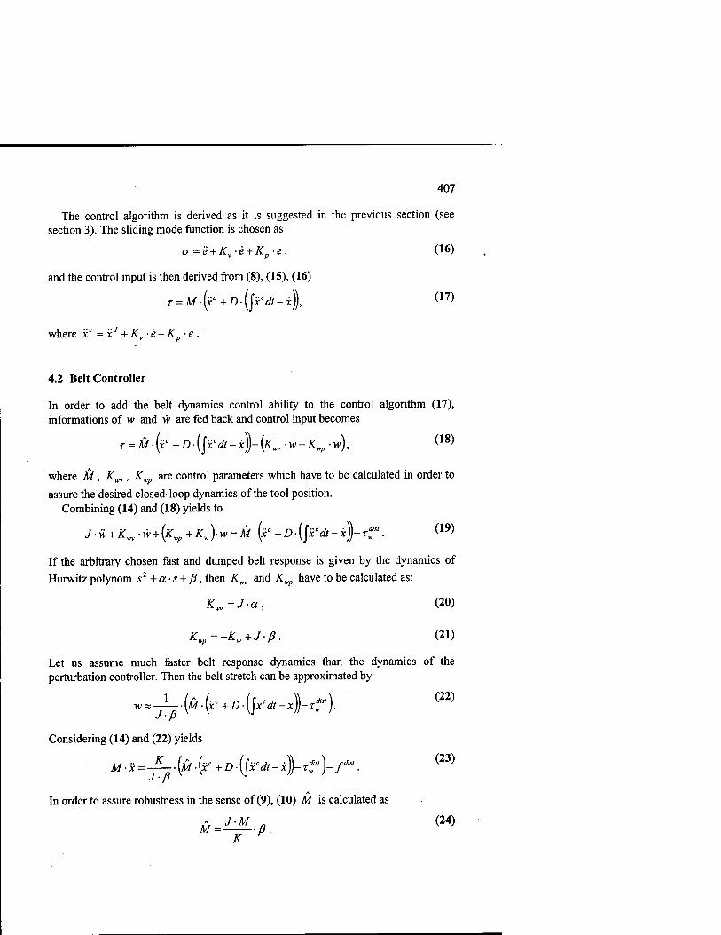
407

The control algorithm is derived as it is suggested in the previous section (see section 3). The sliding mode function is chosen as

<j = e + Kv-e+Kp-e. (16)

and the control input is then derived from (8), (15), (16)

r = M-{xc+D-(\xcdt-x\ (17)

where xc = xd + Kv ■ e + Kp ■ e .

4.2 Belt Controller

In order to add the belt dynamics control ability to the control algorithm (17), informations of w and w are fed back and control input becomes

r = M■ (xc + D■ (\xcdt-x}-(Kwv -w + Kwp-w), <18)

where M, Km,, Kwp are control parameters which have to be calculated in order to

assure the desired closed-loop dynamics of the tool position. Combining (14) and (18) yields to

J.w + Km-w + (Kwp+Kw\w^M-^ +D-{\xcdt-x)-Tf. <19>

If the arbitrary chosen fast and dumped belt response is given by the dynamics of Hurwitzpolynom s2 +a-s + ß, then Kwv and Kwp have to be calculated as:

Km=J-a, (20)

Kwp=-Kw+J-ß. (21)

Let us assume much faster belt response dynamics than the dynamics of the perturbation controller. Then the belt stretch can be approximated by

w,-i-.(M.(F+D.(j^-4-.r). (22) J ■ p

Considering (14) and (22) yields

M.X = ^-{M.^ +D\^dt-x)-rT )-/*• J ■ p

In order to assure robustness in the sense of (9), (10) M is calculated as

uJ-^L.ß. (24)

K

(23)

408

Then system motion considering the desired sliding mode function (16) is governed by

& + D-a=-^—i*s'lß + — -fdisl. J-M w H M J

(25)

Robustness is guaranteed if disturbances change slowly, i.e. t**1 « 0 , /*■" « 0 .

Resulted position tracking controller for the belt-driven mechanism is depicted by

Fig. 6, where Bes,=M-D.

K.

-o

Position controller

M

Perturbation controller

xc

B„

1/3 ■*o

Trzrtr "-wvS + "-wp

Mechanism w

' - Belt controller

Fig. 6. Position tracking controller for a belt-driven mechanism

5 Experimental Results

Experimental tests were performed on the control object described in section 3. Both axes are controlled with the proposed position tracking algorithm. The control algorithms are calculated at 0.4ms. Only position informations of the tool and motor shafts are available. Velocity is not measured. Thus, velocity estimate is used in the control scheme. In order to achieve accurate position tracking performance, the M/T- method of velocity estimation is used, which assures high accuracy over a wide speed range [11]. The test task presented in this paper is given by an octagon in XY plane. At each corner of the octagon, the motion is stopped. The sin2 acceleration profile was used to generate the desired position, velocity, and acceleration. Fig. 7 and Fig. 8 show position tracking results using control scheme with and without the belt- controller. They include position reference and position tracking error (top), and applied reference current (bottom).

409

- -/^—rtf.' posi {mm)—*\ - /

. > jos. error (jim) .

0 12 3 10)

4 5 6

■ -

~^-~~:-

• - ■

*0 1 2 3 •! 5 6

Fig. 7. X axis: a]

b)

i)without the belt-controller: Kp = 625, b)with the belt-controller Kp = 2500

Fig. 8. Y axis: a) without the belt-controller K ' = 300, b) with the belt-controller K = 625

The control parameters were obtained by the trial-and-error method in order to achieve the best possible disturbance rejection performance and stiff position closed loop which assure the smallest position error. When the belt-controller is not used, slow perturbation estimator dynamics can not effectively compensates disturbances, and only low stiffness can be achieved. A large tracking error (up to 1.5mm) can be observed. The error occurs due to the flexible linkage present in the system, and due to the friction phenomena. If the belt-controller is employed, the servo drive behaves as a rigid one, a fast estimator dynamics could be set up, and high stiffness can be achieved. Consequently, the improvement in position error is evident. Position error peaks are ten times smaller (0.15mm). They occur at velocity reversals due to the discontinuous friction changes and belt-stretch reversal delay. Due to the fast estimator dynamics, the error is compensated very fast. The closed loop dynamics is set equivalently for both axes. Due to the high stiction/friction domination in the X axis, position feedback gain is set much larger than in the Y axis, where inertia/mass phenomena dominates.

410

6 Conclusion

The main contribution shown in the paper is the robust control position tracking control algorithm effectively upgraded with the belt-controller. Robustness of the algorithm to the uncertain model structure and parameter variations is assured using continuos SMC law design procedure, while the managing of the present flexibility is worked out based on the information of the difference between motor shaft position and tool position, which is used in the state-space control approach design. As it is demonstrated by experimental results, stiff position servo control can be achieved with position tracking close to zero and without DC offset. Unfortunately, discontinuous changes of static friction can not be completely compensated immediately with the linear compensator. Position tracking errors are nevertheless compensated fast with very simple perturbation estimator control structure.

The proposed control algorithm enables the use of low-cost belt-driven mechanical drives in the accurate motion control of machine tool. Thus, it is used in the industrial application of laser-cutting machine.

References

1. Ohnishi, K., Shibata, M., Murakami, T.: Motion Control for Advanced Mechatronics. IEEE/ASME Trans, on Mechatronics, Vol. 1, No. 1, March 1996, pp. 56-67.

2. Seong H., Tomizuka, M.: Robust Motion Controller Design for High-Accuracy Positioning Systems. IEEE Trans, on Industrial Electronics, Vol. 43, No. 1, February 1996, pp. 48-55.

3. Jezernik, K., Curk, B., and Harnik, J.: Observer-based Sliding Mode Control of a Robotic Manipulator. Robotica, Vol. 12, part 5, Sept.-Oct.1994, pp. 443-448.

4. Slotine, J.J., Sastry, S.: Tracking Control of Nonlinear Systems Using Sliding Surfaces with Application to Robot Manipulators. Int. J. Control, vol. 38, 1983.

5. Sabanoviö, A.: Sliding mode in robotic manipulators control system. Electrotechnical Review, Vol. 60, No. 2-3, Ljubljana, 1993, pp. 99-107.

6. Elmali H., Olgac, N.: Sliding Mode Control with Perturbation Estimation (SMCPE): A New Approach. International Journal of Control, Vol. 56, 1992, pp. 923-941.

7. Bartolini, G., Ferrara, A., Usai, E.: Chattering Avoidance by Second Order Sliding Mode Control. IEEE Trans, on Automatic Control, Vol.43, No. 2, Feb. 1998, pp. 241-246.

8. Ackermann, J., Utkin, V.: Sliding Mode Control Design Based on Ackermann's Formula. IEEE Trans, on Automatic Control, Vol.43, No. 2, Feb. 1998, pp. 234-237.

9. Drazenovic, B.: The Invariance Conditions in Variable Structure Systems. Automatica, vol. 5, no. 3,1969, pp. 287-295.

lO.Utkin, V.: Sliding Modes in Control and Optimization. Springer-Verlag, Berlin 1992. ll.Ohmae, T, Matsuda, T, Kamiyama, K., Tachikawa, M.: A Microprocessor-Controlled

High-Accuracy Wide-Range Speed Regulator for Motor Drives. IEEE Trans, on Industrial Electronics, Vol. 29, No. 3, August 1982, pp. 207-211.

411

Application of a Silicon Microvalve to Pilot-operation of pneumatic Valves

Dipl.-Ing. Götz Günther1

1 Institute of fluid power transmission and control, RWTH Aachen, Univ.-Prof. Dr.-Ing. H. Murrenhoff

Steinbachstr. 53 D-52070 Aachen, Germany

Abstract: Miniaturization is one of the main development goals in the field of pneumatics today, hi this paper a silicon 3/2-way-microvalve is presented that can be applied to pilot-operate conventional pneumatic valves and by this means replace standard electromagnetic actuators. The valve works in the standard pneumatic pressure range and is actuated thermomechanically. Due to its special design, which was optimized by the means of computational fluid dynamics, switching times in the range of 30 ms are achieved. The paper presents the pilot-operation of a standard 5/2-way switching spool valve.

1 Introduction

As in most other fields of technique, the demand for pneumatic components with small and smallest dimensions is continously growing. These small components are used in handling devices as well as in fields as medical technology or micomechanics [1], [4],

The limits of miniaturization with conventional production techniques are easily reached. Though passive components such as cylinders can easily be miniaturized, this is not easily possible for valve actuators. In order to generate sufficiant actuation forces with the electromagnetic principle - typical for standard pneumatics - the actuators must have a certain minimum size.

Comparing miniature pneumatics with standard pneumatics, this leads to an inversion of typical component sizes: While the ratio of mass is about 13:1 for a standard cylinder with a stroke of 500 mm and a compatible 5/3-way-valve, this value is about 1:10 for a miniaturized cylinder with a stroke of 5 mm and a miniaturized conventional valve (figure 1).

412

Fig: 1: Typical dimensions of miniaturized conventional pneumatic components

In order to further miniaturize pneumatic valves, a change of the atuator principle becomes necessary [7], [9], [11]. Different principles such as electrostatic, thermohydraulic, piezoelectric or thennal actuators are available. Typical structures for such micfoactuators are in the range of micrometers and are very difficult or even impossible to produce with conventional machining.

Micromechanics technologies offer new possibilities for miniaturization [2], [3], [10]. Production techniques as the silicon etching technology, developed to produce highly integrated circuits in electronics, allow the production of mechanical components with dimensions in the range of micrometers. This technology can be used to produce very small valves. These microvalves can be applied to cylinder control as stand-alone units, as well as for standard pneumatics. One important field of application is pilot operation of conventional miniaturized valves, where these microvalves can replace standard electromagnetic actuators. For this application the 3/2-way-function of the microvalve is essential to pressurize and exhaust the control chamber with one single pilot valve. Though, this function is not yet realized for commercially available thermically actuated microvalves [5], [6].

2 Pneumatic 3/2-way-microvaIve

In the framework of a joint project between the Institute of fluid power transmission and control (IFAS), Aachen, and the Fraunhofer-Institute of silicon technology (FhG-ISiT), Itzehoe, supported by the Deutsche Forschungsgemeinschaft, prototypes of a thermally actuated 3/2-way-microvalve were developed [7], [8], [9].

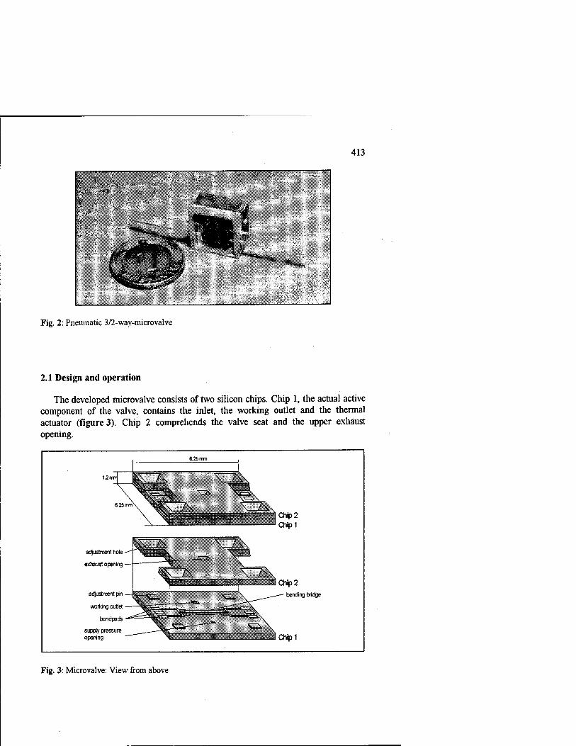
413

Fig. 2: Pneumatic 3/2-way-microvalve

2.1 Design and operation

The developed microvalve consists of two silicon chips. Chip 1, the actual active component of the valve, contains the inlet, the working outlet and the thermal actuator (figure 3). Chip 2 comprehends the valve seat and the upper exhaust opening.

adjustment hole -

exhaust opening -

adjustment pin -

working outlet -

bondpads-

supply pressure opening

Chip 2

bending bridge

Fig. 3: Microvalve: View from above

414

The valve's thermomechanical actuator is a silicon structure in the form of a bridge made of microgalvanically deposited nickel. The heating layer on bottom of the bridge is made of polysilicon, that is surrounded by an isolating coating made of silicon nitrid and silicon oxyd. This isolation avoids a short circuit of the heating layer via the metal during valve operation. Also this layer is used to protect the polysilicon layer during the fabrication process when the sacrifice polysilicon layer under the bridge is etched.

The polysilicon heater is connected to gold bondpads to ensure easy electrical contactability. The inlet and the working outlet are produced by anisotropic etching in KOH and TMAH on the reverse side of chip one. The exhaust opening in chip two is produced in the same way and is placed within a hollow of 80 urn depth. By this means, a maximum stroke of the bridge of 50 um is sufficient in order to completely close the exhaust opening. To improve valve tightness, a metallic valve seat is galvanically deposited around the opening. This seat also reduces flow forces on the bridge, since the area of pressure drop is reduced (see chapter 3). The valve works with the principle of flow division.

In turned-off position (i.e. the bridge is not heated) the bridge is planar and the exhaust opening is open. All three valve ports are connected with each other and the pressure at the working outlet only depends on the openings' geometry. As the inlet opening (smallest opening: 100 x 100 um) is much smaller than the opened exhaust opening (smallest opening: 200 x 200 um), the pressure drops almost completely at the inlet throttle and the pressure at the working outlet equals almost the ambiant pressure (see figure 8).

When an electrical current passes the bridge, electrical energy is dissipated and the bridge temperature increases until there is a dynamic equilibrium between the electrical energy dissipated and the thermal energy conducted to the silicon substratum and the air passing by. Due to this temperature increase mechanical stress in the bridge is increased beyond the critical bending stress and the bridge is bending into a curved shape. The maximum temperature of the bridge reaches about 200 °C.

By the movement of the bridge, the exhaust opening is closed and its flow resistance is increased (variable throttle).

So, the pressure at the working outlet can be continously adjusted. If the exhaust opening is completely closed, the outlet pressure reaches full supply pressure. The valve is designed in a way that the actuator stroke is proportional to the dissipated electrical power. Therefore, an electronical power control is used to operate the valve.

3 Layout optimization using CFD analysis

The actuator design was optimized using analytical and numerical methods to simulate the thermomechanic and the fluidic behavior of the valve. The commercial CFD software TASCFlow3D was employed to simulate three-dimensional flow through the valve. As the valve's geometry is symmetrical, only one half of the valve was modelized. The following example shows the results of a simulation with closed

415

working outlet. Therefore only the inlet channel and the exhaust opening outlet channel are visible (figure 4).

1

laiiij SlillllaS

1°

f X—i«

^^Si^^^^^^^tt5

Fig. 4: Simulated mesh domain with inlet channel (left) and outlet channel (right)

The following boundary conditions were used: At the exhaust outlet static pressure is ambient pressure (1 barabs). At all wall nodes all velocity components are specified to be zero, symmetry nodes' velocity components normal to the symmetry plane are also set to be zero. Inlet pressure was varied in the range of 1 barabs to 8 barsabs. For inlet pressure higher than 2.6 barsabS flow becomes supersonic and mass flow is proportional to the inlet pressure. The following figure shows simulated stream lines in the valve and flow velocities. Inlet pressure is 6.8 barsabs in this example.

416

Fig. 5: Stream lines and flow velocities in the microvalve

Special care was taken to assess the influence of the seat geometry at the outlet. Figure 6 shows the simulation mesh around the seat geometry. In figure 7 one can see the pressure distribution along the bridge with and without seat. It can clearly be seen that the pressure drop is concentrated on the seat geometry. This leads to a reduction of flow forces on the bridge.

Fig. 6: Mesh in the seat area

417

p2= 1 bar

0.1 0.2 0.3 0.4 0.5 0.6 0.7 0.8 0.9

Distance from symmetry plane r [mm]

Fig. 7: Simulated pressure distribution at the bridge with (full line) and without (dashed line) valve seat at the exhaust opening. With the seat, the flow forces are reduced.

4 Experimental results

Figure 8 shows the pressure at the working outlet and the mass flow at the exhaust opening in dependance of the dissipated electrical power. The maximum electrical power is 1.6 W.

4.5 4 3.5 3 2.5 2 1.5 1 0.5 0

.£.450

E 400

350

O 300

250

o 200

150; o E

■i ioo 50

-#—♦.. ■■•—•- r~*~ -•-.- s / i—i

■t y * »

\

•"" k-^

0 0.1 0.2 0.3 0.4 0.5 0.6 0.7 0.8 0.9 1

Power consumption P/P [-] r max

CM a

Fig: 8: Exhaust opening mass flow and working outlet pressure in dependance of electrical power consumption

418

Supply pressure for this measurement was 5 barabs. The maximum supply pressure is about 10 barabs. However, continous adjustment of such high pressure is not possible due to increased flow forces. Operating the valve as a 2/2-way-valve, the maximum mass flow is 1170 standard ml/min for a supply pressure of 5 barsabS.

4.1 Bridge movement dynamics

The upper part of figure 9 shows the bridge movement measured contactlessly with a laser vibrometer. The lower part of this figure shows the rectangular nominal value of the power control and the resulting electrical heating voltage at the valve. The actuator stroke for this measurement was 25 um. the switching time is about 45 ms for heating and about 37 ms for cooling. Switching time for heating is longer than for cooling due to mechanical stress in the bridge inducted while fabrication.

Comparing these results to commercially available thermally actuated valves, the main advantage of the actuator production by means of surface micromachining becomes obvious. As the thermal mass is greatly reduced compared to the structures obtained from boss micromachining, much better valve dynamics can be obtained.

30

E25

-20-

2 15 ♦^ in

■o

CD °

0

E o c

—)

14 ^ > (0 >

0 =>

rJ

/ i r~ /

\

\ \

V V u J ! i (

i

"^-■— V I ( "'■-i.

3 0 H

o.c 0 0.10 0.2 >0 0.30 Time t [ms]

0.' 10 0.J 50 O.C >0

Fig. 9: Bridge movement dynamics

The valve's frequency response is shown in figure 10. The maximum, static amplitude of the bridge movement in this example is 25 um. In this measurement, -3dB-frequency is 23 Hz and -90°-frequency is 102 Hz.

419

11 m*r mi ♦ rfrr -■lc ™_ ^1 »--140

0) T3

■'S 0.1 -

--^ V --- -120 's - I^U ,_,

\ ? . \ - -100 0 L -80 ?

(0 Q. E <

I

JL_. in ----60 S y v

f V - -40 f It " * on

■ _ -^u

U.U1 H

0 1 1 Freq

10 uency [Hz]

100 1000

Fig. 10: Bode-diagram of the bridge movement

5 Micropneumatic pilot operation of a bistable 5/2-way-spoolvalve

One possible application of pneumatic microvalves is pilot-operation of conventional valves. This is especially attractive for small coventional valves, where today the size and weigth of standard electromagnetic actuators are obviously much too big in comparision to the fluidic part of the valves.

Here, big advantages can be achieved by replacing standard electromagnetic actors with micropneumatic pilot-operation. The upper part of figure 11 shows a commercially available bistable standard pneumatic valve actuated with electromagnets on both sides. For this valve a micropneumatic pilot-operation was developed shown in the lower part of the figure. Two microvalves are situated on the left and right side of the main valve. These pilot-valves are supplied electrically and pneumatically from the bottom. Thus, the main valve housing could stay unmodified. With this design, the mass of the main valve actuation could be reduced by 80 % and the lateral dimension of the valve was reduced by more than 50 %.

420

Conventional electromagnetic actuation:

'—' ^ ^_

102.2

Micropneumatic pilot-operation:

Micrnvalve

44.5

_i 1_

28

Fig. 11: Comparison of conventional electromagnetic actuation and micropneumatic pilot- operation

5.1 Experimental results

By integrating the pilot valves directly in the main valve housing, the control chamber volume that needs to be pressurized was reduced to less than 30 mm3 on each side. This is very important for good valve dynamic. For this design switching time is about 40 ms. Figure 12 shows the pressure at the working outlet of a micropneumatically actuated main valve and the input signal for the exhaust pilot valve. Switching frequency is 5 Hz and supply pressure is 9 barabs.

421

— 0 100 200 300 400 500 600 700 800

Time t [ms]

Fig. 12: Pressure at the outlet of a micropneumatically actuated main valve

6 Conclusion

In this paper the application of a silicon 3/2-way-microvalve to pilot operation of a conventional spool valve is presented. The microvalve was developed in the frame- work of a joint project between the Institute of fluid power transmission and control (IFAS). Aachen and the Fraunhofer-Institute of silicon technology (FhG-ISiT), Itzehoe. A thermomechanical bending actor is used. Due to its special design, switching times in the range of 30 ms are achieved.

Applying these microvalves to the pilot operation of a conventional spool valve, the main valve's standard electromagnetic actors were replaced by two"microvalves. By this means, the mass and the volume of the valve could be reduced significantly.

Goals of further development will be the improvement of the microvalve's maximum mass flow and further reduction of switching times.

References

Backe, W. Murrenhoff, H.

Grundlagen der Pneumatik Umdruck zur Vorlesung 8. Auflage 1993, RWTH Aachen

422

2. Büttgenbach, S. Mikromechanik Teubner-Verlag, Stuttgart, 1994

3. Heuberger, A. Mikromechanik: Mikrofertigung mit Methoden der Halbleitertechnologie

Berlin, Heidelberg, New York, London, Paris, Tokyo: Springer 1989

4. Menz, W. Die Mikrosystemtechnik und ihre Anwendungsgebiete Spektrum der Wissenschaft, Dossier Mikrosystemtechnik (S. 32-40), Heidelberg, Jan. 1996

5. N.N. IC Sensors micromachined sensors IC Sensors 1994

6. N.N. Microvalve is built on micromachining techniques Design Engineering, July/August 1993

7. Pott, H. Entwicklungen auf dem Gebiet der Mikropneumatik 11. Aachener Fluidtechnisches Kolloquium, 1994

8. Pott, H. Design and performance of micropneumatic systems Quenzer, H.-J. Proc. Power Transmission International Congress

June, 20-21, 1995, Milano

9. Pott, H. Zwischenbericht zum DFG-Forschungsvorhaben Quenzer, H.-J. „Untersuchung der Möglichkeiten einer Miniaturisierung Murrenhoff. H. in der Pneumatik" Backe, W. Heuberger, A.

10. Vollmer, J. Techniken zur Entwicklung fluidischer Mikroaktorelemente

Schwarz, A. 10. AFK, MP Aachen, 1992 Bley, P. Hein, H. Menz, W.

11. Zengerle, R. Stand der Technik bei mikrofluidischen Aktoren F&M 104 (1996) Carl Hanser Verlag, München

423

Tactile Controlling and Image Manipulating Apparatus for Computer Simulation of Image Guided Surgery

Chee-Kong Chui1, Percy Chen2, Yaoping Wang1, Marcelo H. Ang Jr.2 Yiyu Cai1, Koon-Hou Mak3

'Kent Ridge Digital Labs, National University of Singapore, Singapore 119260 2Dept of Mech & Prod Engineering, National University of Singapore,

3Dept of Cardiology, Tan Tok Seng Hospital, Moulmein Road, Singapore 2mpeangh@,nus.edu,sg

Abstract. Medical simulators have significant potential in reducing healthcare costs through improved training, better pre-treatment planning, and more economic and rapid development of new medical devices. They shift the traditional see one, do one, teach one paradigm of medical education to one that is more experienced-based. Hands-on experience becomes possible in training, before direct patient involvement that carries a significant risk. Image-guided procedures, such as vascular catheterization, angioplasty, and stent deployment, are specially suited for simulation because they typically place the physician at- a-distance from the operative site manipulating surgical instruments and viewing the procedures on video monitors. This paper describes a new mechatronics invention which is a haptic apparatus, TiC (Tactile and Image Control). It is an input-output device and provides a close-to-life resemblance of a CathLab1. TiC consists of two major components: the Tactile Subsystem and Image Manipulation Subsystem. Users can use the Tactile Subsystem to manipulate the movements of catheter and guidewire in real time in a manner similar to that encountered in a clinical catheterization procedure. They can also use the imaging subsystem to manipulate, via a simulation station, the fluoroscopic image displayed in such a way consistent to what they normally practice in the operation room. TiC can be inserted into a manikin to take the shape of a human body to add a degree of realism for a medical simulator. TiC, with its capability of tactile controlling and image manipulating, is extendable to other applications where hand-eye coordination, haptic feel and live imaging are needed.

'The Cardiac CathLab is a laboratory where invasive cardiac procedures are performed to assess the functions of the heart and coronary artery anatomy; in addition, therapeutic procedures such as coronary angioplasty can be performed.

424

1. Introduction

1.1 Medical Relevance

Minimally invasive therapeutic procedures, including surgery and interventional radiology, reduces patient discomfort, hospital stay, and medical costs [1-2]. Research and development efforts include millimeter-scale robotic devices for minimally invasive surgery [3]. The socioeconomic impact of compensation for lost work time is also reduced. In this paper, we focus on the simulation of minimally invsaive procedures for training. Interventional radiology began as a tool for diagnosing and treating vascular disease (defects, notably narrowing in arteries) by catheters that move along the blood vessel while being guided by fluoroscopy. The interventional radiologist uses a catheter passed into a blood vessel through a puncture in the skin to gain internal access to the site of disease. The catheter is then used as a conduit to pass therapeutic devices to treat the condition. Its principal advantage is the avoidance of direct surgical exposure by cutting through the flesh, and many of the procedures are performed on an outpatient basis. This reduces cost and the discomfort to the patient, as well as the time of convalescence.

Most radiology yields recorded images: 2D X-ray film, or 3D CAT/MRI scans. "Live" radiology (fluoroscopy) that yields current images of a changing situation allows the radiologist to work with its guidance. Interventinal radiology is the specialty in which the radiologist utilizes "live" radiologic images to perform therapeutic, as opposed to only diagnostic procedures. Interventional radiologists currently rely on the real-time fluoroscopic 2D images, available as analog video or digital information viewed on TV monitors. Many of these 2D systems have monitors that can rotate; some even have dual images at 90 degrees (biplane imaging).

But these procedures involve delicate and Coordinated hand movements, spatially unrelated to the view on a TV monitor of the remotely controlled surgical instruments. Depth perception is lacking on the flat TV display, and it may be hard to learn to control the tools through the spatially arbitrary linkage. A mistake in this difficult environment can be dangerous. Therefore, a high level of skill is required; and realistic training of these specialists is difficult. In addition, there is no direct engagement of the depth perception for the radiologist, who must make assumptions about the patient's anatomy to deliver therapy and assess the results.

1.2 Computer Simulation

Recent technological innovation in computing, computer graphics, visualization, image processing, physical modeling and virtual reality have provided a promising platform for training of surgical procedures and pre-treatment planning [4-7]. As such, serious consideration must be given to the role of advanced computer

425

Simulation. Medical simulators have significant potential in reducing healthcare costs through improved training, better pre-treatment planning, and more economic and rapid development of new medical devices. They shift the traditional see one, do one, teach one paradigm of medical education to one that is more experienced-based [8,9]. Hands-on experience becomes possible in training, before direct patient involvement that carryies a significant risk. By the end of this century, we expect a widespread use of simulators for training in interventional radiology, laparoscopy, endoscopy and related image-guided procedures [10]. In the first five to ten years of the next century, we foresee early adoption of simulators as part of the surgical certification process, emergence of distributed simulation systems for coordinated training of surgical teams, use of patient specific data for pre-operative rehearsal, and full integration of medical simulators for surgical training and certification.

Image-guided procedures, such as vascular catheterization, angioplasty, and stent placement, are specially suited for simulation because they typically place the physician at-a-distance from the operative site manipulating surgical instruments and viewing the procedures on video monitors. Recent studies [11] have found correlation between levels of training and complications in cardiovascular, neurovasculature and radiology procedures, and clearly demonstrated the potential value of such catheterization simulators in training physicians. Virtual reality based simulation technology also provides an environment to test medical devices and new therapies, train and accredit physicians, and plan interventional procedures using patient- specific data to assist in carrying out actual interventions. HT Medical Inc. has developed a Dawson-Kaufman Interventional Radiology simulator for physicians to practice angioplasty and other techniques [12]. CleMed at the Institute of Systems Science, Singapore (ISS, renamed as Kent Ridge Digital Labs - KRDL, since April 1, 1998) has, jointly with the Johns Hopkins Medical School developed daVinci [13-14], an interventional radiology simulator for catheter navigation. The Bio-Medical Lab at KRDL, has jointly with National Heart Centre/Tan Tock Seng Hospital developed ICard [15], an interactive interventional cardiology simulation system for medical students and physicians to familiarize themselves with techniques of the interventional catheterization procedures.

1.3 Devices and Methods for Medical Simulation

Even though there are examples of successful simulation applications have been found in defense and aviation industries, simulation technology is still just beginning to be applied in medicine. There are a number of technical challenges to overcome. The difficulties in providing hand-feeling haptic device and in creating a realistic simulation environment with a close-to-life resemblance of the operative site for controlling and manipulating the movements of simulated medical devices have actually dampened the development of the simulators for image-guided surgery. The haptic "feel", for example, gives the surgeons another measure, in addition to the fluoroscopic image displayed on the TV monitor, to navigate the catheter into a

426

desired vessel. It is therefore extremely important to provide a haptic device with an interactive hand-feeling capability in an image-guided simulation system.

There are a few simulation devices developed for this purpose. For example, Hechtenberg et al proposed an approach to build a device for modeling or simulating [21] the sense of touch in a surgical instrument. It aims to provide the feeling of tissue-like contact on a layer member for surgical simulation. Researchers at Georgia Institute of Technology have created a device incorporating virtual reality to simulate the look and feel of eye surgery [22]. It has linear tactile feedback for real-time feel of tool-tissue interaction through three sets of levers .and hinges to three servo-motors which collectively generate a resistive force along any direction. Playter et al [23] described a method to provide a sense of touch. Users hold real medical instruments and touch, grasp, and suture two simulated tube organs as they practice end-to-end anastomosis procedures. Barnes, et al also proposed a haptic (force feedback) interface device for the purpose of angioplasty surgery simulation [23]. Immersion Corporation of San Jose in USA has also been providing their force-feedback products for medical simulation applications in laparoscopic/endoscopic surgery, epidural analgesia and catheter procedures. [16-17]. But their products are still in the domain of joysticks, as used in most hand-devices for computer games.

We have not found any serious attempt in the development of simulation system to provide accurate determination of the actual motions and forces imparted upon the proximal portion of the navigating devices and, at the same time, to create a realistic simulation environment of image manipulation and device control. In the following discussion, we proposed our solution approach and mechanism for creating a haptic apparatus, TiC (Tactile and Image Control), to provide tactile controlling and image manipulation for computer simulation of image-guided surgery.

2. TiC - Tactile Controlling and Image Manipulation Apparatus

2.1 Objective of This Invention

The objective of this invention is to create a haptic apparatus, TiC, for tactile controlling and image manipulation in a computer simulation system of image-guided procedures. It is an input-output device and provides a close-to-life resemblance of a CathLab. User can manipulate the movements of catheter and guidewire in real time in a manner similar to that encountered in a clinical catheterization procedure. The user can also manipulate the fluoroscopic image in a way he/she normally practices in the operation room.

427

2.2 Features of TiC

TiC hosts Tactile Subsystem and Image Manipulation Subsystem. The Tactile Subsystem consists of a set of simulated catheters and guidewires that look, feel and resemble their actual counterparts. The catheter and guidewire have been modeled to reflect the physical properties of the device chosen for navigating the volume rendered 3D morphology of the vessels. This apparatus is fully instrumented to measure the user's manual positioning of the simulated catheter and guidewire, as well as the haptic forces exerted by the user's hand and fingers on this device. The measurement unit detects the rotation and displacements of the simulated catheter and guidewire. There are buttons: PAUSE and RESUME to extend the lengths of the catheter and guidewire, and to facilitate the exchange of catheter and guidewire during the simulation procedure. These signals are then transmitted to a microprocessor-based controller for simulation. Subsequently, the controller computes and returns the reaction forces to the subsystem through a force feedback device. These forces can be computed in real time using innovative algorithms such as [18] that have employed the Finite Element Method (FEM). The process of balloon angioplasty, including stent deployment, can also be simulated.

The Image Manipulation Subsystem consists of foötswitch, control panel and syringe to implement all the essential controls to simulate capturing and manipulating fluoroscopic image views in an interventional procedure. The process of generating these fluoroscopic images can be referred to in our publications [19,20]. The pushbuttons on the control panel allow users to simulate rotation, zooming and translation of images similar to those performed using a C-arm in the actual procedure. There are pushbuttons to operate the shutters, and to control the brightness/contrast of the images as well. The foot switch allows the user to simulate the activation of X-ray to produce fluoroscopic and cine images when his/her hands have already been occupied with other surgical devices. Like an actual interventional procedure, there are controls to facilitate the play back, pause, and other video operations related to cine imaging. The cine images are also referred to as roadmaps. In this invention, we have recommended 2 video channels. To facilitate contrast injection, we provided a syringe that resembles the actual one used in the procedure for contrast injection. User can set the amount of contrast to be used with this syringe. The rate of injection depends on how fast the user injects. All these signals are transmitted to the microprocessor-based controller.

In our implementation, we use an IBM PC or compatible as the controller. The controller can also be used to display fluoroscopic images and roadmaps. Hence, the controller and the surgical simulation program can reside in the same computer system. In many cases when the graphic/video processing capabilities of the PC is not sufficient, we can connect the controller to a graphical workstation like Silicon Graphics computer via a serial link. The Silicon Graphics workstation is used to execute the surgical simulation program. For expository convenience, we simply refer to it as a workstation in this article.

428

TiC can be inserted into a manikin to take the shape of a human body to add a degree of realism.

3. TiC Details

Figure 1 shows a perspective view of Tactile and Image Control (TiC) apparatus comprising, the Image Manipulation Subsystem and Tactile Subsystem. The Image Manipulation Subsystem incorporates a control panel, a syringe and footswitches. The Tactile Subsystem consists of simulated catheter and guidewire, and embedded force feedback components. The apparatus can be mounted in a manikin to increase the realism.

To power supply

To controller

Fig. 1. The TiC

The control panel, footswitch and syringe of Image Manipulation Subsystem implement all the essential controls to simulate capturing and manipulating fluoroscopic image views in an image guided procedure (Figure 2). TiC is fully instrumented to measure user's manual positioning of the simulated catheter and

429

guidewire, as well as the haptic forces exerted by the user's hand and fingers on this apparatus. The measurement unit, referred to as motion tracking, detects the rotation and displacements of the simulated catheter and guidewire. Motion Control comprises control buttons that facilitate the exchange of catheter and guidewire during the simulation procedure. The reaction force is feedback to the user via the force feedback component.

Central to TiC is a microprocessor-based controller. The simultaneous manipulation images, monitoring of interventional devices, and force feedback is a complicated and challenging process that is realized with this invention with relatively moderate computational power, cost and size. The controller could be implemented by a suitably programmed personal computer such as IBM compatible PC. The control unit could also be implemented using micro-controllers such as the Motorola MC68HC11 family of single chip micro-controllers. If PC is used, this PC may be doubled up as the simulator to execute surgical simulation program. Standard data acquisition board can also be used to interface the controller and the subsystems. Nevertheless, it is a feature of our invention to use a typical PC that has serial ports, MIDI (or joystick) port and a parallel port. Complicated input/output circuits or expensive external devices are not required.

Apparatus

Image Manipulation Subsystem Tactile Subsystem

Control Panel

-

Image Manipulation

Shutter

Cine (play, pause, etc)

Balloon (pressure, inflate; deflate)

Motion Control

Motion Tracking

Force Feedback

Fluoroscopic

Fig. 2. Block Diagram of TiC

3.1 Deployment

There are various ways of deploying the apparatus in a surgical simulation system. Figure 3 show a deployment plan that includes 2 computing resources, possibly a PC based controller and a workstation based simulator. This could be the most likely deployment since many existing simulators have been built on high-end graphical workstation like Silicon Graphics (SGI) workstations. The connection between workstation and controller can be established through serial ports.

430

The computing and graphical capabilities of PC are improving over the years. It's possible that the computer that is the controller will also be used as the simulator. The apparatus can also be used in a computer network environment.

Apparatus

Control Panel

/~A / A /-^\ Syringe

Image Manipulating Subsystem

Surgical Simulation Program

Motion Control

Motion Tracking

V Force Feedback

Tactile Subsvstem

Fig. 3. Deployment of TiC using Two Computing Resources

3.2 Image Manipulation System

The Image Manipulation Subsystem implement all the essential controls to simulate capturing and manipulating fluoroscopic image views in an image guided procedure.

3.2.1 Control Panel

Figure 4 shows the control panel in greater detail. An important feature of our invention is that the control panel contains abundant controls for typical image guided procedures. The control panel includes a RESET button. Once pressed, a signal will be transmitted to the simulator to set parameters to default value. The TRANSLATION buttons will signal the simulator to move the displayed image in the

a VL ftr

Q B WE

Brightness

Balloon

K/

Shutter

Horizontal

Vertical

Open I 0 0

Roadmap

HE Fig. 4: The Control Panel of the TiC

431

respective directions. The ZOOM buttons will signal the simulator to zoom in and out of the display image. The ROTATION buttons will rotate the image along the x-axis, y-axis and z-axis. The BRIGHTNESS and CONTRAST buttons enable users to control the image brightness and image contrast respectively.

The SHUTTER buttons are used to facilitate the shutter operation in an image guided procedure. By opening and closing the vertical and horizontal shutters, the surgeon/radiologist will be able to minimize the patient's exposure to X-ray. In the simulation, the user first selects the horizontal or vertical shutter to be used, and then depresses the SHUTTER-OPEN and SHUTTER-CLOSE buttons to open or close the chosen shutter.

To inflate or deflate the balloon catheter with BALLOON buttons, the user has to first set the amount of pressure to be used. A typical range is between 0 and 20 bars for interventional cardiology procedures. The pressure is set using a potentiometer that changes resistance by sliding in a circle. We turn the knot to indicate a higher or lower pressure to be used.

The group of ROADMAP buttons are used to operate on the cine images captured in an image guided procedure. These buttons feature controls similar to those available in the video panel. This invention recommends supporting of up to two simultaneous displays of roadmap or channels reflecting the orthogonal views of the target cases. Activation of channel is controlled using ROADMAP buttons labeled 1 and 2 respectively on the panel. The other ROADMAP buttons are used to play, stop, advance and reverse the roadmaps.

3.2.2 Footswitch

When there is a need to activate X-ray to produce updated images of patient, the hands of surgeon/radiologist could be occupied with other equipment. We have simulated this process of X-ray activation using footswitches in the Image Manipulation Subsystem. Since the surgeon/radiologist is standing throughout his/her

Fig. 5 The foot switch. / Fig. 6: The Syringe

procedure, we have recommended a flat pedal for footswitch as shown in Figure 5. We can have 2 footswitches. One to be used for activation of X-ray for fluoroscopic images and another one to record the image sequence as cine images recording or roadmap.

432

3.2.3 Syringe

Injection of drug including contrast medium can be simulated using a syringe and a bar shaped potentiometer. For realism, the syringe used in the simulation (as shown in Figure 6) can be the actual syringe used in clinic. The amount of drug to be used depends on the reading of the syringe. The rate of injection depends on the how fast user injects.

We use a bar shape potentiometer that slides from side to side thereby causing a change of resistance. Figure 7 illustrates the structure of the simulated syringe. The user has a choice on the type of syringe to be used to reflect the requirement of the procedure. An opening that can be as long as the sliding length allowed on the potentiometer is made on the syringe. This syringe is attached to the potentiometer with the sliding bar as shown in Figure 7. We can easily alter the volume and type of drug injection to be simulated by detaching and attaching the syringes.

Syringe Side View

/

^^ Sliding Bar^ Ö

/ Potentiometer

Sliding Bar Potentiometer

Top View

<^> Wire

Syringe

Fig.7: Simulated Syringe for Drug Injection

Figure 8 illustrates the various components for Image Manipulation Subsystem. As described above, the user interacts with the apparatus through a control panel, footswitches and syringe. These signals are multiplexed and input into a microprocessor-based controller. The controller can be a special purpose micro- controller system or IBM compatible PC. The connection between the apparatus and the controller can be achieved through a data acquisition board or a combination of existing interfaces such as parallel port and MIDI port. In many instances, simulators are built upon a graphical workstation such as Silicon Graphics IRIX workstation. The connection between the controller and workstation can be easily achieved through a serial port (RS232C). The parallel port can handle a total of 4 inputs and 8 outputs. We can use only 2 outputs to control the multiplexers. The MIDI port allows

433

4 analog and 4 digital inputs. It is obvious that we have abundant input and output signals for further expansion even if we use only parallel and MIDI ports. Note that in this setting, we use only 1 footswitch.

Brightness/Contrast (4)

Roadmap (6)

Shutter (4)

Reset(1)

Record Roadmap.

Translation (4)

Rotation (6)

Scaling (2)

Inflate/Deflate Balloon (2)

Reserved (2)

Table Panel

Ballooning Pressure

Contrast Injection (volume of contrast, injection rate)

Syringe

(4)

(4)

P).

OL

W.

w.

w,

(4)

(4)

i%

^

<£

Analog Signal (1)

Analog Signal (1)

Digital

Signal

(4)'

(1)

i£L

Rx

Tx

Fig. 8: Schematic Diagram of Control Panel

3.3 Tactile Subsystem

The Tactile Subsystem as shown in Figure 9 deals with catheterization that involve navigation of a combination of catheters and guidewires. The guidewire is inside the catheter. In some interventional cardiology procedures, a guiding catheter can be used. The catheter and guidewire will navigate within this guiding catheter. It will be clear from the following discussion that we can easily extend the existing configuration to include the simulation of guiding catheter. Hence, we will base our illustration on a system with simulated catheter and guidewire only.

3.3.1 Motion Tracking and Force Feedback

The user manipulates the catheter and guidewire by pushing, pulling and rotating them. The movement of catheter and guidewire are tracked and transmitted to the simulator executing the simulation program via the controller. An important feature of this invention is that there is a force feedback mechanism that receives the computed

434

force from the simulator via the controller, and directs the force onto the catheter and guidewire. The manipulation process of catheter and guidewire resembles the actual manipulation in the operation room closely.

A

g V

Simulated Cutheler

Simulated Guidewire

Fig. 9. Perspective view of Tactile Subsystem.

The Motion Tracking and Force Feedback of Tactile Subsystem consists of components illustrated in the schematic diagram in Figure 10.

Stepper Motor A

Stepper

'

Motor Driver A

Parallel ' Poc

Tx

Gnd

.2

o

Ciamp

Push/Pull

Twist

Encoder A < Rx

Gnd

Simulated Catheter

► _ . _

Push/Pull

Twist

Clamp

Vi

g e o U

► Encoder C

Simulated Guidewire Encoder D

i

Parallel

Stepper Motor B

Stepper Motor D iver B

Fig. 10. Block diagram of Tactile Subsystem.

The translation and rotation of catheter and guidewire are measured using incremental type encoders. Encoder A and Encoder B measure the translation and rotational forces of catheter respectively. Encoder C and Encoder D measure the

435

translation and rotational forces of guidewire respectively. The pulse streams generated by each set of two encoders are fed to a 2-byte counter. Figure 11 shows the position of encoders and the rolling ball used to track the movement of catheter and guidewire. The movement of catheter and guidewire can also be tracked using two cylindrical rollers instead of rolling ball as shown in Figure 12. The latter approach could be more accurate since the area of contact is larger.

Encoder

Rolling Ball

Encoder

Simulated Catheter/Guidewire

Fig. 11. Perspective view of rolling ball, encoders and catheter/guidewire.

Encoder

Simulated Catheter/Guidewire

Roller

Encoder Fig. 12. Perspective view of cylindrical rollers, encoders and catheter/guidewire.

Figure 13 shows the sectional view of the mechanism inside the Tactile Subsystem. The catheter is inserted through a hole in the casing and guidewire is inside the catheter. The first set of encoders and roller ball (A) is used to register the movement of the catheter. The second set (with roller ball B) is meant for the guidewire. When the user pushes/pulls the catheter, the rolling ball rotates forward/backward. This movement will be sensed by Encoder A. When the user twists the catheter about its

436

axis, the ball rotates about an axis normal to the axis of Encoder A, and this rotation is sensed by Encoder B. Encoder B then provides a reading corresponding to the amount of twist, along with the direction of rotation (clockwise or anti-clockwise). This setting has been duplicated and placed further up along the axis of the catheter to keep track of the movement of guidewire. We have constrained the movement of catheter so that its tip will not move beyond Clamp B.

Control Button (INSERTION B)

Control Button (INSERTION A) Control Button (PAUSE)

Motor B Motor A

Fig. 13. Sectional view of Tactile Subsystem.

Clamps and motors can be used to control the friction force resisting the motion of the simulated catheter and guidewire. If we are using a stepper motor, a stepper motor driver (an external hardware circuit) may be required to control the stepper motor. The driver can be connected to the controller through the parallel port. Each stepper motor is controlled using two signals for pulse and direction. Since there are 8 outputs from parallel port, we have sufficient outputs to handle all the signals required for the stepper motors required. The stepper motor exerts force to the catheter/guidewire via a clamp.

Figure 14 shows an implementation of the force feedback unit with linear stepper motor. A linear stepper motor is illustrated here since it has the capability to perform internal conversion to linear motion. This eliminates the need for other rotary-to- linear conversions such as belt and pulleys, racks and pinions, or external ball screws. Each normal electrical step sequence results in the linear travel of a mating screw. With a cushion attached to one end of the mating screw, an effective clamp is constructed.

We can also use a DC servo motor similar to the ones used in radio-controlled toy cars (these motors are also referred to as RC servos or radio-controlled servos). This servo motor is a DC motor with built-in amplifiers and control circuitry, gear and sensors. Its attractive feature is the built in position controller that allows simple use. There are three wires (input to the motor) for which two are for the supply (positive

437

and ground) and one for control signal. The control signal is a pulse train whose width and correspond to the desired angular motion of the motor. These motors have strong torque capabilities compared to its weight and operate at very low speeds. They are meant to be position controlled and are small and compact. They are idea for our application.

Side View Front View

Linear step motor

cushion

Simulated Catheter/guidewire"

/

base

///////////// 7777777777777 Fig. 14. Force feedback unit with linear stepper motor.

Figure 15 shows an implementation of the force feedback unit with servo motor. A wheel with rubber coating on its circumference is attached to the servo motor. When there is no required resisting force, the simulated catheter/guidewire can move over the pulley freely. A force feedback signal from the simulator will trigger the servo motor to rotate the wheel such that it makes a contact with the simulated interventional device on the pulley. This is effectively a clamp.

Figure 16 illustrates a mechanism that includes both motion tracking and force feedback in a single unit. In this configuration, the translation and rotation of catheter/guidewire are constrained independently using two linear stepper motors. This is useful when there is a need to distinguish the rotation and translation force feedback felt by the user in navigating catheter/guidewire.

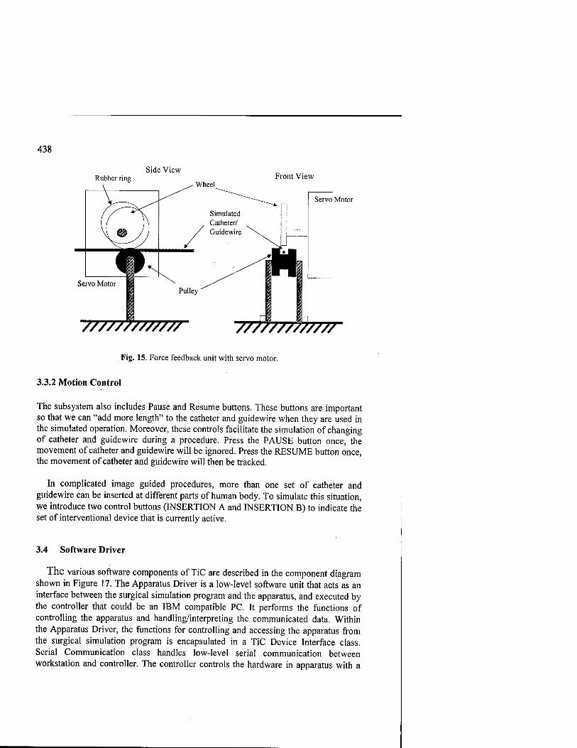
438

Side View Rubber ring Front View

Wheel

Servo Motor

7777777777777

Fig. 15. Force feedback unit with servo motor.

3.3.2 Motion Control

The subsystem also includes Pause and Resume buttons. These buttons are important so that we can "add more length" to the catheter and guidewire when they are used in the simulated operation. Moreover, these controls facilitate the simulation of changing of catheter and guidewire during a procedure. Press the PAUSE button once, the movement of catheter and guidewire will be ignored. Press the RESUME button once, the movement of catheter and guidewire will then be tracked.

In complicated image guided procedures, more than one set of catheter and guidewire can be inserted at different parts of human body. To simulate this situation, we introduce two control buttons (INSERTION A and INSERTION B) to indicate the set of interventional device that is currently active.

3.4 Software Driver

The various software components of TiC are described in the component diagram shown in Figure 17. The Apparatus Driver is a low-level software unit that acts as an interface between the surgical simulation program and the apparatus, and executed by the controller that could be an IBM compatible PC. It performs the functions of controlling the apparatus and handling/interpreting the communicated data. Within the Apparatus Driver, the functions for controlling and accessing the apparatus from the surgical simulation program is encapsulated in a TiC Device Interface class. Serial Communication class handles low-level serial communication between workstation and controller. The controller controls the hardware in apparatus with a

439

set of low-level I/O handling routines. If the simulation program does not reside on the same computing resource as the controller, an agreed communication protocol is required for the communication.

Linear Stepper Motor

Encoder

Simulated Catheter/Guidewire

Roller

Encoder Fig. 16. Mechanism with motion tracking and force feedback.

Process A in Figure 17 denotes the scenario in which the surgical simulation program is executed in a workstation, and the apparatus driver is executed in a controller which could be an IBM compatible PC. The simulation program interacts with the TiC Device Interface of the Apparatus Driver. Since the simulation program and the Apparatus Driver reside on different computing resources, the interaction between the two computing resources is done through Serial Communication Interface and I/O Handling Routines in the Apparatus Driver, according to an agreed protocol.

Process B in Figure 17 denotes the scenario in which the surgical simulation program and the apparatus driver reside in the same computing resource. The simulation program interacts with the TiC Device Interface that in turn calls upon the functions in the I/O Handling Routines.

3.4.1 Apparatus Driver

The objective of device driver is to allow the calling functions in anapplication program to control the apparatus and read data from it without the need to be involved in low level details regarding the serial communication between the workstation and the controller. The driver software could be implemented as shown in the following logical diagram (Figure 18).

440

Process A Apparatus Driver

TiC Driver Interface

Serial Communication Interface

Communication Protocol

I/O Handling Routines

Fig. 17. Component Diagram of Apparatus Driver.

The Serial Communication class handles all the low level communication through the serial ports between the workstation and controller of apparatus. The objective of I/O Handling Routines is to access the values in various controls through the data acquisition board and communication ports such as parallel port, MIDI port and serial ports, and then assemble these data into a single record to be transmitted to the workstation. The I/O Handling Routines consist of several portions: Parallel Port I/O Handling Module, MIDI Port I/O Handling Module, Serial Port Handling Module, Data Acquisition Module and Data Assembling Module.

If a single data acquisition board is not used or insufficient to handle all the input/output requirements, the following is a possible allocation of the communication ports assuming a typical PC configuration with 2 serial ports, 1 parallel port and 1 MIDI port. The Parallel Port I/O Handling Module takes charge of inputs from the parallel port. These are digital inputs for imaging control operation such as zooming and rotation. This module is also responsible for transmitting the signals to the Stepper Motor Driver that is an external hardware circuit. The MIDI Port I/O Handling Module takes charge of analog inputs from the syringe for dye contrast injection, and setting pressure for ballooning. The Serial Port I/O Handling Module takes charge of the serial inputs from the catheter and guidewire encoders in the tactile subsystem. The Serial Port I/O Handling Module is responsible for pushing the assembled record out to the workstation. The Data Assembling Module handles the formulation of the record from the inputs.

441

TiC Driver Interface I/O Handling Routines

Serial Communication Hardware Control Data Assembling

Serial Port Parallel Port MIDI Port Data Acquisition

Fig. 18. Logical view of Apparatus Driver.

3.4.2 Communication Protocol

The communication link between the workstation and PC should be RS-232C. A 5- byte packet of data is used to communicate between the workstation and the apparatus. The first byte of the packet data indicates an ASCII character indicating the type of data contained in the packet. For example, an ASCII 'A' indicates the catheter displacement and rotation.2 The types of data includes the following: guidewire displacement/rotation, balloon inflation/deflation, stent deployment, dye contrast injection, image zooming, panning and rotation, image contrast/brightness, force feedback values, etc. Error codes are also returned in during abnormal situations.

4. Summary

An apparatus for user interaction in simulating an image guided surgical procedure is presented in this paper. The apparatus is a new invention comprising the following capabilities:

• means for simulating the manipulation of images in real time. • means for tracking the motion of navigated catheter/guidewire/guiding catheter in

simulation.

'■ The complete command language/syntax is available as a separate document from the authors.

442

• force feedback means for providing resistive forces to navigated catheter/guidewire/guiding catheter in simulation.

• means to interface the apparatus with microprocessor based controller.

The manipulation of images in real time is simulated through the control panel allowing simulated: • image manipulation • operation of shutter in image guided procedure • operation of cine images in image guided procedure • setting pressure, inflating and deflating balloon catheter in image guided

procedure using a potentiometer that slides in a circle • activation of X-ray for fluoroscopy and cine recording using footswitches. • injection of drug including contrast dye using clinical syringe and potentiometer

with bar shape and side-to-side sliding.

Tracking of the motion of the catheter / guidewire is achieved using cylindrical / spherical rollers and encoders. Force feedback on individual catheter/guidewire/guiding catheter is achieved through clamp controlled by motor such as servo-motor/stepper motors. The motion tracking and force feedback are provided in a single unit comprising motor and rollers that provide independent rotation and translation force feedback.

Pause and Resume controls are implemented to simulate the exchange of catheter and guidewire using. Through the controls, more than one set of catheter/guidewire/guiding catheter can be inserted at different entries in a procedure.

The TiC apparatus includes the controller (personal computer) through an interface consisting of parallel port, MIDI port and serial ports. Communications protocols are designed and software drivers developed to control the operation of the TiC and smooth communications with the workstation.

5. References

1. Verel D. (1978), Cardiac Catheterization and Angiocardiography, 3rd Edition, Longman, New York, USA.

2. Ring E.J. and McLean G.K. (1981), Interventional Radiology: Principles and Techniques, Little, Brown, Boston, USA.

3. Sastry S.S., Cohn M, and Tendick F (1997), "Milli-robotics for remote, minimally invasive surgery," Robotics and Autonomous Systems, Vol. 21, Number 3, pp. 305-316.

4. Meglan D. (1996), Making surgical simulation real, Computer Graphics, November, pp. 37-39.

5. Prew S.J. (1996), Simulated training at the royal college of surgeons of England, Medical Simulation and Training, Vol. 1, Issue 2, pp. 20-22.

443

6. Pandzic I.S., Capin T.K., Magnenat Thalmann N., Thalmann D. (1997), A versatile navigation interface for virtual humans in collaborative virtual environments, Proceedings ofVRST.

7. MEDSIM, Advanced medical simulation, URL: http://www.medsim.com 8. Edmond C, Tacoma W.A. and Billinghurst M., Simulation: the substitute teacher,

Medical Simulation and Training, Vol. 1, Issue 1, pp. 19-20. 9. Sluis, D. (1996), Simulation and surgical training, Medical Simulation and Training,

Vol.1, Issue 2, pp. 26-27. 10. H T Medical, Inc. (1996), Forecasted timetable for adoption of medical simulators,

Medical Simulation and Training, Vo. 1, Issue 2, pp. 23. 11. Jolesz F.A. (1997), Image-guided procedures and the operating room of the future,

Radiology, Vol. 204, pp. 601-612. 12. Higgeins G.A., Meglan D., Millman A.S., Horst R. and Merril G.L., Virtual reality

surgery: implementation of a coronary angioplasty training simulator, Cardiovascular Surgery, Surgical Technology International IV, pp. 379-383.

13. Anderson J., Brody W., Kriz C, Wang Y., Chui C.K., Cai Y.Y., Viswanathan R. and Raghavan R. (1996), daVinci- a vascular catheterization and nterventional radiology-based training and patient pretreatment planning simulator, Society of Cardiovascular and Interventional Radiology 21s' Annal Meeting, March 1996, Seattle, USA.

14. Anderson J.H., Raghavan R., Wang Y.P., Mullick R., and Chui C.K., daVinci- a vascular catheterization simulator, Journal of Vascular and Interventional Radiology, Vol. 8, No. 1, Part 2, pp. 261.

15. Wang Y.P., Chui C.K., Cai Y.Y., Lim H.L., Ooi Y.T. and Mak K.H. (1998), ICard: an interventional cardiology simulator for percutaneous coronary revascularisation, Computer Assisted Radiology and Surgery (CAR '98), Tokyo, June 24-27 1998.

16. Immersion Corporation, San Jose, USA, URL: http://www.force-feedback.com 17. Immersion Corporation (1997), I-Force Studio, San Jose, USA. 18. Hughes, T.J.R. (1987), The Finite Element Method, Prentice-Hall, Inc., Englewood Cliffs,

New Jersey, USA. 19. Wang Y.P., Chui C.K., Cai Y.Y. and Mak. K.H. (1998), Construction of topological

structure of 3D coronary vessels for analysis of catheter navigation in interventional cardiology simulation, SPIE'98, San Diego, USA.

20. Wang Y.P., Chui C.K., Lim, HL, Cai Y.Y. and Mak. K.H. (1998), Real-time interactive surgical simulator for catheterization procedures, Submitted for publication in Journal of Computer Aided Surgery.

21. Hechtenberg, Kurt-Volker, Bosch, Dieter and Hermeking, Hajo (1997), Device for modeling or simulating the sense of touch in a surgical instrument, US Patent No: 5609607, Filed: Sept 26,1994, Issued: March 11, 1997.

22. Sinclair, Michael J. and Peifer, John W. (1998), Surgical simulator and method for simulating surgical procedure', US Patent No: 5766016, Filed: Nov. 14, 1994, Issued: June 16, 1998.

23. Playter R. and Raibert M., (1997), A virtual surgery simulator using advanced haptic feedback, Journal of Minimally Invasive Therapy and Allied Technologies, Volume 6/2, 117-121.

24. Barnes S.Z., Morr D.R., Oggero, E., Pagnacco, G. and Berme, H., (1998), The realization of a haptic (force feedback) interface device for the purpose of angioplasty surgery simulation, Journal ofBiomedical Sciences Instrumentation, Volume: 33, 19-24.

444

Static and Dynamic Modeling of the McKibben Artificial Muscle

Bertrand Tondu1

1LESIA, Departement de Genie Electrique et Informatique Institut National de Sciences Appliquees

Campus de Rangueil, 31077 Toulouse, France, tondu@dge.insa-tlse.fr

Abstract A physical model of the McKibben muscle is presented. This model explains how the artificial muscle generates its contraction force, and brings out a set of geometric and friction parameters from which a static and dynamic ex- pression is built. Comparisons with experimental results recorded on original experimental sites highlight the relevance of the proposed model.

1 Introduction

Hie McKibben muscle is currently one of the most interesting artificial muscles. In- vented in the fifties by the physician Joseph L. McKibben to motorize pneumatic arm orthics [1], [2] as illustrated in Figure 1, it was redesigned in the eighties by the Japa- nese tyre manufacturer Bridgestone to actuate new 'soft' robot-arms [3], [4]. Cur- rently, this very original pneumatic device is still studied within the framework of industrial robots field in order to develop robot-arms able to work in proximity with a human operator [5]-[7]. Neurophysiologists are also interested in the McKibben mus- cle to approximate the human skeletal behaviour [8]. For their part, pneumatic ele- ment manufacturers are interested in searching for deriving benefit from the damped spring nature of the McKibben muscle as the German manufacturer Festo did with its recent 'Airtecture' inflatable building tensioned by 'counterblowing muscles', which are obviously McKibben muscles [9]. Though the applications of the McKibben arti- ficial muscle are expanding, its physics has not been totally clarified yet. This paper proposes a physical model of the McKibben muscle aiming at better understanding its static and dynamic performances.

2 Description and Working Principle of the McKibben Muscle

Due to its structure - a braided shell surrounding a rubber inner tube - the McKibben artificial muscle is like a pneumatic tyre before bending. Moreover it is interesting to consider the original McKibben description with regard to classic treatises of pneu- matic tyre physics [10], [11] as illustrated in Figure 2.

445

(a) (b) Fig. 1. Historical use of a McKibben artificial muscle as an arm orthics for helping the opening and closing of the fingers of a handicapped hand, (a) McKibben muscle components (from [1]), (b) Task example performed by a disabled person with the assistance of a McKibben muscle (from [2]).

m

a —

(a) (b) Fig. 2. Design of pneumatic tyre carcases, (a) Tyre-bending pinciple showing the double helix weaving of the tyre carcase (from [10]), (b) Notion of bias angle (angle B of the figure) asso- ciated to the double helix weaving of the tyre carcase (from [11]).

However, contrary to a tyre carcase weaving, the great originality of the McKibben muscle lies in the use of a bias angle weak enough to allow the inflation of the pressu- rized inner tube. In this way the textile shell can open when the inner tube inflates and then performs a true energetic transformation thanks to the elementary pantograph network formed by its helical weaving. By taking the cylindrical shape of the inner tube, this flexible pantograph network converts the circumferential pressure forces into an axial contraction force as shown on Figure 3.a. This conversion principle is always valid when the muscle contracts because, due to the weaving symmetry, the artificial muscle keeps a global cylindrical shape. This principle has led us to propose

446

a basic parametrization of the McKibben muscle by means of the following three parameters illustrated in Figure 3.b :

The initial braid angle, noted oto, which corresponds to the notion of tyre carcase bias angle, is defined as the angle between the muscle axis and each thread of the braided shell before its expansion. In consequence this braid initial angle cha- racterizes the elementary pantograph initial angle, and in order to geometrically characterize the weaving by this single parameter, it will be assumed that initially the textile shell entirely recovers the rubber inner tube ; The initial muscle length, noted lo, is defined as the active initial muscle length, i.e. the initial length of the muscle shell; The initial muscle radius, noted r0, is defined as the radius of the rubber inner tube assumed initially in contact with the braided shell. This definition involves considering a thin-wall inner tube (this point will be discussed later), and based on this hypothesis, the radius r0 has been drawn in Figure 3.b as the initial internal radius of the muscle braided shell. Then a full transmission of the pressure to the braided shell can be assumed.

braided shell thin wall rubber inner tube

(a) (b) Fig. 3. Working principle of the McKibben muscle, (a) Pressure force transformation principle by means of the pantograph network of the muscle braided shell, (b) Basic geometrical para- metrization of the artificial muscle.

This geometrical parametrization of the McKibben muscle does not take into ac- count two important phenomena:

The non-conservation of the cylindrical shape of the muscle, which takes a conic shape at tips during its contraction as shown in Figure 4. Modeling such phe- nomenon is particularly complex because it depends on the weaving characteris- tics. The analysis of the McKibben muscle by means of finite elements, as it is currently developed at the Washington's BioRobotics laboratory [12], could help to model this phenomenon. On our part we will consider an empirical side effect coefficient (see paragraph 3); The braided shell and the inner rubber tube intrinsic mechanical aspects. The braided shell is assumed to be unstretchable, and we will not care about possible thread distorsions which limit the artificial muscle contraction repeatability. Mo- reover the inner tube is assumed to be fully adapted to the working pressures of

447

the muscle. It is notably assumed that the rubber tube radius and thickness have been correctly chosen for the considered pressure field (see our reference [13] for a discussion on this point).

(a) (b) Fig. 4. Close-up of McKibben muscle designed at the laboratory, (a) Initial contraction state, (b) Maximum contraction state.

This muscle geometrical parametrization is applied to the static McKibben muscle modeling of paragraph 3 on which the dynamic modeling of paragraph 4 is based.

3. Static Modeling of the McKibben Muscle

3.1. Basic Model of the Muscle Force Generator

Supposing in a first stage that the McKibben muscle keeps its cylindrical shape when it contracts, it is easy to determine a basic equation of its force generator by means of the principle of virtual works. During its contraction the muscle radius, initially equal to r0, becomes r and its length, initially equal to 10, becomes 1. If the static contraction force generated by the muscle is noted F in absolute value, and if the positive axis for length variation is chosen in the muscle extension direction, the virtual work of the equilibrium force against the contraction force is F81, where 81 designates the ele- mentary muscle length variation. The virtual work of pressure forces can then be ex- pressed by considering an elementary volume variation 8V, as done by Chou & Han- naford [14]:

P8V = -F81 (1) It is also possible, as we have proposed [13], to split the pressure forces into a lateral

pressure and an axial pressure. The theorem of virtual works ilustrated in Figure 5 leads to the following equation :

° "lateral pressure "*"" ^axial pressure + °™ equilibrium force "

=> (27irlP)(+8r) - (m 2P)(-81) - F(-81) = 0 (2)

448

PdS

dS

"+Sr~

\ \-6l

Fig. 5. Application of the theorem of virtual works to the static McKibben contraction analysis.

In consequence, it is possible to determine an expression of the force F by consid- ering the evolution of the muscle volume imposed by the braided shell. If a designates the current braid angle, the following relationships can immediately be deduced from the elementary pantograph opening principle.

(l/l0) = cosa/cosa0 and r/r0 =sina/sina0

=> r = r0[A/l-cos2a0(l/l0)2 /sina0] (3)

By applying these relationships and their derivatives to the virtual work equation, the following expression of F function of the control pressure P and the contraction ratio E is deduced:

fF(E, P) = 9.8 l(7tr02 )P[a(l - e)2 - b], 0 < s < e max with s = (10 -1) /10 and

(4) [a = 3/tan2(a0), b = l/sin2(a0)

In this expression, the initial muscle section (m02) is given in cm2, the control pressure

in kgf/cm2 and the generated force in N. This model brings to light the force evolution from initial state at zero contraction in which the produced force has a maximum value Fmax to maximum contraction state e^^ for which the force is zero. The corre- sponding expressions are:

JFmax = 9.81(7tr02 )P[a -b] for s = 0

lEmax=1-VbÄä forF = 0

This model is equivalent to the following one, originally proposed by Schutle [15] and reconsidered by Chou & Hannaford [14]:

(5)

F(a,P) = 9.81(7rr920o)P[3cos2a-l],with r^o =1^^/nthread7t, (6)

where T^* designates the muscle radius for a=90° - non-physically reachable - which is in practice determined by using the datum of Uread representing the thread length and the datum of n^hread representing the number of turns of a thread. The equation (4) model parametrized in e however seems to us better adapted for an experimental vali- dation than the model parametrized in a of equation (6). Moreover the demonstration

449

of the muscle force in the equation (4) form leads to prove the Rubbertuator formula given in Bridgestone's technical reports and reported in the research works using Soft- Arms [16]. The relationships of coefficients 'a' and 'b' that we have made explicit do not appear in Bridgestone's reports.

Before dealing with the confrontation between this theoretical model and the ex- periment, it is important to remind that the model reported in this article as well as Chou & Hannaford's model are based on the hypothesis of an infinitely thin inner tube. For this reason, the muscle radius r is the internal braided shell radius. In pratice it is possible to consider that this hypothesis is satisfied if the ratio between the tube thickness and the inner rubber tube is about 1/10 [17]. If the tube thickness rises above this limit, it is no more possible to assume that the pressure forces are fully transmitted to the braided shell. The global analysis by means of virtual work is no longer valid. The local analysis of the distributed forces within the pressurized inner tube would be necessary to determine the proportion of pressure transmitted to the shell. This point will be not discussed here. Within the framework of this paper we will consider a thin rubber tube McKibben muscle, optimum as far as the pressure force conversion is concerned.

The negative aspect of the model is that its design is based on the hypothesis of a continuously cylindrical shape muscle whereas it takes a conic shape at both ends when it contracts. Consequently the more the muscle contracts, the more its active part decreases. This phenomenon involves that the actual maximum contraction ratio is smaller than the maximum one expected from equation (5). In order to take into account this side effect, an empirical parameter k (k>l) is considered, which amplifies the contraction ratio 8 by the factor k. The modified force generator model is:

F(s,P) = 9.81(OT02)P[a(l-kE)2-H0<E<emax (7)

and the maximum contraction ratio is then divided by the factor k:

6max = (i/k)(i-Vb7I) (8)

Two approaches have been considered for the choice of the factor k. In the first approach, a constant value of k has been estimated. It has been remarked that, for our muscles made of rayon braided threads - 10 to 30 cm in initial length, 0.5 to 1 cm in initial radius, 20° to 30° in initial braid angle - a parameter k of 1.25-1.35 is relevant. Figure 7 shows the comparison between the experiment and the force model discussed above in the case of 4 muscles designed at the laboratory and tested on Figure 6 ex- perimental site. For a given pressure generated by an Intensity/Pressure converter, the static muscle force is recorded. A tensioner is used to make the contracted muscle length variable. In this way the static characteristics F(E) at constant pressure is ob- tained. In our experiments the muscles have a braid made in rayon and a rubber tube made of 50 shore hardness butyl. At rest the inner tube has a 10 mm internal diameter and a 0.6 mm thickness.

450

s converter

position encoder

0>) (c) Fig. 6. Experimental site for the static analysis of the McKibben muscle performing an isomet- ric contraction of the artificial muscle (i.e. at constant length), (a) Site components, (b) Muscle zero contraction state at maximum force, (c) Muscle maximum contraction state at zero force.

Experimental results reported in Figure 7 validate the following properties of the McKibben muscle expressed in the force generator model considered: 1. 2. 3. 4.

5.

McKibben muscle static force is globally proportional to muscle initial section, McKibben muscle static force is globally independent of muscle initial length, McKibben muscle static force is globally proportional to control pressure, McKibben muscle maximum static force is all the higher as the muscle initial braid angle is low, McKibben muscle static force decreases almost linearly with contraction ratio according to a slope globally proportional to control pressure.

It is interesting to note that the McKibben muscle shares the first three properties with the pneumatic cylinder. The fourth property highlights the importance of the choice for the initial braid angle to dimension the maximum force generated by the muscle. It also highlights the exceptional McKibben muscle ability for a high maxi- mum force-to-weight ratio (the mean weight of our muscles is about 50 g). The choice for a low initial braid angle is however limited by the rupture in extension of the rub-

451

ber since the lower the initial braid angle is, the more the muscle radius increases. In practice an initial braid angle of about 20° appears to be relevant, and in this case, the size of the muscle varies satisfactorilly during contraction since its radius approxi- mately doubles. The fifth property is its functional analogy with the natural skeletal muscle. The 'natural compliance' notion of the antagonistic muscle actuator, which we have developed elsewhere [18] and which justifies the joint 'softness' of robot- arms actuated by McKibben muscles is based on this analogy.

120

0.1 0.2 contraction ratio

^|feE| I |

0.1 0.2 contraction ratio

0.3

(a) (c)

0.1 0.2 contraction ratio

0.05 0.1 0.15 0.2 0.25 contraction ratio

(b) (d) Fig. 7. Comparison between the experiment (full line) and the force generator model (circles), (a) Reference muscle (ao= 20°, lo=30cm, r0= 0.7cm with k=1.30), (b) Effect of the initial braid angle (oto= 30°, lo=30cm, r0= 0.7cm with k=1.25), (c) Insensitiveness to the initial muscle length (ao= 20°, lo=15cm, r0= 0.7cm with k=1.30), (d) Effect of the initial muscle radius (oo=

20°, lo=30cm, r0= 0.85cm with k=1.35).

452

The force model including the constant factor k has enabled us to experimentally emphasize the basic static properties of the McKibben muscle. However it proves to be faulty at low pressure. This is the reason why we think that the parameter k not only expresses a side effect due to muscle tips but also a sliding effect from the braided shell against the rubber tube particularly obvious as the pressure is low. In order to get a more reliable model in the whole pressure control range for the muscle dynamic model, we have, in a second stage, parametrized the coefficient k function of the pressure P. The following two-parameter relationship has been considered in which ak and bk are constants estimated for each muscle :

k = ake-p+bk (9) Figure 9 shows the comparison between the experiment and the new model for our reference muscle (ao= 20°, lo=30cm, r0= 0.7cm with ak=3.55, bk=1.25) represented by circles. If the model is now better adapted to low pressures, it still neglects the hys- teresis phenomenon which clearly appears on experimental curves.

3.2. Consideration of a Friction Model

Because hysteresis corresponds to a greater generated force when the muscle extends (e decreasing) in comparison with the generated force when the muscle contracts (e increasing), we consider that this phenomenon is due to the friction thread on thread acting inside the muscle braided shell. Friction seems fundamental to understand the McKibben muscle contraction, as we will see in the next paragraph. In this paragraph we will limit our analysis to the static part of the friction. The weaving involves an interlacing of the thread according to the basic scheme of Figure 1. If we assume that no sliding occurs between the rubber tube and the shell, the pressure inside the inner tube is entirely transmitted to the shell and the pressure thread on thread is conse- quently the inflation muscle pressure P. The following expression can, in conse- quence, be considered to model the static dry friction:

|Fstatic dry friction | = f s^P (10)

where fs is the dry fiction coefficient thread on thread and S is the contact surface. If, in the first stage of the demonstration, we neglect the cylindrical shape of the shell thread to assume a full contact between shell threads, we will be able to determine the contact surface as the covering surface of the braided shell against itself due to double helix weaving. This surface is initially, i.e. before muscle contraction begins, the lat- eral surface of the muscle (27ir0lo). The pantograph network opens and the contact surface decreases when contraction begins. It is possible to determine its evolution by using the geometrical characteristics of the pantograph network structure of the braided shell illustrated in Figure 8. The elementary hachured pantograph of Figure 8.a represents a contact elementary surface 'Seiem init=2a2cosaosinao' where 'a' desig- nates the constant side of the pantograph. During contraction this contact elementary surface opens while keeping the side a constant The contact elementary surface be- comes the new hachured surface shown on Figure 8.b. By considering the thread thickness 'e' bound to 'a' by the equation 'e=2acosoosinao' deduced from Figure 8.a, it is possible to determine the contact elementary surface of Figure 8.b

453

'Seiem curreiit=2a2cos2aosin2ao/cosasina'. The total contact surface of the shell against itself, noted S, is deduced from the proportion between these two surfaces. After having considered the specific evolution of the muscle radius function of its length (equation 3) we obtain:

S = (2jtr0l0) Selem current

^elem init = (2OT01 >°m> (2OT010)

sinarj

(l - E)-y/l-cos2a0(l-e)2 (ID

ndly (1-E) is changed into (1-ke) to equate the contact surface analysis with the force productive force analysis. Figure 8.c gives the simulated evolution of the ratio be- tween the contact current surface and the initial one function of the contraction ratio in the case of our reference muscle (oto= 20°, lo=30cm, r0= 0.7cm with k=1.25).

\ \ \ \ \

>-

0.15 02 055 CONTRACTION RATIO

(a) (b) (c) Fig. 8. Contact surface analysis of the McKibben muscle braided shell, (a) and (b) Elementary surface definition, (b) Simulated evolution of the ratio S/(27tr0lo).

Thanks to this contact surface model, we can estimate the friction coefficient from the recording of the static muscle force (Figure 7.a) The resulting model shown on Figure 9 now takes into account the static hysteresis cycle relatively well. It has been obtained with an estimated friction coefficient fs of 0.015. Such a static dry friction is in fact very low. According to the Fibres, Plastics and Rubbers Handbook [19], the viscose rayon on viscose rayon static dry coefficient is equal to about 0.2. Therefore, we must assume that only (1/13) of the textile shell surface is in contact with itself, which appears to be a reasonable assumption in accordance with the shell thread cy- lindrical nature. If we call (1/n) the estimate ratio of the muscle lateral surface rub- bing against itself, the static friction model considered will finally be :

|Fstaticdry&iction| = fs(l/n)SP (12)

The dynamic McKibben muscle analysis extends the static friction analysis.

4 Dynamic Modeling of the McKibben Muscle

The dynamic contraction of the McKibben muscle has been studied from the experi- mental apparatus shown on Figure 10. This apparatus allows the muscle contraction to lift a given load by means of a pulley. An encoder mounted on the pulley axis gives

454

the current muscle length. A special force sensor has been designed on purpose : light and compact, it is directly fixed to the muscle end to record the current force pro- duced by the muscle during its contraction. Initially the load lies on a base, and in response to a numerical signal translated into a pressure by means of the Inten- sity/Pressure converter, the muscle contracts until it reaches its equilibrium position (Figure lO.b). This apparatus performs the isotonic contraction of the muscle lifting away the load m. In the experiments reported below, pressure inside the muscle, force muscle and linear muscle contraction in the form of the position x - x being defined as (lo-l) (Figure 10.a) - are simultaneously recorded. The isotonic contraction proves that the natural damping of the McKibben muscle is very similar to the skeletal mus- cle behaviour [20]. A simple and general model for the dynamic dry friction coefficient f can be considered in the form of the following 3-parameter relationship :

f = fk+(fs-fk)e~(*/i') 03) Here fs represents the dry static coefficient considered previously, fk the maximum

dry kinetic coefficient and xs a velocity constant between fs and fk . In case of solids, fk

coefficient is generally smaller than fs. In case of a textile shell rubbing against itself, our experimental results have shown fk greater than fs. This is the reason why we have represented our friction model on Figure 1 La according to this situation. Its original- ity in comparison with usual solid friction models emphasizes the McKibben muscle originality. A higher kinetic friction, due to hydrodynamic phenomena, is typical of textile threads physics, as illustrated on Figure 1 Lb related to the friction of lubrifi- cated rayon threads (synthetic textile threads are generally lubrificated during their manufacturing) [21].

120

100

120 r

0.1 0.2 contraction ratio

0.1 0.2 contraction ratio

(a) (b) Fig. 9. Comparison between experiment (full line) and the force generator model (circles) including the static dry friction model for our'reference muscle (oto= 20°, lo=30cm, r0= 0.7cm with ^=3.55,1^=1.25 and (fyn)=0.015), (a) Cases of P=l,3,5 bar, (b) Cases of P=2,4 bar.

455

fc

x-»- M

X

W

mg

(a) (b) Fig. 10. Dynamic analysis of the McKibben muscle in isotonic contraction (i.e. at constant load), (a) Principle scheme, (b) Corresponding experimental site.

0-6r

friction coefficient

/

I

100 ToTT «4o 200 Velocity

(a) (b) Fig. 11. Considered friction model for the McKibben muscle shell, (a) Three-parameter friction model, (b) Typical variation of the friction coefficient with speed for rayon thread (from [21], page 69).

However, as it clearly appears in the experiments, the estimated kinetic muscle shell friction coefficient is still higher than designed by rayon physics: an approximate ratio of 7 between the kinetic friction coefficient and the static one will be considered later. To explain this phenomenon, we have considered the global behaviour of the shell: the interlacing of the threads in motion seems to play the role of the rough surface in the friction theory. Finally the complete dynamic McKibben muscle force model, noted Fjyn, where F designates the static expression of equation (7) will be :

Fdyn=F-f(l/n)SPsign(x) (14)

The isotonic contraction performed by using the Figure 10 experimental apparatus can be written in equation system below where t^ divides the two stages of the experi- mental isotonic contraction:

m/mfn

456

Fdyn=mx, 0<t<tlira

Fdyn-mg = mx,t^tlim ( '

It must be noted that the load can be lifted only after the time tiim, when the muscle pressure has increased from zero to the high enough value to produce the sufficient force to the load. It has been possible to solve this equation system by using the Matlab Software Runge-Kutta procedure. The recording of the pressure has been directly used for generating a very accurate linearly interpolated pressure model. Figure 12 presents three examples of results obtained in three different situations of pressure and load: m=30 kg and P=4 bar, m=20 kg and P=3 bar m=10 kg and P=2 bar. In all the experiments the parameter values have been chosen: (fs/n)=0.015, (fk/n)=0.105 - it follows fk/fs is 7 - and X^.lSm/s. The adjustment of the two dynamic parameters fk and xs has been made from the force recording by successive trials in which the *s gives the slope between succesive force extrema and the fk gives the force extremum value. The values selected for the three parameters lead to a good concordance beween experiment and theory for the muscle force shape. The resulting concordance is good for the muscle contraction. However it is less good when the motion starts and in the case of low pressure steps, for which the force generator model is still limited (see Figure 9.a). Other experiments performed for different pressures and loads have confirmed the global validity of the proposed model for the set of considered parameters.

This dynamic model highlights the McKibben muscle dynamic properties: 1. McKibben muscle contraction is naturally damped by a non-linear kinetic friction

inherent to its braided shell, 2. McKibben muscle contraction time has the size of some tenths of a second.

These two dynamic properties, in high analogy with the skeletal natural muscle dy- namic performances, complete the five static McKibben muscle properties given above.

5 CONCLUSION

The McKibben muscle is a pneumatic device characterized by a high maximum force- to-weight ratio since it can easily develop 1000 N for its own weight of 50 g. Moreo- ver it offers other basic properties in great analogy with the human skeletal muscle : while keeping a globally cylindrical shape, the McKibben muscle produces a real contraction force decreasing with its contraction ratio. The static modeling of the McKibben highlights the geometric parameters characterizing the muscle : initial length, initial radius and initial braid angle. The hysteresis phenomenon specific to the artificial muscle is explained and modeled by a dry friction thread on thread inside the braided shell. The dynamic modeling highlights the importance of the weave as a natural damper of the muscle contraction. This damping behaviour is explained and modeled by a kinetic friction function increasing with speed, directly associated to the shell structure. Finally the McKibben muscle seems to be a surprising artificial mus- cle, as powerful, compact, quick and naturally damped as the skeletal muscle.

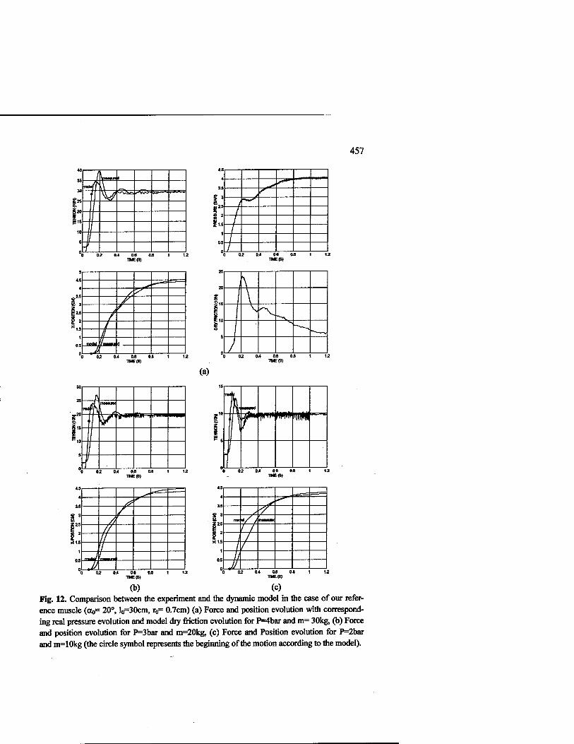
457

40

/ V— 45

4

35

iu25

I' 1

05

™*fT 4 V ~VAß

?» ^20

("15

/ /

02 0.4 OJB 05 TWE(S)

02 04 OJS 04 THE (5)

(a)

&J ,^

B 2 // f '

/ L. ■^

l>m*W* IIN

45

y /f

S3 mix '// |» I

? j / / / //

0 J (b) (c)

Fig. 12. Comparison between the experiment and the dynamic model in Ihe case of our refer- ence muscle (oto= 20°, lo=30cm, r0= 0.7cm) (a) Force and position evolution with correspond- ing real pressure evolution and model dry friction evolution for P=4bar and m= 30kg, (b) Force and position evolution for P=3bar and m=20kg, (c) Force and Position evolution for P=2bar and m=10kg (the circle symbol represents the beginning of the motion according to the model).

458

References

1. Nickel, V.L., Perry, M.D.J., Garret, A.L.: Development of Useful Function in the Severely Paralysed Hand. The Journal of Bone and Joint Surgery. 45-A5(1963) 933-952

2. Engen, T.J.: Development of Externally Powered Upper Extremity Orfhotic Systems. The Journal of Bone and Joint Surgery. 47-B 3 (1965) 465-468

3. E.P.W.: Rubber Muscles Take Robotics One Step Further. Rubber Development. 37 4 (1984) 117-119

4. Bridgestone Corporation and Taicubo Engineering : Soft Arm : Painting System Unit. Prod- uct literature. Tokyo (1987) and: Soft Boy: Advanced Painting System Unit. Product lit- erature. Tokyo (1993)

5. Tondu, B., Boitier, V., Lopez, P.: Naturally Compliant Robot-Arms Actuated by McKibben Artificial Muscles. Proc. of IEEE-SMC Conf San-Antonio (1994) 2635-2640

6. Caldwell, D.G., Medrano-Cerda, G.A., Goodwin, M.: Control of Pneumatic Muscle Actua- tors. IEEE Control Systems Magazine. 15 1 (1995) 40-48

7. London's Shadow Robot Company Ltd. web adress: http://www.shadow. org.uk 8. Chou, C.P., Hannaford, B.: Study of Human Forearm Posture Maintenance with a Physio-

logically Based robotic Arm and Spinal Level Neural Controller. Biological Cybernetics. 76(1997)285-298.

9. Thallemer, A., Riedmüller R.: Hochelastische Kontraktionsschläuche Gewährleisten Sta- bilität einer Lufthalle. Maschinenmarkt. 20 (1997)

10. Maillot, R: Tyre Carcase Construction. In: Genin, G., Morisson, B. (eds): Technological Encyclopedia of Rubber Industry. Dunod, Paris (1956) in french

11. Woods, E.C.: Pneumatic Tyre Design. W. Heffer & Sons Ltd, Cambridge, England (1952) 12. Washington's BioLaboratory web adress : http://rcs.ee.washington.edu/BRL 13. Tondu, B-, Lopez, P.: Theory of an Artificial Pneumatic Muscle and Application to the

Modelling of McKibben Artificial Muscle. C.R.A.S., French National Academy of Sci- ences. 320 Ub (1995) 105-114 -

14. Chou, C.P., Hannaford, B.: Measurement and Modeling of McKibben Artificial Muscles. IEEE Trans, on Robotics and Automation. 12 1 (1996) 90-102

15. Schulte, H.F.: The Characteristics of the McKibben Artificial Muscle. In: The Application of External Power in Prosthetics and Orthotics. Publication 874, American National Academy of Sciences (1961) 94-115

16. Van der Smagt, P., Groen, F., Schulten, K.: Analysis and Control of a Rubbertuator Arm. Biological Cybernetics 75 (1996) 433-440

17. Nash, W.A.: Theory and Problems of Strength of Materials, Schaum's outline, McGraw- Hill (1994)

18. Tondu, B., Lopez, P.: The McKibben Muscle and its Use in Actuating Robot-Arms Show- ing Similarities with Human Arm Behaviour. Industrial Robot 24 6 (1997) 432-439

19. Roff, W.J.: Fibres, Plastics, and Rubbers, A Handbook of Common Polymer. Butterworths Scientific Publications, London (1956)

20. Ghez, C.:Muscles: Effectors of the Motor System. Chap. 36. In: Principles of Neural Sci- ence. Kandel, E.R, Schwartz., J.H., Jessekk, T.M. (eds), Prenctice-Hall (1991) 548-563

21. Howell, H.G., Mieszkis, K.W., Tabor., D.: Friction in Textiles. Butterworths Scientific Publications, London (1959)

459

Faults Identification of Oil Wells Using Neural Networks

Bogdan M. Wilamowski University of Wyoming

Department of Electrical Engineering Laramie WY, 82071

wilam@ieee.org

Abstract. Oil well diagnosis usually requires sophisticated tools and specialized sensors placed on the surface and in the bottom of the well. The purpose of this study is to identify oil well parameters based on the measurement the terminal characteristics of the electrical motor. The quality of the oil well could be monitored continuously and proper adjustments could be made. Such approach may lead to significant savings in electrical energy, which is required to pump the oil. With this approach, motors with smaller nominal power can be used instead of overrated motors operating at a fraction of their nominal power. The application of this new technology could lead to constant and effective monitoring of oil wells. These approach leads to better diagnosis, adjustment, choice of an optimum pumping rate, and more efficient use of energy.

1 Introduction

Several techniques are used for oil well diagnosis. These approaches usually require sophisticated tools and introduce specialized sensors placed on the surface and in the bottom of the well [1][2]. Recently, there is a significant interest in identifying characteristics of the oil well using neural networks [3]-[13]. Neural networks are also used for identifying faults of electrical motors, which are used to drive the oil pump. Such diagnosis of electrical motors, using their terminal parameters is already very advanced [14]-[20]. The purpose of this study is to identify oil well parameters based on the measurement of the terminal characteristics of the electrical motors. This approach does not require special instrumentation and can be used on any oil well with a pump driven by an induction motor. The quality of the oil well could be monitored continuously and proper adjustments could be made. Such approach may lead to significant savings in electrical energy required to pump the oil.

460

2 Oil well model

It would be very difficult and definitely veiy costly to introduce fault in real oil wells (Fig.l). Therefore, a very complex model of an oil well was developed, so that all possible faults can be easily introduced. For the induction motor, the relatively simple, third order model was used. In addition to the three motor state variables, four state variables for the pumpjack were used: angular flywheel velocity, angular flywheel acceleration, beam angle, and beam angular velocity. Note that a relatively complex nonlinear relationship must be used between the angular position of the gear flywheel and the angular position of the pumpjack beam. For deep wells, the diameter of the sucker rod changes and this leads to different stiffness and different mass for every section of sucker rod. This distributed parameter system can be properly approximated by lumped six state variable systems representing displacement and velocities of sucker rod sections. Oil flow in the tube can be modeled by two additional state variables representing displacement and velocity. A three-dimensional model of oil flow through the formation can describe oil pressure distribution around the well. If radial uniformity is assumed, this problem can be reduced to a one-dimensional distributed parameter case, which can be well approximated with 10 state variables representing oil pressure for 10 different distances from the well. Overall the entire system is described by a 25-order system of differential equations and 25 state variables.

counterbalance weight

motor with gear box

and flywheel

Figure not to scale

sucker rod

oil outlet

oil pressure aroun well (not to scale)

traveling valve

standing valve

Fig. 1. Oil well with pump jack.

There are very different time constants in the system. An induction motor operates at 60 Hz and typical time constants are of the order of 0.1 to 0.2 s. A pumpjack operates with cycles varying from 5 to 20 seconds. Transient responses in the well itself have time constants from several hours to several weeks, or even years, when the well capacity

461

is considered. Significant differences in time constants make the system very stiff and difficult to analyze. Traditional forward Euler or Runge-Kuta methods would require the use of very small time steps and an unrealistically long simulation time. Such stiff dynamic systems require implicit integration methods. The key issue was to find an efficient method to simulate this very large set of nonlinear differential equations. It turned out that there is a very simple and efficient solution. Instead of developing dedicated code in FORTRAN or in C the entire system was simulated using the SPICE program, which has an excellently developed algorithm to handle very stiff dynamic systems with second order Gear integration scheme.

dx, L = axi + b(xn-xm)+csin(xk) _x. C=1

Fig. 2. Equivalent diagram for differential equation used in SPICE program. Voltage on each capacitor represents one state variable.

The approach is illustrated by the example with the equivalent circuit for an j-th differential equation for the state variable x, is shown on Fig. 2. Note that recent versions of SPICE programs have nonlinear dependent sources. In the case shown in Fig. 2. three dependent current sources could also be combined into one, controlled by a nonlinear expression of many variables. The system of 25 differential equations is relatively complex, but the simulation time for one set of parameters is usually completed within 15-30 seconds on the Pentium 200MHz computer using PSPICE program version 7.1.

3 Data preprocessing and generation of training patterns

Sample results of oil well simulations using the complex model are shown in Fig. 3 and 4. Fig. 3 shows transient responses during operation in normal conditions and Fig. 4. shows the same responses with a leakage of the traveling valve. Note the significant differences, especially in Fig. 3 (d) and Fig. 4 (d). Unfortunately the measurement of such parameters at the bottom of the well is not easy. The purpose of this work was to identify oil well parameters by sole measurements of the terminal parameters of the induction motor and to use neural networks for data processing.

462

10 Urne [5]

motor torque

10 «me [s]

(C)

X10

6

' at standing ' at traveling' r\ A valve A s\ valve /'■. t\

5 ■ 1 ^ \

^4 \ ! \ f ' I3 ■s

2

1 'at the topi ; ^S~J/ ■ head \ • \ j

time [s]

(d) Fig. 3. Results of simulation of the 1500m deep oil well in normal condition (a) sucker rod displacements, (b) sucker rod velocities, (c) forces and torques, and (d) oil flow.

463

Fig. 4. Results of simulation of the 1500m deep oil well with leaking traveling valve (a) sucker rod displacements, (b) sucker rod velocities, (c) forces and torques, and (d) oil flow.

Measurement of currents and voltages at terminals of the three-phase induction motor operating at 60Hz leads to the collection of tremendous amounts of data. It turns out that most of the important information is contained in the instantaneous power of the induction motor [18]. The data for the transient waveform of the instantaneous power is processed with FFT (Fast Fourier Transform). The Fourier coefficients on the complex plane are generated, as shown in Fig. 5. Since this mechanical system includes several large masses with inertia the system works as high order low-pass filter, therefore, only the first nine Fourier components is used. As a result, each instantaneous power waveform is represented by 19 numeric values: 9 real, 9 imaginary, and one representing the dc offset. These 19 values were used as the input pattern for the neural network

Fourier Coefficients In the Complex Plane mo«)

; «5

8000 '

6000 ■

4000

2000 ■

0 ...""....is* „,.... »3

evF 1

-jono . ;

Fourier Coefficients in the Complex Plane 10000

■ ■ o5

8000

60OO

4000

2000

0 o3

oe o

2 t <A

-mm ; . 3 4

Real Axis x10< Real Axis x10»

(a) (b) Fig. 5. Conversion of instantaneous power waveform into Fourier coefficients: (a) case with normal operation and (b) case with leaking traveling valve.

464

4 Neural network architecture and training

All neural network processing was done using SNNS software, which can be acquired free of charge from http://www.informatik.uni-stuttgart.de/ipvr/bv/projekte/snns/snns.html Various feedforward architectures were explored with one pattern file used for training and with another pattern file used for verification. All input and output patterns were scaled in such a way that input and output values changed within the -1 to +1 range. Good results were obtained using a two hidden layer neural network with full connections across layers with 5 neurons in each hidden layer. Several different training algorithms were explored such as Backpropagation [22], Quickprop[23], RPROP[24], Backpercolation[25], and Conjugate Gradient Method[26]. It turned out that for this case the most efficient was the RPROP algorithm.

(a) (b) Fig. 6. Oil pressure distribution in vicinity of the well: (a) spatial distribution around well with pumping time as parameter and (b) transient response of the pressure in the well with soil permeability as parameter.

The leakage of the traveling valve, the leakage of the standing valve, the effective oil depth, and the location of balance mass on the beam, were four outputs of the neural network. Initially, both training patterns and verification patterns were generated in such way that for each pattern only one variable (for example, leakage of the traveling valve) was modified and the remaining parameters had normal values. In this case the neural network was able to identify the correct fault in 100% cases. More importantly the neural network was also able to identify how much a certain parameter has deteriorated. For example, what is the leakage, what is the effective depth, or what is the location of the

465

balance mass. The accuracy of this identification varied from 10 %, in the case of the effective oil depth, to 50%, in the case of the standing valve leakage.

For the next experiment all four faults were introduced simultaneously by randomly chosen values. In this experiment correct results were obtained only if there was one clearly dominant fault. When several faults were present, then the neural network was often confused and misidentified faults. This means that there are strong interactions of a nonlinear nature between the parameters.

Fortunately, three of four of the investigated parameters (the leakages and the mass location) can be assumed constant during experiments, which leads to the identification of formation permeability and reservoir capacity. As Fig. 6 (a) shows the pressure distribution around a well changes with the pumping time. The only parameter, which can be observed in the wellbore, is the effective depth of the oil table. Fig. 6 (b) shows how the effective oil depth changes with time for different values of the formation permeability. From such transient responses it is possible, using well-established techniques [27] [28], to estimate formation permeability and drainage-area pressure, the reservoir heterogeneity or boundaries.

5 Conclusion

The terminal parameters of the induction motor contain significant information about the oil well, which can be extracted using neural networks. This information is not only about the condition of the oil reservoir, but it may lead to better adjustments of the pump and its ballast so the pumping can be done more efficiently. With this approach, motors with smaller nominal power can be used instead of overrated motors operating in a fraction of their nominal power. The application of this new technology could lead to constant and effective monitoring of oil wells. Measurements may lead to better diagnosis, adjustment, choice of the optimum pumping rate, and more efficient use of energy.

References

1. T. Chakrabarty, 1996, A new robust algorithm for rapid determination of porosity and lithology from well logs, paper CIM 96-17, in 47th annual technical meeting preprints, v. 1: CIM Petroleum Society, Calgary, Alberta, p. 15.

2. B. Braunschweig and R. Day, 1995, Prolegomena—an overview of AI techniques and of their use in the petroleum industry, in Artificial intelligence in the petroleum industry, v. 1 Symbolic and computational applications: Editions Technip, Paris, p.2-37.

3. G.B. Arpat, 1997, Prediction of permeability from wire-line logs using artificial neural networks, in Annual technical conference and exhibition proceedings, v. omega, Formation evaluation and reservoir geology, part 2: Society of Petroleum Engineers, p. 531-537.

466

4. B. Baygun, S.M.Luthi, and I. D. Bryant, 1996, Applications of neutral networks and fuzzy logic in geological modeling of a mature hydrocarbon reservoir, chapter 5, in Braunschweig, B., and Bremdal, B.A., eds., Artificial intelligence in the petroleum industry, v. 2, Symbolic and computational applications: Editions Technip, Paris, p. 125-138.

5. A. Bonarini, A. Corrao, L. Giacometti, and L. Tomada, 1995, A fuzzy logic enhancement to a support system for the recognition of sedimentary environments from core analysis, chapter 12, in Braunschweig, B., and Day, R., eds., Artificial intelligence in petroleum industry, v. 1- -Symbolic and computational applications: Editions Technip, Paris, p.2-37.

6. A. Chawathe, A. Ounes, and W. Weiss, 1997, Predicting unconventional well logs from conventional well logs using neural networks: In Situ, v. 21, no. 2, p. 145-159.

7. C. A. Gonclaves, P. K. Harvey, and M. A. Lovell, 1997, Prediction of petrophysical parameter logs using a multilayer backpropagation neural network, in Lovell, M.A., and Harvey, P.K., eds., Developments in petrophysics: Geological Society [London] Special Publication No. 122, p. 169-180.

8. S. M. Luthi and I. D. Bryant, 1997, Well-log correlation using a back-propagation neural network: Mathematical Geology, v. 29, no. 3, p. 413-425.

9. S. Mohaghegh, R. Arefi, S. Ameri, K. Aminiand, and R. Nutter, 1996, Petroleum reservoir characterization with the aid of artificial neural networks: Journal of Petroleum Science and Engineering, v. 16, no. 4, p. 263-274.

10. M.N. Panda, D. E. Zuacha, G.Perez, and A. K. Chopra, 1996, Application of neural networks to modeling fluid contacts in Prudhoe Bay, SPE-30600: SPEJ, v. 1, no. 3, p. 303-311.

11. A. Schumann, 1997, Neural networks versus statistics—a comparing study of their classification performance on well log data, in Pawlowsky-Glahn, V., ed., 3rd annual conference of the International Association for Mathematical Geology [IAMG '97] proceedings: International Center for Numerical Methods in Engineering, Barcelona, Spain, p. 237-241.

12. N. Shimada, A. Tani, and N. Nishikawa, 1997, Reservoir characterization using artificial neural networks, paper K, in 3rd Well logging symposium of Japan proceedings: Society of Professional Well Log Analysts, Japan Chapter, 6 p.

13. P. M. Wong, D.J, Henderson, and L. J. Brooks, 1997, Reservoir permeability determination from well log data using artificial neural networks—an example from the Rawa field, offshore India, SPE-38034, in Asia Pacific oil and gas conference proceedings: Society of Petroleum Engineers, p. 149-155.

14. M.-Y. Chow, R. N. Sharpe, and J. C. Hung, "On the Application and Design of Artificial Neural Networks for Motor Fault Detection - Part I and Part II IEEE Transactions on Industrial Electronics, vol. 40, pp. 181-197,1993.

15. P. V. Goode and M.-Y. Chow, "Using a Neural/Fuzzy System to Extract Knowledge of Incipient Fault in Induction Motors Part I and Part H" IEEE Transactions on Industrial Electronics, vol. 42, pp. 131-146,1995.

16. M.-Y. Chow, Methodologies of Using Artificial Neural Network and Fuzzy Logic Technologies for Motor Incipient Fault Detection: World Scientific Publishing Co. Re. Ltd., 1997.

17. F. Filipetti, G. Franchescini, and C. Tassoni, "Neural networks aided on-line diagnostics of induction motor faults," IEEE Transactions on Industry Applications, vol. 31, pp. 892-899, 1995.

467

18. S. F. Legowski, A. H. M. S. Ula, and A. M. Trzynadlowski, "Instantaneous Power as a Medium for the Signature Analysis of Induction Motors," IEEE Transactions on Industrial Applications, vol. 32, pp. 904-909,1996.

19. R. R. Schoen, B. K. Lin, T. G. Habetler, J. H. Schlag, and S. Farag, "An Unsupervised, On- Line System for Induction Motor Fault Detection Using Stator Current Monitoring," IEEE Transactions on Industrial Applications, vol. 31, pp. 1280-1286,1995.

20. F. C. Trutt, C. S. Cruz, J. L. Köhler, and J. Sittuke, "Prediction of Electrical Behavior in Deteriorating Induction Motors," IEEE Transactions on Industry Applications, vol. 29, pp. 1239-1243,1993.

21. B. M. Wilamowski and R. C. Jaeger, "Computerized circuit analysis using SPICE programs", McGraw-Hill 1997.

22. D. E. Rumelhart and J. L. McClelland Parallel Distributed Processing, vol. 1 MIT Press, 1986.

23. S. E. Fahlman, Faster-learning variations on back-propagation: An empirical study",1988 Connectionist Models Summer School, San Mateo, CA, 1988. Morgan Kaufmann.

24. M. Riedmiller and H. Braun, "A direct adaptive method for faster backpropagation learning: The RPROP algorithm, Proc. of IEEE Intern, Conf. on Neural Networks 1993.

25. M, F. Möller, "A Scaled conjugate gradient algorithm for fast supervised learning" Neural Networks, pp. 525-533,1993.

26. SNNS- Stuttgart Neural Network Simulator- user manual version 4.1, 27. J. W. Regnier and B. M. Wilamowski" SPICE Simulation and Analysis through Internet and

Intranet Networks" IEEE Circuit and Devices Magazine, May 1998, pp. 9-12. 28. D. R. Homer, "Pressure buildup in wells," Proc. Third World Pet. Con., Hague 1951, pp.

503-523; also Pressure Analysis Methods, Reprint Series, SPE, Dallas 1967, vol 9, pp.25^13. 29. W. M. Cobb and J. T. Smith " An investigation of pressure buildup test in bounded

reservoirs", J. Pet. Tech. Aug. 1975, pp. 991-996.

468

Automated Inspection of Steel Structures

••1 2 Cem Unsalan , Aytül Ereil

Bogazici University, Dept. of Electrical & Electronics Engineering 80815,Bebek, Istanbul Turkey

unsalan@boun.edu.tr 2 Bogazici University, Dept. of Industrial Engineering

80815,Bebek, Istanbul Turkey ercil@boun.edu.tr

Abstract: In this paper, the problem of automatic classification of rust grades on steel surfaces is considered. Three texture analysis methods are studied to form features from steel surfaces. Nearest Neighbor classifier is used for classification of steel surface types. The results indicate that automation of the inspection and classification process is feasible.

1. Introduction

Steel structures, such as bridges, are everyday assets of modern life. The reason to choose steel among all metals is the strength and ease of production of steel. The difficulty with steel structures is that, the steel decays as it contacts with water vapors in time. According to the decay, the rust grades on steel are classified as A, B, C and D from minimum to maximum by human observers in standard form. Images of three rust grades are given in Figure 1.1 to Figure 1.3. Image of Rust Grade D can not be obtained because its formation requires long years of decay.

Fig 1.1 Rust grade 'A' Fig 1.2 Rust grade 'B' Fig 1.3 Rust grade 'C

Steel structures in open air are inspected and cleaned periodically. The main reason is to keep the structure in good condition for a long time period. Currently, human observers do the inspection of rust grades and the cleaning operation using sandblasting, hydro blasting or any other kind of blasting operation. Sandblasting is an operation in which sand and granule particles are sprayed to the steel surface with

469

very high pressure to clean the rust on the surface. The sandblasted forms of the rusty steel surfaces given in Figures 1.1-1.3 are given in Figures 1.4 -1.6.

Fig 1.4 Sandblasted 'A' Fig 1.5 Sandblasted 'B' Fig 1.6 Sandblasted 'C

The sandblasting operation conditions can be very dangerous for humans as in steel bridges or buildings where the movement area is very limited. Also the blasting operation requires high pressure to clean the surface; it can damage the operator or a worker heavily. For this purpose the automation of all the inspection and cleaning operation is very useful. A further problem is the lack of Nondestructive Testing techniques to support continuous quality control during the surface preparation process. The quality of surface preparation is currently judged according to photographic standards. Use of these photographic standards is unreliable due to the effects of surface lighting and hue, and the varying skill of users.

The problem of classification of rust grades on steel surfaces has not been handled before. Don and Fu [1] have classified metal surfaces according to the roughness of the surface. A similar problem, inspection of metal surfaces, is considered by Jain [2]. Ercil [3] et al. worked on defect inspection of metal surfaces.

In this paper, three texture analysis methods are applied on steel surfaces to form features. Nearest Neighbor classifier is used to discriminate six different surface types automatically. The layout of the paper is as follows. In section two, three texture analysis methods are studied and features formed by them are considered. In section three, implementation of these texture analysis methods on steel surfaces and classification results are studied. In the last section conclusions are given.

2. Texture Analysis Methods

Texture could be defined as a structure composed of a large number of more or less ordered similar elements or patterns without one of these drawing special attention [4].

We could think of a strictly ordered array of identical sub-patterns, like a checkerboard for instance. Such a texture is called deterministic. It can be described by the characteristics of one such sub-pattern or "primitive" and by the "placement rules" defining the spatial distribution of the primitives. We could also have in mind a pattern merely obeying some statistical laws. The resulting structure might

470

resemble noise on a television screen. Such a texture is said to be stochastic. Two review papers explore texture analysis methods applied in literature [4,5]. In our problem, rust formations on steel surfaces are taken as stochastic texture. Different types of steel surfaces have different texture formations. Although several other texture analysis techniques (Wavelet transforms, Gabor transforms, shape similarity, etc.) have been studied for this problem, {6] only three of these techniques will be studied in this paper for lack of space.

2.1 Gray Level Co-occurrence Matrices (GLCM)

The Gray Level Co-occurrence Matrix is proposed and used by Haralick [7,8]. The power of features extracted made it popular among other algorithms used for texture analysis.

Obtaining textural features of an image is based on the assumption that the texture information on an image / is contained in the overall or average spatial relationship which the gray tones in the image / have with one another. More specifically, this texture information is adequately specified by a set of gray tone spatial dependence matrices; that are computed for various angular relationships and distances between neighboring resolution cell pairs on the image. The features are derived from these gray tone spatial dependence matrices.

To formalize this procedure: The image / can be represented as a function which assigns some gray tone in

G={0,...,255} to each resolution cell. Let:

Lx be horizontal spatial domain Ly be vertical spatial domain

Image / can then be defined as:

I(x,y):Lx*Ly ->Gx = 1,... ,N,y= 1,... ,M (1)

The probabilities due to distance and direction are

P(i, j, d, 0°)= #{((k, 1), (m, n))e (L/L^WL,) I k-m =0, 11-n | =d, I (k , 1) = i, I(m,n )=j } (2)

P(i, j, d, 45°) = #{((k, 1), (m, n)) e (L/L,)*^*]^) | (k-m = d ,1-n = -d)or (k -m = -d, 1 -n = d), I (k ,1) = i, I ( m , n )= j } (3)

P(i,j,d,90°)= ^((MX^n))^^)*^*^ | |k-m| = d, 1 - n=0, I(k, l)=i, I(m, n)=j } (4)

P( i, j , d ,135° ) = # {((k, 1 ),(m, n)) e (Ly*Lx )*(Ly*Lx) | (k-m = d, 1 - n = d )or (k -m = - d, I - n = - d), I(k ,1) = i, I(m, n) = j } (5)

471

In general, co-occurrence matrices are calculated for four directions. A new matrix is formed as the average of these matrices that is used for feature formation. So the formed features will be rotation invariant at least for 45° steps of rotation. The final co-occurrence matrix formed will be:

P(iJ,d) = ^r2y(Ud,e*45) 4 e=i

The features formed from GLCM data are:

Inverse difference moment:

Maximum probability

Energy

Entropy

Contrast

Variance

YY P(i,j,d)

Vti + O-J)2

Maxp(i,j,d)

IZp(U,d)2

i j

-ZI>(iJ,d)log(p(iJ,d)) i j

Z2>(Ud)*(i-j)2

i j

££(i-^)2*p(i,j,d)

(6)

(7)

(8)

(9)

(10)

(11)

(12) • J

14- _L

12- ■

8- —

-B " ? " "i B 2-

RgA RgB RgC SbA SbB SbC

Fig. 2.1.1 Channel Red, Inverse Difference Moment

RjB RgC SbA SbB SbC

Fig. 2.1.2 Channel Hue, Variance

472

Figures 2.1.1 and 2.1.2 show the boxplots of two of these features (Inverse difference moment for the red channel and variance for hue) for different classes.

2.2 Markov Random Fields (MRF)

MRF is one of the model-based methods in which texture is defined as a mathematical model. Cross and Jain [9] used MRF for modeling and producing textures which resemble real textures. Chellappa [10] used MRF for texture classification. Atalay et al. [11] and Cohen et. al. [12] used MRF for textile fabric inspection. Krishnamachari [13] used MRF for texture segmentation.

The brightness level at a point in an image is highly dependent on the brightness level of neighboring points unless the image is simply a random noise. Markov Random Fields use a precise model of this dependence. These models assume that the intensity at each pixel in the image depends on the intensities of only the neighboring pixels.

Let Np(i,j) denote the neighborhood of the point (i,j). For p=5 the neighborhood is given in Figure 2.2.1. If we assume a unit distance between adjacent graph vertices then the first order MRF corresponds to a neighborhood configuration of radius 1 that consists of the four nearest neighbors labeled as l's. The second order MRF corresponds to a neighborhood configuration of radius 2, that further includes the diagonal neighbors labeled as 2's and so on.

5 4 3 4 5 4 2 1 2 4 3 1 X 1 3

4 2 1 2 4 5 4 3 4 5

Fig. 2.2.1 Fifth order Neighborhood for MRF

If Y (i, j) denotes the brightness level at a point on the N*N lattice L. Simplify the labeling of the Y (i, j) to be Y (i) i = 1,2,..., N*N. Definition 1: Let L be a lattice. A coloring of L (or a coloring of L with G gray levels) denoted by Y is a function from a point of L to the set (0,1... G - 1 ). The notation 0 denotes the function that assigns each point of the lattice to 0.

Definition 2: The point j is said to be a neighbor of the point /' if P(Y(i) | Y(1),Y(2) ,...Y( i -1 )...Y( N*N)) depends on Y( j).

Note that, definition 2 does not imply that the neighbors of a point are necessarily close in terms of distance, although this is usually the case.

Definition 3: A Markov Random Field is a joint probability density, on the set of all possible colorings Y of the lattice L subject to the following conditions: 1 - Positivity: P(Y) > 0 V Y.

473

2 - Markovianity: P(Y (i) | all points in the lattice except i) = P(Y (i) | neighbors of i) 3 - Homogeneity: P(Y (i) | neighbors of i) depends only on the configuration

of neighbors and is translation invariant.

The model of the image can be formulated by:

Y(r)= 2Xv*Y(v) + *(r) (13) V£Wp(r)

where e(r) is Gaussian noise with zero mean and auto correlation function given by:

<r) =

a2 ifv = r

0 otherwise

(14)

where Nr is the specified Neighborhood of the pixel r. ß is a parameter vector of the model to be estimated. However estimating

those parameters brings computational cost. Instead, sufficient statistics that define a parameter set may be estimated. Sufficient statistics are values that can describe a known model completely. Sufficient statistics can be calculated using cliques [3]. A clique is a graph whose vertex set is composed of vertices such that each one is a neighbor of all the others.

As an example, sufficient statistics for a second order model are calculated from cliques as follows [12]: For each pixel, multiply the shaded neighboring pixels shown in the window functions shown in Figure 2.2.2. Add them up for all the pixels in the image. The sums are the sufficient statistics of that image. The boundaries of the images are ignored to simplify the calculations.

n iü ül rra ^

st#l st #2 st#3 st #4 st #5

Fig. 2.2.2 Window functions for calculating five sufficient statistics

Figures 2.2.3 and 2.2.4 show the boxplots of two of these features (sufficient statistics 19 and 23 in channel hue) for different classes.

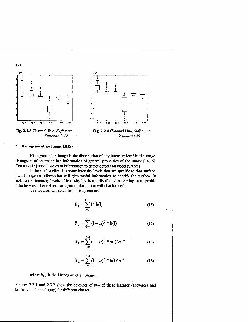
474

RgA RgB Rg C SbA Sb B Sb C

Fig. 2.2.3 Channel Hue, Sufficient Statistics it 19

2.3 Histogram of an Image (HIS)

RgA RgB RgC SbA Sb B Sb C

Fig. 2.2.4 Channel Hue, Sufficient Statistics #23

Histogram of an image is the distribution of any intensity level in the range. Histogram of an image has information of general properties of the image [14,15]. Conners [16] used histogram information to detect defects on wood surfaces.

If the steel surface has some intensity levels that are specific to that surface, then histogram information will give useful information to specify the surface. In addition to intensity levels, if intensity levels are distributed according to a specific ratio between themselves, histogram information will also be useful.

The features extracted from histogram are:

L-l

ft,=£l*h(l) (15) 1=0

L-l

ft2 = Z(1-/")2*h(0 z=o

ft3=Z(l-//)3*h(l)/o- /=o

L-l

ft4=£(l-//)4*h(l)/<x2

(16)

(17)

(18)

where h(l) is the histogram of an image.

Figures 2.3.1 and 2.3.2 show the boxplots of two of these features (skewness and kurtosis in channel gray) for different classes.

475

RgA RgB RgC SbA SbB SbC

iVt ' +

4 ""T"

3.5

3 -r B * 2.5

2

1.5 + + 1—1

0.5 . 1 _|_

0 ■-*- 4- -1-

Fig. 2.3.1. Channel Gray, Skewness

RgA RgB RgC SbA SbB SbC

Fig. 2.3.2. Channel Gray, Kurtosis

3. Implementation and Results

Texture analysis methods considered in previous sections are tested on the image set of steel surfaces in this section. Human expert labeled steel surfaces used in the experiments. The standard used by human expert is ISO 8501-1:1988 international standard on rust grades of steel surfaces and sandblasted forms of them.

To test the effects of color information on classification of steel surfaces, three different color spaces are studied. Firstly YIQ color space is considered and Luminance (called grayscale in this paper) representations of steel surfaces are taken [14]. Secondly RGB space representation of steel surfaces are also taken [14]. Thirdly from HSI color space hue information of steel surfaces are taken. Three texture analysis methods considered in previous sections are applied on these five different representations of steel surface images.

The set of surface images is formed as follows: One image for each type of steel surface is taken. Then the steel surface is rotated by 90° and the image of it is taken again. This way the rotation sensitivity of each texture analysis method is tested, since the reflection of the steel surface is not uniform for all of the directions. The sample size of each surface type is also increased by this operation.

The size of each image captured is 400 pixels by 400 pixels. To increase the sample size for each class, the surface is divided into sub-windows and sliding window approach is applied. Each window has '1/16' of the total surface. The size of each sub-window becomes 100 pixels by 100 pixels. The resolution at this level is sufficient to observe the texture on the steel surface. A total of 1644 sub-windows are obtained for each surface type. Texture analysis methods explained in previous sections are applied on these sub-windows. The number of features formed from each texture analysis method and from each color channel is given in Table 3.1. Total number of samples extracted for each surface type for each feature is given in Table 3.2.

476

Table 3.1. The number of features formed by each method

Red Green Blue Hue Gray Total

GLCM 6 6 6 6 6 30

MRF 25 25 25 25 25 125

HIS 4 4 4 4 4 20

Table 3.2. The Number of samples for each surface type

Surface Type Abbreviation Sample Size Rust Grade A Ra 274 Rust Grade B Rb 274 Rust Grade C Re 274 Sand Blasted, Rust Grade A Sa 274 Sand Blasted, Rust Grade B Sb 274 Sand Blasted, Rust Grade C Sc 274

From Table 3.1 it is clearly seen that, a feature selection algorithm is required to find the most promising feature set for each texture analysis method. For this purpose, different feature selection algorithms are tested on feature sets. Feature selection algorithms applied on steel surface features are given in technical report-2 [6]. Feature selection algorithm used for each texture analysis method is given in the following sections with classification results. For each texture analysis method, selected feature set is fed into the KNN classifier and results are given in table form [17]. Neighborhood for the classifier is taken as three.

In classification part, cross-validation is applied to test performances of feature sets. For this purpose five different data sets are formed such that each training set contains 54 samples and test set contains 220 samples for each steel surface type. Average values of these five different classification tests are given in the following tables as percentages.

3.1 Implementation of Gray Level Co-occurrence Matrices

To obtain rotation invariant features from GLCM, co-occurrence matrix is calculated for four directions as: 0°; 45°; 90°; 135°. The final co-occurrence matrix is formed by the average value of these four matrices. The distance parameter d is taken as one.

Fisher's measure is used for selecting features from GLCM feature set [6]. Following three features are selected by feature selection algorithm:

477

Feature 1: Obtained from color channel red, feature inverse difference moment. Feature 2: Obtained from color channel green, feature inverse difference moment. Feature 3: Obtained from color channel blue, feature inverse difference moment.

Classification results as percentages are given in Table 3.1.1 for feature set formed by Gray Level Co-occurrence Matrices. Test Sample from each class given in column form is classified as six classes in rows.

Table 3.1.1. Classification Results for GLCM

Classified as

Ra Sa Rb Sb Re Sc

en

u a 1 <**

a.

t/3

Ra 87.45 0.00 8.91 0.00 3.64 0.00

Sa 0.09 90,55: 0.00 6.55 0.91 1.91

Rb 7.09 0.00 9136 0.00 1.55 0.00

Sb 0.00 3.27 0.00 79.36 0.00 17.36

Re 1.91 0.00 1.09 0.00 97.00 0.00

Sc 0.00 1.45 0.00 16.64 0.00 8191

From Table 3.1.1 it is seen that six different steel surface types can be discriminated with very high accuracy. The worst case results are obtained in classifying Sand Blasted form of Rust Grade B and Sand Blasted form of Rust Grade C. The lower limit for classification success is %79.36 for Sand Blasted form of Rust Grade B. As seen from the table, classification errors do not generate serious problem, because if a rusty surface is classified wrongly, it will be classified as another rusty surface. The same property holds for sandblasted surfaces also.

3.2 Implementation of Markov Random Fields

For Markov Random Fields, 25 sufficient statistics are calculated which correspond to the 9th order MRF model [12]. The borders of the image are ignored in calculating sufficient statistics to decrease the complexity of the operation.

Fisher's measure with clustering is used for selecting features from MRF feature set [6]. Following three features are selected by feature selection algorithm:

Feature 1: Obtained from color channel hue, feature sufficient statistics 14. Feature 2: Obtained from color channel hue, feature sufficient statistics 19. Feature 3: Obtained from color channel hue, feature sufficient statistics 20.

Classification results as percentages are given in Table 3.2.1 for feature set formed by Markov Random Fields. Test Sample from each class given in column form is classified as six classes in rows.

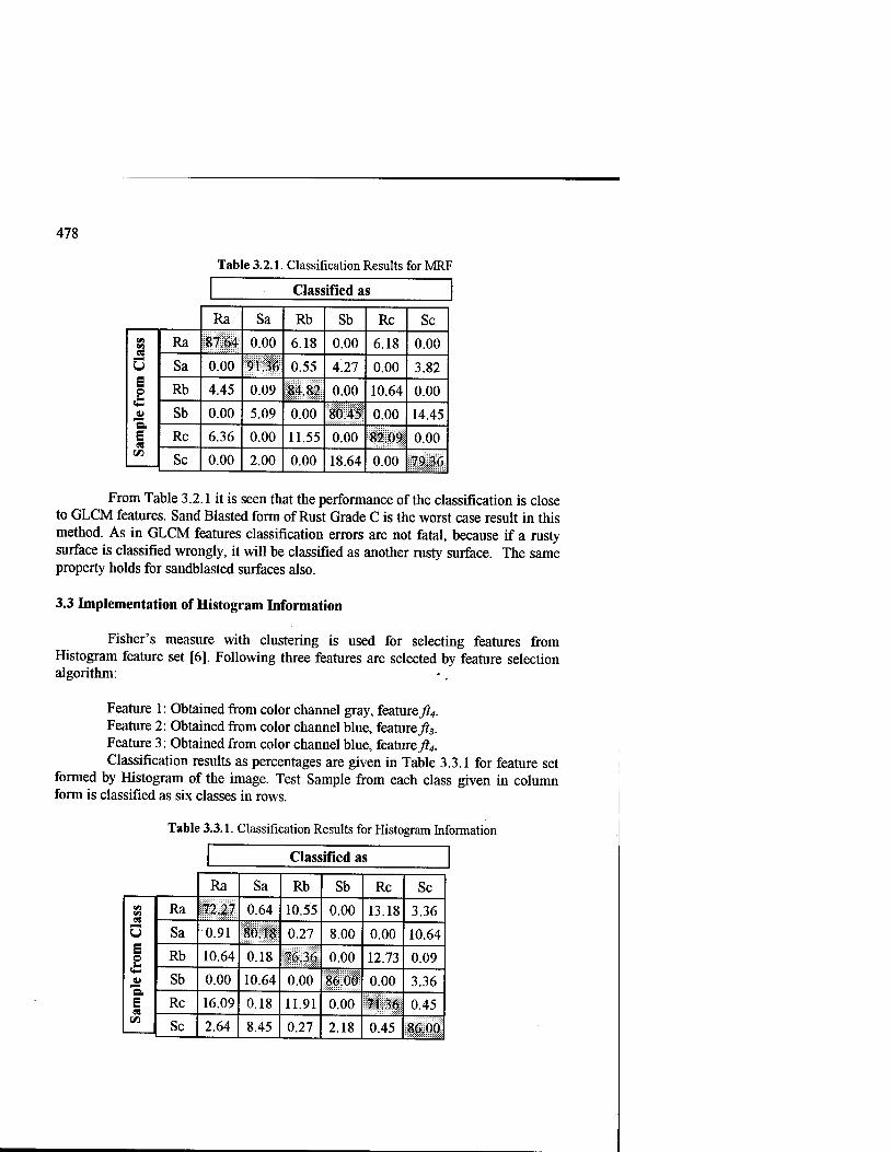
478

Table 3.2.1. Classification Results for MRF

Classified as

Ra Sa Rb Sb Re Sc

en « Ü E 1 ft

C/3

Ra 87.64 0.00 6.18 0.00 6.18 0.00

Sa 0.00 91.36 0.55 4.27 0.00 3.82

Rb 4.45 0.09 84.82 0.00 10.64 0.00

Sb 0.00 5.09 0.00 80 45 0.00 14.45

Re 6.36 0.00 11.55 0.00 82.09 0.00

Sc 0.00 2.00 0.00 18.64 0.00 79.36

From Table 3.2.1 it is seen that the performance of the classification is close to GLCM features. Sand Blasted form of Rust Grade C is the worst case result in this method. As in GLCM features classification errors are not fatal, because if a rusty surface is classified wrongly, it will be classified as another rusty surface. The same property holds for sandblasted surfaces also.

3.3 Implementation of Histogram Information

Fisher's measure with clustering is used for selecting features from Histogram feature set [6]. Following three features are selected by feature selection algorithm:

Feature 1: Obtained from color channel gray, feature ft4. Feature 2: Obtained from color channel blue, feature/^. Feature 3: Obtained from color channel blue, feature^. Classification results as percentages are given in Table 3.3.1 for feature set

formed by Histogram of the image. Test Sample from each class given in column form is classified as six classes in rows.

Table 3.3.1. Classification Results for Histogram Information

Classified as

Ra Sa Rb Sb Re Sc en en « O E 1 ft E

Ra 72:27 0.64 10.55 0.00 13.18 3.36

Sa 0.91 80.18 0.27 8.00 0.00 10.64

Rb 10.64 0.18 76.36 0.00 12.73 0.09

Sb 0.00 10.64 0.00 86 00 0.00 3.36

Re 16.09 0.18 11.91 0.00 7136 0.45

Sc 2.64 8.45 0.27 2.18 0.45 86.00

479

Unlike two feature sets obtained in previous two sections, feature set obtained in this section is not powerful enough to discriminate six types of steel surfaces. The worst case result is in discriminating Rust Grade C.

4. Conclusions

In this paper, texture analysis methods are applied on steel surfaces to form feature set to discriminate steel surface types. Steel surface is considered as having a stochastic texture. Various texture analysis methods are applied on steel surfaces. The aim is to observe the power of these algorithms for forming features to represent different types of steel surfaces.

From the results obtained in section three, it is seen that Gray Level Co- occurrence Matrices and Markov Random Fields can be used as texture analysis methods to form features that could discriminate six types of steel surfaces with very high accuracy using KNN classifier. Both of these texture analysis methods are known for their power of stochastic texture types.

From the results obtained, it is seen that automation of inspection process in discriminating steel surface types is feasible. Future work will be concentrated on implementing the most promising algorithm in a real time system to classify steel surfaces automatically.

References

1 Don, H., Fu, K., Liu, C. R, Lin W " Metal Surface Inspection Using Image Processing Techniques " IEEE Trans. On. SMC, vol. Smc - 14, no 1, pp. 139 - 146, February 1984

2 Jain, A. K.,Farrokhnia, F.,Alman,D. H. "Texture Analysis of Automotive Finishes" Proceedings of Vision 90 Society for Manufacturing Engineers (SME), November 12-15,1990 Detroit

3 Ercil A. Özuyilmaz B. " Automated Visual Inspection of Metallic Surfaces " Proceedings of the Third International Conference on Automation, Robotics and Computer Vision (ICARCV'94), pp. 1950 - 1954 , Singapore, November 1994

4 Van Gool L., Oosterlinck A., "Texture Analysis Anno 1983" Computer Vision Graphics and Image Processing, vol. 29, pp. 336-357, 1985

5 Tuceryan M., Jain A. K., "Texture Analysis" The Handbook of Pattern Recognition and Computer Vision, by C.H. Chen, L.F. Pau, P.S.P. Wang (eds.) World Scientific Publishing Co., 1993

6 Ünsalan C, Ercü A., "Classification of Rust Grades on Steel Surfaces Part 2", Bogazici University Technical Report, FBE-IE-02/98-02; 1998

7 Haralick , R M., Shanmugam , K. "Computer Classification of Reservoir Sandstones" IEEE Trans. On Geo. Elect, vol. GE - 11, pp. 171 -177, October 1973.

8 Haralick,R.M.,Shanmugam K, Dinstein I. "Textural Features for Image Classification" IEEE Trans. On SMC, vol. SMC-3, no 6, pp. 610 - 621, November 1973

480

9 Cross G.R., Jain A. K., "Markov Random Field Texture Models" IEEE Trans. on PAMI, vol. Pami-5, no. 1, pp. 25-39, January 1983

10 Chellapa R.,Chatterjee S., "Classification of Texture Using Gaussian Markov Random Fields" IEEE Trans, on ASSP, vol. Assp-33, no. 4, pp. 959-963 August 1985

11 Atalay, A. "Automated Defect Inspection of Textile Fabrics Using Machine Vision Techniques " M.S. Thesis, Bogazigi University ,1995

12 Cohen F. S., Fan Z., Attali S. "Automated Inspection of Textile Fabrics Using Textural Models" IEEE Trans, on PAMI, vol. Pami-13, no. 8, pp. 803-808, August 1991

13 Krishnamachari S., Chellappa R, "Multiresolution Gauss Markov Random Field Models for Texture Segmentation" IEEE Trans on Image Processing, vol. 6, no. 2, pp. 251-267, February 1997

14 Gonzales,R. C, Woods R.E. Digital Image Processing New York: Addison- Wesley,1992

15 Sonka M., Hlavac V., Boyle R. Image Processing Analysis and Machine Vision Cambridge: Chapman & Hall, 1995

16 Conners, R, Mcmillan, C. W. , Lin, K. , Espinoza R. E. V. " Identifying and Locating Surface Defects in Wood : Part of an Automated Lumber Processing System " IEEE Trans. On PAMI, vol. Pami -5,no. 6, pp. 573 - 583, June 1983

17 Fix E., Hodges J. L., " Discriminatory Analysis: Non Parametric Discrimination: Consistency Properties" project 21-49-004 Report Number 4 USAF School of Aviation Medicine, Randolph Field, pp. 261-279, Texas 1951

481

Fault Detection in Robot Manipulators Using Statistical Tests

Feza Kerestecioglu1 and Bekir Sami Nalbantoglu2

'•'Department of Electrical-Electronics Engineering, Bogazici University Bebek, Istanbul, 80815, Turkey

'Mechatronics Research and Application Center, Bogazici University Bebek, Istanbul, 80815, Turkey

'kerestec@boun.edu.tr

Abstract In this work, application of the Cumulative Sum Test in detecting faults on a two-link robot manipulator is considered. A continuous-time analogue of the CUSUM test, rather than the traditional discrete-time version, is used. The detection is based on the errors of the state estimates produced by Kaiman filters, which use quasi-linear models of the manipulator. This model is obtained by a Taylor series expansion of the nonlinear state equations with respect to the measurement error. Simulations to validate the proposed method for detection of several possible faults such as, sensor bias, actuator torque bias and payload changes are presented.

1 Introduction

Modern industrial processes employ complex automatic systems, which may be subject to unacceptable faults. Small changes or degradations of performance in such plants are of particular interest, since they may be heralds of future catastrophic failures. Even if not, they may go unnoticed for long intervals, which may cause significant economic losses to accumulate. The relevance of the fault detection and isolation problem along with various approaches and applications have been discussed in detail in, e.g., [1],[2],[3] and [4].

Two main parts of a fault detection mechanism are the generation of residuals and decision making. The former aims to generate signals or fault signatures, which carry information on the faults or changes to be detected. An important problem at this stage is that the residuals should emphasize the possible faults and be insensitive to other changes in the system, which are not of concern, such as external disturbances, set point changes, etc.

The decision making, on the other hand, is based in most cases on statistical detection mechanisms, since the data obtained from the system under fault monitoring is usually corrupted in noise or other disturbances that may be modeled in statistical ways. There are two basic criteria to be accounted for by these statistical methods. On the one hand, a relevant change should be detected as quickly as possible after it has

482

occurred. On the other hand, false alarms should be avoided as long as there is no change in the system. These two criteria are typically in conflict which each other; so, most detection methods try to optimize one of them while attaining a reasonable performance with respect to the other. One of the well known likelihood-ratio-based tools in this context is the Cumulative Sum (CUSUM) Test [3], [4]. It is introduced to detect a change in a sequence of random variables from a known statistical hypothesis to another one. In fact, it is also shown that for the cases where the observations are independently distributed, the CUSUM test is achieving the smallest worst average detection time among all test which have mean times between false alarms above a fixed lower limit [5]. It is also possible to extend the CUSUM test to the detection of changes towards unknown or partially-known operating modes [2]. Nevertheless, in this paper, we shall restrict ourselves to the known-hypotheses case.

Our aim is to apply the CUSUM test to detect changes in a robot manipulator. Following this introduction, in the next section, the CUSUM test and its application to linear state-space models will be described. Also, basic criteria of performance for the test will be defined and an analogue of it for continuous-time systems will be introduced. In Section 3, a quasi-linear model, suitable for an application of the CUSUM test, is obtained for a two-link SCARA-type manipulator. This model approximates a standard nonlinear model by including only the first order terms obtained from a series expansion of the dynamic equations with respect to the measurement noise. Various simulations to validate the proposed approach are presented in Section 4. Finally, Section 5 concludes this article.

2 The Cumulative Sum Test

The CUSUM test, which is originally proposed in [6], is an efficient sequential method to detect changes from a known operating mode (or hypothesis, say, H0) to another one (Hi). It is conducted by computing the statistics

S(k) = max[0, S(k -1) + z(k)], (1)

with an initial condition of S(k) = 0 . Here, z(k) is the conditional log-likelihood ratio of the current data, y(k), that is,

=(k)_Pi(y(k)\y(k-i),...,yq)) m

Po(y(k)\y(k-l),...,y(l))' (}

where p, 0 = 0,1) denotes the conditional probability density function of y(k) according to H,. The change decision is given by using the decision rule,

If S(k) > y terminate the test and declare a change

Otherwise carry on with the observations,

with y being is a positive predetermined threshold. In other words, the alarm time is given as

483

n=M{kaS(k)>y}. (4)

Note that an alternative expression for the cumulative sum in (1) is [2] *

S^max Yz(/). (5)

In other words, the test statistics is simply the sum of the increments since the log likelihood ratio between two hypotheses based on all the observations,

K*) = |>(i), (6) /=i

has reached its minimum. We are interested in detecting changes in the dynamics of a linear system described

by a state-space model as

x(*+l) = A,(*)x(*)+B,(*)ii(*)+w,(*)

y(t) = C,(*)x(*)+vj(*) where w, (k) and v, (k) are independent, zero-mean, Gaussian white noise processes with covariance matrices Q,(&) and R,(&), respectively. Note that the subscripts denote the relevant matrices and vectors under either hypothesis. Using the Gaussianity of the w,-(£)and \t(k), and (2), it is possible to show that the increments of the cumulative sum can be obtained by [7]

f \r> tu I u i-J A . (8) m-\ lnKlf )J + eo(*)po'(k\k-\)e0(k)-ej(Är)Pr1 (k\k-l)e,(k)

Fi(k\k-1)\ In (8), e, (k) denote the estimation error in the one-step-ahead prediction of the output vector, namely, y(k | k -1), obtained as

e,(*) = y(*)-y(*|*-l) = y(k)-Ci(k)i(k\k-l)

where x(k | k -1) is the best linear predicted estimate of the state vector, x(&), which can be obtained by a Kaiman filter based on the hypothesis Hi. Further, P, stand for the covariance of the state estimate obtained from the filter corresponding to the relevant hypothesis.

2.1 Performance Criteria

Two important quantities describing the performance of a CUSUM test are the average detection delay (ADD) and the mean time between false alarms (MTBFA). These quantities can be obtained by evaluating the average run length of the test under different hypotheses.

It can be shown that the average increments of the test statistics have opposite signs under either hypothesis; namely positive under Hx and negative under H0 [3], [4], [7]. This means that, as long as there are no deviations from the nominal

484

dynamics, i.e., under H0, the test statistics tends to stick to zero because of the resetting in (1). Therefore, assuming that S(k)» 0 when the change occurs and neglecting the overshoot of S(k) beyond the test threshold at the alarm instant, an approximate expression for the ADD can be given as [3], [4]

E{n\Hx}*7-^e~* (10) E{z(k)\Hx}

On the other hand an approximation for the MTBFA is

E{n\H0},r±t (ID E{z(k)\H0}-

The approximations in (10) and (11) have originally been introduced for the independently distributed data; nevertheless, they are also shown to be valid for detecting changes in the dynamics of linear regression models.

2.2 A Continuous-time Analog of the CUSUM Test

Note that we have assumed up to now that the data from the system under fault monitoring is available in discrete-time and that the dynamics corresponding to different operating modes are specified as discrete-time models. However, in many cases, which also include applications for robot manipulators, the system models can be described as continuous-time models. One alternative for such cases may be to obtain the data in discrete form by sampling the output (or the residuals). Obviously, a discrete-time model corresponding to the sampled output should also be obtained for every operation mode.

Nevertheless, it is also possible to employ a continuous-time version of the CUSUM test to detect changes in the dynamics of continuous-time systems which is given as

i(0 = A,. (0 x(0 + B,. (0 u(0 + G(0 w,- (0 y(t) = Ci(t)x(t) + vi(t)

where w,(0and v,(0 are independent, zero-mean, Gaussian white noise processes with covariance matrices Q, (0 and R, (f), respectively. Also, let us denote the cross-covariance of w,(fc)and v,-(fc) (i = 0,1) as S,-(f) under the ;'-th hypothesis. Mimicking the add-and-reset structure in (1), such a test can simply be obtained by a reset integrator, which is inputted by the continuous-time conditional log-likelihood ratio signal. In fact, in view of the alternative description of the cumulative sum in (5), the test statistics in continuous-time can be written as

S(t) = max \'z(T)dr . (13)

The accumulating signal z{k) in this case will be the continuous-time analog of the increments in (2), namely,

f In /AI -\ (14) m=\ *M+t lntoT7Al + eo W1 «(**(> (0 - e? «Pf' (/Je, (0

485

The estimation errors e0(0 and e,(0 can be obtained from the state estimates generated by two continuous-time Kaiman Filters,

i(0 = A,(0x(0 + B,(f)n(0 + K,(0(y(0-C,(0i(0) » = 0,1 (15)

with the Kaiman gain matrices and the state estimation covariance matrices governed by [8]

K,. (0 = (P, (0C,T (0 + G, (OS, (t))RJl (0, (16)

and

P,(0 = (A.W-G.WS.WRr'COC,,(0)Pi,(0

+p<(o(4i(o-Gi(osi(ORr1(oci(oF-p,(oc?(ORr,(oci(OP*(o (17) +G,. (0 (Q,- (/) - s, (o RJ] (0 s,T (O)G,T (/).

3 Fault Detection in Robot Manipulators

3.1 Robot Dynamics

In this section we shall consider a two-link SCARA-type manipulator. Assuming that the arm is operating in a horizontal plane and omitting the gravitational and frictional forces, the dynamics can be described as

M(q,q)q + C(q,q)q=u (18)

where M and C are 2x2 inertia and Coriolis matrices, respectively and u is the generalized torque vector which consists of the torques applied by the joint actuators [9], [10]. The elements of angular position vector denoted by q = [0, 62 ]T are shown in Fig: 1. The masses of the links, mx and m2 are assumed to be concentrated at the end points. The inertia and Coriolis matrices can be obtained from the geometry displayed in Fig. 1 as

'a + ß + 2/xcos02 /? + //cos02

ß + jucos62 ß M = (19)

and

where ßd] sin02

-ß(2Öx +02)sin6>2

0 (20)

a = (mx+m2)a\, ß = m2a2, n = m2axa2. (21)

486

y V

a. \m2

a. >&. *\l- ■''"'

i

Fig. 1. Two-link robot manipulator

Let us define the state vector for the manipulator dynamics as

x = [xTxjf (22)

with

*i=MF X2=[M2]T. (23)

After straightforward manipulations, it is possible to show that the dynamics in (18) can be represented by a quasi-linear model as [11]

x2(/) = A(x(r))x2(r) + B(x(r))u(0.

In (24), the state and input matrices turn out to be

A = -M'C

D

and

-(ß + ß6xoose2)nsm02 -(20! +ö2)^usin<92

(a0x + ß + 2p6x cos 62 )n sin<92 (ß + ju cos d2 )(20\ + 02 )p sin<92

B = M ' = D

-ß ß + 2jucos02

ß + 2jucos02 a-ß-2jucos02

With D = detM = aß-ju2 cos2 02.

(24)

(25)

(26)

3.2 A Quasi-linear Model

Although (23) is written in a linear state-space model format, its right hand side consists of, in fact, terms that are nonlinear in the state variables. Nevertheless, if x(/) is available, the matrices A and B can be treated as known time-varying quantities. Hence, as far as fault-monitoring purposes are concerned, (24) can be used as a time-varying linear model to check if the system is operating in fault-free condition or not.

487

As a matter of fact, states can be obtained by measurements, which may be subject to noise and random disturbances. Therefore, we consider a measurement equation such as

y(0 = x(0 + e(0, (27)

where the measurement noise, e(0, is assumed to be a Gaussian zero-mean continuous-time white-noise vector. Since only y(0 is available from the system, we need to derive a system equation where A and B matrices are expressed as function of y(0, rather than x(0. In other words, (24) must be written as

i2 (0 = A(y(0) x2 (0 + B(y(0)u(0 + 6(0, (28)

where e(t) is the equation error due to using y(0 in evaluating A and B, instead of x(0. That is,

e(0 = A(x(0)x2(0 + B(x(0)u(0-A(y(/))x2(0-B(y(0)u(0 . (29)

Note that, e(?) would be zero if the actual values of the states were available. So, using (27) in (24), we obtain

i2(0 = A(y(0-e(0)x2(0 + B(y(0-e(0)u(0 . (30)

The elements of A and B depend on x(0 in a nonlinear and quite complicated way as given in (23), (25) and (26). Therefore, it is practically impossible to obtain a complete description of the stochastic process s(0 . Nevertheless, the right hand side of the (30) can be approximated by an expression that depends on e(0 in a linear way. That is,

i2 (0 = A(y(0)x2 (0 + B(y(0)u(0 + G(y(0,u(0)e(0. (31)

In order to obtain such a description one can use a Taylor series expansion of the right hand side of (30) around e(0 = 0 (or y(0 = x(0) and neglect the terms with orders higher than one. After straightforward but tedious derivations [11], the elements of

gn 8n Sn Su #21 #22 #23 SlA _

(32) G

turn out to be as follows:

g„=0 (33)

g12 = — {xßsmy2l + 0.5fj2 sin(2j>21))+ 2$uy22 sin.y21 (34) y

488

_ ju2 sin(2y2l)

Dl

xp.5fj2sm(2y2l)+ß(a + ju)smy2l(2yn +^22) + «, +(ß+fi cos y2l)u2] (35)

-ß-[(aßcosy2X lft + ßcos(2y2X j)yn +ßcosy2X{2yn +y22)y22 + siny2]] +

822 y

_ ßfjy21 smy2X Sl4 - 7j (36)

.v

^21=0 (37)

/ ( 2 \ aßsiny2] ^-yu sin(2y2l) + 2ßfjy22 sin^21

v l J (38)

2 ■

S23 = - M S1"(22>,2l) ([(« - 2ßM)yn + ,0(1 - y22)] sin>>21 - 0.5// sin(2>;21)

D2

-(ß + ß cos y2i)(«i +2ul)-au2)

—i?M2 cos(2>/21 )[(1 + 0.5^22 )^22 +1] + ßft cos j/21 (2^12 + y22 )y22

y

- 3//sin>>2] + (qyn + ß)fjyu cos y2l)

(39)

g24=_i f ..2 ^

^22, (40) /?//sin>>21+^-sin(2.y21) 2 J

where Dy=aß- ju2 cos2 >>21. Note that the elements of G depend not only on the measured state (y) but also on the elements of the input vector u.

Evidently, having the state measurements y(t) at hand, (31) can serve as a quasi- linear model to conduct a CÜSUM test based on Kaiman filtering as described in the previous section.

4 Simulation Examples

In this section, typical results from extensive simulations, which have been done to validate the approach outlined above. The parameters for the manipulator are chosen as given in [12] for the two-link SCARA-type direct drive robot arm manufactured by IMI. For the sake of brevity, we are omitting a list of parameter values. Three types of changes in the changes are considered. These are sensor biases, actuator torque biases and the payload changes. Note that the first two of them can be represented as

489

additive signals at the output and system equations, respectively; whereas the third one in fact causes a change in the dynamics of the arm. The robot arm is assumed to be controlled by a classical PID controller and following a trajectory described by

ft = ft = 0.8sin-f. (41) 1 2 3 This joint angles result in a motion where the end effector of the arm is following a path as shown in Fig. 2, back and forth.

Whenever a fault is simulated it is introduced at / = 2 sec, until when the system is running under the nominal mode. The dynamics for the fault-free and faulty modes of operations can be described as follows: • Normal mode:

x2(0 = A(y(0)x2(0 + B(y(f))u(0 + G(y(/),u(0)e(0

y(0 = x(0 + e(f) Sensor bias:

(43) t2(0 = A(y(f)-ds)x2(0 + B(y(/)-ds)u(0 + G(y(0-ds,u(0)e«

y(0 = x(0 + ds+e(0

• Torque bias: x2(0 = A(y(0)x2(0+B(y(/))(u(0-da) + G(y(0,u(0-da)e(0

y(0 = x(/)+e(0

• Payload change: x2(0 = Af (y(0)x2(0 + Bf (y(/))u(0 + Gf (y(0,u(0)e(0

y(t) = x(t)+ e(0 A sensor bias of 0.2 is assumed to occur in the measurement of the position of the

first joint, i.e., ds = [0.2 0 0 0]. In simulating an actuator fault, on the other hand, a fault on the actuator of the second joint is considered such that the torque delivered to the joint is decreasing by 0.1 Nm, i.e., da = [0 0.1]. Further note that a change in payload corresponds to a change in the mass of the second link, m2. An overload fault is considered where the link mass is increasing 6 kg beyond the nominal value. The matrices Af, Bf and Gf in (45) are to be evaluated under this faulty condition using (25), (26) and (32)-(40).

The values estimated by Monte-Carlo simulations based on 100 runs for different types of faults are presented in Tables 1, 2 and 3. One can immediately note the classical ADD-MTBFA tradeoff comparing the estimates for different thresholds. Namely, increasing the test threshold improves the false alarm performance, nevertheless, also causes extra delay in detection. It is also interesting to observe the monotonicity of the detection delay with respect to the change magnitude, in detecting sensor and actuator biases. Even if the after-change hypotheses are based on the assumption that dü-0.2 and dal =0.1 for the sensor or actuator biases, respectively, larger changes can be detected as well, even faster. This suggests that the detection mechanism can be designed so as to detect the minimum relevant bias.

490

y (m) 0

0.4 0.5 x(m)

Fig. 2. Trajectory of the end effector

0.6

On the other hand, the false alarm times in Tables 1-3 may seem to be low if one considers the potential applicability of the CUSUM test in practice. However, we should note that the thresholds are chosen low in order to make simulation time reasonably small and facilitate a Monte-Carlo analysis. It can be observed from (10) and (11) that the detection delay depends, roughly speaking linearly on y, whereas the MTBFA is increasing exponentially with increasing test threshold. Therefore, practically meaningful false alarm rates can be obtained at the expense of small increases in ADD by choosing larger test thresholds.

Table 1. Estimated ADD and MTBFA in detecting sensor biases

Test threshold r = 2.5 y = 5.0 120.2

7 = 6.0 MTBFA (sec) 50.5 126.7

<*,i=0.1 ADD (sec) dsl = 0.2

rf„ =0.3 *,=0.4

0.556 0.493 0.441 0.403

0.615 0.537 0.497 0.461

0.723 0.566 0.511 0.470

Table 2. Estimated ADD and MTBFA in detecting actuator biases

Test threshold y = 2.5 y = 5.0 176.8

y = 6.0 180.5 MTBFA (sec) 78.9

<*., =o.i rfal=0.2

ADD (sec) rfal = 0.3 rfal=0.4 rf., =0.5

0.512 0.245 0.153 0.116 0.108

0.572 0.291 0.155 0.130 0.113

0.580 0.296 0.156 0.132 0.115

491

Table 3. Estimated ADD and MTBFA in detecting payload changes

Test threshold y = 2.5 y = 5.0 y = 6.0 MTBFA (sec) 19JS 64/7 91.6 ADD (sec) 0511 0591 0.697

5 Conclusions

In this work, we have considered application of statistical tests for detecting faults or dynamical changes in robot manipulators. A continuous-time analog of the well- known CUSUM test has been used to detect biases in the sensors and actuators as well as dynamical changes like payload changes. The detection mechanism uses the estimation errors of Kaiman filters, each of which is based on the before- and after- change operation modes.

Measurements of the joint positions and velocities are assumed to be available. To obtain a quasi-linear description of the plant, which is appropriate for linear filtering, a Taylor series expansion of nonlinear dynamics with respect to the measurement noise is considered. The first order terms obtained from such an expansion are used to approximate the plant. The work in [7] following that of [13] on the metrics of the increments of the CUSUM test suggest that the CUSUM test is robust with respect to modeling errors and, hence the test performance should not be effected seriously by neglecting higher order terms.

Regarding possible further directions of research, continuous-time statistical tests, their properties and performances certainly deserve more investigation, since they may result in detection mechanisms that require simpler hardware in some cases. One interesting point in this context is that the approximations in (10) and (11) are due to the neglecting the overshoot of the test statistics beyond the threshold when an alarm is raised. Their continuous-time analogues will turn out to be exact equalities.

To keep the analysis more clear, we have limited ourselves to the case where the hypotheses before and after the change are known. Although the simulations suggest that in some cases only a minimum level of change which has to be detected needs to be known, the approach outlined above can be extended to statistical tests suitable for detecting changes towards unknown hypotheses [2].

References

1. Pattern, R. J., Frank, P. and Clarke, R: Fault Diagnosis in Dynamic Systems: Theory and Applications. Prentice-Hall, Hemel Hempstead (1989)

2. Basseville, M. and Benveniste, A.: Detection of Abrupt Changes in Dynamical Signals and Systems. Lecture Notes in Control and Information Sciences, Vol. 77. Springer-Verlag, Berlin (1986)

3. Basseville, M. and NiMforov, I. V.: Detection of Abrupt Changes: Theory and Application. Prentice-Hall, Englewood Cliffs (1993)

492

4. Kerestecioglu, F.: Change Detection and Input Design in Dynamical Systems. UMIST Control Systems Centre Series, Vol. 1. Research Studies Press, Somerset (1993)

5. Lorden, G.: Procedures in Reacting to a Change in Distribution. Annals of Mathematical Statistics. 42 (1971) 1897-1908

6. Page, E. S.: Continuous Inspection Schemes. Biometrika. 41 (1953) 100-115 7. Zhang, X. J.: Auxiliary Signal Design in Fault Detection and Diagnosis. Lecture Notes in

Control and Information Sciences, Vol. 134. Springer-Verlag, Berlin (1989) 8. Meditch, J. S.: Stochastic Optimal Linear Estimation and Control. McGraw-Hill New York

(1969) 9. Craig, J. I: Introduction to Robotics: Mechanics and Control. Addison-Wesley New York

(1989) 10. Lewis, F. L., Abdalla, D. M. and Dawson, D. M.: Control of Robot Manipulators.

Macmillan, New York (1993) 11. Nalbantoglu, B. S.: Fault Detection in Robot Manipulators by Using Statistical Tests. M. Sc.

Thesis, Bogazici University (1997) 12. Direct Drive Manipulator R&D Package User Guide. Integrated Motions Incorporated

Berkeley (1992) 13. Baram, Y. and Sandell, N. R.: An Information Theoretic Approach to Dynamical Systems

Modelling and Identification. Proc. IEEE Conference on Decision and Control New Orleans (1977) 1113-1118.

493

Robust Fault-Tolerant Control for Robot Manipulators with Actuator Failures : Fault Detection Strategy and

Fault Recovery Control

Jin-Ho Shin and Ju-Jang Lee

Department of Electrical Engineering Korea Advanced Institute of Science and Technology (KAIST)

373-1, Kusong-dong, Yusong-gu, Taejon, 305-701, KOREA TEL: +82-42-869-5432, FAX: +82-42-869-3410

Email: jhshin@iliad.kaist.ac.kr. iilee@,ee,kaist.ac.kr

Abstract In this paper, a robust fault-tolerant control scheme, including fault detection strategy and fault recovery control, for robot manipulators is proposed to overcome the actuator failures and uncertainties. The joint (or actuator) fault considered in this paper is the free-swinging joint failure that causes the loss of torque on a joint. The presented fault-tolerant control framework includes a normal control with normal (non-failed) operation, a fault detection and a fault recovery control to achieve task completion. After the detection and identification of joint failures, the robot manipulator becomes an underactuated robot system with failed actuators. Then the underactuated manipulator can be controlled by the presented robust controller. To show the feasibility of the proposed fault-tolerant control scheme, simulation results for a three-link planar robot arm with a failed joint are presented.

1 Introduction

The reliability and safety based on fault detection and accommodation (FDA) play a key role in the operation of autonomous and intelligent robotic systems. Fault tolerance has become increasingly important in robotics, especially for those in remote or hazardous environments such as outer space, underwater, nuclear, and medical environments. Robots must have the ability to effectively detect and tolerate internal failures in order to continue to perform their tasks without the need for immediate human intervention [ 1], [2], [3], [4].

An underactuated robot manipulator can be considered as a robot manipulator with failed joints (or actuators). The control of underactuated robot manipulators has been studied since the 1990's [5],[6],[7],[8],[9],[10].

In this paper, a robust fault-tolerant control scheme for robot manipulators is developed. An on-line fault detection method for joint failures in robotic systems is proposed, for cases without and with uncertainties present. A robust fault recovery

494

control scheme that can overcome the uncertainties and actuator failures is presented to achieve task completion. A robot manipulator with failed actuators can be considered as an underactuated robot manipulator with actuators less than the number of total joints. To show the validity of the proposed fault detection and fault recovery control scheme, simulation results for a three-link planar robot arm are presented.

2 Dynamics of Robot Manipulators

The dynamic equation of an n -link rigid robot manipulator is written as follows:

M(q)q + F(q,q)=;u + d(t) (1)

where qeW is the joint coordinates, M(q)e3i'"m is the symmetric positive

definite inertial matrix, F(q,q) = C(q,q)q+G(q), C(q,q)qe9l" represents the

centrifugal and Coriolis torques, G(q) E 5R" is the vector of gravitational torques,

d(t) e 9t" is an external disturbance vector with \\d(t)\\ < dmax where dmm > 0 is

unknown, and u e 9t" is the control torque vector.

Property 1. There exist positive constants mmax, cmax, gmax, fg and fc suchthat

\\M{q)\<mmax, \\C{q,q)\<cmax\q\, \\G(q)\\< gmax, \\F(q,q)\\< fe + fc\\qf [11].

3 Fault-Tolerant Control Framework and Fault Detection Strategy

The term free-swinging failure refers to a hardware or software fault in a robot manipulator that causes the loss of torque (or force) on a joint. Examples include a ruptured seal on a hydraulic actuator, the loss of electric power, and a mechanical failure in a drive system [1]. The joint (or actuator) failure considered in this work is the free-swinging failure rather than the locked-joint failure that has an inability to move. After a free-swinging failure, the failed joint moves freely under the influence of external forces and gravity.

An overall fault-tolerant control framework for joint failures of robot manipulators is shown in Fig. 1.

The procedure used in the presented on-line fault detection for joint failures is as follows:

Stage 1. Detect Fault: Detection of a joint fault. Stage 2. IDFault: Identification of the joint location ofthat fault

495

C"~STAKT>

T Control of the Nonml(Noo-F«ik<l) Robot Bz

^ftaelc Completion CBtroc Cmivageaice'

If »totthMton delected. dap Ottte_FMtt Mage

■JTX

Fault Detection Block

Drtatf Fault: Detection ofa Joint Fault

I ~ i^Afinltii detected? YaVNo^V^

the Detected Faint

k A fiah location faMcatlflod? Y<M<Ko>^-

VES Fault Ibkrant Control:

CafltndofftoUndenctaated Manipulator

Convergence)? ' NO

3s jYES

-KZ END~~5

Fig. 1. A fault-tolerant control framework for joint (actuator) failures.

In this section, an on-line fault detection method for joint failures is presented for cases without and with the presence of uncertainties.

3.1 Case 1: Without Uncertainty

The controller used for the normal operation of a robot manipulator without any parametric uncertainty and disturbances is the Computed Torque Controller (CTC) [11] with a PD feedback control as the following equation,

u = M(q)(qd-Kve-Kpe) + F(q,q) (2)

where qd e5R" is a desired trajectory, e = q-qd eSR" is the joint position error, and Kv and Kp are n x n positive definite constant diagonal gain matrices.

Substituting (2) into (1), with no disturbances (d(t) = 0), the closed-loop stable error dynamics is obtained as

e + Kve + Kpe = 0 (3)

Therefore, the tracking errors e and e are globally exponentially stable. To detect a joint failure, the normal joint position reference signal is needed, which

is compared with the actual joint position signal of the real manipulator. The normal joint position reference signal is obtained numerically by updating the known robot

496

model when the computed torque controller (2) is applied. The actual joint position signals from the real joints are measured by encoders equipped at the joints, when the same computed torque controller is applied.

The criterion for detecting a joint failure is as follows. Let q be the normal joint

position reference vector representing the non-failed or normal state.

\=9-9c0 eSR" (4)

where e^ is the joint position error between the actual joint position and the normal

joint reference position. The first detection stage, that is, DetectFault condition is as follows:

• No fault: continue the control loop if k | = 0

• Occurrence of a fault: go to ID Fault stage if Ik | * 0

The next detection stage, that is, IDFault stage is the stage for identifying the location of the failed joint immediately after a joint fault occurs. In this step, several joint position reference signals are needed to compare them with the actual joint position signals after the fault is detected. The actuator fault dealt with in this work is the free-swinging failure and it is associated with the loss of torque. If an n -joint robot manipulator has p failed joints, the number of reference signals needed in the

tatfn/2) n, IDFault stage is £ :—, where it is assumed that the number of failed joints

P=l p\(n-p)\

p is the highest integer below nil. Thus, 'int(x)' means the highest integer less than or equal to the argument x.

In this stage, the initial values of the reference signals are set as the values of the actual signals at the time of fault occurrence. The reference joint position signals are updated numerically by the known robot dynamics with the failed joint torques. For the i -th joint failure, the i -th joint torque is u, = 0. The remaining normal-joint torques are obtained from the values given by the computed torque controller.

The criterion for identifying the locations of the failed joints is as follows. Without loss of generality, let's consider a 3-joint planar robot manipulator to simplify the problem. For this 3-joint manipulator, the number of reference signals is 3!/(l!x2!) = 3. Let qCi be the reference joint position vector representing the

occurrence of the i -th joint failure. ec,=q-qCl for i = l,2,3 (5)

where ec is the reference joint position error. For this 3-joint manipulator, the

conditions used in the second detection stage (ID_Fault stage) are as follows:

Condition 1: Failure at Joint 1 if Ik 1 = 0.

Condition 2 : Failure at Joint 2 if Ik 1 = 0.

Condition 3 : Failure at Joint 3 if Ik 1 = 0.

497

3.2 Case 2 : With Uncertainty

The computed torque controller (2) with a PD feedback control cannot be used in the presence of uncertainty. Therefore, we use a robust adaptive control scheme for the successful tracking control when the uncertainty is present.

A robust control law that can overcome the uncertainty is as follows:

u = -M(-qd+Ae) + F + ur e9t", (6)

H'=-Zs^HT7' *>0' (7)

,=«>, w4 Iff k-l IHI ll*llf' (8)

A

e=T ^P off] e<Rs, <j>0, (9) M + s

\"

where s=e+Ae is the augmented error and A = Ar >0, K = KT >0 and

r = rr>o. The associated stability and convergence properties are shown by the following

Lyapunov function approach. Let us consider a Lyapunov function as follows,

V = {sTM(q)s + 0TrlO}12 where 6 = 6-6e 91s. Consequently, the derivative of the above Lyapunov function can be obtained as

follows, V^-zTQz/2 + w(p,\\^ where z = (sT 0TJ, ß = block_diag(2Ä\o-),

and w(p,|s||) = 0r0#/2 + p|s|W(|s| + £). Therefore, the errors e and e are

globally uniformly ultimately bounded. In the presence of uncertainty, it is very difficult to detect a joint failure because it

is hard to obtain the accurate reference normal signal. Therefore, in the first stage (DetectFault stage), the tracking position error e and velocity error e are used instead of the reference joint position error e^ .

The actual joint position signals from the real manipulator's joints are measured by the encoders equipped at the joints when using the above robust controller (6) ~ (9).

The criterion for detecting a joint failure is as follows. At the first detection stage (Detect_Fault stage), the condition used is as follows:

• No fault: continue the control loop if |e| +|<j|| ^Be.

• Occurrence of a fault: go to ID Fault stage if ||e|| + ||e| > Be.

Here, the error bound Be can be set as follows. O Regulation Problem:

Be =|g/|+(NI + c*> -||«r||)exp(-A0f +|M+(NK-» -\\efl)txp(-ß2t)] ■

498

O Tracking Problem:

— When ||e,|| * 0, then Be = \\e,\\ + (|e,.|| + ei0 - |e/|)eXp(-yS1of +

(k/||+(|K-|+^-|^|)exP(-AoF. — When 1^1 = 0, then Be = lk| + Ik | .

where et is the initial value of the position error e, et is a user-defined initial offset value of the position error e, ei0 is a user-defined initial offset value of the velocity

error e, ef is a user-defined final value of the position error e, /?, > 0, and ßt > 0.

In this stage, the initial values of the reference signals are set as the values of the actual signals at the time of fault occurrence. For the i -th joint failure, the i -th joint torque is «,. = 0. The remaining normal joint torques without any fault are obtained from the values given by the presented robust adaptive controller. The reference joint position signals cannot be accurately updated numerically by the robot dynamics with the failed joint torques because the accurate robot parameters are not known. Therefore, the strategy for identifying the location of the failed joints under the uncertainty can be shown as follows.

Without loss of generality, we consider the same 3-joint robot manipulator. When the reference joint position error eC( is denoted as (5), at the second detection stage

(ID_Fault stage), the conditions checked for this 3-joint manipulator are as follows:

«•I 2 j| || 2 II II2 || M 2

e.\\ + e, <,BC and \\er\\ + <?, >Br and 1 II II * II II 2 || || ^ || C

kf+kf>ß.

Condition 2 : Failure at Joint 2 if ||ej| +|kj >BC and Ik II +|k| ^Bc and

lkl°4..r>*- Condition 3 : Failure at Joint 3 if \\eA + kJ >Br and Ik II +lk.| >Br. and

II ^11 II * II II 2 II II ^11

kf+lklf SB

■ Else : Calculation of e^ =min(|ej,|kj,|e<|1|) and emIn = min(|eei|,|ec2|,|cC3|)

D Sub-condition 1: Failure at Joint 1 if e^ = Ik | and emla = Ik I.

D Sub-condition 2 : Failure at Joint 2 if emln = Ik | and emla = Ik

D Sub-condition 3 : Failure at Joint 3 if em,„ = \e, and em,„ = k • HIHI II tj M min || Cj ||

D Else : No decision for identifying a fault location : continue the control loop.

Here, Bc is a user-defined small positive constant selected appropriately and ' min( x, y, z)' represents the minimum value of three arguments.

499

4 Robust Fault Recovery Control : Robust Control of Underactuated Manipulators

The failed joints in a robot manipulator are called as the passive joints. Then the remaining normally operating joints are called as the active joints. This work considers that the passive joints have brakes instead of failed actuators. It is assumed that these brakes equipped at passive joints operate normally.

After the failed joints have been detected, the robot manipulator system behaves as an underactuated manipulator with actuators less than the number of total joints. Therefore, the control of the underactuated manipulator with the failed actuators is presented as follows to achieve task completion even when some joints fail.

The control objective considered here is a regulation problem, where all joints have to converge to their desired set-positions. The control procedure of an underactuated manipulator in joint space is as follows.

1. Mode 1 : Control of all passive joints; Control all passive joints using the dynamic coupling between the active joints and the passive ones.

2. Mode 2 : Braking of all passive joints; Brake each passive joint as soon as they reach their set-positions with zero velocity. Practically, the desired small position and velocity error bounds of the passive joints are a priori defined. Wait until all passive joints are locked.

3. Mode 3 : Control of all active joints; Control all active joints by a new control law.

The design procedure of a robot controller for an underactuated manipulator in the absence of uncertainty is here omitted due to the simple derivation. In the presence of parametric uncertainty and external disturbances, a robust adaptive control scheme for underactuated manipulators is proposed based on the Lyapunov direct method with the norm-bounded property of uncertainty.

4.1 Control of Passive Joints

The dynamic equation (1) can be partitioned as M„ MmVq,

KMpa MmJ

fv\

v*,J = U + d(t) : (10)

where qa e SRr is the position vector of active joints, qp e W is the position vector

of passive(failed) joints, u = (rj 0TpJ, ra e W is the actual control torque input

vector applied to the active joints, Op e SRP is the zero vector at the passive joints,

d(t) = (dTa d

TpJ , and the boundedness of d(t) is \\da\\ < d^, \dp\ <dpm, dam>0

anddpm>0.

500

The dynamic equation for the passive joints using the partitioned dynamics (10) is obtained as

'4P=MprTa+Hp e9t> (11)

where MpTa = -M^M^M^ , Mpp = Mpp - MpaM^Mv, and Hp = -MptFa -

M^F +M d +M~ld pp p "*pit**a ' "^pp^p-

The position error and the augmented error of the passive joints are denoted by ep=qp- qPt and sp = ep + Apep where qPa is a desired position vector of the

passive joints and Ap = ATp > 0.

The proposed robust passive joint controller has a structure given by:

va = M*pTa(VPr-Hp) ett% (12)

VPr=Vp+AVp e<R', (13)

VP=9p,-(KP+ApK + KPAPeP e5RP' (14)

(15)

(16)

(17)

where M*^ e W*p is a pseudoinverse matrix of M with the guessed nominal

dynamic parameters MpTa(= -M^M^M'^), and #, = -MprFa - MplFp. MpZa A

and Hp are the nominal models of Mpa and Hp with the guessed values for the

dynamic parameters of the underactuated manipulator, respectively. Kp, Rp and Tp

are positive definite constant diagonal matrices, and yJlaJ) is a chattering

alleviation function such as yp \\ap J= a J + ep with sp > 0 .

Assumption 1. It is assumed that the number of active joints (r) is greater than or equal to the number of passive (failed) joints (p) in the design of the controller, that

is, r^p. Then it is selected that M*Ta = Mpia(M ptaMT

pT )_1 by the property of a

pseudoinverse matrix.

Assumption 2. It is assumed that there is enough dynamic coupling between the passive joints and the active ones in an underactuated manipulator [6]. In other words, it is assumed that a coupling matrix Mpa e SR'"0' is a full-rank matrix with rank = min(p,r) = p.

AKp=-/ . "' . ,- OOP ap=Rpsp 6«',

V,WT"' P,=P,W,.WA tf IM W \h\l

K=rP f II 1

A- IT fl eSR5, crp>0, , w 1) ''

501

Remark 1. Most of articulated planar robot manipulators with all revolute joints

satisfy the full rankness of Mpa. If Mpa is of full rank then MpaM*pa = Jp for the

known dynamic parameters case (Mpa=Mpa). Then finally MpaM*pa=Ip.

Therefore, it is guaranteed that the controller (12) is available.

The closed-loop error dynamics for the augmented error sp becomes

sp = -Kpsp+AVp + j}p (18)

where the lumped uncertainty is ijp =\MpraM*pTa -1 pyPr + \Hp -MpzM*pxHp)

and Ip is a p x p identity matrix.

The norm-bound of lumped uncertainty tjp can be derived as

W * ^.rßL-lJt^^-M^MlH, (19)

Assumption 3. By Property 1, it is assumed that there exist an unknown positive constant c„ such that

MpuK.-h < c0 < 1 (20)

Property 2. By Property 1 and the norm-bounded property of disturbances da and

dp, there exist unknown positive constants cl and c2 such that . ||2

\Hp-MprM*P*ßp\ * «1+C2W (21)

Property 3. By the definition of the control input VPr, it is assumed that there exist

unknown positive constants c3 and c4 such that

rA=Y^^^fA+rvÄ^¥^+e^prc*¥Ä+P' (22> The initial estimate vector 0p(O) is set as a vector of which all elements have

nonnegative values.

Hence, the upper bound of IMI can be described as follows by Assumption 3,

Property 2 and 3.

h\\^ -•Älklf+**<IU+p,)+**M+**H (23)

where 0Pi = c,, 0ft = c2, 6~Pi = c0, 6~Pi = c0c3 and dPi = cac4. From Assumption 3,

it is assumed that 0 ^ 6pj = c0 < 1.

Remark 2. In the above control law (14) and (16), to perform the regulation of each passive joint, their desired acceleration values are set as qPd = 0.

502

Theorem 1. Under Assumptions 1 ~ 3, if we apply the control law (12) ~ (17) to the underactuated robot manipulator system (10), then the errors of passive joints e

and ep are globally uniformly ultimately bounded.

Proof. Let us consider a Lyapunov function candidate, v=\ fa,', +(1-^)ö;r;1öJ=i<PÄ (24)

where 0p=ep-6p, 6Pt = 0Pi /(l - 6Pi) and zp = (^ GTp ).

By some effective manipulations, V <-zTpQpzp l2+wp[pp,pp,lap\\) where

Qp =block_diag(2/?i,^,(l-öP3)£rJ and Wp(pprPp,\a^={^^-eTpc7pep +

J^k(Kl)-klk^+/'/i-^)]- Since both sp and 9p are GUUB as IsJ^fzK/A^Ä^f^and

|£j < [2K/((1 -öP3)^ln(r;1))]"2, the errors ep and ep are also GUUB. See [9] for

the details. <

Therefore, the proposed control law (12) ~ (17) with sufficiently small constants sp and ap takes the passive joint positions to the very close neighborhoods of their desired values and the passive joint velocities to the very close neighborhoods of zero. The brakes at the passive joints will then be engaged and the system will behave as a completely actuated system. Hence, we will now propose a new control law for the remaining active joints.

4.2 Control of Active Joints

Since all passive joints are locked by their brakes, qp = qp = 0. Thus the dynamic equation for the active joints of the robot with the locked passive joints is

k\=M2ra + Ha e3T (25)

where Ha = -M^(Fa-da), M^M^-M^M^M^, Fa = Fa -M^M^F,,

and d =d -M M~ld ""** **a a ap pp p'

The position error and the augmented error of the active joints are denoted by ea~1a~ 1ad

e ^ and sa = ea + Attea where q„d is a desired position vector of the

active joints and Aa = A^ > 0. The proposed robust active joint controller has a structure given by:

Ta^-Maai-q^+AteJ + ^+T, e9T, (26)

503

Tr=-Kasa + AVa e9T, (27)

AK=~ß-jJt3 e*% (28)

Ä ='■>.. r.4 Itf |iU Kll |*.|)\ (29)

0„=r, a * a ^«1 71 < Kl)

<7„0, eft5, o-fl>0, (30)

where JTa and Ta are positive definite constant diagonal matrices, and

MklHM + e. withfa>0. The closed-loop error dynamics for sa becomes

MJa = -{Ka + ^MJsa + AKa •+ ;;„ (31)

A ~ A ~ 1 ~ where ?7a =(Jlf„-JlfB)(-^ + Aaea)-(Fa -Fa) + rfa +-Maasfl is called lumped

It

uncertainty. The final norm-bound of lumped uncertainty is

IM * *,+*„ 1*11 +^|^| + ^|^| + ^H*.| = Ö>. (32)

Theorem 2. //"we ap/?/y the proposed control law (26) ~ (30) to the underactuated manipulator with the locked passive joints, then the errors of the active joints are globally uniformly ultimately bounded (GUUB).

Proof. Consider a Lyapunov function candidate,

V = \ fc#-A + 0aX% }=\zTaPaza (33)

where 6a=6a- 0a is the estimation error and za = \s* 0j) .

By some effective manipulations, we get V<-zTaQazal2 + wa[pa,\s]^ where

Qa =b.ock_diag(2iTfl,,a) and WJ<pA4 = 0^AI2 + ^MzVÄ r.W4

Since both sa. and 6a are GUUB as ^J^pF/A^M^)]1'*and

|öa| < ^/^(r;1)]"2, the errors ea and ea are also GUUB. <

Remark 3. If (sp = Q,<jp=Q) and (sa = 0, aa = 0) in the proposed passive and

active joint controllers, then wp\pp,pp, \ap )=0 and wa(pa»|sa||) = 0, and hence it

is guaranteed that the errors (ep,ep,ea,ea) of the closed-loop control system is globally asymptotically stable. Here, we can find the trade-off between the magnitude of tracking error and the chattering of control input.

504

5 Simulation Study

The robot manipulator simulated is a three-link planar robot arm (M = 3). The simulated three-link planar robot manipulator is shown in Fig. 2.

Kg. 2. A three-link planar robot manipulator.

The simulation is performed for two cases: Case 1 : Without Uncertainty; Case 2 : With Uncertainty.

In order to achieve the normal operation of robot control, the computed torque control (2) with PD feedback and the presented robust control (6) ~ (9) are used for Case 1 and Case 2, respectively.

The numerical real and nominal parameters of the simulated manipulator are given in Table 1. The nominal dynamic parameters used in the robust controller are set to 70% of the real dynamic parameters.

Table 1. Numerical parameter values of the simulated three-link manipulator:

l(L1,m1,I1,Lcl) = (L2,mI,I1,Lc2) = (Li,m3,I3,Lc3)].

Parameters Values Linkl Link 2 Link 3 Length [Lt(m)] Real Values 0.5 0.5 0.5

Mass Real Values 1 1 1 Nominal Values 0.7 0.7 0.7

Moment of inertia Uiikgm1)]

Real Values 0.1 0.1 0.1 Nominal Values 0.07 0.07 0.07

Center of mass position

IM»)] Real Values 0.25 0.25 0.25

Nominal Values 0.175 0.175 0.175

The disturbance inserted at each joint is a random noise whose magnitude is bounded within 0.5, that is, \dt(i)\ < 0.5, for i = 1,2,3.

The initial positions of each joint are ft(O) = -nll{rad), ?2(0) = q3(0) = 0(rad). The initial velocities of each joint are zeros. The final desired set-positions of each joint are qu=nl 2{rad), qld = -n 12{rad) ,wAq3t=nl 2(rad).

505

In this simulation, it is assumed that a joint (actuator) fault at the third joint (^3) occurs at 0.7 (sec). Thus, the torque applied at the third joint is zero after the occurrence of a joint fault. The robot manipulator after an actuator failure at the third joint becomes an underactuated manipulator with a passive third joint. It is assumed that the failed joint has a normal brake. It is assumed that there are no frictions and no joint limits at the manipulator's joints.

The fault-tolerant control results for Case 1 and Case 2 are shown in Fig. 3 and Fig. 4, respectively.

Phsael [FsultOocummoe]:l)~2) Phasen [P.a!ive<F«ilcd) Joint Control]: 2) ~ 3) PhueLl [Aotreefltamil) Joint Control]: 3) ~ 4)

(a) Snapshot of robot motion

— Joint 1 - - Joint 2 Joint 3 (failed)

i- /

OJ <Uf. 0.7

0.71

-y i i / 1/ '1.88 (bmldog time)

"O 0.5 1 1.6 2 2.6 3 3.5 4 4.6 6 time (sec)

0.7 (sec): real fiuilt occurrence time 0.7 (see) : DetectJfrmlt ■ JWrrtnn1 fiuilt ocenrreoce time 0.71 (see) : TDJPmAi: identified finds-position lime

(b) Position errors (e)

/ /

f

A i -" i

- Joint 1 -Joint2

-Joint 3 (failed)

—" T:i

i s-

1/ \

V

10.7 0^0.71

~ i 1.88 (brsloug time)

■

D 0.S 1 1.5 2 2.5 3 3.5 4 4.5 5 time (sec)

0.7 (sec): reel fiuilt occurrence time 0.7 (sec): DetectJfrndt: irtrrttri fault occprfence time 0.71 (sec): IDJfauU: identified fiuflt-nocitioo time

25 20

15

10

5 •

I -5

-10

-16

-20

-26,

o^-|>~-- ̂

- — ufl) u(2) u(3)

[llC»-0«nerkftss]

I

jO.7 0?j>71

0.5 1 1.5

t / 1/

1.88 (bislriog time) 3.5 4 4.5 5 2 2.5 3

time (sec)

0.7 (sec) : reel fault occurrence time 0.7 (sec) : Deted_FauÜ: delBctofl fiuilt occurrence time 0.71 (sec) : IDJbtdt: identified ftult-nosition time

(c) Joint angles (q) (d) Control torque input (rfl)

Fig. 3. Control results for Case 1 (without uncertainty).

For Case 1, the detected fault occurrence time by DetectFault stage is 0.7 (sec), that is, it is equal to the real fault occurrence time. The identified joint location of the fault by ID_Fault stage is the third joint and the time to find out the fault location is

506

0.71 (sec). After 0.71 (sec), the manipulator is controlled by the presented control method for the underactuated manipulator. The braking time of the failed joint is 1.88 (sec). After 1.88 (sec), the failed (third) joint is locked and the remaining normal active joints are controlled to the desired set-points. The angle of the passive joint is transformed into the same angle having a value between -n(rad) and nirad) after it has been locked by its brake.

2

1.6

1

0,5

£ 0 -0.5

-1

-1.5

-2 -2 -1.6 -1 -0.5 0 0.5 1 1.5 2

m Tbucl [Fmh Occurrence] :1)~ 2) Hasen |Pasiwr<Failed)Jbrrrta>urrol]:2)~3) HUH m [Ar*r»r<Narn«u) Joint Crafiojl: 3) - 4)

(a) Snapshot of robot motion

: 1

- \ r;0>

BdikfoSuia Cj$5 ; 3)|1|

Ai4)rmalSute

^ ' 1)

time (sec) 0.7 (sec) : real fault occurrence time 0.82 (sec) : DetectJfault: detected fault occurrence time 0.83 (sec) : TDJimlt: identified fault-position Arne

1

\ \

( / / 7

0.7

i ^ Joint 1 • / j Joint 2 i / Joint 3 (failed) ; / ■

f \ // >0.82 ■/ ^5-U , [2.06 (braUw time)

0 0.5 1 1.6 2 2.5 3 3.5 4 4.5 5

(b) Position errors (e)

— Joint 1 - - Joint 2 Joint 3 (ruled)

/:

0.82 0.83 l&

I / j/

-f-r

2iM5 (braldog dme)

1.6 2 2.6 3 3.6 4 4.6 time (sec)

0.7 (see) : real fault occurrence time 0.82 (sec) : DetectJfauU: delected fault occurrence üme 0.83 (sec) : TDJTaidt: identified fault-position time

(c) Joint angles {q)

BO

60

40

20

I ° -20

-40

-60

^

0.7

HO) uf2) uC3)

W») -0 after knot]

I v> ..

0.82 /u,83

1\ •/

I I |l H 2.06 (braltfcg tin«)

0 0.S 1 1.5 2 2.5 3 &5 4 4.5 5 time (sec)

0.7 (sec) : real fault occurrence time 0.82 (sec) : Detectjfaill: detected fault occurrence time 0.83 (see) : TDJfault: identified fault-position time

(d) Control torque input (ra)

Fig. 4. Control results for Case 2 (with uncertainty).

For Case 2, the detected fault occurrence time is 0.82 (sec) and the time to find out the fault location is 0.83 (sec). The braking time of the failed joint is 2.06 (sec).

From the simulation results, a joint failure at a robot's joint has been successfully detected and recovered, and the original control objective has been achieved. It has been shown that the proposed robust fault-tolerant control scheme is feasible.

507

6 Conclusions

In this paper, a study on the robust fault-tolerant control of robot manipulators that can overcome actuator failures has been performed. A fault detection scheme has been proposed for situations without and with uncertainties. The proposed fault detection scheme uses only encoders and tachometers to measure the position error and velocity error and does not require any other special hardware for detecting a joint failure. A robust adaptive control scheme for underactuated manipulators with failed actuators has been proposed using the brakes equipped at passive joints. The proposed control scheme does not need a priori knowledge of the accurate dynamic parameters and the exact uncertainty bounds. It has been observed that the proposed fault-tolerant control scheme is feasible and robust through simulation results.

The robust fault-tolerant control for robotic systems is more useful in remote or hazardous areas such as outer space, underwater, nuclear power plants, etc., where the repair or replacement of failed actuators is very difficult.

References

I.English, J. D., Maciejewski, A. A.: Fault Tolerance for Kinematically Redundant Manipulators Anticipating Free-Swinging Joint Failures. Proc. IEEE Int. Conf. Robot. Automat. (1996)460-467

2. Visinsky, M. L., Cavallaro, J. R., Walker, I. D.: A Dynamic Fault Tolerance Framework for Remote Robots. IEEE Trans. Robot. Automat. 11(4), (1995) 477-490

3. Ting, Y., Tosunoglu, S., Fernandez, B.: Control Algorithms for Fault-Tolerant Robots. Proc. IEEE Int. Conf. Robot. Automat. (1994) 910-915

4. Papadopoulos, E., Dubowsky, S.: Failure Recovery Control of Space Robotic Systems. Proc. American Control Conf. 2 (1991) 1485-1490

5. Arai, H., Tachi, S.: Position Control of a Manipulator with Passive Joints Using Dynamic Coupling. IEEE Trans. Robot. Automat. 7(4) (1991) 528-534

6. Bergerman, M., Lee, C, Xu, Y.: A Dynamic Coupling Index for Underactuated Manipulators. J. of Robot. Syst. 12(10) (1995) 693-707

7. Bergerman, M., Xu, Y.: Robust Joint and Cartesian Control of Underactuated Manipulators. ASME J. Dyn. Syst., Measure. Contr. 118(3) (1996) 557-565

8. Oriolo, G., Nakamura, Y.: Control of Mechanical Systems with Second-Order Nonholonomic Constraints: Underactuated Manipulators. Proc. IEEE 30th Conf. Decision Contr. (1991)2398-2403

9. Shin, J. H., Lee, J. J.: Dynamics and Robust Control of Underactuated Manipulators. Proc. the 37th SICE Annual Conf. (SICE'98) (1998) 847-852

10. Mukherjee, R, Chen, D: Control of Free-Flying Underactuated Space Manipulators to Equilibrium Manifolds. IEEE Trans, on Robot. Automat. 9(5) (1993) 561-570

11. Lewis, F. L., Abdallah, C. T., Dawson, D. M.: Control of Robot Manipulators. Macmillan Publishing Company (1993)

508

Information Loss in Analog to Digital Conversion Revisited

Craig C. Smith1, David W. Robinson2, David S. Hansen1, and Bryan F. Bihlmaier1

'Department of Mechanical Engineering Brigham Young University

Provo,UT USA smith@byu.edu

department of Mechanical Engineering Massachusetts Institute of Technology

Cambridge, MA USA

Abstract. When an analog signal is digitized, there is potential loss of information, even when the sample rate satisfies the Nyquist sampling criterion. This information loss can be characterized as uncertainty arising because the signal is not known before or after sampling begins, and appears as uncertainty regarding the value of the analog signal between sample points. This uncertainty is greatest near the endppints of the sampled interval or window, and depends upon the autocorrelation or bandwidth of the signal. This error has been characterized mathematically, and guidelines have been given for reproducing analog signals from digital data to any given level of accuracy. This theory, coupled with the theory provided by Shannon and Nyquist in their well-known sampling theorem, provides a complete characterization of the information loss in sampling. Assessment of the need for simultaneous sample and hold for multiple channels in data acquisition provides a significant practical application of the theory.

1 Introduction

Analog to digital conversion has become an integral part of many systems and devices in the last couple of decades due to the development of new and effective digital technologies. Physical processes which are inherently analog are now measured, recorded, and controlled by digital processors which provide robust recordings, intelligent controllers, and great flexibility of analysis. Information processing is much more likely to be done digitally, whereas the processes and systems which the information is to characterize are often inherently analog.

The analog to digital conversion process has been characterized previously, and much is well defined. Amplitude quantization errors are well understood, and sample rate

509

selection to avoid frequency aliasing was long ago defined by Shannon and Nyquist. What has not been defined previously is the information loss caused by truncation of the signal or frequency leakage. Although the phenomena of frequency leakage has been well understood in the context of spectrum analysis, the loss of information in terms of inability to reproduce the original analog signal within the interval over which data is sampled is the focus of the present work.

1.1 Practical Issues

In many situations, variables that are to be measured or controlled, are calculated from signals from multiple sensors. For example, temperature gradients or heat flux are found by differencing temperature sensor outputs, and system identification develops system models by relating measured inputs and outputs. The mathematical models used in these calculations usually assume that the signals used in the calculations are sampled simultaneously. Hardware for simultaneous sample and hold of multiple channels is complex and costly relative to multiplexed multiple signal samplers. But multiplexed samplers results in an offset in sample times between channels. If negligible information is lost in the process of sampling, so that the sampled, digital signal has the same information as the original analog signal, then sufficient information is present so that the original analog signal can be reproduced at any time, and the offset signals contain adequate information to characterize any desired function of the multiple signals. Thus hardware for simultaneous sample and hold is not required if care is taken to reduce all errors to a negligible level.

1.2 Categorization of Errors In Analog to Digital Conversion

Error or information loss during analog to digital conversion can be categorized into three categories: amplitude quantization error, error associated with sample rate, and error associated with signal truncation.

Amplitude Quantization Error. The conversion of the analog amplitude to a discrete amplitude is known as quantization error, and is minimized by correct matching of the corresponding ranges of the analog and digital representations, and choice of the digital word size. This error is not related to the simultaneous sample and hold question, but is here mentioned for completeness.

Errors Related to Sample Rate. The conversion from a continuous time signal to a discrete time signal (sampling) creates error known as frequency aliasing. If significant frequency components are present in the signal above one-half the sampling frequency, these components are indistinguishable from components below one-half the sampling frequency and are said to be aliased to the lower frequency. If the frequency components above one-half the folding frequency are negligible, then the information loss during sampling is negligible. This phenomenon was characterized by Shannon [1] and Nyquist

510

[2], and is referred to as the Shannon sampling theorem. If significant frequency components above one-half the sampling frequency exist in the analog signal, then it is impossible to reproduce the analog signal between samples from its sampled values, even if the signal were sampled for all time.

Errors Related to Signal Truncation. Practical digital signals used for analysis or data storage must begin and end, and so some information may be lost by truncating the signal in time. If frequency domain representations of the signal are used, some assumption must always be made about the nature of the signal before data collection began and after it ended. The two most common assumptions made are (1) that the signal is periodic, and hence the data collected represents one period of a periodic function, or (2) that the signal is zero (or constant) for all time before and after data collection began.

The first of these assumptions is appropriately used for random signals that have no beginning or end, and hence cannot be assumed to be zero outside the "window" of time which is recorded. Therefore the most reasonable assumption is that the signal before and after simply repeats, but when the beginning and end of the signal are compared, it is clear that this assumption of periodicity can't be exactly correct. The error associated with this assumption of periodicity is known as frequency leakage. Since frequency components in the original signal which are not periodic in the window cannot be represented under this assumption, these components will contribute varying portions of their-components to frequencies that are periodic in the window, and are said to be leaked to these other frequencies.

In transient signals for which the second assumption is valid, the signal is known for all time (it is zero everywhere outside of where it is recorded), and no loss of information occurs during truncation, as long as the truncation is done without artificially introducing high frequencies (above one-half the sampling frequency) during truncation. If a transient signal is truncated before it ends, so that it is not effectively zero outside the interval over which it is recorded, then frequency leakage represents the loss of information associated with this truncation.

Clearly frequency leakage will always occur whenever we don't know what a signal is before and after (outside of the window) we recorded it. The only way to recover this information loss is to find out what we didn't record. The most effective way to minimize this loss of information is to record the signal for a longer period of time. Since it is not practical to record any signal forever, and computer memory, data storage, and analysis requirements grow as data array sizes grow, any data collection system must be designed to minimize loss of information by truncation or frequency leakage by trading off the length of time data will be recorded with other issues and constraints.

Summary of A/D Conversion Error. A data collection and analysis system is designed so that loss of information during analog to digital conversion is negligible by

511

1) matching the level of the analog signal and converter range, and choosing the digital word size so amplitude quantization errors are negligible,

2) sampling at a frequency of at least twice the highest non-negligible frequency component in the signal so that frequency aliasing is negligible, and

3) collecting data for a long enough time so that frequency leakage errors are negligible.

If these requirements are met, then sufficient information exists in the sampled (digital) signal to reconstruct the information content of the original analog signal. Hence, information is present to determine the value of the original signal at any point in time required, and the time of sampling is irrelevant to the information content. Therefore, the only justification for simultaneous sample and hold hardware is to simplify or speed the processing in such cases as this is necessary. Otherwise, sampling offset between two signals can always be compensated by processing with negligible loss of information, making simultaneous sample and hold or synchronized separate A/D converters less cost effective than multiplexing systems.

2 Quantitative Description of Information Loss in Signal Truncation

Given a digital sequence, xk, sampled without frequency aliasing at sample interval, T, the signal can be reproduced between samples by filtering with an "ideal" filter that cuts off exactly at the folding frequency, ff = ^ . This is accomplished mathematically by

convolution with the inverse transform of the frequency response function, which is the sine function [3]:.

sin AT ,,. sine m = (1)

where non-dimensional time, x = t/T, has been used for convenience. The resulting continuous signal, y(t) can thus be represented from the digital signal, xk, by the relation

y(r) = YJ xksinc[tf(z--k)] k"° (2) N-l -1 »

= ^ xk sine [O(T -k)] + ^ xk sine [JI(J -k)] + ^ x,. sine [O(T -k)] k-0 k=-» k=N

Since xk is only known over the interval 0 < k < N-l, only the first summation can be evaluated directly. If xk is periodic, the above convolution is easily accomplished in the frequency domain, since a Discrete Fourier Transform (DFT) can be found using the Fast Fourier Transform algorithm, and the convolution process becomes multiplication in the frequency domain. If xk is only known for the interval k = 0 through N-l, error results in either neglecting the terms for which xk is unknown (effectively assuming xk = 0 outside this range), or in assuming the periodic form pk, where pk is the discrete signal that is identical to xk over the interval k=0 through N-l, and then repeats at intervals of

512

N data points. Letting J(x) be the result of doing the convolution with the sequence pk, the difference

N4 N-l

\y(T) - y(r) ] = Y xk sinc[^(T-k)] -£ Pk sinc|>(r-k)] k-0 k=0

+ Z xksinc [*■(*■- k>] - Z Pksinc [x(*- k>] k=-« k=»

00 CO

+ Z xk sinc D^7" k)l "Z Pk sinc [^(r"k)] (3) k=N k=N

NJ -1 = Z (*k -Pk)sinc[^(r-k)]+ £ (Xk -pk)sinc[^(T-k)]

k=0 k=-« 00

+ Z (xk -Pk)sinc[^(r-k)] k=N

But since pk = xk f°r k=0 through N-l, the first summation vanishes and -i »

ty(*0 - y(r)] = Y (xk - pk)sinc[^(T-k)] + Y (xk " pk)sinc[^(T-k)] (4) k=.» k-N

If T « N, the terms in the second summation and terms for k < -N in the first summation are negligible, and

-l

[y(r) - y(r)] = Y (xk - Pk)sinc[^(T-k)] (5) k=-N

Squaring both sides of the equation above, we can write

513

ty(r)-y(r) ]2« £ (xk -Pk>sinc KT -k)l Z (xr " Pr)sinc [*(*- r>]

_ k »N J Lr=-N -1 -1

= Z Z (xk-fc)(xr-pr)smc[;r(*--k)]sinc[?z-(r-r)] k~N l=N

= L L (xkxr-pkxr-xkpr+pkpr)sinc[^(T-k)]sinc[^(r-r)] k -N r=N

-1 -1

= ^] ^ xkxr sinc[^(T - k)] sinc \n (r - r)] k -N r=-N

-2_ zl pkxrsinc[^(r-k)]sinc[^(r-r)] k=-N r~N

-1 -1

-Z Z xkprsinc[^(T-k)]sinc[^(r-r)] k=N r=-N

-1 -1 + Z Z PkPrsinc[^(r-k)]sinc[^(r-r)]

(6)

Since pk is periodic, and is equal to xfc for 0 < k < N-l, over the interval -N < k < -1, Pk = xk+N, thus:

[y(r)-y(T)f «Z Z xkxr sinc[^(r-k)]sinc[^(r-r)] k=-N r=-N

"Z Z xk4Nxrsinc[^(r-k)]sinc[Ä-(r-r)] k=-N l=^N

-1 -1

"Z Z xkx„Nsinc[;r(r-k)] sinc [>r(r-r)] k=-N I=;N

-1 -1 + Z Z PkPrsinc[^(T-k)]sinc[^(r-r)]

(7)

Averaging both sides of the equation, we substitute the autocorrelation functions, and for convenience, we convert the summation range to positive integers by changing signs on the subscripts k and r:

514

Ep[[y(r) -y(r)]2]* £ IX(r -k) sinc[;r(r+k)] sincfar + r)]

N N

■SIRx(r-k + N) sinc[^(r + k)] sinc|>(r+r)]

N N

"Z lX(r"k _N) sinc[^(T + k)] sinc[^(r+r)]

N N

+ £ZRpC-k) sinc[<r + k)] sinc[^(r+ r)]

(8)

where Rx (k) and Rp(k) are the autocorrelation functions of xk and pk respectively, and the operator Ep[ ] denotes the expected value using the periodic function pk to estimate xk outside the interval over which the signal is recorded.

Without loss of generality, we now assume that the signal, X(T), has zero mean, so that the autocorrelation function Rx(x) represents the variance, and Rx(x) —> 0 as x —> w.

N N Further, we will assume that the discrete form, Rx(q) = 0 for q < - y and for q > y .

Using this assumption, and also noting that Rp(q± pN) = Rx(q) for all integers, p (i.e. Rp(q) is periodic), some algebraic manipulation results in the following :

£ ü+k 2 2

Ep [[y(r) - y(r)]2 ]« 2 £ £ R^r -k) sine [*(T + k)] sine [n(r + r)] k=! r=l

N N +2 Z X Rx(r-k) sine [Ä-(t-+k)] sine [^r(T+r)]

k—+1 r=k+I— 2 2

Equation (9) represents the mean-squared error in reproducing the analog signal from the digital signal under the assumption that the signal is periodic (the collected data is one period of a periodic function). Although this assumption is known to be incorrect, the economy of using the Fast Fourier Transform (FFT) to reproduce the signal at desired points in time makes this assumption desirable. If the above process is repeated with the assumption that the signal is zero1 outside the interval over which the data is collected, the mean squared error is reduced to exactly one-half the value under the periodic assumption:

E0[[y(r)-y(z-)]2]*i Ep[[y(r)-y(T)]2] (10)

Although this method reduces the mean squared error by a factor of two, it requires zero padding when using the FFT to determine signal values between samples, effectively

JIf the signal has non-zero mean, this assumption is equivalent to assuming that the signal is equal to the mean value of the signal in the interval over which it is collected.

515

increasing the FFT array size by a factor of two for a given data set. It also requires exact knowledge of the mean of the signal.

3. Experimental Verification

To verify the analytical description above, pseudo analog signals, sampled at various times were created. From signals sampled at one time, signals sampled at other times were recreated. The average errors in recreating these signals at alternate sample times were compared with the analytical error predictions above.

3.1 Pseudo Analog Signal

A series of normally distributed random numbers was generated, representing a pseudo analog signal. This "analog" signal included enough numbers to ensure no transients were introduced from the digital filter, as well as to account for values of the signal at intermediate "time" steps. For example, suppose a block of data with eight data points was desired, with a desired known value of the signal one-half time step forward of each point. A random number sequence, X, is created using the random number generator,

X={c„ X2,^3,....,^i4, ^15,*l } where x;, xj, ..., represent the analog signal at each time step, and X2, X4, the value of the analog signal at intervals half-way between the time steps.

represent

Next, the signal was digitally filtered using an 8th-order butterworth filter with a cut-off frequency of one-half the folding frequency (one-fourth the sampling frequency) - well inside the Nyquist criterion. The characteristics of the butterworth filter can be observed in the unshifted signal's autospectrum, Figure 1.

■3

- 0.8 -I »4 a B 0.4 H

0.0 - fc

Figure 1. Autospectrum of Unshifted Pseudo Analog Signal

"I 1 1 1 1 I 3 0.0 0.2 0.4 0.6 0.8 1.0

t/T Figure 2. Autocorrelation of Unshifted

Pseudo Analog Signal

The filtering at one-half the folding frequency was to ensure no aliasing and to define the signal's autocorrelation function, Figure 2. Scaling of the filtered signal ensured a statistical mean of zero and mean square of one. These filtered random data now represented a pseudo analog signal, with known bandwidth and frequency content.

516

The filtered signal was then stored in two vectors. The first vector represented a sampled signal which we desire to shift in time. The second vector represented the exact value expected of the first signal following the time shift. Following the above example,

^1 = Y:'ux3>x5>—- >x'i5j and %i = \x'2,x'4,x'6,....,x'16f where the prime (') denotes filtered data. These two new sequences were thus two versions of the same band-limited signal sampled at offset time sequences.

The first signal was then shifted forward in time, using the process described below. Finally, the mean square error between the shifted (first) signal and the exact (second) signal was calculated. This entire process was accomplished for 19 intermediate times between whole time steps.

This process was repeated and the results were averaged to account for the faults in the random number generation. It will be noted that even with 500,000 averages, the assumed white noise of the unshifted signal is not completely "flat" in the lower frequency range, although this is not noticeable because of the scale in Figure 1 plotted at small size to save space. This higher frequency content can be observed as well in the non zero values in the midrange of the autocorrelation of the unshifted signal, again not noticeable at the scale of Figure 2.

3.2 Time Shift of a Digital Signal

The Fourier transform is used to map continuous signals from the time domain to the frequency domain. Defining h(t) and H(f) as a Fourier transform pair:

AM o H(f)

An original time signal shifted in time by an offset z transforms as a frequency signal multiplied by a phase shift.

Similar to the continuous domain above, a block of discrete time data is transformed to the frequency domain using the discrete Fourier transform. Additionally, if the block

size of the data is of the power 2 , where n is an integer, the fast Fourier transform (FFT) can be used.

A(4) » H(n)

To shift in time, a phase shift is again applied in the frequency domain. Notice the modification of the phase shift for use with discrete data, but also its similarity in form to that of the continuous transform above.

2m?r

A(*-r)o/J(n> " where k = time sample number, n = frequency sample number, N = total number of data points in the data block, and r = the offset between data points (-1 < r < 1) representing the fraction of the sample interval for the shift between data sequences. The inverse FFT of the phase-shifted data results in the time-shifted discrete time signal.

517

3.3 Comparison to Analytical Expression

The values of the mean square error calculated from the above process were compared to the mean square error calculated from the analytical expression. To calculate a mean square error from the analytical expression, it was necessary to determine the characteristics of the digital butterworth filter. As broad band random noise passes through a butterworth filter, it essentially takes on the characteristic shape of the filter, scaled by the magnitude of the noise. Given the characteristic of the filter, the autocorrelation of a broad band random signal can be determined analytically.

The numerator and denominator of the characteristic polynomial (z transform) for the eighth-order butterworth filter were supplied as input to the "freqz" command in Matlab, giving the complex frequency response function of the butterworth filter. This frequency response function was then multiplied by its complex conjugate to form the autospectrum of the periodic filtered signal, since the input to the filter was white noise. The inverse Fourier transform of the autospectrum, the autocorrelation, was then scaled such that the mean square of the autocorrelation was equal to one. This autocorrelation was then used in the analytical expression for Rx, which goes to zero at the data midpoint and remains at zero.

Comparisons of the mean squared error from the digital experiment to the analytical expression (Equation 9) over the interval from -1 < t < 3 (beginning one time step before data is collected) are shown below in Figure 3. The solid line represents the analytical expression, while the asterisks represent the experimental data. As can be seen, agreement is excellent.

" 40x10 ■' -

20-

0-L

0.0 0.0 1.0 2.0 t/T

Figure 3a Comparison of analytical expression to experimental results

1.0 2.0 t/T

Figure 3b. Comparison of analytical expression to experimental results

Although the analytical expression was developed for low values of time (near zero), by symmetry the error expression should be valid if time is interpreted as measured from either the beginning (forward) or the end (backward) of a dataset. This was also confirmed by comparison with the experimental data described above, and yielded results similar to those shown in Figure 3.

518

4 Effect of Bandwidth on Root Mean-Squared Error

Since the mean squared error in reproducing a signal between sample points is a function of the autocorrelation function, which relates directly to the bandwidth of the signal, it is instructive to examine the sensitivity of this error to the bandwidth of the signal. Although practical signals rarely (if ever) have flat spectra over some band of frequencies with no frequency content outside that band, such spectra represent a limiting case in that they represent signals which are correlated over somewhat longer intervals of time than other signals of the same essential bandwidth but with smoother drop in spectra with frequency, thus we will use these "ideal bandpass" signals to compare the effects of bandwidth. The autocorrelation for such a signal of bandwidth fj, = bff, where ff is the folding frequency (one-half the sampling frequency) can be written as

Rb(k) = sinc (bflk) = sin (bflk)

(bide)2 (11)

The case where b = 1 represents the maximum bandwidth possible for a digital signal, and is therefore a limiting case (maximum error possible). For this case, Ri(k) = 1 for k=0 and Ri(k) = 0 for k#0, and Equation (9) reduces to

E,[[y(r)-y(r)]2] = 2 £ sine2 [a(r+ n)] (12)

and the root mean squared error is found by taking the square root. Using various values of bandwidth fraction, b, the root mean squared error for various bandwidths are shown in Figure 4. It is noted that as the bandwidth fraction, b, gets smaller, the error fairly quickly approaches the limiting case where b = 0. For this limiting case, Ro(k) = 1 for all k (perfect correlation of the signal with itself for all times). tt

■S

M

a pi

A 0.4 -

0.3 - / 1 .", — b=0.0 -- b=0.4 — b=0.8 — b=1.0

•S 0.4

1 0.3 0.2 -

0.1 -

0.0 - fW IM H Sao

b=0.0 , \ - - b=0.4

ft '• "- b=0.8

V '■■■■•-., b=1.0

1

Figure 4. Root mean squared error for various signal bandwidth

i 1 1——1™—r 0 10 20 30 40

Number of Data Points from End of Block Figure 5. The maximum rms error in reproducing an analog signal within a given number of points from the end.

The maximum error in reproducing the signal at any time within a given number of data points from the end is shown in Figure 5. This illustrates even more graphically how quickly the error bounds approach the limit as b approaches 0. Practically, real signals will not have bandwidths near the folding frequency to avoid aliasing. Anti-aliasing filters used in data acquisition will typically cutoff at b ~ 0.5 to 0.8. Since typical real

519

signals will be band limited before filtering, it would be expected that b = 0.4 would be representative of many practical signals.

5 Practical Reconstruction of Analog Signals at Alternate Sample

Times

Analog signals can thus be reconstructed between samples, with error depending upon the time from the end of the collected samples and the position between samples of the time to reconstruct. To perform the reconstruction requires some assumption about the nature of the signal outside the window of time for which it is collected. When two signals are recorded via a multiplexer, the samples for one are offset from the samples of the other by some fraction of the sample interval, depending upon how many signals are multiplexed and the configuration of the multiplexer. The most efficient way computationally to reconstruct one signal at sample times simultaneous with the other is to use the FFT algorithm to transform one time series to the frequency domain. Each frequency term is then shifted by the phase corresponding to the multiplexer offset (phase shift is proportional to frequency). The resulting signal at the offset sample times is then found by using the inverse FFT. Since the FFT implicitly assumes the signal to be periodic (this is required because the frequency spectrum is discrete), the natural assumption is to assume that the signal is periodic in the window. The assumption that the signal is constant outside the window can also be implemented computationally using the FFT by padding the time series with the mean value of the signal, doubling the size of the array to be transformed making at least half of the terms in the array equal to the signal mean. This doubling of the array size reduces the mean squared error to one-half that of the error resulting without padding, where the assumption is that the signal is periodic in the window. Since the error decreases with the time from the end of the array, to reduce the error to the desired level, additional data points should be collected beyond the region for which the data samples will need to be accurately shifted, and then data at the ends of the interval can be discarded. It is expected that for many cases, the number of additional data points that would have to be discarded under the periodic assumption (vs. the constant value assumption) would be less than the number of data points required to perform the padding. Therefore, the periodic assumption is the most practical, even though it increases the mean squared error by a factor of 2 (and rms error by a factor of \ß as compared to the constant value assumption.

Table 1 Number of Data Points at Each End of a Time Series With Error Above the Specified Level After a Time Shift

fb = ff RMS Error Ceiling:

Forward-shift Time-fraction 5% 2.5% 1% 0.5% 0.1%

0.1 7 26 178 599 •

0.2 23 106 551 1580 *

0.3 48 194 916 3665 *

0.4 65 260 1167 4669 *

520

1 0.5 71 284 | 1256 | 5024 * 1

fb = 0.8ff RMS Error Ceiling: Forward-shift Time-fraction 5% 2.5% 1% 0.5% 0.1%

0.1 2 4 10 21 100 0.2 4 8 19 40 177 0.3 5 11 26 54 232 0.4 6 12 32 63 266 0.5 6 13 34 66 277

fb = 0.4ff RMS Error Ceiling: Forward-shift Time-fraction 5% 2.5% 1% 0.5% 0.1%

0.1 1 3 7 17 77 0.2 3 5 14 28 153 0.3 4 8 20 39 218 0.4 4 9 23 46 261 0.5 4 9 24 49 276

4 = 0 (limiting case) RMS Error Ceiling: Forward-shift Time-fraction 5% 2.5% 1% 0.5% 0.1%

0.1 1 2 7 14 65 0.2 2 5 12 26 116 0.3 3 7 17 35 152 0.4 4 8 19 41 174 0.5 4 8 20 43 181

* Number of data points required is outside useful range of data collection.

To aid in determining the number of data points that would need to be dropped from each end of the time series to obtain a given level of error after a time shift, Table 1 has been developed. If data is to be reproduced at times other than the original sample times, one first determines the desired accuracy for which the data must be reproduced. Then for the desired offset between the time at reconstruction and the original sample times, and for the given bandwidth of the signal, the number of data points that will have error beyond the desired level is determined. A data block is selected such that the total number of data points includes the desired extra data points at each end of the data to be retained after reconstruction. Overlapping blocks can thus be used to reproduce accurately a long time series at alternate sample times.

6 Conclusions

When an analog signal is digitized, there is potential loss of information, even when the sample rate satisfies the Nyquist sampling criterion. This information loss can be characterized as uncertainty arising because the signal is not known before or after

521

sampling begins, and appears as uncertainty regarding the value of the analog signal between sample points. An analytical expression has been developed to describe this uncertainty as a function of time after sampling of the data begins or (by symmetry) as a function of time before sampling of the data ends. The analytical expression has been verified by numerical simulation. This uncertainty is greatest near the endpoints of the sampled interval or window, and depends upon the autocorrelation or bandwidth of the signal. Guidelines have been given for reproducing analog signals from digital data to any given level of accuracy. This theory, coupled with the theory provided by Shannon and Nyquist in their well-known sampling theorem, provides a complete characterization of the information loss in sampling analog data. Assessment of the need for simultaneous sample and hold for multiple channels in data acquisition provides a significant practical application of the theory.

References

[1] Shannon, C.E., "Communication in the Presence of Noise," Proceedings of the IRE, pp. 10-21, January, 1949

[2] Nyquist, H., "Certain Factors Affecting Telegraph Speed," Bell Systems Technical Journal, Vol 3, p. 324, April, 1924

[3] Proakis, J.G., and Manolakis, D.G., Digital Signal Processing Principles, Algorithms, and Applications, Second Edition, Macmillan Publishing Co., 1992

522

Design and Modelling of a Two-Degree-of-Freedom Spherical Actuator with Unlimited Angular Range

B. Dehez, V. Froidmont, D. Grenier, B. Raucent

Centre for Research in Mechatronics (CEREM), Universite catholique de Louvain

Bätiment Stevin, Place du Levant, 2 B-1348 Louvain-la-Neuve, Belgium

Abstract. The paper deals with the design and the modelling of a two-degree-of freedom (DOF) spherical actuator. As the target applications require unlimited angular range, the principle chosen for the electromechanical conversion is that of an induction motor. An analytical modelling has been performed considering both the case of a homogeneous rotor (constructed from one only material) and of a bi-material rotor (where the steel inner rotor is overlaid with copper alloy). This model allowed us to study the influence of the various geometrical and electromagnetic parameters on the torque that the motor is able to produce. It is shown that a bi-material rotor produces a better performance. A first prototype has been designed and built. It shows a good agreement between the experimental results and those predicted by the analytical model.

1 Introduction

Appearing as far back as the beginning of the industrial applications of electricity, electromechanical converters have rapidly evolved toward a limited number of machine types which:

- are well adapted to the conversion of electrical energy into mechanical energy (or reciprocally), at constant steady state power and with a high efficiency;

- consumes or provides electrical energy under the form of continuous voltages and currents (DC machines) or of multiphase sinusoidal alternative voltages and currents (AC machines) in such a way that the electrical energy produced by one machine working as generator could be directly useable by a machine of the same kind working as a motor.

In this context the effort of the electrical engineer was limited to the optimization of the conversion of electrical energy to mechanical energy, the latter being quasi- exclusively provided under the form of single DOF motion, more often a rotary motion or more rarely a translational motion (case of linear motors). The adaptation of this type of mechanical energy to the needs of the system to be actuated was then the sometimes difficult task of the mechanical engineers. This was particularly the case for applications requiring complex motions with multiple DOF, for example the actuation of a robot wrist [1], the omnidirectional motion of a mobile robot [2],[3], the orientation of a camera [4] or a telescope. In all these cases, many single DOF motors are generally used and complex mechanisms such as parallel transmissions [1] or universal wheels (wheels equipped with rollers) [2],[3],[4] are used. Such a wheel has unlimited angular range but is

523

sensitive to vibrations arising from the successive shocks occurring each time the contact point passes from one roller to another.

Up till now, the design of an electromechanical system was based on the electrical source (e.g. DC or AC). This leads to a limited choice of motors (only single DOF DC or AC motors). The motion provided by the motor has to be adapted to the customer's needs. The electronics "revolution" (in the field of microelectronics and power electronics) as well as advances in automation and computer science allows new solutions. Indeed:

- power electronics is now able to transform electrical energy under practically any form;

- complex control algorithms can now be used thanks to the increase in real-time computation capabilities;

* computer-aided design (CAD) can be used to optimize product design and functionality.

Today, it is therefore possible to design electromechanical systems taking directly into account the customer wishes. In other words, it is now possible to design a motor that will fit the functional requirement and then to build the electrical supply needed by the motor.

This paper deals with the design of a multiple DOF actuator with at least one being motorized. Such an actuator can drive a sphere around one of its axes while keeping the other DOF free. Fig. 1 presents the principle of the new actuator. The spherical rotor A of the motor is guided by spherical bearings B and actuated by inductors C. The rotor drives the sphere D by friction. This new actuator with unlimited angular range can be used for instance in a mobile robot. In this case the sphere D is one wheel of the robot. Such a wheel can be called "electrical universal" wheel and take

Fig. 1. Principle of the two DOF actuator with unlimited angular range.

524

the place of a classical "mechanical universal" wheel. As a consequence, an omnimobile platform can be designed by combining three or more such electrical universal wheels. Electromechanical conversion can use the principle of the permanent-magnet or switched-reluctance motors [5], [6]. However, the need for an unlimited angular range involves revolution symmetry conditions on the rotor that make these solutions difficult to implement. As a consequence, we decided to use the induction principle. Fig. 2 shows the actuator structure: two pairs of inductors (AA' and BB'), supplied with three-phase currents, can induce currents on surface of the sphere, which generate a rotational motion around the two axes aa' and bb' respectively. Bearing elements are located on the free surfaces of the rotor.

V

Fig. 2. Structure of the spherical actuator with two motorized DOF.

The rotor, can be build either - from a material having good conductivity but low magnetic permeability (copper,

for example), or with high permeability and average conductivity (steel, for example); we speak of homogeneous rotor.

- or even a combination of these two kinds of materials (a steel sphere overlaid with copper alloy, for example); we speak of a bi-material rotor.

The paper is organized as follow. The second section summarizes the different assumptions made for the electromagnetic model. The analysis of the models for the homogenous and the bi-material rotor is given in sections three and four respectively. Finally, the electromagnetic simulation results are compared to experimental measurements in the fifth section.

2 Electromagnetic Assumptions

The aim of the electromagnetic model is to obtain the relationships between the actuator torque and the different parameters, electrical (supply currents and frequency, rotor conductivity,...), geometrical (rotor diameter, inductor size,...),

525

mechanical (rotor rotation speed,...). It is based on Maxwell's equations, which can be solved analytically for such a complex structure under the following assumptions.

2.1 First Assumption

All electromagnetic coupling effects between inductors are assumed to be negligible. In other words, the electromagnetic field distribution around each inductor can be studied independently.

2.2 Second Assumption

The currents in the inductor can be approximated by a surface current js, flowing at the interface between the stator and the airgap. Using angular coordinates a (in the rotational direction), the current density is given by:

h=j,*Aat-pa)My CD where js is the current amplitude, co the supply frequency, p the equivalent number of pole pairs if the stator were spread over the entire rotor circumference. The amplitude of the equivalent surface currents is evaluated by considering only the first harmonic of the spatial distribution:

J.-&0- (2) 71

where N.I is maximal amplitude of the ampere-turns flowing in each slot of the inductors. Under this assumption, the potential vector A (defined by B = V x A , where B is the magnetic induction) is, for any point of the system, a solution of the diffusion equation:

I2 A dA _ (j. a dt

-vxVxA (3)

where u is the magnetic permeability, a the electrical conductivity and v the displacement speed of the material. It can be noted that the expression of the surface current does not appear in the diffusion equation. It appears only in the boundary conditions on the magnetic field H. The boundary condition between two materials (/*) and (/+/), having different electromagnetic characteristics, are indeed given by:

[ü-(B(0-B(/+7))=0

where n is an unitary vector, normal to the interface between the two material.

526

2.3 Third Assumption

Since the electromagnetic phenomena are concentrated in the airgap and on the rotor surface, the spherical geometry can be approximated by a plane. For the rotor layer, the equivalent displacement speed can be then set to a constant value:

v=Qreax (5)

where re is the external radius of the rotor and Q the rotor rotation speed.

2.4 Fourth Assumption

The boundary effects are negligible. For the study of the magnetic field, the inductor size can then be considered as infinite and the 3D problem can hence be reduced to a 2D problem. On the other hand, for the torque computation, the torque per unit surface should be multiplied by the actual size of the inductors.

These first four assumptions allow to reduce the initial 3D-problem to the study of the equivalent 2D-strucrure shown in Fig. 3.

Layer 4: stator

Layer 3 : airgap

Layer 2 : extern rotor layer

Layer 1: inner rotor layer

Fig. 3. Equivalent structure for the computation of the electromagnetic field in the actuator

2.5 Fifth Assumption

The stator material has infinite permeability. The corresponding limit condition can be expressed as follows:

forz>e, H=Ö

On the other hand, at the centre of the rotor:

for z < -re, H has a finite value

(6)

(7)

527

2.6 Sixth Assumption

Only the steady state is considered and all the materials are assumed to be linear. From this assumption and from the previous ones, one can deduce that the potential vector can be written in the following form:

A =A(z)exp\j(at-p/re x)]a. (8)

3 Homogeneous rotor model

The electromagnetic characteristics of the layers of an actuator with an homogeneous rotor are given in Table 1.

Table 1. Electromagnetic characteristic of the layers of an actuator with an homogeneous rotor

Layer 1 and

Layer 2 (rotor)

H(;)=^(2)>Ho

Layer 3 (airgap) H(3) = V-0

Layer 4 (stator)

*{4)>0 U(,)2°o

Resolution of the diffusion equation (3) by taking into account the boundary conditions (4) and the limit conditions (6) and (7), gives the expression of the vector

potential A for any point of the structure, from which the value of the magnetic

induction B can be deduced by B = V x A . The magnetic field H can then be computed using the constitutive relationship B = pH.

Finally the torque dl per unit surface dS can be evaluated by using the Maxwell tensor. It depends only on the magnetic field in the airgap. Straightforward calculations give:

dT = re/JoHx{3)Hzi3)dS (9)

where Hx(3\ and Hy<3\ are the components of the magnetic field along axes X and Y

respectively. The total torque is then given by:

^l\K\cosh (ae)+a\i0 \ih\J\K\ cos§.swh(ae)+a l^)™*1 (ae)J (10)

\i0 J\K\ cosh(ae)+a \ih) sinh(cej

with a= p/ , K=Ja +7^(2) CT(2) (a~P ^) > and 9= &g(K / 2).

From this equation, it can be deduced that the torque is directly proportional to: - the surface of the inductors S, - the number of pole pairs/?,

528

- the square of the number of ampere-turns N.I. Moreover, the torque expression does not depend on the supply-current frequency nor on the rotation speed but only on the rotor-current frequency: cor =a-p Q.

The influence of the other parameters is not so obvious insofar as their relationship with the torque expression is not linear but can be explained by means of the analogy with the classical induction motor (with one DOF).

3.1 Influence of the magnetic permeability

It can be seen from Fig. 4 that, for given rotor radius (rc = 55mm), inductor surface (5 = 56.5x30 mm2), number of pole pairs (p = 6), current amplitude (NI = 360 A.t), rotor conductivity (close to the steel conductivity, i.e. 66000 Sm/m2) and airgap width (e = lmm), the maximal torque (Tm) increases rapidly with the relative permeability of the rotor (jt(]j/fi0) but then reaches a maximal value (about 0.3 Nm). This phenomenon can be explained as follow:

- in the first part of the curve, the rapid torque increase is due to the decrease of the rotor reluctance.

- the rotor reluctance becomes negligible compared to the airgap reluctance. This means that it then no longer has any influence on the total circuit reluctance and hence the Tm no longer increases. The increase of the rotor frequency value for which the torque is maximal (O*„) is, on the other hand, a consequence of the skin effect that increases the equivalent rotor resistance. This equivalent resistance Rr can indeed be written under the following form:

Rr=- tf-V^ö^w^ HD b.8 W

(11)

where a is the length of the equivalent rotor circuit, b its width and S its depth (equal to the skin depth). As in the case of a classical induction motor, an increase of the rotor resistance has no consequence on Tm but leads to an increase in co,.m with a correlative reduction of the electromechanical conversion efficiency.

[Nm] [103 rad/s]

[uency for the maximal torque (au)

300

250

200

150

100

50

0 40 80 120 160 200

Relative magnetic permeability

Fig. 4. Influence of the rotor magnetic permeability on the torque

529

3.2 Influence of the electrical conductivity

For a given rotor magnetic permeability (ji(1) = 2000./x0) - all the other parameters being constant -, Fig. 5 shows that Tm does not vary with the electrical conductivity (cT(ij). According to (11), a higher value of the conductivity leads to a decrease of the equivalent rotor resistance and therefore to an increase in the efficiency of the motor through a reduction of co,m.

[103 rad/s]

Maximal torque (Tm)

Rotor frequency for the maximal torque (a>m)

200

150

0 2 4 6 8 10 12 14

Electrical conductivity [106 Sm/m2]

Fig. 5. Influence of the rotor electrical conductivity on the torque

From this result and from the previous one relative to the influence of the magnetic permeability, we can conclude that a single layer rotor made of a material having very good conductivity but low permeability (a copper alloy, for example) would be able to produce a lower torque than one made of a material having low conductivity but high permeability (steel, for example). But, on the other hand, the rotor made of copper would have a better efficiency than a steel rotor since (%■„ is lower in that case (see Fig. 6).

Torque [Nm] 0.3

0.25

0.2

0.15

0.1

0.05 Tm

Torque [Nm 0.3

0.25

0.2

0.15

0.1

0.05

(Om

12 3 4 5 6

Rotor frequency [103 rad/s]

(a)

(Orm

30

Rotor frequency [10 rad/s]

Fig. 6. Torque / rotor frequency characteristics in the cases of single layer-rotor built in a copper alloy (a) and in steel (b)

530

3.3 Influence of the airgap width

Fig. 7 shows that the airgap width should be reduced to a minimum. However, there is a technical limitation due to the precision on the sphere diameter and the bearing element. It seems difficult to reach an airgap width smaller than 0,5 mm.

[106 rad/s]

Airgap [mm]

Fig. 7. Influence of the airgap width on the torque

4 Bi-material rotor model

The electromagnetic characteristics of the layers of a bi-material rotor actuator (where the rotor is a steel sphere overlaid with copper alloy) are given in Table 2.

Table 2. Electromagnetic characteristics of the layers of an actuator with a bi-material rotor

Layer 1 (rotor)

<7(;)>0

M{i) > Mo Layer 3 (airgap) »{3) = V0

Layer 2 (rotor)

°(2)>0

H2) = vo Layer 4 (stator)

*{4)>0

The torque expression can be obtained using the same method as in the case of the homogeneous rotor. It is much more complex but it can be noted that the torque is once again directly proportional to the surface of the inductors S, the number of pole pairs/? and the square of the number of ampere-turns N.I. The influence of the other parameters (mainly the rotor-current frequency Or, the airgap width e, the thickness rfand the conductivity {a(2)) of the copper-alloy layer) is less obvious a priori.

4.1 Influence of the airgap width

For the same values of the other parameters as in an homogenous rotor and when considering a rotor external layer having a conductivity <j(2) = 13.106 Sm/m2 and a thickness d = 50 fim, Fig. 8 shows the influence of the airgap width on the torque. When comparing these results with Fig. 7, it appears that the addition of a conductive layer on the surface of a steel rotor doubles the delivered torque and above all

531

strongly reduces co,.m. A better efficiency can then be expected from a bi-material rotor when compared with a homogeneous one.

[Nm]

Airgap [mm]

Fig. 8. Influence of the airgap width on the torque

4.2 Influence of the conductive layer thickness

Fig. 9 shows that there is an optimal thickness of this conducting layer for which Tm is maximal. This thickness should not be too large, otherwise the system becomes equivalent to a homogeneous rotor with only the conductive layer 2, nor too small, since when the thickness tends towards zero, the system is once again equivalent to an homogeneous rotor with only the conductive and permeable layer 1. For very small thickness of the conductive layer, it can be noted that 0)^ grows rapidly and, as a consequence, the motor efficiency decreases. A thermal study has shown, see [8], that for a conductive layer thickness equal to 50 fim, the rotor surface temperature for the maximal torque would exceed the melting point of the copper alloy. The same thermal model however predicts a maximal rotor temperature lower than 452 Kforal mm conducting layer thickness.

[Nm] [10J>

\ /^^~ ^\ Maximal 600

0.6

\^ \ torque (Tm) 500

0.5 \ Rotor frequency \ for the maximal

\/ 400

0.4

0.3

0.2

\ torque (arm)

Y V 300

200

100 0.1 ^--—

Thickness of the rotor external layer [fim]

Fig. 9. Influence of the thickness of the rotor external layer on the torque

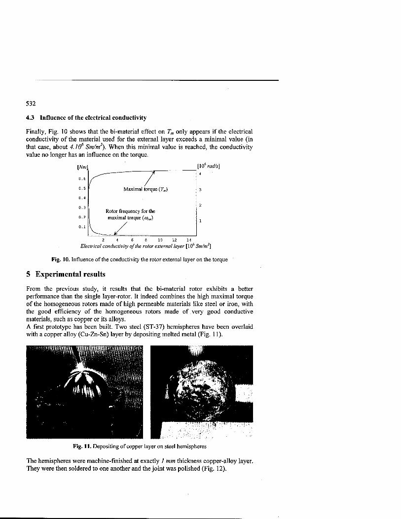
532

4.3 Influence of the electrical conductivity

Finally, Fig. 10 shows that the bi-material effect on Tm only appears if the electrical conductivity of the material used for the external layer exceeds a minimal value (in that case, about 4.106 Sm/m2). When this minimal value is reached, the conductivity value no longer has an influence on the torque.

[Nm] [10" rad/s]

0.6

0.5

0.4

r 7 Maximal torque (Tm)

4

3

0.3

0.2

0.1

Rotor frequency for the maximal torque (corm) L /

2

1

Electrical conductivity of the rotor external layer [106 Sm/m2]

Fig. 10. Influence of the conductivity the rotor external layer on the torque

5 Experimental results

From the previous study, it results that the bi-material rotor exhibits a better performance than the single layer-rotor. It indeed combines the high maximal torque of the homogeneous rotors made of high permeable materials like steel or iron, with the good efficiency of the homogeneous rotors made of very good conductive materials, such as copper or its alloys. A first prototype has been built. Two steel (ST-37) hemispheres have been overlaid with a copper alloy (Cu-Zn-Sn) layer by depositing melted metal (Fig. 11).

^mm

• *' ,il A 'ß r Ü wM KXagggza

%?* '™'"~ ' '*'.'■ i^r,

Fig. 11. Depositing of copper layer on steel hemispheres

The hemispheres were machine-finished at exactly / mm thickness copper-alloy layer. They were then soldered to one another and the joint was polished (Fig. 12).

533

The inductors were built from the stator of a standard AC motor. For each inductor, we kept only the six slots of a 36-slot stator. These slots were filled with 3 coils, each with 3-slot width and shifted from the others by one slot (Fig. 13).

Fig. 12. Bi-material rotor Fig. 13. Inductor

An experimental single motorised DOF device has been built. The purpose of this device was to validate the principle. It was limited to one motorised DOF for obvious technical reasons. The experimental device is represented in Fig. 14. A DC motor, equipped with a torque sensor, has been friction coupled to the spherical rotor in order to simulate a load.

Spherical rotor Spherical bearing

Inductor 1,

Bearing support

DC motor

Inductor 2

Wheel for the motion transmission

Fig. 14. Spherical actuator prototype and the dc motor used for the torque measurement

A first series of measurements has been performed with no supply to spherical actuator. This allowed us to record the friction torque due to bearings and to the

534

measurement system (DC motor). The difference between the torque measured when the spherical motor is supplied and not supplied gives the electromechanical torque generated by the actuator.

0.15

Predicted torque

0.05

250 500 750 1000 1250 1500

Rotor frequency [rad/s]

Fig. 15. Comparison between the measured torque and the one predicted by the analytical model

This measured torque has been compared to the one predicted by the analytical model. Fig. 15 shows good agreement, especially when considering the strong assumptions made in the analytical model and particularly the fact that:

- the boundary effects have been neglected; - electromagnetic properties of the materials (and particularly the steel parts) are

assumed to be linear. As a result, hysteresis losses are neglected. - the permeability of the stator is assumed infinite and hence the eddy currents in

the stator are neglected. Additional errors follow from the inaccuracy of the manufacturing and more particularly, the fact that the conductivity of the copper-alloy layer can have been affected by the soldering process. For the same reason, the thickness of this layer cannot be guaranteed.

6 Conclusion

In this paper, an analytical electromagnetic model of a two-DOF spherical actuator, based on the principle of the induction motor, has been proposed. Both the cases of an homogeneous rotor (made of one material) and double layer rotor (where the steel inner rotor is overlaid with copper alloy) have been considered. It has been shown that the bi-material exhibits better performances since it combines the high maximal torque of the homogeneous rotors made of high permeable materials (steel for example), with the good efficiency of the homogeneous rotors made of very good conductive material (copper, for example). So as to take into account thermal and building constraints, a first prototype has been designed and built. It allows to show good agreement between the experimental results and those predicted by the analytical model.

535

Acknowledgement

This work was sponsored by convention n°9713514 with the Walloon Region and the Belgian Program for Inter-University Attraction Poles initiated by the Belgian State- Prime Minister's Office - Science Policy Program IUAP-24.

References

[1]B. Bederson, R. Wallace, E. Schwartz, «A Miniature Pan-tilt Actuator: the Spherical Pointing Motor », IEEE Trans, on Robotics and Automation, Vol. 10 No. 2 1994, pp. 298-308.

[2] L. Ferriere, Conception d'une plateforme omnidirectonnelle, These de Doctorat de l'Universite" catholique de Louvain - Septembre 1998.

[3] L. Ferriere, B. Raucent « Rollmobs: a new universal wheel concept» Proceedings of the IEEE Conference on Robotics and Automation (ICRA '98), Leuven, Belgium, May 1998, pp. 1877-1882.

[4] F. Smeraldi, O. Carmona, J. Bigiin, «Real-time Head tracking by Saccadic Exploration and Gabor Decomposition », Proceedings of the 5th Advanced Motion Control (AMC '98), Coimbra, Portugal, July 1998, pp. 684-687.

[5] J. Wang, G. Jewell, W. Howe, «Modeling of a Novel Spherical Permanent Magnet Actuator », Proceedings of the 1997 IEEE International Conference on Robotics and Automation, Albuquerque, New-Mexico, April 1997, pp. 1190-1195.

[6] K. Lee, C. Kwan, « Design Concept Development of a Spherical Stepper Motor for Robotic Application », IEEE Trans, on Robotics and Automation, Vol.7, No. 1, 1991, pp. 175-181.

[7] G. J. Vachtsenavos, K. Davey, K. M. Lee, « Development of a Novel Intelligent Robotic Manipulator », IEEE Trans, on Control Syst. Mag., Vol. 7, No. 3, 1987, pp. 9-14.

[8] B. Dehez, V. Froidmont, D. Grenier, B. Raucent « Conception d'un actionneur ä rotor sphfrique et d^battement illimitö», Proceedings of CEMD'99 conference "Conversion electromecanique directe", Cachan, France, February 1999, pp. 65- 71.

536

Self-sensing Magnetic Suspension Using an H-bridge Type Hysteresis Amplifier

Takeshi Mizuno and Yuji Ishino Department of Mechanical Engineering, Saitama University

Shimo-Okubo 255, Urawa, Saitama 338-8570, Japan {mizar, yishino}@mech.saitama-u.ac.jp

Abstract. A hysteresis amplifier with an H-bridge drive is developed for self- sensing magnetic suspension. In this amplifier, a current comparator with some hysteresis controls its switching times so that the switching frequency changes according to load impedance. The gap between the suspended object and the electromagnet can, therefore, be estimated from the frequency. Since the H- bridge reverses the polarity of the voltage applied to the coil alternatively, it is expected from analytical study that the frequency becomes insensitive to the value of current command to the amplifier. Such switching characteristics are confirmed experimentally. The F/V conversion of the switching signal is used for feedback control with the result that self-sensing suspension is realized.

1 Introduction

There are a number of methods of suspending a body without mechanical contact. Magnetic suspension using controlled electromagnets has been applied to ultra- centrifuges, turbomolecular pumps, aerospace instruments and Maglevs [1]. To widen its industrial application areas, the reduction of the cost, size and weight of system is required. To use of an electromagnet both for force generation and for position sensing is an effective approach to this purpose. Magnetic suspension with electromagnets operating in this way is called as "self-sensing" or "sensorless" suspension. Another merit of self-sensing suspension is that the collocation of sensor and actuator is automatically achieved.

There are several methods of self-sensing suspension. They are classified as either (1) using observer-based controller [2-4], or (2) superimposing a high-frequency alternating excitation [2, 5-7].

As one of the second method, the authors investigated self-sensing suspension using a hysteresis amplifier, which is characterized by the sensitivity of the switching frequency to load impedance [8,9]. Since the switching frequency of a hysteresis amplifier changes in proportion to the air gap between the electromagnet and the suspended object, it can be treated as the output of a frequency-type displacement sensor. The Phase Locked Loops (PLLs) was applied to the control of such a self- sensing magnetic suspension; the loop was successfully pulled in lock and as a result the accuracy of positioning was improved, compared with a PD-controlled suspension

537

system [8]. A low-cost digital control system was also developed where the frequency of the switching signal of the hysteresis amplifier was converted to a digital form by counting by a counter circuit [9].

In the previous works, two types of hysteresis amplifiers were developed. One had a bipolar power supply [8] while the other had a unipolar one [9]. The former type can make the switching frequency insensitive to the value of current command to the amplifier; the problem is the cost of the bipolar power supply. The latter is lower in cost; the problem is that its switching frequency is sensitive to the value of current command, which causes a disturbance to the gap estimation when the feedback control is operating.

A new hysterersis amplifier with an H-bridge drive is developed in this research. Since the H-bridge reverses the polarity of the voltage applied to the coil alternatively, it is expected that the frequency becomes insensitive to the value of current command even though a unipolar supply is used. Its switching characteristics are studied experimentally. The switching signal is also used to realize self-sensing suspension.

2. Magnetic Suspension Using a Controlled Electromagnet

Figure 1 compares a self-sensing suspension system (b) with conventional one (a); both are basic models with a single-degree-of-freedom motion. The conventional system consists of

(1) a suspended object with a mass of m, (2) an electromagnet, (3) displacement sensor, (4) a controller, (5) a power amplifier.

/, V////////////Z'

Kr i

/J '//////////////,

iiifci ifflu Amplifier

I

*

Controller

Amplifier

Controller

(a) Conventional magnetic suspension (b) Self-sensing magnetic suspension

Fig. 1. Conventional and sensorless magnetic suspensions

538

The equation of motion is given by

mx = F -mg, (1)

where F is the attractive force of the electromagnet. Assuming that leakage and fringing effects are ignored in the magnetic circuit, the attractive force is given by

D1

where K is the coefficient of the electromagnet, D is the gap between the suspended object and the electromagnet, and I is the coil current.

Each variable is given by the sum of a fixed component (determining its operating point) and a variable component;

D = D0-x, (3)

I = I0+i. (4)

where D0 is the nominal gap, and I0 is the bias current; they are selected to satisfy the following equilibrium condition:

Do Substituting Eqs. (2)-(5) into Eq.(l) and linearizing it leads to

mx = Ktx + Kti (6)

where

KS=2K*\, K,=2K-^-. (7)

Dl 2D\ Suspension system using the attractive force of a DC electromagnet is inherently

unstable, as shown by (6), so that the coil current has to be changed according to the position of the suspended object for stable suspension. The conventional system uses a displacement sensor for detecting the position and an amplifier for changing the current. In self-sensing suspension systems as shown by Fig. 1 (b), the displacement is estimated from the coil current and sometimes coil voltage in addition. In this research, a hysteresis amplifier is used for controlling the current, and the displacement is estimated from its switching signal.

3. Hysteresis Amplifiers

3.1 Hysteresis amplifier with a bipolar power supply

539

Circuit. The schematic diagram of a hysteresis amplifier with a bipolar power supply is shown in Fig.2(a); the principle of operation can be explained by Fig.2(b) where lr represents a current command inputted to the amplifier [8]. In this amplifier, the switching times are controlled by a hysteresis comparator. The actual coil current / has a component of a triangular wave to oscillate within a hysteresis band defined by Alp and Alm above and below the command. When / increases to the upper band limit Ir +Mp , the voltage applied to the coil is turned to -Vm; When / decreases to the lower band limit Ir -AIm, the voltage applied to the coil is turned to Vp. The rates of increase and decrease of / are inversely proportional to the coil inductance; the inductance is also inversely proportional to the gap between the suspended object and the electromagnet. As a result, the switching frequency of this amplifier is proportional to the gap. This will be shown analytically in the following.

Hysteresis T P Electro. comparator Q^ÄV magnet Rotor

IT+AI„

lr-Ml

(a) Configuration

4 M—r„ »i« r-»»<

: Current D(:g!lp) sensing

(b) Operation

Fig. 2. Hysteresis amplifier using a bipolar power supply

540

Analysis. The circuit operation of the amplifier can be divided into two modes; the

voltage applied to the coil is Vp (Mode 1) or -V„ (Mode 2). The command current

Ir is assumed to be constant. When the voltage induced by the movement of the

suspended object is ignored, the equation for the current can be written as

L^L+RI = V (8) d*

where V is the voltage applied to the coil and R is the resistance of the coil. It is assumed that the switching frequency becomes high enough for the current to

change at constant rates. Estimating the rates at I = Ir gives

AT +AIm L^P ?L = v-RIr

TP

■ T „LAI

P+AI»> <9>

Vp-RIr

AT +AT L p m =Vm+RIr

... Tm=LAI'+AI" (10) Vm+RIr

where Tp and Tm are the periods when Vp and -Vm are applied to the coil,

respectively. From (9) and (10) the switching frequency/is given by

1 / = T +T

V V 11

-L(AIp+AIm)(Vp+Vm)X rKVp Vj (ID

If the applied voltages are selected to satisfy

Vp=Vm(=Vc) (12)

the frequency does not depend on command current because (11) becomes

Vc (13) J 2L(AIp+AIm)

The coil inductance is approximately given by

L = — (14) D

Substituting (14) into (13) gives

541

/ = ■ -D

(15) 4K(AIp+AIm)

Equation (15) shows that the switching frequency is proportional to the gap, and insensitive to the value of current command.

3.2 Hysteresis Amplifier with a Unipolar Power Supply

Circuit. Figure 3 shows the schematic diagram of a hysteresis amplifier with a

unipolar power supply [9]. The switching times of the transistor Q are also controlled by a hysteresis comparator. While the transistor is switched on, the coil current / increases because the voltage Vc, applied to the coil, is selected to be rather high. When / increases to the upper band limit Ir+AIp, the transistor is turned off but the current continues to flow through the freewheeling diode Dm . The current decreases because of loss in the coil and a resistor Rm connected in series. When / decreases to

the lower band limit Ir -AIm, the transistor is again switched on.

Analysis. The circuit operation of the amplifier can be divided into two modes. Mode 1 begins when the transistor turns on at I = Ir-AIm, and mode 2 begins when the transistor turns off at I = Ir+ AIp. An equivalent circuit in each mode is shown in

Fig.4. During the mode 1, the coil current / satisfies

Current" ' sensor

Hysteresis comparator Base d^ve

circuit Q

'BE ho— Current setpoint

Fig. 3. Hysteresis amplifier using a monopolar power supply

(a) Mode 1 (b) Mode 2

Fig. 4. Equivalent circuits

542

L*+RI = VC dt

The turn-on time TON is obtained as

T L(AIp+AIm) ToN= V.-RI,

During the mode 2, the current satisfies

L^- + (R + Rm)I = 0 dt

The turn-off time TOFF is approximately given by

T ^L(AIp + AIm) *OFF —

(R + Rm)Ir

From (17) and (19), the switching frequency is given by

1

(16)

(17)

(18)

(19)

/

D

TON + TOFF

— (Vc+RmIr) (20)

Equation (15) shows that the switching frequency is proportional to the gap, and sensitive to the value of current command. This must be considered in the applications where Ir changes significantly.

3.3 H-bridge Type Hysteresis Amplifier

Figure 5 shows a schematic diagram of hysteresis amplifier with an H-bridge output circuit. The H-bridge switches work in pairs to reverse polarity of the voltage applied to the load even though a unipolar power supply is used. It is expected from the analysis described in 3.1 that the switching frequency is given by

/S VJL D <21>

4K(AIp+AIm)

It means that the frequency is insensitive to the value of current command theoretically. Therefore, this type amplifier is superior in performance to the second type, and superior in cost to the first type.

In magnetic suspension systems, the current flowing in the coil is often limited to be unipolar. In such a case, a pair of switches in the H-bridge can be replaced by a pair of diodes.

543

Experiment

A single-degree-of-freedom model shown in Fig. 6 is used in the experiments. It has an arm as a suspended object, and a pair of electromagnets. Each electromagnet has a solid core of ferrite; the turns of the coil are 300. The electromagnet 1 and 2 are energized by a developed hysteresis amplifier and a conventional analog amplifier, respectively. The displacement of the arm is detected by an eddy-current sensor with a resolution of lpm.

The developed hysteresis amplifier uses a power module, SA51 produced by APEX, as an H-bridge drive; the hysteresis band is selected as

AIp = AIm = 20mA.

The switching frequency of the hysteresis amplifier is measured for the range of the gap from 0.2mm to 0.5mm as shown by Fig.7; the arm is fixed during the

Hysteresis H-bridge r comparator driver lr r^ +

HE

J -m^-m

i—1 i—i Current

Coil sensor i—I

Fig. 5. Hysteresis amplifier with an H-bridge drive

V/Ai// Electromagnet 1 '///////

Arm © Electromagnet 2 ///////

Fig. 6. Experimental apparatus

544

10

A:rc=40V 0:F =50V

0.2 0.25 0.3 0.35 0.4 0.45 0.5

Gap [mm]

(a) Efifects of the supplied voltage

>> o G u g- £ a o

-4-J

GO

20

1 1

- FC=40V -i 1 —i

18

^«<5 16

i^fi^ rfS*^-

14 1*** □ :/r=o.iA

12

in

A:/r=o.2A - 0:/r =0.3 A

-i 1 i

0.2 0.25 0.3 0.35 0.4 0.45 0.5

Gap [mm]

(b) Effects of the current setpoint

Fig. 7. Switching frequency of the hysteresis amplifier

545

measurement. The measurement results show the linear relationship between the switching frequency and the air gap between the electromagnet and the suspended object. In Fig.7 (a), the command current Ir is fixed to be 0.2A; the supplied voltage Vc is changed from 30V to 50V (every 10V). It demonstrates that the switching frequency becomes higher as the supplied voltage increases. In Fig.7 (b), Vc is fixed to be 40V; /,. is changed from 0.1A to 0.3 A (every 0.1 A). It shows that the sensitivity of the frequency to current command is smaller than that of the hysteresis amplifier with a unipolar power supply used in the previous work [9]; in particular, there is only a slight difference in frequency between /,. = 0.2Aand Ir = 0.3A .

Figure 8 compares the F/V converted switching signal of the hysteresis amplifier with the output of the eddy-current displacement sensor when the suspension system is made oscillatory. This result shows that the F/V converted signal corresponds to the sensor signal well.

Figure 9 shows a step response of the suspension system when the F/V converted signal is used for feedback control; a simple PD control is applied. This result demonstrates that self-sensing suspension is realized with the developed hysteresis amplifier.

0.50

0.35 0.0 0.5

Time [s]

(a) Eddy-current sensor

1.0

0.50

0.35 0.0 0.5

Time [s]

(b) F/Vconverted switching signal

1.0

Fig. 8. Comparison between the sensor output and the F/V converted switching signal

546

Conclusions

The self-sensing magnetic suspension using hysteresis amplifiers were studied both theoretically and experimentally. The factors determining the switching frequency of hysteresis amplifiers were discussed. The analytical study showed that the switching frequency could be made insensitive to current command when the polarity of the drive was reversed alternatively. A hysteresis amplifier with an H- bridge drive circuit was developed to satisfy this condition even though only one polarity supply was used. It was confirmed experimentally that the switching frequency was rather insensitive to the value of current command in the developed hysteresis amplifier. The F/V converted signal of the switching signal was compared with the output of an eddy-current displacement sensor. The F/V converted signal was used in the feedback control for stabilization with the result that self-sensing suspension was achieved.

0.30

g 8 o o

0.28 -

0.26 0.0 0.5

Time [s]

(a) Eddy-current sensor

1.0

0.30 B

'S e u o

0.28 -

0.26 0.0 0.5

Time [s] (b) F/V converted signal

1.0

Fig. 9. Step response of the suspension system in which the F/V converted switching signal is fed back

547

The developed hysteresis amplifier is still noisy so that intensive works are still continued for the development of higher-performance hysteresis amplifiers. Further experimental works are also under way to improve the dynamic performance of the suspension system by applying advanced control methods.

Acknowledgements

The authors would like to thank Mr. K. Tonegawa for his help with the experiments. The work was supported in part by the Asahi Glass Foundation, and by the Ministry of Education, Science and Culture under Grant-in-Aid for Developmental Scientific Research.

References

1. Schweitzer, G., Bleuler, H. and Traxler, A.: Active Magnetic Bearings, vdf, ETH Zürich (1994).

2. Vischer, D.: Sensorlose und Spannungsgesteuerte Magnetlager, Doctor Thesis Nr.8665, ETH Zürich (1988).

3. Vischer, D., and Bleuler, H.: Self-Sensing Active Magnetic Levitation, IEEE Trans, on Magnetics, Vol.29, No.2 (1993) 1276-1281.

4. Mizuno, T. and Bleuler, H.: Self-Sensing Magnetic Bearing Control System Design Using the Geometric Approach, Control Engineering Practice, Vol.3, No.7 (1995) 925-932.

5. Frazier, R. H., Gilinson, Jr., P. J. and Oberbeck, G. A.: Magnetic and Electric Suspensions, The MTT Press (1974) 265-283.

6. Okada, Y., Matsuda, K. andNagai, B.: Sensorless Magnetic Levitation Control by Measuring PWM Carrier Frequency Component, Proc. 3rd Int. Symp. on Magnetic Bearings, Technomic Publishing Co., Inc. (1992) 176-183.

7. Noh, M. D. and Maslen, E. H.: Self-Sensing Magnetic Bearings (Part I), Proc. 5th Int. Symp. on Magnetic Bearings, Kanazawa University (1996) 95-100.

8. Mizuno, T., Ishii, T., and Araki, K.: Self-sensing Magnetic Suspension Using Hysteresis Amplifiers, Control Engineering Practice, Vol.6 (1998) 1133-1140.

9. Mizuno, T., Araki, K. and Namiki, H.: Control System Design of Frequency-Feedback Magnetic Bearings, Proc. 1997ASMEDesign Engineering Technical Conferences, VIB-3947 (1997).

548

Chaotic Phenomena and Performance Optimization in the Trajectory Control of Redundant Manipulators

Fernando B. M. Duarte1, J. ATenreiro Machado2

'Escola Superior de Tecnologia Viseu, Dep. Matemätica, Campus Politecnico, 3510 Viseu, Portugal

EmaU:fduarte@mat.estv.ipv.pt 2Instituto Superior de Engenharia do Porto

Dep. de Eng. Electrotecnica, Portugal Email: jtm@dee.isep.ipp.pt

Abstract - Redundant manipulators have some advantages when compared with classical arms because they allow the trajectory optimization, both on the free space and on the presence of obstacles, and the resolution of singularities. For this type of manipulators, several kinematic control algorithms adopt generalized inverse matrices. In this line of thought, the generalized inverse control scheme is tested through several experiments that reveal the difficulties that often arise. Motivated by these problems this paper presents a new method that optimizes the manipulability through a least square polynomial approximation to determine the joints positions. Moreover, the article studies the chaos revealed by the kinematics trajectory planning scheme, as well as its influence on the dynamics, when controlling redundant and hyper-redundant manipulators. The experiment confirm the superior performance of the proposed algorithm for redundant and hyper-redundant manipulators, revealing several fundamental properties of the chaotic phenomena, and gives a deeper insight towards the future development of superior trajectory control algorithms.

1. Introduction

A kinematically redundant manipulator is a robotic arm possessing more degrees of freedom (dqf) than those required to establish an arbitrary position and orientation of the end effector. Redundant manipulators offer several potential advantages over non- redundant arms. In a workspace with obstacles, the extra dof can be used to move around or between obstacles and thereby to manipulate in situations that otherwise would be inaccessible [1,2,4]. When a manipulator is redundant, it is anticipated that the inverse kinematics admits an infinite number of solutions. This implies that, for a given location of the manipulator's end effector, it is possible to induce a self-motion of the structure without changing the location of the gripper. Thus, the arm can be reconfigured to find better postures for an assigned set of task requirements. Many techniques for solving the kinematics of redundant manipulators that have been suggested control the end effector indirectly, through the rates at which the joints are driven, using the pseudoinverse of the Jacobian [3]. Nevertheless, these algorithms lead to a kind of chaotic motion with unpredictable arm configurations. Therefore, an

549

important area of research remains open and more efficient algorithms must be envisaged. Having these ideas in mind, the paper is organized as follows. Section 2 develops kinematics and dynamics of redundant manipulators. Based on these concepts, section 3 presents several experiments with the kinematics and dynamics of different redundant robots. The results reveal a chaotic behavior that is further analyzed in section 4. Finally, section 5 draws the main conclusions.

2. Kinematics and Dynamics of Redundant Manipulators

2.1 Problem Formulation

We consider a manipulator with n dof whose joint variables are denoted by q = [q\, 12, -, Qn]T- We assume that a class of tasks we are interested in can be described by m variables, x = fo, x2,..., xm]T (m < n) and that the relation between q and x is given by:

* = /(q) CD

where /is a function representing the direct kinematics. Differentiating (1) with

respect to time yields:

x = j(q)q (2)

where x e SRm, q € 91" and J(q) = 5/(q)/5q e W"x". Several approaches for solving redundancy that have been proposed [5, 8] are based

on the inversion of equation (2). A solution in terms of the joint velocities, is sought as

where J# is one of the generalized inverses [6] of the J.

A direct consequence is that it is possible to generate internal motions that reconfigure the manipulator structure without changing the gripper position and orientation [7, 9]. Another aspect revealed by the solution of (3) is that repetitive trajectories in the operational space do not lead to periodic trajectories in the joint space. This is an obstacle for the solution of many tasks because the resultant robot configurations have similarities with those of an chaotic system. In order to solve this lack of repetition we adopt a distinct approach, entitled Open-Loop Manipulability (OLM) optimization method [10]. For a given point (x,y) in the operational space the new algorithm consists on computing the point in the joint space

that maximizes the manipulability index p. = ydet(jJr J. Given the symmetry of the

robot kinematics, /^ the maximum value of ju, just depends on the radial distance

r = ijx2+y2 of the point from the origin of coordinates and, therefore, we get the set

of n -m joint positions qff),...., qj+„-m(r) optimal in a // perspective. From these values

550

and using a standard least squares method we calculate n-m polynomials that fit approximately the data. Once fixed these variables, the other m joint positions can be calculate through a standard inverse kinematic algorithm. The numerical calculation of the maximum manipulability (/O and the corresponding joint values increase with the number of dof, but they can be computed off-line without imposing an high load to real-time control systems.

2.2 Kinematics of Planar Redundant Manipulators

The direct kinematics and the Jacobian of a Mink manipulator has a simple recursive nature according with the expressions:

X /lC1+/2C12+/3C123+- ■+kc\2---k

y\ _/l-si+/2'Si2+/3'S123+- ■ + kS\2-k_

hs\ hsu — lksl—k ••■ ~lks\---k

IhP 1+/2Q2+- + '*Q.-* ■■■ dfcQ—ifc

(5.a)

(5.b)

where /, is the length of link /, St...fc = Sin{qi + ■ ■ ■ + qk) and Ct..k - Coiqt +---+qk).

During the experiments, for all manipulators, it is considered At = 0.001 sec, h +12+ h ...+ 4=3 and l1 = h = l3...= lk. In the closed-loop pseudoinverse's method (CLP) the joint positions can be computed through the time integration of the velocities (3) according with the block diagram of the inverse kinematics algorithm depicted in Figure 1.

Fig. 1: Block diagram of the closed-loop inverse kinematics algorithm with the pseudoinverse.

2.3 Dynamics of Planar Redundant Manipulators

The symbolic formulae for the inverse dynamics of a Mink planar manipulator can be also formulated recursively as:

551

Ti =£(mi(£(If[j > p,Bl = 0,Bl = l]lp2^Bl)

i=l p=\ u=\

u=\ p=2 k=\

[lf[p==i,B3 = l,B3 = 0llf{j>k,B4 = 0,B4 = l\ If[U>=k + l&&j<=p),B5 = l,B5 = 0\

lk(lpB2 + rpB3)((-SM.p(( £quf + u=k+\

k P p k (6)

u=\ u=k+l u=\ «=1

k k

(SM.p(Z<iu)2+Ck+h.py£qu)B5 +

g(£ W \J > P, 51 = 0, B\ = \\ lpCVpB\)+riCXi))) P=\

where Tt are the joint torques, Bl to B5 are logical conditions, w, is the mass of link /, /•, is the distance from the joint axis to the link center of mass and g is the acceleration due to gravity.

3. Trajectory Control of Redundant and Hyper-Redundant Robots

In this sections we analyze for different manipulators the performances of the trajectory controllers based on the CLP and OLM methods. In this line of thought, we study the joint trajectories for the planar redundant 3R and the planar hyper-redundant 4R robot, when subjected to a repetitive circular trajectory in the operational space with radius R.

3.1 Planar Redundant Manipulators

In this experiment we adopt the 3R arm with an initial posture

q(0) = [;r -nfl -n/2\ .Figure 2 shows the joint positions using the CLP method. In an alternative experiment, Figure 3 shows the joint positions the OLM method. In this case, it is adopted the least square approximation polynomial q3 = 0.5 \r - 2.09 for

, joint 3. In these two experiments we have distinct results. When adopting the CLP, the manipulability is non-optimal and the joint trajectories exhibit sudden changes, which impose large joint velocities. Moreover, the joint trajectories are non-repetitive leading to a kind of chaotic performance. When using the OLM procedure the trajectory is repetitive without large or fest transients.

552

4

2

0

-2

-4

-6

-8

-W<ft?% ̂ Hh V% t 1 1

"\15 ■

20 25 30 ^

—1

35

Fig. 2: The 3i?-robot joint positions versus time using the CLP method.

4

3

2

1

0

-1 :

-2 -

-3

ql

t

10 15 20 25 30 35 q2,q3 VVNAAAAAAAAAAAA,

Fig. 3: The 3i?-robot joint positions versus time using the OLM method.

3.2 Planar Hyper-Redundant Manipulators

In this sub-section we consider the planar 4R hyper-redundant manipulator under the control of the two previous methods. In the CLP method the manipulators initial

configurations are: q(Q)=[o.97r -0.28r -0.4k -0.39^. In the OLM algorithm we adopt least squares polynomial approximations. For joints 3 and 4 of the 4Ä-robot we use: q3 = 0.4\r2 -0.60r-1.62 and q4 = -0.24r2 +1.13r-1.78 .

553

Fig. 4: The 4R-robot joint positions versus time using the CLP method.

4

3 -I

2

1

0

-1

-2

qi

30q4 35

q3

Fig. 5: The 47?-robot joint positions versus time using the OLM method.

In these experiments (Figs. 4 to 5) we observe performances similar to those revealed by the 3Ä-robot. Moreover, for the proposed method, the manipulability index ju seems to show better performances the higher the number of robot dof. This conclusion is consistent with the fact that the larger the number of dof Has. higher the manipulability (for the appropriate robot configuration) as can be seen in Figure 6.. Therefore, the OLM method taker advantage of this property while the CLP algorithm spans a large range of sub-optimal manipulability configurations.

In a second set of experiments we analyze the robot inverse dynamics when subjected to the repetitive circular trajectory in the operational space. Figure 7 and Figure 8 shows the resulting the joint torque for the planar 3R manipulator under the CLP and OLM

554

methods. It is clear that, under the CLP method, the dynamics follows the kinematic non-repetitive responses and, therefore, exhibits the same type of problems.

f^max

3 - AR

2.5 - 3R

2 .

1.5 / // 2R

0.5 .

0 -

Fig. 6: Maximum manipulability /w versus the radial distance r for the 2R, 3R and AR robots.

t2 t3 tl

Fig. 7: The 3i?-robot joint torque versus time using the CLP method (R = 0.5). At t=15.3 sec there isachartpick, for joint 1 torque, with amaximum value ^=158.1. The maximum for joint 2 torque is f2=67.6 at t=l 5.3 sec and the maximum for joint 3 torque is f3=14.7 at t=l 1.57 sec.

555

a

ß

Fig. 8: The 3-R-robot Joint torque versus time using the OLM method (R = 0.5).

4. On the Chaotic Responses of the Pseudoinverse Algorithm

It was shown previously that the pseudoinverse algorithm leads to unpredictable arm configurations, with responses similar to those of a chaotic system [12, 13]. For example, Figure 11 and Figure 12 depict the phase-plane trajectories for joint 1 of the planar 3/?-robot kinematics and dynamics, respectively, when repeating a circular motion with center at r = 1 and radius R = 0.1. Besides the position and velocity drifts, leading to different trajectory loops, we have points that are 'avoided'. Such points correspond to arm configurations where several links are aligned. This characteristic is inherent to the pseudoinverse matrix because the planar 3Ä-robot was tested both under open-loop and closed-loop control, leading to the same type of behavior. In order to gain further insight into the pseudoinverse chaotic nature, the robots under investigation were required to follow the cartesian repetitive circular motion for several radial distances r. The phase-plane joint trajectories were then analyzed and their fractal dimension dim estimated through the standard box-counting method [11]:

dimS = lim In N(s)

e->oln(l/s) (7)

where N(e) denotes the smallest number of bi-dimensional boxes of side length s required in order to completely cover the plot surface. Figure 20 shows the resulting chart revealing that: . for the pseudoinverse method we have dim » 2 due to the position and velocity

drifts, in contrast with the case for the 2R where we have dim = 1. • the fractal dimension diminishes near the maximum radial distance {i.e. r = 3). • for each type of robot the fractal dimension is nearly the same, for all joints.

556

$i 3

2.5

2

1.5

1

0.5

0

-0.5

-1

-1.5

-2 ffl

-3 -2-1 0 1 2 3 Fig. 9: Phase plane trajectory for the 3R- robot -joint 1 at r = 1, R = 0.1, am = 1.62.

»i 100 r

-50

-100 -

-150 -10 0 10 20 30 40

Fig. 10: Phase plane trajectory for the 3R- robot -torque 1 atr= l,R = 0.1,dim = 1.69.

Fig. 11: Fractal dimension dim of the kinematic phase-plane versus the radial distance r for the 3Ä and AR robots, R = 0.1.

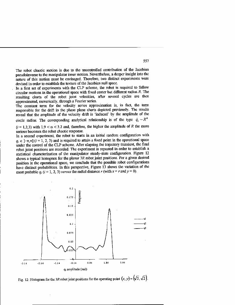
557

The robot chaotic motion is due to the uncontrolled contribution of the Jacobian pseudoinverse to the manipulator inner motion. Nevertheless, a deeper insight into the nature of this motion must be envisaged. Therefore, two distinct experiments were devised in order to establish the texture of the Jacobian null space. In a first set of experiments with the CLP scheme, the robot is required to follow circular motions in the operational space with fixed center but different radius R. The resulting charts of the robot joint velocities, after several cycles are then approximated, numerically, through a Fourier series. The constant term for the velocity series approximation is, in fact, the term responsible for the drift in the phase plane charts depicted previously. The results reveal that the amplitude of the velocity drift is 'induced' by the amplitude of the circle radius. The corresponding analytical relationship is of the type qt ~ Ra

(/ = 1,2,3) with 1.9 < a < 3.2 and, therefore, the higher the amplitude of R the more serious becomes the robot chaotic response. In a second experiment, the robot to starts in an initial random configuration with qt e ]-n,n] (i = 1, 2, 3) and is required to attain a fixed point in the operational space under the control of the CLP scheme. After elapsing the trajectory transient, the final robot joint positions are recorded. The experiment is repeated in order to establish a statistical characterization of the manipulator steady-state configuration. Figure 12 shows a typical histogram for the planar 3R robot joint positions. For a given desired position in the operational space, we conclude that the possible robot configurations have distinct probabilities. In this perspective, Figure 13 shows the variation of the most probable qt (/ = 1,2, 3) versus the radial distance r (with x = r and >> = 0).

0.15 -

0.125

0.075

V/0.025V1

?

-ql

-<& -q3

.3.14 -2.14 -1.14 -0.14 0.86 1.86 2.86

qi amplitude (rad)

Fig. 12: Histogram for the 3i? robot joint positions for the operating point (x, y) = (y 2, V 2 j.

558

Fig. 13: Most probable robot joint positions versus the radial distance r.

559

5. Conclusions

This paper discussed several aspects of the chaotic phenomena generated by the pseudoinverse-based trajectory control of redundant manipulators. Furthermore, the study addressed both the kinematics and dynamics in order to test the influence of each model. In this perspective, the fractal dimension of the responses was analyzed showing that it is independent of the robot joint. In fact, the chaotic motion depends solely on the operational space point and on the amplitude of the exciting repetitive motion. Moreover, a second group of experiments reveals that the robot inner motion, that spans the null space of the Jacobian matrix, leads to 'preferred' configurations while avoiding other areas. Nevertheless, the relationship between the fractal dimension of the phase plane portraits, the amplitude of the exciting repetitive signal and the statistics of the robot joint configurations is not completely clear and further research on this aspects needs still to be done in order to develop superior trajectory planning algorithms.

References 1E. Sahin Conkur, And Rob Buckingham "Clarifying the Definition of Redundancy as

Used in Robotics", Robotica, vol. 15, pp. 583-586,1997. 2 Stefano Chiaverini "Singularity-Robust task-Priority Redundancy Resolution for Real

Time Kinematic Control of Robot Manipulators", IEEE Trans. Robotics Automation, vol. 13, pp. 398-410, 1997.

3 C.A Klein, and C. C Huang, "Review of Pseudoinverse Control for Use With Kinematically Redundant Manipulators", IEEE Trans. Syst. Man, Cyber., vol. 13, pp. 245-250,1983.

4 Yoshikawa, T., "Foundations of Robotics: Analysis and ControV', MIT Press, 1988. 5 Y. Nakamura, "Advanced Robotics: Redundancy and Optimization", Addinson-

Wesley, 1991. 6 Keith L. Doty, C. Melchiorri and C. Bonivento, "A Theory of Generalized Inverses

Applied to Robotics", .M Journal of Robotics Research, vol. 12, pp. 1-19,1993. 7 Bruno Siciliano," Kinematic Control of Redundant Robot Manipulators: A Tutorial",

Journal ojIntelligent and Robotic Systems, vol. 3, pp. 201-212,1990. 8 W.J.Chung, Y. Youm and W. K. Chung, "Inverse Kinematics of Planar Redundant

Manipulators via Virtual Links With Configuration Index", J. of Robotic Systems, vol. 11, pp. 117-128,1994.

9 Sanjeev Seereeram and John T. Wen, "A Global Approach to Path Planning for Redundant Manipulators", IEEE Trans. Robotics Automation, vol. 11, pp. 152-159, 1995.

10 Fernando B.M. Duarte and J.A. Tenreiro Machado, "Kinematic Optimazition of Redundant and Hyper-Redundant Robot Trajectories", ICECS^^"1 IEEE Int. Conference on Electronics, Circuits and Systems, Lisbon, Portugal, 1998.

11 James Theiler, "Estimating Fractal Dimension", Journal Optical Society of America, vol. 7, n°6, pp. 1055-1073, 1990.

12 J.A.Tenreiro Machado and Fernando B. Duarte, "Redundancy Optimization for Mechanical Manipulators", AMC'98-5ih IEEE Int. Workshop on Advanced Motion Control, Coimbra, Portugal, 1998.

13 Fernando B. Duarte and J.A. Tenreiro Machado, "On the Optimal Configuration of Redundant Manipulators", INES'98- 9th IEEE Int: Conf. on Intelligent Engineering Systems, Vienna, Austria, 1998.

560

Stabilization of Nonholonomic Dynamic Systems Based on the Force/Torque

Feedback and Its Application

TatsuoNARIKIYO12 and Masakazu KATOH *

xDep. Information & Control, Toyota Technological Institute, Hisakata 2-12-1, Tempaku, Nagoya 468-8511, Japan

n-tatsuo@toyota-ti.ac.jp 2 BMC Center, RIKEN, Shimoshidami, Moriyama, Nagoya 463-0003Japan

Abstract. This paper presents a control system design methods for stabilizing nonholonomic chained system and nonholonomic Caplygin system. Proposed control inputs are given as the force and torque informations. It can be shown that the proposed control inputs stabilize the chained system and the Caplygin system. In order to demonstrate the usefullness of the proposed control laws, these are applied to the stabilization of the wheeled mobile robot and the planor space robot which are modelled in the configuration space and steered by the force/torque actuator. It also be demonstrated by simulations that the proposed control laws have excellent robustness properties against some modelling errors.

1. Introduction

As pointed out by Brockett[l], the origin of the nonholonomic system which has more degrees of freedom than the number of inputs cannot be stabilized by smooth static state feedback. Thus, many control system design methods have been proposed to solve the stabilization problem via time-varying or discontinuous control laws[2~5]. In our earlier works[6,7], the origin of the nonholonomic chained system has been exponentially stabilized by smooth static state feedback except some initial states and the origin of the nonholonomic Caplygin system has been stabilized by smooth time varying state feedback. In these studies only kinematic models have been treated and assumed that system parameters are exactly known. However, in many control problems, it is more realistic that the mechanical systems are controlled by torque or force inputs and the system parameters may be perturbed[8].

In this paper, we extend our earlier work and convert velocity inputs to force/torque inputs. Because these control laws are differetiable at least once, then input conversion can be successfully performed. The converted

561

force/torque control inputs stabilize the chained system and the Caplygin system. Furthermore numerical simulations show that the proposed control laws have excellent robustness properties against some modelling errors. In order to demonstrate the usefulness of the proposed control laws, these are applied to the stabilization of the wheeled mobile robot and the planor space robot which are modelled in the configuration space and steered by the force/torque actuator.

This paper is organized as follows. In section 2 we present the control laws which appeared in our earlier works [6,7] and convert these control laws to the force/torque feedback controls. In section 3, we show the equations of motion of the wheeled mobile robot and apply the proposed control laws to it. In section 4, the equations of motion of the planor space robot is represented. Some numerical simulations are given to show the usefullness of the proposed control laws. In section 5, final remarks and conclusions are discussed.

2. Control laws

Equations of motion of the mechanical system which is imposed on the

nonholonomic Pfaffian constraint Hq)d=0 can be derived using the Lagrange-d'Alembert equations without difficulty. Where q is n-dim vector and denotes the generalized coordinate, J(q) is n-m x n analytic matrix. Furthermore using the partial linearization technique, the equations of motion for this system can be written in the following form[9].

A. dt

qz

q*)

q3

Jiquqdqs 0

0 0 v (l)

Where ld\T, <lflr=q , 7(</i, <7z) WT"*- and details are given in [9]. In eqn.(l), v denotes new input and has the same physical dimension as force or torque has. However, in many articles following driftless form has been considered for

convenience. By replacing the input v to u as M=03, the driftless equation is obtained.

q=B(q)u (2)

Because of w=<73, u equals to linear or angular velocity vector. At the beginning of this chapter, we consider the two types of nonholonomic

systems described by eqn.(2) and present the stabilizing control laws of these driftless systems.

One of these systems can be written by the following canonical form.

562

qi= Ui qi- «2 , qi- q2Ui ,

qn- q«iUi (3)

Several mechanical systems such as wheeled mobile robots and rolling disk can be converted to this canonical form[9]. Murray and Sastry gave sufficient conditions to convert a generic controllable nonholonomic system to this form [10]. The nonholonomic system which can be described by equations of canonical form (3) is called nonholonomic chained system.

As pointed out in [1], such system cannot be stabilized through continuously differentiable, state feedback control. However, if suitable assumption is given, stabilization problem via smooth state feedback is moved to be solvable as following[6,7]

Proposition 1 Origin of the nonholonomic chained system (3) can be exponentially stabilized by following inputs (4) except for the initial condition q i(0)* 0.

Ui-- Xqi

Uz=- X q2 + eh 0i + a2 q? + • • • + cu-2 q"'2 (4)

Where A > 0 and a = [ a i,..., a»- 2 ]T can be determined by equation (5)

Qi

l 0,-2

Ai, 1 • Ai, «-2

• • •

, A»-2,1 * An-2,11-2 ,

01

. <7»-2 ,

(5)

Where

qi-qi+i-

AiAq\) =

(»+D !

1

?1?2 Au(tfi) 1 £ä. 1

fr-i)!

1

I G+l)! («+/•)! J ■«r

G+l)!***-

(i=l,..., n-2, ;=2,.... «-2)

D

In this theorem, a determined by eqn.(5) is shown to be constant vector and is determined only by the initial condition q i(0)^ 0. In order to calculate a, matrix A(q 1) should be nonsingular. A(q 1) is defined by following (n-2) x (n-2) matrix.

563

Aiqd- A\,\ • Al,n-2

• • •

b An-2,1 * ftn-2,n-2 t

Where A(q 0 is rewritten by following relation.

A (qd=diag[qu .... qr2]A (l)diag[qh ..., qF2]

Determinant of A(l) is easily calculated by integer computation and it can be shown by integer computations that A(l) is nonsingular. Therefore A(q 0 is also nonsingular except n-1 dimensional manifold q i =0.

Remark Prop.l can be easily extended to the multi-input, multi-chain and single generator chained system [11] written by following equations.

qi.trtlz , , qm.iFUm

fl2,l^fl2,oWl, , qm.r^m.dti (6)

q2,n2~q2,n2-Mu • • • • > qm,m-~qm,Mi-iUl

The origin of this multiple input chained system can be stabilized by the inputs

Ui--X tfi

«2=-A. <7z.o + Cb.i <7i + • • • + 02,»2 q"2

Um--\ q„,o + cu,i <7i + • • • + cu.*» <7i""

Where ou,,- (i-2, ...,tn, pi,...,«,) can be specified by the same procedure as shown in Prop.l.

(7)

D

Secondly we consider the class of nonholonomic systems described by equations of the following canonical form.

d_

dt

( — '

Us.

In, (8)

Where <7i € R m, Q* £ R n'm are state vector and u £ R m denotes the input

vector. 7(<7i)(Ä(""M)x" is assumed to be differentiable arbitrarily. We have proposed the control law to stabilize the origin of this type of nonholonomic system. To simplify the problem of stabilizing the origin, we consider 2- inputs,3- states Caplygin system which is written by the following equation.

564

A. dt

Xi [1 1 fo 1 x2 = 0 U\ + 1 Ui

.Xi , . a(*i,*2) , . ß(*i,*2) , (9)

Where x i and « i denote the scalor state and input respectively, a and ß are analytic functions.

Proposition 2 For the Caplygin system (9) .stabilizing control law can be synthesized by the following procedure. Step 1 Compute the Lie bracket [f,g]. Where f=[l 0 a ]T and g=[0 1 ß ]T . And define r such that

-JJL _ J5L ^ax, ~ i«. • (10)

Step 2 Compute the Maclaurin expansion of r and define 0 r such that

#0

r=ao+aii*i+fli3X2+ß2i«i2+ • • •

Or- mini it W, 1,2,3... , , ,. r(xi,x2) }\ hm . . . , .

*l,l2->0 \\X\ | + |#2|.)

1.5 ^// '/ l \ 1 / r = 0 / 1

0.5 r r = const / 7 J S o A,/

-0.5

-1 \^^\ Q ^^

-1.5

/// ! -1.5 -1 -0.5 0 0.5 1 1.5 2

X1

Fig.l Contour lines of r(* i,# 2)

Step 3 Design closed contour C such that the curvilinear integral (11) is not identically zero.

9 adxi+$dx2 (11)

565

The contour C is periodic function of X and satisfies C(0)=0. When Or is 0 or 1, C= [C *i,C xZ]

T can be given as follows.

Gi(x)=-i? cos(kx+Q)+ R cos 9

C,2 (x) =-R sin (fcx+9) + R sin 9 (12) Where R is a radius of the closed contour determined later and k is ± 1 which denotes the direction of the closed contour . 6 is a constant arbitrarily asigned when 0 r=0 and tan ' Y« n/a 10 when 0 r=l. When Or ^ 2, the closed contour can be synthesized schematically. In this case , at first draw contour lines of r(x i,x z) on (x i,x z) plane as shown in Fig.l. And then synthesize the circle which is satisfied following conditions.

[ 0 at (*i,*2)=0

[nonzero at (*i,#2)#0

Step 4 Calculate the curvilinear integral.

A(R,*)=£(JV&,)&, (13)

Where r' is 0 r th order truncated function of r. Via this integral R and k can be determined so that following equation shoud be satisfied.

A (R, k) =~Xl | v=2nn

In order to guarantee the stability, R shoud be less than R m.x. Where

R„m=max{R \ |A»-A(ff,fe)l< |A(R,*)|}

tefadxiWa (14)

Step 5 Synthesize r so that the following conditions are satisfied.

(a) iW^xW for%,ytz,Uih

(b) -j-=0 at T^nT (n=0,1, 2,...,)

In the case of 0 r ^ 1, r is given by x=At-sin(At) (A>0) • (15)

Step 6 Design control inputs as follows. d

ui (t) =-Ai Ofi W -Gi (x)) +—-Cxi (x) at

(16)

niW—A,0c,(f)-G.(T))+—G,(x) , (Xuh>0) dt D

As mentioned above, the control inputs u given in Proposition 1, 2 are synthesized as linear or angular velocity inputs. Therefore, in order to

566

impliment these control laws to the actual mechanical systems written in eqn. (1) the velocity inputs should be converted to the force or torque inputs. However, because the velocity inputs given in Proposition 1,2 are differentiate at least one, then these inputs can be easily converted to the force or torque inputs. In our earlier work [12] we suggested a simple method of these conversion. Following proposition concretes our earlier work.

Proposition 3 Consider the nonholonomic system described by eqn.(l), (3) and (9). The state feedback control law

- duo v=-h(q3-Uo)+— , (Ao>0) (17)

at

stabilizes the nonholonomic chained systems and the Caplygin systems. Where Mo are the velocity inputs given in Proposition 1,2. However, for the nonholonomic chained system written by eqn.( 1) and (3) following constraints are imposed.

(I) ?.(0)#0

(n) (qA0)+ A« 0,(O))tf,(O)*O (18)

(Proof) Substituting eqn.(17) intoeqn.(l) and letting , e=l/Ao , i>=q?. then the following singularly perturbed system is obtained.

i=B(a)P (19)

e(i>-Uo(t,q))=-(fi-Uo(t,<i)) (20)

It can be shown that eqn.(20) has the isolated solution p=Uo(t,q) for 'it,q(R" and right-hand side of eqn.( 19) ,(20) are at least once continuously differentiable for /, q, p. Then the singularly perturbed system (19),(20)has the invariant manifold p=u(t,q,e) and this invariant manifold asymptotically equals to the isolated solution p=u0(,t,q), for t—*°° [ 13,14]. This means that there exists T for sufficiently small e such that

Wq-qoU e\p-u,(t,(l)U , VßT

Where II * IIE denotes Euclid norm and ?o denotes the solution of

q=B(q)ito(t,q)

Therefore the force or torque inputs (17) stabilizes closed loop system . On the other hand, constraint (18) can be easily shown by the following

discussion. Substituting the control (3) and (17) into eqn.(l), then the

solution fllo)=-i-[-a,1(o)+iI(o))«#(-irf)+a^1(0)+i1(0) )«*(-!*)] Ao A

567

is obtained. Inequality (18) is equivalent to the condition that </i (f) does not cross the axis of qi=0 . D

Prop.3 says that Ao has to be selected sufficiently larger than A., Xu h when control input (17) is applied to the mechanical systems.

3. Control of wheeled mobile robot

The third part of this paper is concerned with modelling and control of wheeled mobile robots. A wheeled mobile robot is a wheeled vehicle which is capable of an autonomous motion because it is equipped, for its motion, with actuators that are driven by an embarked computer [15].

The posture kinematic model of the wheeled mobile robot is depicted in Fig.2. We assume that a pair of front wheels is one steering wheel and a pair of rear wheels is one fixed wheel. That is, the kinematic model is represented by the bicycle model. Wheel angles are shown in Fig.2. Propulsive force is generated by torque r«i which rotates the rear wheel about a horizontal axle. Steering force is generated by T e which rotates the front wheel about a vertical axle. Position and orientation of the mobile robot is represented by the coordinate (x,y) and 6 respectively, ß denotes the steering angle. In order to derive equations of motion of the mobile robot, we define kinematic parameters of the mobile robot as follows. Values in parentheses are used for simulations. mo(100); mass of body of the mobile robot, m i (5); mass of rear wheel, m z(5); mass of front wheel, m(110) ;total mass of the mobile robot( m=m o+m i+m i), k o(l);distance between P and center of mass of the mobile robot, A i(l); moment of inertia of rear wheel about a vertical axle, A z(l); moment of inertia of front wheel about a vertical axle, C i (l)ynoment of inertia of rear wheel about a horizontal axle, C i(l); moment of inertia of front wheel about a horizontal axle, I (l)\distance between rear wheel and front wheel, r i (0.2); radius of rear wheel, r z(0.2);radius of front wheel

Yo'

Rear wheel Front wheel

X„

(a)Mobile robot (b)Wheel angles Fig.2 Wheeled mobile robot

568

Constraints which are imposed on the mobile robot are followings.

sind -COS& 0 0 0 0 x

sm(9+ß) -C0s(6+ß) -Icosü 0 0 0 y =o

cosQ sinQ 0 0 -ri 0 •

.co5(9+ß) sm(8+ß) fcwß 0 0 -r2J ß

As mentioned above, these constraints are symbolically written by Jid) Q-0 and are called Pfaffian constraint. Using the Lagrange-d'Alembert equations, equations of motion of the mobile robot can be written as

q=S(q)u

ff(ß)«+/(ß,«)=F(ß)xo (21)

Where

#(ß) = m+—-tan2$+—G+—sec*$& -^tonß

I f\ Ti I

I / tewß

m,u)- —+— If ri J sec2gte«ß«i«2-| — m&mz -tartfyii

I seczßMi«2

To— Wlo 2 ,4

+k«2 +-mJ2+-Ai+-A2 , f(ß) = 1

— 0

10 1J

In eqn.(21) new variable u=[u i,u z]T is defined as follows

To- Xj J

z=B(z)u Where

x

y e

IßJ

, «= l «2 J

, £(*)=

' C058 0

st»0 0

1

/ tenß 0

0 1

(22)

569

u i means the forward velocity and u 2 means the steering rate. Now we synthesize the control torque X 0 in order to partially linearize the

dynamics of the mobile robot. By introduction of new inputs v=[v hv 2]T

control torque r 0 can be given as following.

To=i^(ß)(ff(ß)tH/(ß,«)) (23)

Substitution of eqn.(23) intoeqn(21) yields

q=S(.q)u > u=v , (24)

Eqn.(24) shows the full dynamics of the mobile robot. However, control of the mobile robot is required only control of position and attitude of the body. Therefore, wheel angles 4> i,<t>z can be left out of consideration and resultant equations can be written as

z=B(z)u > u=v (25)

Where the matrix B(z) and u have already given by eqn.(22) . In this system, velocity variables are directly actuated by the new inputs v.

This system can be converted to the chained form by change of inputs and nonlinear transformation of coordinates [ 10]. The input transformation and the nonlinear transformation of coordinates given by

q\,o=x , Vi=cosQui 3 1

fli i=i>i , Vz=—sec3BtanQtan2$Ui+— sec3Qsec2^u2 ! /. ' (26)

ga. 0=—secsQtan$, ap v 1

q%fy » #2,3=i>2

yield 91.0=^1,1 , 01,1-CU

02,0=02,3 , q^.z-Ou

qi.\=qi.<q.\.i

02,2=02,101,1 (27)

In this chained form, physical sense of input a i is considered as a linear or angular acceleration. Then the control law given by eqn.( 17) can be applied to

this system by replacing Qs with [0 1. 1,0 2.3]T .As similar to this discussion, control u given by Proposition 1 can be applied to this system by simple replacement of state variables, such as replacing q 1 with 0 1,0, replacing q 2

570

with q 2, o, replacing q 3 with q 2, i and finally replacing q 4 with # 2, 2 in eqn. (4)-(5).

Fig.3 Performance of parking maneuver

1

<D

«I 0 w

-1

-2

\

— X —- Y ....... e

ß

\p- /- / /

\ " ..__

\...y

10 15 time(sec)

20 25

Fig.4 Time histories of the states for parking maneuver with parameter variations

To demonstrate the performance of the control laws, we include some simulation results. The parking maneuver of the mobile robot is shown in Fig.3. Observe that the motion of the system is smooth and the parking maneuver is

571

performed in one step and without oscillation . Similarity Fig. 4 shows the time histories of the states for a parking maneuver.

However, in this case all physical parameters are treated as uncertain parameters. Nominal values of these parameters are shown previously. In Fig.4, all values of parameters of the mobile robot are 10% more than the values of parameters used for synthesis of the controller. Also in this case parking maneuver is performed successfully.

These results show the usefulness and the robustness property of the proposed control law for the nonholonomic chained system.

4. Control of planor space robot

Fig.5 shows a simplified model of a planor space robot consisting of two arms connected to a central body via revolute joints. If the space robot is free floating, then the law of conservation of angular momentum implies that moving the arms causes the central body rotate. In the case that the angular momentum is zero, this conservation law can be viewed as a Pfaffian constraint on the system [ 10].

Fig.5 Planor space robot

Let m o(=10) and 7o(=5) represent the mass and inertia of the central body. mi(=l) and«iz(=l) represent the mass of the right and left arm respectively. At the tips of the right and left arm balanced masses are equipped and these masses are M i(=l) and M2(=l) respectively. The revolute joints are located a distance b o( =1) from the middle of the central body and the links attached to these joints have length / i(=3) and U=3) respectively. Values in parentheses are used for simulations. At these joints, torque inputs ti and r 2 actuate the hinge angles of the right and left arm.

Let 6 0 be the angle of the central body with respect to the horizontal, 6 1 and 9 2 the angles of the right arm and left arm with respect to the central

572

body. For this system the law of conservation of angular momentum can be given by

the following constraint equation.

{ßi+öüCosGi+asCO^} 60

+{bi+b£osd1} G i+Cci+CaCosGz} 02=O

Where a 1, • • • fi 2 are constant masses of robot parameters. This equation is converted to the form

e„=a(ei,e2)ei+p(9i,e2)02 . (28) Using the law of conservation of linear and angular momentum, the equations of motion of the planor space robot can be written as

H-q+H'q-— h

Where q=[ 6 i,0 2]T. Details are shown in [16].

By the nonlinear feedback and new input v we obtain

q=v

(29)

(30) Eqn.(28) and (30) give the state equation of the planor space robot as followings.

Q=u , Q<>=J(q)u , u=v (31)

.Where /(<?)=[a, ß]7-. it can be easily shown that this canonical system is the Caplygin system. Therefore control u given by Proposition 2 and control law v given by eqn.(17) can be directly applied to this system.

20 30 time (sec)

Fig.6 Time histories of the states for stabilizing control without parameter variations

573

To demonstrate the performance of the control laws, we shows some simulation results. Fig.6 displays the time histories of the states for stabilizing control of the central body. Observe that the motion of the system is smooth and the stabilizing of the central body is performed without oscillation.

Similarity Fig.7 shows the time histories of the the states of the central body. However, in this case some physical parameters are treated as uncertain parameters. In Fig.7, values of M i and 11 of the space robot are 50% more than the values of parameters used for synthesis of the controller.

These results show the usefullness and the robustness property of the proposed control law for the nonholonomic Caplygin system.

time(sec)

Fig.7 Time histories of the states for stabilizing control of central body with parameter variations

5. Conclusions

Smooth static state feedback control laws for the chained system and smooth time varying state feedback control law for the Caplygin system have been proposed. The proposed control laws have been given as force or torque inputs. Therefore these control laws can be directly applied to the mechanical systems which are steered by the force/torque inputs.

To demonstrate the properties of the controlled system two types of mechanical systems have been considered. One is the wheeled mobile robot which is converted to the chained system. The other is the planor space robot which is considered to be intrinsically the Caplygin system. By numerical simulations it has been shown that the proposed control laws are useful for stabilizing the origin and have excellent robustness properties for some parameter variations.

574

This study was supported by the scientific research fund( 10650249) from the Ministry of Education ,Daiko Foundation and TTI High Tech Research Center directed by Prof. Umetani. The authors are deeply thankful to those concerned.

References

1. R.W.Brockett: Asymptotic Stability and Feedback Stabilization, Vol.27 of Progress in Mathematics( 1983)181-191

2. L.Gurvits and Z.X.Li: Smooth Time- Priodic Feedback Solutions for Nonholonomic Motion Planning, In. Z.X.Li and J.F.Canny.editors, Nonholonomic Motion Planning, Kluwer Academic Publishers( 1993)53-108

3. OJ.Sordalen and O.Egeland: Exponential Stabilization of Nonholonomic Chained Systems, IEEE Trans. AC, 40-1( 1995 )35-49

4. G.Lafferriere and HJ.Sussmann : A Differential Geometric Approach to Motion Planning, In Z.X.Li and J.F.Canny, editors, Nonholonomic Motion Planning, Kluwer Academic Publishers( 1993)235-270

5. AAstolfi: Exponential Stabilization of a Car-like Vehicle, International Conference on IEEE Robotics and Automation( 1995)1391-1396

6. T.Narikiyo and S.Sugita:Exponential Stabilization of Nonholonomic Systems Described by Chained Form, Transactions of SICE(in Japanese), Vol.32, No.8(1996)1310-1312

7. S.Sugita and T.Narikiyo: Feedback Stabilization of Nonholonomic Dynamic System, Transactions of SICE(in Japanese), Vol.33(1997)469-476

8. H.Wang, T.Fukao and N.Adachi:Adaptive Tracking Control of Nonholonomic Mobile Robot :A Back stepping Approach, Proc. '98 Japan-US Symposium on Flexible Automation 1998)1093-1096

9. A.M.Bloch et akControl and Stabilization of Nonholonomic Systems, IEEE Trans.AC, 37-11(1992)1746-1757

10. R.M.Murray, Z.Li and S.S.Sastry: A Mathematical Introduction to ROBOTIC MANIPURATOR,CRC Press(1994)

11. G.C.Walsh,L.G.Bushnell:Stabilization of Multiple Input Chained Form Control System Systems & Control Letters, Vol.25( 1995)227-234

12. S.Sugita and T.Narikiyo: Feedback Stabilization of Nonholonomic Dynamic System, Proceedings of ROBOMEC'97( In Japanese) (1997 )809-810

13. AKelley: The Stable, Center-Stable, Center, Center-Unstable, Unstable Manifolds, Journal of Differential Equations,Vol.3 (1967) 546-570

14. V.A.Sobolev: Integral Manifolds and Decomposition of Singularly Perturbed Systems, Systems & Control Letters,Vol.5 (1984) 169-179

15. C.Canudas de Wit, B.Siciliano et al(Eds): Theory of Robot Control,Springer( 1996) 16. K.Yoshida and Y.Umetani: Space Robotics; Dynamics and Control, Kluwer Academic

Publishers( 1993) 165-204

575

A Generic Simulator/Controller for Robot Manipulators

Abdelshakour A. Abuzneid and Tarek M. Sobh

Department of Computer Science and Engineering University of Bridgeport 169 University Avenue

Bridgeport, CT 06601, USA

Abstract. General form application is a very important issue in industrial design. Prototyping a design helps in determining system parameters, ranges and in structuring better systems. Robotics is one of the industrial design fields in which prototyping is crucial for improved functionality. Developing an environment that enables optimal and flexible design using reconfigurable links, joints, actuators and sensors is essential for using robots in the education and industrial fields. We propose a PC-Based software package to control, monitor and simulate a generic SIX-DOF robot including a spherical wrist. This package may be used as a black box for the design implementations or as a white (detailed) box for learning about the basics of robotics and simulation technology.

1 Introduction

To design a complete and efficient robotic system there is a need for performing a sequence of cascaded tasks. The design task starts by determining the application of the robot, the performance requirements, and then determining the robot configuration and parameters suitable for that application. The physical design starts by ordering the parts and assembling the robot, developing the required software (controller, simulator and monitor) and hardware elements is the next task. The following stage includes manipulator testing which determines the performance of the robot and the efficiency of the design. Our aim is to build a complete PC-Based software package for control, monitoring and simulation of a 6-DOF manipulator, including a spherical wrist. The design will be independent of any existing specific robot parameters. The package will be an integration of several packages. Figure 1 shows how such a pc- based robot can be controlled using different schemes [2]. The idea for this work came from a project done in a robotics class at the Department of Computer Science and Engineering, in the School of Science, Engineering and

576

Technology, University of Bridgeport. The project was to design a full integrated package to control, monitor, and simulate an SIR-1 robot. The SIR-1 robot is a 6-DOF robot with a gripper. While work was done on that project, we were continuously wishing for the existence of such a prototyping package in the market. We did a wide range search and exhaustive market survey for what was available. We searched a variety of papers, books, book chapters and Internet sites. We have also talked to a number of companies that manufacture manipulators and we found out that reasonable progress has been done in this field. Some of the companies introduce prototyping for special or specific manipulators. Others try to design a whole prototyping package introducing mainly numerical solutions rather than closed form solutions. Unfortunately a generic pc-based controller/monitor/simulator package for a generic manipulator does not exist at this time. Initially it looked like it is impossible to find complete closed form solutions for a 6-DOF robot by solving a complicated set of nonlinear equations. This view is changing nowadays. There is a large number of research papers that scientists produce to find a general form solution for a certain configuration of a robot [1,6,7]. If the results of these research papers can be tested and then gathered within a complete and well designed package, the dream of a closed form prototyping controller may be reachable. The variety of powerful mathematical packages available nowadays such as Matlab, Mathematica, Maple, MatCom and others help in achieving our goals. From this point of view, we may be able to find closed form solutions for a 6-DOF robot with a spherical wrist to be the Medicare for the complexity of robot control design.

2 Background

The final design of the software package will be a collection of smaller packages. Each of these packages will be independent of any specific set of robot parameters. This can be done by making all calculations symbolically. Needless to say, that will make the mathematics more difficult. By using mathematical application packages available nowadays such as Maple and Mathematica the job will be easier but not trivial. The next few sections give a theoretical background.

2.1 Forward kinematics

Forward kinematics is used to describe the static position and orientation of the manipulator linkages. There are two different ways to express the position of any link: using the Cartesian space, which consists of position (x.y.z), and orientation, which can be represented by a 3x3 matrix called the rotation matrix; or using the joint space, by representing the position by the angles of the manipulator's links. Forward kinematics is the transformation from joint space to Cartesian space. This transformation depends on the configuration of the robot (i.e., link lengths, joint positions, type of each joint, etc.). In order to describe the location of each link relative to its neighbor, a frame is attached to each link, then we specify a set of

577

parameters that characterize this frame. This representation is called the Denavit- Hartenberg notation. Figure 2 shows a physical six-link robot manipulator. The Denavit-Hartenberg parameters are [1]:

a; distance along Xj from O; to the intersection of the x-, and ZM axes.

d; distance along Zu from 0^ to the intersection of the x; and zu axes, d; is variable if joint i is prismatic.

a; the angle between z,.i and Zj measured about Xj.

9i the angle between x^ and Xj measured about zu is variable if joint / is revolute.

The Denavit-Hartenberg parameters for our prototype robot are shown in Table 1. The parameters for the last 3 links are constants with the exception of G's, the joint variables and (^ the offset parameter which represents the offset distance between 03

and the center of the wrist O. a4,a5 and ae are zeros because the distance along Xj from O; to the intersection of Xj and zu is zero.

The corresponding Transformation matrix is

where

AQ — AlA2A:iA4A5A6 (1)

4 = Rotz.ei>TranSz,di>TrCmS*,ai>Rotx,ai (2>

0 \s(a,.) c(«,) d, 0 0 0 1

(3)

578

Digital Control

Analog Control

ooo PID Controller

Amplifier ri Workstation

OO

D-A Chip

3-tint Robot

Simulation Control Mohilori hg

Fig. 1. Controlling the robot using different schemes

2.2 Inverse Kinematics

Inverse kinematics solves for the joint angles given the desired position and orientation in Cartesian space. This is a more difficult problem than forward kinematics. The complexity of inverse kinematics can be described as follows, Given a 4x4 homogeneous transformation which gives the required position and orientation

H = R d

0 1 (4)

The homogeneous transformation matrix results in 12 nonlinear equations in 16-unknownvariables(a1,a2,a3,aiia2,a3,9i ....Q6A\ .d2.d3.d6).

Ty(qv...,q6) = Hy (5)

where i=l,2,3 ,j=l,2,3,4.

579

Link 3i Oti di Öi

1 ai OCl di 0! 2 a2 a2 d2 e2 3 a3 a3 d3 e3 4 0 -90 0 e4 5 0 +90 0 e5 6 0 0 de e6

Table 1: Symbolic DH parameter for the robot

<&<

-t"- Z),Zt

04AA CJfÖt

v /

Öj ~

^xP< 3-d3 Ä.dj"*«

Fig. 2. A physical six-link robot manipulator

580

For example, to find the corresponding joint variables (0,, 02,d3,e 4,0 5,0 6 ) for RRP:RRR manipulator shown in Figure 2 where

&31 "32 (6)

'33

0 0 0 1

We must solve 12 simultaneous set of nonlinear equations. The first glance at a simple homogeneous transformation matrix eliminates the possibility of finding the solution by solving those 12 simultaneous set of nonlinear trigonometric equations. These equations are much too difficult to solve directly in closed form and therefore we need to develop efficient techniques that solves for the particular kinematics structure of the manipulator. To solve the inverse kinematics problem, closed form solution of the equations or a numerical solution could be used. Closed form solution is preferable because in many applications where the manipulator supports or is to be supported by a sensory system, the results need to be supplied rapidly (in real-time) [1]. Since inverse kinematics can result in a range of solutions rather than a unique one, finding a closed form solution will make it easy to implement the fastest possible sensory tracking algorithm.

One aim of this work is to try to find closed solutions for a prototype robot which is a general 3-DOF robot having an arbitrary kinematic configuration connected to a spherical wrist. These closed form solutions could be attained by different approaches [3,6,7]. One possible approach is to decouple the inverse kinematics problem into two simpler problems, known respectively, as inverse position kinematics, and inverse orientation kinematics [1,3]. To put it in another way, for a six-DOF manipulator with a spherical wrist, the inverse kinematics problem may be separated into two simpler problems, by first finding the position of the intersection of the wrist axes, the center, and then finding the orientation of the wrist. Lets suppose that there are exactly six degrees of freedom and the last three joints axes intersect at a point O. We express the rotational and positional equations as

ti(qu...,q6) = R •3*3 (7)

dt(qx,...,q6) = d (8)

581

where d and R are the given position and orientation of the tool frame. The assumption of a spherical wrist means that the axes Z4, z5 and 2« intersects at O and hence the origins 04 and 05 assigned by the D-H convention will always be at the wrist center O. The importance of this assumption for inverse kinematics is that the motion of the final three links about these axes will not change the position of O. The position of the wrist center is thus a function only of the first three joint variables. Since the origin of the tool frame 06 is simply a translation by a distance do along the z5 axes from O, the vector 06 in the frame O0X0Y0 is

06-0 = -d6Rk (9)

Note that R is multiplied by k because it is a translation along z axes. Suppose Pc denotes the vector from the origin of the base frame to the wrist center. Thus, in order to have the end-effector of the robot at the point d with the orientation of the wrist center O located at the point

Pc=d-d6Rk (10)

the orientation of the frame OoX0YZ0 with respect to the base is given by R. If the components of the end-effector position d are denoted by dx,dy,dz and the components of the wrist center Pc are denoted by Px,Py,Pz then this equation results in the relationship

dy -d6T2i (11)

Using equation 10 we may find the values of the first three joint variable. Thus for this class of manipulators, the determination of the inverse kinematics can be summarized in 3 steps [1]:

Step 1: Find qi,q2,q3 such that the wrist center Pc is located at Pc=d-d6k Step 2: Using the joint variables determined in Step 1, evaluate R(0,3). Step 3: Find a set of Euler angles corresponding to the rotation matrix

R! = (R!)-XR

582

2.3 Velocity and Inverse Velocity Kinematics

In order to move the manipulator at constant velocity, or at any prescribed velocity, we must know the relationship between the velocity of the tool and the joint velocities. To calculate the velocity, the Jacobian matrix should be constructed as follows

J — \J \JiJyi iJyl (,\ (12)

where

J,= Vix(0„-0w)' -i-\

(13)

ifi is a revolute and

J,= 0

(14)

if i is a prismatic, where z< is the first three elements in 3rd column of T(0i) and O; is the first three elements in the 4th column of T(0,i). Then forward velocity will be

X = J(q)q (15)

The inverse velocity problem becomes one of solving the system of linear equations. The Inverse Velocity Kinematics will then be

q = J-\q)x (16)

2.4 Acceleration and Inverse Acceleration Kinematics

Differentiating (15) yields the acceleration equation

X = J{q)q+-J{q)q at

By solving 16 for inverse acceleration, we find

(17)

q = J(qr1X-J(qyi^J(q)q at (18)

583

2.5 Singularities

Singularities represent configurations from which certain directions of motion may be unattainable. It is possible to decouple the determination of a singular configurations for those manipulators with a spherical wrist into two simpler problems. The first is to determine the arm singularities, that is, ingularities resulting from motion of the arm, which consists of the first three or more links, while the second is to determine the wrist singularities resulting from motion of the spherical wrist. Suppose that n=6, that is, the manipulator consists of a 3-DOF arm with a 3-DOF spherical wrist. In this case the Jacobian matrix is a 6x6 matrix and a configuration is singular if and only if

det J{q) = 0 (19)

if we now partition the Jacobian matrix into 3x3 blocks as

Jn Jn

J2\ J22

then, since the final three joints are always revolute

"z3x(06-03) z4x(06-04) z5x(06-05) 4> =

(20)

(21)

Since The wrist axes intersect at a common point O, if we choose the coordinate frames so that 03=04=05=06=0, then J0 becomes

Jo = 0 0 0

and the i-th column Jj of J„ is

J, zMx(0-0M)'

if joint i is revolute and

J,=

-i-\

0

(22)

(23)

(24)

if joint i is prismatic. In this case the Jacobian matrix has the block triangular form

584

J =

with determinant

j2i J22^ (25)

det J = det Jx, det J22 (26)

where Jn and J22 are each 3x3 matrices. Jn has i-th column z^ x (O-Oj.i) if joint i is revolute, and Zj.i if joint i is prismatic, while

^22 =k *4 *5] (27)

2.6 Dynamics

Manipulator dynamics is concerned with the equation of motion, the way in which the manipulator moves in response to torques applied by the actuators, or external forces. There are two problems related to manipulator dynamics that are important to solve:

• inverse dynamics in which the manipulator's equations of motion are solved for given motion to determine the generalized forces required for each joint (control stage) and

• direct dynamics in. which the equations of motion are integrated to determine the generalized coordinate response to applied generalized forces (simulation stage).

The equation of motion for an n-axes manipulator are given by

Q = M(q) q+ C(q, q) q+ F(q) + G)q) (28)

Where The equation may be derived via a number of techniques, including the Lagrangian method. Due to the enormous computational cost of this approach it is always difficult to compute manipulator torques for real-time control based on the dynamic equations. To achieve real-time performance many approaches were suggested, including table lookup and approximation [4]. The most common approximation is to ignore the velocity-dependent term C, since accurate positioning and high speed motion are exclusive in typical robot application. Practically, a PID controller might be a good option to achieve a real-time performance,

Q = Öd+kvE+kpE + ki\Edt (29)

585

where kv, kp and kj are the derivative, proportional and integral parameters respectively.

The advantages of using a PID controller are the following: • Simple to implement • Suitable for a real-time control • The behavior of the system can be controlled by changing the feedback gains

2.7 Simulation

To simulate the motion of a manipulator, we may use the simulation module by manipulating (28)

0 = M (q) Q-C(q,q)q-F{q)-G{q) (30)

This represents the direct or integral or forward dynamic formulation giving joint motion in terms of input torques.M(q) is the symmetric joint-space inertia matrix and for a 6-DOF manipulator M is an 6x6 symmetric matrix.C is the manipulator Coiolis/centripetal torque and for 6-DOF manipulator C will be a 6x1 matrix.

X

r -\

Inverse Kinematicsfpo sition, velocity

and acceleration)

ff ^ System Controller

Z » Robot

fi

X £

fi r-t>

X j 1 t v J

Inner update rate

Trajectory Generator

Fig. 3. Trajectory Generator integrated in the control loop

586

2.8 Trajectory Generator

Trajectory generation describes the position velocity and acceleration of each link. This includes how the front user interfaces to describe the desired behavior of the manipulator. This could be a very complicated problem depending on the desired accuracy of the system. In some applications we might need to specify only the goal position, whereas in some application, we might need to specify the velocity with which the end effector should move. Since trajectory generation occurs at run time on a digital computer, the trajectory points are calculated at a certain rate, called the path update rate. One is advantage of using a PID controller is a high update rate is required to achieve reasonable accurcy. Our package role here is to calculate trajectory points which generate a smooth motion for the manipulator. The smoothness of motion is a very important issue due to physical considerations such as the required torques that causes this motion, the friction at the joints, and the frequency of update required to minimize the sampling error. Figure 3 shows how trajectory generator can integrated in the control loop. It also shows two update rates, one is the inner update rate which update the system control with the actual joint position and velocity. The other loop updates the system control with the required joint values. The sampling of the two update rates can be different.

1 RRR:RRR 2 PRRrRRR 3 RPR:RRR 4 PPRrRRR 5 RPP:RRR 6 PRP:RRR 7 RPP:RRR 8 PPP:RRR

Table 2: Possible robot configuration

The black box includes

1. Full control loop implementation (PID & Dynamics based) 2. Full simulation loop 3. GUI with error analysis

587

3 Project Ideas and Progress

One target of the package is to find closed form solutions such that direct substitutions are made when parameters are entered. This requires determining which parameters should be variables and which should be constants. Variables could be robot parameter configuration variables or state variables. The former are variables that define the structure of the manipulator, so they are constants for the same robot (i.e. a's, cc's, dynamic parameters...etc.). The latter describe the state of the robot (Joint Variable). Thus 6; may be a state variable if i-th joint is revolute otherwise, it is a configuration variable. When the program is run, it will ask for the configuration of the robot (one of those listed in Table 2. Then the program will decide what the robot configuration variables are and ask the user to enter them one after another. According to the task the program is asked to run, it will ask for the state variables. For example if the program is asked to calculate the Inverse Kinematics, the program will ask for the target Cartesian position and orientation to get the values of q's as an output. When the front user asks to do a task, the program calls the task handler. The task handler is a large set of equations that are invoked when the front user enters the required input, and displays the results rapidly. Figure 4 shows the task flow chart. The next few sections give a few examples of how we managed to do the mathematics for the different tasks .

588

<^ START \

3 ENTER ROBOT

CONFIGURATION (TABLE 2)

ENTER CONFIGURATION

VARIABLES

"^

CONTROLLER/MONITOR /SIMULATOR

/ END \

I/O

\ END y

Fig. 4. Task flow chart

589

References

1. Spong,M. W.,Vidyasagar,M. , Robot dynamics and control,Join Wiley & Sons (1989).

2. Dekhil,M. ,Sobh,T. M. ,Henderson,T. C. ,Sabbavarpu,A., Mecklenburg^. , Robot manipulator prototyping (Complete design review, University of Utah,7- 17.

3. Ho,C. Y. ,Sriwattanathamma, J., Robot kinematics, Symbolic Automation and Numerical Synthesis, Ablex Publishing Corporation,

4. Corke, P.I., Robotics Toolkit, CSIRO, Division of manufacturing technology, (February 1994)

5. T. M. Sobh, M. Dekhil, T. C. Henderson, and A. Sabbavarapu, "Prototyping a Three-link Robot Manipulator," in ASME Press Series on Robotics and Manufacturing; Recent Trends in Research and Applications, volume 6, pp. 781- 786, 1996.

6. Herrea-Beneru,L. ,Mu,E. ,Cain,J. T., Symbolic Computation of Robot ManipulatorKinematics, Department of Electrical Engineering, University of Pittsburgh

7. Rieseler,H., Wahl,F. M., Fast symbolic computation of the inverse kinematics of robots, Institute for Robotics and computer control, Technical University of Braunschweig.

8. M. Dekhil, T. M. Sobh, T. C. Henderson, and R. Mecklenburg, "UPE: Utah Prototyping Environment for Robot Manipulators." in the Journal of Intelligent and Robotic Systems, 17: 31-60, 1996.

9. M. Dekhil, T. M. Sobh, T. C. Henderson, and R. Mecklenburg, "UPE: Utah Prototyping Environment for Robot Manipulators". In proceedings of the IEEE International Conference on Robotics and Automation, Nagoya, Japan, May 1995.

10. M. Dekhil, T. M. Sobh, and T. Henderson, "URK: Utah Robot Kit - A 3-link Robot Manipulator Prototype.". In proceedings of the IEEE International Conference on Robotics and Automation, San Diego, May 1994