arX

iv:1

011.

2058

v3 [

astr

o-ph

.CO

] 5

Jun

201

1

Galaxy clustering and projected density profiles as traced by satellites in

photometric surveys: Methodology and luminosity dependence

Wenting Wang1,2, Y.P. Jing1, Cheng Li1, Teppei Okumura3,1, Jiaxin Han1,2

ABSTRACT

We develop a new method which measures the projected density distribution wp(rp)n

of photometric galaxies surrounding a set of spectroscopically-identified galaxies, and

simultaneously the projected cross-correlation function wp(rp) between the two popu-

lations. In this method we are able to divide the photometric galaxies into subsam-

ples in luminosity intervals even when redshift information is unavailable, enabling us

to measure wp(rp)n and wp(rp) as a function of not only the luminosity of the spec-

troscopic galaxy, but also that of the photometric galaxy. Extensive tests show that

our method can measure wp(rp) in a statistically unbiased way. The accuracy of the

measurement depends on the validity of the assumption inherent to the method that

the foreground/background galaxies are randomly distributed and are thus uncorrelated

with those galaxies of interest. Therefore, our method can be applied to the cases where

foreground/background galaxies are distributed in large volumes, which is usually valid

in real observations.

We have applied our method to data from the Sloan Digital Sky Survey (SDSS)

including a sample of 105 luminous red galaxies (LRGs) at z ∼ 0.4 and a sample of

about half a million galaxies at z ∼ 0.1, both of which are cross-correlated with a deep

photometric sample drawn from the SDSS. On large scales, the relative bias factor of

galaxies measured from wp(rp) at z ∼ 0.4 depends on luminosity in a manner similar

to what is found for those at z ∼ 0.1, which are usually probed by autocorrelations

of spectroscopic samples in previous studies. On scales smaller than a few Mpc and

at both z ∼ 0.4 and z ∼ 0.1, the photometric galaxies of different luminosities exhibit

similar density profiles around spectroscopic galaxies at fixed luminosity and redshift.

This provides clear observational support for the assumption commonly-adopted in halo

occupation distribution (HOD) models that satellite galaxies of different luminosities

are distributed in a similar way, following the dark matter distribution within their host

halos.

1Key Laboratory for Research in Galaxies and Cosmology of Chinese Academy of Sciences, Max-Panck-Institute

Partner Group, Shanghai Astronomical Observatory, Nandan Road 80, Shanghai 200030, China

2Graduate School of the Chinese Academy of Sciences, 19A, Yuquan Road, Beijing, China

3Institute for the Early Universe, Ewha Womans University, Seoul, 120-750, Korea

– 2 –

1. INTRODUCTION

In cold dark matter dominated cosmological models, dark matter halos form in density peaks

in the universe under the influence of gravity, and thus are clustered in a different way from the

underlying dark matter. In other words, they are biased in spatial distribution relative to dark

matter (e.g. Mo & White 1996; Jing 1998; Seljak & Warren 2004). Galaxies are believed to form

inside these halos (White & Rees 1978), and thus their spatial distribution is also biased with

respect to dark matter (e.g. Kaiser 1984; Davis et al. 1985; Bardeen et al. 1986). On large scales

(& 10Mpc), such biasing is nearly linear and the clustering of dark matter is well described by

linear perturbation theory. On smaller scales, in contrast, galaxies do not trace dark matter simply.

Complicated physical processes involved in galaxy formation and evolution have to be considered

if one desires to fully understand galaxy clustering (e.g. White & Frenk 1991; Kauffmann et al.

1999; Colberg et al. 2000). This leads galaxy clustering and biasing to depend on a variety of

factors including spatial scale, redshift and galaxy properties. Therefore measuring the clustering

of galaxies as a function of their physical properties over large ranges in spatial scale and redshift

is helpful for understanding how galaxies have formed and evolved.

Recent large redshift surveys, in particular the Two Degree Field Galaxy Redshift Survey

(Colless et al. 2001, 2dFGRS) and the Sloan Digital Sky Survey (York et al. 2000, SDSS), have

enabled detailed studies on galaxy clustering in the nearby universe. These studies have well

established that the clustering of galaxies depends on a variety of properties, such as luminosity,

stellar mass, color, spectral type, and morphology (Norberg et al. 2001, 2002; Madgwick et al. 2003;

Zehavi et al. 2002, 2005; Goto et al. 2003; Li et al. 2006; Zehavi et al. 2010). More luminous (mas-

sive) galaxies are found to cluster more strongly than less luminous (massive) galaxies, with the

luminosity (mass) dependence being more remarkable for galaxies brighter than L∗ (the character-

istic luminosity of galaxy luminosity function described by a Schechter function, Schechter (1976)).

Moreover, galaxies with redder colors, older stellar populations and more bulge-dominated structure

show higher clustering amplitudes and steeper slopes in their two-point correlation functions.

There have also been recent studies on galaxy clustering at higher redshifts. At z ∼ 1, the

DEEP2 Galaxy Redshift Survey (Davis et al. 2003) and the VIMOS-VLT Deep Survey (Le Fevre et al.

2005, VVDS) have shown that galaxy clustering depends on luminosity, stellar mass, color, spec-

tral type and morphology, largely consistent with what are found for the local universe (Coil et al.

2004, 2006; Meneux et al. 2006; Coil et al. 2008; Meneux et al. 2008; de la Torre et al. 2009). In

contrast, the zCOSMOS survey (Lilly et al. 2007) shows no clear luminosity dependence of galaxy

clustering over redshift range 0.2 6 z 6 1(Meneux et al. 2009). More surprisingly, the projected

two-point auto-correlation function wp(rp) derived from the zCOSMOS is significantly higher and

flatter than from the VVDS (Meneux et al. 2008, 2009).

The observational measurements of galaxy clustering at both z ∼ 0 and z ∼ 1 as described

above have been widely used to test theories of galaxy formation (e.g. Kauffmann et al. 1997;

Benson et al. 2000; Li et al. 2007; Guo et al. 2010) , as well as to quantify the evolution of galaxy

– 3 –

clustering from high to low redshifts (e.g. Zheng et al. 2007; Meneux et al. 2008; Wang & Jing

2010). Galaxy clustering has also been used to constrain halo occupation distribution(HOD)

models, which provide statistical description on how galaxies are linked to their host halos and

hence useful clues for understanding galaxy formation (e.g., Jing et al. 1998; Jing & Boerner 1998;

Peacock & Smith 2000; Ma & Fry 2000; Seljak 2000; Scoccimarro et al. 2001; Berlind & Weinberg

2002; Cooray & Sheth 2002; Yang et al. 2003; Zheng et al. 2005; Tinker et al. 2005).

At intermediate redshifts (0.2 . z . 1), progress on measuring galaxy clustering has been

relatively hampered by the lack of suitable data sets. A few studies (e.g. Shepherd et al. 2001;

Carlberg et al. 2001; Firth et al. 2002; Phleps et al. 2006) have measured galaxy clustering as a

function of color which are in broad agreement with results found for the local universe. However,

the dependence of clustering on luminosity, which is well seen in the local universe, has not been fully

established at these intermediate redshifts, very likely due to the limited size of the spectroscopic

samples. These samples usually cover small area on the sky, suffering from both sampling noise

and large-scale structure noise (the so-called cosmic variance effect).

In this paper, rather than measuring the auto-correlation of these galaxies as in most pre-

vious studies, we develop a new method for estimating the projected two-point cross-correlation

function wp(rp) between a given set of spectroscopically identified galaxies and a large sample of

photometric galaxies. In brief, we first estimate the angular cross-correlation function between the

spectroscopic and the photometric samples. We then determine the projected, average number

density distribution wp(rp)n of the photometric galaxies surrounding the spectroscopic objects, as

well as the projected two-point cross-correlation function wp(rp). The photometric sample is usu-

ally the parent sample of the spectroscopic galaxies, but goes to much fainter limiting magnitudes.

The spectroscopic sample could be clusters (or groups) of galaxies, central galaxies of dark matter

halos such as the luminous red galaxies (LRGs) in the SDSS, quasars, or any spectroscopic galaxy

populations of interest. Our method can yield a measurement of the projected density distribution

of galaxies with certain physical properties (such as luminosity, color, etc.) around spectroscopic

objects of certain properties. In this paper we focus on presenting our methodology and limit the

application to galaxies of different luminosities. We plan to examine the dependence of wp(rp)n

and wp(rp) on other properties (color, morphology, etc.) in future work.

Previous studies of satellite galaxy distribution around relatively bright galaxies are mostly lim-

ited to low redshifts (z < 0.1, e.g. Lake & Tremaine 1980; Phillipps & Shanks 1987; Vader & Sandage

1991; Lorrimer et al. 1994; Sales & Lambas 2005; Chen et al. 2006). Masjedi et al. (2006) and

Zehavi et al. (2005) have recently investigated cross-correlations between spectroscopic and imag-

ing galaxy samples at intermediate redshift (0.2 . z . 0.4), but with different methods and focuses.

Here we apply our method to a deep, photometric galaxy catalogue and a spectroscopic LRG sam-

ple at z ∼ 0.4, both of which are drawn from the final data release of the SDSS (Abazajian et al.

2009) . The LRGs are expected to be the central galaxy of their host dark matter halos. There-

fore, by measuring wp(rp)n on scales smaller than a few Mpc, we yield an estimate of the density

distribution of satellites galaxies within their host halo, as well as its dependence on luminosities of

– 4 –

both central and satellite galaxies. On larger scales, our analysis leads to a measurement of linear

relative bias factor for photometric galaxies of different luminosities.

We describe our galaxy samples in § 2 and present our methodology in § 3. Applications to

SDSS data are presented in § 4. We summarize and discuss in the last section. Throughout this

paper we assume a cosmology with Ωm = 0.3,ΩΛ = 0.7 and H0 = 100hkms−1Mpc−1 (h = 1).

2. Data

2.1. The LRG sample at intermediate redshift

The LRG sample is constructed from the SDSS data release 7 (DR7 Abazajian et al. 2009),

consisting of 101,658 objects with spectroscopically measured redshift in the range 0.16 < z < 0.47,

absolute magnitude limited to −23.2 < M0.3g < −21.2 and redshift confidence parameter greater

than 0.95. Here M0.3g is the g-band absolute magnitude K- and E-corrected to redshift z = 0.3

(see Eisenstein et al. 2001 for references). We further select those LRGs that are expected to be

the central galaxy of their host dark matter halos, using a method similar to that adopted in

Reid & Spergel (2009) and Okumura et al. (2009). We use linking lengths of 0.8 h−1Mpc and 20

h−1Mpc for separations perpendicular and parallel to the line of sight when linking galaxies into

groups. This leads to a total of 93802 central galaxies (about 92.3% of the initial LRG catalogue),

covering a sky area which is almost the same as that of Kazin et al. (2010). From this catalogue we

select five samples in two luminosity intervals (−23.2 < M0.3g < −21.8 and −21.8 < M0.3g < −21.2)

and in three redshift intervals (0.16 < z < 0.26, 0.26 < z < 0.36 and 0.36 < z < 0.46). Details of

our samples are listed in Table 1. These samples so selected are volume limited, except Sample L4

which is approximately, but not perfectly volume limited as can be seen from fig. 1 of Zehavi et al.

(2005). Figure 1 shows the redshift distributions of our LRGs in the two luminosity intervals.

2.2. The low-redshift galaxy sample

Our spectroscopic galaxy sample in the local Universe is constructed from the New York

University Value Added Galaxy Catalog (NYU-VAGC)4, which is built by Blanton et al. (2005)

based on the SDSS DR7. From the NYU-VAGC we select a magnitude-limited sample of 533,731

objects with 0.001 < z < 0.5 and r-band Petrosian magnitude in the range 10.0 < r < 17.6. The

sample has a median redshift of z = 0.09, with the majority of the galaxies at z < 0.25. The

galaxies are divided into five non-overlapping redshift bins, ranging from z = 0.03 to z = 0.23 with

an equal interval of ∆z = 0.04. The galaxies in each redshift bin are further restricted to various

luminosity ranges, giving rise to a set of eight volume limited samples as listed in Table 2. The r-

4http://sdss.physics.nyu.edu/vagc/

– 5 –

band absolute magnitudeM0.1r isK- and E-corrected to its value at z = 0.1 following Blanton et al.

(2003) (hereafter B03). Figure 2 shows the redshift distribution of the galaxies falling into the three

luminosity ranges which are used to select the samples. These samples by construction are at lower

redshifts when compared to the LRG samples, allowing us to make use of photometric galaxies

for our analysis over wide ranges in luminosity and redshift. We don’t attempt to select central

galaxies as done for LRGs above, as it is not straightforward to do so. Thus one should keep in

mind that by using the low-redshift samples selected here we will measure density profiles and

projected correlations for general populations of galaxies, not only for central galaxies.

2.3. The photometric galaxy sample and random samples

We construct our photometric galaxy sample from the datasweep catalogue which is included

as a part of the NYU-VAGC. This is a compressed version of the full photometric catalogue of

the SDSS DR7 that was used by Blanton et al. (2005) to build the NYU-VAGC. It contains only

decent detections and includes a subset of all photometric quantities, which is enough for our anal-

ysis. Starting from the datasweep catalogue, we select all galaxies with r-band apparent Petrosian

magnitudes in the range 10 < r < 21 after a correction for Galactic extinction and with point

spread function and model fluxes satisfying fmodel > 0.875 × fPSF in all five bands. In order to

select unique objects in a run that are not at the edge of the field, we require the RUN PRIMARY flag

to be set and the RUN EDGE flag not to be set. Finally we also require the galaxies to be located

within target tiles of the Legacy Survey (Blanton et al. 2003). This procedure results in a sample

of ∼ 21.1 million galaxies.

As shown by Ross et al. (2007), the datasweep catalogue needs to be properly masked, oth-

erwise the angular correlation function obtained would be falsely flat on large scales. We describe

the SDSS imaging geometry in terms of disjoint spherical polygons (Hamilton & Tegmark 2002;

Tegmark et al. 2002; Blanton et al. 2005), which accompany the NYU-VAGC release and are avail-

able from the NYU-VAGC website. We exclude all polygons (and thus the galaxies located within

them) which contain any object with seeing greater than 1.5′′ or Galactic extinction Ar > 0.2. We

also exclude polygons that intersect the mask for galaxy M101 as described in Ross et al. (2007).

As a result, a fraction of about 14.32% of the total survey area has been discarded, slightly larger

than in Ross et al. (2007) where the authors exclude image pixels rather than polygons with less

critical criteria than adopted here. We also restrict ourselves to galaxies located in the main con-

tiguous area of the survey in the northern Galactic cap, excluding the three survey strips in the

southern cap (about 10 per cent of the full survey area). These restrictions result in a final sample

of ∼ 19.7 million galaxies.

We have constructed a random sample which has exactly the same geometry and limiting

magnitudes as the real photometric sample. This is done by generating sky positions (RA and Dec)

at random within the polygons covering the real galaxies. In this work both the photometric sample

and the random sample are cross-correlated with a given spectroscopic sample to estimate the

– 6 –

two-point angular cross-correlation function w(θ) between the spectroscopic and the photometric

samples.

3. Methodology

In our method we estimate in the first place the angular cross-correlation function w(θ) between

a given set of spectroscopic galaxies selected by luminosity and redshift (samples listed in Tables 1

and 2) and a set of photometric galaxies that, if they were at the redshift of the spectroscopic

sample, would be expected to fall in a given luminosity range. Next, we convert w(θ) to determine

the projected density distribution wp(rp)n of the photometric galaxies around the spectroscopic

galaxies, from which we further estimate the projected cross-correlation function wp(rp) between

the two populations. In this section we describe how we select photometric galaxies in a given

luminosity range, followed by description of our measures of w(θ) as well as the way of determining

wp(rp)n and wp(rp).

3.1. Selecting photometric galaxies according to luminosity and redshift

Considering a sample of spectroscopic galaxies with absolute magnitude and redshift in the

ranges Ms,1 < Ms < Ms,2 and z1 < zs < z2, we want to measure the cross-correlation of this

sample with a set of photometric galaxies with absolute magnitude Mp,1 < Mp < Mp,2. Due to

the lack of redshift information for the photometric sample, it is not straightforward to determine

which galaxies should be selected in order to have a subset falling in the expected luminosity

range. One can overcome this difficulty by the fact that the cross-correlation signal is dominated

by those photometric galaxies that are at the same redshifts as the spectroscopic objects, while

both foreground (below z1) and background (above z2) galaxies contribute little. This is reasonably

true when the redshift interval z2−z1 and the projected physical separation rp in consideration are

substantially small, for the clustering power decreases rapidly (approximately a power law) with

increasing separation. On large scales, projection effect due to contamination of foreground and

background galaxies becomes relatively large (we will discuss more about this point in § 3.3.1). With

this assumption in mind we restrict ourselves to photometric galaxies with apparent magnitude

mp,1 < mp < mp,2, the magnitude range for photometric galaxies to have absolute magnitude in

the range Mp,1 < Mp < Mp,2 at redshift z1 < zp < z2, when estimating angular cross-correlation

functions.

When calculating the apparent magnitude for a given absolute magnitude and redshift, we

have adopted the empirical formula of K-correction presented by Westra et al. (2010), which works

at r-band as a function of observed g − r color and redshift. Since K-correction value changes

slowly with redshift, we adopt (z1+z2)/2 as the input redshift value when applying the formula for

simplicity. In this paper we adopt the 0.1r-band luminosity function from B03, and so we convert

– 7 –

the apparent magnitude in r to that in 0.1r using the analytical conversion formula provided by

Blanton & Roweis (2007).

3.2. Measuring angular correlation functions

We use two estimators to measure the angular cross correlation function between a spectro-

scopic sample and a photometric sample. For small separations (θ . 1000′′) we use the standard

estimator (Davis & Peebles 1983)

w(θ) =QD(θ)

QR(θ)− 1, (1)

where θ is the angular separation, and QD(θ) and QR(θ) are the cross pair counts between the

spectroscopic sample and the photometric sample, and between the same spectroscopic sample and

the random sample. Note that QR is normalized according to the ratio of the size of the photometric

and random samples. For separations larger than θ ∼ 1000′′, we instead use a Hamilton-like

estimator (Hamilton 1993)

w(θ) =QD(θ)RR(θ)

QR(θ)DR(θ)− 1, (2)

where RR is the pair count of the random sample, and DR the cross pair count between the

photometric and random samples. This estimator is expected to work better on large scales than

the standard one, since it is less sensitive to uncertainties in the mean number density of photometric

galaxies (Hamilton 1993). The two estimators differ in w(θ) by 10% to 20% at θ ∼ 1000′′ in our

cases. On smaller scales the two estimators give almost identical results, with difference at a few

percent level and well within error bars. In order to reduce computation time, we apply the standard

estimator to a random sample of 30 million points for separations θ . 1000′′, while a smaller sample

of 0.9 million random points and the Hamilton-like estimator are used for larger separations.

3.3. Converting w(θ) to wp(rp)n and w(rp)

Given a measurement of w(θ) we estimate the corresponding projected cross-correlation func-

tion wp(rp) and projected density profile wp(rp)n in the following two ways. In this subsection the

photometric and spectroscopic galaxy samples being considered are named Sample 1 and Sample

2, respectively.

– 8 –

3.3.1. Direct conversion from w(θ) to wp(rp)

The relation between angular correlation function w(θ) and real space correlation function ξ(r)

is given by (see Peebles 1980)

w(θ) =

∫

∞

0x21x

22 dx1 dx2a

31a

32n1n2ξ(r1,2)

N1N2

, (3)

where a and x stands for scale factor and comoving distance respectively; r1,2 is the real space

separation between Sample 1 and Sample 2 galaxies; N1 and N2 are the surface number densities

of the two samples; n1 and n2 are their comoving spatial number densities. Taking n2 as a sum of

Dirac delta functions, we have

n2 =∑

k

δ(~r2 − ~rk), (4)

where ~rk stands for galaxy positions in Sample 2. Thus Eqn. (3) becomes

w(θ) =Ω1Ω2

∑

k

∫

∞

0x21x

22 dx1 dx2a

31a

32n1δ(~r2 − ~rk)ξ(r1,2)

N1N2

(5)

=Ω1

∑

k

∫

∞

0x21 dx1a

31n1ξ(r1,k)

N1N2

(6)

=

∑

k

∫

∞

0dN1/dz1ξ(r1,k) dz1

N1N2

, (7)

where

r1,k =√

r21+ r2k − 2r1rkcos(θ), (8)

and r1 and rk are the comoving distances for galaxies in Sample 1 and the kth galaxy in Sample 2.

Here N1 and N2 are the total number of objects in the two samples. Let Nk denote the number of

galaxies with approximately the same distance rk (or redshift zk) in Sample 2, then Eqn. (7) can

be written as

w(θ) =

∑

k Nk

∫

∞

0dN1/dz1ξ(r1,k) dz1

N1N2

. (9)

If the redshift bin of Sample 2 is thin enough, all the galaxies within it can be regarded as at the

same redshift. This gives rise to a much simplified relation between w(θ) and ξ(r):

w(θ) =

∫

∞

0dN1/dz1ξ(r1,2) dz1

N1

. (10)

On the other hand, the relation between wp(rp) and ξ(r) is known to be

wp(rp) = 2

∫

∞

rp

ξ(r)r dr

√

r2 − r2p

=

∫ zu

zl

ξ(r1,2)dD

dz1dz1, (11)

where D is the comoving distance of Sample 1 galaxy, rp the projected physical separation, zl and

zu the lower and upper limits of the redshift interval in consideration. If dN1/dz1 and dD/dz1

– 9 –

change sufficiently slowly with redshift when compared to ξ(r1,k) as a function of r1,k, where r1,kdepends on z1, we can take dN1/dz1 and dD/dz1 out of the integral. Thus for a thin redshift bin

the ratio between w(θ) and wp(rp) is simply approximated by

w(θ)

wp(rp)=

dN1/dz1N1 dD/dz1

∣

∣

∣

∣

z1=zmed

, (12)

where rp = 2D sin(θ2) and zmed is the median of the redshift range. In practice we instead calculate

the ratio in the following way to take into account the redshift dependence (though very weak) of

dN1/dz1 and dN2/dz1:

w(θ)

wp(rp)=

∫ zuzl

(

dN1/dz1N1 dD/dz1

∣

∣

∣

z1=z

)

( dN2/dz) dz

∫ zuzl

( dN2/dz) dz. (13)

We also require the angular separation θ to change accordingly with fixed rp, and thus in

this way the angular separation of our measured w(θ) changes with the redshift of spectroscopic

galaxies when counting galaxy-galaxy pairs. To be more specific, the rp considered here range from

rp ∼ 0.1Mpc/h to rp ∼ 25Mpc/h for LRGs, and from rp ∼ 0.1Mpc/h to rp ∼ 20Mpc/h for galaxies

in the low-redshift sample, with 13 and 12 intervals of equal size in logarithmic space. Quantities

in the right side of Eqn. (13) are determined either from data catalogue directly (N2 and dN2/dz)

or from the luminosity function analytically ( dN1/dz).

In order to understand to what extent Eqn. (13) holds, we have performed two tests. In the

first test, we calculate a linear power spectrum Pl(k) using the CMBFAST code for the cosmology

adopted here (Seljak & Zaldarriaga 1996; Zaldarriaga et al. 1998; Zaldarriaga & Seljak 2000), from

which we calculate the nonlinear power spectrum Pnl(k) following Peacock & Dodds (1996). The

real-space correlation function ξ(r) is then obtained by Fourier transforming Pnl(k). The amplitude

of ξ(r) is arbitrarily given which has no effect on the ratio of w(θ) and wp(rp). Next, the redshift

distribution dN1/dz1 for Sample 1 galaxies in a certain magnitude range is calculated analytically

from the luminosity function of B03. Using Eqn. (9) and (11) we determine w(θ) and wp(rp) for

this magnitude range, giving rise to the true value of their ratio which we denote as ratiotrue. When

integrating the right part of Eqn. (9) we fix rp and let the binning of θ vary accordingly. We also

calculate an approximated value for the same ratio using Eqn. (13), which we denote as ratioanalyand compare to the true ratio in order to test the validity of Eqn. (13).

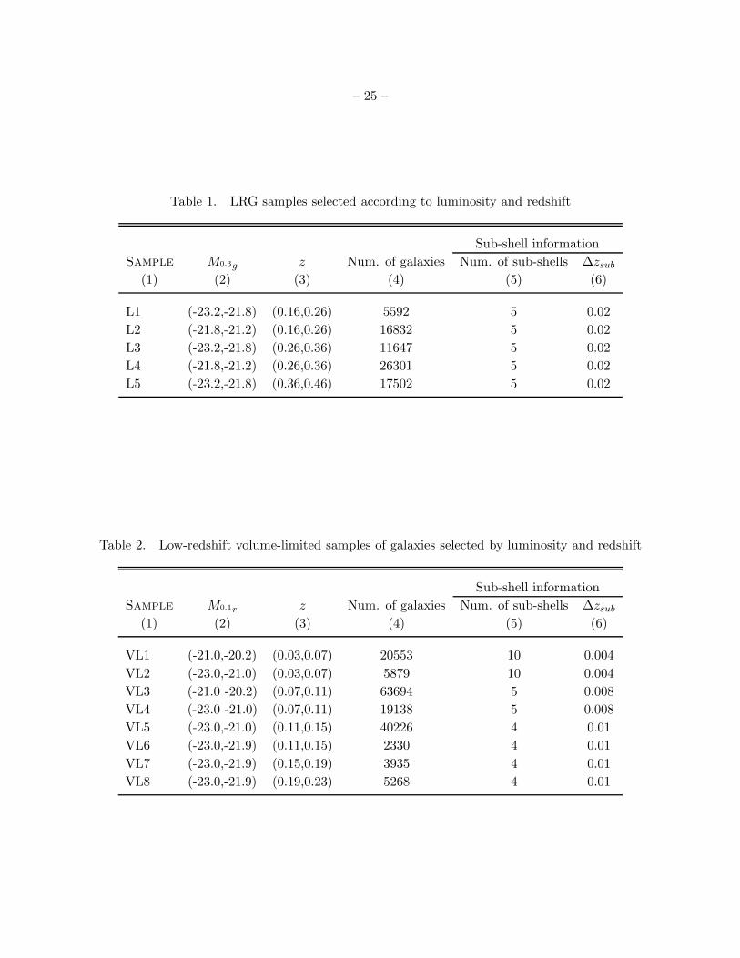
Figure 3 shows the relative difference between the approximated and the true values of the

w(θ)/wp(rp) ratio, (ratioanaly − ratiotrue)/ratiotrue, for Sample 2 galaxies with 0.07 < z2 < 0.078

and −23.0 < M2 < −21.0, and Sample 1 galaxies in several absolute magnitude intervals (as indi-

cated in each panel). The approximated ratio agrees quite well with the true value, at 1% accuracy

or better, for separations rp . 10 Mpc and for all luminosities considered. The discrepancy increases

at larger separations, but well below 3% level even at the largest scale probed (∼ 30Mpc). This

discrepancy mainly comes from the distant-observer approximation adopted here. The accuracy of

– 10 –

Eqn. (13) is expected to be better for higher redshifts where the distant-observer approximation

works better. We thus conclude that our approximation in Eqn. (13) works at substantially high

accuracies for our purpose.

A second test that we have done is to apply our method to spectroscopic samples. Simply

speaking, wp(rp) for a spectroscopic sample can be measured with the redshift information. It can

also be estimated with our method without using the redshift information for the photometric sam-

ple. By comparing the two wp(rp) estimates we are able to understand how well our method works.

For simplicity we consider here a specific case in which a spectroscopic sample of given luminosity

and redshift ranges is cross-correlated with spectroscopic (for the true wp(rp)) or “photometric”

(for the wp(rp) obtained by our method) galaxies in the same ranges. Thus the wp(rp) are reduced

to auto-correlation functions.

The result of this test is shown in Figure 4, where we plot the true wp(rp) in blue curves and the

approximated one in red for SDSS Main galaxies (left column) and LRGs (right column) at different

luminosities and redshifts (indicated in each panel). For LRGs we see good agreement between the

two measurements on all scales and at all redshifts probed (with the difference < 20%). A similar

agreement is seen for the low-redshift samples of −20 < M0.1r < −19 and −21 < M0.1r < −20. All

these results are very encouraging.

However, there is large difference (∼ 50%)between the results of the two methods on large

scales (> 5Mpc/h) for the brightest (−22 < M0.1r < −21) low reshift sample. The deviation may

be caused by a coincident correlation between foreground galaxies in the photometric sample and

the spectroscopic sample. We have performed a further analysis by estimating the cross-correlation

with the foreground, the background, and the right redshift interval separately, for three low-

redshift spectroscopic samples (corresponding to the left-hand panels in Fig. 4). We find that the

contamination comes mainly from the foreground for the brightest sample (−22 < M0.1r < −21),

and from the background for the faintest sample (−20 < M0.1r < −19). For both samples, the

projected cross-correlation wp(rp) with the foreground (for the brightest sample) or the background

(for the faintest sample) shows weak dependence on scale. When compared to the true wp(rp), the

cross-correlation with the foreground/background is negligible on small scales, ∼ 50% smaller at

∼ 10Mpc/h and compatible at ∼ 20Mpc/h. This result clearly shows that the clustering pattern

of the forground/background can contaminate the angular cross correlation function stochastically.

This also explains why we can measure the projected correlation function for the LRG sample

accurately, because the foreground/background galaxies are in big cosmic volumes and thus have

weak correlations themselves.

We conclude that the accuracy of our method relies on the key assumption that foreground/background

galaxies have weak correlation with the spectroscopic galaxies. This assumption is valid for many

real observations, especially for spectroscopic samples at intermediate or high redshift. This is why

we can recover the project correlation function for LRG samples on all scales. For the low red-

shift samples, our method works for the sample of luminosity M∗, since the forground/background

– 11 –

galaxies are relatively small in number compared with those at the redshift of the spectroscopic

sample. For the bright low redshift sample, the foreground galaxies are located in a small volume

and are more numerous, and their clustering pantern can bias the estimation of the projected func-

tion. This effect is smaller for small scales, which is the reason why we can measure the projected

function accurately on scales smaller than ∼ 1 Mpc/h.

3.3.2. Indirect conversion through wp(rp)n

We propose a second method here for estimating wp(rp). Rather than directly converting w(θ)

to wp(rp), we first convert the former to a projected density profile wp(rp)n1, from which we then

estimate wp(rp) by calculating analytically the spatial number density n1 from the luminosity func-

tion. wp(rp)n1 is obtained as a byproduct without suffering from uncertainties in galaxy luminosity

function.

In this method we estimate a weighted angular correlation function w(θ)weight instead of the

traditional function w(θ) as discussed above. This is measured using the same estimators given in

Eqn. (1) and (2), except that each spectroscopic galaxy in Sample 2 is weighted by D−2, inverse

of the square of comoving distance for Sample 2 galaxies. It can be easily proved with Eqn. ( 13)

that for a thin redshift interval of the spectroscopic sample (Sample 2), N1w(θ)weight/Ω equals to

the projected density profile wp(rp)n1, i.e.,

wp(rp)n1 =N1w(θ)weight

Ω, (14)

where N1 and n1 are the number and number density of photometric galaxies in Sample 1, and

Ω the total sky coverage of Sample 1. Given the projected density profile wp(rp)n1 estimated

by Eqn. (14) as well as the spatial number density of galaxies n1 analytically calculated from

the luminosity function, we finally estimate the projected correlation function wp(rp) by dividing

wp(rp)n1 by n1. We emphasize here the projected density profile wp(rp)n1 does not suffer from

uncertainties in luminosity function, because all quantities in the right side of Eqn. (14) can be

obtained from data.

To calculate n1, we adopt the luminosity evolution model and the luminosity function at z = 0.1

from B03 when doing calculation for spectroscopic galaxies at low redshifts (samples selected from

the SDSS Main galaxy catalogue as listed in Table 2). Considering that the evolution model of B03

is based on low-redshift data (z . 0.25), which might not be suitable for higher redshifts, we adopt

the evolution model of Faber et al. (2007) (here after F07) for our LRG samples. Moreover, we

need to convert the F07 model from B-band to the 0.1r-band at which our galaxies are observed.

Assuming that the slope of the luminosity evolution doesn’t depend on waveband, we obtain the0.1r-band luminosity evolution model by simply shifting the amplitude of the B-band model from

F07 so as to have an amplitude at z = 0.1 which is equal to the amplitude of the 0.1r-band model

of B03. In this manner the slopes of the two models remain unmodified, which are Q = −1.23 for

– 12 –

F07 and -1.62 for B03 respectively (see their papers for details)5.

In conclusion, the projected cross-correlation function wp(rp) can be measured either from

Eqn. (13) by direct conversion of w(θ), or from Eqn. (14) by indirect conversion through esti-

mating wp(rp)n. After having made extensive comparisons, we found that the two methods give

rise to almost identical results. In what follows we choose to use the second method only, as it

simultaneously provides both wp(rp) and wp(rp)n.

3.4. Division and combination of redshift subsamples

In this subsection we address an important issue which we have ignored so far. As mentioned

above, our method for selecting photometric galaxies according to luminosity and redshift is valid

only when the redshift interval z2 − z1 is small enough. However, the redshift intervals used to

select our spectroscopic galaxy samples apparently do not satisfy this condition. For example, for

a redshift range of 0.16 < z < 0.26 and an absolute magnitude interval of Mp,2 −Mp,1 = 0.5, the

photometric galaxies selected will cover a much broader apparent magnitude range, mp,2 −mp,1 =

1.7.

Our solution is to further divide the galaxies in a given spectroscopic sample into a number of

subsamples which are equally spaced in redshift (hereafter called redshift sub-shells). See Tables 1

and 2 for the number of redshift sub-shells adopted for our samples. For a given sample, we

measure the weighted angular cross-correlation function w(θ)weight (see above) for each sub-shell

separately by cross-correlating with galaxies selected from the photometric catalogue in the way

described above according to the expected luminosity range and the redshift range of the sub-

shell. Each w(θ)weight measurement is then converted to give the corresponding projected density

profile wp(rp)n as well as the projected cross-correlation function wp(rp), using the second method

described above. Estimates of these quantities for the sub-shells are then averaged to give the

estimates for their parent sample as a whole. In this procedure each sub-shell is weighted by Vi/σ2i ,

with Vi being the comoving volume covered by the ith sub-shell and σ2i the variance of wp(rp)n or

wp(rp) of the sub-shell. In order to estimate σi we have generated 100 bootstrap samples for each

sub-shell. The variance σi of a sub-shell is then estimated by the 1σ scatter between all its bootstrap

samples. This weighting scheme ensures the averaged wp(rp)n or wp(rp) to be determined largely

by sub-shells with relatively large volume and high signal-to-noise ratio (S/N) measurements, thus

effectively reducing the overall sampling noise and cosmic variance.

In order to increase the accuracy of our method, one may want to increase the number of sub-

shells for a given redshift range, at the cost of increasing both the sampling noise and the large-scale

structure noise (the cosmic variance). In practice, we split a spectroscopic sample into redshift sub-

shells by requiring ∆z/z . 0.1, where ∆z is the thickness of the sub-shells and z is the mean redshift

5We have repeated our analysis for LRGs, adopting Q = −1.62 instead of Q = −1.23, and obtained similar results.

– 13 –

of the sample. With this restriction the difference between m2 − m1 and M2 − M1 ranges from

∼ 0.25 occurring for low-redshift sub-shells to ∼ 0.1 for high-redshift ones. Extensive tests show

that our results are robust to reasonable change of the thickness of sub-shells. For instance, taking

Sample L1 from Table 1 as the spectroscopic sample, the cross-correlation function measured by

10 sub-shells differs from the one of 5 sub-shells by at most 10% for photometric galaxies with

−22 < M < −21.5, and by only about 3% for the faintest luminosity bin (−19.5 < M < −19.0).

3.5. Error estimation

We estimate the error in the averaged wp(rp)n or wp(rp) by

∆ =

√

σ2 × χ2

dof. if χ2

dof. > 1

σ if χ2

dof. ≤ 1,(15)

with

σ2 =

Nsub∑

i=1

V 2i

σ2i

/(

Nsub∑

i=1

Vi

σ2i

)2

, (16)

χ2/dof. =1

Nsub − 1

Nsub∑

i=1

(xi − xavg)2 σ−2

i , (17)

where the sum goes over all the sub-shells of a given spectroscopic sample; xi is the measurement

of wp(rp)n or wp(rp) of the ith sub-shell and xavg the average measurement for all the sub-shells

as a whole; Nsub is the number of sub-shells. Overall, Eqn. (15) should be able to include both the

volume effect (through factor Vi) and the sampling noise (through σi), thus providing a reasonable

estimate of the errors in our measurements. By weighting the error by√

χ2

dof. , we mean to take into

account the large variation from sub-shell to sub-shell in some cases.

To better understand the error contribution from different redshift sub-shells, we plot in Fig-

ure 5 the wp(rp) measurements for Sample L1 listed in Table 1. Different panels correspond to

photometric galaxies in different luminosity intervals. In each panel, we plot wp(rp) for all the five

sub-shells with their redshift ranges indicated in the bottom-right panel. Error bars on the wp(rp)

curves are estimated using the bootstrap resampling technique, i.e. σi in Eqn. (16) and (17). We

see that, for photometric galaxies at fixed luminosity, wp(rp) measurements of different sub-shells

are almost on top of each other, indicating that the scatter between sub-shells is fairly small. This

again shows that the correlation functions measured with our method are insensitive to the number

of redshift sub-shells.

We note that the overall error increases rapidly with luminosity at the bright end. This

reflects not only the sampling noise of the small samples, but more importantly, also an effect of

a huge foreground population which significantly suppresses the angular cross-correlation signals.

– 14 –

Letting w′(θ) be the angular correlation function between a spectroscopic sample with z1 < z < z2and a photometric sample including galaxies of all redshifts, and w(θ) the one between the same

spectroscopic sample and a sample of photometric galaxies within z1 < z < z2, one can easily show

that

w′(θ) =NGS

NGw(θ), (18)

where NG and NGS are respectively the number of photometric galaxies in the full sample and in

the redshift range z1 < z < z2. In this case the estimated correlation signal is suppressed by a

factor of NGS

NG, a large effect in particular when NG ≫ NGS as in bright samples.

This is explained more clearly in Figure 6 where we plot the redshift distribution as calculated

using the luminosity function of B03 for photometric galaxies which are selected according to

luminosity and redshift using the method described in § 3.1. Plotted in different lines are the

distributions for different luminosity ranges with redshift range fixed to 0.2 < z < 0.22. According

to our method of dividing photometric sample into luminosity subsamples, photometric galaxies

selected to serve our purpose of a certain luminosity bin have the desired luminosity at the chosen

redshift. As can be seen from the figure, in the brightest luminosity interval (−22.5 < M0.1r <

−22.0, solid line) only a small fraction of the galaxies are located within the expected redshift

range, where the majority of galaxies are intrinsically fainter. It is this population that suppresses

the angular cross-correlations that we measure at the bright end, leading to large uncertainties in

wp(rp), as seen in Figure 5.

Before we apply our method to SDSS data in the next section, we should point out that,

although we have carefully considered both the sampling noise and the large-scale structure noise,

our error estimation doesn’t include the projection effect caused by background and foreground

galaxies. Thus when interpreting our wp(rp)n and wp(rp) presented below, one should keep in mind

that their errors are underestimated to varying degrees, depending on the redshift and luminosity

we consider.

4. Applications to SDSS galaxies

4.1. Projected cross-correlations and density profiles of LRGs

In Figure 7 we show the projected density profile wp(rp)n for LRGs in different intervals of

luminosity and redshift, as traced by surrounding photometric galaxies of different luminosities.

Results are plotted for LRGs with −23.2 < M0.3g < −21.8 in panels on the left and for those with

−21.8 < M0.3g < −21.2 on the right, with panels from top to bottom corresponding to different

redshift bins. The wp(rp)n traced by photometric galaxies in different luminosity ranges are shown

using different lines as indicated in the bottom-right panel. As can be seen, the projected number

density of galaxies around central LRGs decreases as their luminosity increases. This is true for

all redshifts and all scales probed. In particular, such luminosity dependence is weak for galaxies

– 15 –

fainter than the characteristic luminosity of the Schechter luminosity function (M0.1r = −20.44 for

the SDSS), and becomes remarkable for brighter galaxies. The change of the amplitude mainly

reflects the number density of galaxies as a function of their luminosity. From the figure one can

easily read out the number of galaxies in the host halo of the LRGs. For example, on average there

are about 3 galaxies of −20.5 < M < −20 in the host halo of a LRG in Sample L1, assuming the

host halo radius is 0.3h−1Mpc.

In Figure 8 we show projected cross-correlation function wp(rp) obtained from the wp(rp)n

measurements shown in Figure 7, for the same set of LRG samples and the same intervals of

photometric galaxy luminosity. At fixed scale and redshift, the amplitude of wp(rp) increases with

increasing luminosity, a trend which has already been well established by previous studies. It is

interesting to see from both figures that, although both wp(rp)n and wp(rp) show systematic trends

with luminosity in amplitude, their slope remains fairly universal for given redshift and central

galaxy luminosity, regardless of the luminosity of surrounding galaxies we consider. This provides

direct observational evidence that satellite galaxies of different luminosities follow the distribution

of dark matter in the same way within their dark matter halos, an assumption adopted in many

previous studies on HOD modeling of galaxy distribution.

In Figure 9 we plot the wp(rp) again in order to explore the evolution with redshift. Measure-

ments of different photometric galaxy luminosities are shown in different panels, while in each panel

we compare wp(rp) measured at different redshifts for fixed luminosity. Note that in this figure

we have considered the luminosity evolution of galaxies, as we aim to study how the projected

density distribution and cross-correlation around the LRGs have evolved over the redshift range

probed. We do not include E-correction in Figures 5,7 and 8, because we want the results there

to be less affected by possible uncertainty in the luminosity evolution model. From Figure 9, we

see significant increase in the amplitude of wp(rp) as redshift goes from z = 0.4 to 0.2. Taking the

−21.0 < M < −20.5 bin in the left column for example, on average the wp(rp) amplitude differs

by a factor of about 2 between the result of z ∼ 0.2 (blue curve) and z ∼ 0.4 (green curve) at

separations rp < 0.3h−1Mpc, the typical boundary of LRG host halos.

It is important to understand whether the significant evolution seen above could be explained

purely by evolution in dark matter distribution, or additional processes related to galaxies them-

selves are necessary. To the end we have done a simple calculation as follows. We assume that

there is no merger occurring between galaxies or between their host halos. In this case all galaxies

and halos have been evolving in a passive manner, and the total number of each keeps unchanged

during the period in consideration. Thus galaxies at different redshifts are the same population

which are hosted by the same set of halos. We calculate a dark matter density profile averaged

over all dark matter halos that are expected to host LRGs of given redshift and luminosity, by

ρavg(r) =

∫Mmax

Mminρ(r,M)n(M) dM

∫Mmax

Mminn(M) dM

, (19)

where n(M) is the halo mass function from Sheth & Tormen (1999), and ρ(r,M) is the density

– 16 –

profile of halos of mass M assumed to be in the NFW form (Navarro et al. 1997). We determine

the concentration parameter c of halos following Zhao et al. (2009). The lower and upper limits of

halo mass (Mmin and Mmax) are determined by matching the abundance of LRGs in our sample

with that of dark matter halos given by the Sheth-Tormen mass function (Sheth & Tormen 1999).

For this we have adopted the plausible assumption that the luminosity of a central galaxy is an

increasing function of the mass of its halo.

We consider three redshifts which are z =0.21, 0.31 and 0.41, approximately the median

redshifts of our LRG samples. The dark matter density within 0.3h−1 Mpc around LRGs of

−23.2 < M0.3g < −21.8 is predicted to increase by 24.6% from z ∼ 0.4 to ∼ 0.2, and 12.1% from

z ∼ 0.3 and ∼ 0.2. The factor is 10.6% for −21.8 < M0.3g < −21.2 from z ∼ 0.3 to ∼ 0.2. It is

clear that these predictions are much smaller when compared to what we have obtained from the

SDSS data. As can be seen from Figure 9, at rp < 0.3h−1Mpc, the clustering amplitude changes

by a factor of ∼2 between z ∼ 0.4 and ∼ 0.2, and by 20 - 50% between z ∼ 0.3 and ∼ 0.2.

This simple calculation seems to suggest that the evolution of galaxy clustering observed in this

work is caused not only by the evolution of the underlying dark matter, but also by the evolution

of galaxies themselves. However, this argument should not be overemphasized. As selected in r-

band, our photometric sample may be biased to bluer galaxies as one goes to higher redshifts. This

selection effect must be properly taken into account when one addresses the evolution of galaxy

clustering, but such a detailed modeling is out of the scope of our current paper.

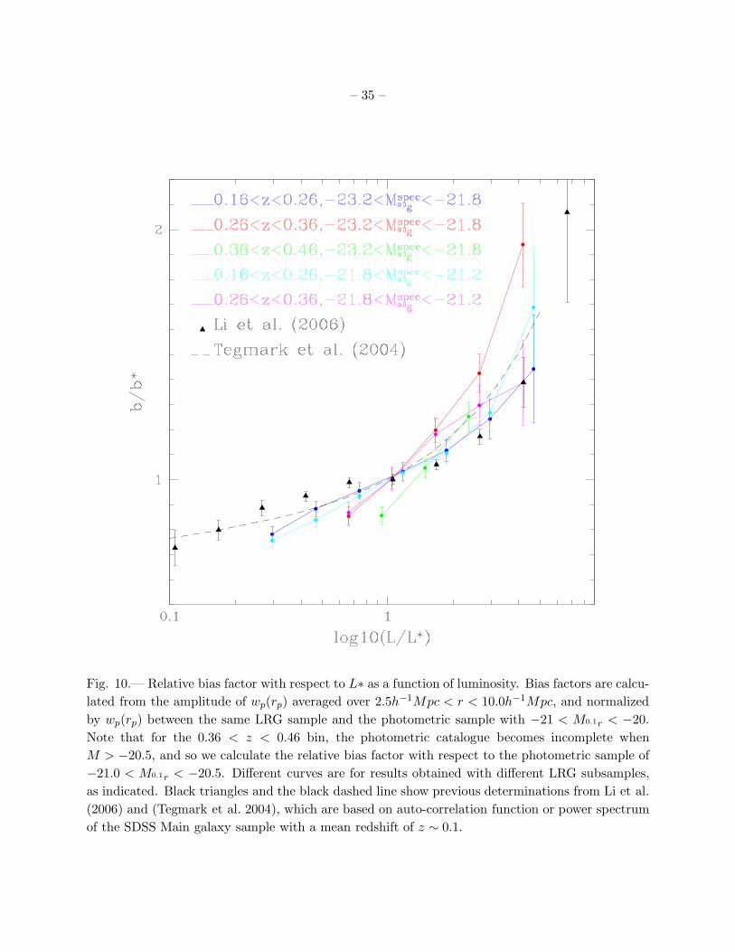
Figure 10 shows the relative bias factor of photometric galaxies with respect to L∗ galaxies

as a function of luminosity. Taking a LRG sample, the bias factor for a sample of photometric

galaxies at given luminosity and redshift is calculated from the amplitude of the wp(rp) between

the LRG and the photometric samples, normalized by the wp(rp) of the same LRG sample with

a photometric sample selected by −21 < M0.1r < −20 (K− and E−corrected to z = 0.1) 6, and

averaged over separations between rp = 2.5h−1Mpc and 10h−1Mpc. The bias factor so obtained

should be virtually identical to the one estimated from the auto-correlation function of the same

set of photometric galaxies. In the figure, curves in different colors refer to results from different

LRG samples in Table 1. Since the photometric sample becomes somewhat incomplete for L . L∗

in the redshift range 0.36 < z < 0.46, the bias factor for this sample (the green line in the figure)

is normalized with respect to a −21.0 < M0.1r < −20.5 sample instead of the −21 < M0.1r < −20

one. Plotted in black triangles is the result of Li et al. (2006). Black dashed line is a fit obtained

from the SDSS power spectrum by Tegmark et al. (2004). Relative bias factors at 0.16 < z < 0.26

(Samples L1 and L2) are well consistent with those previous studies at all luminosities, except the

bright end where our measurement is slightly lower than that from Tegmark et al. (2004). Our

bias factor measurements show that the luminosity dependence of galaxy clustering observed in the

local Universe is very similar to that at intermediate redshift z ∼ 0.4.

6The absolute magnitude range for selecting L∗ samples varies from sub-shell to sub-shell for the photometric

galaxies, so that the corresponding absolute magnitude range at z = 0.1 is always −21 < M0.1r < −20.

– 17 –

4.2. Projected density profiles and clustering of low-z galaxies

We have also measured wp(rp)n and wp(rp) for the eight volume limited samples of low-redshift

galaxies listed in Table 2 and for different intervals of photometric galaxy luminosity. Since the

volume covered by these spectroscopic samples is small due to their small redshift intervals, the

wp(rp)n and wp(rp) measurements are more noisy than presented above for the LRG samples. In

order to improve the S/N of our measurements, for a given luminosity interval of photometric

galaxies we combine the measurements for spectroscopic samples that share a same luminosity

interval but span different redshift ranges. When doing the combination we weight each sample by

its comoving volume divided by the variance of the measurement, in the same way as above when

combining redshift sub-shells. The combined wp(rp)n are plotted in Figure 11. We do not include

independent plots for wp(rp), which show behaviors very similar to wp(rp)n.

In Figure 12 we show the corresponding relative bias factors, based on data points over 1.9 ≤

rp ≤ 10h−1Mpc. Results are plotted in blue, red and green curves for the three luminosity intervals

of spectroscopic galaxies. For comparison we also repeat the bias factors from previous work by

Tegmark et al. (2004) and Li et al. (2006) which are based on spectroscopic samples similar to those

used here. Our measurements are roughly in agreement with these previous determinations. Our

bias factors from the three samples agree with each other at the intermediate luminosities around

L∗, while showing obvious deviations at the bright and faint ends. Again, these differences should

not be regarded as significant due to large uncertainties.

Similar to what is found for LRGs at z ∼ 0.4, the density profiles around galaxies in the local

universe also shows quite similar slope, independent of the luminosity of surrounding photometric

galaxies. Unlike in the LRG samples, the spectroscopic galaxies in our low-redshift samples could

be either centrals or satellites of their host halos. However, the fraction of satellites should be

small as the spectroscopic objects in the SDSS are relatively bright (Zheng et al. 2007). Thus our

conclusion made above for z ∼ 0.4 more or less holds for the local Universe, that is, satellite galaxies

of different luminosities are distributed within their halos in a similar way, if the halos host central

galaxies of similar luminosity. This is consistent with previous studies (e.g. Vale & Ostriker 2004,

2006; Zheng et al. 2007) which have revealed a tight relation between central galaxy luminosity 〈Lc〉

and halo mass. Moreover, halo occupation distribution models usually assume galaxy distribution

inside halos to trace their dark matter, based on studies of satellite distributions in simulations (e.g.

Nagai & Kravtsov 2005; Maccio et al. 2006). Again, our results provide additional, clear evidence

for supporting this assumption.

5. Discussion and Summary

Previous studies on galaxy clustering as a function of luminosity usually make use of spec-

troscopic galaxy catalogue, thus are limited to relatively bright galaxies and low redshifts. In

this work we have developed a new method which measures simultaneously the projected number

– 18 –

density profile wp(rp)n and the projected cross-correlation function wp(rp) of a set of photomet-

ric galaxies, surrounding a set of spectroscopic galaxies. We are able to divide the photometric

galaxies by luminosity even when redshift information is unavailable. This enables us to measure

wp(rp)n and wp(rp) as a function of not only the luminosity of the spectroscopic galaxies, but also

that of the surrounding photometric galaxies. Since photometric samples are usually much larger

and fainter than spectroscopic ones, with our method one can explore the clustering of galaxies to

fainter luminosities at high redshift.

We have applied our method to the SDSS data including a sample of 105 luminous red galaxy

(LRGs) at z ∼ 0.4 and a sample of about half a million galaxies at z ∼ 0.1. Both are cross-correlated

with an SDSS photometric sample consisting of about 20 million galaxies down to r = 21. We have

investigated the dependence of wp(rp)n and wp(rp) on galaxy luminosity and redshift, by dividing

both spectroscopic and photometric galaxies into various luminosity intervals and different redshift

ranges.

The conclusions of this paper can be summarized as follows.

• We develop a new method which measures the projected density distribution wp(rp)n of

photometric galaxies surrounding a set of spectroscopically-identified galaxies, and simulta-

neously the projected cross-correlation function wp(rp) between the two populations. In this

method we are able to divide the photometric galaxies into subsamples in luminosity intervals

even when redshift information is unavailable, enabling us to measure wp(rp)n and wp(rp) as

a function of not only the luminosity of the spectroscopic galaxy, but also that of the pho-

tometric galaxy. Extensive tests show that our method can measure wp(rp) in a statistically

unbiased way. The accuracy of the measurement depends on the validity of the assumption

inherent to the method that the foreground/background galaxies are randomly distributed

and are thus uncorrelated with those galaxies of interest. Therefore, our method can be

applied to the cases where foreground/baground galaxies are distributed in large volumes,

which is usually valid in real observations.

• We find that, for a spectroscopic sample at given luminosity and redshift, the projected cross-

correlation function and projected density profile as traced by photometric galaxies show quite

similar slope to each other, independent of the luminosity of the photometric galaxies. This

indicates that satellite galaxies of different luminosities are distributed in a similar way within

their host dark matter halos. This is true not only for LRGs at intermediate redshifts which

are mostly central galaxies of their halos, but also for the general population of galaxies in

the local Universe. Our result provides observational support for the assumption commonly-

adopted in halo occupation distribution models that the distribution of galaxies follows the

dark matter distribution within their halos.

• The relative bias factors are estimated for photometric galaxies as a function of luminosity

and redshift. In particular, we measured the bias factors of such kind, for the first time, for

galaxies at intermediate redshift (z ∼ 0.4) over a wide range in luminosity (0.3L∗ < L < 5L∗).

– 19 –

There have been previous studies of measuring galaxy clustering by cross-correlations with

imaging data. Although the methods and purposes of these studies are different from ours, it

is worthy of mentioning them and pointing out the findings in common. Eisenstein et al. (2005)

measured the mean overdensity around LRGs in an earlier SDSS release by cross-correlating 32,000

LRGs with 16 million photometric galaxies, using the deprojecting method developed in (Eisenstein

2003). The authors were aimed at understanding the scale- and luminosity-dependence of the

clustering of LRGs, thus using only L∗ galaxies from the photometric sample as a tracer of the

surrounding distribution. In our work we consider luminosity dependence for both LRGs and

photometric galaxies, and this is why we have made considerable efforts on selecting photometric

galaxies of specific luminosities. Our measurements from cross-correlation with L∗ galaxies show

strong dependence in wp(rp) amplitude on LRG luminosity, as well as an obvious transition at

around 1 Mpc/h, which are in agreement with what those authors find.

Masjedi et al. (2006) measured the cross-correlation between ∼25,000 LRGs and an imaging

sample, in order to correct for the effect of fiber collisions on their small-scale measurements of

LRG auto-correlations. They find that the real-space auto-correlation function of LRGs, ξ(r), is

surprisingly close to a r−2 power law over more than 4 orders of magnitude in separation r, down to

r ∼ 15 kpc/h. We don’t have a measurement of auto-correlations ξ(r) or wp(rp) for LRGs, but our

results are not inconsistent with theirs in the sense that the projected cross-correlation of our LRG

samples continuously increases at such small scales, with a slope similar to that on large scales. In

a recent work, White et al. (2011) studied the clustering of massive galaxies at z ∼ 0.5 using the

first semester of BOSS data. The authors computed the projected cross-correlation between their

imaging catalogue and the spectroscopic one, as an additional analysis to emphasize that there is

a significant power on scales below 0.3 Mpc/h where their spectroscopy-based measurements suffer

from fiber collisions. This is obviously consistent with what we have seen from our measurements.

Our method can be applied and extended to many important statistical studies of galaxy for-

mation and evolution. By dividing galaxies into red and blue populations in the photometric sample

according to their colors, we can quantify the evolution of the blue fraction of galaxies in clusters

and groups from redshift 0.4 to the present day (i.e the Butcher-Oemler effect, e.g. Goto et al.

2003; De Propris et al. 2004). Wide deep photometry surveys, such as Pan-Starrs (Kaiser 2004)

and LSST (Tyson 2002), will be available in the next years. Combining such surveys with large

spectroscopic samples, such as BOSS LRG samples, will allow one to explore the clustering of

galaxies from z = 0 up to z = 1 for a wide range of luminosities. The WISE (Wright et al. 2010)

will produce an all-sky catalogue of infrared galaxies. By combining this survey with SDSS spec-

troscopic samples, one can study how infrared galaxies are distributed relative to the network of

optical galaxies.

This work is supported by NSFC (10821302, 10878001), by the Knowledge Innovation Program

of CAS (No. KJCX2-YW-T05), by 973 Program (No. 2007CB815402), and by the CAS/SAFEA

International Partnership Program for Creative Research Teams (KJCX2-YW-T23).

– 20 –

REFERENCES

Abazajian, K. N., et al. 2009, ApJS, 182, 543

Bardeen, J. M., Bond, J. R., Kaiser, N., & Szalay, A. S. 1986, ApJ, 304, 15

Benson, A. J., Baugh, C. M., Cole, S., Frenk, C. S., & Lacey, C. G. 2000, MNRAS, 316, 107

Berlind, A. A., & Weinberg, D. H. 2002, ApJ, 575, 587

Blanton, M. R., et al. 2003, ApJ, 592, 819

Blanton, M. R., Lin, H., Lupton, R. H., Maley, F. M., Young, N., Zehavi, I., & Loveday, J. 2003,

AJ, 125, 2276

Blanton, M. R., et al. 2005, AJ, 129, 2562

Blanton, M. R., & Roweis, S. 2007, AJ, 133, 734

Carlberg, R. G., Yee, H. K. C., Morris, S. L., Lin, H., Hall, P. B., Patton, D. R., Sawicki, M., &

Shepherd, C. W. 2001, ApJ, 563, 736

Chen, J., Kravtsov, A. V., Prada, F., Sheldon, E. S., Klypin, A. A., Blanton, M. R., Brinkmann,

J., & Thakar, A. R. 2006, ApJ, 647, 86

Coil, A. L., et al. 2004, ApJ, 609, 525

Coil, A. L., Newman, J. A., Cooper, M. C., Davis, M., Faber, S. M., Koo, D. C., & Willmer,

C. N. A. 2006, ApJ, 644, 671

Coil, A. L., et al. 2008, ApJ, 672, 153

Colberg, J. M., et al. 2000, MNRAS, 319, 209

Colless, M., et al. 2001, MNRAS, 328, 1039

Cooray, A., & Sheth, R. 2002, Phys. Rep., 372, 1

Davis, M., & Peebles, P. J. E. 1983, ApJ, 267, 465

Davis, M., Efstathiou, G., Frenk, C. S., & White, S. D. M. 1985, ApJ, 292, 371

Davis, M., et al. 2003, Proc. SPIE, 4834, 161

de la Torre, S., et al. 2009, arXiv:0911.2252

De Propris, R., et al. 2004, MNRAS, 351, 125

Eisenstein, D. J., et al. 2001, AJ, 122, 2267

– 21 –

Eisenstein, D. J. 2003, ApJ, 586, 718

Eisenstein, D. J., Blanton, M., Zehavi, I., Bahcall, N., Brinkmann, J., Loveday, J., Meiksin, A., &

Schneider, D. 2005, ApJ, 619, 178

Faber, S. M., et al. 2007, ApJ, 665, 265

Firth, A. E., et al. 2002, MNRAS, 332, 617

Goto, T., Yamauchi, C., Fujita, Y., Okamura, S., Sekiguchi, M., Smail, I., Bernardi, M., & Gomez,

P. L. 2003, MNRAS, 346, 601

Goto, T., et al. 2003, PASJ, 55, 739

Guo, Q., White, S., Li, C., & Boylan-Kolchin, M. 2010, MNRAS, 404, 1111

Hamilton, A. J. S. 1993, ApJ, 417, 19

Hamilton, A. J. S., & Tegmark, M. 2002, MNRAS, 330, 506

Jing, Y. P. 1998, ApJ, 503, L9

Jing, Y. P., Mo, H. J., & Boerner, G. 1998, ApJ, 494, 1

Jing, Y. P., & Boerner, G. 1998, ApJ, 503, 37

Kaiser, N. 1984, ApJ, 284, L9

Kaiser, N. 2004, Proc. SPIE, 5489, 11

Kauffmann, G., Nusser, A., & Steinmetz, M. 1997, MNRAS, 286, 795

Kauffmann, G., Colberg, J. M., Diaferio, A., & White, S. D. M. 1999, MNRAS, 303, 188

Kazin, E. A., et al. 2010, ApJ, 710, 1444

Larson, D., et al. 2010, arXiv:1001.4635

Lake, G., & Tremaine, S. 1980, ApJ, 238, L13

Le Fevre, O., et al. 2005, A&A, 439, 845

Li, C., Kauffmann, G., Jing, Y. P., White, S. D. M., Borner, G., & Cheng, F. Z. 2006, MNRAS,

368, 21

Li, C., Jing, Y. P., Kauffmann, G., Borner, G., Kang, X., & Wang, L. 2007, MNRAS, 376, 984

Lilly, S. J., et al. 2007, ApJS, 172, 70

– 22 –

Lorrimer, S. J., Frenk, C. S., Smith, R. M., White, S. D. M., & Zaritsky, D. 1994, MNRAS, 269,

696

Ma, C.-P., & Fry, J. N. 2000, ApJ, 543, 503

Maccio, A. V., Moore, B., Stadel, J., & Diemand, J. 2006, MNRAS, 366, 1529

Madgwick, D. S., et al. 2003, MNRAS, 344, 847

Masjedi, M., et al. 2006, ApJ, 644, 54

Meneux, B., et al. 2006, A&A, 452, 387

Meneux, B., et al. 2008, A&A, 478, 299

Meneux, B., et al. 2009, A&A, 505, 463

Mo, H. J., & White, S. D. M. 1996, MNRAS, 282, 347

Nagai, D., & Kravtsov, A. V. 2005, ApJ, 618, 557

Navarro, J. F., Frenk, C. S., & White, S. D. M. 1997, ApJ, 490, 493

Norberg, P., et al. 2002, MNRAS, 332, 827

Norberg, P., et al. 2001, MNRAS, 328, 64

Okumura, T., Jing, Y. P., & Li, C. 2009, ApJ, 694, 214

Peacock, J. A., & Dodds, S. J. 1996, MNRAS, 280, L19

Peacock, J. A., & Smith, R. E. 2000, MNRAS, 318, 1144

Phillipps, S., & Shanks, T. 1987, MNRAS, 229, 621

Phleps, S., Peacock, J. A., Meisenheimer, K., & Wolf, C. 2006, A&A, 457, 145

Reid, B. A., & Spergel, D. N. 2009, ApJ, 698, 143

Ross, A. J., Brunner, R. J., & Myers, A. D. 2007, ApJ, 665, 67

Sales, L., & Lambas, D. G. 2005, MNRAS, 356, 1045

Schechter, P. 1976, ApJ, 203, 297

Scoccimarro, R., Sheth, R. K., Hui, L., & Jain, B. 2001, ApJ, 546, 20

Seljak, U., & Zaldarriaga, M. 1996, ApJ, 469, 437

Seljak, U. 2000, MNRAS, 318, 203

– 23 –

Seljak, U., & Warren, M. S. 2004, MNRAS, 355, 129

Shepherd, C. W., Carlberg, R. G., Yee, H. K. C., Morris, S. L., Lin, H., Sawicki, M., Hall, P. B.,

& Patton, D. R. 2001, ApJ, 560, 72

Sheth, R. K., & Tormen, G. 1999, MNRAS, 308, 119

Tegmark, M., Hamilton, A. J. S., & Xu, Y. 2002, MNRAS, 335, 887

Tegmark, M., et al. 2004, ApJ, 606, 702

Tinker, J. L., Weinberg, D. H., Zheng, Z., & Zehavi, I. 2005, ApJ, 631, 41

Tyson, J. A. 2002, Proc. SPIE, 4836, 10

Vader, J. P., & Sandage, A. 1991, ApJ, 379, L1

Vale, A., & Ostriker, J. P. 2006, MNRAS, 371, 1173

Vale, A., & Ostriker, J. P. 2004, MNRAS, 353, 189

Wang, L., & Jing, Y. P. 2010, MNRAS, 402, 1796

Westra, E., Geller, M. J., Kurtz, M. J., Fabricant, D. G., Dell’Antonio, I., Astrophysical Observa-

tory, S., & University, B. 2010, arXiv:1006.2823

White, M., et al. 2010, arXiv:1010.4915

White, S. D. M., & Rees, M. J. 1978, MNRAS, 183, 341

White, S. D. M., & Frenk, C. S. 1991, ApJ, 379, 52

White, M., et al. 2011, ApJ, 728, 126

Wright, E. L., et al. 2010, AJ, 140, 1868

Yang, X., Mo, H. J., & van den Bosch, F. C. 2003, MNRAS, 339, 1057

York, D. G., et al. 2000, AJ, 120, 1579

Zaldarriaga, M., & Seljak, U. 2000, ApJS, 129, 431

Zaldarriaga, M., Seljak, U., & Bertschinger, E. 1998, ApJ, 494, 491

Zehavi, I., et al. 2002, ApJ, 571, 172

Zehavi, I., et al. 2005, ApJ, 621, 22

Zehavi, I., et al. 2005, ApJ, 630, 1

– 24 –

Zehavi, I., et al. 2010, arXiv:1005.2413

Zhao, D. H., Jing, Y. P., Mo, H. J., Borner, G. 2009, ApJ, 707, 354

Zheng, Z., et al. 2005, ApJ, 633, 791

Zheng, Z., Coil, A. L., & Zehavi, I. 2007, ApJ, 667, 760

This preprint was prepared with the AAS LATEX macros v5.0.

– 25 –

Table 1. LRG samples selected according to luminosity and redshift

Sub-shell information

Sample M0.3g z Num. of galaxies Num. of sub-shells ∆zsub(1) (2) (3) (4) (5) (6)

L1 (-23.2,-21.8) (0.16,0.26) 5592 5 0.02

L2 (-21.8,-21.2) (0.16,0.26) 16832 5 0.02

L3 (-23.2,-21.8) (0.26,0.36) 11647 5 0.02

L4 (-21.8,-21.2) (0.26,0.36) 26301 5 0.02

L5 (-23.2,-21.8) (0.36,0.46) 17502 5 0.02

Table 2. Low-redshift volume-limited samples of galaxies selected by luminosity and redshift

Sub-shell information

Sample M0.1r z Num. of galaxies Num. of sub-shells ∆zsub(1) (2) (3) (4) (5) (6)

VL1 (-21.0,-20.2) (0.03,0.07) 20553 10 0.004

VL2 (-23.0,-21.0) (0.03,0.07) 5879 10 0.004

VL3 (-21.0 -20.2) (0.07,0.11) 63694 5 0.008

VL4 (-23.0 -21.0) (0.07,0.11) 19138 5 0.008

VL5 (-23.0,-21.0) (0.11,0.15) 40226 4 0.01

VL6 (-23.0,-21.9) (0.11,0.15) 2330 4 0.01

VL7 (-23.0,-21.9) (0.15,0.19) 3935 4 0.01

VL8 (-23.0,-21.9) (0.19,0.23) 5268 4 0.01

– 26 –

Fig. 1.— Redshift histograms for luminous red galaxies (LRGs) in our sample falling in the two

luminosity intervals, as indicated, which we use to select our subsamples in Table 1. The g-band

absolute magnitude M0.3g is K− and E− corrected to its value at z = 0.3.

– 27 –

Fig. 2.— Redshift histograms for spectroscopic galaxies in our low-redshift sample in three different

luminosity ranges as indicated, which we use to select our subsamples in Table 2. The r-band

absolute magnitude M0.1g is K− and E− corrected to its value at z = 0.1.

– 28 –

-21.0<M<-20.5 -20.5<M<-20.0 -20.0<M<-19.5 -19.5<M<-19.0

-19.0<M<-18.5 -18.5<M<-18.0 -18.0<M<-17.5 -17.5<M<-17.0

Fig. 3.— Relative difference in w(θ)/wp(rp) ratio between the value from Eqn. (13) and the value

from theoretical calculation (see § 3.3.1 for details), for spectroscopic galaxies at 0.07 < z < 0.078

and photometric galaxies at different luminosities, as indicated in each panel.

– 29 –

main galaxies LRGs

Fig. 4.— Plotted in each panel (red symbols connected by a red line) is wp(rp) of spectroscopic

galaxies at given luminosity and redshift ranges (as indicated), estimated from cross-correlation

with photometric galaxies in the same luminosity and redshift ranges. This is compared to the

projected auto-correlation correlation function of the same set of spectroscopic galaxies, as plotted

in blue symbols/lines. Panels in the left-hand columns are for galaxies in the low-redshift sample

and those in the right are for LRGs.

– 30 –

0.16<z<0.180.18<z<0.200.20<z<0.220.22<z<0.240.24<z<0.26

-22.5<M<-22.0 -22.0<M<-21.5 -21.5<M<-21.0 -21.0<M<-20.5

-20.5<M<-20.0 -20.0<M<-19.5 -19.5<M<-19.0

Fig. 5.— Projected cross-correlation function wp(rp) for redshift sub-shells of Sample L1 in Table 1,

estimated by cross correlating each sub-shell with photometric galaxies in different luminosity

intervals as indicated in each panel. Different lines are for different sub-shells with their redshift

ranges indicated in the bottom-right panel.

– 31 –

Fig. 6.— Redshift distribution as predicted by the luminosity function from Blanton et al. (2003)

for photometric galaxies that are expected to fall in the indicated luminosity intervals if they were

located in the redshift range 0.2 < z < 0.22. The two vertical lines mark the redshift range.

– 32 –

0.16<z<0.26

0.26<z<0.36

0.36<z<0.46

0.16<z<0.26

0.26<z<0.36

-22.0<M<-21.5-21.5<M<-21.0-21.0<M<-20.5-20.5<M<-20.0-20.0<M<-19.5-19.5<M<-19.0

Fig. 7.— Projected density profile wp(rp)n in units of Mpc−2h2 surrounding LRGs with different

luminosities (indicated above the figure) and redshifts (indicated in each panel), as traced by

galaxies of different luminosities (shown in different lines in each panel and indicated in the bottom-

right panel).

– 33 –

0.16<z<0.26

0.26<z<0.36

0.36<z<0.46

0.16<z<0.26

0.26<z<0.36

-22.0<M<-21.5-21.5<M<-21.0-21.0<M<-20.5-20.5<M<-20.0-20.0<M<-19.5-19.5<M<-19.0

Fig. 8.— Projected cross-correlation function wp(rp) measured for the same set of LRG samples

and the same intervals of photometric galaxy luminosity as in the previous figure.

– 34 –

-22.0<M<-21.5

-21.5<M<-21.0

-21.0<M<-20.5

-20.5<M<-20.0

0.16<z<0.260.26<z<0.360.36<z<0.46

-22.0<M<-21.5

-21.5<M<-21.0

-21.0<M<-20.5

-20.5<M<-20.0

Fig. 9.— Each panel compares wp(rp) measured at different redshifts (as indicated), but for fixed

luminosity ranges for photometric and spectroscopic galaxies. The luminosity ranges of spectro-

scopic galaxies are indicated above the figure, while those of photometric galaxies are indicated in

each panel.

– 35 –

Fig. 10.— Relative bias factor with respect to L∗ as a function of luminosity. Bias factors are calcu-

lated from the amplitude of wp(rp) averaged over 2.5h−1Mpc < r < 10.0h−1Mpc, and normalized

by wp(rp) between the same LRG sample and the photometric sample with −21 < M0.1r < −20.

Note that for the 0.36 < z < 0.46 bin, the photometric catalogue becomes incomplete when

M > −20.5, and so we calculate the relative bias factor with respect to the photometric sample of

−21.0 < M0.1r < −20.5. Different curves are for results obtained with different LRG subsamples,

as indicated. Black triangles and the black dashed line show previous determinations from Li et al.

(2006) and (Tegmark et al. 2004), which are based on auto-correlation function or power spectrum

of the SDSS Main galaxy sample with a mean redshift of z ∼ 0.1.

– 36 –

-22.0<M<-21.50.11<z<0.23

-21.5<M<-21.00.11<z<0.23

-21.0<M<-20.50.11<z<0.23

-20.5<M<-20.00.11<z<0.23

-20.0<M<-19.50.11<z<0.23

0.11<z<0.15

0.11<z<0.15

0.07<z<0.15

0.07<z<0.15

0.03<z<0.15

0.07<z<0.11

0.07<z<0.11

0.03<z<0.11

Fig. 11.— Projected density profile wp(rp)n between spectroscopic galaxies of different luminosities

(indicated above each column) and photometric galaxies of different luminosities and redshifts (both

indicated in each panel). A solid black line is repeated on every panel to guide the eye.

– 37 –

-19.5<M<-19.00.11<z<0.23

-19.0<M<-18.50.11<z<0.23

-18.5<M<-18.00.11<z<0.19

-18.0<M<-17.50.11<z<0.15

0.11<z<0.23

0.03<z<0.15

0.03<z<0.15

0.03<z<0.15

0.03<z<0.11

0.03<z<0.11

0.03<z<0.11

0.03<z<0.11

-17.5<M<-17.00.03<z<0.11

Fig. 11.— Continued...

– 38 –

Fig. 12.— Relative bias factor as a function of luminosity, measured for low-redshift samples.

Symbols and lines are similar as in Figure 10.