The design and performance of the Gaia photometric system.
26
HAL Id: hal-00085260 https://hal.archives-ouvertes.fr/hal-00085260 Submitted on 19 Nov 2021 HAL is a multi-disciplinary open access archive for the deposit and dissemination of sci- entific research documents, whether they are pub- lished or not. The documents may come from teaching and research institutions in France or abroad, or from public or private research centers. L’archive ouverte pluridisciplinaire HAL, est destinée au dépôt et à la diffusion de documents scientifiques de niveau recherche, publiés ou non, émanant des établissements d’enseignement et de recherche français ou étrangers, des laboratoires publics ou privés. Distributed under a Creative Commons Attribution| 4.0 International License The design and performance of the Gaia photometric system. C. Jordi, E. Høg, A. G. A. Brown, L. Lindegren, C. A. L. Bailer-Jones, J. M. Carrasco, J. Knude, V. Straižys, J. H. J. De Bruijne, J.-F. Claeskens, et al. To cite this version: C. Jordi, E. Høg, A. G. A. Brown, L. Lindegren, C. A. L. Bailer-Jones, et al.. The design and performance of the Gaia photometric system.. Monthly Notices of the Royal Astronomical Society, Oxford University Press (OUP): Policy P - Oxford Open Option A, 2006, 367, pp.290-314. hal- 00085260
-
Upload
khangminh22 -
Category
Documents
-
view
1 -
download
0
Transcript of The design and performance of the Gaia photometric system.
HAL Id: hal-00085260https://hal.archives-ouvertes.fr/hal-00085260
Submitted on 19 Nov 2021
HAL is a multi-disciplinary open accessarchive for the deposit and dissemination of sci-entific research documents, whether they are pub-lished or not. The documents may come fromteaching and research institutions in France orabroad, or from public or private research centers.
L’archive ouverte pluridisciplinaire HAL, estdestinée au dépôt et à la diffusion de documentsscientifiques de niveau recherche, publiés ou non,émanant des établissements d’enseignement et derecherche français ou étrangers, des laboratoirespublics ou privés.
Distributed under a Creative Commons Attribution| 4.0 International License
The design and performance of the Gaia photometricsystem.
C. Jordi, E. Høg, A. G. A. Brown, L. Lindegren, C. A. L. Bailer-Jones, J. M.Carrasco, J. Knude, V. Straižys, J. H. J. De Bruijne, J.-F. Claeskens, et al.
To cite this version:C. Jordi, E. Høg, A. G. A. Brown, L. Lindegren, C. A. L. Bailer-Jones, et al.. The design andperformance of the Gaia photometric system.. Monthly Notices of the Royal Astronomical Society,Oxford University Press (OUP): Policy P - Oxford Open Option A, 2006, 367, pp.290-314. �hal-00085260�

Mon. Not. R. Astron. Soc. 367, 290–314 (2006) doi:10.1111/j.1365-2966.2005.09944.x
The design and performance of the Gaia photometric system
C. Jordi,1,2� E. Høg,3 A. G. A. Brown,4 L. Lindegren,5 C. A. L. Bailer-Jones,6
J. M. Carrasco,1 J. Knude,3 V. Straizys,8 J. H. J. de Bruijne,10 J.-F. Claeskens,11
R. Drimmel,12 F. Figueras,1,2 M. Grenon,7 I. Kolka,13 M. A. C. Perryman,10
G. Tautvaisiene,8 V. Vansevicius,9 P. G. Willemsen,14 A. Bridzius,9 D. W. Evans,15
C. Fabricius,1,2,3 M. Fiorucci,17 U. Heiter,16 T. A. Kaempf,14 A. Kazlauskas,8
A. Kucinskas,5,8 V. Malyuto,13 U. Munari,17 C. Reyle,18 J. Torra,1,2 A. Vallenari,19
K. Zdanavicius,8 R. Korakitis,20 O. Malkov21 and A. Smette22
1Department Astronomia i Meteorologia, Universitat de Barcelona, Avda. Diagonal, 647, E-08028 Barcelona, Spain2Institut d’Estudis Espacials de Catalunya (IEEC), Edif.Nexus, C/Gran Capita, 2-4, 08034 Barcelona, Spain3Niels Bohr Institute, Juliane Maries Vej 32, DK-2100, Copenhagen Ø, Denmark4Sterrewacht Leiden, PO Box 9513, 2300 RA Leiden, the Netherlands5Lund Observatory, Lund University, Box 43, 221 00 Lund, Sweden6Max-Planck-Institut fur Astronomie, Konigstuhl 17, 69117 Heidelberg, Germany7Observatoire de Geneve, Chemin des Maillettes 51, CH-1290 Sauverny, Switzerland8Institute of Theoretical Physics and Astronomy, Vilnius University, Gostauto 12, Vilnius LT-01108, Lithuania9Institute of Physics, Savanoriu 231, LT-02300 Vilnius, Lithuania10ESA/ESTEC, Research and Scientific Support Department, PO Box 299, 2200 AG Noordwijk, the Netherlands11Institut d’Astrophysique et de Geophysique, Universite de Liege, Allee du 6 Aout 17, B-4000 Sart Tilman (Liege), Belgium12INAF – Osservatorio Astronomico di Torino, Strada Osservatorio 20, I-10025 Pino Torinese, Italy13Tartu Observatory, 61602 Toravere, Estonia14 Sternwarte der Universitat Bonn, Auf dem Hugel 71, 53121 Bonn, Germany15Institute of Astronomy, Madingley Road, Cambridge, CB3 0HA16Department of Astronomy and Space Physics, Uppsala University, Box 515, SE-75120 Uppsala, Sweden17INAF – Osservatorio Astronomico di Padova, Sede di Asiago, 36012 Asiago (VI), Italy18CNRS-UMR6091, Observatoire de Besancon, BP 1615, F-25010 Besancon, France19INAF – Osservatorio di Padova, Vicolo Osservatorio 5, 35122 Padova, Italy20Dionysos Satellite Observatory, National Technical University of Athens, Heroon Polytechniou 9, GR-15780 Zografos, Greece21Institute of Astronomy, 48 Pyatnitskaya St. 119017 Moscow, Russia22European Southern Observatory, Casilla 19001, Alonso de Cordova 3107, Vitacura, Santiago, Chile
Accepted 2005 December 1. Received 2005 November 30; in original form 2005 November 18
ABSTRACT
The European Gaia astrometry mission is due for launch in 2011. Gaia will rely on theproven principles of the ESA Hipparcos mission to create an all-sky survey of about onebillion stars throughout our Galaxy and beyond, by observing all objects down to 20 mag.Through its massive measurement of stellar distances, motions and multicolour photometry, itwill provide fundamental data necessary for unravelling the structure, formation and evolutionof the Galaxy. This paper presents the design and performance of the broad- and medium-band set of photometric filters adopted as the baseline for Gaia. The 19 selected passbands(extending from the UV to the far-red), the criteria and the methodology on which this choice hasbeen based are discussed in detail. We analyse the photometric capabilities for characterizingthe luminosity, temperature, gravity and chemical composition of stars. We also discuss theautomatic determination of these physical parameters for the large number of observationsinvolved, for objects located throughout the entire Hertzsprung–Russell diagram. Finally, thecapability of the photometric system (PS) to deal with the main Gaia science case is outlined.
�E-mail: [email protected]
C© 2006 The Authors. Journal compilation C© 2006 RAS
Dow
nloaded from https://academ
ic.oup.com/m
nras/article/367/1/290/1018790 by guest on 19 Novem
ber 2021
A photometric system for Gaia 291
Key words: instrumentation: photometers – space vehicles: instruments – techniques: photo-metric – stars: fundamental parameters – Galaxy: formation – Galaxy: structure.
1 I N T RO D U C T I O N
Gaia has been approved as a cornerstone mission in the ESA sci-entific programme. The main goal is to provide data to study theformation and subsequent dynamical, chemical and star formationevolution of the Milky Way galaxy (Perryman et al. 2001; Mignard2005). Gaia will achieve this by providing an all-sky astrometric andphotometric survey complete to 20 mag in unfiltered light. Duringthe mission, on-board object detection will be employed and morethan 1 billion stars will be observed (as well as non-stellar objects tosimilar completeness limits). The full-mission (5-yr) mean-sky par-allax accuracies are expected to be around 7 microarcsec (7 μas) atV = 10, 12–25 μas at V = 15 and 100–300 μas at V = 20 (dependingon spectral type). Multi-epoch, multicolour photometry covering theoptical wavelength range will reach the same completeness limit.Radial velocities will be obtained for 100–150 million stars brighterthan V � 17–18 mag with accuracies of around 1–15 km s−1, de-pending on the apparent magnitude and spectral type of the starsand the sky density (for details see Katz et al. 2004; Wilkinson et al.2005).
The photometric measurements provide the basic diagnostics forclassifying all objects as stars, quasars, Solar system objects, or oth-erwise and for parametrizing them according to their nature. Stellarclassification and parametrization across the entire Hertzsprung–Russell (HR) diagram is required as well as the identification ofpeculiar objects. This demands observation in a wide wavelengthrange, extending from the UV to the far-red. The photometric datamust determine:
(i) effective temperatures and reddening at least for O–B–A stars(needed both as tracers of Galactic spiral arms and as reddeningprobes);
(ii) at least effective temperatures and abundances for F–G–K–Mgiants and dwarfs;
(iii) luminosities (gravities) for stars having large relative paral-lax errors;
(iv) indications of unresolved multiplicity and peculiarity; and(v) a map of the interstellar extinction in the Galaxy.
All of this has to be done with an accuracy sufficient for stellarage determination in order to allow for a quantitative description ofthe chemical and dynamical evolution of the Galaxy over all galac-tocentric distances. Separate determination of Fe- and α-elementabundances is essential for mapping Galactic chemical evolutionand understanding the formation of the Galaxy.
Photometry is also crucial to identify and characterize the setof ∼500 000 quasars that the mission will detect. Apart from be-ing astrophysically interesting in their own right, quasars are keyobjects for defining the fixed, non-rotating Gaia Celestial Ref-erence Frame, the optical equivalent of the International Celes-tial Reference Frame (Mignard 2005). On the other hand, Gaiawill identify about 900 quasars with multiple images producedby macrolensing. Because this number is sensitive to cosmologi-cal parameters, the Gaia observations will be able to constrain thelatter.
Due to diffraction and the optical aberrations of the instrument,the position of the centre of the stellar images is wavelength depen-dent. To achieve the microarcsec accuracy level, astrometry has tobe corrected for this chromatic aberration through the knowledge ofthe spectral energy distribution (SED) of the observed objects. Pho-tometry is indispensable for this. If uncorrected, chromatic errorscould reach several milliarcsec, cf. Section 5.1.2.
As explained in the following sections, the photometric systems(PSs) proposed during the long development of Gaia have been im-proved along with the increasing collecting area of the telescopes,with better insight into the astrophysical requirements, and withthe development of mathematical tools to compare the various pro-posed systems. The use of charge-coupled devices (CCDs) in ascanning astrometry satellite was first proposed in 1992 (Høg 1993)as the ROEMER project. The proposal included five broad pass-bands, UBVRI, which would obtain much better precision than theB, V of Hipparcos-Tycho although with a similar collecting aper-ture. The Gaia collecting area has increased by up to 10 times withrespect to ROEMER and, consequently, the initial PS has been up-graded several times. Eight medium-width passbands were proposedby Straizys & Høg (1995) and spectrophotometry instead of filterphotometry was also considered in Høg (1998). A system of fourbroad and 11 medium-width passbands was proposed by Grenonet al. (1999) and adopted in the ‘Gaia Study Report’ (ESA 2000).1
The subsequent developments and updates have yielded the presentbaseline with five broad- and 14 medium-width passbands.
This paper deals with the definition of the PS, the relationship ofits passbands with the stellar astrophysical diagnostics and the eval-uation of its performance in terms of the astrophysical parametriza-tion of single stars. This is based on the specific design implementa-tion of the payload commonly referred to as Gaia-2 (cf. Section 2)applicable at the end of the technology assessment phase as of mid-2005. The resulting astrometric and photometric requirements formthe basis of the industrial specifications for the satellite implemen-tation phase, with the consequence that the detailed design, due forfinalization early in 2007, may differ in detail from the present de-scription. Nevertheless, the principles and objectives as well as themethods and assessment tools described in this paper will remainapplicable.
The paper is organized as follows. Section 2 describes the mis-sion observation strategy, telescopes and focal planes. Section 3deals with the measurement of the unfiltered light in the fields ofview. The principles of designing the multicolour PS are outlinedin Section 4, and the purpose of the broad- and medium-passbandsis discussed in detail in Section 5. Synthetic photometry and corre-sponding error estimates are given in Section 6. The performance ofthe PS with respect to astrophysical parameter (AP) determinationis quantified in Section 7. In Section 8, the potential of the PS forGalactic structure and evolution studies as well as the performancesfor quasi-stellar objects (QSOs) are outlined. Finally, Section 9 andAppendix A present the conclusions and describe the ‘Figure of
1 The Gaia technical reports are available from the Gaia Photometry WorkingGroup website: http://gaia.am.ub.es/PWG/documents/MNRAS/
C© 2006 The Authors. Journal compilation C© 2006 RAS, MNRAS 367, 290–314
Dow
nloaded from https://academ
ic.oup.com/m
nras/article/367/1/290/1018790 by guest on 19 Novem
ber 2021
292 C. Jordi et al.
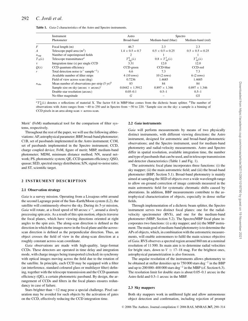
Table 1. Gaia-2 characteristics of the Astro and Spectro instruments.
Instrument Astro SpectroPhotometer Broad-band Medium-band (blue) Medium-band (red)
F Focal length (m) 46.7 2.3 2.3A Telescope pupil area (m2) 1.4 × 0.5 = 0.7 0.5 × 0.5 = 0.25 0.5 × 0.5 = 0.25nsup Number of superimposed fields 2 1 1T 0(λ) Telescope transmittancea T 6
Ag(λ) 0.8 × T 3Al(λ) T 3
Al(λ)τ Integration time (s) per single CCD 3.31 12.0 12.0Q(λ) CCD quantum efficiency CCD-green CCD-blue CCD-redr Total detection noise (e− sample−1) 6.6 7.3 7.3
Available number of filter strips 4 (10 rows) 10 (2 rows) 6 (2 rows)Field of view across scan (deg) 0.7236 1.4685 1.4685
nobs Mean number of observations per strip (5 yr)b 83 84 84Sample size on sky (arcsec × arcsec)c 0.0442 × 1.5912 0.897 × 1.346 0.897 × 1.346Double-star resolution (arcsec) 0.05–0.1 0.5–1 0.5–1No-filter magnitude G – GS
a T nX(λ) denotes n reflections of material X. The factor 0.8 in MBP-blue comes from the dichroic beam splitter. bThe number of
observations with Astro ranges from ∼40 to 250 and in Spectro from ∼50 to 220. cSample size on the sky: a sample is a binning ofCCD pixels in an area along-scan × across-scan.
Merit’ (FoM) mathematical tool for the comparison of filter sys-tems, respectively.
Throughout the rest of the paper, we will use the following abbre-viations: AP, astrophysical parameter; BBP, broad-band photometer;C1B, set of passbands implemented in the Astro instrument; C1M,set of passbands implemented in the Spectro instrument; CCD,charge coupled device; FoM, figure of merit; MBP, medium-bandphotometer; MDM, minimum distance method; NN, neural net-work; PS, photometric system; QE, CCD quantum efficiency; QSO,quasar; SED, spectral energy distribution; S/N, signal-to-noise ratio;and ST, scientific target.
2 I N S T RU M E N T D E S C R I P T I O N
2.1 Observation strategy
Gaia is a survey mission. Operating from a Lissajous orbit aroundthe second Lagrange point of the Sun–Earth/Moon system (L2), thesatellite will continuously observe the sky. During its 5-yr mission,Gaia will rotate, at a fixed speed of 60 arcsec s−1, around a slowlyprecessing spin axis. As a result of this spin motion, objects traversethe focal planes, which have viewing directions oriented at rightangles to the spin axis. The along-scan direction is defined as thedirection in which the images move in the focal plane and the across-scan direction is defined as the perpendicular direction. Thus, anobject crosses the field of view in the along-scan direction at aroughly constant across-scan coordinate.
Gaia observations are made with high-quality, large-formatCCDs. These detectors are operated in time delay and integrationmode, with charge images being transported (clocked) in synchronywith optical images moving across the field due to the rotation ofthe satellite. In principle, each CCD may be equipped with a filter(an interference, standard coloured glass or multilayer filter) defin-ing, together with the telescope transmission and the CCD quantumefficiency (QE), a certain photometric passband. By design, the ar-rangement of CCDs and filters in the focal planes ensures redun-dancy in case of failure.
Stars brighter than ∼12 mag pose a special challenge. Pixel sat-uration may be avoided for such objects by the activation of gateson the CCD, effectively reducing the CCD integration time.
2.2 Gaia instruments
Gaia will perform measurements by means of two physicallydistinct instruments, with different viewing directions: the Astroinstrument, designed for astrometric and broad-band photometricobservations; and the Spectro instrument, used for medium-bandphotometry and radial-velocity measurements. Astro and Spectrodiffer in spatial resolution, available integration time, the numberand type of passbands that can be used, and in telescope transmissionand detector characteristics (Table 1 and Fig. 1).
The astrometric focal plane incorporates three functions: (i) thesky mapper; (ii) the main astrometric field; and (iii) the broad-bandphotometer (BBP; Section 5.1). Broad-band photometry is mainlyaimed at sampling the SED of objects over a wide wavelength rangeto allow on-ground correction of image centroids measured in themain astrometric field for systematic chromatic shifts caused byaberrations. In addition, BBP measurements contribute to the as-trophysical characterization of objects, especially in dense stellarfields.
Through implementation of a dichroic beam splitter, the Spectroinstrument serves two distinct focal planes: one for the radial-velocity spectrometer (RVS), and one for the medium-bandphotometer (MBP; Section 5.2). The Spectro/MBP focal plane in-corporates two functions: (i) a sky mapper; and (ii) the MBP instru-ment. The main goal of medium-band photometry is to determine theAPs of objects, which, in combination with the astrometric measure-ments, will enable astronomers to fulfil the main science objectiveof Gaia. RVS observes a spectral region around 860 nm at a nominalresolution of 11 500. Its main aim is to determine radial velocitiesfor bright stars, down to V � 17–18 mag. For the brightest ones,astrophysical parametrization is also foreseen.
The angular resolution of the instruments allows photometry tobe obtained at stellar densities up to 750 000 stars deg−2 in the BBPand up to 200 000–400 000 stars deg−2 in the MBP (cf. Section 6.3).The resolution limit for double stars is about 0.05–0.1 arcsec in theAstro field and 0.5–1 arcsec in the MBP.
2.3 Sky mappers
Both sky mappers work in unfiltered light and allow autonomousobject detection and confirmation, including rejection of prompt
C© 2006 The Authors. Journal compilation C© 2006 RAS, MNRAS 367, 290–314
Dow
nloaded from https://academ
ic.oup.com/m
nras/article/367/1/290/1018790 by guest on 19 Novem
ber 2021
A photometric system for Gaia 293
ASM AF BBP
1 2 3 41 2 3 4 5 6 7 8 9 10 111 2
10
9
8
7
6
5
4
3
2
1
Row
nu
mb
er
Apparent star motion
MBP MBP
01 02 03 04 05
Row 1
Apparent star motion
Row 2
06 07 08 09 10 11 12 13 14 15 16 17 18 19 20
Red-enhanced CCDs Blue-enhanced CCDs
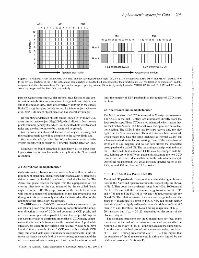
Figure 1. Schematic layout for the Astro field (left) and the Spectro/MBP field (right) in Gaia-2. The designations BBP1–BBP4 and MBP01–MBP20 referto the physical locations of the CCDs in the along-scan direction within the field, independent of their functionality (e.g. for detection or photometry) and theassignment of filters between them. The Spectro sky mapper, operating without filters, is physically located at MBP01, 02, 06, and 07. ASM and AF are theAstro sky mapper and the Astro field, respectively.
particle events (cosmic rays, solar protons, etc.). Detection and con-firmation probabilities are a function of magnitude and object den-sity in the field of view. They are effectively unity up to the surveylimit (20 mag) dropping quickly to zero for fainter objects (Arenouet al. 2005). On-board object detection has several advantages:
(i) sampling of detected objects can be limited to ‘windows’, i.e.areas centred on the object (Høg 2005), which allows to flush uselesspixels containing empty sky, which is of benefit to both CCD readoutnoise and the data volume to be transmitted to ground;
(ii) it allows the unbiased detection of all objects, assuring thatthe resulting catalogue will be complete to the survey limit; and
(iii) unpredictable ‘peculiar objects’, such as supernovae or Solarsystem objects, will be observed, if brighter than the detection limit.
Moreover, on-board detection is mandatory as no input cata-logue exists that is complete to the survey limit at the Gaia spatialresolution.
2.4 Astro/broad-band photometer
Gaia astrometric observations are made without a filter in order tominimize photon noise. The mirror coatings and CCD QE effectivelydefine a broad (white-light) passband, called G (Section 3). TheAstro focal plane receives the light from the superposition of twoviewing directions on the sky, separated by the so-called ‘basicangle’, of order 100◦. This superposition of the two fields of viewwill lead to a number of complications in the data processing, butthroughout this paper we only consider the first-order effect of thedoubling of the diffuse sky-background.
The BBP consists of 40 CCDs, arranged in four across-scan stripsand 10 along-scan rows (the Gaia naming convention for the along-scan direction is rows of CCDs and columns of CCD pixels, andacross-scan we speak of strips of CCDs and lines of pixels). In prin-ciple, the filters can be distributed among the 40 CCDs in any combi-nation that is desirable from a scientific point of view. A preferablesituation, for example for variable-star science, would be to haveidentical filters on each of the 10 CCD rows within a single CCDstrip: this would yield quasi-simultaneous measurements in the dif-ferent passbands on each field-of-view crossing, independent of theacross-scan coordinate of an object. However, such a solution would
limit the number of BBP passbands to the number of CCD strips,i.e. four.
2.5 Spectro/medium-band photometer
The MBP consists of 40 CCDs arranged in 20 strips and two rows.The CCDs in the first 10 strips are illuminated directly from theSpectro telescope. These CCDs are red enhanced, which means theyare thicker than ‘normal CCDs’ and have a red-optimized antireflec-tion coating. The CCDs in the last 10 strips receive only the bluelight from the Spectro telescope. These detectors are blue enhanced,which means they have the same thickness as ‘normal CCDs’ buta blue-optimized antireflection coating. Four of the red-enhancedstrips act as sky mappers and do not have filters; the associatedbroad passband is called GS. The remaining six strips with red- andthe 10 strips with blue-enhanced CCDs may be equipped with fil-ters, defining up to 16 different passbands, assuming the two CCDrows in each strip have identical filters (for the sake of redundancy).One of the red passbands will cover the same spectral region as theRVS, around 860 nm, leaving 15 free strips.
3 T H E G A N D GS PA S S BA N D S
The G and GS passbands corresponding to the white light observa-tions in the Astro and Spectro instruments, respectively, are shownin Fig. 2. They cover the wavelength range from 400 to 1000 nm and350 to 1025 nm, with the maximum energy transmission at ∼715and ∼765 nm and the FWHM of 408 and 456 nm, respectively forG and GS. The relation between the associated magnitudes and theJohnson V magnitude is shown in Fig. 3. Very red objects (eitherintrinsically red or highly reddened) are much brighter in G and GSthan in V and, therefore, the Gaia limiting magnitude of G lim ∼20 translates into V lim ∼ 20–25, depending on the colour of theobserved object.
The estimated precisions for the G magnitudes per focal planetransit and at the end of the mission, computed as described inSection 6.2, are shown in Fig. 4. Taking into account the photon noisefrom the source, the background and the readout noise, precisionsof ∼10 and ∼1 mmag are achievable at V ∼ 19. This implies thatthe precision of the G measurements is ultimately limited by thecalibration errors (see Section 6.4).
C© 2006 The Authors. Journal compilation C© 2006 RAS, MNRAS 367, 290–314
Dow
nloaded from https://academ
ic.oup.com/m
nras/article/367/1/290/1018790 by guest on 19 Novem
ber 2021

294 C. Jordi et al.
200 400 600 800 1000
Wavelength (nm)
0
0.2
0.4
0.6
0.8
1N
orm
aliz
ed
re
sp
on
se
(e
ne
rgy)
G
GS
Figure 2. The G and GS Gaia broad passbands corresponding to the whitelight observations in the Astro and Spectro focal planes, respectively.
0 1 2 3 4 5 6 7
V–Ic
–7
–6
–5
–4
–3
–2
–1
0
G–V
,GS
–V
G
GS
Figure 3. The relation between G − V and GS − V and V − I C for thewhite light passbands in the Astro and Spectro focal planes. Every star inthe spectral library of Pickles (1998) is represented by a filled symbol. Opensymbols correspond to the same stars reddened by AV = 5 mag. Redden-ing vectors run parallel to the colour–colour relationship. Pickles’ librarywas chosen because it extends to very red objects. No appreciable differ-ences for stars with Teff � 4000 K are obtained when using spectral energydistributions from the BaSeL 2.2 library or other libraries.
Gaia will provide distances at the 10 per cent accuracy level forsome 100–200 million stars, which, combined with estimates of theG magnitude and the interstellar extinction, will yield unprecedentedabsolute magnitudes, in both accuracy and number.
The G passband also yields the best signal-to-noise ratio (S/N)for variability detection among all the Gaia passbands. Gaia willmonitor millions of variable stars (eclipsing binaries, Cepheids, RRLyrae, Mira-LPVs, etc.). Eyer (2005) and Eyer & Mignard (2005)provide comparisons with other variability surveys and a detaileddiscussion of the effects of the variable time sampling and numberof observations due to the scanning law.
4 D E S I G N I N G T H E P H OTO M E T R I C S Y S T E M
Many ground-based PSs exist but none satisfies all the requirementsof a space-based mission such as Gaia: portions of the spectrum
13 15 17 19 21 23
V
10–4
10–3
10–2
10–1
100
σ G (
ma
g)
B1V
F2V
G2V
K3III
M0III
per observatio
n (11 CCDs)
end–of–mission (82 observ.)
3 mmag
Figure 4. Estimated precision of the G magnitude per focal plane transitand at the end of the mission according to equation (2) assuming σcal =0. In this paper, the contribution of calibration error to the end-of-missionprecision is assumed to be 3 mmag (horizontal line).
limited on-ground by telluric O3 opacity in the blue and O2 andH2O absorption bands in the red are accessible to Gaia; existingPSs have usually been designed for specific spectral type inter-vals or specific objects, while Gaia photometry must deal with theentire HR diagram, must allow taxonomy classification of Solarsystem objects and must be able to identify quasars and galax-ies. In addition, Gaia allows the extension of stellar photometryto Galactic areas where the classical classification schemes maybe no longer fully valid because of systematic variations in el-ement abundances in stellar atmospheres and in interstellar mat-ter. Finally, Gaia has to astrophysically characterize objects overa very large range of brightness, from G ∼ 6 to the faint limit ofG lim ∼ 20, and consequently the width of the passbands will reflecta trade-off between sensitivity to physical parameters and the pos-sibility to measure faint stars. Therefore, designing a new PS is thebest approach to ensuring that the ambitious goals of Gaia will beachieved. This became clear early on when initial efforts to use ex-isting PSs showed that these failed to cover all Gaia requirements.A fairly complete census of existing PSs can be found in Straizys(1992); Moro & Munari (2000); Fiorucci & Munari (2003); Bessell(2005).
Criteria for the design of a new PS have to be established a priori.As it is widely known, narrow passbands are very efficient in mea-suring specific spectral features, but have low performance for faintobjects; broad passbands yield low photon-noise for faint objectsbut cannot give one-to-one determination of APs. The UV containsimportant information on APs, but Gaia will not be able to measurefaint red objects in this spectral range. Therefore, a compromisebetween the different options (number, location, and width of thepassbands and their total exposure time) is needed to achieve a PSthat is maximally capable of separating objects with different APsin filter flux space. Such a PS should allow both accurate discretesource classification (i.e. identification of stars, galaxies, QSOs, So-lar system objects, etc.) and continuous parametrization (values ofAPs, e.g. for stars Teff, [M/H], etc.) for all Gaia targets across theAP space.
C© 2006 The Authors. Journal compilation C© 2006 RAS, MNRAS 367, 290–314
Dow
nloaded from https://academ
ic.oup.com/m
nras/article/367/1/290/1018790 by guest on 19 Novem
ber 2021

A photometric system for Gaia 295
4.1 Principles for the design
Over the years of mission study and development, the instrumentalconcept of Gaia has evolved. As a consequence, the requirementsand constraints for designing the PS have evolved in terms of thenumber of passbands, the exposure time available per passband, thewavelength coverage in BBP and MBP, the spatial resolution of As-tro and Spectro, the goals of BBP and MBP, and the complementarityof BBP, MBP and RVS measurements, etc.
With the consolidation of the study phase of the Gaia instrumentdesign, the requirements for BBP and MBP are stabilized. The PSaccepted as the baseline for the mission and presented in this paperis based on the following constraints.
(i) The instrument design is as described in Section 2.(ii) Photometry from Astro has to account for chromaticity in
order to achieve microarcsec astrometry, which implies a mea-surement of the SED of each object with contiguous broad pass-bands covering the whole wavelength range of the G passband(see Section 5.1.2).
(iii) The photometry from Spectro has to provide the astrophys-ical characterization of the observed objects.
(iv) The photometry from Astro has to provide the astrophysi-cal characterization of the observed objects in dense fields (at stel-lar densities larger than 200 000–400 000 stars deg−2; mainly in thebulge, some Galactic disc areas and globular clusters).
(v) One of the medium passbands in Spectro has to measure theflux in the wavelength range covered by RVS (848–874 nm).
(vi) The trigonometric parallax is available and has to be used toconstrain the luminosity (or the absolute magnitude).
(vii) The information from RVS is not used for designing the PSbecause of the different limiting magnitude and spatial resolutionof that instrument (in the actual Gaia data processing it is foreseenthat astrometry, photometry and RVS measurements will be usedtogether to derive APs, when possible).
(viii) The Gaia PS is optimized for single stars, where priority isgiven to those types crucial for achieving the Gaia core science case,namely the unravelling of the structure and the formation historyof the Milky Way. These stars are named ‘scientific photometrictargets’ or simply ‘scientific targets’ (STs; see Section 4.3) and theyconstitute our test population.
(ix) Every ST is characterized by its APs, where we considerTeff, log g, chemical composition and AV .2 The chemical compo-sition is described by the metallicity, [M/H], and the α-elementenhancements, [α/Fe].
(x) The error goals for the AP determination are established forevery ST (σk,goal; see Section 4.2 and Appendix A).
(xi) The actual performance of a given PS with respect to theerror goals is measured using an objective ‘FoM’ (see Section 4.2and Appendix A).
(xii) The global degeneracies of the PS have to be evaluated (seeSection 4.5).
(xiii) Additional merits such as, for example, the performancewith respect to discrete object classification, the performance fornon-ST objects, etc. have to be considered.
The procedure to come to a baseline PS (Brown et al. 2004) isbased on the maximization of this ‘FoM’, a minimization of theglobal degeneracies and an evaluation of additional merits.
2 Throughout the paper AV means Aλ=550, i.e. the monochromatic interstellarextinction at λ = 550 nm.
4.2 Figure of merit
For a given PS, the FoM is constructed by calculating for each STand each of its APs, pk, the ratio σk,post/σk,goal. Here, σk,post is theestimate of the error that can be achieved with the given PS forpk and σk,goal is the above mentioned error goal. The procedure forestimating σk,post and the definition of the FoM were proposed byLindegren (2003b). For a given AP, pk and a PS with measured fluxesφ j ( j = 1, n passbands), σk,post is estimated using the sensitivity ofthe PS to that parameter (∂φ j/∂pk) and the errors of the photometricobservations (ε j ). The latter are based on the noise model for theinstrument–PS combination (see Section 6.2). The details are givenin Appendix A.
The global FoM as given in equation (A6) in Appendix A is aweighted sum of the individual FoMs of every ST, which in turnare weighted sums of the ratios σk,post/σk,goal for each of the APspk (equation A4). A higher value of this FoM indicates a betterperformance for the given PS. The global FoM thus describes theperformance of a PS across the HR diagram by taking into accountthe errors that can be achieved and the relative priorities of thedifferent STs and their APs. The local degeneracies in the AP deter-minations (i.e. correlations between the errors for different APs fora given ST, see Section 4.5) are also taken into account in the FoMformalism. Each local degeneracy between APs leads to increasedstandard errors σk,post and thus a lower FoM.
In our implementation, the derivatives ∂φ j/∂pk and the error esti-mates σk,post are calculated numerically from simulated photometricdata (Section 6.1). The calculation thereof requires (synthetic) SEDsof the STs and a noise model for the photometric instruments. Thematrix B from equation (A3) includes the a priori information forthe AP vector p and, in our case, corresponds simply to the rangeof possible values of the parameters pk. The information from theparallax and its error is incorporated into B following Lindegren(2004). Other information could be added (known reddening in acertain Galactic location, ranges of abundances according to Galac-tic population, etc.), but this would introduce our preconceptionsof the structure and stellar populations of the Galaxy into the PSdesign and we therefore did not include such constraints.
The MBP data will have a lower spatial resolution than the BBPdata. For non-crowded regions on the sky (with respect to MBP), weassume that the MBP and BBP photometry will always be combinedfor the estimation of APs. Hence, the calculation of the achievableposterior errors is always done by combining BBP and MBP data.For dense stellar fields, only BBP data will be available and, in thatcase, the achievable AP errors and the FoM have been computedusing only broad-band photometry.
SEDs of the STs in the test population were taken from theBASEL 2.2 (Lejeune, Cuisinier & Buser 1998), NEXTGEN (Hauschildt,Allard & Baron 1999) and MARCS3 (Gustafsson et al. 2003) libraries.The BASEL 2.2 library is a compilation of synthetic spectra from li-braries published by Kurucz (1979), Bessell et al. (1989), Flukset al. (1994) and Hauschildt et al. (1999). It covers the whole HRdiagram and [M/H] abundances from −5 to +1 dex, but with so-lar α-element abundances. A new version of the NEXTGEN library(NEXTGEN 2) has been built taking into account Gaia mission needs(Hauschildt et al. 2003). This library includes SEDs for stars coolerthan 10 000 K with [M/H] ranging from −2 to +0 dex and [α/Fe]from −0.2 to +0.8 dex. A more extended grid is currently available(Brott & Hauschildt 2005). Finally, a new version of the MARCS
3 See also http://marcs.astro.uu.se
C© 2006 The Authors. Journal compilation C© 2006 RAS, MNRAS 367, 290–314
Dow
nloaded from https://academ
ic.oup.com/m
nras/article/367/1/290/1018790 by guest on 19 Novem
ber 2021
296 C. Jordi et al.
library taking into account non-solar α-element abundances hasbeen created specifically for Gaia studies. This library providescoverage between 3000 and 5000 K, [M/H] from −4 to +0.5 dexand [α/Fe] from +0 to +0.4 dex.
Empirical libraries, like those by Gunn & Stryker (1983) andPickles (1998), do not provide full coverage of the HR diagram andthe corresponding chemical composition range and, therefore, theyare not appropriate for computing the FoM values.
Finally, we would like to make a few remarks here about the in-terpretation of the calculated values of σk,post and the correspondingFoM for a set of proposed PSs. The values of σk,post calculated asdescribed in Appendix A should not be taken as the actual errorsthat will be achieved by the Gaia PS. They represent the achievableprecision if the synthetic spectra represent the true stars and if thenoise model is correct. This issue is discussed more thoroughly inSection 7. What makes the FoM a powerful tool is that it enablesan objective comparison of different PS proposals, based on a setof agreed error goals and scientific priorities. In addition, for eachPS, a detailed study can be made of its strengths and weaknesses ascompared with other PSs by examining the FoM for individual STsand for groups of STs (such as specific types of stars, populations incertain Galactic directions, bright versus faint stars, reddened ver-sus unreddened, etc.). Once the best PS proposal has been chosenit can be further tuned by using the FoM procedure to improve itssensitivity to certain APs or to improve the performance for certaingroups of stars. This objective FoM approach has not been usedbefore in the design of a PS.
4.3 Test population and error goals
According to the scientific goals of Gaia (see Table 2), for everyGalactic stellar population, several kinds of stars were selected asSTs and a priority, expressed as a numerical weight, was assignedto them (Jordi et al. 2004d,e). These stars have been consideredin different directions in the Milky Way (toward the centre, theanticentre and perpendicular to the Galactic plane) and at differentdistances (0.5, 1, 2, 5, 10 and 30 kpc) in accordance with a Galaxymodel (Torra et al. 1999). The STs have been reddened accordingto a 3D interstellar extinction model (Drimmel, Cabrera-Lavers &Lopez-Corredoira 2003), assuming a standard extinction law (RV =
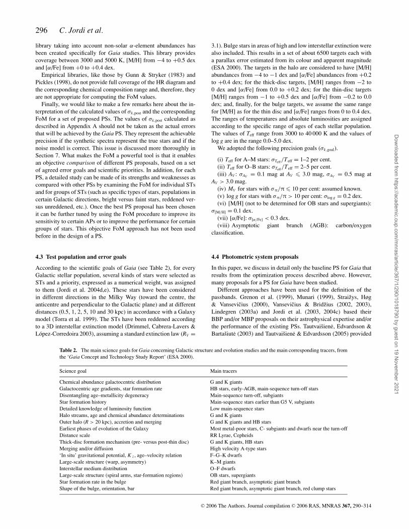
Table 2. The main science goals for Gaia concerning Galactic structure and evolution studies and the main corresponding tracers, fromthe ‘Gaia Concept and Technology Study Report’ (ESA 2000).
Science goal Main tracers
Chemical abundance galactocentric distribution G and K giantsGalactocentric age gradients, star formation rate HB stars, early-AGB, main-sequence turn-off starsDisentangling age–metallicity degeneracy Main-sequence turn-off, subgiantsStar formation history Main-sequence stars earlier than G5 V, subgiantsDetailed knowledge of luminosity function Low main-sequence starsHalo streams, age and chemical abundance determinations G and K giantsOuter halo (R > 20 kpc), accretion and merging G and K giants and HB starsEarliest phases of evolution of the Galaxy Most metal-poor stars, C- subgiants and dwarfs near the turn-offDistance scale RR Lyrae, CepheidsThick-disc formation mechanism (pre- versus post-thin disc) G and K giants, HB starsMerging and/or diffusion High velocity A-type stars‘In situ’ gravitational potential, K z , age–velocity relation F–G–K dwarfsLarge-scale structure (warp, asymmetry) K–M giantsInterstellar medium distribution O–F dwarfsLarge-scale structure (spiral arms, star-formation regions) OB stars, supergiantsStar formation rate in the bulge Red giant branch, asymptotic giant branchShape of the bulge, orientation, bar Red giant branch, asymptotic giant branch, red clump stars
3.1). Bulge stars in areas of high and low interstellar extinction werealso included. This results in a set of about 6500 targets each witha parallax error estimated from its colour and apparent magnitude(ESA 2000). The targets in the halo are considered to have [M/H]abundances from −4 to −1 dex and [α/Fe] abundances from +0.2to +0.4 dex; for the thick-disc targets, [M/H] ranges from −2 to0 dex and [α/Fe] from 0.0 to +0.2 dex; for the thin-disc targets[M/H] ranges from −1 to +0.5 dex and [α/Fe] from −0.2 to 0.0dex; and, finally, for the bulge targets, we assume the same rangefor [M/H] as for the thin disc and [α/Fe] ranges from 0 to 0.4 dex.The ranges of temperatures and absolute luminosities are assignedaccording to the specific range of ages of each stellar population.The values of Teff range from 3000 to 40 000 K and the values oflog g are in the range 0.0–5.0 dex.
We adopted the following precision goals (σk,goal).
(i) Teff for A–M stars: σTeff/Teff = 1–2 per cent.(ii) Teff for O–B stars: σTeff/Teff = 2–5 per cent.(iii) AV : σAV = 0.1 mag at AV � 3.0 mag, σAV = 0.5 mag at
AV > 3.0 mag.(iv) MV for stars with σπ/π � 10 per cent: assumed known.(v) log g for stars with σπ/π > 10 per cent: σlog g = 0.2 dex.(vi) [M/H] (not to be determined for OB stars and supergiants):
σ[M/H] = 0.1 dex.(vii) [α/Fe]: σ[α/Fe] < 0.3 dex.(viii) Asymptotic giant branch (AGB): carbon/oxygen
classification.
4.4 Photometric system proposals
In this paper, we discuss in detail only the baseline PS for Gaia thatresults from the optimization process described above. However,many proposals for a PS for Gaia have been studied.
Different approaches have been used for the definition of thepassbands. Grenon et al. (1999), Munari (1999), Straizys, Høg& Vansevicius (2000), Vansevicius & Bridzius (2002, 2003),Lindegren (2003a) and Jordi et al. (2003, 2004c) based theirBBP and/or MBP proposals on their astrophysical expertise and/orthe performance of the existing PSs. Tautvaisiene, Edvardsson &Bartasiute (2003) and Tautvaisiene & Edvardsson (2005) provided
C© 2006 The Authors. Journal compilation C© 2006 RAS, MNRAS 367, 290–314
Dow
nloaded from https://academ
ic.oup.com/m
nras/article/367/1/290/1018790 by guest on 19 Novem
ber 2021
A photometric system for Gaia 297
guidelines for designing a PS sensitive to C, N, O and α-processelements. We note that the sets of filters by Grenon et al. (1999),Munari (1999), and Straizys et al. (2000) were designed with sub-stantially different constraints imposed in early phases of the Gaiainstrument design.
Bailer-Jones (2004) developed a novel method for designing PSsvia a direct numerical optimization. By considering a filter systemas a set of free parameters (central wavelengths, FWHM etc.), it maybe designed by optimizing an FoM with respect to these parameters.This FoM is a measure of how well the filter system separates thestars in the data space and of how much it avoids degeneracies inthe AP determinations. The resulting filter systems tend to haverather broad and overlapping passbands and large gaps in betweenat the same time. Some commonalities with conventional PSs maybe recognized. Although first analyses showed these systems toyield FoM values only slightly inferior to conventional PS proposals,the method was considered too novel and further studies were notpursued.
Lindegren (2001) proposed several BBP systems, differing in thenumber of passbands and their profiles, and tested their performancewith respect to chromatic effects estimation. He concluded that fivepassbands do not provide a clear advantage over four passbands andthat the overlapping of the passbands is more important.
Heiter et al. (2005) used the Principal Components Analysis tech-nique to design a set of BBP passbands that is optimal for a subset ofSTs with effective temperatures between 3000 and 5000 K. Photom-etry was simulated for a grid of sets of four broad filters each. TheFWHMs were varied in equidistant steps, while the central wave-lengths were determined by requiring contiguous filters covering thewhole wavelength range. The resulting set of passbands was foundto perform better than all other proposals for bulge stars but worsethan all others when evaluated for the complete set of STs (Jordiet al. 2004a).
All proposed PSs were evaluated using the FoM procedure andthe results were returned to the proposers who were then giventhe opportunity to refine their respective PSs and submit improvedversions as a new PS proposal. Updates of the PSs above or new onescame out of every evaluation cycle (Høg & Knude 2004a,b; Jordi& Carrasco 2004a,b; Knude & Høg 2004; Straizys, Zdanavicius &Lazauskaite 2004). Finally, after several trials for the fine tuningof a few individual passbands, the C1B and C1M sets (Jordi et al.2004a,b) were adopted as the baseline PS for Gaia. Detailed resultsof the evaluation of all PS proposals can be found in Jordi et al.(2004a,b).
4.5 Local and global degeneracies
The goal of designing a PS that allows both accurate discrete classi-fication and continuous parametrization of observed sources trans-lates to demanding that the degeneracies in the PS are minimized.
The discrete classification problem concerns the way very dif-ferent parts of AP space are mapped by the PS into the filter fluxspace. For example, due to extinction, a highly reddened O starmay to first order look like a nearby unreddened cool dwarf. Agood PS should as much as possible be free of such ‘global’ de-generacies. The continuous parametrization problem concerns theway a PS maps a small region around a certain object in AP spaceonto filter fluxes. Here, it is the ‘local’ degeneracies that are im-portant. Examples include the well-known degeneracy betweenTeff and AV and the difficulty of disentangling the effects of Teff
and log g for a PS without passbands shortwards of the Balmerjump.
Our method of evaluating the proposed PSs as outlined inSection 4.2 focuses on the local degeneracies. Consider the gra-dient vectors that describe how the filter fluxes respond to changesin particular APs. For a good PS, these gradients should be large withrespect to the noise in the data and they should ideally be orthogonalto each other, where the orthogonality is also defined with respect tothe noise (i.e. for the gradients with components 1/ε j × ∂φ j/∂pk,see Appendix A). Large gradients mean that the PS is sensitive tothe corresponding APs while their orthogonality ensures that thereare no local degeneracies. The FoM takes this into account by cal-culating the posterior errors on estimated APs using the sensitivitymatrix which contains these gradient vectors (see Appendix A formore details). Small gradient vectors are reflected in larger errorson the estimated AP. Non-orthogonal gradient vectors will also leadto larger errors and to non-zero covariances (i.e. correlated errors)in the posterior variance–covariance matrix of the estimated APs.Both effects will lead to a lower FoM (this is explained in moredetail in Appendix A).
The FoM calculations do not take global degeneracies into ac-count. In fact, it is assumed that one already has available a goodclassification of the object to be parametrized so that the linearizedequations from which the FoM is derived apply. The global degen-eracies reflect the highly non-linear mapping from AP space to filterflux space and are difficult to characterize in practice.
We attempted to compare the different PS proposals with respectto global degeneracies by employing self-organizing maps to ex-plore how the different STs cluster in data space and how well theycan be separated. The results were inconclusive as the different PSproposals showed rather similar behaviour. This is plausible becauseto first order all the proposed filter systems were similar. The setsof BBP passbands were very much alike and the sets of MBP pass-bands all had a set of blue and a set of red filters with a gap betweenthese sets from ∼550 to ∼700 nm and they all had an Hα filter inthis gap. With a continuous sampling of stellar parameters, a filtersystem will define a complex manifold in the space of filter fluxvectors onto which each star will be mapped. It is the overall shapeof this manifold that determines the presence or absence of globaldegeneracies in the PS. Hence, it may be that the filter systems thathad been considered all define roughly the same manifold, the dif-ferences between filter systems only being manifest at the local level(where the FoM calculations are more relevant).
Characterizing the global degeneracies will be an important taskin the context of the automatic classification effort for the Gaiadata processing. A full understanding of the behaviour of the GaiaPS is essential for setting up appropriate discrete classification andcontinuous parametrization algorithms.
5 T H E G aia P H OTO M E T R I C S Y S T E M
In this section, we describe in detail the baseline PS for Gaia, calledC1, which consists of the C1B and C1M broad and medium pass-bands. The role of each of the passbands is described in relation tospectral features and astrophysical diagnostics.
5.1 The C1B broad passbands
The C1B component of the Gaia PS has five broad passbands cov-ering the wavelength range of the unfiltered light from the blue tothe far-red (i.e. 400–1000 nm). The basic response curve of the fil-ters versus wavelength is a symmetric quasi-trapezoidal shape. Thefilters were chosen to satisfy both the astrophysical needs and thespecific requirements for chromaticity calibration of the astrometric
C© 2006 The Authors. Journal compilation C© 2006 RAS, MNRAS 367, 290–314
Dow
nloaded from https://academ
ic.oup.com/m
nras/article/367/1/290/1018790 by guest on 19 Novem
ber 2021
298 C. Jordi et al.
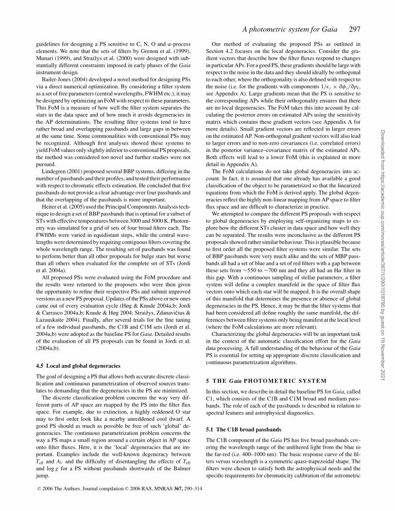
Table 3. Specifications of the filters of C1B implemented in Astro.
Band C1B431 C1B556 C1B655 C1B768 C1B916
λblue (nm) 380 492 620 690 866λred (nm) 482 620 690 846 966λc (nm) 431 556 655 768 916λ (nm) 102 128 70 156 100δλ (nm) 10,40 10,10 10,10 10,40 40,10ε (nm) 2,2 2,2 2,2 2,2 2,2Tmax (per cent) 90 90 90 90 90nstrips 1 0.5 1 0.5 1
λblue, λred: wavelengths at half-maximum transmission. λc: centralwavelength = 0.5(λblue + λred). λ: FWHM. λ: edge width (blue, red)between 10 and 90 per cent of Tmax. ε: manufacturing tolerance intervalscentred on λblue and λred. Tmax: maximum transmission of filter. nstrips:number of CCD strips carrying the filter: C1B556 and C1B768 share oneCCD strip.
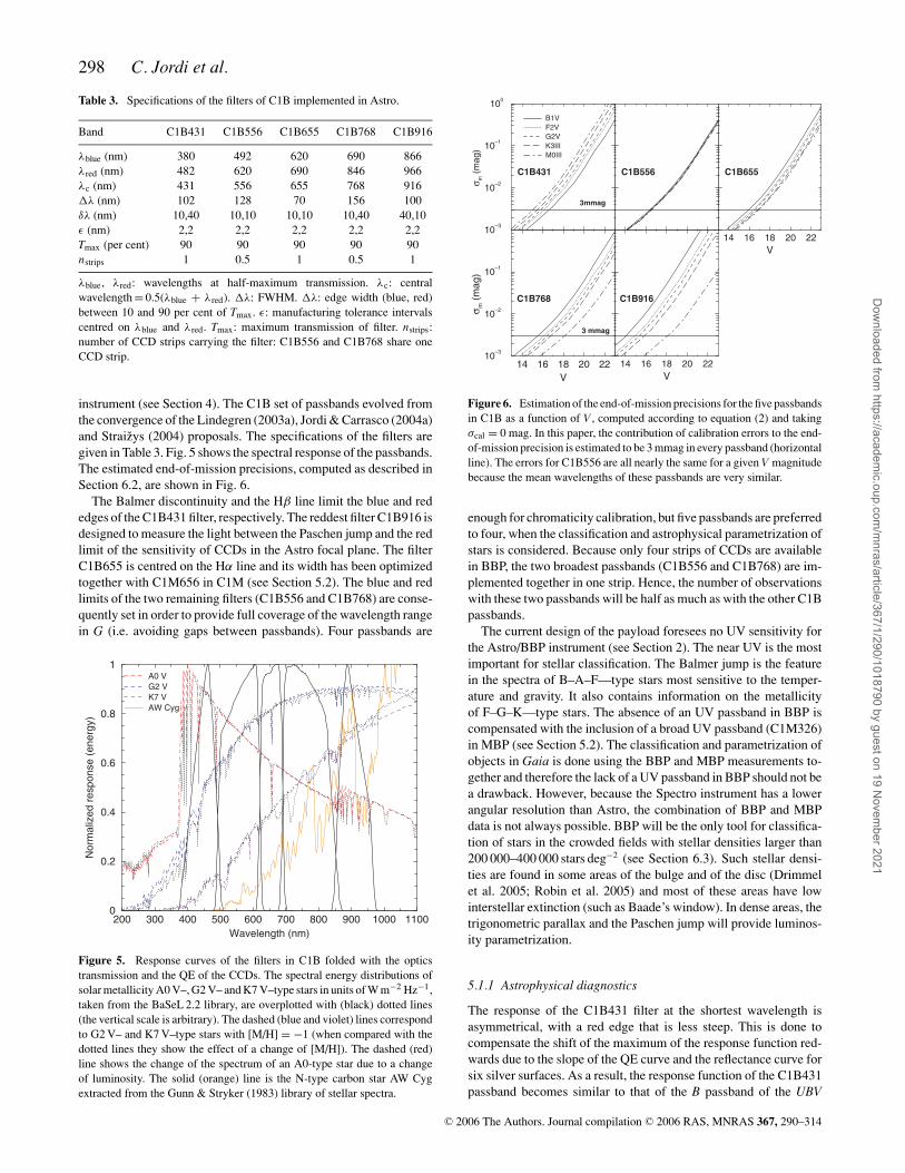
instrument (see Section 4). The C1B set of passbands evolved fromthe convergence of the Lindegren (2003a), Jordi & Carrasco (2004a)and Straizys (2004) proposals. The specifications of the filters aregiven in Table 3. Fig. 5 shows the spectral response of the passbands.The estimated end-of-mission precisions, computed as described inSection 6.2, are shown in Fig. 6.
The Balmer discontinuity and the Hβ line limit the blue and rededges of the C1B431 filter, respectively. The reddest filter C1B916 isdesigned to measure the light between the Paschen jump and the redlimit of the sensitivity of CCDs in the Astro focal plane. The filterC1B655 is centred on the Hα line and its width has been optimizedtogether with C1M656 in C1M (see Section 5.2). The blue and redlimits of the two remaining filters (C1B556 and C1B768) are conse-quently set in order to provide full coverage of the wavelength rangein G (i.e. avoiding gaps between passbands). Four passbands are
200 300 400 500 600 700 800 900 1000 1100
Wavelength (nm)
0
0.2
0.4
0.6
0.8
1
No
rma
lize
d r
esp
on
se
(e
ne
rgy)
A0 V
G2 V
K7 V
AW Cyg
Figure 5. Response curves of the filters in C1B folded with the opticstransmission and the QE of the CCDs. The spectral energy distributions ofsolar metallicity A0 V–, G2 V– and K7 V–type stars in units of W m−2 Hz−1,taken from the BaSeL 2.2 library, are overplotted with (black) dotted lines(the vertical scale is arbitrary). The dashed (blue and violet) lines correspondto G2 V– and K7 V–type stars with [M/H] = −1 (when compared with thedotted lines they show the effect of a change of [M/H]). The dashed (red)line shows the change of the spectrum of an A0-type star due to a changeof luminosity. The solid (orange) line is the N-type carbon star AW Cygextracted from the Gunn & Stryker (1983) library of stellar spectra.
14 16 18 20 22
V
10–3
10–2
10–1
σ m (
mag)
10–3
10–2
10–1
100
σ m (
mag)
B1V
F2V
G2V
K3III
M0III
14 16 18 20 22
V
14 16 18 20 22
V
C1B431 C1B556 C1B655
C1B768 C1B916
3mmag
3 mmag
Figure 6. Estimation of the end-of-mission precisions for the five passbandsin C1B as a function of V , computed according to equation (2) and takingσcal = 0 mag. In this paper, the contribution of calibration errors to the end-of-mission precision is estimated to be 3 mmag in every passband (horizontalline). The errors for C1B556 are all nearly the same for a given V magnitudebecause the mean wavelengths of these passbands are very similar.
enough for chromaticity calibration, but five passbands are preferredto four, when the classification and astrophysical parametrization ofstars is considered. Because only four strips of CCDs are availablein BBP, the two broadest passbands (C1B556 and C1B768) are im-plemented together in one strip. Hence, the number of observationswith these two passbands will be half as much as with the other C1Bpassbands.
The current design of the payload foresees no UV sensitivity forthe Astro/BBP instrument (see Section 2). The near UV is the mostimportant for stellar classification. The Balmer jump is the featurein the spectra of B–A–F—type stars most sensitive to the temper-ature and gravity. It also contains information on the metallicityof F–G–K—type stars. The absence of an UV passband in BBP iscompensated with the inclusion of a broad UV passband (C1M326)in MBP (see Section 5.2). The classification and parametrization ofobjects in Gaia is done using the BBP and MBP measurements to-gether and therefore the lack of a UV passband in BBP should not bea drawback. However, because the Spectro instrument has a lowerangular resolution than Astro, the combination of BBP and MBPdata is not always possible. BBP will be the only tool for classifica-tion of stars in the crowded fields with stellar densities larger than200 000–400 000 stars deg−2 (see Section 6.3). Such stellar densi-ties are found in some areas of the bulge and of the disc (Drimmelet al. 2005; Robin et al. 2005) and most of these areas have lowinterstellar extinction (such as Baade’s window). In dense areas, thetrigonometric parallax and the Paschen jump will provide luminos-ity parametrization.
5.1.1 Astrophysical diagnostics
The response of the C1B431 filter at the shortest wavelength isasymmetrical, with a red edge that is less steep. This is done tocompensate the shift of the maximum of the response function red-wards due to the slope of the QE curve and the reflectance curve forsix silver surfaces. As a result, the response function of the C1B431passband becomes similar to that of the B passband of the UBV
C© 2006 The Authors. Journal compilation C© 2006 RAS, MNRAS 367, 290–314
Dow
nloaded from https://academ
ic.oup.com/m
nras/article/367/1/290/1018790 by guest on 19 Novem
ber 2021
A photometric system for Gaia 299
system. The mean wavelengths of both passbands are also similar:445 nm for C1B431 and 442 nm for B.
The mean wavelength and half width of the C1B556 responsefunction are very similar to that of the V passband. As a result,the colour index C1B431–C1B556 will be easily transformable toJohnson’s B–V and vice versa. Analogously, the C1B768 passbandcan be easily related with the Cousins I, the Sloan Digital Sky Survey(SDSS) i′ and the Hubble Space Telescope (HST) 814 passbands,and the colour index C1B556–C1B768 is transformable to V −I C, r ′ − i ′ and HST 555–814. This will facilitate the comparison ofthe numerous ground-based investigations in the BV system and thelarge number of observations being done in the far-red passbandswith the Gaia results. As can be seen from Fig. 5, the differencesof the ‘blue minus green’, ‘blue minus red’ or ‘blue minus far-red’magnitudes may serve as a measure of metallic-line blanketing, al-though with much less sensitivity than a colour index containing theUV. In the C1B431–C1B556 versus C1B556–C1B768 diagram, thedeviations of F–G metal-deficient dwarfs and G–K metal-deficientgiants from the corresponding sequences of solar metallicity are upto 0.07 and 0.20 mag, respectively.
The combination of the fluxes measured in the C1B655 passbandand the narrow passband C1M656 in MBP form an Hα index pri-marily measuring the strength of the Hα line. The Hα index sharesthe same properties as the β index in the Stromgren–Crawford PS.It is an indicator of luminosity for stars earlier than A0 and of tem-perature for stars later than A3, almost independent of interstellarextinction and chemical composition. The same reddening-free in-dex may be used for the identification of emission-line stars.
The two remaining red and far-red passbands, C1B768 andC1B916, give the height of the Paschen jump which is a functionof temperature and gravity. Although the maximum height of thePaschen jump is 0.3 mag only, i.e. about 4 times smaller than theBalmer jump, it still provides the needed information if its height,C1B768–C1B916, is measured with high accuracy (not lower than1 per cent) and this is reachable up to about V ∼ 17–18 (see Fig. 6).The colour indices C1B556–C1B768 and C1B556–C1B916 forunreddened late-type stars may be used as indicators for the tem-perature. These colour indices (and C1B768–C1B916) also allowfor the separation of cool oxygen-rich (M) and carbon-rich (N)stars.
The C1M326–C1B431 versus C1B431–C1B556 diagram has thesame properties as the U − B versus B − V diagram of Johnson’ssystem or similar diagrams for other systems (Straizys 1992). Su-pergiants are well separated from the main-sequence stars. Metaldeficient F–G dwarfs and G–K giants exhibit UV excesses up to0.4 mag. Blue horizontal branch stars show UV deficiencies up to0.3 mag, while white dwarfs are situated around the interstellar red-dening line of O-type stars.
5.1.2 Chromaticity evaluation
Although no refracting optics are used for the astrometric field,the precise centre of a stellar image is still wavelength dependentbecause of diffraction and its interplay with the optical aberrations ofthe instrument. Differential shifts by up to ∼10 per cent of the widthof the diffraction image (i.e. several milliarcsec) may be caused byodd aberrations such as coma, even though the resolution remainsessentially diffraction limited. As a result, the measured centres ofstellar images will depend on their SEDs, and a careful calibration ofthe effect, known as chromaticity, is mandatory in order to attain theastrometric accuracy goals. The gross SED of each observed target is
therefore needed in the wavelength range of the astrometric CCDs;moreover, these data are needed with the same spatial resolution as inthe astrometric field. As stated before, the BBP set of passbands wasdesigned with this requirement in mind, as well as on astrophysicalgrounds.
Lindegren (2003c) showed that, for the chromaticity calibration,near-rectangular filters are acceptable and that the choice of theseparation wavelengths is more important than the edge widths.The author concluded that the use of four broad passbands cover-ing the wavelength range of the astrometric G passband should beenough to match the chromaticity constraints (rms contribution tothe parallaxes <1 μas).
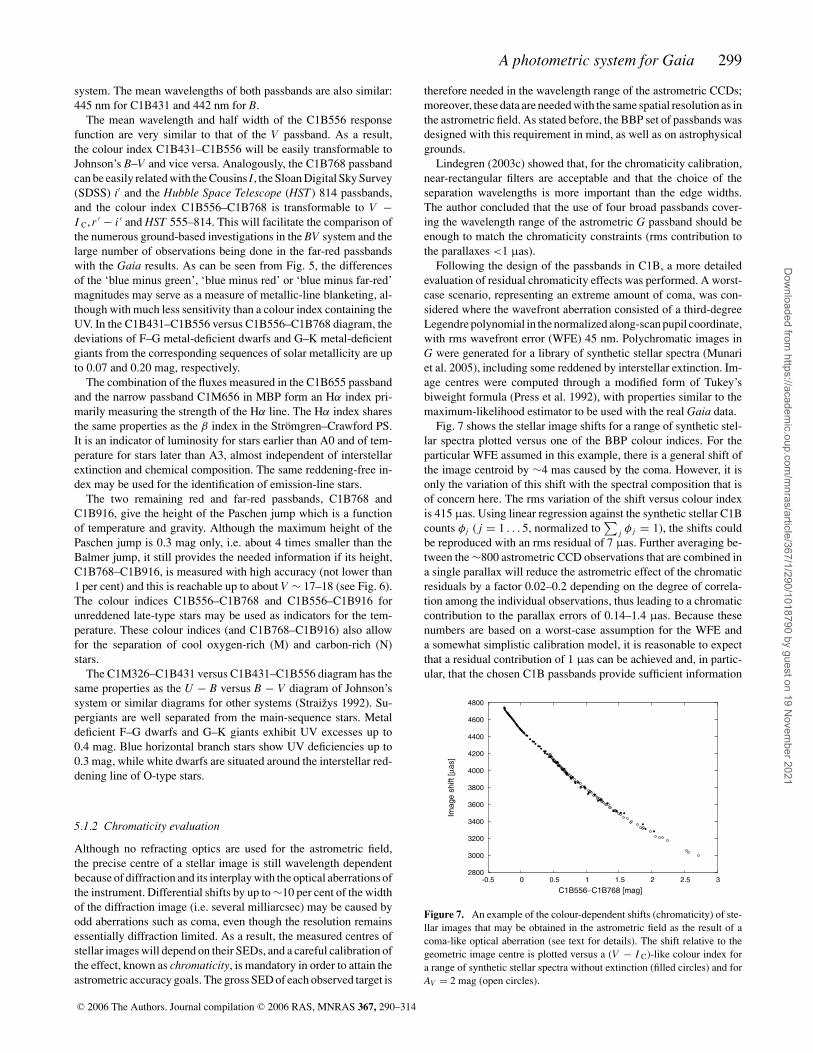
Following the design of the passbands in C1B, a more detailedevaluation of residual chromaticity effects was performed. A worst-case scenario, representing an extreme amount of coma, was con-sidered where the wavefront aberration consisted of a third-degreeLegendre polynomial in the normalized along-scan pupil coordinate,with rms wavefront error (WFE) 45 nm. Polychromatic images inG were generated for a library of synthetic stellar spectra (Munariet al. 2005), including some reddened by interstellar extinction. Im-age centres were computed through a modified form of Tukey’sbiweight formula (Press et al. 1992), with properties similar to themaximum-likelihood estimator to be used with the real Gaia data.
Fig. 7 shows the stellar image shifts for a range of synthetic stel-lar spectra plotted versus one of the BBP colour indices. For theparticular WFE assumed in this example, there is a general shift ofthe image centroid by ∼4 mas caused by the coma. However, it isonly the variation of this shift with the spectral composition that isof concern here. The rms variation of the shift versus colour indexis 415 μas. Using linear regression against the synthetic stellar C1Bcounts φ j ( j = 1 . . . 5, normalized to
∑j φ j = 1), the shifts could
be reproduced with an rms residual of 7 μas. Further averaging be-tween the ∼800 astrometric CCD observations that are combined ina single parallax will reduce the astrometric effect of the chromaticresiduals by a factor 0.02–0.2 depending on the degree of correla-tion among the individual observations, thus leading to a chromaticcontribution to the parallax errors of 0.14–1.4 μas. Because thesenumbers are based on a worst-case assumption for the WFE anda somewhat simplistic calibration model, it is reasonable to expectthat a residual contribution of 1 μas can be achieved and, in partic-ular, that the chosen C1B passbands provide sufficient information
2800
3000
3200
3400
3600
3800
4000
4200
4400
4600
4800
-0.5 0 0.5 1 1.5 2 2.5 3
Image s
hift
[μas]
C1B556−C1B768 [mag]
Figure 7. An example of the colour-dependent shifts (chromaticity) of ste-llar images that may be obtained in the astrometric field as the result of acoma-like optical aberration (see text for details). The shift relative to thegeometric image centre is plotted versus a (V − I C)-like colour index fora range of synthetic stellar spectra without extinction (filled circles) and forAV = 2 mag (open circles).
C© 2006 The Authors. Journal compilation C© 2006 RAS, MNRAS 367, 290–314
Dow
nloaded from https://academ
ic.oup.com/m
nras/article/367/1/290/1018790 by guest on 19 Novem
ber 2021

300 C. Jordi et al.
-300
-200
-100
0
100
200
300
0 1 2 3 4 5 6
Ima
ge
sh
ift
[μa
s]
Redshift z
Figure 8. The chromatic shifts of a quasar image before (dash-dotted curve)and after (solid) correction for the effect calibrated by means of stellar spec-tra. A standard quasar spectrum was assumed to be observed at differentredshifts and subject to the same aberrations as in Fig. 7. (The dash-dottedcurve has been displaced 4000 μas downwards in the diagram to offset theoverall shift caused by the coma.)
on the SED within the G passband for this purpose. The residualeffect is thus small compared with the statistical errors from photonnoise and other sources even for bright stars.
The chromaticity correction based on an empirical calibrationagainst stellar BBP fluxes will be less accurate for objects withstrongly deviating SEDs. Prime examples of this are the quasars,which may exhibit strong emission lines at almost any wavelengthdepending on redshift. Quasars are astrometrically important forestablishing a non-rotating extragalactic reference system for propermotions; thus, chromaticity correction must work also for theseobjects. This was investigated by applying the correction derivedas described above from stellar spectra to synthetic quasar images,calculated from a mean quasar spectrum observed at redshifts inthe range z = 0 to 6. Fig. 8 shows the uncorrected image shift asfunction of z (dash-dotted curve) together with the residual shift
Table 4. Specifications of the filters in C1M implemented in Spectro.
Band C1M326 C1M379 C1M395 C1M410 C1M467 C1M506 C1M515
λblue (nm) 285 367 390 400 458 488 506λred (nm) 367 391 400 420 478 524 524λo (nm) 326 379 395 410 468 506 515λ (nm) 82 24 10 20 20 36 18δλ (nm) 5 5 5 5 5 5 5ε (nm) 2,2 2,2 2,1 1,2 2,2 2,2 2,2Tmax (per cent) 90 90 90 90 90 90 90Type of CCD Blue Blue Blue Blue Blue Blue Bluenstrips 2 2 1 1 1 1 1
Band C1M549 C1M656 C1M716 C1M747 C1M825 C1M861 C1M965
λblue (nm) 538 652.8 703 731 808 845 930λred (nm) 560 659.8 729 763 842 877 1000λc (nm) 549 656.3 717 747 825 861 965λ (nm) 22 7 26 32 34 32 70δλ (nm) 5 2 5 5 5 5 5ε (nm) 2,2 1,1 2,2 2,2 2,2 2,2 2,2Tmax (per cent) 90 90 90 90 90 90 90Type of CCD Blue Red Red Red Red Red Rednstrips 1 1 1 1 1 1 1
λblue, λred: wavelengths at half-maximum transmission. λc: central wavelength = 0.5(λblue + λred). λ: FWHM.λ: edge width (blue, red) between 10 and 90 per cent of Tmax. ε: manufacturing tolerance intervals centred onλblue and λred. Tmax: maximum transmission of filter. nstrips: number of CCD strips carrying the filter.
after correction (solid curve). The rms image shift decreases from170 μas before to 29 μas after correction. The residual curve showsartefacts that are clearly attributable to the limited sampling of thespectral range. For example, the negative slopes for z = 2.3–2.8 andz = 3.1–3.9 correspond to the redshifted Lyman-α emission linemoving through the C1B431 and C1B556 passbands, respectively.
With similar assumptions as for the stars concerning the statisticalaveraging of the effect when propagating to the astrometric param-eters, the residual effect for the quasars will be a few microarcsec.This is acceptable because these are mostly faint objects with muchlarger photon-statistical errors.
Note that the data in Figs 7–8 only represent an example of theimage shifts that may occur. The actual behaviour depends stronglyon the shape and size of WFE, which vary considerably across thefield of view, and on the detailed centroiding algorithm.
5.2 The C1M medium passbands
The C1M component of the Gaia PS consists of 14 passbands andevolved from the convergence of the proposals by Grenon et al.(1999), Vansevicius & Bridzius (2002), Knude & Høg (2004), Jordi& Carrasco (2004b) and Straizys et al. (2004) . The guidelines byTautvaisiene & Edvardsson (2002) for α-element abundance deter-mination were taken into account. The basic response curve of the fil-ters versus wavelength is a symmetric quasi-trapezoidal shape. Theirparameters are listed in Table 4 and the response of the correspond-ing passbands is shown in Fig. 9. Six strips with red-enhanced CCDsare available for MBP and six red passbands have been designed,implemented as one filter for each strip, with the only constraintthat MBP has to measure the flux entering the RVS instrument (seeSection 4.1). For the blue passbands, eight filters are implementedon the 10 strips with blue-enhanced CCDs. Two strips have beenallocated to each of the two UV passbands to increase the S/N ofthe measurements.
The primary purpose of the medium passbands is the classifi-cation and astrophysical parametrization of the observed objects
C© 2006 The Authors. Journal compilation C© 2006 RAS, MNRAS 367, 290–314
Dow
nloaded from https://academ
ic.oup.com/m
nras/article/367/1/290/1018790 by guest on 19 Novem
ber 2021

A photometric system for Gaia 301
300 400 500 600
Wavelength (nm)
0
0.2
0.4
0.6
0.8
1N
orm
aliz
ed
re
sp
on
se
(e
ne
rgy)
A0 V
G2 V
K7 V
AW Cyg
600 700 800 900 1000
Wavelength (nm)
0
0.2
0.4
0.6
0.8
1
Norm
aliz
ed r
esponse (
energ
y)
A0 V
G2 V
K7 V
AW Cyg
Figure 9. Same as Fig. 5 for C1M. Top and bottom figures show the ‘blue’and ‘red’ passbands, respectively.
(stars, QSOs, galaxies, Solar system bodies, etc.). In the case ofthe stars, the goal is to determine effective temperature Teff, gravitylog g or luminosity MV , chemical composition [M/H], [α/Fe] andC/O abundances, peculiarity type, the presence of emission, etc., inthe presence of varying and unknown interstellar extinction. Taxon-omy classification for Solar system objects and photometric redshiftdetermination for QSOs are also aimed for.
5.2.1 Astrophysical diagnostics
The filter at the shortest wavelength is C1M326 with wavelengths athalf-maximum transmission of 285 and 367 nm (thus it is of broadpassband type although implemented in Spectro). Below 280 nm,strong absorption lines, metallicity dependent, are present alreadyin A-type stars. The interstellar extinction increases rapidly below280 nm and reaches a maximum at 218 nm. In space, the UVpassband can be extended down to 280 nm, which improves thedetermination of [M/H] for F–G–K stars because of the presenceof many atomic lines, ionized or of high excitation. For late Gdwarfs, the line blocking in the extended UV passband is about2.7 times larger than in the violet 376–430 nm domain. The red sideof C1M326 is set at the Balmer jump. The colour indices C1M326–
C1B431 or C1M326–C1M410 give the height of the Balmer jump,which is a function of Teff and log g in B–A–F stars. In F–G–K stars,these colour indices measure metallic line blocking in the UV, whichcan be calibrated in terms of [M/H].
The C1M379 passband is placed on the wavelength range wherethe lines corresponding to the higher energy levels of the Balmerseries crowd together in early-type stars. The integrated absorptionin these lines is very sensitive to log g (or MV ). For late-type stars,the position of this passband coincides with the maximum blockingof the spectrum by metallic lines. Hence, the colour index C1M379–C1M467 is a sensitive indicator of metallicity. Analogues in otherPSs are the P magnitude in the Vilnius system and L in the Walravensystem.
The C1M395 passband is introduced mainly to measure the Ca II
H line. The index C1M395–C1M410 shows a strong correlation withW(CaT∗), the equivalent width of the Calcium triplet measured bythe RVS instrument, corrected for the influence of the Paschen lines.The C1M395–C1M410 versus W(CaT∗) may be used as a log gestimator (Kaltcheva, Knude & Georgiev 2003, Knude & Carrasco,private communication). The C1M395–C1M410 versus W(CaT∗)plane is particularly useful because the effect of reddening on thecolour index is only minor due to the small separation of the twopassbands. Additional uses of the C1M395 passband are in assistingthe [α/Fe] determination and in the identification of very metal-poorstars.
The violet C1M410 passband measures the spectrum intensityredwards of the Balmer jump. In combination with C1M326, it givesthe height of the jump. For K–M stars it is the shortest passband that,when combined with longer passbands, can provide temperaturesand luminosities of solar metallicity stars in the presence of inter-stellar reddening (i.e. when the stars are too faint in the UV). Itsanalogues are: v in the Stromgren system, B1 in the Geneva systemand X in the Vilnius system.
The blue C1M467 and green C1M549 passbands measure do-mains where the absorption by atomic and molecular lines is mini-mal. The flux in these domains corresponds to a pseudo-continuum.The colour indices C1M467–C1M549, C1M467–C1M747 andC1M549–C1M747 may be used as indicators of the temperaturefor stars of all spectral types. The analogues of C1M467 are: b inthe Stromgren system, B2 in the Geneva system and Y in the Vilniussystem. The analogues of C1M549 are: y in the Stromgren systemand V in the Vilnius system.
The green C1M515 passband is placed on a broad spectral de-pression seen in the spectra of G- and K-type stars and formed bycrowding of numerous metallic lines. Among them, the strongestfeatures are the Mg I triplet and the MgH band. The depth of this de-pression, the intensity of which reaches a maximum around K7 V, isvery sensitive to gravity, being deeper in dwarfs than in giants. Thesame passband is also useful for the identification of Ap stars of theSr–Cr–Eu type. The same passband (Z) is used in the Vilnius PS.
The C1M506 is much broader and includes the C1M515 passbandregion. The combination of both provides an index that is almostreddening free and its combination with the contiguous pseudo-continuum passbands (C1M467 and C1M549) provides an indexsensitive to Mg abundances and gravity. If the luminosity is knownfrom parallax, Mg abundances can be determined. The Ca II and Mg I
spectral features show inverse behaviour when [M/H] and [α/Fe]change (Tautvaisiene & Edvardsson 2002), and hence, indices usingC1M395 and C1M515 allow the disentangling of Fe and α-processelement abundances.
The narrow passband C1M656 is placed on the Hα line. Asmentioned in Section 5.1, the Hα = C1B655–C1M656 index is a
C© 2006 The Authors. Journal compilation C© 2006 RAS, MNRAS 367, 290–314
Dow
nloaded from https://academ
ic.oup.com/m
nras/article/367/1/290/1018790 by guest on 19 Novem
ber 2021
302 C. Jordi et al.
measure of the intensity of the Hα line, yielding luminosities forstars earlier than A0 and temperatures for stars later than A3. Theindex is most useful for identification of emission-line stars (Be, Oe,Of, T Tau, Herbig Ae/Be, etc.).
C1M716 coincides with one of the deepest TiO absorption bandswith a head at 713 nm (Wahlgren, Lundqvist & Kucinskas 2005),while C1M747 measures a portion of the spectrum where the ab-sorption by TiO bands is minimum. So, the index C1M716–C1M747is a strong indicator of the presence and intensity of TiO, which de-pends on temperature and TiO abundance for late K- and M-typestars. For earlier type stars, both passbands provide measurements ofthe pseudo-continuum. Earlier PS proposals for MBP considered theinclusion of a filter centred on the TiO absorption band at 781 nm.FoM computations and analysis of the σk,post values showed thatthe AP determination improves by more than 10 per cent, for[Ti/H] and Teff, if the passband is centred on 716 nm instead of on781 nm. A similar but narrower passband has been used in the Wingeight-colour far-red system.
The passband C1M825 is designed to measure either the contin-uum bluewards of the Paschen jump (hence its limitation at 842 nmfor the red side mid-transmission wavelength) or the strong Carbon-Nitrogen (CN) band for R- and N-type stars. For M stars, C1M825measures a spectral domain with weak absorption by TiO. The dis-tinction between M and C stars is realized with all red passbands.At a given temperature, the fluxes are similar in the C1M747 andC1M861 for O-rich stars (the M sequence) and for C-rich stars (theC sequence), but very different in the C1M825 and C1M965 pass-bands, namely because of strong CN bands developing redwards of787 nm. The separation between M and C stars is possible even ifthey are heavily reddened.
Similarly, C1M965 measures the continuum redwards of Paschenjump (and in combination with C1M825 yields the height of thejump) or strong absorption bands for R- and N-type stars (see Fig. 9,bottom). Having a passband at these very red wavelengths at the edgeof the CCD QE curve improves the interstellar extinction determi-nation, which was proven through the FoM computations.
The C1M861 passband, in between C1M825 and C1M965, isconstrained by the wavelength range of the RVS instrument (i.e.848–874 nm) and hence includes the Ca infrared triplet. The mea-surement of the flux of the star in this passband will help the RVSdata reduction. The index C1M861–C1M965 measures the gravity-sensitive absorption of the high member lines of the Paschen series.
Finally, the indices C1M825–C1M861 and C1M861-C1M965 area sensitive criterion for the separation of M-, R- and N-type stars(see Fig. 9, bottom).
6 P H OTO M E T R I C P R E C I S I O N
This section describes the simulation of photometric fluxes that willbe measured by Gaia, the associated magnitude errors and the ef-fect on these errors of crowded regions and the calibration of thephotometric measurements.
6.1 Simulated photometry
For the simulation of synthetic white light (G, GS), C1B andC1M fluxes and their corresponding errors, a photometry simulatorGAIAPHOTSIM4 was created. This tool predicts the number of pho-toelectrons per unit time (or per CCD crossing) for every given
4 A web interface is available at http://gaia.am.ub.es/PWG/
passband, observed target and Gaia instrument specification. GA-IAPHOTSIM also estimates the associated magnitude and the magni-tude error per transit and at the end of the mission. The inputs are:the instrument parameters; the SED (from an empirical or syntheticspectral library) of the observed object; its apparent magnitude andradial velocity; the extinction law and the AV value; the brightness ofthe sky background; and, optionally, the coordinates of the object onthe sky. The coordinates allow the derivation of the actual number ofobservations according to the nominal scanning law. The adopted in-terstellar extinction law is that of Cardelli, Clayton & Mathis (1989)and the ratio of total to selective absorption can be chosen. The lat-ter has a default value of 3.1. Simulations can be done for singleand multiple stars, emission-line stars, peculiar stars, Solar systemobjects, QSOs, etc., actually for any given SED.
To compute the object flux sj, measured in a given photometricpassband j and collected after a single CCD crossing, the followingingredients are needed: the object SED; the assumed interstellarextinction and the extinction law all resulting in N(λ) (in units ofphoton m−2 s−1 nm−1); the transmission profile of the passbandTj(λ); the telescope transmittance T(λ); the detector response Q(λ)(the CCD QE); the pupil area A; and the single-CCD integrationtime τ . The object flux is then given by:
s j [e−] = Aτ
∫ λmax, j
λmin, j
dλN (λ)T (λ)Tj (λ)Q(λ). (1)
The flux sj is converted into standard magnitudes mj using the ab-solute flux calibration of Vega (Megessier 1995), with all its coloursset equal to zero. The SED of Vega has been modelled accordingto Bessell, Castelli & Plez (1998; a Kurucz SED of Teff = 9550 K,log g = 3.95, [M/H] = −0.5).
By default, the magnitude of the sky background is assumed to beat the level of the zodiacal light measured in HST observations and isset to V = 22.5 mag arcsec−2. This assumption is very conservativefor most of the sky. For example, HST measurements show that thesky background is V = 23.3 mag arcsec−2 at high ecliptic latitudes.
All simulations in this paper were run with the mean value forthe total number of observations (see Table 1) and with the defaultvalues for the extinction law and the sky background.
6.2 Aperture photometry and associated errors
As discussed in Section 2.3, during the observational process onlythe pixels in the area immediately surrounding the target source aresent to the ground in the form of a ‘window’. In most cases, thepixels in the window are binned in the across-scan direction so thatthe resulting data consists of a 1D set of number counts per sample.Following an ‘aperture photometry’approach, it is assumed that theobject flux sj within a given passband j is measured in a rectangular‘aperture’ of ns samples within the window. Some light loss can beproduced due to vignetting and/or the finite extent of the ‘aperture’.Hence, the actual measured flux will be f aper × sj, where f aper � 1.
The end-of-mission magnitude error (σm, j ) is computed takinginto account:
(i) the total detection noise per sample r, which includes the de-tector readout noise;
(ii) the sky background contribution bj assumed to be derivedfrom nb background samples;
(iii) the contribution of the calibration error per elementary ob-servation σcal; and
(iv) the mean total number of observations n eff = nobs × n strips.
C© 2006 The Authors. Journal compilation C© 2006 RAS, MNRAS 367, 290–314
Dow
nloaded from https://academ
ic.oup.com/m
nras/article/367/1/290/1018790 by guest on 19 Novem
ber 2021
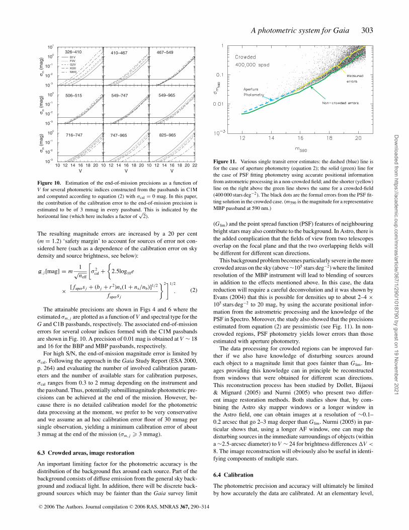
A photometric system for Gaia 303
10 12 14 16 18 20
V
10–3
10–2
10–1
100
σ m (
ma
g)
10–3
10–2
10–1
100
σ m (
ma
g)
10–3
10–2
10–1
100
101
σ m (
ma
g) B1V
F0V
G2V
K0III
M0III
10 12 14 16 18 20
V
10 12 14 16 18 20 22
V
326–410 410–467 467–549
506–515 549–747 549–965
716–747 747–965 825–965
Figure 10. Estimation of the end-of-mission precisions as a function ofV for several photometric indices constructed from the passbands in C1Mand computed according to equation (2) with σcal = 0 mag. In this paper,the contribution of the calibration error to the end-of-mission precision isestimated to be of 3 mmag in every passband. This is indicated by thehorizontal line (which here includes a factor of
√2).
The resulting magnitude errors are increased by a 20 per cent(m = 1.2) ‘safety margin’ to account for sources of error not con-sidered here (such as a dependence of the calibration error on skydensity and source brightness, see below):
σm, j [mag] = m1√neff
[σ 2
cal +{
2.5log10e
× [ fapers j + (b j + r 2)ns(1 + ns/nb)]1/2
fapers j
}2]1/2
. (2)
The attainable precisions are shown in Figs 4 and 6 where theestimated σm, j are plotted as a function of V and spectral type for theG and C1B passbands, respectively. The associated end-of-missionerrors for several colour indices formed with the C1M passbandsare shown in Fig. 10. A precision of 0.01 mag is obtained at V ∼ 18and 16 for the BBP and MBP passbands, respectively.
For high S/N, the end-of-mission magnitude error is limited byσcal. Following the approach in the Gaia Study Report (ESA 2000,p. 264) and evaluating the number of involved calibration param-eters and the number of available stars for calibration purposes,σcal ranges from 0.3 to 2 mmag depending on the instrument andthe passband. Thus, potentially submillimagnitude photometric pre-cisions can be achieved at the end of the mission. However, be-cause there is no detailed calibration model for the photometricdata processing at the moment, we prefer to be very conservativeand we assume an ad hoc calibration error floor of 30 mmag persingle observation, yielding a minimum calibration error of about3 mmag at the end of the mission (σm, j � 3 mmag).
6.3 Crowded areas, image restoration
An important limiting factor for the photometric accuracy is thedistribution of the background flux around each source. Part of thebackground consists of diffuse emission from the general sky back-ground and zodiacal light. In addition, there will be discrete back-ground sources which may be fainter than the Gaia survey limit
Figure 11. Various single transit error estimates: the dashed (blue) line isfor the case of aperture photometry (equation 2); the solid (green) line forthe case of PSF fitting photometry using accurate positional informationfrom astrometric processing in a non-crowded field; and the shorter (yellow)line on the right above the green line shows the same for a crowded-field(400 000 stars deg−2). The black dots are the formal errors from the PSF fit-ting solution in the crowded case. (m590 is the magnitude for a representativeMBP passband at 590 nm.)
(Glim) and the point spread function (PSF) features of neighbouringbright stars may also contribute to the background. In Astro, there isthe added complication that the fields of view from two telescopesoverlap on the focal plane and that the two overlapping fields willbe different for different scan directions.
This background problem becomes particularly severe in the morecrowded areas on the sky (above ∼105 stars deg−2) where the limitedresolution of the MBP instrument will lead to blending of sourcesin addition to the effects mentioned above. In this case, the datareduction will require a careful deconvolution and it was shown byEvans (2004) that this is possible for densities up to about 2–4 ×10⁵ stars deg−2 to 20 mag, by using the accurate positional infor-mation from the astrometric processing and the knowledge of thePSF in Spectro. Moreover, the study also showed that the precisionsestimated from equation (2) are pessimistic (see Fig. 11). In non-crowded regions, PSF photometry yields lower errors than thoseestimated with aperture photometry.
The data processing for crowded regions can be improved fur-ther if we also have knowledge of disturbing sources aroundeach object to a magnitude limit that goes fainter than Glim. Im-ages providing this knowledge can in principle be reconstructedfrom windows that were obtained for different scan directions.This reconstruction process has been studied by Dollet, Bijaoui& Mignard (2005) and Nurmi (2005) who present two differ-ent image restoration methods. Both studies show that, by com-bining the Astro sky mapper windows or a longer window inthe Astro field, one can obtain images at a resolution of ∼0.1–0.2 arcsec that go 2–3 mag deeper than Glim. Nurmi (2005) in par-ticular shows that, using a longer AF window, one can map thedisturbing sources in the immediate surroundings of objects (withina ∼2.5-arcsec diameter) to V ∼ 24 for brightness differences V <
8. The image reconstruction will obviously also be useful in identi-fying components of multiple stars.
6.4 Calibration
The photometric precision and accuracy will ultimately be limitedby how accurately the data are calibrated. At an elementary level,
C© 2006 The Authors. Journal compilation C© 2006 RAS, MNRAS 367, 290–314
Dow
nloaded from https://academ
ic.oup.com/m
nras/article/367/1/290/1018790 by guest on 19 Novem
ber 2021
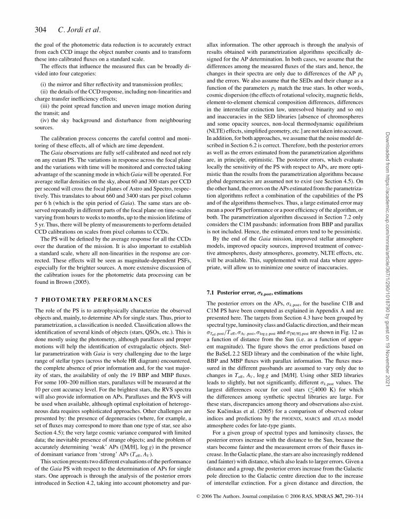
304 C. Jordi et al.
the goal of the photometric data reduction is to accurately extractfrom each CCD image the object number counts and to transformthese into calibrated fluxes on a standard scale.
The effects that influence the measured flux can be broadly di-vided into four categories:
(i) the mirror and filter reflectivity and transmission profiles;(ii) the details of the CCD response, including non-linearities and
charge transfer inefficiency effects;(iii) the point spread function and uneven image motion during
the transit; and(iv) the sky background and disturbance from neighbouring
sources.
The calibration process concerns the careful control and moni-toring of these effects, all of which are time dependent.
The Gaia observations are fully self-calibrated and need not relyon any extant PS. The variations in response across the focal planeand the variations with time will be monitored and corrected takingadvantage of the scanning mode in which Gaia will be operated. Foraverage stellar densities on the sky, about 60 and 300 stars per CCDper second will cross the focal planes of Astro and Spectro, respec-tively. This translates to about 660 and 3400 stars per pixel columnper 6 h (which is the spin period of Gaia). The same stars are ob-served repeatedly in different parts of the focal plane on time-scalesvarying from hours to weeks to months, up to the mission lifetime of5 yr. Thus, there will be plenty of measurements to perform detailedCCD calibrations on scales from pixel columns to CCDs.
The PS will be defined by the average response for all the CCDsover the duration of the mission. It is also important to establisha standard scale, where all non-linearities in the response are cor-rected. These effects will be seen as magnitude-dependent PSFs,especially for the brighter sources. A more extensive discussion ofthe calibration issues for the photometric data processing can befound in Brown (2005).
7 P H OTO M E T RY P E R F O R M A N C E S
The role of the PS is to astrophysically characterize the observedobjects and, mainly, to determine APs for single stars. Thus, prior toparametrization, a classification is needed. Classification allows theidentification of several kinds of objects (stars, QSOs, etc.). This isdone mostly using the photometry, although parallaxes and propermotions will help the identification of extragalactic objects. Stel-lar parametrization with Gaia is very challenging due to the largerange of stellar types (across the whole HR diagram) encountered,the complete absence of prior information and, for the vast major-ity of stars, the availability of only the 19 BBP and MBP fluxes.For some 100–200 million stars, parallaxes will be measured at the10 per cent accuracy level. For the brightest stars, the RVS spectrawill also provide information on APs. Parallaxes and the RVS willbe used when available, although optimal exploitation of heteroge-neous data requires sophisticated approaches. Other challenges arepresented by: the presence of degeneracies (where, for example, aset of fluxes may correspond to more than one type of star, see alsoSection 4.5); the very large cosmic variance compared with limiteddata; the inevitable presence of strange objects; and the problem ofaccurately determining ‘weak’ APs ([M/H], log g) in the presenceof dominant variance from ‘strong’ APs (Teff, AV ).
This section presents two different evaluations of the performanceof the Gaia PS with respect to the determination of APs for singlestars. One approach is through the analysis of the posterior errorsintroduced in Section 4.2, taking into account photometry and par-
allax information. The other approach is through the analysis ofresults obtained with parametrization algorithms specifically de-signed for the AP determination. In both cases, we assume that thedifferences among the measured fluxes of the stars and, hence, thechanges in their spectra are only due to differences of the AP pk
and the errors. We also assume that the SEDs and their change as afunction of the parameters pk match the true stars. In other words,cosmic dispersion (the effects of rotational velocity, magnetic fields,element-to-element chemical composition differences, differencesin the interstellar extinction law, unresolved binarity and so on)and inaccuracies in the SED libraries [absence of chromospheresand some opacity sources, non-local thermodynamic equilibrium(NLTE) effects, simplified geometry, etc.] are not taken into account.In addition, for both approaches, we assume that the noise model de-scribed in Section 6.2 is correct. Therefore, both the posterior errorsas well as the errors estimated from the parametrization algorithmsare, in principle, optimistic. The posterior errors, which evaluatelocally the sensitivity of the PS with respect to APs, are more opti-mistic than the results from the parametrization algorithms becauseglobal degeneracies are assumed not to exist (see Section 4.5). Onthe other hand, the errors on the APs estimated from the parametriza-tion algorithms reflect a combination of the capabilities of the PSand of the algorithms themselves. Thus, a large estimated error maymean a poor PS performance or a poor efficiency of the algorithm, orboth. The parametrization algorithm discussed in Section 7.2 onlyconsiders the C1M passbands: information from BBP and parallaxis not included. Hence, the estimated errors tend to be pessimistic.
By the end of the Gaia mission, improved stellar atmospheremodels, improved opacity sources, improved treatment of convec-tive atmospheres, dusty atmospheres, geometry, NLTE effects, etc.will be available. This, supplemented with real data where appro-priate, will allow us to minimize one source of inaccuracies.
7.1 Posterior error, σk,post, estimations
The posterior errors on the APs, σk,post, for the baseline C1B andC1M PS have been computed as explained in Appendix A and arepresented here. The targets from Section 4.3 have been grouped byspectral type, luminosity class and Galactic direction, and their meanσTeff,post/Teff, σAV ,post, σlog g,post and σ[M/H],post are shown in Fig. 12 asa function of distance from the Sun (i.e. as a function of appar-ent magnitude). The figure shows the error predictions based onthe BaSeL 2.2 SED library and the combination of the white light,BBP and MBP fluxes with parallax information. The fluxes mea-sured in the different passbands are assumed to vary only due tochanges in Teff, AV , log g and [M/H]. Using other SED librariesleads to slightly, but not significantly, different σk,post values. Thelargest differences occur for cool stars (�4000 K) for whichthe differences among synthetic spectral libraries are large. Forthese stars, discrepancies among theory and observations also exist.See Kucinskas et al. (2005) for a comparison of observed colourindices and predictions by the PHOENIX, MARCS and ATLAS modelatmosphere codes for late-type giants.
For a given group of spectral types and luminosity classes, theposterior errors increase with the distance to the Sun, because thestars become fainter and the measurement errors of their fluxes in-crease. In the Galactic plane, the stars are also increasingly reddened(and fainter) with distance, which also leads to larger errors. Given adistance and a group, the posterior errors increase from the Galacticpole direction to the Galactic centre direction due to the increaseof interstellar extinction. For a given distance and direction, the
C© 2006 The Authors. Journal compilation C© 2006 RAS, MNRAS 367, 290–314
Dow
nloaded from https://academ
ic.oup.com/m
nras/article/367/1/290/1018790 by guest on 19 Novem
ber 2021
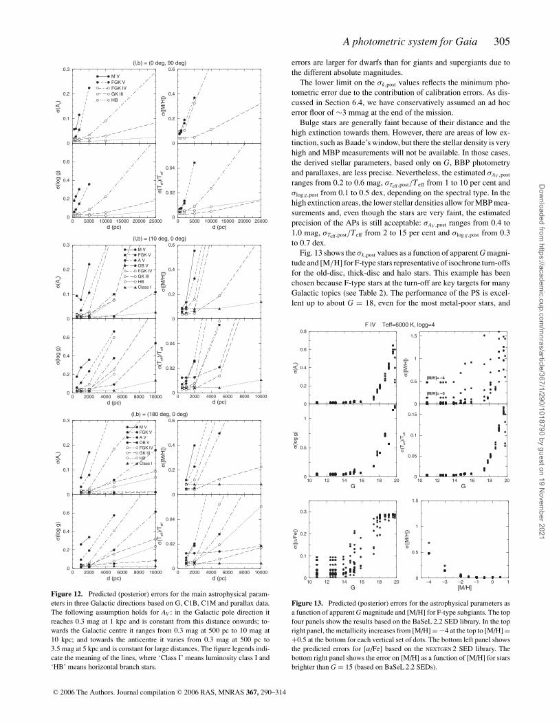
A photometric system for Gaia 305
0 5000 10000 15000 20000 25000
d (pc)
0
0.2
0.4
0.6
σ(lo
g g
)
0
0.1
0.2
0.3
σ(A
v)
(l,b) = (0 deg, 90 deg)
M V
FGK V
FGK IV
GK III
HB
0 5000 10000 15000 20000 25000
d (pc)
0
0.02
0.04
σ(T
eff)/
Te
ff
0
0.2
0.4
0.6
σ([M
/H])
0 2000 4000 6000 8000 10000
d (pc)
0
0.2
0.4
0.6
σ(lo
g g
)
0
0.1
0.2
0.3
σ(A
v)
(l,b) = (10 deg, 0 deg)
M V
FGK V
A V
OB V
FGK IV
GK III
HB
Class I
0 2000 4000 6000 8000 10000
d (pc)
0
0.02
0.04
σ(T
eff)/
Teff
0
0.2
0.4
0.6
σ([M
/H])
0 2000 4000 6000 8000 10000
d (pc)
0
0.2
0.4
0.6
σ(lo
g g
)
0
0.1
0.2
0.3
σ(A
v)
(l,b) = (180 deg, 0 deg)
M V
FGK V
A V
OB V
FGK IV
GK III
HB
Class I
0 2000 4000 6000 8000 10000
d (pc)
0
0.02
0.04
σ(T
eff)/
Te
ff
0
0.2
0.4
0.6
σ([M
/H])
Figure 12. Predicted (posterior) errors for the main astrophysical param-eters in three Galactic directions based on G, C1B, C1M and parallax data.The following assumption holds for AV : in the Galactic pole direction itreaches 0.3 mag at 1 kpc and is constant from this distance onwards; to-wards the Galactic centre it ranges from 0.3 mag at 500 pc to 10 mag at10 kpc; and towards the anticentre it varies from 0.3 mag at 500 pc to3.5 mag at 5 kpc and is constant for large distances. The figure legends indi-cate the meaning of the lines, where ‘Class I’ means luminosity class I and‘HB’ means horizontal branch stars.
errors are larger for dwarfs than for giants and supergiants due tothe different absolute magnitudes.
The lower limit on the σk,post values reflects the minimum pho-tometric error due to the contribution of calibration errors. As dis-cussed in Section 6.4, we have conservatively assumed an ad hocerror floor of ∼3 mmag at the end of the mission.
Bulge stars are generally faint because of their distance and thehigh extinction towards them. However, there are areas of low ex-tinction, such as Baade’s window, but there the stellar density is veryhigh and MBP measurements will not be available. In those cases,the derived stellar parameters, based only on G, BBP photometryand parallaxes, are less precise. Nevertheless, the estimated σAV ,post
ranges from 0.2 to 0.6 mag, σTeff,post/Teff from 1 to 10 per cent andσlog g,post from 0.1 to 0.5 dex, depending on the spectral type. In thehigh extinction areas, the lower stellar densities allow for MBP mea-surements and, even though the stars are very faint, the estimatedprecision of the APs is still acceptable: σAV ,post ranges from 0.4 to1.0 mag, σTeff,post/Teff from 2 to 15 per cent and σlog g,post from 0.3to 0.7 dex.
Fig. 13 shows the σk,post values as a function of apparent G magni-tude and [M/H] for F-type stars representative of isochrone turn-offsfor the old-disc, thick-disc and halo stars. This example has beenchosen because F-type stars at the turn-off are key targets for manyGalactic topics (see Table 2). The performance of the PS is excel-lent up to about G = 18, even for the most metal-poor stars, and
10 12 14 16 18 20
G
0
0.5
1
σ(lo
g g
)
0
0.2
0.4
0.6
0.8
σ(A
v)
F IV Teff=6000 K, logg=4
10 12 14 16 18 20
G
0
0.05
0.1
0.15
σ(T
eff)/
Te
ff0
0.5
1
1.5
σ([M
/H])
[M/H]= –4
[M/H]= –3
10 12 14 16 18 20
G
0
0.1
0.2
0.3
σ([α
/Fe])
–4 –3 –2 –1 0 1
[M/H]
0
0.5
1
1.5
σ([M
/H])
Figure 13. Predicted (posterior) errors for the astrophysical parameters asa function of apparent G magnitude and [M/H] for F-type subgiants. The topfour panels show the results based on the BaSeL 2.2 SED library. In the topright panel, the metallicity increases from [M/H] = −4 at the top to [M/H] =+0.5 at the bottom for each vertical set of dots. The bottom left panel showsthe predicted errors for [α/Fe] based on the NEXTGEN 2 SED library. Thebottom right panel shows the error on [M/H] as a function of [M/H] for starsbrighter than G = 15 (based on BaSeL 2.2 SEDs).
C© 2006 The Authors. Journal compilation C© 2006 RAS, MNRAS 367, 290–314
Dow
nloaded from https://academ
ic.oup.com/m
nras/article/367/1/290/1018790 by guest on 19 Novem
ber 2021
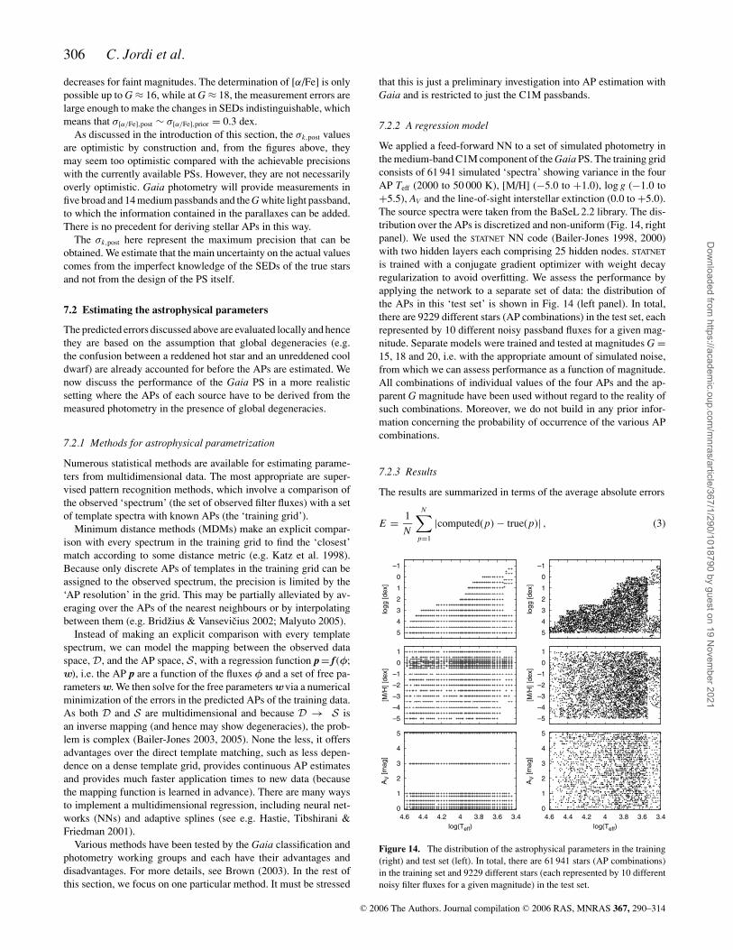
306 C. Jordi et al.
decreases for faint magnitudes. The determination of [α/Fe] is onlypossible up to G ≈ 16, while at G ≈ 18, the measurement errors arelarge enough to make the changes in SEDs indistinguishable, whichmeans that σ[α/Fe],post ∼ σ[α/Fe],prior = 0.3 dex.
As discussed in the introduction of this section, the σk,post valuesare optimistic by construction and, from the figures above, theymay seem too optimistic compared with the achievable precisionswith the currently available PSs. However, they are not necessarilyoverly optimistic. Gaia photometry will provide measurements infive broad and 14 medium passbands and the G white light passband,to which the information contained in the parallaxes can be added.There is no precedent for deriving stellar APs in this way.
The σk,post here represent the maximum precision that can beobtained. We estimate that the main uncertainty on the actual valuescomes from the imperfect knowledge of the SEDs of the true starsand not from the design of the PS itself.
7.2 Estimating the astrophysical parameters
The predicted errors discussed above are evaluated locally and hencethey are based on the assumption that global degeneracies (e.g.the confusion between a reddened hot star and an unreddened cooldwarf) are already accounted for before the APs are estimated. Wenow discuss the performance of the Gaia PS in a more realisticsetting where the APs of each source have to be derived from themeasured photometry in the presence of global degeneracies.
7.2.1 Methods for astrophysical parametrization
Numerous statistical methods are available for estimating parame-ters from multidimensional data. The most appropriate are super-vised pattern recognition methods, which involve a comparison ofthe observed ‘spectrum’ (the set of observed filter fluxes) with a setof template spectra with known APs (the ‘training grid’).
Minimum distance methods (MDMs) make an explicit compar-ison with every spectrum in the training grid to find the ‘closest’match according to some distance metric (e.g. Katz et al. 1998).Because only discrete APs of templates in the training grid can beassigned to the observed spectrum, the precision is limited by the‘AP resolution’ in the grid. This may be partially alleviated by av-eraging over the APs of the nearest neighbours or by interpolatingbetween them (e.g. Bridzius & Vansevicius 2002; Malyuto 2005).
Instead of making an explicit comparison with every templatespectrum, we can model the mapping between the observed dataspace, D, and the AP space, S , with a regression function p = f (φ;w), i.e. the AP p are a function of the fluxes φ and a set of free pa-rameters w. We then solve for the free parameters wvia a numericalminimization of the errors in the predicted APs of the training data.As both D and S are multidimensional and because D → S isan inverse mapping (and hence may show degeneracies), the prob-lem is complex (Bailer-Jones 2003, 2005). None the less, it offersadvantages over the direct template matching, such as less depen-dence on a dense template grid, provides continuous AP estimatesand provides much faster application times to new data (becausethe mapping function is learned in advance). There are many waysto implement a multidimensional regression, including neural net-works (NNs) and adaptive splines (see e.g. Hastie, Tibshirani &Friedman 2001).
Various methods have been tested by the Gaia classification andphotometry working groups and each have their advantages anddisadvantages. For more details, see Brown (2003). In the rest ofthis section, we focus on one particular method. It must be stressed
that this is just a preliminary investigation into AP estimation withGaia and is restricted to just the C1M passbands.
7.2.2 A regression model
We applied a feed-forward NN to a set of simulated photometry inthe medium-band C1M component of the Gaia PS. The training gridconsists of 61 941 simulated ‘spectra’ showing variance in the fourAP Teff (2000 to 50 000 K), [M/H] (−5.0 to +1.0), log g (−1.0 to+5.5), AV and the line-of-sight interstellar extinction (0.0 to +5.0).The source spectra were taken from the BaSeL 2.2 library. The dis-tribution over the APs is discretized and non-uniform (Fig. 14, rightpanel). We used the STATNET NN code (Bailer-Jones 1998, 2000)with two hidden layers each comprising 25 hidden nodes. STATNET
is trained with a conjugate gradient optimizer with weight decayregularization to avoid overfitting. We assess the performance byapplying the network to a separate set of data: the distribution ofthe APs in this ‘test set’ is shown in Fig. 14 (left panel). In total,there are 9229 different stars (AP combinations) in the test set, eachrepresented by 10 different noisy passband fluxes for a given mag-nitude. Separate models were trained and tested at magnitudes G =15, 18 and 20, i.e. with the appropriate amount of simulated noise,from which we can assess performance as a function of magnitude.All combinations of individual values of the four APs and the ap-parent G magnitude have been used without regard to the reality ofsuch combinations. Moreover, we do not build in any prior infor-mation concerning the probability of occurrence of the various APcombinations.
7.2.3 Results
The results are summarized in terms of the average absolute errors
E = 1
N
N∑p=1
|computed(p) − true(p)| , (3)
–1
0
1
2
3
4
5
logg [dex]
–1
0
1
2
3
4
5
logg [dex]
–5
–4
–3
–2
–1
0
1
[M/H
] [d
ex]
–5
–4
–3
–2
–1
0
1
[M/H
] [d
ex]
0
1
2
3
4
5
3.43.63.844.24.44.6
AV [
ma
g]
log(Teff)
0
1
2
3
4
5
3.43.63.844.24.44.6
AV [
ma
g]
log(Teff)
Figure 14. The distribution of the astrophysical parameters in the training(right) and test set (left). In total, there are 61 941 stars (AP combinations)in the training set and 9229 different stars (each represented by 10 differentnoisy filter fluxes for a given magnitude) in the test set.
C© 2006 The Authors. Journal compilation C© 2006 RAS, MNRAS 367, 290–314
Dow
nloaded from https://academ
ic.oup.com/m
nras/article/367/1/290/1018790 by guest on 19 Novem
ber 2021
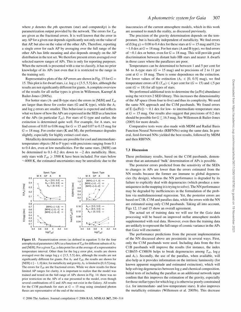
A photometric system for Gaia 307
where p denotes the pth spectrum (star) and computed(p) is theparametrization output provided by the network. The errors for Teff
are given as the fractional errors. It is well known that the error inany AP for a given star depends significantly not only on the value ofthat AP, but also on the value of the other APs. Therefore, reportinga single error for each AP by averaging over the full range of theother APs has little meaning and also depends strongly on the APdistribution in the test set. We therefore present errors averaged overselected narrow ranges of APs. This is only for reporting purposes.When the network is presented with a star to classify, it has no priorknowledge of its APs (not even that it is restricted to the range inthe training set).
Representative plots of the AP errors are shown in Fig. 15 for G =15. This plot is for dwarf stars, i.e. log g ∈ [3.5, 5.5] dex, although theresults are not significantly different for giants. A complete overviewof the results for all stellar types is given in Willemsen, Kaempf &Bailer-Jones (2005a).
For hotter stars (A- and B-type stars) the errors in [M/H] and Teff
are larger than those for cooler stars (G and K type), while the AV
and log g errors are smaller. This behaviour is expected and reflectswhat we know of how the APs are expressed in the SED as a functionof the APs (in particular Teff). For stars of G type and earlier, theextinction is determined quite well. For example, for A stars, wefind errors of 0.03 to 0.06 mag for G = 15 and 0.07 to 0.15 mag forG = 18 mag. For cooler stars (K and M), the performance degradesslightly, especially for highly extinct cool stars.
Metallicity determinations are possible for cool and intermediate-temperature objects (M to F type) with precisions ranging from 0.1to 0.4 dex, even at low metallicities. For the same stars, [M/H] canbe determined to 0.1–0.2 dex down to −2 dex metallicity. Here,only stars with Teff � 3500 K have been included. For stars below∼4000 K, the estimated uncertainties may be unrealistic due to the
0
0.1
0.2
0.3
0.4
0.5BAFGKM
E(A
V)
[mag]
Spect. Type
AV ∈ [3.0, 5.0]AV ∈ [0.5, 3.0]
AV ∈ [0, 0.5]
0
0.2
0.4
0.6
0.8
1
1.2
1.4BAFGKM
E([
M/H
]) [dex]
Spect. Type
[M/H] ∈[–1, 0][M/H] ∈[–2, –1][M/H] ∈[–3,–2]
0
0.1
0.2
0.3
0.4
0.5
0.6
0.7
0.8
3.4 3.6 3.8 4 4.2 4.4
E(logg)
[dex]
log(Teff)
[M/H] ∈[–1,0][M/H] ∈[–2,–1][M/H] ∈[–3,–2]
0
0.04
0.08
0.12
0.16
3.4 3.6 3.8 4 4.2 4.4
fra
cE
(Teff)
[K]
log(Teff)
AV ∈ [3.0, 5.0]AV ∈ [0.5, 3.0]
AV ∈ [0, 0.5]
Figure 15. Parametrization errors (as defined in equation 3) for the fourastrophysical parameters (APs) as a function of Teff for different subsets of AVand [M/H]. For a given Teff, a data point lies at the average of a representativetemperature interval. Other than for the log g error plot, results are shownaveraged over the range log g ∈ [3.5, 5.5] dex, although the results are notsignificantly different for giants. For AV and Teff, the results are shown for[M/H] ∈ [− 1, 0] dex; for metallicity and gravity, AV is limited to [0, 0.5] mag.The errors for Teff are the fractional errors. While we show results for theselimited AP ranges for clarity, it is important to realize that the model wastrained and tested on the full range of APs shown in Fig. 14: there was noprior restriction on the APs of a star presented to the model, even thoughseveral combinations of G and APs may not exist in the Galaxy. All resultsfor the C1M passbands for stars at G = 15 mag using simulated photonfluxes are representative of the end of the mission.
inaccuracies of the current atmosphere models, which in this workare assumed to match the reality, as discussed previously.
The precision of the gravity determination depends on the tem-perature, but is basically independent of metallicity. We find errorsof E(log g) = 0.08 to 0.4 dex for these stars at G = 15 mag and 0.2 to∼1.0 dex at G = 18 mag. For hot stars (A and B type), we find errorsof ∼0.1 dex or better, even for G = 18 mag. This will provide gooddiscrimination between distant halo HB stars and nearer A dwarfsin those cases where the parallaxes are poor.
Temperatures can be determined to between 1 and 5 per cent forM- to A-type stars (G = 15 mag) and to precisions of 2 to 11 percent at G = 18 mag. There is some dependence on the extinction.For lower values of the extinction (AV ∈ [0, 0.5] mag), we findtemperature errors of E (Teff) � 4 per cent for (G = 15) and �5 percent (G = 18) for all types of stars.
We performed additional tests to determine the [α/Fe] abundanceusing the NEXTGEN 2 SED library. This increases the dimensionalityof the AP space (from four to five) and thus its complexity. We usedthe same NN approach and the C1M passbands. We found errorsof E ([α/Fe]) ∼ 0.1 dex for low- to intermediate-temperature starsat G = 15 mag. Our results also suggest that precisions of 0.2 dexshould be possible for G � 16.5 mag. See Willemsen & Bailer-Jones(2005) for more details.
Comparative tests were also made with MDM and Radial BasisFunction Neural Networks (RBFNNs) using the same data. In gen-eral, feed-forward NNs yielded the best results, followed by MDMand then RBFNN.
7.3 Discussion
These preliminary results, based on the C1M passbands, demon-strate that an automated ‘bulk’ determination of APs is possible.
The posterior errors predicted from the sensitivity of the SEDsto changes in APs are lower than the errors estimated from theNN results because the former are immune to global degenera-cies (by design), whereas the NN performance is degraded by itsfailure to explicitly deal with degeneracies (which produce a non-uniqueness in the mapping it is trying to solve). The NN performancemay be degraded by inefficiencies in the formulation of the prob-lem via multidimensional regression. Yet, the posterior errors arebased on C1B, C1M and parallax data, while the errors with the NNare estimated using only C1M passbands. Taking all into account,Figs 12, 13 and 15 show an overall agreement.
The actual set of training data we will use for the Gaia dataprocessing will be based on improved stellar atmosphere modelssupplemented with real data. However, even then the training dataare unlikely to represent the full range of cosmic variance in the APsthat Gaia will encounter.
The performance predictions from the present implementationof the NN discussed above are pessimistic in several ways. First,only the C1M passbands were used. Including data from the fiveC1B passbands will improve the results (for instance, the indexC1B655–C1M656 helps to break degeneracies among Teff, log gand AV ). Secondly, the use of the parallax, when available, willalso help as it provides information on the intrinsic luminosity (forknown apparent magnitude and estimated extinction), which willhelp solving degeneracies between log g and chemical composition.Initial tests of including the parallax as an additional network inputconfirm that this improves the estimation of the gravity, especiallyfor those stellar types for which log g is otherwise poorly constrained(i.e. for intermediate- and low-temperature stars). It also improvesthe metallicity estimates (Willemsen et al. 2005b). This decrease
C© 2006 The Authors. Journal compilation C© 2006 RAS, MNRAS 367, 290–314
Dow
nloaded from https://academ
ic.oup.com/m
nras/article/367/1/290/1018790 by guest on 19 Novem
ber 2021
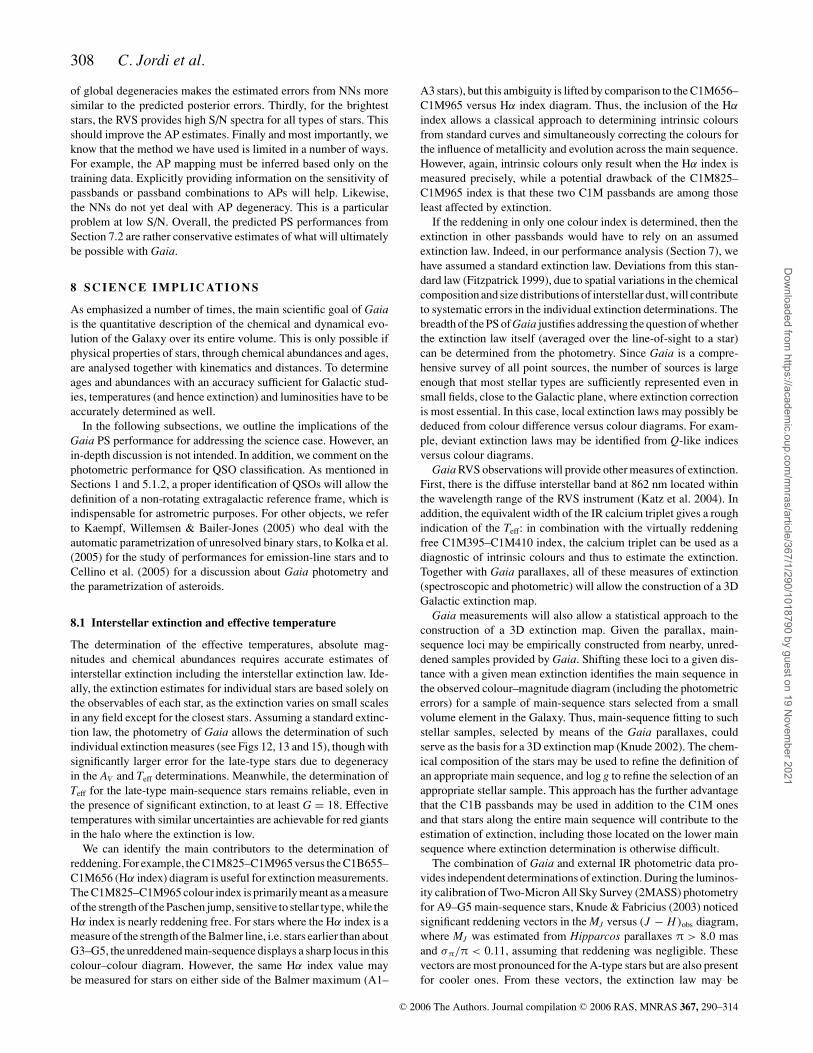
308 C. Jordi et al.
of global degeneracies makes the estimated errors from NNs moresimilar to the predicted posterior errors. Thirdly, for the brighteststars, the RVS provides high S/N spectra for all types of stars. Thisshould improve the AP estimates. Finally and most importantly, weknow that the method we have used is limited in a number of ways.For example, the AP mapping must be inferred based only on thetraining data. Explicitly providing information on the sensitivity ofpassbands or passband combinations to APs will help. Likewise,the NNs do not yet deal with AP degeneracy. This is a particularproblem at low S/N. Overall, the predicted PS performances fromSection 7.2 are rather conservative estimates of what will ultimatelybe possible with Gaia.
8 S C I E N C E I M P L I C AT I O N S
As emphasized a number of times, the main scientific goal of Gaiais the quantitative description of the chemical and dynamical evo-lution of the Galaxy over its entire volume. This is only possible ifphysical properties of stars, through chemical abundances and ages,are analysed together with kinematics and distances. To determineages and abundances with an accuracy sufficient for Galactic stud-ies, temperatures (and hence extinction) and luminosities have to beaccurately determined as well.
In the following subsections, we outline the implications of theGaia PS performance for addressing the science case. However, anin-depth discussion is not intended. In addition, we comment on thephotometric performance for QSO classification. As mentioned inSections 1 and 5.1.2, a proper identification of QSOs will allow thedefinition of a non-rotating extragalactic reference frame, which isindispensable for astrometric purposes. For other objects, we referto Kaempf, Willemsen & Bailer-Jones (2005) who deal with theautomatic parametrization of unresolved binary stars, to Kolka et al.(2005) for the study of performances for emission-line stars and toCellino et al. (2005) for a discussion about Gaia photometry andthe parametrization of asteroids.
8.1 Interstellar extinction and effective temperature
The determination of the effective temperatures, absolute mag-nitudes and chemical abundances requires accurate estimates ofinterstellar extinction including the interstellar extinction law. Ide-ally, the extinction estimates for individual stars are based solely onthe observables of each star, as the extinction varies on small scalesin any field except for the closest stars. Assuming a standard extinc-tion law, the photometry of Gaia allows the determination of suchindividual extinction measures (see Figs 12, 13 and 15), though withsignificantly larger error for the late-type stars due to degeneracyin the AV and Teff determinations. Meanwhile, the determination ofTeff for the late-type main-sequence stars remains reliable, even inthe presence of significant extinction, to at least G = 18. Effectivetemperatures with similar uncertainties are achievable for red giantsin the halo where the extinction is low.
We can identify the main contributors to the determination ofreddening. For example, the C1M825–C1M965 versus the C1B655–C1M656 (Hα index) diagram is useful for extinction measurements.The C1M825–C1M965 colour index is primarily meant as a measureof the strength of the Paschen jump, sensitive to stellar type, while theHα index is nearly reddening free. For stars where the Hα index is ameasure of the strength of the Balmer line, i.e. stars earlier than aboutG3–G5, the unreddened main-sequence displays a sharp locus in thiscolour–colour diagram. However, the same Hα index value maybe measured for stars on either side of the Balmer maximum (A1–
A3 stars), but this ambiguity is lifted by comparison to the C1M656–C1M965 versus Hα index diagram. Thus, the inclusion of the Hα
index allows a classical approach to determining intrinsic coloursfrom standard curves and simultaneously correcting the colours forthe influence of metallicity and evolution across the main sequence.However, again, intrinsic colours only result when the Hα index ismeasured precisely, while a potential drawback of the C1M825–C1M965 index is that these two C1M passbands are among thoseleast affected by extinction.
If the reddening in only one colour index is determined, then theextinction in other passbands would have to rely on an assumedextinction law. Indeed, in our performance analysis (Section 7), wehave assumed a standard extinction law. Deviations from this stan-dard law (Fitzpatrick 1999), due to spatial variations in the chemicalcomposition and size distributions of interstellar dust, will contributeto systematic errors in the individual extinction determinations. Thebreadth of the PS of Gaia justifies addressing the question of whetherthe extinction law itself (averaged over the line-of-sight to a star)can be determined from the photometry. Since Gaia is a compre-hensive survey of all point sources, the number of sources is largeenough that most stellar types are sufficiently represented even insmall fields, close to the Galactic plane, where extinction correctionis most essential. In this case, local extinction laws may possibly bededuced from colour difference versus colour diagrams. For exam-ple, deviant extinction laws may be identified from Q-like indicesversus colour diagrams.
Gaia RVS observations will provide other measures of extinction.First, there is the diffuse interstellar band at 862 nm located withinthe wavelength range of the RVS instrument (Katz et al. 2004). Inaddition, the equivalent width of the IR calcium triplet gives a roughindication of the Teff: in combination with the virtually reddeningfree C1M395–C1M410 index, the calcium triplet can be used as adiagnostic of intrinsic colours and thus to estimate the extinction.Together with Gaia parallaxes, all of these measures of extinction(spectroscopic and photometric) will allow the construction of a 3DGalactic extinction map.
Gaia measurements will also allow a statistical approach to theconstruction of a 3D extinction map. Given the parallax, main-sequence loci may be empirically constructed from nearby, unred-dened samples provided by Gaia. Shifting these loci to a given dis-tance with a given mean extinction identifies the main sequence inthe observed colour–magnitude diagram (including the photometricerrors) for a sample of main-sequence stars selected from a smallvolume element in the Galaxy. Thus, main-sequence fitting to suchstellar samples, selected by means of the Gaia parallaxes, couldserve as the basis for a 3D extinction map (Knude 2002). The chem-ical composition of the stars may be used to refine the definition ofan appropriate main sequence, and log g to refine the selection of anappropriate stellar sample. This approach has the further advantagethat the C1B passbands may be used in addition to the C1M onesand that stars along the entire main sequence will contribute to theestimation of extinction, including those located on the lower mainsequence where extinction determination is otherwise difficult.
The combination of Gaia and external IR photometric data pro-vides independent determinations of extinction. During the luminos-ity calibration of Two-Micron All Sky Survey (2MASS) photometryfor A9–G5 main-sequence stars, Knude & Fabricius (2003) noticedsignificant reddening vectors in the MJ versus (J − H )obs diagram,where MJ was estimated from Hipparcos parallaxes π > 8.0 masand σπ/π < 0.11, assuming that reddening was negligible. Thesevectors are most pronounced for the A-type stars but are also presentfor cooler ones. From these vectors, the extinction law may be
C© 2006 The Authors. Journal compilation C© 2006 RAS, MNRAS 367, 290–314
Dow
nloaded from https://academ
ic.oup.com/m
nras/article/367/1/290/1018790 by guest on 19 Novem
ber 2021
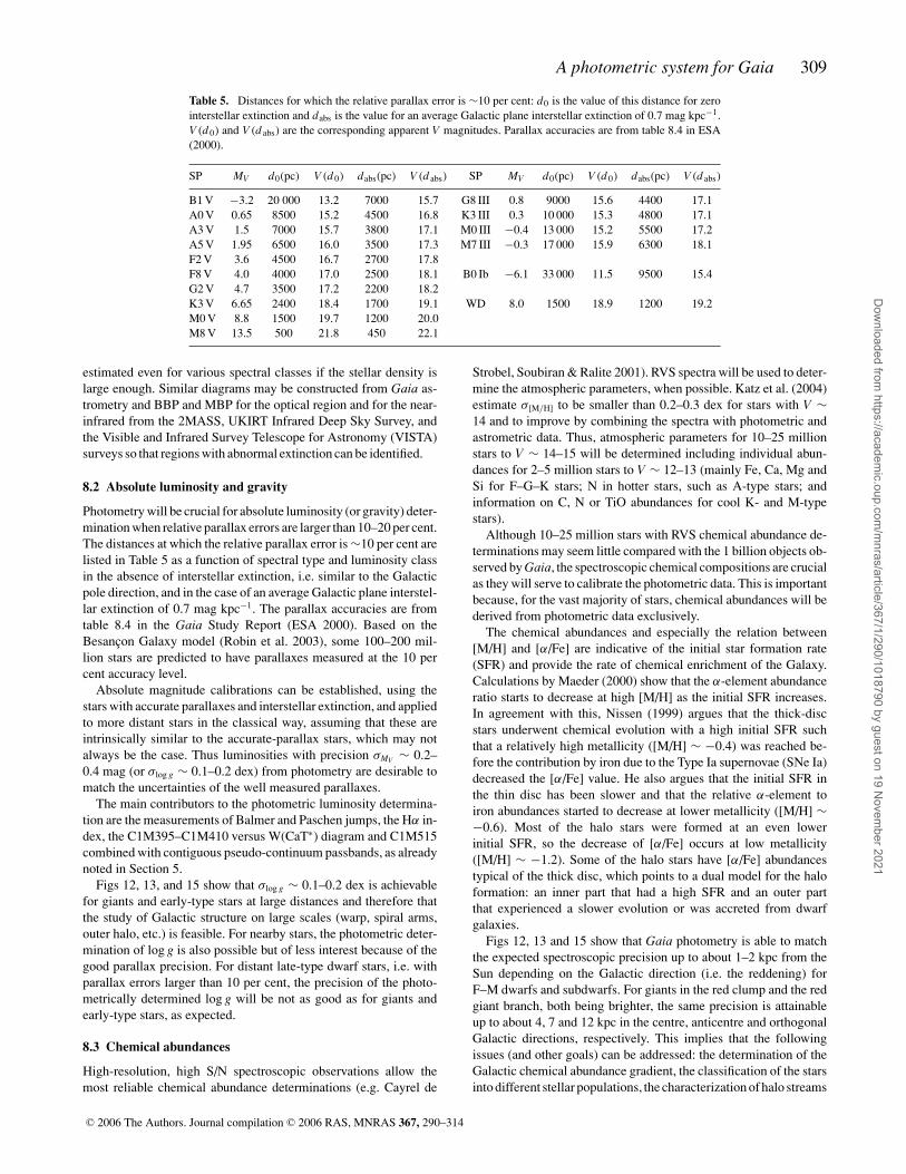
A photometric system for Gaia 309
Table 5. Distances for which the relative parallax error is ∼10 per cent: d0 is the value of this distance for zerointerstellar extinction and dabs is the value for an average Galactic plane interstellar extinction of 0.7 mag kpc−1.V (d 0) and V (d abs) are the corresponding apparent V magnitudes. Parallax accuracies are from table 8.4 in ESA(2000).
SP MV d0(pc) V (d 0) dabs(pc) V (d abs) SP MV d0(pc) V (d 0) dabs(pc) V (d abs)
B1 V −3.2 20 000 13.2 7000 15.7 G8 III 0.8 9000 15.6 4400 17.1A0 V 0.65 8500 15.2 4500 16.8 K3 III 0.3 10 000 15.3 4800 17.1A3 V 1.5 7000 15.7 3800 17.1 M0 III −0.4 13 000 15.2 5500 17.2A5 V 1.95 6500 16.0 3500 17.3 M7 III −0.3 17 000 15.9 6300 18.1F2 V 3.6 4500 16.7 2700 17.8F8 V 4.0 4000 17.0 2500 18.1 B0 Ib −6.1 33 000 11.5 9500 15.4G2 V 4.7 3500 17.2 2200 18.2K3 V 6.65 2400 18.4 1700 19.1 WD 8.0 1500 18.9 1200 19.2M0 V 8.8 1500 19.7 1200 20.0M8 V 13.5 500 21.8 450 22.1
estimated even for various spectral classes if the stellar density islarge enough. Similar diagrams may be constructed from Gaia as-trometry and BBP and MBP for the optical region and for the near-infrared from the 2MASS, UKIRT Infrared Deep Sky Survey, andthe Visible and Infrared Survey Telescope for Astronomy (VISTA)surveys so that regions with abnormal extinction can be identified.
8.2 Absolute luminosity and gravity
Photometry will be crucial for absolute luminosity (or gravity) deter-mination when relative parallax errors are larger than 10–20 per cent.The distances at which the relative parallax error is ∼10 per cent arelisted in Table 5 as a function of spectral type and luminosity classin the absence of interstellar extinction, i.e. similar to the Galacticpole direction, and in the case of an average Galactic plane interstel-lar extinction of 0.7 mag kpc−1. The parallax accuracies are fromtable 8.4 in the Gaia Study Report (ESA 2000). Based on theBesancon Galaxy model (Robin et al. 2003), some 100–200 mil-lion stars are predicted to have parallaxes measured at the 10 percent accuracy level.
Absolute magnitude calibrations can be established, using thestars with accurate parallaxes and interstellar extinction, and appliedto more distant stars in the classical way, assuming that these areintrinsically similar to the accurate-parallax stars, which may notalways be the case. Thus luminosities with precision σMV ∼ 0.2–0.4 mag (or σlog g ∼ 0.1–0.2 dex) from photometry are desirable tomatch the uncertainties of the well measured parallaxes.
The main contributors to the photometric luminosity determina-tion are the measurements of Balmer and Paschen jumps, the Hα in-dex, the C1M395–C1M410 versus W(CaT∗) diagram and C1M515combined with contiguous pseudo-continuum passbands, as alreadynoted in Section 5.
Figs 12, 13, and 15 show that σlog g ∼ 0.1–0.2 dex is achievablefor giants and early-type stars at large distances and therefore thatthe study of Galactic structure on large scales (warp, spiral arms,outer halo, etc.) is feasible. For nearby stars, the photometric deter-mination of log g is also possible but of less interest because of thegood parallax precision. For distant late-type dwarf stars, i.e. withparallax errors larger than 10 per cent, the precision of the photo-metrically determined log g will be not as good as for giants andearly-type stars, as expected.
8.3 Chemical abundances
High-resolution, high S/N spectroscopic observations allow themost reliable chemical abundance determinations (e.g. Cayrel de
Strobel, Soubiran & Ralite 2001). RVS spectra will be used to deter-mine the atmospheric parameters, when possible. Katz et al. (2004)estimate σ[M/H] to be smaller than 0.2–0.3 dex for stars with V ∼14 and to improve by combining the spectra with photometric andastrometric data. Thus, atmospheric parameters for 10–25 millionstars to V ∼ 14–15 will be determined including individual abun-dances for 2–5 million stars to V ∼ 12–13 (mainly Fe, Ca, Mg andSi for F–G–K stars; N in hotter stars, such as A-type stars; andinformation on C, N or TiO abundances for cool K- and M-typestars).
Although 10–25 million stars with RVS chemical abundance de-terminations may seem little compared with the 1 billion objects ob-served by Gaia, the spectroscopic chemical compositions are crucialas they will serve to calibrate the photometric data. This is importantbecause, for the vast majority of stars, chemical abundances will bederived from photometric data exclusively.
The chemical abundances and especially the relation between[M/H] and [α/Fe] are indicative of the initial star formation rate(SFR) and provide the rate of chemical enrichment of the Galaxy.Calculations by Maeder (2000) show that the α-element abundanceratio starts to decrease at high [M/H] as the initial SFR increases.In agreement with this, Nissen (1999) argues that the thick-discstars underwent chemical evolution with a high initial SFR suchthat a relatively high metallicity ([M/H] ∼ −0.4) was reached be-fore the contribution by iron due to the Type Ia supernovae (SNe Ia)decreased the [α/Fe] value. He also argues that the initial SFR inthe thin disc has been slower and that the relative α-element toiron abundances started to decrease at lower metallicity ([M/H] ∼−0.6). Most of the halo stars were formed at an even lowerinitial SFR, so the decrease of [α/Fe] occurs at low metallicity([M/H] ∼ −1.2). Some of the halo stars have [α/Fe] abundancestypical of the thick disc, which points to a dual model for the haloformation: an inner part that had a high SFR and an outer partthat experienced a slower evolution or was accreted from dwarfgalaxies.
Figs 12, 13 and 15 show that Gaia photometry is able to matchthe expected spectroscopic precision up to about 1–2 kpc from theSun depending on the Galactic direction (i.e. the reddening) forF–M dwarfs and subdwarfs. For giants in the red clump and the redgiant branch, both being brighter, the same precision is attainableup to about 4, 7 and 12 kpc in the centre, anticentre and orthogonalGalactic directions, respectively. This implies that the followingissues (and other goals) can be addressed: the determination of theGalactic chemical abundance gradient, the classification of the starsinto different stellar populations, the characterization of halo streams
C© 2006 The Authors. Journal compilation C© 2006 RAS, MNRAS 367, 290–314
Dow
nloaded from https://academ
ic.oup.com/m
nras/article/367/1/290/1018790 by guest on 19 Novem
ber 2021
310 C. Jordi et al.
and the determination of the distance scale through the metallicitydetermination for RR Lyrae.
As expected, low metallicities are determined with less precisionthan solar or higher metallicities. Extensive spectroscopic follow-upefforts from the ground will be necessary to determine the metal-licities of stars with [M/H] < −3.0 with a sufficient accuracy toselect the most interesting targets for high-resolution spectroscopy(Christlieb, private communication).
Photometric chemical composition determinations are not free ofdifficulties. For instance, cool unresolved binaries tend to mimic asingle star with a lower metal content. As an example, for G and Kdwarfs with companions for which m is 1.5–2 mag, the system-atic metallicity error is [M/H] ∼ −0.4. This bias decreases to[M/H] ∼ −0.2 when m = 3.
As discussed in Section 7, the first trials to determine [α/Fe]using the NEXTGEN 2 library ([M/H] ∈ [−2, +0] and [α/Fe] ∈ [−0.2,+0.8]) show that precision of 0.1–0.2 dex for G ∼ 15–16.5 can beachieved. The determination may be improved with the inclusion ofparallax information, because it constrains the value of log g, whichmay break the degeneracy in the variation of the Mg Ib triplet due toluminosity and Mg abundance changes. For stars fainter than G ∼16–17, deriving α-element abundances from photometry is unlikely.
8.4 Age
The location of a star in the HR diagram does not allow for a uniqueage determination as several combinations of chemical composi-tion ([M/H], [α/Fe], Y , etc.) and age are possible (see e.g. Binney& Merrifield 1998). Individually, accurate ages require extremelyaccurate determinations of luminosity, temperature, reddening andchemical composition, which Gaia will provide.
For ages around 10–14 Gyr and assuming a given chemical com-position, a change of log Teff by ∼0.01 dex for the stars in the turn-offtranslates to an age variation of 2 Gyr. Thus, temperatures must beknown with precisions better than a few hundredths in log Teff, i.e.1.5–2 per cent in Teff, for the turn-off stars to determine individuallyaccurate ages. A variation of 0.3 dex in [M/H] is equivalent to achange of log Teff by ∼0.01 dex for a given age. The variation of theα-element abundance has a smaller impact on the age determinationthan the variation of [M/H]. A variation of +0.3 dex in [α/Fe] leadsto a variation of −0.006 dex in the temperature turn-off, yielding anuncertainty of about 1 Gyr in the age.
In summary, an uncertainty of about 4–5 Gyr is estimated for theindividual ages of the stars at the turn-off for the halo, thick-disc andold-thin-disc stars up to about 2, 3 and 5 kpc in the Galactic centre,anticentre and orthogonal directions, respectively, as deduced fromthe PS performances in Section 7.
The age determination for F–G subgiant stars is quite insensitiveto uncertainties in Teff because the isochrones are almost horizontal.An uncertainty in MV of about 0.15 translates to an uncertainty inthe age of about 2 Gyr. Assuming additional uncertainties in [M/H]and [α/Fe] determinations of about 0.3 dex, the final precision ofthe individual ages is about 3–4 Gyr.
Kucinskas et al. (2003) showed that early-AGB stars can pro-vide ages as accurate as the turn-off stars for [M/H] > −1.5 whenσlog Teff ∼ 0.01, σlog g ∼ 0.2, σ[M/H] ∼ 0.2 and σEB−V ∼ 0.03, thus al-lowing the age determination to larger distances than for turn-offand subgiant stars. The Gaia capabilities in the case of metal-poorstars have not yet been investigated.
Subsets of each Galactic population (such as globular clusters,open clusters, OB associations, a given halo stream, an identifiedmerger, a moving group, etc.) can be treated statistically and mean
ages and chemical abundances of the group can be obtained withmuch better precisions than those of the individual members.
The prospects for the determination of the age–metallicity re-lation and the star formation history with Gaia are discussed byHaywood (2005). Assuming the errors on the APs from Section 7,the author recovers the simulated age–metallicity relation in the caseof moderate extinction and for a slowly varying SFR. The details ofthe star formation history, such as a series of prominent short bursts,are not recovered.
8.5 Quasi-stellar objects
QSOs play an important role in the Gaia mission as they will be usedto construct the astrometric reference frame and they are of courseinteresting in their own right. However, because the QSO populationonly represents 0.05 per cent of the stellar population, building asecure QSO sample with no stellar contamination requires a veryefficient rejection algorithm. Although proper motion, parallax andvariability information will help in rejecting stars, these will beavailable with the required precision only at the end of the mission.Therefore, it is important to check the capability to classify QSOsusing only photometric data.
The QSO classification efficiencies of supervised NNs and ofMDMs (see Section 7.2) have been compared using synthetic datagenerated from the BaSeL 2.2 library for stars (Lejeune et al. 1998),from pure-hydrogen atmosphere models for white dwarfs (Koester,private communication) and from a library of QSO synthetic spectra(Claeskens, Smette & Surdej 2005; Claeskens et al. 2006). Properlytrained NNs are found to be capable of rejecting virtually all stars,including white dwarfs. This is at the expense of the completenesslevel of the QSO sample, being only ∼20 per cent at G = 20. How-ever, this provides a sufficient number of objects in the context of thenon-rotating extragalactic reference system determination. MDMsprovide a higher completeness level (∼60 per cent at G = 20),but with a correspondingly higher stellar contamination rate of theQSO sample. MDMs may be preferred at high Galactic latitudes.Not surprisingly, reddened QSOs and weak emission-line objectsare preferentially lost while high-redshift objects are most easilyrecognized.
Assuming an object is a QSO, it is also possible to infer its red-shift from its photometric signature in the C1B+C1M passbands.Unfortunately, there is a colour degeneracy in the QSO spectra thatlimits the expected precision of the technique to about |z|Median �0.2 in the range 0.5 < z spec < 2 (computations were done with aprevious version of the Gaia PS but are not strongly sensitive to theadopted filter sets).
More details on the identification and characterization of QSOswith Gaia can be found in Claeskens et al. (2005).
9 C O N C L U S I O N S
To fully achieve the scientific goals of the Gaia mission, it is essen-tial to complement the astrometric and radial velocity measurementswith highly accurate multicolour photometry. This is necessary bothfor obtaining accurate astrometry and for a proper scientific inter-pretation of the stereoscopic census of the Galaxy Gaia will provide.The latter goal requires that the PS for Gaia is capable of astrophysi-cally parametrizing 1 billion objects across the entire HR diagram inthe presence of varying degrees of reddening and for the full rangeof chemical compositions and ages of stars populating the Galaxyand of identifying peculiar objects and QSOs.
C© 2006 The Authors. Journal compilation C© 2006 RAS, MNRAS 367, 290–314
Dow
nloaded from https://academ
ic.oup.com/m
nras/article/367/1/290/1018790 by guest on 19 Novem
ber 2021
A photometric system for Gaia 311
There are no existing PSs capable of handling this very demand-ing task. We therefore set out to design a new system for the Gaiamission. The broad passbands implemented in the Astro instrumentshould fulfil the chromaticity requirements from the astrometricdata processing, while at the same time allowing for the astrophys-ical characterization of stars in very crowded regions. The mainclassification and astrophysical parametrization task is carried outwith the medium passbands implemented in the Spectro instrument.
The novel development we introduce in this work is the use ofan objective FoM to compare different proposals for the Gaia PS.This FoM is based on the predicted errors that can be obtained forthe parametrization of stars in terms of Teff, log g, AV , [M/H] and[α/Fe]. These errors are calculated by using synthetic spectra toevaluate the sensitivity of each photometric passband to the APs. Atthe same time, the degree of local degeneracy in the APs is taken intoaccount in the FoM. The overall FoM for a PS is calculated takinginto account the priorities of the different STs that were deemed tobe most important for addressing the core science case for Gaia.Using the FoM allows us to choose objectively which of the manyproposed PSs is best in terms of reaching the APs error goals, whileat the same time having the least number of local degeneracies.
The calculation of the predicted posterior errors and the FoM asoutlined in Appendix A can be applied to any PS and can also be usedto predict parametrization errors that can be achieved with spectraof stars. In addition, our method can be extended to the optimizationof systems that can be used for the study of high-redshift galaxies orquasars (for example to derive photometric redshifts), as long as thedependence of the relevant SEDs on parameters such as redshift orSFR are known.
The main contribution of this work is the PS itself. This systemhas been designed based on our astrophysical knowledge and ex-perience with ground-based systems and resulted in five (C1B) and14 (C1M) passbands implemented in the Astro and Spectro instru-ments, respectively. The number of passbands reflects the variety oftargets (all types of stars, QSOs, galaxies, Solar system objects), therequired stellar APs (Teff, log g, AV , [M/H], [α/Fe]) and the needof breaking degeneracies (changes in two or more parameters maytranslate to the same changes in some spectral features but differentchanges in other ones). In summary, three of the broad C1B pass-bands are located to the left of Hβ line, on the Hα line and to theright of Paschen jump. The other two passbands fill the gaps so thatfull coverage of the whole spectral range of Gaia observations isprovided. A broad passband in C1M, implemented in the Spectroinstrument, provides the measurement of the UV flux at wavelengthsbluewards of the Balmer jump. Seven medium passbands are placedon the crowding of Balmer series in early-type stars, on the Ca II Hline, on the Mg I triplet and MgH band, on the Hα line, on one ofTiO absorption bands in cool stars, and on the strong CN band in R-and N-type stars. An additional passband serves to measure the fluxin the wavelength range covered by RVS. Finally, five passbandsare devoted to the measurement of the pseudo-continuum.
The unfiltered light measured in the Astro and Spectro instru-ments provides photometric data in two very broad passbands (from400 to 1000 nm and from 350 to 1025 nm). The G magnitude fromAstro yields the highest S/N among all Gaia magnitudes and henceis the most suitable for variability analysis.
End-of-mission magnitude precisions have been estimated fol-lowing an ‘aperture photometry’ approach. A precision of 0.01 magis obtained at V ∼ 18 and 16 for the C1B and C1M passbands,respectively. In the case of the G passband and for stars brighterthan V∼16 and ∼14 measured with C1B and C1M, respectively,the photometric precision is limited by how accurately the data are
calibrated. Although there is no detailed calibration model, a roughestimation of the number of involved calibration parameters and thenumber of available stars for calibration purposes shows that sub-millimagnitude photometric precisions are potentially achievable.A PSF-fitting approach shows that it is possible to deal with stellardensities up to about 2–4 × 10⁵ stars deg−2 to 20 mag with Spectro,if accurate positional information from astrometry is used.
The performance of the Gaia PS with respect to the determina-tion of APs for single stars has been evaluated using the ‘poste-rior’ errors from the FoM formalism and using algorithms designedfor the astrophysical parametrization of stars (based on MDM andNN). The differences and limitations have been discussed. Bothapproaches demonstrate that precision goals in Section 4.3 are gen-erally achieved to G ∼ 17–18 mag and that the precision for eachparameter depends on temperature, luminosity, chemical compo-sition and interstellar extinction, and apparent magnitude, as ex-pected. Reasonable uncertainties of 0.5–1 dex are obtained evenfor the chemical composition of metal-poor stars ([M/H] = −4.0).The determination of [α/Fe] to a precision of about 0.1–0.2 dex ispossible down to G ∼ 16–17 for low- to intermediate-temperaturestars. Assuming a standard extinction law, the C1B and C1M pass-bands allow the determination of individual extinctions and, hence,the determination of Teff is reliable, even in the presence of signifi-cant extinction, down to at least G = 18. By combining photometryand astrometry, a statistical approach to the construction of a 3DGalactic extinction map is also possible. Gaia will yield parallaxeswith relative uncertainties lower than 10 per cent for some 100–200 million stars allowing absolute magnitude determinationsacross the entire HR diagram if the extinction is known. TheC1B+C1M system is designed to provide the same luminosity er-rors (0.1–0.2 dex in log g) for giants and early-type stars at large dis-tances, ensuring the study of the Galactic structure on large scales.Individual ages of stars at the turn-off of the halo and old-thin andthick disc at distances up to about 2, 3 and 5 kpc in the Galacticcentre, anticentre and orthogonal directions, respectively, can bedetermined with a precision of about 4–5 Gyr. The same precisionscan be obtained for early-AGB stars, thus allowing the probing oflarger distances than with turn-off and subgiant stars. For subgiants,our estimations yield slightly lower uncertainties of 3–4 Gyr. Notethat we quote uncertainties for individual ages. For a group of stars,the mean age will be determined to much better precision.
An additional merit of the Gaia PS is its ability to discriminateQSOs from stars and white dwarfs. This will results in a sufficientnumber of objects for the definition of the non-rotating extragalacticreference system for proper motions.
Finally, the performance of the C1B passbands when dealingwith the chromaticity residuals has been evaluated. Our estimatesshow that the chromatic contribution to the parallax errors is 0.14–1.4 μas. As these numbers are based on a worst-case assumption forthe WFE and a somewhat simplistic calibration model, a residualcontribution of 1 μas for stars and of a few microarcsec for the QSOsis likely achievable.
In summary, the PS C1B+C1M developed by the PhotometryWorking Group satisfies the mission requirements and was thereforeadopted as the baseline by the Gaia Science Team. It has sincebeen adopted by the ESA Project Team as the basis for the formalmission requirements to the industrial teams participating in theESA Invitation to Tender for Gaia.
The experience from the development of the PS, including se-lecting the STs and the ‘FoM’ approach, puts us in a good positionto rapidly optimize new payload proposals that will come from theselected industrial contractor in the course of 2006.
C© 2006 The Authors. Journal compilation C© 2006 RAS, MNRAS 367, 290–314
Dow
nloaded from https://academ
ic.oup.com/m
nras/article/367/1/290/1018790 by guest on 19 Novem
ber 2021

312 C. Jordi et al.
AC K N OW L E D G M E N T S
We would like to acknowledge the contributions by B. Edvardsson,R. Lazauskaite, T. Lejeune and J. Sudzius and the collaborativeeffort of members of the Photometry Working Group within theGaia mission preparation framework. We also thank P. Hauschildt,I. Brott and F. Castelli for making available to us SED librarieswith α-element enhanced abundances. The authors acknowledge thefunding support from the following countries: Belgium, Denmark(through the Danish Ministry of Science), Estonia (through theESF grants nos 5003 and 6106), France, Germany (through theDLR and the Emmy Noether Programme of the DFG), Greece(through GSRT), Italy, Lithuania (through the Ministry of Educationand Science), the Netherlands (through the Netherlands ResearchSchool for Astronomy NOVA and the Netherlands Organisation forScientific Research NWO), Russia, Spain (through MCYT undercontract PNE2003-04352), Sweden, Switzerland and the UnitedKingdom. For Denmark, Estonia, Lithuania and Sweden, supportfrom the Nordic Research Board (ref. NB00-N030 and 2001-2783-4) is gratefully acknowledged. AK acknowledges the Wenner-GrenFellowship. Finally, we would like to thank the referee, M.S. Bessell,for a rapid response and constructive comments that helped improvethe paper.
R E F E R E N C E S
Arenou F., Babusiaux C., Chereau F., Mignot S., 2005, in Perryman M. A. C.,Turon C., O’Flaherty K. S., eds, Proc. Symp. ESA SP-576, The Three Di-mensional Universe with Gaia. ESA Publications Division, Noordwijk,p. 335
Bailer-Jones C. A. L., 1998, Technical report, Statnet. Available athttp://www.mpia.de/homes/calj/statnet.html
Bailer-Jones C. A. L., 2000, A&A 357, 197Bailer-Jones C. A. L., 2003, in Munari U., ed., ASP Conf. Ser. Vol. 298,
GAIA Spectroscopy, Science and Technology. Astron. Soc. Pac., SanFrancisco, p. 199
Bailer-Jones C. A. L., 2004, A&A, 419, 385Bailer-Jones C. A. L., 2005, in Perryman M. A. C., Turon C., O’Flaherty
K. S., eds, Proc. Symp. ESA SP-576, The Three Dimensional Universewith Gaia, ESA Publications Division, Noordwijk, p. 393
Bessell M. S., 2005, ARA&A, 43, 293Bessell M. S., Brett J. M., Scholtz M., Wood P. R., 1989, A&AS, 77, 1Bessell M. S., Castelli F., Plez B., 1998, A&A, 333, 231 (erratum 337, 321)Binney J., Merrifield M., 1998, Galactic Astronomy. Princeton Univ.
Press PrincetonBridzius A., Vansevicius V., 2002, Ap&SS, 280, 41Brott I., Hauschildt P. H., 2005, in Perryman M. A. C., Turon C., O’Flaherty
K. S., eds, Proc. Symp. ESA SP-576, The Three Dimensional Universewith Gaia, ESA Publications Division, Noordwijk, p. 393
Brown A. G. A., 2003, Results of the Second Cycle of Blind Test-ing, Gaia technical report ICAP-AB-004. http://gaia.am.ub.es/PWG/documents/MNRAS
Brown A. G. A., 2005, in Perryman M. A. C., Turon C., O’Flaherty K. S.,eds, Proc. Symp. ESA SP-576, The Three Dimensional Universe withGaia, ESA Publications Division, Noordwijk, p. 377
Brown A. G. A., Jordi C., Knude J., Høg E., 2004, Procedure for Photo-metric Systems Recommendation, Gaia technical report PWG–AB–003.http://gaia.am.ub.es/PWG/documents/MNRAS
Cardelli J. A., Clayton G. C., Mathis J. S., 1989, ApJ, 345, 245Cayrel de Strobel G., Soubiran C., Ralite N., 2001, A&A, 373, 159Cellino A., Delbo M., Dell’Oro A., Zappala V., 2005, in Perryman M. A. C.,
Turon C., O’Flaherty K. S., eds, Proc. Symp. ESA SP-576, The Three Di-mensional Universe with Gaia, ESA Publications Division, Noordwijk,p. 231
Claeskens J.-F., Smette A., Surdej J., 2005, in Perryman M. A. C., Turon C.,O’Flaherty K. S., eds, Proc. Symp. ESA SP-576, The Three DimensionalUniverse with Gaia, ESA Publications Division, Noordwijk, p. 667
Claeskens J.-F., Smette A., Vandenbulcke L., Surdej J., 2006, MNRAS, inpress (doi: 10.1111/j.1365-2966.2006.10024.x)
Dollet C., Bijaoui A., Mignard F., 2005, in Perryman M. A. C., Turon C.,O’Flaherty K. S., eds, Proc. Symp. ESA SP-576, The Three Dimen-sional Universe with Gaia, ESA Publications Division, Noordwijk, p.429
Drimmel R., Cabrera-Lavers A., Lopez-Corredoira M., 2003, A&A, 409,205
Drimmel R., Bucciarelli B., Lattanzi M. G., Spagna A., Jordi C., Robin A.C., Reyle C., Luri X., 2005, in Perryman M. A. C., Turon C., O’FlahertyK. S., eds, Proc. Symp. ESA SP-576, The Three Dimensional Universewith Gaia, ESA Publications Division, Noordwijk, p. 163
ESA-SCI(2000)4, 2000, GAIA: Composition, Formation and Evolution ofthe Galaxy.
Evans D. W., 2004, MBP Profile Fitting in Crowded Regions,Gaia technical report PWG–DWE–001. http://gaia.am.ub.es/PWG/documents/MNRAS
Eyer L., 2005, in Perryman M. A. C., Turon C., O’Flaherty K. S., eds, Proc.Symp. ESA SP-576, The Three Dimensional Universe with Gaia, ESAPublications Division, Noordwijk, p. 513
Eyer L., Mignard F., 2005, MNRAS, 361, 1136Fiorucci M., Munari U., 2003, A&A, 401, 781Fitzpatrick E. L., 1999, PASP, 111, 63Fluks M. A., Plez B., The P. S., de Winter D., Westerlund B. E., Steenman
H. C., 1994, A&AS, 105, 311Grenon M., Jordi C., Figueras F., Torra J., 1999, An intermediate
Band System for GAIA, Gaia technical report MGUB–PWG–002.http://gaia.am.ub.es/PWG/documents/MNRAS
Gunn F. E., Stryker L. L., 1983, ApJS, 52, 121Gustafsson B., Edvardsson B., Eriksson K., Jørgensen U. G., Mizuno-
Wiedner M., Plez B., 2003, in Piskunov N., Weiss W. W., Gray D. F.,eds, Proc. IAU Symp. 210, Modelling of Stellar Atmospheres. Kluwer,Dordrecht, p. A4
Haywood M., 2005, in Perryman M. A. C., Turon C., O’Flaherty K. S., eds,Proc. Symp. ESA SP-576, The Three Dimensional Universe with Gaia,ESA Publications Division, Noordwijk, p. 521
Hastie T., Tibshirani R., Friedman J., 2001, The Elements of StatisticalLearning. Springer-Verlag, New York
Hauschildt P. H., Allard F., Baron E., 1999, ApJ, 512, 377Hauschildt P. H., Allard F., Baron E., Aufdenberg J., Schweitxer A., 2003, in
Munari U., ed., ASP Conf. Ser. Vol. 298, GAIA Spectroscopy, Scienceand Technology. Astron. Soc. Pac., San Francisco, p. 179
Heiter U., Piskunov N., Gustafsson B., Jordi C., Carrasco J. M., 2005, inFavata F., Hussain G., Battrick B., eds, ESA SP-560, Proc. 13thCambridge Workshop on Cool Stars, Stellar Systems and the Sun. ESAPublications Division, Noordwijk, p. 635
Høg E., 1993, in Mueller I. I., Kolaczek B., eds, IAU Symp. 156, Develop-ments in Astrometry and their Impacts on Astrophysics and Geodynam-ics. Kluwer, Dordrecht, p. 37
Høg E., 1998, Spectrophotometry or Filter Photometry for Gaia?,Gaia technical report SAG–CUO–045. http://gaia.am.ub.es/PWG/documents/MNRAS
Høg E., 2005, Summary of Sampling Schemes for ASM, AF,BBP, SSM and MBP, Gaia technical report GAIA–CUO–151V3.http://gaia.am.ub.es/PWG/documents/MNRAS
Høg E., Knude J., 2004a, Two New MBP Systems: K2M and K3M,Gaia technical report GAIA–CUO–152. http://gaia.am.ub.es/PWG/documents/MNRAS
Høg E., Knude J., 2004b, Four New MBP Systems: K4M, K5M, K6M,K7M, Gaia technical report GAIA–CUO–155. http://gaia.am.ub.es/PWG/documents/MNRAS
Jordi C., Carrasco J. M., 2004a, BBP Systems Proposals, Gaia technicalreport UB–PWG–026. http://gaia.am.ub.es/PWG/documents/MNRAS
Jordi C., Carrasco J. M., 2004b, MBP Systems Proposals, Gaia technicalreport UB–PWG–027. http://gaia.am.ub.es/PWG/documents/MNRAS
C© 2006 The Authors. Journal compilation C© 2006 RAS, MNRAS 367, 290–314
Dow
nloaded from https://academ
ic.oup.com/m
nras/article/367/1/290/1018790 by guest on 19 Novem
ber 2021
A photometric system for Gaia 313
Jordi C., Grenon M., Figueras F., Torra J., Carrasco J. M., 2003,The 2F Geneva-Barcelona Medium Band Photometric System forGAIA, Gaia technical report UB–PWG–011. http://gaia.am.ub.es/PWG/documents/MNRAS
Jordi C., Carrasco J. M., Høg E., Brown A. G. A., Knude J., 2004a, BBPPhotometric Systems Evaluation, Gaia technical report UB–PWG–028.http://gaia.am.ub.es/PWG/documents/MNRAS
Jordi C., Carrasco J. M., Høg E., Brown A. G. A., Knude J., 2004b, BBPPhotometric Systems Evaluation, Gaia technical report UB–PWG–029.http://gaia.am.ub.es/PWG/documents/MNRAS
Jordi C., Figueras F., Torra J., Carrasco J. M., 2004c, The 3F Geneva-Barcelona Medium Band Photometric System for Gaia, UB–PWG–016.http://gaia.am.ub.es/PWG/documents/MNRAS
Jordi C., Figueras F., Carrasco J. M., Knude J., 2004d, Gaia Scien-tific Targets for PS Design, Gaia technical report UB–PWG–009v1.1.http://gaia.am.ub.es/PWG/documents/MNRAS
Jordi C., Knude J., Carrasco J. M., Figueras F., 2004e, Gaia Scientific Targetsfor PS Design: Quantification of Priorities, Gaia technical report UB–PWG–015v1.2. http://gaia.am.ub.es/PWG/documents/MNRAS
Kaempf T. A., Willemsen P. G., Bailer-Jones C. A. L., 2005, in PerrymanM. A. C., Turon C., O’Flaherty K. S., eds, Proc. Symp. ESA SP-576,The Three Dimensional Universe with Gaia, ESA Publications Division,Noordwijk, p. 441
Kaltcheva N., Knude J., Georgiev V., 2003, A&A, 407, 377Katz D., Soubiran C., Cayrel R., Adda M., Cautain R., 1998, A&A, 338,
151Katz D. et al., 2004, MNRAS, 354, 1223Knude J., 2002, Ap&SS, 280, 97Knude J., Fabricius C., 2003, Baltic Astron., 12, 508Knude J., Høg E., 2004, A New MBP System: K1M, Gaia technical report
GAIA–CUO–148. http://gaia.am.ub.es/PWG/documents/MNRASKolka I., Eenmae T., Hirv A., Tuvikene T., Kama M., 2005, in Perryman
M. A. C., Turon C., O’Flaherty K. S., eds, Proc. Symp. ESA SP-576,The Three Dimensional Universe with Gaia, ESA Publications Division,Noordwijk, p. 543
Kucinskas A., Lindegren L., Tanabe T., Vansevicius V., 2003, in MunariU., ed., ASP Conf. Ser., Vol. 298, GAIA Spectroscopy, Science andTechnology. Astron. Soc. Pac., San Francisco, p. 415
Kucinskas A., Hauschildt P. H., Ludwig H.-G., Brott I., Vansevicius V.,Lindegren L., Tanabe T., Allard F., 2005, A&A, 442, 281
Kurucz R. L., 1979, ApJS, 40, 1Lejeune T., Cuisinier F., Buser R., 1998, A&AS, 130, 65Lindegren L., 2001, GAIA Chromaticity Calibration and Design of the
Broad Band Photometry System, Gaia technical report GAIA–LL–039.http://gaia.am.ub.es/PWG/documents/MNRAS
Lindegren L., 2003a, Photometric Systems for Gaia’s Broad Band Pho-tometer, Gaia technical report GAIA–LL–045. http://gaia.am.ub.es/PWG/documents/MNRAS
Lindegren L., 2003b, Optimizing Gaia’s Photometric System: Thoughts onDistance Measure and Figure of Merit, Gaia technical report GAIA–LL–047. http://gaia.am.ub.es/PWG/documents/MNRAS
Lindegren L., 2003c, Gaia Chromaticity Calibration and theBBP Filter Shape, Gaia technical report GAIA–LL–049.http://gaia.am.ub.es/PWG/documents/MNRAS
Lindegren L., 2004, Use of Parallax Information in the Photometric Sys-tem Design, Gaia technical report GAIA–LL–054. http://gaia.am.ub.es/PWG/documents/MNRAS
Maeder A., 1999, in Noels A., Magain P., Caro D., Jehin E., Parmentier G.,Thoul A.A., eds, Proc. 35th Liege Internat. Astrophy. Colloq., The Galac-tic Halo: From Globular Clusters to Field Stars. University of Liege,Liege, p. 1
Malyuto V., 2005, in Perryman M. A. C., Turon C., O’Flaherty K. S., eds,Proc. Symp. ESA SP-576, The Three Dimensional Universe with Gaia,ESA Publications Division, Noordwijk, p. 453
Megessier C., 1995, A&A, 296, 771Mignard F., 2005, in Perryman M. A. C., Turon C., O’Flaherty K. S., eds,
Proc. Symp. ESA SP-576, The Three Dimensional Universe with Gaia,ESA Publications Division, Noordwijk, p. 5
Moro D., Munari U., 2000, A&AS, 147, 361Munari U., 1999, Baltic Astron., 8, 123Munari U., Sordo R., Castelli F., Zwitter T., 2005, A&A, 442, 1127Nissen P. E., 1999, in Noels A., Magain P., Caro D., Jehin E., Parmentier
G., Thou A. A., eds, Proceedings of The Galactic halo: From GlobularClusters to Field Stars, Universite de Liege, p. 125
Nurmi P., 2005, Ap&SS, 298, 559Perryman M. A. C. et al., 2001, A&A, 369, 339Pickles A. J., 1998, PASP, 110, 863Press W. H., Teukolsky S. A., Vetterling W. T., Flannery B. P., 1992, Nu-
merical Recipes in Fortran: The Art of Scientific Computing, 2nd edn.Cambridge Univ. Press, Cambridge
Robin A. C., Reyle C., Derriere S., Picaud, S., 2003, A&A, 409, 523Robin A. C., Reyle C., Picaud S., Schultheis M., 2005, A&A, 430, 129Straizys V., 1992, Multicolor Stellar Photometry. Pachart Publishing House,
TucsonStraizys V., 2004, A Revised Version of the BBP System for Gaia:
V1B, Gaia technical report GAIA–VILN–002. http://gaia.am.ub.es/PWG/documents/MNRAS
Straizys V., Høg E., 1995, in Perryman M. A. C., van Leeuwen G., eds, ESASP-379, Future Possibilities for Astrometry in Space. ESA PublicationsDivision, Noordwijk, p. 191
Straizys V., Høg E., Vansevicius V., 2000, The 3G PhotometricSystem, Gaia technical report SAG-CUO-78. http://gaia.am.ub.es/PWG/documents/MNRAS
Straizys V., Zdanavicius K., Lazauskaite R., 2004, A New Version of theMBP System for Gaia: V2M, Gaia technical report GAIA–VILN–001.http://gaia.am.ub.es/PWG/documents/MNRAS
Tautvaisiene G., Edvardsson B., 2002, Ap&SS, 280, 143Tautvaisiene G., Edvardsson B., 2005, in Perryman M. A. C., Turon C.,
O’Flaherty K. S., eds, Proc. Symp. ESA SP-576, The Three DimensionalUniverse with Gaia, ESA Publications Division, Noordwijk, p. 549
Tautvaisiene G., Edvardsson B., Bartasiute S., 2003, Baltic Astron., 12, 532Torra J., Chen B., Figueras F., Jordi C., Luri X., 1999, Baltic Astron., 8, 171Vansevicius V., Bridzius A., 2002, Gaia Photometric Performances,
Gaia technical report GAIA-VIL-008. http://gaia.am.ub.es/PWG/documents/MNRAS
Vansevicius V., Bridzius A., 2003, in Munari U., ed., ASP Conf. Ser. Vol.298, GAIA Spectroscopy, Science and Technology. Astron. Soc. Pac.,San Francisco, p. 41
Wahlgren G. M., Lundqvist M., Kucinskas A., 2005, in Perryman M. A. C.,Turon C., O’Flaherty K. S., eds, Proc. Symp. ESA SP-576, The Three Di-mensional Universe with Gaia, ESA Publications Division, Noordwijk,p. 619
Wilkinson M. I. et al., 2005, MNRAS, 359, 1306Willemsen P. G., Bailer-Jones C. A. L., 2005, Determination of α-
Abundances from Gaia Photometric Data, Gaia technical report ICAP-PW-008. http://gaia.am.ub.es/PWG/documents/MNRAS
Willemsen P. G., Kaempf T. A., Bailer-Jones C. A. L., 2005a, NeuralNetwork Parametrization Performances for the C1M and C1B Photo-metric Systems, Gaia technical report ICAP-PW-006. http://gaia.am.ub.es/PWG/documents/MNRAS
Willemsen P. G., Kaempf T. A., de Boer K. S., Bailer-Jones C. A.L., 2005b, Using Distance Information in the Process of AutomatedParametrization – Preliminary Results, Gaia technical report ICAP-PW-005. http://gaia.am.ub.es/PWG/documents/MNRAS
A P P E N D I X A : F I G U R E O F M E R I T
The definition and the procedure for calculating an FoM for a PSwas proposed by Lindegren (2003b) and we provide the detailshere.
The achievable errors σik,post for a particular ST i can be calcu-lated using the so-called sensitivity matrix Si . The elements of thismatrix are the partial derivatives ∂φi j/∂pk, where φi j is the (noise-free) normalized flux in filter j (in photon counts) for ST i, and pk
stands for the AP k. These derivatives describe how the flux in each
C© 2006 The Authors. Journal compilation C© 2006 RAS, MNRAS 367, 290–314
Dow
nloaded from https://academ
ic.oup.com/m
nras/article/367/1/290/1018790 by guest on 19 Novem
ber 2021
314 C. Jordi et al.
filter changes in response to a change in AP k. Consider the APdetermination as a linearized least-squares estimation of p, theimprovement of the AP vector. The observation equation for ST iresulting from the flux measured in filter j reads
∂ϕi j
∂p1p1 + · · · + ∂ϕi j
∂pKpK = φi j ± εi j , (A1)
where φi j = φi j,obs − φi j (p) is the difference between the observedand predicted flux and εi j indicates the flux uncertainty. Observa-tion equations of unit weight are formed through division by εi j ,whereupon normal equations are formed in the usual manner. Thelinearization is assumed to be made around the true parameter vec-tor p, so that the resulting update p has zero expectation. Then,given the variance–covariance matrix Cφ = diag(ε2
i j ) of the ob-served fluxes, the variance–covariance matrix of the estimated APvector ppost is given by the inverse of the normal equations matrix:
Cp,post = (STC−1
φ S)−1
, (A2)
where the matrices Cp,post, Cφ and S are defined for each ST i sep-arately. The diagonal elements [Cp,post]kk = σik,post of this matrixare the sought after achievable errors for a PS. In reality, degener-acy among the APs will often make the matrix (STC−1
φ S)−1 singularor near-singular, resulting in infinite or very large σik,post as com-puted from equation (A2). This can be avoided by adding a suitablepositive definite matrix B, which makes the whole right-hand sidepositive definite; thus,
Cp,post = (B + STC−1
φ S)−1
. (A3)
B is the a priori information matrix of the APs. In the absence of anyother information on the APs we have B = diag(σik,prior
−2). Thismatrix plays an important role and can be used to incorporate priorinformation on the APs. This matrix can also be used to incorporateconstraining information from the parallax measurements. Whenthe photometric data do not provide any relevant information on agiven AP pk (either because the flux variances in Cφ are too largeor because the elements of the sensitivity matrix S are too small),then σik,post � σik,prior.
In practice, the derivatives ∂φi j/∂pk are calculated numericallyfrom simulated photometric data. The calculation thereof requires(synthetic) SEDs of the STs and a noise model for the photometricinstruments.
The FoM is now calculated as follows. For each ST i and APk (AV , [M/H], log g, Teff, [α/Fe], . . .) the performance of the PS ismeasured by the ratio σik,post/σik,goal. The FoM Qi for each ST i isthen defined as
Qi =∑
k
wk f (σik,post/σik,goal) , (A4)
where wk indicates the relative weight of each AP (with∑
k wk = 1)and f (x) is a non-linear function of x = σik,post/σik,goal with a breakaround 1. The function used is
f (x) = (1 + x2n)−1/n . (A5)
The global FoM (summed over all STs) is the weighted and normal-ized sum:
Q =∑
i wi Qi∑i wi
, (A6)
where the weights wi indicate the priority of each ST i. The valueof Q indicates how close the performance of a PS is to being ‘ideal’(when Q = 1). This global FoM is then calculated for each PS usingthe error goals, weights and priorities defined in Jordi et al. (2004e).
The value of n in the function f (x) from equation (A5) determineshow much weight good performance (x � 1) gets in the FoM asopposed to bad performance (x > 1). We are looking for a PS thatachieves the error goals over all of AP space and we want to avoidgiving a high rank to a system that is extremely good in only onecorner of AP space but very bad everywhere else. The latter will behighly ranked for n = 1 but not for large n. However, for very large n(for which f (x) approaches a step function with f (x) = 0 for x > 1),we will not be able to tell the difference between two PSs that havethe same amount of STs for which x > 1 and x < 1, even thoughone of the two may be preferred because it reaches smaller valuesof x when x < 1. We chose the value of n = 3 as a good compromisebetween these two extremes.
We end with a few remarks about the sensitivity matrix. Thecolumns of Si are the gradient vectors that describe the changesof the fluxes with respect to a change in an AP. Thus, Si containsall the information needed to characterize the behaviour of the PSin the data space (or filter flux space) near ST i. In the ideal case,the gradient vectors would be aligned with the coordinate axes ofthe data space. That is each flux measurement φi j is sensitive toone (and only one) AP. In practice, the gradient vectors are of coursenot aligned with the coordinate axes, which means that each APinfluences some linear combination of fluxes. This also means that,even if all the gradient vectors are orthogonal, the errors in theAPs will still be correlated, because any error on a measured fluxφi j will influence multiple AP determinations. These correlationsare correctly taken into account in the calculation of the variance–covariance matrix of the estimated AP vector and are reflected innon-zero off-diagonal elements in this matrix.
A further complication that will occur in practice is that the gra-dient vectors will not be orthogonal to each other. This means thatthere will be degeneracies between the APs when we try to estimatethem. A well-known example is the degeneracy between Teff and AV
if only the continuum of the spectrum is measured. The behaviourof the PS depends on the noise and we should in fact consider thenoise-weighted gradient vectors which have components 1/εi j ×∂φi j/∂pk. When the orthogonality is defined with respect to thenoise-weighted gradient vectors, non-orthogonal gradient vectorswill lead to larger correlations between the errors in the estimatedAPs and they will also cause the standard errors on each AP toincrease. Without going into the mathematical detail, this can beappreciated if one considers that any degeneracy between two APswill make it more difficult to attribute flux changes to either of them,thus increasing the uncertainty in both parameters.
This means that a PS that contains larger degeneracies will geta lower FoM because of the increased σik,post for degenerate APs.Note, however, that the FoM used in this sense is a measure ofhow good a particular PS is at locally separating stars with differentAPs along orthogonal directions. The FoM does not take globaldegeneracies into account, where very different parts of AP spaceare mapped onto each other in filter flux space.
This paper has been typeset from a TEX/LATEX file prepared by the author.
C© 2006 The Authors. Journal compilation C© 2006 RAS, MNRAS 367, 290–314
Dow
nloaded from https://academ
ic.oup.com/m
nras/article/367/1/290/1018790 by guest on 19 Novem
ber 2021