MNRAS 000, 1–9 (2017) Preprint 15 May 2017 Compiled using MNRAS LATEX style file v3.0

Gaia 1 and 2. A pair of new Galactic star clusters

Sergey E. Koposov,1,2? V. Belokurov,1 G. Torrealba11Institute of Astronomy, University of Cambridge, CB3 0HA2McWilliams Center for Cosmology, Department of Physics, Carnegie Mellon University, 5000 Forbes Avenue, Pittsburgh, PA 15213, USA

Accepted XXX. Received YYY; in original form ZZZ

ABSTRACT

We present the results of the very first search for faint Milky Way satellites in theGaia data. Using stellar positions only, we are able to re-discover objects detected inmuch deeper data as recently as the last couple of years. While we do not identify newprominent ultra-faint dwarf galaxies, we report the discovery of two new star clusters,Gaia 1 and Gaia 2. Gaia 1 is particularly curious, as it is a massive (2.2×104 M�),large (∼9 pc) and nearby (4.6 kpc) cluster, situated 10′ away from the brightest staron the sky, Sirius! Even though this satellite is detected at significance in excess of 10,it was missed by previous sky surveys. We conclude that Gaia possesses powerful andunique capabilities for satellite detection thanks to its unrivalled angular resolutionand highly efficient object classification.

Key words: Galaxy: general – Galaxy: globular clusters – Galaxy: open clusters andassociations – catalogues – Galaxy: structure

1 INTRODUCTION

In 1785, William Herschel introduced “star gauging” as atechnique to understand the shape of the Galaxy. Herschelsuggested that by splitting the heavens into cells and bycounting the number of stars in each, it should be possibleto determine the position of the Sun within the Milky Way.Even though he promoted the method as “the most generaland the most proper”, Herschel was quick to point out thepossibility of strong systematic effects given that differenttelescopes would probe the skies to different depths. Overthe centuries, Herschel’s prophecy of the merit of the tech-nique was confirmed, and most recently, the data from theall-sky surveys such as Two Micron All-Sky Survey (2MASS)(Skrutskie et al. 2006) and Sloan Digital Sky Survey (SDSS)(York et al. 2000) has been used to show off its true power.However, as the telescope-might grew and yet fainter starswere counted, the problem of minute but systematic depthvariations blossomed into a major hindrance to studies ofthe Milky Way structure.

In the Galaxy, the one application that suffers the mostfrom the non-uniform quality of the “star gage” is the searchfor the faint sub-structures in the stellar halo. Ultra-faintsatellites and stellar streams appear as low-level enhance-ments of the stellar density field and as such can either bedestroyed or mimicked by the survey systematics. For exam-ple, for a given exposure on a given telescope, a combinationof the atmosphere stability, the sky brightness and the im-

? E-mail: skoposov@cmu.edu

age resolution controls the limiting magnitude at which starscan be distinguished from galaxies with certainty. Of thesethree factors above, only the camera properties are mostlyinvariant with time, while - as seen from the ground - the skyis constantly changing. Thus, the faint star counts will fluc-tuate as a function of the position on the sky in accordancewith the survey progress. Around the limiting magnitude,the loss of genuine stars due to poor weather conditions isexacerbated by the influx of spurious “stars”, i.e. compactfaint galaxies misclassified as stellar objects. At low Galacticlatitudes, diffraction spikes, blooming and ghosts producedby bright stars also contribute large numbers of fictitious“stars”. As a result, typically, over-densities of bogus stellarobjects caused by misclassified galaxies in galaxy clustersand by artifacts around bright stars outnumber bona-fidesatellites by several orders of magnitude.

Today, some 230 years after Herschel’s first attempt,Gaia, the European Space Astrometric Mission, as part ofthe Data Release 1 (DR1), has produced the most preciseStar Gage ever (Perryman et al. 2001; Gaia Collaborationet al. 2016a,b). Positions, magnitudes and a wealth of addi-tional information on over a billion sources, as recorded inthe GaiaSource table, do not suffer from poor weather con-ditions or dramatic sky brightness variations. Better still,any spurious objects reported by the on-board detection al-gorithm, are double-checked and discarded after subsequentvisits. In terms of the star-galaxy separation, Gaia is trulyunique. Its angular resolution is only approximately a factorof two worse than the resolution of the WFC3 camera on-board of the HST and Gaia can additionally discriminate

c© 2017 The Authors

arX

iv:1

702.

0112

2v2

[as

tro-

ph.G

A]

12

May

201

7

2 S. Koposov et al.

-3 7

Figure 1. The all-sky map of significances of stellar overdensities in Mollweide projection. The map was obtained using a 12′ Gaussian

kernel.

between stars and galaxies based on the differences in theirastrometric behaviour and spectrophotometry. Motivated bythe unique properties of the Gaia DR1 data, here we inves-tigate the mission’s capabilities for satellite detection. ThePaper is organised as follows. Section 2 presents the detailsof the satellite detection algorithm as applied to the GaiaDR1 data. The Gaia discoveries are discussed in Section 3.Section 4 studies the properties of the new satellites andSection 5 concludes the paper.

2 SATELLITE DETECTION WITH GAIA DR1

2.1 GaiaSource all sky catalogue

The entirety of the analysis presented in this paper is basedon the first Gaia data product released in late 2016, theGaiaSource table. For details on the contents and the prop-erties of this catalogue we refer the reader to the Gaia DataRelease 1 paper (Gaia Collaboration et al. 2016b). Notethat in this paper the only quantities from the cataloguethat we use are the stellar positions (RA and Dec), the G-band magnitudes (van Leeuwen et al. 2017) and the valuesof the astrometric_excess_noise parameter (Lindegren etal. 2016).

2.2 Satellite search algorithm

The principal ideas behind our Galactic satellite detectionalgorithm have been extensively covered in the literature(see e.g. Irwin 1994; Belokurov et al. 2007; Koposov et al.2008a,b; Walsh et al. 2009; Willman 2010; Koposov et al.2015; Bechtol et al. 2015). However, the Gaia DR1 data rep-resents a rather unusual and - in parts - challenging datasetto apply these simply “out of the box”. This is primarily dueto the absence of the object colour information, unless, ofcourse, cross-matched with other surveys, which are usuallyeither less deep than Gaia, such as 2MASS and APASS or donot cover the whole sky. Additionally, at magnitudes fainterthan G = 20, the survey’s depth starts to vary significantlyas a function of the position on the sky. As a result, in thisvery early data release, the Gaia sky appears to look likean intricate pattern of gaps of varying sizes (see e.g. GaiaCollaboration et al. 2016b).

The combination of the factors above drove us to intro-duce a slight modification to the stellar overdensity identifi-cation method. We do use the kernel density estimation withGaussian kernels of varying width, however in order to assessthe significance of the density deviation at any given pointon the sky, we do not rely on the Poisson distribution of thestellar number counts. Instead we obtain a local estimate ofthe variance of the density. More precisely, if K(., .) is theproperly normalised density kernel on the sphere, H(α, δ)is the histogram of the star counts (on HEALPix grid onthe sky, Gorski et al. 2005), the density estimate is sim-

MNRAS 000, 1–9 (2017)

Gaia 1 and 2 3

ply the convolution D(α, δ) = K ∗ H and the significanceof the overdensity S(α, δ) = D−<D>A√

V arA(D), where the average

< D >A and the variance V arA(D) are calculated over theHEALPix neighbourhood (annulus) of a given point. Giventhe normalisation by local variance, areas with pronouncednon-uniformities related to the Gaia scanning law, or regionswith large changes in extinction are naturally down-weightedin their contribution to significance.

Given that the first Gaia DR does not provide colourinformation, we have to be particularly careful when select-ing objects for the satellite search (we cannot use colour-magnitude masks based on stellar isochrones, as in i.e. Ko-posov et al. 2015). For the analysis in this paper we applyonly two selection cuts. First cut concerns the Gaia G mag-nitude: 17 < G < 21. The reason for getting rid of brightstars, i.e. those with G < 17 is twofold. First, for abso-lute majority of interesting targets at reasonable distancesfrom the Sun we expect the luminosity function of their stel-lar populations to rapidly rise with magnitude at G > 17.Therefore, in these satellites (globular clusters and dwarfgalaxies), the number of stars fainter than G = 17 shouldvastly overwhelm the number of bright stars. Instead, thebrighter magnitudes are dominated by the foreground con-tamination. Equally important is the fact that most (or all)satellites with significant populations of stars at G < 17have likely been already detected, either through studies ofthe 2MASS photometry (e.g. Koposov et al. 2008b) or viathe inspection of the archival photographic plate data (seee.g. Whiting et al. 2007).

The cut at faint magnitudes G < 21 is less straightfor-ward. Usually, when dealing with large optical ground-basedsurveys, it is advisable to restrict the data to be limited bythe apparent magnitude which gives the most uniform den-sity map. However, in our case, due to the relatively shal-low Gaia DR1 depth in combination with the rising stellarluminosity function for objects of interest, the benefits ofgoing to e.g. G = 21 as compared to G = 20.5 outweigh thedrawbacks of dealing with non-uniform density distribution,caused by spatially varying incompleteness (see e.g. GaiaCollaboration et al. 2016b). Accordingly, for our analysis weset the faint limit at G = 21.

The second and final cut applied to the catalogueconcerns the star/galaxy separation. While the Gaia’s on-board detection algorithm was designed with point sourcesin mind, the observatory nonetheless detects (and reports)compact galaxies at faint magnitudes as well as compactportions of extended galaxies. In fact, in the high latitude(|b|>30◦) area where Gaia overlaps with the SDSS, at mag-nitude G = 20 around 10% of sources detected by Gaiaand reported in the GaiaSource catalogue are classified bythe SDSS as galaxies (bear in mind though that the SDSSstar-galaxy classification is not 100% correct). As galaxiesare much more clustered than stars, it is crucial to filterthem out from the sample before embarking on the searchfor over-densities. In the GaiaSource catalogue, the parame-ter which correlates the most with the object’s non-stellarityis the astrometric_excess_noise metric which measuresthe extra scatter in the astrometric solution of all objects(Lindegren et al. 2016). Here, in order to reject extendedsources in the magnitude range 17 < G < 21 we adoptthe following magnitude-dependent cut on the astromet-

225230

66

67

68

69

δ[d

eg]

Ursa Minor I (S=32.8σ)[7,51]

200202204

32

33

34

35

Canes Venatici I (S=9.1σ)[5,14]

208210212

α [deg]

13

14

15

16

δ[d

eg]

Bootes I (S=6.7σ)[5,15]

50.052.555.057.5

α [deg]

−56

−55

−54

−53

−52

Reticulum 2 (S=6.3σ)[14,26]

Figure 2. The gallery of known faint and ultra-faint Milky Waysatellites. The greyscale shows the density of Gaia sources with

17 < G < 21 and satisfying the stellarity selection (Eq. 1). Thesignificance of the detection of each object is shown in the title.

The number of stars per bin corresponding to white and black

colour in the density maps is given in brackets in the panel titles.

ric_excess_noise parameter:

log10(astrometric excess noise) < 0.15 (G−15)+0.25 (1)

The quality of this selection can be assessed using the SDSScatalogue: in the magnitude range 19 < G < 20, more than95% of Gaia sources rejected by the above cut are classifiedby SDSS as galaxies confirming that this is indeed a veryeffective way to weed out spurious “stars” from the Gaiastellar sample.

Figure 1 shows the map of significances of overdensitiesas measured using the Gaussian kernel with σ = 12′. Thismap is produced using the entire GaiaSource catalogue fil-tered with the cuts described above. Note the compact yel-low spots, the vast majority of which correspond to the over-densities associated with the known Galactic satellites. Theunderlying fine web of green-blue filaments is related to theGaia scanning law.

3 DETECTED OBJECTS

3.1 Known objects

In this paper, we choose to focus only on the most obviousdetections, i.e. those above 6σ in significance. From the suiteof runs of the overdensity detection algorithm with differentkernels ranging from 1.5′ to 24′, a total of 259 such can-didates were identified. At the next step, these were cross-matched with various catalogues of star clusters and nearbygalaxies (Dias et al. 2002; Kontizas et al. 1990; McConnachie2012; Harris 2010; Makarov et al. 2014) as well as the CDS’sSimbad database (Wenger et al. 2000). Out of the 259 ob-jects, 244 had a clear association with a known star cluster or

MNRAS 000, 1–9 (2017)

4 S. Koposov et al.

100.5101101.5102102.5

α [deg]

−18.0

−17.5

−17.0

−16.5

−16.0

−15.5

δ[d

eg]

Density of Gaia Sources

101.3101.4101.5101.6101.7

−16.9

−16.8

−16.7

−16.6

δ[d

eg]

Density of Gaia Sources

101.3101.4101.5101.6101.7

α [deg]

Density of 2MASS Sources

101.3101.4101.5101.6101.7

−16.9

−16.8

−16.7

−16.6

un-WISE image

101.3101.4101.5101.6101.7

Sirius subtracted un-WISE image

101.3101.4101.5101.6101.7

Sirius subtracted un-WISE image

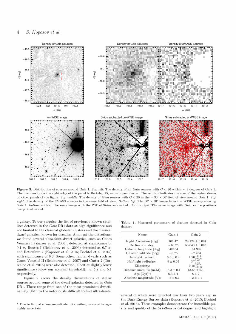
Figure 3. Distribution of sources around Gaia 1. Top left: The density of all Gaia sources with G < 20 within ∼ 3 degrees of Gaia 1.

The overdensity on the right edge of the panel is Berkeley 25, an old open cluster. The red box indicates the size of the region shownon other panels of the figure. Top middle: The density of Gaia sources with G < 20 in the ∼ 30′ × 30′ field of view around Gaia 1. Top

right: The density of the 2MASS sources in the same field of view. Bottom left: The 30′ × 30′ image from the WISE survey showing

Gaia 1. Bottom middle: The same image with the PSF of Sirius subtracted. Bottom right: The same image with Gaia source positionsoverplotted in red.

a galaxy. To our surprise the list of previously known satel-lites detected in the Gaia DR1 data at high significance wasnot limited to the classical globular clusters and the classicaldwarf galaxies, known for decades. Amongst the detections,we found several ultra-faint dwarf galaxies, such as CanesVenatici I (Zucker et al. 2006), detected at significance of9.1 σ, Bootes I (Belokurov et al. 2006) detected at 6.7 σ,and Reticulum 2 (Koposov et al. 2015; Bechtol et al. 2015)with significance of 6.3. Some other, fainter dwarfs such asCanes Venatici II (Belokurov et al. 2007) and Crater 2 (Tor-realba et al. 2016) were also detected, albeit at slightly lowersignificance (below our nominal threshold), i.e. 5.8 and 5.1respectively.

Figure 2 shows the density distributions of stellarsources around some of the dwarf galaxies detected in GaiaDR1. These range from one of the most prominent dwarfs,namely UMi, to the notoriously difficult to find ultra-faints,

1 Due to limited colour magnitude information, we consider ages

highly uncertain

Table 1. Measured parameters of clusters detected in Gaiadataset

Name Gaia 1 Gaia 2

Right Ascension [deg]: 101.47 28.124 ± 0.007

Declination [deg]: −16.75 53.040 ± 0.005Galactic longitude [deg] 202.34 131.909

Galactic latitude [deg] −8.75 −7.764

Half-light radius[′]: 6.5 ± 0.4 1.90+0.4−0.34

Half-light radius[pc]: 9 ± 0.05 3+0.63−0.53

Ellipticity: − 0.18+0.2−0.12

Distance modulus (m-M): 13.3 ± 0.1 13.65 ± 0.1

Age [Gyr]1: 6.3 ± 1 8 ± 2Absolute magnitude (V): −5 ± 0.1 −2 ± 0.1

several of which were detected less than two years ago inthe Dark Energy Survey data (Koposov et al. 2015; Bechtolet al. 2015). These examples demonstrate the incredible pu-rity and quality of the GaiaSource catalogue, and highlight

MNRAS 000, 1–9 (2017)

Gaia 1 and 2 5

Gaia’s superb satellite discovery capabilities even withoutcolour information.

While exploring the candidate over-density list, we havestumbled upon two previously unknown objects detectedwith very high significance, which are going to be the fo-cus of the rest of the paper.

3.2 Gaia 1. You can not be Sirius!

The first stellar overdensity without an obvious counterpart,i.e. without an entry in any of the clusters/galaxies cata-logues available to us, has an estimated significance of ∼10. Note however, that initially, this candidate, dubbed hereGaia 1, was rejected as it is located in close proximity of thebrightest star on the sky – Sirius2. Figure 3 shows the dis-tribution of sources in the area around the candidate fromthree different surveys: Gaia, 2MASS and WISE (Wrightet al. 2010). As the Figure demonstrates, the overdensity inGaia-detected sources is indeed very prominent (top left andtop middle panels). Note a white patch corresponding to adearth of Gaia sources near the centre of the over-density.This is the location of Sirius, where Gaia struggles to detectgenuine stars3. The area affected by Sirius is much larger inthe 2MASS data, as evidenced in the right panel. However,even here, a stellar overdensity corresponding to the candi-date in question is noticeable. The object itself can be seendirectly in the images from the infrared WISE survey (bot-tom row). The bottom panels of Figure 3 show the view ofthe ∼ 30′ × 30′ area around the overdensity as provided bythe un-WISE project (Lang 2014). The left panel displaysthe original WISE data with Sirius in the picture, while themiddle panel has the star subtracted using a circularly sym-metric PSF model. In both cases the overdensity of sourcesin the central parts of Gaia 1 is clearly visible. This is themost straightforward and the most secure confirmation ofthe newly identified satellite.

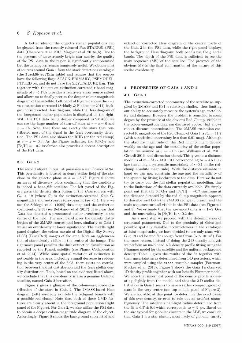
Our next step is to try to assess the nature of theoverdensity by means of studying its colour-magnitude dia-gram properties. Unfortunately, the Gaia DR1 release doesnot contain colour information, so we are forced to usemuch shallower 2MASS data. Left panel of Figure 4 showsthe extinction-corrected Hess diagram obtained by combin-ing 2MASS and Gaia photometry for the field centred onthe Gaia 1 (to get the combined 2MASS/Gaia photom-etry we used the nearest neighbour cross-match betweensurveys with 3′′ aperture). The red giant branch togetherwith prominent red clump (or red horizontal branch) atKs ∼ 11.7 are both clearly visible. The other two panelsof the Figure show the 2MASS-only colour magnitude dia-grams (CMD). The middle panel gives the CMD of the starswithin the central parts of Gaia 1 together with the PAR-SEC isochrone (Bressan et al. 2012) with [Fe/H] = −0.7

2 Previously when working with ground-based surveys such asSDSS, VST and DES the authors usually automatically excludedthe regions around bright stars as CCD saturation, ghost reflec-

tions and diffraction spikes produced by bright stars usually leadto spurious overdensities in the catalogues.3 It is curious that in the Gaia paper on source list creation

by Fabricius et al. (2016) the region around Sirius was used todemonstrate challenges of dealing with such a bright source (see

their Fig. 12)

0 1 2

G−J [mag]

7

8

9

10

11

12

13

14

15

K[m

ag]

Hess diagram

0.0 0.5 1.0

J−K [mag]

Gaia 1 CMD

0.0 0.5 1.0

J−K [mag]

Background CMD

Figure 4. Left panel: The background subtracted and extinc-

tion corrected 2MASS-Gaia Hess diagram of the central 0.1◦ of

Gaia 1 (area within the annulus with inner and outer radii of 0.3and 1 degrees has been used for background); Middle panel: The

2MASS J−Ks,Ks colour-magnitude diagram of Gaia 1 obtained

using sources within 0.1 deg from Gaia 1 centre. The PARSECisochrone with the age of 6.3 Gyr and [Fe/H] = −0.7 at the dis-

tance modulus of m−M = 13.3 is overplotted in red. Right panel:

The colour-magnitude diagram of the background field offset by0.5◦ from Gaia 1 and with the same area as used for the middle

panel.

−0.5 0.0 0.5 1.0

r−z [mag]

12

13

14

15

16

17

18

19

z[m

ag]

−0.5 0.0 0.5 1.0

r−z [mag]

12

13

14

15

16

17

18

19

Figure 5. Left panel: The background subtracted r − z, z Hess

diagram of the central 0.1◦ of Gaia 1 from PS1 data. The PAR-SEC isochrone with the age of 6.3 Gyr and [Fe/H] = −0.7 at the

distance modulus of m − M = 13.3 is overplotted in red. Rightpanel: The Hess diagram of the stellar foreground in the 0.3◦,1◦annulus around Gaia 1.

and age of 6.3 Gyr. The right panel of the Figure displaysthe colour-magnitude distribution of the foreground starsin the part of the sky 0.5 degrees away from the centre ofGaia 1 with the same area as the field shown in the middlepanel. We note that the isochrone reproduces the location ofthe red clump and the red giant branch and that the colour-magnitude diagram distribution in Gaia 1 is clearly differentfrom the distribution of the foreground stars, which providesanother confirmation that the object is a genuine satellite.

MNRAS 000, 1–9 (2017)

6 S. Koposov et al.

A better idea of the object’s stellar populations canbe gleaned from the recently released Pan-STARRS1 (PS1)data (Chambers et al. 2016; Magnier et al. 2016a,b). Due tothe presence of an extremely bright star nearby, the qualityof the PS1 data in the region is significantly compromisedbut the catalogues remain immensely useful. We obtain a listof sources around Gaia 1 from the stack detections catalogue(the StackObjectThin table) and require that the sourceshave the following flags: STACK PRIMARY, PSFMODEL,FITTED on, and do not have the SKY FAILURE flag. Thistogether with the cut on extinction-corrected r-band mag-nitude of r < 17.5 provides a relatively clean source subsetand allows us to finally peer at the deeper colour-magnitudediagram of the satellite. Left panel of Figure 5 shows the r−zvs z extinction corrected (Schlafly & Finkbeiner 2011) back-ground subtracted Hess diagram, while the Hess diagram ofthe foreground stellar population is displayed on the right.With the PS1 data being deeper compared to 2MASS, wecan see the large number of turn-off stars at r − z ∼ 0 andz ∼ 16. Note, that these are exactly the stars that con-tributed most of the signal in the Gaia overdensity detec-tion. The PS1 data also shows the RHB (or the red clump)at r − z ∼ 0.3. As the Figure indicates, the 6.3 Gyr and[Fe/H] = −0.7 isochrone also provides a decent descriptionof the PS1 data.

3.3 Gaia 2

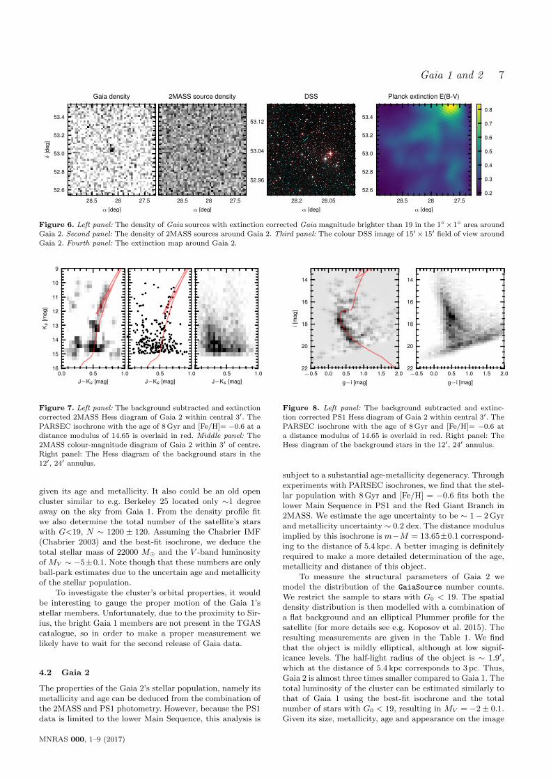
The second object in our list possesses a significance of 9σ.This overdensity is located in dense stellar field of the sky,close to the galactic plane at b = −8.7◦. Figure 6 showsan array of discovery plots confirming that the candidateis indeed a bona-fide satellite. The left panel of the Fig-ure gives the density distribution of the Gaia sources withG0 < 19 (where G0 is the extinction-corrected Gaia G-magnitude) and astrometric excess noise < 5. Here weuse the Schlegel et al. (1998) dust map and the extinctioncoefficient of 2.55 (see Belokurov et al. 2017). It is clear thatGaia has detected a pronounced stellar overdensity in thecentre of the field. The next panel gives the density distri-bution of the 2MASS sources and here, similarly to Gaia 1we see an overdensity at lower significance. The middle rightpanel displays the colour mosaic of the Digital Sky Survey(DSS) (Blue/Red) images of the area. Note an agglomera-tion of stars clearly visible in the centre of the image. Therightmost panel presents the dust extinction distribution asreported by the Planck satellite (see Planck Collaborationet al. 2014). While some spatial variation of extinction isnoticeable in the area, including a small decrease in redden-ing in the very centre of the field, there exists no correla-tion between the dust distribution and the Gaia stellar den-sity distribution. Thus, based on the evidence listed above,we conclude that this overdensity is also a genuine Galacticsatellite, named Gaia 2 hereafter.

Figure 7 gives a glimpse of the colour-magnitude dis-tribution of the stars in Gaia 2. The 2MASS-based Hessdiagram (left) assuredly exhibits the red-giant branch witha possible red clump. Note that both of these CMD fea-tures are clearly absent in the foreground population (rightpanel of the Figure). For Gaia 2, we also utilise the PS1 datato obtain a deeper colour-magnitude diagram of the object.Accordingly, Figure 8 shows the background subtracted and

extinction corrected Hess diagram of the central parts ofthe Gaia 2 in the PS1 data, while the right panel displaysthe background Hess diagram; both panels use the g and ibands. The depth of the PS1 data is sufficient to see themain sequence (MS) of the satellite. The presence of theobvious MS is the final confirmation of the nature of thisstellar overdensity.

4 PROPERTIES OF GAIA 1 AND 2

4.1 Gaia 1

The extinction-corrected photometry of the satellite as sup-plied by 2MASS and PS1 is relatively shallow, thus limitingour ability to accurately measure the system’s age, metallic-ity and distance. However the problem is remedied to somedegree by the presence of the obvious Red Clump, visible inthe colour-magnitude diagram discussed above, that allowsrobust distance determination. The 2MASS extinction cor-rected K magnitude of the Red Clump of Gaia 1 is Ks = 11.7(with a statistical uncertainty less than 0.01 mag). Althoughthe absolute magnitude of the Red Clump might dependweakly on the age and the metallicity of the stellar popu-lation, we assume MK = −1.6 (see Williams et al. 2013;Girardi 2016, and discussion there). This gives us a distancemodulus of m−M ∼ 13.3±0.1 corresponding to ∼ 4.6±0.2kpc (assuming a systematic uncertainty of ∼ 0.1 on the red-clump absolute magnitude). With the distance estimate inhand we can now constrain the age and the metallicity ofthe system by fitting isochrones to the data. Here we do nottry to carry out the full stellar population modelling, dueto the limitations of the data currently available. We simplypoint out that the 6.3 Gyr and [Fe/H] = −0.7 isochrone atthe distance dictated by the red clump magnitude appearsto describe well both the 2MASS red giant branch and themain sequence turn-off visible in the PS1 data (see Figures 4and 5). We estimate that the age uncertainty is ∼ 1−2 Gyrand the uncertainty in [Fe/H] is ∼ 0.2 dex.

As a next step we proceed with the determination ofstructural parameters. Due to the proximity of Sirius andpossible spatially variable incompleteness in the catalogueat faint magnitudes, we have decided to use only stars withG < 19 and located far enough from Sirius (α > 101.4◦). Forthe same reason, instead of doing the 2-D density analysiswe perform an un-binned 1-D density profile fitting using thePlummer model for the satellite and the uniform backgrounddensity. Table 1 gives the results of the fit together withtheir uncertainties as determined from 1-D posteriors, whichwere sampled using the emcee ensemble sampler (Foreman-Mackey et al. 2013). Figure 9 shows the Gaia 1’s observed1D density profile together with our best-fit Plummer model.We note that innermost point of the density profile is devi-ating slightly from the model, and that the 2-D stellar dis-tribution in Gaia 1 seems to have a rather compact group ofstars in the very centre (see top middle panel of Figure 3).We are not able, at this point, to determine the exact causeof this over-density, or even to rule out an artefact unam-biguously. The satellite’s half-light radius determined fromthe fit is 6.5′ ± 0.4 which corresponds to ∼ 9 pc. Based onthe size typical for globular clusters in the MW, we concludethat Gaia 1 is a star cluster, most likely of globular variety

MNRAS 000, 1–9 (2017)

Gaia 1 and 2 7

27.52828.5

α [deg]

52.6

52.8

53.0

53.2

53.4

δ[d

eg]

Gaia density

27.52828.5

α [deg]

2MASS source density

27.52828.5

α [deg]

52.6

52.8

53.0

53.2

53.4

Planck extinction E(B-V)

0.2

0.3

0.4

0.5

0.6

0.7

0.8

28.0528.2

α [deg]

52.96

53.04

53.12

DSS

Figure 6. Left panel: The density of Gaia sources with extinction corrected Gaia magnitude brighter than 19 in the 1◦×1◦ area aroundGaia 2. Second panel: The density of 2MASS sources around Gaia 2. Third panel: The colour DSS image of 15′× 15′ field of view around

Gaia 2. Fourth panel: The extinction map around Gaia 2.

0.0 0.5 1.0J−Ks [mag]

9

10

11

12

13

14

15

16

Ks

[mag

]

0.5 1.0J−Ks [mag]

0.5 1.0J−Ks [mag]

Figure 7. Left panel: The background subtracted and extinction

corrected 2MASS Hess diagram of Gaia 2 within central 3′. ThePARSEC isochrone with the age of 8 Gyr and [Fe/H]= −0.6 at a

distance modulus of 14.65 is overlaid in red. Middle panel: The

2MASS colour-magnitude diagram of Gaia 2 within 3′ of centre.Right panel: The Hess diagram of the background stars in the

12′, 24′ annulus.

given its age and metallicity. It also could be an old opencluster similar to e.g. Berkeley 25 located only ∼1 degreeaway on the sky from Gaia 1. From the density profile fitwe also determine the total number of the satellite’s starswith G<19, N ∼ 1200 ± 120. Assuming the Chabrier IMF(Chabrier 2003) and the best-fit isochrone, we deduce thetotal stellar mass of 22000 M� and the V -band luminosityof MV ∼ −5±0.1. Note though that these numbers are onlyball-park estimates due to the uncertain age and metallicityof the stellar population.

To investigate the cluster’s orbital properties, it wouldbe interesting to gauge the proper motion of the Gaia 1’sstellar members. Unfortunately, due to the proximity to Sir-ius, the bright Gaia 1 members are not present in the TGAScatalogue, so in order to make a proper measurement welikely have to wait for the second release of Gaia data.

4.2 Gaia 2

The properties of the Gaia 2’s stellar population, namely itsmetallicity and age can be deduced from the combination ofthe 2MASS and PS1 photometry. However, because the PS1data is limited to the lower Main Sequence, this analysis is

−0.5 0.0 0.5 1.0 1.5 2.0

g−i [mag]

14

16

18

20

22

i[m

ag]

−0.5 0.0 0.5 1.0 1.5 2.0

g−i [mag]

14

16

18

20

22

Figure 8. Left panel: The background subtracted and extinc-

tion corrected PS1 Hess diagram of Gaia 2 within central 3′. ThePARSEC isochrone with the age of 8 Gyr and [Fe/H]= −0.6 at

a distance modulus of 14.65 is overlaid in red. Right panel: The

Hess diagram of the background stars in the 12′, 24′ annulus.

subject to a substantial age-metallicity degeneracy. Throughexperiments with PARSEC isochrones, we find that the stel-lar population with 8 Gyr and [Fe/H] = −0.6 fits both thelower Main Sequence in PS1 and the Red Giant Branch in2MASS. We estimate the age uncertainty to be ∼ 1− 2 Gyrand metallicity uncertainty ∼ 0.2 dex. The distance modulusimplied by this isochrone is m−M = 13.65±0.1 correspond-ing to the distance of 5.4 kpc. A better imaging is definitelyrequired to make a more detailed determination of the age,metallicity and distance of this object.

To measure the structural parameters of Gaia 2 wemodel the distribution of the GaiaSource number counts.We restrict the sample to stars with G0 < 19. The spatialdensity distribution is then modelled with a combination ofa flat background and an elliptical Plummer profile for thesatellite (for more details see e.g. Koposov et al. 2015). Theresulting measurements are given in the Table 1. We findthat the object is mildly elliptical, although at low signif-icance levels. The half-light radius of the object is ∼ 1.9′,which at the distance of 5.4 kpc corresponds to 3 pc. Thus,Gaia 2 is almost three times smaller compared to Gaia 1. Thetotal luminosity of the cluster can be estimated similarly tothat of Gaia 1 using the best-fit isochrone and the totalnumber of stars with G0 < 19, resulting in MV = −2± 0.1.Given its size, metallicity, age and appearance on the image

MNRAS 000, 1–9 (2017)

8 S. Koposov et al.

1 10

R [arcmin]

30000

40000

50000

60000

70000

80000

Sta

rs/s

q.de

g

Plummer r1/2=6.5’

Figure 9. The 1D density profile of Gaia 1. The red line shows a

Plummer model fit with half-light radius of 6.5′. We also note thatin the very centre there is a tight group of stars which causes the

innermost point in the density profile to deviate from Plummer.

cutouts, it is most likely a globular cluster, or an old opencluster.

5 CONCLUSIONS

This paper presents the results of the very first exploration ofthe Gaia capabilities for Galactic satellite detection. Whilewe have identified a number of new interesting satellite can-didates, here we describe only two objects, Gaia 1 andGaia 2, whose nature can be determined unambiguouslywith extant data. Possessing remarkably high levels of sig-nificance - in excess of 9 (!) - both were, nevertheless, missedby previous imaging surveys. Thus, Gaia appears to offer aunique view of the Galactic stellar distribution, unrivalledeven by datasets reaching to significantly fainter magni-tudes. It is due to the combination of the Gaia’s high angularresolution and the high purity of its stellar sample, objectslike Gaia 1 can be discovered.

Gaia 1 is a large and luminous star cluster. However,it is positioned almost exactly behind Sirius, the brighteststar in the sky, which appears to be the perfect hiding placeeven for a satellite of such grand prominence. Countless gen-erations of astronomers must have stared right at Gaia 1,blissfully unaware of its existence. The area around Sirius isdifficult to analyse as it is littered with artifacts spawned bythis extremely bright star. However, given the Gaia’s multi-epoch data-stream, such artifacts can be weeded out in thepreparation of the GaiaSource catalogue. Each time Gaialooks at Sirius, the spurious sources appear in different po-sitions on the sky compared to the previous visits and thusare mostly discarded due to the DR1 requirement of hav-ing 5 or more detections of a single source (Lindegren et al.

2016). Even if some spurious sources make it to the finalGaiaSource catalogue, they can be identified very efficientlybased on their unusual astrometric behaviour.

We have demonstrated that the Gaia data can be usedto detect classical dwarf galaxies, ultra faint dwarfs and starclusters in a wide range of sizes and luminosities. All of theseare detected with ease using the Gaia’s stellar positions onlyin the catalogue which is known to suffer from spatially-variable incompleteness. We therefore predict with confi-dence, that in the future Gaia Data Releases, when the com-pleteness is stabilised and the colour, distance and propermotion information is added, many new galactic satelliteswill be revealed.

ACKNOWLEDGEMENTS

We acknowledge the usage of the HyperLeda database(http://leda.univ-lyon1.fr). This research has made useof the SIMBAD database, operated at CDS, Strasbourg,France. The research leading to these results has receivedfunding from the European Research Council under the Eu-ropean Union’s Seventh Framework Programme (FP/2007-2013)/ERC Grant Agreement no. 308024. SK thanks theUnited Kingdom Science and Technology Council (STFC)for the award of Ernest Rutherford fellowship (grant num-ber ST/N004493/1). SK also thanks Bernie Shao for theassistance with obtaining the Pan-STARRS1 data. The au-thors thank the anonymous referee for careful reading of themanuscript.

This paper was written in part at the 2016 NYC GaiaSprint, hosted by the Center for Computational Astro-physics at the Simons Foundation in New York City.

This research made use of Astropy, a community-developed core Python package for Astronomy (Astropy Col-laboration et al. 2013) and Q3C extension for PostgreSQL

database (Koposov & Bartunov 2006).This work has made use of data from the Euro-

pean Space Agency (ESA) mission Gaia (http://www.cosmos.esa.int/gaia), processed by the Gaia Data Pro-cessing and Analysis Consortium (DPAC, http://www.

cosmos.esa.int/web/gaia/dpac/consortium). Funding forthe DPAC has been provided by national institutions, inparticular the institutions participating in the Gaia Multi-lateral Agreement.

The Pan-STARRS1 Surveys (PS1) and the PS1 pub-lic science archive have been made possible through contri-butions by the Institute for Astronomy, the University ofHawaii, the Pan-STARRS Project Office, the Max-PlanckSociety and its participating institutes, the Max Planck In-stitute for Astronomy, Heidelberg and the Max Planck In-stitute for Extraterrestrial Physics, Garching, The JohnsHopkins University, Durham University, the University ofEdinburgh, the Queen’s University Belfast, the Harvard-Smithsonian Center for Astrophysics, the Las Cumbres Ob-servatory Global Telescope Network Incorporated, the Na-tional Central University of Taiwan, the Space TelescopeScience Institute, the National Aeronautics and Space Ad-ministration under Grant No. NNX08AR22G issued throughthe Planetary Science Division of the NASA Science Mis-sion Directorate, the National Science Foundation Grant No.AST-1238877, the University of Maryland, Eotvos Lorand

MNRAS 000, 1–9 (2017)

Gaia 1 and 2 9

University (ELTE), the Los Alamos National Laboratory,and the Gordon and Betty Moore Foundation.

REFERENCES

Astropy Collaboration, Robitaille, T. P., Tollerud, E. J., et al.

2013, A&A, 558, A33

Bechtol, K., Drlica-Wagner, A., Balbinot, E., et al. 2015, ApJ,807, 50

Belokurov, V., Zucker, D. B., Evans, N. W., et al. 2006, ApJ, 647,

L111

Belokurov, V., Zucker, D. B., Evans, N. W., et al. 2007, ApJ, 654,

897

Belokurov, V., Erkal, D., Deason, A. J., et al. 2017, MNRAS, 466,

4711

Bressan, A., Marigo, P., Girardi, L., et al. 2012, MNRAS, 427,

127

Chabrier, G. 2003, PASP, 115, 763

Chambers, K. C., Magnier, E. A., Metcalfe, N., et al. 2016,arXiv:1612.05560

Dias, W. S., Alessi, B. S., Moitinho, A., & Lepine, J. R. D. 2002,

A&A, 389, 871

Fabricius, C., Bastian, U., Portell, J., et al. 2016, A&A, 595, A3

Foreman-Mackey, D., Hogg, D. W., Lang, D., & Goodman, J.

2013, PASP, 125, 306

Gaia Collaboration, Prusti, T., de Bruijne, J. H. J., et al. 2016,A&A, 595, A1

Gaia Collaboration, Brown, A. G. A., Vallenari, A., et al. 2016,

A&A, 595, A2

Girardi, L. 2016, ARA&A, 54, 95

Gorski, K. M., Hivon, E., Banday, A. J., et al. 2005, ApJ, 622,

759

Harris, W. E. 2010, arXiv:1012.3224

Irwin, M. J. 1994, European Southern Observatory Conferenceand Workshop Proceedings, 49, 27

Koposov, S., & Bartunov, O. 2006, Astronomical Society of the

Pacific Conference Series, 351, 735

Koposov, S., Belokurov, V., Evans, N. W., et al. 2008, ApJ, 686,279-291

Koposov, S. E., Glushkova, E. V., & Zolotukhin, I. Y. 2008, A&A,

486, 771

Koposov, S. E., Belokurov, V., Torrealba, G., & Evans, N. W.

2015, ApJ, 805, 130

Kontizas, M., Morgan, D. H., Hatzidimitriou, D., & Kontizas, E.

1990, A&AS, 84, 527

Lang, D. 2014, AJ, 147, 108

Lindegren, L., Lammers, U., Bastian, U., et al. 2016, A&A, 595,A4

van Leeuwen, F., Evans, D. W., De Angeli, F., et al. 2017, A&A,599, A32

Magnier, E. A., Chambers, K. C., Flewelling, H. A., et al. 2016,arXiv:1612.05240

Magnier, E. A., Sweeney, W. E., Chambers, K. C., et al. 2016,

arXiv:1612.05244

Makarov, D., Prugniel, P., Terekhova, N., Courtois, H., & Vauglin,

I. 2014, A&A, 570, A13

McConnachie, A. W. 2012, AJ, 144, 4

Perryman, M. A. C., de Boer, K. S., Gilmore, G., et al. 2001,A&A, 369, 339

Planck Collaboration, Abergel, A., Ade, P. A. R., et al. 2014,A&A, 571, A11

Schlegel, D. J., Finkbeiner, D. P., & Davis, M. 1998, ApJ, 500,525

Schlafly, E. F., & Finkbeiner, D. P. 2011, ApJ, 737, 103

Skrutskie, M. F., Cutri, R. M., Stiening, R., et al. 2006, AJ, 131,

1163

Torrealba, G., Koposov, S. E., Belokurov, V., & Irwin, M. 2016,

MNRAS, 459, 2370

Walsh, S. M., Willman, B., & Jerjen, H. 2009, AJ, 137, 450Wenger, M., Ochsenbein, F., Egret, D., et al. 2000, A&AS, 143,

9Whiting, A. B., Hau, G. K. T., Irwin, M., & Verdugo, M. 2007,

AJ, 133, 715

Williams, M. E. K., Steinmetz, M., Binney, J., et al. 2013, MN-RAS, 436, 101

Willman, B. 2010, Advances in Astronomy, 2010, 285454

Wright, E. L., Eisenhardt, P. R. M., Mainzer, A. K., et al. 2010,AJ, 140, 1868-1881

York, D. G., Adelman, J., Anderson, J. E., Jr., et al. 2000, AJ,

120, 1579Zucker, D. B., Belokurov, V., Evans, N. W., et al. 2006, ApJ, 643,

L103

This paper has been typeset from a TEX/LATEX file prepared bythe author.

MNRAS 000, 1–9 (2017)