Anisotropic diffusion of energetic particles in galactic and ...
116
RUHR-UNIVERSITÄT BOCHUM FAKULTÄT FÜR PHYSIK UND ASTRONOMIE Dissertation zur Erlangung des Grades eines Doktors der Naturwissenschaften in der Fakultät für Physik und Astronomie der Ruhr-Universität Bochum Anisotropic Diffusion of Energetic Particles in Galactic and Heliospheric Magnetic Fields Vorgelegt von Frederic Effenberger Bochum September 2012
-
Upload
khangminh22 -
Category
Documents
-
view
1 -
download
0
Transcript of Anisotropic diffusion of energetic particles in galactic and ...
RUHR-UNIVERSITÄT BOCHUM
FAKULTÄT FÜR PHYSIKUND ASTRONOMIE
Dissertationzur Erlangung des Grades eines Doktors der Naturwissenschaften
in der Fakultät für Physik und Astronomie
der Ruhr-Universität Bochum
Anisotropic Diffusion of EnergeticParticles in Galactic and Heliospheric
Magnetic Fields
Vorgelegt von
Frederic Effenberger
BochumSeptember 2012

Themensteller und Gutachter: Priv.-Doz. Dr. habil. Horst Fichtner
Zweiter Gutachter: Prof. Dr. Hans Jörg Fahr
Tag der Disputation: 10.12.2012
Für Anne, Bernd, Dorothee & Fabian

Anisotropic Diffusion of Energetic Particles in Galactic andHeliospheric Magnetic Fields
Abstract: The diffusion of highly energetic particles in interplanetary and interstellarplasma backgrounds is an extensive field of research at the interface between particlephysics and astrophysics. This thesis extends some central aspects in the theoretical de-scription of such diffusive transport processes. They can be summarized in three keyissues. First, the modelling of the galactic cosmic ray transport is extended to incorpo-rate anisotropic diffusion with respect to the background galactic magnetic field. Withinthe framework of the employed numerical model it is thus possible to analyze the az-imuthal steady-state cosmic ray distribution in the Milky Way to a greater detail. Second,anisotropic perpendicular diffusion is introduced into heliospheric modulation models via anovel method. Here, the developed formalism allows to account for general turbulent mag-netic field structures and uses their intrinsic properties to construct the diffusion tensor.Third, anomalous diffusion processes are incorporated into the established propagationmodels. This way, transport equations arise which exhibit space and time derivatives offractional order and can be described by stochastic processes with Lévy-flight behaviorand subordination. The models developed in this work allow for a quantitative analysisof particle spectral intensities measured by spacecraft and ground-based instruments andopen new avenues of astrophysical research.Keywords: Cosmic Rays, Diffusion, Magnetic fields

Anisotrope Diffusion energiereicher Teilchen in galaktischen undheliosphärischen Magnetfeldern
Zusammenfassung: Die Diffusion hochenergetischer geladener Teilchen in interplan-etaren und interstellaren Plasmen ist ein umfangreiches Forschungsfeld an der Schnittstellezwischen Astrophysik und Teilchenphysik. In dieser Arbeit werden einige zentrale As-pekte der theoretischen Beschreibung solcher diffusiver Transportprozesse weiterentwick-elt. Diese lassen sich in drei Schwerpunkte zusammenfassen. Erstens wird die Modellierungdes galaktischen Transports von kosmischer Strahlung (“Cosmic Rays”) um anisotropeDiffusion bezüglich des galaktischen Hintergrundmagnetfeldes erweitert. Im Rahmen desverwendeten numerischen Modells ist es so möglich, die azimutale Gleichgewichtsstruk-tur der kosmischen Teilchenverteilung in der Milchstraße detaillierter als bisher zu un-tersuchen. Zweitens wird die anisotrope Diffusion im Kontext der heliosphärischen Mod-ulation kosmischer Strahlung um anisotrope Senkrechtdiffusion erweitert. Der neu en-twickelte Formalismus erlaubt dabei die Berücksichtigung allgemeiner, turbulenter Mag-netfeldstrukturen und nutzt ihre intrinsischen Eigenschaften zur Konstruktion des Diffu-sionstensors. Drittens werden anomale Diffusionsprozesse in die entwickelten Modelle in-tegriert. Auf diese Weise ergeben sich Transportgleichungen, die eine fraktionale Ordnungin der Orts- oder Zeitableitung aufweisen und durch stochastische Prozesse mit Lévy-Flügen und Subordination beschrieben werden können. Die in dieser Arbeit entwickeltenModelle erlauben eine quantitative Analyse der von Raumsonden und bodengebunde-nen Instrumenten gemessenen spektralen Teilchenintensitäten und eröffnen zusätzlicheErweiterungsmöglichkeiten in der astrophysikalischen Modellierung.Stichwörter: Kosmische Teilchen (Cosmic Rays), Diffusion, Magnetfelder

Contents
1 Introduction 11.1 Cosmic Rays and the Non-Thermal Universe . . . . . . . . . . . . . . . . . 1
1.1.1 Cosmic Ray Sources . . . . . . . . . . . . . . . . . . . . . . . . . . 41.1.2 The Interstellar Medium and the Galactic Magnetic Field . . . . . 61.1.3 Variable Cosmic Environments . . . . . . . . . . . . . . . . . . . . 81.1.4 The Heliosphere . . . . . . . . . . . . . . . . . . . . . . . . . . . . 91.1.5 Cosmic Rays and Climate . . . . . . . . . . . . . . . . . . . . . . . 10
1.2 Contemporary Issues in Cosmic Ray Research . . . . . . . . . . . . . . . . 111.2.1 Anisotropic Diffusion . . . . . . . . . . . . . . . . . . . . . . . . . . 121.2.2 Anomalous Diffusion . . . . . . . . . . . . . . . . . . . . . . . . . . 12
1.3 The Scope and Structure of this Thesis . . . . . . . . . . . . . . . . . . . . 13
2 Transport Theory and Numerical Methods 152.1 General Cosmic Ray Diffusion Theory . . . . . . . . . . . . . . . . . . . . 15
2.1.1 The Vlasov-Maxwell System . . . . . . . . . . . . . . . . . . . . . . 152.1.2 The Fokker-Planck Equation . . . . . . . . . . . . . . . . . . . . . 162.1.3 The Diffusion Approximation . . . . . . . . . . . . . . . . . . . . . 17
2.2 A Closer Look at Diffusion Processes . . . . . . . . . . . . . . . . . . . . . 182.2.1 Stochastic Differential Equations . . . . . . . . . . . . . . . . . . . 192.2.2 The Diffusion Approximation Revisited . . . . . . . . . . . . . . . 21
2.3 Numerical Methods . . . . . . . . . . . . . . . . . . . . . . . . . . . . . . . 222.3.1 The Grid-based Method . . . . . . . . . . . . . . . . . . . . . . . . 222.3.2 The Monte Carlo Method . . . . . . . . . . . . . . . . . . . . . . . 23
3 Galactic Cosmic Ray Transport 273.1 A Galactic Transport Model . . . . . . . . . . . . . . . . . . . . . . . . . . 28
3.1.1 The Anisotropic Diffusion Transport Equation . . . . . . . . . . . . 293.1.2 The Diffusion Tensor Formulation . . . . . . . . . . . . . . . . . . 293.1.3 Galactic Magnetic Field Models . . . . . . . . . . . . . . . . . . . . 313.1.4 Distribution of Matter and Supernovae Abundances . . . . . . . . 323.1.5 Energy Losses . . . . . . . . . . . . . . . . . . . . . . . . . . . . . . 333.1.6 Numerical Solution Methods for the Transport Model . . . . . . . 34
3.2 Calculated Galactic Cosmic Ray Distributions . . . . . . . . . . . . . . . . 353.2.1 Global Steady-State Solutions . . . . . . . . . . . . . . . . . . . . . 353.2.2 Spectral Variation . . . . . . . . . . . . . . . . . . . . . . . . . . . 373.2.3 Orbital Variation . . . . . . . . . . . . . . . . . . . . . . . . . . . . 39
3.3 Conclusions . . . . . . . . . . . . . . . . . . . . . . . . . . . . . . . . . . . 41
viii Contents
4 Heliospheric Cosmic Ray Modulation 434.1 Interplanetary Magnetic Field Models . . . . . . . . . . . . . . . . . . . . 444.2 Fully Anisotropic Diffusion . . . . . . . . . . . . . . . . . . . . . . . . . . 45
4.2.1 Causes for Fully Anisotropic Diffusion . . . . . . . . . . . . . . . . 474.2.2 The Local Diffusion Tensor Elements . . . . . . . . . . . . . . . . . 484.2.3 A Generalized Tensor Transformation . . . . . . . . . . . . . . . . 49
4.3 The Choice of a Local Coordinate System . . . . . . . . . . . . . . . . . . 524.3.1 The “Standard Euler-Burger” Transformation . . . . . . . . . . . . 524.3.2 The “Frenet-Serret Trihedron” Transformation . . . . . . . . . . . . 524.3.3 The Resulting Structure of the Global Diffusion Tensor . . . . . . . 54
4.4 Application to the Modulation of Cosmic Ray Spectra . . . . . . . . . . . 574.5 Conclusions . . . . . . . . . . . . . . . . . . . . . . . . . . . . . . . . . . . 58
5 Anomalous Diffusion 615.1 Superdiffusive and Subdiffusive Processes . . . . . . . . . . . . . . . . . . 615.2 The Fractional Fokker-Planck Equation Transport Model . . . . . . . . . . 63
5.2.1 The Associated Stochastic Differential Equation . . . . . . . . . . . 645.2.2 Lévy flights and Subdiffusion Exemplified . . . . . . . . . . . . . . 655.2.3 Comparison Between Numerical Solutions and Test Cases . . . . . 67
5.3 Superdiffusive Transport of Termination Shock Particles . . . . . . . . . . 705.3.1 The Superdiffusive Fokker-Planck Transport Model . . . . . . . . . 70
5.4 Conclusions . . . . . . . . . . . . . . . . . . . . . . . . . . . . . . . . . . . 73
6 Concluding Remarks 756.1 Summary . . . . . . . . . . . . . . . . . . . . . . . . . . . . . . . . . . . . 756.2 Future Prospects . . . . . . . . . . . . . . . . . . . . . . . . . . . . . . . . 76
A The Semi-analytic Parker Propagator Solution 79
B Random Number Generation 83B.1 Gaussian Distribution . . . . . . . . . . . . . . . . . . . . . . . . . . . . . 83B.2 Symmetric µ-stable Distribution . . . . . . . . . . . . . . . . . . . . . . . 84B.3 Totally Skewed Positive α-stable Distribution . . . . . . . . . . . . . . . . 85
Bibliography 93
Chapter 1
Introduction
I ask you to look both ways. For the road to a knowledgeof the stars leads through the atom; and importantknowledge of the atom has been reached through thestars.
Stars and Atoms (1928), Lecture 1Sir Arthur Eddington
Contents1.1 Cosmic Rays and the Non-Thermal Universe . . . . . . . . . . . . 1
1.1.1 Cosmic Ray Sources . . . . . . . . . . . . . . . . . . . . . . . . . . . 4
1.1.2 The Interstellar Medium and the Galactic Magnetic Field . . . . . . 6
1.1.3 Variable Cosmic Environments . . . . . . . . . . . . . . . . . . . . . 8
1.1.4 The Heliosphere . . . . . . . . . . . . . . . . . . . . . . . . . . . . . 9
1.1.5 Cosmic Rays and Climate . . . . . . . . . . . . . . . . . . . . . . . . 10
1.2 Contemporary Issues in Cosmic Ray Research . . . . . . . . . . . 11
1.2.1 Anisotropic Diffusion . . . . . . . . . . . . . . . . . . . . . . . . . . . 12
1.2.2 Anomalous Diffusion . . . . . . . . . . . . . . . . . . . . . . . . . . . 12
1.3 The Scope and Structure of this Thesis . . . . . . . . . . . . . . . 13
1.1 Cosmic Rays and the Non-Thermal Universe
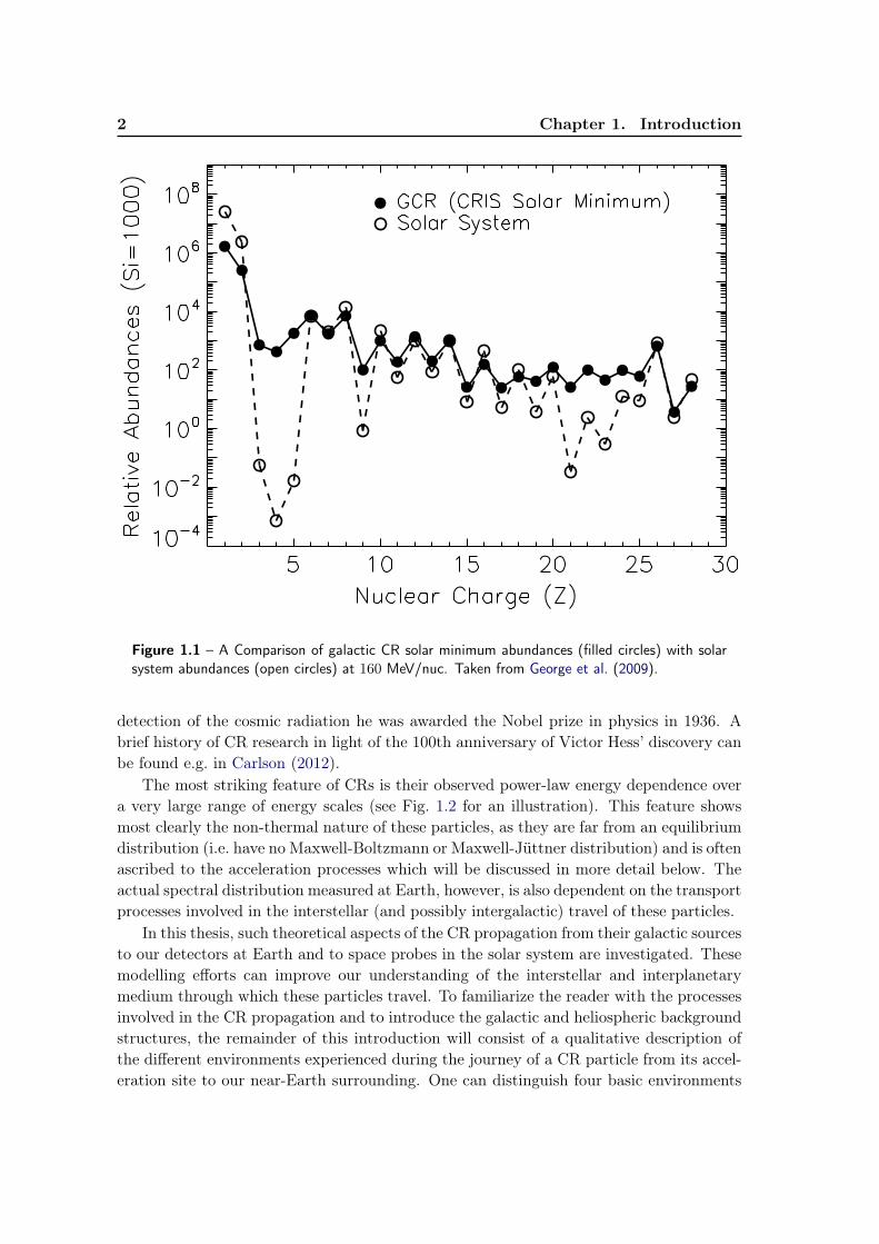
Energetic particles pervade the entire universe. They can have energies up to E ≈ 1020 eVand show a composition which largely resembles the solar elementary abundances, al-though there are also important differences. This means they consist mainly of protonsand helium with only small contributions of electrons and heavier elements (Fig. 1.1). To-day, they are regarded as one of the most prominent features of the non-thermal universe,indicating their origin in violent processes with huge releases of energy.
The activity in cosmic ray (CR) research has been growing ever since their first dis-covery almost exactly a hundred years ago. Around that time, Victor Hess performed hisballoon flights to measure the ionization of the atmosphere. His definite discovery of anincrease in ionization with altitude on August 7, 1912, which excluded a terrestrial origin,can be regarded as starting point of all the discoveries in the following years. For his
2 Chapter 1. Introduction
Figure 1.1 – A Comparison of galactic CR solar minimum abundances (filled circles) with solarsystem abundances (open circles) at 160 MeV/nuc. Taken from George et al. (2009).
detection of the cosmic radiation he was awarded the Nobel prize in physics in 1936. Abrief history of CR research in light of the 100th anniversary of Victor Hess’ discovery canbe found e.g. in Carlson (2012).
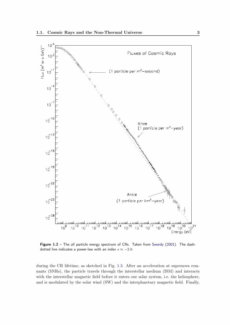
The most striking feature of CRs is their observed power-law energy dependence overa very large range of energy scales (see Fig. 1.2 for an illustration). This feature showsmost clearly the non-thermal nature of these particles, as they are far from an equilibriumdistribution (i.e. have no Maxwell-Boltzmann or Maxwell-Jüttner distribution) and is oftenascribed to the acceleration processes which will be discussed in more detail below. Theactual spectral distribution measured at Earth, however, is also dependent on the transportprocesses involved in the interstellar (and possibly intergalactic) travel of these particles.
In this thesis, such theoretical aspects of the CR propagation from their galactic sourcesto our detectors at Earth and to space probes in the solar system are investigated. Thesemodelling efforts can improve our understanding of the interstellar and interplanetarymedium through which these particles travel. To familiarize the reader with the processesinvolved in the CR propagation and to introduce the galactic and heliospheric backgroundstructures, the remainder of this introduction will consist of a qualitative description ofthe different environments experienced during the journey of a CR particle from its accel-eration site to our near-Earth surrounding. One can distinguish four basic environments
1.1. Cosmic Rays and the Non-Thermal Universe 3
Figure 1.2 – The all particle energy spectrum of CRs. Taken from Swordy (2001). The dash-dotted line indicates a power-law with an index s ≈ −2.8.
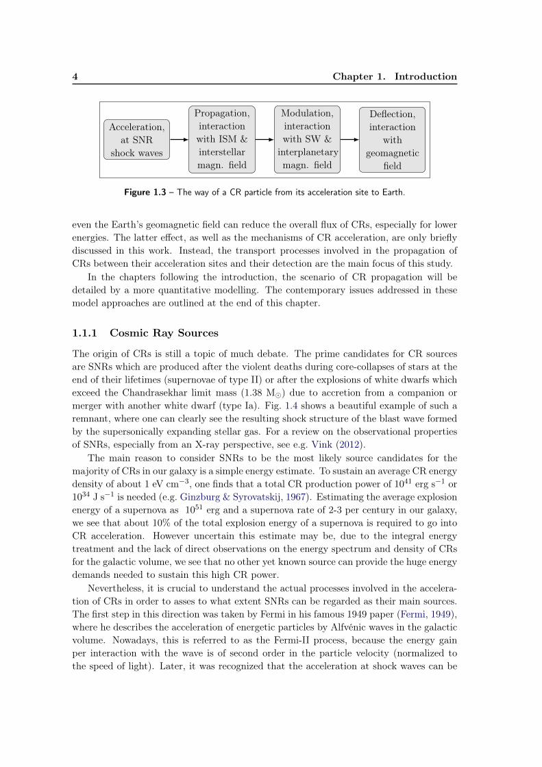
during the CR lifetime, as sketched in Fig. 1.3. After an acceleration at supernova rem-nants (SNRs), the particle travels through the interstellar medium (ISM) and interactswith the interstellar magnetic field before it enters our solar system, i.e. the heliosphere,and is modulated by the solar wind (SW) and the interplanetary magnetic field. Finally,
4 Chapter 1. Introduction
Acceleration,at SNR
shock waves
Propagation,interactionwith ISM &interstellarmagn. field
Modulation,interactionwith SW &
interplanetarymagn. field
Deflection,interaction
withgeomagnetic
field
Figure 1.3 – The way of a CR particle from its acceleration site to Earth.
even the Earth’s geomagnetic field can reduce the overall flux of CRs, especially for lowerenergies. The latter effect, as well as the mechanisms of CR acceleration, are only brieflydiscussed in this work. Instead, the transport processes involved in the propagation ofCRs between their acceleration sites and their detection are the main focus of this study.
In the chapters following the introduction, the scenario of CR propagation will bedetailed by a more quantitative modelling. The contemporary issues addressed in thesemodel approaches are outlined at the end of this chapter.
1.1.1 Cosmic Ray Sources
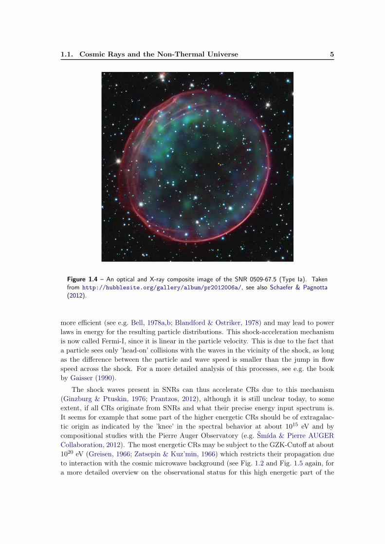
The origin of CRs is still a topic of much debate. The prime candidates for CR sourcesare SNRs which are produced after the violent deaths during core-collapses of stars at theend of their lifetimes (supernovae of type II) or after the explosions of white dwarfs whichexceed the Chandrasekhar limit mass (1.38 M) due to accretion from a companion ormerger with another white dwarf (type Ia). Fig. 1.4 shows a beautiful example of such aremnant, where one can clearly see the resulting shock structure of the blast wave formedby the supersonically expanding stellar gas. For a review on the observational propertiesof SNRs, especially from an X-ray perspective, see e.g. Vink (2012).
The main reason to consider SNRs to be the most likely source candidates for themajority of CRs in our galaxy is a simple energy estimate. To sustain an average CR energydensity of about 1 eV cm−3, one finds that a total CR production power of 1041 erg s−1 or1034 J s−1 is needed (e.g. Ginzburg & Syrovatskij, 1967). Estimating the average explosionenergy of a supernova as 1051 erg and a supernova rate of 2-3 per century in our galaxy,we see that about 10% of the total explosion energy of a supernova is required to go intoCR acceleration. However uncertain this estimate may be, due to the integral energytreatment and the lack of direct observations on the energy spectrum and density of CRsfor the galactic volume, we see that no other yet known source can provide the huge energydemands needed to sustain this high CR power.
Nevertheless, it is crucial to understand the actual processes involved in the accelera-tion of CRs in order to asses to what extent SNRs can be regarded as their main sources.The first step in this direction was taken by Fermi in his famous 1949 paper (Fermi, 1949),where he describes the acceleration of energetic particles by Alfvénic waves in the galacticvolume. Nowadays, this is referred to as the Fermi-II process, because the energy gainper interaction with the wave is of second order in the particle velocity (normalized tothe speed of light). Later, it was recognized that the acceleration at shock waves can be
1.1. Cosmic Rays and the Non-Thermal Universe 5
Figure 1.4 – An optical and X-ray composite image of the SNR 0509-67.5 (Type Ia). Takenfrom http://hubblesite.org/gallery/album/pr2012006a/, see also Schaefer & Pagnotta(2012).
more efficient (see e.g. Bell, 1978a,b; Blandford & Ostriker, 1978) and may lead to powerlaws in energy for the resulting particle distributions. This shock-acceleration mechanismis now called Fermi-I, since it is linear in the particle velocity. This is due to the fact thata particle sees only ’head-on’ collisions with the waves in the vicinity of the shock, as longas the difference between the particle and wave speed is smaller than the jump in flowspeed across the shock. For a more detailed analysis of this processes, see e.g. the bookby Gaisser (1990).
The shock waves present in SNRs can thus accelerate CRs due to this mechanism(Ginzburg & Ptuskin, 1976; Prantzos, 2012), although it is still unclear today, to someextent, if all CRs originate from SNRs and what their precise energy input spectrum is.It seems for example that some part of the higher energetic CRs should be of extragalac-tic origin as indicated by the ’knee’ in the spectral behavior at about 1015 eV and bycompositional studies with the Pierre Auger Observatory (e.g. Šmída & Pierre AUGERCollaboration, 2012). The most energetic CRs may be subject to the GZK-Cutoff at about1020 eV (Greisen, 1966; Zatsepin & Kuz’min, 1966) which restricts their propagation dueto interaction with the cosmic microwave background (see Fig. 1.2 and Fig. 1.5 again, fora more detailed overview on the observational status for this high energetic part of the
6 Chapter 1. Introduction
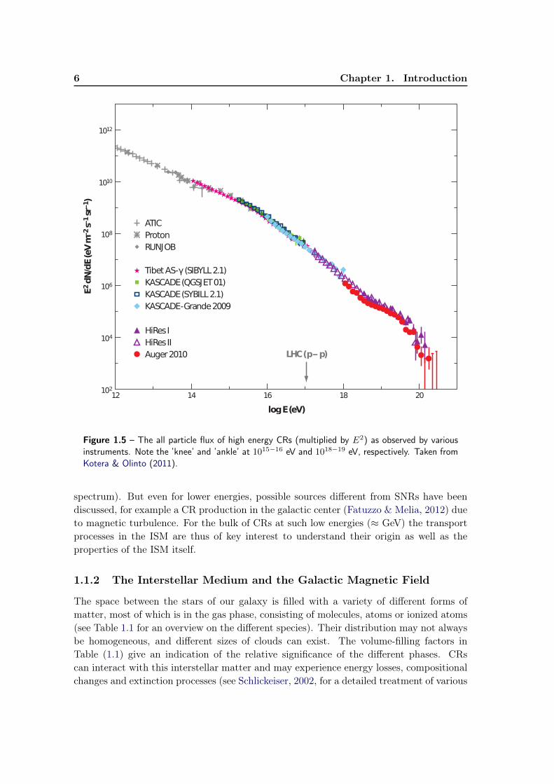
Figure 1.5 – The all particle flux of high energy CRs (multiplied by E2) as observed by variousinstruments. Note the ’knee’ and ’ankle’ at 1015−16 eV and 1018−19 eV, respectively. Taken fromKotera & Olinto (2011).
spectrum). But even for lower energies, possible sources different from SNRs have beendiscussed, for example a CR production in the galactic center (Fatuzzo & Melia, 2012) dueto magnetic turbulence. For the bulk of CRs at such low energies (≈ GeV) the transportprocesses in the ISM are thus of key interest to understand their origin as well as theproperties of the ISM itself.
1.1.2 The Interstellar Medium and the Galactic Magnetic Field
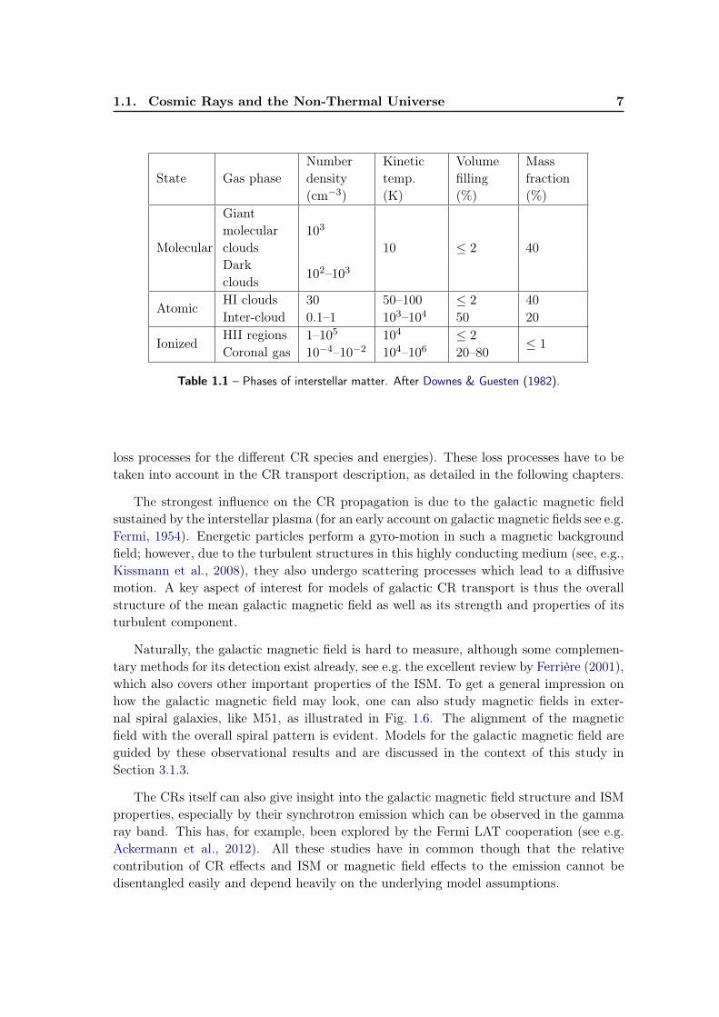
The space between the stars of our galaxy is filled with a variety of different forms ofmatter, most of which is in the gas phase, consisting of molecules, atoms or ionized atoms(see Table 1.1 for an overview on the different species). Their distribution may not alwaysbe homogeneous, and different sizes of clouds can exist. The volume-filling factors inTable (1.1) give an indication of the relative significance of the different phases. CRscan interact with this interstellar matter and may experience energy losses, compositionalchanges and extinction processes (see Schlickeiser, 2002, for a detailed treatment of various
1.1. Cosmic Rays and the Non-Thermal Universe 7
State Gas phaseNumberdensity(cm−3)
Kinetictemp.(K)
Volumefilling(%)
Massfraction(%)
Molecular
Giantmolecularclouds
103
10 ≤ 2 40Darkclouds
102–103
AtomicHI clouds 30 50–100 ≤ 2 40Inter-cloud 0.1–1 103–104 50 20
IonizedHII regions 1–105 104 ≤ 2 ≤ 1Coronal gas 10−4–10−2 104–106 20–80
Table 1.1 – Phases of interstellar matter. After Downes & Guesten (1982).
loss processes for the different CR species and energies). These loss processes have to betaken into account in the CR transport description, as detailed in the following chapters.
The strongest influence on the CR propagation is due to the galactic magnetic fieldsustained by the interstellar plasma (for an early account on galactic magnetic fields see e.g.Fermi, 1954). Energetic particles perform a gyro-motion in such a magnetic backgroundfield; however, due to the turbulent structures in this highly conducting medium (see, e.g.,Kissmann et al., 2008), they also undergo scattering processes which lead to a diffusivemotion. A key aspect of interest for models of galactic CR transport is thus the overallstructure of the mean galactic magnetic field as well as its strength and properties of itsturbulent component.
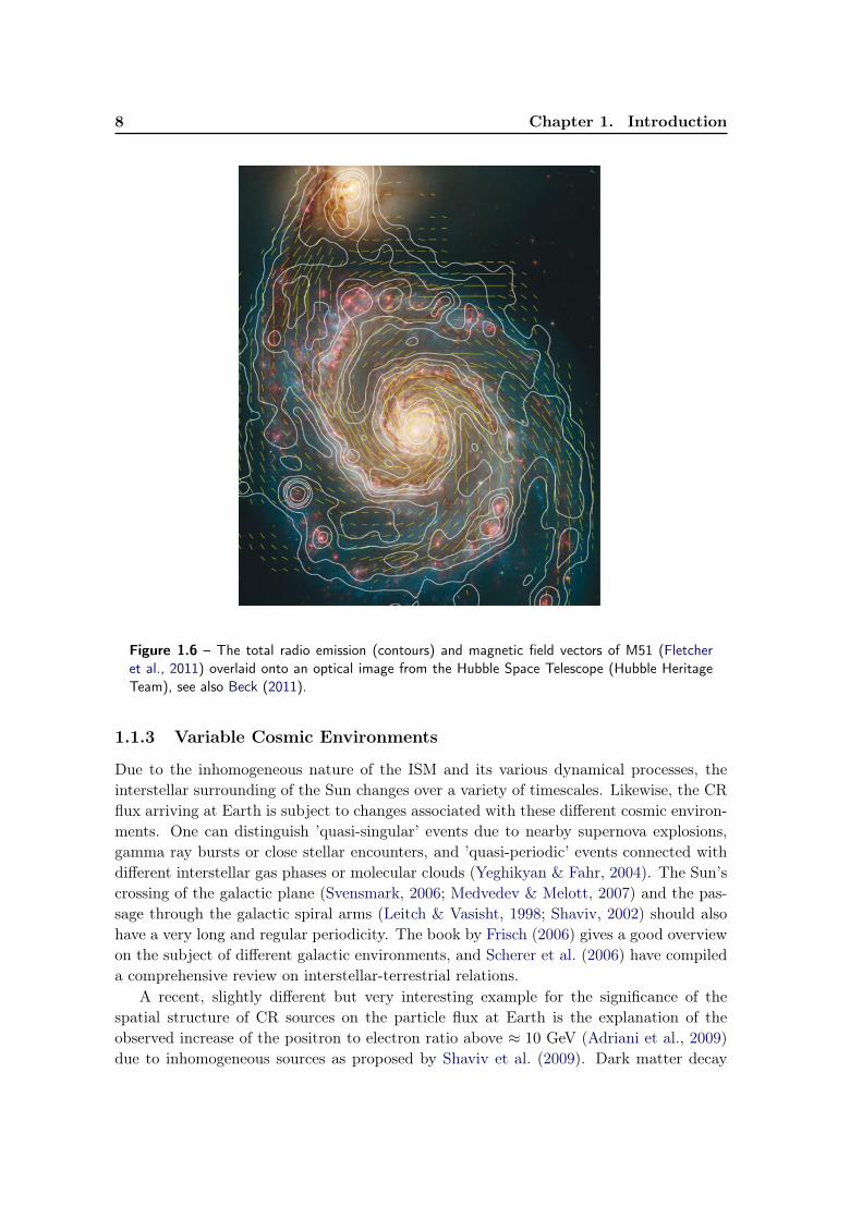
Naturally, the galactic magnetic field is hard to measure, although some complemen-tary methods for its detection exist already, see e.g. the excellent review by Ferrière (2001),which also covers other important properties of the ISM. To get a general impression onhow the galactic magnetic field may look, one can also study magnetic fields in exter-nal spiral galaxies, like M51, as illustrated in Fig. 1.6. The alignment of the magneticfield with the overall spiral pattern is evident. Models for the galactic magnetic field areguided by these observational results and are discussed in the context of this study inSection 3.1.3.
The CRs itself can also give insight into the galactic magnetic field structure and ISMproperties, especially by their synchrotron emission which can be observed in the gammaray band. This has, for example, been explored by the Fermi LAT cooperation (see e.g.Ackermann et al., 2012). All these studies have in common though that the relativecontribution of CR effects and ISM or magnetic field effects to the emission cannot bedisentangled easily and depend heavily on the underlying model assumptions.
8 Chapter 1. Introduction
Figure 1.6 – The total radio emission (contours) and magnetic field vectors of M51 (Fletcheret al., 2011) overlaid onto an optical image from the Hubble Space Telescope (Hubble HeritageTeam), see also Beck (2011).
1.1.3 Variable Cosmic Environments
Due to the inhomogeneous nature of the ISM and its various dynamical processes, theinterstellar surrounding of the Sun changes over a variety of timescales. Likewise, the CRflux arriving at Earth is subject to changes associated with these different cosmic environ-ments. One can distinguish ’quasi-singular’ events due to nearby supernova explosions,gamma ray bursts or close stellar encounters, and ’quasi-periodic’ events connected withdifferent interstellar gas phases or molecular clouds (Yeghikyan & Fahr, 2004). The Sun’scrossing of the galactic plane (Svensmark, 2006; Medvedev & Melott, 2007) and the pas-sage through the galactic spiral arms (Leitch & Vasisht, 1998; Shaviv, 2002) should alsohave a very long and regular periodicity. The book by Frisch (2006) gives a good overviewon the subject of different galactic environments, and Scherer et al. (2006) have compileda comprehensive review on interstellar-terrestrial relations.
A recent, slightly different but very interesting example for the significance of thespatial structure of CR sources on the particle flux at Earth is the explanation of theobserved increase of the positron to electron ratio above ≈ 10 GeV (Adriani et al., 2009)due to inhomogeneous sources as proposed by Shaviv et al. (2009). Dark matter decay

1.1. Cosmic Rays and the Non-Thermal Universe 9
and positrons from pulsars are also discussed in this context (e.g., Malyshev et al., 2009;Büsching & Dejager, 2011).
In this thesis, however, one of the major topics is the variation of the CR flux on thelongest timescale of hundreds of million years, caused by the spiral arm crossings of thesolar system. Indications for a flux variation exist in meteorite exposure histories (e.g.,Schaeffer et al., 1981; Lavielle et al., 1999), but only a few quantitative estimates of thesevariations have been made (see e.g., Shaviv, 2003; Scherer et al., 2006) and appear to beconsistent with the path of the Sun through the galaxy (Gies & Helsel, 2005), althoughrecently Overholt et al. (2009) claimed otherwise. To investigate this topic, a detailedmodel of the galactic source distribution and CR propagation is needed. The aspects andresults of such a model are presented in Chapter 3, while the possible climatic connectionsof this scenario are briefly discussed in Section 1.1.5.
1.1.4 The Heliosphere
The Sun is blowing a bubble into the ISM by emitting its supersonically expanding solarwind (SW). First modelling attempts on this subject can be found e.g. in Parker (1965c)and Weber & Davis (1967). Today, a coherent picture of the structures which result fromthe interaction of the SW with the ISM has emerged. The collision of the SW with theISM causes a sudden decrease in the supersonic speed of the SW to subsonic values andthus creates a shock wave, called the termination shock (TS). Further outwards, a contactdiscontinuity, called the heliopause (HP), separates the solar wind plasma from the ISM,as well as their respective magnetic fields. At the outermost edge a bowshock (BS) mayexist (see, however, McComas et al., 2012; Fichtner & Effenberger, 2012), where the (pos-sibly) supersonic and superalfvénic ISM is shocked due to the “obstacle” heliosphere. Thegeneral shape of these structures is sketched in Fig. 1.7. Hydrodynamic and magnetohy-drodynamic models of the heliosphere have become increasingly more sophisticated duringrecent years and can now reproduce many details of these structures (see e.g., Izmodenovet al., 2009; Opher et al., 2009; Pogorelov et al., 2011; Washimi et al., 2011).
Frozen into the SW is the heliospheric magnetic field (HMF), which in its generalshape was first described by Parker (1958). The presence of such a mean field as well asits turbulent component result, together with the complex structures of the heliosphere,in a modification of the galactic CR energy spectrum, called heliospheric modulation (see,e.g., Potgieter, 2011, for a recent review). So the spectrum measured at Earth, as well aswith spacecraft, is not to be considered as the local interstellar spectrum (LIS) outside ofthe heliosphere. A modulation model describing different effects which change the LIS inthe heliosphere is detailed in Chapter 4. For a recent review on galactic CRs (GCRs) inthe outer heliosphere, see, e.g., Florinski et al. (2011).
Besides the GCRs, there exist even more energetic particle populations in the helio-sphere, which originate from different processes. These particles modify the measuredenergy spectra even further, but can provide new insights into heliospheric structures andacceleration processes as well. Due to this fortunate situation, the heliosphere has oftenbeen termed an astrophysical laboratory for particle acceleration (see e.g., Terasawa &Scholer, 1989). Table (1.2) gives an overview on the most common particle species found

10 Chapter 1. Introduction
Figure 1.7 – Sketch of the fundamental heliospheric structures. Taken from Fichtner (2001).
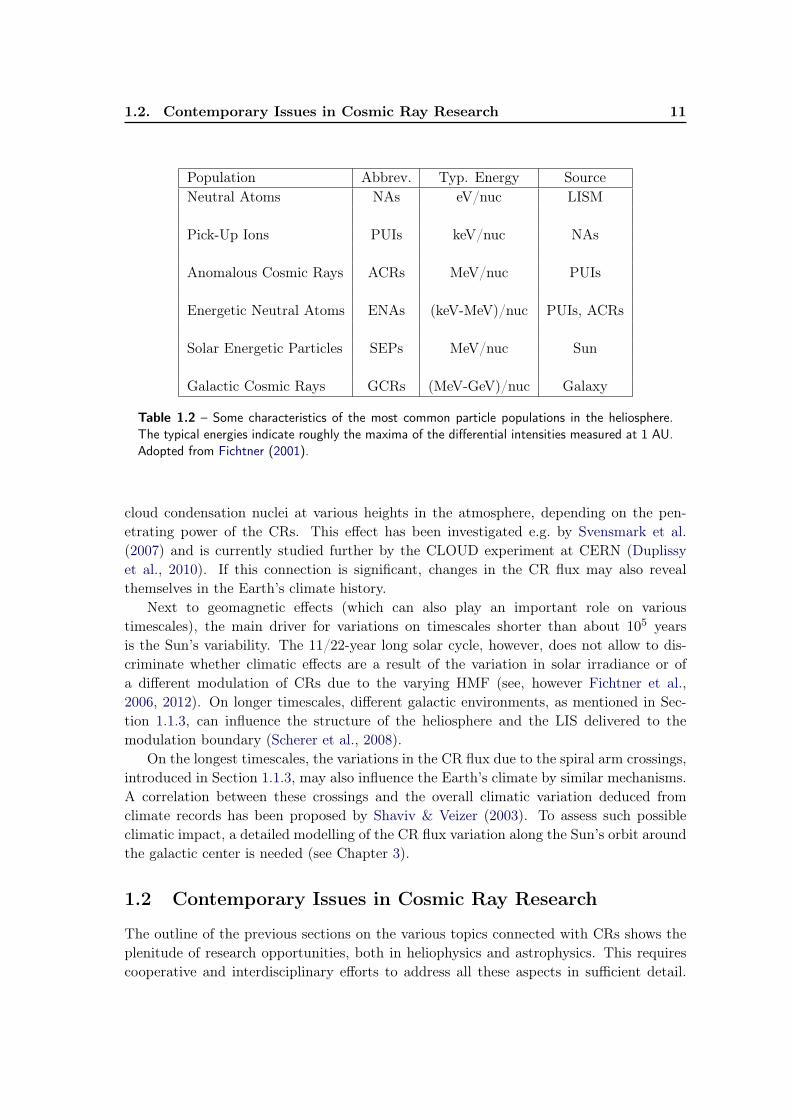
in the heliosphere. Anomalous cosmic rays (ACRs) are produced in the outer heliosphericinterface from pick-up ions (PUIs) convected with the solar wind (see e.g. the reviewby Fichtner, 2001). Solar energetic particles (SEPs) originate from the solar surface andcorona, and are produced during impulsive events like solar flares (Dalla & Browning, 2005;Effenberger et al., 2011b) or coronal mass ejections (Kahler & Vourlidas, 2005). The ener-getic neutral atoms (ENAs) produced via charge exchange from energetic charged particlesin the outer heliosphere can give further insights into the heliospheric structures and arecurrently investigated by the IBEX spacecraft (e.g., McComas et al., 2009). Altogether,this wealth of different particle populations allows for a study of processes in the helio-sphere from very different perspectives and can aid in the comprehension of astrophysicalprocesses with similar prerequisites.
1.1.5 Cosmic Rays and Climate
Apart from their general astrophysical relevance, CR are also an important topic in Earth-climate research; for a general overview, see e.g. the reviews by Kirkby (2007) and Schereret al. (2006). The main reason for this connection is attributed to the ionization of theatmosphere by the CRs, although the actual extend and effect of these processes is stillsomewhat controversial. The produced ionization can then promote the production of
1.2. Contemporary Issues in Cosmic Ray Research 11
Population Abbrev. Typ. Energy SourceNeutral Atoms NAs eV/nuc LISM
Pick-Up Ions PUIs keV/nuc NAs
Anomalous Cosmic Rays ACRs MeV/nuc PUIs
Energetic Neutral Atoms ENAs (keV-MeV)/nuc PUIs, ACRs
Solar Energetic Particles SEPs MeV/nuc Sun
Galactic Cosmic Rays GCRs (MeV-GeV)/nuc Galaxy
Table 1.2 – Some characteristics of the most common particle populations in the heliosphere.The typical energies indicate roughly the maxima of the differential intensities measured at 1 AU.Adopted from Fichtner (2001).
cloud condensation nuclei at various heights in the atmosphere, depending on the pen-etrating power of the CRs. This effect has been investigated e.g. by Svensmark et al.(2007) and is currently studied further by the CLOUD experiment at CERN (Duplissyet al., 2010). If this connection is significant, changes in the CR flux may also revealthemselves in the Earth’s climate history.
Next to geomagnetic effects (which can also play an important role on varioustimescales), the main driver for variations on timescales shorter than about 105 yearsis the Sun’s variability. The 11/22-year long solar cycle, however, does not allow to dis-criminate whether climatic effects are a result of the variation in solar irradiance or ofa different modulation of CRs due to the varying HMF (see, however Fichtner et al.,2006, 2012). On longer timescales, different galactic environments, as mentioned in Sec-tion 1.1.3, can influence the structure of the heliosphere and the LIS delivered to themodulation boundary (Scherer et al., 2008).
On the longest timescales, the variations in the CR flux due to the spiral arm crossings,introduced in Section 1.1.3, may also influence the Earth’s climate by similar mechanisms.A correlation between these crossings and the overall climatic variation deduced fromclimate records has been proposed by Shaviv & Veizer (2003). To assess such possibleclimatic impact, a detailed modelling of the CR flux variation along the Sun’s orbit aroundthe galactic center is needed (see Chapter 3).
1.2 Contemporary Issues in Cosmic Ray Research
The outline of the previous sections on the various topics connected with CRs shows theplenitude of research opportunities, both in heliophysics and astrophysics. This requirescooperative and interdisciplinary efforts to address all these aspects in sufficient detail.
12 Chapter 1. Introduction
In this sense, the thesis is restricted to particular issues of the propagation of CRs in theinterplanetary and interstellar medium. These are briefly introduced below, and will befurther detailed in the respective chapters.
1.2.1 Anisotropic Diffusion
In models for the interplanetary CR transport, it was already recognized very early that thediffusive motion of the particles due to the magnetic field turbulence has to be anisotropicwith respect to the mean background magnetic field (Parker, 1965a). Phenomenologically,it is clear that transport parallel to the magnetic field can be more efficient, due to the gyro-motion of the particles. It has also been recognized that the diffusion may even be fullyanisotropic (Jokipii, 1973), i.e. with two distinct diffusion directions perpendicular to themagnetic field. Later, this has been of particular significance in models of Jovian electrons(i.e. electrons accelerated in the magnetosphere of Jupiter) which required an increasedlatitudinal diffusion coefficient to reproduce high-latitude measurements from the Ulyssesspacecraft (e.g., Ferreira et al., 2001). A coherent theory of anisotropic perpendiculartheory, however, is still lacking, and the approaches so far have only considered specialcases.
In most galactic transport models so far, only a scalar diffusion coefficient has beenemployed, although the observations clearly indicate a significant mean galactic magneticfield with a strength of about the order of the turbulent component (see Section 1.1.2).It has become increasingly evident from both, theoretical considerations (Shalchi et al.,2010a) and simulations for the galactic dynamo (Hanasz et al., 2009), that such mod-els need to take anisotropic diffusion into account. These aspects and implications ofanisotropic diffusion in the heliospheric and astrophysical context will be addressed in therespective subsequent chapters.
1.2.2 Anomalous Diffusion
A further extension to the standard diffusion theory of CRs is the consideration of ananomalous diffusion behavior of energetic particles, i.e. sub- and superdiffusion, with mean-square displacements of the particles which are no longer proportional to time, but to somepower tζ with ζ 6= 1 (see e.g., Metzler & Klafter, 2000, for a comprehensive review). Thisnotion leads to fractional Fokker-Planck equations and Lévy Jump processes, and maybe attributed to e.g. a fractal ISM (Lagutin et al., 2005) in the context of galactic CRtransport, or to effects of compound diffusion in non-uniform media as proposed by leRoux et al. (2010) for heliospheric particle populations. There also exist indications fromthe observation of particle-flux time-profiles that anomalous transport processes can be ofimportance. The power-law behavior in the profiles of SEPs (Trotta & Zimbardo, 2011),particles accelerated in CME driven shock waves (Sugiyama & Shiota, 2011), and termina-tion shock particles (Perri & Zimbardo, 2009) leads to the conjecture that superdiffusioninstead of ’normal’ Gaussian diffusion might be more appropriate description of the re-spective transport processes.
1.3. The Scope and Structure of this Thesis 13
1.3 The Scope and Structure of this Thesis
The objectives of this thesis in the context of the topics introduced above can thus bestated as follows:
• An extension of current galactic CR propagation models to incorporate ananisotropic diffusion tensor which is constructed from a galactic magnetic field model.
• The generalization of the diffusion tensor to three distinct diffusion components forthe application to heliospheric CR modulation.
• The development of an anomalous diffusion model and corresponding numericalsolution methods to address claims of observed super- and subdiffusive behaviormore quantitatively.
The aforementioned issues are subsequently discussed in the main parts of this thesis.Chapter 2 introduces the basis for the quantitative transport models as well as the nec-essary numerical tools to solve the associated equations. In Chapter 3, a transport modelfor the galactic propagation of CRs including anisotropic diffusion and an azimuthallystructured source function is developed and its results are presented and discussed. InChapter 4, a generalization of the heliospheric diffusion tensor for fully-anisotropic diffu-sion in arbitrary magnetic field configurations is introduced and applied to the modulationof GCRs to assess its implications. Chapter 5 then deals with the theoretical descriptionof anomalous diffusion processes and their application to energetic particle transport. Forthis, the numerical methods employed in the previous two chapters have to be extendedas well. The last chapter summarizes the results and gives an outlook on further fields ofstudy connected to the methods and results of this thesis. Some details of numerical andtheoretical aspects are further explicated in the appendices.
The similar methods with regard to the relevant equations and numerical methodsthat can be applied to the topics at hand show at the same time the unity and diversityof astrophysical research. This thesis can be regarded as an attempt to exemplify some ofthese interconnections and to show their potential for further research opportunities.

Chapter 2
Transport Theory and NumericalMethods
A neutron walks into a bar and asks how much for adrink. The bartender replies "for you, no charge".
The Big Bang Theory, Season 3, Episode 18Sheldon Cooper
Contents2.1 General Cosmic Ray Diffusion Theory . . . . . . . . . . . . . . . . 15
2.1.1 The Vlasov-Maxwell System . . . . . . . . . . . . . . . . . . . . . . . 152.1.2 The Fokker-Planck Equation . . . . . . . . . . . . . . . . . . . . . . 162.1.3 The Diffusion Approximation . . . . . . . . . . . . . . . . . . . . . . 17
2.2 A Closer Look at Diffusion Processes . . . . . . . . . . . . . . . . 182.2.1 Stochastic Differential Equations . . . . . . . . . . . . . . . . . . . . 192.2.2 The Diffusion Approximation Revisited . . . . . . . . . . . . . . . . 21
2.3 Numerical Methods . . . . . . . . . . . . . . . . . . . . . . . . . . . 222.3.1 The Grid-based Method . . . . . . . . . . . . . . . . . . . . . . . . . 222.3.2 The Monte Carlo Method . . . . . . . . . . . . . . . . . . . . . . . . 23
2.1 General Cosmic Ray Diffusion Theory
Comprehensive monographs on the physics of CRs have been published by, e.g., Schlick-eiser (2002), Stanev (2004), and Shalchi (2009). Here, only a brief overview on the under-lying transport theory is given to introduce the relevant concepts and equations necessaryto proceed with the more detailed studies in the subsequent chapters.
2.1.1 The Vlasov-Maxwell System
To derive the transport equation governing the propagation of energetic particles in agiven background plasma which is not influenced by this non-thermal component (this isoften termed test-particle approach), we employ the Vlasov equation
∂fα∂t
+ ~vα · ∇fα +~Fαmα· ∇~vfα = 0 (2.1)

16 Chapter 2. Transport Theory and Numerical Methods
which is the collisionless form of the Boltzmann equation for the particle distributionfunction fα(~x,~v, t) of particle species α in phase-space. This equation is an expressionof continuity in phase-space, i.e. a form of the Liouville-Theorem, which states that thedistribution function is constant along any trajectory in phase space (Liouville, 1838). Theassumption of a vanishing collision integral on the right-hand side of Eq. (2.1) is generallyjustified in the description of energetic particles, since their timescale of interaction witheach other is much longer than their response time to the background plasma influences.For the latter, the forces ~Fα have to be specified. These are, in most cases, electromagneticforces described by the Maxwell equations
∇ · ~E =1
ε0
∑β
qβ
∫fβd
3vβ (2.2)
∇ · ~B = 0 (2.3)
∇× ~E = −∂~B
∂t(2.4)
∇× ~B = µ0ε0∂ ~E
∂t+ µ0
∑β
qβ
∫~vβfβd
3vβ (2.5)
Here, the charge and current are given by the corresponding moments of the distributionfunction of the background plasma species fβ . This background plasma is most com-monly treated with fluid theories and linear wave perturbation analyses. In principle, ahydrodynamic theory for CRs could also be derived by taking the velocity moments oftheir distribution function (Drury & Völk, 1981). However, since CRs are known to be farfrom a thermodynamical equilibrium, as discussed in the introductory chapter, in mostcases a kinetic treatment is more appropriate. The next step in a simplification of theVlasov-Maxwell system is known as Fokker-Planck Equation (FPE) in the CR community.
2.1.2 The Fokker-Planck Equation
Generally speaking, a Fokker-Planck equation is a second-order partial differential equa-tion of parabolic type, which has the form
∂f(~ξ, t)
∂t=
− n∑i=1
∂
∂xiVi(~ξ, t) +
n∑i,j=1
∂2
∂xi∂xjDij(~ξ, t)
f(~ξ, t) (2.6)
where ξ = (x1, ..., xn) is a n-dimensional vector of phase space variables and Vi and Dij arethe components of the drift vector and diffusion tensor. For a detailed discussion of thisequation, methods of solution, and applications see for example the comprehensive mono-graph by Risken (1989). All kinetic transport equations for CRs have this general form,as long as their motions are sufficiently random that a diffusive description is appropriate.
In CR physics, however, the term FPE is most often used for a special form of such atransport equation, namely the following:
2.1. General Cosmic Ray Diffusion Theory 17
∂f
∂t+ ~u · ∇f =
∂
∂µ
(Dµµ
∂f
∂µ
)+
∂
∂µ
(Dµp
∂f
∂p
)+
1
p2∂
∂p
(p2Dµp
∂f
∂µ
)+
1
p2∂
∂p
(p2Dpp
∂f
∂p
)+Q(~x, p, µ, t) (2.7)
This equation can be directly derived from the Vlasov-Maxwell system described in theprevious section by applying a second order expansion, an ensemble averaging with respectto the background plasma waves and a gyro-phase averaging with respect to the distribu-tion function. For this, spherical coordinates in momentum space are introduced, where pis the absolute value of the momentum and µ = cos θ is the pitch-angle cosine which mea-sures the orientation between the background mean magnetic field and the gyro-averagedmomentum. Detailed derivations for this basic equation of CR transport can be found e.g.in Schlickeiser (1989a), Schlickeiser (1989b), Berezinskii et al. (1990), Schlickeiser (2002),and Schlickeiser (2011). The most important physical assumption in this derivations is theneglect of the fast gyro motion of the particles, thus the distribution function is no longerdependent on the gyro phase coordinate and the equation is reduced by one dimension.The remaining Fokker-Planck coefficients (Dµµ, Dµp, Dpp) are functions of the wave prop-erties of the underlying magnetic field turbulence. These magnetic fluctuations and theneed for their stochastic description are the ultimate reasons for the diffusive behavior ofthe distribution function, which corresponds to a scattering in pitch angle and momentumof the particles and is accounted for by the second-order terms in the FPE. The FPE mayinvolve even more second-order terms describing the spatial perpendicular diffusion of thegyrocenter, which then yields the diffusion tensor in the momentum-isotropic limit.
Instead of a detailed description of the many turbulence models, which have been de-veloped to derive expressions for the Fokker-Planck coefficients and which depend heavilyon the underlying plasma properties, we move on with a further simplification which isreferred to as diffusion approximation and described in the following.
2.1.3 The Diffusion Approximation
Applying a further average over the pitch-angle µ to the FPE (2.7) yields the followingdiffusion-convection equation
∂f
∂t+ ~u · ∇f = ∇ · (κ∇f) +
1
p2∂
∂p
(p2Dpp
∂f
∂p
)+
1
3(∇ · ~u)
∂f
∂ ln p+ S(~x, p, t) (2.8)
which is often termed Parker Transport Equation due to its first derivation by Parker(1965a), but see also Gleeson & Axford (1967) and Jokipii (1966, 1967) for slightly differenttreatments. The diffusion approximation (i.e. the pitch-angle average) is justified, if thedistribution function f is nearly isotropic in momentum, i.e. only a function of p = |~p| oralternatively of the energy E. The remaining terms describe diffusion in space (first termon the right-hand side of Eq. 2.8) via the diffusion tensor κ and diffusion in momentum(second term) with the momentum diffusion coefficient Dpp. The other terms in thetransport equation (TPE) describe adiabatic energy changes due to the compressibility of

18 Chapter 2. Transport Theory and Numerical Methods
the background flow (third term) and sources of particles (last term), while the advectionwith the background flow is accounted for by the second term on the left-hand side of theTPE.
It is possible to apply yet another average over momentum to yield a description onlybased on the total CR pressure (see e.g. Drury & Völk, 1981), but this way, all kineticinformation would be lost, so that this description is only useful to get rough estimates ofthe spatial behavior of the CR distribution.
All these descriptions of CR transport involve an implicit ordering of timescales, whereisotropization in gyro-phase is assumed to be the fastest process and momentum thermal-ization the slowest. Because of two of the main observational properties of CRs, namelytheir isotropy and their nonthermality, it is most natural to base their description on theTPE introduced above. It has to be kept in mind though, that situations with a differentscope of applicability may exist, i.e. where for example the assumption of isotropy is nolonger valid (as for example in the case of SEPs; see, e.g., Dröge et al., 2010) and thus adescription based on the FPE (2.7) may be more appropriate.
The TPE introduced above will be the basis of all the following investigations, while theparticularities of the different scenarios will be detailed further in the respective chapters.The key ingredient and focus of study is, in any case, the (spatial) diffusion tensor κ. Thefollowing section will shed a little more light on the diffusive processes connected with thistransport quantity.
2.2 A Closer Look at Diffusion Processes
A macroscopic description of a diffusion process starts with the notion that the diffusiveflux ~Φ is proportional to the negative gradient of the distribution f times a diffusioncoefficient κ, which is related to the mean free path λ of the particles, i.e.
~Φ = −1
3λv∇f = −κ∇f (2.9)
where v is the particle speed. This phenomenological description was introduced by Coc-coni (1951) in the context of CR transport and is discussed in a bit more detail in Jokipii(1971). Inserting Eq. (2.9) into the equation of continuity, i.e.
∂f
∂t= −∇ · ~Φ + S (2.10)
yields the usual diffusion equation (or heat-flux equation)
∂f
∂t= ∇ · (κ∇f) + S (2.11)
where S are again particle sources or sinks. At this stage, the diffusion coefficient κ isnot connected to the magnetic field turbulence causing the random motion of the CRs.Establishing this connection has been one major ongoing project in CR research until now(see, e.g., the book by Shalchi, 2009).

2.2. A Closer Look at Diffusion Processes 19
The Fokker-Planck type form of the TPE allows for the application of various solutionmethods developed for these equations (see again Risken, 1989, for a comprehensive treat-ment of many aspects). For example, even methods from quantum field theory, like thepath integral approach, have been successfully applied in CR propagation studies (Zhang,1999b). One approach of particular interest is based on the fundamental equivalence be-tween the FPE and certain stochastic differential equations (SDEs) involving a Wienerprocess, as will be described in the following.
2.2.1 Stochastic Differential Equations
In the context of Brownian motion, it became very clear for the first time that a microscopicaccount of the stochastic processes involved in diffusion is of high scientific value (Einstein,1905). In an attempt to find a simple description of this process, Paul Langevin introducedthe very first stochastic differential equation in his 1908 paper (for an English translation,see Lemons & Gythiel, 1997), namely
m∂2x
∂t2= −6πηa
∂x
∂t+X (2.12)
where x, m and a are the particle’s position, mass and spherical diameter, respectively,and η is the surrounding fluid’s viscosity. The fluctuating force X, however, describes therandomness of the particle’s motion due to the impacts of the fluid particles (with finitetemperature). It took a few decades more, till finally with the theory of stochastic calculus,most prominently associated with the name Kiyoshi Ito, a consistent mathematical theoryof these fluctuations emerged. For a more thorough account of this historical development,as well as many details on SDEs and stochastic processes in general, see Gardiner (2009).The heuristically introduced fluctuating force X can be specified as a Wiener process inthis context and is a key ingredient in the theory of SDEs. It is characterized by a time-stationary normal-distributed probability density with expectation value 0 and variance 1
(N (0, 1)). Such a process can be realized by numerically generated (random-walk) samplepaths, shown in Fig. 2.1 for the most simple two-dimensional SDE:
dxi = dWi , i ∈ 1, 2 (2.13)
where dWi denotes a Wiener process in the respective dimension.The practical importance of SDEs with regard to the diffusion-convection transport
problem, however, stems from the already mentioned equivalence between the solutions ofthe FPE and the ensemble average of sample paths in accordance with particular SDEs.In one dimension, this can be stated as follows (Gardiner, 2009):
If x(t) is a stochastic quantity that obeys the Ito SDE
dx(t) = a[x(t), t]dt+ b[x(t), t]dW (t) (2.14)
that is,
x(t) = x(to) +
∫ t
t0
a[x(t′), t′]dt′ +
∫ t
t0
b[x(t′), t′]dW (t′) (2.15)

20 Chapter 2. Transport Theory and Numerical Methods
-1.5
-1
-0.5
0
0.5
1
1.5
-1.5 -1 -0.5 0 0.5 1 1.5
y
x
Figure 2.1 – Two sample paths of a Wiener process in two dimensions, originating at (0,0).
and p(x, t, x0, t0) is the conditional probability density of x(t), then p obeys the ForwardFokker-Planck Equation
∂tp = −∂x[a(x, t)p] +1
2∂2x[b(x, t)2p] . (2.16)
Similarly, the SDE process can be identified with the Backward Fokker-Planck Equation
∂tp = −a(x, t)∂xp−1
2b(x, t)2∂2xp , (2.17)
if the particle trajectories are integrated backwards in time. Notice that the main differencebetween both formulations is in the implicit and explicit form of the coefficient a and b,respectively and that the time and space coordinates are still the same as in the ForwardFPE (2.16).
The extension to a multidimensional system like the general FPE (2.6) is also possible,and results in SDEs of the form
dxi = Vidt+BijdWj (2.18)

2.2. A Closer Look at Diffusion Processes 21
where the relation BBT = 2 D has to be fulfilled, that is, a root for the diffusion tensor Dhas to be determined. Note that this root is not unique, i.e. a freedom of choice remains.An account on the determination of such a root can be found, e.g., in Kopp et al. (2012).
For more details on the mathematical subject of SDEs and its applications in physics,the reader is referred to Lemons (2002) and Gardiner (2009). How this formalism can beapplied to yield numerical solutions to the TPE will be detailed below in Section 2.3.2.Before proceeding with this, however, the diffusion approximation, only briefly mentionedin Section 2.1.3, will be revisited in the context of SDEs.
2.2.2 The Diffusion Approximation Revisited
The equivalence between the FPE and a corresponding set of SDEs, as outlined in theprevious chapter, allows to re-derive the diffusion approximation in a more accessibleway than on the Fokker-Planck level. The procedure is similar to the Smoluchowskiapproximation in the case of Brownian motion (see, e.g. Chapter 8.2 in Gardiner, 2009).There, the “fast” variable v (i.e. the particle’s velocity) is adiabatically eliminated anda diffusion equation for the particle’s position is obtained. This idea has recently beentransferred to the pitch-angle diffusion of energetic particles by Litvinenko (2012a) andlater been generalized to helicity-dependent pitch-angle diffusion in Litvinenko (2012b).Here, only the derivation for isotropic pitch-angle scattering is outlined to familiarize thereader with this procedure.
The starting point is the focused transport equation
∂fl∂t
= − ∂
∂z(µvfl)−
∂
∂µ
[v
2L(1− µ2)fl +
∂Dµµ
∂µfl
]+
∂2
∂µ2(Dµµfl) (2.19)
(e.g. Roelof, 1969), where fl(z, µ, t) = exp(z/L)f is the (gyro-tropic and mono-energetic)linear particle density which only depends on the position z along a field line, the pitch-angle µ and the time, while v is the particle’s speed. This equation is commonly usedin studies of solar energetic particle events, but can also be regarded as a simple versionof the general Fokker-Planck Equation (2.7), if the limit of infinite focusing L → ∞ (i.e.a homogeneous background magnetic field) is considered. In particular, the followingderivation is not dependent on the specific form of the convective term in the transportequation.
In analogy to the above Ito-equivalence, the following system of SDEs is equivalent tothe transport equation (2.19):
dz = µvdt, (2.20)
dµ =
[v
2L(1− µ2) +
∂Dµµ
∂µ
]dt+
√2DµµdW. (2.21)
Now, if we specify the pitch-angle diffusion coefficient as Dµµ = D0(1−µ2), i.e. we assumeisotropic pitch-angle scattering, and regard µ as a fast variable which relaxes quickly toan isotropic steady-state, we can set dµ ≈ 0 and obtain:
µdt =v
4D0L(1− µ2)dt+
√1− µ22D0
dW (2.22)
22 Chapter 2. Transport Theory and Numerical Methods
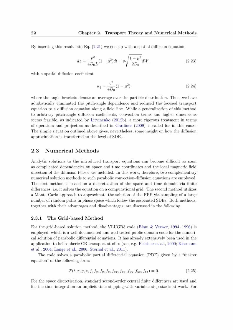
By inserting this result into Eq. (2.21) we end up with a spatial diffusion equation
dz =v2
4D0L(1− µ2)dt+ v
√1− µ22D0
dW . (2.23)
with a spatial diffusion coefficient
κ‖ =v2
4D0〈1− µ2〉 (2.24)
where the angle brackets denote an average over the particle distribution. Thus, we haveadiabatically eliminated the pitch-angle dependence and reduced the focused transportequation to a diffusion equation along a field line. While a generalization of this methodto arbitrary pitch-angle diffusion coefficients, convection terms and higher dimensionsseems feasible, as indicated by Litvinenko (2012b), a more rigorous treatment in termsof operators and projectors as described in Gardiner (2009) is called for in this cases.The simple situation outlined above gives, nevertheless, some insight on how the diffusionapproximation is transferred to the level of SDEs.
2.3 Numerical Methods
Analytic solutions to the introduced transport equations can become difficult as soonas complicated dependencies on space and time coordinates and the local magnetic fielddirection of the diffusion tensor are included. In this work, therefore, two complementarynumerical solution methods to such parabolic convection-diffusion equations are employed.The first method is based on a discretization of the space and time domain via finitedifferences, i.e. it solves the equation on a computational grid. The second method utilizesa Monte Carlo approach to approximate the solution of the FPE via sampling of a largenumber of random paths in phase space which follow the associated SDEs. Both methods,together with their advantages and disadvantages, are discussed in the following.
2.3.1 The Grid-based Method
For the grid-based solution method, the VLUGR3 code (Blom & Verwer, 1994, 1996) isemployed, which is a well-documented and well-tested public domain code for the numeri-cal solution of parabolic differential equations. It has already extensively been used in theapplication to heliospheric CR transport studies (see, e.g. Fichtner et al., 2000; Kissmannet al., 2004; Lange et al., 2006; Sternal et al., 2011).
The code solves a parabolic partial differential equation (PDE) given by a “masterequation” of the following form:
F(t, x, y, z, f, fx, fy, fz, fxx, fxy, fyy, fyz, fzz) = 0. (2.25)
For the space discretisation, standard second-order central finite differences are used andfor the time integration an implicit time stepping with variable step-size is at work. For
2.3. Numerical Methods 23
the application of the code, this means that one has to specify the coefficients in Eq. (2.25)as well as the appropriate boundary and initial conditions for the problem.
The major advantage of this method is that more or less complete space and time infor-mation (depending on the numerical resolution and accuracy) for the given boundary-valueproblem and the chosen domain of integration can be obtained. The transport equationsdescribing the energetic particle transport, however, are at least (3+1+1)-dimensional(three spatial, one momentum and one time dimension) as long as no principle symme-tries can be exploited. This is still too demanding for most computer codes includingVLUGR3, so one has to reduce the problem by one dimension. In principle, it is possibleto average out the momentum information and still obtain results on the spatial structureof the distribution function, but, as already indicated in Section 2.1.3, the spectral infor-mation is of great interest in CR studies. Since the galactic propagation scenario can beregarded as a steady-state problem on long timescales, the best idea is thus to eliminatethe time variable and use the “independent-variable” stepping of the code instead for amomentum-sampling. This means that the diffusion-convection part of the equation isintegrated from high to low energies (or momenta) instead of the time integration, andsince the intensity of CRs falls off rapidly for high energies, a simple zero initial conditioncan be used without loss of generality.
2.3.2 The Monte Carlo Method
To circumvent some of the problems associated with the grid-based methods presentedin the previous section and for the ability to check on the results with a completelyindependent approach, a second solution method to parabolic Fokker-Planck equationsis employed in this work as well, namely a Monte Carlo method based on the stochasticequivalence described in Section 2.2.1. The basic idea is to integrate an Ito SDE likeEq. (2.14) using for example a simple Euler-scheme and an appropriate random numbergenerator for the Wiener process (dW ). The resulting trajectory (see, e.g. again Fig. 2.1as an illustrative example) can be regarded as a stochastic probe of the phase space,i.e. a pseudo particle. By averaging appropriately over many sample realizations of suchtrajectories, one can construct the phase-space distribution function for the correspondingFokker-Planck equation.
In recent years, this kind of Monte Carlo methods have become increasingly popular,because of better computer performance and their conceptual simplicity and robustness. Inthe CR community, their application ranges from diffusive shock acceleration (e.g. Kruells& Achterberg, 1994), heliospheric modulation studies (Zhang, 1999a; Pei et al., 2010;Strauss et al., 2011a) which also emphasize different aspects which were not appropriatelytreatable before, like the influence of the heliospheric current sheet (Strauss et al., 2012)or the detailed analysis of propagation times and energy losses (Strauss et al., 2011b),transport of solar energetic particles (Dröge et al., 2010) to galactic propagation scenarios(Farahat et al., 2008; Effenberger et al., 2011a).
The Ito equivalence allows, in principle, for two different solution approaches, exploit-ing the forward and the backward FPE, as explained in Section 2.2.1. For the forwardmethod, the particles are injected at the sources and the boundaries, and the distribution

24 Chapter 2. Transport Theory and Numerical Methods
function can be constructed in the phase-space and time domain by an averaging processover small parcels, i.e. a binning procedure. This method can be somewhat refined byusing different kernel density estimators (Parzen, 1962) which means that not a simplemean average over one binning cell is taken, but instead an averaging kernel K(x) like forexample a Gaussian is employed.
The backward method integrates the pseudo particle’s trajectory backwards in timeand collects all the contributions from sources and boundaries which it encounters. It isimportant, however, that the integration stops as soon as a particle hits a boundary. Thisway, the distribution function can be determined only at the respective point of interestwhere the integration is started (again by averaging over many sample trajectories startingat that particular phase space point).
A lot more information on numerical methods for stochastic differential equations canbe found in Kloeden & Platen (1995). For this work, the numerical basis was the codewhich is extensively described in Kopp et al. (2012). In particular, the code is writtenvery general to allow for many application scenarios and also involves routines to treatcomplicated diffusion tensor structures, as required for this study. In the course of thiswork, the code has nevertheless been heavily modified to treat the investigated problemsproperly. This has been necessary especially for the treatment of anomalous diffusionprocesses, as described in detail in Chapter 5.


Chapter 3
Galactic Cosmic Ray Transport
What a wonderful and amazing Scheme have we here ofthe magnificent Vastness of the Universe! So many Suns,so many Earths, and every one of them stock’d with somany Herbs, Trees and Animals, and adorn’d with somany Seas and Mountains! And how must our wonderand admiration be encreased when we consider theprodigious distance and multitude of the Stars?
Cosmostheoros (1695)Christiaan Huygens
Contents3.1 A Galactic Transport Model . . . . . . . . . . . . . . . . . . . . . . 28
3.1.1 The Anisotropic Diffusion Transport Equation . . . . . . . . . . . . 29
3.1.2 The Diffusion Tensor Formulation . . . . . . . . . . . . . . . . . . . 29
3.1.3 Galactic Magnetic Field Models . . . . . . . . . . . . . . . . . . . . . 31
3.1.4 Distribution of Matter and Supernovae Abundances . . . . . . . . . 32
3.1.5 Energy Losses . . . . . . . . . . . . . . . . . . . . . . . . . . . . . . . 33
3.1.6 Numerical Solution Methods for the Transport Model . . . . . . . . 34
3.2 Calculated Galactic Cosmic Ray Distributions . . . . . . . . . . . 35
3.2.1 Global Steady-State Solutions . . . . . . . . . . . . . . . . . . . . . . 35
3.2.2 Spectral Variation . . . . . . . . . . . . . . . . . . . . . . . . . . . . 37
3.2.3 Orbital Variation . . . . . . . . . . . . . . . . . . . . . . . . . . . . . 39
3.3 Conclusions . . . . . . . . . . . . . . . . . . . . . . . . . . . . . . . . 41
In this chapter, a quantitative model to describe the propagation of CR protons in ourgalaxy is developed. Two major deficits of most of the propagation models up till now arethat they do not take into account the azimuthal structure of the CR source distributionand assume only a scalar diffusion coefficient. These two aspects will be refined in thepresent model, by imposing a three-dimensionally structured source function aligned tothe galactic spiral arm pattern and by employing a diffusion tensor which is determinedby the galactic magnetic field.
Parts of this chapter have already been published in a proceedings volume, see Effen-berger et al. (2011a), and in Effenberger et al. (2012b).
28 Chapter 3. Galactic Cosmic Ray Transport
3.1 A Galactic Transport Model
The characteristics of galactic transport models depend on the properties of the interstellarmedium (ISM) through which the particles travel. For example, the average galacticmagnetic field and its turbulent component are connected to the transport parameters insuch models and the loss processes depend on the background gas density.
The basic propagation process of CRs in the ISM is the diffusive motion of the particlesdue to scattering at magnetic field fluctuations, as discussed in the previous chapters. Fromnumerous studies in heliospheric physics it is well known that the diffusive transport ofenergetic particles cannot be described by a scalar diffusion coefficient, but requires a diffu-sion tensor which takes into account that parallel and perpendicular diffusion are different(e.g. Jokipii, 1966; Potgieter, 2011). In galactic propagation studies, however, anisotropicdiffusion of CRs has been investigated only for basic magnetic field configurations witha limited scope of application, see, e.g., Chuvilgin & Ptuskin (1993), Breitschwerdt et al.(2002), Snodin et al. (2006) and references therein. While the latter authors were inter-ested in the consequences of anisotropic diffusion for energy equipartition, Hanasz & Lesch(2003) and Ryu et al. (2003) analyzed its importance for the Parker instability.
More recently, Hanasz et al. (2009) found that anisotropic diffusion is an essentialrequirement for the CR-driven magnetic dynamo action in galaxies. Moreover, a recentderivation of the perpendicular diffusion coefficient for galactic propagation, using the en-hanced nonlinear guiding center theory and a Goldreich-Sridhar turbulence model, wasperformed by Shalchi et al. (2010a) and resulted in ratios of the parallel to the perpendicu-lar diffusion coefficient which where much lower than unity, namely κ⊥/κ‖ ≈ 10−4−10−1,depending on particle rigidity.
Many popular models for galactic CR transport, however, include only a single diffusioncoefficient, like the GALPROP code (Strong et al., 2010). Although Strong et al. (2007)principally acknowledge that anisotropic diffusion is of significance, they argue that dueto large-scale fluctuations in the magnetic field on scales of the order of 100pc, the globaldiffusion will be spatially isotropic. Observations of the galactic magnetic field indicatethough that the field has a large-scale ordering with a regular field strength of about thesame magnitude as the turbulent component (see, e.g., Ferrière, 2001). A similar indicationis given by observations of other spiral galaxies (Beck, 2011; Fletcher et al., 2011) whichshow a global magnetic field structure aligned to the spiral arm pattern. Therefore, itmust be concluded that anisotropic diffusion can have an important effect in galactic CRpropagation.
Besides its fundamental astrophysical relevance, the spatial distribution of the CRflux in the galaxy is also of interest in the context of long-term climatology as discussedin the introductory Section 1.1.5. Shaviv (2002) proposed a CR-climate connection onthe timescale of 108 years due to the transit of the solar system through the galacticspiral arms during its orbit around the galactic center. The argument assumes that thelow-altitude cloud coverage increases due to an increased formation of cloud-condensationnuclei when the CR flux is high (Svensmark et al., 2007). Thus, an anti-correlation betweentemperature and CR flux is to be expected and indeed reported by Shaviv & Veizer (2003).Most recently, Svensmark (2012) found further evidence of a connection between nearby
3.1. A Galactic Transport Model 29
supernovae and their CR output and life on Earth (Section 1.1.5). More details on theCR-climate connection can be found in Scherer et al. (2006). Although the author of thepresent study does not adhere to this view in all aspects (see, e.g., the critical remarks inOverholt et al., 2009), it can give a further interesting motivation to study the galacticCR distribution, and especially its longitudinal structure, in greater detail.
The aim of this part of the thesis is to calculate galactic CR spectra at different po-sitions along the Sun’s orbit around the galactic center and to analyse the influence ofanisotropic diffusion on the longitudinal cosmic ray distribution. First, the underlyingpropagation model and its relevant input are presented as a connection to the previouschapter on general transport theory (Chapter 2). The model incorporates the diffusiontensor and its connection to the galactic magnetic field, the three-dimensional sourcedistribution of CR and its connection to the spiral-arm structure and supernova (SN)occurrence, and loss processes in the ISM. Also both numerical solution methods are pre-sented together with their respective results to the CR transport equation. The calculatedCR spectra and orbital flux variations are discussed and conclusions are drawn.
3.1.1 The Anisotropic Diffusion Transport Equation
Starting from the transport equation (2.8) introduced in Chapter 2, the diffusion-convection equation for the differential galactic CR intensity N(~r, p, t) = p2f(~r, p, t) isof the following form:
∂N
∂t= ∇ · (κ · ∇N − ~uN)− ∂
∂p
[pN − p
3(∇ · ~u)N
]+Q (3.1)
see e.g. the review by Strong et al. (2007). Here ~r and p describe the location in space and(isotropic) momentum, respectively, and a galactic cylindrical coordinate system [r, ϕ, z]is used. The source term Q includes primary particle injection which, in this study, isconsidered to be only due to supernovae and their remnant shock features. The spatialdiffusion should, in general, be described by a tensor, but in most applications to galacticpropagation so far, it is simplified to a scalar coefficient κs, i.e. κ = (κij) = (δijκs) (seethe discussion above). An ordered motion of the ISM can be taken into account viathe convection velocity ~u (e.g., Fichtner et al., 1991; Ptuskin et al., 1997; Völk, 2007),but is neglected for this study due to its decreasing importance for higher CR energies.Continuous momentum losses are described by the momentum change rate p. Catastrophicloss processes like, e.g., spallation do not apply, since in this study only galactic protonsare considered.
3.1.2 The Diffusion Tensor Formulation
As discussed above, the diffusion of CR in magnetic fields with a prominent ordered fieldcomponent is generally anisotropic with respect to this field orientation, i.e. stronger infield-parallel direction and weaker in the perpendicular directions. This effect can beincluded in the propagation model by a diffusion tensor which is locally, that is, in a

30 Chapter 3. Galactic Cosmic Ray Transport
field-aligned coordinate system, diagonal:
κL =
κ⊥1 0 0
0 κ⊥2 0
0 0 κ‖
. (3.2)
Here, drift effects or aspects of non-axisymmetric turbulence (Weinhorst et al., 2008),which could lead to off-diagonal elements in the diffusion tensor, are neglected.
Since the CR transport is described in a global frame of reference (i.e. the galacticframe with a cylindrical coordinate system in case of this study) the field-aligned tensorhas to be transformed to this frame by the usual transformation
κ = AκLAT . (3.3)
This transformation is analogous to the Euler angle transformation known from classicalmechanics. The matrix A = R3R2R1 describes three consecutive rotations Ri with A−1 =
AT (since A ∈ SO3). These rotations are defined by the relative orientation of the localand the global coordinate system with respect to each other.
If the two perpendicular diffusion coefficients are not equal, this transformation isof particular importance in establishing the appropriate orientation in the calculation ofthe global diffusion tensor. Recently, Effenberger et al. (2012a) established a generalizedscheme based on the local field geometry to account for this, which will be discussed inmuch more detail in the following chapter on heliospheric modulation. In the presentstudy, however, both perpendicular diffusion coefficients are set equal to reduce the setof unknown parameters (connected to the unknown detailed turbulence properties in theISM), i.e. κ⊥1 = κ⊥2 = κ⊥. Furthermore, since the galactic magnetic field in considerationis to first order parallel to the galactic disk (see the discussion in the following subsection),the field tangential ~et and the z-axis ~ez unit vectors provide, together with the completingthird unit vector ~en = ~ez × ~et, a well-defined coordinate system. These unit vectorsrepresent the columns of the transformation matrix A.
In order to complete the model of the diffusive part of CR propagation, the local tensorelements, i.e. κ‖ and κ⊥ have to be defined. For the parallel diffusion coefficient κ‖, thesame broken power law dependence as has been taken for the scalar diffusion coefficientin Büsching & Potgieter (2008), who also studied this problem, is employed, namely:
κ‖ = κ0
(p
p0
)α(3.4)
with α = 0.6 for p > p0, α = −0.48 for p ≤ p0, κ0 = 0.027 kpc2/Myr and p0 = 4GeV/c.This particular momentum dependence has recently been motivated from basic theory, seeShalchi & Büsching (2010). The perpendicular diffusion κ⊥ is scaled to be a fraction ofκ‖, i.e.
κ⊥ = εκ‖ (3.5)
where the diffusion-anisotropy ε is assumed to be in the range of 0.1 to 0.01 for galacticprotons with GeV energies (Shalchi et al., 2010a). The actual variation of anisotropy withenergy is an interesting aspect, but for the relatively small energy range up to 1 TeV con-sidered in this study, the anisotropy can be regarded to first order as energy independent.

3.1. A Galactic Transport Model 31
Figure 3.1 – Orientation of the galactic spiral arms in the present model. The Norma, Scutum,Saggitarius, and Perseus arms are colored by green, blue, red, and purple, respectively. The blackline shows the solar orbit and the galactic center region is marked in black as well. The fourx-markings indicate the positions at 90, 108, 126, and 144, where the CR spectra have beencalculated (see Section 3.2).
3.1.3 Galactic Magnetic Field Models
As soon as anisotropic diffusion is considered, the knowledge of the large-scale magneticfield in the galaxy becomes important. Reviews on this subject were written, e.g., by Becket al. (1996), Ferrière (2001) and Heiles & Haverkorn (2012). Pulsar rotation measure data(Han et al., 2006) give evidence for a counterclockwise field orientation (viewed from thenorthern galactic pole) in the spiral arms interior to the Sun’s orbit and weaker evidencefor a counterclockwise field in the Perseus arm; see, however the criticism by Wielebinski(2005). In inter-arm regions, including the solar neighbourhood, the data suggests thatthe field is clockwise. Han (2006) proposed that the galactic magnetic field in the disk hasa bi-symmetric structure with reversals on the boundaries of the spiral arms. Magneticfields in the general class of spiral galaxies were studied by, e.g., Wielebinski & Beck(2005) and Dettmar & Soida (2006) and can be compared with that of our own galaxy.The origin of the galactic magnetic field is thought to be constituted by a dynamo action,as already disussed early by Parker (Parker, 1970, 1971). A lot of information can also be
32 Chapter 3. Galactic Cosmic Ray Transport
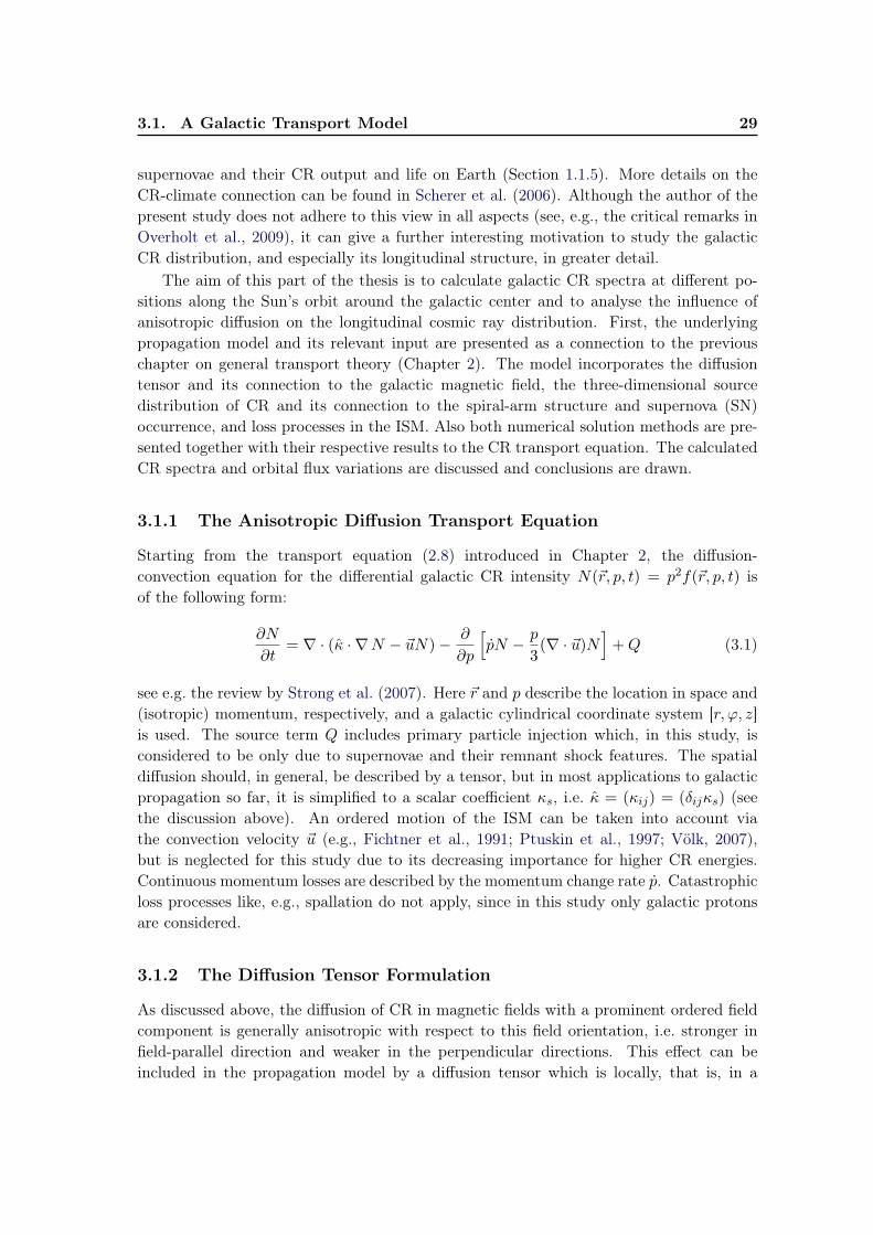
Figure 3.2 – Volume rendering visualization of the input source distribution of CRs. The coloringindicates the source strength from red (low) to yellow (high) in arbitrary units.
found in his textbook on “cosmical magnetic fields” (Parker, 1979). See again Fig. 1.6 foran example of an external galactic magnetic field.
Fortunately, as long as drift effects are neglected, the actual sign-dependent orientationis of no relevance for the diffusion along and perpendicular to the magnetic field, whichallows to employ a simplified model of the galactic magnetic field that has no field reversalsand is aligned to the spiral arm structure in the disc. Neglecting furthermore its weak halo-component, a simple model for the mean galactic magnetic field in cylindrical coordinatesis given by
B = B0(sinψ er + cosψ eϕ)1
rexp
(− z2
2σ2z,m
)(3.6)
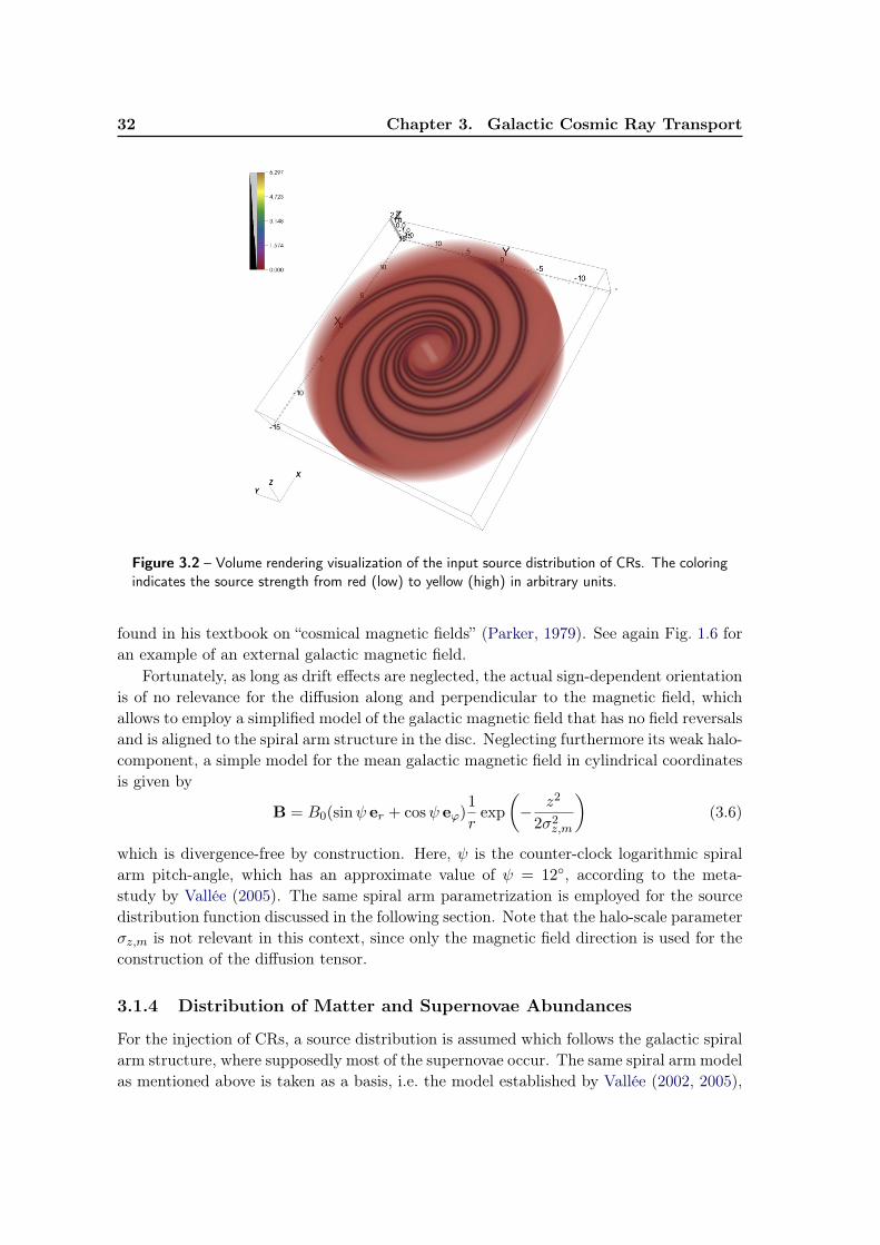
which is divergence-free by construction. Here, ψ is the counter-clock logarithmic spiralarm pitch-angle, which has an approximate value of ψ = 12, according to the meta-study by Vallée (2005). The same spiral arm parametrization is employed for the sourcedistribution function discussed in the following section. Note that the halo-scale parameterσz,m is not relevant in this context, since only the magnetic field direction is used for theconstruction of the diffusion tensor.
3.1.4 Distribution of Matter and Supernovae Abundances
For the injection of CRs, a source distribution is assumed which follows the galactic spiralarm structure, where supposedly most of the supernovae occur. The same spiral arm modelas mentioned above is taken as a basis, i.e. the model established by Vallée (2002, 2005),

3.1. A Galactic Transport Model 33
which consists of four logarithmic and symmetrically positioned arms. Around these, aGaussian shape (analogous to the approach in Shaviv (2003)) is used to yield an analyticexpression for the source term Q, by summing up over all four arms (n ∈ 1,2,3,4):
qn = Q0 p−s exp
(−(r − rn)2
2σ2r− z2
2σ2z
)(3.7)
with rn = r0 exp(k(ϕ+ ϕn)). ϕn introduces the symmetric rotation of each arm by 90,i.e. ϕn = (n − 1)π/2. k = cosψ with ψ = 12 is the constant pitch-angle cosine of thespiral arms. Fig. 3.1 illustrates the orientation of the spiral arms relative to the Sun’sposition and orbit. The respective widths of the arms are taken to be σr = σz = 0.2 kpcto have a reasonable inter-arm separation, while r0 = 2.52 kpc according to Vallée’s model.The model galaxy has the often assumed cylindrical shape with a radius of 15 kpc and aheight of 4 kpc (Büsching et al., 2005) and the Sun’s orbit is at a radius of r = 7.9 kpc.The average spectral index s of the sources’ power law injection in momentum is set tos = 2.3 in agreement with recent estimates on CR source spectra (see e.g. Putze et al.,2011; Ave et al., 2009). Fig. 3.2 gives a visualization of this source distribution. Theoverall source strength Q0 is a free parameter which can be fitted to a given reference likea local interstellar spectrum.
3.1.5 Energy Losses
The two most dominant loss processes for CR protons during their propagation throughthe ISM are energy losses due to pion production for relativistic energies and ionizationprocesses in the ISM plasma for lower energies (see Fig. 1 in Mannheim & Schlickeiser,1994).
According to Chapter 5 in Schlickeiser (2002) the pion losses can be approximated forLorentz factors γ 1 as
−(
dγ
dt
)= 1.4 · 10−16(nHI + 2nH2)A−0.47γ1.28s−1 (3.8)
where we assume a z-dependent ISM gas density with
(nHI + 2nH2) =1.24
cosh(30z/kpc)cm−3 (3.9)
(in units of particles per cm3 and z in kpc, Büsching & Potgieter, 2008). The mass numberA of a proton is just unity. A similar formula for the ionization losses is given by
−(
dp
dt
)= 3.1 · 10−7 Z2 ne
β
x3m + β3eV c−1 s−1 (3.10)
where the electron density is the same as the above gas density and the charge state ofprotons Z is equal to 1. For the purpose of this study, the velocity factor β = v/c ofthe particles is always much greater than the thermal electron βe, which is related toxm by xm = (34π
1/2)1/3βe = 1.10βe. This means that the momentum loss rate scalesapproximately as p−2. The total momentum loss rate entering Eq. (3.1) is the sum ofboth loss processes.
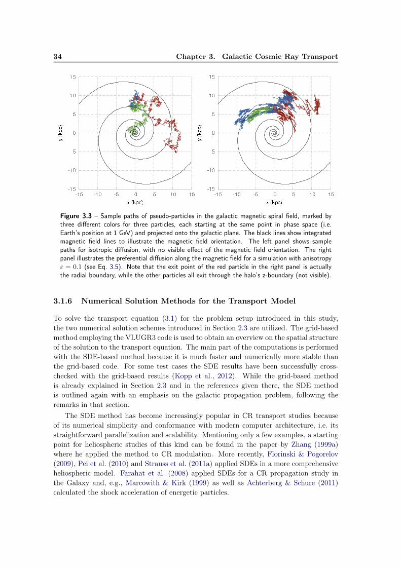
34 Chapter 3. Galactic Cosmic Ray Transport
Figure 3.3 – Sample paths of pseudo-particles in the galactic magnetic spiral field, marked bythree different colors for three particles, each starting at the same point in phase space (i.e.Earth’s position at 1 GeV) and projected onto the galactic plane. The black lines show integratedmagnetic field lines to illustrate the magnetic field orientation. The left panel shows samplepaths for isotropic diffusion, with no visible effect of the magnetic field orientation. The rightpanel illustrates the preferential diffusion along the magnetic field for a simulation with anisotropyε = 0.1 (see Eq. 3.5). Note that the exit point of the red particle in the right panel is actuallythe radial boundary, while the other particles all exit through the halo’s z-boundary (not visible).
3.1.6 Numerical Solution Methods for the Transport Model
To solve the transport equation (3.1) for the problem setup introduced in this study,the two numerical solution schemes introduced in Section 2.3 are utilized. The grid-basedmethod employing the VLUGR3 code is used to obtain an overview on the spatial structureof the solution to the transport equation. The main part of the computations is performedwith the SDE-based method because it is much faster and numerically more stable thanthe grid-based code. For some test cases the SDE results have been successfully cross-checked with the grid-based results (Kopp et al., 2012). While the grid-based methodis already explained in Section 2.3 and in the references given there, the SDE methodis outlined again with an emphasis on the galactic propagation problem, following theremarks in that section.
The SDE method has become increasingly popular in CR transport studies becauseof its numerical simplicity and conformance with modern computer architecture, i.e. itsstraightforward parallelization and scalability. Mentioning only a few examples, a startingpoint for heliospheric studies of this kind can be found in the paper by Zhang (1999a)where he applied the method to CR modulation. More recently, Florinski & Pogorelov(2009), Pei et al. (2010) and Strauss et al. (2011a) applied SDEs in a more comprehensiveheliospheric model. Farahat et al. (2008) applied SDEs for a CR propagation study inthe Galaxy and, e.g., Marcowith & Kirk (1999) as well as Achterberg & Schure (2011)calculated the shock acceleration of energetic particles.

3.2. Calculated Galactic Cosmic Ray Distributions 35
The basic idea in SDE schemes is to trace pseudo-particle trajectories from their originforward in time or, alternatively, integrate backwards in time from the phase space pointof interest. The particle trajectory is given by the integral of an SDE of the following form
dxi = Ai(xi)ds+∑j
Bij(xi)dWj (3.11)
where the relation BBT = 0.5 κ has to be fulfilled, that is, a root for the diffusion tensor κhas to be determined. Here, dWj is a (multidimensional) Wiener process increment, whichhas a time-stationary normal-distributed probability density with expectation value 0 andvariance 1. The deterministic part is directly related to the convection velocity in thetransport equation, i.e. Ai = −ui. Numerically, these SDEs are integrated via a simpleEuler-forward scheme and the Wiener-process is simulated with the Box-Muller method(e.g., Box & Muller, 1958, see also Appendix B) by using
dWi(s) = η(s)√ds (3.12)
where η(s) is equivalent to a Gaussian distribution N (0, 1). The necessary random num-bers are generated with the MTI19937 version of the so called Mersenne Twister (Mat-sumoto & Nishimura, 1998). The integration parameter s is related to physical time by
t = t0 − s (3.13)
where t0 is the final time for the backward method. The source contribution to theindividual particle trajectory is added up by a path amplitude. Finally, in case of thebackward method, all particle trajectories are weighted together to yield the resultingphase space density (i.e. the solution to the associated Fokker-Planck equation) at thestarting phase space point. The boundary and initial conditions can be accounted forin the weighting, but for this study they are simply zero (corresponding to an escapingboundary condition for the CRs). For the present application, only the backward methodis used, since it is well-suited for the given problem. For more details on the numericalscheme and especially on the determination of the root of the diffusion tensor, the readeris referred to Kopp et al. (2012) and Strauss et al. (2011a) where the basis of the codeused in this study is discussed in greater detail.
Exemplary pseudo-particle trajectories are shown in Fig. 3.3. There, the additionalinformation contained in SDE calculations becomes obvious. The pseudo-particles’ pathsfollow the field lines during their stochastic motion as soon as anisotropic diffusion becomesrelevant. Consequently, the modification to the diffusion process becomes directly visiblein such trajectories. However, one has to keep in mind that these are not real particletrajectories or gyro-center motions, but only tracers of the phase space of the diffusion-convection problem.
3.2 Calculated Galactic Cosmic Ray Distributions
3.2.1 Global Steady-State Solutions
To obtain an overview on the spatial structure of the distribution function as a solution tothe galactic propagation model described above, the grid-base code VLUGR3 was adapted
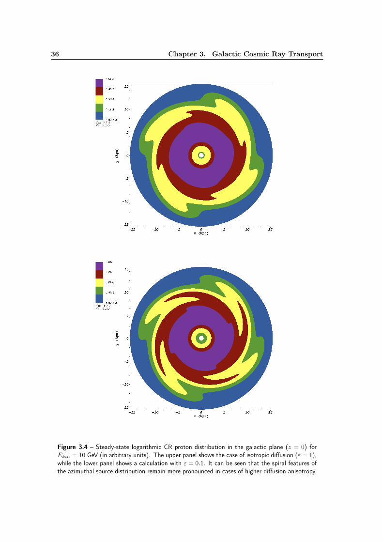
36 Chapter 3. Galactic Cosmic Ray Transport
Figure 3.4 – Steady-state logarithmic CR proton distribution in the galactic plane (z = 0) forEkin = 10 GeV (in arbitrary units). The upper panel shows the case of isotropic diffusion (ε = 1),while the lower panel shows a calculation with ε = 0.1. It can be seen that the spiral features ofthe azimuthal source distribution remain more pronounced in cases of higher diffusion anisotropy.

3.2. Calculated Galactic Cosmic Ray Distributions 37
to solve the steady-state transport equation in the given parameter set. As discussed inSection 2.3.1, momentum is used as the “independent stepping-variable” in the code, toobtain the steady-state solution for all energies of interest.
Fig. 3.4 shows two examples of calculated CR proton distributions in the galacticplane. The upper panel shows the steady-state distribution for an energy of 10 GeV andthe isotropic diffusion case. In the lower panel the same parameters have been used, buta diffusion anisotropy of ε = 0.1 instead of the scalar diffusion coefficient was introduced.The differences between both plots show how the spiral structures of the source distributionremain still more visible in the anisotropic diffusion case. This way, it is already clear thatthe flux variation along the Sun’s galactic orbit will be more pronounced in the anisotropiccase, as will be discussed in more detail below. In principle, the following discussion onspectral and orbital variation could also be based on such results of the grid-based method.For the subsequent sections, however, only results of the SDE method are presented tohave a more uniform and thus simplified numerical model setup.
3.2.2 Spectral Variation
To study the spectral variation at different positions along the Sun’s galactic orbit, CRproton spectra within the introduced model have been calculated at four different galacticpositions, as illustrated in Fig. 3.1. A very long integration time (t0 ≈ 10000 Myrs) hasbeen taken, to assure that a steady-state situation is approached, which is confirmed bychecking that all particles have exited the computational domain. For each phase-spacepoint, 104 pseudo particle trajectories have been computed. A comparison between thecalculated spectra in the case of pure isotropic diffusion (upper panel) and two anisotropiccase, with weak (ε = 0.1, middle panel) and strong (ε = 0.01, lower panel) diffusionanisotropy, is shown in Fig. 3.5. For comparison, the local interstellar spectrum (LIS) givenbyWebber & Higbie (2009) is included in the plots (WH09 hereafter). The parametrizationgiven in Herbst et al. (2010) has been used, where a comparison between a few proposedLIS can be found as well. In face of the still imprecisely known modulation effects onmeasured spectra inside the heliosphere (see, e.g., Florinski et al., 2011; Scherer et al.,2011), such an LIS parametrization can give only a rough orientation on what to expectfor galactic CR propagation studies. The results have been rescaled to fit approximately tothe WH09 LIS in the isotropic diffusion case, by accounting for the free parameterQ0 in thesource strength. The anisotropic spectra have been rescaled again, respectively. To yieldthe good agreement shown in both upper panels of Fig. 3.5 between the calculated spectraand the WH09 LIS, the break in the diffusion coefficient introduced above as well as bothcontinuous loss processes are required. The inclusion of the latter is an improvement overearlier studies, like Büsching & Potgieter (2008), where only a parametrized catastrophicloss term was considered.
The spectra for different positions along the Sun’s galactic orbit show only very littlevariation in the isotropic diffusion case. Particularly, the variation is largely independentof energy over the entire energy range considered. In contrast to this, the variation ismuch stronger for the anisotropic case, depending on the imposed diffusion anisotropy.The differences are, in these cases, dependent on energy as well. For high energies, the
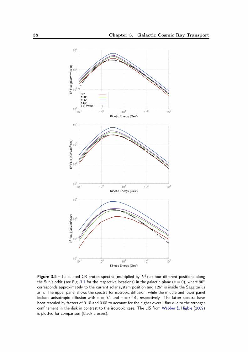
38 Chapter 3. Galactic Cosmic Ray Transport
101
102
103
104
10-1
100
101
102
103
E2 F
lux j(G
eV
/m2/s
/sr)
Kinetic Energy (GeV)
90° 108°
126°
144°
LIS WH09
101
102
103
104
10-1
100
101
102
103
E2 F
lux j(G
eV
/m2/s
/sr)
Kinetic Energy (GeV)
101
102
103
104
10-1
100
101
102
103
E2 F
lux j(G
eV
/m2/s
/sr)
Kinetic Energy (GeV)
Figure 3.5 – Calculated CR proton spectra (multiplied by E2) at four different positions alongthe Sun’s orbit (see Fig. 3.1 for the respective locations) in the galactic plane (z = 0), where 90
corresponds approximately to the current solar system position and 126 is inside the Saggitariusarm. The upper panel shows the spectra for isotropic diffusion, while the middle and lower panelinclude anisotropic diffusion with ε = 0.1 and ε = 0.01, respectively. The latter spectra havebeen rescaled by factors of 0.15 and 0.05 to account for the higher overall flux due to the strongerconfinement in the disk in contrast to the isotropic case. The LIS from Webber & Higbie (2009)is plotted for comparison (black crosses).
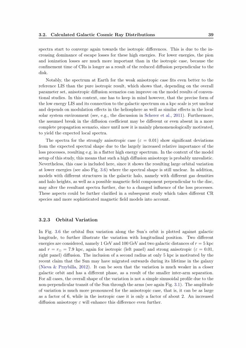
3.2. Calculated Galactic Cosmic Ray Distributions 39
spectra start to converge again towards the isotropic differences. This is due to the in-creasing dominance of escape losses for these high energies. For lower energies, the pionand ionization losses are much more important than in the isotropic case, because theconfinement time of CRs is longer as a result of the reduced diffusion perpendicular to thedisk.
Notably, the spectrum at Earth for the weak anisotropic case fits even better to thereference LIS than the pure isotropic result, which shows that, depending on the overallparameter set, anisotropic diffusion scenarios can improve on the model results of conven-tional studies. In this context, one has to keep in mind however, that the precise form ofthe low energy LIS and its connection to the galactic spectrum on a kpc scale is yet unclearand depends on modulation effects in the heliosphere as well as similar effects in the localsolar system environment (see, e.g., the discussion in Scherer et al., 2011). Furthermore,the assumed break in the diffusion coefficient may be different or even absent in a morecomplete propagation scenario, since until now it is mainly phenomenologically motivated,to yield the expected local spectra.
The spectra for the strongly anisotropic case (ε = 0.01) show significant deviationsfrom the expected spectral shape due to the largely increased relative importance of theloss processes, resulting e.g. in a flatter high energy spectrum. In the context of the modelsetup of this study, this means that such a high diffusion anisotropy is probably unrealistic.Nevertheless, this case is included here, since it shows the resulting large orbital variationat lower energies (see also Fig. 3.6) where the spectral shape is still unclear. In addition,models with different structures in the galactic halo, namely with different gas densitiesand halo heights, as well as a possible magnetic field component perpendicular to the disc,may alter the resultant spectra further, due to a changed influence of the loss processes.These aspects could be further clarified in a subsequent study which takes different CRspecies and more sophisticated magnetic field models into account.
3.2.3 Orbital Variation
In Fig. 3.6 the orbital flux variation along the Sun’s orbit is plotted against galacticlongitude, to further illustrate the variation with longitudinal position. Two differentenergies are considered, namely 1 GeV and 100 GeV and two galactic distances of r = 5 kpcand r = r = 7.9 kpc, again for isotropic (left panel) and strong anisotropic (ε = 0.01,right panel) diffusion. The inclusion of a second radius at only 5 kpc is motivated by therecent claim that the Sun may have migrated outwards during its lifetime in the galaxy(Nieva & Przybilla, 2012). It can be seen that the variation is much weaker in a closergalactic orbit and has a different phase, as a result of the smaller inter-arm separation.For all cases, the overall shape of the variation is not a simple sinusoidal profile due to thenon-perpendicular transit of the Sun through the arms (see again Fig. 3.1). The amplitudeof variation is much more pronounced for the anisotropic case, that is, it can be as largeas a factor of 6, while in the isotropic case it is only a factor of about 2. An increaseddiffusion anisotropy ε will enhance this difference even further.
40 Chapter 3. Galactic Cosmic Ray Transport
0.2
0.4
0.6
0.8
1
1.2
1.4
1.6
1.8
0 60 120 180 240 300 360
Flu
x (
a.u
.)
Galactic longitude (deg)
0.2
0.4
0.6
0.8
1
1.2
1.4
1.6
1.8
0 60 120 180 240 300 360
Flu
x (
a.u
.)
Galactic longitude (deg)
Figure 3.6 – Orbital variation of CR proton flux along the Sun’s orbit, plotted against longitude(with Sun’s position at 90). All curves are rescaled to an offset value of 1 for comparison. Theblack line and green crosses show the variation for an orbit at r = 7.9 kpc and z = 0 for 1 GeVand 100GeV, respectively. The blue line and red boxes show the same energies for an orbit atr = 5 kpc. The upper panel shows the case of isotropic diffusion, while the lower panel hasε = 0.01 and the variation is much more pronounced.
3.3. Conclusions 41
3.3 Conclusions
In this chapter, the effects of anisotropic diffusion of galactic CR protons have been ana-lyzed. For the solution of the steady-state diffusion equation, a numerical method basedon stochastic differential equations has been used which also accounts for energy loss pro-cesses. The computed spectra along the Sun’s galactic orbit show larger variations forthe anisotropic cases when compared to the scalar diffusion model. Furthermore, for thechosen parameters, a moderate diffusion anisotropy (ε = κ⊥/κ‖ = 0.1) leads to a resultwhich, in this setup, is more consistent with recent estimates of the local interstellar protonspectrum than the results for purely isotropic diffusion.
It can therefore be concluded that the diffusion tensor as well as the CR source dis-tribution is an important feature in determining the solution of the transport equationin a three-dimensional model of galactic CR propagation. This result fits well into thefindings by Hanasz et al. (2009) claiming that anisotropic diffusion is an essential require-ment for the CR-driven galactic dynamo effect. Additionally, these results imply that inthe context of the discussed CR-climate connection (Shaviv & Veizer, 2003), the expectedCR flux variation may be even larger than previously estimated, although at present, thistopic is still highly speculative.

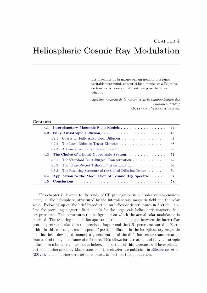
Chapter 4
Heliospheric Cosmic Ray Modulation
Les machines de la nature ont un nombre d’organesvéritablement infini, et sont si bien munies et á l’épreuvede tous les accidents qu’il n’est pas possible de lesdétruire.
Système nouveau de la nature et de la communication dessubstances (1695)
Gottfried Wilhelm Leibniz
Contents4.1 Interplanetary Magnetic Field Models . . . . . . . . . . . . . . . . 444.2 Fully Anisotropic Diffusion . . . . . . . . . . . . . . . . . . . . . . . 45
4.2.1 Causes for Fully Anisotropic Diffusion . . . . . . . . . . . . . . . . . 474.2.2 The Local Diffusion Tensor Elements . . . . . . . . . . . . . . . . . . 484.2.3 A Generalized Tensor Transformation . . . . . . . . . . . . . . . . . 49
4.3 The Choice of a Local Coordinate System . . . . . . . . . . . . . 524.3.1 The “Standard Euler-Burger” Transformation . . . . . . . . . . . . . 524.3.2 The “Frenet-Serret Trihedron” Transformation . . . . . . . . . . . . 524.3.3 The Resulting Structure of the Global Diffusion Tensor . . . . . . . 54
4.4 Application to the Modulation of Cosmic Ray Spectra . . . . . . 574.5 Conclusions . . . . . . . . . . . . . . . . . . . . . . . . . . . . . . . . 58
This chapter is devoted to the study of CR propagation in our solar system environ-ment, i.e. the heliosphere, structured by the interplanetary magnetic field and the solarwind. Following up on the brief introduction on heliospheric structures in Section 1.1.4,first the prevailing magnetic field models for the large-scale heliospheric magnetic fieldare presented. This constitutes the background on which the actual solar modulation ismodeled. The resulting modulation spectra fill the modeling gap between the interstellarproton spectra calculated in the previous chapter and the CR spectra measured at Earthorbit. In this context, a novel aspect of particle diffusion in the interplanetary magneticfield has been developed, namely a generalization of the diffusion tensor transformationfrom a local to a global frame of reference. This allows for a treatment of fully anisotropicdiffusion in a broader context than before. The details of this approach will be explicatedin the following sections. Many aspects of this chapter are published in Effenberger et al.(2012a). The following description is based, in part, on this publication.

44 Chapter 4. Heliospheric Cosmic Ray Modulation
4.1 Interplanetary Magnetic Field Models
To study the heliospheric modulation of CRs, one major input is the heliospheric magneticfield (HMF), which is briefly introduced here as a basis for the subsequent considerations.An analytical representation of the HMF, which is referred to as the hybrid Fisk field, canbe found, e.g., in Scherer et al. (2010) and Sternal et al. (2011). For a constant solar windspeed (usw = 400 km/s), the HMF is represented, using spherical polar coordinates, bythe following formulation:
Br = ABe
(rer
)2,
Bϑ = Brr
uswω∗ sinβ∗ sinϕ∗
Bϕ = Brr
usw[sinϑ(ω∗ cosβ∗ − Ω) (4.1)
+d
dϑ(ω∗ sinβ∗ sinϑ) cosϕ∗ ]
with
β∗(ϑ) = βFs(ϑ)
ω∗(ϑ) = ωFs(ϑ) (4.2)
ϕ∗ = ϕ+Ωusw
(r − r)
where
Fs(ϑ) =
[tanh(δpϑ) + tanh(δp(ϑ− π))− tanh(δe(ϑ− ϑb))]2 0 ≤ ϑ < ϑb
0 ϑb ≤ ϑ ≤ π − ϑb[tanh(δpϑ) + tanh(δp(ϑ− π))− tanh(δe(ϑ− π + ϑb))]
2 π − ϑb < ϑ ≤ π(4.3)
is the transition function introduced by Burger et al. (2008). In the case Fs = 0 the HMFreduces to the standard Parker spiral magnetic field.
In Eq. (4.1), Be denotes the magnetic field strength at re = 1 AU, r is the solarradius, and Ω = 2.9 · 10−6Hz is the averaged solar rotation frequency. The constantA = ±1 in Eq. (4.1) indicates the different field directions in the northern and southernhemisphere. The values for the angle between the rotational and the so-called virtual axesof the Sun β = 12 and the differential rotation rate ω = Ω/4 are taken from Sternalet al. (2011). The parameters δp = 5 and δe = 5 determine the respective contributionsof the Fisk- and Parker field above the poles and in the ecliptic while, ϑb = 80 is thecutoff colatitude for the Fisk field influence. In the following, two cases are considered: apure Parker field (i.e. setting Fs = 0 in Eqs. 4.1 and 4.2) and the hybrid Fisk field withFs from Eq. (4.3). Both fields are illustrated by exemplary field lines in Fig. 4.1. It canbe seen that the field lines of the Parker field stay on a cone of constant latitude, since noϑ component is present in the field representation. For the hybrid Fisk field, however, the
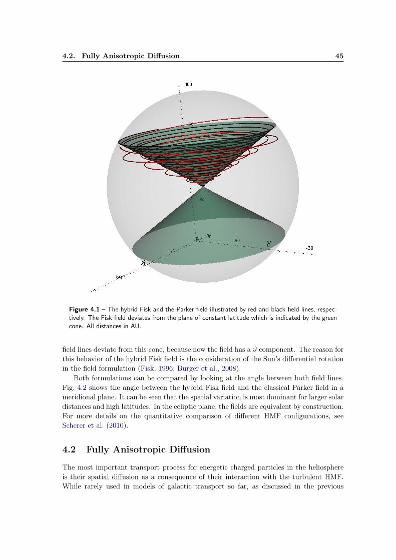
4.2. Fully Anisotropic Diffusion 45
Figure 4.1 – The hybrid Fisk and the Parker field illustrated by red and black field lines, respec-tively. The Fisk field deviates from the plane of constant latitude which is indicated by the greencone. All distances in AU.
field lines deviate from this cone, because now the field has a ϑ component. The reason forthis behavior of the hybrid Fisk field is the consideration of the Sun’s differential rotationin the field formulation (Fisk, 1996; Burger et al., 2008).
Both formulations can be compared by looking at the angle between both field lines.Fig. 4.2 shows the angle between the hybrid Fisk field and the classical Parker field in ameridional plane. It can be seen that the spatial variation is most dominant for larger solardistances and high latitudes. In the ecliptic plane, the fields are equivalent by construction.For more details on the quantitative comparison of different HMF configurations, seeScherer et al. (2010).
4.2 Fully Anisotropic Diffusion
The most important transport process for energetic charged particles in the heliosphereis their spatial diffusion as a consequence of their interaction with the turbulent HMF.While rarely used in models of galactic transport so far, as discussed in the previous

46 Chapter 4. Heliospheric Cosmic Ray Modulation
Figure 4.2 – The angle between the hybrid Fisk- and Parker-field in a meridional plane (in degrees).Note the large spatial variation in regions where the Fisk-type field is dominant. (This figure isalready published in Scherer et al., 2010).
chapter, the concept of anisotropic diffusion is well established (see, e.g., Burger et al.,2000; Schlickeiser, 2002; Shalchi, 2009) for models of heliospheric cosmic ray modulation.In most studies, the anisotropy refers to a difference in the diffusion coefficient parallel (κ‖)and perpendicular (κ⊥) to the magnetic field, and the perpendicular diffusion is treatedas being isotropic.
Although the notion of fully anisotropic diffusion is not new – see an early studyby Jokipii (1973) considering for the first time anisotropic perpendicular diffusion, i.e.κ⊥1 6= κ⊥2 – it was not before the measurements made with the Ulysses spacecraft thatthis concept had to be used to explain the high-latitude observations of cosmic rays,see, e.g., Jokipii et al. (1995), Potgieter et al. (1997), and Ferreira et al. (2001). Thesestudies remained largely phenomenological and did not attempt a rigorous investigationof anisotropic perpendicular diffusion.
More recently, in the context of studies of the transport of solar energetic particles inthe heliospheric Parker field, Tautz et al. (2011) and Kelly et al. (2012) have determinedthe elements of the diffusion tensor from test particle simulations in a local, field-alignedframe. While the former authors find no conclusive result, the latter authors clearlydemonstrated that the scattering in the inhomogeneous Parker field can indeed induceanisotropic perpendicular diffusion.
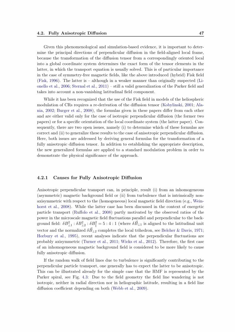
4.2. Fully Anisotropic Diffusion 47
Given this phenomenological and simulation-based evidence, it is important to deter-mine the principal directions of perpendicular diffusion in the field-aligned local frame,because the transformation of the diffusion tensor from a correspondingly oriented localinto a global coordinate system determines the exact form of the tensor elements in thelatter, in which the transport equation is usually solved. This is of particular importancein the case of symmetry-free magnetic fields, like the above introduced (hybrid) Fisk field(Fisk, 1996). The latter is – although in a weaker manner than originally suspected (Li-onello et al., 2006; Sternal et al., 2011) – still a valid generalization of the Parker field andtakes into account a non-vanishing latitudinal field component.
While it has been recognized that the use of the Fisk field in models of the heliosphericmodulation of CRs requires a re-derivation of the diffusion tensor (Kobylinski, 2001; Ala-nia, 2002; Burger et al., 2008), the formulas given in these papers differ from each otherand are either valid only for the case of isotropic perpendicular diffusion (the former twopapers) or for a specific orientation of the local coordinate system (the latter paper). Con-sequently, there are two open issues, namely (i) to determine which of these formulas arecorrect and (ii) to generalize these results to the case of anisotropic perpendicular diffusion.Here, both issues are addressed by deriving general formulas for the transformation of afully anisotropic diffusion tensor. In addition to establishing the appropriate description,the new generalized formulas are applied to a standard modulation problem in order todemonstrate the physical significance of the approach.
4.2.1 Causes for Fully Anisotropic Diffusion
Anisotropic perpendicular transport can, in principle, result (i) from an inhomogeneous(asymmetric) magnetic background field or (ii) from turbulence that is intrinsically non-axisymmetric with respect to the (homogeneous) local magnetic field direction (e.g., Wein-horst et al., 2008). While the latter case has been discussed in the context of energeticparticle transport (Ruffolo et al., 2008) partly motivated by the observed ratios of thepower in the microscale magnetic field fluctuations parallel and perpendicular to the back-ground field: δB2
⊥1 : δB2⊥2 : δB2
‖ = 5 : 4 : 1 (where δ ~B⊥1 is aligned to the latitudinal unit
vector and the normalized δ ~B⊥2 completes the local trihedron, see Belcher & Davis, 1971;Horbury et al., 1995), recent analyses indicate that the perpendicular fluctuations areprobably axisymmetric (Turner et al., 2011; Wicks et al., 2012). Therefore, the first caseof an inhomogeneous magnetic background field is considered to be more likely to causefully anisotropic diffusion.
If the random walk of field lines due to turbulence is significantly contributing to theperpendicular particle transport, one generally has to expect the latter to be anisotropic.This can be illustrated already for the simple case that the HMF is represented by theParker spiral, see Fig. 4.3: Due to the field geometry the field line wandering is notisotropic, neither in radial direction nor in heliographic latitude, resulting in a field linediffusion coefficient depending on both (Webb et al., 2009).
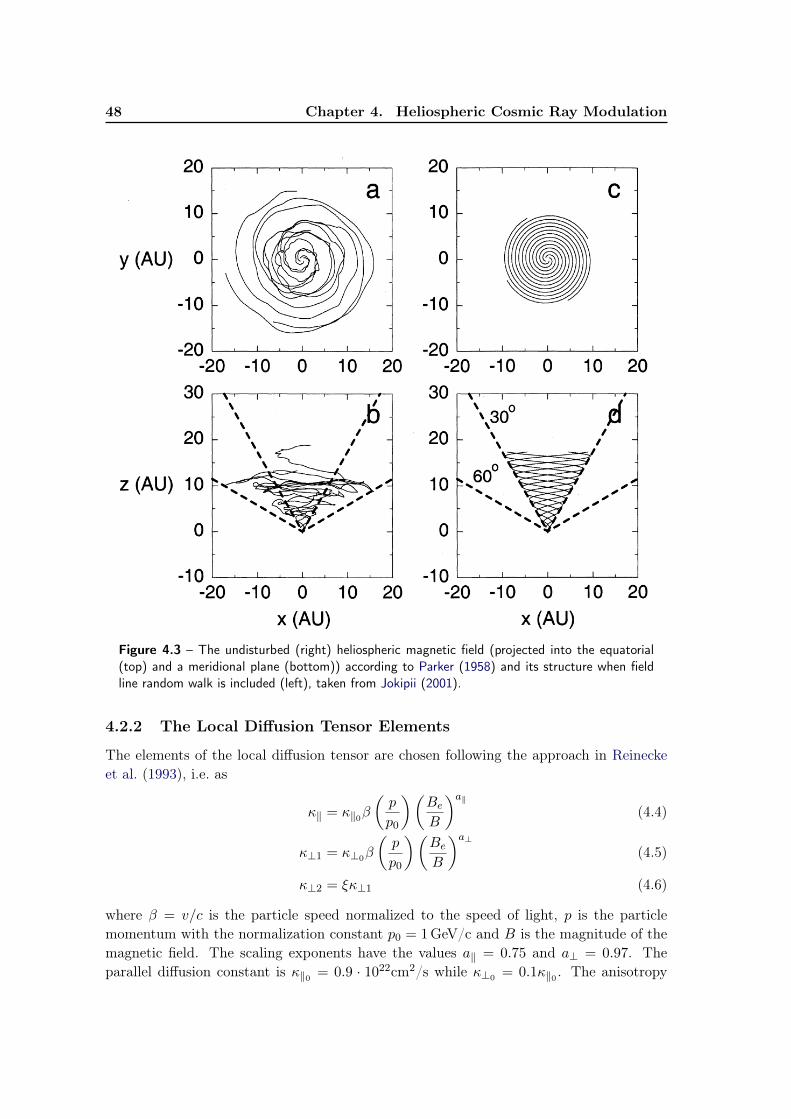
48 Chapter 4. Heliospheric Cosmic Ray Modulation
Figure 4.3 – The undisturbed (right) heliospheric magnetic field (projected into the equatorial(top) and a meridional plane (bottom)) according to Parker (1958) and its structure when fieldline random walk is included (left), taken from Jokipii (2001).
4.2.2 The Local Diffusion Tensor Elements
The elements of the local diffusion tensor are chosen following the approach in Reineckeet al. (1993), i.e. as
κ‖ = κ‖0β
(p
p0
)(BeB
)a‖(4.4)
κ⊥1 = κ⊥0β
(p
p0
)(BeB
)a⊥(4.5)
κ⊥2 = ξκ⊥1 (4.6)
where β = v/c is the particle speed normalized to the speed of light, p is the particlemomentum with the normalization constant p0 = 1GeV/c and B is the magnitude of themagnetic field. The scaling exponents have the values a‖ = 0.75 and a⊥ = 0.97. Theparallel diffusion constant is κ‖0 = 0.9 · 1022cm2/s while κ⊥0 = 0.1κ‖0 . The anisotropy

4.2. Fully Anisotropic Diffusion 49
in perpendicular diffusion is assumed to be solely determined by the factor ξ which is setequal to 2 for the following discussion. This is still a moderate choice compared to thefindings of, e.g., Potgieter et al. (1997).
Although these empirical formulas for the local diffusion coefficients are not directlyrelated to the turbulence evolution in the heliosphere and more sophisticated theoreticalmodels for the corresponding mean free paths in parallel and perpendicular direction exist,they are still a good approximation as is demonstrated in the following. The result fromquasilinear theory (QLT) for the parallel mean free path (see, e.g., Shalchi, 2009) is givenby
λ(QLT)‖ =
3lslab16πC(ν)
(B
δBslab
)2
R2−2ν[
2
(1− ν)(2− ν)+R2ν
](4.7)
withC(ν) =
1
2√π
Γ(ν)
Γ(ν − 1/2)(4.8)
where Γ(x) is the gamma function, 2ν = 5/3 is the inertial range spectral index,R = RL/lslab is the dimensionless rigidity, and RL = pc/(|q|B) is the particle Larmorradius. If one scales the bendover scale of slab turbulence as lslab = 0.03 ρ0.5 (where ρ isthe heliocentric distance in AU) and the slab turbulence variance as δB2
slab = B2eρ−2.15,
the radial dependence of the local tensor elements matches well with the approximativeformulas (4.4) to (4.6) as shown in Fig. 4.4. It is interesting to note that these scalingsare similar to the assumptions made in Burger et al. (2008). They use the same radialdependence for lslab (their exponent of 1/lslab = kmin = 32 ρ0.5 is a typing error, privatecommunication with the authors) and an exponent of −2.5 for the slab turbulence vari-ance δB2
slab, which is slightly larger. Similar arguments can be made for the perpendiculardiffusion, for which the result of the nonlinear guiding center (NLGC) theory of Matthaeuset al. (2003) and Shalchi et al. (2004) is employed, namely
κ(NLGC)⊥ =
[a2v
ν − 1
2√
3ν
√π
Γ(ν/2 + 1)
Γ(ν/2 + 1/2)l2D
δB22D
B2
]2/3κ1/3‖ (4.9)
(see formula (15) in Burger et al. (2008)) with the constant a = 1/√
3. Scaling againthe 2D turbulence correlation length l2D with ρ0.5 and the turbulence variance δB2
2D evenmore weakly with ρ−1.2 yields results similar to those obtained by Reinecke et al. (1993)for the perpendicular diffusion, as shown in Fig. 4.4 as well.
Given the uncertainties both in the actual magnetic turbulence evolution in the helio-sphere with radial distance and latitude (see, e.g., Oughton et al. (2011) for a study inwhich they find a much more complicated radial dependence of the slab variance) and theiractual relation to perpendicular or even anisotropic perpendicular diffusion in connectionwith three-dimensional turbulence (Shalchi, 2010; Shalchi et al., 2010b), in the following,the empirical formulas of Eqs. (4.4) to (4.6) are used.
4.2.3 A Generalized Tensor Transformation
As soon as anisotropic perpendicular diffusion occurs, it is necessary to determine theprincipal axes of the diffusion tensor in a local field-aligned frame (κL), because their

50 Chapter 4. Heliospheric Cosmic Ray Modulation
-5
0
5
10
15
20
25
30
0 20 40 60 80 100
κ [10
22 c
m2/s
]
Radial Distance [AU]
Figure 4.4 – The dependence of the local and global tensor elements on heliocentric distance in theecliptic plane for the Parker field. The local elements from the formulas (4.4)-(4.6) are shown assolid red (κ‖), green (κ⊥1), and blue (κ⊥2) curves. The results for the parallel diffusion coefficientκ(QLT)‖ = 1/3vλ
(QLT)‖ (Eq. 4.7) and the perpendicular coefficient from κ
(NLGC)⊥ (Eq. 4.9) are
drawn as dashed red and green lines, respectively, while the dashed blue curve is just scaled asξκ
(NLGC)⊥ with ξ = 2. The overlayed, color-matched symbols show the nearly perfect alignment
of the κrr (green, ×), κϑϑ (blue, •) and κϕϕ (red, +) global diagonal tensor elements in theecliptic, due to the Parker field structure. All other tensor elements are almost indistinguishablefrom zero, as indicated by the remaining symbols.
orientation determines the tensor elements in the global frame (κ) after a correspondingtransformation given by
κ = AκLAT (4.10)
with
κL =
κ⊥1 κA 0
−κA κ⊥2 0
0 0 κ‖
(4.11)
where, in general, κA denotes the drift coefficient, induced by a non-axisymmetric turbu-lence and by inhomogeneous magnetic fields. The latter drifts can always be described bya drift velocity ~vd in the transport equation (Burger et al., 2008; Tautz & Shalchi, 2012)and are therefore not considered in the following. In Eq. (4.10), analogous to the Euler

4.2. Fully Anisotropic Diffusion 51
local
Aϕ
z
r
ϕ
z
rglobal
T
κ
κlocal RFlocal RF
global RF global RF
A A
L
G
Figure 4.5 – The transformation between local and global coordinates and a sketch of the tensortransformation. The relation κG = AκLA
T holds as usual.
angle transformation known from classical mechanics, the matrix A = R3R2R1 describesthree consecutive rotations Ri with A−1 = AT . These rotations are defined by the relativeorientation of the local and the global coordinate system with respect to each other (seeFig. 4.5 for an illustration).
Due to the latitudinal structuring of the solar wind and, in turn, of the Parker spiralhaving a vanishing Bϑ component, one may argue that in that case the latitudinal directionremains a preferred one so that the local coordinate system could always be defined by theunit vectors ~t (along the field), ~eϑ (from a spherical polar coordinate system) and ~eϑ × ~t.This, however, can obviously not be the case for symmetry-free fields like the Fisk field(Fisk, 1996).
In general, the local trihedron will consist of a unit vector ~t tangential to the magneticfield and two orthogonal ones, ~u and ~v, defining the remaining principal axes. Withthis notation, the transformation (Eq. 4.10) reads, for an arbitrary choice of this localtrihedron:
κ11 = κ⊥1 u21 + κ⊥2 v
21 + κ‖ t
21 (4.12)
κ12 = κ⊥1 u1 u2 + κ⊥2 v1 v2 + κ‖ t1 t2 (4.13)
+ κA (u1 v2 − u2 v1)κ13 = κ⊥1 u1 u3 + κ⊥2 v1 v3 + κ‖ t1 t3 (4.14)
+ κA (u1 v3 − u3 v1)κ21 = κ⊥1 u1 u2 + κ⊥2 v1 v2 + κ‖ t1 t2 (4.15)
− κA (u1 v2 − u2 v1)κ22 = κ⊥1 u
22 + κ⊥2 v
22 + κ‖ t
22 (4.16)
κ23 = κ⊥1 u2 u3 + κ⊥2 v2 v3 + κ‖ t2 t3 (4.17)
+ κA (u2 v3 − u3 v2)κ31 = κ⊥1 u1 u3 + κ⊥2 v1 v3 + κ‖ t1 t3 (4.18)
− κA (u1 v3 − u3 v1)κ32 = κ⊥1 u2 u3 + κ⊥2 v2 v3 + κ‖ t2 t3 (4.19)
− κA (u2 v3 − u3 v2)κ33 = κ⊥1 u
23 + κ⊥2 v
23 + κ‖ t
23 (4.20)
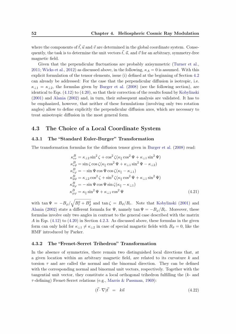
52 Chapter 4. Heliospheric Cosmic Ray Modulation
where the components of ~t, ~u and ~v are determined in the global coordinate system. Conse-quently, the task is to determine the unit vectors ~t, ~u, and ~v for an arbitrary, symmetry-freemagnetic field.
Given that the perpendicular fluctuations are probably axisymmetric (Turner et al.,2011; Wicks et al., 2012) as discussed above, in the following, κA = 0 is assumed. With thisexplicit formulation of the tensor elements, issue (i) defined at the beginning of Section 4.2can already be addressed: For the case that the perpendicular diffusion is isotropic, i.e.κ⊥1 = κ⊥2, the formulas given by Burger et al. (2008) (see the following section), areidentical to Eqs. (4.12) to (4.20), so that their correction of the results found by Kobylinski(2001) and Alania (2002) and, in turn, their subsequent analysis are validated. It has tobe emphasized, however, that neither of these formulations (involving only two rotationangles) allow to define explicitly the perpendicular diffusion axes, which are necessary totreat anisotropic diffusion in the most general form.
4.3 The Choice of a Local Coordinate System
4.3.1 The “Standard Euler-Burger” Transformation
The transformation formulas for the diffusion tensor given in Burger et al. (2008) read:
κBrr = κ⊥2 sin2 ζ + cos2 ζ(κ‖ cos2 Ψ + κ⊥1 sin2 Ψ)
κBrϑ = sin ζ cos ζ(κ‖ cos2 Ψ + κ⊥1 sin2 Ψ− κ⊥2)κBrϕ = − sin Ψ cos Ψ cos ζ(κ‖ − κ⊥1)κBϑϑ = κ⊥2 cos2 ζ + sin2 ζ(κ‖ cos2 Ψ + κ⊥1 sin2 Ψ)
κBϑϕ = − sin Ψ cos Ψ sin ζ(κ‖ − κ⊥1)κBϕϕ = κ‖ sin2 Ψ + κ⊥1 cos2 Ψ (4.21)
with tan Ψ = −Bϕ/√B2r +B2
ϑ and tan ζ = Bϑ/Br. Note that Kobylinski (2001) andAlania (2002) state a different formula for Ψ, namely tan Ψ = −Bϕ/Br. Moreover, theseformulas involve only two angles in contrast to the general case described with the matrixA in Eqs. (4.12) to (4.20) in Section 4.2.3. As discussed above, these formulas in the givenform can only hold for κ⊥1 6= κ⊥2 in case of special magnetic fields with Bϑ = 0, like theHMF introduced by Parker.
4.3.2 The “Frenet-Serret Trihedron” Transformation
In the absence of symmetries, there remain two distinguished local directions that, ata given location within an arbitrary magnetic field, are related to its curvature k andtorsion τ and are called the normal and the binormal direction. They can be definedwith the corresponding normal and binormal unit vectors, respectively. Together with thetangential unit vector, they constitute a local orthogonal trihedron fulfilling the (k- andτ -defining) Frenet-Serret relations (e.g., Marris & Passman, 1969):
(~t · ∇)~t = k~n (4.22)

4.3. The Choice of a Local Coordinate System 53
z
Figure 4.6 – The hybrid Fisk and the Parker field again illustrated by red and black field lines,respectively. The two local trihedrons for the Parker field are indicated with the orange and blue(Frenet-Serret) as well as the yellow and light blue (traditional) lines. Note that the traditionaltrihedron is always aligned to the Parker spiral cone of constant ϑ while for the Frenet-Serrettrihedron one axis (the κ⊥2-binormal axis, orange) is nearly parallel to the z-direction. In theecliptic both coordinate systems coincide by definition. All distances are in units of AU.
(~t · ∇)~n = −k~t+ τ~b (4.23)
(~t · ∇)~b = −τ~n . (4.24)
If no other diffusion axes are preferred by any process, the Frenet-Serret System constitutedby the above definition of ~t, ~n, and ~b is the most natural choice, i.e. ~u = ~n and ~v = ~b inEqs. (4.12) to (4.20).
The transformation of the local diffusion tensor into a global coordinate system ac-cording to these equations thus requires knowledge of the dependence of the Frenet-Serretvectors on a given (non-homogeneous) magnetic field ~B. Evidently, the required relationsare
~t = ~B/| ~B| (4.25)
~n = (~t · ∇)~t/k (4.26)~b = ~t× ~n . (4.27)
This trihedron can, of course, only be established for a spatially non-homogeneous field,but this (weak) condition is fulfilled in most cases of interest. If there existed a region wherethe field would be homogeneous, the choice of the vectors ~n and ~b is arbitrary (signifying

54 Chapter 4. Heliospheric Cosmic Ray Modulation
isotropic perpendicular diffusion), unless no other preferential directions unrelated to thefield geometry can be specified. Other principal directions unrelated to the large-scalegeometry of the field could, for example, arise from non-axisymmetric turbulence. Theabove formulas (4.12) to (4.20) remain unaffected, however: One only needs to specify theappropriate vectors ~t, ~n and ~b.
In the following, the procedure is illustrated for the example of the well-studied HMF.The new tensor is quantitatively compared with the ’traditional’ one which is only valid forisotropic perpendicular diffusion. This comparison reveals that a study of fully anisotropicturbulent diffusion within more complicated fields – like the much-discussed heliosphericFisk field introduced above (Fisk, 1996; Burger & Hitge, 2004; Burger et al., 2008; Sternalet al., 2011) or complex galactic magnetic fields (Ruzmaikin et al., 1988; Beck et al., 1996)– has to be performed with even more caution than thought before.
The Frenet-Serret trihedron for the Parker case of the HMF can be derived analytically(see Barra, 2010). Reducing Eq. (4.1) to the Parker field by setting Fs = 0 one obtains
~t =~er − tanχ~eϕ√
1 + tan2 χ(4.28)
for the tangential vector, with tanχ =ω
usr sinϑ. The easiest way to derive the normal
vector ~n is to calculate (~t · ∇)~t = k~n (where k is the curvature, see Eq. (4.22)) and tonormalize appropriately. After some straightforward calculation, one arrives at
~n = −E(tanχ~er + ~eϕ) + F~eϑ√E2(tan2 χ+ 1) + F 2
(4.29)
where the abbreviations
E =tanχ
r+ω
us
sinϑ
1 + tan2 χand F =
tan2 χ cosϑ
r sinϑ(4.30)
have been introduced. The binormal vector is now simply the cross product ~b = ~t × ~n,which yields
~b =−F (tanχ~er + ~eϕ) + E(tan2 χ+ 1)~eϑ√F 2(tan2 χ+ 1) + E2(tan2 χ+ 1)2
(4.31)
Eqs. (4.28), (4.29), and (4.31) are the explicit formulas for the Frenet-Serret trihedron inthe case of the heliospheric Parker field. Corresponding, but much longer expressions can,in principle, be obtained for the hybrid Fisk field as well.
4.3.3 The Resulting Structure of the Global Diffusion Tensor
Employing the formalism described in the previous section to calculate the global diffusiontensor κ results in tensor elements κij which are different from those ’traditionally’ used,labeled κBij here, with i, j ∈ r, ϑ, ϕ. The latter are derived following the transformationpresented by Burger et al. (2008) as described above, which for the Parker field is equivalentto the assumption that the local system can always be defined by ~t, ~n = ~eϑ×~t, and ~b = ~eϑ.Both local systems are illustrated in Fig. 4.6.
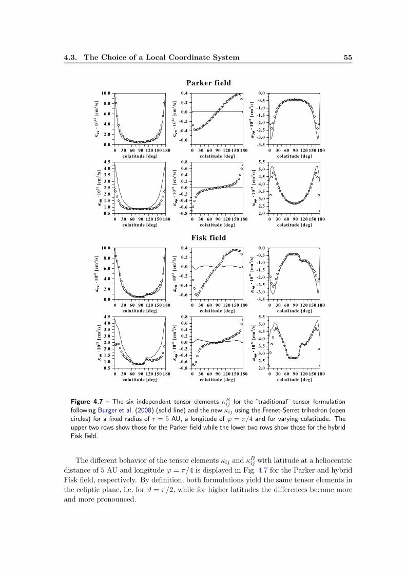
4.3. The Choice of a Local Coordinate System 55
Parker field
0 30 60 90 120 150 180
colatitude [deg]
0.0
2.0
4.0
6.0
8.0
10.01
02
2 [
cm
2/s
]
0 30 60 90 120 150 180
colatitude [deg]
-0.6
-0.4
-0.2
0.0
0.2
0.4
10
22 [
cm
2/s
]
0 30 60 90 120 150 180
colatitude [deg]
-3.5
-3.0
-2.5
-2.0
-1.5
-1.0
-0.5
0.0
10
22 [
cm
2/s
]
0 30 60 90 120 150 180
colatitude [deg]
0.5
1.0
1.5
2.0
2.5
3.0
3.5
4.0
4.5
10
22 [
cm
2/s
]
0 30 60 90 120 150 180
colatitude [deg]
-0.8
-0.6
-0.4
-0.2
0.0
0.2
0.4
0.6
0.8
10
22 [
cm
2/s
]
0 30 60 90 120 150 180
colatitude [deg]
2.0
2.5
3.0
3.5
4.0
4.5
5.0
5.5
10
22 [
cm
2/s
]
Fisk field
0 30 60 90 120 150 180
colatitude [deg]
0.0
2.0
4.0
6.0
8.0
10.0
10
22 [
cm
2/s
]
0 30 60 90 120 150 180
colatitude [deg]
-0.6
-0.4
-0.2
0.0
0.2
0.4
10
22 [
cm
2/s
]
0 30 60 90 120 150 180
colatitude [deg]
-3.5
-3.0
-2.5
-2.0
-1.5
-1.0
-0.5
0.01
02
2 [
cm
2/s
]
0 30 60 90 120 150 180
colatitude [deg]
0.5
1.0
1.5
2.0
2.5
3.0
3.5
4.0
4.5
10
22 [
cm
2/s
]
0 30 60 90 120 150 180
colatitude [deg]
-0.8
-0.6
-0.4
-0.2
0.0
0.2
0.4
0.6
0.8
10
22 [
cm
2/s
]
0 30 60 90 120 150 180
colatitude [deg]
2.0
2.5
3.0
3.5
4.0
4.5
5.0
5.5
10
22 [
cm
2/s
]
Figure 4.7 – The six independent tensor elements κBij for the “traditional” tensor formulationfollowing Burger et al. (2008) (solid line) and the new κij using the Frenet-Serret trihedron (opencircles) for a fixed radius of r = 5 AU, a longitude of ϕ = π/4 and for varying colatitude. Theupper two rows show those for the Parker field while the lower two rows show those for the hybridFisk field.
The different behavior of the tensor elements κij and κBij with latitude at a heliocentricdistance of 5 AU and longitude ϕ = π/4 is displayed in Fig. 4.7 for the Parker and hybridFisk field, respectively. By definition, both formulations yield the same tensor elements inthe ecliptic plane, i.e. for ϑ = π/2, while for higher latitudes the differences become moreand more pronounced.
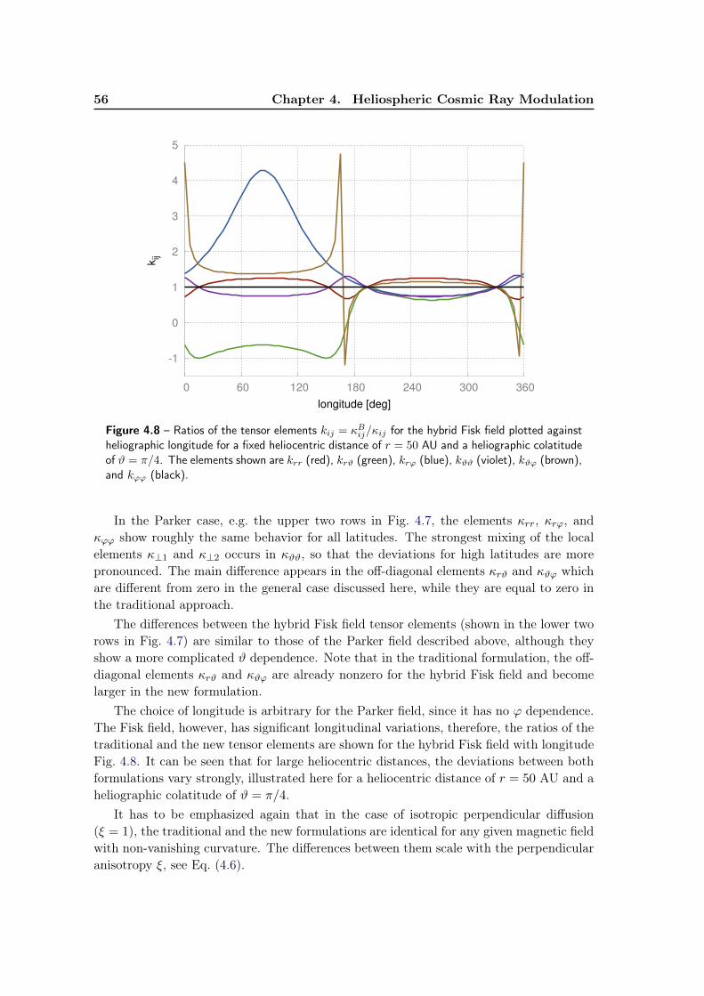
56 Chapter 4. Heliospheric Cosmic Ray Modulation
-1
0
1
2
3
4
5
0 60 120 180 240 300 360
kij
longitude [deg]
Figure 4.8 – Ratios of the tensor elements kij = κBij/κij for the hybrid Fisk field plotted againstheliographic longitude for a fixed heliocentric distance of r = 50 AU and a heliographic colatitudeof ϑ = π/4. The elements shown are krr (red), krϑ (green), krϕ (blue), kϑϑ (violet), kϑϕ (brown),and kϕϕ (black).
In the Parker case, e.g. the upper two rows in Fig. 4.7, the elements κrr, κrϕ, andκϕϕ show roughly the same behavior for all latitudes. The strongest mixing of the localelements κ⊥1 and κ⊥2 occurs in κϑϑ, so that the deviations for high latitudes are morepronounced. The main difference appears in the off-diagonal elements κrϑ and κϑϕ whichare different from zero in the general case discussed here, while they are equal to zero inthe traditional approach.
The differences between the hybrid Fisk field tensor elements (shown in the lower tworows in Fig. 4.7) are similar to those of the Parker field described above, although theyshow a more complicated ϑ dependence. Note that in the traditional formulation, the off-diagonal elements κrϑ and κϑϕ are already nonzero for the hybrid Fisk field and becomelarger in the new formulation.
The choice of longitude is arbitrary for the Parker field, since it has no ϕ dependence.The Fisk field, however, has significant longitudinal variations, therefore, the ratios of thetraditional and the new tensor elements are shown for the hybrid Fisk field with longitudeFig. 4.8. It can be seen that for large heliocentric distances, the deviations between bothformulations vary strongly, illustrated here for a heliocentric distance of r = 50 AU and aheliographic colatitude of ϑ = π/4.
It has to be emphasized again that in the case of isotropic perpendicular diffusion(ξ = 1), the traditional and the new formulations are identical for any given magnetic fieldwith non-vanishing curvature. The differences between them scale with the perpendicularanisotropy ξ, see Eq. (4.6).
4.4. Application to the Modulation of Cosmic Ray Spectra 57
4.4 Application to the Modulation of Cosmic Ray Spectra
To assess the impact of the new tensor formulation on CR modulation a CR protontransport model is used by solving the Parker equation (Parker, 1965a)
∂f
∂t= ∇ · (κ∇f)− ~us · ∇f +
p
3(∇ · ~us)
∂f
∂p(4.32)
to determine the differential CR intensity j(~x, p, t) = p2f(~x, p, t) (with ~x as the position inthree-dimensional configuration space and p as momentum). The solar wind velocity ~usw isradially pointing outwards with a constant speed of 400 km/s and κ is the diffusion tensorin the global frame for the Parker spiral magnetic field. This implies the Frenet-Serrettrihedron of the form explicitly given in Section 4.3.2.
The solution is obtained via a numerical integration of an equivalent system of SDEs(see Eq. 2.18) for an ensemble of pseudo-particles (phase space elements) as already dis-cussed in Section 2.3.2. The numerical method is similar to the solution method used forthe galactic propagation model of the previous chapter. Again, the time-backward Markovstochastic method is employed, meaning that pseudo-particles are traced back from a givenphase space point of interest, until they hit the integration boundary. The solution to thetransport equation (4.32) is then constructed as a proper average over the pseudo-particleorbits. For details on the general method and the numerical scheme, especially in the caseof a general diffusion tensor and in the context of heliospheric modulation, see Kopp et al.(2012), Strauss et al. (2011a), and Strauss et al. (2011b).
The local interstellar spectrum (LIS) of protons jLIS is assumed at a heliocentricdistance of r = 100 AU as a spherically symmetric Dirichlet boundary condition. At theinner boundary of one solar radius r = R the pseudo-particles are reflected, which isequivalent to a vanishing gradient in the CR density there. A standard representation ofthe proton LIS is given by
jLIS = 12.14β(Ekin + 0.5E0)−2.6 (4.33)
and was taken from Reinecke et al. (1993). The proton rest energy E0 is equal to 0.938and Ekin denotes the kinetic energy of a particle (both in units of GeV).
The LIS and the resulting modulated spectra are shown in Fig. 4.9 for both tensorformulations and for several heliocentric distances. The spectra for the new Frenet-Serrettensor are higher by up to 60% at low energies for all heliocentric distances. This isdue to the enhanced diffusive flux from the modulation boundary via an effective inwarddiffusion along the polar axis. In the tensor formulation provided by Burger et al. (2008)this diffusion (determined by κ⊥2) cannot transport particles from the boundary intothe inner heliosphere, it merely distributes the particles on a shell of fixed heliocentricdistance. In the new tensor formulation exists thus a form of ’pseudo drift’ produced bythe off-diagonal tensor elements in the global frame, which were different or even equal tozero in the traditional formulation. This reduced modulation effect is relevant for higherenergies at lower heliocentric distances, since the particles have more time to adiabaticallycool (see the right panel of Fig. 4.9).
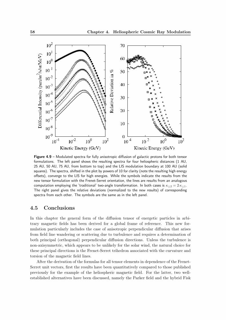
58 Chapter 4. Heliospheric Cosmic Ray Modulation
Figure 4.9 – Modulated spectra for fully anisotropic diffusion of galactic protons for both tensorformulations. The left panel shows the resulting spectra for four heliospheric distances (1 AU,25 AU, 50 AU, 75 AU, from bottom to top) and the LIS modulation boundary at 100 AU (solidsquares). The spectra, shifted in the plot by powers of 10 for clarity (note the resulting high energyoffsets), converge to the LIS for high energies. While the symbols indicate the results from thenew tensor formulation with the Frenet-Serret orientation, the lines are results from an analogouscomputation employing the ’traditional’ two-angle transformation. In both cases is κ⊥2 = 2κ⊥1.The right panel gives the relative deviations (normalized to the new results) of correspondingspectra from each other. The symbols are the same as in the left panel.
4.5 Conclusions
In this chapter the general form of the diffusion tensor of energetic particles in arbi-trary magnetic fields has been derived for a global frame of reference. This new for-mulation particularly includes the case of anisotropic perpendicular diffusion that arisesfrom field line wandering or scattering due to turbulence and requires a determination ofboth principal (orthogonal) perpendicular diffusion directions. Unless the turbulence isnon-axisymmetric, which appears to be unlikely for the solar wind, the natural choice forthese principal directions is the Frenet-Serret trihedron associated with the curvature andtorsion of the magnetic field lines.
After the derivation of the formulas for all tensor elements in dependence of the Frenet-Serret unit vectors, first the results have been quantitatively compared to those publishedpreviously for the example of the heliospheric magnetic field. For the latter, two well-established alternatives have been discussed, namely the Parker field and the hybrid Fisk
4.5. Conclusions 59
field. While the old and new tensor formulations coincide for the case of isotropic perpen-dicular diffusion, the more general case of anisotropic perpendicular diffusion cannot betreated consistently with the earlier approaches. This is manifest in significant differencesof corresponding tensor elements, some of which are no longer zero.
Second, the consequences of the new tensor formulation have been demonstrated inapplication to the modulation of galactic cosmic ray proton spectra in the Parker helio-spheric magnetic field. Solving the cosmic ray transport equation with the method ofstochastic differential equations allowed to quantify the differences between the spectraresulting from both tensor formulations for the case of perpendicular diffusion with ananisotropy of ξ = 2. It was found that those differences amount up to 60% at energiesbelow a few hundred MeV. Given that for this first principal assessment an anisotropythat is moderate as compared to findings from detailed transport and modulation studieshas been used, the fluxes can be influenced even more strongly and at even higher energiesfor more extreme cases.

Chapter 5
Anomalous Diffusion
A philosopher once said: ’It is necessary for the veryexistence of science that the same conditions alwaysproduce the same results’. Well, they do not.
The Character of Physical Law (1965)Richard P. Feynman
Contents5.1 Superdiffusive and Subdiffusive Processes . . . . . . . . . . . . . . 615.2 The Fractional Fokker-Planck Equation Transport Model . . . . 63
5.2.1 The Associated Stochastic Differential Equation . . . . . . . . . . . 645.2.2 Lévy flights and Subdiffusion Exemplified . . . . . . . . . . . . . . . 655.2.3 Comparison Between Numerical Solutions and Test Cases . . . . . . 67
5.3 Superdiffusive Transport of Termination Shock Particles . . . . 705.3.1 The Superdiffusive Fokker-Planck Transport Model . . . . . . . . . . 70
5.4 Conclusions . . . . . . . . . . . . . . . . . . . . . . . . . . . . . . . . 73
5.1 Superdiffusive and Subdiffusive Processes
In recent years, the evidence for a departure from the classical theory of energetic particlediffusion in various physical circumstances has increased significantly. Although still con-troversial, there are many studies now claiming to detect features of anomalous diffusionin observational data. In particular, there have been studies concerning solar energeticparticle events (Trotta & Zimbardo, 2011), particles accelerated in shock waves drivenby coronal mass ejections (Sugiyama & Shiota, 2011) and in interplanetary shocks asso-ciated with co-rotating interaction regions (Perri & Zimbardo, 2008b,a, 2007) as well astermination shock particles (Perri & Zimbardo, 2009). The main clue there, from an ob-servational point of view, is the presence of power law tails in time-profile data of energeticparticles. In a broader astrophysical context, there are models of anomalous transport ofhigh-energy CRs in galactic superbubbles (Barghouty & Schnee, 2012), subdiffusive trans-port in inter-cluster media (Ragot & Kirk, 1997), subdiffusive shock acceleration (Kirket al., 1996; Duffy et al., 1995), leading to steeper acceleration spectra and superdiffusiveshock acceleration (Perri & Zimbardo, 2012b), which leads to flatter acceleration spectra.

62 Chapter 5. Anomalous Diffusion
StochasticProcesses
DeterministicProcesses
Lévy NoiseGaussian NoiseContinuous-
Time RandomWalk (CTRW)
Fokker-PlanckEquation
Space-FractionalFokker-Planck
Equation
Time-FractionalFokker-Planck
Equation
Normal Diffusionζ = 1
Superdiffusionζ > 1
Subdiffusionζ < 1
Figure 5.1 – Overview of anomalous diffusion and their associated Fokker-Planck Equations andstochastic processes. For a definition of ζ see Eq. (5.1).
Despite this wealth of applications, a fundamental theory of anomalous CR transportis still lacking. More principle studies (with however limited scope) have been performede.g. by Kóta & Jokipii (2000), Shalchi & Kourakis (2007), Shalchi et al. (2007), and leRoux et al. (2010). Recently, Shalchi et al. (2012) started to investigate the connectionbetween anomalous pitch-angle scattering and the spatial diffusion behavior, and Perri& Zimbardo (2012a) looked into magnetic variances and pitch-angle scattering times up-stream of interplanetary shocks to exclude a more conventional explanation of power-lawprofiles by a spatially varying diffusion coefficient. A topical review can also be found inZimbardo et al. (2012).
Because of this unclear situation, it is helpful to study the respective physical systemswith a more fundamental approach, i.e. by solving the relevant transport equations con-nected to the anomalous transport behavior. Anomalous diffusion is characterized by apower-law dependence of the mean-square displacement of the form
〈(∆x)2〉 = κtζ (5.1)
with ζ 6= 1 being the anomalous diffusion index. In general, one can distinguish threediffusion regimes depending on ζ, namely subdiffusion (0 < ζ < 1), normal or Browniandiffusion (ζ = 1) and superdiffusion (ζ > 1). In other fields of physics and beyond the
5.2. The Fractional Fokker-Planck Equation Transport Model 63
application of anomalous diffusion models to various problems exhibiting a non-Gaussianbehavior is a vibrant field of activity, especially since the beginning of the new century.A few selected topics are human travel behavior and epidemic spreading (Brockmannet al., 2006), asset pricing (Kleinert, 2002), molecular displacement in porous media (Liet al., 2006) and the kinetics of single molecules in living cells (Barkai et al., 2012). Fora comprehensive overview of anomalous diffusion processes and their description, see e.g.Metzler & Klafter (2000) and Metzler & Klafter (2004). Fig. 5.1 gives an overview of thethree anomalous diffusion regimes and their respective mathematical model descriptions.
In the following sections, some aspects of these approaches will be discussed and ap-plied to a simplified model of energetic particle transport at shocks. In contrast to thepropagator formalism employed by Zimbardo and coworkers, the particle flux distributionis modelled in the framework of a generalized Fokker-Planck transport equation. This ap-proach allows for a detailed calculation of the distribution function of energetic particlesin dependence of the phase-space coordinates and a subsequent extension to higher di-mensions in further studies. After a validation of the results obtained with the respectivenumerical models against semi-analytic solutions (Section 5.2.3), the results for the trans-port of termination shock particles and their comparison with Voyager data are presented(Section 5.3).
5.2 The Fractional Fokker-Planck Equation TransportModel
The generalization of transport equations to anomalous diffusion behavior leads to thenotion of space- and time fractional Fokker-Planck equations (FFPE). In those, the usualsecond-order Laplacian for the spatial diffusion is replaced by a diffusion operator offractional order. A derivation of the fractional diffusion equation following the same lineof argument as presented in Section 2.2, i.e. starting from the equation of continuityand generalizing Fick’s law, can be found in Chaves (1998). As it turns out, the propergeneralization of the Laplacian is the so-called Riesz fractional derivative, which has theFourier transform property
F∇µf(x) = −|k|µf(k) (5.2)
where k is the wave-number in Fourier space and the fractional order µ fulfills the condition0 < µ ≤ 2. The Riesz derivative can also be related to the more common Riemann-Liouville type fractional derivative (Gorenflo et al., 1999), by recognizing that
∇µf(x) = − 1
2 cos(µπ/2)( Dµ−∞ x + Dµ
x +∞)f(x) (5.3)
where the Riemann-Liouville derivative is defined as
D1−α0 t f(t) =
1
Γ(α)
d
dt
∫ t
0(t− s)α−1f(s)ds . (5.4)
A wealth of information on the mathematical properties of fractional derivatives andequations can be found, e.g., in Podlubny (1999).

64 Chapter 5. Anomalous Diffusion
With this definitions of fractional derivatives, the general form of the FFPE with theaddition of an external potential V (x) can be stated as (Metzler & Klafter, 2000)
∂f(x, t)
∂t= D1−α
0 t
(∂
∂xV ′(x) + κ∇µ
)f(x, t) . (5.5)
Here, the time-fractional operator D1−α0 t corresponds to the heavy-tailed waiting time
distribution for times between the jumps of the particle, and the space-fractional Rieszoperator ∇µ describes the heavy-tailed jump distribution, i.e. the Lévy-flight behavior.κ now denotes the fractional diffusion coefficient, which now may have no longer integerdimensionality as well. The limits α = 1 and µ = 2 yield the superdiffusive or subdiffusivecases of a purely space- or time-fractional equation or the usual FPE, respectively. If both,α 6= 1 and µ 6= 2, Eq. (5.5) describes a competition between subdiffusion and Lévy flights.The interpretation of these processes will become clearer in the subsequent Section 5.2.2.Eq. (5.5) has also been derived from a generalized master equation, which may give somefurther insights, see Metzler et al. (1999).
Solutions to the FFPE can either be obtained by taking advantage of the knownFourier-transform properties of the fractional operators or by employing similar numericalmethods as already established for the standard FPE case. Grid-based numerics have beendeveloped for example by Meerschaert & Tadjeran (2004) and Tadjeran & Meerschaert(2007). There, the integrals in the Riemann-Liouville derivative are approximated by finitesummations. In this work, however, an equivalence between the FFPE and a correspond-ing stochastic formulation is employed again, to solve the fractional transport equationnumerically. The grid-based and Fourier methods have only been used to check the SDEresults for some test cases (see Section 5.2.3). In the following section, the generalizedSDE method is introduced.
5.2.1 The Associated Stochastic Differential Equation
Many aspects of a Monte Carlo method for the FFPE have been studied by Magdziarz &Weron (2007). Here, only the central aspects of this approach are presented. To obtain aset of SDEs which is equivalent to the FFPE in a similar sense as in the Ito case for theFPE discussed in Section 2.2.1, the Wiener process has to be replaced by a more generalstochastic motion, known as µ-stable Lévy distribution. This Lévy motion Lµ(t) has tofulfill the Fourier transform characteristic
FeikLµ(t) = e−t|k|µ
(5.6)
This way, the space-fractional Riesz derivative in the FFPE is accounted for. The one-dimensional SDE can thus be written as
dX(τ) = −V ′(X(τ))dτ + κ1/µdLµ(τ) (5.7)
where the time variable has already been changed to τ . This is because the probabilitydistribution function (PDF) p(x, t) of the process described by this SDE is only equivalentto the FFPE (5.5) when the time-fractionality vanishes, i.e. α = 1. To accommodate
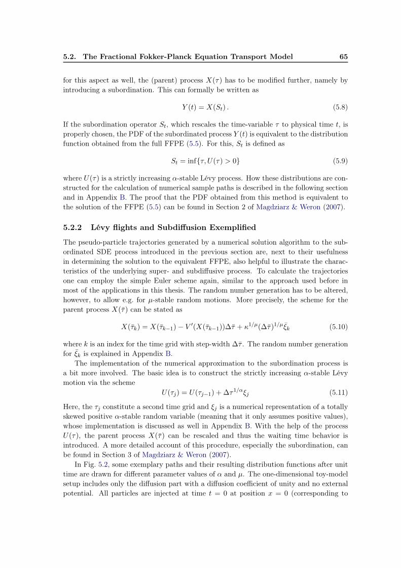
5.2. The Fractional Fokker-Planck Equation Transport Model 65
for this aspect as well, the (parent) process X(τ) has to be modified further, namely byintroducing a subordination. This can formally be written as
Y (t) = X(St) . (5.8)
If the subordination operator St, which rescales the time-variable τ to physical time t, isproperly chosen, the PDF of the subordinated process Y (t) is equivalent to the distributionfunction obtained from the full FFPE (5.5). For this, St is defined as
St = infτ, U(τ) > 0 (5.9)
where U(τ) is a strictly increasing α-stable Lévy process. How these distributions are con-structed for the calculation of numerical sample paths is described in the following sectionand in Appendix B. The proof that the PDF obtained from this method is equivalent tothe solution of the FFPE (5.5) can be found in Section 2 of Magdziarz & Weron (2007).
5.2.2 Lévy flights and Subdiffusion Exemplified
The pseudo-particle trajectories generated by a numerical solution algorithm to the sub-ordinated SDE process introduced in the previous section are, next to their usefulnessin determining the solution to the equivalent FFPE, also helpful to illustrate the charac-teristics of the underlying super- and subdiffusive process. To calculate the trajectoriesone can employ the simple Euler scheme again, similar to the approach used before inmost of the applications in this thesis. The random number generation has to be altered,however, to allow e.g. for µ-stable random motions. More precisely, the scheme for theparent process X(τ) can be stated as
X(τk) = X(τk−1)− V ′(X(τk−1))∆τ + κ1/µ(∆τ)1/µξk (5.10)
where k is an index for the time grid with step-width ∆τ . The random number generationfor ξk is explained in Appendix B.
The implementation of the numerical approximation to the subordination process isa bit more involved. The basic idea is to construct the strictly increasing α-stable Lévymotion via the scheme
U(τj) = U(τj−1) + ∆τ1/αξj (5.11)
Here, the τj constitute a second time grid and ξj is a numerical representation of a totallyskewed positive α-stable random variable (meaning that it only assumes positive values),whose implementation is discussed as well in Appendix B. With the help of the processU(τ), the parent process X(τ) can be rescaled and thus the waiting time behavior isintroduced. A more detailed account of this procedure, especially the subordination, canbe found in Section 3 of Magdziarz & Weron (2007).
In Fig. 5.2, some exemplary paths and their resulting distribution functions after unittime are drawn for different parameter values of α and µ. The one-dimensional toy-modelsetup includes only the diffusion part with a diffusion coefficient of unity and no externalpotential. All particles are injected at time t = 0 at position x = 0 (corresponding to
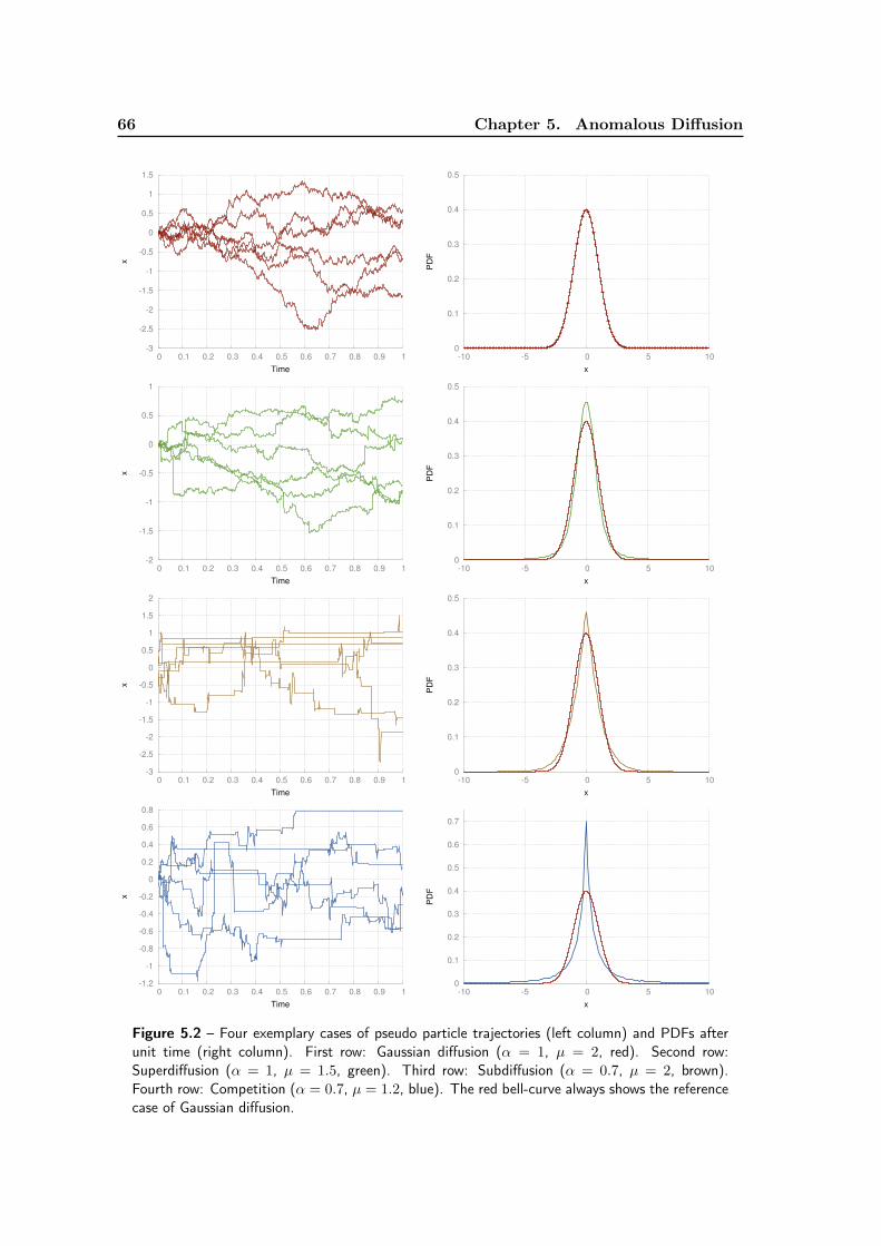
66 Chapter 5. Anomalous Diffusion
-3
-2.5
-2
-1.5
-1
-0.5
0
0.5
1
1.5
0 0.1 0.2 0.3 0.4 0.5 0.6 0.7 0.8 0.9 1
x
Time
0
0.1
0.2
0.3
0.4
0.5
-10 -5 0 5 10
PD
F
x
-2
-1.5
-1
-0.5
0
0.5
1
0 0.1 0.2 0.3 0.4 0.5 0.6 0.7 0.8 0.9 1
x
Time
0
0.1
0.2
0.3
0.4
0.5
-10 -5 0 5 10
PD
F
x
-3
-2.5
-2
-1.5
-1
-0.5
0
0.5
1
1.5
2
0 0.1 0.2 0.3 0.4 0.5 0.6 0.7 0.8 0.9 1
x
Time
0
0.1
0.2
0.3
0.4
0.5
-10 -5 0 5 10
PD
F
x
-1.2
-1
-0.8
-0.6
-0.4
-0.2
0
0.2
0.4
0.6
0.8
0 0.1 0.2 0.3 0.4 0.5 0.6 0.7 0.8 0.9 1
x
Time
0
0.1
0.2
0.3
0.4
0.5
0.6
0.7
-10 -5 0 5 10
PD
F
x
Figure 5.2 – Four exemplary cases of pseudo particle trajectories (left column) and PDFs afterunit time (right column). First row: Gaussian diffusion (α = 1, µ = 2, red). Second row:Superdiffusion (α = 1, µ = 1.5, green). Third row: Subdiffusion (α = 0.7, µ = 2, brown).Fourth row: Competition (α = 0.7, µ = 1.2, blue). The red bell-curve always shows the referencecase of Gaussian diffusion.
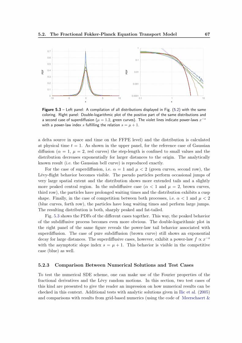
5.2. The Fractional Fokker-Planck Equation Transport Model 67
0
0.1
0.2
0.3
0.4
0.5
0.6
0.7
-10 -5 0 5 10
PD
F
x
0.0001
0.001
0.01
0.1
1
0.1 1 10
PD
F
x
Figure 5.3 – Left panel: A compilation of all distributions displayed in Fig. (5.2) with the samecoloring. Right panel: Double-logarithmic plot of the positive part of the same distributions anda second case of superdiffusion (µ = 1.2, green curves). The violet lines indicate power-laws x−s
with a power-law index s fulfilling the relation s = µ+ 1.
a delta source in space and time on the FFPE level) and the distribution is calculatedat physical time t = 1. As shown in the upper panel, for the reference case of Gaussiandiffusion (α = 1, µ = 2, red curves) the step-length is confined to small values and thedistribution decreases exponentially for larger distances to the origin. The analyticallyknown result (i.e. the Gaussian bell curve) is reproduced exactly.
For the case of superdiffusion, i.e. α = 1 and µ < 2 (green curves, second row), theLévy-flight behavior becomes visible. The pseudo particles perform occasional jumps ofvery large spatial extent and the distribution shows more extended tails and a slightlymore peaked central region. In the subdiffusive case (α < 1 and µ = 2, brown curves,third row), the particles have prolonged waiting times and the distribution exhibits a cuspshape. Finally, in the case of competition between both processes, i.e. α < 1 and µ < 2
(blue curves, forth row), the particles have long waiting times and perform large jumps.The resulting distribution is both, sharply peaked and fat-tailed.
Fig. 5.3 shows the PDFs of the different cases together. This way, the peaked behaviorof the subdiffusive process becomes even more obvious. The double-logarithmic plot inthe right panel of the same figure reveals the power-law tail behavior associated withsuperdiffusion. The case of pure subdiffusion (brown curve) still shows an exponentialdecay for large distances. The superdiffusive cases, however, exhibit a power-law f ∝ x−swith the asymptotic slope index s = µ + 1. This behavior is visible in the competitivecase (blue) as well.
5.2.3 Comparison Between Numerical Solutions and Test Cases
To test the numerical SDE scheme, one can make use of the Fourier properties of thefractional derivatives and the Lévy random motions. In this section, two test cases ofthis kind are presented to give the reader an impression on how numerical results can bechecked in this context. Additional tests with analytic solutions given in Ilic et al. (2005)and comparisons with results from grid-based numerics (using the code of Meerschaert &
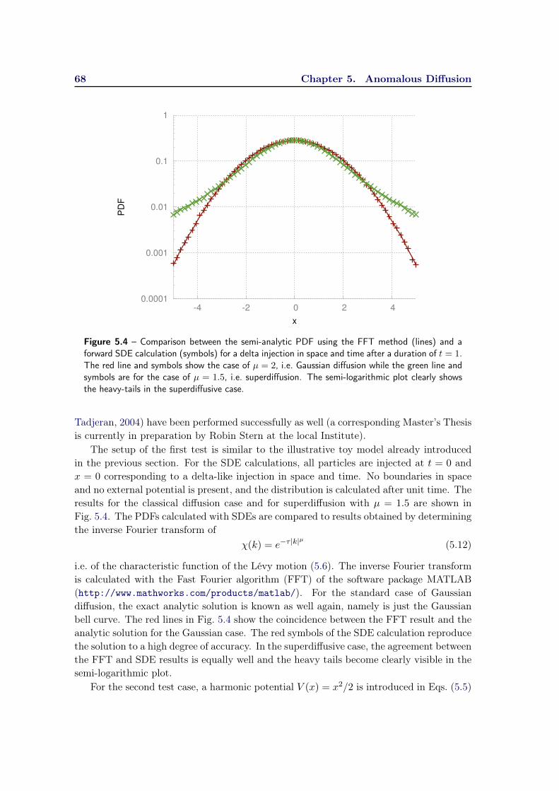
68 Chapter 5. Anomalous Diffusion
0.0001
0.001
0.01
0.1
1
-4 -2 0 2 4
PD
F
x
Figure 5.4 – Comparison between the semi-analytic PDF using the FFT method (lines) and aforward SDE calculation (symbols) for a delta injection in space and time after a duration of t = 1.The red line and symbols show the case of µ = 2, i.e. Gaussian diffusion while the green line andsymbols are for the case of µ = 1.5, i.e. superdiffusion. The semi-logarithmic plot clearly showsthe heavy-tails in the superdiffusive case.
Tadjeran, 2004) have been performed successfully as well (a corresponding Master’s Thesisis currently in preparation by Robin Stern at the local Institute).
The setup of the first test is similar to the illustrative toy model already introducedin the previous section. For the SDE calculations, all particles are injected at t = 0 andx = 0 corresponding to a delta-like injection in space and time. No boundaries in spaceand no external potential is present, and the distribution is calculated after unit time. Theresults for the classical diffusion case and for superdiffusion with µ = 1.5 are shown inFig. 5.4. The PDFs calculated with SDEs are compared to results obtained by determiningthe inverse Fourier transform of
χ(k) = e−τ |k|µ
(5.12)
i.e. of the characteristic function of the Lévy motion (5.6). The inverse Fourier transformis calculated with the Fast Fourier algorithm (FFT) of the software package MATLAB(http://www.mathworks.com/products/matlab/). For the standard case of Gaussiandiffusion, the exact analytic solution is known as well again, namely is just the Gaussianbell curve. The red lines in Fig. 5.4 show the coincidence between the FFT result and theanalytic solution for the Gaussian case. The red symbols of the SDE calculation reproducethe solution to a high degree of accuracy. In the superdiffusive case, the agreement betweenthe FFT and SDE results is equally well and the heavy tails become clearly visible in thesemi-logarithmic plot.
For the second test case, a harmonic potential V (x) = x2/2 is introduced in Eqs. (5.5)

5.2. The Fractional Fokker-Planck Equation Transport Model 69
1e-05
0.0001
0.001
0.01
0.1
1
-4 -2 0 2 4
PD
F
x
0
0.2
0.4
0.6
0.8
1
-4 -2 0 2 4
PD
F
x
Figure 5.5 – The steady-state OU and FOU distribution functions (left panel) and cumulativedistribution functions (right panel). The red line and symbols show the case of µ = 2, i.e. Gaussiandiffusion while the green line and symbols are for the case of µ = 1.5, i.e. superdiffusion. In bothpanels the SDE result is indicated by the symbols, the FFT result is given by the dashed line andthe solid line shows the analytic solution in the Gaussian case.
and (5.7). This way it is possible to approach a steady-state solution after a sufficientduration. This problem setup is discussed in Magdziarz & Weron (2007) as well, and canbe regarded as a generalization of the Ornstein-Uhlenbeck process (OU) to anomalousdiffusion, i.e. a fractional Ornstein-Uhlenbeck process (FOU, see, e.g., Magdziarz, 2008).The stationary solution to the problem in Fourier space can be stated as
wst(k) = exp
(−κ|k|
µ
µ
). (5.13)
From this expression, the solution can be calculated with the inverse fast Fourier transformand compared to the results of an SDE calculation which has approached a steady-statesolution. For the classical case of Gaussian diffusion, an analytic solution exists as welland is given by (Gardiner, 2009)
pst(x) =
√1
πκexp
(−x
2
κ
). (5.14)
Fig. 5.5 shows the resulting PDFs and cumulative distribution functions (CDFs) for thecases µ = 2 (red) and µ = 1.5 (green). The results of the FFT method agree with theanalytic solution in the Gaussian case, although there are slight deviations visible in theCDF. For the superdiffusive case, the SDE and FFT results match to a high degree aswell. The small differences may be due to limited resolution in the FFT method. Theremaining fluctuations in the SDE results are of statistical nature; for each run, 105 pseudo-particle trajectories have been calculated. For this steady-state superdiffusive problem,the elongated tails of the distribution are visible again.
Both examples illustrate how the SDE method employed in the previous chapters canbe successfully extended to cases of anomalous diffusion, and the performed tests justifyconfidence in the obtained results.

70 Chapter 5. Anomalous Diffusion
5.3 Superdiffusive Transport of Termination Shock Particles
In the following part of this chapter, the previously developed methods for the modellingof superdiffusive energetic particle propagation are applied to the transport of terminationshock particles. The work by Perri & Zimbardo (2009) can be regarded as a motivation forthis investigation. In their study, they looked into time profiles of energetic particle fluxesalong the Voyager 2 (V2) spacecraft trajectory during the crossing of the heliospherictermination shock (see again Section 1.1.4 for an account of the relevant heliosphericstructures). The termination shock (TS) is believed to be a source of energetic particlesin the high-keV and low-MeV energy range, which are accelerated at the shock interfacedue to shock acceleration processes (Section 1.1.1) and may also mediate the actual shockstructure themselves (Decker et al., 2008).
The observations of the energetic particle profiles upstream of the shock with the LECPinstrument on board of V2 interestingly point to a power-law behavior for at least threeenergy channels from 540 to 3500 keV (see Fig. 2 in Perri & Zimbardo, 2009). This isunexpected for a simple one-dimensional diffusion model with an energy-dependent butotherwise constant diffusion coefficient. In such a model, an exponential decay is predicted.Therefore, the analysis by Perri and Zimbardo points to a superdiffusive behavior of theseparticles. In their work, the explanation of this connection is based on a propagatorformalism which can be summarized as follows.
According to Zumofen & Klafter (1993) the propagator for superdiffusion, giving theprobability of observing a particle at (x, t), if it was injected at (x′, t′), has, for the one-dimensional case and a planar shock, the general form
P (x− x′, t− t′) = b(t− t′)(x− x′)−s (5.15)
where b is a dimensional constant and s is the power-law index, which is connected to thefractionality in the FFPE via s = µ + 1, i.e. lies between 2 and 3. In their coordinatesystem, the observer is at a position x = 0 and the shock is moving at a constant speedVsh coming from x < 0 at time t < 0. For a normal, Gaussian diffusion, one obtains anexponential decay for the observer of the form
fG(x = 0, E, t) ∝ exp
(V 2sht
κ
). (5.16)
For superdiffusion, however, they derive a power-law decay of the form
fsup(x = 0, E, t) ∝V−(µ+1)sh
(−t)1−µ. (5.17)
An important point here is though that this result derived from the propagator given byEq. (5.15) is only valid at some distance from the shock, i.e. the particle injection, becausethe propagator itself is only an asymptotic approximation.
5.3.1 The Superdiffusive Fokker-Planck Transport Model
To study the flux profiles of shock-injected energetic particles to a greater detail, thegeneric FFPE model developed in the previous sections is applied to the one-dimensional

5.3. Superdiffusive Transport of Termination Shock Particles 71
problem of particle superdiffusion at a solar wind shock interface, and the results arecompared to the V2 observations as well.
The FFPE (5.5) can be reduced in this case to the following form
∂f(x, t)
∂t=
∂
∂x[usw(x)f(x, t)] + κ∇µf(x, t) (5.18)
where the solar wind usw is given by a step function with a velocity of 400 km/s upstreamof the shock and 200 km/s downstream. These values are chosen in reasonable agreementwith the V2 plasma instrument observations during the shock crossing (see, e.g., Richard-son et al., 2008). The model equation is solved with the SDE approach to superdiffusiondeveloped in the previous sections for a time-continuous delta type injection in space at theshock position x = 0 (note the different coordinate system in comparison with Perri andZimbardo). The resulting steady-state spatial profile of particle flux can be converted intoa time profile by imposing a V2 speed of VV 2 = 3.3 AU/yr (the current mission status cane.g. by found at http://voyager.jpl.nasa.gov/mission/weekly-reports/index.htm)and assuming that the shock position is approximately constant (although it may of coursebe moving due to various effects like the solar cycle) during the time of approach, i.e. set-ting Vsh = 0 and calculating the time as t = x/(VV 2 + Vsh). Vice versa the time-profiledata of V2 can be converted into a spatial profile. In the present numerical model setup,the pseudo-particles are injected at the phase-space point of interest, are traced backwardsin time and obtain their flux values due to a fixed boundary condition at the termina-tion shock (x = 0). The only important free parameters remaining are the superdiffusioncoefficient κ and the exponent µ. The boundary condition value is just a normalizationconstant which can be adjusted to fit the data.
Fig. 5.6 shows the comparison of model results for different superdiffusion exponentsµ to the V2 upstream particle flux data in the LECP energy channel of 540 − 990 keV(small purple crosses, obtained via NASA Omniweb, http://omniweb.gsfc.nasa.gov/).For comparison, two exemplary results for standard Gaussian diffusion are included aswell (black dashed lines). As discussed above, the Gaussian case, i.e. µ = 2 is analyticallyknown for this problem, see Eq. (5.16). The SDE result in red, for a ratio Vsw,up/κ =
10/AU, i.e. a diffusion coefficient of 6 · 1019 cm2/s, coincides with the analytic Gaussiandecay and confirms the validity of the model in the normal diffusion scenario. The secondblack dashed result is the analytic solution for a 20 times higher diffusion coefficient andan added underground flux to account for the far distance particle intensity. As can beseen, this significantly higher diffusion coefficient can explain the data sufficiently well, atleast in this particular energy range.
The green and blue curves show the results for two superdiffusive scenarios with µ = 1.5
and µ = 1.7 respectively. In both cases the superdiffusion coefficient has the same numer-ical value as in the Gaussian diffusion model with the low κ value, i.e. 6 · 1019 cmµ/s.The Lévy-flight behavior produces the characteristic power-law decay and allows for muchhigher fluxes far away from the shock than in the normal diffusion case. The result forµ = 1.5 agrees remarkably well with the data, while the result for µ = 1.7 yields too lowfluxes for large shock distances.
The actual diffusion coefficient in this scenario is not well known to the necessary pre-
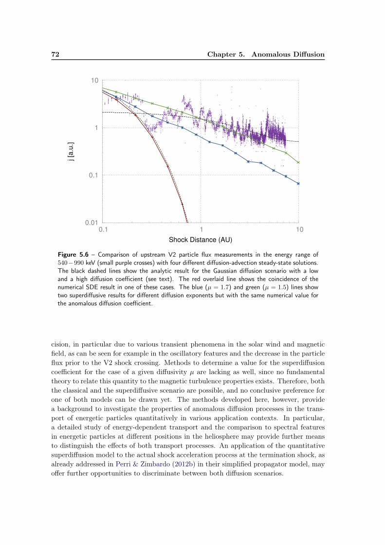
72 Chapter 5. Anomalous Diffusion
0.01
0.1
1
10
0.1 1 10
j [a
.u.]
Shock Distance (AU)
Figure 5.6 – Comparison of upstream V2 particle flux measurements in the energy range of540−990 keV (small purple crosses) with four different diffusion-advection steady-state solutions.The black dashed lines show the analytic result for the Gaussian diffusion scenario with a lowand a high diffusion coefficient (see text). The red overlaid line shows the coincidence of thenumerical SDE result in one of these cases. The blue (µ = 1.7) and green (µ = 1.5) lines showtwo superdiffusive results for different diffusion exponents but with the same numerical value forthe anomalous diffusion coefficient.
cision, in particular due to various transient phenomena in the solar wind and magneticfield, as can be seen for example in the oscillatory features and the decrease in the particleflux prior to the V2 shock crossing. Methods to determine a value for the superdiffusioncoefficient for the case of a given diffusivity µ are lacking as well, since no fundamentaltheory to relate this quantity to the magnetic turbulence properties exists. Therefore, boththe classical and the superdiffusive scenario are possible, and no conclusive preference forone of both models can be drawn yet. The methods developed here, however, providea background to investigate the properties of anomalous diffusion processes in the trans-port of energetic particles quantitatively in various application contexts. In particular,a detailed study of energy-dependent transport and the comparison to spectral featuresin energetic particles at different positions in the heliosphere may provide further meansto distinguish the effects of both transport processes. An application of the quantitativesuperdiffusion model to the actual shock acceleration process at the termination shock, asalready addressed in Perri & Zimbardo (2012b) in their simplified propagator model, mayoffer further opportunities to discriminate between both diffusion scenarios.
5.4. Conclusions 73
5.4 Conclusions
In the previous sections a quantitative model for the anomalous transport of energetic par-ticles has been developed. The numerical solution to the FFPE is based on a generalizedSDE approach, which extends the classical Wiener process to µ-stable Lévy distributionsand allows to include subdiffusive processes by a subordination algorithm. The comparisonto semi-analytic results for simplified test cases obtained by the inverse Fourier transformto the characteristic function of the processes provide confidence in the numerical results.The solutions of the generalized SDE, given as trajectories of pseudo-particles, clarify theunderlying processes further. In the comparison to energetic particle flux profiles obtainedwith the V2 spacecraft, it was found that the superdiffusive scenario is a possible expla-nation for the power-law behavior in the data. Due to the uncertainties connected withthe diffusion coefficient in the classical propagation scenario, which allows to reproducethe data with an appropriate choice of κ, none of the two models can be excluded at thepresent stage.

Chapter 6
Concluding Remarks
Die Unendlichkeit der Schöpfung ist groß genug, um eineWelt, oder eine Milchstraße von Welten gegen sieanzusehen, wie man eine Blume, oder ein Insect inVergleichung gegen die Erde ansieht.
Allgemeine Naturgeschichte und Theorie des Himmels(1797)
Immanuel Kant
Contents6.1 Summary . . . . . . . . . . . . . . . . . . . . . . . . . . . . . . . . . 756.2 Future Prospects . . . . . . . . . . . . . . . . . . . . . . . . . . . . . 76
6.1 Summary
This thesis addresses three major issues in the contemporary modelling efforts for energeticparticle transport. These are (i) the anisotropic diffusion of CRs in galactic magnetic fieldsand their long-term azimuthal flux distribution, (ii) the inclusion of a fully anisotropicdiffusion tensor for arbitrary background magnetic field configurations in the context ofheliospheric CR modulation, and (iii) the extension of the classical Gaussian diffusionmodels to a quantitative anomalous diffusion model for energetic particle propagation.
The numerical methods to solve the respective transport equations in these scenariosexhibit similar characteristics in all three cases and are founded on two complementaryapproaches, namely a grid-based and a stochastic formulation. The traditional grid-basedapproach allows to solve for a global (steady-state) solution of the respective CR distribu-tion. The stochastic method is a more recent development, and its advantages are its sim-pler and more efficiently possible extension to higher dimensionality and its conformancewith modern computer architecture (being an inherently parallel problem). Furthermore,the extension to the anomalous diffusion regime is particularly elegant in this framework.The findings of the performed investigations can be summarized as follows:
(i) With the galactic propagation model it has been found that the CR flux variationalong the Sun’s orbit around the galactic center clearly depends on the imposedanisotropy in the diffusion tensor formulation. This indicates that the inclusion ofsuch a transport effect is an important feature for global galactic propagation models,

76 Chapter 6. Concluding Remarks
especially if they aim for an increased precision in the prediction of observationswhich are connected to the galactic CR flux distribution.
(ii) In the case of heliospheric modulation of CR spectra, the choice of the local frameof reference determines the impact of anisotropic perpendicular diffusion on the re-sulting modulation spectra. The results show differences between the spectral fluxesobtained with the new tensor formulation in comparison to those of the “traditional”one by up to 60% for energies below a few hundred MeV, depending on heliocentricdistance.
(iii) The anomalous diffusion model developed in this work allows to model sub- andsuperdiffusive transport effects more quantitatively than before. In the exemplaryapplication to the superdiffusion of termination shock particles, the differences be-tween the classical diffusion results and the novel transport effects become obvious.Due to the uncertainties in the actual plasma environment and a still incompletetheoretical foundation of anomalous particle transport, a definitive preference forone process over the other cannot be deduced yet, but further studies based on thepresent work may yield further insights.
Some of the possible extensions to the theory and models developed in this thesis andfurther connected fields of study are outlined in the concluding section.
6.2 Future Prospects
The anisotropic galactic propagation model can be extended by including additional effectslike a variable spectral source index and time-variable CR sources, depending on supernovatype. The necessary time-dependent calculations are generally feasible with the currentmodel setup, and the earlier work by Büsching & Potgieter (2008) shows some results onthis already. In general, there is a need for more detailed models of the galactic magneticfield, in order to asses its impact on the transport processes of CRs. The connection of theconcepts of this study to models with a much wider range of included processes like theGALPROP model (Strong et al., 2010) is a possible opportunity to test the implications ofadditional CR species and their relevant loss processes. This may yield further constraintsto the various transport parameters.
Fully anisotropic diffusion may be of significance for the galactic CR propagation aswell. The lack of observational constraints will yet prevent progress in this regard in thenear future. The necessity to study the case of fully anisotropic diffusion in greater detailwithin the framework of more sophisticated models of heliospheric CR modulation hashowever become clear within the present study. The inclusion of this transport effectin modulation models which couple to a global heliospheric plasma model, based e.g. onMHD simulations, will enable us to explain energetic particle measurements throughoutthe heliosphere to higher precision. Solar energetic particle studies may provide a suitabletest-bed to study the relation between plasma turbulence and the occurrence of fullyanisotropic diffusion in detail (e.g., Laitinen et al., 2012; Kelly et al., 2012; Tautz et al.,2011).
6.2. Future Prospects 77
As discussed in Chapter 5, the scope of application for anomalous transport processesis steadily increasing. The developed numerical SDE model will enable future studiesto address these transport effects more quantitatively in various scenarios for energeticparticle transport. Solar energetic particles as well as shock acceleration processes mayprovide the most conclusive observational constraints to the modelling efforts.
An ultimate comprehension of the various processes involved in energetic particle trans-port seems unfeasible for the near future due to their complicated nonlinear and stochasticnature. The ongoing efforts to clarify our understanding within the simplified models athand and their constant refinement by scientists from different fields of interest have nev-ertheless greatly improved on our common view on these processes and allowed for theexplanation of observational data with higher accuracy than before. This enables spacescientists and astrophysicists to address issues raised by related fields like climatology andspace travel with increasing confidence.

Appendix A
The Semi-analytic ParkerPropagator Solution
Stawicki et al. (2000) found an analytic description for the general solution to the spherical-symmetric heliospheric modulation problem. This opens an opportunity to test the nu-merical SDE code used in this thesis against a (semi-) analytic solution for a still somewhatrealistic case of heliospheric modulation. In their paper, they solve the transport equationin the one-dimensional spherically symmetric form:
1
r2∂
∂r
(r2κrr
∂f
∂r
)− V ∂f
∂r+
p
3r2∂
∂r(r2v)
∂f
∂p= −S(r, p) (A.1)
by calculating a Green’s function for this equation for arbitrary power-law dependencefor the spatial diffusion on heliospheric distance r and momentum p, i.e. κrr = κ0r
βppγp .They also allow for a spatial variation of the solar wind speed of the form V (r) = V0r
αp .They find the following exact solution for the differential intensity:
j(r, p) = p2f(r, p)
=3
bp
∫dr0
∫dp0
S(r0, p0)
V (r0)
p0y0fp
(r0r
) 1+βp2
×(p0p
) 3βp−4αp−5
2(2+αp)
exp
(−y0(1 + h2p)
fp
)
× I 1+βp1+αp−βp
(2y0hpfp
). (A.2)
Here, r0 and p0 are integration variables and In a modified Bessel function of the firstkind. The following abbreviations have been used:
fp = 1−(p
p0
) 3νp2+αp
(A.3)
hp =
(r
r0
) 1+αp−βp2
(p
p0
) 32b
(A.4)
y0 = y(r0, p0) =νp
(1 + αp − βp)2r0V
κrr(A.5)
νp = 1 + αp − βp +2 + αp
3γp (A.6)
bp =2 + αp
1 + αp − βp(A.7)

80 Appendix A. The Semi-analytic Parker Propagator Solution
10-4
10-3
10-2
10-1
100
101
102
10-4
10-3
10-2
10-1
100
101
102
Inte
nsi
ty j
(par
t/m
2/s
/sr/
MeV
)
Kinetic Energy [GeV]
10-4
10-3
10-2
10-1
100
101
102
10-4
10-3
10-2
10-1
100
101
102
Inte
nsi
ty j
(par
t/m
2/s
/sr/
MeV
)
Kinetic Energy [GeV]
0
5
10
15
20
25
30
35
40
10-4
10-3
10-2
10-1
100
101
102
Rel
ativ
e D
evia
tio
n i
n %
Kinetic Energy [GeV]
0
5
10
15
20
25
30
35
40
10-4
10-3
10-2
10-1
100
101
102
Rel
ativ
e D
evia
tio
n i
n %
Kinetic Energy [GeV]
Figure A.1 – Comparison between the Parker-Propagator solutions and the SDE solutions forthe modulation problem with βp = 0.2 and γp = 1. The top row shows the spectra for 1 AU,25 AU, 50 AU, 75 AU and 100 AU of heliospheric distance, respectively (from bottom to top).The solid lines represent the solution from the Parker Propagator, while the symbols are the datapoints from the SDE simulations. The lower row shows the relative deviation in percent betweenboth solutions (same symbols). The symbols of the left panel were calculated with a resolutionof 10000 pseudo-particles per phase-space point, while the right panels were calculated with only100 pseudo-particles.
where y(r, p) is also called the modulation parameter, see Jokipii (1967).The solution (A.2) has still two caveats, namely that it only allows to specify a source
function S(r, p) and not a specific boundary condition for the outer heliospheric boundary,and that it includes two integrals which may be hard to solve analytically. In their paper,Stawicki et al. specify a source function for the galactic cosmic ray protons of the form
SGCR(r, p) = SGCR,n(v/p2)(E + 0.5mp)γp−2.6δ(r − rsh) (A.8)
with rsh = 100 AU as the modulation boundary. This way, a power-law spectrum withan exponent of −2.6 at the modulation boundary is nearly reproduced. With this ansatz,the solution Eq. (A.2) requires only one integration over p0 which is done numerically(Piessens et al., 1983).
In Fig. A.1, the results for the modulation spectra obtained with the Parker-Propagatorapproach are compared to the results from SDE calculations (see Chapter 4). The three
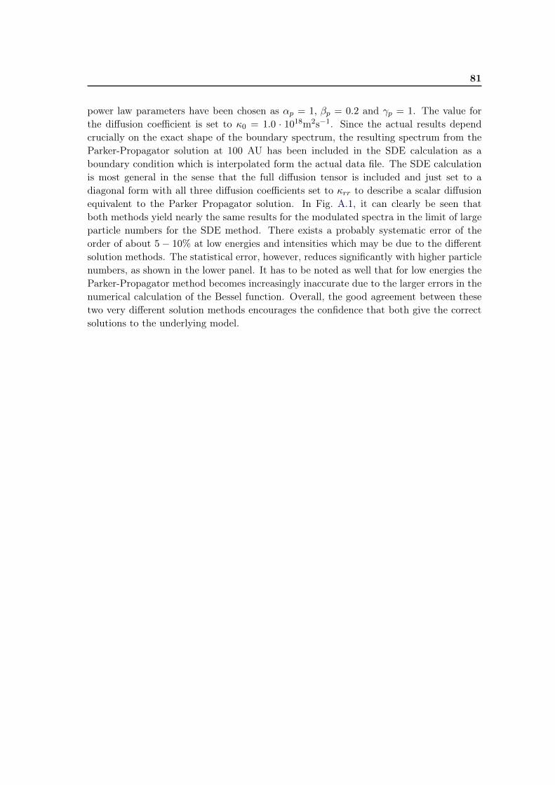
81
power law parameters have been chosen as αp = 1, βp = 0.2 and γp = 1. The value forthe diffusion coefficient is set to κ0 = 1.0 · 1018m2s−1. Since the actual results dependcrucially on the exact shape of the boundary spectrum, the resulting spectrum from theParker-Propagator solution at 100 AU has been included in the SDE calculation as aboundary condition which is interpolated form the actual data file. The SDE calculationis most general in the sense that the full diffusion tensor is included and just set to adiagonal form with all three diffusion coefficients set to κrr to describe a scalar diffusionequivalent to the Parker Propagator solution. In Fig. A.1, it can clearly be seen thatboth methods yield nearly the same results for the modulated spectra in the limit of largeparticle numbers for the SDE method. There exists a probably systematic error of theorder of about 5− 10% at low energies and intensities which may be due to the differentsolution methods. The statistical error, however, reduces significantly with higher particlenumbers, as shown in the lower panel. It has to be noted as well that for low energies theParker-Propagator method becomes increasingly inaccurate due to the larger errors in thenumerical calculation of the Bessel function. Overall, the good agreement between thesetwo very different solution methods encourages the confidence that both give the correctsolutions to the underlying model.

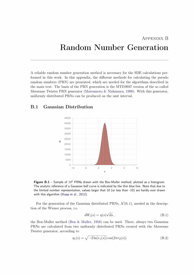
Appendix B
Random Number Generation
A reliable random number generation method is necessary for the SDE calculations per-formed in this work. In this appendix, the different methods for calculating the pseudorandom numbers (PRN) are presented, which are needed for the algorithms described inthe main text. The basis of the PRN generation is the MTI19937 version of the so calledMersenne Twister PRN generator (Matsumoto & Nishimura, 1998). With this generator,uniformly distributed PRNs can be produced on the unit interval.
B.1 Gaussian Distribution
0
5000
10000
15000
20000
25000
30000
35000
40000
45000
-10 -6 -2 2 6 10
N
x
Figure B.1 – Sample of 106 PRNs drawn with the Box-Muller method, plotted as a histogram.The analytic reference of a Gaussian bell curve is indicated by the thin blue line. Note that due tothe limited number representation, values larger that 10 (or less than -10) are hardly ever drawnwith this algorithm (Kopp et al., 2012).
For the generation of the Gaussian distributed PRNs, N (0, 1), needed in the descrip-tion of the Wiener process, i.e.
dWi(s) = η(s)√ds , (B.1)
the Box-Muller method (Box & Muller, 1958) can be used. There, always two GaussianPRNs are calculated from two uniformly distributed PRNs created with the MersenneTwister generator, according to
η1(s) =√−2 ln(r1(s)) cos(2πr2(s)) (B.2)
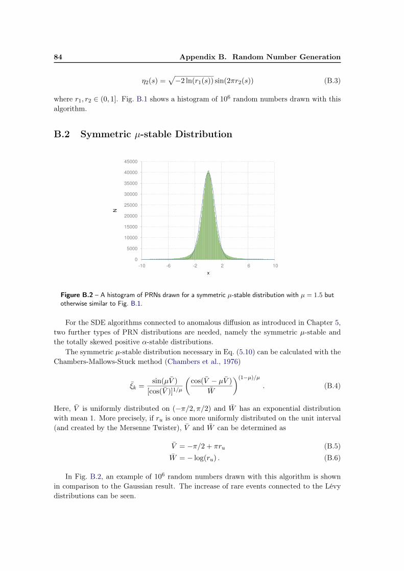
84 Appendix B. Random Number Generation
η2(s) =√−2 ln(r1(s)) sin(2πr2(s)) (B.3)
where r1, r2 ∈ (0, 1]. Fig. B.1 shows a histogram of 106 random numbers drawn with thisalgorithm.
B.2 Symmetric µ-stable Distribution
0
5000
10000
15000
20000
25000
30000
35000
40000
45000
-10 -6 -2 2 6 10
N
x
Figure B.2 – A histogram of PRNs drawn for a symmetric µ-stable distribution with µ = 1.5 butotherwise similar to Fig. B.1.
For the SDE algorithms connected to anomalous diffusion as introduced in Chapter 5,two further types of PRN distributions are needed, namely the symmetric µ-stable andthe totally skewed positive α-stable distributions.
The symmetric µ-stable distribution necessary in Eq. (5.10) can be calculated with theChambers-Mallows-Stuck method (Chambers et al., 1976)
ξk =sin(µV )
[cos(V )]1/µ
(cos(V − µV )
W
)(1−µ)/µ. (B.4)
Here, V is uniformly distributed on (−π/2, π/2) and W has an exponential distributionwith mean 1. More precisely, if ru is once more uniformly distributed on the unit interval(and created by the Mersenne Twister), V and W can be determined as
V = −π/2 + πru (B.5)
W = − log(ru) . (B.6)
In Fig. B.2, an example of 106 random numbers drawn with this algorithm is shownin comparison to the Gaussian result. The increase of rare events connected to the Lévydistributions can be seen.
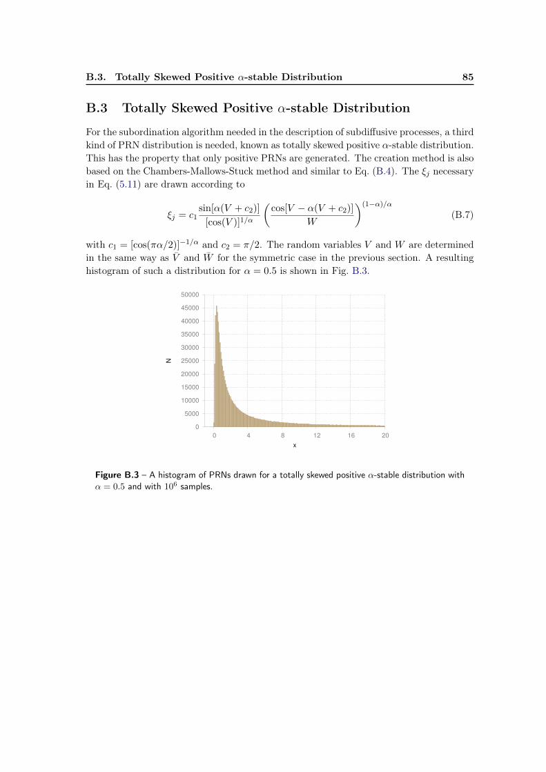
B.3. Totally Skewed Positive α-stable Distribution 85
B.3 Totally Skewed Positive α-stable Distribution
For the subordination algorithm needed in the description of subdiffusive processes, a thirdkind of PRN distribution is needed, known as totally skewed positive α-stable distribution.This has the property that only positive PRNs are generated. The creation method is alsobased on the Chambers-Mallows-Stuck method and similar to Eq. (B.4). The ξj necessaryin Eq. (5.11) are drawn according to
ξj = c1sin[α(V + c2)]
[cos(V )]1/α
(cos[V − α(V + c2)]
W
)(1−α)/α(B.7)
with c1 = [cos(πα/2)]−1/α and c2 = π/2. The random variables V and W are determinedin the same way as V and W for the symmetric case in the previous section. A resultinghistogram of such a distribution for α = 0.5 is shown in Fig. B.3.
0
5000
10000
15000
20000
25000
30000
35000
40000
45000
50000
0 4 8 12 16 20
N
x
Figure B.3 – A histogram of PRNs drawn for a totally skewed positive α-stable distribution withα = 0.5 and with 106 samples.


Acknowledgments
Writing a thesis is an extensive project. During my studies I was happy to meet many inspiringand helpful people. At this point, I want to express my gratitude to them.
• My biggest thanks go to my supervisor Priv.-Doz. Dr. Horst Fichtner, whose constant sup-port and encouragement helped me in innumerable ways. But also apart from scientificquestions, our discussions about life and all the rest were always enjoyable.
• I want to thank Prof. Hans Fahr for his willingness to be the second reviewer of this thesisand for many interesting discussions, especially during our visits in South Africa.
• I thank Prof. Reinhard Schlickeiser for employing me at his institute, for his interestinglectures, and for many helpful critical remarks.
• Many thanks go to my colleagues, especially Klaus Scherer, Ingo Büsching, Andreas Kopp,Tobias Schäfer, Jens Kleimann, Udo Arendt, Giorgi Dalakishvilli, Tobias Wiengarten,Robin Stern, Stefan Artmann, Michael Michno, Stephan Barra, Daniel Verscharen, GiselaBaumann, Oliver Sternal and Björn Eichmann. Thank you for cooperation, many interest-ing discussions connected to work and to all the other things. I also want to thank thosewho took the time to read parts of this manuscript for their helpful comments.
• Thanks go to the TP4 technical staff, especially Bernd Neubacher for providing the necessarycomputing resources and to the secretaries Verena Kubiak and Gisela Buhr, as well as toall the other TP4 members for the nice times at the Institute.
• I thank my former colleagues at TP1, especially Prof. Rainer Grauer, Jürgen Dreher andKai Thust for their ongoing support and scientific connections.
• During my many visits to work-meetings and conferences, I met many decent people fromall around the world. My special thanks go to the South African group, namely Prof. MariusPotgieter, Prof. Stefan Ferreira, Prof. Adri Burger, Du Toit Strauss and Eugene Engelbrecht.I always enjoyed your company and I am very grateful for the opportunities to visit youat your institute. I also want to thank Nir Shaviv for inviting me to his conference inJerusalem, Alexandre Marcowith for the possibility to attend his conference in Montpellierand to Silvia Dalla and Timo Laitinen for welcoming me at their institute in Preston.
• I thank my physics teacher Clemens Piffko for inspiring my interest in physics in schooland all my academic teachers for their inspiring efforts, especially Prof. Storch for hisenthusiastic account of mathematics.
• Last but not least I want to thank my family and (non-university) friends for their companyand support throughout all the years of my studies. You are irreplaceable :)
Over the course of an average lifetime (and a PhD thesis), you meet a lot of people. Some ofthem stick with you and some weave their way through your life and disappear forever. But theyall leave their impression on you in some way or another. Thank you for being those dents in mylife!
Lebenslauf
Persönliche Daten
Frederic Effenberger
E-Mail: [email protected]
Geboren am 06. 01. 1984 in OberhausenLedig, deutsch
Schulbildung
08/1990 - 06/2003 Grundschule und Gymnasium in Oberhausen
06/2003 Abitur, Elsa-Brändström Gymnasium, Oberhausen
Studium
10/2003 - 10/2008 Studium der Physik an der Ruhr-Universität Bochum
09/2005 Vordiplom in Physik
10/2008 Diplom in Physik, Diplomarbeit am Lehrstuhl für TheoretischePhysik I der Ruhr-Universität Bochum (Betreuer: Prof. Dr. R.Grauer)
Diplomarbeit: Numerische Untersuchungen zur Stromschichtbildung in solarenMagnetfeldgeometrien, Note: sehr gut
Seit 10/2008 Zweitstudium der Philosophie an der Ruhr-Universität Bochum
Berufserfahrung
05-2006 - 10/2008 Studentische Hilfskraft am Lehrstuhl für Theoretische Physik I derRuhr-Universität Bochum
Seit 02/2009 Wissenschaftlicher Mitarbeiter am Lehrstuhl für TheoretischePhysik IV der Ruhr-Universität Bochum und Promotionsstudent derWeltraum- und Astrophysik (Betreuer: PD Dr. H. Fichtner)
Own Publications/Eigene Publikationen
• Anisotropic Diffusion of Galactic Cosmic Ray Protons and Their Steady-State Az-imuthal Distribution, Effenberger, F.; Fichtner, H.; Scherer, K.; Büsching, I.,11/2012, Astronomy & Astrophysics, Volume 547, A120
• A Generalized Diffusion Tensor for Fully Anisotropic Diffusion of Energetic Par-ticles in the Heliospheric Magnetic Field, Effenberger, F.; Barra, S.; Fichtner, H.;Kleimann, J.; Scherer, K.; Strauss, R. D., 05/2012, The Astrophysical Journal, Vol-ume 750, p. 108
• The long-term azimuthal structure of the Galactic Cosmic Ray proton distributiondue to anisotropic diffusion, Effenberger, F.; Fichtner, H.; Büsching, I.; Kopp, A.;Scherer, K., 12/2011, Mem. Soc. Astron. Italiana, Volume 82, p. 867
• Cosmic Ray Transport in the Heliosphere and Its Connection to the InterstellarProton Spectrum, Fichtner, H.; Effenberger, F.; Scherer, K.; Büsching, I.; Strauss,R. D.; Ferreira, S. E. S.; Potgieter, M. S.; Fahr, H. J.; Heber, B., 12/2011, Mem.Soc. Astron. Italiana, Volume 82, p. 852
• Numerical simulation of current sheet formation in a quasiseparatrix layer usingadaptive mesh refinement, Effenberger, F.; Thust, K.; Arnold, L.; Grauer, R.;Dreher, J., 03/2011, Physics of Plasmas, Volume 18, Issue 3, p. 032902-032902-6
• Comparison of different analytic heliospheric magnetic field configurations and theirsignificance for the particle injection at the termination shock, Scherer, K.; Ficht-ner, H.; Effenberger, F.; Burger, R. A.; Wiengarten, T., 10/2010, Astronomy &Astrophysics, Volume 521, id.A1


List of Figures
1.1 A Comparison of galactic CR solar minimum abundances with solar systemabundances. . . . . . . . . . . . . . . . . . . . . . . . . . . . . . . . . . . . 2
1.2 The all particle energy spectrum of CRs. . . . . . . . . . . . . . . . . . . . 31.3 The way of a CR particle. . . . . . . . . . . . . . . . . . . . . . . . . . . . 41.4 An optical and X-ray composite image of the SNR 0509-67.5 (Type Ia). . 51.5 The all particle flux of high energy CRs (multiplied by E2) as observed by
various instruments. . . . . . . . . . . . . . . . . . . . . . . . . . . . . . . 61.6 The total radio emission and magnetic field vectors of M51 overlaid onto
an optical image from the Hubble Space Telescope. . . . . . . . . . . . . . 81.7 Sketch of the fundamental heliospheric structures. . . . . . . . . . . . . . . 10
2.1 Two sample paths of a Wiener process in two dimensions. . . . . . . . . . 20
3.1 Orientation of the galactic spiral arms. . . . . . . . . . . . . . . . . . . . . 313.2 Volume rendering visualization of the input source distribution of CRs. . . 323.3 Sample paths of pseudo-particles in the galactic magnetic spiral field. . . . 343.4 Steady-state logarithmic CR proton distribution in the galactic plane. . . 363.5 Calculated CR proton spectra (multiplied by E2) at four different positions
along the Sun’s orbit. . . . . . . . . . . . . . . . . . . . . . . . . . . . . . . 383.6 Orbital variation of CR proton flux along the Sun’s orbit, plotted against
longitude. . . . . . . . . . . . . . . . . . . . . . . . . . . . . . . . . . . . . 40
4.1 The hybrid Fisk and the Parker field illustrated by red and black field lines. 454.2 The angle between the hybrid Fisk- and Parker-field in a meridional plane. 464.3 The undisturbed heliospheric magnetic field and its structure when field
line random walk is included. . . . . . . . . . . . . . . . . . . . . . . . . . 484.4 The dependence of the local and global tensor elements on heliocentric
distance in the ecliptic plane for the Parker field. . . . . . . . . . . . . . . 504.5 The transformation between local and global coordinates and a sketch of
the tensor transformation. . . . . . . . . . . . . . . . . . . . . . . . . . . . 514.6 The two local trihedrons for the Parker and hybrid Fisk field. . . . . . . . 534.7 The six independent tensor elements plotted against colatitude. . . . . . . 554.8 Ratios of the tensor elements for the hybrid Fisk field plotted against heli-
ographic longitude. . . . . . . . . . . . . . . . . . . . . . . . . . . . . . . . 564.9 Modulated spectra for fully anisotropic diffusion of galactic protons for both
tensor formulations. . . . . . . . . . . . . . . . . . . . . . . . . . . . . . . 58
5.1 Overview of anomalous diffusion and their associated Fokker-Planck Equa-tions and stochastic processes. . . . . . . . . . . . . . . . . . . . . . . . . . 62
5.2 Four exemplary cases of pseudo particle trajectories and PDFs after unittime. . . . . . . . . . . . . . . . . . . . . . . . . . . . . . . . . . . . . . . . 66

92 List of Figures
5.3 A compilation of all previous distributions, both linear and logarithmic. . 675.4 Comparison between the semi-analytic PDF using the FFT method and a
forward SDE calculation for a delta injection in space and time . . . . . . 685.5 The steady-state OU and FOU distribution functions and cumulative dis-
tribution functions. . . . . . . . . . . . . . . . . . . . . . . . . . . . . . . . 695.6 Comparison of upstream V2 particle flux measurements in the energy range
of 540−990 keV with four different diffusion-advection steady-state solutions. 72
A.1 Comparison between the Parker-Propagator and SDE solutions. . . . . . . 80
B.1 Sample of 106 PRNs drawn with the Box-Muller method, plotted as a his-togram. . . . . . . . . . . . . . . . . . . . . . . . . . . . . . . . . . . . . . 83
B.2 A histogram of PRNs drawn for a symmetric µ-stable distribution withµ = 1.5. . . . . . . . . . . . . . . . . . . . . . . . . . . . . . . . . . . . . . 84
B.3 A histogram of PRNs drawn for a totally skewed positive α-stable distribu-tion with α = 0.5. . . . . . . . . . . . . . . . . . . . . . . . . . . . . . . . . 85
Bibliography
Achterberg, A. & Schure, K. M. A more accurate numerical scheme for diffusive shock acceleration. 2011,MNRAS, 411, 2628 (ADS) 3.1.6
Ackermann, M. et al. Fermi-LAT Observations of the Diffuse γ-Ray Emission: Implications for CosmicRays and the Interstellar Medium. 2012, ApJ, 750, 3 (ADS) 1.1.2
Adriani, O. et al. An anomalous positron abundance in cosmic rays with energies 1.5-100GeV . 2009,Nature, 458, 607 (ADS) 1.1.3
Alania, M. V. Stochastic Variations of Galactic Cosmic Rays. 2002, AcPPB, 33, 1149 (ADS) 4.2, 4.2.3,4.3.1
Ave, M., Boyle, P. J., Höppner, C., Marshall, J., & Müller, D. Propagation and Source Energy Spectra ofCosmic Ray Nuclei at High Energies. 2009, ApJ, 697, 106 (ADS) 3.1.4
Barghouty, A. F. & Schnee, D. A. Anomalous Transport of High-energy Cosmic Rays in Galactic Super-bubbles. I. Numerical Simulations. 2012, ApJ, 749, 178 (ADS) 5.1
Barkai, E., Garini, Y., & Metzler, R. Strange kinetics of single molecules in living cells. 2012, PhysicsToday, 65, 080000 (ADS) 5.1
Barra, S. Der räumliche Diffusionstensor geladener Teilchen in symmetriefreien Magnetfeldern. 2010,Master Thesis, Ruhr-University, Bochum 4.3.2
Beck, R. Magnetic Fields in Galaxies. 2011, Space Sci. Rev., 135 (ADS) 1.6, 3.1
Beck, R., Brandenburg, A., Moss, D., Shukurov, A., & Sokoloff, D. Galactic Magnetism: Recent Develop-ments and Perspectives. 1996, ARA&A, 34, 155 (ADS) 3.1.3, 4.3.2
Belcher, J. W. & Davis, Jr., L. Large-amplitude Alfvén waves in the interplanetary medium, 2. 1971,J. Geophys. Res., 76, 3534 (ADS) 4.2.1
Bell, A. R. The acceleration of cosmic rays in shock fronts. II . 1978b, MNRAS, 182, 443 (ADS) 1.1.1
—. The acceleration of cosmic rays in shock fronts. I . 1978a, MNRAS, 182, 147 (ADS) 1.1.1
Berezinskii, V. S., Bulanov, S. V., Dogiel, V. A., & Ptuskin, V. S. 1990, Astrophysics of cosmic rays(Amsterdam: North-Holland) (ADS) 2.1.2
Blandford, R. D. & Ostriker, J. P. Particle acceleration by astrophysical shocks. 1978, ApJ, 221, L29(ADS) 1.1.1
Blom, J. & Verwer, J. VLUGR3: a vectorizable adaptive grid solver for PDEs in 3D, part I: algorithmicaspects and applications. 1994, Applied Numerical Mathematics, 16, 129 2.3.1
—. VLUGR3: a vectorizable adaptive grid solver for PDEs in 3D, part II: code description. 1996, AppliedNumerical Mathematics, 22, 329 2.3.1
Box, G. E. P. & Muller, M. E. A Note on the Generation of Random Normal Deviates. 1958, Annals ofMathematical Statistics, 29, 610 3.1.6, B.1
Breitschwerdt, D., Dogiel, V. A., & Völk, H. J. The gradient of diffuse gamma -ray emission in theGalaxy . 2002, A&A, 385, 216 (ADS) 3.1
Brockmann, D., Hufnagel, L., & Geisel, T. The scaling laws of human travel . 2006, Nature, 439, 462(ADS) 5.1
Burger, R. A. & Hitge, M. The Effect of a Fisk-Type Heliospheric Magnetic Field on Cosmic-Ray Modu-lation. 2004, ApJ, 617, L73 (ADS) 4.3.2
Burger, R. A., Krüger, T. P. J., Hitge, M., & Engelbrecht, N. E. A Fisk-Parker Hybrid Heliospheric

94 Bibliography
Magnetic Field With a Solar-Cycle Dependence. 2008, ApJ, 674, 511 (ADS) 4.1, 4.1, 4.2, 4.2.2, 4.2.2,4.2.3, 4.2.3, 4.3.1, 4.3.2, 4.3.3, 4.7, 4.4
Burger, R. A., Potgieter, M. S., & Heber, B. Rigidity dependence of cosmic ray proton latitudinal gradientsmeasured by the Ulysses spacecraft: Implications for the diffusion tensor . 2000, J. Geophys. Res., 105,27447 (ADS) 4.2
Büsching, I. & Dejager, O. C. Signatures of middle aged, nearby pulsars in the cosmic ray lepton spectrum?2011, Cosmic Rays for Particle and Astroparticle Physics, 138 (ADS) 1.1.3
Büsching, I., Kopp, A., Pohl, M., Schlickeiser, R., Perrot, C., & Grenier, I. Cosmic-Ray PropagationProperties for an Origin in Supernova Remnants. 2005, ApJ, 619, 314 (ADS) 3.1.4
Büsching, I. & Potgieter, M. S. The variability of the proton cosmic ray flux on the Sun’s way around thegalactic center . 2008, Advances in Space Research, 42, 504 (ADS) 3.1.2, 3.1.5, 3.2.2, 6.2
Carlson, P. A century of cosmic rays. 2012, Physics Today, 65, 30 (ADS) 1.1
Chambers, J. M., Mallows, C. L., & Stuck, B. W. A Method for Simulating Stable Random Variables.1976, Journal of the American Statistical Association, 71, pp. 340 B.2
Chaves, A. S. A fractional diffusion equation to describe Lévy flights. 1998, Physics Letters A, 239, 13(ADS) 5.2
Chuvilgin, L. G. & Ptuskin, V. S. Anomalous diffusion of cosmic rays across the magnetic field . 1993,A&A, 279, 278 (ADS) 3.1
Cocconi, G. On the Origin of the Cosmic Radiation. 1951, Physical Review, 83, 1193 (ADS) 2.2
Dalla, S. & Browning, P. K. Particle acceleration at a three-dimensional reconnection site in the solarcorona. 2005, A&A, 436, 1103 (ADS) 1.1.4
Decker, R. B., Krimigis, S. M., Roelof, E. C., Hill, M. E., Armstrong, T. P., Gloeckler, G., Hamilton,D. C., & Lanzerotti, L. J. Mediation of the solar wind termination shock by non-thermal ions. 2008,Nature, 454, 67 (ADS) 5.3
Dettmar, R.-J. & Soida, M. Magnetic fields in halos of spiral galaxies. 2006, Astronomische Nachrichten,327, 495 (ADS) 3.1.3
Downes, D. & Guesten, R. Radio studies of galactic structure. 1982, Mitteilungen der AstronomischenGesellschaft Hamburg, 57, 207 (ADS) 1.1
Dröge, W., Kartavykh, Y. Y., Klecker, B., & Kovaltsov, G. A. Anisotropic Three-Dimensional FocusedTransport of Solar Energetic Particles in the Inner Heliosphere. 2010, ApJ, 709, 912 (ADS) 2.1.3, 2.3.2
Drury, L. O. & Völk, J. H. Hydromagnetic shock structure in the presence of cosmic rays. 1981, ApJ, 248,344 (ADS) 2.1.1, 2.1.3
Duffy, P., Kirk, J. G., Gallant, Y. A., & Dendy, R. O. Anomalous transport and particle acceleration atshocks. 1995, A&A, 302, L21 (ADS) 5.1
Duplissy, J. et al. Results from the CERN pilot CLOUD experiment . 2010, Atmospheric Chemistry &Physics, 10, 1635 (ADS) 1.1.5
Effenberger, F., Fichtner, H., Büsching, I., Kopp, A., & Scherer, K. The long-term azimuthal structureof the Galactic Cosmic Ray proton distribution due to anisotropic diffusion. 2011a, Mem. Soc. As-tron. Italiana, 82, 867 (ADS) 2.3.2, 3
Effenberger, F., Fichtner, H., Scherer, K., Barra, S., Kleimann, J., & Strauss, R. D. A GeneralizedDiffusion Tensor for Fully Anisotropic Diffusion of Energetic Particles in the Heliospheric MagneticField . 2012a, ApJ, 750, 108 (ADS) 3.1.2, 4
Effenberger, F., Fichtner, H., Scherer, K., & Büsching, I. Anisotropic diffusion of Galactic cosmic rayprotons and their steady-state azimuthal distribution. 2012b, A&A, 547, A120 (ADS) 3
Effenberger, F., Thust, K., Arnold, L., Grauer, R., & Dreher, J. Numerical simulation of current sheet
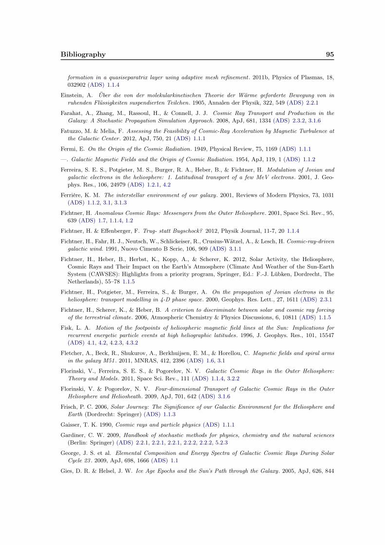
Bibliography 95
formation in a quasiseparatrix layer using adaptive mesh refinement . 2011b, Physics of Plasmas, 18,032902 (ADS) 1.1.4
Einstein, A. Über die von der molekularkinetischen Theorie der Wärme geforderte Bewegung von inruhenden Flüssigkeiten suspendierten Teilchen. 1905, Annalen der Physik, 322, 549 (ADS) 2.2.1
Farahat, A., Zhang, M., Rassoul, H., & Connell, J. J. Cosmic Ray Transport and Production in theGalaxy: A Stochastic Propagation Simulation Approach. 2008, ApJ, 681, 1334 (ADS) 2.3.2, 3.1.6
Fatuzzo, M. & Melia, F. Assessing the Feasibility of Cosmic-Ray Acceleration by Magnetic Turbulence atthe Galactic Center . 2012, ApJ, 750, 21 (ADS) 1.1.1
Fermi, E. On the Origin of the Cosmic Radiation. 1949, Physical Review, 75, 1169 (ADS) 1.1.1
—. Galactic Magnetic Fields and the Origin of Cosmic Radiation. 1954, ApJ, 119, 1 (ADS) 1.1.2
Ferreira, S. E. S., Potgieter, M. S., Burger, R. A., Heber, B., & Fichtner, H. Modulation of Jovian andgalactic electrons in the heliosphere: 1. Latitudinal transport of a few MeV electrons. 2001, J. Geo-phys. Res., 106, 24979 (ADS) 1.2.1, 4.2
Ferrière, K. M. The interstellar environment of our galaxy . 2001, Reviews of Modern Physics, 73, 1031(ADS) 1.1.2, 3.1, 3.1.3
Fichtner, H. Anomalous Cosmic Rays: Messengers from the Outer Heliosphere. 2001, Space Sci. Rev., 95,639 (ADS) 1.7, 1.1.4, 1.2
Fichtner, H. & Effenberger, F. Trug- statt Bugschock? 2012, Physik Journal, 11-7, 20 1.1.4
Fichtner, H., Fahr, H. J., Neutsch, W., Schlickeiser, R., Crusius-Wätzel, A., & Lesch, H. Cosmic-ray-drivengalactic wind. 1991, Nuovo Cimento B Serie, 106, 909 (ADS) 3.1.1
Fichtner, H., Heber, B., Herbst, K., Kopp, A., & Scherer, K. 2012, Solar Activity, the Heliosphere,Cosmic Rays and Their Impact on the Earth’s Atmosphere (Climate And Weather of the Sun-EarthSystem (CAWSES): Highlights from a priority program, Springer, Ed.: F.-J. Lübken, Dordrecht, TheNetherlands), 55–78 1.1.5
Fichtner, H., Potgieter, M., Ferreira, S., & Burger, A. On the propagation of Jovian electrons in theheliosphere: transport modelling in 4-D phase space. 2000, Geophys. Res. Lett., 27, 1611 (ADS) 2.3.1
Fichtner, H., Scherer, K., & Heber, B. A criterion to discriminate between solar and cosmic ray forcingof the terrestrial climate. 2006, Atmospheric Chemistry & Physics Discussions, 6, 10811 (ADS) 1.1.5
Fisk, L. A. Motion of the footpoints of heliospheric magnetic field lines at the Sun: Implications forrecurrent energetic particle events at high heliographic latitudes. 1996, J. Geophys. Res., 101, 15547(ADS) 4.1, 4.2, 4.2.3, 4.3.2
Fletcher, A., Beck, R., Shukurov, A., Berkhuijsen, E. M., & Horellou, C. Magnetic fields and spiral armsin the galaxy M51 . 2011, MNRAS, 412, 2396 (ADS) 1.6, 3.1
Florinski, V., Ferreira, S. E. S., & Pogorelov, N. V. Galactic Cosmic Rays in the Outer Heliosphere:Theory and Models. 2011, Space Sci. Rev., 111 (ADS) 1.1.4, 3.2.2
Florinski, V. & Pogorelov, N. V. Four-dimensional Transport of Galactic Cosmic Rays in the OuterHeliosphere and Heliosheath. 2009, ApJ, 701, 642 (ADS) 3.1.6
Frisch, P. C. 2006, Solar Journey: The Significance of our Galactic Environment for the Heliosphere andEarth (Dordrecht: Springer) (ADS) 1.1.3
Gaisser, T. K. 1990, Cosmic rays and particle physics (ADS) 1.1.1
Gardiner, C. W. 2009, Handbook of stochastic methods for physics, chemistry and the natural sciences(Berlin: Springer) (ADS) 2.2.1, 2.2.1, 2.2.1, 2.2.2, 2.2.2, 5.2.3
George, J. S. et al. Elemental Composition and Energy Spectra of Galactic Cosmic Rays During SolarCycle 23 . 2009, ApJ, 698, 1666 (ADS) 1.1
Gies, D. R. & Helsel, J. W. Ice Age Epochs and the Sun’s Path through the Galaxy . 2005, ApJ, 626, 844

96 Bibliography
(ADS) 1.1.3
Ginzburg, V. L. & Ptuskin, V. S. On the origin of cosmic rays: Some problems in high-energy astrophysics.1976, Reviews of Modern Physics, 48, 161 (ADS) 1.1.1
Ginzburg, V. L. & Syrovatskij, S. I. Cosmic rays in the Galaxy (Introductory Report). 1967, in IAUSymposium, Vol. 31, Radio Astronomy and the Galactic System, ed. H. van Woerden, 411 (ADS) 1.1.1
Gleeson, L. J. & Axford, W. I. Cosmic Rays in the Interplanetary Medium. 1967, ApJ, 149, L115 (ADS)2.1.3
Gorenflo, R., De Fabritiis, G., & Mainardi, F. D iscrete random walk models for symmetric Lévy-Fellerdiffusion processes. 1999, Physica A: Statistical Mechanics and its Applications, 269, 79 5.2
Greisen, K. End to the Cosmic-Ray Spectrum? 1966, Physical Review Letters, 16, 748 (ADS) 1.1.1
Han, J. L. The Galactic magnetic fields. 2006, Journal of Physics Conference Series, 47, 120 (ADS) 3.1.3
Han, J. L., Manchester, R. N., Lyne, A. G., Qiao, G. J., & van Straten, W. Pulsar Rotation Measuresand the Large-Scale Structure of the Galactic Magnetic Field . 2006, ApJ, 642, 868 (ADS) 3.1.3
Hanasz, M. & Lesch, H. Incorporation of cosmic ray transport into the ZEUS MHD code. Application forstudies of Parker instability in the ISM . 2003, A&A, 412, 331 (ADS) 3.1
Hanasz, M., Otmianowska-Mazur, K., Kowal, G., & Lesch, H. Cosmic-ray-driven dynamo in galacticdisks. A parameter study . 2009, A&A, 498, 335 (ADS) 1.2.1, 3.1, 3.3
Heiles, C. & Haverkorn, M. Magnetic Fields in the Multiphase Interstellar Medium. 2012, Space Sci. Rev.,166, 293 (ADS) 3.1.3
Herbst, K., Kopp, A., Heber, B., Steinhilber, F., Fichtner, H., Scherer, K., & Matthiä, D. On the impor-tance of the local interstellar spectrum for the solar modulation parameter . 2010, Journal of GeophysicalResearch (Space Physics), 115, 0 (ADS) 3.2.2
Horbury, T. S., Balogh, A., Forsyth, R. J., & Smith, E. J. Anisotropy of inertial range turbulence in thepolar heliosphere. 1995, Geophys. Res. Lett., 22, 3405 (ADS) 4.2.1
Ilic, M., Liu, F., Turner, I., & Anh, V. Numerical Approximation of a Fractional-In-Space DiffusionEquation, I . 2005, Fractional Calculus and Applied Analysis, 8, 323 5.2.3
Izmodenov, V. V., Malama, Y. G., Ruderman, M. S., Chalov, S. V., Alexashov, D. B., Katushkina,O. A., & Provornikova, E. A. Kinetic-Gasdynamic Modeling of the Heliospheric Interface. 2009,Space Sci. Rev., 146, 329 (ADS) 1.1.4
Jokipii, J. R. Cosmic-Ray Propagation. I. Charged Particles in a Random Magnetic Field . 1966, ApJ,146, 480 (ADS) 2.1.3, 3.1
—. Cosmic-Ray Propagation. II. Diffusion in the Interplanetary Magnetic Field . 1967, ApJ, 149, 405(ADS) 2.1.3, A
—. Propagation of cosmic rays in the solar wind. 1971, Reviews of Geophysics and Space Physics, 9, 27(ADS) 2.2
—. Radial Variation of Magnetic Fluctuations and the Cosmic-Ray Diffusion Tensor in the Solar Wind .1973, ApJ, 182, 585 (ADS) 1.2.1, 4.2
—. Latitudinal heliospheric magnetic field: Stochastic and causal components. 2001, J. Geophys. Res.,106, 15841 (ADS) 4.3
Jokipii, J. R., Kóta, J., Giacalone, J., Horbury, T. S., & Smith, E. J. Interpretation and consequencesof large-scale magnetic variances observed at high heliographic latitude. 1995, Geophys. Res. Lett., 22,3385 (ADS) 4.2
Kahler, S. W. & Vourlidas, A. Fast coronal mass ejection environments and the production of solarenergetic particle events. 2005, Journal of Geophysical Research (Space Physics), 110, 12 (ADS) 1.1.4
Kelly, J., Dalla, S., & Laitinen, T. Cross-field Transport of Solar Energetic Particles in a Large-scale
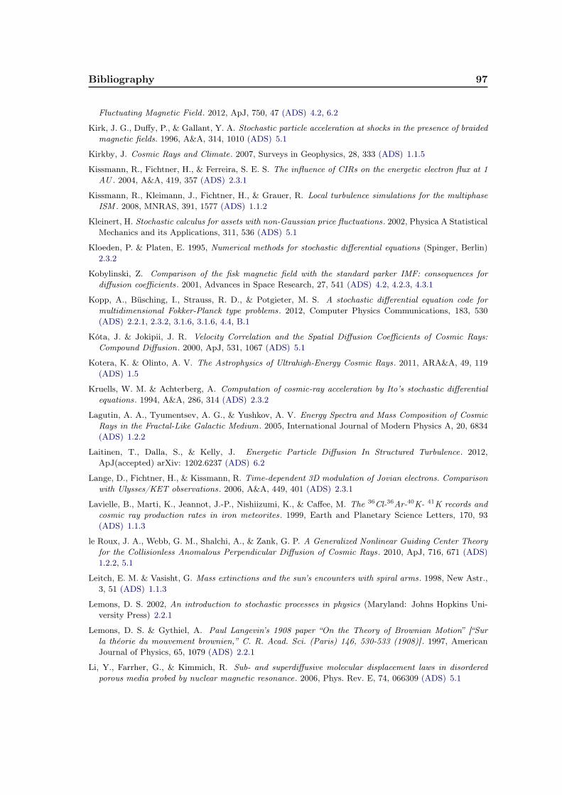
Bibliography 97
Fluctuating Magnetic Field . 2012, ApJ, 750, 47 (ADS) 4.2, 6.2
Kirk, J. G., Duffy, P., & Gallant, Y. A. Stochastic particle acceleration at shocks in the presence of braidedmagnetic fields. 1996, A&A, 314, 1010 (ADS) 5.1
Kirkby, J. Cosmic Rays and Climate. 2007, Surveys in Geophysics, 28, 333 (ADS) 1.1.5
Kissmann, R., Fichtner, H., & Ferreira, S. E. S. The influence of CIRs on the energetic electron flux at 1AU . 2004, A&A, 419, 357 (ADS) 2.3.1
Kissmann, R., Kleimann, J., Fichtner, H., & Grauer, R. Local turbulence simulations for the multiphaseISM . 2008, MNRAS, 391, 1577 (ADS) 1.1.2
Kleinert, H. Stochastic calculus for assets with non-Gaussian price fluctuations. 2002, Physica A StatisticalMechanics and its Applications, 311, 536 (ADS) 5.1
Kloeden, P. & Platen, E. 1995, Numerical methods for stochastic differential equations (Spinger, Berlin)2.3.2
Kobylinski, Z. Comparison of the fisk magnetic field with the standard parker IMF: consequences fordiffusion coefficients. 2001, Advances in Space Research, 27, 541 (ADS) 4.2, 4.2.3, 4.3.1
Kopp, A., Büsching, I., Strauss, R. D., & Potgieter, M. S. A stochastic differential equation code formultidimensional Fokker-Planck type problems. 2012, Computer Physics Communications, 183, 530(ADS) 2.2.1, 2.3.2, 3.1.6, 3.1.6, 4.4, B.1
Kóta, J. & Jokipii, J. R. Velocity Correlation and the Spatial Diffusion Coefficients of Cosmic Rays:Compound Diffusion. 2000, ApJ, 531, 1067 (ADS) 5.1
Kotera, K. & Olinto, A. V. The Astrophysics of Ultrahigh-Energy Cosmic Rays. 2011, ARA&A, 49, 119(ADS) 1.5
Kruells, W. M. & Achterberg, A. Computation of cosmic-ray acceleration by Ito’s stochastic differentialequations. 1994, A&A, 286, 314 (ADS) 2.3.2
Lagutin, A. A., Tyumentsev, A. G., & Yushkov, A. V. Energy Spectra and Mass Composition of CosmicRays in the Fractal-Like Galactic Medium. 2005, International Journal of Modern Physics A, 20, 6834(ADS) 1.2.2
Laitinen, T., Dalla, S., & Kelly, J. Energetic Particle Diffusion In Structured Turbulence. 2012,ApJ(accepted) arXiv: 1202.6237 (ADS) 6.2
Lange, D., Fichtner, H., & Kissmann, R. Time-dependent 3D modulation of Jovian electrons. Comparisonwith Ulysses/KET observations. 2006, A&A, 449, 401 (ADS) 2.3.1
Lavielle, B., Marti, K., Jeannot, J.-P., Nishiizumi, K., & Caffee, M. The 36Cl-36Ar-40K- 41K records andcosmic ray production rates in iron meteorites. 1999, Earth and Planetary Science Letters, 170, 93(ADS) 1.1.3
le Roux, J. A., Webb, G. M., Shalchi, A., & Zank, G. P. A Generalized Nonlinear Guiding Center Theoryfor the Collisionless Anomalous Perpendicular Diffusion of Cosmic Rays. 2010, ApJ, 716, 671 (ADS)1.2.2, 5.1
Leitch, E. M. & Vasisht, G. Mass extinctions and the sun’s encounters with spiral arms. 1998, New Astr.,3, 51 (ADS) 1.1.3
Lemons, D. S. 2002, An introduction to stochastic processes in physics (Maryland: Johns Hopkins Uni-versity Press) 2.2.1
Lemons, D. S. & Gythiel, A. Paul Langevin’s 1908 paper “On the Theory of Brownian Motion” [“Surla théorie du mouvement brownien,” C. R. Acad. Sci. (Paris) 146, 530-533 (1908)] . 1997, AmericanJournal of Physics, 65, 1079 (ADS) 2.2.1
Li, Y., Farrher, G., & Kimmich, R. Sub- and superdiffusive molecular displacement laws in disorderedporous media probed by nuclear magnetic resonance. 2006, Phys. Rev. E, 74, 066309 (ADS) 5.1

98 Bibliography
Lionello, R., Linker, J. A., Mikić, Z., & Riley, P. The Latitudinal Excursion of Coronal Magnetic FieldLines in Response to Differential Rotation: MHD Simulations. 2006, ApJ, 642, L69 (ADS) 4.2
Liouville, J. 1838, Journ. de Math., 3, 349 2.1.1
Litvinenko, Y. E. The Parallel Diffusion Coefficient and Adiabatic Focusing of Cosmic-Ray Particles.2012a, ApJ, 745, 62 (ADS) 2.2.2
—. Effects of Non-isotropic Scattering, Magnetic Helicity, and Adiabatic Focusing on Diffusive Transportof Solar Energetic Particles. 2012b, ApJ, 752, 16 (ADS) 2.2.2, 2.2.2
Magdziarz, M. Fractional Ornstein Uhlenbeck processes. Joseph effect in models with infinite variance.2008, Physica A Statistical Mechanics and its Applications, 387, 123 (ADS) 5.2.3
Magdziarz, M. & Weron, A. Competition between subdiffusion and Lévy flights: A Monte Carlo approach.2007, Phys. Rev. E, 75, 056702 (ADS) 5.2.1, 5.2.1, 5.2.2, 5.2.3
Malyshev, D., Cholis, I., & Gelfand, J. Pulsars versus dark matter interpretation of ATIC/PAMELA.2009, Phys. Rev. D, 80, 063005 (ADS) 1.1.3
Mannheim, K. & Schlickeiser, R. Interactions of cosmic ray nuclei . 1994, A&A, 286, 983 (ADS) 3.1.5
Marcowith, A. & Kirk, J. G. Computation of diffusive shock acceleration using stochastic differentialequations. 1999, A&A, 347, 391 (ADS) 3.1.6
Marris, A. W. & Passman, S. L. Vector fields and flows on developable surfaces. 1969, Archive for RationalMechanics and Analysis, 32, 29 (ADS) 4.3.2
Matsumoto, M. & Nishimura, T. M ersenne twister: a 623-dimensionally equidistributed uniform pseudo-random number generator. 1998, ACM Trans. Model. Comput. Simul., 8, 3 3.1.6, B
Matthaeus, W. H., Qin, G., Bieber, J. W., & Zank, G. P. Nonlinear Collisionless Perpendicular Diffusionof Charged Particles. 2003, ApJ, 590, L53 (ADS) 4.2.2
McComas, D. J., Alexashov, D., Bzowski, M., Fahr, H., Heerikhuisen, J., Izmodenov, V., Lee, M. A.,Möbius, E., Pogorelov, N., Schwadron, N. A., & Zank, G. P. The Heliosphere’s Interstellar Interaction:No Bow Shock . 2012, Science, 336, 1291 (ADS) 1.1.4
McComas, D. J. et al. Global Observations of the Interstellar Interaction from the Interstellar BoundaryExplorer (IBEX). 2009, Science, 326, 959 (ADS) 1.1.4
Medvedev, M. V. & Melott, A. L. Do Extragalactic Cosmic Rays Induce Cycles in Fossil Diversity? 2007,ApJ, 664, 879 (ADS) 1.1.3
Meerschaert, M. M. & Tadjeran, C. Finite difference approximations for fractional advection-dispersionflow equations. 2004, Journal of Computational and Applied Mathematics, 172, 65 (ADS) 5.2, 5.2.3
Metzler, R., Barkai, E., & Klafter, J. Deriving fractional Fokker-Planck equations from a generalisedmaster equation. 1999, EPL (Europhysics Letters), 46, 431 (ADS) 5.2
Metzler, R. & Klafter, J. The random walk’s guide to anomalous diffusion: a fractional dynamics approach.2000, Phys. Rep., 339, 1 (ADS) 1.2.2, 5.1, 5.2
—. TOPICAL REVIEW: The restaurant at the end of the random walk: recent developments in thedescription of anomalous transport by fractional dynamics. 2004, Journal of Physics A MathematicalGeneral, 37, 161 (ADS) 5.1
Nieva, M.-F. & Przybilla, N. Present-day cosmic abundances. A comprehensive study of nearby early B-type stars and implications for stellar and Galactic evolution and interstellar dust models. 2012, A&A,539, A143 (ADS) 3.2.3
Opher, M., Richardson, J. D., Toth, G., & Gombosi, T. I. Confronting Observations and Modeling: TheRole of the Interstellar Magnetic Field in Voyager 1 and 2 Asymmetries. 2009, Space Sci. Rev., 143,43 (ADS) 1.1.4
Oughton, S., Matthaeus, W. H., Smith, C. W., Breech, B., & Isenberg, P. A. Transport of solar wind

Bibliography 99
fluctuations: A two-component model . 2011, J. Geophys. Res., 116, 8105 (ADS) 4.2.2
Overholt, A. C., Melott, A. L., & Pohl, M. Testing the Link Between Terrestrial Climate Change andGalactic Spiral Arm Transit . 2009, ApJ, 705, L101 (ADS) 1.1.3, 3.1
Parker, E. N. Dynamics of the Interplanetary Gas and Magnetic Fields. 1958, ApJ, 128, 664 (ADS) 1.1.4,4.3
—. The passage of energetic charged particles through interplanetary space. 1965a, Planet. Space Sci., 13,9 (ADS) 1.2.1, 2.1.3, 4.4
—. Dynamical Theory of the Solar Wind . 1965c, Space Sci. Rev., 4, 666 (ADS) 1.1.4
—. The Generation of Magnetic Fields in Astrophysical Bodies. I. The Dynamo Equations. 1970, ApJ,162, 665 (ADS) 3.1.3
—. The Generation of Magnetic Fields in Astrophysical Bodies. II. The Galactic Field . 1971, ApJ, 163,255 (ADS) 3.1.3
—. 1979, Cosmical magnetic fields: Their origin and their activity (New York: Oxford University Press)(ADS) 3.1.3
Parzen, E. On Estimation of a Probability Density Function and Mode. 1962, The Annals of MathematicalStatistics, 33, pp. 1065 2.3.2
Pei, C., Bieber, J. W., Burger, R. A., & Clem, J. A general time-dependent stochastic method for solvingParker’s transport equation in spherical coordinates. 2010, Journal of Geophysical Research (SpacePhysics), 115, 12107 (ADS) 2.3.2, 3.1.6
Perri, S. & Zimbardo, G. Evidence of Superdiffusive Transport of Electrons Accelerated at InterplanetaryShocks. 2007, ApJ, 671, L177 (ADS) 5.1
—. Observations of anomalous transport of energetic electrons in the heliosphere. 2008a, Astrophysics andSpace Sciences Transactions, 4, 27 (ADS) 5.1
—. Superdiffusive transport of electrons accelerated at corotating interaction regions. 2008b, Journal ofGeophysical Research (Space Physics), 113, 3107 (ADS) 5.1
—. Ion Superdiffusion at the Solar Wind Termination Shock . 2009, ApJ, 693, L118 (ADS) 1.2.2, 5.1, 5.3
—. Magnetic Variances and Pitch-angle Scattering Times Upstream of Interplanetary Shocks. 2012a, ApJ,754, 8 (ADS) 5.1
—. Superdiffusive Shock Acceleration. 2012b, ApJ, 750, 87 (ADS) 5.1, 5.3.1
Piessens, R., deDoncker Kapenga, E., Überhuber, C., & Kahaner, D. 1983, QUADPACK, A SubroutinePackage for Automatic Integration (Berlin: Springer) A
Podlubny, I. 1999, Fractional Differential Equations (San Diego: Academic Press) 5.2
Pogorelov, N. V., Heerikhuisen, J., Zank, G. P., Borovikov, S. N., Frisch, P. C., & McComas, D. J.Interstellar Boundary Explorer Measurements and Magnetic Field in the Vicinity of the Heliopause.2011, ApJ, 742, 104 (ADS) 1.1.4
Potgieter, M. S. Cosmic Rays in the Inner Heliosphere: Insights from Observations, Theory and Models.2011, Space Sci. Rev., 107 (ADS) 1.1.4, 3.1
Potgieter, M. S., Haasbroek, L. J., Ferrando, P., & Heber, B. The modelling of the latitude dependence ofcosmic ray protons and electrons in the inner heliosphere. 1997, Advances in Space Research, 19, 917(ADS) 4.2, 4.2.2
Prantzos, N. On the origin and composition of Galactic cosmic rays. 2012, A&A, 538, A80 (ADS) 1.1.1
Ptuskin, V. S., Voelk, H. J., Zirakashvili, V. N., & Breitschwerdt, D. Transport of relativistic nucleons ina galactic wind driven by cosmic rays. 1997, A&A, 321, 434 (ADS) 3.1.1
Putze, A., Maurin, D., & Donato, F. p, He, and C to Fe cosmic-ray primary fluxes in diffusion models.
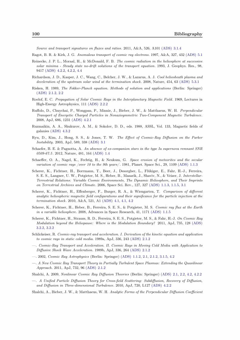
100 Bibliography
Source and transport signatures on fluxes and ratios. 2011, A&A, 526, A101 (ADS) 3.1.4
Ragot, B. R. & Kirk, J. G. Anomalous transport of cosmic ray electrons. 1997, A&A, 327, 432 (ADS) 5.1
Reinecke, J. P. L., Moraal, H., & McDonald, F. B. The cosmic radiation in the heliosphere at successivesolar minima - Steady state no-drift solutions of the transport equation. 1993, J. Geophys. Res., 98,9417 (ADS) 4.2.2, 4.2.2, 4.4
Richardson, J. D., Kasper, J. C., Wang, C., Belcher, J. W., & Lazarus, A. J. Cool heliosheath plasma anddeceleration of the upstream solar wind at the termination shock . 2008, Nature, 454, 63 (ADS) 5.3.1
Risken, H. 1989, The Fokker-Planck equation. Methods of solution and applications (Berlin: Springer)(ADS) 2.1.2, 2.2
Roelof, E. C. Propagation of Solar Cosmic Rays in the Interplanetary Magnetic Field . 1969, Lectures inHigh-Energy Astrophysics, 111 (ADS) 2.2.2
Ruffolo, D., Chuychai, P., Wongpan, P., Minnie, J., Bieber, J. W., & Matthaeus, W. H. PerpendicularTransport of Energetic Charged Particles in Nonaxisymmetric Two-Component Magnetic Turbulence.2008, ApJ, 686, 1231 (ADS) 4.2.1
Ruzmaikin, A. A., Shukurov, A. M., & Sokolov, D. D., eds. 1988, ASSL, Vol. 133, Magnetic fields ofgalaxies (ADS) 4.3.2
Ryu, D., Kim, J., Hong, S. S., & Jones, T. W. The Effect of Cosmic-Ray Diffusion on the ParkerInstability . 2003, ApJ, 589, 338 (ADS) 3.1
Schaefer, B. E. & Pagnotta, A. An absence of ex-companion stars in the type Ia supernova remnant SNR0509-67.5 . 2012, Nature, 481, 164 (ADS) 1.4
Schaeffer, O. A., Nagel, K., Fechtig, H., & Neukum, G. Space erosion of meteorites and the secularvariation of cosmic rays /over 10 to the 9th years/ . 1981, Planet. Space Sci., 29, 1109 (ADS) 1.1.3
Scherer, K., Fichtner, H., Borrmann, T., Beer, J., Desorgher, L., Flükiger, E., Fahr, H.-J., Ferreira,S. E. S., Langner, U. W., Potgieter, M. S., Heber, B., Masarik, J., Shaviv, N., & Veizer, J. Interstellar-Terrestrial Relations: Variable Cosmic Environments, The Dynamic Heliosphere, and Their Imprintson Terrestrial Archives and Climate. 2006, Space Sci. Rev., 127, 327 (ADS) 1.1.3, 1.1.5, 3.1
Scherer, K., Fichtner, H., Effenberger, F., Burger, R. A., & Wiengarten, T. Comparison of differentanalytic heliospheric magnetic field configurations and their significance for the particle injection at thetermination shock . 2010, A&A, 521, A1 (ADS) 4.1, 4.1, 4.2
Scherer, K., Fichtner, H., Heber, B., Ferreira, S. E. S., & Potgieter, M. S. Cosmic ray flux at the Earthin a variable heliosphere. 2008, Advances in Space Research, 41, 1171 (ADS) 1.1.5
Scherer, K., Fichtner, H., Strauss, R. D., Ferreira, S. E. S., Potgieter, M. S., & Fahr, H.-J. On Cosmic RayModulation beyond the Heliopause: Where is the Modulation Boundary? 2011, ApJ, 735, 128 (ADS)3.2.2, 3.2.2
Schlickeiser, R. Cosmic-ray transport and acceleration. I. Derivation of the kinetic equation and applicationto cosmic rays in static cold media. 1989a, ApJ, 336, 243 (ADS) 2.1.2
—. Cosmic-Ray Transport and Acceleration. II. Cosmic Rays in Moving Cold Media with Application toDiffusive Shock Wave Acceleration. 1989b, ApJ, 336, 264 (ADS) 2.1.2
—. 2002, Cosmic Ray Astrophysics (Berlin: Springer) (ADS) 1.1.2, 2.1, 2.1.2, 3.1.5, 4.2
—. A New Cosmic Ray Transport Theory in Partially Turbulent Space Plasmas: Extending the QuasilinearApproach. 2011, ApJ, 732, 96 (ADS) 2.1.2
Shalchi, A. 2009, Nonlinear Cosmic Ray Diffusion Theories (Berlin: Springer) (ADS) 2.1, 2.2, 4.2, 4.2.2
—. A Unified Particle Diffusion Theory for Cross-field Scattering: Subdiffusion, Recovery of Diffusion,and Diffusion in Three-dimensional Turbulence. 2010, ApJ, 720, L127 (ADS) 4.2.2
Shalchi, A., Bieber, J. W., & Matthaeus, W. H. Analytic Forms of the Perpendicular Diffusion Coefficient

Bibliography 101
in Magnetostatic Turbulence. 2004, ApJ, 604, 675 (ADS) 4.2.2
Shalchi, A. & Büsching, I. Influence of Turbulence Dissipation Effects on the Propagation of Low-energyCosmic Rays in the Galaxy . 2010, ApJ, 725, 2110 (ADS) 3.1.2
Shalchi, A., Büsching, I., Lazarian, A., & Schlickeiser, R. Perpendicular Diffusion of Cosmic Rays for aGoldreich-Sridhar Spectrum. 2010a, ApJ, 725, 2117 (ADS) 1.2.1, 3.1, 3.1.2
Shalchi, A. & Kourakis, I. A new theory for perpendicular transport of cosmic rays. 2007, A&A, 470, 405(ADS) 5.1
Shalchi, A., Kourakis, I., & Dosch, A. Generalized compound transport of charged particles in turbulentmagnetized plasmas. 2007, Journal of Physics A Mathematical General, 40, 11191 (ADS) 5.1
Shalchi, A., Li, G., & Zank, G. P. Analytic forms of the perpendicular cosmic ray diffusion coefficient foran arbitrary turbulence spectrum and applications on transport of Galactic protons and acceleration atinterplanetary shocks. 2010b, Ap&SS, 325, 99 (ADS) 4.2.2
Shalchi, A., Webb, G. M., & le Roux, J. A. Parallel transport of cosmic rays for non-diffusive pitch-anglescattering: I. Using the standard Fokker-Planck equation. 2012, Phys. Scr, 85, 065901 (ADS) 5.1
Shaviv, N. & Veizer, J. C elestial driver of Phanerozoic climate? 2003, GSA Today, 13, 4 1.1.5, 3.1, 3.3
Shaviv, N. J. Cosmic Ray Diffusion from the Galactic Spiral Arms, Iron Meteorites, and a PossibleClimatic Connection. 2002, Physical Review Letters, 89, 051102 (ADS) 1.1.3, 3.1
—. The spiral structure of the Milky Way, cosmic rays, and ice age epochs on Earth. 2003, New Astr., 8,39 (ADS) 1.1.3, 3.1.4
Shaviv, N. J., Nakar, E., & Piran, T. Inhomogeneity in Cosmic Ray Sources as the Origin of the ElectronSpectrum and the PAMELA Anomaly . 2009, Physical Review Letters, 103, 111302 (ADS) 1.1.3
Snodin, A. P., Brandenburg, A., Mee, A. J., & Shukurov, A. Simulating field-aligned diffusion of a cosmicray gas. 2006, MNRAS, 373, 643 (ADS) 3.1
Stanev, T. 2004, High Energy Cosmic Rays (Chichester: Springer) (ADS) 2.1
Stawicki, O., Fichtner, H., & Schlickeiser, R. The Parker propagator for spherical solar modulation. 2000,A&A, 358, 347 (ADS) A
Sternal, O., Engelbrecht, N. E., Burger, R. A., Ferreira, S. E. S., Fichtner, H., Heber, B., Kopp, A.,Potgieter, M. S., & Scherer, K. Possible Evidence for a Fisk-type Heliospheric Magnetic Field. I.Analyzing Ulysses/KET Electron Observations. 2011, ApJ, 741, 23 (ADS) 2.3.1, 4.1, 4.1, 4.2, 4.3.2
Strauss, R. D., Potgieter, M. S., Büsching, I., & Kopp, A. Modeling the Modulation of Galactic and JovianElectrons by Stochastic Processes. 2011a, ApJ, 735, 83 (ADS) 2.3.2, 3.1.6, 3.1.6, 4.4
—. Modelling heliospheric current sheet drift in stochastic cosmic ray transport models. 2012, Ap&SS,339, 223 (ADS) 2.3.2
Strauss, R. D., Potgieter, M. S., Kopp, A., & Büsching, I. On the propagation times and energy lossesof cosmic rays in the heliosphere. 2011b, Journal of Geophysical Research (Space Physics), 116, 12105(ADS) 2.3.2, 4.4
Strong, A. W., Moskalenko, I. V., Porter, T. A., Jóhannesson, G., Orlando, E., & Digel, S. W. GALPROP:Code for Cosmic-ray Transport and Diffuse Emission Production. 2010, Astrophysics Source CodeLibrary, 10028 (ADS) 3.1, 6.2
Strong, A. W., Moskalenko, I. V., & Ptuskin, V. S. Cosmic-Ray Propagation and Interactions in theGalaxy . 2007, Annual Review of Nuclear and Particle Science, 57, 285 (ADS) 3.1, 3.1.1
Sugiyama, T. & Shiota, D. Sign for Super-diffusive Transport of Energetic Ions Associated with a Coronal-mass-ejection-driven Interplanetary Shock . 2011, ApJ, 731, L34 (ADS) 1.2.2, 5.1
Svensmark, H. Imprint of Galactic dynamics on Earth’s climate. 2006, Astronomische Nachrichten, 327,866 (ADS) 1.1.3
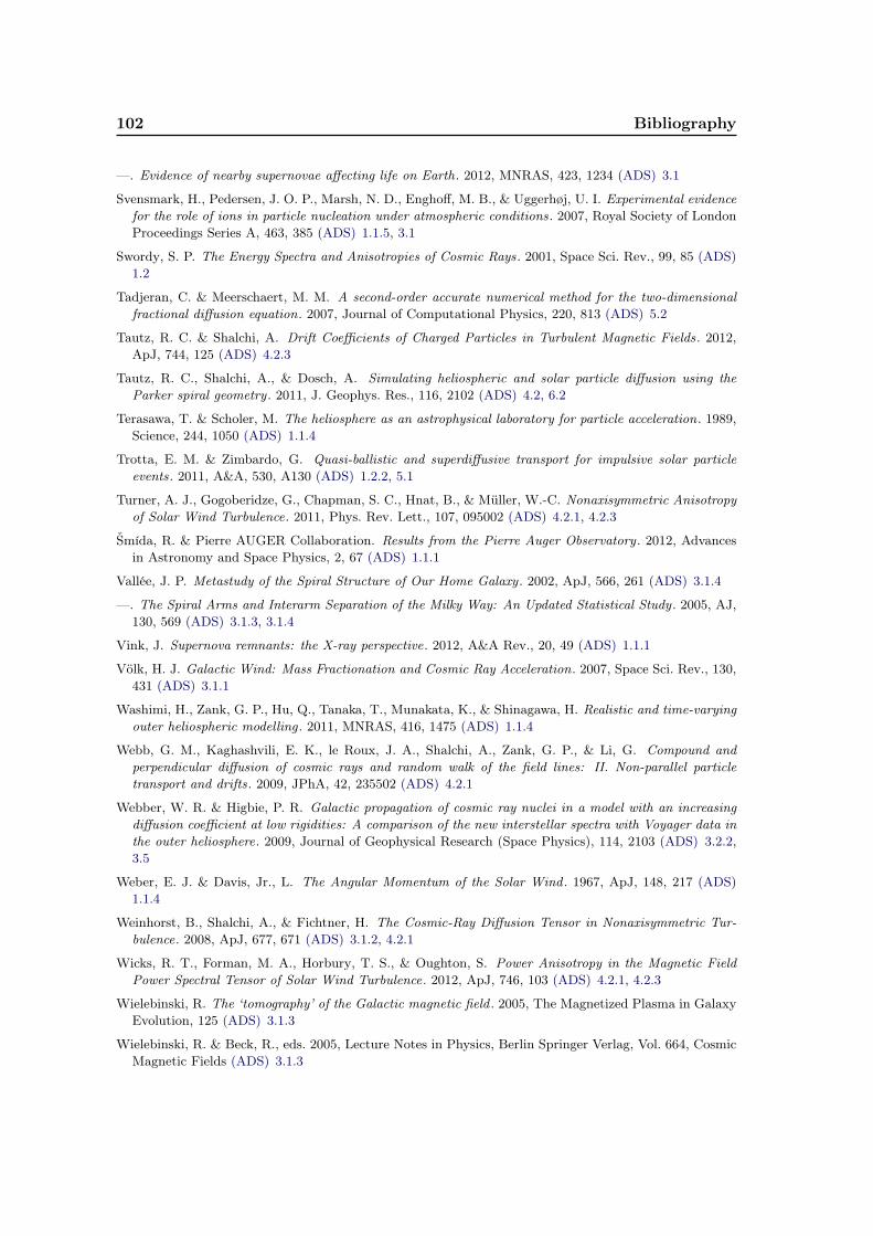
102 Bibliography
—. Evidence of nearby supernovae affecting life on Earth. 2012, MNRAS, 423, 1234 (ADS) 3.1
Svensmark, H., Pedersen, J. O. P., Marsh, N. D., Enghoff, M. B., & Uggerhøj, U. I. Experimental evidencefor the role of ions in particle nucleation under atmospheric conditions. 2007, Royal Society of LondonProceedings Series A, 463, 385 (ADS) 1.1.5, 3.1
Swordy, S. P. The Energy Spectra and Anisotropies of Cosmic Rays. 2001, Space Sci. Rev., 99, 85 (ADS)1.2
Tadjeran, C. & Meerschaert, M. M. A second-order accurate numerical method for the two-dimensionalfractional diffusion equation. 2007, Journal of Computational Physics, 220, 813 (ADS) 5.2
Tautz, R. C. & Shalchi, A. Drift Coefficients of Charged Particles in Turbulent Magnetic Fields. 2012,ApJ, 744, 125 (ADS) 4.2.3
Tautz, R. C., Shalchi, A., & Dosch, A. Simulating heliospheric and solar particle diffusion using theParker spiral geometry . 2011, J. Geophys. Res., 116, 2102 (ADS) 4.2, 6.2
Terasawa, T. & Scholer, M. The heliosphere as an astrophysical laboratory for particle acceleration. 1989,Science, 244, 1050 (ADS) 1.1.4
Trotta, E. M. & Zimbardo, G. Quasi-ballistic and superdiffusive transport for impulsive solar particleevents. 2011, A&A, 530, A130 (ADS) 1.2.2, 5.1
Turner, A. J., Gogoberidze, G., Chapman, S. C., Hnat, B., & Müller, W.-C. Nonaxisymmetric Anisotropyof Solar Wind Turbulence. 2011, Phys. Rev. Lett., 107, 095002 (ADS) 4.2.1, 4.2.3
Šmída, R. & Pierre AUGER Collaboration. Results from the Pierre Auger Observatory . 2012, Advancesin Astronomy and Space Physics, 2, 67 (ADS) 1.1.1
Vallée, J. P. Metastudy of the Spiral Structure of Our Home Galaxy . 2002, ApJ, 566, 261 (ADS) 3.1.4
—. The Spiral Arms and Interarm Separation of the Milky Way: An Updated Statistical Study . 2005, AJ,130, 569 (ADS) 3.1.3, 3.1.4
Vink, J. Supernova remnants: the X-ray perspective. 2012, A&A Rev., 20, 49 (ADS) 1.1.1
Völk, H. J. Galactic Wind: Mass Fractionation and Cosmic Ray Acceleration. 2007, Space Sci. Rev., 130,431 (ADS) 3.1.1
Washimi, H., Zank, G. P., Hu, Q., Tanaka, T., Munakata, K., & Shinagawa, H. Realistic and time-varyingouter heliospheric modelling . 2011, MNRAS, 416, 1475 (ADS) 1.1.4
Webb, G. M., Kaghashvili, E. K., le Roux, J. A., Shalchi, A., Zank, G. P., & Li, G. Compound andperpendicular diffusion of cosmic rays and random walk of the field lines: II. Non-parallel particletransport and drifts. 2009, JPhA, 42, 235502 (ADS) 4.2.1
Webber, W. R. & Higbie, P. R. Galactic propagation of cosmic ray nuclei in a model with an increasingdiffusion coefficient at low rigidities: A comparison of the new interstellar spectra with Voyager data inthe outer heliosphere. 2009, Journal of Geophysical Research (Space Physics), 114, 2103 (ADS) 3.2.2,3.5
Weber, E. J. & Davis, Jr., L. The Angular Momentum of the Solar Wind . 1967, ApJ, 148, 217 (ADS)1.1.4
Weinhorst, B., Shalchi, A., & Fichtner, H. The Cosmic-Ray Diffusion Tensor in Nonaxisymmetric Tur-bulence. 2008, ApJ, 677, 671 (ADS) 3.1.2, 4.2.1
Wicks, R. T., Forman, M. A., Horbury, T. S., & Oughton, S. Power Anisotropy in the Magnetic FieldPower Spectral Tensor of Solar Wind Turbulence. 2012, ApJ, 746, 103 (ADS) 4.2.1, 4.2.3
Wielebinski, R. The ‘tomography’ of the Galactic magnetic field . 2005, The Magnetized Plasma in GalaxyEvolution, 125 (ADS) 3.1.3
Wielebinski, R. & Beck, R., eds. 2005, Lecture Notes in Physics, Berlin Springer Verlag, Vol. 664, CosmicMagnetic Fields (ADS) 3.1.3
Bibliography 103
Yeghikyan, A. & Fahr, H. Effects induced by the passage of the Sun through dense molecular clouds. I.Flow outside of the compressed heliosphere. 2004, A&A, 415, 763 (ADS) 1.1.3
Zatsepin, G. T. & Kuz’min, V. A. Upper Limit of the Spectrum of Cosmic Rays. 1966, Soviet Journal ofExperimental and Theoretical Physics Letters, 4, 78 (ADS) 1.1.1
Zhang, M. A Path Integral Approach to the Theory of Heliospheric Cosmic-Ray Modulation. 1999b, ApJ,510, 715 (ADS) 2.2
—. A Markov Stochastic Process Theory of Cosmic-Ray Modulation. 1999a, ApJ, 513, 409 (ADS) 2.3.2,3.1.6
Zimbardo, G., Perri, S., Pommois, P., & Veltri, P. Anomalous particle transport in the heliosphere. 2012,Advances in Space Research, 49, 1633 (ADS) 5.1
Zumofen, G. & Klafter, J. Scale-invariant motion in intermittent chaotic systems. 1993, Phys. Rev. E,47, 851 (ADS) 5.3


Epilog
“Thousands of years ago tribes of human beings suffered great privations in the struggleto survive. In this struggle it was important not only to be able to handle a club, but alsoto possess the ability to think reasonably, to take care of the knowledge and experiencegarnered by the tribe, and to develop the links that would provide cooperation withother tribes. Today the entire human race is faced with a similar test. In infinite spacemany civilizations are bound to exist, among them civilizations that are also wiser andmore "successful" than ours. I support the cosmological hypothesis which states that thedevelopment of the universe is repeated in its basic features an infinite number of times. Inaccordance with this, other civilizations, including more "successful" ones, should exist aninfinite number of times on the "preceding" and the "following" pages of the Book of theUniverse. Yet this should not minimize our sacred endeavors in this world of ours, where,like faint glimmers of light in the dark, we have emerged for a moment from the nothingnessof dark unconsciousness of material existence. We must make good the demands of reasonand create a life worthy of ourselves and of the goals we only dimly perceive.”(Andrei Sakharov, Nobel Peace Prize Lecture, December 11, 1975)