Inflationary Perturbations in Anisotropic, Shear-Free Universes

Thiago S. Pereira,1, 2, ∗ Saulo Carneiro,3, 4 and Guillermo A. Mena Marugan5

1Departamento de Física, Universidade Estadual de Londrina,

86051-990, Londrina, Paraná, Brazil2Institute of Theoretical Astrophysics,

University of Oslo, M-0315 Oslo, Norway3Instituto de Física, Universidade Federal da Bahia, 40210-340, Salvador, Bahia, Brazil

4International Centre for Theoretical Physics,

Strada Costiera 11, 34151, Trieste, Italy.b

5Instituto de Estructura de la Materia,

IEM-CSIC, Serrano 121, 28006 Madrid, Spain

(Dated: March 12, 2012)

AbstractIn this work, the linear and gauge-invariant theory of cosmological perturbations in a class of

anisotropic and shear-free spacetimes is developed. After constructing an explicit set of complete

eigenfunctions in terms of which perturbations can be expanded, we identify the effective degrees

of freedom during a generic slow-roll inflationary phase. These correspond to the anisotropic equiv-

alent of the standard Mukhanov-Sasaki variables. The associated equations of motion present a

remarkable resemblance to those found in perturbed Friedmann-Robertson-Walker spacetimes with

curvature, apart from the spectrum of the Laplacian, which exhibits the characteristic frequencies of

the underlying geometry. In particular, it is found that the perturbations cannot develop arbitrarily

large super-Hubble modes.

PACS numbers: 98.80.Jk,04.25.Nx,98.80.Cq

b Associate Member∗ tspereira@uel.br

1

arX

iv:1

203.

2072

v1 [

astr

o-ph

.CO

] 9

Mar

201

2

I. INTRODUCTION

The unprecedented isotropy of the cosmic microwave background radiation revealed by

modern CMB experiments is – justifiably enough – usually taken as an indication that

we inhabit an isotropic universe. Together with the apparent (but far more debatable)

homogeneity of matter distribution at scales & 100h−1Mpc, this observation suggests a

generalization of the Copernican principle: our universe is, on average, homogeneous and

isotropic. At present, the Copernican principle remains a hallmark of cosmology, and its

modification would profoundly alter the way we understand the physical universe. As a

matter of fact, challenges to this scenario have largely boosted research in cosmology in the

past, and will certainly do so in the foreseeable future.

In the last decade, new possibilities for a different approach to the cosmological principle

have emerged from two different types of observations. On the one hand, the detection of

the accelerated expansion of the universe [1–3] has motivated dark-energy-free cosmological

models in which our (allegedly) privileged position in the universe would be perceived as

a global cosmic acceleration [4, 5]. On the other hand, discovered large-angles Cosmic

Microwave Background (CMB) anomalies are being interpreted as a manifestation of a

preferred direction in the universe (see Ref. [6] for a recent review). Regardless of which

description might turn out to be the best, these investigations are certainly well founded

from the observational point of view – not to mention that they constitute a necessary step

to be faced in the so-called era of precision cosmology.

From a theoretical perspective, it is legitimate to ask when one can establish a one-to-one

relation between our observations and the symmetries of the universe we live in. Although

a homogeneous and isotropic universe would certainly lead to the observed CMB, is the

converse true? Actually, Ehlers, Geren and Sachs (EGS) proved that the converse holds in

an expanding universe provided that the isotropic CMB is measured by fundamental ob-

servers in a dust universe [7]. However, there are important counterexamples which allow

the engineering of a richer class of models without jeopardizing well-established cosmolog-

ical observations [8–10]. The theorem demonstrated by EGS admits generalizations to a

matter content given by a generic perfect fluid [8], and for an almost isotropic CMB [11],

case for which the associated geometry is only approximately homogeneous and isotropic.

But, how can we phenomenologically conceive an anisotropic model of the universe in which

2

basic observables, like for instance the redshift, remain isotropic, at least at dominant or-

der? One example was proposed by Mimoso and Crawford in 1993 [12]. They showed that

some anisotropic spacetimes, namely Bianchi type-III (BIII) and Kantowski-Sachs (KS)

spacetimes, admit a shear-free expansion in which the scale factor has the same dynam-

ics as a spatially curved Friedmann-Robertson-Walker (FRW) universe, provided that the

anisotropic stress-tensor of the cosmological budget is in direct proportion to the electric

part of the Weyl tensor. Since the dynamics is governed by a single scale factor, the met-

ric can be brought to a conformally static form. It then follows by another EGS result

that the radiation will be isotropic, in accordance with basic observations [7] (see also [10]).

Further and independent developments have shown that this scenario can also be realized

by endowing the universe with other forms of matter fields. In Ref. [13], for example, a

shear-free model with anisotropic curvature was constructed by means of a two-form field.

Another interesting possibility was proposed in Ref. [14] (and further discussed in Ref. [15]),

where a massless and anisotropic scalar field was used to counterbalance the curvature of a

BIII universe, producing an anisotropic model with a FRW-like background dynamics. This

latter example is particularly interesting, given the role that scalar fields play in modeling

early-universe physics.

Evidently, this alternate scenario may become appealing and competitive only if one is

able to extract distinctive cosmological signatures from it. A possible observable at the

level of the background geometry is the luminosity distance function: because the geome-

try traversed by photons along our line of sight is characterized by an anisotropic (spatial)

curvature, the luminosity distance function will not have a direct correspondence to the

standard one used in FRW models. One can then envisage a setting in which supernova sur-

veys can be used to detect anisotropic modulations of the luminosity function [13], therefore

rendering the proposed model falsifiable. However, if one wants to confront this theoretical

scenario against cosmological data, then a much broader class of observables can be attained

by considering perturbation theory, rather than focusing on the background. In particular,

the whole framework of the inflationary era and its connection to structure formation pro-

vides a vast arena within which one can discuss the physical consequences of anisotropic

models with isotropic expansion and put them to the test.

The theory of linear perturbations in non-FRW cosmological backgrounds has been an

active field of research by its own, where many different models have been studied. The

3

case of isotropic and inhomogeneous Lemaître-Tolman-Bondi spacetimes, for example, has

been recently worked out in Ref. [16], while the theory of perturbations in homogeneous and

globally anisotropic Bianchi I spacetimes has been presented in Refs. [17–19]. Quite inde-

pendently, the dynamics of linear perturbations in spatially curved anisotropic backgrounds

has been investigated in Ref. [20], where the BIII case has been considered, and also in Ref.

[21], where both the BIII and KS cases have been analyzed.

This paper presents the formalism necessary to extract the signatures that shear-free

anisotropic models of the BIII family would generically produce in linear cosmological per-

turbations, specialized to situations where the universe is dominated by a slowly-varying

scalar field, as it typically happens during inflation. With this aim, as well as to make more

precise statements such as “up to conditions on the behavior at infinity”, which are usually

employed in a rather vague sense, we introduce an explicit set of complete eigenfunctions

in terms of which perturbations can be expanded. This is a crucial step in perturbation

theory that is sometimes overlooked in the literature, and unavoidable if we want to apply

perturbation theory to specific cosmological models. To the best of our knowledge, these

eigenfunctions have not been considered elsewhere.

As we will show, during a generic slow-roll inflationary phase, the dynamics of the per-

turbations can be described by effective degrees of freedom which have a remarkable re-

semblance to the standard Mukhanov-Sasaki (MS) variables [22, 23]. However, since the

eigenmodes of the Laplacian on the spatial sections are not given by standard plane-waves,

we might expect non-trivial features in the morphology of both the temperature and matter

fields of the universe. A particular signature which arises immediately from the spectrum

of the Laplacian is the obstruction to have arbitrarily large super-Hubble modes. Because

the curvature naturally introduces a spatial scale, the largest possible wave modes will be

comparable to this scale. We also comment on the possibility of detecting specific features

of shear-free anisotropy in the spectrum of gravitational waves.

This paper is structured as follows. We begin by reviewing the fundamental ideas behind

anisotropic shear-free spacetimes in Sec. II, where we also introduce basic notations and

definitions. In Sec. III we discuss the appropriate mode decomposition of the perturbations

and use it to construct gauge-invariant variables. We close this section by determining a

convenient basis of eigenfunctions of the Laplace operator. The dynamical equations of the

cosmological perturbations are presented in Sec. IV, where we also construct the anisotropic

4

equivalent of the MS variables. We conclude in Sec. V. In this work we will adopt units such

that c = 1 = 8πG, and spacetime signature (−,+,+,+). We follow the standard convention

that Greek and Latin indices label spacetime and spatial coordinates, respectively. The

spacetimes we will consider have a residual symmetry along one direction. We choose this

preferred direction to lie along the z-axis and let the indices a, b, c run from 1 to 2, so as

to span the xy-plane.

II. SHEAR-FREE BACKGROUND DYNAMICS

The simplest example of anisotropic universe is the one described by a Bianchi I spacetime.

Since in this family of models the shear is entirely due to the anisotropic expansion of the

universe, the spacetime cannot be both anisotropic and shear-free. This behavior is of

course expected, since Bianchi I models contain the flat FRW case in the shear-free limit.

The possibility of having anisotropic shear-free models with isotropic expansion relies on

the fact that some anisotropic spacetimes do not possess a FRW limit. In these cases, the

anisotropy of the space does not have to be encoded in the shear, but can instead be caused

by imperfections of other kind in the fluid filling the universe.

An example of such spacetime is found in the BIII type. The BIII spacetime in question

is spatially curved and possesses residual isotropy with respect to one direction. We choose

the preferred axis of symmetry to point along the z direction. Spatial sections are described

by the direct product of the real line with a pseudo-sphere, R×H2, thus providing a space

with negative constant curvature. In this work we will adopt a coordinate system in which

the shear-free BIII metric can be written as:

ds2 = a(η)2(−dη2 + γabdx

adxb + dz2), (1)

where a(η) is the isotropic scale factor, η =∫

dt/a is the conformal time, and γab is the

standard metric of H2, which in a convenient coordinate system xa = x, y reads:

γabdxadxb = dx2 + e2xdy2 . (2)

Following [14], we will consider a matter sector composed by the standard inflaton field ϕ

5

plus a massless scalar field ϑ:

T µ(ϕ) ν = ∂µϕ∂νϕ− δµν(

1

2∂λϕ∂λϕ+ V (ϕ)

), (3)

T µ(ϑ) ν = ∂µϑ∂νϑ− δµν(

1

2∂λϑ∂λϑ

). (4)

The inflaton field being homogeneous, ϕ = ϕ(η), satisfies the standard Klein-Gordon equa-

tion:

ϕ′′ + 2Hϕ′ + a2V,ϕ = 0 . (5)

The prime denotes the derivative with respect to the conformal time. The massless field, on

the other hand, obeys

ϑ′′ + 2Hϑ′ −∇2ϑ = 0 . (6)

Here, ∇2 = DaDa + ∂23 and Da is the covariant derivative compatible with γab. It is easy

to check that the choice ϑ = Cz, where C is an arbitrary constant, not only solves Eq. (6),

but also produces a diagonal energy-momentum tensor:

ρ(ϑ) = p⊥(ϑ) = −p‖(ϑ) =C2

2a2,

where p⊥(ϑ) and p‖(ϑ) represent the pressures perpendicular and parallel to the xy-plane, re-

spectively. With these definitions, we can proceed and obtain Einstein equations:

3H2 = a2ρ(ϕ) +C2

2+ 1 , (7)

H2 + 2H′ = −a2p(ϕ) +C2

2, (8)

H2 + 2H′ = −a2p(ϕ) −C2

2+ 1 . (9)

It is then clear that if we choose C2 = 1,1 Eqs. (8) and (9) turn out to coincide, while

the whole system of equations becomes the standard Friedmann equations with curvature

κ = −1/2:

H2 =1

3

(ϕ′2

2+ a2V (ϕ)

)− κ , (10)

H′ = −1

3(ϕ′2 − a2V (ϕ)) . (11)

1 The ambiguity in the sign of C comes from the freedom in orienting the z-axis, which can be chosen at

will.

6

This is indeed remarkable, since the dynamics is essentially that of an isotropic FRW

universe with a perfect fluid source. On the other hand, it is worth noticing that our

discussion surpasses the model obtained with our specific choice of solution for the scalar

field; indeed, the same results can be obtained by endowing the universe with matter fields

sustained by other considerations, such as a two-form field [13] or an imperfect fluid with

stress [12]. In this work we will adopt a rather pragmatic route and consider the solution ϑ =

Cz as a way to unveil the generic signatures of inflationary perturbations in an anisotropic

spacetime, while experiencing isotropic dynamics at the background level. As we will see,

the main signatures of an inflationary era are rather insensitive to the perturbations of this

field.

In order to find reduced dynamical variables for the perturbations, it will prove convenient

to work with Eqs. (10) and (11) combined in the following form:H′

H2= 1 +

2κ− ϕ′2

2H2. (12)

Finally, let us also introduce here the standard slow-roll parameters, which will be needed

to identify the effective degrees of freedom during inflation. They are defined by:

ε ≡ 1− H′

H2, δ ≡ 1− ϕ′′

Hϕ′. (13)

The first order slow-roll approximation is defined by the requirements that ε and δ remain

small during inflation 2:

ε 1 , δ 1 . (14)

This is always true provided that the inflaton evolves under a considerably flat potential. In

this regime, one can also show that:

H ≈ −1

η

1

1− ε, (15)

where, we remind the reader, η =∫

dt/a =∫

da/(aH).

III. LINEAR PERTURBATION THEORY

We start by describing the general framework for the consideration of linear perturbations.

The metric and its inverse are written as a background piece plus contributions treated as2 The constancy of ε and δ is automatically ensured because their time derivatives are of second order in

these parameters [24].

7

perturbations:

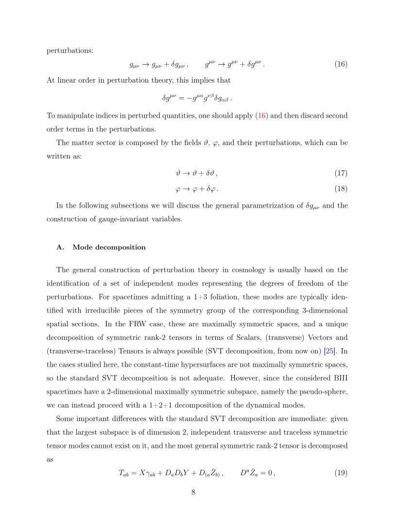
gµν → gµν + δgµν , gµν → gµν + δgµν . (16)

At linear order in perturbation theory, this implies that

δgµν = −gµαgνβδgαβ .

To manipulate indices in perturbed quantities, one should apply (16) and then discard second

order terms in the perturbations.

The matter sector is composed by the fields ϑ, ϕ, and their perturbations, which can be

written as:

ϑ→ ϑ+ δϑ , (17)

ϕ→ ϕ+ δϕ . (18)

In the following subsections we will discuss the general parametrization of δgµν and the

construction of gauge-invariant variables.

A. Mode decomposition

The general construction of perturbation theory in cosmology is usually based on the

identification of a set of independent modes representing the degrees of freedom of the

perturbations. For spacetimes admitting a 1+3 foliation, these modes are typically iden-

tified with irreducible pieces of the symmetry group of the corresponding 3-dimensional

spatial sections. In the FRW case, these are maximally symmetric spaces, and a unique

decomposition of symmetric rank-2 tensors in terms of Scalars, (transverse) Vectors and

(transverse-traceless) Tensors is always possible (SVT decomposition, from now on) [25]. In

the cases studied here, the constant-time hypersurfaces are not maximally symmetric spaces,

so the standard SVT decomposition is not adequate. However, since the considered BIII

spacetimes have a 2-dimensional maximally symmetric subspace, namely the pseudo-sphere,

we can instead proceed with a 1+2+1 decomposition of the dynamical modes.

Some important differences with the standard SVT decomposition are immediate: given

that the largest subspace is of dimension 2, independent transverse and traceless symmetric

tensor modes cannot exist on it, and the most general symmetric rank-2 tensor is decomposed

as

Tab = Xγab +DaDbY +D(aZb) , DaZa = 0 , (19)

8

where X and Y are scalars, Za is a transverse vector, and we recall that Da is the covariant

derivative in H2. Likewise, any vector Va will be decomposed as

Va = DaV + Va , DaVa = 0 , (20)

where V is a scalar and Va is again transverse. Notice that the transversality condition

eliminates one of the two variables of the transverse vectors, so that they are described by

one single scalar function. Nonetheless we will maintain the standard terminology and refer

to the splitting (19) and (20) as a Scalar-Vector (SV) decomposition. In the following, every

barred vector will refer to a transverse vector.

Based on the discussion above, we can parametrize the most general perturbation δgµν

as

ds2 = a2[−(1 + 2A)dη2 + 2Badx

adη + 2Eadxadz + 2Cdηdz + habdx

adxb + 2Fdz2], (21)

where

Ba = DaB + Ba , (22)

Ea = DaE + Ea , (23)

hab = 2Sγab + 2DaDbU + 2D(aVb) . (24)

This decomposition is unique, and the introduced functions and vectors completely specify

the 10 degrees of freedom in δgµν .

B. Gauge-Invariant Variables

Let us specify the gauge transformations of the above free functions. Under an infinites-

imal gauge transformation of the form

xµ = xµ − ξµ , (25)

any perturbed quantity δQ transforms as

δQ→ δQ = δQ+ LξQ , (26)

where Q denotes the background quantity to be perturbed. By definition, gauge-invariant

variables are those for which

LξQ = 0 . (27)

9

According to the 1+2+1 splitting of the spacetime, the gauge vector ξµ will be parametrized

by

ξµ = (T,DaL+ La, J) , (28)

where T , L, and J are scalars and La is a transverse vector.

1. Metric

If the quantity Q is the spacetime metric, then the gauge transformation (26) becomes

Lξgµν = 2∇(µξν) ,

where ∇ is the full covariant derivative compatible with the background metric (1) and, as

usual, the parentheses denote symmetrization of indices. Using Eqs. (21) and (28), we find

the following gauge transformations for the scalar variables:

A→ A+ T ′ +HT , (29)

B → B − T + L′ , (30)

C → C − ∂zT + J ′ , (31)

S → S +HT , (32)

U → U + L , (33)

E → E + ∂zL+ J , (34)

F → F +HT + ∂zJ . (35)

In a similar manner, vector modes are found to transform as:

B → B + L′ , (36)

V → V + L , (37)

E → E + ∂zL . (38)

In total we have seven scalar modes (A,B,C, S, U,E, F ) and three transverse vector

modes (B, E, V ), for a total of ten free functions in δgµν . We can now use the four free

10

functions in ξµ to construct six gauge-invariant variables. One possibility is

Φ ≡ A+1

a[a(B − U ′)]′ , (39)

Ψ ≡ S +H(B − U ′) , (40)

Π ≡ −C + E ′ + ∂z(B − 2U ′) , (41)

Λ ≡ F +H(B − U ′)− ∂z(E − ∂zU) , (42)

for the scalar sector, and

Γa ≡ V ′a − Ba , (43)

Ωa ≡ Ea − ∂zVa , (44)

for the vector sector. Other variables exist, like for example Σa ≡ E ′a − ∂zBa. But they are

not functionally independent; for instance, it is easy to check that Σa = Ω′a + ∂zΓa.

2. Matter

We will consider the perturbations to both the inflaton and the anisotropic scalar field.

Under the gauge transformation (28), any perturbation to ϑ and ϕ will transform respectively

as

Lξϑ = J∂zϑ , (45)

Lξϕ = ϕ′T . (46)

Combining these formulas with the metric potentials, we can define the following gauge-

invariant perturbations:

δϑ = δϑ− E + ∂zU , (47)

δϕ = δϕ+ ϕ′(B − U ′) . (48)

Altogether, the system of variables composed by (39-44) and (47-48) span the space of

cosmological perturbations, implying that fully gauge-invariant linear equations are possible.

However, in practice it is much easier to perform computations in some specific gauge and

convert the final result to gauge-invariant expressions. For this purpose, a suitable choice is

B = E = U = 0 = Va .

11

This choice fixes the gauge completely and determines the free functions of δgµν and δTµν in

terms of gauge-invariant variables. We can therefore perform our calculations in this gauge,

and translate the final result into gauge-invariant quantities. This is always possible in linear

theory due to the Stewart-Walker lemma [26].

C. Eigenfunctions

The natural home to define functions on the spatial sections, and in particular scalar

perturbations, is the Hilbert space of square integrable functions with measure provided by

the volume element exdxdydz. Since the Laplacian is a self-adjoint operator on this space, we

can obtain a spectral decomposition of the identity associated with it. This decomposition

can then be employed to express any perturbation as a series in terms of eigenmodes of the

Laplacian.

In the coordinates defined by Eq. (2) the Laplacian takes the following form:

∇2 = ∂x + ∂2x + e−2x∂2y + ∂2z . (49)

We now want to solve the eigenvalue problem

∇2φ(x, y, z) = −q2φ(x, y, z) , q ∈ R .

We recall that the solutions must be (generalized) states in our Hilbert space of square

integrable functions. The problem can be solved by means of a simple separation of variables,

φ(x, y, z) = f(x)g(y)h(z) ,

in terms of which the eigenvalue problem becomes:

1

f

(df

dx+d2f

dx2

)+ e−2x

1

g

d2g

dy2+

1

h

d2h

dz2= −q2 .

This equation has a nontrivial solution provided that

1

g

d2g

dy2= −m2 ,

1

h

d2h

dz2= −n2 ,

d2f

du2+

(q2 − n2

u2− 1

)f = 0 , (50)

with real numbers m and n and u ≡ me−x. The first two equations admit standard plane-

wave solutions, while the third has a solution in terms of modified Bessel functions:

f(u) = C1

√uIν(u) + C2

√uKν(u) , (51)

12

0 1 2 3 4 5 60

5

10

15

20

25

30

35

u

uK

Ν,

uI Ν

0 1 2 3 4 5 6

-0.4

-0.2

0.0

0.2

0.4

0.6

0.8

1.0

u

uK

ΝHu

L

FIG. 1. Eigenfunctions of the Laplacian in Bianchi III spacetimes. The left panel shows√uIν

(continuous line) and√uKν (dashed line) for real values of ν. The behavior of

√uKν for imaginary

ν is shown in the right panel. The values of (q, n) used were: (0,2), (4,5), and (7,8) (left); (3,2),

(4,3), and (5,4) (right).

with the eigenvalue ν given by

ν =

√1− 4(q2 − n2)

4. (52)

For real values of ν, the solutions√uIν(u) and

√uKν(u) diverge at u → ∞ and u →

0, respectively. Actually, these solutions are not appropriate for the description of linear

perturbations, since one can check that they do not belong to the Hilbert space of functions

under consideration [27] (square integrable with the measure exdx or, equivalently, du/u2),

not even as generalized delta-normalizable states. However, we can find well-behaved (and

real) solutions if we restrict ν to imaginary values. In other words, admissible solutions are

possible if

q2 ≥ 1

4+ n2 . (53)

We show some plots of these solutions for some representative values of ν in Fig. (1). Note

that the restriction (53) implies a lower bound on the wavenumber q, which is equivalent

to an upper bound on the associated wavelength λ = 2π/q. If we consider the limiting

case n = 0, we see that q ≥ 1/2 = |κ|. In other words, at a given instant η, no physical

wavelength can be bigger than 4πa(η). This is an important signature of the model which, in

principle, might be detected in CMB multipoles via the Grishchuk-Zel’dovich effect [28, 29].

We will however postpone this analysis to a forthcoming paper [30].

Returning to the analysis of the eigenfunctions, we have now a complete set in terms of

13

which perturbations can be expanded:

φ(ω,m,n)(x, y, z) =

√2ω sinh(πω)

2π2e−x/2Kν(|m|e−x)eimyeinz , (54)

where ν ≡ iω and where the constant prefactor ensures that these functions are delta-

normalized [30]. In conclusion, any perturbation f(x, y, z) can now be expanded as:

f(x, y, z) =

∫ ∞0

dω

∫ ∞−∞

dn

∫ ∞−∞

dm φ(ω,m,n)(x, y, z)f(ω,m, n) , (55)

its inverse being given by:

f(ω,m, n) =

∫R3

exdxdydz φ∗(ω,m,n)(x, y, z)f(x, y, z) . (56)

The symbol ∗ denotes complex conjugation. Note also that, since Kν(u) = Kν∗(u), only

positive values of ω contribute to Eq. (55).

IV. MASTER EQUATIONS

We are now in an adequate position to identify the effective degrees of freedom and write

down the master equations for the perturbations. A generic feature of perturbation theory in

anisotropic spacetimes containing shear is a coupling, already at first order in perturbations,

between different perturbative modes [18, 31]. Since we are working in a shear-free scenario,

such couplings will not appear. However, we will still find a residual coupling between

different scalar modes. In our case, this is due to the way scalar variables are divided in the

1+2+1 splitting, and also to the spatial curvature of the background spacetime.

The expressions for the fully linearized Einstein and energy-momentum tensors are pre-

sented in the Appendix. Here we explain how to gather their combinations into the final

master equations.

A. Scalar modes

All linearized Einstein equations contain scalar modes which can be combined to derive

master dynamical equations. Before we proceed, note that Eq. (A5) (with a 6= b) implies

for the scalar modes that

Λ = −Φ . (57)

14

This extra constraint is similar to what happens in the FRW case when the matter source

does not contain stress at first perturbative order (which is also the case considered here).

This relation is always true provided that the spatial average of the perturbations vanishes

(see Ref. [32]). From now on, we will substitute this constraint in all the equations.

The first dynamical scalar equation can be obtained from the perturbed Klein-Gordon

equation. Dropping the tilde in definition (48) for convenience, we find from ∇µTµ0 = 0 that

δϕ′′ + 2Hδϕ′ −∇2δϕ+ a2V,ϕϕδϕ = ϕ′(2Φ′ + 4HΦ− 2Ψ′ − ∂zΠ) + 2ϕ′′Φ . (58)

Using the constraint (A3) to replace ∂zΠ in the expression above, this equation reduces to:

δϕ′′ + 2Hδϕ′ − (∇2 − a2V,ϕϕ)δϕ = 2ϕ′2δϕ+ 2ϕ′′Φ . (59)

The second scalar equation can be found by subtracting (A2) from the trace of (A5).

We then use the constraint (A3) to substitute ∂zΠ in terms of Φ, Ψ, and δϕ. The resulting

equation is:

X ′′ + 2HX ′ − (∇2 + 4κ)X = 4H′Φ− 2ϕ′′δϕ . (60)

Here X ≡ Ψ − Φ. Eqs. (59) and (60) are clearly coupled, and in principle one could

expect that they were reducible to a single but closed dynamical equation involving some

combination of Ψ, Φ, and δϕ. However, we will show in Subsec. IVC that a closed equation

for these variables is not generally attainable. Strictly speaking, we can reach an equation

with those properties only during a slow-roll inflationary phase.

The dynamics of the scalar sector is also described by the equation for the variable Π.

By combining Eqs. (A2), (A4), (A6), and the corresponding equations for δT µν we find that:

Π′′ + 2HΠ′ − (∇2 − 2H′ + 4κ)Π = 0 . (61)

Finally, we have also the dynamics of the perturbed field δϑ. By combining its Klein-Gordon

equation with Eq. (A6) one gets (also dropping the tilde in the definition (47)):

δϑ′′ + 2Hϑ′ −∇2ϑ− 4κϑ = 0 . (62)

It is interesting to note that, even though the scalar sector is being sourced by the two

matter fields, the above equation is completely decoupled from other perturbed variables

and, in particular, from the perturbations of the inflaton. This property is reminiscent from

the fact that ϑ is a massless field without dynamics at the background level.

15

B. Vector modes

The dynamics of vector modes are contained in the coupled system of equations (A5)

and (A6). Because the constraint (A3) does not allow us to decouple them, in principle we

have to treat Ωa and Γa implicitly as one degree of freedom. However, from Eq. (A5) we

see that:

∂zΩa + Γ′a + 2HΓa = f(η, z)ζa , (63)

where ζa is a Killing vector of H2 and f is arbitrary in principle. On the other hand, it is

not difficult to check that the fact that the perturbations must belong to the space of square

integrable functions with respect to the volume element defined by the spatial background

metric implies that the vector ζa must be normalizable with respect to the measure exdxdy.

But there exists no Killing vector on H2 with this property (see Eqs. (1.4) in Ref. [33]).

Therefore, the only possibility left is that f = 0. In this case we can use Eq. (63) to decouple

the system of equations (A5) and (A6), leaving us with one single equation for the variable

Ωa:

Ω′′a + 2HΩ′a − (∇2 + 2κ)Ωa = 0 . (64)

Remarkably, this equation is formally the same as the equation for the polarizations of

gravitational waves in a curved FRW universe, where the contribution from the curvature

appears with opposite sign (see Ref. [24]). This difference in sign is due to the 1+2+1

splitting of the perturbative modes, as can be checked directly from the perturbed Einstein

equations (see the Appendix).

C. Reduced equations

The system of equations (59-62) and (64) fully characterizes the dynamics. Note that

Eqs. (61), (62), and (64) are decoupled, and therefore represent three independent degrees

of freedom of the system. Given that we have eight gauge-invariant variables (6 metric

potentials plus two scalar field perturbations) and four constraints from Einstein equations,

we would in principle expect that the coupled scalar equations (59) and (60) could be

combined into one single scalar equation. When inflation is driven by a single scalar field in a

flat FRW background, this reduction is always possible and leads to the dynamical equation

for the scalar MS variable. In the present case this reduction does not seem possible in

16

its full generality. Curiously, this difficulty does not arise owing to the anisotropy of the

spacetime, which generically couples perturbative modes, but rather by the presence of the

spatial curvature. As a matter of fact, precisely the same difficulty appears in curved FRW

universes, where a nonzero spatial curvature seriously compromises the direct identification

of the scalar MS variable (see Ref. [34], though). Fortunately, the terms which prevent

Eqs. (59) and (60) to be combined into one single dynamical equation are precisely the ones

proportional to the slow-roll parameters. If inflation lasts for at least 60 e-folds, so as to

solve the standard big bang problems, the dynamics of the scalar perturbations will be given

by just one scalar MS-like variable. To see that, we introduce a new variable v defined as

v ≡ a

(δϕ− ϕ′

2HX

). (65)

If we now combine Eqs. (59) and (60), using the background equation (12) and the constraint

(A3), we get the following equation after a lengthy but straightforward calculation:

v′′ −∇2v −z′′

z+ 2κ

[1

ϕ′

(ϕ′

H

)′+ 2

]v =

a

2

(ϕ′

H

)′ [∂zΠ−

X

H

], (66)

where z = aϕ′/H.

We now employ the slow-roll coefficients, in terms of which we have

z′′

z= H2

[2− 3δ + 2ε+ δ2 − εδ +

ε′ − δ′

H

], (67)(

ϕ′

H

)′=√

2H2ε+ κ (ε− δ) . (68)

These expressions are exact. Their expansion at first-order in a slow-roll approximation can

be directly obtained by means of Eqs. (14) and (15):

z′′

z≈ 1

η2(2 + 6ε− 3δ), (69)(

ϕ′

H

)′≈√

2ε

η(ε− δ) . (70)

where in the last equality we have assumed that κ/H2 can be neglected compared to ε, since

during inflation H = aH grows almost exponentially, whereas κ remains constant. Taking

the above expansions into consideration, we finally obtain:

v′′ −[∇2 +

1

η2(2 + 6ε− 3δ)

]v = 0 . (71)

This equation is remarkably close to the one found in the isotropic FRW case except, obvi-

ously, from the different spectrum of the Laplacian.

17

The remaining MS variables are much easier to obtain. With a suitable scaling of Π, ϑ

and Ωa, Eqs. (61), (62), and (64) can be rewritten as:

u′′ −(∇2 − a′′

a+ 2H2 + 4κ

)u = 0 , (72)

θ′′ −(∇2 − a′′

a+ 4κ

)θ = 0 , (73)

y′′a −(∇2 +

a′′

a+ 2κ

)ya = 0 , (74)

where the new variables that have been introduced are explicitly given by:

u ≡ aΠ , θ = aδϑ , ya ≡ aΩa . (75)

Differently from Eq. (71), these equations are valid regardless of the slow-roll approximation.

For completeness, however, we present their expressions during this stage. Using:

a′′

a≈ 2 + 3ε

η2, H2 ≈ 1

η2(1 + 2ε) , (76)

and again neglecting κ compared to H2ε ≈ ε/η2, the above equations become:

u′′ −(∇2 +

ε

η2

)u = 0 , (77)

θ′′ −(∇2 − 2 + 3ε

η2

)θ = 0 , (78)

y′′a −(∇2 +

2 + 3ε

η2

)ya = 0 . (79)

We remind the reader that, despite its appearance, ya is a transverse vector represented by

one single (scalar) function.

Equations (71), and (77-79) are the central result of this work, and govern the dynamics

of the effective degrees of freedom of inflationary perturbations in the considered BIII back-

ground spacetime. Given that Eq. (71) clearly describes the scalar perturbative mode, and

that u and ya are pure metric potentials, we can interpret Eqs. (77) and (79) as representing

the two polarizations of the gravitational waves. We notice that these two polarizations have

different dynamics, a fact which is a generic feature of anisotropic spacetimes.

As a final remark, we want to make some comments regarding the massless scalar field

ϑ used in this work. While its presence is necessary to ensure the FRW dynamics of the

anisotropic background, its perturbation is completely decoupled from the perturbation of

18

the inflaton field. In other words, equation (71), which is the central equation regarding

inflationary predictions, remains unchanged regardless of whether we perturb or not ϑ.

Nonetheless, had we chosen not to perturb this field, the equation for u would not be given

by (72), but rather by:

u′′ −(∇2 − a′′

a+ 2H2

)u = 0 , (80)

as the reader can directly check using the equations in the Appendix and taking δT µ(ϑ) ν = 0.

This indirect influence of δϑ in u, as well as the different dynamics of the two polarizations

of the gravitational waves, might, in principle, lead to observational signatures in their

spectrum.

V. CONCLUSION

The possibility that our current cosmological observations can be made compatible with

a universe with anisotropic geometry is challenging but really exciting, since this would

naturally lead us to consider extensions of the cosmological principle beyond our present

basis for the standard cosmological model. In this context, a especially nice scenario is

offered by anisotropic spacetimes which are conformally flat (shear-free), since they admit

an isotropic background expansion, and therefore an isotropic redshift. In this work, we

have unveiled the dynamics that cosmological perturbations would have in a BIII spacetime

of this kind during a generic slow-roll inflationary phase. Based on a 1+2+1 splitting of

the spacetime, we have constructed the full set of linear and gauge-invariant perturbations,

from which a set of four canonical degrees of freedom have been identified, and described

by variables of the MS type in the slow-roll regime. Interestingly, these canonical variables

have a remarkable similarity to their isotropic (FRW) counterparts. It is worth pointing out

that, although the identification of the scalar MS variable is only possible during a strict

slow-roll inflationary phase, the same happens in spatially curved FRW universes. In this

latter case, the identification of the scalar MS variable becomes severely obstructed by the

appearance of non-local terms owing to the spatial curvature [34]. We have shown here that

these terms are of higher order in a slow-roll expansion, and can therefore be ignored during

inflation.

In order to expand our equations in natural modes of our system, simplifying in this way

their resolution and avoiding complicated couplings, we have constructed a complete set

19

of eigenfunctions adapted to the symmetries of the spacetime. This also selects a specific

functional space that provides the natural home for the perturbations, and allows us to deal

with issues related with boundary conditions on these perturbations in a straightforward

manner. A footprint of cosmological perturbations in this cosmological scenario is their

inability to develop arbitrary super-Hubble modes. This seems to be a general feature of

spaces with hyperbolic spatial sections, since the same happens in open FRW models as well.

In this FRW case, analytic extensions of the eigenfunctions are usually invoked in order to

access the physics of superhorizon perturbations [29]. Whether superhorizon modes will have

an appreciable impact in future CMB observations or not, and whether such extensions are

necessary in the present model is a question for further investigation.

ACKNOWLEDGMENTS

We would like to thank David Mota, Cyril Pitrou, Miguel Quartin, Mikjel Thorsrud

and Jean-Philippe Uzan for useful conversations during the realization of this paper. This

work was supported by the Research Council of Norway under project No. 211124, by

Conselho Nacional de Desenvolvimento Científico e Tecnológico (Brazil) under project No.

308758/2011-0, and by the research grants No. MICINN/MINECO FIS2011-30145-C03-02

and CPAN CSD2007-00042 from Spain. T.S.P. thanks the Instituto de Estructura de la

Materia of the CSIC in Spain and the Institute for Theoretical Astrophysics of Norway for

their hospitality during the development of this work.

20

Appendix A: Useful expressions

We collect here useful expressions needed to derive the main equations in the paper. Since

the SV decomposition is unique, different mode contributions can be extracted and treated

separately in Einstein equations.

1. Einstein Tensor

a. Background

a2G00 = −3H2 + 1 , a2Ga

b =

(H2 − 2

a′′

a

)δab , a2Gz

z = H2 − 2a′′

a+ 1 . (A1)

The time index is denoted by 0.

b. Perturbations

In the expressions below we keep general the value of the curvature constant κ. However,

one can always replace it with −1/2.

a2δG00 = 6H2Φ− 2H∂zΠ− 2HΛ′ +DcDcΛ + 4κΨ− 4HΨ′ + 2∂2zΨ +DcDcΨ , (A2)

a2δG0a = DbD[aΓ

b] − 1

2∂2z Γa − 2κΓa +

1

2∂z∂aΠ−

1

2∂zΩ

′a + ∂aΛ

′

−2H∂aΦ + ∂aΨ′ , (A3)

a2δG0z = −2H∂zΦ + 2∂zΨ

′ − 1

2DaDaΠ , (A4)

a2δGab = δab

[2Φ(H2 + 2H′) + 2HΦ′ + ∂2zΨ−Ψ′′ − 2HΨ′ − 2H∂zΠ− Λ′′ − 2HΛ′

+DcDcΦ + ∂2zΦ− ∂zΠ′ +DcDcΛ]−D(aDb)(Λ + Φ) +D(a∂zΩb)

+D(aΓ′b) + 2HD(aΓb) , (A5)

a2δGza = −∂a(∂zΦ + ∂zΨ) +H∂aΠ +

1

2∂aΠ

′ +H∂zΓa +1

2∂zΓ

′a

+1

2Ω′′a +HΩ′a − κΩa −

1

2DcD

cΩa , (A6)

a2δGzz = 2Φ(H2 + 2H′) + 2HΦ′ +DcDcΦ− 2(Ψ′′ + 2HΨ′ − 2κΨ) +DcDcΨ . (A7)

As usual, indices between square brackets are anti-symmetrized.

A useful expression in the derivation of equations for the vector modes is

DcDaZc = −Za ,

21

where Za is any transverse vector. This identity follows from the commutator of two covari-

ant derivatives and from the fact that R(2)ab = −γab for the pseudo-sphere.

2. Energy-Momentum Tensor

a. Background

The non-zero components of the anisotropic scalar field ϑ and the inflaton field are:

a2T 0(ϑ) 0 = −C

2

2, a2T a(ϑ) b = −C

2

2δab , a2T 3

(ϑ) z =C2

2. (A8)

a2T 0(ϕ) 0 = −

(ϕ′2

2+ a2V

), a2T a(ϕ) b =

(ϕ′2

2− a2V

)δab , a2T z(ϕ) z =

(ϕ′2

2− a2V

).

(A9)

b. Perturbations

The non-zero components of the perturbed energy-momentum tensor are:

a2δT 0(ϑ) 0 = Λ− ∂zδφ , (A10)

a2δT 0(ϑ) z = −Π− δφ′ , (A11)

a2δT a(ϑ) b = (Λ− ∂zδφ) δab , (A12)

a2δT z(ϑ) a = ∂aδφ , (A13)

a2δT z(ϑ) z = −Λ + ∂zδφ . (A14)

and

a2δT 0(ϕ) 0 = −ϕ′δϕ′ + Φϕ′2 − a2V ′δϕ , (A15)

a2δT 0(ϕ) a = −ϕ′∂aδϕ , (A16)

a2δT 0(ϕ) z = −ϕ′∂zδϕ , (A17)

a2δT a(ϕ) b = (ϕ′δϕ′ − Φϕ′2 − a2V ′δϕ)δab , (A18)

a2δT z(ϕ) z = ϕ′δϕ′ − Φϕ′2 − a2V ′δϕ . (A19)

22

3. Klein-Gordon equations

a. Perturbations

The perturbed Klein-Gordon equations for δϑ and δϕ can be directly found by means of

∇µTµν = 0. At first order in perturbations, they are given respectively by:

δϑ′′ −∇2δϑ+ 2Hδϑ′ + Π′ + 2HΠ− ∂z(Φ + 2Ψ− Λ) = 0 , (A20)

δϕ′′ −∇2δϕ+ 2Hδϕ′ − Φ′ϕ′ − 4Hϕ′Φ− 2Φϕ′′ + 2Ψ′ϕ′

+ϕ′∂zΠ + ϕ′Λ′ + a2δϕV,ϕϕ = 0 , (A21)

where V,ϕϕ stands for d2V/dϕ2.

[1] A. G. Riess et al., Astron. J. 116, 1009 (1998), astro-ph/9805201.

[2] S. Perlmutter et al., Astrophys. J. 517, 565 (1999), astro-ph/9812133.

[3] A. G. Riess et al., Astrophys. J. 607, 665 (2004), astro-ph/0402512.

[4] C. Clarkson, B. Bassett, and T. H.-C. Lu, Phys. Rev. Lett. 101, 011301 (2008), 0712.3457.

[5] J.-P. Uzan, C. Clarkson, and G. F. Ellis, Phys. Rev. Lett. 100, 191303 (2008), 0801.0068.

[6] C. J. Copi, D. Huterer, D. J. Schwarz, and G. D. Starkman, Adv. Astron. 2010, 847541 (2010),

1004.5602.

[7] J. Ehlers, P. Geren, and R. Sachs, J. Math. Phys. 9, 1344 (1968).

[8] J. J. Ferrando, J. A. Morales, and M. Portilla, Phys. Rev. D 46, 578 (1992).

[9] G. F. R. Ellis, R. Maartens, and S. D. Nel, Mon. Not. R. Astron. Soc. 46, 439 (1978).

[10] C. A. Clarkson and R. Barrett, Class. Quant. Grav. 16, 3781 (1999), gr-qc/9906097.

[11] S. Stoeger, William R., R. Maartens, and G. Ellis, Astrophys. J. 443, 1 (1995).

[12] J. Mimoso and P. Crawford, Class. Quant. Grav. 10, 315 (1993).

[13] T. S. Koivisto, D. F. Mota, M. Quartin, and T. G. Zlosnik, Phys. Rev. D83, 023509 (2011),

1006.3321.

[14] S. Carneiro and G. A. Mena Marugan, Phys. Rev. D64, 083502 (2001), gr-qc/0109039.

[15] S. Carneiro and G. A. Mena Marugan, Lect. Notes Phys. 617, 302 (2003), gr-qc/0203025.

[16] C. Clarkson, T. Clifton, and S. February, JCAP 0906, 025 (2009), 0903.5040.

[17] K. Tomita and M. Den, Phys. Rev. D34, 3570 (1986).

23

[18] T. S. Pereira, C. Pitrou, and J.-P. Uzan, JCAP 0709, 006 (2007), 0707.0736.

[19] A. Gumrukcuoglu, C. R. Contaldi, and M. Peloso, JCAP 0711, 005 (2007), 0707.4179.

[20] M. Vasu, Class. Quant. Grav. 25, 225010 (2008).

[21] T. Zlosnik, (2011), 1107.0389.

[22] V. F. Mukhanov, JETP Lett. 41, 493 (1985).

[23] M. Sasaki, Prog. Theor. Phys. 76, 1036 (1986).

[24] P. Peter and J.-P. Uzan, Primordial cosmology. Oxford Graduate Texts (Oxford Univ. Press,

Oxford, 2009).

[25] J. Stewart, Class. Quant. Grav. 7, 1169 (1990).

[26] J. Stewart and M. Walker, Proc. Roy. Soc. Lond. A341, 49 (1974).

[27] I. S. Gradshteyn and I. M. Ryzhik, Table of Integrals, Series, and Products, 5th edition ed.

(Academic Press, 1994).

[28] L. P. Grishchuk and I. B. Zeldovich, Astron. Zh. 55, 209 (1978).

[29] J. Garcia-Bellido, A. R. Liddle, D. H. Lyth, and D. Wands, Phys. Rev. D52, 6750 (1995),

astro-ph/9508003.

[30] S. Carneiro, G. A. Mena Marugan, and T. S. Pereira, to appear .

[31] C. Pitrou, T. S. Pereira, and J.-P. Uzan, JCAP 0804, 004 (2008), 0801.3596.

[32] V. F. Mukhanov, H. Feldman, and R. H. Brandenberger, Phys. Rept. 215, 203 (1992).

[33] M. Reboucas and J. Tiomno, Phys. Rev. D28, 1251 (1983).

[34] J. Garriga and V. F. Mukhanov, Phys. Lett. B458, 219 (1999), hep-th/9904176.

24