arX

iv:g

r-qc

/000

9056

v2 1

9 O

ct 2

001

Dust-Filled Axially Symmetric Universes

with Cosmological Constant

Paulo Aguiar∗and Paulo Crawford†

Centro de Fısica Nuclear e Departamento de Fısica

da Faculdade de Cienicas da Universidade de Lisboa

Av. Prof. Gama Pinto, 2; 1649-003 Lisboa – Portugal

Abstract

Following the recent recognition of a positive value for the vacuum energy densityand the realization that a simple Kantowski-Sachs model might fit the classical testsof cosmology, we study the qualitative behavior of three anisotropic and homogeneousmodels: Kantowski-Sachs, Bianchi type-I and Bianchi type-III universes, with dustand a cosmological constant, in order to find out which are physically permitted. Wefind that these models undergo isotropization up to the point that the observationswill not be able to distinguish between them and the standard model, except for theKantowski-Sachs model (Ωk0

< 0) and for the Bianchi type-III (Ωk0> 0) with ΩΛ0

smaller than some critical value ΩΛM. Even if one imposes that the Universe should be

nearly isotropic since the last scattering epoch (z ≈ 1000), meaning that the Universeshould have approximately the same Hubble parameter in all directions (consideringthe COBE 4-Year data), there is still a large range for the matter density parametercompatible with Kantowsky-Sachs and Bianchi type-III if |Ω0 +ΩΛ0

−1| ≤ δ, for a verysmall δ . The Bianchi type-I model becomes exactly isotropic owing to our restrictionsand we have Ω0 + ΩΛ0

= 1 in this case. Of course, all these models approach locallyan exponential expanding state provided the cosmological constant ΩΛ > ΩΛM

.

1 Introduction

Over the last five years, the issue of whether or not there is a nonzero value for the vacuumenergy density, or cosmological constant, has been raised quite often. Indeed, the possibilityof a nonzero cosmological constant Λ has been entertained several times in the past fortheoretical and observational reasons (the early history of Λ as a parameter in GeneralRelativity has been reviewed by [1], [2], and [3]). Recent supernovae results [4], [5] stronglysupport a positive and possibly quite large cosmological constant. Even taking the Hubbleconstant to be in the range 60-75 km/s/Mpc it is possible to show [6] that the standardmodel of flat space with vanishing cosmological constant is ruled out. In a very nice review[7] it is argued that postulating an ΩΛ-dominated model seems to solve a lot of problems at

∗Email address: paguiar@cosmo.cii.fc.ul.pt†Email address: crawford@cosmo.cii.fc.ul.pt

1

once. And again, in a quite recent review on the physics and cosmology of the cosmologicalconstant, it is added that “recent years have provided the best evidence yet that this elusivequantity does play an important dynamical role in the universe” [8].

On the other hand, if the classical tests of cosmology are applied to a simple Kantowski-Sachs metric and the results compared with those obtained for the standard model, theobservations will not be able to distinguish between these models if the Hubble parametersalong the orthogonal directions are assumed to be approximately equal [9]. Indeed, as [10]points out, the number of cosmological solutions which demonstrate exact isotropy well afterthe big bang origin of the Universe is a small fraction of the set of allowable solutions ofthe cosmological equations. It is therefore prudent to take seriously the possibility that theUniverse is expanding anisotropically. Note also that some shear free anisotropic modelsdisplay a FLRW-like behavior, as it is shown in [11].

2 The global behavior of the Λ 6= 0 models

Taking all this into consideration, we discuss the behavior of some homogeneous but anisotropicmodels with axial symmetry, filled with a pressureless perfect fluid (dust) and a non vanishingcosmological constant. For this, we will restrict our study to the the metric forms

ds2 = −c2dt2 + a2(t)dr2 + b2(t)(

dθ2 + f 2

k (θ)dφ2)

, (1)

with the two scale factors a(t) and b(t); k is the curvature index of the 2-dimensional surfacedθ2 + f 2

k (θ)dφ2 and can take the values +1, 0,−1 implying fk(θ) equal sin(θ), θ, sinh(θ),respectively, giving the following three different metrics: Kantowski-Sachs, Bianchi type-I,and Bianchi type-III [12], [13].

Einstein equations for the metric (1), for which the matter content is in the form of aperfect fluid and a cosmological term, Λ, are then as follows [12], [13]:

2a

a

b

b+

b2

b2+

kc2

b2= 8πGρ + Λc2, (2)

2b

b+

b2

b2+

kc2

b2= −8πG

p

c+ Λc2, (3)

a

a+

b

b+

a

a

b

b= −8πG

p

c+ Λc2, (4)

where ρ is the matter density and p is the (isotropic) pressure of the fluid. Here G is theNewton’s gravitational constant and c is the speed of light. If we consider a vanishingpressure (p = 0), which is compatible with the present conditions for the Universe, the lasttwo equations take the form

2b

b+

b2

b2+

kc2

b2= Λc2, (5)

a

a+

b

b+

a

a

b

b= Λc2, (6)

and equation (5) can easily be integrated to give

b2

b2=

M1

b3− kc2

b2+

Λ

3c2, (7)

2

where M1 is a constant of integration.The Hubble parameters corresponding to the scale factors a(t) and b(t) are defined by

Ha ≡ a/a and Hb ≡ b/b.

Using them to introduce the following dimensionless parameters, in analogy with whichit is usually done in the Friedmann-Lemaıtre-Robertson-Walker (FLRW) universes, let usdefine

M1

b3H2b

≡ ΩM , (8)

− kc2

b2H2b

≡ Ωk (9)

andΛc2

3H2b

≡ ΩΛ. (10)

The conservation equation (7) can now be rewritten as

ΩM + Ωk + ΩΛ = 1. (11)

Now defining the dimensionless variable y = b/b0 where b0 = b(t0) is the angular scalefactor for the present age of the Universe, and using equation (11) (taken for t = t0), onemay rewrite equation (7) as

y = ±Hb0

√

ΩM0(1

y− 1) + ΩΛ0

(y2 − 1) + 1, (12)

where the density parameters defined previously and Hb with the zero subscript, denoteas before these quantities at the present time t0. In this way, the number of independentparameters have been reduced. Substituting equation (7) into equation (2) gives

a =Mρ − M1

ab

+ 2

3Λc2ab2

2√

M1b − kc2b2 + Λ

3c2b4

, (13)

where Mρ is a constant proportional to the matter in the Universe,

Mρ = 8πGρab2. (14)

Using the procedure above, equation (13) can be rewritten in the form

Ωρ − ΩM + 2 ΩΛ = 2Ha

Hb, (15)

where

Ωρ =Mρ

ab2H2b

. (16)

From equation (2) one may define a matter density parameter. For this, we introduce thenotion of mean Hubble factor H such that 3H = Ha +2Hb. Also, for these models, the shearscalar σ [13] is given by

σ =1√3(Ha − Hb) (17)

3

Thus, equation (2) may be rewritten [12] as

3H2 +kc2

b2= 8πGρ + σ2 + Λc2. (18)

As in FLRW we call critical matter density ρc when k = 0 and Λ = 0

ρc =3H2 − σ2

8πG. (19)

The matter density is generally defined as Ω = ρ/ρc, then

Ω =8πGρ

3H2 − σ2≡ 8πGρ

2HaHb + H2b

, (20)

just like in FLRW models, and such that Ω = 1 when k = 0 and Λ = 0, and which is relatedto Ωρ by

Ω =Ωρ

1 + 2Ha

Hb

. (21)

Although ΩM is not the matter density parameter, it performs the same important role. Weemphasize the fact that if for one particular time Ha = Hb and ΩΛ = 1, then, by equations(11), (15) and (21), 3Ω = Ωρ = ΩM = −Ωk; and if 0 < ΩΛ ≪ 1 and ΩM = 1, then, −Ωk = ΩΛ

and Ω ≃ 1.Introducing another dimensionless variable x = a/a0, equation (13) takes the form

x = Hb0

ΩM0

2(1 − x

y) + ΩΛ0

(−1 + xy2) +Ha0

Hb0

y√

ΩM0( 1

y− 1) + ΩΛ0

(y2 − 1) + 1, (22)

and its number of independent parameters was also reduced, now at the expense of equation(15) taken for the present time t = t0.

Now, we want to find the time dependence of b(t) in a qualitative way, starting fromequation (12). Since the model universe will be defined only where y2 ≥ 0, as was previouslydone by [14] for FLRW models, the problem is reduced to find out the zeros of y, with y 6= 0.

There are two ΩΛ values which characterize two zones of distinct behavior for the scalefactor b. Starting with condition y = 0 one may obtain

ΩΛ0=

(ΩM0− 1)y − ΩM0

y3 − y(23)

If we consider ΩΛ0= ΩΛ0

(y), as a function of y, then this function presents a relativeminimum and a maximum, that we will denote by ΩΛc

and ΩΛM, respectively. The relative

minimum depends on ΩM0in the following way [14]: For ΩM0

< 1/2 we have

ΩΛc=

3ΩM0

2

√

√

√

√

(ΩM0− 1)2

Ω2M0

− 1 +1 − ΩM0

ΩM0

1/3

+

1[√

(ΩM0− 1)2/Ω2

M0− 1 + (1 − ΩM0

)/ΩM0

]1/3

− (ΩM0− 1), (24)

4

for ΩM0≥ 1/2 the expression is

ΩΛc= −3ΩM0

cos

(

θ + 2π

3

)

− (ΩM0− 1). (25)

The relative maximum is done by

ΩΛM= −3ΩM0

cos

(

θ + 4π

3

)

− (ΩM0− 1), (26)

where θ = cos−1

(

ΩM0−1

ΩM0

)

. These expressions are limiting zones of the (ΩΛ0, ΩM0

) plane,

where y = 0 has three or one solutions (for details see [14]). The ΩΛMexpression is also

defined for ΩM0> 1/2, but it has the meaning of a maximum only for ΩM0

> 1. The ΩΛ0

less or equal to ΩΛMimposes the recollapse of scale factor b, while greater values produces

inflexional behaviors for b. The ΩΛ0values greater or equal to ΩΛc

are physically “forbidden”because they don’t reproduce the present Universe (see [14]). Obviously, ΩΛM

< ΩΛcalways.

Although we are considering anisotropic models, the equation (12) for y as a function ofΩM0

is mathematically the same as equation (2) obtained by [14] for the homogeneous andisotropic FLRW models. From equations (12) and (22) one obtains the differential equation

dx

dy=

ΩM0

2(1 − x

y) + ΩΛ0

(−1 + xy2) +Ha0

Hb0

ΩM0(1 − y) + ΩΛ0

(y3 − y) + y. (27)

This equation automatically complies with the two conservation equations (11) and (15)evaluated at t0. There are some particular values of the parameters (ΩM0

, ΩΛ0) for which

this equation has exact solutions. However, for the majority of the values of the parameters,the solution has only been obtained by numerical integration.

We may admit that at a certain moment of time, which we can take as the present time t0,the Hubble parameters along the orthogonal directions may be assumed to be approximatelyequal, Ha ≃ Hb, even though we started with an anisotropic geometry. This hypothesis hasbeen considered in [9] for the case of a Kantowski-Sachs (KS) model. From this study wasderived the conclusion that the classical tests of cosmology are not at present sufficientlyaccurate to distinguish between a FLRW model and the KS defined in that paper, with(Ha0

≃ Hb0), except for small values of b0.Taking Ha0

= Hb0 for simplicity, one can then integrate equation (27) and find threedifferent solutions, one for each k value. Figure 1 and Figure 2 shows the three kinds ofbehaviors as a result of integration.

The behavior for the Kantowski-Sachs and Bianchi type-III cases depends on the ΩΛ0

value. If ΩΛ0≤ ΩΛM

, there will be a maximum value for y, (ym), and since then y(ym) = 0, theslope of the curve x = x(y) will be infinite at that point. Specifically, we have x(ym) = +∞for Kantowski-Sachs, and x(ym) = −∞ for Bianchi type-III, even though x(ym) is finite.When ΩΛM

< ΩΛ0< ΩΛc

, after x = y = 1 is reached we find an almost linear relationbetween the two scale factors x and y for the two models. While for Bianchi type-I model wehave x = y for the present restrictions. So, we see that for the KS model, the scale factor a(t)starts from infinity if b(t) starts from zero. For the Bianchi type-I model, the scale factorsare always proportional or even equal. In this situation we don’t have an anisotropic model;in fact, we can easily prove that this model is isotropic by a properly reparametrization ofthe coordinates. For the Bianchi type-III model, the scale factor b(t) never starts from zero,

5

Figure 1: Scale factors relation, that is, the x y dependence for the three models Kantowski-Sachs (k = 1), Bianchi type-I (k = 0) and Bianchi type-III (k = −1). We show the behaviourof x(y) when ΩΛ0

< ΩΛM. Concretely we have for Kantowski-Sachs ΩM0

= 9 and ΩΛ0= 1.5;

for Bainchi type-I ΩM0= 2 and ΩΛ0

= −1; for Bainchi type-III ΩM0= 1 and ΩΛ0

= −1.

Figure 2: Scale factors relation, that is, the x y dependence for the three models Kantowski-Sachs (k = 1), Bianchi type-I (k = 0) and Bianchi type-III (k = −1). We show the behaviourof x(y) when ΩΛM

< ΩΛ0< ΩΛc

. The particular values for the plotting are, for Kantowski-Sachs ΩM0

= 2 and ΩΛ0= 1.5; for Bainchi type-I ΩM0

= 0.5 and ΩΛ0= 0.5; for Bianch

type-III ΩM0= 0.2 and ΩΛ0

= 0.4.

but has an initial value different from zero when a is null. The following plot shows the zonesin the 2-dimensional parameter space (ΩM0

, ΩΛ0) where each model is allowed (Figure 3).

Taking into account the analysis given in [14], we may easily derive the qualitative be-havior of y(t), since our equation (12) is mathematically equivalent to his equation (3). Now,going back to Figure 1 and Figure 2, one can then determine the x(t). The plotting belowsummarizes the several possibilities for the three models: Kantowski-Sachs, Bianchi type-I

6

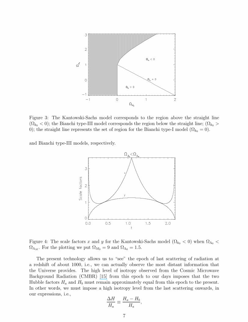
Figure 3: The Kantowski-Sachs model corresponds to the region above the straight line(Ωk0

< 0); the Bianchi type-III model corresponds the region below the straight line; (Ωk0>

0); the straight line represents the set of region for the Bianchi type-I model (Ωk0= 0).

and Bianchi type-III models, respectively.

Figure 4: The scale factors x and y for the Kantowski-Sachs model (Ωk0< 0) when ΩΛ0

<ΩΛM

. For the plotting we put ΩM0= 9 and ΩΛ0

= 1.5.

The present technology allows us to “see” the epoch of last scattering of radiation ata redshift of about 1000, i.e., we can actually observe the most distant information thatthe Universe provides. The high level of isotropy observed from the Cosmic MicrowaveBackground Radiation (CMBR) [15] from this epoch to our days imposes that the twoHubble factors Ha and Hb must remain approximately equal from this epoch to the present.In other words, we must impose a high isotropy level from the last scattering onwards, inour expressions, i.e.,

∆H

Ha

≡ Ha − Hb

Ha

,

7

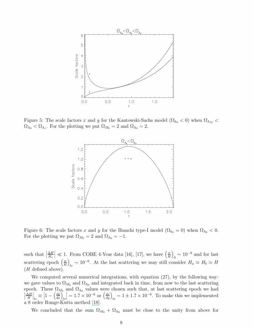
Figure 5: The scale factors x and y for the Kantowski-Sachs model (Ωk0< 0) when ΩΛM

<ΩΛ0

< ΩΛc. For the plotting we put ΩM0

= 2 and ΩΛ0= 2.

Figure 6: The scale factors x and y for the Bianchi type-I model (Ωk0= 0) when ΩΛ0

< 0.For the plotting we put ΩM0

= 2 and ΩΛ0= −1.

such that∣

∣

∣

∆HHa

∣

∣

∣ ≪ 1. From COBE 4-Year data [16], [17], we have(

σH

)

0∼ 10−9 and for last

scattering epoch(

σH

)

ls∼ 10−6. At the last scattering we may still consider Ha ≃ Hb ≃ H

(H defined above).

We computed several numerical integrations, with equation (27), by the following way:we gave values to ΩM0

and ΩΛ0and integrated back in time, from now to the last scattering

epoch. These ΩM0and ΩΛ0

values were chosen such that, at last scattering epoch we had∣

∣

∣

∆HH

∣

∣

∣

ls≡∣

∣

∣1 −(

dydx

)

ls

∣

∣

∣ = 1.7× 10−6 or(

dxdy

)

ls= 1± 1.7× 10−6. To make this we implemented

a 8 order Runge-Kutta method [18].

We concluded that the sum ΩM0+ ΩΛ0

must be close to the unity from above for

8

Figure 7: The scale factors x and y for Bianchi type-I model (Ωk0= 0) when ΩΛ0

≥ 0. Forthe plotting we put ΩM0

= 0.5 and ΩΛ0= 0.5.

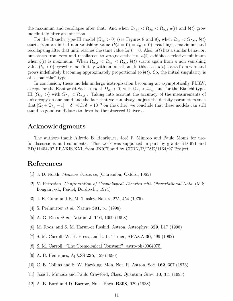
Figure 8: The scale factors x and y for the Bianchi type-III model (Ωk0> 0) when ΩΛ0

<ΩΛM

. For the plotting we put ΩM0= 1 and ΩΛ0

= −1.

Kantowski-Sachs and from below for Bianchi type-III models1. We summarized in the tablebelow the result of imposing

∣

∣

∣

∆HH

∣

∣

∣

ls∼ 1.7 × 10−6 for Kantowski-Sachs and Bianchi type-III

models, supposing Ha0= Hb0 (because

(

σH

)

0∼ 10−9).

From the table above we concluded that all combinations of Ω0 + ΩΛ0near the unity

are equally acceptable for reproducing a small anisotropy ((σ/H)ls ∼ 10−6) at the lastscattering. Nevertheless we paid special attention to the values of Ω0 ∼ 0.3 and ΩΛ0

∼ 0.7,since they reproduce the better fit to recent observations [19]. We have in this scenario|∆H/H| < 2 × 10−6 for Kantowski-Sachs and Bianchi type-III universes. All these models

1It is obvious that for Bianchi type-I model (ΩM0+ ΩΛ0

= 1), with our restrictions, we have always∆H/Ha = 0.

9

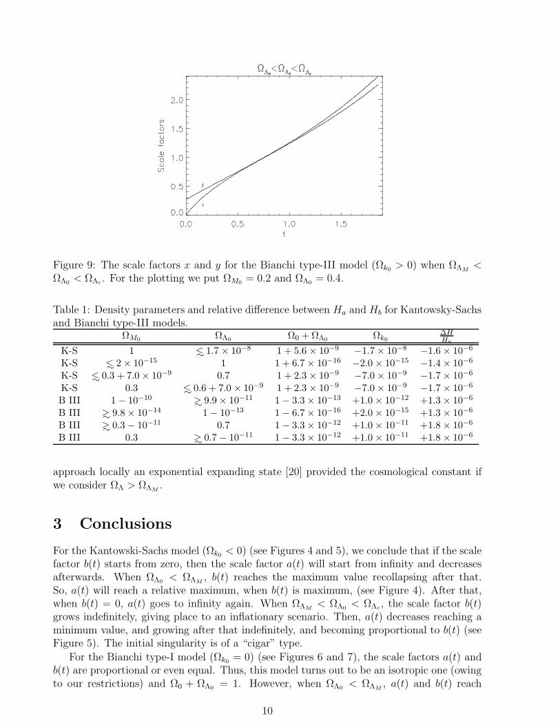
Figure 9: The scale factors x and y for the Bianchi type-III model (Ωk0> 0) when ΩΛM

<ΩΛ0

< ΩΛc. For the plotting we put ΩM0

= 0.2 and ΩΛ0= 0.4.

Table 1: Density parameters and relative difference between Ha and Hb for Kantowsky-Sachsand Bianchi type-III models.

ΩM0ΩΛ0

Ω0 + ΩΛ0Ωk0

∆HHa

K-S 1 ∼< 1.7 × 10−8 1 + 5.6 × 10−9 −1.7 × 10−8 −1.6 × 10−6

K-S ∼< 2 × 10−15 1 1 + 6.7 × 10−16 −2.0 × 10−15 −1.4 × 10−6

K-S ∼< 0.3 + 7.0 × 10−9 0.7 1 + 2.3 × 10−9 −7.0 × 10−9 −1.7 × 10−6

K-S 0.3 ∼< 0.6 + 7.0 × 10−9 1 + 2.3 × 10−9 −7.0 × 10−9 −1.7 × 10−6

B III 1 − 10−10 ∼> 9.9 × 10−11 1 − 3.3 × 10−13 +1.0 × 10−12 +1.3 × 10−6

B III ∼> 9.8 × 10−14 1 − 10−13 1 − 6.7 × 10−16 +2.0 × 10−15 +1.3 × 10−6

B III ∼> 0.3 − 10−11 0.7 1 − 3.3 × 10−12 +1.0 × 10−11 +1.8 × 10−6

B III 0.3 ∼> 0.7 − 10−11 1 − 3.3 × 10−12 +1.0 × 10−11 +1.8 × 10−6

approach locally an exponential expanding state [20] provided the cosmological constant ifwe consider ΩΛ > ΩΛM

.

3 Conclusions

For the Kantowski-Sachs model (Ωk0< 0) (see Figures 4 and 5), we conclude that if the scale

factor b(t) starts from zero, then the scale factor a(t) will start from infinity and decreasesafterwards. When ΩΛ0

< ΩΛM, b(t) reaches the maximum value recollapsing after that.

So, a(t) will reach a relative maximum, when b(t) is maximum, (see Figure 4). After that,when b(t) = 0, a(t) goes to infinity again. When ΩΛM

< ΩΛ0< ΩΛc

, the scale factor b(t)grows indefinitely, giving place to an inflationary scenario. Then, a(t) decreases reaching aminimum value, and growing after that indefinitely, and becoming proportional to b(t) (seeFigure 5). The initial singularity is of a “cigar” type.

For the Bianchi type-I model (Ωk0= 0) (see Figures 6 and 7), the scale factors a(t) and

b(t) are proportional or even equal. Thus, this model turns out to be an isotropic one (owingto our restrictions) and Ω0 + ΩΛ0

= 1. However, when ΩΛ0< ΩΛM

, a(t) and b(t) reach

10

the maximum and recollapse after that. And when ΩΛM< ΩΛ0

< ΩΛc, a(t) and b(t) grow

indefinitely after an inflection.For the Bianchi type-III model (Ωk0

> 0) (see Figures 8 and 9), when ΩΛ0< ΩΛM

, b(t)starts from an initial non vanishing value (b(t = 0) = b0 > 0), reaching a maximum andrecollapsing after that until reaches the same value for t = 0. Also, a(t) has a similar behavior,but starts from zero and recollapses to zero,nevertheless, a(t) exhibits a relative minimumwhen b(t) is maximum. When ΩΛM

< ΩΛ0< ΩΛc

, b(t) starts again from a non vanishingvalue (b0 > 0), growing indefinitely with an inflection. In this case, a(t) starts from zero andgrows indefinitely becoming approximately proportional to b(t). So, the initial singularity isof a “pancake” type.

In conclusion, these models undergo isotropization becoming an asymptotically FLRW,except for the Kantowski-Sachs model (Ωk0

< 0) with ΩΛ0< ΩΛM

and for the Bianchi type-III (Ωk0

>) with ΩΛ0< ΩΛM0

. Taking into account the accuracy of the measurements ofanisotropy on one hand and the fact that we can always adjust the density parameters suchthat |Ω0 + ΩΛ0

− 1| = δ, with δ ∼ 10−9 on the other, we conclude that these models can stillstand as good candidates to describe the observed Universe.

Acknowledgments

The authors thank Alfredo B. Henriques, Jose P. Mimoso and Paulo Moniz for use-ful discussions and comments. This work was supported in part by grants BD 971 andBD/11454/97 PRAXIS XXI, from JNICT and by CERN/P/FAE/1164/97 Project.

References

[1] J. D. North, Measure Universe, (Clarendon, Oxford, 1965)

[2] V. Petrosian, Confrontation of Cosmological Theories with Obsvertational Data, (M.S.Longair, ed., Reidel, Dordrecht, 1974)

[3] J. E. Gunn and B. M. Tinsley, Nature 275, 454 (1975)

[4] S. Perlmutter et al., Nature 391, 51 (1998)

[5] A. G. Riess et al., Astron. J. 116, 1009 (1998).

[6] M. Roos, and S. M. Harun-or Rashid, Astron. Astrophys. 329, L17 (1998)

[7] S. M. Carroll, W. H. Press, and E. L. Turner, ARA&A 30, 499 (1992)

[8] S. M. Carroll, “The Cosmological Constant”, astro-ph/0004075.

[9] A. B. Henriques, Ap&SS 235, 129 (1996)

[10] C. B. Collins and S. W. Hawking, Mon. Not. R. Astron. Soc. 162, 307 (1973)

[11] Jose P. Mimoso and Paulo Crawford, Class. Quantum Grav. 10, 315 (1993)

[12] A. B. Burd and D. Barrow, Nucl. Phys. B308, 929 (1988)

11

[13] S. Byland and D. Scialom, Phys. Rev. D 57, 6065 (1998)

[14] M. Moles, Astrophys. J. 382, 369 (1991)

[15] Peter Coles and F. Lucchin, Cosmology - The Origin and Evolution of Cosmic Structure

(West Sussex: John Wiley & Sons Ltd, 1995), p. 91

[16] E. F. Bunn, P. G. Ferreira, and J. Silk, Phys. Rev. Lett. V77 N14, 2883 (1996)

[17] A. Kogut, G. Hinshaw, and A. J. Banday, Phys. Rev. D 55, 1901 (1997)

[18] Ernst Hairer, S. P. Norsett, and G. Wanner, Solving Ordinary Differential Equations I

(Springer – Verlag, Second Revised Edition, 1993)

[19] Michael S. Turner, astro-ph/9904049 (1999). To be published in the proceedings ofType Ia Supernovae: Theory and Cosmology (held at the University of Chicago, 29-31 October 1998), edited by Jens Niemeyer and James Truran (Cambridge UniversityPress, Cambridge, UK).

[20] P. Moniz, Phys. Rev. D 47, 4315 (1993)

12