arX

iv:h

ep-t

h/05

0324

7v1

31

Mar

200

5

hep-th/0503247

Naturalness in Cosmological Initial Conditions

F. Nittia, M. Porratia,b and J.-W. Romboutsa

a Department of Physics, NYU, 4 Washington Pl., New York, NY 10003, USA

b Scuola Normale Superiore, Piazza dei Cavalieri 7, I-56126, Pisa, Italy

ABSTRACT

We propose a novel approach to the problem of constraining cosmological initial con-

ditions. Within the framework of effective field theory, we classify initial conditions

in terms of boundary terms added to the effective action describing the cosmolog-

ical evolution below Planckian energies. These boundary terms can be thought of

as spacelike branes which may support extra instantaneous degrees of freedom and

extra operators. Interactions and renormalization of these boundary terms allow

us to apply to the boundary terms the field-theoretical requirement of naturalness,

i.e. stability under radiative corrections. We apply this requirement to slow-roll

inflation with non-adiabatic initial conditions, and to cyclic cosmology. This allows

us to define in a precise sense when some of these models are fine-tuned. We also

describe how to parametrize in a model-independent way non-Gaussian initial con-

ditions; we show that in some cases they are both potentially observable and pass

our naturalness requirement.

e-mail: francesco.nitti@physics.nyu.edu, massimo.porrati@nyu.edu, jan-willem.rombouts@physics.nyu.edu

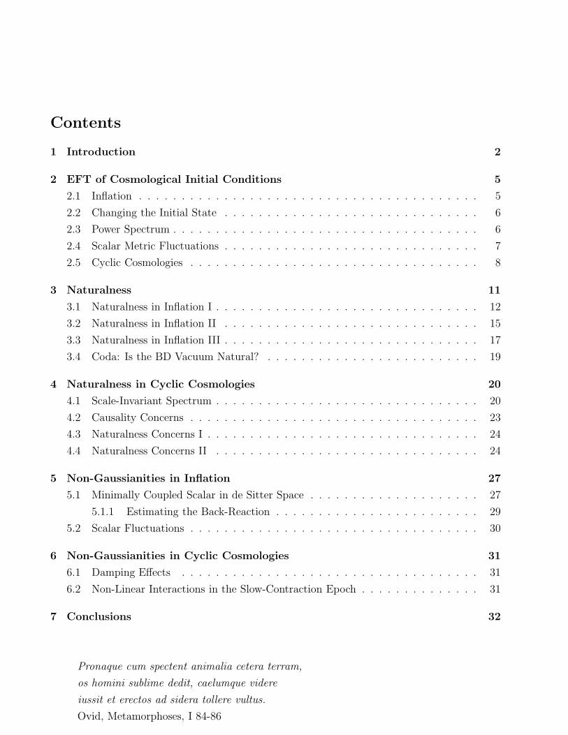
Contents

1 Introduction 2

2 EFT of Cosmological Initial Conditions 5

2.1 Inflation . . . . . . . . . . . . . . . . . . . . . . . . . . . . . . . . . . . . . . . . 5

2.2 Changing the Initial State . . . . . . . . . . . . . . . . . . . . . . . . . . . . . . 6

2.3 Power Spectrum . . . . . . . . . . . . . . . . . . . . . . . . . . . . . . . . . . . . 6

2.4 Scalar Metric Fluctuations . . . . . . . . . . . . . . . . . . . . . . . . . . . . . . 7

2.5 Cyclic Cosmologies . . . . . . . . . . . . . . . . . . . . . . . . . . . . . . . . . . 8

3 Naturalness 11

3.1 Naturalness in Inflation I . . . . . . . . . . . . . . . . . . . . . . . . . . . . . . . 12

3.2 Naturalness in Inflation II . . . . . . . . . . . . . . . . . . . . . . . . . . . . . . 15

3.3 Naturalness in Inflation III . . . . . . . . . . . . . . . . . . . . . . . . . . . . . . 17

3.4 Coda: Is the BD Vacuum Natural? . . . . . . . . . . . . . . . . . . . . . . . . . 19

4 Naturalness in Cyclic Cosmologies 20

4.1 Scale-Invariant Spectrum . . . . . . . . . . . . . . . . . . . . . . . . . . . . . . . 20

4.2 Causality Concerns . . . . . . . . . . . . . . . . . . . . . . . . . . . . . . . . . . 23

4.3 Naturalness Concerns I . . . . . . . . . . . . . . . . . . . . . . . . . . . . . . . . 24

4.4 Naturalness Concerns II . . . . . . . . . . . . . . . . . . . . . . . . . . . . . . . 24

5 Non-Gaussianities in Inflation 27

5.1 Minimally Coupled Scalar in de Sitter Space . . . . . . . . . . . . . . . . . . . . 27

5.1.1 Estimating the Back-Reaction . . . . . . . . . . . . . . . . . . . . . . . . 29

5.2 Scalar Fluctuations . . . . . . . . . . . . . . . . . . . . . . . . . . . . . . . . . . 30

6 Non-Gaussianities in Cyclic Cosmologies 31

6.1 Damping Effects . . . . . . . . . . . . . . . . . . . . . . . . . . . . . . . . . . . 31

6.2 Non-Linear Interactions in the Slow-Contraction Epoch . . . . . . . . . . . . . . 31

7 Conclusions 32

Pronaque cum spectent animalia cetera terram,

os homini sublime dedit, caelumque videre

iussit et erectos ad sidera tollere vultus.

Ovid, Metamorphoses, I 84-86

1 Introduction

This old privilege notwithstanding, it took a long time to transform our gazing into the sky

into physics. The study of the early universe truly left the mist of myth and speculation to

become science only in the 1930’s, with the discovery of cosmic expansion. We had to wait

until the 1960’s, with the discovery of the cosmic microwave background (CMB), to be able

to discriminate between the Hot Big Bang and alternative cosmologies, and only in the early

1990’s, with the detection of CMB’s inhomogeneities, did cosmology fully become a quantitative

science.

The celebrated WMAP survey [1] has spectacularly confirmed some general predictions of

slow-roll inflation, and offered the possibility of significantly constraining alternative explana-

tions for the primordial power spectrum. Future experiments may be able to go beyond the

power spectrum and check for other features of the CMB, as, for instance, primordial non-

Gaussianities.

Present data already make it meaningful to ask about finer details of the mechanism that

generates an almost scale-invariant power spectrum. We just mentioned one such detail: pos-

sible non-Gaussian features. Another one is whether the correct initial state of the universe is

the standard adiabatic “Bunch-Davies” vacuum [2]. Deviations from the standard inflationary

vacuum offer the exciting possibility of observing very high-energy, “trans-Planckian” physics in

the cosmic microwave background radiation, thanks to the enormous stretch in proper distance

due to inflation [3]. This effect, which may present us with a real chance for probing string

theory or any other model of quantum gravity, has received considerable attention, once the

possibility was raised that these effects could be as large as H/M , with H the Hubble parameter

during inflation, and M the scale of new physics (e.g. the string scale).

Due to our ignorance of the ultimate theory governing high-energy physics, the most natural,

model-independent approach to studying modifications to the primordial power spectrum is

effective field theory (EFT) [4, 5]. Using an EFT approach [4] concluded that the signature of

any trans-Planckian modification of the standard inflationary power spectrum is O(H2/M2),

well beyond the reach of observation even in the most favorable scenario (H ∼ 1014 GeV,M ∼1016 GeV).

What was absent from e.g. ref. [4] was a systematic EFT approach to initial conditions.

Ref. [4] presented convincing arguments against the (in)famous α-vacua [6] of de Sitter space,

but it did not give a complete parametrization of finite-energy, non-thermal states. That

parametrization was given in [7, 8], where the EFT approach was systematically extended to

the choice of initial conditions. Refs. [7, 8] conclude that changes in the initial conditions for

inflation are under control and may give O(H/M) corrections to the primordial power spectrum.

According to [7, 8], these corrections are quite characteristic of UV modifications to physics and

can be distinguished from other corrections arising instead from IR changes in the vacuum state.

In this paper, we shall argue that other constraints on the EFT of initial conditions make

O(H/M) changes in the primordial power spectrum unnatural, in the same sense that a light

Fermi scale is unnatural in the Standard Model. Before explaining further this point, we need

to sketch the approach of refs. [7, 8]. The most important difference between that and other

approaches is that in [7, 8] initial conditions for modes of any wavelength are specified at the same

initial time t∗. Other approaches give the initial conditions separately for each mode, at the time

it crosses the horizon. The latter prescription is useful in the context of inflationary cosmology,

but it obscures the field-theoretical meaning of the perturbation and/or initial condition: it does

not easily account for the fact that after t∗ curvatures and energy densities are small, so the

field theory is under control, and it does not easily translate into an EFT language. The former

prescription, instead, leads naturally to a simple classification of initial conditions in terms of

local operators defined at the space-like boundary (i.e. initial surface) t = t∗. It also allows one

to rephrase the question of naturalness of initial conditions for inflation in terms of the usual

field-theoretical notion of naturalness.

In field theory we have a naturalness problem whenever the UV cutoff of the theory, M

is much bigger than the observed value of the coefficients of unprotected relevant operators.

For instance, a quadratically-divergent scalar mass term m2φ2 is unnatural (or, equivalently,

fine tuned) whenever m ≪ M . In our EFT theory of initial conditions, we shall define a

parallel notion. Initial conditions will be deemed unnatural whenever they require to fine-tune

coefficients of relevant boundary operators to values much smaller than M3−∆, where ∆ is the

dimension of the operator.

Section 2 is devoted to summarize the EFT approach of [7, 8]. There, we also generalize

their formalism to the case where 3-d boundary interactions are not added at an “initial” time,

but they are used instead to parametrize an unknown period in the history of the universe. We

shall do that to apply EFT methods to ekpyrotic/cyclic [9] or pre-big bang cosmologies [10].

In a sentence: we shall replace the unknown physics at the bounce –where the scale factor

shrinks to zero to originate a spacelike singularity– with a spacelike (instantaneous) brane,

whose world-volume supports local operators and additional degrees of freedom (see fig. 1).

Section 3 explains in greater details the concept of naturalness for initial conditions. Nat-

uralness is then applied to constrain possible changes in the B.D. vacuum of inflation. They

turn out to be either unnatural or IR universal; therefore, ill-suited to characterize signals of

new high-energy physics.

In section 4, we show that the spacelike brane that parametrizes the unknown Planckian

physics at the bounce in cyclic/ekpyrotic/pre-big bang cosmologies can give raise to the correct

power spectrum P ∼ k−3, generically at the price of severe non-localities on the brane. We

scale factor

time

Planckian Era

FRW

Pre Big Bang

Figure 1: A schematic view of the EFT description of a cyclic cosmology. It plots the scale factor vs.time. The Planckian era around the bounce is replaced by an effective space-like brane (S-brane).

show that typically these non-localities lead after the bounce to faster-than light propagation of

signals originating in the pre-big bang phase. This pathology may not be lethal for these models,

since Lorentz invariance is explicitly broken by the brane. Nevertheless, it is troublesome. It is

avoided with a particular choice of interaction terms on the brane, which we proceed to show is

unnatural according to our general prescription, since it requires the fine-tuning to zero of an

unprotected relevant operator. The rest of section 4 is used to show how to write in local form a

non-local boundary interaction on the brane, which can generate the correct post-bounce power

spectrum. We show that the boundary term can be written in terms of local operators, but only

at the price of introducing extra auxiliary fields that propagate only on the spacelike brane. We

then conclude the section by showing that, besides leading to faster-than-light propagation, a

generic boundary term also requires to fine-tune certain relevant operators, and it is thus also

unnatural. Our argument confirms and complements the analysis of [11] (see also [12]).

Section 5 shows how to compute the effect of changes in the initial state of inflation that do

not affect the power spectrum, but that do change the three-point function of scalar fluctuations.

We show that the changes induced by cubic boundary operators can lead to observable non-

Gaussianities, different from those studied in [13], without requiring undue fine-tunings.

Section 6 studies the three point function of scalar fluctuations in cyclic cosmologies. Set-

ting aside naturalness considerations, we show that, in this scenario, any pre-big bang non-

Gaussianity is damped. Finally, we show that the particular form of the scalar potential used in

cyclic cosmologies sets a bound on how close to the singularity is the space-like brane. Specif-

ically, if we want to avoid uncontrollably large interactions, the pre-big bang cosmic evolution

must be cut off and replaced by an effective brane at a time parametrically larger than M−1p .

In section 7 we summarize our findings and conclude pointing out to possible developments

of our formalism to other problems involving spacelike singularities.

2 EFT of Cosmological Initial Conditions

2.1 Inflation

Differently from other approaches, here as in [7, 8] we give initial conditions for modes of all

wavelengths at the same initial time t∗.

The prescription starts by supplementing the EFT action describing all relevant low energy

fields with a boundary term that encodes the standard thermal vacuum. To be concrete, we

begin by working out the example of a massless scalar field in a time-dependent background.

The 4d (bulk) action plus a 3d boundary term is

S = S4 + S3, S4 =1

2

∫ ∞

t∗dt∫

d3x√−ggµν∂µχ∗∂νχ,

S3 =1

2

∫

d3x√

h∗(x)∫

d3y√

h∗(y)χ∗(x)κ(x, y)χ(y)

∣

∣

∣

∣

t∗. (1)

Here h∗ij is the induced metric on the surface t = t∗. The role of S3 is to specify the wave

functional for the scalar χ at t = t∗:

Ψ[χ(x)] = exp(iS3[χ]). (2)

Selecting an initial state for χmeans in this language to choose a particular κ(x, y). For instance,

in de Sitter space with line element

ds2 = a(η)2(−dη2 + dxidxi), a(η) = − 1

Hη, i = 1, 2, 3, −∞ < η < 0, (3)

the standard thermal [2] vacuum is obtained by choosing

κ(k) = − |k|2η∗1 + i|k|η∗ . (4)

Here, a tilde denotes the Fourier transform from space coordinates to co-moving momenta k

(|k| ≡√k · k) and η∗ is the initial (conformal) time.1 This expression for κ makes it clear that

the choice of such initial time is conventional, since a change in η∗ changes only κ, not the wave

functional. From now on, whenever needed, the standard vacuum functional will be called |0〉.1From now on, η, η∗ will denote the conformal time, t, t∗ will denote the synchronous proper time, and a()

will always denote the scale factor. Notice that η∗ here is negative.

2.2 Changing the Initial State

Next, we want to find a convenient classification of changes to the initial state. This can be

done by adding a new boundary term to the action: S → S + ∆S3. To determine ∆S3, we

notice that, at any finite time t after t∗, we are insensitive to changes that only affect very low

co-moving momenta k: co-moving momenta |k| < H(t)a(t) correspond to perturbations with

superhorizon physical wavelength λp > 1/H(t), which are unobservable at time t. So, since we

are interested in changes that can be observed in the CMB of the present epoch, we have an

IR cutoff naturally built into the theory. This IR cutoff tells us that observable changes in the

initial conditions can be parametrized by local operators:

∆S3 =∑

i

βiM3−∆i

∫

d3x√h∗Oi

∣

∣

∣

∣

t∗. (5)

Here Oi are operators of scaling dimension ∆i, M is the high-energy cutoff of the EFT and the

βi’s are dimensionless parameters. The dimension ∆i determines among other things how “blue”

is the change in the power spectrum: the fractional change in the power spectrum is proportional

to k∆i−2. Since the EFT makes sense only for k < M , operators of high conformal dimension do

not significantly change the observable spectrum. So, the most significant observable changes in

the primordial fluctuation spectrum are parametrized by a few local operators of low conformal

dimension.

We just mentioned that the EFT needs a UV cutoff. This means that the operators Oi must

be suitably regulated at short distance. In other words, they are local only up to the cutoff

scale M . As a simple example, consider the dimension-four operator O4 = (β/M)(∂iχ)2. It has

to be smeared at short distance, for instance by the replacement

∂iχ∂iχ→ ∂iχf(−∂2/a2(t∗)M2)∂iχ. (6)

Here f(x) is a smooth function obeying f(x) = 1, for x ≤ 1 − ǫ; f(x) = 0, for x ≥ 1 + ǫ; ǫ is

a small positive number. The scale factor a(t∗) appears because we want to cutoff at M the

physical momentum |k|/a(t∗), not the co-moving momentum |k|.

2.3 Power Spectrum

As a first application, let us derive the change in the power spectrum of a minimally-coupled

scalar field in de Sitter space, induced by the operator O4 introduced in the previous subsec-

tion [7]. The change in initial conditions ∆S3, is equivalent to perturbing the Hamiltonian of

the system by an instantaneous interaction HI = −δ(η − η∗)∆S3. So, the perturbed two-point

correlation function is

G(k) = limη→0−

〈|χ(k, η)|2〉 = limη→0−

〈0| exp(−i∆S3)|χ(k, η)|2 exp(i∆S3)|0〉. (7)

To first order in β, the change is

δG(k) = −i βM

∫

d3xa(η∗)〈0|[O4(x), |χ(k, 0)|2]|0〉. (8)

This quantity is easily computed in terms of commutators of free fields in de Sitter space,

resulting in [7, 14, 15]

δG(k) = − β

Ma(η∗)

H2

|k|3 Im [χ+(η∗, k)]2|k|2f(|k|2/a2(η∗)M2). (9)

The canonically normalized, positive frequency solution of the free-field equations of motion is

χ+(η, k) =H

√

2|k|3(1 + i|k|η) exp(−i|k|η), (10)

and 〈0||χ(k, 0)|2|0〉 = H2/|k|3 is the unperturbed two-point function. For |k||η∗| ∼ 1, the effect

of O4 on the power spectrum, P (k) = (k/2π)3G(k), can be as large as δP/P ∼ βH/M , i.e.

in the observable range when β is O(1). For |k||η∗| > 1, the oscillating exponential gives a

characteristic periodic signature [8]. The signal rapidly decays for |k||η∗| ≫ 1, so, it can be

detected only if inflation lasts for a relatively short period; otherwise, O4 would only affect

unobservable super-horizon fluctuation.

2.4 Scalar Metric Fluctuations

Of course, we are not really interested in the fluctuations of a minimally coupled scalar. Those

describe at best tensor perturbations of the metric. We want instead scalar perturbations of

the metric. In the standard setting for slow-roll inflation, where the field content is the metric

gµν plus the inflaton φ. It is convenient to use the ADM formalism and decompose gµν into 3-d

metric hij , shift N i and lapse N :

ds2 = −N2dt2 + hij(dxi +N idt)(dxj +N jdt). (11)

Metric and scalar field split into background values plus fluctuations as hij = exp(2ρ)(δij +γij),

a(t) ≡ exp(ρ), ψ = φ(t) + ϕ. The last equation means that the background scalar field, φ(t), is

a function of the time t only. A particularly convenient gauge is [13]

hij = exp(2ρ+ 2ζ)(δij + γij), ∂iγij = 0, γii = 0, ϕ = 0. (12)

In this gauge, the scalar fluctuations are given by ζ , which is also the gauge invariant variable

of [16] (see also [17]). The quadratic bulk action for ζ is almost identical with that of a massless

scalar field

S =1

16πG

∫

dtd3xφ2

ρ2

[

−e3ρζ2 + eρ(∂ζ)2]

. (13)

=1

16πG

∫

dηd3xφ′2

ρ′2a2(η)

[

−ζ ′2 + (∂ζ)2]

. (14)

For future reference, we have written the action both in synchronous time t and in conformal

time η. Derivative w.r.t. t is denoted by a dot while a prime denotes derivation w.r.t. η; G is

the Newton constant.

This formula shows that scalar fluctuations can be treated as a non-canonically normalized

scalar fields. So, the equations derived in the previous subsections translate into formulas for

changes in the CMB. One may worry that this conclusion has been reached with a very special

choice of gauge. This is not the case, though. In the 4-d bulk, in any gauge, only the combination

ζ−(φ/ρ)ϕ propagates. This combination is indeed the gauge-invariant definition of the Bardeen

variable (see [16] and [17] section 10.3), and it is this quantity that appears in the action. On

the initial-time boundary, instead, both ζ and ϕ appear [17], but the latter appears only as a

non-dynamical field, without a genuine kinetic term. Schematically:

Sboundary =∫

d3xF [ζ(x, t∗), ϕ(x, t∗)], (15)

where F [ζ, ϕ] is a quadratic function of its variables. Therefore, after imposing the non-

dynamical ϕ equations of motion, ∂F/∂ϕ = 0, ϕ becomes a linear function of ζ , that can

be plugged back into the boundary term to yield a quadratic function of ζ only.

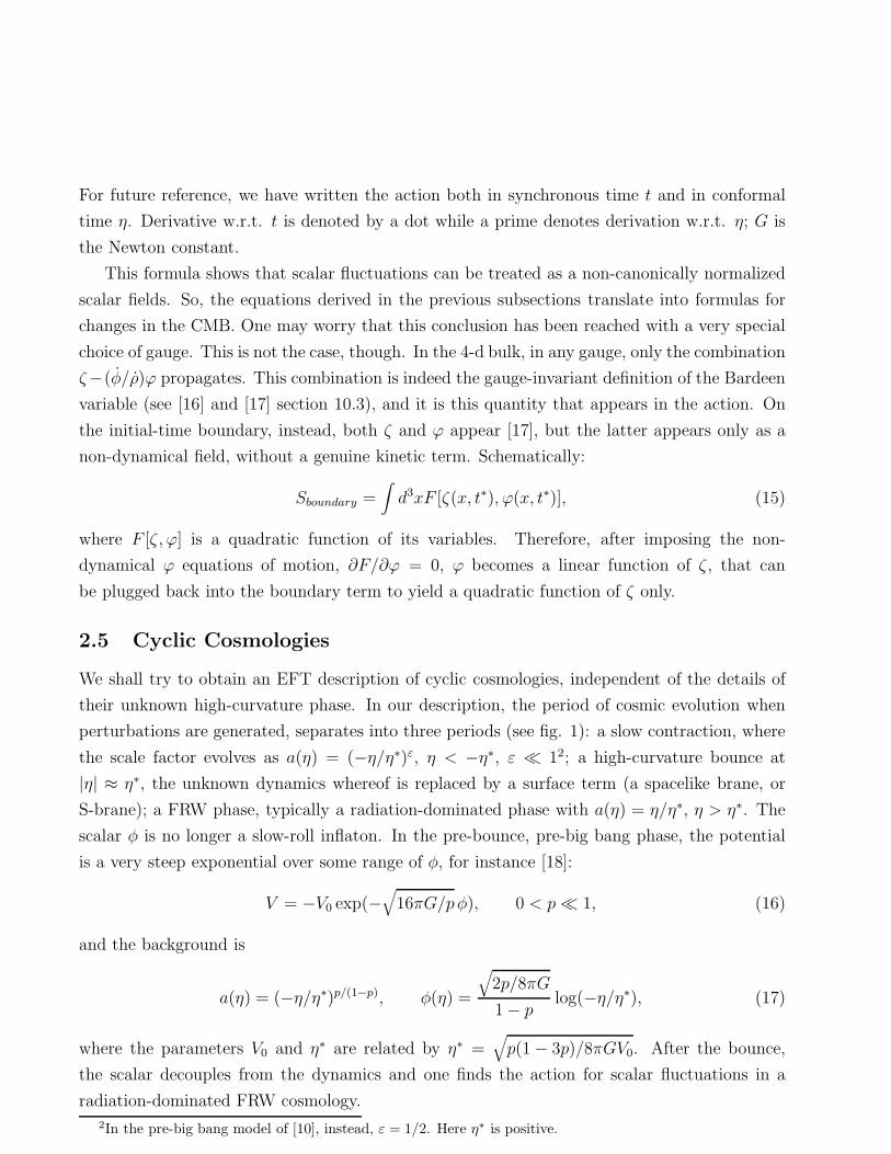
2.5 Cyclic Cosmologies

We shall try to obtain an EFT description of cyclic cosmologies, independent of the details of

their unknown high-curvature phase. In our description, the period of cosmic evolution when

perturbations are generated, separates into three periods (see fig. 1): a slow contraction, where

the scale factor evolves as a(η) = (−η/η∗)ε, η < −η∗, ε ≪ 12; a high-curvature bounce at

|η| ≈ η∗, the unknown dynamics whereof is replaced by a surface term (a spacelike brane, or

S-brane); a FRW phase, typically a radiation-dominated phase with a(η) = η/η∗, η > η∗. The

scalar φ is no longer a slow-roll inflaton. In the pre-bounce, pre-big bang phase, the potential

is a very steep exponential over some range of φ, for instance [18]:

V = −V0 exp(−√

16πG/pφ), 0 < p≪ 1, (16)

and the background is

a(η) = (−η/η∗)p/(1−p), φ(η) =

√

2p/8πG

1 − plog(−η/η∗), (17)

where the parameters V0 and η∗ are related by η∗ =√

p(1 − 3p)/8πGV0. After the bounce,

the scalar decouples from the dynamics and one finds the action for scalar fluctuations in a

radiation-dominated FRW cosmology.

2In the pre-big bang model of [10], instead, ε = 1/2. Here η∗ is positive.

To match the two phases, we need to add a boundary term, an S-brane, with nonzero tension.

Its form is largely free; we can only say that it must contain at least the following terms:

T+

∫

d3x√

h∗+ − T−

∫

d3x√

h∗− + .... (18)

Here T+ and T− are constant tensions, needed to satisfy the junction conditions at η = η∗ and

η = −η∗, respectively. h∗± is the determinant of the induced metric on the surface η = ±η∗ and

... stands for gradient terms that vanish on the background ζ = 0.

The nonzero tensions generate a stress-energy tensor, which is conserved but which violates

the null energy condition (NEC). This is unavoidable if we want a spatially flat bounce.

Thanks to the S-brane, we can have a bounce and we can write the action for scalar fluctu-

ations in the gauge (12) as

16πGS =∫ ∞

η∗dη∫

d3x

(

η

η∗

)2[

−ζ ′2 + (∂ζ)2]

+2

p

∫ −η∗

−∞dη∫

d3x

(

−ηη∗

)2p/(1−p)[

−ζ ′2 + (∂ζ)2]

+∫

d3x {Λ[ζ(η∗) − α(∂)ζ(−η∗)] + ζ(η∗)F (∂)ζ(η∗)} . (19)

This is one of the most important equations in our paper, and it is worth of a few comments.

First of all, the boundary term parametrizing the unknown high-energy physics at the bounce

is made of two pieces. The first is the one containing the Lagrange multiplier Λ(x). This is a

non-dynamical field whose role is to link the value of the field ζ after the bounce, at η = η∗, to

its value before the bounce, at η = −η∗. ζ can be continuous at the bounce, for α = 1, or it

can jump, whenever α 6= 1. α(∂) is a local function of spatial gradients. So, ζ(η∗) is generically

a function of ζ(−η∗) and its derivatives along the brane. Likewise, F (∂) is a function of spatial

gradients. Generically, it is nonlocal. Its role is to mimic super-horizon correlations induced

by the unknown physics at the bounce. Superhorizon correlations do not necessarily signal

acausalities, because our parametrization can also fit a “long” bounce, lasting for an arbitrarily

long time.

Notice that we did not introduce dζ/dη in the boundary term. The reason is that dζ/dη

terms render the variation of eq. (19) ill-defined. So, whenever they do appear in a boundary

term, they should be eliminated by an appropriate discontinuous field redefinition [7], or by using

the bulk equations of motion to convert them into functions of ζ and its spacelike gradients.

We wrote eq. (19) in a specific gauge. To write it in a 3-d covariant form, we must re-

express ζ in terms of the intrinsic curvature on surfaces defined by ϕ = 0. To write it in a fully

4-d covariant manner, we must furthermore express the position of the bounce in terms of a

covariant (scalar) equation involving, say, ψ and the scalar curvature.

We may worry about two features of this procedure.

1. A covariant equation for the position of the bounce reduces, in the gauge (12), to

η = G(ζ) + η∗. (20)

The function G is smooth and it vanishes at ζ = 0, but is otherwise unknown. So,

generically, the bounce does not sit at a constant value of the time η = η∗. This is

not a problem since at quadratic order this bending of the brane only generates further

quadratic terms of the form ζFζ , plus a finite renormalization of the brane tensions T±.3

Explicitly, the induced metric on the brane is

h∗ij = ∂iG∂jGg00(G(x), x) + ∂iGg0j(G(x), x) + ∂jGg0i(G(x), x) + gij(G(x), x). (21)

By substituting this formula into the universal term T∫

d3x√h∗ we get, at linear order in

ζ

T∫

d3xa3(3ζ + 3ρ′Gζζ), Gζ ≡dG

dζ

∣

∣

∣

∣

∣

η=G(x)

. (22)

This term induces a finite renormalization of the brane tension, T → T (1 + ρ′Gζ). At

quadratic order in ζ we find as announced a term of the form ζFζ , after eliminating time

derivatives by the bulk equations of motion:

T∫

d3xa3[

G2ζ(∂iζ)

2 + 2Gζ∂iζNia−2 + 3(2ρ

′2 + ρ′′)G2ζζ

2 + 6ζ2 + 6Gζζζ′+

3ρ′Gζζζ2 +

3

4(2ζ + 2ρ′Gζζ)

2]

. (23)

2. The functions α and F we introduced, are quite arbitrary. They can even break explicitly

3-d rotations and translations, even though we will not do that in the following. So,

neither the momentum constraint nor the Hamiltonian constraint impose any restriction

on them. This is because our “initial time” brane is different from the boundary brane

introduced in the context of de Sitter holography in [19]. For us the brane is real. It

either parametrizes a very specific time in cosmic evolution (the bounce), or a specific

choice of quantum state at some time early in the inflationary epoch. Since we use the

brane to specify an initial state, which is then used to compute expectation values of ζ

at η → ∞ (that is today), we can change the value of η∗, together with the form of the

boundary terms, in such a way as to keep the late-time correlators constant. An example

of this “renormalization group” is our eq. (4). So, our boundary terms at η∗ are the analog

of arbitrary initial conditions for the RG group. In ref. [19] instead, the late-time brane

is a regulator, and the time evolution of all fields is fixed, because both late-time and

early-time boundary conditions are fixed. The difference between the two approaches is

schematically shown in fig. 2.

3The brane bending also introduces terms in ζ′. As we have already mentioned, these terms must be canceledby field redefinitions, or expressed in terms of gradients via the equations of motion.

scale factor scale factor

time time

Figure 2: On the left, a schematic view of our brane, its position is represented by the vertical lines.By changing the operators on the brane and/or its position, we can change the initial conditions forthe flow, hence the flow itself. On the left, the holographic brane of ref. [19]. Its boundary operatorsare constrained by requiring that the flow remains the same when its position is changed.

3 Naturalness

In particle physics, stability under radiative corrections is a powerful guide for constraining

high-energy extensions of the standard model or of any EFT. By construction, an EFT has a

built-in UV cutoff. In other words, the EFT only describes the low-energy sector of a theory

whose UV completion is unknown. EFT is a powerful method whenever there is a large energy

gap between a known low-energy sector (say the standard model) and an unknown high-energy

sector –typically made of heavy particles– that decouples below a cutoff M . In this case, the

effect of integrating out the high-energy sector is to introduce irrelevant operators in the EFT.

They have dimension ∆ > 4 and appear in the EFT with coefficients O(M4−∆). A change in

the UV physics –as for instance a change in masses and couplings of the heavy sector– induces

a small modification in the coefficients of these irrelevant operators. So, low-energy physics is

shielded from changes in the UV physics, and EFT can be predictive even in the absence of a

complete knowledge of high-energy physics. The problem lies in the relevant operators; those

with dimension ∆ < 4. Their coefficients must be much smaller than M4−∆, otherwise, the EFT

would describe a trivial physics with no light states at all. A simple example of this pathology

is a theory with two scalars, one heavy, with mass M , and another one with mass m. Below the

energy scale M only one scalar propagates, and only if m ≪ M . Relevant operators are very

sensitive to changes in the UV physics, the more so the lower their dimension. Generically, they

appear in the EFT with coefficients O(M4−∆). Even if the tree-level values of these parameters

are small, radiative corrections typically bring them to values O(M4−∆). Equivalently, any

small change in masses, couplings etc. in the heavy sector bring these coefficients to their

typical value.

The best known naturalness problem in particle physics is that associated with the Fermi

scale MF ≈ 100 GeV or, equivalently, the Higgs mass. Suppose that the standard model holds

up to a high energy scale M ≈ 1016 − 1019 GeV. Then, unless the Higgs mass is protected by

symmetries (e.g. supersymmetry) it would be destabilized by radiative corrections, and driven

to the UV cutoff.

In our setting, we have a naturalness problem too. It arises because we change the cosmo-

logical initial state by adding boundary terms to a bulk action as in eq. (5). These boundary

terms are generically unstable under radiative corrections. So, even if we begin by modifying our

theory by adding a (safe) irrelevant boundary operator4, we may end up generating dangerous

relevant operators.

3.1 Naturalness in Inflation I

We begin by studying in detail the example given in section 2.3. There we computed the change

induced in the fluctuation spectrum of a minimally-coupled massless scalar by the dimension-4

operator

O4 =β

M(∂iχ)2. (24)

This boundary term is not complete. It must be covariantized with respect to 3-d general

coordinate transformations, which are not broken by a choice of initial conditions. The covari-

antization is obvious and gives the following boundary term

∆S3 =β

M

∫

d3x√hhij∂iχ∂jχ. (25)

Once we impose a shift symmetry χ → χ + constant, O4 is the lowest-dimension boundary

operator quadratic in χ. So, it is not unnatural to set to zero the coefficient of the relevant

–and potentially dangerous– operator O2 = αMχ2.

4Since the boundary is a 3-d field theory, all operators of dimension greater than 3 are irrelevant.

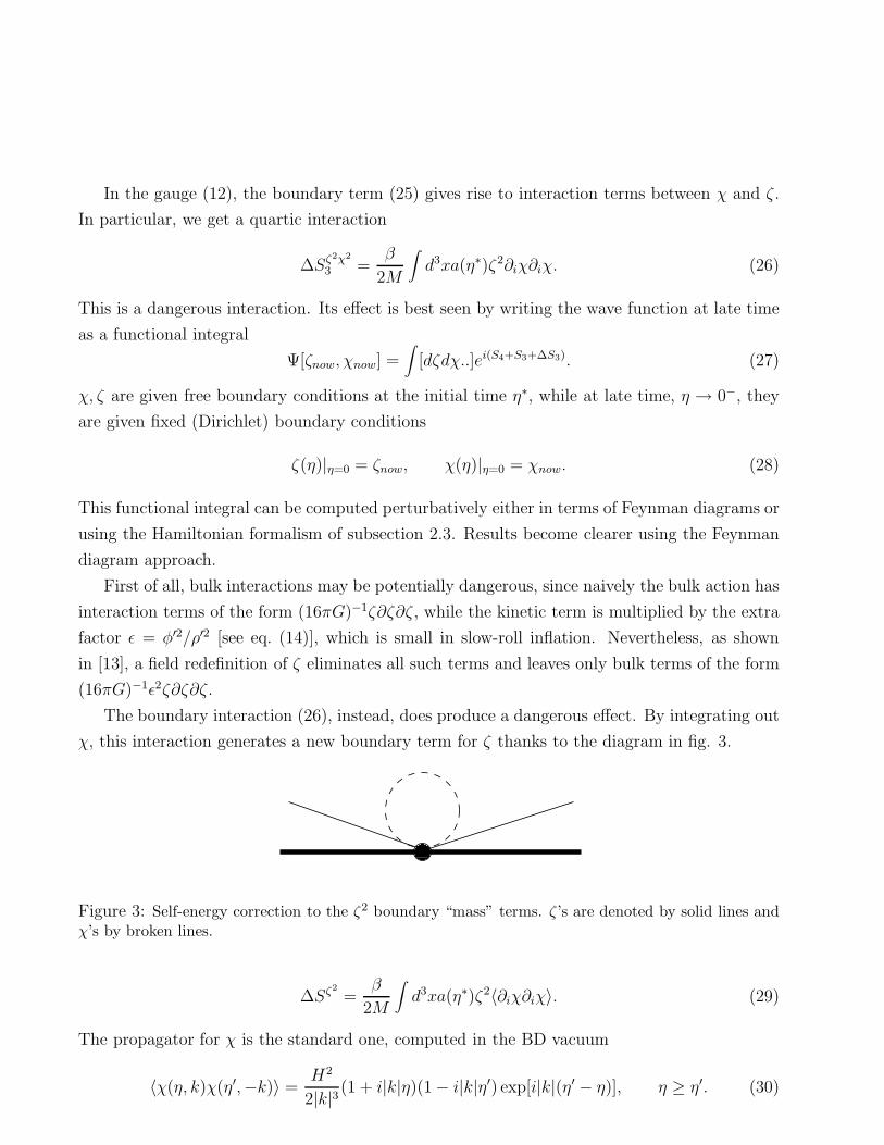
In the gauge (12), the boundary term (25) gives rise to interaction terms between χ and ζ .

In particular, we get a quartic interaction

∆Sζ2χ2

3 =β

2M

∫

d3xa(η∗)ζ2∂iχ∂iχ. (26)

This is a dangerous interaction. Its effect is best seen by writing the wave function at late time

as a functional integral

Ψ[ζnow, χnow] =∫

[dζdχ..]ei(S4+S3+∆S3). (27)

χ, ζ are given free boundary conditions at the initial time η∗, while at late time, η → 0−, they

are given fixed (Dirichlet) boundary conditions

ζ(η)|η=0 = ζnow, χ(η)|η=0 = χnow. (28)

This functional integral can be computed perturbatively either in terms of Feynman diagrams or

using the Hamiltonian formalism of subsection 2.3. Results become clearer using the Feynman

diagram approach.

First of all, bulk interactions may be potentially dangerous, since naively the bulk action has

interaction terms of the form (16πG)−1ζ∂ζ∂ζ , while the kinetic term is multiplied by the extra

factor ǫ = φ′2/ρ′2 [see eq. (14)], which is small in slow-roll inflation. Nevertheless, as shown

in [13], a field redefinition of ζ eliminates all such terms and leaves only bulk terms of the form

(16πG)−1ǫ2ζ∂ζ∂ζ .

The boundary interaction (26), instead, does produce a dangerous effect. By integrating out

χ, this interaction generates a new boundary term for ζ thanks to the diagram in fig. 3.

����

Figure 3: Self-energy correction to the ζ2 boundary “mass” terms. ζ’s are denoted by solid lines andχ’s by broken lines.

∆Sζ2

=β

2M

∫

d3xa(η∗)ζ2〈∂iχ∂iχ〉. (29)

The propagator for χ is the standard one, computed in the BD vacuum

〈χ(η, k)χ(η′,−k)〉 =H2

2|k|3 (1 + i|k|η)(1 − i|k|η′) exp[i|k|(η′ − η)], η ≥ η′. (30)

By substituting this expression, computed at η = η∗, into eq. (29) we get

∆Sζ2 ≈ β

2M

∫

d3xa(η∗)ζ2∫

|k|a(η∗)

≤M

d3k

(2π)3

H2

2|k|3 |k|2(1 + |k|2η∗2) ≈ β

96π2M3

∫

d3xa3(η∗)ζ2. (31)

Here we used a sharp momentum cutoff and the inequality M ≫ H . Any other cutoff would

give a like result.

The effect of this term on the power spectrum is enormous, since the kinetic term for scalar

fluctuations is multiplied by the small number ǫ. If we canonically normalize ζ by

ζ =

√

8πG

ǫv, (32)

we can use the same technique as in subsection 2.3 to get

δP (k)

P (k)= Ca3(η∗)Im [v+(η∗, k)]2, v+(η, k) =

H√

2|k|3(1+ i|k|η) exp(−i|k|η), |k|

a(η∗)≪M.

(33)

With our normalization, C = βGM3/12πǫ. So, for k ∼ 1/η∗, the power spectrum receives

corrections O(βGM3/12πHǫ). By imposing the observational constraint δP (k)/P (k) <∼ ǫ we

arrive at our first naturalness constraint on β

β <∼ 12πǫ2(GM2)−1 H

M. (34)

Notice that the power corrections we computed in section 2.3 were at most O(βH/M). Since

the term (31) is also linear in β and as large as βGM3/12πHǫ, it dominates over the tree-level

term whenever GM4/12πǫH >∼ 1. Constraints of this kind were derived with a different method

in [14, 15]. The method used here makes it clear that the bound comes from asking that the

correction to the BD initial state is generic and robust under radiative corrections. Of course, as

with any divergence, even that in eq. (31) can be canceled by appropriately choosing boundary

counter-terms. The point is that this choice implies a fine-tuned UV completion of our EFT,

which we should not assume without a valid reason such as a symmetry, or a better knowledge

of the UV physics.

Notice that the counter-term that cancels (31) is not the same that renormalizes the brane

tension. The brane tension is renormalized because when we expand eq. (25) in powers of ζ , we

also get a linear term

∆Sζχ2

3 =β

M

∫

d3xa(η∗)ζ∂iχ∂iχ. (35)

This term can be canceled by changing the tension of the term

T∫

d3x√h = T

∫

d3xa3(η∗)e3ζ = T∫

d3xa3(η∗)(

1 + 3ζ +9

2ζ2 + ..

)

. (36)

Equation (31) implies we can cancel the linear term (35) by changing the tension as

3δT +β

48π2M3 = 0. (37)

To cancel the quadratic term, instead, we would need to change the tension as

9δT +β

48π2M3 = 0. (38)

3.2 Naturalness in Inflation II

In the previous subsection, we introduced an extra scalar field, χ, besides the inflaton. This

was done to simplify our analysis and is by no means necessary. We could have introduced a

boundary interaction involving only ζ , for instance5

∆S3 =γ

M

ǫ

8πG

∫

d3xa(η∗)ζ∂2ζ. (39)

This boundary term can be covariantized by recalling that at linear order the 3-d Ricci curvature

Rij is proportional to ∂i∂jζ plus a term linear in the transverse traceless fluctuation γij. So,

the 3-d covariant form of eq. (39) becomes

∆S3 =γ

M

ǫ

8πG

∫

d3x√hR. (40)

Besides the quadratic term (39), eq. (40) produces, among others, a quartic interaction term.

In terms of the canonically normalized field v it reads

∆Sv4

3 =4πGγ

Mǫ

∫

d3x1

a(η∗)v3∂2v. (41)

The self-energy loop now produces a boundary term of the form

γGM3

9πǫ

∫

d3xa3(η∗)v2. (42)

Following the same steps we used to arrive to eq. (34) we obtain a constraint on γ

γ <∼ 9πǫ2(GM2)−1 H

M. (43)

Covariantization of the boundary terms is just one of many ways in which dangerous bound-

ary interactions appear. In the next subsection we will show that such interactions are induced

at the one-loop level when we include the cubic vertices of the bulk theory. One interesting

5The factor ǫ(8πG)−1 is included for convenience so that for the canonically normalized field v the coefficientreduces to γ/M .

source of boundary interactions is the field redefinition needed to make all bulk self-interactions

of ζ O(ǫ2). As it was pointed out in [13], all O(ǫ) bulk cubic interactions assemble into the form

Sζ3

4 =ǫ

8πG

∫

dηd3xf(ζ)

[

− d

dηa2(η)

d

dηζ + a2(η)∂2ζ

]

, (44)

where f(ζ) is a quadratic function of ζ . Since they vanish on the linearized equations of motion,

in brackets, they can be canceled by a local field redefinition of the form ζ → ζ + f(ζ) [13].

When substituted in eq. (39), this field redefinition generates quartic boundary interactions

∆Sζ4

3 =γ

M

ǫ

8πG

∫

d3xa(η∗)f(ζ)∂2f(ζ). (45)

The function f(ζ) is given in [13], and we shall use its explicit form in the next subsection, to

estimate the size of induced boundary interactions. Here, it suffices to notice that it contains,

among others, terms like (a/2a′)2(∂ζ)2, which contain no factors of ǫ. So, the interaction (45)

can generate a large boundary mass term through a diagram as in figure 4.

To sum up, small corrections by seemingly benign irrelevant boundary operators generically

induce by radiative corrections large, dangerous, relevant boundary operators. This problem

does not signal an outright inconsistency of non-BD initial conditions for inflation, but it makes

their description in terms of an EFT unnatural, that is very sensitive to its UV completion.

An equivalent way of stating the problem is simply that the first correction to be expected

in a generic EFT of initial conditions is

αM∫

d3xa3(η∗)v2, (46)

where α is a small coefficient at most of order ǫH/M (because of experimental constraints!). This

is the first universal correction to the BD vacuum that generically dominates over all others. Any

UV modification of physics, be it strings, non-Lorentz invariant dispersion relations, or simply

phase transitions in the late stages of inflation, reduces to this same term. In this perspective,

modifications of the primordial power spectrum seem ill suited to discriminate among different

types of new high-energy physics.

We could have guessed this result because (46) is the lowest-dimension local operator that

can be written with the field v and its derivatives. The only question is whether this operator

is generated after all. Our explicit calculation answered in the affirmative. There is one last

subtlety to explain. Locality depends on the variable we choose to parametrize scalar fluctua-

tions. The correct one is the canonical scalar field v, which has scaling dimension one. It is in

terms of this field that one finds that radiative corrections renormalize the coefficients of rele-

vant operators as M3−∆ etc. We can rewrite (46) or any other local operator in v in manifestly

covariant form using the 3-d metric hij . This expression need not be local in hij . One possible

covariantization of (46) is

αMǫ

8πG

∫

d3x√hR∆−2R, (47)

where ∆ is the covariant scalar Laplacian in 3-d.

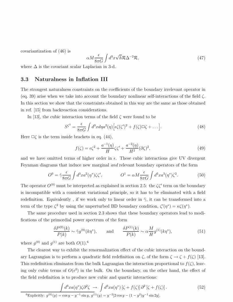
3.3 Naturalness in Inflation III

The strongest naturalness constraints on the coefficients of the boundary irrelevant operator in

(eq. 39) arise when we take into account the boundary nonlinear self-interactions of the field ζ .

In this section we show that the constraints obtained in this way are the same as those obtained

in ref. [15] from backreaction considerations.

In [13], the cubic interaction terms of the field ζ were found to be

Sζ3

=ǫ

8πG

∫

d3xdηa2(η)[

ǫζ(ζ ′)2 + f(ζ)2ζ + . . .]

. (48)

Here 2ζ is the term inside brackets in eq. (44),

f(ζ) = ǫζ2 +a−1(η)

Hζζ ′ +

a−2(η)

H2(∂ζ)2, (49)

and we have omitted terms of higher order in ǫ. These cubic interactions give UV divergent

Feynman diagrams that induce new marginal and relevant boundary operators of the form

O0 = γǫ

8πG

∫

d3xa2(η∗)ζζ ′, O1 = αMǫ

8πG

∫

d3xa3(η∗)ζ2. (50)

The operator O(0) must be interpreted as explained in section 2.5: the ζζ ′ term on the boundary

is incompatible with a consistent variational principle, so it has to be eliminated with a field

redefinition. Equivalently , if we work only to linear order in γ, it can be transformed into a

term of the type ζ2 by using the unperturbed BD boundary condition, ζ ′(η∗) = κζ(η∗).

The same procedure used in section 2.3 shows that these boundary operators lead to modi-

fications of the primordial power spectrum of the form

δP (0)(k)

P (k)∼ γg(0)(kη∗), and

δP (1)(k)

P (k)∼ α

M

Hg(1)(kη∗), (51)

where g(0) and g(1) are both O(1).6

The clearest way to exhibit the renormalization effect of the cubic interaction on the bound-

ary Lagrangian is to perform a quadratic field redefinition on ζ , of the form ζ → ζ + f(ζ) [13].

This redefinition eliminates from the bulk Lagrangian the interaction proportional to f(ζ), leav-

ing only cubic terms of O(ǫ2) in the bulk. On the boundary, on the other hand, the effect of

the field redefinition is to produce new cubic and quartic interactions:∫

d3xa(η∗)ζ∂2ζ →∫

d3xa(η∗) [ζ + f(ζ)]∂2 [ζ + f(ζ)] . (52)

6Explicitly: g(0)(y) = cos y − y−1 sin y, g(1)(y) = y−2[2 cos y − (1 − y2)y−1 sin 2y].

Using the explicit form of f(ζ), eq. (49), we see that new boundary action contains, among

others, the terms

∆Sb1 =γ

M

ǫ

8πG

∫

d3xǫ

Hζ2∂2 (ζζ ′) , ∆Sb2 =

γ

M

ǫ

8πG

∫

d3x1

a2(η∗)H3ζζ ′∂2(∂ζ)2. (53)

These interactions induce boundary operators of the form (50), through the Feynman diagram

shown in fig. 4.

����

Figure 4: Effective boundary two-point vertex induced at one loop by the field redefinition ζ → ζ+f(ζ).The quartic interaction is proportional to γf∂2f .

By plugging the interaction ∆Sb1 in the vertex of this diagram we arrive at a contribution to

the effective action for ζ :

∆Sζ2 ≈ ǫ

8πG

γ

M

ǫ

H

∫

d3q

(2π)3ζ2(q, η∗)

∫

d3k

(2π)3k2〈ζ(k, η∗)ζ ′(−k, η∗)〉 (54)

≈ ǫHγ

M

∫ d3q

(2π)3ζ2(q, η∗)

∫

|k|≤Ma(η∗)

d3k

(2π)3k2η∗2 (55)

≈ ǫγM4

H

∫

d3xa3(η∗)ζ2(η∗), (56)

where in the third line we have considered only the most divergent term, and we used for ζ the

scalar field propagator given in eq. (30), up to an normalization factor 8πGǫ−1:

〈ζ(k, η)ζ(−k, η′)〉 =8πG

ǫ〈χ(k, η)χ(−k, η′)〉. (57)

The induced boundary term is the operator O(1) in eq. (50), with a coefficient

α ∼ γ8πGM3

H. (58)

A similar calculation shows that, by plugging the interaction ∆Sb2 in (53) in the vertex of

the diagram in fig. 4, one generates the operator O(0) given in eq. (50), with a coefficient

γ ∼ γ

ǫ

8πGM5

H3. (59)

By asking that δP (1)(k)/P (k) and δP (0)(k)/P (k) are within the presently acceptable deviation

from scale invariance in the power spectrum, i.e. that they are smaller that the combination of

slow-roll parameters (ǫ+η), we get, from eq. (51), the constraints found in [15] for the coefficient

γ:

γ <∼ ǫ(GM2)−1 H2

M2, γ <∼ ǫ2(GM2)−1 H

3

M3, γ <∼ ǫη(GM2)−1 H

3

M3. (60)

Again, we want to stress that these are naturalness bounds, in that they can be avoided by

tuning the coefficient of the boundary operators in eq. (50) to a much smaller value than they

would generically have in the presence of the boundary perturbation, eq. (39).

3.4 Coda: Is the BD Vacuum Natural?

In the previous subsections we applied standard techniques borrowed from field theory to study

the naturalness of initial conditions that, below the cutoff energy M , differ from those specified

by the Bunch-Davis vacuum. One might wonder what happens in the absence of these modifica-

tions: in particular, one might worry that the methods we used make even the unperturbed BD

vacuum fine tuned, thus making the naturalness bounds we found less interesting. This would

happen if one could find Feynman diagrams producing large boundary renormalizations that do

not arise from the perturbation γ, i.e. they do not vanish at γ = 0. This is not the case, if one

uses as the unperturbed vacuum, i.e. the one corresponding to γ = 0 in eq. (39), the vacuum of

the interacting theory. Indeed, the interacting BD vacuum is defined by the functional integral

ΨBD[ζ ] =∫

[dζ...] exp(iS), (61)

where S =∫

dηL is the action of the interacting theory, and the integration in η runs from η∗

to η = −∞+ iǫ. The Eucildean continuation in η selects the BD (or Hartle-Hawking [20]) wave

function. In the language of ref. [7] we are thus choosing “transparent” boundary conditions.

Now, the wave function at any later time η′ > η∗ is also defined by the functional integral (61),

with the range of integration ranging from η′ to −∞ + iǫ. In this representation, there is no

boundary at η∗, so the field redefinition will not produce any large boundary term.

By splitting the integration in two regions, before and after the “initial” time η∗, this ob-

vious result is reinterpereted as a cancelation between boundary terms arising from the field

redefinition of the bulk action∫

η>η∗ dηL, and the boundary terms defining the BD vacuum. So,

the only nonlinear interactions left will be bulk terms suppressed by powers of the slow-roll

parameter. This result shows that the slow-roll inflation background is stable against both

bulk and boundary radiative corrections. In the presence of the boundary perturbation (39),

however, this argument breaks down, and new boundary terms containing f(ζ) are generated

by the field redefinition.

Finally, we should point out again another important feature that distinguishes the BD

vacuum from all others. As we have seen, a modification of the BD vacuum by new physics at

a physical energy scale M generically manifests itself in the EFT by the boundary term (46).

Generically, one would expect the coefficient α to be O(1), yet observation constrains it to be

smaller than O(ǫH/M). Since this constraint comes from the size of δP (k)/P (k) at |k| = |η∗|−1,

i.e. at |k|phys = |k|/a(η∗) = H , an alternative route to make the correction (46) compatible

with experiment is to make inflation last long enough to stretch |k|phys above today’s horizon

scale. This requires a(ηnow)/a(η∗) > H/Hnow. In other words, the change in the initial state

of inflation behaves exactly as any other pre-inflation inhomogeneity. Moreover, its effect is

generically described almost entirely by a single operator, eq. (46), no matter what originated

the change. So, the BD vacuum is natural also thanks to the very property that defines inflation:

wait long enough, and all changes will be diluted away.

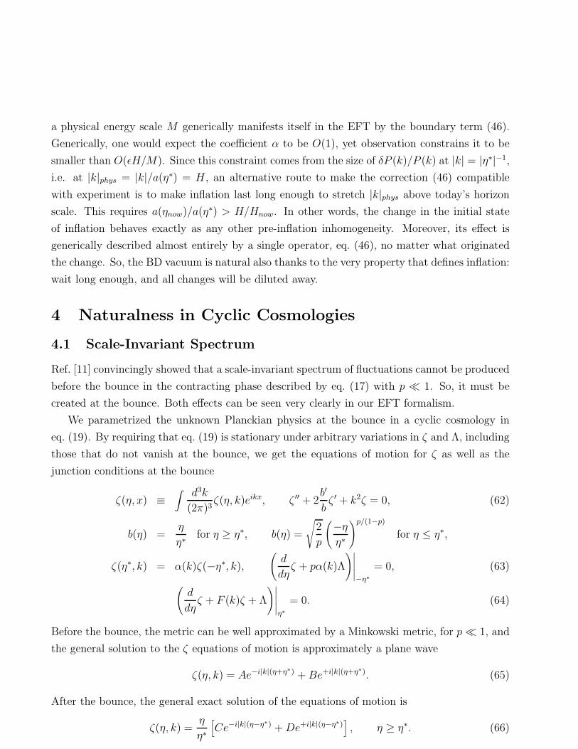
4 Naturalness in Cyclic Cosmologies

4.1 Scale-Invariant Spectrum

Ref. [11] convincingly showed that a scale-invariant spectrum of fluctuations cannot be produced

before the bounce in the contracting phase described by eq. (17) with p ≪ 1. So, it must be

created at the bounce. Both effects can be seen very clearly in our EFT formalism.

We parametrized the unknown Planckian physics at the bounce in a cyclic cosmology in

eq. (19). By requiring that eq. (19) is stationary under arbitrary variations in ζ and Λ, including

those that do not vanish at the bounce, we get the equations of motion for ζ as well as the

junction conditions at the bounce

ζ(η, x) ≡∫ d3k

(2π)3ζ(η, k)eikx, ζ ′′ + 2

b′

bζ ′ + k2ζ = 0, (62)

b(η) =η

η∗for η ≥ η∗, b(η) =

√

2

p

(

−ηη∗

)p/(1−p)

for η ≤ η∗,

ζ(η∗, k) = α(k)ζ(−η∗, k),(

d

dηζ + pα(k)Λ

)∣

∣

∣

∣

∣

−η∗

= 0, (63)

(

d

dηζ + F (k)ζ + Λ

)∣

∣

∣

∣

∣

η∗

= 0. (64)

Before the bounce, the metric can be well approximated by a Minkowski metric, for p≪ 1, and

the general solution to the ζ equations of motion is approximately a plane wave

ζ(η, k) = Ae−i|k|(η+η∗) +Be+i|k|(η+η

∗). (65)

After the bounce, the general exact solution of the equations of motion is

ζ(η, k) =η

η∗

[

Ce−i|k|(η−η∗) +De+i|k|(η−η

∗)]

, η ≥ η∗. (66)

The wave function of the fluctuation ζ(η, k) is given by the functional integral

Ψ[ζ(η, k)] =∫

[dζdΛ] exp(iS[ζ,Λ]), (67)

where S is given in (19). The boundary condition at η → −∞ is ζ(η, k) → Ae−i|k|η, because the

pre-big bang initial state is the standard Minkowski vacuum. We want to compute the visible

primordial spectrum, so we must compute Ψ[ζ(η, k)] well after the bounce, at η → +∞. So, the

value of ζ at the late-time boundary is fixed: ζ(η, k) → ζ(k). In the quadratic approximation

used in (19), the wave function is Gaussian

Ψ[ζ(k)] =∏

k

exp

[

−γ(k)2

ζ2(k)

]

. (68)

The power spectrum is a function of the equal time, two point correlator of ζ :

〈ζ(k)ζ(k′)〉 =(2π)3

k3δ3(k + k′)P (k) (69)

〈ζ(k)ζ(k′)〉 =∫

[dζ ]ζ(k)ζ(k′)|Ψ[ζ ]|2/∫

[dζ ]|Ψ[ζ ]|2 = (2π)3δ3(k + k′)1

2Re γ(k). (70)

To compute γ(k) we perform the functional integral (67). Since it is Gaussian, it reduces to

Ψ[ζ(k)] = limη→+∞

exp

−i16πG

∫

d3k

(

η

η∗

)2

ζ ′(η, k)ζ(η,−k)

. (71)

The boundary at η → −∞ has been discarded using the +iǫ prescription to select the positive-

frequency Minkowski vacuum, that is by running the contour of integration in η over Euclidean

time in the far past. This prescription selects the true vacuum even in the interacting theory7.

It is this prescription that generates a real part in γ, which is naively purely imaginary.

A major simplification occurs because we are interested in observable modes, whose wave-

length is much larger than the Hubble radius immediately after the bounce: 2π/|k| ≫ 1/H(η∗) =

η∗. In this case one can use the boundary condition at late time, ζ = ζ(k), to approximate the

post-bounce evolution of ζ as

ζ(η, k) = ζ(k) + Eη∗

η+O(|k|η), 2π

|k| ≫ η ≥ η∗. (72)

Before the bounce, boundary conditions at η → −∞ set

ζ(η, k) = A[1 − i|k|(η + η∗)] +O(|k|2η2), −2π

|k| ≪ η ≤ −η∗. (73)

The matching conditions at the bounce, eqs. (63,64), are then easily solved to give

E =i|k|/p|α|2 + F

1/η∗ − F − i|k|/p|α|2ζ(k). (74)

7See [13] for another application of this method to cosmology.

By substituting into eq. (71) we find

γ(k) =1

8πG

|k|/p|α|2 − iF

1 − η∗F − i|k|η∗/p|α|2 , (75)

whence(2π)3

k3P (k) = 4πG

(1 − η∗ReF )2 + (η∗ImF + |k|η∗/p|α|2)2

|k|/p|α|2 − ImF. (76)

Continuity at the bounce sets α(k) = 1, F (k) = 0. In this case we get P (k) ∝ |k|2 +η∗|k|3 ∼|k|2, instead of the scale invariant spectrum P (k) ∝ cst. This result agrees with ref. [11].

This means that all the features of the primordial spectrum are due to the unknown physics

at the bounce, where the NEC is violated. This is an unavoidable [11], unpleasant feature of

cyclic cosmologies, that makes the whole pre-big bang phase almost useless. Almost, but not

completely. We can consider η∗ as “the earliest” time and integrate out all the pre-big bang

evolution, but in doing so, we would need nonlocal operators on the brane to generate a scale

invariant spectrum. The long pre-big bang phase, instead, allows for one good choice of local

coefficients on the brane:

F (k) = 0, α(k) =σ|k|2η∗2√

p, (77)

where the constant σ can be related to the inflationary parameters H and ǫ introduced in section

3 by comparing eq. (76) to the standard inflationary power spectrum, P (k) = 4πGH2/(2π)3ǫ,

which leads to ση∗ ∼ √ǫ/H .

Another natural choice is to require that ζ is continuous at the bounce. This sets α(k) =

1, F (k) = (√pση∗2|k|)−1, with the same constant σ as before. We shall call these junction

conditions the “short bounce.”

An interesting feature shared by all boundary conditions is that ζ keeps evolving well into the

FRW phase, because the coefficient E of the decaying part of ζ must be much bigger than ζ(k)

to create the correct scale-invariant power spectrum. For the junction conditions in eq. (77),

for instance,

ζnow ≡ ζ(k) ∼ σ−2(|k|η∗)−3ζ(η∗). (78)

This evolution could be in itself a problem for the cyclic cosmology scenario. Eq. (78) shows

that right after the bounce, in the radiation-dominated FRW phase, fluctuations are minuscule,

compared to today. So, they can be affected by tiny inhomogeneities developing in the FRW

phase, which we have ignored in our formalism. This is another potential source of fine-tuning,

besides that due to our ignorance of the physics at the bounce, but we will not investigate it

here.

Finally, the post-bounce evolution effectively erases any non-Gaussianity that could exist at

the bounce. We shall discuss this effect in more details in section 6.

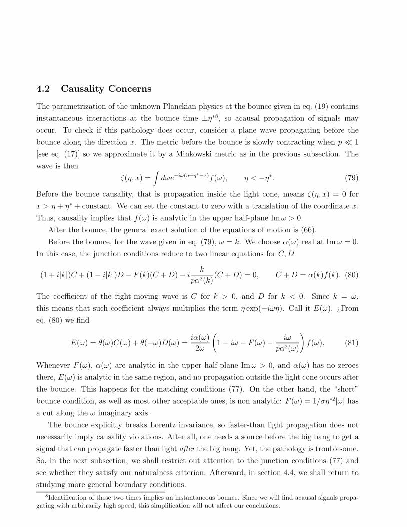
4.2 Causality Concerns

The parametrization of the unknown Planckian physics at the bounce given in eq. (19) contains

instantaneous interactions at the bounce time ±η∗8, so acausal propagation of signals may

occur. To check if this pathology does occur, consider a plane wave propagating before the

bounce along the direction x. The metric before the bounce is slowly contracting when p ≪ 1

[see eq. (17)] so we approximate it by a Minkowski metric as in the previous subsection. The

wave is then

ζ(η, x) =∫

dωe−iω(η+η∗−x)f(ω), η < −η∗. (79)

Before the bounce causality, that is propagation inside the light cone, means ζ(η, x) = 0 for

x > η + η∗ + constant. We can set the constant to zero with a translation of the coordinate x.

Thus, causality implies that f(ω) is analytic in the upper half-plane Imω > 0.

After the bounce, the general exact solution of the equations of motion is (66).

Before the bounce, for the wave given in eq. (79), ω = k. We choose α(ω) real at Imω = 0.

In this case, the junction conditions reduce to two linear equations for C,D

(1 + i|k|)C + (1− i|k|)D− F (k)(C +D) − ik

pα2(k)(C +D) = 0, C +D = α(k)f(k). (80)

The coefficient of the right-moving wave is C for k > 0, and D for k < 0. Since k = ω,

this means that such coefficient always multiplies the term η exp(−iωη). Call it E(ω). ¿From

eq. (80) we find

E(ω) = θ(ω)C(ω) + θ(−ω)D(ω) =iα(ω)

2ω

(

1 − iω − F (ω) − iω

pα2(ω)

)

f(ω). (81)

Whenever F (ω), α(ω) are analytic in the upper half-plane Imω > 0, and α(ω) has no zeroes

there, E(ω) is analytic in the same region, and no propagation outside the light cone occurs after

the bounce. This happens for the matching conditions (77). On the other hand, the “short”

bounce condition, as well as most other acceptable ones, is non analytic: F (ω) = 1/ση∗2|ω| has

a cut along the ω imaginary axis.

The bounce explicitly breaks Lorentz invariance, so faster-than light propagation does not

necessarily imply causality violations. After all, one needs a source before the big bang to get a

signal that can propagate faster than light after the big bang. Yet, the pathology is troublesome.

So, in the next subsection, we shall restrict out attention to the junction conditions (77) and

see whether they satisfy our naturalness criterion. Afterward, in section 4.4, we shall return to

studying more general boundary conditions.

8Identification of these two times implies an instantaneous bounce. Since we will find acausal signals propa-gating with arbitrarily high speed, this simplification will not affect our conclusions.

4.3 Naturalness Concerns I

The quadratic junction conditions given in subsection 4.1 need to be covariantized with respect

to 3-d coordinate transformations. This is particularly simple for the conditions (77). It suffices

to notice that at linear order ∂2ζ ∼ R. Then the action contains the term

S3 =ση∗2

16πG√p

∫

d3x√hRΛ

∣

∣

∣

∣

−η∗. (82)

By expanding this equation we get a coupling Sζ3Λ

3 ∼ ζ2∂2ζΛ. The equal-time ζ propagator is

now ∝ |k|−1 so Sζ3Λ

3 produces a self-energy diagram as in fig. 3, which gives a one-loop correction

of the form (recall that a(η∗) = 1 here )

Sζ2

3 ∼ ση∗2M4

4π2√p∫

d3xζΛ

∣

∣

∣

∣

−η∗. (83)

This correction destroys the scale invariance of the spectrum for all momenta |k| < O(√GM4).

Again, a scale invariant spectrum turns out to be possible by fine-tuning the operators

inserted on the brane. Since they parametrize our ignorance of the high-energy physics occurring

at the bounce, this means that a scale invariant spectrum depends on a very special completion

of our EFT instead of being a robust, generic feature.

Our analysis requires that we do not know in detail the history of the bounce. If we know

what happens at the bounce, then we cannot invoke a genericity argument. To appreciate this

point, imagine that we ignore the whole history of the universe before the bounce, i.e. we

integrate out ζ(η) for η < −η∗ and we substitute for it the boundary term

S3 =1

16πG

∫

d3k

(2π)3i|k||ζ(η, k)|2

∣

∣

∣

∣

∣

−η∗

. (84)

A generic covariantization of this term would produce a self-energy correction resulting in a

“mass” term ∼ M3ζ2 that changes the spectrum for all momenta |k| <∼ O(GM3). In this case

though, we do know the previous history of the universe. It is a long slowly contracting phase, in

which the power spectrum 1/|k| is due to the masslessness of ζ , which is guaranteed by it being

part of a gauge field: the metric. Essentially the same argument tells us that the scale-invariant

power spectrum of inflation is natural.

4.4 Naturalness Concerns II

The function F (∂) that we introduced in eq. (19) parametrizes how the superhorizon modes get

modified during the bounce. As we noted earlier in this section, in the case of a short bounce

this function must be nonlocal to reproduce scale invariance at late times:

F (∂) =1

√pση∗2

√−∂2

. (85)

The nonlocality of this interaction on the S-brane complicates the study of its stability under

radiative corrections.

Our strategy is to rewrite the part of the action containing F (∂) as a fully local action,

by introducing auxiliary fields localized on the S-brane. Covariantization of this local action

introduces then certain universal interactions of ζ with the additional fields, which allow us to

study the radiative stability of this system in the same way as in the previous section.

To introduce the technique, consider a three dimensional scalar with action:

S[φ] =∫

d3xφ1√−∂2

φ. (86)

To render this action local, introduce an additional, massless field ϕ that couples to φ as follows:

S[φ, ϕ] =∫

d3x[

λφϕ2 + ϕ∂2ϕ]

. (87)

In terms of the variables φ, ϕ, this action is fully local. The field ϕ appears quadratically in it,

so we can integrate ϕ out exactly. After integration, we are left with an effective action for φ

only, which possesses a nonlocal propagator. A calculation of the diagram in figure 5 gives:

Seff [φ] =1

4π

∫

d3xφλ2

√−∂2

φ+ ..., (88)

The ellipses denote terms of order φ3 or higher, that we do not need for computing the power

spectrum. The quadratic term is indeed the nonlocal action of eq. (86). We note that this

mechanism depends crucially on the masslessness of the scalar ϕ. If radiative corrections induce

a mass m for ϕ, the form of the action eq. (86) is spoiled for all momenta |k| <∼ m.

Figure 5: The one-loop, UV finite diagram giving rise to the effective action in equation (88). Thesolid line denotes ϕ, whereas dashed lines denote φ.

In our case, the fundamental scalar is the ζ-field. We cannot exactly use the above mechanism

with φ → ζ , because the action in eq. (87) cannot be covariantized consistently. Indeed, the

interaction term ζϕ2 is uniquely covariantized by the local expression√hϕ2. At zeroth order in

the metric fluctuation however, this term gives a mass to ϕ, which makes the one-loop induced

term regular in the infrared, instead of being divergent as |k|−1.

For this reason we must resort to a more complicated system to generate an action of the

form (86) for ζ . The following covariant action satisfies our requirements:

S[ζ, ϕ, ψ] =∫

d3x√h[

αRϕ+ βψ(/D∆ϕ)ψ + ψ∆ψ]

. (89)

Here ϕ is a scalar, ψ is a spinor, and ∆ is the covariant Laplacian. Notice that these fields have

non-minimal kinetic terms. To see how the effective action for ζ looks like we proceed in two

steps, by first integrating out ψ and next ϕ. Integrating out ψ at one-loop, as shown in figure 6,

we arrive at an effective action for ϕ and ζ that to quadratic order reads:

S[ζ, ϕ] =∫

d3x[

α∂2ζϕ+ β2ϕ(−∂2)5/2ϕ]

. (90)

Next, integrating out ϕ the effective quadratic action for ζ reduces to:

Seff [ζ ] =∫

d3x

[

ζα2

β2√−∂2

ζ

]

(91)

By appropriately choosing α and β, we can make α2/β2 = (√pση∗2)−1, so that this interaction

at the S-brane is indeed ζF (∂)ζ .

Figure 6: The one-loop diagram giving rise to the effective action in equation (91). Dashed linesrepresent ψ, whereas dashed-dotted lines represent ϕ.

The Lagrangian in (89) is our starting point for investigating if the induced action in (91) is

stable under radiative corrections. The interactions in (89) come from the covariantization of the

action, with ζ coupling universally to the other fields in the action. Now, we must check if any

of these interactions feed down to dangerous relevant operators. For us a “dangerous operator”

means an operator that spoils the scale invariance of the spectrum after the bounce, such as a

large mass term for ψ or ϕ. In principle, a mass smaller than the IR-cutoff, aH|now, is allowed,

since we cannot probe the spectrum below this scale. After all, the function F (k) ∼ |k|−1 should

be regulated by that IR cutoff in order not to generate infinite backreaction at zero momentum.

The point is that we will show that the natural induced mass is much larger than the IR cutoff.

For example, we see that the covariant kinetic term for the ψ-field in eq. (89) contains terms

like:

∆Sζψψ ∼∫

d3xψ∂iζ∂iψ. (92)

This interaction gives rise to a mass term by the one-loop diagram shown in figure 7. Cutting

off the momentum integral at the scale M , we obtain:

∆Sψψ ∼ M4

M2P

∫

d3xψψ. (93)

This relevant interaction dominates the original kinetic term for ψ at momentum scales |k| <∼ M2

Mp.

Figure 7: The one-loop diagram giving rise to the effective action in equation (91). Dashed linesrepresent ψ and the solid line represents ζ.

More importantly, the one-loop induced operator in eq. (90) is modified to:

∆Sϕ2 ∼ β2M

4P

M5

∫

d3xϕ(∂2)3ϕ. (94)

Now, by integrating out the field ϕ we obtain the following operator:

∆Sζ2 ∼ 1√

pση∗2M5

M4P

∫

d3xζ1

∂2ζ. (95)

This term is clearly IR dominant over the original term in eq. (91), for all momenta |k| <∼M(M/Mp)4

and it produces an unacceptably red spectrum after the bounce over the whole range of scales

relevant for observation. To avoid the appearance of this term, we must tune the mass term

of the fermion in eq. (93) to the much smaller value (by about thirty orders of magnitude!)

discussed above, by adding a counterterm in the bare Lagrangian. This is the exact analogue

of the mass instability of light fundamental scalars in the standard model. Our analysis here

clearly indicates that the choice for the function F (∂) in eq. (85) is fine-tuned in an effective

field theory perspective, and that only a very specific UV-completion of the short bounce can

guarantee scale invariance at late times.

One can show that similar considerations apply to other choices of boundary non-local oper-

ators that reproduce the correct power-spectrum when inserted in eq. (76). By an appropriate

choice of auxiliary fields one can make these operators local. This always requires some of the

auxiliary fields to have an unnaturally small value for the coefficient of an unprotected operator,

that receives correction due to its universal interactions with the metric.

5 Non-Gaussianities in Inflation

5.1 Minimally Coupled Scalar in de Sitter Space

A minimally coupled scalar models tensor fluctuations in the CMB, so it has an intrinsic interest

besides offering a simple example of our method. The scalar action S4 + S3, given in eq. (1), is

only the quadratic part of an action that can contain nonlinear terms both in the 4-d bulk and

in the 3-d boundary. We shall consider here the effect of adding a boundary interaction

∆Sχ3

3 =∫

d3xa3(η∗)λχ3, (96)

while keeping the bulk action S4 quadratic. We could compute the effect of this term on late-

time correlators in a Hamiltonian formalism, as in subsection 2.3, but we will use instead a

Lagrangian approach, which is simpler for taking into account back-reaction effects and for

application to cyclic cosmology. In this case, the effect at late time η → 0−, is [cfr. eq. (27)]

Ψ[χnow] =∫

[dχ..]ei(S4+S3+∆Sχ3

3 ). (97)

The boundary condition at late time is χ(0, x) = χnow(x) while at early time is obtained by

making the action S4 +S3 +∆Sχ3

3 stationary w.r.t. free variations of χ, including those that do

not vanish on the boundary. The resulting initial condition, written for the Fourier components

χ(0, k), is

χ′(η∗, k) + κ(k)χ(η∗, k) + 3λa(η∗)∫

d3l

(2π)3χ(η∗, l)χ(η∗, k − l) = 0. (98)

In the bulk, χ obeys a free equation of motion, whose general solution is

χ(η, k) = A(1 − i|k|η) exp(−i|k|η) +B(1 + i|k|η) exp(i|k|η). (99)

At tree level, the wave function (96) is Ψ[χ] = exp(iS4 + iS3 + i∆Sχ3

3 ), computed on shell.

We only need quadratic and cubic terms in the action, so we can expand the solution of the

equations of motion as χ(η, k) = χ0(η, k) + λχ1(η, k), and keep only terms at most of linear

order in λ. The coefficients χ0(η, k), χ1(η, k) obey the boundary conditions

χ0(0, k) = χ(k), χ1(0, k) = 0, χ′0(η

∗, k) + κ(k)χ0(η∗, k) = 0. (100)

We need not write the boundary condition for χ1(η∗, k) because of the following reason. On

shell and to linear order in λ, we can integrate by part the free action and use the free bulk

equations of motion to arrive at

S4 + S3 + ∆Sχ3

3 = limη→0−

{

−1

2

∫

d3k

(2π)3a2(η)χ′

0(η, k)[χ0(η,−k) + 2λχ1(η,−k)]+

1

2

∫ d3k

(2π)3a2(η∗)[χ′

0(η∗, k) + κ(k)χ0(η

∗, k)][χ0(η∗,−k) + 2λχ1(η

∗,−k)] +

∫

d3xa3(η∗)λχ30(η

∗, x)}

. (101)

Boundary conditions (100) now make all terms within brackets vanish, except the first that

reduces to χ(−k). Therefore, the action reduces to the standard quadratic term, which gives

rise to Gaussian fluctuations, plus a cubic term obtained simply by writing the free field χ at

η∗ in terms of its late-time value χ(k).

S4 + S3 + ∆Sχ3

3 =∫

d3k

(2π)3i|k|3H2

|χ(k)|2 + ∆Sχ3

3 [χ30(η

∗, k)]. (102)

In this formula, we have dropped a real divergent term, which does not contribute to expectation

values, since it disappears in taking the square norm of the wave function. Using eq. (99) and

the boundary conditions (100), the cubic term finally reads

∆Sχ3

3 [χ30(η

∗, k)] = λ∫

d9k

(2π)9a3(η∗)(2π)3δ3(k1 +k2 +k3)

3∏

j=1

χ(kj)(1− i|kj|η∗) exp(i|kj|η∗). (103)

The cubic non-Gaussianity is

〈χ(k1)χ(k2)χ(k3)〉 =

∫

[dχ]χ(k1)χ(k2)χ(k3)|Ψ[χ(k)]|2∫

[dχ(k)]|Ψ[χ(k)]|2 . (104)

To first order in λ this integral is

〈χ(k1)χ(k2)χ(k3)〉 = 6(2π)3δ3(k1 + k2 + k3)λ(k1, k2, k3)3∏

j=1

H2

2|kj|3(105)

λ(k1, k2, k3) = −2a3(η∗)Im

3∏

j=1

(1 − i|kj |η∗) exp(i|kj|η∗)

. (106)

Notice that the oscillating exponent in λ makes it vanish for momenta |k| ≫ 1/|η∗|, i.e. for

physical momenta |k|/a ≫ H . So, the effect of the boundary term is significant only for

momenta that crossed the horizon before the time η∗. Physically, this effect can be understood

by interpreting the boundary term ∆Sχ3

as a “summary” of cosmic evolution prior to η∗ -such

as phase transitions, decoupling of heavy particles etc.. In this picture, any effect of this early

history is washed away by inflation in all modes that keep evolving after η∗. This cutoff at η∗

is another manifestation of the key property of inflating backgrounds, namely that they dilute

away any primordial inhomogeneity. It also makes it difficult to detect such a non-Gaussianity

unless Ha(η∗)/a(ηnow) > Hnow.

For momenta |k| ≪ 1/|η∗| and λ real, eq. (106) becomes

〈χ(k1)χ(k2)χ(k3)〉 = −(2π)3δ3(k1 + k2 + k3)H3λ

2

∑

l>m

|kl|−3|km|−3. (107)

5.1.1 Estimating the Back-Reaction

The coupling λχ3 has dimension 3 so it is marginal in the boundary EFT. Loops can only

renormalize it logarithmically, so it can be naturally small. At O(λ2), there exists a potential

contribution to the boundary “mass” term∫

d3xa3χ2. On dimensional grounds, we can easily

estimate its coefficient as O(λ2M). So, as long as

λ2 <∼ ǫH/M, (108)

the induced “mass” term is not in conflict with experimental bounds.

5.2 Scalar Fluctuations

Scalar fluctuations ζ have model independent non-Gaussianities [13, 21] of the form

〈ζ3〉 = (2π)3δ3(k1 + k2 + k3)64π2G2H4

ǫF (k1, k2, k3), (109)

where F is a homogeneous function of degree −6 in the momenta. To compare with the results

of the previous subsection, it is convenient to express the three point function in terms of the

canonically normalized field v defined in eq. (32). Then the size of 〈v3〉 is O(√

8πGǫH4k−6).

Eventual non-Gaussianities in the initial conditions are instead O(H3λk−6). Clearly, for λ large

enough, the boundary non-Gaussianity can be dominant for momenta |k| < 1/|η∗|. We must

only check that the new cubic interactions do not introduce unacceptably large boundary “mass”

renormalization. We already saw that this condition gives the bound λ <∼√

ǫH/M . Another

bound comes from the mixed term due to the universal bulk cubic interaction [13] ∼ µv∂v∂v,

where µ = O(√

8πGǫ). It is a dimension-5 operator that can induce at a boundary term O(µλ)

via the self-energy diagram shown in fig. 8. On dimensional grounds the induced boundary

Figure 8: A mixed bulk-boundary interaction may generate a boundary mass term. The black squaredenotes the bulk interaction µv∂v∂v, the black circle denotes the boundary interaction λv3.

“mass” term is at most O(λµM2)∫

d3xa3χ2. This gives another bound on λ:

λ <∼√ǫH

M

Mp

M, Mp ≡ (8πG)−1/2. (110)

For ǫ ∼ 10−2, M ∼ 1016 GeV and H ∼ 1014 GeV this bound is even weaker than (108).

The ratio of the non-Gaussianity induced by boundary terms over the universal bulk term

is λMp/√ǫH . For the extremal value λ ∼

√

ǫH/M , it becomes Mp/√HM = O(104). So, there

is definitely room for an observable signal here! A word of caution is necessary, tough. First

of all, in order to see a clear signal we need that inflation does not last too long. Otherwise,

thanks to the cutoff at |k| ∼ 1/|η∗|, the initial non-Gaussianity would only affect unobservable

super-horizon fluctuations. Moreover, in deriving the bound λ <∼√

ǫH/M we only demanded

that the induced change in the power spectrum is less than ǫ. More stringent bounds on the

power spectrum give a stronger bound on λ [15].

6 Non-Gaussianities in Cyclic Cosmologies

6.1 Damping Effects

As we mentioned earlier, in cyclic cosmologies, a scale invariant power spectrum for scalar

fluctuations needs significant evolution after the bounce, well into the (radiation dominated)

FRW phase. For the junction conditions (77), for instance, ζnow ≡ ζ(k) = σ−2(|k|η∗)−3ζ(η∗) =

σ−1(|k|η∗)−1ζ(−η∗). Suppose now that the wave function of the fluctuations just before the

bounce contains a non-Gaussianity

Ψ[ζ−] =∏

k

exp

[

− |k|16πG

|ζ−(k)|2 + λ(k1, k2, k3)ζ−(k3)ζ−(k3)ζ−(k3)

]

, ζ− ≡ ζ(−η∗). (111)

The three-point function can be computed as we did for inflation:

〈ζ3−〉 =

∫

[dζ ]ζ3|Ψ[ζ ]|2∫

[dζ ]|Ψ[ζ ]|2 ∼ λ(16πG)3

|k|3 . (112)

Assume for sake of example that bulk non-Gaussianities are negligible; then the late-time form

of Ψ is obtained by evolving ζ with its quadratic equations of motion, and by expressing ζ− in

terms of ζnow: ζ− = σ|k|η∗ζnow

Ψ[ζnow] =∏

k

exp

[

−σ2η∗2|k|316πG

|ζnow(k)|2 + λ(k1, k2, k3)ζnow(k3)ζnow(k3)ζnow(k3)

]

,(113)

λ(k1, k2, k3) = σ3η∗3|k1||k2||k3|λ(k,k2, k3). (114)

Finally, the magnitude of 〈ζ3now〉 is

〈ζ3now〉/(〈ζ2

now〉)3/2 ∼ (ση∗|k|)3〈ζ3−〉/(〈ζ2

−〉)3/2 ≪ 〈ζ3−〉/(〈ζ2

−〉)3/2. (115)

So, any pre-bounce non-Gaussianity is damped by the extremely small factor (ση∗|k|)3. Similar

estimates hold for other choices of junction conditions.

Evidently, only very dramatic non-Gaussianities have a chance to survive the smoothing

effect of the bounce. In the next subsection we investigate whether this may happen.

6.2 Non-Linear Interactions in the Slow-Contraction Epoch

There is one last subtlety about the size of non-Gaussianities in the cyclic models we are consid-

ering that needs been addressed. It relates to the consistency of the perturbative expansion in

this backgrounds. Looking at the scalar potential (17), one may worry that for small p the non-

linearities of the theory may become important, and the model may become strongly coupled.

Indeed, if we consider the action to non-linear order, we may worry about terms containing

self-interactions of the scalar, since on our background, for instance, V ′′′(φ) ∼ 1/√p.

Consider the situation in the harmonic (de Donder) gauge, in which the kinetic term of

the metric reduces to hνµ2hµν , where hνµ = hνµ − 1/2δνµh

λλ, and every component of the metric

propagates. In this gauge, all interactions that involve the background metric are necessarily

proportional to positive powers of H/Mp or φ′/Mp, since we are not solving for some of the fields

in terms of other fields using the constraints. The only potentially large interaction is the cubic

term in the expansion for the scalar field potential. Using the background solution, eq. (17),

this term reads

∆Sφ3 ≃

∫

d4x1

3

√

8πG

3p

1

η2ϕ3, (116)

The crucial fact is that this term is time-dependent. This means that we can trust perturbation

theory before some critical time ηc that will be related to the value of p, but not afterwards9. In

other words, we cannot follow the contracting solution arbitrarily close to the singularity. This

means that, if we want to use perturbation theory, we are forced to place our S-brane at an

earlier time than ηc.

An easy way to get an estimate for ηc is to consider the quartic coupling, V ′′′′(φ)ϕ4. This is a

dimension four operator, and its dimensionless coupling is (pM2p η

2)−1. By requiring that this is

smaller than O(1), we arrive at the estimate ηc ≈ (Mp√p)−1. Since we know that η∗σ =

√ǫH−1,

and we need η∗ > ηc our estimate of ηc translates into p > (H/√ǫMp)

2σ2 ≈ 10−5σ2. This should

be combined with the requirement that the initial time is not outside of the effective field theory

regime, η∗ > 1/M .

7 Conclusions

We presented a general method to describe unknown “dark” periods in cosmology, where high

energy/Planckian curvature effects become important. These are, among others, the Planck-

ian era at the beginning of inflation, and the singularity (bounce) in cyclic cosmologies. The

unknown cosmic evolution during such times is replaced by a spacelike brane which can be

endowed with extra degrees of freedom localized on it. These extra degrees of freedom allow

for a general parametrization of the unknown UV physics by local operators of ever increasing

dimension.

There is an infinite number of irrelevant operators, which parametrize the effect of the dark

period and its unknown UV physics, as well as a finite number of relevant operators. On the

boundary, relevant operators have dimension strictly less than three.

If the coefficients of the relevant operators are too small, they may be unstable against

changes in the UV physics (or, equivalently, the details of the cosmic evolution during the

9Recall that in the contracting solution we are considering, time runs from η = −∞ to η = 0, at which thespace-time is singular.

dark period). The EFT parametrizes our ignorance of the dark period, so small coefficients

of relevant operators signal a non-generic evolution, which is fine-tuned unless we have some

additional knowledge of the dark period itself. From the point of view of the EFT then, such

parameters are unnatural.

We applied this naturalness requirement to constrain possible deviations of the initial state

of inflation from the BD vacuum. We found that the generic signal of any such modification in

the power spectrum of primordial fluctuations is a universal boundary “mass” term, no matter

what is the origin of the UV modification. From this point of view, the power spectrum is not

well suited to detect a clear, distinctive signal of new UV physics. For instance, trans-Planckian

modifications to dispersion relations and late-time phase transitions during inflation would give

an essentially identical signal.

The naturalness requirement is quite powerful in constraining cyclic cosmologies. From this

point of view, they are all fine-tuned. Many of them also allow for faster-than light propagation

of signals and may be unstable against small inhomogeneities during the radiation-dominated

phase of cosmic evolution.

We also studied other signals of changes in initial conditions, besides those affecting the

spectrum. We found that a short inflation still allows some initial non-Gaussianities to survive

and be large enough for detection. Unlike the case of changes in the power spectrum, these

non-Gaussianities can be large without generically inducing a large distortion of the power

spectrum.

Finally, we studied non-Gaussian features in cyclic cosmologies. We found that these cos-

mologies generically damp all pre-bounce non-Gaussianities. We also showed that the request of

no exceedingly large non-linear interactions in the pre-bounce, slow contraction epoch, demands

that the S-brane cuts off cosmic evolution at a time parametrically larger than the Planck time.

Our method extends the formalism set up in [7] to situations where cosmic evolution is

known after and before a “dark” era, but not during it. The dark era is excised and substituted

with an S-brane. It is fascinating to speculate that this method may shed new light on other

cases where matter passes through (or ends on) a region that can be traded for an S-brane.

The most interesting case is of course the singularity inside a non-extremal black hole, which is

conjectured to be generically spacelike and of BKL [22] type.

We want to end on a constructive note, by pointing out that naturalness could also become a

guiding principle in the search for a UV completion of cosmic evolution near singularities, much

in the same spirit as naturalness has guided particle physics in the search for a UV completion

of the standard model.

Acknowledgments

We would like to thank K. Schalm and J.P. van der Schaar for discussions and comments.

F. Nitti is supported by an NYU McArthur Fellowship. M.P. is supported in part by NSF

grant PHY-0245068, and in part by a Marie Curie Chair, contract MEXC-CT-2003-509748

(SAG@SNS). J.-W.R. is supported by an NYU Henry M. McCracken Fellowship.

References

[1] C. L. Bennett et al., Astrophys. J. Suppl. 148, 1 (2003) [arXiv:astro-ph/0302207].

[2] N. D. Birrell and P. C. W. Davies, Quantum Fields In Curved Space, Cambridge Univ.

Press (1982).

[3] J. Martin and R. H. Brandenberger, arXiv:astro-ph/0012031.

[4] N. Kaloper, M. Kleban, A. E. Lawrence and S. Shenker, Phys. Rev. D 66, 123510 (2002)

[arXiv:hep-th/0201158]; N. Kaloper, M. Kleban, A. Lawrence, S. Shenker and L. Susskind,

JHEP 0211, 037 (2002) [arXiv:hep-th/0209231].

[5] C. P. Burgess, J. M. Cline, F. Lemieux and R. Holman, JHEP 0302, 048 (2003)

[arXiv:hep-th/0210233]; C. P. Burgess, J. M. Cline and R. Holman, JCAP 0310, 004

(2003) [arXiv:hep-th/0306079]; C. P. Burgess, J. Cline, F. Lemieux and R. Holman,

arXiv:astro-ph/0306236.

[6] N. A. Chernikov and E. A. Tagirov, Annales Poincare Phys. Theor. A 9 109 (1968);

E. A. Tagirov, Annals Phys. 76, 561 (1973); E. Mottola, Phys. Rev. D 31, 754 (1985);

B. Allen, Phys. Rev. D 32, 3136 (1985); J. Geheniau and C. Schomblond, Bull. Class. Sci.

Acad. Roy. Belg. 54, 1147 (1968); C. Schomblond and P. Spindel, Annales Poincare Phys.

Theor. A 25, 67 (1976).

[7] K. Schalm, G. Shiu and J. P. van der Schaar, arXiv:hep-th/0401164.

[8] B. R. Greene, K. Schalm, G. Shiu and J. P. van der Schaar, arXiv:hep-th/0411217.

[9] J. Khoury, B. A. Ovrut, P. J. Steinhardt and N. Turok, Phys. Rev. D 64, 123522 (2001)

[arXiv:hep-th/0103239]; P. J. Steinhardt and N. Turok, Phys. Rev. D 65, 126003 (2002)

[arXiv:hep-th/0111098].

[10] M. Gasperini and G. Veneziano, Phys. Rept. 373, 1 (2003) [arXiv:hep-th/0207130].

[11] P. Creminelli, A. Nicolis and M. Zaldarriaga, arXiv:hep-th/0411270.

[12] V. Bozza and G. Veneziano, arXiv:hep-th/0502047.

[13] J. Maldacena, JHEP 0305, 013 (2003) [arXiv:astro-ph/0210603].

[14] M. Porrati, Phys. Lett. B 596, 306 (2004) [arXiv:hep-th/0402038].

[15] M. Porrati, arXiv:hep-th/0409210.

[16] J. M. Bardeen, Phys. Rev. D 22 (1980) 1882.

[17] V. F. Mukhanov, H. A. Feldman and R. H. Brandenberger, Phys. Rept. 215, 203 (1992).

[18] J. Khoury, B. A. Ovrut, P. J. Steinhardt and N. Turok, Phys. Rev. D 66, 046005 (2002)

[arXiv:hep-th/0109050].

[19] F. Larsen and R. McNees, JHEP 0307, 051 (2003) [arXiv:hep-th/0307026]; JHEP 0407,

062 (2004) [arXiv:hep-th/0402050].

[20] J. B. Hartle and S. W. Hawking, Phys. Rev. D 28, 2960 (1983).

[21] N. Bartolo, E. Komatsu, S. Matarrese and A. Riotto, Phys. Rept. 402, 103 (2004)

[arXiv:astro-ph/0406398]; V. Acquaviva, N. Bartolo, S. Matarrese and A. Riotto, Nucl.

Phys. B 667, 119 (2003) [arXiv:astro-ph/0209156].

[22] V. A. Belinsky, I. M. Khalatnikov and E. M. Lifshitz, Adv. Phys. 19, 525 (1970); Sov.

Phys. JETP 35, 838 (1972); Adv. Phys. 31, 639 (1982).