
Cosmological consequences from sub-Planckian inflation
118
Cosmological consequences from Sub-Planckian inflation Sayantan Choudhury Physics and Applied Mathematics Unit Indian Statistical Institute, Kolkata Date : 31/07/2014 Contact: [email protected] Webpage: http://isical.academia.edu/sayantanchoudhury
Transcript of Cosmological consequences from sub-Planckian inflation

Cosmological consequencesfrom Sub-Planckian inflation
Sayantan Choudhury
Physics and Applied Mathematics UnitIndian Statistical Institute, Kolkata
Date : 31/07/2014Contact: [email protected]
Webpage: http://isical.academia.edu/sayantanchoudhury

PLAN OF THESIS
1. Introduction
2. MSSM inflation from various flat directions
3. Inflation from background supergravity
4. Reheating & Leptogenesis in a supergravityinspired brane inflation
5.Primordial non-Gaussian features from DBIGalileon inflation
6.Improved constraints on primordial graviataionalwaves for sub-Planckian models of inflation
1

PLAN OF THESIS
1. Introduction
2. MSSM inflation from various flat directions ⇐=
3. Inflation from background supergravity
4. Reheating & Leptogenesis in a supergravityinspired brane inflation
5.Primordial non-Gaussian features from DBIGalileon inflation
6.Improved constraints on primordial graviataionalwaves for sub-Planckian models of inflation ⇐=
2
PUBLICATIONS(Thesis is based on the papers marked by the symbol ∗)
1. SC and S. Pal, PRD 85, 043529 (2012)∗.2. SC and S. Pal, NPB 857 (2012) 85∗.3. SC and S. Pal, JCAP 04 (2012) 018∗. ⇐=
4. SC and S. Pal, NPB 874 (2013) 85∗.5. SC and S. Pal, arXiv:1210.4478 ∗.6. SC, A. Mazumdar and S. Pal, JCAP 07 (2013) 041∗. ⇐=
7. SC and A. Mazumdar, NPB 882 (2014) 386∗. ⇐=
8. SC and A. Mazumdar, PLB 733 (2014) 270∗.9. SC and S. SenGupta, JHEP 02 (2013) 136.10. SC, T. Chakraborty and S. Pal, NPB 880 (2014) 155.11. SC and S. SenGupta, arXiv:1306.0492 .12. SC, S. Sadhukhan and S. SenGupta, arXiv:1308.1477 .13. SC and A. Dasgupta, NPB 882 (2014) 195.14. SC and S. SenGupta, arXiv:1311.0730 .
3

PUBLICATIONS15. SC, A. Mazumdar and E. Pukartas,JHEP 04 (2014) 077.16. SC, JHEP 04 (2014) 105.17. SC, PLB 735 (2014) 138 . ⇐=
18. SC and A. Mazumdar, arXiv:1403.5549 .⇐=
19. SC and A. Mazumdar, arXiv:1404.3398 .20. SC, J. Mitra and S. SenGupta, Accepted in JHEP .21. SC, arXiv:1406.7618 . ⇐=
22. SC , J. Mitra and S. SenGupta, To appear soon .23. SC , B. K. Pal, B. Basu and P. Bandyopadhyay To appearsoon .24. SC and S. Panda, To appear soon .25. SC, To appear soon .26. SC and A. Dasgupta, To appear soon .Conference Proceedings:1. SC and S. Pal, J. Phys.: Conf. Series 405 (2012) 012009.
4

Highlights · · ·
⋆Basics of inflation and allied issues....
⋆Observational status....
⋆Low scale saddle point inflation.....
⋆High scale inflection point inflation.....
⋆Anti Lyth bound after Planck and BICEP2.....
⋆Reconstruction of potential (from GR andbraneworld).....
⋆Bottom lines....
⋆Open issues....
⋆Future projects....
5

Basics of inflation and allied issues · · ·
6

•What is Inflation (in Cosmology)?
7

•What is Inflation (in Cosmology)?⇒Evolution of the comoving Hubble radius, (aH)−1 , which
implies the comoving Hubble sphere shrinks during inflationand expands after inflation. Inflation is therefore a mechani smto ‘zoom-in’ on a smooth sub-horizon patch .
7-A

•What is Inflation (in Cosmology)?⇒Evolution of the comoving Hubble radius, (aH)−1 , which
implies the comoving Hubble sphere shrinks during inflationand expands after inflation. Inflation is therefore a mechani smto ‘zoom-in’ on a smooth sub-horizon patch .
7-B

•Inflation (from Friedmann eqn.) ⇒a > 0 ⇐⇒ d
dt (aH)−1 < 0 ⇐⇒ − HH2
(= d lnH
dN
)> 0 ⇐⇒ (ρ+ 3P ) < 0.
where N = ln(aend
a ) =∫ tend
tHdt measures the no. of e-foldings.
8

•Inflation (from Friedmann eqn.) ⇒a > 0 ⇐⇒ d
dt (aH)−1 < 0 ⇐⇒ − HH2
(= d lnH
dN
)> 0 ⇐⇒ (ρ+ 3P ) < 0.
where N = ln(aend
a ) =∫ tend
tHdt measures the no. of e-foldings.
• Inflation (via Slow-Roll) ⇒1. |φ| << |3Hφ|, V ′
(φ) ⇒ 3Hφ ≈ −V′(φ).
2. φ2 << V (φ) ⇒ H2 ≈ V (φ)3M2
p.
8-A

•Inflation (from Friedmann eqn.) ⇒a > 0 ⇐⇒ d
dt (aH)−1 < 0 ⇐⇒ − HH2
(= d lnH
dN
)> 0 ⇐⇒ (ρ+ 3P ) < 0.
where N = ln(aend
a ) =∫ tend
tHdt measures the no. of e-foldings.
• Inflation (via Slow-Roll) ⇒1. |φ| << |3Hφ|, V ′
(φ) ⇒ 3Hφ ≈ −V′(φ).
2. φ2 << V (φ) ⇒ H2 ≈ V (φ)3M2
p.
⇒Flatness/Slow-Roll Parameters ⇒ǫV =
M2p
2
(
V′(φ)
V (φ)
)2
, ǫV = M2p
(
V′′(φ)
V (φ)
)
ξ2V = M4p
(V ′(φ)V ′′′(φ)
V 2(φ)
)
, σ3V = M6
p
(V ′2(φ)V ′′′′(φ)
V 3(φ)
)
.
where in slow-roll regime ǫV , |ηV |, |ξ2V |, |σ3V | << 1.
⋆Inflation ends when the SR violated (i.e. ηV (φend) = 1 · · · ).
8-B

•Inflation (and Observables) ⇒
9
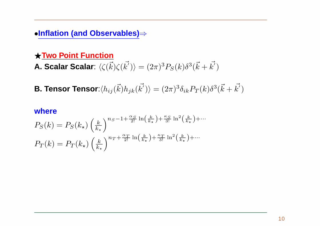
•Inflation (and Observables) ⇒
⋆Two Point FunctionA. Scalar Scalar : 〈ζ(~k)ζ(~k′)〉 = (2π)3PS(k)δ
3(~k + ~k′)
B. Tensor Tensor :〈hij(~k)hjk(~k′)〉 = (2π)3δikPT (k)δ
3(~k + ~k′)
where
PS(k) = PS(k⋆)(
kk⋆
)nS−1+αS2! ln( k
k⋆)+κS
3! ln2( kk⋆)+···
PT (k) = PT (k⋆)(
kk⋆
)nT+αT2! ln( k
k⋆)+κT
3! ln2( kk⋆)+···
10

•Inflation (and Observables) ⇒
⋆Two Point FunctionA. Scalar Scalar : 〈ζ(~k)ζ(~k′)〉 = (2π)3PS(k)δ
3(~k + ~k′)
B. Tensor Tensor :〈hij(~k)hjk(~k′)〉 = (2π)3δikPT (k)δ
3(~k + ~k′)
where
PS(k) = PS(k⋆)(
kk⋆
)nS−1+αS2! ln( k
k⋆)+κS
3! ln2( kk⋆)+···
PT (k) = PT (k⋆)(
kk⋆
)nT+αT2! ln( k
k⋆)+κT
3! ln2( kk⋆)+···
In GR1. Scalar power spectrum : PS(k⋆) =
V24π2ǫV M4
p
2. Tensor power spectrum : PT (k⋆) =2V
3π2M4p
3. Tensor-to-scalar ratio : r(k⋆) =PT (k⋆)PS(k⋆)
= 16ǫV
10-A

•Inflation (and Observables) ⇒
4. Scalar spectral tilt : nS(k⋆)− 1 = d lnPS(k)d ln k |⋆ = 2ηV − 6ǫV
5. Tensor spectral tilt : nT (k⋆) =d lnPT (k)
d ln k |⋆ = −2ǫV
6. Running of scalar spectral tilt :αS(k⋆) =
dnS
d ln k |⋆ = 16ηV ǫV − 24ǫ2V − 2ξ2V7. Running of tensor spectral tilt :
αT (k⋆) =dnT
d ln k |⋆ = 4ηV ǫV − 8ǫ2V8. Running of the running of scalar spectral tilt :
κS(k⋆) =d2nS
d ln k2 |⋆ = 192ǫ2V ηV − 192ǫ3V + 2σ3V − 24ǫV ξ
2V
+ 2ηV ξ2V − 32η2V ǫV
9. Running of the running of tensor spectral tilt :κT (k⋆) =
d2nT
d ln k2 |⋆ = 56ηV ǫ2V − 64ǫ3V − 8η2V ǫV − 4ǫV ξ
2V
⋆Note: Slow Roll ≡ Cosmological perturbation.
11

•Inflation (and Observables) ⇒
12

•Inflation (and Consistency relations) ⇒
nT = −r
8
(
2− r
8− nS
)
+ · · · , αT =dnT
d ln k=
r
8
(r
8+ nS − 1
)
+ · · · ,
nr =dr
d ln k=
16
9
(
nS − 1 +3r
4
)(
2nS − 2 +3r
8
)
+ · · · ,
κT =d2nT
d ln k2=
2
9
(
nS − 1 +3r
4
)(
2nS − 2 +3r
8
)(r
8+ nS − 1
)
+r
8
[
αS +2
9
(
nS − 1 +3r
4
)(
2nS − 2 +3r
8
)]
+ · · · ,
κr =d2r
d ln k2
=16
9
(
2nS − 2 +3r
8
)
αS +4
3
(
nS − 1 +3r
4
)(
2nS − 2 +3r
8
)
+16
9
(
nS − 1 +3r
4
)
2αS +2
3
(
nS − 1 +3r
4
)(
2nS − 2 +3r
8
)
+ · · · .
13

Observational status · · ·
Sr. Inflationary PLANCK+WP(+BICEP2) PLANCK+WP
No. observables
1 ln(1010PS) 3.089+0.024−0.027 3.089+0.024
−0.027
2 nS 0.9600± 0.0071 0.9603± 0.0073
3 αS −0.022± 0.010 −0.013± 0.009
4 κS 0.020+0.016−0.015 0.020+0.016
−0.015
5 r 0.2+0.07−0.05 < 0.12
6 nT 1.36± 0.83 ?
> −0.76 ?
14

Observational status · · ·
Sr. Inflationary PLANCK+WP(+BICEP2) PLANCK+WP
No. observables
1 ln(1010PS) 3.089+0.024−0.027 3.089+0.024
−0.027
2 nS 0.9600± 0.0071 0.9603± 0.0073
3 αS −0.022± 0.010 −0.013± 0.009
4 κS 0.020+0.016−0.015 0.020+0.016
−0.015
5 r 0.2+0.07−0.05 < 0.12
(r = 0 ruled out at 7σ)
6 nT 1.36± 0.83 (Blue = NBD/bounce..) ?
> −0.76 (Red = Inf + ...) ?
(nT = 0 ruled out at 3σ)
15

•Blue Gravity Waves from BICEP2? ⇒
16

•Constraints from Planck+WP+high L+BICEP2+.....? ⇒
17

•Scale of Inflation and Reheating temperature ⇒
A. V ≤ (1.96× 10¹⁶GeV)4 r0.12
B. H ≤ 9.241× 10¹³√
r⋆0.12 GeV
C. Trh ≤(
30π2g⋆
) 14
(1.96× 10¹⁶GeV) 4√
r0.12 .
18

•Scale of Inflation and Reheating temperature ⇒
A. V ≤ (1.96× 10¹⁶GeV)4 r0.12
B. H ≤ 9.241× 10¹³√
r⋆0.12 GeV
C. Trh ≤(
30π2g⋆
) 14
(1.96× 10¹⁶GeV) 4√
r0.12 .
•Inflaton (and CMBPOL) ⇒
1. < (aXlm)∗aYl′m′ >= CXY
l δll′ δmm′ where m = −l, ...,+l,X, Y = T,E,B
2. CXYl = 2
π
∫ kH(>k⋆)
kL(=ke)dk k2
INFLATION︷ ︸︸ ︷
P (k)
ANISOTROPIES︷ ︸︸ ︷
∆Xl(k)∆Y l(k) .where P (k) := PS(k), PT (k)
and∆Xl(k) =
∫ η0
0dη SX(k, η)
︸ ︷︷ ︸
SOURCES
PXl(k[η0 − η])︸ ︷︷ ︸
PROJECTION
.
18-A

19

20

⇒ SC, PLB 735 (2014) 138
21

Low scale saddle point inflation · · ·
⇒ SC and SP, JCAP 04 (2012) 018
Gauge invariant superpotential
W4 ≈ λ4
4MΦ4 ∀QQQL,QuQd,QuLe,uude
22

Low scale saddle point inflation · · ·
⇒ SC and SP, JCAP 04 (2012) 018
Gauge invariant superpotential
W4 ≈ λ4
4MΦ4 ∀QQQL,QuQd,QuLe,uude
Effective potential
V(φ, θ) = 12m2
φφ2 + λ4A
4Mφ4Cos(4θ + θA) +
λ2
4
M2φ6
⇒λ4 = λ4,0
[
1 + D3 log
(
φ2
µ20
)]
, A =
A0
[
1+D2 log
(
φ2
µ20
)]
[
1+D3 log
(
φ2
µ20
)] , m2φ
= m20
[
1 + D1 log
(
φ2
µ20
)]
mφ soft SUSY breaking mass, Φ = φ exp(iθ) (∈ C)
22-A

Low scale saddle point inflation · · ·
⇒ SC and SP, JCAP 04 (2012) 018
Gauge invariant superpotential
W4 ≈ λ4
4MΦ4 ∀QQQL,QuQd,QuLe,uude
Effective potential
V(φ, θ) = 12m2
φφ2 + λ4A
4Mφ4Cos(4θ + θA) +
λ2
4
M2φ6
⇒λ4 = λ4,0
[
1 + D3 log
(
φ2
µ20
)]
, A =
A0
[
1+D2 log
(
φ2
µ20
)]
[
1+D3 log
(
φ2
µ20
)] , m2φ
= m20
[
1 + D1 log
(
φ2
µ20
)]
mφ soft SUSY breaking mass, Φ = φ exp(iθ) (∈ C)
Flat direction contentQI1
a = 1√2(Φ, 0)T ,QI2
b = 1√2(Φ, 0)T ,QI3
c = 1√2(Φ, 0)T ,LI4
3 =1√2(0,Φ)T ,dB1
a = Φ√2,uB2
b = Φ√2,uB3
c = Φ√2, e3 = Φ√
2
22-B

Saddle point condition
(1) V′(φ0) = 0 ⇒
φ0 =√
M4λ4(3+D3)
[
A(1 + D2
2
)±
√
A2(1 + D2
2
)2 − 8m2φ(1 +D1)(3 +D3)
] 12
(2) V′′(φ0) = 0 ⇒
A =√
2(3 +D3)G1G2G3mφ(φ0)
(3) V′′′(φ0) = 0 ⇒
D3 = MA0
4λ4,0φ20
(
37+60 log(
φ0µ0
))
D2
(
13 + 12 log(
φ0
µ0
))
−2m2
φ(φ0)D1M
λ4,0A0φ20
+ 6
(
1− 20λ4,0φ20
MA0
)
(4) V′′′′(φ0) < 0
where Gi = Gi(D1, D2, D3) for i=1,2,3.
23

Saddle point condition
(1) V′(φ0) = 0 ⇒
φ0 =√
M4λ4(3+D3)
[
A(1 + D2
2
)±
√
A2(1 + D2
2
)2 − 8m2φ(1 +D1)(3 +D3)
] 12
(2) V′′(φ0) = 0 ⇒
A =√
2(3 +D3)G1G2G3mφ(φ0)
(3) V′′′(φ0) = 0 ⇒
D3 = MA0
4λ4,0φ20
(
37+60 log(
φ0µ0
))
D2
(
13 + 12 log(
φ0
µ0
))
−2m2
φ(φ0)D1M
λ4,0A0φ20
+ 6
(
1− 20λ4,0φ20
MA0
)
(4) V′′′′(φ0) < 0
where Gi = Gi(D1, D2, D3) for i=1,2,3.Inflaton potential
Around the saddle point φ0 V (φ) = C0 + C4(φ− φ0)4
23-A

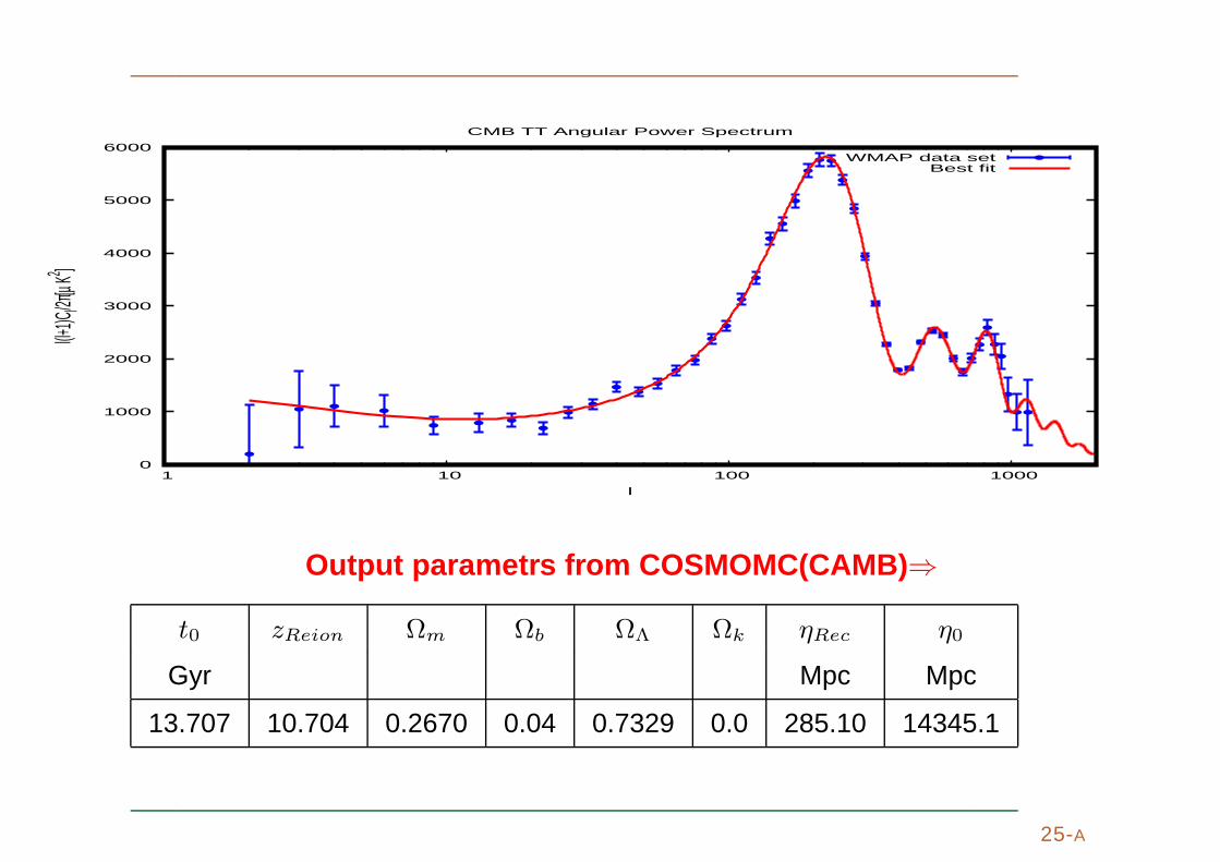
For C0 = 2.867× 10−36M4, C4 = −1.685× 10⁻¹³ and N = 70 weget: Ps(= ∆2
s) = 2.498× 10⁻⁹, ns = 0.957, nt = −1.550× 10⁻³⁰,r = 1.240× 10⁻²⁹, αs = −0.612× 10⁻³, κs = 1.749× 10⁻⁵.
0.92 0.93 0.94 0.95 0.96 0.97
0.00002
0.00004
0.00006
0.00008
0.0001
ns
Ds
24

0
1000
2000
3000
4000
5000
6000
1 10 100 1000
l(l+1)C
l/2π[µ K
2 ]
l
CMB TT Angular Power Spectrum
WMAP data setBest fit
25
0
1000
2000
3000
4000
5000
6000
1 10 100 1000
l(l+1)C
l/2π[µ K
2 ]
l
CMB TT Angular Power Spectrum
WMAP data setBest fit
Output parametrs from COSMOMC(CAMB) ⇒
t0 zReion Ωm Ωb ΩΛ Ωk ηRec η0
Gyr Mpc Mpc
13.707 10.704 0.2670 0.04 0.7329 0.0 285.10 14345.1
25-A

One loop RG flowD1 ≈ −0.056ζ2, D1
2 ≈ −0.074ζ, D22 ≈ −0.071ζ,
D32 ≈ −0.031ζ, D1
3 = D23 = D3
3 ≈ −0.048− 0.168ζ2 where ζ = m/mφ.
0 5 10 15 20 25
1
H L
0 5 10 15 20 25
2
4
H L
0 5 10 15 20 25
1.0
1.2
1.4
1.6
1.8
H L
0 5 10 15 20 254
6
8
10
12
14
H L
0 5 10 15 20 250.5
1.0
1.5
2.0
2.5
H L
0.0
0.2
0.4
0.6
0.8
H L
26

One loop RG flowD1 ≈ −0.056ζ2, D1
2 ≈ −0.074ζ, D22 ≈ −0.071ζ,
D32 ≈ −0.031ζ, D1
3 = D23 = D3
3 ≈ −0.048− 0.168ζ2 where ζ = m/mφ.
0 5 10 15 20 25
1
2
3
4
5
log10HΜL
A1HΜL
A1HΜ
0L
U
0 5 10 15 20 25
1
2
3
4
5
log10HΜL
A2HΜL
A2HΜ
0L
D
0 5 10 15 20 250.4
0.6
0.8
1.0
1.2
1.4
1.6
1.8
log10HΜL
A3HΜL
A3HΜ
0Lã
0 5 10 15 20 254
6
8
10
12
14
log10HΜL
miHΜLH
GevL
0 5 10 15 20 250.5
1.0
1.5
2.0
2.5
log10HΜL
mΦ2@ΜD
mΦ2@Μ
0D
Qu
Qd
0 5 10 15 200.0
0.2
0.4
0.6
0.8
log10HΜLΛΒHΜL
ΛΒHΜ
0L
26-A

High scale inflection point inflation · · ·
⇒ SC, AM and SP, JCAP 07 (2013) 041
Gauge invariant superpotential
W6 ≈ λ6MPL
Φ6 ∀udd,LLe
27

High scale inflection point inflation · · ·
⇒ SC, AM and SP, JCAP 07 (2013) 041
Gauge invariant superpotential
W6 ≈ λ6MPL
Φ6 ∀udd,LLe
High scale potential ( H ≫ mφ)
V (φ) = V0 +cHH2
2 |φ|2 − aHHφ6
6M3PL
+ λ2|φ|10M6
PL
27-A

High scale inflection point inflation · · ·
⇒ SC, AM and SP, JCAP 07 (2013) 041
Gauge invariant superpotential
W6 ≈ λ6MPL
Φ6 ∀udd,LLe
High scale potential ( H ≫ mφ)
V (φ) = V0 +cHH2
2 |φ|2 − aHHφ6
6M3PL
+ λ2|φ|10M6
PL
Inflection point constraints
(1)Tuning ⇒ a2H
40c2H
= 1− 4δ2
(2)Flatness ⇒ V ′′(φ0) = 0
(3)VEV/IP⇒ φ0 =(√
cH10 HM3
PL
)1/4
27-B

High scale inflection point inflation · · ·
⇒ SC, AM and SP, JCAP 07 (2013) 041
Gauge invariant superpotential
W6 ≈ λ6MPL
Φ6 ∀udd,LLe
High scale potential ( H ≫ mφ)
V (φ) = V0 +cHH2
2 |φ|2 − aHHφ6
6M3PL
+ λ2|φ|10M6
PL
Inflection point constraints
(1)Tuning ⇒ a2H
40c2H
= 1− 4δ2
(2)Flatness ⇒ V ′′(φ0) = 0
(3)VEV/IP⇒ φ0 =(√
cH10 HM3
PL
)1/4
Inflaton potential Around the inflection point φ0
V (φ) = α + β(φ− φ0) + γ(φ− φ0)3 + κ(φ− φ0)
4
27-C

⇒ α = V (φ0) = V0 +(
415 + 4
3δ2)cHH2φ2
0 +O(δ4),
β = V′(φ0) = 4δ2cHH2φ0 +O(δ4),
γ = V′′′
(φ0)3! = cHH2
φ0
(32− 80δ2
)+O(δ4),
κ = V′′′′
(φ0)4! = cHH2
φ20
(384− 1260δ2
)+O(δ4)
SHAPE OF THE POTENTIAL
0.0 0.2 0.4 0.6 0.8 1.0
4.5´10-9
5.´10-9
5.5´10-9
6.´10-9
6.5´10-9
ΦHin MPLL
VHΦLH
inM
PL
4L
POTENTIAL NEAR INFLECTION
Point of inflection
0.000 0.001 0.002 0.003 0.004 0.005 0.0064.45´10-9
4.5´10-9
4.55´10-9
4.6´10-9
4.65´10-9
4.7´10-9
xHin MPLL
VHxLH
inM
PL
4L
Here x := φ− φ0.
28

⇒ SC, AM and EP, JHEP 04 (2014) 077
29

⇒ SC, AM and EP, JHEP 04 (2014) 077
Kahler corrections
K(1) = φ†φ+ s†s+a
M2p
φ†φs†s+ · · · ,
K(2) = φ†φ+ s†s+b
2Mps†φφ+ h.c.+ · · · ,
K(3) = φ†φ+ s†s+c
4M2p
s†s†φφ+ h.c.+ · · · ,
K(4) = φ†φ+ s†s+d
Mpsφ†φ+ h.c.+ · · · ,
Parameter Space
cH ∼ O(10− 10−6) ,
aH ∼ O(30− 10−3) ,
Ms(= V1/40 ) ∼ O(9.50× 10¹⁰ − 1.77× 10¹⁶) GeV .
30

cS = 0.02
cS = 1
0.00 0.02 0.04 0.06 0.08 0.10 0.12
0.9996
0.9997
0.9998
0.9999
1.0000
r*
a
a vs r* plot
cS = 0.02
cS = 1
0.00 0.02 0.04 0.06 0.08 0.10 0.12
0.92
0.94
0.96
0.98
1.00
r*
b
b vs r* plot
cS = 1
cS = 0.02
0.00 0.02 0.04 0.06 0.08 0.10 0.120.3
0.4
0.5
0.6
0.7
0.8
0.9
1.0
r*
c
c vs r* plot
cS = 0.02
cS = 1
0.00 0.02 0.04 0.06 0.08 0.10 0.120.4
0.5
0.6
0.7
0.8
0.9
1.0
r*
d
d vs r* plot
31
32
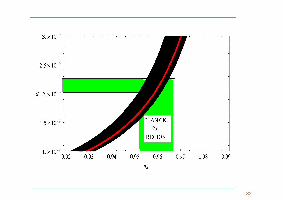
cS = 0.02
cS = 1
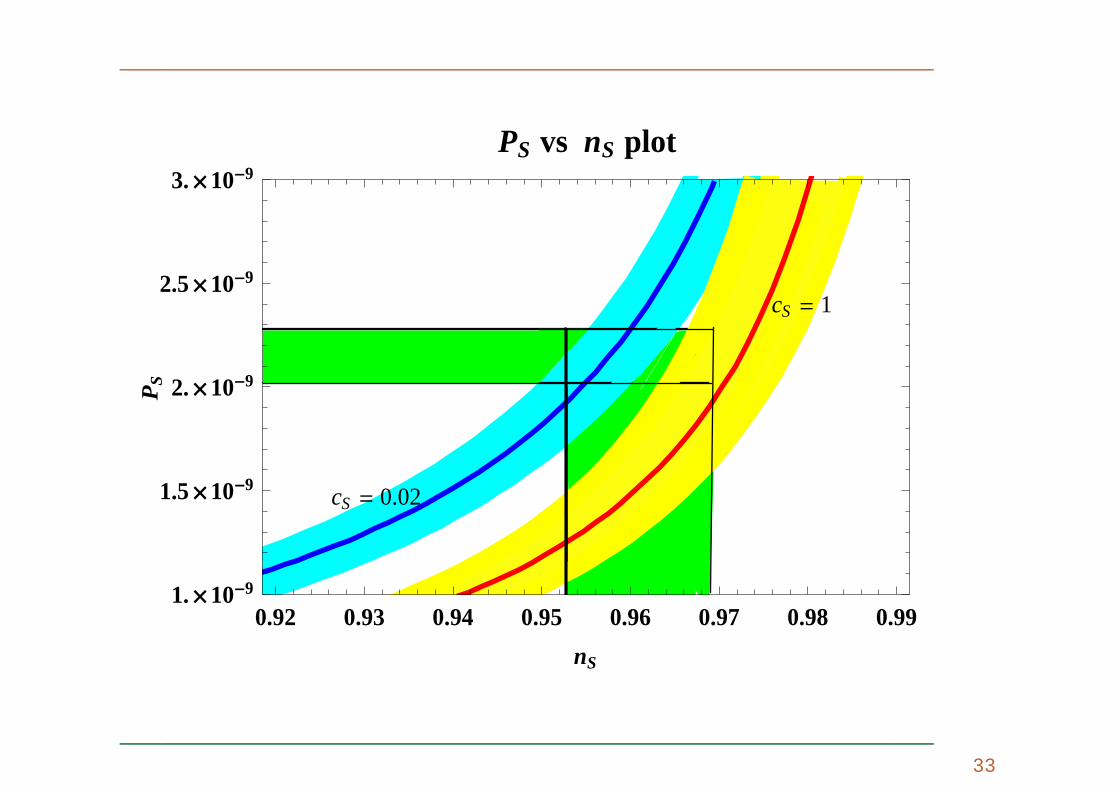
0.92 0.93 0.94 0.95 0.96 0.97 0.98 0.991.´10-9
1.5´10-9
2.´10-9
2.5´10-9
3.´10-9
nS
PS
PS vs nS plot
33

34

35

36

37

Anti Lyth bound after Planck and BICEP2 · · ·
⇒ SC and AM, NPB 882 (2014) 386In this work we provide an accurate bound on generatingprimordial gravitational waves from inflation, where inflat ionoccurs below the Planck scale.
Large tensor to scalar ratio can be generated as required byPLANCK and BICEP2.
38

Anti Lyth bound after Planck and BICEP2 · · ·
⇒ SC and AM, NPB 882 (2014) 386In this work we provide an accurate bound on generatingprimordial gravitational waves from inflation, where inflat ionoccurs below the Planck scale.
Large tensor to scalar ratio can be generated as required byPLANCK and BICEP2.
If inflation has to make connection with the real particlephysics it must be explained within an EFT description whereit can be trustable below the UV cut-off of the scale of gravit y.
We also establish a new closed relationship between VEV,scale of inflation, tensor to scalar ratio in a modelindependent fashion.
38-A

What is “THE LYTH BOUND”?A useful way of normalizing the primordial GW amplitude isthe tensor-to-scalar ratio
r(k⋆) =PT (k⋆)PS(k⋆)
= 16ǫV = 8M2
pl
φ2
H2 = 8M2
pl
(dφ
dN
)2
The value of r(k⋆) determines whether primordial GW aredetectable in future CMB observations.
39

What is “THE LYTH BOUND”?A useful way of normalizing the primordial GW amplitude isthe tensor-to-scalar ratio
r(k⋆) =PT (k⋆)PS(k⋆)
= 16ǫV = 8M2
pl
φ2
H2 = 8M2
pl
(dφ
dN
)2
The value of r(k⋆) determines whether primordial GW aredetectable in future CMB observations.
The total field evolution between the time when CMBfluctuations exited the horizon and the end of inflation
⇒LYTH BOUND
∆φ
Mpl=
∫ N⋆
NenddN
√r(N)8
=∫ k⋆
kend
dkk
√r(k)8
≃ O(1)×√
r(k⋆)0.01
39-A

Detectable large values of the tensor-to- scalar ratio,r(k⋆) > 0.01 and correlates with ∆φ > Mpl.∆φ > Mpl implies preferance to the large-field models ofinflation. Example: String theory.
40

Detectable large values of the tensor-to- scalar ratio,r(k⋆) > 0.01 and correlates with ∆φ > Mpl.∆φ > Mpl implies preferance to the large-field models ofinflation. Example: String theory.This implies the lower bound of the energy scale of inflation
is around the GUT scale (V 1/4 ≥ O(1016 GeV )) but cannotaccomodate feasible αS & κS .For ∆φ > Mpl one can go beyond the upper cut-off of theeffective theory of gravity ΛUV = Mpl but the models becomeUV unprotective.
40-A

Detectable large values of the tensor-to- scalar ratio,r(k⋆) > 0.01 and correlates with ∆φ > Mpl.∆φ > Mpl implies preferance to the large-field models ofinflation. Example: String theory.This implies the lower bound of the energy scale of inflation
is around the GUT scale (V 1/4 ≥ O(1016 GeV )) but cannotaccomodate feasible αS & κS .For ∆φ > Mpl one can go beyond the upper cut-off of theeffective theory of gravity ΛUV = Mpl but the models becomeUV unprotective.Within ∆φ < Mpl it is possible to accomodate feasible αS &κS which can generate large “r” as observed by BICEP2 andPlanck.
⋆NOTE:Higher order SL corrections (HOSLC) ≡ PrecisionCosmology (fits CMBPOL within 2 < l < 2500.)
40-B
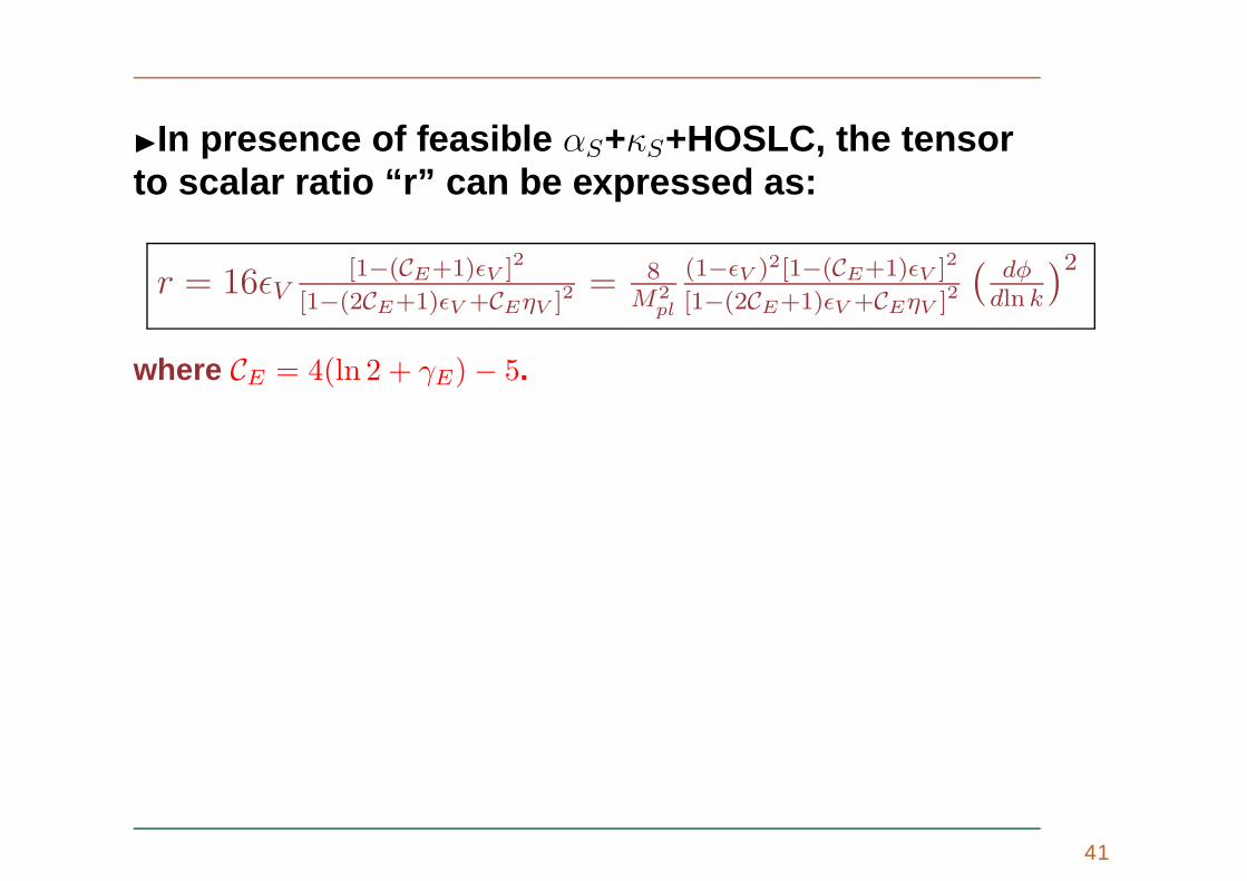
In presence of feasible αS+κS+HOSLC, the tensorto scalar ratio “r” can be expressed as:
r = 16ǫV[1−(CE+1)ǫV ]2
[1−(2CE+1)ǫV +CEηV ]2= 8
M2pl
(1−ǫV )2[1−(CE+1)ǫV ]2
[1−(2CE+1)ǫV +CEηV ]2
(dφ
dln k
)2
where CE = 4(ln 2 + γE)− 5.
41

In presence of feasible αS+κS+HOSLC, the tensorto scalar ratio “r” can be expressed as:
r = 16ǫV[1−(CE+1)ǫV ]2
[1−(2CE+1)ǫV +CEηV ]2= 8
M2pl
(1−ǫV )2[1−(CE+1)ǫV ]2
[1−(2CE+1)ǫV +CEηV ]2
(dφ
dln k
)2
where CE = 4(ln 2 + γE)− 5.
To evaluate the total field evolution ∆φ:
∫ k⋆
ke
dkk
√
r(k)8
≈∆φ
Mpl
1 + 1∆φ
[
(2CE − 1)∫ φ⋆
φedφ ǫV − 2CE
∫ φ⋆
φedφ ηV
]
+ ....
where
r(k) = PT (k)PS(k)
= r(k⋆)(
kk⋆
)a+ b2ln( k
k⋆)+ c
6ln2( k
k⋆)+....
with
a = nT − nS + 1, b = (αT − αS) , c = (κT − κS).
41-A

We Taylor expand a generic inflationary potential V (φ)
around the vicinity of VEV φ0 where inflation occurs.
√r(k⋆)
8
∣∣(a2 − b
2 + c2 − 2
) [1− e−∆N
]−(a2 − b
2 + c2 − 1
)∆N e−∆N
+(b4 − c
4
)(∆N)2 e−∆N − c
12 (∆N)3 e−∆N∣∣ ≈ ∑∞
n=0 Gn
(|∆φ|Mp
)n
where Gn =
1 +∞∑
m=0
Am
(φe − φ0
Mp
)m
︸ ︷︷ ︸
≪1
∼ 1 for n = 1
<< 1 for n ≥ 2 ,
and Am = Mm+2p
[(CE − 1
2
)Cm − CEDm
].
⋆NOTE: Gn << 1 reqd. for convergence of the Taylor series.
42

Here the slow-roll parameters show non-monotonicbehaviour within the interval ∆N = Ne −N⋆ = ln
(k⋆
ke
)
≈ 17.
0.00 0.02 0.04 0.06 0.08 0.10
0.000
0.002
0.004
0.006
0.008
0.010
0.012
0.014
HΦ-Φ0L in Mp
Ε VHΦL
ΕV HΦL vs HΦ-Φ0L plot
0.00 0.02 0.04 0.06 0.08 0.10
0.005
0.010
0.015
0.020
0.025
0.030
0.035
HΦ-Φ0L in Mp
ÈΗVHΦLÈ
ÈΗV HΦLÈ vs HΦ-Φ0L plot
0.00 0.02 0.04 0.06 0.08 0.10
0.000
0.002
0.004
0.006
0.008
0.010
HΦ-Φ0L in Mp
ÈΞ2 VHΦLÈ
ÈΞ2V HΦLÈ vs HΦ-Φ0L plot
0.00 0.02 0.04 0.06 0.08 0.10
0.002
0.004
0.006
0.008
0.010
0.012
0.014
HΦ-Φ0L in Mp
ÈΣ3 VHΦLÈ
ÈΣ3V HΦLÈ vs HΦ-Φ0L plot
43

10-5 10-4 0.001 0.01 0.1 1
2.0´10-9
1.5´10-9
kHin Mpc-1L
P SHkL
PSHkL vs k plot
10-5 10-4 0.001 0.01 0.10.9
1.
1.1
1.2
1.3
kHin Mpc-1L
n SHkL
nSHkL vs k plot
0.0000 0.0005 0.0010 0.0015 0.0020 0.0025 0.0030
-0.35
-0.30
-0.25
-0.20
-0.15
-0.10
-0.05
kHin Mpc-1L
ΑSH
kL
ΑSHkL vs k plot
-25 -20 -15 -10 -5 0 5 10
3.9
4.
4.1
4.2
4.3
4.4
lnHkMpc-1L
lnNHkL
lnNHkL vs lnk plot
44

Neglecting the Planck scale suppressed contribution in thelimit ∆φ < Mpl we get relation between tensor-to-scalar ratioand ∆φ:
√r(k⋆)
2
∣∣∣
r(k⋆)16 − ηV (k⋆)
2 − 1−(6CE + 23
3
)ǫ2V (k⋆)−
η2V (k⋆)6 + (CE − 1)
ξ2V (k⋆)2
−(2CE − 8
3
)ηV (k⋆)ǫV (k⋆)− σ3
V (k⋆)2 + · · ·
∣∣∣ ≈ |∆φ|
Mp
45

Neglecting the Planck scale suppressed contribution in thelimit ∆φ < Mpl we get relation between tensor-to-scalar ratioand ∆φ:
√r(k⋆)
2
∣∣∣
r(k⋆)16 − ηV (k⋆)
2 − 1−(6CE + 23
3
)ǫ2V (k⋆)−
η2V (k⋆)6 + (CE − 1)
ξ2V (k⋆)2
−(2CE − 8
3
)ηV (k⋆)ǫV (k⋆)− σ3
V (k⋆)2 + · · ·
∣∣∣ ≈ |∆φ|
Mp
SCALE OF INFALTION: V ≤ (1.96× 10¹⁶GeV)4 r(k⋆)0.12
45-A

Neglecting the Planck scale suppressed contribution in thelimit ∆φ < Mpl we get relation between tensor-to-scalar ratioand ∆φ:
√r(k⋆)
2
∣∣∣
r(k⋆)16 − ηV (k⋆)
2 − 1−(6CE + 23
3
)ǫ2V (k⋆)−
η2V (k⋆)6 + (CE − 1)
ξ2V (k⋆)2
−(2CE − 8
3
)ηV (k⋆)ǫV (k⋆)− σ3
V (k⋆)2 + · · ·
∣∣∣ ≈ |∆φ|
Mp
SCALE OF INFALTION: V ≤ (1.96× 10¹⁶GeV)4 r(k⋆)0.12
Finally we get a relation between ∆φ and scale of inflation:
|∆φ|Mpl
≤√V
(2.20×10⁻² Mpl)2
∣∣∣
V
(2.78×10⁻²Mpl)4− ηV (k⋆)
2 − 1
−(6CE + 23
3
)ǫ2V (k⋆)−
η2V (k⋆)6 + · · ·
∣∣∣
45-B
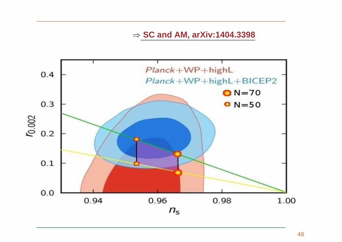
⇒ SC and AM, arXiv:1404.3398
46

⇒ SC and AM, arXiv:1404.3398
N = 70
N = 50
0.90 0.92 0.94 0.96 0.98 1.00-0.040
-0.035
-0.030
-0.025
-0.020
nS
n T
nT vs nS plot
N = 70
N = 50
0.950 0.955 0.960 0.965 0.970-0.0006
-0.0005
-0.0004
-0.0003
-0.0002
-0.0001
0.0000
0.0001
nS
ΑT
ΑT vs nS plot
N = 70N = 50
0.950 0.955 0.960 0.965 0.970
-0.00060
-0.00055
-0.00050
-0.00045
-0.00040
-0.00035
nS
Κ T
ΚT vs nS plot
N = 70
N = 50
0.10 0.15 0.20 0.25 0.30-0.005
0.000
0.005
0.010
0.015
r0.002
n r
nr vs r0.002 plot
47

Reconstruction (in GR) : ⇒ SC and AM, arXiv:1404.3398
V (φ⋆) =32PS(k⋆)r(k⋆)π
2M4p ,
V′(φ⋆) =
32PS(k⋆)r(k⋆)π
2√
r(k⋆)8 M3
p ,
V′′(φ⋆) =
34PS(k⋆)r(k⋆)π
2(
nS(k⋆)− 1 + 3r(k⋆)8
)
M2p ,
V′′′(φ⋆) =
32PS(k⋆)r(k⋆)π
2[√
2r(k⋆)(
nS(k⋆)− 1 + 3r(k⋆)8
)
− 12
(r(k⋆)
8
) 32 − αS(k⋆)
√2
r(k⋆)
]
Mp,
V′′′′(φ⋆) = 12PS(k⋆)π
2
κS(k⋆)2 − 1
2
(r(k⋆)
8
)2 (
nS(k⋆)− 1 + 3r(k⋆)8
)
+ 12(
r(k⋆)8
)3
+ r(k⋆)(
nS(k⋆)− 1 + 3r(k⋆)8
)2
+
[√
2r(k⋆)(
nS(k⋆)− 1 + 3r(k⋆)8
)
− 12
(r(k⋆)
8
) 32 − αS(k⋆)
2r(k⋆)
]
×[√
r(k⋆)8
(
nS(k⋆)− 1 + 3r(k⋆)8
)
− 6(
r(k⋆)8
) 32
]
48

⇒ SC, arXiv:1406.7618
r(k) =
r(k∗)
r(k∗)(
kk∗
)nT (k∗)−nS(k∗)+1
r(k∗)(
kk∗
)nT (k∗)−nS(k∗)+1+αT (k∗)−αS(k∗)
2! ln( kk∗ )
r(k∗)(
kk∗
)nT (k∗)−nS(k∗)+1+αT (k∗)−αS(k∗)
2! ln( kk∗ )+
κT (k∗)−κS(k∗)
3! ln2( kk∗ )
⇓ ⇓ ⇓ ⇓
49

⇒ SC, arXiv:1406.7618
r(k) =
r(k∗)
r(k∗)(
kk∗
)nT (k∗)−nS(k∗)+1
r(k∗)(
kk∗
)nT (k∗)−nS(k∗)+1+αT (k∗)−αS(k∗)
2! ln( kk∗ )
r(k∗)(
kk∗
)nT (k∗)−nS(k∗)+1+αT (k∗)−αS(k∗)
2! ln( kk∗ )+
κT (k∗)−κS(k∗)
3! ln2( kk∗ )
⇓ ⇓ ⇓ ⇓
Field− excursion (in GR) :
∣∣∣∣
∆φ
Mp
∣∣∣∣=
O(2.7− 5.1)
O(2.7− 4.6)
O(0.6− 1.8)
O(0.2− 0.3)
49-A

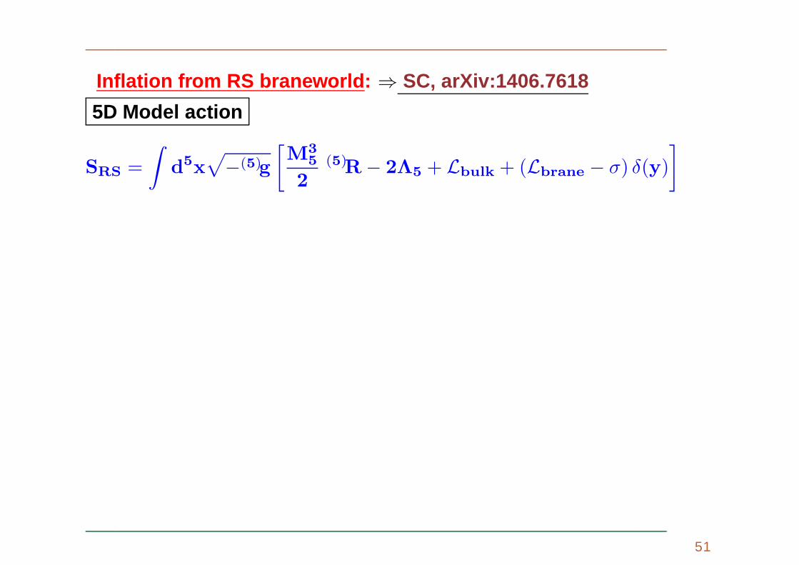
Inflation from RS braneworld : ⇒ SC, arXiv:1406.7618
5D Model action
SRS =
∫
d5x√
−(5)g
[M3
5
2(5)R− 2Λ5 + Lbulk + (Lbrane − σ) δ(y)
]
50

Inflation from RS braneworld : ⇒ SC, arXiv:1406.7618
5D Model action
SRS =
∫
d5x√
−(5)g
[M3
5
2(5)R− 2Λ5 + Lbulk + (Lbrane − σ) δ(y)
]
50-A
Inflation from RS braneworld : ⇒ SC, arXiv:1406.7618
5D Model action
SRS =
∫
d5x√
−(5)g
[M3
5
2(5)R− 2Λ5 + Lbulk + (Lbrane − σ) δ(y)
]
51

Inflation from RS braneworld : ⇒ SC, arXiv:1406.7618
5D Model action
SRS =
∫
d5x√
−(5)g
[M3
5
2(5)R− 2Λ5 + Lbulk + (Lbrane − σ) δ(y)
]
4D Modified Friedmann Equation within Slow-Roll ⇒CovariantShiromizu-Maeda-Sasaki approach+ Isriel-Junction condi tion
H2 ≈ ρ
3M2p
1+
︷︸︸︷ρ
2σCorrection term
≈ V(φ)
3M2p
(
1+V(φ)
2σ
)
Cut-off scale and brane tension
M35 =
√
4πσ
3Mp σ =
√
− 3
4πM3
5Λ5 > 0
51-A
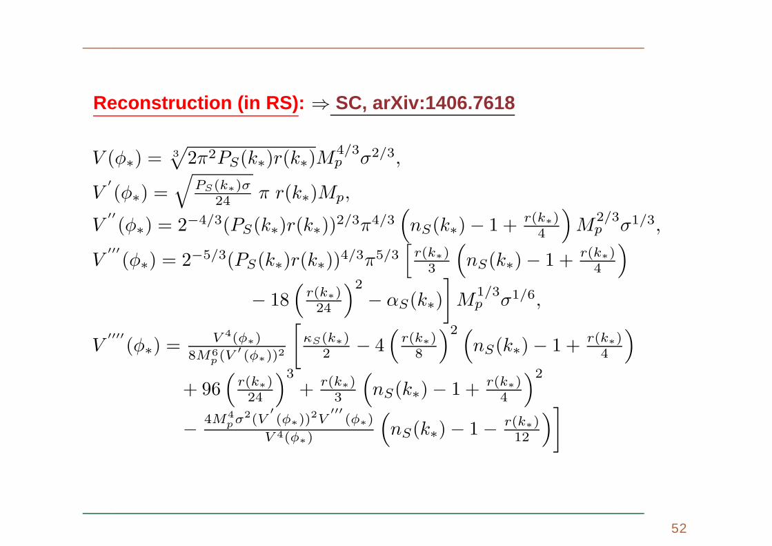
Reconstruction (in RS) : ⇒ SC, arXiv:1406.7618
V (φ∗) =3√
2π2PS(k∗)r(k∗)M4/3p σ2/3,
V′(φ∗) =
√PS(k∗)σ
24 π r(k∗)Mp,
V′′(φ∗) = 2−4/3(PS(k∗)r(k∗))2/3π4/3
(
nS(k∗)− 1 + r(k∗)4
)
M2/3p σ1/3,
V′′′(φ∗) = 2−5/3(PS(k∗)r(k∗))4/3π5/3
[r(k∗)
3
(
nS(k∗)− 1 + r(k∗)4
)
− 18(
r(k∗)24
)2
− αS(k∗)
]
M1/3p σ1/6,
V′′′′(φ∗) =
V 4(φ∗)
8M6p (V
′ (φ∗))2
[
κS(k∗)2 − 4
(r(k∗)
8
)2 (
nS(k∗)− 1 + r(k∗)4
)
+ 96(
r(k∗)24
)3
+ r(k∗)3
(
nS(k∗)− 1 + r(k∗)4
)2
− 4M4pσ
2(V′(φ∗))
2V′′′
(φ∗)
V 4(φ∗)
(
nS(k∗)− 1− r(k∗)12
)]
52

⇒ SC, arXiv:1406.7618
Brane tension : σ ≤ O(10−9) M4p,
5D Scale : M5 ≤ O(0.04) Mp,
5D Cosmological Constant : Λ5 ≥ −O(10−15) M5p
⇓ ⇓ ⇓ ⇓
53

⇒ SC, arXiv:1406.7618
Brane tension : σ ≤ O(10−9) M4p,
5D Scale : M5 ≤ O(0.04) Mp,
5D Cosmological Constant : Λ5 ≥ −O(10−15) M5p
⇓ ⇓ ⇓ ⇓
Field− excursion (in RS) :
∣∣∣∣
∆φ
Mp
∣∣∣∣=
O(0.24− 0.81)
O(0.24− 0.73)
O(0.05− 0.28)
O(0.02− 0.05)
53-A

⇒ SC, arXiv:1406.7618
Brane tension : σ ≤ O(10−9) M4p,
5D Scale : M5 ≤ O(0.04) Mp,
5D Cosmological Constant : Λ5 ≥ −O(10−15) M5p
⇓ ⇓ ⇓ ⇓
Field− excursion (in RS) :
∣∣∣∣
∆φ
Mp
∣∣∣∣=
O(0.24− 0.81)
O(0.24− 0.73)
O(0.05− 0.28)
O(0.02− 0.05)
⋆⋆⋆
Note:Large (detectable) r+ |∆φ| < Mp (EFT)= running/Beyond GR
(RS)/muiltifield/.....
53-B

BOTTOM LINES
•High scale inflation is more favoured after Planck andBICEP2.
54

BOTTOM LINES
•High scale inflation is more favoured after Planck andBICEP2.
•Large tensor modes can be generated from high scalemodels.
54-A

BOTTOM LINES
•High scale inflation is more favoured after Planck andBICEP2.
•Large tensor modes can be generated from high scalemodels.
• High scale models fitted well with the CMB TT spectra asobserved by Planck within 2 < l < 2500.
54-B

BOTTOM LINES
•High scale inflation is more favoured after Planck andBICEP2.
•Large tensor modes can be generated from high scalemodels.
• High scale models fitted well with the CMB TT spectra asobserved by Planck within 2 < l < 2500.
•Using higher order corrections to slow roll accurateanalytical bound on tensor modes has been established inpresence of considerable amount of running.
54-C

BOTTOM LINES
•High scale inflation is more favoured after Planck andBICEP2.
•Large tensor modes can be generated from high scalemodels.
• High scale models fitted well with the CMB TT spectra asobserved by Planck within 2 < l < 2500.
•Using higher order corrections to slow roll accurateanalytical bound on tensor modes has been established inpresence of considerable amount of running.
•Super-Planckian models (String Theory) cannot provideconsiderable amount of running.
54-D

BOTTOM LINES
•High scale inflation is more favoured after Planck andBICEP2.
•Large tensor modes can be generated from high scalemodels.
• High scale models fitted well with the CMB TT spectra asobserved by Planck within 2 < l < 2500.
•Using higher order corrections to slow roll accurateanalytical bound on tensor modes has been established inpresence of considerable amount of running.
•Super-Planckian models (String Theory) cannot provideconsiderable amount of running.
•To get large ‘r’+ sub-Planckian field excursionrunning+HOSLC, braneworld, multi field etc are required.
54-E

OPEN ISSUES
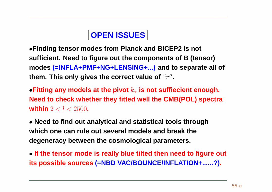
•Finding tensor modes from Planck and BICEP2 is notsufficient. Need to figure out the components of B (tensor)modes (=INFLA+PMF+NG+LENSING+...) and to separate all ofthem. This only gives the correct value of “r′′.
55

OPEN ISSUES
•Finding tensor modes from Planck and BICEP2 is notsufficient. Need to figure out the components of B (tensor)modes (=INFLA+PMF+NG+LENSING+...) and to separate all ofthem. This only gives the correct value of “r′′.
•Fitting any models at the pivot k⋆ is not suffiecient enough.Need to check whether they fitted well the CMB(POL) spectrawithin 2 < l < 2500.
55-A

OPEN ISSUES
•Finding tensor modes from Planck and BICEP2 is notsufficient. Need to figure out the components of B (tensor)modes (=INFLA+PMF+NG+LENSING+...) and to separate all ofthem. This only gives the correct value of “r′′.
•Fitting any models at the pivot k⋆ is not suffiecient enough.Need to check whether they fitted well the CMB(POL) spectrawithin 2 < l < 2500.
• Need to find out analytical and statistical tools throughwhich one can rule out several models and break thedegeneracy between the cosmological parameters.
55-B
OPEN ISSUES
•Finding tensor modes from Planck and BICEP2 is notsufficient. Need to figure out the components of B (tensor)modes (=INFLA+PMF+NG+LENSING+...) and to separate all ofthem. This only gives the correct value of “r′′.
•Fitting any models at the pivot k⋆ is not suffiecient enough.Need to check whether they fitted well the CMB(POL) spectrawithin 2 < l < 2500.
• Need to find out analytical and statistical tools throughwhich one can rule out several models and break thedegeneracy between the cosmological parameters.
• If the tensor mode is really blue tilted then need to figure outits possible sources (=NBD VAC/BOUNCE/INFLATION+......?) .
55-C

OPEN ISSUES
•Need to check whether the models really can address thethermal history of early universe (i.e. reheating etc.).
56

OPEN ISSUES
•Need to check whether the models really can address thethermal history of early universe (i.e. reheating etc.).
•The primordial non-Gausiianity is not yet been detected wit hhigh statistical accuracy (i.e. f local
NL = 2.7± 5.8 andτ localNl ≤ 2800). But if it is detected in future CMB experimentsthen it is possible to rule out various models.
56-A
FUTURE PROJECTS
•FERMION LOCALIZATION IN 5D WITHOUT ANY EXTERNALFIELD: SC, J. Mitra and S. SenGupta.
•MAGNETOGENESIS BEYOND GR: SC.
• CONSTRAINTS ON ASSISTED TACHYONIC NFLATION: SCand S. Panda.
57

FUTURE PROJECTS
•FERMION LOCALIZATION IN 5D WITHOUT ANY EXTERNALFIELD: SC, J. Mitra and S. SenGupta.
•MAGNETOGENESIS BEYOND GR: SC.
• CONSTRAINTS ON ASSISTED TACHYONIC NFLATION: SCand S. Panda.
•TORSION INDUCED INFLATION FROM ECKS THEORY OFGRAVITY: SC, B. K. Pal, B. Basu and P. Bandyopadhyay.
•MODEL INDEPENDENT ANALYSIS FOR UNIFYING INFLATIONAND DARK MATTER IN BRANEWORLD: SC and A. Dasgupta.
•ISSUE OF CLASSICALIZATION AND IMPACT ONCONSISTENCY RELATIONS: SC and M. Sami.
57-A

FUTURE PROJECTS
•BOUNCING FROM HIGHER RANK TENSOR FIELDS: ANALTERNATIVE APPROACH TO INFLATION: SC, S. Kar and S.SenGupta.
•WIMPY BARYOGENESIS MIRACLE IN BRANEWORLD: SC andA. Dasgupta.
• EFFECTIVE THEORY OF DARKOLEPTOGENESIS: SC and S.Sadhukhan.
58
FUTURE PROJECTS
•BOUNCING FROM HIGHER RANK TENSOR FIELDS: ANALTERNATIVE APPROACH TO INFLATION: SC, S. Kar and S.SenGupta.
•WIMPY BARYOGENESIS MIRACLE IN BRANEWORLD: SC andA. Dasgupta.
• EFFECTIVE THEORY OF DARKOLEPTOGENESIS: SC and S.Sadhukhan.
•LOOPS AND LEGS I: A COMPLETE FEYNRULE FOR FORCMB LENSING SC.
•LOOPS AND LEGS II: DIAGRAMATICS FOR LARGE SCALESTRUCTURE: SC.
•LOOPS AND LEGS III: BEHAVIOUR OF IR AND UVDIVERGENCES AND SPECTRAL REGULARIZATION: SC.
58-A

SPECIAL THANKS TO .........
⋆Soumitra SenGupta ⋆R. H. Brandenberger
⋆Sayan Kar ⋆Marc Kamionkowski
⋆Sudhakar Panda ⋆Daniel Baumann
⋆Md. Sami ⋆Leonardo Senatore
⋆Anupam Mazumdar ⋆Cliff Burgess
⋆Supratik Pal
⋆Andrew Liddle
⋆David H. Lyth
⋆Claudia-de-Rahm
59

THANKS FOR YOUR TIME.........
60

THANKS FOR YOUR TIME.........
61

BACK UP SLIDES.........
62

BETA FUNCTIONS FOR QQQL,QuQd,QuLe,uude ⇒(a) For Soft mass:µ(m2
φ)QQQL = 18π2
(3m2
Q3+m2
U3+ |A33
U |2) (
λ33U
)2
− 18π2
(3g22 |m2|2 + 4g23 |m3|2
),
µ(m2φ)QuQd = 1
2π2
(m2
Q3+m2
U3
) (λ33U
)2
− 18π2
(32g
22 |m2|2 + 16
3 g23 |m3|2),
µ(m2φ)QuLe = 3
8π2
(m2
Q3+m2
U3
) (λ33U
)2
− 18π2
(32g
22 |m2|2 + 8
3g23 |m3|2
),
µ(m2φ)uude = 1
2π2
(m2
Q3+m2
U3
) (λ33U
)2 − 12π2 g
23 |m3|2,
(b) For Trilinear A- term:
µAaaD = δb3
(λ33U
)2 A33U
8π2
− 14π2
(718g
21 |m1|2 + 3
2g22 |m2|2 + 8
3g23 |m3|2
),
µAabU =
3(1+δa3)A33U
8π2
(λ33U
)2
− 14π2
(1318g
21 |m1|2 + 3
2g22 |m2|2 + 8
3g23 |m3|2
),
µAaaE = − 1
4π2
(32g
21 |m1|2 + 3
2g22 |m2|2
),
63

(c) For Fourth level Yukawa coupling:µλaa
U = 3(1+δa3)8π2
(λ33U
)3 − λaaU
4π2
(1318g
21 +
32g
22 +
83g
23
),
µλabD = δb3
(λ33U
)2 λabD
8π2 − λabD
4π2
(718g
21 +
32g
22 +
83g
23
),
µλaaE = −λaa
E
4π2
(32g
22 +
32g
23
)
(d) Gaugino masses and couplings:
µgi =di
2 g3i , µ
(mi
g2i
)
= 0 ∀ i where
a, b = 1, 2, 3(family), i = 1(U(1)Y), 2(SU(2)L), 3(SU(3)C) andd1 = 11
8π2 ,d2 = 18π2 ,d3 = − 3
8π2 .
SOLUTION ⇒gi(µ) =
gi(µ0)√
1−dig2i (µ0) ln
(
µµ0
)
,mi(µ) = mi(µ0)(
gi(µ)gi(µ0)
)2
,
∆m2φ =
∑3i=1 f
iF∆m2
i , ∆Aabβ = 1
2
∑3i=1(C
iβ)
ab∆mi,
λabβ (µ) = λab
β (µ0)∏3
i=1
(gi(µ0)gi(µ)
)(Ciβ)
ab
with ∆Aβ = Aβ(µ)−Aβ(µ0), ∆mi = mi(µ0)−mi(µ),∆m2
φ = m2φ(µ)−m2
φ(µ0),∆m2i = m2
i (µ0)−m2i (µ),
64

.
CONSTANTS DETERMINED FROM RGE
D1 = − 18π2
∑3i=1 Ji
(mi
mφ0
)2
g2i (µ0), Dβ2 = − 1
4π2
∑3i=1K
βi(
mi
A0
)
g2i (µ0)
where J1 = 0,J2 = 3 and J3 = 4 for i = 1, 2, 3 and
Kβi i = 1(U(1)Y) i = 2(SU(2)L) i = 3(SU(3)C)
β=1(U) 1318
32
83
β=2(D) 718
32
83
β=3(E) 32
32 0
Universal mSUGRA B. C. at GUT scale Constraints on λ0 from proton decay ( p → π0
e+, p → π+νe
etc.) ⇒D1 ≈ −0.056ζ2, D1
2 ≈ −0.074ζ, D22 ≈ −0.071ζ, D3
2 ≈ −0.031ζ,
D13 = D2
3 = D33 ≈ −0.048− 0.168ζ2 where ζ = m/mφ.
65

New constraint between PGW and PBH · · ·
PBH formation by Press-Schechter theory
f(≥ M) = 2γ∫∞Θth
dΘP(Θ;M(kPBH)) = γ erf[
Θth√2ΣΘ(kPBH)
]
66

New constraint between PGW and PBH · · ·
PBH formation by Press-Schechter theory
f(≥ M) = 2γ∫∞Θth
dΘP(Θ;M(kPBH)) = γ erf[
Θth√2ΣΘ(kPBH)
]
where P(Θ; kPBH) =1√
2πΣΘ(kPBH)exp
(
− Θ2
2Σ2Θ(kPBH)
)
ΣΘ(kPBH) =
√∫∞0
dkk
exp(
− k2
k2PBH
)
PΘ(k)
Θ(k) = 25
(kaH
)2Rc(k)
PΘ(k) =425
(1+w)2
(1+ 35w)
2
(kaH
)4PS(k)
PS(k) = PS(k⋆)(
kk⋆
)nS−1+αS2
ln( kk⋆)+κS
6ln2( k
k⋆)+···
kPBH =√γ
5.54×10⁻²⁴
(MPBH
1 g
)− 12 ( g⋆
3.36
)− 16 Mpc−1
66-A

New constraint between PGW and PBH · · ·
ΣΘ(kPBH) = 15
(1+w)√
PS(k⋆)
(1+ 35w)
(k⋆
aH)2 A+BnS(k⋆) + CαS(k⋆)
+DκS(k⋆) + · · · 12
where A = 2B =4k2
PBHk2⋆
[
1 − exp
(
−k2Λ
k2PBH
)]
,
C = 12
ln
(
kΛk⋆
)
+ 14
Γ
[
0,k2L
k2PBH
]
− Γ
[
0,k2Λ
k2PBH
]
,
D =k2Λ
6k2PBH
P FQ
[
(1, 1, 1) ; (2, 2, 2) ;−k2Λ
k2PBH
]
+k2PBH3k2
⋆
ln2(
kΛk⋆
)
+ γE ln
(
kLkΛ
)
.
0 2´1012 4´1012 6´1012 8´1012 1´1013
0.14
0.16
0.18
0.20
MPBHHgmL
fHMPB
HL
67

New constraint between PGW and PBH · · ·
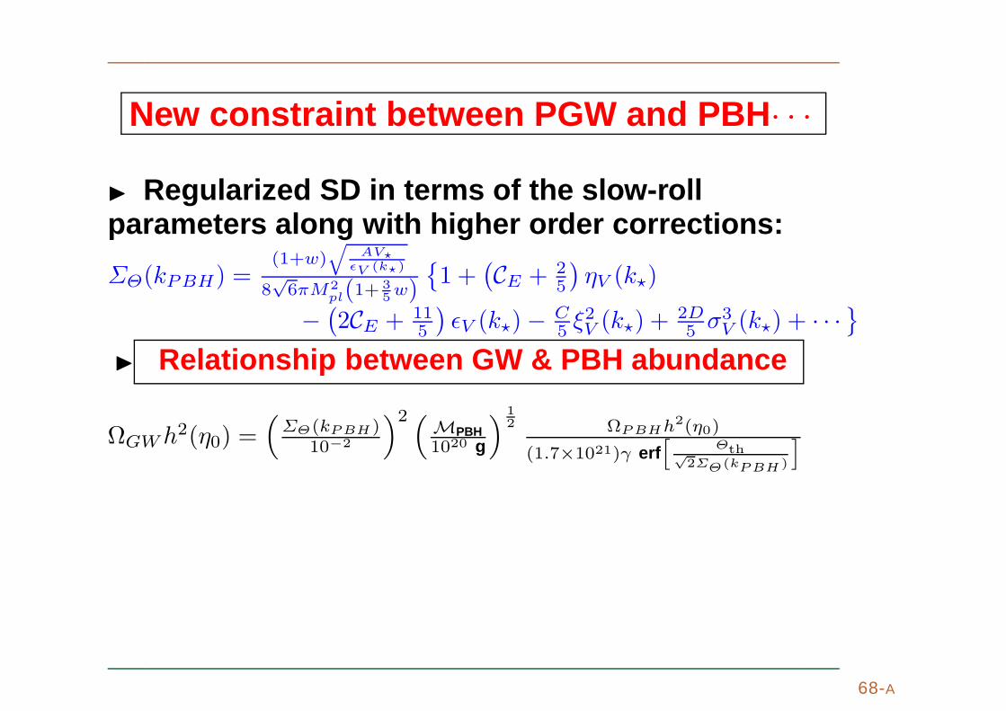
Regularized SD in terms of the slow-rollparameters along with higher order corrections:
ΣΘ(kPBH) =(1+w)
√
AV⋆ǫV (k⋆)
8√6πM2
pl(1+35w)
1 +
(CE + 2
5
)ηV (k⋆)
−(2CE + 11
5
)ǫV (k⋆)− C
5 ξ2V (k⋆) +
2D5 σ3
V (k⋆) + · · ·
68
New constraint between PGW and PBH · · ·
Regularized SD in terms of the slow-rollparameters along with higher order corrections:
ΣΘ(kPBH) =(1+w)
√
AV⋆ǫV (k⋆)
8√6πM2
pl(1+35w)
1 +
(CE + 2
5
)ηV (k⋆)
−(2CE + 11
5
)ǫV (k⋆)− C
5 ξ2V (k⋆) +
2D5 σ3
V (k⋆) + · · ·
Relationship between GW & PBH abundance
ΩGWh2(η0) =(
ΣΘ(kPBH)10−2
)2 ( MPBH1020 g
) 12 ΩPBHh2(η0)
(1.7×10²¹)γ erf[
Θth√2ΣΘ(kPBH )
]
68-A

New constraint between PGW and PBH · · ·
Regularized SD in terms of the slow-rollparameters along with higher order corrections:
ΣΘ(kPBH) =(1+w)
√
AV⋆ǫV (k⋆)
8√6πM2
pl(1+35w)
1 +
(CE + 2
5
)ηV (k⋆)
−(2CE + 11
5
)ǫV (k⋆)− C
5 ξ2V (k⋆) +
2D5 σ3
V (k⋆) + · · ·
Relationship between GW & PBH abundance
ΩGWh2(η0) =(
ΣΘ(kPBH)10−2
)2 ( MPBH1020 g
) 12 ΩPBHh2(η0)
(1.7×10²¹)γ erf[
Θth√2ΣΘ(kPBH )
]
Next we use the constraints for sub-Planckianinflation.
68-B

New constraint between PGW and PBH · · ·
Regularized SD in terms of the slow-rollparameters along with higher order corrections:
ΣΘ(kPBH) =(1+w)
√
AV⋆ǫV (k⋆)
8√6πM2
pl(1+35w)
1 +
(CE + 2
5
)ηV (k⋆)
−(2CE + 11
5
)ǫV (k⋆)− C
5 ξ2V (k⋆) +
2D5 σ3
V (k⋆) + · · ·
Relationship between GW & PBH abundance
ΩGWh2(η0) =(
ΣΘ(kPBH)10−2
)2 ( MPBH1020 g
) 12 ΩPBHh2(η0)
(1.7×10²¹)γ erf[
Θth√2ΣΘ(kPBH )
]
Next we use the constraints for sub-Planckianinflation.Further using the real root from the closed
constraint relation we express “r′′ in terms of thefield displacement ∆φ.
68-C

New constraint between PGW and PBH · · ·
Hence we express the regularized SD in terms ofinflationary observables using the sub-Planckianconstraints.
69

New constraint between PGW and PBH · · ·
Hence we express the regularized SD in terms ofinflationary observables using the sub-Planckianconstraints.Finally we get a colsed cosmic constraint relation
between GW & PBH abundance connected via thethe sub-Planckian inflationary constraints:
ΩGWh2 ≤ 6×10⁻¹⁸
γ
(MPBH1020 g
) 12 O2
PBHΩPBHh2
erf
(
Θth√2OPBH
)
whereOPBH = 5
√A(1+w)(8.17×10⁻³)2
12√2π(1+ 3
5w)
1 + 2ηV (k⋆)5
+ 1500
(r(k⋆)0.12
)
− 3ǫV (k⋆)−C
5ξ2V (k⋆) +
2D
5σ3V (k⋆) + · · ·
69-A

New constraint between PGW and PBH · · ·
PLANCK 1Σ
BAND
-0.025 -0.020 -0.015 -0.010 -0.005 0.000 0.005
0.009970
0.009971
0.009972
0.009973
0.009974
0.009975
WPBHh2 vs ΑS plot
70

New constraint between PGW and PBH · · ·
71

POWER SPECTRUM
PS(k⋆) = [1− (2CE + 1)ǫV + CEηV ]2V
24π2M4PLǫV
PT (k⋆) = [1− (CE + 1)ǫV ]2 2V
3π2M4PL
SPECTRAL TILT
nS − 1 ≈ (2ηV − 6ǫV )− 2CEξ2V +2
3η2V + 2(8CE + 3)ǫ2V
+2ǫV ηV
(
6CE +7
3
)
−4CE(CE+1)ξ2V ǫV +2C2EηV ξ
2V
nT ≈ −2ǫV + 2
(
2CE +5
3
)
ǫV ηV − 2
(
4CE +13
3
)
ǫ2V
72

RUNNING OF SPECTRAL TILTαS ≈
(16ηV ǫV − 24ǫ2V − 2ξ2V
)− 2CE(4ǫV ξ2V − ηV ξ
2V − σ3
V )
+4
3ηV (2ηV ǫV − ξ2V ) + 4(8CE + 3)ǫV (4ǫ
2V − 2ηV ǫV )
− 4CE(CE +1)[ǫV (4ǫV ξ
2V − ηV ξ
2V − σ3
V ) + ξ2V (4ǫ2V − 2ηV ǫV )
]
+ 2C2Eξ
2V (2ηV ǫV − ξ2V ) + 2C2
EηV (4ǫV ξ2V − ηV ξ
2V − σ3
V )
αT ≈ (4ηV ǫV − 8ǫ2V ) + 2
(
2CE +5
3
)[ǫV (2ηV ǫV − ξ2V )
+ ηV (4ǫ2V − 2ηV ǫV )
]− 4
(
4CE +13
3
)
ǫV (4ǫ2V − 2ηV ǫV )
⋆NOTE:HIGHER ORDER SLOW ROLL CORRECTIONS≡PRECISION COSMOLOGY (FITS CMBPOL THROUGHOUT THEMULTIPOLE 2 < l < 2500.)
73

74

INFLATON POTENTIALAround the saddle point φ0
V (φ) = C0 + C4(φ− φ0)4
where(1) C0 = V (φ0) =
m3φ(φ0)M
6√6λ4
3(1 + D1
2 − D3
6
)
[
1 +D1 log(
φ20
µ20
)]
− 3(1 + D1
2 − D3
6
)2[
1 +D2 log(
φ20
µ20
)]
+(1 + D1
2 − D3
6
)2[
1 +D2 log(
φ20
µ20
)]
,
(2) C4 = 14!V
′′′′(φ0) =
m2φ(φ0)
24√6φ2
0
(1 + D1
2 − D3
6
)
[(360√
6− 12
√6)
+ (684D3 − 50√6D2)
] (1 + D1
2 − D3
6
)
− 2√6D1
(1+D12 −D3
6 )
+(1 + D1
2 − D3
6
) (360D3√
6− 12
√6D2
)
log(
φ20
µ20
)
.
75