Testing and Emulating Modified

Gravity on Cosmological Scales

by

Andrius Tamosiunas

This thesis is submitted in partial fulfilment of

the requirements for the award of the degree of

Doctor of Philosophy of the University of Portsmouth.

Supervisors:

Prof. Bob Nichol, Prof. David Bacon, Prof. Kazuya Koyama

November 18, 2020

arX

iv:2

011.

0878

6v1

[as

tro-

ph.C

O]

17

Nov

202

0

Abstract

This thesis explores methods and techniques for testing and emulating models

of modified gravity. In particular, the thesis can be split into two parts.

The first part corresponding to chapters 2, 3 and 4 introduces a method

of testing modified gravity models on galaxy cluster scales. In more detail,

chapter 2 introduces the main concepts from galaxy cluster physics, which are

important in the context of testing modified gravity. I present a summary

of the different probes of mass in galaxy clusters. More specifically, the

properties of the X-ray-emitting intracluster medium are discussed in the

context of measuring hydrostatic masses. In addition, the key equations for

weak lensing of background galaxies by galaxy clusters are summarized in

terms of their importance for measuring cluster lensing masses.

Chapter 3 introduces a technique for detecting the modifications of grav-

ity using a combination of X-ray and weak lensing data obtained by stacking

multiple galaxy clusters. This technique first discussed in Terukina et al.

(2014) and Wilcox et al. (2015) allows us to put some of the most competi-

tive constraints on scalar-tensor theories with chameleon screening as well as

the closely related f(R) gravity models. Chapter 3 also contains a discussion

of the key theoretical concepts of scalar-tensor models and their relationship

to f(R) gravity. Finally, the chapter is concluded by introducing novel re-

sults which update the tests done in Wilcox et al. (2015) with an improved

dataset consisting of 77 galaxy clusters from the XCS and CFHTLenS sur-

veys. The updated dataset containing less noisy tangential shear data allows

us to put tight constraints on the chameleon field background value and the

i

related fR0 parameter: φ∞ < 8× 10−5Mpl and |fR0| < 6.5× 10−5.

Chapter 4 expands the mentioned techniques for testing a different type of

a model. In particular, the model of emergent gravity (introduced in Verlinde

(2017)) is tested by using a variation of the techniques introduced in chapter

3. The key prediction of Verlinde’s emergent gravity is a scaling relation sim-

ilar to the baryonic Tully-Fisher relation, which allows us to determine the

dark matter distribution in a cluster directly from the baryonic mass distribu-

tion. The mentioned scaling relation was tested by determining the baryonic

mass from the X-ray surface brightness data and calculating the predicted

weak lensing tangential shear profile, which was then compared against the

ΛCDM prediction based on the Navarro-Frenk-White profile. The test was

performed for the Coma Cluster using data from Terukina et al. (2014) and

for the 58 galaxy cluster stack from Wilcox et al. (2015). The obtained re-

sults indicate that according to the Coma Cluster data, the emergent gravity

predictions agree with the ΛCDM predictions only in the range of r ≈ 250-

700 kpc. Outside the mentioned radial range the standard model results

are preferred according to the Bayesian information criterion analysis (de-

spite needing two extra free parameters). The same general conclusion can

be drawn from the 58 cluster stack data, which indicates a good agreement

between the models only for r ≈ 1-2 Mpc. Outside of that radial range the

standard model is strongly preferred.

The second part of the thesis, referring specifically to chapters 5 and 6,

contains a study of machine learning techniques for emulating cosmological

simulations. More specifically, generative adversarial networks are studied as

an effective tool for emulating N -body simulation data quickly and efficiently.

Chapter 5 contains a brief discussion of the different machine learning algo-

rithms in the context of emulators. Specifically, artificial neural networks are

introduced along with gradient boosting algorithms. Chapter 6 introduces

a generative adversarial network algorithm for emulating cosmic web data

along with weak lensing convergence map data coming from N -body simu-

lations. The presented approach is based on the cosmoGAN algorithm first

ii

described in Mustafa et al. (2019), which allows us to generate thousands of

realistic weak lensing convergence maps in a matter of seconds. The men-

tioned approach is then modified to allow emulating cosmic web and weak

lensing data for ΛCDM and f(R) gravity with different cosmological parame-

ters and redshifts. In addition, a similar approach was used to simultaneously

emulate dark matter and baryonic simulation data coming from the Illustris

simulation. The obtained results indicate a 1-20% difference between the

power spectra of the emulated and original (N -body simulation) datasets

depending on the training data used. Finally, the chapter contains an in-

depth study of the technique of latent space interpolation and how it can

be applied to control the cosmological/modified gravity parameters during

the emulation procedure. The obtained results illustrate that such machine

learning algorithms will play an important role in producing accurate mock

data in the era of future large scale observational surveys.

iii

Table of Contents

Abstract i

Declaration xiii

Acknowledgements xiv

Dissemination xv

Notation xvi

1 Introduction 1

1.1 General Relativity . . . . . . . . . . . . . . . . . . . . . . . . 4

1.2 The Standard Model of Cosmology . . . . . . . . . . . . . . . 6

1.3 The Standard Model: Problems and Challenges . . . . . . . . 9

1.3.1 The Validity of the Cosmological Principle . . . . . . . 9

1.3.2 The Validity of GR on Different Scales . . . . . . . . . 10

1.3.3 Issues Related to Dark Matter . . . . . . . . . . . . . . 12

1.3.4 Issues Related to Dark Energy . . . . . . . . . . . . . . 13

1.3.5 Tensions in the Cosmological Parameters . . . . . . . . 14

1.4 Modified Gravity: Tests and Current Developments . . . . . . 17

1.4.1 Laboratory Tests . . . . . . . . . . . . . . . . . . . . . 20

1.4.2 Solar System Tests . . . . . . . . . . . . . . . . . . . . 21

1.4.3 Gravitational Wave Tests . . . . . . . . . . . . . . . . . 24

1.4.4 Galaxy Scale Tests . . . . . . . . . . . . . . . . . . . . 26

1.4.5 Galaxy Cluster Tests . . . . . . . . . . . . . . . . . . . 27

iv

1.4.6 Large Scale Structure Tests . . . . . . . . . . . . . . . 28

2 Galaxy Clusters 31

2.1 The Structure and Basic Properties of Galaxy Clusters . . . . 31

2.2 Intracluster Medium and X-ray Observations . . . . . . . . . . 35

2.3 Methods To Estimate Cluster Masses . . . . . . . . . . . . . . 38

2.3.1 Hydrostatic Equilibrium . . . . . . . . . . . . . . . . . 38

2.3.2 Galaxy kinematics . . . . . . . . . . . . . . . . . . . . 41

2.4 Weak Lensing in Galaxy Clusters . . . . . . . . . . . . . . . . 42

2.4.1 The Basics of Gravitational Lensing . . . . . . . . . . . 42

2.4.2 Weak Lensing by NFW Halos . . . . . . . . . . . . . . 48

3 Modified Gravity on Galaxy Cluster Scales 51

3.1 Scalar-Tensor Gravity with Chameleon Screening . . . . . . . 52

3.1.1 The Action . . . . . . . . . . . . . . . . . . . . . . . . 52

3.1.2 Properties of the Effective Potential . . . . . . . . . . . 54

3.2 f(R) Gravity . . . . . . . . . . . . . . . . . . . . . . . . . . . 57

3.3 Testing Modified Gravity on Galaxy Cluster Scales . . . . . . 60

3.3.1 Non-Thermal Pressure and the Modified Hydrostatic

Equilibrium Equation . . . . . . . . . . . . . . . . . . . 60

3.3.2 Weak Lensing in Chameleon Gravity . . . . . . . . . . 63

3.3.3 X-ray Surface Brightness . . . . . . . . . . . . . . . . . 65

3.3.4 X-ray and Weak Lensing Datasets . . . . . . . . . . . . 66

3.3.5 MCMC Fitting . . . . . . . . . . . . . . . . . . . . . . 74

3.3.6 Results . . . . . . . . . . . . . . . . . . . . . . . . . . . 77

3.4 Implications for the Gravitational Slip Parameter . . . . . . . 83

3.4.1 Gravitational Slip in Galaxy Clusters . . . . . . . . . . 83

3.4.2 Constraining the Deviations from the Hydrostatic Equi-

librium and the Gravitational Slip Parameter . . . . . 86

4 Testing Emergent Gravity on Galaxy Cluster Scales 91

4.1 Motivations for Emergent Gravity . . . . . . . . . . . . . . . . 91

v

4.2 Verlinde’s Emergent Gravity . . . . . . . . . . . . . . . . . . . 94

4.2.1 The Predictions of the Model . . . . . . . . . . . . . . 94

4.2.2 The Main Assumptions . . . . . . . . . . . . . . . . . . 99

4.3 Testing Emergent Gravity . . . . . . . . . . . . . . . . . . . . 101

4.3.1 Testing Emergent Gravity with the Coma Cluster . . . 101

4.3.2 Testing Emergent Gravity with Stacked Galaxy Clusters110

4.4 The Current State of the Model . . . . . . . . . . . . . . . . . 119

4.5 Covariant Emergent Gravity . . . . . . . . . . . . . . . . . . . 121

5 A Brief Introduction to Machine Learning 125

5.1 Machine Learning and Artificial Intelligence . . . . . . . . . . 126

5.2 Machine Learning in Cosmology and Astrophysics . . . . . . . 127

5.3 Decision Trees and Gradient Boosting . . . . . . . . . . . . . . 129

5.4 Artificial Neural Networks . . . . . . . . . . . . . . . . . . . . 135

5.5 Convolutional Neural Networks . . . . . . . . . . . . . . . . . 139

5.6 Generative Adversarial Networks . . . . . . . . . . . . . . . . 143

6 Using GANs for Emulating Cosmological Simulation Data 147

6.1 The Need for Cosmological Emulators . . . . . . . . . . . . . . 147

6.2 DCGAN Architecture for Emulating Cosmological Simulation

Data . . . . . . . . . . . . . . . . . . . . . . . . . . . . . . . . 149

6.3 Latent Space Interpolation . . . . . . . . . . . . . . . . . . . . 153

6.4 Riemannian Geometry of GANs . . . . . . . . . . . . . . . . . 157

6.5 Datasets and the Training Procedure . . . . . . . . . . . . . . 160

6.5.1 Weak Lensing Convergence Map Data . . . . . . . . . 160

6.5.2 Cosmic Web Slice Data . . . . . . . . . . . . . . . . . . 162

6.5.3 Dark Matter, Gas and Internal Energy Data . . . . . . 163

6.5.4 The Training Procedure . . . . . . . . . . . . . . . . . 164

6.6 Diagnostics . . . . . . . . . . . . . . . . . . . . . . . . . . . . 166

6.7 Results . . . . . . . . . . . . . . . . . . . . . . . . . . . . . . . 168

6.7.1 Weak Lensing Map Results . . . . . . . . . . . . . . . 168

6.7.2 Weak Lensing Maps of Multiple Cosmologies . . . . . . 170

vi

6.7.3 Cosmic Web for Multiple Redshifts . . . . . . . . . . . 172

6.7.4 Cosmic Web for Multiple Cosmologies and Modified

Gravity Models . . . . . . . . . . . . . . . . . . . . . . 175

6.7.5 Dark Matter, Gas and Internal Energy Results . . . . . 176

6.7.6 Latent Space Interpolation Results . . . . . . . . . . . 178

6.8 Analysis and Conclusions . . . . . . . . . . . . . . . . . . . . . 185

7 Conclusions and Future Work 189

Appendices 194

A 195

A.1 Availability of Data and Codes . . . . . . . . . . . . . . . . . 195

A.2 Samples of the GAN-produced Data . . . . . . . . . . . . . . . 195

A.3 MCMC Contours . . . . . . . . . . . . . . . . . . . . . . . . . 197

Bibliography 201

vii

List of Tables

1.1 Base-ΛCDM cosmological parameters from Planck 2018 . . . . 8

3.1 Comparison of the best-fit parameters in Terukina et al. (2014)

and Wilcox (2016). . . . . . . . . . . . . . . . . . . . . . . . . 77

3.2 Comparison of the best-fit parameters in Wilcox et al. (2015)

and this work . . . . . . . . . . . . . . . . . . . . . . . . . . . 79

3.3 Modified gravity constraints from previous works in the liter-

ature . . . . . . . . . . . . . . . . . . . . . . . . . . . . . . . . 80

4.1 The typical values of the rmin parameter . . . . . . . . . . . . 101

4.2 The best-fit parameters for the Coma Cluster test of emergent

gravity . . . . . . . . . . . . . . . . . . . . . . . . . . . . . . . 107

4.3 Goodness of fit statistics for the Coma Cluster test of emergent

gravity . . . . . . . . . . . . . . . . . . . . . . . . . . . . . . . 109

4.4 Best-fit parameters for the EG and the standard model fits

using the cluster stack data . . . . . . . . . . . . . . . . . . . 113

4.5 Goodness of fit statistics for the cluster stack results . . . . . . 116

6.1 Architecture of the generator neural network . . . . . . . . . . 151

6.2 Architecture of the discriminator neural network . . . . . . . . 152

6.3 The used XGBoost settings . . . . . . . . . . . . . . . . . . . 183

viii

List of Figures

1.1 Observational tests of modified gravity . . . . . . . . . . . . . 11

1.2 Recent cosmological constraints from multiple probes in the

Dark Energy Survey . . . . . . . . . . . . . . . . . . . . . . . 13

1.3 The H0 tension . . . . . . . . . . . . . . . . . . . . . . . . . . 15

1.4 Modified gravity models . . . . . . . . . . . . . . . . . . . . . 19

1.5 Summary of laboratory tests of gravity . . . . . . . . . . . . . 22

1.6 Summary of modified gravity models after GW170817 . . . . . 26

1.7 Summary of the observational constraints on f(R) gravity . . 30

2.1 The mass distribution in the Bullet Cluster . . . . . . . . . . . 33

2.2 Sunyaev-Zel’dovich effect . . . . . . . . . . . . . . . . . . . . . 38

2.3 The geometry of gravitational lensing . . . . . . . . . . . . . . 44

2.4 The weak lensing effects on an image of a background galaxy . 47

3.1 The effects of the local density on the shape of the chameleon

potential . . . . . . . . . . . . . . . . . . . . . . . . . . . . . . 56

3.2 Analysis of the cluster separation . . . . . . . . . . . . . . . . 69

3.3 X-ray and tangential shear profile dataset from Wilcox et al.

(2015) . . . . . . . . . . . . . . . . . . . . . . . . . . . . . . . 70

3.4 A sample of sources misclassified as galaxy clusters in the orig-

inal XCS-CFHTLenS dataset in Wilcox et al. (2015) . . . . . . 71

3.5 A comparison of the original and the updated XCS-CFHTLenS

datasets . . . . . . . . . . . . . . . . . . . . . . . . . . . . . . 72

ix

3.6 The stacked X-ray surface brightness and tangential shear pro-

files for the updated 77 cluster dataset . . . . . . . . . . . . . 73

3.7 X-ray surface brightness from two types of simulations from

Wilcox (2016) . . . . . . . . . . . . . . . . . . . . . . . . . . . 75

3.8 A comparison of the modified gravity constraints from the

Coma Cluster (Terukina et al., 2014), the 58 galaxy cluster

stack from (Wilcox et al., 2015) and the 77 cluster stack de-

scribed in this work . . . . . . . . . . . . . . . . . . . . . . . . 81

3.9 A comparison of the modified gravity constraints from the

ΛCDM and f(R) simulations with 103 and 99 clusters stacked

correspondingly and the 77 cluster stack described in this work 82

3.10 Checking the validity of the assumption of hydrostatic equi-

librium . . . . . . . . . . . . . . . . . . . . . . . . . . . . . . . 86

3.11 The gravitational slip parameter calculated using the X-ray

and the weak lensing data from Wilcox et al. (2015). . . . . . 87

3.12 Estimate of the gravitational slip constraints using ∼100 and

∼1000 stacked galaxy clusters. . . . . . . . . . . . . . . . . . . 90

4.1 Emergent gravity effects . . . . . . . . . . . . . . . . . . . . . 96

4.2 The Coma Cluster . . . . . . . . . . . . . . . . . . . . . . . . 103

4.3 The Coma Cluster galaxy mass distribution . . . . . . . . . . 105

4.4 The results for the test of emergent gravity using the Coma

Cluster . . . . . . . . . . . . . . . . . . . . . . . . . . . . . . . 108

4.5 An illustration of the effects of stacking galaxy clusters . . . . 111

4.6 The galaxy mass distribution for the cluster stack . . . . . . . 112

4.7 The results of testing emergent gravity with stacked galaxy

clusters (T > 2.5 keV bin) . . . . . . . . . . . . . . . . . . . . 114

4.8 The results of testing emergent gravity with stacked galaxy

clusters (T < 2.5 keV bin) . . . . . . . . . . . . . . . . . . . . 115

4.9 Analysis of the various systematics . . . . . . . . . . . . . . . 118

5.1 Gradient boosting training procedure . . . . . . . . . . . . . . 132

x

5.2 An example of a decision tree . . . . . . . . . . . . . . . . . . 133

5.3 Biological and artificial neurons . . . . . . . . . . . . . . . . . 136

5.4 A multilayer perceptron . . . . . . . . . . . . . . . . . . . . . 137

5.5 RGB images and the procedure of convolution . . . . . . . . . 140

5.6 Edge extraction from an image . . . . . . . . . . . . . . . . . 141

5.7 GAN training procedure . . . . . . . . . . . . . . . . . . . . . 145

5.8 GAN training procedure for MNIST images . . . . . . . . . . 146

6.1 The pipeline of training a GAN on cosmic web slice data . . . 153

6.2 Illustration of the linear latent space interpolation procedure . 156

6.3 Riemannian geometry of generative adversarial networks . . . 158

6.4 Samples of the Illustris dataset . . . . . . . . . . . . . . . . . 165

6.5 The effects of Gaussian smoothing on Minkowski functionals . 168

6.6 The power spectrum and the pixel intensity histogram for the

weak lensing convergence maps (ΛCDM) . . . . . . . . . . . . 169

6.7 Minkowski functional analysis for the weak lensing conver-

gence maps (ΛCDM) . . . . . . . . . . . . . . . . . . . . . . . 170

6.8 The power spectrum and the pixel intensity histogram for the

weak lensing convergence maps (σ8 = 0.436, 0.814) . . . . . 171

6.9 Minkowski functional analysis for the weak lensing conver-

gence maps (σ8 = 0.436, 0.814) . . . . . . . . . . . . . . . . 173

6.10 The power spectra and the overdensity histogram for the cos-

mic web slices with different redshifts: z = 0, 1 . . . . . . . 174

6.11 Minkowski functional analysis for the cosmic web slices with

different redshifts: z = 0, 1 . . . . . . . . . . . . . . . . . . . 175

6.12 The power spectra and the overdensity histogram for the cos-

mic web slices with σ8 = 0.7, 0.9 . . . . . . . . . . . . . . . . 177

6.13 Minkowski functional analysis for the cosmic web slices with

σ8 = 0.7, 0.9 . . . . . . . . . . . . . . . . . . . . . . . . . . . 178

6.14 The power spectra and the overdensity histogram for the cos-

mic web slices with fR0 = 10−7, 10−1 . . . . . . . . . . . . . 179

xi

6.15 Minkowski functional analysis for the cosmic web slices with

fR0 = 10−7, 10−1 . . . . . . . . . . . . . . . . . . . . . . . . 180

6.16 Diagnostics for the dark matter, gas and internal energy results181

6.17 Minkowski functional analysis for the dark matter, gas and

internal energy results . . . . . . . . . . . . . . . . . . . . . . 182

6.18 Latent space interpolation results . . . . . . . . . . . . . . . . 184

6.19 Samples of data produced by the latent space interpolation

procedure . . . . . . . . . . . . . . . . . . . . . . . . . . . . . 185

A.1 A comparison of 4 randomly selected weak lensing convergence

maps. . . . . . . . . . . . . . . . . . . . . . . . . . . . . . . . 196

A.2 A comparison of 4 randomly selected cosmic web slices. . . . . 196

A.3 The MCMC contours from Terukina et al. (2014) . . . . . . . 198

A.4 The MCMC contours from Wilcox et al. (2015) . . . . . . . . 199

A.5 The MCMC contours of the best-fit parameters determined in

this work . . . . . . . . . . . . . . . . . . . . . . . . . . . . . . 200

xii

Declaration

Whilst registered as a candidate for the above degree, I have not been regis-

tered for any other research award. The results and conclusions embodied in

this thesis are the work of the named candidate and have not been submitted

for any other academic award.

Word count: 41,724 words.

xiii

Acknowledgements

I would like to use this opportunity to express my sincere gratitude to the

people that made this thesis possible. Firstly, I would like to thank my lovely

family for their never-ending love and support. I am grateful to my Dad, who

has sparked in me the love for science and education. I am grateful to my

Mom for always being there for me. And I am grateful to my brother for

being someone I can look up to.

I would also like to thank my dear supervisors Prof. Bob Nichol, David

Bacon and Kazuya Koyama for their infinite patience, kindness and keeping

my passion for learning new things aflame. Thanks for teaching me so much

about myself and the Universe. In turn, I would like to extend my sincere

gratitude to all my teachers and mentors (from primary school to university),

who have taught me so much. Likewise I am grateful to the people who have

influenced me in many different ways throughout the years including: Prof.

Andrew Liddle, Bruce Bassett and Kathy Romer.

Finally, my gratitude goes to my friends and colleagues in the ICG.

Thanks to my academic brothers and sisters – Michael, Mike, Maria, Sam Y.,

Sam L. and Natalie, for sharing the academic path and for the fun times and

the endless nights in the pubs of Portsmouth. I am also sincerely grateful to

everyone in the ICG for making the institute a warm and welcoming place

to work and study in.

xiv

Dissemination

Chapter 3 contains work in preparation for publication. Chapters 4 and 5

contain original work described in the following publications:

A. Tamosiunas, H. A. Winther, K. Koyama, D. J. Bacon, R. C. Nichol,

B. Mawdsley. Towards Universal Cosmological Emulators with Generative

Adversarial Networks. April 2020. Submitted for publication in the Jour-

nal of Computational Astrophysics and Cosmology. arXiv: arXiv:2004.10223

[astro-ph.CO].

A. Tamosiunas. D. J. Bacon, K. Koyama, R. C. Nichol. Testing Emergent

Gravity on Galaxy Cluster Scales. January 2019. Published in JCAP. DOI:

10.1088/1475-7516/2019/05/053. arXiv: arXiv:1901.05505 [astro-ph.CO]

xv

Notation and Abbreviations

Description: Abbreviation:

Active galactic nuclei AGN

Bayesian information criterion BIC

Canada-France-Hawaii Telescope Lensing Survey CFHTLenS

The cosmic microwave background CMB

Convolutional neural networks CNN

Deep convolutional generative adversarial networks DCGAN

The theory of emergent gravity EG

The Friedman-Lemaıtre-Robertson-Walker metric FLRW

Generative adversarial network GAN

Graphical processing unit GPU

The theory of general relativity GR

Intracluster medium in galaxy clusters ICM

The Markov chain Monte Carlo algorithm MCMC

Modified Newtonian dynamics MOND

The Navarro-Frenk-White density profile NFW

The Sunyaev-Zeldovich effect SZ

The XMM Cluster Survey XCS

The standard model of cosmology ΛCDM

xvi

Chapter 1

Introduction

The science of cosmology dates back to ancient times. When defined in a

broad sense cosmology is inseparable from the earliest inquiries into how na-

ture works by ancient cultures as described in the historical records (Kragh,

2017). Initially such inquiries were tightly intertwined with religion and su-

perstition. The principles of what is now known as modern cosmology were

arguably first combined into a consistent framework in ancient Greece. As

an example, the great philosopher Plato in his works Timaeus and Republic

introduced the two-sphere model, which placed Earth at the centre of the

Universe, surrounded by a celestial sphere holding the stars and other heav-

enly bodies (Evans, 1998). Another school of philosophy, the Pythagoreans,

sought to build models of the celestial motion based on known mathematical

principles. A key stepping stone to mention here is that the Pythagoreans

treated astronomy as one of the key mathematical arts (along with arith-

metic, geometry and music). Such a high regard for natural philosophy

eventually led to the formulation of the first known heliocentric model of the

solar system by the mathematician and astronomer Aristarchus of Samos

(Heath, 1991). The model of Aristarchus placed the Sun at the centre of

the known Universe with the Earth and the other known planets orbiting

around it. Another visionary insight by Aristarchus was that the stars were

in fact objects analogous to the Sun at such great distances from Earth

1

that no parallax was observed (Wright, 1995). The original texts describing

Aristarchus’ models were later lost for over a millennium with only references

in contemporary texts surviving.

Another visionary work that came from this historical period is The Sand

Reckoner (Gr: Ψαμμίτης) by Archimedes (Hirshfeld, 2009). In this work

Archimedes sets out to calculate the number of grains of sand that fit into

the Universe. In order to do this, Archimedes had to estimate the size of he

Universe based on Aristarchus’ model. In addition, Archimedes had to invent

new mathematical notation for dealing with large numbers. The obtained

results estimated the diameter of the Universe to be no more than 1014 stadia

or roughly 2 light-years in contemporary units. Equivalently, a Universe of

such size could fit 1063 grains of sand. The importance of this work lies in

the fact that it is likely the first known systematic estimate of the size of the

Universe based on mathematics and the known principles of astronomy.

Major leaps in understanding of cosmology and astronomy were made

during the Renaissance. The works of Nicolaus Copernicus reintroduced

the heliocentric model from relative obscurity due to the original works of

Aristarchus being mostly unknown. The works of Copernicus, when com-

bined with astronomical observations, allowed predictions of planetary mo-

tions and orbital periods as well as experimental comparison of the two com-

peting theories of geocentrism and heliocentrism. The observational tradition

of Copernicus was carried on by later astronomers including Tycho Brahe and

Johannes Kepler, the work of whom led to the three laws of Kepler. Another

key discovery from this historical period came from Galileo, who is tradi-

tionally credited as one of the discoverers of the telescope. The mentioned

theoretical and observational efforts culminated in the work of Newton and

in particular Newton’s law of universal gravitation, which formed the core of

our understanding of gravity for over two centuries after its discovery (Taton

et al., 2003; Curley, 2012).

Arguably the most important theoretical development in the modern era

of cosmology came with Einstein’s theory of general relativity (GR) (Einstein,

2

1916). GR revolutionized our understanding of gravity by promoting space

and time from a mere stage in which events take place to a 4-dimensional

dynamical canvas that interacts with matter and energy in intricate ways

(spacetime tells matter how to move; matter tells spacetime how to curve

according to John A. Wheeler).

After more than a century GR has been extensively confirmed observa-

tionally and now forms the basis of our understanding of how gravity behaves

in a wide range of systems starting with the solar system and galaxies and

ending with the Universe as a whole. For this reason GR is also the theoret-

ical basis behind the currently most complete model of standard cosmology

– the ΛCDM model. The ΛCDM model has been extremely successful in

explaining structure formation in the Universe along with the anisotropies

of the cosmic microwave background (CMB). However, as the name implies,

in order to make accurate predictions, the theory requires two extra compo-

nents – the cosmological constant (Λ) or some other form of dark energy along

with non-luminous non-baryonic matter (CDM). Dark matter, in particular,

was first inferred to exist by Fritz Zwicky by studying the mass distribu-

tion in the Coma Cluster in 1933 (Andernach and Zwicky, 2017). Now we

know that some form of dark matter is crucial for explaining galaxy rotation

curves and large scale structure formation in general. Another key discov-

ery came in 1998, when the Supernova Cosmology Project and the High-Z

Supernova Search Team found evidence for the accelerating expansion of the

Universe using data from type Ia supernovae (Riess et al., 1998). To explain

the accelerating expansion, some form of dark energy is required.

Today we know a lot about dark energy and dark matter, but the physical

origin of them still eludes astronomers and particle physicists. This is one of

the key motivations for developing models that modify GR. Since the pub-

lication of the original theory in 1915 a plethora of modified gravity models

have been proposed. These models can be generally classified based on the

type of modification they introduce to the original GR framework. Namely,

modified models can introduce extra scalar, vector and tensor fields, extra

3

spatial dimensions and higher order derivatives. In addition, certain assump-

tions that exist in the original model can be relaxed (e.g. non-local theories).

These approaches form a complex family of modified gravity models, each

of which comes with unique observational signatures. A need to discrimi-

nate between the different families of modifications of gravity has led to a

variety of observational tests on scales ranging from the laboratory, to the

solar system and all the way to cosmological scales (Koyama, 2016). In this

thesis special emphasis will be put on galaxy cluster-related methods for test-

ing for such modification of gravity. In addition, various machine learning

techniques will be explored as tools for emulating modified gravity simula-

tions. The rest of chapter 1 will introduce the relevant basic concepts in GR

and cosmology. In addition, a brief overview of the current theoretical and

observational developments in the field of modified gravity will be given.

1.1 General Relativity

Einstein’s theory of general relativity published in 1915 forms the basis of the

modern understanding of gravity. One of the key postulates of the theory is

the equivalence principle, which equates the gravitational and inertial masses

of a given body. This at first glance inconsequential idea, with its roots dating

back to the observations of Galileo, has led Einstein on a path towards finding

deep connections between gravity and the geometry of spacetime. Namely, by

demonstrating the equivalence of the forces felt by a body in an accelerated

frame and those felt in a gravitational field, Einstein was able to generalize

the tools and techniques first developed for his theory of special relativity

(Wald, 2010).

GR relates the energy-momentum contents of a given gravitational system

to the geometric effects on spacetime. Hence, if the mass/energy distribu-

tion in a given system is known, accurate predictions can be made about

the resulting dynamics of the system. A key equation in this regard is the

Einstein-Hilbert action. Describing GR in terms of an action has a number of

4

advantages. In particular, it allows to describe the theory following a similar

formalism as in the other classical field theories (e.g. Maxwell theory). Vary-

ing the action allows a straightforward way for deriving the field equations.

In addition, the effects of other fields (e.g. matter fields) can be easily added

to the total action. The Einstein-Hilbert action is given by:

SEH =

∫d4x

√−g

2κ(R− 2Λ) + Sm [ψM , gµν ] , (1.1)

where gµν is the spacetime metric, g is the determinant of the metric, κ =

8πG, G is the gravitational constant, R is the Ricci scalar, Λ is the cosmolog-

ical constant and Sm is the matter action governed by the matter field ψM .

The Ricci scalar can be obtained by contracting the indices of the Ricci ten-

sor R ≡ gµνRµν , which, in turn, can be derived from the Riemann curvature

tensor:

Rρσµν = ∂µΓρσν − ∂νΓρσµ + ΓρλµΓλσν − ΓρλνΓ

λσµ. (1.2)

The Riemann curvature tensor quantifies the amount of curvature in the 4-D

spacetime manifold. Here Γ refers to the Christoffel symbols, given by:

Γρσν =1

2gργ(∂gγν∂xσ

+∂gγσ∂xν

− ∂gσν∂xγ

). (1.3)

By varying the Einstein-Hilbert action, w.r.t. the spacetime metric the

Einstein field equations are obtained:

Gµν = κTµν − Λgµν , (1.4)

where Gµν = Rµν − Rgµν/2 is the Einstein tensor. Tµν refers to the energy-

momentum tensor, defined by:

T µν = − 2√−g

δSmδgµν

. (1.5)

In the case of a perfect fluid with density ρ, pressure p and the four-

velocity Uµ:

5

T µν =(ρc2 + p

)UµUν + pgµν . (1.6)

In this framework, the dynamics of bodies can be deduced from the

geodesic equation, which generalizes the notion of a straight line to curved

spaces:

d2xµ

ds2+ Γµαβ

dxα

ds

dxβ

ds= 0. (1.7)

Hence, if the metric gµν describing a given gravitational system is known,

one can solve eq. 1.7 to obtain the trajectory of a body in terms of the four

spacetime coordinates and some affine parameter xµ(λ).

The key significance of GR in the context of cosmology comes from its

ability to relate mass/energy distributions to the corresponding effects on

spacetime and ultimately the resulting motion of bodies. This makes GR

one of the key foundations of the standard model of cosmology.

1.2 The Standard Model of Cosmology

The ΛCDM model is currently the most well-tested framework capable of

describing a wide range of phenomena, such as the anisotropies of the CMB

and the underlying large-scale structure formation. The standard model is

based on three key assumptions (Peebles, 1993; Li and Koyama, 2019a):

i) The cosmological principle. This principle refers to the matter distri-

bution, on large scales, being homogeneous and isotropic.

ii) The known laws of gravity are universal. Or, more specifically, in the

context of cosmology, gravity is described by GR everywhere in the

Universe.

iii) The matter-energy budget of the Universe contains a significant con-

tribution from some form of non-luminous, non-baryonic matter (dark

matter) along with the usual baryonic matter and radiation.

6

The first assumption can be expressed mathematically by choosing the

most general metric fulfilling the needed conditions of isotropy and homo-

geneity – the Friedman-Lemaıtre-Robertson-Walker (FLRW) metric (Fried-

mann, 1922; Lemaıtre, 1931). The FLRW metric is obtained by starting

with the most general metric in 4-D and constraining the form of the metric

to account for isotropy, homogeneity and the different types of the spatial

curvature of the Universe. This leads to the following form:

ds2 = dt2 − a(t)2

(dr2

1− kr2+ r2dθ2 + r2 sin2 dφ2

), (1.8)

where t is proper time, r, θ, φ are the usual spherical coordinates, a(t) is the

scale factor and k is a constant related to spatial curvature. The numerical

values of k = −1, 0, 1 (in the units of length−2) refer to an open, flat and

closed spatial curvature of the Universe correspondingly.

Applying the FLRW metric to the Einstein field equations results in the

two equations that govern the evolution of the scale factor a(t) known as the

Friedmann equations:

H2 =

(a

a

)2

=8πG

3ρ− k

a2+

Λ

3, (1.9)

a

a= −4πG

3(ρ+ 3p) +

Λ

3, (1.10)

where a and a correspond to the time derivatives of the scale factor, ρ is the

density, p is the pressure and Λ is the cosmological constant. The Friedmann

equations are profound as they describe the expansion of space and relate it to

the matter content. Hence, assuming that the underlying density distribution

can be determined, one can deduce the future evolution of the Universe.

The ΛCDM model is based on 6 main parameters that are needed to fit the

key observational datasets such as the CMB anisotropies, large scale galaxy

clustering and the redshift/brightness relation for supernovae. These parame-

ters are the baryon density parameter ΩBh2 (with h = H0/

(100kms−1Mpc−1

)as the dimensionless Hubble parameter), the dark matter density parameter

7

Ωch2, the angular scale of the sound horizon at the last scattering θ∗, the

scalar spectral index ns, the initial super-horizon curvature fluctuation am-

plitude (at k0 = 0.05 Mpc−1) As and the reionization optical depth τ .

Physically, the ΩB and the Ωc parameters quantify the amount of baryonic

and dark matter relative to the critical density. The θ∗ parameter quantifies

the ratio between the sound horizon (i.e. the distance sound waves could

have traveled in the time before recombination) and the distance to the sur-

face of last scattering. The spectral index ns quantifies the scale dependence

of the primordial fluctuations (with ns = 1 referring to scale invariant case).

Finally, in the context of the CMB observations, the optical depth to reion-

ization, τ , is a unitless quantity which provides a measure of the line-of-sight

free-electron opacity to CMB radiation. This is the case as Thomson scat-

tering of the CMB photons by the free electrons produced by reionization

serves as an opacity source that suppresses the amplitude of the observed

primordial anisotropies.

Table 1.1 lists the values of the 6 key parameters according to the recent

Planck results. Knowing these values with sufficient accuracy allows us to

determine other parameters of interest, such as the Hubble parameter and the

dark energy density. More generally, being able to measure these parameters

with accuracy leads to the most detailed picture of the Universe we have as

of yet: a spatially flat Universe expanding at an accelerated rate.

Parameter: Constraint:

ΩBh2 0.02233 ± 0.00015

Ωch2 0.1198 ± 0.0012

100θ∗ 1.04089 ± 0.00031

ln(1010As) 3.043 ± 0.014

ns 0.9652 ± 0.0042

τ 0.0540 ± 0.0074

Table 1.1: Base-ΛCDM cosmological parameters from Planck 2018

TT,TE,EE + LowE + lensing results (Planck Collaboration et al., 2018).

8

The standard model is successful not only in being able to fit the obser-

vational data, but also in terms of making testable predictions. Namely, the

polarization of the CMB, predicted by the model has been discovered in 2002

(Kovacs et al., 2002). Similarly, the prediction and detection of the baryon

acoustic oscillations is another recent success of the model (Cole et al., 2005).

Despite the great successes of the ΛCDM model, a number of challenges

remain. Starting with the validity of the outlined key assumptions and ending

with the reliance on the existence of dark energy and dark matter, the issues

facing the standard model must be discussed in greater detail.

1.3 The Standard Model: Problems and

Challenges

1.3.1 The Validity of the Cosmological Principle

The key assumptions of the ΛCDM framework have been criticized thor-

oughly ever since the inception of the standard model. Namely, it is clear that

the cosmological principle, i.e. the homogeneity and isotropy of the structure

in the Universe, does not hold on some scales (e.g. the Local Group with its

complex structure is far from being homogeneous and isotropic). Multiple

observational tests have been performed to test the cosmological principle,

generally confirming it on large scales (Lahav, 2001; Bengaly et al., 2019).

However, on smaller scales multiple questions remain, such as what effects do

local deviations from isotropy and homogeneity have on our measurements

of the accelerating expansion of the Universe. More specifically, different

models of inhomogeneous cosmology argue that inhomogeneities on different

scales affect the local gravitational forces leading to skewed measurements

of the expansion of the Universe. However, these models also suffer from

various issues (see Bolejko and Korzynski (2017) for an overview).

9

1.3.2 The Validity of GR on Different Scales

The second key assumption of the standard model, i.e. GR being valid on

all scales, can be challenged as well. Firstly, it is known that the theory is

incomplete in terms of not being able to describe systems where quantum

effects have to be fully taken into account. This implies that the very early

Universe along with some astrophysical systems, such as black holes, cannot

be fully described by the theory. This touches a more fundamental problem

in theoretical physics of not being able to reconcile GR with quantum field

theory. GR is thought to be an effective theory only valid up to around the

Planck scale. This has led to a search for a complete quantum gravity theory

resulting in multiple prominent approaches, such as string theory, the theory

of loop quantum gravity and a plethora of modified gravity models (Mukhi,

2011; Agullo and Singh, 2016).

In a more observational context, the assumption of the validity of GR has

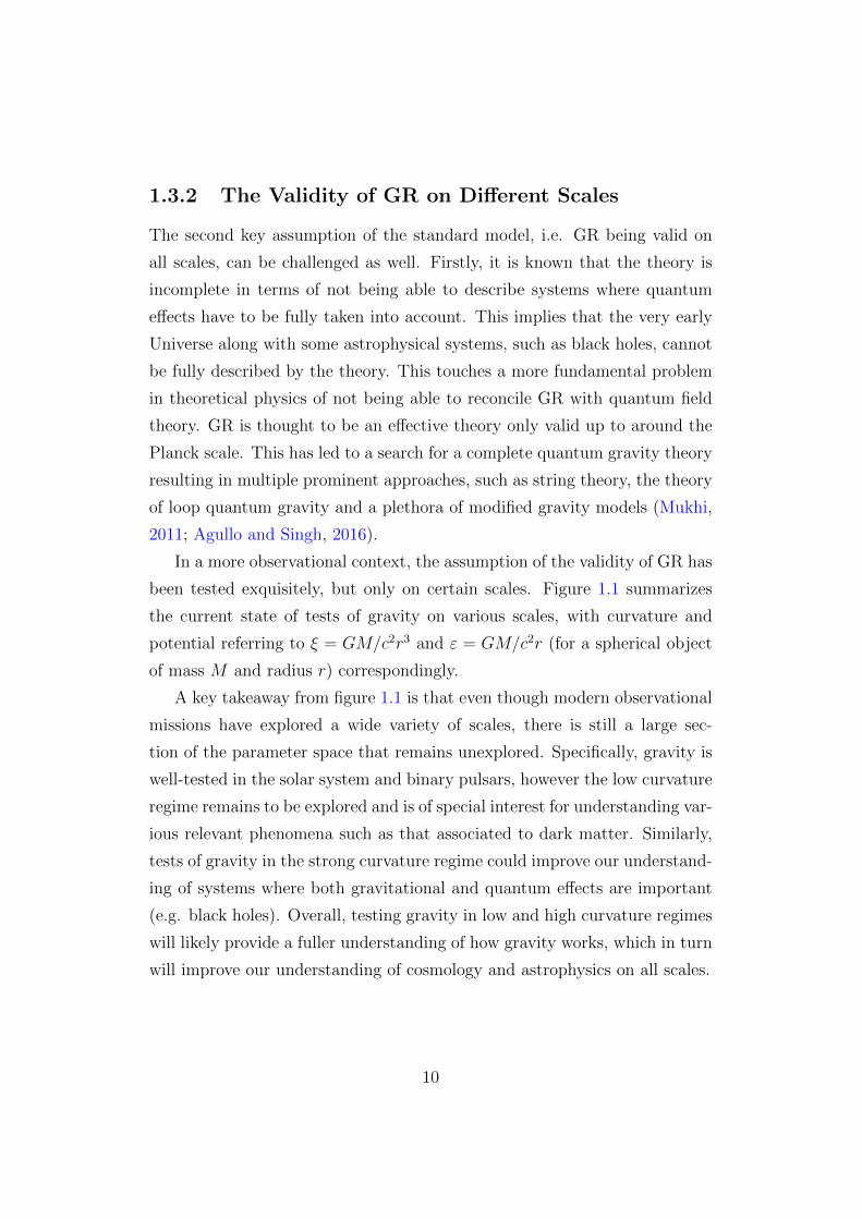
been tested exquisitely, but only on certain scales. Figure 1.1 summarizes

the current state of tests of gravity on various scales, with curvature and

potential referring to ξ = GM/c2r3 and ε = GM/c2r (for a spherical object

of mass M and radius r) correspondingly.

A key takeaway from figure 1.1 is that even though modern observational

missions have explored a wide variety of scales, there is still a large sec-

tion of the parameter space that remains unexplored. Specifically, gravity is

well-tested in the solar system and binary pulsars, however the low curvature

regime remains to be explored and is of special interest for understanding var-

ious relevant phenomena such as that associated to dark matter. Similarly,

tests of gravity in the strong curvature regime could improve our understand-

ing of systems where both gravitational and quantum effects are important

(e.g. black holes). Overall, testing gravity in low and high curvature regimes

will likely provide a fuller understanding of how gravity works, which in turn

will improve our understanding of cosmology and astrophysics on all scales.

10

Figure 1.1: The observational parameter space of gravity tests from Baker

et al. (2015). The meaning of the key abbreviations is as follows: PPN

= Parameterized Post-Newtonian region, Inv. Sq. = laboratory tests of the

inverse square law of gravity, Atom = atom interferometry experiments, EHT

= the Event Horizon Telescope, Facility = a futuristic large radio telescope

such as the Square Kilometre Array, DETF4 = a hypothetical ”stage 4”

experiment according to the classification scheme of the Dark Energy Task

Force. The other abbreviations correspond to observational mission names

or specific objects.

11

1.3.3 Issues Related to Dark Matter

The third base assumption that the ΛCDM model is based on is related to the

existence of dark matter. Historically some form of dark matter was hypoth-

esized to exist in order to explain the rotation curves of galaxies. Most recent

observational evidence indicates that dark matter is crucial for explaining the

formation and evolution of galaxy clusters and large scale structure as well

(Freese, 2017). Other key evidence comes from weak lensing surveys, CMB

anisotropies and baryon acoustic oscillations (Roos, 2010). Figure 1.2 shows

the combined constraints on ΩΛ and Ωm coming from the weak lensing, large

scale structure, supernovae and baryon acoustic oscillation data. These re-

sults clearly illustrate a need for some form of dark energy and non-baryonic

matter to explain the currently available observational data.

Despite the great success of the cold dark matter paradigm, certain ques-

tions remain unanswered. This is especially clear in the context of galaxy

formation where a number of challenges to the ΛCDM model have emerged

in recent years. These include the missing satellites problem, which indicates

a mismatch between the observed dwarf galaxy numbers and the correspond-

ing prediction from numerical simulations. Similarly, the cusp/core problem

indicates a mismatch between the predicted and observed cuspiness and den-

sity of the dark matter dominated galaxies. Another inconsistency comes in

the form of the too big to fail problem, which states that the observed satel-

lites in the Milky Way are not massive enough to be consistent with the

ΛCDM predictions (Bullock and Boylan-Kolchin, 2017). These issues can be

viewed in a wider context of reconciling theoretical predictions with the cos-

mological simulations and observational data. Inconsistencies could originate

due to the lack of understanding of the galaxy formation processes, difficulty

of building realistic simulations of such processes or a lack of understanding

of the fundamental nature of dark matter.

12

Figure 1.2: Recent cosmological constraints from the DES survey. Left: con-

straints on the present-day dark energy density ΩΛ and matter density Ωm.

Black contours correspond to DES data alone (including information from

weak lensing, large scale structure, type Ia supernovae and BAO data); green

contours correspond to best available constraints from external data; orange

contours correspond to DES supernovae constraints alone. Right: equiva-

lent constraints on the dark energy equation of state w and matter density

Ωm. The dashed blue contours show the low redshift supernovae constraints.

The contours in both plots correspond to 68% and 95% confidence limits. Ex-

ternal data specifically refers to Planck, Pantheon and BOSS DR12 datasets

(Abbott et al., 2019). Note that the significant tension between the DES

and the external data is related to the known tension in the measurements

of the S8 parameter in DES and the Planck tomographic weak lensing data

as discussed in Joudaki et al. (2020).

1.3.4 Issues Related to Dark Energy

Another key challenge that the standard model of cosmology is facing at the

moment is explaining the nature of dark energy. As illustrated by figure 1.2,

ΩΛ dominates the total energy budget of the Universe. Some form of dark en-

13

ergy is required to account for the accelerated expansion of the Universe. The

energy scale for the cosmological constant deduced from the available obser-

vational data is of the order of: ρΛ ≡ Λ/8πG ≈ (10−3 eV)4 (Koyama, 2016).

However, arguments in quantum field theory and semi-classical gravity sug-

gest existence of vacuum energy T vacµν ≡ −ρvacgµν , which should contribute

to the total energy budget of the Universe. Calculations in quantum field

theory suggest |ρvac| ≈ 2 × 108 GeV4, which is a huge value comparable to

2 × 1011ρnucl , where ρnucl is the density of atomic nuclei (Weinberg, 1989).

Such a major contribution to the total energy budget is clearly not observed

in the available data, which leads to the old cosmological constant problem

(why doesn’t the vacuum energy gravitate as expected? ). In addition, a related

problem arises when trying to explain the observed accelerating expansion

of the Universe. Namely, extreme fine tuning is required between the value

of the cosmological constant and the predicted vacuum energy in order to

explain the observed cosmological expansion. This is referred to as the new

cosmological constant problem.

Other conundrums include the why now? problem, as in why is the

current vacuum energy density of similar magnitude to the matter energy

density at this particular cosmic epoch (Lombriser, 2019)? These issues have

been studied extensively and various possible solutions have been proposed

in the context of different models of dark energy and modified gravity (e.g.

see Li et al. (2011)).

1.3.5 Tensions in the Cosmological Parameters

Another key contemporary challenge to the standard model is the existence

of the various tensions between the different observables. A prime example

of this is the tension between the early and late Universe measurements for

the expansion rate parameter H0. In more detail, the local measurements

of H0 using the distance ladder indicate a significantly higher value when

compared to the Planck CMB measurements (at around 3.5-σ level) (Riess

et al., 2018). Such a tension could indicate various systematic problems both

14

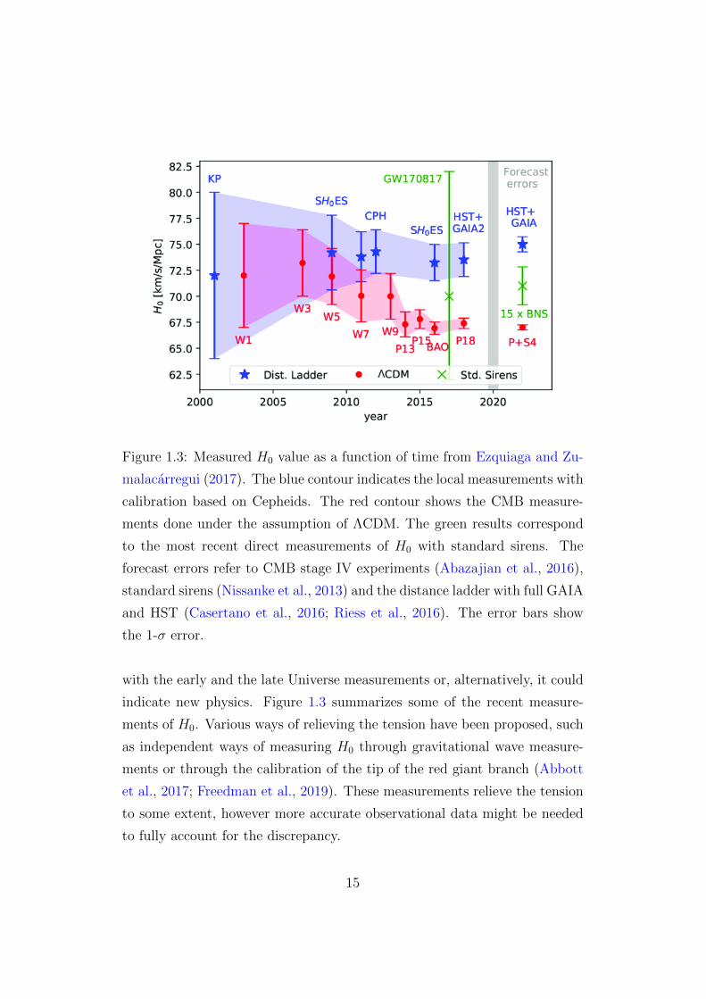
Figure 1.3: Measured H0 value as a function of time from Ezquiaga and Zu-

malacarregui (2017). The blue contour indicates the local measurements with

calibration based on Cepheids. The red contour shows the CMB measure-

ments done under the assumption of ΛCDM. The green results correspond

to the most recent direct measurements of H0 with standard sirens. The

forecast errors refer to CMB stage IV experiments (Abazajian et al., 2016),

standard sirens (Nissanke et al., 2013) and the distance ladder with full GAIA

and HST (Casertano et al., 2016; Riess et al., 2016). The error bars show

the 1-σ error.

with the early and the late Universe measurements or, alternatively, it could

indicate new physics. Figure 1.3 summarizes some of the recent measure-

ments of H0. Various ways of relieving the tension have been proposed, such

as independent ways of measuring H0 through gravitational wave measure-

ments or through the calibration of the tip of the red giant branch (Abbott

et al., 2017; Freedman et al., 2019). These measurements relieve the tension

to some extent, however more accurate observational data might be needed

to fully account for the discrepancy.

15

Another example of a tension between the different types of cosmological

measurements is the S8 tension, where S8 = σ8

√Ωm/0.3. The σ8 parameter

here refers to the amplitude of the linear power spectrum on the scale of 8

h−1 Mpc. It is one of the key cosmological parameters due to being related to

the growth of the fluctuations in the early Universe. As described in Joudaki

et al. (2020), there is a 2.5-σ tension between the combined Kilo Degree

Survey (KV450), DES-Y1 and the Planck weak lensing measurements of the

S8 parameter. This tension is also likely one of the key reasons behind the

significant difference in the cosmological parameter constraints observed in

figure 1.2. As is the case with the H0 tension, it is not exactly clear what

is the root cause for such a divergence of measurements. As illustrated by

the results in Joudaki et al. (2020), the DES measurements reduce but do

not solve the tension observed between the KV450 and the Planck datasets.

Data from the surveys in the upcoming decade will likely give additional

clues about the nature of the S8 and other related tensions.

The outlined problems indicate that despite the great success of the

ΛCDM model many issues remain. It is possible that these issues could

be resolved rather naturally with high quality observational data from the

upcoming surveys along with more realistic simulations and a better under-

standing of the properties of dark matter and dark energy. However, it could

also indicate a need for new physics. In either case, all the discussed phe-

nomena are intimately related to our understanding of how gravity works on

different scales. Starting with the intricacies of galaxy formation and ending

with the issues related to the accelerated expansion, a better understanding

of gravity could help resolve some of the key issues outlined above. Because

of this, modifying GR has been proposed as a possible solution to the many

conundrums facing the standard model of cosmology.

16

1.4 Modified Gravity: Tests and Current

Developments

The motivations for modifying GR are generally trifold: accounting for the

accelerated expansion of the Universe, explaining the nature of the missing

mass on cosmological scales and giving a deeper understanding of how gravity

relates to quantum field theory. These are all goals of key importance and

making significant progress in any of these directions could account for the

various shortcomings of the ΛCDM model. For these reasons, a vast family

of modified gravity models has been developed.

One rather natural way of classifying modifications to GR can be defined

in the context of Lovelock’s theorem. Lovelock’s theorem states the follow-

ing: in 4-D the only divergence-free symmetric rank-2 tensor constructed from

only the metric gµν and its derivatives up to second order, and preserving dif-

feomorphism invariance, is the Einstein tensor with a cosmological constant

term. In slightly simpler words, Einstein field equations are unique equa-

tions of motion for a single metric derivable from a covariant action in 4-D

(Berti et al., 2015; Li and Koyama, 2019a). This theorem is profound as

it shows that GR in this context is the simplest theory of gravity with the

outlined properties. Hence, if one was to modify GR, some of the outlined

conditions would necessarily have to be broken. In fact, Lovelock’s theorem

gives a recipe on how to generate modified gravity theories: a modification

of gravity will have one (or multiple) of the following features:

i) Extra degrees of freedom. This refers to extra scalar, vector and tensor

fields introduced to the action. This class of models includes the Horn-

deski theory, which is the most general scalar-tensor theory in 4 dimen-

sions leading to second order equations of motion (Horndeski, 1974).

Horndeski theory includes many familiar theories such as Brans-Dicke

gravity, chameleon gravity and quintessence. This class also contains

models such as massive gravity and bi-gravity (Kenna-Allison et al.,

2019a,b).

17

ii) Lorentz Violations. These models break the Lorentz invariance. Exam-

ples models include Horava gravity, Einstein-Aether theory and n-DBI

gravity (Blas and Lim, 2014).

iii) Higher spacetime dimensionality. Early models including extra space-

time dimensions, such as the Kaluza-Klein theory, have inspired a num-

ber of contemporary models such as string theory. Other prominent

models in this class include braneworld models (Maartens and Koyama,

2010).

iv) Non-locality. Non-local models contain terms of the form of Rf(−1R)

or m2R−2R in the Einstein-Hilbert action. More generally, various

string-inspired non-local models have gained popularity in recent years.

Such models have been used in the context of dark energy, inflation and

bouncing cosmology scenarios (Koshelev, 2011).

v) Higher derivatives. These models introduce higher degree derivatives to

the action. Such theories are difficult to construct as higher derivatives

can lead to Ostrogradsky instability. However, there are ways to avoid

such instabilities, as shown in beyond Horndeski models (Langlois and

Noui, 2016).

Figure 1.4 shows some of the more popular models classified according

to Lovelock’s theorem. It is important to note that there are many models

that do not easily fit into such classification. A prime example of this in

the context of this thesis refers to various emergent/entropic gravity models.

Emergent gravity can refer to a wide class of not necessarily related theories

that describe gravity as an emergent phenomenon. Such theories combine

ideas from black hole thermodynamics and condensed matter physics in or-

der to explore the possible emergence of gravity with prime examples being

approaches described in Padmanabhan (2015) and Verlinde (2017).

The mentioned models can give insight into the various conundrums of the

standard model. In particular, the mentioned classes of models can explain

18

Figure 1.4: A classification of modified gravity models based on Lovelock’s

theorem (Berti et al., 2015). The abbreviations refer to the weak and the

strong equivalence principles (WEP and SEP) and to diffeomorphism invari-

ance.

the accelerating expansion with various degrees of success. Or, additionally,

some of the models can give insights into the problem of dark matter and

shine light on the various incompatibilities between GR and quantum physics.

However, as of yet, there is no single framework that fully accounts for the

effects associated with dark energy and dark matter while also fitting all the

key observational datasets. Observational constraints, in particular, play a

crucial role in exploring the space of the allowed theories. There is a plethora

of astrophysical and cosmological tests on scales ranging from laboratory

and interferometry tests all the way to large scale structure tests of modified

gravity. Here we will review the main types of observational and experimental

tests in a rough order of scale. A deeper discussion of the cluster scale tests

will be given in chapters 2 and 3.

19

1.4.1 Laboratory Tests

Laboratory tests aim to detect fifth force effects on the smallest scales acces-

sible by the currently available instruments (µm and larger). A key challenge

for these types of experiments is reducing the Newtonian force effects from

the environment. This can be done by using vacuum chambers and optimiz-

ing the geometry of the experiment (i.e. the geometry of the mass/density

distribution).

At sub-mm scales one could in principle detect the Casimir force effects,

which are predicted by quantum electrodynamics, manifesting as an interac-

tion between two parallel uncharged plates. At these scales one can also de-

tect chameleon forces, which would dominate over the Casimir force. Hence,

the deviation from the predicted Casimir force can be used as a probe for

chameleon force effects. Chameleon models refer to a class of scalar-tensor

theories that avoid the solar system constraints by employing a special form

of a non-linear potential. A common general choice for chameleon models is

of the following inverse power law form (Burrage and Sakstein, 2018):

V (φ) = Λ40 +

Λ4+n0

φn, (1.11)

where φ is the scalar field, and the different choices of the Λ0,Λ0, n param-

eters corresponds to different models. Λ0 can be set to ≈ 10−3 eV to account

for the accelerating expansion (discussed further in chapter 3).

When it comes to Casimir force experiments, the most precise measure-

ments are achieved by measuring the force between a plate and a sphere

rather than two plates, which leads to the chameleon force scaling with the

distance between the sphere and the plate, d as follows:

Fφ ∼ d2−nn+2 , (1.12)

with Fφ as the chameleon force and n as a constant that dictates the scaling.

Stringent constraints can be put for n = −4 and n = −6 models (Burrage

and Sakstein, 2016).

20

Other experiments that probe the Casimir force effects include optically

levitated dielectric spheres with radii ranging around r ∼ O(µm). In these

types of experiments laser beams are used to counter the Earth’s Newtonian

gravity effects. Such an approach can put constraints on the n = 1 models

(Burrage and Sakstein, 2018).

Atom interferometry is another powerful technique that can be used for

constraining chameleon models. These experiments employ interferometers,

which allow probing the acceleration experienced by atoms due to chameleon

forces. In particular, atoms are put into a superposition of states related to

the two different paths that can be taken (the two arms of the interferometer).

The two paths are later recombined and a measurement is made that allows

to put constraints on the acceleration of the atoms with precisions of around

10−6g, with g ≈ 9.8 m/s2 (Elder et al., 2016).

Another class of laboratory tests that is worth mentioning is precision

neutron tests. Neutrons, being electrically neutral particles, are perfect for

isolating the fifth force effects from the gravitational and electromagnetic

forces due to the environment. Different experiments using neutrons place

constraints on the chameleon coupling strength Mc. For instance, using ultra

cold neutrons interacting with a mirror one can put a constraint in the range

of Mc > 1.7× 106 TeV (Jenke et al., 2014). Figure 1.5 summarizes some the

currently available laboratory constraints on chameleon models.

1.4.2 Solar System Tests

Solar system tests of GR date back to the very beginnings of Einstein’s

revolutionary theory. In fact, long before the development of GR, deviations

of the perihelion precession of Mercury from the Newtonian gravity prediction

were known. This observation later led to one of the key tests confirming the

validity of GR.

Another early test confirming the validity of GR was performed by mea-

suring the deflection of light by the Sun. The observations of Arthur Edding-

ton and collaborators during the solar eclipse of 1919 measured the displace-

21

Figure 1.5: A summary of the observational and laboratory tests constrain-

ing chameleon models. The different regions mark the excluded subsets of

the parameter space. The black, blue and red dots show the lower bounds

(indicated by the arrow) on the coupling strength Mc at the dark energy

scale coming from neutron bouncing and interferometry experiments respec-

tively. The dark energy scale refers to Λ0 = 2.4× 10−3 eV and is marked by

the dotted lines. The two plots refer to the constraints with Λ0 fixed to the

dark energy scale and positive values of n (left figure) and negative values

(right figure). The red hashed area refers to regions where the model does

not possess chameleon screening. Finally, the brown subsets correspond to

parameter space regions accessible by cosmological observations (Hamilton

et al., 2015; Lemmel et al., 2015; Li et al., 2016; Burrage and Sakstein, 2016).

ment of the position of stars behind the sun proving one of the key tenets of

the theory.

Modern tests put some of the tightest constraints on the deviations from

GR. Experiments, such as the Shapiro time delay measurements, which give

the relativistic time day experienced by radar signals in a round trip to Mer-

cury and Venus, agree with the theoretical GR prediction at 5% level (Shapiro

et al., 1971). More recently measurements based on the same basic principle

22

were performed using the data from the Cassini spacecraft, which measured

the frequency shift of radio photons to and from the spacecraft. This ex-

periment constrains the parametrized post-Newtonian formalism Eddington

parameter γ (which quantifies the deflection of light by a gravitational source)

with high precision: γ = 1 + (2.1± 2.3)× 10−5 (Bertotti et al., 2003).

Tests of the strong equivalence principle (laws of gravity are independent

of velocity and location) are of special importance in the context of modified

gravity models. A wide class of theories predict violations to the strong

equivalence principle on some level. In general, tests of the strong equivalence

principle test the universality of free fall, which is measured by comparing

accelerations a1 and a2 of two different bodies:

∆a

a=

a1 − a2

12

(a1 + a2)=

(MG

MI

)1

−(MG

MI

)2

, (1.13)

with MG and MI as gravitational and inertial masses correspondingly. In the

case of the solar system tests of the equivalence princple, the two bodies are

the Earth and the Moon as measured in the lunar laser ranging experiments.

These experiments put strong constraints on the anomalous perihelion an-

gular advance of the Moon: |δθ| < 2.4 × 10−11 (Williams et al., 2004; Li

and Koyama, 2019b). Such experiments also constrain the time variation

of Newton’s constant: G/G = (2 ± 7) × 10−13 per year (Williams et al.,

2009). Finally, the constraints from the lunar laser ranging experiments can

be combined with the Eot-Wash torsion balance measurements to provide a

confirmation for the strong equivalence principle at 0.04% (Merkowitz, 2010).

The solar system constraints have had a profound influence on the the-

oretical development of modified gravity models. The outlined constraints

clearly indicate that GR is valid in the solar system, leaving nearly no space

for even miniscule modifications of the model. This has led to the develop-

ment of various screening mechanisms, which suppress the fifth force effects

in the solar system, while still allowing interesting effects on cosmological

scales.

23

1.4.3 Gravitational Wave Tests

In terms of observational constraints, one of the key developments at the time

of writing this thesis has been the detection of the gravitational wave and

gamma ray burst signals from a neutron star merger event GW170817/GRB

170817A. The event resulted in a 100 second gravitational wave signal and

a corresponding 2 second duration gamma-ray burst caused by the merger

(Abbott et al., 2017). The optical counterpart of the event has subsequently

been observed by over 70 observatories marking the beginning of this type

of multi-messenger astronomy (Nicholl et al., 2017).

The key significance of the mentioned gravitational wave observation in

the context of this thesis comes in terms of the constraints on modified grav-

ity models. In general, introducing new fields coupled to gravity in modified

models of gravity affects the propagation speed of gravitational waves. Hence,

the speed of the propagation of gravitational waves can be used as reliable

probe of modified gravity. Probing modified gravity models with gravita-

tional waves has a number of advantages, such as the fact that gravitational

waves can be used to test theories with screening mechanisms (given that the

signals come from extragalactic sources). In addition, even small deviations

from the speed of light in gravitational wave propagation can accumulate

over large distances, making such a probe extremely sensitive. In particular,

the observed event GW170817 allowed putting extremely tight constraints on

the speed of the gravitational waves: |cGW/c− 1| ≤ 5× 10−16 (Abbott et al.,

2017). This result has single-handedly ruled out a wide subset of modifica-

tions of gravity. More specifically, such a strong constraint practically rules

out any model that predicts variation of the gravitational wave propagation

speed with respect to the speed of light. It is useful at this point to discuss

some of the effects of the gravitational wave results on the various classes of

models discussed previously without going into great detail. In this regard,

it is useful to introduce Horndeski theory, which contains several models im-

portant to this thesis as subsets of the theory. Models of special importance

to this thesis will be discussed further in chapters 3 and 4.

24

As previously mentioned, Horndeski theory refers to the most general

scalar-tensor theory with 2nd degree equations of motion. The theory can

be described by the following Lagrangian:

LH =G2(φ,X)−G3(φ,X)φ+G4(φ,X)R +G4,X(φ,X)[(φ)2 − (∇µ∇νφ)2]+

G5(φ,X)Gµν∇µ∇νφ−1

6G5,X(φ,X)

[(φ)3 − 3φ (∇µ∇νφ)2 + 2 (∇µ∇νφ)3] ,

(1.14)where G2, G3, G4 and G5 are free functions of the scalar field φ and X ≡−1/2gµν∂µφ∂νφ, Gµν is the Einstein tensor, R is the Ricci scalar, φ =

∇µ∇µφ and the subscript commas denote derivatives (Horndeski, 1974). The

different choices for the set of functions G2, G3, G4, G5 represent different

scalar-tensor models.

The gravitational wave speed in Horndeski theory can be deduced via the

tensor sound speed αT by noting that c2GW = 1+αT. The tensor sound speed

has been shown to have the following form (Kobayashi et al., 2011; Li and

Koyama, 2019a):

αT =2X[2G4,X +G5,φ − (φ−Hφ)G5,X

]2[G4 − 2XG4,X − 1

2XG5,φ − φHXG5,X

] . (1.15)

The observational requirement of cGW ≈ c (or equivalently αT ≈ 0) can be

satisfied by setting G5 = 0 and G4 = G4(φ). This ultimately results in only

the following class of Lagrangians surviving:

LH = G4(φ)R +G2(φ,X)−G3(φ,X)φ. (1.16)

The effect of this is that a wide class of Horndeski and beyond Horndeski

models are ruled out (see Sakstein and Jain (2017) and Baker et al. (2017)

for a wider discussion). This includes some important models in the context

of the accelerating expansion of the Universe. In particular, a subclass of

Galileon models, which can account for the accelerated expansion without a

need for a cosmological constant are ruled out. Similarly, a wide subset of

degenerate higher order scalar-tensor theories (DHOST) has been ruled out.

25

Figure 1.6: Summary of the state of modified gravity models after the

GW170817 gravitational wave results (Ezquiaga and Zumalacarregui, 2017).

The models are classified according to the predicted value of the gravitational

wave speed cg = cGW.

The same can be said about the Fab Four models that contain interesting

cosmological solutions.

The surviving models include a class of theories where gravity is mini-

mally coupled like the kinetic gravity braiding models and quintessence. The

k-essence models are also still valid. So are the models relevant to this the-

sis, such as the f(R) and Brans-Dicke theories. Figure 1.6 summarizes the

current state of the various modified gravity models after the release of the

gravitational wave results.

1.4.4 Galaxy Scale Tests

Observations of galaxies have historically played an important role in the the-

oretical development of dark matter and modified gravity models. Namely,

galaxy rotation curve measurements acted as one of the initial pieces of evi-

dence for the existence of dark matter. More generally, the complex morphol-

ogy of galaxies allows testing modified gravity models with different screening

mechanisms along with alternative models of dark matter.

26

Theories with screening mechanisms predict different effects on the gas

and the stars that make up galaxies. This is the case, as stars are generally

screened, while the diffuse gas is not. Hence, comparing the rotation curves

of stars and gas allows putting constraints on theories with screening. As an

example, this method has been used to constrain the fR0 parameter to values

of fR0 < 10−6 in f(R) models (see chapter 3 for a wider discussion of these

models) (Vikram et al., 2018). More generally, for theories with screening,

the self-screening parameter has been constrained to values of: χc < 10−6.

In addition, screening can lead to morphological and kinematical dis-

tortions of galaxies. In this case the stellar component of a dwarf galaxy is

self-screened while the surrounding dark matter halo and gaseous component

are unscreened. Different fifth force effects experienced by the different parts

of galaxies lead to an offset of stellar disks from the HI (neutral atomic hy-

drogen) gaseous components. In addition, galactic disks are warped in a way

whereby the screened stars are displaced from the principal axis. A recent

example of such measurements includes Desmond et al. (2018), where offsets

between the optical and HI centroids were constrained. The mentioned mea-

surements also put a constraint on the f(R) theories: 3 |fR0| /2 < 1.5×10−6.

Galaxies also offer ways of testing gravity via gravitational lensing. A

recent example of such a measurement comes from the ESO 325-G004 ellip-

tical galaxy. Comparing the mass estimates from the stellar motion and weak

lensing data coming from the Hubble Space Telescope and the Very Large

Telescope indicated no significant deviation from GR with γ = 0.97 ± 0.09

with 1-σ confidence (Collett et al., 2018).

The mentioned techniques are only a small subset of the tests performed

on galaxy scales in recent years. For a more systematic review see Jain and

VanderPlas (2011); Vikram et al. (2013); Koyama (2016).

1.4.5 Galaxy Cluster Tests

Galaxy clusters and superclusters, being the largest gravitationally bound

structures, offer a multitude of ways of testing the effects of gravity on large

27

scales. Galaxy clusters contain anywhere from hundreds to thousands of

galaxies, with total masses in the range of 1014 − 1015 M. The mass dis-

tribution of galaxy clusters is dominated by galaxies and the lower density

intracluster medium (ICM) with temperatures ranging between 2-15 keV

(Kravtsov and Borgani, 2012). This combination of high density regions

(where the fifth force would be screened) and lower density intracluster gas,

especially in the outskirts of clusters (where there would be no screening),

makes clusters great for testing modified gravity theories.

Various modified gravity models with screening mechanisms can leave

imprints in the observational properties of galaxy clusters. More specifically,

modifications of GR can affect cluster density profiles and correspondingly

X-ray surface brightness and weak lensing profiles. As an example, recent

work in Schmidt et al. (2009) and Cataneo et al. (2016) investigated the

abundance of massive halos as a tool for detecting f(R) gravity effects. Both

studies found similar constraints for f(R) models: |fR0| . 10−4.

As discussed, the effects of modified gravity with chameleon screening

would not be detectable in the high density galaxy cluster cores, however,

the fifth force would have an effect in the outskirts of clusters. This introduces

a deviation between the hydrostatic and lensing masses, which, in principle,

can be observed by combining X-ray and weak lensing measurements. Using

this technique, the constraints of |fR0| . 6 × 10−5 at 95% confidence were

obtained in Terukina et al. (2014) and Wilcox et al. (2015).

These and other cluster scale constraints are discussed in greater detail

in chapter 3.

1.4.6 Large Scale Structure Tests

Large scale structure formation is sensitive to the underlying model of grav-

ity. Most types of deviations from GR should in principle be detectable in

the CMB anisotropy data. Furthermore, measurements of the CMB power

spectrum and the secondary bispectrum have some sensitivity to modified

gravity growth of structure effects through the large-scale integrated Sachs-

28

Wolfe effect and weak lensing. Another method of constraining gravity is via

redshift space distortions. This refers to the spatial distribution of galaxies

appearing distorted when their positions are plotted as a function of their

redshift rather than as a function of their distance. Comparing these ef-

fects against the theoretical GR predictions places stringent constraints on

modifications of the standard laws of gravity.

As a concrete example, competitive constraints on f(R) models were ob-

tained in Lombriser et al. (2012), where a subclass of f(R) models designed

to reproduce the ΛCDM expansion history was tested. In the context of

the expansion history, such models can be parametrized by B0, which corre-

sponds to the Compton wavelength parameter. By combining the data from

supernovae distances, baryon acoustic oscillations and the CMB, constrains

of B0 < 1.1× 10−3 at 95% confidence were determined.

Needless to say, the outlined list of the observational probes is far from

complete. A number of techniques will be left undiscussed due to being out

of scope of this thesis. In addition, a much deeper discussion of the f(R)

model and the corresponding constraints is given in chapter 3. Finally, figure

1.7 shows a summary of the relevant constraints on f(R) models.

29

Figure 1.7: Summary of different observational constraints on the fR0 pa-

rameter as a function of scale. Figure from Wilcox (2016), originally adapted

from Terukina et al. (2014).

30

Chapter 2

Galaxy Clusters

Chapter 2 introduces the key ideas from galaxy cluster physics. In particu-

lar, the basic structure of galaxy clusters is introduced and discussed in the

context of the underlying astrophysics. In addition, the properties of the

intracluster medium are discussed in the context of measuring X-ray surface

brightness as one of the key probes in our tests of modified gravity. Similarly,

the key features of the SZ effect are introduced. Galaxy kinematics is dis-

cussed as an important technique for measuring cluster masses. Finally, weak

lensing by galaxy clusters is summarized as a key tool for testing modified

gravity as discussed in chapters 3 and 4.

2.1 The Structure and Basic Properties of

Galaxy Clusters

Historically the observational studies of galaxy clusters date back to the work

of Herschel and Messier, who were the first to notice the tendency of galaxies

(then only known as galactic nebulae) to cluster (Kravtsov and Borgani,

2012). Later work by Hubble in 1926 showed that galactic nebulae are in

fact galaxies, which in turn resulted in a better understanding of the nature

of galaxy clusters (Heilbron, 2005). In 1933, under the assumption of virial

equilibrium, Zwicky made a crucial discovery that the visible mass in the

31

Coma Cluster is not enough to account for the motion of galaxies in the

cluster (Andernach and Zwicky, 2017). In particular, Zwicky calculated the

dispersion of radial velocities of 8 galaxies in the Coma Cluster and found

the value of σ = 1019 ± 360 km/s (Figueras et al., 2007). Comparing this

result against the prediction derived using hydrostatic equilibrium equations

Zwicky found that the Coma Cluster had to be over 400 times more massive

than the mass contained in the visible parts of galaxies in the cluster. This

marks the beginning of the observational studies of dark matter.

Modern multi-wavelength studies of galaxy clusters allow us to draw a

detailed picture of the physical properties of these objects. Galaxy clusters,

being among the largest gravitationally bound structures, contain from hun-

dreds to thousands of galaxies. Typical masses of galaxy clusters fall in the

range of 1014 − 1015 M (Sarazin, 1988). A key feature of galaxy clusters

is the high energy intracluster medium (ICM), consisting of heated, X-ray

emitting gas with temperatures of around 2− 15 keV (Fabian, 1992). Mea-

suring the composition of galaxy clusters is difficult, as it varies significantly

among individual clusters. However, as a guideline, dark matter makes up

∼ 84% of the mass budget in clusters, with the leftover ∼ 16% corresponding

to the high-energy ICM and stars (Rosati et al., 2002).

Modern studies of galaxy clusters have played a crucial role in under-

standing the properties of dark matter. A prime example of this is the case

of merging galaxy clusters. During a merger the different components that

make up a cluster interact differently. In particular, visible matter located in

stars and galaxies is mostly not affected by the collision. High energy ICM as

detected by X-ray observations, however, is slowed down significantly due to

the electromagnetic interactions. Finally, the major mass component in the

form of dark matter passes through the baryonic matter with no interaction.

This results in a mass distribution where the bulk of the mass resides in

regions different to those dominated by the X-ray emitting ICM. The most

well-known system of merging clusters is the Bullet Cluster, which provides

some of the best existing evidence for the existence of dark matter on galaxy

32

cluster scales (Clowe et al., 2006). Figure 2.1 illustrates the total and the

ICM mass distributions in the Bullet Cluster clearly showing that the two

mass components appear in different locations in the merging cluster system.

In the case of modified gravity models, such as modified Newtonian dynam-

ics (MOND), which assume no existence of dark matter, most of the mass in

merging clusters should coincide with the visible baryonic mass distribution.

Hence merging clusters, such as the Bullet Cluster, give important evidence

against modified gravity models of such kind.

Figure 2.1: Left: an optical image of the Bullet Cluster taken by the Mag-

ellan telescope with overplotted contours representing the total mass distri-

bution inferred by gravitational lensing. Right: the hot plasma distribution

(in red) in the Bullet Cluster inferred by the Chandra X-ray data with the

same mass contours plotted over. (Clowe et al., 2006).

Other properties that are worthy of discussion are related to the formation

and the spatial distribution of galaxy clusters. It is widely accepted that the

likely cause of the observed large scale structure in the Universe is the seed

density fluctuations that were formed during the period of cosmic inflation.

Due to gravitational instability these initial perturbations have been ampli-

fied and eventually collapsed to form an intricate web of filaments and voids.

Observing galaxy clusters allows us to deduce the various properties of the

structure of the Universe on the largest accessible scales. In addition, cluster

observations give information about the underlying cosmological model. The

simplest models of inflation assume the primordial density fluctuations to

33

be Gaussian. However, more complicated models predict varying amounts

of non-Gaussianity. Detecting such non-Gaussianity via the CMB or other

means would be of great interest in the early Universe studies. A number

of recent studies have been dedicated to investigating the viability of using

galaxy clusters as an alternative probe for non-Gausianities (Mana et al.,

2013; Trindade and da Silva, 2017).

Clusters are known to be much more strongly clustered than galaxies

(Bahcall, 1988). This can be expressed in terms of the two-point corre-

lation function that follows a power law of the form ξcc(r) = (r/R0)−1.8.

More specifically, ξcc(r) refers to the two-point spatial correlation function

which is related to the joint probability of finding two objects at separation

r. R0 has been shown to obey the following scaling relation: R0 ≈ 0.4Dc

for 20h−1Mpc < Dc < 100h−1Mpc and Dc ≡ n−1/3c , with nc as the mean

space density of clusters (Bahcall and Cen, 1992). This agrees well with the

more recent observational results described in Basilakos and Plionis (2004);

Balaguera-Antolınez (2014). Recent studies also reinforce the conclusion that

the spatial distribution of the tracers of the large scale structure, such as

galaxies and clusters of galaxies, are a powerful probe for the early Universe

physics. In particular, combining cluster and galaxy power spectra along

with the cross power spectrum offers a way of accessing a plethora of infor-

mation about the underlying cosmology. Hence future surveys such as Euclid

will place unprecedented constrains on primordial non-Gaussianity (Euclid

Theory Working Grp, 2018).

Another key quantity to discuss is the cluster mass function, which is of

special importance when studying large scale structure formation. In partic-

ular, the cluster mass function quantifies the number of clusters of a given

mass at a given redshift: n(M, z). The mass function can be estimated using

the Press-Schechter formalism, which assumes that the fraction of matter

that ends up in objects with mass M can be deduced from the portion of

the initial density field (smoothed on the mass scale M) lying at an overden-

sity exceeding a given critical threshold value δc. The gradient of the mass

34

function can be shown to take the following form (Press and Schechter, 1974;

Borgani, 2008):

dn(M, z)

dM=

√2

π

ρcM2

δcσM(z)

∣∣∣∣d log σM(z)

d logM

∣∣∣∣ exp

(− δ2

c

2σM(z)2

), (2.1)

with ρc as the mean cluster density and σM(z) is the variance at mass scale

M linearly extrapolated to redshift z. The key takeaway from equation 2.1

is that there is an intimate link between the early Universe primordial per-

turbations and the late Universe structure. Through the linear perturbation

growth factor the value of σM can be directly related to the power spectrum

and the cosmological density parameters. This further illustrates the value

of galaxy clusters as probes for the formation and evolution of large scale

structure and, in turn, for the underlying model of cosmology.

There are other important galaxy cluster probes of the underlying cos-

mology. These include the mass-to-light ratio and the baryon fraction. The

mass-to-light ratio quantifies the ratio between the total mass in a given vol-

ume versus the corresponding luminosity. This ratio can be used to deduce

the matter density Ωm. The baryon fraction also provides a constraint on the

matter density parameter (assuming that the cosmic baryon density param-

eter is known). With an additional assumption that the baryon fraction does

not evolve in galaxy clusters, one can constrain the dark energy equation of

state parameters (Borgani, 2008).

2.2 Intracluster Medium and X-ray

Observations

The ICM is composed of high-energy superheated X-ray emitting plasma.

The ICM mainly consists of ionized helium and hydrogen, which dominates

the total baryonic content of galaxy clusters. Heavier elements, such as iron,

can also be found as quantified by the ratio to hydrogen known as metallicity.

Average values of metallicity range from one third to a half of the value

35

observed in the Sun (Mantz et al., 2017). Studying the chemical structure of

the ICM and its evolution with redshift offers a record of the overall element

production and evolution throughout the history of the Universe.

The high temperature of the ICM leads to X-ray emission via the pro-

cess known as bremsstrahlung radiation. Bremsstrahlung radiation refers to

the braking radiation produced by deceleration of charged particles when

deflected by other charges. A typical example of such a process is the deflec-

tion of electrons by atomic nuclei leading to X-ray emission with a frequency

proportional to the energy change. The emissivity at frequency ν for an ion

of charge Z in a plasma with an electron temperature Te is (Sarazin, 1988):

εffv =32πe6Z2neni

3mec3

√2π

3kBTeme

gff(Te, v)e−hv/kBTe , (2.2)

with e as the elementary charge, ni and ne as the number densities of ions and

electrons, me as the electron mass, gff as the Gaunt factor which corrects for

quantum effects, kB as the Boltzmann constant and h as the Planck constant.

The Gaunt factor in this case is given by (Nozawa et al., 1998):

gff ≈3√π

ln

(9kBTe4hv

), (2.3)

The total emission including all the other components (such as line emission)

is then given by:

εν =

∫ ∞0

effv dv ≈ 3.0× 10−27

√Te

1 K

( ne1 cm−3

)2

erg · cm−3s−1. (2.4)

The different emission processes described in equation 2.4 can be written as

follows:

εv =∑i

nineλc (ni, Te) , (2.5)

where λc (ni, Te) is the temperature and ion dependent cooling function that

is related to the emission mechanism. Observationally a more natural quan-

36

tity to work with is the surface brightness, which is equal to the integral of

εν (Terukina et al., 2014; Wilcox et al., 2015):

SB (r⊥) =1

4π(1 + zcl)4

∫n2

e

(√r2⊥ + z2

)λc (ne, Te) dz. (2.6)

Here we assumed spherical symmetry and switched to projected coordinates,

such that a point at some radius r from the centre of the cluster is given

by r =√r2⊥ + z2, with r⊥ as the perpendicular radial distance and z as

the distance from the centre in the direction parallel to the line of sight. In

addition, we assumed that the gas within a given cluster at redshift zcl is

dominated by hydrogen, i.e. ni = ne. The 4π factor comes from the assump-

tion that the emissivity is isotropic, while the (1 + zcl)4 term accounts for

the cosmological transformations of spectral surface brightness and energy.

The electron number density ne is clearly related to the gas distribution in a

cluster which allows us to use surface brightness as a probe for the underlying

mass distribution.

Another cluster scale observable worthy of discussion is the Sunyaev-

Zeldovich (SZ) effect. The SZ effect refers to the distortion of the CMB

through inverse Compton scattering by high-energy electrons from the ICM.

The SZ effect, more specifically, is a combination of multiple primary and sec-

ondary effects. These include thermal interactions between the CMB photons

and the high-energy electrons as well as secondary kinematic and polariza-

tion effects. This method does not depend on redshift and provides a way

of measuring cluster masses as well as detecting clusters at great distances.

In addition, it is possible to use a combination of the SZ effect and X-ray

measurements to accurately deduce distances to clusters.

As CMB photons pass through massive clusters, there is around 1% prob-

ability of interacting with a high-energy ICM electrons (Birkinshaw, 1999).

This results in a boost of energy of the photons by kBTe/mec2, where Te and

me, as before, are the temperature and the mass of the electrons correspond-

ingly. This results in distortion of . 1 mK in the CMB spectrum (see figure

2.2). More accurately, the SZ effect spectral distortions can be expressed as

37

follows (Rephaeli, 1995):

∆TSZ

TCMB

= f(x)

∫nekBTemec2

σTd`, (2.7)

where f(x) is a function of a dimensionless frequency x = hν/kBTCMB, ne is

the electron number density, me is the associated mass and σT is the Thomson

cross-section.

Figure 2.2: The CMB spectrum, undistorted (dashed line) and distorted by

the SZ effect. The SZ distortion is shown for a fictional cluster 1000 times

more massive than an average cluster in order to illustrate the effect (Sunyaev

and Zeldovich, 1980; Annual Reviews of Astronomy and Astrophysics, 2002).

2.3 Methods To Estimate Cluster Masses

2.3.1 Hydrostatic Equilibrium

A key notion when it comes to measuring galaxy cluster masses is that of

hydrostatic equilibrium. The hydrostatic equilibrium equation relates the

38

pressure gradient with the gravitational force in a galaxy cluster. Under

spherical symmetry, the hydrostatic equilibrium equation is given by (Teruk-

ina et al., 2014; Wilcox et al., 2015):

dPtotal

dr= −ρgas

GM(< r)

r2, (2.8)

where Ptotal and ρgas are the pressure and the density of the gas and r is the

radial coordinate. Ptotal refers to the total gas pressure, including the thermal

and non-thermal pressure contributions: Ptotal = Pthermal + Pnon−thermal (dis-

cussed in more detail in chapter 3). Similarly, M(< r) is the mass enclosed

in radius r and can also be split into the two contributions (Lagana et al.,

2010):

M(< r) = − r2

Gρgas(r)

(dPthermal (r)

dr+dPnon−thermal(r)

dr

). (2.9)

Intuitively, equation 2.8 represents a balance between the pressure and the

gravitational force in a galaxy cluster. This indicates that the galaxy cluster

is not undergoing formation processes or is not taking part in a merger.

Using the equation of state for gas with a number density ngas and tem-

perature Tgas: Pthermal = kBngasTgas, one can rewrite the thermal mass com-

ponent in a more useful form:

Mthermal(r) = −kBTgas(r)r

µmpG

(d ln ρgas(r)

d ln r+d lnTgas(r)

d ln r

). (2.10)

Here the identity ρgas = µmpngas was used, with µ as the mean molecular

weight and mp as the proton mass. The mean molecular weight for the fully

ionised gas is given by µ(ne + nH + nHe)mp = mpnH + 4mpnHe, where nH

and nHe are the number densities of hydrogen and helium correspondingly

(Ettori et al., 2013).

The fraction of the non-thermal contribution to the total pressure is given

by (Shaw et al., 2012):

Pnon-thermal (r) = αnt(1 + z)βnt(

r

r500

)nnt(

M200

3× 1014M

)nM

Ptotal(r), (2.11)

39

where αnt, βnt, nnt and nM are parameters determined by hydrodynamical

simulations. The r500 parameter corresponds to the radius at which the dark

matter halo average density is equal to five hundred times the critical density.

Analogously, M200 corresponds to the mass at r200.

Equation 2.8 is of key significance as it allows us to relate the mass distri-

bution in galaxy clusters to the observed pressure/temperature distribution,

which can be inferred via X-ray surveys. Such a way of measuring masses

is based on two key assumptions: that the majority of observed clusters

are in fact in hydrostatic equilibrium and that most clusters are on average

spherical. In general, effects of non-spherical geometries of clusters can be

averaged out by stacking a large numbers of clusters. The hydrostatic equi-

librium equation can also be tested by comparing independent measurements

of cluster masses. More concretely, one can compare the X-ray determined

masses to those deduced by weak lensing. As an example, recent measure-

ments by Smith et al. (2016) indicate that the mean ratio of X-ray to lensing

masses for 50 LoCuSS clusters at 0.15 < z < 0.3 is βX = 0.95± 0.05, hence

showing no significant deviation from the hydrostatic equilibrium assump-

tion. Note, however, that the results of such measurements strongly depend

on the method and the dataset used. For instance, the results in ? derived

using simulated galaxy clusters show variations up to 10-20% up to the virial

radius.

At this stage it is important to discuss the various astrophysical effects

that can lead to biases when estimating cluster masses. In particular, an

important concept in the context of galaxy cluster formation is that of viri-

alization. Theoretically, the cluster merging and formation processes cease

once virialization is reached (i.e. when the forces acting on the cluster are

in balance and the potential energy is twice the negative kinetic energy as

described by the virial theorem). Many real-world clusters, however, are not

fully virialized, with the inner regions being more relaxed than the outer

parts of the cluster. In addition, there is an ongoing accretion of gas and

dark matter in the outer parts of the cluster. These effects complicate the

40

mass estimates using the SZ effect and the galaxy kinematics. In addition,

these effects could introduce extra bias when constraining models of modi-

fied gravity using the methods described in chapters 3 and 4. However, it

is important to note that the mentioned effects have been investigated in

the previous studies and found to be subdominant when compared to the

non-thermal pressure effects and the predicted deviation between the dif-

ferent mass estimates due to modified gravity (for a wider discussion see

Wilcox (2016); ?); ?). Nonetheless, effects such as these are important to

understand and to quantify using both observational data and simulations.

Further analysis of some of these systematics is given in chapters 3 and 4.

2.3.2 Galaxy kinematics

Another important method of estimating cluster masses uses the kinematics

of the member galaxies. Under the assumption of the virial theorem, one can

express the mass as follows (Borgani, 2008):

Mkin =π

2

3σ2vRV

G, (2.12)

where σv is the line-of-sight velocity dispersion and RV is the viral radius.

The virial radius can be estimated if a sufficient sample of member galaxies

is available:

RV = N2

(∑i>j

r−1ij

)−1

, (2.13)

with N as the number of galaxies and rij as the separation between the i-th

and the j-th galaxies.

Such a method of determining cluster mass comes with a set of challenges.

Namely, as previously discussed, the assumption of the virial theorem can

be valid to varying degrees in different populations of galaxies (for instance

late and early types of galaxies). Another challenge in the context of ob-

servational data, comes in terms of non-member (foreground or background)

galaxies that can bias the mass measurements. Algorithms for filtering out

41

such interloper galaxies are of special importance for accurate mass estimates

(Girardi et al., 1993; van Haarlem et al., 1997).

A key issue when it comes to such virial theorem-based approaches is not

knowing the full underlying dark matter distribution. Such approaches are

based on the assumption that, in general, dark matter follows the visible mass

distribution. However, if one were to relax this assumption, the under/over-

estimation of the cluster mass is given by (Sadat, 1997):

µcl =[1 + 2CcRtrue + CλR

2true]

[1 + CvRtrue], (2.14)

where Rtrue is the true ratio of the dark matter and galaxy masses, while the

Cc, Cλ, Cv are the relative concentration parameters.

A related method of determining the underlying mass distribution in clus-

ters is via the orbits of member galaxies. In particular, assuming hydrostatic

equilibrium, one can show that the mass distribution is given by:

M(< r) =−Gngal(r)

r2

[dngal(r)

drσr(r)

2 +2ngal(r)

r

[σr(r)

2 − σt(r)2]], (2.15)

where ngal is the number density of galaxies, and the dispersion parameters

σt and σr control the shape of the orbit (σt = σr for isotropic orbits). The

drawback of this particular method is that the velocity dispersion profiles are

not well known, leading to bias in the mass estimates (Wojtak and Lokas,

2010).

2.4 Weak Lensing in Galaxy Clusters

2.4.1 The Basics of Gravitational Lensing

One of the most important astronomical probes used to track the underlying

cluster mass distribution is gravitational lensing. Gravitational lensing effect

refers to the bending of light by large distributions of matter. The existence

of such an effect was known long before the development of GR. In fact, if

42

one allows the possibility of light having even a minuscule mass, Newtonian

physics predicts bending of light rays by massive bodies (Yajnik, 2019). As

later shown and calculated by the German astronomer Johann Georg von

Soldner, the deflection angle of light due to a massive body is proportional

to the gradient of the gravitational potential (Gine, 2008). This turned out to

be a surprisingly accurate prediction that agreed with the initial calculations

of Einstein as of 1911. Only in the final version of GR in 1915 Einstein

managed to obtain the correct result, which was equal to twice the predicted

Newtonian value. More specifically, Einstein predicted a deflection of 1.7 arc

seconds for light passing the Sun (Einstein, 1916).

Here we will lay out some of the equations for a single lens system as

well as extended mass distributions e.g. galaxy clusters. The derivations are

based primarily on Wright and Brainerd (1999) and Bartelmann and Maturi

(2017).

To estimate the deflection angle our starting point is assuming that the

Newtonian potential in cosmological systems is small, i.e. |Ψ|/c2 1. In

addition, the peculiar velocities that mass distributions have on cosmological

scales are relatively small. These assumptions allow us to describe gravita-

tional lensing by using the perturbed Minkowski metric:

ds2 = −c2

(1 +

2Ψ

c2

)dt2 +

(1− 2Φ

c2

)d~x2. (2.16)

For propagating light ds = 0, which gives:

c′ =

∣∣∣∣d~xdt∣∣∣∣ = c

(1 +

2ΦL

c2

), (2.17)

where c′ is the effective light speed (note that the gravitational potential

is negative) and ΦL = (Ψ + Φ)/2. Note that in GR (in the absence of

anisotropic stress) Φ = Ψ, however, this is not generally the case in modified

gravity models. To be consistent with the analysis in the later parts of this

chapter, we are using a more general notation here. Also note here that the

form of equation 2.17 allows us to define the refraction index in the usual

manner: c′ = c/n, giving n = 1− 2ΦL/c2. Here, by analogy, we are treating

43

a spacetime region with a gravitational potential ΦL present as a material of

refractive index n. One can then apply Fermat’s principle, which states that

the path taken by light rays minimizes the time of travel, i.e.:

δτ = δ

∫ B

A

c

ndt = 0, (2.18)

where τ is the path of the photon, A and B are the initial and final points

and δ stands for a variation. Varying equation 2.18 w.r.t. the light path

leads to the identity for the deflection angle:

~α = − 2

c2

∫~∇⊥ΦLdl, (2.19)

where the gradient is taken perpendicular to the line of sight. Note that this

calculation gives the correct result as predicted by GR and is twice larger

than the corresponding Newtonian result.

Figure 2.3: The geometry of gravitational lensing. The image of a source S

as observed by an observer O is displaced by the deflection angle α due to

the gravitational potential of the lensing mass in the centre (Bartelmann and

Maturi, 2017).

44

The integral in equation 2.19 is not easy to evaluate, however a simplified

result can be obtained by using the Born approximation. In particular, for

small deflection angles (of the order arc seconds or smaller), the integration

path can be approximated by straight lines:

α = − 2

c2

∂

∂b

∫ ∞−∞

dzGM√b2 + z2

=4GM

bc2=

2RS

b, (2.20)

where the deflection angle was calculated for a point mass M at the origin

with the light ray propagating parallel to the z axis with an impact parameter

b. Rs here refers to the Schwarzschild radius. For the Sun, M ≈ 2 · 1033 g,

resulting in a deflection angle of α ≈ 8.6 · 10−6 ≈ 1.7′′ at the solar radius

R = 7 · 105 km. This is the famous result confirmed by the observational

data collected by Dyson, Eddington and Davidson in 1919 (Dyson et al.,

1920).

More complicated mass distributions require a more complex treatment.

However, if the lensing mass distribution is thin compared to the distances

in the lens system, the light ray paths between the source, the lens and the

observer can be approximated as straight lines as shown in figure 2.3. This is

known as the thin-lens approximation and is sufficient to describe the basic

lensing properties of isolated masses such as galaxy clusters.

Following the geometry in figure 2.3 one can define the reduced deflection

angle ~α:

~α ≡ DLS

DS

~α, (2.21)

with DLS and DS as the (angular diameter) distance between the lens and

the source and the distance to the source correspondingly. This allows us

to relate the angles shown in figure 2.3 in the following way: ~β = ~θ − ~α.

Equation 2.21 can also be expressed as:

~α = ~∇⊥[

2

c2

DLS

DS

∫ΦLdz

], (2.22)

45

where equation 2.19 was used and the ~∇⊥ refers to the perpendicular gradi-

ent. The perpendicular gradient can be replaced with the angular gradient

w.r.t. angle θ: ~∇⊥ = D−1L~∇θ. This finally allows writing ~α in terms of the

quantity ψ, which refers to the lensing potential: ~α = ~∇θψ, with:

ψ ≡ 2

c2

DLS

DLDS

∫ΦLdz. (2.23)

The lensing potential captures the key imaging properties of a gravitational

lens.

Given equation 2.23, one can define two quantities: κ (convergence) and

γ (shear), such that:

κ(~θ) =1

2

(∂2ψ

∂θ21

+∂2ψ

∂θ22

), (2.24)

γ1(~θ) =1

2

(∂2ψ

∂θ21

− ∂2ψ

∂θ22

), (2.25)

γ2(~θ) =∂2ψ

∂θ1∂θ2

=∂2ψ

∂θ2∂θ1

. (2.26)

The magnitude of shear is then simply given by: γ = |γ| = (γ21 + γ2

2)1/2

. Fig-

ure 2.4 illustrates how a background source is deformed due to weak lensing

and how these effects are related to quantities κ and γ. More specifically,

ellipticity of a deformed source galaxy can be defined as:

ε ≡ a− ba+ b

=γ

1− κ, (2.27)

where a and b are the semi-major and semi-minor axes as illustrated in figure

2.4. For most weak lensing systems κ 1, resulting in ε ≈ γ.

An archetypal example of a weak lensing system is that of galaxy clusters

distorting the shapes of the background galaxies. More specifically, galaxy

clusters imprint a coherent distortion pattern onto the distant background

galaxies as measured by their ellipticities. Hence statistically studying the

distortions of the ellipticity of the background galaxies allows us to ultimately

46

Figure 2.4: The weak lensing effects on an image of a background galaxy as

quantified by convergence κ and shear γ. Image from Shuntov (2019).

deduce the mass distribution of the lens cluster. Such measurements, how-

ever, are highly complicated by the fact that the background galaxies have

an intrinsic ellipticity εS, which is generally not known. A crucial assump-

tion taken in weak lensing studies is that the average intrinsic ellipticity, for

a sufficiently large sample of galaxies, is expected to be: 〈εS〉 ≈ 0 (Hirata

et al., 2007). As discussed in Bartelmann and Maturi (2017), the standard

deviation of the intrinsic ellipticity is measured to be σε ≈ 0.2 and averaging

over N faint galaxy images reduces the scatter of the intrinsic ellipticity to:

∆ 〈εS〉 ≈σε√N. (2.28)

As illustrated by the description above, the distortion of the ellipticities of

the background sources by a foreground lens mass ultimately depends on the

lensing mass distribution. Hence, studying the weak lensing effects we can

infer the underlying distribution of the lensing system. In fact, weak lensing

offers one of the most powerful probes for studying the properties of galaxy

clusters.

47

2.4.2 Weak Lensing by NFW Halos

Recent observational evidence along with evidence from numerical simula-

tions strongly supports the idea that there is a universal density profile for

dark matter haloes (Navarro et al., 1997; Bartelmann et al., 1998; Young,

2017). In fact, the mentioned evidence shows that systems ranging from

globular clusters to large galaxy clusters can be described by the same uni-

versal density profile. That, of course, refers to the well-studied Navarro,

Frenk, White (NFW) profile given by (Navarro et al., 1996):

ρ(r) =δcρc

(r/rs) (1 + r/rs)2 , (2.29)

where ρc = (3H2(z))/(8πG) is the critical density, and rs = r200/cv is the

scale radius. The virial radius term r200 refers to the radius inside which the

mass density of the halo is equal to 200ρc. Here δc refers to the characteristic

overdensity of the halo, given by:

δc =200

3

c3v

ln(1 + cv)− cv/(1 + cv). (2.30)

Equation 2.29 describes the underlying dark matter distribution in galaxy

clusters. Hence, assuming the NFW profile, one can derive an analytic ex-

pression for the radial dependence of the convergence and the shear due to

the dark matter halos in galaxy clusters (Wright and Brainerd, 1999).

The local value of convergence can be described by:

κ(~θ) =Σ(~θ)

Σc

, (2.31)

where Σ(~θ) refers to the surface mass density and Σc is the critical surface

mass density given by:

Σc ≡c2

4πG

DS

DLDLS

. (2.32)

Assuming spherical symmetry, the surface mass density is simply given by:

48

Σ(R) = 2

∫ ∞0

ρ(R, z)dz, (2.33)

where the integral is evaluated over the coordinate z along the line of sight

and R = DL (θ21 + θ2

2)1/2

is the projected radius relative to the center of the

lens. Equation 2.29 can then be integrated along the line of sight to give:

ΣNFW(x) =

2rsδcρc(x2−1)

[1− 2√

1−x2 arctanh√

1−x1+x

](x < 1)

2rsδcρc3

(x = 1)

2rsδcρc(x2−1)

[1− 2√

x2−1arctan

√x−11+x

](x > 1),

(2.34)

where a dimensionless radial distance was defined as x = R/rs. The tangen-

tial shear for an NFW density distribution is then given by:

γNFW(x) =ΣNFW(x)− ΣNFW(x)

Σc

, (2.35)

where ΣNFW(x) refers to the mean surface density inside radius x. More

specifically, the mean surface density is given by the following integral:

ΣNFW(x) =2

x2

∫ x

0

x′ΣNFW (x′) dx′. (2.36)

Putting everything together and evaluting the integrals gives the following

result:

γNFW(x) =

rsδcρc

Σcg<(x) (x < 1)

rsδcρcΣc

(103

+ 4 ln (12))

(x = 1)

rsδcρcΣc

g>(x) (x > 1),

(2.37)

where the two functions g<(x) and g>(x) were defined for convenience. The

two functions are given explicitly by:

g<(x) =8 arctan(

√(1− x)/(1 + x))

x2√

1− x2+

4

x2ln (x/2)

− 2

(x2 − 1)+

4 arctan(√

(1− x)/(1 + x))

(x2 − 1)(1− x2)1/2,

(2.38)

49

g>(x) =8 arctan(

√(1− x)/(1 + x))

x2√x2 − 1

+4

x2ln (x/2)

− 2

(x2 − 1)+

4 arctan(√

(1− x)/(1 + x))

(x2 − 1)3/2.

(2.39)

In summary, the concepts introduced in this chapter clearly illustrate how

various observational probes can be used to measure the underlying mass dis-

tribution of galaxy clusters. In addition, astrophysics in galaxy clusters is

shown to be tightly related to the properties of dark matter and the under-

lying model of gravity. For this reason galaxy clusters have been extremely

important in testing models of modified gravity on cosmological scales. Chap-

ter 3 delves deeper into the effects of modified gravity on galaxy clusters. In

addition, a technique for testing chameleon gravity using combined X-ray

and weak lensing data from stacked galaxy clusters is introduced.

50

Chapter 3

Modified Gravity on Galaxy

Cluster Scales

This chapter introduces chameleon and f(R) gravity models along with an

effective technique for testing modified gravity on galaxy cluster scales. More

specifically, the chapter starts by introducing the relationship between the

scalar-tensor models and f(R) gravity. In addition, a technique of testing

models of modified gravity with chameleon gravity using cluster X-ray and

weak lensing data based on the previous work in Terukina et al. (2014) and

Wilcox et al. (2015) is introduced. Original results reproducing the tests

described in Wilcox et al. (2015) with an updated dataset are presented.

Finally, the implications of the results for model-independent tests of gravity

are discussed in the last section of the chapter. The original results presented

in this chapter were produced in collaboration with Carlos Vergara and Kathy

Romer, as described in Vergara-Cervantes (2019).

51

3.1 Scalar-Tensor Gravity with Chameleon

Screening

3.1.1 The Action

As discussed in chapter 1, modified gravity models offer a novel approach

in tackling some of the key issues in modern cosmology. However, a major

shortcoming of such modified gravity approaches comes in the context of the

stringent observational constraints in the solar system. In this respect, mod-

els with different types of screening mechanisms are of special importance as

they can avoid the rigid solar system constraints while still possessing a cos-

mologically interesting phenomenology. A natural question to ask, however,

is how natural and fine-tuned such models are? Undeniably, most models

that allow screening behaviour are fine-tuned to turn off the fifth force on

the scales of the solar system to avoid the strict constraints. However, it

should be noted that similar screening behaviour can be observed in various

scenarios in electromagnetism and hence it is not entirely unnatural to expect

a scalar field to posses screening. Here the key features of the scalar-tensor

models with chameleon screening are summarized based primarily on Khoury

and Weltman (2004); Waterhouse (2006); Burrage and Sakstein (2018).

The chameleon model can be described by introducing a scalar field φ

with a potential V (φ). The dynamics of the theory can then be captured

by the action, which, as usual, refers to a functional that, when varied w.r.t.

the metric and the scalar field, gives the set of equations of motion. In this

case the action for a scalar field φ is given by:

Sφ = −∫d4x√−g

1

2(∂φ)2 + V (φ)

. (3.1)

This can be combined with the standard Einstein-Hilbert action with a term

describing the matter fields ψm (equation 1.1) giving the following combined

action:

52

S = SEH + Sφ + Sm =

=

∫d4x√−gM2

pl

2R− 1

2∇µφ∇µφ− V (φ)− 1√

−gLm

(ψ(i)

m , g(i)µν

).

(3.2)

Note that the last term is generalized to allow multiple matter species, while

g(i)µν refers to the Jordan frame metric, that is conformally related to the

Einstein frame metric gµν by:

g(i)µν ≡ e2βiφ/Mplgµν . (3.3)

Note that here we allow for different coupling constants βi for different mat-

ter species. Jordan and Einstein frames refer to the two different ways of

expressing the scalar-tensor action. In particular, in the Jordan frame the

scalar field (or some function of it) is multiplied by the Ricci scalar, while in

the Einstein frame it is not. More formally, the Jordan frame refers to the

frame in which the matter is minimally coupled to the metric. The equations

appearing in this section can be translated between the different frames by

using the conformal transformation defined in equation 3.3. Also, it is impor-

tant to note that the Jordan frame metric g(i)µν is the metric that the matter

experiences.

As usual, varying the action w.r.t. φ allows us to obtain the equations of

motion for the scalar field:

δS =

∫d4x√−g

∇2φ− V,φ(φ)−

∑i

1√−g

∂Lm∂g

(i)µν

2βiMpl

g(i)µν

δφ = 0. (3.4)

The terms in the brackets give the equation of motion for the field φ. The

last term can be expressed more explicitly by noting that energy density for

matter species i in the Einstein frame is given by:

ρi = e−(1−3wi)βiφ/Mpl1

1− 3wi

2√−g

∂Lm

∂g(i)µν

g(i)µν , (3.5)

53

where wi relates the pressure and the density in the equation of state and the

index i refers to the i-th species of matter as before. Using this expression

the equation of motion can then be written as:

∇2φ = V,φ(φ) +∑i

(1− 3wi)βiMpl

ρie(1−3wi)βiφ/Mpl . (3.6)

The shape of equation 3.6 allows us to conveniently define an effective po-

tential Veff(φ), such that:

Veff(φ) ≡ V (φ) +∑i

ρie(1−3wi)βiφ/Mpl . (3.7)

The equation of motion can then be written succinctly:

∇2φ = Veff,φ(φ). (3.8)

3.1.2 Properties of the Effective Potential

The behaviour of the chameleon field can be controlled by choosing a par-

ticular form of the bare potential V (φ). As discussed in Waterhouse (2006),

as a starting point, one might choose a potential such that it can give rise

to cosmic acceleration via slow roll. In addition, we also want it to have the

screened behaviour, such that the fifth force effects are suppressed in high

density regions. It is important to note, however, that there are certain no-go

theorems that prohibit scalar-tensor models, which possess both a screening

mechanism and self-acceleration (Wang et al., 2012). In other words, if our

theory possesses a screening mechanism it will still require some form of dark

energy to account for the accelerating expansion.

In order to possess screening, the potential V (φ) has to be continuous

and bounded from below, while also strictly decreasing. In addition, its first

derivative V,φ should be negative and increasing. The second derivative V,φφ

should be positive and decreasing. Finally, the potential should have the

following behaviour for vanishing φ values: limφ→0 V (φ) =∞.

54

The two often-used potentials possessing the outlined properties are an

exponential potential of the form:

V (φ) = M4 exp

(Mn

φn

), (3.9)

and the inverse power-law potential of the form:

V (φ) =M4+n

φn. (3.10)

M here refers to a constant with a dimension of mass while n is a positive

constant.

The effective potential has an important feature such that if the coupling

βi is positive, there exists a minimum at φ = φmin:

V,φ (φmin) +∑i

(1− 3wi)βiMpl

ρie(1−3wi)βiφmin/Mpl = 0. (3.11)

In addition, one can define a mass m associated with the field φ:

m2 ≡ Veff,φφ(φ) = V,φφ(φ) +∑i

(1− 3wi)2 β2

i

M2pl

ρie(1−3wi)βiφ/Mpl . (3.12)

Setting φ = φmin in equation 3.12 gives m2 = m2min. The minimum mass

mmin is of special importance as it is equal to the inverse of the characteristic

range of the chameleon force. Figure 3.1 illustrates the behaviour of the

effective potential and the minimum mass for different values of the local

density. More specifically, as illustrated by equation 3.12, when the density ρi

increases, the minimum value φmin decreases while the mmin value increases.

In other words, for larger density regions, such as the solar system, the

characteristic range of the chameleon force becomes very short and hence the

modified gravity effects are suppressed. This is true as V,φ and e(1−3wi)βiφ/Mpl

are increasing functions of φ, while V,φφ is a decreasing function of φ.

The interaction between the chameleon field and matter can be deter-

mined by the geodesic equation:

55

Figure 3.1: The effects of a local mass density ρ on the shape of the effec-

tive potential Veff(φ) with all the constants suppressed. The red dotted line

corresponds to the φ−1 term. The dashed blue line corresponds to the ρeφ

term. The black line corresponds to the sum of the two terms. The density

is set to a numerical value of ρ = 1 in the figure on the left and ρ = 100 in

the figure on the right. The figure is author’s own.

xρ + Γρµν xµxν = 0, (3.13)

where Γρµν is the Christoffel symbol corresponding to the Jordan frame metric

g(i)µν , while the dot is the derivative w.r.t. the proper time τ . Remembering

that the Jordan frame metric is related to the Einstein frame metric via a

conformal transformation (equation 3.3), one can evaluate the needed metric

derivatives:

g(i)µν,σ =

(2βiMpl

φ,σgµν + gµν,σ

)e2βiφ/Mpl . (3.14)

This expression can be used to evaluate the Jordan frame Christoffel symbols

in terms of the Einstein frame metric. The geodesic equation can then be

expressed as:

56

xρ + Γρµν xµxν = xρ + Γρµν x

µxν +βiMpl

(2φ,µxµxρ + gσρφ,σ) = 0, (3.15)

where Γρµν corresponds to the Einstein frame Christoffel symbols. The second

term in the equation above is the familiar gravitational term, while the last

term corresponds to the force due to the chameleon field. More specifically,

in the non-relativistic limit, a test mass of matter species i experiences a

force Fφ, which can simply be expressed as:

~Fφm

= − βiMpl

~∇φ. (3.16)

3.2 f (R) Gravity

Another type of modified gravity theory important in the context of this

chapter is f(R) gravity. This refers to a family of theories in which the Ricci

scalar is replaced by a general function f(R). Depending on the function

used, such theories can modify GR in a way that accounts for the acceler-

ated expansion and offers possible solutions to some of the other contempo-

rary issues in cosmology. However, many functional forms are ruled out by

theoretical arguments and observational constraints (e.g. see De Felice and

Tsujikawa (2010); Jain et al. (2013); de la Cruz-Dombriz et al. (2016)). Such

theories can also contain a time and scale dependent gravitational constant

and also exhibit massive gravitational waves. Finally, an important feature

of f(R) theories is that performing a certain conformal transformation allows

us to write them in a form equivalent to scalar-tensor theories. This means

that the observational constraints on scalar-tensor theories with chameleon

screening can be converted to the equivalent constraints on a subset of f(R)

theories.

The action for f(R) gravity takes the following form:

Sf(R) =

∫d4x√−g

M2pl

2f(R) + Smatter [ψ, gµν ] , (3.17)

57

where we simplified the notation for clarity by setting g(i)µν = gµν . Here the

tilde denotes quantities in the Jordan frame. Also note that now we assume

a single matter species. The equation of motion in f(R) theories takes the

following form:

Rµνf′(R)− 1

2f(R)gµν =

Tmatterµν

M2pl

+∇µ∇νf′(R)− gµνf ′(R), (3.18)

where Tmatterµν is the energy-momentum tensor and = gµν∇µ∇ν , while the

prime symbol denotes a derivative w.r.t. R.

The action described above can be recast as a scalar-tensor theory by

defining a scalar field φ as follows:

exp

(−2βφ

Mpl

)= f ′(R), (3.19)

where β =√

1/6. Using equation 3.19 and switching to Einstein frame

(equation 3.3) allows to rewrite the action 3.17 in the exact same form as the

scalar-tensor action in equation 3.2, if we express the potential as:

V (φ) =M2

pl

(Rf ′(R)− f(R)

)2f ′(R)2

. (3.20)

In other words, a subset of f(R) theories defined via equation 3.19 are equiv-

alent to a scalar-tensor theory with the potential defined above. The pos-

sibility of recasting the f(R) model as a scalar-tensor model where a new

scalar field sources the accelerated expansion (e.g. quintessence) also leads

to a nuanced question of what is the difference between models of modi-

fied gravity and dark energy. As illustrated above, in the case of the f(R)

model, it can be interpreted as both a modified gravity and a dark energy

model depending on the chosen frame. Similarly many other models, such

as Brans-Dicke theory can be transformed to the familiar scalar-tensor form

(eq. 3.2) by choosing a suitable conformal rescaling. It should be noted,

however, that not every model can be recast in such a way. Also, there has

been a long-running debate on whether the Einstein and the Jordan frames

58

are equivalent or alternatively, which of the frames is the physical one (see ?

for a more in-depth discussion).

A concrete example of an f(R) model with an interesting phenomenology

is the Hu-Sawicki model, with:

f(R) = −m21

c1

(R/m2

1

)nc2

(R/m2

1

)n+ 1

, (3.21)

with m1, n, c1 and c2 as constants. The constants can be chosen such that

the accelerated expansion can be accounted for while also mimicking the

expansion history of the standard concordance model.

More specifically, in the high curvature regime when R m21, equation

3.21 can be expanded (Hu and Sawicki, 2007):

limm2

1/R→0f(R) ≈ −c1

c2

m21 +

c1

c22

m21

(m2

1

R

)n. (3.22)

In the limiting case of c1/c22 → 0, the c1/c2 term acts as the cosmological

constant. Furthermore, at finite c1/c22, the curvature freezes to a fixed value

and stops declining with the matter density resulting in a class of models

which accelerate in a manner similar to ΛCDM. Finally, the constants can

be chosen such that the potential has a form that exhibits the chameleon

mechanism as shown in figure 3.1. Note, however, that the previous com-

ments regarding the no-go theorems that prohibit models with both screening

and self-acceleration apply here as well.

59

3.3 Testing Modified Gravity on Galaxy

Cluster Scales

3.3.1 Non-Thermal Pressure and the Modified

Hydrostatic Equilibrium Equation

Galaxy clusters, as discussed in the previous chapter, being among the largest

gravitationally bound structures in the Universe with regions of high and

low densities, offer a plethora of ways to test modifications of gravity. In

this section, a specific approach first introduced in Terukina et al. (2014)

and later extended in Wilcox et al. (2015) is discussed and summarized.

In particular, it is an approach based on combining multiple galaxy cluster

probes, such as X-ray surface brightness and weak lensing data, in order to

constrain modifications of gravity predicted by chameleon scalar-tensor and

the related f(R) models. As discussed, a key feature of such models is the

suppression of the fifth force effects in the high density regions. In the context

of galaxy clusters, such suppression would manifest in the fifth force being

screened in the dense cluster cores, but not in the outskirts of clusters. In the

outskirts of clusters the intracluster gas would be affected by the usual force of

gravity plus an additional fifth force, which would then result in the gas being

slightly more compact than predicted by GR. This, in turn, would lead to a

slightly higher temperature and the corresponding X-ray surface brightness.

Analogously, the hydrostatic mass inferred using X-ray measurements would

be affected as well. In contrast, the weak gravitational lensing profile is not

affected in chameleon gravity models (discussed later in the section). Hence

by comparing the X-ray and the weak lensing measurements, the fifth force

effects can be constrained observationally.

A key assumption when comparing the hydrostatic and the weak lensing

masses is that of the hydrostatic equilibrium (equation 2.8). In particular, it

describes the balance between the gas pressure gradient and the gravitational

force in the cluster. The total pressure described in equation 2.8 can be split

60

into thermal and non-thermal contributions: Ptotal = Pthermal + Pnon-thermal.

The non-thermal pressure component here is related to a variety of effects

such as the bulk motion and turbulence of the ICM gas along with the effects

of the cosmic rays and magnetic fields. Such effects are important to account

for when estimating the hydrostatic mass (Lagana et al., 2010). More specif-

ically, observational evidence and hydrostatic simulations indicate a common

trend of the non-thermal fraction increasing towards large radii and becom-

ing comparable to the thermal pressure at around the virial radius (Shi and

Komatsu, 2014). The hydrostatic equilibrium assumption then allows us

to define the mass components corresponding to thermal and non-thermal

pressure: M(< r) = Mthermal (r) +Mnon-thermal (r), where:

Mthermal (r) ≡ − r2

Gρgas (r)

dPthermal (r)

dr, (3.23)

Mnon-thermal (r) ≡ − r2

Gρgas (r)

dPnon-thermal (r)

dr. (3.24)

The thermal mass component can be re-expressed in terms of the density

and temperature distributions by using the equation of state: Pthermal =

kBngasTgas and ρgas = µmpngas:

Mthermal (r) = −kBTgas(r)r

µmpG

(d ln ρgas(r)

d ln r+d lnTgas(r)

d ln r

). (3.25)

Here µ and mp refer to the mean molecular weight and the proton mass

correspondingly. The mean molecular weight for a fully ionised cluster gas

can be defined as: µ(ne+nH+nHe)mp = mpnH+4mpnHe with ne = nH+2nHe,

where ne, nH , nHe refer to the number density of the electrons, hydrogen and

helium respectively (Terukina et al., 2014). Adopting the mass fraction of

hydrogen of nH/ (nH + 4nHe) = 0.75 leads to µ = 0.59.

The non-thermal pressure effects can be redefined as a fraction g(r) of

the total pressure:

Pnon-thermal (r) ≡ g(r)Ptotal (r). (3.26)

61

And hence Ptotal = g−1Pnon-thermal = (1− g)−1Pthermal , allowing us to write

the non-thermal component as:

Pnon-thermal (r) =g(r)

1− g(r)ngas (r)kBTgas (r). (3.27)

The functional shape of g(r) has been studied using hydrodynamical simu-

lations (Shaw et al., 2010; Battaglia et al., 2012). In particular, the cited

works show that the non-thermal pressure fraction can be represented by:

g(r) = αnt(1 + z)βnt(

r

r500

)nnt(

M200

3× 1014M

)nM

. (3.28)

with αnt, βnt, nnt and nM as constants. The set of values of (αnt, βnt, nnt, nM) =

(0.3, 0.5, 0.8, 0.2) was determined in Shaw et al. (2012). These are also the

values used in the related works in the literature (Terukina et al., 2014;

Wilcox et al., 2015; Vergara-Cervantes, 2019).

Having discussed the thermal and the non-thermal pressure terms, we can

now write down the modified hydrostatic equilibrium equation that takes into

account the fifth force effects:

1

ρgas(r)

Ptotal(r)

dr= −GM(r)

r2− β

Mpl

dφ(r)

dr, (3.29)

where the last term is due to the chameleon force. The last term can also be

used to define a mass corresponding to the chameleon gravity effects:

Mφ(r) ≡ −r2

G

β

Mpl

dφ(r)

dr. (3.30)

The Mφ then modifies the mass inferred by using the hydrostatic equilibrium

equation, such that the total mass is given by:

M(< r) = Mthermal (r) +Mnon-thermal (r) +Mφ(r). (3.31)

At this point it’s worthwhile to summarize the underlying assumptions

that allow us to calculate the cluster mass using the equations above. In

particular, the key assumptions that lead the equations to have the form

62

laid out above are those of hydrostatic equilibrium and spherical symmetry.

In addition, to get the correct mean molecular weight, a good knowledge

of the intracluster gas composition is assumed. Finally, the non-thermal

pressure effects are based on studies that come from hydrodynamical simu-

lations, which are assumed to be sufficiently realistic to approximate the real

cluster astrophysics. As previously discussed, all these assumptions can be

challenged to some degree and, as always, further work is need both in the

context of simulations and observational data. These assumptions will be

further examined in the rest of this chapter and chapter 4.

3.3.2 Weak Lensing in Chameleon Gravity

A key aspect of the tests of the chameleon gravity described throughout this

chapter is that the weak lensing effects are not affected by the fifth force

in such models of modified gravity. This is the case as the chameleon field

is coupled to the trace of the energy-momentum tensor. More specifically,

as shown in Arnold et al. (2014), if one adopts the Newtonian gauge in a

spatially flat background:

ds2 = a(η)2[−(1 + 2Ψ)dη2 + (1− 2Φ)dx2

], (3.32)

then the gravitational lensing potential is given by: ΦL = (Φ + Ψ)/2. Note

that η here denotes conformal time, which is related to cosmic time t via

the scale factor a(η): a(η)dη ≡ dt. The equations for the two potentials

Φ and Ψ can then be derived in f(R) gravity under the assumptions of

weak field limit (|Φ| 1 and |Ψ| 1), quasi-static approximation and

the energy-momentum being described by the pressureless perfect fluid, such

that T00 = ρa2. Then it can be shown that the modified Poisson equation is

given by:

1

a2∇2Ψ = ∇2

physΨ =16πG

3δρ− 1

6δR, (3.33)

where∇phys denotes the Laplace operator with respect to the physical coordi-

63

nates (rather than the comoving coordinates). Similarly, for the Φ potential:

1

a2∇2Φ = ∇2

physΦ =8πG

3δρ+

1

6δR. (3.34)

Hence, for the lensing potential ΦL we have:

∇2physΦL =

∇2physΦ +∇2

physΨ

2= 4πGδρ = ∇2

physφN, (3.35)

which has the usual form for the Newtonian gravitational potential φN . This

means that we can use the familiar equations described in section 2.4 to

described lensing in case of chameleon gravity as well. Note that in the

context of f(R) models this argument is true only for |fR0| 1.

Assuming the NFW profile (equation 2.29), the mass inferred from weak

lensing can then be expressed as follows:

MWL(< r) = 4π

∫ r

0

drr2ρ(r) = 4πρsr3s

[ln (1 + r/rs)−

r/rs

1 + r/rs

], (3.36)

where ρs and rs as before are the characteristic density and the characteristic

scale – the two parameters used in the NFW profile. Note that the rs term

here can be expressed as follows:

rs =1

c

(3M200

4πρcδc

)1/3

, (3.37)

where δc is given in equation 2.30 and M200 refers to the mass enclosed by

r200, i.e. the radius at which the average density of the halo is equal to 200ρc,

where ρc = 3H2(z)/8πG. In summary, this means that the NFW profile can

be characterised by two free parameters, the concentration parameter cv and

the mass parameter M200.

Given the assumption of the hydrostatic equilibrium along with the fact

that the weak lensing mass is not affected by the fifth force effects we can

then relate all the defined masses as follows:

Mthermal +Mnon-thermal +Mφ = MWL. (3.38)

64

Hence, assuming that we can measure the Mthermal and the Mnon-thermal terms

using X-ray data along with MWL using the corresponding shear data, the

chameleon mass term can be constrained.

3.3.3 X-ray Surface Brightness

The hydrostatic equilibrium equation for the thermal pressure component

can be integrated to obtain an expression for gas pressure:

Pthermal(r) = Pthermal,0 + µmp

∫ r

0

ngas(r)

(−GM(< r)

r2− β

Mpl

dφ(r)

dr

)dr,

(3.39)

where Pthermal,0 is the central pressure and we used: ρgas = µmpngas. Note

that this expression can also be written in terms of the electron pressure Pe

and the electron number density ne by noting that:

ne =2 + µ

5ngas, (3.40)

Pe = nekBTgas =2 + µ

5Pthermal , (3.41)

where µ is the mean molecular weight as before. This then gives an expression

for the electron pressure:

Pe(r) = Pe,0 + µmp

∫ r

0

ne(r)

(−GM(< r)

r2− β

Mpl

dφ(r)

dr

)dr. (3.42)

The electron distribution in a cluster dictates the form of the ne(r) function.

A standard choice to parametrize it adapted in Terukina et al. (2014) and

Wilcox et al. (2015) is the isothermal beta model:

ne(r) = n0

[1 +

(r

r1

)2]b1

, (3.43)

with n0, r1 and b1 as the free parameters.

65

By using the equation of state of gas in equation 3.42, the temperature

of gas in the cluster can be directly related to the X-ray surface brightness:

SB (r⊥) =1

4π(1 + zcl)4

∫n2

e

(√r2⊥ + z2

)λc (Tgas) dz, (3.44)

where λc is the cooling function and zcl is the cluster redshift. The form of the

cooling function was obtained in Wilcox et al. (2015) by using the XSPEC

software and the APEC model over the range of 0.5 - 2.0 keV (Arnaud,

1996; Smith et al., 2001). The mentioned model takes gas temperature, the

cluster redshift and the cluster metallicity and outputs X-ray cluster flux for

a range of temperatures. The metallicity value of Z = 0.3Z was adopted

following Sato et al. (2011). Fitting equation 3.44 to X-ray data, allows us

to determine the free parameters in the isothermal beta profile in equation

3.43, which can then be used to calculate the thermal and the non-thermal

masses.

3.3.4 X-ray and Weak Lensing Datasets

Here the key datasets used to compare our results against the previous results

in the literature are discussed. The general technique of combining multiple

observational probes on galaxy cluster scales in order to constrain chameleon

gravity was first described in Terukina et al. (2014). More specifically, in the

mentioned work the modified gravity constraints were obtained by performing

a multi-dataset MCMC analysis. In particular, this was done by using a

combined dataset consisting of the X-ray temperature data from Snowden

et al. (2008) and Wik et al. (2009), X-ray surface brightness profile data

from Churazov et al. (2012), SZ effect data from Ade et al. (2016) and the

tangential shear data from Okabe et al. (2010). The mentioned datasets are

described in more detail in the later parts of this chapter and chapter 4.

The techniques described in Terukina et al. (2014) were later expanded

Wilcox et al. (2015) where the surface brightness and tangential shear pro-

files were produced by stacking data from 58 galaxy clusters. In particular,

66

the mentioned dataset contains data from 58 galaxy clusters, at redshifts

0.1 < z < 1.2 from the XMM Cluster Survey (XCS) and the Canada France

Hawaii Telescope Lensing Survey (CFHTLenS). The clusters were stacked in

order to improve the signal to noise ratio and to remove various irregularities

that individual clusters posses. Combining observations of multiple clusters

is a complicated procedure, as the cluster images have to be rescaled in a

consistent matter while also taking into account the fact that each observa-

tion comes with different background properties and flare corrected exposure

times. In order to produce a single stack, the 58 individual cluster images

were rescaled to a common projected size by estimating the M500 and M200

masses using the approach described in Hu and Kravtsov (2003); Sahlen et al.

(2009). Subsequently, the r200 radius was calculated for each cluster, which

in turn allowed rescaling each image to a 500 × 500 pixel format, such that

each cluster had an r200 equivalent to 125 pixels. Each of the images was

then centered on the source centroid given in the XCS data. The final stacked

surface brightness map was produced by taking the mean value for each pixel

across all the images.

The tangential shear profiles were calculated using the ellipticity compo-

nents and the photometric redshifts for each source galaxy, as given in the

CFHTLenS catalogue. In particular, for each galaxy the tangential and the

cross-shear components γt, γx were calculated as a function of their position

relative to the cluster position (as measured by an angle φg relative to the

baseline of zero declination). The tangential shear around each XCS cluster

centroid was then binned into 24 equally spaced logarithmic annuli reaching

10 × r200. The shear values were then stacked by summing the profiles of

each cluster and calculating an average shear value in each radial bin.

The dataset was also split into two bins based on the X-ray tempera-

ture. The temperature for each cluster was determined by using a mass-

temperature relation following the procedure laid out in Stott et al. (2010).

In particular, the cluster stack was cut into a low temperature bin (T < 2.5

keV) with a median redshift z = 0.32 and a high temperature bin (T > 2.5

67

keV) with z = 0.34. This roughly corresponds to splitting the dataset into

galaxy groups and galaxy clusters. The logic for such a split was based

on tests, where different splits were considered with a goal of producing the

tightest possible constraints of the modified gravity parameters. More specif-

ically, having multiple temperature bins were shown not to have a significant

effect on the modified gravity constraints, hence two bins were used.

An important aspect of the dataset described in Wilcox et al. (2015)

is that the majority of the mentioned 58 clusters are sufficiently isolated

from the neighbouring clusters. This is of key importance, as if clusters

are not sufficiently isolated, they might be screened by the neighbouring

clusters essentially suppressing any fifth force effects. In order to measure

the separation of individual clusters in the dataset, the separation parameter

D which quantifies the separation between a given cluster and the nearest

cluster scaled by the r200 for each given cluster was calculated (Zhao et al.,

2011). In such a parametrization, D > 1 corresponds to a well isolated

cluster. Figure 3.2 shows the D values for each cluster in the dataset. Only

5 clusters are found to be not sufficiently isolated from the local environment.

The stacked X-ray surface brightness and the tangential shear profiles for

both temperature bins are shown in figure 3.3. The best-fit results and the

corresponding modified gravity constraints were obtained using an MCMC

analysis (described at the end of this section).

A recent analysis of the original 58 cluster dataset, as described in great

detail in section 3.2 in Vergara-Cervantes (2019), indicated that a number

of sources were possibly misclasified as galaxy clusters. In particular, the

newest XCS master source list indicated that the XCS automated pipeline

algorithm (XAPA), that is used to detect X-ray sources, flagged 8 of the

objects as point sources and 11 as extended sources with a point spread

function warning flag (indicating a need for further investigation). After

further investigation, a total of 27 sources were removed as a precaution due

to being possibly misclassified. More specifically, the mentioned 27 sources

were found to resemble AGN sources rather than multiple galaxies with an

68

Figure 3.2: Analysis of the 58 cluster stack dataset in terms of the separation

parameter D, which is a measure of the distance between a given cluster and

the nearest overdensity in the top 30% and 10% overdensity values in the

given dataset correspondingly shown as red dots and blue crosses (Wilcox

et al., 2015).

extended X-ray emission (see a sample of the misclassified sources in figure

3.4). The removed sources can be split into bins in terms of the photon

counts of over and less than 200. For the case of ≤ 200 the removed sources

had 〈z〉 = 0.459 and 〈T 〉 = 2.0854 keV. While, for the case of ≥ 200 photons,

the mean redshift and X-ray temperature were correspondingly 〈z〉 = 0.4842

and 〈T 〉 = 2.1458 keV.

In addition to a significant part of the original dataset being removed,

new clusters were added to the original dataset as described in detail in

Vergara-Cervantes (2019). More specifically, new XCS cluster candidates in

the CFHTLenS footprint were analyzed. A cross-match between the latest

XCS master source catalogue and the CFHTLenS 3-D matched-filter cata-

logue was performed in order to find clusters with both the X-ray and the

69

Figure 3.3: The X-ray surface brightness and the tangential shear profiles

for the 58 galaxy cluster dataset from Wilcox et al. (2015). The blue lines

correspond to the best-fit results from the MCMC analysis. The best-fit

values are given in table 3.2.

corresponding weak lensing data. Extended sources with a photon count of

≥ 200 were chosen for the updated dataset. Combining the new cluster sam-

ples with the existing correctly classified samples from the original dataset

resulted in a dataset of 77 X-ray selected, optically confirmed clusters in the

CFHTLenS footprint. Note that the new clusters were also chosen to satisfy

70

Figure 3.4: A sample of sources misclassified as clusters in the original XCS-

CFHTLenS dataset from Wilcox et al. (2015). The top row corresponds

to the optical images with the X-ray contours while the bottom row shows

the corresponding X-ray images. Image adapted from figure 4.7 in Vergara-

Cervantes (2019).

the log10(D) > 1 condition in the same fashion as the majority of the clus-

ters in the original dataset (see figure 3.2). Figure 3.5 shows a comparison

between the original and the updated datasets in terms of the redshift and

the X-ray temperature distribution.

The updated dataset of the 77 clusters was then used to produce stacked

X-ray surface brightness and weak lensing profiles using an identical proce-

dure to the one used to produce the original 58 cluster stack.

Combining the non-cluster sources along with the genuine galaxy clusters

71

Figure 3.5: A comparison of the original and the updated XCS-CFHTLenS

datasets (Vergara-Cervantes, 2019).

has multiple effects on the X-ray surface brightness and tangential shear

profiles. Specifically, a lot of the misclassified sources were AGNs, which have

different surface brightness profiles when compared to clusters. In addition,

such sources would not produce a shear signal comparable to that of galaxy

clusters. These two factors affect the shape and the errors of the resulting

stacked profiles, however it is important to emphasize that the magnitude

of such effect is limited due to the averaging procedure. In other words,

irregularities of the individual sources are mostly averaged out during the

stacking procedure as long as the number of the misclassified sources is not

dominant in the dataset. In our case the resulting updated dataset profiles

are generally similar to the original dataset profiles. However, as expected,

removing the misclassified sources resulted in lower tangential shear errors.

Nonetheless, the updated dataset had less clusters being stacked for the lower

X-ray temperature bin T < 2.5 keV, which results in slightly higher error

bars for the corresponding surface brightness profile. Figures 3.3 and 3.6

show the X-ray surface brightness and the tangential shear profiles for the

original and the updated datasets.

Another dataset that is important to discuss for comparison purposes is

the dataset produced in Wilcox (2016). In particular, this dataset includes

simulated galaxy clusters produced using the MGENZO simulation, which is

72

Figure 3.6: The stacked tangential shear and X-ray surface brightness profiles

produced using the updated XCS-CFHTLenS 77 cluster dataset as described

in (Vergara-Cervantes, 2019). The blue lines correspond to the best-fit results

from the MCMC analysis. The best-fit values are given in table 3.2.

an extension of the ENZO code allowing hydrodynamical simulations with

f(R) and scalar-tensor gravity (Bryan et al., 2014). Two types of simulations

were produced, one with the standard ΛCDM parameters (103 clusters) and

the second one with an f(R) gravity (99 clusters) with |fR0| = 10−5. Both

simulations were run with 2× 1283 particles with 4× 1011M mass and 128

Mpc/h box size. The Rockstar Friends-of-Friends (FOF) algorithm was then

73

used to locate the main dark matter haloes (Behroozi et al., 2013). The

X-ray images were created using the PHOX software, which is designed to

obtain synthetic observations from hydro-numerical simulations (Biffi et al.,

2011). Since the used simulation does not simulate the effects of lensing, the

expected convergence κ was estimated using the following equation:

κ =3H2

0 Ωm

2c2

∑i

∆χiχi(χclust − χi)

χclust

δiai, (3.45)

where the Born approximation was used and the sumation is over the co-

moving distance χi, using bins of width ∆χi and δi is the overdensity and

ai as the scale factor. Once the X-ray and the weak lensing images were

produced, they were stacked using an analogous procedure to the one in

Wilcox et al. (2015) to allow a detailed comparison of the results. Figure 3.7

shows the described datasets.

3.3.5 MCMC Fitting

The same general procedure was used to constrain the modified gravity pa-

rameters in Terukina et al. (2014), Wilcox et al. (2015) and our approach

described in this thesis. More specifically, the only free parameters appearing

in the surface brightness and the weak lensing equations are n0, b1, r1 (from

the electron number density profile), T0 (the central temperature value) and

M200 and c characterizing the NFW density profile. Given that the dataset

is split into two bins in terms of X-ray temperature, the total set of free pa-

rameters includes: T I0, n

I0, b

I1, r

I1,M

I200, c

Iv, T

II0 , n

II0 , b

II1 , r

II1 ,M

II200, c

IIv , β2, φ∞,2.

The superscript notation here refers to the two temperature bins of T <

2.5 and T > 2.5 keV respectively. The last two parameters are used to

parametrize the modifications of gravity and refer to the rescaled coupling

constant and the field value at r → ∞, such that: β2 = β/(1 + β) and

φ∞,2 = 1 − exp (−φ∞/10−4Mpl). The following priors were used when ex-

ploring the parameter space: T I0 = [0.1, 50] keV, nI

0 = [1 × 10−5, 10] cm−2,

bI1 = [−10,−1× 10−7], rI

1 = [1× 10−3, 1.0] Mpc, M I200 = [1× 10−13, 4× 1015]

74

Figure 3.7: The X-ray surface brightness and weak lensing profiles from clus-

ters produced using two types of MGENZO simulations: ΛCDM (top) and

f(R) with |fR0| = 10−5 (bottom) (Wilcox, 2016). In the case of the ΛCDM

simulation, 103 clusters were stacked; in the case of the f(R) simulation, 99

clusters were stacked. The best-fit lines correspond to the best-fitting analyt-

ical model with (dashed line) and without (solid line) non-thermal pressure

component added. The best-fit values are given in table 3.1.

M, cIv = [0.1, 40], T II

0 = [0.1, 50] keV, nII0 = [1 × 10−5, 10] cm−2, bII

1 =

[−10,−1 × 10−7], rII1 = [1 × 10−4, 1.0] Mpc, M II

200 = [1 × 1013, 4 × 1015] M,

cIIv = [0.1, 40], β2 = [0.0, 1.0], φ∞,2 = [0.0, 1.0].

The goodness of fit can then be quantified as follows:

χ2(T I0, n

I0, b

I1, r

I1,M

I200, c

Iv, T

II0 , n

II0 , b

II1 , r

II1 ,M

II200, c

IIv , β2, φ∞,2) =

= χI 2WL + χII 2

WL + χI 2SB + χII 2

SB ,(3.46)

75

where the total χ2 is split into contributions due to the two temperature bins

for the weak lensing and surface brightness datasets. The goodness of fit

components can be quantified by evaluating the squared residuals between

the predicted and the observed values divided by the corresponding error

values:

χI 2WL =

∑i

(γt

(rI⊥,i)− γobs,I

t,i

)2

(∆γobs,I

t,i

)2 , (3.47)

χII 2WL =

∑i

(γt

(rII⊥,i)− γobs,II

t,i

)2

(∆γobs,II

t,i

)2 , (3.48)

χI 2SB =

∑i,j

(SB

(rI⊥,i)− Sobs,I

B,i

)C−1i,j

(SB

(rI⊥,j)− Sobs,I

B,j

), (3.49)

χII 2SB =

∑i,j

(SB

(rII⊥,i)− Sobs,II

B,i

)C−1i,j

(SB

(rII⊥,j)− Sobs,II

B,j

). (3.50)

Here SB(r⊥) is the X-ray surface brightness at a perpendicular radial dis-

tance from the cluster centre, γt(r⊥) refers to tangential shear, ∆γ is the

corresponding error and Ci,j refers to the components of the covariance ma-

trix. The covariance, in particular, is a measure of how changes in one surface

brightness bin affect the values in the other bins. Following the assumption

in Terukina et al. (2014) and Wilcox et al. (2015), the covariance matrix for

the weak lensing dataset was approximated as diagonal. More specifically,

this choice was based on the correlation matrices having dominant diagonal

terms in all the described weak lensing datasets.

The χ2 in equation 3.46 was then optimized using an MCMC sampler.

In particular, the Zeus sampler was used to find the optimal values of the

outlined free parameters (Karamanis and Beutler, 2020). The sampler was

run using 42 walkers for 10000 steps with 4000 steps removed as burn-in.

76

3.3.6 Results

Table 3.2 summarizes the best-fit parameter values corresponding to the fits

in figures 3.3 and 3.6. Similarly, the best-fit results from Terukina et al.

(2014) and Wilcox (2016) are given for comparison in table 3.1. The best-fit

parameter values were generally found to be degenerate in the sense that

multiple combinations of the parameters can lead to equivalent best-fit re-

sults.

Parameters: Terukina et al. (2014) Wilcox et al. (2016)

T0 (keV) 11.3 26.5

n0 (cm−2) 2.34× 10−3 1.10× 10−3

r1 (Mpc) 0.30 0.63

M200 (M) 24.6× 1014 10.0× 1014

b1 -0.915 -2.0

cv 2.64 9.0

β2 0.94 0.75

φ∞,2 0.98 0.50

Table 3.1: Comparison of the best-fit parameters in Terukina et al. (2014)

and Wilcox (2016). In the case of the Wilcox (2016) results the ΛCDM best-

fit values are shown. For the information about the likelihood and the errors

of the best-fit parameters see figure A.3.

The results for the constraints on the modified gravity parameters are

shown in figures 3.8 and 3.9. These figures compare the modified gravity

constraints derived in this work against the previous works in the literature.

More specifically, figure 3.8 shows the comparison against the results de-

scribed in Terukina et al. (2014) and Wilcox et al. (2015). The contours in

light and dark grey correspond to the parameter space regions that are ruled

out at 95% and 99% confidence correspondingly, while the dashed and dotted

contours are the corresponding results from the previous work in the litera-

ture. The vertical lines in all the plots correspond to the value of β =√

1/6

77

and hence allow converting the constraints on the φ∞,2 parameter to the

constraints on the fR0 parameter. More specifically, the portion of the line

that is in the allowed region of the parameter space gives the allowed values

of the φ∞,2 parameter, which can be converted back to φ∞ and then to the

fR0 by noting that: fR0 = −√

2/3 (φ∞/Mpl). Figure 3.9 shows the corre-

sponding comparison against the ΛCDM and f(R) simulation results from

Wilcox (2016). The contours correspond to the ruled-out parameter space

regions coming from the 103 and 99 cluster stacks produced in ΛCDM and

f(R) simulations correspondingly. The red points in both plots refer to the

fiducial f(R) simulation value of |fR0| = 10−5.

In general, the constraints derived in this work using the updated 77 clus-

ter stack are similar to the previous results in the literature. More specifically,

comparing the new results against the constraints derived using the original

dataset of 58 clusters in Wilcox et al. (2015) shows that both results are

capable of ruling out a region of the parameter space of nearly identical size.

This is somewhat expected as, even though the tangential shear errors are

smaller in the updated dataset, the surface brightness errors for the T < 2.5

keV bin are significantly larger due to a different number of clusters being

stacked in that bin. The main difference between our results and the original

58 cluster results is the fact that the triangular area of the ruled out pa-

rameter values is shifted towards lower values of β2. The triangular shape of

the contours originates from the relationship between the critical radius rcrit

and the values of the coupling constant β and the φ∞, which is connected to

the effectiveness of the screening mechanism. More specifically, the critical

radius is given by (Wilcox et al., 2015):

rcrit =βρsr

3s

Mplφ∞− rs, (3.51)

where ρs is the density at this particular radius. Hence for very small values

of β, the deviations from GR are too insignificant to be observed given the

observational data errors. Similarly, as β increases, a lower value of φ∞ is

required to obtain rcrit that is inside the cluster. This sets an upper limit on

78

β/φ∞ and results in the triangular shape seen in all the result plots.

Parameters: Wilcox et al. (2015) This work

T I0 (keV) 12.6 20.8

T II0 (keV) 7.8 9.1

nI0 (cm−2) 2× 10−2 1.1× 10−2

nII0 (cm−2) 4.90× 10−2 1.38× 10−2

rI1 (Mpc) 6.0× 10−2 8.9× 10−2

rII1 (Mpc) 5.0× 10−2 9.0× 10−2

M I200 (M) 12.2× 1014 21.2× 1014

M II200 (M) 13.7× 1014 25.8× 1014

bI1 -0.42 -0.6

bII1 -0.89 -0.74

cIv 3.5 4.7

cIIv 3.8 4.5

β2 0.67 0.57

φ∞,2 0.88 0.39

Table 3.2: Comparison of the best-fit parameters in Wilcox et al. (2015) and

this work. The bin notation of I and II here refers to the T < 2.5 keV and

T > 2.5 keV bins correspondingly. For the information about the likelihood

and the best-fit parameter errors, see figures A.4 and A.5.

Our results derived from the updated cluster stack profiles offer some of

the most competitive constraints on cosmological scales. Due to the contours

being shifted towards the lower β2 values, when compared to the results

for the Coma Cluster and the 58 cluster stack, the constraints on the fR0

parameter are slightly weaker. Table 3.3 summarizes the constraints on the

fR0 parameter from all the previously mentioned works. In summary, our

results agree well with the previous work with the |fR0| constraints being

slightly weaker that those in Terukina et al. (2014) and Wilcox et al. (2015),

but stronger than those in Wilcox (2016) in the case of ΛCDM.

The outlined results show that combining cluster X-ray and weak lensing

79

φ∞ (95% CL): |fR0| (95% CL):

Terukina et al. (2014): . 7× 10−5 Mpl . 6× 10−5

Wilcox et al. (2015): < 5.8× 10−5 Mpl < 6× 10−5

Wilcox et al. (2016) ΛCDM: < 1.1× 10−4 Mpl < 1.1× 10−4

Wilcox et al. (2016) f(R): < 5.7× 10−5 Mpl < 5.5× 10−5

This work: < 8× 10−5 Mpl < 6.5× 10−5

Table 3.3: Modified gravity constraints from previous works in the literature

compared with the constraints derived in this work. Note that constraints

in Terukina et al. (2014) are rounded to a different significant figure, which

gives the same general result to the one in Wilcox et al. (2015) despite the

slightly different φ∞values.

data and, in particular, stacking cluster profiles offers a reliable technique

of putting some of the strongest constraints on galaxy cluster scales. It is,

however, important to discuss the validity of the key assumptions taken in

this work. One of such assumptions was that galaxy clusters are spherically

symmetric. This, of course, is not valid for real clusters, however, in our work

we stack multiple clusters, which averages out the deviations from spherical

symmetry. A natural question to ask then is how our results would be af-

fected by introducing small deviations from spherical symmetry. This was

investigated in Terukina et al. (2014), where a small perturbation δne in the

electron number density profile is introduced:

ne(r, θ, ϕ) = ne(r) [1 + δne(r, θ, ϕ)] , (3.52)

where ne is the mean electron number value. Assuming that 〈δne〉 = 0 and⟨δ2ne

⟩6= 0, allows us to express the effect on the X-ray surface brightness:

SB ∝∫n2

edz =(1 +

⟨δ2ne

⟩) ∫n2

edz. (3.53)

Here 1 +⟨δ2ne

⟩is usually referred to as the clumping factor and it can be

estimated observationally. As an example for the cluster Abell 1835, the

80

Figure 3.8: A comparison of the results presented in this work against the

previous work in the literature. Left: modified gravity constraints from

the 77 cluster stack with the 95% confidence limits in light grey and the

99% confidence limits in dark grey. The dash and the dotted lines are the

equivalent constraints from the 58 galaxy cluster stack as described in Wilcox

et al. (2015). Right: the 77 cluster stack constraints (in light and dark grey

as before) compared against the constraints calculated using the data from

the Coma Cluster (shown as contours in dashed and dotted lines) as described

in Terukina et al. (2014). The vertical lines correspond to β =√

1/6 and

allows us to put the following constraints on the modifications of gravity:

φ∞ < 8× 10−5 Mpl or equivalently |fR0| < 6.5× 10−5 at 95% confidence.

clumping factor is ∼ 1.5 (Morandi et al., 2013). This can then be used to

calculate the effect on the estimates of the hydrostatic mass resulting in a

factor of ∼ 1.2. In summary, the systematics from the clumpiness of typical

galaxy clusters can then be estimated to be of order of a few ×10%. For a

more accurate estimate a detailed study is required using observational and

simulation data, which is out of the scope of this work.

Another key point to discuss is how the quality of the data affects our

constraints. More specifically, it is clear that in all of the discussed datasets

the weak lensing data is the dominant source of uncertainty. This is the case,

as measuring weak lensing is complicated and, even after stacking a signif-

81

Figure 3.9: A comparison of the results presented in this work against the

previous work in the literature. Left: modified gravity constraints from the

77 cluster stack with the 95% confidence limits in light grey and the 99%

confidence limits in dark grey. The dashed and dotted lines are the corre-

sponding results derived from the 103 cluster stack produced by the ΛCDM

simulation (with the non-thermal pressure effects included) as described in

Wilcox (2016). Right: same as the left, but compared against the f(R)

simulation 99 cluster stack results (with the non-thermal pressure effects in-

cluded) in Wilcox (2016). The vertical lines correspond to β =√

1/6 and give

the corresponding fR0 parameter constraints. The red points corresponds to

fiducial model value of |fR0| = 10−5 that was used in the f(R) simulations.

icant number of clusters, the errors are relatively large when compared to

the corresponding surface brightness errors. In addition, even after stacking,

multiple outlier points remain. In order to investigate how these points af-

fect our results we tested removing the first few lensing data points that are

closest to the cluster center. We found that the outlier points did not have a

significant effect on the best-fit parameters and the related constraints. To

understand why, it is important to emphasize that we are fitting all the four

datasets simultaneously rather than each dataset individually. Hence a small

change in the best-fit profile of the shear data does not have a significant ef-

fect on the corresponding constraints.

82

3.4 Implications for the Gravitational Slip

Parameter

3.4.1 Gravitational Slip in Galaxy Clusters

The modified gravity tests described in the previous sections are model de-

pendent – i.e. the results depend on the model-specific assumptions and gen-

erally cannot be easily converted to the corresponding constraints on other

models (except the f(R) model, which is directly related to the chameleon

scalar-tensor model via a conformal transformation). Recently there has

been a lot of interest in exploring model-independent tests of modified grav-

ity. These are tests that do not depend on a specific model and can be used to

constrain deviations from GR in a way that allows to apply the constraints

to a wide class of models. One such way of testing modifying gravity in

a model-independent way is by measuring the gravitational slip parameter.

This section discusses how our techniques can be adapted to calculated the

gravitational slip parameter. In addition, the estimation of the constraints

on the gravitational slip is calculated using different DES datasets.

As mentioned, one way to parametrize deviations from GR is via the

so-called gravitational slip parameter. The gravitational slip parameter is

defined as the ratio of the two gravitational potentials appearing in equation

3.32, ηs ≡ Φ/Ψ. More specifically, the gravitational slip parameter can be

interpreted as the ratio between the effective gravitational coupling of light

to the coupling of matter. In GR, ηs = 1 (in the absence of anisotropic

stress), however, in a large class of modified gravity models the gravitational

slip parameter deviates from unity.

A detailed study of constraining the gravitational slip parameter using

simulated galaxy cluster data was done in Pizzuti et al. (2019). This work,

in particular, studied the viability of constraining ηs using a combination of

simulated strong and weak gravitational lensing data along with the data

from galaxy dynamics. The key point presented in Pizzuti et al. (2019) is

83

that deviation from ηs = 1 in the context of galaxy clusters is equivalent to

the deviation between the dynamical and the lensing cluster masses. The

key concepts discussed in Pizzuti et al. (2019) are summarized here in the

context of our results presented in the previous sections.

The two gravitational potentials used in the definition of the gravitational

slip parameter can be related to the properties of galaxy clusters. For in-

stance, the cluster galaxy dynamics can be described by the Jeans equation:

∂ (νσ2r)

∂t+ 2β(r)

νσ2r

r= −ν(r)

∂Ψ

∂r, (3.54)

where ν(r) is the number density of tracers, σ2r is the velocity dispersion

along the radial direction and β ≡ 1−(σ2θ + σ2

φ

)/2σ2

r , with σθ and σφ as the

velocity dispersion along the angular directions. The potential Ψ is given by

the Poisson equation:

∇2Ψ = 4πGρm, (3.55)

with ρm as the total mass density in a cluster (dominated by the dark matter,

gas and galaxy mass components). The total mass enclosed in some radius

R is simply:

Mtot(R) = 4π

∫ R

0

r2ρm(r)dr. (3.56)

The gravitational potential Ψ can then be expressed as:

Ψ(R) = G

∫ R

R0

ds

s2Mdyn(s), (3.57)

where we identified the total mass as the mass measured by galaxy kinemat-

ics.

A similar expression can be found for the lensing mass. In this case, the

geodesics of light respond to the sum of the two mentioned potentials: Ψ+Φ,

such that:

∇2(Φ + Ψ) = 8πGρlens . (3.58)

84

The ρlens term here is the density corresponding to the lensing mass, which

is given by:

Mlens =r2

2G

d

dr(Φ + Ψ). (3.59)

Equations 3.58 and 3.57 allow us to express the Φ potential as:

Φ(r) = G

∫ r

0

ds

s2[2Mlens(s)−Mdyn(s)] . (3.60)

Finally, this allows expressing the gravitational slip parameter in terms of

the lensing and dynamical mass of a galaxy cluster:

ηs(r) =

∫r

0

dss2

[2Mlens(s)−Mdyn(s)]∫r

0

dss2Mdyn(s)

. (3.61)

This expression shows that the gravitational slip essentially quantifies the de-

viation between the lensing and the dynamical masses at different radii. Note

that the gravitational slip parameter can be easily related to the hydrostatic

mass inferred from the intra-cluster gas studies, by noticing that the hydro-

static equilibrium equation (eq. 2.8) is related to the gravitational potential

Ψ. In other words, the same potential that dictates the cluster galaxy kine-

matics also affects the intra-cluster gas, allowing us to treat the dynamical

mass in equation 3.61 as equivalent to the hydrostatic mass, which is equal to

the sum of Mthermal +Mnon−thermal. Replacing Mdyn with Mthermal +Mthermal

in equation 3.61 allows us to calculate the gravitational slip parameter fol-

lowing an approach similar to the one described in the previous sections in

this chapter. More specifically, the gravitational slip parameter is directly

related to the validity of the hydrostatic equilibrium, i.e. the equivalence of

the lensing and the hydrostatic masses in a galaxy cluster.

85

3.4.2 Constraining the Deviations from the

Hydrostatic Equilibrium and the Gravitational

Slip Parameter

The question of the validity of the hydrostatic equilibrium assumption has

been investigated in detail in Terukina et al. (2014) and Wilcox et al. (2015).

In particular, cluster masses inferred by the weak lensing data were compared

against the masses inferred from the X-ray data. The results are shown

in figure 3.10. The results show a general agreement between the gas and

the weak lensing masses for the full radial range covered by the dataset.

An important conclusion that can be drawn from figure 3.10 is that the

non-thermal pressure effects are increasingly more important at large radii.

However, if the non-thermal term is added, given the weak lensing errors,

there is a good agreement between the lensing and the gas masses, justifying

the hydrostatic equilibrium assumption.

Figure 3.10: A comparison of the hydrostatic and weak lensing masses from

Wilcox et al. (2015). The coloured bands in both plots correspond to the

lensing mass uncertainty (1-σ) region. The mass profiles were extrapolated

above the radii marked by the vertical dashed line to show that the masses

also agree well in the outskirts of clusters if the non-thermal term is added.

86

The mass profiles shown in figure 3.10 can be used to calculate the grav-

itational slip parameter. In particular, ηs is proportional to the integrated

difference between the two mass profiles, leading to the results shown in fig-

ure 3.11. The results indicate that the mean value of ηs approaches 1 only

at high r values. However, given the dominant weak lensing errors, the value

of ηs = 1 is well within the allowed region. This illustrates the two key is-

sues when measuring ηs using galaxy cluster data. First, the available weak

lensing data has very high error bars, which result in poor constraints for

the gravitational slip. In addition, the complex astrophysics happening in

the core regions of clusters complicate the different mass estimates in those

regions, hence the validity of hydrostatic equilibrium in the inner region of

clusters has been debated extensively (eg. see Fabian (1992); Peterson and

Fabian (2006); Fujita and Ohira (2011)).

Figure 3.11: The gravitational slip parameter calculated using the mass pro-

files described in figure 3.10. The dotted lines correspond to the mean values

for each temperature bin. The x-axis variable was converted from r/r200

to r (in order to allow an easier comparison with the other results in the

literature) by noting that r200 ≈ 2.2 Mpc for this particular dataset.

An interesting question to ask is whether stacking more clusters for the

87

X-ray and the weak lensing profiles would bring the gravitational slip con-

straint errors close to those predicted by simulated data. This, however, is

complicated by the lack of access to cluster data that contains both high-

quality X-ray and weak lensing information. Hence, in order to estimate the

errors on the gravitational slip resulting from a larger weak lensing dataset

(which is dominates the errors in figure 3.11), a significantly higher number

of clusters were stacked when calculating the tangential shear profile. For

this estimation, instead of the CFHTLenS data, the DES year 1 cluster cata-

logue was used hoping to get smaller weak lensing errors. In particular, DES

Y1 Gold catalogue was used, which includes measurements of 137 million

objects in 5 filters over 1800 square degrees of the sky as described in full

detail in Drlica-Wagner et al. (2018). The clusters were chosen such that

the resulting dataset would be as similar as possible to the original 58 XCS-

CFHTLenS clusters. In particular, as shown in figure 3.5, the original 58

cluster dataset span redshifts between 0.1 . z . 0.9 and temperatures be-

tween 0.1 . T . 5.0, hence the new clusters were chosen from the DES data

to have a similar redshift and temperature distribution. In addition, clus-

ter richness was taken into account, by removing clusters that had richness

significantly higher/lower than the mean richness of the original 58 cluster

stack. More specifically, values larger or smaller than the mean value by 50%

were removed from the list. Other values, such as 25% and 75% were tried,

but the effect on the resulting weak lensing profiles was not significant. A

list of ∼ 100 and ∼ 1000 clusters was then chosen in a way that the mean

redshift and temperature values were as close as possible to 〈z〉 = 0.33 and

〈T 〉 = 2.3 keV (i.e. the median values of the original dataset). Finally the

results were split into two temperature bins as before.

Once a list of clusters was obtained, the tangential shear profiles were

obtained by using xpipe, which is a software package that automates the

pipeline for producing weak lensing profiles using DES data (Tamas N. Varga

and Maria E. S. Pereira, 2020). More specifically, xpipe automates the stack-

ing procedure by calculating the r200 and M200, rescaling each cluster to the

88

same size, calculating the tangential shear and averaging the results in each

radial bin. This resulted in two tangential shear profiles for ∼100 and ∼1000

clusters with errors significantly lower than those shown in figure 3.3.

Finally, the gravitational slip parameter was estimated in two different

ways. In the first instance, we used the X-ray data from the 58 cluster stack

(T > 2.5 keV bin) and the corresponding 58 cluster weak lensing data, how-

ever, the lensing error bars were rescaled by a factor determined from the 100

and 1000 cluster stacks from the DES data. In more detail, this was done

by splitting the 100 and the 1000 cluster stacks into radial bins and calcu-

lating the mean error bar size in each bin, which was then compared against

the original 58 cluster stack error bars. The original dataset error bars were

then rescaled by that factor to estimate how the errors would be reduced by

stacking a significantly higher number of clusters. The second calculation

was done by using the original 58 cluster X-ray data, but the weak lensing

data was replaced entirely by the new weak lensing shear profiles. The ob-

tained results were compared against the previously mentioned simulation

results from Pizzuti et al. (2019), where simulated data was used to derive

the gravitational slip estimate from the Mdyn and Mlens masses. Figure 3.12

summarizes the results. In summary, the results indicate that stacking 1000

galaxy clusters significantly improves the gravitational slip constraints. Here

it is important to emphasize that these constraints should not be taken as

a rigid estimation of ηs, but rather as a back of an envelope estimation of

the associated errors, as we are using different clusters for the X-ray and the

shear data. The results however are a good estimate of how competitive the

constraints can become once high quality X-ray and weak lensing data be-

comes available from DES and future surveys. In comparison, the simulation

results from Pizzuti et al. (2019) are much stronger; however, it is important

to note that these results were produced using different methodology and us-

ing simulated data that is significantly less noisy than observational data. In

order to improve our estimates in figure 3.12, more high-quality X-ray data

with the weak lensing counterpart is required from the newest DES data and

89

future X-ray surveys.

Figure 3.12: Analysis of the estimated gravitational slip constraints using

stacked galaxy clusters. Left: the estimated galaxy cluster constraints cal-

culated using the original 58 cluster dataset (figure 3.3, T > 2.5 keV bin)

with the weak lensing error bars rescaled according to the errors calculated

by stacking 100 and 1000 DES year 1 clusters. Right: the estimated galaxy

cluster constraints calculated using the original 58 cluster dataset X-ray data

along with the 96 and 1000 DES year 1 cluster weak lensing data. The results

are compared against the simulation results for 15 (red), 30 (green) and 75

(grey) clusters from Pizzuti et al. (2019) (adapted from figure 5).

90

Chapter 4

Testing Emergent Gravity on

Galaxy Cluster Scales

Chapter 4 introduces a novel test of the theory of emergent gravity using

the data described in chapter 3. The methods and techniques described in

chapter 3 are adapted to test a different type of a model hence illustrating

that our tests can be generalized quite easily. In addition, a more detailed

discussion of the various assumptions and systematics is given.

The material in this chapter is primarily based on the results obtained

in Tamosiunas et al. (2019). Note that at the time of writing the paper,

the newest 77 cluster stack data was not yet available. Hence, the results

presented in this chapter were produced using the Coma Cluster data as

described in Terukina et al. (2014). The cluster stack results were produced

using the original 58 cluster stack produced using CFHTLenS and XCS data

as described in Wilcox et al. (2015). Reproducing the tests with the newest

77 cluster stack data is left for future work.

4.1 Motivations for Emergent Gravity

Emergent gravity (EG) refers to a family of theories united by a common

principle that gravity can be described as an emergent phenomenon. Ideas

91

of such kind date back to the early work of Jacob Bekenstein, who, in a

great stroke of ingenuity in 1973, demonstrated that black holes are ther-

modynamical objects with an entropy proportional to the area of the event

horizon:

SBH = kBηcA

`d−2pl

, (4.1)

with kB as the Boltzmann constant, ηc as a numerical constant, A as the area

of the event horizon, and `d−2pl ≡ (~G/c3)

1d−2 as the d-dimensional Planck

length (Bekenstein, 1973). Soon after the results by Bekenstein were pub-

lished the numerical constant was determined by Hawking to have the value

of ηc = 1/4 (Hawking, 1974, 1975). This insight was shown to be far from

just a mere analogy, as illustrated by the later work of Bekenstein, Hawking

and others, which established a clear link between black hole physics and

classical thermodynamics. In fact, one can define consistent laws of black

hole mechanics which are analogous to the four laws of thermodynamics.

The four laws can be summarized as follows (Wald, 2010; Carlip, 2014):

0. The event horizon has a constant surface gravity κg (for stationary

black holes). In this respect a stationary black hole is comparable to

a body in thermal equilibrium and κg is comparable to temperature T

in classical thermodynamics.

1. The change in energy of a black hole is proportional to the changes to

the area of the event horizon, the angular momentum and the electric

charge, i.e.:

dE =κg8πdA+ ΩdJ + ΦedQ, (4.2)

where κg is the surface gravity, A is the area of the event horizon, Ω

is the angular velocity, J is the angular momentum, Φe is the elec-

trostatic potential and Q is the charge. As before, this law can be

related to the first law of classical thermodynamics, which stems from

the conservation of energy.

92

2. The area of the event horizon does not decrease with time:

dA

dt≥ 0. (4.3)

Hence the event horizon area is analogous to entropy in the second law

of thermodynamics. It is important to note that later work by Hawking

showed that black holes radiate, which over long enough periods of time

can eventually lead to the decrease of the event horizon area.

3. Black holes cannot have κg = 0. This indicates that one cannot produce

black holes with naked singularities. The analogy with the classical

thermodynamics here is a bit more subtle, but it turns out that this is

indeed equivalent to the third law in classical thermodynamics, which

states that as T → 0 entropy is a well defined constant.

The exact nature of this correspondence between black hole and classical

thermodynamics has been a matter of an ongoing debate since the formu-

lation of the 4 laws. One fascinating possibility is that the analogies laid

out in the laws above hint towards certain fundamental properties of gravity

and spacetime. For instance, in classical thermodynamics it has been long

known that macroscopic quantities ultimately have a microscopic nature. As

an example, the temperature of a body can be directly related to the energy

stored in the discrete microscopic degrees of freedom. Realizations of such

kind historically led to the discovery of the discrete atomic nature of matter.

Given the deep connections between gravitational systems and thermody-

namics, as outlined above, a natural question to ask is whether spacetime

itself has an underlying microscopic structure (sometimes referred to as atoms

of spacetime). Suspicions of such kind have only been strengthened by the

discovery of the Fulling-Davies-Unruh effect, which allows accelerating ob-

servers to observe the vacuum as having a well-defined temperature (Fulling,

1973; Davies, 1975; Unruh, 1976). These observations have inspired a family

of different approaches, which treat gravity as a phenomenon that emerges

from the underlying microscopic dynamics that obeys the laws of thermody-

namics.

93

The research program of EG has resulted in a number of important break-

throughs in our understanding of the fundamental nature of gravity. A prime

example of this is the result by Jacobson, which demonstrates that the Ein-

stein field equations can be derived starting from general considerations re-

lated to the entropy-area relation (equation 4.1) (Jacobson, 1995). More

generally, later results by Padmanabhan showed that it is possible to derive

the field equations for a large class of gravitational theories from the thermo-

dynamic extremum principle (Padmanabhan and Paranjape, 2007; Padman-

abhan, 2008). These and other recent successes of the emergent paradigm

are discussed in full detail in Padmanabhan (2015).

4.2 Verlinde’s Emergent Gravity

4.2.1 The Predictions of the Model

One of the most recent additions to the family of emergent theories has been

proposed by Eric Verlinde. Here we will lay out some of the key results

of this approach primarily based on Verlinde (2017); Brouwer et al. (2017);

Tamosiunas et al. (2019). From hereon, EG will refer specifically to the

approach introduced in Verlinde (2011) and Verlinde (2017). The figures

and the results described in this chapter are the author’s own (as described

in Tamosiunas et al. (2019)) unless specified otherwise.

In Verlinde (2011) Newton’s laws are derived starting from general consid-

erations in statistical mechanics and the holographic principle. In particular,

the mentioned work shows that gravitation can be described as an entropic

force arising from the changes in the information associated with the positions

of material bodies in a gravitational system. In addition, Verlinde specifies

a method for deriving Einstein’s field equations from general considerations

along the same lines.

A key notion in such an emergent description of gravity is the holographic

principle, which states that the information in a volume of space can be

thought of as encoded on a lower-dimensional boundary to the region. This

94

principle has been originally inspired by the insight in black hole thermo-

dynamics, that the information about the objects that have fallen into the

hole might be stored entirely in the surface fluctuations of the event hori-

zon (Susskind, 1995). A prime example of an application of the holographic

principle is the AdS/CFT correspondence, which refers to a certain duality

between string theory models described in anti-de Sitter space and conformal

field theories (Maldacena, 1999). In his work Verlinde uses the holographic

principle as a tool for relating changes in the configuration of masses to the

corresponding change in entropy. In particular, the holographic principle al-

lows us to generalize the ideas used in black hole thermodynamics to other

gravitational systems. As a concrete example, one of the main results in

Verlinde (2011) shows how changes in the entropy of a gravitational system

can be related to the changes in the gravitational potential acting on a test

mass near a spherical mass distribution enclosed by a holographic screen:

∆S

n= −kB

∆ΦN

2c2, (4.4)

where ∆S is the change in entropy, n is the number of bits of information

stored on the holographic screen bounding the system, ∆ΦN is the change

in the gravitational potential and kB and c are the Boltzmann constant and

the speed of light.

The more recent proposal by Verlinde extends these ideas in an attempt

to describe gravity as an emergent force in cosmological scenarios (Verlinde,

2017). As previously discussed, the entropy-area relationship is of monu-

mental importance in the EG model and can be used to derive the familiar

laws of gravity (e.g. the Einstein field equations). However, in Verlinde

(2017) the author argues that due to the presence of positive dark energy

in our Universe an extra contribution to the total entropy1 in the form of

a volume law must exist. In particular, Verlinde argues that modifying the

1Technically, this is the entanglement entropy of the underlying microscopic degrees

of freedom (see Verlinde (2017) for a more detailed explanation). From hereon the terms

entropy and entanglement entropy are used interchangeably.

95

entropy-area relationship leads to extra gravitational effects that become im-

portant on scales set by the Hubble acceleration scale: a0 = cH0. Another

key achievement in Verlinde (2017) is extending a number of important ideas

in the EG paradigm, which are best described in anti-de Sitter space, to a

more cosmologically realistic de Sitter space.

In terms of extra gravitational effects, Verlinde shows that introducing a

central baryonic mass distribution on galaxy and galaxy cluster scales results

in the reduction of the total entanglement entropy of the system, which is

equivalent to extra gravitational effects (i.e. a force pointing towards the

matter distribution (see figure 4.1)). These extra gravity effects are compa-

rable in size to the effects usually associated with those of cold dark matter.

Figure 4.1: Diagram illustrating the physical effects predicted by EG. Intro-

ducing a central baryonic distribution MB(r) (for instance a galaxy cluster

here shown in dark purple) causes a reduction of the entanglement entropy

SM , which is quantified by the displacement field u(r). This results in a cen-

tral force and a potential ΦD(r), which can be calculated using the scaling

relation (equation 4.9). These effects are expected to become significant at

radii larger than rmin (determined from equation 4.11).

The entropy change in a spherical system caused by introducing a spherical

96

central distribution of baryonic matter MB can be expressed through the

displacement field u(r), such that:

SM(r) =u(r)A(r)

V ∗0with V ∗0 =

2G~cH0

, (4.5)

where SM is the amount of displaced entropy, A(r) = 4πr2 is the surface

area of the system, G is the gravitational constant, c is the speed of light,

~ is the reduced Planck constant and H0 is the current value of the Hubble

parameter.

To fully describe the entropy displacement effect by baryonic matter Ver-

linde draws a useful analogy with the effects of inclusions in elastic materials

as described by the linear theory of elasticity. This seemingly random con-

nection turns out surprisingly useful in calculating the changes in entropy

caused by inclusions of baryonic matter in gravitational systems. Namely,

introducing inclusions into elastic materials causes strain ε, which can be

related to the change in entropy of the system. In Verlinde (2017) the author

notices that the effects of inclusions in elastic materials share certain simi-

larities with the effects of baryonic matter distributions on the entanglement

entropy in de Sitter space. An elasticity/gravity correspondence2 is then es-

tablished to derive the exact result for the extra gravitational effects due to

entropy displacement. Note that similarities between the theory of elasticity

and gravity has been studied previously in some detail in the literature. As

an example, in 1967 Sakharov introduced the idea of induced gravity, which

argues that gravitation emerges from quantum field theory in roughly the

same sense that hydrodynamics or continuum elasticity theory emerges from

molecular physics (Visser, 2002). More recently, Padmanabhan discusses a

similar approach treating gravity as elasticity of spacetime (Padmanabhan,

2004).

If spacetime in our system is mathematically treated as an incompressible

elastic medium, the strain caused by the baryonic matter εD(r) = u′(r) is

then given by:

2For a better understanding of this correspondence see table 1 in Verlinde (2017)

97

∫ r

0

ε2D(r′)A(r′)dr′ = VMB, (4.6)

where A is the area of a sphere we are integrating over and VMBis a quantity

related to the amount of entropy displaced by the baryonic matter distribu-

tion MB3 and is given below in equation 4.8. In Verlinde (2017) it is shown

that in de Sitter space SM(r) = (−2πMr)/~, which leads to εD(r) being

given by:

εD(r) =8πG

cH0

MD(r)

A(r), (4.7)

where MD(r) refers to the apparent dark matter distribution4. The VMBterm

is given by:

VMB=

8πG

3cH0

MB(r)r. (4.8)

Substituting equations (4.7) and (4.8) into (4.6) and integrating leads to

the main result which is tested in this chapter:

M2D(r) =

cH0r2

6G

d(MB(r)r)

dr, (4.9)

where MD(r) is the apparent dark matter mass enclosed in r and MB(r)

is the baryonic mass. This can be interpreted as an effective dark matter

distribution caused by gravity acting differently on large scales, rather than

a new form of matter as in the ΛCDM framework. Hence Verlinde’s EG

offers an alternative solution to the problem of dark matter.

This result has a number of interesting consequences. For instance, com-

puting the total acceleration due to MB and MD, assuming that the baryonic

3Note that VMBis equal to the volume that would contain the amount of entropy that

is removed by a mass MB inside a sphere of radius r, if that volume was filled with the

average entropy density of the universe (see Brouwer et al. (2017) for a wider discussion).4Here we want to emphasize that in EG, there is only baryonic matter. However, gravity

acts differently on large scales, which can be modeled as a consequence of an effective extra

mass distribution, here called MD. The effects of MD can then be compared against those

of dark matter in standard cosmology.

98

mass is concentrated in the centre, leads to the result below that agrees well

with the baryonic Tully-Fisher relation as seen in MOND-like theories:

GMD(r)

r2=

√a0GMB(r)

6r2, (4.10)

with a0 = cH0 as the scale familiar from modified Newtonian dynamics (Mil-

grom and Sanders, 2016). Similarly, applying equation 4.9, for extended

mass distributions in galaxy clusters, highly reduces the missing mass prob-

lem, hence possibly offering an alternative to dark matter on galaxy and

cluster scales.

The points outlined above illustrate that the EG model is of special in-

terest in the context of dark matter on galaxy and galaxy cluster scales.

In the point mass approximation limit, EG reproduces the original MOND

predictions, while still leading to unique results for more general mass dis-

tributions. This is an attractive feature of the model, as it could potentially

resolve some of the issues of the non-relativistic MOND framework, such as

generally poor fit to data on galaxy cluster scales.

The result in equation 4.9 offers a testable prediction for a ratio between

the dark matter and baryonic matter mass distributions with no free param-

eters. The rest of this chapter is dedicated to introducing a novel test of this

relation on galaxy cluster scales. In addition, we will review the current theo-

retical criticisms and observational constraints of Verlinde’s theory. However,

before introducing the methods for testing this relation, it is worthwhile to

lay out all the key assumptions under which equation 4.9 is valid.

4.2.2 The Main Assumptions

The current predictions of EG are valid only under a certain set of assump-

tions. Here I will list those key assumptions in the context of the observa-

tional data that is used to test the model:

• The EG predictions are only applicable for approximately spherically

symmetric, sufficiently isolated and non-dynamic mass distributions.

99

This means that, for instance, the Bullet Cluster would not be a valid

test case for EG. This is rather unfortunate, as the Bullet Cluster

offers a perfect test case for theories that predict a scaling relationship

between the dark matter and baryonic matter distributions. Figure 2.1

clearly shows the bulk of the baryonic matter being centered in different

parts of the merging cluster system when compared against the total

dark matter distribution. This is clear evidence against scaling relations

of the form of equation 4.9. However, given that the EG prediction

was derived assuming spherical symmetry and the mass distributions

being approximately static, merging cluster systems, such as the Bullet

Cluster, cannot be used to test this particular model.

• Since there is no rigid description of cosmology in EG yet, all the

equations are only valid for the current value of the Hubble parameter,

H0 (i.e. H(z) will be approximated as H0 and only small redshift

clusters will be considered). This also implies that Verlinde’s theory is

not capable of addressing such phenomena as the CMB and structure

formation. However, note that more recent EG approaches, such as

Hossenfelder’s covariant approach (see Hossenfelder (2017) and section

4.5), could in principle address the CMB.

• There is also no geodesic equation in EG as of yet, so a crucial as-

sumption will be made that weak lensing works in EG the same way

as in GR. In particular, following the work in Brouwer et al. (2017), it

will be assumed that the extra gravity effects predicted by the model

affect the paths of photons in the same way as dark matter does in

GR. In turn, this implies that dark matter is distributed according to

equation 4.9, which allows us to derive the weak lensing predictions.

Future theoretical and observational work will be required to test the

validity of this assumption.

• As discussed in (Brouwer et al., 2017), the effects of EG are only ex-

pected to become important in the regime where the volume law con-

100

tribution to the total entropy (S ∝ V ) is significantly larger than the

entropy displaced by baryonic matter MB. This, following equation 18

in Brouwer et al. (2017), is expressed by introducing a minimal radius,

rmin, above which we expect the EG effects to become noticeable, as

described by the following inequality:

r >

√2MB(r)G

cH0

. (4.11)

Solving equation 4.11 gives the value for rmin. Table 4.1 lists the typical

values for rmin for various systems of different sizes and masses.

Scale Typical mass (M) Typical size (Mpc) rmin (Mpc)

Solar system 1.0014 5.8× 10−10 2× 10−8

Galaxy 1010 − 1011 3− 6× 10−2 2− 6× 10−3

Galaxy cluster 1014 − 1015 2− 10 0.2 - 0.64

Coma Cluster 2.2× 1013 6 0.094

Cluster stack 1.3× 1013 4 0.073

Table 4.1: The typical sizes and average masses of different objects along

with the values of rmin assuming the point mass approximation. For the

Coma Cluster and the cluster stack (see section 4.3.2), we have chosen the

mean mass in the region of interest covered by our data rather than the full

mass (see sections 4.3.1 and 4.3.2 for more details). The typical sizes were

chosen in the same manner.

4.3 Testing Emergent Gravity

4.3.1 Testing Emergent Gravity with the Coma

Cluster

Galaxy clusters, being the largest gravitationally bound systems, offer a nat-

ural setting for testing models of gravity. Having regions of high and low

101

density as well as a mass distribution dominated by dark matter, clusters

have been used extensively for testing models with screening mechanisms

and comparing the predictions with general relativity. In this section an ap-

proach similar to the one developed in Terukina et al. (2014) and Wilcox

et al. (2015) is used, where chameleon and f(R) gravity models were tested

in the Coma Cluster as well as a 58 cluster stack coming for CFHTLenS

and XCS surveys. More specifically, in these works multiple probes are used

to constrain the modified gravity effects in the outskirts of galaxy clusters

under the assumption of hydrostatic equilibrium.

Here we use the intracluster gas temperature profile to determine the

baryonic mass distribution in the Coma Cluster and to calculate the predicted

weak lensing signal, which is then compared with the actual weak lensing

data. The same procedure is done for the standard model (GR + cold dark

matter described by a Navarro-Frenk-White profile) and the EG model. The

results are then compared in terms of the χ2 and the Bayesian information

criterion (BIC) values.

The Coma Cluster (Abel 1656) is a large well-studied nearby (z = 0.0231)

galaxy cluster with over 1,000 identified galaxies (Gavazzi et al., 2009). The

cluster has an extensively-studied mass distribution and has been the subject

of numerous weak lensing and X-ray studies. Figure 4.2 shows the underlying

distribution of the Coma Cluster as seen in SZ and X-ray data. It is important

to note that the cluster is not entirely spherical and evidence of substructures

of various sizes can be seen distributed around the main mass distribution of

the cluster.

The equations below illustrate how the temperature profile of the Coma

Cluster can be used to determine the total mass distribution and, in turn, to

calculate the predicted weak lensing signal. Assuming hydrostatic equilib-

rium we can relate pressure to the mass using the same equation as described

in chapter 3:

1

ρgas(R)

dPtotal

dr= −GM(< r)

r2, (4.12)

102

Figure 4.2: The Coma Cluster (Abell 1656). Top left: the cluster as seen

by using the Planck data for the SZ effect. Top right: the cluster as seen

by using the X-ray data from the ROSAT PSPC survey. Bottom left: the

contours from the figure on the top left superimposed on a wide-field optical

image of the Coma Cluster from the Digital Sky Survey. Bottom right: the

contours from the figure on top right superimposed on a wide-field optical

image from the Digital Sky Survey. The colours in all images correspond to

the intensity of the signal, while the contours are the X-ray signal overlaid.

Image courtesy of the ESA/LFI & HFI Consortia, the Max Planck Institute

and the Digital Sky Survey (ESA-Planck, 2010).

where ρgas is the gas density, Ptotal is the total pressure and M(< r) is the

mass enclosed in radius r. This allows us to calculate the gas tempera-

ture corresponding to the thermal pressure term by using the ideal gas law:

103

Pthermal = ngaskTgas. Integrating equation 4.12 gives:

Tgas(r) = − mpµ

ne(r)k

(∫ r

0

ne(r′)GM(< r′)

r′2+ Pthermal,0

)dr′, (4.13)

where we switched to electron number density and µ is the mean molecular

weight, mp is the proton mass, ne(r) is the electron number density and the

last term, the central pressure, is an integration constant. As before, for

a fully ionised gas, the mean molecular weight is given by µ = 0.59. The

non-thermal pressure terms can be derived in the same manner (as already

discussed in section 3.3.1). Equation (4.13) then allows us to determine the

underlying mass distribution in the Coma Cluster, given that we have a way

to measure the temperature accurately.

In this work we adopted the standard beta-model electron density profile

(Cavaliere and Fusco-Femiano, 1976). The baryonic mass distribution is then

given by:

MB(< r) = Mgal(< r) + 4πma

∫ r

0

ne(r′)r′2dr′, (4.14)

where we summed the total stellar galaxy mass with the intracluster gas

mass and ma is the average mass of an atom in the cluster gas, given by

2mH/(1 +X) where mH is the Hydrogen mass and X is the mass fraction of

the Hydrogen atoms.

In order to estimate the galaxy mass distribution in the Coma Cluster, we

queried the SDSS data catalogue (Data Release 14) for the median estimate of

the total stellar masses of galaxies located within the 180 arcminute diameter

around the central point of the cluster for 0.01 < z < 0.05 (Paris, Isabelle

et al., 2018). This region was then split into radial bins of 5 arcminutes, and

for each cylindrical shell we summed the stellar masses for all the detected

galaxies. This results in a galaxy mass distribution in a spherical region

of r ' 2.5 Mpc around the centre of the cluster. Figure 4.3 shows the

results for the galaxy mass distribution. Summing the stellar galaxy and

the X-ray emitting gas mass distributions gives a good measure of the total

104

baryonic mass distribution, which can then be used to calculate the total

mass distribution using eq. (4.9). Finally, having obtained the total mass

distribution for the cluster, we have all that is needed to compute the weak

lensing predictions.

Figure 4.3: Galaxy mass distribution of the Coma Cluster with the 1-σ errors

shown as the blue band.

In order to compare the predictions from EG with those from standard

cosmology (GR + dark matter), we chose to describe the dark matter distri-

bution in the cluster by the NFW profile:

MNFW(< r) = 4πρsr3s

(ln(1 + r/rs)−

r/rs1 + r/rs

), (4.15)

where ρs is the characteristic density and rs is the characteristic scale (Wright

and Brainerd, 1999). This was then used to calculate the total mass in the

cluster and, in turn, to predict the weak lensing profile. Note that in the

case of EG, the model assumes only the existence of baryonic matter and the

apparent dark matter effects are fully described by equation 4.9.

Following the approach taken by Brouwer et al. (2017) and using the

105

equations described in Wright and Brainerd (1999), we calculated the weak

lensing profiles as follows:

γt(r) =Σ(r)− Σ(r)

Σc

, (4.16)

where γt(r) is the tangential shear, while Σ(r) and Σc(r) are correspondingly

the surface density and critical surface density (see section 2.4 for more in-

formation). The surface density of a given radial density distribution is given

by:

Σ(r) =

∫ ∞−∞

ρ(r)dr =

∫ ∞−∞

ρ(R, z)dz, (4.17)

where we switched to cylindrical coordinates (R, φ, z) centered on the central

point of our cluster. ∆Σ(R) for both baryonic and apparent dark matter can

be calculated using the general expression:

∆Σ(R) = Σ(< R)− Σ(R) =2π∫

R

0R′Σ(R′)dR′

πR2− Σ(R). (4.18)

In the case of EG, the shear equations are then given by:

γt(r) =∆ΣEG(R)

Σc

=∆ΣB(R) + ∆ΣD(R)

Σc

, (4.19)

where we have split ∆Σ into contributions from baryonic and apparent dark

matter for the surface density.

Having laid out the main equations at this point it is worth noticing

that in order to derive the total mass distribution of the cluster we need

to choose a way of parametrizing the electron number density ne(r). As

previously, this is done by using the simple isothermal beta profile of the

following form: ne = n0(1 + (r/r1)2)b1 . The only free parameters for the EG

model appearing in the equations above are then n0, r1, b1 and T0 (central

temperature). On the other hand (given our assumption that dark matter

is distributed according to the NFW profile), for the GR model we have the

following free parameters: n0, r1, b1 and T0, cv and M200 (where the last two

106

parameters refer to concentration and the mass enclosed by r200). The values

for the free parameters were then obtained by looking for solutions that fit

the temperature profile data and, at the same time, produce weak lensing

predictions which agree well with the observational data (in other words,

both datasets were fit simultaneously by minimizing the combined value of

χ2Tgas

+χ2γt). The data used included the X-ray temperature profile (combined

from Snowden et al. (2008) and Wik et al. (2009)) and the weak-lensing profile

(Gavazzi et al. (2009), Okabe et al. (2010)) of the Coma Cluster.

The data fitting was performed by minimizing the combined residuals us-

ing the limited memory Broyden–Fletcher–Goldfarb–Shanno (L-BFGS) algo-

rithm available from the SciPy python library (Virtanen et al., 2020). The

1-σ confidence intervals were determined using the in-built features of the

SciPy.optimize library, which use the estimated inverse Hessian matrix to

calculate the standard deviation of each best-fit parameter. The χ2 values

were calculated using the standard formula: χ2 =∑

i(Ci−Oi)2/σ2

i , where Ci

refers to the calculated values, Oi to the observed values, σi to the variance at

a given data point. The covariance matrix here was assumed to be diagonal,

however, in the case of the cluster stack data, we used the full covariance

matrix. The best-fit results for the standard model (GR + dark matter) and

EG results are summarized in table 4.2 and figure 4.4. The goodness of fit

statistics are given in table 4.3.

n0 (cm−3) r1 (Mpc) b1 T0 (keV) M200 (M) cv

GR: 4.2+0.21−0.17 × 10−3 0.07+0.04

−0.04 −0.201+0.512−0.512 8.77+0.60

−0.61 2.39+1.18−1.16 × 1014 4.68+1.37

−1.36

EG: 3.2+0.21−0.20 × 10−3 0.26+0.026

−0.025 −0.615+0.056−0.062 9.18+0.13

−0.14 n/a n/a

Table 4.2: The best-fit parameters for the standard model (GR + dark mat-

ter) and the model with gravity behaving according to EG fitted to the Coma

Cluster data (see figure 4.4).

The Coma Cluster results above indicate that EG is capable of producing

fits that are generally comparable to the standard model fits and are in

107

(a) Gas temperature fit in EG and GR (b) Weak-lensing fit in EG and GR

(c) Total mass profiles in the two models (d) Ratio of the mass profiles

Figure 4.4: A comparison of the EG and the standard model (GR + dark

matter described by the NFW profile) results. Figure a shows the gas tem-

perature fit for both models. Figure b shows the weak lensing fits. Figure

c shows the mass distributions calculated using the best-fit parameters for

both models (with the contours corresponding to the 1-σ confidence inter-

vals). Figure d shows the ratio of the two mass distributions. The goodness

of fit statistics are summarized in table 4.3.

108

χ2Tgas

χ2γt N

Tgasd.o.f. Nγt

d.o.f. BICTgas BICγt

GR: 0.9 1.3 8.0 5.0 0.8 16.7

EG: 3.0 1.7 9.0 4.0 18.1 6.2

Table 4.3: Goodness of fit statistics. BIC is the Bayesian information crite-

rion statistic. Nd.o.f. corresponds to the number of degrees of freedom, i.e.

the difference between the number of data points and the number of free

parameters being fit (i.e. parameters seen in table 4.2). The χ2 values here

correspond to the reduced chi-squared statistic (i.e. chi-squared per d.o.f.).

Note that the rather high χ2γt for the GR fit originates due to the outlier

point at around 8× 10−2 Mpc. Removing the outlier point reduces the chi-

squared statistic to χ2γt = 0.89. Also note that the combined BIC values

are BICEG = 21.8 and BICGR = 20.3 with no outlier points removed. With

the outlier point removed, BICEG = 20.1 and BICGR = 20.8. Note, how-

ever, that the BIC difference in both cases is too small to be conclusive in

determining the preferred model for this dataset.

agreement with the observational data (within the shown uncertainties). The

best-fit parameters from the gas temperature and the weak lensing data then

result in mass distributions for the two models that are in agreement for 250

kpc < r < 700 kpc. The calculated mass distributions can be compared with

the other results in the literature, such as Brownstein and Moffat (2006),

where the total mass profile was determined using X-ray data or Lokas and

Mamon (2003), where elliptical galaxy velocity moments were used instead.

In general, our GR + dark matter profile, within the given uncertainties,

is in good agreement with the mentioned results from the literature, with

the exception of around r ∼ 1 Mpc, where the profiles in the mentioned

papers fall between our EG and GR results. Overall this indicates that the

EG result underestimates the total mass distribution for r . 250 kpc and

overestimates it for r & 800 kpc given 1-σ confidence. The values in table 4.3

indicate that, despite requiring more free parameters, GR is still the preferred

model according to the χ2 analysis. The BIC analysis is not conclusive, with

109

both models having very similar BIC values. This is the case, as, even though

EG has a poorer fit to the temperature data, it has significantly better fit to

the weak lensing data and less free parameters.

There are, however, a number of important issues that need to be dis-

cussed in terms of using the Coma Cluster data for testing EG. In particular,

as is shown in figure 4.2, the cluster is not exactly spherical and is not com-

pletely isolated for external mass distributions. Recent investigations in the

structure of the Coma Cluster show that Coma is a typical example of a z = 0

cluster in terms of its internal kinematics. However, the X-ray temperature

in the cluster has been shown to be significantly higher than in a sample of

clusters of similar masses (Pimbblet et al., 2014). In addition, as shown in

figure 4.4, the data for the Coma Cluster is limited, especially for the weak

lensing profile. This is generally true when using single galaxy cluster data,

as acquiring high accuracy weak lensing data is difficult. Hence, in order

to avoid various biases and problems due to non-spherical symmetry, a test

of the EG model with the data coming from 58 stacked galaxy clusters is

introduced in the next section.

4.3.2 Testing Emergent Gravity with Stacked Galaxy

Clusters

Stacking multiple galaxy clusters allows us to form a dataset that is repre-

sentative of typical galaxy cluster properties at a given redshift. Figure 4.5

illustrates the effects on the projected mass distribution due to stacking 50

galaxy clusters.

To mitigate some of the mentioned issues with using the data from the

Coma Cluster and to test the effects of EG with a larger sample of galaxy

clusters we followed an approach similar to that taken in chapter 3, where 58

clusters with redshifts ranging between 0.1 < z < 1.2 were stacked using X-

ray (from the XMM Cluster Survey) and weak lensing data (from the Canada

France Hawaii Telescope Lensing Survey) Mehrtens et al. (2012); Erben et al.

(2013). Stacking clusters in such a way averages away most irregularities

110

in shape and density and provides an approximation to an average galaxy

cluster. In addition, the signal to noise ratio is improved. More importantly,

stacking multiple well-isolated low redshift clusters produces a perfect dataset

to test the predictions of EG.

Figure 4.5: An illustration of the effects of stacking galaxy clusters (starting

with a sample of 5 and ending with 50) on the density distribution and shape.

Adapted from Okabe et al. (2013).

The dataset used to test EG consisted of the original 58 cluster stack, as

described in detail in chapter 3 and in Wilcox et al. (2015). The cluster stack

has a number of important properties in the context of the assumptions under

which EG predictions are significant. In particular, most galaxy clusters in

the dataset are isolated from the other nearby mass distributions (see figure

4 in Wilcox et al. (2015)). In addition, our dataset consists of clusters with a

mean redshift of z ≈ 0.33, justifying the assumption that we can neglect the

effects of varying the Hubble parameter H(z) in our test. Finally, the cluster

stack has been binned in terms of temperature, to approximately separate

it into galaxy groups and galaxy clusters. This allows us to investigate how

well the theory in question works for objects of significantly different masses.

In order to determine the galaxy mass distribution for our cluster stack,

we queried the CFHTLenS survey catalog (as described in Erben et al.

(2013)) for each individual cluster following a similar procedure as before for

111

the Coma Cluster (the main difference being that we adjusted the angular

region that we queried based on the distance to each cluster). In particular,

for each cluster the galaxy stellar masses were summed in concentric cylin-

drical shells (allowing the redshift to vary in each direction by ∼ z/4). The

results for each cluster were then linearly fitted and extrapolated to cover the

same range. Finally, we then averaged over the masses for each cluster for

each value of radii to determine the mean galaxy mass and the corresponding

uncertainty. Figure 4.6 illustrates the procedure and the obtained results.

Figure 4.6: Results for the galaxy mass distribution of the 58 cluster stack.

The result on the left contains galaxy masses Mgal(< r) at different r for

each cluster in the stack along with the extrapolated best-fit lines to bring

the measurements to the same scale. The figure on the right shows the mean

and the standard deviation of the cluster stack galaxy masses.

As previously, we used equation 4.16 to calculate the tangential shear

profiles. In order to determine the underlying baryonic mass distribution

the projected surface brightness data was fit by using equation 3.44. This

then results in the same free parameters of n0, r1, b1 and T0 for EG plus

and extra two free parameters cv and M200 for the standard model (GR +

dark matter) due to the assumption of the NFW profile. The free parame-

ters were determined by simultaneously fitting the surface brightness and the

weak lensing datasets. The total mass profiles were then calculated using the

obtained best-fit parameters. The results were compared with the analogous

results calculated in GR. The best-fit was performed using the non-linear

112

least-squares minimization using the python LmFit library (Newville et al.,

2014). In particular, the Levenberg–Marquardt algorithm was used to deter-

mine the best-fit parameter values along with the corresponding confidence

limits.

The goodness of fit was evaluated by following the approach taken in

chapter 3 and the appendix A in Wilcox et al. (2015). In particular, for

the weak lensing data we approximated the covariance matrix as diagonal.

For the surface brightness data the covariance matrix was included in the χ2

calculations to account for the correlations between the surface brightness

radial bins. The results (split into two temperature bins) are summarized in

table 4.4. The goodness of fit statistics are summarized in table 4.5.

n0 (cm−3) r1 (Mpc) b1 T0 (keV) M200 (M) cv

GR (Bin 1): 5.5+1.8−1.8 × 10−3 0.023+0.009

−0.009 −0.59+0.04−0.04 7.7+5.5

−5.3 4.0+2.2−2.0 × 1014 7.00+1.37

−1.49

GR (Bin 2): 8.9+1.8−1.8 × 10−3 0.021+0.008

−0.009 −0.57+0.04−0.04 6.6+5.5

−5.3 9.61+2.52−2.47 × 1014 4.95+1.42

−1.51

EG (Bin 1): 5.5+0.4−0.3 × 10−3 0.096+0.03

−0.02 −1.00+0.04−0.03 8.3+0.95

−0.92 n/a n/a

EG (Bin 2): 3.2+0.4−0.4 × 10−3 0.062+0.03

−0.02 −0.70+0.03−0.03 7.0+0.93

−1.01 n/a n/a

Table 4.4: The best-fit parameters for the standard model (GR + dark mat-

ter) and the EG model for the 58 cluster stack data. Bins 1 and 2 refer to

the T > 2.5 keV and T < 2.5 keV temperature bins correspondingly.

Figure 4.7 shows the results for the clusters with temperatures higher

than 2.5 keV, which roughly corresponds to galaxy clusters (rather than

galaxy groups). In this case the surface brightness fits are comparable for

both models. However, the tangential shear profile fit in EG is significantly

worse than the corresponding GR result. In general we found that EG could

not simultaneously fit both datasets with accuracy. In other words, if we

want to fit the surface brightness profiles accurately for r/r200 . 2 × 10−1,

the resulting tangential shear profile will have a gradient that is too large to

agree with the observational data for large values of r. This results in the

113

(a) X-ray surface brightness fits (b) Weak lensing fits

(c) Mass distributions in the two models (d) Ratio of the mass distributions

Figure 4.7: A comparison of the EG and the standard model (GR + dark

matter described by the NFW profile) results (for the T > 2.5 keV bin

roughly corresponding to more massive galaxy clusters). Figure a shows

the surface brightness fit for both models. Figure b shows the weak lensing

(tangential shear) fit for both models. Figures c and d show the corresponding

masses calculated using the best-fit parameters from figures a and b. The

blue and red bands correspond to the 1-σ confidence intervals. The goodness

of fit statistics are summarized in table 4.5. Note that the rather poor EG fit

to the lensing data indicates that the model is not capable of simultaneously

fitting X-ray and shear data due to the form of equation 4.9.

total mass distributions in EG and GR that agree only at around r & 800

kpc.

114

(a) X-ray surface brightness fits (b) Weak lensing fits

(c) Mass distributions in the two models (d) Ratio of the mass distributions

Figure 4.8: A comparison of the EG and the standard model (GR + dark

matter described by the NFW profile) results (for the T < 2.5 keV bin

roughly corresponding to galaxy groups). Figure a shows the surface bright-

ness fit for both models. Figure b shows the weak lensing (tangential shear)

fit for both models. The mass profiles in figures c and d were calculated

using the best-fit parameters from figures a and b. The blue and red bands

correspond to the 1-σ confidence intervals. The goodness of fit statistics are

summarized in table 4.5. Note that the rather poor EG fit to the lensing

data indicates that the model is not capable of simultaneously fitting X-ray

and shear data due to the form of equation 4.9.

In figure 4.8, for the T < 2.5 keV bin (roughly corresponding to galaxy

groups) a similar trend emerges. In this case, the EG tangential shear fits

115

are even poorer resulting in total mass distributions that agree well only for

r & 1.5 Mpc. Otherwise, for r & 10 Mpc, the EG fits are in strong tension

with the data. The values in table 4.5 also indicate that GR is strongly

preferred. Also, it is important to note that the rather high values of the χ2

are dominated by the contribution from the outlier points at r/r200 ≈ 2.7,

r/r200 ≈ 5.0 for bin 1 and r/r200 ≈ 2× 10−1 as well as r/r200 ≈ 4.0 for bin 2.

However, removing the outlier points does not lead to a different conclusion

regarding the preferred model.

χ2SB

χ2γt NSB

d.o.f. Nγtd.o.f. BICSB BICγt

GR (bin 1): 0.7 4.1 13.0 22.0 4.1 3.1

GR (bin 2): 1.2 2.0 12.0 21.0 13.2 19.2

EG (bin 1): 6.0 16.4 14.0 21.0 37.2 48.5

EG (bin 2): 1.84 6.3 13.0 20.0 21.8 46.6

Table 4.5: Goodness of fit statistics. BIC is the Bayesian information crite-

rion statistic. Nd.o.f. corresponds to the number of degrees of freedom, i.e.

the difference between the number of data points and the number of free pa-

rameters being fit. The χ2 values here correspond to the reduced chi-squared

statistic (i.e. chi-squared per d.o.f.). Note that the rather high χ2γt for the

GR fit originates due to the outlier points. For bin 1, removing the two

outlier points at r/r200 = 2.7 and r/r200 = 5 reduces the chi-squared statistic

to χ2γt = 1.1. For bin 2, removing points at around r/r200 = 2 × 10−1 and

r/r200 = 4 reduces the chi-squared statistic to χ2γt = 1.3. Likewise, remov-

ing the outliers also reduces the EG fit χ2γt , however it does not change the

preferred model, hence the outliers were not removed in the final analysis.

Comparing the results for the galaxy clusters, groups and the Coma Clus-

ter indicates that, in general, EG seems to work better for massive clusters.

This in turn means that accurate measurements of the total galaxy mass

distribution (which dominates over the intracluster gas mass at low radii

and hence could push the predicted mass profiles closer to those predicted in

GR), are of special importance. In order to test the importance of the stellar

116

galaxy mass measurements on our final results, we repeated the analysis out-

lined above, for the 58 cluster stack with various Mgal(r) distributions (which

were compared against the galaxy mass distribution of the Coma Cluster).

In particular the total mass distributions were deduced in the same way as

in figure 4.7, but now with a galaxy mass distribution closer to that of the

Coma Cluster (i.e. being equal to 0.33−1.5 × MComagal (r), where MComa

gal (r)

is the Coma galaxy mass distribution determined from the SDSS data). As

figure 4.9a illustrates, having significantly larger galaxy masses (while keep-

ing the intracluster gas component unchanged) results in a better agreement

between the standard model (GR + cold dark matter), EG and the observa-

tional data.

Finally, we investigated how the results were affected by relaxing some

of the assumptions in the derivation of the scaling relation in equation 4.9.

In particular, as the authors point out in Halenka and Miller (2018), the

mentioned scaling relation originally comes from the inequality, which is ul-

timately set to be equal (this results in equation 4.6; for more information

see section 7.1 in (Verlinde, 2017)). Hence, they propose a phenomenological

model, in which the r2 term in the numerator of equation 4.9 is replaced by

rar, where ra is a constant, leading to:

M2D(r) =

cH0rar

6G

d(MB(r)r)

dr. (4.20)

The ra parameter, more specifically, describes how the elastic medium in

Verlinde’s theory is affected by the baryonic matter. Analysis in Halenka and

Miller (2018) shows that ra = 1.2 Mpc leads to a good agreement between

the EG prediction and the data.

If we use the modified scaling relation and carry out our analysis again,

the results in figure 4.9b are obtained. In agreement with the results in

Halenka and Miller (2018) and Tortora et al. (2018), for values of ra ≈ 1.2

we find a good agreement between GR and EG.

The results in figures 4.7 and 4.8 are in agreement with most of the other

results in the literature. Specifically, in Ettori et al. (2017) X-ray and SZ

117

(a) Results with different Mgal(r) (b) Results with modified MD(r)

Figure 4.9: Analysis of how the main results are affected by varying the

galaxy mass function (compared to the Coma Cluster) and modifying the

scaling relation for MD(r).

effect data is used to deduce the baryonic and, in turn, the total mass distri-

butions for EG and the standard model, resulting in distributions very similar

to ours (see figure 3 in Ettori et al. (2017) in particular). More recently, in

Ettori et al. (2019) the same approach was extended for a larger sample of

clusters, once again resulting in mass distributions that agree only at around

1 Mpc radial scales. In Hodson and Zhao (2017) the EG scaling relation is

used to calculate the acceleration radial distributions again resulting in pro-

files for GR and EG, that only become comparable for r & 2 Mpc. Finally,

the results reported in Halenka and Miller (2018) (without modifying the

original EG scaling relation) are closer to our results for the Coma Cluster.

Note, however, that such comparisons with other results in the literature

should be treated with caution, as the methods and the datasets used to

derive them are in general distinct and are affected by different systematics.

To conclude, it should be noted that it is impressive that a prediction

derived from considerations in black hole thermodynamics and information

theory leads to a result (with no free parameters) for the dark matter distri-

bution that is of the right magnitude. However, as indicated by our results

and the results from the literature, it is now clear that the scaling relation in

118

equation 4.9 cannot fully account for the effects associated with non-baryonic

matter on galaxy cluster scales. To some degree this was expected, as equa-

tion 4.9 was derived based on a number of simplifying assumptions, such

as the mass distributions being spherical, non-dynamic and isolated. All of

these assumptions are broken in real clusters to varying degrees, hence a nat-

ural question to ask is what effect does breaking these assumptions have on

the main predictions of the model. In this regard, the covariant EG model

introduced in Hossenfelder (2017) offers a way forward by introducing more

general covariant equations that could in principle be solved for non-spherical

mass distributions (see section 4.5 for a brief review of the key features on

the covariant EG model). In addition, the covariant approach also allows for

calculating the weak lensing predictions, which do not rely on simplifying

assumptions, such as that the lensing works in the same way as it does in

GR (assumption made in this work). Interestingly, as pointed out in the

literature, the covariant EG approach shares many mathematical similari-

ties with the model of superfluid dark matter introduced in Berezhiani and

Khoury (2015). More specifically, both models predict MOND-like effects in

the non-relativistic limit similar to those predicted in Verlinde’s EG. These

similarities could ultimately hint at some deeper connection between the phe-

nomena described in Verlinde’s work and the different phases of dark matter.

Such considerations are outside the scope of this thesis, however, they point

out some interesting directions for future work.

The next two sections contain a brief review of some of the theoretical

criticisms and other observational tests of the EG model along with a sum-

mary of the key features of the covariant EG formulation.

4.4 The Current State of the Model

As previously mentioned, the theory has already been tested using several

methods and on a range of scales. Here for completeness the key observational

tests and their results are summarized with an emphasis on their significance

119

to the validity of Verlinde’s model on different scales.

In Brouwer et al. (2017) the average surface mass density profiles of iso-

lated central galaxies were used to perform the first known test the model. In

particular, the average surface mass density profiles of 33,613 isolated central

galaxies were compared against the theoretical predictions. The study found

that the predictions of the model are in good agreement with the measured

galaxy-galaxy lensing profiles in four different stellar mass bins.

More recently the predictions of EG were compared against the predic-

tions from a list of selected modified gravity theories for a single galaxy

cluster, showing that the model only approaches the measured acceleration

profile data at the outskirts of the cluster Hodson and Zhao (2017). Simi-

larly, the X-ray and weak lensing data from the A1689 cluster was used in

Nieuwenhuizen (2017) to compare the predictions of EG with some selected

modified gravity models, also finding that model fails to account for the

missing mass in the mentioned cluster.

In Halenka and Miller (2018) the authors used mass densities from a

sample of 23 galaxy clusters to test the predictions of EG on galaxy cluster

scales. They found that EG could only correctly predict the baryon and dark

matter mass profiles at around the virial radius, while being ruled out at a

5-σ level in the other parts of the clusters. However, as the authors pointed

out, fully accounting for the systematic uncertainties and modifying certain

assumptions in the model leads to a much better agreement between GR and

EG.

A similar study in ZuHone and Sims (2019) used matter densities of

relaxed, massive clusters of galaxies using a combination of X-ray and weak

lensing data. A key improvement in this work was to include the baryon

mass contribution of the brightest cluster galaxy in each system along with

the total mass profiles from gravitational lensing. The results indicate that

the EG predictions for the mass profiles and baryon mass fractions disagree

with the observational data by a factor of up to ∼ 2-6 for radii in the range

of 100-200 kpc.

120

In a more theoretical context, Verlinde’s theory has received numerous

criticisms. In Dai and Stojkovic (2017a) the authors argue against the idea

of treating gravity as a force of entropic origin. Namely, Newtonian gravi-

tational force is conservative, which implies that the dynamics of bodies in

gravitational systems as well as the action should be reversible. This implies

that gravitational dynamics cannot be caused purely by the increase of en-

tropy in the gravitational system. More specifically the authors point out

that the equation F∆x = T∆S in Verlinde (2011), where F is the force,

∆x is the change in position, T is the temperature and ∆S is the change

in entropy, is missing a term corresponding to the change of kinetic energy

of the system ∆Ek. Including the missing term leads to a conclusion that

gravity cannot be an entropic force arising solely from the change in entropy

in the system.

A further criticism in Dai and Stojkovic (2017a) points out a flaw with the

averaging procedure used in the derivation of the MOND scaling relations

(equations at the end of the section 4.4 in Verlinde (2017)). This point,

however, was later criticised in Yoon (2020), where it was shown that the

criticism in Dai and Stojkovic (2017a) stemmed from a misunderstanding of

the details of the gravity-elasticity correspondence in the Verlinde’s original

argument.

More generally, it has been shown that fully accounting for energy-momentum

conservation and cosmological homogeneity and isotropy conditions severely

restricts a wide class of possible entropic gravity models (Wang, 2012).

4.5 Covariant Emergent Gravity

Another recent development that is important to discuss in more detail is

the covariant EG model introduced by Hossenfelder (Hossenfelder, 2017). In

particular, Hossenfelder introduces a model in which a vector field fills the

de Sitter space and via interactions with baryonic matter results in effects

similar to those of to dark matter. In the non-relativistic limit this model

121

reproduces the main predictions of Verlinde’s EG along with correction terms.

In addition, the covariant formulation also demonstrates that the introduced

vector field can mimic the effects of dark energy.

In Hossenfelder’s covariant formulation, the displacement field u(r) (in-

troduced in equation 4.5) is treated as an extra vector field that originates

from the volume term in the total entropy equations in Verlinde’s theory.

The vector field couples to baryonic matter and drags on it to create an

effect similar to dark matter. The proposed Langragian is given by:

L = M2plR + LM −

uµuν

LuTµν +

M2pl

L2χ3/2 −

λ2M2pl

L4(uκu

κ)2, (4.21)

with R as the Ricci scalar, LM as the matter Lagrangian, L as the Hubble

radius, Tµν as the stress-energy tensor, χ as the kinetic term of the vector

field and λ as the mass term.

Noting that the gravitational potential is given by φu =√−uαuα/L,

equation (4.21) can used to derive an equation of motion for the field and

solve it for φu(r). For a covariant, spherically symmetric case the solution is

given by:

φu(r) =

√M

LM4pl

[γ

(−C+ln

(rM2

pl

M

))+

3M

M2plr

+O

((M

M2plr

)2)], (4.22)

where γ(r) = 1 − 2M/M2plr and C is an integration constant that needs to

be set using boundary or initial conditions. As discussed in Hossenfelder

(2017), C should be set by taking the limit r −→ ∞, however, given the

assumptions used to derive 4.22 this is not possible; the other option is to

treat it as a free parameter and to deduce it numerically given some baryonic

mass distribution. In general the result given in equation 4.22 is expected

to be different from the potential due to apparent dark matter in Verlinde’s

original formulation (i.e. it will contain correction terms). Hence, solving

equation 4.22 is the natural next step in both the theoretical development

and the observational tests of the model.

122

More generally, the form of the Lagrangian in equation 4.21 indicates

some clear differences between the Verlinde’s and Hossenfelder’s formula-

tions. In particular, the extra terms in the Lagrangian indicate that even

when no baryonic mass is present in the system, the field uα does not van-

ish. Or, in other words, stress-energy conservation would require the field

uα to be a source of gravity as well. This means that the solutions for the

total potential for general gravitational systems will not be identical to those

derived by Verlinde and will contain correction terms. Another interesting

feature of the Lagrangian is the 2/3 power of the kinetic term. There have

been multiple modified gravity approaches that have a similar kinetic term,

most notably Berezhiani and Khoury (2015), where a theory of dark matter

superfluidity is proposed.

As discussed in Hossenfelder (2017), the Langrangian above can be solved

for φu, however the solution contains an integration constant that cannot be

determined analytically and would require numerical solutions. Finding these

solutions is out of the scope of this thesis. However, further exploration of

the covariant formulation of EG for spherical and non spherical mass distri-

butions, and comparison of the results with the predictions from Verlinde’s

original formulation will be an interesting direction for future work.

It is also important to discuss some general criticisms to the covariant

formalism. Namely, as pointed out in Dai and Stojkovic (2017b), small per-

turbations around the de Sitter space in Hossenfelder (2017) grow rapidly

indicating unstable cosmology. However the authors point out that adding

matter and radiation to the model could in principle provide stability.

More generally, models with fractional powers of the kinetic term (such

as described in equation 4.21 and by the model of superfluid dark matter in

Berezhiani and Khoury (2015)) have been criticised in Zatrimaylov (2020).

In this work the author investigates the effects of enforcing certain theoretical

and observational constraints on the family of models described above. More

specifically, Zatrimaylov (2020) imposes the constraints of the energy density

being bounded from below, superluminal propagation being absent in rela-

123

tivistic settings and the models being able to account for gravitational lensing

effects. The conclusions indicate that scalar, vector and tensor theories with

fractional kinetic terms in generally struggle to satisfy the mentioned en-

ergy density conditions while also abiding by the observational constraints

(for instance, the LIGO results for the speed of gravitational waves). This

also applies to f(R) models with MOND-like potentials, which reproduce

MOND effects on galaxy and cluster scales, similar to those predicted by the

superfluid dark matter and covariant EG models.

124

Chapter 5

A Brief Introduction to

Machine Learning

Chapter 5 marks the beginning of the second part of the thesis. The main

focus of the second part is on machine learning techniques in the context ofN -

body simulation emulators. Chapter 5 contains an overview of basic machine

learning techniques and their relevance to natural sciences. This includes a

more in-depth look at decision tree algorithms, artificial neural networks,

generative adversarial networks (GANs) and gradient boosting. Chapter 6

consists of a novel technique for emulating N -body simulation data using a

GAN algorithm. In particular, an algorithm capable of efficiently emulating

cosmic web and weak lensing convergence maps is introduced.

The key goal of the algorithms introduced in the upcoming chapters is to

produce realistic mock data quickly and efficiently. In particular, emulating

N -body simulation data from ΛCDM and modified gravity simulations is of

great importance for survey mock data generation as well as modified grav-

ity tests. More concretely, such emulators could be used to generate mock

weak lensing and galaxy cluster data without resorting to computationally

expensive hydrodynamic simulations. In this respect, the topics discussed in

chapters 5 and 6 are nicely linked with the topics discussed in the preceding

chapters.

125

5.1 Machine Learning and Artificial

Intelligence

The field of machine learning dates back to the beginning of the 20th century

and is intimately linked with the studies of the human brain and the field

of neuroscience. In fact, the theoretical basis for the studies of the human

brain in this context dates back even earlier to the work by Alexander Bain

and William James, who independently proposed a model of the brain as a

network of neurons (Bain, 1873; James, 2012). Later, in 1943 Warren Mc-

Culloch and Walter Pitts created a computational model for neural networks

(McCulloch Warren, 1943). In 1958 this culminated in the invention of the

perceptron algorithm by Frank Rosenblatt, which is a precursor to modern

artificial neural networks (Rosenblatt, 1958).

The term machine learning itself dates back to 1959 and refers to the

study of techniques and algorithms that make decisions and predictions with-

out having been programmed to do so explicitly (Samuel, 1959). In this re-

gard, machine learning is closely related to the fields of computational statis-

tics, automation, data science, mathematical optimization and robotics. The

studied algorithms can be broadly classified into supervised learning, unsu-

pervised learning and reinforcement learning. Supervised learning algorithms

are programmed to deduce a rule that maps a certain set of inputs to a set of

outputs based on a training dataset, which contains data split into categories.

An archetypal example of such a machine learning task is image classifica-

tion, often done using artificial neural networks, decision forests and other

commonly used algorithms. Unsupervised learning algorithms, on the other

hand, deduce patterns and correlations in a given dataset without it being

explicitly classified into categories before the training procedure. Algorithms

of such type generally work based on principle component and cluster analy-

sis. Reinforcement learning algorithms, on the other hand, are trained based

on their interactions with a dynamic environment with the aim of perform-

ing a specified goal. Reinforcement learning algorithms are often applied to

126

solve problems in robotics and gaming (e.g. the AlphaZero algorithm) (Silver

et al., 2017).

Another class of models that does not easily fit into the classification

outlined above (and often contains a combination of supervised and unsu-

pervised techniques) contains generative models. Generative models refer to

a class of algorithms that aim to generate statistically realistic mock data

based on a training dataset. More specifically, given a set of data instances

X and the corresponding set of labels Y , a generative model is trained to

capture the joint probability P (X, Y ). The two prime examples of generative

algorithms are variational autoencoders (VAEs) and generative adversarial

networks (GANs) (Zamorski et al., 2019). The latter will be discussed in

greater detail at the end of this chapter.

5.2 Machine Learning in Cosmology and

Astrophysics

The key goal of machine learning (and data science more generally) is to ex-

tract useful information from data. This makes machine learning techniques

an important tool in the natural sciences where the key goal is to build

physical models based on observational and experimental data. Naturally,

throughout the last few decades, machine learning techniques have become

an important tool in the toolset of astrophysicists and cosmologists. Here we

overview some of the key machine learning techniques used in cosmology.

Recently a combination of techniques (naive Bayes, k-nearest neighbours,

support vector machines and neural networks) have been studied as a tool for

photometric supernova classification (Lochner et al., 2016). Machine learning

techniques are also key for the photometric LSST astronomical time-series

classification challenge (PLAsTiCC) (The PLAsTiCC team et al., 2018).

In the field of CMB studies, extracting constraints on cosmological param-

eters is of key importance. In this regard, machine learning has been shown

to provide competitive techniques for calculating these constraints quickly

127

and efficiently. These techniques are of special importance when studying

the non-Gaussian foreground contributions in particular. An example of ma-

chine learning used for such data is the DeepCMB algorithm, which uses

deep convolutional neural networks (CNN) for cosmological parameter esti-

mation and lensing reconstruction (Caldeira et al., 2019). Similarly, a 3-D

CNN algorithm has been used to extract cosmological paramters from large

scale structure data in Ravanbakhsh et al. (2017).

Galaxy cluster mass estimation is another important task that has greatly

benefited from using different machine learning approaches. Recently, it has

been shown that machine learning techniques (support distribution machines,

support vector regression, decision trees, CNNs and others) allow significant

reduction in the scatter in cluster mass estimates when compared to the more

traditional statistical methods (Ntampaka et al., 2015; Armitage et al., 2019;

Ho et al., 2019).

In weak lensing CNNs have been used as quick and efficient tools for

discriminating between different models of modified gravity especially in

the context of non-Gaussian information encoded in the weak lensing maps

(Gupta et al., 2018; Ribli et al., 2019). Machine learning has also been used

with strong lensing data, where it was found to be significantly faster and

more efficient in identifying strong lensing arcs (Lanusse et al., 2017).

It is also important to mention generative models, which have found great

use in emulating cosmological simulation data. GANs (Goodfellow et al.,

2014), in particular, have been employed to produce statistically realistic

mock data for both weak lensing convergence maps and cosmic web slices

(Rodrıguez et al., 2018; Mustafa et al., 2019).

The methods and techniques mentioned in this section clearly illustrate

the effectiveness of machine learning when applied to a variety of problems

in astrophysics and cosmology. However, it is also important to discuss some

of the common drawbacks that a lot of the mentioned models have. In par-

ticular, many machine learning models suffer from being difficult to interpret

(i.e. the ”black box” problem). This is is especially true in the case of neu-

128

ral networks. Similarly, when it comes to most algorithms, it is generally

difficult to introduce prior physics knowledge that would be used when mak-

ing predictions. With some models one could introduce priors in a Bayesian

fashion, however, with many models that might not be possible. In addition,

another important issue with many models is that it is not easy to implement

physical constraints (i.e. conservation of energy etc.). These and similar is-

sues might not be problematic depending on the application at hand, but

nonetheless should be taken into consideration when choosing an algorithm

to tackle a specific problem.

The rest of this chapter is dedicated to introducing some of the key ma-

chine learning algorithms in terms of relevance for this thesis. In particular,

decision trees and gradient boosting is introduced as a tool for accurate clas-

sification. Similarly, different types of neural networks are reviewed. Finally

the GAN algorithm is discussed as a tool for emulating cosmological data.

5.3 Decision Trees and Gradient Boosting

An algorithm that has recently gained significant popularity in the literature

is the XGBoost algorithm (Chen and Guestrin, 2016). XGBoost refers to

extreme gradient boosting, which is a technique that produces a prediction

based on an ensemble of weak prediction models that are optimized during

the training procedure. The employed prediction models are usually modeled

using decision trees. Here we overview some of the main features of the

gradient boosting procedure more generally and in the context of decision

trees.

Generally speaking gradient boosting algorithms work by iteratively im-

proving the prediction of a model by fitting the residual points and adding

extra terms to the model to account for those residuals. This leads to such

models being very successive in approximating complex functions, as during

the training procedure gradient boosting allows the algorithm to focus on

the data points that the initial model struggled to fit and to incrementally

129

improve this. Here this procedure will be described mathematically based

primarily on Friedman (2001).

The goal of most supervised machine learning models is to produce ac-

curate predictions based on a training dataset: (x1, y1) , . . . , (xn, yn). Here

xi is a vector corresponding to the training data, while yi is either a class

in a classification task or a value that the model tries to predict in a re-

gression task. More specifically, a machine learning algorithm aims to find

an accurate approximation F (x) of the function F (x) that minimizes some

cost function E(y, F (x)). More formally, the function F (x) is determined by

evaluating the following:

F = arg minF

Ex,y[E(y, F (x))], (5.1)

where E refers to the expectation function. Algorithms, such as XGBoost,

determine the function F (x) by expressing it as a sum of weighted functions

hi(x):

F (x) =M∑i=1

γihi(x) + const, (5.2)

where γi are the weight parameters and M is the number of iterations. In

case of the XGBoost algorithm, the functions hi represent decision trees that

fit the residuals between the prediction of the model and the training data

at each iteration of training.

Here a brief overview of the gradient boosting training algorithm is given

in pseudo-code without going into full detail (for more information see Fried-

man (2001); Hastie et al. (2013)):

1. The model is initialized with a constant value. This can be an average

value based on the data or a simple fit based on the cost function

(note that γ here should not be confused with the previously mentioned

weight parameters, as it simply denotes the initial fit that minimizes

the cost function):

130

F0(x) = arg minγ

n∑i=1

E (yi, γ) . (5.3)

2. For iterations m = 1 to M do:

i) evaluate the pseudo-residuals (for i = 1, ..., n):

rim = −[∂E (yi, F (xi))

∂F (xi)

]F (x)=Fm−1(x)

. (5.4)

ii) Fit a weak learner (e.g. a decision tree algorithm) hm(x) to the

residuals. This is done by training hm(x) on the residual dataset:

(xi, rim)ni=1.

iii) Evaluate the weight parameter γm via optimization:

γm = arg minγ

n∑i=1

E (yi, Fm−1 (xi) + γhm (xi)) . (5.5)

iv) Update the model:

Fm(x) = Fm−1(x) + γmhm(x). (5.6)

end for

3. Output the final result F (x) = FM(x).

Figure 5.1 illustrates the gradient boosting procedure on a sample dataset.

The final point to discuss is how the hm(x) functions are actually deter-

mined. As mentioned, this is usually done by using decision trees, however

it could be any algorithm capable of fitting the residual data. Decision trees

refer to a technique of splitting a dataset in a way that allows making ac-

curate predictions (in a classification or a regression task). The technique is

easiest to understand by referring to a simple example. A classic dataset used

to illustrate machine learning classification problems is the Fisher-Anderson

Iris flower dataset Anderson (1936); Dua and Graff (2017). This dataset

131

Figure 5.1: Illustration of the gradient boosting procedure. A sample dataset

x (in blue) is fit by a model Fm(x) (red line). After each iteration, the residual

points (in green) are calculated and fit using a decision tree algorithm hm(x),

which is then added to the original model. After several iterations, the total

model fits the data nearly perfectly. Image credit: Grover (2017).

contains 50 data samples of the length and the width of the sepals and the

petals for 3 different species of Iris flowers (Iris Setosa, Iris Virginica and Iris

Versicolor). The dataset is often used as a pedagogical example on building

machine learning classification algorithms with the goal of using the petal

132

and sepal features in order to predict the flower type. With decision trees

this can be done by finding an optimal way of splitting the dataset into cat-

egories based on the values of the mentioned features. In particular, decision

tree algorithms are optimized to find the optimal way of splitting the train-

ing data into categories in a way that allows predicting the flower type as

accurately as possible. Figure 5.2 illustrates such a decision tree.

Figure 5.2: An example of a decision tree based on the Iris flower dataset.

Image from Anam and Nitol (2018).

A natural question to ask is how does one quantify which way of splitting

the data leads to the most accurate predictions. This is done by measuring

the pureness of a subset of the decision tree. A commonly used measure for

this is entropy IH . For a particular node of the decision tree the entropy can

be calculated as follows:

IH(t) = −C∑i=1

p(i | t) log2 p(i | t), (5.7)

where p(i | t) is the proportion of the samples that belong to class i for a

particular node, t is the training subset of the parent node and C refers to

133

the number of unique class labels. The entropy can then be used to estimate

the information gain due to a given split in the data, as quantified by the

information gain parameter Gs:

Gs (Dp, xi) = IH (Dp)−Nleft

Np

IH (Dleft)−Nright

Np

IH (Dright) , (5.8)

where Dp is the training subset of the node under consideration, xi is the

feature that the split is being performed for, Np is the number of samples

in the parent node, Nleft is the number of samples in the left child node,

Nright is the number of samples in the right child node, Dleft is the training

subset of the left child node and Dright is the training subset of the right child

node. Note that this equation is only correct for decision trees where only

two splits are available at each node, however, it is easy to generalize the

equation above for further possible splits by adding analogous further terms.

To put it simply, equation 5.8 is the measurement of the difference in

entropy before and after the split. In particular, equation 5.8 can be better

understood by looking at a concrete example, i.e. the decision tree shown in

figure 5.2. For instance, the information gain parameter corresponding to the

right-hand side node (sepal length of < 6) can be calculated by considering

the number of the data samples that correspond to Versicolor and Virginica

Iris flowers. In this case Nleft corresponds to the size of the subset of data in

the left child note, Nright is analogous and Dp corresponds to the subset of

data that has sepal length of < 6 and is used to calculate the entropy of the

parent node. Analogously, the entropy of child nodes can be calculated by

using the corresponding data subsets in those nodes.

Given these ways of quantifying the change in entropy due to any split

in the dataset, decision trees can then be optimized to maximise the purity

(information gain) of those splits. Decision trees are greedy algorithms in the

sense that they optimize the information gain for each split sequentially.

In summary, decision tree algorithms can be used for both regression and

classification and are relatively easy to interpret (the decision splits can be

134

plotted graphically). However, the models tend to be prone to overfitting,

i.e. performing poorly when making predictions on unseen data. There

are a number of remedies for overfitting, for instance carefully choosing the

hyperparameters corresponding to the maximum allowed depth and number

of leaves of the decision tree during the optimization procedure.

The described gradient boosting techniques and decision forests are com-

bined in the XGBoost algorithm that offers cutting edge accuracy when it

comes to classification and regression tasks. In the upcoming chapter XG-

Boost will be used for classifying the produced weak lensing and overdensity

field data based on cosmological parameters. This will be crucial for proper

analysis of the emulated data sets.

5.4 Artificial Neural Networks

The main building block of artificial neural networks is the previously men-

tioned Rosenblat’s perceptron which mimics the key features of biological

neurons. Figure 5.3 illustrates the key difference and similarities of the bi-

ological and artificial neurons. In addition, the figure also summarizes the

key components of the biological neurons. The signals received from the

neighbouring neurons are delivered via protoplasmic nerve extensions called

dendrites and sent to the cell body, where the signals are processed. If suf-

ficient input signal is received, the neuron generates an action potential.

The action potential is then transmitted via longer cytoplasmic protrusions

(known as axons) to the other neighbouring neurons. If sufficiently strong

input is not received, the signal quickly decays and no action potential is

generated.

Artificial neurons are built to mimic the key elements of their biological

counterparts. As illustrated by figure 5.3, they contain a node that is equiv-

alent to the cell body, which receives multiple inputs, processes them and

produces an output. The received inputs are usually weighted and processed

by a non-linear activation function. This process can be expressed as follows:

135

Figure 5.3: A: a biological neuron. B: an artificial neuron (perceptron).

Diagram adapted from figure 1 in Malatarollo et al. (2013).

yi = f

(n∑j=0

wijxj

), (5.9)

where wij refers to the set of the weight parameters, f is the activation func-

tion, xj is the set of inputs and yi refers to the output(s). The activation

function improves the training procedure for multi-layered neural networks

and allows the network to approximate non-linear functions easier. A com-

monly used function is the sigmoid logistic function:

f(x) =1

1 + e−x=

ex

ex + 1. (5.10)

The sigmoid function has a characteristic S shape and the following asymp-

totic behaviour: f(x) → 1 for x → ∞ and f(x) → 0 for x → −∞.

Many other functions can be used, which all share the common S -like shape:

tanh(x), arctan(x), erf(x) (the error function), f(x) = x/√

1 + x2 etc. The

output values (and the asymptotic behaviour) can be controlled by normal-

izing the mentioned functions to the needed range of [ymin, ymax] (which is

usually [0, 1] or [−1, 1] depending on the value range of the training data).

Joining multiple artificial perceptrons into a layered structure results in

the familiar multilayer perceptron architecture shown in figure 5.4. In a

multilayer perceptron each node is a single artificial neuron, with multiple

136

inputs coming in, being processed by an activation function and sent out as

output signals to be received by other neurons.

Figure 5.4: The multilayer perceptron architecture. Image from scikit-learn

(2020).

One minor difference in this architecture, is the addition of bias nodes, which

add a certain value to the output of each layer in the network. The bias term

introduces a slight shift to the activation function, which has been shown to

significantly improve the performance of artificial neural networks (Hellstrom

et al., 2020). A succinct way of representing the multilayered structure of a

neural network is by using a function composition notation, where a neural

network N maps an input vector xi to an output in each layer as follows:

N = l1 l2 ... ln with lik(xi) = f(W i

kxi + bi). (5.11)

Here each layer li maps from an input xi to an output as shown above with lik

137

as the k-th element of the i-th layer, f as an activation function, bi as the bias

term, W ik as the weight matrix. The function composition is an operation

for two functions g(x) and h(x) that can be defined as (g h)(x) = g(h(x)).

Hence an artificial neural network N can be treated as a complicated

non-linear function that maps an input xi to an output and the goal of the

training procedure is to find the optimal set of the weight parameters in the

weight matrix W ik. The training procedure for multilayered neural networks

as described above is usually done using the backpropagation algorithm with

gradient descent.

A key quantity when evaluating the performance of an artificial neural

network during the training procedure is the cost (error) function E. For an

input-output data pair (x, y) the cost function can be something as simple

as the square difference between the output of the network and the true

value corresponding to a given input (e.g. the correct class of an image

in an image classification task or the correct value in a regression task):

E(t, y) = (t − y)2. More sophisticated cost functions are usually used in

modern neural networks, such as the cross-entropy function:

ECE(t, y) = −(t log(y) + (1− t) log(1− y)). (5.12)

Given a cost function, the goal of the optimization/training procedure is then

to minimize the cost function w.r.t. the set of the weight parameters. The

change in the weight parameters, ∆wij is calculated in an iterative gradient

descent procedure:

∆wij = −ηL∂E

∂wij= −ηLyiδj, (5.13)

where ηL is the learning rate parameter, yi is the output of the layer i and

δj is the gradient at the layer j. Namely, the aim of the procedure is then

to calculate the partial derivative of the cost function term w.r.t. the weight

parameters, which is done by backpropagation, i.e. evaluating the gradient

terms for each layer starting with the final layer. Assuming the cost and the

activation functions are well-behaved and their derivatives can be calculated,

138

each gradient can be evaluated and the weight parameters can be updated in

a way that reduces the value of the cost function. If the training procedure

converges, gradient descent finds the minimum (this is usually one of the

local minima). After the training procedure, assuming there is enough data

and the neural network architecture is well-chosen, the network is capable

of making accurate predictions in classification, regression and other tasks.

Modern software packages, such as TensorFlow allow performing gradient

descent quickly and efficiently for a pre-defined architecture (Abadi et al.,

2015).

5.5 Convolutional Neural Networks

Another type of artificial neural networks that are important to discuss are

CNNs. CNNs share a lot of the features with the previously discussed mul-

tilayer perceptrons with one major difference being that they extract useful

features from the data using convolutions. To put it simply, the convolution

procedure refers to convolving a filter (kernel) with different parts of an im-

age, which allows extracting visual features from that image. In this respect,

CNNs draw inspiration from the human visual cortex. The extracted visual

features (edges, corners, main shapes etc.) are then processed and combined

in order to make a prediction in a classification or another kind of machine

learning task.

Mathematically, the procedure of convolving a kernel with an image can

be described as:

I′(x, y) = k(x, y) ∗ I(x, y) =

a∑dx=−a

b∑dy=−b

k(dx, dy)I(x+ dx, y + dy), (5.14)

where k(x, y) refers to the kernel (filter) matrix, I(x, y) is the original image

and I′(x, y) is the convolved image with the matrix values spanning −a ≤

dx ≤ a and −b ≤ dy ≤ b. Figure 5.14 illustrates the convolution procedure

for a simple 2×2 kernel with trivial values, which simply sums all the values

139

Figure 5.5: a: representing a coloured image as an RGB array; b: a 2 × 2

kernel; c: the procedure of convolving a kernel with a single plane of an image.

Image adapted from Wu (2017); End-to-End Machine Learning (2020).

in the corresponding section of an image. Choosing different values for the

kernel matrix allows extracting different visual features from a given image.

Figure 5.6 illustrates the results of this procedure for a simple greyscale

image.

CNNs work most naturally with full-colour RGB images (figure 5.5) which

can be represented as 3-dimensional arrays. More generally, any dataset can

be represented as a N -dimensional array (tensor1). In particular, we can

denote the input data to the l-th CNN layer as: xl ∈ RHl×W l×Dl , where H,

W , D refer to the height, width and the number of channels in the input array

(see figure 5.5). During the training procedure CNNs are often trained on

batches of input images, which can be represented as 4-dimensional arrays:

RHl×W l×Dl×N , where N is the number of the images in a batch. Hence a

CNN receives an input xl, transforms it (by convolving it or applying some

other operation) all the way till the final layer xL ∈ RC , which corresponds

to an array of values representing probabilities of the input image belonging

to some class (classification task). Alternatively, the output of CNN could

1Note regarding the terminology: tensors in machine learning and computer science

literature often simply refer to N -dimensional arrays, rather than algebraic objects with

specific transformation properties.

140

Figure 5.6: a: a greyscale image representing a hand-written digit; b: hori-

zontal features extracted by convolving the image with a horizontal edge ker-

nel and passing it through a rectifier (ReLU) layer (i.e. f(x) = max(0, x));

c: vertical features extracted by convolving the image with a vertical edge

kernel and passing it through a rectifier layer. Image adpated from: Prateek

Karkare (2019).

be another image xL ∈ RH×W .

Convolution kernels can be easily described as 2-dimensional or more gen-

erally as multiple N -dimensional arrays. In addition, in real CNNs kernels

do not necessarily have to convolve images by covering every pixel and in-

stead can skip every n-th pixel. This behaviour is summarized by the stride

parameter. Putting everything together, the output of the l-th layer can be

denoted as:

yil+1,jl+1,d =H∑i=0

W∑j=0

Dl∑dl=0

ki,j,dl,d × xlil+1+i,jl+1+j,dl , (5.15)

where k as before denotes the kernel matrix. Equation 5.15 looks complex,

but it simply generalizes equation 5.14 for any input image shape and mul-

tiple kernels of custom size.

As mentioned the training procedure of CNNs is in principle the same

as for the multilayer perceptron networks. In particular, the arrays in the

141

network can be vectorized and each value weighted, making the goal of the

training procedure, as before, to find the optimal values for those weight

parameters (see equation 5.13). Using the chain rule, for the (i+ 1)-th layer,

the main part of the optimization procedure is calculating the dependence of

the loss/error function on the input and the weight parameters (Wu, 2017):

∂E

∂(

vec (wi)T) =

∂E

∂(

vec (xi+1)T) ∂ vec (xi+1)

∂(

vec (wi)T) , (5.16)

∂E

∂(

vec (xi)T) =

∂E

∂(

vec (xi+1)T) ∂ vec (xi+1)

∂(

vec (xi)T) , (5.17)

where vec represents the vectorization operation. Calculating these terms is

more challenging than in the case of ordinary multilayer networks, but can

be done quite efficiently with modern software and graphical processing unit

(GPU) support.

Finally, an important topic to discuss in the context of the architecture

of CNNs is the variety of the types of layers that can be used. Here some of

the most important types of layers are listed and discussed:

• Batch normalisation layers. These layers basically normalize the

input data to have a zero mean and unit variance (or other specified

values). This has been demonstrated to increase the efficiency of the

training procedure, while also adding stability.

• Pooling layers. These layers reduce the dimensionality of the input

data by using averaging, summing or maximization operations. For

instance, this can simply refer to extracting the maximum values in

each section of an input array by a simple kernel.

• Softmax layer. A layer of this type is used as a final layer to provide

the output values corresponding to probabilities of an object belonging

to one of the K classes in a classification problem.

• Flatten layers. These layers vectorize the N -dimensional input arrays

to 1-dimensional vectors.

142

5.6 Generative Adversarial Networks

As mentioned, generative models form an important class of machine learn-

ing algorithms that have been applied to solve a wide variety of problems in

science. With the discovery of GANs in Goodfellow et al. (2014), an entirely

new way of using artificial neural networks has been discovered. The GAN

algorithm refers to a system of two neural networks (these can be convolu-

tional, but it is not necessary for the algorithm to work), a generator and a

discriminator that are trained adversarially to produce novel statistically re-

alistic data. In particular, the two neural networks compete in an adversarial

fashion during the training process – the generator is optimized to produce

realistic datasets statistically identical to the training data and hence to

fool the discriminator. Mathematically, such an optimization corresponds to

minimizing the cost function E:

minGθ

maxDφ

E(Dθ, Gφ) = −EX∼pdata log(Dθ(X))− EZ∼pg log(1−Dθ(Gφ(Z))),

(5.18)

where E refers to the expectation function, Dθ to the discriminator with

weights θ, Gφ to the generator with weights φ, pr to the distribution of the

data we are aiming for, pg to the generated distribution, X to the data (real

or generated) analyzed by the discriminator and Z to the random noise vector

input to the generator.

Such an optimization procedure is a nice example of game theory where

the two agents (the generator and the discriminator) compete in a two player

zero sum game and adjust their strategies (neural network weights) based

on the common cost function. In case of perfect convergence, the GAN

would reach Nash equilibrium, i.e. the generator and the discriminator would

reach optimal configurations (optimal sets of weights). In practice, however,

reaching convergence is difficult and the training procedure is often unstable

and prone to mode collapse2 (Farnia and Ozdaglar, 2020).

2This refers to the generator overpowering the discriminator, which results in the gen-

143

The two neural networks, the discriminator and the generator, have two

different training procedures. In particular, the discriminator classifies the

datasets into real (coming from the training dataset) or fake (produced by

the generator) and is penalized for misclassification via the discriminator

loss term. The discriminator weights are updated through backpropagation

as usual. The generator, on the other hand, samples random noise, produces

an image, gets the classification of that image from the discriminator and

updates its weights accordingly via backpopagation using the generator loss

function term. The full training procedure is done by alternating between

the discriminator and the generator training cycles.

The described training procedure can be summarized more formally in

pseudo-code (this is the original algorithm for the simplest version of a GAN

described in great detail in Goodfellow et al. (2014)):

1. For training iterations n = 1 to N do:

i) for k steps do:

• Sample a minibatch ofm random noise samplesZ(1), . . . , Z(m)

from the noise prior distribution pg(Z).

• Sample a minibatch of m samplesX(1), . . . , X(m)

from the

training data distribution pdata(X).

• Update the discriminator neural network by evaluating its

stochastic gradient:

∇θ1

m

m∑i=1

[logDθ

(X(i)

)+ log

(1−Dθ

(Gφ

(Z(i))))]

. (5.19)

end for

ii) Sample a minibatch of m random noise samplesZ(1), . . . , Z(m)

from the noise prior distribution pg(Z).

erator getting stuck in producing a small subset of identical or nearly identical realistic

outputs.

144

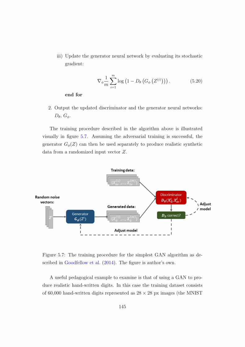
iii) Update the generator neural network by evaluating its stochastic

gradient:

∇φ1

m

m∑i=1

log(1−Dθ

(Gφ

(Z(i))))

. (5.20)

end for

2. Output the updated discriminator and the generator neural networks:

Dθ, Gφ.

The training procedure described in the algorithm above is illustrated

visually in figure 5.7. Assuming the adversarial training is successful, the

generator Gφ(Z) can then be used separately to produce realistic synthetic

data from a randomized input vector Z.

Figure 5.7: The training procedure for the simplest GAN algorithm as de-

scribed in Goodfellow et al. (2014). The figure is author’s own.

A useful pedagogical example to examine is that of using a GAN to pro-

duce realistic hand-written digits. In this case the training dataset consists

of 60,000 hand-written digits represented as 28× 28 px images (the MNIST

145

dataset described in ?). The training procedure then consists of the gener-

ator producing a batch of hand-written images from a random noise vector.

The produced and the training image batches are used by the discriminator

for updating the discriminator cost function, which in turn is passed to the

generator for updating the corresponding error function. During the initial

stages of training the generated images are not-realistic, however, after a few

epochs, the generator weights are updated sufficiently in order to produce

high quality images. Once the training is finished (provided that the com-

mon problem of mode collapse is avoided), the generator neural network can

be used to produce high quality realistic hand-written images from a batch

of noise vectors. The training procedure for the MNIST dataset is illustrated

pictorially in figure 5.8.

Figure 5.8: The training procedure for the simplest GAN algorithm as de-

scribed in Goodfellow et al. (2014) for the MNIST dataset. Image from ?.

146

Chapter 6

Using GANs for Emulating

Cosmological Simulation Data

This chapter contains a novel GAN algorithm that is used for emulating

cosmological simulation data. More specifically, a brief summary of the mo-

tivations and approaches to cosmological simulation emulators is given. In

addition, various properties of GAN algorithms are discussed. And finally,

an approach of emulating simulations of different cosmological parameters,

redshifts and modified gravity parameters is introduced. The algorithm is a

modified version of the cosmoGAN code described in great detail in Mustafa

et al. (2019). Most figures are from Tamosiunas et al. (2020) unless otherwise

specified. The calculations, coding and the result analysis was done by the

author with consultation and the supervision by the supervisors and the co-

authors. The L-PICOLA and MG-PICOLA simulation data was produced

primarily by Hans Winther. The other datasets are given in appendix A.1.

6.1 The Need for Cosmological Emulators

In the era of precision cosmology an important tool for studying the evolution

of large scale structure is N -body simulations. Such simulations evolve a large

number of particles under the influence of gravity (and possibly other forces)

147

throughout cosmic time and allow detailed studies of the non-linear struc-

ture formation. Modern cosmological simulations are highly realistic and

extremely complex and may include galaxy evolution, feedback processes,

massive neutrinos, weak lensing and many other effects. Such complexity

however comes at a price in terms of computational resources and large sim-

ulations may take several days or even weeks to run. In addition, to fully

account for galaxy formation and other effects various simplification schemes

and semi-analytical models are required. To address these issues a variety

of emulation techniques have been discussed in the literature (Kwan et al.,

2015; Winther et al., 2019; Knabenhans et al., 2019). In light of upcoming

surveys like Euclid, such emulators will be an invaluable tool for producing

mock data quickly and efficiently.

Lately, machine learning techniques have also been applied as an alter-

native to the traditional emulation methods. For instance, deep learning has

been used to accurately predict non-linear structure formation (He et al.,

2019). Similarly GANs and variational autoencoders have been used to pro-

duce novel realistic cosmic web 2-D projections, weak lensing maps and to

perform dark energy model selection (Rodrıguez et al., 2018; Mustafa et al.,

2019; Li et al., 2019). In addition the GAN approach has also been used to

produce realistic cosmic microwave background temperature anisotropy 2-D

patches as well as deep field astronomical images (Mishra et al., 2019; Smith

and Geach, 2019). Finally, generating full 3-D cosmic web data has been

discussed in Perraudin et al. (2019); Kodi Ramanah et al. (2020). The cited

works show that GANs are capable of reproducing a variety of cosmological

simulation outputs efficiently and with high accuracy.

However, certain challenges remain: the training process of the GAN algo-

rithm is complicated and prone to failure and producing full scale 3-D results

is computationally expensive. A common problem when training GANs is

mode collapse, when the generator neural network overpowers the discrimi-

nator and gets stuck in producing a small sample of identical outputs. Mode

collapse can be addressed in multiple ways – modern GAN architectures in-

148

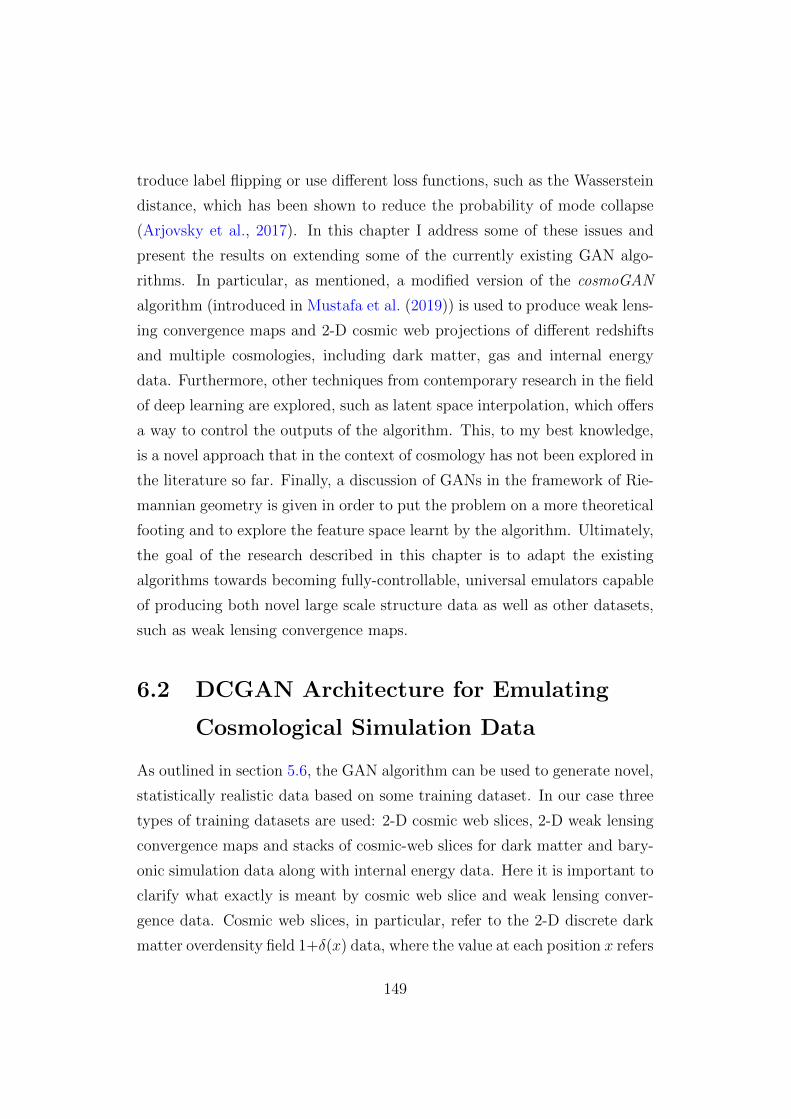
troduce label flipping or use different loss functions, such as the Wasserstein

distance, which has been shown to reduce the probability of mode collapse

(Arjovsky et al., 2017). In this chapter I address some of these issues and

present the results on extending some of the currently existing GAN algo-

rithms. In particular, as mentioned, a modified version of the cosmoGAN

algorithm (introduced in Mustafa et al. (2019)) is used to produce weak lens-

ing convergence maps and 2-D cosmic web projections of different redshifts

and multiple cosmologies, including dark matter, gas and internal energy

data. Furthermore, other techniques from contemporary research in the field

of deep learning are explored, such as latent space interpolation, which offers

a way to control the outputs of the algorithm. This, to my best knowledge,

is a novel approach that in the context of cosmology has not been explored in

the literature so far. Finally, a discussion of GANs in the framework of Rie-

mannian geometry is given in order to put the problem on a more theoretical

footing and to explore the feature space learnt by the algorithm. Ultimately,

the goal of the research described in this chapter is to adapt the existing

algorithms towards becoming fully-controllable, universal emulators capable

of producing both novel large scale structure data as well as other datasets,

such as weak lensing convergence maps.

6.2 DCGAN Architecture for Emulating

Cosmological Simulation Data

As outlined in section 5.6, the GAN algorithm can be used to generate novel,

statistically realistic data based on some training dataset. In our case three

types of training datasets are used: 2-D cosmic web slices, 2-D weak lensing

convergence maps and stacks of cosmic-web slices for dark matter and bary-

onic simulation data along with internal energy data. Here it is important to

clarify what exactly is meant by cosmic web slice and weak lensing conver-

gence data. Cosmic web slices, in particular, refer to the 2-D discrete dark

matter overdensity field 1+δ(x) data, where the value at each position x refers

149

to the density relative to the average density (i.e. δ(x) = (ρ(x)− ρ)/ρ). Sim-

ilarly, weak lensing maps refer to the discrete 2-D corvengence fields, where

the numerical value at each position x simply refers to the value of conver-

gence κc(x). Both types of datasets can be represented as 2-D arrays, where

each entry of the array corresponds to the value of the overdensity or con-

vergence. Analogously, these arrays can be represented visually as images,

with each pixel value corresponding to the mentioned quantities (note that

in some cases the pixel values are rescaled for visualization purposes).

Since we are dealing with data that can be naturally represented in a vi-

sual form, a straightforward choice is to pick a GAN architecture that works

well with image data. In this regard, deep convolutional generative adversar-

ial networks (DCGANs) have shown good results in producing statistically

realistic novel visual data. Thus, in order to generate cosmic web and weak

lensing convergence data, we chose to use the DCGAN architecture, as de-

scribed in (Mustafa et al., 2019). More specifically, as a starting point the

DCGAN implementation publicly available in Mustafa et al. (2017) was used.

Tables 6.1 and 6.2 describe the key features of the architecture. Both the

discriminator and the generator are standard convolutional neural networks

using primarily ReLU and leaky ReLU activation functions along with trans-

posed convolutional and standard convolutional layers.

To adapt the outlined architecture to the problem at hand, I experimented

with different activation functions, different strides and different sizes of the

convolutional layers. The results indicated that the architecture used in

Mustafa et al. (2019) with minor variations generally worked well for pro-

ducing realistic cosmic web and weak lensing data as well as the combined

dark matter and baryonic data samples. More specifically, for the cosmic

web data, the input shape (i.e. the size of the random noise vector) was

changed from 64 to 256 to account for the higher complexity of the cosmic

web images when compared to the weak lensing maps. In the case of emulat-

ing dark matter, gas and internal energy slices, the public code was adapted

to work with multi-channel data (i.e. RGB input arrays). In addition, the

150

Activ. Output shape Params.

Latent − 64 −Dense − 512× 16× 16 8.5M

BatchNorm ReLU 512× 16× 16 1024

TConv 5× 5 − 256× 32× 32 3.3M

BatchNorm ReLU 256× 32× 32 512

TConv 5× 5 − 128× 64× 64 819K

BatchNorm ReLU 128× 64× 64 256

TConv 5× 5 − 64× 128× 128 205K

BatchNorm ReLU 64× 128× 128 128

TConv 5× 5 Tanh 1× 256× 256 1601

Total trainable parameters 12.3M

Table 6.1: The architecture of the generator neural network as described in

Mustafa et al. (2019). TConv corresponds to the transposed convolutional

layer with stride = 2 (and the kernel size given by the shown numerical

values). ReLU corresponds to the rectified linear unit activation function.

default batch size (number of input arrays that the algorithm uses during

an iteration of training) was changed from 32 to 64. Extra functions were

also added to the code to allow performing the latent space interpolation

easier (see section 6.3 and appendix A.1). Finally, when training on weak

lensing convergence maps, the architecture was left unchanged as one of the

key goals was to reproduce the results described in Mustafa et al. (2019).

In summary, if we choose convolutional neural networks (rather than

simple multi-layer perceptrons) for the generator and the discriminator, the

training procedure described in section 5.6 essentially remains the same. In

fact, any algorithm that is capable of producing and classifying data could be

used as the generator and the discriminator. And then, if we represent the

cosmic web and the weak lensing data as 2-D arrays, the pipeline of training

a GAN on our data is summarized in figure 6.1. In particular, the simulation

151

Activ. Output shape Params.

Input map − 1× 256× 256 −Conv 5× 5 LReLU 64× 128× 128 1664

Conv 5× 5 − 128× 64× 64 205K

BatchNorm LReLU 128× 64× 64 256

Conv 5× 5 − 256× 32× 32 819K

BatchNorm LReLU 256× 32× 32 512

Conv 5× 5 − 512× 16× 16 3.3M

BatchNorm LReLU 512× 16× 16 1024

Linear Sigmoid 1 131K

Total trainable parameters 4.4M

Table 6.2: The architecture of the discriminator neural network as described

in Mustafa et al. (2019). Conv stands for convolutional layers with stride = 2

the kernel size given by the numerical value. LReLU stands for the leaky

rectified linear unit activation function with the leakiness parameter = 0.2.

data is used to produce the 2-D cosmic web slices, which are then used

as a training dataset. More specifically, during the training procedure the

generator network produces a batch of 64 images from a batch of 64 random

noise vectors (drawn from a Gaussian distribution centered around 0), which

is then sent to the discriminator network, where it is combined with a batch

of 64 training images for classification. In the case of a training dataset with

multi-channel images (RGB images), the generator and the discriminator

process batches of images of the following shape: (64, 3, 256, 256), where the

second value corresponds to the number of channels.

To summarize, the problem at hand is to emulate cosmological simulation

data using GANs. More specifically, the aim is to emulate novel dark matter

overdensity fields, represented by 2-D arrays produced via mesh painting from

the raw simulation output data. In addition, we also aim to produce realistic

convergence field and gas density data from hydrodynamic simulations. In

152

all cases the training data consists of batches of 2-D arrays, which, when

plotted visually, represent the mentioned fields (projected to 2-D). A more

technical discussion of the datasets is given in section 6.5. Once the training

is completed, the generator neural network can be used to produce realistic

novel 2-D arrays in the same format as the training dataset. Note that

the problem at hand is fundamentally analogous to that of generating hand-

written images (i.e. figure 5.8) the only difference being the size of the dataset

arrays and the architecture of the neural networks used.

Figure 6.1: The pipeline of training a GAN on cosmic web slice data. The

numbers in the brackets are the sizes of the input/output arrays and corre-

spond to the number of images in the batch along with the channel number,

height and the width of the images.

6.3 Latent Space Interpolation

Before discussing the different datasets and the training procedure, it is im-

portant to review another important feature of the GAN algorithms. Latent

space interpolation refers to the procedure of interpolating between a pair of

outputs produced by a GAN. This procedure not only allows us to study the

153

feature space learnt by the algorithm, but also allows us to control which out-

puts the algorithm produces. Here a review of the procedure and its various

uses is given.

If the training procedure is successful, the generator Gφ(Zi) learns to

map the values of a random vector Zi to the values of a statistically realistic

output vector X iG, which can be reshaped to the original 2-D array shape

representing an image XjkG (a cosmic web slice or a convergence map in our

case). This can be viewed as mapping from a low-dimensional latent space

Z ⊆ Rd to a higher-dimensional data (pixel) space X ⊆ RD (where d is the

size of the noise input vector and D is the total number of the of the output

image pixels; for more details see Shao et al. (2017)). For a generator neural

network d D (in our case d = 256 or 64, while D = 2562).

The training procedure can be viewed as the generator learning to map

clusters in the Z space to the clusters in the X space. Hence, if we treat

the random input vectors1 Zi as points in a d-dimensional space, we can

interpolate between multiple input vectors and produce a transition between

the corresponding outputs. In particular, if we choose two input vectors that

correspond to points Z1 and Z2 and find a line connecting them, sampling

intermediate input points along that line leads to a set of outputs that cor-

respond to an almost smooth transition between the output points X1 and

X2.

As an example, if we train the generator to produce cosmic web slices

of two different redshifts, we can produce a set of outputs corresponding to

a transition between those two redshifts by linearly interpolating between

the input points Z1 and Z2 (see figure 6.2). More concretely, if we train the

algorithm on cosmic web slices of redshifts 0.0, 1.0, somewhere between

the two input points, one can find a point Z′, which produces an output

that has a matter power spectrum approximately corresponding to a red-

shift z′ ≈ 0.5. This is fascinating given that the training dataset did not

1Note regarding notation: here a superscript refers to input/output vectors, while a

subscript refers to the corresponding point in the latent/output data space.

154

include intermediate redshift data. Here it is important to note that such

an interpolation procedure does not necessarily produce a perfectly smooth

transition in the data space, i.e. the produced outputs corresponding to the

points Xi between X1 and X2 are not always realistic (in terms of the

matter power spectrum and other statistics; see figure 6.19 and section 6.7.6

for further details). Also, one might naively think that the point Z′

lies

in the middle of the line connecting Z1 and Z2, but in general we found it

not to be the case (as the middle of the mentioned line does not necessary

correspond to the middle between X1 and X2 in the data space, which is

known to be non-Euclidean (see section 6.4)). In the upcoming chapters I

investigate whether the latent space interpolation procedure can be used to

map between outputs of different redshifts and cosmologies and whether the

produced datasets are physically realistic.

The latent space interpolation technique was performed by randomly

choosing two input points Z1 and Z2, finding the line connecting the two

points in the 256 (64)-dimensional space (256 (64) is the size of the corre-

sponding input vectors) and then sampling 64 equally spaced points along

that line. The outputs of the generator neural network of those intermediate

input points Gφ(Zinti ) then correspond to cosmic web slices and weak lens-

ing maps that represent a transition between the two outputs Gφ(Z1) and

Gφ(Z2).

In order to perform linear latent space interpolation it is crucial to have

the ability to distinguish between different data classes produced by the GAN

(e.g. cosmic web slices of different redshifts). This was resolved by employ-

ing a combination of the usual summary statistics like the power spectrum

and the Minkowski functionals along with two different machine learning

algorithms. In particular, deep convolutional neural network and gradient

boosted decision trees were used for distinguishing the different classes of

datasets produced by the GAN (Chen and Guestrin, 2016).

155

Figure 6.2: Illustration of the latent space interpolation procedure. Train-

ing the GAN algorithm on the cosmic web slices of two different redshifts

encodes two different clusters in the latent space (which is a subset of a 256-

dimensional space, i.e. the size of the random noise input vector). Sampling

a point from the line connecting two input points Z1 and Z2 in this space

produces an output with redshift z′. In the case of our dataset with z1 = 1.0

and z2 = 0.0, several points near the centre of this line correspond to outputs

approximately emulating z′ ≈ 0.5.

156

6.4 Riemannian Geometry of GANs

The latent space interpolation procedure described in the previous section is

a good example of how Riemannian geometry can be employed to describe

certain features of the GAN algorithm. Recently various connections between

GANs and Riemannian geometry have been explored in the machine learning

literature in a more general context. Such connections are important to

explore not only for the sake of curiosity, but also because they allow us to

describe GANs and their optimization procedure in a language more familiar

to physicists. A Riemannian geometry description of GANs is also powerful

when exploring the latent space of a trained generator neural network and

the outputs that it produces. Finally, a differential geometry description

could shine some light on the connections between generative models and

information geometry, which is a well-established field and could offer some

new insights into training and analyzing the outputs of such models.

Recent work in Shao et al. (2017) proposes treating the trained generator

neural network as a mapping from a lower dimensional latent space Z to

the higher dimensional data space X: Gφ : Z → X (see fig. 6.3). More

specifically, the generator Gφ(Zi) maps the latent space vectors of size n (in

our case n = 256 or 64) to a manifold M of dimensionality m (256 × 256,

i.e. the number of pixels in the output images). Manifold M here simply

refers to a subset of the data space (all possible combinations of pixel values),

which correspond to realistic images of weak lensing/cosmic web slices. The

existence of such a manifold is postulated by the manifold hypothesis in

deep learning, which states that high-dimensional data can be encoded on a

manifold of a much lower dimension (Fefferman et al., 2013).

Hence if we treat the generator neural network Gφ as a mapping for the

latent space to the data space manifold, one can naturally define an induced

metric g, which then allows to quantify the distance between the points on the

manifold and the length of curves. For a mapping described by the generator

neural network, the metric is simply equal to a product of the Jacobian and

the transposed Jacobian (Shao et al., 2017):

157

Figure 6.3: Riemannian geometry of generative adversarial networks. The

generator Gφ(Zi) can be treated as a mapping from the lower dimensional

Euclidean latent space Z (corresponding to the random noise input) to a high

dimensional data (pixel) space M (in general non-Euclidean). Each point on

M corresponds to a cosmic web slice (or a weak lensing map).

g = J(Z)TJ(Z). (6.1)

The Jacobian in our case refers to the partial derivative of each output value

w.r.t. to each input value, i.e.:

J =

∂X1

∂Z1∂X1

∂Z2 . . . ∂X1

∂Zn

......

. . .

∂Xm

∂Z1∂Xm

∂Z2 . . . ∂Xm

∂Zn

.Once a metric is defined, one can use the usual tools to describe geodesics

on the manifold M . For instance, one can define a curve κZ between two

points a and b in the latent space Z parametrized by some parameter t.

Using the mapping Gφ, the corresponding curve on the manifold M is then:

Gφ(κZ(t)) ∈ M . To find a curve that corresponds to a geodesic on the

manifold one has to solve the Euler-Lagrange equation, which gives:

158

d2καZdt2

= −ΓαβγdκβZdt

dκγZdt

, (6.2)

where Γ is the usual Christoffel symbol, given by:

Γαβγ =1

2gαδ(∂gδβ∂Xγ

+∂gδγ∂Xα

− ∂gαβ∂Xδ

). (6.3)

As discussed in Shao et al. (2017) geodesics between points on the mani-

fold are of special importance, as they give the smoothest possible transition

between multiple outputs. One of the main findings in Shao et al. (2017)

was that the Riemannian curvature of the manifold corresponding to the

their data was surprisingly small and, hence, linear interpolation produced

realistic results comparable to the results produced by calculating a geodesic

curve between the outputs. In our work we also found that linear inter-

polation generally produced realistic results. However, to ensure that the

outputs produced via the latent space interpolation are indeed realistic, one

would have to interpolate on a curve in the latent space (corresponding to

the geodesic connecting the needed outputs on the data manifold M) rather

than a line.

Another important connection to Riemannian geometry comes in the con-

text of the discriminator neural network. The discriminator can be viewed

as a mapping from the data manifold to a probability manifold P , where

each point on the manifold corresponds to the probability of a given data

sample being real (i.e. belonging to the training dataset). Such a manifold

looks remarkably similar to the statistical manifolds studied in the field of

information geometry. Insights from information geometry have a long tra-

dition of being used in neural network optimization (e.g. Hauser and Ray

(2017)). Exploring such connections could lead to deeper insights into the

GAN training process, which is an interesting direction for future work.

159

6.5 Datasets and the Training Procedure

This section contains a detailed introduction to the datasets that were used

to train the GAN algorithm described in the previous sections. In each case

the simulations that were used to produce the dataset are described as well.

Finally, the cosmological parameters and the used smoothing techniques are

described as well.

6.5.1 Weak Lensing Convergence Map Data

Gravitational potentials influence the path of photons in such a way that they

introduce coherent distortions in the apparent shape (shear) and position of

light sources. Weak gravitional lensing introduces ellipticity changes in ob-

jects of the order of ≈ 1% and can be measured across the sky, meaning that

maps of the lensing distortion of objects can be made and related to maps of

the mass distribution in the Universe. The magnitude of the shear depends

upon the combined effect of the gravitational potentials between the source

and the observer. An observer will detect this integrated effect and maps

of the integrated mass, or convergence, can be made. Gravitational lensing

has the significant advantage that it is sensitive to both luminous and dark

matter, and can therefore directly detect the combined matter distribution.

In addition, weak lensing convergence maps allow for detecting the growth of

structure in the Universe and hence they can also be used for probing statis-

tics beyond two point correlation functions, such as in the higher moments of

the convergence field or by observing the topology of the field with Minkowski

functionals and peak statistics (Dietrich and Hartlap, 2010; Mawdsley et al.,

2020). As future surveys attempt to further probe the non-linear regime of

structure growth, the information held in these higher order statistics will

become increasingly important, and will also require accurate simulations in

order to provide cosmological constraints. This requirement for large num-

bers of simulations that also model complex physical phenomena means that

more computationally efficient alternatives to N -body simulations, such as

160

the GAN approach proposed in this work, are required.

In order to train the GAN algorithm to produce realistic convergence

maps, publicly available datasets were used. In particular, to test whether

we could reproduce the original results from Mustafa et al. (2019) the publicly

available data from Mustafa et al. (2017) was used. The dataset consists of

8000 weak lensing maps that were originally produced by running a Gadget2

(Springel, 2005) simulation with 5123 particles in a 240 Mpc/h box. To

perform ray tracing the Gadget weak lensing simulation pipeline was used.

The simulation box was rotated multiple times for each ray tracing procedure,

resulting in 1000 12 sq. degree maps per simulation box.

In order to train the GAN algorithm on convergence maps of different

cosmologies and redshifts, the dataset publicly available at (Zorrilla Matilla

et al., 2016; Gupta et al., 2018; Columbia Lensing, 2020) was used. The

available dataset contains weak lensing convergence maps covering a field

of view of 3.5 deg × 3.5 deg, with resolution of 1024 × 1024 pixels. The

maps were originally produced using Gadget2 DM-only simulation data with

240 Mpc/h side box and 5123 particles. The dataset includes 96 different

cosmologies (with varying Ωm and σ8 parameters). The values of Ωm = 0.260

and σ8 = 0.8 were used as the fiducial cosmology. In this work only a small

subset of this dataset was used, namely, the maps where only one of the two

cosmological parameter varies. In particular, the dataset consisting of the

maps with σ8 = 0.436, 0.814 with a common value of Ωm = 0.233 was used.

This was done in order to simplify the latent space analysis.

For the weak lensing map data the same architecture as described in

tables 6.1 and 6.2 was used. In fact the same basic architecture with minor

variations was used for training all the datasets described later on. The key

parameter in terms of the training procedure is the learning rate. For all the

cosmic web slice datasets, I found the learning rate value of RL = 3 × 10−5

to work well. In the case of all the considered weak lensing datasets RL =

9 × 10−6 was used. The training procedure and all the key parameters are

described in great detail in the publicly available code (see appendix A.1 for

161

more information).

6.5.2 Cosmic Web Slice Data

The cosmic web or the dark matter overdensity field refers to the intricate

network of filaments and voids as seen in the output data of N -body simu-

lations. The statistical features of the cosmic web contain important infor-

mation about the underlying cosmology and could hide imprints of modifica-

tions to the standard laws of gravity. In addition, emulating a large number

of overdensity fields is important for reliable estimation of the errors of cos-

mological parameters. Hence, emulators, such as the one proposed in this

work, are of special importance for the statistical analysis in the context of

the upcoming observational surveys.

The cosmic web training dataset was produced by employing a similar

procedure to the one outlined in Rodrıguez et al. (2018). In particular, we

ran L-PICOLA (Howlett et al., 2015) to produce a total of 15 independent

simulation boxes with different cosmologies. Initially, the same cosmology

as described in Rodrıguez et al. (2018) was used with h = 0.7, ΩΛ = 0.72

and Ωm = 0.28. Subsequently, the effects of varying one of the cosmological

parameters, namely the σ8 parameter, was studied. The values of σ8 =

0.7, 0.8, 0.9 along with ΩΛ = 0.7, Ωm = 0.3 and h = 0.67 were explored.

For each different set of simulations, snapshots at 3 different redshifts: z =

0.0, 0.5, 1.0 were saved. For each simulation, a box size of 512 Mpc/h was

used with 5123 particles. For the latent space interpolation procedure, the

GAN was trained on slices with redshifts 0.0, 1.0, with a common value of

σ8 = 0.8.

To produce the slices for training the GAN, I used nbodykit (Hand et al.,

2018), which allows painting an overdensity field from a catalogue of sim-

ulated particles. To obtain the needed slices, the simulation box was cut

into sections of 2 Mpc width in x, y, z directions and for each section a mesh

painting procedure was done. This refers to splitting the section into cells,

where the numerical value of each cell corresponds to the dark matter over-

162

density 1 + δ(x). Finally, after a 2-D projection of each slice, a 2562 px

image was obtained, with each pixel value corresponding to the overden-

sity field. To emphasize the features of the large scale structure, I applied

the same non-linear transformation as described in Rodrıguez et al. (2018):

s(x) = 2x/(x + a) − 1, with a = 250, which rescales the overdensity values

to [−1, 1] and increases the contrast of the images.

In order to emulate modified gravity effects the MG-PICOLA code was

used. MG-PICOLA extends the original L-PICOLA code in order to allow

simulating theories that exhibit scale-dependent growth (Scoccimarro et al.,

2012; Tassev et al., 2013; Winther et al., 2017; H. A. Winther, 2020). This

includes models such as f(R) theories, which replace the Ricci scalar with

a more general function in the Einstein-Hilbert action (see Li and Koyama

(2019b) and chapter 3 for an overview of the phenomenology of such models).

In particular, multiple runs of MG-PICOLA were run with the following

range of the fR0 parameter: [10−7, 10−1]. Such a wide range was chosen to

make the latent space interpolation procedure easier. The f(R) simulations

were also run with the same seed as the corresponding ΛCDM simulations,

making the two datasets described above directly comparable.

6.5.3 Dark Matter, Gas and Internal Energy Data

Simultaneously generating dark matter and the corresponding baryonic over-

density field data is a great challenge from both the theoretical and the

computational perspectives. Namely, generating the baryonic distribution

requires detailed hydrodynamical simulations that account for the intricacies

of galaxy formation and feedback processes, which leads to a major increase

in the required computational resources. For this reason, emulating large

amounts of hydrodynamical simulation data is of special importance.

To produce the dark matter, baryonic matter and the internal energy

distribution slices I used the publicly available Illustris-3 simulation data

(Vogelsberger et al., 2014; Nelson et al., 2015). Illustris-3 refers to the low

resolution Illustris run including the full physics model with a box size of

163

75000 kpc/h and over 9 × 107 dark matter and gas tracer particles. The

cosmology of the simulation can be summarized by the following parameters:

Ωm = 0.2726, ΩΛ = 0.7274, h = 0.704. The simulation included the following

physical effects: radiative gas cooling, star formation, galactic-scale winds

from star formation feedback, supermassive black hole formation, accretion,

and feedback.

To form the training dataset I used an analogous procedure to the one

used for the cosmic web slices in section 6.5.2. In particular, the full simu-

lation box was cut into slices of 100 kpc/h and for each slice mesh painting

was done to obtain the overdensity field. This was done for the dark matter

and gas data. In addition, the available internal energy (thermal energy in

the units of (km/s)2) distribution data was used as well. Figure 6.4 shows a

few samples from the dataset.

To investigate whether the GAN algorithm could be trained on multidi-

mensional array data, the DM, gas and energy distribution 2-D slices were

treated as RGB planes in a single image. In particular, a common way of

representing colors in an image is forming a full color image out of three

planes, each corresponding to the pixel values for red, green and blue colours

(see figure 5.5). In this framework, a full-color image corresponds to a 3-D

array. Convolutional neural networks, including the one that the cosmoGAN

algorithm is based on are originally designed to be trained on such RGB im-

ages. Hence we combined the mentioned DM, gas and internal energy slices

into a set of RGB arrays that were used as a training set.

6.5.4 The Training Procedure

The initial stages of training (i.e. reproducing the results in (Rodrıguez et al.,

2018; Mustafa et al., 2019) were done using the Google Cloud computing

platform. The following setup was used: 4 standard vCPUs with 15 GB

memory, 1 NVIDIA Tesla K80 GPU and 2TB of SSD hard drive space.

Later stages of training (i.e. training the GAN on different cosmology,

modified gravity and redshift data) were done using the local Sciama HPC

164

(a) DM overdensity field (b) Gas overdensity field

(c) Internal energy field (d) All components combined

Figure 6.4: Samples from the Illustris simulation dataset used to train the

GAN algorithm: 2-D slices of the different simulation components (box size:

75000 kpc/h).

cluster, which has 3702 cores of 2.66 GHz Intel Xeon processors with 2 GB

of memory per core.

Given how unstable the GAN training procedure is, a simple way of eval-

uating the best checkpoint was used: I calculated the mean square difference

between the mean values of the GAN-produced and the training dataset

power spectra, pixel histograms and the Minkowski functionals. The set of

GAN weights that minimizes this value was used for the plots displayed in

the result section.

165

6.6 Diagnostics

A key aspect of the analysis of the produced samples is being able to quantify

how realistic the GAN-generated data is. This was done at an ensemble level

– i.e. we generated multiple batches of data (see figures in section 6.7) and

calculated the average summary statistics, which were then compared against

analogous results produced using the training dataset.

The results produced by the algorithm were investigated using the follow-

ing diagnostics: the 2-D matter power spectrum, overdensity (pixel) value

histogram and the three Minkowski functionals. In addition, the cross and

the auto power spectrum were computed in order to investigate the corre-

lations between the datasets on different scales. The cross-power spectrum

was calculated using:

〈δ1(l)δ∗2(l′)〉 = (2π)2δD(l − l′)P×(l), (6.4)

where δ1 and δ∗2 are the Fourier transforms of the two overdensity fields at

some Fourier bin l and δD is the Dirac delta function.

The Minkowski functionals are a useful tool in studying the morphological

features of fields that provide not only the information of spatial correlations

but also the information on object shapes and topology. For some field f(x)

in 2-D we can define the three Minkowski functionals as follows:

V0(ν) =

∫Qν

dΩ, V1(ν) =

∫∂Qν

1

4dl, V2(ν) =

∫∂Qν

1

2πκbdl. (6.5)

Where Qν ≡ x ∈ R2|f(x) > ν is the area and ∂Qν ≡ x ∈ R2|f(x) =

ν is the boundary of the field at the threshold value ν. The integrals V0, V1,

V2 correspond to the area, boundary length and the integrated geodesic cur-

vature κb along the boundary. To put it simply, the procedure of measuring

the Minkowski functionals refers to taking the values of the field at and above

a given threshold ν, evaluating the integrals in eq. 6.5 and then changing the

threshold for a range of values. In the case of the 2-D fields one can imagine

166

the field values at different positions as height in the third dimension. Then

a 2-D convergence map or an overdensity field can be visualised as a 3-D

surface. And the Minkowski functionals then correspond to taking slices of

the 3-D surface at and above the different heights and measuring the area,

curve length and the geodesic curvature as described in equation 6.5. In this

way Minkowski functionals allow to capture detailed morphological features

of the generated field data which can then be directly compared against the

training dataset.

Minkowski functionals are also a useful tool in weak lensing convergence

map studies as they allow us to capture non-Gaussian information on the

small scales, which is not fully accessed by the power spectrum alone. In ad-

dition, Minkowski functionals have been used to detect different cosmologies,

modified gravity models and the effects of massive neutrinos in weak lensing

convergence maps (Petri et al., 2013; Ling et al., 2015; Marques et al., 2019).

Given the usefulness of Minkowski functionals in accessing the non-Gaussian

information on the small scales, the functionals were chosen for studying the

produced cosmic web data as well. To calculate the Minkowski functionals

properly on a 2-D grid I used the minkfncts2d algorithm, which utilizes a

marching square algorithm as well as pixel weighting to capture the boundary

lengths correctly (Mantz et al., 2008; minkfncts2d Python package, 2020).

Minkowski functionals are sensitive to the Gaussian smoothing applied to

the GAN-produced images and the training data. Hence, it is important to

study the effects of Gaussian smoothing as it might give a deeper insight into

the detected differences between the datasets. The procedure of smoothing

refers to a convolution between a chosen kernel and the pixels of an image.

In more detail, a chosen kernel matrix is centered on each pixel of an im-

age and each surounding pixel is multiplied by the values of the kernel and

subsequently summed. In the simplest case, such a procedure corresponds to

averaging a chosen number of pixels in a given image. In the case of Gaussian

filtering, a Gaussian kernel is used instead.

To filter the noise we used Gaussian smoothing with a 3×3 kernel window

167

and a standard deviation of 1 px. The Minkowski functionals were found to be

especially sensitive to any kind of smoothing. For instance, the position and

the shape of the trough of the third Minkowski functional is highly sensitive

to the existence of any small-scale noise. Figure 6.5 illustrates the effects

of Gaussian smoothing with different kernel sizes on the three Minkowski

functionals.

Figure 6.5: An illustration of the effects of Gaussian smoothing on the

Minkowski functionals calculated using cosmic web slices from the training

data with redshift z = 0.0. The colored bands correspond to the mean and

the standard deviation of the functionals calculated using different sizes of

Gaussian smoothing kernels on a batch of 64 images.

6.7 Results

6.7.1 Weak Lensing Map Results

After around 150 epochs (corresponding to around 96 hours on a local HPC)

the GAN started producing statistically realistic convergence maps as mea-

sured by the power spectrum and the Minkowski functionals. The diagnostics

were computed at an ensemble level – 100 batches of 64 convergence maps

were produced by the GAN and the mean values along with the standard

deviation were computed and compared with the training data. An anal-

168

ogous procedure was done when calculating the pixel intensity distribution

histograms.

(a) Power spectrum (b) Pixel intensity histogram

Figure 6.6: The matter power spectrum (with the relative difference) and the

pixel intensity histogram for an ensemble of 6400 weak lensing convergence

maps. The dashed lines correspond to the mean values, while the contours

correspond to the standard deviation. Note that the pixel intensity values

were normalized to the range of [−1, 1].

The power spectra agree well between the GAN-produced and the training

data, with minor differences on the small scales (see figure 6.6). In particular,

the difference between the training and the GAN-produced dataset power

spectra is around 5% or lower for most values of k. Only at the smallest

scales a significant difference of 10% is reached. Similarly, the pixel intensity

histogram in general shows a good agreement with significant differences

appearing only for the highest and the lowest pixel intensity values (which

is also detected in the original work in Mustafa et al. (2019)). A selection of

GAN-produced maps are presented for visual inspection in figure A.1.

Minkowski functionals were also calculated for the GAN-produced and

the training datasets. The results are shown in figure 6.7. In general there is

a good agreement between the training data and the GAN-produced maps,

given the standard deviation, however, some minor differences can be de-

169

tected in the Euler characteristic and the boundary functional, likely result-

ing from noise.

Figure 6.7: A comparison of the Minkowski functionals evaluated using 100

batches of 64 ramdomly selected maps for both datasets.

6.7.2 Weak Lensing Maps of Multiple Cosmologies

The results also indicate that the GAN is capable of producing realistic weak

lensing maps for multiple cosmologies. This is an important result as it shows

that the algorithm is able to pick up on the various subtle statistical differ-

ences between different cosmologies that usually requires a detailed study of

the power spectrum, Minkowski functionals and other statistics.

However, the training procedure was found to be highly prone to mode

collapse. A wide hyperparameter search had to be performed to find an opti-

mal set of parameters that did not lead to full or partial mode collapse. The

most important parameter in this context was found to be the learning rate.

As a rule of thumb, decreasing the learning rate led to mode collapse hap-

pening later in the training procedure. When the learning rate was reduced

below a certain value (discussed further in the analysis section), mode col-

lapse was avoided altogether. As in the case with the cosmic web slice data,

applying a transformation to each pixel of the image in order to increase the

contrast had a positive effect in reducing the probability of mode collapse as

170

well.

Figure 6.8: A selection of diagnostics to compare the training and the GAN-

produced weak lensing convergence maps for σ8 = 0.436, 0.814 with Ωm =

0.233. Top left: power spectra for an ensemble of 64 randomly chosen shear

maps; top right: power spectra (mean and standard deviation) with and

without Gaussian smoothing produced using 1000 randomly chosen shear

maps with σ8 = 0.814; bottom left: same as top right, but for σ8 = 0.436;

bottom right: the pixel intensity distribution (for both datasets combined).

The blue and the green dots give Ptr/PGAN − 1 with and without Gaussian

smoothing applied correspondingly.

171

Figure 6.8 summarizes the results of training the GAN on shear maps with

different σ8 values. The results indicate an agreement of the power spectra

in the range of 5-10% for k > 10−1 h Mpc−1 for σ8 = 0.814. In the case

of σ8 = 0.436 the agreement is significantly better, ranging between 1-3%

on most scales. Interestingly, Gaussian smoothing increases the difference

to around 5-15% in this particular case. This shows that for this dataset

Gaussian noise is not the major source of the statistical differences between

the training and the GAN-generated datasets.

Figure 6.9 compares the Minkowski functionals calculated using the train-

ing and the GAN-produced datasets. Given the standard deviation in both

datasets, the results overlap for all threshold values. However, for thresholds

in the range of [0.0, 0.4] there is a significant difference between the training

and the GAN-generated datasets. We found that this is partially due to

small-scale noise in the GAN-produced data (see figure 6.5). However, after

experimenting with adding artificial noise to the training dataset images, it

is clear that the noise alone cannot fully account for the observed differences

in the Minkowski functionals. Another reason for the observed differences

could be a relatively small size of the used dataset consisting of a few thou-

sand weak lensing maps. It is likely that having more training data samples

could significantly improve the results.

6.7.3 Cosmic Web for Multiple Redshifts

The results also indicate that the GAN approach is capable of producing real-

istic cosmic web slices for different redshifts. As before with the weak lensing

maps of different cosmologies, this illustrates that the algorithm in general

does not get confused between the two different redshifts and is capable of

detecting subtle statistical differences between the different datasets (figure

6.10). In addition, I found that using Gaussian smoothing, as before, led to

a better agreement between the training and the GAN-produced datasets.

The effect is especially noticeable in the Minkowski functional analysis (fig-

ure 6.11). Visual samples of the produced cosmic web slices are shown in

172

Figure 6.9: A comparison of the Minkowski functionals evaluated using 1000

randomly selected weak lensing convergence maps with σ8 = 0.436, 0.814.Gaussian smoothing is applied for all datasets.

figure A.2.

The power spectra results for both redshift values were found to be very

similar. Namely, for the non-smoothed case the difference between the train-

ing and the GAN-produced power specta ranges between 5-10%. The results

are similar for the smoothed case, with exception of k values around 1 h

Mpc−1 where the difference reaches 20%.

The effects of the Gaussian smoothing on both the power spectra and the

Minkowski functionals illustrate that one of the reasons for the differences

between the GAN-generated and the training datasets is noise appearing on

different scales in the GAN-produced images. Applying Gaussian smoothing,

in general, filters the majority of such noise, however, it cannot fully account

for all the differences appearing in the different statistical diagnostics. In

addition, smoothing can improve the results on some scales, while worsening

them on others. As an example, in figure 6.10, Gaussian smoothing increases

the difference between the GAN-produced and the training dataset power

spectra on the smallest scales.

173

Figure 6.10: A selection of diagnostics to compare the training and the GAN-

produced cosmic web slices for redshifts z = 0.0 and z = 1.0 with σ8 = 0.8.

Top left: power spectra for an ensemble of 64 randomly chosen slices for

two different redshifts; top right: mean and standard deviation of the power

spectra produced using 1000 randomly chosen slices with z = 0.0; bottom

left: same as top right, but for z = 1.0; bottom right: the overdensity

histogram (no smoothing). The blue and the green dots give Ptr/PGAN − 1

with and without Gaussian smoothing applied correspondingly.

174

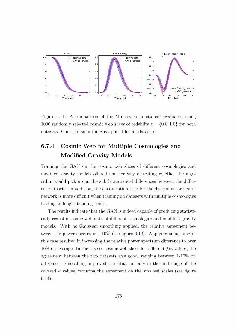
Figure 6.11: A comparison of the Minkowski functionals evaluated using

1000 randomly selected cosmic web slices of redshifts z = 0.0, 1.0 for both

datasets. Gaussian smoothing is applied for all datasets.

6.7.4 Cosmic Web for Multiple Cosmologies and

Modified Gravity Models

Training the GAN on the cosmic web slices of different cosmologies and

modified gravity models offered another way of testing whether the algo-

rithm would pick up on the subtle statistical differences between the differ-

ent datasets. In addition, the classification task for the discriminator neural

network is more difficult when training on datasets with multiple cosmologies

leading to longer training times.

The results indicate that the GAN is indeed capable of producing statisti-

cally realistic cosmic web data of different cosmologies and modified gravity

models. With no Gaussian smoothing applied, the relative agreement be-

tween the power spectra is 1-10% (see figure 6.12). Applying smoothing in

this case resulted in increasing the relative power spectrum difference to over

10% on average. In the case of cosmic web slices for different fR0 values, the

agreement between the two datasets was good, ranging between 1-10% on

all scales. Smoothing improved the situation only in the mid-range of the

covered k values, reducing the agreement on the smallest scales (see figure

6.14).

175

Figure 6.13 shows the Minkowski functional analysis. In this case, very

little deviation is observed. In general, there is a good agreement between

the GAN-produced and the training datasets, especially for the first and

the second Minkowski functionals. For the third Minkowski functional, the

results diverge around the lower trough area, which is also observed for other

datasets. This is at least in part related to small-scale noise as indicated by

the previous analysis.

The results are similar for the GAN trained on cosmic web slices corre-

sponding to different f(R) models (figure 6.15). In general, a good agreement

between the datasets was found (given the standard deviation of the data

and the GAN-produced results). Gaussian smoothing, in this case, was more

effective in reducing some of the offset observed in the power spectrum anal-

ysis. However, it increased the offset on the smallest scales.

6.7.5 Dark Matter, Gas and Internal Energy Results

In the case of training the GAN algorithm on multiple components at the

same time, the training procedure was relatively quick and efficient (around

1.3 times quicker compared to the datasets discussed previously) despite the

training dataset being 3 times bigger. This is most likely due to the fact

that the cosmic web slices in this particular dataset corresponded to a much

larger simulation box and hence were not as detailed on the smallest scales.

As before, the relative difference between the GAN-produced and the

training datasets was calculated. The internal energy slices were analysed

using Minkowski functionals as well as the cross-power spectrum (figure 6.16).

The analysis was done for both dark matter and the gas components. The

relative difference between the power spectra for both DM and gas cosmic

web slices was found to be at around 5% level for all the covered range.

Gaussian smoothing reduced this value to 1-5%. In addition, the cross-power

spectrum was calculated for all the components. For both the dark matter-

gas and the gas-energy pairs there is a good agreement between the training

and the GAN-produced datasets given the large standard deviation. Both

176

Figure 6.12: A selection of diagnostics to compare the training and the GAN-

produced cosmic web slices for σ8 = 0.7 and σ8 = 0.9 at z = 0.0. Top

left: power spectra for an ensemble of 64 randomly chosen slices for both

datasets; top right: mean and standard deviation of the power spectra

computed using 1000 randomly chosen slices of σ8 = 0.9; bottom left: same

as top right, but for σ8 = 0.7; bottom right: the overdensity histogram (no

smoothing). The blue and the green dots give Ptr/PGAN−1 with and without

Gaussian smoothing applied correspondingly.

plots show values well above zero for most k values, indicating a significant

correlation between the dark matter and the corresponding gas as well as the

internal energy distributions on all scales as expected.

177

Figure 6.13: A comparison of the Minkowski functionals evaluated using

1000 randomly selected cosmic web slices from the dataset with two different

values of σ8 = 0.7, 0.9. Gaussian smoothing is applied for both datasets.

The Minkowski functional analysis (figure 6.17) revealed a generally good

agreement between the two datasets, with significant differences appearing

only in the boundary and the Euler characteristic Minkowski functionals for

the energy cosmic web slices. This is somewhat surprising as the internal

energy slices, in general, are significantly less complex on the smallest of

scales when compared to the corresponding dark matter and gas data (see

figure 6.4), hence we expected the GAN to easily learn to reproduce the

named dataset. However, we also found that the internal energy data and

the corresponding Minkowski functionals are especially sensitive to adding

any small scale artificial noise. A more detailed Minkowski functional analysis

is required to determine the reason for this divergence.

6.7.6 Latent Space Interpolation Results

To perform the latent space interpolation procedure I trained the GAN to

produce cosmic web slices of two different redshifts along with weak lensing

maps of different σ8 values. Once trained, a batch of outputs was produced

and in each case a pair of slices/maps corresponding to different redshifts or

σ8 values was chosen. Subsequently, I interpolated between the input points

178

Figure 6.14: A selection of diagnostics to compare the training and the

GAN-produced cosmic web slices for fR0 = 10−7, 10−1 (with σ8 = 0.8

and z = 0.0). Top left: power spectra for an ensemble of 64 randomly cho-

sen slices for both datasets; top right: mean and standard deviation of the

power spectra produced using 1000 randomly chosen slices with fR0 = 10−1;

bottom left: same as top right, but for fR0 = 10−7; bottom right: the

overdensity histogram (no smoothing). The blue and the green dots give

Ptr/PGAN−1 with and without Gaussian smoothing applied correspondingly.

Z1 and Z2 corresponding to the outputs with different redshifts and σ8 values

(see figure 6.2).

179

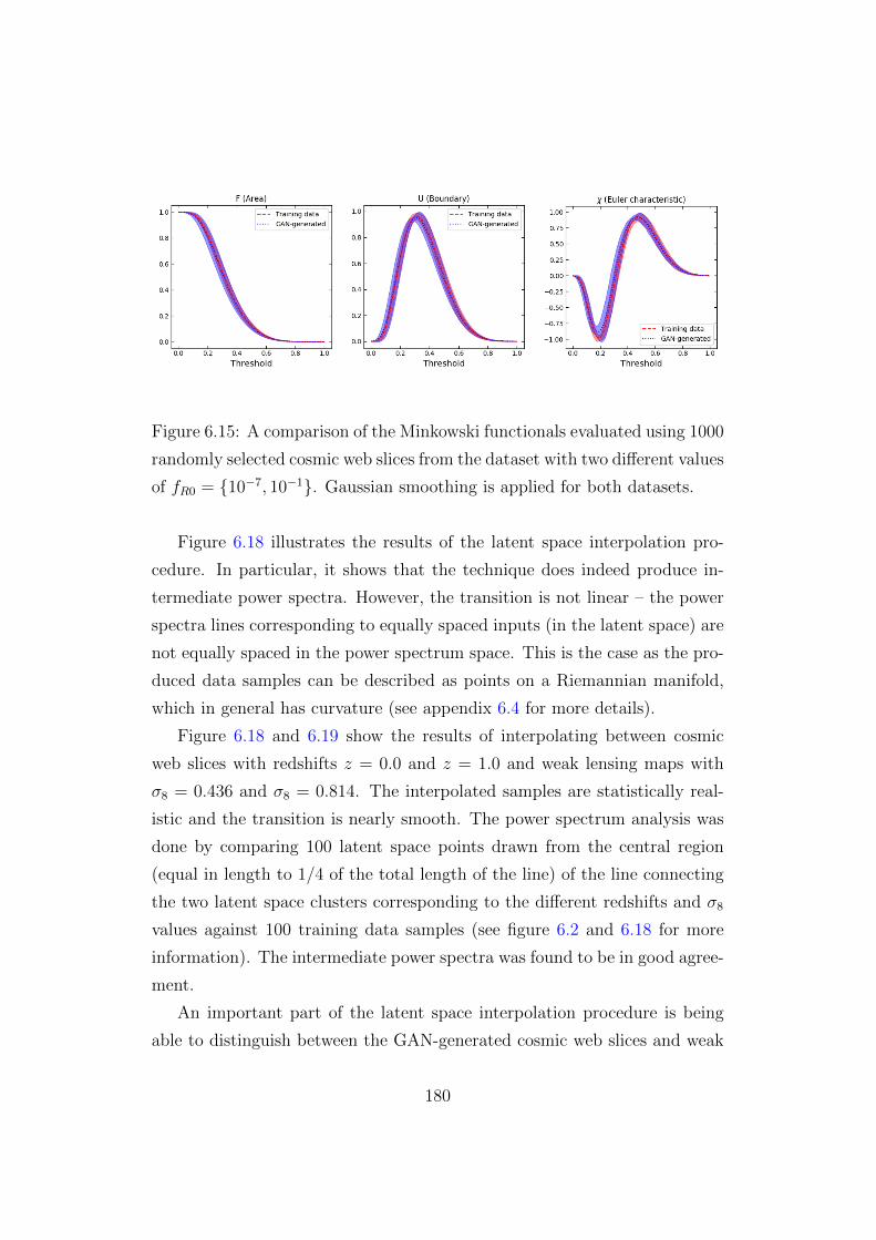
Figure 6.15: A comparison of the Minkowski functionals evaluated using 1000

randomly selected cosmic web slices from the dataset with two different values

of fR0 = 10−7, 10−1. Gaussian smoothing is applied for both datasets.

Figure 6.18 illustrates the results of the latent space interpolation pro-

cedure. In particular, it shows that the technique does indeed produce in-

termediate power spectra. However, the transition is not linear – the power

spectra lines corresponding to equally spaced inputs (in the latent space) are

not equally spaced in the power spectrum space. This is the case as the pro-

duced data samples can be described as points on a Riemannian manifold,

which in general has curvature (see appendix 6.4 for more details).

Figure 6.18 and 6.19 show the results of interpolating between cosmic

web slices with redshifts z = 0.0 and z = 1.0 and weak lensing maps with

σ8 = 0.436 and σ8 = 0.814. The interpolated samples are statistically real-

istic and the transition is nearly smooth. The power spectrum analysis was

done by comparing 100 latent space points drawn from the central region

(equal in length to 1/4 of the total length of the line) of the line connecting

the two latent space clusters corresponding to the different redshifts and σ8

values against 100 training data samples (see figure 6.2 and 6.18 for more

information). The intermediate power spectra was found to be in good agree-

ment.

An important part of the latent space interpolation procedure is being

able to distinguish between the GAN-generated cosmic web slices and weak

180

Figure 6.16: A selection of diagnostics to compare the training and the GAN-

produced multi-component cosmic web slices. Top left: the mean and the

standard deviation of the power spectrum for 1000 randomly chosen slices for

both datasets along with the corresponding relative difference between the

datasets (green for P gasTr /P

gasGAN − 1 and blue for PDM

Tr /PDMGAN − 1); top right:

same as top left, but with Gaussian smoothing applied; bottom left: the

cross-power spectrum calculated between 1000 randomly chosen dark matter

and the corresponding gas cosmic web pairs for both the training and the

GAN-produced datasets; bottom right: same as bottom left, but for the

gas-energy cross-power.

181

Figure 6.17: Results of the Minkowski functional analysis for the GAN

trained on the DM, gas and the internal energy data. Top row: Minkowski

functionals for the DM cosmic web slices; middle row: Minkowski func-

tionals for the gas overdensity slice data; bottom row: the corresponding

Minkowski functionals for the internal energy data. In all cases Gaussian

smoothing is applied.

182

lensing maps of different redshifts, cosmologies and modified gravity param-

eters. In this regard, I have tested two machine learning algorithms: a con-

volutional neural network and gradient boosted decision trees. Initially a

convoluational neural network architecture described in table 6.2 was used,

as we already knew that such neural networks are effective in classifying cos-

mic web slices and convergence maps. This resulted in accuracy of around

90% when classifying unseen data samples. However, the training procedure

was prone to overfitting, requiring a thorough hyperparameter optimization.

In addition, I found that the small scale noise appearing would highly reduce

the prediction accuracy of the CNN. This is a known problem in the deep

learning literature and can be mitigated to a certain degree by adding artifi-

cial noise to the training dataset (Liu et al., 2017). However, finding the right

amount of noise needed to mimic the noise appearing in the GAN-generated

outputs is difficult.

The gradient boosted decision tree algorithm (XGBoost (Chen and Guestrin,

2016)) was found to be faster and more accurate in predicting the dataset

class. In particular, 95-98% accuracy was reached (depending on the dataset

and hyperparameters used), when predicting the dataset class of unseen test

samples. Table 6.3 summarizes the parameters used when training the XG-

Boost algorithm.

Parameter: Learning rate Max. tree depth Training step Objective

Value: 0.08 2 0.3 multi:softprob

Table 6.3: The XGBoost parameters used for classifying the cosmic web

slices with redshifts z = 0.0, 1.0 and the weak lensing maps with σ8 =

0.436, 0.814.

Combining such a machine learning approach with a power spectrum

analysis allowed us to distinguish between the different classes of the GAN-

produced outputs reliably.

The latent space interpolation results illustrate a number of interesting

features of GANs. Firstly, the results illustrate that the GAN training pro-

183

(a) CW slice redshift interpolation (b) WL σ8 interpolation

Figure 6.18: The results of the linear latent space interpolation technique.

Left: the matter power spectrum corresponding to a linear interpolation

between two cosmic web slices of redshifts z = 0.0 and z = 1.0. The lines in

grey are the intermediate output slices generated by the procedure, while the

black line corresponds to the mean value of the power spectrum calculated

by choosing 100 random (training data) slices of redshift z = 0.5. The green

dashed line corresponds to the mean of 100 outputs produced using latent

space points lying close to the centre of the line connecting the two clusters

of redshifts z = 0.0 and z = 1.0. More specifically, 100 points from a region

equal to 1/4 of the total length of the line centered at the middle point was

sampled. Right: interpolating between two randomly chosen weak lensing

maps with different values of σ8. As before, the black line corresponds to

the mean power spectrum produced from 100 random maps with σ8 = 0.625.

The green line is the mean power spectrum of 100 outputs generated using

latent space points lying close to the centre of the line connecting the two

clusters corresponding to σ8 = 0.436 and σ8 = 0.814

cedure tightly encodes the various features discovered in our training dataset

in the high-dimensional latent space. By finding clusters in this latent space,

corresponding to outputs of different redshifts or cosmology parameters, and

linearly interpolating between them, we can produce outputs with intermedi-

184

ate values of the mentioned parameters. This allows us to control the outputs

produced by the generator.

Figure 6.19: The results of the latent space interpolation procedure for cosmic

web slices of redshifts z = 0.0 (far right) and z = 1.0 (far left) and weak

lensing convergence maps of σ18 = 0.436 (far left) and σ1

8 = 0.814 (far right).

6.8 Analysis and Conclusions

The main goal of this work was to investigate whether GANs can be used

as a universal, fast and efficient emulator capable of producing realistic and

novel mock data. The results of this work are encouraging, illustrating that

GANs are indeed capable of producing realistic mock datasets. In addi-

tion, I have shown that GANs can be used to emulate dark matter, gas and

internal energy distribution data simultaneously. This is a key result, as

generating realistic gas distributions requires complex and computationally

expensive hydrodynamical simulations. Hence, producing vast amounts of

realistic multi-component mock data quickly and efficiently will be of special

importance in the context of upcoming observational surveys.

The GAN-produced data in general cannot be distinguished from the

training dataset visually. In terms of the power spectrum analysis, the rela-

tive difference between the GAN-produced and the training data ranges be-

185

tween 1-20% depending on the dataset and whether Gaussian smoothing was

applied. The Minkowski functional analysis revealed a generally good agree-

ment between the two datasets with an exception of the third Minkowski

functional corresponding to curvature, which showed subtle differences for

all studied datasets. In addition, greater differences were observed when

training the GAN on datasets with multiple data classes. This is somewhat

expected, as the training task becomes more difficult. In general, these dif-

ferences can be partially accounted for as a result of small-scale noise in the

GAN-generated images. Gaussian smoothing with a 3 × 3 pixel kernel size

was found to be effective in filtering away most of such noise. In addition, the

training datasets used in this work are smaller than those used in (Rodrıguez

et al., 2018; Mustafa et al., 2019), which, at least partially, accounts for the

differences between our and their corresponding results.

A commonly used technique of latent space interpolation was also inves-

tigated as a tool for controlling the outputs of the generator neural network.

Interestingly, the results indicated that such a procedure allows us to gen-

erate samples with intermediate redshift/cosmology/fR0 parameter values,

even if our model had not been explicitly trained on those particular values.

In general, the latent space interpolation procedure offers a powerful way of

controlling the outputs of the GAN as well as a tool for investigating the

feature space of the generator neural network. However, it is important to

point out some of the drawbacks of this procedure. Namely, as pointed out

in machine learning literature, the latent space of a convolutional GAN is

known to be entangled. In other words, moving in a different direction in the

latent space necessarily causes multiple changes to the outputs of the GAN.

As a concrete example, finding a latent space line that induces a change in

redshift of a given output necessarily also introduces other subtle changes to

the output (e.g. the depth of the voids or the distribution of the filaments).

So if we take a random output of redshift z = 1.0 and perform the linear

interpolation procedure to obtain a cosmic web slice of z = 0.0, the obtained

slice will correspond to a realistic but different distribution of the required

186

redshift. This is a drawback as in an ideal case we would love to have full

control of individual parameters, while not affecting other independent fea-

tures of a dataset. There are however other generative models discussed in

the literature that allow such manipulation of the latent space. Namely, the

β-VAE variational autoencoder and the InfoGAN algorithms, allow encod-

ing features into the latent space in a special way that allows full control of

individual key parameters without affecting the other features of the dataset

(latent space disentanglement) (Chen and Guestrin, 2016; Higgins et al.,

2017; Burgess et al., 2018).

Another important pitfall to discuss is the problem of mode collapse. As

is widely discussed in the literature, the generator neural network is prone

to getting stuck in producing a very small subsample of realistic mock dat-

apoints that fool the discriminator neural network. Resolving mode collapse

is an important open problem in the field of deep learning, with a variety

of known strategies ranging from choosing a particular GAN architecture,

to altering the training procedure or the cost function (Srivastava et al.,

2017; Yicheng and Hong, 2019). Mode collapse was encountered multiple

times in our training procedure as well. As a rule of thumb, I found that

reducing the learning rate parameter had the biggest effect towards resolving

mode collapse for all studied datasets. Learning rates around the values of

RL = 3×10−5 for the cosmic web data and RL = 9×10−6 for the weak lensing

maps were found to be the most effective in avoiding any mode collapse.

As indicated by the results, GANs can be used to generate novel 2-D

data efficiently. A natural question to ask is whether this also applies to

3-D data. As an example, an analogous emulator capable of generating 3-D

cosmic web data, such as that produced by state of the art hydrodynamic

and DM-only simulations would be very useful. In principle there is no

limit on the dimensionality of the data used for training a GAN, however,

in practice, going from 2-D to 3-D data leads to a significant increase of the

generator and the discriminator networks. In addition, in the case of 3-D

cosmic web data, forming a big enough training dataset would become an

187

issue, as running thousands of simulations would be required. However, as

previously mentioned, there are sophisticated ways of emulating 3-D cosmic

web data as shown in (Perraudin et al., 2019), where a system of GANs

is used to upscale small resolution comic web cubes to full size simulation

boxes. Note that the techniques introduced in this work (e.g. latent space

interpolation) can be readily combined with the mentioned 3-D approach.

A number of interesting directions can be explored in future work. Namely,

it would be interesting to further investigate the latent space interpolation

techniques in the context of more advanced generative models, such as the

InfoGAN algorithm. In addition, a more detailed investigation into the Rie-

mannian geometry of GANs could lead to a better understanding of the

feature space of the algorithm. Finally, many other datasets could be ex-

plored. With upcoming surveys such as Euclid generating mock galaxy and

galaxy cluster data quickly and efficiently is of special interest. A GAN

could be used to generate galaxies with realistic intrinsic alignments, den-

sity distributions and other properties. Similarly, GANs could be used to

quickly emulate realistic galaxy cluster density distributions at a fraction of

the computational cost required to run full hydrodynamic simulations.

To conclude, GANs offer an entirely new approach for cosmological data

emulation. Such a game theory based approach has been demonstrated to

offer a quick and efficient way of producing novel data for a low computa-

tional cost. As we have shown in this work, the trade-off for this is a 1-20%

difference in the power spectrum, which can be satisfactory or not depending

on what application such an emulator is used for. Even though a number

of questions remain to be answered regarding the stability of the training

procedure and training on higher dimensional data, GANs will undoubtedly

be a useful tool for emulating cosmological data in the era of modern N -body

simulations and precision cosmology.

188

Chapter 7

Conclusions and Future Work

The main goal of this thesis was to introduce tools and techniques for study-

ing modified gravity. In summary, a method of testing modified gravity, first

introduced in Terukina et al. (2014) and Wilcox et al. (2015), was extended

by generating a new more accurate dataset and by testing a new theory. In

addition, machine learning techniques were explored in the context of emu-

lating ΛCDM and modified gravity N -body simulations.

In terms of all the mentioned projects, a lot of work remains to be done.

In particular, the outlined technique of testing modified gravity relies on

stacking multiple galaxy clusters. Stacking clusters, in some sense, produces

an idealized galaxy cluster by averaging out the various irregularities that

individual clusters possess. This is a powerful technique capable of produc-

ing competitive modified gravity constraints, however, the produced stack

dataset is only an approximation of real galaxy clusters. In nature, no clus-

ter is exactly spherical, hence it is important to understand what effects

deviations from spherical symmetry would have in the context of chameleon

gravity. Deviations from spherical symmetry must be better understood on

two fronts. Firstly, the hydrostatic equilibrium equations used in our work

must be generalized for arbitrary 3-D mass, pressure/temperature and sur-

face brightness distributions. Alternatively, the bias due to non-spherical

mass distributions can be quantified and accounted for in the mass calcula-

189

tions. Such bias has been studied both observationally and in the context

of hydrodynamic simulations, e.g. see Morandi et al. (2010); Martizzi and

Agrusa (2016). Secondly, it is important to understand how the theoretical

predictions are affected by breaking the assumption of spherical symmetry.

This is of special importance to the model of EG, the main predictions of

which were derived under the key assumption of spherical symmetry. Hence,

the predictions of the model for the relationship between the baryonic and the

apparent dark matter distributions must be generalized for arbitrary mass

distributions. This might be easier to accomplish in different models of EG,

such as Hossenfelder’s covariant EG.

The original motivation for stacking galaxy clusters is mainly due to the

dominant weak lensing profile errors. This particular issue will be possible to

address when the newest data from DES and future surveys such as Euclid

becomes available. Another approach is to employ different data. As shown

in Terukina et al. (2014), stringent constraints can be calculated using the

data from a single cluster. However, the main difference in that work when

compared to our approach is that the SZ effect and temperature profile data

is used in addition to the surface brightness and weak lensing profiles. As the

mentioned results show, including these extra datasets leads to constraints

comparable to the results presented in this work, even if a single cluster with

high quality is used rather than a stack of clusters. Hence, a straightforward

extension of our work is to introduce extra datasets, which could significantly

improve the constraints.

In addition to the previously mentioned shortcomings of EG, it is im-

portant to mention the lack of a rigid description of cosmology and weak

lensing. More concretely, the original formulation of EG as described in Ver-

linde (2017) is only valid for redshifts z ∼ 0 and H(z) ∼ H0. In addition, a

thorough description of lensing would require deriving a geodesic equation,

which, in turn, requires a full covariant description of the theory. A covari-

ant description of the theory does exist, as described in Hossenfelder (2017),

however, the lensing equations have not been derived yet. Hence, on the

190

theoretical front, the key issues to tackle are related to extending the orig-

inal Verlinde’s EG framework to account for cosmological effects and weak

lensing. Alternatively, Hossenfelder’s framework can be extended by deriv-

ing the geodesic equation. Here, however, it is important to point out that,

strictly speaking, these two theories are not identical and agree only in the

non-relativistic, stationary spherical mass distribution limit. The exact rela-

tionship between the two approaches deserves a more detailed investigation

as well.

In summary, EG undoubtedly suffers from certain theoretical and obser-

vational shortcomings. However, the theory has been successful in encourag-

ing further studies of the various connections between thermodynamics and

gravity. Multiple recent studies have extended Verlinde’s ideas in different

contexts, e.g. Vacaru and Bubuianu (2019); Peach (2019). Finally, Verlinde’s

work has also contributed to the current resurgence of the rather unique ap-

proach of treating gravity as spacetime elasticity previously studied in Visser

(2002); Padmanabhan (2004).

In terms of the machine learning algorithms discussed in chapters 5 and 6

a lot of work remains to be done as well. As mentioned, the results in Tamo-

siunas et al. (2020) are encouraging, however, multiple issues remain to be

addressed. Firstly, using GANs for emulating 3-D simulation data remains

an issue in terms of the memory issues and the availability of large 3-D train-

ing datasets. These and other issues have already been partially addressed

in the literature. As an example, the training procedure of the GAN can

be modified such that small 3-D overdensity cubes are patched together to

form a full-size 3-D overdensity field as shown in Perraudin et al. (2019). An

alternative approach is to start with a low resolution mock dataset, which is

gradually upscaled during a multi-stage training procedure (e.g. see Ledig

et al. (2016)). These sort of approaches combined with modern GPU training

will likely make emulating 3-D datasets easy and efficient in the near future.

Another key issue encountered in our work was controlling the outputs.

In particular, when training the algorithm on a dataset consisting of differ-

191

ent data classes, the simple DCGAN architecture does not allow to control

which outputs will be produced. In other words, one cannot choose the out-

put class due to the inherent randomness of the generation procedure. The

proposed workaround discussed in this work was to use the latent space in-

terpolation procedure, which resolves the problem partially. However, the

key issue with the procedure is that it is not efficient as it requires one to

manually detect interesting regions of the latent space that can be used in

the interpolation. A much more elegant approach is to use a different GAN

architecture that is specifically designed for producing multi-class data. In

particular, the conditional GAN architecture (CGAN) allows to take full con-

trol of the generation procedure. In this architecture the neural networks are

trained using labeled data and hence the outputs of the generator can be

controlled by directly specifying the label of the class to be generated. As a

concrete example, this type of architecture has been recently used to gener-

ate convergence maps with different cosmological parameters as described in

Perraudin et al. (2020). Hence a natural extension of our work would be to

apply the techniques described in this thesis on different GAN architectures.

This would lead not only to more control of the data generation, but also to

a better understanding of the latent space. Finally, alternative architectures,

such as the mentioned CGAN algorithm, would make it easier to explore

the Riemannian geometry of the latent space produced during the training

procedure.

As shown in this work, generative models offer a completely new approach

of generating mock data. Like any algorithm such models come with a set

of shortcomings. However, the ability to generate large multi-class mock

datasets quickly and efficiently undoubtedly makes such algorithms useful.

This is especially true in the context of the upcoming large scale surveys such

as Euclid and SKA, which will require accurate and fast emulators.

In conclusion, observational tests of gravity have traditionally played an

important role in the theoretical development of theories of modified grav-

ity and dark energy. Starting with the initial tests of GR and ending with

192

cutting edge gravitational wave tests, viable theories of gravity have always

been firmly constrained by the most recent observational data. The set of

techniques described in this work draws an optimistic picture for the near

future of cosmological tests of modified gravity. With the next generation

of observational surveys and new high quality data becoming available, con-

straints of unprecedented accuracy will become possible. Similarly, with the

new machine learning techniques becoming available, new ways of emulating

modified gravity will become possible as well. And hence the techniques de-

scribed in this work will hopefully play an important role in forming a better

understanding of gravity.

193

Appendices

194

Appendix A

A.1 Availability of Data and Codes

The key datasets generated and analysed in this work are available at the fol-

lowing GitHub repository: https://github.com/AndriusT/cw wl GAN. The

link also contains detailed instructions on how to produce the data samples

from the publicly available Illustris data. The full Illustris datasets can be

found at: https://www.illustris-project.org/data/.

The used weak lensing data can be accessed at: http://columbialensing.org/.

A.2 Samples of the GAN-produced Data

This section contains a selection of GAN-produced samples for visual inspec-

tion. Fig. A.1 contains randomly selected weak lensing convergence maps

produced by the GAN algorithm (these are the samples described in sections

6.7.2 and 6.7.3).

Fig. A.2 shows a selection of randomly selected cosmic web 2-D slices for

two different redshifts. Both the training data and the produced slices have

been Gaussian-smoothed.

195

Figure A.1: A comparison of 4 randomly selected weak lensing convergence

maps. The colors are log-normalized to emphasize the main features and to

allow a direct comparison with the results in Mustafa et al. (2019).

Figure A.2: A comparison of 4 randomly selected cosmic web slices. Columns

1 and 3 correspond to redshift 0.0 while columns 2 and 4 are redshift 1.0.

196

A.3 MCMC Contours

This section contains the MCMC contours along with the corresponding like-

lihood distributions for the key datasets used in chapter 3. In particular, the

MCMC results from Terukina et al. (2014), Wilcox et al. (2015) and our

results produced using the newest dataset consisting of 77 galaxy clusters.

In all cases, the light gray contours correspond to the 99% CL, while the

dark gray contours are the 95% CL for each best-fit parameter. Notice also

that the colors in the individual modified gravity parameter plots appearing

in chapter 3 are inverted for the sake of clarity when comparing the results

from different papers.

197

Figure A.3: The MCMC marginalised contours of the 6 model parameters

used in Terukina et al. (2014) to fit the data. The light gray and the dark

gray contours show the 95% and the 99% CL correspondingly. The right-

most panels show the marginalised 1-dimensional constraints (solid) and the

likelihood distribution (dotted).

198

Figure A.4: The MCMC marginalised contours of the 14 model parameters

used in Wilcox et al. (2015) to fit the data. The light gray and the dark gray

contours show the 95% and the 99% CL correspondingly. The rightmost

panels show the likelihood distribution.

199

Figure A.5: The MCMC marginalised contours of the 14 model parameters

determined using the newest dataset of 77 galaxy clusters. The light gray

and the dark gray contours show the 95% and the 99% CL correspondingly.

The rightmost panels show the likelihood distribution.

200

Bibliography

M. Abadi, A. Agarwal, P. Barham, E. Brevdo, Z. Chen, C. Citro, G. S. Cor-

rado, A. Davis, J. Dean, M. Devin, S. Ghemawat, I. Goodfellow, A. Harp,

G. Irving, M. Isard, Y. Jia, R. Jozefowicz, L. Kaiser, M. Kudlur, J. Lev-

enberg, D. Mane, R. Monga, S. Moore, D. Murray, C. Olah, M. Schus-

ter, J. Shlens, B. Steiner, I. Sutskever, K. Talwar, P. Tucker, V. Van-

houcke, V. Vasudevan, F. Viegas, O. Vinyals, P. Warden, M. Wattenberg,

M. Wicke, Y. Yu, and X. Zheng. TensorFlow: Large-scale machine learning

on heterogeneous systems, 2015. URL https://www.tensorflow.org/.

Software available from tensorflow.org.

K. N. Abazajian, P. Adshead, Z. Ahmed, S. W. Allen, D. Alonso, K. S.

Arnold, C. Baccigalupi, J. G. Bartlett, N. Battaglia, B. A. Benson, C. A.

Bischoff, J. Borrill, V. Buza, E. Calabrese, R. Caldwell, J. E. Carlstrom,

C. L. Chang, T. M. Crawford, F.-Y. Cyr-Racine, F. De Bernardis, T. de

Haan, S. di Serego Alighieri, J. Dunkley, C. Dvorkin, J. Errard, G. Fab-

bian, S. Feeney, S. Ferraro, J. P. Filippini, R. Flauger, G. M. Fuller,

V. Gluscevic, D. Green, D. Grin, E. Grohs, J. W. Henning, J. C. Hill,

R. Hlozek, G. Holder, W. Holzapfel, W. Hu, K. M. Huffenberger, R. Keski-

talo, L. Knox, A. Kosowsky, J. Kovac, E. D. Kovetz, C.-L. Kuo, A. Kusaka,

M. Le Jeune, A. T. Lee, M. Lilley, M. Loverde, M. S. Madhavacheril,

A. Mantz, D. J. E. Marsh, J. McMahon, P. D. Meerburg, J. Meyers, A. D.

Miller, J. B. Munoz, H. N. Nguyen, M. D. Niemack, M. Peloso, J. Peloton,

L. Pogosian, C. Pryke, M. Raveri, C. L. Reichardt, G. Rocha, A. Rotti,

E. Schaan, M. M. Schmittfull, D. Scott, N. Sehgal, S. Shandera, B. D. Sher-

201

win, T. L. Smith, L. Sorbo, G. D. Starkman, K. T. Story, A. van Engelen,

J. D. Vieira, S. Watson, N. Whitehorn, and W. L. Kimmy Wu. CMB-S4

Science Book, First Edition. arXiv e-prints, art. arXiv:1610.02743, Oct.

2016.

B. P. Abbott, LIGO Scientific Collaboration, and Virgo Collaboration.

GW170817: Observation of Gravitational Waves from a Binary Neu-

tron Star Inspiral. Phys. Rev. Lett, 119(16):161101, Oct. 2017. doi:

10.1103/PhysRevLett.119.161101.

B. P. Abbott et al. Gravitational Waves and Gamma-rays from a Binary

Neutron Star Merger: GW170817 and GRB 170817A. Astrophys. J., 848

(2):L13, 2017. doi: 10.3847/2041-8213/aa920c.

T. Abbott et al. Cosmological Constraints from Multiple Probes in the Dark

Energy Survey. Phys. Rev. Lett., 122(17):171301, 2019. doi: 10.1103/

PhysRevLett.122.171301.

B. P. Abbott et al. A gravitational-wave standard siren measurement of

the Hubble constant. Nature, 551(7678):85–88, Nov. 2017. doi: 10.1038/

nature24471.

P. Ade et al. Planck intermediate results. XL. The Sunyaev-Zeldovich signal

from the Virgo cluster. A&A, 596:A101, 2016. doi: 10.1051/0004-6361/

201527743.

I. Agullo and P. Singh. Loop Quantum Cosmology: A brief review. arXiv

e-prints, art. arXiv:1612.01236, Dec. 2016.

T. Anam and F. F. Nitol. Decision tree, 2018. URL

http://rstudio-pubs-static.s3.amazonaws.com/381472_

c2054f778a4b46aabe36e6a7dd410db9.html#(1). [Online; accessed

November 18, 2020].

202

H. Andernach and F. Zwicky. English and Spanish Translation of Zwicky’s

(1933) The Redshift of Extragalactic Nebulae. arXiv e-prints, art.

arXiv:1711.01693, Nov. 2017.

E. Anderson. The species problem in iris. Annals of the Missouri Botanical

Garden, 23(3):457–469, 10 1936. doi: 10.2307/2394164.

Annual Reviews of Astronomy and Astrophysics. The Sunyaev-Zel’Dovich

Effect. https://ned.ipac.caltech.edu/level5/Sept05/Carlstrom/

Carlstrom2.html, 2002. [Online; accessed November 18, 2020].

M. Arjovsky, S. Chintala, and L. Bottou. Wasserstein GAN. arXiv e-prints,

art. arXiv:1701.07875, Jan 2017.

T. J. Armitage, S. T. Kay, and D. J. Barnes. An application of machine

learning techniques to galaxy cluster mass estimation using the MACSIS

simulations. MNRAS, 484(2):1526–1537, Apr. 2019. doi: 10.1093/mnras/

stz039.

K. A. Arnaud. XSPEC: The First Ten Years, volume 101 of Astronomical

Society of the Pacific Conference Series, page 17. Astronomical Society of

the Pacific Conference Series, 1996.

C. Arnold, E. Puchwein, and V. Springel. Scaling relations and mass bias in

hydrodynamical f(R) gravity simulations of galaxy clusters. MNRAS, 440

(1):833–842, May 2014. doi: 10.1093/mnras/stu332.

N. A. Bahcall. Large-scale structure in the universe indicated by galaxy

clusters. Annual Review of Astronomy and Astrophysics, 26:631–686, Jan.

1988. doi: 10.1146/annurev.aa.26.090188.003215.

N. A. Bahcall and R. Cen. Galaxy Clusters and Cold Dark Matter: A

Low-Density Unbiased Universe? ApJ Lett., 398:L81, Oct. 1992. doi:

10.1086/186582.

203

A. Bain. Mind and Body. The Theories of their Relation. New York: D.

Appleton and Company, 1873. URL https://archive.org/details/

mindbodytheories00bain/.

T. Baker, D. Psaltis, and C. Skordis. LINKING TESTS OF GRAVITY ON

ALL SCALES: FROM THE STRONG-FIELD REGIME TO COSMOL-

OGY. ApJ, 802(1):63, mar 2015. doi: 10.1088/0004-637x/802/1/63.

T. Baker, E. Bellini, P. G. Ferreira, M. Lagos, J. Noller, and I. Sawicki. Strong

Constraints on Cosmological Gravity from GW170817 and GRB 170817A.

Phys. Rev. Lett., 119(25):251301, Dec. 2017. doi: 10.1103/PhysRevLett.

119.251301.

A. Balaguera-Antolınez. What can the spatial distribution of galaxy clusters

tell about their scaling relations? A&A, 563:A141, Mar. 2014. doi: 10.

1051/0004-6361/201322029.

M. Bartelmann and M. Maturi. Weak gravitational lensing. Scholarpedia, 12

(1):32440, Jan. 2017. doi: 10.4249/scholarpedia.32440.

M. Bartelmann, A. Huss, J. M. Colberg, A. Jenkins, and F. R. Pearce. Arc

statistics with realistic cluster potentials. IV. Clusters in different cosmolo-

gies. A&A, 330:1–9, Feb. 1998.

S. Basilakos and M. Plionis. Modelling the two-point correlation function of

galaxy clusters in the Sloan Digital Sky Survey. MNRAS, 349(3):882–888,

04 2004. ISSN 0035-8711. doi: 10.1111/j.1365-2966.2004.07559.x.

N. Battaglia, J. R. Bond, C. Pfrommer, and J. L. Sievers. On the Clus-

ter Physics of Sunyaev-Zel’dovich and X-Ray Surveys. I. The Influence

of Feedback, Non-thermal Pressure, and Cluster Shapes on Y-M Scaling

Relations. ApJ, 758(2):74, Oct. 2012. doi: 10.1088/0004-637X/758/2/74.

P. S. Behroozi, R. H. Wechsler, and H.-Y. Wu. The ROCKSTAR Phase-space

Temporal Halo Finder and the Velocity Offsets of Cluster Cores. ApJ, 762

(2):109, Jan. 2013. doi: 10.1088/0004-637X/762/2/109.

204

J. D. Bekenstein. Black holes and entropy. Phys. Rev. D, 7:2333–2346, Apr

1973. doi: 10.1103/PhysRevD.7.2333. URL https://link.aps.org/doi/

10.1103/PhysRevD.7.2333.

C. A. Bengaly, R. Maartens, N. Randriamiarinarivo, and A. Baloyi. Testing

the cosmological principle in the radio sky. JCAP, 2019(09):025–025, sep

2019. doi: 10.1088/1475-7516/2019/09/025.

L. Berezhiani and J. Khoury. Theory of dark matter superfluidity. Phys.

Rev. D, 92(10):103510, Nov. 2015. doi: 10.1103/PhysRevD.92.103510.

E. Berti et al. Testing general relativity with present and future astrophysical

observations. Classical and Quantum Gravity, 32(24):243001, Dec. 2015.

doi: 10.1088/0264-9381/32/24/243001.

B. Bertotti, L. Iess, and P. Tortora. A test of general relativity using radio

links with the Cassini spacecraft. Nature, 425:374–376, 2003. doi: 10.1038/

nature01997.

V. Biffi, K. Dolag, H. Boehringer, and G. Lemson. PHOX: X-ray Photon

Simulator, Dec. 2011.

M. Birkinshaw. The Sunyaev-Zel’dovich effect. Phys. Rep., 310(2-3):97–195,

Mar. 1999. doi: 10.1016/S0370-1573(98)00080-5.

D. Blas and E. Lim. Phenomenology of theories of gravity without Lorentz

invariance: The preferred frame case. International Journal of Modern

Physics D, 23(13):1443009, Jan. 2014. doi: 10.1142/S0218271814430093.

K. Bolejko and M. Korzynski. Inhomogeneous cosmology and backreaction:

Current status and future prospects. International Journal of Modern

Physics D, 26(6):1730011, Jan. 2017. doi: 10.1142/S0218271817300117.

S. Borgani. Cosmology with clusters of galaxies. Lect. Notes Phys., 740:287,

2008. doi: 10.1007/978-1-4020-6941-3\ 9.

205

M. M. Brouwer, M. R. Visser, A. Dvornik, H. Hoekstra, K. Kuijken, E. A.

Valentijn, M. Bilicki, C. Blake, S. Brough, H. Buddelmeijer, T. Erben,

C. Heymans, H. Hildebrandt, B. W. Holwerda, A. M. Hopkins, D. Klaes,

J. Liske, J. Loveday, J. McFarland, R. Nakajima, C. Sifon, and E. N. Tay-

lor. First test of Verlinde’s theory of emergent gravity using weak gravita-

tional lensing measurements. MNRAS, 466(3):2547–2559, Apr. 2017. doi:

10.1093/mnras/stw3192.

J. R. Brownstein and J. W. Moffat. Galaxy cluster masses without non-

baryonic dark matter. MNRAS, 367(2):527–540, Apr. 2006. doi: 10.1111/

j.1365-2966.2006.09996.x.

G. L. Bryan, M. L. Norman, B. W. O’Shea, T. Abel, J. H. Wise, M. J.

Turk, D. R. Reynolds, D. C. Collins, P. Wang, S. W. Skillman, B. Smith,

R. P. Harkness, J. Bordner, J.-h. Kim, M. Kuhlen, H. Xu, N. Goldbaum,

C. Hummels, A. G. Kritsuk, E. Tasker, S. Skory, C. M. Simpson, O. Hahn,

J. S. Oishi, G. C. So, F. Zhao, R. Cen, Y. Li, and Enzo Collaboration.

ENZO: An Adaptive Mesh Refinement Code for Astrophysics. ApJS, 211

(2):19, Apr. 2014. doi: 10.1088/0067-0049/211/2/19.

J. S. Bullock and M. Boylan-Kolchin. Small-Scale Challenges to the ΛCDM

Paradigm. Anual Review of Astronomy and Astrophysics, 55(1):343–387,

Aug. 2017. doi: 10.1146/annurev-astro-091916-055313.

C. P. Burgess, I. Higgins, A. Pal, L. Matthey, N. Watters, G. Desjardins,

and A. Lerchner. Understanding disentangling in β-VAE. arXiv e-prints,

art. arXiv:1804.03599, Apr. 2018.

C. Burrage and J. Sakstein. A compendium of chameleon constraints. JCAP,

2016(11):045, Nov. 2016. doi: 10.1088/1475-7516/2016/11/045.

C. Burrage and J. Sakstein. Tests of chameleon gravity. Living Reviews in

Relativity, 21(1):1, Mar. 2018. doi: 10.1007/s41114-018-0011-x.

206

J. Caldeira, W. L. K. Wu, B. Nord, C. Avestruz, S. Trivedi, and K. T. Story.

DeepCMB: Lensing reconstruction of the cosmic microwave background

with deep neural networks. Astronomy and Computing, 28:100307, July

2019. doi: 10.1016/j.ascom.2019.100307.

S. Carlip. Black hole thermodynamics. International Journal of

Modern Physics D, 23(11):1430023-736, Oct. 2014. doi: 10.1142/

S0218271814300237.

S. Casertano, A. G. Riess, J. Anderson, R. I. Anderson, J. B. Bowers, K. I.

Clubb, A. R. Cukierman, A. V. Filippenko, M. L. Graham, J. W. MacK-

enty, C. Melis, B. E. Tucker, and G. Upadhya. Parallax of Galactic

Cepheids from Spatially Scanning the Wide Field Camera 3 on the Hub-

ble Space Telescope: The Case of SS Canis Majoris. ApJ, 825(1):11, July

2016. doi: 10.3847/0004-637X/825/1/11.

M. Cataneo, D. Rapetti, L. Lombriser, and B. Li. Cluster abundance in

chameleon f(R) gravity I: toward an accurate halo mass function predic-

tion. JCAP, 2016(12):024, Dec. 2016. doi: 10.1088/1475-7516/2016/12/

024.

A. Cavaliere and R. Fusco-Femiano. X-rays from hot plasma in clusters of

galaxies. A&A, 500:95–102, May 1976.

T. Chen and C. Guestrin. XGBoost: A Scalable Tree Boosting System. arXiv

e-prints, art. arXiv:1603.02754, Mar. 2016.

T. Chen and C. Guestrin. Xgboost: A scalable tree boosting system.

In Proceedings of the 22nd ACM SIGKDD International Conference on

Knowledge Discovery and Data Mining, KDD ’16, pages 785–794, New

York, NY, USA, 2016. Association for Computing Machinery. ISBN

9781450342322. doi: 10.1145/2939672.2939785. URL https://doi.org/

10.1145/2939672.2939785.

207

E. Churazov, A. Vikhlinin, I. Zhuravleva, A. Schekochihin, I. Parrish, R. Sun-

yaev, W. Forman, H. Bohringer, and S. Randall. X-ray surface brightness

and gas density fluctuations in the Coma cluster. MNRAS, 421(2):1123–

1135, 03 2012. ISSN 0035-8711. doi: 10.1111/j.1365-2966.2011.20372.x.

URL https://doi.org/10.1111/j.1365-2966.2011.20372.x.

D. Clowe, M. Bradac, A. H. Gonzalez, M. Markevitch, S. W. Randall,

C. Jones, and D. Zaritsky. A Direct Empirical Proof of the Exis-

tence of Dark Matter. ApJ Lett., 648(2):L109–L113, Sept. 2006. doi:

10.1086/508162.

S. Cole, W. J. Percival, J. A. Peacock, P. Norberg, C. M. Baugh, C. S.

Frenk, I. Baldry, J. Bland-Hawthorn, T. Bridges, R. Cannon, M. Colless,

C. Collins, W. Couch, N. J. G. Cross, G. Dalton, V. R. Eke, R. de Pro-

pris, S. P. Driver, G. Efstathiou, R. S. Ellis, K. Glazebrook, C. Jackson,

A. Jenkins, O. Lahav, I. Lewis, S. Lumsden, S. Maddox, D. Madgwick,

B. A. Peterson, W. Sutherland, K. Taylor, and T. 2dFGRS Team. The

2dF Galaxy Redshift Survey: power-spectrum analysis of the final data set

and cosmological implications. MNRAS, 362(2):505–534, 09 2005. ISSN

0035-8711. doi: 10.1111/j.1365-2966.2005.09318.x.

T. E. Collett, L. J. Oldham, R. J. Smith, M. W. Auger, K. B. Westfall,

D. Bacon, R. C. Nichol, K. L. Masters, K. Koyama, and R. van den Bosch.

A precise extragalactic test of general relativity. Science, 360(6395):1342–

1346, 2018. ISSN 0036-8075. doi: 10.1126/science.aao2469.

Columbia Lensing. Columbia Lensing Group Data Products. http://

columbialensing.org, Online; accessed 2020-01-24, 2020.

R. Curley. Scientists and Inventors of the Renaissance. The Renaissance.

Rosen Publishing Group, 2012. ISBN 9781615308842.

D.-C. Dai and D. Stojkovic. Inconsistencies in Verlinde’s emergent gravity.

JHEP, 2017(11):7, Nov. 2017a. doi: 10.1007/JHEP11(2017)007.

208

D.-C. Dai and D. Stojkovic. Comment on “Covariant version of Verlinde’s

emergent gravity”. Phys. Rev. D, 96(10):108501, Nov. 2017b. doi: 10.

1103/PhysRevD.96.108501.

P. C. W. Davies. Scalar production in schwarzschild and rindler met-

rics. Journal of Physics A: Mathematical and General, 8(4):609–616, apr

1975. doi: 10.1088/0305-4470/8/4/022. URL https://doi.org/10.1088%

2F0305-4470%2F8%2F4%2F022.

A. De Felice and S. Tsujikawa. f(R) Theories. Living Reviews in Relativity,

13(1):3, June 2010. doi: 10.12942/lrr-2010-3.

A. de la Cruz-Dombriz, P. K. S. Dunsby, S. Kand hai, and D. Saez-Gomez.

Theoretical and observational constraints of viable f(R) theories of gravity.

Phys. Rev. D, 93(8):084016, Apr. 2016. doi: 10.1103/PhysRevD.93.084016.

H. Desmond, P. G. Ferreira, G. Lavaux, and J. Jasche. Reconstructing the

gravitational field of the local Universe. MNRAS, 474(3):3152–3161, Mar.

2018. doi: 10.1093/mnras/stx3062.

J. P. Dietrich and J. Hartlap. Cosmology with the shear-peak statistics.

MNRAS, 402(2):1049–1058, 02 2010. ISSN 0035-8711. doi: 10.1111/j.

1365-2966.2009.15948.x. URL https://doi.org/10.1111/j.1365-2966.

2009.15948.x.

A. Drlica-Wagner, I. Sevilla-Noarbe, E. S. Rykoff, R. A. Gruendl, B. Yanny,

D. L. Tucker, B. Hoyle, A. Carnero Rosell, G. M. Bernstein, K. Bechtol,

M. R. Becker, A. Benoit-Levy, E. Bertin, M. Carrasco Kind, C. Davis,

J. de Vicente, H. T. Diehl, D. Gruen, W. G. Hartley, B. Leistedt, T. S.

Li, J. L. Marshall, E. Neilsen, M. M. Rau, E. Sheldon, J. Smith, M. A.

Troxel, S. Wyatt, Y. Zhang, T. M. C. Abbott, F. B. Abdalla, S. Allam,

M. Banerji, D. Brooks, E. Buckley-Geer, D. L. Burke, D. Capozzi, J. Car-

retero, C. E. Cunha, C. B. D’Andrea, L. N. da Costa, D. L. DePoy, S. De-

sai, J. P. Dietrich, P. Doel, A. E. Evrard, A. Fausti Neto, B. Flaugher,

209

P. Fosalba, J. Frieman, J. Garcıa-Bellido, D. W. Gerdes, T. Giannanto-

nio, J. Gschwend, G. Gutierrez, K. Honscheid, D. J. James, T. Jeltema,

K. Kuehn, S. Kuhlmann, N. Kuropatkin, O. Lahav, M. Lima, H. Lin,

M. A. G. Maia, P. Martini, R. G. McMahon, P. Melchior, F. Menan-

teau, R. Miquel, R. C. Nichol, R. L. C. Ogand o, A. A. Plazas, A. K.

Romer, A. Roodman, E. Sanchez, V. Scarpine, R. Schindler, M. Schub-

nell, M. Smith, R. C. Smith, M. Soares-Santos, F. Sobreira, E. Suchyta,

G. Tarle, V. Vikram, A. R. Walker, R. H. Wechsler, J. Zuntz, and

DES Collaboration. Dark Energy Survey Year 1 Results: The Pho-

tometric Data Set for Cosmology. ApJS, 235(2):33, Apr. 2018. doi:

10.3847/1538-4365/aab4f5.

D. Dua and C. Graff. UCI machine learning repository, 2017. URL http:

//archive.ics.uci.edu/ml.

F. W. Dyson, A. S. Eddington, and C. Davidson. Ix. a determination

of the deflection of light by the sun’s gravitational field, from observa-

tions made at the total eclipse of may 29, 1919. Philosophical Trans-

actions of the Royal Society of London. Series A, Containing Papers of

a Mathematical or Physical Character, 220(571-581):291–333, 1920. doi:

10.1098/rsta.1920.0009. URL https://royalsocietypublishing.org/

doi/abs/10.1098/rsta.1920.0009.

A. Einstein. Die grundlage der allgemeinen relativitatstheorie. Annalen der

Physik, 354(7):769–822, 1916. doi: 10.1002/andp.19163540702.

B. Elder, J. Khoury, P. Haslinger, M. Jaffe, H. Muller, and P. Hamilton.

Chameleon dark energy and atom interferometry. Phys. Rev. D, 94(4):

044051, Aug. 2016. doi: 10.1103/PhysRevD.94.044051.

End-to-End Machine Learning. Machine Learning Course Library. https:

//e2eml.school/blog.html, 2020. [Online; accessed November 18, 2020].

T. Erben, H. Hildebrandt, L. Miller, L. van Waerbeke, C. Heymans,

H. Hoekstra, T. D. Kitching, Y. Mellier, J. Benjamin, C. Blake, C. Bon-

210

nett, O. Cordes, J. Coupon, L. Fu, R. Gavazzi, B. Gillis, E. Grocutt,

S. D. J. Gwyn, K. Holhjem, M. J. Hudson, M. Kilbinger, K. Kuijken,

M. Milkeraitis, B. T. P. Rowe, T. Schrabback, E. Semboloni, P. Si-

mon, M. Smit, O. Toader, S. Vafaei, E. van Uitert, and M. Velander.

CFHTLenS: the Canada-France-Hawaii Telescope Lensing Survey - imag-

ing data and catalogue products. MNRAS, 433(3):2545–2563, Aug. 2013.

doi: 10.1093/mnras/stt928.

ESA-Planck. The coma cluster. https://sci.esa.int/web/planck/-/

47695-the-coma-cluster, 2010. Accessed: 2020-05-03.

S. Ettori, A. Donnarumma, E. Pointecouteau, T. H. Reiprich, S. Giodini,

L. Lovisari, and R. W. Schmidt. Mass Profiles of Galaxy Clusters from

X-ray Analysis. Space Science Reviews, 177(1-4):119–154, Aug. 2013. doi:

10.1007/s11214-013-9976-7.

S. Ettori, V. Ghirardini, D. Eckert, F. Dubath, and E. Pointecouteau. Dark

matter distribution in X-ray luminous galaxy clusters with Emergent Grav-

ity. MNRAS, 470(1):L29–L33, Sept. 2017. doi: 10.1093/mnrasl/slx074.

S. Ettori, V. Ghirardini, D. Eckert, E. Pointecouteau, F. Gastaldello,

M. Sereno, M. Gaspari, S. Ghizzardi, M. Roncarelli, and M. Rossetti.

Hydrostatic mass profiles in X-COP galaxy clusters. A&A, 621:A39, Jan.

2019. doi: 10.1051/0004-6361/201833323.

Euclid Theory Working Grp. Cosmology and fundamental physics with the

euclid satellite. Living Reviews in Relativity, 21:1–345, 4 2018. ISSN 1433-

8351. doi: 10.1007/s41114-017-0010-3.

J. Evans. The History and Practice of Ancient Astronomy. Oxford University

Press, USA, 1998. ISBN 9780195095395.

J. M. Ezquiaga and M. Zumalacarregui. Dark Energy After GW170817:

Dead Ends and the Road Ahead. Phys. Rev. Lett., 119(25):251304, Dec.

2017. doi: 10.1103/PhysRevLett.119.251304.

211

A. Fabian. Clusters and superclusters of galaxies. NATO ASI series: Math-

ematical and physical sciences. Kluwer Academic Publishers, 1992. ISBN

9780792317029.

F. Farnia and A. Ozdaglar. GANs May Have No Nash Equilibria. arXiv

e-prints, art. arXiv:2002.09124, Feb. 2020.

C. Fefferman, S. Mitter, and H. Narayanan. Testing the Manifold Hypothesis.

arXiv e-prints, art. arXiv:1310.0425, Oct. 2013.

F. Figueras, J. Girart, M. Hernanz, and C. Jordi. Highlights of Spanish As-

trophysics IV: Proceedings of the Seventh Scientific Meeting of the Spanish

Astronomical Society (SEA) held in Barcelona, Spain, September 12-15,

2006. Proceedings of the 7th Scientific Meeting of the Spanish Astro-

nomical Society (Sea) Held in Barcelona, Spain, September 12-15, 2006.

Springer Netherlands, 2007. ISBN 9781402060007.

W. L. Freedman, B. F. Madore, D. Hatt, T. J. Hoyt, I. S. Jang, R. L. Beaton,

C. R. Burns, M. G. Lee, A. J. Monson, J. R. Neeley, M. M. Phillips,

J. A. Rich, and M. Seibert. The Carnegie-Chicago Hubble Program. VIII.

An Independent Determination of the Hubble Constant Based on the Tip

of the Red Giant Branch. ApJ, 882(1):34, Sept. 2019. doi: 10.3847/

1538-4357/ab2f73.

K. Freese. Status of dark matter in the universe. International Jour-

nal of Modern Physics D, 26(6):1730012-223, Jan. 2017. doi: 10.1142/

S0218271817300129.

J. H. Friedman. Greedy function approximation: A gradient boosting

machine. Ann. Statist., 29(5):1189–1232, 10 2001. doi: 10.1214/aos/

1013203451. URL https://doi.org/10.1214/aos/1013203451.

A. Friedmann. Uber die Krummung des Raumes. Zeitschrift fur Physik, 10:

377–386, Jan. 1922. doi: 10.1007/BF01332580.

212

Y. Fujita and Y. Ohira. STABLE HEATING OF CLUSTER COOLING

FLOWS BY COSMIC-RAY STREAMING. The Astrophysical Journal,

738(2):182, aug 2011. doi: 10.1088/0004-637x/738/2/182. URL https:

//doi.org/10.1088%2F0004-637x%2F738%2F2%2F182.

S. A. Fulling. Nonuniqueness of canonical field quantization in rie-

mannian space-time. Phys. Rev. D, 7:2850–2862, May 1973. doi:

10.1103/PhysRevD.7.2850. URL https://link.aps.org/doi/10.1103/

PhysRevD.7.2850.

R. Gavazzi, C. Adami, F. Durret, J. C. Cuillandre, O. Ilbert, A. Mazure,

R. Pello, and M. P. Ulmer. A weak lensing study of the Coma cluster.

A&A, 498(2):L33–L36, May 2009. doi: 10.1051/0004-6361/200911841.

J. Gine. On the origin of the deflection of light. Chaos, Solitons & Fractals,

35(1):1 – 6, 2008. ISSN 0960-0779. doi: https://doi.org/10.1016/j.chaos.

2007.06.097.

M. Girardi, A. Biviano, G. Giuricin, F. Mardirossian, and M. Mezzetti.

Velocity Dispersions in Galaxy Clusters. ApJ, 404:38, Feb. 1993. doi:

10.1086/172256.

I. J. Goodfellow, J. Pouget-Abadie, M. Mirza, B. Xu, D. Warde-Farley,

S. Ozair, A. Courville, and Y. Bengio. Generative Adversarial Networks.

arXiv e-prints, art. arXiv:1406.2661, June 2014.

P. Grover. Gradient boosting from scratch, 2017. URL https://medium.

com/mlreview/gradient-boosting-from-scratch-1e317ae4587d.

A. Gupta, J. M. Z. Matilla, D. Hsu, and Z. Haiman. Non-Gaussian infor-

mation from weak lensing data via deep learning. Phys. Rev. D, 97(10):

103515, May 2018. doi: 10.1103/PhysRevD.97.103515.

H. A. Winther. MG-PICOLA. https://github.com/HAWinther/

MG-PICOLA-PUBLIC, Online; accessed 2020-03-26, 2020.

213

V. Halenka and C. J. Miller. Testing Emergent Gravity with mass densities

of galaxy clusters. arXiv e-prints, art. arXiv:1807.01689, July 2018.

P. Hamilton, M. Jaffe, P. Haslinger, Q. Simmons, H. Muller, and J. Khoury.

Atom-interferometry constraints on dark energy. Science, 349(6250):849–

851, Aug. 2015. doi: 10.1126/science.aaa8883.

N. Hand, Y. Feng, F. Beutler, Y. Li, C. Modi, U. Seljak, and Z. Slepian.

nbodykit: An Open-source, Massively Parallel Toolkit for Large-scale

Structure. The Astronomical Journal, 156(4):160, Oct 2018. doi: 10.

3847/1538-3881/aadae0.

T. Hastie, R. Tibshirani, and J. Friedman. The Elements of Statistical Learn-

ing: Data Mining, Inference, and Prediction. Springer Series in Statistics.

Springer New York, 2013. ISBN 9780387216065.

M. Hauser and A. Ray. Principles of riemannian geometry in neu-

ral networks. In I. Guyon, U. V. Luxburg, S. Bengio, H. Wallach,

R. Fergus, S. Vishwanathan, and R. Garnett, editors, Advances in

Neural Information Processing Systems 30, pages 2807–2816. Cur-

ran Associates, Inc., 2017. URL http://papers.nips.cc/paper/

6873-principles-of-riemannian-geometry-in-neural-networks.

pdf.

S. Hawking. Black hole explosions. Nature, 248:30–31, 1974. doi: 10.1038/

248030a0.

S. Hawking. Particle Creation by Black Holes. Commun. Math.

Phys., 43:199–220, 1975. doi: 10.1007/BF02345020. [Erratum: Com-

mun.Math.Phys. 46, 206 (1976)].

S. He, Y. Li, Y. Feng, S. Ho, S. Ravanbakhsh, W. Chen, and B. Poczos.

Learning to predict the cosmological structure formation. Proceedings of

the National Academy of Science, 116(28):13825–13832, July 2019. doi:

10.1073/pnas.1821458116.

214

T. Heath. Greek Astronomy. Dover books on astronomy. Dover Publications,

1991. ISBN 9780486266206.

J. Heilbron. The Oxford Guide to the History of Physics and Astronomy.

Oxford University Press, 2005. ISBN 9780199883769.

T. Hellstrom, V. Dignum, and S. Bensch. Bias in Machine Learning What is

it Good (and Bad) for? arXiv e-prints, art. arXiv:2004.00686, Apr. 2020.

I. Higgins, L. Matthey, A. Pal, C. Burgess, X. Glorot, M. M. Botvinick,

S. Mohamed, and A. Lerchner. beta-vae: Learning basic visual concepts

with a constrained variational framework. In ICLR, 2017.

C. M. Hirata, R. Mandelbaum, M. Ishak, U. Seljak, R. Nichol, K. A. Pimb-

blet, N. P. Ross, and D. Wake. Intrinsic galaxy alignments from the

2SLAQ and SDSS surveys: luminosity and redshift scalings and impli-

cations for weak lensing surveys. MNRAS, 381(3):1197–1218, Nov. 2007.

doi: 10.1111/j.1365-2966.2007.12312.x.

A. Hirshfeld. Eureka Man: The Life and Legacy of Archimedes. Walker,

2009. ISBN 9780802716187. URL https://books.google.co.uk/books?

id=C8MoAQAAIAAJ.

M. Ho, M. M. Rau, M. Ntampaka, A. Farahi, H. Trac, and B. Poczos.

A Robust and Efficient Deep Learning Method for Dynamical Mass

Measurements of Galaxy Clusters. ApJ, 887(1):25, Dec. 2019. doi:

10.3847/1538-4357/ab4f82.

A. O. Hodson and H. Zhao. Galaxy Cluster A1689 in Modified MOND, MOG

and Emergent Gravity. arXiv e-prints, art. arXiv:1703.10219, Mar. 2017.

G. W. Horndeski. Second-order scalar-tensor field equations in a four-

dimensional space. Int. J. Theor. Phys., 10:363–384, 1974. doi: 10.1007/

BF01807638.

215

S. Hossenfelder. Covariant version of Verlinde’s emergent gravity. Phys. Rev.

D, 95(12):124018, June 2017. doi: 10.1103/PhysRevD.95.124018.

C. Howlett, M. Manera, and W. Percival. L-picola: A parallel code

for fast dark matter simulation. Astronomy and Computing, 12:109 –

126, 2015. ISSN 2213-1337. doi: https://doi.org/10.1016/j.ascom.2015.

07.003. URL http://www.sciencedirect.com/science/article/pii/

S2213133715000700.

W. Hu and A. V. Kravtsov. Sample Variance Considerations for Cluster

Surveys. ApJ, 584(2):702–715, Feb. 2003. doi: 10.1086/345846.

W. Hu and I. Sawicki. Models of f(R) cosmic acceleration that evade so-

lar system tests. Phys. Rev. D, 76(6):064004, Sept. 2007. doi: 10.1103/

PhysRevD.76.064004.

T. Jacobson. Thermodynamics of Spacetime: The Einstein Equation of State.

Phys. Rev. Lett., 75(7):1260–1263, Aug. 1995. doi: 10.1103/PhysRevLett.

75.1260.

B. Jain and J. VanderPlas. Tests of modified gravity with dwarf galaxies.

JCAP, 2011(10):032, Oct. 2011. doi: 10.1088/1475-7516/2011/10/032.

B. Jain, V. Vikram, and J. Sakstein. Astrophysical Tests of Modified Gravity:

Constraints from Distance Indicators in the Nearby Universe. ApJ, 779(1):

39, Dec. 2013. doi: 10.1088/0004-637X/779/1/39.

W. James. The Principles of Psychology. Dover Publications, 2012. ISBN

9780486123493.

T. Jenke, G. Cronenberg, J. Burgdorfer, L. A. Chizhova, P. Geltenbort,

A. N. Ivanov, T. Lauer, T. Lins, S. Rotter, H. Saul, U. Schmidt, and

H. Abele. Gravity Resonance Spectroscopy Constrains Dark Energy and

Dark Matter Scenarios. Phys. Rev. Lett., 112(15):151105, Apr. 2014. doi:

10.1103/PhysRevLett.112.151105.

216

S. Joudaki, H. Hildebrandt, D. Traykova, N. E. Chisari, C. Heymans,

A. Kannawadi, K. Kuijken, A. H. Wright, M. Asgari, T. Erben, H. Hoek-

stra, B. Joachimi, L. Miller, T. Troster, and J. L. van den Busch.

KiDS+VIKING-450 and DES-Y1 combined: Cosmology with cosmic

shear. A&A, 638:L1, June 2020. doi: 10.1051/0004-6361/201936154.

M. Karamanis and F. Beutler. Ensemble Slice Sampling. arXiv e-prints, art.

arXiv:2002.06212, Feb. 2020.

M. Kenna-Allison, A. E. Gumrukcuoglu, and K. Koyama. Viability of

bigravity cosmology. Phys. Rev. D, 99(10):104032, May 2019a. doi:

10.1103/PhysRevD.99.104032.

M. Kenna-Allison, A. E. Gumrukcuoglu, and K. Koyama. Stable Cosmology

in Generalised Massive Gravity. arXiv e-prints, art. arXiv:1912.08560,

Dec. 2019b.

J. Khoury and A. Weltman. Chameleon Fields: Awaiting Surprises for Tests

of Gravity in Space. Phys. Rev. Lett., 93(17):171104, Oct. 2004. doi:

10.1103/PhysRevLett.93.171104.

M. Knabenhans, J. Stadel, S. Marelli, D. Potter, R. Teyssier, L. Legrand,

A. Schneider, B. Sudret, L. Blot, S. Awan, C. Burigana, C. S. Carvalho,

H. Kurki-Suonio, G. Sirri, and Euclid Collaboration. Euclid preparation:

II. The EUCLIDEMULATOR - a tool to compute the cosmology depen-

dence of the nonlinear matter power spectrum. MNRAS, 484(4):5509–5529,

Apr 2019. doi: 10.1093/mnras/stz197.

T. Kobayashi, M. Yamaguchi, and J. Yokoyama. Generalized G-Inflation –

Inflation with the Most General Second-Order Field Equations. Progress

of Theoretical Physics, 126(3):511–529, Sept. 2011. doi: 10.1143/PTP.126.

511.

D. Kodi Ramanah, T. Charnock, F. Villaescusa-Navarro, and B. D. Wandelt.

217

Super-resolution emulator of cosmological simulations using deep physical

models. arXiv e-prints, art. arXiv:2001.05519, Jan 2020.

A. S. Koshelev. Modified non-local gravity. arXiv e-prints, art.

arXiv:1112.6410, Dec. 2011.

J. M. Kovacs, E. M. Leitch, C. L. Pryke, J. E. Carlstrom, N. W. Halverson,

and W. L. Holzapfel. Detection of Polarization in the Cosmic Microwave

Background using DASI. Nature, 420(astro-ph/0209478):772–787. 20 p,

Sep 2002.

K. Koyama. Cosmological tests of modified gravity. Reports on Progress in

Physics, 79(4):046902, mar 2016. doi: 10.1088/0034-4885/79/4/046902.

H. Kragh. Cosmology and the Origin of the Universe: Historical and Con-

ceptual Perspectives. arXiv e-prints, art. arXiv:1706.00726, June 2017.

A. V. Kravtsov and S. Borgani. Formation of Galaxy Clusters. Annual

Review of Astronomy and Astrophysics, 50:353–409, Sept. 2012. doi: 10.

1146/annurev-astro-081811-125502.

J. Kwan, K. Heitmann, S. Habib, N. Padmanabhan, E. Lawrence, H. Finkel,

N. Frontiere, and A. Pope. Cosmic Emulation: Fast Predictions for

the Galaxy Power Spectrum. ApJ, 810(1):35, Sep 2015. doi: 10.1088/

0004-637X/810/1/35.

T. F. Lagana, R. S. de Souza, and G. R. Keller. On the influence of non-

thermal pressure on the mass determination of galaxy clusters. A&A, 510:

A76, Feb. 2010. doi: 10.1051/0004-6361/200911855.

O. Lahav. Observational Tests for the Cosmological Principle and World

Models. In R. G. Crittenden and N. G. Turok, editors, NATO ASIC Proc.

565: Structure Formation in the Universe, volume 565, page 131, Jan.

2001.

218

D. Langlois and K. Noui. Degenerate higher derivative theories beyond Horn-

deski: evading the Ostrogradski instability. JCAP, 2016(2):034, Feb. 2016.

doi: 10.1088/1475-7516/2016/02/034.

F. Lanusse, Q. Ma, N. Li, T. E. Collett, C.-L. Li, S. Ravanbakhsh, R. Man-

delbaum, and B. Poczos. CMU DeepLens: deep learning for automatic

image-based galaxy–galaxy strong lens finding. MNRAS, 473(3):3895–

3906, 07 2017. ISSN 0035-8711. doi: 10.1093/mnras/stx1665. URL

https://doi.org/10.1093/mnras/stx1665.

C. Ledig, L. Theis, F. Huszar, J. Caballero, A. Cunningham, A. Acosta,

A. Aitken, A. Tejani, J. Totz, Z. Wang, and W. Shi. Photo-Realistic

Single Image Super-Resolution Using a Generative Adversarial Network.

arXiv e-prints, art. arXiv:1609.04802, Sept. 2016.

G. Lemaıtre. Expansion of the universe, A homogeneous universe of constant

mass and increasing radius accounting for the radial velocity of extra-

galactic nebulae. MNRAS, 91:483–490, Mar. 1931. doi: 10.1093/mnras/

91.5.483.

H. Lemmel, P. Brax, A. Ivanov, T. Jenke, G. Pignol, M. Pitschmann, T. Po-

tocar, M. Wellenzohn, M. Zawisky, and H. Abele. Neutron interferometry

constrains dark energy chameleon fields. Physics Letters B, 743:310 – 314,

2015. ISSN 0370-2693. doi: https://doi.org/10.1016/j.physletb.2015.02.

063.

B. Li and K. Koyama. Modified Gravity: Progresses and Outlook of Theories,

Numerical Techniques and Observational Tests. World Scientific Publish-

ing Company Pte Limited, 2019a. ISBN 9789813273993.

B. Li and K. Koyama. Modified Gravity: Progresses and Outlook of Theories,

Numerical Techniques and Observational Tests. World Scientific Publish-

ing Company Pte Limited, 2019b. ISBN 9789813273993.

219

K. Li, M. Arif, D. G. Cory, R. Haun, B. Heacock, M. G. Huber, J. Nsofini,

D. A. Pushin, P. Saggu, D. Sarenac, C. B. Shahi, V. Skavysh, W. M. Snow,

and A. R. Young. Neutron limit on the strongly-coupled chameleon field.

Phys. Rev. D, 93:062001, Mar 2016. doi: 10.1103/PhysRevD.93.062001.

M. Li, X.-D. Li, S. Wang, and Y. Wang. Dark energy. Communications in

Theoretical Physics, 56(3):525–604, sep 2011. doi: 10.1088/0253-6102/56/

3/24.

S.-Y. Li, Y.-L. Li, and T.-J. Zhang. Model comparison of dark energy models

using deep network. Research in Astronomy and Astrophysics, 19(9):137,

Sept. 2019. doi: 10.1088/1674-4527/19/9/137.

C. Ling, Q. Wang, R. Li, B. Li, J. Wang, and L. Gao. Distinguish-

ing general relativity and f(R) gravity with the gravitational lensing

Minkowski functionals. Phys. Rev. D, 92(6):064024, Sept. 2015. doi:

10.1103/PhysRevD.92.064024.

X. Liu, M. Cheng, H. Zhang, and C.-J. Hsieh. Towards Robust Neural Net-

works via Random Self-ensemble. arXiv e-prints, art. arXiv:1712.00673,

Dec. 2017.

M. Lochner, J. D. McEwen, H. V. Peiris, O. Lahav, and M. K. Winter.

Photometric Supernova Classification with Machine Learning. ApJS, 225

(2):31, Aug. 2016. doi: 10.3847/0067-0049/225/2/31.

E. L. Lokas and G. A. Mamon. Dark matter distribution in the Coma clus-

ter from galaxy kinematics: Breaking the mass - anisotropy degeneracy.

MNRAS, 343:401, 2003. doi: 10.1046/j.1365-8711.2003.06684.x.

L. Lombriser. On the cosmological constant problem. Physics Letters B, 797:

134804, 2019. ISSN 0370-2693. doi: https://doi.org/10.1016/j.physletb.

2019.134804.

220

L. Lombriser, A. Slosar, U. Seljak, and W. Hu. Constraints on f(R) gravity

from probing the large-scale structure. Phys. Rev. D, 85(12):124038, June

2012. doi: 10.1103/PhysRevD.85.124038.

R. Maartens and K. Koyama. Brane-World Gravity. Living Reviews in

Relativity, 13(1):5, Sept. 2010. doi: 10.12942/lrr-2010-5.

V. G. Malatarollo, K. M. Honorio, and A. B. F. da Silva. Applications

of artificial neural networks in chemical problems. In K. Suzuki, editor,

Artificial Neural Networks, chapter 10. IntechOpen, Rijeka, 2013. doi:

10.5772/51275. URL https://doi.org/10.5772/51275.

J. Maldacena. The Large-N Limit of Superconformal Field Theories and

Supergravity. International Journal of Theoretical Physics, 38:1113–1133,

Jan. 1999. doi: 10.1023/A:1026654312961.

A. Mana, T. Giannantonio, J. Weller, B. Hoyle, G. Hutsi, and B. Sartoris.

Combining clustering and abundances of galaxy clusters to test cosmology

and primordial non-Gaussianity. MNRAS, 434(1):684–695, 07 2013. doi:

10.1093/mnras/stt1062.

A. B. Mantz, S. W. Allen, R. G. Morris, A. Simionescu, O. Urban, N. Werner,

and I. Zhuravleva. The metallicity of the intracluster medium over cosmic

time: further evidence for early enrichment. MNRAS, 472(3):2877–2888,

Dec. 2017. doi: 10.1093/mnras/stx2200.

H. Mantz, K. Jacobs, and K. Mecke. Utilizing minkowski functionals for

image analysis: a marching square algorithm. Journal of Statistical

Mechanics: Theory and Experiment, 2008(12):P12015, dec 2008. doi:

10.1088/1742-5468/2008/12/p12015. URL https://doi.org/10.1088/

1742-5468/2008/12/p12015.

G. A. Marques, J. Liu, J. M. Zorrilla Matilla, Z. Haiman, A. Bernui, and

C. P. Novaes. Constraining neutrino mass with weak lensing Minkowski

221

Functionals. JCAP, 2019(6):019, June 2019. doi: 10.1088/1475-7516/

2019/06/019.

D. Martizzi and H. Agrusa. Mass modeling of galaxy clusters: quantifying

hydrostatic bias and contribution from non-thermal pressure. arXiv e-

prints, art. arXiv:1608.04388, Aug. 2016.

B. Mawdsley, D. Bacon, C. Chang, P. Melchior, E. Rozo, S. Seitz, N. Jeffrey,

M. Gatti, E. Gaztanaga, D. Gruen, W. G. Hartley, B. Hoyle, S. Samuroff,

E. Sheldon, M. A. Troxel, J. Zuntz, T. M. C. Abbott, J. Annis, E. Bertin,

S. L. Bridle, D. Brooks, E. Buckley-Geer, D. L. Burke, A. Carnero Rosell,

M. Carrasco Kind, J. Carretero, L. N. da Costa, J. De Vicente, S. Desai,

H. T. Diehl, P. Doel, A. E. Evrard, B. Flaugher, P. Fosalba, J. Frieman,

J. Garcıa-Bellido, D. W. Gerdes, R. A. Gruendl, J. Gschwend, G. Gutier-

rez, D. L. Hollowood, K. Honscheid, D. J. James, M. Jarvis, T. Jeltema,

K. Kuehn, N. Kuropatkin, M. Lima, M. A. G. Maia, J. L. Marshall,

R. Miquel, A. A. Plazas, A. Roodman, E. Sanchez, V. Scarpine, S. Ser-

rano, I. Sevilla-Noarbe, M. Smith, R. C. Smith, F. Sobreira, E. Suchyta,

M. E. C. Swanson, G. Tarle, D. L. Tucker, V. Vikram, A. R. Walker, and

DES Collaboration. Dark Energy Survey Year 1 Results: Wide-field mass

maps via forward fitting in harmonic space. MNRAS, 493(4):5662–5679,

Mar. 2020. doi: 10.1093/mnras/staa565.

P. Mazzotta, E. Rasia, L. Moscardini, and G. Tormen. Comparing the tem-

peratures of galaxy clusters from hydrodynamical N-body simulations to

Chandra and XMM-Newton observations. MNRAS, 354(1):10–24, Oct.

2004. doi: 10.1111/j.1365-2966.2004.08167.x.

P. W. McCulloch Warren. A Logical Calculus of Ideas Immanent in Nervous

Activity. Bulleting of Mathematical Biophysics, 5:115–133, 1943. doi:

10.1007/2FBF02478259.

N. Mehrtens, A. K. Romer, M. Hilton, E. J. Lloyd-Davies, C. J. Miller, S. A.

Stanford, M. Hosmer, B. Hoyle, C. A. Collins, A. R. Liddle, P. T. P. Viana,

222

R. C. Nichol, J. P. Stott, E. N. Dubois, S. T. Kay, M. Sahlen, O. Young,

C. J. Short, L. Christodoulou, W. A. Watson, M. Davidson, C. D. Harri-

son, L. Baruah, M. Smith, C. Burke, J. A. Mayers, P.-J. Deadman, P. J.

Rooney, E. M. Edmondson, M. West, H. C. Campbell, A. C. Edge, R. G.

Mann, K. Sabirli, D. Wake, C. Benoist, L. da Costa, M. A. G. Maia,

and R. Ogando. The XMM Cluster Survey: optical analysis methodology

and the first data release. MNRAS, 423(2):1024–1052, June 2012. doi:

10.1111/j.1365-2966.2012.20931.x.

S. M. Merkowitz. Tests of Gravity Using Lunar Laser Ranging. Living Rev.

Rel., 13:7, 2010. doi: 10.12942/lrr-2010-7.

M. Milgrom and R. H. Sanders. Perspective on MOND emergence from

Verlinde’s “emergent gravity” and its recent test by weak lensing. arXiv

e-prints, art. arXiv:1612.09582, Dec. 2016.

A. Mishra, P. Reddy, and R. Nigam. CMB-GAN: Fast Simulations of Cosmic

Microwave background anisotropy maps using Deep Learning. arXiv e-

prints, art. arXiv:1908.04682, Aug 2019.

A. Morandi, K. Pedersen, and M. Limousin. UNVEILING THE THREE-

DIMENSIONAL STRUCTURE OF GALAXY CLUSTERS: RESOLVING

THE DISCREPANCY BETWEEN x-RAY AND LENSING MASSES. The

Astrophysical Journal, 713(1):491–502, mar 2010. doi: 10.1088/0004-637x/

713/1/491. URL https://doi.org/10.1088%2F0004-637x%2F713%2F1%

2F491.

A. Morandi, D. Nagai, and W. Cui. Non-parametric method for measuring

gas inhomogeneities from X-ray observations of galaxy clusters. MNRAS,

436(2):1123–1129, 09 2013. ISSN 0035-8711. doi: 10.1093/mnras/stt1636.

URL https://doi.org/10.1093/mnras/stt1636.

S. Mukhi. String theory: the first 25 years. Classical and Quantum Gravity,

28(15):153001, jun 2011. doi: 10.1088/0264-9381/28/15/153001.

223

M. Mustafa, D. Bard, W. Bhimji, Z. Lukic, R. Al-Rfou, and J. M. Kratochvil.

cosmoGAN. https://github.com/MustafaMustafa/cosmoGAN, Online;

accessed 2020-01-24, 2017.

M. Mustafa, D. Bard, W. Bhimji, Z. Lukic, R. Al-Rfou, and J. M. Kra-

tochvil. CosmoGAN: creating high-fidelity weak lensing convergence maps

using Generative Adversarial Networks. Computational Astrophysics and

Cosmology, 6(1):1, May 2019. doi: 10.1186/s40668-019-0029-9.

J. F. Navarro, C. S. Frenk, and S. D. M. White. The Structure of Cold Dark

Matter Halos. ApJ, 462:563, May 1996. doi: 10.1086/177173.

J. F. Navarro, C. S. Frenk, and S. D. M. White. A Universal Density Profile

from Hierarchical Clustering. ApJ, 490(2):493–508, Dec. 1997. doi: 10.

1086/304888.

D. Nelson, A. Pillepich, S. Genel, M. Vogelsberger, V. Springel, P. Torrey,

V. Rodriguez-Gomez, D. Sijacki, G. F. Snyder, B. Griffen, F. Marinacci,

L. Blecha, L. Sales, D. Xu, and L. Hernquist. The illustris simulation:

Public data release. Astronomy and Computing, 13:12–37, Nov. 2015. doi:

10.1016/j.ascom.2015.09.003.

M. Newville, T. Stensitzki, D. B. Allen, and A. Ingargiola. LMFIT: Non-

Linear Least-Square Minimization and Curve-Fitting for Python, Sept.

2014. URL https://doi.org/10.5281/zenodo.11813.

M. Nicholl, E. Berger, D. Kasen, B. D. Metzger, J. Elias, C. Briceno,

K. D. Alexander, P. K. Blanchard, R. Chornock, P. S. Cowperthwaite,

T. Eftekhari, W. Fong, R. Margutti, V. A. Villar, P. K. G. Williams,

W. Brown, J. Annis, A. Bahramian, D. Brout, D. A. Brown, H. Y. Chen,

J. C. Clemens, E. Dennihy, B. Dunlap, D. E. Holz, E. Marchesini, F. Mas-

saro, N. Moskowitz, I. Pelisoli, A. Rest, F. Ricci, M. Sako, M. Soares-

Santos, and J. Strader. The Electromagnetic Counterpart of the Binary

224

Neutron Star Merger LIGO/Virgo GW170817. III. Optical and UV Spec-

tra of a Blue Kilonova from Fast Polar Ejecta. ApJ Lett., 848(2):L18, Oct.

2017. doi: 10.3847/2041-8213/aa9029.

T. M. Nieuwenhuizen. How Zwicky already ruled out modified gravity the-

ories without dark matter. Fortschritte der Physik, 65:201600050, Apr.

2017.

S. Nissanke, D. E. Holz, N. Dalal, S. A. Hughes, J. L. Sievers, and C. M.

Hirata. Determining the Hubble constant from gravitational wave obser-

vations of merging compact binaries. arXiv e-prints, art. arXiv:1307.2638,

July 2013.

S. Nozawa, N. Itoh, and Y. Kohyama. Relativistic thermal bremsstrahlung

gaunt factor for the intracluster plasma. The Astrophysical Journal, 507

(2):530–557, nov 1998. doi: 10.1086/306352.

M. Ntampaka, H. Trac, D. J. Sutherland, N. Battaglia, B. Poczos, and

J. Schneider. A MACHINE LEARNING APPROACH FOR DYNAMI-

CAL MASS MEASUREMENTS OF GALAXY CLUSTERS. The Astro-

physical Journal, 803(2):50, apr 2015. doi: 10.1088/0004-637x/803/2/50.

URL https://doi.org/10.1088%2F0004-637x%2F803%2F2%2F50.

N. Okabe, Y. Okura, and T. Futamase. Weak-lensing Mass Measurements of

Substructures in Coma Cluster with Subaru/Suprime-cam. ApJ, 713(1):

291–303, Apr. 2010. doi: 10.1088/0004-637X/713/1/291.

N. Okabe, M. Takada, K. Umetsu, T. Futamase, and G. P. Smith. LoCuSS:

Subaru Weak Lensing Study of 30 Galaxy Clusters. Publ. Astron. Soc.

Jap., 62:811–870, 2010. doi: 10.1093/pasj/62.3.811.

N. Okabe, G. P. Smith, K. Umetsu, M. Takada, and T. Futamase. LoCuSS:

The Mass Density Profile of Massive Galaxy Clusters at z = 0.2. ApJ Lett.,

769(2):L35, June 2013. doi: 10.1088/2041-8205/769/2/L35.

225

T. Padmanabhan. Gravity as elasticity of spacetime: A Paradigm to under-

stand horizon thermodynamics and cosmological constant. Int. J. Mod.

Phys. D, 13:2293–2298, 2004. doi: 10.1142/S0218271804006358.

T. Padmanabhan. Dark energy and gravity. General Relativity and Gravita-

tion, 40(2-3):529–564, Feb. 2008. doi: 10.1007/s10714-007-0555-7.

T. Padmanabhan. Emergent gravity paradigm: Recent progress. Mod-

ern Physics Letters A, 30:1540007, Feb. 2015. doi: 10.1142/

S0217732315400076.

T. Padmanabhan and A. Paranjape. Entropy of null surfaces and dy-

namics of spacetime. Phys. Rev. D, 75(6):064004, Mar. 2007. doi:

10.1103/PhysRevD.75.064004.

Paris, Isabelle, Petitjean, Patrick, Aubourg, Eric, Myers, Adam D., Stre-

blyanska, Alina, Lyke, Brad W., Anderson, Scott F., Armengaud, Eric,

Bautista, Julian, Blanton, Michael R., Blomqvist, Michael, Brinkmann,

Jonathan, Brownstein, Joel R., Brandt, William Nielsen, Burtin, Etienne,

Dawson, Kyle, de la Torre, Sylvain, Georgakakis, Antonis, Gil-Marın,

Hector, Green, Paul J., Hall, Patrick B., Kneib, Jean-Paul, LaMassa,

Stephanie M., Le Goff, Jean-Marc, MacLeod, Chelsea, Mariappan, Vivek,

McGreer, Ian D., Merloni, Andrea, Noterdaeme, Pasquier, Palanque-

Delabrouille, Nathalie, Percival, Will J., Ross, Ashley J., Rossi, Graziano,

Schneider, Donald P., Seo, Hee-Jong, Tojeiro, Rita, Weaver, Benjamin A.,

Weijmans, Anne-Marie, Yeche, Christophe, Zarrouk, Pauline, and Zhao,

Gong-Bo. The sloan digital sky survey quasar catalog: Fourteenth data

release. A&A, 613:A51, 2018. doi: 10.1051/0004-6361/201732445. URL

https://doi.org/10.1051/0004-6361/201732445.

A. Peach. Emergent dark gravity from (non)holographic screens. JHEP,

2019(2):151, Feb. 2019. doi: 10.1007/JHEP02(2019)151.

P. Peebles. Principles of Physical Cosmology. Princeton Series in Physics.

Princeton University Press, 1993. ISBN 9780691019338.

226

N. Perraudin, A. Srivastava, A. Lucchi, T. Kacprzak, T. Hofmann, and

A. Refregier. Cosmological N-body simulations: a challenge for scalable

generative models. Computational Astrophysics and Cosmology, 6(1):5,

Dec 2019. doi: 10.1186/s40668-019-0032-1.

N. Perraudin, S. Marcon, A. Lucchi, and T. Kacprzak. Emulation of cosmo-

logical mass maps with conditional generative adversarial networks. arXiv

e-prints, art. arXiv:2004.08139, Apr. 2020.

J. Peterson and A. Fabian. X-ray spectroscopy of cooling clusters. Physics

Reports, 427(1):1 – 39, 2006. ISSN 0370-1573. doi: https://doi.org/

10.1016/j.physrep.2005.12.007. URL http://www.sciencedirect.com/

science/article/pii/S0370157306000020.

A. Petri, Z. Haiman, L. Hui, M. May, and J. M. Kratochvil. Cosmology

with Minkowski functionals and moments of the weak lensing convergence

field. Phys. Rev. D, 88(12):123002, Dec. 2013. doi: 10.1103/PhysRevD.88.

123002.

K. A. Pimbblet, S. J. Penny, and R. L. Davies. How typical is the Coma

cluster? MNRAS, 438(4):3049–3057, Mar. 2014. doi: 10.1093/mnras/

stt2411.

L. Pizzuti, I. D. Saltas, S. Casas, L. Amendola, and A. Biviano. Future con-

straints on the gravitational slip with the mass profiles of galaxy clusters.

MNRAS, 486(1):596–607, June 2019. doi: 10.1093/mnras/stz825.

Planck Collaboration, N. Aghanim, Y. Akrami, M. Ashdown, J. Aumont,

C. Baccigalupi, M. Ballardini, A. J. Banday, R. B. Barreiro, N. Bar-

tolo, S. Basak, R. Battye, K. Benabed, J. P. Bernard, M. Bersanelli,

P. Bielewicz, J. J. Bock, J. R. Bond, J. Borrill, F. R. Bouchet, F. Boulanger,

M. Bucher, C. Burigana, R. C. Butler, E. Calabrese, J. F. Cardoso, J. Car-

ron, A. Challinor, H. C. Chiang, J. Chluba, L. P. L. Colombo, C. Com-

bet, D. Contreras, B. P. Crill, F. Cuttaia, P. de Bernardis, G. de Zotti,

227

J. Delabrouille, J. M. Delouis, E. Di Valentino, J. M. Diego, O. Dore,

M. Douspis, A. Ducout, X. Dupac, S. Dusini, G. Efstathiou, F. Elsner,

T. A. Enßlin, H. K. Eriksen, Y. Fantaye, M. Farhang, J. Fergusson,

R. Fernandez-Cobos, F. Finelli, F. Forastieri, M. Frailis, A. A. Fraisse,

E. Franceschi, A. Frolov, S. Galeotta, S. Galli, K. Ganga, R. T. Genova-

Santos, M. Gerbino, T. Ghosh, J. Gonzalez-Nuevo, K. M. Gorski, S. Grat-

ton, A. Gruppuso, J. E. Gudmundsson, J. Hamann, W. Handley, F. K.

Hansen, D. Herranz, S. R. Hildebrandt, E. Hivon, Z. Huang, A. H. Jaffe,

W. C. Jones, A. Karakci, E. Keihanen, R. Keskitalo, K. Kiiveri, J. Kim,

T. S. Kisner, L. Knox, N. Krachmalnicoff, M. Kunz, H. Kurki-Suonio,

G. Lagache, J. M. Lamarre, A. Lasenby, M. Lattanzi, C. R. Lawrence,

M. Le Jeune, P. Lemos, J. Lesgourgues, F. Levrier, A. Lewis, M. Liguori,

P. B. Lilje, M. Lilley, V. Lindholm, M. Lopez-Caniego, P. M. Lubin, Y. Z.

Ma, J. F. Macıas-Perez, G. Maggio, D. Maino, N. Mandolesi, A. Mangilli,

A. Marcos-Caballero, M. Maris, P. G. Martin, M. Martinelli, E. Martınez-

Gonzalez, S. Matarrese, N. Mauri, J. D. McEwen, P. R. Meinhold, A. Mel-

chiorri, A. Mennella, M. Migliaccio, M. Millea, S. Mitra, M. A. Miville-

Deschenes, D. Molinari, L. Montier, G. Morgante, A. Moss, P. Natoli, H. U.

Nørgaard-Nielsen, L. Pagano, D. Paoletti, B. Partridge, G. Patanchon,

H. V. Peiris, F. Perrotta, V. Pettorino, F. Piacentini, L. Polastri, G. Po-

lenta, J. L. Puget, J. P. Rachen, M. Reinecke, M. Remazeilles, A. Renzi,

G. Rocha, C. Rosset, G. Roudier, J. A. Rubino-Martın, B. Ruiz-Granados,

L. Salvati, M. Sandri, M. Savelainen, D. Scott, E. P. S. Shellard, C. Sirig-

nano, G. Sirri, L. D. Spencer, R. Sunyaev, A. S. Suur-Uski, J. A. Tauber,

D. Tavagnacco, M. Tenti, L. Toffolatti, M. Tomasi, T. Trombetti, L. Valen-

ziano, J. Valiviita, B. Van Tent, L. Vibert, P. Vielva, F. Villa, N. Vittorio,

B. D. Wand elt, I. K. Wehus, M. White, S. D. M. White, A. Zacchei,

and A. Zonca. Planck 2018 results. VI. Cosmological parameters. arXiv

e-prints, art. arXiv:1807.06209, July 2018.

Prateek Karkare. Convolutional Neural Networks Simplified. https://

medium.com/x8-the-ai-community/cnn-9c5e63703c3f, 2019. [Online;

228

accessed November 18, 2020].

W. H. Press and P. Schechter. Formation of Galaxies and Clusters of Galaxies

by Self-Similar Gravitational Condensation. ApJ, 187:425–438, Feb. 1974.

doi: 10.1086/152650.

S. Ravanbakhsh, J. Oliva, S. Fromenteau, L. C. Price, S. Ho, J. Schneider,

and B. Poczos. Estimating Cosmological Parameters from the Dark Matter

Distribution. arXiv e-prints, art. arXiv:1711.02033, Nov. 2017.

Y. Rephaeli. Comptonization Of The Cosmic Microwave Background: The

Sunyaev-Zeldovich Effect. Annual Review of Astronomy and Astrophysics,

33:541–580, Jan. 1995. doi: 10.1146/annurev.aa.33.090195.002545.

D. Ribli, B. A. Pataki, and I. Csabai. An improved cosmological parameter

inference scheme motivated by deep learning. Nature Astronomy, 3:93–98,

Jan. 2019. doi: 10.1038/s41550-018-0596-8.

A. G. Riess, A. V. Filippenko, P. Challis, A. Clocchiatti, A. Diercks, P. M.

Garnavich, R. L. Gilliland, C. J. Hogan, S. Jha, R. P. Kirshner, B. Lei-

bundgut, M. M. Phillips, D. Reiss, B. P. Schmidt, R. A. Schommer, R. C.

Smith, J. Spyromilio, C. Stubbs, N. B. Suntzeff, and J. Tonry. Observa-

tional evidence from supernovae for an accelerating universe and a cosmo-

logical constant. The Astronomical Journal, 116(3):1009–1038, sep 1998.

doi: 10.1086/300499.

A. G. Riess, L. M. Macri, S. L. Hoffmann, D. Scolnic, S. Casertano, A. V.

Filippenko, B. E. Tucker, M. J. Reid, D. O. Jones, J. M. Silverman,

R. Chornock, P. Challis, W. Yuan, P. J. Brown, and R. J. Foley. A 2.4%

Determination of the Local Value of the Hubble Constant. ApJ, 826(1):

56, July 2016. doi: 10.3847/0004-637X/826/1/56.

A. G. Riess, S. Casertano, W. Yuan, L. Macri, J. Anderson, J. W. MacKenty,

J. B. Bowers, K. I. Clubb, A. V. Filippenko, D. O. Jones, and B. E. Tucker.

New Parallaxes of Galactic Cepheids from Spatially Scanning the Hubble

229

Space Telescope: Implications for the Hubble Constant. ApJ, 855(2):136,

Mar. 2018. doi: 10.3847/1538-4357/aaadb7.

A. C. Rodrıguez, T. Kacprzak, A. Lucchi, A. Amara, R. Sgier, J. Fluri,

T. Hofmann, and A. Refregier. Fast cosmic web simulations with generative

adversarial networks. Computational Astrophysics and Cosmology, 5(1):4,

Nov. 2018. doi: 10.1186/s40668-018-0026-4.

M. Roos. Dark Matter: The evidence from astronomy, astrophysics and

cosmology. arXiv e-prints, art. arXiv:1001.0316, Jan. 2010.

P. Rosati, S. Borgani, and C. Norman. The Evolution of X-ray Clusters of

Galaxies. Annual Review of Astronomy and Astrophysics, 40:539–577, Jan.

2002. doi: 10.1146/annurev.astro.40.120401.150547.

F. F. Rosenblatt. The perceptron: a probabilistic model for information

storage and organization in the brain. Psychological review, 65 6:386–408,

1958.

R. Sadat. Clusters of galaxies and mass estimates. ASP Conf. Ser., 126:349,

1997.

M. Sahlen, P. T. P. Viana, A. R. Liddle, A. K. Romer, M. Davidson, M. Hos-

mer, E. Lloyd-Davies, K. Sabirli, C. A. Collins, P. E. Freeman, M. Hilton,

B. Hoyle, S. T. Kay, R. G. Mann, N. Mehrtens, C. J. Miller, R. C. Nichol,

S. A. Stanford, and M. J. West. The XMM Cluster Survey: forecasting

cosmological and cluster scaling-relation parameter constraints. MNRAS,

397(2):577–607, Aug. 2009. doi: 10.1111/j.1365-2966.2009.14923.x.

J. Sakstein and B. Jain. Implications of the Neutron Star Merger GW170817

for Cosmological Scalar-Tensor Theories. Phys. Rev. Lett., 119(25):251303,

Dec. 2017. doi: 10.1103/PhysRevLett.119.251303.

A. L. Samuel. Some studies in machine learning using the game of checkers.

IBM JOURNAL OF RESEARCH AND DEVELOPMENT, pages 71–105,

1959.

230

C. Sarazin. X-Ray Emission from Clusters of Galaxies. Cambridge Astro-

physics. Cambridge University Press, 1988. ISBN 9780521329576.

T. Sato, K. Matsushita, N. Ota, K. Sato, K. Nakazawa, and C. L. Sarazin.

Suzaku Observations of Iron K-Lines from the Intracluster Medium of the

Coma Cluster. Publications of the Astronomical Society of Japan, 63(sp3):

S991–S1007, 11 2011. ISSN 0004-6264. doi: 10.1093/pasj/63.sp3.S991.

URL https://doi.org/10.1093/pasj/63.sp3.S991.

F. Schmidt, A. Vikhlinin, and W. Hu. Cluster constraints on f(R) gravity.

Phys. Rev. D, 80(8):083505, Oct. 2009. doi: 10.1103/PhysRevD.80.083505.

scikit-learn. Neural network models (supervised). https://scikit-learn.

org/stable/modules/neural_networks_supervised.html, 2020. Ac-

cessed: 2020-05-10.

R. Scoccimarro, L. Hui, M. Manera, and K. C. Chan. Large-scale bias

and efficient generation of initial conditions for nonlocal primordial non-

gaussianity. Phys. Rev. D, 85:083002, Apr 2012. doi: 10.1103/PhysRevD.

85.083002. URL https://link.aps.org/doi/10.1103/PhysRevD.85.

083002.

H. Shao, A. Kumar, and P. T. Fletcher. The Riemannian Geometry of Deep

Generative Models. arXiv e-prints, art. arXiv:1711.08014, Nov 2017.

I. I. Shapiro, M. E. Ash, R. P. Ingalls, W. B. Smith, D. B. Campbell, R. B.

Dyce, R. F. Jurgens, and G. H. Pettengill. Fourth Test of General Rela-

tivity: New Radar Result. Phys. Rev. Lett., 26(18):1132–1135, May 1971.

doi: 10.1103/PhysRevLett.26.1132.

L. D. Shaw, D. Nagai, S. Bhattacharya, and E. T. Lau. Impact of Cluster

Physics on the Sunyaev-Zel’dovich Power Spectrum. ApJ, 725(2):1452–

1465, Dec. 2010. doi: 10.1088/0004-637X/725/2/1452.

231

L. D. Shaw, D. H. Rudd, and D. Nagai. DECONSTRUCTING THE

KINETIC SZ POWER SPECTRUM. ApJ, 756(1):15, aug 2012. doi:

10.1088/0004-637x/756/1/15.

X. Shi and E. Komatsu. Analytical model for non-thermal pressure in galaxy

clusters. MNRAS, 445, 01 2014. doi: 10.1093/mnras/stu858.

M. Shuntov. Cosmic Magnification in COSMOS. PhD thesis, Institut

d’astrophysique de Paris, 06 2019.

D. Silver, T. Hubert, J. Schrittwieser, I. Antonoglou, M. Lai, A. Guez,

M. Lanctot, L. Sifre, D. Kumaran, T. Graepel, T. Lillicrap, K. Simonyan,

and D. Hassabis. Mastering Chess and Shogi by Self-Play with a General

Reinforcement Learning Algorithm. arXiv e-prints, art. arXiv:1712.01815,

Dec. 2017.

G. P. Smith, P. Mazzotta, N. Okabe, F. Ziparo, S. L. Mulroy, A. Babul,

A. Finoguenov, I. G. McCarthy, M. Lieu, Y. M. Bahe, H. Bourdin, A. E.

Evrard, T. Futamase, C. P. Haines, M. Jauzac, D. P. Marrone, R. Martino,

P. E. May, J. E. Taylor, and K. Umetsu. LoCuSS: Testing hydrostatic

equilibrium in galaxy clusters. MNRAS, 456(1):L74–L78, Feb. 2016. doi:

10.1093/mnrasl/slv175.

M. J. Smith and J. E. Geach. Generative deep fields: arbitrarily sized,

random synthetic astronomical images through deep learning. MNRAS,

490(4):4985–4990, Dec 2019. doi: 10.1093/mnras/stz2886.

R. K. Smith, N. S. Brickhouse, D. A. Liedahl, and J. C. Raymond. Collisional

plasma models with APEC/APED: Emission line diagnostics of hydrogen-

like and helium-like ions. ApJ, 556:L91–L95, 2001. doi: 10.1086/322992.

S. L. Snowden, R. F. Mushotzky, K. D. Kuntz, and D. S. Davis. A catalog

of galaxy clusters observed by XMM-Newton. A&A, 478(2):615–658, Feb.

2008. doi: 10.1051/0004-6361:20077930.

232

V. Springel. The cosmological simulation code gadget-2. MNRAS, 364(4):

1105–1134, 12 2005. ISSN 0035-8711. doi: 10.1111/j.1365-2966.2005.09655.

x. URL https://doi.org/10.1111/j.1365-2966.2005.09655.x.

A. Srivastava, L. Valkov, C. Russell, M. U. Gutmann, and C. Sutton. VEE-

GAN: Reducing Mode Collapse in GANs using Implicit Variational Learn-

ing. arXiv e-prints, art. arXiv:1705.07761, May 2017.

J. P. Stott, C. A. Collins, M. Sahlen, M. Hilton, E. Lloyd-Davies, D. Capozzi,

M. Hosmer, A. R. Liddle, N. Mehrtens, C. J. Miller, A. K. Romer, S. A.

Stanford, P. T. P. Viana, M. Davidson, B. Hoyle, S. T. Kay, and R. C.

Nichol. THE XMM CLUSTER SURVEY: THE BUILD-UP OF STELLAR

MASS IN BRIGHTEST CLUSTER GALAXIES AT HIGH REDSHIFT.

ApJ, 718(1):23–30, jun 2010. doi: 10.1088/0004-637x/718/1/23. URL

https://doi.org/10.1088%2F0004-637x%2F718%2F1%2F23.

R. A. Sunyaev and I. B. Zeldovich. Microwave background radiation as a

probe of the contemporary structure and history of the universe. Annual

Review of Astronomy and Astrophysics, 18:537–560, Jan. 1980. doi: 10.

1146/annurev.aa.18.090180.002541.

L. Susskind. The world as a hologram. Journal of Mathematical Physics, 36

(11):6377–6396, Nov. 1995. doi: 10.1063/1.531249.

Tamas N. Varga and Maria E. S. Pereira. XPIPE weak lensing toolset.

https://github.com/des-science/xpipe, 2020. [Online; accessed

November 18, 2020].

A. Tamosiunas, D. Bacon, K. Koyama, and R. C. Nichol. Testing Emergent

Gravity on Galaxy Cluster Scales. JCAP, 05:053, 2019. doi: 10.1088/

1475-7516/2019/05/053.

A. Tamosiunas, H. A. Winther, K. Koyama, D. J. Bacon, R. C. Nichol, and

B. Mawdsley. Towards Universal Cosmological Emulators with Generative

Adversarial Networks. arXiv e-prints, art. arXiv:2004.10223, Apr. 2020.

233

S. Tassev, M. Zaldarriaga, and D. J. Eisenstein. Solving large scale struc-

ture in ten easy steps with COLA. JCAP, 2013(06):036–036, jun 2013.

doi: 10.1088/1475-7516/2013/06/036. URL https://doi.org/10.1088%

2F1475-7516%2F2013%2F06%2F036.

R. Taton, C. Wilson, and M. Hoskin. Planetary Astronomy from the Renais-

sance to the Rise of Astrophysics, Part A, Tycho Brahe to Newton. Number

pt. 1 in General History of Astronomy. Cambridge University Press, 2003.

ISBN 9780521542050.

A. Terukina, L. Lombriser, K. Yamamoto, D. Bacon, K. Koyama, and R. C.

Nichol. Testing chameleon gravity with the Coma cluster. JCAP, 2014(4):

013, Apr. 2014. doi: 10.1088/1475-7516/2014/04/013.

minkfncts2d Python package. https://github.com/cefarix/minkfncts2d,

Online; accessed 2020-03-09, 2020.

The PLAsTiCC team, J. Allam, Tarek, A. Bahmanyar, R. Biswas, M. Dai,

L. Galbany, R. Hlozek, E. E. O. Ishida, S. W. Jha, D. O. Jones, R. Kessler,

M. Lochner, A. A. Mahabal, A. I. Malz, K. S. Mand el, J. R. Martınez-

Galarza, J. D. McEwen, D. Muthukrishna, G. Narayan, H. Peiris, C. M.

Peters, K. Ponder, C. N. Setzer, The LSST Dark Energy Science Collab-

oration, T. LSST Transients, and Variable Stars Science Collaboration.

The Photometric LSST Astronomical Time-series Classification Challenge

(PLAsTiCC): Data set. arXiv e-prints, art. arXiv:1810.00001, Sept. 2018.

C. Tortora, L. V. E. Koopmans, N. R. Napolitano, and E. A. Valentijn.

Testing Verlinde’s emergent gravity in early-type galaxies. MNRAS, 473

(2):2324–2334, Jan. 2018. doi: 10.1093/mnras/stx2432.

A. Trindade and A. da Silva. Effect of primordial non-Gaussianities on galaxy

clusters scaling relations. Mon. Not. Roy. Astron. Soc., 469(1):551–560,

2017. doi: 10.1093/mnras/stx763.

234

W. G. Unruh. Notes on black-hole evaporation. Phys. Rev. D, 14:870–892,

Aug 1976. doi: 10.1103/PhysRevD.14.870. URL https://link.aps.org/

doi/10.1103/PhysRevD.14.870.

S. I. Vacaru and L. Bubuianu. Exact solutions for E. Verlinde emergent

gravity and generalized G. Perelman entropy for geometric flows. arXiv

e-prints, art. arXiv:1904.05149, Mar. 2019.

M. P. van Haarlem, C. S. Frenk, and S. D. M. White. Projection effects in

cluster catalogues. MNRAS, 287(4):817–832, 06 1997. ISSN 0035-8711.

doi: 10.1093/mnras/287.4.817. URL https://doi.org/10.1093/mnras/

287.4.817.

C. F. Vergara-Cervantes. PhD thesis: A new catalogue of XCS sources in

the DES-Y3 region and its application to test gravity models using galaxy

cluster profiles. PhD thesis, University of Sussex, 09 2019.

E. Verlinde. On the origin of gravity and the laws of Newton. JHEP, 2011:

29, Apr. 2011. doi: 10.1007/JHEP04(2011)029.

E. Verlinde. Emergent Gravity and the Dark Universe. SciPost Physics, 2

(3):016, May 2017. doi: 10.21468/SciPostPhys.2.3.016.

V. Vikram, A. Cabre, B. Jain, and J. T. Vand erPlas. Astrophysical tests of

modified gravity: the morphology and kinematics of dwarf galaxies. JCAP,

2013(8):020, Aug. 2013. doi: 10.1088/1475-7516/2013/08/020.

V. Vikram, J. Sakstein, C. Davis, and A. Neil. Astrophysical tests of modified

gravity: Stellar and gaseous rotation curves in dwarf galaxies. Phys. Rev.

D, 97:104055, May 2018. doi: 10.1103/PhysRevD.97.104055.

P. Virtanen, R. Gommers, T. E. Oliphant, M. Haberland, T. Reddy, D. Cour-

napeau, E. Burovski, P. Peterson, W. Weckesser, J. Bright, S. J. van der

Walt, M. Brett, J. Wilson, K. Jarrod Millman, N. Mayorov, A. R. J.

Nelson, E. Jones, R. Kern, E. Larson, C. Carey, I. Polat, Y. Feng, E. W.

235

Moore, J. Vand erPlas, D. Laxalde, J. Perktold, R. Cimrman, I. Henriksen,

E. A. Quintero, C. R. Harris, A. M. Archibald, A. H. Ribeiro, F. Pedregosa,

P. van Mulbregt, and S. . . Contributors. SciPy 1.0: Fundamental Algo-

rithms for Scientific Computing in Python. Nature Methods, 17:261–272,

2020. doi: https://doi.org/10.1038/s41592-019-0686-2.

M. Visser. Sakharov’s Induced Gravity. Modern Physics Letters A, 17(15-17):

977–991, Jan. 2002. doi: 10.1142/S0217732302006886.

M. Vogelsberger, S. Genel, V. Springel, P. Torrey, D. Sijacki, D. Xu, G. Sny-

der, S. Bird, D. Nelson, and L. Hernquist. Properties of galaxies reproduced

by a hydrodynamic simulation. Nature, 509(7499):177–182, May 2014. doi:

10.1038/nature13316.

R. Wald. General Relativity. University of Chicago Press, 2010. ISBN

9780226870373.

J. Wang, L. Hui, and J. Khoury. No-Go Theorems for Generalized Chameleon

Field Theories. Phys. Rev. Lett., 109(24):241301, Dec. 2012. doi: 10.1103/

PhysRevLett.109.241301.

T. Wang. Modified entropic gravity revisited. arXiv e-prints, art.

arXiv:1211.5722, Nov. 2012.

T. P. Waterhouse. An Introduction to Chameleon Gravity. arXiv e-prints,

art. astro-ph/0611816, Nov. 2006.

S. Weinberg. The cosmological constant problem. Rev. Mod. Phys., 61:1–23,

Jan 1989. doi: 10.1103/RevModPhys.61.1.

D. R. Wik, C. L. Sarazin, A. Finoguenov, K. Matsushita, K. Nakazawa, and

T. E. Clarke. A Suzaku Search for Nonthermal Emission at Hard X-Ray

Energies in the Coma Cluster. ApJ, 696(2):1700–1711, May 2009. doi:

10.1088/0004-637X/696/2/1700.

236

H. Wilcox. Constraining gravity models with clusters of galaxies. PhD thesis,

ICG, University of Portsmouth, November 2016.

H. Wilcox, D. Bacon, R. C. Nichol, P. J. Rooney, A. Terukina, A. K.

Romer, K. Koyama, G.-B. Zhao, R. Hood, R. G. Mann, M. Hilton,

M. Manolopoulou, M. Sahlen, C. A. Collins, A. R. Liddle, J. A. May-

ers, N. Mehrtens, C. J. Miller, J. P. Stott, and P. T. P. Viana. The XMM

Cluster Survey: testing chameleon gravity using the profiles of clusters.

MNRAS, 452(2):1171–1183, Sept. 2015. doi: 10.1093/mnras/stv1366.

J. G. Williams, S. G. Turyshev, and D. H. Boggs. Progress in Lunar Laser

Ranging Tests of Relativistic Gravity. Phys. Rev. Lett, 93(26):261101, Dec.

2004. doi: 10.1103/PhysRevLett.93.261101.

J. G. Williams, S. G. Turyshev, and D. H. Boggs. Lunar Laser Ranging

Tests of the Equivalence Principle with the Earth and Moon. International

Journal of Modern Physics D, 18(7):1129–1175, Jan. 2009. doi: 10.1142/

S021827180901500X.

H. A. Winther, K. Koyama, M. Manera, B. S. Wright, and G.-B. Zhao. COLA

with scale-dependent growth: applications to screened modified gravity

models. JCAP, 2017(08):006–006, aug 2017. doi: 10.1088/1475-7516/

2017/08/006. URL https://doi.org/10.1088%2F1475-7516%2F2017%

2F08%2F006.

H. A. Winther, S. Casas, M. Baldi, K. Koyama, B. Li, L. Lombriser, and

G.-B. Zhao. Emulators for the nonlinear matter power spectrum beyond

ΛCDM. Phys. Rev. D, 100(12):123540, Dec. 2019. doi: 10.1103/PhysRevD.

100.123540.

R. Wojtak and E. L. Lokas. Mass profiles and galaxy orbits in nearby galaxy

clusters from the analysis of the projected phase space. MNRAS, 408(4):

2442–2456, Nov. 2010. doi: 10.1111/j.1365-2966.2010.17297.x.

237

C. O. Wright and T. G. Brainerd. Gravitational lensing by nfw halos. arXiv

e-prints, 8 1999.

M. Wright. Cosmology in Antiquity. Sciences of antiquity. Routledge, 1995.

ISBN 9780415121835.

J. Wu. Introduction to convolutional neural networks, 2017.

U. A. Yajnik. The comprehensive theory of light. arXiv e-prints, art.

arXiv:1905.11608, May 2019.

Yicheng and Hong. Comparison of Generative Adversarial Networks

Architectures Which Reduce Mode Collapse. arXiv e-prints, art.

arXiv:1910.04636, Oct. 2019.

Y. Yoon. Comment on “Inconsistencies in Verlinde’s emergent gravity”.

arXiv e-prints, art. arXiv:2003.03198, Mar. 2020.

B.-L. Young. A survey of dark matter and related topics in cosmology. Front.

Phys. (Beijing), 12(2):121201, 2017. doi: 10.1007/s11467-016-0583-4. [Er-

ratum: Front.Phys.(Beijing) 12, 121202 (2017)].

M. Zamorski, A. Zdobylak, M. Zieba, and J. Swiatek. Generative Adversarial

Networks: recent developments. arXiv e-prints, art. arXiv:1903.12266,

Mar. 2019.

K. Zatrimaylov. A Critique of Covariant Emergent Gravity. arXiv e-prints,

art. arXiv:2003.10410, Mar. 2020.

G.-B. Zhao, B. Li, and K. Koyama. Testing gravity using the environmental

dependence of dark matter halos. Physical review letters, 107:071303, 08

2011. doi: 10.1103/PhysRevLett.107.071303.

J. M. Zorrilla Matilla, Z. Haiman, D. Hsu, A. Gupta, and A. Petri. Do dark

matter halos explain lensing peaks? Phys. Rev. D, 94(8):083506, Oct.

2016. doi: 10.1103/PhysRevD.94.083506.

238

J. A. ZuHone and J. Sims. Testing Emergent Gravity with Optical, X-Ray,

and Weak Lensing Measurements in Massive, Relaxed Galaxy Clusters.

ApJ, 880(2):145, Aug. 2019. doi: 10.3847/1538-4357/ab2b34.

239