arX

iv:0

707.

0736

v1 [

astr

o-ph

] 5

Jul

200

7

Theory of cosmological perturbations in an anisotropic universe

Thiago S. Pereira∗

Instituto de Fısica, Universidade de Sao Paulo CP 66318, 05315-970 Sao Paulo, Brazil.

Cyril Pitrou† and Jean-Philippe Uzan‡

Institut d’Astrophysique de Paris, Universite Pierre & Marie Curie - Paris VI,

CNRS-UMR 7095, 98 bis, Bd Arago, 75014 Paris, France.

(Dated: 5 July 2007)

AbstractThis article describes the theory of cosmological perturbations around a homogeneous and

anisotropic universe of the Bianchi I type. Starting from a general parameterisation of the per-

turbed spacetime a la Bardeen, a complete set of gauge invariant variables is constructed. Three

physical degrees of freedom are identified and it is shown that, in the case where matter is de-

scribed by a scalar field, they generalize the Mukhanov-Sasaki variables. In order to show that

they are canonical variables, the action for the cosmological perturbations at second order is de-

rived. Two major physical imprints of the primordial anisotropy are identified: (1) a scalar-tensor

“see-saw” mechanism arising from the fact that scalar, vector and tensor modes do not decouple

and (2) an explicit dependence of the statistical properties of the density perturbations and gravity

waves on the wave-vector instead of its norm. This analysis extends, but also sheds some light

on, the quantization procedure that was developed under the assumption of a Friedmann-Lemaıtre

background spacetime, and allows to investigate the robustness of the predictions of the standard

inflationary scenario with respect to the hypothesis on the symmetries of the background space-

time. These effects of a primordial anisotropy may be related to some anomalies of the cosmic

microwave background anisotropies on large angular scales.

PACS numbers: 98.80.Cq, 04.62.+v,04.20.cv

∗Electronic address: thiago@if.usp.br; also at Institut d’Astrophysique de Paris, Universite Pierre & Marie

Curie - Paris VI, CNRS-UMR 7095, 98 bis, Bd Arago, 75014 Paris, France.†Electronic address: pitrou@iap.fr‡Electronic address: uzan@iap.fr

1

Inflation [1, 2] (see Ref. [3] for a recent review of its status and links with high en-ergy physics) is now a cornerstone of the standard cosmological model. Besides solving thestandard problems of the big-bang model (homogeneity, horizon, isotropy, flatness,...), itprovides a scenario for the origin of the large scale structure of the universe. In its sim-plest form, inflation has very definite predictions: the existence of adiabatic initial scalarperturbations and gravitational waves, both with Gaussian statistics and an almost scaleinvariant power spectrum [4, 5]. Other variants, which in general involve more fields, allowe.g. for isocurvature perturbations [7], non-Gaussianity [8], and modulated fluctuations [9].All these features let us hope that future data will allow a better understanding of the details(and physics) of this primordial phase.

The predictions of inflation are in agreement with most cosmological data and in par-ticular those of the cosmic microwave background (CMB) by the WMAP satellite [6]. Theorigin of the density perturbations is related to the amplification of vacuum quantum fluc-tuations of a scalar field during inflation. In particular, the identification of the degreesof freedom that should be quantized (known as the Mukhanov-Sasaki variables [10]), hasbeen performed assuming a Friedmann-Lemaıtre background spacetime [5]. This meansthat homogeneity and isotropy (and even flatness) are in fact assumed from the start ofthe computation. In the standard lore, one assumes that inflation lasts long enough so thatall classical inhomogeneities (mainly spatial curvature and shear) have decayed so that itis perfectly justified to start with a flat Friedmann-Lemaıtre background spacetime whendealing with the computation of the primordial power spectra for the cosmologically ob-servable modes. This is backed up by the ideas of chaotic inflation and eternal inflation [3].Note however that a (even small) deviation from flatness [11] or isotropy [12] may have animpact on the dynamics of inflation. It would however be more satisfactory to start from anarbitrary spacetime and understand (1) under which conditions it can be driven toward aFriedmann-Lemaıtre spacetime during inflation and (2) what are the effects on the evolutionand quantization of the perturbations.

The first issue has been adressed by considering the onset of inflation in inhomogenousand spherically symmetric universes, both numerically in Ref. [13] and semi-analytically inRef. [14]. The isotropization of the universe was also investigated by considering the evolu-tion of four-dimensional Bianchi spacetimes [15, 16, 17] and even Bianchi braneworld [18].No study has focused on the second issue, i.e. the evolution and the quantization of per-turbations during a non-Friedmannian inflationary stage, even though the quantization oftest fields and particle production in anisotropic spacetime has been considered [19]. Suchan analysis would shed some light on the specificity of the standard quantization procedurewhich assumes a flat Friedmannian background (see however Ref. [20]).

From an observational perspective, a debate concerning possible anomalies on large an-gular scales in the WMAP has recently driven a lot of activity. Among these anomalies, wecount the lack of power in the lowest multipoles, the alignment of the lowest multipoles, andan asymmetry between the two hemispheres (see e.g. Refs. [21]). The last two, which pointtoward a departure from the expected statistical isotropy of the CMB temperature field,appear much stronger. Various explanations for these anomalies, besides an understoodsystematic effect that may be related to foreground (see e.g. Ref. [22]), have been proposed(such as e.g. the imprint of the topology of space [23, 24] the breakdown of local isotropydue to multiple scalar fields [25] or the existence of a primordial preferred direction [26, 27]).

The broken statistical isotropy of the temperature fluctuations may also be related to aviolation of local isotropy, and thus from a departure from the Friedmann-Lemaıtre symme-

2

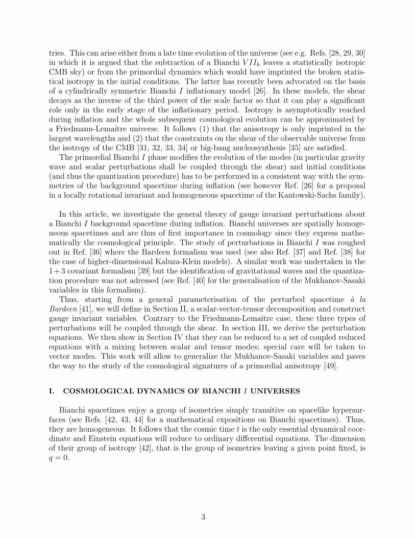
tries. This can arise either from a late time evolution of the universe (see e.g. Refs. [28, 29, 30]in which it is argued that the subtraction of a Bianchi V IIh leaves a statistically isotropicCMB sky) or from the primordial dynamics which would have imprinted the broken statis-tical isotropy in the initial conditions. The latter has recently been advocated on the basisof a cylindrically symmetric Bianchi I inflationary model [26]. In these models, the sheardecays as the inverse of the third power of the scale factor so that it can play a significantrole only in the early stage of the inflationary period. Isotropy is asymptotically reachedduring inflation and the whole subsequent cosmological evolution can be approximated bya Friedmann-Lemaıtre universe. It follows (1) that the anisotropy is only imprinted in thelargest wavelengths and (2) that the constraints on the shear of the observable universe fromthe isotropy of the CMB [31, 32, 33, 34] or big-bang nucleosynthesis [35] are satisfied.

The primordial Bianchi I phase modifies the evolution of the modes (in particular gravitywave and scalar perturbations shall be coupled through the shear) and initial conditions(and thus the quantization procedure) has to be performed in a consistent way with the sym-metries of the background spacetime during inflation (see however Ref. [26] for a proposalin a locally rotational invariant and homogeneous spacetime of the Kantowski-Sachs family).

In this article, we investigate the general theory of gauge invariant perturbations abouta Bianchi I background spacetime during inflation. Bianchi universes are spatially homoge-neous spacetimes and are thus of first importance in cosmology since they express mathe-matically the cosmological principle. The study of perturbations in Bianchi I was roughedout in Ref. [36] where the Bardeen formalism was used (see also Ref. [37] and Ref. [38] forthe case of higher-dimensional Kaluza-Klein models). A similar work was undertaken in the1+3 covariant formalism [39] but the identification of gravitational waves and the quantiza-tion procedure was not adressed (see Ref. [40] for the generalisation of the Mukhanov-Sasakivariables in this formalism).

Thus, starting from a general parameterisation of the perturbed spacetime a la

Bardeen [41], we will define in Section II, a scalar-vector-tensor decomposition and constructgauge invariant variables. Contrary to the Friedmann-Lemaıtre case, these three types ofperturbations will be coupled through the shear. In section III, we derive the perturbationequations. We then show in Section IV that they can be reduced to a set of coupled reducedequations with a mixing between scalar and tensor modes; special care will be taken tovector modes. This work will allow to generalize the Mukhanov-Sasaki variables and pavesthe way to the study of the cosmological signatures of a primordial anisotropy [49].

I. COSMOLOGICAL DYNAMICS OF BIANCHI I UNIVERSES

Bianchi spacetimes enjoy a group of isometries simply transitive on spacelike hypersur-faces (see Refs. [42, 43, 44] for a mathematical expositions on Bianchi spacetimes). Thus,they are homogeneous. It follows that the cosmic time t is the only essential dynamical coor-dinate and Einstein equations will reduce to ordinary differential equations. The dimensionof their group of isotropy [42], that is the group of isometries leaving a given point fixed, isq = 0.

3

A. General form of the metric

Bianchi I spacetimes are the simplest anisotropic universe models. They allow for differ-ent expansion factors in three orthogonal directions. In comoving coordinates, the metrictakes the general form

ds2 = gµνdxµdxν = −dt2 +

3∑

i=1

X2i (t)

(

dxi)2

. (1.1)

It includes Friedmann-Lemaıtre spacetimes as a subcase when the three scale factors areequal. The average scale factor, defined by

a(t) ≡ [X1(t)X2(t)X3(t)]1/3 , (1.2)

characterizes the volume expansion. It follows that we can recast the metric (1.1) as

ds2 = −dt2 + a2(t)γij(t)dxidxj . (1.3)

The “spatial metric” γij is the metric on constant time hypersurfaces. It can be decomposedas

γij = exp [2βi(t)] δij , (1.4)

with the constraints3∑

i=1

βi = 0 . (1.5)

Let us emphasize that βi are not the components of a vector so that they are not subjectedto the Einstein summation rule. Note also that all latin indices i, j, . . . are lowered with themetric γij . The decomposition (1.4) implies that γij = 2βiγij, where a dot refers to a deriva-tive with respect to the cosmic time, and it can be checked that the spatial hypersurfacesare flat. This relation, together with the constraint (1.5), implies that the determinant ofthe spatial metric is constant

γ = γijγij = 0 .

This simply means that any comoving volume remains constant during the expansion of theuniverse, even if this expansion is anisotropic. We define the shear as

σij ≡1

2γij (1.6)

and introduce the scalar σ2 ≡ σij σij. This definition is justified from the relation to the 1+3

covariant formalism (see Appendix A3). Let us emphasize at this point that (γij)· = −2σij

differs from γij ≡ γipγjkγpk = +2σij.Introducing the conformal time as dt ≡ adη, the metric (1.3) can be recast as

ds2 = a2(η)[

−dη2 + γij(η)dxidxj]

. (1.7)

We define the comoving Hubble parameter by H ≡ a′/a, where a prime refers to a derivativewith respect to the conformal time. The shear tensor, now defined as

σij ≡1

2γ′

ij , (1.8)

4

is related to σij by σij = aσij . From the relation (γij)′ = γ′

ij = 2β ′iγij, the definition

σ2 ≡ σijσij (1.9)

is explicitely given by

σ2 =

3∑

i=1

(β ′i)

2 , (1.10)

and is related to its cosmic time analogous by σ = σa. Again, we stress that (γij)′ = −2σij

differs from (γ′)ij ≡ γipγjkγ′pk = +2σij.

B. Background equations

We concentrate on an inflationary phase during which the matter content of the universeis assumed to be described by a minimally coupled scalar field, ϕ, with stress-energy tensor

Tµν = ∂µϕ∂νϕ −(

1

2∂αϕ∂αϕ + V

)

gµν . (1.11)

Making use of the expressions (A6-A7) (see Appendix A2), we easily obtain the Friedmannequations

H2 =κ

3

[

1

2ϕ′2 + V (ϕ)a2

]

+1

6σ2, (1.12)

H′ = −κ

3[ϕ′2 − V (ϕ)a2] − 1

3σ2 (1.13)

(σij)

′ = −2Hσij , (1.14)

where κ ≡ 8πG. The first two are similar to the ones usually used in a Friedmann-Lemaıtreuniverse, up to the contribution of the shear (which acts as an extra massless field). Thelatter equation arises from the trace-free part of the “ij”-Einstein equations and gives anextra-equation compared to the Friedmann-Lemaıtre case. We can easily integrate it andconclude that the shear evolves as

σij =

Sij

a2(1.15)

where Sij is a constant tensor, (Si

j)′ = 0. This implies that

σ2 =S2

a4⇒ σ2 =

S2

a6, (1.16)

(with S2 ≡ SijSj

i ) from which we deduce that

σ′ = −2Hσ . (1.17)

Let us note that these equations can be combined to give

2H2 + H′ = κa2V , κ(ϕ′)2 = 2H2 − 2H′ − σ2 . (1.18)

These equations are completed by a Klein-Gordon equation, which keeps its Friedmann-Lemaıtre form,

ϕ′′ + 2Hϕ′ + a2Vϕ = 0. (1.19)

The general solution for the evolution of the scale factor from these equations is detailed inAppendix A4.

5

II. GAUGE INVARIANT VARIABLES

This section is devoted to the definition of the gauge invariant variables that describe theperturbed spacetime. We follow a method a la Bardeen. In order to define scalar, vectorand tensor modes, we will need to use a Fourier transform. We start, in § IIA, by recallingits definition and stressing its differences with the standard Friedmann-Lemaıtre case. In§ II B, we perform a general gauge transformation to identify the gauge invariant variables.

A. Mode decomposition

1. Definition of the Fourier transform

We decompose any quantity in Fourier modes as follows. First, we pick up a comovingcoordinates system, xi, on the constant time hypersurfaces. Then, we decompose anyscalar function as

f(

xj , η)

=

∫

d3ki

(2π)3/2f (ki, η) eikix

i

, (2.1)

with the inverse Fourier transform

f (kj , η) =

∫

d3xi

(2π)3/2f(

xi, η)

e−ikixi

. (2.2)

In the Fourier space, the comoving wave co-vectors ki are constant, k′i = 0. We now define

ki ≡ γijkj that is obviously a time-dependent quantity. Contrary to the standard Friedmann-Lemaıtre case, we must be careful not to trivially identify ki and ki, since this does notcommute with the time evolution. Note however that xik

i = xiki remains constant so thatthere is no extra-time dependency entering our definitions (2.1-2.2). In the following ofthis article, we will forget the “hat” and use the notation f (xj , η) and f (kj, η) both for afunction and its Fourier transform.

It is easily checked, using the definition (1.8), that

(ki)′ = −2σipkp . (2.3)

This implies that the modulus of the comoving wave vector, k2 = kiki = γijkikj, is nowtime-dependent and that its rate of change is explicitely given by

k′

k= −σij kikj , (2.4)

where we have introduced the unit vector

ki ≡ki

k. (2.5)

This vector will turn to be particularly useful for our analysis and we note that it evolves as

(ki)′ = (σpqkpkq)ki − 2σipkp . (2.6)

Indeed, we find that in the standard Friedmann-Lemaıtre limit (σij = 0), ki and k areconstant.

6

2. Decomposition of the vector and tensor modes

We shall now decompose the perturbations in their scalar, vector and tensor modes.Any (3-dimensional) vector field, V i, can be decomposed as

Vi = ∂iV + Vi , with ∂iVi = 0 , (2.7)

Note that we have chosen orthogonal (but not Cartesian) coordinates on the (Euclidean) spa-tial sections (in particular spatial flatness and homogeneity imply that in these coordinatesthe Christoffel symbols vanish and that ∂kγij = 0). It follows that its Fourier componentscan be split as

Vi = kiV + Vi, with kiVi = 0, (2.8)

so that V i lives in the subspace perpendicular to ki. This is a 2-dimensional subspace so thatVi has been split into 1 scalar (V ) and two vector modes (Vi) that correspond to transversemodes. Let us now consider the base e1, e2 of the subspace perpendicular to ki. Byconstruction, it satisfies the orthonormalisation conditions

eai kjγ

ij = 0, eai e

bjγ

ij = δab.

Such a basis is defined up to a rotation about the axis ki. Now, the vector modes can bedecomposed on this basis as

Vi(ki, η) =∑

a=1,2

Va(ki, η) eai (ki) , (2.9)

which defines the two degrees of freedom, Va, which depend on ki since the decompositiondiffers for each wave number. The two basis vectors allow to define a projection operatoronto the subspace perpendicular to ki as

Pij ≡ e1i e

1j + e2

i e2j = γij − kikj. (2.10)

It trivially satisfies P ijP

jk = P i

k, P ijk

j = 0 and P ijγij = 2. It is also the projector on vectormodes so that we can always make the scalar-vector decomposition

Vi = [kjVj]ki + P ji Vj . (2.11)

Analogously, any (3-dimensional) symmetric tensor field, Vij, can be decomposed as

Vij = Tγij + ∆ijS + 2∂(iVj) + 2Vij , (2.12)

where ∆ij ≡ ∂i∂j − ∆γij/3 and

∂iVi = 0, V i

i = 0 = ∂iVij. (2.13)

The symmetric tensor Vij is transverse and trace-free. Hence it has only two independentcomponents and can be decomposed as

Vij(ki, η) =∑

λ=+,×

Vλ(ki, η) ελ

ij(ki) (2.14)

7

where the polarization tensors have been defined as

ελij =

e1i e

1j − e2

i e2j√

2δλ+ +

e1i e

2j + e2

i e1j√

2δλ×. (2.15)

It can be checked that they are traceless (ελijγ

ij = 0), transverse (ελijk

i = 0), and that the

two polarizations are perpendicular (ελijε

ijµ = δλ

µ). This defines the two tensor degrees offreedom.

In order to deal with the properties of the polarization tensors, it is useful to define twonew quantities

Qij ≡ e1i e

2j − e2

i e1j , and ηλµ ≡ δ+

λ δ×µ − δ+µ δ×λ . (2.16)

The tensor Qij trivially satisfies

PijQij = 0 , QijQ

ij = 2 . (2.17)

They allow us to simplify the product of two and three polarization tensors as

ελikε

kµj =

1

2

(

Pijδλµ + Qijη

λµ)

, ελikε

kjµ εi

jν = 0 . (2.18)

Introducing the projector operator on tensor modes by

Λabij = P a

i P bj − 1

2PijP

ab ,

and the “trace extracting” operator

T ji = kik

j − 1

3δji ,

the scalar-vector-tensor terms in the decomposition of Eq. (2.12) are extracted as follows

Vij =

[

1

3Vabγ

ab

]

γij +

[

3

2VabT

ab

]

Tij + 2k(i

[

P aj)k

bVab

]

+ Λabij Vab. (2.19)

In this expression, Vij has been split into 2 scalars (T and S), two vector modes (Vi) andtwo tensor modes (Vij). Thus, we can always split any equation Vi = 0 by projecting along

ki (scalar) and P ij (vector) and any equation Vij = 0 by projecting along γij (scalar), T ij

(scalar), P il k

j (vector) and Λijab (tensor).

3. Properties of the projectors, polarization vectors and tensors

The previous SVT decomposition matches the one used in the perturbation theory abouta Friedmann-Lemaıtre spacetime. There is however an important difference that we willhave to deal with. As we pointed out, in a Bianchi I spacetime, the spatial metric is time-dependent. It implies in particular that, in order to remain an orthonormal basis perpen-dicular to ki during the time evolution, the polarization vectors, and thus the polarizationtensors, must have a non-vanishing time derivative. Indeed, since (ki)

′ = 0, the vector (eia)

′

is orthogonal to ki and is thus a linear combination of e1 and e2, that is

(eia)

′ =∑

b

Rab eib .

8

In each time hypersurface, there is a remaining freedom in the choice of this basis becauseof the rotational invariance around ki. We can continuously fix the choice of the basis byimposing

R[ab] = 0 .

The orthonormalisation condition implies that (eiae

bi)

′ = 0 and thus that

Rab = −σij eiae

jb. (2.20)

Consequently, the time derivative of any polarization vector is given by

(eai )

′ =∑

b

Rab ebi + 2σije

ja , (2.21)

from which we deduceki(ea

i )′ = 2σpi kp ea

i . (2.22)

This allows us to derive the expression of the time derivative of the polarization tensor.Starting from their definitions (2.15), we easily obtain that

(

ελij

)′= −(σklελ

kl)Pij − (σklPkl)ελij + 4σk

(iελj)k , (2.23)

from which we can deduce some useful algebra

kikj(

ελij

)′= 0 , γij

(

ελij

)′= 2σijελ

ij , ki(

ελij

)′= 2σipkpε

λij . (2.24)

We also have that(

εiλj

)′εjµ

i = 0 . (2.25)

We gather in Appendix B some other useful relations concerning the polarization vectorsand tensors.

For the sake of completeness, we shall define here two important matrices for the followingof our computation,

Mλab ≡ ελ

ijeiae

jb , (2.26)

which is manifestly symmetric in ab and

Nab ≡ Qijeiae

jb , (2.27)

which is anti-symmetric in ab. We stress that a and λ are not indices but only labels. It caneasily be checked that

Mλab =

1√2

(

1 00 −1

)

δλ+ +

1√2

(

0 11 0

)

δλ× , (2.28)

and that∑

a

Mλaa = 0 . (2.29)

9

B. Defining gauge invariant variables

1. Gauge invariant variables for the geometry

Let us consider the most general metric of an almost Bianchi I spacetime. It can alwaysbe decomposed as

ds2 = a2[

− (1 + 2A) dη2 + 2Bidxidη + (γij + hij) dxidxj]

. (2.30)

Bi and hij can be further conveniently decomposed as

Bi = ∂iB + Bi , (2.31)

hij ≡ 2C(

γij +σij

H)

+ 2∂i∂jE + 2∂(iEj) + 2Eij , (2.32)

with∂iB

i = 0 = ∂iEi, Ei

i = 0 = ∂iEij . (2.33)

Note that this decomposition of hij involves the shear. This judicious choice is justified, aposteriori, by the simplicity of the transformation properties of the perturbation variables,as we shall now see.

Let us consider an active transformation of the coordinate system defined by a vectorfield ξ. The coordinates of any point change according to

xµ → xµ = xµ − ξµ (xν) (2.34)

so that the spacetime metric transforms as

gµν → gµν + Lξgµν , (2.35)

where Lξgµν is the Lie derivative of gµν along ξ. At first order in the perturbations, wedecompose the metric as gµν = gµν + δgµν and it follows that

δgµν → δgµν + Lξgµν . (2.36)

The vector field ξ is now decomposed into a scalar and vector part as

ξ0 = T(

xi, η)

, ξi = ∂iL(xj , η) + Li(

xj , η)

, (2.37)

with ∂iLi = 0. With the use of the expressions (C1), we deduce that the perturbations of

the metric transform as (in Fourier space)

A → A + T ′ + HT (2.38)

B → B − T +(k2L)

′

k2(2.39)

C → C + HT (2.40)

E → E + L , (2.41)

for the scalar variables, and as

Bi → Bi + γij(Lj)′ − 2ikjσljP

liL (2.42)

Ei → Ei + Li , (2.43)

10

for the vector variables. We also obtain that the tensor modes are readily gauge invariant,

Eij → Eij . (2.44)

Had we not included the shear in the decompostion (2.31), this would not be the case.Let us also note that the transformation rule of the vector modes is different from the

one derived in Ref. [36] where the non-commutativity between the projection and the timeevolution has been neglected.

From the gauge transformations (2.38-2.41), we can construct a set of gauge invariantvariables for the scalar sector. Only two degrees of freedom remain, the two other beingabsorbed by the scalar part of the gauge transformation. We define the two gravitationalpotentials

Φ ≡ A +1

a

a

[

B − (k2E)′

k2

]′

, (2.45)

Ψ ≡ −C −H[

B − (k2E)′

k2

]

. (2.46)

From the gauge transformations (2.42-2.43), we deduce that a gauge invariant vector per-turbation is given by

Φi ≡ Bi − γij

(

Ej)′

+ 2ikjσljPliE, (2.47)

It is obvious from these expressions that when γij is time-independent, that is whenσij = 0, these variables reduce to the standard Bardeen variables defined in the Friedmann-Lemaıtre case. By analogy, we define the Newtonian gauge by the conditions

B = Bi = E = 0 , (2.48)

so thatA = Φ , C = −Ψ , Φi = −(Ei)′ , (2.49)

the latter condition being equivalent to Φi = −E ′i + 2σijE

j.

2. Gauge invariant variables for the matter

We focus our analysis on the scalar field case, which is the most relevant for the study ofinflation. Under a gauge transformation of the form (2.34), it transforms as ϕ → ϕ + £ξϕ.At first order in the perturbations, we get

δϕ → δϕ + £ξϕ, (2.50)

that isδϕ → δϕ + £ξϕ = δϕ + ϕ′T , (2.51)

with use of Eq. (2.37). Thus, we can define the two gauge invariant variables

Q ≡ δϕ − C

Hϕ′ (2.52)

and

χ ≡ δϕ +

[

B − (k2E)′

k2

]

ϕ′ . (2.53)

They are related by

Q = χ +Ψ

Hϕ′ . (2.54)

11

III. PERTURBATIONS EQUATIONS

Once the gauge invariant variables have been defined, we can derive their equations ofevolution. The mode decomposition will require a decomposition of the shear tensor in abasis adapted to each wave-number. We start by defining this decomposition and then wederive the perturbed Klein-Gordon and Einstein equations.

A. Decomposition of the shear tensor

The shear σij is a symmetric tracefree tensor and, as such, has 5 independent components.In the coordinates system (1.3-1.4), it was expressed in terms of only two independentfunctions of time βi(η). The 3 remaining degrees of freedom are related to the 3 Eulerangles needed to shift to a general coordinate system.

1. Components of the shear

As mentioned before, when working out the perturbations in Fourier space, it would befruitful to decompose the shear in a local basis adapted to the mode we are considering.The shear, being a symmetric trace-free tensor, can be decomposed on the basis ki, e

1i , e

2j

as

σij =3

2

(

kikj −1

3γij

)

σ‖+ 2

∑

a=1,2

σVa k(ie

aj) +

∑

λ=+,×

σTλ ελ

ij. (3.1)

This decomposition involves 5 independent components of the shear in a basis adapted tothe wavenumber ki. We must stress however that (σ

‖, σ

Va, σTλ) must not be interpreted asthe Fourier components of the shear, even if they explicitely depend on ki. This dependencearises from the local anisotropy of space.

Using Eq. (3.1), it can be easily worked out that

σijγij = 0 ,

σij ki = σ

‖kj +

∑

a

σVae

aj , σij k

ikj = σ‖,

andσijε

ijλ = σ

Tλ , σij kiej

a = σVa .

The scalar shear is explicitely given by

σ2 = σijσij =

3

2σ2

‖+ 2

∑

a

σ2Va +

∑

λ

σ2Tλ , (3.2)

which is independent of ki. We emphasize that the local positivity of the energy density ofmatter implies that σ2/6 < H2 and thus

1

2σ

‖≤ 1√

6σ < H . (3.3)

This, in turn, implies thatσ

‖< 2H , (3.4)

12

a property that shall turn to be very useful in the following of our discussion. Analogously,we have that

σTλ <

√6H . (3.5)

The following derivations will involve the contraction of the shear with the polarizationvectors,

σijeiae

jb = −1

2σ

‖δab +

∑

λ

σTλMλ

ab , (3.6)

from which we deduce thatσijP

ij = −σ‖. (3.7)

It will also involve the contraction of the shear with the polarization tensors,

σil εljλ = −1

2σ

‖εjλ

i +∑

a

σVakie

al ε

ljλ +

∑

µ

σTµε

µilε

ljλ , (3.8)

which implies that

σilεljλ P i

j = σTλ , σilε

ljλ εiµ

j = −1

2σ

‖δλµ . (3.9)

To finish, we will make use of the following expression

ebl e

ja σjm εlm

λ = −1

2σ

‖Mλ

ab +1

2δab σTλ +

1

2Nab

(

σT+δ×λ − σ

T×δ+λ

)

. (3.10)

2. Time evolution of the components of the shear

In the previous paragraph we detailed the definition of the components of the shear in abasis adapted to the wave mode ki. The time evolution of these modes is easily obtainedfrom Eq. (1.14)

σ′‖+ 2Hσ

‖= −2

∑

a

σ2Va , (3.11)

σ′Va + 2Hσ

Va =3

2σ

Vaσ‖−∑

b,λ

σVbσTλMλ

ab , (3.12)

σ′Tλ + 2Hσ

Tλ = 2∑

a,b

MλabσVaσVb , (3.13)

where the matrix Mλab is defined in Eq. (2.26).

These equations allow us to derive some important constraints on the rate of change ofσ

‖and σ

Tλ. Since Eq. (3.11) implies that

∣

∣

∣

∣

1

a2

(

a2σ‖

)′∣

∣

∣

∣

= 2∑

a

σ2Va < σ2 < 6H2 , (3.14)

we can conclude that∣

∣

∣

∣

1

a2

(

a2σ‖

)′∣

∣

∣

∣

< 6H2 . (3.15)

13

Identically, Eq. (3.13) implies that∣

∣

∣

∣

1

a2

(

a2σTλ

)′

∣

∣

∣

∣

= 2∑

a,b

MλabσVaσVb <

σ2

√2,

so that∣

∣

∣

∣

1

a2

(

a2σTλ

)′

∣

∣

∣

∣

< 3√

2H2 . (3.16)

The two relations (3.15-3.16) will be important at the end of our analysis.

B. Klein-Gordon equation

The Klein-Gordon equation, ϕ = Vϕ, can be rewritten under the form

gµν∇µ∂νϕ = Vϕ(ϕ) . (3.17)

When expanded at first order in the perturbations, the r.h.s. is trivially given by Vϕ(ϕ) +Vϕϕ(ϕ)χ. It follows that the Klein-Gordon equation at first order in the perturbations isthen obtained to be

χ′′ + 2Hχ′ − γij∂i∂jχ + a2Vϕϕχ = 2(ϕ′′ + 2Hϕ′)Φ + ϕ′(Φ′ + 3Ψ′) , (3.18)

where Vϕϕ is the second derivative of the potential with respect to the scalar field. Surpris-ingly, it has the same form as in the Friedmann-Lemaıtre case. This can be understood ifwe remind that the d’Alembertian can be expressed as ϕ = ∂ν [

√−ggµν∂µϕ] /√−g, and if

we realize that√−g does not involve the shear. Thus, at first order in the perturbations,

the only place where the shear σij could appear would be associated with δgij. But then itwould multiply ∂iϕ which vanishes. Consequently the Klein-Gordon equation is not modi-fied. This result is not specific to the scalar field case as the conservation equation in thefluid case is also the same as for a Friedmann-Lemaıtre spacetime, indeed only as long asthe anisotropic stress vanishes [see Eq. (A22)].

C. Einstein equations

The procedure to obtain the mode decomposition of the Einstein equations is somehowsimple. We start from the general perturbed equation δGµ

ν = κδT µν with the expressions (C2-

C4) and (C10-C12) respectively for the stress-energy tensor and the Einstein tensor and wethen project them, as described in § IIA 2.

Special care must however be taken. In the Friedmann-Lemaıtre case, the projections onthe scalar, vector and tensor modes commute with the time evolution. This no more thecase in a Bianchi I universe, as explained in § IIA 3. Let us take an example and considerthe extraction of the vector part of an equation involving a term of the form (Φi)′ + HΦi.We project this equation on the polarization tensor ea

i to get

eai

[

(Φi)′ + HΦi]

= (eai Φ

i)′ − Φi(eai )

′ + HΦa.

We then use Eq. (2.21) to rewrite Φi(eai )

′, and we develop the shear in the basis adapted tothe mode ki. This implies, in particular, that contrary to the Friedmann-Lemaıtre case, thescalar, vector and tensor modes will be coupled.

14

This being said, the extraction of the mode decomposition of the Einstein equation is alengthy but straightforward computation that we carry in the Newtonian gauge. It reducesto (1) Fourier transforming the Einstein equations, (2) projecting them on the modes, (3)commuting the projection operators and the time evolution in order to extract the evolutionof the polarizations and (4) finally expressing the decomposition of the shear.

1. Scalar modes

There are 4 scalar Einstein equations. The first is obtained from δG00 = κδT 0

0 and gives

k2Ψ + 3H(Ψ′ + HΦ) − κ

2

(

ϕ′2Φ − ϕ′χ′ − Vϕa2χ)

=

1

2σ2 [X − 3Ψ] +

1

2

k2

Hσ‖Ψ − 1

2k2∑

a

σVaΦa −

1

2

∑

λ

[σTλE

′λ + (σ′

Tλ + 2HσTλ)Eλ],(3.19)

where we have defined the extremely useful variable [2]

X ≡ Φ + Ψ +

(

Ψ

H

)′

, (3.20)

and the quantityσ

Va ≡ ikσVa . (3.21)

As an example, the only tricky term which appears when deriving this equation is σij(E

ji )

′,which is obtained from

σij(E

ji )

′ = (σijE

ji )

′ − Eji (σ

ij)

′ =∑

(σTλEλ)

′ − Eji (−2Hσi

j) =∑

(σTλEλ)

′ + 2HσTλEλ ,

where we have used Eq. (1.14) to compute (σij)

′. We will not detail these steps in thefollowing.

The second equation is obtained from kiδG0i = κkiδT 0

i . We find

Ψ′ + HΦ − κ

2ϕ′χ = − 1

2Hσ2Ψ +1

2σ

‖X +

1

2

∑

λ

σTλEλ . (3.22)

The two remaining equations are obtained from

δijδG

ji = κδi

jδTji ,

(

kikj −1

3δij

)

δGji = κ

(

kikj −1

3δij

)

δT ji

and take the form

Ψ′′ + 2HΨ′ + HΦ′ + (2H′ + H2)Φ − 1

3k2(Φ − Ψ) +

κ

2

[

ϕ′2Φ − ϕ′χ′ + Vϕa2χ]

=

−1

2σ2 [X − 3Ψ] +

1

6

k2

Hσ‖Ψ +

1

2k2∑

a

σVaΦa

+1

2

∑

λ

[σTλE

′λ + (σ′

Tλ + 2HσTλ)Eλ] , (3.23)

2

3k2(Φ − Ψ) = σ

‖

[

X ′ − k2Ψ

3H

]

+ 4k2∑

λ,a,b

Mλabσ

aVσb

VEλ − 2k2

∑

a

σVaΦa . (3.24)

It can be checked that indeed Eqs. (3.19, 3.22-3.24) reduces to their well-known Friedman-nian form when the shear vanishes.

15

2. Vector modes

The two vector equations are obtained from

eiaδG

0i = 0, kie

jaδG

ij = 0 .

They respectively give

Φa = −2σVaX + 4

∑

b,λ

MλabσVbEλ , (3.25)

and

Φ′a + 2HΦa −

5

2σ

‖Φa +

∑

bλ

MλabσTλΦb = −2σ

VaX′ + 4

∑

b,λ

MλabσVbE

′λ

+4∑

bλ

NabσVb

(

σT+δ×λ − σ

T×δ+λ

)

Eλ , (3.26)

where the matrix Nab is defined in Eq. (2.27). It can be shown that Eq. (3.26) resultsfrom the time derivative of Eq. (3.25) once Eqs. (3.11-3.13) are used to express the timederivatives of the shear. This a consequence of the Bianchi identities.

3. Tensor modes

The equation of evolution of the tensor modes is obtained from εjλi δGi

j = 0. To simplify,we shall use the shorthand notation (1 − λ) for the opposite polarization of λ, i.e. it meansthat if λ = +, then (1 − λ) = ×, and vice-versa. With the use of Eq. (B6), we obtain

E ′′λ + 2HE ′

λ + k2Eλ = σTλ

[

k2

(

Ψ

H

)

+ X ′

]

+ 2k2∑

a,b

MλabσVaΦb

−2k2∑

a

σ2VaEλ − 2σ

T×σT+E(1−λ) + 2σ2

T (1−λ)Eλ . (3.27)

It can be shown that in the long wavelength limit, the former equations (3.18, 3.19-3.24,3.25-3.26, 3.27) are equivalent to the ones obtained in a more general gradient expansion ofEinstein equations on large scales [45].

IV. REDUCED EQUATIONS AND MUKHANOV-SASAKI VARIABLES

The previous equations (3.18, 3.19-3.24, 3.25-3.26, 3.27) form a coupled set of equationsfor the scalar, vector and tensor modes. In a Friedmann-Lemaıtre spacetime, the three kindof perturbations decouple and one can arbitrarily set one of the contributions to zero tofocus on a given type of mode. This is no more possible here, and in particular, it is notpossible to neglect the vector modes. Their contribution, as we shall see, is in fact centralto get the correct set of reduced equations.

First, we introduce the Mukhanov-Sasaki variables [10] for scalar and tensor modes as

v ≡ aQ ,√

κµλ ≡ aEλ, (4.1)

16

exactly in the same way as in a Friedmann-Lemaıtre spacetime. These three variables wereshown to be the canonical degrees of freedom that shall be quantized during inflation whena Friedmann-Lemaıtre universe is assumed [5].

A. Scalar modes

Let us introduce these variables in our analysis and start by focusing on the scalar modes.First, we note that Eq. (3.22) can be recast under the more compact form

(2H− σ‖)X =

κ

aϕ′v +

∑

λ

σTλEλ . (4.2)

If we now combine Eq. (3.19) with Eq. (3.23), replace the vector mode by its expression (3.25)and use the background equations (1.18), we obtain

HX ′ + 2(H′ + 2H2)X + κaVϕv + k2Ψ =k2

3(Φ − Ψ) +

2

3

k2

Hσ‖Ψ . (4.3)

Now, using Eq. (3.24) to simplify the r.h.s., and again replacing the vector mode by itsexpression (3.25), we get

(

2H− σ‖

)

(

X ′ +k2

HΨ

)

+ 4κa2V X + 2κaVϕv = 4k2

(

∑

a

σ2V aX −

∑

a,b,λ

MλabσV aσV bEλ

)

.

(4.4)Then, forcing Q in the Klein-Gordon equation (3.18), using also its background version, weobtain

Q′′ + 2HQ + k2Q + a2VϕϕQ + 2a2VϕX − ϕ′

(

X ′ +k2

HΨ

)

= 0 . (4.5)

Now, we can replace the last term by using Eq. (4.4) and the next to last by using Eq. (4.2)to get

Q′′ + 2HQ + k2Q + a2VϕϕQ + 2a2VϕX =

ϕ′

(2H− σ‖)

[

4k2

(

∑

a

σ2V aX −

∑

a,b,λ

MλabσV aσV bEλ

)

− 4κa2V X − 2κaV ′v

]

.(4.6)

Introducing the definitions (4.1), we obtain, after some algebra which requires in particularEqs (3.11-3.13) to express terms such as

∑

a,b MλabσV aσV b,

v′′ +

(

k2 − a′′

a+ a2V,ϕϕ

)

v =1

a2

(

2a2ϕ′2

2H− σ‖

)′

κv +∑

ν

1

a2

(

2a2ϕ′σTν

2H− σ‖

)′ √κµν . (4.7)

This equation is the first central result of this section.

17

B. Tensor modes

The scalar contribution of the tensor equation (3.27) is exactly given by the relation (4.4),so that it reduces, after replacing the vector mode by its expression (3.25), to

µ′′λ +

(

k2 − a′′

a

)

µλ = −2µ(1−λ)σT+σT× + 2µλσ

2T(1−λ) +

1

a2

(

2a2ϕ′σTλ

2H− σ‖

)′ √κv

+∑

ν

1

a2

(

2a2σTνσTλ

2H− σ‖

)′

µν +

(

a2σ‖

)′

a2µλ (4.8)

This equation is the second central result of this section.

C. Summary

We have reduced the perturbation equations to a set of three coupled equations for thevariables v and µλ defined in Eq. (4.1). If we define two new functions zs and zλ by

z′′szs

(η, ki) ≡ a′′

a− a2V,ϕϕ +

1

a2

(

2a2κϕ′2

2H− σ‖

)′

z′′λzλ

(η, ki) ≡ a′′

a+ 2σ2

T(1−λ) +1

a2

(

a2σ‖

)′

+1

a2

(

2a2σ2Tλ

2H− σ‖

)′

, (4.9)

the system reduces to

v′′ +

(

k2 − z′′szs

)

v =∑

ν

1

a2

(

2a2ϕ′σTν

2H− σ‖

)′ √κµν , (4.10)

µ′′λ +

(

k2 − z′′λzλ

)

µλ =1

a2

(

2a2ϕ′σTλ

2H− σ‖

)′ √κv

+

[

1

a2

(

2a2σT×σ

T+

2H− σ‖

)′

− 2σT×σ

T+

]

µ(1−λ). (4.11)

Formally, it can be rewritten as

V ′′ + k2V + ΩV = ΥV , (4.12)

where V ≡ (v, µ+, µ×). The matrices Ω and Υ are defined by

V ′′ +

k2 − z′′szs

0 0

0 k2 − z′′+z+

0

0 0 k2 − z′′×z×

V =

0 ℵ+ ℵ×

ℵ+ 0 i

ℵ× i 0

V , (4.13)

and the functions ℵλ(η, ki) and i(η, ki) can be read on Eqs. (4.10-4.11). This is one of thecentral results of our study.

18

When the shear vanishes, these equations decouple and we recover the usual equations [5]for the variables v and µλ so that we only have three physical degrees of freedom. Now, theanisotropy of space is at the origin of some interesting effects. First the functions zs and zλ

are not functions of time only. They depend on ki explicitely through the components ofthe decomposition of the shear. Second, the two types of modes are coupled through a non-diagonal mass term. The mass term and the evolution operator cannot be diagonalized atthe same time so that we expect the equivalent of a see-saw mechanism. The importance ofthe vector modes, that cannot be neglected, has to be emphasized again. Had we neglectedthem, the mass term would not be correct.

D. Sub-Hubble limit

Let us consider the behaviour of the mass term appearing in Eqs. (4.10-4.11) in thesub-Hubble limit in which k/H ≫ 1. We introduce the two slow-roll parameters as

ǫ ≡ 3ϕ′2

ϕ′2 + 2a2V, δ ≡ 1 − ϕ′′

Hϕ′, (4.14)

in terms of which the Friedmann equations take the form

H2 =κ

3 − ǫV a2 +

1

6σ2 , (3 − δ)Hϕ′ + Vϕa2 = 0 , (4.15)

and

H′ = (1 − ǫ)H2 +

(

ǫ − 3

6

)

σ2

We now focus on the behaviour of the functions ℵλ, i, z′′s /zs and z′′λ/zλ in the sub-Hubbleregime. We define x ≡ σ/

√6H and use the fact that, since σ

‖/2 ≤ σ/

√6 [see Eq. (3.4)],

there exists α < 1 such that 0 ≤ x < α due to the positive energy condition [see Eq. (3.3)].Starting from the definition (4.10) for ℵλ we have

|ℵλ| <

∣

∣

∣

∣

1

a2

(

a2σTλ

)′

∣

∣

∣

∣

×∣

∣

∣

∣

∣

2√

κϕ′

2H− σ‖

∣

∣

∣

∣

∣

+ 2|σTλ| ×

∣

∣

∣

∣

∣

( √κϕ′

2H− σ‖

)′∣∣

∣

∣

∣

. (4.16)

Now, the property (3.16) implies that the first term of the right hand side of the inequalityis smaller than

3√

2H2

∣

∣

∣

∣

∣

2√

κϕ′

2H− σ‖

∣

∣

∣

∣

∣

.

Then,∣

∣

∣

∣

∣

2√

κϕ′

2H− σ‖

∣

∣

∣

∣

∣

=√

2ǫ

√

H2 − σ2

6

H− σ‖

2

≤√

2ǫ

√

1 + x

1 − x. (4.17)

Now, since x varies in the range 0 ≤ x < α, we deduce that√

(1 + x)/(1 − x) ≤√

(1 + α)/(1 − α). Eq. (3.5) then implies that the second term of the inequality (4.16)is smaller than

2√

6H×∣

∣

∣

∣

∣

( √κϕ′

2H− σ‖

)′∣∣

∣

∣

∣

.

19

Then, the absolute value is bounded by

∣

∣

∣

∣

∣

( √κϕ′

2H− σ‖

)′∣∣

∣

∣

∣

<

∣

∣

∣

∣

∣

√κϕ′′

2H− σ‖

∣

∣

∣

∣

∣

+

∣

∣

∣

∣

∣

√κϕ′

2H− σ‖

∣

∣

∣

∣

∣

∣

∣

∣

∣

∣

2H′ − σ′‖

2H− σ‖

∣

∣

∣

∣

∣

.

Using the fact that Eq. (3.4) implies |σ′‖| < 10H2 (|σ′

‖| < 6H2 + |2Hσ

‖|), we obtain that

∣

∣

∣

∣

∣

( √κϕ′

2H− σ‖

)′∣∣

∣

∣

∣

≤√

ǫH√2

√1 + α√1 − α

[

(1 − δ) +2(1 − ǫ) +

(

1 − ǫ3

)√6 + 10

2(1 − α)

]

.

Gathering all these terms, we thus conclude that

|ℵλ| <√

ǫH2

√

1 + α

1 − α

[

6 + 2√

3

(

(1 − δ) +2(1 − ǫ) +

(

1 − ǫ3

)√6 + 10

2(1 − α)

)]

. (4.18)

To summarize, we have shown that

|ℵλ| < ZH2 , (4.19)

where Z is a finite constant. This constant can in principle be quite large since α can bearbitrarily close to unity in the worst case of an empty universe. A large Z also correspondsto a very ellipsoidal Hubble radius, and this explains why the short wavelength limit has tobe taken much smaller than the average Hubble radius.

The same reasoning can be applied for |i|, |z′′s /zs| and |z′′λ/zλ|. Thus, it follows that onsub-Hubble scales the three physical degrees of freedom decouple and behave as harmonicoscillators,

V ′′ + k2V = 0 . (4.20)

V. PERTURBATION OF THE ACTION

In order to construct canonical quantization variables and to properly normalize the am-plitude of their quantum fluctuations, one needs to derive the action for the cosmologicalperturbations. We will now demonstrate that the previous equations (4.10-4.11) can be ob-tained from the expansion of the action, written in the ADM formalism [46], at second order.Another simpler route would have been to infer the action from the equations of motion,which is always possible up to an overall factor, that could then be fixed by considering asimple limiting case. Still, we prefer to work out the action at second order since it providesa check of the previous computations.

A. ADM formalism

In the ADM formalism, we expand the metric as

ds2 = −(

N2 − NiNi)

dt2 + 2Nidxidt + gijdxidxj , (5.1)

20

and the Einstein-Hilbert action for a minimally coupled scalar field, takes the form

S =1

2κ

∫

dtd3x√−g

[

NR(3) + N(

KijKij − K2

)

− κN(

gij∂iϕ∂jϕ + 2V (ϕ))

+κN−1(

ϕ − N i∂iϕ)2]

, (5.2)

where R(3) is the Ricci scalar constructed with the metric gij and Kij is the extrinsic curva-ture, defined as

Kij ≡N−1

2

(

gij − 2∇(iNj)

)

, K = Kii . (5.3)

Every spatial index is now manipulated with the metric gij. The ADM metric is designedin such a way that the constraints arising from the Einstein equations can be immediatelyderived from the action. Varying Eq. (5.2) with respect to the lapse N and the shift Ni, weget the Hamiltonian and momentum constraints, respectively

R(3) −(

KijKij − K2

)

− 2V − κgij∂iϕ∂jϕ + N−2κ(

ϕ − N i∂iϕ)2

= 0 , (5.4)

∇j

(

Kji − Kδj

i

)

− N−1κ(

ϕ − N j∂jϕ)

∂iϕ = 0 . (5.5)

Comparing the form (2.30) of the metric in Newtonian gauge with Eq. (5.1), we concludethat the lapse N and the shift Ni are given by

N2 = (1 + 2Φ) , Ni = 0 (5.6)

and that the metric gij is

gij = a2

[

γij − 2Ψ

(

γij +σij

H

)

+ 2∂(iEj) + 2Eij

]

. (5.7)

It follows that the Hamiltonian and momentum constraints reduce, at first order, to

2

a2∆Ψ − 1

a2σij∂i∂j

(

Ψ

H

)

− 6HΨ +

(

Ψ

H

).σ2 − 3Ψσ2 − Φ

(

6H2 − σ2 − ϕ2)

+1

aσi

j∂iΦj − σi

j

(

Eij

)

− κVϕδϕ − κϕδϕ = 0 , (5.8)

and

σ2∂i

(

Ψ

H

)

−σji ∂j

[

Φ +

(

Ψ

H

).]

+2∂i

(

Ψ + HΦ)

− 1

2a∆Φi+2σjl∂jEil−σjl∂iEjl−κϕ∂iδϕ = 0 ,

(5.9)respectively. Once Fourier transformed, written in conformal time and projected along itsscalar and vector components, we recover precisely Eqs. (3.19) and (3.22).

In order to expand the action up to second order in all first order perturbed quantities,we expand the spatial metric as

gij = a2 (γij + hij) .

The inverse metric and its determinant are then given by

gij = a−2(

γij − hij + hilhjl

)

,√

g = a3

[

1 +1

2h +

1

8h2 − 1

4hi

jhji

]

,

wherehij = −2Ψ (γij + σij/H) + 2∂(iEj) + 2Eij . (5.10)

21

B. Action at zeroth and first orders

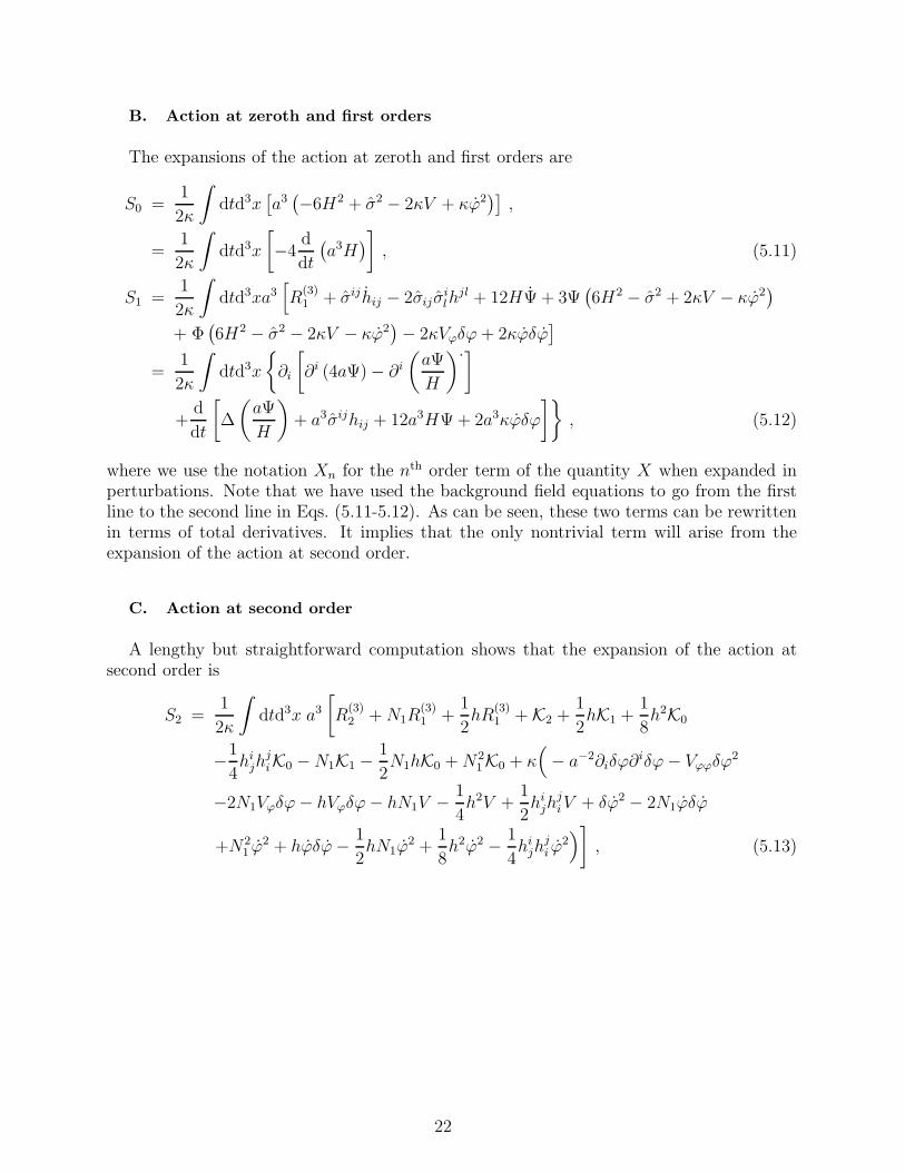
The expansions of the action at zeroth and first orders are

S0 =1

2κ

∫

dtd3x[

a3(

−6H2 + σ2 − 2κV + κϕ2)]

,

=1

2κ

∫

dtd3x

[

−4d

dt

(

a3H)

]

, (5.11)

S1 =1

2κ

∫

dtd3xa3[

R(3)1 + σijhij − 2σij σ

ilh

jl + 12HΨ + 3Ψ(

6H2 − σ2 + 2κV − κϕ2)

+ Φ(

6H2 − σ2 − 2κV − κϕ2)

− 2κVϕδϕ + 2κϕδϕ]

=1

2κ

∫

dtd3x

∂i

[

∂i (4aΨ) − ∂i

(

aΨ

H

).]

+d

dt

[

∆

(

aΨ

H

)

+ a3σijhij + 12a3HΨ + 2a3κϕδϕ

]

, (5.12)

where we use the notation Xn for the nth order term of the quantity X when expanded inperturbations. Note that we have used the background field equations to go from the firstline to the second line in Eqs. (5.11-5.12). As can be seen, these two terms can be rewrittenin terms of total derivatives. It implies that the only nontrivial term will arise from theexpansion of the action at second order.

C. Action at second order

A lengthy but straightforward computation shows that the expansion of the action atsecond order is

S2 =1

2κ

∫

dtd3x a3

[

R(3)2 + N1R

(3)1 +

1

2hR

(3)1 + K2 +

1

2hK1 +

1

8h2K0

−1

4hi

jhjiK0 − N1K1 −

1

2N1hK0 + N2

1K0 + κ(

− a−2∂iδϕ∂iδϕ − Vϕϕδϕ2

−2N1Vϕδϕ − hVϕδϕ − hN1V − 1

4h2V +

1

2hi

jhjiV + δϕ2 − 2N1ϕδϕ

+N21 ϕ2 + hϕδϕ − 1

2hN1ϕ

2 +1

8h2ϕ2 − 1

4hi

jhji ϕ

2)

]

, (5.13)

22

where

a2R(3)1 = 4

(

∆ − σij∂i∂j

2H

)

Ψ , (5.14)

a2R(3)2 = −∂lh

lj∂ihij − 2hjl∂j∂ih

il − 9∂iΨ∂iΨ − 1

4∂lh

ij∂lhij −1

2∂lhij∂

ihlj

−6∂i

(

hji∂jΨ)

+1

2∂i∂i

(

hjlhjl

)

, (5.15)

K0 = −6H2 + σ2 , (5.16)

K1 = −2Hh + σijhij − 2σij σjl h

li , (5.17)

K2 = 2Hhijhij − 4Hσijh

ilhjl − 2σl

ihimhml + 2σij σ

jl h

imhlm +

1

4hijhij ,

+σij σlmhimhjl − 1

4h2 . (5.18)

The construction of the action at second order shall be pursued in Fourier space, sincemany non-local operators appear, such as inverse Laplacian ∆−1 or (σij∂i∂j)

−1, when usingthe constraints. Also, it simplifies the use of the background equations (3.11-3.13) for thecomponents of the shear σ

‖, σ

Va and σTλ which were defined in Fourier space. We recall

that these components are not the Fourier transforms of the shear but its decomposition ina basis adapted to a given mode ki.

The integral of any 3-divergence is clearly zero in Fourier space. For instance, let usconsider a typical term like ∂l(Ψ∂lΨ), then

∫

dηd3x ∂l

(

Ψ∂lΨ)

=

∫

dηd3kd3q [−k · (k + q)ΨkΨq] δ(3)(k + q) = 0 . (5.19)

Thus, we first express S2 in terms of the Fourier modes and then use conformal time.Next, hij is replaced by its expression (5.10) in function of the variables Ψ, Ej and Eij.

All terms involving Ej either vanish or have the form (Ej)′, and thus reduce to −Φj in

Newtonian gauge. Then, we decompose Φj and Eij according to Eqs. (2.9) and (2.14). Theconstraint (5.9), once expressed in conformal time and in Fourier space, can be projectedonto its scalar and vector parts in order to obtain the scalar constraint (4.2) and the vectorconstraint (3.25). Then, we replace Φa in function of X and Eλ using the vector constraintand substitute Φ by X − Ψ − (Ψ/H)′. We then eliminate X using the scalar constraint.Finally, we replace Eλ and δϕ by their expressions in terms of the variables µλ and v [seeEq. (4.1)].

After a tedious calculation, that strictly follows the recipe described just above, the actionS2 can be recast under a form that contains only the physical degrees of freedom,

S2 =1

2

∫

dηd3k

v′v′∗ +

(

zs′′

zs− k2

)

vv∗ +∑

ν

1

a2

(

2a2√

κϕ′σTν

2H− σ‖

)′

(v∗µν + vµ∗ν) (5.20)

∑

λ

[

µ′λµ

′∗λ +

(

zλ′′

zλ− k2

)

µλµ∗λ +

[

−2σT×σ

T+ +1

a2

(

2a2σT×σ

T+

2H− σ‖

)′]

µ(1−λ)µ∗λ

]

+ T

,

that is, in a more compact way, as

S2 =1

2

∫

dηd3k(

|V ′|2 − k2|V |2 + tV (Ω − Υ)V ∗ + T)

, (5.21)

23

where T is a total derivative which, for the sake of completeness, is explicitely given inAppendix D.

It is clear under this form that the variation of this action with respect to the physicaldegrees of freedom leads directly to the equations of motion (4.7) and (4.8). More important,it shows that the overall factor is unity. It also follows from this action that the canonicalmomentum associated with v and µλ are πv = v′∗ and πλ = µ′∗

λ.

VI. DISCUSSION AND CONCLUSIONS

In this article, we have presented a full and complete analysis of the theory of cosmologicalperturbations around a homogeneous but anisotropic background spacetime of the Bianchi Itype. We have described the scalar-vector-tensor decomposition and the construction ofgauge invariant variables. We have reduced our analysis to a scalar field but it can be easilyextended to include hydrodynamical matter.

After presenting the full set of evolution equations for the gauge invariant variables, wehave shown that the vector modes can be algebraically expressed in terms of scalar andtensor modes, so that only three physical degrees of freedom remain, one for the scalarsector and two for the tensor sector. Contrary to the Friedmann-Lemaıtre case, the scalar,vector and tensor perturbation equations do not decorrelate and it was important for theconsistency of the computation not to neglect the vector modes. We have shown that thesephysical degrees of freedom are the trivial generalization of the Mukhanov-Sasaki variablesthat were derived in a flat Friedmann-Lemaıtre universe.

We have also constructed the action for the cosmological perturbations up to secondorder and demonstrated that, after use of the constraints was made, it only contains thephysical degrees of freedom and takes a canonical form. We have also shown that in thesub-Hubble limit the scalar and tensor degrees of freedom decouple and behave as standardharmonic oscillators. It follows that one can apply the standard quantization procedure [5]and properly define the normalization of the amplitude of their quantum fluctuations.

The anisotropy of the underlying space induces two physical effects: (1) the equationsof motion explicitely involve the wave-number ki and (2) a non-diagonal mass term thatdescribes the coupling between scalar perturbation and gravitational waves is at the originof a scalar-tensor see-saw mechanism.

Since the shear decays as the inverse of the second power of the scale factor, the universeisotropizes and tends toward a Friedmann-Lemaıtre spacetime. The modes that exit theHubble radius during inflation while the shear is non-negligible will experience the see-sawmechanism and will have the primordial anisotropy imprinted on their statistical properties.Modes of smaller wavelength will not reflect the anisotropy. It follows that an early Bianchi Iphase may be at the origin of a primordial anisotropy of the cosmological perturbations,mainly on large angular scales. The companion article [49] describes such a scenario of earlyanisotropic slow-roll inflation. Since the post-inflationary evolution is well described by aFriedmann-Lemaıtre spacetime, observable effects, and in particular those related to theCMB anomalies we alluded to in the introduction, can be taken into account easily oncethe initial conditions are known. This investigation, that we plan to do later, is beyond thescope of the present work.

Our analysis extends and sheds some light on the robustness of the quantization procedurethat was developed under the assumption of a Friedmann-Lemaıtre background, and thuson the predictions of the standard inflationary scenario. We emphasize that this work is

24

very conservative and that no new speculative hypothesis was invoked. Indeed, we are notclaiming that such a primordial anisotropy is needed. On the one hand, it can be usedto set stronger constraints on the primordial shear. On the other hand it can also be auseful example for the study of second order perturbations, in which a shear appears onlyat first order and induces a correlation between scalar and tensor at second order [47, 48],and more generally for the understanding of quantum field theory in curved (cosmological)spacetimes [19]. One may for instance wonder whether this analysis can be further extendedto other Bianchi type or to non-spatially flat spacetimes.

Acknowlegements

We thank Nathalie Deruelle for her thorough remarks on an early version of this text,Marco Peloso, Misao Sasaki and Alberto Vallinotto for enlightning discussions and JohnBarrow, Lev Kofman and Slava Mukhanov for communication and for pointing to us com-plementary references. TSP thanks the Institute of Astrophysics for hospitality during theduration of this work, and the Brazilian research agency Fapesp for financial support.

[1] A.D. Linde, Particle physics and inflationary cosmology, Harwood (Chur, Switzerland, 1990);

S. Mukhanov, Fundamental cosmology, Cambridge University Press (Cambrige, UK, 2005).

[2] P. Peter and J.-P. Uzan, Cosmologie primordiale, Belin (Paris, France, 2005).

[3] A. Linde, [arXiv:0705.0164 [hep-th]].

[4] V. Mukhanov and G.V. Chibisov, JETP Lett. 33 (1981) 532;

S.W. Hawking, Phys. Lett. B 115 (1982) 295.

[5] V.F. Mukhanov, F.A. Feldman and R.H. Brandenberger, Phys. Rep. 215, 203 (1992).

[6] D. Spergel et al., Astrophys. J. Suppl. 170, 377 (2007), [arXiv:astro-ph/0603449].

[7] A.D. Linde, Phys. Lett. B 158, 375 (1985);

J. Garcıa-Bellido and D. Wands, Phys. Rev. D 53, 5437 (1996);

V.F. Mukhanov and P.J. Steinhardt, Phys. Lett. B 422 52 (1998);

D. Langlois, Phys. Rev. D 59, 123512 (1999).

[8] E. Komatsu et al., Phys. Rep. 402, 103 (2006), [arXiv:astro-ph/0406398];

A. Linde and V. Mukhanov, Phys. Rev. D 56 (1997) 535, [arXiv:astro-ph/9610219];

F. Bernardeau and J.-P. Uzan, Phys. Rev. D 66, 103506 (2002), [arXiv:hep-ph/0207295];

F. Bernardeau and J.-P. Uzan, Phys. Rev. D 67, 121301(R) (2003),

[arXiv:astro-ph/0209330].

[9] F. Bernardeau, L. Kofman, and J.-P. Uzan, Phys. Rev. D 70, 083004 (2004),

[arXiv:astro-ph/0403315].

[10] V.F. Mukhanov, JETP Lett. 41, 493 (1985) [Pisma Zh. Eksp. Teor. Fiz. 41, 402 (1985)];

M. Sasaki, Prog. Theor. Phys. 76, 1036 (1986).

[11] G.F.R. Ellis et al., Gen. Rel. Grav. 34, 1445 (2002), [arXiv:gr-qc/0109023]; J.-P.

Uzan, U. Kirchner, and G.F.R. Ellis, Month. Not. R. Astron. Soc. 344, L65 (2003),

[arXiv:astro-ph/0302597].

[12] A. Rothman and G.F.R. Ellis, Phys. Lett. B 180, 19 (1986); A. Raychaudhuri and B. Modak,

Class. Quant. Grav. 5, 225 (1988).

25

[13] D.S Goldwirth and T. Piran, Phys. Rev. D 40, 3263 (1989);

D.S Goldwirth and T. Piran, Phys. Rev. Lett. 64, 2852 (1990);

O. Iguchi and H. Ishihara, Phys. Rev. D 56, 3216 (1997), [arXiv:gr-qc/9611047].

[14] N. Deruelle and D.S Goldwirth, Phys. Rev. D 51, 1563 (1995), [arXiv:gr-qc/9409056].

[15] C.B. Collins and S.W. Hawking, Astrophys. J. 180, 317 (1973);

R.M. Wald, Phys. Rev. D 28, 2118 (1983);

J.D. Barrow, Quart. J. Roy. Astron. Soc. 23, 344 (1982).

[16] A.B. Burd and J.D. Barrow, Nuc. Phys. B 308, 929 (1988);

S. Byland and D. Scialom, Phys. Rev. D57, 6065 (1998), [arXiv:gr-qc/9802043].

[17] J. Aguirregabiria and A. Chamorro, Phys. Rev. D62, 084028 (2000), [arXiv:gr-qc/0006108];

J.D. Barrow and S. Hervik, Class. Quant. Grav. 23, 3053 (2006), [arXiv:gr-qc/0511127].

[18] R. Maartens, V. Sahni, and T.D. Saini, Phys. Rev. D 63, 063509 (2001)

[arXiv:gr-qc/0011105];

M.G. Santos, F. Vernizzi, and P.G. Ferreira, Phys. Rev. D 64, 063506 (2001),

[arXiv:hep-ph/0103112];

B.C. Paul, Phys. Rev. D 64, 124001 (2001), [arXiv:gr-qc/0107005];

J. Aguirregabiria, L.P. Chimento, and R. Lazkoz, Class. Quant. Grav. 21, 823 (2004),

[arXiv:gr-qc/0303096].

[19] Y.B. Zeldovich and A.A. Starobinsky, Sov. Phys. JETP 34, 1159 (1972);

B.J. Berger, Phys. Rev. D 12, 368 (1975);

P.K. Suresh, [arXiv:gr-qc/0308080].

[20] J. Garriga et al., Nucl. Phys. B 513, 343 (1998); [arXiv:astro-ph/9706229];

J. Garriga and V.F. Mukhanov, Phys. Lett. B 458, 219 (1999), [arXiv:9904176].

[21] A. Oliveira-Costa et al., Phys. Rev. D 69, 063516 (2004), [arXiv:astro-ph/0307282];

H.K. Eriksen et al., Astrophys. J. 605, 14 (2004), [arXiv:astro-ph/0307507];

D.J. Schwartz et al., Phys. Rev. Lett. 93, 0403353 (2004), [arXiv:astro-ph/0403353];

K. Land and J. Magueijo, Phys. Rev. Lett. 95, 071301 (2005), [arXiv:astro-ph/0502237].

[22] S. Prunet et al., Phys. Rev. D 71, 083508 (2005), [arXiv:astro-ph/0406364].

[23] J.-P. Luminet et al., Nature 425, 593 (2003), [arXiv:astro-ph/0310253];

A. Riazuelo et al., Phys. Rev. D 69, 103514 (2004, [arXiv:astro-ph/0311314];

J.-P. Uzan et al., Phys. Rev. D 69, 043003 (2004), [arXiv:astro-ph/0303580].

[24] R. Lehoucq, J-P. Uzan, and J. Weeks, Kodai Math. Journal 26, 119 (2003),

[arXiv:math.SP/0202072];

E. Gausmann et al., Class. Quant. Grav. 18, 5155 (2001), [arXiv:gr-qc/0106038];

R. Lehoucq et al., Class. Quant. Grav. 19, 4683 (2002), [arXiv:gr-qc/0205009];

J.D. Barrow and H. Kodama, Class. Quant. Grav. 18, 1753 (2001), [arXiv:gr-qc/0012074].

[25] C. Armendariz-Picon, [arXiv:0705.1167].

[26] A.E. Gumrukcuoglu, C.R. Contaldi and M. Peloso, [arXiv:astro-ph/0608405].

[27] L. Ackerman, S.M. Caroll, and M.B. Wise, Phys. Rev. D 75, 083502 (2007),

[arXiv:astro-ph/0701357].

[28] T.R. Jaffe, et al., Astrophys. J. Lett. 629, L1 (2005), [arXiv:astro-ph/0503213].

[29] T.R. Jaffe, et al., [arXiv:astro-ph/0606046].

[30] A. Pontzen and A. Challinor, [arXiv:0706.207 [astro-ph]].

[31] R. Marteens, G.F.R. Ellis, and W.R. Stoeger, Asron. Astrophys. 309, L7 (1996),

[astro-ph/9501016];

R. Marteens, G.F.R. Ellis, and W.R. Stoeger, Phys. Rev. D 51, 1525 (1995),

26

[astro-ph/9510126].

[32] W.R. Stoeger, M.E Araujo, and T. Gebbie, Astrophys. J. 476, 435 (1997),

[astro-ph/9904346].

[33] A. Kogut, G. Hinshaw, and A.J. Banday, Phys. Rev. D 55, 1901 (1997), [astro-ph/9701090].

[34] E. Martinez-Gonzalez and J.L. Sanz, Astron. Astrophys. 300, 346 (1995).

[35] K.S. Thorne, Astrophys. J. 148, 51 (1967).

[36] K. Tomita and M. Den, Phys. Rev. D 34, 3570 (1986).

[37] H. Noh and J.-C. Hwang, Phys. Rev. D 52, 1970 (1995).

[38] R.B. Abbott, B. Bednarz and D. Ellis, Phys. Rev. D 33, 2147 (1986).

[39] P. Dunsby, Phys. Rev. D 48, 3562 (1993).

[40] C. Pitrou and J.-P. Uzan, Phys. Rev. D 75, 087302 (2007), [arXiv:gr-qc/0701121].

[41] J.M. Bardeen, Phys. Rev. D 22, 1882 (1980);

U. Gerlach and U. Sengupta, Phys. Rev. D 18, 1789 (1978).

[42] H. van Elst and G.F.R Ellis, [arXiv:gr-qc/9812046].

[43] M.P. Ryan, Homogeneous relativistic cosmologies (Princeton University Press, Princeton,

1975).

[44] G.F.R. Ellis and M.A.H. MacCallum, Comm. Math. Phys. 12, 108 (1969).

[45] D. Salopek, Class. Quant. Grav. 9, 1943 (1992);

N. Deruelle and D. Langlois, Phys. Rev. D 52, 2007 (1995).

[46] R. Arnowitt, S. Deser, and C.W. Misner, in Gravitation: an introduction to current research

Louis Witten ed., Wilew 1962, chap. 7, pp. 227-265, [arXiv:gr-qc/0405109].

[47] B. Osano et al., JCAP 004, 003 (2007), [arXiv:gr-qc/0612108].

[48] J. Maldacena, JHEP 0305, 013 (2005), [arXiv:astro-ph/0210603].

[49] C. Pitrou, T. S. Pereira, and J.-P. Uzan, in preparation.

27

APPENDIX A: DETAILS ON BIANCHI I UNIVERSES

1. Geometrical quantities in conformal time

Starting from the metric (1.7) in conformal time, the expressions of the Christoffel sym-bols are

Γ000 = H , Γ0

ij = Hγij + σij , Γi0j = Hδi

j + σij . (A1)

where we have used the definition of the shear to express γ′ij = 2σij so that

(γij)′ = −2σij , (A2)

and indeed trivially (γij)

′ = (δij)

′ = 0.We deduce that the non-vanishing components of the Ricci tensor are given by

a2R00 = 3H′ + σ2 (A3)

a2Rij =

(

H′ + 2H2)

δij + 2Hσi

j + (σij)

′, (A4)

where we recall that σ2 = σijσij. The Ricci scalar is

a2R = 6(

H′ + H2)

+ σ2. (A5)

The non-vanishing components of the Einstein tensor are thus given by

a2G00 = −3H2 +

1

2σ2 (A6)

a2Gij = −

(

2H′ + H2 +1

2σ2

)

δij + 2Hσi

j + (σij)

′. (A7)

For a general fluid with stress-energy tensor of the form

Tµν = ρuµuν + P (gµν + uµuν) + πµν , (A8)

where ρ is the energy density, P the isotropic pressure and πµν the anisotropic stress (πµνuµ =

0 and πµµ = 0), it implies that the Einstein equation takes the form

3H2 = κa2ρ +1

2σ2 , (A9)

H′ = −κa2

6(ρ + 3P ) − 1

3σ2 , (A10)

(σij)

′ = −2Hσij + κa2πi

j , (A11)

which correspond respectively to the “00”-component and trace and trace-free part of the“ij”-equation. The conservation equation for matter reads

ρ′ + 3H(ρ + P ) + σij πij = 0 , (A12)

where the ij-component of πµν has been defined as a2πij (so that πij = γikπkj).

To close this sytem, one needs to specify, as usual, an equation of state for the fluid, thatis an equation P (ρ), but also to provide a description for πµν . The latter vanishes for aperfect fluid and for a scalar field.

28

2. Bianchi I universes in cosmic time

Starting from the metric (1.3) in cosmic time, the expressions of the Christoffel symbolsare

Γ0ij = a2

[

Hγij +1

2γij

]

, Γi0j = a2

[

Hδij +

1

2γikγkj

]

. (A13)

The Einstein equations take the form

3H2 = κρ +1

2σ2 , (A14)

a

a= −κ

6(ρ + 3P ) − 1

3σ2 , (A15)

(σij)

. = −3Hσij + κπi

j , (A16)

and the conservation equation for the matter reads

ρ + 3H(ρ + P ) + σij πij = 0 . (A17)

3. Bianchi I universes in the 1 + 3 formalism

The dynamics of Bianchi universes can be discussed in terms of the 1 + 3 covariantformalism (see e.g. Refs. [39, 42]). This description assumes the existence of a preferredcongruence of worldlines representing the average motion of matter. The central object isthe 4-velocity uµ of these worldlines. The symmetries imply that it is orthogonal to thehypersurfaces of homogeneity,

uµ = −δµ0 , uµ = δµ0. (A18)

The projection operator on the constant time hypersurfaces is defined as

⊥µν= gµν + uµuν .

Its only non-vanishing components being ⊥ij= a2(t)γij(t).The central kinematical quantities arise from the decomposition

∇µuν = −uµuν +1

3Θ ⊥µν +Σµν + ωµν . (A19)

For a Bianchi I universe, homogeneity implies that Dµf = 0 for all scalar functions (wherethe spatial derivative operator is defined as DµT

α =⊥µ′

µ ⊥αα′ ∇µ′T α′

etc.) Since DµP = 0,the flow is geodesic and irrotational (ωµν = 0) so that the acceleration also vanishes, aµ = 0,and we are just left with the expansion, Θ, and the shear Σµν .

It is clear from the form (1.3) that

Θ = 3H. (A20)

The only non-vanishing components of the shear is expressed simply in terms of the trace-freepart of the Christoffel symbol Γ0

ij as

Σij = a2σij

29

so that

Σ2 = σ2 =

3∑

i=1

β2i . (A21)

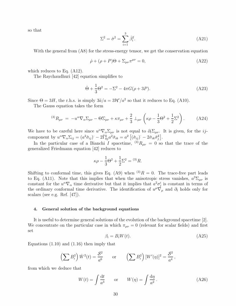
With the general from (A8) for the stress-energy tensor, we get the conservation equation

ρ + (ρ + P )Θ + Σµνπµν = 0, (A22)

which reduces to Eq. (A12).The Raychaudhuri [42] equation simplifies to

Θ +1

3Θ2 = −Σ2 − 4πG(ρ + 3P ). (A23)

Since Θ = 3H , the r.h.s. is simply 3a/a = 3H′/a2 so that it reduces to Eq. (A10).The Gauss equation takes the form

(3)Rµν = −uα∇αΣµν − ΘΣµν + κπµν +2

3⊥µν

(

κρ − 1

3Θ2 +

1

2Σ2

)

. (A24)

We have to be careful here since uα∇αΣµν is not equal to ∂tΣµν . It is given, for the ij-

component by uα∇αΣij = (a2σij)· − 2Γk

0ja2σik = a2

[

(σij)· − 2σikσ

kj

]

.

In the particular case of a Bianchi I spacetime, (3)Rµν = 0 so that the trace of thegeneralized Friedmann equation [42] reduces to

κρ − 1

3Θ2 +

1

2Σ2 = (3)R.

Shifting to conformal time, this gives Eq. (A9) when (3)R = 0. The trace-free part leadsto Eq. (A11). Note that this implies that when the anisotropic stress vanishes, a3Σµν isconstant for the uα∇α time derivative but that it implies that a2σi

j is constant in terms ofthe ordinary conformal time derivative. The identification of uµ∇µ and ∂t holds only forscalars (see e.g. Ref. [47]).

4. General solution of the background equations

It is useful to determine general solutions of the evolution of the background spacetime [2].We concentrate on the particular case in which πµν = 0 (relevant for scalar fields) and firstset

βi = BiW (t). (A25)

Equations (1.10) and (1.16) then imply that

(

∑

B2i

)

W 2(t) =S2

a6or

(

∑

B2i

)

[W ′(η)]2 =S2

a4,

from which we deduce that

W (t) =

∫

dt

a3or W (η) =

∫

dη

a2. (A26)

30

The constraints (1.5) and (1.10) imply that the Bi must satisfy

3∑

i=1

Bi = 0,3∑

i=1

B2i = S2 , (A27)

which are trivially solved by setting

Bi =

√

2

3S sin αi, αp = α +

2π

3p, p ∈ 1, 2, 3. (A28)

Thus, the general solution is of the form

βi(t) =

√

2

3S sin

(

α +2π

3i

)

× W, (A29)

where a is solution of

3H2 = κρ +1

2

S2

a6. (A30)

Once an equation of state is specified, the conservation equation gives ρ[a] and we can solvefor a(t).

As an example, consider the case of a pure cosmological constant, V = const. and ϕ = 0.The Friedmann equation takes the form

H2 = V0

[

1 +(a∗

a

)6]

,

with V0 ≡ κV/3 and a∗ ≡ (S/6V0)1/6. It can be integrated easily to get

a(t) = a∗

[

sinh(

3√

V0t)]1/3

. (A31)

Asymptotically, it behaves as the scale factor of a de Sitter universe, a ∝ exp(√

V0t) but atearly time the shear dominates and a ∝ t1/3.

APPENDIX B: PROPERTIES OF THE POLARIZATIONS

We summarize here the main properties of the polarization tensors, defined in § IIA.The time derivative of the polarization tensor is given by

(

ελij

)′= −(σklελ

kl) Pij − (σklPkl) ελij + 4σk

(iελj)k , (B1)

or equivalently,

(

εiλj

)′= −(σklελ

kl)Pij − (σklPkl)ε

iλj + 2σk

j εiλk . (B2)

In terms of the decomposition (3.1) of the shear tensor, it takes the forms

(ελij)

′ = −σTλPij + σ

‖ελ

ij + 4σk(iε

λj)k , (B3)

31

and

(εiλj )′ = −σ

TλPij + σ

‖εiλ

j + 2σkj ε

iλk . (B4)

and the time derivative of the projection operator Pij is given by

(P ij)′ = −2σT+εij

+ + 2σ‖P ij . (B5)

Let us also give the following relations that turn to be useful for the derivation of theevolution equation of the tensor modes

σilεljλ σjpε

piλ =

1

4σ2

‖+

1

2

(

σ2λ − σ2

(1−λ)

)

σilεljλ σjpε

pi(1−λ) = σ

T×σT+

σilεljλ σipελ

jp =1

4σ2

‖+

1

2

(

σ2T+ + σ2

T×

)

+1

2

∑

a

σ2Va

σilεljλ σipε

(1−λ)jp = 0 . (B6)

APPENDIX C: PERTURBED QUANTITIES

For the sake of completeness, let us give the expression of the Lie derivative (2.36) of thedisplacement ξ (2.37)

Lξg00 = −2a2 (T ′ + HT )

Lξg0i = a2(

ξ′i − ∂iT − 2σjiξj)

Lξgij = a2[

2∂(iξj) + 2HTγij + 2Tσij

]

. (C1)

The expression of the components of the stress-energy tensor of the scalar field at firstorder is

a2δT 00 = ϕ′2Φ − ϕ′χ′ − Vϕa2χ , (C2)

a2δT 0i = −∂i [ϕ

′χ] , (C3)

a2δT ji = −δi

j

[

ϕ′2Φ − ϕ′χ′ + Vϕa2χ]

. (C4)

Note that they are exactly the same expressions than in a Friedmann-Lemaıtre spacetime.It comes from the fact that δgij never appears. Indeed, the δTij etc. components will bedifferent compared to the Friedmann-Lemaıtre case.

In Newtonian gauge the Christoffel symbols at first order take the form

δΓ000 = Φ′ (C5)

δΓ00j = ∂jΦ (C6)

δΓ0ij = Hhij +

1

2h′

ij − 2HΦγij − 2Φσij (C7)

δΓi0j =

1

2hi′

j − σkjhki (C8)

=1

2(hi

j)′ − σkjh

ki + hkjσki

δΓijk =

1

2γli (∂jhlk + ∂khjl − ∂lhjk) . (C9)

32

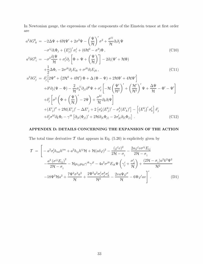
In Newtonian gauge, the expressions of the components of the Einstein tensor at first orderare

a2δG00 = −2∆Ψ + 6HΨ′ + 2σ2Ψ −

(

Ψ

H

)′

σ2 +σij

H ∂i∂jΨ

−σij∂iΦj +(

Eij

)′σj

i + (6H2 − σ2)Φ , (C10)

a2δG0i = −σ2 ∂iΨ

H + σji ∂j

[

Φ + Ψ +

(

Ψ

H

)′]

− 2∂i(Ψ′ + HΦ)

+1

2∆Φi − 2σjk∂jEik + σjk∂iEjk , (C11)

a2δGij = δi

j

[

2Ψ′′ +(

2H2 + 4H′)

Φ + ∆ (Φ − Ψ) + 2HΦ′ + 4HΨ′]

+∂i∂j(Ψ − Φ) − 2

Hσ(ik ∂j)∂

kΨ + σij

[

−H(

Ψ′

H2

)′

+

(H′

H2

)′

Ψ +∆Ψ

H − Φ′ − Ψ′

]

+δij

[

σ2

(

Φ +

(

Ψ

H

)′

− 2Ψ

)

+σkl

H ∂k∂lΨ

]

+(Eij)

′′ + 2H(Eij)

′ − ∆Eij + 2

[

σik(E

kj)

′ − σkj (E

ik)

′]

−[

(

Ekl

)′σl

k

]

δij

+δijσ

kl∂kΦl − γik[

∂(k(Φj))′ + 2H∂(kΦj) − 2σl

(k∂|l|Φj)

]

. (C12)

APPENDIX D: DETAILS CONCERNING THE EXPANSION OF THE ACTION

The total time derivative T that appears in Eq. (5.20) is explicitely given by

T =

[

− a2σlihmlh

im + a2hijhijH + H(aδϕ)2 − (ϕ′v)2

2H− σ‖

− 2aϕ′vσijEij

2H− σ‖

−a2 (σijEij)2

2H− σ‖

−Hµijµklγikγjl − 4a2σjkEikΨ

(

γij +

σij

H

)

+(2H− σ

‖)a2k2Ψ2

H2

−18Ψ2Ha2 +7Ψ2σ2a2

H +2Ψ2a2σj

i σkj σ

ik

H2− 2vaΨϕ′′

H − 6Ψϕ′av

]′

. (D1)

33